10 Word Sense Disambiguation: A Survey ROBERTO NAVIGLI Universit ` a di Roma La Sapienza Word sense disambiguation (WSD) is the ability to identify the meaning of words in context in a compu- tational manner. WSD is considered an AI-complete problem, that is, a task whose solution is at least as hard as the most difficult problems in artificial intelligence. We introduce the reader to the motivations for solving the ambiguity of words and provide a description of the task. We overview supervised, unsupervised, and knowledge-based approaches. The assessment of WSD systems is discussed in the context of the Sen- seval/Semeval campaigns, aiming at the objective evaluation of systems participating in several different disambiguation tasks. Finally, applications, open problems, and future directions are discussed. Categories and Subject Descriptors: I.2.7 [Artificial Intelligence]: Natural Language Processing—Text analysis; I.2.4 [Artificial Intelligence]: Knowledge Representation Formalisms and Methods General Terms: Algorithms, Experimentation, Measurement, Performance Additional Key Words and Phrases: Word sense disambiguation, word sense discrimination, WSD, lexical semantics, lexical ambiguity, sense annotation, semantic annotation ACM Reference Format: Navigli, R. 2009. Word sense disambiguation: A survey. ACM Comput. Surv. 41, 2, Article 10 (February 2009), 69 pages DOI = 10.1145/1459352.1459355 http://doi.acm.org/10.1145/1459352.1459355 1. INTRODUCTION 1.1. Motivation Human language is ambiguous, so that many words can be interpreted in multiple ways depending on the context in which they occur. For instance, consider the following sentences: (a) I can hear bass sounds. (b) They like grilled bass. The occurrences of the word bass in the two sentences clearly denote different mean- ings: low-frequency tones and a type of fish, respectively. Unfortunately, the identification of the specific meaning that a word assumes in context is only apparently simple. While most of the time humans do not even think This work was partially funded by the Interop NoE (508011) 6th EU FP. Author’s address: R. Navigli, Dipartimento di Informatica, Universit` a di Roma La Sapienza, Via Salaria, 113-00198 Rome, Italy; email: [email protected]. Permission to make digital or hard copies of part or all of this work for personal or classroom use is granted without fee provided that copies are not made or distributed for profit or commercial advantage and that copies show this notice on the first page or initial screen of a display along with the full citation. Copyrights for components of this work owned by others than ACM must be honored. Abstracting with credit is permitted. To copy otherwise, to republish, to post on servers, to redistribute to lists, or to use any component of this work in other works requires prior specific permission and/or a fee. Permissions may be requested from Publications Dept., ACM, Inc., 2 Penn Plaza, Suite 701, New York, NY 10121-0701 USA, fax +1 (212) 869- 0481, or [email protected]. c 2009 ACM 0360-0300/2009/02-ART10 $5.00. DOI 10.1145/1459352.1459355 http://doi.acm.org/10.1145/ 1459352.1459355 ACM Computing Surveys, Vol. 41, No. 2, Article 10, Publication date: February 2009.

Word sense disambiguation a survey
Aug 28, 2014
Welcome message from author
This document is posted to help you gain knowledge. Please leave a comment to let me know what you think about it! Share it to your friends and learn new things together.
Transcript
10
Word Sense Disambiguation: A Survey
ROBERTO NAVIGLI
Universita di Roma La Sapienza
Word sense disambiguation (WSD) is the ability to identify the meaning of words in context in a compu-
tational manner. WSD is considered an AI-complete problem, that is, a task whose solution is at least as
hard as the most difficult problems in artificial intelligence. We introduce the reader to the motivations for
solving the ambiguity of words and provide a description of the task. We overview supervised, unsupervised,
and knowledge-based approaches. The assessment of WSD systems is discussed in the context of the Sen-
seval/Semeval campaigns, aiming at the objective evaluation of systems participating in several different
disambiguation tasks. Finally, applications, open problems, and future directions are discussed.
Categories and Subject Descriptors: I.2.7 [Artificial Intelligence]: Natural Language Processing—Textanalysis; I.2.4 [Artificial Intelligence]: Knowledge Representation Formalisms and Methods
General Terms: Algorithms, Experimentation, Measurement, Performance
Additional Key Words and Phrases: Word sense disambiguation, word sense discrimination, WSD, lexical
semantics, lexical ambiguity, sense annotation, semantic annotation
ACM Reference Format:Navigli, R. 2009. Word sense disambiguation: A survey. ACM Comput. Surv. 41, 2, Article 10 (February 2009),
69 pages DOI = 10.1145/1459352.1459355 http://doi.acm.org/10.1145/1459352.1459355
1. INTRODUCTION
1.1. Motivation
Human language is ambiguous, so that many words can be interpreted in multipleways depending on the context in which they occur. For instance, consider the followingsentences:
(a) I can hear bass sounds.
(b) They like grilled bass.
The occurrences of the word bass in the two sentences clearly denote different mean-ings: low-frequency tones and a type of fish, respectively.
Unfortunately, the identification of the specific meaning that a word assumes incontext is only apparently simple. While most of the time humans do not even think
This work was partially funded by the Interop NoE (508011) 6th EU FP.
Author’s address: R. Navigli, Dipartimento di Informatica, Universita di Roma La Sapienza, Via Salaria,113-00198 Rome, Italy; email: [email protected].
Permission to make digital or hard copies of part or all of this work for personal or classroom use is grantedwithout fee provided that copies are not made or distributed for profit or commercial advantage and thatcopies show this notice on the first page or initial screen of a display along with the full citation. Copyrights forcomponents of this work owned by others than ACM must be honored. Abstracting with credit is permitted.To copy otherwise, to republish, to post on servers, to redistribute to lists, or to use any component of thiswork in other works requires prior specific permission and/or a fee. Permissions may be requested fromPublications Dept., ACM, Inc., 2 Penn Plaza, Suite 701, New York, NY 10121-0701 USA, fax +1 (212) 869-0481, or [email protected]©2009 ACM 0360-0300/2009/02-ART10 $5.00. DOI 10.1145/1459352.1459355 http://doi.acm.org/10.1145/
1459352.1459355
ACM Computing Surveys, Vol. 41, No. 2, Article 10, Publication date: February 2009.
10:2 R. Navigli
about the ambiguities of language, machines need to process unstructured textual in-formation and transform them into data structures which must be analyzed in orderto determine the underlying meaning. The computational identification of meaning forwords in context is called word sense disambiguation (WSD). For instance, as a resultof disambiguation, sentence (b) above should be ideally sense-tagged as “They like/ENJOY
grilled/COOKED bass/FISH.”WSD has been described as an AI-complete problem [Mallery 1988], that is, by anal-
ogy to NP-completeness in complexity theory, a problem whose difficulty is equivalentto solving central problems of artificial intelligence (AI), for example, the Turing Test[Turing 1950]. Its acknowledged difficulty does not originate from a single cause, butrather from a variety of factors.
First, the task lends itself to different formalizations due to fundamental questions,like the approach to the representation of a word sense (ranging from the enumerationof a finite set of senses to rule-based generation of new senses), the granularity ofsense inventories (from subtle distinctions to homonyms), the domain-oriented versusunrestricted nature of texts, the set of target words to disambiguate (one target wordper sentence vs. “all-words” settings), etc.
Second, WSD heavily relies on knowledge. In fact, the skeletal procedure of anyWSD system can be summarized as follows: given a set of words (e.g., a sentence ora bag of words), a technique is applied which makes use of one or more sources ofknowledge to associate the most appropriate senses with words in context. Knowl-edge sources can vary considerably from corpora (i.e., collections) of texts, either unla-beled or annotated with word senses, to more structured resources, such as machine-readable dictionaries, semantic networks, etc. Without knowledge, it would be impos-sible for both humans and machines to identify the meaning, for example, of the abovesentences.
Unfortunately, the manual creation of knowledge resources is an expensive and time-consuming effort [Ng 1997], which must be repeated every time the disambiguationscenario changes (e.g., in the presence of new domains, different languages, and evensense inventories). This is a fundamental problem which pervades the field of WSD,and is called the knowledge acquisition bottleneck [Gale et al. 1992b].
The hardness of WSD is also attested by the lack of applications to real-world tasks.The exponential growth of the Internet community, together with the fast pace develop-ment of several areas of information technology (IT), has led to the production of a vastamount of unstructured data, such as document warehouses, Web pages, collections ofscientific articles, blog corpora, etc. As a result, there is an increasing urge to treat thismass of information by means of automatic methods. Traditional techniques for textmining and information retrieval show their limits when they are applied to such hugecollections of data. In fact, these approaches, mostly based on lexicosyntactic analysisof text, do not go beyond the surface appearance of words and, consequently, fail inidentifying relevant information formulated with different wordings and in discardingdocuments which are not pertinent to the user needs. Text disambiguation can poten-tially provide a major breakthrough in the treatment of large-scale amounts of data,thus constituting a fundamental contribution to the realization of the so-called seman-tic Web, “an extension of the current Web, in which information is given well-definedmeaning, better enabling computers and people to work in cooperation” [Berners-Leeet al. 2001, page 2].
The potential of WSD is also clear when we deal with the problem of machine transla-tion: for instance, the Italian word penna can be translated in English as feather, pen,or author depending upon the context. There are thousands and thousands of thesecases where disambiguation can play a crucial role in the automated translation oftext, a historical application of WSD indeed.
ACM Computing Surveys, Vol. 41, No. 2, Article 10, Publication date: February 2009.
Word Sense Disambiguation: A Survey 10:3
WSD is typically configured as an intermediate task, either as a stand-alone moduleor properly integrated into an application (thus performing disambiguation implicitly).However, the success of WSD in real-world applications is still to be shown. Application-oriented evaluation of WSD is an open research area, although different works andproposals have been published on the topic.
The results of recent comparative evaluations of WSD systems—mostly concerning astand-alone assessment of WSD—show that most disambiguation methods have inher-ent limitations in terms, among others, of performance and generalization capabilitywhen fine-grained sense distinctions are employed. On the other hand, the increasingavailability of wide-coverage, rich lexical knowledge resources, as well as the construc-tion of large-scale coarse-grained sense inventories, seems to open new opportunitiesfor disambiguation approaches, especially when aiming at semantically enabling ap-plications in the area of human-language technology.
1.2. History in Brief
The task of WSD is a historical one in the field of Natural Language Processing (NLP).In fact, it was conceived as a fundamental task of Machine Translation (MT) alreadyin the late 1940s [Weaver 1949]. At that time, researchers had already in mind essen-tial ingredients of WSD, such as the context in which a target word occurs, statisticalinformation about words and senses, knowledge resources, etc. Very soon it becameclear that WSD was a very difficult problem, also given the limited means availablefor computation. Indeed, its acknowledged hardness [Bar-Hillel 1960] was one of themain obstacles to the development of MT in the 1960s. During the 1970s the prob-lem of WSD was attacked with AI approaches aiming at language understanding (e.g.,Wilks [1975]). However, generalizing the results was difficult, mainly because of thelack of large amounts of machine-readable knowledge. In this respect, work on WSDreached a turning point in the 1980s with the release of large-scale lexical resources,which enabled automatic methods for knowledge extraction [Wilks et al. 1990]. The1990s led to the massive employment of statistical methods and the establishmentof periodic evaluation campaigns of WSD systems, up to the present days. The in-terested reader can refer to Ide and Veronis [1998] for an in-depth early history ofWSD.
1.3. Outline
The article is organized as follows: first, we formalize the WSD task (Section 2), andpresent the main approaches (Sections 3, 4, 5, and 6). Next, we turn to the evalu-ation of WSD (Sections 7 and 8), and discuss its potential in real-world applications(Section 9). We explore open problems and future directions in Section 10, and concludein Section 11.
2. TASK DESCRIPTION
Word sense disambiguation is the ability to computationally determine which sense ofa word is activated by its use in a particular context. WSD is usually performed on oneor more texts (although in principle bags of words, i.e., collections of naturally occurringwords, might be employed). If we disregard the punctuation, we can view a text T asa sequence of words (w1, w2, . . . , wn), and we can formally describe WSD as the task ofassigning the appropriate sense(s) to all or some of the words in T , that is, to identifya mapping A from words to senses, such that A(i) ⊆ SensesD(wi), where SensesD(wi) is
ACM Computing Surveys, Vol. 41, No. 2, Article 10, Publication date: February 2009.
10:4 R. Navigli
the set of senses encoded in a dictionary D for word wi,1 and A(i) is that subset of the
senses of wi which are appropriate in the context T . The mapping A can assign morethan one sense to each word wi ∈ T , although typically only the most appropriate senseis selected, that is, | A(i) |= 1.
WSD can be viewed as a classification task: word senses are the classes, and an auto-matic classification method is used to assign each occurrence of a word to one or moreclasses based on the evidence from the context and from external knowledge sources.Other classification tasks are studied in the area of natural language processing (for anintroduction see Manning and Schutze [1999] and Jurafsky and Martin [2000]), suchas part-of-speech tagging (i.e., the assignment of parts of speech to target words in con-text), named entity resolution (the classification of target textual items into predefinedcategories), text categorization (i.e., the assignment of predefined labels to target texts),etc. An important difference between these tasks and WSD is that the former use a sin-gle predefined set of classes (parts of speech, categories, etc.), whereas in the latter theset of classes typically changes depending on the word to be classified. In this respect,WSD actually comprises n distinct classification tasks, where n is the size of the lexicon.
We can distinguish two variants of the generic WSD task:
—Lexical sample (or targeted WSD), where a system is required to disambiguate arestricted set of target words usually occurring one per sentence. Supervised systemsare typically employed in this setting, as they can be trained using a number ofhand-labeled instances (training set) and then applied to classify a set of unlabeledexamples (test set);
—All-words WSD, where systems are expected to disambiguate all open-class words ina text (i.e., nouns, verbs, adjectives, and adverbs). This task requires wide-coveragesystems. Consequently, purely supervised systems can potentially suffer from theproblem of data sparseness, as it is unlikely that a training set of adequate size isavailable which covers the full lexicon of the language of interest. On the other hand,other approaches, such as knowledge-lean systems, rely on full-coverage knowledgeresources, whose availability must be assured.
We now turn to the four main elements of WSD: the selection of word senses (i.e.,classes), the use of external knowledge sources, the representation of context, and theselection of an automatic classification method.
2.1. Selection of Word Senses
A word sense is a commonly accepted meaning of a word. For instance, consider thefollowing two sentences:
(c) She chopped the vegetables with a chef ’s knife.
(d) A man was beaten and cut with a knife.
The word knife is used in the above sentences with two different senses: a tool (c)and a weapon (d). The two senses are clearly related, as they possibly refer to thesame object; however the object’s intended uses are different. The examples make itclear that determining the sense inventory of a word is a key problem in word sensedisambiguation: are we intended to assign different classes to the two occurrences ofknife in sentences (c) and (d)?
A sense inventory partitions the range of meaning of a word into its senses. Wordsenses cannot be easily discretized, that is, reduced to a finite discrete set of entries,
1Here we are assuming that senses can be enumerated, as this is the most viable approach if we want tocompare and assess word sense disambiguation systems. See Section 2.1 below.
ACM Computing Surveys, Vol. 41, No. 2, Article 10, Publication date: February 2009.
Word Sense Disambiguation: A Survey 10:5
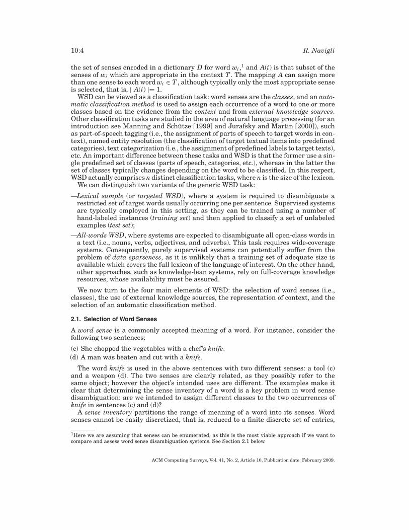
knife n. 1. a cutting tool composed of a blade with a sharp point and a handle. 2. an instrumentwith a handle and blade with a sharp point used as a weapon.
Fig. 1. An example of an enumerative entry for noun knife.
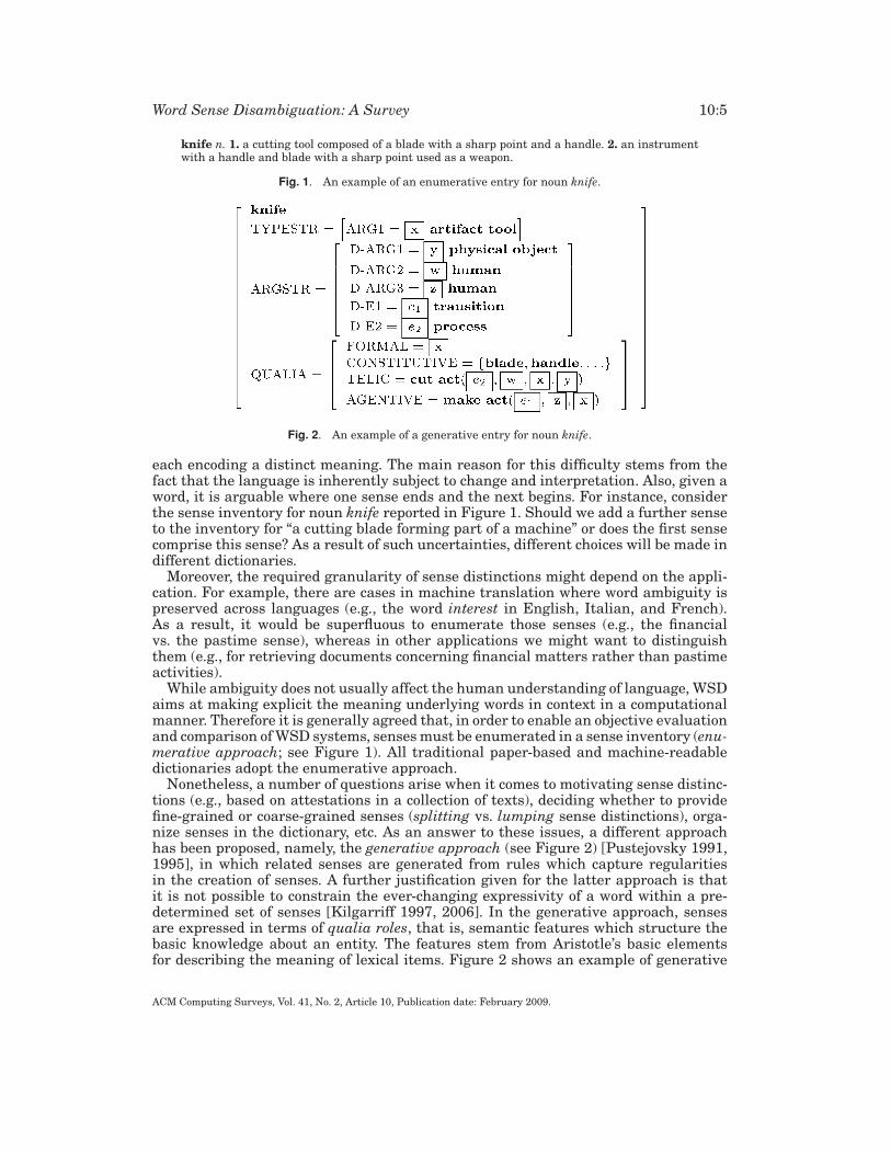
Fig. 2. An example of a generative entry for noun knife.
each encoding a distinct meaning. The main reason for this difficulty stems from thefact that the language is inherently subject to change and interpretation. Also, given aword, it is arguable where one sense ends and the next begins. For instance, considerthe sense inventory for noun knife reported in Figure 1. Should we add a further senseto the inventory for “a cutting blade forming part of a machine” or does the first sensecomprise this sense? As a result of such uncertainties, different choices will be made indifferent dictionaries.
Moreover, the required granularity of sense distinctions might depend on the appli-cation. For example, there are cases in machine translation where word ambiguity ispreserved across languages (e.g., the word interest in English, Italian, and French).As a result, it would be superfluous to enumerate those senses (e.g., the financialvs. the pastime sense), whereas in other applications we might want to distinguishthem (e.g., for retrieving documents concerning financial matters rather than pastimeactivities).
While ambiguity does not usually affect the human understanding of language, WSDaims at making explicit the meaning underlying words in context in a computationalmanner. Therefore it is generally agreed that, in order to enable an objective evaluationand comparison of WSD systems, senses must be enumerated in a sense inventory (enu-merative approach; see Figure 1). All traditional paper-based and machine-readabledictionaries adopt the enumerative approach.
Nonetheless, a number of questions arise when it comes to motivating sense distinc-tions (e.g., based on attestations in a collection of texts), deciding whether to providefine-grained or coarse-grained senses (splitting vs. lumping sense distinctions), orga-nize senses in the dictionary, etc. As an answer to these issues, a different approachhas been proposed, namely, the generative approach (see Figure 2) [Pustejovsky 1991,1995], in which related senses are generated from rules which capture regularitiesin the creation of senses. A further justification given for the latter approach is thatit is not possible to constrain the ever-changing expressivity of a word within a pre-determined set of senses [Kilgarriff 1997, 2006]. In the generative approach, sensesare expressed in terms of qualia roles, that is, semantic features which structure thebasic knowledge about an entity. The features stem from Aristotle’s basic elementsfor describing the meaning of lexical items. Figure 2 shows an example of generative
ACM Computing Surveys, Vol. 41, No. 2, Article 10, Publication date: February 2009.
10:6 R. Navigli
entry for noun knife (the example is that of Johnston and Busa [1996]; see alsoPustejovsky [1995]). Four qualia roles are provided, namely: formal (a superordinateof knife), constitutive (parts of a knife), telic (the purpose of a knife), and agentive(who uses a knife). The instantiation of a combination of roles allows for the creationof a sense. Following the generative approach, Buitelaar [1998] proposed the creationof a resource, namely, CoreLex, which identifies all the systematically related sensesand allows for underspecified semantic tagging. Other approaches which aim at fuzziersense distinctions include methods for sense induction, which we discuss in Section 4,and, more on linguistic grounds, ambiguity tests based on linguistic criteria [Cruse1986].
In the following, given its widespread adoption within the research community, wewill adopt the enumerative approach. However, works based on a fuzzier notion of wordsense will be mentioned throughout the survey. We formalize the association of discretesense distinctions with words encoded in a dictionary D as a function:
SensesD : L × POS → 2C,
where L is the lexicon, that is, the set of words encoded in the dictionary, POS ={n, a, v, r} is the set of open-class parts of speech (respectively nouns, adjectives, verbs,and adverbs), and C is the full set of concept labels in dictionary D (2C denotes thepower set of its concepts).
Throughout this survey, we denote a word w with wp where p is its part of speech(p ∈ POS), that is, we have wp ∈ L × POS. Thus, given a part-of-speech tagged wordwp, we abbreviate SensesD(w, p) as SensesD(wp), which encodes the senses of wp asa set of the distinct meanings that wp is assumed to denote depending on the contextin which it cooccurs. We note that the assumption that a word is part-of-speech (POS)tagged is a reasonable one, as modern POS taggers resolve this type of ambiguity withvery high performance.
We say that a word wp is monosemous when it can convey only one meaning, thatis, | SensesD(wp) |= 1. For instance, well-beingn is a monosemous word, as it denotes asingle sense, that of being comfortable, happy or healthy. Conversely, wp is polysemousif it can convey more meanings (e.g., racen as a competition, as a contest of speed, as ataxonomic group, etc.). Senses of a word wp which can convey (usually etimologically)unrelated meanings are homonymous (e.g., racen as a contest vs. racen as a taxonomicgroup). Finally, we denote the ith word sense of a word w with part of speech p as wi
p(other notations are in use, such as, e.g., w#p#i).
For a good introduction to word senses, the interested reader is referred to Kilgarriff[2006], and to Ide and Wilks [2006] for further discussion focused on WSD and appli-cations.
2.2. External Knowledge Sources
Knowledge is a fundamental component of WSD. Knowledge sources provide data whichare essential to associate senses with words. They can vary from corpora of texts, eitherunlabeled or annotated with word senses, to machine-readable dictionaries, thesauri,glossaries, ontologies, etc. A description of all the resources used in the field of WSDis out of the scope of this survey. Here we will give a brief overview of these resources(for more details, cf. Ide and Veronis [1998]; Litkowski [2005]; Agirre and Stevenson[2006]).
—Structured resources:
—Thesauri, which provide information about relationships between words, like syn-onymy (e.g., carn is a synonym of motorcarn), antonymy (representing oppositemeanings, e.g., uglya is an antonym of beautifula) and, possibly, further relations
ACM Computing Surveys, Vol. 41, No. 2, Article 10, Publication date: February 2009.
Word Sense Disambiguation: A Survey 10:7
[Kilgarriff and Yallop 2000]. The most widely used thesaurus in the field of WSD isRoget’s International Thesaurus [Roget 1911]. The latest edition of the thesauruscontains 250,000 word entries organized in six classes and about 1000 categories.Some researchers also use the Macquarie Thesaurus [Bernard 1986], which encodesmore than 200,000 synonyms.
—Machine-readable dictionaries (MRDs), which have become a popular source ofknowledge for natural language processing since the 1980s, when the first dictio-naries were made available in electronic format: among these, we cite the CollinsEnglish Dictionary, the Oxford Advanced Learner’s Dictionary of Current English,the Oxford Dictionary of English [Soanes and Stevenson 2003], and the LongmanDictionary of Contemporary English (LDOCE) [Proctor 1978]. The latter has beenone of the most widely used machine-readable dictionaries within the NLP re-search community (see Wilks et al. [1996] for a thorough overview of researchusing LDOCE), before the diffusion of WordNet [Miller et al. 1990; Fellbaum 1998],presently the most utilized resource for word sense disambiguation in English.WordNet is often considered one step beyond common MRDs, as it encodes a richsemantic network of concepts. For this reason it is usually defined as a computa-tional lexicon;
—Ontologies, which are specifications of conceptualizations of specific domains of in-terest [Gruber 1993], usually including a taxonomy and a set of semantic relations.In this respect, WordNet and its extensions (cf. Section 2.2.1) can be considered asontologies, as well as the Omega Ontology [Philpot et al. 2005], an effort to reorga-nize and conceptualize WordNet, the SUMO upper ontology [Pease et al. 2002], etc.An effort in a domain-oriented direction is the Unified Medical Language System(UMLS) [McCray and Nelson 1995], which includes a semantic network providinga categorization of medical concepts.
—Unstructured resources:
—Corpora, that is, collections of texts used for learning language models. Corporacan be sense-annotated or raw (i.e., unlabeled). Both kinds of resources are used inWSD, and are most useful in supervised and unsupervised approaches, respectively(see Section 2.4):
—Raw corpora: the Brown Corpus [Kucera and Francis 1967], a million word bal-anced collection of texts published in the United States in 1961; the British Na-tional Corpus (BNC) [Clear 1993], a 100 million word collection of written and spo-ken samples of the English language (often used to collect word frequencies andidentify grammatical relations between words); the Wall Street Journal (WSJ)corpus [Charniak et al. 2000], a collection of approximately 30 million wordsfrom WSJ; the American National Corpus [Ide and Suderman 2006], which in-cludes 22 million words of written and spoken American English; the GigawordCorpus, a collection of 2 billion words of newspaper text [Graff 2003], etc.
—Sense-Annotated Corpora: SemCor [Miller et al. 1993], the largest and most usedsense-tagged corpus, which includes 352 texts tagged with around 234,000 senseannotations; MultiSemCor [Pianta et al. 2002], an English-Italian parallel corpusannotated with senses from the English and Italian versions of WordNet; the line-hard-serve corpus [Leacock et al. 1993] containing 4000 sense-tagged examplesof these three words (noun, adjective, and verb, respectively); the interest corpus[Bruce and Wiebe 1994] with 2369 sense-labeled examples of noun interest; theDSO corpus [Ng and Lee 1996], produced by the Defence Science Organisation(DSO) of Singapore, which includes 192,800 sense-tagged tokens of 191 wordsfrom the Brown and Wall Street Journal corpora; the Open Mind Word Expert
ACM Computing Surveys, Vol. 41, No. 2, Article 10, Publication date: February 2009.
10:8 R. Navigli
data set [Chklovski and Mihalcea 2002], a corpus of sentences whose instances of288 nouns were semantically annotated by Web users in a collaborative effort; theSenseval and Semeval data sets, semantically-annotated corpora from the fourevaluation campaigns (presented in Section 8). All these corpora are annotatedwith different versions of the WordNet sense inventory, with the exception of theinterest corpus (tagged with LDOCE senses), and the Senseval-1 corpus, whichwas sense-labeled with the HECTOR sense inventory, a lexicon and corpus from ajoint Oxford University Press/Digital project [Atkins 1993].
—Collocation resources, which register the tendency for words to occur regularly withothers: examples include the Word Sketch Engine,2 JustTheWord,3 The British Na-tional Corpus collocations,4 the Collins Cobuild Corpus Concordance,5 etc. Recently,a huge dataset of text cooccurrences has been released, which has rapidly gaineda large popularity in the WSD community, namely, the Web1T corpus [Brants andFranz 2006]. The corpus contains frequencies for sequences of up to five words ina one trillion word corpus derived from the Web.
—Other resources, such as word frequency lists, stoplists (i.e., lists of undiscrimi-nating noncontent words, like a, an, the, and so on), domain labels [Magnini andCavaglia 2000], etc.
In the following subsections, we provide details for two knowledge sources whichhave been widely used in the field: WordNet and SemCor.
2.2.1. WordNet. WordNet [Miller et al. 1990; Fellbaum 1998] is a computational lexi-con of English based on psycholinguistic principles, created and maintained at Prince-ton University.6 It encodes concepts in terms of sets of synonyms (called synsets). Itslatest version, WordNet 3.0, contains about 155,000 words organized in over 117,000synsets. For example, the concept of automobile is expressed with the following synset(recall superscript and subscript denote the word’s sense identifier and part-of-speechtag, respectively): {
car1n, auto1
n, automobile1n, machine4
n, motorcar1n
}.
We can view a synset as a set of word senses all expressing (approximately) the samemeaning. According to the notation introduced in Section 2.1, the following functionassociates with each part-of-speech tagged word wp the set of its WordNet senses:
SensesW N : L × POS → 2 SYNSETS,
where SYNSETS is the entire set of synsets in WordNet. For example:
SensesW N (carn) = {{car1
n, auto1n, automobile1
n, machine4n, motorcar1
n
},{
car2n, rail car1
n, rail way car1n, rail road car1
n
},{
cable car1n, car3
n
},{
car4n, gondola3
n
},{
car5n, elevator car1
n
}}.
2http://www.sketchengine.co.uk.3http://193.133.140.102/JustTheWord.4Available through the SARA system from http://www.natcorp.ox.ac.uk.5http://www.collins.co.uk/Corpus/CorpusSearch.aspx.6http://wordnet.princeton.edu.
ACM Computing Surveys, Vol. 41, No. 2, Article 10, Publication date: February 2009.
Word Sense Disambiguation: A Survey 10:9
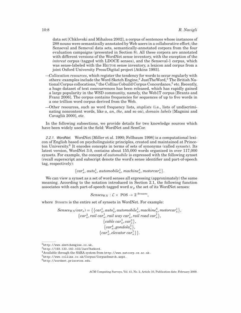
Fig. 3. An excerpt of the WordNet semantic network.
We note that each word sense univocally identifies a single synset. For instance,given car1
n the corresponding synset {car1n, auto1
n, automobile1n, machine4
n, motorcar1n}
is univocally determined. In Figure 3 we report an excerpt of the WordNet semanticnetwork containing the car1
n synset. For each synset, WordNet provides the followinginformation:
—A gloss, that is, a textual definition of the synset possibly with a set of usage examples(e.g., the gloss of car1
n is “a 4-wheeled motor vehicle; usually propelled by an internal
combustion engine; ‘he needs a car to get to work’ ”).7
—Lexical and semantic relations, which connect pairs of word senses and synsets, re-spectively: while semantic relations apply to synsets in their entirety (i.e., to allmembers of a synset), lexical relations connect word senses included in the respec-tive synsets. Among the latter we have the following:—Antonymy: X is an antonym of Y if it expresses the opposite concept (e.g., good1
a isthe antonym of bad1
a). Antonymy holds for all parts of speech.
—Pertainymy: X is an adjective which can be defined as “of or pertaining to” a noun(or, rarely, another adjective) Y (e.g., dental1
a pertains to tooth1n).
—Nominalization: a noun X nominalizes a verb Y (e.g., service2n nominalizes the verb
serve4v).
Among the semantic relations we have the following:—Hypernymy (also called kind-of or is-a): Y is a hypernym of X if every X is a (kind
of) Y (motor vehicle1n is a hypernym of car1
n). Hypernymy holds between pairs ofnominal or verbal synsets.
7Recently, Princeton University released the Princeton WordNet Gloss Corpus, a corpus of manually andautomatically sense-annotated glosses from WordNet 3.0, available from the WordNet Web site.
ACM Computing Surveys, Vol. 41, No. 2, Article 10, Publication date: February 2009.
10:10 R. Navigli
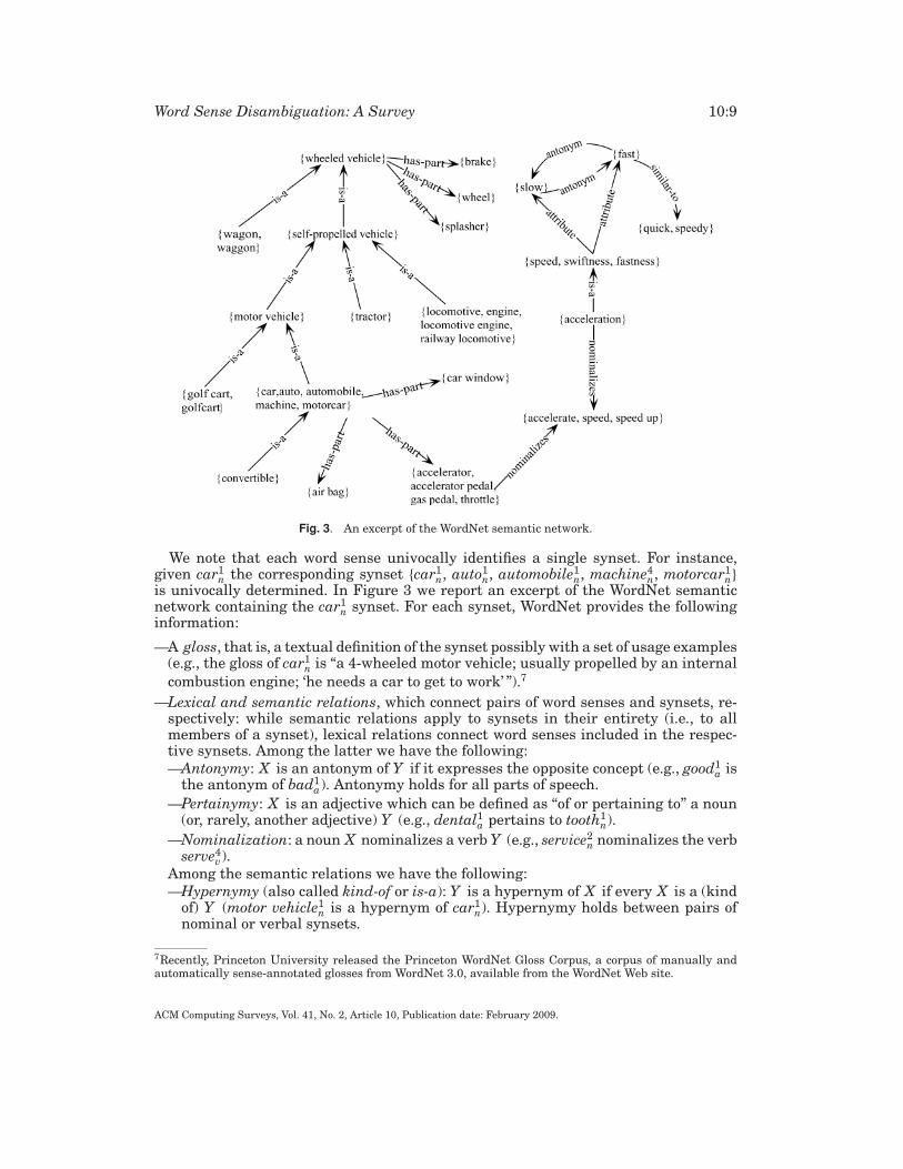
Fig. 4. An excerpt of the WordNet domain labels taxonomy.
—Hyponymy and troponymy: the inverse relations of hypernymy for nominal andverbal synsets, respectively.
—Meronymy (also called part-of ): Y is a meronym of X if Y is a part of X (e.g., flesh3n
is a meronym of fruit1n). Meronymy holds for nominal synsets only.
—Holonymy: Y is a holonym of X if X is a part of Y (the inverse of meronymy).
—Entailment: a verb Y is entailed by a verb X if by doing X you must be doing Y (e.g.,snore1
v entails sleep1v).
—Similarity: an adjective X is similar to an adjective Y (e.g., beautiful1a is similar to
pretty1a).
—Attribute: a noun X is an attribute for which an adjective Y expresses a value (e.g.,hot1
a is a value of temperature1n).
—See also: this is a relation of relatedness between adjectives (e.g., beautiful1a is
related to attractive1a through the see also relation).
Magnini and Cavaglia [2000] developed a data set of domain labels for WordNetsynsets.8 WordNet synsets have been semiautomatically annotated with one or moredomain labels from a predefined set of about 200 tags from the Dewey Decimal Clas-sification (e.g. FOOD, ARCHITECTURE, SPORT, etc.) plus a generic label (FACTOTUM) when nodomain information is available. Labels are organized in a hierarchical structure (e.g.,PSYCHOANALYSIS is a kind of PSYCHOLOGY domain). Figure 4 shows an excerpt of the domaintaxonomy.
Given its widespread diffusion within the research community, WordNet can be con-sidered a de facto standard for English WSD. Following its success, wordnets for severallanguages have been developed and linked to the original Princeton WordNet. The firsteffort in this direction was made in the context of the EuroWordNet project [Vossen1998], which provided an interlingual alignment between national wordnets. Nowa-days there are several ongoing efforts to create, enrich, and maintain wordnets fordifferent languages, such as MultiWordNet [Pianta et al. 2002] and BalkaNet [Tufiset al. 2004]. An association, namely, the Global WordNet Association,9 has been foundedto share and link wordnets for all languages in the world. These projects make not onlyWSD possible in other languages, but can potentially enable the application of WSD tomachine translation.
8IRST domain labels are available at http://wndomains.itc.it.9http://www.globalwordnet.org.
ACM Computing Surveys, Vol. 41, No. 2, Article 10, Publication date: February 2009.
Word Sense Disambiguation: A Survey 10:11
As of Sunday1n night1
n there was4v no word2
n of a resolution1n being offered2
v there1r to rescind1
vthe action1
n. Pelham pointed out1v that Georgia1
n voters1n last1
r November1n rejected2
v a
constitutional1a amendment1n to allow2
v legislators1n to vote1
n on pay1n raises1
n for future1a
Legislature1n sessions2
n.
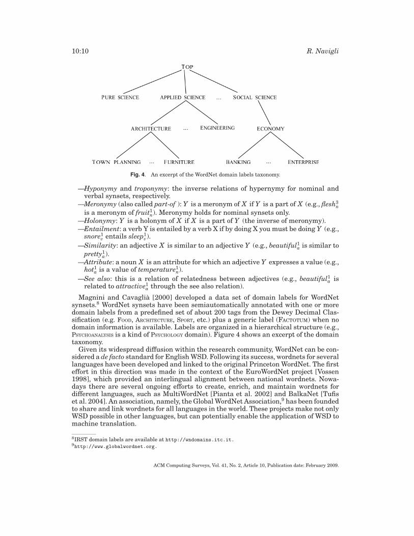
Fig. 5. An excerpt of the SemCor semantically annotated corpus.
2.2.2. SemCor. SemCor [Miller et al. 1993] is a subset of the Brown Corpus [Kuceraand Francis 1967] whose content words have been manually annotated with part-of-speech tags, lemmas, and word senses from the WordNet inventory. SemCor is composedof 352 texts: in 186 texts all the open-class words (nouns, verbs, adjectives, and adverbs)are annotated with these information, while in the remaining 166 texts only verbs aresemantically annotated with word senses.
Overall, SemCor comprises a sample of around 234,000 semantically annotatedwords, thus constituting the largest sense-tagged corpus for training sense classifiersin supervised disambiguation settings. An excerpt of a text in the corpus is reportedin Figure 5. For instance, wordn is annotated in the first sentence with sense #2, de-fined in WordNet as “a brief statement” (compared, e.g., to sense #1 defined as “a unitof language that native speakers can identify”). The original SemCor was annotatedaccording to WordNet 1.5. However, mappings exist to more recent versions (e.g., 2.0,2.1, etc.).
Based on SemCor, a bilingual corpus was created by Bentivogli and Pianta [2005]:MultiSemCor is an English/Italian parallel corpus aligned at the word level whichprovides for each word its part of speech, its lemma, and a sense from the English andItalian versions of WordNet (namely, MultiWordNet [Pianta et al. 2002]). The corpuswas built by aligning the Italian translation of SemCor at the word level. The originalword sense tags from SemCor were then transferred to the aligned Italian words.
2.3. Representation of Context
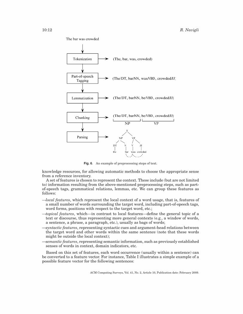
As text is an unstructured source of information, to make it a suitable input to anautomatic method it is usually transformed into a structured format. To this end, apreprocessing of the input text is usually performed, which typically (but not necessar-ily) includes the following steps:
—tokenization, a normalization step, which splits up the text into a set of tokens (usuallywords);
—part-of-speech tagging, consisting in the assignment of a grammatical category toeach word (e.g., “the/DT bar/NN was/VBD crowded/JJ,” where DT, NN, VBD and JJare tags for determiners, nouns, verbs, and adjectives, respectively);
—lemmatization, that is, the reduction of morphological variants to their base form(e.g. was → be, bars → bar);
—chunking, which consists of dividing a text in syntactically correlated parts (e.g., [thebar]NP [was crowded]VP, respectively the noun phrase and the verb phrase of the
example).
—parsing, whose aim is to identify the syntactic structure of a sentence (usually in-volving the generation of a parse tree of the sentence structure).
We report an example of the processing flow in Figure 6. As a result of thepreprocessing phase of a portion of text (e.g., a sentence, a paragraph, a full docu-ment, etc.), each word can be represented as a vector of features of different kinds or inmore structured ways, for example, as a tree or a graph of the relations between words.The representation of a word in context is the main support, together with additional
ACM Computing Surveys, Vol. 41, No. 2, Article 10, Publication date: February 2009.
10:12 R. Navigli
Fig. 6. An example of preprocessing steps of text.
knowledge resources, for allowing automatic methods to choose the appropriate sensefrom a reference inventory.
A set of features is chosen to represent the context. These include (but are not limitedto) information resulting from the above-mentioned preprocessing steps, such as part-of-speech tags, grammatical relations, lemmas, etc. We can group these features asfollows:
—local features, which represent the local context of a word usage, that is, features ofa small number of words surrounding the target word, including part-of-speech tags,word forms, positions with respect to the target word, etc.;
—topical features, which—in contrast to local features—define the general topic of atext or discourse, thus representing more general contexts (e.g., a window of words,a sentence, a phrase, a paragraph, etc.), usually as bags of words;
—syntactic features, representing syntactic cues and argument-head relations betweenthe target word and other words within the same sentence (note that these wordsmight be outside the local context);
—semantic features, representing semantic information, such as previously establishedsenses of words in context, domain indicators, etc.
Based on this set of features, each word occurrence (usually within a sentence) canbe converted to a feature vector. For instance, Table I illustrates a simple example of apossible feature vector for the following sentences:
ACM Computing Surveys, Vol. 41, No. 2, Article 10, Publication date: February 2009.
Word Sense Disambiguation: A Survey 10:13
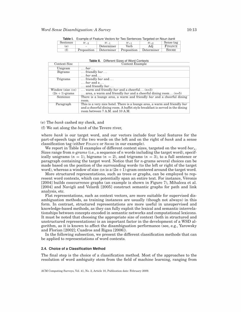
Table I. Example of Feature Vectors for Two Sentences Targeted on Noun bankSentence w−2 w−1 w+1 w+2 Sense tag
(e) - Determiner Verb Adj FINANCE
(f) Preposition Determiner Preposition Determiner SHORE
Table II. Different Sizes of Word ContextsContext Size Context Example
Unigram . . . bar . . .
Bigrams . . . friendly bar . . .
. . . bar and . . .
Trigrams . . . friendly bar and . . .
. . . bar and a . . .
. . . and friendly bar . . .
Window (size ±n) . . . warm and friendly bar and a cheerful . . . (n=3)(2n + 1)-grams . . . area, a warm and friendly bar and a cheerful dining room . . . (n=5)
Sentence There is a lounge area, a warm and friendly bar and a cheerful diningroom.
Paragraph This is a very nice hotel. There is a lounge area, a warm and friendly barand a cheerful dining room. A buffet style breakfast is served in the diningroom between 7 A.M. and 10 A.M.
(e) The bank cashed my check, and
(f) We sat along the bank of the Tevere river,
where bank is our target word, and our vectors include four local features for thepart-of-speech tags of the two words on the left and on the right of bank and a senseclassification tag (either FINANCE or SHORE in our example).
We report in Table II examples of different context sizes, targeted on the word barn.Sizes range from n-grams (i.e., a sequence of n words including the target word), specif-ically unigrams (n = 1), bigrams (n = 2), and trigrams (n = 3), to a full sentence orparagraph containing the target word. Notice that for n-grams several choices can bemade based on the position of the surrounding words (to the left or right of the targetword), whereas a window of size ±n is a (2n+1)-gram centered around the target word.
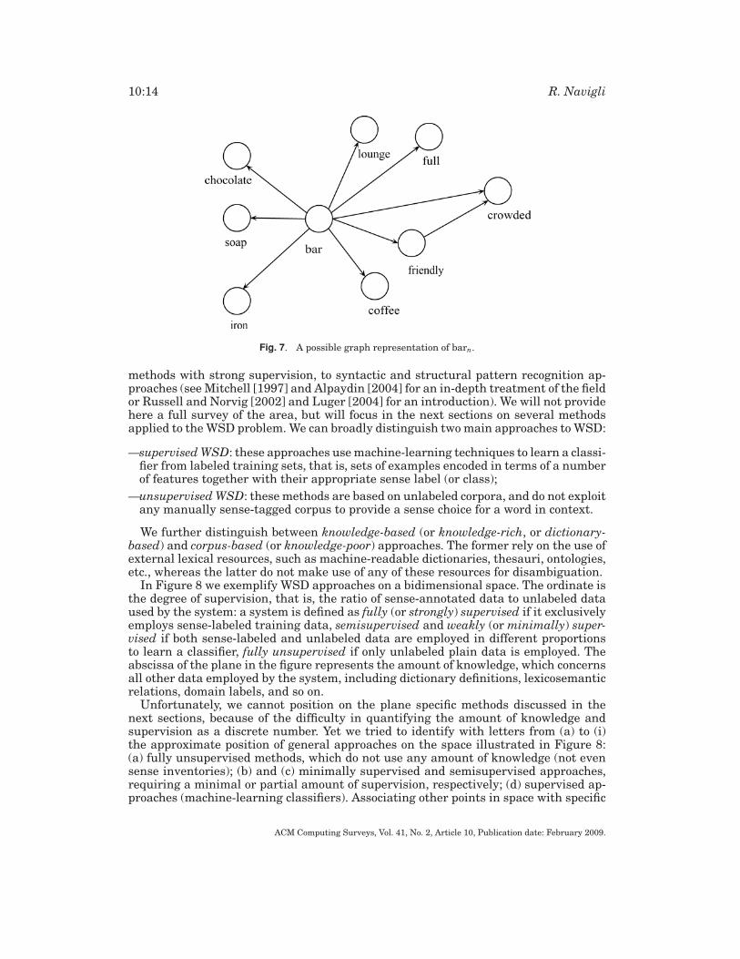
More structured representations, such as trees or graphs, can be employed to rep-resent word contexts, which can potentially span an entire text. For instance, Veronis[2004] builds cooccurrence graphs (an example is shown in Figure 7), Mihalcea et al.[2004] and Navigli and Velardi [2005] construct semantic graphs for path and linkanalysis, etc.
Flat representations, such as context vectors, are more suitable for supervised dis-ambiguation methods, as training instances are usually (though not always) in thisform. In contrast, structured representations are more useful in unsupervised andknowledge-based methods, as they can fully exploit the lexical and semantic interrela-tionships between concepts encoded in semantic networks and computational lexicons.It must be noted that choosing the appropriate size of context (both in structured andunstructured representations) is an important factor in the development of a WSD al-gorithm, as it is known to affect the disambiguation performance (see, e.g., Yarowskyand Florian [2002]; Cuadros and Rigau [2006]).
In the following subsection, we present the different classification methods that canbe applied to representations of word contexts.
2.4. Choice of a Classification Method
The final step is the choice of a classification method. Most of the approaches to theresolution of word ambiguity stem from the field of machine learning, ranging from
ACM Computing Surveys, Vol. 41, No. 2, Article 10, Publication date: February 2009.
10:14 R. Navigli
Fig. 7. A possible graph representation of barn.
methods with strong supervision, to syntactic and structural pattern recognition ap-proaches (see Mitchell [1997] and Alpaydin [2004] for an in-depth treatment of the fieldor Russell and Norvig [2002] and Luger [2004] for an introduction). We will not providehere a full survey of the area, but will focus in the next sections on several methodsapplied to the WSD problem. We can broadly distinguish two main approaches to WSD:
—supervised WSD: these approaches use machine-learning techniques to learn a classi-fier from labeled training sets, that is, sets of examples encoded in terms of a numberof features together with their appropriate sense label (or class);
—unsupervised WSD: these methods are based on unlabeled corpora, and do not exploitany manually sense-tagged corpus to provide a sense choice for a word in context.
We further distinguish between knowledge-based (or knowledge-rich, or dictionary-based) and corpus-based (or knowledge-poor) approaches. The former rely on the use ofexternal lexical resources, such as machine-readable dictionaries, thesauri, ontologies,etc., whereas the latter do not make use of any of these resources for disambiguation.
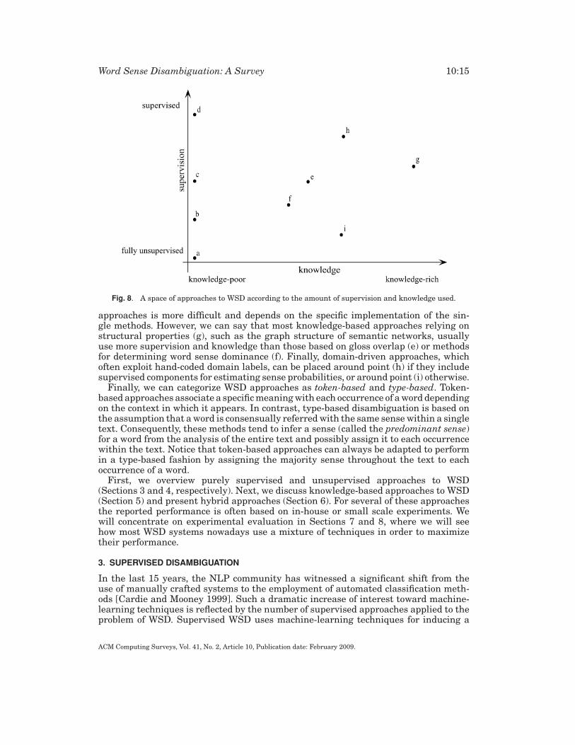
In Figure 8 we exemplify WSD approaches on a bidimensional space. The ordinate isthe degree of supervision, that is, the ratio of sense-annotated data to unlabeled dataused by the system: a system is defined as fully (or strongly) supervised if it exclusivelyemploys sense-labeled training data, semisupervised and weakly (or minimally) super-vised if both sense-labeled and unlabeled data are employed in different proportionsto learn a classifier, fully unsupervised if only unlabeled plain data is employed. Theabscissa of the plane in the figure represents the amount of knowledge, which concernsall other data employed by the system, including dictionary definitions, lexicosemanticrelations, domain labels, and so on.
Unfortunately, we cannot position on the plane specific methods discussed in thenext sections, because of the difficulty in quantifying the amount of knowledge andsupervision as a discrete number. Yet we tried to identify with letters from (a) to (i)the approximate position of general approaches on the space illustrated in Figure 8:(a) fully unsupervised methods, which do not use any amount of knowledge (not evensense inventories); (b) and (c) minimally supervised and semisupervised approaches,requiring a minimal or partial amount of supervision, respectively; (d) supervised ap-proaches (machine-learning classifiers). Associating other points in space with specific
ACM Computing Surveys, Vol. 41, No. 2, Article 10, Publication date: February 2009.
Word Sense Disambiguation: A Survey 10:15
Fig. 8. A space of approaches to WSD according to the amount of supervision and knowledge used.
approaches is more difficult and depends on the specific implementation of the sin-gle methods. However, we can say that most knowledge-based approaches relying onstructural properties (g), such as the graph structure of semantic networks, usuallyuse more supervision and knowledge than those based on gloss overlap (e) or methodsfor determining word sense dominance (f). Finally, domain-driven approaches, whichoften exploit hand-coded domain labels, can be placed around point (h) if they includesupervised components for estimating sense probabilities, or around point (i) otherwise.
Finally, we can categorize WSD approaches as token-based and type-based. Token-based approaches associate a specific meaning with each occurrence of a word dependingon the context in which it appears. In contrast, type-based disambiguation is based onthe assumption that a word is consensually referred with the same sense within a singletext. Consequently, these methods tend to infer a sense (called the predominant sense)for a word from the analysis of the entire text and possibly assign it to each occurrencewithin the text. Notice that token-based approaches can always be adapted to performin a type-based fashion by assigning the majority sense throughout the text to eachoccurrence of a word.
First, we overview purely supervised and unsupervised approaches to WSD(Sections 3 and 4, respectively). Next, we discuss knowledge-based approaches to WSD(Section 5) and present hybrid approaches (Section 6). For several of these approachesthe reported performance is often based on in-house or small scale experiments. Wewill concentrate on experimental evaluation in Sections 7 and 8, where we will seehow most WSD systems nowadays use a mixture of techniques in order to maximizetheir performance.
3. SUPERVISED DISAMBIGUATION
In the last 15 years, the NLP community has witnessed a significant shift from theuse of manually crafted systems to the employment of automated classification meth-ods [Cardie and Mooney 1999]. Such a dramatic increase of interest toward machine-learning techniques is reflected by the number of supervised approaches applied to theproblem of WSD. Supervised WSD uses machine-learning techniques for inducing a
ACM Computing Surveys, Vol. 41, No. 2, Article 10, Publication date: February 2009.
10:16 R. Navigli
Table III. An Example of Decision ListFeature Prediction Score
account with bank Bank/FINANCE 4.83stand/V on/P . . . bank Bank/FINANCE 3.35
bank of blood Bank/SUPPLY 2.48work/V . . . bank Bank/FINANCE 2.33the left/J bank Bank/RIVER 1.12
of the bank - 0.01
classifier from manually sense-annotated data sets. Usually, the classifier (often calledword expert) is concerned with a single word and performs a classification task in orderto assign the appropriate sense to each instance of that word. The training set used tolearn the classifier typically contains a set of examples in which a given target word ismanually tagged with a sense from the sense inventory of a reference dictionary.
Generally, supervised approaches to WSD have obtained better results than unsu-pervised methods (cf. Section 8). In the next subsections, we briefly review the mostpopular machine learning methods and contextualize them in the field of WSD. Addi-tional information on the topic can be found in Manning and Schutze [1999], Jurafskyand Martin [2000], and Marquez et al. [2006].
3.1. Decision Lists
A decision list [Rivest 1987] is an ordered set of rules for categorizing test instances(in the case of WSD, for assigning the appropriate sense to a target word). It can beseen as a list of weighted “if-then-else” rules. A training set is used for inducing a setof features. As a result, rules of the kind (feature-value, sense, score) are created. Theordering of these rules, based on their decreasing score, constitutes the decision list.
Given a word occurrence w and its representation as a feature vector, the decisionlist is checked, and the feature with highest score that matches the input vector selectsthe word sense to be assigned:
S = argmaxSi∈SensesD(w) score(Si).
According to Yarowsky [1994], the score of sense Si is calculated as the maximumamong the feature scores, where the score of a feature f is computed as the logarithmof the probability of sense Si given feature f divided by the sum of the probabilities ofthe other senses given feature f :
score(Si) = maxf
log
(P (Si | f )∑
j �=i P (Sj | f )
).
The above formula is an adaptation to an arbitrary number of senses due to Agirreand Martinez [2000] of Yarowsky’s [1994] formula, originally based on two senses.The probabilities P (Sj | f ) can be estimated using the maximum-likelihood estimate.Smoothing can be applied to avoid the problem of zero counts. Pruning can also beemployed to eliminate unreliable rules with very low weight.
A simplified example of a decision list is reported in Table III. The first rule in theexample applies to the financial sense of bank and expects account with as a left context,the third applies to bank as a supply (e.g., a bank of blood, a bank of food), and so on(notice that more rules can predict a given sense of a word).
It must be noted that, while in the original formulation [Rivest 1987] each rule in thedecision list is unweighted and may contain a conjunction of features, in Yarowsky’sapproach each rule is weighted and can only have a single feature. Decision lists havebeen the most successful technique in the first Senseval evaluation competitions (e.g.,
ACM Computing Surveys, Vol. 41, No. 2, Article 10, Publication date: February 2009.
Word Sense Disambiguation: A Survey 10:17
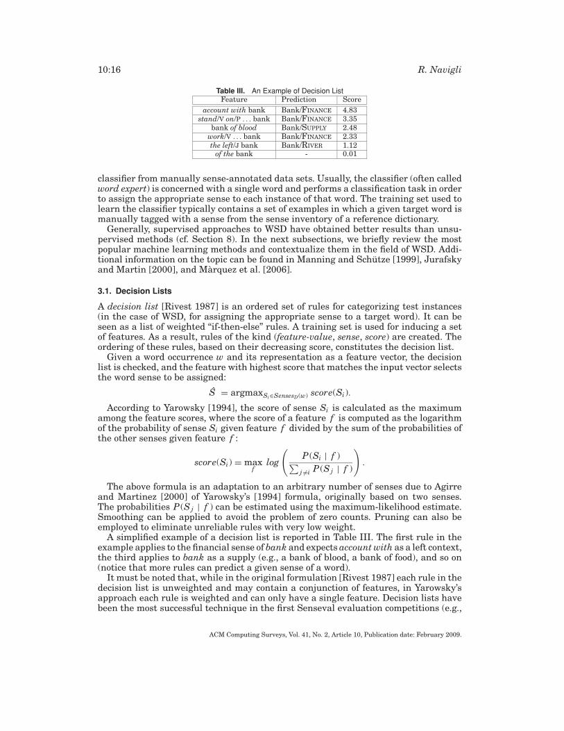
Fig. 9. An example of a decision tree.
Yarowsky [2000], cf. Section 8). Agirre and Martinez [2000] applied them in an attemptto relieve the knowledge acquisition bottleneck caused by the lack of manually taggedcorpora.
3.2. Decision Trees
A decision tree is a predictive model used to represent classification rules with a treestructure that recursively partitions the training data set. Each internal node of a de-cision tree represents a test on a feature value, and each branch represents an outcomeof the test. A prediction is made when a terminal node (i.e., a leaf) is reached.
In the last decades, decision trees have been rarely applied to WSD (in spite of somerelatively old studies by, e.g., Kelly and Stone [1975] and Black [1988]). A popularalgorithm for learning decision trees is the C4.5 algorithm [Quinlan 1993], an extensionof the ID3 algorithm [Quinlan 1986]. In a comparative experiment with several machinelearning algorithms for WSD, Mooney [1996] concluded that decision trees obtainedwith the C4.5 algorithm are outperformed by other supervised approaches. In fact,even though they represent the predictive model in a compact and human-readableway, they suffer from several issues, such as data sparseness due to features with alarge number of values, unreliability of the predictions due to small training sets, etc.
An example of a decision tree for WSD is reported in Figure 9. For instance, if thenoun bank must be classified in the sentence “we sat on a bank of sand,” the tree istraversed and, after following the no-yes-no path, the choice of sense bank/RIVER is made.The leaf with empty value (-) indicates that no choice can be made based on specificfeature values.
3.3. Naive Bayes
A Naive Bayes classifier is a simple probabilistic classifier based on the application ofBayes’ theorem. It relies on the calculation of the conditional probability of each senseSi of a word w given the features f j in the context. The sense S which maximizes thefollowing formula is chosen as the most appropriate sense in context:
S = argmaxSi∈SensesD(w)
P (Si | f1, . . . , fm) = argmaxSi∈SensesD(w)
P ( f1, . . . , fm | Si)P (Si)
P ( f1, . . . , fm)
= argmaxSi∈SensesD(w)
P (Si)
m∏j=1
P ( f j | Si),
ACM Computing Surveys, Vol. 41, No. 2, Article 10, Publication date: February 2009.
10:18 R. Navigli
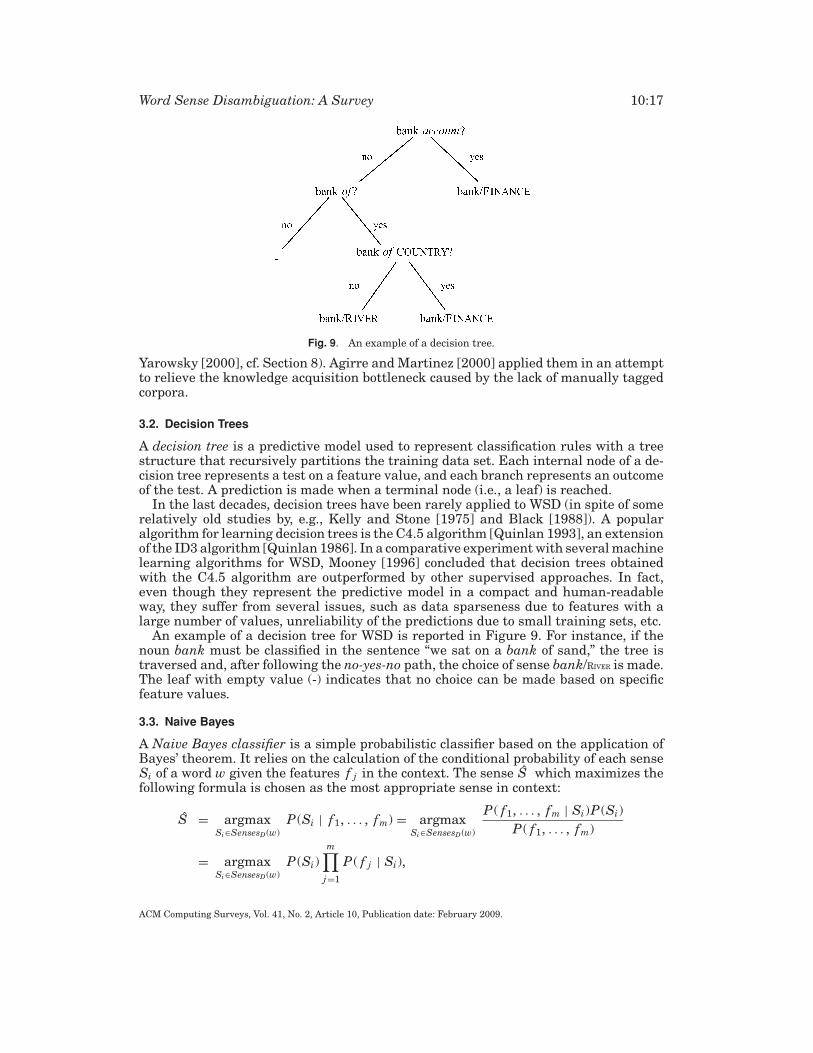
Fig. 10. An example of a Bayesian network.
where m is the number of features, and the last formula is obtained based on the naiveassumption that the features are conditionally independent given the sense (the de-nominator is also discarded as it does not influence the calculations). The probabilitiesP (Si) and P ( f j | Si) are estimated, respectively, as the relative occurrence frequenciesin the training set of sense Si and feature f j in the presence of sense Si. Zero countsneed to be smoothed: for instance, they can be replaced with P (Si)/N where N is thesize of the training set [Ng 1997; Escudero et al. 2000c]. However, this solution leadsprobabilities to sum to more than 1. Backoff or interpolation strategies can be usedinstead to avoid this problem.
In Figure 10 we report a simple example of a naive bayesian network. For instance,suppose that we want to classify the occurrence of noun bank in the sentence The bankcashed my check given the features: {w−1 = the, w+1 = cashed, head = bank, subj-verb =cash, verb-obj = −}, where the latter two features encode the grammatical role of nounbank as a subject and direct object in the target sentence. Suppose we estimated fromthe training set that the probability of these five features given the financial sense ofbank are P (w−1 = the | bank/FINANCE) = 0.66, P (w+1 = cashed | bank/FINANCE) = 0.35,P (head = bank | bank/FINANCE) = 0.76, P (subj-verb = cash | bank/FINANCE) = 0.44,P (verb-obj = − | bank/FINANCE) = 0.6. Also, we estimated the probability of occurrenceof P (bank/FINANCE) = 0.36. The final score is
score(bank /FINANCE) = 0.36 · 0.66 · 0.35 · 0.76 · 0.44 · 0.6 = 0.016.
In spite of the independence assumption, the method compares well with other su-pervised methods [Mooney 1996; Ng 1997; Leacock et al. 1998; Pedersen 1998; Bruceand Wiebe 1999].
3.4. Neural Networks
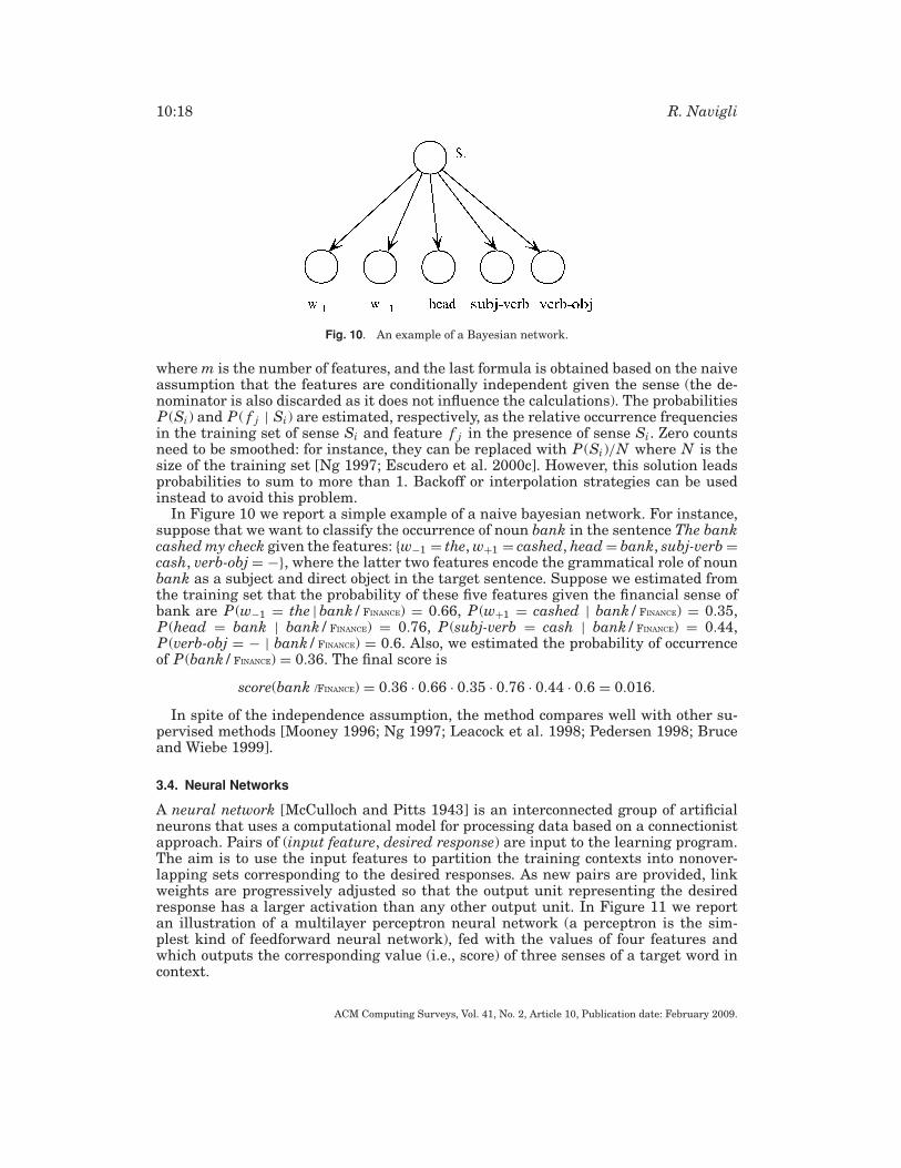
A neural network [McCulloch and Pitts 1943] is an interconnected group of artificialneurons that uses a computational model for processing data based on a connectionistapproach. Pairs of (input feature, desired response) are input to the learning program.The aim is to use the input features to partition the training contexts into nonover-lapping sets corresponding to the desired responses. As new pairs are provided, linkweights are progressively adjusted so that the output unit representing the desiredresponse has a larger activation than any other output unit. In Figure 11 we reportan illustration of a multilayer perceptron neural network (a perceptron is the sim-plest kind of feedforward neural network), fed with the values of four features andwhich outputs the corresponding value (i.e., score) of three senses of a target word incontext.
ACM Computing Surveys, Vol. 41, No. 2, Article 10, Publication date: February 2009.
Word Sense Disambiguation: A Survey 10:19
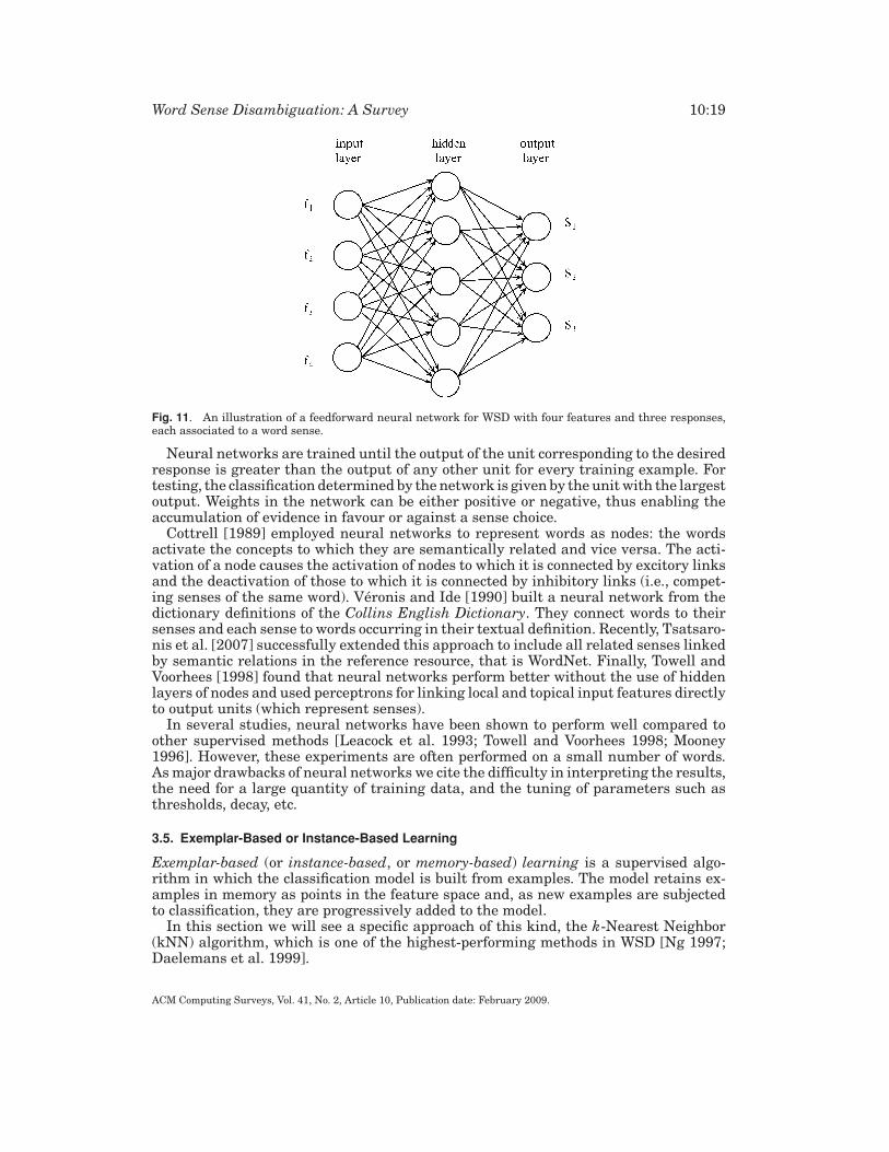
Fig. 11. An illustration of a feedforward neural network for WSD with four features and three responses,each associated to a word sense.
Neural networks are trained until the output of the unit corresponding to the desiredresponse is greater than the output of any other unit for every training example. Fortesting, the classification determined by the network is given by the unit with the largestoutput. Weights in the network can be either positive or negative, thus enabling theaccumulation of evidence in favour or against a sense choice.
Cottrell [1989] employed neural networks to represent words as nodes: the wordsactivate the concepts to which they are semantically related and vice versa. The acti-vation of a node causes the activation of nodes to which it is connected by excitory linksand the deactivation of those to which it is connected by inhibitory links (i.e., compet-ing senses of the same word). Veronis and Ide [1990] built a neural network from thedictionary definitions of the Collins English Dictionary. They connect words to theirsenses and each sense to words occurring in their textual definition. Recently, Tsatsaro-nis et al. [2007] successfully extended this approach to include all related senses linkedby semantic relations in the reference resource, that is WordNet. Finally, Towell andVoorhees [1998] found that neural networks perform better without the use of hiddenlayers of nodes and used perceptrons for linking local and topical input features directlyto output units (which represent senses).
In several studies, neural networks have been shown to perform well compared toother supervised methods [Leacock et al. 1993; Towell and Voorhees 1998; Mooney1996]. However, these experiments are often performed on a small number of words.As major drawbacks of neural networks we cite the difficulty in interpreting the results,the need for a large quantity of training data, and the tuning of parameters such asthresholds, decay, etc.
3.5. Exemplar-Based or Instance-Based Learning
Exemplar-based (or instance-based, or memory-based) learning is a supervised algo-rithm in which the classification model is built from examples. The model retains ex-amples in memory as points in the feature space and, as new examples are subjectedto classification, they are progressively added to the model.
In this section we will see a specific approach of this kind, the k-Nearest Neighbor(kNN) algorithm, which is one of the highest-performing methods in WSD [Ng 1997;Daelemans et al. 1999].
ACM Computing Surveys, Vol. 41, No. 2, Article 10, Publication date: February 2009.
10:20 R. Navigli
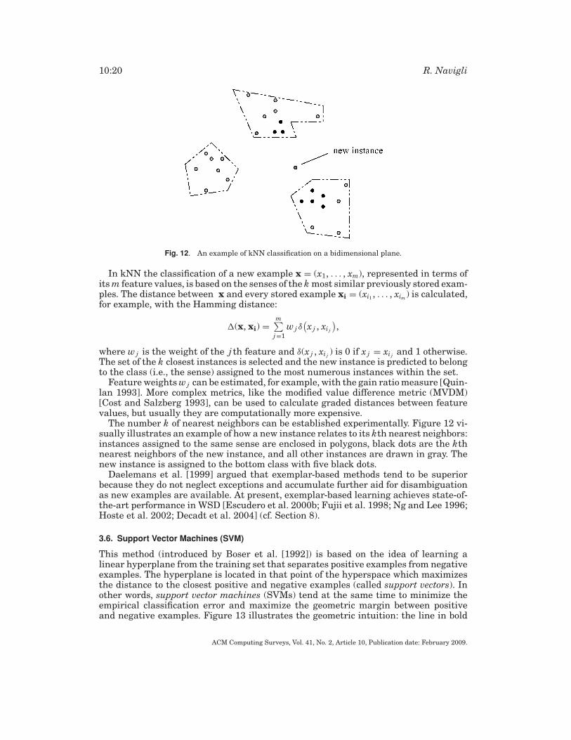
Fig. 12. An example of kNN classification on a bidimensional plane.
In kNN the classification of a new example x = (x1, . . . , xm), represented in terms ofits m feature values, is based on the senses of the k most similar previously stored exam-ples. The distance between x and every stored example xi = (xi1 , . . . , xim) is calculated,for example, with the Hamming distance:
�(x, xi) =m∑
j=1
wj δ(x j , xi j
),
where wj is the weight of the j th feature and δ(x j , xi j ) is 0 if x j = xi j and 1 otherwise.The set of the k closest instances is selected and the new instance is predicted to belongto the class (i.e., the sense) assigned to the most numerous instances within the set.
Feature weights wj can be estimated, for example, with the gain ratio measure [Quin-lan 1993]. More complex metrics, like the modified value difference metric (MVDM)[Cost and Salzberg 1993], can be used to calculate graded distances between featurevalues, but usually they are computationally more expensive.
The number k of nearest neighbors can be established experimentally. Figure 12 vi-sually illustrates an example of how a new instance relates to its kth nearest neighbors:instances assigned to the same sense are enclosed in polygons, black dots are the kthnearest neighbors of the new instance, and all other instances are drawn in gray. Thenew instance is assigned to the bottom class with five black dots.
Daelemans et al. [1999] argued that exemplar-based methods tend to be superiorbecause they do not neglect exceptions and accumulate further aid for disambiguationas new examples are available. At present, exemplar-based learning achieves state-of-the-art performance in WSD [Escudero et al. 2000b; Fujii et al. 1998; Ng and Lee 1996;Hoste et al. 2002; Decadt et al. 2004] (cf. Section 8).
3.6. Support Vector Machines (SVM)
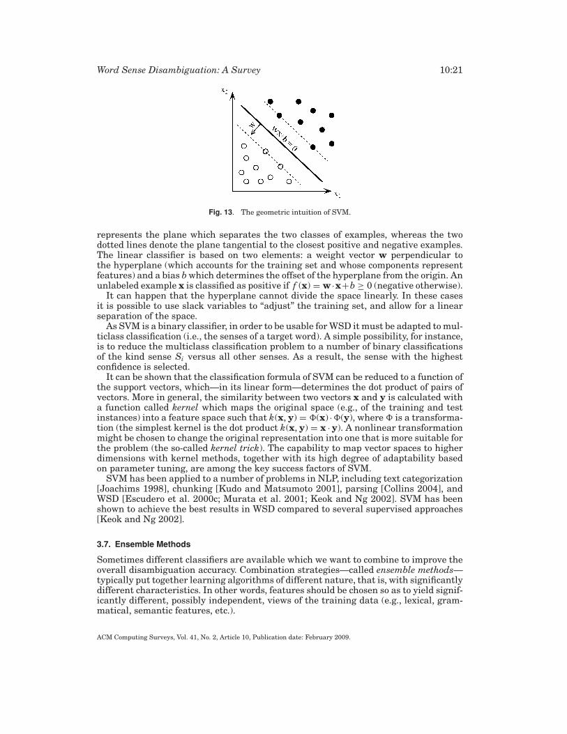
This method (introduced by Boser et al. [1992]) is based on the idea of learning alinear hyperplane from the training set that separates positive examples from negativeexamples. The hyperplane is located in that point of the hyperspace which maximizesthe distance to the closest positive and negative examples (called support vectors). Inother words, support vector machines (SVMs) tend at the same time to minimize theempirical classification error and maximize the geometric margin between positiveand negative examples. Figure 13 illustrates the geometric intuition: the line in bold
ACM Computing Surveys, Vol. 41, No. 2, Article 10, Publication date: February 2009.
Word Sense Disambiguation: A Survey 10:21
Fig. 13. The geometric intuition of SVM.
represents the plane which separates the two classes of examples, whereas the twodotted lines denote the plane tangential to the closest positive and negative examples.The linear classifier is based on two elements: a weight vector w perpendicular tothe hyperplane (which accounts for the training set and whose components representfeatures) and a bias b which determines the offset of the hyperplane from the origin. Anunlabeled example x is classified as positive if f (x) = w ·x+b ≥ 0 (negative otherwise).
It can happen that the hyperplane cannot divide the space linearly. In these casesit is possible to use slack variables to “adjust” the training set, and allow for a linearseparation of the space.
As SVM is a binary classifier, in order to be usable for WSD it must be adapted to mul-ticlass classification (i.e., the senses of a target word). A simple possibility, for instance,is to reduce the multiclass classification problem to a number of binary classificationsof the kind sense Si versus all other senses. As a result, the sense with the highestconfidence is selected.
It can be shown that the classification formula of SVM can be reduced to a function ofthe support vectors, which—in its linear form—determines the dot product of pairs ofvectors. More in general, the similarity between two vectors x and y is calculated witha function called kernel which maps the original space (e.g., of the training and testinstances) into a feature space such that k(x, y) = �(x) ·�(y), where � is a transforma-tion (the simplest kernel is the dot product k(x, y) = x · y). A nonlinear transformationmight be chosen to change the original representation into one that is more suitable forthe problem (the so-called kernel trick). The capability to map vector spaces to higherdimensions with kernel methods, together with its high degree of adaptability basedon parameter tuning, are among the key success factors of SVM.
SVM has been applied to a number of problems in NLP, including text categorization[Joachims 1998], chunking [Kudo and Matsumoto 2001], parsing [Collins 2004], andWSD [Escudero et al. 2000c; Murata et al. 2001; Keok and Ng 2002]. SVM has beenshown to achieve the best results in WSD compared to several supervised approaches[Keok and Ng 2002].
3.7. Ensemble Methods
Sometimes different classifiers are available which we want to combine to improve theoverall disambiguation accuracy. Combination strategies—called ensemble methods—typically put together learning algorithms of different nature, that is, with significantlydifferent characteristics. In other words, features should be chosen so as to yield signif-icantly different, possibly independent, views of the training data (e.g., lexical, gram-matical, semantic features, etc.).
ACM Computing Surveys, Vol. 41, No. 2, Article 10, Publication date: February 2009.
10:22 R. Navigli
Ensemble methods are becoming more and more popular as they allow one to over-come the weaknesses of single supervised approaches. Several systems participatingin recent evaluation campaigns employed these methods (see Section 8). Klein et al.[2002] and Florian et al. [2002] studied the combination of supervised WSD methods,achieving state-of-the-art results on the Senseval-2 lexical sample task (cf. Section8.2). Brody et al. [2006] reported a study on ensembles of unsupervised WSD methods.When employed on a standard test set, such as that of the Senseval-3 all-words WSDtask (cf. Section 8.3), ensemble methods overcome state-of-the-art performance amongunsupervised systems (up to +4% accuracy).
Single classifiers can be combined with different strategies: here we introduce major-ity voting, probability mixture, rank-based combination, and AdaBoost. Other ensemblemethods have been explored in the literature, such as weighted voting, maximum en-tropy combination, etc. (see, e.g., Klein et al. [2002]). In the following, we denote thefirst-order classifiers (i.e., the systems to be combined, or ensemble components) asC1, C2, . . . , Cm.
3.7.1. Majority Voting. Given a target word w, each ensemble component can give onevote for a sense of w. The sense S which has the majority of votes is selected:
S = argmaxSi∈SensesD(w) | { j : vote(Cj ) = Si} |,where vote is a function that, given a classifier, outputs the sense chosen by that clas-sifier. In case of tie, a random choice can be made among the senses with a majorityvote. Alternatively, the ensemble does not output any sense.
3.7.2. Probability Mixture. Supposing the first-order classifiers provide a confidencescore for each sense of a target word w, we can normalize and convert these scoresto a probability distribution over the senses of w. More formally, given a method Cj and
its scores {score(Cj , Si)}|SensesD(w)|i=1 , we can obtain a probability PCj (Si) = score(Cj ,Si )
maxk score(Cj ,Sk )
for the ith sense of w. These probabilities (i.e., normalized scores) are summed, and thesense with the highest overall score is chosen:
S = argmaxSi∈SensesD(w)
m∑j=1
PCj (Si).
3.7.3. Rank-Based Combination. Supposing that each first-order classifier provides aranking of the senses for a given target word w, the rank-based combination consistsin choosing that sense S of w which maximizes the sum of its ranks output by thesystems C1, . . . , Cm (we negate ranks so that the best ranking sense provides the highestcontribution):
S = argmaxSi∈SensesD(w)
m∑j=1
−RankCj (Si),
where RankCj (Si) is the rank of Si as output by classifier Cj (1 for the best sense, 2 forthe second best sense, and so on).
3.7.4. AdaBoost. AdaBoost or adaptive boosting [Freund and Schapire 1999] is a gen-eral method for constructing a “strong” classifier as a linear combination of several
ACM Computing Surveys, Vol. 41, No. 2, Article 10, Publication date: February 2009.
Word Sense Disambiguation: A Survey 10:23
“weak” classifiers. The method is adaptive in the sense that it tunes subsequent clas-sifiers in favor of those instances misclassified by previous classifiers. AdaBoost learnsthe classifiers from a weighted training set (initially, all the instances in the data setare equally weighted). The algorithm performs m iterations, one for each classifier.At each iteration, the weights of incorrectly classified examples are increased, so asto cause subsequent classifiers to focus on those examples (thus reducing the overallclassification error). As a result of each iteration j ∈ {1, . . . , m}, a weight α j is acquiredfor classifier Cj which is typically a function of the classification error of Cj over thetraining set. The classifiers are combined as follows:
H(x) = sign
(m∑
j=1
α j Cj (x)
),
where x is an example from the training set, C1, . . . , Cm are the first-order classifiersthat we want to improve, α j determines the importance of classifier Cj , and H is theresulting “strong” classifier. H is the sign function of the linear combination of the“weak” classifiers, which is interpreted as the predicted class (the basic AdaBoost worksonly with binary outputs, −1 or +1). The confidence of this choice is given by themagnitude of its argument. An extension of AdaBoost which deals with multiclassmultilabel classification is AdaBoost.MH [Schapire and Singer 1999].
AdaBoost has its roots in a theoretical framework for studying machine learningcalled the Probably Approximately Correct (PAC) learning model. It is sensitive to noisydata and outliers, although it is less susceptible to the overfitting problem than mostlearning algorithms. An application of AdaBoost to WSD was illustrated by Escuderoet al. [2000a].
3.8. Minimally and Semisupervised Disambiguation
The boundary between supervised and unsupervised disambiguation is not alwaysclearcut. In fact, we can define minimally or semisupervised methods which learnsense classifiers from annotated data with minimal or partial human supervision, re-spectively. In this section we describe two WSD approaches of this kind, based on theautomatic bootstrapping of a corpus from a small number of manually tagged examplesand on the use of monosemous relatives.
3.8.1. Bootstrapping. The aim of bootstrapping is to build a sense classifier with lit-tle training data, and thus overcome the main problems of supervision: the lack ofannotated data and the data sparsity problem. Bootstrapping usually starts from fewannotated data A, a large corpus of unannotated data U , and a set of one or more basicclassifiers. As a result of iterative applications of a bootstrapping algorithm, the an-notated corpus A grows increasingly and the untagged data set U shrinks until somethreshold is reached for the remaining examples in U . The small set of initial examplesin A can be generated from hand-labeling [Hearst 1991] or from the automatic selectionwith the aid of accurate heuristics [Yarowsky 1995].
There are two main approaches to bootstrapping in WSD: cotraining and self-training. Both approaches create a subset U ′ ⊂ U of p unlabeled examples chosen atrandom. Each classifier is trained on the annotated data set A and applied to label theset of examples in U ′. As a result of labeling, the most reliable examples are selectedaccording to some criterion, and added to A. The procedure is repeated several times(at each iteration U ′ includes a new subset of p random examples from U ). Within thissetting, the main difference between cotraining and self-training is that the formeralternates two classifiers, whereas the latter uses only one classifier, and at each
ACM Computing Surveys, Vol. 41, No. 2, Article 10, Publication date: February 2009.
10:24 R. Navigli
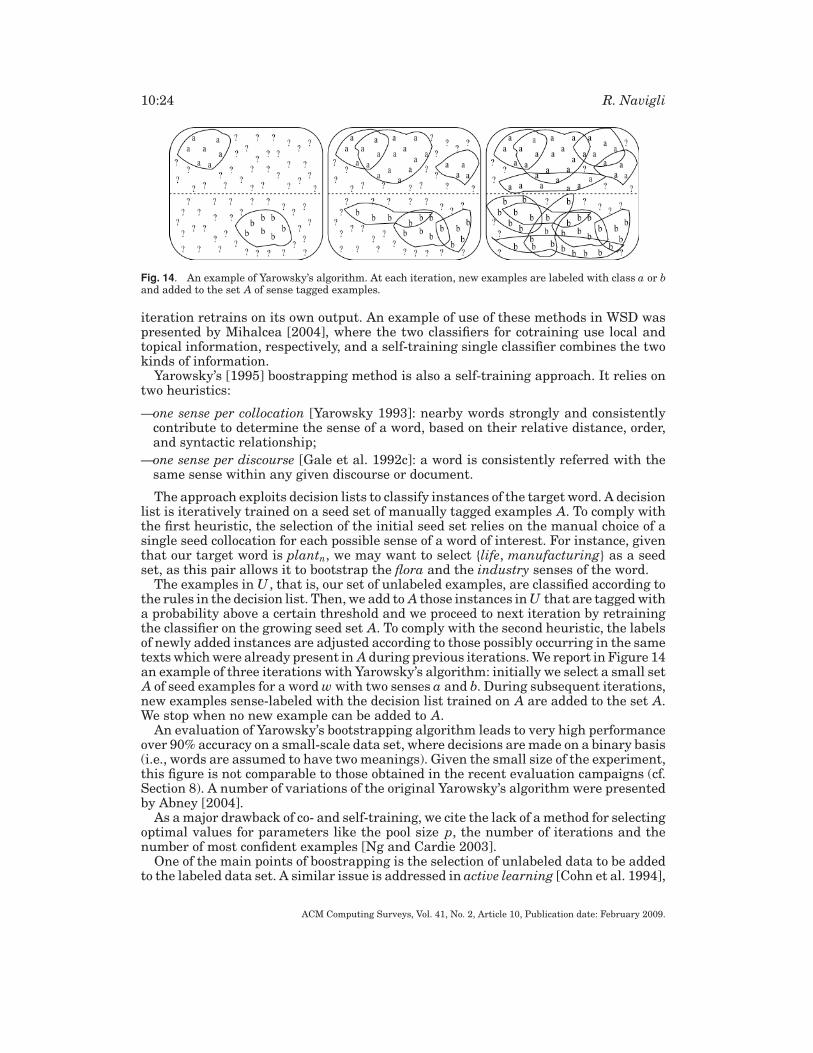
Fig. 14. An example of Yarowsky’s algorithm. At each iteration, new examples are labeled with class a or band added to the set A of sense tagged examples.
iteration retrains on its own output. An example of use of these methods in WSD waspresented by Mihalcea [2004], where the two classifiers for cotraining use local andtopical information, respectively, and a self-training single classifier combines the twokinds of information.
Yarowsky’s [1995] boostrapping method is also a self-training approach. It relies ontwo heuristics:
—one sense per collocation [Yarowsky 1993]: nearby words strongly and consistentlycontribute to determine the sense of a word, based on their relative distance, order,and syntactic relationship;
—one sense per discourse [Gale et al. 1992c]: a word is consistently referred with thesame sense within any given discourse or document.
The approach exploits decision lists to classify instances of the target word. A decisionlist is iteratively trained on a seed set of manually tagged examples A. To comply withthe first heuristic, the selection of the initial seed set relies on the manual choice of asingle seed collocation for each possible sense of a word of interest. For instance, giventhat our target word is plantn, we may want to select {life, manufacturing} as a seedset, as this pair allows it to bootstrap the flora and the industry senses of the word.
The examples in U , that is, our set of unlabeled examples, are classified according tothe rules in the decision list. Then, we add to A those instances in U that are tagged witha probability above a certain threshold and we proceed to next iteration by retrainingthe classifier on the growing seed set A. To comply with the second heuristic, the labelsof newly added instances are adjusted according to those possibly occurring in the sametexts which were already present in A during previous iterations. We report in Figure 14an example of three iterations with Yarowsky’s algorithm: initially we select a small setA of seed examples for a word w with two senses a and b. During subsequent iterations,new examples sense-labeled with the decision list trained on A are added to the set A.We stop when no new example can be added to A.
An evaluation of Yarowsky’s bootstrapping algorithm leads to very high performanceover 90% accuracy on a small-scale data set, where decisions are made on a binary basis(i.e., words are assumed to have two meanings). Given the small size of the experiment,this figure is not comparable to those obtained in the recent evaluation campaigns (cf.Section 8). A number of variations of the original Yarowsky’s algorithm were presentedby Abney [2004].
As a major drawback of co- and self-training, we cite the lack of a method for selectingoptimal values for parameters like the pool size p, the number of iterations and thenumber of most confident examples [Ng and Cardie 2003].
One of the main points of boostrapping is the selection of unlabeled data to be addedto the labeled data set. A similar issue is addressed in active learning [Cohn et al. 1994],
ACM Computing Surveys, Vol. 41, No. 2, Article 10, Publication date: February 2009.
Word Sense Disambiguation: A Survey 10:25
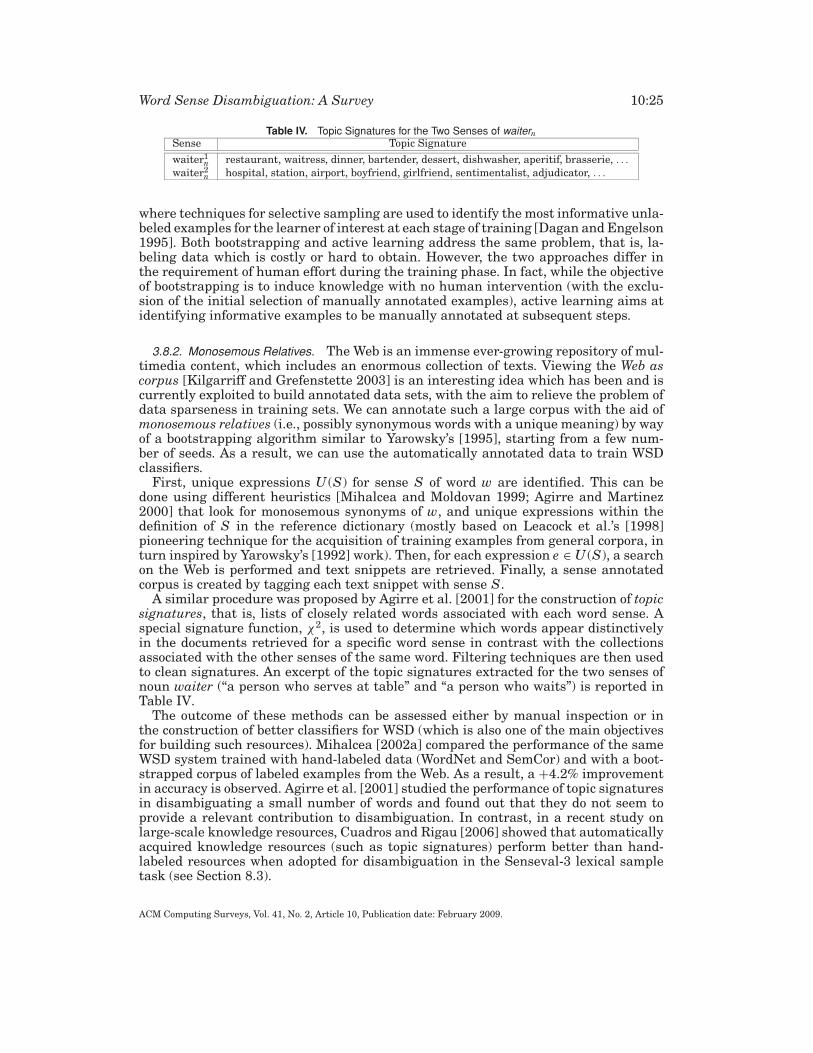
Table IV. Topic Signatures for the Two Senses of waiternSense Topic Signature
waiter1n restaurant, waitress, dinner, bartender, dessert, dishwasher, aperitif, brasserie, . . .
waiter2n hospital, station, airport, boyfriend, girlfriend, sentimentalist, adjudicator, . . .
where techniques for selective sampling are used to identify the most informative unla-beled examples for the learner of interest at each stage of training [Dagan and Engelson1995]. Both bootstrapping and active learning address the same problem, that is, la-beling data which is costly or hard to obtain. However, the two approaches differ inthe requirement of human effort during the training phase. In fact, while the objectiveof bootstrapping is to induce knowledge with no human intervention (with the exclu-sion of the initial selection of manually annotated examples), active learning aims atidentifying informative examples to be manually annotated at subsequent steps.
3.8.2. Monosemous Relatives. The Web is an immense ever-growing repository of mul-timedia content, which includes an enormous collection of texts. Viewing the Web ascorpus [Kilgarriff and Grefenstette 2003] is an interesting idea which has been and iscurrently exploited to build annotated data sets, with the aim to relieve the problem ofdata sparseness in training sets. We can annotate such a large corpus with the aid ofmonosemous relatives (i.e., possibly synonymous words with a unique meaning) by wayof a bootstrapping algorithm similar to Yarowsky’s [1995], starting from a few num-ber of seeds. As a result, we can use the automatically annotated data to train WSDclassifiers.
First, unique expressions U (S) for sense S of word w are identified. This can bedone using different heuristics [Mihalcea and Moldovan 1999; Agirre and Martinez2000] that look for monosemous synonyms of w, and unique expressions within thedefinition of S in the reference dictionary (mostly based on Leacock et al.’s [1998]pioneering technique for the acquisition of training examples from general corpora, inturn inspired by Yarowsky’s [1992] work). Then, for each expression e ∈ U (S), a searchon the Web is performed and text snippets are retrieved. Finally, a sense annotatedcorpus is created by tagging each text snippet with sense S.
A similar procedure was proposed by Agirre et al. [2001] for the construction of topicsignatures, that is, lists of closely related words associated with each word sense. Aspecial signature function, χ2, is used to determine which words appear distinctivelyin the documents retrieved for a specific word sense in contrast with the collectionsassociated with the other senses of the same word. Filtering techniques are then usedto clean signatures. An excerpt of the topic signatures extracted for the two senses ofnoun waiter (“a person who serves at table” and “a person who waits”) is reported inTable IV.
The outcome of these methods can be assessed either by manual inspection or inthe construction of better classifiers for WSD (which is also one of the main objectivesfor building such resources). Mihalcea [2002a] compared the performance of the sameWSD system trained with hand-labeled data (WordNet and SemCor) and with a boot-strapped corpus of labeled examples from the Web. As a result, a +4.2% improvementin accuracy is observed. Agirre et al. [2001] studied the performance of topic signaturesin disambiguating a small number of words and found out that they do not seem toprovide a relevant contribution to disambiguation. In contrast, in a recent study onlarge-scale knowledge resources, Cuadros and Rigau [2006] showed that automaticallyacquired knowledge resources (such as topic signatures) perform better than hand-labeled resources when adopted for disambiguation in the Senseval-3 lexical sampletask (see Section 8.3).
ACM Computing Surveys, Vol. 41, No. 2, Article 10, Publication date: February 2009.
10:26 R. Navigli
4. UNSUPERVISED DISAMBIGUATION
Unsupervised methods have the potential to overcome the knowledge acquisition bot-tleneck [Gale et al. 1992b], that is, the lack of large-scale resources manually annotatedwith word senses. These approaches to WSD are based on the idea that the same senseof a word will have similar neighboring words. They are able to induce word senses frominput text by clustering word occurrences, and then classifying new occurrences into theinduced clusters. They do not rely on labeled training text and, in their purest version,do not make use of any machine–readable resources like dictionaries, thesauri, ontolo-gies, etc. However, the main disadvantage of fully unsupervised systems is that, as theydo not exploit any dictionary, they cannot rely on a shared reference inventory of senses.
While WSD is typically identified as a sense labeling task, that is, the explicit as-signment of a sense label to a target word, unsupervised WSD performs word sensediscrimination, that is, it aims to divide “the occurrences of a word into a number ofclasses by determining for any two occurrences whether they belong to the same senseor not” [Schutze 1998, page 97]. Consequently, these methods may not discover clus-ters equivalent to the traditional senses in a dictionary sense inventory. For this reason,their evaluation is usually more difficult: in order to assess the quality of a sense clus-ter we should ask humans to look at the members of each cluster and determine thenature of the relationship that they all share (e.g., via questionnaires), or employ theclusters in end-to-end applications, thus measuring the quality of the former based onthe performance of the latter.
Admittedly, unsupervised WSD approaches have a different aim than supervised andknowledge-based methods, that is, that of identifying sense clusters compared to thatof assigning sense labels. However, sense discrimination and sense labeling are bothsubproblems of the word sense disambiguation task [Schutze 1998] and are strictlyrelated, to the point that the clusters produced can be used at a later stage to sense tagword occurrences.
Hereafter, we present the main approaches to unsupervised WSD, namely: methodsbased on context clustering (Section 4.1), word clustering (Section 4.2), and cooccurrencegraphs (Section 4.3). For further discussion on the topic the reader can refer to Manningand Schutze [1999] and Pedersen [2006].
4.1. Context Clustering
A first set of unsupervised approaches is based on the notion of context clustering. Eachoccurrence of a target word in a corpus is represented as a context vector. The vectorsare then clustered into groups, each identifying a sense of the target word.
A historical approach of this kind is based on the idea of word space [Schutze 1992].that is, a vector space whose dimensions are words. A word w in a corpus can berepresented as a vector whose j th component counts the number of times that word wjcooccurs with w within a fixed context (a sentence or a larger context). The underlyinghypothesis of this model is that the distributional profile of words implicitly expressestheir semantics.
Figure 15(a) shows two examples of word vectors, restaurant = (210, 80) and money =(100, 250), where the first dimension represents the count of cooccurrences with wordfood and the second counts the cooccurrences with bank.
The similarity between two words v and w can then be measured geometrically, forexample, by the cosine between the corresponding vectors v and w:
sim(v, w) = v · w| v || w | =
∑mi=1 viwi√∑m
i=1 v2i∑m
i=1 w2i
,
ACM Computing Surveys, Vol. 41, No. 2, Article 10, Publication date: February 2009.
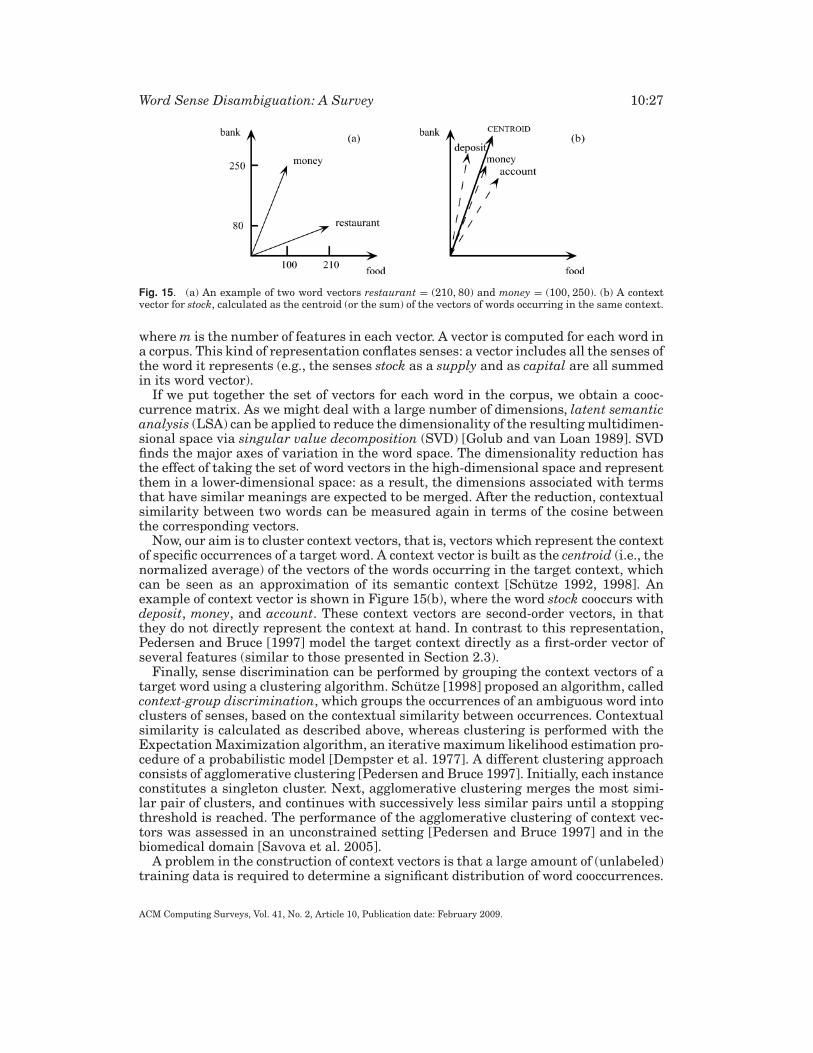
Word Sense Disambiguation: A Survey 10:27
Fig. 15. (a) An example of two word vectors restaurant = (210, 80) and money = (100, 250). (b) A contextvector for stock, calculated as the centroid (or the sum) of the vectors of words occurring in the same context.
where m is the number of features in each vector. A vector is computed for each word ina corpus. This kind of representation conflates senses: a vector includes all the senses ofthe word it represents (e.g., the senses stock as a supply and as capital are all summedin its word vector).
If we put together the set of vectors for each word in the corpus, we obtain a cooc-currence matrix. As we might deal with a large number of dimensions, latent semanticanalysis (LSA) can be applied to reduce the dimensionality of the resulting multidimen-sional space via singular value decomposition (SVD) [Golub and van Loan 1989]. SVDfinds the major axes of variation in the word space. The dimensionality reduction hasthe effect of taking the set of word vectors in the high-dimensional space and representthem in a lower-dimensional space: as a result, the dimensions associated with termsthat have similar meanings are expected to be merged. After the reduction, contextualsimilarity between two words can be measured again in terms of the cosine betweenthe corresponding vectors.
Now, our aim is to cluster context vectors, that is, vectors which represent the contextof specific occurrences of a target word. A context vector is built as the centroid (i.e., thenormalized average) of the vectors of the words occurring in the target context, whichcan be seen as an approximation of its semantic context [Schutze 1992, 1998]. Anexample of context vector is shown in Figure 15(b), where the word stock cooccurs withdeposit, money, and account. These context vectors are second-order vectors, in thatthey do not directly represent the context at hand. In contrast to this representation,Pedersen and Bruce [1997] model the target context directly as a first-order vector ofseveral features (similar to those presented in Section 2.3).
Finally, sense discrimination can be performed by grouping the context vectors of atarget word using a clustering algorithm. Schutze [1998] proposed an algorithm, calledcontext-group discrimination, which groups the occurrences of an ambiguous word intoclusters of senses, based on the contextual similarity between occurrences. Contextualsimilarity is calculated as described above, whereas clustering is performed with theExpectation Maximization algorithm, an iterative maximum likelihood estimation pro-cedure of a probabilistic model [Dempster et al. 1977]. A different clustering approachconsists of agglomerative clustering [Pedersen and Bruce 1997]. Initially, each instanceconstitutes a singleton cluster. Next, agglomerative clustering merges the most simi-lar pair of clusters, and continues with successively less similar pairs until a stoppingthreshold is reached. The performance of the agglomerative clustering of context vec-tors was assessed in an unconstrained setting [Pedersen and Bruce 1997] and in thebiomedical domain [Savova et al. 2005].
A problem in the construction of context vectors is that a large amount of (unlabeled)training data is required to determine a significant distribution of word cooccurrences.
ACM Computing Surveys, Vol. 41, No. 2, Article 10, Publication date: February 2009.
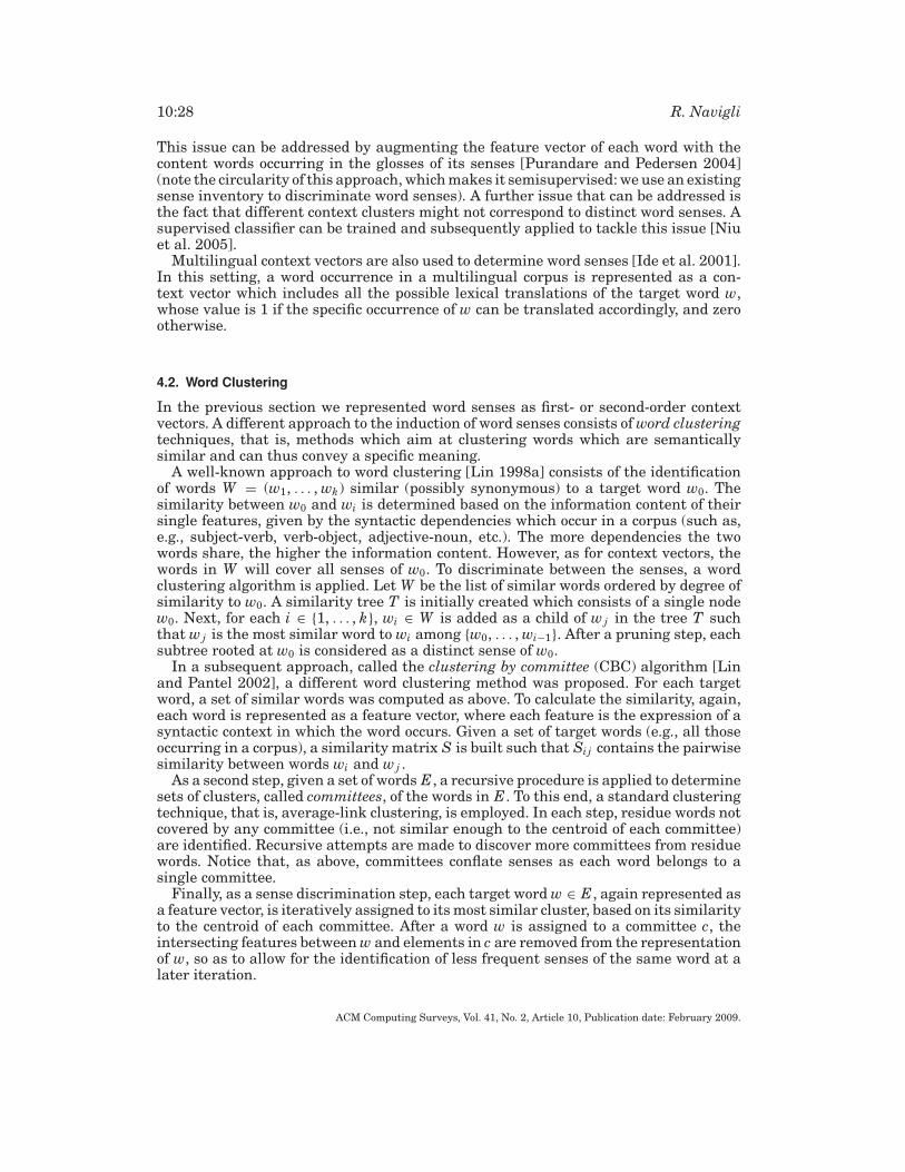
10:28 R. Navigli
This issue can be addressed by augmenting the feature vector of each word with thecontent words occurring in the glosses of its senses [Purandare and Pedersen 2004](note the circularity of this approach, which makes it semisupervised: we use an existingsense inventory to discriminate word senses). A further issue that can be addressed isthe fact that different context clusters might not correspond to distinct word senses. Asupervised classifier can be trained and subsequently applied to tackle this issue [Niuet al. 2005].
Multilingual context vectors are also used to determine word senses [Ide et al. 2001].In this setting, a word occurrence in a multilingual corpus is represented as a con-text vector which includes all the possible lexical translations of the target word w,whose value is 1 if the specific occurrence of w can be translated accordingly, and zerootherwise.
4.2. Word Clustering
In the previous section we represented word senses as first- or second-order contextvectors. A different approach to the induction of word senses consists of word clusteringtechniques, that is, methods which aim at clustering words which are semanticallysimilar and can thus convey a specific meaning.
A well-known approach to word clustering [Lin 1998a] consists of the identificationof words W = (w1, . . . , wk) similar (possibly synonymous) to a target word w0. Thesimilarity between w0 and wi is determined based on the information content of theirsingle features, given by the syntactic dependencies which occur in a corpus (such as,e.g., subject-verb, verb-object, adjective-noun, etc.). The more dependencies the twowords share, the higher the information content. However, as for context vectors, thewords in W will cover all senses of w0. To discriminate between the senses, a wordclustering algorithm is applied. Let W be the list of similar words ordered by degree ofsimilarity to w0. A similarity tree T is initially created which consists of a single nodew0. Next, for each i ∈ {1, . . . , k}, wi ∈ W is added as a child of wj in the tree T suchthat wj is the most similar word to wi among {w0, . . . , wi−1}. After a pruning step, eachsubtree rooted at w0 is considered as a distinct sense of w0.
In a subsequent approach, called the clustering by committee (CBC) algorithm [Linand Pantel 2002], a different word clustering method was proposed. For each targetword, a set of similar words was computed as above. To calculate the similarity, again,each word is represented as a feature vector, where each feature is the expression of asyntactic context in which the word occurs. Given a set of target words (e.g., all thoseoccurring in a corpus), a similarity matrix S is built such that Sij contains the pairwisesimilarity between words wi and wj .
As a second step, given a set of words E, a recursive procedure is applied to determinesets of clusters, called committees, of the words in E. To this end, a standard clusteringtechnique, that is, average-link clustering, is employed. In each step, residue words notcovered by any committee (i.e., not similar enough to the centroid of each committee)are identified. Recursive attempts are made to discover more committees from residuewords. Notice that, as above, committees conflate senses as each word belongs to asingle committee.
Finally, as a sense discrimination step, each target word w ∈ E, again represented asa feature vector, is iteratively assigned to its most similar cluster, based on its similarityto the centroid of each committee. After a word w is assigned to a committee c, theintersecting features between w and elements in c are removed from the representationof w, so as to allow for the identification of less frequent senses of the same word at alater iteration.
ACM Computing Surveys, Vol. 41, No. 2, Article 10, Publication date: February 2009.
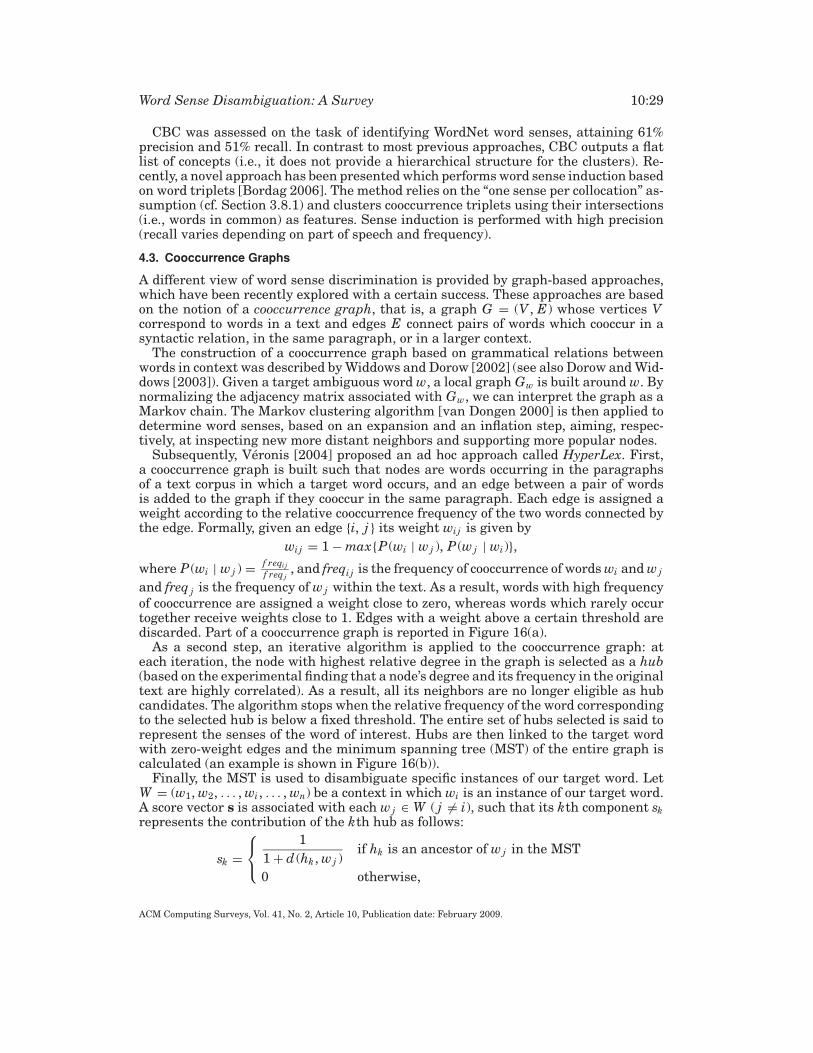
Word Sense Disambiguation: A Survey 10:29
CBC was assessed on the task of identifying WordNet word senses, attaining 61%precision and 51% recall. In contrast to most previous approaches, CBC outputs a flatlist of concepts (i.e., it does not provide a hierarchical structure for the clusters). Re-cently, a novel approach has been presented which performs word sense induction basedon word triplets [Bordag 2006]. The method relies on the “one sense per collocation” as-sumption (cf. Section 3.8.1) and clusters cooccurrence triplets using their intersections(i.e., words in common) as features. Sense induction is performed with high precision(recall varies depending on part of speech and frequency).
4.3. Cooccurrence Graphs
A different view of word sense discrimination is provided by graph-based approaches,which have been recently explored with a certain success. These approaches are basedon the notion of a cooccurrence graph, that is, a graph G = (V , E) whose vertices Vcorrespond to words in a text and edges E connect pairs of words which cooccur in asyntactic relation, in the same paragraph, or in a larger context.
The construction of a cooccurrence graph based on grammatical relations betweenwords in context was described by Widdows and Dorow [2002] (see also Dorow and Wid-dows [2003]). Given a target ambiguous word w, a local graph Gw is built around w. Bynormalizing the adjacency matrix associated with Gw, we can interpret the graph as aMarkov chain. The Markov clustering algorithm [van Dongen 2000] is then applied todetermine word senses, based on an expansion and an inflation step, aiming, respec-tively, at inspecting new more distant neighbors and supporting more popular nodes.
Subsequently, Veronis [2004] proposed an ad hoc approach called HyperLex. First,a cooccurrence graph is built such that nodes are words occurring in the paragraphsof a text corpus in which a target word occurs, and an edge between a pair of wordsis added to the graph if they cooccur in the same paragraph. Each edge is assigned aweight according to the relative cooccurrence frequency of the two words connected bythe edge. Formally, given an edge {i, j } its weight wij is given by
wij = 1 − max{P (wi | wj ), P (wj | wi)},where P (wi | wj ) = f reqi j
f req j, and freqi j is the frequency of cooccurrence of words wi and wj
and freq j is the frequency of wj within the text. As a result, words with high frequency
of cooccurrence are assigned a weight close to zero, whereas words which rarely occurtogether receive weights close to 1. Edges with a weight above a certain threshold arediscarded. Part of a cooccurrence graph is reported in Figure 16(a).
As a second step, an iterative algorithm is applied to the cooccurrence graph: ateach iteration, the node with highest relative degree in the graph is selected as a hub(based on the experimental finding that a node’s degree and its frequency in the originaltext are highly correlated). As a result, all its neighbors are no longer eligible as hubcandidates. The algorithm stops when the relative frequency of the word correspondingto the selected hub is below a fixed threshold. The entire set of hubs selected is said torepresent the senses of the word of interest. Hubs are then linked to the target wordwith zero-weight edges and the minimum spanning tree (MST) of the entire graph iscalculated (an example is shown in Figure 16(b)).
Finally, the MST is used to disambiguate specific instances of our target word. LetW = (w1, w2, . . . , wi, . . . , wn) be a context in which wi is an instance of our target word.A score vector s is associated with each wj ∈ W ( j �= i), such that its kth component skrepresents the contribution of the kth hub as follows:
sk =⎧⎨⎩
1
1 + d (hk , wj )if hk is an ancestor of wj in the MST
0 otherwise,
ACM Computing Surveys, Vol. 41, No. 2, Article 10, Publication date: February 2009.
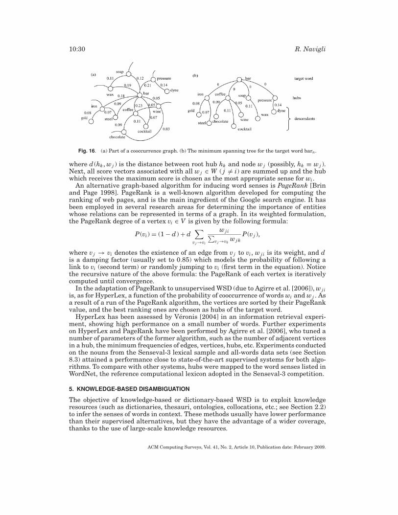
10:30 R. Navigli
Fig. 16. (a) Part of a cooccurrence graph. (b) The minimum spanning tree for the target word barn.
where d (hk , wj ) is the distance between root hub hk and node wj (possibly, hk ≡ wj ).Next, all score vectors associated with all wj ∈ W ( j �= i) are summed up and the hubwhich receives the maximum score is chosen as the most appropriate sense for wi.
An alternative graph-based algorithm for inducing word senses is PageRank [Brinand Page 1998]. PageRank is a well-known algorithm developed for computing theranking of web pages, and is the main ingredient of the Google search engine. It hasbeen employed in several research areas for determining the importance of entitieswhose relations can be represented in terms of a graph. In its weighted formulation,the PageRank degree of a vertex vi ∈ V is given by the following formula:
P (vi) = (1 − d ) + d∑
vj →vi
w j i∑vj →vk
w j kP (vj ),
where vj → vi denotes the existence of an edge from vj to vi, wji is its weight, and dis a damping factor (usually set to 0.85) which models the probability of following alink to vi (second term) or randomly jumping to vi (first term in the equation). Noticethe recursive nature of the above formula: the PageRank of each vertex is iterativelycomputed until convergence.
In the adaptation of PageRank to unsupervised WSD (due to Agirre et al. [2006]), wjiis, as for HyperLex, a function of the probability of cooccurrence of words wi and wj . Asa result of a run of the PageRank algorithm, the vertices are sorted by their PageRankvalue, and the best ranking ones are chosen as hubs of the target word.
HyperLex has been assessed by Veronis [2004] in an information retrieval experi-ment, showing high performance on a small number of words. Further experimentson HyperLex and PageRank have been performed by Agirre et al. [2006], who tuned anumber of parameters of the former algorithm, such as the number of adjacent verticesin a hub, the minimum frequencies of edges, vertices, hubs, etc. Experiments conductedon the nouns from the Senseval-3 lexical sample and all-words data sets (see Section8.3) attained a performance close to state-of-the-art supervised systems for both algo-rithms. To compare with other systems, hubs were mapped to the word senses listed inWordNet, the reference computational lexicon adopted in the Senseval-3 competition.
5. KNOWLEDGE-BASED DISAMBIGUATION
The objective of knowledge-based or dictionary-based WSD is to exploit knowledgeresources (such as dictionaries, thesauri, ontologies, collocations, etc.; see Section 2.2)to infer the senses of words in context. These methods usually have lower performancethan their supervised alternatives, but they have the advantage of a wider coverage,thanks to the use of large-scale knowledge resources.
ACM Computing Surveys, Vol. 41, No. 2, Article 10, Publication date: February 2009.
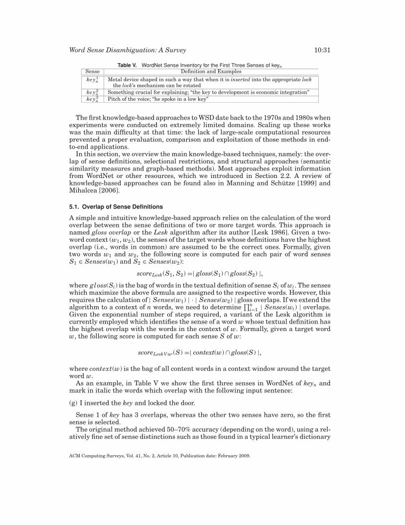
Word Sense Disambiguation: A Survey 10:31
Table V. WordNet Sense Inventory for the First Three Senses of keynSense Definition and Examples
ke y1n Metal device shaped in such a way that when it is inserted into the appropriate lock
the lock’s mechanism can be rotated
ke y2n Something crucial for explaining; “the key to development is economic integration”
ke y3n Pitch of the voice; “he spoke in a low key”
The first knowledge-based approaches to WSD date back to the 1970s and 1980s whenexperiments were conducted on extremely limited domains. Scaling up these workswas the main difficulty at that time: the lack of large-scale computational resourcesprevented a proper evaluation, comparison and exploitation of those methods in end-to-end applications.
In this section, we overview the main knowledge-based techniques, namely: the over-lap of sense definitions, selectional restrictions, and structural approaches (semanticsimilarity measures and graph-based methods). Most approaches exploit informationfrom WordNet or other resources, which we introduced in Section 2.2. A review ofknowledge-based approaches can be found also in Manning and Schutze [1999] andMihalcea [2006].
5.1. Overlap of Sense Definitions
A simple and intuitive knowledge-based approach relies on the calculation of the wordoverlap between the sense definitions of two or more target words. This approach isnamed gloss overlap or the Lesk algorithm after its author [Lesk 1986]. Given a two-word context (w1, w2), the senses of the target words whose definitions have the highestoverlap (i.e., words in common) are assumed to be the correct ones. Formally, giventwo words w1 and w2, the following score is computed for each pair of word sensesS1 ∈ Senses(w1) and S2 ∈ Senses(w2):
scoreLesk(S1, S2) =| gloss(S1) ∩ gloss(S2) |,where gloss(Si) is the bag of words in the textual definition of sense Si of wi. The senseswhich maximize the above formula are assigned to the respective words. However, thisrequires the calculation of | Senses(w1) | · | Senses(w2) | gloss overlaps. If we extend thealgorithm to a context of n words, we need to determine
∏ni=1 | Senses(wi) | overlaps.
Given the exponential number of steps required, a variant of the Lesk algorithm iscurrently employed which identifies the sense of a word w whose textual definition hasthe highest overlap with the words in the context of w. Formally, given a target wordw, the following score is computed for each sense S of w:
scoreLeskV ar (S) =| context(w) ∩ gloss(S) |,
where context(w) is the bag of all content words in a context window around the targetword w.
As an example, in Table V we show the first three senses in WordNet of keyn andmark in italic the words which overlap with the following input sentence:
(g) I inserted the key and locked the door.
Sense 1 of key has 3 overlaps, whereas the other two senses have zero, so the firstsense is selected.
The original method achieved 50–70% accuracy (depending on the word), using a rel-atively fine set of sense distinctions such as those found in a typical learner’s dictionary
ACM Computing Surveys, Vol. 41, No. 2, Article 10, Publication date: February 2009.
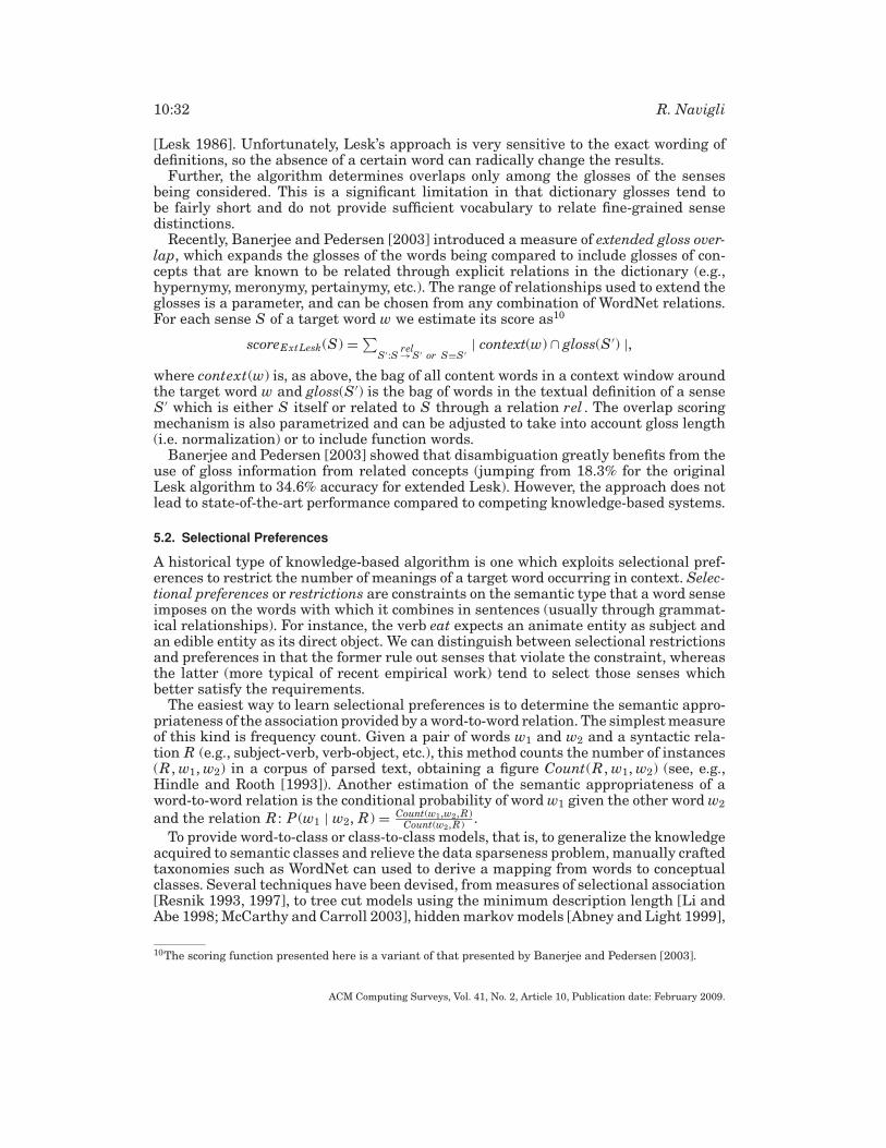
10:32 R. Navigli
[Lesk 1986]. Unfortunately, Lesk’s approach is very sensitive to the exact wording ofdefinitions, so the absence of a certain word can radically change the results.
Further, the algorithm determines overlaps only among the glosses of the sensesbeing considered. This is a significant limitation in that dictionary glosses tend tobe fairly short and do not provide sufficient vocabulary to relate fine-grained sensedistinctions.
Recently, Banerjee and Pedersen [2003] introduced a measure of extended gloss over-lap, which expands the glosses of the words being compared to include glosses of con-cepts that are known to be related through explicit relations in the dictionary (e.g.,hypernymy, meronymy, pertainymy, etc.). The range of relationships used to extend theglosses is a parameter, and can be chosen from any combination of WordNet relations.For each sense S of a target word w we estimate its score as10
scoreExtLesk(S) = ∑S′:S →rel
S′ or S≡S′| context(w) ∩ gloss(S′) |,
where context(w) is, as above, the bag of all content words in a context window aroundthe target word w and gloss(S′) is the bag of words in the textual definition of a senseS′ which is either S itself or related to S through a relation rel . The overlap scoringmechanism is also parametrized and can be adjusted to take into account gloss length(i.e. normalization) or to include function words.
Banerjee and Pedersen [2003] showed that disambiguation greatly benefits from theuse of gloss information from related concepts (jumping from 18.3% for the originalLesk algorithm to 34.6% accuracy for extended Lesk). However, the approach does notlead to state-of-the-art performance compared to competing knowledge-based systems.
5.2. Selectional Preferences
A historical type of knowledge-based algorithm is one which exploits selectional pref-erences to restrict the number of meanings of a target word occurring in context. Selec-tional preferences or restrictions are constraints on the semantic type that a word senseimposes on the words with which it combines in sentences (usually through grammat-ical relationships). For instance, the verb eat expects an animate entity as subject andan edible entity as its direct object. We can distinguish between selectional restrictionsand preferences in that the former rule out senses that violate the constraint, whereasthe latter (more typical of recent empirical work) tend to select those senses whichbetter satisfy the requirements.
The easiest way to learn selectional preferences is to determine the semantic appro-priateness of the association provided by a word-to-word relation. The simplest measureof this kind is frequency count. Given a pair of words w1 and w2 and a syntactic rela-tion R (e.g., subject-verb, verb-object, etc.), this method counts the number of instances(R, w1, w2) in a corpus of parsed text, obtaining a figure Count(R, w1, w2) (see, e.g.,Hindle and Rooth [1993]). Another estimation of the semantic appropriateness of aword-to-word relation is the conditional probability of word w1 given the other word w2
and the relation R: P (w1 | w2, R) = Count(w1,w2,R)Count(w2,R)
.
To provide word-to-class or class-to-class models, that is, to generalize the knowledgeacquired to semantic classes and relieve the data sparseness problem, manually craftedtaxonomies such as WordNet can used to derive a mapping from words to conceptualclasses. Several techniques have been devised, from measures of selectional association[Resnik 1993, 1997], to tree cut models using the minimum description length [Li andAbe 1998; McCarthy and Carroll 2003], hidden markov models [Abney and Light 1999],
10The scoring function presented here is a variant of that presented by Banerjee and Pedersen [2003].
ACM Computing Surveys, Vol. 41, No. 2, Article 10, Publication date: February 2009.

Word Sense Disambiguation: A Survey 10:33
class-based probability [Clark and Weir 2002; Agirre and Martinez 2001], Bayesiannetworks [Ciaramita and Johnson 2000], etc. Almost all these approaches exploit largecorpora and model the selectional preferences of predicates by combining observedfrequencies with knowledge about the semantic classes of their arguments (the latterobtained from corpora or dictionaries). Disambiguation is then performed with differentmeans based on the strength of a selectional preference towards a certain conceptualclass (i.e., sense choice).
A comparison of word-to-word, word-to-class, and class-to-class approaches was pre-sented by Agirre and Martinez [2001], who found out that the coverage grows as wemove from the former to the latter methods (26% for word-to-word preferences, 86.7%for word-to-class, 97.3% for class-to-class methods), and that precision decreases ac-cordingly (from 95.9% to 66.9% to 66.6%, respectively).
In general, we can say that approaches to WSD based on selectional restrictions havenot been found to perform as well as Lesk-based methods or the most frequent senseheuristic (see Section 7.2.2).
5.3. Structural Approaches
Since the availability of computational lexicons like WordNet, a number of structuralapproaches have been developed to analyze and exploit the structure of the conceptnetwork made available in such lexicons. The recognition and measurement of pat-terns, both in a local and a global context, can be collocated in the field of structuralpattern recognition [Fu 1982; Bunke and Sanfeliu 1990], which aims at classifying data(specifically, senses) based on the structural interrelationships of features. We presenttwo main approaches of this kind: similarity-based and graph-based methods.
5.3.1. Similarity Measures. Since the early 1990s, when WordNet was introduced, anumber of measures of semantic similarity have been developed to exploit the networkof semantic connections between word senses. Given a measure of semantic similaritydefined as
score : SensesD × SensesD → [0, 1],
where SensesD is the full set of senses listed in a reference lexicon, we can define a gen-eral disambiguation framework based on our similarity measure. We disambiguate atarget word wi in a text T = (w1, . . . , wn) by choosing the sense S of wi which maximizesthe following sum:
S = argmaxS∈SensesD(wi )
∑wj ∈T :wj �=wi
maxS′∈SensesD(wj )
score(S, S′).
Given a sense S of our target word wi, the formula sums the contribution of themost appropriate sense of each context word wj �= wi. The sense with the highest sumis chosen. Similar disambiguation strategies can be applied (e.g., thresholds can beintroduced; cf. Pedersen et al. [2005]). We now turn to the most well-known measuresof semantic similarity in the literature.
Rada et al. [1989] introduced a simple metric based on the calculation of the shortestdistance in WordNet between pairs of word senses. The hypothesis is that, given a pairof words w and w′ occurring in the same context, choosing the senses that minimize thedistance between them selects the most appropriate meanings. The measure is definedas follows:
scoreRada(Sw, Sw′ ) = d (Sw, Sw′ ),
ACM Computing Surveys, Vol. 41, No. 2, Article 10, Publication date: February 2009.
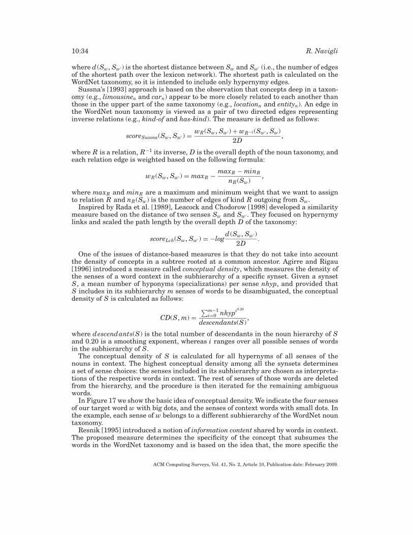
10:34 R. Navigli
where d (Sw, Sw′ ) is the shortest distance between Sw and Sw′ (i.e., the number of edgesof the shortest path over the lexicon network). The shortest path is calculated on theWordNet taxonomy, so it is intended to include only hypernymy edges.
Sussna’s [1993] approach is based on the observation that concepts deep in a taxon-omy (e.g., limousinen and carn) appear to be more closely related to each another thanthose in the upper part of the same taxonomy (e.g., locationn and entityn). An edge inthe WordNet noun taxonomy is viewed as a pair of two directed edges representinginverse relations (e.g., kind-of and has-kind). The measure is defined as follows:
scoreSussna(Sw, Sw′ ) = wR(Sw, Sw′ ) + wR−1 (Sw′ , Sw)
2D,
where R is a relation, R−1 its inverse, D is the overall depth of the noun taxonomy, andeach relation edge is weighted based on the following formula:
wR(Sw, Sw′ ) = maxR − maxR − minR
nR(Sw),
where maxR and minR are a maximum and minimum weight that we want to assignto relation R and nR(Sw) is the number of edges of kind R outgoing from Sw.
Inspired by Rada et al. [1989], Leacock and Chodorow [1998] developed a similaritymeasure based on the distance of two senses Sw and Sw′ . They focused on hypernymylinks and scaled the path length by the overall depth D of the taxonomy:
scoreLch(Sw, Sw′ ) = −logd (Sw, Sw′)
2D.
One of the issues of distance-based measures is that they do not take into accountthe density of concepts in a subtree rooted at a common ancestor. Agirre and Rigau[1996] introduced a measure called conceptual density, which measures the density ofthe senses of a word context in the subhierarchy of a specific synset. Given a synsetS, a mean number of hyponyms (specializations) per sense nhyp, and provided thatS includes in its subhierarchy m senses of words to be disambiguated, the conceptualdensity of S is calculated as follows:
CD(S, m) =∑m−1
i=0 nhypi0.20
descendants(S),
where descendants(S) is the total number of descendants in the noun hierarchy of Sand 0.20 is a smoothing exponent, whereas i ranges over all possible senses of wordsin the subhierarchy of S.
The conceptual density of S is calculated for all hypernyms of all senses of thenouns in context. The highest conceptual density among all the synsets determinesa set of sense choices: the senses included in its subhierarchy are chosen as interpreta-tions of the respective words in context. The rest of senses of those words are deletedfrom the hierarchy, and the procedure is then iterated for the remaining ambiguouswords.
In Figure 17 we show the basic idea of conceptual density. We indicate the four sensesof our target word w with big dots, and the senses of context words with small dots. Inthe example, each sense of w belongs to a different subhierarchy of the WordNet nountaxonomy.
Resnik [1995] introduced a notion of information content shared by words in context.The proposed measure determines the specificity of the concept that subsumes thewords in the WordNet taxonomy and is based on the idea that, the more specific the
ACM Computing Surveys, Vol. 41, No. 2, Article 10, Publication date: February 2009.
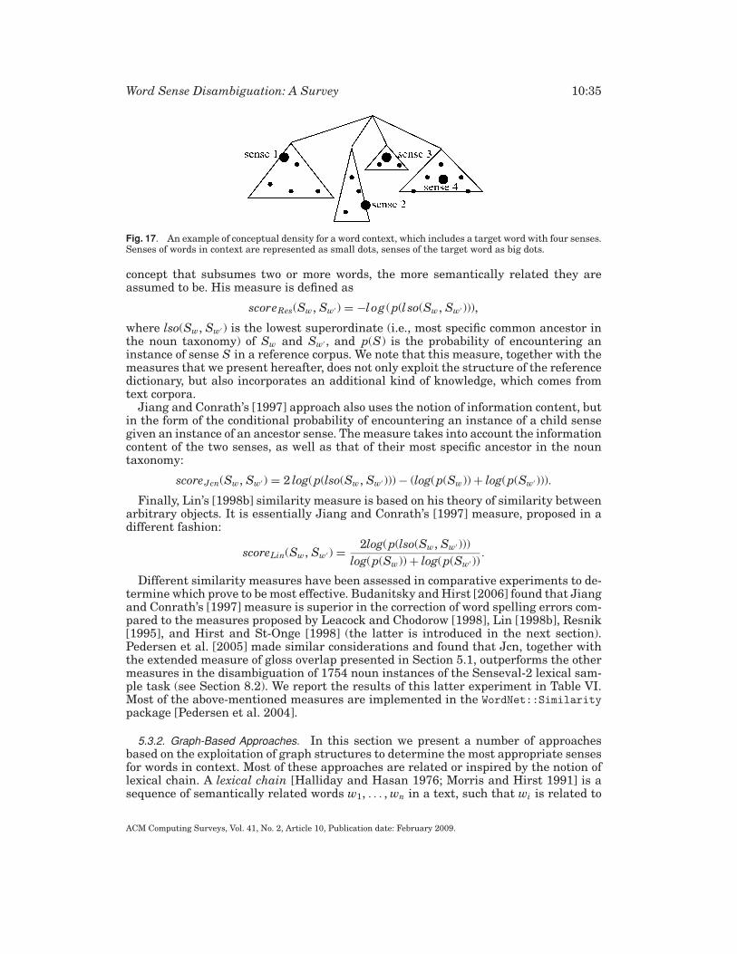
Word Sense Disambiguation: A Survey 10:35
Fig. 17. An example of conceptual density for a word context, which includes a target word with four senses.Senses of words in context are represented as small dots, senses of the target word as big dots.
concept that subsumes two or more words, the more semantically related they areassumed to be. His measure is defined as
scoreRes(Sw, Sw′ ) = −log (p(lso(Sw, Sw′ ))),
where lso(Sw, Sw′ ) is the lowest superordinate (i.e., most specific common ancestor inthe noun taxonomy) of Sw and Sw′ , and p(S) is the probability of encountering aninstance of sense S in a reference corpus. We note that this measure, together with themeasures that we present hereafter, does not only exploit the structure of the referencedictionary, but also incorporates an additional kind of knowledge, which comes fromtext corpora.
Jiang and Conrath’s [1997] approach also uses the notion of information content, butin the form of the conditional probability of encountering an instance of a child sensegiven an instance of an ancestor sense. The measure takes into account the informationcontent of the two senses, as well as that of their most specific ancestor in the nountaxonomy:
scoreJcn(Sw, Sw′ ) = 2 log(p(lso(Sw, Sw′ ))) − (log(p(Sw)) + log(p(Sw′ ))).
Finally, Lin’s [1998b] similarity measure is based on his theory of similarity betweenarbitrary objects. It is essentially Jiang and Conrath’s [1997] measure, proposed in adifferent fashion:
scoreLin(Sw, Sw′ ) = 2log(p(lso(Sw, Sw′)))
log(p(Sw)) + log(p(Sw′ )).
Different similarity measures have been assessed in comparative experiments to de-termine which prove to be most effective. Budanitsky and Hirst [2006] found that Jiangand Conrath’s [1997] measure is superior in the correction of word spelling errors com-pared to the measures proposed by Leacock and Chodorow [1998], Lin [1998b], Resnik[1995], and Hirst and St-Onge [1998] (the latter is introduced in the next section).Pedersen et al. [2005] made similar considerations and found that Jcn, together withthe extended measure of gloss overlap presented in Section 5.1, outperforms the othermeasures in the disambiguation of 1754 noun instances of the Senseval-2 lexical sam-ple task (see Section 8.2). We report the results of this latter experiment in Table VI.Most of the above-mentioned measures are implemented in the WordNet::Similaritypackage [Pedersen et al. 2004].
5.3.2. Graph-Based Approaches. In this section we present a number of approachesbased on the exploitation of graph structures to determine the most appropriate sensesfor words in context. Most of these approaches are related or inspired by the notion oflexical chain. A lexical chain [Halliday and Hasan 1976; Morris and Hirst 1991] is asequence of semantically related words w1, . . . , wn in a text, such that wi is related to
ACM Computing Surveys, Vol. 41, No. 2, Article 10, Publication date: February 2009.
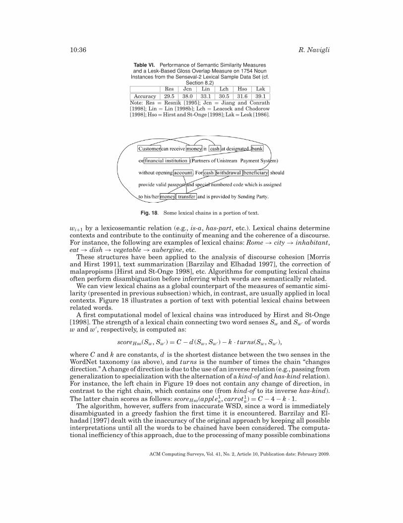
10:36 R. Navigli
Table VI. Performance of Semantic Similarity Measuresand a Lesk-Based Gloss Overlap Measure on 1754 Noun
Instances from the Senseval-2 Lexical Sample Data Set (cf.Section 8.2)
Res Jcn Lin Lch Hso Lsk
Accuracy 29.5 38.0 33.1 30.5 31.6 39.1
Note: Res = Resnik [1995]; Jcn = Jiang and Conrath[1998]; Lin = Lin [1998b]; Lch = Leacock and Chodorow[1998]; Hso = Hirst and St-Onge [1998]; Lsk = Lesk [1986].
Fig. 18. Some lexical chains in a portion of text.
wi+1 by a lexicosemantic relation (e.g., is-a, has-part, etc.). Lexical chains determinecontexts and contribute to the continuity of meaning and the coherence of a discourse.For instance, the following are examples of lexical chains: Rome → city → inhabitant,eat → dish → vegetable → aubergine, etc.
These structures have been applied to the analysis of discourse cohesion [Morrisand Hirst 1991], text summarization [Barzilay and Elhadad 1997], the correction ofmalapropisms [Hirst and St-Onge 1998], etc. Algorithms for computing lexical chainsoften perform disambiguation before inferring which words are semantically related.
We can view lexical chains as a global counterpart of the measures of semantic simi-larity (presented in previous subsection) which, in contrast, are usually applied in localcontexts. Figure 18 illustrates a portion of text with potential lexical chains betweenrelated words.
A first computational model of lexical chains was introduced by Hirst and St-Onge[1998]. The strength of a lexical chain connecting two word senses Sw and Sw′ of wordsw and w′, respectively, is computed as:
scoreHso(Sw, Sw′ ) = C − d (Sw, Sw′ ) − k · turns(Sw, Sw′ ),
where C and k are constants, d is the shortest distance between the two senses in theWordNet taxonomy (as above), and turns is the number of times the chain “changesdirection.” A change of direction is due to the use of an inverse relation (e.g., passing fromgeneralization to specialization with the alternation of a kind-of and has-kind relation).For instance, the left chain in Figure 19 does not contain any change of direction, incontrast to the right chain, which contains one (from kind-of to its inverse has-kind).
The latter chain scores as follows: scoreHso(apple1n, carrot1
n) = C − 4 − k · 1.The algorithm, however, suffers from inaccurate WSD, since a word is immediately
disambiguated in a greedy fashion the first time it is encountered. Barzilay and El-hadad [1997] dealt with the inaccuracy of the original approach by keeping all possibleinterpretations until all the words to be chained have been considered. The computa-tional inefficiency of this approach, due to the processing of many possible combinations
ACM Computing Surveys, Vol. 41, No. 2, Article 10, Publication date: February 2009.
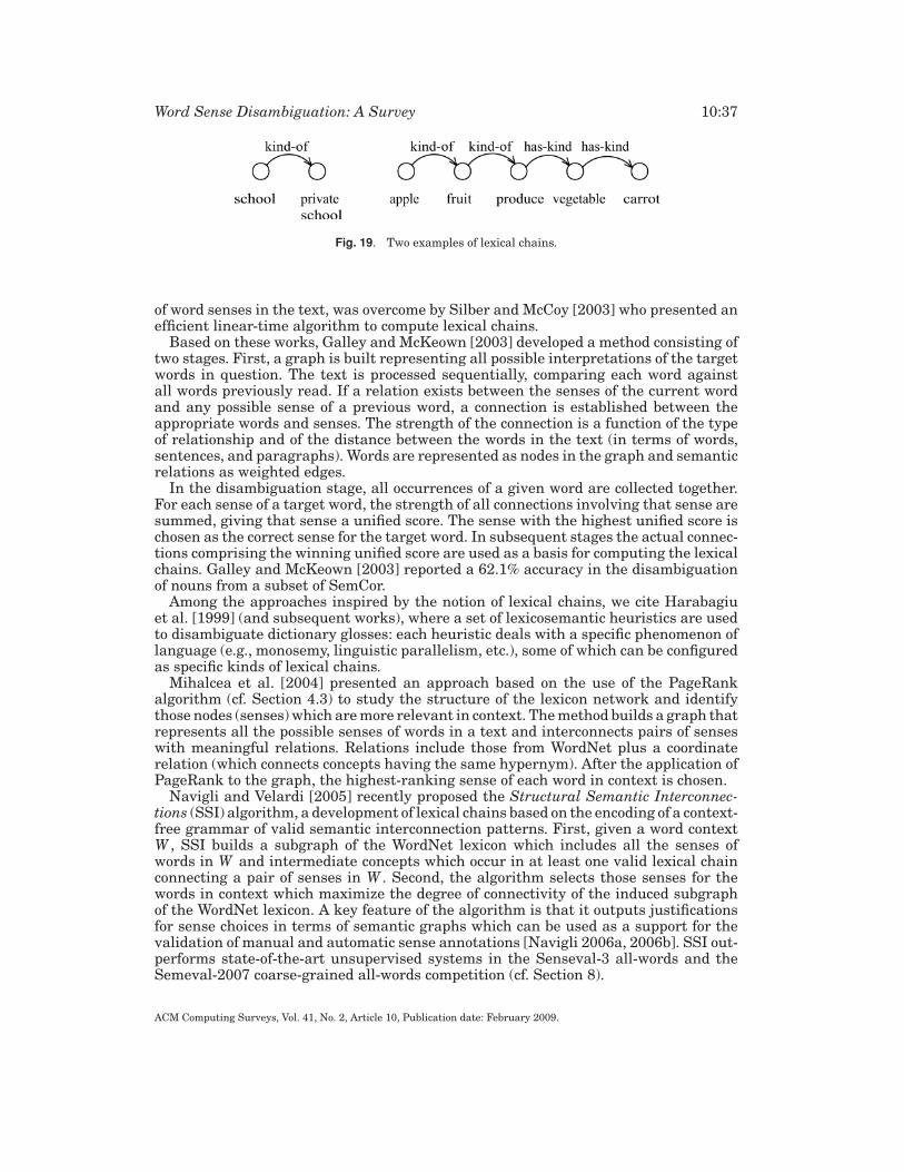
Word Sense Disambiguation: A Survey 10:37
Fig. 19. Two examples of lexical chains.
of word senses in the text, was overcome by Silber and McCoy [2003] who presented anefficient linear-time algorithm to compute lexical chains.
Based on these works, Galley and McKeown [2003] developed a method consisting oftwo stages. First, a graph is built representing all possible interpretations of the targetwords in question. The text is processed sequentially, comparing each word againstall words previously read. If a relation exists between the senses of the current wordand any possible sense of a previous word, a connection is established between theappropriate words and senses. The strength of the connection is a function of the typeof relationship and of the distance between the words in the text (in terms of words,sentences, and paragraphs). Words are represented as nodes in the graph and semanticrelations as weighted edges.
In the disambiguation stage, all occurrences of a given word are collected together.For each sense of a target word, the strength of all connections involving that sense aresummed, giving that sense a unified score. The sense with the highest unified score ischosen as the correct sense for the target word. In subsequent stages the actual connec-tions comprising the winning unified score are used as a basis for computing the lexicalchains. Galley and McKeown [2003] reported a 62.1% accuracy in the disambiguationof nouns from a subset of SemCor.
Among the approaches inspired by the notion of lexical chains, we cite Harabagiuet al. [1999] (and subsequent works), where a set of lexicosemantic heuristics are usedto disambiguate dictionary glosses: each heuristic deals with a specific phenomenon oflanguage (e.g., monosemy, linguistic parallelism, etc.), some of which can be configuredas specific kinds of lexical chains.
Mihalcea et al. [2004] presented an approach based on the use of the PageRankalgorithm (cf. Section 4.3) to study the structure of the lexicon network and identifythose nodes (senses) which are more relevant in context. The method builds a graph thatrepresents all the possible senses of words in a text and interconnects pairs of senseswith meaningful relations. Relations include those from WordNet plus a coordinaterelation (which connects concepts having the same hypernym). After the application ofPageRank to the graph, the highest-ranking sense of each word in context is chosen.
Navigli and Velardi [2005] recently proposed the Structural Semantic Interconnec-tions (SSI) algorithm, a development of lexical chains based on the encoding of a context-free grammar of valid semantic interconnection patterns. First, given a word contextW , SSI builds a subgraph of the WordNet lexicon which includes all the senses ofwords in W and intermediate concepts which occur in at least one valid lexical chainconnecting a pair of senses in W . Second, the algorithm selects those senses for thewords in context which maximize the degree of connectivity of the induced subgraphof the WordNet lexicon. A key feature of the algorithm is that it outputs justificationsfor sense choices in terms of semantic graphs which can be used as a support for thevalidation of manual and automatic sense annotations [Navigli 2006a, 2006b]. SSI out-performs state-of-the-art unsupervised systems in the Senseval-3 all-words and theSemeval-2007 coarse-grained all-words competition (cf. Section 8).
ACM Computing Surveys, Vol. 41, No. 2, Article 10, Publication date: February 2009.
10:38 R. Navigli
6. OTHER APPROACHES
6.1. Determining Word Sense Dominance
It has been noted that, given a word, the frequency distribution of its senses is highlyskewed in texts [Kilgarriff and Rosenzweig 2000], thus affecting the performance ofWSD. Methods for the determination of word sense dominance perform type-baseddisambiguation (cf. Section 2.4) based on this observation.
McCarthy et al. [2004, 2007] proposed an unsupervised method for automaticallyranking the senses of ambiguous words from raw text. Key in their approach is theobservation that distributionally similar neighbors often provide cues about the sensesof a word. Assuming that a set of neighbors is available for a target word, sense rankingis equivalent to quantifying the degree of similarity among the neighbors and the sensedescriptions of the polysemous target word.
Let N (w) = {n1, n2, . . . , nk} be the k most (distributionally) similar words to an am-biguous target word w and SensesD(w) = {S1, S2, . . . , Sn} the usual set of senses for w.Distributional similarity of neighbors in N (w) is calculated with Lin’s [1998a] methodfor the automatic construction of thesauri (as described in Section 4.2; see also Lee[1999] for an overview).
For each sense Si of w and for each neighbor nj , the algorithm selects the neighbor’ssense which has the highest WordNet similarity score (simWN) with regard to Si. Thesimilarity simWN between pairs of senses is calculated with a measure of semanticsimilarity which weights the contribution that each neighbor provides to the varioussenses of the target word (Jcn was found to perform best among different similaritymeasures; cf. Section 5.3.1).
The ranking score of sense Si is then determined as a function of the semantic sim-ilarity score and the distributional similarity score (simdist) between the target wordand the neighbors:
scorePrev(Si) =∑
n∈N (w)
simdist(w, n)simWN(Si, n)∑
S j ∈SensesD(w)
simWN(Sj , n),
where
simWN(Si, n) = maxNx∈SensesD(n)
simWN(Si, Nx).
For example, given a target word starn, let us assume that the set of neigh-bors N (starn) = {actorn, footballern, planetn} (a simplified version of the examplein McCarthy et al. [2007]). Suppose the distributional similarity was calculatedas follows: simdist(starn, actorn) = 0.22, simdist(starn, footballern) = 0.12, and
simdist(starn, planetn) =0.08. Now, we can calculate the score for each sense of starn(here we show the calculation of the two best-ranking senses):
scorePrev(star1
n
) = 0.22 · 0.01
0.48+ 0.12 · 0.01
0.57+ 0.08 · 0.68
0.93= 0.068,
scorePrev(star5
n
) = 0.22 · 0.42
0.48+ 0.12 · 0.53
0.57+ 0.08 · 0.02
0.93= 0.314,
where star1n denotes the sense of celestial body and star5
n the celebrity sense of starn (thevalues of simWN are taken from the original example of McCarthy et al. [2007]). As a re-sult, the predominant sense is simply the sense with the highest-ranking scorePrev (star5
nin the example) and can be consequently used to perform type-based disambiguation.
ACM Computing Surveys, Vol. 41, No. 2, Article 10, Publication date: February 2009.
Word Sense Disambiguation: A Survey 10:39
Mohammad and Hirst [2006] presented a different approach to the acquisition of thepredominant sense. Rather than building a thesaurus from an unlabeled corpus, theyrelied on a preexisting thesaurus, namely, the Macquarie Thesaurus [Bernard 1986].Given the categories encoded in the thesaurus, they built a word-category cooccurrencematrix M , such that Mij is the number of times word wi occurs in a text corpus ina predetermined window around a term in the thesaurus category Cj . The strengthof association between a sense of a target word and its cooccurring words (i.e., itsneighbors) is not calculated with the aid of WordNet, as McCarthy et al. [2004] did.The degree of similarity is rather calculated by applying a statistic on the contingencytable M (the authors experimented on a number of measures, such as Dice, cosine, odds,etc.). Finally, given a target word w, they proposed four different measures to determinewhich sense is predominant in a text based on implicit or explicit disambiguation andweighted or unweighted voting of cooccurring words. The best-performing measure,which combines explicit disambiguation with weighted voting of cooccurring words, isdefined as follows:
scorePrev(Ci) = | {W ∈ Xw : Sense(W, w) = Ci} || Xw | ,
where W is the set of words cooccurring in a window around a specific occurrence of w,Xw is the set of all such W , Ci is a category in the thesaurus which includes the targetword w (i.e., a “sense” of w), and Sense(W, w) is the category C of the target word wwhich maximizes the sum of the strengths of association of C with the co-occurringwords in W .
Finally, we cite a third approach to the determination of predominant senses whichrelies on word association [Lapata and Keller 2007]. Given a sense S of a word w, themethod counts the cooccurrences in a given corpus of w with the other synonyms of S(according to WordNet). As a result, a ranking of the senses of w is obtained and thebest-ranking sense can be used as the predominant sense in the corpus.
6.2. Domain-Driven Disambiguation
Domain-driven disambiguation [Gliozzo et al. 2004; Buitelaar et al. 2006] is a WSDmethodology that makes use of domain information. The sense of a target word is chosenbased on a comparison between the domains of the context words and the domainof the target sense. To this end, WordNet domain labels are typically employed (cf.Section 2.2.1).
This approach achieves good precision and possibly low recall, due to the fact thatdomain information can be used to disambiguate mainly domain words. Domain infor-mation is represented in terms of domain vectors, that is, vectors whose componentsrepresent information from distinct domains. Given a word sense S, a synset vector isdefined as S = (R(D1, S), R(D2, S), . . . , R(Dd , S)), where Di are the domains available(i ∈ {1, . . . , d }) and R(Di, S) is defined as follows:
R(Di, S) =⎧⎨⎩
1/ | Dom(S) | if Di ∈ Dom(S),
1/d if Dom(S) = { FACTOTUM },0 otherwise,
where Dom(S) is the set of labels assigned to sense S in the WordNet domain labelsresource and the FACTOTUM label represents the absence of domain pertinence. For in-
stance, Dom(authority1n) = { ADMINISTRATION, LAW, POLITICS}; thus the vector associated
to authority1n is (0, . . . , 0, 1/3, 0, . . . , 0, 1/3, 0, . . . , 0, 1/3, 0, . . . , 0). Given a target word
ACM Computing Surveys, Vol. 41, No. 2, Article 10, Publication date: February 2009.
10:40 R. Navigli
w occurring in a text T , the most appropriate sense S of w is selected as follows:
S = argmaxSi∈SensesD(w)
P (Si | w)sim(Si, T)∑S∈SensesD(w) P (S | w)sim(S, T)
,
where sim is the measure of cosine similarity (cf. Section 4.1), P (Si | w) describes theprobability of sense Si for word w based on the distribution of sense annotations in theSemCor corpus (cf. Section 2.2.2), and T is a domain vector of a window of T around wordw, estimated with an unsupervised method, namely, the Gaussian mixture approach.Specific parameters are estimated from a large-scale corpus using the ExpectationMaximization (EM) algorithm.
The use of P (Si | w) makes this approach supervised, as it exploits a sense-labeledcorpus to determine the probability of sense Si for word w. A modified, unsupervisedversion of this approach [Strapparava et al. 2004] performed best among unsupervisedsystems in the Senseval-3 all-words task (see Section 8.3).
The interesting aspect of domain-driven disambiguation as well as methods for de-termining word sense dominance is that they shift the focus from the linguistic under-standing to a domain-oriented type-based vision of sense ambiguity. We believe thatthis direction will be further explored in the future, especially with the aim of enablingsemantic-aware applications (see also Section 10).
6.3. WSD from Cross-Lingual Evidence
Finally, we introduce an approach to disambiguation based on the evidence from trans-lation information. The strategy consists of disambiguating target words by labelingthem with the appropriate translation.
The main idea behind this approach is that the plausible translations of a word incontext restrict its possible senses to a subset [Resnik and Yarowsky 1997, 1999]. Forinstance, the English word sentence can be translated to the French peine or phrasedepending on the context. However, this method does not necessarily performs a fulldisambiguation, as it is not uncommon that different meanings of the same word havethe same translation (e.g., both the senses of wing as an organ and as part of a buildingtranslate to the Italian ala). In their seminal article, Resnik and Yarowsky [1997]proposed that only senses which are lexicalized cross-linguistically in a minimum setof languages should be considered. For instance, table is translated as table in Frenchand tavola in Italian, both in the sense of piece of furniture, and a company of people ata table. This regular polysemy is preserved across the three languages, and allows forthe identification of a single sense. To implement this proposal, Ide [2000] suggestedthe use of a coherence index for identifying the tendency to lexicalize senses differentlyacross languages.
Several methods have been described in the literature based on cross-lingual evi-dence. Brown et al. [1991] proposed an unsupervised approach which, after performingword alignment on a parallel corpus, determines the most appropriate translation for atarget word according to the most informative feature from a set of contextual features.
Gale et al. [1992d] proposed a method which uses parallel corpora for the automaticcreation of a sense-tagged data set. Given a target word, each sentence in the sourcelanguage is tagged with the translation of the word in the target language. A naiveBayes classifier is then trained with the resulting data set and applied in a WSD task.Experiments show a very high accuracy (above 90%) on a small number of words.
More recently, Diab [2003] presented an unsupervised approach for sense taggingparallel corpora which clusters source words translating to the same target word and
ACM Computing Surveys, Vol. 41, No. 2, Article 10, Publication date: February 2009.
Word Sense Disambiguation: A Survey 10:41
disambiguates them based on a measure of similarity. Finally, the method assigns themost similar sense tag to the target word occurring in the source corpus (and possiblyprojects the sense assignment to the corresponding word in the target corpus).
Ide et al. [2002] and Tufis et al. [2004] presented a knowledge-based approach whichexploits EuroWordNet (cf. Section 2.2.1). Given two aligned words in a parallel corpus,they sense tag them with those synsets of the two words which are mapped throughEuroWordNet’s interlingual index. The most frequent sense baseline is used as a backoffin case more than one sense of the word in the source language maps to senses of theword in the target language. 75% accuracy is achieved in disambiguating a manuallytagged portion of Orwell’s 1984.
In recent studies, it has been found that approaches that use cross-lingual evidencefor WSD attain state-of-the-art performance in all-words disambiguation (e.g., Ng et al.[2003]; Chklovski et al. [2004]; Chan and Ng [2005]). However, the main problem ofthese approaches lies in the knowledge acquisition bottleneck: there is a lack of parallelcorpora for several languages, which can potentially be relieved by collecting corporaon the Web [Resnik and Smith 2003]. To overcome this problem, Dagan and Itai [1994]proposed the use of a bilingual lexicon to find all possible translations (considered asthe set of target senses) of an ambiguous word occurring in a syntactic relation, andthen use statistics on the translations in a target corpus to perform disambiguation.
7. EVALUATION METHODOLOGY
We present here the evaluation measures and baselines employed for in vitro evalu-ation of WSD systems, that is, as if they were stand-alone, independent applications.However, one of the real objectives of WSD is to demonstrate that it improves the per-formance of applications such as information retrieval, machine translation, etc. Theevaluation of WSD as a module embedded in applications is called in vivo or end-to-endevaluation. We will discuss this second kind of evaluation in later sections.
7.1. Evaluation Measures
The assessment of word sense disambiguation systems is usually performed in terms ofevaluation measures borrowed from the field of information retrieval, that we introducehereafter.
Let T = (w1, . . . , wn) be a test set and A an “answer” function that associates witheach word wi ∈ T the appropriate set of senses from the dictionary D (i.e., A(i) ⊆SensesD(wi)). Then, given the sense assignments A′(i) ∈ SensesD(wi) ∪ {ε} provided byan automatic WSD system11 (i ∈ {1, . . . , n}), we can define coverage C as the percentageof items in the test set for which the system provided a sense assignment that is:
C = # answers provided
# total answers to provide= | {i ∈ {1, . . . , n} : A′(i) �= ε} |
n,
where we indicate with ε the case in which the system does not provide an answerfor a specific word wi (i.e., in that case we assume that A′(i) = ε). The total number ofanswers is given by n =| T |. The precision P of a system is computed as the percentageof correct answers given by the automatic system, that is:
P = # correct answers provided
# answers provided= | {i ∈ {1, . . . , n} : A′(i) ∈ A(i)} |
| {i ∈ {1, . . . , n} : A′(i) �= ε} | .
11We assume that the annotations to be assessed assign to each word a single sense from the inventory. Wenote that more than one annotation can be allowed by extending this notation.
ACM Computing Surveys, Vol. 41, No. 2, Article 10, Publication date: February 2009.
10:42 R. Navigli
Precision determines how good are the answers given by the system being assessed.Recall R is defined as the number of correct answers given by the automatic systemover the total number of answers to be given:
R = # correct answers provided
# total answers to provide= | {i ∈ {1, . . . , n} : A′(i) ∈ A(i)} |
n.
According to the above definitions, we have that R ≤ P . When coverage is 100%, wehave that P = R. In the WSD literature, recall is also referred to as accuracy, althoughthese are two different measures in the machine learning and information retrievalliterature.
Finally, a measure which determines the weighted harmonic mean of precision andrecall, called the F1-measure or balanced F -score, is defined as
F1 = 2P RP + R
.
The F1-measure is a specialization of a general formula, the Fα-score, defined as
Fα = 1
α 1P + (1 − α) 1
R
= (β2 + 1)P Rβ2 P + R
,
where α = 1/(β2 + 1). The F1-measure is obtained by choosing β = 1 (or, equivalently,
α = 12), thus equally balancing precision and recall. F1 is useful to compare systems
with a coverage lower than 100%. Note that an easy-to-build system with P = 100% andalmost-zero recall would get around 50% performance if we used a simple arithmeticmean ( P+R
2), whereas a harmonic mean such as F1 is dramatically penalized by low
values of either precision or recall.It has been argued that the above measures do not reflect the ability of systems to
output a degree of confidence for a given sense choice. In this direction, Resnik andYarowsky [1999] proposed an evaluation metric which weighs misclassification errorsby the distance between the selected and correct senses. As a result, if the chosensense is a fine-grained distinction of the correct sense, this error will be penalised lessheavily than between coarser sense distinctions. Even more refined metrics, such asthe receiver operation characteristic (ROC), have been proposed [Cohn 2003]. How-ever these metrics are not often used, also for reasons of comparison with previouslyestablished results, mostly measured in terms of precision, recall, and F1.
7.2. Baselines
A baseline is a standard method to which the performance of different approaches iscompared. Here we present two basic baselines, the random baseline (Section 7.2.1)and the first sense baseline (Section 7.2.2). Other baselines have also been employedin the literature, such as the Lesk approach (cf. Section 5.1).
7.2.1. The Random Baseline. Let D be the reference dictionary and T = (w1, w2,. . . , wn) be a test set such that word wi (i ∈ {1, . . . , n}) is a content word in the cor-pus. The chance or random baseline consists in the random choice of a sense fromthose available for each word wi. Under the uniform distribution, for each word wi the
probability of success of such a choice is 1|SensesD(wi )| .
ACM Computing Surveys, Vol. 41, No. 2, Article 10, Publication date: February 2009.
Word Sense Disambiguation: A Survey 10:43
The accuracy of the random baseline is obtained by averaging over all the contentwords in the test set T :
AccChance = 1
n
n∑i=1
1
| SensesD(wi) | .
7.2.2. The First Sense Baseline. The first sense baseline (or most frequent sense baseline)is based on a ranking of word senses. This baseline consists in choosing the first senseaccording to such a ranking for each word in a corpus, independent of its context.
For instance, in WordNet, senses of the same word are ranked based on the frequencyof occurrence of each sense in the SemCor corpus (cf. Section 2.2.2). Let SC be theSemCor corpus, ASC(i) the set of manual annotations for the ith word in the corpus,and let Count(w j
p) be a function that counts the number of occurrences of sense w jp in
SC, such that
Count(w j
p
) = | {i ∈ {1, . . . , | SC |} : w jp ∈ ASC(i)} |
| SC | .
Given a word sense w jp, the counts determine the following ranking:
RankF S(w j
p
) = Count(w j
p
)∑|SensesD(wp)|
i=1 Count(wi
p
) .
Now let us assume that word senses are ordered by a ranking based on occurrencecounts, that is, w1
p occurs equally or more frequently than w2p, and so on (possibly
remaining senses with no occurrence are ordered randomly). Let T = (w1, w2, . . . , wn)be a test set and A be the set of sense tags manually assigned to T by one or moreannotators, that is, A(i) ⊆ SensesD(wi). The accuracy of the first sense baseline iscalculated as follows:
AccF S = | {i ∈ {1, . . . , n} : w1i ∈ A(i)} |
n.
In other words, this is the accuracy of assigning the sense of each word which is mostfrequent in SemCor (or, analogously, in another reference sense-tagged data set).
7.3. Lower and Upper Bounds
Lower and upper bounds are performance figures that indicate the range within whichthe performance of any system should fall. Specifically, a lower bound usually measuresa performance obtained with an extremely simple method and which any system shouldbe able to exceed. A typical lower bound is the random baseline. Gale et al. [1992a]proposed the selection of the most likely sense as a lower bound (i.e., the first sensebaseline). This baseline poses serious difficulties to WSD systems as it is often hard tobeat, as we will discuss in the next section.
An upper bound specifies the highest performance reasonably attainable. In WSD,a typical upper bound is the interannotator agreement or intertagger agreement (ITA),that is, the percentage of words tagged with the same sense by two or more humanannotators. The interannotator agreement on coarse-grained, possibly binary, senseinventories is calculated around 90% [Gale et al. 1992a; Navigli et al. 2007], whereason fine-grained, WordNet-style sense inventories the inter-annotator agreement is esti-mated between 67% and 80% [Chklovski and Mihalcea 2003; Snyder and Palmer 2004;Palmer et al. 2007].
ACM Computing Surveys, Vol. 41, No. 2, Article 10, Publication date: February 2009.
10:44 R. Navigli
As Gale et al. [1992a] stated, it is unclear how to interpret a performance which beatsthe interannotator agreement: if humans cannot agree more than a certain percentageof times, what does it mean if a system overcomes that figure and is more accurate? Apossible answer might be that some sense assignments in a data set or some distinctionsin the adopted sense inventory are disputable. This poses a problem especially for fine-grained WSD: it might be that the task itself needs to be rethought (we further discussthis point in Sections 8.4 and 8.5).
Another upper bound that turns out to be useful is the oracle. An oracle is a hypotheticsystem which is always supposed to know the correct answer (i.e., the appropriate sensechoice) among those available. An oracle constitutes a good upper bound to comparethe performance of ensemble methods (cf. Section 3.7). Its accuracy is determined bythe number of word instances for which at least one of the systems output the correctsense. As a result, given the output of first-order WSD systems, the oracle performanceprovides the maximum hypothetical performance of any combination method aimingat improving the results of the single systems.
Another use of the oracle is in calculating the impact of WSD on applications: infact, an oracle which performs 100% accurate disambiguation (e.g., in disambiguat-ing queries, document bases, translations, etc.) allows it to determine the maximum(theoretical) degree of impact of WSD on the application of interest (for instance, whatis the maximum improvement when performing 100%-accurate disambiguation in aninformation retrieval task?).
8. EVALUATION: THE SENSEVAL/SEMEVAL COMPETITIONS
Comparing and evaluating different WSD systems is extremely difficult, because ofthe different test sets, sense inventories, and knowledge resources adopted. Beforethe organization of specific evaluation campaigns, which we introduce in this section,most systems were assessed on in-house, often small-scale, data sets. Therefore, mostof the pre-Senseval results are not comparable with subsequent approaches in thefield.
Senseval12 (now renamed Semeval) is an international word sense disambiguationcompetition, held every three years since 1998. The objective of the competition is toperform a comparative evaluation of WSD systems in several kinds of tasks, includingall-words and lexical sample WSD for different languages, and, more recently, newtasks such as semantic role labeling, gloss WSD, lexical substitution, etc. The systemssubmitted for evaluation to these competitions usually integrate different techniquesand often combine supervised and knowledge-based methods (especially for avoidingbad performance in lack of training examples). The Senseval workshops are the bestreference to study the recent trends of WSD and the future research directions in thefield. Moreover, they lead to the periodic release of data sets of high value for theresearch community.
We now review and discuss the four competitions held between 1998 and 2007. Areview of the first three Senseval competitions can also be found in Martinez [2004]and Palmer et al. [2006].
8.1. Senseval-1
The first edition of Senseval took place in 1998 at Herstmonceux Castle, Sussex[Kilgarriff 1998; Kilgarriff and Palmer 2000]. The importance of this edition is givenby the fact that WSD researchers joined their efforts and discussed several issues
12http://www.senseval.org.
ACM Computing Surveys, Vol. 41, No. 2, Article 10, Publication date: February 2009.
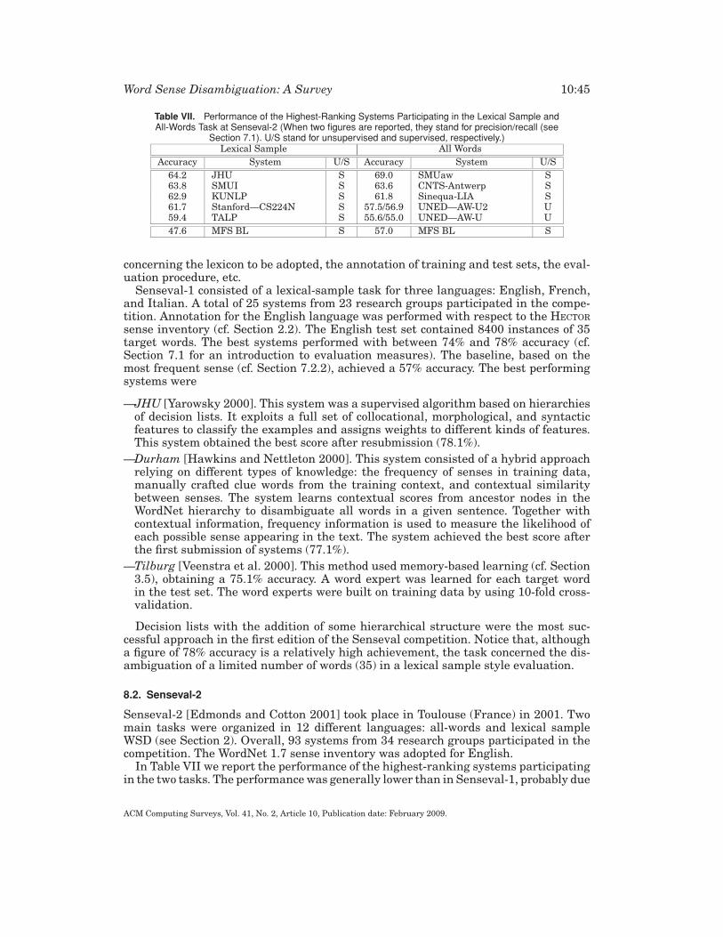
Word Sense Disambiguation: A Survey 10:45
Table VII. Performance of the Highest-Ranking Systems Participating in the Lexical Sample andAll-Words Task at Senseval-2 (When two figures are reported, they stand for precision/recall (see
Section 7.1). U/S stand for unsupervised and supervised, respectively.)Lexical Sample All Words
Accuracy System U/S Accuracy System U/S
64.2 JHU S 69.0 SMUaw S63.8 SMUI S 63.6 CNTS-Antwerp S62.9 KUNLP S 61.8 Sinequa-LIA S61.7 Stanford—CS224N S 57.5/56.9 UNED—AW-U2 U59.4 TALP S 55.6/55.0 UNED—AW-U U
47.6 MFS BL S 57.0 MFS BL S
concerning the lexicon to be adopted, the annotation of training and test sets, the eval-uation procedure, etc.
Senseval-1 consisted of a lexical-sample task for three languages: English, French,and Italian. A total of 25 systems from 23 research groups participated in the compe-tition. Annotation for the English language was performed with respect to the HECTOR
sense inventory (cf. Section 2.2). The English test set contained 8400 instances of 35target words. The best systems performed with between 74% and 78% accuracy (cf.Section 7.1 for an introduction to evaluation measures). The baseline, based on themost frequent sense (cf. Section 7.2.2), achieved a 57% accuracy. The best performingsystems were
—JHU [Yarowsky 2000]. This system was a supervised algorithm based on hierarchiesof decision lists. It exploits a full set of collocational, morphological, and syntacticfeatures to classify the examples and assigns weights to different kinds of features.This system obtained the best score after resubmission (78.1%).
—Durham [Hawkins and Nettleton 2000]. This system consisted of a hybrid approachrelying on different types of knowledge: the frequency of senses in training data,manually crafted clue words from the training context, and contextual similaritybetween senses. The system learns contextual scores from ancestor nodes in theWordNet hierarchy to disambiguate all words in a given sentence. Together withcontextual information, frequency information is used to measure the likelihood ofeach possible sense appearing in the text. The system achieved the best score afterthe first submission of systems (77.1%).
—Tilburg [Veenstra et al. 2000]. This method used memory-based learning (cf. Section3.5), obtaining a 75.1% accuracy. A word expert was learned for each target wordin the test set. The word experts were built on training data by using 10-fold cross-validation.
Decision lists with the addition of some hierarchical structure were the most suc-cessful approach in the first edition of the Senseval competition. Notice that, althougha figure of 78% accuracy is a relatively high achievement, the task concerned the dis-ambiguation of a limited number of words (35) in a lexical sample style evaluation.
8.2. Senseval-2
Senseval-2 [Edmonds and Cotton 2001] took place in Toulouse (France) in 2001. Twomain tasks were organized in 12 different languages: all-words and lexical sampleWSD (see Section 2). Overall, 93 systems from 34 research groups participated in thecompetition. The WordNet 1.7 sense inventory was adopted for English.
In Table VII we report the performance of the highest-ranking systems participatingin the two tasks. The performance was generally lower than in Senseval-1, probably due
ACM Computing Surveys, Vol. 41, No. 2, Article 10, Publication date: February 2009.
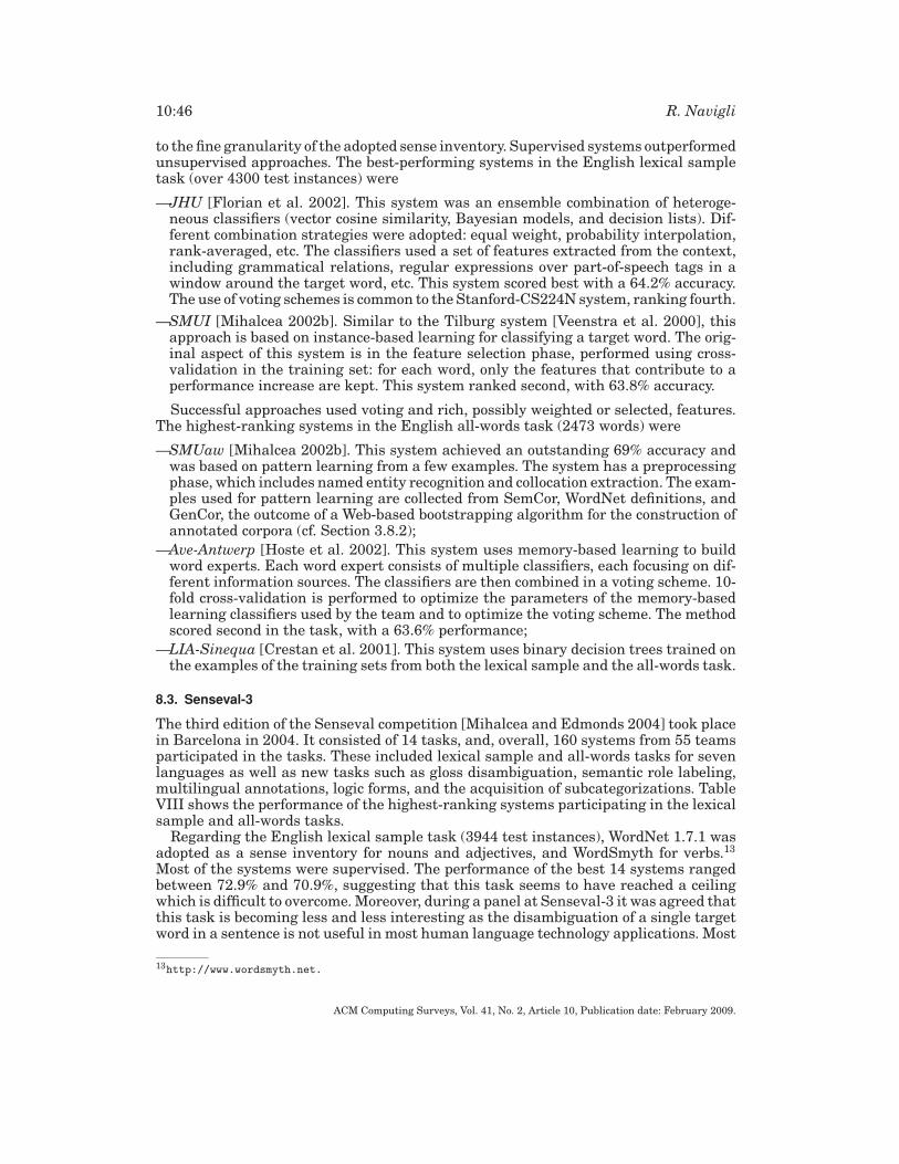
10:46 R. Navigli
to the fine granularity of the adopted sense inventory. Supervised systems outperformedunsupervised approaches. The best-performing systems in the English lexical sampletask (over 4300 test instances) were
—JHU [Florian et al. 2002]. This system was an ensemble combination of heteroge-neous classifiers (vector cosine similarity, Bayesian models, and decision lists). Dif-ferent combination strategies were adopted: equal weight, probability interpolation,rank-averaged, etc. The classifiers used a set of features extracted from the context,including grammatical relations, regular expressions over part-of-speech tags in awindow around the target word, etc. This system scored best with a 64.2% accuracy.The use of voting schemes is common to the Stanford-CS224N system, ranking fourth.
—SMUI [Mihalcea 2002b]. Similar to the Tilburg system [Veenstra et al. 2000], thisapproach is based on instance-based learning for classifying a target word. The orig-inal aspect of this system is in the feature selection phase, performed using cross-validation in the training set: for each word, only the features that contribute to aperformance increase are kept. This system ranked second, with 63.8% accuracy.
Successful approaches used voting and rich, possibly weighted or selected, features.The highest-ranking systems in the English all-words task (2473 words) were
—SMUaw [Mihalcea 2002b]. This system achieved an outstanding 69% accuracy andwas based on pattern learning from a few examples. The system has a preprocessingphase, which includes named entity recognition and collocation extraction. The exam-ples used for pattern learning are collected from SemCor, WordNet definitions, andGenCor, the outcome of a Web-based bootstrapping algorithm for the construction ofannotated corpora (cf. Section 3.8.2);
—Ave-Antwerp [Hoste et al. 2002]. This system uses memory-based learning to buildword experts. Each word expert consists of multiple classifiers, each focusing on dif-ferent information sources. The classifiers are then combined in a voting scheme. 10-fold cross-validation is performed to optimize the parameters of the memory-basedlearning classifiers used by the team and to optimize the voting scheme. The methodscored second in the task, with a 63.6% performance;
—LIA-Sinequa [Crestan et al. 2001]. This system uses binary decision trees trained onthe examples of the training sets from both the lexical sample and the all-words task.
8.3. Senseval-3
The third edition of the Senseval competition [Mihalcea and Edmonds 2004] took placein Barcelona in 2004. It consisted of 14 tasks, and, overall, 160 systems from 55 teamsparticipated in the tasks. These included lexical sample and all-words tasks for sevenlanguages as well as new tasks such as gloss disambiguation, semantic role labeling,multilingual annotations, logic forms, and the acquisition of subcategorizations. TableVIII shows the performance of the highest-ranking systems participating in the lexicalsample and all-words tasks.
Regarding the English lexical sample task (3944 test instances), WordNet 1.7.1 wasadopted as a sense inventory for nouns and adjectives, and WordSmyth for verbs.13
Most of the systems were supervised. The performance of the best 14 systems rangedbetween 72.9% and 70.9%, suggesting that this task seems to have reached a ceilingwhich is difficult to overcome. Moreover, during a panel at Senseval-3 it was agreed thatthis task is becoming less and less interesting as the disambiguation of a single targetword in a sentence is not useful in most human language technology applications. Most
13http://www.wordsmyth.net.
ACM Computing Surveys, Vol. 41, No. 2, Article 10, Publication date: February 2009.
Word Sense Disambiguation: A Survey 10:47
Table VIII. Performance of the Highest-Ranking Systems Participating in the Lexical Sample andAll-Words Tasks at Senseval-3 (When two figures are reported, they stand for precision/recall (see
Section 7.1). U/S stand for unsupervised and supervised, respectively. The baseline for the all-wordstask achieves 60.9% or 62.4% depending on the treatment of multiwords and hyphenated words)
Lexical sample All words
Accuracy System U/S Accuracy System U/S
72.9 htsa3 S 65.1 GAMBL-AW S72.6 IRST-Kernels S 65.1/64.2 SenseLearner S72.4 nusels S .
.
....
.
.
.72.4 htsa4 S72.3 BCU comb S 58.3/58.2 IRST-DDD-00 U
55.2 MFS BL S 60.9-62.4 MFS BL S
of the top systems used kernel methods (cf. Section 3.6). Other approaches include thevoted combination of algorithms and the use of a rich set of features, comprising domaininformation and syntactic relations. We outline here the two top-ranking systems:
—Htsa3 [Grozea 2004]. This system obtained the best performance (72.9% accuracy)by applying the regularized least-squares classification (RLSC), a technique basedon kernels and Tikhonov regularization. The features used include collocations andlemmas around the target word. Htsa3 used a linear kernel: its weight values werenormalized with the frequency of the senses in the training set. A normalization stepis performed to deal with the implicit bias of RLSC which favours frequent senses.The regularization parameter and a further parameter for smooth normalizationwere estimated using the previous Senseval corpora.
—IRST-Kernels [Strapparava et al. 2004]. This system ranked second with 72.6% ac-curacy and is based on SVM (see Section 3.6). The kernel function combines hetero-geneous sources of information and is the result of the combination of two differentkernels, a paradigmatic and a syntagmatic kernel.
—The syntagmatic kernel determines the similarity of two contexts based on thenumber of word sequences they have in common. It is implemented in terms of twoother kernels which take into account collocation information and part-of-speechsequences.
—The paradigmatic kernel exploits information about the domain of the input textand combines again two other kernels: a bag of words kernel and a latent semanticindexing kernel. The latter aims to relieve the problem of data sparseness of theformer kernel.
The English all-words task [Snyder and Palmer 2004] saw the participation of 26 sys-tems from 16 teams. The test set included 2037 sense-tagged words. The best systemattained a 65.1% accuracy, whereas the first sense baseline (cf. Section 7.2.2) achieved60.9% or 62.4% depending on the treatment of multiwords and hyphenated words. InTable VIII we report the best two supervised systems together with the best unsuper-vised system (IRST-DDD):
—GAMBL-AW [Decadt et al. 2004]. GAMBL is a supervised method that learns wordexperts from extensive corpora. The training corpus includes SemCor, the previousSenseval corpora, usage examples in WordNet, etc. The features extracted from theresulting training set include a local context and contextual keywords. GAMBL isbased on memory-based learning, with an additional optimization of features andparameters performed with genetic algorithms. The system classified first in the all-words task with 65.1% accuracy.
—SenseLearner [Mihalcea and Faruque 2004]. SenseLearner classified second in thetask, with 65.1% precision and 64.2% recall. This approach uses a small number of
ACM Computing Surveys, Vol. 41, No. 2, Article 10, Publication date: February 2009.
10:48 R. Navigli
hand-tagged examples, and heavily relies on SemCor and the WordNet taxonomy. Itperforms two main steps:
—First, a semantic model for each part of speech is learned from SemCor basedon cooccurrence features (memory-based learning is employed). Then, the modelmakes a prediction for each instance in the test set. This method leads to 85.6%coverage;
—Second, a semantic generalization step is applied with the aid of WordNet andthe use of syntactic dependencies: during a training phase, all the dependencypairs in SemCor are acquired (e.g. (drinkv, watern)). Each pair is generalized withthe hypernyms of the nouns and verbs involved, thus creating generalized featurevectors. During testing, for each dependency pair, and for all possible combinationsof senses, feature vectors are created. Memory-based learning is applied to eachvector, thus obtaining a positive or negative value for each of them. Finally, a sensechoice is made based on these values.
—IRST-DDD [Strapparava et al. 2004]. The approach basically compares the domainof the context surrounding the target word w with the domains of each sense ofw (cf. Section 6.2) and uses a version of WordNet augmented with domain labels(e.g., ECONOMY, GEOGRAPHY, etc.; cf. Section 2.2.1).
8.4. Semeval-2007
The fourth edition of Senseval, held in 2007, has been renamed Semeval-2007 [Agirreet al. 2007b], given the presence of tasks of semantic analysis not necessarily relatedto word sense disambiguation. Some of the tasks proposed for Semeval-2007 dealtwith the observations and conclusions drawn during the discussion and panels in theSenseval-3 workshop. Among the 18 tasks organized, those related to WSD can beclassified as follows:
—explicit WSD tasks, that is, tasks requiring an explicit assignment of word senses totarget words. These include
—lexical sample and all-words coarse-grained WSD tasks (discussed below), aimingat understanding the impact of sense granularity on WSD accuracy;
—a preposition disambiguation task [Litkowski and Hargraves 2007];
—the evaluation of WSD on Cross-Language Information Retrieval [Agirre et al.2007a], which constitutes an important effort towards in vivo evaluation;
—the resolution of metonymies [Markert and Nissim 2007], that is, the substitutionof the attribute or feature of a thing for the thing itself (e.g., glass to express thecontent of a glass, rather than the container itself).
—implicit WSD tasks, that is, tasks where the system output implies some kind ofimplicit disambiguation. These include
—word sense induction and discrimination [Agirre and Soroa 2007], for a comparativeassessment of unsupervised systems among themselves and with supervised andknowledge-based systems;
—a lexical substitution task [McCarthy and Navigli 2007], aiming at the objectiveevaluation of both supervised and unsupervised systems, and applicable in thefuture to the evaluation of knowledge resources.
The coarse-grained English lexical sample task [Pradhan et al. 2007] saw the partic-ipation of 13 systems. The test set contained 4851 tagged instances of 100 words. Thebest system attained an 88.70% accuracy, whereas the first sense baseline achieved
ACM Computing Surveys, Vol. 41, No. 2, Article 10, Publication date: February 2009.
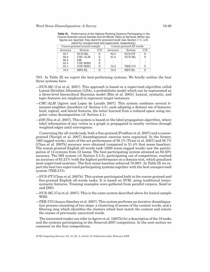
Word Sense Disambiguation: A Survey 10:49
Table IX. Performance of the Highest-Ranking Systems Participating in theCoarse-Grained Lexical Sample and All-Words Tasks at Semeval (When two
figures are reported, they stand for precision/recall (see Section 7.1). U/Sstand for unsupervised and supervised, respectively.)
Coarse-grained Lexical sample Coarse-grained All words
Accuracy System U/S Accuracy System U/S
88.7 NUS-ML S 82.5 NUS-PT S86.9 UBC-ALM S 81.6 NUS-ML S86.4 I2R S .
.
....
.
.
.85.4 USP-IBM2 S85.1 USP-IBM1 S 70.2 TKB-UO U
78.0 MFS BL S 78.9 MFS BL S
78%. In Table IX we report the best-performing systems. We briefly outline the bestthree systems here:
—NUS-ML [Cai et al. 2007]. This approach is based on a supervised algorithm calledLatent Dirichlet Allocation (LDA), a probabilistic model which can be represented asa three-level hierarchical Bayesian model [Blei et al. 2003]. Lexical, syntactic, andtopic features are employed to represent target instances.
—UBC-ALM [Agirre and Lopez de Lacalle 2007]. This system combines several k-nearest neighbor classifiers (cf. Section 3.5), each adopting a distinct set of features:local, topical, and latent features, the latter learned from a reduced space using sin-gular value decomposition (cf. Section 4.1).
—I2R [Niu et al. 2007]. This system is based on the label propagation algorithm, wherelabel information of any vertex in a graph is propagated to nearby vertices throughweighted edges until convergence.
Concerning the all-words task, both a fine-grained [Pradhan et al. 2007] and a coarse-grained [Navigli et al. 2007] disambiguation exercise were organized. In the former,(465 tagged words), state-of-the-art performance of 59.1% [Tratz et al. 2007] and 58.7%[Chan et al. 2007b] accuracy were obtained (compared to 51.4% first sense baseline).The coarse-grained English all-words task (2269 sense-tagged words) saw the partici-pation of 14 systems from 12 teams. The best participating system attained an 82.50%accuracy. The SSI system (cf. Section 5.3.2), participating out of competition, reachedan accuracy of 83.21% (with the highest performance on a domain text, which penalizedmost supervised systems). The first sense baseline achieved 78.89%. In Table IX we re-port the best two supervised participating systems together with the best unsupervisedsystem (TKB-UO):
—NUS-PT [Chan et al. 2007b]. This system participated both in the coarse-grained andfine-grained English all-words tasks. It is based on SVM, using traditional lexico-syntactic features. Training examples were gathered from parallel corpora, SemCorand DSO.
—NUS-ML [Cai et al. 2007]. This is the same system described above for lexical sampleWSD.
—TKB-UO [Anaya-Sanchez et al. 2007]. This system performs an iterative disambigua-tion process consisting of two steps: a clustering of senses of the context words, and afiltering step which identifies the clusters which best match the context and selectsthe senses of previously uncovered words.
The interested reader can refer to Agirre et al. [2007b] for a description of the 18 tasksand the systems participating in the Semeval-2007 competition. In the next section wecomment on the four competitions.
ACM Computing Surveys, Vol. 41, No. 2, Article 10, Publication date: February 2009.
10:50 R. Navigli
8.5. Remarks on the Senseval/Semeval Competitions
Admittedly, it is very difficult to compare the performance of state-of-the-art systemsacross the four evaluation campaigns for several reasons. First, different dictionar-ies have been adopted (HECTOR in Senseval-1, WordNet 1.7 in Senseval-2, WordNet1.7.1 in Senseval-3, WordNet 2.1 and coarse-grained inventories in Semeval-2007): theadoption of WordNet caused a substantial drop in performance (from 78% to 64% ac-curacy in the lexical sample task from Senseval-1 to Senseval-2). Second, it is hardto extrapolate the contribution of single techniques in most systems, as they usuallycombine different approaches. Third, supervised systems are trained on different cor-pora, and knowledge-based systems exploit different resources. Finally, Semeval-2007shifted the focus toward coarse-grained WSD. However, we want to comment on thefollowing points:
—the performance variations are quite consistent with the baseline changes across thecompetitions: for the lexical sample task, there is a general decrease in performancebetween Senseval-1 and -2 and a general increase between Senseval-2 and -3 for bothsupervised and unsupervised systems; for the all-words task, with the exception ofSMUaw (which did not participate in Senseval-3), there is a general increase inperformance from Senseval-2 to Senseval-3; however, we note that for the lexicalsample task the best systems increase of +21 (Senseval-1), +16.6 (Senseval-2), +17.7points (Senseval-3), over the first sense baseline, while for the fine-grained all-wordstask, the difference changes from +12 (Senseval-2) to just +3 (Senseval-3), and +7.7(Semeval-2007);
—performance in the lexical sample task seems to have reached a plateau around 73%accuracy when a fine-grained lexicon such as WordNet was adopted: this is a clearclue that supervised systems, specifically trained on a set of words, cannot exceedthat performance within this setting;
—performance in the fine-grained all-words task can be established between 65%and 70% when WordNet is adopted, whereas better results, between 78% and 81%,have been reported in the literature when coarse-grained senses are used (see, e.g.,Kohomban and Lee [2005]; Navigli [2006c]); the latter results are also confirmed bythe state-of-the-art performance of 82–83% accuracy obtained in the Semeval-2007coarse-grained all-words task; potentially, these figures might be even improved giventhe fact that to date most supervised systems have not been retrained on a full-fledgedcoarse-grained sense inventory;
—among supervised methods, memory-based learning and SVM approaches proved tobe among the best systems in several competitions: systems based on the formerranked third in Senseval-1 lexical sample [Veenstra et al. 2000], second in both theSenseval-2 lexical sample and all-words tasks [Mihalcea 2002b; Hoste et al. 2002],first and second in Senseval-3 all-words [Decadt et al. 2004; Mihalcea and Faruque2004], second in the Semeval-2007 lexical sample [Agirre and Lopez de Lacalle 2007];SVM approaches to WSD also proved to perform best, when applied both in the lexicalsample [Grozea 2004; Strapparava et al. 2004] and all-words exercises [Chan et al.2007b]; these supervised methods definitely proved superior to other approaches;
—the first sense baseline is a real challenge for all-words WSD systems: only few sys-tems are able to exceed it; this fact does not recur in lexical sample WSD, as usuallymore training data is available and the task is less likely to reflect the real distri-bution of word meanings within texts (e.g., consider the extreme case of an equallybalanced frequency of the meanings of a word: the first sense baseline would per-form with accuracy equal to the random baseline); the fact that most methods find it
ACM Computing Surveys, Vol. 41, No. 2, Article 10, Publication date: February 2009.
Word Sense Disambiguation: A Survey 10:51
difficult to overcome the first sense baseline is an indicator that most of the effortsseem to be of little use; in this respect, knowledge-based methods, and specificallystructural approaches, which achieve performance close or equal to the first sensebaseline, have the advantage of providing justifications for their sense choices interms of semantic graphs, patterns, lexical chains, etc; as a result, and in contrast tothe output of the baseline and most supervised systems, the output of these methodscan be exploited to (graphically) support humans in tasks such as the semantic an-notation and validation of texts [Navigli 2006a, 2008], semiautomatic acquisition ofknowledge resources, lexicography, and so on;
—the organization of coarse-grained tasks at Semeval-2007 allowed for the assessmentof state-of-the-art systems on sense inventories with a lower granularity than Word-Net; as a result, the performance obtained was much higher: 88.7% in the lexicalsample, and 82–83% accuracy in the all-words task; this is very good news for thefield of WSD, thus showing that the problem of word sense representation is a rel-evant one to obtain performance in the 80%–90% accuracy range and, at the sametime, maintain meaningful distinctions between word senses;
—finally, the organization of other evaluation exercises, like those introduced in Section8.4, can potentially open new research directions in the field of WSD, such as the objec-tive assessment of unsupervised systems (also in comparison with their supervisedand knowledge-based alternatives), the development of frameworks for end-to-endevaluation, etc.
9. APPLICATIONS
Unfortunately, to date explicit WSD has not yet demonstrated real benefits in humanlanguage technology applications. Nevertheless, the lack of end-to-end applications isa consequence of the current performance of WSD, and will not prevent more accuratedisambiguation systems (or even oracles, for theoretical assessments) to possibly se-mantically enable NLP applications in the future. We note that a higher accuracy maynot only derive from innovative methods, but also from different settings for the dis-ambiguation task (e.g., sense granularity, evaluation setting, disambiguation coverage,etc.).
Here we summarize a number of real-world applications which might benefit fromWSD and on which experiments have been (and are being) conducted (see Ide andVeronis [1998] and Resnik [2006] for a thorough account).
9.1. Information Retrieval (IR)
State-of-the-art search engines do not use explicit semantics to prune out documentswhich are not relevant to a user query. An accurate disambiguation of the documentbase, together with a possible disambiguation of the query words, would allow it toeliminate documents containing the same words used with different meanings (thusincreasing precision) and to retrieve documents expressing the same meaning withdifferent wordings (thus increasing recall).
Most of the early work on the contribution of WSD to IR resulted in no performanceimprovement (e.g. Salton [1968]; Salton and McGill [1983]; Krovetz and Croft [1992];Voorhees [1993]). Krovetz and Croft [1992] and Sanderson [2000] showed that only asmall percentage of query words are not used in their most frequent (or predominant)sense (cf. Section 7.2.2), indicating that WSD must be very precise on uncommon items,rather than on frequent words. Sanderson [1994] concluded that, in the presence ofqueries with a large number of words, WSD cannot benefit IR. He also pointed out thatvery short queries can be potentially very ambiguous. The experiments were conducted
ACM Computing Surveys, Vol. 41, No. 2, Article 10, Publication date: February 2009.
10:52 R. Navigli
with the aid of pseudowords [Schutze 1992; Yarowsky 1993], that is, artificial wordscreated by replacing in the test collection the occurrences of two or more words (e.g., theoccurrences of pizza and window are substituted with the pseudoword pizza/window).As a result, lexical ambiguity is introduced and the IR performance can be assessedat various levels of WSD accuracy. Sanderson [1994] indicated that improvements inIR performance would be observed only if WSD could be performed with at least 90%accuracy. However, as discussed in Schutze and Pedersen [1995], the general validityof this result is debated, due to arguable experimental settings.
Clear, encouraging evidence of the usefulness of WSD in IR has come from Schutzeand Pedersen [1995] and Stokoe et al. [2003] (the latter provided a broad overview ofpast research in this field). Assuming a WSD accuracy greater than 90%, Schutze andPedersen [1995] showed that the use of WSD in IR improves the precision by about4.3% (from 29.9% to 34.2%). With lower WSD accuracy (62.1%), Stokoe et al. [2003]showed that a small improvement (1.73% on average) can still be obtained.
9.2. Information Extraction (IE)
In specific domains it is interesting to distinguish between specific instances of concepts:for example, in the medical domain we might be interested in identifying all kinds ofdrugs across a text, whereas in bioinformatics we would like to solve the ambiguitiesin naming genes and proteins. Tasks like named-entity recognition (NER), acronymexpansion (e.g., MP as member of parliament or military police), etc., can all be castas disambiguation problems, although this is still a relatively new area (e.g., Dill et al.[2003]).
Jacquemin et al. [2002] presented a dictionary-based method which consists of theapplication of disambiguation rules at the lexical, domain, and syntactic and semanticlevel. Malin et al. [2005] proposed the application of a link analysis method basedon random walks to solve the ambiguity of named entities. Hassan et al. [2006] used alink analysis algorithm in a semisupervised fashion to weigh entity extraction patternsbased on their impact on a set of instances. Finally, Ciaramita and Altun [2006] proposedthe use of a supersense tagger, which assigns a class selected from a restricted set ofWordNet synsets to words of interest. The approach, based on sequence labeling withhidden Markov models, needs a training step.
Some tasks at Semeval-2007 more or less directly dealt with WSD for information ex-traction. Specifically, the metonymy task [Markert and Nissim 2007] required systemsto associate the appropriate metonymy with target named entities. For instance, in thesentence the BMW slowed down, BMW is a car company, but here we refer to a specificcar instance produced by BMW. Similarly, the Web People Search task [Artiles et al.2007] required systems to disambiguate people names occurring in Web documents,that is, to determine the occurrence of specific instances of people within texts.
9.3. Machine Translation (MT)
The automatic identification of the correct translation of a word in context, that is,machine translation (MT), is a very difficult task. Word sense disambiguation has beenhistorically conceived as the main task to be solved in order to enable machine transla-tion, based on the intuitive idea that the disambiguation of texts should help translationsystems choose better candidates. In fact, depending on the context, words can havecompletely different translations. For instance, the English word line can be trans-lated in Italian as linea, riga, verso, filo, corda, etc. Unfortunately, WSD has been muchharder than expected, as we know after years of comparative evaluations. As mentionedin Section 1.2, the initial failure of WSD during the 1960s led to an acute crisis of the
ACM Computing Surveys, Vol. 41, No. 2, Article 10, Publication date: February 2009.
Word Sense Disambiguation: A Survey 10:53
field of MT. Nowadays, there is contrasting evidence that WSD can benefit MT: for in-stance, Carpuat and Wu [2005] claimed that WSD cannot be integrated into presentMT applications, while Dagan and Itai [1994] and Vickrey et al. [2005] show that theproper use of WSD leads to an increase in the translation performance.
More recently, Carpuat and Wu [2007] and Chan et al. [2007a] showed that wordsense disambiguation can help improve machine translation. In these works, predefinedsense inventories were abandoned in favor of WSD models which allow it to select themost likely translation phrase. However, these results leave the research field open tohypotheses on the contribution of classical WSD to the success of machine translation.
9.4. Content Analysis
The analysis of the general content of a text in terms of its ideas, themes, etc., cancertainly benefit from the application of sense disambiguation. For instance, the classi-fication of blogs has recently been gaining more and more interest within the Internetcommunity: as blogs grow at an exponential pace, we need a simple yet effective wayto classify them, determine their main topics, and identify relevant (possibly semantic)connections between blogs and even between single blog posts. A second related areaof research is that of (semantic) social network analysis, which is becoming more andmore active with the recent evolutions of the Web.
Although some works have been recently presented on the semantic analysis of con-tent (e.g., on semantic blog analysis with the aid of structural WSD [Berendt and Navigli2006], on the disambiguation of entities in social networks [Aleman-Meza et al. 2006],etc.), this is an open and stimulating research area.
9.5. Word Processing
Word processing is a relevant application of natural language processing, whose impor-tance has been recognized for a long time [Church and Rau 1995]. Word sense disam-biguation can aid in correcting the spelling of a word [Yarowsky 1994], for case change,or to determine when diacritics should be inserted (e.g., in Italian for changing da (=from) to da (= gives), or Papa (= Pope) to papa (= dad), based on semantic evidencein context about the correct spelling). Given the increasing interest in Arabic NLP,WSD might play an increasingly relevant role in the determination and correction ofdiacritics.
9.6. Lexicography
WSD and lexicography (i.e., the professional writing of dictionaries) can certainly ben-efit from each other: WSD can help provide empirical sense groupings and statisticallysignificant indicators of context for new or existing senses. Moreover, WSD can help cre-ate semantic networks out of machine-readable dictionaries [Richardson et al. 1998].On the other side, a lexicographer can provide better sense inventories and sense-annotated corpora which can benefit WSD (see, e.g., the HECTOR project [Atkins 1993]and the Sketch Engine [Kilgarriff et al. 2004]).
9.7. The Semantic Web
Finally, the semantic Web vision [Berners-Lee et al. 2001] can potentially benefit frommost of the above-mentioned applications, as it inherently needs domain-oriented andunrestricted sense disambiguation to deal with the semantics of (Web) documents,and enable interoperability between systems, ontologies, and users. WSD has beenused in semantic Web-related research fields, like ontology learning, to build domain
ACM Computing Surveys, Vol. 41, No. 2, Article 10, Publication date: February 2009.
10:54 R. Navigli
taxonomies [Navigli et al. 2003; Navigli and Velardi 2004; Cimiano 2006] and enrichlarge-scale semantic networks [Navigli and Velardi 2005; Pennacchiotti and Pantel2006; Snow et al. 2006].
10. OPEN PROBLEMS AND FUTURE DIRECTIONS
In this section we sum up the main open problems, partially discussed throughout thesurvey, and outline some future directions for the field of WSD.
10.1. The Representation of Word Senses
The choice of how to represent word senses is a foundational problem of WSD thatwe introduced in Section 2.1. On the one hand, an enumerative lexicon seems themost viable approach for an objective assessment of WSD systems. On the other hand,unsupervised algorithms can be more easily evaluated in vivo, that is, in end-to-endapplications. In this respect, tasks such as WSD evaluation in cross-lingual informationretrieval and lexical substitution held at Semeval-2007 shed some light on the realnecessity for discrete sense inventories.
As a consequence of the widespread adoption of the enumerative approach, the prob-lem of how to divide senses immediately arises [Ide and Veronis 1998]. Several re-searchers (e.g., Wilks and Slator [1989], Fellbaum et al. [2001], Palmer et al. [2004],Ide and Wilks [2006]) have remarked that the sense divisions in most dictionaries areoften too fine-grained for most NLP applications. As discussed throughout this survey,this especially holds for WordNet, which is widely adopted within the NLP community.
One of the objectives of establishing an adequate level of granularity is to exceedthe ceiling of ∼70% accuracy of state-of-the-art fine-grained disambiguation systems[Edmonds and Kilgarriff 2002]. While this is still an open problem and in spite ofskeptical positions like Kilgarriff’s [1997], there are several past and ongoing effortstoward the identification of different levels of granularity for specific application needs.Among these we cite works on sense clustering [Dolan 1994; Agirre and Lopez de Lacalle2003; Chklovski and Mihalcea 2003; McCarthy 2006; Ide 2006; Navigli 2006c; Palmeret al. 2007], and word sense induction from text (see Section 4). An interesting featureof algorithms which are able to rank the strength of the relationship between sensesof the same word is that the granularity of the sense inventory can be tuned for thespecific application at hand (see, e.g., McCarthy [2006]).
The tasks of coarse-grained lexical sample and all-words WSD organized at Semeval-2007 also aimed at attacking the granularity problem. The two tasks were based onthe works by Hovy et al. [2006] and Navigli [2006c], respectively. Hovy et al. [2006]—inthe context of the OntoNotes project—created coarse senses for the Omega Ontology[Philpot et al. 2005], starting with the WordNet sense inventory, and iteratively par-titioning senses until an interannotator agreement of 90% was reached in the senseannotation task (see also Duffield et al. [2007]). In contrast, Navigli [2006c] createdWordNet sense clusters via an automatic mapping to sense entries in the Oxford Dictio-nary of English, which encodes a hierarchy of word senses, thus distinguishing betweenhomonyms, polysemous senses, and, possibly, microdistinctions.
A clear position on the granularity issue was taken by Ide and Wilks [2006], who sug-gested that the level of sense distinctions required by applications corresponds roughlyto that of homonyms, with the exception of some etimologically related senses (i.e.,polysemous distinctions) which are actually perceived as homonyms by humans (e.g.,paper as material made of cellulose, and paper as a newspaper).
A further problem which concerns the representation of senses is their ever-changingnature: the adoption of an enumerative lexicon leads inevitably to the continuous
ACM Computing Surveys, Vol. 41, No. 2, Article 10, Publication date: February 2009.
Word Sense Disambiguation: A Survey 10:55
discovery of missing senses in the sense inventory. A sense might be missing due toa new usage, a new word, a usage in a specialized context that the lexicographers didnot want to cover, or simply an omission.
Unsupervised systems such as those described in Section 4 can be employed in thedetection of emerging senses from a corpus of documents. Mapping a sense inventoryto a different dictionary can also help identify missing senses (e.g., Navigli [2006c]).Sense discovery techniques can help lexicographers in the difficult task of covering thefull range of meanings expressed by a word. As a result, WSD approaches can rely onwider-coverage sense inventories.
10.2. The Knowledge Acquisition Bottleneck
Virtually all WSD methods heavily rely on knowledge, either corpora or dictionaries.Therefore, the so-called knowledge acquisition bottleneck is undoubtedly one of themost important issues in WSD. We already discussed in previous sections a numberof techniques for alleviating this problem: bootstrapping and active learning (Section3.8.1), the automatic acquisition of training corpora (Section 3.8.2), the use of cross-lingual information (Section 6.3), etc. We discuss here a further trend aiming at re-lieving the knowledge acquisition bottleneck: the automatic enrichment of knowledgeresources, specifically of machine-readable dictionaries and computational lexicons.
Knowledge enrichment dates back to pioneering works by Amsler [1980] andLitkowski [1978] on the structure of dictionary definitions. Methods for extracting in-formation from definitions were developed (e.g., Chodorow et al. [1985]; Rigau et al.[1998]). The intuitive approach to extracting taxonomic information is based on threesteps: (i) definition parsing to obtain the genus (i.e., the concept hypernym); (ii) genusdisambiguation; (iii) taxonomy construction. However, idiosyncrasies and inconsisten-cies have been identified that make the task harder than it appears [Ide and Veronis1993]. In recent years dating from the seminal article by Hearst [1992], a large bodyof work on the enrichment of knowledge resources has focused on the use of corporafor extracting collocations and relation triples of different kinds [Etzioni et al. 2004;Chklovski and Pantel 2004; Ravichandran and Hovy 2002; Girju et al. 2003], acquiringlists of concepts [Lin and Pantel 2002], inducing topically related words from the Web[Agirre et al. 2001], etc.
In order to enrich existing resources such as WordNet with new semantic relations,collocations and relation triples need to be disambiguated (ontologization of relations,e.g., transforming (carn, drivern) into (car1
n, driver1n)). To this end, Pantel [2005] pro-
posed a method for the creation of ontological cooccurrence vectors. Navigli [2005] andPennacchiotti and Pantel [2006] presented methods for disambiguating relation triples.Harabagiu et al. [1999] (and subsequent works) also aimed at augmenting WordNetwith morphological and semantic information, based on a set of structural heuristics.Supervised machine learning approaches have also been used for the disambiguationof relation triples [Girju et al. 2003], although they usually require a strong endeavorin the annotation of training sets.
Finally, we cite two manual efforts to relieve the knowledge acquisition bottleneck.One is a collaborative platform for knowledge acquisition, namely, the Open Mind WordExpert [Chklovski and Mihalcea 2002], where human volunteers on the Web are askedto sense annotate words in context. The approach relies on the agreement between (pos-sibly unskilled) Web annotators. A wide agreement is exploited to determine the mostlikely sense assignment for a target word instance. A second effort, presently ongoingat Princeton, concerns the enrichment of WordNet with semantically annotated glossesand the semiautomatic addition of semantic relations based on concept evocation (e.g.,egg-bacon, yell-voice, etc.) in the WordNetPlus project [Boyd-Graber et al. 2006].
ACM Computing Surveys, Vol. 41, No. 2, Article 10, Publication date: February 2009.
10:56 R. Navigli
We strongly believe that recent, large-scale efforts in knowledge acquisition and en-richment will enable wide coverage, and more accurate WSD systems (see, e.g., Cuadrosand Rigau [2006] and Navigli and Lapata [2007]).
10.3. Domain-Oriented WSD
The successful use of WSD in applications is one of the most important objectives of thisresearch field. Applications are often focused on a specific domain of interest. However,little attention has been paid to domain-oriented disambiguation, that is, WSD whichfocuses on a specific branch of knowledge. The main hypothesis is that the knowledge ofa domain of interest can help disambiguate words in a domain-specific text. Works onthe identification of the predominant sense (cf. Section 6.1), as well as domain-drivendisambiguation (cf. Section 6.2) and domain tuning, that is, the automated selection ofsenses which are most appropriate to a target domain [Basili et al. 1997; Cucchiarelliand Velardi 1998; Buitelaar and Sacaleanu 2001], go in this direction.
The importance of domain-based WSD is determined by the increasing demand fordomain-oriented applications, for example, in the domains of biomedicine, computerscience, tourism, and so on. Also, the semantic Web vision requires the ability to dealwith domain-specific ontologies (cf. Section 9). Therefore, the ability to work in specificfields of knowledge will be more and more critical for the success of semantic-awaredomain-oriented applications.
11. CONCLUSIONS
In this article we surveyed the field of word sense disambiguation. WSD is a hard taskas it deals with the full complexities of language and aims at identifying a semanticstructure from apparently unstructured sources of text. Research in the field of WSDhas been conducted since the early 1950s. A broad account of the history and literaturein the field can be found in Ide and Veronis [1998] and Agirre and Edmonds [2006] (seealso Hirst [1987] for a basic introduction to the issues involved in WSD and Manningand Schutze [1999] and Jurafsky and Martin [2000] for a review of WSD approaches).
The hardness of WSD strictly depends on the granularity of the sense distinctionstaken into account. Yarowsky [1995] and Stevenson and Wilks [2001] showed that anaccuracy above or around 95% can be attained in the disambiguation of homonyms. Theproblem gets much harder when it comes to a more general notion of polysemy, wheresense granularity makes the difference both in the performance of disambiguationsystems and in the agreement between human annotators.
Supervised methods undoubtedly perform better than other approaches. However, re-lying on the availability of large training corpora for different domains, languages, andtasks is not a realistic assumption. Ng [1997] estimated that, to obtain a high-accuracywide-coverage disambiguation system, we probably need a corpus of about 3.2 millionsense-tagged words. The human effort for constructing such a training corpus can beestimated to be 27 person-years, at a throughput of one word per minute [Edmonds2000]. It might well be that, with such a resource at hand, supervised systems wouldperform with a significantly higher accuracy than the current state of the art. However,this is just a hypothesis.
On the other hand, knowledge-based approaches seem to be most promising inthe short-medium term for several reasons: first, it has been shown that the more(especially structured) knowledge is available, the better the performance [Cuadrosand Rigau 2006; Navigli and Lapata 2007]; second, the resources they rely on areincreasingly enriched (for instance, consider the evolution over time of WordNetand other wordnets, and the future release of WordNetPlus; cf. Section 10.2); third,
ACM Computing Surveys, Vol. 41, No. 2, Article 10, Publication date: February 2009.
Word Sense Disambiguation: A Survey 10:57
applications in the semantic Web need knowledge-rich methods which can exploit thepotential of domain ontologies and enable semantic interoperability between users,enterprises, and systems.
We are not arguing against supervised approaches in general. Consider, for exam-ple, the importance they have for part-of-speech tagging, where supervision is criticalto achieve very high performance. It is interesting to note that, while part-of-speechtagging requires words to be labeled with a fixed set of predefined tags, in WSD sensetags vary for each word. As a result, WSD supervised systems require vast amountsof annotated data which are not usually available for all the words of interest (thusleading to the phenomenon of data sparseness). This is why in all-words settings, su-pervised approaches are often integrated with first sense or knowledge-based back-offstrategies, which are used in lack of training instances. However, it must be noted thatvirtually all systems recur to these strategies, including knowledge-based ones, as oftenthe knowledge encoded in lexical resources is not sufficient to constrain the senses ofall words in context.
There is a general agreement that WSD needs to show its relevance in vivo, that is, inapplications such as information retrieval or machine translation. On the one hand, thecommunity must not discontinue in vitro (i.e., stand-alone) evaluations of WSD, as thereare still unclear points to be settled. On the other hand, full-fledged applications shouldbe built including WSD either as an integrated or a pluggable component. Some of thetasks in the Semeval competition went in this direction. Also, theoretical experimentscould be performed to determine more precisely which minimum WSD performance(90%, 95%, 100% accuracy?) is needed to enable which application.
Although some contrasting works have been published on the topic, no conclusiveresult has been reported in favor or against the use of sense inventories and theirgranularity in applications. Unsupervised approaches might prove successful, showingthat we do not need to rely on predefined lists of senses. However, it might be as wellthat the use of sense inventories with a certain granularity (not too fine-grained nortrivially coarse) allow knowledge-rich and supervised methods to provide a decisivecontribution.
The usefulness of all-words disambiguation in an applicative perspective is quiteevident. Nonetheless, we think that disambiguating all content words sometimes provesto be an academic exercise. For instance, almost 8% of the Senseval-3 all-words test setis composed of word tokens lemmatized as bev. We doubt that in Information Retrievalapplications such a common verb can have a strong influence in the success of userqueries. Moreover, sentences such as Phil was like that, thanks anyhow or I’m justnumb (again from the Senseval-3 all-words test set) do not convey enough meaning forbeing disambiguated at a fine-grained level even by human annotators (more contextdoes not necessarily help). Including these sentences in the in vitro assessment ofWSD systems needlessly lowers their performance and does not provide additionalinsights into the benefits for end-to-end applications. We note that several systems, bothsupervised or knowledge-based, can perform with high precision (sometimes beyond90%) and low recall, even when fine-grained sense distinctions are adopted. This settingmight also prove useful to foster a WSD vision of the semantic Web: the availability ofsystems able to disambiguate textual resources on the Web would certainly enable somedegree of semantic interoperability. Again, it might not be necessary to disambiguateall the words in a Web page, but rather a substantial subset of them, that is, thoseconveying the real content of the resource. Words might be disambiguated with respectto computational lexicons and domain ontologies, depending on the meaning they canconvey. We believe that performance tuning (“disambiguate less, disambiguate better”)should be further investigated in the future in applicative settings and in comparativetasks during the evaluation campaigns to come.
ACM Computing Surveys, Vol. 41, No. 2, Article 10, Publication date: February 2009.
10:58 R. Navigli
ACKNOWLEDGMENTS
This work is dedicated to the memory of Sandro Bichara. The author wishes to thank Francesco Maria Tucci
for his invaluable support, Paola Velardi for her encouragement and advice, Ed Hovy for his useful remarks
on an early version of this work, and Diana McCarthy and the four anonymous reviewers for their useful
comments.
REFERENCES
ABNEY, S. 2004. Understanding the Yarowsky algorithm. Computat. Ling. 30, 3, 365–395.
ABNEY, S. AND LIGHT, M. 1999. Hiding a semantic class hierarchy in a Markov model. In Proceedings of theACL Workshop on Unsupervised Learning in Natural Language Processing (College Park, MD). 1–8.
AGIRRE, E., ANSA, O., MARTINEZ, D., AND HOVY, E. 2001. Enriching WordNet concepts with topic signatures. InProceedings of the NAACL Workshop on WordNet and Other lexical Resources: Applications, Extensionsand Customizations (Pittsburg, PA). 23–28.
AGIRRE, E. AND EDMONDS, P., Eds. 2006. Word Sense Disambiguation: Algorithms and Applications.Springer, New York, NY.
AGIRRE, E. AND LOPEZ DE LACALLE, O. 2003. Clustering WordNet word senses. In Proceedings of the Confer-ence on Recent Advances on Natural Language Processing (RANLP, Borovets, Bulgaria). 121–130.
AGIRRE, E. AND LOPEZ DE LACALLE, O. 2007. UBC-ALM: Combining k-nn with SVD for WSD. In Proceedingsof the 4th International Workshop on Semantic Evaluations (SemEval, Prague, Czech Republic). 342–345.
AGIRRE, E., MAGNINI, B., DE LACALLE, O., OTEGI, A., RIGAU, G., AND VOSSEN, P. 2007a. Semeval-2007 task01: Evaluating WSD on cross-language information retrieval. In Proceedings of the 4th InternationalWorkshop on Semantic Evaluations (SemEval, Prague, Czech Republic). 1–6.
AGIRRE, E., MARQUEZ, L., AND WICENTOWSKI, R., Eds. 2007b. Proceedings of the 4th International Workshopon Semantic Evaluations (SemEval). Association for Computational Linguistics, Prague, Czech Republic.
AGIRRE, E. AND MARTINEZ, D. 2000. Exploring automatic word sense disambiguation with decision lists andthe web. In Proceedings of the 18th International Conference on Computational Linguistics (COLING,Saarbrucken, Germany). 11–19.
AGIRRE, E. AND MARTINEZ, D. 2001. Learning class-to-class selectional preferences. In Proceedings of the 5thConference on Computational Natural Language Learning (CoNLL, Toulouse, France). 15–22.
AGIRRE, E., MARTıNEZ, D., LOPEZ DE LACALLE, O., AND SOROA, A. 2006. Two graph-based algorithms for state-of-the-art wsd. In Proceedings of the 2006 Conference on Empirical Methods in Natural Language Processing(Sydney, Australia). 585–593.
AGIRRE, E. AND RIGAU, G. 1996. Word sense disambiguation using conceptual density. In Proceedings of the16th International Conference on Computational Linguistics (COLING, Copenhagen, Denmark). 16–22.
AGIRRE, E. AND SOROA, A. 2007. Semeval-2007 task 02: Evaluating word sense induction and discriminationsystems. In Proceedings of the 4th International Workshop on Semantic Evaluations (SemEval, Prague,Czech Republic). 7–12.
AGIRRE, E. AND STEVENSON, M. 2006. Knowledge sources for WSD. In Word Sense Disambiguation: Algo-rithms and Applications, E. Agirre and P. Edmonds, Eds. Springer, New York, NY, 217–251.
ALEMAN-MEZA, B., NAGARAJAN, M., RAMAKRISHNAN, C., DING, L., KOLARI, P., SHETH, A., ARPINAR, I., JOSHI, A.,AND FININ, T. 2006. Semantic analytics on social networks: Experiences in addressing the problem ofconflict of interest detection. In Proceedings of the 15th International Conference on World Wide Web(WWW, Edinburgh, Scotland, U.K.). 407–416.
ALPAYDIN, E. 2004. Introduction to Machine Learning. MIT Press, Cambridge, MA.
AMSLER, R. A. 1980. The structure of the Merriam-Webster pocket dictionary. Ph.D. dissertation. Univer-sity of Texas at Austin, Austin, TX.
ANAYA-SANCHEZ, H., PONS-PORRATA, A., AND BERLANGA-LLAVORI, R. 2007. TKB-UO: Using sense clustering forwsd. In Proceedings of the 4th International Workshop on Semantic Evaluations (SemEval, Prague, CzechRepublic). 322–325.
ARTILES, J., GONZALO, J., AND SEKINE, S. 2007. The Semeval-2007 WEPS evaluation: Establishing a bench-mark for the Web people search task. In Proceedings of the 4th International Workshop on SemanticEvaluations (SemEval, Prague, Czech Republic). 64–69.
ATKINS, S. 1993. Tools for computer-aided corpus lexicography: The Hector project. Acta Linguistica Hun-garica 41, 5–72.
BANERJEE, S. AND PEDERSEN, T. 2003. Extended gloss overlaps as a measure of semantic relatedness. In Pro-ceedings of the 18th International Joint Conference on Artificial Intelligence (IJCAI, Acapulco, Mexico).805–810.
ACM Computing Surveys, Vol. 41, No. 2, Article 10, Publication date: February 2009.
Word Sense Disambiguation: A Survey 10:59
BAR-HILLEL, Y. 1960. The present status of automatic translation of languages. Advan. Comput. 1, 91–163.
BARZILAY, R. AND ELHADAD, M. 1997. Using lexical chains for text summarization. In Proceedings of the ACLWorkshop on Intelligent Scalable Text Summarization (Madrid, Spain). 10–17.
BASILI, R., ROCCA, M. D., AND PAZIENZA, M. T. 1997. Contextual word sense tuning and disambiguation. Appl.Artific. Intell. 11, 3, 235–262.
BENTIVOGLI, L. AND PIANTA, E. 2005. Exploiting parallel texts in the creation of multilingual semanticallyannotated resources: The MultiSemCor Corpus. J. Nat. Lang. Eng. 11, 3, 247–261.
BERENDT, B. AND NAVIGLI, R. 2006. Finding your way through blogspace: Using semantics for cross-domainblog analysis. In Proceedings of the AAAI Spring Symposium 2006 (AAAIS) on Computational Approachesto Analysing Weblogs (CAAW, Palo Alto, CA). 1–8.
BERNARD, J. R. L., Ed. 1986. Macquarie Thesaurus. Macquarie, Sydney, Australia.
BERNERS-LEE, T., HENDLER, J., AND LASSILA. O. 2001. The semantic Web. http://www.sciam.com/article.cfm?id=the-semantic-web&page=2.
BLACK, E. 1988. An experiment in computational discrimination of English word senses. IBM J. Res. De-vel. 32, 2, 185–194.
BLEI, D. M., NG, A. Y., AND JORDAN, M. I. 2003. Latent Dirichlet allocation. J. Mach. Learn. Res. 3, 993–1022.
BORDAG, S. 2006. Word sense induction: Triplet-based clustering and automatic evaluation. In Proceedingsof the 11th Conference of the European Chapter of the Association for Computational Linguistics (EACL,Trento, Italy). 137–144.
BOSER, B. E., GUYON, I. M., AND VAPNIK, V. N. 1992. A training algorithm for optimal margin classifiers. InProceedings of the 5th Annual Workshop on Computational Learning Theory (Pittsburgh, PA). 144–152.
BOYD-GRABER, J., FELLBAUM, C., OSHERSON, D., , AND SCHAPIRE, R. 2006. Adding dense, weighted connectionsto WordNet. In Proceedings of the 3rd International WordNet Conference (Jeju Island, Korea).
BRANTS, T. AND FRANZ, A. 2006. Web 1t 5-gram, ver. 1, ldc2006t13. Linguistic Data Consortium,Philadelphia, PA.
BRIN, S. AND PAGE, M. 1998. Anatomy of a large-scale hypertextual Web search engine. In Proceedings ofthe 7th Conference on World Wide Web (Brisbane, Australia). 107–117.
BRODY, S., NAVIGLI, R., AND LAPATA, M. 2006. Ensemble methods for unsupervised WSD. In Proceedings of the44th Annual Meeting of the Association for Computational Linguistics joint with the 21st InternationalConference on Computational Linguistics (COLING-ACL, Sydney, Australia). 97–104.
BROWN, P. F., PIETRA, S. A. D., PIETRA, V. J. D., AND MERCER, R. L. 1991. Word-sense disambiguation using sta-tistical methods. In Proceedings of 29th Annual Meeting of the Association for Computational Linguistics(Berkeley, CA). 264–270.
BRUCE, R. AND WIEBE, J. 1994. Word-sense disambiguation using decomposable models. In Proceedingsof the 32nd Annual Meeting of the Association for Computational Linguistics (ACL, Las Cruces, NM).139–145.
BRUCE, R. AND WIEBE, J. 1999. Decomposable modeling in natural language processing. Comput. Ling. 25, 2,195–207.
BUDANITSKY, A. AND HIRST, G. 2006. Evaluating WordNet-based measures of semantic distance. Computat.Ling. 32, 1, 13–47.
BUITELAAR, P. 1998. Corelex: An ontology of systematic polysemous classes. In Formal Ontology in Infor-mation Systems, N. Guarino, Ed. IOS Press, Amsterdam, The Netherlands. 221–235.
BUITELAAR, P., MAGNINI, B., STRAPPARAVA, C., AND VOSSEN, P. 2006. Domain-specific WSD. In Word SenseDisambiguation: Algorithms and Applications, E. Agirre and P. Edmonds, Eds. Springer, New York, NY,275–298.
BUITELAAR, P. AND SACALEANU, B. 2001. Ranking and selecting synsets by domain relevance. In Proceed-ings of the NAACL Workshop on WordNet and Other lexical Resources: Applications, Extensions andCustomizations (Pittsburgh, PA).
BUNKE, H. AND SANFELIU, A., Eds. 1990. Syntactic and Structural Pattern Recognition: Theory and Applica-tions. Vol. 7. World Scientific Series in Computer Science, World Scientific, Singapore
CAI, J. F., LEE, W. S., AND TEH, Y. W. 2007. NUS-ML: Improving word sense disambiguation using topicfeatures. In Proceedings of the 4th International Workshop on Semantic Evaluations (SemEval, Prague,Czech Republic). 249–252.
CARDIE, C. AND MOONEY, R. J. 1999. Guest editors’ introduction: Machine learning and natural language.Mach. Learn. 34, 1–3, 5–9.
CARPUAT, M. AND WU, D. 2005. Word sense disambiguation vs. statistical machine translation. In Proceed-ings of the 43rd Annual Meeting of the Association for Computational Linguistics (ACL, Ann Arbor, MI).387–394.
ACM Computing Surveys, Vol. 41, No. 2, Article 10, Publication date: February 2009.
10:60 R. Navigli
CARPUAT, M. AND WU, D. 2007. Improving statistical machine translation using word sense disambiguation.In Proceedings of the 2007 Joint Conference on Empirical Methods in Natural Language Processing andComputational Natural Language Learning (EMNLP-CoNLL, Prague, Czech Republic). 61–72.
CHAN, Y. S. AND NG, H. T. 2005. Scaling up word sense disambiguation via parallel texts. In Proceedings ofthe 20th National Conference on Artificial Intelligence (AAAI, Pittsburgh, PA). 1037–1042.
CHAN, Y. S., NG, H. T., AND CHIANG, D. 2007a. Word sense disambiguation improves statistical machinetranslation. In Proceedings of the 45th Annual Meeting of the Association of Computational Linguistics(Prague, Czech Republic). 33–40.
CHAN, Y. S., NG, H. T., AND ZHONG, Z. 2007b. NUS-PT: Exploiting parallel texts for word sense disam-biguation in the English all-words tasks. In Proceedings of the 4th International Workshop on SemanticEvaluations (SemEval, Prague, Czech Republic). 253–256.
CHARNIAK, E., BLAHETA, D., GE, N., HALL, K., HALE, J., AND JOHNSON, M. 2000. Bllip 1987-89 WSJ corpusrelease 1. Tech. rep. LDC2000T43. Linguistic Data Consortium (Philadelphia, PA).
CHKLOVSKI, T. AND MIHALCEA, R. 2002. Building a sense tagged corpus with Open Mind Word Expert. InProceedings of ACL 2002 Workshop on WSD: Recent Successes and Future Directions (Philadelphia, PA).
CHKLOVSKI, T. AND MIHALCEA, R. 2003. Exploiting agreement and disagreement of human annotators forword sense disambiguation. In Proceedings of the Conference on Recent Advances on Natural LanguageProcessing (RANLP, Borovets, Bulgaria).
CHKLOVSKI, T., MIHALCEA, R., PEDERSEN, T., AND PURANDARE, A. 2004. The Senseval-3 multilingual English-Hindi lexical sample task. In Proceedings of the 3rd International Workshop on the Evaluation of Systemsfor the Semantic Analysis of Text (Senseval-3, Barcelona, Spain). 5–8.
CHKLOVSKI, T. AND PANTEL, P. 2004. Verbocean: Mining the Web for fine-grained semantic verb relations.In Proceedings of the 2004 Conference on Empirical Methods in Natural Language Processing (EMNLP,Barcelona, Spain).
CHODOROW, M., BYRD, R., AND HEIDORN, G. 1985. Extracting semantic hierarchies from a large on-line dic-tionary. In Proceedings of the 23rd Annual Meeting of the Association for Computational Linguistics(Chicago, IL). 299–304.
CHURCH, K. W. AND RAU, L. F. 1995. Commercial applications of natural language processing. Commun.ACM 38, 11, 71–79.
CIARAMITA, M. AND ALTUN, Y. 2006. Broad-coverage sense disambiguation and information extraction witha supersense sequence tagger. In Proceedings of the 2006 Conference on Empirical Methods in NaturalLanguage Processing (EMNLP, Sydney, Australia). 594–602.
CIARAMITA, M. AND JOHNSON, M. 2000. Explaining away ambiguity: Learning verb selectional restrictionswith Bayesian networks. In Proceedings of the 18th International Conference on Computational Linguis-tics (COLING, Saarbrucken, Germany). 187–193.
CIMIANO, P. 2006. Ontology Learning and Population from Text: Algorithms, Evaluation and Applications.Springer, New York, NY.
CLARK, S. AND WEIR, D. 2002. Class-based probability estimation using a semantic hierarchy. Computat.Ling. 28, 2, 187–206.
CLEAR, J. 1993. The British National Corpus. In The Digital Word: Text-Based Computing in the Human-ities, P. Delany and G. P. Landow, Eds. MIT Press, Cambridge, MA. 163–187.
COHN, D., ATLAS, R., AND LADNER, R. 1994. Improving generalization with active learning. Mach. Learn. 15, 2,201–221.
COHN, T. 2003. Performance metrics for word sense disambiguation. In Proceedings of the AustralasianLanguage Technology Workshop (Melbourne, Australia). 49–56.
COLLINS, M. 2004. Parameter estimation for statistical parsing models: Theory and practice of distribution-free methods. In New Developments in Parsing Technology, H. Bunt, J. Carroll, and G. Satta, Eds. Kluwer,Dordrecht, The Netherlands, 19–55.
COST, S. AND SALZBERG, S. 1993. A weighted nearest neighbor algorithm for learning with symbolic features.Mach. Learn. 10, 1, 57–78.
COTTRELL, G. W. 1989. A Connectionist Approach to Word Sense Disambiguation. Pitman, London, U.K.
CRESTAN, E., EL-BZE, M., AND LOUPY, C. D. 2001. Improving WSD with multi-level view of context monitoredby similarity measure. In Proceedings of the 2nd International Workshop on Evaluating Word SenseDisambiguation Systems (Senseval-2, Toulouse, France). 67–70.
CRUSE, D. A. 1986. Lexical Semantics. Cambridge University Press, Cambridge, U.K.
CUADROS, M. AND RIGAU, G. 2006. Quality assessment of large scale knowledge resources. In Proceedings ofthe 2006 Conference on Empirical Methods in Natural Language Processing (EMNLP, Sydney, Australia).534–541.
ACM Computing Surveys, Vol. 41, No. 2, Article 10, Publication date: February 2009.
Word Sense Disambiguation: A Survey 10:61
CUCCHIARELLI, A. AND VELARDI, P. 1998. Finding a domain-appropriate sense inventory for semanticallytagging a corpus. J. Nat. Lang. Eng. 4, 4, 325–344.
DAELEMANS, W., VAN DEN BOSCH, A., AND ZAVREL, J. 1999. Forgetting exceptions is harmful in language learn-ing. Mach. Learn. 34, 1, 11–41.
DAGAN, I. AND ENGELSON, S. 1995. Selective sampling in natural language learning. In Proceedings of theIJCAI Workshop on New Approaches to Learning for Natural Language Processing (Montreal, P.Q.,Canada). 41–48.
DAGAN, I. AND ITAI, A. 1994. Word sense disambiguation using a second language monolingual corpus.Computat. Ling. 20, 4, 563–596.
DECADT, B., HOSTE, V., DAELEMANS, W., AND VAN DEN BOSCH, A. 2004. GAMBL, genetic algorithm optimizationof memory-based WSD. In Proceedings of the 3rd International Workshop on the Evaluation of Systemsfor the Semantic Analysis of Text (Senseval-3, Barcelona, Spain). 108–112.
DEMPSTER, A., LAIRD, N., AND RUBIN, D. 1977. Maximum likelihood from incomplete data via the EM algo-rithm. J. Roy. Statist. Soc. 39, 1–38.
DIAB, M. 2003. Word sense disambiguation within a multilingual framework. Ph.D. dissertation. Univer-sity of Maryland, College Park, College of Park, MD.
DILL, S., EIRON, N., GIBSON, D., GRUHL, D., GUHA, R., JHINGRAN, A., KANUNGO, T., RAJAGOPALAN, S., TOMKINS, A.,TOMLINE, J. A., AND ZIEN, J. Y. 2003. Semtag and Seeker: Bootstrapping the semantic Web via automatedsemantic annotation. In Proceedings of the 20th International Conference on World Wide Web (WWW,Budapest, Hungary). 178–186.
DOLAN, W. B. 1994. Word sense ambiguation: Clustering related senses. In Proceedings of the 15th Confer-ence on Computational Linguistics (COLING). Kyoto, Japan.
DOROW, B. AND WIDDOWS, D. 2003. Discovering corpus-specific word senses. In Proceedings of the 10th Con-ference of the European Chapter of the Association for Computational Linguistics (Budapest, Hungary).79–82.
DUFFIELD, C. J., HWANG, J. D., BROWN, S. W., DLIGACH, D., VIEWEG, S. E., DAVIS, J., AND PALMER, M. 2007. Criteriafor the manual grouping of verb senses. In Proceedings of the Linguistic Annotation Workshop (Prague,Czech Republic).
EDMONDS, P. 2000. Designing a task for SENSEVAL-2. Tech. note. University of Brighton, Brighton. U.K.
EDMONDS, P. AND COTTON, S. 2001. Senseval-2: Overview. In Proceedings of the 2nd International Workshopon Evaluating Word Sense Disambiguation Systems (Senseval-2, Toulouse, France). 1–6.
EDMONDS, P. AND KILGARRIFF, A. 2002. Introduction to the special issue on evaluating word sense disam-biguation systems. J. Nat. Lang. Eng. 8, 4, 279–291.
ESCUDERO, G., MARQUEZ, L., AND RIGAU, G. 2000a. Boosting applied to word sense disambiguation. In Pro-ceedings of the 11th European Conference on Machine Learning (ECML, Barcelona, Spain). 129–141.
ESCUDERO, G., MARQUEZ, L., AND RIGAU, G. 2000b. Naive Bayes and exemplar-based approaches to wordsense disambiguation revisited. In Proceedings of the 14th European Conference on Artificial Intelligence(ECAI, Berlin, Germany). 421–425.
ESCUDERO, G., MARQUEZ, L., AND RIGAU, G. 2000c. On the portability and tuning of supervised word sensedisambiguation. In Proceedings of the Joint SIGDAT Conference on Empirical Methods in Natural Lan-guage Processing and Very Large Corpora (EMNLP/VLC, Hong Kong, China). 172–180.
ETZIONI, O., CAFARELLA, M., DOWNEY, D., KOK, S., POPESCU, A.-M., SHAKED, T., SODERLAND, S., WELD, D. S., AND
YATES, A. 2004. Web-scale information extraction in Knowitall. In Proceedings of the 13th InternationalConference on World Wide Web (WWW, New York, NY). 100–110.
FELLBAUM, C., Ed. 1998. WordNet: An Electronic Database. MIT Press, Cambridge, MA.
FELLBAUM, C., PALMER, M., DANG, H. T., DELFS, L., AND WOLF, S. 2001. Manual and automatic semantic anno-tation with WordNet. In Proceedings of the NAACL Workshop on WordNet and Other Lexical Resources:Applications, Extensions and Customizations (Pittsburgh, PA). 3–10.
FLORIAN, R., CUCERZAN, S., SCHAFER, C., AND YAROWSKY, D. 2002. Combining classifiers for word sense disam-biguation. J. Nat. Lang. Eng. 8, 4, 1–14.
FREUND, Y. AND SCHAPIRE, R. 1999. A short introduction to boosting. J. Japanese Soci. Artific. Intell. 14,771–780.
FU, K. 1982. Syntactic Pattern Recognition and Applications. Prentice-Hall, Engelwood Cliffs, NJ.
FUJII, A., INUI, K., TOKUNAGA, T., AND TANAKA, H. 1998. Selective sampling for example-based word sensedisambiguation. Computat. Ling. 24, 4, 573–598.
GALE, W. A., CHURCH, K., AND YAROWSKY, D. 1992a. Estimating upper and lower bounds on the performanceof word-sense disambiguation programs. In Proceedings of the 30th Annual Meeting of the Associationfor Computational Linguistics (Newark, NJ). 249–256.
ACM Computing Surveys, Vol. 41, No. 2, Article 10, Publication date: February 2009.
10:62 R. Navigli
GALE, W. A., CHURCH, K., AND YAROWSKY, D. 1992b. A method for disambiguating word senses in a corpus.Comput. Human. 26, 415–439.
GALE, W. A., CHURCH, K., AND YAROWSKY, D. 1992c. One sense per discourse. In Proceedings of the DARPASpeech and Natural Language Workshop (Harriman, NY). 233–237.
GALE, W. A., CHURCH, K., AND YAROWSKY, D. 1992d. Using bilingual materials to develop word sense disam-biguation methods. In Proceedings of the 4th International Conference on Theoretical and MethodologicalIssues in Machine Translation (Montreal, P.Q., Canada). 101–112.
GALLEY, M. AND MCKEOWN, K. 2003. Improving word sense disambiguation in lexical chaining. In Pro-ceedings of the 18th International Joint Conference on Artificial Intelligence (IJCAI, Acapulco, Mexico).1486–1488.
GIRJU, R., BADULESCU, A., AND MOLDOVAN, D. 2003. Learning semantic constraints for the automatic discoveryof part-whole relations. In Proceedings of the Conference of the North American Chapter of the Associationfor Computational Linguistics on Human Language Technology (Edmonton, Alta., Canada). 1–8.
GLIOZZO, A., MAGNINI, B., AND STRAPPARAVA, C. 2004. Unsupervised domain relevance estimation for wordsense disambiguation. In Proceedings of the 2004 Conference on Empirical Methods in Natural LanguageProcessing (EMNLP, Barcelona, Spain). 380–387.
GOLUB, G. H. AND VAN LOAN, C. F. 1989. Matrix Computations. The John Hopkins University Press,Baltimore, MD.
GRAFF, D. 2003. English gigaword. Tech. rep. LDC2003T05. Linguistic Data Consortium, Philadelphia, PA.
GROZEA, C. 2004. Finding optimal parameter settings for high performance word sense disambiguation. InProceedings of the 3rd International Workshop on the Evaluation of Systems for the Semantic Analysisof Text (Senseval-3, Barcelona, Spain). 125–128.
GRUBER, T. R. 1993. Toward principles for the design of ontologies used for knowledge sharing. In Proceed-ings of the International Workshop on Formal Ontology (Padova, Italy).
HALLIDAY, M. A. AND HASAN, R., Eds. 1976. Cohesion in English. Longman Group Ltd, London, U.K.
HARABAGIU, S., MILLER, G., AND MOLDOVAN, D. 1999. WordNet 2—a morphologically and semantically en-hanced resource. In Proceedings of the ACL SIGLEX Workshop: Standardizing Lexical Resources. 1–8.
HASSAN, H., HASSAN, A., AND NOEMAN, S. 2006. Graph based semi-supervised approach for information ex-traction. In Proceedings of the TextGraphs Workshop in the Human Language Technology Conference ofthe North American Chapter of the Association of Computational Linguistics (HLT/NAACL, New York,NY). 9–16.
HAWKINS, P. AND NETTLETON, D. 2000. Large scale WSD using learning applied to senseval. Comput.Human. 34, 1-2, 135–140.
HEARST, M. 1991. Noun homograph disambiguation using local context in large text corpora. In Proceedingsof the 7th Annual Conference of the UW Centre for the New OED and Text Research: Using Corpora(Oxford, U.K). 1–19.
HEARST, M. 1992. Automatic acquisition of hyponyms from large text corpora. In Proceedings of the 14th
International Conference on Computational Linguistics (COLING, Nantes, France). 539–545.
HINDLE, D. AND ROOTH, M. 1993. Structural ambiguity and lexical relations. Computat. Ling. 19, 1, 103–120.
HIRST, G., Ed. 1987. Semantic Interpretation and the Resolution of Ambiguity. Cambridge University Press,Cambridge, U.K.
HIRST, G. AND ST-ONGE, D. 1998. Lexical chains as representations of context for the detection and correctionof malapropisms. In WordNet: An Electronic Lexical Database, C. Fellbaum, Ed. MIT Press, Cambridge,MA, 305–332.
HOSTE, V., HENDRICKX, I., DAELEMANS, W., AND VAN DEN BOSCH, A. 2002. Parameter optimization for machinelearning of word sense disambiguation. J. Nat. Lang. Eng. 8, 4, 311–325.
HOVY, E., MARCUS, M., PALMER, M., RAMSHAW, L., AND WEISCHEDEL, R. 2006. Ontonotes: The 90% solution. InProceedings of the Human Language Technology Conference of the NAACL, Comp. Volume (New York,NY). 57–60.
IDE, N. 2000. Cross-lingual sense determination: Can it work? Comput. Human. 34, 1–2, 223–234.
IDE, N. 2006. Making senses: Bootstrapping sense-tagged lists of semantically-related words. In Compu-tational Linguistics and Intelligent Text, A. Gelbukh, Ed. Lecture Notes in Computer Science, vol. 3878.Springer, Berlin, Germeny, 13–27.
IDE, N., ERJAVEC, T., AND TUFIS, D. 2001. Automatic sense tagging using parallel corpora. In Proceedings ofthe 6th Natural Language Processing Pacific Rim Symposium (Tokyo, Japan). 83–89.
IDE, N., ERJAVEC, T., AND TUFIS, D. 2002. Sense discrimination with parallel corpora. In Proceedings of ACLWorkshop on Word Sense Disambiguation: Recent Successes and Future Directions (Philadelphia, PA).54–60.
ACM Computing Surveys, Vol. 41, No. 2, Article 10, Publication date: February 2009.
Word Sense Disambiguation: A Survey 10:63
IDE, N. AND SUDERMAN, K. 2006. Integrating linguistic resources: The American National Corpus model. InProceedings of the 5th Language Resources and Evaluation Conference (LREC, Genoa, Italy).
IDE, N. AND VERONIS, J. 1993. Extracting knowledge bases from machine-readable dictionaries: Have wewasted our time? In Proceedings of the Workshop on Knowledge Bases and Knowledge Structures (Tokyo,Japan). 257–266.
IDE, N. AND VERONIS, J. 1998. Word sense disambiguation: The state of the art. Computat. Ling. 24, 1, 1–40.
IDE, N. AND WILKS, Y. 2006. Making sense about sense. In Word Sense Disambiguation: Algorithms andApplications, E. Agirre and P. Edmonds, Eds. Springer, New York, NY, 47–73.
JACQUEMIN, B., BRUN, C., AND ROUX, C. 2002. Enriching a text by semantic disambiguation for informationextraction. In Proceedings of the Workshop on Using Semantics for Information Retrieval and Filteringin the 3rd International Conference on Language Resources and Evaluations (LREC, Las Palmas, Spain).
JIANG, J. J. AND CONRATH, D. W. 1997. Semantic similarity based on corpus statistics and lexical taxonomy.In Proceedings of the 10th International Conference on Research in Computational Linguistics (Taiwan,ROC).
JOACHIMS, T. 1998. Text categorization with support vector machines: Learning with many relevant fea-tures. In Proceedings of the 10th European Conference on Machine Learning (ECML, Heidelberg,Germany). 137–142.
JOHNSTON, M. AND BUSA, F. 1996. Qualia structure and the compositional interpretation of compounds. InProceedings of the ACL SIGLEX Workshop on Breadth and Depth of Semantic Lexicons (Santa Cruz,CA).
JURAFSKY, D. AND MARTIN, J. 2000. Speech and Language Processing. Prentice Hall, Upper Saddle River, NJ.
KELLY, E. AND STONE, P. 1975. Computer Recognition of English Word Senses. Vol. 3 of North HollandLinguistics Series. Elsevier, Amsterdam, The Netherlands.
KEOK, L. Y. AND NG, H. T. 2002. An empirical evaluation of knowledge sources and learning algorithmsfor word sense disambiguation. In Proceedings of the 2002 Conference on Empirical Methods in NaturalLanguage Processing (EMNLP, Philadelphia, PA). 41–48.
KILGARRIFF, A. 1997. I don’t believe in word senses. Comput. Human. 31, 2, 91–113.
KILGARRIFF, A. 1998. Senseval: An exercise in evaluating word sense disambiguation programs. In Pro-ceedings of the 1st International Conference on Language Resources and Evaluation (LREC, Granada,Spain). 1255–1258.
KILGARRIFF, A. 2006. Word senses. In Word Sense Disambiguation: Algorithms and Applications, E. Agirreand P. Edmonds, Eds. Springer, New York, NY, 29–46.
KILGARRIFF, A. AND GREFENSTETTE, G. 2003. Introduction to the special issue on the Web as corpus. Computat.Ling. 29, 3, 333–347.
KILGARRIFF, A. AND PALMER, M. 2000. Introduction to the special issue on Senseval. Comput. Human. 34, 1-2,1–13.
KILGARRIFF, A. AND ROSENZWEIG, J. 2000. English Senseval: Report and results. In Proceedings of the 2ndConference on Language Resources and Evaluation (LREC, Athens, Greece).
KILGARRIFF, A., RYCHLY, P., SMRZ, P., AND TUGWELL, D. 2004. The Sketch Engine. In Proceedings of the 11thEURALEX International Congress (Lorient, France). 105–116.
KILGARRIFF, A. AND YALLOP, C. 2000. What’s in a thesaurus? In Proceedings of the 2nd Conference on Lan-guage Resources and Evaluation (LREC, Athens, Greece). 1371–1379.
KLEIN, D., TOUTANOVA, K., ILHAN, T. H., KAMVAR, S. D., AND MANNING, C. D. 2002. Combining heterogeneousclassifiers for word-sense disambiguation. In Proceedings of the ACL workshop on Word Sense Disam-biguation: Recent Successes and Future Directions (Philadelphia, PA). 74–80.
KOHOMBAN, U. S. AND LEE, W. S. 2005. Learning semantic classes for word sense disambiguation. In Pro-ceedings of the 43rd Annual Meeting of the Association for Computational Linguistics (Ann Arbor, MI).34–41.
KROVETZ, R. AND CROFT, W. B. 1992. Lexical ambiguity and information retrieval. ACM Trans. Inform.Syst. 10, 2, 115–141.
KUCERA, H. AND FRANCIS, W. N. 1967. Computational Analysis of Present-Day American English. BrownUniversity Press, Providence, RI.
KUDO, T. AND MATSUMOTO, Y. 2001. Chunking with support vector machines. In Proceedings of NAACL(Pittsburgh, PA). 137–142.
LAPATA, M. AND KELLER, F. 2007. An information retrieval approach to sense ranking. In Proceedings of theHuman Language Technology Conference of the North American Chapter of the Association for Compu-tational Linguistics (HLT-NAACL, Rochester, NY). 348–355.
ACM Computing Surveys, Vol. 41, No. 2, Article 10, Publication date: February 2009.
10:64 R. Navigli
LEACOCK, C. AND CHODOROW, M. 1998. Combining local context and WordNet similarity for word sense iden-tification. In WordNet: An electronic Lexical Database, C. Fellbaum, Ed. MIT Press, Cambridge, MA,265–283.
LEACOCK, C., CHODOROW, M., AND MILLER, G. 1998. Using corpus statistics and WordNet relations for senseidentification. Computat. Ling. 24, 1, 147–166.
LEACOCK, C., TOWELL, G., AND VOORHEES, E. 1993. Corpus-based statistical sense resolution. In Proceedingsof the ARPA Workshop on Human Language Technology (Princeton, NJ). 260–265.
LEE, L. 1999. Measures of distributional similarity. In Proceedings of the 37th Annual Meeting of theAssociation for Computational Linguistics (College Park, MD). 25–32.
LESK, M. 1986. Automatic sense disambiguation using machine readable dictionaries: How to tell a pinecone from an ice cream cone. In Proceedings of the 5th SIGDOC (New York, NY). 24–26.
LI, H. AND ABE, N. 1998. Generalizing case frames using a thesaurus and the MDL principle. Computat.Ling. 24, 2, 217–244.
LIN, D. 1998a. Automatic retrieval and clustering of similar words. In Proceedings of the 17th InternationalConference on Computational linguistics (COLING, Montreal, P.Q., Canada). 768–774.
LIN, D. 1998b. An information-theoretic definition of similarity. In Proceedings of the 15th InternationalConference on Machine Learning (ICML, Madison, WI). 296–304.
LIN, D. AND PANTEL, P. 2002. Discovering word senses from text. In Proceedings of the 8th ACM SIGKDDInternational Conference on Knowledge Discovery and Data Mining (Edmonton, Alta., Canada). 613–619.
LITKOWSKI, K. C. 1978. Models of the semantic structure of dictionaries. Amer. J. Computat. Ling. 81, 25–74.
LITKOWSKI, K. C. 2005. Computational lexicons and dictionaries. In Encyclopedia of Language and Lin-guistics (2nd ed.), K. R. Brown, Ed. Elsevier Publishers, Oxford, U.K., 753–761.
LITKOWSKI, K. C. AND HARGRAVES, O. 2007. Semeval-2007 task 06: Word-sense disambiguation of preposi-tions. In Proceedings of the 4th International Workshop on Semantic Evaluations (SemEval, Prague,Czech Republic). 24–29.
LUGER, G. F. 2004. Artificial Intelligence: Structures and Strategies for Complex Problem-Solving, 5th ed.Addison Wesley, Reading, MA.
MAGNINI, B. AND CAVAGLIA, G. 2000. Integrating subject field codes into WordNet. In Proceedings of the 2ndConference on Language Resources and Evaluation (LREC, Athens, Greece). 1413–1418.
MALIN, B., AIROLDI, E., AND CARLEY, K. M. 2005. A network analysis model for disambiguation of names inlists. Computat. Math. Organizat. Theo. 11, 2, 119–139.
MALLERY, J. C. 1988. Thinking about foreign policy: Finding an appropriate role for artificial intelligencecomputers. Ph.D. dissertation. MIT Political Science Department, Cambridge, MA.
MANNING, C. AND SCHUTZE, H. 1999. Foundations of Statistical Natural Language Processing. MIT Press,Cambridge, MA.
MARKERT, K. AND NISSIM, M. 2007. Semeval-2007 task 08: Metonymy resolution at Semeval-2007. In Pro-ceedings of the 4th International Workshop on Semantic Evaluations (SemEval, Prague, Czech Republic).36–41.
MARQUEZ, L., ESCUDERO, G., MARTINEZ, D., AND RIGAU, G. 2006. Supervised corpus-based methods for WSD.In Word Sense Disambiguation: Algorithms and Applications, E. Agirre and P. Edmonds, Eds. Springer,New York, NY, 167–216.
MARTINEZ, D. 2004. Supervised word sense disambiguation: Facing current challenges, Ph.D. dissertation.University of the Basque Country, Spain.
MCCARTHY, D. 2006. Relating wordnet senses for word sense disambiguation. In Proceedings of the ACLWorkshop on Making Sense of Sense (Trento, Italy). 17–24.
MCCARTHY, D. AND CARROLL, J. 2003. Disambiguating nouns, verbs and adjectives using automatically ac-quired selectional preferences. Computat. Ling. 29, 4, 639–654.
MCCARTHY, D., KOELING, R., WEEDS, J., AND CARROLL, J. 2004. Finding predominant senses in untagged text.In Proceedings of the 42nd Annual Meeting of the Association for Computational Linguistics (Barcelona,Spain). 280–287.
MCCARTHY, D., KOELING, R., WEEDS, J., AND CARROLL, J. 2007. Unsupervised acquisition of predominant wordsenses. Computat. Ling. 33, 4, 553–590.
MCCARTHY, D. AND NAVIGLI, R. 2007. Semeval-2007 task 10: English lexical substitution task. In Proceedingsof the 4th International Workshop on Semantic Evaluations (SemEval, Prague, Czech Republic). 48–53.
MCCRAY, A. T. AND NELSON, S. J. 1995. The representation of meaning in the UMLS. Meth. Inform. Med. 34,193–201.
ACM Computing Surveys, Vol. 41, No. 2, Article 10, Publication date: February 2009.
Word Sense Disambiguation: A Survey 10:65
MCCULLOCH, W. AND PITTS, W. 1943. A logical calculus of the ideas immanent in nervous activity. Bull.Math. Biophys. 5, 115–133.
MIHALCEA, R. 2002a. Bootstrapping large sense tagged corpora. In Proceedings of the 3rd InternationalConference on Language Resources and Evaluations (LREC, Las Palmas, Spain).
MIHALCEA, R. 2002b. Word sense disambiguation with pattern learning and automatic feature selection.J. Nat. Lang. Eng. 8, 4, 348–358.
MIHALCEA, R. 2004. Co-training and self-training for word sense disambiguation. In Proceedings of the 8thConference on Computational Natural Language Learning (CoNLL, Boston, MA). 33–40.
MIHALCEA, R. 2006. Knowledge-based methods for WSD. In Word Sense Disambiguation: Algorithms andApplications, E. Agirre and P. Edmonds, Eds. Springer, New York, 107–131.
MIHALCEA, R. AND EDMONDS, P., Eds. 2004. Proceedings of the 3rd International Workshop on the Evaluationof Systems for the Semantic Analysis of Text (Senseval-3, Barcelona, Spain).
MIHALCEA, R. AND FARUQUE, E. 2004. Senselearner: Minimally supervised word sense disambiguation forall words in open text. In Proceedings of the 3rd International Workshop on the Evaluation of Systemsfor the Semantic Analysis of Text (Senseval-3, Barcelona, Spain). 155–158.
MIHALCEA, R. AND MOLDOVAN, D. 1999. An automatic method for generating sense tagged corpora. In Pro-ceedings of the 16th National Conference on Artificial Intelligence (AAAI, Orlando, FL). 461–466.
MIHALCEA, R., TARAU, P., AND FIGA, E. 2004. Pagerank on semantic networks, with application to wordsense disambiguation. In Proceedings of the 20th International Conference on Computational Linguistics(COLING, Geneva, Switzerland). 1126–1132.
MILLER, G. A., BECKWITH, R., FELLBAUM, C. D., GROSS, D., AND MILLER, K. 1990. WordNet: An online lexicaldatabase. Int. J. Lexicograph. 3, 4, 235–244.
MILLER, G. A., LEACOCK, C., TENGI, R., AND BUNKER, R. T. 1993. A semantic concordance. In Proceedings ofthe ARPA Workshop on Human Language Technology. 303–308.
MITCHELL, T. 1997. Machine Learning. McGraw Hill, New York, NY .
MOHAMMAD, S. AND HIRST, G. 2006. Determining word sense dominance using a thesaurus. In Proceedingsof the 11th Conference on European chapter of the Association for Computational Linguistics (EACL,Trento, Italy). 121–128.
MOONEY, R. J. 1996. Comparative experiments on disambiguating word senses: An illustration of the roleof bias in machine learning. In Proceedings of the 1996 Conference on Empirical Methods in NaturalLanguage Processing (EMNLP). 82–91.
MORRIS, J. AND HIRST, G. 1991. Lexical cohesion computed by thesaural relations as an indicator of thestructure of text. Computat. Ling. 17, 1.
MURATA, M., UTIYAMA, M., UCHIMOTO, K., MA, Q., AND ISAHARA, H. 2001. Japanese word sense disambiguationusing the simple Bayes and support vector machine methods. In Proceedings of the 2nd InternationalWorkshop on Evaluating Word Sense Disambiguation Systems (Senseval-2, Toulouse, France). 135–138.
NAVIGLI, R. 2005. Semi-automatic extension of large-scale linguistic knowledge bases. In Proceedings ofthe 18th Florida Artificial Intelligence Research Society Conference (FLAIRS, Clearwater Beach, FL).548–553.
NAVIGLI, R. 2006a. Consistent validation of manual and automatic sense annotations with the aid of se-mantic graphs. Computat. Ling. 32, 2, 273–281.
NAVIGLI, R. 2006b. Experiments on the validation of sense annotations assisted by lexical chains. In Pro-ceedings of the 11th Conference of the European Chapter of the Association for Computational Linguistics(EACL, Trento, Italy). 129–136.
NAVIGLI, R. 2006c. Meaningful clustering of senses helps boost word sense disambiguation performance. InProceedings of the 44th Annual Meeting of the Association for Computational Linguistics joint with the21st International Conference on Computational Linguistics (COLING-ACL, Sydney, Australia). 105–112.
NAVIGLI, R. 2008. A structural approach to the automatic adjudication of word sense disagreements. J.Nat. Lang. Eng. 14, 4, 547–573.
NAVIGLI, R. AND LAPATA, M. 2007. Graph connectivity measures for unsupervised word sense disam-biguation. In Proceedings of the 20th International Joint Conference on Artificial Intelligence (IJCAI,Hyderabad, India). 1683–1688.
NAVIGLI, R., LITKOWSKI, K. C., AND HARGRAVES, O. 2007. Semeval-2007 task 07: Coarse-grained English all-words task. In Proceedings of the 4th International Workshop on Semantic Evaluations (SemEval, Prague,Czech Republic). 30–35.
NAVIGLI, R. AND VELARDI, P. 2004. Learning domain ontologies from document warehouses and dedicatedWebsites. Computat. Ling. 30, 2, 151–179.
ACM Computing Surveys, Vol. 41, No. 2, Article 10, Publication date: February 2009.
10:66 R. Navigli
NAVIGLI, R. AND VELARDI, P. 2005. Structural semantic interconnections: A knowledge-based approach toword sense disambiguation. IEEE Trans. Patt. Anal. Mach. Intell. 27, 7, 1075–1088.
NAVIGLI, R., VELARDI, P., AND GANGEMI, A. 2003. Ontology learning and its application to automated termi-nology translation. IEEE Intell. Syst. 18, 1, 22–31.
NG, H. T. AND LEE, H. B. 1996. Integrating multiple knowledge sources to disambiguate word senses: Anexamplar-based approach. In Proceedings of the 34th Annual Meeting of the Association for Computa-tional Linguistics (Santa Cruz, CA). 40–47.
NG, H. T., WANG, B., AND CHAN, Y. S. 2003. Exploiting parallel texts for word sense disambiguation: an em-pirical study. In Proceedings of the 41st Annual Meeting of the Association for Computational Linguistics(Sapporo, Japan). 455–462.
NG, T. H. 1997. Getting serious about word sense disambiguation. In Proceedings of the ACL SIGLEXWorkshop on Tagging Text with Lexical Semantics: Why, What, and How? (Washington D.C.). 1–7.
NG, V. AND CARDIE, C. 2003. Weakly supervised natural language learning without redundant views. InProceedings of the Human Language Technology Conference of the North American Chapter of the Asso-ciation for Computational Linguistics (HLT/NAACL, Edmonton, Alta., Canada). 173–180.
NIU, C., LI, W., SRIHARI, R., AND LI, H. 2005. Word independent context pair classification model for wordsense disambiguation. In Proceedings of the 9th Conference on Computational Natural Language Learn-ing (CoNLL, Ann Arbor, MI).
NIU, Z.-Y., JI, D.-H., AND TAN, C.-L. 2007. I2r: Three systems for word sense discrimination, Chinese wordsense disambiguation, and English word sense disambiguation. In Proceedings of the 4th InternationalWorkshop on Semantic Evaluations (SemEval, Prague, Czech Republic). 177–182.
PALMER, M., BABKO-MALAYA, O., AND DANG, H. T. 2004. Different sense granularities for different applica-tions. In Proceedings of the 2nd Workshop on Scalable Natural Language Understanding Systems inHLT/NAACL (Boston, MA). 49–56.
PALMER, M., DANG, H., AND FELLBAUM, C. 2007. Making fine-grained and coarse-grained sense distinctions,both manually and automatically. J. Nat. Lang. Eng. 13, 2, 137–163.
PALMER, M., NG, H. T., AND DANG, H. T. 2006. Evaluation of WSD systems. In Word Sense Disambiguation:Algorithms and Applications, E. Agirre and P. Edmonds, Eds. Springer, New York, NY, 75–106.
PANTEL, P. 2005. Inducing ontological co-occurrence vectors. In Proceedings of the 43rd Annual Meeting ofthe Association for Computational Linguistics (Ann Arbor, MI). 125–132.
PEASE, A., NILES, I., AND LI, J. 2002. The suggested upper merged ontology: A large ontology for the semanticWeb and its applications. In Proceedings of the AAAI-2002 Workshop on Ontologies and the SemanticWeb (Edmonton, Alta., Canada).
PEDERSEN, T. 1998. Learning probabilistic models of word sense disambiguation, Ph.D. dissertation.Southern Methodist University, Dallas, TX.
PEDERSEN, T. 2006. Unsupervised corpus-based methods for WSD. In Word Sense Disambiguation:Algorithms and Applications, E. Agirre and P. Edmonds, Eds. Springer, New York, NY, 133–166.
PEDERSEN, T., BANERJEE, S., AND PATWARDHAN, S. 2005. Maximizing semantic relatedness to perform wordsense disambiguation. Res. rep. UMSI 2005/25. University of Minnesota Supercomputing Institute,Minneapolis, MN.
PEDERSEN, T. AND BRUCE, R. 1997. Distinguishing word senses in untagged text. In Proceedings of the1997 Conference on Empirical Methods in Natural Language Processing (EMNLP, Providence, RI). 197–207.
PEDERSEN, T., PATWARDHAN, S., AND MICHELIZZI, J. 2004. WordNet::Similarity—measuring the relatedness ofconcepts. In Proceedings of the 19th National Conference on Artificial Intelligence (AAAI, San Jose, CA)144–152.
PENNACCHIOTTI, M. AND PANTEL, P. 2006. Ontologizing semantic relations. In Proceedings of the 44th Associ-ation for Computational Linguistics (ACL) Conference joint with the 21th Conference on ComputationalLinguistics (COLING, Sydney, Australia). 793–800.
PHILPOT, A., HOVY, E., AND PANTEL, P. 2005. The Omega Ontology. In Proceedings of the IJCNLP Workshopon Ontologies and Lexical Resources (OntoLex, Jeju Island, South Korea). 59–66.
PIANTA, E., BENTIVOGLI, L., AND GIRARDI, C. 2002. MultiWordNet: Developing an aligned multilingualdatabase. In Proceedings of the 1st International Conference on Global WordNet (Mysore, India) 21–25.
PRADHAN, S., LOPER, E., DLIGACH, D., AND PALMER, M. 2007. Semeval-2007 task-17: English lexical sample,SRL and all words. In Proceedings of the 4th International Workshop on Semantic Evaluations (SemEval,Prague, Czech Republic). 87–92.
ACM Computing Surveys, Vol. 41, No. 2, Article 10, Publication date: February 2009.
Word Sense Disambiguation: A Survey 10:67
PROCTOR, P., Ed. 1978. Longman Dictionary of Contemporary English. Longman Group, Harlow, U.K.
PURANDARE, A. AND PEDERSEN, T. 2004. Improving word sense discrimination with gloss augmented featurevectors. In Proceedings of the Workshop on Lexical Resources for the Web and Word Sense Disambiguation(Puebla, Mexico). 123–130.
PUSTEJOVSKY, J. 1991. The generative lexicon. Computat. Ling. 17, 4, 409–441.
PUSTEJOVSKY, J. 1995. The Generative Lexicon. MIT Press, Cambridge, MA.
QUINLAN, J. R. 1986. Induction of decision trees. Mach. Learn. 1, 1, 81–106.
QUINLAN, J. R. 1993. Programs for Machine Learning. Morgan Kaufmann, San Francisco, CA.
RADA, R., MILI, H., BICKNELL, E., AND BLETTNER, M. 1989. Development and application of a metric onsemantic nets. IEEE Trans. Syst. Man Cybernet. 19, 1, 17–30.
RAVICHANDRAN, D. AND HOVY, E. 2002. Learning surface text patterns for a question answering system. InProceedings of 40th Annual Meeting of the Association for Computational Linguistics (Philadelphia, PA).41–47.
RESNIK, P. 1995. Using information content to evaluate semantic similarity in a taxonomy. In Proceedingsof the 14th International Joint Conference on Artificial Intelligence (IJCAI, Montreal, P.Q., Canada).448–453.
RESNIK, P. 1997. Selectional preference and sense disambiguation. In Proceedings of the ACL SIGLEXWorkshop on Tagging Text with Lexical Semantics: Why, What, and How? (Washington, D.C.). 52–57.
RESNIK, P. 2006. Word sense disambiguation in NLP applications. In Word Sense Disambiguation: Algo-rithms and Applications, E. Agirre and P. Edmonds, Eds. Springer, New York, NY.
RESNIK, P. AND SMITH, N. A. 2003. The Web as a parallel corpus. Computat. Ling. 29, 3, 349–380.
RESNIK, P. AND YAROWSKY, D. 1997. A perspective on word sense disambiguation methods and their evalua-tion. In Proceedings of the ACL SIGLEX Workshop on Tagging Text with Lexical Semantics: Why, What,and How? (Washington, D.C.). 79–86.
RESNIK, P. AND YAROWSKY, D. 1999. Distinguishing systems and distinguishing senses: new evaluation meth-ods for word sense disambiguation. J. Nat. Lang. Eng. 5, 2, 113–133.
RESNIK, P. S., Ed. 1993. Selection and information: A class-based approach to lexical relationships, Ph.D.dissertation. University of Pennsylvania, Pennsylvania, Philadelphia, PA.
RICHARDSON, S. D., DOLAN, W. B., AND VANDERWENDE, L. 1998. Mindnet: Acquiring and structuring semanticinformation from text. In Proceedings of the 17th International Conference on Computational Linguistics(COLING, Montreal, P.Q., Canada). 1098–1102.
RIGAU, G., RODRIGUEZ, H., AND AGIRRE, E. 1998. Building accurate semantic taxonomies from monolingualMRDs. In Proceedings of the 17th International Conference on Computational Linguistics (COLING,Montreal, P.Q., Canada). 1103–1109.
RIVEST, R. L. 1987. Learning decision lists. Mach. Learn. 2, 3, 229–246.
ROGET, P. M. 1911. Roget’s International Thesaurus, 1st ed. Cromwell, New York, NY.
RUSSELL, S. AND NORVIG, P. 2002. Artificial Intelligence: A Modern Approach, 2nd ed. Prentice Hall,Englewood Cliffs, NJ.
SALTON, G. 1968. Automatic Information Organization and Retrieval. McGraw-Hill, New York, NY.
SALTON, G. AND MCGILL, M. 1983. Introduction to Modern Information Retrieval. McGraw-Hill, New York,NY.
SANDERSON, M. 1994. Word sense disambiguation and information retrieval. In Proceedings of the SpecialInterest Group on Information Retrieval (SIGIR, Dublin, Ireland). 142–151.
SANDERSON, M. 2000. Retrieving with good sense. Inform. Retriev. 2, 1, 49–69.
SAVOVA, G., PEDERSEN, T., PURANDARE, A., AND KULKARNI, A. 2005. Resolving ambiguities in biomedical textwith unsupervised clustering approaches. Res. rep. UMSI 2005/80. University of Minnesota Supercom-puting Institute, Minneapolis, MN.
SCHAPIRE, R. E. AND SINGER, Y. 1999. Improved boosting algorithms using confidence-rated predictions.Mach. Learn. 37, 3, 297–336.
SCHUTZE, H. 1992. Dimensions of meaning. In Supercomputing ’92: Proceedings of the 1992 ACM/IEEEConference on Supercomputing. IEEE Computer Society Press, Los Alamitos, CA. 787–796.
SCHUTZE, H. 1998. Automatic word sense discrimination. Computat. Ling. 24, 1, 97–124.
SCHUTZE, H. AND PEDERSEN, J. 1995. Information retrieval based on word senses. In Proceedings of SDAIR’95(Las Vegas, NV). 161–175.
SILBER, H. G. AND MCCOY, K. F. 2003. Efficient text summarization using lexical chains. In Proceedings ofthe 5th International Conference on Intelligent User Interfaces (New Orleans, LA). 252–255.
ACM Computing Surveys, Vol. 41, No. 2, Article 10, Publication date: February 2009.
10:68 R. Navigli
SNOW, R., JURAFSKY, D., AND NG, A. Y. 2006. Semantic taxonomy induction from heterogenous evidence. InProceedings of the 44th Annual Meeting of the Association for Computational Linguistics joint with the21th Conference on Computational Linguistics (COLING-ACL, Sydney, Australia).
SNYDER, B. AND PALMER, M. 2004. The English all-words task. In Proceedings of the 3rd International Work-shop on the Evaluation of Systems for the Semantic Analysis of Text (Senseval-3, Barcelona, Spain).41–43.
SOANES, C. AND STEVENSON, A., Eds. 2003. Oxford Dictionary of English. Oxford University Press, Oxford,U.K.
STEVENSON, M. AND WILKS, Y. 2001. The interaction of knowledge sources in word sense disambiguation.Computat. Ling. 27, 3, 321–349.
STOKOE, C., OAKES, M. J., AND TAIT, J. I. 2003. Word sense disambiguation in information retrieval revisited.In Proceedings of the 26th Annual International ACM SIGIR Conference on Research and Developmentin Information Retrieval (Toronto, Onto., Canada). 159–166.
STRAPPARAVA, C., GLIOZZO, A., AND GIULIANO, C. 2004. Pattern abstraction and term similarity for wordsense disambiguation: Irst at Senseval-3. In Proceedings of the 3rd International Workshop onthe Evaluation of Systems for the Semantic Analysis of Text (Senseval-3, Barcelona, Spain). 229–234.
SUSSNA, M. 1993. Word sense disambiguation for free-text indexing using a massive semantic network.In Proceedings of the 2nd International Conference on Information and Knowledge Base Management(Washington D.C.). 67–74.
TOWELL, G. AND VOORHEES, E. 1998. Disambiguating highly ambiguous words. Computat. Ling. 24, 1, 125–145.
TRATZ, S., SANFILIPPO, A., GREGORY, M., CHAPPELL, A., POSSE, C., AND WHITNEY, P. 2007. PNNL: A supervisedmaximum entropy approach to word sense disambiguation. In Proceedings of the 4th International Work-shop on Semantic Evaluations (SemEval, Prague, Czech Republic). 264–267.
TSATSARONIS, G., VAZIRGIANNIS, M., AND ANDROUTSOPOULOS, I. 2007. Word sense disambiguation with spread-ing activation networks generated from thesauri. In Proceedings of the 20th International Joint Confer-ence on Artificial Intelligence (IJCAI, Hyderabad, India). 1725–1730.
TUFIS, D., CRISTEA, D., AND STAMOU, S. 2004. Balkanet: Aims, methods, results and perspectives. A generaloverview. Romanian J. Sci. Tech. Inform. (Special Issue on Balkanet) 7, 1-2, 9–43.
TUFIS, D., ION, R., AND IDE, N. 2004. Fine-grained word sense disambiguation based on parallel corpora, wordalignment, word clustering, and aligned WordNets. In Proceedings of the 20th International Conferenceon Computational Linguistics (COLING, Geneva, Switzerland).
TURING, A. M. 1950. Computing machinery and intelligence. Mind 54, 443–460.
VAN DONGEN, S. 2000. Graph Clustering by Flow Simulation, Ph.D. dissertation. University of Utrecht,Utrecht, The Netherlands.
VEENSTRA, J., DEN BOSCH, A. V., BUCHHOLZ, S., DAELEMANS, W., AND ZAVREL, J. 2000. Memory-based word sensedisambiguation. Comput. Human. 34, 1–2.
VERONIS, J. 2004. Hyperlex: Lexical cartography for information retrieval. Comput. Speech Lang. 18, 3,223–252.
VERONIS, J. AND IDE, N. 1990. Word sense disambiguation with very large neural networks extracted frommachine readable dictionaries. In Proceedings of the 13th International Conference on ComputationalLinguistics (COLING, Helsinki, Finland). 389–394.
VICKREY, D., BIEWALD, L., TEYSSIER, M., AND KOLLER, D. 2005. Word sense disambiguation for machine trans-lation. In Proceedings of the 2005 Conference on Empirical Methods in Natural Language Processing(EMNLP, Vancouver, B.C., Canada). 771–778.
VOORHEES, E. M. 1993. Using wordnet to disambiguate word senses for text retrieval. In Proceedings ofthe 16th Annual International ACM SIGIR Conference on Research and Development in InformationRetrieval (Pittsburgh, PA). 171–180.
VOSSEN, P., Ed. 1998. EuroWordNet: A Multilingual Database with Lexical Semantic Networks. Kluwer,Dordrecht, The Netherlands.
WEAVER, W. 1949. Translation. In Machine Translation of Languages: Fourteen Essays (written in 1949,published in 1955), W. N. Locke and A. D. Booth, Eds. Technology Press of MIT, Cambridge, MA, andJohn Wiley & Sons, New York, NY, 15–23.
WIDDOWS, D. AND DOROW, B. 2002. A graph model for unsupervised lexical acquisition. In Proceedings of the19th International Conference on Computational Linguistics (COLING, Taipei, Taiwan). 1–7.
WILKS, Y. 1975. Preference semantics. In Formal Semantics of Natural Language, E. L. Keenan, Ed.Cambridge University Press, Cambridge, U.K., 329–348.
ACM Computing Surveys, Vol. 41, No. 2, Article 10, Publication date: February 2009.
Word Sense Disambiguation: A Survey 10:69
WILKS, Y. AND SLATOR, B. 1989. Towards semantic structures from dictionary entries. In Proceedings of the2nd Annual Rocky Mountain Conference on AI (Boulder, CO). 85–96.
WILKS, Y., SLATOR, B., AND GUTHRIE, L., Eds. 1996. Electric Words: Dictionaries, Computers and Meanings.MIT Press, Cambridge, MA, USA.
WILKS, Y. A., FASS, D. C., GUO, C.-M., MCDONALD, J. E., PLATE, T., AND BRIAN, B. M. 1990. Providing machine-tractable dictionary tools. Mach. Transl. 5, 99–154.
YAROWSKY, D. 1992. Word-sense disambiguation using statistical models of Roget’s categories trainedon large corpora. In Proceedings of the 14th International Conference on Computational Linguistics(COLING, Nantes, France). 454–460.
YAROWSKY, D. 1993. One sense per collocation. In Proceedings of the ARPA Workshop on Human LanguageTechnology (Princeton, NJ). 266–271.
YAROWSKY, D. 1994. Decision lists for lexical ambiguity resolution: Application to accent restoration inSpanish and French. In Proceedings of the 32nd Annual Meeting of the Association for ComputationalLinguistics (Las Cruces, NM). 88–95.
YAROWSKY, D. 1995. Unsupervised word sense disambiguation rivaling supervised methods. In Proceedingsof the 33rd Annual Meeting of the Association for Computational Linguistics (Cambridge, MA). 189–196.
YAROWSKY, D. 2000. Hierarchical decision lists for word sense disambiguation. Comput. Human. 34, 1-2,179–186.
YAROWSKY, D. AND FLORIAN, R. 2002. Evaluating sense disambiguation across diverse parameter spaces. J.Nat. Lang. Eng. 9, 4, 293–310.
Received December 2006; revised January 2008; accepted March 2008
ACM Computing Surveys, Vol. 41, No. 2, Article 10, Publication date: February 2009.
Related Documents


![Biomedical Word Sense Disambiguation presentation [Autosaved]](https://static.cupdf.com/doc/110x72/58781e691a28aba12d8b6001/biomedical-word-sense-disambiguation-presentation-autosaved.jpg)