The Use of Newton Trajectories in MechanoChemistry and Catalysis Wolfgang Quapp & Josep Maria Bofill Mathematical Institute, University Leipzig & Universitat de Barcelona, Spain Bridging-Time Scale Techniques and their Applications in Atomistic Computational Science Dresden, September 12-15, 2016

Welcome message from author
This document is posted to help you gain knowledge. Please leave a comment to let me know what you think about it! Share it to your friends and learn new things together.
Transcript

The Use of Newton Trajectories inMechanoChemistry and Catalysis
Wolfgang Quapp & Josep Maria Bofill
Mathematical Institute, University Leipzig& Universitat de Barcelona, Spain
Bridging-Time Scale Techniques and their Applicationsin Atomistic Computational ScienceDresden, September 12-15, 2016

Last year we detected that Newton trajectories are an importanttool for Mechanochemistry.Under a pull one has two anchor atoms where a force is added.An enzyme acts by an electrostatic force.

Abstract
The talk starts with the definition of Newton trajectories (NT).1
On an NT, at every point the gradient of the potential energy surface (PES) points into the same direction.
Definitions of NTs and different calculation methods are reviewed.2
NTs connect stationary points of the PES, thus, they can be used to find saddle points.
Another important property of NTs is: they bifurcate at valley-ridge inflection points (VRI).
The problem to find unsymmetric VRIs is solved by a variational theory ansatz.3
Second part:We apply NTs to Mechanochemistry and Catalysis:
NTs describe the movement of stationary points on an effective PES under an external force.4
It can be a mechanical pulling or an electrostatic force of an enzyme.
1W.Quapp, M.Hirsch, O.Imig, D.Heidrich, J.Computat.Chem. 19 (1998) 1087;
W.Quapp, M.Hirsch, D.Heidrich, Theor.Chem.Acc. 100 (1998) 285
2W.Quapp, J.Theoret.Computat.Chem. 2 (2003) 385, and 8 (2009) 101
3W.Quapp, Theor.Chem.Acc. 121 (2008) 227; and 128 (2011) 47, 132 (2012) 1305 (with B.Schmidt)
4W.Quapp, J.M.Bofill, J.Phys.Chem. B 120 (2016) 2644; Theor.Chem.Acc. 135 (2016) 113
and J. Computat. Chem. 37 (2016) 2467

In the next two slights I show for Your imagination three kinds ofcurves on a surface:Gradient extremal and steepest descent, and Newtontrajectories.The surface has central a quasi-shoulder. The dashed curvesare the convexity-border: The steepest descent crosses here aridge; but the Gradient extremal follows the minimum energypathway.

Example 1
Gradient extremal (black) and IRC (red)
(b)
MinSP
0 1 2 3
-3
-2
-1
0
x
y
The IRC leaves the valley and goes over a ridge:M.Hirsch, W.Quapp: Chem. Phys. Lett. 395 (2004) 150-156

On the next slight are some Newton trajectories. Along everyNT, the gradient of the surface points into the same direction.Here, all the NTs have turning points of their energy. Thus theyare not good reaction path models.The green curve is discussed later.

Example 1
Some Newton Trajectories (blue)
(a)
Min
*
SP
0 1 2 3
-3
-2
-1
0
x
y
Green is the BBP condition det(H) = 0.

Definition
A Reaction Pathway (RP)I Is a monotone way between Minimum and Transition StateI It looks nice if going through a valley of the PESI It would be nice if indicating bifurcations of the valley
A synonyme for RP would be Minimum Energy Path.From the point of view of practical calculations, it would also behelpful if we could calculate the RP beginning at the minimum.Examples
I Steepest descent from SP, IRCI Gradient ExtremalI Newton Trajectory
Note: none of the examples fulfills all properties, in all cases.Thus, we can treat different RP-Examples on an equal footing.

I Historical Source: Distinguished CoordinateChoose a driving coordinate along the valley of theminimum, go a step in this direction, and perform anenergy optimization of the residual coordinates.
I This leads to problems if the valley ends . . .I The Distinguished Coordinate jumps
AlternativeI Use another definition: Newton Trajectory.

I Historical Source: Distinguished CoordinateChoose a driving coordinate along the valley of theminimum, go a step in this direction, and perform anenergy optimization of the residual coordinates.
I This leads to problems if the valley ends . . .I The Distinguished Coordinate jumps
-1.5 -1 -0.5 0 0.5 1
0
0.5
1
1.5
2
Startpunkt
Sprung
distinguished coordinate
Umkehrpunkt
Umkehrpunkt
AlternativeI Use another definition: Newton Trajectory.

The first use of NTs in Chemistry was named distinguishedcoordinate.The famous Müller-Brown surface was constructed todemonstrate the difficulties of this method.The correct use of the NT-definition solves the jump-problem ofthe old distinguished coordinate method:The jump point convertes into a turning point.

Definition of Newton TrajectoryI W. Quapp M. Hirsch O. Imig D. Heidrich, J Comput Chem 19 1998, 1087-1100, "Searching for Saddle Points
of Potential Energy Surfaces by Following a Reduced Gradient"
I W. Quapp M. Hirsch D. Heidrich, Theor Chem Acc 100 (1998) No 5/6, 285-299 "Following the streambed
reaction on potential-energy surfaces: a new robust method"
I Chose a Search Direction r. -1.5 -1 -0.5 0 0.5 1
0
0.5
1
1.5
2
Startpunkt
Sprung
distinguished coordinate
Umkehrpunkt
Umkehrpunkt
I Build the Projector Matrix Pr =I-r rT where r is a unit vector.I Search the Curve Pr g=0. It is the Newton Trajectory.
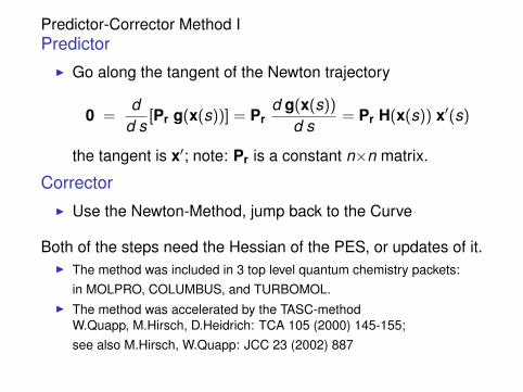
Predictor-Corrector Method IPredictor
I Go along the tangent of the Newton trajectory
0 =d
d s[Pr g(x(s))] = Pr
d g(x(s))d s
= Pr H(x(s)) x′(s)
the tangent is x′; note: Pr is a constant n×n matrix.
CorrectorI Use the Newton-Method, jump back to the Curve
Both of the steps need the Hessian of the PES, or updates of it.I The method was included in 3 top level quantum chemistry packets:
in MOLPRO, COLUMBUS, and TURBOMOL.I The method was accelerated by the TASC-method
W.Quapp, M.Hirsch, D.Heidrich: TCA 105 (2000) 145-155;see also M.Hirsch, W.Quapp: JCC 23 (2002) 887

Predictor-Corrector Method II
TASC-methodI Use the tangent of the Newton trajectory for the next
search direction r.The result is a Gradient Extremal (GE).
I Quapp, Hirsch, Heidrich: Theor. Chem. Acc. 105 (2000) 145
Definition of a GEI At every point the gradient of the PES is an eigenvector of
the Hessian.H g = λg
and λ is the corresponding eigenvalue.
I D.K.Hoffman, R.S.Nord, K.Ruedenberg: TCA 69 (1986) 265-279.”Gradient Extremals”
I W.Quapp: TCA 75 (1989) 447-460.”Gradient Extremals and Valley Floor Bifurcations on PES”

Gradient Extremal (GE)
At every point the gradient of the PES is an eigenvector of theHessian: H g = λ g, and λ is the Eigenvalue.
-2 -1 0 1 2
-2
-1
0
1
2
The fat curves are the GEs,they are fixed curves.
The thin dashes are NTs.They form a field.

NTs indicate Bifurcations of the ValleyI NTs have a second definition by a differential equation
dx(t)dt
= ±A(x(t)) g(x(t))
named the Branin equation.It uses the adjoint matrix A of the Hessian H,which is [(−1)i+j mij ]
T , where mij is the minor of H.It is A H = Det(H) I.
I The singular points of the equation are zeros ofA(x) g(x) = 0, thus(i) stationary points, if also g(x) = 0, or(ii) valley-ridge inflection points (VRI), if g(x) 6= 0
If A(x) g(x) = 0 and g(x) 6= 0, then an eigenvector of theHessian to eigenvalue zero is orthogonal to the gradient.

Branin is the desingularized, continuous Newton equationI A Newton step is
x1 = x0 − H−1(x0) g(x0)
I One may change this difference into a differential equation,the continuous Newton equation
dx(t)dt
= −H−1(x(t)) g(x(t)
I However, the inverse Hessian is singular, if the Hessianhas a zero determinat. The way out is a desingularizationof the differential equation
dx(t)dt
= −Det(H(x(t))H−1(x(t))g(x(t))

String Method
I Chose an initial Chain between two Minimums.I Change the Chain by a controlled Newton-Method, step by
step, back to the searched Newton Trajectory.
60 90 120 150 180
Φ
-180
-150
-120
-90
-60
Ψ
60 90 120 150 180
-180
-150
-120
-90
-60
6-31G
C7ax
TP
BP
BP
TS
C5
*
The colored curves are different NTs(W.Quapp, JTCC 8, (2009) 101-117"The growing string method for flows of
NTs by a second order corrector")The PES concerns Alanine-Dipeptide:CH3CO-NHCHCH3CO-NHCH3The dimension is (3N-6)=60, N=22 atomsOne of the blue NTs shows
Predictor- and Corrector steps

Effort for the String Method
I Example Alanine-Dipeptide, 60 internal coordinates,(2 dihedrals fixed, thus 58 coordinates optimized)
I Used: GamesUS on PC, DFT calculationsB3LYP/6-31G basis set
I Number of chains calculated: 9I Number of nodes per chain: 30I Number of corrector steps per node: 2-3
60 90 120 150 180
Φ
-180
-150
-120
-90
-60
Ψ
60 90 120 150 180
-180
-150
-120
-90
-60
6-31G
C7ax
TP
BP
BP
TS
C5
*
With such a nice convergence velocity,one can calculate many nodes per chain,and many NTs at all,
so to say, a flow of NTs.

The Index Theorem
Index Theorem: Let a and b be stationary points connected bya regular Newton trajectory. Then it holds
index(a) 6= index(b) ,and the difference is one.
-1.5 -1 -0.5 0 0.5 1 1.5 2
-1
-0.5
0
0.5
1
1.5
Regular NTs connect a SP (index 1)and a minimum (index 0).The PES shows two adjacent SPsof index one.There is no regular NT connectingthe SPs.Between the SPs a VRI pointhas to exist.One singular NT leads to the VRI pointand branches there.Hirsch, Quapp: JMSt THEOCHEM 683 (2004) 1

Two consecutive saddles can be connected only by a singularNewton trajectory which crosses a valley-ridge inflection (VRI)point.

Index Theorem: Let a and b be stationary points connected bya regular Newton trajectory. Then it holds
index(a) 6= index(b) ,and the difference is one.
-1 -0.5 0 0.5 1-1
-0.5
0
0.5
1
-1 -0.5 0 0.5 1-1
-0.5
0
0.5
1
-1 -0.5 0 0.5 1-1
-0.5
0
0.5
1
1’
0
1
2
Regular NTs Singular NT Regular NTsAt the bottom may be a minimum, at the top an index-2 SP, and left and right may be an index-1 SP.
The VRI point divides the two families of NTs to the two index-1 SPs.

Mechanochemistry and Catalysis
Apply a pulling force f to the PES:the generally accepted model consists in a first orderperturbation on the PES of the unperturbed molecular systemdue to a catalytic or pulling force by
Vf (r) = V (r)− fT (r− ro)
Vf is named the effective PES. The disarrangement of thestationary points of the new effective PES is described by NTs:The stationary points are given by the zero of the derivation
∇rVf (r) = 0 = g− f
g is the gradient of the PES. One searches a point where thegradient of the original PES has to be equal to the force, f. If fpoints always into the same direction then the solution is an NT.

Apply a force to a molecule: it means apply the force also to thePES.

Example 1
To start with we treat a one-dimensional case.
V
V1Min
BBP V2.275
1 2 3 4x
-6
-4
-2
2
4
6
PES
1D Morse potential over the x-axis: the upper curve. Below aretwo effective potential curves with increasing forces. Theminimum moves to increasing x-values, where the SP moves todecreasing values. The lowest potential is the final case:minimum and SP coalesce to a shoulder. The former barrier isbroken. The point is named barrier breckdown point (BBP).

Example 2Let be two minimums connected by regular NTs over an SP.
Min
Min
TP
SP
-2 -1 0 1 2-2
-1
0
1
2
Pulling into a defind direction uses a respective NT for the movement ofminimum and SP. The arc of the NT can be of different length. Thindashed NTs have a turning point (TP): pulling along such NTs is possible.

Example 2
We include a green BBP line whith Det(H)=0 (barrier break).1
Min
Min
TP
TP
VRIVRISP
-2 0 2 4
-2
-1
0
1
2
x
y
The energy, as well as the gradient norm variate on the green line.1Konda, Avdoshenko, Makarov, J.Chem.Phys. 140 (2014) 927,
Quapp, Bofill, Theoret. Chem. Acc. 135 (2016) 113.

Example 2
Norm of the gradient over three inner NTs (thick blue curves).
Min(a)
SP
-1.5 -1.0 -0.5 0.5 1.0x
10
20
30
40
50
60
|g|
The gradient norm variate with the crossing of the green line:there must be a minimum: the optimal BBP.

Example 2Optimal Newton trajectory
Min
Min
TPTP
VRIVRI SP
-2 0 2 4-2
-1
0
1
2
x
y
A special regular NT (blue) and a Gradient Extremal (thick black) cross thegreen line at the same point. This point is the BBP with lowest |g| withrespect to the others NTs crossing the green line. The regular NT indicatesthe optimal pulling direction.Proof: Quapp / Bofill, TCA 135 (2016) 113

Example 2
Extreme case of a regular NT with a turning point (TP).
R
TP
F=10F=30 F=50 F=100 F=150
BBP
SP
-1 0 1 2
-1.0
-0.5
0.0
0.5
x
y
The NT goes from minimum R over a TP and along a ridge back to the SP.The red point is its BBP.The effective stationary points are black points.The sticks are the connections between theeffective SPs (above on the ridge) and theeffective minimums (below in the valley) at the forces, F .

Example 3aDevelopment of effective PESs
R P
Max
SPl
SPu
-3 -2 -1 0 1 2 3
-3
-2
-1
0
1
2
3
x
y
(a)
PR
NTlow
SPl
SPu
-3 -2 -1 0 1 2 3
-3
-2
-1
0
1
2
x
y
(b)
PR
NTlowSPl
SPu
-3 -2 -1 0 1 2 3
-3
-2
-1
0
1
2
x
y
(c)
P
Shoulder
NTlow
SPu
-3 -2 -1 0 1 2 3
-3
-2
-1
0
1
2
x
y
Left above F=0.0, original PES with GE and optimal BBPs (red points).(a)-(c): Effective PESs for f=F l with pull direction l=(0.98,0.18)T and(a) F=1.4, (b) F=2.8, and (c) F=4.25 force along the same NT.The Reff , SPl,eff and SPu,eff are marked by black points.

Example 3b
PRMax
SPup
SPlow
NT1
BBP2BBP3
BBP4BBP1
-2 -1 0 1 2
-2
-1
0
1
2
x
y
GEs (fat) on a surface with 2 pathways. Crossings (red points) with thegreen lines are optimal BBPs. The optimal NT for a pulling over SPup isNT1. It intersects the left upper BBP1. A pulling moves R and SPup
together, but it moves also Max and SPlow together. Thus, the hight of SPup
decreases, but of SPlow increases.

A pull to the upper saddle along NT1 can circumvent theWoodward-Hoffman rules: it drives the reaction over theheigher saddle point.NT1 is here the optimal NT. On this NT, the minimum R and theSPup move together.However, the NT goes after the SPup over the maximum toSPlow , and then to the product minimum, P.This is allowed by the Index Theorem.Inverting this pulling causes a hysteresis.The pull along NT1 makes that the height of SPup decreases,however that of SPlow increases.In the next slight are shown the reactivity consequences.

Example 3bReaction Rates:kF ,up = ko,up Exp[−(VF (SPup)− VF (Min))/kT ]kF ,low = ko,lowExp[−(VF (SPlow )− VF (Min))/kT ]
(a)
2 4 6 8F
-15
-10
-5
log(kF,up)
(b)
0.5 1.0 1.5 2.0 2.5 3.0F
-10.0
-9.5
-9.0
-8.5
log(kF)
(c)
2 4 6 8F
-15
-14
-13
-12
-11
log(kF,low)
Eyring rates for the pulling force in the direction of NT1uphill to the high SPup.Left (a): exit over SPup,center (b) full rate of a reaction R→P, kF = kF ,up + kF ,low
right (c): exit over SPlow .
See: Quapp / Bofill, JCC 37 (2016) 2467.

Summary: How to find a curve ofForce Displaced Stationary Points, FDSPs?
I Describe the FDSPs by Newton Trajectories:it is tractable – in many practical cases.
I Find the BBP by Newton Trajectories: it is tractable.I Find VRI-Bifurcations by special Newton Trajectories:
it is tractable.
Acknowledgement
I I thank Prof. Josep Maria Bofill from Barcelona.The results presented here are born in discussions withhim, and are published in the papers:WQ, JMB: J. Phys. Chem. B 120 (2016) 2644WQ, JMB: Theoret. Chem. Acc. 135 (2016) 113WQ, JMB: J. Computat. Chem. 37 (2016) 2467.
Thank You for Your interest !

Some older References to Newton TrajectoriesWQ, M.Hirsch, O.Imig, D.Heidrich, J.Computat.Chem.19 (1998) 1087WQ, M.Hirsch, D.Heidrich, Theor.Chem.Acc.100 (1998) 285M.Hirsch, WQ, D.Heidrich, Phys.Chem.Chem.Phys.1 (1999) 5291WQ, M.Hirsch, D.Heidrich, Theoret.Chem.Acc.105 (2000) 145WQ, V.Melnikov, Phys.Chem.Chem.Phys.3 (2001) 2735WQ, J.Computat.Chem.22 (2001) 537J.M.Anglada,E.Besalu,J.M.Bofill,R.Crehuet, J.Comp.Chem.22 (2001) 387J.M.Bofill, J.M.Anglada, Theor.Chem.Acc.105 (2001) 463R.Crehuet, J.M.Bofill, J.M.Anglada, Theor.Chem.Acc.107 (2002) 130M.Hirsch, WQ, J.Math.Chem.36 (2004) 307M.Hirsch, WQ, Chem.Phys.Lett.395 (2004) 150WQ, J.Computat.Chem.25 (2004) 1277M.Hirsch, WQ, J.Mol.Struct.THEOCHEM 683 (2004) 1WQ, J.Mol.Struct.695-696 (2004) 95WQ, J.Chem.Phys.122 (2005) 174106WQ, J.Computat.Chem.28 (2007) 1834WQ, E.Kraka, D.Cremer, J.Phys.Chem.A 111 (2007) 11287H.Joo, E.Kraka, WQ, D.Cremer, Mol.Phys.105 (2007) 2697WQ, J.Theoret.Computat.Chem.8 (2009) 101J.M.Bofill, J.Chem.Phys.130 (2009) 176102WQ, B.Schmidt: Theoret.Chem.Acc. 128, Iss 1 (2011) 47-61J.M.Bofill, WQ: J. Chem. Phys. 134 (2011) 074101WQ, J.M.Bofill, J. Aguilar-Mogas: Theor. Chem. Acc. 129 (2011) 803WQ, J.M.Bofill: J. Math. Chem. 50, Iss 5 (2012) 2061WQ, J.M.Bofill, M.Caballero: Chem. Phys. Lett. 541 (2012) 122B.Schmidt, WQ: Theoret. Chem. Acc. 132 (2012) 1305WQ, J.M.Bofill: Int.J.Quant.Chem. 115 (2015) 1635J.M.Bofill: J. Chem. Phys. 143 (2015) 247101WQ: J. Math. Chem 54 (2015) 137-148
Related Documents


