Undergraduate Lecture Notes in Physics Wolfgang Demtröder Mechanics and Thermodynamics

Welcome message from author
This document is posted to help you gain knowledge. Please leave a comment to let me know what you think about it! Share it to your friends and learn new things together.
Transcript

Undergraduate Lecture Notes in Physics
Wolfgang Demtröder
Mechanics and Thermodynamics
Undergraduate Lecture Notes in Physics
Series editors
N. Ashby, University of Colorado, Boulder, USA
W. Brantley, Department of Physics, Furman University, Greenville, USA
M. Deady, Physics Program, Bard College, Annandale-on-Hudson, USA
M. Fowler, Dept of Physics, Univ of Virginia, Charlottesville, USA
M. Hjorth-Jensen, Dept. of Physics, University of Oslo, Oslo, Norway
M. Inglis, Earth &Space Sci, Smithtown Sci Bld, SUNY Suffolk County Community College, LongIsland, USA
H. Klose, Humboldt University, Oldenburg, Germany
H. Sherif, Department of Physics, University of Alberta, Edmonton, Canada

Undergraduate Lecture Notes in Physics (ULNP) publishes authoritative texts covering topics through-out pure and applied physics. Each title in the series is suitable as a basis for undergraduate instruction,typically containing practice problems, worked examples, chapter summaries, and suggestions for fur-ther reading.
ULNP titles must provide at least one of the following:
� An exceptionally clear and concise treatment of a standard undergraduate subject.
� A solid undergraduate-level introduction to a graduate, advanced, or non-standard subject.
� A novel perspective or an unusual approach to teaching a subject.
ULNP especially encourages new, original, and idiosyncratic approaches to physics teaching at theundergraduate level.
The purpose of ULNP is to provide intriguing, absorbing books that will continue to be the reader’spreferred reference throughout their academic career.
More information about this series athttp://www.springer.com/series/8917
Wolfgang Demtröder
Mechanics andThermodynamics
Wolfgang DemtröderKaiserslautern, [email protected]
ISSN 2192-4791 ISSN 2192-4805 (electronic)Undergraduate Lecture Notes in PhysicsISBN 978-3-319-27875-9 ISBN 978-3-319-27877-3 (eBook)DOI 10.1007/978-3-319-27877-3Library of Congress Control Number: 2016944491
© Springer International Publishing Switzerland 2017This work is subject to copyright. All rights are reserved by the Publisher, whether the whole or part of the material isconcerned, specifically the rights of translation, reprinting, reuse of illustrations, recitation, broadcasting, reproductionon microfilms or in any other physical way, and transmission or information storage and retrieval, electronic adaptation,computer software, or by similar or dissimilar methodology now known or hereafter developed.The use of general descriptive names, registered names, trademarks, service marks, etc. in this publication does not imply,even in the absence of a specific statement, that such names are exempt from the relevant protective laws and regulationsand therefore free for general use.The publisher, the authors and the editors are safe to assume that the advice and information in this book are believedto be true and accurate at the date of publication. Neither the publisher nor the authors or the editors give a warranty,express or implied, with respect to the material contained herein or for any errors or omissions that may have been made.
Printed on acid-free paper
This Springer imprint is published by Springer NatureThe registered company is Springer International Publishing AGThe registered company address is: Gewerbestrasse 11, 6330 Cham, Switzerland

Preface
The present textbook represents the first part of a four-volume series on experimental Physics. It coversthe field of Mechanics and Thermodynamics. One of its goal is to illustrate, that the explanation of ourworld and of all natural processes by Physics is always the description of models of our world, whichare formulated by theory and proved by experiments. The continuous improvement of these modelsleads to a more detailled understanding of our world and of the processes that proceed in it.
The representation of this textbook starts with an introductory chapter giving a brief survey of the his-tory and development of Physics and its present relevance for other sciences and for technology. Sinceexperimental Physics is based on measuring techniques and quantitative results, a section discussesbasic units, techniques for their measurements and the accuracy and possible errors of measurements.
In all further chapters the description of the real world by successively refined models is outlined. Itbegins with the model of a point mass, its motion under the action of forces and its limitations. Sincethe description of moving masses requires a coordinate system, the transformation of results obtainedin one system to another system moving against the first one is described. This leads to the theoryof special relativity, which is discussed in Chap. 3. The next chapter upgrades the model of pointmasses to spatially extended rigid bodies, where the spatial extension of a body cannot be ignoredbut influences the results. Then the deformation of bodies under the influence of forces is discussedand phenomena caused by this deformation are explained. The existence of different phases (solid,liquid and gaseous) and their relation with external influences such as temperature and pressure, arediscussed.
The properties of gases and liquids at rest and the effects caused by streaming gases and liquids areoutlined in Chap. 7 and 8.
Many insights in natural phenomena, in particular in the area of atomic and molecular physics couldonly be explored after sufficiently good vacua could be realized. Therefore Chap. 9 discusses brieflythe most important facts of vacuum physics, such as the realization and measurement of evacuatedvolumina.
Thermodynamics governs important aspects of our life. Therefore an extended chapter about defini-tions and measuring techniques for temperatures, heat energy and phase transitions should emphazisethe importance of thermodynamics. The three principle laws ot thermodynamics and their relevanvefor energy transformation and dissipation are discussed.
Chapter 11 deals with oscillations and waves, a subject which is closely related to acoustics and optics.
While all foregoing chapters discuss classical physics which had been developed centuries ago,Chap. 12 covers a modern subject, namely nonlinear phenomena and chaos theory. It should givea feeling for the fact, that most phenomena in classical physics can be described only approximatelyby linear equations. A closer inspection shows that the accurate description demands nonlinear equa-tions with surprising solutions.
A description of phenomena in physics requires someminimummathematical knowledge. Therefore abrief survey about vector algebra and vector analysis, about complex numbers and different coordinatesystems is provided in the last chapter.
A real understanding of the subjects covered in this textbook can be checked by solving problems,which are given at the end of each chapter. A sketch of the solutions can be found at the end of thebook.
For further studies and a deeper insight into special subjects some selected literature is given at theend of each chapter.
v

vi Preface
The author hopes that this book can transfer some of his enthusiasm for the fascinating field of physics.He is grateful for any comments and suggestions, also for hints to possible errors. Every e-mail willbe answered as soon as possible.
Several people have contributed to the realization of this book. Many thanks go the Dr. Schneiderand Ute Heuser, Springer Verlag Heidelberg, who supported and encouraged the authors over thewhole period needed for translating this book from a German version. Nadja Kroke and her team(le-tex publishing services GmbH) did a careful job for the layout of the book and induced the authorto improve ambiguous sentences or unclear hints to equations or figures. I thank them all for theirefforts.
Last but not least I thank my wife Harriet, who showed much patience when her husband disappearedinto his office for the work on this book.
Kaiserslautern, December 2016 Wolfgang Demtröder
Contents
1 Introduction and Survey . . . . . . . . . . . . . . . . . . . . . . . . . . . . . . . . . . . . 1
1.1 The Importance of Experiments . . . . . . . . . . . . . . . . . . . . . . . . . . . 2
1.2 The Concept of Models in Physics . . . . . . . . . . . . . . . . . . . . . . . . . 3
1.3 Short Historical Review . . . . . . . . . . . . . . . . . . . . . . . . . . . . . . . . 51.3.1 The Natural Philosophy in Ancient Times . . . . . . . . . . . . . . . 51.3.2 The Development of Classical Physics . . . . . . . . . . . . . . . . . . 71.3.3 Modern Physics . . . . . . . . . . . . . . . . . . . . . . . . . . . . . . . . 10
1.4 The Present Conception of Our World . . . . . . . . . . . . . . . . . . . . . . 11
1.5 Relations Between Physics and Other Sciences . . . . . . . . . . . . . . . . . 141.5.1 Biophysics and Medical Physics . . . . . . . . . . . . . . . . . . . . . . 141.5.2 Astrophysics . . . . . . . . . . . . . . . . . . . . . . . . . . . . . . . . . . . 151.5.3 Geophysics and Meteorology . . . . . . . . . . . . . . . . . . . . . . . 151.5.4 Physics and Technology . . . . . . . . . . . . . . . . . . . . . . . . . . . 151.5.5 Physics and Philosophy . . . . . . . . . . . . . . . . . . . . . . . . . . . 16
1.6 The Basic Units in Physics, Their Standards and Measuring Techniques 161.6.1 Length Units . . . . . . . . . . . . . . . . . . . . . . . . . . . . . . . . . . 171.6.2 Measuring Techniques for Lengths . . . . . . . . . . . . . . . . . . . 191.6.3 Time-Units . . . . . . . . . . . . . . . . . . . . . . . . . . . . . . . . . . . . 201.6.4 How to measure Times . . . . . . . . . . . . . . . . . . . . . . . . . . . 231.6.5 Mass Units and Their Measurement . . . . . . . . . . . . . . . . . . . 231.6.6 Molar Quantity Unit . . . . . . . . . . . . . . . . . . . . . . . . . . . . . 241.6.7 Temperature Unit . . . . . . . . . . . . . . . . . . . . . . . . . . . . . . . 241.6.8 Unit of the Electric Current . . . . . . . . . . . . . . . . . . . . . . . . 251.6.9 Unit of Luminous Intensity . . . . . . . . . . . . . . . . . . . . . . . . . 251.6.10 Unit of Angle . . . . . . . . . . . . . . . . . . . . . . . . . . . . . . . . . . 25
1.7 Systems of Units . . . . . . . . . . . . . . . . . . . . . . . . . . . . . . . . . . . . . 26
1.8 Accuracy and Precision; Measurement Uncertainties and Errors . . . . . 271.8.1 Systematic Errors . . . . . . . . . . . . . . . . . . . . . . . . . . . . . . . 271.8.2 Statistical Errors, Distribution of Experimental Values, Mean
Values . . . . . . . . . . . . . . . . . . . . . . . . . . . . . . . . . . . . . . . 271.8.3 Variance and its Measure . . . . . . . . . . . . . . . . . . . . . . . . . . 291.8.4 Error Distribution Law . . . . . . . . . . . . . . . . . . . . . . . . . . . . 291.8.5 Error Propagation . . . . . . . . . . . . . . . . . . . . . . . . . . . . . . . 311.8.6 Equalization Calculus . . . . . . . . . . . . . . . . . . . . . . . . . . . . 32
Summary . . . . . . . . . . . . . . . . . . . . . . . . . . . . . . . . . . . . . . . . . . . . . . . 34
Problems . . . . . . . . . . . . . . . . . . . . . . . . . . . . . . . . . . . . . . . . . . . . . . . 35
References . . . . . . . . . . . . . . . . . . . . . . . . . . . . . . . . . . . . . . . . . . . . . 35
2 Mechanics of a Point Mass . . . . . . . . . . . . . . . . . . . . . . . . . . . . . . . . . . 39
2.1 The Model of the Point Mass; Trajectories . . . . . . . . . . . . . . . . . . . . 40
2.2 Velocity and Acceleration . . . . . . . . . . . . . . . . . . . . . . . . . . . . . . . 41
vii
viii Contents
2.3 Uniformly Accelerated Motion . . . . . . . . . . . . . . . . . . . . . . . . . . . 422.3.1 The Free Fall . . . . . . . . . . . . . . . . . . . . . . . . . . . . . . . . . . 432.3.2 Projectile Motion . . . . . . . . . . . . . . . . . . . . . . . . . . . . . . . 43
2.4 Motions with Non-Constant Acceleration . . . . . . . . . . . . . . . . . . . . 442.4.1 Uniform Circular Motion . . . . . . . . . . . . . . . . . . . . . . . . . . 442.4.2 Motions on Trajectories with Arbitrary Curvature . . . . . . . . . 45
2.5 Forces . . . . . . . . . . . . . . . . . . . . . . . . . . . . . . . . . . . . . . . . . . . . 472.5.1 Forces as Vectors; Addition of Forces . . . . . . . . . . . . . . . . . . 472.5.2 Force-Fields . . . . . . . . . . . . . . . . . . . . . . . . . . . . . . . . . . . 482.5.3 Measurements of Forces; Discussion of the Force Concept . . . 50
2.6 The Basic Equations of Mechanics . . . . . . . . . . . . . . . . . . . . . . . . . 512.6.1 The Newtonian Axioms . . . . . . . . . . . . . . . . . . . . . . . . . . . 512.6.2 Inertial and Gravitational Mass . . . . . . . . . . . . . . . . . . . . . . 522.6.3 The Equation of Motion of a Particle in Arbitrary Force Fields . 53
2.7 Energy Conservation Law of Mechanics . . . . . . . . . . . . . . . . . . . . . 562.7.1 Work and Power . . . . . . . . . . . . . . . . . . . . . . . . . . . . . . . 562.7.2 Path-Independent Work; Conservative Force-Fields . . . . . . . . 582.7.3 Potential Energy . . . . . . . . . . . . . . . . . . . . . . . . . . . . . . . . 592.7.4 Energy Conservation Law in Mechanics . . . . . . . . . . . . . . . . 612.7.5 Relation Between Force Field and Potential . . . . . . . . . . . . . 62
2.8 Angular Momentum and Torque . . . . . . . . . . . . . . . . . . . . . . . . . . 63
2.9 Gravitation and the Planetary Motions . . . . . . . . . . . . . . . . . . . . . . 642.9.1 Kepler’s Laws . . . . . . . . . . . . . . . . . . . . . . . . . . . . . . . . . . 642.9.2 Newton’s Law of Gravity . . . . . . . . . . . . . . . . . . . . . . . . . . 662.9.3 Planetary Orbits . . . . . . . . . . . . . . . . . . . . . . . . . . . . . . . . 662.9.4 The Effective Potential . . . . . . . . . . . . . . . . . . . . . . . . . . . 682.9.5 Gravitational Field of Extended Bodies . . . . . . . . . . . . . . . . 692.9.6 Measurements of the Gravitational Constant G . . . . . . . . . . . 712.9.7 Testing Newton’s Law of Gravity . . . . . . . . . . . . . . . . . . . . . 722.9.8 Experimental Determination of the Earth Acceleration g . . . . 74
Summary . . . . . . . . . . . . . . . . . . . . . . . . . . . . . . . . . . . . . . . . . . . . . . . 76
Problems . . . . . . . . . . . . . . . . . . . . . . . . . . . . . . . . . . . . . . . . . . . . . . . 77
References . . . . . . . . . . . . . . . . . . . . . . . . . . . . . . . . . . . . . . . . . . . . . 79
3 Moving Coordinate Systems and Special Relativity . . . . . . . . . . . . . . . . . . 81
3.1 Relative Motion . . . . . . . . . . . . . . . . . . . . . . . . . . . . . . . . . . . . . 82
3.2 Inertial Systems and Galilei-Transformations . . . . . . . . . . . . . . . . . . 82
3.3 Accelerated Systems; Inertial Forces . . . . . . . . . . . . . . . . . . . . . . . . 833.3.1 Rectilinear Accelerated Systems . . . . . . . . . . . . . . . . . . . . . 833.3.2 Rotating Systems . . . . . . . . . . . . . . . . . . . . . . . . . . . . . . . 853.3.3 Centrifugal- and Coriolis-Forces . . . . . . . . . . . . . . . . . . . . . 863.3.4 Summary . . . . . . . . . . . . . . . . . . . . . . . . . . . . . . . . . . . . . 89
3.4 The Constancy of the Velocity of Light . . . . . . . . . . . . . . . . . . . . . . 89
3.5 Lorentz-Transformations . . . . . . . . . . . . . . . . . . . . . . . . . . . . . . . 90
3.6 Theory of Special Relativity . . . . . . . . . . . . . . . . . . . . . . . . . . . . . . 923.6.1 The Problem of Simultaneity . . . . . . . . . . . . . . . . . . . . . . . 923.6.2 Minkowski-Diagram . . . . . . . . . . . . . . . . . . . . . . . . . . . . . 933.6.3 Lenght Scales . . . . . . . . . . . . . . . . . . . . . . . . . . . . . . . . . . 933.6.4 Lorentz-Contraction of Lengths . . . . . . . . . . . . . . . . . . . . . 943.6.5 Time Dilatation . . . . . . . . . . . . . . . . . . . . . . . . . . . . . . . . 96
Contents ix
3.6.6 The Twin-Paradox . . . . . . . . . . . . . . . . . . . . . . . . . . . . . . . 973.6.7 Space-time Events and Causality . . . . . . . . . . . . . . . . . . . . . 99
Summary . . . . . . . . . . . . . . . . . . . . . . . . . . . . . . . . . . . . . . . . . . . . . . . 100
Problems . . . . . . . . . . . . . . . . . . . . . . . . . . . . . . . . . . . . . . . . . . . . . . . 100
References . . . . . . . . . . . . . . . . . . . . . . . . . . . . . . . . . . . . . . . . . . . . . 101
4 Systems of Point Masses; Collisions . . . . . . . . . . . . . . . . . . . . . . . . . . . . 103
4.1 Fundamentals . . . . . . . . . . . . . . . . . . . . . . . . . . . . . . . . . . . . . . . 1044.1.1 Centre of Mass . . . . . . . . . . . . . . . . . . . . . . . . . . . . . . . . . 1044.1.2 Reduced Mass . . . . . . . . . . . . . . . . . . . . . . . . . . . . . . . . . 1054.1.3 Angular Momentum of a System of Particles . . . . . . . . . . . . 105
4.2 Collisions Between Two Particles . . . . . . . . . . . . . . . . . . . . . . . . . . 1074.2.1 Basic Equations . . . . . . . . . . . . . . . . . . . . . . . . . . . . . . . . 1084.2.2 Elastic Collisions in the Lab-System . . . . . . . . . . . . . . . . . . . 1094.2.3 Elastic Collisions in the Centre-of Mass system . . . . . . . . . . . 1114.2.4 Inelastic Collisions . . . . . . . . . . . . . . . . . . . . . . . . . . . . . . . 1134.2.5 Newton-Diagrams . . . . . . . . . . . . . . . . . . . . . . . . . . . . . . . 114
4.3 What Do We Learn from the Investigation of Collisions? . . . . . . . . . . 1154.3.1 Scattering in a Spherical Symmetric Potential . . . . . . . . . . . . 1154.3.2 Reactive Collisions . . . . . . . . . . . . . . . . . . . . . . . . . . . . . . 118
4.4 Collisions at Relativistic Energies . . . . . . . . . . . . . . . . . . . . . . . . . . 1194.4.1 Relativistic Mass Increase . . . . . . . . . . . . . . . . . . . . . . . . . . 1194.4.2 Force and Relativistic Momentum . . . . . . . . . . . . . . . . . . . . 1204.4.3 The Relativistic Energy . . . . . . . . . . . . . . . . . . . . . . . . . . . . 1214.4.4 Inelastic Collisions at relativistic Energies . . . . . . . . . . . . . . . 1224.4.5 Relativistic Formulation of Energy Conservation . . . . . . . . . . 122
4.5 Conservation Laws . . . . . . . . . . . . . . . . . . . . . . . . . . . . . . . . . . . . 1234.5.1 Conservation of Momentum . . . . . . . . . . . . . . . . . . . . . . . 1234.5.2 Energy Conservation . . . . . . . . . . . . . . . . . . . . . . . . . . . . . 1244.5.3 Conservation of Angular Momentum . . . . . . . . . . . . . . . . . 1244.5.4 Conservation Laws and Symmetries . . . . . . . . . . . . . . . . . . . 124
Summary . . . . . . . . . . . . . . . . . . . . . . . . . . . . . . . . . . . . . . . . . . . . . . . 125
Problems . . . . . . . . . . . . . . . . . . . . . . . . . . . . . . . . . . . . . . . . . . . . . . . 126
References . . . . . . . . . . . . . . . . . . . . . . . . . . . . . . . . . . . . . . . . . . . . . 127
5 Dynamics of rigid Bodies . . . . . . . . . . . . . . . . . . . . . . . . . . . . . . . . . . . . 129
5.1 The Model of a Rigid Body . . . . . . . . . . . . . . . . . . . . . . . . . . . . . . 130
5.2 Center of Mass . . . . . . . . . . . . . . . . . . . . . . . . . . . . . . . . . . . . . . 130
5.3 Motion of a Rigid Body . . . . . . . . . . . . . . . . . . . . . . . . . . . . . . . . 131
5.4 Forces and Couple of Forces . . . . . . . . . . . . . . . . . . . . . . . . . . . . . 132
5.5 Rotational Inertia and Rotational Energy . . . . . . . . . . . . . . . . . . . . 1335.5.1 The Parallel Axis Theorem (Steiner’s Theorem) . . . . . . . . . . . 134
5.6 Equation of Motion for the Rotation of a Rigid Body . . . . . . . . . . . . 1365.6.1 Rotation About an Axis for a Constant Torque . . . . . . . . . . . 1375.6.2 Measurements of rotational inertia; Rotary Oscillations About
a Fixed Axis . . . . . . . . . . . . . . . . . . . . . . . . . . . . . . . . . . . 1395.6.3 Comparison Between Translation and Rotation . . . . . . . . . . . 139
x Contents
5.7 Rotation About Free Axes; Spinning Top . . . . . . . . . . . . . . . . . . . . . 1395.7.1 Inertial Tensor and Inertial Ellipsoid . . . . . . . . . . . . . . . . . . 1405.7.2 Principal Moments of Inertia . . . . . . . . . . . . . . . . . . . . . . . 1415.7.3 Free Rotational axes . . . . . . . . . . . . . . . . . . . . . . . . . . . . . 1435.7.4 Euler’s Equations . . . . . . . . . . . . . . . . . . . . . . . . . . . . . . . 1445.7.5 The Torque-free Symmetric Top . . . . . . . . . . . . . . . . . . . . . 1455.7.6 Precession of the Symmetric Top . . . . . . . . . . . . . . . . . . . . . 1475.7.7 Superposition of Nutation and Precession . . . . . . . . . . . . . . 148
5.8 The Earth as Symmetric Top . . . . . . . . . . . . . . . . . . . . . . . . . . . . . 149
Summary . . . . . . . . . . . . . . . . . . . . . . . . . . . . . . . . . . . . . . . . . . . . . . . 151
Problems . . . . . . . . . . . . . . . . . . . . . . . . . . . . . . . . . . . . . . . . . . . . . . . 151
References . . . . . . . . . . . . . . . . . . . . . . . . . . . . . . . . . . . . . . . . . . . . . 152
6 Real Solid and Liquid Bodies . . . . . . . . . . . . . . . . . . . . . . . . . . . . . . . . . 153
6.1 Atomic Model of the Different Aggregate States . . . . . . . . . . . . . . . 154
6.2 Deformable Solid Bodies . . . . . . . . . . . . . . . . . . . . . . . . . . . . . . . 1556.2.1 Hooke’s Law . . . . . . . . . . . . . . . . . . . . . . . . . . . . . . . . . . 1566.2.2 Transverse Contraction . . . . . . . . . . . . . . . . . . . . . . . . . . . 1576.2.3 Shearing and Torsion Module . . . . . . . . . . . . . . . . . . . . . . . 1586.2.4 Bending of a Balk . . . . . . . . . . . . . . . . . . . . . . . . . . . . . . . 1596.2.5 Elastic Hysteresis; Energy of Deformation . . . . . . . . . . . . . . . 1616.2.6 The Hardness of a Solid Body . . . . . . . . . . . . . . . . . . . . . . . 162
6.3 Static Liquids; Hydrostatics . . . . . . . . . . . . . . . . . . . . . . . . . . . . . . 1626.3.1 Free Displacement and Surfaces of Liquids . . . . . . . . . . . . . . 1626.3.2 Static Pressure in a Liquid . . . . . . . . . . . . . . . . . . . . . . . . . 1636.3.3 Buoyancy and Floatage . . . . . . . . . . . . . . . . . . . . . . . . . . . 165
6.4 Phenomena at Liquid Surfaces . . . . . . . . . . . . . . . . . . . . . . . . . . . 1666.4.1 Surface Tension . . . . . . . . . . . . . . . . . . . . . . . . . . . . . . . . 1666.4.2 Interfaces and Adhesion Tension . . . . . . . . . . . . . . . . . . . . . 1686.4.3 Capillarity . . . . . . . . . . . . . . . . . . . . . . . . . . . . . . . . . . . . 1706.4.4 Summary of Section 6.4 . . . . . . . . . . . . . . . . . . . . . . . . . . . 171
6.5 Friction Between Solid Bodies . . . . . . . . . . . . . . . . . . . . . . . . . . . . 1716.5.1 Static Friction . . . . . . . . . . . . . . . . . . . . . . . . . . . . . . . . . . 1716.5.2 Sliding Friction . . . . . . . . . . . . . . . . . . . . . . . . . . . . . . . . . 1726.5.3 Rolling Friction . . . . . . . . . . . . . . . . . . . . . . . . . . . . . . . . . 1736.5.4 Significance of Friction for Technology . . . . . . . . . . . . . . . . 174
6.6 The Earth as Deformable Body . . . . . . . . . . . . . . . . . . . . . . . . . . . 1746.6.1 Ellipticity of the Rotating Earth . . . . . . . . . . . . . . . . . . . . . 1756.6.2 Tidal Deformations . . . . . . . . . . . . . . . . . . . . . . . . . . . . . . 1756.6.3 Consequences of the Tides . . . . . . . . . . . . . . . . . . . . . . . . . 1786.6.4 Measurements of the Earth Deformation . . . . . . . . . . . . . . . 179
Summary . . . . . . . . . . . . . . . . . . . . . . . . . . . . . . . . . . . . . . . . . . . . . . . 180
Problems . . . . . . . . . . . . . . . . . . . . . . . . . . . . . . . . . . . . . . . . . . . . . . . 181
References . . . . . . . . . . . . . . . . . . . . . . . . . . . . . . . . . . . . . . . . . . . . . 181
7 Gases . . . . . . . . . . . . . . . . . . . . . . . . . . . . . . . . . . . . . . . . . . . . . . . . . 183
7.1 Macroscopic Model . . . . . . . . . . . . . . . . . . . . . . . . . . . . . . . . . . . 184
7.2 Atmospheric Pressure and Barometric Formula . . . . . . . . . . . . . . . . 185
Contents xi
7.3 Kinetic Gas Theory . . . . . . . . . . . . . . . . . . . . . . . . . . . . . . . . . . . . 1887.3.1 The Model of the Ideal Gas . . . . . . . . . . . . . . . . . . . . . . . . 1887.3.2 Basic Equations of the Kinetic Gas Theory . . . . . . . . . . . . . . 1897.3.3 Mean Kinetic Energy and Absolute Temperature . . . . . . . . . . 1907.3.4 Distribution Function . . . . . . . . . . . . . . . . . . . . . . . . . . . . 1907.3.5 Maxwell–Boltzmann Velocity Distribution . . . . . . . . . . . . . . 1917.3.6 Collision Cross Section and Mean Free Path Length . . . . . . . . 195
7.4 Experimental Proof of the Kinetic Gas Theory . . . . . . . . . . . . . . . . . 1967.4.1 Molecular Beams . . . . . . . . . . . . . . . . . . . . . . . . . . . . . . . 196
7.5 Transport Phenomena in Gases . . . . . . . . . . . . . . . . . . . . . . . . . . . 1987.5.1 Diffusion . . . . . . . . . . . . . . . . . . . . . . . . . . . . . . . . . . . . . 1987.5.2 Brownian Motion . . . . . . . . . . . . . . . . . . . . . . . . . . . . . . . 2007.5.3 Heat Conduction in Gases . . . . . . . . . . . . . . . . . . . . . . . . . 2017.5.4 Viscosity of Gases . . . . . . . . . . . . . . . . . . . . . . . . . . . . . . . 2027.5.5 Summary of Transport Phenomena . . . . . . . . . . . . . . . . . . . 203
7.6 The Atmosphere of the Earth . . . . . . . . . . . . . . . . . . . . . . . . . . . . 204
Summary . . . . . . . . . . . . . . . . . . . . . . . . . . . . . . . . . . . . . . . . . . . . . . . 206
Problems . . . . . . . . . . . . . . . . . . . . . . . . . . . . . . . . . . . . . . . . . . . . . . . 207
References . . . . . . . . . . . . . . . . . . . . . . . . . . . . . . . . . . . . . . . . . . . . . 208
8 Liquids and Gases in Motion; Fluid Dynamics . . . . . . . . . . . . . . . . . . . . . . 209
8.1 Basic Definitions and Types of Fluid Flow . . . . . . . . . . . . . . . . . . . . 210
8.2 Euler Equation for Ideal Liquids . . . . . . . . . . . . . . . . . . . . . . . . . . . 212
8.3 Continuity Equation . . . . . . . . . . . . . . . . . . . . . . . . . . . . . . . . . . 212
8.4 Bernoulli Equation . . . . . . . . . . . . . . . . . . . . . . . . . . . . . . . . . . . 213
8.5 Laminar Flow . . . . . . . . . . . . . . . . . . . . . . . . . . . . . . . . . . . . . . . 2168.5.1 Internal Friction . . . . . . . . . . . . . . . . . . . . . . . . . . . . . . . . 2168.5.2 Laminar Flow Between Two Parallel Walls . . . . . . . . . . . . . . 2188.5.3 Laminar Flows in Tubes . . . . . . . . . . . . . . . . . . . . . . . . . . . 2198.5.4 Stokes Law, Falling Ball Viscometer . . . . . . . . . . . . . . . . . . . 220
8.6 Navier–Stokes Equation . . . . . . . . . . . . . . . . . . . . . . . . . . . . . . . . 2208.6.1 Vortices and Circulation . . . . . . . . . . . . . . . . . . . . . . . . . . . 2218.6.2 Helmholtz Vorticity Theorems . . . . . . . . . . . . . . . . . . . . . . 2228.6.3 The Formation of Vortices . . . . . . . . . . . . . . . . . . . . . . . . . 2238.6.4 Turbulent Flows; Flow Resistance . . . . . . . . . . . . . . . . . . . . 224
8.7 Aerodynamics . . . . . . . . . . . . . . . . . . . . . . . . . . . . . . . . . . . . . . . 2268.7.1 The Aerodynamical Buoyancy . . . . . . . . . . . . . . . . . . . . . . . 2268.7.2 Relation between Dynamical and Flow Resistance . . . . . . . . . 2278.7.3 Forces on a flying Plane . . . . . . . . . . . . . . . . . . . . . . . . . . . 228
8.8 Similarity Laws; Reynolds’ Number . . . . . . . . . . . . . . . . . . . . . . . . . 228
8.9 Usage of Wind Energy . . . . . . . . . . . . . . . . . . . . . . . . . . . . . . . . . 229
Summary . . . . . . . . . . . . . . . . . . . . . . . . . . . . . . . . . . . . . . . . . . . . . . . 233
Problems . . . . . . . . . . . . . . . . . . . . . . . . . . . . . . . . . . . . . . . . . . . . . . . 234
References . . . . . . . . . . . . . . . . . . . . . . . . . . . . . . . . . . . . . . . . . . . . . 235
9 Vacuum Physics . . . . . . . . . . . . . . . . . . . . . . . . . . . . . . . . . . . . . . . . . . 237
9.1 Fundamentals and Basic Concepts . . . . . . . . . . . . . . . . . . . . . . . . . 2389.1.1 The Different Vacuum Ranges . . . . . . . . . . . . . . . . . . . . . . 2389.1.2 Influence of the Molecules at the Walls . . . . . . . . . . . . . . . . 239
xii Contents
9.1.3 Pumping Speed and Suction Capacity of Vacuum Pumps . . . . 2399.1.4 Flow Conductance of Vacuum Pipes . . . . . . . . . . . . . . . . . . 2409.1.5 Accessible Final Pressure . . . . . . . . . . . . . . . . . . . . . . . . . . 241
9.2 Generation of Vacuum . . . . . . . . . . . . . . . . . . . . . . . . . . . . . . . . . 2419.2.1 Mechanical Pumps . . . . . . . . . . . . . . . . . . . . . . . . . . . . . . 2429.2.2 Diffusion Pumps . . . . . . . . . . . . . . . . . . . . . . . . . . . . . . . . 2449.2.3 Cryo- and Sorption-Pumps; Ion-Getter Pumps . . . . . . . . . . . . 246
9.3 Measurement of Low Pressures . . . . . . . . . . . . . . . . . . . . . . . . . . . 2479.3.1 Liquid Manometers . . . . . . . . . . . . . . . . . . . . . . . . . . . . . . 2489.3.2 Membrane Manometer . . . . . . . . . . . . . . . . . . . . . . . . . . . 2489.3.3 Heat Conduction Manometers . . . . . . . . . . . . . . . . . . . . . . 2499.3.4 Ionization Gauge and Penning Vacuum Meter . . . . . . . . . . . 2499.3.5 Rotating Ball Vacuum Gauge . . . . . . . . . . . . . . . . . . . . . . . 250
Summary . . . . . . . . . . . . . . . . . . . . . . . . . . . . . . . . . . . . . . . . . . . . . . . 251
Problems . . . . . . . . . . . . . . . . . . . . . . . . . . . . . . . . . . . . . . . . . . . . . . . 251
References . . . . . . . . . . . . . . . . . . . . . . . . . . . . . . . . . . . . . . . . . . . . . 252
10 Thermodynamics . . . . . . . . . . . . . . . . . . . . . . . . . . . . . . . . . . . . . . . . . 253
10.1 Temperature and Amount of Heat . . . . . . . . . . . . . . . . . . . . . . . . . 25410.1.1 Temperature Measurements, Thermometer, and Temperature
Scales . . . . . . . . . . . . . . . . . . . . . . . . . . . . . . . . . . . . . . . 25410.1.2 Thermal Expansion of Liquids and Solids . . . . . . . . . . . . . . . 25610.1.3 Thermal Expansion of Gases; Gas Thermometer . . . . . . . . . . 25810.1.4 Absolute Temperature Scale . . . . . . . . . . . . . . . . . . . . . . . . 25910.1.5 Amount of Heat and Specific Heat Capacity . . . . . . . . . . . . . 26010.1.6 Molar Volume and Avogadro Constant . . . . . . . . . . . . . . . . 26110.1.7 Internal Energy and Molar Heat Capacity of Ideal Gases . . . . . 26110.1.8 Specific Heat of a Gas at Constant Pressure . . . . . . . . . . . . . 26210.1.9 Molecular Explanation of the Specific Heat . . . . . . . . . . . . . 26310.1.10 Specific Heat Capacity of Solids . . . . . . . . . . . . . . . . . . . . . . 26410.1.11 Fusion Heat and Heat of Evaporation . . . . . . . . . . . . . . . . . 265
10.2 Heat Transport . . . . . . . . . . . . . . . . . . . . . . . . . . . . . . . . . . . . . . 26610.2.1 Convection . . . . . . . . . . . . . . . . . . . . . . . . . . . . . . . . . . . 26610.2.2 Heat Conduction . . . . . . . . . . . . . . . . . . . . . . . . . . . . . . . 26710.2.3 The Heat Pipe . . . . . . . . . . . . . . . . . . . . . . . . . . . . . . . . . 27110.2.4 Methods of Thermal Insulation . . . . . . . . . . . . . . . . . . . . . . 27110.2.5 Thermal Radiation . . . . . . . . . . . . . . . . . . . . . . . . . . . . . . 273
10.3 The Three Laws of Thermodynamics . . . . . . . . . . . . . . . . . . . . . . . . 27910.3.1 Thermodynamic Variables . . . . . . . . . . . . . . . . . . . . . . . . . 27910.3.2 The First Law of Thermodynamics . . . . . . . . . . . . . . . . . . . . 28010.3.3 Special Processes as Examples of the First Law of Thermody-
namics . . . . . . . . . . . . . . . . . . . . . . . . . . . . . . . . . . . . . . 28110.3.4 The Second Law of Thermodynamics . . . . . . . . . . . . . . . . . . 28210.3.5 The Carnot Cycle . . . . . . . . . . . . . . . . . . . . . . . . . . . . . . . 28310.3.6 Equivalent Formulations of the Second Law . . . . . . . . . . . . . 28610.3.7 Entropy . . . . . . . . . . . . . . . . . . . . . . . . . . . . . . . . . . . . . . 28610.3.8 Reversible and Irreversible Processes . . . . . . . . . . . . . . . . . . 29010.3.9 Free Energy and Enthalpy . . . . . . . . . . . . . . . . . . . . . . . . . 29110.3.10 Chemical Reactions . . . . . . . . . . . . . . . . . . . . . . . . . . . . . . 29210.3.11 Thermodynamic Potentials; Relations Between Thermody-
namic Variables . . . . . . . . . . . . . . . . . . . . . . . . . . . . . . . . 29210.3.12 Equilibrium States . . . . . . . . . . . . . . . . . . . . . . . . . . . . . . . 29310.3.13 The Third Law of Thermodynamics . . . . . . . . . . . . . . . . . . . 29410.3.14 Thermodynamic Engines . . . . . . . . . . . . . . . . . . . . . . . . . . 295
Contents xiii
10.4 Thermodynamics of Real Gases and Liquids . . . . . . . . . . . . . . . . . . . 29910.4.1 Van der Waals Equation of State . . . . . . . . . . . . . . . . . . . . . 29910.4.2 Matter in Different Aggregation States . . . . . . . . . . . . . . . . 30110.4.3 Solutions and Mixed States . . . . . . . . . . . . . . . . . . . . . . . . 307
10.5 Comparison of the Different Changes of State . . . . . . . . . . . . . . . . . 309
10.6 Energy Sources and Energy Conversion . . . . . . . . . . . . . . . . . . . . . . 30910.6.1 Hydro-Electric Power Plants . . . . . . . . . . . . . . . . . . . . . . . . 31210.6.2 Tidal Power Stations . . . . . . . . . . . . . . . . . . . . . . . . . . . . . 31210.6.3 Wave Power Stations . . . . . . . . . . . . . . . . . . . . . . . . . . . . 31310.6.4 Geothermal Power Plants . . . . . . . . . . . . . . . . . . . . . . . . . 31310.6.5 Solar-Thermal Power Stations . . . . . . . . . . . . . . . . . . . . . . . 31410.6.6 Photovoltaic Power Stations . . . . . . . . . . . . . . . . . . . . . . . . 31510.6.7 Bio-Energy . . . . . . . . . . . . . . . . . . . . . . . . . . . . . . . . . . . . 31610.6.8 Energy Storage . . . . . . . . . . . . . . . . . . . . . . . . . . . . . . . . . 316
Summary . . . . . . . . . . . . . . . . . . . . . . . . . . . . . . . . . . . . . . . . . . . . . . . 317
Problems . . . . . . . . . . . . . . . . . . . . . . . . . . . . . . . . . . . . . . . . . . . . . . . 318
References . . . . . . . . . . . . . . . . . . . . . . . . . . . . . . . . . . . . . . . . . . . . . 319
11 Mechanical Oscillations and Waves . . . . . . . . . . . . . . . . . . . . . . . . . . . . . 321
11.1 The Free Undamped Oscillator . . . . . . . . . . . . . . . . . . . . . . . . . . . 322
11.2 Mathematical Notations of Oscillations . . . . . . . . . . . . . . . . . . . . . 323
11.3 Superposition of Oscillations . . . . . . . . . . . . . . . . . . . . . . . . . . . . . 32411.3.1 One-Dimensional Superposition . . . . . . . . . . . . . . . . . . . . . 32411.3.2 Two-dimensional Superposition; Lissajous-Figures . . . . . . . . . 327
11.4 The Free Damped Oscillator . . . . . . . . . . . . . . . . . . . . . . . . . . . . . 32811.4.1 � < !0, i. e. weak damping . . . . . . . . . . . . . . . . . . . . . . . . . 32911.4.2 � > !0, i. e. strong Damping . . . . . . . . . . . . . . . . . . . . . . . . 32911.4.3 � D !0 (aperiodic limiting case) . . . . . . . . . . . . . . . . . . . . . . 330
11.5 Forced Oscillations . . . . . . . . . . . . . . . . . . . . . . . . . . . . . . . . . . . . 33011.5.1 Stationary State . . . . . . . . . . . . . . . . . . . . . . . . . . . . . . . . 33111.5.2 Transient State . . . . . . . . . . . . . . . . . . . . . . . . . . . . . . . . . 333
11.6 Energy Balance for the Oscillation of a Point Mass . . . . . . . . . . . . . . 333
11.7 Parametric Oscillator . . . . . . . . . . . . . . . . . . . . . . . . . . . . . . . . . . 334
11.8 Coupled Oscillators . . . . . . . . . . . . . . . . . . . . . . . . . . . . . . . . . . . 33511.8.1 Coupled Spring Pendulums . . . . . . . . . . . . . . . . . . . . . . . . 33511.8.2 Forced Oscillations of Two Coupled Oscillators . . . . . . . . . . . 33811.8.3 Normal Vibrations . . . . . . . . . . . . . . . . . . . . . . . . . . . . . . 339
11.9 Mechanical Waves . . . . . . . . . . . . . . . . . . . . . . . . . . . . . . . . . . . . 33911.9.1 Different Representations of Harmonic Plane Waves . . . . . . . 34011.9.2 Summary . . . . . . . . . . . . . . . . . . . . . . . . . . . . . . . . . . . . . 34111.9.3 General Description of Arbitrary Waves; Wave-Equation . . . . 34111.9.4 Different Types of Waves . . . . . . . . . . . . . . . . . . . . . . . . . . 34211.9.5 Propagation of Waves in Different Media . . . . . . . . . . . . . . 34411.9.6 Energy Density and Energy Transport in a Wave . . . . . . . . . . 35011.9.7 Dispersion; Phase- and Group-Velocity . . . . . . . . . . . . . . . . . 350
11.10 Superposition of Waves; Interference . . . . . . . . . . . . . . . . . . . . . . . 35211.10.1 Coherence and Interference . . . . . . . . . . . . . . . . . . . . . . . . 35211.10.2 Superposition of Two Harmonic Waves . . . . . . . . . . . . . . . . 353
xiv Contents
11.11 Diffraction, Reflection and Refraction of Waves . . . . . . . . . . . . . . . . 35411.11.1 Huygens’s Principle . . . . . . . . . . . . . . . . . . . . . . . . . . . . . . 35511.11.2 Diffraction at Apertures . . . . . . . . . . . . . . . . . . . . . . . . . . 35611.11.3 Summary . . . . . . . . . . . . . . . . . . . . . . . . . . . . . . . . . . . . . 35811.11.4 Reflection and Refraction of Waves . . . . . . . . . . . . . . . . . . . 358
11.12 Standing Waves . . . . . . . . . . . . . . . . . . . . . . . . . . . . . . . . . . . . . 35911.12.1 One-Dimensional Standing Waves . . . . . . . . . . . . . . . . . . . . 35911.12.2 Experimental Demonstrations of Standing Waves . . . . . . . . . 36011.12.3 Two-dimensional Resonances of Vibrating Membranes . . . . . 361
11.13 Waves Generated by Moving Sources . . . . . . . . . . . . . . . . . . . . . . . 36311.13.1 Doppler-Effect . . . . . . . . . . . . . . . . . . . . . . . . . . . . . . . . . 36311.13.2 Wave Fronts for Moving Sources . . . . . . . . . . . . . . . . . . . . . 36411.13.3 Shock Waves . . . . . . . . . . . . . . . . . . . . . . . . . . . . . . . . . . 365
11.14 Acoustics . . . . . . . . . . . . . . . . . . . . . . . . . . . . . . . . . . . . . . . . . . 36611.14.1 Definitions . . . . . . . . . . . . . . . . . . . . . . . . . . . . . . . . . . . . 36611.14.2 Pressure Amplitude and Energy Density of Acoustic Waves . . . 36711.14.3 Sound Generators . . . . . . . . . . . . . . . . . . . . . . . . . . . . . . . 36811.14.4 Sound-Detectors . . . . . . . . . . . . . . . . . . . . . . . . . . . . . . . . 36811.14.5 Ultrasound . . . . . . . . . . . . . . . . . . . . . . . . . . . . . . . . . . . 36911.14.6 Applications of Ultrasound . . . . . . . . . . . . . . . . . . . . . . . . 37011.14.7 Techniques of Ultrasonic Diagnosis . . . . . . . . . . . . . . . . . . . 371
11.15 Physics of Musical Instruments . . . . . . . . . . . . . . . . . . . . . . . . . . . . 37211.15.1 Classification of Musical Instruments . . . . . . . . . . . . . . . . . . 37211.15.2 Chords, Musical Scale and Tuning . . . . . . . . . . . . . . . . . . . . 37211.15.3 Physics of the Violin . . . . . . . . . . . . . . . . . . . . . . . . . . . . . 37411.15.4 Physics of the Piano . . . . . . . . . . . . . . . . . . . . . . . . . . . . . 375
Summary . . . . . . . . . . . . . . . . . . . . . . . . . . . . . . . . . . . . . . . . . . . . . . . 376
Problems . . . . . . . . . . . . . . . . . . . . . . . . . . . . . . . . . . . . . . . . . . . . . . . 378
References . . . . . . . . . . . . . . . . . . . . . . . . . . . . . . . . . . . . . . . . . . . . . 379
12 Nonlinear Dynamics and Chaos . . . . . . . . . . . . . . . . . . . . . . . . . . . . . . . 381
12.1 Stability of Dynamical Systems . . . . . . . . . . . . . . . . . . . . . . . . . . . 383
12.2 Logistic Growth Law; Feigenbaum-Diagram . . . . . . . . . . . . . . . . . . 386
12.3 Parametric Oscillator . . . . . . . . . . . . . . . . . . . . . . . . . . . . . . . . . . 388
12.4 Population Explosion . . . . . . . . . . . . . . . . . . . . . . . . . . . . . . . . . . 389
12.5 Systems with Delayed Feedback . . . . . . . . . . . . . . . . . . . . . . . . . . 390
12.6 Self-Similarity . . . . . . . . . . . . . . . . . . . . . . . . . . . . . . . . . . . . . . . 391
12.7 Fractals . . . . . . . . . . . . . . . . . . . . . . . . . . . . . . . . . . . . . . . . . . . 392
12.8 Mandelbrot Sets . . . . . . . . . . . . . . . . . . . . . . . . . . . . . . . . . . . . . 393
12.9 Consequences for Our Comprehension of the Real World . . . . . . . . . 397
Summary . . . . . . . . . . . . . . . . . . . . . . . . . . . . . . . . . . . . . . . . . . . . . . . 397
Problems . . . . . . . . . . . . . . . . . . . . . . . . . . . . . . . . . . . . . . . . . . . . . . . 398
References . . . . . . . . . . . . . . . . . . . . . . . . . . . . . . . . . . . . . . . . . . . . . 399
13 Supplement . . . . . . . . . . . . . . . . . . . . . . . . . . . . . . . . . . . . . . . . . . . . . 401
13.1 Vector Algebra and Analysis . . . . . . . . . . . . . . . . . . . . . . . . . . . . . 40213.1.1 Definition of Vectors . . . . . . . . . . . . . . . . . . . . . . . . . . . . . 40213.1.2 Representation of Vectors . . . . . . . . . . . . . . . . . . . . . . . . . 402
Contents xv
13.1.3 Polar and Axial Vectors . . . . . . . . . . . . . . . . . . . . . . . . . . . 40313.1.4 Addition and Subtraction of Vectors . . . . . . . . . . . . . . . . . . 40313.1.5 Multiplication of Vectors . . . . . . . . . . . . . . . . . . . . . . . . . . 40413.1.6 Differentiation of Vectors . . . . . . . . . . . . . . . . . . . . . . . . . 405
13.2 Coordinate Systems . . . . . . . . . . . . . . . . . . . . . . . . . . . . . . . . . . . 40713.2.1 Cartesian Coordinates . . . . . . . . . . . . . . . . . . . . . . . . . . . . 40813.2.2 Cylindrical Coordinates . . . . . . . . . . . . . . . . . . . . . . . . . . . 40813.2.3 Spherical Coordinates . . . . . . . . . . . . . . . . . . . . . . . . . . . . 409
13.3 Complex Numbers . . . . . . . . . . . . . . . . . . . . . . . . . . . . . . . . . . . . 41013.3.1 Calculation rules of Complex Numbers . . . . . . . . . . . . . . . . . 41013.3.2 Polar Representation . . . . . . . . . . . . . . . . . . . . . . . . . . . . . 411
13.4 Fourier-Analysis . . . . . . . . . . . . . . . . . . . . . . . . . . . . . . . . . . . . . . 411
14 Solutions of the Problems . . . . . . . . . . . . . . . . . . . . . . . . . . . . . . . . . . . 413
14.1 Chapter 1 . . . . . . . . . . . . . . . . . . . . . . . . . . . . . . . . . . . . . . . . . . 414
14.2 Chapter 2 . . . . . . . . . . . . . . . . . . . . . . . . . . . . . . . . . . . . . . . . . . 414
14.3 Chapter 3 . . . . . . . . . . . . . . . . . . . . . . . . . . . . . . . . . . . . . . . . . . 418
14.4 Chapter 4 . . . . . . . . . . . . . . . . . . . . . . . . . . . . . . . . . . . . . . . . . . 420
14.5 Chapter 5 . . . . . . . . . . . . . . . . . . . . . . . . . . . . . . . . . . . . . . . . . . 423
14.6 Chapter 6 . . . . . . . . . . . . . . . . . . . . . . . . . . . . . . . . . . . . . . . . . . 425
14.7 Chapter 7 . . . . . . . . . . . . . . . . . . . . . . . . . . . . . . . . . . . . . . . . . . 426
14.8 Chapter 8 . . . . . . . . . . . . . . . . . . . . . . . . . . . . . . . . . . . . . . . . . . 429
14.9 Chapter 9 . . . . . . . . . . . . . . . . . . . . . . . . . . . . . . . . . . . . . . . . . . 431
14.10 Chapter 10 . . . . . . . . . . . . . . . . . . . . . . . . . . . . . . . . . . . . . . . . . 433
14.11 Chapter 11 . . . . . . . . . . . . . . . . . . . . . . . . . . . . . . . . . . . . . . . . . 436
14.12 Chapter 12 . . . . . . . . . . . . . . . . . . . . . . . . . . . . . . . . . . . . . . . . . 441
Index . . . . . . . . . . . . . . . . . . . . . . . . . . . . . . . . . . . . . . . . . . . . . . . . . . . . . . 445
Chap
ter1Introduction and Survey 1
1.1 The Importance of Experiments . . . . . . . . . . . . . . . . . . . . . . . 2
1.2 The Concept of Models in Physics . . . . . . . . . . . . . . . . . . . . . 3
1.3 Short Historical Review . . . . . . . . . . . . . . . . . . . . . . . . . . . 5
1.4 The Present Conception of Our World . . . . . . . . . . . . . . . . . . . 11
1.5 Relations Between Physics and Other Sciences . . . . . . . . . . . . . 14
1.6 The Basic Units in Physics, Their Standards and Measuring Techniques 16
1.7 Systems of Units . . . . . . . . . . . . . . . . . . . . . . . . . . . . . . . 26
1.8 Accuracy and Precision; Measurement Uncertainties and Errors . . . . 27
Summary . . . . . . . . . . . . . . . . . . . . . . . . . . . . . . . . . . . . 34
Problems . . . . . . . . . . . . . . . . . . . . . . . . . . . . . . . . . . . . 35
References . . . . . . . . . . . . . . . . . . . . . . . . . . . . . . . . . . . 35
1© Springer International Publishing Switzerland 2017W. Demtröder, Mechanics and Thermodynamics, Undergraduate Lecture Notes in Physics, DOI 10.1007/978-3-319-27877-3_1

Chapter1
2 1 Introduction and Survey
The name “Physics” comes from the Greek (“'�� i��” Dnature, creation, origin) which comprises, according to the def-inition of Aristotle (384–322 BC) the theory of the materialworld in contrast to metaphysics, which deals with the world ofideas, and which is treated in the book by Aristotle after (Greek:meta) the discussion of physics.
Definition
The modern definition of physics is: Physics is a basic sci-ence, which deals with the fundamental building blocks ofour world and the mutual interactions between them.
The goal of research in physics is the basic understandingof even complex bodies and their composition of smallerelementary particles with interactions that can be catego-rized into only four fundamental forces. Complex eventsobserved in our world should be put down to simplelaws which allow not only to explain these events quan-titatively but also to predict future events if their initialconditions are known.
In other words: Physicists try to find laws and correla-tions for our world and the complex natural events and toexplain all observations by a few fundamental principles.
Note, however, that complex systems that are composed ofmany components, often show characteristics, which cannot bereduced to the properties of these components. The amalga-mation of small particles to larger units brings about new andunforeseen characteristics, which are based on cooperative pro-cesses. The whole is more than the sum of its parts (Heisenberg1973, Aristotle; metaphysics VII). Examples are living biologi-cal cells, which are composed of lifeless molecules or moleculeswith certain chemical properties consisting of atoms that do notshow these properties of the molecule.
The treatment of such complex systems requires new scientificmethods, which have to be developed.
This should remind enthusiastic physicists, that physics alonemight not explain everything although it has been very success-ful to expands the borderline of its realm farther and farther inthe course of time.
1.1 The Importance of Experiments
The more astronomically oriented observations of ancient Baby-lonians brought about a better knowledge of the yearly periodsof the star sky. The epicycle model of Ptolemy gave a nearlyquantitative description of the movements of the planets. How-ever, modern Physics in the present meaning started only muchlater withGalileo Galilei (1564–1642, Fig. 1.1), who performedas the first physicist well planned experiments under definedconditions, which could give quantitative answers to open ques-tions. These experiments can be performed at any time under
conditions chosen by the experimentalist independent of exter-nal influences. This distinguishes them from the observationsof natural phenomena, such as thunderstorms, lightening or vol-canism, which cannot be influenced. This freedom of choosingthe conditions is the great advantage of experiments, becauseall perturbing external influences can be partly or even com-pletely eliminated (e. g. air friction in experiments on free fallingbodies). This facilitates the analysis of the experimental resultsconsiderably.
Experiments are aimed questions to nature, which yieldunder defined conditions definite answers.
The goal of all experiments is to find reasons and causes for allphenomena observed in nature, to see connections between themanifold of observations and to categorize them under a com-mon law. Even more ambitious is the quantitative prediction offuture experimental results, if the initial conditions of the exper-iments are known.
A physical law connects measurable quantities and con-cepts. Its clear form is a mathematical equation.
Such mathematical descriptions give a clearer insight into therelations between different physical laws. It can reduce the man-ifold of experimental findings, which might seem at first glanceuncorrelated but turn out to be special cases of the same generallaw that is valid in all fields of physics.
Examples
1. Based on many careful measurements of planetary or-bits by Tycho de Brahe (1546–1601), Johannes Kepler(1571–1630) could postulate his three famous lawsfor the quantitative description of distances and move-ments of the planets. He did not find the cause forthese movements, which was discovered only later byIsaac Newton (1642–1727) as the gravitational forcebetween the sun and the planets. However, Newton’sgravitation law did not only describe the planetary or-bits but all movements of bodies in gravitational fields.The problem to unite the gravitational force with theother forces (electromagnetic, weak and strong force)has not yet been solved, but is the subject of intensecurrent research.
2. The laws of energy and momentum conservation wereonly found after the analysis of many experiments indifferent fields. Now they explain and unify manyexperimental findings. Such a unified summary ofdifferent physical laws and principles to a consistentgeneral description is called a physical theory. J

1.2 The Concept of Models in Physics 3
Chap
ter1
Figure 1.1 Left: Galileo Galilei. Right: Looking of Cardinales through Galilio’s Telescope
Its range of validity and predictive capability is checkedby experiments.
Since the formulation of a theory requires a mathematicaldescription, a profound knowledge of basic mathematics is in-dispensible for every physicist.
1.2 The Concept of Models inPhysics
The close relation between theory and experiments is illustratedby the following consideration:
If a free falling body in a vacuum container at the surface ofthe earth is observed one finds that the fall time over a definitedistance is independent of the size or form of the body and alsoindependent of its weight. In contrast to this result is the fallof a body in any fluid, instead of vacuum where the form ofthe body does play a role because here perturbing influences,such as friction often cannot be neglected. Neglecting these per-turbations one can replace the body by the model of a pointmass. With other words: In these experiments the falling body
behaves like a point mass, because its size does not matter. Thetheory can now give a complete description of the movement ofpoint masses under the influence of gravitational forces and itcan predict the results of corresponding future experiments (seeChap. 2).
Now the experimental conditions are changed: For a bodyfalling in water the velocity and fall time do depend on sizeand weight of the body, because of friction and buoyancy. Inthis case the model of a point mass is no longer valid and has tobe broadened to the model of spatially extended rigid bodies(see Chap. 5). This model can predict and quantitatively explainthe movements of extended rigid bodies under the influence ofexternal forces.
If we now further extend our experimental condition and let amassive body fall onto a deformable elastic steel plate, our rigidbody model is no longer valid but we must include in our modelthe deformation of the body, This results in the model of ex-tended deformable bodies, which describes the interaction andthe forces between different parts of the body and explains elas-ticity and deformation quantitatively (see Chap. 6).
The theory of phenomena in our environment is always thedescription of a model, which describes the observations.If new phenomena are discovered which are not correctly
Chapter1
4 1 Introduction and Survey
represented by the model, it has to be broadened and re-fined or even completely revised.
The details of the model depend on the formulation of the ques-tion asked to nature and on the kind of experiments whichshould be explained. Generally a single experiment tests onlycertain statements of the model. If such an experiment confirmsthese statements, we say, that nature behaves in this experimentlike the model predicts, i. e. nature gives the same answer to se-lected experiments as the model.
Since theory can in principle calculate all properties of an ac-cepted model it often gives valuable hints, which experimentscould best test the validity of the model.
Such a cooperation and mutual inspiration of theoreticaland experimental physics contribute in an outstandingwayto the progress in physical knowledge.
An impressive example is the development of quantum chro-modynamics. This modern theory describes the substructureof particles, which had been regarded as elementary, such asprotons, neutrons and mesons, but are really composed of stillsmaller particles, the quarks. Theoretical predictions about thepossible masses of unstable particles, composed of these quarks,which appear as resonances in the collision cross sections, al-lowed the experimentalists to restrict their search which is likethe search for a needle in the haystack, to the predicted energyrange, which facilitated their efforts considerably.
The model concept for the description of observations in natureis in particular obvious in the world of microphysics (atomic,molecular and nuclear physics), because here the particles can-not be seen with the naked eye and therefore a vivid picturecannot be given. Attempts to transfer vivid models useful inmacrophysics to microphysics have often led to misunderstand-ings and wrong ideas. One example is the particle-wave dualismfor the description of microparticles (see Vol. 3).
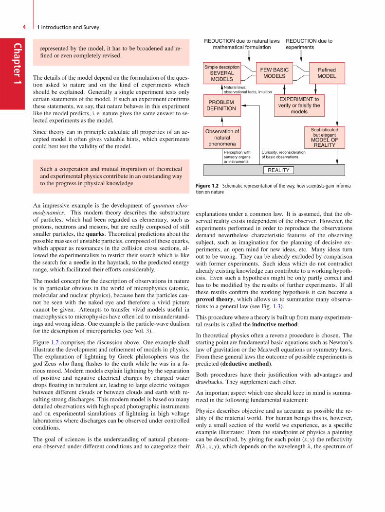
Figure 1.2 comprises the discussion above. One example shallillustrate the development and refinement of models in physics.The explanation of lightning by Greek philosophers was thegod Zeus who flung flashes to the earth while he was in a fu-rious mood. Modern models explain lightning by the separationof positive and negative electrical charges by charged waterdrops floating in turbulent air, leading to large electric voltagesbetween different clouds or between clouds and earth with re-sulting strong discharges. This modern model is based on manydetailed observations with high speed photographic instrumentsand on experimental simulations of lightning in high voltagelaboratories where discharges can be observed under controlledconditions.
The goal of sciences is the understanding of natural phenom-ena observed under different conditions and to categorize their
REDUCTION due to natural lawsmathematical formulation
Simple descriptionSEVERALMODELS
FEW BASICMODELS
RefinedMODEL
PROBLEMDEFINITION
Observation ofnatural
phenomena
Perception withsensory organsor instruments
Curiosity, reconsiderationof basic observations
Natural laws,observational facts, intuition
Sophisticatedbut elegant
MODEL OFREALITY
REALITY
EXPERIMENT toverify or falsify the
models
REDUCTION due toexperiments
Figure 1.2 Schematic representation of the way, how scientists gain informa-tion on nature
explanations under a common law. It is assumed, that the ob-served reality exists independent of the observer. However, theexperiments performed in order to reproduce the observationsdemand nevertheless characteristic features of the observingsubject, such as imagination for the planning of decisive ex-periments, an open mind for new ideas, etc. Many ideas turnout to be wrong. They can be already excluded by comparisonwith former experiments. Such ideas which do not contradictalready existing knowledge can contribute to a working hypoth-esis. Even such a hypothesis might be only partly correct andhas to be modified by the results of further experiments. If allthese results confirm the working hypothesis it can become aproved theory, which allows us to summarize many observa-tions to a general law (see Fig. 1.3).
This procedure where a theory is built up frommany experimen-tal results is called the inductive method.
In theoretical physics often a reverse procedure is chosen. Thestarting point are fundamental basic equations such as Newton’slaw of gravitation or the Maxwell equations or symmetry laws.From these general laws the outcome of possible experiments ispredicted (deductive method).
Both procedures have their justification with advantages anddrawbacks. They supplement each other.
An important aspect which one should keep in mind is summa-rized in the following fundamental statement:
Physics describes objective and as accurate as possible the re-ality of the material world. For human beings this is, however,only a small section of the world we experience, as a specificexample illustrates: From the standpoint of physics a paintingcan be described, by giving for each point .x; y/ the reflectivityR.�; x; y/, which depends on the wavelength �, the spectrum of

1.3 Short Historical Review 5
Chap
ter1
Mathematics
Reality
Imaginationof physicist
IdeaWorking hypothesis
Theory
Subjectiveinterpretation
Objective know-ledge about reality
ObservationExperiment
Results ofmeasurements
Objectivephysical law
Figure 1.3 Schematic diagram of gaining insight into natural phenomena
the illuminating radiation source and the angles of incidence andobservation direction. A computer which is fed with these char-acteristic input data can reproduce the painting very accurately.
Nevertheless this physical description lacks an essential part ofthe painting, which is in the mind of the observer. When look-ing at the painting a human being might remember other similarpaintings which he compares with the present painting, even ifthese other paintings are not present but only in the mind theystill change the subjective impression of the observer. The sub-ject of the painting may induce cheerful or sad feelings in themind of the observer, it may call back remembrances of formerevents or impressions which are related to this painting. Allthese different influences will determine the judgement aboutthe painting, which therefore might be different for different ob-servers.
All these aspects are not the realm of physics, because theyare subjective, although they are essential for the quality of thepainting as judged by human beings and they represent an im-portant part of the “reality” as perceived by us.
These remarks should warn physicists, not to forget that our fas-cinating science is only competent for the description of thematerial basis of our world. Although the other nonmaterialrealms are based on the material world their description andunderstanding reaches far beyond physics. The question, howliving cells are built from inanimate molecules and how thehuman mind is related to the structure of the brain are still pend-ing but exciting problems, which might be solved in the future.This is related to the question whether the human brain is morethan a highly developed computer, which is the subject of hotdiscussions between the supporter of artificial intelligence andbiologists.
For more detailed discussions of these questions, the reader isreferred to the literature [1.1a–1.6].
1.3 Short Historical Review
The historical development of physics can be roughly dividedinto three periods:
The natural philosophy in ancient timesThe development of classical physicsThe modern physics.
1.3.1 The Natural Philosophy in Ancient Times
The investigation of natural phenomena and the efforts to ex-plain them by rational arguments started already 4000 yearsago. The astronomical observation of the Babylonian and theEgyptian scientists were important for the prediction of an-nual occurrences, such as the Nile flood or the correct timefor sowing. The Greek philosophers produced many ideas forthe explanation of the observed natural phenomena. All theseideas were treated within the framework of general philosophy.For example, the textbook on Physics ('�� i�� ˛�%o˛� i& Dlectures on physics) by Aristotle contains mainly philosophicalconsiderations about space and time, movements of bodies andtheir causes.
Probably the most important achievement of Greek philosophywas the overcoming of the widespread mythology, where thelife of mankind was governed by a hierarchy of gods, whosemood was not predictable and everybody had to win the lik-ing of gods by sacrificing precious gifts to them. Most Greekphilosophers abandoned the belief, that the world was a playingground for gods, demons and ghosts who generated thunder-storm, floods, sunshine or disastrous droughts just according totheir mood (see Homer’s Odyssey).
The Greek philosophers believed that all natural phenomenaobeyed eternal unchanging laws which were not always obvious
Chapter1
6 1 Introduction and Survey
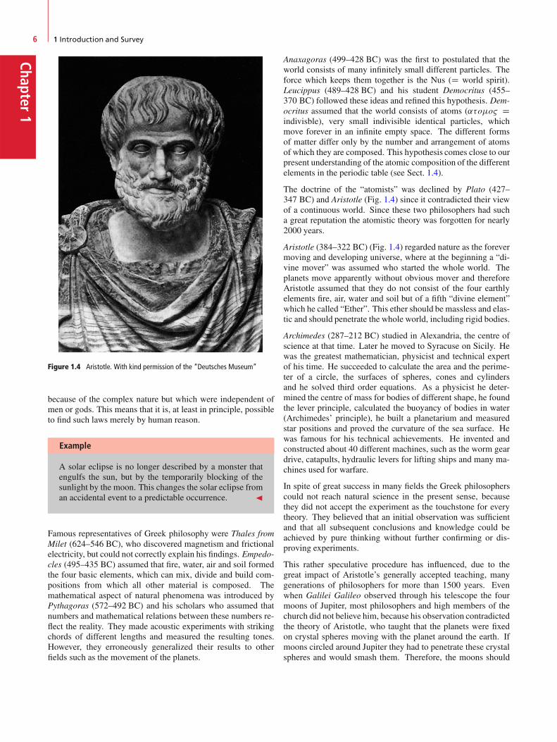
Figure 1.4 Aristotle. With kind permission of the “Deutsches Museum”
because of the complex nature but which were independent ofmen or gods. This means that it is, at least in principle, possibleto find such laws merely by human reason.
Example
A solar eclipse is no longer described by a monster thatengulfs the sun, but by the temporarily blocking of thesunlight by the moon. This changes the solar eclipse froman accidental event to a predictable occurrence. J
Famous representatives of Greek philosophy were Thales fromMilet (624–546 BC), who discovered magnetism and frictionalelectricity, but could not correctly explain his findings. Empedo-cles (495–435 BC) assumed that fire, water, air and soil formedthe four basic elements, which can mix, divide and build com-positions from which all other material is composed. Themathematical aspect of natural phenomena was introduced byPythagoras (572–492 BC) and his scholars who assumed thatnumbers and mathematical relations between these numbers re-flect the reality. They made acoustic experiments with strikingchords of different lengths and measured the resulting tones.However, they erroneously generalized their results to otherfields such as the movement of the planets.
Anaxagoras (499–428 BC) was the first to postulated that theworld consists of many infinitely small different particles. Theforce which keeps them together is the Nus (D world spirit).Leucippus (489–428 BC) and his student Democritus (455–370 BC) followed these ideas and refined this hypothesis. Dem-ocritus assumed that the world consists of atoms (˛�oo& Dindivisble), very small indivisible identical particles, whichmove forever in an infinite empty space. The different formsof matter differ only by the number and arrangement of atomsof which they are composed. This hypothesis comes close to ourpresent understanding of the atomic composition of the differentelements in the periodic table (see Sect. 1.4).
The doctrine of the “atomists” was declined by Plato (427–347 BC) and Aristotle (Fig. 1.4) since it contradicted their viewof a continuous world. Since these two philosophers had sucha great reputation the atomistic theory was forgotten for nearly2000 years.
Aristotle (384–322 BC) (Fig. 1.4) regarded nature as the forevermoving and developing universe, where at the beginning a “di-vine mover” was assumed who started the whole world. Theplanets move apparently without obvious mover and thereforeAristotle assumed that they do not consist of the four earthlyelements fire, air, water and soil but of a fifth “divine element”which he called “Ether”. This ether should be massless and elas-tic and should penetrate the whole world, including rigid bodies.
Archimedes (287–212 BC) studied in Alexandria, the centre ofscience at that time. Later he moved to Syracuse on Sicily. Hewas the greatest mathematician, physicist and technical expertof his time. He succeeded to calculate the area and the perime-ter of a circle, the surfaces of spheres, cones and cylindersand he solved third order equations. As a physicist he deter-mined the centre of mass for bodies of different shape, he foundthe lever principle, calculated the buoyancy of bodies in water(Archimedes’ principle), he built a planetarium and measuredstar positions and proved the curvature of the sea surface. Hewas famous for his technical achievements. He invented andconstructed about 40 different machines, such as the worm geardrive, catapults, hydraulic levers for lifting ships and many ma-chines used for warfare.
In spite of great success in many fields the Greek philosopherscould not reach natural science in the present sense, becausethey did not accept the experiment as the touchstone for everytheory. They believed that an initial observation was sufficientand that all subsequent conclusions and knowledge could beachieved by pure thinking without further confirming or dis-proving experiments.
This rather speculative procedure has influenced, due to thegreat impact of Aristotle’s generally accepted teaching, manygenerations of philosophers for more than 1500 years. Evenwhen Galilei Galileo observed through his telescope the fourmoons of Jupiter, most philosophers and high members of thechurch did not believe him, because his observation contradictedthe theory of Aristotle, who taught that the planets were fixedon crystal spheres moving with the planet around the earth. Ifmoons circled around Jupiter they had to penetrate these crystalspheres and would smash them. Therefore, the moons should
1.3 Short Historical Review 7
Chap
ter1
be impossible. Even when Galilei offered to the sceptics to lookthrough the telescope (Fig. 1.1b) many of them refused and said:“Why should we look and be deceived by optical illusions whenwe are sure about Aristotle’s statements”.
Although some inconsistencies in Aristotle’s teaching had beenfound before, Galilee was the first to disprove by his observa-tions and experiments the whole theory of the shining exampleof Greek philosophy, in particular when he also advertised thenew astronomy of Copernicus, which brought him many ene-mies and even a trial before the catholic court.
1.3.2 The Development of Classical Physics
One may call Galileo the first physicist in the present meaning.He tried as the first scientist to prove or disprove physical the-ories by specific well-planned experiments. Famous examplesare his experiments on the movement of a body with constantacceleration under the influence of gravity. He also consideredhow large the accuracy of his experimental results must be in or-der to decide between two different versions for the descriptionof such movements. He therefore did not choose the free fall(it is often erroneously reported, that he observed bodies fallingfrom the Leaning tower in Pisa). This could never reach the re-quired accuracy with the clocks available at that time. He choseinstead the sliding of a body on an inclined plane with an angle˛ against the horizontal. Here only the fraction g � sin˛ acts onthe body and thus the acceleration is much smaller.
His astronomical observations (phases of Venus, Moons ofJupiter) with a self-made telescope (after he had learned aboutits invention by the optician Hans Lipershey (1570–1619) inHolland) helped the Copernican model of the planets circlingaround the sun instead of the earth, finally to become generallyaccepted (in spite of severe discrepancies with the dogmatic ofthe church and heavy oppression by the church council).
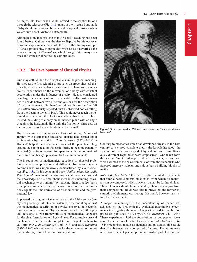
The introduction of mathematical equations to physical prob-lems, which comprises several different observations into acommon law, was impressively demonstrated by Isaac New-ton (Fig. 1.5). In his centennial book “Philosophiae NaturalisPrincipia Mathematica” he summarizes all observations andthe knowledge of his time about mechanics (including celes-tial mechanics D astronomy) by reducing them to a few basicprinciples (principle of inertia, actio D reactio, the force on abody equals the time derivative of his momentum and the grav-itational law).
Supported by progress of mathematics in the 17th century (an-alytical geometry, infinitesimal calculus, differential equations)the mathematical description of physical observations becomesmore and more common. Physics emancipates from Philosophyand develops its own framework using mathematical languagefor the clear formulation of physical laws. For example classicalmechanics experiences its complete and elegant mathemati-cal form by J. L. de-Lagrange (1736–1813) and W.R. Hamilton(1805–1865) who reduced all laws for the movement of bodiesunder arbitrary forces to a few basic equations.
Figure 1.5 Sir Isaac Newton. With kind permission of the “Deutsches MuseumMünchen”
Contrary to mechanics which had developed already in the 18thcentury to a closed complete theory the knowledge about thestructure of matter was very sketchy and confused. Simultane-ously different hypotheses were emphasized: One taken formthe ancient Greek philosophy, where fire, water, air and soilwere assumed as the basic elements, or from the alchemists whofavoured mercury, sulphur and salt as basic building blocks ofmatter.
Robert Boyle (1627–1591) realized after detailed experimentsthat simple basic elements must exist, from which all materi-als can be composed, which however, cannot be further divided.These elements should be separated by chemical analysis fromtheir composition. Boyle was able to prove that the former as-sumption of elements was wrong. He could, however, not yetfind the real elements.
A major breakthrough in the understanding of matter wasachieved by the first critically evaluated quantitative experi-ments investigating the mass changes involved in combustionprocesses, published in 1772 by A. L. de Lavoisier (1743–1794).These experiments laid the foundations of our present ideasabout the structure of matter. Lavoisier and John Dalton (1766–1844) recognised metals as elements and postulated like Boylethat all substances were composed of atoms. The atoms werenow, however, not just simple non-divisible particles, but had

Chapter1
8 1 Introduction and Survey
specific characteristics which determined the properties of thecomposed substance. Karl Wilhelm Scheele (1724–1786) foundthat air consisted of nitrogen and oxygen.
Antoine-Laurent Lavoisier furthermore found that the mass ofa substance increased when it was burnt, if all products of thecombustion process were collected. He recognized that thismass increase was caused by oxygen which combined with thesubstance during the burning process. He formulated the lawof mass conservation for all chemical processes. Two elementscan combine in different mass ratios to form different chemicalproducts where the relative mass ratios always are small integernumbers.
The British Chemist John Dalton was able to explain this lawbased on the atom hypothesis.
Examples
1. For the molecules carbon monoxide and carbon diox-ide the mass ratio of oxygen combining with the sameamount of carbon is 1 W 2 because in CO one oxygenatom and in CO2 two oxygen atoms combine with onecarbon atom.
2. For the gases N2O (Di-Nitrogen oxide), NO (nitrogenmono oxide), N2O3 (nitrogen trioxide), and NO2) ni-trogen dioxide) oxygen combines with the same massof nitrogen each time in the ratio 1 W 2 W 3 W 4. J
Dalton also recognized that the relative atomic weights con-stitute a characteristic property of chemical elements. Thefurther development of these ideas lead to the periodic systemof elements by Julius Lothar Meyer (1830–1895) and DimitriMendelejew (1834–1907), who arranged all known elements ina table in such a way that the elements in the same columnshowed similar chemical properties, such as the alkali atoms inthe first column or the noble gases in the last column.
Why these elements had similar chemical properties was recog-nized only much later after the development of quantum theory.
The idea of atoms was supported by Amedeo Avogadro (1776–1856), who proposed in 1811 that equal volumes of differentgases at equal temperature and pressure contain an equal numberof elementary particles.
A convincing experimental indication of the existence of atomswas provided by the Brownian motion, where the randommove-ments of small particles in gases or liquids could be directlyviewed under a microscope. This was later quantitativelyexplained by Einstein, who showed that this movement was in-duced by collisions of the particles with atoms or molecules.
Although the atomic hypothesis scored indisputable successesand was accepted as a working hypothesis by most chemistsand physicists, the existence of atoms as real entities was a mat-ter of discussion among many serious scientists until the end ofthe 19th century. The reason was the fact that one cannot seeatoms but had only indirect clues, derived from the macroscopicbehaviour of matter in chemical reactions. Nowadays the im-provement of experimental techniques allows one to see images
of single atoms and the theoretical basis of atomic theory leavesno doubt about the real existence of atoms and molecules.
The theory of heat began to become a quantitative science afterthermometers for the measurement of temperatures had been de-veloped (air-thermoscope by Galilei, alcohol thermometer 1641in Florence, mercury thermometer 1640 in Rome). The Swedishphysicist Anders Celsius (1701–1744) introduced the divisioninto 100 equal intervals between melting point (0 ıC) and boil-ing point (100 ıC) of water at normal pressure. Lord Kelvin(1824–1907) postulated the absolute temperature, based on gasthermometers and the general gas law. On this scale the zeropoint T D 0K D �273:15 ıC is the lowest temperature whichcan be closely approached but never reached (see Chap. 10).
Denis Papin (1647–1712) investigated the process of boilingand condensation of water vapour (Papin’s steam pressure pot).He built the first steam engine, which James Watt (1736–1819)later improved to reliable technical performance. The termsamount of heat and heat capacity were introduced by the En-glish physicist and chemist Joseph Black (1728–1799). Hediscovered that during the melting process heat was absorbedwhich was released again during solidification.
The more precise formulation of the theory of heat was es-sentially marked by establishing general laws. Robert Mayer(1814–1878) postulated the first law of the theory of heat, whichstates that for all processes the total amount of energy is con-served. Nicolas Carnot (1796–1832) started 1831 after someinitial errors a fresh successful attempt to describe the conver-sion of heat into mechanical energy (Carnot’s cycle process).This was later more precisely formulated by Rudolf Clausius(1822–1888) in the second law of heat theory.
A real understanding of heat was achieved, when the kineticgas theory was formulated. Here the connection between heatproperties and mechanical energy was for the first time clearlyformulated. Since the dynamical properties of molecules mov-ing around in a gas were related to the temperature of a gas, theheat theory was now called thermodynamics, which was for-mulated by several scientists (Clausius, Avogadro, Boltzmann)(see Fig. 1.6). They proved under the assumption that gases con-sist of many essentially free atoms or molecules, which moverandomly around and collide with each other, that the heat en-ergy of a gas is equivalent to the kinetic energy of these particles.The Austrian physicist Joseph Loschmidt (1821–1895) foundthat under normal pressure the gas contains the enormous num-ber of about 3 � 1019 atoms per cm3.
Optics is one of the oldest branches of physics which was al-ready studied more than 2000 years ago where the focussing oflight by concave mirrors was used to ignite a fire. However,only in the 17th century optical instruments and their imag-ing properties were studied systematically. A milestone wasthe fabrication of lenses and the invention of telescopes. Willi-brord Snellius (1580–1626) formulated his law of refraction(see Vol. 2, Chap. 9), Newton found the separation of differ-ent colours when white sun light passed through a prism. Theexplanation of the properties of light was the subject of hot dis-cussions. While Newton believed that light consisted of smallparticles (in our present model these are the photons) the ex-periments on interference and diffraction of light by Grimaldi
1.3 Short Historical Review 9
Chap
ter1
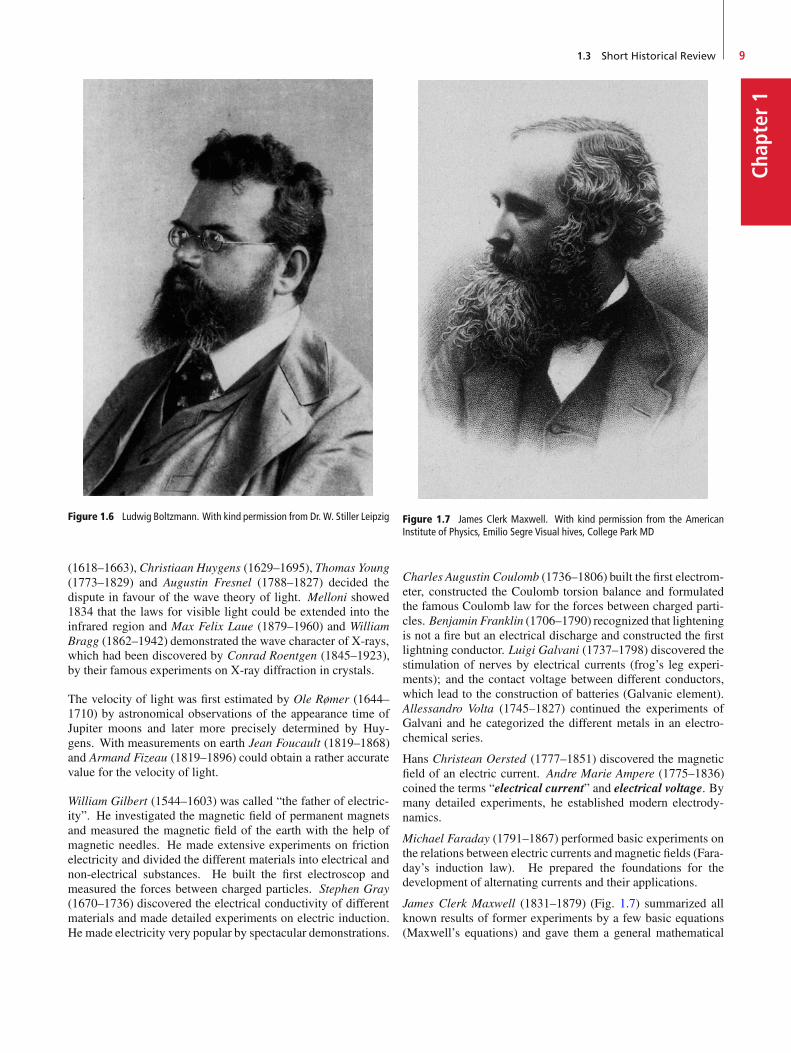
Figure 1.6 Ludwig Boltzmann. With kind permission from Dr. W. Stiller Leipzig
(1618–1663), Christiaan Huygens (1629–1695), Thomas Young(1773–1829) and Augustin Fresnel (1788–1827) decided thedispute in favour of the wave theory of light. Melloni showed1834 that the laws for visible light could be extended into theinfrared region and Max Felix Laue (1879–1960) and WilliamBragg (1862–1942) demonstrated the wave character of X-rays,which had been discovered by Conrad Roentgen (1845–1923),by their famous experiments on X-ray diffraction in crystals.
The velocity of light was first estimated by Ole Rømer (1644–1710) by astronomical observations of the appearance time ofJupiter moons and later more precisely determined by Huy-gens. With measurements on earth Jean Foucault (1819–1868)and Armand Fizeau (1819–1896) could obtain a rather accuratevalue for the velocity of light.
William Gilbert (1544–1603) was called “the father of electric-ity”. He investigated the magnetic field of permanent magnetsand measured the magnetic field of the earth with the help ofmagnetic needles. He made extensive experiments on frictionelectricity and divided the different materials into electrical andnon-electrical substances. He built the first electroscop andmeasured the forces between charged particles. Stephen Gray(1670–1736) discovered the electrical conductivity of differentmaterials and made detailed experiments on electric induction.He made electricity very popular by spectacular demonstrations.
Figure 1.7 James Clerk Maxwell. With kind permission from the AmericanInstitute of Physics, Emilio Segre Visual hives, College Park MD
Charles Augustin Coulomb (1736–1806) built the first electrom-eter, constructed the Coulomb torsion balance and formulatedthe famous Coulomb law for the forces between charged parti-cles. Benjamin Franklin (1706–1790) recognized that lighteningis not a fire but an electrical discharge and constructed the firstlightning conductor. Luigi Galvani (1737–1798) discovered thestimulation of nerves by electrical currents (frog’s leg experi-ments); and the contact voltage between different conductors,which lead to the construction of batteries (Galvanic element).Allessandro Volta (1745–1827) continued the experiments ofGalvani and he categorized the different metals in an electro-chemical series.
Hans Christean Oersted (1777–1851) discovered the magneticfield of an electric current. Andre Marie Ampere (1775–1836)coined the terms “electrical current” and electrical voltage. Bymany detailed experiments, he established modern electrody-namics.
Michael Faraday (1791–1867) performed basic experiments onthe relations between electric currents andmagnetic fields (Fara-day’s induction law). He prepared the foundations for thedevelopment of alternating currents and their applications.
James Clerk Maxwell (1831–1879) (Fig. 1.7) summarized allknown results of former experiments by a few basic equations(Maxwell’s equations) and gave them a general mathematical
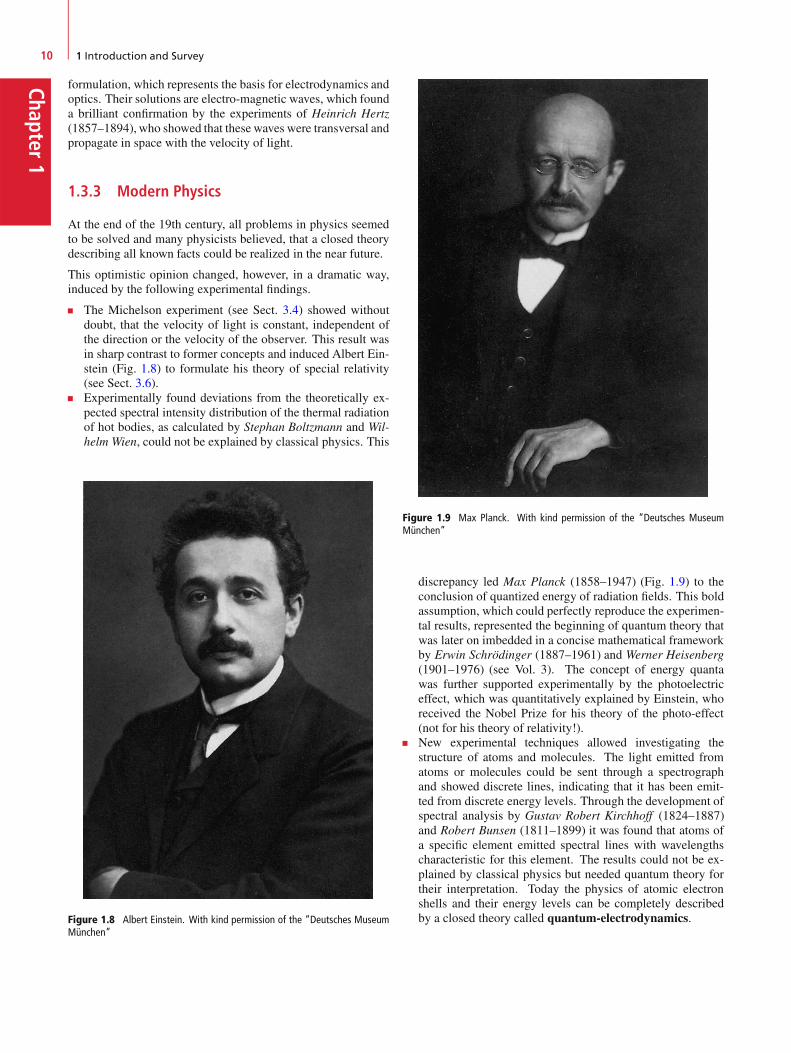
Chapter1
10 1 Introduction and Survey
formulation, which represents the basis for electrodynamics andoptics. Their solutions are electro-magnetic waves, which founda brilliant confirmation by the experiments of Heinrich Hertz(1857–1894), who showed that these waves were transversal andpropagate in space with the velocity of light.
1.3.3 Modern Physics
At the end of the 19th century, all problems in physics seemedto be solved and many physicists believed, that a closed theorydescribing all known facts could be realized in the near future.
This optimistic opinion changed, however, in a dramatic way,induced by the following experimental findings.
The Michelson experiment (see Sect. 3.4) showed withoutdoubt, that the velocity of light is constant, independent ofthe direction or the velocity of the observer. This result wasin sharp contrast to former concepts and induced Albert Ein-stein (Fig. 1.8) to formulate his theory of special relativity(see Sect. 3.6).Experimentally found deviations from the theoretically ex-pected spectral intensity distribution of the thermal radiationof hot bodies, as calculated by Stephan Boltzmann and Wil-helm Wien, could not be explained by classical physics. This
Figure 1.8 Albert Einstein. With kind permission of the “Deutsches MuseumMünchen”
Figure 1.9 Max Planck. With kind permission of the “Deutsches MuseumMünchen”
discrepancy led Max Planck (1858–1947) (Fig. 1.9) to theconclusion of quantized energy of radiation fields. This boldassumption, which could perfectly reproduce the experimen-tal results, represented the beginning of quantum theory thatwas later on imbedded in a concise mathematical frameworkby Erwin Schrödinger (1887–1961) and Werner Heisenberg(1901–1976) (see Vol. 3). The concept of energy quantawas further supported experimentally by the photoelectriceffect, which was quantitatively explained by Einstein, whoreceived the Nobel Prize for his theory of the photo-effect(not for his theory of relativity!).New experimental techniques allowed investigating thestructure of atoms and molecules. The light emitted fromatoms or molecules could be sent through a spectrographand showed discrete lines, indicating that it has been emit-ted from discrete energy levels. Through the development ofspectral analysis by Gustav Robert Kirchhoff (1824–1887)and Robert Bunsen (1811–1899) it was found that atoms ofa specific element emitted spectral lines with wavelengthscharacteristic for this element. The results could not be ex-plained by classical physics but needed quantum theory fortheir interpretation. Today the physics of atomic electronshells and their energy levels can be completely describedby a closed theory called quantum-electrodynamics.

1.4 The Present Conception of Our World 11
Chap
ter1
This illustrates that always in the history of natural sciences newexperimental results forced physicists to revise former conceptsand to formulate new theories which, however, should includeproved earlier results. In most cases the old theories were notcompletely abandoned but their validity range was restricted andmore precisely characterized. For example the classical physicsis perfectly correct for the description of the motion of macro-scopic bodies or for many applications in daily life, while forthe description of the micro-world of atoms and molecules itmay completely fail and quantum theory is necessary.
The properties of atomic nuclei could be only investigated af-ter appropriate detectors had been developed. Nuclear physicsis therefore a rather new field where most of the results wereobtained in the 20th century. The substructure of atomic nucleiand the physics of elementary particles could start after parti-cle accelerators could be operated and many results in this fieldhave been achieved only recently.
This short historical review should illustrate that many conceptswhich today are taken for granted, are not as old and have beenaccepted only after erroneous ideas and a long way of successivecorrections, guided by new experiments. It is worthwhile forevery physicist to look into some original papers and follow thegradual improvements of concepts and representation of results.
More extensive literature about the historical development ofphysics and about bibliographies of physicists can be found inthe references [1.6–1.14c].
1.4 The Present Conception of OurWorld
As the result of all experimental and theoretical investigationsour present model of the material world has been established(Fig. 1.10). In this introduction, we will give only a short sum-mary. The subject will be discussed more thoroughly in Vol. 3and 4 of this textbook series.
Macroscopic bodies(solid, liquid and gaseous)
Nuclei and electrons
Quarks, gluons
Atoms Molecules
Atomic nuclei(protons + neutrons)
Figure 1.10 Build up of our material world (H. J. Jodl [1.14b])
Elementary Particles
The entire material world known up to now is composed ofonly a few different particles. The three most important are theelectron (e�), the proton (pC) and the neutron (n). All otherelementary particles (muons, -Mesons, Kaons, �-particlesetc.) exist after their production only a very short time (10�6–10�15 s). They convert either spontaneously or by collisions intoother particles which finally decay into pC, e�, neutrinos or pho-tons h ��. Although neutrinos are stable particles they show sucha small interaction with matter that they are difficult to detectand they therefore play no role in daily life.
Recent experiments and theoretical consideration have shown,that the particles pC, n, mesons and hyperons, which had beenregarded as elementary, show a substructure (see Vol. 4), Ac-cording to our present understanding they consists of smallerparticles, called “quarks”, which occur in 6 different species.
All building blocks of matter can be divided into two groups:
1. the quarks, which build up the heavy particles (baryons),such as proton, neutron, mesons and hyperons
2. the light particles (leptons) electron, myon and neutrino.
Each of these two groups consists of three families of elemen-tary particles, which are listed in Tab. 1.1. For each of theseparticles there exists an anti-particle with equal mass but oppo-site charge. For instance the anti-particle of the electron e� is thepositron eC, the proton pC has as anti-particle the anti-proton p�and the anti-neutron has the same mass and the charge zero asthe neutron.
According to present theories the interaction between the parti-cles can be described by the exchange of “interaction particles”,which are called the quanta of the interaction field. For exam-ple the quanta of the electromagnetic field, which determine theinteraction between charged particles are the photons h � �.The quanta of the strong interaction between nucleons are calledgluons. The gravitons are the quanta of the gravitational field.Our present knowledge is that there exist only four differentkinds of interaction, which are summarized in Tab. 1.2.
An essential goal of present research is to reduce the four typesof interaction to one common force (grand unification). The re-duction of the manifold of different particles to two groups ofelementary particles was in a certain sense successful, becausethe classification into two groups with three families in eachgroup gives a rather simple arrangement. However, the num-ber of 24 different particles together with their antiparticles isstill large and adding the 15 interaction quanta the total numberof elementary particles is 39. Whether the “grand unification”will allow a further reduction or a simpler ordering scheme isstill an open question.
This field of research is very interesting because it ventures tothe limit where matter and energy might become indistinguish-able. It is also closely related to processes occurring at the verybeginning of our universe where elementary particles and theirinteraction played a major role in the extremely hot fireball dur-ing the first seconds of the big bang.
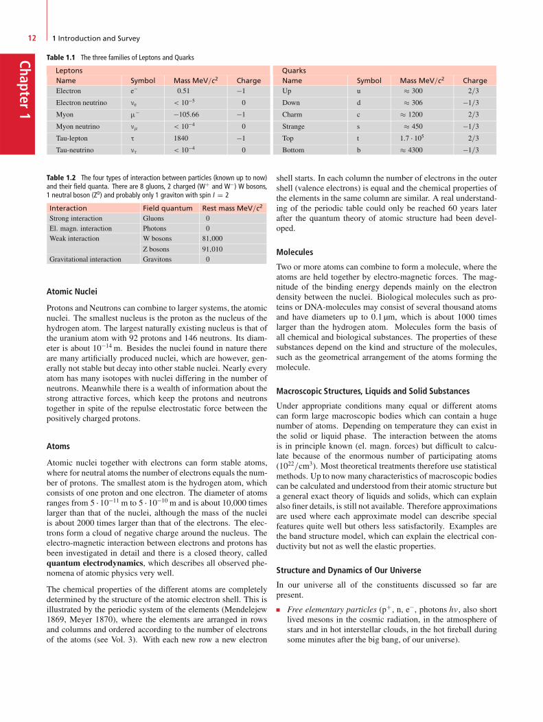
Chapter1
12 1 Introduction and Survey
Table 1.1 The three families of Leptons and Quarks
LeptonsName Symbol Mass MeV=c2 ChargeElectron e� 0.51 �1
Electron neutrino e < 10�5 0
Myon �� �105:66 �1
Myon neutrino < 10�4 0
Tau-lepton £ 1840 �1
Tau-neutrino � < 10�4 0
QuarksName Symbol Mass MeV=c2 ChargeUp u � 300 2=3
Down d � 306 �1=3
Charm c � 1200 2=3
Strange s � 450 �1=3
Top t 1:7 � 105 2=3
Bottom b � 4300 �1=3
Table 1.2 The four types of interaction between particles (known up to now)and their field quanta. There are 8 gluons, 2 charged (WC and W�) W bosons,1 neutral boson (Z0) and probably only 1 graviton with spin I D 2
Interaction Field quantum Rest mass MeV=c2
Strong interaction Gluons 0El. magn. interaction Photons 0Weak interaction W bosons 81;000
Z bosons 91;010Gravitational interaction Gravitons 0
Atomic Nuclei
Protons and Neutrons can combine to larger systems, the atomicnuclei. The smallest nucleus is the proton as the nucleus of thehydrogen atom. The largest naturally existing nucleus is that ofthe uranium atom with 92 protons and 146 neutrons. Its diam-eter is about 10�14 m. Besides the nuclei found in nature thereare many artificially produced nuclei, which are however, gen-erally not stable but decay into other stable nuclei. Nearly everyatom has many isotopes with nuclei differing in the number ofneutrons. Meanwhile there is a wealth of information about thestrong attractive forces, which keep the protons and neutronstogether in spite of the repulse electrostatic force between thepositively charged protons.
Atoms
Atomic nuclei together with electrons can form stable atoms,where for neutral atoms the number of electrons equals the num-ber of protons. The smallest atom is the hydrogen atom, whichconsists of one proton and one electron. The diameter of atomsranges from 5 � 10�11 m to 5 � 10�10 m and is about 10;000 timeslarger than that of the nuclei, although the mass of the nucleiis about 2000 times larger than that of the electrons. The elec-trons form a cloud of negative charge around the nucleus. Theelectro-magnetic interaction between electrons and protons hasbeen investigated in detail and there is a closed theory, calledquantum electrodynamics, which describes all observed phe-nomena of atomic physics very well.
The chemical properties of the different atoms are completelydetermined by the structure of the atomic electron shell. This isillustrated by the periodic system of the elements (Mendelejew1869, Meyer 1870), where the elements are arranged in rowsand columns and ordered according to the number of electronsof the atoms (see Vol. 3). With each new row a new electron
shell starts. In each column the number of electrons in the outershell (valence electrons) is equal and the chemical properties ofthe elements in the same column are similar. A real understand-ing of the periodic table could only be reached 60 years laterafter the quantum theory of atomic structure had been devel-oped.
Molecules
Two or more atoms can combine to form a molecule, where theatoms are held together by electro-magnetic forces. The mag-nitude of the binding energy depends mainly on the electrondensity between the nuclei. Biological molecules such as pro-teins or DNA-molecules may consist of several thousand atomsand have diameters up to 0:1 µm, which is about 1000 timeslarger than the hydrogen atom. Molecules form the basis ofall chemical and biological substances. The properties of thesesubstances depend on the kind and structure of the molecules,such as the geometrical arrangement of the atoms forming themolecule.
Macroscopic Structures, Liquids and Solid Substances
Under appropriate conditions many equal or different atomscan form large macroscopic bodies which can contain a hugenumber of atoms. Depending on temperature they can exist inthe solid or liquid phase. The interaction between the atomsis in principle known (el. magn. forces) but difficult to calcu-late because of the enormous number of participating atoms(1022=cm3). Most theoretical treatments therefore use statisticalmethods. Up to nowmany characteristics of macroscopic bodiescan be calculated and understood from their atomic structure buta general exact theory of liquids and solids, which can explainalso finer details, is still not available. Therefore approximationsare used where each approximate model can describe specialfeatures quite well but others less satisfactorily. Examples arethe band structure model, which can explain the electrical con-ductivity but not as well the elastic properties.
Structure and Dynamics of Our Universe
In our universe all of the constituents discussed so far arepresent.
Free elementary particles (pC, n, e�, photons h�, also shortlived mesons in the cosmic radiation, in the atmosphere ofstars and in hot interstellar clouds, in the hot fireball duringsome minutes after the big bang, of our universe).
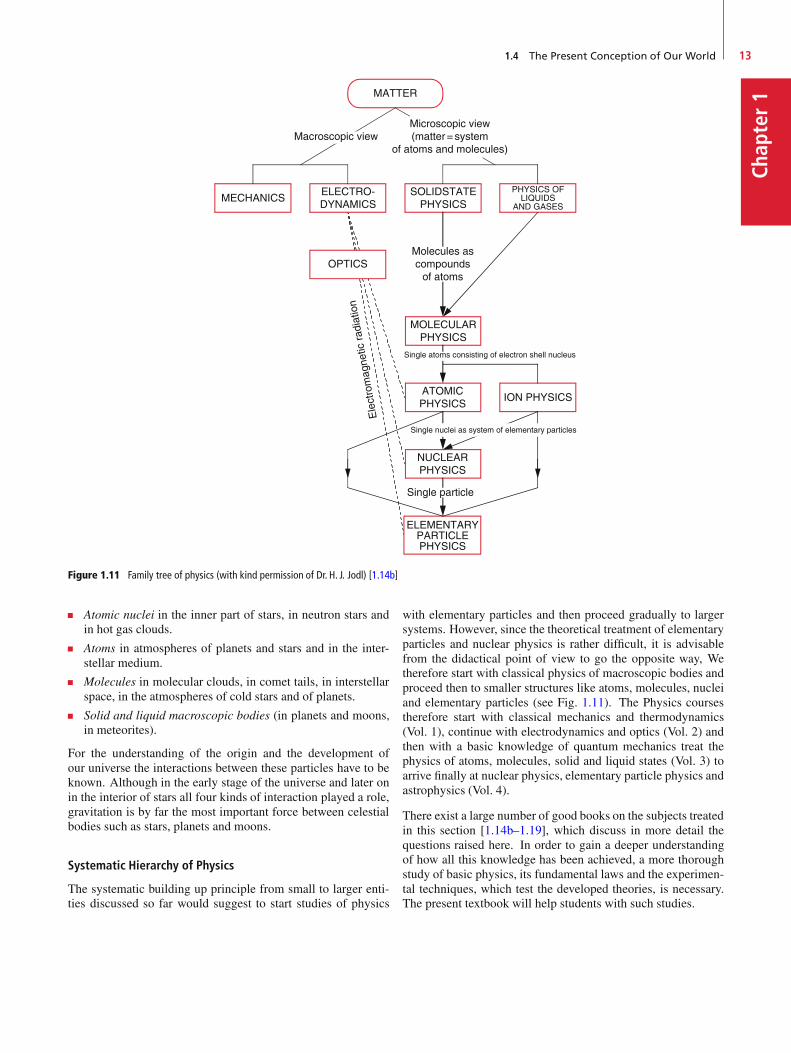
1.4 The Present Conception of Our World 13
Chap
ter1
Ele
ctro
mag
netic
rad
iatio
n
MATTER
MECHANICS
OPTICS
ION PHYSICS
ELECTRO-DYNAMICS
SOLIDSTATEPHYSICS
ELEMENTARYPARTICLEPHYSICS
NUCLEARPHYSICS
Macroscopic view
Molecules ascompounds
of atoms
Single atoms consisting of electron shell nucleus
Single nuclei as system of elementary particles
Single particle
Microscopic view(matter = system
of atoms and molecules)
ATOMICPHYSICS
MOLECULARPHYSICS
PHYSICS OFLIQUIDS
AND GASES
Figure 1.11 Family tree of physics (with kind permission of Dr. H. J. Jodl) [1.14b]
Atomic nuclei in the inner part of stars, in neutron stars andin hot gas clouds.
Atoms in atmospheres of planets and stars and in the inter-stellar medium.
Molecules in molecular clouds, in comet tails, in interstellarspace, in the atmospheres of cold stars and of planets.
Solid and liquid macroscopic bodies (in planets and moons,in meteorites).
For the understanding of the origin and the development ofour universe the interactions between these particles have to beknown. Although in the early stage of the universe and later onin the interior of stars all four kinds of interaction played a role,gravitation is by far the most important force between celestialbodies such as stars, planets and moons.
Systematic Hierarchy of Physics
The systematic building up principle from small to larger enti-ties discussed so far would suggest to start studies of physics
with elementary particles and then proceed gradually to largersystems. However, since the theoretical treatment of elementaryparticles and nuclear physics is rather difficult, it is advisablefrom the didactical point of view to go the opposite way, Wetherefore start with classical physics of macroscopic bodies andproceed then to smaller structures like atoms, molecules, nucleiand elementary particles (see Fig. 1.11). The Physics coursestherefore start with classical mechanics and thermodynamics(Vol. 1), continue with electrodynamics and optics (Vol. 2) andthen with a basic knowledge of quantum mechanics treat thephysics of atoms, molecules, solid and liquid states (Vol. 3) toarrive finally at nuclear physics, elementary particle physics andastrophysics (Vol. 4).
There exist a large number of good books on the subjects treatedin this section [1.14b–1.19], which discuss in more detail thequestions raised here. In order to gain a deeper understandingof how all this knowledge has been achieved, a more thoroughstudy of basic physics, its fundamental laws and the experimen-tal techniques, which test the developed theories, is necessary.The present textbook will help students with such studies.

Chapter1
14 1 Introduction and Survey
1.5 Relations Between Physics andOther Sciences
Since physics deals with the basic elements of our materialworld it represents in principle the foundations of every naturalscience. However, until a few decades ago the scientific meth-ods in chemistry, biology and medicine were more empiricallyoriented. Because of the complex nature of the objects studiedin these sciences it was not possible to start the investigations“ab initio” in order to understand the atomic structure of largecomplex molecules and biological cells to say nothing of thehuman body and its complex reactions as the research object inmedicine. Therefore, in former years a more phenomenologicalmethod was preferred.
With refined experimental techniques developed in recent years(electron microscopy, (Fig. 1.12), tunnel microscopy, x-raystructural analysis, neutron diffraction, nuclear magnetic res-onance tomography and laser spectroscopy) in many cases itbecame possible to uncover the atomic structure even of com-plex molecules such as the DNA (Fig. 1.13). Here physics washelpful in a twofold way: First of all physicists developed, of-ten in cooperation with engineers, the experimental equipmentand secondly it provided the theoretical understanding for theatomic basis of the research objects. Therefore the differencesin the research methods become less and less important and thecooperation between researchers of different fields is rapidly in-creasing, indicated by the growing number of interdisciplinaryresearch projects. For example the essential question of therelation between molecular structure and chemical binding isattacked in common efforts by experimental chemists, theoret-ical quantum chemists and physicists. Overstated one may saythat chemistry is applied quantum theory and therefore a branchof physics.
Due to the complex diagnostic techniques in medicine the coop-eration between physicists and medical doctors has enormouslyincreased as will be outlined in the next section.
Figure 1.12 Scavenger Cells visualized with an electron microscope
Bases
Phosphates
Nucleotid-sequence
Strand I
Strand II
Figure 1.13 Double Helix of DNA (deoxyribonucleic acid)
1.5.1 Biophysics and Medical Physics
Meanwhile biophysics has developed to an independent branchof physics. Some of the many research projects are the physi-cal processes in living cells, e. g. the energy balance during cellprocesses, the ion transport through cell membranes, the pene-tration of bacteria and viruses into cells, the different steps ofphotosynthesis or the visual process. The very sensitive detec-tion techniques for the detection of single molecules, developedin physics laboratories, allow the tracing of single laser excitedmolecules on their way from outside a cell through membranechannels into the cell interior. In particular the realization ofultra short laser pulses down to below a femtosecond (10�15 s)opens for the first time the possibility to view ultrafast processessuch as molecular isomerisation.
In recent years, medical physics has been established at manyuniversities and research institutes. The development of newdiagnostic techniques and therapy methods are based on exper-imental techniques invented and optimized in physics laborato-ries and on new insights about the interaction between radiationand tissue. Examples of such new methods are ultrasonic di-agnostics with improved spatial resolution, nuclear magneticresonance tomography, thermography or laser-induced cell flu-orescence. One specific example is the localization of braintumours by optical coherence tomography and methods for
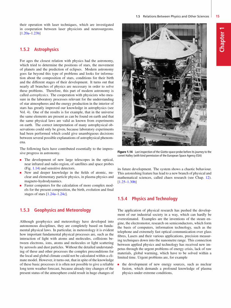
1.5 Relations Between Physics and Other Sciences 15
Chap
ter1
their operation with laser techniques, which are investigatedin cooperation between laser physicists and neurosurgeons.[1.20a–1.23b]
1.5.2 Astrophysics
For ages the closest relation with physics had the astronomy,which tried to determine the positions of stars, the movementof planets and the prediction of eclipses. Modern astronomygoes far beyond this type of problems and looks for informa-tion about the composition of stars, conditions for their birthand the different stages of their development. It turns out thatnearly all branches of physics are necessary in order to solvethese problems. Therefore, this part of modern astronomy iscalled astrophysics. The cooperation with physicists who mea-sure in the laboratory processes relevant for the understandingof star atmospheres and the energy production in the interior ofstars has greatly improved our knowledge in astrophysics (seeVol. 4). One of the results is for example, that in the universethe same elements are present as can be found on earth and thatthe same physical laws are valid as known from experimentson earth. The correct interpretation of many astrophysical ob-servations could only be given, because laboratory experimentshad been performed which could give unambiguous decisionsbetween several possible explanations of astrophysical phenom-ena.
The following facts have contributed essentially to the impres-sive progress in astronomy.
The development of new large telescopes in the optical,near infrared and radio region, of satellites and space probes(Fig. 1.14) and sensitive detectors.New and deeper knowledge in the fields of atomic, nu-clear and elementary particle physics, in plasma physics andmagneto-hydrodynamics.Faster computers for the calculation of more complex mod-els for the present composition, the birth, evolution and finalstages of stars [1.24a–1.24c].
1.5.3 Geophysics and Meteorology
Although geophysics and meteorology have developed intoautonomous disciplines, they are completely based on funda-mental physical laws. In particular, in meteorology it is evidenthow important fundamental physical processes are, such as theinteraction of light with atoms and molecules, collisions be-tween electrons, ions, atoms and molecules or light scatteringby aerosols and dust particles. Without the detailed understand-ing of these and other processes the complex preconditions forthe local and global climate could not be calculated within a cli-mate model. However, it turns out, that in spite of the knowledgeof these basic processes it is often not possible to give a reliablelong term weather forecast, because already tiny changes of thepresent status of the atmosphere could result in huge changes of
Figure 1.14 Last inspection of the Giotto-space probe before its journey to thecomet Halley (with kind permission of the European Space Agency ESA)
its future development. The system shows a chaotic behaviour.This astonishing feature has lead to a new branch of physical andmathematical sciences, called chaos research (see Chap. 12).[1.25–1.30b]
1.5.4 Physics and Technology
The application of physical research has pushed the develop-ment of our industrial society in a way, which can hardly beoverestimated. Examples are the inventions of the steam en-gine, the electromotor, research on semiconductors, which formthe basis of computers, information technology, such as thetelephone and extremely fast optical communication over glassfibres, Lasers and their various applications, precision measur-ing techniques down into the nanometre range. This connectionbetween applied physics and technology has received new im-petus through the urgent problems of energy crisis, lack of rawmaterials, global warming, which have to be solved within alimited time. Urgent problems are, for example
the development of new energy sources, such as nuclearfusion, which demands a profound knowledge of plasmaphysics under extreme conditions,

Chapter1
16 1 Introduction and Survey
Figure 1.15 Hexagonal structure of a graphite surface, visualized by a tunnelmicroscope (M. Müller, H. Öchsner, TU Kaiserslautern)
the optimization of wind converters,the development of solar cells with sufficiently high efficien-cies,increasing the conversion efficiency from heat into electricalenergy,improving the transport efficiency of energy.
Further examples are the development of reliable electricallydriven cars with new designs of batteries, hydrogen technology,magnetically levitated railways (trans-rapid), development of “-clean air cars” etc.
Of particular interest for many branches of industry is the re-search on new materials such as met-glasses (amorphous metalswith particular properties such as high tensile strength), com-pound materials or amorphous semiconductors, which havefound meanwhile numerous applications. Surface science(Fig. 1.15) has given the basic understanding for corrosion pro-cesses, catalytic effects and the properties of thin films in opticsand for the creation of very hard surfaces of tools, which de-crease the wear and tear of such tools considerably.
One should keep in mind that for densely populated countriessuch as Germany, which do not have sufficient raw material attheir disposal, technological innovations and inventions of newproducts as well as progress in environmental protection are es-sential for a better and safe life in the future. Here physicistsencounter great challenges and new ideas and a critical but prag-matic way of thinking are demanded, characteristics, which aretrained during the physics education. [1.30a–1.30b]
1.5.5 Physics and Philosophy
Since its beginning in the Greek period, physics always had aclose relation to philosophy (see Sect. 1.3). Already for theGreek philosophers recognition in natural sciences gave new
directions to the philosophical way of thinking. The essentialgoal of modern physics is the understanding and the detailed de-scription of our world and the reduction of many observationsto a few general laws. The essential point is, that the humanconsciousness and the attitude against the human surroundingsare changed by this new knowledge. The fascinating question,how cognitive faculty is received by communication with otherthinking persons and whether the structured mind which allowsto process this information to form a unique world view, hadbeen already formed prenatal had been extensively discussedby the great philosopher Immanuel Kant (1724–1804) in his fa-mous book “Kritik der reinen Vernunft”.
Nowadays biophysicists and neurologists try to understand bywell aimed experiments the connection between specified partsof the brain and the storage of information which we receivefrom outside. All these progress in natural sciences has influ-enced philosophical theories. Although the approach to thissubject is often different for philosophers and scientists, an in-tense discussion between the representatives of the two campscould remove many misunderstandings and could lead to a moreextensive view of our world. If such discussions should be fruit-ful, both sides have to learn more about the way of thinking andarguing of the other side. The study of physics and its way ofarguing can shape the way we are looking onto our world andrepresents an essential part of our culture.
An important aspect of such cooperation is the critical evalu-ation of ethical questions related to scientific research, whichhave found more and more concern in our society. Since the de-velopments in physics and their applications, essentially changeour daily life, physicists have to think about the consequences oftheir scientific results. The research itself is unbiased and value-free. Ethical problems arise when the results of basic researchare applied in such a way, that society might be damaged bysuch applications. For instance, the discovery of nuclear fissionby Otto Hahn could be used for peaceful applications as well asto build an atomic bomb; lasers can be used for health treatmentin medicine or as laser weapons.
People who demand social relevance for every research projectsforget that this is a question of possible applications, which canoften not be predicted from basic research. There are manyexamples where basic research was done without any ideas ofpossible benefit for the public, such as the beginning of solidstate physics, low temperature physics, semiconductor research.[1.31–1.35]
1.6 The Basic Units in Physics,Their Standards andMeasuring Techniques
Since any objective description of nature demands quantitativerelations between measurements of different objects, which canbe expressed by numbers, one has to define units for the resultsof measurements. This means that every numerical result of a
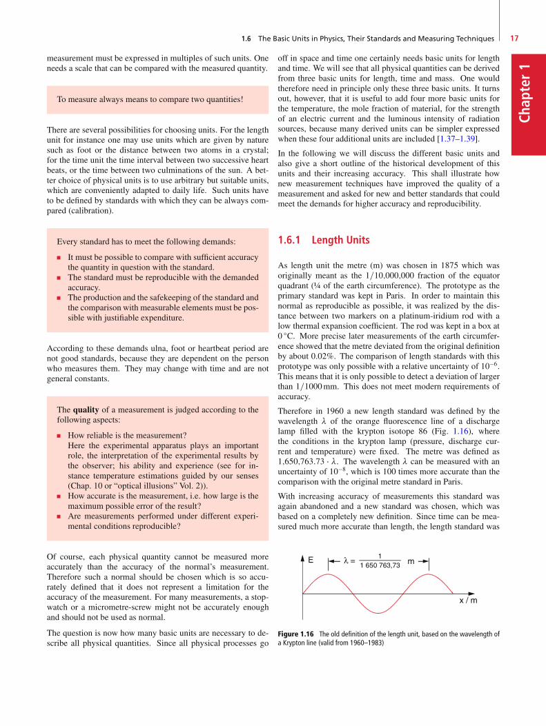
1.6 The Basic Units in Physics, Their Standards and Measuring Techniques 17
Chap
ter1
measurement must be expressed in multiples of such units. Oneneeds a scale that can be compared with the measured quantity.
To measure always means to compare two quantities!
There are several possibilities for choosing units. For the lengthunit for instance one may use units which are given by naturesuch as foot or the distance between two atoms in a crystal;for the time unit the time interval between two successive heartbeats, or the time between two culminations of the sun. A bet-ter choice of physical units is to use arbitrary but suitable units,which are conveniently adapted to daily life. Such units haveto be defined by standards with which they can be always com-pared (calibration).
Every standard has to meet the following demands:
It must be possible to compare with sufficient accuracythe quantity in question with the standard.The standard must be reproducible with the demandedaccuracy.The production and the safekeeping of the standard andthe comparison with measurable elements must be pos-sible with justifiable expenditure.
According to these demands ulna, foot or heartbeat period arenot good standards, because they are dependent on the personwho measures them. They may change with time and are notgeneral constants.
The quality of a measurement is judged according to thefollowing aspects:
How reliable is the measurement?Here the experimental apparatus plays an importantrole, the interpretation of the experimental results bythe observer; his ability and experience (see for in-stance temperature estimations guided by our senses(Chap. 10 or “optical illusions” Vol. 2)).How accurate is the measurement, i.e. how large is themaximum possible error of the result?Are measurements performed under different experi-mental conditions reproducible?
Of course, each physical quantity cannot be measured moreaccurately than the accuracy of the normal’s measurement.Therefore such a normal should be chosen which is so accu-rately defined that it does not represent a limitation for theaccuracy of the measurement. For many measurements, a stop-watch or a micrometre-screw might not be accurately enoughand should not be used as normal.
The question is now how many basic units are necessary to de-scribe all physical quantities. Since all physical processes go
off in space and time one certainly needs basic units for lengthand time. We will see that all physical quantities can be derivedfrom three basic units for length, time and mass. One wouldtherefore need in principle only these three basic units. It turnsout, however, that it is useful to add four more basic units forthe temperature, the mole fraction of material, for the strengthof an electric current and the luminous intensity of radiationsources, because many derived units can be simpler expressedwhen these four additional units are included [1.37–1.39].
In the following we will discuss the different basic units andalso give a short outline of the historical development of thisunits and their increasing accuracy. This shall illustrate hownew measurement techniques have improved the quality of ameasurement and asked for new and better standards that couldmeet the demands for higher accuracy and reproducibility.
1.6.1 Length Units
As length unit the metre (m) was chosen in 1875 which wasoriginally meant as the 1=10;000;000 fraction of the equatorquadrant (¼ of the earth circumference). The prototype as theprimary standard was kept in Paris. In order to maintain thisnormal as reproducible as possible, it was realized by the dis-tance between two markers on a platinum-iridium rod with alow thermal expansion coefficient. The rod was kept in a box at0 ıC. More precise later measurements of the earth circumfer-ence showed that the metre deviated from the original definitionby about 0.02%. The comparison of length standards with thisprototype was only possible with a relative uncertainty of 10�6.This means that it is only possible to detect a deviation of largerthan 1=1000mm. This does not meet modern requirements ofaccuracy.
Therefore in 1960 a new length standard was defined by thewavelength � of the orange fluorescence line of a dischargelamp filled with the krypton isotope 86 (Fig. 1.16), wherethe conditions in the krypton lamp (pressure, discharge cur-rent and temperature) were fixed. The metre was defined as1;650;763:73 � �. The wavelength � can be measured with anuncertainty of 10�8, which is 100 times more accurate than thecomparison with the original metre standard in Paris.
With increasing accuracy of measurements this standard wasagain abandoned and a new standard was chosen, which wasbased on a completely new definition. Since time can be mea-sured much more accurate than length, the length standard was
Figure 1.16 The old definition of the length unit, based on the wavelength ofa Krypton line (valid from 1960–1983)

Chapter1
18 1 Introduction and Survey
Table 1.3 Range of actual lengths in our world
Object Dimension/mRadius of the electron � 10�18
Radius of the proton 10�15
Distance between atoms in solids 10�10
Thickness of the skin of a soap bubble 10�7
Mean distance between air molecules at 105 Pa 10�6
Radius of the earth 6 � 106Distance earth–moon 4 � 108Distance earth–sun 1:5 � 1011Diameter of the solar system 1014
Distance to the nearest star 4 � 1016Diameter of our galaxy 3 � 1020Extension of the universe 3 � 1025
related to time measurements via the velocity c of light. Theweighted average of the most precise measurement of the speedof light in vacuum is now defined as
c D 299;792;458m=s :
This means that the speed of light is no longer a result of newmeasurements but is defined as a fixed value.
Definition
The length unit 1m is now fixed by the following defini-tion:
One metre is the length of the path that is travelled bylight in vacuum during the time interval 1=299;792;485 s.
From the relation c D � �� between speed of light c, frequency �and wavelength � of an electro-magnetic wave the wavelength �of any spectral line can now be determined from the frequency� (which can be measured with a much higher accuracy thanwavelengths) and the defined speed of light (see Sect. 1.6.2 and1.6.4).
The order of magnitude of length-scales in physics covers theenormous range from 10�18 m for the size of elementary parti-cles to 10C25 m for the radius of the present universe (Tab. 1.3).It is therefore appropriate to give metre scales in powers of ten.For specific powers a shorthand notation is used, e. g. 10�6 m D1 micrometer (µm); 103 m D 1 kilometer (km). These shorthandnotations are listed in Tab. 1.4.
In astronomy, the distances are very large. Therefore, appro-priate units are used. The astronomical unit AU is the meandistance between earth and sun. The new and more exact def-inition, adopted 1976 by the International Astronomical Unionis the following:
Table 1.4 Labels for different orders of magnitude of length units
1 attometer D 1 am D 10�18 m
1 femtometer D 1 fm D 10�15 m
1 picometer D 1 pm D 10�12 m
1 nanometer D 1 nm D 10�9 m
1 micrometer D 1 µm D 10�6 m
1 millimeter D 1mm D 10�3 m
1 centimeter D 1 cm D 10�2 m
1 dezimeter D 1 dm D 10�1 m
1 kilometer D 1 km D 103 mOften used units in– atomic and nuclear physics
1 fermi D 1 femtometer D 10�15 m
1 X-unit D 1XU D 1:00202 � 10�13 m
1 Ångström D 1Å D 10�10 m– astronomy:1 astronomical unit D 1AU
� mean distance earth–sun � 1:496 � 1011 m1 light year D 1 ly D 9:5 � 1015 m1 parsec D 1 pc D 3 � 1016 m D 3:2 ly
Definition
1AU is the distance to the centre of the sun, which a hypo-thetical body with negligible mass would have, if it moveson a circle around the sun in 365.2568983 days.
One light-year (1 ly) is the distance, which light travels in 1 year.An object has a distance of one parsec (1 pc) if the astronomicalunit seen from this object appears under an angle of one secondof arc (100) (Fig. 1.17). The distance d of a star, where this angleis ˛ is d D 1AU= tan˛. With tan 100 D 4:85 � 10�6 we obtain
1 pc D 2:06 � 105 AU D 3:2 ly :
Note: In some countries other non-metric length units arein use: 1 inch D 2.54 cm D 0.0245m and 1 yard (1 yd) D0.9144m, 1 mile (1mi) D 1609.344m.
However, in this textbook only SI units are used.
Figure 1.17 Definition of the astronomical units 1 AU and 1 pc

1.6 The Basic Units in Physics, Their Standards and Measuring Techniques 19
Chap
ter1
Edge-like surfacesfor measurementsof inside diameters
Set screw
Pole for depthmeasurements
Slider
Vermier scale
FixedLeg
Movable
Zero position
Measurement: 5.4 mm
Figure 1.18 Caliper gauge with vernier scale
1.6.2 Measuring Techniques for Lengths
For measuring of lengths in daily life secondary standards areused which are not as accurate as the primary standards but aremore readily usable. The accuracy of such standards is adaptedto the application for which they are constructed. One sim-ple example is the sliding vernier (Fig. 1.18). Its accuracy isbased on the nonius principle. The upper scale is divided intomillimetres, the lower scale has 10 scale divisions for 9mm,which means that every division is 9=10mm. For the situationin Fig. 1.18b the division mark 9mm on the upper scale coin-cides with the division mark 4 on the lower scale. The distanceD between the two fold limbs is then
D D .9 � 4 � 9=10/mm D 5:4mm :
The uncertainty of the measurement is about 0.1mm.
Higher accuracies can be reached with a micrometer screw(Fig. 1.19) where a full turn of the micrometer drum corre-sponds to a translation of 1mm. If the scale on the drum isdivided into 100 divisions each division mark corresponds to
Anvil Measuring arbor
Bow
Reference lineMeasuringsurfaces
of carbide Arbor fixing screw
Scale cylinderCoarsesetting
Figure 1.19 Micrometer caliper
0.01mm. The shackle is thermally isolated in order to minimizethermal expansion, With differential micrometer screws, whichhave two coaxial drums turning into opposite directions, whereone drum produces a translation of 1mm per turn, the other of�0:9mm in the backward direction, one full turn correspondsnow to 0.1mm. This allows an accuracy of 0:001mm D 1 µm.This is about the accuracy limit of mechanical devices.
More accurate length measurements are based on optical tech-niques. For distances below 1m interferometric methods arepreferable (see Vol. 2) where lasers (see Vol. 3) are used aslight sources. Here distances are compared to the wavelengthof the light source. Modern interferometers reach accuraciesof �=100. With a wavelength of � D 500 nm an accuracy of5 nm D 5 � 10�9 m can be achieved.
Larger distances can be measured via the travel time of a lightpulse. For instance the distance of the retro-reflector which theastronauts have positioned on the moon, can be measured withina few cm using laser pulses with 10�12 s pulse width (LIDARtechnique see Fig. 1.20). Measuring this distance from differ-ent locations on earth at different times even allows to detectcontinental drifts of the earth crust plates [1.41–1.42].
For the exact location of planes, ships or land vehicles the globalpositioning system GPS has been developed. Its principle isillustrated by Fig. 1.21.
The navigator, who wants to determine his position, measuressimultaneously the phases of radio signals emitted from at leastfour different satellites. The radio signals on frequencies at1575MHz and 1227MHz are modulated. This allows to de-termine unambiguously the distances di from the receiver to thesatellites Si from the measured phase differences �i. From thesefour distances di the position (x; y; z) of the receiver can be deter-mined with an uncertainty of only a few cm if relativistic effects(see Sect. 3.6) are taken into account! In order to achieve thisaccuracy, the frequencies of the radio signals must be kept sta-ble within 10�10. This can be realized with atomic clocks which
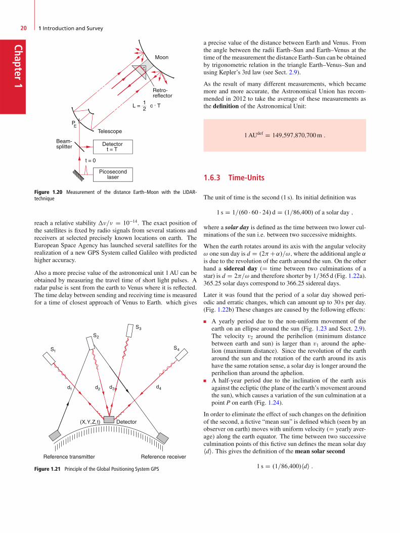
Chapter1
20 1 Introduction and Survey
Figure 1.20 Measurement of the distance Earth–Moon with the LIDAR-technique
reach a relative stability ��=� D 10�14. The exact position ofthe satellites is fixed by radio signals from several stations andreceivers at selected precisely known locations on earth. TheEuropean Space Agency has launched several satellites for therealization of a new GPS System called Galileo with predictedhigher accuracy.
Also a more precise value of the astronomical unit 1AU can beobtained by measuring the travel time of short light pulses. Aradar pulse is sent from the earth to Venus where it is reflected.The time delay between sending and receiving time is measuredfor a time of closest approach of Venus to Earth. which gives
Figure 1.21 Principle of the Global Positioning System GPS
a precise value of the distance between Earth and Venus. Fromthe angle between the radii Earth–Sun and Earth–Venus at thetime of the measurement the distance Earth–Sun can be obtainedby trigonometric relation in the triangle Earth–Venus–Sun andusing Kepler’s 3rd law (see Sect. 2.9).
As the result of many different measurements, which becamemore and more accurate, the Astronomical Union has recom-mended in 2012 to take the average of these measurements asthe definition of the Astronomical Unit:
1AUdef D 149;597;870;700m :
1.6.3 Time-Units
The unit of time is the second (1 s). Its initial definition was
1 s D 1=.60 � 60 � 24/ d D .1=86;400/ of a solar day ;
where a solar day is defined as the time between two lower cul-minations of the sun i.e. between two successive midnights.
When the earth rotates around its axis with the angular velocity! one sun day is d D .2C˛/=!;where the additional angle ˛is due to the revolution of the earth around the sun. On the otherhand a sidereal day (D time between two culminations of astar) is d D 2=! and therefore shorter by 1=365d (Fig. 1.22a).365.25 solar days correspond to 366.25 sidereal days.
Later it was found that the period of a solar day showed peri-odic and erratic changes, which can amount up to 30 s per day.(Fig. 1.22b) These changes are caused by the following effects:
A yearly period due to the non-uniform movement of theearth on an ellipse around the sun (Fig. 1.23 and Sect. 2.9).The velocity v2 around the perihelion (minimum distancebetween earth and sun) is larger than v1 around the aphe-lion (maximum distance). Since the revolution of the eartharound the sun and the rotation of the earth around its axishave the same rotation sense, a solar day is longer around theperihelion than around the aphelion.A half-year period due to the inclination of the earth axisagainst the ecliptic (the plane of the earth’s movement aroundthe sun), which causes a variation of the sun culmination at apoint P on earth (Fig. 1.24).
In order to eliminate the effect of such changes on the definitionof the second, a fictive “mean sun” is defined which (seen by anobserver on earth) moves with uniform velocity (D yearly aver-age) along the earth equator. The time between two successiveculmination points of this fictive sun defines the mean solar dayhdi. This gives the definition of the mean solar second
1 s D .1=86;400/hdi :
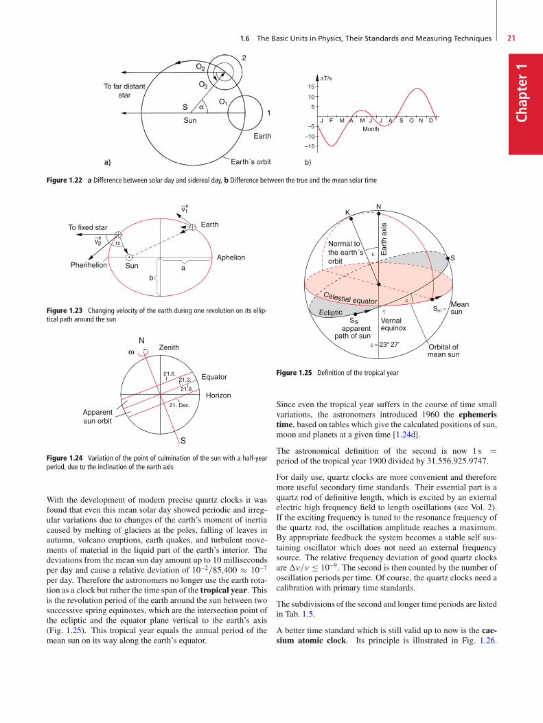
1.6 The Basic Units in Physics, Their Standards and Measuring Techniques 21
Chap
ter1
To far distantstar
Sun
Earth´s orbit
Earth
Figure 1.22 a Difference between solar day and sidereal day, b Difference between the true and the mean solar time
Figure 1.23 Changing velocity of the earth during one revolution on its ellip-tical path around the sun
Figure 1.24 Variation of the point of culmination of the sun with a half-yearperiod, due to the inclination of the earth axis
With the development of modern precise quartz clocks it wasfound that even this mean solar day showed periodic and irreg-ular variations due to changes of the earth’s moment of inertiacaused by melting of glaciers at the poles, falling of leaves inautumn, volcano eruptions, earth quakes, and turbulent move-ments of material in the liquid part of the earth’s interior. Thedeviations from the mean sun day amount up to 10 millisecondsper day and cause a relative deviation of 10�2=85;400 � 10�7
per day. Therefore the astronomers no longer use the earth rota-tion as a clock but rather the time span of the tropical year. Thisis the revolution period of the earth around the sun between twosuccessive spring equinoxes, which are the intersection point ofthe ecliptic and the equator plane vertical to the earth’s axis(Fig. 1.25). This tropical year equals the annual period of themean sun on its way along the earth’s equator.
Figure 1.25 Definition of the tropical year
Since even the tropical year suffers in the course of time smallvariations, the astronomers introduced 1960 the ephemeristime, based on tables which give the calculated positions of sun,moon and planets at a given time [1.24d].
The astronomical definition of the second is now 1 s Dperiod of the tropical year 1900 divided by 31;556;925:9747.
For daily use, quartz clocks are more convenient and thereforemore useful secondary time standards. Their essential part is aquartz rod of definitive length, which is excited by an externalelectric high frequency field to length oscillations (see Vol. 2).If the exciting frequency is tuned to the resonance frequency ofthe quartz rod, the oscillation amplitude reaches a maximum.By appropriate feedback the system becomes a stable self sus-taining oscillator which does not need an external frequencysource. The relative frequency deviation of good quartz clocksare��=� � 10�9. The second is then counted by the number ofoscillation periods per time. Of course, the quartz clocks need acalibration with primary time standards.
The subdivisions of the second and longer time periods are listedin Tab. 1.5.
A better time standard which is still valid up to now is the cae-sium atomic clock. Its principle is illustrated in Fig. 1.26.
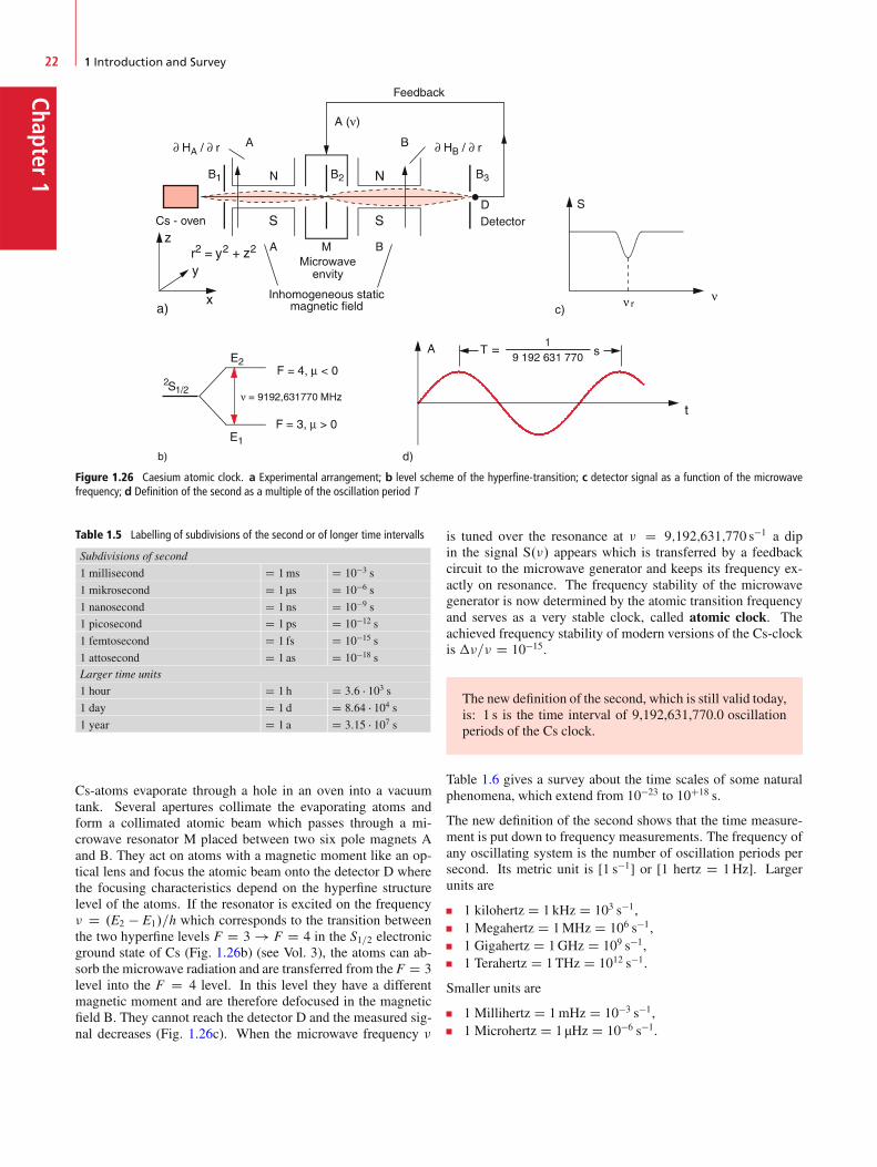
Chapter1
22 1 Introduction and Survey
Figure 1.26 Caesium atomic clock. a Experimental arrangement; b level scheme of the hyperfine-transition; c detector signal as a function of the microwavefrequency; d Definition of the second as a multiple of the oscillation period T
Table 1.5 Labelling of subdivisions of the second or of longer time intervalls
Subdivisions of second
1 millisecond D 1ms D 10�3 s
1 mikrosecond D 1 µs D 10�6 s
1 nanosecond D 1 ns D 10�9 s
1 picosecond D 1 ps D 10�12 s
1 femtosecond D 1 fs D 10�15 s
1 attosecond D 1 as D 10�18 sLarger time units
1 hour D 1 h D 3:6 � 103 s1 day D 1 d D 8:64 � 104 s1 year D 1 a D 3:15 � 107 s
Cs-atoms evaporate through a hole in an oven into a vacuumtank. Several apertures collimate the evaporating atoms andform a collimated atomic beam which passes through a mi-crowave resonator M placed between two six pole magnets Aand B. They act on atoms with a magnetic moment like an op-tical lens and focus the atomic beam onto the detector D wherethe focusing characteristics depend on the hyperfine structurelevel of the atoms. If the resonator is excited on the frequency� D .E2 � E1/=h which corresponds to the transition betweenthe two hyperfine levels F D 3 ! F D 4 in the S1=2 electronicground state of Cs (Fig. 1.26b) (see Vol. 3), the atoms can ab-sorb the microwave radiation and are transferred from the F D 3level into the F D 4 level. In this level they have a differentmagnetic moment and are therefore defocused in the magneticfield B. They cannot reach the detector D and the measured sig-nal decreases (Fig. 1.26c). When the microwave frequency �
is tuned over the resonance at � D 9;192;631;770 s�1 a dipin the signal S.�/ appears which is transferred by a feedbackcircuit to the microwave generator and keeps its frequency ex-actly on resonance. The frequency stability of the microwavegenerator is now determined by the atomic transition frequencyand serves as a very stable clock, called atomic clock. Theachieved frequency stability of modern versions of the Cs-clockis ��=� D 10�15.
The new definition of the second, which is still valid today,is: 1 s is the time interval of 9,192,631,770.0 oscillationperiods of the Cs clock.
Table 1.6 gives a survey about the time scales of some naturalphenomena, which extend from 10�23 to 10C18 s.
The new definition of the second shows that the time measure-ment is put down to frequency measurements. The frequency ofany oscillating system is the number of oscillation periods persecond. Its metric unit is [1 s�1] or [1 hertz D 1Hz]. Largerunits are
1 kilohertz D 1 kHz D 103 s�1,1 Megahertz D 1MHz D 106 s�1,1 Gigahertz D 1GHz D 109 s�1,1 Terahertz D 1THz D 1012 s�1.
Smaller units are
1 Millihertz D 1mHz D 10�3 s�1,1 Microhertz D 1 µHz D 10�6 s�1.
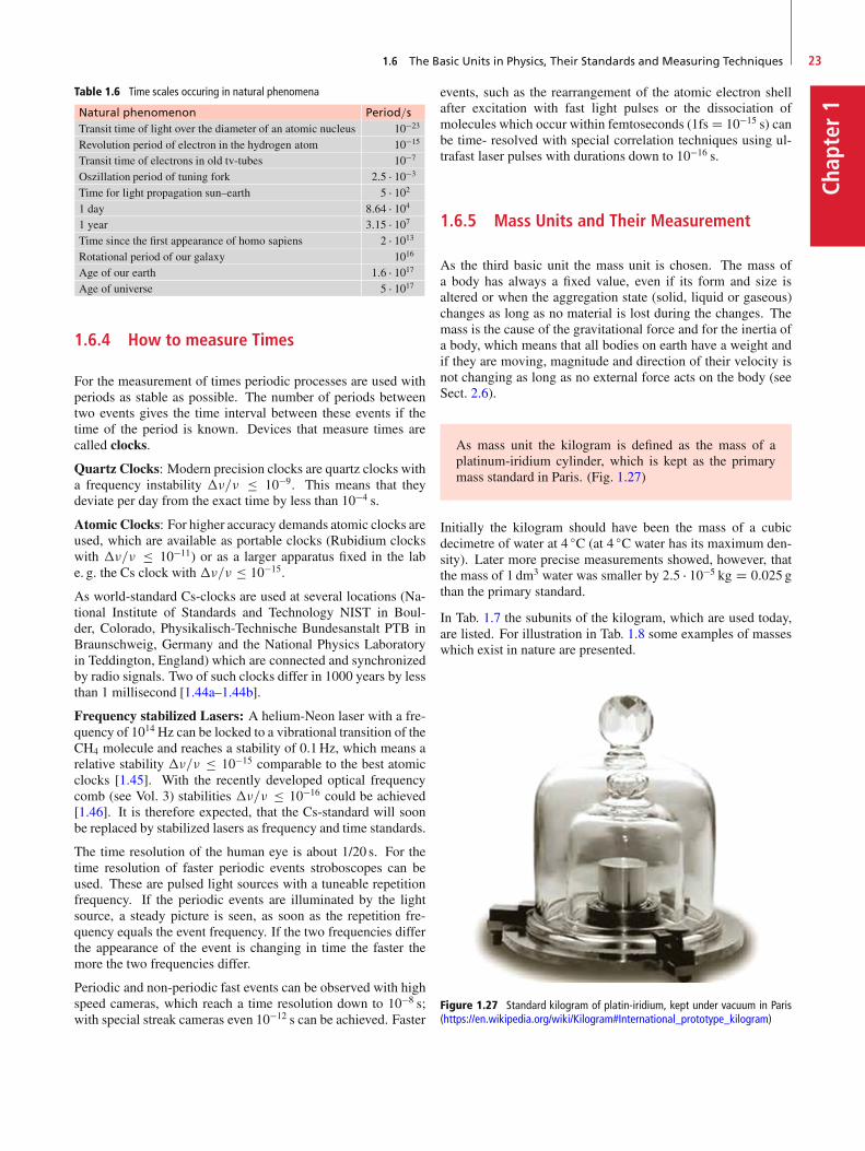
1.6 The Basic Units in Physics, Their Standards and Measuring Techniques 23
Chap
ter1
Table 1.6 Time scales occuring in natural phenomena
Natural phenomenon Period=sTransit time of light over the diameter of an atomic nucleus 10�23
Revolution period of electron in the hydrogen atom 10�15
Transit time of electrons in old tv-tubes 10�7
Oszillation period of tuning fork 2:5 � 10�3
Time for light propagation sun–earth 5 � 1021 day 8:64 � 1041 year 3:15 � 107Time since the first appearance of homo sapiens 2 � 1013Rotational period of our galaxy 1016
Age of our earth 1:6 � 1017Age of universe 5 � 1017
1.6.4 How to measure Times
For the measurement of times periodic processes are used withperiods as stable as possible. The number of periods betweentwo events gives the time interval between these events if thetime of the period is known. Devices that measure times arecalled clocks.
Quartz Clocks: Modern precision clocks are quartz clocks witha frequency instability ��=� � 10�9. This means that theydeviate per day from the exact time by less than 10�4 s.
Atomic Clocks: For higher accuracy demands atomic clocks areused, which are available as portable clocks (Rubidium clockswith ��=� � 10�11) or as a larger apparatus fixed in the labe. g. the Cs clock with ��=� � 10�15.
As world-standard Cs-clocks are used at several locations (Na-tional Institute of Standards and Technology NIST in Boul-der, Colorado, Physikalisch-Technische Bundesanstalt PTB inBraunschweig, Germany and the National Physics Laboratoryin Teddington, England) which are connected and synchronizedby radio signals. Two of such clocks differ in 1000 years by lessthan 1 millisecond [1.44a–1.44b].
Frequency stabilized Lasers: A helium-Neon laser with a fre-quency of 1014 Hz can be locked to a vibrational transition of theCH4 molecule and reaches a stability of 0.1Hz, which means arelative stability ��=� � 10�15 comparable to the best atomicclocks [1.45]. With the recently developed optical frequencycomb (see Vol. 3) stabilities ��=� � 10�16 could be achieved[1.46]. It is therefore expected, that the Cs-standard will soonbe replaced by stabilized lasers as frequency and time standards.
The time resolution of the human eye is about 1/20 s. For thetime resolution of faster periodic events stroboscopes can beused. These are pulsed light sources with a tuneable repetitionfrequency. If the periodic events are illuminated by the lightsource, a steady picture is seen, as soon as the repetition fre-quency equals the event frequency. If the two frequencies differthe appearance of the event is changing in time the faster themore the two frequencies differ.
Periodic and non-periodic fast events can be observed with highspeed cameras, which reach a time resolution down to 10�8 s;with special streak cameras even 10�12 s can be achieved. Faster
events, such as the rearrangement of the atomic electron shellafter excitation with fast light pulses or the dissociation ofmolecules which occur within femtoseconds (1fs D 10�15 s) canbe time- resolved with special correlation techniques using ul-trafast laser pulses with durations down to 10�16 s.
1.6.5 Mass Units and Their Measurement
As the third basic unit the mass unit is chosen. The mass ofa body has always a fixed value, even if its form and size isaltered or when the aggregation state (solid, liquid or gaseous)changes as long as no material is lost during the changes. Themass is the cause of the gravitational force and for the inertia ofa body, which means that all bodies on earth have a weight andif they are moving, magnitude and direction of their velocity isnot changing as long as no external force acts on the body (seeSect. 2.6).
As mass unit the kilogram is defined as the mass of aplatinum-iridium cylinder, which is kept as the primarymass standard in Paris. (Fig. 1.27)
Initially the kilogram should have been the mass of a cubicdecimetre of water at 4 ıC (at 4 ıC water has its maximum den-sity). Later more precise measurements showed, however, thatthe mass of 1 dm3 water was smaller by 2:5 � 10�5 kg D 0:025 gthan the primary standard.
In Tab. 1.7 the subunits of the kilogram, which are used today,are listed. For illustration in Tab. 1.8 some examples of masseswhich exist in nature are presented.
Figure 1.27 Standard kilogram of platin-iridium, kept under vacuum in Paris(https://en.wikipedia.org/wiki/Kilogram#International_prototype_kilogram)

Chapter1
24 1 Introduction and Survey
Table 1.7 Subdivisions and multiples of the kilogram
Unit Denotion Mass/kg1 gram D 1 g 10�3
1 milligram D 1mg 10�6
1 microgram D 1 µg 10�9
1 nanogram D 1 ng 10�12
1 pikogram D 1 pg 10�15
1 ton 103
1 megaton 109
1 atomic mass unit D 1AMU 1:6605402 � 10�27
Table 1.8 The masses of particles and bodies found in nature
Body Mass/kgElectron 9:1 � 10�31
Proton 1:7 � 10�27
Uranium nucleus 4 � 10�25
Protein molecule 10�22
Bacterium 10�11
Fly 10�3
Man 102
Earth 6 � 1024Sun 2 � 1030Galaxy � 1042
Masses can be measured either by their inertia or they weight,since both properties are proportional to their mass and un-ambiguously defined (see Sect. 2.6). The inertia of a mass ismeasured by the oscillation period of a spring pendulum. Herethe mass measurement is reduced to a time measurement.
The weight of a mass is determined by comparison with a massnormal on a spring balance or a beam balance and therefore re-duced to a length measurement. Today balances are availablewith a lower detection limit of at least 10�10 kg (magnetic bal-ance, electromagnetic balance, quartz fibre microbalance).
Note: In some countries non-metrical units are used: 1 pound D0:453 kg.
1.6.6 Molar Quantity Unit
As already mentioned in the beginning of this section in ad-dition to the three basic units for length, time and mass fourfurther units (molar quantity, temperature, electric current andluminous intensity of a radiation source) are introduced becauseof pragmatic reasons. Strictly speaking they are not real basicunits because they can be expressed by the three basic units.
Definition
The unit of molar quantity is the mol, which is defined asfollows:
1mol is the amount of a substance that consist of as manyparticles as the number N of atoms in 0.012kg of the car-bon nuclide 12C.
These particles can be atoms, molecules, ions or electrons.The number N of particles per mol with the numerical valueN D 6:02 � 1023=mol, is called Avogadro’s number (AmedeoAvogadro 1776–1856).
Example
1mol helium has a mass of 0:004 kg, 1mol copper cor-responds to 0:064 kg, one mol hydrogen gas H2 has themass 2 � 0:001 kg D 0:002 kg. J
1.6.7 Temperature Unit
The unit of the temperature is 1 Kelvin (1K). This unit can bedefined by the thermo-dynamic temperature scale and can be re-duced to the kinetic energy of the molecules (see Sect. 10.1.4).Because of principal considerations and also measuring tech-niques, which are explained in Chap. 10, the following defini-tion was chosen:
1 Kelvin is the fraction (1=273:16) of the thermodynamictemperature of the triple point of water.
The triple point is that temperature where all three phases ofwater (ice, liquid water and water vapour) can simultaneouslyexist (Fig. 1.28).
There are plans for a new definition of 1K which is independenton the choice of a special material (here water). It reads:
1 Kelvin is the temperature change which corresponds toa change �.kT/ D 1:3806505 � 10�23 Joule of the ther-mal energy kT , where k D 13;806;505 � 10�23 J=K is theBoltzmann constant.
Figure 1.28 Phase diagram and triple point of water

1.6 The Basic Units in Physics, Their Standards and Measuring Techniques 25
Chap
ter1
New very accurate measurements of the Boltzmann constantallow a much better definition of the temperature T with an un-certainty of �T=T � 8 � 10�6.
1.6.8 Unit of the Electric Current
The unit of the electric current is 1 Ampere (1A) (named afterAndre-Marie Ampère 1775–1836). It is defined as follows:
1 Ampere corresponds to a constant electric currentthrough two straight parallel infinitely long wires witha distance of 1m which experience a mutual force of2 � 10�7 Newton per m wire length (Fig. 1.29).
The definition of the electric current unit is therefore based onthe measurement of the mechanical quantities length and force(see Vol. 2)
1.6.9 Unit of Luminous Intensity
The luminous intensity of a radiation source is the radiationpower emitted into the solid angle 1 Sterad D 1=.4/. It couldbe defined in Watt=Sterad, which gives the radiation power in-dependent of the observing human eye. However, in order tocharacterize the visual impression of the light intensity of a lightsource, the spectral characteristics of the radiation must be takeninto account, because the sensitivity of the human eye dependson the wavelength. Therefore the definition of the light inten-sity is adapted to the spectral sensitivity maximum of the eye ata wavelength � D 555 nm. The luminosity unit is called 1 can-dela (1 cd).
1 cd is the radiation power of (1/6839)W/Sterad emittedby a source at the frequency 540 THz (� D 555 nm) intoa selected direction.
Note: 1. The luminous intensity of a source can differ for dif-ferent directions.
2. The definition of the candela is related to the radi-ation power in Watt=Sterad, which shows that thecandela is not a basic unit.
Figure 1.29 Illustration how the unit of the electric current is defined
1.6.10 Unit of Angle
Plane angles are generally measured in degrees of arc. The fullangle of a circle is 360ı. The subdivisions are minutes of arc(1ı D 600) and seconds of arc (10 D 6000 ! 1ı D 360000). Oftenit is convenient to use dimensionless units by reducing anglemeasurements to length measurements of the arc length L of acircle, which corresponds to the angle ˛ (Fig. 1.30).
The circular measure (radian) of the angle ˛ is defined as theratio L=R of circular arc L and radius R of the circle. The unitof this dimensionless quantity is 1 radian (rad) which is realizedfor L D R. Since the total circumference of the circle is 2R theangle ˛ D 360ı in the unit degrees corresponds to ˛ D 2 inthe units radian D rad.
The conversion from radians to degrees is
1 rad D 360ı
2D 57:296ı D 57ı1704500 :
While the plane angle ˛ D L=R cuts the arc with length L outof a circle with radius R the solid angle ˝ D A=R2 is the angelof a cone that cuts the area A D ˝R2 out of a full sphere witharea 4R2 and radius R (Fig. 1.31). The dimensionless unit ofthe solid angle is 1 steradian (1 sr) for which A D R2.
Definition
1 sr is the solid angle of a cone which cuts an area A D1m2 out of the unit sphere with R D 1m.
Since the total surface of a sphere is 4R2 the total solid anglearound the centre of the sphere with A D 4R2 is ˝ D 4 .
The three planes xy, xz, yz through the positive coordinate axisCx, Cy, Cz cut a sphere around the origin (0; 0; 0) into 8 oc-tands, The solid angle of one octand is
˝ D 1
8� 4 D 1
2 sr :
Note: The numerical values of the units for the basic physi-cal quantities discussed so far have been often adapted by theInternational Comission for Weights and Measures (CIPM for
Figure 1.30 To the definition of the radian ˛ D L=R

Chapter1
26 1 Introduction and Survey
Figure 1.31 a To the definition of the solid angle ˝ ; b Illuration of the solidangel element d˝ D dA=r2
the French comite international des poids et measures) in or-der to take into account the results of new and more accuratemeasurements. At present, considerations are made to reduceall quantities to combinations of fundamental constants in orderto give them more accurate and time independent values. Thishas been realized up to now only for the length unit which isdefined through the fixed speed of light and the frequency of theCs-clock. This might be soon generalized to all physical unitsin order to get a system of time-independent values for the unitswhich do not need to be corrected in future times.
One example is the mass unit. There are many efforts in severallaboratories to create a better and more accurately defined massnormal. One realistic proposal is a large silicon single crystalin form of a polished sphere, where the atomic distances in thecrystal have been precisely measured with X-ray interferometry.This allows the determination of the total number of atoms in thecrystal and the mass of the crystal can be related to the mass ofa silicon atom and is therefore reduced to atomic mass units andthe Avogadro constant [1.48a]. Although it has been shown, thatsuch a mass normal would be more accurate (�m=m � 10�8)and would represent a durable mass standard, it has not yet beeninternationally acknowledged.
Similar considerations are discussed for the temperature unit1K which might be reduced to the Boltzmann constant k (seeabove).
1.7 Systems of Units
As has been discussed in Sect. 1.6 the three basic quantities andtheir units in physics are
length with the unit 1 Meter D 1mtime with the unit 1 second D 1 smass with the unit 1 kilogram D 1 kg
with four additional quantities
molar quantity with the unit 1 mole D 1moltemperature with the unit 1 Kelvin D 1Kelectric current with the unit 1 Ampere D 1Aradiation luminosity with the unit 1 candela D 1 cd
where these four quantities can be reduced in principle to thethree basic quantities and are therefore no real basic quantities.
All other quantities in physics can be expressed by these 3 basicquantities with the additional 4 quantities for convenient use.This will be shown for each derived quantity in this textbookwhen the corresponding quantity is introduced.
Each physical quantity is defined by its unit and its numericalvalue. For instance the speed of light is c D 2:9979 � 108 m/s orthe earth acceleration g D 9:81m/s2 etc.
In a physical equation all summands must have the sameunits.
These units or the products of units are called the dimension ofa quantity. The check, whether all summands in a equation havethe same dimension is called dimensional analysis. It is a veryhelpful tool to avoid errors in conversion of different systems ofunits.
Each physical quantity can be expressed in different units, forexample, times in seconds, minutes or hours. The numericalvalue differs for the different units. For instance the velocityv D 10m/s equals v D 36 km/h. In order to avoid such numeri-cal conversions one can use a definite fixed system of units.
If the three basic units are chosen as
1m for the length unit,1 s for the time unit,1 kg for the mass unit.
The system is called the mks-system. If the unit Ampere for theelectric current is added, the system is called the mksA.-system,often named the SI-System after the French nomenclature Sys-tem International d’Unites. It has the very useful advantage thatfor the conversion from mechanical into electrical and magneticunits all numerical conversion factors have the value 1. All basicunits and also the units derived from them are called SI units.
In theoretical physics often the cgs system is used, where thebasic units are 1 cm (instead of 1m), 1 Gramm (instead of 1 kg)and only the time unit is 1 s as in the SI-system. According tointernational agreements from 1972 only the SI-system shouldbe used. In this textbook exclusively SI units are used.
For a more detailed representation of the subject the reader isreferred to the literature [1.37–1.39,1.50].
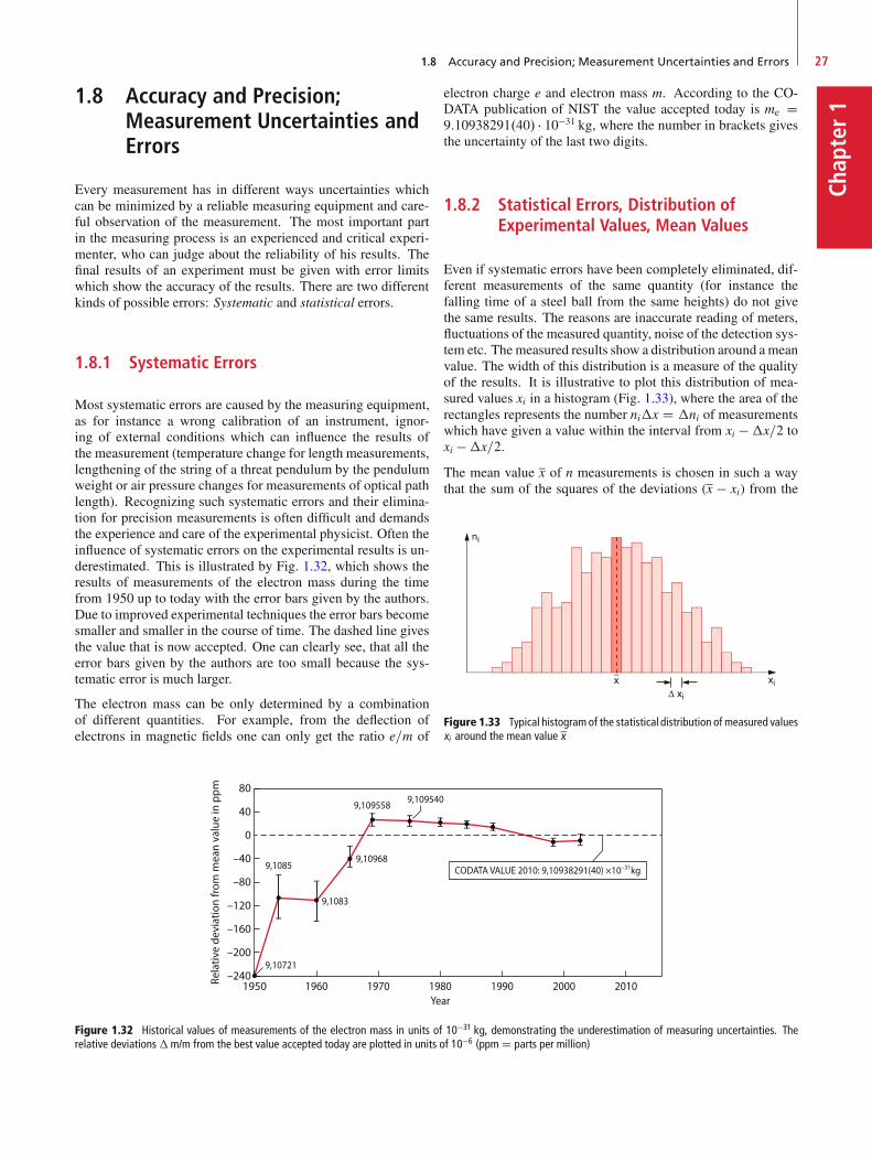
1.8 Accuracy and Precision; Measurement Uncertainties and Errors 27
Chap
ter11.8 Accuracy and Precision;
Measurement Uncertainties andErrors
Every measurement has in different ways uncertainties whichcan be minimized by a reliable measuring equipment and care-ful observation of the measurement. The most important partin the measuring process is an experienced and critical experi-menter, who can judge about the reliability of his results. Thefinal results of an experiment must be given with error limitswhich show the accuracy of the results. There are two differentkinds of possible errors: Systematic and statistical errors.
1.8.1 Systematic Errors
Most systematic errors are caused by the measuring equipment,as for instance a wrong calibration of an instrument, ignor-ing of external conditions which can influence the results ofthe measurement (temperature change for length measurements,lengthening of the string of a threat pendulum by the pendulumweight or air pressure changes for measurements of optical pathlength). Recognizing such systematic errors and their elimina-tion for precision measurements is often difficult and demandsthe experience and care of the experimental physicist. Often theinfluence of systematic errors on the experimental results is un-derestimated. This is illustrated by Fig. 1.32, which shows theresults of measurements of the electron mass during the timefrom 1950 up to today with the error bars given by the authors.Due to improved experimental techniques the error bars becomesmaller and smaller in the course of time. The dashed line givesthe value that is now accepted. One can clearly see, that all theerror bars given by the authors are too small because the sys-tematic error is much larger.
The electron mass can be only determined by a combinationof different quantities. For example, from the deflection ofelectrons in magnetic fields one can only get the ratio e=m of
80
40
0
–40
–80
–120
–160
–200
–2401950 1960
9,10721
9,1085
9,1083
9,10968
9,109558 9,109540
CODATA VALUE 2010: 9,10938291(40) ×10–31kg
1970 1980Year
1990 2000 2010Rela
tive
devi
atio
n fr
om m
ean
valu
e in
ppm
Figure 1.32 Historical values of measurements of the electron mass in units of 10�31 kg, demonstrating the underestimation of measuring uncertainties. Therelative deviations�m/m from the best value accepted today are plotted in units of 10�6 (ppm D parts per million)
electron charge e and electron mass m. According to the CO-DATA publication of NIST the value accepted today is me D9:10938291.40/ � 10�31 kg, where the number in brackets givesthe uncertainty of the last two digits.
1.8.2 Statistical Errors, Distribution ofExperimental Values, Mean Values
Even if systematic errors have been completely eliminated, dif-ferent measurements of the same quantity (for instance thefalling time of a steel ball from the same heights) do not givethe same results. The reasons are inaccurate reading of meters,fluctuations of the measured quantity, noise of the detection sys-tem etc. The measured results show a distribution around a meanvalue. The width of this distribution is a measure of the qualityof the results. It is illustrative to plot this distribution of mea-sured values xi in a histogram (Fig. 1.33), where the area of therectangles represents the number ni�x D �ni of measurementswhich have given a value within the interval from xi ��x=2 toxi ��x=2.
The mean value x of n measurements is chosen in such a waythat the sum of the squares of the deviations (x � xi) from the
Figure 1.33 Typical histogram of the statistical distribution of measured valuesxi around the mean value x
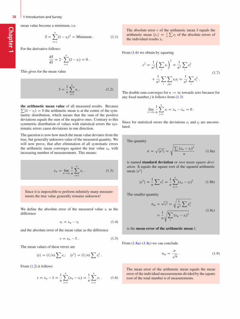
Chapter1
28 1 Introduction and Survey
mean value become a minimum, i.e.
S DnX
iD1
.x � xi/2 D Minimum : (1.1)
For the derivative follows:
dS
dxD 2 �
nX
iD1
.x � xi/ D 0 :
This gives for the mean value
x D 1
n
nX
iD1
xi ; (1.2)
the arithmetic mean value of all measured results. BecauseP.x � xi/ D 0 the arithmetic mean is at the centre of the sym-
metric distribution, which means that the sum of the positivedeviations equals the sum of the negative ones. Contrary to thissymmetric distribution of values with statistical errors the sys-tematic errors cause deviations in one direction.
The question is now howmuch the mean value deviates from thetrue, but generally unknown value of the measured quantity. Wewill now prove, that after elimination of all systematic errorsthe arithmetic mean converges against the true value xw withincreasing number of measurements. This means:
xw D limn!1
1
n
nX
iD1
xi : (1.3)
Since it is impossible to perform infinitely many measure-ments the true value generally remains unknown!
We define the absolute error of the measured value xi as thedifference
ei D xw � xi (1.4)
and the absolute error of the mean value as the difference
" D xw � x : (1.5)
The mean values of these errors are
hei D .1=n/X
eiI he2i D .1=n/X
e2i :
From (1.2) it follows
" D xw � x D 1
n
nX
iD1
.xw � xi/ D 1
n
nX
iD1
ei : (1.6)
The absolute error " of the arithmetic mean x equals thearithmetic mean he1i D 1
n
Pei of the absolute errors of
the individual results xi.
From (1.6) we obtain by squaring
"2 D 1
n2
�X
i
ei
�2
D 1
n2
X
i
e2i
C 1
n2
X
i
X
j¤i
eiej � 1
n2
X
i
e2i :
(1.7)
The double sum converges for n ! 1 towards zero because forany fixed number j it follows from (1.3)
limn!1
1
n
nX
iD1
ei D xw � xw D 0 :
Since for statistical errors the deviations ei and ej are uncorre-lated.
The quantity
� Dp
he2i DsP
.xw � xi/2
n(1.8a)
is named standard deviation or root mean square devi-ation. It equals the square root of the squared arithmeticmean he2i
he2i D 1
n
Xe2i D 1
n
nX
iD1
.xw � xi/2 (1.8b)
The smaller quantity
�m Dp"2 D
r1
n2
Xe2i
D 1
n
sX
i
.xw � xi/2
(1.8c)
is the mean error of the arithmetic mean x.
From (1.8a)–(1.8c) we can conclude
�m D �pn: (1.9)
The mean error of the arithmetic mean equals the meanerror of the individual measurements divided by the squareroot of the total number n of measurements.
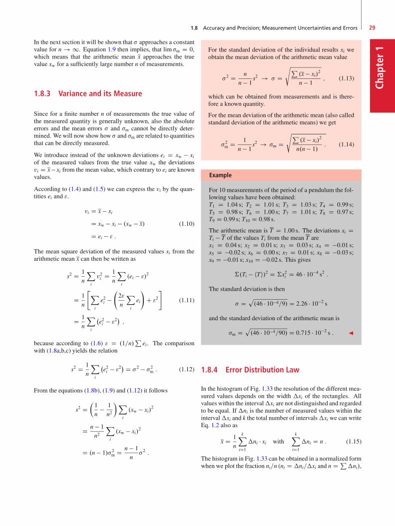
1.8 Accuracy and Precision; Measurement Uncertainties and Errors 29
Chap
ter1
In the next section it will be shown that � approaches a constantvalue for n ! 1. Equation 1.9 then implies, that lim �m D 0,which means that the arithmetic mean x approaches the truevalue xw for a sufficiently large number n of measurements.
1.8.3 Variance and its Measure
Since for a finite number n of measurements the true value ofthe measured quantity is generally unknown, also the absoluteerrors and the mean errors � and �m cannot be directly deter-mined. We will now show how � and �m are related to quantitiesthat can be directly measured.
We introduce instead of the unknown deviations ei D xw � xiof the measured values from the true value xw the deviationsvi D x� xi from the mean value, which contrary to ei are knownvalues.
According to (1.4) and (1.5) we can express the vi by the quan-tities ei and ".
vi D x � xi
D xw � xi � .xw � x/
D ei � " :(1.10)
The mean square deviation of the measured values xi from thearithmetic mean x can then be written as
s2 D 1
n
X
i
v2i D 1
n
X
i
.ei � "/2
D 1
n
"X
i
e2i � 2"
n
X
i
ei
!C "2
#
D 1
n
X
i
�e2i � "2� ;
(1.11)
because according to (1.6) " D .1=n/P
ei. The comparisonwith (1.8a,b,c) yields the relation
s2 D 1
n
X
i
�e2i � "2� D �2 � �2
m : (1.12)
From the equations (1.8b), (1.9) and (1.12) it follows
s2 D�1
n� 1
n2
�X
i
.xw � xi/2
D n � 1
n2
X
i
.xw � xi/2
D .n � 1/�2m D n � 1
n�2 :
For the standard deviation of the individual results xi weobtain the mean deviation of the arithmetic mean value
�2 D n
n � 1s2 ! � D
sP.x � xi/
2
n � 1; (1.13)
which can be obtained from measurements and is there-fore a known quantity.
For the mean deviation of the arithmetic mean (also calledstandard deviation of the arithmetic means) we get
�2m D 1
n � 1s2 ! �m D
sP.x � xi/
2
n.n � 1/: (1.14)
Example
For 10 measurements of the period of a pendulum the fol-lowing values have been obtained:T1 D 1:04 s; T2 D 1:01 s; T3 D 1:03 s; T4 D 0:99 s;T5 D 0:98 s; T6 D 1:00 s; T7 D 1:01 s; T8 D 0:97 s;T9 D 0:99 s; T10 D 0:98 s.
The arithmetic mean is T D 1:00 s. The deviations xi DTi � T of the values Ti from the mean T arex1 D 0:04 s; x2 D 0:01 s; x3 D 0:03 s; x4 D �0:01 s;x5 D �0:02 s; x6 D 0:00 s; x7 D 0:01 s; x8 D �0:03 s;x9 D �0:01 s; x10 D �0:02 s. This gives
†.Ti � hTi/2 D †x2i D 46 � 10�4 s2 :
The standard deviation is then
� Dp.46 � 10�4=9/ D 2:26 � 10�2 s
and the standard deviation of the arithmetic mean is
�m Dp.46 � 10�4=90/ D 0:715 � 10�2 s : J
1.8.4 Error Distribution Law
In the histogram of Fig. 1.33 the resolution of the different mea-sured values depends on the width �xi of the rectangles. Allvalues within the interval�xi are not distinguished and regardedto be equal. If �ni is the number of measured values within theinterval�xi and k the total number of intervals�xi we can writeEq. 1.2 also as
x D 1
n
kX
iD1
�ni � xi withkX
iD1
�ni D n : (1.15)
The histogram in Fig. 1.33 can be obtained in a normalized formwhen we plot the fraction ni=n (ni D �ni=�xi and n D P
�ni/,
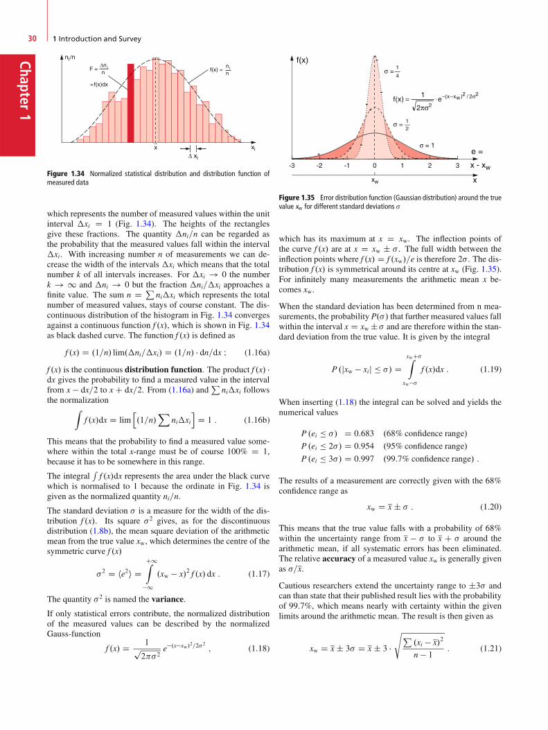
Chapter1
30 1 Introduction and Survey
Figure 1.34 Normalized statistical distribution and distribution function ofmeasured data
which represents the number of measured values within the unitinterval �xi D 1 (Fig. 1.34). The heights of the rectanglesgive these fractions. The quantity �ni=n can be regarded asthe probability that the measured values fall within the interval�xi. With increasing number n of measurements we can de-crease the width of the intervals �xi which means that the totalnumber k of all intervals increases. For �xi ! 0 the numberk ! 1 and �ni ! 0 but the fraction �ni=�xi approaches afinite value. The sum n D P
ni�xi which represents the totalnumber of measured values, stays of course constant. The dis-continuous distribution of the histogram in Fig. 1.34 convergesagainst a continuous function f .x/, which is shown in Fig. 1.34as black dashed curve. The function f .x/ is defined as
f .x/ D .1=n/ lim.�ni=�xi/ D .1=n/ � dn=dx I (1.16a)
f .x/ is the continuous distribution function. The product f .x/ �dx gives the probability to find a measured value in the intervalfrom x � dx=2 to x C dx=2. From (1.16a) and
Pni�xi follows
the normalizationZ
f .x/dx D limh.1=n/
Xni�xi
iD 1 : (1.16b)
This means that the probability to find a measured value some-where within the total x-range must be of course 100% D 1,because it has to be somewhere in this range.
The integralRf .x/dx represents the area under the black curve
which is normalised to 1 because the ordinate in Fig. 1.34 isgiven as the normalized quantity ni=n.
The standard deviation � is a measure for the width of the dis-tribution f .x/. Its square �2 gives, as for the discontinuousdistribution (1.8b), the mean square deviation of the arithmeticmean from the true value xw, which determines the centre of thesymmetric curve f .x/
�2 D he2i DC1Z
�1.xw � x/2 f .x/ dx : (1.17)
The quantity �2 is named the variance.
If only statistical errors contribute, the normalized distributionof the measured values can be described by the normalizedGauss-function
f .x/ D 1p2�2
e�.x�xw/2=2�2 ; (1.18)
Figure 1.35 Error distribution function (Gaussian distribution) around the truevalue xw for different standard deviations �
which has its maximum at x D xw. The inflection points ofthe curve f .x/ are at x D xw ˙ � . The full width between theinflection points where f .x/ D f .xw/=e is therefore 2� . The dis-tribution f .x/ is symmetrical around its centre at xw (Fig. 1.35).For infinitely many measurements the arithmetic mean x be-comes xw.
When the standard deviation has been determined from n mea-surements, the probability P.�/ that further measured values fallwithin the interval x D xw ˙� and are therefore within the stan-dard deviation from the true value. It is given by the integral
P .jxw � xij � �/ DxwC�Z
xw��f .x/dx : (1.19)
When inserting (1.18) the integral can be solved and yields thenumerical values
P .ei � �/ D 0:683 .68% confidence range/
P .ei � 2�/ D 0:954 .95% confidence range/
P .ei � 3�/ D 0:997 .99:7% confidence range/ :
The results of a measurement are correctly given with the 68%confidence range as
xw D x ˙ � : (1.20)
This means that the true value falls with a probability of 68%within the uncertainty range from x � � to x C � around thearithmetic mean, if all systematic errors has been eliminated.The relative accuracy of a measured value xw is generally givenas �=x.
Cautious researchers extend the uncertainty range to ˙3� andcan than state that their published result lies with the probabilityof 99.7%, which means nearly with certainty within the givenlimits around the arithmetic mean. The result is then given as
xw D x ˙ 3� D x ˙ 3 �sP
.xi � x/2
n � 1: (1.21)

1.8 Accuracy and Precision; Measurement Uncertainties and Errors 31
Chap
ter1
Since the arithmetic mean is more accurate than the individualmeasurements often the uncertainty range is given as the stan-dard deviation �m of the arithmetic mean which is smaller than� . The result is then given as
xw D x ˙ �m D x ˙sP
.xi � x/2
n.n � 1/: (1.22)
Example
For our example of the measurements of the periods of apendulum the result would be given with the 69% confi-dence range as
Tw D hTi ˙ � D .1:000 ˙ 0:025/ s
and for the 99.7% confidence range as
Tw D hTi ˙ 3� D .1:000 ˙ 0:075/ s :
For the standard deviation �m of the arithmetic mean onegets
Tw D hTi ˙ �m D .1:0000˙ 0:0079/ s :
The relative uncertainty of the true value is then with aprobability of 68%
�Tw=Tw D 7:9 � 10�3 D 0:79% : J
Remark. For statistical processes where the measured quan-tity is an integer number xi D ni that statistically fluctuates (forinstance the number of electrons emitted per sec by a hot cath-ode, or the number of decaying radioactive nuclei per sec) oneobtains instead of the Gaussian function (1.18) a Poisson distri-bution
f .x/ D xx
xŠe�x x D integer number : (1.23)
1.8.5 Error Propagation
If a quantity y D f .x/ depends in some way on the measuredquantity x, the uncertainty dy is related to dx by (Fig. 1.36)
dy D df .x/
dxdx : (1.24)
When the quantity x has been measured n-times its standard de-viation is
�x DsP
.Nx � xi/2
n � 1;
Figure 1.36 Error propagation for a function y D f .x/
which results in the standard deviation of the yi values
�y DsP
.Ny � yi/2
n � 1DsP�
f .Nx/ � f .xi/�2
n � 1
D�df .x/
dx
�
Nx� �x :
(1.25)
Often the value of a quantity, which is not directly accessible tomeasurements, and its uncertainty should be known. Examplesare the density of a body which can be calculated as the ratio ofmass and volume of the body, or the acceleration of a movingmass which is determined from measurements of distances andtimes.
The question is now: What is the accuracy of a quantity f .x; y/,if the uncertainties of the measurements of x and y are known.
Assume one has made n measurements of the quantity x fromwhich the uncertainty range of the arithmetic mean is deter-mined as
x ˙ �x D x ˙sP
v2in � 1
with vi D xi � x
and m measurements of the quantity y with the mean
y ˙ �y D y ˙sP
u2km � 1
with uk D yk � y ;
one obtains the quantity
fik D f .xi; yk/ D f .x C vi; y C uk/
D f .x; y/C vi
�@f .x; y/
@x
�
0
C uk
�@f .x; y/
@y
�
0C : : :
(1.26)
by a Taylor expansion, where .@f =@x/0 is the partial derivativefor the values x; y. Often the deviations vi and uk are so small

Chapter1
32 1 Introduction and Survey
that the higher powers in the expansion can be neglected. Themean value of all fik is then
f D 1
n � mX
i
X
k
fik D 1
n � mnX
iD1
mX
kD1
�f .x; y/
C vi@f
@x.x; y/C uk
@f
@y.x; y/
�
D 1
n � m�n � m � f .x; y/C m
X
i
vi@f
@x
C nX
k
uk@f
@y
�D f .x; y/ ;
(1.27)
because @f =@xjx;y is constant andPvi D P
ui D 0.
The arithmetic mean f of all values fik equals the valuef .x; y/ of the function f .x; y/ for the arithmetic means x; yof the measured values xiyk.
In books about error calculus [1.53a–1.55] it is shown, that thestandard deviation of the derived quantity f is related to the stan-dard deviations �x and �y of the measured values xi, yk by
�f Ds
�2x
�@f
@x
�2C �2
y
�@f
@y
�2: (1.28)
The mean uncertainties �x and �y propagate to the uncertainty�f of the derived mean f .x; y/. The 68% confidence range of thetrue value fw.x; y/ D f .xw; yw/ is then
fw.x; y/ D f .x; y/˙s
�2x
�@f
@x
�2C �2
y
�@f
@y
�2: (1.29)
With the inequalitypa2 C b2 � jaj C jbj the uncertainty (1.29)
can be also written as
�f D fw � f .x; y/ �ˇ̌ˇ̌�x@f
@x
ˇ̌ˇ̌C
ˇ̌ˇ̌�y@f
@y
ˇ̌ˇ̌ : (1.30)
Examples
1. The length L is divided into two sections x and y withL D xC y which are separately measured (Fig. 1.37a).The final result of L is then, according to (1.27) and(1.28) with @f =@x D @f =@y D 1,
L D x C y ˙q�2x C �2
y :
This means: the mean error of a sum (or a difference)equals the square root of the sum of squared errors ofthe measured values.
Figure 1.37 a Mean error of a length measurement, that consists oftwo individual measurements x and y; b Error propagation for the mea-surement of an area x � y2. The area A D x � y of a rectangle shall be determined
for the measured side lengths x and y. The true valuesof x and y are
xw D x ˙ �x ; yw D y ˙ �y ;
@A
@x.x; y/ D y ;
@A
@y.x; y/ D x ;
A D x � y ˙ �xy
D x � y ˙q�
y � �x�2 C �
x � �y�2:
The relative error of the product A D x � y
�xy
ADs�
�x
x
�2C��y
y
�2
equals the Pythagorean sum of the relative errors ofthe two factors x and y.
3.
y D ln x I x D x ˙ �x ) @y
@xD 1=x
y D ln x ˙ �x=x
The mean absolute error of the logarithm of a mea-sured value x equals the relative error of x. J
1.8.6 Equalization Calculus
Up to now we have discussed the case, where the same quantityhas been measured several times and how the arithmetic meansof the different measured values and its uncertainty can be ob-tained. Often the problem arises that a quantity y.x/, whichdepends on another quantity x shall be determined for differ-ent values of x and the question is how accurate the functiony.x/ can be determined if the measured values of x have a givenuncertainty.
Example
1. A falling mass passes during the time t the distanced D 1
2g � t2 and its velocity v D g � t is measured atdifferent times ti.
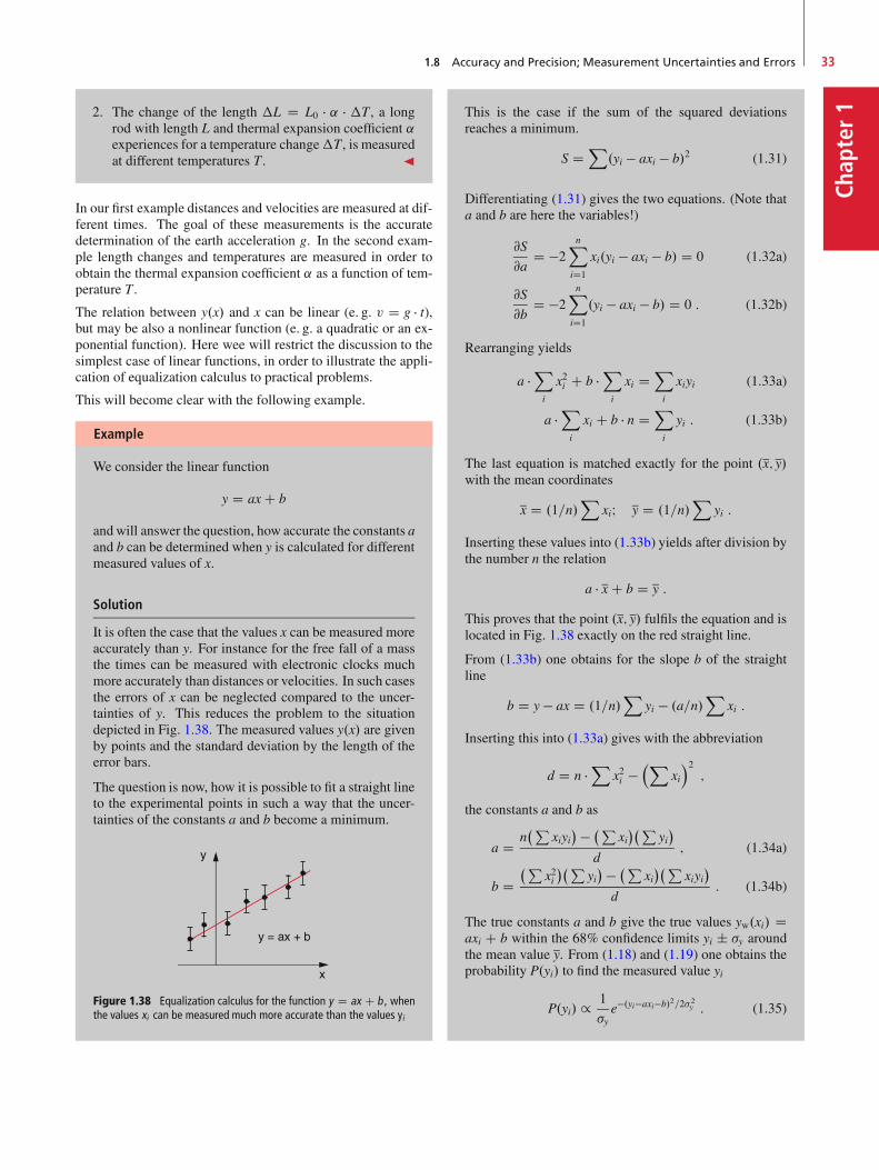
1.8 Accuracy and Precision; Measurement Uncertainties and Errors 33
Chap
ter12. The change of the length �L D L0 � ˛ � �T , a long
rod with length L and thermal expansion coefficient ˛experiences for a temperature change�T , is measuredat different temperatures T . J
In our first example distances and velocities are measured at dif-ferent times. The goal of these measurements is the accuratedetermination of the earth acceleration g. In the second exam-ple length changes and temperatures are measured in order toobtain the thermal expansion coefficient ˛ as a function of tem-perature T .
The relation between y.x/ and x can be linear (e. g. v D g � t),but may be also a nonlinear function (e. g. a quadratic or an ex-ponential function). Here wee will restrict the discussion to thesimplest case of linear functions, in order to illustrate the appli-cation of equalization calculus to practical problems.
This will become clear with the following example.
Example
We consider the linear function
y D ax C b
and will answer the question, how accurate the constants aand b can be determined when y is calculated for differentmeasured values of x.
Solution
It is often the case that the values x can be measured moreaccurately than y. For instance for the free fall of a massthe times can be measured with electronic clocks muchmore accurately than distances or velocities. In such casesthe errors of x can be neglected compared to the uncer-tainties of y. This reduces the problem to the situationdepicted in Fig. 1.38. The measured values y.x/ are givenby points and the standard deviation by the length of theerror bars.
The question is now, how it is possible to fit a straight lineto the experimental points in such a way that the uncer-tainties of the constants a and b become a minimum.
Figure 1.38 Equalization calculus for the function y D ax C b , whenthe values xi can be measured much more accurate than the values yi
This is the case if the sum of the squared deviationsreaches a minimum.
S DX
.yi � axi � b/2 (1.31)
Differentiating (1.31) gives the two equations. (Note thata and b are here the variables!)
@S
@aD �2
nX
iD1
xi.yi � axi � b/ D 0 (1.32a)
@S
@bD �2
nX
iD1
.yi � axi � b/ D 0 : (1.32b)
Rearranging yields
a �X
i
x2i C b �X
i
xi DX
i
xiyi (1.33a)
a �X
i
xi C b � n DX
i
yi : (1.33b)
The last equation is matched exactly for the point .x; y/with the mean coordinates
x D .1=n/X
xiI y D .1=n/X
yi :
Inserting these values into (1.33b) yields after division bythe number n the relation
a � x C b D y :
This proves that the point .x; y/ fulfils the equation and islocated in Fig. 1.38 exactly on the red straight line.
From (1.33b) one obtains for the slope b of the straightline
b D y � ax D .1=n/X
yi � .a=n/X
xi :
Inserting this into (1.33a) gives with the abbreviation
d D n �X
x2i ��X
xi2;
the constants a and b as
a D n�P
xiyi� � �P
xi��P
yi�
d; (1.34a)
b D�P
x2i��P
yi� � �P
xi��P
xiyi�
d: (1.34b)
The true constants a and b give the true values yw.xi/ Daxi C b within the 68% confidence limits yi ˙ �y aroundthe mean value y. From (1.18) and (1.19) one obtains theprobability P.yi/ to find the measured value yi
P.yi/ / 1
�ye�.yi�axi�b/2=2�2y : (1.35)
Chapter1
34 1 Introduction and Survey
The uncertainties of the constants a and b can be obtainedaccording to the error propagation rules. The results are
�2a D n � �2
y
d; �2
b D �2y
Px2i
d: (1.36)
The full width between the two points P.yw/=e is �y � p2.
For more information on error analysis and regression fitssee [1.53a–1.56]. J
Summary
Physics deals with the basic building blocks of our world,their mutual interactions and the synthesis of material fromthese basic particles.The gain of knowledge is pushed by specific experiments.Their results serve for the development of a general theoryof nature and to confirm or contradict existing theories.Experimental physics started in the 16th century(e. g. Galilei, Kepler) and led to a more and more refinedand extensive theory, which is, however, even today not yetcomplete and consistent.All physical quantities can be reduced to three basic quanti-ties of length, time and mass with the basic units 1m, 1 s, and1 kg. For practical reasons four more basic quantities are in-troduced for molar mass (1mol), temperature (1K), electriccurrent (1A) and the luminous power (1 cd).The system of units which uses these basic 3 C 4 units iscalled SI-system with the units 1m, 1 s, 1 kg, 1mol, 1K, 1Aand 1 cd.Every measurement means the comparison of the measuredquantity with a normal (standard).The length standard is the distance which light travels invacuum within a time interval of .1=299;792;458/ s. Thetime standard is the transition frequency between two hy-perfine levels in the Cs atom measured with the caesiumatomic clock. The present mass standard is the mass of theplatinum-iridium kilogram, kept in Paris.Each measurement has uncertainties. One distinguishes be-tween systematic errors and statistical errors. The meanvalue of n independent measurements with measured valuesxi is chosen as the arithmetic mean
x D 1
n
nX
iD1
xi ;
which meets the minimum condition
nX
iD1
.x � xi/2 D minimum:
If all systematic errors could be eliminated the distributionof the measured values x show the statistical Gaussian distri-bution
f .x/ / e�.x�xw/2=2�2 ;
about the most probable value, which equals the true valuexw. The half-with of the distribution between the pointsf .xw/=e D f .xw ˙ �/ is � � p2 Within the range x D xw ˙ �fall 68% of all measured values. The standard deviation � ofindividual measurements is
� DsP
.x � xi/2
n � 1;
the standard deviation of the arithmetic means is
�m DsP
.x � xi/2
n.n � 1/:
The true value xw lies with the probability of 68% within theinterval xw ˙ � , with a probability of 99.7% in the intervalxw ˙ 3� . The Gaussian probability distribution for the mea-sured values xoi has a full width at half maximum of
�x1=2 D 2�p2 � ln 2 D 2:35� :
References 35
Chap
ter1
Problems
1.1 The speed limit on a motorway is 120 km/h. An interna-tional commission decides to make a new definition of the hour,such that the period of the earth rotation about its axis is only16 h. What should be the new speed limit, if the same safetyconsiderations are valid?
1.2 Assume that exact measurements had found that the di-ameter of the earth decreases slowly. How sure can we be, thatthis is not just an increase of the length of the meter standard?
1.3 Discuss the following statement: “The main demand fora length standard is that its length fluctuations are smaller thanlength changes of the distances to be measured”.
1.4 Assume that the duration of the mean solar day increasesby 10ms in 100 years due to the deceleration of the earth rota-tion. a) After which time would the day length be 30 hours? b)How often would it be necessary to add a leap second in orderto maintain synchronization with the atomic clock time?
1.5 The distance to the next star (˛-Centauri) is d D 4:3 �1016 m. How long is the travelling time of a light pulse fromthis star to earth? Under which angle appears the distance earth-sun from ˛-Centauri? If the accuracy of angular measurementsis 0:100 what is the uncertainty of the distance measurement?
1.6 A length L is seen from a point P which is 1 km (per-pendicular to L) away from the centre of L, under an angle of˛ D 1ı. How accurate can the length be determined by anglemeasurements from P if the uncertainty of ˛ is 10?
1.7 Why does the deviation of the earth orbit from a circlecause a variation of the solar day during the year? Give some
arguments why the length of the mean solar day can change fordifferent years?
1.8 How many hydrogen atoms are included in 1 kg of hy-drogen gas?
1.9 How many water molecules H2O are included in 1 litrewater?
1.10 The radius of a uranium nucleus (A D 238) is 8:68 �10�15 m. What is its mean mass density?
1.11 The fall time of a steel ball over a distance of 1m ismeasured 40 times, with an uncertainty of 0.1 s for each mea-surement. What is the accuracy of the arithmetic mean?
1.12 For which values of x has the error distribution functionexpŒ�x2=2� fall to 0.5 and to 0.1 of its maximum value?
1.13 Assume the quantity x D 1000 has been measured witha relative uncertainty of 10�3 and y D 30 with 3 � 10�3. What isthe error of the quantity A D .x � y2/?
1.14 What is the maximum relative error of a good quartzclock with a relative error of 10�9 after 1 year? Compare thiswith an atomic clock (��=� D 10�14).
1.15 Determine the coefficients a and b of the straight liney D axCb which gives the minimum squared deviations for thepoints .x; y/ D .0;2/; .1;3/; .2;3/; .4; 5/ and .5;5/. How largeis the standard deviation of a and b?
References
1.1a. R.D. Jarrard, Scientific Methods. An online book:https://webct.utah.edu/webct/RelativeResourceManager/288712009021/Public%20Files/sm/sm0.htm
1.1b. K. Popper, The Logic of of Scientific Discovery. (Rout-ledgen 2002)
1.2. R. Feynman, The Character of Physical Laws (ModernLibrary, 1994)
1.3. W. Heisenberg, Physics and Philosophy (Harper Peren-nial Modern Thoughts, 2015)
1.4. A. Franklin, Phys. Persp. 1(1), 35–53 (1999)1.5. L. Susskind, G. Hrabovsky, The theoretical Minimum.
What you need to know to start doing Physics (BasicBooks, 2013)
1.6. J.Z. Buchwald, R. Fox (eds.), The Oxford Handbook ofthe History of Physics (2014)
1.7. A. Einstein, The evolution of Physics From early Con-cepts to Relativity and Quanta (Touchstone, 1967)
1.8. D.C. Lindberg, E. Whitney, The Beginning of westernSciences (University of Chicago Press, 1992)
1.9. https://en.wikipedia.org/wiki/History_of_physics1.10. H.Th. Milhorn, H.T. Milhorn, The History of Physics
(Virtualbookworm.com publishing)1.11a. W.H. Cropper, Great Physicists: The Life and Times
of Leading Physicists from Galileo to Hawking (Ox-ford University Press, 2004) https://en.wikipedia.org/wiki/Special:BookSources/0-19-517324-4
Chapter1
36 1 Introduction and Survey
1.11b. John L. Heilbron, The Oxford Guide to the His-tory of Physics and Astronomy (Oxford Univer-sity Press, 2005) https://en.wikipedia.org/wiki/Special:BookSources/0-19-517198-5
1.11c. J.Z. Buchwald, I.B. Cohen (eds.), Isaac Newton’s naturalphilosophy (Cambridge, Mass. and London, MIT Press,2001)
1.12. J.T. Cushing, Philosophical Concepts in Physics: Thehistorical Relation between Philosophy and Physics(Cambridge Univ. Press, 2008)
1.13a. E. Segrè, From Falling Bodies to Radio Waves: Clas-sical Physicists and Their Discoveries (W.H. Freeman,New York, 1984) https://en.wikipedia.org/wiki/Special:BookSources/0-7167-1482-5, https://www.worldcat.org/oclc/9943504
1.13b. E. Segrè, From X-Rays to Quarks: Modern Physi-cists and Their Discoveries (W.H. Freeman, SanFrancisco, 1980) https://en.wikipedia.org/wiki/Special:BookSources/0-7167-1147-8, https://www.worldcat.org/oclc/237246197+56100286+5946636
1.13c. G. Gamov, The Great Physicists from Galileo to Ein-stein (Dover Publ., revised edition 2014) ISBN: 978-0486257679
1.14a. P. Fara, Science, A Four Thousand Year History (OxfordUniv. Press, 2010) ISBN: 978-0199580279
1.14b. H.J. Jodl, in: E. Lüscher, H.J. Jodl, (eds.), Physik,Gestern, Heute, Morgen (München, Heinz Moos-Verlag1971)
1.14c. N.N., From Big to Small: The Hierarchy Prob-lem in Physics (String Theory) (what-when-how – InDepth Tutorials and Information) http://what-when-how.com/string-theory/from-big-to-small-the-hierarchy-problem-in-physics-string-theory/
1.15. St. Weinberg, The Discovery of Subatomic Particles (Sci-entifique American Library Freeman Oxford, 1984)
1.16a. G. Gamov: One, Two, Three . . . Infinity. Facts and Spec-ulations of Science (Dover Publications, 1989) ISBN:978-0486256641
1.16b. G. Gamov: Mr. Tomkins in Paperback (Cambridge Univ.Press, reprint 2012) ISBN: 978-1107604681
1.17. N. Manton, Symmetries, Fields and Particles. (Univer-sity of Cambridge), http://www.damtp.cam.ac.uk/user/examples/3P2.pdf
1.18. F. Close, Particle Physics: A Very Short Introduction.(Oxford Univ. Press, 2004)
1.19. R. Oerter, The Theory of Almost Everything: The Stan-dard Model, the Unsung Triumph of Modern Physics.(Plume, Reprint edition, 2006)
1.20a. T. Plathotnik, E.A. Donley, U.P. Wild, Single MoleculeSpectroscopüy. Ann. Rev. Phys. Chem. 48, 181 (1997)
1.20b. N.G. Walter, Single Molecule Detection, Analysis, andManipulation, in Encyclopedia of Analytical Chemistry,ed. by R.A. Meyers (John Wiley & Sons Ltd, 2008)
1.21. E. Schrödinger,What is life? (Macmillan, 1944)1.22a. D. Goldfarb, Biophyiscs Demystified. (Mc Grawhill,
2010) ISBN: 978-00716336421.22b. R. Glaser, Biophysics: An Introduction. (Springer,
Berlin, Heidelberg, 2012) ISBN: 978-3642252112
1.23a. K. Nouri (ed.), Lasers in Dermatology and Medicine.(Springer, Berlin, Heidelberg, 2012) ISBN: 978-0-85729-280-3
1.23b. K. Nouri (ed.), Laser Applications in Medicine Inter-national Journal for Laser Treatment and Research.(Elsevier, Amsterdam)
1.24a. St. Hawking, The Universe in a Nutshell. (Bantam Press,2001)
1.24b. L.M. Krauss, A Universe from Nothing. (Atria Books,2012)
1.24c. E. Chaisson, St. McMillan, Astronomy Today. (AddisonWesley, 2010)
1.24d. T. Dickinson, A. Schaller, T. Ferris, Night watch. A prac-tical Guide to viewing the Universe. (Firefly Books)
1.24e. B.W. Carroll, D.A. Ostlie, An Introduction to Modern As-trophysics. (Pearson Education, 2013)
1.25. A.E. Musset, M. Aftab Khan, S. Button, Looking intothe Earth: An Introduction to Geological Geophysics,1st edn. (Cambridge University Press, 2000) ISBN: 978-0521785747
1.26a. C.D. Ahrens, Meteorology Today: Introduction toWheather, Climate and the Environment. (Brooks Cole,2012) ISBN: 978-0840054999
1.26b. St.A. Ackerman, J.A. Knox, Meteorology: Understand-ing the Atmosphere, 4th edn. (Jones & Bartlett Learning,2013)
1.27. P.J. Crutzen, Pure Appl. Chem. 70(7), 1319–1326 (1998)1.28. P. Saundry, Environmental physics. (The Encyclope-
dia of Earth, 2011), http://www.eoearth.org/view/article/152632
1.29a. F.K. Lutgens, E.J. Tarbuck, D.G. Tasa, Essentials of Ge-ology, 11th edn. (Prentice Hall) ISBN: 978-0321714725
1.29b. W.S. Broecker, How to Build a Habitable Planet. (Eldi-gio Press, 1988)
1.30a. R.A. Müller, Physics and Technology für Future Presi-dents. (Princeton Univ. Press, 2010)
1.30b. M.L. Forlan, Modern Physics and Technology. (WorldScientific, Singapore, 2015)
1.31. L. Sklar, Philosophy of Physics. (Oxford UniversityPress, 1990) ISBN: 978-0198751380
1.32. Th. Brody, The Philosophy behind Physics. (Springer,Berlin, Heidelberg, 1994)
1.33. St. Cole, Am. J. Sociol. 89(1) 111–139 (1983)1.34a. B.R. Cohen, Endeavour 25(1) 8–12 (2001)1.34b. R.M. Young, Science and Humanities in the understand-
ing of human nature. (The Human Nature Review),http://human-nature.com/rmyoung/papers/pap131h.html
1.35. W. Heisenberg, Physics and Beyond: Encounters andConversations. (Harper & Row, 1971)
1.36a. P. Becker, The new kilogram is approaching. (PTB-news, 3/2011), http://www.ptb.de/en/aktuelles/archiv/presseinfos/pi2011/pitext/pi110127.html
1.36b. S. Hadington, The kilogram is dead, long livethe kilogram! (The Royal Society of Chemistry,2011), http://www.rsc.org/chemistryworld/News/2011/October/31101101.asp
1.37. N.N., SI based Units. (Wikipedia), https://en.wikipedia.org/wiki/SI_base_unit
References 37
Chap
ter1
1.38. N.N., https://www.bing.com/search?q=Phyiscal%20basis%20for%20SI%20units&pc=cosp&ptag=ADC890F4567&form=CONMHP&conlogo=CT3210127
1.39. B.W. Petley, The fundamental physical constants and thefrontiers of measurements. (Adam Hilger, 1985)
1.40. N.N., History of the Meter. (Wikipedia), https://en.wikipedia.org/wiki/History_of_the_metre
1.41. J. Levine, Ann. Rev. Earth Planet Sci. 5 357 (1977)1.42. J. Müller et al., Lunar Laser Ranging. Recent Results.
(AG Symposia Series, Vol 139, Springer, 2013)1.43a. K.M. Borkowski, Journal of the Royal Astronomical So-
ciety of Canada 85 121 (1991)1.43b. http://en.wikipedia.org/wiki/Tropical_year1.44a. N.N., Atomic clock. (Wikipedia), https://en.wikipedia.
org/wiki/Atomic_clock1.44b. N.N., Clock network. (Wikipedia), https://en.wikipedia.
org/wiki/Clock_network1.45. A. deMarchi (ed.), Frequency Standards and Metrology.
(Springer, Berlin, Heidelberg, 1989)1.46. S.A. Diddams, T.W. Hänsch et al., Phys. Rev. Lett. 84
5102 (2000)1.47. Ch. Gaiser, Metrologia 48 382 (2011)1.48a. N.N., Kilogram (Wikipedia), https://en.wikipedia.org/
wiki/Kilogram1.48b. N.N., Mole (unit) (Wikipedia), https://en.wikipedia.org/
wiki/Mole_(unit)
1.49. V.V. Krutikov, Measurement Techniques. (Springer,Berlin, Heidelberg, 2013)
1.50. Journal of Measurement Techniques (Springer Berlin,Heidelberg)
1.51. K.T.V. Grattan (ed.), Measurement: Journal of Inter-national Measuring Confederation (IMEKO) (Elsevier,Amsterdam), ISSN: 0263-2241
1.52. L. Marton (ed.), Methods of experimental Physics.(29 Vol.) (Academic Press, New York, 1959–1996) (con-tinued as Experimental Methods in the Physical Sciencesup to Vol. 49, published by Elsevier Amsterdam in 2014),ISBN 13: 978-0-12-417011-7
1.53a. J.R. Taylor, An Introduction to Error Analysis:The Studyof Uncertainties in Physical measurements, 2nd ed.(University Science Books, 1996)
1.53b. D. Roberts, Errors, discrepancies, and the nature ofphysics. (The Physics Teacher, March 1983) a very use-ful introduction
1.54. J.W. Foremn, Data Smart: Using Data Science to trans-form Information into Insight. (Wiley, 2013)
1.55. R.C. Sprinthall, Basic statistical Analysis, 9th ed. (Pear-son, 2011)
1.56. J. Schmuller, Statistical Analysis with Excel for Dum-mies, 3rd ed. (For Dummies, 2013)
Chap
ter2
Mechanics of a Point Mass 22.1 The Model of the Point Mass; Trajectories . . . . . . . . . . . . . . . . 40
2.2 Velocity and Acceleration . . . . . . . . . . . . . . . . . . . . . . . . . . 41
2.3 Uniformly Accelerated Motion . . . . . . . . . . . . . . . . . . . . . . . 42
2.4 Motions with Non-Constant Acceleration . . . . . . . . . . . . . . . . . 44
2.5 Forces . . . . . . . . . . . . . . . . . . . . . . . . . . . . . . . . . . . . . 47
2.6 The Basic Equations of Mechanics . . . . . . . . . . . . . . . . . . . . . 51
2.7 Energy Conservation Law of Mechanics . . . . . . . . . . . . . . . . . . 56
2.8 Angular Momentum and Torque . . . . . . . . . . . . . . . . . . . . . . 63
2.9 Gravitation and the Planetary Motions . . . . . . . . . . . . . . . . . . 64
Summary . . . . . . . . . . . . . . . . . . . . . . . . . . . . . . . . . . . . 76
Problems . . . . . . . . . . . . . . . . . . . . . . . . . . . . . . . . . . . . 77
References . . . . . . . . . . . . . . . . . . . . . . . . . . . . . . . . . . . 79
39© Springer International Publishing Switzerland 2017W. Demtröder, Mechanics and Thermodynamics, Undergraduate Lecture Notes in Physics, DOI 10.1007/978-3-319-27877-3_2
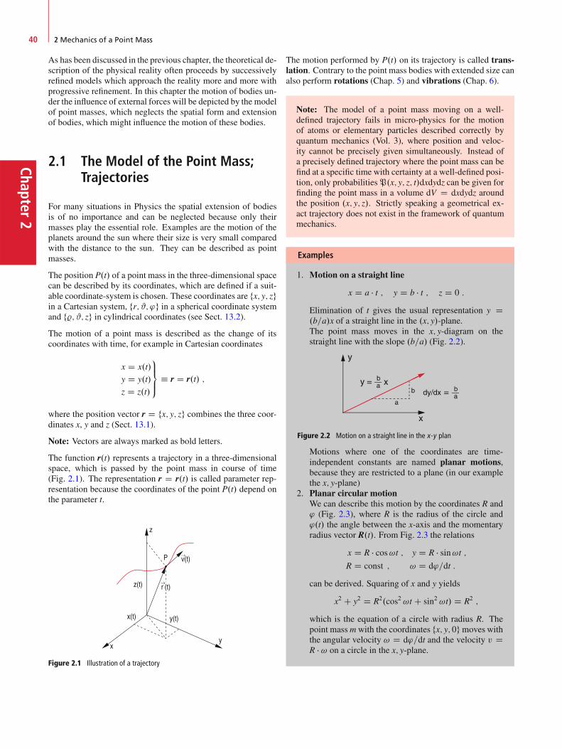
Chapter2
40 2 Mechanics of a Point Mass
As has been discussed in the previous chapter, the theoretical de-scription of the physical reality often proceeds by successivelyrefined models which approach the reality more and more withprogressive refinement. In this chapter the motion of bodies un-der the influence of external forces will be depicted by the modelof point masses, which neglects the spatial form and extensionof bodies, which might influence the motion of these bodies.
2.1 The Model of the Point Mass;Trajectories
For many situations in Physics the spatial extension of bodiesis of no importance and can be neglected because only theirmasses play the essential role. Examples are the motion of theplanets around the sun where their size is very small comparedwith the distance to the sun. They can be described as pointmasses.
The position P.t/ of a point mass in the three-dimensional spacecan be described by its coordinates, which are defined if a suit-able coordinate-system is chosen. These coordinates are fx; y; zgin a Cartesian system, fr; #; 'g in a spherical coordinate systemand f%; #; zg in cylindrical coordinates (see Sect. 13.2).The motion of a point mass is described as the change of itscoordinates with time, for example in Cartesian coordinates
x D x.t/
y D y.t/
z D z.t/
9>=
>;� r D r.t/ ;
where the position vector r D fx; y; zg combines the three coor-dinates x, y and z (Sect. 13.1).
Note: Vectors are always marked as bold letters.
The function r.t/ represents a trajectory in a three-dimensionalspace, which is passed by the point mass in course of time(Fig. 2.1). The representation r D r.t/ is called parameter rep-resentation because the coordinates of the point P.t/ depend onthe parameter t.
Figure 2.1 Illustration of a trajectory
The motion performed by P.t/ on its trajectory is called trans-lation. Contrary to the point mass bodies with extended size canalso perform rotations (Chap. 5) and vibrations (Chap. 6).
Note: The model of a point mass moving on a well-defined trajectory fails in micro-physics for the motionof atoms or elementary particles described correctly byquantum mechanics (Vol. 3), where position and veloc-ity cannot be precisely given simultaneously. Instead ofa precisely defined trajectory where the point mass can befind at a specific time with certainty at a well-defined posi-tion, only probabilitiesP.x; y; z; t/dxdydz can be given forfinding the point mass in a volume dV D dxdydz aroundthe position .x; y; z/. Strictly speaking a geometrical ex-act trajectory does not exist in the framework of quantummechanics.
Examples
1. Motion on a straight line
x D a � t ; y D b � t ; z D 0 :
Elimination of t gives the usual representation y D.b=a/x of a straight line in the .x; y/-plane.The point mass moves in the x; y-diagram on thestraight line with the slope .b=a/ (Fig. 2.2).
Figure 2.2 Motion on a straight line in the x-y plan
Motions where one of the coordinates are time-independent constants are named planar motions,because they are restricted to a plane (in our examplethe x; y-plane)
2. Planar circular motionWe can describe this motion by the coordinates R and' (Fig. 2.3), where R is the radius of the circle and'.t/ the angle between the x-axis and the momentaryradius vector R.t/. From Fig. 2.3 the relations
x D R � cos!t ; y D R � sin!t ;R D const ; ! D d'=dt :
can be derived. Squaring of x and y yields
x2 C y2 D R2.cos2 !t C sin2 !t/ D R2 ;
which is the equation of a circle with radius R. Thepoint massmwith the coordinates fx; y; 0g moves withthe angular velocity ! D d'=dt and the velocity v DR � ! on a circle in the x; y-plane.
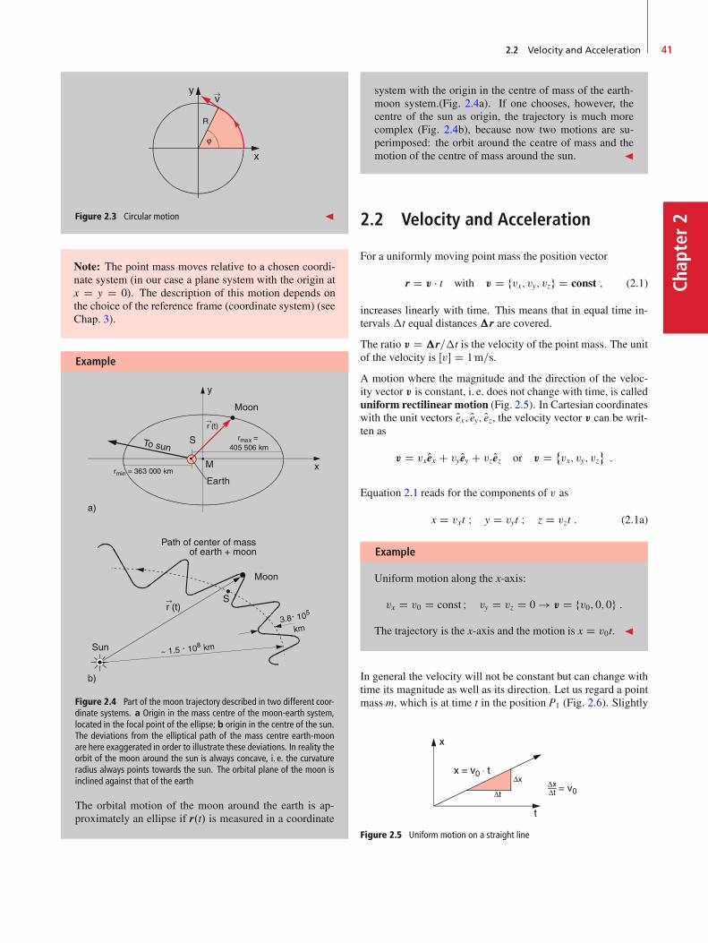
2.2 Velocity and Acceleration 41
Chap
ter2Figure 2.3 Circular motion J
Note: The point mass moves relative to a chosen coordi-nate system (in our case a plane system with the origin atx D y D 0). The description of this motion depends onthe choice of the reference frame (coordinate system) (seeChap. 3).
Example
Figure 2.4 Part of the moon trajectory described in two different coor-dinate systems. a Origin in the mass centre of the moon-earth system,located in the focal point of the ellipse; b origin in the centre of the sun.The deviations from the elliptical path of the mass centre earth-moonare here exaggerated in order to illustrate these deviations. In reality theorbit of the moon around the sun is always concave, i. e. the curvatureradius always points towards the sun. The orbital plane of the moon isinclined against that of the earth
The orbital motion of the moon around the earth is ap-proximately an ellipse if r.t/ is measured in a coordinate
system with the origin in the centre of mass of the earth-moon system.(Fig. 2.4a). If one chooses, however, thecentre of the sun as origin, the trajectory is much morecomplex (Fig. 2.4b), because now two motions are su-perimposed: the orbit around the centre of mass and themotion of the centre of mass around the sun. J
2.2 Velocity and Acceleration
For a uniformly moving point mass the position vector
r D v � t with v D fvx; vy; vzg D const ; (2.1)
increases linearly with time. This means that in equal time in-tervals �t equal distances �r are covered.
The ratio v D �r=�t is the velocity of the point mass. The unitof the velocity is Œv� D 1m=s.
A motion where the magnitude and the direction of the veloc-ity vector v is constant, i. e. does not change with time, is calleduniform rectilinear motion (Fig. 2.5). In Cartesian coordinateswith the unit vectors Oex; Oey; Oez, the velocity vector v can be writ-ten as
v D vx Oex C vy Oey C vz Oez or v D ˚vx; vy; vz
:
Equation 2.1 reads for the components of v as
x D vxt I y D vyt I z D vzt : (2.1a)
Example
Uniform motion along the x-axis:
vx D v0 D const I vy D vz D 0 ! v D fv0; 0;0g :
The trajectory is the x-axis and the motion is x D v0t. J
In general the velocity will not be constant but can change withtime its magnitude as well as its direction. Let us regard a pointmass m, which is at time t in the position P1 (Fig. 2.6). Slightly
Figure 2.5 Uniform motion on a straight line
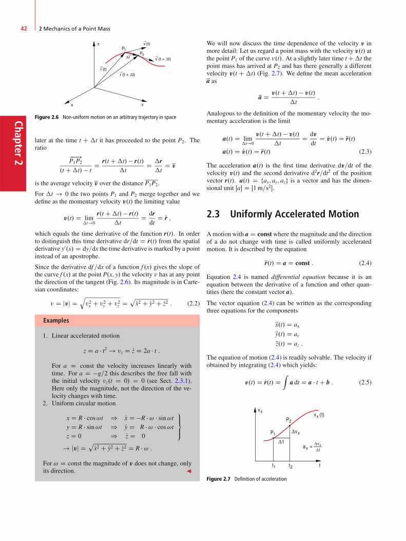
Chapter2
42 2 Mechanics of a Point Mass
Figure 2.6 Non-uniform motion on an arbitrary trajectory in space
later at the time t C �t it has proceeded to the point P2. Theratio
���!P1P2
.t C�t/ � tD r.t C�t/ � r.t/
�tD �r�t
D v
is the average velocity v over the distance P1P2.
For �t ! 0 the two points P1 and P2 merge together and wedefine as the momentary velocity v.t/ the limiting value
v.t/ D lim�t!0
r.t C�t/ � r.t/�t
D drdt
D Pr ;
which equals the time derivative of the function r.t/. In orderto distinguish this time derivative dr=dt D Pr.t/ from the spatialderivative y0.x/ D dy=dx the time derivative is marked by a pointinstead of an apostrophe.
Since the derivative df =dx of a function f .x/ gives the slope ofthe curve f .x/ at the point P.x; y/ the velocity v has at any pointthe direction of the tangent (Fig. 2.6). Its magnitude is in Carte-sian coordinates:
v D jvj Dqv2x C v2y C v2z D
pPx2 C Py2 C Pz2 : (2.2)
Examples
1. Linear accelerated motion
z D a � t2 ! vz D Pz D 2a � t :
For a D const the velocity increases linearly withtime. For a D �g=2 this describes the free fall withthe initial velocity vz.t D 0/ D 0 (see Sect. 2.3.1).Here only the magnitude, not the direction of the ve-locity changes with time.
2. Uniform circular motion
x D R � cos!t ) Px D �R � ! � sin!ty D R � sin!t ) Py D R � ! � cos!tz D 0 ) Pz D 0
9>=
>;
! jvj Dp
Px2 C Py2 C Pz2 D R � ! :
For ! D const the magnitude of v does not change, onlyits direction. J
We will now discuss the time dependence of the velocity v inmore detail: Let us regard a point mass with the velocity v.t/ atthe point P1 of the curve v.t/. At a slightly later time t C�t thepoint mass has arrived at P2 and has there generally a differentvelocity v.t C �t/ (Fig. 2.7). We define the mean accelerationa as
a D v.t C�t/ � v.t/
�t:
Analogous to the definition of the momentary velocity the mo-mentary acceleration is the limit
a.t/ D lim�t!0
v.t C�t/ � v.t/
�tD dv
dtD Pv.t/ D Rr.t/
a.t/ D Pv.t/ D Rr.t/ (2.3)
The acceleration a.t/ is the first time derivative dv=dt of thevelocity v.t/ and the second derivative d2r=dt2 of the positionvector r.t/. a.t/ D fax; ay; azg is a vector and has the dimen-sional unit Œa� D Œ1m=s2�.
2.3 Uniformly Accelerated Motion
Amotion with a D constwhere the magnitude and the directionof a do not change with time is called uniformly acceleratedmotion. It is described by the equation
Rr.t/ D a D const : (2.4)
Equation 2.4 is named differential equation because it is anequation between the derivative of a function and other quan-tities (here the constant vector a).
The vector equation (2.4) can be written as the correspondingthree equations for the components
Rx.t/ D axRy.t/ D ayRz.t/ D az :
The equation of motion (2.4) is readily solvable. The velocity ifobtained by integrating (2.4) which yields:
v.t/ D Pr.t/ DZ
a dt D a � t C b : (2.5)
Figure 2.7 Definition of acceleration
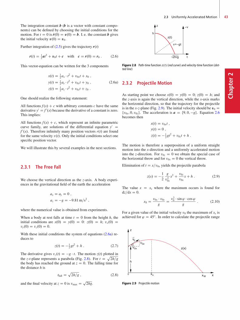
2.3 Uniformly Accelerated Motion 43
Chap
ter2
The integration constant b (b is a vector with constant compo-nents) can be defined by choosing the initial conditions for themotion. For t D 0 is Pr.0/ D v.0/ D b. I. e. the constant b givesthe initial velocity v.0/ D v0.
Further integration of (2.5) gives the trajectory r.t/
r.t/ D 12at
2 C v0t C c with c D r.0/ D r0 : (2.6)
This vector-equation can be written for the 3 components
x.t/ D 12ax � t2 C v0xt C x0 ;
y.t/ D 12ay � t2 C v0yt C y0 ;
z.t/ D 12az � t2 C v0zt C z0 :
(2.6a)
One should realize the following statement:
All functions f .x/C c with arbitrary constants c have the samederivative y0 D f 0.x/ because the derivative of a constant is zero.This implies:
All functions f .x/ C c, which represent an infinite parametriccurve family, are solutions of the differential equation y0 Df 0.x/. Therefore infinitely many position vectors r.t/ are foundfor the same velocity v.t/. Only the initial conditions select onespecific position vector.
We will illustrate this by several examples in the next sections.
2.3.1 The Free Fall
We choose the vertical direction as the z-axis. A body experi-ences in the gravitational field of the earth the acceleration
ax D ay D 0 ;
az D �g D �9:81m=s2 ;
where the numerical value is obtained from experiments.
When a body at rest falls at time t D 0 from the height h, theinitial conditions are x.0/ D y.0/ D 0: z.0/ D h; vx.0/ Dvy.0/ D vz.0/ D 0.
With these initial conditions the system of equations (2.6a) re-duces to
z.t/ D � 12gt
2 C h : (2.7)
The derivative gives vz.t/ D �g � t. The motion z.t/ plotted inthe z-t-plane represents a parabola (Fig. 2.8). For t D p
2h=gthe body has reached the ground at z D 0. The falling time forthe distance h is
tfall Dp2h=g ; (2.8)
and the final velocity at z D 0 is vmax D p2hg.
t
z
hz(t)
v=–gt
–v
√2h/g
Figure 2.8 Path-time function z.t/ (red curve) and velocity-time function (dot-ted line)
2.3.2 Projectile Motion
As starting point we choose x.0/ D y.0/ D 0; z.0/ D h; andthe z-axis is again the vertical direction, while the x-axis marksthe horizontal direction, so that the trajectory for the projectileis in the x-z-plane (Fig. 2.9). The initial velocity should be v0 Dfv0x; 0; v0zg. The acceleration is a D f9; 0;�gg. Equation 2.6becomes then
x.t/ D v0xt ;
y.t/ D 0 ;
z.t/ D � 12gt
2 C v0zt C h :
The motion is therefore a superposition of a uniform straightmotion into the x-direction and a uniformly accelerated motioninto the z-direction. For v0z D 0 we obtain the special case ofthe horizontal throw and for v0x D 0 the vertical throw.
Elimination of t D x=v0x yields the projectile parabola
z.x/ D �1
2
g
v20xx2 C v0z
v0xx C h : (2.9)
The value x D xs where the maximum occurs is found fordz=dx D 0.
xS D v0x � v0zg
D v20 � sin ' � cos'g
: (2.10)
For a given value of the initial velocity v0 the maximum of xs isachieved for ' D 45ı. In order to calculate the projectile range
Figure 2.9 Projectile motion
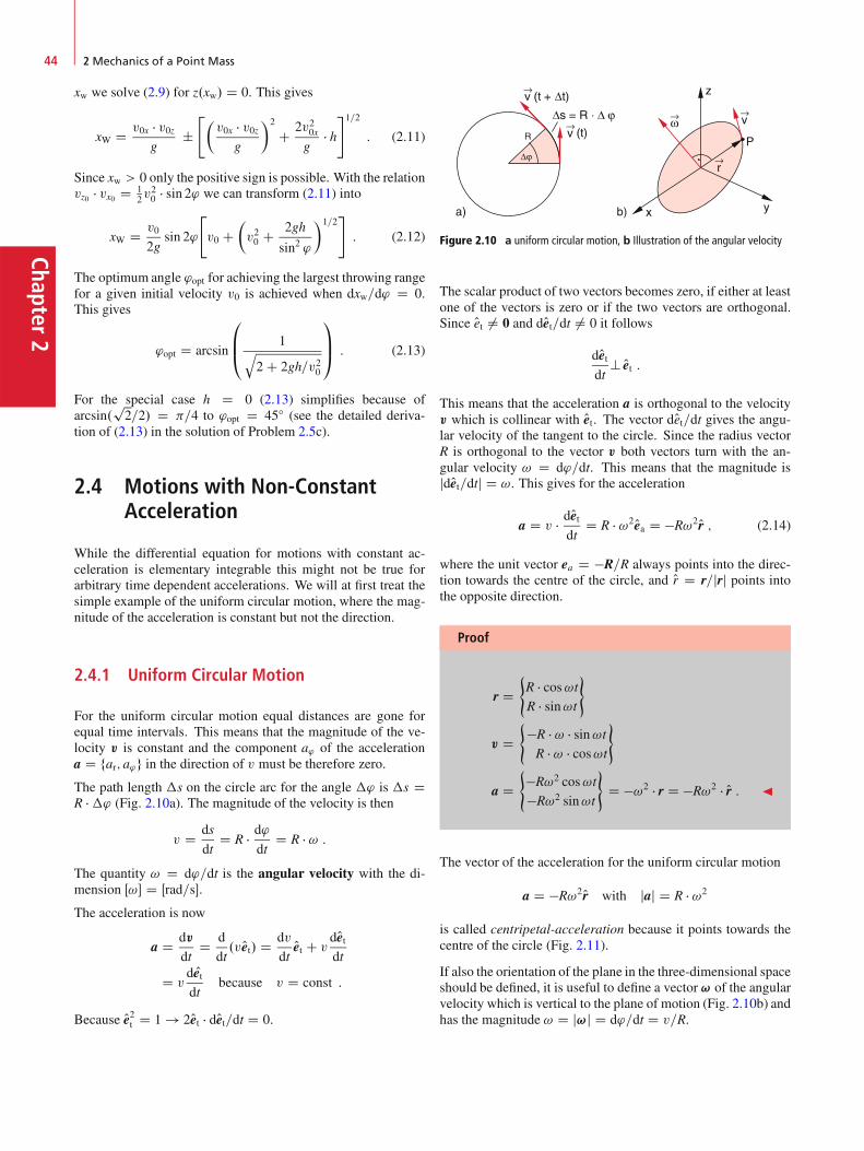
Chapter2
44 2 Mechanics of a Point Mass
xw we solve (2.9) for z.xw/ D 0. This gives
xW D v0x � v0zg
˙"�
v0x � v0zg
�2
C 2v20xg
� h#1=2
: (2.11)
Since xw > 0 only the positive sign is possible. With the relationvz0 � vx0 D 1
2v20 � sin 2' we can transform (2.11) into
xW D v0
2gsin 2'
"v0 C
�v20 C 2gh
sin2 '
�1=2#: (2.12)
The optimum angle 'opt for achieving the largest throwing rangefor a given initial velocity v0 is achieved when dxw=d' D 0.This gives
'opt D arcsin
0
B@1q
2 C 2gh=v20
1
CA : (2.13)
For the special case h D 0 (2.13) simplifies because ofarcsin.
p2=2/ D =4 to 'opt D 45ı (see the detailed deriva-
tion of (2.13) in the solution of Problem 2.5c).
2.4 Motions with Non-ConstantAcceleration
While the differential equation for motions with constant ac-celeration is elementary integrable this might not be true forarbitrary time dependent accelerations. We will at first treat thesimple example of the uniform circular motion, where the mag-nitude of the acceleration is constant but not the direction.
2.4.1 Uniform Circular Motion
For the uniform circular motion equal distances are gone forequal time intervals. This means that the magnitude of the ve-locity v is constant and the component a' of the accelerationa D far; a'g in the direction of v must be therefore zero.
The path length �s on the circle arc for the angle �' is �s DR ��' (Fig. 2.10a). The magnitude of the velocity is then
v D ds
dtD R � d'
dtD R � ! :
The quantity ! D d'=dt is the angular velocity with the di-mension Œ!� D Œrad=s�.
The acceleration is now
a D dv
dtD d
dt.vOet/ D dv
dtOet C v
dOetdt
D vd Oetdt
because v D const :
Because Oe2t D 1 ! 2Oet � dOet=dt D 0.
Figure 2.10 a uniform circular motion, b Illustration of the angular velocity
The scalar product of two vectors becomes zero, if either at leastone of the vectors is zero or if the two vectors are orthogonal.Since Oet ¤ 0 and dOet=dt ¤ 0 it follows
dOetdt
? Oet :
This means that the acceleration a is orthogonal to the velocityv which is collinear with Oet. The vector dOet=dt gives the angu-lar velocity of the tangent to the circle. Since the radius vectorR is orthogonal to the vector v both vectors turn with the an-gular velocity ! D d'=dt. This means that the magnitude isjdOet=dtj D !. This gives for the acceleration
a D v � dOetdt
D R � !2Oea D �R!2Or ; (2.14)
where the unit vector ea D �R=R always points into the direc-tion towards the centre of the circle, and Or D r=jrj points intothe opposite direction.
Proof
r D(R � cos!tR � sin!t
)
v D(
�R � ! � sin!tR � ! � cos!t
)
a D(
�R!2 cos!t�R!2 sin!t
)D �!2 � r D �R!2 � Or : J
The vector of the acceleration for the uniform circular motion
a D �R!2Or with jaj D R � !2
is called centripetal-acceleration because it points towards thecentre of the circle (Fig. 2.11).
If also the orientation of the plane in the three-dimensional spaceshould be defined, it is useful to define a vector ! of the angularvelocity which is vertical to the plane of motion (Fig. 2.10b) andhas the magnitude ! D j!j D d'=dt D v=R.
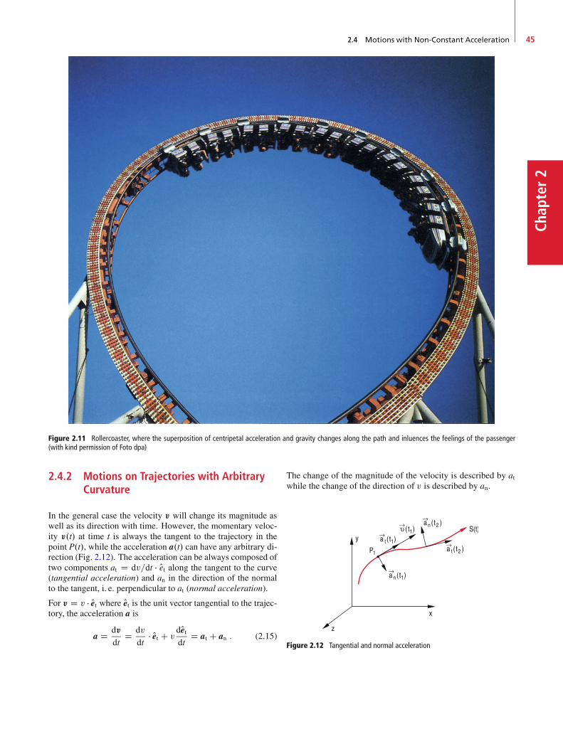
2.4 Motions with Non-Constant Acceleration 45
Chap
ter2
Figure 2.11 Rollercoaster, where the superposition of centripetal acceleration and gravity changes along the path and inluences the feelings of the passenger(with kind permission of Foto dpa)
2.4.2 Motions on Trajectories with ArbitraryCurvature
In the general case the velocity v will change its magnitude aswell as its direction with time. However, the momentary veloc-ity v.t/ at time t is always the tangent to the trajectory in thepoint P.t/, while the acceleration a.t/ can have any arbitrary di-rection (Fig. 2.12). The acceleration can be always composed oftwo components at D dv=dt � Oet along the tangent to the curve(tangential acceleration) and an in the direction of the normalto the tangent, i. e. perpendicular to at (normal acceleration).
For v D v � Oet where Oet is the unit vector tangential to the trajec-tory, the acceleration a is
a D dv
dtD dv
dt� Oet C v
dOetdt
D at C an : (2.15)
The change of the magnitude of the velocity is described by atwhile the change of the direction of v is described by an.
Figure 2.12 Tangential and normal acceleration

Chapter2
46 2 Mechanics of a Point Mass
Figure 2.13 a Derivation of the normal acceleration. b Local radius of curva-ture of a trajectory with arbitrary curvature %
For an D 0 the trajectory is a straight line, where the bodymoves with changing velocity if at ¤ 0. For at D 0 the pointmass moves with a constant velocity jvj on a curve which is de-termined by an.t/. For the free fall of Sect. 2.3.1 is an D 0 andat D const., while for the uniform circular motion at D 0 andan D const.
For the motion on trajectories with arbitrary curvature the accel-eration can be obtained as follows: We choose the x-y-plane asthe plane of the two vectors v.t/ and a.t/, which implies that allvectors have zero z-components.
According to Fig. 2.13a the two mutually vertical unit vectors Oetand Oen can be composed as
Oet D cos' Oex C sin ' OeyOen D cos.' C
2/Oex C sin.' C
2/Oey
D � sin ' Oex C cos' OeyThere we get
dOetdt
D � sin'd'
dtOex C cos'
d'
dtOey
D d'
dtOen
The normal acceleration is therefore
an D vd'
dtOen :
We regard in Fig. 2.13b an infinitesimal section between thepoints A and A0 of an arbitrary curve and approximate thissection by a circular arc AA0 with the center of curvature M.Shortening the section AA0 more and more, i.e. the points Aand A0 converge towards the point P1 the curve section AA0 ap-proaches more and more the circular arc with radius MP1. Theradius % D MP1 is the radius of curvature of the curve in thepoint P1.
For the small section of the curve we get
ds D %d' (2.16a)
d'
dtD d'
ds
ds
dtD d'
dsv D 1
%v : (2.16b)
The acceleration vector becomes
a D dv
dtOet C v2
%Oen (2.16c)
Examples
1. Assume a motion on a straight line experiences theacceleration a.x/ D b � x4.Calculate the velocity v.x/ for the initial conditionv.0/ D v0.
Solution
a D dv
dtD dv
dx� dxdt
D dv
dx� v ;
xZ
x0
adx DvZ
v0
vdv :
Inserting a and integration yields
15b�x5 � x50
� D 12
�v2.x/ � v20
�:
Resolving this equation for v.x/ gives
v.x/ Dq
25b�x5 � x50
�C v20 :
2. The open parachute of a parachutist experiences, dueto air friction, a negative acceleration besides the ac-celeration by gravity.
a D �b � v2 with b D 0:3m�1 :
a) What is his constant final velocity ve?b) What is the time-dependent velocity v.t/, if the
parachutist opens his parachute only after t0 D 10 sfree fall for which friction can be neglected?
Solution
a) A constant final velocity is reached, when the total ac-celeration becomes zero. This is the case when
g � b � v2e D 0 ! ve Dpg=b D 5:7m=s :
b) The equation of motion after the parachute is opened iswith the z-axis in the vertical direction
Rz D g � b � Pz2 :
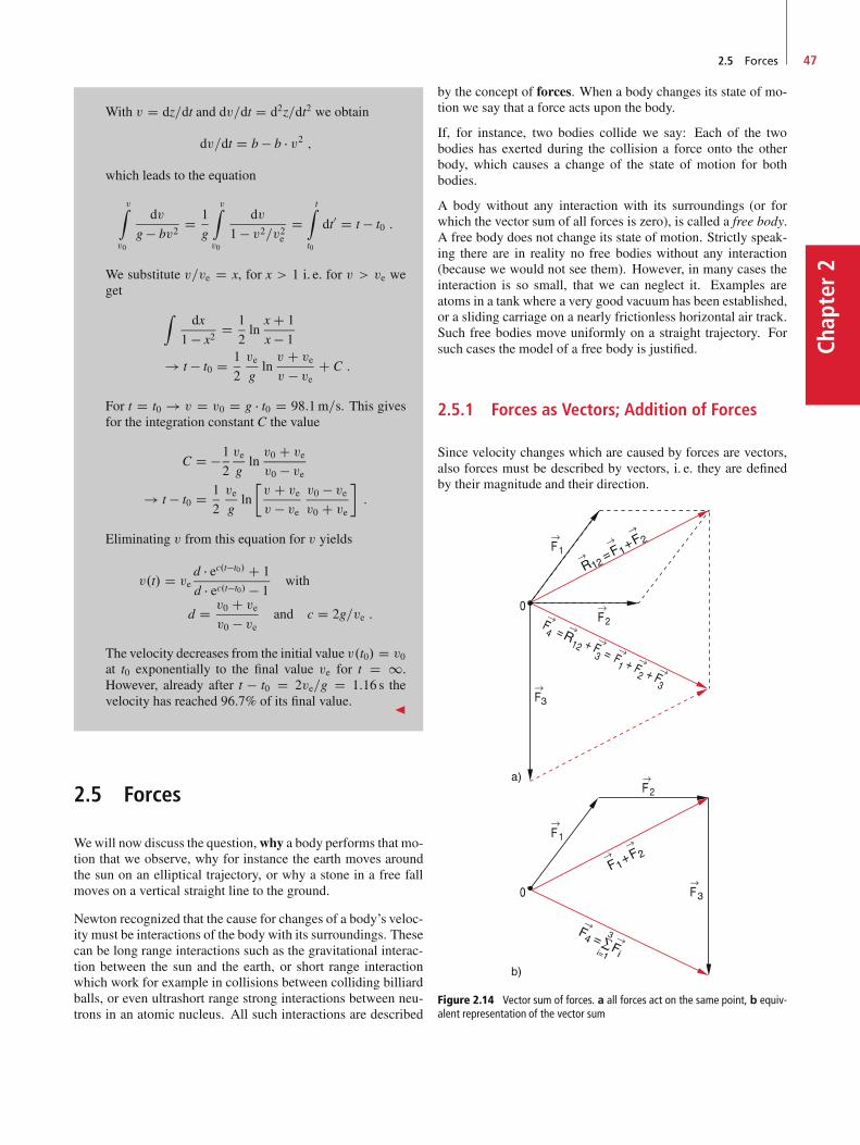
2.5 Forces 47
Chap
ter2
With v D dz=dt and dv=dt D d2z=dt2 we obtain
dv=dt D b � b � v2 ;
which leads to the equation
vZ
v0
dv
g � bv2D 1
g
vZ
v0
dv
1 � v2=v2eD
tZ
t0
dt0 D t � t0 :
We substitute v=ve D x, for x > 1 i. e. for v > ve weget
Zdx
1 � x2D 1
2ln
x C 1
x � 1
! t � t0 D 1
2
ve
glnv C ve
v � ve C C :
For t D t0 ! v D v0 D g � t0 D 98:1m=s. This givesfor the integration constant C the value
C D �1
2
ve
glnv0 C ve
v0 � ve! t � t0 D 1
2
ve
gln
�v C ve
v � vev0 � vev0 C ve
�:
Eliminating v from this equation for v yields
v.t/ D ved � ec.t�t0/ C 1
d � ec.t�t0/ � 1with
d D v0 C ve
v0 � ve and c D 2g=ve :
The velocity decreases from the initial value v.t0/ D v0at t0 exponentially to the final value ve for t D 1.However, already after t � t0 D 2ve=g D 1:16 s thevelocity has reached 96.7% of its final value. J
2.5 Forces
Wewill now discuss the question,why a body performs that mo-tion that we observe, why for instance the earth moves aroundthe sun on an elliptical trajectory, or why a stone in a free fallmoves on a vertical straight line to the ground.
Newton recognized that the cause for changes of a body’s veloc-ity must be interactions of the body with its surroundings. Thesecan be long range interactions such as the gravitational interac-tion between the sun and the earth, or short range interactionwhich work for example in collisions between colliding billiardballs, or even ultrashort range strong interactions between neu-trons in an atomic nucleus. All such interactions are described
by the concept of forces. When a body changes its state of mo-tion we say that a force acts upon the body.
If, for instance, two bodies collide we say: Each of the twobodies has exerted during the collision a force onto the otherbody, which causes a change of the state of motion for bothbodies.
A body without any interaction with its surroundings (or forwhich the vector sum of all forces is zero), is called a free body.A free body does not change its state of motion. Strictly speak-ing there are in reality no free bodies without any interaction(because we would not see them). However, in many cases theinteraction is so small, that we can neglect it. Examples areatoms in a tank where a very good vacuum has been established,or a sliding carriage on a nearly frictionless horizontal air track.Such free bodies move uniformly on a straight trajectory. Forsuch cases the model of a free body is justified.
2.5.1 Forces as Vectors; Addition of Forces
Since velocity changes which are caused by forces are vectors,also forces must be described by vectors, i. e. they are definedby their magnitude and their direction.
Figure 2.14 Vector sum of forces. a all forces act on the same point, b equiv-alent representation of the vector sum
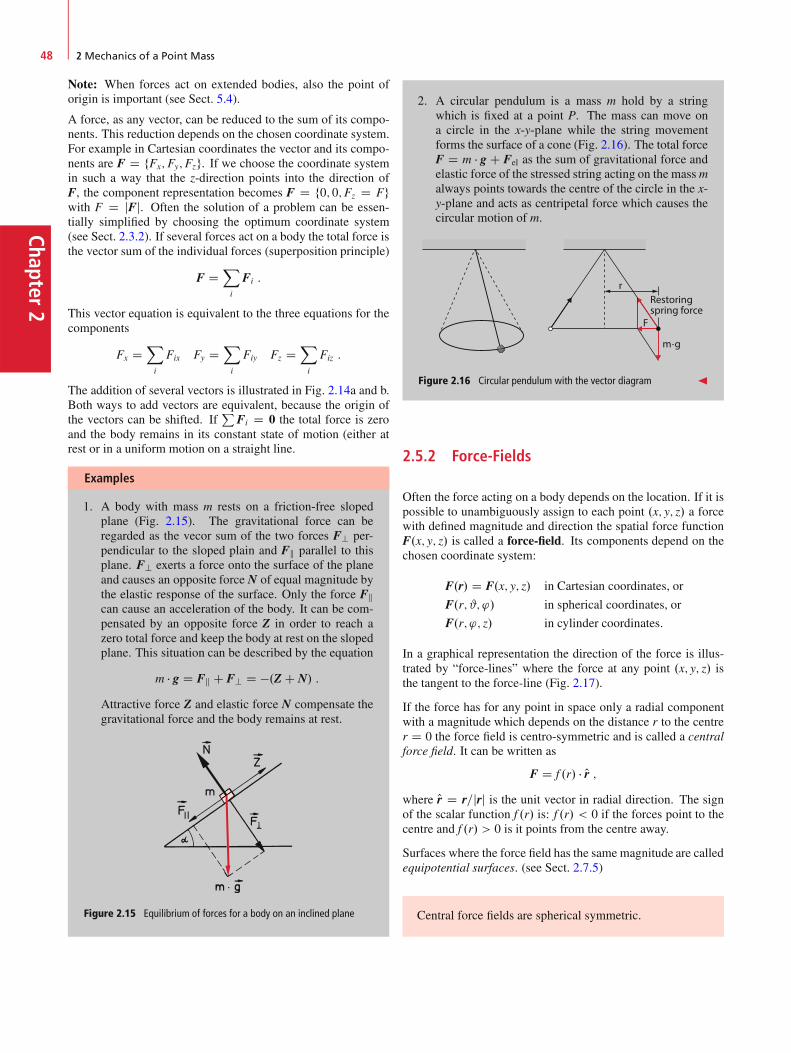
Chapter2
48 2 Mechanics of a Point Mass
Note: When forces act on extended bodies, also the point oforigin is important (see Sect. 5.4).
A force, as any vector, can be reduced to the sum of its compo-nents. This reduction depends on the chosen coordinate system.For example in Cartesian coordinates the vector and its compo-nents are F D fFx;Fy;Fzg. If we choose the coordinate systemin such a way that the z-direction points into the direction ofF, the component representation becomes F D f0; 0;Fz D Fgwith F D jFj. Often the solution of a problem can be essen-tially simplified by choosing the optimum coordinate system(see Sect. 2.3.2). If several forces act on a body the total force isthe vector sum of the individual forces (superposition principle)
F DX
i
Fi :
This vector equation is equivalent to the three equations for thecomponents
Fx DX
i
Fix Fy DX
i
Fiy Fz DX
i
Fiz :
The addition of several vectors is illustrated in Fig. 2.14a and b.Both ways to add vectors are equivalent, because the origin ofthe vectors can be shifted. If
PFi D 0 the total force is zero
and the body remains in its constant state of motion (either atrest or in a uniform motion on a straight line.
Examples
1. A body with mass m rests on a friction-free slopedplane (Fig. 2.15). The gravitational force can beregarded as the vecor sum of the two forces F? per-pendicular to the sloped plain and Fk parallel to thisplane. F? exerts a force onto the surface of the planeand causes an opposite force N of equal magnitude bythe elastic response of the surface. Only the force Fkcan cause an acceleration of the body. It can be com-pensated by an opposite force Z in order to reach azero total force and keep the body at rest on the slopedplane. This situation can be described by the equation
m � g D Fk C F? D �.Z C N/ :
Attractive force Z and elastic force N compensate thegravitational force and the body remains at rest.
Figure 2.15 Equilibrium of forces for a body on an inclined plane
2. A circular pendulum is a mass m hold by a stringwhich is fixed at a point P. The mass can move ona circle in the x-y-plane while the string movementforms the surface of a cone (Fig. 2.16). The total forceF D m � g C Fel as the sum of gravitational force andelastic force of the stressed string acting on the massmalways points towards the centre of the circle in the x-y-plane and acts as centripetal force which causes thecircular motion of m.
m·g
Restoringspring force
F
r
Figure 2.16 Circular pendulum with the vector diagram J
2.5.2 Force-Fields
Often the force acting on a body depends on the location. If it ispossible to unambiguously assign to each point .x; y; z/ a forcewith defined magnitude and direction the spatial force functionF.x; y; z/ is called a force-field. Its components depend on thechosen coordinate system:
F.r/ D F.x; y; z/ in Cartesian coordinates, or
F.r; #; '/ in spherical coordinates, or
F.r; '; z/ in cylinder coordinates.
In a graphical representation the direction of the force is illus-trated by “force-lines” where the force at any point .x; y; z/ isthe tangent to the force-line (Fig. 2.17).
If the force has for any point in space only a radial componentwith a magnitude which depends on the distance r to the centrer D 0 the force field is centro-symmetric and is called a centralforce field. It can be written as
F D f .r/ � Or ;where Or D r=jrj is the unit vector in radial direction. The signof the scalar function f .r/ is: f .r/ < 0 if the forces point to thecentre and f .r/ > 0 is it points from the centre away.
Surfaces where the force field has the same magnitude are calledequipotential surfaces. (see Sect. 2.7.5)
Central force fields are spherical symmetric.
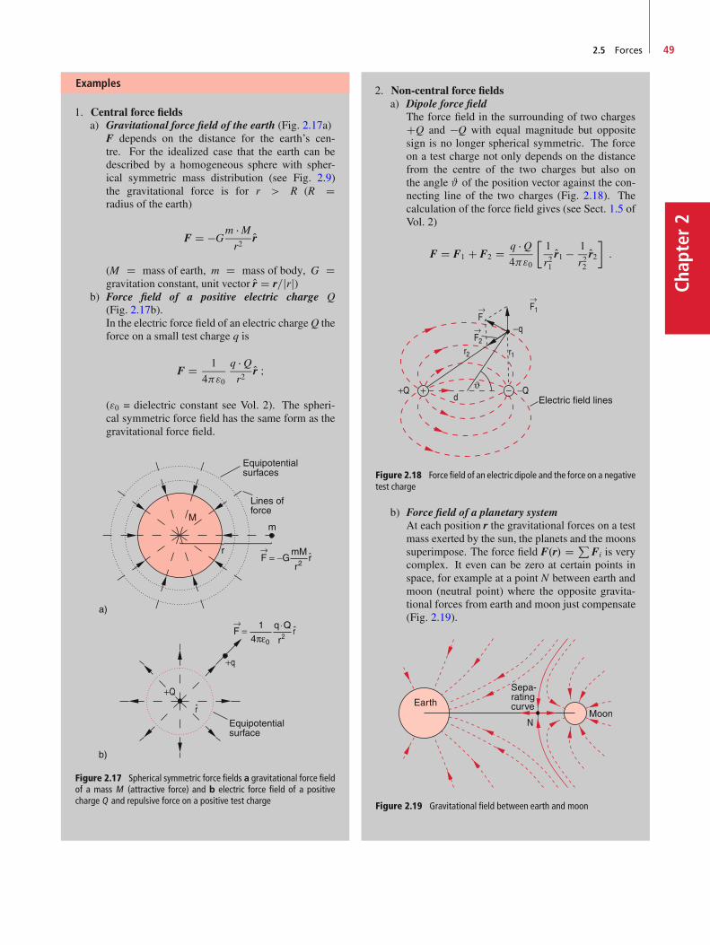
2.5 Forces 49
Chap
ter2
Examples
1. Central force fieldsa) Gravitational force field of the earth (Fig. 2.17a)
F depends on the distance for the earth’s cen-tre. For the idealized case that the earth can bedescribed by a homogeneous sphere with spher-ical symmetric mass distribution (see Fig. 2.9)the gravitational force is for r > R (R Dradius of the earth)
F D �Gm � Mr2
Or
(M D mass of earth, m D mass of body, G Dgravitation constant, unit vector Or D r=jrj)
b) Force field of a positive electric charge Q(Fig. 2.17b).In the electric force field of an electric chargeQ theforce on a small test charge q is
F D 1
4"0
q � Qr2
Or I
("0 = dielectric constant see Vol. 2). The spheri-cal symmetric force field has the same form as thegravitational force field.
Figure 2.17 Spherical symmetric force fields a gravitational force fieldof a mass M (attractive force) and b electric force field of a positivecharge Q and repulsive force on a positive test charge
2. Non-central force fieldsa) Dipole force field
The force field in the surrounding of two chargesCQ and �Q with equal magnitude but oppositesign is no longer spherical symmetric. The forceon a test charge not only depends on the distancefrom the centre of the two charges but also onthe angle # of the position vector against the con-necting line of the two charges (Fig. 2.18). Thecalculation of the force field gives (see Sect. 1.5 ofVol. 2)
F D F1 C F2 D q � Q4"0
�1
r21Or1 � 1
r22Or2�:
Figure 2.18 Force field of an electric dipole and the force on a negativetest charge
b) Force field of a planetary systemAt each position r the gravitational forces on a testmass exerted by the sun, the planets and the moonssuperimpose. The force field F.r/ D P
Fi is verycomplex. It even can be zero at certain points inspace, for example at a point N between earth andmoon (neutral point) where the opposite gravita-tional forces from earth and moon just compensate(Fig. 2.19).
Figure 2.19 Gravitational field between earth and moon
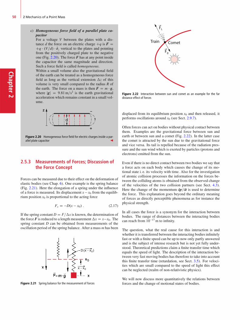
Chapter2
50 2 Mechanics of a Point Mass
c) Homogeneous force field of a parallel plate ca-pacitorFor a voltage V between the plates with a dis-tance d the force on an electric charge Cq is F DCq � .V=d/ � Oez vertical to the plates and pointingfrom the positively charged plate to the negativeone (Fig. 2.20). The force F has at any point insidethe capacitor the same magnitude and direction.Such a force field is called homogeneous.Within a small volume also the gravitational fieldof the earth can be treated as a homogeneous forcefield as long as the vertical extension �z of thisvolume is very small compared to the radius R ofthe earth. The force on a mass is then F D m � g,where jgj D 9:81m=s2 is the earth gravitationalacceleration which remains constant in a small vol-ume.
Z
d
–
+
Figure 2.20 Homogeneous force field for electric charges inside a par-allel plate capacitor J
2.5.3 Measurements of Forces; Discussion ofthe Force Concept
Forces can be measured due to their effect on the deformation ofelastic bodies (see Chap. 6). One example is the spring balance(Fig. 2.21). Here the elongation of a spring under the influenceof a force is measured. Its displacement x� x0 from the equilib-rium position x0 is proportional to the acting force
Fx D �D.x � x0/ : (2.17)
If the spring constantD D F=�x is known, the determination ofthe forceF is reduced to a length measurement�x D x�x0. Thespring constant D can be obtained from measurements of theoscillation period of the spring balance. After a massm has been
Figure 2.21 Spring balance for the measurement of forces
Train Comet
FL
Fg
Figure 2.22 Interaction between sun and comet as an example for the fardistance effect of forces
displaced from its equilibrium position x0 and then released, itperforms oscillations around x0 (see Sect. 2.9.7).
Often forces can act on bodies without physical contact betweenthem. Examples are the gravitational force between sun andearth or between sun and a comet (Fig. 2.22). In the latter casethe comet is attracted by the sun due to the gravitational forceand vice versa. Its tail is repelled because of the radiation pres-sure and the sun wind which is exerted by particles (protons andelectrons) emitted from the sun.
Even if there is no direct contact between two bodies we say thata force acts on each body which causes the change of its mo-tional state i. e. its velocity with time. Also for the investigationof atomic collision processes the information on the forces be-tween the colliding atoms is obtained from the observed changeof the velocities of the two collision partners (see Sect. 4.3).Here the change of the momentum dp=dt is used to determinethe force. This explanation goes beyond the ordinary meaningof forces as directly perceptible phenomena as for instance thephysical strength.
In all cases the force is a synonym for the interaction betweenbodies. The range of distances between the interacting bodiescan reach from 10�17 m to infinity.
The question, what the real cause for this interaction is andwhether it is transferred between the interacting bodies infinitelyfast or with a finite speed can be up to now only partly answeredand is the subject of intense research but is not yet fully under-stood. Theoretical predictions claim a finite transfer time whichequals the speed of light. The description of the interaction be-tween very fast moving bodies has therefore to take into accountthis finite transfer time (retardation, see Sect. 3.5). For veloci-ties which are small compared to the speed of light this effectcan be neglected (realm of non-relativistic physics).
We will now discuss more quantitatively the relations betweenforces and the change of motional states of bodies.
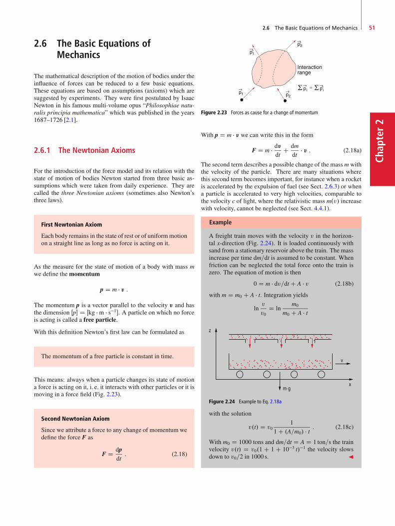
2.6 The Basic Equations of Mechanics 51
Chap
ter2
2.6 The Basic Equations ofMechanics
The mathematical description of the motion of bodies under theinfluence of forces can be reduced to a few basic equations.These equations are based on assumptions (axioms) which aresuggested by experiments. They were first postulated by IsaacNewton in his famous multi-volume opus “Philosophiae natu-ralis principia mathematica” which was published in the years1687–1726 [2.1].
2.6.1 The Newtonian Axioms
For the introduction of the force model and its relation with thestate of motion of bodies Newton started from three basic as-sumptions which were taken from daily experience. They arecalled the three Newtonian axioms (sometimes also Newton’sthree laws).
First Newtonian Axiom
Each body remains in the state of rest or of uniformmotionon a straight line as long as no force is acting on it.
As the measure for the state of motion of a body with mass mwe define themomentum
p D m � v :
The momentum p is a vector parallel to the velocity v and hasthe dimension Œp� D Œkg � m � s�1�. A particle on which no forceis acting is called a free particle.
With this definition Newton’s first law can be formulated as
The momentum of a free particle is constant in time.
This means: always when a particle changes its state of motiona force is acting on it, i. e. it interacts with other particles or it ismoving in a force field (Fig. 2.23).
Second Newtonian Axiom
Since we attribute a force to any change of momentum wedefine the force F as
F D dpdt: (2.18)
Figure 2.23 Forces as cause for a change of momentum
With p D m � v we can write this in the form
F D m � dv
dtC dm
dt� v : (2.18a)
The second term describes a possible change of the mass m withthe velocity of the particle. There are many situations wherethis second term becomes important, for instance when a rocketis accelerated by the expulsion of fuel (see Sect. 2.6.3) or whena particle is accelerated to very high velocities, comparable tothe velocity c of light, where the relativistic mass m.v/ increasewith velocity, cannot be neglected (see Sect. 4.4.1).
Example
A freight train moves with the velocity v in the horizon-tal x-direction (Fig. 2.24). It is loaded continuously withsand from a stationary reservoir above the train. The massincrease per time dm=dt is assumed to be constant. Whenfriction can be neglected the total force onto the train iszero. The equation of motion is then
0 D m � dv=dt C A � v (2.18b)
with m D m0 C A � t. Integration yieldslnv
v0D ln
m0
m0 C A � t
Figure 2.24 Example to Eq. 2.18a
with the solution
v.t/ D v01
1 C .A=m0/ � t : (2.18c)
With m0 D 1000 tons and dm=dt D A D 1 ton=s the trainvelocity v.t/ D v0.1 C 1 C 10�3 t/�1 the velocity slowsdown to v0=2 in 1000 s. J
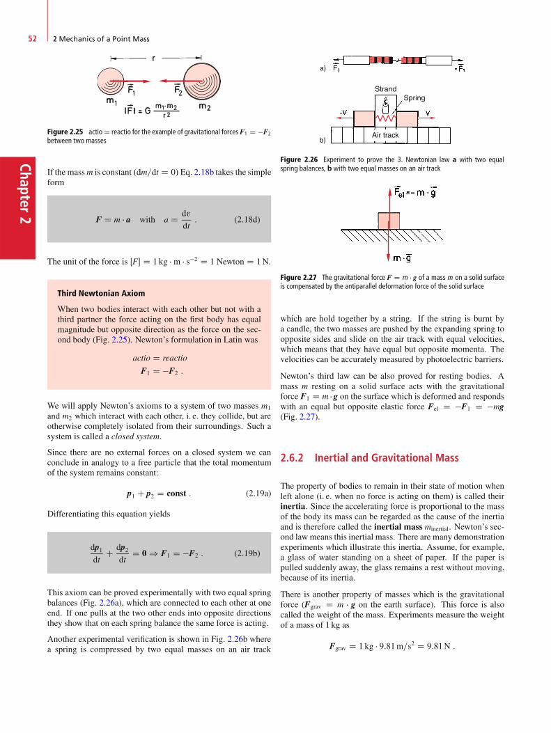
Chapter2
52 2 Mechanics of a Point Mass
Figure 2.25 actioD reactio for the example of gravitational forcesF1 D �F2
between two masses
If the massm is constant .dm=dt D 0/Eq. 2.18b takes the simpleform
F D m � a with a D dv
dt: (2.18d)
The unit of the force is ŒF� D 1 kg � m � s�2 D 1 Newton D 1N.
Third Newtonian Axiom
When two bodies interact with each other but not with athird partner the force acting on the first body has equalmagnitude but opposite direction as the force on the sec-ond body (Fig. 2.25). Newton’s formulation in Latin was
actio D reactio
F1 D �F2 :
We will apply Newton’s axioms to a system of two masses m1
and m2 which interact with each other, i. e. they collide, but areotherwise completely isolated from their surroundings. Such asystem is called a closed system.
Since there are no external forces on a closed system we canconclude in analogy to a free particle that the total momentumof the system remains constant:
p1 C p2 D const : (2.19a)
Differentiating this equation yields
dp1dt
C dp2dt
D 0 ) F1 D �F2 : (2.19b)
This axiom can be proved experimentally with two equal springbalances (Fig. 2.26a), which are connected to each other at oneend. If one pulls at the two other ends into opposite directionsthey show that on each spring balance the same force is acting.
Another experimental verification is shown in Fig. 2.26b wherea spring is compressed by two equal masses on an air track
StrandSpring
Air track
Figure 2.26 Experiment to prove the 3. Newtonian law a with two equalspring balances, b with two equal masses on an air track
Figure 2.27 The gravitational force F D m � g of a mass m on a solid surfaceis compensated by the antiparallel deformation force of the solid surface
which are hold together by a string. If the string is burnt bya candle, the two masses are pushed by the expanding spring toopposite sides and slide on the air track with equal velocities,which means that they have equal but opposite momenta. Thevelocities can be accurately measured by photoelectric barriers.
Newton’s third law can be also proved for resting bodies. Amass m resting on a solid surface acts with the gravitationalforce F1 D m � g on the surface which is deformed and respondswith an equal but opposite elastic force Fel D �F1 D �mg(Fig. 2.27).
2.6.2 Inertial and Gravitational Mass
The property of bodies to remain in their state of motion whenleft alone (i. e. when no force is acting on them) is called theirinertia. Since the accelerating force is proportional to the massof the body its mass can be regarded as the cause of the inertiaand is therefore called the inertial mass minertial. Newton’s sec-ond lawmeans this inertial mass. There are many demonstrationexperiments which illustrate this inertia. Assume, for example,a glass of water standing on a sheet of paper. If the paper ispulled suddenly away, the glass remains a rest without moving,because of its inertia.
There is another property of masses which is the gravitationalforce (Fgrav D m � g on the earth surface). This force is alsocalled the weight of the mass. Experiments measure the weightof a mass of 1 kg as
Fgrav D 1 kg � 9:81m=s2 D 9:81N :
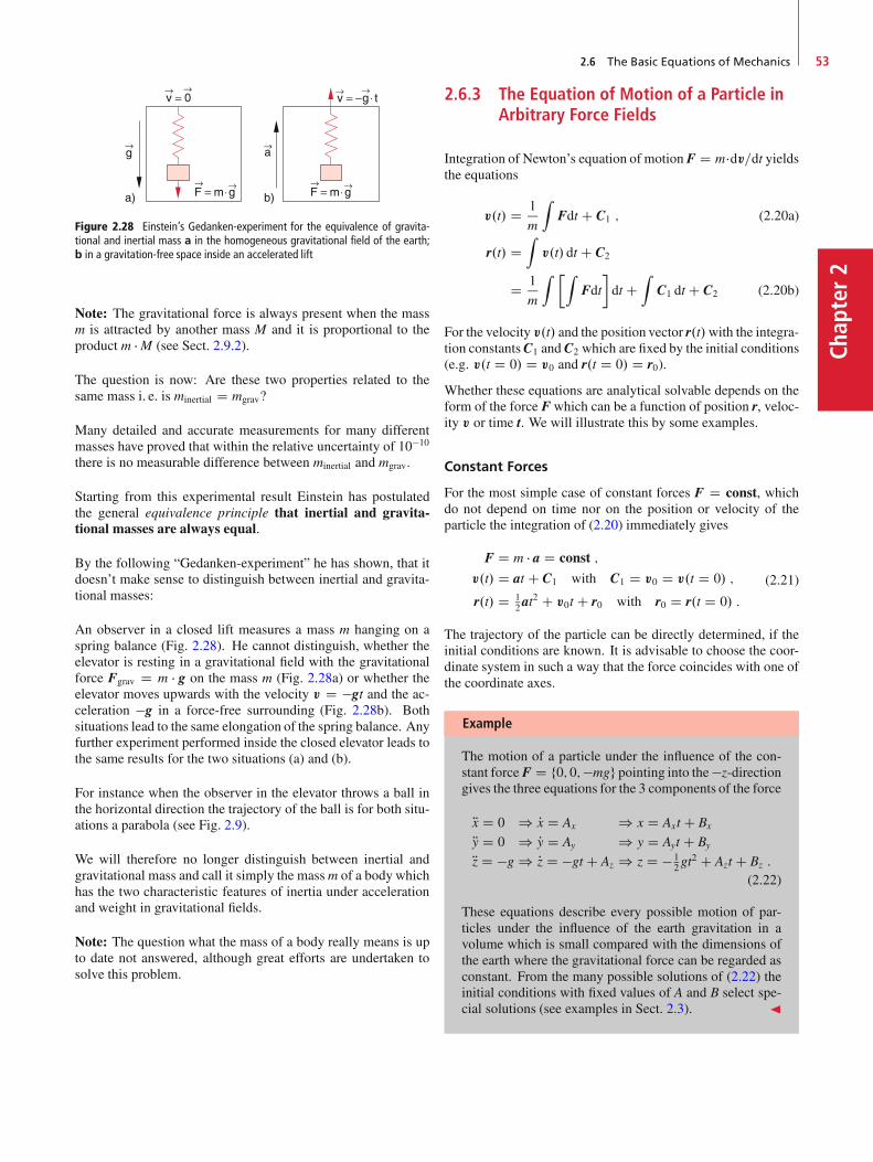
2.6 The Basic Equations of Mechanics 53
Chap
ter2
Figure 2.28 Einstein’s Gedanken-experiment for the equivalence of gravita-tional and inertial mass a in the homogeneous gravitational field of the earth;b in a gravitation-free space inside an accelerated lift
Note: The gravitational force is always present when the massm is attracted by another mass M and it is proportional to theproduct m � M (see Sect. 2.9.2).
The question is now: Are these two properties related to thesame mass i. e. is minertial D mgrav?
Many detailed and accurate measurements for many differentmasses have proved that within the relative uncertainty of 10�10
there is no measurable difference between minertial and mgrav.
Starting from this experimental result Einstein has postulatedthe general equivalence principle that inertial and gravita-tional masses are always equal.
By the following “Gedanken-experiment” he has shown, that itdoesn’t make sense to distinguish between inertial and gravita-tional masses:
An observer in a closed lift measures a mass m hanging on aspring balance (Fig. 2.28). He cannot distinguish, whether theelevator is resting in a gravitational field with the gravitationalforce Fgrav D m � g on the mass m (Fig. 2.28a) or whether theelevator moves upwards with the velocity v D �gt and the ac-celeration �g in a force-free surrounding (Fig. 2.28b). Bothsituations lead to the same elongation of the spring balance. Anyfurther experiment performed inside the closed elevator leads tothe same results for the two situations (a) and (b).
For instance when the observer in the elevator throws a ball inthe horizontal direction the trajectory of the ball is for both situ-ations a parabola (see Fig. 2.9).
We will therefore no longer distinguish between inertial andgravitational mass and call it simply the massm of a body whichhas the two characteristic features of inertia under accelerationand weight in gravitational fields.
Note: The question what the mass of a body really means is upto date not answered, although great efforts are undertaken tosolve this problem.
2.6.3 The Equation of Motion of a Particle inArbitrary Force Fields
Integration of Newton’s equation of motionF D m�dv=dt yieldsthe equations
v.t/ D 1
m
ZFdt C C1 ; (2.20a)
r.t/ DZ
v.t/ dt C C2
D 1
m
Z �ZFdt
�dt C
ZC1 dt C C2 (2.20b)
For the velocity v.t/ and the position vector r.t/with the integra-tion constantsC1 andC2 which are fixed by the initial conditions(e.g. v.t D 0/ D v0 and r.t D 0/ D r0).
Whether these equations are analytical solvable depends on theform of the force F which can be a function of position r, veloc-ity v or time t. We will illustrate this by some examples.
Constant Forces
For the most simple case of constant forces F D const, whichdo not depend on time nor on the position or velocity of theparticle the integration of (2.20) immediately gives
F D m � a D const ;
v.t/ D at C C1 with C1 D v0 D v.t D 0/ ;
r.t/ D 12at
2 C v0t C r0 with r0 D r.t D 0/ :
(2.21)
The trajectory of the particle can be directly determined, if theinitial conditions are known. It is advisable to choose the coor-dinate system in such a way that the force coincides with one ofthe coordinate axes.
Example
The motion of a particle under the influence of the con-stant force F D f0; 0;�mgg pointing into the�z-directiongives the three equations for the 3 components of the force
Rx D 0 ) Px D Ax ) x D Axt C Bx
Ry D 0 ) Py D Ay ) y D Ayt C By
Rz D �g ) Pz D �gt C Az ) z D � 12gt
2 C Azt C Bz :
(2.22)
These equations describe every possible motion of par-ticles under the influence of the earth gravitation in avolume which is small compared with the dimensions ofthe earth where the gravitational force can be regarded asconstant. From the many possible solutions of (2.22) theinitial conditions with fixed values of A and B select spe-cial solutions (see examples in Sect. 2.3). J
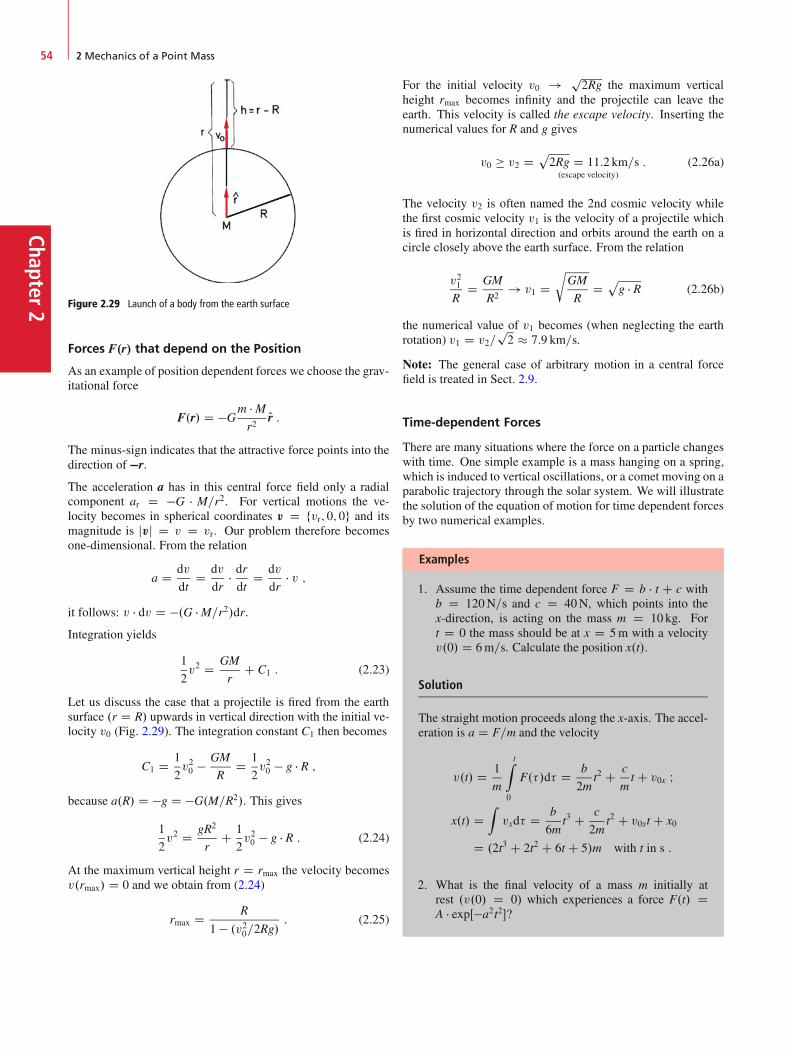
Chapter2
54 2 Mechanics of a Point Mass
Figure 2.29 Launch of a body from the earth surface
Forces F.r/ that depend on the Position
As an example of position dependent forces we choose the grav-itational force
F.r/ D �Gm � Mr2
Or :
The minus-sign indicates that the attractive force points into thedirection of �r.
The acceleration a has in this central force field only a radialcomponent ar D �G � M=r2. For vertical motions the ve-locity becomes in spherical coordinates v D fvr; 0; 0g and itsmagnitude is jvj D v D vr. Our problem therefore becomesone-dimensional. From the relation
a D dv
dtD dv
dr� drdt
D dv
dr� v ;
it follows: v � dv D �.G � M=r2/dr.Integration yields
1
2v2 D GM
rC C1 : (2.23)
Let us discuss the case that a projectile is fired from the earthsurface .r D R/ upwards in vertical direction with the initial ve-locity v0 (Fig. 2.29). The integration constant C1 then becomes
C1 D 1
2v20 � GM
RD 1
2v20 � g � R ;
because a.R/ D �g D �G.M=R2/. This gives
1
2v2 D gR2
rC 1
2v20 � g � R : (2.24)
At the maximum vertical height r D rmax the velocity becomesv.rmax/ D 0 and we obtain from (2.24)
rmax D R
1 � .v20=2Rg/: (2.25)
For the initial velocity v0 ! p2Rg the maximum vertical
height rmax becomes infinity and the projectile can leave theearth. This velocity is called the escape velocity. Inserting thenumerical values for R and g gives
v0 � v2 D p2Rg D 11:2 km=s
(escape velocity): (2.26a)
The velocity v2 is often named the 2nd cosmic velocity whilethe first cosmic velocity v1 is the velocity of a projectile whichis fired in horizontal direction and orbits around the earth on acircle closely above the earth surface. From the relation
v21R
D GM
R2! v1 D
rGM
RD p
g � R (2.26b)
the numerical value of v1 becomes (when neglecting the earthrotation) v1 D v2=
p2 � 7:9 km=s.
Note: The general case of arbitrary motion in a central forcefield is treated in Sect. 2.9.
Time-dependent Forces
There are many situations where the force on a particle changeswith time. One simple example is a mass hanging on a spring,which is induced to vertical oscillations, or a comet moving on aparabolic trajectory through the solar system. We will illustratethe solution of the equation of motion for time dependent forcesby two numerical examples.
Examples
1. Assume the time dependent force F D b � t C c withb D 120N=s and c D 40N, which points into thex-direction, is acting on the mass m D 10 kg. Fort D 0 the mass should be at x D 5m with a velocityv.0/ D 6m=s. Calculate the position x.t/.
Solution
The straight motion proceeds along the x-axis. The accel-eration is a D F=m and the velocity
v.t/ D 1
m
tZ
0
F.�/d� D b
2mt2 C c
mt C v0x I
x.t/ DZvxd� D b
6mt3 C c
2mt2 C v0xt C x0
D .2t3 C 2t2 C 6t C 5/m with t in s :
2. What is the final velocity of a mass m initially atrest .v.0/ D 0/ which experiences a force F.t/ DA � expŒ�a2t2�?
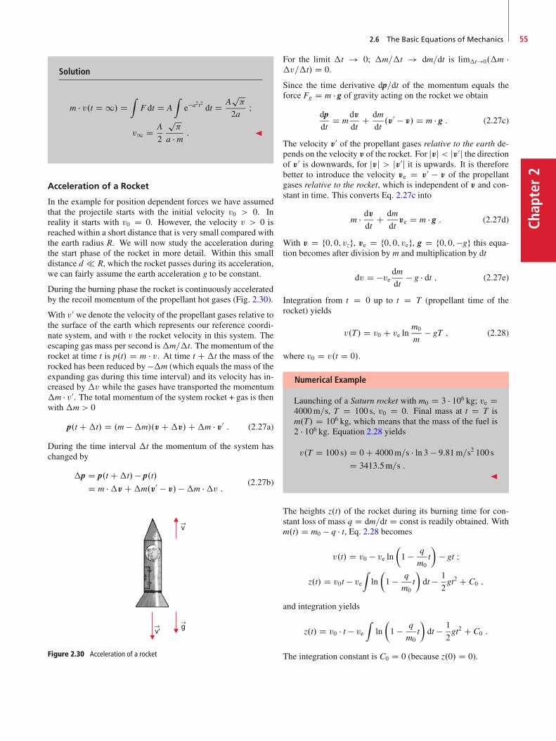
2.6 The Basic Equations of Mechanics 55
Chap
ter2
Solution
m � v.t D 1/ DZ
F dt D AZ
e�a2t2 dt D Ap
2aI
v1 D A
2
p
a � m : J
Acceleration of a Rocket
In the example for position dependent forces we have assumedthat the projectile starts with the initial velocity v0 > 0. Inreality it starts with v0 D 0. However, the velocity v > 0 isreached within a short distance that is very small compared withthe earth radius R. We will now study the acceleration duringthe start phase of the rocket in more detail. Within this smalldistance d R, which the rocket passes during its acceleration,we can fairly assume the earth acceleration g to be constant.
During the burning phase the rocket is continuously acceleratedby the recoil momentum of the propellant hot gases (Fig. 2.30).
With v0 we denote the velocity of the propellant gases relative tothe surface of the earth which represents our reference coordi-nate system, and with v the rocket velocity in this system. Theescaping gas mass per second is�m=�t. The momentum of therocket at time t is p.t/ D m � v. At time t C�t the mass of therocked has been reduced by ��m (which equals the mass of theexpanding gas during this time interval) and its velocity has in-creased by �v while the gases have transported the momentum�m � v0. The total momentum of the system rocket + gas is thenwith �m > 0
p.t C�t/ D .m ��m/.v C�v/C�m � v0 : (2.27a)
During the time interval �t the momentum of the system haschanged by
�p D p.t C�t/ � p.t/
D m ��v C�m.v0 � v/ ��m ��v : (2.27b)
Figure 2.30 Acceleration of a rocket
For the limit �t ! 0; �m=�t ! dm=dt is lim�t!0.�m ��v=�t/ D 0.
Since the time derivative dp=dt of the momentum equals theforce Fg D m � g of gravity acting on the rocket we obtain
dpdt
D mdv
dtC dm
dt.v0 � v/ D m � g : (2.27c)
The velocity v0 of the propellant gases relative to the earth de-pends on the velocity v of the rocket. For jvj < jv0j the directionof v0 is downwards, for jvj > jv0j it is upwards. It is thereforebetter to introduce the velocity ve D v0 � v of the propellantgases relative to the rocket, which is independent of v and con-stant in time. This converts Eq. 2.27c into
m � dv
dtC dm
dtve D m � g : (2.27d)
With v D f0; 0; vzg, ve D f0; 0; veg, g D f0; 0;�gg this equa-tion becomes after division by m and multiplication by dt
dv D �ve dmdt � g � dt ; (2.27e)
Integration from t D 0 up to t D T (propellant time of therocket) yields
v.T/ D v0 C ve lnm0
m� gT ; (2.28)
where v0 D v.t D 0/.
Numerical Example
Launching of a Saturn rocket with m0 D 3 � 106 kg; ve D4000m=s, T D 100 s, v0 D 0. Final mass at t D T ism.T/ D 106 kg, which means that the mass of the fuel is2 � 106 kg. Equation 2.28 yields
v.T D 100 s/ D 0 C 4000m=s � ln 3 � 9:81m=s2 100 s
D 3413:5m=s :J
The heights z.t/ of the rocket during its burning time for con-stant loss of mass q D dm=dt D const is readily obtained. Withm.t/ D m0 � q � t, Eq. 2.28 becomes
v.t/ D v0 � ve ln�1 � q
m0t
�� gt I
z.t/ D v0t � veZln�1 � q
m0t
�dt � 1
2gt2 C C0 ;
and integration yields
z.t/ D v0 � t � veZ
ln
�1 � q
m0t
�dt � 1
2gt2 C C0 :
The integration constant is C0 D 0 (because z.0/ D 0).
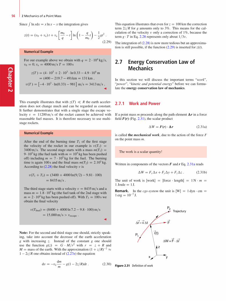
Chapter2
56 2 Mechanics of a Point Mass
SinceRln xdx D x ln x � x the integration gives
z.t/ D .v0 C ve/ t C ve
�m0
q� t
�ln
�1 � q
m0t
�� 1
2gt2 :
(2.29)
Numerical Example
For our example above we obtain with q D 2 � 104 kg=s,v0 D 0; ve D 4000m=s T D 100 s
z.T / D .4 � 105 C 2 � 103 � ln 0:33 � 4:9 � 104 mD .400 � 219:7 � 49/ km D 131 km ;
v.T / D ��4 � 103 � ln.0:33/� 981�m=s D 3413m=s ;
J
This example illustrates that with z.T/ R the earth acceler-ation does not change much and can be regarded as constant.It further demonstrates that with a single stage the escape ve-locity v D 11200m=s of the rocket cannot be achieved withreasonable fuel masses. It is therefore necessary to use multi-stage rockets.
Numerical Example
After the end of the burning time T1 of the first stagethe velocity of the rocket in our example is v.T1/ D3400m=s. The second stage starts with a mass m.T1/ D9 � 105 kg (the fuel tank with m D 105 kg has been pushedoff) including m D 7 � 105 kg for the fuel. The burningtime is again 100 s and the final mass m.T2/ D 2:105 kg.According to (2.28) the final velocity v is
v.T1 C T2/ D .3400 C 4000 ln.9=2/� 9:81 � 100/D 8435m=s :
The third stage starts with a velocity v D 8435m=s and amass m D 1:8 � 105 kg (the fuel tank of the 2nd stage withm D 2 � 104 kg has been pushed off). With T3 D 100 s weobtain the final velocity
v.Tfinal/ D .8400 C 4000 ln 7:2 � 9:8 � 100/m=sD 15;000m=s > vescape :
J
Note: For the second and third stage one should, strictly speak-ing, take into account the decrease of the earth accelerationg with increasing z. Instead of the constant g one shoulduse the function g.z/ D G � M=r2 with r D z C R andM D mass of the earth. With the approximation .1 C z=R/�2 �1 � 2z=R one obtains instead of (2.27e) the equation
dv D �ve dmm
� g.1 � 2z=R/dt : (2.30)
This equation illustrates that even for z D 100 km the correctionterm 2z=R for g amounts only to 3%. This means for the cal-culation of the velocity v only a correction of 1%, because theterm g � T in Eq. 2.28 represents only about 1=3v.
The integration of (2.28) is nowmore tedious but an approxima-tion is still possible, if the function (2.29) is inserted for z.t/.
2.7 Energy Conservation Law ofMechanics
In this section we will discuss the important terms “work”,“power”, “kinetic and potential energy” before we can formu-late the energy conservation law of mechanics.
2.7.1 Work and Power
If a point mass m proceeds along the path element �r in a forcefield F.r/ (Fig. 2.31), the scalar product
�W D F.r/ � �r (2.31a)
is called the mechanical work, due to the action of the force Fon the point mass m.
The work is a scalar quantity!
Written in components of the vectors F and r Eq. 2.31a reads
�W D Fx�x C Fy�y C Fz�z : (2.31b)
The unit of work is Œwork� D Œforce � length� D 1N � m D1 Joule D 1 J.
Remark. In the cgs-system the unit is ŒW� D 1 dyn � cm D1 erg D 10�7 J.
Figure 2.31 Definition of work
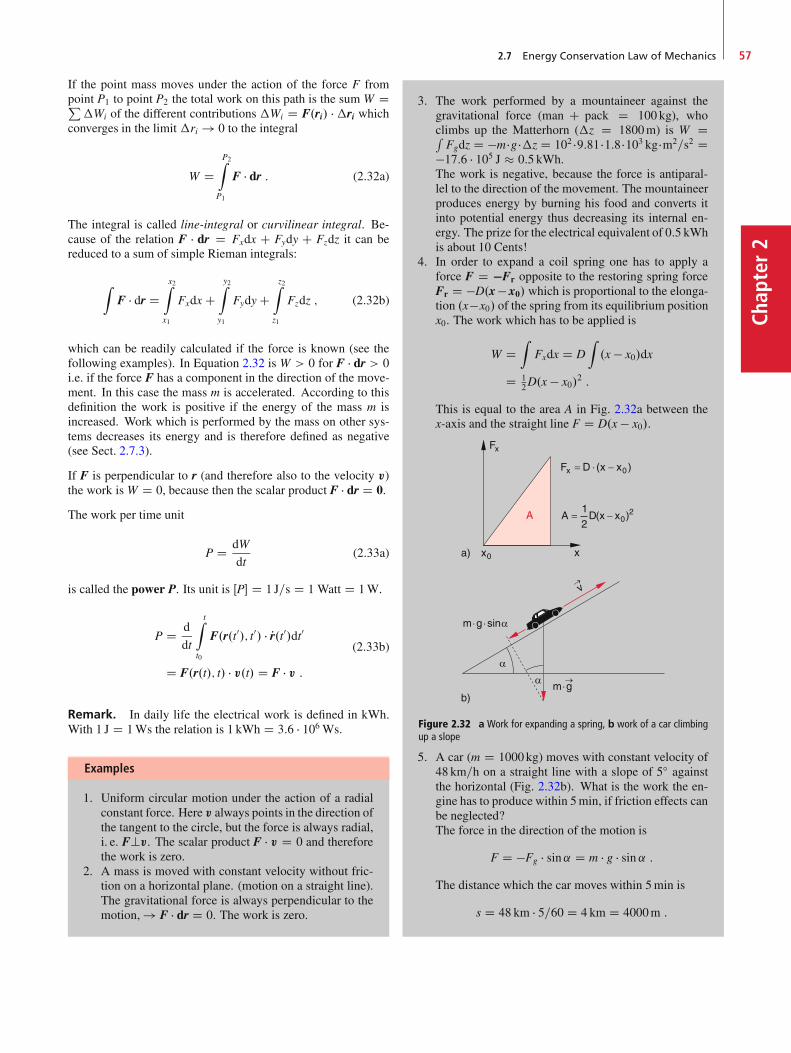
2.7 Energy Conservation Law of Mechanics 57
Chap
ter2
If the point mass moves under the action of the force F frompoint P1 to point P2 the total work on this path is the sum W DP�Wi of the different contributions �Wi D F.ri/ ��ri which
converges in the limit �ri ! 0 to the integral
W DP2Z
P1
F � dr : (2.32a)
The integral is called line-integral or curvilinear integral. Be-cause of the relation F � dr D Fxdx C Fydy C Fzdz it can bereduced to a sum of simple Rieman integrals:
ZF � dr D
x2Z
x1
Fxdx Cy2Z
y1
Fydy Cz2Z
z1
Fzdz ; (2.32b)
which can be readily calculated if the force is known (see thefollowing examples). In Equation 2.32 is W > 0 for F � dr > 0i.e. if the force F has a component in the direction of the move-ment. In this case the mass m is accelerated. According to thisdefinition the work is positive if the energy of the mass m isincreased. Work which is performed by the mass on other sys-tems decreases its energy and is therefore defined as negative(see Sect. 2.7.3).
If F is perpendicular to r (and therefore also to the velocity v)the work isW D 0, because then the scalar product F � dr D 0.
The work per time unit
P D dW
dt(2.33a)
is called the power P. Its unit is ŒP� D 1 J=s D 1 Watt D 1W.
P D d
dt
tZ
t0
F.r.t0/; t0/ � Pr.t0/dt0
D F.r.t/; t/ � v.t/ D F � v :
(2.33b)
Remark. In daily life the electrical work is defined in kWh.With 1 J D 1Ws the relation is 1 kWh D 3:6 � 106 Ws.
Examples
1. Uniform circular motion under the action of a radialconstant force. Here v always points in the direction ofthe tangent to the circle, but the force is always radial,i. e. F?v. The scalar product F � v D 0 and thereforethe work is zero.
2. A mass is moved with constant velocity without fric-tion on a horizontal plane. (motion on a straight line).The gravitational force is always perpendicular to themotion, ! F � dr D 0. The work is zero.
3. The work performed by a mountaineer against thegravitational force (man C pack D 100 kg), whoclimbs up the Matterhorn (�z D 1800m) is W DRFgdz D �m �g ��z D 102 �9:81 �1:8 �103 kg�m2=s2 D
�17:6 � 105 J � 0:5 kWh.The work is negative, because the force is antiparal-lel to the direction of the movement. The mountaineerproduces energy by burning his food and converts itinto potential energy thus decreasing its internal en-ergy. The prize for the electrical equivalent of 0:5 kWhis about 10 Cents!
4. In order to expand a coil spring one has to apply aforce F D �Fr opposite to the restoring spring forceFr D �D.x� x0/ which is proportional to the elonga-tion .x�x0/ of the spring from its equilibrium positionx0. The work which has to be applied is
W DZ
Fxdx D DZ.x � x0/dx
D 12D.x � x0/
2 :
This is equal to the area A in Fig. 2.32a between thex-axis and the straight line F D D.x � x0/.
Figure 2.32 a Work for expanding a spring, b work of a car climbingup a slope
5. A car (m D 1000kg) moves with constant velocity of48 km=h on a straight line with a slope of 5ı againstthe horizontal (Fig. 2.32b). What is the work the en-gine has to produce within 5min, if friction effects canbe neglected?The force in the direction of the motion is
F D �Fg � sin˛ D m � g � sin˛ :The distance which the car moves within 5min is
s D 48 km � 5=60 D 4 km D 4000m :
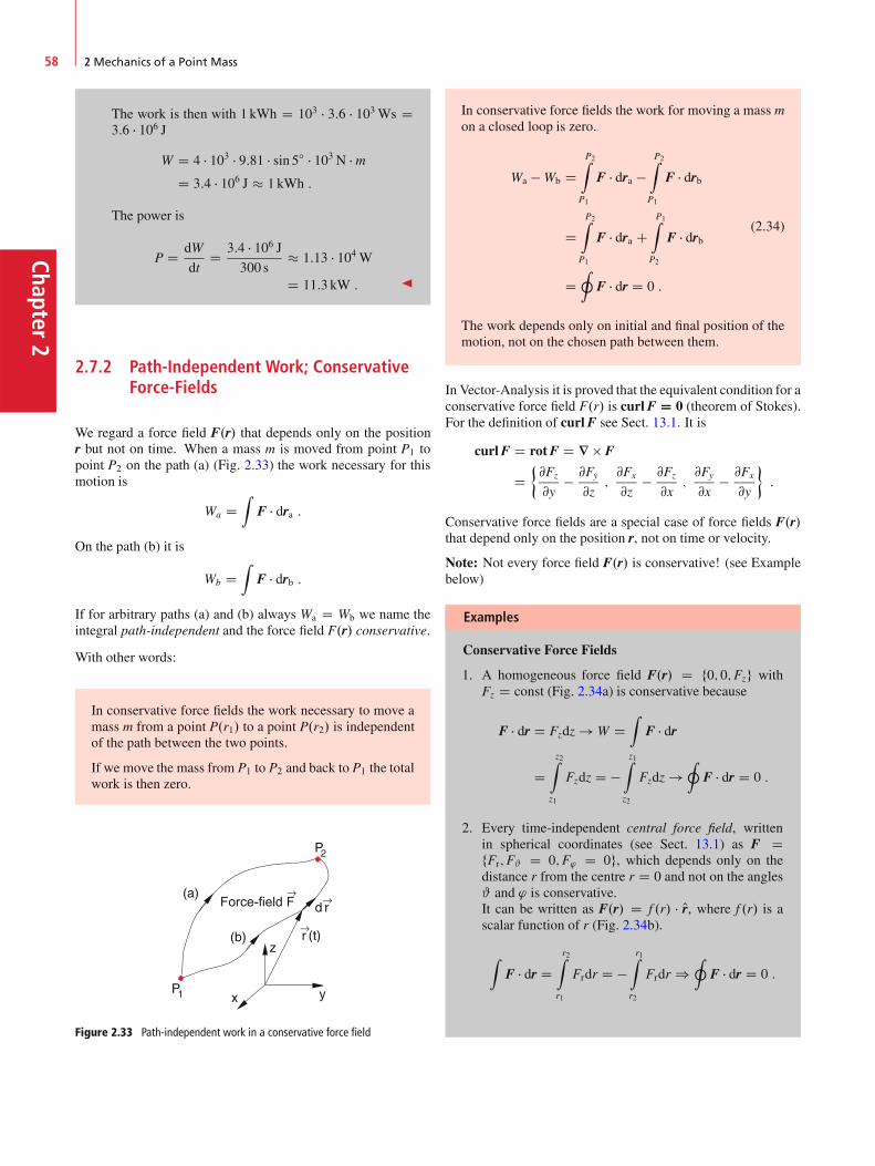
Chapter2
58 2 Mechanics of a Point Mass
The work is then with 1 kWh D 103 � 3:6 � 103 Ws D3:6 � 106 J
W D 4 � 103 � 9:81 � sin 5ı � 103 N � mD 3:4 � 106 J � 1 kWh :
The power is
P D dW
dtD 3:4 � 106 J
300 s� 1:13 � 104 WD 11:3 kW : J
2.7.2 Path-Independent Work; ConservativeForce-Fields
We regard a force field F.r/ that depends only on the positionr but not on time. When a mass m is moved from point P1 topoint P2 on the path (a) (Fig. 2.33) the work necessary for thismotion is
Wa DZ
F � dra :
On the path (b) it is
Wb DZ
F � drb :
If for arbitrary paths (a) and (b) always Wa D Wb we name theintegral path-independent and the force field F.r/ conservative.
With other words:
In conservative force fields the work necessary to move amass m from a point P.r1/ to a point P.r2/ is independentof the path between the two points.
If we move the mass from P1 to P2 and back to P1 the totalwork is then zero.
Force-field F
Figure 2.33 Path-independent work in a conservative force field
In conservative force fields the work for moving a mass mon a closed loop is zero.
Wa � Wb DP2Z
P1
F � dra �P2Z
P1
F � drb
DP2Z
P1
F � dra CP1Z
P2
F � drb
DI
F � dr D 0 :
(2.34)
The work depends only on initial and final position of themotion, not on the chosen path between them.
In Vector-Analysis it is proved that the equivalent condition for aconservative force field F.r/ is curlF D 0 (theorem of Stokes).For the definition of curlF see Sect. 13.1. It is
curlF D rotF D r F
D @Fz
@y� @Fy
@z;@Fx
@z� @Fz
@x;@Fy
@x� @Fx
@y
�:
Conservative force fields are a special case of force fields F.r/that depend only on the position r, not on time or velocity.
Note: Not every force field F.r/ is conservative! (see Examplebelow)
Examples
Conservative Force Fields
1. A homogeneous force field F.r/ D f0; 0;Fzg withFz D const (Fig. 2.34a) is conservative because
F � dr D Fzdz ! W DZ
F � dr
Dz2Z
z1
Fzdz D �z1Z
z2
Fzdz !I
F � dr D 0 :
2. Every time-independent central force field, writtenin spherical coordinates (see Sect. 13.1) as F DfFr;F# D 0;F' D 0g, which depends only on thedistance r from the centre r D 0 and not on the angles# and ' is conservative.It can be written as F.r/ D f .r/ � Or, where f .r/ is ascalar function of r (Fig. 2.34b).
ZF � dr D
r2Z
r1
Frdr D �r1Z
r2
Frdr )I
F � dr D 0 :
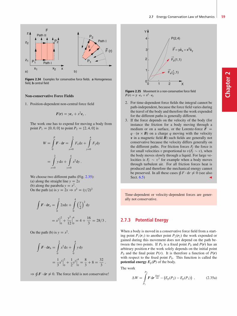
2.7 Energy Conservation Law of Mechanics 59
Chap
ter2
Figure 2.34 Examples for conservative force fields. a Homogeneousfield, b central field
Non-conservative Force Fields
1. Position-dependent non-central force field
F.r/ D yex C x2ey :
The work one has to expend for moving a body frompoint P1 D f0; 0; 0g to point P2 D f2; 4; 0g is
W DPZ
0
F � dr D2Z
xD0
Fxdx C4Z
yD0
Fydy
D2Z
xD0
y dx C4Z
yD0
x2dy :
We choose two different paths (Fig. 2.35):(a) along the straight line y D 2x(b) along the parabola y D x2.On the path (a) is y D 2x ) x2 D .y=2/2
ZF � dra D
2Z
0
2xdx C4Z
0
� y2
2dy
D x2ˇ̌ˇ2
0C y3
12
ˇ̌ˇ4
0D 4 C 16
3D 28=3 ;
On the path (b) is y D x2.
ZF � drb D
2Z
0
x2dx C4Z
0
y dy
D 1
3x3ˇ̌ˇ2
0C 1
2y2ˇ̌ˇ4
0D 8
3C 8 D 32
3:
) HF � dr ¤ 0. The force field is not conservative!
Figure 2.35 Movement in a non-conservative force fieldF.r/ D y � ex C x2 � ey2. For time-dependent force fields the integral cannot be
path-independent, because the force field varies duringthe travel of the body and therefore the work expendedfor the different paths is generally different.
3. If the force depends on the velocity of the body (forinstance the friction for a body moving through amedium or on a surface, or the Lorentz-force F Dq � .v B/ on a charge q moving with the velocityv in a magnetic field B) such fields are generally notconservative because the velocity differs generally onthe different paths. For friction forces Ff the force isfor small velocities v proportional to v.Ff � v/, whenthe body moves slowly through a liquid. For large ve-locities is Ff � v3 for example when a body movesthrough turbulent air. For all friction forces heat isproduced and therefore the mechanical energy cannotbe preserved. In all these cases
HF � dr ¤ 0 (see also
Sect. 6.5) J
Time-dependent or velocity-dependent forces are gener-ally not conservative.
2.7.3 Potential Energy
When a body is moved in a conservative force field from a start-ing point P1.r1/ to another point P2.r2/ the work expended orgained during this movement does not depend on the path be-tween the two points. If P0 is a fixed point P0 and P.r/ has anarbitrary position r the work solely depends on the initial pointP0 and the final point P.r/. It is therefore a function of P.r/with respect to the fixed point P0. This function is called thepotential energy Ep.P/ of the body.
The work
�W DP2Z
P1
F drDefD � �Ep.P2/ � Ep.P1/
�; (2.35a)
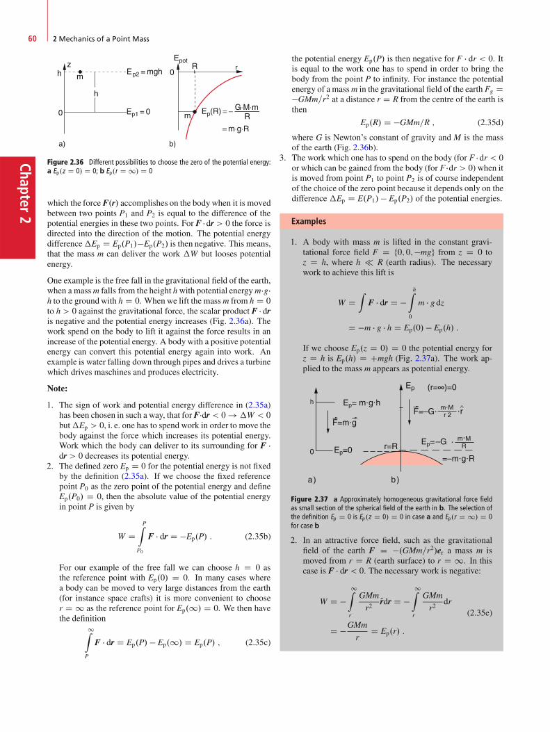
Chapter2
60 2 Mechanics of a Point Mass
Figure 2.36 Different possibilities to choose the zero of the potential energy:a Ep.z D 0/ D 0; b Ep.r D 1/ D 0
which the force F.r/ accomplishes on the bodywhen it is movedbetween two points P1 and P2 is equal to the difference of thepotential energies in these two points. For F � dr > 0 the force isdirected into the direction of the motion. The potential energydifference�Ep D Ep.P1/�Ep.P2/ is then negative. This means,that the mass m can deliver the work �W but looses potentialenergy.
One example is the free fall in the gravitational field of the earth,when a massm falls from the height hwith potential energym�g�h to the groundwith h D 0. When we lift the massm from h D 0to h > 0 against the gravitational force, the scalar product F � dris negative and the potential energy increases (Fig. 2.36a). Thework spend on the body to lift it against the force results in anincrease of the potential energy. A bodywith a positive potentialenergy can convert this potential energy again into work. Anexample is water falling down through pipes and drives a turbinewhich drives maschines and produces electricity.
Note:
1. The sign of work and potential energy difference in (2.35a)has been chosen in such a way, that forF�dr < 0 ! �W < 0but�Ep > 0, i. e. one has to spend work in order to move thebody against the force which increases its potential energy.Work which the body can deliver to its surrounding for F �dr > 0 decreases its potential energy.
2. The defined zero Ep D 0 for the potential energy is not fixedby the definition (2.35a). If we choose the fixed referencepoint P0 as the zero point of the potential energy and defineEp.P0/ D 0, then the absolute value of the potential energyin point P is given by
W DPZ
P0
F � dr D �Ep.P/ : (2.35b)
For our example of the free fall we can choose h D 0 asthe reference point with Ep.0/ D 0. In many cases wherea body can be moved to very large distances from the earth(for instance space crafts) it is more convenient to chooser D 1 as the reference point for Ep.1/ D 0. We then havethe definition
1Z
P
F � dr D Ep.P/ � Ep.1/ D Ep.P/ ; (2.35c)
the potential energy Ep.P/ is then negative for F � dr < 0. Itis equal to the work one has to spend in order to bring thebody from the point P to infinity. For instance the potentialenergy of a massm in the gravitational field of the earth Fg D�GMm=r2 at a distance r D R from the centre of the earth isthen
Ep.R/ D �GMm=R ; (2.35d)
where G is Newton’s constant of gravity and M is the massof the earth (Fig. 2.36b).
3. The work which one has to spend on the body (for F � dr < 0or which can be gained from the body (for F �dr > 0) when itis moved from point P1 to point P2 is of course independentof the choice of the zero point because it depends only on thedifference �Ep D E.P1/ � Ep.P2/ of the potential energies.
Examples
1. A body with mass m is lifted in the constant gravi-tational force field F D f0; 0;�mgg from z D 0 toz D h, where h R (earth radius). The necessarywork to achieve this lift is
W DZ
F � dr D �hZ
0
m � g dz
D �m � g � h D Ep.0/� Ep.h/ :
If we choose Ep.z D 0/ D 0 the potential energy forz D h is Ep.h/ D Cmgh (Fig. 2.37a). The work ap-plied to the mass m appears as potential energy.
Ep
Ep= m⋅g⋅h
F=m⋅g
Ep=0 r=R
h
0
(r=∞)=0
F=–G⋅ m⋅Mr 2 ⋅r
Ep=–G ⋅ m⋅MR
=–m⋅g⋅R
∧
a) b)
Figure 2.37 a Approximately homogeneous gravitational force fieldas small section of the spherical field of the earth in b. The selection ofthe definition Ep D 0 is Ep .z D 0/ D 0 in case a and Ep .r D 1/ D 0for case b
2. In an attractive force field, such as the gravitationalfield of the earth F D �.GMm=r2/er a mass m ismoved from r D R (earth surface) to r D 1. In thiscase is F � dr < 0. The necessary work is negative:
W D �1Z
r
GMm
r2Ordr D �
1Z
r
GMm
r2dr
D �GMm
rD Ep.r/ :
(2.35e)

2.7 Energy Conservation Law of Mechanics 61
Chap
ter2
Ep.r/ is negative because E.r D 1/ D 0. To raise themass m work has to be applied, which is converted tothe increase of potential energy (Fig. 2.37b).For repulsive potentials (e.g. the Coulomb potential oftwo positive electrical charges q1 and q2)
F D .q1 � q2=r2/erthe potential energy is positive and one wins workwhen the charge separation increases, while the po-tential energy decreases.When a body with mass m should be moved from theearth surface r D R to r D 1 one needs the workW D �GMm=R. With g D GM=R2 this can be writtenas W D �mgR.Numerical example: With g D 9:81m=s2, R D6371 km, the work to launch a mass of 100 kg isW D 6:25 � 109 J D 1736kWh. J
2.7.4 Energy Conservation Law in Mechanics
Multiplying the Newton equation
F D m � dv
dt
scalar with the velocity v and integrating over time yields
ZF � vdt D m
t1Z
t0
dv
dt� v dt : (2.36)
The integral on the left hand side gives with v D dr=dt
ZF � vdt D
P1Z
P0
F � dr D Ep.P0/ � Ep.P1/ ;
where the last equality is valid for conservative force fields.
The right hand side of (2.36) gives
m �Z
dv
dt� v dt D m
v1Z
v0
v � dv D m
2v21 � m
2v20 :
The expression
Ekin D mv2=2 (2.37)
is called the kinetic energy of a body with mass m and velocityv D jvj.The integral
RF � dr represents the workW which is supplied to
the body. The statement of Eq. 2.36 can therefore be formulatedas:
�Ekin D �W : (2.38a)
The increase of kinetic energy of a body is equal to thework supplied to this body.
In conservative force fieldsRF � dr is equal to the change of
potential energy. Then Eq. 2.36 states:
Ep.P0/C Ekin.P0/ D Ep.P/C Ekin.P/ D E : (2.38b)
When a body is moved in a conservative force field froma point P0 to a point P the total mechanical energy E (sumof potential and kinetic energy) is conserved, i. e. it has forall positions in the force field the same amount.
Examples
1. For the free fall starting from z D h with the velocityv.h/ D 0 we choose Ep.h D 0/ D 0. For arbitrary zthe following equations hold:
Ep.z/ D �zZ
0
�mgdz D mgz :
With v D g � t and s D h � z D 12gt
2 ! 12v
2 D12g
2t2 D g.h � z/ (see Sect. 2.3).This gives
Ekin.z/ D 12mv
2 D m � g � .h � z/ :
The sum Ep.z/ C Ekin.z/ D mgh is independent of zand for all z equal to the total energy E D mgh.
2. A body with mass m oscillates in the x-direction,driven by the force F D �D � x. For each point of itspath the total energy is E D Ep.x/C Ekin.x/ D const.For x D 0 the potential energy is zero. In the upperturning points for x D ˙xm the velocity is zero andtherefore Ekin D 0. (Fig. 2.38).
Figure 2.38 Example of energy conservation for a harmonic motion
The oscillation can be described by
x D xm sin!t ! v D dx=dt D xm! cos!t :
The potential energy is Ep D RDxdx D 1
2Dx2 D
12Dx
2m sin2 !t. The kinetic energy is Ekin D 1
2mv2 D
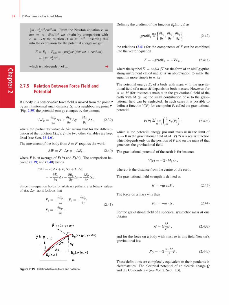
Chapter2
62 2 Mechanics of a Point Mass
12m � x2m!2 cos2 !t. From the Newton equation F Dma D m � d2x=dt2 we obtain by comparison withF D �Dx the relation D D m � !2. Inserting thisinto the expression for the potential energy we get
E D Ep C Ekin D 12mx
2m!
2.sin2 !t C cos2 !t/
D 12m � x2m!2 ;
which is independent of x. J
2.7.5 Relation Between Force Field andPotential
If a body in a conservative force field is moved from the point Pby an infinitesimal small distance�r to a neighbouring point P0(Fig. 2.39) the potential energy changes by the amount
�Ep D @Ep
@x�x C @Ep
@y�y C @Ep
@z�z ; (2.39)
where the partial derivative @E=@x means that for the differen-tiation of the function E.x; y; z/ the two other variables are keptfixed (see Sect. 13.1.6).
The movement of the body from P to P0 requires the work
�W D F ��r D ��Ep ; (2.40)
where F is an average of F.P/ and F.P0/. The comparison be-tween (2.39) and (2.40) yields
F�r D Fx�x C Fy�y C Fz�z
D �@Ep
@x�x � @Ep
@y�y � @Ep
@z�z :
Since this equation holds for arbitrary paths, i. e. arbitrary valuesof �x, �y, �z it follows that
Fx D �@Ep
@xI Fy D �@Ep
@yI
Fz D �@Ep
@z:
(2.41)
Figure 2.39 Relation between force and potential
Defining the gradient of the function Ep.x; y; z/ as
gradEpDefD @Ep
@x;@Ep
@y;@Ep
@z
�; (2.42)
the relations (2.41) for the components of F can be combinedinto the vector equation
F D �gradEp D �rEp ; (2.41a)
where the symbolr D nabla (r has the form of an old Egyptianstring instrument called nabla) is an abbreviation to make theequation more simple to write.
The potential energy Ep of a body with mass m in the gravita-tional field of a mass M depends on both masses. However, form M (for instance a mass m in the gravitational field of theearth with M � m) the small contribution of m to the gravi-tational field can be neglected. In such cases it is possible todefine a function V.P/ for each point P, called the gravitationalpotential
V.P/DefD lim
m!0
�1
mEp.P/
�I (2.42a)
which is the potential energy pro unit mass m in the limit ofm ! 0 in the gravitational field ofM. V.P/ is a scalar functionwhich depends only on the position of P and on the massM thatgenerates the gravitational field.
The gravitational potential of the earth is for instance
V.r/ D �G � ME=r ;
where r is the distance from the centre of the earth.
The gravitational field strength is defined as
G D �gradV : (2.43)
The force on a mass m is then
FG D �m � G : (2.44)
For the gravitational field of a spherical symmetric massM oneobtains
G D GM
r2Or ; (2.43a)
and for the force on a body with mass m in this field Newton’sgravitational law
FG D �Gm � Mr2
Or : (2.44a)
These definitions are completely equivalent to their pendants inelectrostatics: The electrical potential of an electric charge Qand the Coulomb law (see Vol. 2, Sect. 1.3).

2.8 Angular Momentum and Torque 63
Chap
ter2
2.8 Angular Momentum and Torque
Assume a point mass moving with the momentum p D m � v
on an arbitrary path r D r.t/ (Fig. 2.40). We define its angularmomentum L with respect to the coordinate origin r D 0 as thevector product
L D .r p/ D m � .r v/ : (2.45)
Note, that L is perpendicular to r and v!
In Cartesian coordinates L has the components (see Sect. 13.4)
Lx D ypz � zpy I Ly D zpx � xpz ILz D xpy � ypx :
(2.46)
If the body moves in a plane but on an arbitrarily curved pathwe can compose the velocity in any point of the path of a radialcomponent vr k r and a tangential component v' ? r usingpolar coordinates r and ' (Fig. 2.40). This gives the relations:
L D m � Œr .vr C v'/�
D m � .r v'/ because r vr D 0 :
The value of L is
jLj D m � r2 � d'dt
because jr v' j D r2 � d'dt
D r2 � ! :
These equations describe the following facts:
For planar motions the angular momentum L alwayspoints into the direction of the plane-normal perpendic-ular to the plane (Fig. 2.40). The vector product (r v)forms a right-handed screw.
When the angular momentum is constant, the motion proceedsin a plane perpendicular to the angular momentum vector.
Figure 2.40 Angular momentum L referred to an arbitrarily chosen origin 0for a plain motion of a point mass m
Example
For the uniform circular motion the constant angular mo-mentum points into the direction of the axis through the
circle centre perpendicular to the circular plane, i. e. intothe direction of the angular velocity vector ! (Fig. 2.41).
jLj D L D m � r � v � sin.r; v/ D m � r � v D m � r2 � ! :
sin.r; v/ D 1 because r ? v : (2.47)
For the uniform circular motion is r D constant and v Dconstant ! L D constant.
Figure 2.41 Constant angular momentum of the uniform circular mo-tion J
Differentiating (2.45) with respect to time we obtain
dLdt
D�drdt
p�
C�r dp
dt
�
D .v p/C .r Pp/ D .r Pp/; because v k p ;
dLdt
D .r F/; because F D dpdt:
(2.48)
The vector product
D D .r F/ (2.49)
is the torque of the force around the origin r D 0 acting on themass m at the position r. Equation 2.48 can then be written as
dLdt
D D : (2.49a)
The change of the angular momentumL with time is equalto the torque D.
In other words: If the torque on a mass is zero, its angular mo-mentum remains constant.
Note the equivalence between linear momentum p and angularmomentum L:
dpdt
D F;dLdt
D D ; (2.50)
p D constant for F D 0 and L D constant for D D 0.
In central force fields F.r/ D f .r/ � Or the torque D D r F D 0because F k r. Therefore the angular momentum is constant
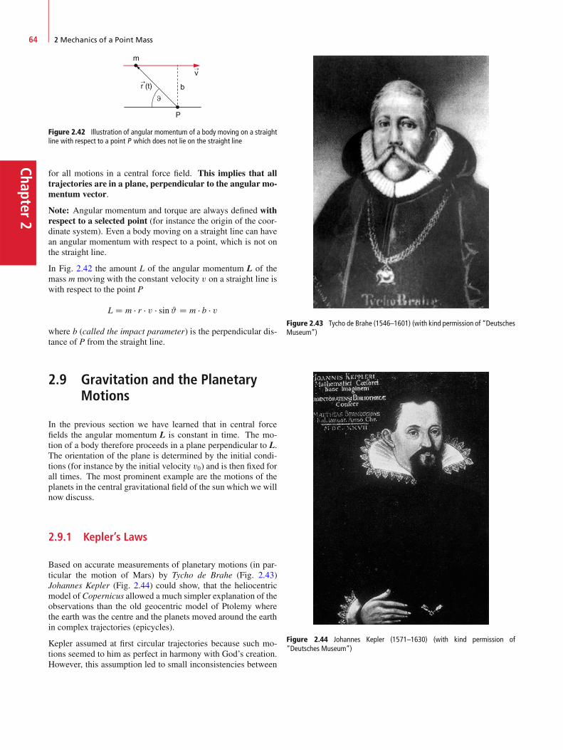
Chapter2
64 2 Mechanics of a Point Mass
Figure 2.42 Illustration of angular momentum of a body moving on a straightline with respect to a point P which does not lie on the straight line
for all motions in a central force field. This implies that alltrajectories are in a plane, perpendicular to the angular mo-mentum vector.
Note: Angular momentum and torque are always defined withrespect to a selected point (for instance the origin of the coor-dinate system). Even a body moving on a straight line can havean angular momentum with respect to a point, which is not onthe straight line.
In Fig. 2.42 the amount L of the angular momentum L of themass m moving with the constant velocity v on a straight line iswith respect to the point P
L D m � r � v � sin# D m � b � v
where b (called the impact parameter) is the perpendicular dis-tance of P from the straight line.
2.9 Gravitation and the PlanetaryMotions
In the previous section we have learned that in central forcefields the angular momentum L is constant in time. The mo-tion of a body therefore proceeds in a plane perpendicular to L.The orientation of the plane is determined by the initial condi-tions (for instance by the initial velocity v0) and is then fixed forall times. The most prominent example are the motions of theplanets in the central gravitational field of the sun which we willnow discuss.
2.9.1 Kepler’s Laws
Based on accurate measurements of planetary motions (in par-ticular the motion of Mars) by Tycho de Brahe (Fig. 2.43)Johannes Kepler (Fig. 2.44) could show, that the heliocentricmodel of Copernicus allowed a much simpler explanation of theobservations than the old geocentric model of Ptolemy wherethe earth was the centre and the planets moved around the earthin complex trajectories (epicycles).
Kepler assumed at first circular trajectories because such mo-tions seemed to him as perfect in harmony with God’s creation.However, this assumption led to small inconsistencies between
Figure 2.43 Tycho de Brahe (1546–1601) (with kind permission of “DeutschesMuseum”)
Figure 2.44 Johannes Kepler (1571–1630) (with kind permission of“Deutsches Museum”)
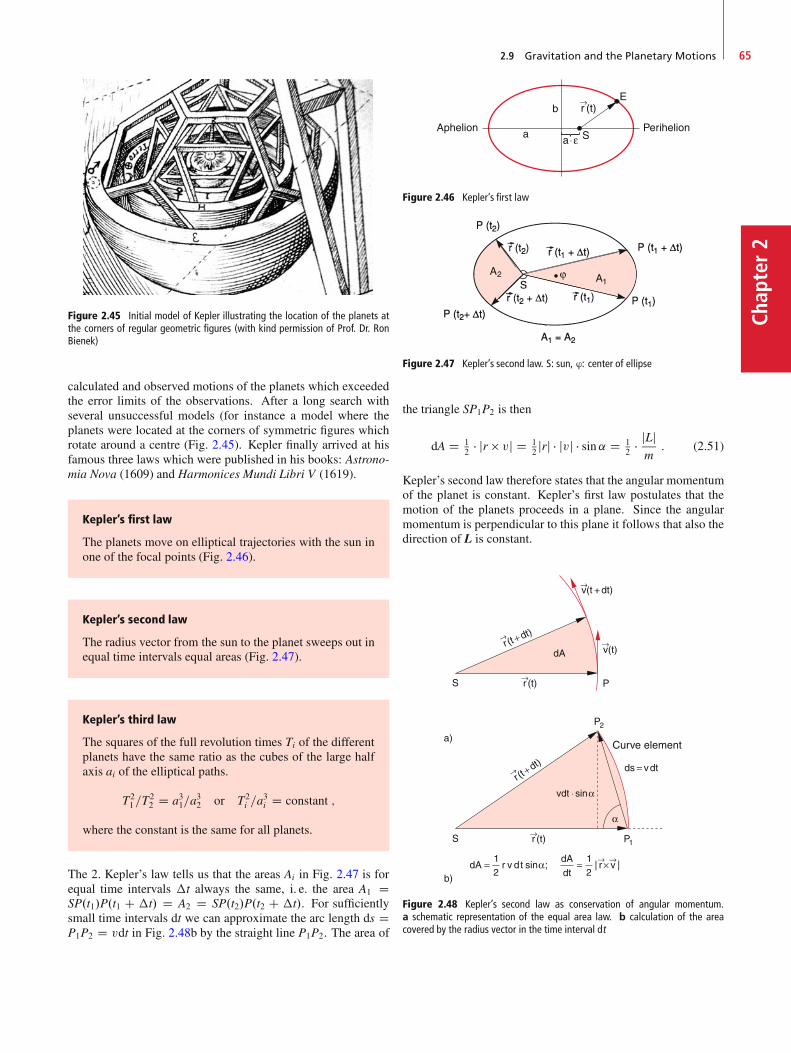
2.9 Gravitation and the Planetary Motions 65
Chap
ter2
Figure 2.45 Initial model of Kepler illustrating the location of the planets atthe corners of regular geometric figures (with kind permission of Prof. Dr. RonBienek)
calculated and observed motions of the planets which exceededthe error limits of the observations. After a long search withseveral unsuccessful models (for instance a model where theplanets were located at the corners of symmetric figures whichrotate around a centre (Fig. 2.45). Kepler finally arrived at hisfamous three laws which were published in his books: Astrono-mia Nova (1609) and Harmonices Mundi Libri V (1619).
Kepler’s first law
The planets move on elliptical trajectories with the sun inone of the focal points (Fig. 2.46).
Kepler’s second law
The radius vector from the sun to the planet sweeps out inequal time intervals equal areas (Fig. 2.47).
Kepler’s third law
The squares of the full revolution times Ti of the differentplanets have the same ratio as the cubes of the large halfaxis ai of the elliptical paths.
T21=T
22 D a31=a
32 or T2
i =a3i D constant ;
where the constant is the same for all planets.
The 2. Kepler’s law tells us that the areas Ai in Fig. 2.47 is forequal time intervals �t always the same, i. e. the area A1 DSP.t1/P.t1 C �t/ D A2 D SP.t2/P.t2 C �t/. For sufficientlysmall time intervals dt we can approximate the arc length ds DP1P2 D vdt in Fig. 2.48b by the straight line P1P2. The area of
Figure 2.46 Kepler’s first law
ϕ
Figure 2.47 Kepler’s second law. S: sun, ®: center of ellipse
the triangle SP1P2 is then
dA D 12 � jr vj D 1
2 jrj � jvj � sin˛ D 12 � jLj
m: (2.51)
Kepler’s second law therefore states that the angular momentumof the planet is constant. Kepler’s first law postulates that themotion of the planets proceeds in a plane. Since the angularmomentum is perpendicular to this plane it follows that also thedirection of L is constant.
Figure 2.48 Kepler’s second law as conservation of angular momentum.a schematic representation of the equal area law. b calculation of the areacovered by the radius vector in the time interval dt

Chapter2
66 2 Mechanics of a Point Mass
2.9.2 Newton’s Law of Gravity
Newton came to the conclusion that the free fall of a body aswell as the motion of the planets have a common cause: thegravitational attraction between two masses. In order to find aquantitative formulation of the gravitational force he started hisconsiderations with Kepler’s laws. Since the angular momentumof the planetary motion is constant the force field has to be acentral force field
F.r/ D f .r/ � Or :The gravitational force which acts on a body with mass m at thesurface of the earth with mass M (which is equal to its weight)is proportional to m. According to the principle actio D reactioand also because of symmetry principles the equal but oppositeforce acting on M should be also proportional to the mass M ofthe earth (Fig. 2.25). It is therefore reasonable to postulate thatthe gravitational force is proportional to the productm �M of thetwo masses. We therefore can write for the force between twomasses m1 and m2
Fg D G � m1 � m2 � f .r/ � Or : (2.52a)
The proportionality factorG is theNewtonian gravitational con-stant.
The function f .r/ can be determined from Kepler’s third law.Since (2.52a) must be also valid for circular orbits we obtain forthe motion of a planet with mass m around the sun with massMˇ the equation
G � m � Mˇ � f .r/ D m � !2 � r ; (2.52b)
because the gravitational force is the centripetal force whichcauses the circular motion of the planet with the angular velocity! D v=r. The revolution period of the planet is T D 2=!. Forthe orbits of two different planets Kepler’s third law postulates:
T2=r3 D const :
With ! D 2=T this gives !2 � r3 D const or !2 � r�3.
Inserting this into (2.52b) yields f .r/ � r�2.
We then obtain Newton’s law of gravity
Fg.r/ D �G � m � Mˇr2
Or : (2.52c)
The minus sign indicates that the force is attractive.
The gravitational force
F.r/ D �G � m1 � m2
r2Or
acts not only between sun and planets but also between arbitrarymasses m1 and m2 separated by the distance r. However, theforce between masses realized in the laboratory is very small
and it demands special very sensitive detection techniques inorder to measure it. The gravitational constant G can be deter-mined from such experiments in the lab. Among all physicalconstant it is that with the largest uncertainty. Therefore manyefforts are undertaken to determine G with new laser techniqueswhich should improve the accuracy [2.5a–2.5b]. The presentaccepted numerical value is
G D 6:67384.80/ � 10�11 N � m2=kg2
with a relative uncertainty of 1:2 � 10�4.
Note: The gravitational force is always attractive, never repul-sive! This differs from the static electric forces between twocharges Q1 and Q2
F.r/ � Q1 � Q2=r2C ;
which can be attractive or repulsive, depending on the sign ofthe charges Qi.
2.9.3 Planetary Orbits
Since the gravitational force field is conservative the sum of po-tential and kinetic energy of a planet is constant. Because it is acentral field also the angular momentum L D r p is constant.This can be used to determine the orbit of a planet which pro-ceeds in a plane with constant orientation perpendicular to L.We use polar coordinates r and ' with the centre of the sun ascoordinate origin (Fig. 2.49).
The kinetic energy is
Ekin D m
2v2 D m
2
�v2r C v2'
D m
2
�Pr2 C r2 P'2�:
(2.53)
The amount L D jLj of the angular momentum L is
L D mr2 P' D const : (2.54)
Figure 2.49 Elliptical orbit in Cartesian and in polar coordinates
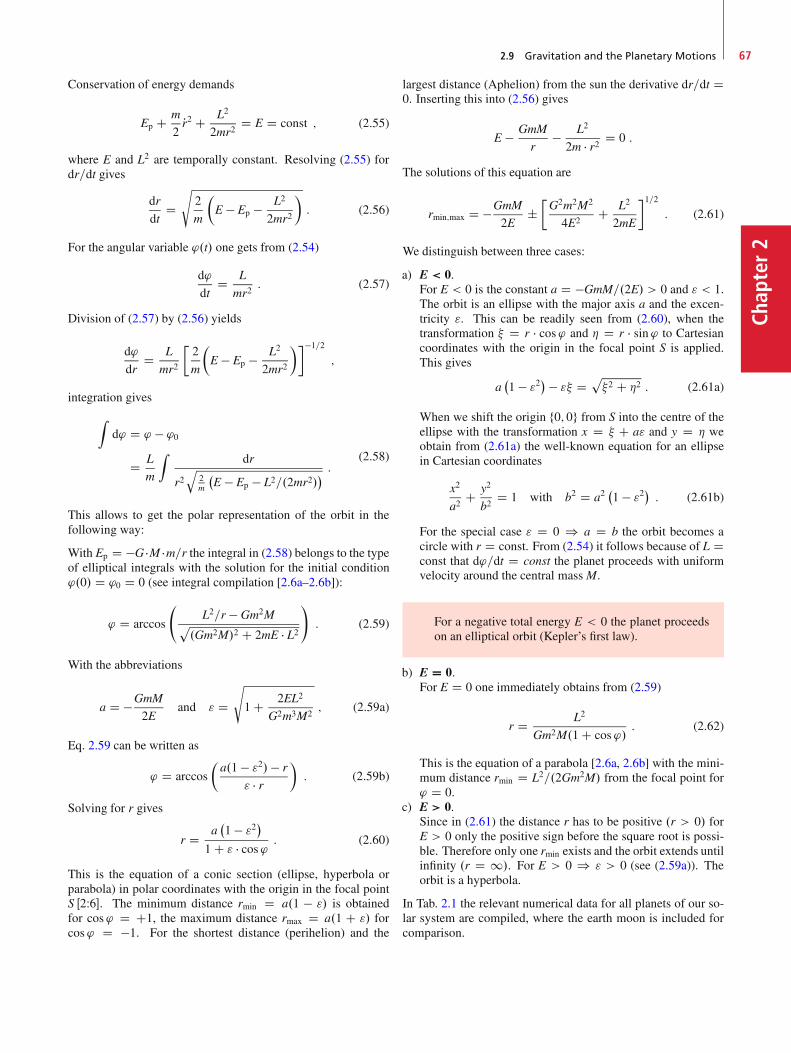
2.9 Gravitation and the Planetary Motions 67
Chap
ter2
Conservation of energy demands
Ep C m
2Pr2 C L2
2mr2D E D const ; (2.55)
where E and L2 are temporally constant. Resolving (2.55) fordr=dt gives
dr
dtDs
2
m
�E � Ep � L2
2mr2
�: (2.56)
For the angular variable '.t/ one gets from (2.54)
d'
dtD L
mr2: (2.57)
Division of (2.57) by (2.56) yields
d'
drD L
mr2
�2
m
�E � Ep � L2
2mr2
���1=2
;
integration gives
Zd' D ' � '0
D L
m
Zdr
r2q
2m
�E � Ep � L2=.2mr2/
� :(2.58)
This allows to get the polar representation of the orbit in thefollowing way:
With Ep D �G �M �m=r the integral in (2.58) belongs to the typeof elliptical integrals with the solution for the initial condition'.0/ D '0 D 0 (see integral compilation [2.6a–2.6b]):
' D arccos
L2=r � Gm2M
p.Gm2M/2 C 2mE � L2
!: (2.59)
With the abbreviations
a D �GmM
2Eand " D
s
1 C 2EL2
G2m3M2; (2.59a)
Eq. 2.59 can be written as
' D arccos�a.1 � "2/ � r
" � r�: (2.59b)
Solving for r gives
r D a�1 � "2�
1 C " � cos' : (2.60)
This is the equation of a conic section (ellipse, hyperbola orparabola) in polar coordinates with the origin in the focal pointS Œ2W6�. The minimum distance rmin D a.1 � "/ is obtainedfor cos' D C1, the maximum distance rmax D a.1 C "/ forcos' D �1. For the shortest distance (perihelion) and the
largest distance (Aphelion) from the sun the derivative dr=dt D0. Inserting this into (2.56) gives
E � GmM
r� L2
2m � r2 D 0 :
The solutions of this equation are
rmin;max D �GmM
2E˙�G2m2M2
4E2C L2
2mE
�1=2: (2.61)
We distinguish between three cases:
a) E < 0.For E < 0 is the constant a D �GmM=.2E/ > 0 and " < 1.The orbit is an ellipse with the major axis a and the excen-tricity ". This can be readily seen from (2.60), when thetransformation � D r � cos' and � D r � sin ' to Cartesiancoordinates with the origin in the focal point S is applied.This gives
a�1 � "2� � "� D
p�2 C �2 : (2.61a)
When we shift the origin f0; 0g from S into the centre of theellipse with the transformation x D � C a" and y D � weobtain from (2.61a) the well-known equation for an ellipsein Cartesian coordinates
x2
a2C y2
b2D 1 with b2 D a2
�1 � "2� : (2.61b)
For the special case " D 0 ) a D b the orbit becomes acircle with r D const. From (2.54) it follows because of L Dconst that d'=dt D const the planet proceeds with uniformvelocity around the central massM.
For a negative total energy E < 0 the planet proceedson an elliptical orbit (Kepler’s first law).
b) E D 0.For E D 0 one immediately obtains from (2.59)
r D L2
Gm2M.1 C cos'/: (2.62)
This is the equation of a parabola [2.6a, 2.6b] with the mini-mum distance rmin D L2=.2Gm2M/ from the focal point for' D 0.
c) E > 0.Since in (2.61) the distance r has to be positive .r > 0/ forE > 0 only the positive sign before the square root is possi-ble. Therefore only one rmin exists and the orbit extends untilinfinity .r D 1/. For E > 0 ) " > 0 (see (2.59a)). Theorbit is a hyperbola.
In Tab. 2.1 the relevant numerical data for all planets of our so-lar system are compiled, where the earth moon is included forcomparison.
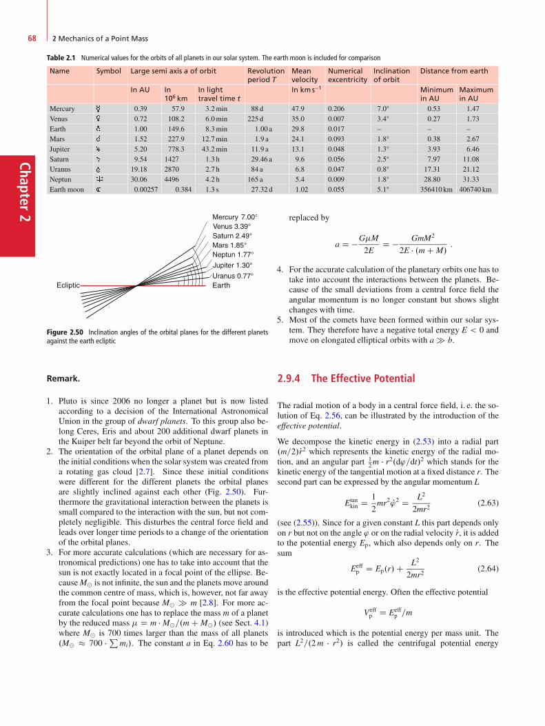
Chapter2
68 2 Mechanics of a Point Mass
Table 2.1 Numerical values for the orbits of all planets in our solar system. The earth moon is included for comparison
Name Symbol Large semi axis a of orbit Revolutionperiod T
Meanvelocity
Numericalexcentricity
Inclinationof orbit
Distance from earth
In AU In106 km
In lighttravel time t
In kms�1 Minimumin AU
Maximumin AU
Mercury � 0.39 57.9 3:2min 88 d 47.9 0.206 7:0ı 0.53 1.47Venus � 0.72 108.2 6:0min 225 d 35.0 0.007 3:4ı 0.27 1.73Earth � 1.00 149.6 8:3min 1:00 a 29.8 0.017 – – –Mars � 1.52 227.9 12:7min 1:9 a 24.1 0.093 1:8ı 0.38 2.67Jupiter � 5.20 778.3 43:2min 11:9 a 13.1 0.048 1:3ı 3.93 6.46Saturn � 9.54 1427 1:3 h 29:46 a 9.6 0.056 2:5ı 7.97 11.08Uranus � 19.18 2870 2:7 h 84 a 6.8 0.047 0:8ı 17.31 21.12Neptun � 30.06 4496 4:2 h 165 a 5.4 0.009 1:8ı 28.80 31.33Earth moon 0.00257 0.384 1:3 s 27:32 d 1.02 0.055 5:1ı 356410 km 406740 km
Figure 2.50 Inclination angles of the orbital planes for the different planetsagainst the earth ecliptic
Remark.
1. Pluto is since 2006 no longer a planet but is now listedaccording to a decision of the International AstronomicalUnion in the group of dwarf planets. To this group also be-long Ceres, Eris and about 200 additional dwarf planets inthe Kuiper belt far beyond the orbit of Neptune.
2. The orientation of the orbital plane of a planet depends onthe initial conditions when the solar systemwas created froma rotating gas cloud [2.7]. Since these initial conditionswere different for the different planets the orbital planesare slightly inclined against each other (Fig. 2.50). Fur-thermore the gravitational interaction between the planets issmall compared to the interaction with the sun, but not com-pletely negligible. This disturbes the central force field andleads over longer time periods to a change of the orientationof the orbital planes.
3. For more accurate calculations (which are necessary for as-tronomical predictions) one has to take into account that thesun is not exactly located in a focal point of the ellipse. Be-causeMˇ is not infinite, the sun and the planets move aroundthe common centre of mass, which is, however, not far awayfrom the focal point because Mˇ � m [2.8]. For more ac-curate calculations one has to replace the mass m of a planetby the reduced mass D m � Mˇ=.m C Mˇ/ (see Sect. 4.1)where Mˇ is 700 times larger than the mass of all planets.Mˇ � 700 � Pmi/. The constant a in Eq. 2.60 has to be
replaced by
a D �GM
2ED � GmM2
2E � .m C M/:
4. For the accurate calculation of the planetary orbits one has totake into account the interactions between the planets. Be-cause of the small deviations from a central force field theangular momentum is no longer constant but shows slightchanges with time.
5. Most of the comets have been formed within our solar sys-tem. They therefore have a negative total energy E < 0 andmove on elongated elliptical orbits with a � b.
2.9.4 The Effective Potential
The radial motion of a body in a central force field, i. e. the so-lution of Eq. 2.56, can be illustrated by the introduction of theeffective potential.
We decompose the kinetic energy in (2.53) into a radial part.m=2/Pr2 which represents the kinetic energy of the radial mo-tion, and an angular part 1
2m � r2.d'=dt/2 which stands for thekinetic energy of the tangential motion at a fixed distance r. Thesecond part can be expressed by the angular momentum L
Etankin D 1
2mr2 P'2 D L2
2mr2(2.63)
(see (2.55)). Since for a given constant L this part depends onlyon r but not on the angle ' or on the radial velocity Pr, it is addedto the potential energy Ep, which also depends only on r. Thesum
Eeffp D Ep.r/C L2
2mr2(2.64)
is the effective potential energy. Often the effective potential
Veffp D Eeff
p =m
is introduced which is the potential energy per mass unit. Thepart L2=.2m � r2/ is called the centrifugal potential energy
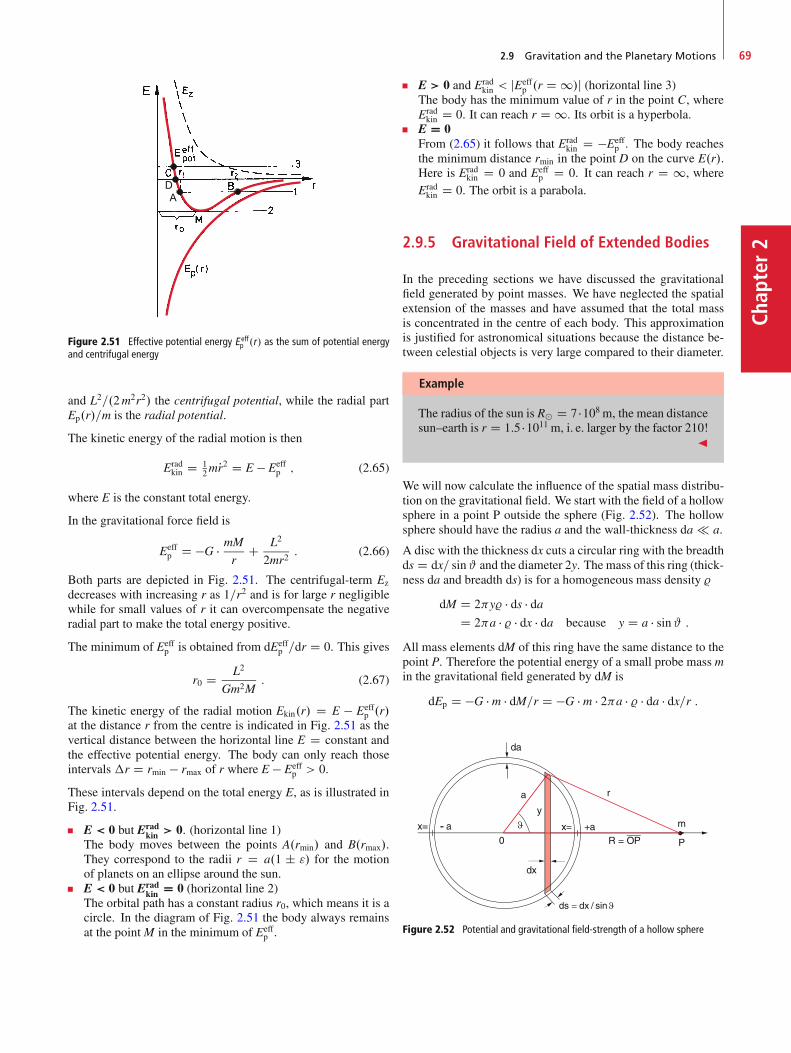
2.9 Gravitation and the Planetary Motions 69
Chap
ter2
DA
Figure 2.51 Effective potential energy E effp .r/ as the sum of potential energy
and centrifugal energy
and L2=.2m2r2/ the centrifugal potential, while the radial partEp.r/=m is the radial potential.
The kinetic energy of the radial motion is then
Eradkin D 1
2mPr2 D E � Eeffp ; (2.65)
where E is the constant total energy.
In the gravitational force field is
Eeffp D �G � mM
rC L2
2mr2: (2.66)
Both parts are depicted in Fig. 2.51. The centrifugal-term Ez
decreases with increasing r as 1=r2 and is for large r negligiblewhile for small values of r it can overcompensate the negativeradial part to make the total energy positive.
The minimum of Eeffp is obtained from dEeff
p =dr D 0. This gives
r0 D L2
Gm2M: (2.67)
The kinetic energy of the radial motion Ekin.r/ D E � Eeffp .r/
at the distance r from the centre is indicated in Fig. 2.51 as thevertical distance between the horizontal line E D constant andthe effective potential energy. The body can only reach thoseintervals �r D rmin � rmax of r where E � Eeff
p > 0.
These intervals depend on the total energy E, as is illustrated inFig. 2.51.
E < 0 but Eradkin > 0. (horizontal line 1)
The body moves between the points A.rmin/ and B.rmax/.They correspond to the radii r D a.1 ˙ "/ for the motionof planets on an ellipse around the sun.E < 0 but Erad
kin D 0 (horizontal line 2)The orbital path has a constant radius r0, which means it is acircle. In the diagram of Fig. 2.51 the body always remainsat the pointM in the minimum of Eeff
p .
E > 0 and Eradkin < jEeff
p .r D 1/j (horizontal line 3)The body has the minimum value of r in the point C, whereEradkin D 0. It can reach r D 1. Its orbit is a hyperbola.
E D 0From (2.65) it follows that Erad
kin D �Eeffp . The body reaches
the minimum distance rmin in the point D on the curve E.r/.Here is Erad
kin D 0 and Eeffp D 0. It can reach r D 1, where
Eradkin D 0. The orbit is a parabola.
2.9.5 Gravitational Field of Extended Bodies
In the preceding sections we have discussed the gravitationalfield generated by point masses. We have neglected the spatialextension of the masses and have assumed that the total massis concentrated in the centre of each body. This approximationis justified for astronomical situations because the distance be-tween celestial objects is very large compared to their diameter.
Example
The radius of the sun is Rˇ D 7 �108 m, the mean distancesun–earth is r D 1:5 �1011 m, i. e. larger by the factor 210!
J
We will now calculate the influence of the spatial mass distribu-tion on the gravitational field. We start with the field of a hollowsphere in a point P outside the sphere (Fig. 2.52). The hollowsphere should have the radius a and the wall-thickness da a.
A disc with the thickness dx cuts a circular ring with the breadthds D dx= sin# and the diameter 2y. The mass of this ring (thick-ness da and breadth ds) is for a homogeneous mass density %
dM D 2y% � ds � daD 2a � % � dx � da because y D a � sin# :
All mass elements dM of this ring have the same distance to thepoint P. Therefore the potential energy of a small probe mass min the gravitational field generated by dM is
dEp D �G � m � dM=r D �G � m � 2a � % � da � dx=r :
Figure 2.52 Potential and gravitational field-strength of a hollow sphere
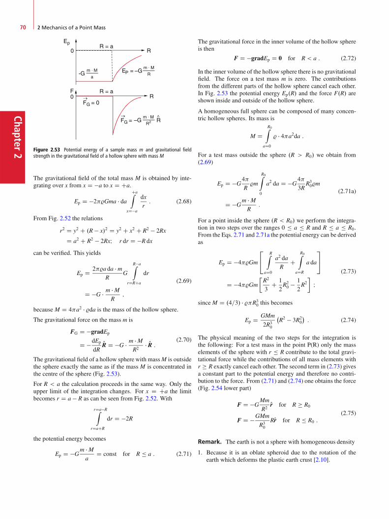
Chapter2
70 2 Mechanics of a Point Mass
Figure 2.53 Potential energy of a sample mass m and gravitational fieldstrength in the gravitational field of a hollow sphere with mass M
The gravitational field of the total mass M is obtained by inte-grating over x from x D �a to x D Ca.
Ep D �2%Gma � daCaZ
xD�a
dx
r: (2.68)
From Fig. 2.52 the relations
r2 D y2 C .R � x/2 D y2 C x2 C R2 � 2Rx
D a2 C R2 � 2RxI r dr D �R dx
can be verified. This yields
Ep D 2%a da � mR
G
R�aZ
rDRCa
dr
D �G � m � MR
;
(2.69)
becauseM D 4a2 � %da is the mass of the hollow sphere.
The gravitational force on the mass m is
FG D �gradEp
D �dEp
dROR D �G � m � M
R2� OR : (2.70)
The gravitational field of a hollow sphere with massM is outsidethe sphere exactly the same as if the mass M is concentrated inthe centre of the sphere (Fig. 2.53).
For R < a the calculation proceeds in the same way. Only theupper limit of the integration changes. For x D Ca the limitbecomes r D a � R as can be seen from Fig. 2.52. With
rDa�RZ
rDaCR
dr D �2R
the potential energy becomes
Ep D �Gm � Ma
D const for R � a : (2.71)
The gravitational force in the inner volume of the hollow sphereis then
F D �gradEp D 0 for R < a : (2.72)
In the inner volume of the hollow sphere there is no gravitationalfield. The force on a test mass m is zero. The contributionsfrom the different parts of the hollow sphere cancel each other.In Fig. 2.53 the potential energy Ep.R/ and the force F.R/ areshown inside and outside of the hollow sphere.
A homogeneous full sphere can be composed of many concen-tric hollow spheres. Its mass is
M DR0Z
aD0
% � 4a2da :
For a test mass outside the sphere .R > R0/ we obtain from(2.69)
Ep D �G4
R%m
R0Z
0
a2 da D �G4
3RR30%m
D �Gm � MR
:
(2.71a)
For a point inside the sphere .R < R0/ we perform the integra-tion in two steps over the ranges 0 � a � R and R � a � R0.From the Eqs. 2.71 and 2.71a the potential energy can be derivedas
Ep D �4%Gm
2
4RZ
aD0
a2 da
RC
R0Z
aDR
a da
3
5
D �4%Gm
�R2
3C 1
2R20 � 1
2R2
�I
(2.73)
sinceM D .4=3/ � %R30 this becomes
Ep D GMm
2R30
�R2 � 3R2
0
�: (2.74)
The physical meaning of the two steps for the integration isthe following: For a test mass in the point P(R) only the masselements of the sphere with r � R contribute to the total gravi-tational force while the contributions of all mass elements withr � R exactly cancel each other. The second term in (2.73) givesa constant part to the potential energy and therefore no contri-bution to the force. From (2.71) and (2.74) one obtains the force(Fig. 2.54 lower part)
F D �GMm
R2Or for R � R0
F D �GMm
R30
ROr for R � R0 :(2.75)
Remark. The earth is not a sphere with homogeneous density
1. Because it is an oblate spheroid due to the rotation of theearth which deforms the plastic earth crust [2.10].
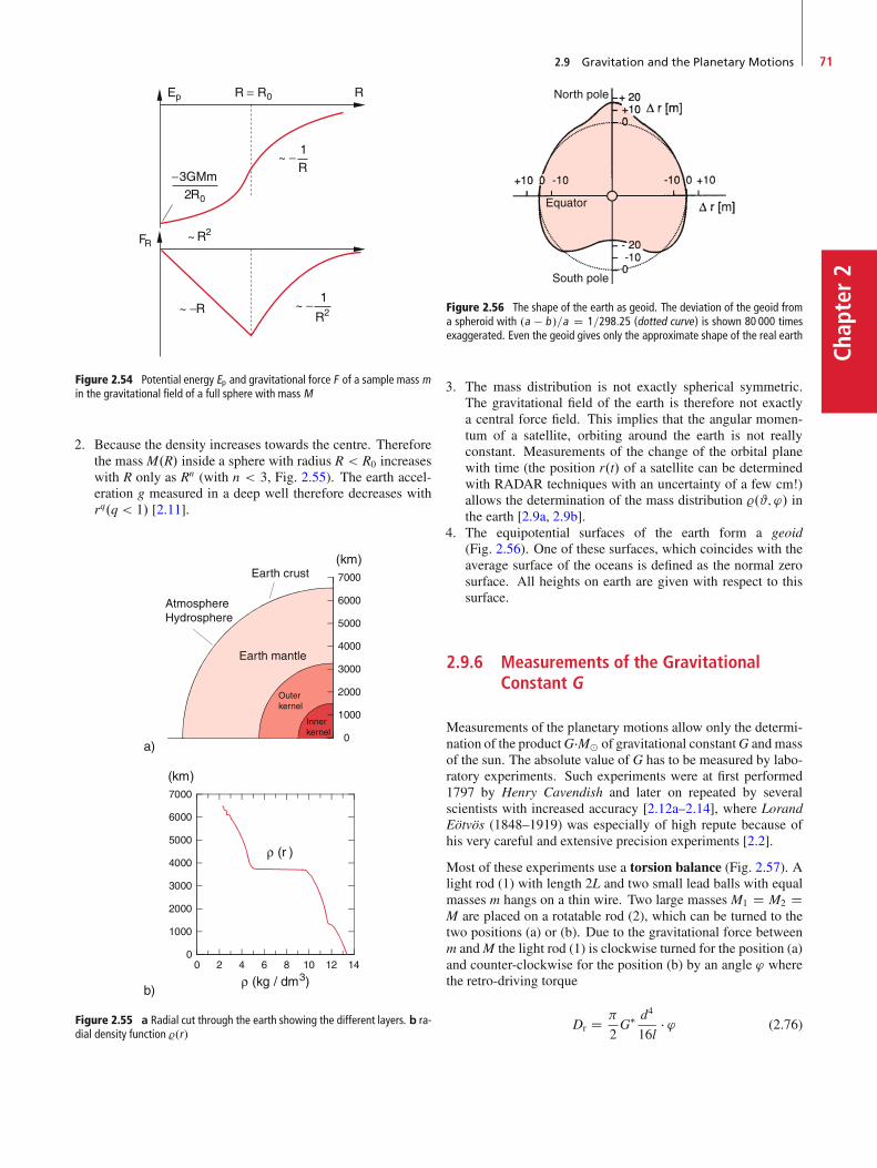
2.9 Gravitation and the Planetary Motions 71
Chap
ter2
Figure 2.54 Potential energy Ep and gravitational force F of a sample mass min the gravitational field of a full sphere with mass M
2. Because the density increases towards the centre. Thereforethe mass M.R/ inside a sphere with radius R < R0 increaseswith R only as Rn (with n < 3, Fig. 2.55). The earth accel-eration g measured in a deep well therefore decreases withrq.q < 1/ [2.11].
Figure 2.55 a Radial cut through the earth showing the different layers. b ra-dial density function %.r/
North pole
South pole
Equator
Figure 2.56 The shape of the earth as geoid. The deviation of the geoid froma spheroid with .a � b /=a D 1=298:25 (dotted curve) is shown 80 000 timesexaggerated. Even the geoid gives only the approximate shape of the real earth
3. The mass distribution is not exactly spherical symmetric.The gravitational field of the earth is therefore not exactlya central force field. This implies that the angular momen-tum of a satellite, orbiting around the earth is not reallyconstant. Measurements of the change of the orbital planewith time (the position r.t/ of a satellite can be determinedwith RADAR techniques with an uncertainty of a few cm!)allows the determination of the mass distribution %.#; '/ inthe earth [2.9a, 2.9b].
4. The equipotential surfaces of the earth form a geoid(Fig. 2.56). One of these surfaces, which coincides with theaverage surface of the oceans is defined as the normal zerosurface. All heights on earth are given with respect to thissurface.
2.9.6 Measurements of the GravitationalConstant G
Measurements of the planetary motions allow only the determi-nation of the productG�Mˇ of gravitational constantG and massof the sun. The absolute value of G has to be measured by labo-ratory experiments. Such experiments were at first performed1797 by Henry Cavendish and later on repeated by severalscientists with increased accuracy [2.12a–2.14], where LorandEötvös (1848–1919) was especially of high repute because ofhis very careful and extensive precision experiments [2.2].
Most of these experiments use a torsion balance (Fig. 2.57). Alight rod (1) with length 2L and two small lead balls with equalmasses m hangs on a thin wire. Two large masses M1 D M2 DM are placed on a rotatable rod (2), which can be turned to thetwo positions (a) or (b). Due to the gravitational force betweenm andM the light rod (1) is clockwise turned for the position (a)and counter-clockwise for the position (b) by an angle ' wherethe retro-driving torque
Dr D
2G� d4
16l� ' (2.76)
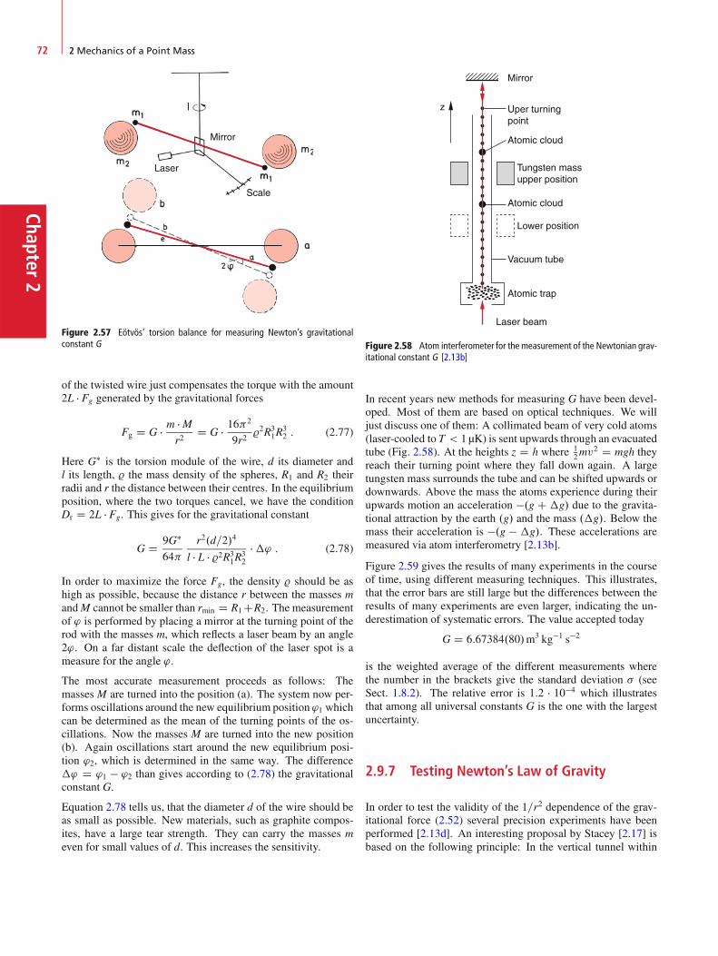
Chapter2
72 2 Mechanics of a Point Mass
Mirror
Laser
Scale
Figure 2.57 Eötvös’ torsion balance for measuring Newton’s gravitationalconstant G
of the twisted wire just compensates the torque with the amount2L � Fg generated by the gravitational forces
Fg D G � m � Mr2
D G � 162
9r2%2R3
1R32 : (2.77)
Here G� is the torsion module of the wire, d its diameter andl its length, % the mass density of the spheres, R1 and R2 theirradii and r the distance between their centres. In the equilibriumposition, where the two torques cancel, we have the conditionDr D 2L � Fg. This gives for the gravitational constant
G D 9G�
64
r2.d=2/4
l � L � %2R31R
32
��' : (2.78)
In order to maximize the force Fg, the density % should be ashigh as possible, because the distance r between the masses mandM cannot be smaller than rmin D R1CR2. The measurementof ' is performed by placing a mirror at the turning point of therod with the masses m, which reflects a laser beam by an angle2'. On a far distant scale the deflection of the laser spot is ameasure for the angle '.
The most accurate measurement proceeds as follows: Themasses M are turned into the position (a). The system now per-forms oscillations around the new equilibrium position '1 whichcan be determined as the mean of the turning points of the os-cillations. Now the masses M are turned into the new position(b). Again oscillations start around the new equilibrium posi-tion '2, which is determined in the same way. The difference�' D '1 � '2 than gives according to (2.78) the gravitationalconstant G.
Equation 2.78 tells us, that the diameter d of the wire should beas small as possible. New materials, such as graphite compos-ites, have a large tear strength. They can carry the masses meven for small values of d. This increases the sensitivity.
Mirror
z Uper turningpoint
Atomic cloud
Atomic cloud
Tungsten massupper position
Lower position
Vacuum tube
Atomic trap
Laser beam
Figure 2.58 Atom interferometer for the measurement of the Newtonian grav-itational constant G [2.13b]
In recent years new methods for measuring G have been devel-oped. Most of them are based on optical techniques. We willjust discuss one of them: A collimated beam of very cold atoms(laser-cooled to T < 1 µK) is sent upwards through an evacuatedtube (Fig. 2.58). At the heights z D h where 1
2mv2 D mgh they
reach their turning point where they fall down again. A largetungsten mass surrounds the tube and can be shifted upwards ordownwards. Above the mass the atoms experience during theirupwards motion an acceleration �.g C �g/ due to the gravita-tional attraction by the earth .g/ and the mass .�g/. Below themass their acceleration is �.g � �g/. These accelerations aremeasured via atom interferometry [2.13b].
Figure 2.59 gives the results of many experiments in the courseof time, using different measuring techniques. This illustrates,that the error bars are still large but the differences between theresults of many experiments are even larger, indicating the un-derestimation of systematic errors. The value accepted today
G D 6:67384.80/m3 kg�1 s�2
is the weighted average of the different measurements wherethe number in the brackets give the standard deviation � (seeSect. 1.8.2). The relative error is 1:2 � 10�4 which illustratesthat among all universal constants G is the one with the largestuncertainty.
2.9.7 Testing Newton’s Law of Gravity
In order to test the validity of the 1=r2 dependence of the grav-itational force (2.52) several precision experiments have beenperformed [2.13d]. An interesting proposal by Stacey [2.17] isbased on the following principle: In the vertical tunnel within
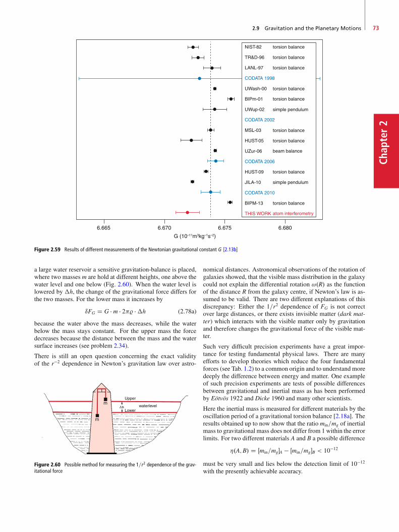
2.9 Gravitation and the Planetary Motions 73
Chap
ter2
6.665 6.670 6.675 6.680
G (10–11m3kg–1s–2)
NIST-82
TR&D-96
LANL-97
CODATA 1998
UWash-00
BIPm-01
UWup-02
CODATA 2002
MSL-03
HUST-05
UZur-06
CODATA 2006
HUST-09
JILA-10
CODATA 2010
BIPM-13
THIS WORK
torsion balance
torsion balance
torsion balance
torsion balance
torsion balance
torsion balance
torsion balance
torsion balance
torsion balance
atom interferometry
beam balance
simple pendulum
simple pendulum
Figure 2.59 Results of different measurements of the Newtonian gravitational constant G [2.13b]
a large water reservoir a sensitive gravitation-balance is placed,where two masses m are hold at different heights, one above thewater level and one below (Fig. 2.60). When the water level islowered by �h, the change of the gravitational force differs forthe two masses. For the lower mass it increases by
ıFG D G � m � 2% ��h (2.78a)
because the water above the mass decreases, while the waterbelow the mass stays constant. For the upper mass the forcedecreases because the distance between the mass and the watersurface increases (see problem 2.34).
There is still an open question concerning the exact validityof the r�2 dependence in Newton’s gravitation law over astro-
Upper
Lowerwaterlevel
Figure 2.60 Possible method for measuring the 1=r2 dependence of the grav-itational force
nomical distances. Astronomical observations of the rotation ofgalaxies showed, that the visible mass distribution in the galaxycould not explain the differential rotation !.R/ as the functionof the distance R from the galaxy centre, if Newton’s law is as-sumed to be valid. There are two different explanations of thisdiscrepancy: Either the 1=r2 dependence of FG is not correctover large distances, or there exists invisible matter (dark mat-ter) which interacts with the visible matter only by gravitationand therefore changes the gravitational force of the visible mat-ter.
Such very difficult precision experiments have a great impor-tance for testing fundamental physical laws. There are manyefforts to develop theories which reduce the four fundamentalforces (see Tab. 1.2) to a common origin and to understand moredeeply the difference between energy and matter. One exampleof such precision experiments are tests of possible differencesbetween gravitational and inertial mass as has been performedby Eötvös 1922 and Dicke 1960 and many other scientists.
Here the inertial mass is measured for different materials by theoscillation period of a gravitational torsion balance [2.18a]. Theresults obtained up to now show that the ratio min=mg of inertialmass to gravitational mass does not differ from 1 within the errorlimits. For two different materials A and B a possible difference
�.A;B/ D Œmin=mg�A � Œmin=mg�B < 10�12
must be very small and lies below the detection limit of 10�12
with the presently achievable accuracy.
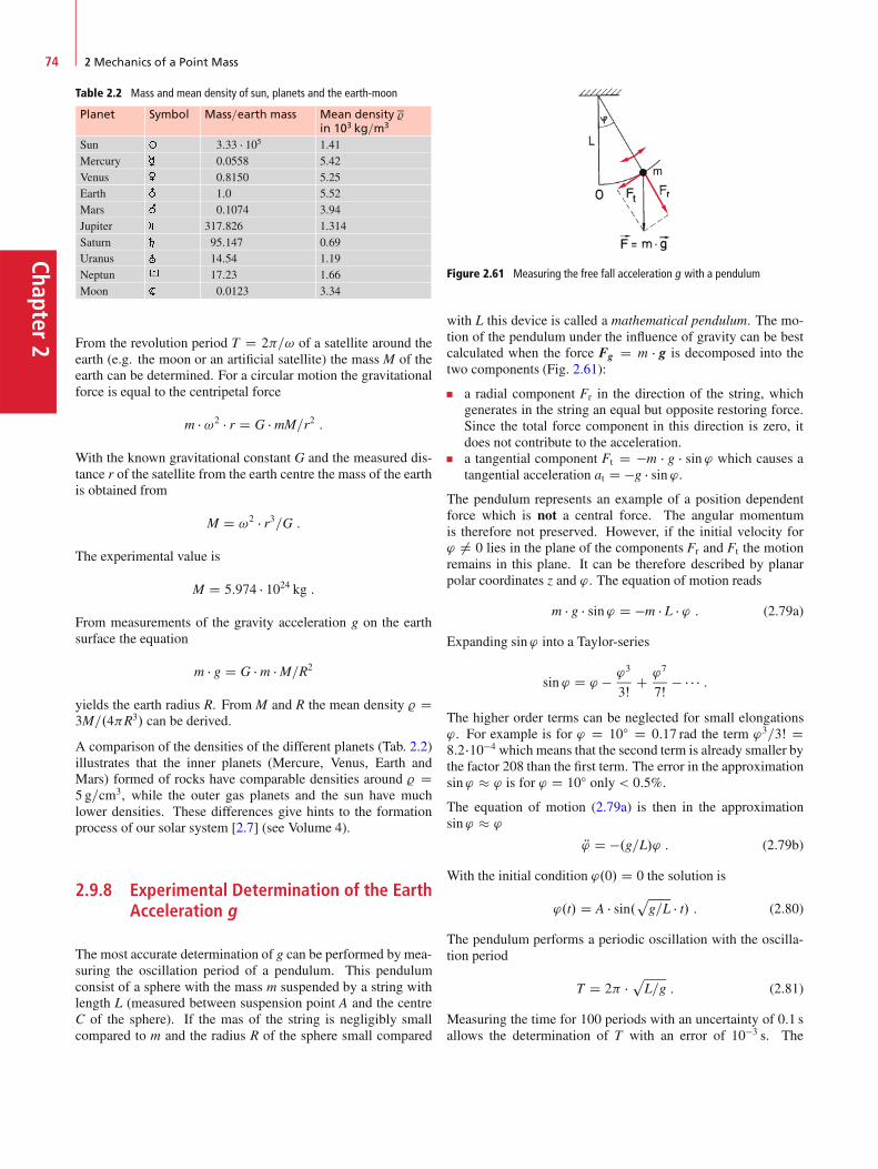
Chapter2
74 2 Mechanics of a Point Mass
Table 2.2 Mass and mean density of sun, planets and the earth-moon
Planet Symbol Mass=earth mass Mean density %in 103 kg=m3
Sun 3:33 � 105 1.41Mercury � 0:0558 5.42Venus � 0:8150 5.25Earth � 1:0 5.52Mars � 0:1074 3.94Jupiter � 317:826 1.314Saturn � 95:147 0.69Uranus � 14:54 1.19Neptun � 17:23 1.66Moon 0:0123 3.34
From the revolution period T D 2=! of a satellite around theearth (e.g. the moon or an artificial satellite) the mass M of theearth can be determined. For a circular motion the gravitationalforce is equal to the centripetal force
m � !2 � r D G � mM=r2 :
With the known gravitational constant G and the measured dis-tance r of the satellite from the earth centre the mass of the earthis obtained from
M D !2 � r3=G :
The experimental value is
M D 5:974 � 1024 kg :
From measurements of the gravity acceleration g on the earthsurface the equation
m � g D G � m � M=R2
yields the earth radius R. From M and R the mean density % D3M=.4R3/ can be derived.
A comparison of the densities of the different planets (Tab. 2.2)illustrates that the inner planets (Mercure, Venus, Earth andMars) formed of rocks have comparable densities around % D5 g=cm3, while the outer gas planets and the sun have muchlower densities. These differences give hints to the formationprocess of our solar system [2.7] (see Volume 4).
2.9.8 Experimental Determination of the EarthAcceleration g
The most accurate determination of g can be performed by mea-suring the oscillation period of a pendulum. This pendulumconsist of a sphere with the mass m suspended by a string withlength L (measured between suspension point A and the centreC of the sphere). If the mas of the string is negligibly smallcompared to m and the radius R of the sphere small compared
Figure 2.61 Measuring the free fall acceleration g with a pendulum
with L this device is called a mathematical pendulum. The mo-tion of the pendulum under the influence of gravity can be bestcalculated when the force Fg D m � g is decomposed into thetwo components (Fig. 2.61):
a radial component Fr in the direction of the string, whichgenerates in the string an equal but opposite restoring force.Since the total force component in this direction is zero, itdoes not contribute to the acceleration.a tangential component Ft D �m � g � sin ' which causes atangential acceleration at D �g � sin '.
The pendulum represents an example of a position dependentforce which is not a central force. The angular momentumis therefore not preserved. However, if the initial velocity for' ¤ 0 lies in the plane of the components Fr and Ft the motionremains in this plane. It can be therefore described by planarpolar coordinates z and '. The equation of motion reads
m � g � sin' D �m � L � ' : (2.79a)
Expanding sin' into a Taylor-series
sin ' D ' � '3
3ŠC '7
7Š� � � � :
The higher order terms can be neglected for small elongations'. For example is for ' D 10ı D 0:17 rad the term '3=3Š D8:2�10�4 which means that the second term is already smaller bythe factor 208 than the first term. The error in the approximationsin' � ' is for ' D 10ı only < 0:5%.
The equation of motion (2.79a) is then in the approximationsin' � '
R' D �.g=L/' : (2.79b)
With the initial condition '.0/ D 0 the solution is
'.t/ D A � sin.pg=L � t/ : (2.80)
The pendulum performs a periodic oscillation with the oscilla-tion period
T D 2 �pL=g : (2.81)
Measuring the time for 100 periods with an uncertainty of 0:1 sallows the determination of T with an error of 10�3 s. The

2.9 Gravitation and the Planetary Motions 75
Chap
ter2
largest uncertainty comes from the measurement of the lengthL. The errors for L and T in the determination of
g D 42 � LT2
give a total error of g according to
ˇ̌ˇ̌�g
g
ˇ̌ˇ̌ � 2
ˇ̌ˇ̌�T
T
ˇ̌ˇ̌C �L
L:
Example
�T=T D 5 � 10�5, �L=L D 10�3 for L D 1m. )�g=g D 1:1 � 10�3. J
For a more accurate solution of (2.79a) we use the energy con-servation law (see Sect. 2.7), which saves one integration. FromFig. 2.62 we see that
Ep D m � g � L � .1 � cos'/
Ekin D 12m � v2 D 1
2mL2 � '2 :
The constant total energy is
E D Ep C Ekin D m
2L2 P'2 C mgL.1 � cos'/
D mgL.1 � cos'0/ :
Where '0 is the angle at the turning point where Ekin D 0. Solv-ing for ' gives
d'
dtDr
2g.cos' � cos'0/
L:
Integration yields
sL
2g
'0Z
'D0
d'pcos' � cos'0
DT=4Z
tD0
dt D T=4 : (2.82)
Figure 2.62 Illustration of the integration of the pendulum equation based onthe energy conservation
Figure 2.63 Dependence of the oscillation period on the deflection of the pen-dulum
With the substitution sin � D sin.'=2/= sin.'0=2/ the integralcan be reduced to an elliptical integral
T D 4pL=g
=2Z
0
d�p1 � k2sin2�
with k D sin.'0=2/ ;
(2.83)
which can be solved by a Taylor expansion of the inte-grand [2.18b]. The result is
T.'0/ D 2
sL
g
�1 C 1
16'20 C � � �
�: (2.84)
For the accurate determination of T the oscillation period ismeasured as a function of the elongation '0 and the measuredvalues are extrapolated towards '0 D 0 (Fig. 2.63).
If the shape of the earth is approximated by a spheroid the de-pendence of g on the latitude ˇ D 90ı �# can be approximatedby the formula
g.ˇ/ � ge�1 C 0:0053024 sin2 ˇ
� 5:8 � 106sin2 2ˇ� (2.85)
where ge D g.ˇ D 0/ D 9:780327m=s2 is the earth acceler-ation at the equator. This formula takes into account, that g isdiminished by the centrifugal acceleration of the rotating earthwhich depends on ˇ (see Sect. 3.2). Because of the inhomoge-neous mass distribution of the earth additional local changes ofg appear which are not considered in (2.85).
Instead of the pendulum nowadays modern gravimeters are usedfor the determination of g. These are sensitive spring balanceswhich had been calibrated with a precision pendulum. Therestoring force F D �D.x � x0/ is determined by measuringthe displacement from the equilibrium position by a calibratedmass m and gets the local variation of the earth acceleration gaccording to [2.19]
m � g D �D.x � x0/ :
Recently two identical satellites were launched which orbitaround the earth on identical paths with an angle distance �'.
Chapter2
76 2 Mechanics of a Point Mass
This distance can be measured very accurately (within a fewmillimetres) by the time laser pulses need to travel from onesatellite to the other and back. Local variations of the gravitycause a different local acceleration which changes the distanced D R ��' between the satellites. This allows the determinationof even tiny changes of the gravity force [2.20a, 2.20b, 2.20c].
Summary
A body with massm can be described by the model of a pointmass as long as its spatial extensions are small compared toits distance to other bodies.The motion of a body is described by a trajectory r.t/, whichthe body traverses in the course of time. Its momentary ve-locity is v.t/ D Pr D dr=dt and its acceleration is a.t/ Ddv=dt D d2r=dt2.Motions with a.t/ D 0 are called uniform straight-line mo-tions. Magnitude and direction of the velocity are constant.For the uniform circular motion the magnitude ja.t/j is con-stant, but the direction of a.t/ changes uniformly with theangular velocity !.A force acting on a freely movable body causes an accelera-tion and therefore a change of its state of motion.A body is in an equilibrium state if the vector sum of all act-ing forces is zero. In this case it does not change its state ofmotion.The state of motion of a body with mass m and velocity v isdefined by the momentum p D m � v.The force F acting on a body is defined as F D dp=dt(2. Newton’s law).For two bodies with masses m1 and m2 which interact witheach other but not with other bodies the 3. Newtonian law isvalid: F1 D �F2 (F1 is the force acting on m1, F2 acting onm2/.The work executed by the force F.r/ on a body moving alongthe trajectory r.t/ is the scalar quantityW D R
F.r/dr.Force fields where the work depends only on the initial pointP1 and the final point P2 but not on the choice of the pathbetween P1 and P2 are called conservative. For such fieldsis rotF D 0. All central force fields are conservative.To each point P in a conservative force field a potential en-ergy Ep.P/ can be attributed. The work
RF.r/dr D E.P1/�
E.P2/ executed on a body to move it from P1 to P2 is equalto the difference of the potential energies in P1 and P2. Thechoice of the point of zero energy is arbitrarily. Often onechooses E.r D 0/ D 0 or E.r D 1/ D 0.The potential energy E.P/ and the force F.r/ in a conserva-tive force field are related by F.r/ D �gradEp.The kinetic energy of a mass mmoving with the velocity v isEkin D 1
2mv2.
In a conservative force field the total energy E D Ep C Ekin
is constant (law of energy conservation).The angular momentum of a mass m with momentum p, re-ferred to the origin of the coordinate system is L D r p Dm � .r v/. The torque acting on a body in a force field F.r/is D D r F. It is D D dL=dt.All planets of our solar system move in the central force fieldF.r/ D �G � .m � M=r2/Or of the sun. Therefore their an-gular momentum is constant. Their motion is planar. Theirtrajectories are ellipses with the sun in one focal point.The gravitational field of extended bodies depends on themass distribution. For spherical symmetric mass distribu-tions with radius R the force field outside the body (r > R)is exactly that of a point mass, inside the body (r < R) theforce F.r/ increases for homogeneous distributions linearlywith r from F D 0 at the centre r D 0 to the maximum valueat r D R.The free fall acceleration g of a body with mass m equals thegravitational field strength G D F=m at the surface r D R ofthe earth with mass M. With Newton’s law of gravity g canbe expressed as g D G � .M=R2/Or (G D gravitational con-stant). It can be determined from the measured oscillationperiod T D 2
pL=g of a pendulum with length L, or with
gravitational balances.

Problems 77
Chap
ter2
Problems
2.1 A car drives on a road behind a foregoing truck (lengthof 25m) with a constant safety distance of 40m and a constantvelocity of 80 km=h. As soon as the driver can foresee a freedistance of 300m he starts to overtake. Therefore he accelerateswith a D 1:3m=s2 until he reaches a velocity of v D 100 km=h.Can he safely overtake? How long are time and path length ofthe overtaking procedure if he considers the same safety dis-tance after the overtaking? Draw for illustration a diagram fors.t/ and v.t/.
2.2 A car drives half of a distance x with the velocity v1 D80 km=h and the second half with v2 D 40 km=h. Estimate andcalculate the mean velocity hvi as the function of v1 and v2.Make the same consideration if x1 D 1=3x and x2 D 2=3x.
2.3 A body moves with constant acceleration along the x-axis. It passes the origin x D 0 with v D 6 cm=s. 2 s later itarrives at x D 10 cm. Calculate magnitude and direction of theacceleration.
2.4 An electron is emitted from the cathode with a velocityv0 and experiences in an electric field over a distance of 4 cm aconstant acceleration a D 3 � 1014 m=s2, reaching a velocity of7 � 106 m=s. How large was v0?
2.5 A body is thrown from a height h D 15m with an initialvelocity v0 D 5m=sa) upwards,b) downwards.Calculate for both cases the time until it reaches the ground.c) Derive Eq. 2.13.
2.6 Give examples where both the magnitude and the di-rection of the acceleration are constant but the body movesnevertheless not on a straight line. Which conditions must befulfilled for a straight line?
2.7 A car crashes with a velocity of 100 km=h against a thicktree. From which heights must it fall down in order to experi-ence the same velocity when reaching the ground? Compare thiswith two equal cars with velocities of 100 km=h crashing headon against each other.
2.8a) A body moves with constant angular velocity ! D 3 rad=s
on a vertical circle in the x-z-plane with radius R D 1m inthe gravity field F D f0; 0;�gg of the earth. How large areits velocities at the lowest and the highest point on the circle?How large is the difference between the two values? Couldyou relate this to the potential energy?
b) A body starts with v0 D 0 from the point A.z D h/ inFig. 2.64 on the frictionless looping path. How large are
velocities and accelerations in the points B and C of the cir-cular path with radius R? What is the maximum ratio R=h toprevent that the body falls down in B? How large is then thevelocity v.B/?
Figure 2.64 Looping path (Probl. 2.8 b)
2.9 How large is the escape velocitya) of the moon (d D 384 000 km) in the gravitational field of
the earth?b) of a body on the surface of the moon in the gravitational field
of the moon?
2.10 What is the minimum fuel mass of a one stage rocketwith a payload of 500 kg for a horizontal launch at the equatorto bring the rocket to the first escape velocity of v1 D 7:9 km=swhen the velocity of the propellant gas relative to the rocket isve D 4:5 km=ha) in the east directionb) in the west direction?
2.11 Check the energy conservation law for the examplesgiven in the text. Show, that (2.26) follows directly from thecondition Ekin � Ep, i. e. 1
2mv2 � m � g � R.
2.12 A rocket to the moon is launched from a point at theequator. How much energy is saved compared to a verticallaunch, when it is shot in the eastern direction under 30ı againstthe horizontal?
2.13 A wooden cylinder (radius r D 0:1m, heights h D0:6m) is vertically immersed in water with 2=3 of its lengthwhich is its equilibrium position. Which work has to be per-formed when it is pulled out of the water? How is the situationif the cylinder lies horizontally in the water? How deep does itimmerse?
2.14 A body with mass m D 0:8 kg is vertically thrown up-wards. In the heights h D 10m its kinetic energy is 200 J. Whatis the maximum heights it can reach?
Chapter2
78 2 Mechanics of a Point Mass
2.15 A spiral spring of steel with length L0 D 0:8m is ex-panded by the force F D 20N to a length L D 0:85m. Whichwork is needed to expand the spring to twice its initial length, ifthe force is always proportional to the expansion�L D L � L0?
2.16 What is the minimum initial velocity of a body at a ver-tical launch from the earth when it should reach the moon?
2.17 What is the distance of a geo-stationary satellite fromthe centre of the earth? Which energy is needed to launch it?How accurate has its distance to the earth centre be stabilized inorder to maintain its position relative to a point on earth within0:1 km=d?
2.18 What is the change of potential, kinetic and total energyof a satellite when its radius r on a stable circular orbit aroundthe earth centre is changed? What is the ratio Ekin=Ep? Doesit depend on r? Express the total energy E by m, g, r and themassME of the earth. Are these quantities sufficient or are moreneeded?
2.19 Prove, that the force F D m � g � sin ' � et for the math-ematical pendulum is conservative and that for arbitrary valuesof ' conservation of energy Ekin C Ep D const holds.
2.20 Assume one is able to measure the length L D 10m ofa pendulum within 0:1mm and the period T within 10ms. Howmany oscillation periods have to be measured in order to equal-ize the contribution of �L and �T to the accuracy of g? Howlarge is then the uncertainty of g?
2.21 Howmuch accuracy is gained for the determination ofGwith the gravity balance if the large masses M are increased bya factor of 10? How accurate has the measurement of the angle' to be in order to determine G with an accuracy of 10�4? Givesome physical reasons for the limits of the accuracy of '.
2.22 The comet Halley has a period of 76 years. His small-est distance to the sun is 0.59AU. How large is its maximumdistance to the sun and what is the eccentricity of its ellipticalorbit? Hint: Look for a relation between T and rmin D a.1 � "/and rmax D a.1 C "/.
2.23 Assume that the gravity acceleration at the equator ofa rotating planet is 11:6m=s2, the centripetal acceleration a D0:3m=s2 and the escape velocity for a vertical launch 23:6m=s.At the heights h D 5000 km above the surface is g D 8:0m=s2.What are the radius R and the massM of the planet. How fast isit rotating? Which planet meets these requirements?
2.24 The gravitational force exerted by the sun onto the moonis about twice as large as that exerted by the earth. Why is themoon still circling around the earth and has not escaped?
2.25 Which oscillation period would a pendulum have on themoon, if its period on the earth is 1 s?
2.26 A vertical straight tunnel is cut through the earth be-tween opposite points A to B on the earth surface.a) Show that without friction a body released in A performs a
harmonic oscillation between A and B.b) What is the oscillation period?c) Compare this value with the period of a satellite, which cir-
cles around the earth closely above the surface.d) A straight tunnel is cut between London and New York.
What is the travel time of a train without friction and extradriving force (besides gravity) which starts in London withthe velocity v0 D 0? How much does the time change, ifv0 D 40m=s?
2.27 Calculate the distance earth-moon from the period ofrevolution of the moon T D 27 d (mass of the earth is M D6 � 1024 kg).
2.28 Saturn has a massM D 5:7 � 1026 kg and a mean densityof 0:71 g=cm3. How large is the gravitational acceleration on itssurface?
2.29 How large is the relative change of the gravity acceler-ation g between a point on the earth surface and a point withh D 160 km above the surface?
2.30 How large is the change�g of the earth acceleration dueto the attraction bya) the moon andb) the sun?Compare the two changes and discuss them. How large is therelative change�g=g?
2.31 Two spheres made of lead with masses m1 D m2 D20 kg are suspended by two thin wires with length L D 100mwhere the suspension points are 0:2m apart. What is the dis-tance between the centres of the spheres, when the gravitationalfield of the earth is assumed to be spherical symmetric?a) withoutb) with the gravitational force between the two masses.
2.32 Based on the energy conservation law determine thevelocity of the earth in its closest distance from the sun (Per-ihelion) and for the largest distance (aphelion). How large isthe difference �v to the mean velocity? Discuss the relationbetween the eccentricity of the elliptical orbit and �v.
2.33 A satellite orbiting around the earth has the velocityvA D 5 km=s in the aphelion and vP D 7 km=s in its perihe-lion. How large are minor and major half axes of its ellipticalorbit?
2.34 Prove the equation (2.78a).
References 79
Chap
ter2
References
2.1. F. Cajori (ed.), Sir Isaac Newton’s Mathematical Princi-ples of Natural Philosophy and His System of the World.(Principia). (University of California Press, Berkely,1962)
2.2. R.V. Eötvös, D. Pekart, F. Fekete, Ann. Phys. 68 11(1922)
2.3. A.P. French, Special Relativity Theory. (MIT Interoduc-tor Series Norton & Company, 1968)
2.4. A. Beer, P. Beer (ed.) Kepler. Four Hundred Years. (Perg-amon, Oxford, 1975)
2.5a. J. Stuhler, M. Fattori, T. Petelski, G.M. Tino, J. Opt. B:Quantum Semiclass. Opt. 5 75 (2003)
2.5b. A. Bertoldi et al., Europ Phys. Journal D 40, 271 (2006)2.6a. B.R. Martin, C. Shaw Mathematics for Physicists.
Manchester Physics Series. (Wiley, London, 2015)2.6b. A. Jeffrey, D. Zwillinger, Table of Integrals, Series and
Products. 8th ed. (Elsevier Oxford, 2014)2.7. M.A. Seeds, D. Backman, Foundations of Astronomy,
13th ed. (Cangage Learning, 2015)2.8. E. Chaisson, St. McMillan, A Beginners Guide to the
Universe. 7th ed (Benjamin Cummings Publ. Comp.,2012)
2.9a. W.M. Kaula, Satellite Measurements of the Earth’s Grav-ity Field. in Methods of Experimental Physics. ed. byR. Celotta, J. Levine, Ch.G. Sammis, Th.L. Henyey,Vol. 24, part B (Academic Press, San Diego, 1987), p.163
2.9b. Ch. Hirt et al., Geophys. Research Lett. 40(16), 4279(2013)
2.9c. http://en.wikipedia.org/wiki/Gravity_of_Earth2.10. R.H. Rapp, F. Sanso (ed.) Determination of the Geoid.
(Springer, Berlin, Heidelberg, 1991)
2.11. C.M.R. Fowler The Solid Earth: An Introduction toGlobal Geophysics, 2nd ed. (Cambridge Univ. Press,Cambridge, 2004)
2.12a. https://en.wikipedia.org/wiki/Gravitational_constant2.12b. B. Fixler, G.T. Foster, J.M. McGuirk, M.A. Kasevich,
Science 315(5808), 74 (2007)2.13a. H.V. Parks, Phys. Rev. Lett. 105, 110801 (2010)2.13b. G. Rosi et al., Nature 510, 518 (2014)2.13c. C. Moskowitz, Puzzling Measurement of “Big G” Grav-
itational Constant. Scientific American, Sept. 18, 20132.13d. T. Quinn, Nature 408, 919 (2000)2.14. P.J. Mohr, B.N. Taylor, Rev. Mod. Physics 80, 633 (2008)2.15. NIST: Reference on constants, units and uncertainties.
http://physics.nist.gov/cuu/2.16a. C.C. Speake, T.M. Niebauer et al., Phys. Rev. Lett. 65,
1967 (1990)2.16b. C.W. Misner, K.S. Thorne, J.A. Wheeler, Gravitation.
(Freeman, San Franscisco, 1973)2.17. F. Stacey, G. Tuck, Phys. World 1(12), 29 (1988)2.18a. C.B. Braginski, V.I. Panov, Sov. Phys. JETP 34, 464
(1971)2.18b. https://en.wikipedia.org/wiki/Elliptic_Intergral2.19. R. Celotta, J. Levine, Ch.G. Sammis, Th.L. Henyey (ed.),
Methods od experimental Physics, Vol. 24 (AcademicPress, San Diego, 1987)
2.20a. https://en.wikipedia.org/wiki/Geographic_information_system
2.20b. http://www.stevenswater.com/telemetry_com/leo_info.aspx
2.20c. Ch. Hwang, C.K. Shum, J. Li (ed.), Satellite Altimetryfor Geodesy, Geophysics and Oceanography. (Springer,Berlin, Heidelberg, 2004)
Chap
ter3
Moving Coordinate Systemsand Special Relativity 33.1 Relative Motion . . . . . . . . . . . . . . . . . . . . . . . . . . . . . . . . 82
3.2 Inertial Systems and Galilei-Transformations . . . . . . . . . . . . . . . . 82
3.3 Accelerated Systems; Inertial Forces . . . . . . . . . . . . . . . . . . . . . 83
3.4 The Constancy of the Velocity of Light . . . . . . . . . . . . . . . . . . . 89
3.5 Lorentz-Transformations . . . . . . . . . . . . . . . . . . . . . . . . . . . 90
3.6 Theory of Special Relativity . . . . . . . . . . . . . . . . . . . . . . . . . . 92
Summary . . . . . . . . . . . . . . . . . . . . . . . . . . . . . . . . . . . . 100
Problems . . . . . . . . . . . . . . . . . . . . . . . . . . . . . . . . . . . . 100
References . . . . . . . . . . . . . . . . . . . . . . . . . . . . . . . . . . . 101
81© Springer International Publishing Switzerland 2017W. Demtröder, Mechanics and Thermodynamics, Undergraduate Lecture Notes in Physics, DOI 10.1007/978-3-319-27877-3_3

Chapter3
82 3 Moving Coordinate Systems and Special Relativity
For the description of the location and the velocity of a body ina three-dimensional space one needs a coordinate system wherethe position vectors r.t/ and its time derivative dr=dt D v.t/ aredefined. Of course are all physical processes independent of thechoice of the coordinate system. However, their mathematicalformulation can be much simpler in a suitable coordinate systemthan in other systems. It is therefore essential to choose that sys-tem which allows the optimum description of a process and tofind the transformation equations to change from one to anothercoordinate system.
For example is the coordinate system connected with the earthwhich moves around the sun, the best choice for the descrip-tion of measurements on earth. For astronomical observationsthe results of such measurements must be transformed into agalactic coordinate system which has its origin in the galacticcentre and moves with the rotating galaxy, in order to eliminatethe complex motion of the earth relative to the galactic centre.For coordinate systems at rest these transformations impose noproblems. The situation is different for systems which moveagainst each other.
In this chapter we will discuss question which arise for trans-formations between moving coordinate systems when physicalprocesses are described in different systems. It turns out thatmany concepts derived from daily life experience which weretaken for granted, had to be revised. The mathematical frame-work for such revisions is the special relativity theory developedby Albert Einstein, which will be briefly treated in this chapter.
3.1 Relative Motion
An observer, sitting in the origin O of a coordinate system looksat two objects A and B with the coordinates rA and rB and therelative distance
rAB D rA � rB ; (3.1)
which move with the velocities
vA D drAdt
and vB D drBdt
relative to the coordinate system O (Fig. 3.1). The velocity of Arelative to B is then
vAB D drABdt
D vA � vB ; (3.2a)
while the velocity of B relative to A
vBA D vB � vA D �vAB : (3.2b)
This illustrates that position vector and velocity do depend onthe reference system.
Figure 3.1 Definition of the relative distance
3.2 Inertial Systems andGalilei-Transformations
Two observers B and B0 sit in the originsO andO0 of two coordi-nate systems S.x; y; z/ and S0.x0; y0; z0/ which move against eachother with the constant velocity u (Fig. 3.2). Both observersmeasure the motion of an object A. which has the position vec-tor r.x; y; z/ in the system S and r0.x0; y0; z0/ in the system S0.
As can be erived from Fig. 3.2 it is
r0 D r � u � t ; (3.3)
which can be written for the components as
8ˆ̂̂<
ˆ̂̂:
x0.t/D x.t/ � ux � ty0.t/D y.t/ � uy � tz0.t/D z.t/ � uz � t
t0 D t
9>>>=
>>>;; (3.3a)
where t D t0 means that both observers use synchronized equalclocks for their time measurements. This is not obvious and isgenerally not true if the velocity u approaches the velocity oflight (see Sect. 3.4). For the velocity of A the two observers find
v D drdt
and v0 D dr0
dt: (3.4)
From (3.3) follows
v0 D v � u : (3.5)
Figure 3.2 The coordinates of a point A, described in two different systems Oand O 0 which move against each other with the constant velocity u
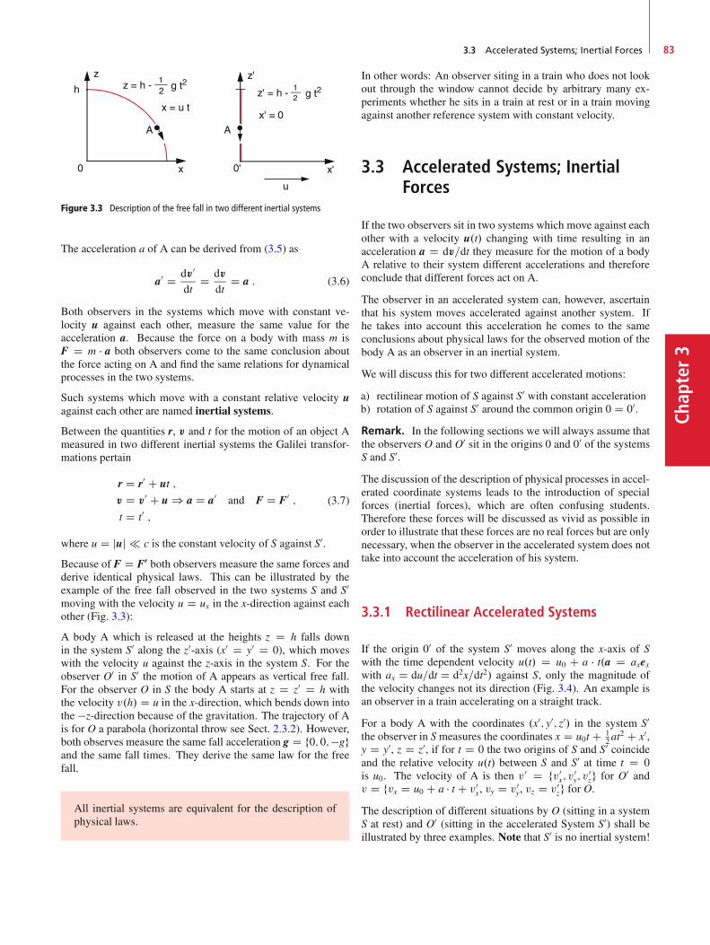
3.3 Accelerated Systems; Inertial Forces 83
Chap
ter3
Figure 3.3 Description of the free fall in two different inertial systems
The acceleration a of A can be derived from (3.5) as
a0 D dv0
dtD dv
dtD a : (3.6)
Both observers in the systems which move with constant ve-locity u against each other, measure the same value for theacceleration a. Because the force on a body with mass m isF D m � a both observers come to the same conclusion aboutthe force acting on A and find the same relations for dynamicalprocesses in the two systems.
Such systems which move with a constant relative velocity uagainst each other are named inertial systems.
Between the quantities r, v and t for the motion of an object Ameasured in two different inertial systems the Galilei transfor-mations pertain
r D r0 C ut ;
v D v0 C u ) a D a0 and F D F0 ;t D t0 ;
(3.7)
where u D juj c is the constant velocity of S against S0.
Because of F D F0 both observers measure the same forces andderive identical physical laws. This can be illustrated by theexample of the free fall observed in the two systems S and S0moving with the velocity u D ux in the x-direction against eachother (Fig. 3.3):
A body A which is released at the heights z D h falls downin the system S0 along the z0-axis (x0 D y0 D 0), which moveswith the velocity u against the z-axis in the system S. For theobserver O0 in S0 the motion of A appears as vertical free fall.For the observer O in S the body A starts at z D z0 D h withthe velocity v.h/ D u in the x-direction, which bends down intothe �z-direction because of the gravitation. The trajectory of Ais for O a parabola (horizontal throw see Sect. 2.3.2). However,both observes measure the same fall acceleration g D f0; 0;�ggand the same fall times. They derive the same law for the freefall.
All inertial systems are equivalent for the description ofphysical laws.
In other words: An observer siting in a train who does not lookout through the window cannot decide by arbitrary many ex-periments whether he sits in a train at rest or in a train movingagainst another reference system with constant velocity.
3.3 Accelerated Systems; InertialForces
If the two observers sit in two systems which move against eachother with a velocity u.t/ changing with time resulting in anacceleration a D dv=dt they measure for the motion of a bodyA relative to their system different accelerations and thereforeconclude that different forces act on A.
The observer in an accelerated system can, however, ascertainthat his system moves accelerated against another system. Ifhe takes into account this acceleration he comes to the sameconclusions about physical laws for the observed motion of thebody A as an observer in an inertial system.
We will discuss this for two different accelerated motions:
a) rectilinear motion of S against S0 with constant accelerationb) rotation of S against S0 around the common origin 0 D 00.
Remark. In the following sections we will always assume thatthe observers O and O0 sit in the origins 0 and 00 of the systemsS and S0.
The discussion of the description of physical processes in accel-erated coordinate systems leads to the introduction of specialforces (inertial forces), which are often confusing students.Therefore these forces will be discussed as vivid as possible inorder to illustrate that these forces are no real forces but are onlynecessary, when the observer in the accelerated system does nottake into account the acceleration of his system.
3.3.1 Rectilinear Accelerated Systems
If the origin 00 of the system S0 moves along the x-axis of Swith the time dependent velocity u.t/ D u0 C a � t.a D axexwith ax D du=dt D d2x=dt2/ against S, only the magnitude ofthe velocity changes not its direction (Fig. 3.4). An example isan observer in a train accelerating on a straight track.
For a body A with the coordinates .x0; y0; z0/ in the system S0the observer in Smeasures the coordinates x D u0t C 1
2at2 C x0,
y D y0, z D z0, if for t D 0 the two origins of S and S0 coincideand the relative velocity u.t/ between S and S0 at time t D 0is u0. The velocity of A is then v0 D fv0
x; v0y; v
0zg for O0 and
v D fvx D u0 C a � t C v0x, vy D v0
y, vz D v0zg for O.
The description of different situations by O (sitting in a systemS at rest) and O0 (sitting in the accelerated System S0) shall beillustrated by three examples. Note that S0 is no inertial system!
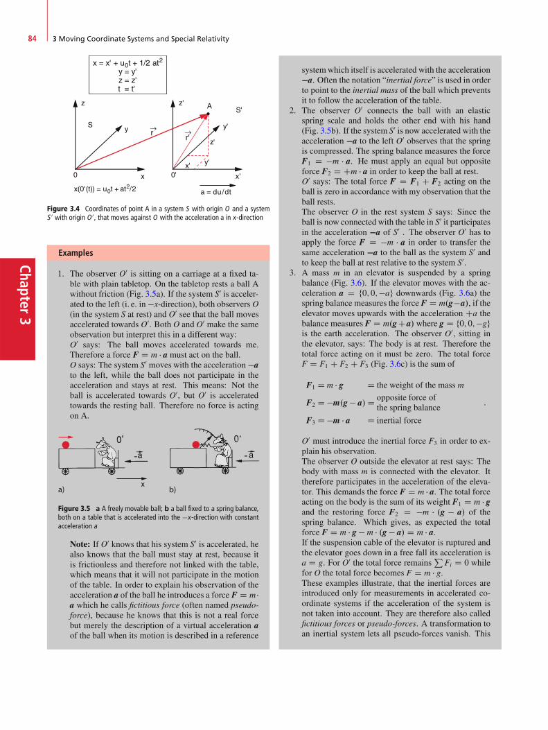
Chapter3
84 3 Moving Coordinate Systems and Special Relativity
Figure 3.4 Coordinates of point A in a system S with origin O and a systemS 0 with origin O 0, that moves against O with the acceleration a in x-direction
Examples
1. The observer O0 is sitting on a carriage at a fixed ta-ble with plain tabletop. On the tabletop rests a ball Awithout friction (Fig. 3.5a). If the system S0 is acceler-ated to the left (i. e. in �x-direction), both observers O(in the system S at rest) and O0 see that the ball movesaccelerated towards O0. Both O and O0 make the sameobservation but interpret this in a different way:O0 says: The ball moves accelerated towards me.Therefore a force F D m � a must act on the ball.O says: The system S0 moves with the acceleration �ato the left, while the ball does not participate in theacceleration and stays at rest. This means: Not theball is accelerated towards O0, but O0 is acceleratedtowards the resting ball. Therefore no force is actingon A.
a) b)
Figure 3.5 a A freely movable ball; b a ball fixed to a spring balance,both on a table that is accelerated into the �x-direction with constantacceleration a
Note: If O0 knows that his system S0 is accelerated, healso knows that the ball must stay at rest, because itis frictionless and therefore not linked with the table,which means that it will not participate in the motionof the table. In order to explain his observation of theacceleration a of the ball he introduces a force F D m �a which he calls fictitious force (often named pseudo-force), because he knows that this is not a real forcebut merely the description of a virtual acceleration aof the ball when its motion is described in a reference
systemwhich itself is accelerated with the acceleration�a. Often the notation “inertial force” is used in orderto point to the inertial mass of the ball which preventsit to follow the acceleration of the table.
2. The observer O0 connects the ball with an elasticspring scale and holds the other end with his hand(Fig. 3.5b). If the system S0 is now accelerated with theacceleration �a to the left O0 observes that the springis compressed. The spring balance measures the forceF1 D �m � a. He must apply an equal but oppositeforce F2 D Cm � a in order to keep the ball at rest.O0 says: The total force F D F1 C F2 acting on theball is zero in accordance with my observation that theball rests.The observer O in the rest system S says: Since theball is now connected with the table in S0 it participatesin the acceleration �a of S0 . The observer O0 has toapply the force F D �m � a in order to transfer thesame acceleration �a to the ball as the system S0 andto keep the ball at rest relative to the system S0.
3. A mass m in an elevator is suspended by a springbalance (Fig. 3.6). If the elevator moves with the ac-celeration a D f0; 0;�ag downwards (Fig. 3.6a) thespring balance measures the force F D m.g�a/, if theelevator moves upwards with the acceleration Ca thebalance measures F D m.gCa/ where g D f0; 0;�ggis the earth acceleration. The observer O0, sitting inthe elevator, says: The body is at rest. Therefore thetotal force acting on it must be zero. The total forceF D F1 C F2 C F3 (Fig. 3.6c) is the sum of
F1 D m � g D the weight of the mass m
F2 D �m.g � a/D opposite force ofthe spring balance
F3 D �m � a D inertial force
:
O0 must introduce the inertial force F3 in order to ex-plain his observation.The observer O outside the elevator at rest says: Thebody with mass m is connected with the elevator. Ittherefore participates in the acceleration of the eleva-tor. This demands the force F D m � a. The total forceacting on the body is the sum of its weight F1 D m � gand the restoring force F2 D �m � .g � a/ of thespring balance. Which gives, as expected the totalforce F D m � g � m � .g � a/ D m � a.If the suspension cable of the elevator is ruptured andthe elevator goes down in a free fall its acceleration isa D g. For O0 the total force remains
PFi D 0 while
for O the total force becomes F D m � g.These examples illustrate, that the inertial forces areintroduced only for measurements in accelerated co-ordinate systems if the acceleration of the system isnot taken into account. They are therefore also calledfictitious forces or pseudo-forces. A transformation toan inertial system lets all pseudo-forces vanish. This

3.3 Accelerated Systems; Inertial Forces 85
Chap
ter3
means an observer O in an inertial system does notneed any pseudo-force for the explanation of the ob-served physical processes.
Figure 3.6 Elevator experiment. Description of the forces acting ona mass m, that hangs on a spring balance in an elevator accelerateddownwards in a and upwards in b. In c the forces are listed as observedby O 0 in the elevator (left hand side) and by O at rest outside the elevator(right hand side) J
3.3.2 Rotating Systems
We regard two coordinate systems S.x; y; z/ and S0.x0; y0; z0/withthe unit vectors Oex, Oey, Oez and Oex0 , Oey0 , Oez0 of the coordinate axesand a common origin 0 D 00. S0 rotates against S with the con-stant angular velocity! D f!x; !y; !zg around 0 D 00 (Fig. 3.7).S0 is therefore no inertial system. We assume that for all times0 D 00.
A point A should have at time t in the system S the positionvector
r.t/ D x.t/ � Oex C y.t/ � Oey C z.t/ � Oez (3.8)
and the velocity
v.t/ D dx
dtOex C dy
dtOey C dz
dtOez : (3.9)
The same point A has in the system S0 the position vector
r0.t/ D r.t/ D x0 Oex0 C y0 Oey0 C z0 Oez0 : (3.10)
y
Figure 3.7 A system S 0, that rotates around the axis ! against S . Both sys-tems have the same origin O D O 0
Note: r D r0 means that we regard the same vector in bothsystems with the same magnitude but different components.
If the observer O0 does not take into account that his systemrotates, he will define as the velocity of A in his system
v0.t/ D dr0
dtD dx0
dtOex0 C dy0
dtOey0 C dz0
dtOez0 : (3.11)
However, if the observer O in the inertial system S describes thevelocity of A in the coordinates of S0. he knows that the axis ofS0 are rotating and therefore not constant in time. He thereforemust write:
v.x0; y0; z0/ D�dx0
dtOex0 C dy0
dtOey0 C dz0
dtOez0�
C�x0 dOex0
dtC y0 dOey0
dtC z0 dOez0
dt
�
D v0 C u :
(3.12)
The endpoints of the unit vectors Oex0 , Oey0 , Oez0 perform a circu-lar motion with the angular velocity ! around 0 D 00. Theirvelocity is then
dOex0
dtD ! Oex0 I dOey0
dtD ! Oey0 I dOez0
dtD ! Oe0
z : (3.13)
Inserting this into (3.12) the second term in (3.12) becomes
u D .! Oex0/x0 C .! Oey0/y0 C .! Oez0/z0
D ! .Oex0x0 C Oey0y0 C Oez0z0/D ! r0 D ! r; because r � r0 :
We therefore get the transformation between the velocity v ofthe point A measured by O in the system S and the velocity v0measured by O0 in the system S0
v D v0 C .! r/ : (3.14)

Chapter3
86 3 Moving Coordinate Systems and Special Relativity
Note: v0 is the velocity measured by O0, if he does not take intoaccount, that his system S0 rotates with the angular velocity !,while v in (3.9) is the velocity in the resting system S and v
in (3.14) the velocity of A measured by O but expressed in thecoordinates of the rotating system S0.
The acceleration a can be obtained by differentiating (3.14). Theresult is
a D dv
dtD dv0
dtC�
! drdt
�; (3.15)
because we have assumed that ! D const. The observer O0 getsthe result for a, expressed in the coordinates of his system S0:
dv0
dtD�
Oex0dv0
x
dtC Oey0
dv0y
dtC Oez0 dv
0z
dt
�
C�dOex0
dtv0x C dOey0
dtv0y C dOez0
dtv0z
�
D a0 C .! v0/ ;
(3.16)
where a0 is again the acceleration of A measured by O0 in thesystem S0. We therefore obtain with (3.15)
a D dv
dtD a0 C .! v0/C .! v/ :
Inserting for v the expression (3.14) we finally obtain from(3.15)
a D a0 C 2.! v0/C ! .! r/ ; (3.17)
and for a0a0 D a C 2.v0 !/C ! .r !/
D a C aC C acf :(3.18)
While the observer in his resting system S measures the accel-eration a D dv=dt, the observer O0 in his rotating system S0 hasto add additional terms for the acceleration in order to describethe same motion of A. These are
the Coriolis-acceleration
aC D 2.v0 !/ ; (3.19a)
the centrifugal acceleration
acf D ! .r !/ : (3.20a)
Special Cases: If the point A moves parallel to the rotationaxis we have v k ! and therefore the Coriolis acceleration be-comes aC D 0. The Coriolis acceleration appears only, if v0 hasa component perpendicular to !. When we choose the z-axisas the direction of ! (Fig. 3.8), both the Coriolis accelerationaC and the centrifugal acceleration acf lie in the x-y-plane. Thecentrifugal acceleration points outwards in the radial direction.The direction of the Coriolis acceleration depends on the direc-tion of the velocity v0 in the coordinate system .x0; y0; z0/. Sincethe v0
z-component does not contribute to aC only the projectionv? D fv0
x; v0yg is responsible for the determination of the vector
aC D ! � fv0y;�v0
x; 0g :
The vector aC is perpendicular to v? as can be immediately seenwhen forming the scalar product aC � v0
?.
azf
Figure 3.8 Centrifugal- and Coriolis-force acting on a mass m in A.x; y ; z D0/ described in a system S 0, that rotates with constant angular velocity! aroundthe z-axis
3.3.3 Centrifugal- and Coriolis-Forces
According to Newton’s laws accelerations are caused by forces.Therefore the observer O0, who measures in his rotating sys-tem S0 additional accelerations has to introduce additional forcesbased on the equation F D m � a These are the Coriolis force
FC D 2m � .v0 !/ ; (3.19b)
and the centrifugal force
Fcf D m � ! .r !/ : (3.20b)
Both forces are inertial forces or virtual forces because they arenot real forces due to interactions between bodies. They haveonly to be introduced if the rotation of the coordinate axes ofthe rotating system S0 are not taken into account. If the samemotion of the body A are described in an inertial system S or inthe rotating system S0 where the rotation of the coordinate axesin considered, these forces do not appear.
We will illustrate these important facts by some examples.
Examples
1. A mass m is attached to one end of a string with lengthL while the other end is connected to the end of a barwith length d which rotates with the angular velocity! around a vertical axis fixed to the centre of a rotatingtable (Fig. 3.9). In the equilibrium position the stringforms an angle ˛ against the vertical direction, where˛ depends on !, d and L. The observer O in the rest-ing frame S and the observer O0 sitting on the rotatingtable describe their observations as follows:
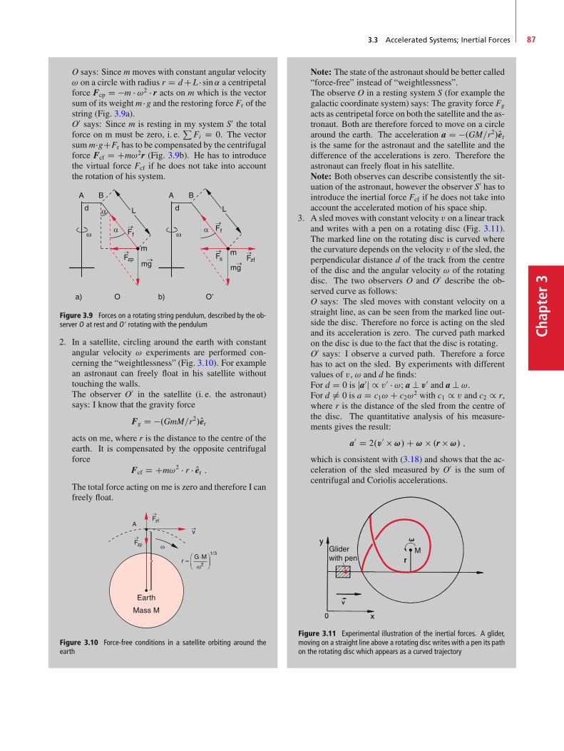
3.3 Accelerated Systems; Inertial Forces 87
Chap
ter3
O says: Since m moves with constant angular velocity! on a circle with radius r D dCL � sin˛ a centripetalforce Fcp D �m � !2 � r acts on m which is the vectorsum of its weightm �g and the restoring force Fr of thestring (Fig. 3.9a).O0 says: Since m is resting in my system S0 the totalforce on m must be zero, i. e.
PFi D 0. The vector
summ�gCFr has to be compensated by the centrifugalforce Fcf D Cm!2r (Fig. 3.9b). He has to introducethe virtual force Fcf if he does not take into accountthe rotation of his system.
Figure 3.9 Forces on a rotating string pendulum, described by the ob-server O at rest and O 0 rotating with the pendulum
2. In a satellite, circling around the earth with constantangular velocity ! experiments are performed con-cerning the “weightlessness” (Fig. 3.10). For examplean astronaut can freely float in his satellite withouttouching the walls.The observer O0 in the satellite (i. e. the astronaut)says: I know that the gravity force
Fg D �.GmM=r2/Oeracts on me, where r is the distance to the centre of theearth. It is compensated by the opposite centrifugalforce
Fcf D Cm!2 � r � Oer :The total force acting on me is zero and therefore I canfreely float.
Mass M
Earth
Figure 3.10 Force-free conditions in a satellite orbiting around theearth
Note: The state of the astronaut should be better called“force-free” instead of “weightlessness”.The observe O in a resting system S (for example thegalactic coordinate system) says: The gravity force Fg
acts as centripetal force on both the satellite and the as-tronaut. Both are therefore forced to move on a circlearound the earth. The acceleration a D �.GM=r2/Oeris the same for the astronaut and the satellite and thedifference of the accelerations is zero. Therefore theastronaut can freely float in his satellite.Note: Both observes can describe consistently the sit-uation of the astronaut, however the observer S0 has tointroduce the inertial force Fcf if he does not take intoaccount the accelerated motion of his space ship.
3. A sled moves with constant velocity v on a linear trackand writes with a pen on a rotating disc (Fig. 3.11).The marked line on the rotating disc is curved wherethe curvature depends on the velocity v of the sled, theperpendicular distance d of the track from the centreof the disc and the angular velocity ! of the rotatingdisc. The two observers O and O0 describe the ob-served curve as follows:O says: The sled moves with constant velocity on astraight line, as can be seen from the marked line out-side the disc. Therefore no force is acting on the sledand its acceleration is zero. The curved path markedon the disc is due to the fact that the disc is rotating.O0 says: I observe a curved path. Therefore a forcehas to act on the sled. By experiments with differentvalues of v, ! and d he finds:For d D 0 is ja0j / v0 � !; a ? v0 and a ? !.For d ¤ 0 is a D c1! C c2!2 with c1 / v and c2 / r,where r is the distance of the sled from the centre ofthe disc. The quantitative analysis of his measure-ments gives the result:
a0 D 2.v0 !/C ! .r !/ ;
which is consistent with (3.18) and shows that the ac-celeration of the sled measured by O0 is the sum ofcentrifugal and Coriolis accelerations.
MGliderwith pen
Figure 3.11 Experimental illustration of the inertial forces. A glider,moving on a straight line above a rotating disc writes with a pen its pathon the rotating disc which appears as a curved trajectory

Chapter3
88 3 Moving Coordinate Systems and Special Relativity
This example illustrates clearly that the two acceler-ations and the corresponding forces are only virtual,because the sled moves in fact with constant veloc-ity on a straight line and therefore experiences no realforces.
4. A hollow sphere filled with sand hangs on a stringwhich is connected to a fixed suspension point andswings in the fixed x-z-plane of a resting system S,driven by the gravity force Fg D m � g with g Df0; 0;�gg.Below the swinging pendulum is a rotating table in thex-y-plane which rotates with the angular velocity !around a vertical axis through the minimum positionof the pendulum.If the sand flows through a small hole in the hollowsphere it draws for ! D 0 a straight line on the ta-ble while for ! ¤ 0 a rosette-like figure is drawn(Fig. 3.12) with a curvature which depends on the ra-tio of oscillation period T1 of the pendulum to rotationperiod T2 of the rotating table.The two observers give the following explanations:O says: The x-z-oscillation plane remains constantbecause the driving force Fg D m � g � sin˛ (seeSect. 2.9.7) lies always in the x-z-plane and thereforethe motion must stay in this plane. The projection ofthe trajectory onto the x-y-plane should be a straightline. The curved trajectory drawn on the rotating ta-ble is caused by the rotation and not by an additionalforce.O0 says sitting on the rotating table: I see a curved pathwhich must be caused by forces, which depend on !,v0 and r. Its form can be explained by the centrifu-gal and the Coriolis forces. My careful measurementsprove that the paths is due to the action of the total ac-celeration a0 D acf C aC in accordance with Eq. 3.18.
Figure 3.12 Apparent trajectory written on a rotating disc by a sandpendulum than oscillates in a constant plane
5. Foucault pendulum. Since our earth is a rotating sys-tem, the path drawn by a linearly swinging pendulum
onto the ground must show curved lines as discussedin example 4). However, because of the slow earth ro-tation (! D 7:3 � 10�5 s�1) the curvature is very small.Using a pendulum with a large length L and a cor-responding large oscillation period T the rotation ofthe earth under the linearly swinging pendulum couldbe first demonstrated 1850 by Leon Foucault (1819–1868) who used a copper ball (m D 28 kg) suspendedby a 67m long string (T D 16:4 s). The turn of theoscillation plane against the rotating ground occurswith the angular velocity !s D ! � sin' where ' isthe geographic latitude of the pendulum (Fig. 3.13).in Kaiserslautern with ' D 49ı the pendulum planeturns in 1 h by 11ı320, which can be readily measured.Using shadow projection of the pendulum string defin-ing the oscillation plane this turn can be quantitativelymeasured within a physics lecture.
Figure 3.13 Explanation of the turning plane of oscillation of theFoucault-pendulums on the surface the rotating earth
6. An impressive demonstration of the Coriolis force isprovided by the motion of cloud formations arounda low pressure region as for instance realized by tor-nados or typhoons (Fig. 3.14). For an observer onthe rotating earth looking from above onto the groundthe wind does not blow radially into the low pres-sure region but rotates on the northern hemisphereanticlockwise around it, on the southern hemisphereclockwise. Around a high pressure region the ro-tation is clockwise on the northern hemisphere andanticlockwise on the southern.
Note: If a small balloon which floats in the air is usedas indicator of the wind flow an observer on earthwould see the balloon moving on one of the lines inFig. 3.14. An observer O at a fixed position outsidethe earth, would however see, that the balloon moveson a straight line radially into the centre of the deeppressure region or out from the centre of a high pres-sure region. These centres are fixed at a point on earthand rotate with the earth.

3.4 The Constancy of the Velocity of Light 89
Chap
ter3
Figure 3.14 Stream-lines of the air around a deep-pressure region.a on the northern hemisphere; b on the southern hemisphere. On thenorthern hemisphere the Coriolis force acts (seen in the wind directionfrom above) in the right direction against the radial force of the pressuregradient, on the southern hemisphere in the left direction. c Satellitephoto of the “death-hurricane” north of Hawaii (with kind permission ofNASA photo HP 133) J
3.3.4 Summary
Inertial forces (virtual forces) have to be introduced, if the mo-tion of bodies are described in accelerated coordinate systems.These forces are not caused by real interactions between bodiesbut only reflect the acceleration of the coordinate system. Theydo not appear if the same motion is described in an inertial sys-tem.
In rotating systems with a fixed centre the inertial forces are cen-trifugal and Coriolis forces. In systemswith arbitrarily changingvelocities further inertial forces have to be introduced.
3.4 The Constancy of the Velocity ofLight
We consider a body A which has the velocity v measured inthe system S but the velocity v0 in a system S0, which movesitself with the velocity u against the resting system S. Accordingto the Galilei transformations the different velocities are relatedthrough the vector sum (Fig. 3.15)
v D v0 C u : (3.21a)
Therefore one might suggest, that also the velocity of light,emitted from a light source which is fixed in a system S0 movingwith the velocity u against the system S, should be measured inthe system S as the vector sum
c D c0 C u ; (3.21b)
where c0 is the velocity measured by O0 in his system S0. Thismeans that the observer O should measure the velocity c1 Dc0 Cu if c0 and u have the same direction, and c2 D c0 �u if theyhave opposite directions.
Very careful measurements performed 1881 by Albert Abra-ham Michelson and Edward Morley [3.2a, 3.3] and later on bymany other researchers [3.4a, 3.4b] produced evidence that thevelocity of light is independent of the relative velocity u be-tween source and observer. For example measurements of thevelocity of light from a star at different times of the year always
Figure 3.15 Galilei transformations of velocities in two inertial systems
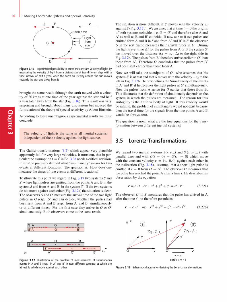
Chapter3
90 3 Moving Coordinate Systems and Special Relativity
Figure 3.16 Experimental possibility to prove the constant velocity of light, bymeasuring the velocity of light from a distant star at two different days with atime interval of half a year, when the earth on its way around the sun movestowards the star and away from it
brought the same result although the earth moved with a veloc-ity of 30 km=s at one time of the year against the star and halfa year later away from the star (Fig. 3.16). This result was verysurprising and brought about many discussions but induced theformulation of the theory of special relativity by Albert Einstein.
According to these unambiguous experimental results we mustconclude:
The velocity of light is the same in all inertial systems,independent of their velocity against the light source.
The Galilei-transformations (3.7) which appear very plausibleapparently fail for very large velocities. It turns out, that in par-ticular the assumption t D t0 in Eq. 3.3a needs a critical revision.It must be precisely defined what “simultaneity” means for twoevents at different locations. The question is: How does onemeasure the times of two events at different locations?
To illustrate this point we regard in Fig. 3.17 two systems S andS0 where light pulses are emitted from the points A and B in thesystem S and from A0 and B0 in the system S0. If the two systemsdo not move against each other (Fig. 3.17a) the situation is clear:The observers O and O0 measure the arrival time of the two lightpulses in O resp. O0 and can decide, whether the pulses hadbeen sent from A and B resp. from A0 and B0 simultaneouslyor at different times. For the first case they arrive in O or O0simultaneously. Both observers come to the same result.
Figure 3.17 Illustration of the problem of measurements of simultaneousevents in A and B resp. in A0 and B0 in two different systems: a which areat rest, b which move against each other
The situation is more difficult, if S0 moves with the velocity vxagainst S (Fig. 3.17b). We assume, that at time t D 0 the originsof both systems coincide, i. e. O D O0 and therefore also A andA0 as well as B and B0 coincide. If now at t D 0 two pulses areemitted form A and B in S and from A0 and B0 in S0 the observerO in the rest frame measures their arrival times in O. Duringthe light travel time�t for the pulses from A or B the system S0has moved over the distance �x D vx � �t to the right side inFig. 3.17b. The pulses from B0 therefore arrive earlier in O0 thanthose from A0. Therefore O0 concludes that the pulses from B0had been sent earlier than those from A0.
Now we will take the standpoint of O0, who assumes that hissystem S0 is at rest and that Smoves with the velocity �vx to theleft in Fig. 3.17b. He now defines the Simultaneity of the eventsin A0 and B0 if he receives the light pulses at O0 simultaneously.Now the pulses from A arrive for O earlier that those from B.This illustrates that the definition of simultaneity depends on thesystem in which the pulses are measured. The reason for thisambiguity is the finite velocity of light. If this velocity wouldbe infinite, the problem of simultaneity would not exist becausethen the travel time for the signals from the two points A and Bwould be always zero.
The question is now: what are the true equations for the trans-formation between different inertial systems?
3.5 Lorentz-Transformations
We regard two inertial systems S.x; y; z/ and S0.x0; y0; z0/ withparallel axes and with O.t D 0/ D O0.t0 D 0/ which movewith the constant velocity v D fvx; 0; 0g against each other inthe x-direction (Fig. 3.18). Assume, that a short light pulse isemitted at t D 0 from O D O0. The observer O measures thatthe pulse has reached the point A after a time t. He describes hisobservation by the equation
r D c � t or: x2 C y2 C z2 D c2 � t2 : (3.22a)
The observer O0 in S0 measures that the pulse has arrived in Aafter the time t0. he therefore postulates:
r0 D c � t0 or: x0 2 C y0 2 C z0 2 D c2 � t0 2 : (3.22b)
Figure 3.18 Schematic diagram for deriving the Lorentz-transformations
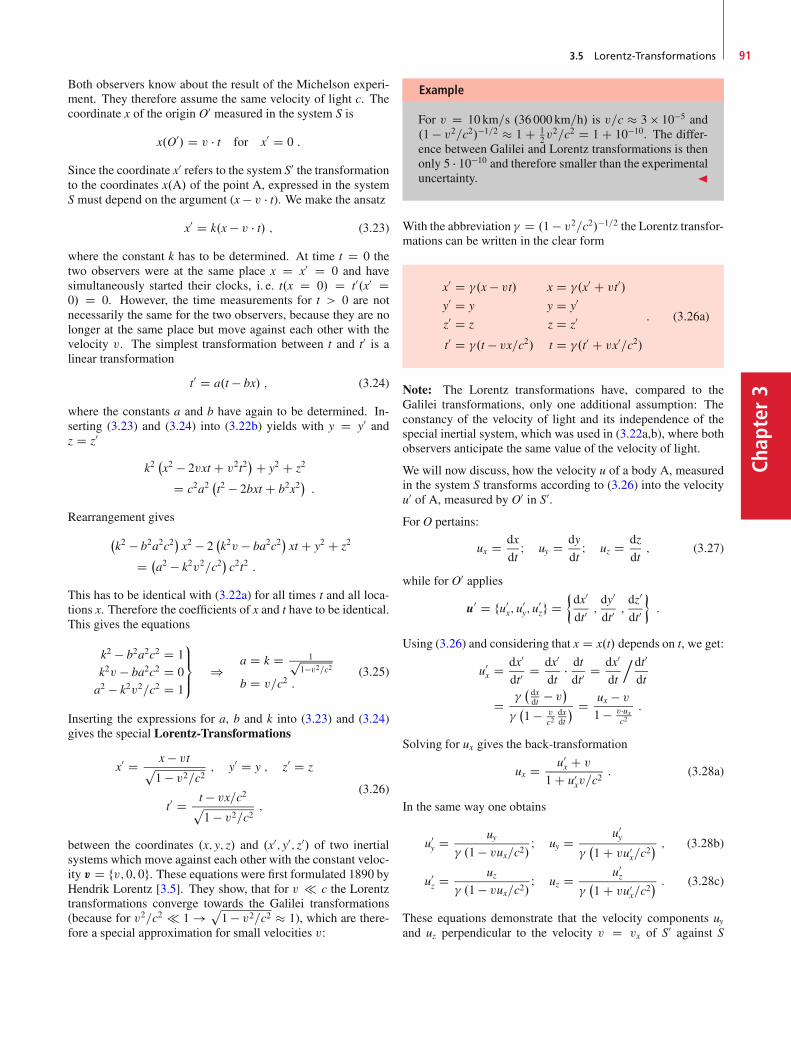
3.5 Lorentz-Transformations 91
Chap
ter3
Both observers know about the result of the Michelson experi-ment. They therefore assume the same velocity of light c. Thecoordinate x of the origin O0 measured in the system S is
x.O0/ D v � t for x0 D 0 :
Since the coordinate x0 refers to the system S0 the transformationto the coordinates x.A/ of the point A, expressed in the systemS must depend on the argument (x � v � t). We make the ansatz
x0 D k.x � v � t/ ; (3.23)
where the constant k has to be determined. At time t D 0 thetwo observers were at the same place x D x0 D 0 and havesimultaneously started their clocks, i. e. t.x D 0/ D t0.x0 D0/ D 0. However, the time measurements for t > 0 are notnecessarily the same for the two observers, because they are nolonger at the same place but move against each other with thevelocity v. The simplest transformation between t and t0 is alinear transformation
t0 D a.t � bx/ ; (3.24)
where the constants a and b have again to be determined. In-serting (3.23) and (3.24) into (3.22b) yields with y D y0 andz D z0
k2�x2 � 2vxt C v2t2
�C y2 C z2
D c2a2�t2 � 2bxt C b2x2
�:
Rearrangement gives
�k2 � b2a2c2
�x2 � 2
�k2v � ba2c2
�xt C y2 C z2
D �a2 � k2v2=c2
�c2t2 :
This has to be identical with (3.22a) for all times t and all loca-tions x. Therefore the coefficients of x and t have to be identical.This gives the equations
k2 � b2a2c2 D 1k2v � ba2c2 D 0a2 � k2v2=c2 D 1
9>=
>;) a D k D 1p
1�v2=c2b D v=c2 :
(3.25)
Inserting the expressions for a, b and k into (3.23) and (3.24)gives the special Lorentz-Transformations
x0 D x � vtp1 � v2=c2 ; y0 D y ; z0 D z
t0 D t � vx=c2p1 � v2=c2 ;
(3.26)
between the coordinates .x; y; z/ and .x0; y0; z0/ of two inertialsystems which move against each other with the constant veloc-ity v D fv; 0; 0g. These equations were first formulated 1890 byHendrik Lorentz [3.5]. They show, that for v c the Lorentztransformations converge towards the Galilei transformations(because for v2=c2 1 ! p
1 � v2=c2 � 1), which are there-fore a special approximation for small velocities v:
Example
For v D 10 km=s .36 000 km=h/ is v=c � 3 10�5 and.1 � v2=c2/�1=2 � 1 C 1
2v2=c2 D 1 C 10�10. The differ-
ence between Galilei and Lorentz transformations is thenonly 5 � 10�10 and therefore smaller than the experimentaluncertainty. J
With the abbreviation � D .1 � v2=c2/�1=2 the Lorentz transfor-mations can be written in the clear form
x0 D �.x � vt/ x D �.x0 C vt0/y0 D y y D y0
z0 D z z D z0
t0 D �.t � vx=c2/ t D �.t0 C vx0=c2/
: (3.26a)
Note: The Lorentz transformations have, compared to theGalilei transformations, only one additional assumption: Theconstancy of the velocity of light and its independence of thespecial inertial system, which was used in (3.22a,b), where bothobservers anticipate the same value of the velocity of light.
We will now discuss, how the velocity u of a body A, measuredin the system S transforms according to (3.26) into the velocityu0 of A, measured by O0 in S0.
For O pertains:
ux D dx
dtI uy D dy
dtI uz D dz
dt; (3.27)
while for O0 applies
u0 D fu0x; u
0y; u
0zg D
dx0
dt0;dy0
dt0;dz0
dt0
�:
Using (3.26) and considering that x D x.t/ depends on t, we get:
u0x D dx0
dt0D dx0
dt� dt
dt0D dx0
dt
.dt0
dt
D ��dxdt � v�
��1 � v
c2dxdt
� D ux � v1 � v�ux
c2:
Solving for ux gives the back-transformation
ux D u0x C v
1 C u0xv=c
2: (3.28a)
In the same way one obtains
u0y D uy
� .1 � vux=c2/ I uy D u0y
��1 C vu0
x=c2� ; (3.28b)
u0z D uz
� .1 � vux=c2/ I uz D u0z
��1 C vu0
x=c2� : (3.28c)
These equations demonstrate that the velocity components uyand uz perpendicular to the velocity v D vx of S0 against S
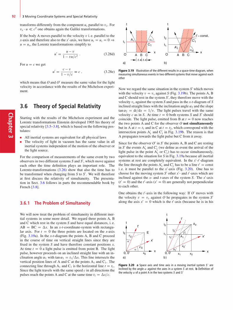
Chapter3
92 3 Moving Coordinate Systems and Special Relativity
transforms differently from the component ux parallel to vx. Forvx � u c2 one obtains again the Galilei transformations.
If the body A moves parallel to the velocity v i. e. parallel to thex-axis and therefore also to the x0-axis, we have uy D uz D 0 )u D ux, the Lorentz transformations simplify to
u0 D u � v1 � vu=c2 : (3.28d)
For u D c we get
u0 D c � v1 � v=c � c ; (3.28e)
which means that O and O0 measure the same value for the lightvelocity in accordance with the results of the Michelson experi-ment.
3.6 Theory of Special Relativity
Starting with the results of the Michelson experiment and theLorentz transformations Einstein developed 1905 his theory ofspecial relativity [3.5–3.8], which is based on the following pos-tulates:
All inertial systems are equivalent for all physical lawsThe velocity of light in vacuum has the same value in allinertial systems independent of the motion of the observer orthe light source.
For the comparison of measurements of the same event by twoobservers in two different systems S and S0, which move againsteach other the time definition plays an important role. TheLorentz-transformations (3.26) show that also the time has tobe transformed when changing from S to S0. We will thereforeat first discuss the relativity of simultaneity. The presenta-tion in Sect. 3.6 follows in parts the recommendable book byFrench [3.8].
3.6.1 The Problem of Simultaneity
We will now treat the problem of simultaneity in different iner-tial systems in some more detail. We regard three points A, Band C which rest in the system S and have equal distances, i. e.AB D BC D �x. In an x-t-coordinate-system with rectangu-lar axis. For t D 0 the three points are located on the x-axis(Fig. 3.19a). In the x-t-diagram the points A, B and C proceedin the course of time on vertical straight lines since they arefixed in the system S and have therefore constant positions x.At time t D 0 a light pulse is emitted from point B. The lightpulse, however proceeds on an inclined straight line with an in-clination angle ˛1 with tan˛1 D t1=�x. This line intersects thevertical position lines of A and C at the points A1 and C1. Theconnecting line through A1 and C1 is the horizontal line t D t1.Since the light travels with the same speed c in all directions thepulses reach the points A and C at the same time t1 D �x=c.
Figure 3.19 Illustration of the different results in a space-time diagram, whenmeasuring simultaneous events in two different systems that move against eachother
Now we regard the same situation in the system S0 which moveswith the velocity v D vx against S (Fig. 3.19b). The points A, Band C should rest in the system S0, they therefore move with thevelocity vx against the system S and pass in the x-t-diagram of Sinclined straight lines with the inclination angle ˛2 and the slopetan˛2 D dt=dx D 1=v. The light pulses travel with the samevelocity c as in S. At time t D 0 both systems S and S0 shouldcoincide. The light pulse, emitted from B at t D 0 now reachesthe two points A and C for the observer O not simultaneouslybut in A at t D t1 and in C at t D t2, which correspond with theintersection points A0
1 and C01 in Fig. 3.19b. The reason is that
A propagates towards the light pulse but C from it away.
Since for the observer O0 in S0 the points A, B and C are restingin S0 the events A0
1 and C01 (we define as event the arrival of the
light pulse in the point A01 or C0
1) has to occur simultaneously,equivalent to the situation for S in Fig. 3.19a because all inertialsystems at rest are completely equivalent. In the x0-t0-diagramthe line through the points A0
1 and C01 has to be a line t
0 D consti. e. it must be parallel to the x0-axis (Fig. 3.20). One has tochoose for the moving system S0 other x0- and t0-axes which areinclined against the x- and t-axes of the system S. The x0-axis(t0 D 0) and the t0-axis (x0 D 0) are generally not perpendicularto each other.
One obtains the t0-axis in the following way: If O0 moves withthe velocity v D vx against O he propagates in the system S0along the axis x0 D 0 which is the t0-axis (because he is in his
Figure 3.20 a Space axis and time axis in a moving inertial system S 0 areinclined by the angle ˛ against the axes in a system S at rest. b Definition ofthe velocity u of a point A in the two systems S and S 0

3.6 Theory of Special Relativity 93
Chap
ter3
system S0 always resting at the origin x0 D 0). In the system Sthis axis is x D v � t which is inclined against the t-axis x D 0 bythe angle ˛ with tan˛ D v=c. The slope of the t0-axis againstthe x-axis in the system S is dt=dx D 1=v.
Any event E is completely defined by its coordinates .x; t/ in Sor .x0; t0/ in S0.
Note, however, that for the same event E the spatial and timecoordinates .xE; tE/ for O in S are different from .x0
E; t0E/ for O
0in S0 (Fig. 3.20)
For each observer the simultaneity of two events at dif-ferent spatial points depends on the coordinate system inwhich the events are described.
We regard a point mass A which moves with the velocity uxagainst O and with u0
x against O0. Its velocity is determined by
O and O0 by measuring the coordinates x1.t1/ and x2.t2/ in Sresp. x0
1.t01/ and x
02.t
02/ in S0 (Fig. 3.20b).
O obtains: ux D x2 � x1t2 � t1
;
O0 obtains: u0x D x0
2 � x01
t02 � t01:
The velocity ux is represented in S by the reciprocal slope�x=�t D ux of the straight line A1A2, In S0 however byu0x D �x0=�t0. One can see already from, Fig. 3.20b that
ux ¤ u0x, which is quantitatively described by Eq. 3.28.
3.6.2 Minkowski-Diagram
The relativity of observations and their dependence of the refer-ence system can be illustrated by space-time-diagrams as shownin Fig. 3.20. Each physical event which occurs at the loca-tion r D fx; y; zg at time t can be represented by a point inthe four-dimensional space-time fx; y; z; tg. For simplicity wewill restrict the following to one spatial dimension x and therelative motion of S0 against S should occur only in the x-direction. Then the four-dimensional representation reduces to
Figure 3.21 Minkowski diagram showing the world lines of a point A restingin the system, of a point B moving in the system with the velocity u and a lightpulse emitted at time t D o from the origin
Figure 3.22 Minkowski diagram of the axes .x; t/ of a system S at rest, of theaxes .x 0; t 0/ of a system S 0 that moves with the velocity v against S and of theaxes .x 00; t 00/ of a system S 00, moving with �v against S
a two-dimensional one. Furthermore the time axis t is changedto c � t in order to have the same physical dimension [m] for bothaxes. Such a depiction is calledMinkowski-diagram (Fig. 3.21).
A body A at rest propagates in an orthogonal .x; ct/ diagramon a vertical line while a body B with the constant velocity vrelative to O propagates on a sloped straight line with the slopec � �t=�x D c=v. A light pulse which is emitted from x D 0at t D 0 and propagates with the velocity c into the x-directiontraverses on a straight line with the inclination of 45ı against thex-axis because the slope is tan˛ D c=c D 1. It is representedby the diagonal in an orthogonal .x; ct/-diagram. Such lines formoving bodies or for light pulses are called world lines or space-time-lines, which can be also curved. Two events A and B occurin the system S simultaneously, if their points in the Minkowski-diagram lie on the line t D t1 parallel to the x-axis (Fig. 3.19).The ct0-axis in S0 is the world line of O0.
We had already discussed in the preceding section that the axisof two inertial systems S and S0, which move against eachother with the constant velocity vx are inclined against eachother. If the x- and the ct-axes in system S are orthogonalthe ct0-axis has the slope tan˛ D c=vx against the x-axis.Also the x0-axis is inclined against the x-axis. According tothe Lorentz-transformations the relation t0 D 0 ) t D v � x=c2must be satisfied (Fig. 3.22). Its slope against the x-axis is there-fore dt0=dx D tanˇ0 D v=c. The angle between the x0 and thect0 axes is � D ˛-ˇ0 D arctan.c=v/ � arctan.v=c/.
For illustration also a third system S00 is shown in Fig. 3.22,which moves with the velocity v D �vx against S. The slope ofthe x00-axis against the x-axis is now tanˇ00 D �vx=c. the anglebetween ct00-axis and ct-axis is also ˇ00. The ct00-axis forms anangle ı D 2.ˇ0 C ˇ00/C � > 90ı against the x00-axis.
3.6.3 Lenght Scales
Not only the inclination of the axis but also their scaling is dif-ferent in the systems S, S0 and S00. Since the velocity of lightis the same in all inertial systems (which implies c D dx=dt D
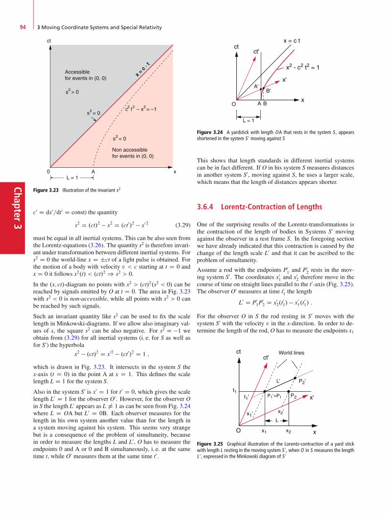
Chapter3
94 3 Moving Coordinate Systems and Special Relativity
Figure 3.23 Illustration of the invariant s2
c0 D dx0=dt0 D const) the quantity
s2 D .ct/2 � x2 D .ct0/2 � x0 2 (3.29)
must be equal in all inertial systems. This can be also seen fromthe Lorentz-equations (3.26). The quantity s2 is therefore invari-ant under transformation between different inertial systems. Fors2 D 0 the world-line x D ˙ct of a light pulse is obtained. Forthe motion of a body with velocity v < c starting at t D 0 andx D 0 it follows x2.t/ < .ct/2 ) s2 > 0.
In the .x; ct/-diagram no points with x2 > .ct/2.s2 < 0/ can bereached by signals emitted by O at t D 0. The area in Fig. 3.23with s2 < 0 is non-accessible, while all points with s2 > 0 canbe reached by such signals.
Such an invariant quantity like s2 can be used to fix the scalelength in Minkowski-diagrams. If we allow also imaginary val-ues of s, the square s2 can be also negative. For s2 D �1 weobtain from (3.29) for all inertial systems (i. e. for S as well asfor S0) the hyperbola
x2 � .ct/2 D x02 � .ct0/2 D 1 ;
which is drawn in Fig. 3.23. It intersects in the system S thex-axis .t D 0/ in the point A at x D 1. This defines the scalelength L D 1 for the system S.
Also in the system S0 is x0 D 1 for t0 D 0, which gives the scalelength L0 D 1 for the observer O0. However, for the observer Oin S the length L0 appears as L ¤ 1 as can be seen from Fig. 3.24where L D OA but L0 D 0B. Each observer measures for thelength in his own system another value than for the length ina system moving against his system. This seems very strangebut is a consequence of the problem of simultaneity, becausein order to measure the lengths L and L0, O has to measure theendpoints 0 and A or 0 and B simultaneously, i. e. at the sametime t, while O0 measures them at the same time t0.
Figure 3.24 A yardstick with length OA that rests in the system S , appearsshortened in the system S 0 moving against S
This shows that length standards in different inertial systemscan be in fact different. If O in his system S measures distancesin another system S0, moving against S, he uses a larger scale,which means that the length of distances appears shorter.
3.6.4 Lorentz-Contraction of Lengths
One of the surprising results of the Lorentz-transformations isthe contraction of the length of bodies in Systems S0 movingagainst the observer in a rest frame S. In the foregoing sectionwe have already indicated that this contraction is caused by thechange of the length scale L0 and that it can be ascribed to theproblem of simultaneity.
Assume a rod with the endpoints P01 and P0
2 rests in the mov-ing system S0. The coordinates x0
1 and x02 therefore move in the
course of time on straight lines parallel to the t0-axis (Fig. 3.25).The observer O0 measures at time t01 the length
L0 D P01P
02 D x0
2.t01/ � x0
1.t01/ :
For the observer O in S the rod resting in S0 moves with thesystem S0 with the velocity v in the x-direction. In order to de-termine the length of the rod, O has to measure the endpoints x1
Figure 3.25 Graphical illustration of the Lorentz-contraction of a yard stickwith length L resting in the moving system S 0, when O in S measures the lengthL 0, expressed in the Minkowski diagram of S 0
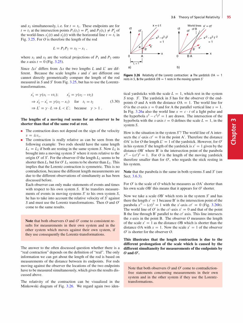
3.6 Theory of Special Relativity 95
Chap
ter3
and x2 simultaneously, i. e. for t D t1. These endpoints are fort D t1 at the intersection points P1.t1/ D P0
1 and P2.t1/ ¤ P02 of
the world-lines x01.t/ and x0
2.t/ with the horizontal line t D t1 inFig. 3.25. For O is therefore the length of the rod
L D P1P2 D x2 � x1 ;
where x1 and x2 are the vertical projections of P1 and P2 ontothe x-axis t D 0 (Fig. 3.25).
Since �x0 differs from �x the two lengths L and L0 are dif-ferent. Because the scale lengths s and s0 are different onecannot directly geometrically compare the length of the rodmeasured in S and S0 from Fig. 3.25, but has to use the Lorentz-transformations.
x01 D �.x1 � vt1/I x0
2 D �.x2 � vt2/) x0
2 � x01 D �.x2 � x1/ for t1 D t2
) L0 D � � L ) L < L0I because � > 1 :
(3.30)
The lengths of a moving rod seems for an observer to beshorter than that of the same rod at rest.
The contraction does not depend on the sign of the velocityv D ˙vx.The contraction is really relative as can be seen from thefollowing example: Two rods should have the same lengthL1 D L2 if both are resting in the same system S. Now L2 isbrought into a moving system S0 where it rests relative to theorigin O0 of S0. For the observer O the length L2 seems to beshorter then L1 but forO0 L1 seems to be shorter than L2. Thisimplies that the Lorentz contraction is symmetric. This is nocontradiction, because the different length measurements aredue to the different observations of simultaneity as has beendiscussed before.Each observer can only make statements of events and timeswith respect to his own system S. If he transfers measure-ments of events in moving systems S0 to his own system S,he has to take into account the relative velocity of S0 againstS and must use the Lorentz transformations. Then O and O0come to the same results.
Note that both observers O and O0 come to consistent re-sults for measurements in their own system and in theother system which moves against their own system, ifthey use consequently the Lorentz-transformations.
The answer to the often discussed question whether there is a“real contraction” depends on the definition of “real”. The onlyinformation we can get about the length of the rod is based onmeasurements of the distance between its endpoints. For rodsmoving against the observer the locations of the two endpointshave to be measured simultaneously, which gives the results dis-cussed above.
The relativity of the contraction can be visualized in theMinkowski diagram of Fig. 3.26. We regard again two iden-
Figure 3.26 Relativity of the Lorentz contraction: a The yardstick OA D 1rests in S , b the yardstick OB D 1 rests in the moving system S 0
tical yardsticks with the scale L D 1, which rest in the systemS resp. S0. The yardstick in S has for the observer O the end-points O and A with the distance OA D 1. The world line forO is the ct-axis x D 0 and for A the parallel vertical line x D 1.In Fig. 3.26a also the world line x D c � t of a light pulse andthe hyperbola x2 � c2t2 D 1 are drawn. The intersection of thehyperbola with the x-axis t D 0 defines the scale L D 1, in thesystem S.
How is the situation in the system S0? The world line of A inter-sects the x0-axis ct0 D 0 in the point A0. Therefore the distanceOA0 is for O the length L0 D 1 of the yardstick. However, for O0in his system S0 the length of the yardstick is x0 D 1 given by thedistance OB0 where B0 is the intersection point of the parabolax02 � .ct0/2 D 1. For O is the length of the moving yardsticktherefore smaller than for O0, who regards the stick resting inhis system.
Note that the parabola is the same in both systems S and S0 (seeSect. 3.6.3).
For O0 is the scale of O which he measures as OA0 shorter thanhis own scale OB0 this means that it appears for O0 shorter.
Now we take a scale OB0 which rests in the system S0 and hasthere the length x0 D 1 because B0 is the intersection point of theparabola x02 � .ct/2 D 1 with the x0-axis ct0 D 0 (Fig. 3.26b).The world line of O0 is the ct0-axis x0 D 0 and that of the pointB the line through B0 parallel to the ct0 axis. This line intersectsthe x-axis in the point B. The observer O measures the lengthof the scale x0 D 1 as the distance OB which is shorter than thedistance OA with x D 1. Now the scale x0 D 1 of the observerO0 is shorter for the observer O.
This illustrates that the length contraction is due to thedifferent prolongation of the scale which is caused by thedifferent simultaneity for measurements of the endpoints byO and O0.
Note that both observers O and O0 come to contradiction-free statements concerning measurements in their ownsystem and in the other system if they use the Lorentz-transformations.
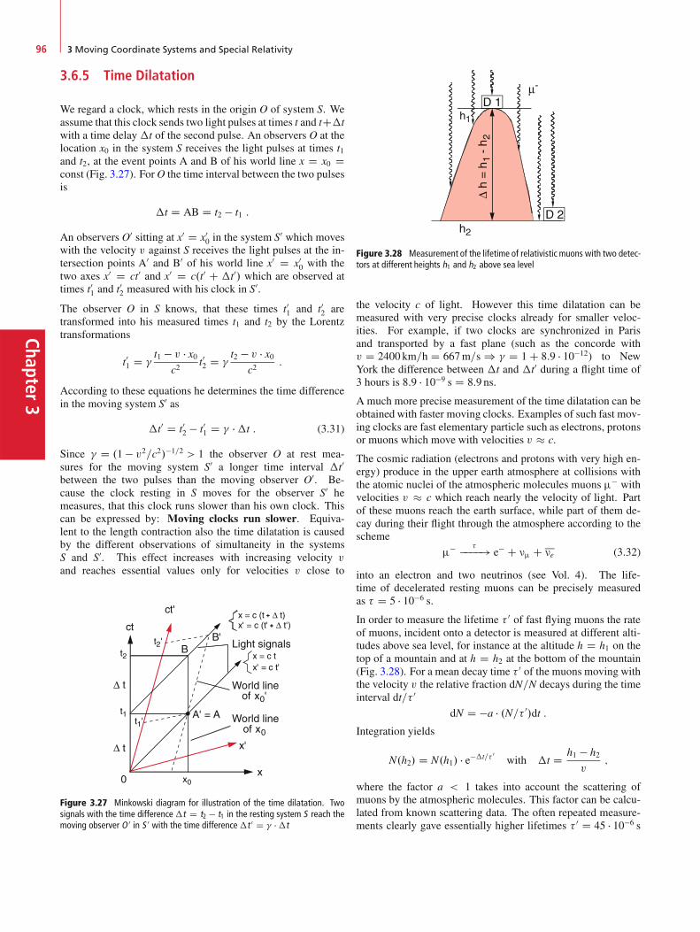
Chapter3
96 3 Moving Coordinate Systems and Special Relativity
3.6.5 Time Dilatation
We regard a clock, which rests in the origin O of system S. Weassume that this clock sends two light pulses at times t and tC�twith a time delay �t of the second pulse. An observers O at thelocation x0 in the system S receives the light pulses at times t1and t2, at the event points A and B of his world line x D x0 Dconst (Fig. 3.27). ForO the time interval between the two pulsesis
�t D AB D t2 � t1 :
An observers O0 sitting at x0 D x00 in the system S0 which moves
with the velocity v against S receives the light pulses at the in-tersection points A0 and B0 of his world line x0 D x0
0 with thetwo axes x0 D ct0 and x0 D c.t0 C �t0/ which are observed attimes t01 and t
02 measured with his clock in S0.
The observer O in S knows, that these times t01 and t02 aretransformed into his measured times t1 and t2 by the Lorentztransformations
t01 D �t1 � v � x0
c2t02 D �
t2 � v � x0c2
:
According to these equations he determines the time differencein the moving system S0 as
�t0 D t02 � t01 D � ��t : (3.31)
Since � D .1 � v2=c2/�1=2 > 1 the observer O at rest mea-sures for the moving system S0 a longer time interval �t0between the two pulses than the moving observer O0. Be-cause the clock resting in S moves for the observer S0 hemeasures, that this clock runs slower than his own clock. Thiscan be expressed by: Moving clocks run slower. Equiva-lent to the length contraction also the time dilatation is causedby the different observations of simultaneity in the systemsS and S0. This effect increases with increasing velocity vand reaches essential values only for velocities v close to
Figure 3.27 Minkowski diagram for illustration of the time dilatation. Twosignals with the time difference�t D t2 � t1 in the resting system S reach themoving observer O 0 in S 0 with the time difference�t 0 D � ��t
Figure 3.28 Measurement of the lifetime of relativistic muons with two detec-tors at different heights h1 and h2 above sea level
the velocity c of light. However this time dilatation can bemeasured with very precise clocks already for smaller veloc-ities. For example, if two clocks are synchronized in Parisand transported by a fast plane (such as the concorde withv D 2400 km=h D 667m=s ) � D 1 C 8:9 � 10�12) to NewYork the difference between �t and �t0 during a flight time of3 hours is 8:9 � 10�9 s D 8:9 ns.
A much more precise measurement of the time dilatation can beobtained with faster moving clocks. Examples of such fast mov-ing clocks are fast elementary particle such as electrons, protonsor muons which move with velocities v � c.
The cosmic radiation (electrons and protons with very high en-ergy) produce in the upper earth atmosphere at collisions withthe atomic nuclei of the atmospheric molecules muons �� withvelocities v � c which reach nearly the velocity of light. Partof these muons reach the earth surface, while part of them de-cay during their flight through the atmosphere according to thescheme
�� �����! e� C � C e (3.32)
into an electron and two neutrinos (see Vol. 4). The life-time of decelerated resting muons can be precisely measuredas � D 5 � 10�6 s.
In order to measure the lifetime � 0 of fast flying muons the rateof muons, incident onto a detector is measured at different alti-tudes above sea level, for instance at the altitude h D h1 on thetop of a mountain and at h D h2 at the bottom of the mountain(Fig. 3.28). For a mean decay time � 0 of the muons moving withthe velocity v the relative fraction dN=N decays during the timeinterval dt=� 0
dN D �a � .N=� 0/dt :
Integration yields
N.h2/ D N.h1/ � e��t=� 0with �t D h1 � h2
v;
where the factor a < 1 takes into account the scattering ofmuons by the atmospheric molecules. This factor can be calcu-lated from known scattering data. The often repeated measure-ments clearly gave essentially higher lifetimes � 0 D 45 � 10�6 s

3.6 Theory of Special Relativity 97
Chap
ter3
Figure 3.29 Einstein’s “light-clock” for illustration of the time dilatation
of the moving muons than � D 5 � 10�6 s for muons at rest.From � 0 D � � � follows � D 9 ! v D 0:994c. The muonshave a velocity v which is smaller than c by only 6‰.
Meanwhile many short-lived elementary particles can be pro-duced and accelerated to high velocities. Comparing thelifetimes of these particles at rest and while moving, unam-biguously confirms the time dilatation postulated by the Lorentztransformations.
The relativistic time dilatation can be illustrated by an“gedanken-experiment” proposed by Einstein using a light pulseclock (Fig. 3.29). The system consists of a box with length L.On one side a flash lamp is mounted at the point A and on theopposite end a mirror M1. The flash lamp emits a short lightpulse and starts a clock. The light pulse reflected by M1 is re-ceived by a detector which stops the clock. The time interval�t0 D 2L=c is used as time scale in the system S in which thelight clock rests.
Now we let the system S move with the velocity v relative to asystem S0 in a direction perpendicular to the length L. For theobserver O0 in S0 the light pulse now travels from A to B andis reflected to C. With AN D NC D v � �t=2 it follows fromFig. 3.29
AB C BC D 2 �"L2 C
�v�t0
2
�2#1=2
D c ��t0
) �t0 D 2L
.c2 � v2/1=2:
(3.33)
The observer Omeasures�t D 2L=c. The comparison between�t and �t0 gives:
�t0 D �t
.1 � v2=c2/1=2D � ��t ; (3.34)
which turns out to be identical with (3.31).
3.6.6 The Twin-Paradox
No other problem of special relativity has aroused so manycontroversial discussions as the twin paradox (often called the
Figure 3.30 Minkowski diagram for the twin paradox
clock-paradox), discussed by Einstein in his first paper 1905about relativity. It deals with the following situation:
Two clocks which are synchronized show equal time intervalswhen sitting in the same system S at rest. One of the clocksis taken by O0 on a fast moving spacecraft and returns after thetravel time T (measured byO in S) back to the other clock whichalways had stayed in the system S. A comparison of the twoclocks shows that the moved clock is delayed, that means that itshows a smaller value T 0 than T [3.8–3.11].
This “gedanken-experiment” has meanwhile be realized and thetime dilatation has been fully verified (see previous section). Formanned space missions this means that an astronaut A after hisreturn to earth after a longer journey through space is youngerthan his twin brother B who has stayed at home. The “gained”time span is, however, for velocities of spacecrafts which canbe realized up to now, very small and therefore insignificant.Nevertheless an understanding of the twin paradox is of princi-pal significance because it illustrates the meaning of relativity,which is often used in a popular but wrong way.
We have discussed in the previous section that the time dilata-tion is relative, i. e. for each of the two observers O and O0 thetime scale of the other seems to be prolonged. Why is it thenpossible to decide unambiguously that A and not B is youngerafter his return?
The essential point is that A is not strictly in an inertial system,even if he moves with constant velocity, because at his return-ing point he changes the system from one that moves with thevelocity Cv into one that moves with �v against B. This showsthat the measurements of A and B are not equivalent.
In order to simplify the discussionwe will categorize the journeyof A into three sections, which are illustrated in the Minkowskidiagram of the resting system S of B in Fig. 3.30.
A starts his journey from x D 0 at time t D t0 D 0, reachesin a negligibly small time interval his final speed v until hearrives at his point of return P1.xr;T=2/ after the time t1 DT=2.At time t1 D T=2 he decelerates to v D 0 and acceleratesagain to �v. This should all happen within a time intervalwhich is negligibly small compared with the travel time T .Astronaut A flies with v2 D �v back to B and reaches B inx D 0 at t2 D T .

Chapter3
98 3 Moving Coordinate Systems and Special Relativity
While the world line of B in Fig. 3.30 is the vertical line x D 0,A follows the line x D v � t ! ct D .c=v/x until the pointof return P1 from where he travels on the line x D xr � v.t �T=2/ ) ct D .c=v/.xr � x/ C cT=2, until the point P2.0;T/where he meets with B.
From (3.29) we obtain for the invariant
ds2 D c2dt2 � dx2 D c2dt02 � dx02 :
This yields the different travel times for A and B: For B is al-ways dx D 0. We therefore get for the total distance s in theMinkowski diagram:
s DZ
ds D c �Z
dt D c � T :
For the moving astronaut A the resting observer B measures onthe way OP1: dx D v � dt ! ds2 D c2dt2 � v2dt2, which givesfor the total path
Zds D
pc2 � v2
Zdt D c � T
2�D cT 0
2;
and on the way P1P2 back: dx D �vdt:Z
ds Dpc2 � v2
Zdt D c � T
2�D cT 0
2:
The total travel time measured by B in S for the system S0 of histwin A is then T 0 D T=� < T . This result can be also explainedby the Lorentz contraction: For A is the path L shortened bythe factor � . Therefore the travel time T for A is shorter by thefactor � since A as well as B measure the same velocity v of Arelative to B.
The asymmetry of the problem can be well illustrated by regard-ing light pulses sent at constant intervals by A to B and by B toA. Both the observer B and the astronaut A send these light sig-nals at the frequency f0 measured with their clocks. The sum ofthe sent pulses at a frequency f0 D 1=s gives the total travel timein seconds (Fig. 3.31).
Figure 3.31 Illustration of the twin paradox, using the signals sent and re-ceived by A and B
Figure 3.32 Doppler-effect of the signal frequency illustrated in the Minkowskidiagram
While A moves away from B both observers receive the pulsesat a lower frequncy f1 because each successive pulse has to travela longer way than the preceding pulse. The asymmetry occurs atthe turning point P1. While A on his way back now receives thepulses with a higher frequency f2 directly after he turns around,B receives the pulses from A with the frequency f2 only at times�t � c � x0 after the return time. He receives the same totalnumber N 0 of pulses as has been sent by A but he receives for alonger time signals with lower frequency than A. Therefore hemeasures a longer travel time for A than A himself.
This is illustrated in Fig. 3.31 for v D 0:6c. B sends duringthe travel time of A altogether 20 pulses, which are all receivedby A. While B sends his signals at constant time intervals �0,A receives them on the outbound trip with larger time intervals�1 i. e. lower frequency and on the way back with shorter timeintervals �2, i. e. higher frequency. Measured in the system S0of A the travel time T 0 is shorter by the factor � . The astronautA sends during this time only N 0 D N=� D 16 pulses whichare all received by B. Since B receives the signal sent by A atthe return time only delayed, he receives signals with the largerinterval �1 (lower frequency) for a longer time and only after thetime t0r C L=2c the signals with the shorter intervals �2.
This is further illustrated by the Minkowski diagram of Fig. 3.32which explains the relativistic Doppler-effect. The astronaut Ais at time t D 0 at the point .x D 0; t D 0/ in the Minkowskidiagram. He moves, measured by B on the line
x D v � t ! c � t D c
vx :
The observer B sitting always at x D 0 sends light pulses at arepetition frequency f0. A pulse sent by B at time t0 travels inthe .x; ct/-diagram on lines with a 45ı slope which intersects theworld line of A in the point .x1; t1/, where it is received by A.The next pulse is sent by B at time t D t0 C � D t0 C 1=f0and reaches A at .x2; t2/. According to Fig. 3.31 the following
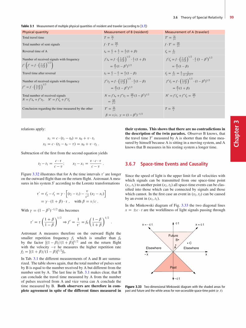
3.6 Theory of Special Relativity 99
Chap
ter3
Table 3.1 Measurement of multiple physical quantities of resident and traveler (according to [3.7])
Physical quantity Measurement of B (resident) Measurement of A (traveler)
Total travel time T D 2Lv
T 0 D 2L�v
Total number of sent signals f � T D 2fLv
f � T 0 D 2fL�v
Reversal time of A tu D Lv
C Lc D L
v.1 C ˇ/ t0u D L
�v
Number of received signals with frequency
f 0�f 0 D f �
�1�ˇ1Cˇ
1=2�f 0tu D f �
�1�ˇ1Cˇ
1=2 � Lv.1 C ˇ/
D fLv.1 � ˇ2/1=2
f 0t0u D f ��
1�ˇ1Cˇ
1=2 � Lv
�1 � ˇ2�1=2
D fLv.1 � ˇ/
Travel time after reversal t2 D Lv
� Lc D L
v.1 � ˇ/ t02 D L
�vD L
v1
.1�ˇ2/1=2
Number of received signals with frequency
f 00 D f ��1Cˇ1�ˇ
1=2f 00t2 D f �
�1Cˇ1�ˇ
1=2 � Lv.1 � ˇ/
D fLv.1 � ˇ2/1=2
f 00t02 D f ��
1Cˇ1�ˇ
1=2 � .1 � ˇ2/1=2
D fLv.1 C ˇ/
Total number of received signalsN D f 0tu C f 00t2; N0 D f 0t0u C f 00t02
N D f 0tu C f 00t2 D 2fLv.1 � ˇ2/1=2
D 2fL� �v
N0 D f 0t0u C f 00t02 D 2fLv
Conclusion regarding the time measured by the other T 0 D 2L�v
ˇ D v=c; � D .1 � ˇ2/�1=2
T D 2Lv
relations apply:
x1 D c � .t1 � t0/ D x0 C v � t1x2 D c � .t2 � t0 � �/ D x0 C v � t2 :
Subtraction of the first from the second equation yields
t2 � t1 D c � �c � v I x2 � x1 D v � c � �
c � v :
Figure 3.32 illustrates that for A the time intervals � 0 are longeron the outward flight than on the return flight. Astronaut A mea-sures in his system S0 according to the Lorentz transformations
� 0 D t02 � t01 D � �h.t2 � t1/ � v
c2.x2 � x1/
i
D � � .1 C ˇ/ � � ; with ˇ D v=c :
With � D .1 � ˇ2/�1=2 this becomes
� 0 D �
�1 C ˇ
1 � ˇ�1=2
) f 0 D 1
� 0 D f0
�1 � ˇ1 C ˇ
�1=2
:
Astronaut A measures therefore on the outward flight thesmaller repetition frequency f1 which is smaller than f0by the factor Œ.1 � ˇ/=.1 C ˇ/�1=2 and on the return flightwith the velocity �v he measures the higher repetition ratef2 D Œ.1 C ˇ/=.1 � ˇ/�1=2f0.In Tab. 3.1 the different measurements of A and B are summa-rized. The table shows again, that the total number of pulses sentby B is equal to the number received by A but different from thenumber sent by A. The last line in Tab. 3.1 makes clear, that Bcan conclude the travel time measured by A from the numberof pulses received from A and vice versa can A conclude thetime measured by B. Both observers are therefore in com-plete agreement in spite of the different times measured in
their systems. This shows that there are no contradictions inthe description of the twin paradox. Observer B knows, thatthe travel time T 0 measured by A is shorter than the time mea-sured by himself because A is sitting in a moving system, and Aknows that B measures in his resting system a longer time.
3.6.7 Space-time Events and Causality
Since the speed of light is the upper limit for all velocities withwhich signals can be transmitted from one space-time point.x1; t1/ to another point .x2; t2/ all space-time events can be clas-sified into those which can be connected by signals and thosewhich cannot. In the first case an event in .x2; t2/ can be causedby an event in .x1; t1/.
In the Minkowski diagram of Fig. 3.33 the two diagonal linesx D ˙c � t are the worldliness of light signals passing through
Figure 3.33 Two-dimensional Minkowski diagram with the shaded areas forpast and future and the white areas for non-accessible space-time point .r; t/
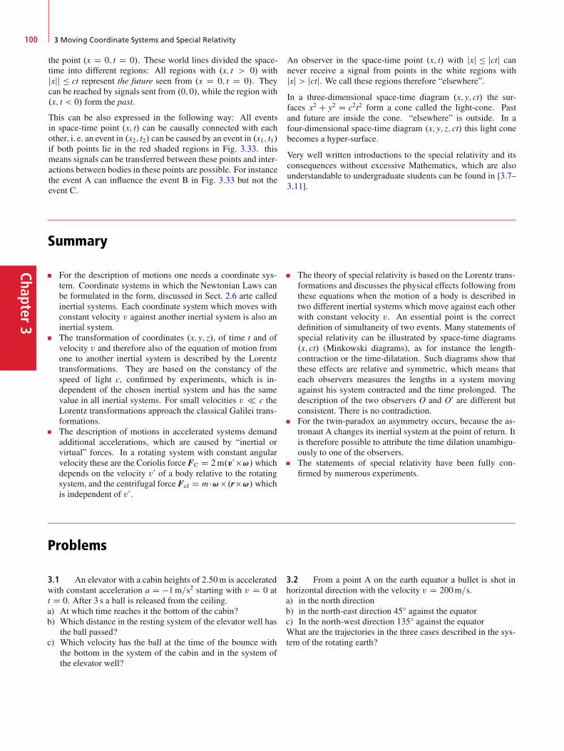
Chapter3
100 3 Moving Coordinate Systems and Special Relativity
the point .x D 0; t D 0/. These world lines divided the space-time into different regions: All regions with .x; t > 0/ withjxjj � ct represent the future seen from .x D 0; t D 0/. Theycan be reached by signals sent from .0;0/, while the region with.x; t < 0/ form the past.
This can be also expressed in the following way: All eventsin space-time point .x; t/ can be causally connected with eachother, i. e. an event in .x2; t2/ can be caused by an event in .x1; t1/if both points lie in the red shaded regions in Fig. 3.33. thismeans signals can be transferred between these points and inter-actions between bodies in these points are possible. For instancethe event A can influence the event B in Fig. 3.33 but not theevent C.
An observer in the space-time point .x; t/ with jxj � jctj cannever receive a signal from points in the white regions withjxj > jctj. We call these regions therefore “elsewhere”.
In a three-dimensional space-time diagram .x; y; ct/ the sur-faces x2 C y2 D c2t2 form a cone called the light-cone. Pastand future are inside the cone. “elsewhere” is outside. In afour-dimensional space-time diagram .x; y; z; ct/ this light conebecomes a hyper-surface.
Very well written introductions to the special relativity and itsconsequences without excessive Mathematics, which are alsounderstandable to undergraduate students can be found in [3.7–3.11].
Summary
For the description of motions one needs a coordinate sys-tem. Coordinate systems in which the Newtonian Laws canbe formulated in the form, discussed in Sect. 2.6 arte calledinertial systems. Each coordinate system which moves withconstant velocity v against another inertial system is also aninertial system.The transformation of coordinates .x; y; z/, of time t and ofvelocity v and therefore also of the equation of motion fromone to another inertial system is described by the Lorentztransformations. They are based on the constancy of thespeed of light c, confirmed by experiments, which is in-dependent of the chosen inertial system and has the samevalue in all inertial systems. For small velocities v c theLorentz transformations approach the classical Galilei trans-formations.The description of motions in accelerated systems demandadditional accelerations, which are caused by “inertial orvirtual” forces. In a rotating system with constant angularvelocity these are the Coriolis force FC D 2m.v0 !/ whichdepends on the velocity v0 of a body relative to the rotatingsystem, and the centrifugal force Fcf D m �! .r!/ whichis independent of v0.
The theory of special relativity is based on the Lorentz trans-formations and discusses the physical effects following fromthese equations when the motion of a body is described intwo different inertial systems which move against each otherwith constant velocity v. An essential point is the correctdefinition of simultaneity of two events. Many statements ofspecial relativity can be illustrated by space-time diagrams.x; ct/ (Minkowski diagrams), as for instance the length-contraction or the time-dilatation. Such diagrams show thatthese effects are relative and symmetric, which means thateach observers measures the lengths in a system movingagainst his system contracted and the time prolonged. Thedescription of the two observers O and O0 are different butconsistent. There is no contradiction.For the twin-paradox an asymmetry occurs, because the as-tronaut A changes its inertial system at the point of return. Itis therefore possible to attribute the time dilation unambigu-ously to one of the observers.The statements of special relativity have been fully con-firmed by numerous experiments.
Problems
3.1 An elevator with a cabin heights of 2:50m is acceleratedwith constant acceleration a D �1m=s2 starting with v D 0 att D 0. After 3 s a ball is released from the ceiling.a) At which time reaches it the bottom of the cabin?b) Which distance in the resting system of the elevator well has
the ball passed?c) Which velocity has the ball at the time of the bounce with
the bottom in the system of the cabin and in the system ofthe elevator well?
3.2 From a point A on the earth equator a bullet is shot inhorizontal direction with the velocity v D 200m=s.a) in the north directionb) in the north-east direction 45ı against the equatorc) In the north-west direction 135ı against the equatorWhat are the trajectories in the three cases described in the sys-tem of the rotating earth?

References 101
Chap
ter3
3.3 A ball hanging on a 10m long string is deflected fromits vertical position and rotates around the vertical axis with! D 2 � 0:2 s�1. What is the angle of the string against thevertical and what is the velocity v of the ball?
3.4 In the edge region of a typhoon over Japan (geographicallatitude ' D 40ı) the horizontally circulating air has a velocityof 120 km=h. What is the radius of curvature r of the path of theair in this region?
3.5 A fast train .m D 3 � 106 kg/ drives from Cologne toBasel with a velocity of v D 200 km=h exactly in north-southdirection passing 48ı latitude. How large is the Coriolis forceacting on the rail? Into which direction is it acting?
3.6 A body with mass m D 5 kg is connected to a string withL D 1m and rotatesa) in a horizontal plane around a vertical axisb) in a vertical plane around a horizontal axisAt which angular velocity breaks the string in the cases a) andb) when the maximum tension force of the string is 1000N?
3.7 A plane disc rotates with a constant angular velocity! D 2 � 10 s�1 around an axis through the centre of the discperpendicular to the disc plane. At time t D 0 a ball islaunched with the velocity v D fvr; v'g with vr D 10m=s,v' D 5m=s (measured in the resting system) starting from thepoint A .r D 0:1m; ' D 0ı/. At which point .r; '/ does the ballreach the edge of the disc?
3.8 A bullet with mass m D 1 kg is shot with the velocityv D 7 km=s from a point A on the earth surface with the ge-ographical latitude ' D 45ı into the east direction. How largeare centrifugal and Coriolis force directly after the launch? Atwhich latitude is its impact?
3.9 Two inertial systems S and S0 move against each otherwith the velocity v D vx D c=3. A body A moves in the systemS with the velocity u D fux D 0:5c; uy D 0:1c; uz D 0g. Whatis the velocity vector u0 in the system S0 when using
a) the Galilei transformations andb) the Lorentz transformations?How large is the error of a) compared to b)?
3.10 Ameter scale moves with the velocity v D 2:8 � 108 m=spassing an observer B at rest. Which length is B measuring?
3.11 A space ship flies with constant velocity v to the planetNeptune and reaches Neptune at its closest approach to earth.How large must be the velocity v if the travel time, measured bythe astronaut is 1 day? How long is then the travel time mea-sured by an observer on earth?
3.12 Light pulses are sent simultaneously from the two end-points A and B of a rod at rest. Where should an observer Osit in order to receive the pulses simultaneously? Is the answerdifferent when A, B and O moves with the constant velocity v?At which point in the system S an observer O0 moving with avelocity vx against S receives the pulses simultaneously if heknows that the pulses has been sent in the system S simultane-ously from A and B?
3.13 At January 1st 2010 the astronaut A starts with the con-stant velocity v D 0:8c to our next star ˛-Centauri, with adistance of 4 light years from earth. After arriving at the star,A immediately returns and flies back with v D 0:8c and reachesthe earth according to the measurement of B on earth at the 1stof January 2020. A and B had agreed to send a signal on eachNew Year’s Day. Show that B sends 10 signals, but A only 6.How many signals does A receive on his outbound trip and howmany on his return trip?
3.14 Astronaut A starts at t D 0 his trip to the star Sirius (dis-tance 8.61 light years) with the velocity v1 D 0:8c. One yearlater B starts with the velocity v2 D 0:9c to the same star. Atwhich time does B overtake A, measureda) in the system of A,b) of B andc) of an observer C who stayed at home?At which distance from C measured in the system of C does thisoccur?
References
3.1. https://en.wikipedia.org/wiki/Fictitious_force3.2a. A.A. Michelson, E.W. Morley, Am. J. Sci. 34, 333 (1887)3.2b. R. Shankland, Am. J. Phys. 32, 16 (1964)3.3. A.A. Michelson, Studies in Optics. (Chicago Press, 1927)3.4a. A. Brillet, J.L. Hall, in Laser Spectroscopy IV, Proc. 4th
Int. Conf. Rottach Egern, Germany, June 11–15 1979.(Springer Series Opt. Sci. Vol 21, Springer, Berlin, Hei-delberg, 1979)
3.4b. W. Rowley et al., Opt. and Quant. Electr. 8, 1 (1976)3.5. A. Einstein, H.A. Lorentz, H. Minkowski, H. Weyl, The
principles of relativity. (Denver, New York, 1958)3.6. R. Resnik, Introduction to Special Relativity. (Wiley,
1968)
3.7. E.F. Taylor, J.A. Wheeler, Spacetime Physics: Intro-duction to Special Relativity, 2nd ed. (W.H. Freeman &Company, 1992)
3.8. A.P. French, Special Relativity Theory. (W.W. Norton,1968)
3.9. D.H. Frisch, H.J. Smith, Am. J. Phys. 31, 342 (1963)3.10. N.M. Woodhouse, Special Relativity. (Springer, Berlin,
Heidelberg, 2007)3.11. C. Christodoulides, The Special Theory of Relativity:
Theory, Verification and Applications. (Springer, Berlin,Heidelberg, 2016)
Chap
ter4
Systems of Point Masses;Collisions 44.1 Fundamentals . . . . . . . . . . . . . . . . . . . . . . . . . . . . . . . . . . 104
4.2 Collisions Between Two Particles . . . . . . . . . . . . . . . . . . . . . . 107
4.3 What Do We Learn from the Investigation of Collisions? . . . . . . . . . 115
4.4 Collisions at Relativistic Energies . . . . . . . . . . . . . . . . . . . . . . 119
4.5 Conservation Laws . . . . . . . . . . . . . . . . . . . . . . . . . . . . . . . 123
Summary . . . . . . . . . . . . . . . . . . . . . . . . . . . . . . . . . . . . 125
Problems . . . . . . . . . . . . . . . . . . . . . . . . . . . . . . . . . . . . 126
References . . . . . . . . . . . . . . . . . . . . . . . . . . . . . . . . . . . 127
103© Springer International Publishing Switzerland 2017W. Demtröder, Mechanics and Thermodynamics, Undergraduate Lecture Notes in Physics, DOI 10.1007/978-3-319-27877-3_4

Chapter4
104 4 Systems of Point Masses; Collisions
In the preceding chapters we have discussed the motion of asingle particle and its trajectory under the influence of externalforces. In this chapter we will deal with systems of many par-ticles, where besides possible external forces also interactionsbetween the particles play an important role.
4.1 Fundamentals
At first we introduce several expressions and definitions of fun-damental terms and notations for systems of many particles.
4.1.1 Centre of Mass
We consider N point masses with position vectors ri and defineas the centre of mass the point with the position vector
RS DP
i mi riPi mi
D 1
M
X
i
mi ri ; (4.1)
where M D Pmi is the total mass of all N particles (Fig. 4.1).
When the masses mi move with the velocities vi D dri=dt wedefine the velocity vS of the centre of mass as
vS D dRS
dtD 1
M
X
i
mivi : (4.2a)
With the momenta pi D mi � vi (4.2a) can be also expressed bythe total momentum P D P
pi as
P D MvS : (4.2b)
If no external forces are acting on the particles, we need to re-gard only internal forces, i. e. interactions between the particles.Such a system without external forces is called a closed system.
From the Newtonian law Fik D �Fki it follows:P
i
Pk¤i Fik D
0. In a closed system the vector sum of all forces is zero.
With Fi D Pk¤i Fik and Fi D dpi=dt the total momentum of the
system
P DX
pi D const : (4.3)
Since P is the momentum of the centre of mass we can state:
The centre of mass of a closed systemmoves with constantmomentum. This implies that its velocity does not change.
If an external total force F ¤ 0 acts onto the system we canwrite
F D d
dt
Xpi D dP
dt; (4.4)
RS
Figure 4.1 Definition of center of mass
With the acceleration of the centre of mass aS D dvS=dt weobtain
F D MaS : (4.5)
The centre of mass of an arbitrary system of particlesmoves in the same way as a body with the total massM D P
mi would move under the action of the externalforce F.
Often it is useful to choose a coordinate system with the centreof mass as origin, which moves with the velocity vS of the centreof mass against the fixed laboratory system. Such a system iscalled the centre of mass system (CM-system).
The position vectors ri in the lab-system are related to the posi-tion vectors riS in the CM-system (Fig. 4.1) by
ri D riS C RS : (4.6a)
Inserting into (4.1) gives
X
i
miriS DX
i
mi .ri � RS/
DX
i
miri � RS
X
i
mi D 0 ;
XmiriS D 0 (4.6b)
This implies that in the CM-system the position vector RS of thecentre-of-mass is RS D .1=M/
PmiriS D 0.
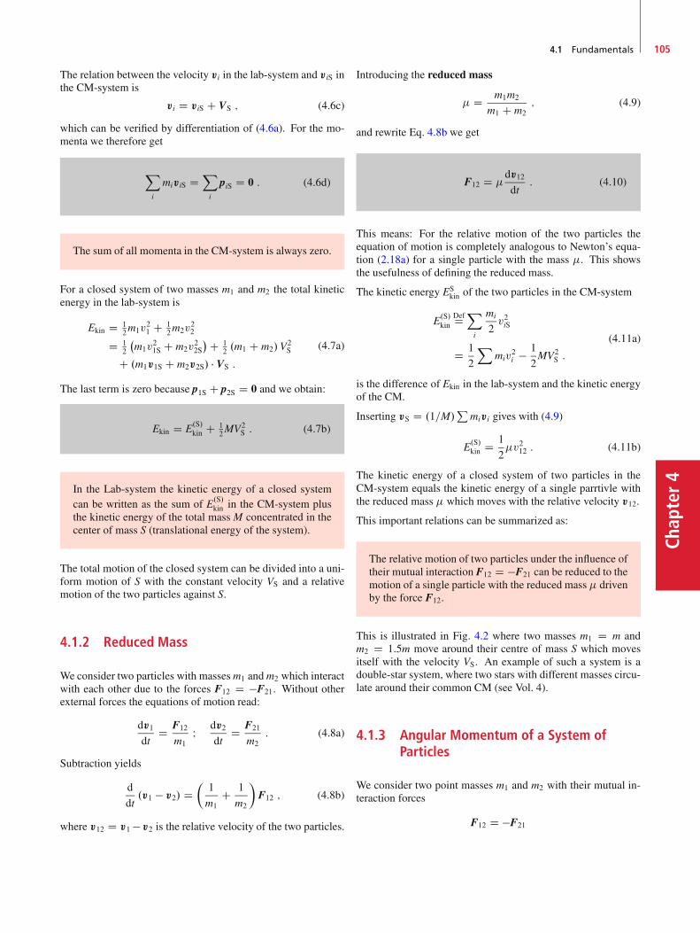
4.1 Fundamentals 105
Chap
ter4
The relation between the velocity vi in the lab-system and viS inthe CM-system is
vi D viS C VS ; (4.6c)
which can be verified by differentiation of (4.6a). For the mo-menta we therefore get
X
i
miviS DX
i
piS D 0 : (4.6d)
The sum of all momenta in the CM-system is always zero.
For a closed system of two masses m1 and m2 the total kineticenergy in the lab-system is
Ekin D 12m1v
21 C 1
2m2v22
D 12
�m1v
21S C m2v
22S
�C 12 .m1 C m2/V
2S
C .m1v1S C m2v2S/ � VS :
(4.7a)
The last term is zero because p1S C p2S D 0 and we obtain:
Ekin D E.S/kin C 12MV2
S : (4.7b)
In the Lab-system the kinetic energy of a closed systemcan be written as the sum of E.S/kin in the CM-system plusthe kinetic energy of the total mass M concentrated in thecenter of mass S (translational energy of the system).
The total motion of the closed system can be divided into a uni-form motion of S with the constant velocity VS and a relativemotion of the two particles against S.
4.1.2 Reduced Mass
We consider two particles with massesm1 andm2 which interactwith each other due to the forces F12 D �F21. Without otherexternal forces the equations of motion read:
dv1
dtD F12
m1I dv2
dtD F21
m2: (4.8a)
Subtraction yields
d
dt.v1 � v2/ D
�1
m1C 1
m2
�F12 ; (4.8b)
where v12 D v1 � v2 is the relative velocity of the two particles.
Introducing the reduced mass
D m1m2
m1 C m2; (4.9)
and rewrite Eq. 4.8b we get
F12 D dv12
dt: (4.10)
This means: For the relative motion of the two particles theequation of motion is completely analogous to Newton’s equa-tion (2.18a) for a single particle with the mass . This showsthe usefulness of defining the reduced mass.
The kinetic energy ESkin of the two particles in the CM-system
E.S/kinDefDX
i
mi
2v2iS
D 1
2
Xmiv
2i � 1
2MV2
S :
(4.11a)
is the difference of Ekin in the lab-system and the kinetic energyof the CM.
Inserting vS D .1=M/P
mivi gives with (4.9)
E.S/kin D 1
2v212 : (4.11b)
The kinetic energy of a closed system of two particles in theCM-system equals the kinetic energy of a single parrtivle withthe reduced mass which moves with the relative velocity v12.
This important relations can be summarized as:
The relative motion of two particles under the influence oftheir mutual interaction F12 D �F21 can be reduced to themotion of a single particle with the reduced mass drivenby the force F12.
This is illustrated in Fig. 4.2 where two masses m1 D m andm2 D 1:5m move around their centre of mass S which movesitself with the velocity VS. An example of such a system is adouble-star system, where two stars with different masses circu-late around their common CM (see Vol. 4).
4.1.3 Angular Momentum of a System ofParticles
We consider two point masses m1 and m2 with their mutual in-teraction forces
F12 D �F21
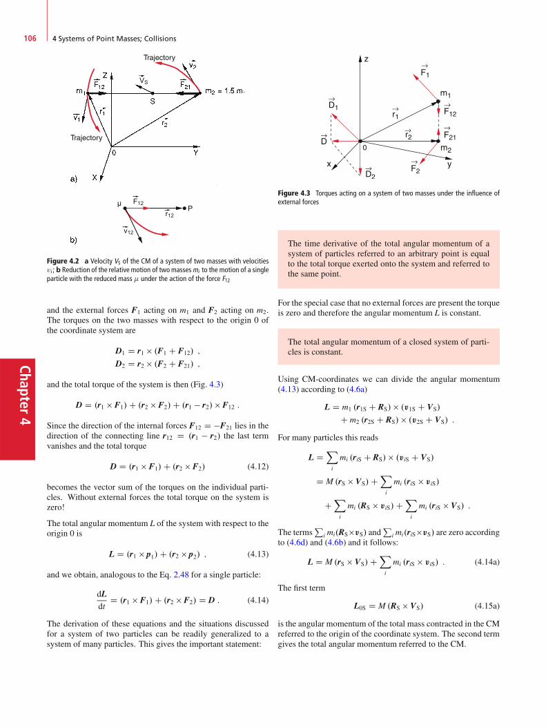
Chapter4
106 4 Systems of Point Masses; Collisions
VS
F12
r12
v12
μ
Figure 4.2 a Velocity VS of the CM of a system of two masses with velocitiesvi ; b Reduction of the relative motion of twomasses mi to the motion of a singleparticle with the reduced mass under the action of the force F12
and the external forces F1 acting on m1 and F2 acting on m2.The torques on the two masses with respect to the origin 0 ofthe coordinate system are
D1 D r1 .F1 C F12/ ;
D2 D r2 .F2 C F21/ ;
and the total torque of the system is then (Fig. 4.3)
D D .r1 F1/C .r2 F2/C .r1 � r2/ F12 :
Since the direction of the internal forces F12 D �F21 lies in thedirection of the connecting line r12 D .r1 � r2/ the last termvanishes and the total torque
D D .r1 F1/C .r2 F2/ (4.12)
becomes the vector sum of the torques on the individual parti-cles. Without external forces the total torque on the system iszero!
The total angular momentum L of the system with respect to theorigin 0 is
L D .r1 p1/C .r2 p2/ ; (4.13)
and we obtain, analogous to the Eq. 2.48 for a single particle:
dLdt
D .r1 F1/C .r2 F2/ D D : (4.14)
The derivation of these equations and the situations discussedfor a system of two particles can be readily generalized to asystem of many particles. This gives the important statement:
Figure 4.3 Torques acting on a system of two masses under the influence ofexternal forces
The time derivative of the total angular momentum of asystem of particles referred to an arbitrary point is equalto the total torque exerted onto the system and referred tothe same point.
For the special case that no external forces are present the torqueis zero and therefore the angular momentum L is constant.
The total angular momentum of a closed system of parti-cles is constant.
Using CM-coordinates we can divide the angular momentum(4.13) according to (4.6a)
L D m1 .r1S C RS/ .v1S C VS/
C m2 .r2S C RS/ .v2S C VS/ :
For many particles this reads
L DX
i
mi .riS C RS/ .viS C VS/
D M .rS VS/CX
i
mi .riS viS/
CX
i
mi .RS viS/CX
i
mi .riS VS/ :
The termsP
i mi.RSvS/ andP
i mi.riSvS/ are zero accordingto (4.6d) and (4.6b) and it follows:
L D M .rS VS/CX
i
mi .riS viS/ : (4.14a)
The first term
L0S D M .RS VS/ (4.15a)
is the angular momentum of the total mass contracted in the CMreferred to the origin of the coordinate system. The second termgives the total angular momentum referred to the CM.
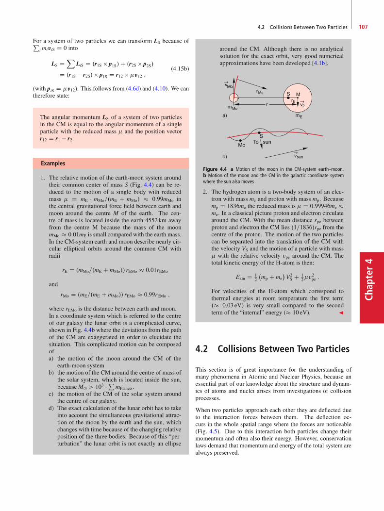
4.2 Collisions Between Two Particles 107
Chap
ter4
For a system of two particles we can transform LS because ofPi miviS D 0 into
LS DX
LiS D .r1S p1S/C .r2S p2S/
D .r1S � r2S/ p1S D r12 v12 ;(4.15b)
(with piS D v12). This follows from (4.6d) and (4.10). We cantherefore state:
The angular momentum LS of a system of two particlesin the CM is equal to the angular momentum of a singleparticle with the reduced mass and the position vectorr12 D r1 � r2.
Examples
1. The relative motion of the earth-moon system aroundtheir common center of mass S (Fig. 4.4) can be re-duced to the motion of a single body with reducedmass D mE � mMo=.mE C mMo/ � 0:99mMo inthe central gravitational force field between earth andmoon around the centre M of the earth. The cen-tre of mass is located inside the earth 4552 km awayfrom the centre M because the mass of the moonmMo � 0:01mE is small compared with the earth mass.In the CM-system earth and moon describe nearly cir-cular elliptical orbits around the common CM withradii
rE D .mMo=.mE C mMo// rEMo � 0:01rEMo
and
rMo D .mE=.mE C mMo// rEMo � 0:99rEMo ;
where rEMo is the distance between earth and moon.In a coordinate system which is referred to the centreof our galaxy the lunar orbit is a complicated curve,shown in Fig. 4.4b where the deviations from the pathof the CM are exaggerated in order to elucidate thesituation. This complicated motion can be composedofa) the motion of the moon around the CM of the
earth-moon systemb) the motion of the CM around the centre of mass of
the solar system, which is located inside the sun,becauseMˇ > 103 �PmPlanets.
c) the motion of the CM of the solar system aroundthe centre of our galaxy.
d) The exact calculation of the lunar orbit has to takeinto account the simultaneous gravitational attrac-tion of the moon by the earth and the sun, whichchanges with time because of the changing relativeposition of the three bodies. Because of this “per-turbation” the lunar orbit is not exactly an ellipse
around the CM. Although there is no analyticalsolution for the exact orbit, very good numericalapproximations have been developed [4.1b].
Figure 4.4 a Motion of the moon in the CM-system earth–moon.b Motion of the moon and the CM in the galactic coordinate systemwhere the sun also moves
2. The hydrogen atom is a two-body system of an elec-tron with mass me and proton with mass mp. Becausemp D 1836me the reduced mass is D 0:99946me �me. In a classical picture proton and electron circulatearound the CM. With the mean distance rpe betweenproton and electron the CM lies .1=1836/rpe from thecentre of the proton. The motion of the two particlescan be separated into the translation of the CM withthe velocity VS and the motion of a particle with mass with the relative velocity vpe around the CM. Thetotal kinetic energy of the H-atom is then:
Ekin D 12
�mp C me
�V2S C 1
2v2pe :
For velocities of the H-atom which correspond tothermal energies at room temperature the first term.� 0:03 eV/ is very small compared to the secondterm of the “internal” energy (� 10 eV). J
4.2 Collisions Between Two Particles
This section is of great importance for the understanding ofmany phenomena in Atomic and Nuclear Physics, because anessential part of our knowledge about the structure and dynam-ics of atoms and nuclei arises from investigations of collisionprocesses.
When two particles approach each other they are deflected dueto the interaction forces between them. The deflection oc-curs in the whole spatial range where the forces are noticeable(Fig. 4.5). Due to this interaction both particles change theirmomentum and often also their energy. However, conservationlaws demand that momentum and energy of the total system arealways preserved.
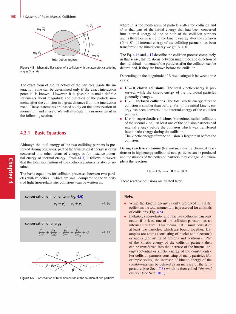
Chapter4
108 4 Systems of Point Masses; Collisions
Figure 4.5 Schematic illustration of a collision with the asymptotic scatteringangles �1 an �2
The exact form of the trajectory of the particles inside the in-teraction zone can be determined only if the exact interactionpotential is known. However, it is possible to make definitestatements about magnitude and direction of the particle mo-menta after the collision in a great distance from the interactionzone. These statements are based solely on the conservation ofmomentum and energy. We will illustrate this in more detail inthe following section.
4.2.1 Basic Equations
Although the total energy of the two colliding partners is pre-served during collisions, part of the translational energy is oftenconverted into other forms of energy, as for instance poten-tial energy or thermal energy. From (4.3) it follows however,that the total momentum of the collision partners is always re-tained.
The basic equations for collision processes between two parti-cles with velocities v which are small compared to the velocityc of light (non-relativistic collisions) can be written as:
conservation of momentum (Fig. 4.6)
p01 C p0
2 D p1 C p2 (4.16)
conservation of energy
p021
2m01
C p022
2m02
D p212m1
C p222m2
C U (4.17)
Figure 4.6 Conservation of total momentum at the collision of two particles
where p0i is the momentum of particle i after the collision and
U is that part of the initial energy that had been convertedinto internal energy of one or both of the collision partnersand is therefore missing in the kinetic energy after the collision(U < 0). If internal energy of the colliding partners has beentransferred into kinetic energy we get U > 0.
The Eq. 4.16 and 4.17 describe the collision process completelyin that sense, that relations between magnitude and direction ofthe individual momenta of the particles after the collision can bedetermined, if they are known before the collision.
Depending on the magnitude of U we distinguish between threecases:
U D 0, elastic collisions. The total kinetic energy is pre-served, while the kinetic energy of the individual particlesgenerally changes.U < 0, inelastic collisions. The total kinetic energy after thecollision is smaller than before. Part of the initial kinetic en-ergy has been converted into internal energy of the collisionpartners.U > 0, superelastic collisions (sometimes called collisionsof the second kind). At least one of the collision partners hadinternal energy before the collision which was transferredinto kinetic energy during the collision.The kinetic energy after the collision is larger than before thecollision.
During reactive collisions (for instance during chemical reac-tions or in high energy collisions) new particles can be producedand the masses of the collision partners may change. An exam-ple is the reaction
H2 C Cl2 �! HCl C HCl :
These reactive collisions are treated later.
Note:
While the kinetic energy is only preserved in elasticcollisions the total momentum is preserved for all kindsof collisions (Fig. 4.6).Inelastic, super-elastic and reactive collisions can onlyoccur, if at least one of the collision partners has aninternal structure. This means that it must consist ofat least two particles, which are bound together. Ex-amples are atoms (consisting of nuclei and electrons)or nuclei (consisting of protons and neutrons). Partof the kinetic energy of the collision partners thencan be transferred into the increase of the internal en-ergy (potential or kinetic energy of the constituents).For collision partners consisting of many particles (forexample solids) the increase of kinetic energy of theconstituents can be defined as an increase of the tem-perature (see Sect. 7.3) which is then called “thermalenergy” (see Sect. 10.1).
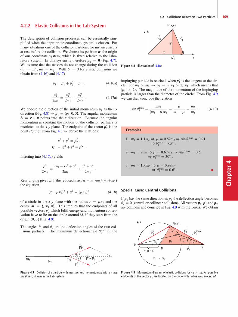
4.2 Collisions Between Two Particles 109
Chap
ter4
4.2.2 Elastic Collisions in the Lab-System
The description of collision processes can be essentially sim-plified when the appropriate coordinate system is chosen. Formany situations one of the collision partners, for instance m2, isat rest before the collision. We choose its position as the originof our coordinate system, which is fixed relative to the labo-ratory system. In this system is therefore p2 D 0 (Fig. 4.7).We assume that the masses do not change during the collision(m1 D m0
1, m2 D m02). With U D 0 for elastic collisions we
obtain from (4.16) and (4.17)
p1 D p01 C p0
2 D p0 ; (4.16a)
p212m1
D p021
2m1C p02
2
2m2: (4.17a)
We choose the direction of the initial momentum p1 as the x-direction (Fig. 4.8) ) p1 D fp1; 0; 0g. The angular momentumL D r p points into the z-direction. Because the angularmomentum is constant the motion of the collision partners isrestricted to the x-y-plane. The endpoint of the vector p0
2 is thepoint P.x; y/. From Fig. 4.8 we derive the relations:
x2 C y2 D p022 ;
.p1 � x/2 C y2 D p021 :
Inserting into (4.17a) yields
p212m1
D .p1 � x/2 C y2
2m1C x2 C y2
2m2:
Rearranging gives with the reduced mass D m1 �m2=.m1Cm2/the equation
.x � v1/2 C y2 D .v1/2 (4.18)
of a circle in the x-y-plane with the radius r D v1 and thecentre M D fv1; 0g. This implies that the endpoints of allpossible vectors p0
2 which fulfil energy-and momentum conser-vation have to lie on the circle around M, if they start from theorigin f0; 0g (Fig. 4.9).The angles �1 and �2 are the deflection angles of the two col-lisions partners. The maximum deflectionangle �max
1 of the
Figure 4.7 Collision of a particle with mass m1 and momentum p1 with a massm2 at rest, drawn in the Lab-system
Figure 4.8 Illustration of (4.18)
impinging particle is reached, when p01 is the tangent to the cir-
cle. For m1 > m2 ! p1 D m1v1 > 2v1, which means thatjp1j > 2r. The magnitude of the momentum of the impingingparticle is larger than the diameter of the circle. From Fig. 4.9we can then conclude the relation
sin �max1 D v1
.m1 � /v1 D
m1 � D m2
m1: (4.19)
Examples
1. m1 D 1:1m2 ) D 0:52m2 ) sin �max1 D 0:91
) �max1 D 65ı :
2. m1 D 2m2 ) D 0:67m2 ) sin �max1 D 0:5
) �max1 D 30ı :
3. m1 D 100m2 ) D 0:99m2
) �max1 D 0:6ı : J
Special Case: Central Collisions
If p02 has the same direction as p1 the deflection angle becomes
�2 D 0 (central or collinear collision). All vectors p1, p01 and p2
are collinear and coincide in Fig. 4.9 with the x-axis. We obtain
Figure 4.9 Momentum diagram of elastic collisions for m1 > m2. All possibleendpoints of the vector p0
2 are located on the circle with radius v1 around M

Chapter4
110 4 Systems of Point Masses; Collisions
from Fig. 4.9:
p1 D 2v1 C p01
)m1v01 D m1v1 � 2
m1m2
m1 C m2v1
)v01 D m1 � m2
m1 C m2v1 I
p02 D 2v1
)v02 D 2
m2v1 D 2m1
m1 C m2v1 :
(4.20)
The momentum of the pushed particle gets its maximum valuep02 D 2v1 for collinear collisions.
Also the kinetic energy, transferred from m1 to m2 during acollinear elastic collision reaches its maximum value
�Ekin D p022
2m2� �Emax
kin D 2m21m2
.m1 C m2/2v21
�Emaxkin D 4
m1m2
M2E1 D 42
m1m2E1 ;
(4.21)
which equals the fraction 42=.m1m2/ of the initial energy E1 ofthe impinging mass m1. In Fig. 4.10 this maximum transferredfraction is shown as a function of the mass ratio m1=m2.
For m1 D m2 it is v01 D 0 and v0
2 D v1. The two massesexchange their momentum during the collision, i. e. after the col-lision m1 is at rest and m2 moves with the momentum p0
2 D p1.
For equal massesm1 D m2 the energy of the incident parti-cle is completely transferred to the resting massm2 duringa collinear collision.
1,0
0,5
010 5 10 15 20
(m1/m2)
Ekinmax
E1Δ
= 4m1m2
(m1+m2)2 =
4(m1/m2)+2+1/(m1/m2)
Figure 4.10 Maximum energy transfer �E D E � E 01 for a collinear elastic
collison of a particle with mass m1 onto a mass m2 at rest for different ratiosm1=m2
Special cases of non-collinear collisions
We will now discuss the general case of non-collinear collisionsand illustrate it by some important special cases of the mass ratiom1=m2.
m1 D m2 D m ) � D 12m:
Equation 4.18 gives for the radius of the circle in Fig. 4.9r D 1
2mv1, which implies that the momentum p1 D mv1 ofthe incident particle is the diameter of the circle (Fig. 4.11). Fornon-collinear collisions the momenta p0
1 and p02 after the colli-
sion are perpendicular to each other according to the theorem ofThales. For the deflection angles it follows �1 C �2 D =2.
The paths of the two particles are perpendicular to eachother after the non-collinear collision, i. e. p0
1 ? p02.
Example
For the deceleration of neutrons in nuclear reactors amaterial with many hydrogen atoms is the best choice.Because the protons have nearly the same mass as neu-trons. J
m1 � m2 ) � � m1
The radius of the circle in Fig. 4.9 becomes for the limiting casem1=m2 ! 0 equal to the momentum p1 D m1v1 of the inci-dent particle (Fig. 4.12a). The magnitude of p1 does not changeduring the collision .jp1j D jp0
1j/ but all directions of p01 are
possible. The scattering angle �1 can take all values in the range� � �1 � C .The maximum momentum transfer onto m2 is
jp02jmax D 2r D 2p1 :
The maximum transferred energy is
�Emaxkin D .2p1/2
2m2D 4p21
2m1
m1
m2D 4
m1
m2E1 : (4.22)
Figure 4.11 Elastic collision between particles of equal mass
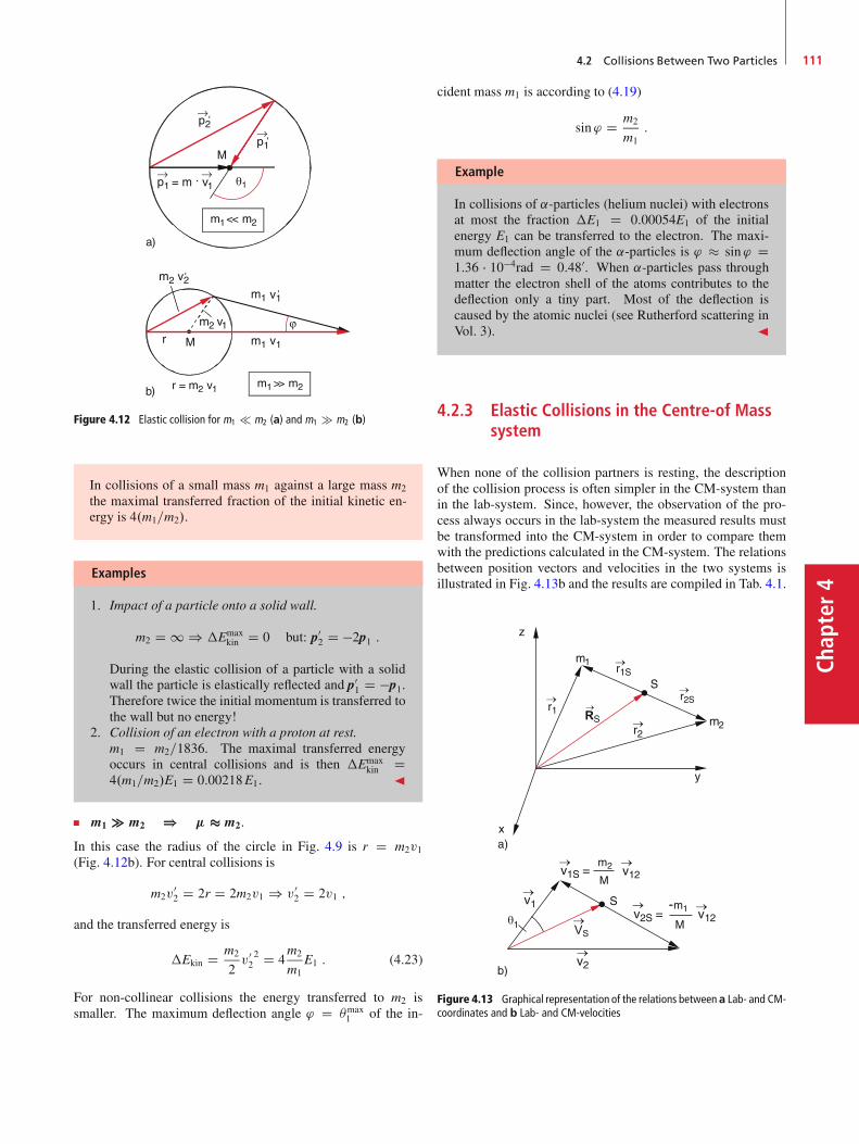
4.2 Collisions Between Two Particles 111
Chap
ter4
Figure 4.12 Elastic collision for m1 m2 (a) and m1 � m2 (b)
In collisions of a small mass m1 against a large mass m2
the maximal transferred fraction of the initial kinetic en-ergy is 4.m1=m2/.
Examples
1. Impact of a particle onto a solid wall.
m2 D 1 ) �Emaxkin D 0 but: p0
2 D �2p1 :
During the elastic collision of a particle with a solidwall the particle is elastically reflected and p0
1 D �p1.Therefore twice the initial momentum is transferred tothe wall but no energy!
2. Collision of an electron with a proton at rest.m1 D m2=1836. The maximal transferred energyoccurs in central collisions and is then �Emax
kin D4.m1=m2/E1 D 0:00218E1. J
m1 � m2 ) � � m2.
In this case the radius of the circle in Fig. 4.9 is r D m2v1(Fig. 4.12b). For central collisions is
m2v02 D 2r D 2m2v1 ) v0
2 D 2v1 ;
and the transferred energy is
�Ekin D m2
2v022 D 4
m2
m1E1 : (4.23)
For non-collinear collisions the energy transferred to m2 issmaller. The maximum deflection angle ' D �max
1 of the in-
cident mass m1 is according to (4.19)
sin' D m2
m1:
Example
In collisions of ˛-particles (helium nuclei) with electronsat most the fraction �E1 D 0:00054E1 of the initialenergy E1 can be transferred to the electron. The maxi-mum deflection angle of the ˛-particles is ' � sin' D1:36 � 10�4rad D 0:480. When ˛-particles pass throughmatter the electron shell of the atoms contributes to thedeflection only a tiny part. Most of the deflection iscaused by the atomic nuclei (see Rutherford scattering inVol. 3). J
4.2.3 Elastic Collisions in the Centre-of Masssystem
When none of the collision partners is resting, the descriptionof the collision process is often simpler in the CM-system thanin the lab-system. Since, however, the observation of the pro-cess always occurs in the lab-system the measured results mustbe transformed into the CM-system in order to compare themwith the predictions calculated in the CM-system. The relationsbetween position vectors and velocities in the two systems isillustrated in Fig. 4.13b and the results are compiled in Tab. 4.1.
VS
RS
Figure 4.13 Graphical representation of the relations betweena Lab- and CM-coordinates and b Lab- and CM-velocities
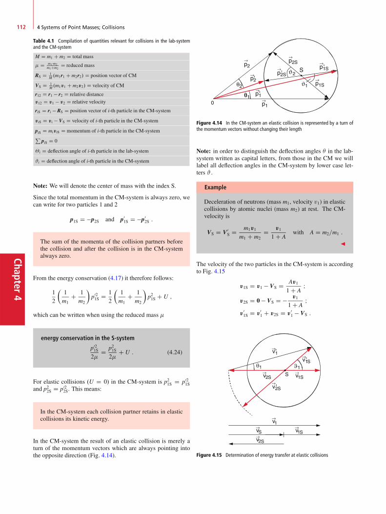
Chapter4
112 4 Systems of Point Masses; Collisions
Table 4.1 Compilation of quantities relevant for collisions in the lab-systemand the CM-system
M D m1 C m2 D total mass
D m1 �m2m1Cm2
D reduced mass
RS D 1M .m1r1 C m2r2/ D position vector of CM
VS D 1M .m1v1 C m2v2/ D velocity of CM
r12 D r1 � r2 D relative distance
v12 D v1 � v2 D relative velocity
riS D ri � RS D position vector of i-th particle in the CM-system
viS D vi � VS D velocity of i-th particle in the CM-system
piS D miviS D momentum of i-th particle in the CM-systemP
piS D 0
�i D deflection angle of i-th particle in the lab-system
#i D deflection angle of i-th particle in the CM-system
Note: We will denote the center of mass with the index S.
Since the total momentum in the CM-system is always zero, wecan write for two particles 1 and 2
p1S D �p2S and p01S D �p0
2S :
The sum of the momenta of the collision partners beforethe collision and after the collision is in the CM-systemalways zero.
From the energy conservation (4.17) it therefore follows:
1
2
�1
m1C 1
m2
�p021S D 1
2
�1
m1C 1
m2
�p21S C U ;
which can be written when using the reduced mass
energy conservation in the S-system
p021S
2D p21S
2C U : (4.24)
For elastic collisions .U D 0/ in the CM-system is p21S D p021S
and p22S D p022S. This means:
In the CM-system each collision partner retains in elasticcollisions its kinetic energy.
In the CM-system the result of an elastic collision is merely aturn of the momentum vectors which are always pointing intothe opposite direction (Fig. 4.14).
Figure 4.14 In the CM-system an elastic collision is represented by a turn ofthe momentum vectors without changing their length
Note: in order to distinguish the deflection angles � in the lab-system written as capital letters, from those in the CM we willlabel all deflection angles in the CM-system by lower case let-ters # .
Example
Deceleration of neutrons (mass m1, velocity v1) in elasticcollisions by atomic nuclei (mass m2) at rest. The CM-velocity is
VS D V0S D m1v1
m1 C m2D v1
1 C Awith A D m2=m1 :
J
The velocity of the two particles in the CM-system is accordingto Fig. 4.15
v1S D v1 � VS D Av1
1 C AI
v2S D 0 � VS D � v1
1 C AI
v01S D v0
1 C v2S D v01 � VS :
S
Figure 4.15 Determination of energy transfer at elastic collisions
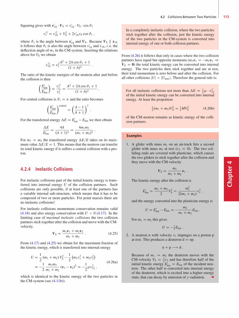
4.2 Collisions Between Two Particles 113
Chap
ter4
Squaring gives with v01S � VS D v0
1S � VS � cos#1v021 D v02
1S C V2S C 2v0
1SvS cos#1 ;
where #1 is the angle between v01S and VS. Because VS k v1S
it follows that #1 is also the angle between v01S and v1S, i. e. the
deflection angle of m1 in the CM-system. Inserting the relationsabove for VS we obtain
v021S D v21
A2 C 2A cos#1 C 1
.1 C A/2:
The ratio of the kinetic energies of the neutron after and beforethe collision is then
�E0kin
Ekin
�D v02
1
v21D A2 C 2A cos#1 C 1
.1 C A/2:
For central collisions is #1 D and the ratio becomes�E0kin
Ekin
�central
D�A � 1
A C 1
�2
:
For the transferred energy �E D E0kin � Ekin we then obtain
�E
EkinD 4A
.A C 1/2D 4m1m2
.m1 C m2/2:
For m1 D m2 the transferred energy �E=E takes on its maxi-mum value�E=E D 1. This means that the neutron can transferits total kinetic energy if it suffers a central collision with a pro-ton.
4.2.4 Inelastic Collisions
For inelastic collisions part of the initial kinetic energy is trans-ferred into internal energy U of the collision partners. Suchcollisions are only possible, if at least one of the partners hasa variable internal sub-structure, which means that it has to becomposed of two or more particles. For point masses there areno inelastic collisions!
For inelastic collisions momentum conservation remains valid(4.16) and also energy conservation with U < 0 (4.17). In thelimiting case of maximal inelastic collisions the two collisionpartners stick together after the collision and move with the CM-velocity.
VS D m1v1 C m2v2
m1 C m2: (4.25)
From (4.17) and (4.25) we obtain for the maximum fraction ofthe kinetic energy, which is transferred into internal energy
U D 1
2.m1 C m2/V
2S � 1
2
�m1v
21 C m2v
22
�
D �1
2
m1m2
m1 C m2.v1 � v2/
2 D �1
2v212 ;
(4.26a)
which is identical to the kinetic energy of the two particles inthe CM-system (see (4.11b)).
In a completely inelastic collision, where the two particlesstick together after the collision, just the kinetic energyof the two particles in the CM-system is converted intointernal energy of one or both collision partners.
From (4.26) it follows that only in cases where the two collisionpartners have equal but opposite momenta (m1v1 D �m2v2 )VS D 0) the total kinetic energy can be converted into internalenergy. The two particles then stick together and are at rest,their total momentum is zero before and after the collision. Forall other collisions jUj < jUmaxj. Therefore the general rule is:
For all inelastic collisions not more than �E D 12 � v212
of the initial kinetic energy can be converted into internalenergy. At least the proportion
12 .m1 C m2/V
2S D 1
2MV2S (4.26b)
of the CM-motion remains as kinetic energy of the colli-sion partners.
Examples
1. A glider with mass m1 on an air-track hits a secondglider with mass m2 at rest .v2 D 0/. The two col-liding ends are covered with plasticine, which causesthe two gliders to stick together after the collision andthey move with the CM-velocity
VS D m1
m1 C m2v1 :
The kinetic energy after the collision is
E0kin D m1 C m2
2V2S D m2
1
2.m1 C m2/v21 ;
and the energy converted into the plasticine energy is
U D E0kin � Ekin D � m2
m1 C m2Ekin :
For m1 D m2 this gives
U D � 12Ekin :
2. A neutron n with velocity v1 impinges on a proton pat rest. This produces a deuteron d D np.
n C p �! d :
Because of m1 D m2 the deuteron moves with theCM-velocity VS D 1
2v1 and has therefore half of theinitial kinetic energy E0
kin D Ekin of the incident neu-tron. The other half is converted into internal energyof the deuteron, which is excited into a higher energystate, that can decay by emission of � -radiation. J
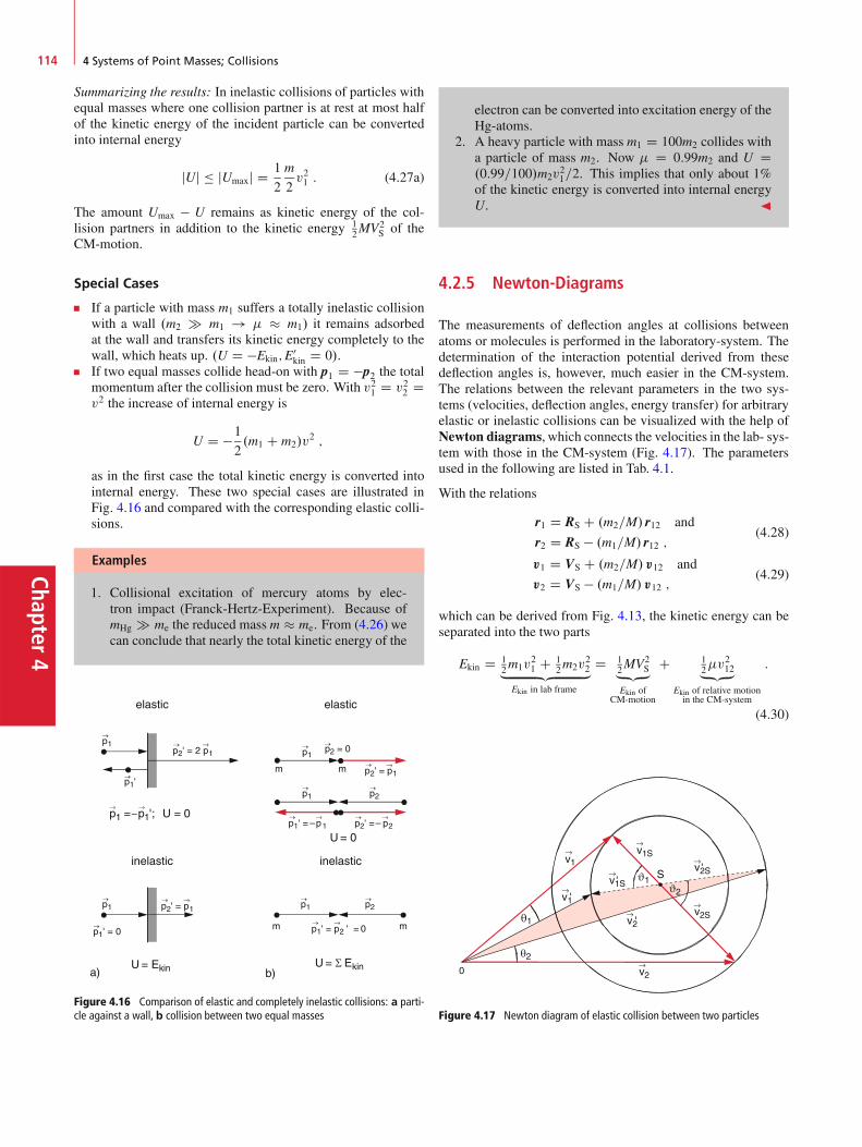
Chapter4
114 4 Systems of Point Masses; Collisions
Summarizing the results: In inelastic collisions of particles withequal masses where one collision partner is at rest at most halfof the kinetic energy of the incident particle can be convertedinto internal energy
jUj � jUmaxj D 1
2
m
2v21 : (4.27a)
The amount Umax � U remains as kinetic energy of the col-lision partners in addition to the kinetic energy 1
2MV2S of the
CM-motion.
Special Cases
If a particle with mass m1 suffers a totally inelastic collisionwith a wall .m2 � m1 ! � m1/ it remains adsorbedat the wall and transfers its kinetic energy completely to thewall, which heats up. .U D �Ekin;E0
kin D 0/.If two equal masses collide head-on with p1 D �p2 the totalmomentum after the collision must be zero. With v21 D v22 Dv2 the increase of internal energy is
U D �1
2.m1 C m2/v
2 ;
as in the first case the total kinetic energy is converted intointernal energy. These two special cases are illustrated inFig. 4.16 and compared with the corresponding elastic colli-sions.
Examples
1. Collisional excitation of mercury atoms by elec-tron impact (Franck-Hertz-Experiment). Because ofmHg � me the reduced massm � me. From (4.26) wecan conclude that nearly the total kinetic energy of the
Figure 4.16 Comparison of elastic and completely inelastic collisions: a parti-cle against a wall, b collision between two equal masses
electron can be converted into excitation energy of theHg-atoms.
2. A heavy particle with mass m1 D 100m2 collides witha particle of mass m2. Now D 0:99m2 and U D.0:99=100/m2v
21=2. This implies that only about 1%
of the kinetic energy is converted into internal energyU. J
4.2.5 Newton-Diagrams
The measurements of deflection angles at collisions betweenatoms or molecules is performed in the laboratory-system. Thedetermination of the interaction potential derived from thesedeflection angles is, however, much easier in the CM-system.The relations between the relevant parameters in the two sys-tems (velocities, deflection angles, energy transfer) for arbitraryelastic or inelastic collisions can be visualized with the help ofNewton diagrams, which connects the velocities in the lab- sys-tem with those in the CM-system (Fig. 4.17). The parametersused in the following are listed in Tab. 4.1.
With the relations
r1 D RS C .m2=M/ r12 and
r2 D RS � .m1=M/ r12 ;(4.28)
v1 D VS C .m2=M/v12 and
v2 D VS � .m1=M/v12 ;(4.29)
which can be derived from Fig. 4.13, the kinetic energy can beseparated into the two parts
Ekin D 12m1v
21 C 1
2m2v22„ ƒ‚ …
Ekin in lab frame
D 12MV2
S„ƒ‚…Ekin of
CM-motion
C 12v
212„ƒ‚…
Ekin of relative motionin the CM-system
:
(4.30)
Figure 4.17 Newton diagram of elastic collision between two particles
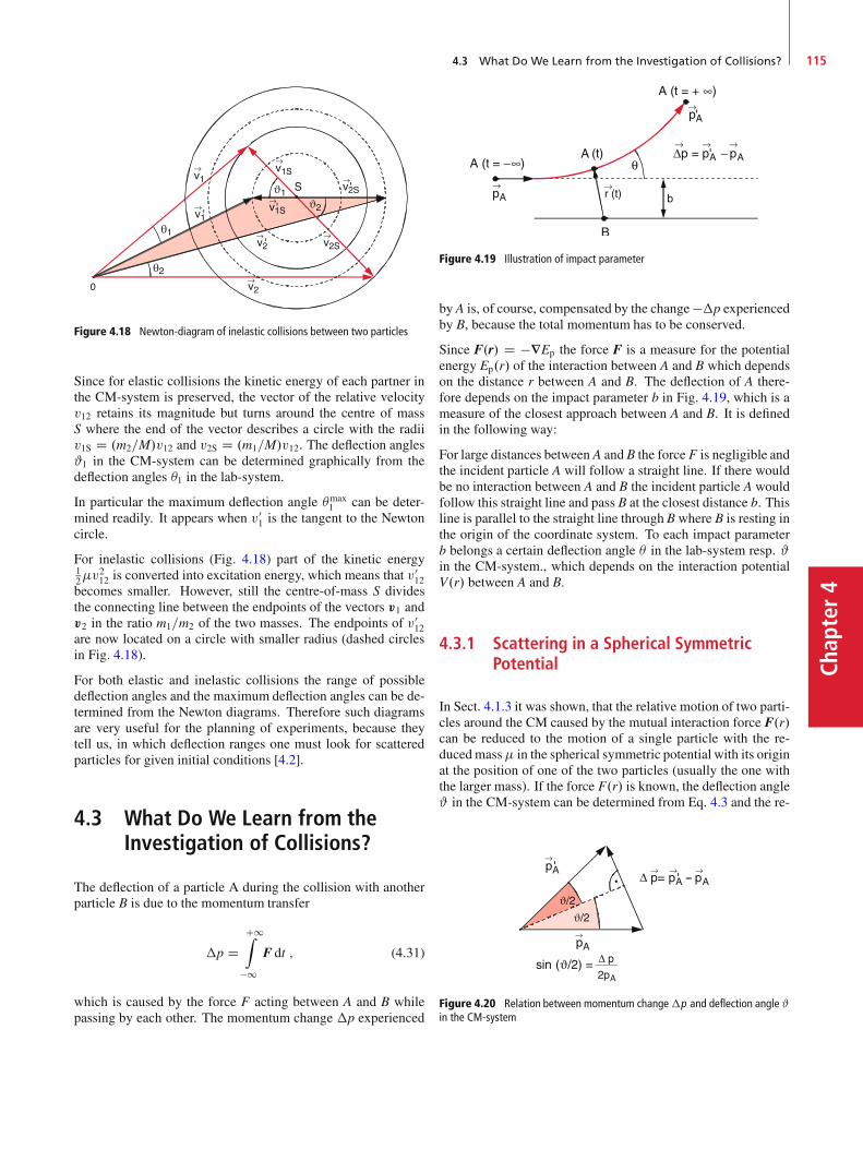
4.3 What Do We Learn from the Investigation of Collisions? 115
Chap
ter4
Figure 4.18 Newton-diagram of inelastic collisions between two particles
Since for elastic collisions the kinetic energy of each partner inthe CM-system is preserved, the vector of the relative velocityv12 retains its magnitude but turns around the centre of massS where the end of the vector describes a circle with the radiiv1S D .m2=M/v12 and v2S D .m1=M/v12. The deflection angles#1 in the CM-system can be determined graphically from thedeflection angles �1 in the lab-system.
In particular the maximum deflection angle �max1 can be deter-
mined readily. It appears when v01 is the tangent to the Newton
circle.
For inelastic collisions (Fig. 4.18) part of the kinetic energy12v
212 is converted into excitation energy, which means that v0
12becomes smaller. However, still the centre-of-mass S dividesthe connecting line between the endpoints of the vectors v1 andv2 in the ratio m1=m2 of the two masses. The endpoints of v0
12are now located on a circle with smaller radius (dashed circlesin Fig. 4.18).
For both elastic and inelastic collisions the range of possibledeflection angles and the maximum deflection angles can be de-termined from the Newton diagrams. Therefore such diagramsare very useful for the planning of experiments, because theytell us, in which deflection ranges one must look for scatteredparticles for given initial conditions [4.2].
4.3 What Do We Learn from theInvestigation of Collisions?
The deflection of a particle A during the collision with anotherparticle B is due to the momentum transfer
�p DC1Z
�1F dt ; (4.31)
which is caused by the force F acting between A and B whilepassing by each other. The momentum change �p experienced
Figure 4.19 Illustration of impact parameter
by A is, of course, compensated by the change ��p experiencedby B, because the total momentum has to be conserved.
Since F.r/ D �rEp the force F is a measure for the potentialenergy Ep.r/ of the interaction between A and B which dependson the distance r between A and B. The deflection of A there-fore depends on the impact parameter b in Fig. 4.19, which is ameasure of the closest approach between A and B. It is definedin the following way:
For large distances between A and B the force F is negligible andthe incident particle A will follow a straight line. If there wouldbe no interaction between A and B the incident particle A wouldfollow this straight line and pass B at the closest distance b. Thisline is parallel to the straight line through B where B is resting inthe origin of the coordinate system. To each impact parameterb belongs a certain deflection angle � in the lab-system resp. #in the CM-system., which depends on the interaction potentialV.r/ between A and B.
4.3.1 Scattering in a Spherical SymmetricPotential
In Sect. 4.1.3 it was shown, that the relative motion of two parti-cles around the CM caused by the mutual interaction force F.r/can be reduced to the motion of a single particle with the re-ducedmass in the spherical symmetric potential with its originat the position of one of the two particles (usually the one withthe larger mass). If the force F.r/ is known, the deflection angle# in the CM-system can be determined from Eq. 4.3 and the re-
Figure 4.20 Relation between momentum change�p and deflection angle #in the CM-system

Chapter4
116 4 Systems of Point Masses; Collisions
lation sin.#=2/ D 12�ppA
(Fig. 4.20). In Sect. 4.2.5 it was shownhow the angle � measured in the lab-system can be transformedinto the angle # in the CM-system.
The deflection of particles in a potential is called potentialscattering. We will illustrate this potential scattering and itstreatment by some examples.
Examples
1. Collision of two hard spheres with radii r1 and r2(Fig. 4.21).If the impact parameter b is larger the sum r1 C r2no collision takes place. The hard sphere A moves ona straight line and passes B without deflection. Forb � r1 C r2 the colliding partner A is reflected at thesurface of B (Fig. 4.21a). In order to determine thedeflection angle # of A we decompose the momentump1 of A into a component pr parallel to the connectingline M1M2 at the touch of the two spheres and a com-ponent pt in the tangential direction perpendicular topr (Fig. 4.21b). We assume the surface of the spheresas frictionless. Then no rotation of the spheres can beexcited and the component pt does not change duringthe collision. For the component pr we can concludefrom (4.20) for central collisions
p0r D m1 � m2
m1 C m2pr : (4.32a)
Figure 4.21 Determination of the deflection function for collisionsbetween two hard spheres. a Definition of impact parameter, b decom-position of impact momentum, c momentum vector addition
For m2 � m1 this gives p0r D �pr. In this case is in
Fig. 4.21c ˇ D ˛ and the deflection angle becomes� D 2˛.
From Fig. 4.21b one can deduce from b D r1 C r2 for� D 2˛ the dependence of the deflection angle on theimpact parameter b
�.b/ D 2 arccosb
r1 C r2: (4.32b)
For b D 0 is � D i. e. A is reflected back., forb > r1 C r2 is � D 0. The function �.b/ is calleddeflection function. Its curve depends on the interac-tion potential .V.r//. For the collision of two hardspheres the potential is a step function (Fig. 4.22a) andthe deflection function is the monotonic curved shownin Fig. 4.22b for m2 � m1.For the general case of arbitrary ratios m1=m2 we ob-tain from Fig. 4.21c:
� D ˛ C ˇ
with pr=pt D tan˛ it follows
tanˇ D p0r=pr D �.m1 � m2/=.m1 C m2/ :
While (4.32b) is only strictly valid for m2 D 1, thedeflection function
#.b/ D arccosb
r1 C r2(4.32c)
in the CM-system is correct for arbitrary ratiosm1=m2.
Figure 4.22 a Potential V .r/ for hard spheres; b deflection functionfor hard sphere collisions
2. Scattering of a particle in a potential V.r/ / 1=r.This important case applies for instance for theCoulomb-scattering of charged particles (electronsor ˛-particles) on atomic nuclei (see Vol. 3) or theKepler-orbit of comets in the gravitational field of thesun.For a potential V.r/ with the potential energy Ep Da=r the force between the interacting particles A andB with masses m1 and m2 is
F D � gradEp D a
r2Or : (4.33)
For a > 0 a repulsion between the particles occur, fora < 0 an attraction. The angular momentum in theCM-system is according to (4.15)
L D r � v with D m1m2
m1 C m2;
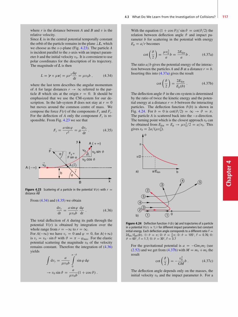
4.3 What Do We Learn from the Investigation of Collisions? 117
Chap
ter4
where r is the distance between A and B and v is therelative velocity.Since L is in the central potential temporally constantthe orbit of the particle remains in the plane?L, whichwe choose as the x-y-plane (Fig. 4.23). The particle Ais incident parallel to the x-axis with an impact param-eter b and the initial velocity v0. It is convenient to usepolar coordinates for the description of its trajectory.The magnitude of L is then
L D jr vj D r2d'
dtD v0b ; (4.34)
where the last term describes the angular momentumof A for large distances r ! 1 referred to the par-ticle B which sits at the origin r D 0. It should beemphasized that we use the CM-system for our de-scription. In the lab-system B does not stay at r D 0but moves around the common centre of mass. Wecompose the force F.r/ of the components Fx and Fy.For the deflection of A only the component Fy is re-sponsible. From Fig. 4.23 we see that
Fy D a sin '
r2D
dvydt
: (4.35)
A ( r )
Figure 4.23 Scattering of a particle in the potential V .r/ with r Ddistance AB
From (4.34) and (4.35) we obtain
dvydt
D a sin'
v0b
d'
dt: (4.36)
The total deflection of A during its path through thepotential V.r/ is obtained by integration over thewhole range from r D �1 to r D 1.For A.�1/ we have vy D 0 and ' D 0, for A.C1/is vy D v0 � sin# with # D � 'max. For the elasticpotential scattering the magnitude v0 of the velocityremains constant. Therefore the integration of (4.36)yields
Zdvy D a
v0b
�#Z
0
sin ' d'
! v0 sin# D a
v0b.1 C cos#/ :
With the equation .1 C cos#/= sin# D cot.#=2/ therelation between deflection angle # and impact pa-rameter b for scattering in the potential with energyEp D a=r becomes
cot
�#
2
�D v20
ab D 2Ekin
ab : (4.37a)
The ratio a=b gives the potential energy of the interac-tion between the particles A and B at a distance r D b.Inserting this into (4.37a) gives the result
cot
�#
2
�D 2Ekin
Ep.b/: (4.37b)
The deflection angle # in the cm-system is determinedby the ratio of twice the kinetic energy and the poten-tial energy at a distance r D b between the interactingparticles. The deflection function #.b/ is shown inFig. 4.24. For b D 0 is cot.#=2/ D 1 ! # D .The particle A is scattered back into the �x-direction.The turning point which is the closest approach r0 canbe obtained from Ekin D Ep ! v20=2 D a=r0. Thisgives r0 D 2a=.v20/.
Figure 4.24 Deflection function #.b / (a) and trajectories of a particlein a potential V .r/ / 1=r for different impact parameters but constantinitial energy. Each deflection angle corresponds to a different ratio f D2Ekin=Epot.b /. ➀: # D ; ➁: # D 3
4 ; ➂: # D 105ı, f D 0:76; ➃:# D 60ı, f D 1:7; ➄: # D 30ı, f D 3:7
For the gravitational potential is a D �Gm1m2 (see(2.52) and we get from (4.37b) withM D m1 Cm2 theresult
cot
�#
2
�D � v20
GMb : (4.37c)
The deflection angle depends only on the masses, theinitial velocity v0 and the impact parameter b. For a
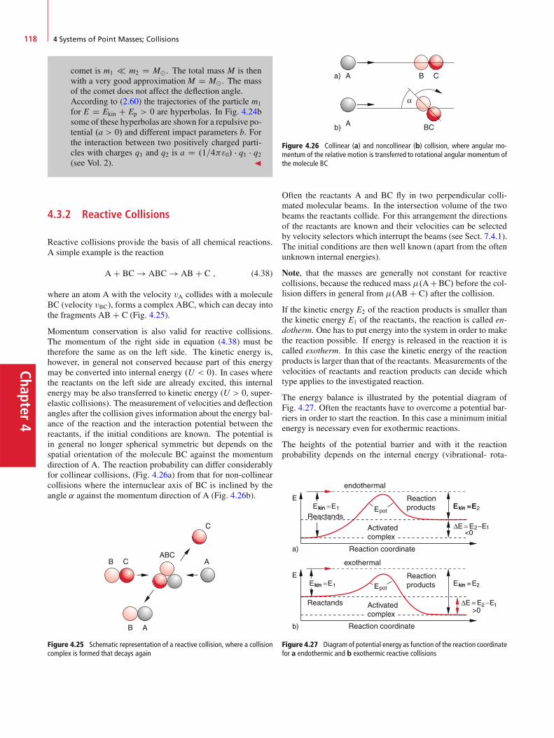
Chapter4
118 4 Systems of Point Masses; Collisions
comet is m1 m2 D Mˇ. The total mass M is thenwith a very good approximation M D Mˇ. The massof the comet does not affect the deflection angle.According to (2.60) the trajectories of the particle m1
for E D Ekin C Ep > 0 are hyperbolas. In Fig. 4.24bsome of these hyperbolas are shown for a repulsive po-tential .a > 0/ and different impact parameters b. Forthe interaction between two positively charged parti-cles with charges q1 and q2 is a D .1=4"0/ � q1 � q2(see Vol. 2). J
4.3.2 Reactive Collisions
Reactive collisions provide the basis of all chemical reactions.A simple example is the reaction
A C BC ! ABC ! AB C C ; (4.38)
where an atom A with the velocity vA collides with a moleculeBC (velocity vBC), forms a complex ABC, which can decay intothe fragments AB C C (Fig. 4.25).
Momentum conservation is also valid for reactive collisions.The momentum of the right side in equation (4.38) must betherefore the same as on the left side. The kinetic energy is,however, in general not conserved because part of this energymay be converted into internal energy .U < 0/. In cases wherethe reactants on the left side are already excited, this internalenergy may be also transferred to kinetic energy (U > 0, super-elastic collisions). The measurement of velocities and deflectionangles after the collision gives information about the energy bal-ance of the reaction and the interaction potential between thereactants, if the initial conditions are known. The potential isin general no longer spherical symmetric but depends on thespatial orientation of the molecule BC against the momentumdirection of A. The reaction probability can differ considerablyfor collinear collisions, (Fig. 4.26a) from that for non-collinearcollisions where the internuclear axis of BC is inclined by theangle ˛ against the momentum direction of A (Fig. 4.26b).
Figure 4.25 Schematic representation of a reactive collision, where a collisioncomplex is formed that decays again
Figure 4.26 Collinear (a) and noncollinear (b) collision, where angular mo-mentum of the relative motion is transferred to rotational angular momentum ofthe molecule BC
Often the reactants A and BC fly in two perpendicular colli-mated molecular beams. In the intersection volume of the twobeams the reactants collide. For this arrangement the directionsof the reactants are known and their velocities can be selectedby velocity selectors which interrupt the beams (see Sect. 7.4.1).The initial conditions are then well known (apart from the oftenunknown internal energies).
Note, that the masses are generally not constant for reactivecollisions, because the reduced mass .ACBC/ before the col-lision differs in general from .AB C C/ after the collision.
If the kinetic energy E2 of the reaction products is smaller thanthe kinetic energy E1 of the reactants, the reaction is called en-dotherm. One has to put energy into the system in order to makethe reaction possible. If energy is released in the reaction it iscalled exotherm. In this case the kinetic energy of the reactionproducts is larger than that of the reactants. Measurements of thevelocities of reactants and reaction products can decide whichtype applies to the investigated reaction.
The energy balance is illustrated by the potential diagram ofFig. 4.27. Often the reactants have to overcome a potential bar-riers in order to start the reaction. In this case a minimum initialenergy is necessary even for exothermic reactions.
The heights of the potential barrier and with it the reactionprobability depends on the internal energy (vibrational- rota-
Figure 4.27 Diagram of potential energy as function of the reaction coordinatefor a endothermic and b exothermic reactive collisions

4.4 Collisions at Relativistic Energies 119
Chap
ter4
tional or even electronic energy) of the reaction partners. Forthe measurement of these internal energy several spectroscopictechniques have been developed which allow to determine theexcitation state of the partners involved in the reaction.
An ideal experiments should allow to measure all relevant pa-rameters of a collision process such as the internal energies, thedeflection angles and the velocities of all particles. Such moderntechniques are discussed in Vol. 3.
4.4 Collisions at Relativistic Energies
Up to now we have used the Newtonian laws (energy- and mo-mentum conservation) for the description of collision processesand we have assumed that the masses of the reaction partners areconstant (besides in reactive collisions). This is justified as longas the velocities of the collision partners are small comparedwith the velocity c of light (see Chap. 3).
For the investigation of interactions between elementary parti-cles and atomic nuclei, higher energies of the collision partnersare required. Such energies, where the velocity of particlescomes close to the velocity of light can be realized in particleaccelerators and storage rings (see Vol. 4). We will now discuss,how the rules governing collisions at relativistic energies (thedomain of high energy physics) must be formulated.
4.4.1 Relativistic Mass Increase
We regard two particles A and B which have equal masses m1 Dm2 D m, if they are at rest. We assume that A and B move in asystem S with velocities
v1 D fvx1;�vy1g and v2 D f0; vy2gagainst each other where vy1 D vy2 (Fig. 4.28a).
The particle B should suffer an elastic striking collision with Asuch that during the collision the x-component vx1 of A remainsconstant but the y-component is reversed. The velocity of A afterthe collision is then v0
1 D fvx1; vy1g. The magnitude of its veloc-
ity jv1j Dqv2x1 C v2y1 is therefore also preserved. Because the
momentummust be constant the velocity of B after the collisionmust be
v02 D f0;�vy2g :
We assume that vy vx. For the magnitudes of the velocitiesthis implies
v1 D .v2x1 C v2y1/.1=2/ � vx1 and v2 v1 :
Now we describe this collision between A and B in a system S�which moves against S with the velocity v D vx1 into the x-direction (Fig. 4.28b). In this system we get for the velocities ofA and B:
v�x1 D 0 but v�
x2 D �vx1 ;
* *
Figure 4.28 Grazing elastic collision between A and B at relativistic velocities.a In the system S has A a large and B a small velocity since Vy Vx . b In thesytem S �, that moves relativ to S the situation is reversed
which implies that the roles of A and B are just interchanged.
According to Eq. 3.28 for the transformation of velocities whenchanging from system S to S� the observer O� in S� measuresthe velocity component
v�y D vy=�
1 � vxv=c2 : (4.39)
Since in the system S for the particle A holds: vx1 D v0x1 ¤ 0,
for B, however, vx2 D v0x2 D 0 the observer O� measures for the
two particles different y-components of the velocities
v�y1 D vy1=�
1 � vx1v=c2 D vy1=�
1 � v2=c2 D �vy1 ;
since v � vx1 ;
(4.40a)
v�y2 D vy2=�
1 � vx2v=c2 D vy2=� ; (4.40b)
while for the observer O in S the velocity component of A is vy1and for B it is vy2.
In both inertial systems S and S� the conservation of total mo-mentum holds, since the physical laws are independent of thechosen inertial system (see Sect. 3.2). This yields for the y-component of the total momentum
mAvy1 � mBvy2 D m�Av
�y1 � m�
Bv�y2 D 0 : (4.41)

Chapter4
120 4 Systems of Point Masses; Collisions
For mA D m�A and mB D m�
B this condition cannot be fulfilled,i. e. the conservation of momentum would fail, because accord-ing to (4.40) vy1=v�
y1 is different from vy2=v�y2. We are therefore
forced (if we will not give up the well proved conservation ofmomentum) to assume that the mass of a particle is changingwith its velocity. For the limiting case vx1 � vy1 � 0 we canwrite:
vA � vx1 D v I v�A � 0 ;
vB � 0 I v�B � vx1 � v :
We therefore get with m.v D 0/ D m0 for (4.41)
m.v/vy1 C m0vy2 D 0 ; (4.42a)
m0v�y1 C m.v/v�
y2 D 0 ; (4.42b)
with (4.40) this gives
.m.v//2
m20
D vy2
v�y2
� v�y1
vy1D �2
) m.v/ D �m0 D m0p1 � v2=c2 : (4.43)
The mass m.v/ of a moving particle increases with its velocityv. the mass m0 D m.v D 0/ is called its rest-mass. This massincrease is noticeable only for large velocities [4.3].
Examples
1. For v D 0:01c ) m D 1:00005m0. The relative massincrease �m=m D .m � m0/=m0 � 5 � 10�5.
2. For v D 0:9c ) m D 2:29m0.3. For v D 0:99c ) m D 7m0. J
In Fig. 4.29 the increase of the mass m.v/ is plotted against thenormalized velocity v=c. This illustrates also, that the maxi-mum velocity of a particle with m0 ¤ 0 is always smaller thanthe velocity of light because for v ! c it follows from (4.43)m.v/ ! 1.
Figure 4.29 Dependence of a mass m on the ratio v=c
4.4.2 Force and Relativistic Momentum
The work, which has to be spent for the acceleration of a massis used with increasing velocity more and more for the increaseof the mass and less for the increase of the velocity.
The Newton-equation (2.18) between force and momentumwiththe inclusion of the relativistic mass increase (4.43) is
F D dpdt
D d
dt.mv/ D d
dt
vm0p
1 � v2=c2
!
D d
dt
m0p1 � v2=c2
!v C ma :
(4.44a)
This gives with d=dt D .dv=dt/ � .d=dv/
F D m0�v=c2
�a
.1 � v2=c2/3=2v C ma
D �3m0a
�v2
c2Oev C
�1 � v2
c2
�Oea�;
(4.44b)
where Oev and Oea are unit vectors in the direction of v and a.
These equations show that for large velocities v the force F isno longer parallel to the acceleration a but has a component inthe direction of v. For v c the first term in (4.44b) can beneglected and we obtain the classical Newton equationF D m�a.In order to keep the Newton equation F D dp=dt the relativisticmomentum
p.v/ D m.v/ � v D � � m0 � v (4.45a)
has to be used which has the magnitude
p D ˇ�m0c .ˇ D v=c/ : (4.45b)
For the relativistic momentum the conservation law (4.41) is ful-filled for all velocities.
We will now discuss, how the components of the force are trans-formed for a transition from a system S where a particle has avelocity v and a mass m D �m0 into a system S� which moveswith the velocity U D Cv against S. In S� is therefore v� D 0andm� D m0. We choose the axes of the coordinate system suchthat v D fvx; 0; 0g. It follows then from (4.44) with Oev D Oea
Fx D dpxdt
D �3m0ax : (4.45c)
In S� the x-component of the acceleration a becomes
a�x D �3ax
as can be seen from (3.26) and (3.28). Therefore the componentof the force in the system S� becomes
F�x D m0 � a�
x D �3m0 � ax � Fx : (4.45d)
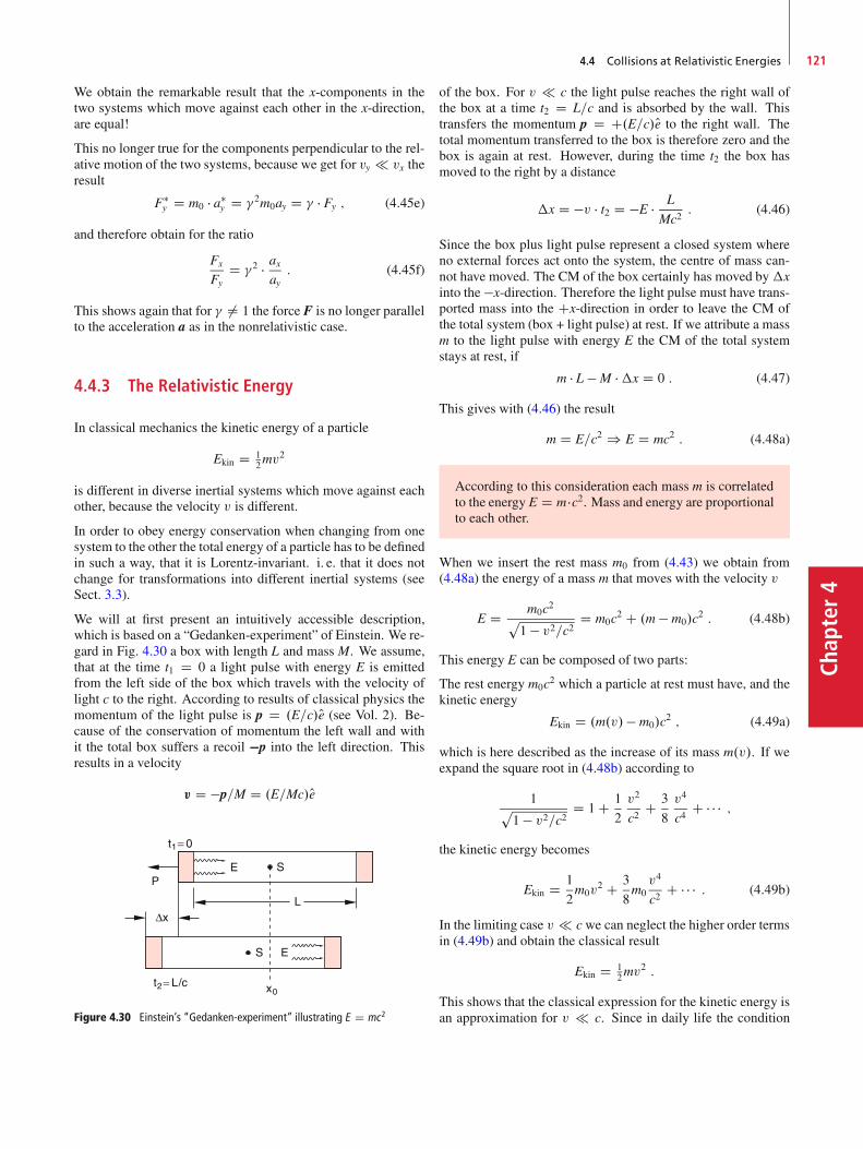
4.4 Collisions at Relativistic Energies 121
Chap
ter4
We obtain the remarkable result that the x-components in thetwo systems which move against each other in the x-direction,are equal!
This no longer true for the components perpendicular to the rel-ative motion of the two systems, because we get for vy vx theresult
F�y D m0 � a�
y D �2m0ay D � � Fy ; (4.45e)
and therefore obtain for the ratio
Fx
FyD �2 � ax
ay: (4.45f)
This shows again that for � ¤ 1 the force F is no longer parallelto the acceleration a as in the nonrelativistic case.
4.4.3 The Relativistic Energy
In classical mechanics the kinetic energy of a particle
Ekin D 12mv
2
is different in diverse inertial systems which move against eachother, because the velocity v is different.
In order to obey energy conservation when changing from onesystem to the other the total energy of a particle has to be definedin such a way, that it is Lorentz-invariant. i. e. that it does notchange for transformations into different inertial systems (seeSect. 3.3).
We will at first present an intuitively accessible description,which is based on a “Gedanken-experiment” of Einstein. We re-gard in Fig. 4.30 a box with length L and mass M. We assume,that at the time t1 D 0 a light pulse with energy E is emittedfrom the left side of the box which travels with the velocity oflight c to the right. According to results of classical physics themomentum of the light pulse is p D .E=c/Oe (see Vol. 2). Be-cause of the conservation of momentum the left wall and withit the total box suffers a recoil �p into the left direction. Thisresults in a velocity
v D �p=M D .E=Mc/Oe
Figure 4.30 Einstein’s “Gedanken-experiment” illustrating E D mc2
of the box. For v c the light pulse reaches the right wall ofthe box at a time t2 D L=c and is absorbed by the wall. Thistransfers the momentum p D C.E=c/Oe to the right wall. Thetotal momentum transferred to the box is therefore zero and thebox is again at rest. However, during the time t2 the box hasmoved to the right by a distance
�x D �v � t2 D �E � L
Mc2: (4.46)
Since the box plus light pulse represent a closed system whereno external forces act onto the system, the centre of mass can-not have moved. The CM of the box certainly has moved by�xinto the �x-direction. Therefore the light pulse must have trans-ported mass into the Cx-direction in order to leave the CM ofthe total system (box + light pulse) at rest. If we attribute a massm to the light pulse with energy E the CM of the total systemstays at rest, if
m � L � M ��x D 0 : (4.47)
This gives with (4.46) the result
m D E=c2 ) E D mc2 : (4.48a)
According to this consideration each mass m is correlatedto the energy E D m �c2. Mass and energy are proportionalto each other.
When we insert the rest mass m0 from (4.43) we obtain from(4.48a) the energy of a mass m that moves with the velocity v
E D m0c2p1 � v2=c2 D m0c
2 C .m � m0/c2 : (4.48b)
This energy E can be composed of two parts:
The rest energy m0c2 which a particle at rest must have, and thekinetic energy
Ekin D .m.v/� m0/c2 ; (4.49a)
which is here described as the increase of its mass m.v/. If weexpand the square root in (4.48b) according to
1p1 � v2=c2 D 1 C 1
2
v2
c2C 3
8
v4
c4C � � � ;
the kinetic energy becomes
Ekin D 1
2m0v
2 C 3
8m0v4
c2C � � � : (4.49b)
In the limiting case v cwe can neglect the higher order termsin (4.49b) and obtain the classical result
Ekin D 12mv
2 :
This shows that the classical expression for the kinetic energy isan approximation for v c. Since in daily life the condition

Chapter4
122 4 Systems of Point Masses; Collisions
v c is always fulfilled, the relativistic expression is importantonly for cases where v approaches c as in high energy physicsor astrophysics.
Squaring (4.48b) and multiplying both sides with c2 gives
E2 D m20c
6
c2 � v2 D m20c
4 C m2c2v2 : (4.50)
Inserting (4.45) for the relativistic momentum yields
E2 D m20c
4 C p2c2 :
This gives the relativistic relation between total energy Eand momentum p
E D cqm2
0c2 C p2 : (4.51)
For v c the square root can be expanded and gives the result
Ekin D E � m0c2 � p2
2mD 1
2m0v
2
with the classical momentum p D m0 � v.
4.4.4 Inelastic Collisions at relativisticEnergies
The relativistic energy and its conservation can be illustratedby the example of a collinear completely inelastic collision(Fig. 4.31). We regard two particles A and B with equal massesm which fly against each other width velocities v1 D fv1; 0; 0gand v2 D f�v1; 0; 0g, measured in the system S. In a com-pletely inelastic collision their total kinetic energy is convertedinto internal energy of the collision partners (see Sect. 4.2.4).After the collision they form a compound particle AB with thevelocity v D 0 (Fig. 4.31 upper part).
In a system S�, which moves with the velocity v D v1 againstS the particle A has the velocity v�
1 D 0, the compound particleAB which rests in S has in S� the velocity u D �v1. The particle
Figure 4.31 Description of a collinear completely inelastic collision in two dif-ferent inertial systems S and S �
B has in S� according to the relativistic addition of velocities(3.28) the velocity
v�2 D v2 � v
1 � v2v=c2 D �2v
1 C v2=c2; (4.52)
where v2 D �v1 is the velocity of B in S and v D v1 is thevelocity of S� against S.
The conservation of momentum demands for the collision de-scribed in S�
m�v�2
� � v�2 D Mu D �Mv1 ; (4.53)
whereM is the mass of the compound AB with the velocity u D�v1 measured in S�.
Conservation of energy requires, when dividing by c2
m�v�2
�C m0 D M : (4.54)
Inserting from (4.53) the relationM D �m.v�2 /�v�
2=v into (4.54)we obtain
m�v�2
�
m0D � v
v�2 C v
: (4.55)
Equation 4.52 gives the relation between v and v�2
v D � c2
v�2
"1 C
�1 � v�2
2
c2
�1=2#
I (4.56)
inserting this into (4.55) gives the mass ratio
m�v�2
�
m0D�1 � v�2
2
c2
��1=2
D ��v�2
�; (4.57)
and therefore again the general relation
m.v/ D m0p1 � v2=c2 D �.v/m0 ; (4.58)
which has been already derived in Sect. 4.4.1.
4.4.5 Relativistic Formulation of EnergyConservation
In order to show, that the relativistic energy E D m � c2 isconserved we must discuss the relativistic formulation of theNewton equation F D dp=dt. Thereto we replace the classicalposition vector r by the Lorentz four-vector
R D xOex C yOey C zOez C ictOet D r C ictOet ; (4.59)
defined in the four-dimensional Minkowski space .x; y; z; ict/(see Sect. 3.6.2), where the unit vector Oet is perpendicular tothe three spatial axes. From (4.59) one can derive that R2 Dr2 � c2t2.
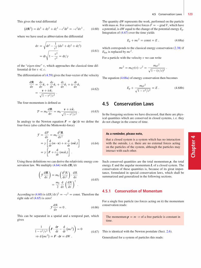
4.5 Conservation Laws 123
Chap
ter4
This gives the total differential
�dR2
� D dx2 C dy2 C dz2 � c2dt2 D �c2d�2 ; (4.60)
where we have used as abbreviation the differential
d� Drdt2 � 1
c2.dx2 C dy2 C dz2/
D dt
s
1 � v2
c2D dt=�
(4.61)
of the “eigen-time” � , which approaches the classical time dif-ferential dt for v c.
The differentiation of (4.59) gives the four-vector of the velocity
dRd�
D dx
d�Oex C dy
d�Oey C dz
d�Oez C ic
dt
d�Oet
D v C icOetp1 � v2=c2 :
(4.62)
The four-momentum is defined as
P D m0dRd�
D m0v C icOetp1 � v2=c2 : (4.63)
In analogy to the Newton equation F D dp=dt we define thefour-force (also called the Minkowski-force)
F D dPd�
D m0d2Rd�2
D �
�d
dt.m � v/C ic
d
dt.mOet/
�
D �
�F C i
d
dt.mcOet/
�:
(4.64)
Using these definitions we can derive the relativistic energy con-servation law. We multiply (4.64) with dR=d�
�F dR
d�
�D m0
�d2Rd�2
�� dRd�
D m0
2
d
d�
�dRd�
�2
:
(4.65)
According to (4.60) is .dR=d�/2 D �c2 D const. Therefore theright side of (4.65) is zero!
F dRd�
D 0 : (4.66)
This can be separated in a spatial and a temporal part, whichgives
1
1 � v2=c2�F � dr
dt� d
dt
�mc2
�� D 0
) d�mc2
� D F � dr D dW :
(4.67)
The quantity dW represents the work, performed on the particlewith massm. For conservative forces F D � gradV, which havea potential, is dW equal to the change of the potential energy Ep.Integration of (4.67) over the time yields
Ep C mc2 D const D E ; (4.68a)
which corresponds to the classical energy conservation (2.38) ifEkin is replaced by mc2.
For a particle with the velocity v we can write
mc2 D m0�.v/ � c2 D m0c2p1 � .v=c/2 :
The equation (4.68a) of energy conservation then becomes
Ep C m0c2p1 � v2=c2 D E : (4.68b)
4.5 Conservation Laws
In the foregoing sections we have discussed, that there are phys-ical quantities which are conserved in closed systems, i. e. theydo not change in the course of time.
As a reminder, please note,
that a closed system is a system which has no interactionwith the outside, i. e. there are no external forces actingon the particles of the system, although the particles mayinteract with each other.
Such conserved quantities are the total momentum p, the totalenergy E and the angular momentum L of a closed system. Theconservation of these quantities is, because of its great impor-tance, formulated in special conservation laws, which shall besummarized and generalized in the following sections.
4.5.1 Conservation of Momentum
For a single free particle (no forces acting on it) the momentumconservation reads:
The momentum p D m � v of a free particle is constant intime.
This is identical with the Newton postulate (Sect. 2.6).
Generalized for a system of particles this reads:
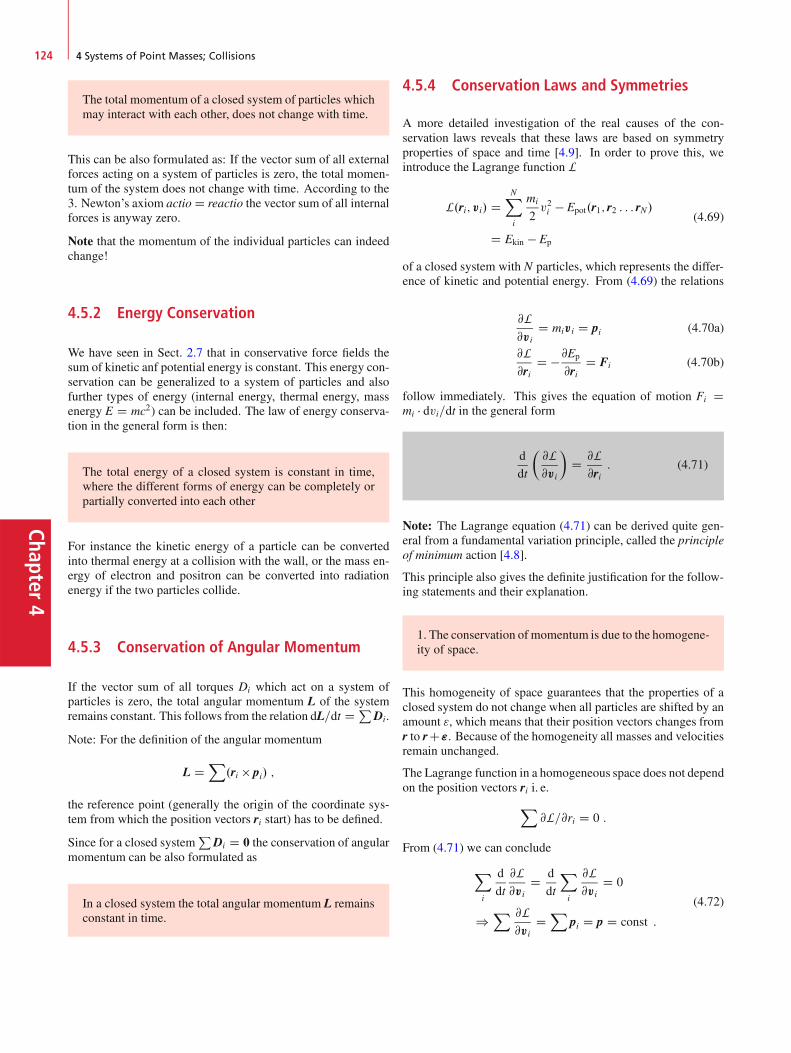
Chapter4
124 4 Systems of Point Masses; Collisions
The total momentum of a closed system of particles whichmay interact with each other, does not change with time.
This can be also formulated as: If the vector sum of all externalforces acting on a system of particles is zero, the total momen-tum of the system does not change with time. According to the3. Newton’s axiom actio D reactio the vector sum of all internalforces is anyway zero.
Note that the momentum of the individual particles can indeedchange!
4.5.2 Energy Conservation
We have seen in Sect. 2.7 that in conservative force fields thesum of kinetic anf potential energy is constant. This energy con-servation can be generalized to a system of particles and alsofurther types of energy (internal energy, thermal energy, massenergy E D mc2) can be included. The law of energy conserva-tion in the general form is then:
The total energy of a closed system is constant in time,where the different forms of energy can be completely orpartially converted into each other
For instance the kinetic energy of a particle can be convertedinto thermal energy at a collision with the wall, or the mass en-ergy of electron and positron can be converted into radiationenergy if the two particles collide.
4.5.3 Conservation of Angular Momentum
If the vector sum of all torques Di which act on a system ofparticles is zero, the total angular momentum L of the systemremains constant. This follows from the relation dL=dt D P
Di.
Note: For the definition of the angular momentum
L DX
.ri pi/ ;
the reference point (generally the origin of the coordinate sys-tem from which the position vectors ri start) has to be defined.
Since for a closed systemP
Di D 0 the conservation of angularmomentum can be also formulated as
In a closed system the total angular momentum L remainsconstant in time.
4.5.4 Conservation Laws and Symmetries
A more detailed investigation of the real causes of the con-servation laws reveals that these laws are based on symmetryproperties of space and time [4.9]. In order to prove this, weintroduce the Lagrange function L
L.ri; vi/ DNX
i
mi
2v2i � Epot.r1; r2 : : : rN/
D Ekin � Ep
(4.69)
of a closed system with N particles, which represents the differ-ence of kinetic and potential energy. From (4.69) the relations
@L@vi
D mivi D pi (4.70a)
@L@ri
D �@Ep
@riD Fi (4.70b)
follow immediately. This gives the equation of motion Fi Dmi � dvi=dt in the general form
d
dt
�@L@vi
�D @L@ri
: (4.71)
Note: The Lagrange equation (4.71) can be derived quite gen-eral from a fundamental variation principle, called the principleof minimum action [4.8].
This principle also gives the definite justification for the follow-ing statements and their explanation.
1. The conservation of momentum is due to the homogene-ity of space.
This homogeneity of space guarantees that the properties of aclosed system do not change when all particles are shifted by anamount ", which means that their position vectors changes fromr to rC". Because of the homogeneity all masses and velocitiesremain unchanged.
The Lagrange function in a homogeneous space does not dependon the position vectors ri i. e.
X@L=@ri D 0 :
From (4.71) we can conclude
X
i
d
dt
@L@vi
D d
dt
X
i
@L@vi
D 0
)X @L
@viDX
pi D p D const :
(4.72)

Summary 125
Chap
ter4
2. The conservation of energy follows from the homogene-ity of time.
The homogeneity of time implies that the Lagrange function Ldoes not explicitly depend on time. Which means that @L=@t D0.
The total derivation of L is
dLdt
D3NX
iD1
@L@xi
Pxi CX @L
@ Pxi Rxi :
If we replace according to (4.71) @L=@xi by d=dt.@L=@Oe/ weobtain
dLdt
DX
Pxi ddt@L@ Pxi C
X @L@ Pxi Rxi D
X d
dt
�@L@ Pxi Pxi
�
) d
dt
�XPxi @L@ Pxi � L
�D 0
)X
Pxi @L@ Pxi � L D E D const ;
(4.73)
which means that E is constant in time.
Finally the conservation of angular momentum follows fromthe isotropy of space, which means that no specific directionin space is preferred.
This isotropy implies that an arbitrary rotation of a closed sys-tem does not change the mechanical properties of the system.In particular the Lagrange function should not change when thesystem rotates by an angle @'.
We introduce the vector ı' with the magnitude ı' and the di-rection of the rotation axis. The change of the position vector riof the point P is (Fig. 4.32)
ıri D ı' ri : (4.74a)
The velocity of P is then changing by
ıvi D ı' vi : (4.74b)
Figure 4.32 Definition of ı' and ır
For the change ıL D 0 of the Lagrange function L we obtain
ıL DX
i
@L@riıri C @L
@viıv D 0 : (4.75)
With the relations
@L=@vi D pi and @L=@ri D Fi D dpidt
we can write (4.75) in the form
X
i
Ppi .ı' ri/C pi .ı' vi/ D 0
) ı'
"X
i
..ri Ppi/C .vi pi//
#
D ı'd
dt
X.ri pi/ D 0 :
(4.76)
Since this must hold for arbitrary values of ı' it follows
X.ri pi/ D L D const : (4.77)
Summary
The centre of mass of a system of N point massesmi with theposition vectors ri has the position vector
rS D 1Pmi
Xmiri D 1
M
Xmiri :
The coordinate system with the CM as origin is called thecentre-of-mass systemThe vector sum of all momenta mivi of the masses mi in theCM-system is always zero.
The reduced mass of two masses m1 and m2 is defined as
D m1 � m2
m1 C m2:
The relative motion of two particles with the mutual interac-tion forces F12 D �F21 can be reduced to the motion of asingle particle with the reduced mass which moves withthe velocity v12 D v1 � v2 around the centre of m1.
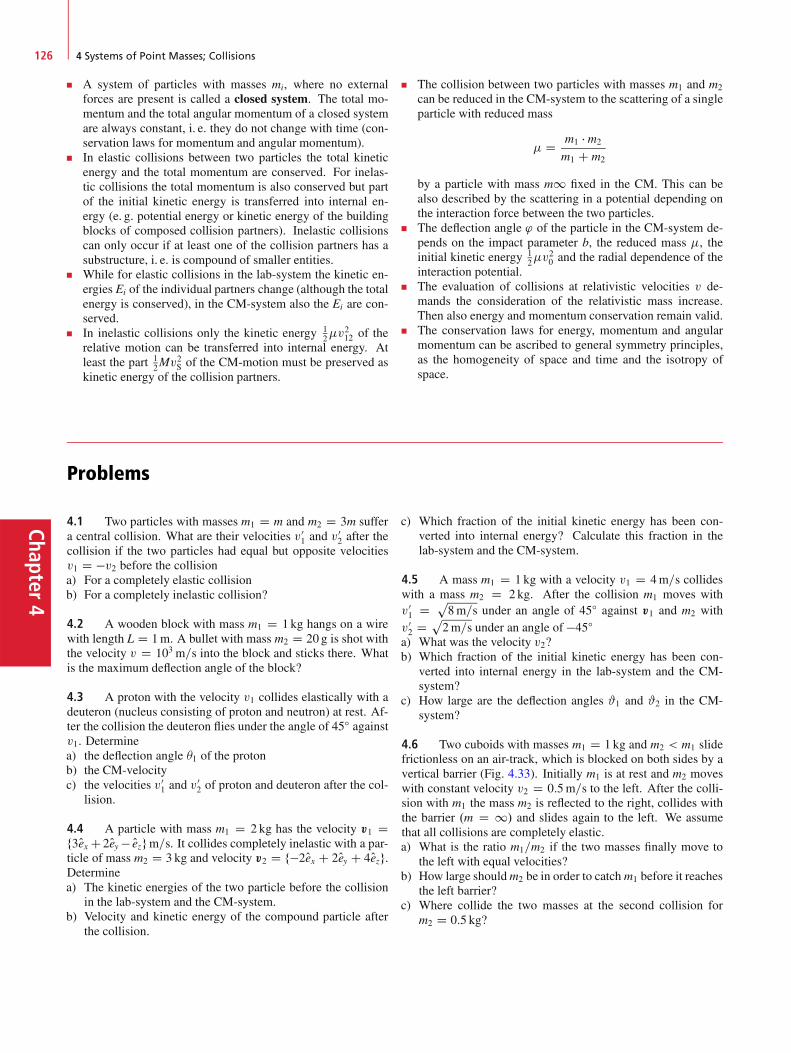
Chapter4
126 4 Systems of Point Masses; Collisions
A system of particles with masses mi, where no externalforces are present is called a closed system. The total mo-mentum and the total angular momentum of a closed systemare always constant, i. e. they do not change with time (con-servation laws for momentum and angular momentum).In elastic collisions between two particles the total kineticenergy and the total momentum are conserved. For inelas-tic collisions the total momentum is also conserved but partof the initial kinetic energy is transferred into internal en-ergy (e. g. potential energy or kinetic energy of the buildingblocks of composed collision partners). Inelastic collisionscan only occur if at least one of the collision partners has asubstructure, i. e. is compound of smaller entities.While for elastic collisions in the lab-system the kinetic en-ergies Ei of the individual partners change (although the totalenergy is conserved), in the CM-system also the Ei are con-served.In inelastic collisions only the kinetic energy 1
2v212 of the
relative motion can be transferred into internal energy. Atleast the part 1
2Mv2S of the CM-motion must be preserved as
kinetic energy of the collision partners.
The collision between two particles with masses m1 and m2
can be reduced in the CM-system to the scattering of a singleparticle with reduced mass
D m1 � m2
m1 C m2
by a particle with mass m1 fixed in the CM. This can bealso described by the scattering in a potential depending onthe interaction force between the two particles.The deflection angle ' of the particle in the CM-system de-pends on the impact parameter b, the reduced mass , theinitial kinetic energy 1
2v20 and the radial dependence of the
interaction potential.The evaluation of collisions at relativistic velocities v de-mands the consideration of the relativistic mass increase.Then also energy and momentum conservation remain valid.The conservation laws for energy, momentum and angularmomentum can be ascribed to general symmetry principles,as the homogeneity of space and time and the isotropy ofspace.
Problems
4.1 Two particles with masses m1 D m and m2 D 3m suffera central collision. What are their velocities v0
1 and v02 after the
collision if the two particles had equal but opposite velocitiesv1 D �v2 before the collisiona) For a completely elastic collisionb) For a completely inelastic collision?
4.2 A wooden block with mass m1 D 1 kg hangs on a wirewith length L D 1m. A bullet with mass m2 D 20 g is shot withthe velocity v D 103 m=s into the block and sticks there. Whatis the maximum deflection angle of the block?
4.3 A proton with the velocity v1 collides elastically with adeuteron (nucleus consisting of proton and neutron) at rest. Af-ter the collision the deuteron flies under the angle of 45ı againstv1. Determinea) the deflection angle �1 of the protonb) the CM-velocityc) the velocities v0
1 and v02 of proton and deuteron after the col-
lision.
4.4 A particle with mass m1 D 2 kg has the velocity v1 Df3Oex C2Oey � Oezgm=s. It collides completely inelastic with a par-ticle of mass m2 D 3 kg and velocity v2 D f�2Oex C 2Oey C 4Oezg.Determinea) The kinetic energies of the two particle before the collision
in the lab-system and the CM-system.b) Velocity and kinetic energy of the compound particle after
the collision.
c) Which fraction of the initial kinetic energy has been con-verted into internal energy? Calculate this fraction in thelab-system and the CM-system.
4.5 A mass m1 D 1 kg with a velocity v1 D 4m=s collideswith a mass m2 D 2 kg. After the collision m1 moves withv01 D p
8m=s under an angle of 45ı against v1 and m2 withv02 D p
2m=s under an angle of �45ıa) What was the velocity v2?b) Which fraction of the initial kinetic energy has been con-
verted into internal energy in the lab-system and the CM-system?
c) How large are the deflection angles #1 and #2 in the CM-system?
4.6 Two cuboids with masses m1 D 1 kg and m2 < m1 slidefrictionless on an air-track, which is blocked on both sides by avertical barrier (Fig. 4.33). Initially m1 is at rest and m2 moveswith constant velocity v2 D 0:5m=s to the left. After the colli-sion with m1 the mass m2 is reflected to the right, collides withthe barrier .m D 1/ and slides again to the left. We assumethat all collisions are completely elastic.a) What is the ratio m1=m2 if the two masses finally move to
the left with equal velocities?b) How large shouldm2 be in order to catchm1 before it reaches
the left barrier?c) Where collide the two masses at the second collision for
m2 D 0:5 kg?

References 127
Chap
ter4
Figure 4.33 Illustrating Probl. 4.6
4.7 A steel ball with mass m1 D 1 kg hangs on a wirewith L D 1m, vertically above the left edge of a resting massm2 D 5 kg which can slide without friction on a horizontal air-track. (Fig. 4.34). The steel ball with the wire is lifted by anangle ' D 90ı from the vertical into the horizontal position andthen released. It collides elastically with the glider. What is themaximum angle ' of m1 after the collision?
Figure 4.34 Illustration of Probl. 4.7
4.8 An elevator ascends with constant velocity v D 2m=s.When its ceiling is still 30m below the upper point A of the liftshaft a ball is released from A which falls freely down and hitselastically the ceiling of the elevator, from where it is elasticallyreflected upwards.a) Where does it hit the elevator ceiling?b) What is its maximum height after the reflection?c) Where does it hit the elevator ceiling a second time?
4.9 An ˛-particle (nucleus of the He-atom) hits with the ve-locity v1 an oxygen nucleus at rest .m2 D 4m1/. The ˛-particleis deflected by 64ı, the oxygen nucleus by �51ı against v1. Thecollision is completely elastic.a) What is the ratio v0
1=v02 of the velocities after the collision?
b) What is the ratio of the kinetic energies after the collision?
4.10 A particle has in a system S a kinetic energy of 6GeV.and the momentum P D 6GeV=c. What is its energy in a sys-tem S0, where its momentum is measured as 5GeV=c? What isthe relative velocity of S0 against S?
References
4.1a. http://berkeleyscience.com/pm.htm4.1b. A. Tan, Theoryof Orbital Motion. (World Scientific Publ.,
2008)4.2. R. D. Levine, Moleclar Reaction Dynamics. (Cambridge
Univ. Press, 2005)4.3. A. Einstein, N. Calder, Relativity: The special and the
general Theory.4.4a. E.F. Taylor, J.A. Wheeler, Spacetime Physics: Introduc-
tion to Special Relativity, 2nd ed., (W. H. Freeman &Company, 1992)
4.4b. W. Rindler, Introduction to Special Relativity, 2nd ed.,(Oxford University Press, 1991)
4.5. R.M. Dreizler, C.S. Lüdde, Theoretical Mechanics.(Springer, Berlin, Heidelberg, 2010)
4.6. A.P. French, Special Relativity. (W.W. Norton& Co, 1968)4.7. A. Das, The Special Theory of Relativity. (Springer,
Berlin, Heidelberg, 1996)4.8. Goldstein, Classical Mechanics. (Addison Wesley, 2001)4.9. J. Schwichtenberg, Physics from Symmetry. (Springer,
Heidelberg, 2015)
Chap
ter5
Dynamics of rigid Bodies 55.1 The Model of a Rigid Body . . . . . . . . . . . . . . . . . . . . . . . . . 130
5.2 Center of Mass . . . . . . . . . . . . . . . . . . . . . . . . . . . . . . . . 130
5.3 Motion of a Rigid Body . . . . . . . . . . . . . . . . . . . . . . . . . . . 131
5.4 Forces and Couple of Forces . . . . . . . . . . . . . . . . . . . . . . . . 132
5.5 Rotational Inertia and Rotational Energy . . . . . . . . . . . . . . . . . 133
5.6 Equation of Motion for the Rotation of a Rigid Body . . . . . . . . . . 136
5.7 Rotation About Free Axes; Spinning Top . . . . . . . . . . . . . . . . . 139
5.8 The Earth as Symmetric Top . . . . . . . . . . . . . . . . . . . . . . . . . 149
Summary . . . . . . . . . . . . . . . . . . . . . . . . . . . . . . . . . . . . 151
Problems . . . . . . . . . . . . . . . . . . . . . . . . . . . . . . . . . . . . 151
References . . . . . . . . . . . . . . . . . . . . . . . . . . . . . . . . . . . 152
129© Springer International Publishing Switzerland 2017W. Demtröder, Mechanics and Thermodynamics, Undergraduate Lecture Notes in Physics, DOI 10.1007/978-3-319-27877-3_5
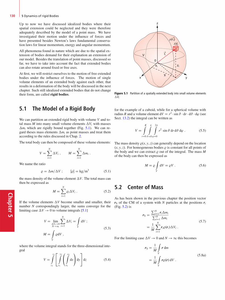
Chapter5
130 5 Dynamics of rigid Bodies
Up to now we have discussed idealized bodies where theirspatial extension could be neglected and they were thereforeadequately described by the model of a point mass. We haveinvestigated their motion under the influence of forces andhave presented besides Newton’s laws fundamental conserva-tion laws for linear momentum, energy and angular momentum.
All phenomena found in nature which are due to the spatial ex-tension of bodies demand for their explanation an extension ofour model. Besides the translation of point masses, discussed sofar, we have to take into account the fact that extended bodiescan also rotate around fixed or free axes.
At first, we will restrict ourselves to the motion of free extendedbodies under the influence of forces. The motion of singlevolume elements of an extended body against each other, thatresults in a deformation of the body will be discussed in the nextchapter. Such still idealized extended bodies that do not changetheir form, are called rigid bodies.
5.1 The Model of a Rigid Body
We can partition an extended rigid body with volume V and to-tal mass M into many small volume elements �Vi with masses�mi which are rigidly bound together (Fig. 5.1). We can re-gard theses mass elements �mi as point masses and treat themaccording to the rules discussed in Chap. 2.
The total body can then be composed of these volume elements:
V DNX
iD1
�Vi ; M DNX
iD1
�mi :
We name the ratio
% D �m=�V I Œ%� D kg=m3 (5.1)
the mass density of the volume element �V. The total mass canthen be expressed as
M DNX
iD1
%i�Vi : (5.2)
If the volume elements �V become smaller and smaller, theirnumber N correspondingly larger, the sums converge for thelimiting case �V ! 0 to volume integrals [5.1]
V D lim�Vi!0N!1
NX
iD1
�Vi DZ
V
dV I
M DZ
V
%dV ;
(5.3)
where the volume integral stands for the three-dimensional inte-gral
V Dz2Z
z1
2
4y2Z
y1
0
@x2Z
x1
dx
1
A dy
3
5 dz (5.4)
Figure 5.1 Partition of a spatially extended body into small volume elements�Vi
for the example of a cuboid, while for a spherical volume withradius R and a volume element dV D r2 � sin# � dr � d# � d' (seeSect. 13.2) the integral can be written as
V DRZ
rD0
Z
#D0
2Z
'D0
r2 sin# dr d# d' : (5.5)
The mass density %.x; y; z/ can generally depend on the location.x; y; z/. For homogeneous bodies % is constant for all points ofthe body and we can extract % out of the integral. The mass Mof the body can then be expressed as
M D %
Z
V
dV D %V : (5.6)
5.2 Center of Mass
As has been shown in the previous chapter the position vectorrS of the CM of a system with N particles at the positions ri(Fig. 5.2) is
rS DPN
iD1 ri�miPNiD1�mi
D 1
M
NX
iD1
ri%.ri/�Vi :
(5.7)
For the limiting case �V ! 0 and N ! 1 this becomes
rS D 1
M
Z
V
r dm
D 1
M
Z
V
r%.r/ dV :(5.8a)
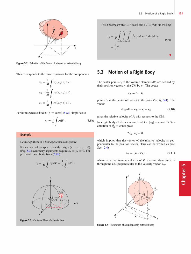
5.3 Motion of a Rigid Body 131
Chap
ter5
Figure 5.2 Definition of the Center of Mass of an extended body
This corresponds to the three equations for the components
xS D 1
M
Z
V
x%.x; y; z/ dV ;
yS D 1
M
Z
V
y%.x; y; z/ dV ;
zS D 1
M
Z
V
z%.x; y; z/ dV :
For homogeneous bodies (% D const) (5.8a) simplifies to
rS D 1
V
Z
V
r dV : (5.8b)
Example
Center of Mass of a homogeneous hemisphere.
If the center of the sphere is at the origin .x D y D z D 0/(Fig. 5.3) symmetry arguments require xS D yS D 0. For% D const we obtain from (5.8b)
zS D 1
M
Z
V
z% dV D 1
V
Z
V
z dV :
Figure 5.3 Center of Mass of a hemisphere
This becomes with z D r�cos# and dV D r2dr�sin#d#d'
zS D 1
V
RZ
rD0
=2Z
#D0
2Z
'D0
r3 cos# sin# dr d# d'
D 3
8R :
(5.9)
J
5.3 Motion of a Rigid Body
The center points Pi of the volume elements dVi are defined bytheir position vectors ri, the CM by rS. The vector
riS D ri � rS
points from the center of mass S to the point Pi (Fig. 5.4). Thevector
driS=dt D viS D vi � vS (5.10)
gives the relative velocity of Pi with respect to the CM.
In a rigid body all distances are fixed, i.e. jriSj D const. Differ-entiation of r2iS D const gives
2riS � vS D 0 ;
which implies that the vector of the relative velocity is per-pendicular to the position vector. This can be written as (seeSect. 2.4)
viS D .! riS/ ; (5.11)
where ! is the angular velocity of Pi rotating about an axisthrough the CM perpendicular to the velocity vector viS.
Figure 5.4 The motion of a rigid spatially extended body
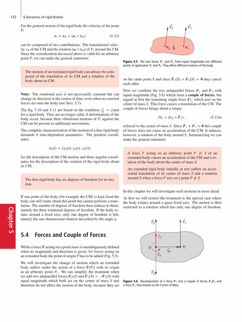
Chapter5
132 5 Dynamics of rigid Bodies
For the general motion of the rigid body the velocity of the pointPi
vi D vS C .! riS/ (5.12)
can be composed of two contributions: The translational veloc-ity vS of the CM and the rotation .! riS/ of Pi around the CM.Since the consideration discussed above is valid for an arbitrarypoint Pi we can make the general statement:
The motion of an extended rigid body can always be com-posed of the translation of its CM and a rotation of thebody about its CM.
Note: The rotational axis is not necessarily constant but canchange its direction in the course of time, even when no externalforces act onto the body (see Sect. 5.7).
The Eq. 5.10 and 5.11 are based on the condition r2ik D constfor a rigid body. They are no longer valid, if deformations of thebody occur, because then vibrational motions of Pi against theCM can be present as additional movements.
The complete characterization of the motion of a free rigid bodydemands 6 time-dependent parameters: The position coordi-nates
rS.t/ D fxS.t/; yS.t/; zS.t/g
for the description of the CM-motion and three angular coordi-nates for the description of the rotation of the rigid body aboutits CM.
The free rigid body has six degrees of freedom for its mo-tion.
If one point of the body (for example the CM) is kept fixed thebody can still rotate about this point but cannot perform a trans-lation. The number of degrees of freedom then reduces to three,namely the three rotational degrees of freedom. If the body ro-tates around a fixed axis, only one degree of freedom is left,namely the one-dimensional rotation described by the angle '.
5.4 Forces and Couple of Forces
While a forceF acting on a point mass is unambiguously definedwhen its magnitude and direction is given, for forces acting onan extended body the point of origin P has to be added (Fig. 5.5).
We will investigate the change of motion which an extendedbody suffers under the action of a force F.Pi/ with its originin an arbitrary point Pi. We can simplify the treatment whenwe add two antiparallel forces F2.S/ and F3.S/ D �F2.S/ withequal magnitude which both act on the center of mass S andtherefore do not affect the motion of the body, because they act
Figure 5.5 The two forces F1 and F2 have equal magnitudes but differentpoints of application P1 and P2. They effect different motions of the body
on the same point S and since F2.S/C F3.S/ D 0 they canceleach other.
Now we combine the two antiparallel forces F1 and F3 withequal magnitude (Fig. 5.6) which form a couple of forces, butregard at first the remaining single force F2, which acts on thecenter of mass S. This force causes a translation of the CM. Thecouple of forces brings about a torque
DS D .riS F1/ ; (5.13a)
referred to the center of mass S. Since F1 C F3 D 0 this coupleof forces does not cause an acceleration of the CM. It induces,however, a rotation of the body around S. Summarizing we canmake the general statement:
A force F acting on an arbitrary point P ¤ S of anextended body causes an acceleration of the CM and a ro-tation of the body about the center of mass S.
An extended rigid body initially at rest suffers an accel-erated translation of its center of mass S and a rotationaround S when a force F acts on a point P ¤ S.
In this chapter we will investigate such motions in more detail.
At first we will restrict the treatment to the special case wherethe body rotates around a space-fixed axis. The motion is thenrestricted to a rotation which has only one degree of freedom.
Figure 5.6 Decomposition of a force F1 into a couple of forces F1F3 anda force F2 that attacks at the Center of Mass

5.5 Rotational Inertia and Rotational Energy 133
Chap
ter5
P
Ft
r
Figure 5.7 Rotation of a rigid body about a fixed axis A , induced by a forceF attacking at the point P . Decomposition of the projection of F onto the x-y-plane into a normal and a tangential component
We choose the direction of the rotation axis A as the z-directionand the x-y-plane through the point P.r/ where the force F actson the body, which has the distance r from the rotation axis(Fig. 5.7). We can then decompose the force into the three com-ponents Fz k A, the radial component Fr k r and the tangentialcomponent Ft ? r and ? A. Fz is perpendicular to the x-y-planeand the other two components are in the x-y-plane.
The torque exerted by the force F onto the body is
D D .r F/ D .r Ft/C .r Fz/ ;
since .r Fn/ D 0.
The first term causes a torque about the z-axis, and therefore anacceleration of the rotation about the z-axis. The second termwould change the direction of the rotation axis. If this axis isfixed by axle bearings the torque only acts on the bearings anddoes not lead to a change of motion.
If the rotation axis intersects the center of mass S (Fig. 5.8)which we choose as the origin of our coordinate system, thetorque exerted by the weight Fw D M � g of the body is zero, ascan be seen by the following derivation:
The torque with respect to the rotation axis caused by the grav-itational force �mi � g on the mass element �mi is Di D
Figure 5.8 Contribution of the mass element�m to the torque about an axisthrough the Center of Mass, due to the weight of�m
Figure 5.9 Principle of beam balance
.riS �mi � g/. The torque exerted by the weight of the wholebody is then
D DZ
V
.r g/ dm D �g Z
V
r dm
D � .g MrS/ D 0 ;
(5.13b)
because the center of mass S is the origin and therefore is rS D 0.
If a body can rotate around an axis through the CM it isalways at equilibrium, independent on the space orienta-tion of the axis because the torque exerted by its weight isalways zero.
All beam balances are based on this principle (Fig. 5.9). Thebalance is at equilibrium if
PDi D 0, which means
r1 F1 C r2 F2 D 0 :
This is the equilibrium condition for a balance as two-armedlever.
5.5 Rotational Inertia and RotationalEnergy
We consider an extended body which rotates about a fixed axisA with the angular velocity ! (Fig. 5.10). The mass element�mi with the distance ri? D jrij from the axis A has the velocityvi D ri � !. Its kinetic energy is then
Ekin.�mi/ D 12�miv
2i D 1
2�mir2i !
2 :
Figure 5.10 Definition of moment of inertia
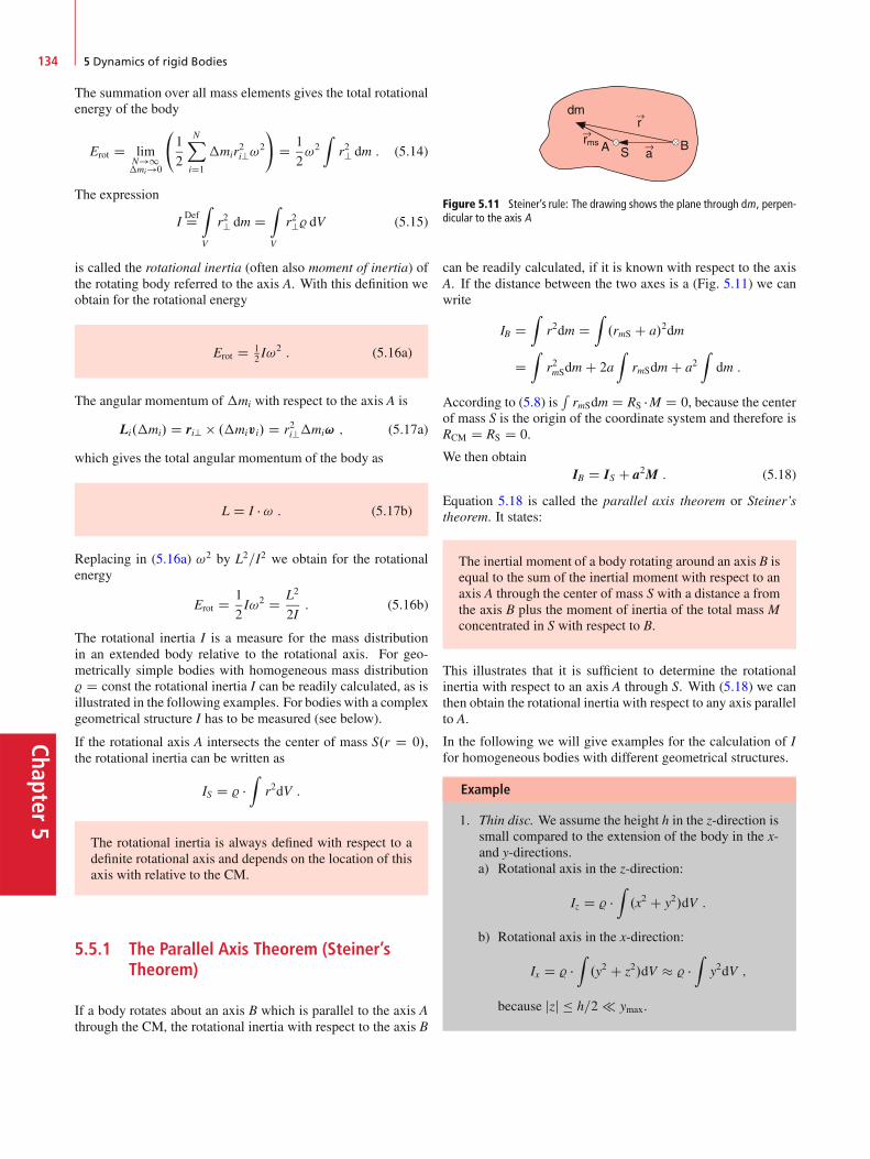
Chapter5
134 5 Dynamics of rigid Bodies
The summation over all mass elements gives the total rotationalenergy of the body
Erot D limN!1�mi!0
1
2
NX
iD1
�mir2i?!
2
!D 1
2!2Z
r2? dm : (5.14)
The expression
IDefDZ
V
r2? dm DZ
V
r2?% dV (5.15)
is called the rotational inertia (often also moment of inertia) ofthe rotating body referred to the axis A. With this definition weobtain for the rotational energy
Erot D 12 I!
2 : (5.16a)
The angular momentum of �mi with respect to the axis A is
Li.�mi/ D ri? .�mivi/ D r2i?�mi! ; (5.17a)
which gives the total angular momentum of the body as
L D I � ! : (5.17b)
Replacing in (5.16a) !2 by L2=I2 we obtain for the rotationalenergy
Erot D 1
2I!2 D L2
2I: (5.16b)
The rotational inertia I is a measure for the mass distributionin an extended body relative to the rotational axis. For geo-metrically simple bodies with homogeneous mass distribution% D const the rotational inertia I can be readily calculated, as isillustrated in the following examples. For bodies with a complexgeometrical structure I has to be measured (see below).
If the rotational axis A intersects the center of mass S.r D 0/,the rotational inertia can be written as
IS D % �Z
r2dV :
The rotational inertia is always defined with respect to adefinite rotational axis and depends on the location of thisaxis with relative to the CM.
5.5.1 The Parallel Axis Theorem (Steiner’sTheorem)
If a body rotates about an axis B which is parallel to the axis Athrough the CM, the rotational inertia with respect to the axis B
Figure 5.11 Steiner’s rule: The drawing shows the plane through dm, perpen-dicular to the axis A
can be readily calculated, if it is known with respect to the axisA. If the distance between the two axes is a (Fig. 5.11) we canwrite
IB DZ
r2dm DZ.rmS C a/2dm
DZ
r2mSdm C 2aZ
rmSdm C a2Z
dm :
According to (5.8) isRrmSdm D RS �M D 0, because the center
of mass S is the origin of the coordinate system and therefore isRCM D RS D 0.
We then obtainIB D IS C a2M : (5.18)
Equation 5.18 is called the parallel axis theorem or Steiner’stheorem. It states:
The inertial moment of a body rotating around an axis B isequal to the sum of the inertial moment with respect to anaxis A through the center of mass S with a distance a fromthe axis B plus the moment of inertia of the total mass Mconcentrated in S with respect to B.
This illustrates that it is sufficient to determine the rotationalinertia with respect to an axis A through S. With (5.18) we canthen obtain the rotational inertia with respect to any axis parallelto A.
In the following we will give examples for the calculation of Ifor homogeneous bodies with different geometrical structures.
Example
1. Thin disc. We assume the height h in the z-direction issmall compared to the extension of the body in the x-and y-directions.a) Rotational axis in the z-direction:
Iz D % �Z.x2 C y2/dV :
b) Rotational axis in the x-direction:
Ix D % �Z.y2 C z2/dV � % �
Zy2dV ;
because jzj � h=2 ymax.
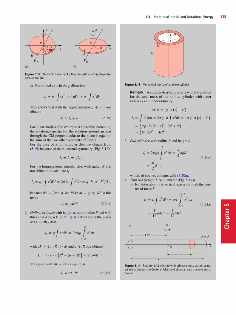
5.5 Rotational Inertia and Rotational Energy 135
Chap
ter5
Figure 5.12 Moment of inertia of a thin disc with arbitrary shape (a),circular disc (b)
c) Rotational axis in the y-direction:
Iy D % �Z.x2 C z2/dV � % �
Zx2dV :
This shows that with the approximation z x; y oneobtains
Iz � Ix C Iy : (5.19)
For plane bodies (for example a triatomic molecule)the rotational inertia for the rotation around an axisthrough the CM perpendicular to the plane is equal tothe sum of the two other moments of inertia.For the case of a thin circular disc we obaqin from(5.19) because of the rotational symmetry (Fig. 5.12b)
Ix D Iy D 12 Iz :
For the homogeneous circular disc with radius R it isnot difficult to calculate Iz:
Iz D % �Z
r2dV D 2h%Z
r3dr D % � h � � R4=2 ;
because dV D 2r � h � dr. WithM D % � �R2 � h thisgives
Iz D 12MR2 : (5.20a)
2. Hollow cylinder with height h, outer radius R and wallthickness d R (Fig. 5.13). Rotation about the z-axisas symmetry axis:
Iz D %
Z
V
r2dV D 2h%
RZ
R�d
r3 dr ;
with dV D 2 � R � h � dr and d R one obtains
Iz D h � % � �R4 � .R � d/4� � 2%hR3d :
This gives withM D 2 � r � % � d � h
Iz D M � R2 : (5.20b)
Figure 5.13 Moment of inertia of a hollow cylinder
Remark. A simpler derivation starts with the relationfor the total mass of the hollow cylinder with outerradius r2 and inner radius r1:
M D � % � h �r22 � r21�:
Iz DZ
r2 dm D 2% � hZ
r3dr D 12% � h �r42 � r41
�
D 12% � h �r22 � r21
� � �r22 C r21�
� 12M � 2R2 D MR2 :
3. Full cylinder with radius R and height h.
Iz D 2%h
RZ
0
r3 dr D
2h%R4
D M
2R2 ;
(5.20c)
which, of course, concurs with (5.20a).4. Thin rod (length L � diameter (Fig. 5.14))
a) Rotation about the vertical axis a through the cen-ter of mass S.
IS D %
Zx2 dV D %A
CL=2Z
�L=2
x2 dx
D 1
12%AL3 D 1
12ML2 :
(5.21a)
Figure 5.14 Rotation of a thin rod with arbitrary cross section aboutan axis a through the Center of Mass and about an axis b at one end ofthe rod
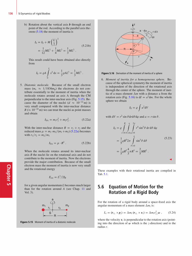
Chapter5
136 5 Dynamics of rigid Bodies
b) Rotation about the vertical axis b through an endpoint of the rod. According to the parallel axis the-orem (5.18) the moment of inertia is
Ib D IS C M
�L
2
�2
D 1
12ML2 C 1
4ML2 D 1
3ML2 :
(5.21b)
This result could have been obtained also directlyfrom
Ib D %A
LZ
0
x2 dx D 1
3%AL3 D 1
3ML2 :
5. Diatomic molecule. Because of the small electronmass .me � 1=1836mp/ the electrons do not con-tribute essentially to the moment of inertia when themolecule rotates around an axis A through the CMperpendicular to the inter-nuclear axis (Fig. 5.15). Be-cause the diameter of the nuclei .d � 10�14 m/ isvery small compared with the inter-nuclear distanceR .� 10�10 m/ we can treat the nuclei as point massesand obtain
ISA D m1r21 C m2r
22 : (5.22a)
With the inter-nuclear distance R D r1 C r2 and thereduced mass D m1 �m2=.m1Cm2/ (5.22a) becomeswith r1=r2 D m2=m1
ISA D � R2 : (5.22b)
When the molecule rotates around its inter-nuclearaxis B the nuclei lie on the rotational axis and do notcontribute to the moment of inertia. Now the electronsprovide the major contribution. Because of the smallelectron mass the moment of inertia is now very smalland the rotational energy
Erot D L2=2IB
for a given angular momentum L becomes much largerthan for the rotation around A (see Chap. 11 andVol. 3).
Figure 5.15 Moment of inertia of a diatomic molecule
Figure 5.16 Derivation of the moment of inertia of a sphere
6. Moment of inertia for a homogeneous sphere. Be-cause of the spherical symmetry the moment of inertiais independent of the direction of the rotational axisthrough the center of the sphere. The moment of iner-tia of a mass element �m with a distance a from therotation axis (Fig. 5.16) is dI D a2dm. For the wholesphere we obtain
IS D %
Za2dV
with dV D r2 sin#drd#d' and a D r sin# .
IS D %
RZ
rD0
Z
#D0
2Z
'D0
r4 sin3# dr d# d'
D 1
5%R52
Z
#D0
sin3# d#
D 2
5%R2 4
3R3 D 2
5MR2 :
(5.23)
J
These examples with their rotational inertia are compiled inTab. 5.1.
5.6 Equation of Motion for theRotation of a Rigid Body
For the rotation of a rigid body around a space-fixed axis theangular momentum of a mass element�mi is:
Li D .ri? pi/ D �mi .ri? vi/ D �mir2i?! ; (5.24)
where the velocity vi is perpendicular to the rotation axis (point-ing into the direction of ! which is the z-direction) and to theradius r.

5.6 Equation of Motion for the Rotation of a Rigid Body 137
Chap
ter5
Table 5.1 Moments of inertia of some symmetric bodies that rotate about asymmetry axis
Geometrical figure Realization Moment of inertia
Thin disc 12MR2
Hollow cylinderwith thin wall
Full cylinder
MR2
12MR2
Thin rod L � r 112ML2
Homogeneous sphere
Hollow spherewith thin wall
25MR2
23MR2
Cuboid Ix D 112M.b
2 C c2/
Iy D 112M.a
2 C c2/
Iz D 112M.a
2 C b2/
Diatomic molecule I D m1m2m1Cm2
� R2
The time-derivative of (5.24) is
dLidt
D �mi
�ri? dvi
dt
�D .ri? Ft/ D Dik ; (5.25)
where Dik D ri? � Fi is the component of the torque Di parallelto the rotation axis A. The other components Fz and Fr of theforce F are compensated by elastic forces of the mounting of thefixed axis A (Fig. 5.17).
For the magnitudeDi D jDikj of the not compensated torque weobtain from (5.24) and (5.25)
Di D �mir2i?d!
dt: (5.26)
Figure 5.17 Torque acting on the rotation about a fixed axis induced by a forceF attacking at the point P
The integration overall mass elements yields
D D I � d!dt
D I � d2'
dt2; (5.27)
where ' is the angle of r against the x-axis.
5.6.1 Rotation About an Axis for a ConstantTorque
For a constant torque which does not change with time the in-tegration of (5.27) yields the equation of rotation analogous to(2.6) for the translation of a body
' D D
2It2 C At C B : (5.28a)
The integration constants A and B are specified by the initialconditions '.0/ D '0 and d'.0/=dt D !0. This gives for(5.28a)
' D D
2It2 C !0t C '0 : (5.28b)
Example
1. A full cylinder, a hollow cylinder and a ball with equalmasses M and equal radii r role down an inclinedplane. All three bodies start at the same time. Whowill win the race? The question can be answered ex-perimentally as demonstration experiment during thelecture and arises always astonishment.Solution: The rotation takes place around the momen-tary rotation axis which is the contact line betweenthe body and the plane (Fig. 5.18). The torque act-ing on the body is D D M � g � sin˛ where ˛ is theinclination angel of the plane. The rotational inertia is

Chapter5
138 5 Dynamics of rigid Bodies
according to the parallel axis theorem I D IS C Mr2.Equation 5.27 then becomes
Mgr sin˛ D �IS C Mr2
� P! : (5.29)
The translational acceleration a D d2s=dt2 of the cen-ter of mass S is equal to the acceleration r � d!=dt ofthe perimeter which rolls on the inclined plane. Thisgives the relation
d2s
dt2D r P! D r
Mgr sin˛
IS C Mr2
D g sin˛
1 C IS=Mr2D a :
(5.30)
Compare this with the acceleration of a body whichslides frictionless down the plane without rolling. Inthis case the acceleration is at D g � sin˛.For the rolling body part of the potential energy isconverted into rotational energy and only the rest isavailable for translational energy. The translational ac-celeration is reduced by the factor b D .1 C IS=Mr2/,which depends on the moment of inertia IS of therolling body. The race is therefore won by the bodywith the smallest moment of inertia. According toSect. 5.5.1 these are:
Ball: b D 7=5 ! a D 5=7 � g � sin˛ ;Full cylinder: b D 3=2 ! a D 2=3 � g � sin˛ ;Hollow cylinder: b D 2 ! a D 1=2 � g � sin˛ :
Therefore the ball wins the race barely before the fullcylinder, while the hollow cylinder arrives last. It isinstructive to consider the situation from another pointof view: When the body has travelled the distance sfrom the starting point on the inclined plane the lossof potential energy is�Epot D M �g �h D M �g �s �sin˛which is converted into kinetic energy Ekin D Etrans CErot D 1
2 .Mv2 C !2IS/ D 1
2Mv2.1 C IS=Mv2/. This
gives for the translational velocity
v2 D 2gs sin˛
1 C IS=Mr2:
Differentiation yields with d.v2/=dt D 2�v �a the result(5.30) for the acceleration a.
Figure 5.18 Rolling cylinder on an inclined plane
2. Maxwell’s Wheel. A cylindrical disc with radius R,mass M and rotational inertia IS D 1
2MR2 is centeredon a thin axis through S with radius r R. The dischangs on a strand which is wrapped around the axis(Fig. 5.19). The mass of the axis should be negligi-ble compared with the mass M of the disc. When thewheel is released it will roll down on the strand underthe influence of the torque D D rMg and will movedown with the acceleration
a D rd2'
dt2D rD
I
D r2Mg12MR2 C Mr2
D g
1 C R2=2r2:
The acceleration g is therefore reduced by the factor.1 C 1
2R2=r2/. This allows to observe this small ac-
celeration when performing the experiment. After theCM of the wheel has travelled the distance h the totalpotential energy Mgh has been converted into kineticenergyMgh D Ekin D Etrans C Erot where
Etrans D 1
2Mv2trans D 1
2Mr2!2
D Mgh2r2
R2 C 2r2and
Erot D 1
2I!2
D MghR2
R2 C 2r2:
Hint: The result is obtained from the relations r2!2 Dv2t and v2t D g2T2=.1 C 1
2R2=r2/2 with the fall time
T D Œ.2h=g/.1 C 12R
2=r2/�1=2. By far the larger frac-tion 1=.1 C 2r2=R2/ of the total energy is convertedinto rotational energy.At the lowest point of its path where the strand is com-pletely unwound, the wheel continues to rotate in thesame sense (why?) and the strand winds up again,which causes the wheel to rise nearly up to the startingpoint. Because of frictional losses it does not com-pletely reach its original starting heights.
Figure 5.19 Maxwell’s wheel J
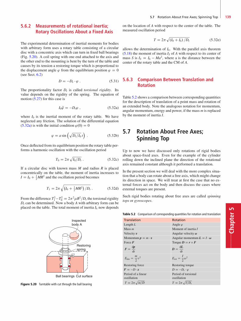
5.7 Rotation About Free Axes; Spinning Top 139
Chap
ter5
5.6.2 Measurements of rotational inertia;Rotary Oscillations About a Fixed Axis
The experimental determination of inertial moments for bodieswith arbitrary form uses a rotary table consisting of a circulardisc with a concentric axis which can turn in fixed ball bearings(Fig. 5.20). A coil spring with one end attached to the axis andthe other end to the mounting is bent by the turn of the table andcauses by its tension a restoring torque which is proportional tothe displacement angle ' from the equilibrium position ' D 0(see Sect. 6.2)
D D �Dr � ' : (5.31)
The proportionality factor Dr is called torsional rigidity. Itsvalue depends on the rigidity of the spring. The equation ofmotion (5.27) for this case is
I0 R' D �Dr' ; (5.32a)
where I0 is the inertial moment of the rotary table. We haveneglected any friction. The solution of the differential equation(5.32a) is with the initial condition '.0/ D 0
' D a sin�p
Dr=I0 t: (5.32b)
Once deflected from its equilibrium position the rotary table per-forms a harmonic oscillation with the oscillation period
T0 D 2pI0=Dr : (5.32c)
If a circular disc with known mass M and radius R is placedconcentrically on the table, the moment of inertia increases toI D I0 C 1
2MR2 and the oscillation period becomes
T1 D 2q�
I0 C 12MR2
�=Dr : (5.32d)
From the difference T21 �T2
0 D 22R2=Dr the torsional rigidityDr can be determined. Now a body A with arbitrary form can beplaced on the table. The total moment of inertia IA now depends
Figure 5.20 Turntable with cut through the ball bearing
on the location of A with respect to the center of the table. Themeasured oscillation period
T D 2p.I0 C IA/ =Dr (5.32e)
allows the determination of IA. With the parallel axis theorem(5.18) the moment of inertia IS of A with respect to its center ofmass S is IS D IA � Ma2, where a is the distance between thecenter of the rotary table and the CM of A.
5.6.3 Comparison Between Translation andRotation
Table 5.2 shows a comparison between corresponding quantitiesfor the description of translation of a point mass and rotation ofan extended body. Note the analogous notation for momentum,angular momentum, energy and power, if the mass m is replacedby the moment of inertia I.
5.7 Rotation About Free Axes;Spinning Top
Up to now we have discussed only rotations of rigid bodiesabout space-fixed axes. Even for the example of the cylinderrolling down the inclined plane the direction of the rotationalaxis remained constant although it performed a translation.
In the present section we will deal with the more complex situa-tion that a body can rotate about a free axis, which might changeits direction in space. We will treat at first the case that no ex-ternal forces act on the body and then discuss the cases whereexternal torques are present.
Such rigid bodies rotating about free axes are called spinningtops or gyroscopes.
Table 5.2 Comparison of corresponding quantities for rotation and translation
Translation RotationLength L Angle 'Mass m Moment of inertia IVelocity v Angular velocity !
Momentum p D m � v Angular momentum L D I � !
Force F Torque D D r F
F D dpdt
D D dLdt
Ekin D m
2v2 Erot D I
2!2
Restoring force Restoring torqueF D �D � x D D �Dr � 'Period of a linearoszillation
Period of torsionaloszillation
T D 2pm=D T D 2
pI=Dr
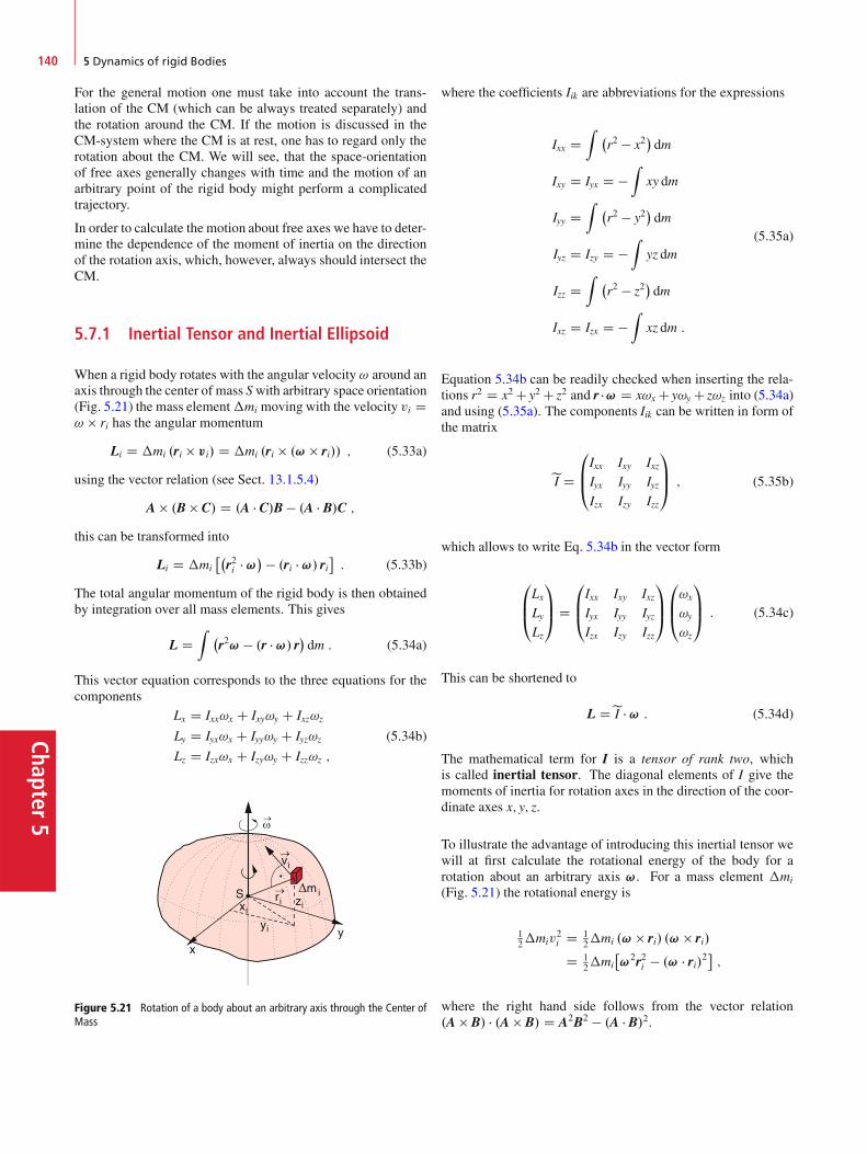
Chapter5
140 5 Dynamics of rigid Bodies
For the general motion one must take into account the trans-lation of the CM (which can be always treated separately) andthe rotation around the CM. If the motion is discussed in theCM-system where the CM is at rest, one has to regard only therotation about the CM. We will see, that the space-orientationof free axes generally changes with time and the motion of anarbitrary point of the rigid body might perform a complicatedtrajectory.
In order to calculate the motion about free axes we have to deter-mine the dependence of the moment of inertia on the directionof the rotation axis, which, however, always should intersect theCM.
5.7.1 Inertial Tensor and Inertial Ellipsoid
When a rigid body rotates with the angular velocity ! around anaxis through the center of mass Swith arbitrary space orientation(Fig. 5.21) the mass element�mi moving with the velocity vi D! ri has the angular momentum
Li D �mi .ri vi/ D �mi .ri .! ri// ; (5.33a)
using the vector relation (see Sect. 13.1.5.4)
A .B C/ D .A � C/B � .A � B/C ;this can be transformed into
Li D �mi��r2i � !
� � .ri � !/ ri�: (5.33b)
The total angular momentum of the rigid body is then obtainedby integration over all mass elements. This gives
L DZ �
r2! � .r � !/ r�dm : (5.34a)
This vector equation corresponds to the three equations for thecomponents
Lx D Ixx!x C Ixy!y C Ixz!z
Ly D Iyx!x C Iyy!y C Iyz!z
Lz D Izx!x C Izy!y C Izz!z ;
(5.34b)
Figure 5.21 Rotation of a body about an arbitrary axis through the Center ofMass
where the coefficients Iik are abbreviations for the expressions
Ixx DZ �
r2 � x2�dm
Ixy D Iyx D �Z
xy dm
Iyy DZ �
r2 � y2�dm
Iyz D Izy D �Z
yz dm
Izz DZ �
r2 � z2�dm
Ixz D Izx D �Z
xz dm :
(5.35a)
Equation 5.34b can be readily checked when inserting the rela-tions r2 D x2 C y2 C z2 and r � ! D x!x C y!y C z!z into (5.34a)and using (5.35a). The components Iik can be written in form ofthe matrix
eI D
0
B@Ixx Ixy IxzIyx Iyy IyzIzx Izy Izz
1
CA ; (5.35b)
which allows to write Eq. 5.34b in the vector form
0
B@LxLyLz
1
CA D
0
B@Ixx Ixy IxzIyx Iyy IyzIzx Izy Izz
1
CA
0
B@!x
!y
!z
1
CA : (5.34c)
This can be shortened to
L DeI � ! : (5.34d)
The mathematical term for I is a tensor of rank two, whichis called inertial tensor. The diagonal elements of I give themoments of inertia for rotation axes in the direction of the coor-dinate axes x; y; z.
To illustrate the advantage of introducing this inertial tensor wewill at first calculate the rotational energy of the body for arotation about an arbitrary axis !. For a mass element �mi
(Fig. 5.21) the rotational energy is
12�miv
2i D 1
2�mi .! ri/ .! ri/
D 12�mi
�!2r2i � .! � ri/2
�;
where the right hand side follows from the vector relation.A B/ � .A B/ D A2B2 � .A � B/2.

5.7 Rotation About Free Axes; Spinning Top 141
Chap
ter5
The spatial integration over all mass elements gives the rota-tional energy of the whole rigid body
Erot D !2
2
Zr2dm � 1
2
Z.! � r/2 dm
D !2x C !2
y C !2z
2
Z �x2 C y2 C z2
�dm
� 1
2
Z �!xx C !yy C !zz
�2dm
D 1
2
�!2x Ixx C !2
y Iyy C !2z Izz
�
C !x!yIxy C !x!zIxz C !y!zIyz ;
(5.36)
where the definitions (5.35b) have been used. Within the tensornotation (5.36) can be written as
Erot D 12!T � QI � ! ;
which explicitly means
Erot D 1
2.!x!y!z/
0
B@Ixx Ixy IxzIyx Iyy IyzIzx Izy Izz
1
CA
0
B@!x
!y
!z
1
CA :
This shows that for arbitrary orientations of the rotationaxis all elements of the inertial tensor can contribute tothe rotational energy.
When the rotation axis ! forms the angles ˛; ˇ; � with the co-ordinate axes the components of ! are
!x D ! � cos˛ ; !y D ! � cosˇ ; !z D ! � cos � :
When the rotational energy is written in the form of Eq. 5.16 as
Erot D 12 I!
2 ;
the comparison with (5.36) yields for the scalar moment of in-ertia
I D cos2˛ Ixx C cos2ˇ Iyy C cos2� IzzC 2 cos˛ cosˇ Ixy C 2 cos˛ cos � IxzC 2 cosˇ cos � Iyz :
(5.37a)
When we introduce a vector R in the direction of the rotationaxis with the components x D R � cos˛; y D R � cosˇ; z DR � cos � Eq. 5.37a can be written as
R2I D x2Ixx C y2Iyy C z2IzzC 2xyIxy C 2xzIxz C 2yzIyz :
(5.37b)
This is a quadratic equation in x, y, and z with constant coeffi-cients Iik . All points .x; y; z/ for which R2 � I D const are locatedon an ellipsoid because (5.37) describes for R2 � I D k D const
Figure 5.22 Inertial ellipsoid
an ellipsoid, with axes which depend on the coefficients Iik .Since I / M � R2
m the constant k D M � R4m has the dimension
Œk� D kg �m4. Its value depends on the massM of the rigid bodyand the mass distribution relative to the center of mass S whichis expressed by a mean distance Rm.
The moment of inertia I! D k=R2 for a rotation about an ar-bitrary axis ! D f!x; !y; !zg is proportional to 1=R2 whereR is the distance from the center of the ellipsoid to its surface(Fig. 5.22). With this notation one can say that the scalar valueI of the moment of inertia as a function of the spatial orientation.˛; ˇ; �/ of the rotation axis represents the inertial ellipsoid.
5.7.2 Principal Moments of Inertia
We introduce a coordinate system .�; �; �/ which is generatedby three orthogonal vectors �, � and � with axes which pointinto the directions of the principal axes a, b and c of the inertialellipsoid (Fig. 5.23). Their magnitude is normalized when di-viding by
pk. In this coordinate system the ellipsoid equation
(5.37) becomes with R2 � I D 1
�2Ia C �2Ib C �2Ic D 1 : (5.38)
In this principal axis coordinate system all off-diagonal ele-ments Iik with i ¤ k of the inertial tensor I are zero and the
Figure 5.23 Definition of principal axes of inertia
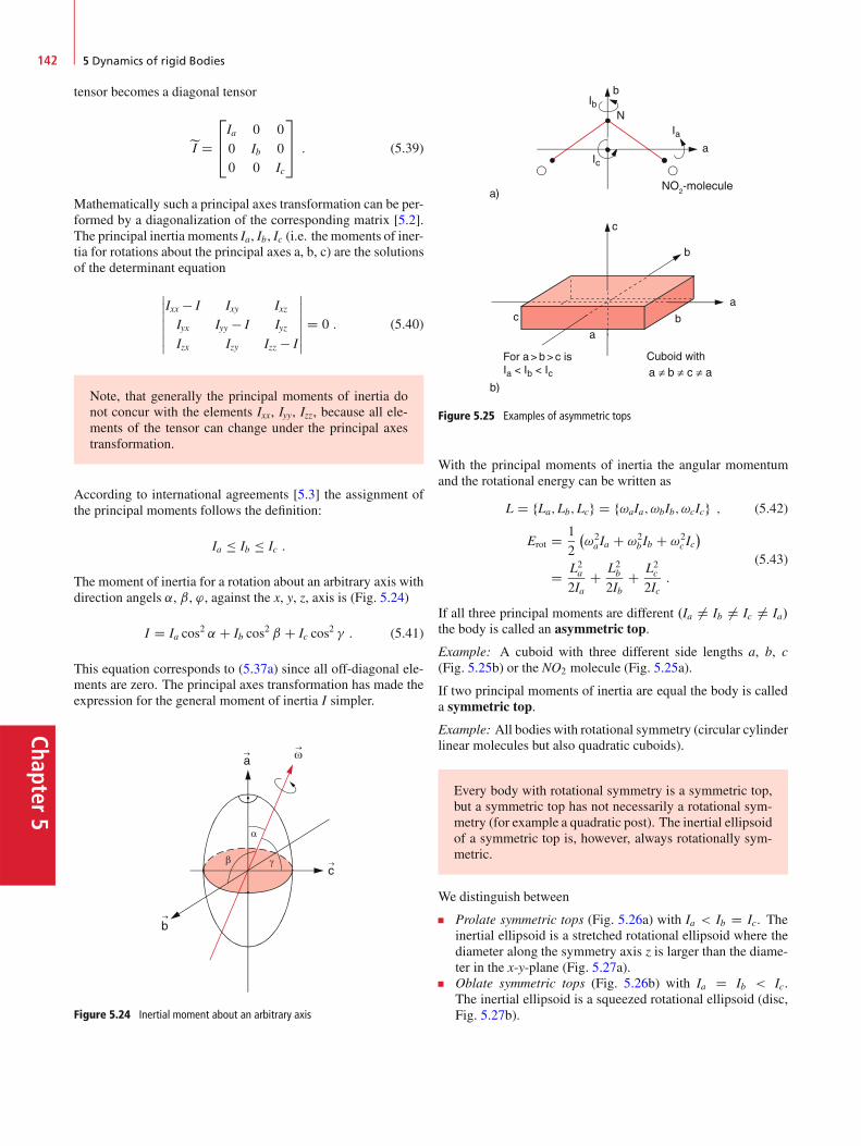
Chapter5
142 5 Dynamics of rigid Bodies
tensor becomes a diagonal tensor
eI D
2
64Ia 0 00 Ib 00 0 Ic
3
75 : (5.39)
Mathematically such a principal axes transformation can be per-formed by a diagonalization of the corresponding matrix [5.2].The principal inertia moments Ia, Ib, Ic (i.e. the moments of iner-tia for rotations about the principal axes a, b, c) are the solutionsof the determinant equation
ˇ̌ˇ̌ˇ̌ˇ
Ixx � I Ixy IxzIyx Iyy � I IyzIzx Izy Izz � I
ˇ̌ˇ̌ˇ̌ˇ
D 0 : (5.40)
Note, that generally the principal moments of inertia donot concur with the elements Ixx, Iyy, Izz, because all ele-ments of the tensor can change under the principal axestransformation.
According to international agreements [5.3] the assignment ofthe principal moments follows the definition:
Ia � Ib � Ic :
The moment of inertia for a rotation about an arbitrary axis withdirection angels ˛, ˇ, ', against the x, y, z, axis is (Fig. 5.24)
I D Ia cos2 ˛ C Ib cos
2 ˇ C Ic cos2 � : (5.41)
This equation corresponds to (5.37a) since all off-diagonal ele-ments are zero. The principal axes transformation has made theexpression for the general moment of inertia I simpler.
Figure 5.24 Inertial moment about an arbitrary axis
Figure 5.25 Examples of asymmetric tops
With the principal moments of inertia the angular momentumand the rotational energy can be written as
L D fLa;Lb; Lcg D f!aIa; !bIb; !cIcg ; (5.42)
Erot D 1
2
�!2a Ia C !2
b Ib C !2c Ic�
D L2a2Ia
C L2b2Ib
C L2c2Ic
:
(5.43)
If all three principal moments are different .Ia ¤ Ib ¤ Ic ¤ Ia/the body is called an asymmetric top.
Example: A cuboid with three different side lengths a, b, c(Fig. 5.25b) or the NO2 molecule (Fig. 5.25a).
If two principal moments of inertia are equal the body is calleda symmetric top.
Example: All bodies with rotational symmetry (circular cylinderlinear molecules but also quadratic cuboids).
Every body with rotational symmetry is a symmetric top,but a symmetric top has not necessarily a rotational sym-metry (for example a quadratic post). The inertial ellipsoidof a symmetric top is, however, always rotationally sym-metric.
We distinguish between
Prolate symmetric tops (Fig. 5.26a) with Ia < Ib D Ic. Theinertial ellipsoid is a stretched rotational ellipsoid where thediameter along the symmetry axis z is larger than the diame-ter in the x-y-plane (Fig. 5.27a).Oblate symmetric tops (Fig. 5.26b) with Ia D Ib < Ic.The inertial ellipsoid is a squeezed rotational ellipsoid (disc,Fig. 5.27b).
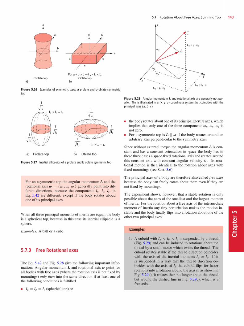
5.7 Rotation About Free Axes; Spinning Top 143
Chap
ter5
Prolate top Oblate topFor
Figure 5.26 Examples of symmetric tops: a prolate and b oblate symmetrictop
Figure 5.27 Inertial ellipsoids of a prolate and b oblate symmetric top
For an asymmetric top the angular momentum L and therotational axis ! D f!x; !y; !zg generally point into dif-ferent directions, because the components Ix, Iy, Iz, inEq. 5.42 are different, except if the body rotates aboudone of its principal axes.
When all three principal moments of inertia are equal, the bodyis a spherical top, because in this case its inertial ellipsoid is asphere.
Examples: A ball or a cube.
5.7.3 Free Rotational axes
The Eq. 5.42 and Fig. 5.28 give the following important infor-mation: Angular momentum L and rotational axis ! point forall bodies with free axes (where the rotation axis is not fixed bymountings) only then into the same direction if at least one ofthe following conditions is fulfilled.
Ia D Ib D Ic (spherical top) or
Figure 5.28 Angular momentum L and rotational axis are generally not par-allel. This is illustrated in a .x ; y ; z/ coordinate system that coincides with theprincipal axes .a ; b ; c/
the body rotates about one of its principal inertial axes, whichimplies that only one of the three components !x, !y, !z isnot zero.For a symmetric top is L k ! if the body rotates around anarbitrary axis perpendicular to the symmetry axis.
Since without external torque the angular momentum L is con-stant and has a constant orientation in space the body has inthese three cases a space fixed rotational axis and rotates aroundthis constant axis with constant angular velocity !. Its rota-tional motion is then identical to the rotation about axes withfixed mountings (see Sect. 5.6)
The principal axes of a body are therefore also called free axesbecause the body can freely rotate about them even if they arenot fixed by mountings.
The experiment shows, however, that a stable rotation is onlypossible about the axes of the smallest and the largest momentof inertia. For the rotation about a free axis of the intermediatemoment of inertia any tiny perturbation makes the motion in-stable and the body finally flips into a rotation about one of theother two principal axes.
Examples
1. A cuboid with Ia < Ib < Ic is suspended by a thread(Fig. 5.29) and can be induced to rotations about thethread by a small motor which twists the thread. Thecuboid rotates stable if the thread direction coincideswith the axis of the inertial moments Ia or Ic. If itis suspended in a way that the thread direction co-incides with the axis of Ib the cuboid flips for fasterrotations into a rotation around the axis b, as shown inFig. 5.29c), it rotates then no longer about the threadbut around the dashed line in Fig. 5.29c), which is afree axis.
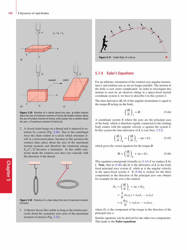
Chapter5
144 5 Dynamics of rigid Bodies
Figure 5.29 Rotation of a cuboid about free axes: a stable rotationabout the axis of maximum moment of inertia; b instable rotation aboutthe axis of median moment of inertia, which jumps into a rotation aboutthe axis c of maximum moment of inertia (c)
2. A closed chain hangs on a thread and is induced to ro-tations by a motor (Fig. 5.30). Due to the centrifugalforce the chain widens to a circle which orientates it-self in a horizontal plane, because in this position therotation takes place about the axis of the maximuminertial moment and therefore the rotational energyErotL2=2I becomes a minimum. In this stable rota-tional mode the rotation axis does not coincide withthe direction of the thread.
Figure 5.30 Rotation of a chain about the axis of maximum momentof inertia
3. A thrown discus flies stable as long as the rotation pro-ceeds about the symmetry axis (axis of the maximummoment of inertia) (Fig. 5.31).
Figure 5.31 Stable flight of a discus J
5.7.4 Euler’s Equations
For an arbitrary orientation of the rotation axis angular momen-tum L and rotation axis ! are no longer parallel. The motion ofthe body is now more complicated. In order to investigate thismotion as seen by an observer sitting in a space-fixed inertialcoordinate system S, we have to describe it in this system S.
The time derivative dL=dt of the angular momentum is equal tothe torque D acting on the body.
�dLdt
�
S
D D : (5.44)
A coordinate system K where the axes are the principal axesof the body, which is therefore rigidly connected to the rotatingbody rotates with the angular velocity ! against the system S.In this system the time derivative of L is (see Sect. 3.3.2)
�dLdt
�
K
D�dLdt
�
S
� .! L/ ; (5.45)
which gives the vector equation for the torque D
D D�dLdt
�
K
C .! L/ : (5.46)
This equation corresponds formally to (3.14) if we replace L byr. Note, that in (5.46) dL=dt is the derivative of L in the bodyfixed principal axes system K, while ! is the angular velocityin the space-fixed system S. If (5.46) is written for the threecomponents in the direction of the principal axes one obtainsfor example for the axis a the relation
Da D�dLdt
�
a
C .! L/a
D d
dt.Ia!a/C .!bLc � !cLb/
D Iad!a
dtC !bIc!c � !cIb!b ;
where Da is the component of the torque in the direction of theprincipal axis a.
Similar equations can be derived for the other two components.This leads to the Euler-equations

5.7 Rotation About Free Axes; Spinning Top 145
Chap
ter5
Iad!a
dtC .Ic � Ib/ !c!b D Da
Ibd!b
dtC .Ia � Ic/ !a!c D Db
Icd!c
dtC .Ib � Ia/ !b!a D Dc :
(5.47)
5.7.5 The Torque-free Symmetric Top
A symmetric top has two equal principal moments of inertia. Ifthe symmetry axis of its inertial ellipsoid is the axis c we haveIa D Ib ¤ Ic. For rotational symmetric bodies the symmetryaxis is also called the figure axis. For a bicycle wheel as sym-metric top this is the visible wheel axis (Fig. 5.32). Without anyexternal torque .D D 0/ the magnitude and the direction of theangular momentum L is constant. Such a top with D D 0 iscalled force-free top although it should be called more correctlytorque-free top.
When the top rotates about its figure axis, L and ! coincidewith this axis. The top rotates as if its axis would be hold by astable mounting (see Sect. 5.6). If, however, ! points into anarbitrary direction which does not coincide with the figure axisthe motion becomes complicated.
For the description of this motion one has to distinguish betweenthree axes (Fig. 5.33a):
The space-fixed angular momentum axis LThe momentary (not space-fixed) rotation axis !
The figure axis of the symmetric top, which is only space-fixed, if L coincides with this axis.
We can win a qualitative picture for the motion of the figureaxis by the following consideration: For D D 0 the angularmomentum L and the rotational energy Erot are both constant.
Figure 5.32 Bicycle wheel as symmetric top
Figure 5.33 Figure axis c, angular momentum L and momentary rotationaxis !: a Decomposition of ! and L into the components parallel and per-pendicular to the figure axis of the symmetric top. b Nutation cone of EL andE!
Then we obtain from Eq. 5.43
L2x C L2y C L2z D const D C1 ; (5.48a)
L2aIa
C L2bIb
C L2cIc
D const D C2 : (5.48b)
In a space-fixed coordinate system with the axes Lx, Ly, Lz(5.48a) represents the equation of a sphere. Equation 5.48bdescribes an ellipsoid in the principal axes system. Sincethe components of the space-fixed vector L must obey bothequations, the endpoint of L can only move on the curve of in-tersection between sphere and ellipsoid (Fig. 5.34). Since theellipsoid is determined by the principal axes system of the top,i.e. rotates with the top, while L is space-fixed, the top andtherefore also its inertial ellipsoid move in such a way, that theendpoint of L always remains on the curve of intersection. Thiscauses a nutation of the figure axis and the momentary rotationaxis ! about the space-fixed axis L (Fig. 5.33b).
While the figure axis can be seen straight forward, the momen-tary rotation axis can be made visible by an experimental trick:A circular disc with red, black and white circular segments is
Figure 5.34 The top of the angular momentum vector moves on the intersec-tion curve of angular momentum sphere and energy ellipsoid
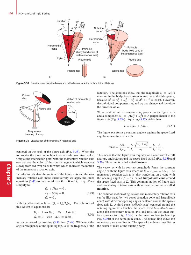
Chapter5
146 5 Dynamics of rigid Bodies
Figure 5.36 Nutation cone, herpolhode cone and polhode cone for a the prolate, b the oblate top
Figure 5.35 Visualization of the momentary rotational axis
centered on the peak of the figure axis (Fig. 5.35). When thetop rotates the three colors blur to an olive-brown mixed color.Only at the intersection point with the momentary rotation axisone can see the color of the specific segment which wandersslowly from red over black to white which indicates the motionof the momentary rotation axis.
In order to calculate the motion of the figure axis and the mo-mentary rotation axis more quantitatively we apply the Eulerequations (5.47) to the special case D D 0 and Ia D Ib. Theysimplify to
P!a C˝!b D 0 ;
P!b �˝!a D 0 ;
P!c D 0 ;
(5.49)
with the abbreviation ˝ D ..Ic � Ia/=Ia/!c. The solutions ofthis system of equations are
˝a D A cos˝t ; ˝b D A sin˝t ;
˝c D C with A;C D const ;(5.50)
as can be proved by inserting (5.50) into (5.49). While ! is theangular frequency of the spinning top,˝ is the frequency of the
nutation. The solutions show, that the magnitude ! D j!j isconstant in the body-fixed system as well as in the lab-system,because !2 D !2
a C !2b C !2
c D A2 C C2 D const. However,the individual components !a and !b can change and thereforethe direction of !.
We separate ! into a component !c parallel to the figure axisand a component !? D p
.!2a C !2
b/ D A perpendicular to thefigure axis (Fig. 5.33a) . Squaring (5.42) yields then
L D Ia!? C Ic!c : (5.51)
The figure axis forms a constant angle ˛ against the space-fixedangular momentum axis with
tan˛ D Ia!?Ic!c
D IaIc
q!2a C !2
b
!cD Ia
Ic� A
!c:
This means that the figure axis migrates on a cone with the fullaperture angle 2˛ around the space-fixed axis L (Fig. 5.33b and5.36). This cone is called nutation-cone.
The vector ! with its constant magnitude forms the constantangle ˇ with the figure axis where sinˇ D !?=! D A=!c. Themomentary rotation axis ! is also wandering on a cone withthe opening angel 2.ˇ � ˛/, called herpolhode cone aroundthe space fixed axis of L. This common motion of figure axisand momentary rotation axis without external torque is callednutation.
The common motion of figure axis and momentary rotation axiscan be illustrated by two cones (nutation cone and herpolhodecone) with different opening angles centered around the space-fixed axis L. A third cone (polhode cone) centered around thenutating figure axis touches the space fixed herpolhode conealong the momentary rotation axis and rolls on the outer sur-face (prolate top Fig. 5.36a) or the inner surface (oblate topFig. 5.36b) of the herpolhode cone. The contact line shows themomentary rotation line !. The apex of the three cones lies inthe center of mass of the nutating body.

5.7 Rotation About Free Axes; Spinning Top 147
Chap
ter5
5.7.6 Precession of the Symmetric Top
If an external torque D acts on the body the angular momentumis no longer space-fixed, because of D D dL=dt. Depending onthe direction of D relative to the figure axis the direction andalso the magnitude of L changes with time. At first we willdiscuss the simplest case where the body rotates with the angularvelocity ! around its figure axis c and all three axis L, ! and ccoincide. In this case there is no nutation and for D D 0 thebody would rotate with ! D const about the space-fixed figureaxis.
If the top is not supported in its CM, the gravitational force gen-erates a torque
D D r m � g ;where r is the vector from the support point to the CM. If thesymmetric top spins with the angular momentum L the torque isperpendicular to L and therefore changes only its direction butnot its magnitude (Fig. 5.37). During the time interval dt thedirection of L changes by the angle d' and we can derive fromFig. 5.37
jdLj D jLj � d' ! D D dL
dtD jLjd'
dt:
The angular momentum axis and with it the coincidental figureaxis rotate with the angular velocity
!p D d'
dtD D
LD D
I!(5.52)
about an axis perpendicular to the plane of D and L where wehave assumed that !p !. This motion is called precession.
If the figure axis forms the angle ˛ against the vertical directionthe magnitude of the torque is D D m � g � sin˛. The change dLof the angular momentum L is now for dL L (Fig. 5.38)
dL D jLj sin˛ � d' :For !p ! therefore the equation for the precession frequencybecomes
!p D mgr sin˛
I! sin˛D mgr
I!; (5.53)
Figure 5.37 The gravitational force causes a torque acting on a top, that is notsupported in the Center of Mass
Figure 5.38 Precession of a spinning top
which shows that !p is independent of the space orientation ofthe figure axis and depends only on the angular momentum Land the torque D.
The general treatment of precession has to take into account thethree vectors (Fig. 5.39)
1. The angular velocity !F about the figure axis2. The angular velocity !p of precession around the vertical z-
axis3. The total angular velocity ! D !F C !p
According to Fig. 5.39 we get the relations:
!F D ! � e with e D fsin � cos'; sin � sin'; cos �g!p D P' � f0; 0; 1g! D f! � sin � cos'; ! � sin � sin'; ! � cos � C P'g :
(5.53a)
We separate ! into a component !k parallel and !? perpendic-ular to the figure axis e.
!k D e � .! C P' cos �/!? D e .! e/
D P' sin � � f� cos � cos';� cos � sin '; sin �g :(5.53b)
θ
Figure 5.39 Illustration of the equation of motion for a spinning top
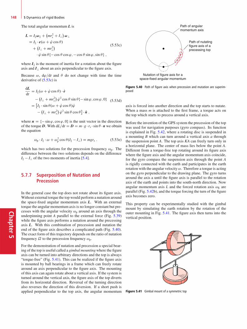
Chapter5
148 5 Dynamics of rigid Bodies
The total angular momentum L is
L D Ik!k C �mr2s C I?
�!?
D Ik � e.! C P' cos �/C �
I? C mr2s�
� P' sin �f� cos � cos';� cos � sin'; sin �g ;
(5.53c)
where Ik is the moment of inertia for a rotation about the figureaxis and I? about an axis perpendicular to the figure axis.
Because !, d'=dt and � do not change with time the timederivative of (5.53c) is
dLdt
D Ik.! C P' cos �/ � Pe� �
I? C mr2s� P'2 cos � sin �f� sin '; cos'; 0g
D �Ik � sin �.! C P' cos �/ P'� �
I? C mr2s� P'2 sin � cos �
� � On :
(5.53d)
where n D f� sin '; cos'; 0g is the unit vector in the directionof the torque D. With dL=dt D D D m � g � rs � sin � � n we obtainthe equation
!p � Ik � ! C !2p cos �.Ik � I?/ D mgrs : (5.53e)
which has two solutions for the precession frequency !p. Thedifference between the two solutions depends on the differenceIk � I? of the two moments of inertia [5.4].
5.7.7 Superposition of Nutation andPrecession
In the general case the top does not rotate about its figure axis.Without external torque the top would perform a nutation aroundthe space-fixed angular momentum axis L. With an externaltorque the angular momentum axis is no longer constant but pre-cesses with the angular velocity !p around an axis through theunderpinning point A parallel to the external force (Fig. 5.39)while the figure axis performs a nutation around the precessingaxis L. With this combination of precession and nutation theend of the figure axis describes a complicated path (Fig. 5.40).The exact form of this trajectory depends on the ratio of nutationfrequency˝ to the precession frequency !p.
For the demonstration of nutation and precession a special bear-ing of the top is useful called a gimbal mountingwhere the figureaxis can be turned into arbitrary directions and the top is always“torque-free” (Fig. 5.41). This can be realized if the figure axisis mounted by ball bearings in a frame which can freely rotatearound an axis perpendicular to the figure axis. The mountingof this axis can again rotate about a vertical axis. If the system isturned around the vertical axis, the figure axis of the top divertsfrom its horizontal direction. Reversal of the turning directionalso reverses the direction of this diversion. If a short push isapplied perpendicular to the top axis, the angular momentum
Figure 5.40 Path of figure axis when precession and mutation are superim-posed
axis is forced into another direction and the top starts to nutate.When a mass m is attached to the first frame, a torque acts onthe top which starts to precess around a vertical axis.
Before the invention of the GPS system the precession of the topwas used for navigation purposes (gyro compass). Its functionis explained in Fig. 5.42, where a rotating disc is suspended ina mounting B which can turn around a vertical axis a throughthe suspension point A. The top axis KA can freely turn only ina horizontal plane. The center of mass lies below the point A.Different from a torque-free top rotating around its figure axiswhere the figure axis and the angular momentum axis coincide,for the gyro compass the suspension axis through the point Ais rigidly connected with the earth and participates in the earthrotation with the angular velocity!. Therefore a torque is actingon the gyro perpendicular to the drawing plane. The gyro turnsaround the axis a until the figure axis is parallel to the rotationaxis of the earth and points into the south-north direction. Nowangular momentum axis L and the forced rotation axis !E areparallel (Fig. 5.42b), and the torque forcing the turn of the figureaxis becomes zero.
This property can be experimentally studied with the gimbalmount by simulating the earth rotation by the rotation of theouter mounting in Fig. 5.41. The figure axis then turns into thevertical position.
Figure 5.41 Gimbal mount of a symmetric top
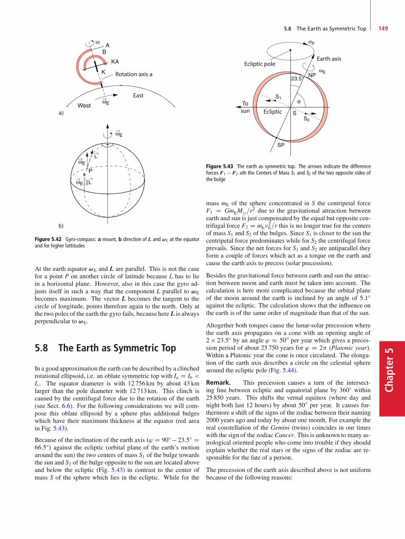
5.8 The Earth as Symmetric Top 149
Chap
ter5
Figure 5.42 Gyro-compass: a mount, b direction of L and !E at the equatorand for higher lattitudes
At the earth equator !E and L are parallel. This is not the casefor a point P on another circle of latitude because L has to liein a horizontal plane. However, also in this case the gyro ad-justs itself in such a way that the component L parallel to !E
becomes maximum. The vector L becomes the tangent to thecircle of longitude, points therefore again to the north. Only atthe two poles of the earth the gyro fails, because here L is alwaysperpendicular to !E.
5.8 The Earth as Symmetric Top
In a good approximation the earth can be described by a clinchedrotational ellipsoid, i.e. an oblate symmetric top with Ia D Ib <Ic. The equator diameter is with 12 756 km by about 43 kmlarger than the pole diameter with 12 713 km. This clinch iscaused by the centrifugal force due to the rotation of the earth(see Sect. 6.6). For the following considerations we will com-pose this oblate ellipsoid by a sphere plus additional bulgeswhich have their maximum thickness at the equator (red areain Fig. 5.43).
Because of the inclination of the earth axis .' D 90ı � 23:5ı D66:5ı/ against the ecliptic (orbital plane of the earth’s motionaround the sun) the two centers of mass S1 of the bulge towardsthe sun and S2 of the bulge opposite to the sun are located aboveand below the ecliptic (Fig. 5.43) in contrast to the center ofmass S of the sphere which lies in the ecliptic. While for the
Figure 5.43 The earth as symmetric top. The arrows indicate the differenceforces F1 � F2 ath the Centers of Mass S1 and S2 of the two opposite sides ofthe bulge
mass mE of the sphere concentrated in S the centripetal forceF1 D GmEMˇ=r2 due to the gravitational attraction betweenearth and sun is just compensated by the equal but opposite cen-trifugal force F2 D mEv
2E=r this is no longer true for the centers
of mass S1 and S2 of the bulges. Since S1 is closer to the sun thecentripetal force predominates while for S2 the centrifugal forceprevails. Since the net forces for S1 and S2 are antiparallel theyform a couple of forces which act as a torque on the earth andcause the earth axis to precess (solar precession).
Besides the gravitational force between earth and sun the attrac-tion between moon and earth must be taken into account. Thecalculation is here more complicated because the orbital planeof the moon around the earth is inclined by an angle of 5:1ıagainst the ecliptic. The calculation shows that the influence onthe earth is of the same order of magnitude than that of the sun.
Altogether both torques cause the lunar-solar precession wherethe earth axis propagates on a cone with an opening angle of2 23:5ı by an angle ' � 5000 per year which gives a preces-sion period of about 25 750 years for ' D 2 (Platonic year).Within a Platonic year the cone is once circulated. The elonga-tion of the earth axis describes a circle on the celestial spherearound the ecliptic pole (Fig. 5.44).
Remark. This precession causes a turn of the intersect-ing line between ecliptic and equatorial plane by 360ı within25 850 years. This shifts the vernal equinox (where day andnight both last 12 hours) by about 5000 per year. It causes fur-thermore a shift of the signs of the zodiac between their naming2000 years ago and today by about one month. For example thereal constellation of the Gemini (twins) coincides in our timeswith the sign of the zodiac Cancer. This is unknown to many as-trological oriented people who come into trouble if they shouldexplain whether the real stars or the signs of the zodiac are re-sponsible for the fate of a person.
The precession of the earth axis described above is not uniformbecause of the following reasons:
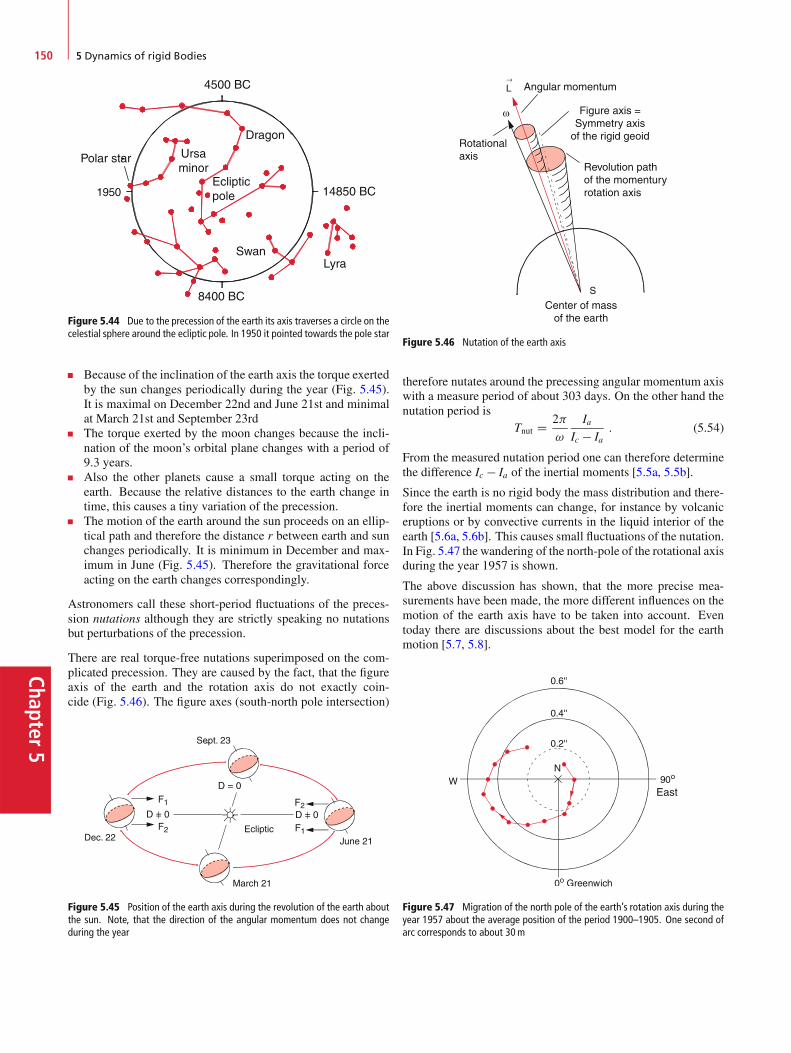
Chapter5
150 5 Dynamics of rigid Bodies
Figure 5.44 Due to the precession of the earth its axis traverses a circle on thecelestial sphere around the ecliptic pole. In 1950 it pointed towards the pole star
Because of the inclination of the earth axis the torque exertedby the sun changes periodically during the year (Fig. 5.45).It is maximal on December 22nd and June 21st and minimalat March 21st and September 23rdThe torque exerted by the moon changes because the incli-nation of the moon’s orbital plane changes with a period of9.3 years.Also the other planets cause a small torque acting on theearth. Because the relative distances to the earth change intime, this causes a tiny variation of the precession.The motion of the earth around the sun proceeds on an ellip-tical path and therefore the distance r between earth and sunchanges periodically. It is minimum in December and max-imum in June (Fig. 5.45). Therefore the gravitational forceacting on the earth changes correspondingly.
Astronomers call these short-period fluctuations of the preces-sion nutations although they are strictly speaking no nutationsbut perturbations of the precession.
There are real torque-free nutations superimposed on the com-plicated precession. They are caused by the fact, that the figureaxis of the earth and the rotation axis do not exactly coin-cide (Fig. 5.46). The figure axes (south-north pole intersection)
Figure 5.45 Position of the earth axis during the revolution of the earth aboutthe sun. Note, that the direction of the angular momentum does not changeduring the year
Figure 5.46 Nutation of the earth axis
therefore nutates around the precessing angular momentum axiswith a measure period of about 303 days. On the other hand thenutation period is
Tnut D 2
!
IaIc � Ia
: (5.54)
From the measured nutation period one can therefore determinethe difference Ic � Ia of the inertial moments [5.5a, 5.5b].
Since the earth is no rigid body the mass distribution and there-fore the inertial moments can change, for instance by volcaniceruptions or by convective currents in the liquid interior of theearth [5.6a, 5.6b]. This causes small fluctuations of the nutation.In Fig. 5.47 the wandering of the north-pole of the rotational axisduring the year 1957 is shown.
The above discussion has shown, that the more precise mea-surements have been made, the more different influences on themotion of the earth axis have to be taken into account. Eventoday there are discussions about the best model for the earthmotion [5.7, 5.8].
Figure 5.47 Migration of the north pole of the earth’s rotation axis during theyear 1957 about the average position of the period 1900–1905. One second ofarc corresponds to about 30m
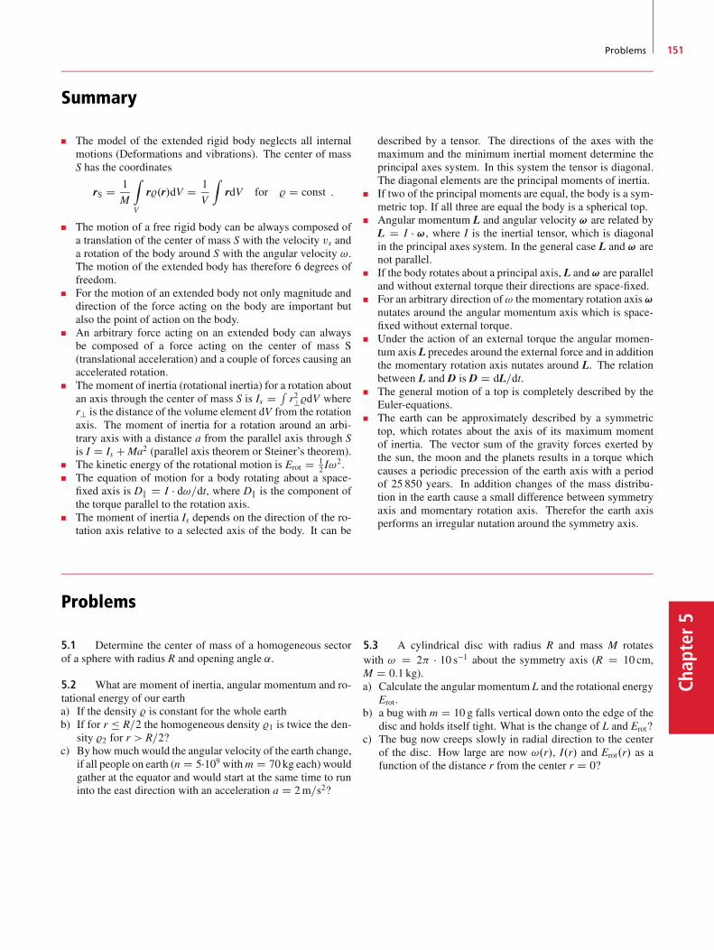
Problems 151
Chap
ter5
Summary
The model of the extended rigid body neglects all internalmotions (Deformations and vibrations). The center of massS has the coordinates
rS D 1
M
Z
V
r%.r/dV D 1
V
ZrdV for % D const :
The motion of a free rigid body can be always composed ofa translation of the center of mass S with the velocity vs anda rotation of the body around S with the angular velocity !.The motion of the extended body has therefore 6 degrees offreedom.For the motion of an extended body not only magnitude anddirection of the force acting on the body are important butalso the point of action on the body.An arbitrary force acting on an extended body can alwaysbe composed of a force acting on the center of mass S(translational acceleration) and a couple of forces causing anaccelerated rotation.The moment of inertia (rotational inertia) for a rotation aboutan axis through the center of mass S is Is D R
r2?%dV wherer? is the distance of the volume element dV from the rotationaxis. The moment of inertia for a rotation around an arbi-trary axis with a distance a from the parallel axis through Sis I D Is CMa2 (parallel axis theorem or Steiner’s theorem).The kinetic energy of the rotational motion is Erot D 1
2 I!2.
The equation of motion for a body rotating about a space-fixed axis is Dk D I � d!=dt, where Dk is the component ofthe torque parallel to the rotation axis.The moment of inertia Is depends on the direction of the ro-tation axis relative to a selected axis of the body. It can be
described by a tensor. The directions of the axes with themaximum and the minimum inertial moment determine theprincipal axes system. In this system the tensor is diagonal.The diagonal elements are the principal moments of inertia.If two of the principal moments are equal, the body is a sym-metric top. If all three are equal the body is a spherical top.Angular momentum L and angular velocity ! are related byL D I � !, where I is the inertial tensor, which is diagonalin the principal axes system. In the general case L and ! arenot parallel.If the body rotates about a principal axis, L and ! are paralleland without external torque their directions are space-fixed.For an arbitrary direction of ! the momentary rotation axis !
nutates around the angular momentum axis which is space-fixed without external torque.Under the action of an external torque the angular momen-tum axis L precedes around the external force and in additionthe momentary rotation axis nutates around L. The relationbetween L and D is D D dL=dt.The general motion of a top is completely described by theEuler-equations.The earth can be approximately described by a symmetrictop, which rotates about the axis of its maximum momentof inertia. The vector sum of the gravity forces exerted bythe sun, the moon and the planets results in a torque whichcauses a periodic precession of the earth axis with a periodof 25 850 years. In addition changes of the mass distribu-tion in the earth cause a small difference between symmetryaxis and momentary rotation axis. Therefor the earth axisperforms an irregular nutation around the symmetry axis.
Problems
5.1 Determine the center of mass of a homogeneous sectorof a sphere with radius R and opening angle ˛.
5.2 What are moment of inertia, angular momentum and ro-tational energy of our eartha) If the density % is constant for the whole earthb) If for r � R=2 the homogeneous density %1 is twice the den-
sity %2 for r > R=2?c) By howmuchwould the angular velocity of the earth change,
if all people on earth (n D 5�109 withm D 70 kg each) wouldgather at the equator and would start at the same time to runinto the east direction with an acceleration a D 2m=s2?
5.3 A cylindrical disc with radius R and mass M rotateswith ! D 2 � 10 s�1 about the symmetry axis (R D 10 cm,M D 0:1 kg).a) Calculate the angular momentum L and the rotational energy
Erot.b) a bug with m D 10 g falls vertical down onto the edge of the
disc and holds itself tight. What is the change of L and Erot?c) The bug now creeps slowly in radial direction to the center
of the disc. How large are now !.r/, I.r/ and Erot.r/ as afunction of the distance r from the center r D 0?
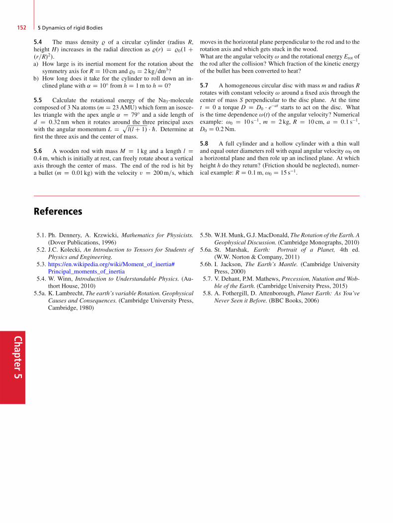
Chapter5
152 5 Dynamics of rigid Bodies
5.4 The mass density % of a circular cylinder (radius R,height H) increases in the radial direction as %.r/ D %0.1 C.r=R/2/.a) How large is its inertial moment for the rotation about the
symmetry axis for R D 10 cm and %0 D 2 kg=dm3?b) How long does it take for the cylinder to roll down an in-
clined plane with ˛ D 10ı from h D 1m to h D 0?
5.5 Calculate the rotational energy of the Na3-moleculecomposed of 3 Na atoms (m D 23AMU) which form an isosce-les triangle with the apex angle ˛ D 79ı and a side length ofd D 0:32 nm when it rotates around the three principal axeswith the angular momentum L D p
l.l C 1/ � „. Determine atfirst the three axis and the center of mass.
5.6 A wooden rod with mass M D 1 kg and a length l D0:4m, which is initially at rest, can freely rotate about a verticalaxis through the center of mass. The end of the rod is hit bya bullet (m D 0:01 kg) with the velocity v D 200m=s, which
moves in the horizontal plane perpendicular to the rod and to therotation axis and which gets stuck in the wood.What are the angular velocity ! and the rotational energy Erot ofthe rod after the collision? Which fraction of the kinetic energyof the bullet has been converted to heat?
5.7 A homogeneous circular disc with mass m and radius Rrotates with constant velocity ! around a fixed axis through thecenter of mass S perpendicular to the disc plane. At the timet D 0 a torque D D D0 � e�at starts to act on the disc. Whatis the time dependence !.t/ of the angular velocity? Numericalexample: !0 D 10 s�1, m D 2 kg, R D 10 cm, a D 0:1 s�1,D0 D 0:2Nm.
5.8 A full cylinder and a hollow cylinder with a thin walland equal outer diameters roll with equal angular velocity !0 ona horizontal plane and then role up an inclined plane. At whichheight h do they return? (Friction should be neglected), numer-ical example: R D 0:1m, !0 D 15 s�1.
References
5.1. Ph. Dennery, A. Krzwicki, Mathematics for Physicists.(Dover Publications, 1996)
5.2. J.C. Kolecki, An Introduction to Tensors for Students ofPhysics and Engineering.
5.3. https://en.wikipedia.org/wiki/Moment_of_inertia#Principal_moments_of_inertia
5.4. W. Winn, Introduction to Understandable Physics. (Au-thort House, 2010)
5.5a. K. Lambrecht, The earth’s variable Rotation. GeophysicalCauses and Consequences. (Cambridge University Press,Cambridge, 1980)
5.5b. W.H.Munk, G.J. MacDonald, The Rotation of the Earth. AGeophysical Discussion. (Cambridge Monographs, 2010)
5.6a. St. Marshak, Earth: Portrait of a Planet, 4th ed.(W.W. Norton & Company, 2011)
5.6b. I. Jackson, The Earth’s Mantle. (Cambridge UniversityPress, 2000)
5.7. V. Dehant, P.M. Mathews, Precession, Nutation and Wob-ble of the Earth. (Cambridge University Press, 2015)
5.8. A. Fothergill, D. Attenborough, Planet Earth: As You’veNever Seen it Before. (BBC Books, 2006)
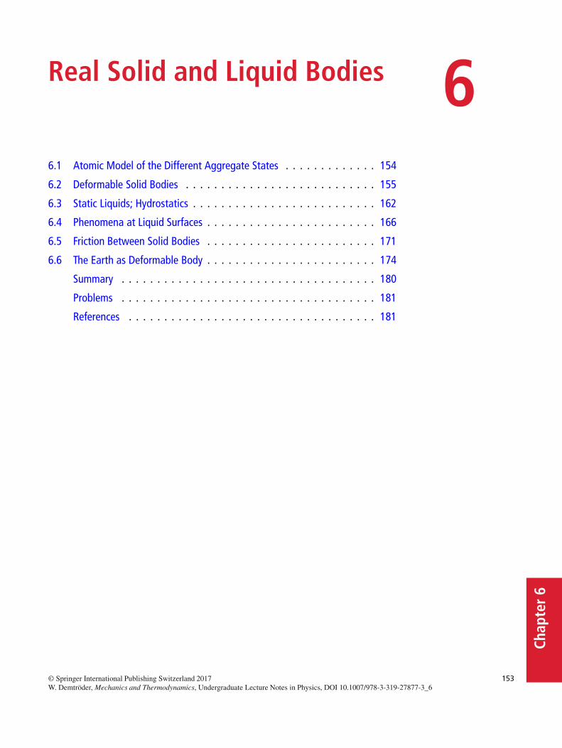
Chap
ter6
Real Solid and Liquid Bodies 66.1 Atomic Model of the Different Aggregate States . . . . . . . . . . . . . 154
6.2 Deformable Solid Bodies . . . . . . . . . . . . . . . . . . . . . . . . . . . 155
6.3 Static Liquids; Hydrostatics . . . . . . . . . . . . . . . . . . . . . . . . . . 162
6.4 Phenomena at Liquid Surfaces . . . . . . . . . . . . . . . . . . . . . . . . 166
6.5 Friction Between Solid Bodies . . . . . . . . . . . . . . . . . . . . . . . . 171
6.6 The Earth as Deformable Body . . . . . . . . . . . . . . . . . . . . . . . . 174
Summary . . . . . . . . . . . . . . . . . . . . . . . . . . . . . . . . . . . . 180
Problems . . . . . . . . . . . . . . . . . . . . . . . . . . . . . . . . . . . . 181
References . . . . . . . . . . . . . . . . . . . . . . . . . . . . . . . . . . . 181
153© Springer International Publishing Switzerland 2017W. Demtröder, Mechanics and Thermodynamics, Undergraduate Lecture Notes in Physics, DOI 10.1007/978-3-319-27877-3_6
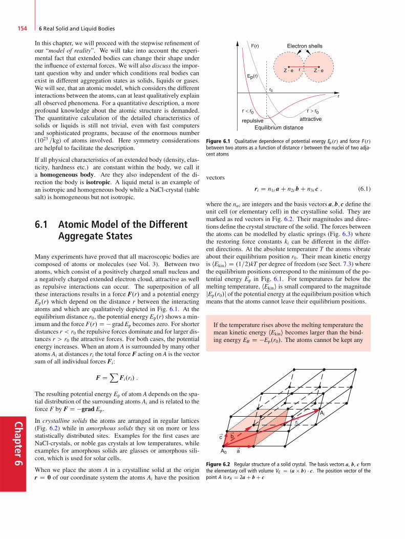
Chapter6
154 6 Real Solid and Liquid Bodies
In this chapter, we will proceed with the stepwise refinement ofour “model of reality”. We will take into account the experi-mental fact that extended bodies can change their shape underthe influence of external forces. We will also discuss the impor-tant question why and under which conditions real bodies canexist in different aggregation states as solids, liquids or gases.We will see, that an atomic model, which considers the differentinteractions between the atoms, can at least qualitatively explainall observed phenomena. For a quantitative description, a moreprofound knowledge about the atomic structure is demanded.The quantitative calculation of the detailed characteristics ofsolids or liquids is still not trivial, even with fast computersand sophisticated programs, because of the enormous number(1023 =kg) of atoms involved. Here symmetry considerationsare helpful to facilitate the description.
If all physical characteristics of an extended body (density, elas-ticity, hardness etc.) are constant within the body, we call ita homogeneous body. Are they also independent of the di-rection the body is isotropic. A liquid metal is an example ofan isotropic and homogeneous body while a NaCl-crystal (tablesalt) is homogeneous but not isotropic.
6.1 Atomic Model of the DifferentAggregate States
Many experiments have proved that all macroscopic bodies arecomposed of atoms or molecules (see Vol. 3). Between twoatoms, which consist of a positively charged small nucleus anda negatively charged extended electron cloud, attractive as wellas repulsive interactions can occur. The superposition of allthese interactions results in a force F.r/ and a potential energyEp.r/ which depend on the distance r between the interactingatoms and which are qualitatively depicted in Fig. 6.1. At theequilibrium distance r0, the potential energy Ep.r/ shows a min-imum and the force F.r/ D � gradEp becomes zero. For shorterdistances r < r0 the repulsive forces dominate and for larger dis-tances r > r0 the attractive forces. For both cases, the potentialenergy increases. When an atom A is surrounded by many otheratoms Ai at distances ri the total force F acting on A is the vectorsum of all individual forces Fi:
F DX
Fi.ri/ :
The resulting potential energy Ep of atom A depends on the spa-tial distribution of the surrounding atoms Ai and is related to theforce F by F D �grad Ep.
In crystalline solids the atoms are arranged in regular lattices(Fig. 6.2) while in amorphous solids they sit on more or lessstatistically distributed sites. Examples for the first cases areNaCl-crystals, or noble gas crystals at low temperatures, whileexamples for amorphous solids are glasses or amorphous sili-con, which is used for solar cells.
When we place the atom A in a crystalline solid at the originr D 0 of our coordinate system the atoms Ai have the position
Figure 6.1 Qualitative dependence of potential energy Ep .r/ and force F .r/between two atoms as a function of distance r between the nuclei of two adja-cent atoms
vectors
ri D n1i a C n2i b C n3i c ; (6.1)
where the n˛i are integers and the basis vectors a; b; c define theunit cell (or elementary cell) in the crystalline solid. They aremarked as red vectors in Fig. 6.2. Their magnitudes and direc-tions define the crystal structure of the solid. The forces betweenthe atoms can be modelled by elastic springs (Fig. 6.3) wherethe restoring force constants ki can be different in the differ-ent directions. At the absolute temperature T the atoms vibrateabout their equilibrium position r0. Their mean kinetic energyis hEkini D .1=2/kT per degree of freedom (see Sect. 7.3) wherethe equilibrium positions correspond to the minimum of the po-tential energy Ep in Fig. 6.1. For temperatures far below themelting temperature, hEkini is small compared to the magnitudejEp.r0/j of the potential energy at the equilibrium position whichmeans that the atoms cannot leave their equilibrium positions.
If the temperature rises above the melting temperature themean kinetic energy hEkini becomes larger than the bind-ing energy EB D �Ep.r0/. The atoms cannot be kept any
Figure 6.2 Regular structure of a solid crystal. The basis vectors a, b, c formthe elementary cell with volume VE D .a b/ � c. The position vector of thepoint A is rA D 2a C b C c

6.2 Deformable Solid Bodies 155
Chap
ter6
Figure 6.3 Springmodel of a solid crystal. The restoring force is for an isotropiccrystal equal for all three directions a, b, c, for an unisotropic crystal they differ
longer on their positions ri but can diffuse around. Thecrystalline solid melts and converts to the liquid state.
Also in the liquid state the minimum of the potential energy re-mains at the mean distance hr0i between the atoms. This meansthat the density in the liquid state is not very different from thatin the solid state. However, now a single atom is no longerbound to a fixed position but can move freely within the liq-uid. Nevertheless, there is still a certain order. If one plots theprobability W.r/ that an atom A occupies a position with thedistance r from its neighbors (Fig. 6.4) a pronounced maximumis found at r D r0 which is close to the minimum distance r0in the crystalline solid. Similar to the amorphous solid the liq-uid has a short range order, while a crystalline solid has a longrange order, because it is possible to assign a definite positionr D n1a C n2b C n3c (with integers ni) to each atom regardlesshow far away it is (Fig. 6.2). While the crystalline solid can bedescribed by the spring model of Fig. 6.3, many features of liq-uids can be modelled by the string model of Fig. 6.5. Here theatoms are connected by strings of constant lengths where the di-rections can be arbitrarily altered. The balls in this mechanicalmodel can move similar to the atoms in a liquid.
A further increase of the temperature above the boiling pointmakes the mean kinetic energy large compared to the magnitudeof the potential energy. The potential energy is then negligible
P(r)
P(r)
rr0
Figure 6.4 Probability P .r/ that an atom A1 in a liquid has the distance r toan arbitrary other atom A2
Figure 6.5 Atomic model of a liquid. The balls are connected with each otherby strings. The model illustrates the free mobility of each atom
and the atoms can move freely. They form a gas that fills the to-tal accessible volume. The interaction energy is only noticeableduring collisions of the atoms with each other.
The mean distance hri between the atoms or molecules andtherefore also the density % D M=V of the gas with total massMdepends on the volume V which is accessible to the N D M=mmolecules with mass m. At normal pressure p D 1 bar the den-sity of the gas is about three orders of magnitude smaller thanthat of solids or liquids.
Examples
The density of air at p D 1 bar and T D 300K.� 20 ıC/is % D 1:24 kg=m3, while the density of water is about103 kg=m3 and that of lead is 11:3 � 103 kg=m3. J
The considerations above show that the aggregation state of ma-terial depends on the ratio hEkini=Ep and therefore on the tem-perature and on the binding energy of the atoms or molecules ofthe body.
We will now discuss the most important characteristic featuresof the different aggregation states in a phenomenological man-ner. The more detailed treatment is given in Vol. 3.
6.2 Deformable Solid Bodies
External forces can change the shape of solid bodies. If thebody returns to its original shape after the exposure to the exter-nal forces we call it elastic. For a plastic body the deformationremains.

Chapter6
156 6 Real Solid and Liquid Bodies
6.2.1 Hooke’s Law
If a pulling force acts onto the end face of an elastic rod withlength L and cross section A, which is hold tight at the other endx D 0 (Fig. 6.6) the length L is prolonged by �L. The linearrelation between the magnitude F D jFj of the force and theprolongation�L
F D E � A ��L=L (6.2)
is called Hooke’s law, which is valid for sufficiently small rel-ative length changes �L=L. The proportional factor E is theelastic modulus with the dimension N=m2. For technical ap-plications often the dimension kN=mm2 D 109 N=m2 is used.Table 6.1 gives numerical values for some materials.
For materials with a large elastic modulus E one needsa large force to achieve a given relative change of length�L=L. With other words: Materials with a large value ofE show for a given force a small relative length change.
Introducing the tensile stress (D pulling force=cross section A)
� D F=A
and the relative stretch or strain " D �L=L Hooke’s law can bewritten in the clearer form
� D E � " : (6.2a)
For sufficiently small relative stretches ", tensile stress and strainare proportional. In this proportional range the distances be-tween neighboring atoms vary only within a small range aroundr0 (Fig. 6.1) where the interatomic force F.r/ D a � r is ap-proximately a linear function of the distance r and the potentialenergy Ep.r/ can be approximated by a parabola.
Note: This linear relation is only an approximation for smallvalues of ". For larger " nonlinear forces appear that cannot beneglected.
Expanding Ep.r/ into a Taylor series around the equilibrium po-sition r0
Ep.r/ D1X
nD0
.r � r0/n
nŠ
�@nEp
@rn
�
rDr0
(6.3a)
Figure 6.6 A rod fixed at x D 0 expands under the action of a force EF by�L D F � L=.E � A /
Table 6.1 Elastic constants of some solid materials. E D elastic modulus;G D modulus of shear; K D compressibility modulus; D inverse contractionnumber D Poisson number; [6.1]
Material E Œ109 N=m2� G Œ109 N=m2� K Œ109 N=m2�
Aluminium 71 26 74 0.34Cast iron 64–181 25–71 48–137 0.28Ferrite steel 108–212 42–83 82–161 0.28Stainless steel 200 80 167 0.3Copper 125 46 139 0.35Tungsten 407 158 323 0.29Lead 19 7 53 0.44Fused silica 75 32 38 0.17Water ice (�4 ıC) 10 3.6 9 0.33
and choosing the minimum of Ep.r/ as Ep.r0/ D 0, the firsttwo members of the Taylor series (6.3a) vanish because also@Ep=@rjrD0 D 0. This reduces (6.3a) to
Ep.r/ D 1
2.r � r0/
2
�@2Ep
@r2
�
rDr0
C 1
6.r � r0/
3
�@3Ep
@r3
�
rDr0
C : : : :
(6.3b)
For small elongations .r � r0/ all higher order terms with pow-ers n � 3 can be neglected and (6.3b) gives for the forceF D �grad Ep the linear relation of Hooke’s law. For largerelongations, however, the higher order terms can no longer beneglected and must be taken into account.
Surpassing the linear range at the point P in Fig. 6.7 the relativestretch " increases faster than the tensile stress � (Fig. 6.7). Thematerial is still elastic until the point F, i.e. it returns nearlyto its initial length after the stress is released. Above the yieldpoint F, internal shifts of atomic layers (lattice planes) occur(Fig. 6.8). The body becomes malleable and the plastic flowstarts. Permanent changes of shape remain after the terminationof the external force. While for the elastic stretch the distancesr between the atoms increases linearly by �r � .�L=L/r0 the
Figure 6.7 Relative length change " of a body caused by an external tensileforce � . Beyond the point P the linear elongation changes to a nonlinear one.The point F marks the yield point, the point Z the tear point
Figure 6.8 Model of plastic flow of a solid explained by shift of atomic planes
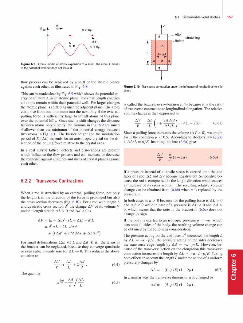
6.2 Deformable Solid Bodies 157
Chap
ter6
Figure 6.9 Atomic model of elastic expansion of a solid. The atom A movesin the potential well but does not leave it
flow process can be achieved by a shift of the atomic planesagainst each other, as illustrated in Fig. 6.8.
This can be made clear by Fig. 6.9 which shows the potential en-ergy of an atom A in an atomic plane. For small length changesall atoms remain within their potential well. For larger changesthe atomic plane is shifted against the adjacent plane. The atomcan move from one minimum into the next only if the externalpulling force is sufficiently large to lift all atoms of this planeover the potential hills. Since such a shift changes the distancebetween atoms only slightly, the minima in Fig. 6.9 are muchshallower than the minimum of the potential energy betweentwo atoms in Fig. 6.1. The barrier height and the modulationperiod of Ep.�L/ depends for an anisotropic crystal on the di-rection of the pulling force relative to the crystal axes.
In a real crystal lattice, defects and dislocations are presentwhich influence the flow process and can increase or decreasethe renitence against stretches and shifts of crystal planes againsteach other.
6.2.2 Transverse Contraction
When a rod is stretched by an external pulling force, not onlythe length L in the direction of the force is prolonged but alsothe cross section decreases (Fig. 6.10). For a rod with length Land quadratic cross section d2 the change �V of its volume Vunder a length stretch �L > 0 and �d < 0 is
�V D .d C�d/2 � .L C�L/ � d2L
D d2�L C 2L � d�d
C �L�d2 C 2d�d�L C�L�d2
�:
For small deformations (�L L and �d d), the terms inthe bracket can be neglected, because they converge quadraticor even cubic towards zero for�L ! 0. This reduces the aboveequation to
�V
V� �L
LC 2
�d
d: (6.4)
The quantity
DefD ��d
d
��L
L(6.5)
Figure 6.10 Transverse contraction under the influence of longitudinal tensilestress
is called the transverse contraction ratio because it is the ratioof transverse contraction to longitudinal elongation. The relativevolume change is then expressed as
�V
VD �L
L
�1 C 2�d=d
�L=L
�D " .1 � 2/ : (6.6a)
Since a pulling force increases the volume (�V > 0), we obtainfor the condition < 0:5. According to Hooke’s law (6.2a)is �L=L D �=E. Inserting this into (6.6a) gives
�V
VD �
E.1 � 2/ : (6.6b)
If a pressure instead of a tensile stress is exerted onto the endfaces of a rod,�L and�V become negative but�d positive be-cause the rod is compressed in the length direction which causesan increase of its cross section. The resulting relative volumechange can be obtained from (6.6b) when � is replaced by thepressure p.
In both cases is > 0 because for the pulling force is �L > 0and �d < 0 while in case of a pressure is �L < 0 and �d >0, which means that the ratio in the bracket in (6.6a) does notchange its sign.
If the body is exerted to an isotropic pressure p D �� , whichacts onto all sides of the body, the resulting volume change canbe obtained by the following consideration.
The pressure acting on the end faces d2 decreases the length Lby �L D �L � p=E, the pressure acting on the sides decreasesthe transverse edge length by �d D �d � p=E. However, be-cause of the transverse action on the elongation this transversecontraction increases the length by �L D C � L � p=E. Takingboth effects in account the length L under the action of a uniformpressure p changes by
�L D � .L � p=E/ .1 � 2/ : (6.7)
In a similar way the transverse dimension d is changed by
�d D � .d � p=E/ .1 � 2/ :
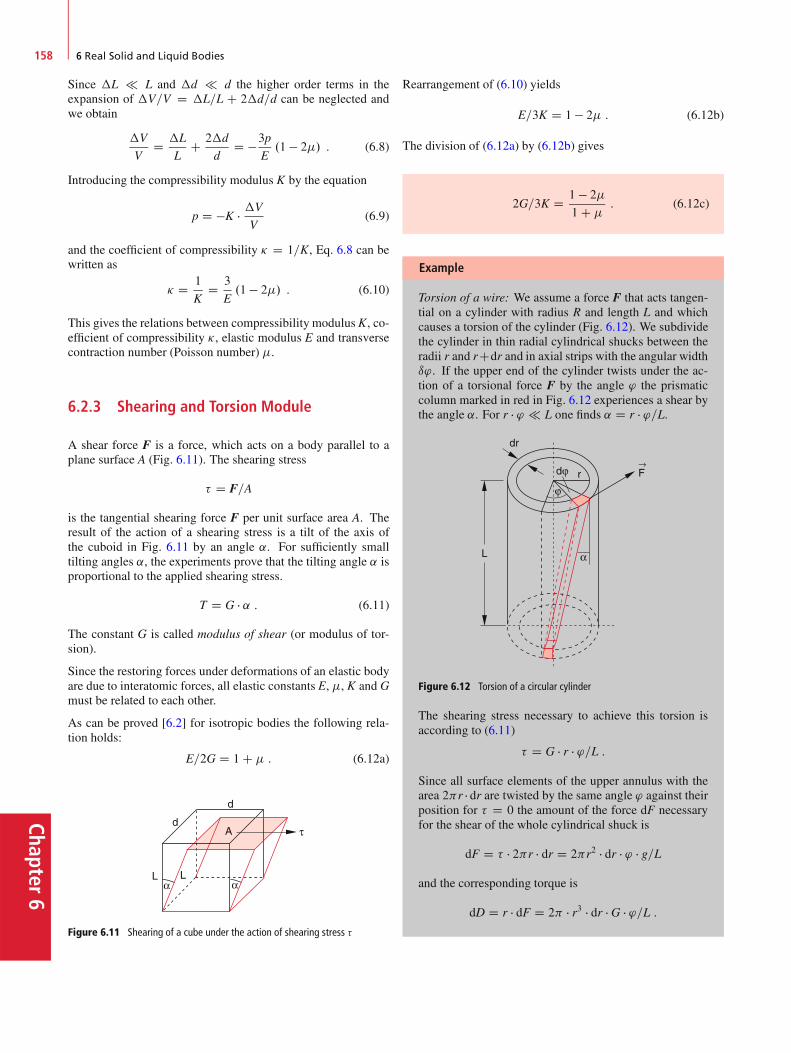
Chapter6
158 6 Real Solid and Liquid Bodies
Since �L L and �d d the higher order terms in theexpansion of �V=V D �L=L C 2�d=d can be neglected andwe obtain
�V
VD �L
LC 2�d
dD �3p
E.1 � 2/ : (6.8)
Introducing the compressibility modulus K by the equation
p D �K � �V
V(6.9)
and the coefficient of compressibility � D 1=K, Eq. 6.8 can bewritten as
� D 1
KD 3
E.1 � 2/ : (6.10)
This gives the relations between compressibility modulusK, co-efficient of compressibility �, elastic modulus E and transversecontraction number (Poisson number) .
6.2.3 Shearing and Torsion Module
A shear force F is a force, which acts on a body parallel to aplane surface A (Fig. 6.11). The shearing stress
� D F=A
is the tangential shearing force F per unit surface area A. Theresult of the action of a shearing stress is a tilt of the axis ofthe cuboid in Fig. 6.11 by an angle ˛. For sufficiently smalltilting angles ˛, the experiments prove that the tilting angle ˛ isproportional to the applied shearing stress.
T D G � ˛ : (6.11)
The constant G is called modulus of shear (or modulus of tor-sion).
Since the restoring forces under deformations of an elastic bodyare due to interatomic forces, all elastic constants E, , K and Gmust be related to each other.
As can be proved [6.2] for isotropic bodies the following rela-tion holds:
E=2G D 1 C : (6.12a)
Figure 6.11 Shearing of a cube under the action of shearing stress �
Rearrangement of (6.10) yields
E=3K D 1 � 2 : (6.12b)
The division of (6.12a) by (6.12b) gives
2G=3K D 1 � 2
1 C : (6.12c)
Example
Torsion of a wire: We assume a force F that acts tangen-tial on a cylinder with radius R and length L and whichcauses a torsion of the cylinder (Fig. 6.12). We subdividethe cylinder in thin radial cylindrical shucks between theradii r and rCdr and in axial strips with the angular widthı'. If the upper end of the cylinder twists under the ac-tion of a torsional force F by the angle ' the prismaticcolumn marked in red in Fig. 6.12 experiences a shear bythe angle ˛. For r � ' L one finds ˛ D r � '=L.
Figure 6.12 Torsion of a circular cylinder
The shearing stress necessary to achieve this torsion isaccording to (6.11)
� D G � r � '=L :
Since all surface elements of the upper annulus with thearea 2r � dr are twisted by the same angle ' against theirposition for � D 0 the amount of the force dF necessaryfor the shear of the whole cylindrical shuck is
dF D � � 2r � dr D 2r2 � dr � ' � g=L
and the corresponding torque is
dD D r � dF D 2 � r3 � dr � G � '=L :
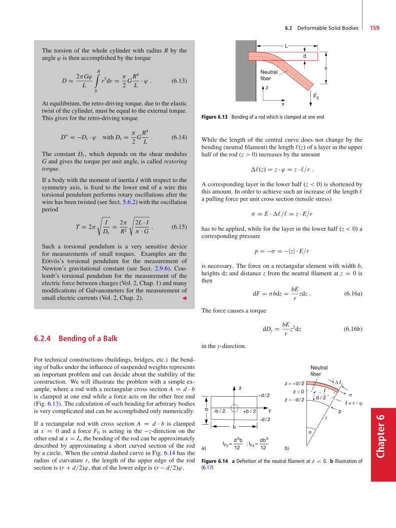
6.2 Deformable Solid Bodies 159
Chap
ter6
The torsion of the whole cylinder with radius R by theangle ' is then accomplished by the torque
D D 2G'
L
RZ
0
r3dr D
2GR4
L� ' : (6.13)
At equilibrium, the retro-driving torque, due to the elastictwist of the cylinder, must be equal to the external torque.This gives for the retro-driving torque
D� D �Dr � ' with Dr D
2GR4
L: (6.14)
The constant Dr, which depends on the shear modulusG and gives the torque per unit angle, is called restoringtorque.
If a body with the moment of inertia I with respect to thesymmetry axis, is fixed to the lower end of a wire thistorsional pendulum performs rotary oscillations after thewire has been twisted (see Sect. 5.6.2) with the oscillationperiod
T D 2
sI
DrD 2
R2
s2L � I � G : (6.15)
Such a torsional pendulum is a very sensitive devicefor measurements of small torques. Examples are theEötvös’s torsional pendulum for the measurement ofNewton’s gravitational constant (see Sect. 2.9.6), Cou-lomb’s torsional pendulum for the measurement of theelectric force between charges (Vol. 2, Chap. 1) and manymodifications of Galvanometers for the measurement ofsmall electric currents (Vol. 2, Chap. 2). J
6.2.4 Bending of a Balk
For technical constructions (buildings, bridges, etc.) the bend-ing of balks under the influence of suspended weights representsan important problem and can decide about the stability of theconstruction. We will illustrate the problem with a simple ex-ample, where a rod with a rectangular cross section A D d � bis clamped at one end while a force acts on the other free end(Fig. 6.13). The calculation of such bending for arbitrary bodiesis very complicated and can be accomplished only numerically.
If a rectangular rod with cross section A D d � b is clampedat x D 0 and a force F0 is acting in the �z-direction on theother end at x D L, the bending of the rod can be approximatelydescribed by approximating a short curved section of the rodby a circle. When the central dashed curve in Fig. 6.14 has theradius of curvature r, the length of the upper edge of the rodsection is .r C d=2/', that of the lower edge is .r � d=2/'.
Figure 6.13 Bending of a rod which is clamped at one end
While the length of the central curve does not change by thebending (neutral filament) the length `.z/ of a layer in the upperhalf of the rod (z > 0) increases by the amount
�`.z/ D z � ' D z � `=r :
A corresponding layer in the lower half .z < 0/ is shortened bythis amount. In order to achieve such an increase of the length `a pulling force per unit cross section (tensile stress)
� D E ��`=` D z � E=r
has to be applied, while for the layer in the lower half .z < 0/ acorresponding pressure
p D �� D �jzj � E=r
is necessary. The force on a rectangular element with width b,heights dz and distance z from the neutral filament at z D 0 isthen
dF D �bdz D bE
rzdz : (6.16a)
The force causes a torque
dDy D bE
rz2dz (6.16b)
in the y-direction.
Figure 6.14 a Definition of the neutral filament at z D 0. b Illustration of(6.17)
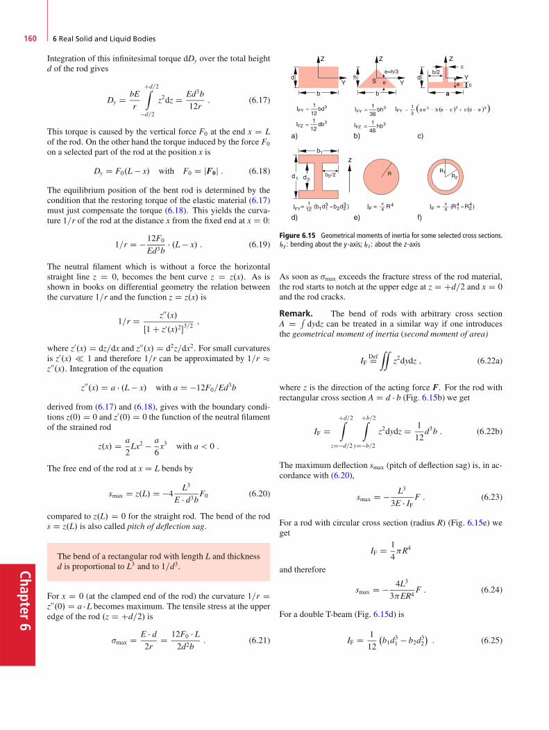
Chapter6
160 6 Real Solid and Liquid Bodies
Integration of this infinitesimal torque dDy over the total heightd of the rod gives
Dy D bE
r
Cd=2Z
�d=2
z2dz D Ed3b
12r: (6.17)
This torque is caused by the vertical force F0 at the end x D Lof the rod. On the other hand the torque induced by the force F0
on a selected part of the rod at the position x is
Dy D F0.L � x/ with F0 D jF0j : (6.18)
The equilibrium position of the bent rod is determined by thecondition that the restoring torque of the elastic material (6.17)must just compensate the torque (6.18). This yields the curva-ture 1=r of the rod at the distance x from the fixed end at x D 0:
1=r D �12F0
Ed3b� .L � x/ : (6.19)
The neutral filament which is without a force the horizontalstraight line z D 0, becomes the bent curve z D z.x/. As isshown in books on differential geometry the relation betweenthe curvature 1=r and the function z D z.x/ is
1=r D z00.x/
Œ1 C z0.x/2�3=2;
where z0.x/ D dz=dx and z00.x/ D d2z=dx2. For small curvaturesis z0.x/ 1 and therefore 1=r can be approximated by 1=r �z00.x/. Integration of the equation
z00.x/ D a � .L � x/ with a D �12F0=Ed3b
derived from (6.17) and (6.18), gives with the boundary condi-tions z.0/ D 0 and z0.0/ D 0 the function of the neutral filamentof the strained rod
z.x/ D a
2Lx2 � a
6x3 with a < 0 :
The free end of the rod at x D L bends by
smax D z.L/ D �4L3
E � d3bF0 (6.20)
compared to z.L/ D 0 for the straight rod. The bend of the rods D z.L/ is also called pitch of deflection sag.
The bend of a rectangular rod with length L and thicknessd is proportional to L3 and to 1=d3.
For x D 0 (at the clamped end of the rod) the curvature 1=r Dz00.0/ D a � L becomes maximum. The tensile stress at the upperedge of the rod .z D Cd=2/ is
�max D E � d2r
D 12F0 � L2d2b
: (6.21)
Figure 6.15 Geometrical moments of inertia for some selected cross sections.IFy : bending about the y-axis; IFz : about the z-axis
As soon as �max exceeds the fracture stress of the rod material,the rod starts to notch at the upper edge at z D Cd=2 and x D 0and the rod cracks.
Remark. The bend of rods with arbitrary cross sectionA D R
dydz can be treated in a similar way if one introducesthe geometrical moment of inertia (second moment of area)
IFDefD“
z2dydz ; (6.22a)
where z is the direction of the acting force F. For the rod withrectangular cross section A D d � b (Fig. 6.15b) we get
IF DCd=2Z
zD�d=2
Cb=2Z
yD�b=2
z2dydz D 1
12d3b : (6.22b)
The maximum deflection smax (pitch of deflection sag) is, in ac-cordance with (6.20),
smax D � L3
3E � IF F : (6.23)
For a rod with circular cross section (radius R) (Fig. 6.15e) weget
IF D 1
4R4
and therefore
smax D � 4L3
3ER4F : (6.24)
For a double T-beam (Fig. 6.15d) is
IF D 1
12
�b1d
31 � b2d
32
�: (6.25)
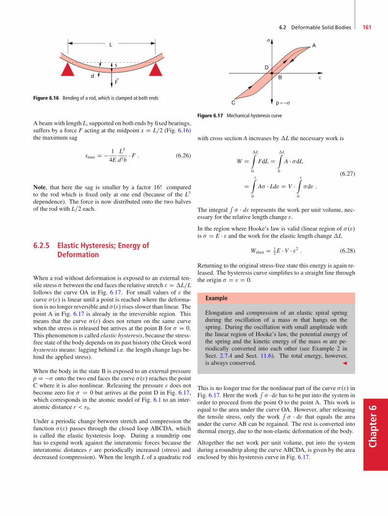
6.2 Deformable Solid Bodies 161
Chap
ter6
Figure 6.16 Bending of a rod, which is clamped at both ends
A beam with length L, supported on both ends by fixed bearings,suffers by a force F acting at the midpoint x D L=2 (Fig. 6.16)the maximum sag
smax D � 1
4E
L3
d3b� F : (6.26)
Note, that here the sag is smaller by a factor 16! comparedto the rod which is fixed only at one end (because of the L3
dependence). The force is now distributed onto the two halvesof the rod with L=2 each.
6.2.5 Elastic Hysteresis; Energy ofDeformation
When a rod without deformation is exposed to an external ten-sile stress � between the end faces the relative stretch " D �L=Lfollows the curve OA in Fig. 6.17. For small values of " thecurve �."/ is linear until a point is reached where the deforma-tion is no longer reversible and �."/ rises slower than linear. Thepoint A in Fig. 6.17 is already in the irreversible region. Thismeans that the curve �."/ does not return on the same curvewhen the stress is released but arrives at the point B for � D 0.This phenomenon is called elastic hysteresis, because the stress-free state of the body depends on its past history (the Greek wordhysteresis means: lagging behind i.e. the length change lags be-hind the applied stress).
When the body in the state B is exposed to an external pressurep D �� onto the two end faces the curve �."/ reaches the pointC where it is also nonlinear. Releasing the pressure " does notbecome zero for � D 0 but arrives at the point D in Fig. 6.17,which corresponds in the atomic model of Fig. 6.1 to an inter-atomic distance r < r0.
Under a periodic change between stretch and compression thefunction �."/ passes through the closed loop ABCDA, whichis called the elastic hysteresis loop. During a roundtrip onehas to expend work against the interatomic forces because theinteratomic distances r are periodically increased (stress) anddecreased (compression). When the length L of a quadratic rod
Figure 6.17 Mechanical hysteresis curve
with cross section A increases by �L the necessary work is
W D�LZ
0
FdL D�LZ
0
A � �dL
D"Z
0
A� � Ld" D V �"Z
0
�d" :
(6.27)
The integralR� � d" represents the work per unit volume, nec-
essary for the relative length change ".
In the region where Hooke’s law is valid (linear region of �."/is � D E � " and the work for the elastic length change�L
Welast D 12E � V � "2 : (6.28)
Returning to the original stress-free state this energy is again re-leased. The hysteresis curve simplifies to a straight line throughthe origin � D " D 0.
Example
Elongation and compression of an elastic spiral springduring the oscillation of a mass m that hangs on thespring. During the oscillation with small amplitude withthe linear region of Hooke’s law, the potential energy ofthe spring and the kinetic energy of the mass m are pe-riodically converted into each other (see Example 2 inSect. 2.7.4 and Sect. 11.6). The total energy, however,is always conserved. J
This is no longer true for the nonlinear part of the curve �."/ inFig. 6.17. Here the work
R� �d" has to be put into the system in
order to proceed from the point O to the point A. This work isequal to the area under the curve OA. However, after releasingthe tensile stress, only the work
R� � d" that equals the area
under the curve AB can be regained. The rest is converted intothermal energy, due to the non-elastic deformation of the body.
Altogether the net work per unit volume, put into the systemduring a roundtrip along the curve ABCDA, is given by the areaenclosed by this hysteresis curve in Fig. 6.17.

Chapter6
162 6 Real Solid and Liquid Bodies
Table 6.2 Hardness scale according to Mohs
Selected materialsas measurement standards
1. Tallow 6. Feldspar2. Gypsum 7. Quartz3. Calcite 8. Topaz4. Fluorite 9. Corundum5. Apatite 10. Diamond
ExamplesAluminium 2.3–2.9Lead 1.5Chromium 8Iron 3.5–4.5Graphite 1Tungsten 7
Figure 6.18 Hardness test according to Brinell
6.2.6 The Hardness of a Solid Body
The hardness of a body is a measure for the resistance, whichthe body sets against a penetration of another body. Dependingon the measuring technique, there are some slightly differenthardness values. The scratch-method introduced 1820 by Mohs,defines a body A as harder than a body B if it is possible toscratch B with A. The hardness scale of Mohr is based on thisdefinition. Here the hardness scale is divided into 10 degrees ofhardness based on 10 selected minerals, listed in Tab. 6.2.
The scratch method measures in fact mainly the hardness ofthe surface. This surface hardness is of particular importancefor technical applications, because the attrition of tools or ofaxes and bearings depends on the surface hardness. Therefore,several techniques have been developed for the enhancement ofthe surface hardness. One example is the transformation of thesurface layers of a crystalline solid into an amorphous state byirradiation with a powerful laser. Another example is the coverof solid tools, e.g. drills or steel mills, with a thin layer of a hardmaterial such as carbon-nitride NC or titanium Ti.
For measuring the hardness of a body, often a technique is usedwhich had been proposed by Brinell in 1900. Here a hardenedsteel ball with diameter D is pressed vertically with a constantforce F D a � D2 into the sample (Fig. 6.18). The diameter d ofthe resulting circular notch in the sample gives the penetrationdepth, which is a measure for the Brinell-hardness.
6.3 Static Liquids; Hydrostatics
In order to achieve a change of the shape of solid bodies sub-stantial forces are required, even if the volume of the body doesnot change (for example for a shear or a torsion). Although sim-ilarly large forces are necessary for a compression of liquids,a mere deformation of liquids at constant volume requires only
very small forces and are merely caused by friction or surfaceeffects.
At first we will discuss the simplified model of an ideal liquid,where surface effects and friction are neglected. For the staticcase of a liquid at rest, friction does not occur anyway. Surfaceeffects will be treated in Sect. 6.4 and the influence of frictionfor streaming liquids is discussed in Chap. 8.
6.3.1 Free Displacement and Surfaces ofLiquids
For ideal liquids without friction, there is no force necessary todeform a given liquid volume. In the atomic model this means:While in solid bodies the atoms can vibrate around fixed equi-librium positions, which do not change much under moderateexternal forces, the atoms or molecules in liquids can freelymove around within the given liquid volume, determined by thesolid container (Fig. 6.5). In the macroscopic model this freemovement can be expressed by the statement:
The shear modulus of an ideal liquid is zero.
This implies that at the surface of an ideal liquid no tangentialforces can be present, because they would immediately deformthe liquid until the forces disappear and a minimum energy isachieved. This force-free condition represents a stable state ofthe liquid.
The surface of an ideal liquid is always perpendicular to the totalexternal force.
Examples
1. If only gravity acts onto a liquid, the surface of theliquid forms always a horizontal plane (Fig. 6.19a)
2. The surface of a liquid in a cylinder which rotatesabout a vertical axis (Fig. 6.19b) forms a surfacewhere the total force composed of gravity m � g in the�z-direction and centrifugal force m!2 � r in the ra-dial direction points perpendicular to the surface. Theslope of the intersection curve z.r/ of the surface at thepoint A in Fig. 6.19b is
tan˛ D m!2r
m � g D !2r
g:
On the other hand the slope of the curve z.r/ is givenby tan˛ D dz=dr. Integration yields
z.r/ D !2
g
Zrdr D !2
2gr2 C C :

6.3 Static Liquids; Hydrostatics 163
Chap
ter6
For z.0/ D z0 is C D z0 and we get
z.r/ D !2
2gr2 C z0 : (6.29)
The surface forms a rotational paraboloid with its axiscoincident with the rotation axis.
Figure 6.19 a Horizontal liquid surface in a container at rest. b Sur-face as rotational paraboloid in a rotating container J
6.3.2 Static Pressure in a Liquid
Any external force acts only vertically on the surface of a liq-uid. If a container with a liquid is closed by a movable pistonwith surface A, onto which a vertical force F acts (Fig. 6.20) wedefine the pressure onto the liquid as
p D F=A; with F D jFj :
6.3.2.1 Forces onto a Liquid Volume Element
We consider an arbitrary cuboid volume element dV D dx�dy�dzinside the liquid (Fig. 6.21). We assume that a pressure p actsin x-direction onto the left side dy � dz of the cuboid. Then apressure
p C @p=@x � dxacts onto the opposite side. The resulting force on the volumeelement is then
Fx D p � dydz ��p C @p
@xdx
�dydz D �@p
@xdV :
Figure 6.20 The force F , acting on a piston with area A generates a pressurep D F=A in the liquid
Figure 6.21 Relation between the pressure inside a volume element dV andthe forces acting onto the sides of dV
In an analogousway we obtain the force components in the otherdirections
Fy D �@p@y
dV and Fz D �@p@z
dV :
We can condense these three equations into the vector equation
F D �grad p � dV : (6.30)
Because of the free mobility of any volume element inside theliquid the total force onto a volume element at rest must be zero.This implies that grad p D 0.
The pressure inside the whole liquid is constant as long asno unisotropic forces act onto the liquid.
For a static liquid the same pressure acts onto all surface ele-ments of the container!
This can be experimentally demonstrated by the simple deviceshown in Fig. 6.22. A spherical container with small holes inseveral directions of the x-y-plane is filled with dyed water andplaced above a blotting paper in the plane z D 0. When a piston
Figure 6.22 Demonstration of the isotropic pressure in a liquid. When thepiston is moved the pressure p increases and the dyed water splashes throughholes onto a white paper below the device, where the spots form a circle aroundthe center, indication equal pressure

Chapter6
164 6 Real Solid and Liquid Bodies
Figure 6.23 Hydraulic press (forces are drawn not to scale)
is pressed to increase the pressure the water streams out of theholes and all water filaments follow projectile trajectories. Theirpoints of impact on the blotting paper in the plane z D 0 forma circle which proves that they all had the same initial velocity,i.e. they stream out driven by the same pressure.
Application: Hydraulic press (Fig. 6.23)Two cylinders with cross sections A1 and A2 � A1 that are con-nected with each other, and are therefore at the same pressurep, are filled with a liquid. Applying the force F1 D p � A1 ona piston in the narrow cylinder causes a force F2 D pA2 D.A2=A1/ �F1 � F1 acting on a piston in the large cylinder whichpresses a sample against a fixed mounting. For demonstrationexperiments, large stones can be cracked by this device. Fora displacement �x2 of the large piston, the small piston has tomove by the much larger amount�x1 D .A2=A1/ ��x1, becausethe volume�V2 D A2 ��x2 D �V1 D A1 ��x1 transferred fromthe small to the large cylinder must be of course equal.
6.3.2.2 Hydrostatic Pressure
Taking into account that every volume element �V of a liquidhas a weight % �g ��V in the gravity field of the earth, even with-out external force a pressure onto the bottom of the container ispresent due to the weight of the liquid above the bottom. For aheight z D H of the liquid the hydrostatic pressure at the bottomwith area A is with dV D A � dz
p.z D 0/ DHZ
0
% � g � AA
dz D % � g � H ; (6.31)
if we assume that the density % is independent of the pressure p.
For real liquids, there is a small change of % with the pressure p.A measure for this dependence is the compressibility
�DefD � 1
V
@V
@p; (6.32)
which describes the relative volume change�V=V for a change�p of the pressure.
For liquids � is very small (for example for water is � D5 � 10�10 m2=N/. This shows that the density % of a liquidchanges only by a tiny amount with pressure and in most casesthe density %.p/ D %0 can be assumed to be constant.
Figure 6.24 Pressure p.z/ in an incompressible liquid in the gravity field ofthe earth, as a function of height z above ground
Then it follows from (6.31) for the pressure p.z/ in a liquid withtotal heights H (Fig. 6.24)
p.z/ D % � g � .H � z/ :
The SI unit for the pressure is 1 Pascal D 1 Pa D 1N=m2, whichcorresponds to 10�5 bar.
Examples
1. A water column of 10m heights causes a hydrostaticpressure of p D % �g �h D 9:81 �104 Pa D 0:981 bar D1 atmosphere. At an ocean depth of 10:000m (Philip-pine rift) the hydrostatic pressure is � 108 Pa (about1000 atm). The total force onto the outer surface of ahollow steel sphere of an aquanaut with 3m diameteris at this depth F D 2:8 � 109 N.
Figure 6.25 a Water pressure acting onto a dam wall; b Additionalsupport by the mountain walls for a curved dam wall
2. The total force F onto the river dam with length Lcaused by the water with heights H can be obtainedby integration over all contributions F.z/dz onto thesurface elements L � dz of the dam.
F D LZ
p.z/dz D % � g � LZ.H � z/dz
D 12% � g � L � H2
This force can be partly supported by choosing acurved dam where part of the force are balanced bythe mountain walls (Fig. 6.25b). The thickness of thedam decreases with z in order to take into account thedecreasing hydrostatic pressure (Fig. 6.25a). J
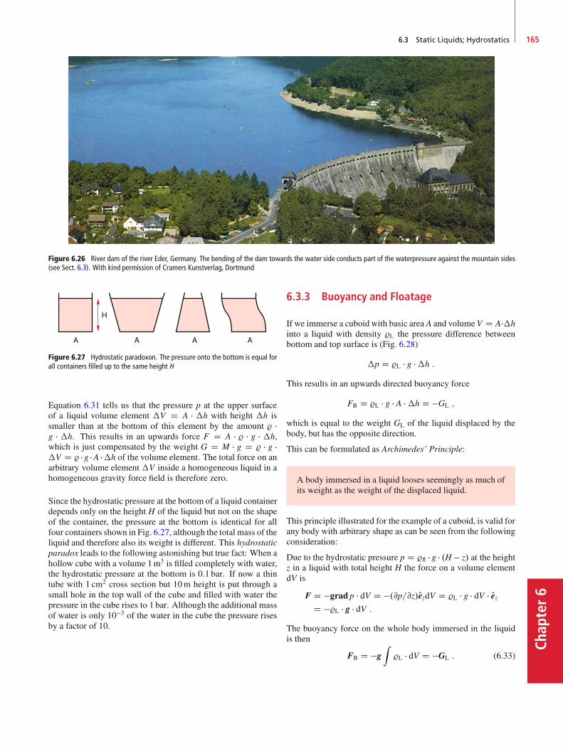
6.3 Static Liquids; Hydrostatics 165
Chap
ter6
Figure 6.26 River dam of the river Eder, Germany. The bending of the dam towards the water side conducts part of the waterpressure against the mountain sides(see Sect. 6.3). With kind permission of Cramers Kunstverlag, Dortmund
Figure 6.27 Hydrostatic paradoxon. The pressure onto the bottom is equal forall containers filled up to the same height H
Equation 6.31 tells us that the pressure p at the upper surfaceof a liquid volume element �V D A � �h with height �h issmaller than at the bottom of this element by the amount % �g � �h. This results in an upwards force F D A � % � g � �h,which is just compensated by the weight G D M � g D % � g ��V D % � g �A ��h of the volume element. The total force on anarbitrary volume element �V inside a homogeneous liquid in ahomogeneous gravity force field is therefore zero.
Since the hydrostatic pressure at the bottom of a liquid containerdepends only on the height H of the liquid but not on the shapeof the container, the pressure at the bottom is identical for allfour containers shown in Fig. 6.27, although the total mass of theliquid and therefore also its weight is different. This hydrostaticparadox leads to the following astonishing but true fact: When ahollow cube with a volume 1m3 is filled completely with water,the hydrostatic pressure at the bottom is 0:1 bar. If now a thintube with 1 cm2 cross section but 10m height is put through asmall hole in the top wall of the cube and filled with water thepressure in the cube rises to 1 bar. Although the additional massof water is only 10�3 of the water in the cube the pressure risesby a factor of 10.
6.3.3 Buoyancy and Floatage
If we immerse a cuboid with basic area A and volumeV D A��hinto a liquid with density %L the pressure difference betweenbottom and top surface is (Fig. 6.28)
�p D %L � g ��h :
This results in an upwards directed buoyancy force
FB D %L � g � A ��h D �GL ;
which is equal to the weight GL of the liquid displaced by thebody, but has the opposite direction.
This can be formulated as Archimedes’ Principle:
A body immersed in a liquid looses seemingly as much ofits weight as the weight of the displaced liquid.
This principle illustrated for the example of a cuboid, is valid forany body with arbitrary shape as can be seen from the followingconsideration:
Due to the hydrostatic pressure p D %fl � g � .H � z/ at the heightz in a liquid with total height H the force on a volume elementdV is
F D �grad p � dV D �.@p=@z/OezdV D %L � g � dV � OezD �%L � g � dV :
The buoyancy force on the whole body immersed in the liquidis then
FB D �gZ%L � dV D �GL : (6.33)
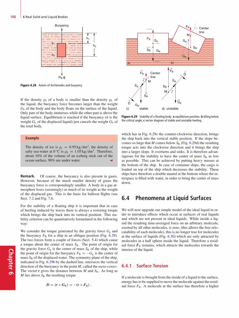
Chapter6
166 6 Real Solid and Liquid Bodies
Buoyancy
p1
p2
h1
h2
Figure 6.28 Axiom of Archimedes and buoyancy
If the density %b of a body is smaller than the density %L ofthe liquid, the buoyancy force becomes larger than the weightGb of the body and the body floats on the surface of the liquid.Only part of the body immerses while the other part is above theliquid surface. Equilibrium is reached if the buoyancy (it is theweight GL of the displaced liquid) just cancels the weight Gb ofthe total body.
Example
The density of ice is %i D 0:95 kg=dm3, the density ofsalty sea-water at 0 ıC is %L D 1:05 kg=dm3. Therefore,about 10% of the volume of an iceberg stick out of theocean surface, 90% are under water. J
Remark. Of course, the buoyancy is also present in gases.However, because of the much smaller density of gases thebuoyancy force is correspondingly smaller. A body in a gas at-mosphere loses (seemingly) as much of its weight as the weightof the displaced gas. This is the basis for balloon flights (seeSect. 7.2 and Fig. 7.6.
For the stability of a floating ship it is important that in caseof heeling induced by waves there is always a restoring torquewhich brings the ship back into its vertical position. This sta-bility criterion can be quantitatively formulated in the followingway:
We consider the torque generated by the gravity force Gg andthe buoyancy FB for a ship in an oblique position (Fig. 6.29).The two forces form a couple of forces (Sect. 5.4) which causea torque about the center of mass SK. The point of origin forthe gravity force Gg is the center of mass SK of the ship, whilethe point of origin for the buoyancy FB D �Gg is the center ofmass SB of the displaced water. The symmetry plane of the ship,indicated in Fig. 6.29b by the dashed line, intersects the verticaldirection of the buoyancy in the pointM, called themeta-center.The vector r gives the distance between M and SK. As long asM lies above SK the resulting torque
D D .r GK/ D �.r FB/ ;
FB
FBFB
D
d)
FB
SBSB
SB
SB
D
Figure 6.29 Stability of a floating body. a equilibrium position, b tilting belowthe critical angle, c vector diagram of stable and unstable heeling
which has in Fig. 6.29c the counter-clockwise direction, bringsthe ship back into the vertical stable position. If the slope be-comes so large thatM comes below SK (Fig. 6.29d) the resultingtorque acts into the clockwise direction and it brings the shipinto a larger slope. It overturns and sinks. It is therefore advan-tageous for the stability to have the center of mass SK as lowas possible. This can be achieved by putting heavy masses atthe bottom of the ship. In case of container ships, the cargo isloaded on top of the ship which decreases the stability. Theseships have therefore a double mantel at the bottom where the in-terspace is filled with water, in order to bring the center of massdown.
6.4 Phenomena at Liquid Surfaces
We will now upgrade our simple model of the ideal liquid in or-der to introduce effects which occur at surfaces of real liquidsand which are not present in ideal liquids. While inside a liq-uid the resulting time-averaged force on an arbitrary molecule,exerted by all other molecules, is zero, (this allows the free relo-catability of each molecule), this is no longer true for moleculesat the surface of liquids (Fig. 6.30) which are only attracted bymolecules in a half sphere inside the liquid. Therefore a resid-ual force FR remains, which attracts the molecules towards theinterior of the liquid.
6.4.1 Surface Tension
If a molecule is brought from the inside of a liquid to the surface,energy has to be supplied to move the molecule against the resid-ual force FR. A molecule at the surface has therefore a higher

6.4 Phenomena at Liquid Surfaces 167
Chap
ter6
Figure 6.30 Resulting force on a molecule by all other surrounding moleculesinside a liquid and at the surface of a liquid
Figure 6.31 Determination of surface tension by measuring the force on asliding straight wire, that extends a liquid skin
energy than a molecule inside the liquid. In order to enlarge thesurface by an amount �A molecules have to be transferred tothe surface which needs the energy�W . The ratio
" D �W
�AI Œ"� D J
m2(6.34)
is the specific surface energy. The value of " depends on thebinding forces between the molecules of the liquid. It can bemeasured with the equipment shown in Fig. 6.31. Between thetwo sides of a U-shaped frame a horizontal wire with lengthL can be shifted vertically. When the system is dipped into aliquid, a liquid lamella is formed with the surface area (on bothsides) A D 2L � s. For moving the horizontal wire by �s, theforce F is necessary. One has to supply the energy
�W D F ��s D " ��A D " � 2 � L ��s : (6.35)
The restoring force F, which is directed tangential to the surfaceof the lamella, produces a tensile strain � D F=2L per lengthunit which is called surface tension. According to (6.35) is
� D " :
Surface tension � and specific surface energy " are identi-cal.
The surface tension can be impressively demonstrated by the ap-paratus shown in Fig. 6.32. A metal strip bent into a circle hangs
Figure 6.32 Measurement of surface tension by liftig an immersed metal ring
on a spring balance. It is immersed into a glass container filledwith a liquid. When the container is lowered or the metal ring isuplifted, the lower rim of the ring emerges more and more outof the liquid, carrying a cylindrical liquid lamella. With soapywater more than 10 cm heights of the lamella can be reached.The spring balance measures the force
F D 4 � r � � ;because the lamella has two surfaces, inside and outside of thecylindrical membrane. The work necessary to lift the lamella upto the height h is
W D 4 � r � � � h :
Example
Surface tension and pressure in a soap bubble (Fig. 6.33).Because of its surface tension, the bubble tries to reduceits surface. This increases the pressure inside the bubble.Equilibrium is reached, if the work against the increas-ing pressure during the decrease �r of the bubble radiusis equal to the work gained by the reduction �A of thesurface area A
" � 2 � 4.r2 � .r ��r/2/ D 4 � r2 ��p :
Manometer
Figure 6.33 Measurement of overpressure �p in a soap bubble,caused by surface tension
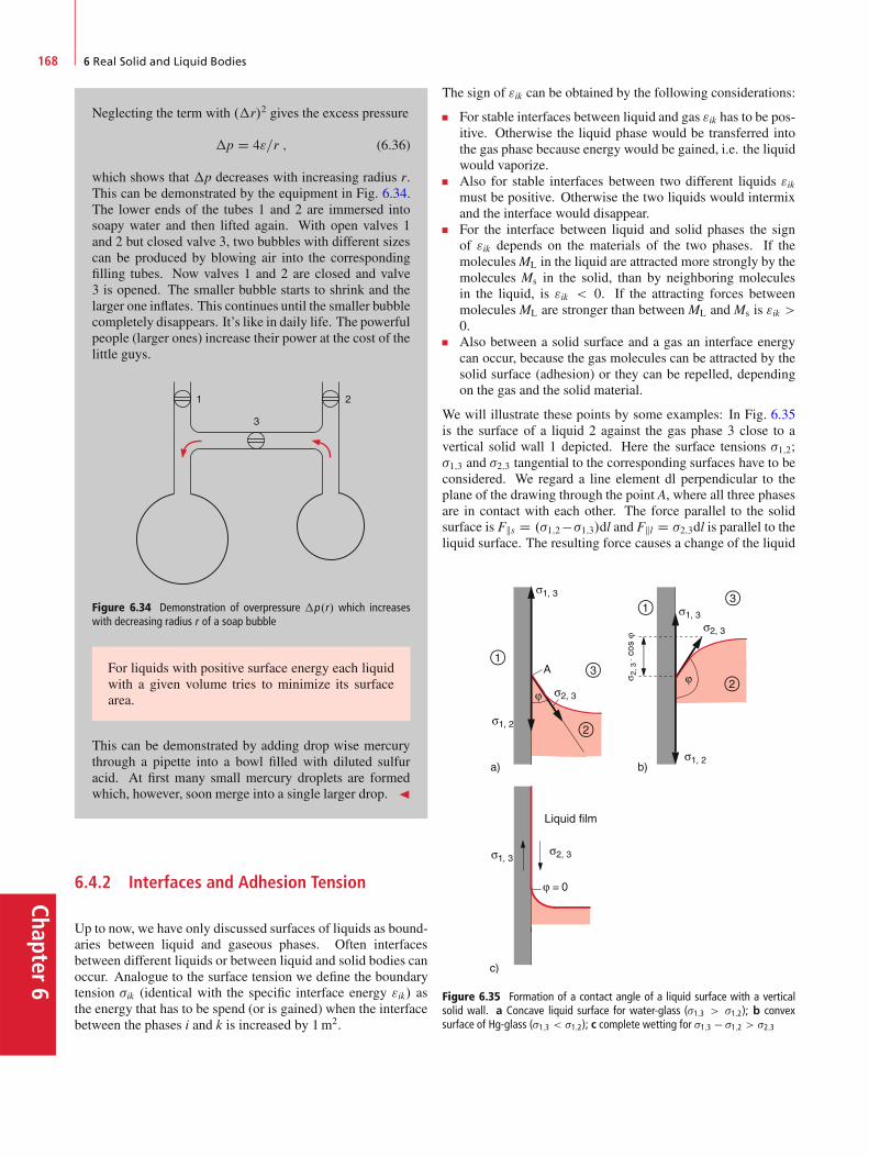
Chapter6
168 6 Real Solid and Liquid Bodies
Neglecting the term with .�r/2 gives the excess pressure
�p D 4"=r ; (6.36)
which shows that �p decreases with increasing radius r.This can be demonstrated by the equipment in Fig. 6.34.The lower ends of the tubes 1 and 2 are immersed intosoapy water and then lifted again. With open valves 1and 2 but closed valve 3, two bubbles with different sizescan be produced by blowing air into the correspondingfilling tubes. Now valves 1 and 2 are closed and valve3 is opened. The smaller bubble starts to shrink and thelarger one inflates. This continues until the smaller bubblecompletely disappears. It’s like in daily life. The powerfulpeople (larger ones) increase their power at the cost of thelittle guys.
21
3
Figure 6.34 Demonstration of overpressure �p.r/ which increaseswith decreasing radius r of a soap bubble
For liquids with positive surface energy each liquidwith a given volume tries to minimize its surfacearea.
This can be demonstrated by adding drop wise mercurythrough a pipette into a bowl filled with diluted sulfuracid. At first many small mercury droplets are formedwhich, however, soon merge into a single larger drop. J
6.4.2 Interfaces and Adhesion Tension
Up to now, we have only discussed surfaces of liquids as bound-aries between liquid and gaseous phases. Often interfacesbetween different liquids or between liquid and solid bodies canoccur. Analogue to the surface tension we define the boundarytension �ik (identical with the specific interface energy "ik/ asthe energy that has to be spend (or is gained) when the interfacebetween the phases i and k is increased by 1m2.
The sign of "ik can be obtained by the following considerations:
For stable interfaces between liquid and gas "ik has to be pos-itive. Otherwise the liquid phase would be transferred intothe gas phase because energy would be gained, i.e. the liquidwould vaporize.Also for stable interfaces between two different liquids "ikmust be positive. Otherwise the two liquids would intermixand the interface would disappear.For the interface between liquid and solid phases the signof "ik depends on the materials of the two phases. If themoleculesML in the liquid are attracted more strongly by themolecules Ms in the solid, than by neighboring moleculesin the liquid, is "ik < 0. If the attracting forces betweenmolecules ML are stronger than between ML and Ms is "ik >0.Also between a solid surface and a gas an interface energycan occur, because the gas molecules can be attracted by thesolid surface (adhesion) or they can be repelled, dependingon the gas and the solid material.
We will illustrate these points by some examples: In Fig. 6.35is the surface of a liquid 2 against the gas phase 3 close to avertical solid wall 1 depicted. Here the surface tensions �1;2;�1;3 and �2;3 tangential to the corresponding surfaces have to beconsidered. We regard a line element dl perpendicular to theplane of the drawing through the point A, where all three phasesare in contact with each other. The force parallel to the solidsurface is Fks D .�1;2��1;3/dl and Fkl D �2;3dl is parallel to theliquid surface. The resulting force causes a change of the liquid
Liquid film
Figure 6.35 Formation of a contact angle of a liquid surface with a verticalsolid wall. a Concave liquid surface for water-glass (�1;3 > �1;2); b convexsurface of Hg-glass (�1;3 < �1;2); c complete wetting for �1;3 � �1;2 > �2;3
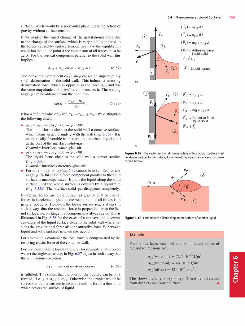
6.4 Phenomena at Liquid Surfaces 169
Chap
ter6
surface, which would be a horizontal plane under the action ofgravity without surface tension.
If we neglect the small change of the gravitational force dueto the change of the surface, which is very small compared tothe forces caused by surface tension, we have the equilibriumcondition that in the point A the vector sum of all forces must bezero. For the vertical component parallel to the solid wall thisimplies:
�1;2 C �2;3 cos' � �1;3 D 0 : (6.37)
The horizontal component �2;3 � sin' causes an imperceptiblysmall deformation of the solid wall. This induces a restoringdeformation force which is opposite to the force �2;3 and hasthe same magnitude and therefore compensates it. The wettingangle ' can be obtained from the condition
cos' D �1;3 � �1;2�2;3
: (6.37a)
It has a definite value only for j�1;3��1;2j � �2;3. We distinguishthe following cases:
�1;3 > �1;2 ! cos' > 0 ! ' < 90ı.The liquid forms close to the solid wall a concave surface,which forms an acute angle ' with the wall (Fig. 6.35a). It isenergetically favorable to increase the interface liquid-solidat the cost of the interface solid–gas.Example: Interfaces water–glas–air.�1:3 < �1;2 ! cos' < 0 ! ' > 90ı.The liquid forms close to the solid wall a convex surface(Fig. 6.35b).Example: interfaces mercury–glas–air.For j�1;3 � �1;2j > �2;3 Eq. 6.37 cannot been fulfilled for anyangle '. In this case a force component parallel to the solidsurface is uncompensated. It pulls the liquid along the solidsurface until the whole surface is covered by a liquid film(Fig. 6.35c). The interface solid–gas disappears completely.
If external forces are present, such as gravitational or inertialforces in accelerated systems, the vector sum of all forces is ingeneral not zero. However, the liquid surface reacts always insuch a way, that the resultant force is perpendicular to the liq-uid surface, i.e. its tangential component is always zero. This isillustrated in Fig. 6.36 for the cases of a concave and a convexcurvature of the liquid surface close to the solid wall where be-sides the gravitational force also the attractive force F4 betweenliquid and solid surfaces is taken into account.
For a liquid in a container the total force is compensated by therestoring elastic force of the container wall.
For two non-mixable liquids 1 and 2 (for example a fat drop onwater) the angles '1 and '2 in Fig. 6.37 adjust in such a way thatthe equilibrium condition
�1;3 D �2;3 cos'2 C �1;2 cos'1 (6.38)
is fulfilled. This shows that a droplet of the liquid 2 can be onlyformed, if �1;3 < �2;3 C �1;2. Otherwise the droplet would bespread out by the surface tension �1;3 until it forms a thin film,which covers the surface of liquid 1.
Figure 6.36 The vector sum of all forces acting onto a liquid sureface mustbe always vertical to the surface, for non-wetting liquids. a Concave, b convexcurved surface
Figure 6.37 Formation of a liquid drop on the surface of another liquid
Example
For the interfaces water–oil–air the numerical values ofthe surface tensions are:
�1:3(water-air) D 72:5 � 10�3 J=m2
�1;2(water-oil) D 46 � 10�3 J=m2
�2;3(oil-air) D 32 � 10�3 J=m2 :
This shows that �1;3 > �2;3 C �1;2. Therefore, oil cannotform droplets on a water surface. J
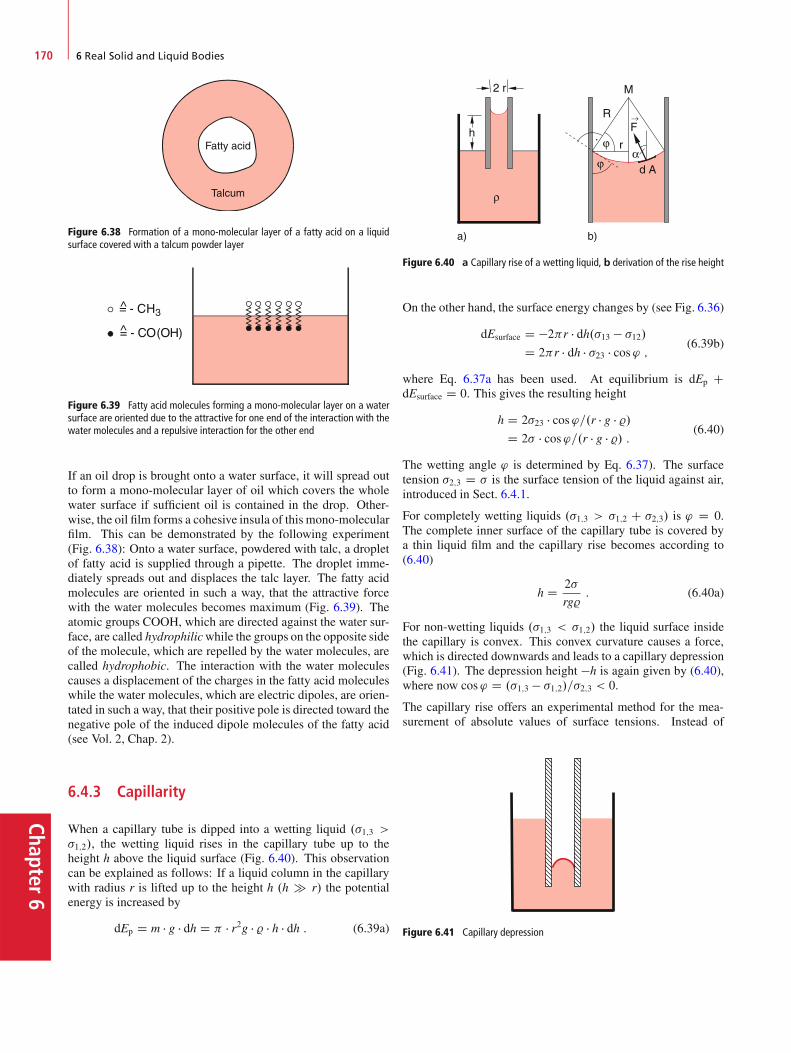
Chapter6
170 6 Real Solid and Liquid Bodies
Fatty acid
Talcum
Figure 6.38 Formation of a mono-molecular layer of a fatty acid on a liquidsurface covered with a talcum powder layer
Figure 6.39 Fatty acid molecules forming a mono-molecular layer on a watersurface are oriented due to the attractive for one end of the interaction with thewater molecules and a repulsive interaction for the other end
If an oil drop is brought onto a water surface, it will spread outto form a mono-molecular layer of oil which covers the wholewater surface if sufficient oil is contained in the drop. Other-wise, the oil film forms a cohesive insula of this mono-molecularfilm. This can be demonstrated by the following experiment(Fig. 6.38): Onto a water surface, powdered with talc, a dropletof fatty acid is supplied through a pipette. The droplet imme-diately spreads out and displaces the talc layer. The fatty acidmolecules are oriented in such a way, that the attractive forcewith the water molecules becomes maximum (Fig. 6.39). Theatomic groups COOH, which are directed against the water sur-face, are called hydrophilicwhile the groups on the opposite sideof the molecule, which are repelled by the water molecules, arecalled hydrophobic. The interaction with the water moleculescauses a displacement of the charges in the fatty acid moleculeswhile the water molecules, which are electric dipoles, are orien-tated in such a way, that their positive pole is directed toward thenegative pole of the induced dipole molecules of the fatty acid(see Vol. 2, Chap. 2).
6.4.3 Capillarity
When a capillary tube is dipped into a wetting liquid .�1;3 >�1;2/, the wetting liquid rises in the capillary tube up to theheight h above the liquid surface (Fig. 6.40). This observationcan be explained as follows: If a liquid column in the capillarywith radius r is lifted up to the height h .h � r/ the potentialenergy is increased by
dEp D m � g � dh D � r2g � % � h � dh : (6.39a)
Figure 6.40 a Capillary rise of a wetting liquid, b derivation of the rise height
On the other hand, the surface energy changes by (see Fig. 6.36)
dEsurface D �2r � dh.�13 � �12/D 2r � dh � �23 � cos' ; (6.39b)
where Eq. 6.37a has been used. At equilibrium is dEp CdEsurface D 0. This gives the resulting height
h D 2�23 � cos'=.r � g � %/D 2� � cos'=.r � g � %/ : (6.40)
The wetting angle ' is determined by Eq. 6.37). The surfacetension �2;3 D � is the surface tension of the liquid against air,introduced in Sect. 6.4.1.
For completely wetting liquids .�1;3 > �1;2 C �2;3/ is ' D 0.The complete inner surface of the capillary tube is covered bya thin liquid film and the capillary rise becomes according to(6.40)
h D 2�
rg%: (6.40a)
For non-wetting liquids .�1;3 < �1;2/ the liquid surface insidethe capillary is convex. This convex curvature causes a force,which is directed downwards and leads to a capillary depression(Fig. 6.41). The depression height �h is again given by (6.40),where now cos' D .�1;3 � �1;2/=�2;3 < 0.
The capillary rise offers an experimental method for the mea-surement of absolute values of surface tensions. Instead of
Figure 6.41 Capillary depression
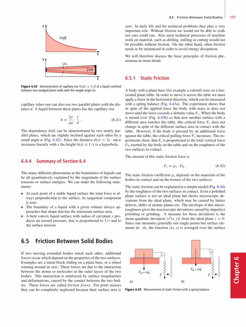
6.5 Friction Between Solid Bodies 171
Chap
ter6
Figure 6.42 Demonstration of capillary rise h .d / / 1=d of a liquid confinedbetween two wedged plane walls with the wegde angle 2˛
capillary tubes one can also use two parallel plates with the dis-tance d. A liquid between these plates has the capillary rise
h D 2�
%g� 1d: (6.41)
The dependence h.d/ can be demonstrated by two nearly par-allel plates, which are slightly inclined against each other by asmall angle ˛ (Fig. 6.42). Since the distance d.x/ D 2x � tan˛increases linearly with x the height h.x/ / 1=x is a hyperbola.
6.4.4 Summary of Section 6.4
The many different phenomena at the boundaries of liquids canbe all quantitatively explained by the magnitude of the surfacetensions or surface energies. We can make the following state-ments:
At each point of a stable liquid surface the total force is al-ways perpendicular to the surface, its tangential componentis zero.The boundary of a liquid with a given volume always ap-proaches that shape that has the minimum surface area.A bent convex liquid surface with radius of curvature r pro-duces an inward pressure, that is proportional to 1=r and tothe surface tension.
6.5 Friction Between Solid Bodies
If two moving extended bodies touch each other, additionalforces occur which depend on the properties of the two surfaces.Examples are a metal block sliding on a plane base, or a wheelrotating around an axis. These forces are due to the interactionbetween the atoms or molecules in the outer layers of the twobodies. This interaction is reinforced by surface irregularitiesand deformations, caused by the contact between the two bod-ies. These forces are called friction forces. For point massesthey can be completely neglected because their surface area is
zero. In daily life and for technical problems they play a veryimportant role. Without friction we would not be able to walknor cars could run. Also most technical processes of machinework on material, such as drilling, milling or cutting would notbe possible without friction. On the other hand, often frictionneeds to be minimized in order to avoid energy dissipation.
We will therefore discuss the basic principles of friction phe-nomena in more detail.
6.5.1 Static Friction
A body with a plane base (for example a cuboid) rests on a hor-izontal plane table. In order to move it across the table we mustapply a force in the horizontal direction, which can be measuredwith a spring balance (Fig. 6.43a). The experiment shows thatin spite of the applied force the body with mass m does notmove until the force exceeds a definite value Fs. When the bodyis turned over (Fig. 6.43b) so that now another surface with adifferent area touches the table, this critical force Fs does notchange in spite of the different surface area in contact with thetable. However, if the body is pressed by an additional forceagainst the table, the critical pulling force Fs increases. The ex-periments show, that Fs is proportional to the total vertical forceFN exerted by the body on the table and on the roughness of thetwo surfaces in contact.
The amount of this static friction force is
Fs D s � FN : (6.42)
The static friction coefficient s depends on the materials of thebodies in contact and on the texture of the two surfaces.
The static friction can be explained in a simple model (Fig. 6.44)by the roughness of the two surfaces in contact. Even a polishedplane surface is not an ideal plane but shows microscopic de-viations from the ideal plane, which may be caused by latticedefects, shifts of atomic planes etc. The envelope of this micro-roughness gives the macroscopic deviations caused by imperfectpolishing or grinding. A measure for these deviations is themean quadratic deviation hz2.x; y/i from the ideal plane z D 0.Since one measures generally not single points but surface ele-ments dx � dy, the function z.x; y/ is averaged over the surface
Figure 6.43 Measurement of static friction with a spring balance

Chapter6
172 6 Real Solid and Liquid Bodies
Figure 6.44 Schematic model of the surface roughness as the cause of friction.a micro roughness (exagerated) and macroscopic coarseness; b static frictioncaused by interlocking of two rough surfaces
elements dx � dy and this average depends on the spatial resolu-tion of the analyzing instrument i.e. on the size of the resolvedelements dx � dy. With modern surface analysis, using tunnel-microscopes (see Vol. 3) even the roughness on an atomic scalecan be spatially resolved.
The two surfaces in contact interlock each other due to the forcethat presses them together (Fig. 6.44b) and the force Fs is nec-essary to release this interlocking. This can be achieved bybreaking away the “hills” of the rough surface, or by lifting thebody over these hills.
A possible way to determine experimentally the coefficient ofstatic friction uses the inclined plane with a variable inclinationangle ˛ in Fig. 6.45. The angle ˛ is continuously increased untilthe body B with mass m starts to slide down for ˛ D ˛max.
The weight force G D m � g can be decomposed into two com-ponents:
1. A component Fk D m � g � sin˛ parallel to the inclined plane
Figure 6.45 Measurement of coefficient of static friction with the inclinedplane
2. A component F? D m �g �cos˛ perpendicular to the inclinedplane, which is compensated by the opposite restoring forceof the elastic deformation of the plane.
The body starts to slide downwards as soon as Fk becomes largerthan the static friction force Fs D s � F? D s � m � g � cos˛.This gives the condition for the coefficient s
s D Fk.˛max/
F?.˛max/D tan˛max : (6.43)
If ˛ is increased beyond ˛max the body performs an acceleratedsliding motion. This indicates that the sliding friction force issmaller than the static friction force.
6.5.2 Sliding Friction
When the body in Fig. 6.43 is moved by a force jFj > jFsjthe sliding motion is accelerated. In order to reach a uniformmotion of a sliding body with constant velocity, where the totalforce is zero, one needs only the smaller force jFslj < jFsj.Analogue to the static friction force, the sliding friction forceFsl is proportional to the force FN normal to the surface of thetable on which it slides.
Fsl D sl � FN : (6.44)
The coefficient of sliding friction sl depends again on the ma-terial of body and basis, but also on the relative velocity. It is,however, always smaller than the coefficient of static friction.This can be explained by the simplified model of the two sur-faces in contact, shown schematically in Fig. 6.44, where theroughness of the surfaces has been exaggerated. If the two bod-ies are at rest the peaks and the valleys of the micro-mountainsinterlock. This allows a minimum distance between the two at-tracting surfaces resulting in a minimum energy. At the slidingmotion the two surfaces move above the peaks and the mean dis-tance between the surfaces is larger. During the sliding motion,parts of the peaks are ablated. This results in an attrition of thesurfaces.
The sliding motion dissipates energy, even for a horizontal mo-tion. If the body is moved by the distance �x, the necessarywork isW D Fsl ��x, which is converted into heat.
Experiments show that the sling friction force increases withthe relative velocity. The reason is that with increasing velocitymore material of the two surfaces is ablated. The power P DdW=dt, necessary to maintain the velocity v of a sliding motion,increases with vn where n > 1.
Note: The friction between a moving body and the surroundingair has different reasons. If the body moves through air at rest,a thin layer of air close to the surface of the body sticks at thesurface and is therefore accelerated by the moving body. Thisrequires the energy 1=2mL � v2 where mL is the mass of the airlayer that also increases with the velocity v.
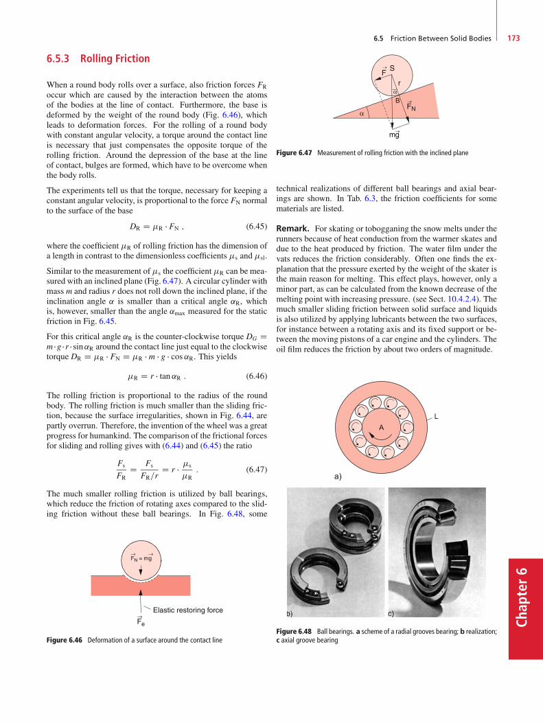
6.5 Friction Between Solid Bodies 173
Chap
ter6
6.5.3 Rolling Friction
When a round body rolls over a surface, also friction forces FR
occur which are caused by the interaction between the atomsof the bodies at the line of contact. Furthermore, the base isdeformed by the weight of the round body (Fig. 6.46), whichleads to deformation forces. For the rolling of a round bodywith constant angular velocity, a torque around the contact lineis necessary that just compensates the opposite torque of therolling friction. Around the depression of the base at the lineof contact, bulges are formed, which have to be overcome whenthe body rolls.
The experiments tell us that the torque, necessary for keeping aconstant angular velocity, is proportional to the force FN normalto the surface of the base
DR D R � FN ; (6.45)
where the coefficient R of rolling friction has the dimension ofa length in contrast to the dimensionless coefficients s and sl.
Similar to the measurement ofs the coefficient R can be mea-sured with an inclined plane (Fig. 6.47). A circular cylinder withmass m and radius r does not roll down the inclined plane, if theinclination angle ˛ is smaller than a critical angle ˛R, whichis, however, smaller than the angle ˛max measured for the staticfriction in Fig. 6.45.
For this critical angle ˛R is the counter-clockwise torque DG Dm �g � r � sin˛R around the contact line just equal to the clockwisetorque DR D R � FN D R � m � g � cos˛R. This yields
R D r � tan˛R : (6.46)
The rolling friction is proportional to the radius of the roundbody. The rolling friction is much smaller than the sliding fric-tion, because the surface irregularities, shown in Fig. 6.44, arepartly overrun. Therefore, the invention of the wheel was a greatprogress for humankind. The comparison of the frictional forcesfor sliding and rolling gives with (6.44) and (6.45) the ratio
Fs
FRD Fs
FR=rD r � s
R: (6.47)
The much smaller rolling friction is utilized by ball bearings,which reduce the friction of rotating axes compared to the slid-ing friction without these ball bearings. In Fig. 6.48, some
Figure 6.46 Deformation of a surface around the contact line
Figure 6.47 Measurement of rolling friction with the inclined plane
technical realizations of different ball bearings and axial bear-ings are shown. In Tab. 6.3, the friction coefficients for somematerials are listed.
Remark. For skating or tobogganing the snow melts under therunners because of heat conduction from the warmer skates anddue to the heat produced by friction. The water film under thevats reduces the friction considerably. Often one finds the ex-planation that the pressure exerted by the weight of the skater isthe main reason for melting. This effect plays, however, only aminor part, as can be calculated from the known decrease of themelting point with increasing pressure. (see Sect. 10.4.2.4). Themuch smaller sliding friction between solid surface and liquidsis also utilized by applying lubricants between the two surfaces,for instance between a rotating axis and its fixed support or be-tween the moving pistons of a car engine and the cylinders. Theoil film reduces the friction by about two orders of magnitude.
Figure 6.48 Ball bearings. a scheme of a radial grooves bearing; b realization;c axial groove bearing
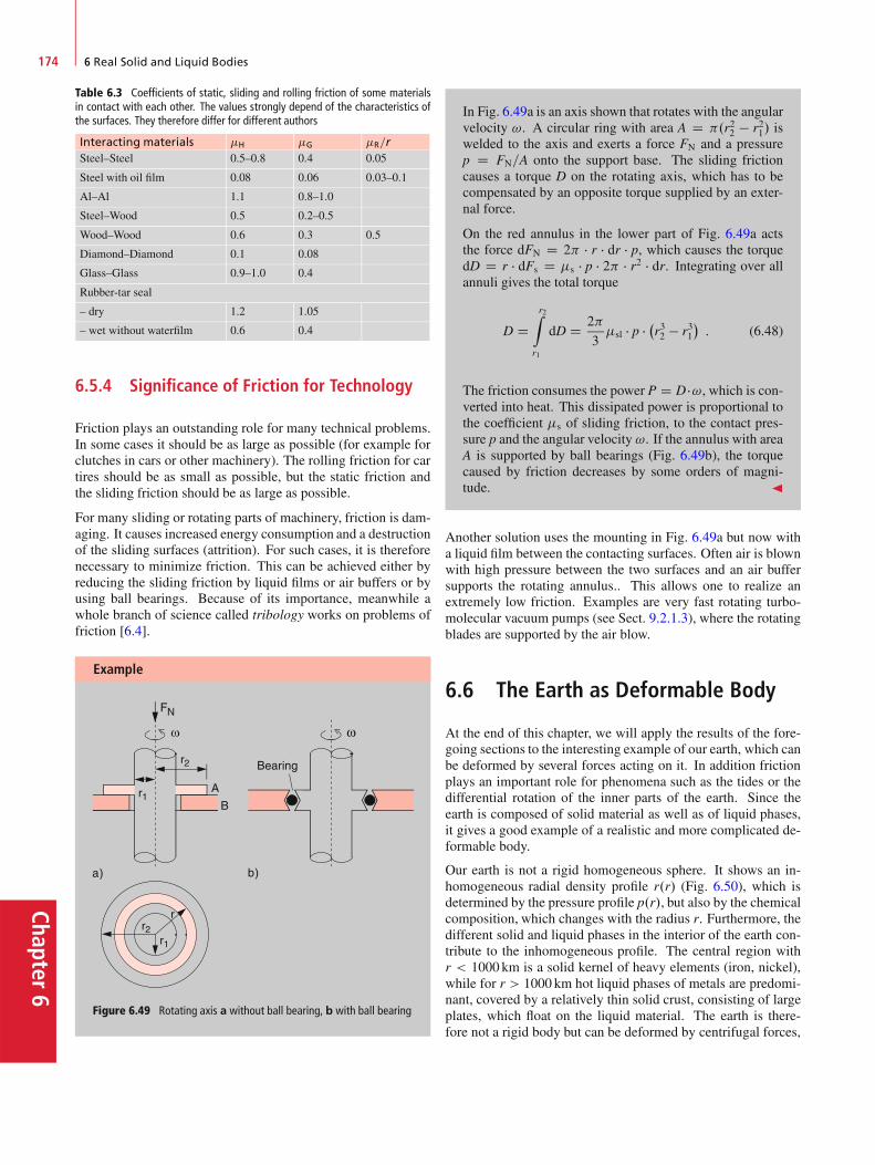
Chapter6
174 6 Real Solid and Liquid Bodies
Table 6.3 Coefficients of static, sliding and rolling friction of some materialsin contact with each other. The values strongly depend of the characteristics ofthe surfaces. They therefore differ for different authors
Interacting materials H G R=rSteel–Steel 0.5–0.8 0.4 0.05
Steel with oil film 0.08 0.06 0.03–0.1
Al–Al 1.1 0.8–1.0
Steel–Wood 0.5 0.2–0.5
Wood–Wood 0.6 0.3 0.5
Diamond–Diamond 0.1 0.08
Glass–Glass 0.9–1.0 0.4
Rubber-tar seal
– dry 1.2 1.05
– wet without waterfilm 0.6 0.4
6.5.4 Significance of Friction for Technology
Friction plays an outstanding role for many technical problems.In some cases it should be as large as possible (for example forclutches in cars or other machinery). The rolling friction for cartires should be as small as possible, but the static friction andthe sliding friction should be as large as possible.
For many sliding or rotating parts of machinery, friction is dam-aging. It causes increased energy consumption and a destructionof the sliding surfaces (attrition). For such cases, it is thereforenecessary to minimize friction. This can be achieved either byreducing the sliding friction by liquid films or air buffers or byusing ball bearings. Because of its importance, meanwhile awhole branch of science called tribology works on problems offriction [6.4].
Example
Figure 6.49 Rotating axis a without ball bearing, b with ball bearing
In Fig. 6.49a is an axis shown that rotates with the angularvelocity !. A circular ring with area A D .r22 � r21/ iswelded to the axis and exerts a force FN and a pressurep D FN=A onto the support base. The sliding frictioncauses a torque D on the rotating axis, which has to becompensated by an opposite torque supplied by an exter-nal force.
On the red annulus in the lower part of Fig. 6.49a actsthe force dFN D 2 � r � dr � p, which causes the torquedD D r � dFs D s � p � 2 � r2 � dr. Integrating over allannuli gives the total torque
D Dr2Z
r1
dD D 2
3sl � p � �r32 � r31
�: (6.48)
The friction consumes the power P D D �!, which is con-verted into heat. This dissipated power is proportional tothe coefficient s of sliding friction, to the contact pres-sure p and the angular velocity !. If the annulus with areaA is supported by ball bearings (Fig. 6.49b), the torquecaused by friction decreases by some orders of magni-tude. J
Another solution uses the mounting in Fig. 6.49a but now witha liquid film between the contacting surfaces. Often air is blownwith high pressure between the two surfaces and an air buffersupports the rotating annulus.. This allows one to realize anextremely low friction. Examples are very fast rotating turbo-molecular vacuum pumps (see Sect. 9.2.1.3), where the rotatingblades are supported by the air blow.
6.6 The Earth as Deformable Body
At the end of this chapter, we will apply the results of the fore-going sections to the interesting example of our earth, which canbe deformed by several forces acting on it. In addition frictionplays an important role for phenomena such as the tides or thedifferential rotation of the inner parts of the earth. Since theearth is composed of solid material as well as of liquid phases,it gives a good example of a realistic and more complicated de-formable body.
Our earth is not a rigid homogeneous sphere. It shows an in-homogeneous radial density profile r.r/ (Fig. 6.50), which isdetermined by the pressure profile p.r/, but also by the chemicalcomposition, which changes with the radius r. Furthermore, thedifferent solid and liquid phases in the interior of the earth con-tribute to the inhomogeneous profile. The central region withr < 1000 km is a solid kernel of heavy elements (iron, nickel),while for r > 1000 km hot liquid phases of metals are predomi-nant, covered by a relatively thin solid crust, consisting of largeplates, which float on the liquid material. The earth is there-fore not a rigid body but can be deformed by centrifugal forces,
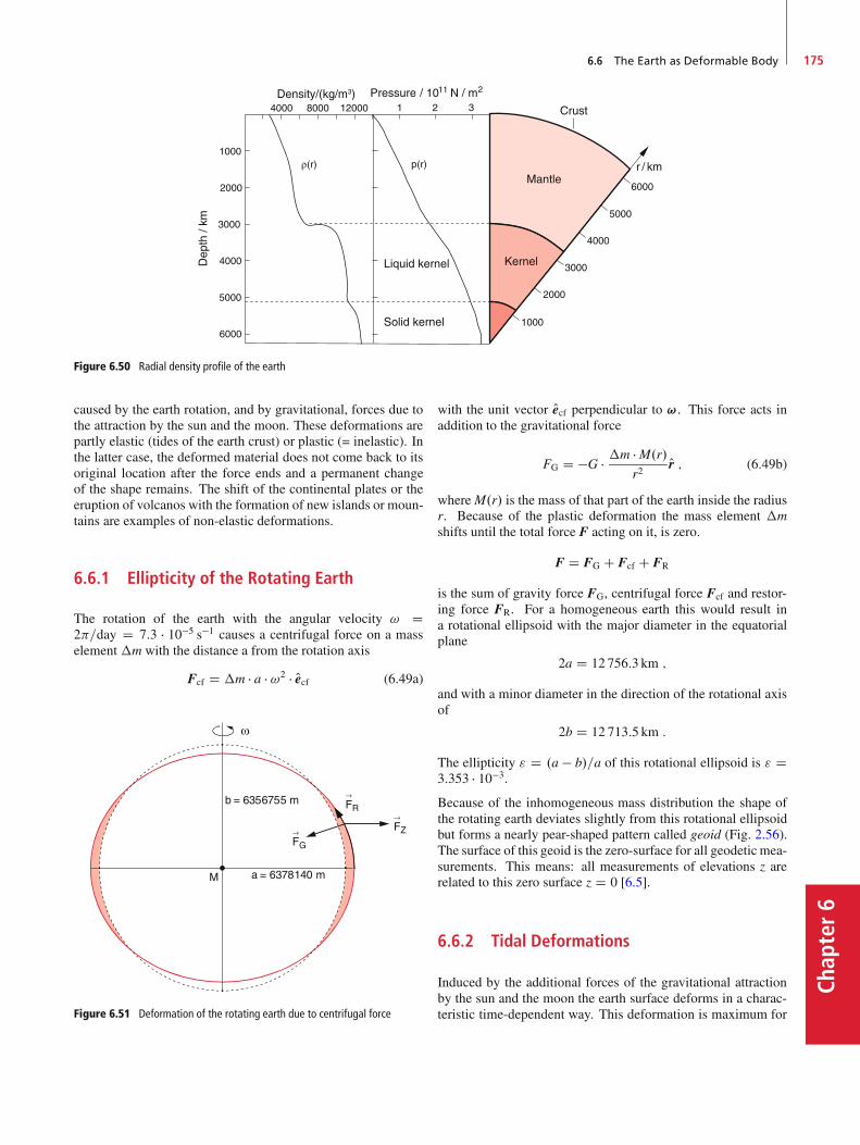
6.6 The Earth as Deformable Body 175
Chap
ter6
Figure 6.50 Radial density profile of the earth
caused by the earth rotation, and by gravitational, forces due tothe attraction by the sun and the moon. These deformations arepartly elastic (tides of the earth crust) or plastic (= inelastic). Inthe latter case, the deformed material does not come back to itsoriginal location after the force ends and a permanent changeof the shape remains. The shift of the continental plates or theeruption of volcanos with the formation of new islands or moun-tains are examples of non-elastic deformations.
6.6.1 Ellipticity of the Rotating Earth
The rotation of the earth with the angular velocity ! D2=day D 7:3 � 10�5 s�1 causes a centrifugal force on a masselement �m with the distance a from the rotation axis
Fcf D �m � a � !2 � Oecf (6.49a)
Figure 6.51 Deformation of the rotating earth due to centrifugal force
with the unit vector Oecf perpendicular to !. This force acts inaddition to the gravitational force
FG D �G � �m � M.r/r2
Or ; (6.49b)
whereM.r/ is the mass of that part of the earth inside the radiusr. Because of the plastic deformation the mass element �mshifts until the total force F acting on it, is zero.
F D FG C Fcf C FR
is the sum of gravity force FG, centrifugal force Fcf and restor-ing force FR. For a homogeneous earth this would result ina rotational ellipsoid with the major diameter in the equatorialplane
2a D 12 756:3 km ;
and with a minor diameter in the direction of the rotational axisof
2b D 12 713:5 km :
The ellipticity " D .a � b/=a of this rotational ellipsoid is " D3:353 � 10�3.
Because of the inhomogeneous mass distribution the shape ofthe rotating earth deviates slightly from this rotational ellipsoidbut forms a nearly pear-shaped pattern called geoid (Fig. 2.56).The surface of this geoid is the zero-surface for all geodetic mea-surements. This means: all measurements of elevations z arerelated to this zero surface z D 0 [6.5].
6.6.2 Tidal Deformations
Induced by the additional forces of the gravitational attractionby the sun and the moon the earth surface deforms in a charac-teristic time-dependent way. This deformation is maximum for
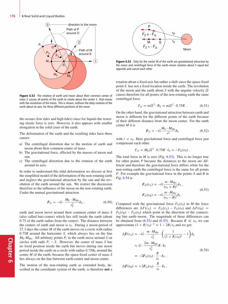
Chapter6
176 6 Real Solid and Liquid Bodies
Figure 6.52 The rotation of earth and moon about their common center ofmass S causes all points of the earth to rotate about the center S , that moveswith the revolution of the moon. This is shown, without the daily rotation of theearth about its axis, for three different positions of the moon
the oceans (low tides and high tides) since for liquids the restor-ing elastic force is zero. However, it also appears with smallerelongation in the solid crust of the earth.
The deformation of the earth and the resulting tides have threecauses:
a) The centrifugal distortion due to the motion of earth andmoon about their common center of mass.
b) The gravitational force, effected by the masses of moon andsun.
c) The centrifugal distortion due to the rotation of the eartharound its axis.
In order to understand this tidal deformation we discuss at firstthe simplified model of the deformation of the non-rotating earthand neglect the gravitational attraction by the sun and the rev-olution of the earth around the sun. We restrict the discussiontherefore to the influence of the moon on the non-rotating earth.Under the mutual gravitational attraction
FG D �G � ME � MMo
r20Or0 ; (6.50)
earth and moon move around their common center of mass S(also called bari-center) which lies still inside the earth (about0.75 of the earth radius from the center). The distance betweenthe centers of earth and moon is r0. During a moon-period of27.3 days the centerM of the earth moves on a circle with radius0:75R around the baricenter S, which always lies on the lineME-MMo. All arbitrary points Pi in the earth move around S oncircles with radii Pi � S. However, the center of mass S hasno fixed position inside the earth but moves during one moonperiod inside the earth on a circle with radius 0:75RE around thecenter M of the earth, because the space-fixed center of mass Slies always on the line between earth-center and moon center.
The motion of the non-rotating earth as extended body, de-scribed in the coordinate system of the earth, is therefore not a
Figure 6.53 Only for the center M of the earth are gravitational attraction bythe moon and centrifugal force of the earth–moon rotation about S equal butopposite and cancel each other
rotation about a fixed axis but rather a shift since the space-fixedpoint S. has not a fixed location inside the earth. The revolutionof the moon and the earth about S with the angular velocity ˝causes therefore for all points of the non-rotating earth the samecentrifugal force
Fcf D m˝2 � RS D m˝2 � 0:75R : (6.51)
On the other hand, the gravitational attraction between earth andmoon is different for the different points of the earth becauseof their different distance from the moon center. For the earthcenterM it is
FG D �GME � MMo
r2Or0 (6.52)
with r D r0. Here gravitational force and centrifugal force justcompensate each other.
Fcf D ME˝2 � 0:75R � Or0 D �FG.r0/ :
The total force in M is zero (Fig. 6.53). This is no longer truefor other points P because the distances to the moon are dif-ferent and therefore the gravitational force differs while for thenon-rotting earth the centrifugal force is the same for all pointsP. For example the gravitational force in the points A and B inFig. 6.54 is
FG.rA/ D �Gm � MMo
.r0 C R/2Or0 ;
FG.rB/ D �Gm � MMo
.r0 � R/2Or0 :
(6.53)
Compared with the gravitational force FG.r0/ in M the forcedifferences are �F.rA/ D FG.rA/ � FG.r0/ and �F.rB/ DFG.rB/ � FG.r0/ which point in the direction of the connect-ing line earth–moon. The magnitude of these differences canbe obtained from (6.52) and (6.53). Because R r0, we canapproximate .1 C R=r0/�2 � 1 � 2R=r0 and we get:
�F.rA/ D �G � m � MMo
r20��
1
.1 C R=r0/2� 1
�Or0
� G � 2m � MMo
r30R � Or0
D �2FG.r0/ � Rr0
� Or0 ;
�F.rB/ D C2FG.r0/ � Rr0
� Or0 ;
(6.54)
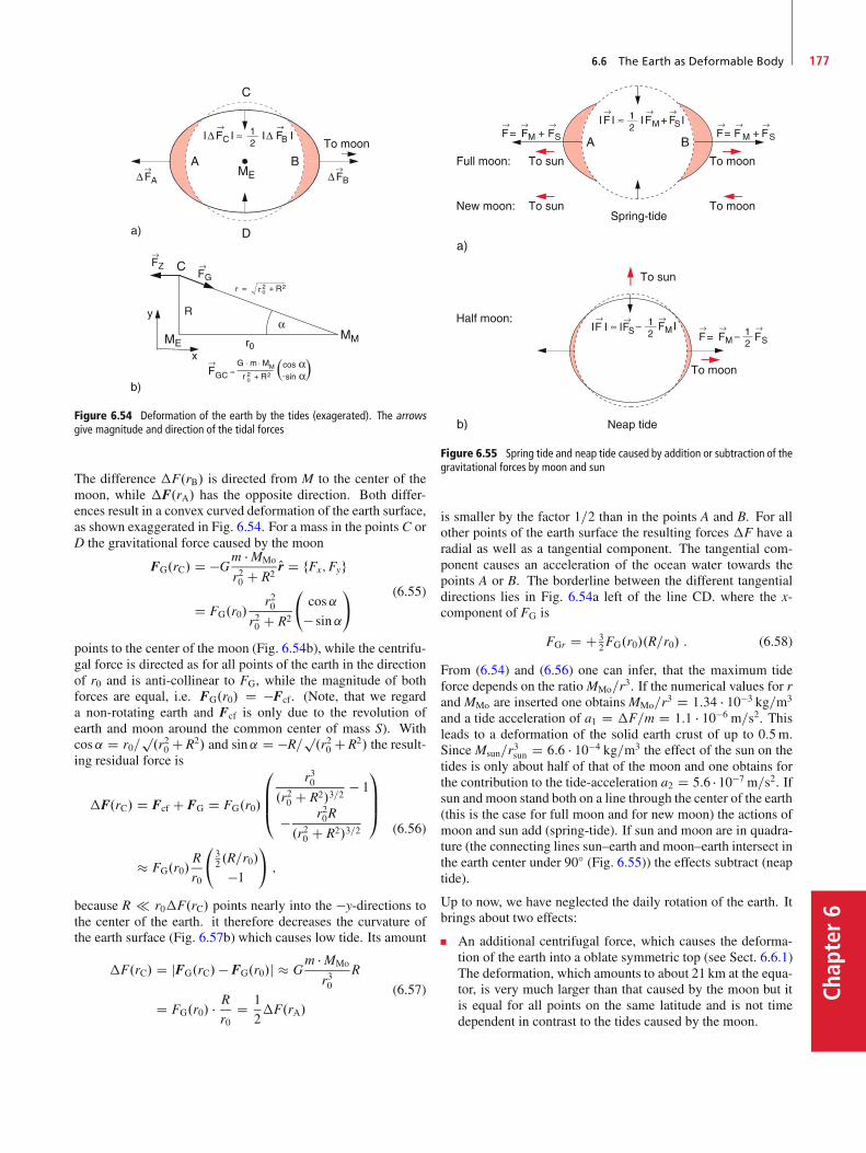
6.6 The Earth as Deformable Body 177
Chap
ter6
Figure 6.54 Deformation of the earth by the tides (exagerated). The arrowsgive magnitude and direction of the tidal forces
The difference �F.rB/ is directed from M to the center of themoon, while �F.rA/ has the opposite direction. Both differ-ences result in a convex curved deformation of the earth surface,as shown exaggerated in Fig. 6.54. For a mass in the points C orD the gravitational force caused by the moon
FG.rC/ D �Gm � MMo
r20 C R2Or D fFx;Fyg
D FG.r0/r20
r20 C R2
cos˛
� sin˛
! (6.55)
points to the center of the moon (Fig. 6.54b), while the centrifu-gal force is directed as for all points of the earth in the directionof r0 and is anti-collinear to FG, while the magnitude of bothforces are equal, i.e. FG.r0/ D �Fcf. (Note, that we regarda non-rotating earth and Fcf is only due to the revolution ofearth and moon around the common center of mass S). Withcos˛ D r0=
p.r20 CR2/ and sin˛ D �R=
p.r20 CR2/ the result-
ing residual force is
�F.rC/ D Fcf C FG D FG.r0/
0
BB@
r30.r20 C R2/3=2
� 1
� r20R
.r20 C R2/3=2
1
CCA
� FG.r0/R
r0
32 .R=r0/
�1
!;
(6.56)
because R r0�F.rC/ points nearly into the �y-directions tothe center of the earth. it therefore decreases the curvature ofthe earth surface (Fig. 6.57b) which causes low tide. Its amount
�F.rC/ D jFG.rC/ � FG.r0/j � Gm � MMo
r30R
D FG.r0/ � Rr0
D 1
2�F.rA/
(6.57)
Figure 6.55 Spring tide and neap tide caused by addition or subtraction of thegravitational forces by moon and sun
is smaller by the factor 1=2 than in the points A and B. For allother points of the earth surface the resulting forces �F have aradial as well as a tangential component. The tangential com-ponent causes an acceleration of the ocean water towards thepoints A or B. The borderline between the different tangentialdirections lies in Fig. 6.54a left of the line CD. where the x-component of FG is
FGr D C 32FG.r0/.R=r0/ : (6.58)
From (6.54) and (6.56) one can infer, that the maximum tideforce depends on the ratioMMo=r3. If the numerical values for rand MMo are inserted one obtainsMMo=r3 D 1:34 � 10�3 kg=m3
and a tide acceleration of a1 D �F=m D 1:1 � 10�6 m=s2. Thisleads to a deformation of the solid earth crust of up to 0:5m.Since Msun=r3sun D 6:6 � 10�4 kg=m3 the effect of the sun on thetides is only about half of that of the moon and one obtains forthe contribution to the tide-acceleration a2 D 5:6 � 10�7 m=s2. Ifsun and moon stand both on a line through the center of the earth(this is the case for full moon and for new moon) the actions ofmoon and sun add (spring-tide). If sun and moon are in quadra-ture (the connecting lines sun–earth and moon–earth intersect inthe earth center under 90ı (Fig. 6.55)) the effects subtract (neaptide).
Up to now, we have neglected the daily rotation of the earth. Itbrings about two effects:
An additional centrifugal force, which causes the deforma-tion of the earth into a oblate symmetric top (see Sect. 6.6.1)The deformation, which amounts to about 21 km at the equa-tor, is very much larger than that caused by the moon but itis equal for all points on the same latitude and is not timedependent in contrast to the tides caused by the moon.
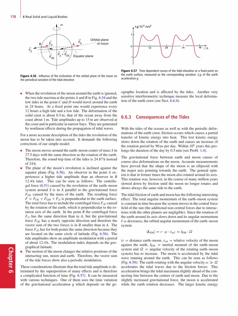
Chapter6
178 6 Real Solid and Liquid Bodies
Figure 6.56 Influence of the inclination of the orbital plane of the moon onthe periodical variation of the tidal elevation
When the revolution of the moon around the earth is ignored,the two tide maxima at the points A and B in Fig. 6.54 and thelow tides in the point C and D would travel around the earthin 24 hours. At a fixed point one would experience every12 hours a high tide and a low tide. The deformation of thesolid crust is about 0:5m, that of the ocean away from thecoast about 1m. Tide amplitudes up to 15m are observed atthe coast and in particular in narrow bays. They are generatedby nonlinear effects during the propagation of tidal waves.
For a more accurate description of the tides the revolution of themoon has to be taken into account. It demands the followingcorrections of our simple model:
The moon moves around the earth–moon-center of mass S in27.5 days with the same direction as the rotation of the earth.Therefore, the round-trip time of the tides is 24:87 h insteadof 24 h.The plane of the moon’s revolution is inclined against theequator plane (Fig. 6.56). An observer in the point A ex-periences a higher tide amplitude than an observer in B12:4 h later. This can be seen as follows: The centrifu-gal force (6.51) caused by the revolution of the earth–moonsystem around S is in A parallel to the gravitational forceFGE caused by the mass of the earth. The resulting forceF D FGE C FGM C Fcf is perpendicular to the earth surface.The total force has to include the centrifugal force FcE causedby the rotation of the earth, which is perpendicular to the ro-tation axis of the earth. In the point B the centrifugal forceFcf has the same direction than in A, but the gravitationalforce FGE has a nearly opposite direction and therefore thevector sum of the two forces is in B smaller than in A. Theforce FcE has for both points the same direction because theyare located on the same circle of latitude (Fig. 6.56). Thetide amplitudes show an amplitude modulation with a periodof about 12:4 h. The modulation index depends on the geo-graphical latitude.The motion of the moon changes the relative positions of theinteracting sun, moon and earth. Therefore, the vector sumof the tide forces show also a periodic modulation.
These considerations illustrate that the total tide amplitude is de-termined by the superposition of many effects and is thereforea complicated function of time (Fig. 6.57). It can be measuredwith various techniques. One of them uses the time variationof the gravitational acceleration g which depends on the ge-
Figure 6.57 Time dependent course of the tidal elevation at a fixed point onthe earth surface, measured as the corresponding variation �g of the earthacceleration g
ographic location and is affected by the tides. Another verysensitive interferometric technique measure the local deforma-tion of the earth crust (see Sect. 6.6.4).
6.6.3 Consequences of the Tides
With the tides of the oceans as well as with the periodic defor-mations of the earth crust, friction occurs which causes a partialtransfer of kinetic energy into heat. This lost kinetic energyslows down the rotation of the earth and causes an increase ofthe rotation period by 90 ns per day. Within 106 years this pro-longs the duration of the day by 0:5min (see Probl. 1.4).
The gravitational force between earth and moon causes ofcourse also deformations on the moon. Accurate measurementshave proved that the shape of the moon is an ellipsoid withthe major axis pointing towards the earth. The general opin-ion is that in former times the moon also rotated around its axis.This rotation was, however, in the course of many million yearsslowed down by friction until the moon no longer rotates andshows always the same side to the earth.
The tidal friction of earth andmoon has the following interestingeffect: The total angular momentum of the earth–moon systemis constant in time because the system moves in the central forcefield of the sun (the additional non-central forces due to interac-tions with the other planets are negligible). Since the rotation ofthe earth around its axis slows down and its angular momentumI �! decreases, the orbital angular momentum of the earth–moonsystem
jLEMj D r � � vrel� D IEM �˝
(r D distance earth–moon, vrel D relative velocity of the moonagainst the earth, IEM D inertial moment of the earth–moonsystem and ˝ D angular velocity of the rotating earth–moonsystem) has to increase. The moon is accelerated by the tidalwave running around the earth. This can be seen as follows(Fig. 6.58): The earth rotating with the angular velocity ! � ˝accelerates the tidal waves due to the friction forces: Thisacceleration brings the tidal maximum slightly ahead of the con-necting line between the centers of earth and moon. Due to theslightly increased gravitational force, the moon is acceleratedwhile the earth rotation decreases. The larger kinetic energy

6.6 The Earth as Deformable Body 179
Chap
ter6
Figure 6.58 Deceleration of the earth rotation and acceleration of the orbitalvelocity of the moon by the tidal friction
of the moon increases its total energy .Ekin C Epot/ and there-fore also its distance to the earth. In former times the moonwas closer to the earth. The nowadays generally accepted the-ory [6.7a, 6.7b] assumes that the moon was part of the earth buthas been catapulted out of the earth by the impact of a heavyasteroid some billion years ago (see Vol. 4).
6.6.4 Measurements of the Earth Deformation
The deformation of the earth by tidal effects can be measuredwith different techniques. We will shortly discuss three of them:
6.6.4.1 Changes of the Gravitational Force
According to (6.54) the additional gravitational force caused bythe moon in the points A and B in Fig. 6.54 is
�FG � 2mMMo
r3Mo
R : (6.59)
In the gravity meter shown in Fig. 6.59 a massm is suspended bya spring in such a way, that a small change�FG D m ��g due tothe corresponding change of g causes a large vertical deflectionof the arrow on the scale. This is achieved by a sloped mountingof the spring with length L and a restoring force Fr D �D ��L.With the slope angle ˛, the vertical deflection�z causes a lengthincrease of the spring�L D �z � sin˛ (Fig. 6.59b) and a changeof the restoring force �Fr D m ��g � sin˛.
α
α
tension spring
compression spring
Figure 6.59 Measurement of the gravitational force with a special spring bal-ance
Well Wire
BallCondensorplates
C ∝ 1/d
Figure 6.60 Measurement of the deviation of g from the vertical direction
The device measures the periodic changes of FG with a pe-riod of 24:87 h from which the tidal amplitudes can be inferred(Fig. 6.57). Because of the different contributing effects, �g.t/follows a complicated curve.
The experimental arrangement of Fig. 6.60 allows to measurethe deviation from the vertical direction of the earth accelerationg. Without external perturbation, g would point nearly to theearth center (only for a spherical mass distribution it would pointexactly to the center). The additional gravitational force ex-erted by the moon causes a slight deviation from this direction.The maximum angular deviation, which depends on the latitude,amounts only to about 2:1 � 10�6 rad.D 0:400/, the measurementmust be sufficiently accurate. This required accuracy can bereached with a pendulum [6.9]. A metal ball suspended on along wire in a well is connected with one plate of a charged ca-pacitor, while the other plate is fixed on the wall of the well. Anydeviation of the pendulum from the vertical direction changesthe distance between the two plates and therefore the voltage ofthe capacitor (see Vol. 2, Sect. 5).
6.6.4.2 Measurements of the Earth Deformation
Here the change �L of the length L between two points A1 andA2 connected with the earth ground is measured. Figure 6.61illustrates the method. A very sensitive Laser interferometer islocated in a gold mine deep in the ground in order to eliminateacoustic noise from the surroundings. The two mirrors of thelaser resonator are mounted on the ground base at the points A1
and A2 separated by the distance L. The optical frequency of thelaser �L D m � c=.2L/ is determined by the length L of the res-onator and the large integer m � 1. If the length L changes dueto the deformation of the earth crust, the laser frequency changesaccordingly. This frequency change can be measured very accu-rately, when the laser beam is superimposed on a detector withthe output beam of a reference laser with stabilized frequency �r.The difference frequency �L � �r in the radio-frequency rangecan be counted by a digital frequency counter. Existing deviceshave resonator lengths of 100m up to several km. They canmeasure deformations of the earth crust of less than 10�9 m (seeVol. 2, Sect. 10.4). This sensitivity is sufficient to measure thedeformation of the ground base in the Rocky Mountains causedby the tidal waves of the Pacific Ocean [6.10].
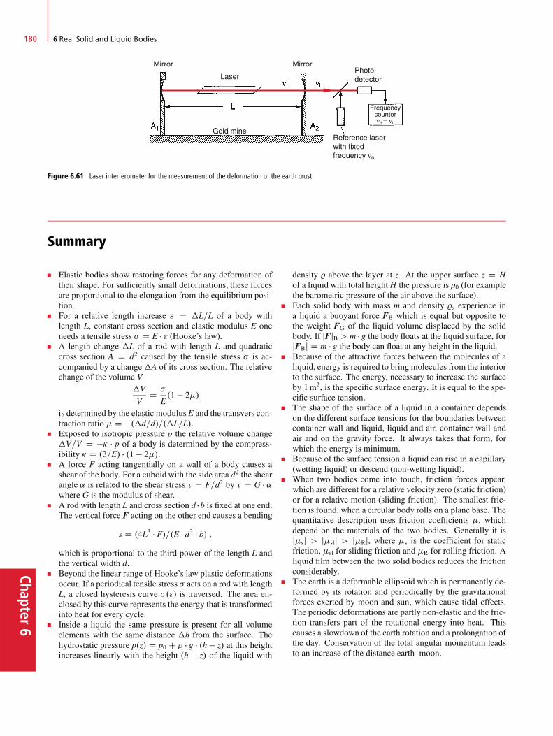
Chapter6
180 6 Real Solid and Liquid Bodies
Mirror Mirror
Gold mineReference laserwith fixedfrequency νR
FrequencycounterνR – νL
LaserPhoto-detector
Figure 6.61 Laser interferometer for the measurement of the deformation of the earth crust
Summary
Elastic bodies show restoring forces for any deformation oftheir shape. For sufficiently small deformations, these forcesare proportional to the elongation from the equilibrium posi-tion.For a relative length increase " D �L=L of a body withlength L, constant cross section and elastic modulus E oneneeds a tensile stress � D E � " (Hooke’s law).A length change �L of a rod with length L and quadraticcross section A D d2 caused by the tensile stress � is ac-companied by a change �A of its cross section. The relativechange of the volume V
�V
VD �
E.1 � 2/
is determined by the elastic modulusE and the transvers con-traction ratio D �.�d=d/=.�L=L/.Exposed to isotropic pressure p the relative volume change�V=V D �� � p of a body is determined by the compress-ibility � D .3=E/ � .1 � 2/.A force F acting tangentially on a wall of a body causes ashear of the body. For a cuboid with the side area d2 the shearangle ˛ is related to the shear stress � D F=d2 by � D G � ˛where G is the modulus of shear.A rod with length L and cross section d �b is fixed at one end.The vertical force F acting on the other end causes a bending
s D .4L3 � F/=.E � d3 � b/ ;which is proportional to the third power of the length L andthe vertical width d.Beyond the linear range of Hooke’s law plastic deformationsoccur. If a periodical tensile stress � acts on a rod with lengthL, a closed hysteresis curve �."/ is traversed. The area en-closed by this curve represents the energy that is transformedinto heat for every cycle.Inside a liquid the same pressure is present for all volumeelements with the same distance �h from the surface. Thehydrostatic pressure p.z/ D p0 C % � g � .h � z/ at this heightincreases linearly with the height .h � z/ of the liquid with
density % above the layer at z. At the upper surface z D Hof a liquid with total heightH the pressure is p0 (for examplethe barometric pressure of the air above the surface).Each solid body with mass m and density %s experience ina liquid a buoyant force FB which is equal but opposite tothe weight FG of the liquid volume displaced by the solidbody. If jFjB > m � g the body floats at the liquid surface, forjFBj D m � g the body can float at any height in the liquid.Because of the attractive forces between the molecules of aliquid, energy is required to bring molecules from the interiorto the surface. The energy, necessary to increase the surfaceby 1m2, is the specific surface energy. It is equal to the spe-cific surface tension.The shape of the surface of a liquid in a container dependson the different surface tensions for the boundaries betweencontainer wall and liquid, liquid and air, container wall andair and on the gravity force. It always takes that form, forwhich the energy is minimum.Because of the surface tension a liquid can rise in a capillary(wetting liquid) or descend (non-wetting liquid).When two bodies come into touch, friction forces appear,which are different for a relative velocity zero (static friction)or for a relative motion (sliding friction). The smallest fric-tion is found, when a circular body rolls on a plane base. Thequantitative description uses friction coefficients , whichdepend on the materials of the two bodies. Generally it isjsj > jslj > jRj, where s is the coefficient for staticfriction, sl for sliding friction and R for rolling friction. Aliquid film between the two solid bodies reduces the frictionconsiderably.The earth is a deformable ellipsoid which is permanently de-formed by its rotation and periodically by the gravitationalforces exerted by moon and sun, which cause tidal effects.The periodic deformations are partly non-elastic and the fric-tion transfers part of the rotational energy into heat. Thiscauses a slowdown of the earth rotation and a prolongation ofthe day. Conservation of the total angular momentum leadsto an increase of the distance earth–moon.

References 181
Chap
ter6
Problems
6.1 What is the change�L of a steel rope with L D 9 km,a) which hangs in a vertical well?b) What is the maximum length of the rope before its rupture?c) How large is �L when the rope is lowered from a ship into
the ocean? (E D 2 � 1011 N=m2; %steel D 7:7 � 103 kg=m3,%ocean D 1:03 � 103 kg=m3)
6.2 A steel beam with L D 10m is clamped at one end. Aforce F D 103 N acts on the other end in vertical z-direction.How large is the bending of this enda) for a rectangular cross section d � b with d D �z D 0:1m;
b D �y D d=2?b) for a double T-profile (Fig. 6.15d) with b1 D d1 D 0:1m,
b2 D d2 D 0:05m?
6.3 The deep ocean aquanaut Picard reached in his sphericalsteel submarine a depth of 10:000m in the Philippine trench.How large are pressure and total force exerted on the sphere?What is the volume change�V=V caused by the pressurea) for a hollow sphere with wall thickness of 0:2m?b) for a full sphere?
6.4 A turbine drives a generator connected to a steel shaftwith length L and diameter D. By which angle ˛ are the twoends of the shaft twisted if the power P D 300 kW is transferredat a frequency ! D 2 � 25 s�1
a) for a steel shaft as full cylinder with D D 0:1m; L D 20m?b) for a hollow cylinder with D1 D 5 cm and D2 D 10 cm?
6.5 What is the density of water with a compressibility � D4:8 � 10�10 m2=N at a depth of 10:000m?
6.6 A hollow steel cube .% D 7:8 � 103 kg=m3/ with edgelength a D 1m and a wall thickness of d D 0:02m and with anopen upper side floats on water.
a) How deep does it immerse?b) What is the location of center of mass and metacenter?c) What is the maximum angle of its symmetry axis against the
vertical direction before it becomes unstable?
6.7 Which energy has to be spent in order to lift a full cubeof steel from the bottom of a swimming pool with the waterdepth of 4m to a position where the lower side of the cube is atthe surface of the water?
6.8 Which force was necessary to separate the two hemi-spheres in the demonstration experiment by Guericke in Magde-burg with a diameter of 0:6m, when the pressure differencebetween inside and outside was �p D 90 kPa? Guericke hadused 16 horses. What should have been done in order to sepa-rate the hemi-spheres already with 8 horses?
6.9 In order to verify that a gold bar is really made of gold.%gold D 19:3 kg=dm3/ a goldsmith measures its weight in airand when totally immersed in water. Which ratio of the twovalues is obtaineda) for a 100% gold bar?b) for a 20% admixture of copper .% D 8:9 kg=dm3/?c) What is the minimum required accuracy of the measure-
ments for unambiguously distinguishing between the twocases? What is the accuracy if an admixture of 1% of coppershould be detected?
6.10 A round cylinder of wood (L D 1m, d D 0:2m,% D 525 kg=m3) is floating in water. How deep does it immersea) in a horizontal position?b) if a steel ball with m D 1 kg is attached to one end in order
to bring it into a vertical floating position?
References
6.1. W.D. Callister, D.G. Rethwisch,Material Science and En-gineering. An Introduction. (Wiley, 2013)
6.2. Deformation, ed. by M. Hazewinkel Encyclopedia ofMathematics. (Springer, 2001)
6.3. S. Lipschitz, Schaum’s Outline of mathematical Hand-book of Formulas. (McGraw Hill, 2012)
6.4. M. Abramowitz, I. Stergun, Handbook of MathematicalFunctions. (Martino Fine Books)
6.5. R.H. Rapp, F. Sanso (ed.), Determination of the Geoid.(Springer, Berlin, Heidelberg, 1991)
6.6a. V.M. Lyathker, Tidal Power. Harnessing Energy from Wa-ter Currents. (Wiley Scrivener, 2014)
6.6b. L. Peppas, Ocean, Tidal and Wave energy. (Crabtree Publ.Comp., 2008)
6.6c. https://en.wikipedia.org/wiki/List_of_tidal_power_stations
6.6d. https://en.wikipedia.org/wiki/Tidal_power6.7a. http://novan.com/earth.htm6.7b. P. Brosche, H. Schuh, Surveys in Geophysics 19, 417
(1998)

Chapter6
182 6 Real Solid and Liquid Bodies
6.8a. D. Flannagan, The Dynamic Earth. (Freeman, 1983)6.8b. G.M.R. Fowler, The Solid Earth. An Introduction to
Global Geophysics. (Cambridge Univ. Press, 2004)6.9. D. Wolf, M. Santoyo, J. Fernadez (ed.), Deformation and
Gravity Change. (Birkhäuser, 2013)6.10. J. Levine, J.L. Hall, J. Geophys. Res. 77, 2595 (1972)
6.11. A.E. Musset, M.A. Khan, Looking into the Earth: An In-troduction to Geological Geophysics. (Cambridge Univ.Press, 2000)
6.12. M. Goldsmith, M.A. Garlick, Earth: The Life on ourPlanet. (Kingfisher, 2011)

Chap
ter7Gases 7
7.1 Macroscopic Model . . . . . . . . . . . . . . . . . . . . . . . . . . . . . . 184
7.2 Atmospheric Pressure and Barometric Formula . . . . . . . . . . . . . . 185
7.3 Kinetic Gas Theory . . . . . . . . . . . . . . . . . . . . . . . . . . . . . . . 188
7.4 Experimental Proof of the Kinetic Gas Theory . . . . . . . . . . . . . . . 196
7.5 Transport Phenomena in Gases . . . . . . . . . . . . . . . . . . . . . . . 198
7.6 The Atmosphere of the Earth . . . . . . . . . . . . . . . . . . . . . . . . . 204
Summary . . . . . . . . . . . . . . . . . . . . . . . . . . . . . . . . . . . . 206
Problems . . . . . . . . . . . . . . . . . . . . . . . . . . . . . . . . . . . . 207
References . . . . . . . . . . . . . . . . . . . . . . . . . . . . . . . . . . . 208
183© Springer International Publishing Switzerland 2017W. Demtröder, Mechanics and Thermodynamics, Undergraduate Lecture Notes in Physics, DOI 10.1007/978-3-319-27877-3_7
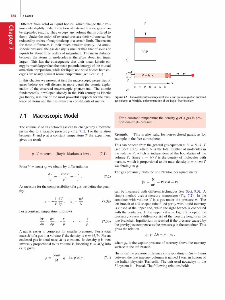
Chapter7
184 7 Gases
Different from solid or liquid bodies, which change their vol-ume only slightly under the action of external forces, gases canbe expanded readily. They occupy any volume that is offered tothem. Under the action of external pressure their volume can bereduced by orders of magnitude up to a certain limit. The reasonfor these differences is their much smaller density. At atmo-spheric pressure, the gas density is smaller than that of solids orliquids by about three orders of magnitude. The mean distancebetween the atoms or molecules is therefore about ten timeslarger. This has the consequence that their mean kinetic en-ergy is much larger than the mean potential energy of the mutualattraction or repulsion, while for liquid and solid bodies both en-ergies are nearly equal at room temperature (see Sect. 6.1).
In this chapter we present at first the macroscopic properties ofgases before we will discuss in more detail the atomic expla-nation of the observed macroscopic phenomena. The atomicfundamentals, developed already in the 19th century as kineticgas theory, was one of the most powerful supports for the exis-tence of atoms and their relevance as constituents of matter.
7.1 Macroscopic Model
The volume V of an enclosed gas can be changed by a movablepiston due to a variable pressure p (Fig. 7.1). For the relationbetween V and p at a constant temperature T the experimentgives the result
p � V D const (Boyle–Mariotte’s law) : (7.1)
From V D const =p we obtain by differentiation
dV
dpD �const
p2D �V
p: (7.2)
As measure for the compressibility of a gas we define the quan-tity
� D � 1
V
@V
@p; Œ�� D m2
N: (7.3a)
For a constant temperature it follows
@V
@pD dV
dpD �V
p) � D 1
p: (7.3b)
A gas is easier to compress for smaller pressures. For a totalmass M of a gas in a volume V the density is % D M=V. For anenclosed gas its total mass M is constant. Its density % is theninversely proportional to its volume V. Inserting V D M=% into(7.1) gives
p D const
M� % i.e. p / % : (7.4)
Figure 7.1 A movable piston changes volume V and pressure p of an enclosedgas volume. a Principle, b demonstration of the Boyle–Marriotte law
For a constant temperature the density % of a gas is pro-portional to its pressure.
Remark. This is also valid for non-enclosed gases, as forexample in the free atmosphere.
This can be seen from the general gas equation p � V D N � k � T(see Sect. 10.3), where N is the total number of molecules inthe volume V, which is independent of the boundaries of thevolume V. Since n D N=V is the density of molecules withmass m, which is proportional to the mass density % D n � m=Vwe obtain p / %.
The gas pressure p with the unit Newton per square meter
Œp� D N
m2D Pascal D Pa
can be measured with different techniques (see Sect. 9.3). Asimple method uses a mercury manometer (Fig. 7.2). In thecontainer with volume V is a gas under the pressure p. Theleft branch of a U-shaped tube filled partly with liquid mercuryis closed at the upper end, while the right branch is connectedwith the container. If the upper valve in Fig. 7.2 is open, thepressure p causes a difference �h of the mercury heights in thetwo branches. Equilibrium is reached if the pressure caused bythe gravity just compensates the pressure p in the container. Thisgives the relation
% � g ��h D p � p0 ;
where p0 is the vapour pressure of mercury above the mercurysurface in the left branch.
Historical the pressure difference corresponding to �h D 1mmbetween the two mercury columns is named 1 torr, in honour ofthe Italian physicist Torricelli. The unit used nowadays in theSI-system is 1 Pascal. The following relations hold:
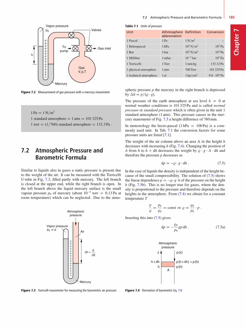
7.2 Atmospheric Pressure and Barometric Formula 185
Chap
ter7
Figure 7.2 Measurement of gas pressure with a mercury manometer
1 Pa D 1N=m2
1 standard atmosphere D 1 atm D 101 325Pa
1 torr D .1=760/ standard atmosphere D 133:3Pa :
7.2 Atmospheric Pressure andBarometric Formula
Similar to liquids also in gases a static pressure is present dueto the weight of the air. It can be measured with the TorricelliU-tube in Fig. 7.3, filled partly with mercury. The left branchis closed at the upper end, while the right branch is open. Inthe left branch above the liquid mercury surface is the smallvapour pressure p0 of mercury (about 10�3 torr D 0:13 Pa atroom temperature) which can be neglected. Due to the atmo-
Figure 7.3 Torricelli manometer for measuring the barometric air pressure
Table 7.1 Units of pressure
Unit Athmosphereabbreviation
Definition Conversion
1 Pascal 1 Pa 1N=m2 –
1 Hektopascal 1 hPa 102 N=m2 102 Pa
1 Bar 1 bar 105 N=m2 105 Pa
1 Millibar 1mbar 10�3 bar 102 Pa
1 Torricelli 1 Torr 1mmhg 133:32 Pa
1 physical atmosphere 1 atm 760Torr 101 325 Pa
1 technical atmosphere 1 at 1 kp=cm2 9:8 � 104 Pa
spheric pressure p the mercury in the right branch is depressedby �h D p=.% � g/.The pressure of the earth atmosphere at sea level h D 0 atnormal weather conditions is 101 325Pa and is called normalpressure or standard pressure which is often given in the unit 1standard atmosphere (1 atm). This pressure causes in the mer-cury manometer of Fig. 7.3 a height difference of 760mm.
In meteorology the hecto-pascal .1 hPa D 100Pa/ is a com-monly used unit. In Tab. 7.1 the conversion factors for somepressure units are listed [7.1].
The weight of the air column above an area A in the height hdecreases with increasing h (Fig. 7.4). Changing the position ofA from h to h C dh decreases the weight by % � g � A � dh andtherefore the pressure p decreases as
dp D �% � g � dh : (7.5)
In the case of liquids the density is independent of the height be-cause of the small compressibility. The solution of (7.5) showsthe linear dependence p D �% �g �h of the pressure on the heighth (Fig. 7.5b). This is no longer true for gases, where the den-sity is proportional to the pressure and therefore depends on theheights in the atmosphere. From (7.4) we obtain for a constanttemperature T
p
%D p0%0
D const ) % D %0
p0� p :
Inserting this into (7.5) gives
dp D �%0p0
gp dh : (7.5a)
Figure 7.4 Derivation of barometric Eq. 7.6
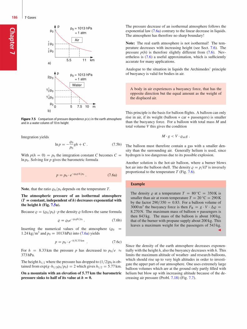
Chapter7
186 7 Gases
Figure 7.5 Comparison of pressure dependence p.s/ in the earth atmosphereand in a water column of 10m height
Integration yields
ln p D �%0p0
gh C C : (7.5b)
With p.h D 0/ D p0 the integration constant C becomes C Dln p0. Solving for p gives the barometric formula
p D p0 � e�%0g�h=p0 : (7.6a)
Note, that the ratio %0=p0 depends on the temperature T .
The atmospheric pressure of an isothermal atmosphere(T D constant, independent of h) decreases exponential withthe height h (Fig. 7.5a).
Because % D .%0=p0/ � p the density % follows the same formula
% D %0e�%0gh=p0 : (7.6b)
Inserting the numerical values of the atmosphere (%0 D1:24 kg=m3 and p0 D 1013hPa) into (7.6a) yields
p D p0 � e�h=8:33 km : (7.6c)
For h D 8:33 km the pressure p has decreased to p0=e �373 hPa.
The height h1=2 where the pressure has dropped to .1=2/p0 is ob-tained from exp.g �h1=2%0=p0/ D 2 which gives h1=2 D 5:77 km.
On a mountain with an elevation of 5:77 km the barometricpressure sinks to half of its value at h D 0.
The pressure decrease of an isothermal atmosphere follows theexponential law (7.6a) contrary to the linear decrease in liquids.The atmosphere has therefore no sharp boundary!
Note: The real earth atmosphere is not isothermal! The tem-perature decreases with increasing height (see Sect. 7.6). Thepressure p.h/ is therefore slightly different from (7.6). Nev-ertheless is (7.6) a useful approximation, which is sufficientlyaccurate for many applications.
Analogue to the situation in liquids the Archimedes’ principleof buoyancy is valid for bodies in air.
A body in air experiences a buoyancy force, that has theopposite direction but the equal amount as the weight ofthe displaced air.
This principle is the basis for balloon flights. A balloon can onlyrise in air, if its weight (balloon + car + passengers) is smallerthan the buoyancy force. For a balloon with total mass M andtotal volume V this gives the condition
M � g < V � %airg :
The balloon must therefore contain a gas with a smaller den-sity than the surrounding air. Generally helium is used, sincehydrogen is too dangerous due to its possible explosion.
Another solution is the hot-air balloon, where a burner blowshot air into the balloon shell. The density % D p=kT is inverselyproportional to the temperature T (Fig. 7.6).
Example
The density % at a temperature T D 80 ıC D 350K issmaller than air at room temperature T D 20 ıC D 290Kby the factor 290=350 D 0:83. For a balloon volume of3000m3 the buoyancy force is then FB D g � V � �% D8:270N. The maximum mass of balloon + passengers isthen 843 kg. The mass of the balloon is about 100 kg,that of the burner with propane supply about 200 kg. Thisleaves a maximum weight for the passengers of 543 kg.
J
Since the density of the earth atmosphere decreases exponen-tially with the height h, also the buoyancy decreases with h. Thislimits the maximum altitude of weather- and research-balloons,which should rise up to very high altitudes in order to investi-gate the upper part of our atmosphere. One uses extremely largeballoon volumes which are at the ground only partly filled withhelium but blow up with increasing altitude because of the de-creasing air pressure (Probl. 7.18) (Fig. 7.7).
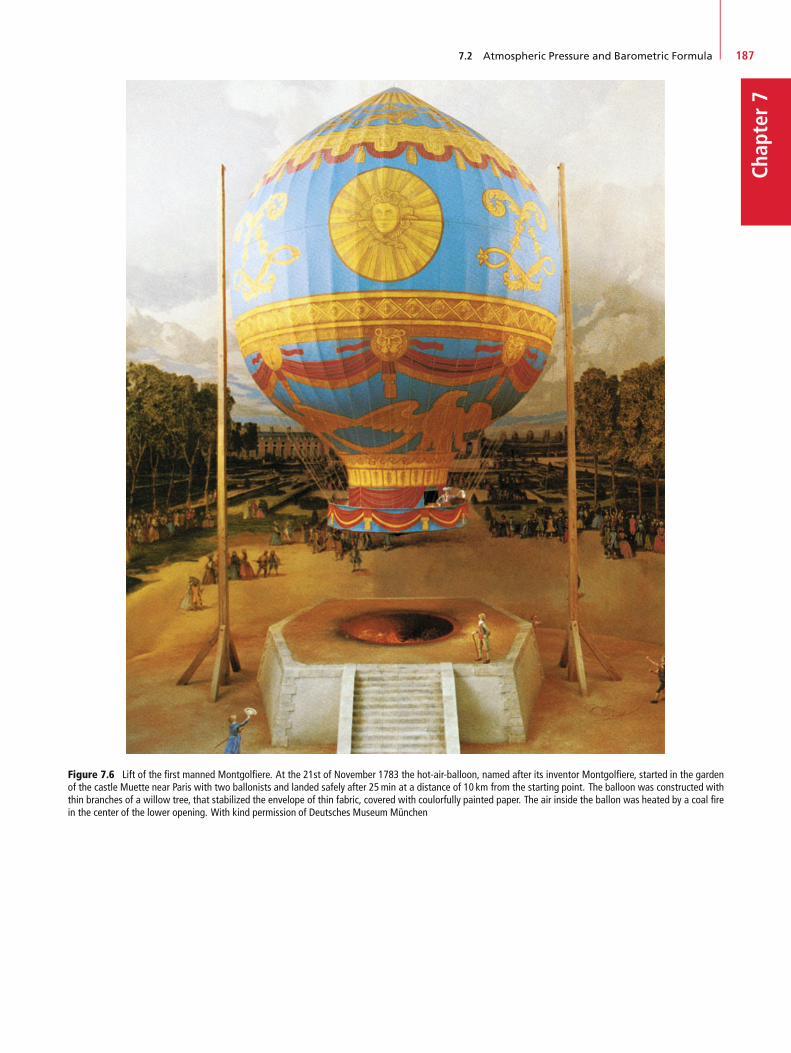
7.2 Atmospheric Pressure and Barometric Formula 187
Chap
ter7
Figure 7.6 Lift of the first manned Montgolfiere. At the 21st of November 1783 the hot-air-balloon, named after its inventor Montgolfiere, started in the gardenof the castle Muette near Paris with two ballonists and landed safely after 25min at a distance of 10 km from the starting point. The balloon was constructed withthin branches of a willow tree, that stabilized the envelope of thin fabric, covered with coulorfully painted paper. The air inside the ballon was heated by a coal firein the center of the lower opening. With kind permission of Deutsches Museum München
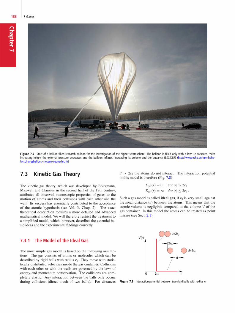
Chapter7
188 7 Gases
Figure 7.7 Start of a helium-filled research balloon for the investigation of the higher stratosphere. The balloon is filled only with a low He-pressure. Withincreasing height the external pressure decreases and the balloon inflates, increasing its volume and the buoancy (SSC/DLR) (http://www.eskp.de/turmhohe-forschungsballons-messen-ozonschicht/)
7.3 Kinetic Gas Theory
The kinetic gas theory, which was developed by Boltzmann,Maxwell and Clausius in the second half of the 19th century,attributes all observed macroscopic properties of gases to themotion of atoms and their collisions with each other and thewall. Its success has essentially contributed to the acceptanceof the atomic hypothesis (see Vol. 3, Chap. 2). The exacttheoretical description requires a more detailed and advancedmathematical model. We will therefore restrict the treatment toa simplified model, which, however, describes the essential ba-sic ideas and the experimental findings correctly.
7.3.1 The Model of the Ideal Gas
The most simple gas model is based on the following assump-tions: The gas consists of atoms or molecules which can bedescribed by rigid balls with radius r0. They move with statis-tically distributed velocities inside the gas container. Collisionswith each other or with the walls are governed by the laws ofenergy-and momentum conservation. The collisions are com-pletely elastic. Any interaction between the balls only occursduring collisions (direct touch of two balls). For distances
d > 2r0 the atoms do not interact. The interaction potentialin this model is therefore (Fig. 7.8)
Epot.r/D 0 for jrj > 2r0Epot.r/D 1 for jrj � 2r0 :
Such a gas model is called ideal gas, if r0 is very small againstthe mean distance hdi between the atoms. This means that theatomic volume is negligible compared to the volume V of thegas container. In this model the atoms can be treated as pointmasses (see Sect. 2.1).
Figure 7.8 Interaction potential between two rigid balls with radius r0

7.3 Kinetic Gas Theory 189
Chap
ter7Example
At a pressure of 1 bar and room temperature (T D 300K)1 cm3 of a gas contains about 3 � 1019 molecules. Theirmean relative distance is hdi D 3 nm. For helium atomsis r0 � 0:05 nm, which implies r0=hdi D 0:017 1.Helium at a pressure of 1 bar can be therefore regarded asideal gas. J
The pressure that the gas exerts onto the wall is caused by themomentum transfer of the atoms to the wall. The force F actingon the area A of the wall during collision of the atoms with thewall is equal to the momentum transfer per second to the area A.The pressure p D F=A is then
p D d
dt
�momentum transfer to area A
area A
�: (7.7)
If for instance N � dt atoms with mass m hit the wall within thetime interval dt with a velocity v in the direction of the surfacenormal, the momentum transfer per second for elastic collisionsis 2N � m � v and the pressure onto the wall is p D 2N � m � v=A.
7.3.2 Basic Equations of the Kinetic GasTheory
We will at first regard the atoms as point masses and only takeinto account their translational energy. The discussion of ro-tationally or vibrationally excited molecules demands a fartherreaching discussion which will be postponed to Sect. 10.2
For N molecules in a volume V the number density is n D N=V.At first we regard only that part nx of all molecules per cm3 ina cubical volume, which move with the velocity vx into the x-direction (Fig. 7.9). Within the time interval �t
Z D nx � vx � A ��t
molecules hit the surface area A. These are just those moleculesin the cuboid with length vx�t and cross section A, illustratedin Fig. 7.9. Each of these molecules transfers the momentum
Figure 7.9 Derivation of Eq. 7.8
Figure 7.10 Momentum transfer for elastic collisions with a wall
�px D 2m � vx. The force onto the area A is then F D Z ��px=�t D 2Z � m � vx=�t and the pressure onto the wall is
p D F=A D 2m � nxv2x : (7.8)
When molecules with the velocity v D fvx; vy; vzg do notmove vertically to the wall, still only the momentum 2m � vx istransferred, because the tangential components do not transfermomentum to the wall (Fig. 7.10).
Not all molecules have the same velocity. Under station-ary conditions the velocities of the molecules are isotropicallydistributed, which means that each direction has the same prob-ability. Since the pressure of a gas is isotropic, the meanmomentum transfer must be equal into all directions. The meansquare value of the velocities is�
hv2x i D v2x D 1
N
ZN.vx/ v
2x dvx D v2y D v2z ; (7.9)
where N.vx/dvx is the number of molecules in the volume Vwith the velocity components vx in the interval from vx to vx Cdvx. Because on the average half of the molecules move intothe Cx-direction and the other half into the �x-direction, thepressure, exerted by all molecules with a number density n DN=V in the x-direction on the wall in the y-z-plane is given by
p D 12n � 2mv2x D n � m � v2x : (7.10)
With v2 D v2x C v2y C v2z it follows from (7.9)
v2x D v2y D v2z D 13v
2 : (7.11)
This gives with (7.10)
p D 1
3m � nv2 D 2
3n � m
2v2 D 2
3n � Ekin ; (7.12a)
where Ekin D .m=2/ � n � v2 is the mean kinetic energy permolecule. With n D N=V this can be written as
p � V D 23N � 1
2mv2 ; (7.12b)
where N D n � V is the total number of molecules in the volumeV.
� Remark. We use for the average values of a quantity A the notations hAias well as A.
Chapter7
190 7 Gases
7.3.3 Mean Kinetic Energy and AbsoluteTemperature
All experiments give the result that the product p � V dependssolely on the temperature and is for constant temperature con-stant (Boyle–Mariotte’s law). This implies also that the meankinetic energy Ekin D .m=2/v2 depends on the temperature. Itturns out that it is convenient to define an absolute temperaturewhich is proportional to Ekin.
The absolute temperature T (with the unit 1 Kelvin D 1K) isdefined by the relation
m
2v2 D 3
2kT ; (7.13)
where k D 1:38054 � 10�23 J=K is the Boltzmann constant.
With this definition Eq. 7.12 becomes the general gas-equation
p � V D N � k � T ; (7.14)
which represents a generalization of Boyle–Mariotte’s law (7.1)and which reduces to (7.1) for T D const.
Each molecule can move into three directions x, y, and z. Thismeans it has three degrees of freedom for its translation. Col-lisions with other molecules change direction and magnitude ofits velocity. In the time-average all directions are equally prob-able. We therefore obtain for the mean square velocities therelations
˝v2x˛tD ˝v2y˛tD ˝v2z˛tD 1
3
˝v2˛tD 1
3v2 :
The mean kinetic energy of a molecule at the temperature T isthen
Ekin D 12kT per degree of freedom :
Remark. In statistical physics it is proved [7.2] that in a closedsystem of many mutually interacting particles at thermal equi-librium the time average hAit of a physical quantity A is equalto the ensemble average
A D 1
N
XAi ;
averaged over all particles of the ensemble and determined ata fixed time (ergoden hypothesis). This is however, only trueunder certain conditions, which have to be proved for each case.The “ergoden-theory” is a current field of research in mathemat-ics and statistical physics.
Real molecules can rotate and vibrate. The energy of these de-grees of freedom have to be taken into account in addition to thetranslational energy. The number of degrees of freedom there-fore becomes larger. For example diatomic molecules can rotatearound two axes perpendicular to the molecular axis. This givesthe additional energy Erot D L2=2I, where L is the angular mo-mentum of the rotation and I the inertial moment (see Sect. 5.5).
At sufficiently high temperatures also vibrations of moleculescan be excited (see Sect. 10.3) which contribute to the total en-ergy.
Equipartition Law
In a gas that is kept sufficiently long at a constant temper-ature T the energy of the atoms or molecules is uniformlydistributed by collisions over all degrees of freedom.Therefore each molecule has on the average the energyEkin D f � .1=2/kT where f is the number of degrees offreedom, accessible to the molecule.
7.3.4 Distribution Function
After the descriptive discussion of the relation between meankinetic energy and the pressure of a gas for the special case ofa cuboid container we will now give a more quantitative repre-sentation for the general case of an arbitrary volume. For thispurpose the velocity distribution has to be defined in a quanti-tative way. This can be achieved with the distribution functionf .u/ (see Sect. 1.8), which describes how the quantity u is dis-tributed among the different molecules. For u D vx we obtain
f .vx/dvx D N.vx/dvxN
with N DC1Z
�1N.vx/dvx :
(7.15)
The quantity f .vx/dvxq gives the fraction of all molecules with avelocity component vx in the interval vx to vxCdvx. The numberof all particles within the interval vx to vx C dvx is then
N.vx/dvx D N � f .vx/dvx : (7.15a)
The number of molecules with vx � u is then
N.vx � u/ D N
1Z
vxDu
f .vx/dvx : (7.15b)
From (7.15) we obtain the normalization condition
C1Z
�1f .vx/dvx D 1
N
C1Z
�1N.vx/dvx D 1 : (7.16)
For u D jvj D v the quantity f .v/dv gives the fraction of allmolecules with velocity amounts between v and v C dv. Thenormalization is now
1Z
0
f .v/dv D 1 : (7.16a)

7.3 Kinetic Gas Theory 191
Chap
ter7Unit sphere
(r = 1)F
dA
ϑ
ϑ
φ
ϑdA·cos ϑ
dϑ
dφ
1
sin ϑ dφ
dΩ = dϑ·sin ϑ·dφ
sin ϑ
Figure 7.11 Illustration of Eq. 7.17 and 7.18. Because of the small area dA and the solid angle d˝ the velocity vectors of particles hitting dA within the solidangle d˝ are approximately parallel
We consider a surface element dA, which is hit by moleculesfrom the upper half space (Fig. 7.11). Within the time interval�t the number Z of molecules within the velocity interval fromv to vCdv coming from the angular range d˝ around the angle# against the surface normal and impinging on dA is
Z D n � f .v/dv � dA cos# � v�t � d˝4
: (7.17)
This can be seen as follows: The product n � f .v/dv gives theparticle density within the velocity interval dv. Within the timeinterval�t all molecules up to a distance v ��t from the surfaceelement dA can reach dA. From all molecules with isotropicvelocity distribution only the fraction d˝=4 reaches the effec-tive area dA � cos# within the solid angle d˝ . The momentumchange j�pj of a molecule at the impact on dA is
j�pj D 2m � v � cos# :
The momentum transfer of Z molecules per sec is then
�ptotal=dt D Z � j�pj=dt : (7.17a)
Integration over all velocities v and over all impact angles #yields the total momentum transfer per sec which is equal to theproduct p � dA of pressure p acting onto dA and the area dA.
Remark. The bold vector p denotes the momentum while thescalar quantity p indicates the pressure. Although both quanti-ties are labelled with the same letter (this is in agreement withthe general convention), there should be no confusion, becauseit is clear from the text, which of the two quantities is meant.With the solid angle
d˝ D r � d# � r � sin# � d'r2
D d# � sin# � d' ; (7.18)
the pressure p can be obtained from (7.17)–(7.18) as
p Dj�pjtotaldA ��t
D 2n � m4
1Z
vD0
v2f .v/dv
2Z
'D0
=2Z
#D0
cos2 # � sin# d# d' :
(7.19)
The first integral gives the quadratic means v2. The second dou-ble integral can be analytically solved and has the solution 2=3.
This gives finally the pressure p onto the area dA
p D 13n � m � v2 ;
in accordance with (7.12a). In order to calculate the meansquare v2 we must determine the distribution function f .v/. Thiswill be the task of the next section.
7.3.5 Maxwell–Boltzmann VelocityDistribution
The decrease of the air density with increasing height in ouratmosphere (barometric formula) discussed in the previous sec-tion can be explained by the velocity distribution f .v/ of the airmolecules.
If we extend the exponent in (7.6b) with the volume V0 of agas with mass M D %0 � V0 and insert for p0 � V0 the generalgas-equation 7.14 Eq. 7.6b becomes
% D %0 � e�.Mgh/=.NkT/ : (7.20a)
For the number density n D %=m of gas molecules with mass mwe obtain with m D M=N
n.h/ D n0 � e�.mgh/=.kT/ D n0 � e�Ep=kT : (7.20b)

Chapter7
192 7 Gases
Figure 7.12 Only molecules with initial velocites Vz .h D 0/ > u reach theheight z D h
The exponent in (7.20b) represents the ratio of potential en-ergy Ep D mgh at the height h above ground and twice themean kinetic energy Ekin D .1=2/kT per degree of freedomof a molecule, due to its thermal motion at the temperatureT . We regard here at first only a one-dimensional motion inthe z-direction, which is described by the distribution of the z-components vz of the velocity v.
The barometric formula gives for an isothermal atmosphere theratio of particle densities in layers �z at different heights h. Ifthe molecules had no kinetic energy, they would all rest on theearth surface and form a solid layer, i.e. the earth atmospherewould disappear.
Let us first assume the atmosphere had been built up bymolecules that start from the ground z D 0 upwards with thevelocity vz D u. They reach the height h, given by
1
2m � u2 D m � g � h
before they fall down in the earth gravitational field (Fig. 7.12).In fact the primary earth atmosphere had been formed bymolecules outgassing through volcanos.
Since we have assumed an isothermal atmosphere, the veloc-ity distribution at z D h must be the same as for z D 0. Thismeans, there are at z D h also molecules with vz D u whichmove upwards until their kinetic energy is just cancelled by theincrease of the potential energy. The density of these moleculesis, however, smaller at z D h than at z D 0 because the num-ber density n.h/ decreases exponentially with h according to thebarometric formula (7.20b). The specific choice of the group ofmolecules starting from z D 0 does not constrict the followingargumentation.
Remark.
1. Some readers have argued that the decrease of v.z/ withincreasing z contradicts the assumption of an isothermalatmosphere. This is, however, not true, because the tem-perature is determined by the velocity distribution of allmolecules but not only by that of an arbitrarily selected sub-group.
2. In the real atmosphere the temperature decreases with in-creasing z. The main reason for that is the decreasing heatflow from the ground into the atmosphere and the decreas-ing absorption of the infrared radiation emitted by the earthsurface.
We will assume in the following an isothermal atmospherewhere collisions can be neglected, although collisions are re-sponsible for the equipartition of the total energy onto allmolecules and therefore for establishing a temperature. How-ever, this does not influence the validity of the followingderivation where we select a subgroup of all molecules with avelocity component vz in the Cz-direction which fly upwards.
The number N>u.z D 0/ of molecules that start from a unitarea at z D 0 with velocity components vz > u is equal to thenumber N>0.z D h/q of molecules that fly through a unit area inthe plane z D h with velocities vz > 0.
N>u.z D 0/ D N>0.z D h/ : (7.20c)
The number N.vz/ of molecules that pass per unit time with thevelocity vz through a unit surface (flux density) is given by theproduct
N.vz/ D n.vz/ � vz
of number density n.vz/ and velocity vz (Fig. 7.13).
For an isothermal atmosphere with the constant temperature Tthe mean square velocity v2 and the distribution function f .vz/must be independent of h, since they depend only on the tem-perature.
The flux density N>0.z D h/ can be expressed as
N�0.z D h/ D n.h/ �1Z
vzD0
vzf .vz/dvz : (7.21a)
It is smaller than the flux density
N>0.z D 0/ D n.0/
1Z
0
vzf .vz/dvz : (7.21b)
Since the two integrals in the two equations are equal, it followswith (7.20c)
Nvz>u.0/
Nvz>0.0/D Nvz>0.z D h/
Nvz>0.0/D n.h/
n.0/: (7.21c)
Figure 7.13 Number of particles per unit volume n.vz /dvz within the intervallu � vz � u C du

7.3 Kinetic Gas Theory 193
Chap
ter7
From the definition of the distribution function f .vz/ in (7.15b)and (7.15) it follows for the flux densities
Nvz�0.z D 0/ D n0
1Z
vzD0
vzf .vz/dvz
Nvz�u.z D 0/ D n0
1Z
vzDu
vzf .vz/dvz ;
(7.22)
with (7.20b) and the relation m � g � h D .1=2/m � v2 we obtain1Z
u
vzf .vz/dvz D C1 � e� m2 u
2=kT ; (7.23)
where C1 is a constant which depends on the temperature T .
Differentiating both sides with respect to the lower limit u yieldson the left side the negative integrand for vz D u:
� u � f .u/ D �m � ukT
� C1 � e� m2 u
2=kT
) f .u/ D C2 � e� m2 u
2=kT
with C2 D C1 � m
kTD const :
The constant C2 can be obtained from the normalization condi-tion Z
f .u/du D 1
and the integrationRe�x2dx D p
. This gives C2 D.m=2kT/.1=2/.
Replacing u by vz, finally yields the distribution function
f .vz/ Dr
m
2kT� e� m
2 v2z =kT : (7.24)
This is a symmetric Gauss-distribution illustrated in Fig. 7.14.
For a gas in a closed volume V, where the mean kinetic energyis large compared to the difference of potential energies inside
Figure 7.14 Distribution function f .vz / of the velocity component vz
the volume, no direction for the motion of the molecules is pre-ferred, all directions are equally probable as has been discussedin Sect. 7.3.2. The distributions of the velocity components areequal for all three components vx, vy, vz and are described by(7.24).
The probability to find a molecule with the velocity v Dfvx; vy; vzg is equal to the product of the probabilities for vx, vyand vz. One therefore obtains for the distribution function
f .vx; vy; vz/ D�
m
2kT
�.3=2/e�.mv2/=.2kT / : (7.25)
In many cases only the magnitude jvj of the velocity is of in-terest, where the direction can be arbitrary. The heads of allvelocity arrows with a length between v and v C dv are locatedwithin a spherical shell with the volume 4v2dv. Therefore theintegration Z
vx;vy;vz
f .vx; vy; vz/ dvx dvy dvz
over all values of v D fvx; vy; vzg within this spherical shellgives for the number density n.v/dv of all molecules per unitvolume with velocities between v and v C dv the result
n.v/dv D n ��
m
2kT
�.3=2/� 4v2 � e�mv2=2kTdv :
(7.26)
This is the Maxwell–Boltzmann velocity distribution(Fig. 7.15). The normalized distribution function is thenf .v/ D n.v/=n, where n is the total number density of moleculeswith any velocity.
Note
Contrary to the symmetric distribution for the velocitycomponents, which extends from �1 to 1, the distri-bution for the velocity magnitude is restricted to the rangev � 0, because there are no negative velocities. The dis-tribution is therefore asymmetric. Because of the factor v2
it is also not symmetric around a mean value v.
Figure 7.15 Maxwell–Boltzmann velocity distribution n.v/dv with most prob-able velocity vw , mean velocity hvi and the square root of the mean velocity
squarepv2
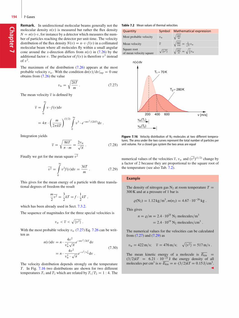
Chapter7
194 7 Gases
Remark. In unidirectional molecular beams generally not themolecular density n.v/ is measured but rather the flux densityN D n.v/�v, for instance by a detector which measures the num-ber of particles reaching the detector per unit time. The velocitydistribution of the flux density N.v/ D n �v � f .v/ in a collimatedmolecular beam where all molecules fly within a small angularcone around the x-direction differs from n.v/ in (7.26) by theadditional factor v. The prefactor of f .v/ is therefore v3 insteadof v2.
The maximum of the distribution (7.26) appears at the mostprobable velocity vw . With the condition dn.v/=dvjmp D 0 oneobtains from (7.26) the value
vw Dr
2kT
m: (7.27)
The mean velocity v is defined by
v D1Z
0
v � f .v/dv
D 4 ��
m
2kT
�.3=2/ 1Z
0
v3 � e�mv2=.2kT/dv :
Integration yields
v Dr
8kT
� m D 2vwp: (7.28)
Finally we get for the mean square v2
v2 D1Z
0
v2f .v/dv D 3kT
m: (7.29)
This gives for the mean energy of a particle with three transla-tional degrees of freedom the result
m
2v2 D 3
2kT D f � 1
2kT ;
which has been already used in Sect. 7.3.2.
The sequence of magnitudes for the three special velocities is
vw < v <p
hv2i :With the most probable velocity vw (7.27) Eq. 7.26 can be writ-ten as
n.v/dv D n � 4v2
v3wpe�mv2=2kTdv
D n � 4v2
v3w � pe�v2=v2wdv :
(7.30)
The velocity distribution depends strongly on the temperatureT . In Fig. 7.16 two distributions are shown for two differenttemperatures T1 and T2 which are related by T1=T2 D 1 W 4. The
Table 7.2 Mean values of thermal velocities
Quantity Symbol Mathematical expression
Most probable velocity vw
q2kTm
Mean velocity v
q8kTm D 2p
vw
Square rootof mean velocity square
phv2iq
3kTm D
q32vw
Figure 7.16 Velocity distribution of N2-molecules at two different tempera-tures. The area under the two curves represent the total number of particles perunit volume. For a closed gas system the two areas are equal
numerical values of the velocities v, vw and .v2/.1=2/ change bya factor of 2 because they are proportional to the square root ofthe temperature (see also Tab. 7.2).
Example
The density of nitrogen gas N2 at room temperature T D300K and at a pressure of 1 bar is
%.N2/ D 1:12 kg=m3;m.n2/ D 4:67 � 10�26 kg :
This gives
n D %=m D 2:4 � 1025 N2 molecules=m3
D 2:4 � 1019 N2 molecules=cm3 :
The numerical values for the velocities can be calculatedfrom (7.27) and (7.29) as
vw D 422m=sI v D 476m=sIp
hv2i D 517m=s :
The mean kinetic energy of a molecule is Ekin D.3=2/kT D 6:21 � 10�21 J the energy density of allmolecules per cm3 is n �Ekin D n � .3=2/kT D 0:15 J=cm3.
J
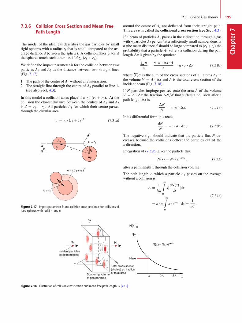
7.3 Kinetic Gas Theory 195
Chap
ter77.3.6 Collision Cross Section and Mean Free
Path Length
The model of the ideal gas describes the gas particles by smallrigid spheres with a radius ri that is small compared to the av-erage distance d between the spheres. A collision takes place ifthe spheres touch each other, i.e. if d � .r1 C r2/.
We define the impact parameter b for the collision between twoparticles A1 and A2 as the distance between two straight lines(Fig. 7.17):
1. The path of the centre of A1 without any interaction.2. The straight line through the centre of A2 parallel to line 1.
(see also Sect. 4.3).
In this model a collision takes place if b � .r1 C r2/. At thecollision the closest distance between the centres of A1 and A2
is d D r1 C r2. All particles A1 for which their centre passesthrough the circular area
� D � .r1 C r2/2 (7.31a)
Figure 7.17 Impact parameter b and collision cross section � for collisions ofhard spheres with radiii r1 and r2
N0·
N0
N0/e
N
ATotal cross section(circles) as fractionof total areaScattering volume
of gas particles
Incident particlesas point masses
∆x
σ
Figure 7.18 Illustration of collision cross section and mean free path length� [7.10]
around the centre of A2 are deflected from their straight path.This area � is called the collisional cross section (see Sect. 4.3).
If a beam of particles A1 passes in the x-direction through a gaswith n particles A2 per cm3 at a sufficiently small number densityn (the mean distance d should be large compared to .r1 C r2/ theprobability that a particle A1 suffers a collision during the pathlength �x is given by the quotient
P�
AD n � � ��x � A
AD n � � ��x (7.31b)
whereP� is the sum of the cross sections of all atoms A2 in
the volume V D A � �x and A is the total cross section of theincident beam (Fig. 7.18).
If N particles impinge per sec onto the area A of the volumeV D A � �x the fraction �N=N that suffers a collision after apath length �x is
�N
ND n � � ��x: (7.32a)
In its differential form this reads
dN
ND �n � � � dx : (7.32b)
The negative sign should indicate that the particle flux N de-creases because the collisions deflect the particles out of thex-direction.
Integration of (7.32b) gives the particle flux
N.x/ D N0 � e�n�x ; (7.33)
after a path length x through the collision volume.
The path length � which a particle A1 passes on the averagewithout a collision is
� D 1
N0
1Z
0
xjdN.x/dx
jdx
D n � �1Z
0
x � e�n�xdx D 1
n�;
(7.34a)

Chapter7
196 7 Gases
where jdN.x/=dxj � dx gives the number of collisions on the pathinterval dx. The probability of a collision in the interval dx isthen jdN.x/=N0j.The quantity � D 1=.n � �/ is called mean free path.
The mean free path � represents that path length afterwhich the number of particles in the incident beam has de-creased to 1=e of its initial value.
The average time interval � between two successive collisionscan then be defined as
� D �
hvi D 1
n�hvi : (7.34b)
If both particles A1 and A2 move with velocities v1 and v2 themean velocity hvi in (7.34b) has to be replaced by the meanrelative velocity �v D v1 � v2 D
p2v2. For collisions in a gas
at the temperature Tone then obtains instead of (7.34b) the meanfree collision time
� D 1
n � � �p2v2
: (7.34c)
Examples
1. At atmospheric pressure p D 105 Pa the numberdensity of molecules in the atmosphere is n � 3 �1019 cm�3. For the elastic collision cross section � D45 � 10�16 cm2 the mean free path is
� D 1
n � � � 7 � 10�6 cm D 70 nm :
With the mean velocity hvi D 475m=s at T D 300Kthe mean flight time between two collisions becomes
� D �p2hv2i D �
rm
6kTD 1:1 � 10�10 s :
This means that nitrogen molecules in a gas undernormal conditions (p D 105 Pa, T D 300K) suffer1:34 � 1010 collisions per second!
2. In an evacuated container with a residual pressureof p D 10�4 Pa (10�9 bar) the density is n D 3 �1010 cm�3. Now the mean free path is 70m andtherefore large compared with the dimensions of thecontainer. Collisions between molecules are seldomand the molecules fly on straight lines until they hitthe walls of the vacuum container. J
7.4 Experimental Proof of theKinetic Gas Theory
There are many experimental methods to prove the statementsof kinetic gas theory and to measure important quantities such asvelocity distribution, collision cross sections, mean free path at
different gas pressures and temperatures. We will here discussonly a few of them that are based on molecular beams or ontransport phenomena in gases such as diffusion, viscosity andheat conduction in gases.
7.4.1 Molecular Beams
When atoms or molecules effuse out of a reservoir (pressure p,volume V, temperature T) through a small hole A into a vac-uum chamber they fly on straight paths until they hit the wall, iftheir mean free path � is longer than the dimensions D of thechamber (Fig. 7.19). The pressure in the vacuum chamber mustbe low enough which can be reached with diffusion pumps (seeSect. 9.2).
Placing a slit B with width b at a distance d from A, onlymolecules can be transmitted by the slit, that fly into the an-gular range j# j < " with tan " D b=2d around the x-axis.After passing the slit they form a collimated molecular beam.For not too high pressures p in the reservoir the molecules inthe beam follow a modified Maxwell–Boltzmann-distributionN.v/ D n �v � f .v/ and the angular distribution N.#/ / N0 �cos#shows a cosine dependence. The angular distribution can bemeasured with a detector slewing over the angular range # .
With a velocity selector (Fig. 7.20) subgroups of molecules withvelocities within the range vs � .1=2/�v < v < vs C .1=2/�vcan be selected.
Such a selector consist in principal of two metallic circular discswith radius R at a distance a, each having a slit with width�S DR � �'. The two slits are twisted against each other by S DR � '. When the discs rotate with the angular velocity ! only
Figure 7.19 Schematic depiction of a molecular beam apparatus
Figure 7.20 Principle of mechanical velocity selector
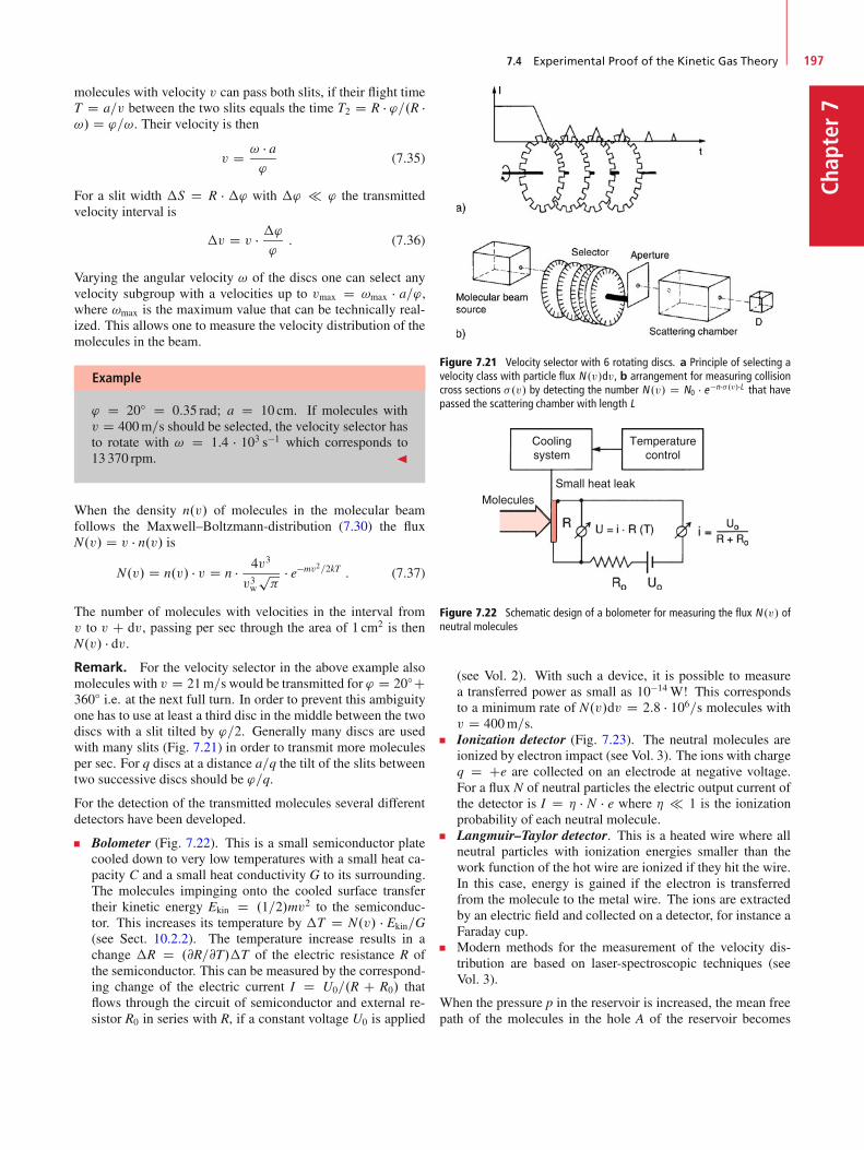
7.4 Experimental Proof of the Kinetic Gas Theory 197
Chap
ter7
molecules with velocity v can pass both slits, if their flight timeT D a=v between the two slits equals the time T2 D R � '=.R �!/ D '=!. Their velocity is then
v D ! � a'
(7.35)
For a slit width �S D R � �' with �' ' the transmittedvelocity interval is
�v D v � �''
: (7.36)
Varying the angular velocity ! of the discs one can select anyvelocity subgroup with a velocities up to vmax D !max � a=',where !max is the maximum value that can be technically real-ized. This allows one to measure the velocity distribution of themolecules in the beam.
Example
' D 20ı D 0:35 rad; a D 10 cm. If molecules withv D 400m=s should be selected, the velocity selector hasto rotate with ! D 1:4 � 103 s�1 which corresponds to13 370 rpm. J
When the density n.v/ of molecules in the molecular beamfollows the Maxwell–Boltzmann-distribution (7.30) the fluxN.v/ D v � n.v/ is
N.v/ D n.v/ � v D n � 4v3
v3wp
� e�mv2=2kT : (7.37)
The number of molecules with velocities in the interval fromv to v C dv, passing per sec through the area of 1 cm2 is thenN.v/ � dv.Remark. For the velocity selector in the above example alsomolecules with v D 21m=s would be transmitted for ' D 20ıC360ı i.e. at the next full turn. In order to prevent this ambiguityone has to use at least a third disc in the middle between the twodiscs with a slit tilted by '=2. Generally many discs are usedwith many slits (Fig. 7.21) in order to transmit more moleculesper sec. For q discs at a distance a=q the tilt of the slits betweentwo successive discs should be '=q.
For the detection of the transmitted molecules several differentdetectors have been developed.
Bolometer (Fig. 7.22). This is a small semiconductor platecooled down to very low temperatures with a small heat ca-pacity C and a small heat conductivity G to its surrounding.The molecules impinging onto the cooled surface transfertheir kinetic energy Ekin D .1=2/mv2 to the semiconduc-tor. This increases its temperature by �T D N.v/ � Ekin=G(see Sect. 10.2.2). The temperature increase results in achange �R D .@R=@T/�T of the electric resistance R ofthe semiconductor. This can be measured by the correspond-ing change of the electric current I D U0=.R C R0/ thatflows through the circuit of semiconductor and external re-sistor R0 in series with R, if a constant voltage U0 is applied
Figure 7.21 Velocity selector with 6 rotating discs. a Principle of selecting avelocity class with particle flux N .v/dv, b arrangement for measuring collisioncross sections �.v/ by detecting the number N .v/ D N0 � e�n ��.v/�L that havepassed the scattering chamber with length L
Coolingsystem
Temperaturecontrol
MoleculesSmall heat leak
Figure 7.22 Schematic design of a bolometer for measuring the flux N .v/ ofneutral molecules
(see Vol. 2). With such a device, it is possible to measurea transferred power as small as 10�14 W! This correspondsto a minimum rate of N.v/dv D 2:8 � 106=s molecules withv D 400m=s.Ionization detector (Fig. 7.23). The neutral molecules areionized by electron impact (see Vol. 3). The ions with chargeq D Ce are collected on an electrode at negative voltage.For a flux N of neutral particles the electric output current ofthe detector is I D � � N � e where � 1 is the ionizationprobability of each neutral molecule.Langmuir–Taylor detector. This is a heated wire where allneutral particles with ionization energies smaller than thework function of the hot wire are ionized if they hit the wire.In this case, energy is gained if the electron is transferredfrom the molecule to the metal wire. The ions are extractedby an electric field and collected on a detector, for instance aFaraday cup.Modern methods for the measurement of the velocity dis-tribution are based on laser-spectroscopic techniques (seeVol. 3).
When the pressure p in the reservoir is increased, the mean freepath of the molecules in the hole A of the reservoir becomes
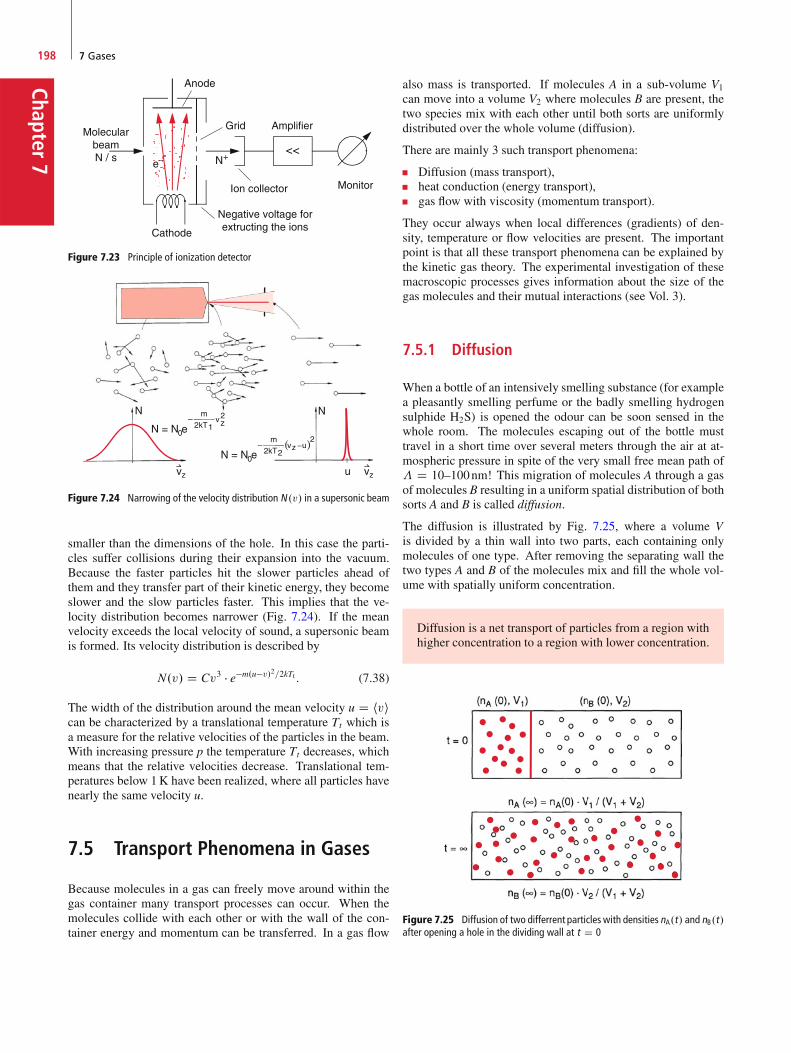
Chapter7
198 7 Gases
Figure 7.23 Principle of ionization detector
z
Figure 7.24 Narrowing of the velocity distribution N .v/ in a supersonic beam
smaller than the dimensions of the hole. In this case the parti-cles suffer collisions during their expansion into the vacuum.Because the faster particles hit the slower particles ahead ofthem and they transfer part of their kinetic energy, they becomeslower and the slow particles faster. This implies that the ve-locity distribution becomes narrower (Fig. 7.24). If the meanvelocity exceeds the local velocity of sound, a supersonic beamis formed. Its velocity distribution is described by
N.v/ D Cv3 � e�m.u�v/2=2kTt : (7.38)
The width of the distribution around the mean velocity u D hvican be characterized by a translational temperature Tt which isa measure for the relative velocities of the particles in the beam.With increasing pressure p the temperature Tt decreases, whichmeans that the relative velocities decrease. Translational tem-peratures below 1K have been realized, where all particles havenearly the same velocity u.
7.5 Transport Phenomena in Gases
Because molecules in a gas can freely move around within thegas container many transport processes can occur. When themolecules collide with each other or with the wall of the con-tainer energy and momentum can be transferred. In a gas flow
also mass is transported. If molecules A in a sub-volume V1
can move into a volume V2 where molecules B are present, thetwo species mix with each other until both sorts are uniformlydistributed over the whole volume (diffusion).
There are mainly 3 such transport phenomena:
Diffusion (mass transport),heat conduction (energy transport),gas flow with viscosity (momentum transport).
They occur always when local differences (gradients) of den-sity, temperature or flow velocities are present. The importantpoint is that all these transport phenomena can be explained bythe kinetic gas theory. The experimental investigation of thesemacroscopic processes gives information about the size of thegas molecules and their mutual interactions (see Vol. 3).
7.5.1 Diffusion
When a bottle of an intensively smelling substance (for examplea pleasantly smelling perfume or the badly smelling hydrogensulphide H2S) is opened the odour can be soon sensed in thewhole room. The molecules escaping out of the bottle musttravel in a short time over several meters through the air at at-mospheric pressure in spite of the very small free mean path of� D 10–100nm! This migration of molecules A through a gasof molecules B resulting in a uniform spatial distribution of bothsorts A and B is called diffusion.
The diffusion is illustrated by Fig. 7.25, where a volume Vis divided by a thin wall into two parts, each containing onlymolecules of one type. After removing the separating wall thetwo types A and B of the molecules mix and fill the whole vol-ume with spatially uniform concentration.
Diffusion is a net transport of particles from a region withhigher concentration to a region with lower concentration.
Figure 7.25 Diffusion of two differrent particles with densities nA.t/ and nB.t/after opening a hole in the dividing wall at t D 0
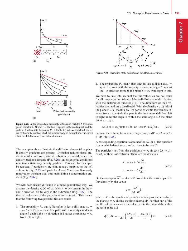
7.5 Transport Phenomena in Gases 199
Chap
ter7
Figure 7.26 a Density gradient driving the diffusion of particles A through agas of particles B . At time t D 0 a hole is opened in the dividing wall and theparticles A diffuse into the volume V2. b On the left side NA particles A per secare continuously supplied, which are pumped away on the right side. The curvesshow the distribution nA.x/ at different times ti
The examples above illustrate that diffusion always takes placeif density gradients are present. Diffusion reduces these gra-dients until a uniform spatial distribution is reached, where thedensity gradients are zero (Fig. 7.26a) unless external conditionsmaintain a stationary density gradient. This can, for example,be realized if particles A are continuously supplied to the leftvolume in Fig. 7.25 and particles A and B are simultaneouslyremoved on the right side, thus maintaining a concentration gra-dient (Fig. 7.26b).
We will now discuss diffusion in a more quantitative way. Weassume the density nA.x/ of particles A to be constant in the y-and z-direction but to vary in the x-direction (Fig. 7.27). Thethermal velocities of the particles A are isotropic. This meansthat the following two probabilities are equal:
1. The probability P� that A flies after its last collision at x� Dx0���cos# (� D mean free path) with a velocity v under anangle # against the Cx-direction and passes the plane x D x0from left to right.
Figure 7.27 Illustration of the derivation of the diffusion coefficient
2. The probability PC that A flies after its last collision at xC Dx0 C � � cos# with the velocity v under an angle # againstthe �x-direction through the plane x D x0 from right to left.
We have to take into account that the velocities are not equalfor all molecules but follow a Maxwell–Boltzmann distributionwith the distribution function f .v/. The directions of their ve-locities are randomly distributed. With the density nC.x/ left ofthe plane x D x0 the flux dNC of particles within the velocity in-terval from v to vC dv that pass in the time interval dt from leftto right under the angle # within the solid angle d˝ the planedA at x D x0 is
dNC.v/ D nCf .v/dv v dt � dA � cos# � d˝=4 ; (7.39)
because the volume from where they come, is dV D dA � cos# �v � dt (Fig. 7.28).A corresponding equation is obtained for dN�.v/. The questionis now which densities nC and n� have to be used?
The particles start from the position x D x0 ˙ �x .�x � � �cos#/ of their last collision. There are the densities
nC D n0 C�xdn
dx:
n� D n0 ��xdn
dx:
(7.40)
On the average is�x D � �cos# . We define the vertical particleflux density by the vector
j D dN
dA � dt Oe
where dN is the number of particles which pass the area dA inthe plane x D x0 during the time interval dt. For that part of thenet flux of particles with the velocity v in the interval dv withinthe solid angle d˝
dj.v/dv D � 1
dA
�dNC.v/
dt� dN�.v/
dt
�dv (7.41)

Chapter7
200 7 Gases
Figure 7.28 The number of particles passing during the time interval dtthrough the area dA inclined under the angle # against the x-direction isdn D n � f .v/ � v dv dt dA � cos#d#=4
we obtain from (7.39) with d˝ D sin# � d# � d'
djx.v/dv D �2�f .v/v dvcos2 # sin# d#d'
4
dn
dx: (7.41a)
Integration over ' gives the factor 2 , over # .0 � # � =2/the factor 1=3, while the integration over all velocities gives themean velocity
v DZv � f .v/dv : (7.42)
One obtains finally for the total mean particle flux in the x-direction
Fick’s Law:
jx D �� � v3
� dndx
D �D � dndx: (7.43)
For the general three-dimensional case this modifies to the vec-tor equation
j D �D � grad n:
The particle flux j due to diffusion is equal to the product ofdiffusion coefficient D and concentration gradient grad n.
The diffusion coefficient
D D 13� � v (7.44)
is proportional to the product of mean free path � and meanvelocity v. Using (7.34) and (7.28) we can express the diffusioncoefficient
D D � � v3
D 1
n � �
r8kT
9m(7.45)
for the diffusion of particles A through a gas of particles B withdensity n by the collision cross section � and the mass m ofparticles A. This shows that heavy particles diffuse slower thanlight ones.
This can be demonstrated by the experiment shown in Fig. 7.29.A porous cylinder of clay shows in air the same pressure insideand outside. At time t1 a baker is put over the cylinder and he-lium is blown into the baker. The pressure gauge shows at firsta higher pressure inside the cylinder, which gradually decreasesuntil it becomes equal to the pressure outside. At time t2 the
Figure 7.29 Demonstration of the fact that light particles diffuse faster thanheavy particles
baker is removed. Now the pressure inside the cylinder dropsbelow the external pressure until it finally approaches the exter-nal pressure.
The explanation is the larger diffusion velocity of the lighter he-lium atoms. It diffuses faster into the cylinder than the air in thecylinder diffuses out. The total pressure therefore increases, un-til the air has diffused out and the pressure difference betweeninside and outside becomes zero. After the baker has been re-moved there is no longer helium outside. Therefore, the heliumdiffuses from the inside of the cylinder to the outside faster thanthe air diffuses the opposite way. Therefore the pressure insidedrops at first below the outside pressure.
7.5.2 Brownian Motion
The diffusion of a microscopic particle A suffering collisionswith molecules B in a gas at atmospheric pressure can be ob-served through a microscope if the mass of A is much largerthan that of the molecules B. This can be realized with cigarettesmoke particles that have diameters of about 0:1 µm. Illuminat-ing the diffusion chamber, makes the particles A visible (even iftheir diameter is small compared to the wavelength of the illumi-nating light) because they scatter the incident light and appearin the microscope as bright spots (see Vol. 2). This particle Awhich contains still about 105 molecules, performs a randomwalk through the gas with particles B (Fig. 7.30a). When ob-serving the motion of A with sufficient local and time resolutionthe motion appears on short straight lines between successivecollisions that abruptly change the direction of the motion. Thelength of these straight lines is the mean free path length of theparticle A. The directions of the straight lines are statistically

7.5 Transport Phenomena in Gases 201
Chap
ter7
Figure 7.30 a Random path of a particle (Brownian Motion) induced by colli-sions with air molecules. b Histogram of the distribution of the mean free pathbetween successive collisions
distributed. Such a random walk can be mathematically simu-lated, if the lengths and the directions are generated by a randomgenerator. Figure 7.30b shows a histogram N.Li/ for the lengthsLi of the straight lines. Each bar indicates how often the lengthLi is observed within the interval L to L C �L. The analyticalcurve as envelope of the different bars gives the probability offinding the length L. It has the form
W.L/ D a � e�L=� : (7.46)
The random motion of microscopic particles in liquid solutionswas first discovered 1827 by the English botanist Robert Brownwho believed initially that he observed small living microbesuntil he realized that the motion was completely irregular andshould be attributed to lifeless particles. Magnified by a micro-scope and put on a large screen it allows a fascinating view intothe micro-world, accessible to a large auditorium.
The mathematical description first given by Albert Einstein willbe treated in Vol. 3.
The Brownian motion can be simulated by moving pucks on anair bearing stage, where a large number of small discs are keptin motion by vibrating wires at the 4 edges of the stage. A largerpuck with a small light bulb moves in between the small discsand its random motion is detected by a video camera. In fact,the random path in Fig. 7.30a has been obtained in this way.
7.5.3 Heat Conduction in Gases
Heat conduction is also based on the motion of molecules whichtransfer during collisions part of their kinetic energy to the col-lision partner. This results in a transport of energy from regionswith higher temperature to those of lower temperature. Themechanism of heat conduction is different for gases, liquids andsolid bodies (see Sect. 10.2). In solids the atoms are fixed todefinite positions while they can freely move in gases.
We start the discussion of heat conduction in gases with a gasbetween two parallel plates at a distance d (Fig. 7.31) that arekept at different temperatures T1 and T2. The transport of heat
dA1
T1 T2<
P1 P2v1
n1 > n2
d
v2
Figure 7.31 Heat conduction in gases. The distance d is small compared tothe extensions of the plates. A pressure sensor measures the different pressuresp1 and p2 at different sides of the sensor
energy from the hotter to the cooler plate depends on the ratio�=d of free mean path � to plate separation d.
At low gas pressures is� > d and the molecules can fly betweenthe two plates without suffering collisions in the gas volume.Molecules that leave the plate 1 have the mean kinetic energy
Ek1 D 12m � v2 D 3
2kT1
For an isotropic distribution of the velocity directions of themolecules with a density n
�Z D n cos# �A
�Zvf .v/dv
���t � d˝=4
molecules leaving plate 1 with velocities v within the solid angled˝ D sin# �d# �d' under the angle # against the surface normalreach within the time interval �t the surface element �A onplate 2 (see Fig. 7.28).
Integration over all possible velocities yields
Z D n v�A�t
4
=2Z
0
sin# cos# d#
2Z
'D0
d'
D n
4v�A with v D
1Z
0
vf .v/ dv :
(7.47)
We will assume that every molecule impinging on plate 2 willstay there for a short time, adapt the temperature of plate 2 anddesorbs again. The surface element �A of plate 1 loses energybecause of the desorbing molecules
dW1
dt�A D � Z1
�t�A � U1 ; (7.48a)
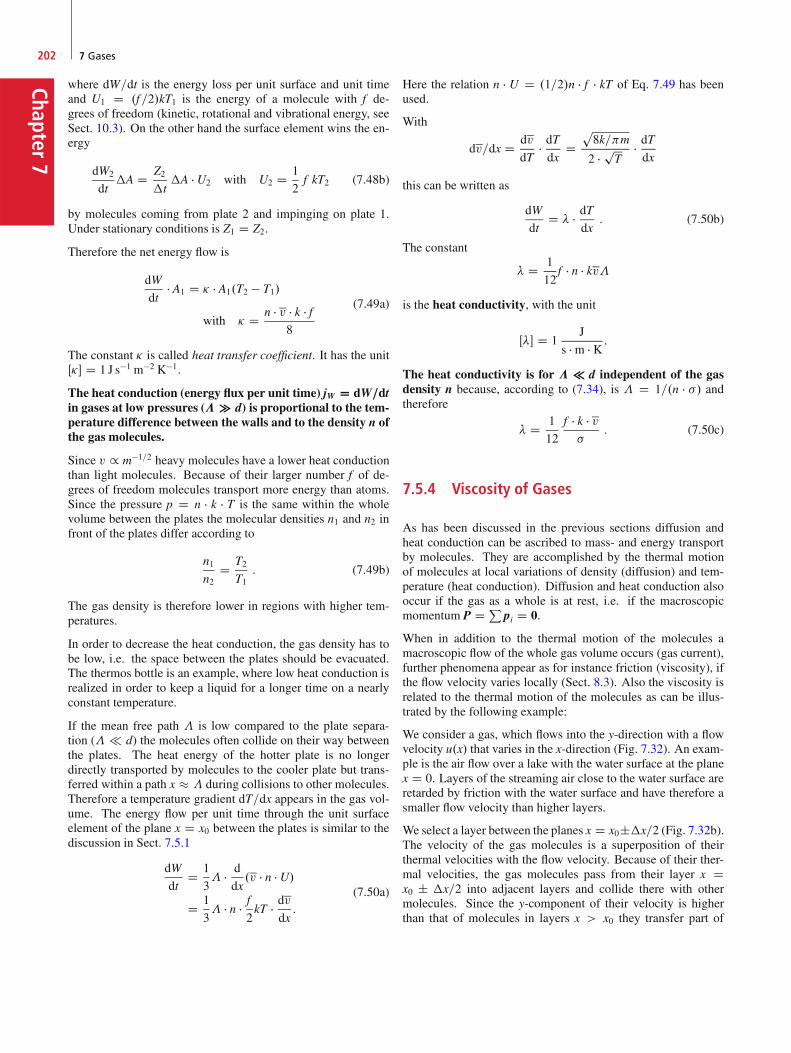
Chapter7
202 7 Gases
where dW=dt is the energy loss per unit surface and unit timeand U1 D .f =2/kT1 is the energy of a molecule with f de-grees of freedom (kinetic, rotational and vibrational energy, seeSect. 10.3). On the other hand the surface element wins the en-ergy
dW2
dt�A D Z2
�t�A � U2 with U2 D 1
2f kT2 (7.48b)
by molecules coming from plate 2 and impinging on plate 1.Under stationary conditions is Z1 D Z2.
Therefore the net energy flow is
dW
dt� A1 D � � A1.T2 � T1/
with � D n � v � k � f8
(7.49a)
The constant � is called heat transfer coefficient. It has the unitŒ�� D 1 J s�1 m�2 K�1.
The heat conduction (energy flux per unit time) jW D dW=dtin gases at low pressures (� � d) is proportional to the tem-perature difference between the walls and to the density n ofthe gas molecules.
Since v / m�1=2 heavy molecules have a lower heat conductionthan light molecules. Because of their larger number f of de-grees of freedom molecules transport more energy than atoms.Since the pressure p D n � k � T is the same within the wholevolume between the plates the molecular densities n1 and n2 infront of the plates differ according to
n1n2
D T2T1: (7.49b)
The gas density is therefore lower in regions with higher tem-peratures.
In order to decrease the heat conduction, the gas density has tobe low, i.e. the space between the plates should be evacuated.The thermos bottle is an example, where low heat conduction isrealized in order to keep a liquid for a longer time on a nearlyconstant temperature.
If the mean free path � is low compared to the plate separa-tion (� d) the molecules often collide on their way betweenthe plates. The heat energy of the hotter plate is no longerdirectly transported by molecules to the cooler plate but trans-ferred within a path x � � during collisions to other molecules.Therefore a temperature gradient dT=dx appears in the gas vol-ume. The energy flow per unit time through the unit surfaceelement of the plane x D x0 between the plates is similar to thediscussion in Sect. 7.5.1
dW
dtD 1
3� � d
dx.v � n � U/
D 1
3� � n � f
2kT � dv
dx:
(7.50a)
Here the relation n � U D .1=2/n � f � kT of Eq. 7.49 has beenused.
With
dv=dx D dv
dT� dTdx
Dp8k=m
2 � pT
� dTdx
this can be written as
dW
dtD � � dT
dx: (7.50b)
The constant
� D 1
12f � n � kv�
is the heat conductivity, with the unit
Œ�� D 1J
s � m � K :
The heat conductivity is for � � d independent of the gasdensity n because, according to (7.34), is � D 1=.n � �/ andtherefore
� D 1
12
f � k � v�
: (7.50c)
7.5.4 Viscosity of Gases
As has been discussed in the previous sections diffusion andheat conduction can be ascribed to mass- and energy transportby molecules. They are accomplished by the thermal motionof molecules at local variations of density (diffusion) and tem-perature (heat conduction). Diffusion and heat conduction alsooccur if the gas as a whole is at rest, i.e. if the macroscopicmomentum P D P
pi D 0.
When in addition to the thermal motion of the molecules amacroscopic flow of the whole gas volume occurs (gas current),further phenomena appear as for instance friction (viscosity), ifthe flow velocity varies locally (Sect. 8.3). Also the viscosity isrelated to the thermal motion of the molecules as can be illus-trated by the following example:
We consider a gas, which flows into the y-direction with a flowvelocity u.x/ that varies in the x-direction (Fig. 7.32). An exam-ple is the air flow over a lake with the water surface at the planex D 0. Layers of the streaming air close to the water surface areretarded by friction with the water surface and have therefore asmaller flow velocity than higher layers.
We select a layer between the planes x D x0˙�x=2 (Fig. 7.32b).The velocity of the gas molecules is a superposition of theirthermal velocities with the flow velocity. Because of their ther-mal velocities, the gas molecules pass from their layer x Dx0 ˙ �x=2 into adjacent layers and collide there with othermolecules. Since the y-component of their velocity is higherthan that of molecules in layers x > x0 they transfer part of
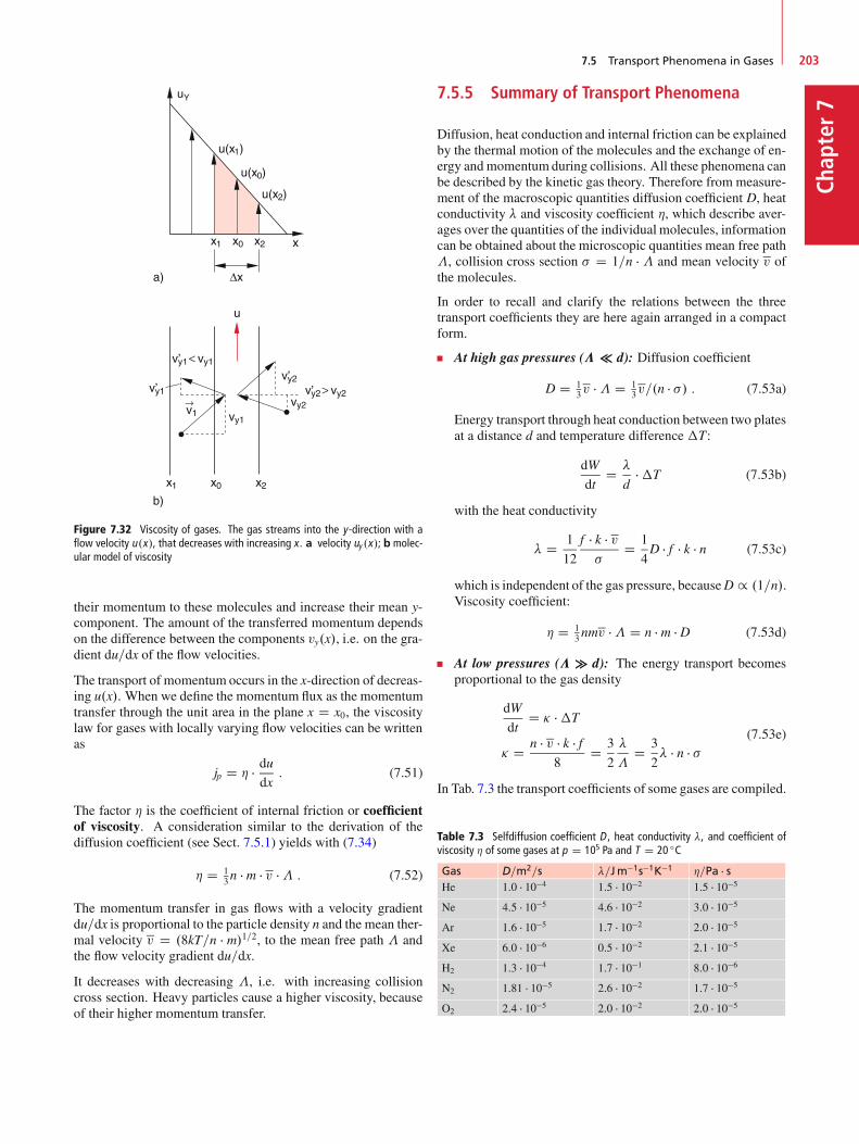
7.5 Transport Phenomena in Gases 203
Chap
ter7
Figure 7.32 Viscosity of gases. The gas streams into the y-direction with aflow velocity u.x/, that decreases with increasing x. a velocity uy .x/; b molec-ular model of viscosity
their momentum to these molecules and increase their mean y-component. The amount of the transferred momentum dependson the difference between the components vy.x/, i.e. on the gra-dient du=dx of the flow velocities.
The transport of momentum occurs in the x-direction of decreas-ing u.x/. When we define the momentum flux as the momentumtransfer through the unit area in the plane x D x0, the viscositylaw for gases with locally varying flow velocities can be writtenas
jp D � � dudx: (7.51)
The factor � is the coefficient of internal friction or coefficientof viscosity. A consideration similar to the derivation of thediffusion coefficient (see Sect. 7.5.1) yields with (7.34)
� D 13n � m � v �� : (7.52)
The momentum transfer in gas flows with a velocity gradientdu=dx is proportional to the particle density n and the mean ther-mal velocity v D .8kT=n � m/1=2, to the mean free path � andthe flow velocity gradient du=dx.
It decreases with decreasing �, i.e. with increasing collisioncross section. Heavy particles cause a higher viscosity, becauseof their higher momentum transfer.
7.5.5 Summary of Transport Phenomena
Diffusion, heat conduction and internal friction can be explainedby the thermal motion of the molecules and the exchange of en-ergy and momentum during collisions. All these phenomena canbe described by the kinetic gas theory. Therefore from measure-ment of the macroscopic quantities diffusion coefficient D, heatconductivity � and viscosity coefficient �, which describe aver-ages over the quantities of the individual molecules, informationcan be obtained about the microscopic quantities mean free path�, collision cross section � D 1=n � � and mean velocity v ofthe molecules.
In order to recall and clarify the relations between the threetransport coefficients they are here again arranged in a compactform.
At high gas pressures (� � d): Diffusion coefficient
D D 13v �� D 1
3v=.n � �/ : (7.53a)
Energy transport through heat conduction between two platesat a distance d and temperature difference �T:
dW
dtD �
d��T (7.53b)
with the heat conductivity
� D 1
12
f � k � v�
D 1
4D � f � k � n (7.53c)
which is independent of the gas pressure, becauseD / .1=n/.Viscosity coefficient:
� D 13nmv �� D n � m � D (7.53d)
At low pressures (� � d): The energy transport becomesproportional to the gas density
dW
dtD � ��T
� D n � v � k � f8
D 3
2
�
�D 3
2� � n � �
(7.53e)
In Tab. 7.3 the transport coefficients of some gases are compiled.
Table 7.3 Selfdiffusion coefficient D , heat conductivity �, and coefficient ofviscosity � of some gases at p D 105 Pa and T D 20 ıC
Gas D=m2=s �=Jm�1s�1K�1 �=Pa � sHe 1:0 � 10�4 1:5 � 10�2 1:5 � 10�5
Ne 4:5 � 10�5 4:6 � 10�2 3:0 � 10�5
Ar 1:6 � 10�5 1:7 � 10�2 2:0 � 10�5
Xe 6:0 � 10�6 0:5 � 10�2 2:1 � 10�5
H2 1:3 � 10�4 1:7 � 10�1 8:0 � 10�6
N2 1:81 � 10�5 2:6 � 10�2 1:7 � 10�5
O2 2:4 � 10�5 2:0 � 10�2 2:0 � 10�5

Chapter7
204 7 Gases
7.6 The Atmosphere of the Earth
Our atmosphere consists of a mixture of molecular and atomicgases. In the lower part it contains also water vapour, aerosolsand dust particles. Its composition is listed in Tab. 7.4. Thedensity gradient dn=dz, described by Eq. 7.6 causes diffusionwhich tries to establish a uniform density. However, the gravityacts against this tendency and results in the exponential densityfunction n.z/. Stationary equilibrium is reached, when for allvalues of z the upwards directed diffusion current jD is just com-pensated by the downwards directed current jg of particles in thegravity field of the earth
jD.z/C jg.z/ D 0 : (7.54)
The diffusion current is according to (7.43)
jD D �D � dndz:
With n D n0 � e�.mgz=kT/ ) dn=dz D �.mg=kT/ � n one obtains
jD D CD � m � gk � T � n : (7.54a)
Opposite to the gravitational force is the friction force acting onthe falling molecules. This results in a constant fall velocity vgand therefore a constant particle current
jg D n � vg : (7.55)
Since jg D �jD we obtain for the constant sink velocity
vg D �jD=n D m � gkT
� D : (7.56)
It depends on the diffusion constant D and therefore accordingto (7.44) on the mean free path �.
From (7.54) and (7.56) we obtain
�Ddn
dzD n � m � g
kT� D : (7.57)
Table 7.4 Gas composition of the earth atmosphere
Component Volume %Nitrogen N2 78.084
Oxygen O2 20.947
Argon Ar 0.934
Carbon-Dioxyd CO2 0.032
Neon Ne 0.0018
Helium He 5:2 � 10�4
Methane CH4 2 � 10�4
Krypton Kr 1:1 � 10�4
Hydrogen H2 5 � 10�5
trace gases (e.g. SO2, O3, NO2) < 5 � 10�4
Figure 7.33 Stationary density distribution n.z/ in the isothermal atmosphere,caused by the superposition of upwards diffusion and downward particle flux inthe gravitational field of the earth
Integration yields again the barometric formula
n D n0 � e�mgz=.kT/ : (7.58)
The exponential decrease of the density in the isothermalatmosphere is due to the common action of diffusion andgravitational force, namely the compensation of the upwardsdiffusion due to the density gradient and the downwardsmotion of the molecules due to the gravitation (Fig. 7.33).
The concentration ni.z/ of molecules with mass mi thereforedepends on their mass mi. For the different molecular compo-nents in the earth atmosphere a different z-dependence appears(Fig. 7.34). The density of the heavier components shoulddecrease more rapidly with increasing height than the lightercomponent. However, the measurements show that the compo-sition of the atmosphere up to altitudes of about 30 km does notchange much with the altitude. This has the following reason:The atmosphere is not isothermal but the temperature changeswith increasing altitude (Fig. 7.35). These temperature dif-ferences causes pressure differences and strong upwards anddownwards air currents which mix the different layers of the
Heavier componentm1
Lightercomponentm2
Figure 7.34 Density distribution of two molecular components with differentmasses in an atmosphere in the gravity field of the earth, if the atmosphere isgoverned by diffusion

7.6 The Atmosphere of the Earth 205
Chap
ter7
a) b)
Figure 7.35 Temperature trend T .h / in the earth atmosphere. a Measured dependence on a logarithmic scale; b Temperature trend on a linear scale. The blackcurve gives the dependence T .h / of the standard atmosphere [7.10]
atmosphere. The temperature and its dependence on z is deter-mined by the locally varying net energy flux into the differentlayers.
There are at first the absorption of the sun radiation which heatsup the atmosphere. Furthermore the absorption of the infraredradiation emitted by the earth surface contributes to the energyflux. The radiation scattered back by the atmosphere diminishesthe energy of the different parts of the atmosphere in a differentway [7.5–7.8].
In order to standardize the description of the atmosphere, amodel atmosphere was defined which serves as the standard at-mosphere [7.7]. It is divided into different layers (Fig. 7.35).Within these layers the temperature T.h/ is a defined functionwhich should be close to the measured values. Between theselayers small regions appear where the temperature is nearly con-stant. They are called “pauses”.
The troposphere extends from the ground to altitudes of about8–12 km, where the upper limit depends on the season of theyear. In the troposphere our weather takes place. The temper-ature decreases with increasing height with a slope dT=dz �6ı=km from a mean value T.z D 0/ D 17 ıC to T.z D12 km/ D �52 ıC. The nearly linear temperature decrease iscaused by the heat transport from the earth surface into the at-mosphere (convection, heat conduction and infrared radiation)which decreases nearly linear with increasing z.
Above the troposphere lies a thin layer, the tropopause, wherethe temperature stays nearly constant. The range between 10to 50 km altitudes is the stratosphere. In the lower part of thestratosphere the temperature is nearly constant. With increasing
altitude it increases up to 0 ıC. The reason for the temperatureincrease is the ozone layer between 30–50km, which containsO3-molecules that absorb the UV-radiation from the sun and areexcited into higher energy states. The excited ozone moleculescollide with other atmospheric molecules and transfer their ex-citation energy into kinetic energy of the collision partners thusraising the temperature.
Above the stratosphere lies the stratopause, followed by themesosphere between 50–80km altitude. Here the tempera-ture decreases with increasing altitude down to �93 ıC and themolecular composition changes. With increasing altitude thelighter elements prevail as shown in Fig. 7.34. Because of thelower density the collision rate is much lower than in the tropo-sphere and the mean free path is several kilometres. Thereforeair currents are less effective in mixing the different layers.
Themesopause separates the mesosphere form the higher ther-mosphere, (85 km until 500–800km) where the temperaturerises up to 1700 ıC. The temperature rise is due to collisionswith high energy particles (electrons and protons) from the sun(sun wind) which also cause the polar light phenomena (aurorapolaris). The density decreases down to 10�6 Pa D 10�11 bar. Inspite of the low density, friction effects are-non negligible. Theinternational space station ISS in about 350 km above groundflies through the thermosphere and it has to be lifted from timeto time, because it loses kinetic energy and therefore altitude dueto friction. The extreme ultraviolet radiation and the solar windcause dissociation and ionization of the atmospheric molecules.Part of the components in the thermosphere are therefore ions.The thermosphere is part of a larger range in the atmospherecalled the ionosphere which extends far into the space around

Chapter7
206 7 Gases
Figure 7.36 Dependence of pressure p.h / and density n.h / on a logarithmicscale [7.11]
the earth. It is no longer spherical symmetric because the mag-netic field of the earth influences the path of charged particles(see Vol. 2) which move on spiral paths around the magneticfield lines. The variation of the temperature T.h/ with increas-ing height h implicates that density n.h/ and pressure p.h/ areno longer strictly proportional (Fig. 7.36).
The evaporation and condensation of water plays an importantrole in the lower atmosphere. Also the spurious concentrationsof molecules with dipole moment such as OH, CO, CO2, NH4
etc. and dust particles and other aerosols have a pronouncedinfluence on the weather conditions in the troposphere. TheChemistry of the atmosphere based on reaction of the differ-ent species by collisions with each other, is a subject of intenseresearch and there are still many open questions [7.3a–7.5].
Summary
For a constant temperature the pressure p of a gas in aclosed but variable volume V obeys the Boyle–Mariotte law:p � V D constThe air pressure in an isothermal atmosphere decreasesexponential with the altitude h above ground, due to the grav-itational force.For the particle density n.h/ holds:
N.h/ D n.0/ � expŒ�mgh=kT� :
Without mixing effects in the atmosphere the concentrationof particles with larger mass m therefore decreases fasterwith h than for those with lighter mass.The real earth atmosphere in not isothermal. Due to up-wards and downwards air currents the different layers of theatmosphere are mixed which leads to an equilibrium of theconcentrations of different masses.The kinetic gas theory explains the macroscopic featuresof gases such as pressure and temperature by the averagemomentum and the kinetic energy of the gas molecules.With the Boltzmann constant k the mean kinetic energy ofmolecules with mass m is related to the temperature T by.1=2/mv2 D .3=2/kT .The velocity distribution n.v/ of gas molecules at ther-mal equilibrium is the Maxwell–Boltzmann distributionn.v/dv D v2 � expŒ�.1=2/mv2=kT�dv for the magnitudev D jvj of the velocity. The distribution n.vi/, .i D x; y; z/ ofthe velocity components vi is a Gaussian function, symmet-ric to vi D 0.These distributions can be experimentally determined inmolecular beams using mechanical velocity selectors. The
molecular beams are formed by expanding a gas from a reser-voir through a small hole into the vacuum, where the meanfree path is longer than the dimensions of the vacuum cham-ber. The beam can be collimated by small apertures whichtransmit only molecules with small transverse velocities.Always when gradients of concentrations in a gas exist,diffusion processes occur which try to equalize the concen-trations. The mean diffusion particle flux jD D �D � grad nis proportional to the gradient of the particle density n. Thediffusion constant D depends on the kind of particles. Dif-fusion causes a mass transport from regions of high particledensity n to those of low density.If velocity gradient in a gas flow appear, viscosity causes mo-mentum transfer from particles with higher flow velocity tothose with lower velocity.If temperature gradients appear in a gas, energy is transportedby diffusing molecules from regions of higher temperature tothose of lower temperature. For a one-dimensional tempera-ture gradient dT=dx the transferred heat power is dW=dt D� � dT=dx. The heat conductivity � depends on the particledensity n, the mean velocity v, and the mean free path �.The density distribution n.h/ in the atmosphere is determinedby the common action of gravitational attraction of the airmolecules by the earth and the diffusion current from regionswith higher density to those with lower density. In the realearth atmosphere furthermore vertical and horizontal air cur-rents occur caused by local heat sources due to absorption ofsun radiation and infrared radiation from the earth surface.This convection leads to a mixing of different layers in thelower atmosphere.
Problems 207
Chap
ter7
Problems
7.1 What would be the density distribution in the atmo-sphere, if the dependence of the gravitational force on thealtitude is taken into account?
7.2 At which altitude exists, according to (7.6), a pressureof 1mbar, if the constant value T D 300K is assumed for thetemperature T.h/?
7.3 Calculate from (7.6) the pressure at h D 100 km and thedensity n for T D 250K.
7.4 A balloon with V D 3000m3 floats at h D 1000m anda temperature of 20 ıC. What is the maximum weight of bal-loon with ballast mass and passengers (without the weight ofthe filling gas) if one uses as filling gasa) heliumb) hydrogen gas H2
at a pressure equal to the external air pressure.(%air D 1:293 kg=m3, %He D 0:1785 kg=m3, %H2 D 0:09 kg=m3
at T D 20 ıC and p D 105 Pa).
7.5 A shop for diving equipment offers for measuring thediving depth a glass tube with movable piston that compresses agas volume V D A � x. Down to which depth is the uncertaintyof the device �z � 1m if the piston edge can be read with anaccuracy of 1mm and x.p0/ D 0:2m.
7.6 Which fraction of all gas molecules has a free path thatis larger thana) the mean free path �b) 2�?
7.7 Calculate the probability that N2-molecules in a gas atT D 300K have velocities within the interval 900m=s � v �1000m=s. What is the total number N.v/ of molecules with ve-locities within this interval in a volume V D 1m3 at T D 300Kand p D 105 Pa?
7.8 What is the thickness �z of an isothermal atmosphericlayer at T D 280K between the altitudes z1 and z2 with p.z1/ D1000 hPa and p.z2/ D 900 hPa?
7.9 What is the square root of the mean square relative ve-locities between two gas moleculesa) for a Maxwell distributionb) if the magnitudes of all velocities are equal but the directions
uniformly distributed?
7.10 The mean free path � in a gas at p D 105 Pa andT D 20 ıC is for argon atoms �Ar D 1 � 10�7 m and for N2
molecules �N2 D 2:7 � 10�7 m.a) What are the collision cross sections �Ar and �N2?b) How large are the mean times between two successive colli-
sions?
7.11 In a container is 0:1 kg helium at p D 105 Pa and T D300K. Calculatea) the number of He-atoms,b) the mean free path �,c) the sum
PSi of all path lengths Si which is passed by all
molecules in 1 s. Give this sum in the unitsm and light years.
7.12 The rotating disc of a velocity selector with a slit allowsN2 molecules with a Maxwellian distribution at T D 500K topass for a time interval �t D 10�3 s. A detector at 1m distancefrom the disc measures the time distribution of the molecules.What is the half width of this distribution?
7.13 What is the minimum velocity of a helium atom at100 km above ground for leaving the earth into space? At whichtemperature would half of the N2-molecules above 100 km alti-tude escape into space?
7.14 The exhaust gases of a factory escaping out of a 50mhigh smokestack have the density % D 0:85 kg=m3. How largeis the pressure difference at the base of the smokestack to thatof the surrounding air with %air D 1:29 kg=m3?
7.15 Up to which volume a children’s balloon (m = 10g) hasto be blown and filled with helium at a pressure of 1.5 bar, inorder to let it float in air?
7.16 In the centre of the sun the density of protons and elec-trons is estimated as n D 5 � 1029=m3 at a temperature of1:5 � 107 K.a) What is the mean kinetic energy of electrons and protons?
Compare this with the ionization energy of the hydrogenatom (Eion D 13:6 eV).
b) What are the mean velocities?c) How large is the pressure?
7.17 Determine the total mass of the earth atmosphere fromthe pressure p D 1 atm D 1013hPa the atmosphere exerts ontothe earth surface.
7.18 A research balloon has without filling a mass m D300 kg. How large must be the volume of helium inside theballoon to let it rise up if the helium pressure at any height isalways 0.1 bar higher than that of the surrounding air? (T.h D0/ D 300K, T.h D 20 km/ D 217K)
7.19 What would be the height of the earth atmospherea) if the atmosphere is compressed with a pressure at the up-
per edge (assumed to be sharp) of 10 atm at a temperature of300K?
b) at T D 0K where all gases are solidified?
Chapter7
208 7 Gases
References
7.1. L.F. Reichl, A Modern Course in Statistical Physics. (Wi-ley VCH, Weinheim, 2016)
7.2. M. Scott Shell, Thermodynamics and Statistical Mechan-ics. (Cambridge Series in Chemical Engineering, 2015)
7.3a. R.P. Wayne, Chemistry of the Atmosphere. (Oxford Sci-ence Publ., Oxford Univ. Press, 1991)
7.3b. S. Kshudiram, The Earth Atmosphere. (Springer, Berlin,Heidelberg, 2008)
7.4. St.E. Manahan, Enviromental Chemistry. (CRC Press,2009)
7.5. T.E. Graedel, P. Crutzen, Atmospheric Change: An EarthSystem Perspective. (Freeman and Co., 1993)
7.6. J.M. Wallace, P.V. Hobbs, Atmospheric Science. (Aca-demic Press, 2006)
7.7. US Standard Atmosphere. (Government Printing Of-fice, Washington, 1976) https://en.wikipedia.org/wiki/U.S._Standard_Atmosphere
7.8. C.D. Ahrens, Essentials of Metereology. (ThomsonBroodge, 2011)
7.9a. St.A. Ackerman, J.A. Knox,Metereology: Understandingthe Atmosphere. (Jones & Bartlett Learning, 2011)
7.9b. Ch. Taylor-Butler, Metereology: The Study of Weather.(Scholastic, 2012)
7.10. P. Staub, Physics. (TU Wien)7.11. https://en.wikipedia.org/wiki/Atmosphere_of_Earth
Chap
ter8
Liquids and Gases in Motion;Fluid Dynamics 88.1 Basic Definitions and Types of Fluid Flow . . . . . . . . . . . . . . . . . 210
8.2 Euler Equation for Ideal Liquids . . . . . . . . . . . . . . . . . . . . . . 212
8.3 Continuity Equation . . . . . . . . . . . . . . . . . . . . . . . . . . . . . 212
8.4 Bernoulli Equation . . . . . . . . . . . . . . . . . . . . . . . . . . . . . . 213
8.5 Laminar Flow . . . . . . . . . . . . . . . . . . . . . . . . . . . . . . . . . 216
8.6 Navier–Stokes Equation . . . . . . . . . . . . . . . . . . . . . . . . . . . 220
8.7 Aerodynamics . . . . . . . . . . . . . . . . . . . . . . . . . . . . . . . . . 226
8.8 Similarity Laws; Reynolds’ Number . . . . . . . . . . . . . . . . . . . . 228
8.9 Usage of Wind Energy . . . . . . . . . . . . . . . . . . . . . . . . . . . . 229
Summary . . . . . . . . . . . . . . . . . . . . . . . . . . . . . . . . . . . . 233
Problems . . . . . . . . . . . . . . . . . . . . . . . . . . . . . . . . . . . . 234
References . . . . . . . . . . . . . . . . . . . . . . . . . . . . . . . . . . . 235
209© Springer International Publishing Switzerland 2017W. Demtröder, Mechanics and Thermodynamics, Undergraduate Lecture Notes in Physics, DOI 10.1007/978-3-319-27877-3_8
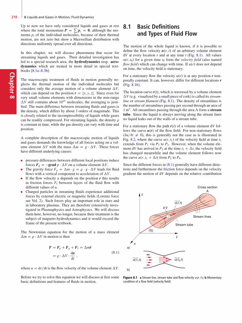
Chapter8
210 8 Liquids and Gases in Motion; Fluid Dynamics
Up to now we have only considered liquids and gases at restwhere the total momentum P D P
pi D 0, although the mo-menta pi of the individual molecules, because of their thermalmotion, are not zero but show a Maxwellian distribution withdirections uniformly spread over all directions.
In this chapter, we will discuss phenomena that occur forstreaming liquids and gases. Their detailed investigation hasled to a special research area, the hydrodynamics resp. aero-dynamics which are treated in more detail in special text-books [8.1a–8.3b].
The macroscopic treatment of fluids in motion generally ne-glects the thermal motion of the individual molecules butconsiders only the average motion of a volume element �V,which can depend on the position r D fx; y; zg. Since even forvery small volume elements with dimensions in the mm-range�V still contains about 1015 molecules, the averaging is justi-fied. The main difference between streaming fluids and gases isthe density, which differs by about 3 orders of magnitude. Thisis closely related to the incompressibility of liquids while gasescan be readily compressed. For streaming liquids, the density %is constant in time, while the gas density can vary with time andposition.
A complete description of the macroscopic motion of liquidsand gases demands the knowledge of all forces acting on a vol-ume element �V with the mass �m D % � �V. These forceshave different underlying causes:
pressure differences between different local positions induceforces Fp D �grad p ��V on a volume element�V.The gravity force Fg D �m � g D % � g � �V leads for fluidflows with a vertical component to acceleration of�V.If the flow velocity u depends on the position r this resultsin friction forces Ff between layers of the fluid flow withdifferent values of u.Charged particles in streaming fluids experience additionalforces by external electric or magnetic fields (Lorentz forcesee Vol. 2). Such forces play an important role in stars andin laboratory plasmas. They are therefore extensively inves-tigated in Plasmaphysics and Astrophysics. We will discussthem here, however, no longer, because their treatment is thesubject of magneto-hydrodynamics and it would exceed theframe of the present textbook.
The Newtonian equation for the motion of a mass element�m D % ��V in motion is then
F D Fp C Fg C Ff D �mRrD % ��V � du
dt;
(8.1)
where u D dr=dt is the flow velocity of the volume element�V.
Before we try to solve this equation we will discuss at first somebasic definitions and features of fluids in motion.
8.1 Basic Definitionsand Types of Fluid Flow
The motion of the whole liquid is known, if it is possible todefine the flow velocity u.r; t/ of an arbitrary volume elementdV at every location r and at any time t (Fig. 8.1). All valuesu.r; t0/ for a given time t0 form the velocity field (also namedflow field) which can change with time. If u.r/ does not dependon time, the velocity field is stationary.
For a stationary flow the velocity u.r/ is at any position r tem-porally constant. It can, however, differ for different locations r(Fig. 8.1b).
The location curve r.t/, which is traversed by a volume element�V (e.g. visualized by a small piece of cork) is called its stream-line or stream filament (Fig. 8.1). The density of streamlines isthe number of streamlines passing per second through an area of1m2. All streamlines passing through the area A form a streamtube. Since the liquid is always moving along the stream linesno liquid leaks out of the walls of a stream tube.
For a stationary flow the path r.t/ of a volume element dV fol-lows the curve u.r/ of the flow field. For non-stationary flows(@u=@t ¤ 0), this is generally not the case as is illustrated inFig. 8.2, where the curve u.r; t1/ of the velocity field at time t1extends from P1 via P2 to P3. However, when the volume ele-ment dV has arrived in P2 at the time t1 C�t, the velocity fieldhas changed meanwhile and the volume element follows nowthe curve u.r; t1 C�t/ from P2 to P4.
Since the different forces in (8.1) generally have different direc-tions and furthermore the friction force depends on the velocitygradient the motion of dV depends on the relative contribution
Figure 8.1 a Stream line, stream tube and flow velocity u.r; t/; bMomentarycondition of a flow field (velocity field)
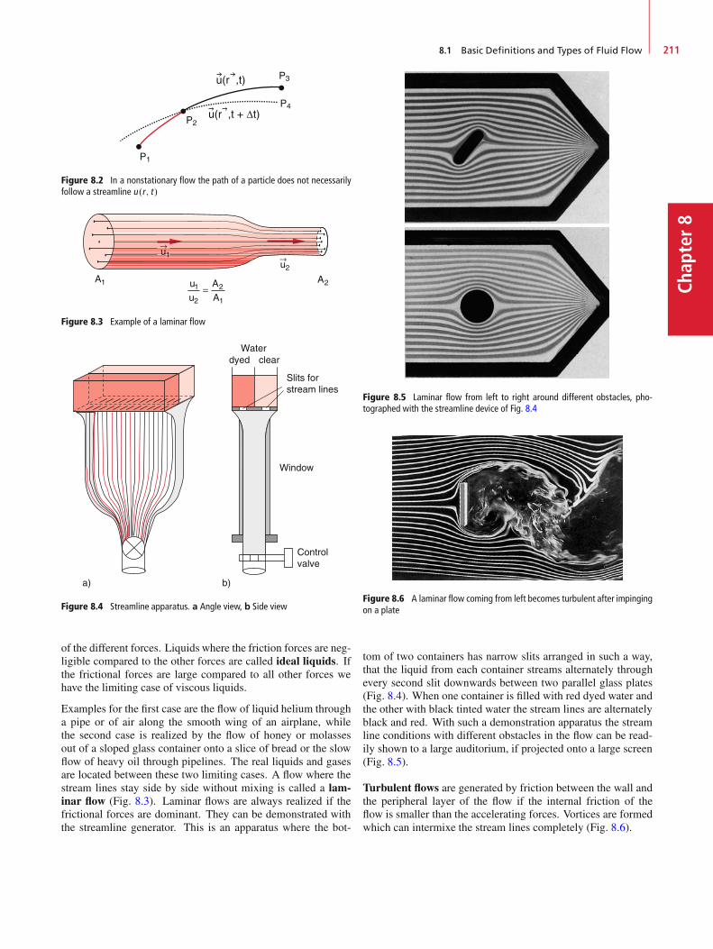
8.1 Basic Definitions and Types of Fluid Flow 211
Chap
ter8
Figure 8.2 In a nonstationary flow the path of a particle does not necessarilyfollow a streamline u.r ; t/
Figure 8.3 Example of a laminar flow
Figure 8.4 Streamline apparatus. a Angle view, b Side view
of the different forces. Liquids where the friction forces are neg-ligible compared to the other forces are called ideal liquids. Ifthe frictional forces are large compared to all other forces wehave the limiting case of viscous liquids.
Examples for the first case are the flow of liquid helium througha pipe or of air along the smooth wing of an airplane, whilethe second case is realized by the flow of honey or molassesout of a sloped glass container onto a slice of bread or the slowflow of heavy oil through pipelines. The real liquids and gasesare located between these two limiting cases. A flow where thestream lines stay side by side without mixing is called a lam-inar flow (Fig. 8.3). Laminar flows are always realized if thefrictional forces are dominant. They can be demonstrated withthe streamline generator. This is an apparatus where the bot-
Figure 8.5 Laminar flow from left to right around different obstacles, pho-tographed with the streamline device of Fig. 8.4
Figure 8.6 A laminar flow coming from left becomes turbulent after impingingon a plate
tom of two containers has narrow slits arranged in such a way,that the liquid from each container streams alternately throughevery second slit downwards between two parallel glass plates(Fig. 8.4). When one container is filled with red dyed water andthe other with black tinted water the stream lines are alternatelyblack and red. With such a demonstration apparatus the streamline conditions with different obstacles in the flow can be read-ily shown to a large auditorium, if projected onto a large screen(Fig. 8.5).
Turbulent flows are generated by friction between the wall andthe peripheral layer of the flow if the internal friction of theflow is smaller than the accelerating forces. Vortices are formedwhich can intermixe the stream lines completely (Fig. 8.6).
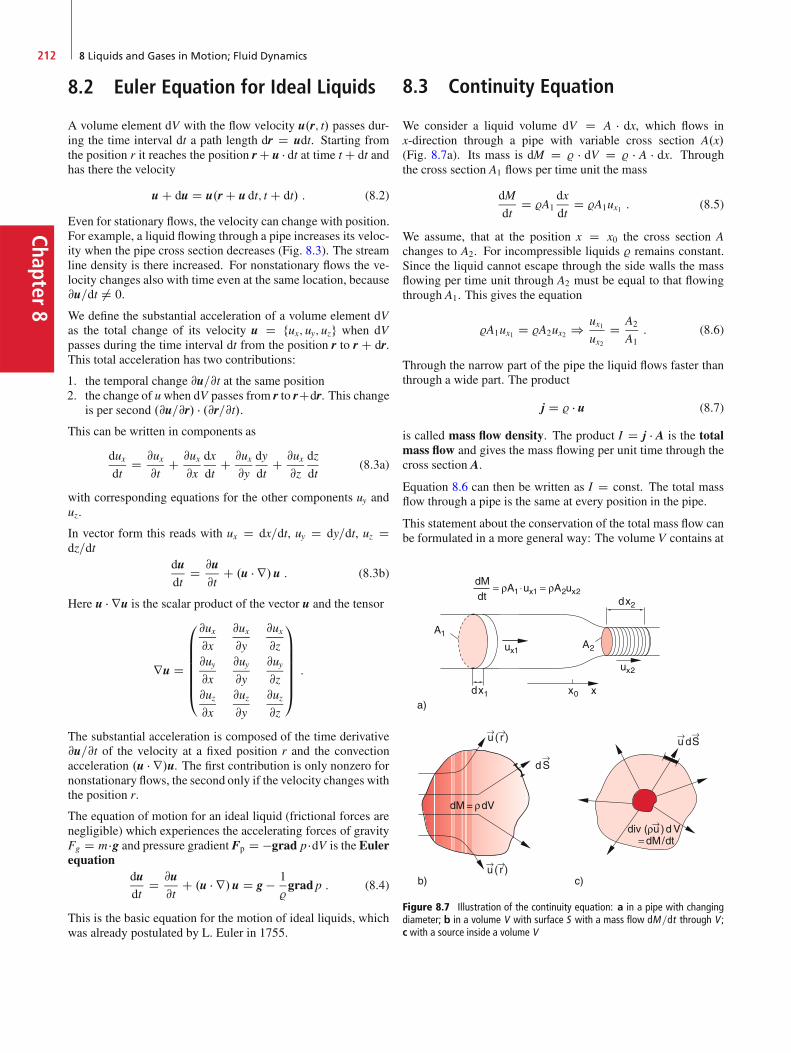
Chapter8
212 8 Liquids and Gases in Motion; Fluid Dynamics
8.2 Euler Equation for Ideal Liquids
A volume element dV with the flow velocity u.r; t/ passes dur-ing the time interval dt a path length dr D udt. Starting fromthe position r it reaches the position rC u � dt at time t C dt andhas there the velocity
u C du D u.r C u dt; t C dt/ : (8.2)
Even for stationary flows, the velocity can change with position.For example, a liquid flowing through a pipe increases its veloc-ity when the pipe cross section decreases (Fig. 8.3). The streamline density is there increased. For nonstationary flows the ve-locity changes also with time even at the same location, because@u=dt ¤ 0.
We define the substantial acceleration of a volume element dVas the total change of its velocity u D fux; uy; uzg when dVpasses during the time interval dt from the position r to r C dr.This total acceleration has two contributions:
1. the temporal change @u=@t at the same position2. the change of uwhen dV passes from r to rCdr. This change
is per second .@u=@r/ � .@r=@t/.This can be written in components as
duxdt
D @ux@t
C @ux@x
dx
dtC @ux@y
dy
dtC @ux
@z
dz
dt(8.3a)
with corresponding equations for the other components uy anduz.
In vector form this reads with ux D dx=dt, uy D dy=dt, uz Ddz=dt
dudt
D @u@t
C .u � r/u : (8.3b)
Here u � ru is the scalar product of the vector u and the tensor
ru D
0
BBBBBB@
@ux@x
@ux@y
@ux@z
@uy@x
@uy@y
@uy@z
@uz@x
@uz@y
@uz@z
1
CCCCCCA:
The substantial acceleration is composed of the time derivative@u=@t of the velocity at a fixed position r and the convectionacceleration .u � r/u. The first contribution is only nonzero fornonstationary flows, the second only if the velocity changes withthe position r.
The equation of motion for an ideal liquid (frictional forces arenegligible) which experiences the accelerating forces of gravityFg D m �g and pressure gradient Fp D �grad p �dV is the Eulerequation
dudt
D @u@t
C .u � r/u D g � 1
%grad p : (8.4)
This is the basic equation for the motion of ideal liquids, whichwas already postulated by L. Euler in 1755.
8.3 Continuity Equation
We consider a liquid volume dV D A � dx, which flows inx-direction through a pipe with variable cross section A.x/(Fig. 8.7a). Its mass is dM D % � dV D % � A � dx. Throughthe cross section A1 flows per time unit the mass
dM
dtD %A1
dx
dtD %A1ux1 : (8.5)
We assume, that at the position x D x0 the cross section Achanges to A2. For incompressible liquids % remains constant.Since the liquid cannot escape through the side walls the massflowing per time unit through A2 must be equal to that flowingthrough A1. This gives the equation
%A1ux1 D %A2ux2 ) ux1ux2
D A2
A1: (8.6)
Through the narrow part of the pipe the liquid flows faster thanthrough a wide part. The product
j D % � u (8.7)
is called mass flow density. The product I D j � A is the totalmass flow and gives the mass flowing per unit time through thecross section A.
Equation 8.6 can then be written as I D const. The total massflow through a pipe is the same at every position in the pipe.
This statement about the conservation of the total mass flow canbe formulated in a more general way: The volume V contains at
Figure 8.7 Illustration of the continuity equation: a in a pipe with changingdiameter; b in a volume V with surface S with a mass flow dM=dt through V ;c with a source inside a volume V
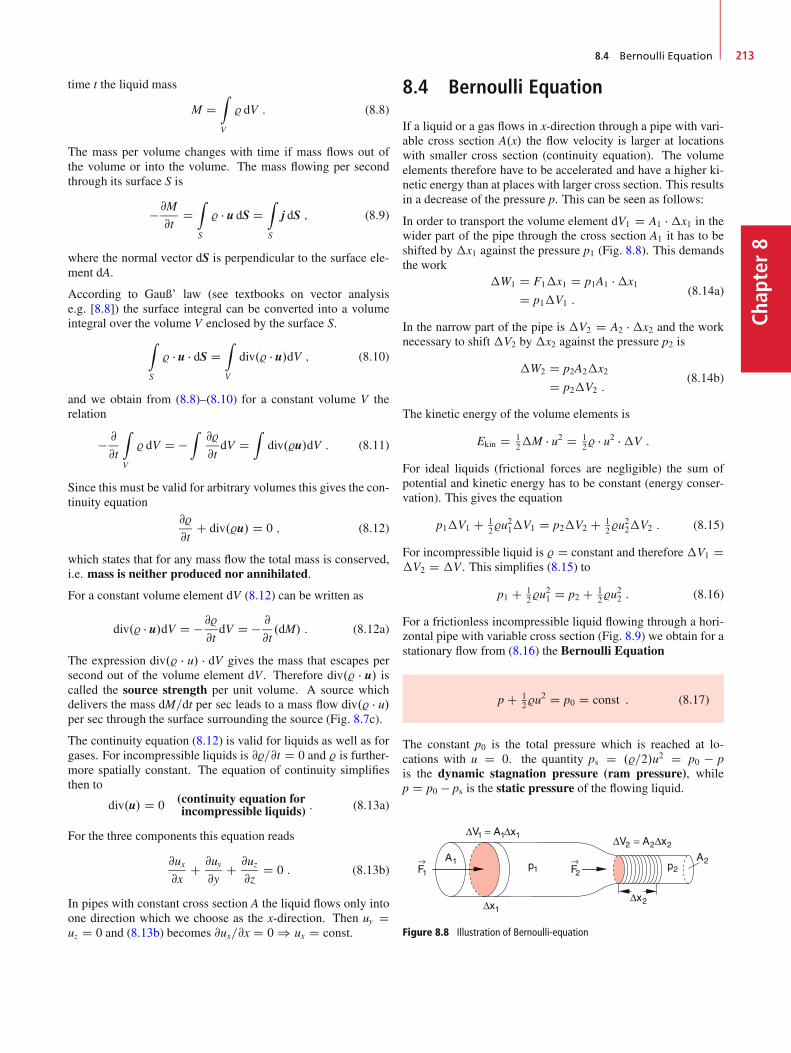
8.4 Bernoulli Equation 213
Chap
ter8
time t the liquid mass
M DZ
V
% dV : (8.8)
The mass per volume changes with time if mass flows out ofthe volume or into the volume. The mass flowing per secondthrough its surface S is
�@M@t
DZ
S
% � u dS DZ
S
j dS ; (8.9)
where the normal vector dS is perpendicular to the surface ele-ment dA.
According to Gauß’ law (see textbooks on vector analysise.g. [8.8]) the surface integral can be converted into a volumeintegral over the volume V enclosed by the surface S.
Z
S
% � u � dS DZ
V
div.% � u/dV ; (8.10)
and we obtain from (8.8)–(8.10) for a constant volume V therelation
� @
@t
Z
V
% dV D �Z@%
@tdV D
Zdiv.%u/dV : (8.11)
Since this must be valid for arbitrary volumes this gives the con-tinuity equation
@%
@tC div.%u/ D 0 ; (8.12)
which states that for any mass flow the total mass is conserved,i.e. mass is neither produced nor annihilated.
For a constant volume element dV (8.12) can be written as
div.% � u/dV D �@%@t
dV D � @
@t.dM/ : (8.12a)
The expression div.% � u/ � dV gives the mass that escapes persecond out of the volume element dV. Therefore div.% � u/ iscalled the source strength per unit volume. A source whichdelivers the mass dM=dt per sec leads to a mass flow div.% � u/per sec through the surface surrounding the source (Fig. 8.7c).
The continuity equation (8.12) is valid for liquids as well as forgases. For incompressible liquids is @%=@t D 0 and % is further-more spatially constant. The equation of continuity simplifiesthen to
div.u/ D 0 (continuity equation forincompressible liquids) : (8.13a)
For the three components this equation reads
@ux@x
C @uy@y
C @uz@z
D 0 : (8.13b)
In pipes with constant cross section A the liquid flows only intoone direction which we choose as the x-direction. Then uy Duz D 0 and (8.13b) becomes @ux=@x D 0 ) ux D const.
8.4 Bernoulli Equation
If a liquid or a gas flows in x-direction through a pipe with vari-able cross section A.x/ the flow velocity is larger at locationswith smaller cross section (continuity equation). The volumeelements therefore have to be accelerated and have a higher ki-netic energy than at places with larger cross section. This resultsin a decrease of the pressure p. This can be seen as follows:
In order to transport the volume element dV1 D A1 � �x1 in thewider part of the pipe through the cross section A1 it has to beshifted by �x1 against the pressure p1 (Fig. 8.8). This demandsthe work
�W1 D F1�x1 D p1A1 ��x1D p1�V1 :
(8.14a)
In the narrow part of the pipe is �V2 D A2 � �x2 and the worknecessary to shift �V2 by �x2 against the pressure p2 is
�W2 D p2A2�x2D p2�V2 :
(8.14b)
The kinetic energy of the volume elements is
Ekin D 12�M � u2 D 1
2% � u2 ��V :
For ideal liquids (frictional forces are negligible) the sum ofpotential and kinetic energy has to be constant (energy conser-vation). This gives the equation
p1�V1 C 12%u
21�V1 D p2�V2 C 1
2%u22�V2 : (8.15)
For incompressible liquid is % D constant and therefore �V1 D�V2 D �V. This simplifies (8.15) to
p1 C 12%u
21 D p2 C 1
2%u22 : (8.16)
For a frictionless incompressible liquid flowing through a hori-zontal pipe with variable cross section (Fig. 8.9) we obtain for astationary flow from (8.16) the Bernoulli Equation
p C 12%u
2 D p0 D const : (8.17)
The constant p0 is the total pressure which is reached at lo-cations with u D 0. the quantity ps D .%=2/u2 D p0 � pis the dynamic stagnation pressure (ram pressure), whilep D p0 � ps is the static pressure of the flowing liquid.
Figure 8.8 Illustration of Bernoulli-equation
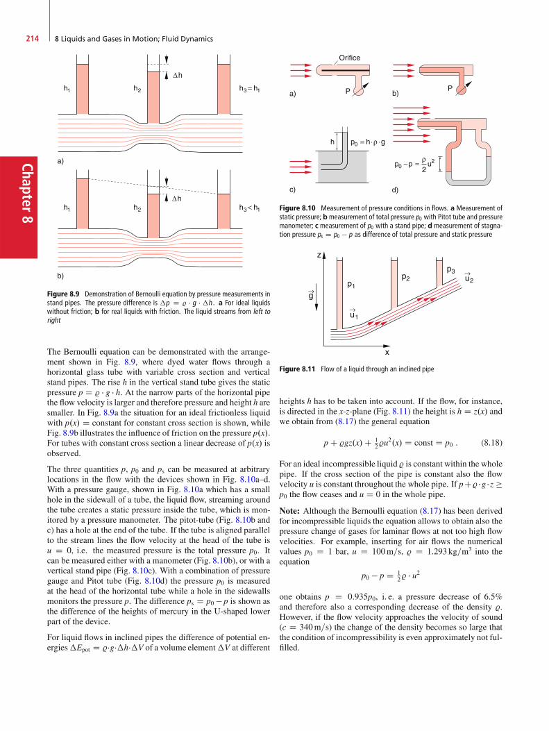
Chapter8
214 8 Liquids and Gases in Motion; Fluid Dynamics
Figure 8.9 Demonstration of Bernoulli equation by pressure measurements instand pipes. The pressure difference is �p D % � g � �h . a For ideal liquidswithout friction; b for real liquids with friction. The liquid streams from left toright
The Bernoulli equation can be demonstrated with the arrange-ment shown in Fig. 8.9, where dyed water flows through ahorizontal glass tube with variable cross section and verticalstand pipes. The rise h in the vertical stand tube gives the staticpressure p D % � g � h. At the narrow parts of the horizontal pipethe flow velocity is larger and therefore pressure and height h aresmaller. In Fig. 8.9a the situation for an ideal frictionless liquidwith p.x/ D constant for constant cross section is shown, whileFig. 8.9b illustrates the influence of friction on the pressure p.x/.For tubes with constant cross section a linear decrease of p.x/ isobserved.
The three quantities p, p0 and ps can be measured at arbitrarylocations in the flow with the devices shown in Fig. 8.10a–d.With a pressure gauge, shown in Fig. 8.10a which has a smallhole in the sidewall of a tube, the liquid flow, streaming aroundthe tube creates a static pressure inside the tube, which is mon-itored by a pressure manometer. The pitot-tube (Fig. 8.10b andc) has a hole at the end of the tube. If the tube is aligned parallelto the stream lines the flow velocity at the head of the tube isu D 0, i.e. the measured pressure is the total pressure p0. Itcan be measured either with a manometer (Fig. 8.10b), or with avertical stand pipe (Fig. 8.10c). With a combination of pressuregauge and Pitot tube (Fig. 8.10d) the pressure p0 is measuredat the head of the horizontal tube while a hole in the sidewallsmonitors the pressure p. The difference ps D p0 � p is shown asthe difference of the heights of mercury in the U-shaped lowerpart of the device.
For liquid flows in inclined pipes the difference of potential en-ergies�Epot D %�g��h��V of a volume element�V at different
Figure 8.10 Measurement of pressure conditions in flows. a Measurement ofstatic pressure; bmeasurement of total pressure p0 with Pitot tube and pressuremanometer; c measurement of p0 with a stand pipe; d measurement of stagna-tion pressure ps D p0 � p as difference of total pressure and static pressure
Figure 8.11 Flow of a liquid through an inclined pipe
heights h has to be taken into account. If the flow, for instance,is directed in the x-z-plane (Fig. 8.11) the height is h D z.x/ andwe obtain from (8.17) the general equation
p C %gz.x/C 12%u
2.x/ D const D p0 : (8.18)
For an ideal incompressible liquid % is constant within the wholepipe. If the cross section of the pipe is constant also the flowvelocity u is constant throughout the whole pipe. If pC% �g � z �p0 the flow ceases and u D 0 in the whole pipe.
Note: Although the Bernoulli equation (8.17) has been derivedfor incompressible liquids the equation allows to obtain also thepressure change of gases for laminar flows at not too high flowvelocities. For example, inserting for air flows the numericalvalues p0 D 1 bar, u D 100m=s, % D 1:293 kg=m3 into theequation
p0 � p D 12% � u2
one obtains p D 0:935p0, i. e. a pressure decrease of 6.5%and therefore also a corresponding decrease of the density %.However, if the flow velocity approaches the velocity of sound(c D 340m=s) the change of the density becomes so large thatthe condition of incompressibility is even approximately not ful-filled.

8.4 Bernoulli Equation 215
Chap
ter8
Figure 8.12 Hydrodynamic paradox: a Two curved aluminium plates, whichcan swing around a yoke, are pressed together when blowing air between them;b the lower circular plate is attracted to the upper plate when air is blownthrough the pipe
The Bernoulli equation can be demonstrated by many simple ex-periments which often astound the auditorium. One example isthe hydrodynamic paradox. Two curved aluminum plates arehanging on a U-shaped wire bar (Fig. 8.12a). If one blows airbetween the two plates they move towards each other, contraryto the expectation that they will be pushed away from each other.When air is blown through a vertical pipe fixed on one end to acircular disc S1 with a hole (Fig. 8.12b) a second disc S2 belowthe fixed disc is lifted to the upper disc by the air streaming be-tween the two discs. The distance d between the two discs witharea A must be below a critical value where the flow velocity uof the air is sufficiently large to cause an attractive force
F D A.p0 � p/ D 12% � u2 � A � m � g
between the two discs which can balance the weight m � g of thelower disc.
The Bernoulli theorem is used for many practical applications.Examples are the vaporizer or the spray bottle (Fig. 8.13) whereair streams out of a narrow nozzle and generates a reducedpressure, which sucks the liquid out of the bottle into the airstream. Here it is nebulized. Another example is the waterjet vacuum pump (Fig. 8.14). Here water streams with a largevelocity through a narrow nozzle where it generates a reduced
Figure 8.13 Vaporizer
Figure 8.14 Water jet pump
pressure. The air from the surrounding diffuses into the regionwith reduced pressure where it penetrates into the water jet andis transported out of the container into the outer space A, thusevacuating the container. With such a device reduced pressuresdown to 30 mbar can be achieved.
Undesirable effects of the Bernoulli theorem are the unroofingof houses under the action of typhoons (Fig. 8.15). When wind
Figure 8.15 A strong wind can unroof a house due to the reduced pressureabove the roof
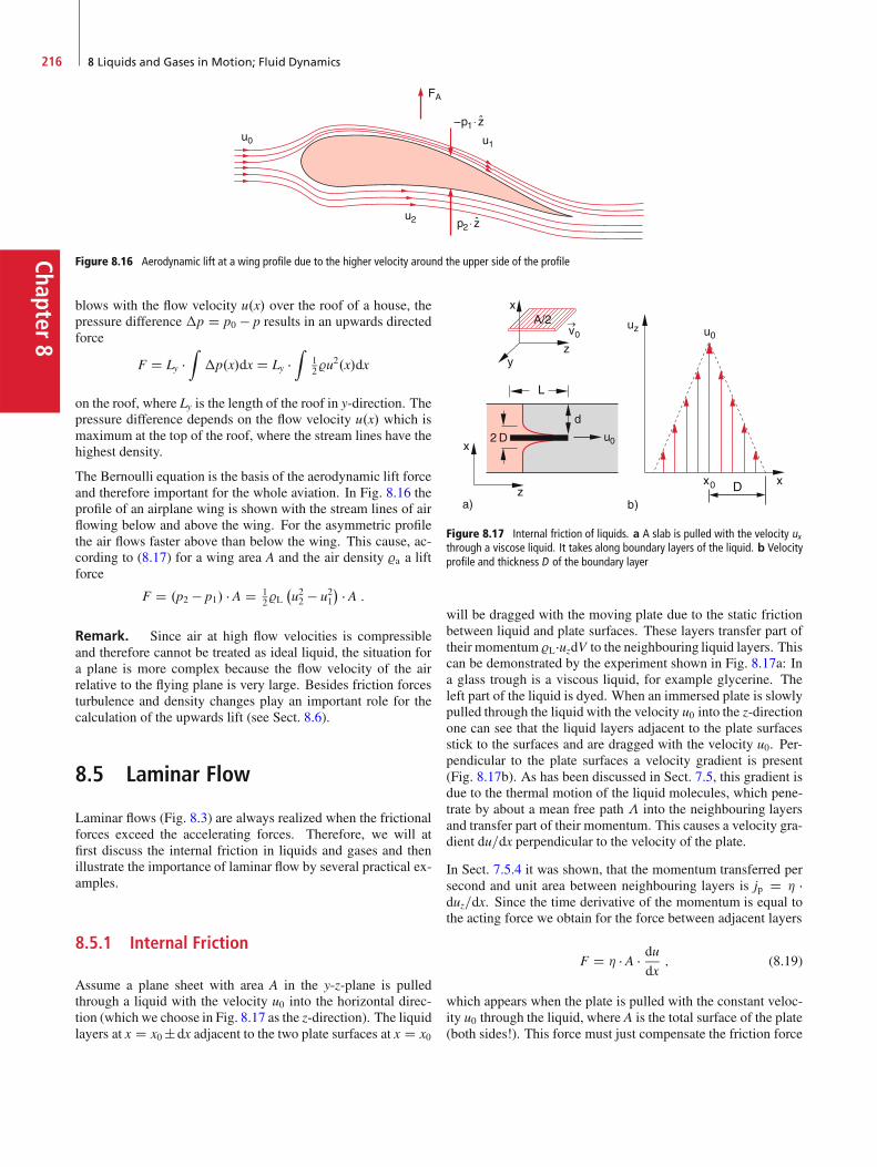
Chapter8
216 8 Liquids and Gases in Motion; Fluid Dynamics
Figure 8.16 Aerodynamic lift at a wing profile due to the higher velocity around the upper side of the profile
blows with the flow velocity u.x/ over the roof of a house, thepressure difference �p D p0 � p results in an upwards directedforce
F D Ly �Z�p.x/dx D Ly �
Z12%u
2.x/dx
on the roof, where Ly is the length of the roof in y-direction. Thepressure difference depends on the flow velocity u.x/ which ismaximum at the top of the roof, where the stream lines have thehighest density.
The Bernoulli equation is the basis of the aerodynamic lift forceand therefore important for the whole aviation. In Fig. 8.16 theprofile of an airplane wing is shown with the stream lines of airflowing below and above the wing. For the asymmetric profilethe air flows faster above than below the wing. This cause, ac-cording to (8.17) for a wing area A and the air density %a a liftforce
F D .p2 � p1/ � A D 12%L
�u22 � u21
� � A :
Remark. Since air at high flow velocities is compressibleand therefore cannot be treated as ideal liquid, the situation fora plane is more complex because the flow velocity of the airrelative to the flying plane is very large. Besides friction forcesturbulence and density changes play an important role for thecalculation of the upwards lift (see Sect. 8.6).
8.5 Laminar Flow
Laminar flows (Fig. 8.3) are always realized when the frictionalforces exceed the accelerating forces. Therefore, we will atfirst discuss the internal friction in liquids and gases and thenillustrate the importance of laminar flow by several practical ex-amples.
8.5.1 Internal Friction
Assume a plane sheet with area A in the y-z-plane is pulledthrough a liquid with the velocity u0 into the horizontal direc-tion (which we choose in Fig. 8.17 as the z-direction). The liquidlayers at x D x0˙dx adjacent to the two plate surfaces at x D x0
Figure 8.17 Internal friction of liquids. a A slab is pulled with the velocity uxthrough a viscose liquid. It takes along boundary layers of the liquid. b Velocityprofile and thickness D of the boundary layer
will be dragged with the moving plate due to the static frictionbetween liquid and plate surfaces. These layers transfer part oftheir momentum %L�uzdV to the neighbouring liquid layers. Thiscan be demonstrated by the experiment shown in Fig. 8.17a: Ina glass trough is a viscous liquid, for example glycerine. Theleft part of the liquid is dyed. When an immersed plate is slowlypulled through the liquid with the velocity u0 into the z-directionone can see that the liquid layers adjacent to the plate surfacesstick to the surfaces and are dragged with the velocity u0. Per-pendicular to the plate surfaces a velocity gradient is present(Fig. 8.17b). As has been discussed in Sect. 7.5, this gradient isdue to the thermal motion of the liquid molecules, which pene-trate by about a mean free path � into the neighbouring layersand transfer part of their momentum. This causes a velocity gra-dient du=dx perpendicular to the velocity of the plate.
In Sect. 7.5.4 it was shown, that the momentum transferred persecond and unit area between neighbouring layers is jp D � �duz=dx. Since the time derivative of the momentum is equal tothe acting force we obtain for the force between adjacent layers
F D � � A � dudx; (8.19)
which appears when the plate is pulled with the constant veloc-ity u0 through the liquid, where A is the total surface of the plate(both sides!). This force must just compensate the friction force
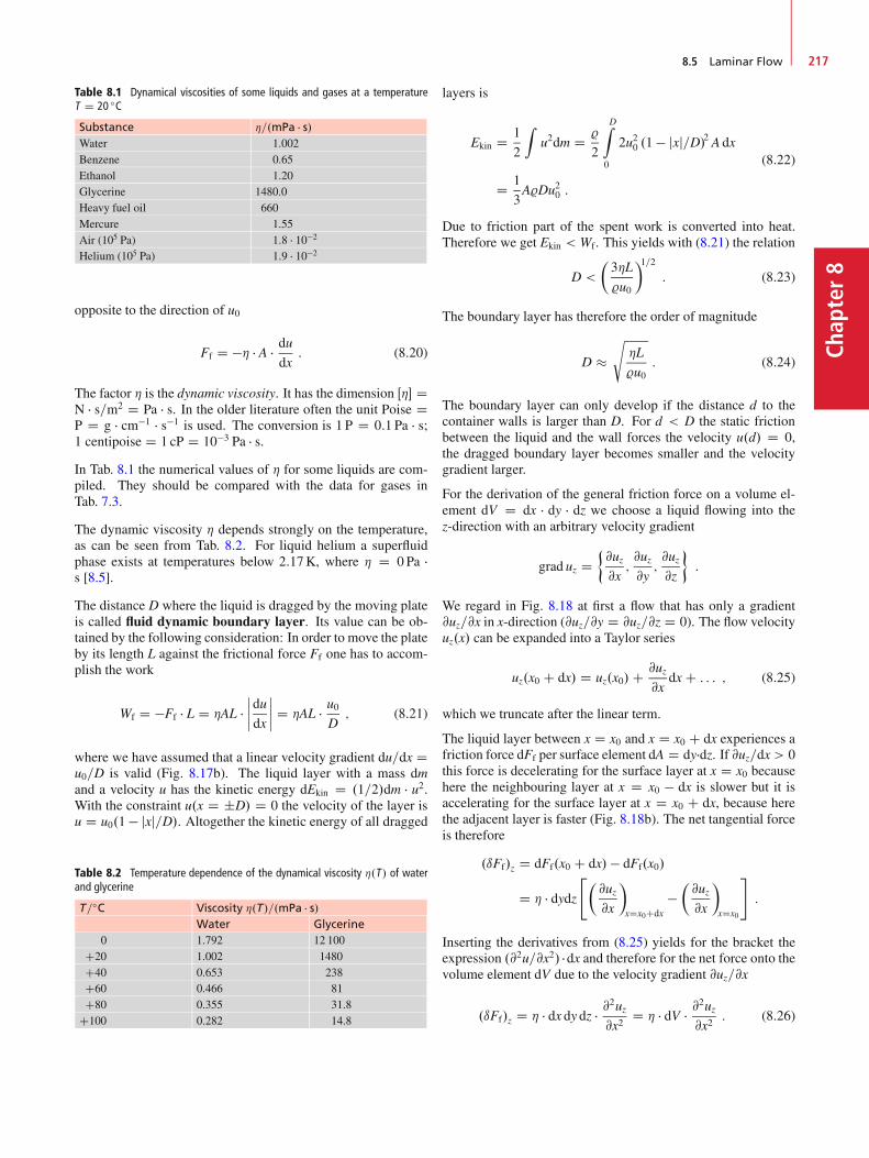
8.5 Laminar Flow 217
Chap
ter8
Table 8.1 Dynamical viscosities of some liquids and gases at a temperatureT D 20 ıC
Substance �=.mPa � s/Water 1.002Benzene 0.65Ethanol 1.20Glycerine 1480.0Heavy fuel oil 660Mercure 1.55Air (105 Pa) 1:8 � 10�2
Helium (105 Pa) 1:9 � 10�2
opposite to the direction of u0
Ff D �� � A � dudx: (8.20)
The factor � is the dynamic viscosity. It has the dimension Œ�� DN � s=m2 D Pa � s. In the older literature often the unit Poise DP D g � cm�1 � s�1 is used. The conversion is 1 P D 0:1 Pa � s;1 centipoise D 1 cP D 10�3 Pa � s.In Tab. 8.1 the numerical values of � for some liquids are com-piled. They should be compared with the data for gases inTab. 7.3.
The dynamic viscosity � depends strongly on the temperature,as can be seen from Tab. 8.2. For liquid helium a superfluidphase exists at temperatures below 2:17K, where � D 0 Pa �s [8.5].
The distance D where the liquid is dragged by the moving plateis called fluid dynamic boundary layer. Its value can be ob-tained by the following consideration: In order to move the plateby its length L against the frictional force Ff one has to accom-plish the work
Wf D �Ff � L D �AL �ˇ̌ˇ̌dudx
ˇ̌ˇ̌ D �AL � u0
D; (8.21)
where we have assumed that a linear velocity gradient du=dx Du0=D is valid (Fig. 8.17b). The liquid layer with a mass dmand a velocity u has the kinetic energy dEkin D .1=2/dm � u2.With the constraint u.x D ˙D/ D 0 the velocity of the layer isu D u0.1 � jxj=D/. Altogether the kinetic energy of all dragged
Table 8.2 Temperature dependence of the dynamical viscosity �.T / of waterand glycerine
T=ıC Viscosity �.T/=.mPa � s/Water Glycerine
0 1.792 12 100C20 1.002 1480C40 0.653 238C60 0.466 81C80 0.355 31.8
C100 0.282 14.8
layers is
Ekin D 1
2
Zu2dm D %
2
DZ
0
2u20 .1 � jxj=D/2 A dx
D 1
3A%Du20 :
(8.22)
Due to friction part of the spent work is converted into heat.Therefore we get Ekin < Wf. This yields with (8.21) the relation
D <
�3�L
%u0
�1=2: (8.23)
The boundary layer has therefore the order of magnitude
D �s�L
%u0: (8.24)
The boundary layer can only develop if the distance d to thecontainer walls is larger than D. For d < D the static frictionbetween the liquid and the wall forces the velocity u.d/ D 0,the dragged boundary layer becomes smaller and the velocitygradient larger.
For the derivation of the general friction force on a volume el-ement dV D dx � dy � dz we choose a liquid flowing into thez-direction with an arbitrary velocity gradient
grad uz D @uz@x;@uz@y;@uz@z
�:
We regard in Fig. 8.18 at first a flow that has only a gradient@uz=@x in x-direction (@uz=@y D @uz=@z D 0). The flow velocityuz.x/ can be expanded into a Taylor series
uz.x0 C dx/ D uz.x0/C @uz@x
dx C : : : ; (8.25)
which we truncate after the linear term.
The liquid layer between x D x0 and x D x0 C dx experiences afriction force dFf per surface element dA D dy�dz. If @uz=dx > 0this force is decelerating for the surface layer at x D x0 becausehere the neighbouring layer at x D x0 � dx is slower but it isaccelerating for the surface layer at x D x0 C dx, because herethe adjacent layer is faster (Fig. 8.18b). The net tangential forceis therefore
.ıFf/z D dFf.x0 C dx/ � dFf.x0/
D � � dydz"�
@uz@x
�
xDx0Cdx��@uz@x
�
xDx0
#:
Inserting the derivatives from (8.25) yields for the bracket theexpression .@2u=@x2/ �dx and therefore for the net force onto thevolume element dV due to the velocity gradient @uz=@x
.ıFf/z D � � dx dy dz � @2uz@x2
D � � dV � @2uz@x2
: (8.26)
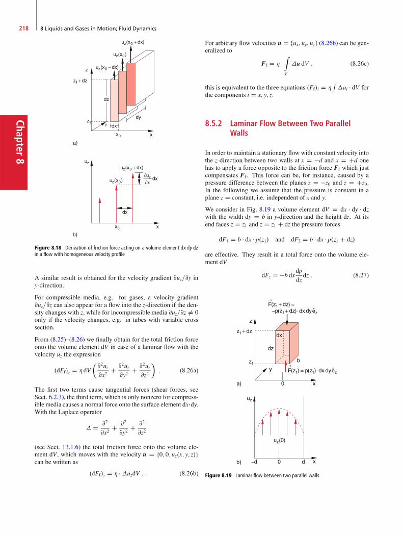
Chapter8
218 8 Liquids and Gases in Motion; Fluid Dynamics
Figure 8.18 Derivation of friction force acting on a volume element dx dy dzin a flow with homogeneous velocity profile
A similar result is obtained for the velocity gradient @uz=@y iny-direction.
For compressible media, e.g. for gases, a velocity gradient@uz=@z can also appear for a flow into the z-direction if the den-sity changes with z, while for incompressible media @uz=@z ¤ 0only if the velocity changes, e.g. in tubes with variable crosssection.
From (8.25)–(8.26) we finally obtain for the total friction forceonto the volume element dV in case of a laminar flow with thevelocity uz the expression
.dFf/z D � dV�@2uz@x2
C @2uz@y2
C @2uz@z2
�: (8.26a)
The first two terms cause tangential forces (shear forces, seeSect. 6.2.3), the third term, which is only nonzero for compress-ible media causes a normal force onto the surface element dx�dy.With the Laplace operator
� D @2
@x2C @2
@y2C @2
@z2
(see Sect. 13.1.6) the total friction force onto the volume ele-ment dV, which moves with the velocity u D f0; 0; uz.x; y; z/gcan be written as
.dFf/z D � ��uzdV : (8.26b)
For arbitrary flow velocities u D fux; uy; uzg (8.26b) can be gen-eralized to
Ff D � �Z
V
�u dV ; (8.26c)
this is equivalent to the three equations .Ff/i D �R�ui � dV for
the components i D x; y; z.
8.5.2 Laminar Flow Between Two ParallelWalls
In order to maintain a stationary flow with constant velocity intothe z-direction between two walls at x D �d and x D Cd onehas to apply a force opposite to the friction force Ff which justcompensates Ff. This force can be, for instance, caused by apressure difference between the planes z D �z0 and z D Cz0.In the following we assume that the pressure is constant in aplane z D constant, i.e. independent of x and y.
We consider in Fig. 8.19 a volume element dV D dx � dy � dzwith the width dy D b in y-direction and the height dz. At itsend faces z D z1 and z D z1 C dz the pressure forces
dF1 D b � dx � p.z1/ and dF2 D b � dx � p.z1 C dz/
are effective. They result in a total force onto the volume ele-ment dV
dFz D �b dxdp
dzdz : (8.27)
Figure 8.19 Laminar flow between two parallel walls
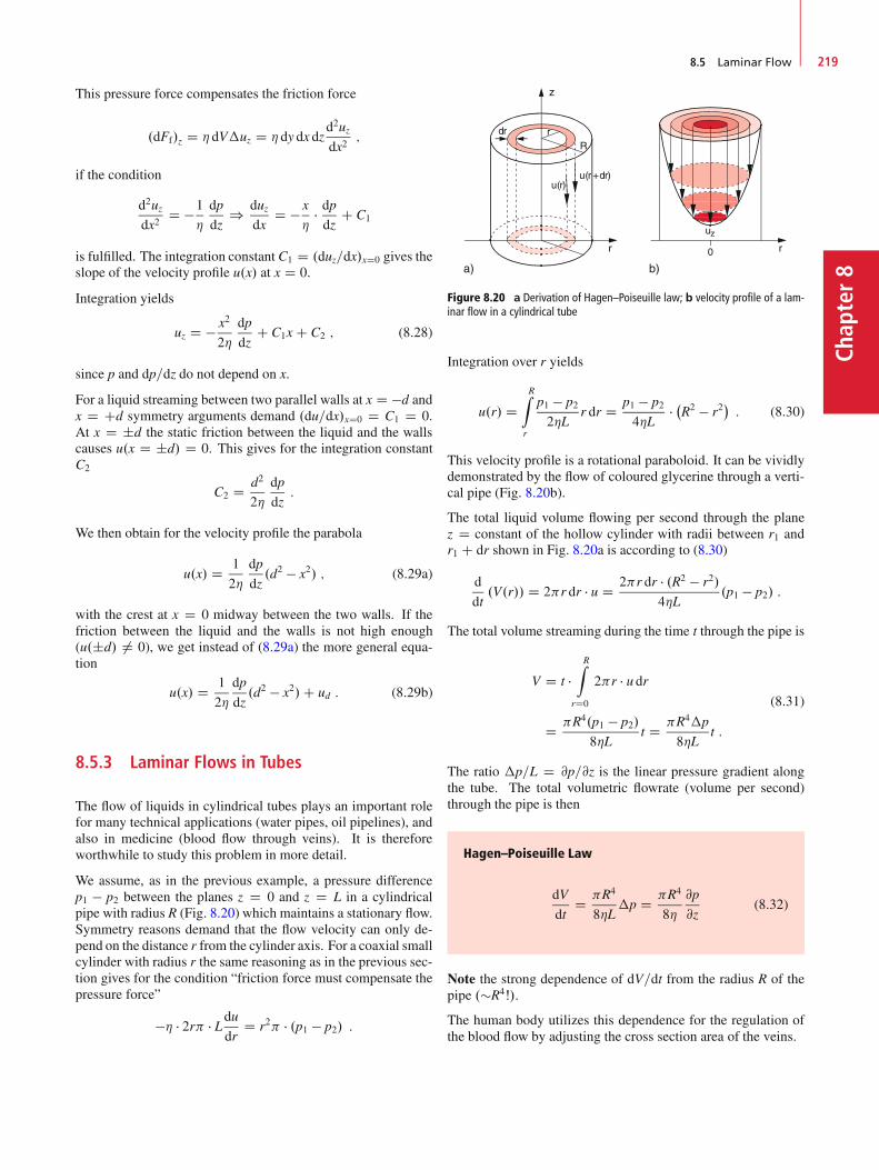
8.5 Laminar Flow 219
Chap
ter8
This pressure force compensates the friction force
.dFf/z D � dV�uz D � dy dx dzd2uzdx2
;
if the condition
d2uzdx2
D �1
�
dp
dz) duz
dxD � x
�� dpdz
C C1
is fulfilled. The integration constant C1 D .duz=dx/xD0 gives theslope of the velocity profile u.x/ at x D 0.
Integration yields
uz D � x2
2�
dp
dzC C1x C C2 ; (8.28)
since p and dp=dz do not depend on x.
For a liquid streaming between two parallel walls at x D �d andx D Cd symmetry arguments demand .du=dx/xD0 D C1 D 0.At x D ˙d the static friction between the liquid and the wallscauses u.x D ˙d/ D 0. This gives for the integration constantC2
C2 D d2
2�
dp
dz:
We then obtain for the velocity profile the parabola
u.x/ D 1
2�
dp
dz.d2 � x2/ ; (8.29a)
with the crest at x D 0 midway between the two walls. If thefriction between the liquid and the walls is not high enough(u.˙d/ ¤ 0), we get instead of (8.29a) the more general equa-tion
u.x/ D 1
2�
dp
dz.d2 � x2/C ud : (8.29b)
8.5.3 Laminar Flows in Tubes
The flow of liquids in cylindrical tubes plays an important rolefor many technical applications (water pipes, oil pipelines), andalso in medicine (blood flow through veins). It is thereforeworthwhile to study this problem in more detail.
We assume, as in the previous example, a pressure differencep1 � p2 between the planes z D 0 and z D L in a cylindricalpipe with radius R (Fig. 8.20) which maintains a stationary flow.Symmetry reasons demand that the flow velocity can only de-pend on the distance r from the cylinder axis. For a coaxial smallcylinder with radius r the same reasoning as in the previous sec-tion gives for the condition “friction force must compensate thepressure force”
�� � 2r � Ldudr
D r2 � .p1 � p2/ :
Figure 8.20 a Derivation of Hagen–Poiseuille law; b velocity profile of a lam-inar flow in a cylindrical tube
Integration over r yields
u.r/ DRZ
r
p1 � p22�L
r dr D p1 � p24�L
� �R2 � r2�: (8.30)
This velocity profile is a rotational paraboloid. It can be vividlydemonstrated by the flow of coloured glycerine through a verti-cal pipe (Fig. 8.20b).
The total liquid volume flowing per second through the planez D constant of the hollow cylinder with radii between r1 andr1 C dr shown in Fig. 8.20a is according to (8.30)
d
dt.V.r// D 2r dr � u D 2r dr � .R2 � r2/
4�L.p1 � p2/ :
The total volume streaming during the time t through the pipe is
V D t �RZ
rD0
2r � u dr
D R4.p1 � p2/
8�Lt D R4�p
8�Lt :
(8.31)
The ratio �p=L D @p=@z is the linear pressure gradient alongthe tube. The total volumetric flowrate (volume per second)through the pipe is then
Hagen–Poiseuille Law
dV
dtD R4
8�L�p D R4
8�
@p
@z(8.32)
Note the strong dependence of dV=dt from the radius R of thepipe .�R4Š/.
The human body utilizes this dependence for the regulation ofthe blood flow by adjusting the cross section area of the veins.
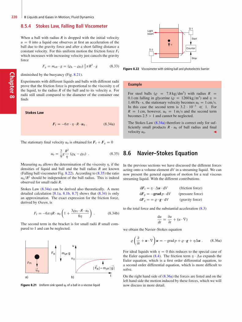
Chapter8
220 8 Liquids and Gases in Motion; Fluid Dynamics
8.5.4 Stokes Law, Falling Ball Viscometer
When a ball with radius R is dropped with the initial velocityu D 0 into a liquid one observes at first an acceleration of theball due to the gravity force and after a short falling distance aconstant velocity. For this uniform motion the friction force Ff
which increases with increasing velocity just cancels the gravityforce
Fg D meff � g D .%k � %Fl/ 43R
3 � g (8.33)
diminished by the buoyancy (Fig. 8.21).
Experiments with different liquids and balls with different radiiprove that the friction force is proportional to the viscosity � ofthe liquid, to the radius R of the ball and to its velocity u. Forradii still small compared to the diameter of the container onefinds
Stokes Law
Ff D �6 � � � R � u0 : (8.34a)
The stationary final velocity u0 is obtained for Ff C Fg D 0
u0 D 2
9gR2
�.%K � %Fl/ : (8.35)
Measuring u0 allows the determination of the viscosity �, if thedensities of liquid and ball and the ball radius R are known(Falling ball viscometer Fig. 8.22). According to (8.35) the ratiou0=R2 should be independent of the ball radius. This is indeedobserved for small radii R.
Stokes Law (8.34a) can be derived also theoretically. A moredetailed calculation [8.1a, 8.1b, 8.7] shows that (8.34) is onlyan approximation. The exact expression for the friction force,derived by Oseen, is
Ff D �6�R � u0�1 C 3%Fl � R � u0
8�
�: (8.34b)
The second term in the bracket is for small radii R small com-pared to 1 and can be neglected.
Figure 8.21 Uniform sink speed u0 of a ball in a viscose liquid
Figure 8.22 Viscosimeter with sinking ball and photoelectric barrier
Example
For steel balls .% D 7:8 kg=dm3/ with radius R D0:1 cm falling in glycerine (% D 1260kg=m3) and � D1:48 Pa � s, the stationary velocity becomes u0 D 1 cm=s.In this case the second term is 3:2 � 10�3 1. ForR D 1 cm, however, u0 D 1m=s and the second termbecomes 2:5 > 1 and cannot be neglected.
The Stokes Law (8.34a) therefore is correct only for suf-ficiently small products R � u0 of ball radius and finalvelocity u0. J
8.6 Navier–Stokes Equation
In the previous sections we have discussed the different forcesacting onto a volume element dV in a streaming liquid. We cannow present the general equation of motion for a real viscousstreaming liquid. With the different contributions
dFf D � ��u � dV (friction force)
dFp D �grad p � dV (pressure force)
dFg D D % � g � dV (gravity force)
to the total force and the substantial acceleration (8.3)
du
dtD @u
@tC .u � r/
we obtain the Navier–Stokes equation
%
�@
@tC u � r
�u D � grad p C % � g C ��u : (8.36a)
For ideal liquids with � D 0 this reduces to the special case ofthe Euler equation (8.4). The friction term � � �u expands theEuler equation, which is a first order differential equation, toa second order differential equation, which is more difficult tosolve.
On the right hand side of (8.36a) the forces are listed and on theleft hand side the motion induced by these forces, which we willnow discuss in more detail.
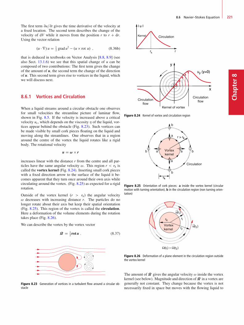
8.6 Navier–Stokes Equation 221
Chap
ter8
The first term @u=@t gives the time derivative of the velocity ata fixed location. The second term describes the change of thevelocity of dV while it moves from the position r to r C dr.Using the vector relation
.u � r/ u D 12 grad u
2 � .u rot u/ ; (8.36b)
that is deduced in textbooks on Vector Analysis [8.8, 8.9] (seealso Sect. 13.1.6) we see that this spatial change of u can becomposed of two contributions: The first term gives the changeof the amount of u, the second term the change of the directionof u. This second term gives rise to vortices in the liquid, whichwe will discuss next.
8.6.1 Vortices and Circulation
When a liquid streams around a circular obstacle one observesfor small velocities the streamline picture of laminar flow,shown in Fig. 8.5. If the velocity is increased above a criticalvelocity uc, which depends on the viscosity � of the liquid, vor-tices appear behind the obstacle (Fig. 8.23). Such vortices canbe made visible by small cork pieces floating on the liquid andmoving along the streamlines. One observes that in a regionaround the centre of the vortex the liquid rotates like a rigidbody. The rotational velocity
u D ! r
increases linear with the distance r from the centre and all par-ticles have the same angular velocity !. This region r < rk iscalled the vortex kernel (Fig. 8.24). Inserting small cork pieceswith a fixed direction arrow to the surface of the liquid it be-comes apparent that they turn once around their own axis whilecirculating around the vortex. (Fig. 8.25) as expected for a rigidrotation.
Outside of the vortex kernel .r > rk/ the angular velocity! decreases with increasing distance r. The particles do nolonger rotate about their axis but keep their spatial orientation(Fig. 8.25). This region of the vortex is called the circulation.Here a deformation of the volume elements during the rotationtakes place (Fig. 8.26).
We can describe the vortex by the vortex vector
˝ D 12rotu : (8.37)
Figure 8.23 Generation of vortices in a turbulent flow around a circular ob-stacle
Kernel Circulation
Circulationflow
Circulationflow
Kernel of vortex
Figure 8.24 Kernel of vortex and circulation region
Figure 8.25 Orientation of cork pieces: a inside the vortex kernel (circularmotion with turning orientation), b in the circulation region (non turning orien-tation)
Figure 8.26 Deformation of a plane element in the circulation region outsidethe vortex kernel
The amount of ˝ gives the angular velocity ! inside the vortexkernel (see below). Magnitude and direction of˝ in a vortex aregenerally not constant. They change because the vortex is notnecessarily fixed in space but moves with the flowing liquid to
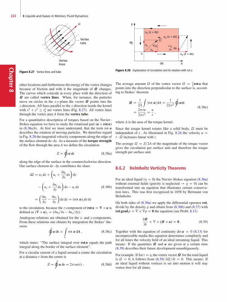
Chapter8
222 8 Liquids and Gases in Motion; Fluid Dynamics
Vertextube
Vertexlines
Figure 8.27 Vortex lines and tube
other locations and furthermore the energy of the vortex changesbecause of friction and with it the magnitude of ˝ changes.The curves which coincide at every place with the direction of˝ are called vortex lines. When, for instance, the particlesmove on circles in the x-y-plane the vector ˝ points into thez-direction. All lines parallel to the z-direction inside the kernelwith x2 C y2 � r2k are vortex lines (Fig. 8.27). All vortex linesthrough the vortex area A form the vortex tube.
For a quantitative description of torques based on the Navier–Stokes equation we have to study the rotational part .u rotu/in (8.36a,b). At first we must understand, that the term rot udescribes the rotation of moving particles. We therefore regardin Fig. 8.28 the tangential velocity components along the edge ofthe surface element dx �dy. As a measure of the torque strengthof the flow through the area A we define the circulation
Z DI
u ds (8.38a)
along the edge of the surface in the counterclockwise direction.Our surface element dx � dy contributes the share
dZ D ux dx C�uy C @uy
@xdx
�dy
��ux C @ux
@ydy
�dx � uy dy
D�@uy@x
� @ux@y
�dx dy D .rot u/zdx dy
(8.38b)
to the circulation, because the z-component of rotu D r u isdefined as .r u/z D .@uy=@x � @ux=@y/.Analogous relations are obtained for the x- and y-components.From these relations one obtains by integration the Stokes’ the-orem I
u ds DZ
A
rot u dA ; (8.38c)
which states: “The surface integral over rotu equals the pathintegral along the border of the surface element”.
For a circular current of a liquid around a centre the circulationat a distance r from the centre is
Z DI
u ds D 2ru.r/ : (8.38d)
Figure 8.28 Explanation of circulation and its relation with rot u
The average amount ˝ of the vortex vector ˝ D 12rotu that
points into the direction perpendicular to the surface is, accord-ing to Stokes’ theorem
˝ D 1
2A
Zjrot uj dA D 1
2r2
Iuds
D 2ru
2r2D u
r;
(8.38e)
where A is the area of the torque kernel.
Since the torque kernel rotates like a solid body, ˝ must beindependent of r. As illustrated in Fig. 8.24 the velocity u Dr �˝ increases linear with r.
The average ˝ D Z=2A of the magnitude of the torque vectorgives the circulation per surface unit and therefore the torquestrength per surface unit.
8.6.2 Helmholtz Vorticity Theorems
For an ideal liquid .� D 0/ the Navier–Stokes equation (8.36a)without external fields (gravity is neglected ! g D 0) can betransformed into an equation that illustrates certain conserva-tion laws. This was first recognized in 1858 by Hermann vonHelmholtz.
On both sides of (8.36a) we apply the differential operator rot,divide by the density % and obtain from (8.36b) and (8.37) withrot grad p D r rp D 0 the equation (see Probl. 8.11)
@˝
@tC r .˝ u/ D 0 : (8.39)
Together with the equation of continuity divu D 0 (8.13) forincompressible media this equation determines completely andfor all times the velocity field of an ideal streaming liquid. Thismeans: If the quantities ˝ and u are given at a certain time(8.39) describes their future development unambiguously.
For example: If for t D t0 the vortex vector ˝ for the total liquidis ˝ D 0, it follows from (8.39) @˝=@t D 0. This means: Ifan ideal liquid without vortices is set into motion it will stayvortex-free for all times.
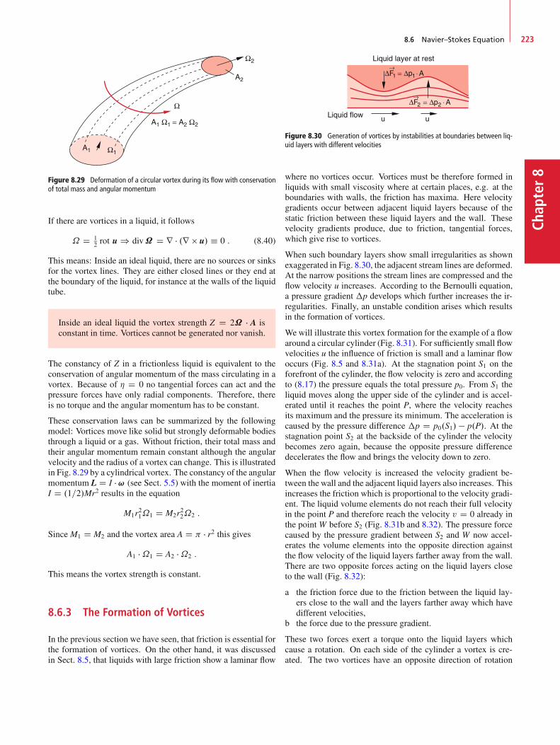
8.6 Navier–Stokes Equation 223
Chap
ter8
Figure 8.29 Deformation of a circular vortex during its flow with conservationof total mass and angular momentum
If there are vortices in a liquid, it follows
˝ D 12 rot u ) div˝ D r � .r u/ � 0 : (8.40)
This means: Inside an ideal liquid, there are no sources or sinksfor the vortex lines. They are either closed lines or they end atthe boundary of the liquid, for instance at the walls of the liquidtube.
Inside an ideal liquid the vortex strength Z D 2˝ � A isconstant in time. Vortices cannot be generated nor vanish.
The constancy of Z in a frictionless liquid is equivalent to theconservation of angular momentum of the mass circulating in avortex. Because of � D 0 no tangential forces can act and thepressure forces have only radial components. Therefore, thereis no torque and the angular momentum has to be constant.
These conservation laws can be summarized by the followingmodel: Vortices move like solid but strongly deformable bodiesthrough a liquid or a gas. Without friction, their total mass andtheir angular momentum remain constant although the angularvelocity and the radius of a vortex can change. This is illustratedin Fig. 8.29 by a cylindrical vortex. The constancy of the angularmomentum L D I � ! (see Sect. 5.5) with the moment of inertiaI D .1=2/Mr2 results in the equation
M1r21˝1 D M2r
22˝2 :
Since M1 D M2 and the vortex area A D � r2 this givesA1 �˝1 D A2 �˝2 :
This means the vortex strength is constant.
8.6.3 The Formation of Vortices
In the previous section we have seen, that friction is essential forthe formation of vortices. On the other hand, it was discussedin Sect. 8.5, that liquids with large friction show a laminar flow
Figure 8.30 Generation of vortices by instabilities at boundaries between liq-uid layers with different velocities
where no vortices occur. Vortices must be therefore formed inliquids with small viscosity where at certain places, e.g. at theboundaries with walls, the friction has maxima. Here velocitygradients occur between adjacent liquid layers because of thestatic friction between these liquid layers and the wall. Thesevelocity gradients produce, due to friction, tangential forces,which give rise to vortices.
When such boundary layers show small irregularities as shownexaggerated in Fig. 8.30, the adjacent stream lines are deformed.At the narrow positions the stream lines are compressed and theflow velocity u increases. According to the Bernoulli equation,a pressure gradient �p develops which further increases the ir-regularities. Finally, an unstable condition arises which resultsin the formation of vortices.
We will illustrate this vortex formation for the example of a flowaround a circular cylinder (Fig. 8.31). For sufficiently small flowvelocities u the influence of friction is small and a laminar flowoccurs (Fig. 8.5 and 8.31a). At the stagnation point S1 on theforefront of the cylinder, the flow velocity is zero and accordingto (8.17) the pressure equals the total pressure p0. From S1 theliquid moves along the upper side of the cylinder and is accel-erated until it reaches the point P, where the velocity reachesits maximum and the pressure its minimum. The acceleration iscaused by the pressure difference �p D p0.S1/ � p.P/. At thestagnation point S2 at the backside of the cylinder the velocitybecomes zero again, because the opposite pressure differencedecelerates the flow and brings the velocity down to zero.
When the flow velocity is increased the velocity gradient be-tween the wall and the adjacent liquid layers also increases. Thisincreases the friction which is proportional to the velocity gradi-ent. The liquid volume elements do not reach their full velocityin the point P and therefore reach the velocity v D 0 already inthe pointW before S2 (Fig. 8.31b and 8.32). The pressure forcecaused by the pressure gradient between S2 and W now accel-erates the volume elements into the opposite direction againstthe flow velocity of the liquid layers farther away from the wall.There are two opposite forces acting on the liquid layers closeto the wall (Fig. 8.32):
a the friction force due to the friction between the liquid lay-ers close to the wall and the layers farther away which havedifferent velocities,
b the force due to the pressure gradient.
These two forces exert a torque onto the liquid layers whichcause a rotation. On each side of the cylinder a vortex is cre-ated. The two vortices have an opposite direction of rotation
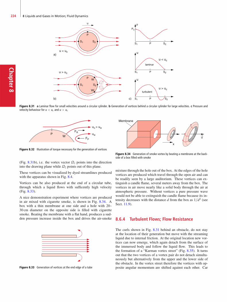
Chapter8
224 8 Liquids and Gases in Motion; Fluid Dynamics
Figure 8.31 a Laminar flow for small velocities around a circular cylinder. b Generation of vortices behind a circular cylinder for large velocities. c Pressure andvelocity behaviour for u < uc and u > uc
Figure 8.32 Illustration of torque necessary for the generation of vortices
(Fig. 8.31b), i.e. the vortex vector ˝1 points into the directioninto the drawing plane while ˝2 points out of this plane.
These vortices can be visualized by dyed streamlines producedwith the apparatus shown in Fig. 8.4.
Vortices can be also produced at the end of a circular tube,through which a liquid flows with sufficently high velocity(Fig. 8.33).
A nice demonstration experiment where vortices are producedin air mixed with cigarette smoke, is shown in Fig. 8.34. Abox with a thin membrane at one side and a hole with 20–30 cm diameter on the opposite side is filled with cigarettesmoke. Beating the membrane with a flat hand, produces a sud-den pressure increase inside the box and drives the air-smoke
Figure 8.33 Generation of vortices at the end edge of a tube
Figure 8.34 Generation of smoke vortex by beating a membrane at the back-side of a box filled with smoke
mixture through the hole out of the box. At the edges of the holevortices are produced which travel through the open air and canbe readily seen by a large auditorium. These vortices can ex-tinguish a candle flame, several meters away from the box. Thevortices in air move nearly like a solid body through the air atatmospheric pressure. Without vortices a pure pressure wavewould not be able to extinguish the candle flame because its in-tensity decreases with the distance d from the box as 1=d2 (seeSect. 11.9).
8.6.4 Turbulent Flows; Flow Resistance
The curls shown in Fig. 8.31 behind an obstacle, do not stayat the location of their generation but move with the streamingliquid due to internal friction. At the original location new vor-tices can now emerge, which again detach from the surface ofthe immersed body and follow the liquid flow. This leads tothe formation of a “Karman vortex street” (Fig. 8.35). It turnsout that the two vortices of a vortex pair do not detach simulta-neously but alternatively from the upper and the lower side ofthe obstacle. In the vortex street therefore the vortices with op-posite angular momentum are shifted against each other. Car
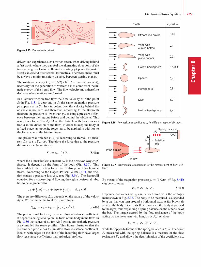
8.6 Navier–Stokes Equation 225
Chap
ter8
Figure 8.35 Karman vortex street
drivers can experience such a vortex street, when driving behinda fast truck, where they can feel the alternating directions of thetransverse gust of winds. Behind a starting jet plane the vortexstreet can extend over several kilometres. Therefore there mustbe always a minimum safety distance between starting planes.
The rotational energy Erot D .I=2/ �˝2 (I D inertial moment),necessary for the generation of vortices has to come from the ki-netic energy of the liquid flow. The flow velocity must thereforedecrease when vortices are formed.
In a laminar friction-free flow the flow velocity u in the pointS2 in Fig. 8.31 is zero and in S2 the same stagnation pressurep0 appears as in S1. In a turbulent flow the velocity behind theobstacle is not zero and therefore, according to the Bernoullitheorem the pressure is lower than p0, causing a pressure differ-ence between the regions before and behind the obstacle. Thisresults in a force F D �p � A on the obstacle with the cross sec-tion A in the direction of the flow. In order to keep the body ata fixed place, an opposite force has to be applied in addition tothe force against the friction force.
The pressure difference at S2 is according to Bernoulli’s theo-rem �p / .1=2/% � u2. Therefore the force due to the pressuredifference can be written as
FD D cD � %2u2A ; (8.41a)
where the dimensionless constant cD is the pressure drag coef-ficient. It depends on the form of the body (Fig. 8.36). Thisforce adds to the friction force that is also present for laminarflows. According to the Hagen–Poiseuille law (8.31) the fric-tion causes a pressure loss �pf (see Fig. 8.9b). The Bernoulliequation for a viscose liquid flowing through a horizontal tube,has to be augmented to
p1 C 12%u
21 D p2 C�pf C 1
2%u22 I �pf < 0 :
The pressure difference�pf depends on the square of the veloc-ity u. We can write the total resistance force
Ftotal D Ff C FD D 12cw � % � u2 � A : (8.41b)
The proportional factor cw is called flow resistance coefficient.It depends analogue to cD on the form of the body in the flow. InFig. 8.36 the values of cw for Air flows at atmospheric pressureare compiled for some profiles. This figure illustrates that thestreamlined profile has the smallest flow resistance coefficient.Bodies with edges on the side of the incoming flow have largerflow resistance coefficients than spherical profiles.
Figure 8.36 Flow resistance coefficents cw for different shapes of obstacles
Figure 8.37 Experimental arrangement for the measurement of flow resis-tance
By means of the stagnation pressure ps D .1=2/% � u2 Eq. 8.41bcan be written as
Fw D cw � ps � A : (8.41c)
Experimental values of cw can be measured with the arrange-ment shown in Fig. 8.37. The body to be measured is suspendedby a bar that can turn around a horizontal axis. A fan blows airagainst the body. Due to its flow resistance the body is pressedto the right, thus expanding a spring balance on the other side ofthe bar. The torque exerted by the flow resistance of the bodyacting on the lever arm with length a is Fw � a where
Fw D 12 � cw � % � u2 � A ;
while the opposite torque of the spring balance is Fs�b. The forceFs measured with the spring balance is a measure of the flowresistance Fw and allows the determination of the coefficient cw.
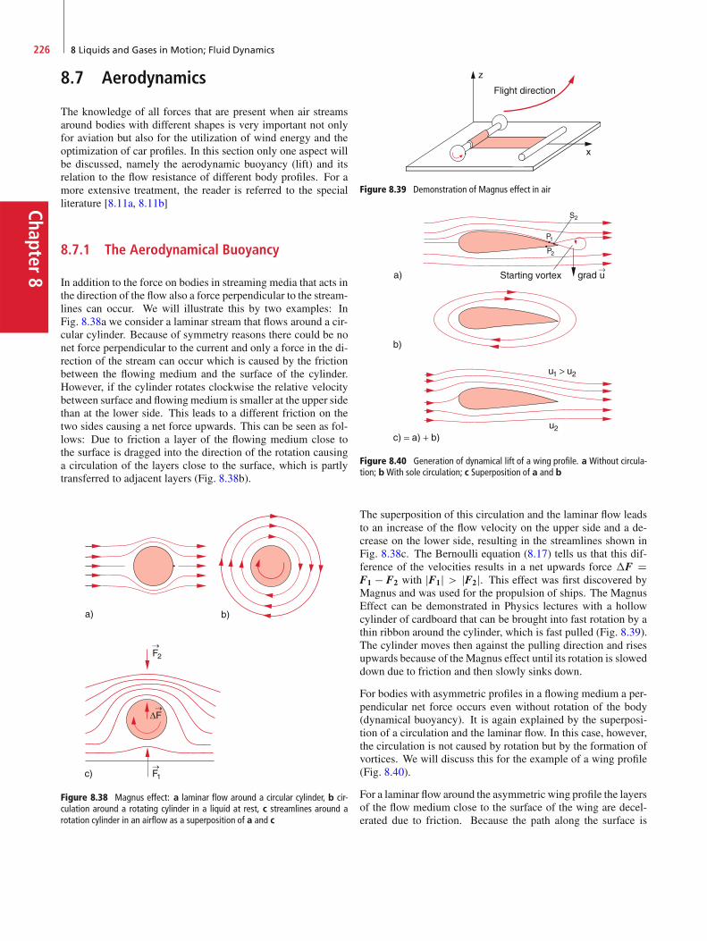
Chapter8
226 8 Liquids and Gases in Motion; Fluid Dynamics
8.7 Aerodynamics
The knowledge of all forces that are present when air streamsaround bodies with different shapes is very important not onlyfor aviation but also for the utilization of wind energy and theoptimization of car profiles. In this section only one aspect willbe discussed, namely the aerodynamic buoyancy (lift) and itsrelation to the flow resistance of different body profiles. For amore extensive treatment, the reader is referred to the specialliterature [8.11a, 8.11b]
8.7.1 The Aerodynamical Buoyancy
In addition to the force on bodies in streaming media that acts inthe direction of the flow also a force perpendicular to the stream-lines can occur. We will illustrate this by two examples: InFig. 8.38a we consider a laminar stream that flows around a cir-cular cylinder. Because of symmetry reasons there could be nonet force perpendicular to the current and only a force in the di-rection of the stream can occur which is caused by the frictionbetween the flowing medium and the surface of the cylinder.However, if the cylinder rotates clockwise the relative velocitybetween surface and flowing medium is smaller at the upper sidethan at the lower side. This leads to a different friction on thetwo sides causing a net force upwards. This can be seen as fol-lows: Due to friction a layer of the flowing medium close tothe surface is dragged into the direction of the rotation causinga circulation of the layers close to the surface, which is partlytransferred to adjacent layers (Fig. 8.38b).
Figure 8.38 Magnus effect: a laminar flow around a circular cylinder, b cir-culation around a rotating cylinder in a liquid at rest, c streamlines around arotation cylinder in an airflow as a superposition of a and c
Flight direction
Figure 8.39 Demonstration of Magnus effect in air
Figure 8.40 Generation of dynamical lift of a wing profile. a Without circula-tion; bWith sole circulation; c Superposition of a and b
The superposition of this circulation and the laminar flow leadsto an increase of the flow velocity on the upper side and a de-crease on the lower side, resulting in the streamlines shown inFig. 8.38c. The Bernoulli equation (8.17) tells us that this dif-ference of the velocities results in a net upwards force �F DF1 � F2 with jF1j > jF2j. This effect was first discovered byMagnus and was used for the propulsion of ships. The MagnusEffect can be demonstrated in Physics lectures with a hollowcylinder of cardboard that can be brought into fast rotation by athin ribbon around the cylinder, which is fast pulled (Fig. 8.39).The cylinder moves then against the pulling direction and risesupwards because of the Magnus effect until its rotation is sloweddown due to friction and then slowly sinks down.
For bodies with asymmetric profiles in a flowing medium a per-pendicular net force occurs even without rotation of the body(dynamical buoyancy). It is again explained by the superposi-tion of a circulation and the laminar flow. In this case, however,the circulation is not caused by rotation but by the formation ofvortices. We will discuss this for the example of a wing profile(Fig. 8.40).
For a laminar flow around the asymmetric wing profile the layersof the flow medium close to the surface of the wing are decel-erated due to friction. Because the path along the surface is
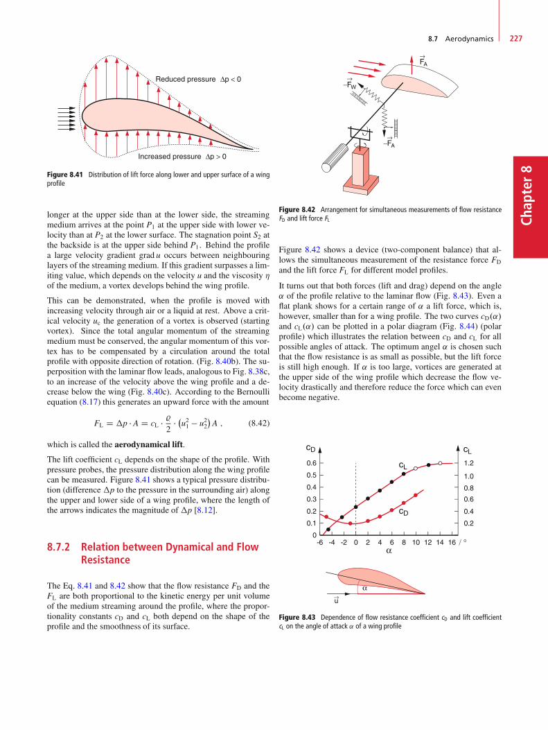
8.7 Aerodynamics 227
Chap
ter8Figure 8.41 Distribution of lift force along lower and upper surface of a wing
profile
longer at the upper side than at the lower side, the streamingmedium arrives at the point P1 at the upper side with lower ve-locity than at P2 at the lower surface. The stagnation point S2 atthe backside is at the upper side behind P1. Behind the profilea large velocity gradient grad u occurs between neighbouringlayers of the streaming medium. If this gradient surpasses a lim-iting value, which depends on the velocity u and the viscosity �of the medium, a vortex develops behind the wing profile.
This can be demonstrated, when the profile is moved withincreasing velocity through air or a liquid at rest. Above a crit-ical velocity uc the generation of a vortex is observed (startingvortex). Since the total angular momentum of the streamingmedium must be conserved, the angular momentum of this vor-tex has to be compensated by a circulation around the totalprofile with opposite direction of rotation. (Fig. 8.40b). The su-perposition with the laminar flow leads, analogous to Fig. 8.38c,to an increase of the velocity above the wing profile and a de-crease below the wing (Fig. 8.40c). According to the Bernoulliequation (8.17) this generates an upward force with the amount
FL D �p � A D cL � %2
� �u21 � u22�A ; (8.42)
which is called the aerodynamical lift.
The lift coefficient cL depends on the shape of the profile. Withpressure probes, the pressure distribution along the wing profilecan be measured. Figure 8.41 shows a typical pressure distribu-tion (difference �p to the pressure in the surrounding air) alongthe upper and lower side of a wing profile, where the length ofthe arrows indicates the magnitude of �p [8.12].
8.7.2 Relation between Dynamical and FlowResistance
The Eq. 8.41 and 8.42 show that the flow resistance FD and theFL are both proportional to the kinetic energy per unit volumeof the medium streaming around the profile, where the propor-tionality constants cD and cL both depend on the shape of theprofile and the smoothness of its surface.
Figure 8.42 Arrangement for simultaneous measurements of flow resistanceFD and lift force FL
Figure 8.42 shows a device (two-component balance) that al-lows the simultaneous measurement of the resistance force FD
and the lift force FL for different model profiles.
It turns out that both forces (lift and drag) depend on the angle˛ of the profile relative to the laminar flow (Fig. 8.43). Even aflat plank shows for a certain range of ˛ a lift force, which is,however, smaller than for a wing profile. The two curves cD.˛/and cL.˛/ can be plotted in a polar diagram (Fig. 8.44) (polarprofile) which illustrates the relation between cD and cL for allpossible angles of attack. The optimum angel ˛ is chosen suchthat the flow resistance is as small as possible, but the lift forceis still high enough. If ˛ is too large, vortices are generated atthe upper side of the wing profile which decrease the flow ve-locity drastically and therefore reduce the force which can evenbecome negative.
Figure 8.43 Dependence of flow resistance coefficient cD and lift coefficientcL on the angle of attack ˛ of a wing profile
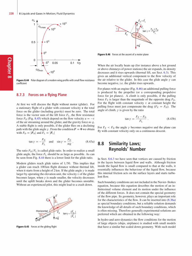
Chapter8
228 8 Liquids and Gases in Motion; Fluid Dynamics
Figure 8.44 Polar diagram of a modern wing profile with small flow resistancecoefficient
8.7.3 Forces on a flying Plane
At first we will discuss the flight without motor (glider). Fora stationary flight of a glider with constant velocity v the totalforce on the glider (including gravity) must be zero. The totalforce is the vector sum of the lift force FL, the flow resistanceforce FD (Fig. 8.45) which depend on the flow velocity u D �vof the air streaming around the glider, and the gravity force m �g.A stable flight is only possible, if the glider flies on a decliningpath with the glide angle � . From the conditionF D 0we obtainwith FD D jFDj and FL D jFLj
tan � D �FD
FLand sin � D FD
mg: (8.43a)
The ratio FD=FL is called glide ratio. In order to realize a smallglide angle, the force FL should be as large as possible. As canbe seen from Fig. 8.44 there is a lower limit for the glide ratio.
Modern gliders reach glide ratios of 1=50. This implies thata glider can reach 100 km flight distance without thermal lift,when it starts from a height of 2 km. If the glide angle � is madelarger by operating the elevation unit, the velocity v of the gliderbecomes larger, when � is made smaller, the velocity decreasesuntil the uplift breaks down and the glider becomes unstable.Without an experienced pilot, this might lead to a crash down.
Figure 8.45 Forces at the gliding flight
Figure 8.46 Forces at the ascent of a motor plane
When the air locally heats up (for instance above a hot groundor above chimneys of power stations) the air expands, its densitydecreases and it rises upwards (thermal lift, see Sect. 6.3). Thisgives an additional vertical component to the flow velocity ofthe air relative to the glider. In this case the glide angle � canbecome negative, i.e. the glider rises upwards.
For planes with an engine (Fig. 8.46) an additional pulling forceis produced by the propeller (or a corresponding propulsiveforce for jet planes). A climb is only possible, if the pullingforce FZ is larger than the magnitude of the opposite drag FD.For the flight with constant velocity v at constant height thepulling force must just compensate the drag .FZ D FD/. Theangle of climb, � is given by the ratio
tan � D FZ � FD
FL: (8.43b)
For FZ < FD the angle � becomes negative and the plane canfly with constant velocity only on a continuous descent.
8.8 Similarity Laws;Reynolds’ Number
In Sect. 8.6.3 we have seen that vortices are caused by frictionin the layers between liquid flow and walls. Although frictioninside the liquid flow is small compared to that at the walls, itessentially influences the behaviour of the liquid flow, becausethis internal friction acts on the surface layers and starts turbu-lent flow.
Such boundary conditions are not included in the Navier–Stokesequation, because this equation describes the motion of an in-finitesimal volume element and its motion under the influenceof the different forces. It does not contain the special geometryof the flow pipe. Its geometry, however, plays an important rolefor the characteristics of the flow. It can be inserted into (8.36a)as special boundary conditions, but a reliable solution demandsthe knowledge of all details of such boundary conditions, whichis often missing. Therefore generally experimental solutions arepreferred which are obtained in the following way:
In hydro-and aero-dynamics the flow conditions for the motionof large objects (ships, airplanes) is studied with small modelsthat have a similar but scaled down geometry. With such model

8.9 Usage of Wind Energy 229
Chap
ter8
experiments in wind channels or in small liquid flow chambers,the optimum shape of a wing or a hulk can be found. In order toobtain realistic results, not only the shape of the model must bea true scaled down version of the true object, but also the flowconditions must be accordingly scaled down in a correct way.How this can be achieved, will be shortly outlined:
We normalize all length dimensions by a unit length L, all timesby a unit time T and all velocities by L=T . We therefore definenew values of length, time and velocity:
l0 D l=L I t0 D t=T I u0 D u=.L=T/ D u � T=L: (8.44a)
This gives for the gradient r0 and the pressure p0
r0 D r � L I p0 D p � .T=L/2=% ; (8.44b)
where r0 D L � .@=@x; @=@y; @=@z/, L0, t0, u0 and p0 are dimen-sionless quantities.
With these normalized quantities the Navier–Stokes equationbecomes
@u0
@t0C .u0 � r0/u0 D �r0p0 C 1
Re�0u0 ; (8.45)
with the dimensionless Reynolds’-Number
Re D % � L2� � T D % � U � L
�; with U D L
T: (8.46)
The quantity U D L=T is the flow velocity averaged over thelength L. For ideal liquids is � D 0 ! Re D 1. Here thefollowing statement can be made:
Flows of ideal liquids in geometrical similar containers forwhich (8.44) is valid, are described by the same equation (8.45)with the same boundary conditions. This means: At correspond-ing positions r0 and times t0 one obtains the same dimensionlessquantities p0 and u0 in (8.45). Even non-stationary flows have thesame progression within time intervals that are proportional tothe container dimensions and inversely proportional to the flowvelocity u.
For viscous liquids with � ¤ 0 this is only valid if the Reynoldsnumber Re has the same value. Flows of viscous liquids areonly similar if the Reynolds number Re has the same value andthe flow proceeds in containers with similar geometrical dimen-sions.
We will illustrate the physical meaning of the Reynolds num-ber Re. When we multiply numerator and denuminator in thefraction (8.46) by L2 � U we obtain
Re D % � L3 � U2
�L2 � U D 2Ekin
Wf: (8.47)
The numerator gives twice the kinetic energy of a volumeelement L3, which moves with the velocity U, while the denom-inator is the friction energy Wf, which is dissipated when thevolume element L3 moves with the velocityU over a distance L.
For small Reynolds’ numbers Ekin Wf, which implies that theaccelerating forces are small compared to the friction forces.
The flow is laminar. Turbulent flows occur above a criticalReynolds’ number Rec.
Experimental findings give for water flows in circular pipes withdiameter d the critical Reynolds’ Number
Rec D % � d � Uc=� D 2300 :
For prevention of turbulent flows the normalized flow velocitymust always obey the condition U < Uc ! Re < Rec. If Re isonly slightly smaller than Rec vortices are formed, which, how-ever, have diameters that are smaller than the flow pipe diameter.Their rotational energy is small compared to the kinetic energyof the laminar flow and they therefore do not impede the flowvery much. Only for Re � Rec their rotational energy becomescomparable to the friction energy and macroscopic vortices aregenerated. The flow becomes completely turbulent.
8.9 Usage of Wind Energy
The kinetic energy of streaming air can be utilized for the gener-ation of electric power by wind energy converters. This had beenalready realized for many centuries by wind mills for grindinggrain or for pumping water.
Modern wind converters generally have three rotor blades(coloured pictures 3 and 4). According to new insight in theflow conditions of air around the rotor blades, the shape ofthese rotors is formed in a complicated way in order to optimizethe conversion efficiency of wind energy into mechanic rota-tion energy of the rotor, which is then further converted throughtransmission gears and electric generators into electric power.
Most of the wind energy converters produce alternating current,which is then rectified and again converted by dc-ac convertersinto alternating current. This is necessary in order to synchro-nize the phase of the ac-current with that of the countrywidenetwork.
The kinetic energy of a volume element dV of the airflow mov-ing with the velocity v is
Ekin D 12mv
2 D 12%v
2dV : (8.48)
The air volume impinging per second onto the vertical area A isdV D v �A. The maximum power (energy per second) of the airflow hitting the area A is then
PW D 12% � v3 � A : (8.49)
In reality, only a fraction of the power can be converted intorotational energy of the wind converter. Firstly the wind is notcompletely decelerated to v D 0, because for v D 0 a tailbackof air would build up behind the wind converter which wouldimpede the air flow to the converter. Secondly, friction lossesdiminish the kinetic flow energy and rise the temperature.
If the velocity of the air inflow is v1, it is decelerated to v < v1because of the stagnation at the rotor blades, where the pressure
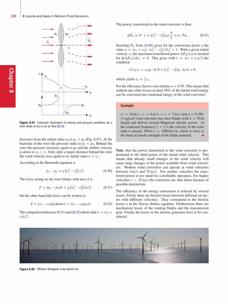
Chapter8
230 8 Liquids and Gases in Motion; Fluid Dynamics
Figure 8.47 Schematic illustration of velocity and pressure conditions for arotor blade at rest in an air flow [8.13]
increases from the initial value p0 to p1 > p0 (Fig. 8.47). At thebackside of the rotor the pressure sinks to p2 < p0. Behind therotor the pressure increases again to p0 and the airflow velocityis down to v2 < v. Only after a larger distance behind the rotorthe wind velocity rises again to its initial value v D v1.
According to the Bernoulli equation is
p1 � p2 D %�v21 � v22
�=2 : (8.50)
The force acting on the rotor blades with area A is
F D .p1 � p2/A D %�v21 � v22
�A=2 : (8.51)
On the other hand this force can be written as
F D .v1 � v2/d=dt.mv/ D .v1 � v2/%vA : (8.52)
The comparison between (8.51) and (8.52) shows that v D .v1Cv2/=2.
Figure 8.48 Offshore Windpark in the North Sea
The power, transferred to the wind converter is then
�Pw D F � v D �v21 � v22
�%v
A
2D a � PW : (8.53)
Inserting Pw from (8.49) gives for the conversion factor a thevalue a D .v1 C v2/ � .v21 � v22/=2v
31 < 1. With a given initial
velocity v1 the maximum transferred power�Pw.v2/ is reachedfor d.�Pw/=dv2 D 0. This gives with v D .v1 C v2/=2 thecondition
�2v2.v1 C v2/% � A=4 C .v21 � v22/% � A=4 D 0 ;
which yields v2 D 13v1.
For the efficiency factor a one obtains a D 0:59. This means thatwithout any other losses at most 59% of the initial wind energycan be converted into rotational energy of the wind converter!
Example
v1 D 10m=s, v2 D 4m=s ! v D 7m=s and a D 0:588.A typical wind converter has rotor blades with L D 50mlength and deliver several Megawatt electric power. Atthe rotational frequency f D 1=s the velocity of the rotorends is already 300m=s D 1080 km=h, which is close tothe limit of tensile strength of the blade material. J
Note, that the power transferred to the wind converter is pro-portional to the third power of the initial wind velocity. Thismeans that already small changes of the wind velocity willcause large changes of the power available from wind convert-ers. Modern wind converters can operate at wind velocitiesbetween 4m=s and 25m=s. For smaller velocities the trans-ferred power is too small for a profitable operation. For highervelocities v > 25m=s the converters are shut down because ofpossible destruction.
The efficiency of the energy conversion is reduced by severallosses. Firstly there are friction losses between different air lay-ers with different velocities. They correspond to the frictionlosses � in the Navier–Stokes equation. Furthermore there aremechanical losses of the rotating blades and the transmissiongear. Finally the losses in the electric generator have to be con-sidered.

8.9 Usage of Wind Energy 231
Chap
ter8
Figure 8.49 Windfarm Krummhörn. Rotor span width is 30m, the nominal electric power output is 300 kW per wind converter. (With kind permission of EWEcorporation, Oldenbourg)
The available electric power is then
Pelectric D a � �air � �mech � �electric � Pw :
For our considerations about the wind velocities before and be-hind the wind converter we have assumed that the rotor bladesare at rest. Because of their rotation the relative velocity be-tween initial wind velocity and rotor velocity is smaller and thewind does no longer impinge perpendicular to the blades. Thisgives not only a smaller effective area Aeff < A but also a smallervalue of the transferred energy.
The power delivered by a wind converter, averaged over oneyear, is only between 10% and 40% of the installed powerdepending on the wind conditions at the converter location.The highest efficiency is reached for offshore wind converters(Fig. 8.48), because here the wind blows continuously and hasgenerally a higher velocity than above undulating solid ground.For wind converters on solid ground the height should be as
30
25
20
15
10
5
01990 91 92 93 94 95 96 97 98 99200001 02 03 04 05 06 07 08 09 10 11 12 13To
tal i
nsta
lled
elec
tric
pow
er p
er y
ear [
GW
]
Figure 8.50 Growth of worldwide annually installed eletric power of wind converters in GW
large as technically possible, because the wind velocity at 100maltitude is much higher than directly above ground (Fig. 8.49).
In Tab. 8.3 the total installed electric power of wind convert-ers is listed for the countries with the highest usage of windenergy and in Fig. 8.50 the impressive increase of worldwideannually new installed electric power from wind converters isillustrated.
Now we will discuss the energy conversion of wind convertersin more detail: The forces driving the rotor blades can be com-posed of the flow resistance force and the Bernoulli-force. Theirratio depends on the shape of the blades and on their angle of at-tack ˛. This is similar to the situation for air flowing around awing profile of an air plane (see Sect. 8.7.2 and Figs. 8.41 and8.46). The pressure dependence p.x/ along a wing profile at restis shown for the upper and lower side of the profile in Fig. 8.51.The pressure difference generates a lift force and a torque aboutan axis in x-direction. Depending on the orientation of the pro-
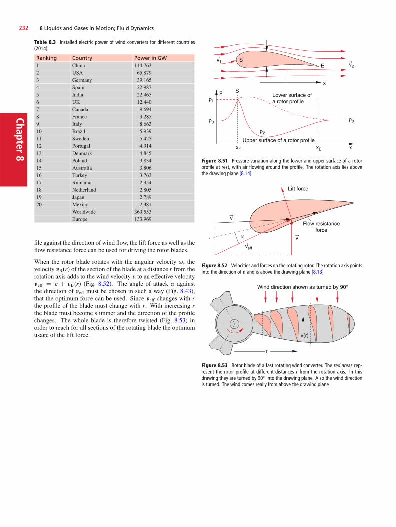
Chapter8
232 8 Liquids and Gases in Motion; Fluid Dynamics
Table 8.3 Installed electric power of wind converters for different countries(2014)
Ranking Country Power in GW1 China 114.7632 USA 65.8793 Germany 39.1654 Spain 22.9875 India 22.4656 UK 12.4407 Canada 9.6948 France 9.2859 Italy 8.66310 Brazil 5.93911 Sweden 5.42512 Portugal 4.91413 Denmark 4.84514 Poland 3.83415 Australia 3.80616 Turkey 3.76317 Rumania 2.95418 Netherland 2.80519 Japan 2.78920 Mexico 2.381
Worldwide 369.553Europe 133.969
file against the direction of wind flow, the lift force as well as theflow resistance force can be used for driving the rotor blades.
When the rotor blade rotates with the angular velocity !, thevelocity vB.r/ of the section of the blade at a distance r from therotation axis adds to the wind velocity v to an effective velocityveff D v C vB.r/ (Fig. 8.52). The angle of attack ˛ againstthe direction of veff must be chosen in such a way (Fig. 8.43),that the optimum force can be used. Since veff changes with rthe profile of the blade must change with r. With increasing rthe blade must become slimmer and the direction of the profilechanges. The whole blade is therefore twisted (Fig. 8.53) inorder to reach for all sections of the rotating blade the optimumusage of the lift force.
Figure 8.51 Pressure variation along the lower and upper surface of a rotorprofile at rest, with air flowing around the profile. The rotation axis lies abovethe drawing plane [8.14]
Figure 8.52 Velocities and forces on the rotating rotor. The rotation axis pointsinto the direction of v and is above the drawing plane [8.13]
Figure 8.53 Rotor blade of a fast rotating wind converter. The red areas rep-resent the rotor profile at different distances r from the rotation axis. In thisdrawing they are turned by 90ı into the drawing plane. Also the wind directionis turned. The wind comes really from above the drawing plane
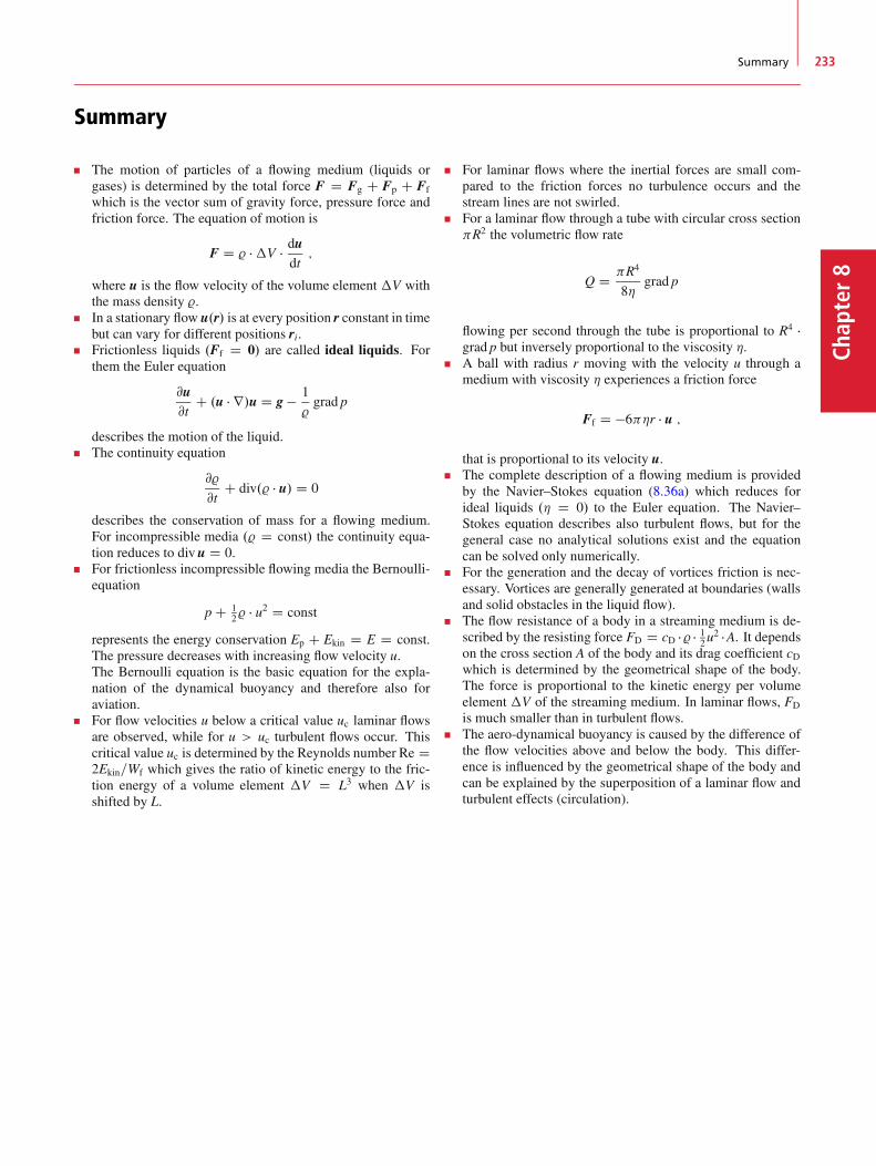
Summary 233
Chap
ter8
Summary
The motion of particles of a flowing medium (liquids orgases) is determined by the total force F D Fg C Fp C Ff
which is the vector sum of gravity force, pressure force andfriction force. The equation of motion is
F D % ��V � dudt;
where u is the flow velocity of the volume element �V withthe mass density %.In a stationary flow u.r/ is at every position r constant in timebut can vary for different positions ri.Frictionless liquids .Ff D 0/ are called ideal liquids. Forthem the Euler equation
@u@t
C .u � r/u D g � 1
%grad p
describes the motion of the liquid.The continuity equation
@%
@tC div.% � u/ D 0
describes the conservation of mass for a flowing medium.For incompressible media .% D const/ the continuity equa-tion reduces to div u D 0.For frictionless incompressible flowing media the Bernoulli-equation
p C 12% � u2 D const
represents the energy conservation Ep C Ekin D E D const.The pressure decreases with increasing flow velocity u.The Bernoulli equation is the basic equation for the expla-nation of the dynamical buoyancy and therefore also foraviation.For flow velocities u below a critical value uc laminar flowsare observed, while for u > uc turbulent flows occur. Thiscritical value uc is determined by the Reynolds number Re D2Ekin=Wf which gives the ratio of kinetic energy to the fric-tion energy of a volume element �V D L3 when �V isshifted by L.
For laminar flows where the inertial forces are small com-pared to the friction forces no turbulence occurs and thestream lines are not swirled.For a laminar flow through a tube with circular cross sectionR2 the volumetric flow rate
Q D R4
8�grad p
flowing per second through the tube is proportional to R4 �grad p but inversely proportional to the viscosity �.A ball with radius r moving with the velocity u through amedium with viscosity � experiences a friction force
Ff D �6�r � u ;
that is proportional to its velocity u.The complete description of a flowing medium is providedby the Navier–Stokes equation (8.36a) which reduces forideal liquids .� D 0/ to the Euler equation. The Navier–Stokes equation describes also turbulent flows, but for thegeneral case no analytical solutions exist and the equationcan be solved only numerically.For the generation and the decay of vortices friction is nec-essary. Vortices are generally generated at boundaries (wallsand solid obstacles in the liquid flow).The flow resistance of a body in a streaming medium is de-scribed by the resisting force FD D cD �% � 1
2u2 �A. It depends
on the cross section A of the body and its drag coefficient cDwhich is determined by the geometrical shape of the body.The force is proportional to the kinetic energy per volumeelement �V of the streaming medium. In laminar flows, FD
is much smaller than in turbulent flows.The aero-dynamical buoyancy is caused by the difference ofthe flow velocities above and below the body. This differ-ence is influenced by the geometrical shape of the body andcan be explained by the superposition of a laminar flow andturbulent effects (circulation).
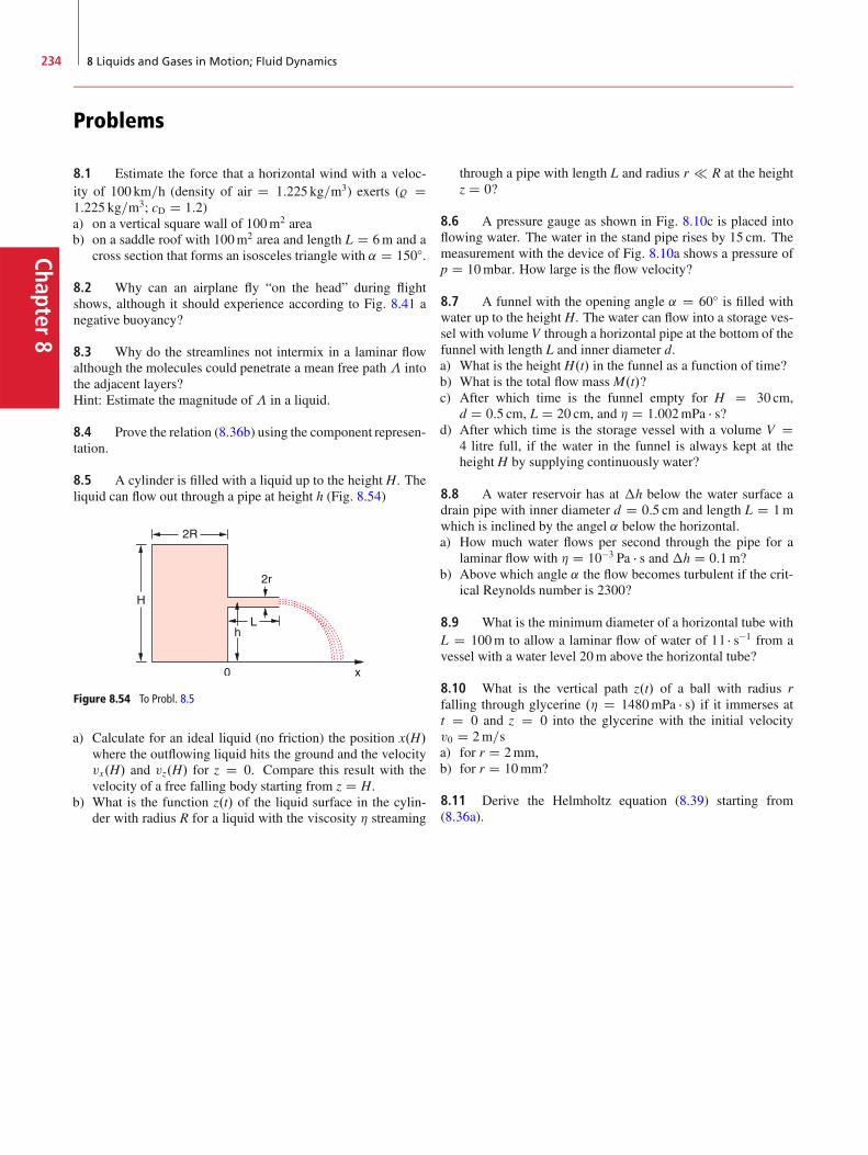
Chapter8
234 8 Liquids and Gases in Motion; Fluid Dynamics
Problems
8.1 Estimate the force that a horizontal wind with a veloc-ity of 100 km=h (density of air D 1:225 kg=m3) exerts (% D1:225 kg=m3; cD D 1:2)a) on a vertical square wall of 100m2 areab) on a saddle roof with 100m2 area and length L D 6m and a
cross section that forms an isosceles triangle with ˛ D 150ı.
8.2 Why can an airplane fly “on the head” during flightshows, although it should experience according to Fig. 8.41 anegative buoyancy?
8.3 Why do the streamlines not intermix in a laminar flowalthough the molecules could penetrate a mean free path � intothe adjacent layers?Hint: Estimate the magnitude of� in a liquid.
8.4 Prove the relation (8.36b) using the component represen-tation.
8.5 A cylinder is filled with a liquid up to the height H. Theliquid can flow out through a pipe at height h (Fig. 8.54)
Figure 8.54 To Probl. 8.5
a) Calculate for an ideal liquid (no friction) the position x.H/where the outflowing liquid hits the ground and the velocityvx.H/ and vz.H/ for z D 0. Compare this result with thevelocity of a free falling body starting from z D H.
b) What is the function z.t/ of the liquid surface in the cylin-der with radius R for a liquid with the viscosity � streaming
through a pipe with length L and radius r R at the heightz D 0?
8.6 A pressure gauge as shown in Fig. 8.10c is placed intoflowing water. The water in the stand pipe rises by 15 cm. Themeasurement with the device of Fig. 8.10a shows a pressure ofp D 10mbar. How large is the flow velocity?
8.7 A funnel with the opening angle ˛ D 60ı is filled withwater up to the height H. The water can flow into a storage ves-sel with volume V through a horizontal pipe at the bottom of thefunnel with length L and inner diameter d.a) What is the height H.t/ in the funnel as a function of time?b) What is the total flow mass M.t/?c) After which time is the funnel empty for H D 30 cm,
d D 0:5 cm, L D 20 cm, and � D 1:002mPa � s?d) After which time is the storage vessel with a volume V D
4 litre full, if the water in the funnel is always kept at theheight H by supplying continuously water?
8.8 A water reservoir has at �h below the water surface adrain pipe with inner diameter d D 0:5 cm and length L D 1mwhich is inclined by the angel ˛ below the horizontal.a) How much water flows per second through the pipe for a
laminar flow with � D 10�3 Pa � s and �h D 0:1m?b) Above which angle ˛ the flow becomes turbulent if the crit-
ical Reynolds number is 2300?
8.9 What is the minimum diameter of a horizontal tube withL D 100m to allow a laminar flow of water of 1 l � s�1 from avessel with a water level 20m above the horizontal tube?
8.10 What is the vertical path z.t/ of a ball with radius rfalling through glycerine .� D 1480mPa � s/ if it immerses att D 0 and z D 0 into the glycerine with the initial velocityv0 D 2m=sa) for r D 2mm,b) for r D 10mm?
8.11 Derive the Helmholtz equation (8.39) starting from(8.36a).
References 235
Chap
ter8
References
8.1a. G. Birkhoff, Hydrodynamics. (Princeton Univ. Press,2015)
8.1b. E. Guyon, J.P. Hulin, Physical Hydrodynamics. (OxfordUniv. Press, 2012)
8.2. J.E.A. John, Th.G. Keith, Gasdynamics. (Prentice Hall,2006)
8.3a. R.K. Bansal, A Textbook on Fluid Mechanics. (FirewallMedia, 2005)
8.3b. G.K. Batchelor, Introduction to Fluid Mechanics. (Cam-bridge Univ. Press, 2000)
8.4a. J.P. Freidberg, Ideal Magnetohydrodynamics. (PlenumPress, 1987)
8.4b. P.A. Davidson, An Introduction to Magnetohydrodynam-ics. (Cambridge University Press, Cambridge, England,2001)
8.5. F. Pobell, Matter and Methods at Low Termperatures.(Springer, Berlin, Heidelberg, 1992)
8.6. D. Even, N. Shurter, E. Gundersen, Applied Physics. (Pen-tice Hall, 2010)
8.7. A.E. Dunstan, The Viscosity of Liquids. (Hard Press Publ.,2013)
8.8. L. Brand, Vector Analysis. (Dover Publications, 2006)
8.9. K. Weltner, S. John,Mathematics for Physicists and Engi-neers. (Springer Berlin, Heidelberg, 2014)
8.10. G.B. Arfken, H.J. Weber, Mathematical Methods forPhysicists. A Comprehensive Guide. (Elsevier Ltd., Ox-ford, 2012)
8.11a. L.J. Clancy, Aerodynamics. (Pitman, London, 1978)8.11b. J.D. Anderson, Fundamentals of Aerodynamics. (Mc-
GrawHill, 2012)8.12. D. Pigott, Understanding Gliding. (A&C Black, London)8.13. M. Diesendorf,GreenhouseSolutions with sustainable En-
ergy. (University of New South Wales, 2007)8.14. J.F. Manwell, J.G. McGowan, A.L. Rogers, Wind En-
ergy Explained: Theory, Design and Applications. (Wiley,2010)
8.15. R. Ferry, E. Monoian, A Field Guide to Renewable EnergyTechnologies. (Society for Cultural Exchange, 2012)
8.16a. T. Burton et al., Wind Energy Handbook. (Wiley, 2001)8.16b. N. Walker, Generating Wind Power. (Crabtree Publ.,
2007)8.17. The European Wind Energy Association, Wind Energy:
The Facts. A Guide to the Technology, Economics and Fu-ture of Wind Power. (Routledge, 2009)

Chap
ter9
Vacuum Physics 99.1 Fundamentals and Basic Concepts . . . . . . . . . . . . . . . . . . . . . 238
9.2 Generation of Vacuum . . . . . . . . . . . . . . . . . . . . . . . . . . . . 241
9.3 Measurement of Low Pressures . . . . . . . . . . . . . . . . . . . . . . . 247
Summary . . . . . . . . . . . . . . . . . . . . . . . . . . . . . . . . . . . . 251
Problems . . . . . . . . . . . . . . . . . . . . . . . . . . . . . . . . . . . . 251
References . . . . . . . . . . . . . . . . . . . . . . . . . . . . . . . . . . . 252
237© Springer International Publishing Switzerland 2017W. Demtröder, Mechanics and Thermodynamics, Undergraduate Lecture Notes in Physics, DOI 10.1007/978-3-319-27877-3_9
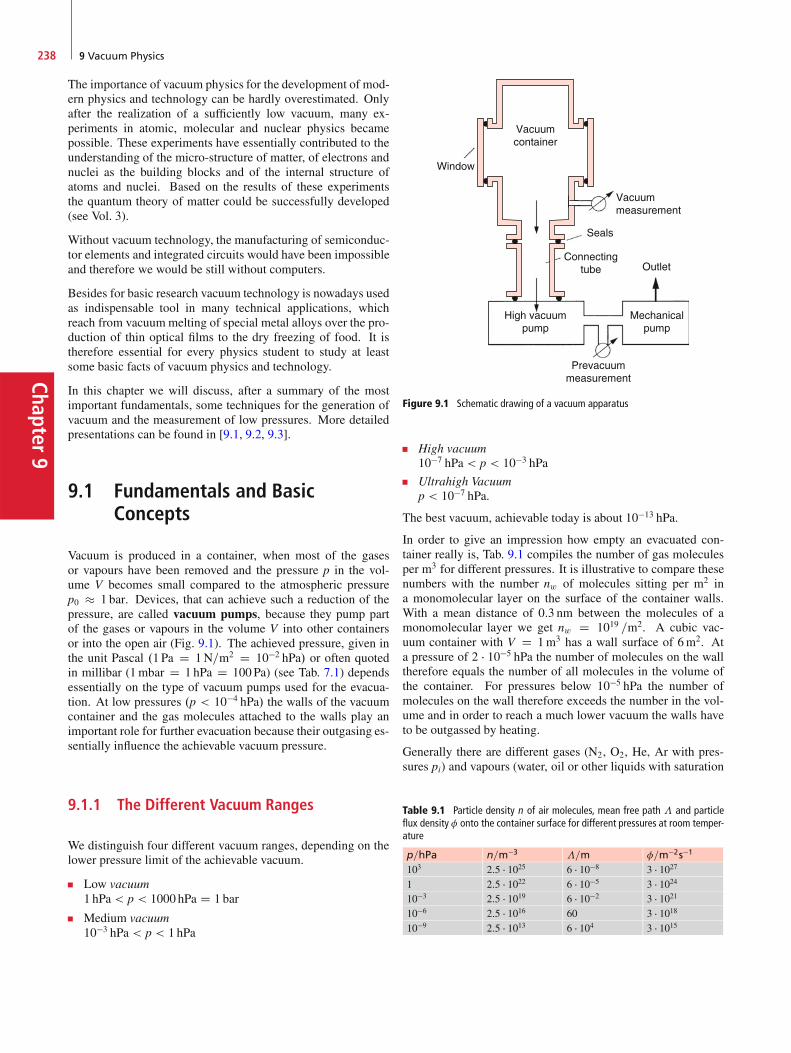
Chapter9
238 9 Vacuum Physics
The importance of vacuum physics for the development of mod-ern physics and technology can be hardly overestimated. Onlyafter the realization of a sufficiently low vacuum, many ex-periments in atomic, molecular and nuclear physics becamepossible. These experiments have essentially contributed to theunderstanding of the micro-structure of matter, of electrons andnuclei as the building blocks and of the internal structure ofatoms and nuclei. Based on the results of these experimentsthe quantum theory of matter could be successfully developed(see Vol. 3).
Without vacuum technology, the manufacturing of semiconduc-tor elements and integrated circuits would have been impossibleand therefore we would be still without computers.
Besides for basic research vacuum technology is nowadays usedas indispensable tool in many technical applications, whichreach from vacuummelting of special metal alloys over the pro-duction of thin optical films to the dry freezing of food. It istherefore essential for every physics student to study at leastsome basic facts of vacuum physics and technology.
In this chapter we will discuss, after a summary of the mostimportant fundamentals, some techniques for the generation ofvacuum and the measurement of low pressures. More detailedpresentations can be found in [9.1, 9.2, 9.3].
9.1 Fundamentals and BasicConcepts
Vacuum is produced in a container, when most of the gasesor vapours have been removed and the pressure p in the vol-ume V becomes small compared to the atmospheric pressurep0 � 1 bar. Devices, that can achieve such a reduction of thepressure, are called vacuum pumps, because they pump partof the gases or vapours in the volume V into other containersor into the open air (Fig. 9.1). The achieved pressure, given inthe unit Pascal .1Pa D 1N=m2 D 10�2 hPa/ or often quotedin millibar (1mbar D 1 hPa D 100Pa) (see Tab. 7.1) dependsessentially on the type of vacuum pumps used for the evacua-tion. At low pressures .p < 10�4 hPa/ the walls of the vacuumcontainer and the gas molecules attached to the walls play animportant role for further evacuation because their outgasing es-sentially influence the achievable vacuum pressure.
9.1.1 The Different Vacuum Ranges
We distinguish four different vacuum ranges, depending on thelower pressure limit of the achievable vacuum.
Low vacuum1 hPa < p < 1000 hPa D 1 bar
Medium vacuum10�3 hPa < p < 1 hPa
Figure 9.1 Schematic drawing of a vacuum apparatus
High vacuum10�7 hPa < p < 10�3 hPa
Ultrahigh Vacuump < 10�7 hPa.
The best vacuum, achievable today is about 10�13 hPa.
In order to give an impression how empty an evacuated con-tainer really is, Tab. 9.1 compiles the number of gas moleculesper m3 for different pressures. It is illustrative to compare thesenumbers with the number nw of molecules sitting per m2 ina monomolecular layer on the surface of the container walls.With a mean distance of 0:3 nm between the molecules of amonomolecular layer we get nw D 1019 =m2. A cubic vac-uum container with V D 1m3 has a wall surface of 6m2. Ata pressure of 2 � 10�5 hPa the number of molecules on the walltherefore equals the number of all molecules in the volume ofthe container. For pressures below 10�5 hPa the number ofmolecules on the wall therefore exceeds the number in the vol-ume and in order to reach a much lower vacuum the walls haveto be outgassed by heating.
Generally there are different gases (N2, O2, He, Ar with pres-sures pi) and vapours (water, oil or other liquids with saturation
Table 9.1 Particle density n of air molecules, mean free path � and particleflux density � onto the container surface for different pressures at room temper-ature
p=hPa n=m�3 �=m �=m�2s�1
103 2:5 � 1025 6 � 10�8 3 � 10271 2:5 � 1022 6 � 10�5 3 � 102410�3 2:5 � 1019 6 � 10�2 3 � 102110�6 2:5 � 1016 60 3 � 101810�9 2:5 � 1013 6 � 104 3 � 1015
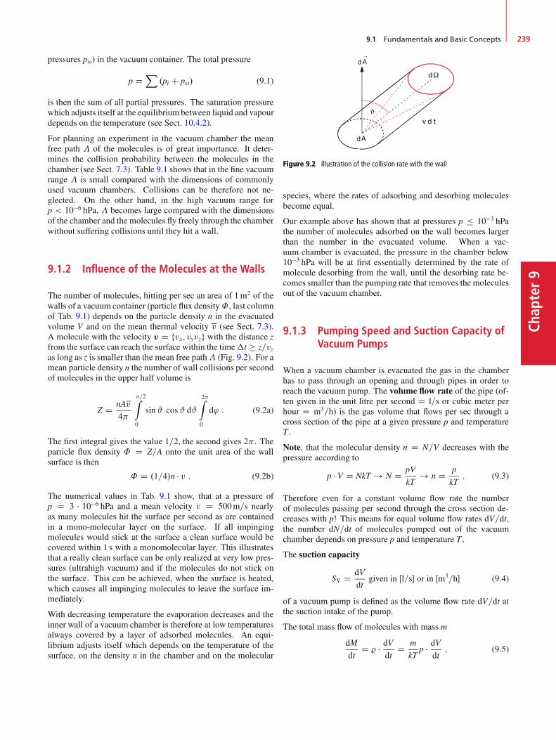
9.1 Fundamentals and Basic Concepts 239
Chap
ter9
pressures psi) in the vacuum container. The total pressure
p DX
.pi C psi/ (9.1)
is then the sum of all partial pressures. The saturation pressurewhich adjusts itself at the equilibrium between liquid and vapourdepends on the temperature (see Sect. 10.4.2).
For planning an experiment in the vacuum chamber the meanfree path � of the molecules is of great importance. It deter-mines the collision probability between the molecules in thechamber (see Sect. 7.3). Table 9.1 shows that in the fine vacuumrange � is small compared with the dimensions of commonlyused vacuum chambers. Collisions can be therefore not ne-glected. On the other hand, in the high vacuum range forp < 10�6 hPa, � becomes large compared with the dimensionsof the chamber and the molecules fly freely through the chamberwithout suffering collisions until they hit a wall.
9.1.2 Influence of the Molecules at the Walls
The number of molecules, hitting per sec an area of 1m2 of thewalls of a vacuum container (particle flux density˚ , last columnof Tab. 9.1) depends on the particle density n in the evacuatedvolume V and on the mean thermal velocity v (see Sect. 7.3).A molecule with the velocity v D fvx; vyvzg with the distance zfrom the surface can reach the surface within the time�t � z=vzas long as z is smaller than the mean free path� (Fig. 9.2). For amean particle density n the number of wall collisions per secondof molecules in the upper half volume is
Z D nAv
4
=2Z
0
sin# cos# d#
2Z
0
d' : (9.2a)
The first integral gives the value 1=2, the second gives 2 . Theparticle flux density ˚ D Z=A onto the unit area of the wallsurface is then
˚ D .1=4/n � v : (9.2b)
The numerical values in Tab. 9.1 show, that at a pressure ofp D 3 � 10�6 hPa and a mean velocity v D 500m=s nearlyas many molecules hit the surface per second as are containedin a mono-molecular layer on the surface. If all impingingmolecules would stick at the surface a clean surface would becovered within 1 s with a monomolecular layer. This illustratesthat a really clean surface can be only realized at very low pres-sures (ultrahigh vacuum) and if the molecules do not stick onthe surface. This can be achieved, when the surface is heated,which causes all impinging molecules to leave the surface im-mediately.
With decreasing temperature the evaporation decreases and theinner wall of a vacuum chamber is therefore at low temperaturesalways covered by a layer of adsorbed molecules. An equi-librium adjusts itself which depends on the temperature of thesurface, on the density n in the chamber and on the molecular
Figure 9.2 Illustration of the collision rate with the wall
species, where the rates of adsorbing and desorbing moleculesbecome equal.
Our example above has shown that at pressures p � 10�3 hPathe number of molecules adsorbed on the wall becomes largerthan the number in the evacuated volume. When a vac-uum chamber is evacuated, the pressure in the chamber below10�3 hPa will be at first essentially determined by the rate ofmolecule desorbing from the wall, until the desorbing rate be-comes smaller than the pumping rate that removes the moleculesout of the vacuum chamber.
9.1.3 Pumping Speed and Suction Capacity ofVacuum Pumps
When a vacuum chamber is evacuated the gas in the chamberhas to pass through an opening and through pipes in order toreach the vacuum pump. The volume flow rate of the pipe (of-ten given in the unit litre per second D l=s or cubic meter perhour D m3=h) is the gas volume that flows per sec through across section of the pipe at a given pressure p and temperatureT .
Note, that the molecular density n D N=V decreases with thepressure according to
p � V D NkT ! N D pV
kT! n D p
kT: (9.3)
Therefore even for a constant volume flow rate the numberof molecules passing per second through the cross section de-creases with p! This means for equal volume flow rates dV=dt,the number dN=dt of molecules pumped out of the vacuumchamber depends on pressure p and temperature T .
The suction capacity
SV D dV
dtgiven in Œl=s� or in Œm3=h� (9.4)
of a vacuum pump is defined as the volume flow rate dV=dt atthe suction intake of the pump.
The total mass flow of molecules with mass m
dM
dtD % � dV
dtD m
kTp � dV
dt; (9.5)
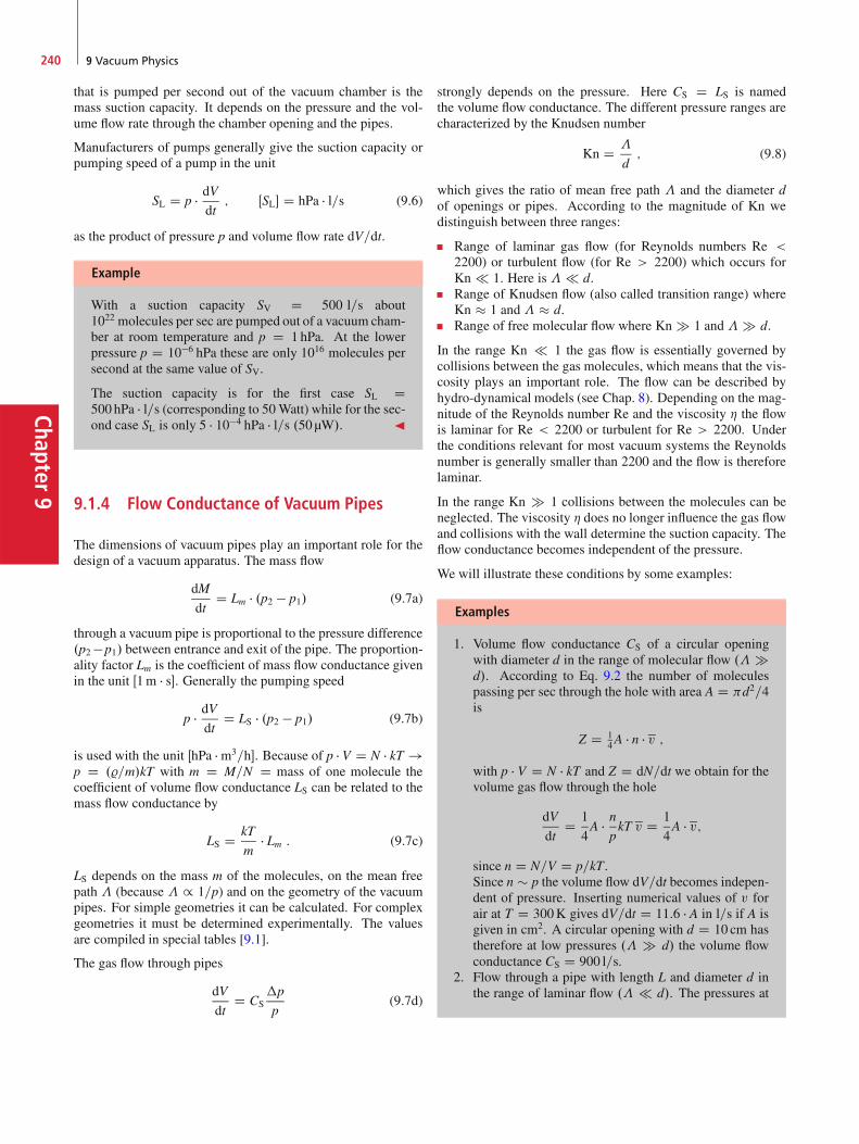
Chapter9
240 9 Vacuum Physics
that is pumped per second out of the vacuum chamber is themass suction capacity. It depends on the pressure and the vol-ume flow rate through the chamber opening and the pipes.
Manufacturers of pumps generally give the suction capacity orpumping speed of a pump in the unit
SL D p � dVdt; ŒSL� D hPa � l=s (9.6)
as the product of pressure p and volume flow rate dV=dt.
Example
With a suction capacity SV D 500 l=s about1022 molecules per sec are pumped out of a vacuum cham-ber at room temperature and p D 1 hPa. At the lowerpressure p D 10�6 hPa these are only 1016 molecules persecond at the same value of SV.
The suction capacity is for the first case SL D500 hPa � l=s (corresponding to 50Watt) while for the sec-ond case SL is only 5 � 10�4 hPa � l=s .50 µW/. J
9.1.4 Flow Conductance of Vacuum Pipes
The dimensions of vacuum pipes play an important role for thedesign of a vacuum apparatus. The mass flow
dM
dtD Lm � .p2 � p1/ (9.7a)
through a vacuum pipe is proportional to the pressure difference.p2 �p1/ between entrance and exit of the pipe. The proportion-ality factor Lm is the coefficient of mass flow conductance givenin the unit Œ1m � s�. Generally the pumping speed
p � dVdt
D LS � .p2 � p1/ (9.7b)
is used with the unit ŒhPa � m3=h�. Because of p � V D N � kT !p D .%=m/kT with m D M=N D mass of one molecule thecoefficient of volume flow conductance LS can be related to themass flow conductance by
LS D kT
m� Lm : (9.7c)
LS depends on the mass m of the molecules, on the mean freepath � (because � / 1=p) and on the geometry of the vacuumpipes. For simple geometries it can be calculated. For complexgeometries it must be determined experimentally. The valuesare compiled in special tables [9.1].
The gas flow through pipes
dV
dtD CS
�p
p(9.7d)
strongly depends on the pressure. Here CS D LS is namedthe volume flow conductance. The different pressure ranges arecharacterized by the Knudsen number
Kn D �
d; (9.8)
which gives the ratio of mean free path � and the diameter dof openings or pipes. According to the magnitude of Kn wedistinguish between three ranges:
Range of laminar gas flow (for Reynolds numbers Re <2200) or turbulent flow (for Re > 2200) which occurs forKn 1. Here is � d.Range of Knudsen flow (also called transition range) whereKn � 1 and � � d.Range of free molecular flow where Kn � 1 and � � d.
In the range Kn 1 the gas flow is essentially governed bycollisions between the gas molecules, which means that the vis-cosity plays an important role. The flow can be described byhydro-dynamical models (see Chap. 8). Depending on the mag-nitude of the Reynolds number Re and the viscosity � the flowis laminar for Re < 2200 or turbulent for Re > 2200. Underthe conditions relevant for most vacuum systems the Reynoldsnumber is generally smaller than 2200 and the flow is thereforelaminar.
In the range Kn � 1 collisions between the molecules can beneglected. The viscosity � does no longer influence the gas flowand collisions with the wall determine the suction capacity. Theflow conductance becomes independent of the pressure.
We will illustrate these conditions by some examples:
Examples
1. Volume flow conductance CS of a circular openingwith diameter d in the range of molecular flow .� �d/. According to Eq. 9.2 the number of moleculespassing per sec through the hole with area A D d2=4is
Z D 14A � n � v ;
with p � V D N � kT and Z D dN=dt we obtain for thevolume gas flow through the hole
dV
dtD 1
4A � n
pkT v D 1
4A � v;
since n D N=V D p=kT .Since n � p the volume flow dV=dt becomes indepen-dent of pressure. Inserting numerical values of v forair at T D 300K gives dV=dt D 11:6 � A in l=s if A isgiven in cm2. A circular opening with d D 10 cm hastherefore at low pressures .� � d/ the volume flowconductance CS D 900 l=s.
2. Flow through a pipe with length L and diameter d inthe range of laminar flow .� d/. The pressures at

9.2 Generation of Vacuum 241
Chap
ter9
the two ends of the pipe are p1 and p2. According tothe Hagen-Poisseuille-law (8.32)
p � dVdt
D � d4128 �L
� p1 C p22
.p1 � p2/ ; (9.9)
we obtain for d D 5 cm, L D 1m, p1 D 2 hPa, p2 D 0,�air D 0:018mPa � s, the numerical value p � dV=dt D170Pa �m2=s. According to (9.7) the volume flow con-ductance then becomes CS D 0:85m3=s D 850 l=s.At a lower pressure of 10�1 hPa, where � D 0:06 cm(Tab. 9.1) which is still smaller than d the flow con-ductance decreases according to (9.7) and (9.9) toCS D 42 l=s. Equation 9.9 is in this range, how-ever, only approximately valid and the accurate valueis CS D 80 l=s.In the range of molecular flow .� > d/ CS con-verges with decreasing pressure towards the valueCS D 16 l=s. J
The reciprocal of the flow conductance
RS D 1=CS (9.10)
is the flow resistance. Completely analogue to the electrical re-sistance in electricity the flow resistance of consecutive flowpipes is the sum of the individual resistances, while for flowpipes in parallel arrangements the individual flow conductancesadd to the total conductance, as can be immediately seen from(9.7).
9.1.5 Accessible Final Pressure
Every vacuum chamber has openings that allow access to theexperimental setup in its inside. They are closed by flange seals.However, there are always leaks which are often difficult to findand to close. Through these leaks molecules can penetrate fromthe outside into the vacuum chamber. We define the gas ratedGL=dt D p0 � dVL=dt (p0 D atmospheric pressure) which pen-etrates through all leaks into the vacuum chamber as the leakrate. It is given in the same units hPa � l=s as the pumping speeddefined in (9.6).
As has been previously discussed molecules can also be des-orbed from the inner walls and delivered into the volume of thevacuum chamber. This leads without pumping to a pressure in-crease �p.
For the rate dNd=dt of desorbing molecules we obtain with p �V D N � kT the pressure increase per second
dp
dtD kT
V
dNd
dt: (9.11)
The total rate of desorbed gas is
dGd
dtD V � dp
dtD kT
dNd
dt: (9.12)
Desorption rate
Leak rate
Pumping speed
Figure 9.3 The achievable final pressure is determined by the compensationof pumping speed by leak rate C desorption rate
The final pressure achieved in the vacuum chamber is deter-mined by the pumping speed, the leak rate and the total rate ofdesorbing molecules (Fig. 9.3). At the final pressure the pump-ing speed just equals the sum of leak rate and desorbing gas rate.
SeffL .p/ D dGL
dtC dGd
dt; (9.13)
where SeffL is the effective pumping speed at the outlet openingof the chamber to the pumping pipes. It is equal to the pumpingspeed of the pump minus the flow conductance of the vacuumlines between chamber and pump.
The attainable final pressure pf results then from (9.13) with(9.6) and (9.12):
pf D dGd=dt C dGL=dt
SV; (9.14)
where SV D dVp=dt is the effective suction capacity at the exitof the vacuum chamber.
Example
For a suction capacity SV D 103 l=s, a leak rate of10�4 hPa � l=s and a desorbing gas rate of 10�3 hPa � l=sa final pressure of pf D 1:1 � 10�6 hPa can be reached.After heating the walls the desorbing rate sinks below theleak rate and a final pressure of pf D 10�7 hPa can beachieved. J
9.2 Generation of Vacuum
In order to remove gas particles out of the vacuum chamber vac-uum pumps are used. The different types can be divided intothree classes (Tab. 9.2):
Mechanical pumps,Diffusion pumps (fluid acceleration vacuum pump),Cryo pumps and sorption pumps.
We will briefly discuss these three classes. In Fig. 9.4 the pres-sure ranges are compiled where the different pumps can be used.

Chapter9
242 9 Vacuum Physics
Table 9.2 Classification of the most important types of vacuum pumps
Mechanicalpumps
Fuel accelerationpumps
Condensation pumps,sorption pumps
Rotary vane pumps Liquid jet pumps Cool trapsRoots pumps Vapor jet pumps Kryo pumps,
sorption pumpsTurbopumps Diffusion pumps ion getterpumps
Rotary vane pump
Roots pump
Steam jet pump
Diffusion pump
Turbo-molecular pump
Kryo-pump
Mass spectrometer
Friction ball manometer
Capacitor membrane mano.
McLoid mano.
Ionization manometer
Penning mano.
Heat conduction mano.
Membrane mano.
Figure 9.4 Pressure ranges a of the differrent types of vacuum pumps, b ofpressure detectors
9.2.1 Mechanical Pumps
Already around 1600 Galileo Galilei has produced a low vac-uum in a container by using a movable piston. More detailedexperiments were performed in 1643 by Evangelista Torricelli,who was Galileo’ successor in Florence. In honour of Torricellithe unit of pressure has been named torr (1 torr is the pressure of1mmmercury column D 133:3Pa). The unit torr has been usedfor several centuries before the SI unit 1 Pa was introduced.
Spectacular experiments with evacuated spheres were per-formed 1645 by Otto von Guericke, the major of the Germancity Magdeburg. He put two hemi-spheres together, sealed themup with leather gaskets and evacuated the interior. This pressedthe two hemi-spheres tightly together. In order to demonstratethe force on the hemi-spheres due to the external pressure heroped 8 horses in on each side who tried unsuccessfully to sep-arate the hemi-spheres. The large auditorium was very muchastonished that 16 horses could not separate the hemi-spheresalthough they could be readily separated after the evacuatedsphere was filled again with air at the external pressure. Su-perstitious people believed in a ghost inside the sphere. Anengraving of Caspar Schott illustrates this spectacular exper-
Figure 9.5 The demonstration experiment by Otto von Guericke. Engraving byCaspar Schott
Figure 9.6 Ancient mechanical vacuum pump
iment (Fig. 9.5). At that time the evacuation with piston airpumps (Fig. 9.6) was tedious, because the seals were imperfect.
Nowadays the mechanical pumps are mainly rotary vane pumps,Roots pumps or turbo-molecular pumps, which are all driven byelectro motors.

9.2 Generation of Vacuum 243
Chap
ter9
9.2.1.1 Rotary Vane Pumps
The basic principle of rotary vane pumps is schematically illus-trated in Fig. 9.7. An eccentrically mounted rotor R1 rotates in acylindrical bore with an inlet S1 from the vacuum chamber andan outlet A1 into the open air at atmospheric pressure. The rotorhas a slit in which two sliders are pushed by a coil spring againstthe wall of the bore. When the rotor rotates in the direction ofthe arrow the right side of the sliders sucks the gas from S1 anddrives it during half of a rotation period towards A1. This is re-peated every half turn thus continuously evacuating the vacuumchamber behind S1.
For single-stage pumps the outlet A1 is connected to the openair (or an exhaust gas line) and the pressure p in A1 equals theatmospheric pressure. Due to the pressure difference betweenA1 and S1 always some gas can flow back from A1 to S1 becausethe slider in the rotor does not completely seal the connectionbetween A1 and S1. This limits the attainable final pressure inS1. In order to keep the leak rate as small as possible the pumpis filled with oil which forms a film between slider and walland not only gives a better seal but also acts as lubricant thatprevents jamming of the rotor. With such single-stage pumpsfinal pressures of 10�1–10�2 hPa are reached.
In order to obtain lower final pressures the outlet A1 can beconnected to a second pump (Fig. 9.8), which produces in A1 al-
Figure 9.7 Principle operation of a rotating vane pump [9.1]. With kind per-mission of Leybold GmbH
Figure 9.8 Two stage rotary vane pump [9.1]. With kind permission of LeyboldGmbH
ready a pressure of 10�1 hPa, thus reducing the back-streamingconsiderably. This leads to a final pressure of permanent gasesin S1 of about 10�3 to 10�4 hPa. However, now the saturationvapour pressure of the pump oil (ps � 10�3 hPa at T D 350K)is the limiting factor for the final pressure. Using a cool trapbetween S1 and the vacuum chamber can reduce the saturationpressure and realizes an oil-free vacuum in the chamber.
Typical pumping speeds of such rotary van pumps reach from1m3=h for small pumps to 60m3=h for larger ones. To preventback streaming of atmospheric pressure from A to S in case ofan accidental standstill of the pump a blocking valve V is builtin at A2.
9.2.1.2 Roots-Pump
The principle of a roots pump is shown in Fig. 9.9. Two symmet-rically shaped rotors R1 and R2 rotate with opposite directionsabout two axes. They are arranged in such a way that their sur-faces nearly touch each other. The gap width between the tworotors and between the rotors and the wall are only a few tenthof a millimetre. For the momentary situation shown in Fig. 9.9the gas volume V1 enclosed by the left rotor R2 is compressedand pushed to the outlet A when the rotor rotates counterclock-wise. A quarter of a full turn later the oppositely turning rotorR1 pushes gas from S to a similar enclosed volume on the rightside and presses it to A. Since the rotors do not touch, there is no
Figure 9.9 Principle operation of roots pump [9.1]. With kind permission ofLeybold GmbH

Chapter9
244 9 Vacuum Physics
material abrasion and roots pumps can rotate with high angularvelocities, thus increasing the pumping speed. The disadvantageof the gap between the rotors is the backstream of gas from Ato S. With decreasing pressure in A the flow resistance of thegaps with width d becomes larger as soon as � � d. Thereforethe pressure in A should be lowered by a one-stage rotary vanepump. Roots pumps need a forepump. Large roots pumps reachpumping speeds of up to 105 m3=h.
9.2.1.3 Turbo-Molecular Pumps
The turbo-molecular pump, developed 1958 by W. Becker [9.5]is based on the principle that molecules hitting a fast movingsurface, gain momentum in the direction of the surface motion(Fig. 9.10).
The turbo pump consists of a staple of fast rotating rotors withmany blades (Fig. 9.11). Assume a gas molecule M with thethermal velocity v impinges on a blade of the rotor which has thesame temperature T as the gas. For a resting rotor the moleculeM would desorb from the blade after a short time with the ve-locity v0 which has about the same magnitude as v, (jvj � jv0j)while its directions are distributed around the surface normal.
If the rotor blade moves with the velocity u the total velocity ofthe desorbing molecules is the vector sum v� D v0 C u. Due
Figure 9.10 a Momentum transfer at the reflection of molecules M at a fastmoving surface; b basic principle of turbo pump
Figure 9.11 Rotor of a turbo pump. With kind permission of CIT VacuumTechnique
to the direction of u to the left in Fig. 9.10, the number of im-pinging molecules from the left half space is larger than that ofmolecules from the right one. Because of the inclined blades thevelocities v0 are preferentially directed into the downward direc-tion. The rotating blades therefore transport molecules from theupper space (inlet of the pump) to the lower space (outlet of thepump).
This is illustrated in Fig. 9.10b. If the rotor blade moves withthe velocity u to the left, molecules moving with the velocityv0 < u from the upper space 1 can hit the blade only on the leftside.
9.2.2 Diffusion Pumps
Diffusion pumps are used for the generation of high- andultrahigh-vacuum. Their principle is shown in Fig. 9.12. Apumping fluid 2 (oil or mercury) is evaporated by the heater atthe bottom of the pump. The vapour rises in the inner part ofthe pump and leaves it at the upper end through nozzles whereit gains supersonic speed forming fast vapour jets, which aredirected downwards. Molecules from the vacuum chamber dif-fuse into the vapour jets and are pushed downwards by collisions

9.2 Generation of Vacuum 245
Chap
ter9
Figure 9.12 Operation principle of a diffusion pump. 1 D Heating, 2 D boil-ing region, 3 D pump body, 4 D water cooling, 5 D high vacuum side, 6 Dparticles from high vacuum side, 7 D vapor jet, 8 D pre vacuum tube, A–D Dnozzles for vapor jets. With kind permission of Leybold GmbH [9.1]
with the vapour molecules. Since the vapour jets are initiallyfree of gas, the diffusion rate into the jet is higher than out of thejet.
After diffusion into the vapor jet the gas molecules experienceby collisions with the jet molecules an additional momentumdownwards into the direction of the jet. They come into lowerregions where they diffuse into the lower jets where they expe-rience more collisions and are transported farther downwards.Finally they reach the outlet of the diffusion pump where theyare pumped away by a mechanical pump. A pressure ratiopi=p0 � 10�7 between the pressure pi at the input and p0 atthe outlet of the diffusion pump can be reached. When the fore-pump maintains a pressure p0 D 10�2 hPa a pressure as low as10�9 hPa can be realized at the high vacuum side.
The hot vapor jets hit the cooled wall of the pump where theycondense and flow as liquid film down to the heater. Here theyare again vaporized. In order to form oil vapor jets the free meanpath � must be sufficiently large, i.e. the pressure sufficientlylow. Diffusion pumps therefore can operate only at pressuresbelow 10�2–10�3 hPa. They do need a forepump, which gener-ates the necessary minimum starting pressure.
The total pressure at the high vacuum side of the diffusionpump is the sum of all partial pressures, including the saturationpressure of the pump fuel. For mercury as fuel the saturationpressure is 10�3 hPa at room temperature. For mercury pumps
Figure 9.13 a Cooled baffle for reduction of oil return flow. b Liquid nitrogencondensation trap
therefore liquid nitrogen cool traps above the diffusion pumpare necessary in order to obtain a better high vacuum. Oil-diffusion pumps operate with special oils that have saturationpressures below 10�7 hPa. Therefore nowadays mainly oil dif-fusion pumps are used.
In order to prevent oil molecules from reaching the vacuum con-tainer a cooled baffle is mounted above the pump (Fig. 9.13a)which blocks the direct way of the molecules. Another solutionis a liquid nitrogen trap (Fig.9.13b) where every oil moleculeon its way to the vacuum container hits at least one cooled wallwhere the molecules are adsorbed.
The pumping speed of modern vacuum diffusion pumps rangesfrom 60 l=s (for a small pump with 20 cm heights) to 50 000 l=s(about 4–5m high). Diffusion pumps are the favorite types ofhigh vacuum pumps. In Fig. 9.14 the pumping speed of mediumsized diffusion pumps as a function of the pressure on the highvacuum side is compared with the performance of a turbo pump.Important for the optimum performance of a pumping system is
Figure 9.14 Pumping speed S .p/ of different types of pumps
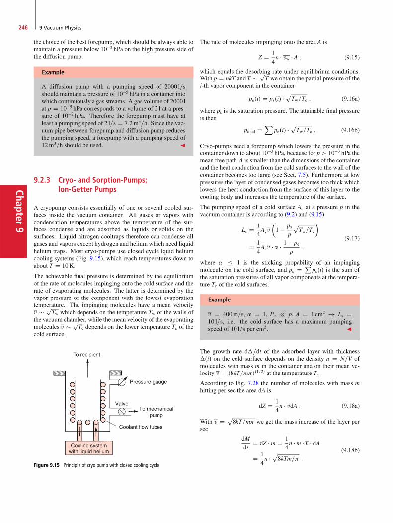
Chapter9
246 9 Vacuum Physics
the choice of the best forepump, which should be always able tomaintain a pressure below 10�2 hPa on the high pressure side ofthe diffusion pump.
Example
A diffusion pump with a pumping speed of 2000 l=sshould maintain a pressure of 10�5 hPa in a container intowhich continuously a gas streams. A gas volume of 2000 lat p D 10�5 hPa corresponds to a volume of 2 l at a pres-sure of 10�2 hPa. Therefore the forepump must have atleast a pumping speed of 2 l=s D 7:2m3=h. Since the vac-uum pipe between forepump and diffusion pump reducesthe pumping speed, a forepump with a pumping speed of12m3=h should be used. J
9.2.3 Cryo- and Sorption-Pumps;Ion-Getter Pumps
A cryopump consists essentially of one or several cooled sur-faces inside the vacuum container. All gases or vapors withcondensation temperatures above the temperature of the sur-faces condense and are adsorbed as liquids or solids on thesurfaces. Liquid nitrogen cooltraps therefore can condense allgases and vapors except hydrogen and helium which need liquidhelium traps. Most cryo-pumps use closed cycle lquid heliumcooling systems (Fig. 9.15), which reach temperatures down toabout T D 10K.
The achievable final pressure is determined by the equilibriumof the rate of molecules impinging onto the cold surface and therate of evaporating molecules. The latter is determined by thevapor pressure of the component with the lowest evaporationtemperature. The impinging molecules have a mean velocityv � p
Tw which depends on the temperature Tw of the walls ofthe vacuum chamber, while the mean velocity of the evaporatingmolecules v � p
Tc depends on the lower temperature Tc of thecold surface.
Figure 9.15 Principle of cryo pump with closed cooling cycle
The rate of molecules impinging onto the area A is
Z D 1
4n � vw � A ; (9.15)
which equals the desorbing rate under equilibrium conditions.With p D nkT and v � p
T we obtain the partial pressure of thei-th vapor component in the container
pe.i/ D ps.i/ �pTw=Tc ; (9.16a)
where ps is the saturation pressure. The attainable final pressureis then
ptotal DX
pe.i/ �pTw=Tc : (9.16b)
Cryo-pumps need a forepump which lowers the pressure in thecontainer down to about 10�3 hPa, because for p > 10�3 hPa themean free path� is smaller than the dimensions of the containerand the heat conduction from the cold surfaces to the wall of thecontainer becomes too large (see Sect. 7.5). Furthermore at lowpressures the layer of condensed gases becomes too thick whichlowers the heat conduction from the surface of this layer to thecooling body and increases the temperature of the surface.
The pumping speed of a cold surface Ac at a pressure p in thevacuum container is according to (9.2) and (9.15)
Ls D 1
4Acv
�1 � ps
p
pTw=Tc
�
D 1
4Acv � ˛ � 1 � pe
p;
(9.17)
where ˛ � 1 is the sticking propability of an impingingmolecule on the cold surface, and ps D P
ps.i/ is the sum ofthe saturation pressures of all vapor components at the tempera-ture Tc of the cold surfaces.
Example
v D 400m=s, ˛ D 1, Pe p, A D 1 cm2 ! Ls D10 l=s, i.e. the cold surface has a maximum pumpingspeed of 10 l=s per cm2. J
The growth rate d�=dt of the adsorbed layer with thickness�.t/ on the cold surface depends on the density n D N=V ofmolecules with mass m in the container and on their mean ve-locity v D .8kT=m/.1=2/ at the temperature T .
According to Fig. 7.28 the number of molecules with mass mhitting per sec the area dA is
dZ D 1
4n � vdA : (9.18a)
With v D p8kT=m we get the mass increase of the layer per
sec
dM
dtD dZ � m D 1
4n � m � v � dA
D 1
4n �p8kTm= :
(9.18b)
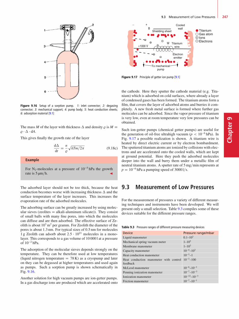
9.3 Measurement of Low Pressures 247
Chap
ter9
Figure 9.16 Setup of a sorption pump. 1: inlet connector; 2: degasingconnector; 3: mechanical support; 4: pump body; 5: heat conduction sheets;6: adsorption material [9.1]
The massM of the layer with thickness� and density % isM D% �� � dA.This gives finally the growth rate of the layer
d�
dtD n
%
pkTm=2 (9.18c)
Example
For N2-molecules at a pressure of 10�5 hPa the growthrate is 5 µm=h. J
The adsorbed layer should not be too thick, because the heatconduction becomes worse with increasing thickness � and thesurface temperature of the layer increases. This increases theevaporation rate of the adsorbed molecules.
The adsorbing surface can be greatly increased by using molec-ular sieves (zeolites D alkali-aluminum silicate)). They consistof small balls with many fine pores, into which the moleculescan diffuse and are then adsorbed. The effective surface of Ze-olith is about 103 m2 per gramm. For Zeolith the diameter of thepores is about 1:3 nm. For typical sizes of 0:5 nm for molecules1 g Zeolith can adsorb about 2:5 � 1021 molecules in a mono-layer. This corresponds to a gas volume of 10 000 l at a pressureof 10�2 hPa.
The adsorption of the molecular sieves depends strongly on thetemperature. They can be therefore used at low temperatures(liquid nitrogen temperature D 78K) as a cryopump and lateron they can be degassed at higher temperatures and used againas pumps. Such a sorption pump is shown schematically inFig. 9.16.
Another solution for high vacuum pumps are ion-getter pumps.In a gas discharge ions are produced which are accelerated onto
Figure 9.17 Principle of getter ion pump [9.1]
the cathode. Here they sputter the cathode material (e.g. Tita-nium) which is adsorbed on cold surfaces, where already a layerof condensed gases has been formed. The titanium atoms form afilm, that covers the layer of adsorbed atoms and burries it com-pletely. A new fresh metal surface is formed where further gasmolecules can be adsorbed. Since the vapor pressure of titaniumis very low, even at room temperature very low pressures can beobtained.
Such ion-getter pumps (chemical getter pumps) are useful forthe generation of oil-free ultrahigh vacuum (p < 10�6 hPa). InFig. 9.17 a possible realization is shown. A titanium wire isheated by direct electric current or by electron bombardment.The sputtered titanium atoms are ionized by collisions with elec-trons and are accelerated onto the cooled walls, which are keptat ground potential. Here they push the adsorbed moleculesdeeper into the wall and burry them under a metallic film ofneutral titanium atoms. A sputter rate of 5mg=min represents atp D 10�6 hPa a pumping speed of 3000 l=s.
9.3 Measurement of Low Pressures
For the measurement of pressures a variety of different measur-ing techniques and instruments have been developed. We willpresent only a small selection. Table 9.3 compiles some of thesedevices suitable for the different pressure ranges.
Table 9.3 Pressure ranges of different pressure measuring devices
Device Pressure range/mbarLiquid manometer 0:1–103
Mechanical spring vacuum meter 1–103
Membrane manometer 1–103
Capacity manometer 10�4–103
Heat conduction manometer 10�3–1Heat conduction manometer with controlfeedback
10�3–100
McLeod manometer 10�6–10�1
Penning ionization manometer 10�7–10�3
Ionization manometer 10�12–10�3
Friction manometer 10�7–10�1
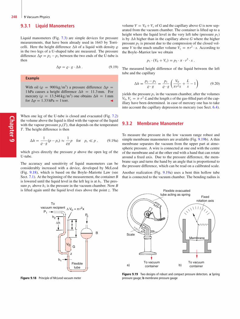
Chapter9
248 9 Vacuum Physics
9.3.1 Liquid Manometers
Liquid manometers (Fig. 7.3) are simple devices for pressuremeasurements, that have been already used in 1643 by Torri-celli. Here the height difference �h of a liquid with density %in the two legs of a U-shaped tube are measured. The pressuredifference �p D p2 � p1 between the two ends of the U-tube isthen
�p D % � g ��h : (9.19)
Example
With oil (% D 900 kg=m3) a pressure difference �p D1 hPa causes a height difference �h D 11:3mm. Formercury (% D 13;546 kg=m3) one obtains �h D 1mmfor �p D 1:33 hPa D 1 torr. J
When one leg of the U-tube is closed and evacuated (Fig. 7.2)the volume above the liquid is filed with the vapour of the liquidwith the vapour pressure ps.T/, that depends on the temperatureT . The height difference is then
�h D 1
% � g .p � ps/ � 1
%gp for ps p ; (9.19a)
which gives directly the pressure p above the open leg of theU-tube.
The accuracy and sensitivity of liquid manometers can beconsiderably increased with a device, developed by McLeod(Fig. 9.18), which is based on the Boyle–Mariotte Law (seeSect. 7.1). At the beginning of the measurement, the container Bis lowered until the liquid level in the left leg is at h1. The pres-sure p1 above h1 is the pressure in the vacuum chamber. Now Bis lifted again until the liquid level rises above the point z. The
Figure 9.18 Principle of McLeod vacuum meter
volume V D V0 CVc of G and the capillary aboveG is now sep-arated from the vacuum chamber. The container is lifted up to aheight where the liquid level in the very left tube (pressure p1)is by �h higher than in the capillary above G where the higherpressure p2 is present due to the compression of the closed vol-ume V to the much smaller volume Vc D r2 � x. According tothe Boyle–Marriot law we obtain
p1 � .V0 C Vc/ D p2 � � r2 � x :The measured height difference of the liquid between the lefttube and the capillary
�h D p2 � p1% � g D p1
% � g�
V0
r2xC L
x� 1
�(9.20)
yields the pressure p1 in the vacuum chamber, after the volumesV0, Vc D �r2 �L and the length x of the gas-filled part of the cap-illary have been determined. in case of mercury one has to takeinto account the capillary depression to mercury (see Sect. 6.4).
9.3.2 Membrane Manometer
To measure the pressure in the low vacuum range robust andsimple membrane manometers are available (Fig. 9.19b). A thinmembrane separates the vacuum from the upper part at atmo-spheric pressure. A wire is connected at one end with the centreof the membrane and at the other end with a hand that can rotatearound a fixed axis. Due to the pressure difference, the mem-brane sags and turns the hand by an angle that is proportional tothe pressure difference, which can be read on a calibrated scale.
Another realization (Fig. 9.19a) uses a bent thin hollow tubethat is connected to the vacuum chamber. The bending radius is
Flexible evacuatedtube acting as spring
To vacuumcontainer
ScaleMembrane
a) b)To vacuumcontainer
Fixedrotation axis
Figure 9.19 Two designs of robust and compact pressure detectors. a Springpressure gauge; b membrane pressure gauge

9.3 Measurement of Low Pressures 249
Chap
ter9
Figure 9.20 Membrane capacitor vacuum gauge. A thin membrane M pro-vides together with two curved fixed plates two capacities C1 and C2, which arearranged in a bridge circuit (see Vol. 2, Chap. 2). They are fed by two identicalac-voltage sources
dependent on the pressure. When it changes the upper end of thetube moves a hand which indicates the pressure on a calibratedscale.
For lower pressures in the high vacuum range (p < 10�5 hPa)capacitance membrane manometers (Fig. 9.20) can be used.Here a thin membrane which separates the vacuum chamberfrom a chamber with a fixed reference pressure. It forms oneelectrode of two electric capacitors C1 and C2, When the pres-sure in the vacuum chamber decreases the membrane bends tothe left side and decreases the electrode separation of C1 butincreases that of C2, thus increasing the capacitance of C1 anddecreases that of C2. This changes their AC resistance in an op-posite direction, which can be measured with an electric bridgearrangement where the two capacitors are charged by two iden-tical AC voltage supplies (see Vol. 2. Chap. 1).
9.3.3 Heat Conduction Manometers
As has been shown in Sect. 7.5 the heat conduction of a gas inthe pressure range where the mean free path � is larger thanthe dimensions of the vacuum chamber, is proportional to thepressure p. This fact is used in the heat conduction manome-ter (Fig. 9.21) for measuring pressures. A filament of lengthL, heated by an electric current I, is clamped between to yokesalong the axis of a small cylindrical tube. Its temperature Td isdetermined by the supplied electric power I2 � R and the powerloss due to heat conduction.
dW
dtD 2r � L � �.Td � Tw/ ; (9.21)
which is given by the surface 2r � L of the filament, the heatconduction � of the gas and the temperature difference �T D.Td�Tw/ between filament and wall (see Sect. 7.5.3). Stationaryconditions are established, when the supplied power equals thepower loss. This yields
I2 � R D 2r � L � � ��T : (9.21a)
The coefficient of heat transfer
� D n � v � k � f =8 D v � p � f =8T ; (9.21b)
Figure 9.21 Heat conduction vacuum gauge. a Mechanical design; b electriccircuit
(7.49a) is proportional to the gas density n D p=kT and thereforeto the pressure p and to the degrees of freedom f of the gasmolecules. The electric resistance then becomes
R.Td/ D 2r � L � p � v � f � .Td � Tw/
4.Td C Tw/: (9.21c)
It depends on the temperature Td. It can be measured with anelectric bridge (Fig. 9.21b) (see Vol. 2, Sect. 2.4.3) and yieldsthe wanted pressure measurement.
Since the heat conduction in the low vacuum range (� d)is independent of the pressure (see Tab. 9.1) heat conductionmanometers can be used only in the medium vacuum range(1 � 10�3 hPa), for instance between diffusion pump and back-ing pump. For pressures below 10�3 hPa the heat conductionthrough the gas becomes smaller than other heat leaks (forexample through the yokes of the filament). Therefore theaccuracy of pressure measurements decreases strongly belowp D 10�3 hPa.
9.3.4 Ionization Gauge and Penning VacuumMeter
The vacuum meters that are used most often in the high vac-uum range are the ionization gauge (Fig. 9.22) and the Penningvacuum meter (Fig. 9.23). The ionization gauge consists of aheated filament as cathode K emitting electrons that are acceler-ated onto the anode A. On their way from K to A, they collidewith gas molecules and ionize them (see Vol. 3). When the freemean path of the electrons is larger than the distance K–A thenumber Nion of produced ions is proportional to the density nof the gas molecules in the manometer and therefore also to thepressure p D n � kT . It is
Nion D Nel �X
i
ni � ˛i.Eel/ ; (9.22)
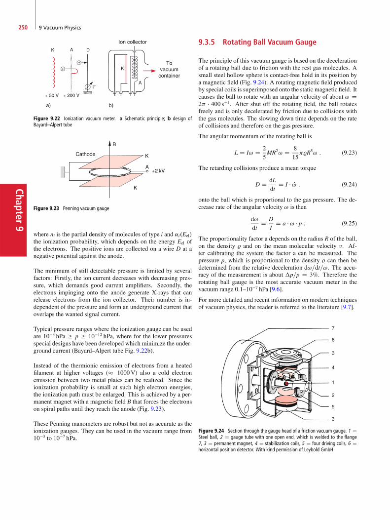
Chapter9
250 9 Vacuum Physics
Ion collector
Tovacuum
container
a) b)
Figure 9.22 Ionization vacuum meter. a Schematic principle; b design ofBayard–Alpert tube
Figure 9.23 Penning vacuum gauge
where ni is the partial density of molecules of type i and ˛i.Eel/the ionization probability, which depends on the energy Eel ofthe electrons. The positive ions are collected on a wire D at anegative potential against the anode.
The minimum of still detectable pressure is limited by severalfactors: Firstly, the ion current decreases with decreasing pres-sure, which demands good current amplifiers. Secondly, theelectrons impinging onto the anode generate X-rays that canrelease electrons from the ion collector. Their number is in-dependent of the pressure and form an underground current thatoverlaps the wanted signal current.
Typical pressure ranges where the ionization gauge can be usedare 10�3 hPa � p � 10�12 hPa, where for the lower pressuresspecial designs have been developed which minimize the under-ground current (Bayard–Alpert tube Fig. 9.22b).
Instead of the thermionic emission of electrons from a heatedfilament at higher voltages (� 1000V) also a cold electronemission between two metal plates can be realized. Since theionization probability is small at such high electron energies,the ionization path must be enlarged. This is achieved by a per-manent magnet with a magnetic field B that forces the electronson spiral paths until they reach the anode (Fig. 9.23).
These Penning manometers are robust but not as accurate as theionization gauges. They can be used in the vacuum range from10�3 to 10�7 hPa.
9.3.5 Rotating Ball Vacuum Gauge
The principle of this vacuum gauge is based on the decelerationof a rotating ball due to friction with the rest gas molecules. Asmall steel hollow sphere is contact-free hold in its position bya magnetic field (Fig. 9.24). A rotating magnetic field producedby special coils is superimposed onto the static magnetic field. Itcauses the ball to rotate with an angular velocity of about ! D2 � 400 s�1. After shut off the rotating field, the ball rotatesfreely and is only decelerated by friction due to collisions withthe gas molecules. The slowing down time depends on the rateof collisions and therefore on the gas pressure.
The angular momentum of the rotating ball is
L D I! D 2
5MR2! D 8
15%R5! : (9.23)
The retarding collisions produce a mean torque
D D dL
dtD I � P! ; (9.24)
onto the ball which is proportional to the gas pressure. The de-crease rate of the angular velocity ! is then
d!
dtD D
ID a � ! � p : (9.25)
The proportionality factor a depends on the radius R of the ball,on the density % and on the mean molecular velocity v. Af-ter calibrating the system the factor a can be measured. Thepressure p, which is proportional to the density % can then bedetermined from the relative deceleration d!=dt=!. The accu-racy of the measurement is about �p=p D 3%. Therefore therotating ball gauge is the most accurate vacuum meter in thevacuum range 0:1–10�7 hPa [9.6].
For more detailed and recent information on modern techniquesof vacuum physics, the reader is referred to the literature [9.7].
Figure 9.24 Section through the gauge head of a friction vacuum gauge. 1 DSteel ball, 2 D gauge tube with one open end, which is welded to the flange7, 3 D permanent magnet, 4 D stabilization coils, 5 D four driving coils, 6 Dhorizontal position detector. With kind permission of Leybold GmbH

Problems 251
Chap
ter9
Summary
A volume V is called evacuated if the total gas pressure in Vis small compared to the atmospheric pressure.The different vacuum ranges are:Low vacuum (1 hPa � p � 103 hPa)Medium vacuum (10�3 hPa � p � 1 hPa)High vacuum (10�7 hPa � p � 10�3 hPa)Ultrahigh vacuum (p � 10�7 hPa)Vacuum is generated with vacuum pumps. The most im-portant types are mechanical pumps (rotary vane pumps)and roots-pumps, (which are used as fore pumps for thegeneration of fine vacuum), turbo-molecular pumps for thegeneration of oil-free high- and ultrahigh vacuum, oil- andmercury diffusion pumps, cryo-pumps and ion getter pumpsfor the generation of ultrahigh vacuum.The gas pressure in a vacuum chamber can be measured withone of the following devices:liquid barometer (0:1 hPa � p � 103 hPa)membrane manometer (p � 1 hPa)
heat conduction manometer (p � 10�3 hPa)capacitance manometer (p � 10�5 hPa)friction vacuum manometer (p � 10�7 hPa)ionization gauge (p � 10�12 hPa)The suction capability SV D dV=dt is the gas volume flowthrough the suction connection of a pump. Often the productSL D p � SV of pressure and suction capability is called thepumping speed.The vacuum lines (tubes and pump connectors) between vac-uum chamber and pump reduce the total suction capability.Their flow conductance LS D p � dV=.p2 � p1/ should beas high as possible, in order to make the pressure differencebetween entrance and exit of the vacuum line small.The achievable final pressure in the vacuum chamber is de-termined by the pumping speed of the pump, by the leak rateand the desorption rate of molecules from the inner walls ofthe chamber.
Problems
9.1 A vacuum chamber is connected to the outside at atmo-spheric pressure through a capillary tube with length L D 10 cmand 0:5mm inner diameter. What should be the effective suctioncapacity of the vacuum pump in order to maintain a pressure of10�3 hPa?
9.2 Which force was necessary to separate the two hemi-spheres of Guericke’s demonstration experiment, when the di-ameter of the spheres was 60 cm and the inner pressure 100 hPa?
9.3 In a cubic vacuum chamber with a volume V D 0:4m3
a pressure of p D 10�5 hPa is maintained. What are the particledensity n, the mean free path � and the mean time � betweentwo successive collisions between particles at room tempera-ture? How large is the ratio Z1=Z2 of the rate Z1 for mutualcollision between particles to the rate Z2 for collision of parti-cles with the walls? How large is the total mean path length thata particle traverses within 1 s, and what is the sum of the pathlengths of all particle in the chamber?
9.4 Assume, the vacuum chamber of Probl. 9.3 is operatedunder ultrahigh vacuum and the inner walls are free from all ad-sorbed molecules. At t D 0 oxygen is let in until the pressurerises to 10�7 hPa. How long does it take until the walls are cov-
ered by a monomolecular layer, if each oxygen molecule coversan area of 0:15 0:2 nm2 and its sticking probability is 1?
9.5 A vacuum chamber should be evacuated down to a pres-sure of 10�6 hPa using a diffusion pump with the effectivepumping speed of 3000 l=s. What is the minimum effectivepumping speed of the mechanical fore pump in order to main-tain a vacuum of 0:1 hPa at the outlet of the diffusion pump?
9.6 The ionization cross section of nitrogen molecules N2
for collisions with electrons of 100 eV energy is � D 1 �10�18 cm2. How large is for an electron current of 10mA the ioncurrent at a pressure of 10�7 hPa in the ionization gauge whenthe path length of the electrons is 2 cm?
9.7 Through the heated filament of a thermal conductivitygauge flows the electric current I D U=R.T/ at a constantvoltage U. The heating power under vacuum conditions isPel D U2=R0. What is the dissipation power due to heat con-duction in a cylindrical chamber with diameter of 2 cm at a gaspressure of p D 10�2 hPa when the temperature of the filamentis T1 D 450K and that of the wall is T2 D 300K? (The length ofthe filament is 5 cm, its diameter 0:5mm, the distance filament-wall is 1 cm). Which fraction of the electric energy Eel D U � Iis dissipated by heat conduction if U D 0:5V and I D 2A?
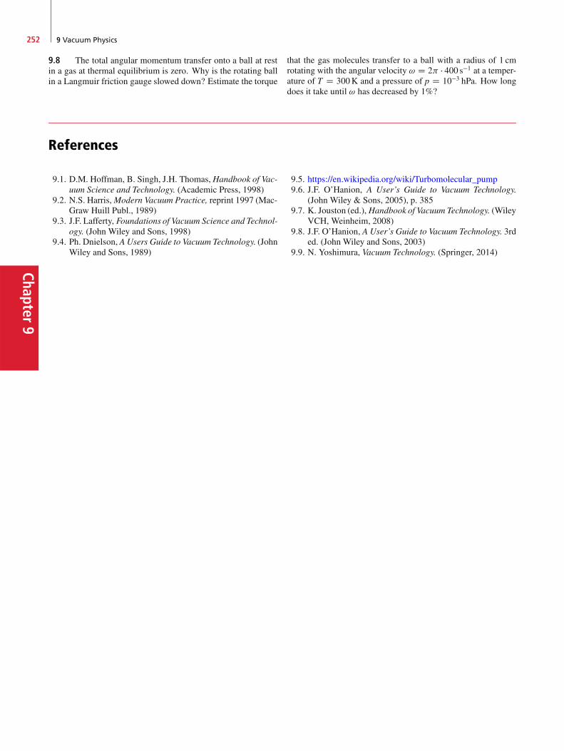
Chapter9
252 9 Vacuum Physics
9.8 The total angular momentum transfer onto a ball at restin a gas at thermal equilibrium is zero. Why is the rotating ballin a Langmuir friction gauge slowed down? Estimate the torque
that the gas molecules transfer to a ball with a radius of 1 cmrotating with the angular velocity ! D 2 � 400 s�1 at a temper-ature of T D 300K and a pressure of p D 10�3 hPa. How longdoes it take until ! has decreased by 1%?
References
9.1. D.M. Hoffman, B. Singh, J.H. Thomas, Handbook of Vac-uum Science and Technology. (Academic Press, 1998)
9.2. N.S. Harris,Modern Vacuum Practice, reprint 1997 (Mac-Graw Huill Publ., 1989)
9.3. J.F. Lafferty, Foundations of Vacuum Science and Technol-ogy. (John Wiley and Sons, 1998)
9.4. Ph. Dnielson, AUsers Guide to Vacuum Technology. (JohnWiley and Sons, 1989)
9.5. https://en.wikipedia.org/wiki/Turbomolecular_pump9.6. J.F. O’Hanion, A User’s Guide to Vacuum Technology.
(John Wiley & Sons, 2005), p. 3859.7. K. Jouston (ed.), Handbook of Vacuum Technology. (Wiley
VCH, Weinheim, 2008)9.8. J.F. O’Hanion, A User’s Guide to Vacuum Technology. 3rd
ed. (John Wiley and Sons, 2003)9.9. N. Yoshimura, Vacuum Technology. (Springer, 2014)
Chap
ter10
Thermodynamics 1010.1 Temperature and Amount of Heat . . . . . . . . . . . . . . . . . . . . . 254
10.2 Heat Transport . . . . . . . . . . . . . . . . . . . . . . . . . . . . . . . . 266
10.3 The Three Laws of Thermodynamics . . . . . . . . . . . . . . . . . . . . 279
10.4 Thermodynamics of Real Gases and Liquids . . . . . . . . . . . . . . . 299
10.5 Comparison of the Different Changes of State . . . . . . . . . . . . . . 309
10.6 Energy Sources and Energy Conversion . . . . . . . . . . . . . . . . . . 309
Summary . . . . . . . . . . . . . . . . . . . . . . . . . . . . . . . . . . . . 317
Problems . . . . . . . . . . . . . . . . . . . . . . . . . . . . . . . . . . . . 318
References . . . . . . . . . . . . . . . . . . . . . . . . . . . . . . . . . . . 319
253© Springer International Publishing Switzerland 2017W. Demtröder, Mechanics and Thermodynamics, Undergraduate Lecture Notes in Physics, DOI 10.1007/978-3-319-27877-3_10
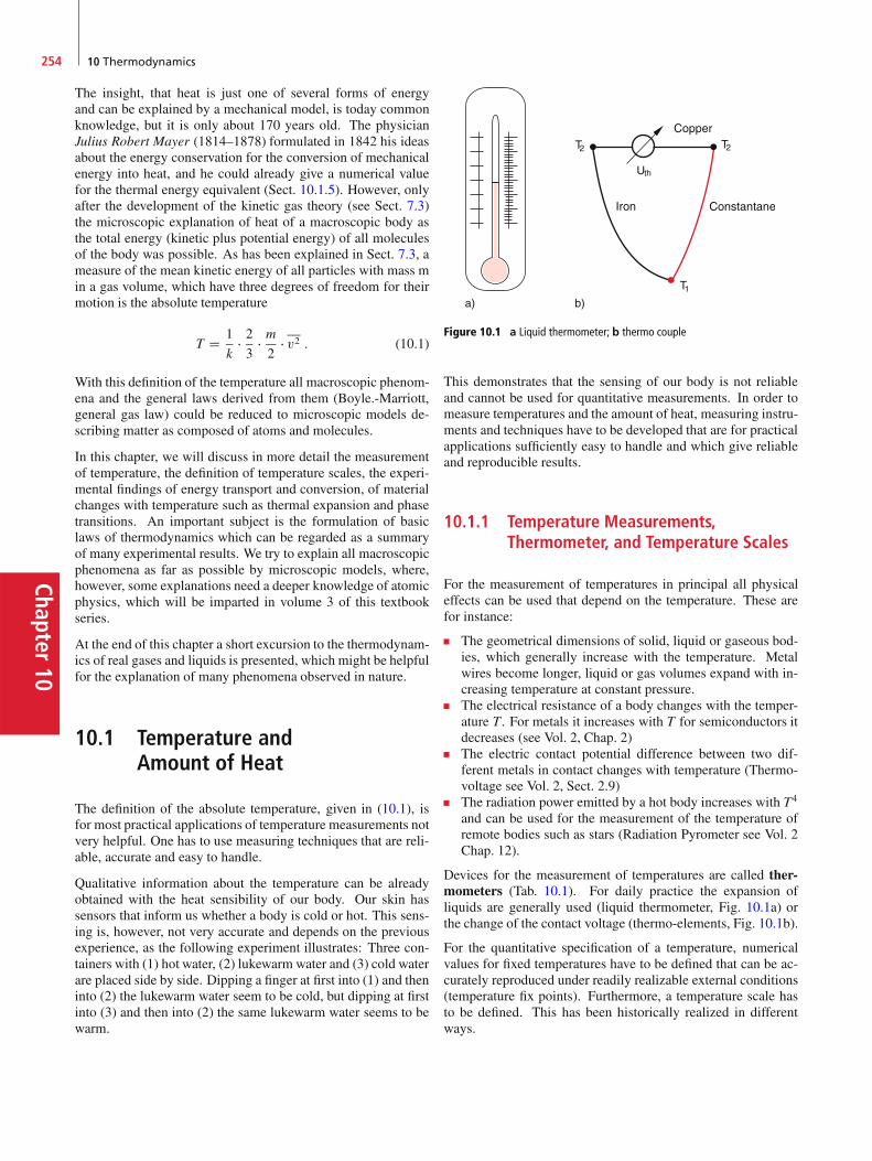
Chapter10
254 10 Thermodynamics
The insight, that heat is just one of several forms of energyand can be explained by a mechanical model, is today commonknowledge, but it is only about 170 years old. The physicianJulius Robert Mayer (1814–1878) formulated in 1842 his ideasabout the energy conservation for the conversion of mechanicalenergy into heat, and he could already give a numerical valuefor the thermal energy equivalent (Sect. 10.1.5). However, onlyafter the development of the kinetic gas theory (see Sect. 7.3)the microscopic explanation of heat of a macroscopic body asthe total energy (kinetic plus potential energy) of all moleculesof the body was possible. As has been explained in Sect. 7.3, ameasure of the mean kinetic energy of all particles with mass min a gas volume, which have three degrees of freedom for theirmotion is the absolute temperature
T D 1
k� 23
� m2
� v2 : (10.1)
With this definition of the temperature all macroscopic phenom-ena and the general laws derived from them (Boyle.-Marriott,general gas law) could be reduced to microscopic models de-scribing matter as composed of atoms and molecules.
In this chapter, we will discuss in more detail the measurementof temperature, the definition of temperature scales, the experi-mental findings of energy transport and conversion, of materialchanges with temperature such as thermal expansion and phasetransitions. An important subject is the formulation of basiclaws of thermodynamics which can be regarded as a summaryof many experimental results. We try to explain all macroscopicphenomena as far as possible by microscopic models, where,however, some explanations need a deeper knowledge of atomicphysics, which will be imparted in volume 3 of this textbookseries.
At the end of this chapter a short excursion to the thermodynam-ics of real gases and liquids is presented, which might be helpfulfor the explanation of many phenomena observed in nature.
10.1 Temperature andAmount of Heat
The definition of the absolute temperature, given in (10.1), isfor most practical applications of temperature measurements notvery helpful. One has to use measuring techniques that are reli-able, accurate and easy to handle.
Qualitative information about the temperature can be alreadyobtained with the heat sensibility of our body. Our skin hassensors that inform us whether a body is cold or hot. This sens-ing is, however, not very accurate and depends on the previousexperience, as the following experiment illustrates: Three con-tainers with (1) hot water, (2) lukewarm water and (3) cold waterare placed side by side. Dipping a finger at first into (1) and theninto (2) the lukewarm water seem to be cold, but dipping at firstinto (3) and then into (2) the same lukewarm water seems to bewarm.
Figure 10.1 a Liquid thermometer; b thermo couple
This demonstrates that the sensing of our body is not reliableand cannot be used for quantitative measurements. In order tomeasure temperatures and the amount of heat, measuring instru-ments and techniques have to be developed that are for practicalapplications sufficiently easy to handle and which give reliableand reproducible results.
10.1.1 Temperature Measurements,Thermometer, and Temperature Scales
For the measurement of temperatures in principal all physicaleffects can be used that depend on the temperature. These arefor instance:
The geometrical dimensions of solid, liquid or gaseous bod-ies, which generally increase with the temperature. Metalwires become longer, liquid or gas volumes expand with in-creasing temperature at constant pressure.The electrical resistance of a body changes with the temper-ature T . For metals it increases with T for semiconductors itdecreases (see Vol. 2, Chap. 2)The electric contact potential difference between two dif-ferent metals in contact changes with temperature (Thermo-voltage see Vol. 2, Sect. 2.9)The radiation power emitted by a hot body increases with T4
and can be used for the measurement of the temperature ofremote bodies such as stars (Radiation Pyrometer see Vol. 2Chap. 12).
Devices for the measurement of temperatures are called ther-mometers (Tab. 10.1). For daily practice the expansion ofliquids are generally used (liquid thermometer, Fig. 10.1a) orthe change of the contact voltage (thermo-elements, Fig. 10.1b).
For the quantitative specification of a temperature, numericalvalues for fixed temperatures have to be defined that can be ac-curately reproduced under readily realizable external conditions(temperature fix points). Furthermore, a temperature scale hasto be defined. This has been historically realized in differentways.

10.1 Temperature and Amount of Heat 255
Chap
ter10
Table 10.1 The mostly used thermometers
Thermometer type Temperature range = ıC Measuring principle Error limitsLiquid thermometers:
Mercury �38 to C800
Alcohol �110 to C210
Pentane mixture �200 to �C30
Thermal expansion of liquid in glas capillary depending on scale division 0:1–1 ıC
Solid state thermometers:
Metal rod �150 to C1000dependent on specific metal
Thermal expansion of metals 1–2% of scale range
Bimetal �150 to C500 Length expansion difference Dependent on model
Resistance thermometers:
Metal wire �250 to C1000 Temperature dependence of electric resistance 0:1–1 ıCSemiconductor �273 to C400
Thermo couple:
Fe-CuNi (iron-constantan) �200 to C760 Temperature dependence of thermovoltage 0:1–1 ıCNi-CrNi �270 to C1000
Ni-CrNi �200 to C1370
Pt-PtRh �50 to C1700
W-WMo �200 to C3000
Pyrometer C800 to C3000 Heat radiation 2–10 ıC
10.1.1.1 The Celsius Scale
The astronomer Anders Celsius (1701–1744) proposed 1742 touse the expansion of a mercury column for the measurementof temperatures (mercury thermometer). Two fix points weredefined for the temperature scale: The melting point of ice(TC D 0 ıC) and the boiling point of water (TC D 100 ıC ata pressure of 1 atm D 1013:25hPa). The range between thesetwo fix points is divided into 100 equal units, where each unitcorresponds to 1 ıC.
Note: We will label the Celsius temperature with TC in order todistinguish it from the Fahrenheit temperature (TF) and Kelvintemperature T .
10.1.1.2 The Fahrenheit Scale
The Fahrenheit scale, which was proposed by Daniel GabrielFahrenheit (1686–1736) is still used in the USA. It defines asfix points the melting point of a defined ice-water-ammoniachloride solution at TF D 0 ıF (�17:8 ıC) and the normalbody temperature at TF D 100 ıF (C37:7 ıC). The range be-tween the two fix points is equally divided into 100 units where1 unit corresponds to 1 ıF. From this definition it follows that0 ıC D 32 ıF and 100 ıC D 212 ıF. The conversion betweenthe two scales is as follows (Fig. 10.2):
TC=ıC D 5
9 .TF=ıF � 32/
TF=ıF D 9
5 .TC=ıC C 32/ :
(10.2)
10.1.1.3 The Absolute Temperature Scale
The absolute temperature scale needs only one fix point, whichis the triple point of water (see below). It is measured with gasthermometers.
Figure 10.2 Comparison of Celsius and Fahrenheit scale. For the Kelvin scalethere is only one fixpoint (triple point of water at 0:01 ıC)
Its definition is: The Kelvin is the unit of the thermodynamictemperature scale. 1K is the 273.16th part of the temperatureTp of the triple point of water. The zero point of the Kelvinscale is the lower absolute limit of possible temperatures and isdefined by general laws of thermodynamics (see Sect. 10.3).
10.1.1.4 Accuracy of Thermometers
The temperature scale of liquid thermometers depends on thechoice of the liquid and also of the glass of the thermometer cap-illary, because not only the liquid but also the glass expands withrising temperature. The thermal expansion of liquids and solidsis generally not constant over the temperature range measuredby thermometers and is not necessarily linear (see next Section).For mercury, the deviation from linearity is small. The compar-ison with an alcohol thermometer shows that its scale differsfrom that for the mercury thermometer and is not equidistant(Fig. 10.3).
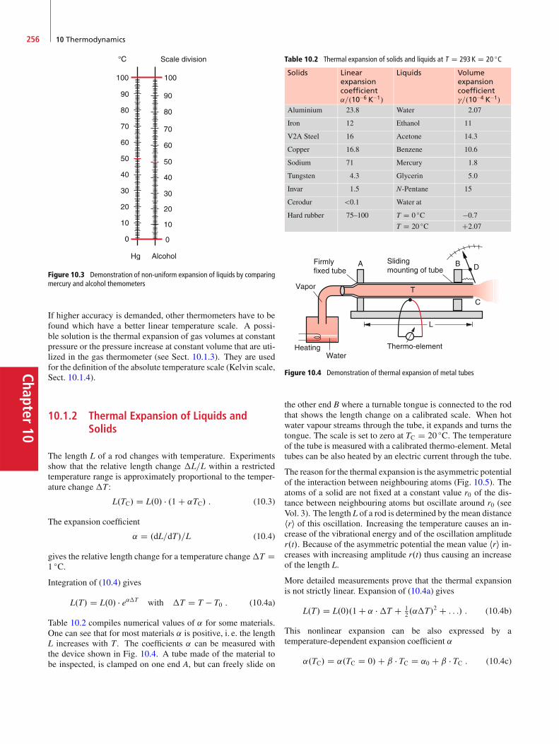
Chapter10
256 10 Thermodynamics
Figure 10.3 Demonstration of non-uniform expansion of liquids by comparingmercury and alcohol themometers
If higher accuracy is demanded, other thermometers have to befound which have a better linear temperature scale. A possi-ble solution is the thermal expansion of gas volumes at constantpressure or the pressure increase at constant volume that are uti-lized in the gas thermometer (see Sect. 10.1.3). They are usedfor the definition of the absolute temperature scale (Kelvin scale,Sect. 10.1.4).
10.1.2 Thermal Expansion of Liquids andSolids
The length L of a rod changes with temperature. Experimentsshow that the relative length change �L=L within a restrictedtemperature range is approximately proportional to the temper-ature change�T:
L.TC/ D L.0/ � .1 C ˛TC/ : (10.3)
The expansion coefficient
˛ D .dL=dT/=L (10.4)
gives the relative length change for a temperature change�T D1 ıC.
Integration of (10.4) gives
L.T/ D L.0/ � e˛�T with �T D T � T0 : (10.4a)
Table 10.2 compiles numerical values of ˛ for some materials.One can see that for most materials ˛ is positive, i. e. the lengthL increases with T . The coefficients ˛ can be measured withthe device shown in Fig. 10.4. A tube made of the material tobe inspected, is clamped on one end A, but can freely slide on
Table 10.2 Thermal expansion of solids and liquids at T D 293 K D 20 ıC
Solids Linearexpansioncoefficient˛=.10�6 K�1/
Liquids Volumeexpansioncoefficient�=.10�4 K�1/
Aluminium 23.8 Water 2.07
Iron 12 Ethanol 11
V2A Steel 16 Acetone 14.3
Copper 16.8 Benzene 10.6
Sodium 71 Mercury 1.8
Tungsten 4.3 Glycerin 5.0
Invar 1.5 N-Pentane 15
Cerodur <0.1 Water at
Hard rubber 75–100 T D 0 ıC �0.7
T D 20 ıC C2.07
Figure 10.4 Demonstration of thermal expansion of metal tubes
the other end B where a turnable tongue is connected to the rodthat shows the length change on a calibrated scale. When hotwater vapour streams through the tube, it expands and turns thetongue. The scale is set to zero at TC D 20 ıC. The temperatureof the tube is measured with a calibrated thermo-element. Metaltubes can be also heated by an electric current through the tube.
The reason for the thermal expansion is the asymmetric potentialof the interaction between neighbouring atoms (Fig. 10.5). Theatoms of a solid are not fixed at a constant value r0 of the dis-tance between neighbouring atoms but oscillate around r0 (seeVol. 3). The length L of a rod is determined by the mean distancehri of this oscillation. Increasing the temperature causes an in-crease of the vibrational energy and of the oscillation amplituder.t/. Because of the asymmetric potential the mean value hri in-creases with increasing amplitude r.t/ thus causing an increaseof the length L.
More detailed measurements prove that the thermal expansionis not strictly linear. Expansion of (10.4a) gives
L.T/ D L.0/.1 C ˛ ��T C 12 .˛�T/2 C : : :/ : (10.4b)
This nonlinear expansion can be also expressed by atemperature-dependent expansion coefficient ˛
˛.TC/ D ˛.TC D 0/C ˇ � TC D ˛0 C ˇ � TC : (10.4c)
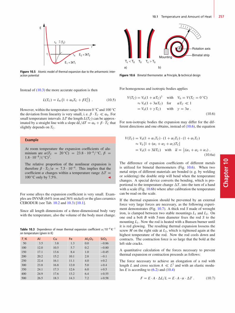
10.1 Temperature and Amount of Heat 257
Chap
ter10
Figure 10.5 Atomic model of thermal expansion due to the anharmonic inter-action potential
Instead of (10.3) the more accurate equation is then
L.TC/ D L0�1 C ˛0TC C ˇT2
C
�: (10.5)
However, within the temperature range between 0 ıC and 100 ıCthe deviation from linearity is very small, i. e. ˇ � TC ˛0. Forsmall temperature intervals�T the length L.TC/ can be approx-imated by a straight line with a slope dL=dT D ˛0 C ˇ � TC thatslightly depends on TC.
Example
At room temperature the expansion coefficients of alu-minium are ˛.TC D 20 ıC/ D 23:8 � 10�6= ıC, ˇ D1:8 � 10�8=. ıC/2.
The relative proportion of the nonlinear expansion istherefore ˇ � TC=˛ D 7:5 � 10�4. This implies that thecoefficient ˛ changes within a temperature range �T D100 ıC only by 7:5%. J
For some alloys the expansion coefficient is very small. Exam-ples are INVAR (64% iron and 36% nickel) or the glass ceramicsCERODUR (see Tab. 10.2 and 10.3) [10.1].
Since all length dimensions of a three-dimensional body varywith the temperature, also the volume of the body must change.
Table 10.3 Dependence of mean thermal expansion coefficient ˛=10�6 K�1
on temperature (given in K)
T=K Al Cu Fe Al2O3 SiO2
50 3.5 3.8 1.3 0.0 �0:86100 12.0 10.5 5.7 0.2 �0:80150 17.1 13.6 8.4 1.0 �0:45200 20.2 15.2 10.1 2.8 �0:1250 22.4 16.1 11.1 4.0 C0:2300 23.8 16.8 12.0 5.0 C0:4350 24.1 17.3 12.6 6.0 C0:5400 24.9 17.6 13.2 6.4 C0:55500 26.5 18.3 14.3 7.2 C0:58
Figure 10.6 Bimetal thermometer. a Principle, b technical design
For homogenous and isotropic bodies applies
V.TC/D V0.1 C ˛TC/3 with V0 D V.TC D 0 ıC/� V0.1 C 3˛TC/ for ˛TC 1
D V0.1 C �TC/ with � D 3˛ :(10.6)
For non-isotropic bodies the expansion may differ for the dif-ferent directions and one obtains, instead of (10.6), the equation
V.TC/ D V0.1 C ˛1TC/ � .1 C ˛2TC/ � .1 C ˛3TC/
� V0 Œ1 C .˛1 C ˛2 C ˛3/TC�
D V0.1 C 3˛TC/ with ˛ D 13 .˛1 C ˛2 C ˛3/ :
(10.6a)
The difference of expansion coefficients of different metalsis utilized for bimetal thermometers (Fig. 10.6). When twometal strips of different materials are bonded (e. g. by weldingor soldering) the double strip will bend when the temperaturechanges. A special device converts the bending, which is pro-portional to the temperature change �T , into the turn of a handwith a scale (Fig. 10.6b) where after calibration the temperaturecan be read on the scale.
If the thermal expansion should be prevented by an externalforce very large forces are necessary, as the following experi-ment demonstrates (Fig. 10.7). A thick rod S made of wroughtiron, is clamped between two stable mountings L1 and L2. Onone end a bolt B with 5mm diameter fixes the rod S to themounting L1. Now the rod is heated with a Bunsen burner untilit is red glowing. The resulting thermal expansion loosens thescrew M on the right side at L2, which is tightened again at thehighest temperature of the rod. Now the rod cools down andcontracts. The contraction force is so large that the bold at theleft side cracks.
A quantitative calculation of the forces necessary to preventthermal expansion or contraction proceeds as follows:
The force necessary to achieve an elongation of a rod withlength L and cross section A L2 and with an elastic modu-lus E is according to (6.2) and (10.4)
F D E � A ��L=L D E � A � ˛ ��T : (10.7)
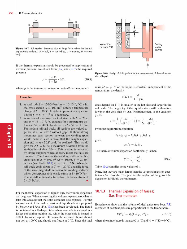
Chapter10
258 10 Thermodynamics
Figure 10.7 Bolt cracker. Demonstration of large forces when the thermalexpansion is hindered. (B D bolt, S D hot rod, L1, L2 D mounts, M D screwnut)
If the thermal expansion should be prevented by application ofexternal pressure, we obtain from (6.7) and (10.7) the requiredpressure
p D ˛ � E1 � 2
��T ; (10.8)
where is the transverse contraction ratio (Poisson number).
Examples
1. A steel rod (E D 120GN=m2, ˛ D 16 �10�6= ıC) withthe cross section A D 100 cm2 suffers a temperaturechange�T D 30 ıC. In order to prevent its expansiona force F D 5:76 � 105 N is necessary.
2. A section of a railroad track of steel with L D 20mand ˛ D 16 � 10�6= ıC expands for a temperature dif-ference �T D 40 ıC by �L D ˛ � L � �T D 1:3 cm.For modern railroad tracks all sections are welded to-gether at T D 20 ıC without gap. Without strongmountings each section between the welding spotswould bend in such a way, that the length expan-sion �L D ˛ � L�T could be realized. This wouldgive for �T D 60 ıC a maximum deviation from thestraight line of about 30 cm. This bending is preventedby strong supports where at every meter the rails aremounted. The force on the welding surfaces with across section A D 0:02m2 (d D 10 cm, b D 20 cm)is then (see Probl. 10.2) F D 1:5 � 106 N. When therail track cools down to T D �20 ıC a tensile forceof the same magnitude acts onto the welding surfaceswhich corresponds to a tensile stress of 8 � 107 N=m2.This is still sufficiently far below the break stress of7 � 108 N=m2. J
For the thermal expansion of liquids only the volume expansioncan be given. When measuring this volume expansion one has totake into account that the solid container also expands. For themeasurement of thermal expansion of liquids a device proposedby Dulong and Petit (Fig. 10.8) has been developed. The liquidis contained in a U-shaped tube where one side is encased in ajacket containing melting ice, while the other side is heated to100 ıC by water vapour. Of course the inspected liquid shouldnot boil at 100 ıC and should not freeze at 0 ıC. Since the total
Water-icemixture 0°C
Boilingwater100°C
Figure 10.8 Design of Dulong–Petit for the measurement of thermal expan-sion of liquids
mass M D % � V of the liquid is constant, independent of thetemperature, the density
%.TC/ D %0
1 C �TC
does depend on T: It is smaller in the hot side and larger in thecold side. The height h0 of the liquid surface will be thereforelower in the cold side by �h. Rearrangement of the equationyields
� D 1
TC
�%0
%.TC/� 1
�D 1
TC� �%
%.TC/:
From the equilibrium condition
h0 � %0 � g D h.TC/ � %.TC/ � ggives
%0=% D h=h0 :
The thermal volume expansion coefficient � is then
� D 1
TC� �h
h0: (10.9)
Table 10.2 compiles some values of � .
Note, that they are much larger than the volume expansion coef-ficients 3˛ of solids. This justifies the neglect of the glass tubeexpansion for liquid thermometers.
10.1.3 Thermal Expansion of Gases;Gas Thermometer
Experiments show that the volume of ideal gases (see Sect. 7.3)increases at constant pressure proportional to the temperature.
V.TC/ D V0.1 C �V � TC/ ; (10.10)
where the temperature is measured in ıC andV0 DV.TC D0 ıC/.

10.1 Temperature and Amount of Heat 259
Chap
ter10
Table 10.4 Thermal expansion coefficient of some gases
Gas �=.10�3=K/Ideal Gas 3.661He 3.660Ar 3.671O2 3.674CO2 3.726
The expansion coefficient
�V D V.TC/ � V0
V0 � TC (10.11)
gives the relative change �V=V0 per 1 ıC. The experimentallyobtained numerical values of �V are compiled in Tab. 10.4.
For Helium, which comes closest to an ideal gas, one finds
�V D 1
273:15ıC�1 D 3:661 � 10�3 ıC�1 :
Accurate experiments performed at a constant gas volume givefor the temperature dependence of the pressure the completelyanalogue relation
p D p0.1 C �p � TC/with �p D �V D � D 1
273:15ıC�1 :
(10.12)
(Law of Gay-Lussac).
The gas thermometer (Fig. 10.9) utilizes this pressure depen-dence for the measurement of temperatures. The volume V isconnected with a U-shaped tube filled with mercury. The heightof Hg in the left side of the U-tube can be changed by up- anddown lifting of the right side, which is connected with the leftside by a flexible tube. When the gas volume is heated, the pres-sure rises. In order to keep the gas volume constant, the levelof the Hg in the left side is always kept at the same height. Thepressure is then indicated by the difference �h between the leftand the right side. It is p D %Hg � g � �h. The temperature,obtained from (10.12)
TC D 1
�� p � p0
p0D 273:15
�p
p0ıC (10.13)
Figure 10.9 Gas thermometer
is therefore determined by a pressure measurement. At the tem-perature TC D 0 which is realized by immersing the gas volumeinto a melting ice-water mixture, the height difference is ad-justed to �h D 0. The pressure in the gas volume V is thenp D p0.
10.1.4 Absolute Temperature Scale
We will now discuss the relation between the Celsius scale andthe absolute temperature scale, which is also called (after itscreator Lord Kelvin) Kelvin scale or thermo-dynamical tem-perature scale. In Sect. 7.3 the absolute temperature T wasused in the general gas equation
p � V D N � k � T ; (10.14a)
relating pressure p, particle number N in the gas volume V withT . The absolute temperature T was defined by Eq. 10.1, which isbased on the results of the kinetic gas theory (see Sect. 7.3). Thegeneral gas equation (10.14a) states that for constant pressureand temperature the gas volume has a definite value, which isthe same for all ideal gases independent of the specific kind.
At a temperature T0 (at 0 ıC) and a pressure p0 D 1 bar D103 hPa (normal conditions) Eq. 10.14a becomes
p0 � V0 D N � k � T0 : (10.14b)
From (10.14a) and (10.14b) we can conclude
p D p0 � V0
V� T
T0: (10.14c)
In the gas thermometer the volume V D V0 is kept constant.The comparison of (10.14c) with (10.12) yields
p D p0 � T
T0D p0.1 C � � TC/ : (10.15)
This gives with the experimental value � D .273:15/�1 the re-lation
T D T0 � .1 C �TC/ D T0 C T0273:15
� TC (10.16)
between the absolute temperature T and the Celsius scale TC.
Note: The unit oft the absolute temperature scale is the Kelvin.It is the 273.16th part of the thermodynamic temperature ofthe triple point of water.
A definition of the absolute temperature that is independentof the specific substance, can be given with their help of theCarnot-Cycle (see Sect. 10.3.5)
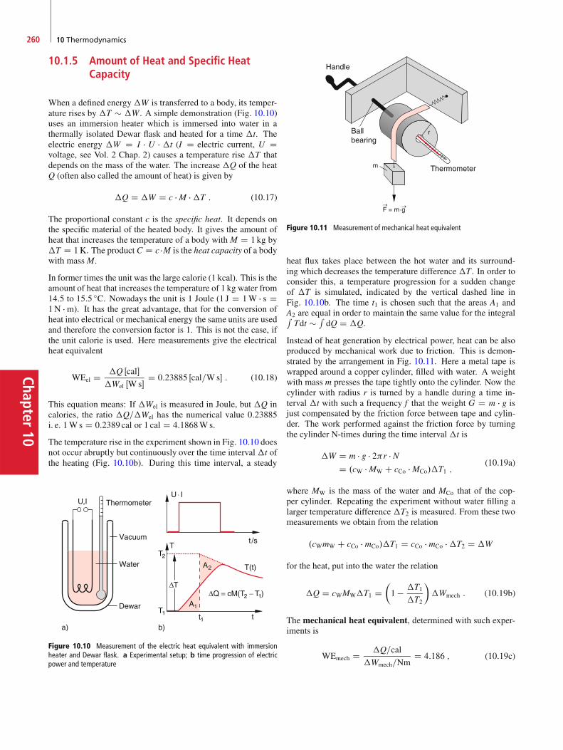
Chapter10
260 10 Thermodynamics
10.1.5 Amount of Heat and Specific HeatCapacity
When a defined energy �W is transferred to a body, its temper-ature rises by �T � �W . A simple demonstration (Fig. 10.10)uses an immersion heater which is immersed into water in athermally isolated Dewar flask and heated for a time �t. Theelectric energy �W D I � U � �t (I D electric current, U Dvoltage, see Vol. 2 Chap. 2) causes a temperature rise �T thatdepends on the mass of the water. The increase �Q of the heatQ (often also called the amount of heat) is given by
�Q D �W D c � M ��T : (10.17)
The proportional constant c is the specific heat. It depends onthe specific material of the heated body. It gives the amount ofheat that increases the temperature of a body with M D 1 kg by�T D 1K. The product C D c �M is the heat capacity of a bodywith massM.
In former times the unit was the large calorie (1 kcal). This is theamount of heat that increases the temperature of 1 kg water from14:5 to 15:5 ıC. Nowadays the unit is 1 Joule (1 J D 1W � s D1N � m). It has the great advantage, that for the conversion ofheat into electrical or mechanical energy the same units are usedand therefore the conversion factor is 1. This is not the case, ifthe unit calorie is used. Here measurements give the electricalheat equivalent
WEel D �Q Œcal�
�Wel ŒWs�D 0:23885 Œcal=Ws� : (10.18)
This equation means: If �Wel is measured in Joule, but �Q incalories, the ratio �Q=�Wel has the numerical value 0:23885i. e. 1W s D 0:2389 cal or 1 cal D 4:1868W s.
The temperature rise in the experiment shown in Fig. 10.10 doesnot occur abruptly but continuously over the time interval�t ofthe heating (Fig. 10.10b). During this time interval, a steady
Figure 10.10 Measurement of the electric heat equivalent with immersionheater and Dewar flask. a Experimental setup; b time progression of electricpower and temperature
Thermometer
Handle
Ballbearing
Figure 10.11 Measurement of mechanical heat equivalent
heat flux takes place between the hot water and its surround-ing which decreases the temperature difference �T . In order toconsider this, a temperature progression for a sudden changeof �T is simulated, indicated by the vertical dashed line inFig. 10.10b. The time t1 is chosen such that the areas A1 andA2 are equal in order to maintain the same value for the integralRTdt � R
dQ D �Q.
Instead of heat generation by electrical power, heat can be alsoproduced by mechanical work due to friction. This is demon-strated by the arrangement in Fig. 10.11. Here a metal tape iswrapped around a copper cylinder, filled with water. A weightwith mass m presses the tape tightly onto the cylinder. Now thecylinder with radius r is turned by a handle during a time in-terval �t with such a frequency f that the weight G D m � g isjust compensated by the friction force between tape and cylin-der. The work performed against the friction force by turningthe cylinder N-times during the time interval �t is
�W D m � g � 2r � ND .cW � MW C cCo � MCo/�T1 ;
(10.19a)
where MW is the mass of the water and MCo that of the cop-per cylinder. Repeating the experiment without water filling alarger temperature difference �T2 is measured. From these twomeasurements we obtain from the relation
.cWmW C cCo � mCo/�T1 D cCo � mCo ��T2 D �W
for the heat, put into the water the relation
�Q D cWMW�T1 D�1 � �T1
�T2
��Wmech : (10.19b)
The mechanical heat equivalent, determined with such exper-iments is
WEmech D �Q=cal
�Wmech=NmD 4:186 ; (10.19c)
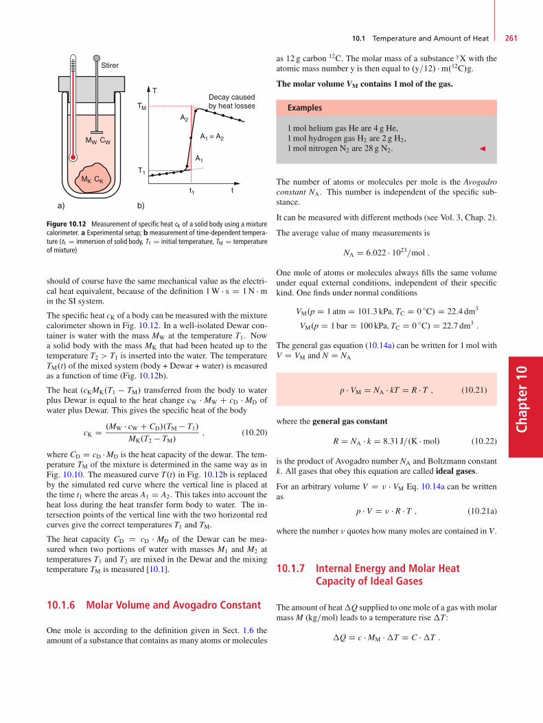
10.1 Temperature and Amount of Heat 261
Chap
ter10
A2
A1
A1 = A2
Figure 10.12 Measurement of specific heat cK of a solid body using a mixturecalorimeter. a Experimental setup; b measurement of time-dependent tempera-ture (t1 D immersion of solid body, T1 D initial temperature, TM D temperatureof mixture)
should of course have the same mechanical value as the electri-cal heat equivalent, because of the definition 1W � s D 1N � min the SI system.
The specific heat cK of a body can be measured with the mixturecalorimeter shown in Fig. 10.12. In a well-isolated Dewar con-tainer is water with the mass MW at the temperature T1. Nowa solid body with the mass MK that had been heated up to thetemperature T2 > T1 is inserted into the water. The temperatureTM.t/ of the mixed system (body + Dewar + water) is measuredas a function of time (Fig. 10.12b).
The heat (cKMK.T1 � TM/ transferred from the body to waterplus Dewar is equal to the heat change cW � MW C cD � MD ofwater plus Dewar. This gives the specific heat of the body
cK D .MW � cW C CD/.TM � T1/
MK.T2 � TM/; (10.20)
where CD D cD �MD is the heat capacity of the dewar. The tem-perature TM of the mixture is determined in the same way as inFig. 10.10. The measured curve T.t/ in Fig. 10.12b is replacedby the simulated red curve where the vertical line is placed atthe time t1 where the areas A1 D A2. This takes into account theheat loss during the heat transfer form body to water. The in-tersection points of the vertical line with the two horizontal redcurves give the correct temperatures T1 and TM.
The heat capacity CD D cD � MD of the Dewar can be mea-sured when two portions of water with masses M1 and M2 attemperatures T1 and T2 are mixed in the Dewar and the mixingtemperature TM is measured [10.1].
10.1.6 Molar Volume and Avogadro Constant
One mole is according to the definition given in Sect. 1.6 theamount of a substance that contains as many atoms or molecules
as 12 g carbon 12C. The molar mass of a substance yX with theatomic mass number y is then equal to .y=12/ � m.12C/g.The molar volume VM contains 1mol of the gas.
Examples
1mol helium gas He are 4 g He,1mol hydrogen gas H2 are 2 g H2,1mol nitrogen N2 are 28 g N2. J
The number of atoms or molecules per mole is the Avogadroconstant NA. This number is independent of the specific sub-stance.
It can be measured with different methods (see Vol. 3, Chap. 2).
The average value of many measurements is
NA D 6:022 � 1023=mol :
One mole of atoms or molecules always fills the same volumeunder equal external conditions, independent of their specifickind. One finds under normal conditions
VM.p D 1 atm D 101:3 kPa;TC D 0 ıC/ D 22:4 dm3
VM.p D 1 bar D 100 kPa; TC D 0 ıC/ D 22:7 dm3 :
The general gas equation (10.14a) can be written for 1mol withV D VM and N D NA
p � VM D NA � kT D R � T ; (10.21)
where the general gas constant
R D NA � k D 8:31 J=.K � mol/ (10.22)
is the product of Avogadro number NA and Boltzmann constantk. All gases that obey this equation are called ideal gases.
For an arbitrary volume V D � � VM Eq. 10.14a can be writtenas
p � V D � � R � T ; (10.21a)
where the number � quotes howmany moles are contained in V.
10.1.7 Internal Energy and Molar HeatCapacity of Ideal Gases
The amount of heat�Q supplied to onemole of a gas with molarmassM (kg=mol) leads to a temperature rise �T:
�Q D c � MM ��T D C ��T :
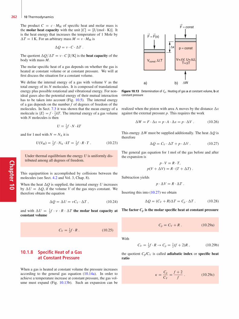
Chapter10
262 10 Thermodynamics
The product C D c � MM of specific heat and molar mass isthe molar heat capacity with the unit ŒC� D ŒJ=.mol � K/�. Itis the heat energy that increases the temperature of 1 Mole by�T D 1K. For an arbitrary massM D � � MM is
�Q D � � C ��T :
The quotient�Q=�T D � � C ŒJ=K� is the heat capacity of thebody with massM.
The molar specific heat of a gas depends on whether the gas isheated at constant volume or at constant pressure. We will atfirst discuss the situation for a constant volume.
We define the internal energy of a gas with volume V as thetotal energy of its N molecules. It is composed of translationalenergy plus possible rotational and vibrational energy. For non-ideal gases also the potential energy of their mutual interactionhas to be taken into account (Fig. 10.5). The internal energyof a gas depends on the number f of degrees of freedom of themolecules. In Sect. 7.3 it was shown that the mean energy of amolecule is hEi D f � 1
2kT . The internal energy of a gas volumewith N molecules is then
U D 12 f � N � kT
and for 1mol with N D NA it is
U.VM/ D 12 f � NA � kT D 1
2 f � R � T : (10.23)
Under thermal equilibrium the energy U is uniformly dis-tributed among all degrees of freedom.
This equipartition is accomplished by collisions between themolecules (see Sect. 4.2 and Vol. 3, Chap. 8).
When the heat �Q is supplied, the internal energy U increasesby �U D �Q, if the volume V of the gas stays constant. Wetherefore obtain the equation
�Q D �U D �CV ��T ; (10.24)
and with �U D 12 f � � � R � �T the molar heat capacity at
constant volume
CV D 12 f � R : (10.25)
10.1.8 Specific Heat of a Gasat Constant Pressure
When a gas is heated at constant volume the pressure increasesaccording to the general gas equation (10.14a). In order toachieve a temperature increase at constant pressure, the gas vol-ume must expand (Fig. 10.13b). Such an expansion can be
Figure 10.13 Determination of Cp . Heating of gas a at constant volume, b atconstant pressure
realized when the piston with area A moves by the distance �xagainst the external pressure p. This requires the work
�W D F ��x D p � A ��x D p ��V : (10.26)
This energy �W must be supplied additionally. The heat �Q istherefore
�Q D CV ��T C p ��V : (10.27)
The general gas equation for 1mol of the gas before and afterthe expansion is
p � V D R � T;p.V C�V/ D R � .T C�T/ :
Subtraction yields
p ��V D R ��T :
Inserting this into (10.27) we obtain
�Q D .CV C R/�T D Cp ��T : (10.28)
The factor Cp is the molar specific heat at constant pressure
Cp D CV C R : (10.29a)
With
CV D 12 f � R ! Cp D 1
2 .f C 2/R ; (10.29b)
the quotient Cp/CV is called adiabatic index or specific heatratio
� D Cp
CVD f C 2
f: (10.29c)

10.1 Temperature and Amount of Heat 263
Chap
ter10
10.1.9 Molecular Explanation of the SpecificHeat
Since atoms or molecules can move into three directions, theyhave three degrees of freedom of translation. Their mean trans-lational energy is therefore
Etrans D 3 � 12kT ;
the molar specific heat of atomic gases is therefore
CV D .3=2/R :
For molecules the supplied energy can be also converted intorotational or vibrational energy. Nonlinear molecules can rotatearound three orthogonal axis. They have therefore three degreesof freedom for the rotation. Linear molecules have only 2 rota-tional degrees of freedom, because of the following reason:
The rotational energyErot D L2=2I
is determined by the angular momentum L and the momentof inertia I (see Sect. 5.5). As shown in Quantum physics(see Vol. 3 Chap. 4) the angular momentum has the amountL D .l � .lC1//.1=2/ � „ with l D 1I 2I 3I : : :. The smallest angularmomentum is then Lmin D p
2 � „, where „ D h=2 is Planck’squantum constant, divided by 2 . The moment of inertia fora rotation around the axis of a linear molecule is very smallbecause the heavy nuclei are located on the axis and the lightelectrons do not contribute much to I. Therefore the rotationalenergy is very large, generally much larger than the translationalenergy at accessible temperatures. Collisions cannot excited thisrotation and it therefore cannot contribute to the accessible en-ergy.
The vibration of diatomic molecules is one-dimensional andhas therefore only one degree of freedom. However, the vi-brational energy has two contributions: The kinetic and thepotential energy (see Sect. 11.6). The mean value of both contri-butions is equal to 1
2kT and the thermal energy of the vibrationis kT . Therefore two degrees of freedom .f D 2/ are for-mally attributed to the vibration. A diatomic molecule has thenf D 3 C 2 C 2 D 7 degrees of freedom, if the temperature issufficiently high to excite the vibrations.
Note: Quantum Theory shows (see Vol. 3) that the classicalmodel of a vibrating oscillator with regard to the total energyE D Ekin C Epot is correct, but that the energy can be only ab-sorbed in discrete quanta h ��. This does, however, not influenceour argumentation above.
For polyatomic molecules with j atoms each atom has three de-grees of freedom. If we subtract 3 degrees of freedom for thetranslational motion of the whole molecule and 3 degrees offreedom for the rotation (2 degrees for a linear molecule) weend up with fvib D 3j � 6 (3j � 5 for linear molecules) vibra-tional degrees of freedom.
The total internal energy U of a molecule with j atoms is then
U D 12 � f � NA � kT with f D ftrans C frot C fvib : (10.30)
a
b
Figure 10.14 Excitation of rotational degrees of freedom of a diatomicmolecule induced by collisions. The collision with an atom A causes a rota-tion of the molecule about an axis perpendicular to the drawing plane (a), orcauses the excitation of a molecular vibration (b)
Since collisions can transfer translational energy to rotations orvibrations only if the thermal energy of the collision partnersis sufficiently high, at low temperatures only translational de-grees of freedom are available and feff D 3. With increasingtemperature at first the rotation can be excited (feff D 6 resp.5 for linear molecules) and at still higher temperature also thevibrations contribute to the specific heat, because their energy ishigher than that of the rotations (feff D 3C 3C 2 � .3j� 6/ resp.3C 2C 2.3j� 5/ for linear molecules). This gives for diatomicmolecules feff D 3 C 2 C 2 D 7.
The molar specific heat is
CV D�@U
@T
�
V
D 1
2feff � R : (10.31)
Here the partial derivative is used, because U can depend onseveral variables (p, V, T). The index V indicates that the energysupply occurs at constant volume.
Examples
1. For the atomic gas Helium is f D 3. Since the trans-lational energy is not quantized all three degrees offreedom are excited even at low temperatures. There-fore the specific heat of Helium is independent of thetemperature (Fig. 10.15).
Figure 10.15 Temperature dependence of molar heat capacity of he-lium, nitrogen N2 and nitrogen dioxyde NO2 (see also Sect. 10.1.10)

Chapter10
264 10 Thermodynamics
2. For nitrogen gas consisting of the diatomic moleculesN2 kT is for very low temperatures smaller than theenergy of the lowest rotational level (see Probl. 10.3).The rotational energy cannot be excited. Thereforefeff D 3. With increasing temperature when kT �Erot feff approaches the value feff D 5. For still highertemperatures kT � Evib feff becomes feff D 7 becausethe vibrational degrees of freedom are counted twice(see Sect. 10.1.9). The specific heat of a molecular gasis therefore dependent on the temperature and reachesits maximum value only if kT is sufficiently high toexcite all degrees of freedom.
3. Polyatomic gas (e. g. NO2 at T > 200K where NO2
has a sufficiently high gas pressure). At this tempera-ture already all three rotational modes can be excited.We then obtain f D 3 C 3 D 6.Above T D 300K the bending vibration can be ex-cited, rising f to f D 8. Only above T D 800Kall three vibrational mods can be excited and we havef D 12. The molar specific heat is then CV D 6R. J
10.1.10 Specific Heat Capacity of Solids
With decreasing temperature all gases become liquids and passfinally into the solid state (except helium, which solidifies onlyunder high pressures). Considerations about the specific heat ofsolids require a knowledge about the possible degrees of free-dom for atoms and molecules in solids. Since the atoms in asolid can only oscillate in three directions around their fixedequilibrium positions but have no degrees of freedom for trans-lation or rotation we would expect f D 2 � 3 D 6. However,it turns out that the oscillation frequencies of all atoms are notthe same but spread over a large frequency range. In order toget an idea about the frequency distribution, we regard a one-dimensional arrangement of atoms in an ideal crystal whereall atoms are regularly placed at a distance d (Fig. 10.16a).When an atom oscillates around its equilibrium positions, theoscillation can be transferred to the neighbouring atoms, dueto the coupling force between the atoms. This results in elas-tic waves travelling through the crystal (see Sect. 11.8). Thewaves are reflected at the end faces of the crystal, superimposewith the incoming waves and form stationary standing waves.Longitudinal as well as transversal standing waves can develop,depending on whether the oscillation occurs in the direction ofwave propagation or perpendicular to it. The standing wave withthe smallest possible wavelength � (i. e. the highest frequency� D c=�) is realized, when the neighbouring atoms oscillatesagainst each other (Fig. 10.16a, b lowest line). The oscillationwith the largest possible wavelength (� D L with L D length ofthe crystal) has the lowest energy h ��. At low temperatures onlythose vibrations with the lowest energy can be excited. With in-creasing temperature more and more vibrations can be excited.The number of possible vibrations Z � N3 is proportional to
Figure 10.16 Stationary vibrational modes of a linear chain. a Transversal;b longitudinal standing waves. c Number of vibrational modes per energy inter-val dE of a solid body as function of temperature T
the third power of the number N of atoms in the crystal. Thismeans that the specific heat rises continuously with the temper-ature (Fig. 10.16c) until at kT � Emax
vib all vibrations are excitedand the specific heat takes its maximum value. Since the in-teraction between neighbouring atoms depends on the specifickind of atoms the progression C.T/ differs for the different ma-terials (Fig. 10.17). However, all curves C.T/ approach for hightemperatures the same value of the molar specific heat
CV D 6 � 12NA � k D 3R (Dulong–Petit law) : (10.32)
Measurements of the temperature-dependent progression ofCV.T/ gives information about the distribution of the vibrationalfrequencies and therefore about the coupling forces between theatoms of the solid. They are furthermore a convincing experi-mental proof of quantum theory (see Vol. 3).
Table 10.5 gives numerical values of CV for some materials.
Figure 10.17 Qualitative temperature dependence of molar heat capacity ofdifferent solids
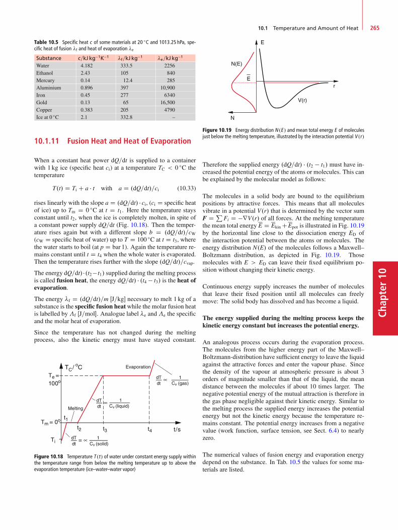
10.1 Temperature and Amount of Heat 265
Chap
ter10
Table 10.5 Specific heat c of some materials at 20 ıC and 1013:25 hPa, spe-cific heat of fusion �f and heat of evaporation �e
Substance c=kJ kg�1K�1 �f=kJ kg�1 �e=kJ kg�1
Water 4.182 333.5 2256Ethanol 2.43 105 840Mercury 0.14 12.4 285Aluminium 0.896 397 10,900Iron 0.45 277 6340Gold 0.13 65 16,500Copper 0.383 205 4790Ice at 0 ıC 2.1 332.8 –
10.1.11 Fusion Heat and Heat of Evaporation
When a constant heat power dQ=dt is supplied to a containerwith 1 kg ice (specific heat ci) at a temperature TC < 0 ıC thetemperature
T.t/ D Ti C a � t with a D .dQ=dt/=ci (10.33)
rises linearly with the slope a D .dQ=dt/ � ci, (ci D specific heatof ice) up to Tm D 0 ıC at t D t1. Here the temperature staysconstant until t2, when the ice is completely molten, in spite ofa constant power supply dQ=dt (Fig. 10.18). Then the temper-ature rises again but with a different slope b D .dQ=dt/=cW(cW D specific heat of water) up to T D 100 ıC at t D t3, wherethe water starts to boil (at p D bar 1). Again the temperature re-mains constant until t D t4 when the whole water is evaporated.Then the temperature rises further with the slope .dQ=dt/=cvap.
The energy dQ=dt/ �.t2� t1/ supplied during the melting processis called fusion heat, the energy dQ=dt/ � .t4 � t3/ is the heat ofevaporation.
The energy �f D .dQ=dt/=m ŒJ=kg� necessary to melt 1 kg of asubstance is the specific fusion heatwhile the molar fusion heatis labelled by�f ŒJ=mol�. Analogue label �e and�e the specificand the molar heat of evaporation.
Since the temperature has not changed during the meltingprocess, also the kinetic energy must have stayed constant.
Figure 10.18 Temperature T .t/ of water under constant energy supply withinthe temperature range from below the melting temperature up to above theevaporation temperature (ice–water–water vapor)
Figure 10.19 Energy distribution N .E / and mean total energy E of moleculesjust below the melting temperature, illustrated by the interaction potential V .r/
Therefore the supplied energy .dQ=dt/ � .t2 � t1/ must have in-creased the potential energy of the atoms or molecules. This canbe explained by the molecular model as follows:
The molecules in a solid body are bound to the equilibriumpositions by attractive forces. This means that all moleculesvibrate in a potential V.r/ that is determined by the vector sumF D P
Fi D �rV.r/ of all forces. At the melting temperaturethe mean total energy E D Ekin CEpot is illustrated in Fig. 10.19by the horizontal line close to the dissociation energy ED ofthe interaction potential between the atoms or molecules. Theenergy distribution N.E/ of the molecules follows a Maxwell–Boltzmann distribution, as depicted in Fig. 10.19. Thosemolecules with E > ED can leave their fixed equilibrium po-sition without changing their kinetic energy.
Continuous energy supply increases the number of moleculesthat leave their fixed position until all molecules can freelymove: The solid body has dissolved and has become a liquid.
The energy supplied during the melting process keeps thekinetic energy constant but increases the potential energy.
An analogous process occurs during the evaporation process.The molecules from the higher energy part of the Maxwell–Boltzmann-distribution have sufficient energy to leave the liquidagainst the attractive forces and enter the vapour phase. Sincethe density of the vapour at atmospheric pressure is about 3orders of magnitude smaller than that of the liquid, the meandistance between the molecules if about 10 times larger. Thenegative potential energy of the mutual attraction is therefore inthe gas phase negligible against their kinetic energy. Similar tothe melting process the supplied energy increases the potentialenergy but not the kinetic energy because the temperature re-mains constant. The potential energy increases from a negativevalue (work function, surface tension, see Sect. 6.4) to nearlyzero.
The numerical values of fusion energy and evaporation energydepend on the substance. In Tab. 10.5 the values for some ma-terials are listed.
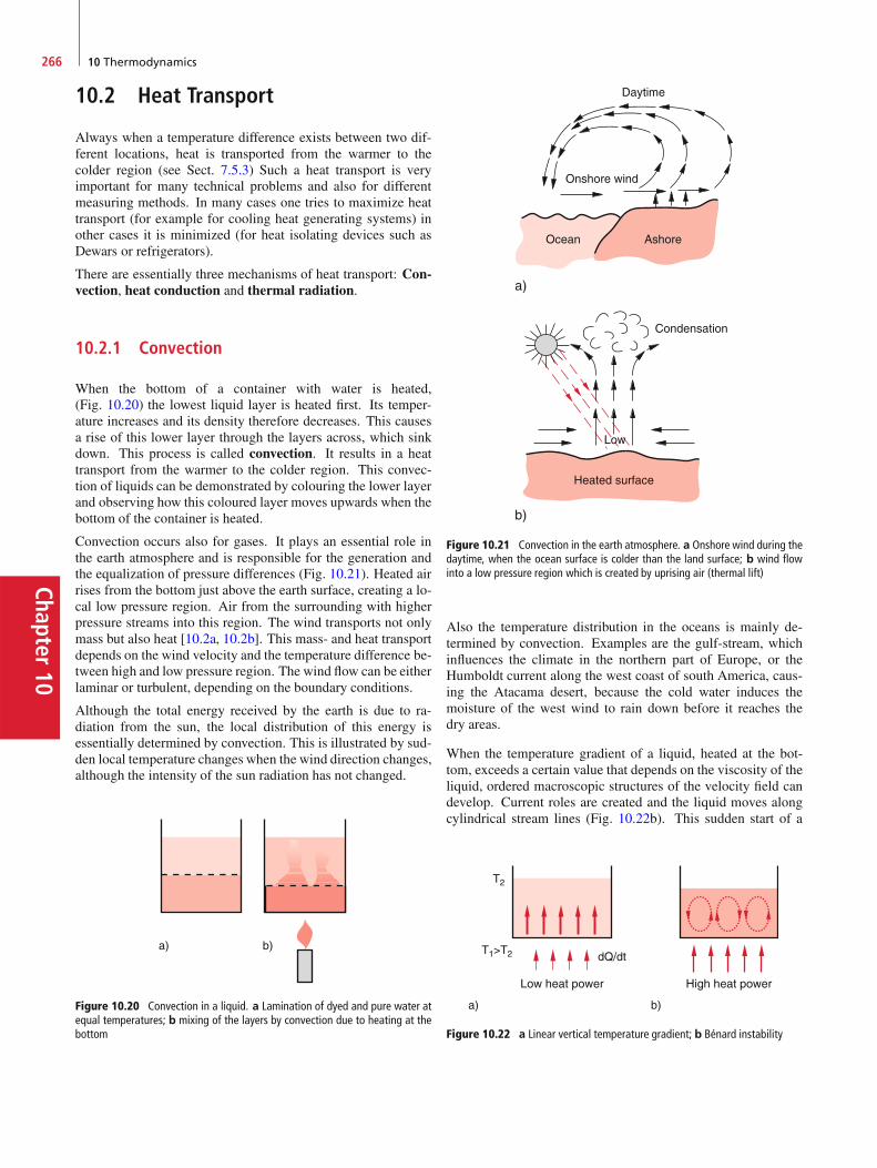
Chapter10
266 10 Thermodynamics
10.2 Heat Transport
Always when a temperature difference exists between two dif-ferent locations, heat is transported from the warmer to thecolder region (see Sect. 7.5.3) Such a heat transport is veryimportant for many technical problems and also for differentmeasuring methods. In many cases one tries to maximize heattransport (for example for cooling heat generating systems) inother cases it is minimized (for heat isolating devices such asDewars or refrigerators).
There are essentially three mechanisms of heat transport: Con-vection, heat conduction and thermal radiation.
10.2.1 Convection
When the bottom of a container with water is heated,(Fig. 10.20) the lowest liquid layer is heated first. Its temper-ature increases and its density therefore decreases. This causesa rise of this lower layer through the layers across, which sinkdown. This process is called convection. It results in a heattransport from the warmer to the colder region. This convec-tion of liquids can be demonstrated by colouring the lower layerand observing how this coloured layer moves upwards when thebottom of the container is heated.
Convection occurs also for gases. It plays an essential role inthe earth atmosphere and is responsible for the generation andthe equalization of pressure differences (Fig. 10.21). Heated airrises from the bottom just above the earth surface, creating a lo-cal low pressure region. Air from the surrounding with higherpressure streams into this region. The wind transports not onlymass but also heat [10.2a, 10.2b]. This mass- and heat transportdepends on the wind velocity and the temperature difference be-tween high and low pressure region. The wind flow can be eitherlaminar or turbulent, depending on the boundary conditions.
Although the total energy received by the earth is due to ra-diation from the sun, the local distribution of this energy isessentially determined by convection. This is illustrated by sud-den local temperature changes when the wind direction changes,although the intensity of the sun radiation has not changed.
Figure 10.20 Convection in a liquid. a Lamination of dyed and pure water atequal temperatures; b mixing of the layers by convection due to heating at thebottom
Figure 10.21 Convection in the earth atmosphere. a Onshore wind during thedaytime, when the ocean surface is colder than the land surface; b wind flowinto a low pressure region which is created by uprising air (thermal lift)
Also the temperature distribution in the oceans is mainly de-termined by convection. Examples are the gulf-stream, whichinfluences the climate in the northern part of Europe, or theHumboldt current along the west coast of south America, caus-ing the Atacama desert, because the cold water induces themoisture of the west wind to rain down before it reaches thedry areas.
When the temperature gradient of a liquid, heated at the bot-tom, exceeds a certain value that depends on the viscosity of theliquid, ordered macroscopic structures of the velocity field candevelop. Current roles are created and the liquid moves alongcylindrical stream lines (Fig. 10.22b). This sudden start of a
Figure 10.22 a Linear vertical temperature gradient; b Bénard instability

10.2 Heat Transport 267
Chap
ter10
“self-organization” is called Bénard-instability. When the liq-uid is further heated, the rolls begin a wave-like motion alongthe cylinder axis. Such organized motions that develop fromrandom conditions play an important role for the creation of or-ganized structures from disordered systems. These processesare investigated in the rapidly developing field of Synergetics,which represents a frontier area between Physics, Chemistry,Biology and Computer Science [10.3, 10.4].
10.2.2 Heat Conduction
Contrary to the situation for convection, for heat conductiononly energy transport takes place, but generally no mass trans-port. Heat conduction can only occur in matter, i. e. in vacuumno heat conduction is possible while thermal radiation also takesplace in vacuum (otherwise we would not receive the sun radia-tion).
We will at first discuss heat conduction in solids, where theatoms or molecules are bound to fixed equilibrium positions andno convection can happen.
10.2.2.1 Heat Conduction in Solids
A rod with length L and cross section A is connected at bothends with thermal reservoirs that keep the two ends always atthe fixed temperatures T1 and T2 with T1 < T2 (Fig. 10.23).After a sufficient long time a stationary state appears, where atemperature gradient dT=dx is established that depends on thetemperature difference �T D T1 � T2, and on the length L. Ifwe neglect heat losses through the side wall of the rod, a con-stant heat energy
dQ
dtD �� � A � dT
dx(10.34a)
flows per sec through the cross section A of the rod . The con-stant �.Œ�� D ŒW � m�1 � K�1�/ depends on the substance of therod and is called heat conductivity. In Tab. 10.6 the heat con-ductivities of some substances are listed.
For a homogeneous rod with constant cross section A, the sta-tionary temperature T(x) is a linear function of x, as can be seenby integrating (10.34a), which yields
T.x/ D �dQ=dt
� � A x C C : (10.34b)
Figure 10.23 Heat conduction in a stab
Table 10.6 Heat conduction coefficient of some materials at 20 ıC
Substance �=.Wm�1K�1/
Aluminium 221Iron 67Gold 314Copper 393Zinc 112Lead 35Normal concrete 2.1Foamed concrete 0.22Glas 0.8Glas wool 0.04Wood 0.13Ice 2.2Water 0.6Air (p D 1 atm) 0.026CO2 (p D 1 atm) 0.015Helium (p D 1 atm) 0.14
The integration constant C is determined by the boundary con-dition T.x D 0/ D T1 D C. The energy supply necessaryto maintain the given temperature gradient dT=dx, is obtainedfrom
dQ=dt D � � A � .T1 � T2/=L :
For the general nonstationary heat conduction through inho-mogeneous bodies with variable cross section the temperaturefunction T.x; t/ is more complicated. For its derivation we re-gard a volume element dV between the planes x D x1 and x2(Fig. 10.24).
Figure 10.24 Derivation of the heat conduction equation
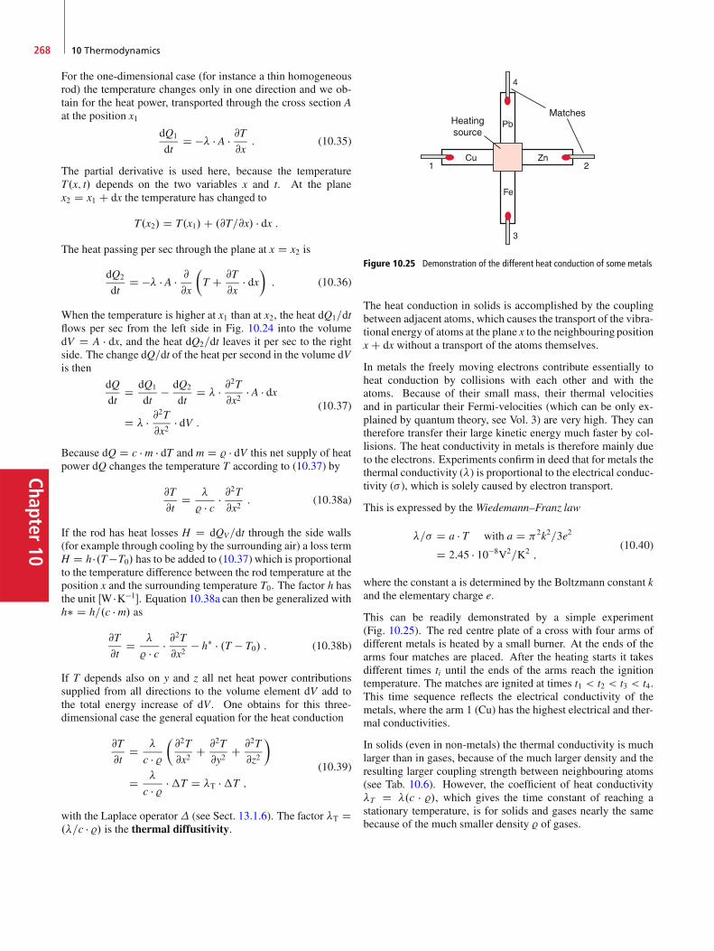
Chapter10
268 10 Thermodynamics
For the one-dimensional case (for instance a thin homogeneousrod) the temperature changes only in one direction and we ob-tain for the heat power, transported through the cross section Aat the position x1
dQ1
dtD �� � A � @T
@x: (10.35)
The partial derivative is used here, because the temperatureT.x; t/ depends on the two variables x and t. At the planex2 D x1 C dx the temperature has changed to
T.x2/ D T.x1/C .@T=@x/ � dx :
The heat passing per sec through the plane at x D x2 is
dQ2
dtD �� � A � @
@x
�T C @T
@x� dx
�: (10.36)
When the temperature is higher at x1 than at x2, the heat dQ1=dtflows per sec from the left side in Fig. 10.24 into the volumedV D A � dx, and the heat dQ2=dt leaves it per sec to the rightside. The change dQ=dt of the heat per second in the volume dVis then
dQ
dtD dQ1
dt� dQ2
dtD � � @
2T
@x2� A � dx
D � � @2T
@x2� dV :
(10.37)
Because dQ D c � m � dT and m D % � dV this net supply of heatpower dQ changes the temperature T according to (10.37) by
@T
@tD �
% � c � @2T
@x2: (10.38a)
If the rod has heat losses H D dQV=dt through the side walls(for example through cooling by the surrounding air) a loss termH D h �.T�T0/ has to be added to (10.37) which is proportionalto the temperature difference between the rod temperature at theposition x and the surrounding temperature T0. The factor h hasthe unit ŒW �K�1�. Equation 10.38a can then be generalized withh� D h=.c � m/ as
@T
@tD �
% � c � @2T
@x2� h� � .T � T0/ : (10.38b)
If T depends also on y and z all net heat power contributionssupplied from all directions to the volume element dV add tothe total energy increase of dV. One obtains for this three-dimensional case the general equation for the heat conduction
@T
@tD �
c � %�@2T
@x2C @2T
@y2C @2T
@z2
�
D �
c � % ��T D �T ��T ;
(10.39)
with the Laplace operator� (see Sect. 13.1.6). The factor �T D.�=c � %/ is the thermal diffusitivity.
Figure 10.25 Demonstration of the different heat conduction of some metals
The heat conduction in solids is accomplished by the couplingbetween adjacent atoms, which causes the transport of the vibra-tional energy of atoms at the plane x to the neighbouring positionx C dx without a transport of the atoms themselves.
In metals the freely moving electrons contribute essentially toheat conduction by collisions with each other and with theatoms. Because of their small mass, their thermal velocitiesand in particular their Fermi-velocities (which can be only ex-plained by quantum theory, see Vol. 3) are very high. They cantherefore transfer their large kinetic energy much faster by col-lisions. The heat conductivity in metals is therefore mainly dueto the electrons. Experiments confirm in deed that for metals thethermal conductivity (�) is proportional to the electrical conduc-tivity (�), which is solely caused by electron transport.
This is expressed by the Wiedemann–Franz law
�=� D a � T with a D 2k2=3e2
D 2:45 � 10�8V2=K2 ;(10.40)
where the constant a is determined by the Boltzmann constant kand the elementary charge e.
This can be readily demonstrated by a simple experiment(Fig. 10.25). The red centre plate of a cross with four arms ofdifferent metals is heated by a small burner. At the ends of thearms four matches are placed. After the heating starts it takesdifferent times ti until the ends of the arms reach the ignitiontemperature. The matches are ignited at times t1 < t2 < t3 < t4.This time sequence reflects the electrical conductivity of themetals, where the arm 1 (Cu) has the highest electrical and ther-mal conductivities.
In solids (even in non-metals) the thermal conductivity is muchlarger than in gases, because of the much larger density and theresulting larger coupling strength between neighbouring atoms(see Tab. 10.6). However, the coefficient of heat conductivity�T D �.c � %/, which gives the time constant of reaching astationary temperature, is for solids and gases nearly the samebecause of the much smaller density % of gases.
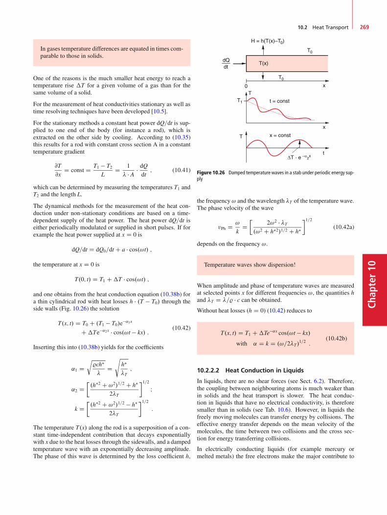
10.2 Heat Transport 269
Chap
ter10
In gases temperature differences are equated in times com-parable to those in solids.
One of the reasons is the much smaller heat energy to reach atemperature rise �T for a given volume of a gas than for thesame volume of a solid.
For the measurement of heat conductivities stationary as well astime resolving techniques have been developed [10.5].
For the stationary methods a constant heat power dQ=dt is sup-plied to one end of the body (for instance a rod), which isextracted on the other side by cooling. According to (10.35)this results for a rod with constant cross section A in a constanttemperature gradient
@T
@xD const D T1 � T2
LD 1
� � A � dQdt
; (10.41)
which can be determined by measuring the temperatures T1 andT2 and the length L.
The dynamical methods for the measurement of the heat con-duction under non-stationary conditions are based on a time-dependent supply of the heat power. The heat power dQ=dt iseither periodically modulated or supplied in short pulses. If forexample the heat power supplied at x D 0 is
dQ=dt D dQ0=dt C a � cos.!t/ ;
the temperature at x D 0 is
T.0; t/ D T1 C�T � cos.!t/ ;
and one obtains from the heat conduction equation (10.38b) fora thin cylindrical rod with heat losses h � .T � T0/ through theside walls (Fig. 10.26) the solution
T.x; t/ D T0 C .T1 � T0/e�˛1x
C�Te�˛2x � cos.!t � kx/ :(10.42)
Inserting this into (10.38b) yields for the coefficients
˛1 Dr%ch�
�Ds
h�
�T;
˛2 D�.h�2 C !2/1=2 C h�
2�T
�1=2I
k D�.h�2 C !2/1=2 � h�
2�T
�1=2:
The temperature T.x/ along the rod is a superposition of a con-stant time-independent contribution that decays exponentiallywith x due to the heat losses through the sidewalls, and a dampedtemperature wave with an exponentially decreasing amplitude.The phase of this wave is determined by the loss coefficient h,
Figure 10.26 Damped temperature waves in a stab under periodic energy sup-ply
the frequency! and the wavelength �T of the temperature wave.The phase velocity of the wave
vPh D !
kD�
2!2 � �T.!2 C h�2/1=2 C h�
�1=2(10.42a)
depends on the frequency !.
Temperature waves show dispersion!
When amplitude and phase of temperature waves are measuredat selected points x for different frequencies !, the quantities hand �T D �=% � c can be obtained.Without heat losses (h D 0) (10.42) reduces to
T.x; t/ D T1 C�Te�˛x cos.!t � kx/
with ˛ D k D .!=2�T/1=2 :
(10.42b)
10.2.2.2 Heat Conduction in Liquids
In liquids, there are no shear forces (see Sect. 6.2). Therefore,the coupling between neighbouring atoms is much weaker thanin solids and the heat transport is slower. The heat conduc-tion in liquids that have no electrical conductivity, is thereforesmaller than in solids (see Tab. 10.6). However, in liquids thefreely moving molecules can transfer energy by collisions. Theeffective energy transfer depends on the mean velocity of themolecules, the time between two collisions and the cross sec-tion for energy transferring collisions.
In electrically conducting liquids (for example mercury ormelted metals) the free electrons make the major contribute to
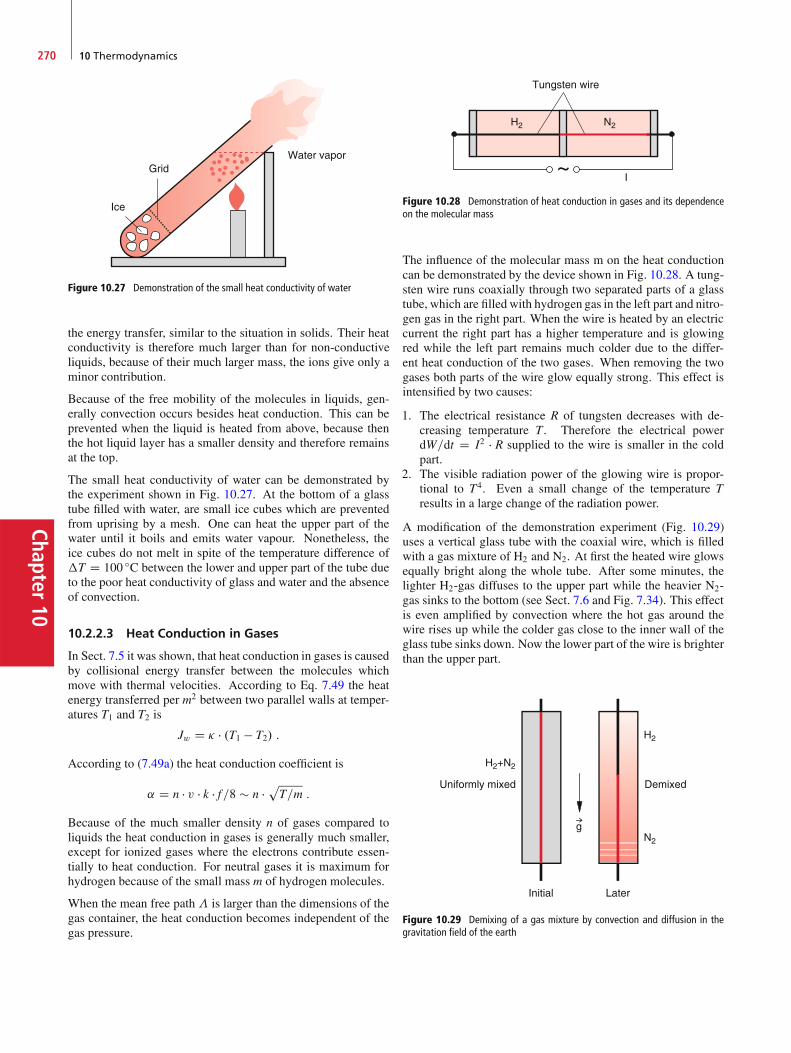
Chapter10
270 10 Thermodynamics
Ice
GridWater vapor
Figure 10.27 Demonstration of the small heat conductivity of water
the energy transfer, similar to the situation in solids. Their heatconductivity is therefore much larger than for non-conductiveliquids, because of their much larger mass, the ions give only aminor contribution.
Because of the free mobility of the molecules in liquids, gen-erally convection occurs besides heat conduction. This can beprevented when the liquid is heated from above, because thenthe hot liquid layer has a smaller density and therefore remainsat the top.
The small heat conductivity of water can be demonstrated bythe experiment shown in Fig. 10.27. At the bottom of a glasstube filled with water, are small ice cubes which are preventedfrom uprising by a mesh. One can heat the upper part of thewater until it boils and emits water vapour. Nonetheless, theice cubes do not melt in spite of the temperature difference of�T D 100 ıC between the lower and upper part of the tube dueto the poor heat conductivity of glass and water and the absenceof convection.
10.2.2.3 Heat Conduction in Gases
In Sect. 7.5 it was shown, that heat conduction in gases is causedby collisional energy transfer between the molecules whichmove with thermal velocities. According to Eq. 7.49 the heatenergy transferred per m2 between two parallel walls at temper-atures T1 and T2 is
Jw D � � .T1 � T2/ :
According to (7.49a) the heat conduction coefficient is
˛ D n � v � k � f =8 � n �pT=m :
Because of the much smaller density n of gases compared toliquids the heat conduction in gases is generally much smaller,except for ionized gases where the electrons contribute essen-tially to heat conduction. For neutral gases it is maximum forhydrogen because of the small mass m of hydrogen molecules.
When the mean free path � is larger than the dimensions of thegas container, the heat conduction becomes independent of thegas pressure.
Tungsten wire
Figure 10.28 Demonstration of heat conduction in gases and its dependenceon the molecular mass
The influence of the molecular mass m on the heat conductioncan be demonstrated by the device shown in Fig. 10.28. A tung-sten wire runs coaxially through two separated parts of a glasstube, which are filled with hydrogen gas in the left part and nitro-gen gas in the right part. When the wire is heated by an electriccurrent the right part has a higher temperature and is glowingred while the left part remains much colder due to the differ-ent heat conduction of the two gases. When removing the twogases both parts of the wire glow equally strong. This effect isintensified by two causes:
1. The electrical resistance R of tungsten decreases with de-creasing temperature T . Therefore the electrical powerdW=dt D I2 � R supplied to the wire is smaller in the coldpart.
2. The visible radiation power of the glowing wire is propor-tional to T4. Even a small change of the temperature Tresults in a large change of the radiation power.
A modification of the demonstration experiment (Fig. 10.29)uses a vertical glass tube with the coaxial wire, which is filledwith a gas mixture of H2 and N2. At first the heated wire glowsequally bright along the whole tube. After some minutes, thelighter H2-gas diffuses to the upper part while the heavier N2-gas sinks to the bottom (see Sect. 7.6 and Fig. 7.34). This effectis even amplified by convection where the hot gas around thewire rises up while the colder gas close to the inner wall of theglass tube sinks down. Now the lower part of the wire is brighterthan the upper part.
Uniformly mixed Demixed
Initial Later
Figure 10.29 Demixing of a gas mixture by convection and diffusion in thegravitation field of the earth
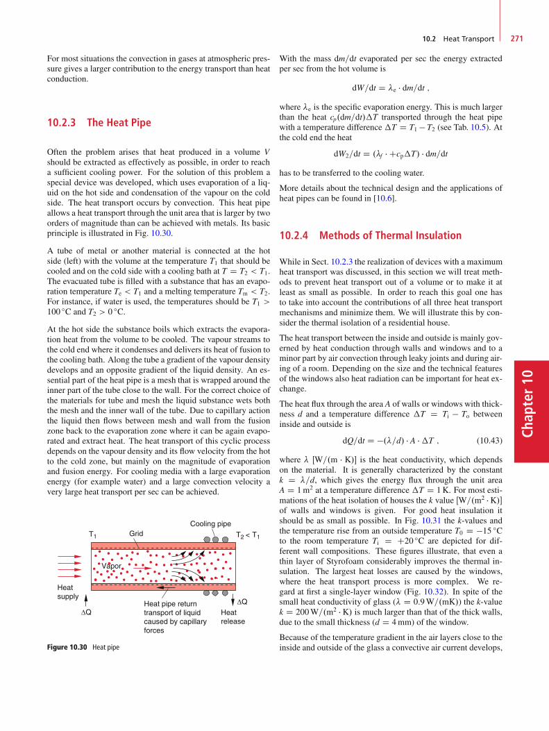
10.2 Heat Transport 271
Chap
ter10
For most situations the convection in gases at atmospheric pres-sure gives a larger contribution to the energy transport than heatconduction.
10.2.3 The Heat Pipe
Often the problem arises that heat produced in a volume Vshould be extracted as effectively as possible, in order to reacha sufficient cooling power. For the solution of this problem aspecial device was developed, which uses evaporation of a liq-uid on the hot side and condensation of the vapour on the coldside. The heat transport occurs by convection. This heat pipeallows a heat transport through the unit area that is larger by twoorders of magnitude than can be achieved with metals. Its basicprinciple is illustrated in Fig. 10.30.
A tube of metal or another material is connected at the hotside (left) with the volume at the temperature T1 that should becooled and on the cold side with a cooling bath at T D T2 < T1.The evacuated tube is filled with a substance that has an evapo-ration temperature Te < T1 and a melting temperature Tm < T2.For instance, if water is used, the temperatures should be T1 >100 ıC and T2 > 0 ıC.
At the hot side the substance boils which extracts the evapora-tion heat from the volume to be cooled. The vapour streams tothe cold end where it condenses and delivers its heat of fusion tothe cooling bath. Along the tube a gradient of the vapour densitydevelops and an opposite gradient of the liquid density. An es-sential part of the heat pipe is a mesh that is wrapped around theinner part of the tube close to the wall. For the correct choice ofthe materials for tube and mesh the liquid substance wets boththe mesh and the inner wall of the tube. Due to capillary actionthe liquid then flows between mesh and wall from the fusionzone back to the evaporation zone where it can be again evapo-rated and extract heat. The heat transport of this cyclic processdepends on the vapour density and its flow velocity from the hotto the cold zone, but mainly on the magnitude of evaporationand fusion energy. For cooling media with a large evaporationenergy (for example water) and a large convection velocity avery large heat transport per sec can be achieved.
Figure 10.30 Heat pipe
With the mass dm=dt evaporated per sec the energy extractedper sec from the hot volume is
dW=dt D �e � dm=dt ;where �e is the specific evaporation energy. This is much largerthan the heat cp.dm=dt/�T transported through the heat pipewith a temperature difference �T D T1 � T2 (see Tab. 10.5). Atthe cold end the heat
dW2=dt D .�f � Ccp�T/ � dm=dthas to be transferred to the cooling water.
More details about the technical design and the applications ofheat pipes can be found in [10.6].
10.2.4 Methods of Thermal Insulation
While in Sect. 10.2.3 the realization of devices with a maximumheat transport was discussed, in this section we will treat meth-ods to prevent heat transport out of a volume or to make it atleast as small as possible. In order to reach this goal one hasto take into account the contributions of all three heat transportmechanisms and minimize them. We will illustrate this by con-sider the thermal isolation of a residential house.
The heat transport between the inside and outside is mainly gov-erned by heat conduction through walls and windows and to aminor part by air convection through leaky joints and during air-ing of a room. Depending on the size and the technical featuresof the windows also heat radiation can be important for heat ex-change.
The heat flux through the area A of walls or windows with thick-ness d and a temperature difference �T D Ti � To betweeninside and outside is
dQ=dt D �.�=d/ � A ��T ; (10.43)
where � ŒW=.m � K/� is the heat conductivity, which dependson the material. It is generally characterized by the constantk D �=d, which gives the energy flux through the unit areaA D 1m2 at a temperature difference �T D 1K. For most esti-mations of the heat isolation of houses the k value ŒW=.m2 �K/�of walls and windows is given. For good heat insulation itshould be as small as possible. In Fig. 10.31 the k-values andthe temperature rise from an outside temperature T0 D �15 ıCto the room temperature Ti D C20 ıC are depicted for dif-ferent wall compositions. These figures illustrate, that even athin layer of Styrofoam considerably improves the thermal in-sulation. The largest heat losses are caused by the windows,where the heat transport process is more complex. We re-gard at first a single-layer window (Fig. 10.32). In spite of thesmall heat conductivity of glass (� D 0:9W=.mK/) the k-valuek D 200W=.m2 � K/ is much larger than that of the thick walls,due to the small thickness (d D 4mm) of the window.
Because of the temperature gradient in the air layers close to theinside and outside of the glass a convective air current develops,

Chapter10
272 10 Thermodynamics
Figure 10.31 Thermal insulation. a Temperature behaviour across a plasteredclaybrick wall; b plastered wall of pumice stone; c pumice stone wall with styro-foam layer. The arrows give the direction of the convection current
Figure 10.32 Heat transport across a single pane window
Figure 10.33 Double pane glas window. a Composition and temperature change across the window; b k -values as a function of the thickness d of the gas layerbetween the two glas panes; c decrease of k -values through technical progress
which is for To < Ti downwards at the inside and upwards atthe outside (Fig. 10.32). Due to friction between glass and aira thin boundary layer of air adheres on both sides of the glass(see Sect. 8.4). The heat passes through these layers to the con-vective air layers. Since the heat conduction is smaller for gasat atmospheric pressure than for glass, the k-value is smaller forthese adhered air layers then for the pane of glass.
From Eq. 8.24 one obtains a thickness of 5mm for the boundaryair layer with a k-value k D 3:4W=.m2 � K/ for heat conduction,compared to k D 200W=.m2 � K/ for the pane of glass.Another heat transport mechanism is heat radiation (seeSect. 10.2.5). The room temperature in the inner part of thehouse causes infrared radiation, which can escape through thewindows. The heat loss can be estimated as 4:6W=.m2 � K/.This gives a total k-value of the inner air layer k D8W=.m2 � K/.For the outer convective air layer the k-value is different becausethe air flows upwards against the gravitation. Detailed calcula-tions give a value k D 20W=.m2 � K/ including radiation losses.For successive layers the reciprocal k-values add (analogous toelectrostatics where the reciprocal electric conductivities add)and we obtain from
1
kD 1
kiC 1
kgC 1
ko(10.44)
the total k-value k D 5:5W=.m2 � K/. The comparison with thek-value of the walls k < 1W=.m2 � K/ shows that windows witha single pane of glass constitute a major heat loss.
A much better heat insulation can be achieved with windows oftwo panes of glass and an inert gas enclosed between the panes(Fig. 10.33a).
The k-value of the gas depends on the thickness d of the gasbetween the glass panes. For d � 1 cm the heat conduction isdominant, while for larger values of d convection undertakes themajor part of heat transfer. Fig. 10.33b shows, that for d D 1 cmthe minimum k-value is reached because the boundary layersthat adhere to the glass walls, prevent convection.
For such a double glass window, the k-value for heat conductionis substantially smaller than for a single pane window. In order

10.2 Heat Transport 273
Chap
ter10
to minimize also the radiation losses, the glass panes are cov-ered by a thin dielectric layer [10.8], which reflects the infraredradiation from the inside of the house (see Vol. 2, Sect. 10.4).Without a reflecting layer, k-values of k � 3W=.m2 � K/ can berealized, while with reflecting layer the k-value decreases downto k � 0:6W=.m2 � K/. The k-values are then comparable tothose of the walls [10.8, 10.9].
The considerations above illustrate that all three heat-transferprocesses as heat conduction, convection and radiation have tobe taken into account in order to optimize the heat insulation ofa house. In Fig. 10.33c the technical progress of minimizing thetotal k-value is illustrated.
A more quantitative representation of heat insulation can befound in [10.7] and the references gives there and also in manybooks on energy saving new house construction [10.9].
10.2.5 Thermal Radiation
Every body at a temperature TK exchanges energy with itssurrounding. If TK is higher than the temperature TS of thesurrounding, the energy emitted by the body is larger than theenergy received from the surrounding. If no energy is suppliedto the system body +surrounding, the system approaches ther-mal equilibrium, where the temperature of the body is equal tothat of the surrounding (Fig. 10.34). This energy balance can bereached by heat conduction, convection or radiation. If the bodyis kept in vacuum, (for instance our earth) radiation is the onlyway to exchange energy with the surrounding, because both heatconduction and convection need matter for the transport of en-ergy.
Extensive experiments have proved, that radiation emitted byhot bodies represents electromagnetic waves, which can trans-port energy through matter and also through vacuum.
Figure 10.34 Energy exchange by thermal radiation between a body and itssurroundings. At thermal equilibrium is dW1=dt D dW2=dt and TK D T2
Since the intensity and the spectral distribution of the radiationemitted by a body depends essentially on the temperature ofthe body, this radiation is called heat radiation or thermal ra-diation. In this section we will discuss the characteristics ofthermal radiation.
10.2.5.1 Emissivity and Absorptivity of a Body
At first we will experimentally study, how the intensity of ther-mal radiation depends on the surface conditions of the body. Weuse a metal hollow cube filled with hot water, where the four sidewalls have a different surface structure (black, white, shiny andrough). All side walls have the same temperature. Four equal ra-diation detectors, which measure the total radiation (integratedover all wavelengths) are placed at the same distance d from thefour walls (Fig. 10.35). They all show different radiation pow-ers. When the cube is turned by n � 90ı (n D 1, 2, 3, : : :) abouta vertical axis, it can be proved that the difference is not due todifferences of the detectors but that the different sidewalls reallyemit different radiation powers. The experiment shows surpris-ingly that the black side wall emits the maximum power and theshiny white surface the minimum power. The radiation poweremitted from the surface area dA into the solid angle d˝ can bequantitatively described by
dW
dtD E� � dA � d˝ :
The constant E� is the emissivity of the surface. It gives theradiation power dW=dt, integrated over all wavelengths that isemitted from a surface element dA D 1m2 into the solid angled˝ D 1 sr around the surface normal (Fig. 10.36). Accordingto the experiment the emissivity E� of a black surface is largerthan that of a white surface at the same temperature.
The integral absorptivity A� is defined as the mean value of thequotient A� D absorbed radiation power = incident radiationpower, averaged over all wavelengths.
The ratio
K.T/ D E�.T/A�.T/
(10.45)
Figure 10.35 Experimental setup for the measurement of emission

Chapter10
274 10 Thermodynamics
Figure 10.36 Illustration of the emissivity E � of a surface element dA
depends solely on the temperature T and not on the material ofthe body, as can be demonstrated by the following experiment:
Experiment
We place in Fig. 10.37a in front of the black surface A1
of the hot cube an equivalent surface A01 of the detector at
a distance d and in front of the shiny surface A2 a shinydetector surface A0
2 at the same distance d. Measuring thetemperatures T1 of A0
1 and T2 of A02 one finds that T1 > T2.
Since the surface structure of A01 is equal to that of A1, and
that of A02 is equal to that of A2, the absorptivity A�
1 mustbe equal to A0�
1 and A�2 D A0�
2 .
Figure 10.37 Derivation of (10.47)
The power absorbed by the two detector surfaces is
dW 01=dt � E�
1 � A0�1 and dW 0
2=dt � E�2 � A0�
2 :
Since E�1 > E�
2 (according to the foregoing experiment,a black surface emits a larger power than a shiny one) and
A0�1 > A0�
2 (a black surface has a higher absorptivity than ashiny one) it follows that dW 0
1=dt > dW 02=dt ! T1 > T2.
Now the cube is turned about a vertical axis by 180ı andthe surface A1 now faces A0
2 and A2 faces A01 (Fig. 10.37b).
The absorbed powers are
dW1=dt � E�2 � A0�
1 and dW2=dt � E�1 � A0�
2 :
The experimental result is now T1 D T2 ! dW1=dt DdW2=dt.
) E�1 .T/
A�1
D E�2 .T/
A�2
: (10.46)
J
A separate experiment proves that the absorptivity of the sur-faces does not depend on the temperature at least within thetemperature range from 0–100 ıC, which is covered in the exper-iment above. Therefore it follows from (10.46) for an arbitrarybody
E�1 .T/
A�1
D E�2 .T/
A�2
D K.T/ : (10.47)
The ratio of emissivity to absorptivity can be describedfor any body by a function K.T/ that depends solely onthe temperature T .
A body with A� D 1 is called a black body.
It completely absorbs any incident radiation. According to(10.47) a black body must also have the maximum emissivitycompared to all other bodies with equal temperature.
Note: Bodies with a large absorption coefficient ˛ but a sud-den increase of ˛ at the glossy surface are not a black body,because their reflectivity also increases (Fig. 10.38a). There-fore the major part of the incident radiation is reflected and onlythe minor part, that penetrates into the body is absorbed (seeVol. 2, Chap. 8). In order to realize a black body, the absorp-tion coefficient should not increase suddenly at the surface butmust continuously increase over a distance�z > � ( � D wave-length of the incident radiation) from zero to its maximum value(Fig. 10.38b). This can be for instance realized by a roughenedsurface (black velvet, soot or graphite with a rough surface)where the optical density rises slowly from the outside to theinner part of the body. The sun is an example of a nearly perfectblack body, because the gas density and with it the absorptivityincreases slowly from the diffuse outer edge of the photosphereto the interior.
Often the problem arises to keep a body at a constant tempera-ture TK, that differs from the temperature TS of its surroundingby supporting (TK > TS) or extracting (TK < TS) energy. Thisenergy can be minimized when heat conduction, convection andradiation are minimized. The experimental realization uses ma-terials with low heat conductance and radiation shields.

10.2 Heat Transport 275
Chap
ter10
Figure 10.38 a For bodies with a large gradient d˛=dz at the surface incidentradiation is mainly reflected and only partly absorbed inspite of the large ab-sorption coefficient ˛. b Most of the incident radiation is absoorbed, if d˛=dzis small, i. e. ˛.z/ rises slowly from ˛ D 0 to ˛ D ˛max
Examples
Shive with lowheat conductance
Reflective coating
Vacuum
Vacuum
a)
b)
Glass wall
Glass or steel wall
Vaporization
Hot liquid
Liquid air
Heat insulation andshock absorption
Figure 10.39 a Thermos bottle; b Dewar gasket
1. A thermos bottle (Fig. 10.39a) consists of a doublewall glass flask. The space between the two wallsis evacuated and the two inner sides of the walls aremirrored. The vacuum prevents heat conduction andconvection. The reflective walls minimize the escapeof thermal radiation to the outside. Therefore, the heatlosses from the inner volume are very small and thecoffee stays hot for a long time or cold drinks remaincold.
2. For the storage of liquid nitrogen a Dewar is used(Fig. 10.39b), which is based on the same principle asthe thermos bottle. Here the heat transfer from the out-side is minimized in order to keep the evaporation ofthe cold liquid nitrogen (T D 77K) as low as possible.The small portion of evaporating nitrogen extracts theheat of evaporation and keeps the temperature in theDewar low.If liquid air is used (78%N2 and 21%O2/, the nitrogenevaporates faster because of its higher vapour pressureand the concentration of the reactive oxygen increasesuntil an explosive concentration is reached. Therefore,generally liquid air is dangerous and is only used forspecial purposes. J
10.2.5.2 Characteristic Features of Thermal Radiation
The energy that is emitted by the surface element dA into thesolid angle d˝ around the direction � against the surface nor-mal can be measured with a radiation detector (for example athermo-couple connected to a black surface). The detector areadA2 at a distance r from the radiation source receives the radia-tion within the solid angel
d˝ D dA2
r2:
Experiments prove that for many radiation sources the angulardistribution of the measured radiation power is
dW.�/=dt D S� cos� � dA � d˝ : (10.48)
The quantity S� is the emittance or radiation density of thesource. It describes the radiation power per m2 of the radia-tion source, emitted into the solid angle d˝ D 1 sr around thesurface normal (Fig. 10.40a).
The radiant intensity
J.�/ DZ
F
S� cos �dA ; ŒJ� D 1W
sr(10.49)
is the total radiation power emitted by the radiation source intothe solid angle d˝ D 1 sr around the direction � against thesurface normal.
Note: The relation between the radiation density S� and theemissivity E� is outlined in Sect. 10.2.5.3.
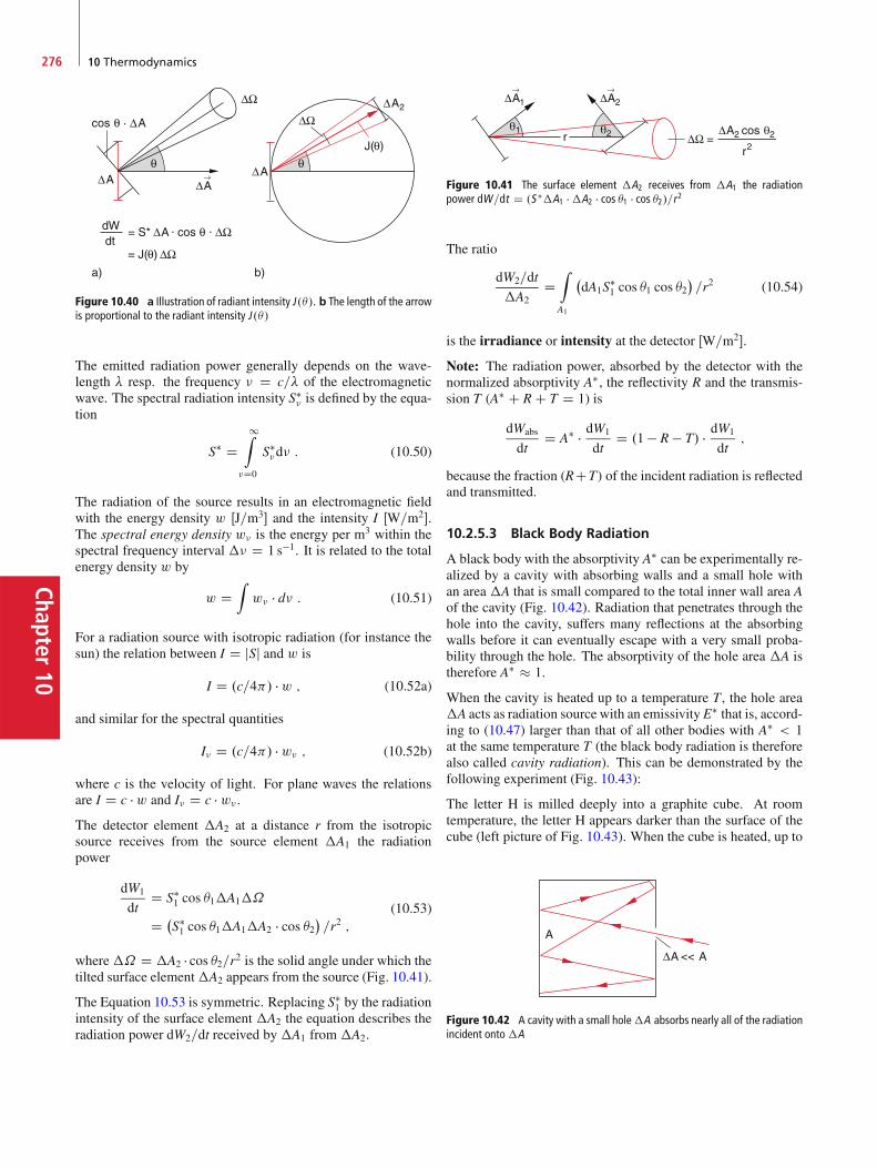
Chapter10
276 10 Thermodynamics
Figure 10.40 a Illustration of radiant intensity J .�/. b The length of the arrowis proportional to the radiant intensity J .�/
The emitted radiation power generally depends on the wave-length � resp. the frequency � D c=� of the electromagneticwave. The spectral radiation intensity S�
� is defined by the equa-tion
S� D1Z
�D0
S��d� : (10.50)
The radiation of the source results in an electromagnetic fieldwith the energy density w ŒJ=m3� and the intensity I ŒW=m2�.The spectral energy density w� is the energy per m3 within thespectral frequency interval �� D 1 s�1. It is related to the totalenergy density w by
w DZw� � d� : (10.51)
For a radiation source with isotropic radiation (for instance thesun) the relation between I D jSj and w is
I D .c=4/ �w ; (10.52a)
and similar for the spectral quantities
I� D .c=4/ � w� ; (10.52b)
where c is the velocity of light. For plane waves the relationsare I D c �w and I� D c � w� .The detector element �A2 at a distance r from the isotropicsource receives from the source element �A1 the radiationpower
dW1
dtD S�
1 cos �1�A1�˝
D �S�1 cos �1�A1�A2 � cos �2
�=r2 ;
(10.53)
where�˝ D �A2 � cos �2=r2 is the solid angle under which thetilted surface element�A2 appears from the source (Fig. 10.41).
The Equation 10.53 is symmetric. Replacing S�1 by the radiation
intensity of the surface element �A2 the equation describes theradiation power dW2=dt received by �A1 from �A2.
Figure 10.41 The surface element �A2 receives from �A1 the radiationpower dW=dt D .S ��A1 ��A2 � cos �1 � cos �2/=r2
The ratio
dW2=dt
�A2DZ
A1
�dA1S
�1 cos �1 cos �2
�=r2 (10.54)
is the irradiance or intensity at the detector ŒW=m2�.
Note: The radiation power, absorbed by the detector with thenormalized absorptivity A�, the reflectivity R and the transmis-sion T (A� C R C T D 1) is
dWabs
dtD A� � dW1
dtD .1 � R � T/ � dW1
dt;
because the fraction (RCT) of the incident radiation is reflectedand transmitted.
10.2.5.3 Black Body Radiation
A black body with the absorptivity A� can be experimentally re-alized by a cavity with absorbing walls and a small hole withan area �A that is small compared to the total inner wall area Aof the cavity (Fig. 10.42). Radiation that penetrates through thehole into the cavity, suffers many reflections at the absorbingwalls before it can eventually escape with a very small proba-bility through the hole. The absorptivity of the hole area �A istherefore A� � 1.
When the cavity is heated up to a temperature T , the hole area�A acts as radiation source with an emissivityE� that is, accord-ing to (10.47) larger than that of all other bodies with A� < 1at the same temperature T (the black body radiation is thereforealso called cavity radiation). This can be demonstrated by thefollowing experiment (Fig. 10.43):
The letter H is milled deeply into a graphite cube. At roomtemperature, the letter H appears darker than the surface of thecube (left picture of Fig. 10.43). When the cube is heated, up to
Figure 10.42 A cavity with a small hole�A absorbs nearly all of the radiationincident onto�A
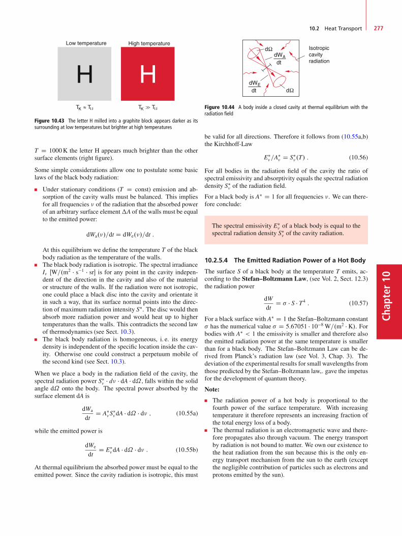
10.2 Heat Transport 277
Chap
ter10
Low temperature High temperature
Figure 10.43 The letter H milled into a graphite block appears darker as itssurrounding at low temperatures but brighter at high temperatures
T D 1000K the letter H appears much brighter than the othersurface elements (right figure).
Some simple considerations allow one to postulate some basiclaws of the black body radiation:
Under stationary conditions (T D const) emission and ab-sorption of the cavity walls must be balanced. This impliesfor all frequencies � of the radiation that the absorbed powerof an arbitrary surface element�A of the walls must be equalto the emitted power:
dWa.�/=dt D dWe.�/=dt :
At this equilibrium we define the temperature T of the blackbody radiation as the temperature of the walls.The black body radiation is isotropic. The spectral irradianceI� ŒW=.m2 � s�1 � sr� is for any point in the cavity indepen-dent of the direction in the cavity and also of the materialor structure of the walls. If the radiation were not isotropic,one could place a black disc into the cavity and orientate itin such a way, that its surface normal points into the direc-tion of maximum radiation intensity S�. The disc would thenabsorb more radiation power and would heat up to highertemperatures than the walls. This contradicts the second lawof thermodynamics (see Sect. 10.3).The black body radiation is homogeneous, i. e. its energydensity is independent of the specific location inside the cav-ity. Otherwise one could construct a perpetuum mobile ofthe second kind (see Sect. 10.3).
When we place a body in the radiation field of the cavity, thespectral radiation power S�
� � d� � dA � d˝ , falls within the solidangle d˝ onto the body. The spectral power absorbed by thesurface element dA is
dWa
dtD A�
�S��dA � d˝ � d� ; (10.55a)
while the emitted power is
dWe
dtD E�
�dA � d˝ � d� : (10.55b)
At thermal equilibrium the absorbed power must be equal to theemitted power. Since the cavity radiation is isotropic, this must
Figure 10.44 A body inside a closed cavity at thermal equilibrium with theradiation field
be valid for all directions. Therefore it follows from (10.55a,b)the Kirchhoff-Law
E�� =A
�� D S�
� .T/ : (10.56)
For all bodies in the radiation field of the cavity the ratio ofspectral emissivity and absorptivity equals the spectral radiationdensity S�
� of the radiation field.
For a black body is A� D 1 for all frequencies �. We can there-fore conclude:
The spectral emissivity E�� of a black body is equal to the
spectral radiation density S�� of the cavity radiation.
10.2.5.4 The Emitted Radiation Power of a Hot Body
The surface S of a black body at the temperature T emits, ac-cording to the Stefan–Boltzmann Law, (see Vol. 2, Sect. 12.3)the radiation power
dW
dtD � � S � T4 : (10.57)
For a black surface with A� D 1 the Stefan–Boltzmann constant� has the numerical value � D 5:67051 � 10�8 W=.m2 � K/. Forbodies with A� < 1 the emissivity is smaller and therefore alsothe emitted radiation power at the same temperature is smallerthan for a black body. The Stefan–Boltzmann Law can be de-rived from Planck’s radiation law (see Vol. 3, Chap. 3). Thedeviation of the experimental results for small wavelengths fromthose predicted by the Stefan–Boltzmann law,. gave the impetusfor the development of quantum theory.
Note:
The radiation power of a hot body is proportional to thefourth power of the surface temperature. With increasingtemperature it therefore represents an increasing fraction ofthe total energy loss of a body.The thermal radiation is an electromagnetic wave and there-fore propagates also through vacuum. The energy transportby radiation is not bound to matter. We own our existence tothe heat radiation from the sun because this is the only en-ergy transport mechanism from the sun to the earth (exceptthe negligible contribution of particles such as electrons andprotons emitted by the sun).
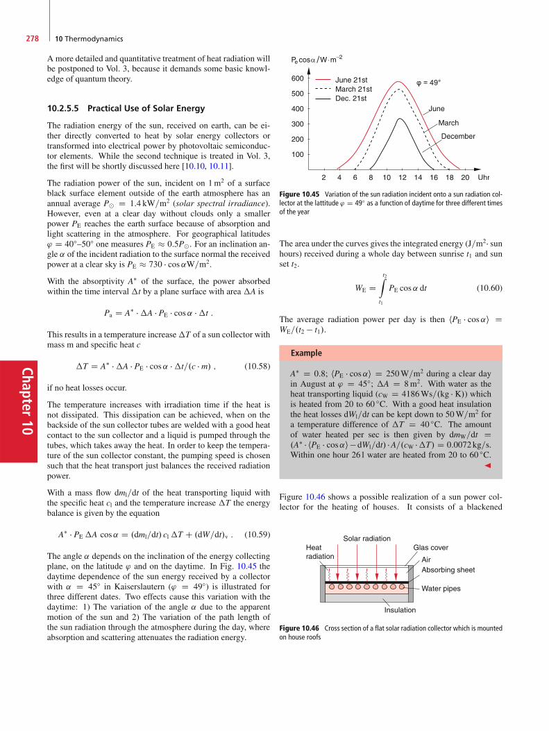
Chapter10
278 10 Thermodynamics
Amore detailed and quantitative treatment of heat radiation willbe postponed to Vol. 3, because it demands some basic knowl-edge of quantum theory.
10.2.5.5 Practical Use of Solar Energy
The radiation energy of the sun, received on earth, can be ei-ther directly converted to heat by solar energy collectors ortransformed into electrical power by photovoltaic semiconduc-tor elements. While the second technique is treated in Vol. 3,the first will be shortly discussed here [10.10, 10.11].
The radiation power of the sun, incident on 1m2 of a surfaceblack surface element outside of the earth atmosphere has anannual average Pˇ D 1:4 kW=m2 (solar spectral irradiance).However, even at a clear day without clouds only a smallerpower PE reaches the earth surface because of absorption andlight scattering in the atmosphere. For geographical latitudes' D 40ı–50ı one measures PE � 0:5Pˇ. For an inclination an-gle ˛ of the incident radiation to the surface normal the receivedpower at a clear sky is PE � 730 � cos˛W=m2.
With the absorptivity A� of the surface, the power absorbedwithin the time interval�t by a plane surface with area �A is
Pa D A� ��A � PE � cos˛ ��t :
This results in a temperature increase�T of a sun collector withmass m and specific heat c
�T D A� ��A � PE � cos˛ ��t=.c � m/ ; (10.58)
if no heat losses occur.
The temperature increases with irradiation time if the heat isnot dissipated. This dissipation can be achieved, when on thebackside of the sun collector tubes are welded with a good heatcontact to the sun collector and a liquid is pumped through thetubes, which takes away the heat. In order to keep the tempera-ture of the sun collector constant, the pumping speed is chosensuch that the heat transport just balances the received radiationpower.
With a mass flow dml=dt of the heat transporting liquid withthe specific heat cl and the temperature increase �T the energybalance is given by the equation
A� � PE�A cos˛ D .dml=dt/ cl�T C .dW=dt/v : (10.59)
The angle ˛ depends on the inclination of the energy collectingplane, on the latitude ' and on the daytime. In Fig. 10.45 thedaytime dependence of the sun energy received by a collectorwith ˛ D 45ı in Kaiserslautern (' D 49ı) is illustrated forthree different dates. Two effects cause this variation with thedaytime: 1) The variation of the angle ˛ due to the apparentmotion of the sun and 2) The variation of the path length ofthe sun radiation through the atmosphere during the day, whereabsorption and scattering attenuates the radiation energy.
Figure 10.45 Variation of the sun radiation incident onto a sun radiation col-lector at the lattitude ' D 49ı as a function of daytime for three different timesof the year
The area under the curves gives the integrated energy (J=m2� sunhours) received during a whole day between sunrise t1 and sunset t2.
WE Dt2Z
t1
PE cos˛ dt (10.60)
The average radiation power per day is then hPE � cos˛i DWE=.t2 � t1/.
Example
A� D 0:8; hPE � cos˛i D 250W=m2 during a clear dayin August at ' D 45ı; �A D 8m2. With water as theheat transporting liquid (cW D 4186Ws=.kg � K/) whichis heated from 20 to 60 ıC. With a good heat insulationthe heat losses dWl=dt can be kept down to 50W=m2 fora temperature difference of �T D 40 ıC. The amountof water heated per sec is then given by dmW=dt D.A� � hPE � cos˛i �dWl=dt/ �A=.cW ��T/ D 0:0072kg=s.Within one hour 26 l water are heated from 20 to 60 ıC.
J
Figure 10.46 shows a possible realization of a sun power col-lector for the heating of houses. It consists of a blackened
Solar radiationHeatradiation
Glas cover
Air
Water pipes
Absorbing sheet
Insulation
Figure 10.46 Cross section of a flat solar radiation collector which is mountedon house roofs
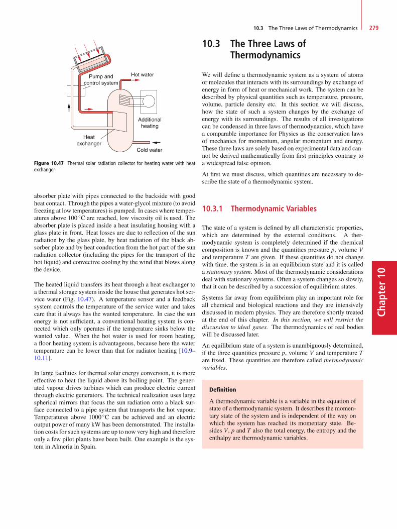
10.3 The Three Laws of Thermodynamics 279
Chap
ter10
Pump andcontrol system
Hot water
Cold water
Heatexchanger
Additionalheating
Figure 10.47 Thermal solar radiation collector for heating water with heatexchanger
absorber plate with pipes connected to the backside with goodheat contact. Through the pipes a water-glycol mixture (to avoidfreezing at low temperatures) is pumped. In cases where temper-atures above 100 ıC are reached, low viscosity oil is used. Theabsorber plate is placed inside a heat insulating housing with aglass plate in front. Heat losses are due to reflection of the sunradiation by the glass plate, by heat radiation of the black ab-sorber plate and by heat conduction from the hot part of the sunradiation collector (including the pipes for the transport of thehot liquid) and convective cooling by the wind that blows alongthe device.
The heated liquid transfers its heat through a heat exchanger toa thermal storage system inside the house that generates hot ser-vice water (Fig. 10.47). A temperature sensor and a feedbacksystem controls the temperature of the service water and takescare that it always has the wanted temperature. In case the sunenergy is not sufficient, a conventional heating system is con-nected which only operates if the temperature sinks below thewanted value. When the hot water is used for room heating,a floor heating system is advantageous, because here the watertemperature can be lower than that for radiator heating [10.9–10.11].
In large facilities for thermal solar energy conversion, it is moreeffective to heat the liquid above its boiling point. The gener-ated vapour drives turbines which can produce electric currentthrough electric generators. The technical realization uses largespherical mirrors that focus the sun radiation onto a black sur-face connected to a pipe system that transports the hot vapour.Temperatures above 1000 ıC can be achieved and an electricoutput power of many kW has been demonstrated. The installa-tion costs for such systems are up to now very high and thereforeonly a few pilot plants have been built. One example is the sys-tem in Almeria in Spain.
10.3 The Three Laws ofThermodynamics
We will define a thermodynamic system as a system of atomsor molecules that interacts with its surroundings by exchange ofenergy in form of heat or mechanical work. The system can bedescribed by physical quantities such as temperature, pressure,volume, particle density etc. In this section we will discuss,how the state of such a system changes by the exchange ofenergy with its surroundings. The results of all investigationscan be condensed in three laws of thermodynamics, which havea comparable importance for Physics as the conservation lawsof mechanics for momentum, angular momentum and energy.These three laws are solely based on experimental data and can-not be derived mathematically from first principles contrary toa widespread false opinion.
At first we must discuss, which quantities are necessary to de-scribe the state of a thermodynamic system.
10.3.1 Thermodynamic Variables
The state of a system is defined by all characteristic properties,which are determined by the external conditions. A ther-modynamic system is completely determined if the chemicalcomposition is known and the quantities pressure p, volume Vand temperature T are given. If these quantities do not changewith time, the system is in an equilibrium state and it is calleda stationary system. Most of the thermodynamic considerationsdeal with stationary systems. Often a system changes so slowly,that it can be described by a succession of equilibrium states.
Systems far away from equilibrium play an important role forall chemical and biological reactions and they are intensivelydiscussed in modern physics. They are therefore shortly treatedat the end of this chapter. In this section, we will restrict thediscussion to ideal gases. The thermodynamics of real bodieswill be discussed later.
An equilibrium state of a system is unambiguously determined,if the three quantities pressure p, volume V and temperature Tare fixed. These quantities are therefore called thermodynamicvariables.
Definition
A thermodynamic variable is a variable in the equation ofstate of a thermodynamic system. It describes the momen-tary state of the system and is independent of the way onwhich the system has reached its momentary state. Be-sides V, p and T also the total energy, the entropy and theenthalpy are thermodynamic variables.

Chapter10
280 10 Thermodynamics
Figure 10.48 a Heating at constant pressure; b heating at constant volume;c no heat supply
The thermodynamic variables are related to each other by theequation of state for a gas volume V of an ideal gas with Nmolecules
p � V D � � R � T ; (10.61)
where � D N=NA is the number of moles and NA the Avogadronumber. Also for real gases a corresponding equation can bederived (see Sect. 10.4). For a given volume V and a pressure pthe temperature T determines the internal energy
U D 12 � � � f � R � T (10.62)
of molecules with f degrees of freedom. For ideal gases (forinstance helium) is f D 3. If the volume decreases (dV < 0) ata constant pressure p the necessary work is
dW D �p � dV : (10.63)
The sign is chosen in such a way that the applied workis positive, if the energy of the system increases. Workperformed by the system means a decrease of its internalenergy and is therefore defined as negative.
When a gas is heated at constant pressure p its volume increases(Fig. 10.48a). The quantity
�p D 1
V��@V
@T
�
p
; (10.64)
that describes the relative volume change per Kelvin tempera-ture rise, is the isobaric expansion coefficient.
In an analogous way the heating of a gas at a constant volume(Fig. 10.48b, where the pressure increases, is described by theisochoric pressure coefficient
�V D 1
p��@p
@T
�
V
; (10.65)
which describes the relative pressure increase �p=p for a tem-perature rise of 1K.
The isothermal compressibility
�T D � D � 1
V��@V
@p
�
T
(10.66)
gives the relative volume change �V=V for a pressure change�p at a constant temperature T .
As recollection keep in mind:
isothermal: T D const
isobaric: p D const
isochoric: V D const :
The total change dV of the volumeV.p;T/, when both quantitiesp and T are changing is
dV D�@V
@p
�
T
dp C�@V
@T
�
p
dT
D �� � V � dp C �p � V � dT :(10.67)
For isochoric processes the volume V stays constant, i. e. dV D0. Then (10.67) reduces to
0 D � � � V � .dp/V C �p � V � .dT/V) � � dp D �p � dT : (10.68)
Division by dT yields with .dp=dT/V D �V � p the relation
�p D � � �V � p (10.69)
between isobaric expansion coefficient �p, isothermic compress-ibility �, isochoric expansion coefficient �V and pressure p.
10.3.2 The First Law of Thermodynamics
The heat�Q applied to a system can be either used for rising thetemperature T at a constant volume V, or for the expansion ofthe volume V against the external pressure p where the systemhas to perform the work �W . Energy conservation demands
�Q D �U ��W ; (10.70a)
where, as defined before, �W < 0 if the system performswork (which decreases its own energy). This sign definitionis in agreement with the definition (2.35) for the work. If thesystem, for instance, performs work against an external forceF D �p � A when a piston with area A is moved along the dis-tance �x against the external pressure p, the work is
�W D F � �x D �p � A ��x D �p ��V with �V > 0 :

10.3 The Three Laws of Thermodynamics 281
Chap
ter10
Equation 10.70 is the first law of thermodynamics. It is a spe-cial case of the general law of energy conservation. It can beformulated as:
The sum of the external heat �Q, applied to a thermody-namic system, and the supplied mechanical energy �W isequal to the increase �U of the total internal energy U.
�U D �Q C�W (10.70b)
When the system performs work against an external force, is�W < 0 and therefore �U < 0. Many inventors have triedto construct machines that deliver more energy than they con-sume. Such a machine could use part of the delivered energy forits own operation. It could run continuously delivering energywithout external energy input. Therefore this hypothetical ma-chine is called a perpetuum mobile. Because it contradicts thefirst law of thermodynamics it is also called perpetuum mobileof the first kind.
Equation 10.70 can be also formulated in a more floppy way as:
A perpetuum mobile of the first kind is impossible.
Note: This statement cannot be proved mathematically. It issolely based on empirical knowledge.
For ideal gases the work performed during the expansion of thevolume V by infinitesimal amount dV against the external pres-sure p is
dW D p � dV :The first law of thermodynamics for ideal gases can therefore bewritten in a differential form as
dU D dQ � p � dV : (10.71)
For dV > 0 the system releases energy and according to (10.71)dU < dQ, i. e. the loss of internal energy cannot be compensatedby the supplied heat dQ. For dV < 0 the volume is compressedand the system gains the energy p � dV. Now dU > dQ, the gainof internal energy is larger than the supplied heat.
The relation between the thermodynamic variables p, V, T canbe derived from (10.71) for special processes where in each caseone of the variables p, V, T or the quantity Q is kept constant.
Note, that the quantity Q is not a thermodynamic variable! Thestate of a system does change with the supply of heat dQ, butone cannot unambiguously determine the final state of the sys-tem, because either U or V or both variables can change. In amathematical language this means: dQ is not a complete differ-ential.
10.3.3 Special Processes as Examples of theFirst Law of Thermodynamics
Note: We will discuss the following processes for one mole ofa gas where the number of moles is � D V=VM D 1.
10.3.3.1 Isochoric Processes (V = const)
With dV D 0 it follows from (10.71)
dQ D dU D CV � dT : (10.72)
The heat supplied to the system is used solely for the increase ofthe internal energy U. We can therefore relate the specific heatto the internal energy U by
CV D�@U
@T
�
V
: (10.73)
10.3.3.2 Isobaric Processes (p = const)
The first law of thermodynamics has now the form
dQ D dU C p � dV D Cp � dT ; (10.74)
where we have used (10.28). When we introduce the enthalpy
H D U C p � V (10.75)
as new thermodynamic variable with
dH D dU C p � dV C V � dp D dQ C V � dp ; (10.76)
we can write the first law of thermodynamics as
dH D dU C p � dV D dQ : (10.77)
For isobaric processes the increase dH of the enthalpy His equal to the supplied heat dQ.
The specific heat at constant pressure is then
Cp D�@H
@T
�
p
: (10.78)
The variable H is often used for phase changes, chemical reac-tions or other processes that take place at constant pressure, butwhere the volume can change. A further example is the expan-sion of a gas from a reservoir with constant pressure into thevacuum where the pressure p D 0 is maintained by pumps.
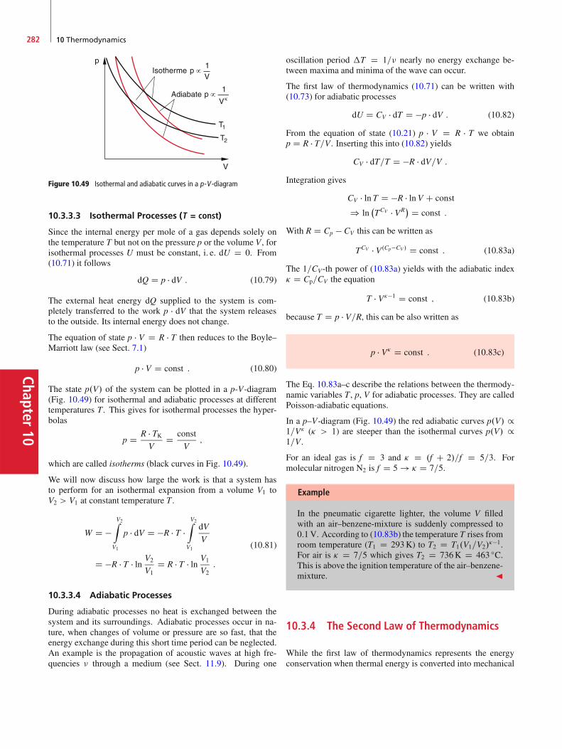
Chapter10
282 10 Thermodynamics
Figure 10.49 Isothermal and adiabatic curves in a p-V -diagram
10.3.3.3 Isothermal Processes (T = const)
Since the internal energy per mole of a gas depends solely onthe temperature T but not on the pressure p or the volume V, forisothermal processes U must be constant, i. e. dU D 0. From(10.71) it follows
dQ D p � dV : (10.79)
The external heat energy dQ supplied to the system is com-pletely transferred to the work p � dV that the system releasesto the outside. Its internal energy does not change.
The equation of state p � V D R � T then reduces to the Boyle–Marriott law (see Sect. 7.1)
p � V D const : (10.80)
The state p.V/ of the system can be plotted in a p-V-diagram(Fig. 10.49) for isothermal and adiabatic processes at differenttemperatures T . This gives for isothermal processes the hyper-bolas
p D R � TKV
D const
V;
which are called isotherms (black curves in Fig. 10.49).
We will now discuss how large the work is that a system hasto perform for an isothermal expansion from a volume V1 toV2 > V1 at constant temperature T .
W D �V2Z
V1
p � dV D �R � T �V2Z
V1
dV
V
D �R � T � ln V2
V1D R � T � ln V1
V2:
(10.81)
10.3.3.4 Adiabatic Processes
During adiabatic processes no heat is exchanged between thesystem and its surroundings. Adiabatic processes occur in na-ture, when changes of volume or pressure are so fast, that theenergy exchange during this short time period can be neglected.An example is the propagation of acoustic waves at high fre-quencies � through a medium (see Sect. 11.9). During one
oscillation period �T D 1=� nearly no energy exchange be-tween maxima and minima of the wave can occur.
The first law of thermodynamics (10.71) can be written with(10.73) for adiabatic processes
dU D CV � dT D �p � dV : (10.82)
From the equation of state (10.21) p � V D R � T we obtainp D R � T=V. Inserting this into (10.82) yields
CV � dT=T D �R � dV=V :Integration gives
CV � ln T D �R � lnV C const
) ln�TCV � VR
� D const :
With R D Cp � CV this can be written as
TCV � V.Cp�CV / D const : (10.83a)
The 1=CV-th power of (10.83a) yields with the adiabatic index� D Cp=CV the equation
T � V��1 D const ; (10.83b)
because T D p � V=R, this can be also written as
p � V� D const : (10.83c)
The Eq. 10.83a–c describe the relations between the thermody-namic variables T , p, V for adiabatic processes. They are calledPoisson-adiabatic equations.
In a p–V-diagram (Fig. 10.49) the red adiabatic curves p.V/ /1=V� (� > 1) are steeper than the isothermal curves p.V/ /1=V.
For an ideal gas is f D 3 and � D .f C 2/=f D 5=3. Formolecular nitrogen N2 is f D 5 ! � D 7=5.
Example
In the pneumatic cigarette lighter, the volume V filledwith an air–benzene-mixture is suddenly compressed to0:1V. According to (10.83b) the temperature T rises fromroom temperature (T1 D 293K) to T2 D T1.V1=V2/
��1.For air is � D 7=5 which gives T2 D 736K D 463 ıC.This is above the ignition temperature of the air–benzene-mixture. J
10.3.4 The Second Law of Thermodynamics
While the first law of thermodynamics represents the energyconservation when thermal energy is converted into mechanical

10.3 The Three Laws of Thermodynamics 283
Chap
ter10
energy, the second law of thermodynamics gives the maximumfraction of thermal energy that can be really transferred into me-chanical energy.
As we will see, this is connected with the question, into whichdirection the transfer of one form of energy into another formproceeds by its own, i. e. without external action. All of ourexperience tells us, that heat flows by its own only from thehotter region into the colder one, not vice versa. Furthermore allexperiments show, that mechanical energy can be completelyconverted into heat, but that for the opposite process only partof the heat can be converted into mechanical energy.
This fact, that is based solely on experimental experience, isformulated in the second law of thermodynamics:
Heat flows by its own only from the warmer body to thecolder one, never into the opposite direction.
We will now discuss more quantitatively the transformation ofheat into mechanical work. This will be illustrated by con-sidering thermodynamic cyclic processes, which leads us to aquantitative formulation of the second law of thermodynamics.
10.3.5 The Carnot Cycle
A thermodynamic cycle is a series of processes where a ther-modynamic system passes through several different states untilit finally reaches again its initial state. At the end of this cycle,the system shows again the same thermodynamic variables as inthe initial state, although it has passed during the cycle throughdifferent states with different variables. A simple example is asystem that is heated and then cooled again until it has reachedthe initial temperature.
If the cyclic process can traverse into both directions the cycle iscalled reversible (Fig. 10.50) otherwise it is called irreversible.Although such reversible processes can occur in micro-physicsif only a few particles are involved, they represent in the
Figure 10.50 Thermodynamic cycle from the state 1 .T1; p1; V1/ via the state2 .T2; p2; V2/ back to the state 1. a In a p–V -diagram; b in the temperature-time diagram. Note: The cycle shown here, can only proceed, if energy is fedinto the system during the first step and energy is taken away from the systemduring the second step
Figure 10.51 Carnot’s cycle
real world of many-particle systems only idealized “Gedanken-experiments”, which represent limiting cases of real processesthat are always irreversible.
All periodically operating machines, such as steam engines orcar motors traverse irreversible cyclic processes. Although theyarrive at the end of the cycle again at the initial state, if they areregarded as isolated systems, but they have lost energy duringthe cycle (for instance friction losses) which has to be replacedfor each cycle.
The most famous reversible cyclic process is the Carnot-cyclethat represents an idealized loss-free cycle. It was publishedin 1824 by Nicolas Leonard Sadi Carnot. This cyclic processwill enable us to calculate the maximum fraction of heat thatcan be transformed into mechanical energy and therefore allowsthe quantitative formulation of the second law of thermodynam-ics. Furthermore, it illustrates nicely the difference betweenreversible and irreversible processes.
The Carnot Cycle is a “Gedanken-Experiment”, where a ther-modynamic system passes through two isothermal and two adi-abatic processes during two expansion and compression events,until it finally reaches its initial state again (Fig. 10.51).
Note: The following considerations are valid for 1mol of anideal gas, where in Eq. 10.61 V D VM and � D 1.
The state of the system at the starting point 1 is defined by thethermodynamic variables .V1; p1;T1/. The isothermal expan-sion brings the system to the state 2 D .V2; p2;T1/. During thisprocess, the heat �Q1 has to be supplied to the system in orderto keep the temperature constant. Now an adiabatic expansionfollows and the system gets to the state 3 D .V3; p3;T2 < T1/.In the next step the system is isothermally compressed andreaches the state 4 with the conditions (V4, p4, T2). Herethe heat �Q2 has to be removed from the system. Finallyan adiabatic compression brings the system back to its initialstate 1 D .V1; p1;T1/. Such a virtual thermodynamic systemthat passes through a Carnot cycle is called a Carnot Machine.
We will now calculate the heat energies �Q1 and �Q2 whichare exchanged between the system and a heat reservoir duringthe isothermal processes.
1st process: Isothermal expansion from the state 1 to thestate 2. According to the first law of thermodynamics we ob-

Chapter10
284 10 Thermodynamics
tain for an isothermal expansion
dQ D p � dV :
The heat supplied to the system is equal to the mechanicalwork the system performs during the expansion.
With (10.81) it follows:
�Q1 D ��W12 DV2Z
V1
p dV
D R � T1 � ln.V2=V1/ :
(10.84a)
2nd process: Adiabatic expansion from state 2 to state 3.For adiabatic processes the heat exchange is zero. We thereforeobtain:
dQ D 0 ! dU D �p � dV D �W23 : (10.84b)
The work performed during the expansion is negative, becauseit is delivered from the system to the surrounding. This resultsin a decrease �U D U.T2/ � U.T1/ of the internal energy Ubecause T2 < T1.
3rd process: Isothermal compression from state 3 to state 4.Similar to step 1 is the heat �Q2 delivered at the lower temper-ature T2 to the heat reservoir equal to the work �W34 necessaryto compress the volume V
�W34 D R � T2 � ln.V3=V4/ D ��Q2 > 0 : (10.84c)
4th process: Adiabatic compression from state 4 to the start-ing conditions in state 1. Similar to step 2 is here no heatexchange with the surrounding and the work performed duringthe compression is converted to the increase �U of the internalenergy
�U D U.T1/ � U.T2/ : (10.84d)
Total energy balance: The work delivered to the surroundingduring the 2nd process is equal to the work supplied to thesystem during the 4th process. Therefore, only during theisothermal processes a net energy is transferred. The net me-chanical work during the Carnot cycle (Fig. 10.52) is
�W D �W12 C�W34
D R � T1 � ln.V1=V2/C R � T2 � ln.V3=V4/ :
For the adiabatic processes 2 ! 3 and 4 ! 1 the relations hold
T1 � V��12 D T2 � V��1
3 and
T1 � V��11 D T2 � V��1
4 :
Division of the two equations yields
V2=V1 D V3=V4 ) ln.V3=V4/ D � ln.V1=V2/ :
Figure 10.52 Heat exchange and net mechanical energy �W D �W34 ��W12 of Carnot’s cycle
The net work is then
�W D R � .T1 � T2/ � ln.V1=V2/ : (10.85)
The Carnot Engine has received the heat �Q1 and has suppliedthe mechanical work �W < 0 to the outside.
Such a machine that transfers heat into mechanical energy iscalled heat engine.
The heat �Q2 supplied to the surrounding, is generally lost.Therefore the efficiency of the engine is defined as the mechan-ical work supplied by the engine divided by the heat �Q1 putinto the engine.
The efficiency of the Carnot Engine is then
� Dˇ̌ˇ̌�W
�Q1
ˇ̌ˇ̌ D R.T1 � T2/ � ln.V2=V1/
R � T1 � ln.V2=V1/D T1 � T2
T1
� D T1 � T2T1
: (10.86)
This is a remarkable result: During the cycle the total receivedheat cannot be transformed into mechanical work, but only thefraction � D .T1 � T2/=T1 < 1. This fraction is called ex-ergy. The remaining part (1� �) of the input energy (Anergy) isexchanged as heat �Q2 to the surrounding at the lower temper-ature T2. The conservation of total energy can be written as
Energy D Exergy C Anergy :
The efficiency of the Carnot Engine increases with increasingtemperature difference T1 � T2. It is therefore advantageous tochoose T1 as high as possible and T2 as low as possible. We willsee in Sect. 10.3.10 that it is impossible to reach T2 D 0K.
This implies that � is always smaller than 1.
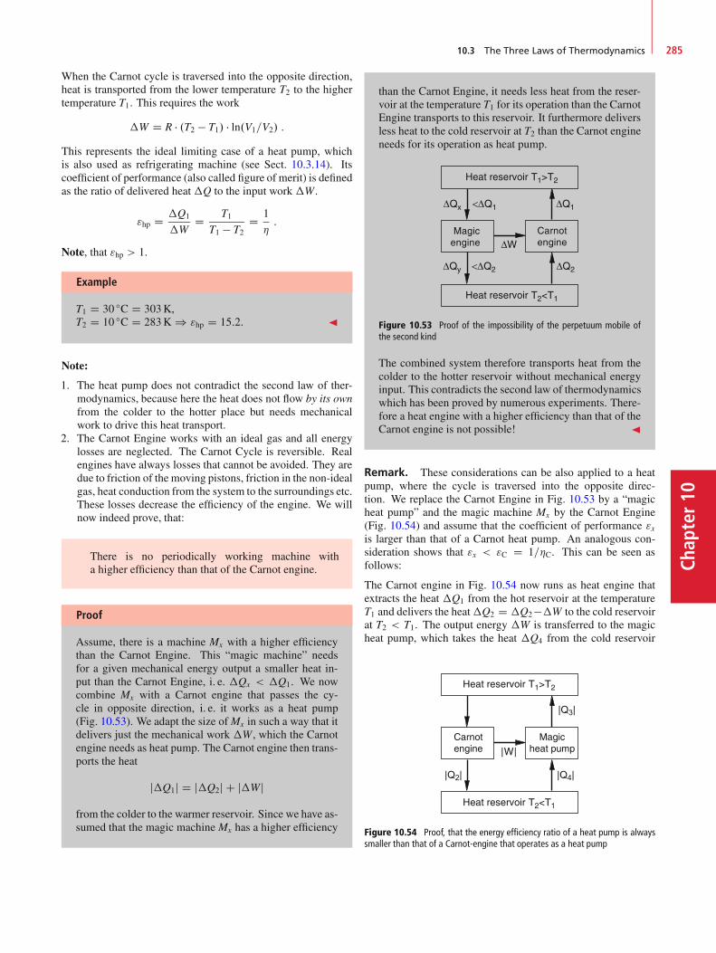
10.3 The Three Laws of Thermodynamics 285
Chap
ter10
When the Carnot cycle is traversed into the opposite direction,heat is transported from the lower temperature T2 to the highertemperature T1. This requires the work
�W D R � .T2 � T1/ � ln.V1=V2/ :
This represents the ideal limiting case of a heat pump, whichis also used as refrigerating machine (see Sect. 10.3.14). Itscoefficient of performance (also called figure of merit) is definedas the ratio of delivered heat�Q to the input work �W .
"hp D �Q1
�WD T1
T1 � T2D 1
�:
Note, that "hp > 1.
Example
T1 D 30 ıC D 303K,T2 D 10 ıC D 283K ) "hp D 15:2. J
Note:
1. The heat pump does not contradict the second law of ther-modynamics, because here the heat does not flow by its ownfrom the colder to the hotter place but needs mechanicalwork to drive this heat transport.
2. The Carnot Engine works with an ideal gas and all energylosses are neglected. The Carnot Cycle is reversible. Realengines have always losses that cannot be avoided. They aredue to friction of the moving pistons, friction in the non-idealgas, heat conduction from the system to the surroundings etc.These losses decrease the efficiency of the engine. We willnow indeed prove, that:
There is no periodically working machine witha higher efficiency than that of the Carnot engine.
Proof
Assume, there is a machine Mx with a higher efficiencythan the Carnot Engine. This “magic machine” needsfor a given mechanical energy output a smaller heat in-put than the Carnot Engine, i. e. �Qx < �Q1. We nowcombine Mx with a Carnot engine that passes the cy-cle in opposite direction, i. e. it works as a heat pump(Fig. 10.53). We adapt the size ofMx in such a way that itdelivers just the mechanical work �W , which the Carnotengine needs as heat pump. The Carnot engine then trans-ports the heat
j�Q1j D j�Q2j C j�Wj
from the colder to the warmer reservoir. Since we have as-sumed that the magic machine Mx has a higher efficiency
than the Carnot Engine, it needs less heat from the reser-voir at the temperature T1 for its operation than the CarnotEngine transports to this reservoir. It furthermore deliversless heat to the cold reservoir at T2 than the Carnot engineneeds for its operation as heat pump.
Figure 10.53 Proof of the impossibility of the perpetuum mobile ofthe second kind
The combined system therefore transports heat from thecolder to the hotter reservoir without mechanical energyinput. This contradicts the second law of thermodynamicswhich has been proved by numerous experiments. There-fore a heat engine with a higher efficiency than that of theCarnot engine is not possible! J
Remark. These considerations can be also applied to a heatpump, where the cycle is traversed into the opposite direc-tion. We replace the Carnot Engine in Fig. 10.53 by a “magicheat pump” and the magic machine Mx by the Carnot Engine(Fig. 10.54) and assume that the coefficient of performance "xis larger than that of a Carnot heat pump. An analogous con-sideration shows that "x < "C D 1=�C. This can be seen asfollows:
The Carnot engine in Fig. 10.54 now runs as heat engine thatextracts the heat �Q1 from the hot reservoir at the temperatureT1 and delivers the heat�Q2 D �Q2��W to the cold reservoirat T2 < T1. The output energy �W is transferred to the magicheat pump, which takes the heat �Q4 from the cold reservoir
| |
|Q3|
|Q2| |Q4|
Carnotengine
Magicheat pump
Figure 10.54 Proof, that the energy efficiency ratio of a heat pump is alwayssmaller than that of a Carnot-engine that operates as a heat pump
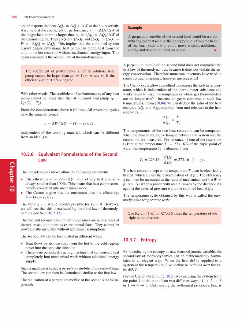
Chapter10
286 10 Thermodynamics
and transports the heat �Q3 D �Q C�W to the hot reservoir.Assume that the coefficient of performance "x D �Q3=�W ofthe magic heat pump is larger than "C D 1=�C D �Q1=�W ofthe Carnot engine. Then j�Q3j > j�Q1j and j�Q4j D j�Q3j �W > j�Q2j D j�Q1j This implies that the combined systemCarnot engine plus magic heat pump can pump heat from thecold to the hot reservoir without mechanical energy input. Thisagain contradicts the second law of thermodynamics.
The coefficient of performance "x of an arbitrary heatpump cannot be larger than "C D 1=�C where �C is theefficiency of the Carnot engine.
With other words: The coefficient of performance "x of any heatpump cannot be larger than that of a Carnot heat pump "C DT1=.T1 � T2/.
From the considerations above it follows: All reversible cycleshave the same efficiency
� D �W=�Q1 D .T1 � T2/=T1 ;
independent of the working material, which can be differentfrom an ideal gas.
10.3.6 Equivalent Formulations of the SecondLaw
The considerations above allow the following statements:
The efficiency � D �W=�Q1 < 1 of any heat engine isalways smaller than 100%. This means that heat cannot com-pletely converted into mechanical work.The Carnot engine has the maximum possible efficiency:� D .T1 � T2/=T1.
The value � D 1 would be only possible for T2 D 0. However,we will see that this is excluded by the third law of thermody-namics (see Sect. 10.3.13)
The first and second laws of thermodynamics are purely rules ofthumb, based on numerous experimental facts. They cannot beproved mathematically without additional assumptions.
The second law can be formulated in different ways:
Heat flows by its own only from the hot to the cold region,never into the opposite direction.There is no periodically acting machine that can convert heatcompletely into mechanical work without additional energysupply.
Such a machine is called a perpetuummobile of the second kind.The second law can then be formulated similar to the first law:
The realization of a perpetuum mobile of the second kind is im-possible.
Example
A perpetuum mobile of the second kind could be a shipwith engines that receive their energy solely from the heatof the sea. Such a ship could move without additionalenergy and would not need oil or coal. J
A perpetuum mobile of the second kind does not contradict thefirst law of thermodynamics, because it does not violate the en-ergy conservation. Therefore numerous inventors have tried toconstruct such machines, however unsuccessful!
The Carnot cycle allows a method tomeasure the Kelvin temper-ature, which is independent of the thermometer substance andworks down to very low temperatures where gas thermometersare no longer useful, because all gases condense at such lowtemperatures. From (10.84) we can deduce the ratio of the heatenergies �Q1 and �Q2 supplied from and released to the heatreservoirs
�Q1
�Q2D T1
T2:
The temperatures of the two heat reservoirs can be compared,when the heat energies, exchanged between the system and thereservoirs, are measured. For instance, if one of the reservoirsis kept at the temperature T1 D 273:16K of the triple point ofwater the temperature T2 is obtained from
T2 D 273:16 � j�Q2jj�Q1j D 273:16 � .1 � �/ :
The heat reservoir, kept at the temperature T1, can be electricallyheated, which allows the determination of �Q1. The efficiency� can then be measured as the ratio of mechanical work �W Dp ��A ��x when a piston with area A moves by the distance�xagainst the external pressure p and the supplied heat �Q1.
The temperature scale obtained by this way is called the ther-modynamic temperature scale.
One Kelvin (1K) is 1/273.16 times the temperature of thetriple point of water.
10.3.7 Entropy
By introducing the entropy as new thermodynamic variable, thesecond law of thermodynamics can be mathematically formu-lated in an elegant way. When the heat dQ is supplied to asystem at the temperature T we define as reduced heat the ra-tio dQ=T .
For the Carnot cycle in Fig. 10.51 we can bring the system fromthe point 1 to the point 3 on two different ways: 1 ! 2 ! 3or 1 ! 4 ! 3. Only during the isothermal processes, heat is

10.3 The Three Laws of Thermodynamics 287
Chap
ter10
exchanged with the surroundings. The absolute values of thereduced heat energies j�Q1j=T1 and j�Q2j=T2 on the two waysare equal, as can be seen from (10.84a–c). This means: Thereduced energies do not depend on the way but only on startingand final state of the system. This is not only valid for the Carnotcycle but for all reversible processes.
We introduce the thermodynamic variable S called the entropywith the dimension ŒS� D ŒJ=K�, in the following way. We definethe change dS of the entropy as the reduced heat exchanged onan infinitesimal part of a reversible process
dS D dQ=T :
Since the change�S for a system that is brought from a definedinitial state into a defined final state is independent of the waybetween these two states, and depends solely on initial and finalstates of the system, the quantity S is a thermodynamic vari-able which describes together with pressure p, temperature Tand volume V the state of a thermodynamic system.
In the Carnot Cycle the reduced heat energies change only dur-ing the isothermal processes. According to (10.84) the entropythen changes by
�S D �Q
TD ˙R � ln V2
V1: (10.87)
For the complete reversible cycle we have
�Q1
T1D ��Q2
T2;
and therefore
�S D 0 :
For a reversible cycle the entropy S is constant.
Processes where S D const are called isentropic processes. Forthese processes is �S D 0 and therefore �Q D 0 and T Dconst. During isentropic processes the system must be kept ata constant temperature. This distinguishes isentropic processesfrom adiabatic processes where also �Q D 0 but where thetemperature changes.
With the first law of thermodynamics (10.71) the entropy changedS during reversible processes of an ideal gas can be calculatedas
dS D dQrev
TD dU C p dV
T: (10.88)
For 1 mol of the gas is dU D CV � dT and p � VM D R � T . Thisconverts (10.88) to
dS D CVdT
TC R � dV
V: (10.89)
Integration over the temperature range from T1 to T2 where themolar heat capacity can be assumed as constant, yields for iso-baric processes where V and T can change but p D const.
�Sisobar D CV lnT2T1
C R � ln V2
V1: (10.90)
In a similar way one obtains for isochoric processes (V D const)with CV D Cp � R and p1=T1 D p2=T2
�Sisochor D CV lnT2T1
D .Cp � R/ lnT2T1
D Cp lnT2T1
� R lnT2T1
�Sisochor D Cp lnT2T1
� R � ln p2p1: (10.91)
Since the entropy S is a thermodynamic variable, its change �Sdoes not depend on the kind of process but only on initial andfinal state of the process. We can therefore determine �S alsofor irreversible processes. This can be seen as follows:
We consider a substance at the temperature T1 (e. g. a solidbody) in a gas volume V. The body should be in thermal contactwith the gas. Now the gas is slowly expanded in an adiabaticprocess, which results in a slow decrease of the temperature. Ifthis proceeds sufficiently slowly, the temperature of the bodyis always equal to that of the gas, because sufficient time isavailable for reaching temperature equilibrium. Finally the tem-perature has decreased to T2. This process is reversible becausethe initial state can be retrieved by slow adiabatic compression.
When the solid body is regarded as isolated body without thegas, the cooling process is irreversible, because heat is trans-ferred to the surrounding. The entropy change of the body is
�S D �Qirr
T
D CV
T2Z
T1
dT
T
D CV � ln T2T1< 0 for T2 < T1 ;
(10.92)
as in the reversible process. However, since heat has beentransferred to the surroundings the entropy of the surroundingsincreases. For the total change of the system body + surround-ings �Sirrev > 0, i. e. the entropy increases!
Example
1. We regard in Fig. 10.55 two equal bodies with massm and specific heat c which have been brought by dif-ferent energy supply to different temperatures T1 andT2 < T1. Their heat energies are then Q1 D m � c � T1and Q2 D m � c � T2. When they are brought into
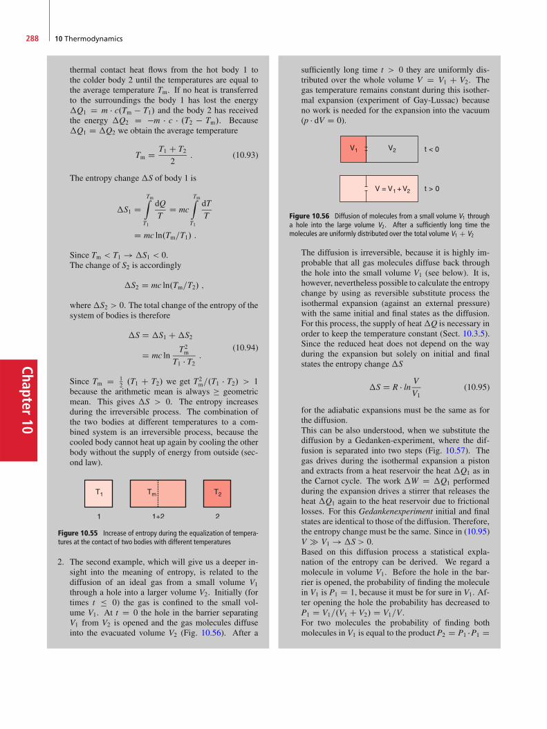
Chapter10
288 10 Thermodynamics
thermal contact heat flows from the hot body 1 tothe colder body 2 until the temperatures are equal tothe average temperature Tm. If no heat is transferredto the surroundings the body 1 has lost the energy�Q1 D m � c.Tm � T1/ and the body 2 has receivedthe energy �Q2 D �m � c � .T2 � Tm/. Because�Q1 D �Q2 we obtain the average temperature
Tm D T1 C T22
: (10.93)
The entropy change�S of body 1 is
�S1 DTmZ
T1
dQ
TD mc
TmZ
T1
dT
T
D mc ln.Tm=T1/ :
Since Tm < T1 ! �S1 < 0.The change of S2 is accordingly
�S2 D mc ln.Tm=T2/ ;
where�S2 > 0. The total change of the entropy of thesystem of bodies is therefore
�S D �S1 C�S2
D mc lnT2m
T1 � T2 :(10.94)
Since Tm D 12 .T1 C T2/ we get T2
m=.T1 � T2/ > 1because the arithmetic mean is always � geometricmean. This gives �S > 0. The entropy increasesduring the irreversible process. The combination ofthe two bodies at different temperatures to a com-bined system is an irreversible process, because thecooled body cannot heat up again by cooling the otherbody without the supply of energy from outside (sec-ond law).
Figure 10.55 Increase of entropy during the equalization of tempera-tures at the contact of two bodies with different temperatures
2. The second example, which will give us a deeper in-sight into the meaning of entropy, is related to thediffusion of an ideal gas from a small volume V1
through a hole into a larger volume V2. Initially (fortimes t � 0) the gas is confined to the small vol-ume V1. At t D 0 the hole in the barrier separatingV1 from V2 is opened and the gas molecules diffuseinto the evacuated volume V2 (Fig. 10.56). After a
sufficiently long time t > 0 they are uniformly dis-tributed over the whole volume V D V1 C V2. Thegas temperature remains constant during this isother-mal expansion (experiment of Gay-Lussac) becauseno work is needed for the expansion into the vacuum(p � dV D 0).
Figure 10.56 Diffusion of molecules from a small volume V1 througha hole into the large volume V2. After a sufficiently long time themolecules are uniformly distributed over the total volume V1 C V2
The diffusion is irreversible, because it is highly im-probable that all gas molecules diffuse back throughthe hole into the small volume V1 (see below). It is,however, nevertheless possible to calculate the entropychange by using as reversible substitute process theisothermal expansion (against an external pressure)with the same initial and final states as the diffusion.For this process, the supply of heat�Q is necessary inorder to keep the temperature constant (Sect. 10.3.5).Since the reduced heat does not depend on the wayduring the expansion but solely on initial and finalstates the entropy change �S
�S D R � ln V
V1(10.95)
for the adiabatic expansions must be the same as forthe diffusion.This can be also understood, when we substitute thediffusion by a Gedanken-experiment, where the dif-fusion is separated into two steps (Fig. 10.57). Thegas drives during the isothermal expansion a pistonand extracts from a heat reservoir the heat �Q1 as inthe Carnot cycle. The work �W D �Q1 performedduring the expansion drives a stirrer that releases theheat �Q1 again to the heat reservoir due to frictionallosses. For this Gedankenexperiment initial and finalstates are identical to those of the diffusion. Therefore,the entropy change must be the same. Since in (10.95)V � V1 ! �S > 0.Based on this diffusion process a statistical expla-nation of the entropy can be derived. We regard amolecule in volume V1. Before the hole in the bar-rier is opened, the probability of finding the moleculein V1 is P1 D 1, because it must be for sure in V1. Af-ter opening the hole the probability has decreased toP1 D V1=.V1 C V2/ D V1=V.For two molecules the probability of finding bothmolecules in V1 is equal to the product P2 D P1 �P1 D
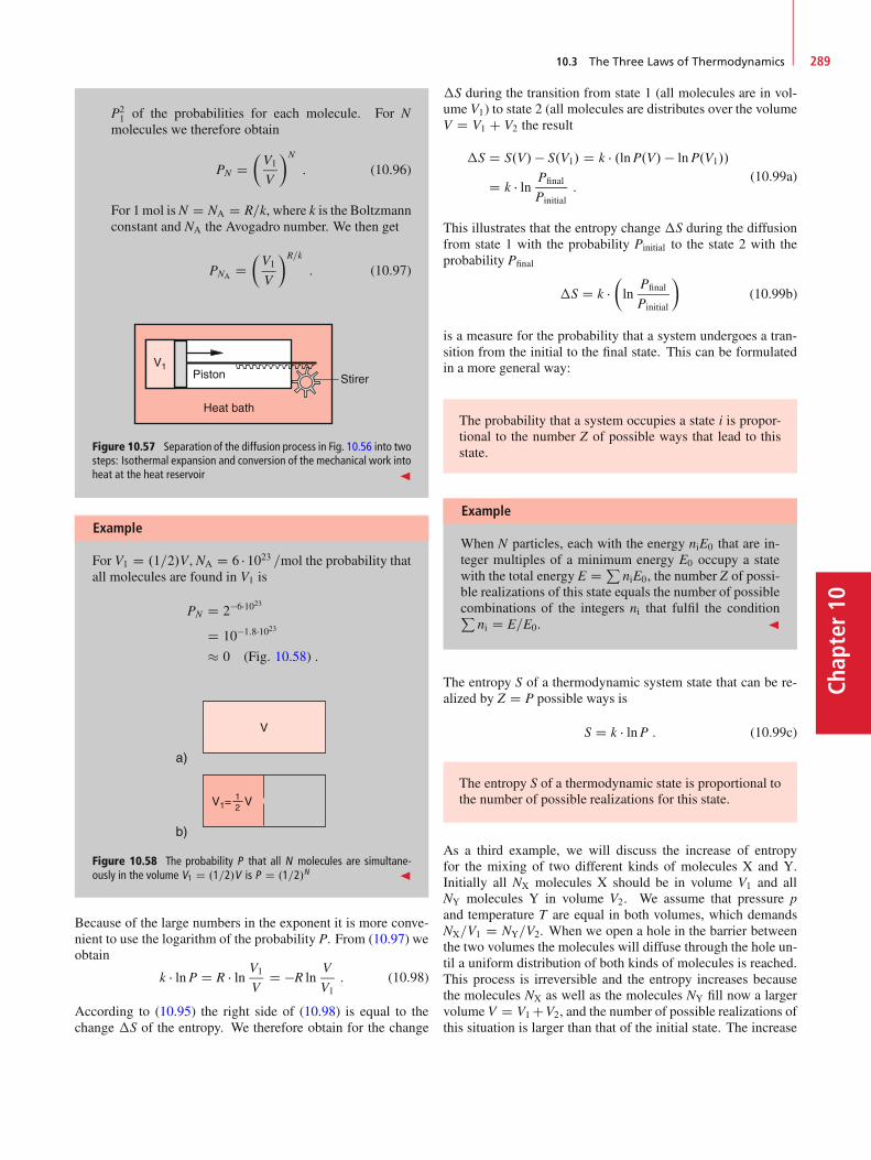
10.3 The Three Laws of Thermodynamics 289
Chap
ter10
P21 of the probabilities for each molecule. For N
molecules we therefore obtain
PN D�V1
V
�N
: (10.96)
For 1mol isN D NA D R=k, where k is the Boltzmannconstant and NA the Avogadro number. We then get
PNA D�V1
V
�R=k
: (10.97)
Piston
Heat bath
Stirer
Figure 10.57 Separation of the diffusion process in Fig. 10.56 into twosteps: Isothermal expansion and conversion of the mechanical work intoheat at the heat reservoir J
Example
For V1 D .1=2/V, NA D 6 � 1023 =mol the probability thatall molecules are found in V1 is
PN D 2�6�1023
D 10�1:8�1023
� 0 (Fig. 10.58) :
Figure 10.58 The probability P that all N molecules are simultane-ously in the volume V1 D .1=2/V is P D .1=2/N J
Because of the large numbers in the exponent it is more conve-nient to use the logarithm of the probability P. From (10.97) weobtain
k � lnP D R � ln V1
VD �R ln
V
V1: (10.98)
According to (10.95) the right side of (10.98) is equal to thechange �S of the entropy. We therefore obtain for the change
�S during the transition from state 1 (all molecules are in vol-ume V1) to state 2 (all molecules are distributes over the volumeV D V1 C V2 the result
�S D S.V/� S.V1/ D k � .lnP.V/ � lnP.V1//
D k � ln Pfinal
Pinitial:
(10.99a)
This illustrates that the entropy change �S during the diffusionfrom state 1 with the probability Pinitial to the state 2 with theprobability Pfinal
�S D k ��ln
Pfinal
Pinitial
�(10.99b)
is a measure for the probability that a system undergoes a tran-sition from the initial to the final state. This can be formulatedin a more general way:
The probability that a system occupies a state i is propor-tional to the number Z of possible ways that lead to thisstate.
Example
When N particles, each with the energy niE0 that are in-teger multiples of a minimum energy E0 occupy a statewith the total energy E D P
niE0, the number Z of possi-ble realizations of this state equals the number of possiblecombinations of the integers ni that fulfil the conditionP
ni D E=E0. J
The entropy S of a thermodynamic system state that can be re-alized by Z D P possible ways is
S D k � lnP : (10.99c)
The entropy S of a thermodynamic state is proportional tothe number of possible realizations for this state.
As a third example, we will discuss the increase of entropyfor the mixing of two different kinds of molecules X and Y.Initially all NX molecules X should be in volume V1 and allNY molecules Y in volume V2. We assume that pressure pand temperature T are equal in both volumes, which demandsNX=V1 D NY=V2. When we open a hole in the barrier betweenthe two volumes the molecules will diffuse through the hole un-til a uniform distribution of both kinds of molecules is reached.This process is irreversible and the entropy increases becausethe molecules NX as well as the molecules NY fill now a largervolume V D V1 CV2, and the number of possible realizations ofthis situation is larger than that of the initial state. The increase
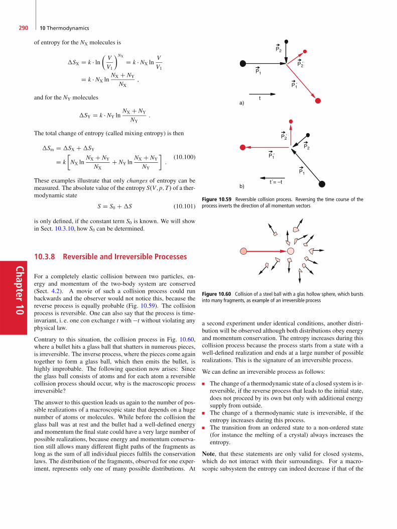
Chapter10
290 10 Thermodynamics
of entropy for the NX molecules is
�SX D k � ln�V
V1
�NX
D k � NX lnV
V1
D k � NX lnNX C NY
NX;
and for the NY molecules
�SY D k � NY lnNX C NY
NY:
The total change of entropy (called mixing entropy) is then
�Sm D �SX C�SY
D k
�NX ln
NX C NY
NXC NY ln
NX C NY
NY
�:
(10.100)
These examples illustrate that only changes of entropy can bemeasured. The absolute value of the entropy S.V;p;T/ of a ther-modynamic state
S D S0 C�S (10.101)
is only defined, if the constant term S0 is known. We will showin Sect. 10.3.10, how S0 can be determined.
10.3.8 Reversible and Irreversible Processes
For a completely elastic collision between two particles, en-ergy and momentum of the two-body system are conserved(Sect. 4.2). A movie of such a collision process could runbackwards and the observer would not notice this, because thereverse process is equally probable (Fig. 10.59). The collisionprocess is reversible. One can also say that the process is time-invariant, i. e. one con exchange t with �t without violating anyphysical law.
Contrary to this situation, the collision process in Fig. 10.60,where a bullet hits a glass ball that shatters in numerous pieces,is irreversible. The inverse process, where the pieces come againtogether to form a glass ball, which then emits the bullet, ishighly improbable. The following question now arises: Sincethe glass ball consists of atoms and for each atom a reversiblecollision process should occur, why is the macroscopic processirreversible?
The answer to this question leads us again to the number of pos-sible realizations of a macroscopic state that depends on a hugenumber of atoms or molecules. While before the collision theglass ball was at rest and the bullet had a well-defined energyand momentum the final state could have a very large number ofpossible realizations, because energy and momentum conserva-tion still allows many different flight paths of the fragments aslong as the sum of all individual pieces fulfils the conservationlaws. The distribution of the fragments, observed for one exper-iment, represents only one of many possible distributions. At
Figure 10.59 Reversible collision process. Reversing the time course of theprocess inverts the direction of all momentum vectors
Figure 10.60 Collision of a steel ball with a glas hollow sphere, which burstsinto many fragments, as example of an irreversible process
a second experiment under identical conditions, another distri-bution will be observed although both distributions obey energyand momentum conservation. The entropy increases during thiscollision process because the process starts from a state with awell-defined realization and ends at a large number of possiblerealizations. This is the signature of an irreversible process.
We can define an irreversible process as follows:
The change of a thermodynamic state of a closed system is ir-reversible, if the reverse process that leads to the initial state,does not proceed by its own but only with additional energysupply from outside.The change of a thermodynamic state is irreversible, if theentropy increases during this process.The transition from an ordered state to a non-ordered state(for instance the melting of a crystal) always increases theentropy.
Note, that these statements are only valid for closed systems,which do not interact with their surroundings. For a macro-scopic subsystem the entropy can indeed decrease if that of the
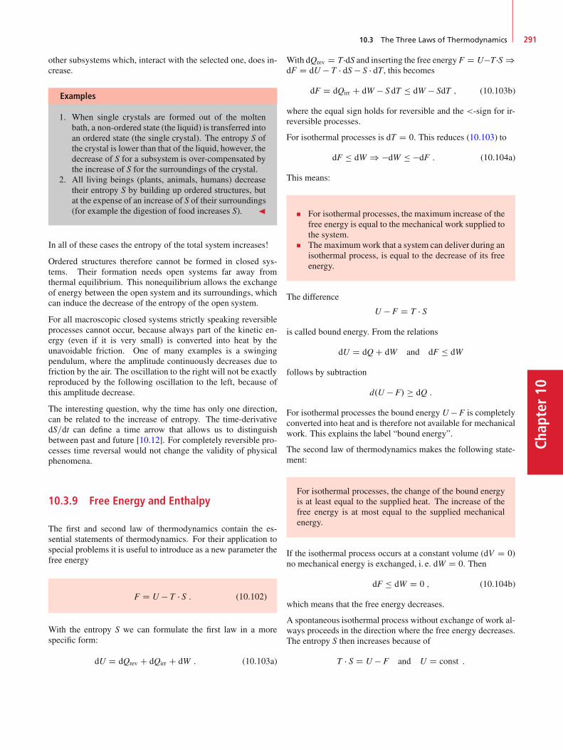
10.3 The Three Laws of Thermodynamics 291
Chap
ter10
other subsystems which, interact with the selected one, does in-crease.
Examples
1. When single crystals are formed out of the moltenbath, a non-ordered state (the liquid) is transferred intoan ordered state (the single crystal). The entropy S ofthe crystal is lower than that of the liquid, however, thedecrease of S for a subsystem is over-compensated bythe increase of S for the surroundings of the crystal.
2. All living beings (plants, animals, humans) decreasetheir entropy S by building up ordered structures, butat the expense of an increase of S of their surroundings(for example the digestion of food increases S). J
In all of these cases the entropy of the total system increases!
Ordered structures therefore cannot be formed in closed sys-tems. Their formation needs open systems far away fromthermal equilibrium. This nonequilibrium allows the exchangeof energy between the open system and its surroundings, whichcan induce the decrease of the entropy of the open system.
For all macroscopic closed systems strictly speaking reversibleprocesses cannot occur, because always part of the kinetic en-ergy (even if it is very small) is converted into heat by theunavoidable friction. One of many examples is a swingingpendulum, where the amplitude continuously decreases due tofriction by the air. The oscillation to the right will not be exactlyreproduced by the following oscillation to the left, because ofthis amplitude decrease.
The interesting question, why the time has only one direction,can be related to the increase of entropy. The time-derivativedS=dt can define a time arrow that allows us to distinguishbetween past and future [10.12]. For completely reversible pro-cesses time reversal would not change the validity of physicalphenomena.
10.3.9 Free Energy and Enthalpy
The first and second law of thermodynamics contain the es-sential statements of thermodynamics. For their application tospecial problems it is useful to introduce as a new parameter thefree energy
F D U � T � S : (10.102)
With the entropy S we can formulate the first law in a morespecific form:
dU D dQrev C dQirr C dW : (10.103a)
With dQrev D T �dS and inserting the free energy F D U�T �S )dF D dU � T � dS � S � dT , this becomes
dF D dQirr C dW � S dT � dW � SdT ; (10.103b)
where the equal sign holds for reversible and the <-sign for ir-reversible processes.
For isothermal processes is dT D 0. This reduces (10.103) to
dF � dW ) �dW � �dF : (10.104a)
This means:
For isothermal processes, the maximum increase of thefree energy is equal to the mechanical work supplied tothe system.The maximumwork that a system can deliver during anisothermal process, is equal to the decrease of its freeenergy.
The difference
U � F D T � Sis called bound energy. From the relations
dU D dQ C dW and dF � dW
follows by subtraction
d.U � F/ � dQ :
For isothermal processes the bound energy U � F is completelyconverted into heat and is therefore not available for mechanicalwork. This explains the label “bound energy”.
The second law of thermodynamics makes the following state-ment:
For isothermal processes, the change of the bound energyis at least equal to the supplied heat. The increase of thefree energy is at most equal to the supplied mechanicalenergy.
If the isothermal process occurs at a constant volume (dV D 0)no mechanical energy is exchanged, i. e. dW D 0. Then
dF � dW D 0 ; (10.104b)
which means that the free energy decreases.
A spontaneous isothermal process without exchange of work al-ways proceeds in the direction where the free energy decreases.The entropy S then increases because of
T � S D U � F and U D const :
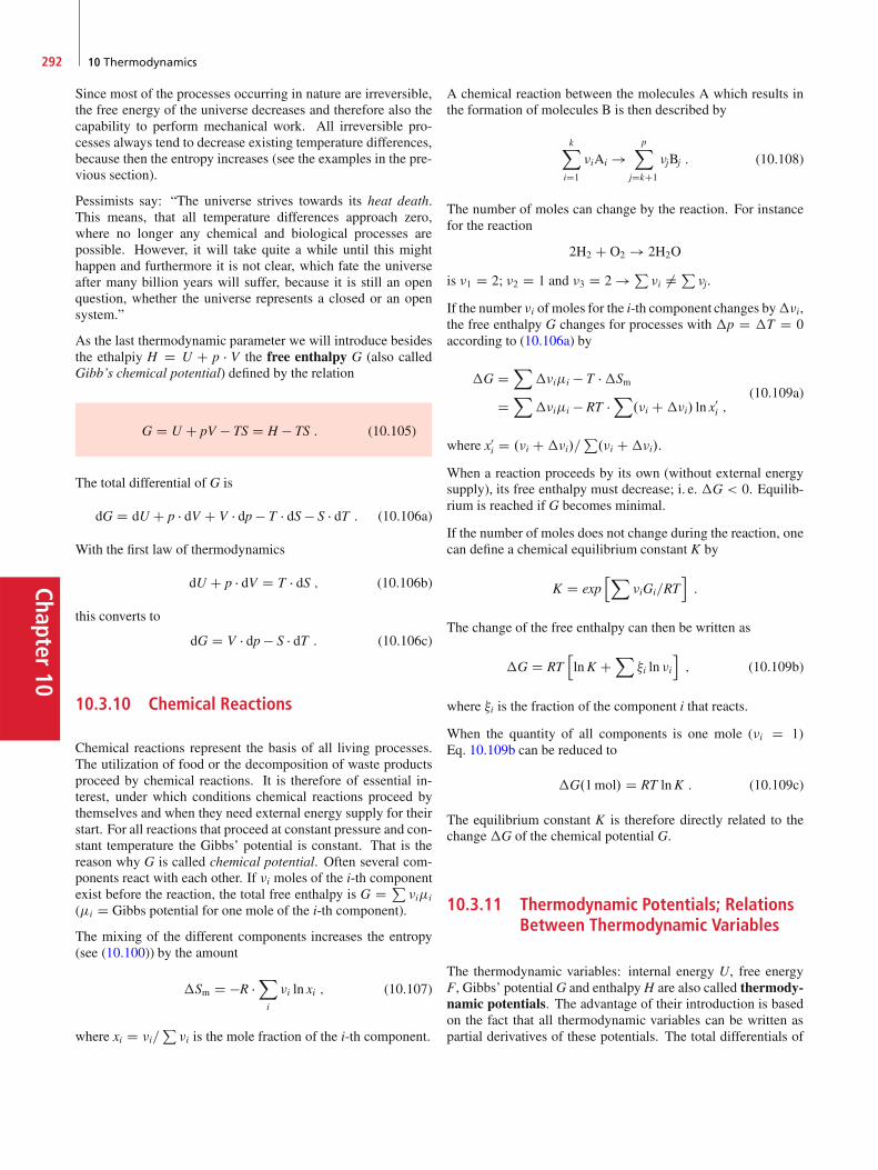
Chapter10
292 10 Thermodynamics
Since most of the processes occurring in nature are irreversible,the free energy of the universe decreases and therefore also thecapability to perform mechanical work. All irreversible pro-cesses always tend to decrease existing temperature differences,because then the entropy increases (see the examples in the pre-vious section).
Pessimists say: “The universe strives towards its heat death.This means, that all temperature differences approach zero,where no longer any chemical and biological processes arepossible. However, it will take quite a while until this mighthappen and furthermore it is not clear, which fate the universeafter many billion years will suffer, because it is still an openquestion, whether the universe represents a closed or an opensystem.”
As the last thermodynamic parameter we will introduce besidesthe ethalpiy H D U C p � V the free enthalpy G (also calledGibb’s chemical potential) defined by the relation
G D U C pV � TS D H � TS : (10.105)
The total differential of G is
dG D dU C p � dV C V � dp � T � dS � S � dT : (10.106a)
With the first law of thermodynamics
dU C p � dV D T � dS ; (10.106b)
this converts to
dG D V � dp � S � dT : (10.106c)
10.3.10 Chemical Reactions
Chemical reactions represent the basis of all living processes.The utilization of food or the decomposition of waste productsproceed by chemical reactions. It is therefore of essential in-terest, under which conditions chemical reactions proceed bythemselves and when they need external energy supply for theirstart. For all reactions that proceed at constant pressure and con-stant temperature the Gibbs’ potential is constant. That is thereason why G is called chemical potential. Often several com-ponents react with each other. If �i moles of the i-th componentexist before the reaction, the total free enthalpy is G D P
�ii
(i D Gibbs potential for one mole of the i-th component).
The mixing of the different components increases the entropy(see (10.100)) by the amount
�Sm D �R �X
i
�i ln xi ; (10.107)
where xi D �i=P�i is the mole fraction of the i-th component.
A chemical reaction between the molecules A which results inthe formation of molecules B is then described by
kX
iD1
�iAi !pX
jDkC1
�jBj : (10.108)
The number of moles can change by the reaction. For instancefor the reaction
2H2 C O2 ! 2H2O
is �1 D 2; �2 D 1 and �3 D 2 ! P�i ¤ P
�j.
If the number �i of moles for the i-th component changes by��i,the free enthalpy G changes for processes with �p D �T D 0according to (10.106a) by
�G DX
��ii � T ��Sm
DX
��ii � RT �X
.�i C��i/ ln x0i ;
(10.109a)
where x0i D .�i C��i/=
P.�i C��i/.
When a reaction proceeds by its own (without external energysupply), its free enthalpy must decrease; i. e. �G < 0. Equilib-rium is reached if G becomes minimal.
If the number of moles does not change during the reaction, onecan define a chemical equilibrium constant K by
K D exphX
�iGi=RTi:
The change of the free enthalpy can then be written as
�G D RThlnK C
X�i ln �i
i; (10.109b)
where �i is the fraction of the component i that reacts.
When the quantity of all components is one mole (�i D 1)Eq. 10.109b can be reduced to
�G.1mol/ D RT lnK : (10.109c)
The equilibrium constant K is therefore directly related to thechange�G of the chemical potential G.
10.3.11 Thermodynamic Potentials; RelationsBetween Thermodynamic Variables
The thermodynamic variables: internal energy U, free energyF, Gibbs’ potentialG and enthalpy H are also called thermody-namic potentials. The advantage of their introduction is basedon the fact that all thermodynamic variables can be written aspartial derivatives of these potentials. The total differentials of

10.3 The Three Laws of Thermodynamics 293
Chap
ter10
the potentials are
dF D�@F
@V
�
T
dV C�@F
@T
�
V
dT
dU D�@U
@V
�
S
dV C�@U
@S
�
V
dS
dG D�@G
@p
�
T
dp C�@G
@T
�
p
dT
dH D�@H
@S
�
p
dS C�@H
@p
�
S
dp ;
where the lower index at the brackets denotes the quantity thatis kept constant. The comparison with the equations derived inthe previous sections
dF D �pdV � SdT ; (10.103)
dU D �pdV C TdS ; (10.88)
dG D Vdp � SdT ; (10.106c)
dH D dU C pdV C Vdp (10.76)
D dQ C Vdp
gives the following relations between the thermodynamic vari-ables and the potentials.
For the entropy we obtain
S D ��@G
@T
�
p
D ��@F
@T
�
V
; (10.110a)
and for the pressure
p D ��@F
@V
�
T
D ��@U
@V
�
S
; (10.110b)
while the relation for the volume V is
V D�@G
@p
�
T
D�@H
@p
�
S
: (10.110c)
In the “Guggenheim Square”, each thermodynamic potentialcan be placed in such a way, that the results of their deriva-tives can be immediately seen by the following procedure: Onegoes in the scheme from the potential symbol to the derivativevariable and from there to the opposite corner on the diagonal.If this way on the diagonal is in the direction of the arrow, theresult is positive, if it is opposite to the arrow, it is negative.
Examples
@U
@S
ˇ̌ˇ̌V
D T I @G
@T
ˇ̌ˇ̌p
D �S I
@F
@V
ˇ̌ˇ̌T
D �p I @H
@p
ˇ̌ˇ̌V
D V : J
An example for the application of thermodynamic potentials isgiven in Sect. 10.4.2.
10.3.12 Equilibrium States
The thermodynamic potentials play a comparable role in ther-modynamics as the mechanical potential Ep that determines theforces F D �gradEp which governs the motion of particles.In a similar way the gradient of the thermodynamic potentialskeeps the chemical processes running until the minimum of thepotentials is reached.
A system is at equilibrium, if without the action of external in-fluences the state of the system does not change. If the state of asystem changes due to external action, but returns to its originalconditions after the external action ends, the equilibrium is sta-ble. If, however, the system further removes from equilibrium,even after the termination of the external influence, the equilib-rium is unstable. A mechanical example is a mass m which isfixed to a rigid rod that can rotate around a horizontal axis. Atthe minimum of the potential energy, where the mass is just be-low the horizontal axis the mass is in a stable equilibrium. Whenthe mass is at its maximum height vertically above the horizon-tal axis, the equilibrium is unstable. Every slight perturbationbrings m downwards. In a thermodynamic system, the thermo-dynamic potentials take the role of the potential energy in ourexample. We will illustrate this for several specific processes.
We assume a thermodynamic system with the internal energy Uand the volume V at the temperature T and the pressure p. Anarbitrary change of the conditions of the system is described bythe differentials dU, dV, dT and dp. If the change is reversible,the work dW D �p � dV performed by the system during anadiabatic expansion, causes a decrease dU D dW of the internalenergy.
For irreversible processes, the system loses heat which causes adecrease of the total energy. Equilibrium is reached, if no fur-ther irreversible process is possible. Since for all irreversibleprocesses with constant volume the entropy increases, the equi-librium condition can be formulated as
dS � 0 : (10.111)
For all possible processes, which bring a thermodynamicsystem away from equilibrium the entropy must decrease.

Chapter10
294 10 Thermodynamics
With other words:
A closed system with constant volume is in an equilibriumstate if its entropy is maximal.
The thermodynamic potentials of an equilibrium state have theirminimum value. This can be seen as follows:
With the change of entropy dS D dQ=T we obtain from the firstlaw of thermodynamics (10.71)
dU C p � dV � T � dS D 0 : (10.112)
For isothermal-isochoric processes is dV D 0 and T D const.From (10.111) it follows: dS � 0. Inserting this into (10.112)gives
d.U � TdS/ � 0 ! dF � 0 : (10.113)
Under isothermal and isochoric conditions a system hasreached its equilibrium state, if the free energy F has itsminimum value.
Under isothermal-isobaric conditions ( dT D 0 and dp D 0)equilibrium is reached if
dU C pdV � TdS D d.U C p � V � T � S/ D dG D 0 ;
because for all processes that drive the system away from equi-librium dG > 0, as can be seen in an analogous way as thearguments above for dF > 0.
Under isothermal-isobaric conditions a system is in anequilibrium state, if the Gibbs’ potential is minimal.
In a similar way it can be proved, that for adiabatic-isobaric pro-cesses (dQ D 0 and dp D 0) the system is in an equilibrium stateif the enthalpy H D U C p � V is minimal.
For adiabatic-isochoric processes (dQ D 0 and dV D 0) theinternal energy < U must be minimal at equilibrium.
All reactions that are possible without external interactionmust start from states far away from equilibrium.
Therefore the thermodynamic treatment of chemical reactionsand biological processes is based on the description of systemsthat are not at thermodynamic equilibrium.
10.3.13 The Third Law of Thermodynamics
We have seen in Sect. 10.3.7 that the entropy S is only deter-mined apart from an additive constant S0. We will now show,that for T ! 0
lim S.T/ D 0 :
This fixes the constant S0 D S.T D 0/ D 0.
For the proof we start with the free energy F D U � T � S.Because of (10.110a) this can be also written as
F D U C T
�@F
@T
�
V
: (10.114a)
We regard an isothermal chemical reaction where the systemstarts with the free energy F1 and ends at F2. The change�F DF1 � F2 is
�F D �U C T
�@
@T�F
�
V
: (10.114b)
For T > 0 the changes �F and �U differ, but for T ! 0 thedifference approaches zero
lim.�F ��U/ D 0 : (10.114c)
Nernst observed that with decreasing temperature the deriva-tives d.�F/=dT and d.�U=dT/ decreased and that they ap-proached zero for T ! 0. This means that the curves �F.T/and �U.T/ come towards each other with horizontal slopes(Fig. 10.61).
Nernst therefore postulated that also for the general case
limT!0
�@�F
@T
�
V
D 0 and (10.115a)
limT!0
�@�U
@T
�
V
D 0 : (10.115b)
because of (10.114a) it follows then
limT!0
�@U
@T� @F
@T
�D 0 : (10.115c)
Figure 10.61 Nernst’s theorem: Temperature course of �U .T /; �F .T / nearthe absolute zero temperature
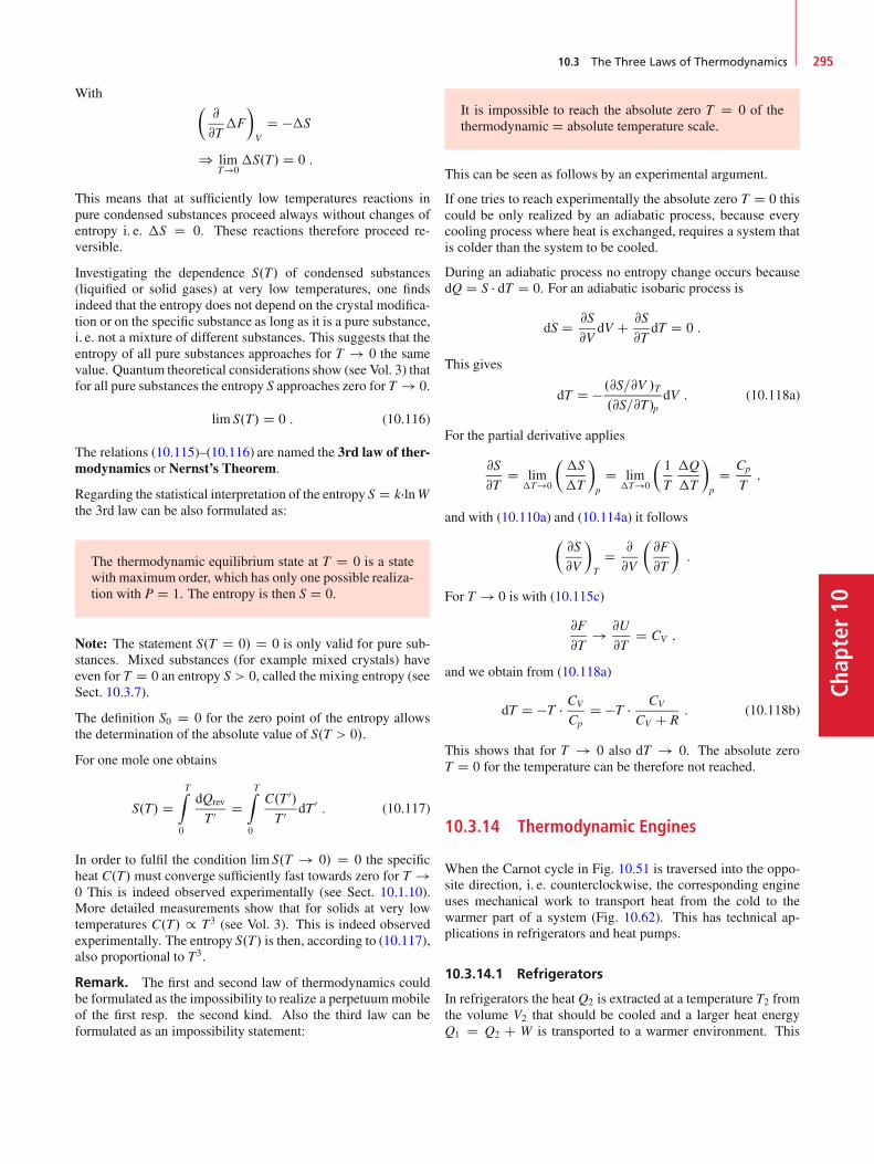
10.3 The Three Laws of Thermodynamics 295
Chap
ter10
With�@
@T�F
�
V
D ��S
) limT!0
�S.T/ D 0 :
This means that at sufficiently low temperatures reactions inpure condensed substances proceed always without changes ofentropy i. e. �S D 0. These reactions therefore proceed re-versible.
Investigating the dependence S.T/ of condensed substances(liquified or solid gases) at very low temperatures, one findsindeed that the entropy does not depend on the crystal modifica-tion or on the specific substance as long as it is a pure substance,i. e. not a mixture of different substances. This suggests that theentropy of all pure substances approaches for T ! 0 the samevalue. Quantum theoretical considerations show (see Vol. 3) thatfor all pure substances the entropy S approaches zero for T ! 0.
lim S.T/ D 0 : (10.116)
The relations (10.115)–(10.116) are named the 3rd law of ther-modynamics or Nernst’s Theorem.
Regarding the statistical interpretation of the entropy S D k�lnWthe 3rd law can be also formulated as:
The thermodynamic equilibrium state at T D 0 is a statewith maximum order, which has only one possible realiza-tion with P D 1. The entropy is then S D 0.
Note: The statement S.T D 0/ D 0 is only valid for pure sub-stances. Mixed substances (for example mixed crystals) haveeven for T D 0 an entropy S > 0, called the mixing entropy (seeSect. 10.3.7).
The definition S0 D 0 for the zero point of the entropy allowsthe determination of the absolute value of S.T > 0/.
For one mole one obtains
S.T/ DTZ
0
dQrev
T 0 DTZ
0
C.T 0/T 0 dT 0 : (10.117)
In order to fulfil the condition lim S.T ! 0/ D 0 the specificheat C.T/ must converge sufficiently fast towards zero for T !0 This is indeed observed experimentally (see Sect. 10.1.10).More detailed measurements show that for solids at very lowtemperatures C.T/ / T3 (see Vol. 3). This is indeed observedexperimentally. The entropy S.T/ is then, according to (10.117),also proportional to T3.
Remark. The first and second law of thermodynamics couldbe formulated as the impossibility to realize a perpetuummobileof the first resp. the second kind. Also the third law can beformulated as an impossibility statement:
It is impossible to reach the absolute zero T D 0 of thethermodynamic D absolute temperature scale.
This can be seen as follows by an experimental argument.
If one tries to reach experimentally the absolute zero T D 0 thiscould be only realized by an adiabatic process, because everycooling process where heat is exchanged, requires a system thatis colder than the system to be cooled.
During an adiabatic process no entropy change occurs becausedQ D S � dT D 0. For an adiabatic isobaric process is
dS D @S
@VdV C @S
@TdT D 0 :
This gives
dT D � .@S=@V /T.@S=@T/p
dV : (10.118a)
For the partial derivative applies
@S
@TD lim
�T!0
��S
�T
�
p
D lim�T!0
�1
T
�Q
�T
�
p
D Cp
T;
and with (10.110a) and (10.114a) it follows
�@S
@V
�
T
D @
@V
�@F
@T
�:
For T ! 0 is with (10.115c)
@F
@T! @U
@TD CV ;
and we obtain from (10.118a)
dT D �T � CV
CpD �T � CV
CV C R: (10.118b)
This shows that for T ! 0 also dT ! 0. The absolute zeroT D 0 for the temperature can be therefore not reached.
10.3.14 Thermodynamic Engines
When the Carnot cycle in Fig. 10.51 is traversed into the oppo-site direction, i. e. counterclockwise, the corresponding engineuses mechanical work to transport heat from the cold to thewarmer part of a system (Fig. 10.62). This has technical ap-plications in refrigerators and heat pumps.
10.3.14.1 Refrigerators
In refrigerators the heat Q2 is extracted at a temperature T2 fromthe volume V2 that should be cooled and a larger heat energyQ1 D Q2 C W is transported to a warmer environment. This
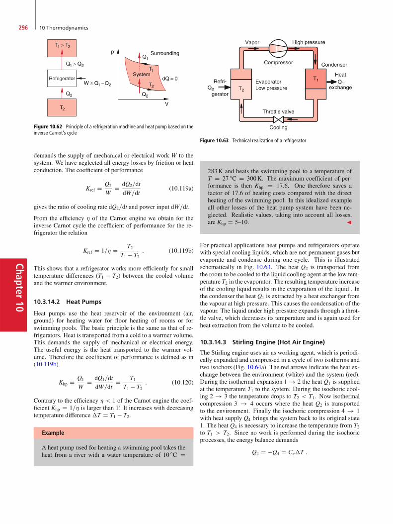
Chapter10
296 10 Thermodynamics
Figure 10.62 Principle of a refrigerationmachine and heat pump based on theinverse Carnot’s cycle
demands the supply of mechanical or electrical work W to thesystem. We have neglected all energy losses by friction or heatconduction. The coefficient of performance
Kref D Q2
WD dQ2=dt
dW=dt(10.119a)
gives the ratio of cooling rate dQ2=dt and power input dW=dt.
From the efficiency � of the Carnot engine we obtain for theinverse Carnot cycle the coefficient of performance for the re-frigerator the relation
Kref D 1=� D T2T1 � T2
: (10.119b)
This shows that a refrigerator works more efficiently for smalltemperature differences (T1 � T2) between the cooled volumeand the warmer environment.
10.3.14.2 Heat Pumps
Heat pumps use the heat reservoir of the environment (air,ground) for heating water for floor heating of rooms or forswimming pools. The basic principle is the same as that of re-frigerators. Heat is transported from a cold to a warmer volume.This demands the supply of mechanical or electrical energy.The useful energy is the heat transported to the warmer vol-ume. Therefore the coefficient of performance is defined as in(10.119b)
Khp D Q1
WD dQ1=dt
dW=dtD T1
T1 � T2: (10.120)
Contrary to the efficiency � < 1 of the Carnot engine the coef-ficient Khp D 1=� is larger than 1! It increases with decreasingtemperature difference �T D T1 � T2.
Example
A heat pump used for heating a swimming pool takes theheat from a river with a water temperature of 10 ıC D
Figure 10.63 Technical realization of a refrigerator
283K and heats the swimming pool to a temperature ofT D 27 ıC D 300K. The maximum coefficient of per-formance is then Khp D 17:6. One therefore saves afactor of 17:6 of heating costs compared with the directheating of the swimming pool. In this idealized exampleall other losses of the heat pump system have been ne-glected. Realistic values, taking into account all losses,are Khp D 5–10. J
For practical applications heat pumps and refrigerators operatewith special cooling liquids, which are not permanent gases butevaporate and condense during one cycle. This is illustratedschematically in Fig. 10.63. The heat Q2 is transported fromthe room to be cooled to the liquid cooling agent at the low tem-perature T2 in the evaporator. The resulting temperature increaseof the cooling liquid results in the evaporation of the liquid . Inthe condenser the heat Q1 is extracted by a heat exchanger fromthe vapour at high pressure. This causes the condensation of thevapour. The liquid under high pressure expands through a throt-tle valve, which decreases its temperature and is again used forheat extraction from the volume to be cooled.
10.3.14.3 Stirling Engine (Hot Air Engine)
The Stirling engine uses air as working agent, which is periodi-cally expanded and compressed in a cycle of two isotherms andtwo isochors (Fig. 10.64a). The red arrows indicate the heat ex-change between the environment (white) and the system (red).During the isothermal expansion 1 ! 2 the heat Q1 is suppliedat the temperature T1 to the system. During the isochoric cool-ing 2 ! 3 the temperature drops to T2 < T1. Now isothermalcompression 3 ! 4 occurs where the heat Q2 is transportedto the environment. Finally the isochoric compression 4 ! 1with heat supply Q4 brings the system back to its original state1. The heat Q4 is necessary to increase the temperature from T2to T1 > T2. Since no work is performed during the isochoricprocesses, the energy balance demands
Q2 D �Q4 D Cv�T :
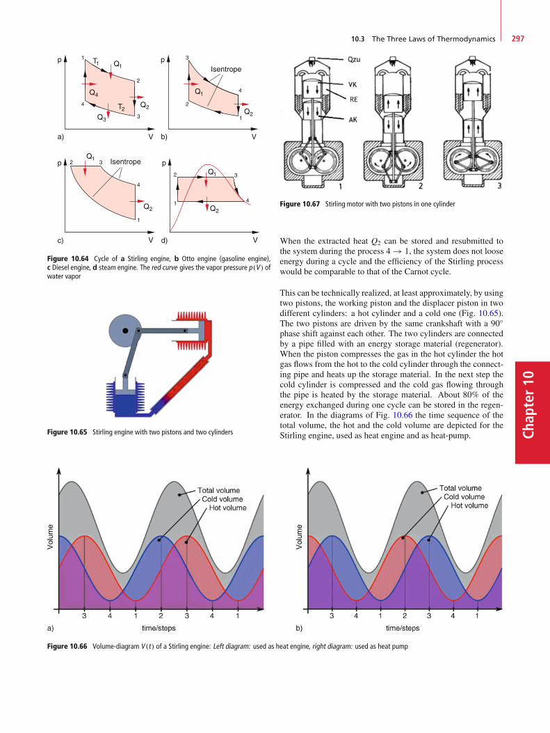
10.3 The Three Laws of Thermodynamics 297
Chap
ter10
Figure 10.64 Cycle of a Stirling engine, b Otto engine (gasoline engine),c Diesel engine, d steam engine. The red curve gives the vapor pressure p.V / ofwater vapor
Figure 10.65 Stirling engine with two pistons and two cylinders
Figure 10.66 Volume-diagram V .t/ of a Stirling engine: Left diagram: used as heat engine, right diagram: used as heat pump
Figure 10.67 Stirling motor with two pistons in one cylinder
When the extracted heat Q2 can be stored and resubmitted tothe system during the process 4 ! 1, the system does not looseenergy during a cycle and the efficiency of the Stirling processwould be comparable to that of the Carnot cycle.
This can be technically realized, at least approximately, by usingtwo pistons, the working piston and the displacer piston in twodifferent cylinders: a hot cylinder and a cold one (Fig. 10.65).The two pistons are driven by the same crankshaft with a 90ıphase shift against each other. The two cylinders are connectedby a pipe filled with an energy storage material (regenerator).When the piston compresses the gas in the hot cylinder the hotgas flows from the hot to the cold cylinder through the connect-ing pipe and heats up the storage material. In the next step thecold cylinder is compressed and the cold gas flowing throughthe pipe is heated by the storage material. About 80% of theenergy exchanged during one cycle can be stored in the regen-erator. In the diagrams of Fig. 10.66 the time sequence of thetotal volume, the hot and the cold volume are depicted for theStirling engine, used as heat engine and as heat-pump.
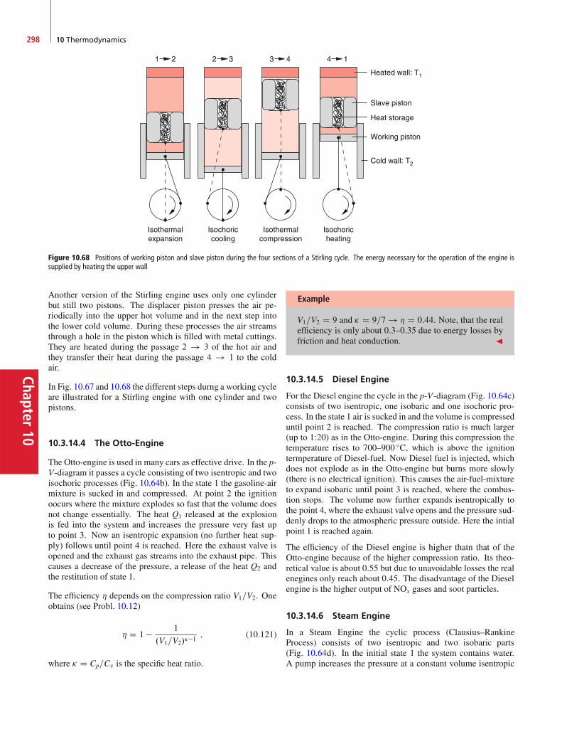
Chapter10
298 10 Thermodynamics
Isothermalcompression
Isochoriccooling
Isothermalexpansion
Isochoricheating
Heated wall: T1
Cold wall: T2
Slave piston
Heat storage
Working piston
Figure 10.68 Positions of working piston and slave piston during the four sections of a Stirling cycle. The energy necessary for the operation of the engine issupplied by heating the upper wall
Another version of the Stirling engine uses only one cylinderbut still two pistons. The displacer piston presses the air pe-riodically into the upper hot volume and in the next step intothe lower cold volume. During these processes the air streamsthrough a hole in the piston which is filled with metal cuttings.They are heated during the passage 2 ! 3 of the hot air andthey transfer their heat during the passage 4 ! 1 to the coldair.
In Fig. 10.67 and 10.68 the different steps durng a working cycleare illustrated for a Stirling engine with one cylinder and twopistons.
10.3.14.4 The Otto-Engine
The Otto-engine is used in many cars as effective drive. In the p-V-diagram it passes a cycle consisting of two isentropic and twoisochoric processes (Fig. 10.64b). In the state 1 the gasoline-airmixture is sucked in and compressed. At point 2 the ignitionoocurs where the mixture explodes so fast that the volume doesnot change essentially. The heat Q1 released at the explosionis fed into the system and increases the pressure very fast upto point 3. Now an isentropic expansion (no further heat sup-ply) follows until point 4 is reached. Here the exhaust valve isopened and the exhaust gas streams into the exhaust pipe. Thiscauses a decrease of the pressure, a release of the heat Q2 andthe restitution of state 1.
The efficiency � depends on the compression ratio V1=V2. Oneobtains (see Probl. 10.12)
� D 1 � 1
.V1=V2/��1; (10.121)
where � D Cp=Cv is the specific heat ratio.
Example
V1=V2 D 9 and � D 9=7 ! � D 0:44. Note, that the realefficiency is only about 0:3–0:35 due to energy losses byfriction and heat conduction. J
10.3.14.5 Diesel Engine
For the Diesel engine the cycle in the p-V-diagram (Fig. 10.64c)consists of two isentropic, one isobaric and one isochoric pro-cess. In the state 1 air is sucked in and the volume is compresseduntil point 2 is reached. The compression ratio is much larger(up to 1:20) as in the Otto-engine. During this compression thetemperature rises to 700–900 ıC, which is above the ignitiontermperature of Diesel-fuel. Now Diesel fuel is injected, whichdoes not explode as in the Otto-engine but burns more slowly(there is no electrical ignition). This causes the air-fuel-mixtureto expand isobaric until point 3 is reached, where the combus-tion stops. The volume now further expands isentropically tothe point 4, where the exhaust valve opens and the pressure sud-denly drops to the atmospheric pressure outside. Here the intialpoint 1 is reached again.
The efficiency of the Diesel engine is higher thatn that of theOtto-engine because of the higher compression ratio. Its theo-retical value is about 0:55 but due to unavoidable losses the realenegines only reach about 0:45. The disadvantage of the Dieselengine is the higher output of NOx gases and soot particles.
10.3.14.6 Steam Engine
In a Steam Engine the cyclic process (Clausius–RankineProcess) consists of two isentropic and two isobaric parts(Fig. 10.64d). In the initial state 1 the system contains water.A pump increases the pressure at a constant volume isentropic
10.4 Thermodynamics of Real Gases and Liquids 299
Chap
ter10
from p1 to p2. From point 2 to 3 heat is supplied at constantpressure, which causes the volume to expand and increases thetemperature above the boiling point of water. The hot vapourdrives a piston during the isentropic expansion and the sys-tem reaches point 4 where the temperature is cooled down, thevapour condenses and the heat Q2 is transferred to the surround-ing. Now the initial point 1 is reached again. Mechanical workis performed on the part 3 ! 4.
The red curve in Fig. 10.64d gives part of the Van der Waalscurve p.V/ for water vapour (see Sect. 10.4.1). Inside this curvewater and vapour can exist simultaneously, in the region left ofthe curve only the liquid phase exists, to the right hand of thecurve only the vapour phase.
10.3.14.7 Thermal Power Plants
In thermal power plants, heat is produced by burning fossil fuels,such as coal, oil, wood or gas, or by fission of atomic nuclei.For fossil fuels the heat comes from the reaction heat that isreleased during the oxidation of atoms or molecules and is dueto the different chemical binding energies of reaction partnersand reaction products. The essential part of this energy stemsfrom the oxidation of carbon atoms C to CO2. The producedheat is 8 kcal D 33 kJ for 1 g C. The fission of 1 g Uraniumproduces an energy of 2:5 � 107 kJ. This is 7:5 � 105 times more!
The heat produced in thermal power plants is converted intothe generation of hot water vapour under high pressure, driv-ing turbines that propel electric generators for the production ofelectric energy. The maximum efficiency depends, according tothe second law, on the initial temperature T1 and the final tem-perature T2.
The initial temperature is limited by technical conditions (heatand pressure resistance of the hot vapour tank. Typical valuesare between 600 and 700 ıC. Only for the high temperature re-actors, temperatures above 800 ıC are realized.
For the choice of the final temperature T2 two options exist:
1. One chooses T2 D 100 ıC (condensation temperature of wa-ter) and uses the rest energy of the hot water for heating ofhouses. The efficiency for the conversion of heat into me-chanical (or electric) energy is then for an initial temperatureof T1 D 600 ıC D 873K: � D 500=873 D 0:57. In addi-tion the heat �Q of the hot water can be delivered to housesnearby the power station.
2. The final temperature of the water vapour is chosen asT2 D 30 ıC. In order to avoid condensation one has tolower the pressure below the atmospheric pressure by pump-ing the expanding volume. This increases the efficiency to� D 570=873 D 0:65. The work needed for evacuating theexpanding volume against the external pressure is smallerthan the additional energy gain due to the lower final tem-perature.
In case 1 one does not win the total energy of the hot water �Qcompared to case 2 because here one could use the extra energydue to the higher efficiency �2 D .600 � 30/=873 to transportelectric energy for heating. The increase of the efficiency for
case 2 compared to case 1 is
�2 � �1 D .70=873� "/�Q
D .0:19 � "/�Q ;
where " � �Q is the mechanical work of the pump, necessaryto evacuate the volume down to a pressure that is equal to thevapour pressure of water at T D 30 ıC.
10.4 Thermodynamics of Real Gasesand Liquids
Up to now, we have discussed the thermodynamics of idealgases, where the interaction between the atoms of the gas hasbeen neglected.
We will now discuss, which rules have to be generalized andwhich are still valid without restrictions, when we treat the ther-modynamics of real atoms and molecules including their sizeand their mutual interactions.
While ideal gases remain gaseous at any temperature, real gasescondense below their boiling temperature and they can even be-come solids below the melting temperature. In this section, wewill investigate what are the conditions for transitions betweenthe different phases solid, liquid and gaseous and what are theequilibrium conditions of the different phases.
10.4.1 Van der Waals Equation of State
At very high pressures, the density of atoms or molecules be-comes so high, that the internal volume of the molecules (alsocalled covolume) cannot be neglected compared with the freevolume V that is available for the molecules.
When we describe the atoms as rigid balls with radius r, twoatoms cannot come closer to each other than at a minimum dis-tance d D 2r. If one atom is in the volume V the other atomscannot penetrate into the volume Vforbidden D .4=3/d3 D 8Va,where Va is the volume of one atom in the model of rigid balls(Fig. 10.69a). Furthermore the centres of all balls must have theminimum distance d D r from the walls of the container.
Assume there were only two atoms in the cubic volume V D l3.The volume available for the second atom is then
V2 D .L � 2r/3 � 8Va (Fig. 10.69b) :
A third atom could only be found in the volume
V3 D .L � 2r/3 � 2 � 8Va ;
and the rest volume available for the n-th atom is then
Vn D .L � 2r/3 � .n � 1/ � 8Va :

Chapter10
300 10 Thermodynamics
Figure 10.69 Illustration of the co-volume. a The center of B cannot be in thebright red circle. b Forbidden volume (bright red ) of molecule B in the volumeL3 with one atom A
An estimation of the real sizes shows, however, that, for ex-ample, for N D 1020 atoms in a volume with L D 0:1m theforbidden volume at the wall is with r � 10�10 m completelynegligible compared to the internal volumeN �Va of the N atomsin the volume V. The average over all N atoms gives then forthe mean volume available to each atom
V D .L � 2r/3 � 1
N
NX
nD1
.n � 1/ � 8Va
D L3 � 6r � L2 � 6r2 � L C 8r3 � 4NVa
� L3 � 4NVa for N � 1 :
(10.122)
because the 2nd, 3rd and 4th term are neglible compared to the1st and last term.
We therefore have to replace in the general gas-equation (10.21)the volume V by the reduced volume
V � b D L3 � 4 � N � Va with b D 4N � Va :
For the situation N � 1 the volume Vavailable available tothe N atoms in a volume V is reduced by 4 times the totalatomic volume N � Va D N � .4=3/ � r3.
The next question concerns possible corrections for the pressurep due to the attractive or repulsive forces between the atoms. Atlow temperatures or for high densities the interaction betweenthe atoms can be no longer neglected. The total force on a se-lected atom resulting from the interaction with all other atoms
Figure 10.70 Illustration of the internal pressure. Forces on an atom A a insidea gas, b at the boundary between wall and gas
cancels for atoms inside a liquid or a gas volume, because theinteraction forces are in the average uniformly distributed overall directions (Fig. 10.70a) (see the similar discussion about thesurface tension in Sect. 6.4.1). At the boundaries between liquidand gas or between gas and wall, the interaction forces are nolonger uniformly distributed but are directed only into the halfspace of the medium. They do not cancel and the total force Fa
on one atom is not zero but is proportional to the number den-sity na of atoms in the half-sphere shown in Fig. 10.70b, whichmeans to the density % D M=V, whereM is the total mass of thegas in the volume V.
The amount of the total force F D jPFij / na � Fa onto all naatoms is therefore proportional to n2a / %2. The force is directedtowards the interior of the gas and causes an intrinsic pressure
pb D a � %2 / a=V2 ;
which acts onto the atoms in addition to the external pressure p.
Taking into account this intrinsic pressure and the co-volumeb D 4N � Va the general gas equation for one mole of an idealgas
p � VM D R � Thas to be modified to the van der Waals-equation of real gases
�p C a
V2
�� .VM � b/ D R � T ; (10.123)
where the constant b D 4 � Na � Va gives 4-times the internalvolume of the NA atoms in the mole volume VM.
The progression of the function p.V/ at constant T for a realgas, described by (10.123), depends on the constants a and b. InFig. 10.71 the isotherms of CO2 are shown for different temper-atures. They confirm, that for high temperatures (Ekin � jEpotj)the curves are similar to those of an ideal gas, but for lowtemperatures closely above the condensation temperature theydeviate strongly.

10.4 Thermodynamics of Real Gases and Liquids 301
Chap
ter10
Figure 10.71 Van-der-Waals-isotherms of CO2 for different temperatures
Solving (10.123) for p at constant T gives a polynomial p.V/of third order, which shows for low temperatures a maximumand a minimum (Fig. 10.71). How looks the comparison of thistheoretical curve with experimental results? Let’s see this forthe example of CO2.
If one mole of CO2 is compressed at the temperature T D 0 ıCstarting at low pressures one finds in deed that the curve p.V/follows quite nicely the theoretical curve until the point A inFig. 10.71. Further compression does not increase the pressurep, which stays constant until the point C is reached where thepressure shows a steep increase and follows again the van derWaals curve.
The reason for this strange behaviour is the condensation of theCO2 vapour that starts at the point A. On the way from A toC the fraction of the liquid phase continuously increases untilin C the vapour is completely liquefied. On the way from C tosmaller volumes, the pressure increases steeply because of thesmall compressibility of the liquid. Between A and C gas andliquid can both exist (co-existence range).
For a quantitative description of the condensation process wemust discuss the different phases (aggregation states) in moredetail.
10.4.2 Matter in Different Aggregation States
The different aggregation states of matter (solid, liquid gas) arecalled its phases. In this section we will discuss, under whichconditions a phase transition solid ! liquid, liquid ! gas orsolid ! gas can occur and when two or three phases can existside by side.
10.4.2.1 Vapour Pressure and Liquid–Gas Equilibrium
When a liquid is enclosed in a container which it fills only partly,one finds that part of the liquid is vaporized and in the volume
Figure 10.72 Measurement of vapor pressure curve ps.T /
above the liquid surface a vapour phase has established at avapour pressure ps.T/ that acts upon the walls and the liquidsurface. The dependence of the vapour pressure ps.T/ on thetemperature can be measured with the pressure tank shown inFig. 10.72 that is equipped with a thermometer and a manome-ter.
At a constant temperature T a constant saturation vapour pres-sure ps.T/ is present where the liquid and the gaseous phase canexist simultaneously under stable conditions.
The explanation given by molecular physics is based on the ki-netic gas theory (Sect. 7.4). Similar to the situation in a gas alsothe molecules in a liquid show a velocity distribution with ki-netic energies that follow the Maxwell–Boltzmann distribution.The fastest molecules in the high energy tail of the velocity dis-tribution can leave the liquid, if their energy is larger than thesurface tension of the liquid (See Sect. 6.4). On the other hand,when molecules in the gas phase hit the liquid surface, they canenter into the liquid.
At the saturation vapour pressure ps.T/ the liquid and the gas-phase are at equilibrium, which means that the rate of moleculesleaving the liquid is equal to the rate of molecules that reenterthe liquid from the gas phase.
The higher the temperature the more molecules have sufficientenergy to leave the liquid, i. e. the vapour pressure rises with in-creasing temperature (Fig. 10.72). The quantitative form of thevapour pressure curve ps.T/ can be calculated in the followingway:
In Fig. 10.73 we regard for 1mol of the evaporating liquid acyclic process in the p, V-diagram of Fig. 10.71. In the stateC0.T C dT; ps C dps/ the vapour should be completely con-densed and the liquid occupies the volume Vl. Now the volumeis isothermally expanded at the temperature T C dT , while thepressure is kept constant. Here the heat dQ1 D �, which isequal to the evaporation energy of 1mol, has to be suppliedin order to keep the temperature constant. At A0 the total liq-uid is evaporated. During the next step, the adiabatic expansionA0 ! A, pressure and temperature are lowered by an infinites-imal small amount. The system remains in the vapour phaseand reaches the point A.ps;T/. Now the vapour is isothermallycompressed while the pressure remains constant, because con-densation progresses during the path from A to the point C. The
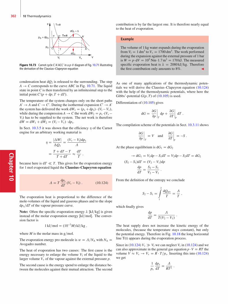
Chapter10
302 10 Thermodynamics
Figure 10.73 Carnot cycle C0A0ACC0 in a p-V diagram of Fig. 10.71 illustratingthe derivation of the Clausius–Clapeyron-equation
condensation heat dQ2 is released to the surrounding. The stepA ! C corresponds to the curve ABC in Fig. 10.71. The liquidstate in point C is then transferred by an infinitesimal step to theinitial point C0.p C dp;T C dT/.
The temperature of the system changes only on the short pathsA0 ! A and C ! C0. During the isothermal expansion C0 ! A0the system has delivered the work dW1 D .ps C dps/ � .Vl �Vv/,while during the compression A ! C the work dW2 D ps �.Vv�Vl/ has to be supplied to the system. The net work is thereforedW D dW1 C dW2 D .Vl � Vv/ � dps.In Sect. 10.3.5 it was shown that the efficiency � of the Carnotengine for an arbitrary working material is
� D j�Wj�Q1
D .Vv � Vl/dps�
D T C dT � T
T C dT� dT
T;
because here is dT T . This gives for the evaporation energyfor 1mol evaporated liquid the Clausius–Clapeyron equation
� D TdpsdT
.Vv � Vl/ : (10.124)
The evaporation heat is proportional to the difference of themole-volumes of the liquid and gaseous phases and to the slopedps=dT of the vapour pressure curve.
Note: Often the specific evaporation energy � ŒkJ=kg� is giveninstead of the molar evaporation energy ŒkJ=mol�. The conver-sion factor is
1 kJ=mol D .10�3M/ kJ=kg ;
where M is the molar mass in g=mol.
The evaporation energy pro molecule is w D �=NA with NA DAvogadro number.
The heat of evaporation has two causes: The first cause is theenergy necessary to enlarge the volume Vl of the liquid to thelarger volume Vv of the vapour against the external pressure p.
The second cause is the energy spend to enlarge the distance be-tween the molecules against their mutual attraction. The second
contribution is by far the largest one. It is therefore nearly equalto the heat of evaporation.
Example
The volume of 1 kg water expands during the evaporationfrom Vl D 1 dm3 to Vv D 1700 dm3. The work performedduring the expansion against the external pressure of 1 barisW D p �dV D 105 Nm �1:7m3 D 170 kJ. The measuredspecific evaporation heat is � D 2080 kJ=kg. Thereforethe first contribution only amounts to 8%. J
As one of many applications of the thermodynamic poten-tials we will derive the Clausius–Clapeyron equation (10.124)with the help of the thermodynamic potentials, where here theGibbs’-potential G.p;T/ of (10.105) is used.
Differentiation of (10.105) gives
dG D @G
@p
ˇ̌ˇ̌T
dp C @G
@T
ˇ̌ˇ̌p
dT :
The compilation scheme of the potentials in Sect. 10.3.11 shows
@G
@p
ˇ̌ˇ̌T
D V and@G
@T
ˇ̌ˇ̌p
D �S :
At the phase equilibrium is dG1 D dG2
! dG1 D V1dp � S1dT D V2dp � S2dT D dG2
.S2 � S1/dT D .V2 � V1/dp
dp
dTD S2 � S1
V2 � V1:
From the definition of the entropy we conclude
S2 � S1 D2Z
1
dQrev
TD �
T;
which finally gives
dp
dTD �
T.V2 � V1/:
The heat supply does not increase the kinetic energy of themolecules, (because the temperature stays constant), but onlythe potential energy. Therefore in Fig. 10.18 the long horizontalline T(t) appears during the evaporation process.
Since in (10.124) Vv � Vl we can neglect Vl in (10.124) and wecan also approximate in the general gas equation p �V D RT thevolume V � Vv ! Vv D R � T=ps. Inserting this into (10.124)we get
1
ps
dpsdT
D �
RT2:
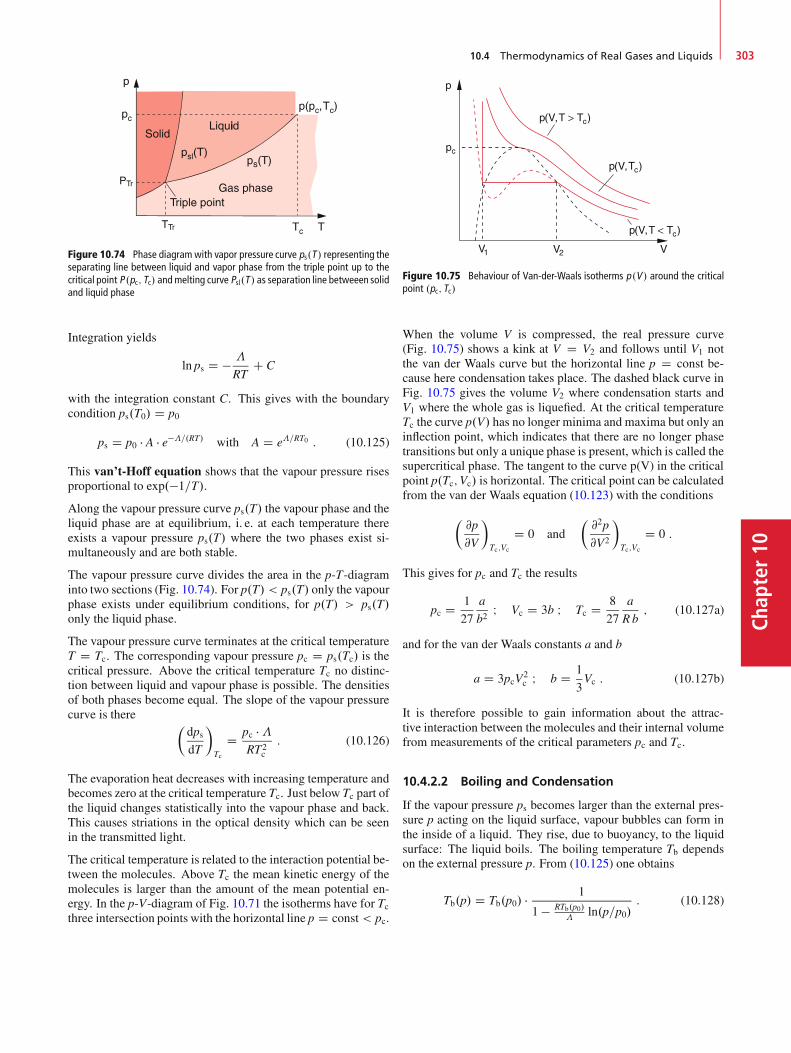
10.4 Thermodynamics of Real Gases and Liquids 303
Chap
ter10
Figure 10.74 Phase diagram with vapor pressure curve ps.T / representing theseparating line between liquid and vapor phase from the triple point up to thecritical point P .pc; Tc/ andmelting curve Psl.T / as separation line betweeen solidand liquid phase
Integration yields
ln ps D � �
RTC C
with the integration constant C. This gives with the boundarycondition ps.T0/ D p0
ps D p0 � A � e��=.RT/ with A D e�=RT0 : (10.125)
This van’t-Hoff equation shows that the vapour pressure risesproportional to exp.�1=T/.
Along the vapour pressure curve ps.T/ the vapour phase and theliquid phase are at equilibrium, i. e. at each temperature thereexists a vapour pressure ps.T/ where the two phases exist si-multaneously and are both stable.
The vapour pressure curve divides the area in the p-T-diagraminto two sections (Fig. 10.74). For p.T/ < ps.T/ only the vapourphase exists under equilibrium conditions, for p.T/ > ps.T/only the liquid phase.
The vapour pressure curve terminates at the critical temperatureT D Tc. The corresponding vapour pressure pc D ps.Tc/ is thecritical pressure. Above the critical temperature Tc no distinc-tion between liquid and vapour phase is possible. The densitiesof both phases become equal. The slope of the vapour pressurecurve is there �
dpsdT
�
Tc
D pc ��RT2
c: (10.126)
The evaporation heat decreases with increasing temperature andbecomes zero at the critical temperature Tc. Just below Tc part ofthe liquid changes statistically into the vapour phase and back.This causes striations in the optical density which can be seenin the transmitted light.
The critical temperature is related to the interaction potential be-tween the molecules. Above Tc the mean kinetic energy of themolecules is larger than the amount of the mean potential en-ergy. In the p-V-diagram of Fig. 10.71 the isotherms have for Tcthree intersection points with the horizontal line p D const < pc.
Figure 10.75 Behaviour of Van-der-Waals isotherms p.V / around the criticalpoint .pc; Tc/
When the volume V is compressed, the real pressure curve(Fig. 10.75) shows a kink at V D V2 and follows until V1 notthe van der Waals curve but the horizontal line p D const be-cause here condensation takes place. The dashed black curve inFig. 10.75 gives the volume V2 where condensation starts andV1 where the whole gas is liquefied. At the critical temperatureTc the curve p.V/ has no longer minima and maxima but only aninflection point, which indicates that there are no longer phasetransitions but only a unique phase is present, which is called thesupercritical phase. The tangent to the curve p(V) in the criticalpoint p.Tc;Vc/ is horizontal. The critical point can be calculatedfrom the van der Waals equation (10.123) with the conditions
�@p
@V
�
Tc;Vc
D 0 and�@2p
@V2
�
Tc;Vc
D 0 :
This gives for pc and Tc the results
pc D 1
27
a
b2I Vc D 3b I Tc D 8
27
a
R b; (10.127a)
and for the van der Waals constants a and b
a D 3pcV2c I b D 1
3Vc : (10.127b)
It is therefore possible to gain information about the attrac-tive interaction between the molecules and their internal volumefrom measurements of the critical parameters pc and Tc.
10.4.2.2 Boiling and Condensation
If the vapour pressure ps becomes larger than the external pres-sure p acting on the liquid surface, vapour bubbles can form inthe inside of a liquid. They rise, due to buoyancy, to the liquidsurface: The liquid boils. The boiling temperature Tb dependson the external pressure p. From (10.125) one obtains
Tb.p/ D Tb.p0/ � 1
1 � RTb.p0/�
ln.p=p0/: (10.128)
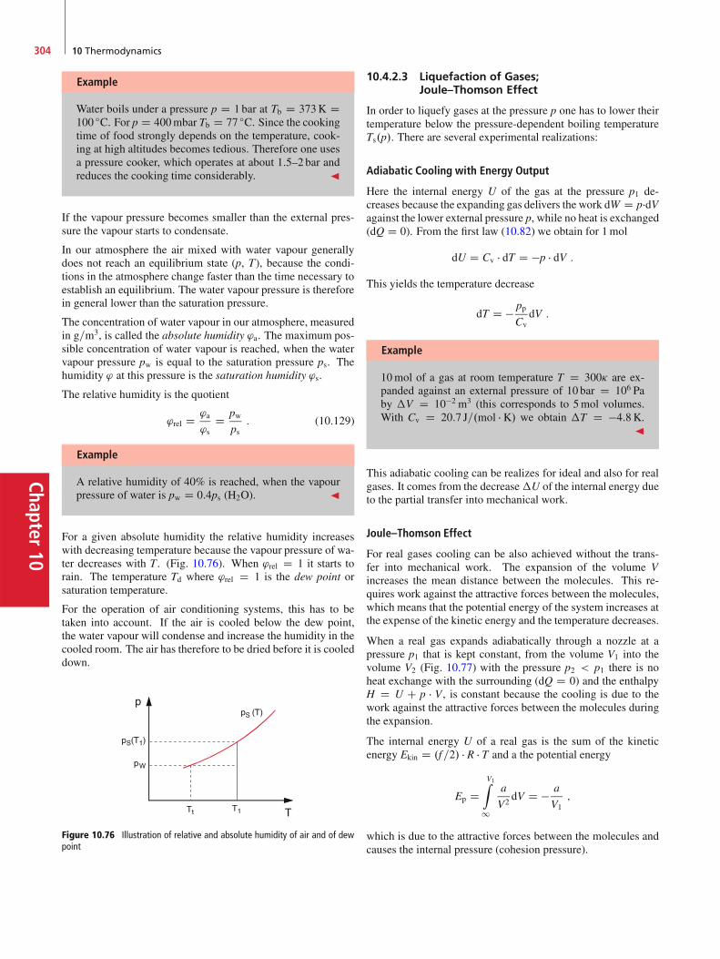
Chapter10
304 10 Thermodynamics
Example
Water boils under a pressure p D 1 bar at Tb D 373K D100 ıC. For p D 400mbar Tb D 77 ıC. Since the cookingtime of food strongly depends on the temperature, cook-ing at high altitudes becomes tedious. Therefore one usesa pressure cooker, which operates at about 1:5–2 bar andreduces the cooking time considerably. J
If the vapour pressure becomes smaller than the external pres-sure the vapour starts to condensate.
In our atmosphere the air mixed with water vapour generallydoes not reach an equilibrium state (p, T), because the condi-tions in the atmosphere change faster than the time necessary toestablish an equilibrium. The water vapour pressure is thereforein general lower than the saturation pressure.
The concentration of water vapour in our atmosphere, measuredin g=m3, is called the absolute humidity 'a. The maximum pos-sible concentration of water vapour is reached, when the watervapour pressure pw is equal to the saturation pressure ps. Thehumidity ' at this pressure is the saturation humidity 's.
The relative humidity is the quotient
'rel D 'a
'sD pw
ps: (10.129)
Example
A relative humidity of 40% is reached, when the vapourpressure of water is pw D 0:4ps (H2O). J
For a given absolute humidity the relative humidity increaseswith decreasing temperature because the vapour pressure of wa-ter decreases with T . (Fig. 10.76). When 'rel D 1 it starts torain. The temperature Td where 'rel D 1 is the dew point orsaturation temperature.
For the operation of air conditioning systems, this has to betaken into account. If the air is cooled below the dew point,the water vapour will condense and increase the humidity in thecooled room. The air has therefore to be dried before it is cooleddown.
Figure 10.76 Illustration of relative and absolute humidity of air and of dewpoint
10.4.2.3 Liquefaction of Gases;Joule–Thomson Effect
In order to liquefy gases at the pressure p one has to lower theirtemperature below the pressure-dependent boiling temperatureTs.p/. There are several experimental realizations:
Adiabatic Cooling with Energy Output
Here the internal energy U of the gas at the pressure p1 de-creases because the expanding gas delivers the work dW D p�dVagainst the lower external pressure p, while no heat is exchanged(dQ D 0). From the first law (10.82) we obtain for 1mol
dU D Cv � dT D �p � dV :
This yields the temperature decrease
dT D � ppCv
dV :
Example
10mol of a gas at room temperature T D 300� are ex-panded against an external pressure of 10 bar D 106 Paby �V D 10�2 m3 (this corresponds to 5mol volumes.With Cv D 20:7 J=.mol � K/ we obtain �T D �4:8K.
J
This adiabatic cooling can be realizes for ideal and also for realgases. It comes from the decrease�U of the internal energy dueto the partial transfer into mechanical work.
Joule–Thomson Effect
For real gases cooling can be also achieved without the trans-fer into mechanical work. The expansion of the volume Vincreases the mean distance between the molecules. This re-quires work against the attractive forces between the molecules,which means that the potential energy of the system increases atthe expense of the kinetic energy and the temperature decreases.
When a real gas expands adiabatically through a nozzle at apressure p1 that is kept constant, from the volume V1 into thevolume V2 (Fig. 10.77) with the pressure p2 < p1 there is noheat exchange with the surrounding (dQ D 0) and the enthalpyH D U C p � V, is constant because the cooling is due to thework against the attractive forces between the molecules duringthe expansion.
The internal energy U of a real gas is the sum of the kineticenergy Ekin D .f =2/ � R � T and a the potential energy
Ep DV1Z
1
a
V2dV D � a
V1;
which is due to the attractive forces between the molecules andcauses the internal pressure (cohesion pressure).
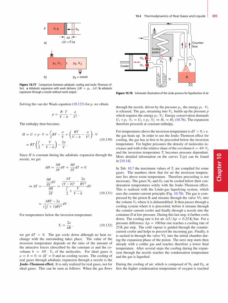
10.4 Thermodynamics of Real Gases and Liquids 305
Chap
ter10
Figure 10.77 Comparison between adiabatic cooling and Joule–Thomson ef-fect. a Adiabatic expansion with work delivery �W D pa � �V ; b adiabaticexpansion through a nozzle without work output
Solving the van der Waals equation (10.123) for p, we obtain
p D R � TV � b
� a
V2:
The enthalpy then becomes
H D U C p � V D f
2RT � a
VC�
RT
V � b� a
V2
�� V
D RT
�f
2C V
V � b
�� 2a
V:
(10.130)
Since H is constant during the adiabatic expansion through thenozzle, we get
dH D @H
@VdV C @H
@TdT D 0
) dT D �@H
@VdV
@H
@T
DbT
.V � b/2� 2a
RV2
f
2C V
V � b
dV
� bRT � 2a
. 12 f C 1/RV2dV :
(10.131)
For temperatures below the inversion temperature
Ti D 2a
bR; (10.132)
we get dT < 0. The gas cools down although no heat ex-change with the surrounding takes place. The value of theinversion temperature depends on the ratio of the amount ofthe attractive forces (described by the constant a) and the co-volume b D 4N � Va of the molecules. For ideal gases isa D b D 0 ) dT D 0 and no cooling occurs. The cooling ofreal gases through adiabatic expansion through a nozzle is theJoule–Thomson effect. It is only realized for real gases, not forideal gases. This can be seen as follows: When the gas flows
Figure 10.78 Schematic illustration of the Linde-process for liquefaction of air
through the nozzle, driven by the pressure p1, the energy p1 � V1
is released. The gas, streaming into V2, builds up the pressure pwhich requires the energy p2 �V2. Energy conservation demandsU1 Cp1 �V1 D U2 Cp2 �V2 ) H1 D H2 (10.76). The expansiontherefore proceeds at constant enthalpy.
For temperatures above the inversion temperature is dT > 0, i. e.the gas heats up. In order to use the Joule–Thomson effect forcooling, the gas has at first to be precooled below the inversiontemperature. For higher pressures the density of molecules in-creases and with it the relative share of the covolume b D 4N �Va
and the inversion temperature Ti becomes pressure dependent.More detailed information on the curves Ti.p/ can be foundin [10.14].
In Tab. 10.7 the maximum values of Ti are compiled for somegases. The numbers show that for air the inversion tempera-ture lies above room temperature. Therefore precooling is notnecessary. The gases N2 and O2 can be cooled below their con-densation temperatures solely with the Joule–Thomson effect.This is realized with the Linde-gas liquefying system, whichuses the counter-current principle (Fig. 10.78). The gas is com-pressed by the piston K and streams through the valve Vl1 intothe volume V2 where it is dehumidified. It then passes through acooling system where it is precooled, before it streams throughthe counter current cooler and finally through a nozzle into thecontainerD at low pressure. During this last step, it further coolsdown. The cooling rate is for air �T=�p D 0:25K=bar. For apressure difference �p D 100 bar one reaches a cooling rate of25K per step. The cold vapour is guided through the counter-current cooler and helps to precool the incoming gas. Finally, itis sucked in through the valve Vl2 into the initial chamber dur-ing the expansion phase of the piston. The next step starts thenalready with a colder gas and reaches therefore a lower finaltemperature. After several steps the cooling during the expan-sion through the nozzle reaches the condensation temperatureand the gas is liquefied.
During the cooling of air, which is composed of N2 and O2, atfirst the higher condensation temperature of oxygen is reached

Chapter10
306 10 Thermodynamics
Table 10.7 Critical temperatures Tc, critical pressure pc, maximum inversion temperature Ti and boiling temperature for some gases
Gas Tc=K Pc=bar a=N � m4=mol2 b=106 m3=mol Ti=K Ts=K at p0 D 1:013barHelium 5.19 2.26 0.0033 24 30 4.2Hydrogen 33.2 13 0.025 27 200 20.4Nitrogen 126 35 0.136 38.5 620 77.4Oxygen 154.6 50.8 0.137 31.6 765 90.2Air 132.5 37.2 – – 650 80.2CO2 304.2 72.9 0.365 42.5 >1000 194.7NH3 405.5 108.9 0.424 37.2 >1000 –Water vapor 647.15 217.0 – – – 373.2
before N2 liquefies. Therefore the two gases can be readily sep-arated.
Nowadays liquid nitrogen rather than liquid air is used formany applications, because liquid oxygen contains the explo-sive ozone O3. Liquid air that is kept in a Dewar increases itsO2 and O3 concentration in the course of time since N2 evapo-rates faster due to its higher vapour pressure and therefore aftersome time liquid air reaches a critical concentration of O3 whichexplodes above a critical temperature.
The gases H2, He of Ne can be liquefied by precooling themwith liquid nitrogen below the inversion temperature before theycan be further cooled by the Joule–Thomson effect.
10.4.2.4 Equilibrium Between Solid and LiquidPhase; Melting Curve
If the temperature of a solid material is increased above a certaintemperature that depends on the material, the solid phase startsto convert into the liquid phase. Only at the melting tempera-ture Tm, both phases can coexist under equilibrium conditions.The pressure dependence dTm=dp of the melting temperatureis much smaller than that of the evaporation temperature, i. e.the slope of the curve p.T/ in the p-T-diagram of Fig. 10.79is much larger than that of the evaporation curve. One of thereasons is the much smaller change of the volume during themelting process, compared with the much larger change duringthe evaporation process. A similar consideration as that result-ing in Eq. 10.124 for the heat of evaporation gives the heat offusion
�m D T � dpdT.Vliquid � Vsolid/ : (10.133)
For most materials the density decreases during the meltingprocess, i. e. Vliquid > Vsolid. This gives dp=dT > 0, be-cause �m > 0. There are some substances (e. g. water) whereVliquid < Vsolid. For these substances is dp=dT < 0, the meltingcurve has a negative slope (anomaly of water) (Fig. 10.79b).
Note: The fact that for water Vliquid < Vsolid ! %liquid > %solidis essential for many processes in nature. Lakes freeze up fromthe top to the bottom. Since the heat conductivity of ice is small,this gives an isolating layer at the top, preventing the completefreezing of the water, thus protecting fishes and other sensitivecreatures.
The fact, that water has its maximum density at T D 4 ıC iscalled its anomaly. It is due to the temperature dependent molec-ular structure of water. Liquid water does not solely consist of
H2O molecules but also contains multimers (H2O)n in a con-centration that depends on the temperature and on the distancefrom the surface of water. In the multimers the different H2Omolecules are connected by hydrogen bonds. At higher temper-atures theses weak bonds break and a structural change resultsin a change of the mean distance and therefore also a change ofthe density. In the solid phase the H2O-molecules form a regularlattice with empty space between the molecules. Therefore thedensity of the solid is smaller than that of the liquid phase.
Example
At T D 0 ıC the density of solid ice is % D 0:917 kg=dm3,that of sea water is % D 1:04 kg=dm3. Therefore, onlyabout 12% of an iceberg are above the seawater surface,but 88% are below. J
Application of external pressure decreases the mean distance be-tween the molecules and therefore the ice can melt, according tothe principle of minimum constraint. This is utilized by skaters,
Figure 10.79 Melting curve, vapor pressure curve and triple point for a a pos-itive, b a negative slope of the melting curve. a represents the phase diagramof CO2, b that of water

10.4 Thermodynamics of Real Gases and Liquids 307
Chap
ter10
Wire Ice block
Weight
mg
Figure 10.80 Apparently convincing demonstration of the lowering of themelting temperature by pressure
where the high pressure below the sharp ice skates forms a thinliquid layer with low friction (see, however, the remarks below).
The lowering of the melting temperature �Tm D .dTm=dp/ ��pis often demonstrated by a wire that is pulled through an iceblock by a heavy weight (Fig. 10.80).
Remark. More detailed calculations show, however, that themajor part of the necessary melting energy comes from heatconduction from the higher temperature of the wire to the icesurface (see Probl. 10.11).
Even without external pressure a thin liquid layer is formed atthe surface of ice above T D �33 ıC. The necessary energyfor melting this layer is provided by the gain in surface en-ergy. The boundary ice-air needs more energy for evaporatingmolecules than the boundary ice-liquid. A liquid layer thereforehas a lower potential energy and the loss of potential energy islarger than the melting energy.
10.4.2.5 Coexistence of different phases; Triple Point
Since the melting curve in the p-V-diagram of Fig. 10.76 has alarger slope than the vapor curve the two curves must intersectin a point .ptr;Ttr/, called the triple point. Here the three phasessolid, liquid and gase can coexist.
For T < Ttr there is one boundary curve (sublimation curve)that separates the solid and the gaseous phases. It has in the.p;V/-diagram generally a positive slope. Solid materials candirectly pass into the gaseous phase without becoming liquid.This process is called sublimation. Because of the small vaporpressure of solids this process is, however, very slow.
If there are more than one phase of a material in a container,pressure p and temperature T are no longer independent of eachother. For example, the coexistence of the liquid and the vaporphase is only possible on the vapor curve pS.T/. This impliesthat p and T are related by the evaporation coefficient � in(10.125). It is possible to change T but then pS.T/ is fixed.At the triple point .ptr; Ttr/ p and T are connected by two con-ditions: the vapor curve and the sublimation curve. This means
that none of the two variables p and T can be changed withoutleaving the triple point.
This can be generalized byGibb’s phase rule, which relates thenumber f of the degrees of freedom in the choice of the variablesp and T with the number q of coexisting phases. It states:
f D 3 � q (10.134)
At the triple point is q D 3 ! f D 0, i.e. no degree of freedomin choosing the variables p and T . If only one phase is present.q D 1/ we obtain f D 2. The pressure p as well as the temper-ature T can be chosen independently (within certain limits). Onthe vapor curve is q D 2 and therefore f D 1. We can chooseone variable and the other is then fixed.
For a mixture of different chemical components, which can bepresent in different phases the generalized Gibbs phase rulestates:
f D k C 2 � q (10.135)
where k is the number of components.
10.4.3 Solutions and Mixed States
Up to now we have discussed only pure substances, which arecomposed of only one component and do not contain any impu-rities. We have explained the different phases of solid, liquid andgaseous states and possible transitions between these phases.In nature, however, often mixed substances are present wheremolecules of different species are mixed together. Examples areNaCl-molecules or sugar molecules, which are dissolved in wa-ter and dissociate into their atomic components. Other examplesare metal alloys
For the complete characterization of such mixed states pressureand temperature are not sufficient, but also the concentration ofthe different components have to be defined.
The concentration of a substance dissolved in a liquid is gen-erally given in g/litre or in mole/litre. Often not the completesubstance has dissolved but a rest remains as solid sediment(if %solid > %liquid) or as layer on the liquid surface (if %solid <%liquid).
The solution of substances can alter the characteristic features ofthe liquid considerably. In this section we will shortly discussthe most important features of solutions.
10.4.3.1 Osmosis and Osmotic Pressure
Assume a container with a semipermeable membrane includinga solution with the concentration c of the dissolved substanceis submerged into a reservoir with the pure liquid (Fig. 10.81).One observes that the level of the solution in a standing piperises above the level of the pure solution, if the molecules of thesolvent can penetrate through the semipermeable membrane butnot the molecules of the dissolved substance. Such permeable
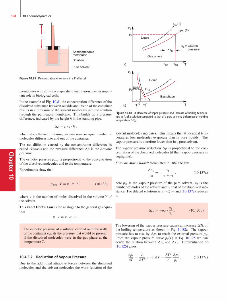
Chapter10
308 10 Thermodynamics
Semipermeablemembrane
Solution
h
Pure solvent
Figure 10.81 Demonstration of osmosis in a Pfeffer cell
membranes with substance-specific transmission play an impor-tant role in biological cells.
In the example of Fig. 10.81 the concentration difference of thedissolved substance between outside and inside of the containerresults in a diffusion of the solvent molecules into the solutionthrough the permeable membrane. This builds up a pressuredifference, indicated by the height h in the standing pipe.
�p D % � g � h ;which stops the net diffusion, because now an equal number ofmolecules diffuses into and out of the container.
The net diffusion caused by the concentration difference iscalled Osmosis and the pressure difference �p is the osmoticpressure.
The osmotic pressure posm is proportional to the concentrationof the dissolved molecules and to the temperature.
Experiments show that
posm � V D � � R � T ; (10.136)
where � is the number of moles dissolved in the volume V ofthe solvent.
This van’t Hoff’s Law is the analogue to the general gas equa-tion
p � V D � � R � T :
The osmotic pressure of a solution exerted onto the wallsof the container equals the pressure that would be present,if the dissolved molecules were in the gas phase at thetemperature T .
10.4.3.2 Reduction of Vapour Pressure
Due to the additional attractive forces between the dissolvedmolecules and the solvent molecules the work function of the
Figure 10.82 a Decrease of vapor pressure and increase of boiling tempera-ture�Tb of a solution compared to that of a pure solvent; b decrease of meltingtemperature�Tm
solvent molecules increases. This means that at identical tem-peratures less molecules evaporate than in pure liquids. Thevapour pressure is therefore lower than in a pure solvent.
The vapour pressure reduction �p is proportional to the con-centration of the dissolved molecules (if their vapour pressure isnegligible).
Francois Marie Raoult formulated in 1882 the law
�psps0
D � �1
�0 C �1; (10.137a)
here ps0 is the vapour pressure of the pure solvent, �0 is thenumber of moles of the solvent and �1 that of the dissolved sub-stance. For diluted solutions is �1 �0 and (10.137a) reducesto
�ps D �ps0 � �1�0: (10.137b)
The lowering of the vapour pressure causes an increase �Tb ofthe boiling temperature as shown in Fig. 10.82a. The vapourpressure has to rise by �ps to reach the external pressure pa.From the vapour pressure curve ps.T/ in Eq. 10.125 we canderive the relation between �ps and �Tb. Differentiation of(10.125) gives
dpsdT
D �
RT2ps ) �T D RT2
�
�psps
: (10.137c)
10.5 Comparison of the Different Changes of State 309
Chap
ter10
Together with (10.137) this yields the Raoult’ Law
�Tb D RT2
�
�1
�0: (10.138a)
When several substances with the molar concentrations �i aredissolved, this generalizes to
�Tb D RT2
��0
X
i
�i : (10.138b)
Since�Tb depends on the molar evaporation heat�, it is depen-dent not only on the dissolved substances but also on the specificsolvent.
For dissolved substances that partly dissociate (for instance dis-sociates NaCl into NaC + Cl�) the sum in (10.138b) extendsover all dissociated and non-dissociated components dissolvedin the solvent.
The lowering of the vapour pressure also results in a lowering ofthe melting temperature Tm (Fig. 10.82b). Similar to (10.138a)one gets
�Tm D �RT2
�m
�1
�0; (10.139)
where �m is the molar melting heat.
Example
For water with the concentration of �1 moles of a dis-solved substance is the lowering of the melting tempera-ture
�Tm D �1:85K � �1 :
When 50 g NaCl are dissolved in 1 litre water, (1molNaCl are 58 g), the lowering of the melting temperatureis with
P�i D 2 � 50=58 D 1:72mol: �Tm D �3:2K.
J
Seawater has a melting temperature that lies several degrees be-low 0 ıC depending on the salt concentration.
The lowering of the melting temperature is used to clear icyroads from ice and snow by salting the roads.
The zero point of the Fahrenheit temperature scale is defined bythe melting temperature of a specific salt-water solution. From(10.2) and (10.139) the zero point can be obtained as
0 ıF D �17:8 ıC :
Solutions with dissolved substances have generally alarger temperature range of the liquid phase than pure sol-vents, because the boiling point rises and the melting pointis lowered.
10.5 Comparison of the DifferentChanges of State
Here we will summarize all possible changes of thermodynamicstates and the corresponding equations.
1. Isochoric processes: V D const
dQ D CV � dT (10.140a)
2. Isobaric processes: p D const
dQ D Cp � dT D dU C p � dV (10.140b)
3. Isothermal processes: T D const
dU D 0; dQ D p � dV; p � V D const (10.140c)
4. Adiabatic processes: dQ D 0
p � V� D constI � D Cp=CV (10.140d)
5. Isentropic processes: S D const
dS D CV � dT=T C R � dV=V D 0
) T � V��1 D const(10.140e)
A reversible adiabatic process is always isentropic, butnot every isentropic process is also adiabatic.
6. Isoenthalpic processes
H D U C p � V D const
dH D .@H=@p/TDconst C .@H=@T/pDconst(10.140f)
10.6 Energy Sources and EnergyConversion
The supply of sufficient energy that can replace to a large extentmanual work, has changed our life considerably. It is fair to saythat only the provision of sufficient and affordable energy hasessentially improved our standard of life. This is the reason whyin developing countries the desire for more energy will cause adrastic increase of worldwide energy consumption.
The first law of thermodynamics teaches us, however, that en-ergy can be neither generated nor annihilated. The phrase“energy generation” (for example in power stations) means cor-rectly speaking the conversion of energy from a specific forminto another (for instance from thermal energy into electric en-ergy).
In fossil power stations the potential energy of CO- andCO2-molecules is transferred into heat (kinetic energy of themolecules and atoms), which is further converted via turbinesinto mechanic energy of the rotating turbine, which drives anelectric generator that produces electric energy.

Chapter10
310 10 Thermodynamics
Figure 10.83 Cooling towers of the coal power plant Staudinger. The plant delivers 500MW electric power and 300MW heat power. It reaches an efficiency of42.5% (With kind permission of Preußen Elektra AG, Hannover)
In car engines this molecular potential energy is converted intomechanical energy that drives the car. In nuclear power stationsthe potential energy of uranium nuclei (which exceeds that ofmolecular bindings by 6 orders of magnitude) is converted bynuclear fission into kinetic energy of the fission products andthen into heat of circulating cooling water.
Wind energy converters convert the kinetic energy of airflowinto rotation energy of the converter rotor blades, which drive
an electric generator. The wind energy has its origin in the solarradiation energy, which in turn stems from nuclear fusion energyin the interior of the sun.
In order to realize an energy conversion efficiency as high aspossible, one has to understand the basic physical processesof the different conversion processes. We have learned inSect. 10.3.3 that the maximum possible conversion factor forthe conversion of heat into mechanical energy is given by the
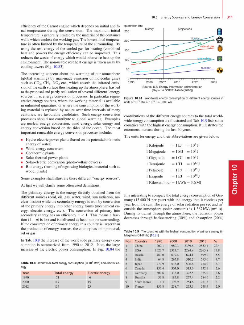
10.6 Energy Sources and Energy Conversion 311
Chap
ter10
efficiency of the Carnot engine which depends on initial and fi-nal temperature during the conversion. The maximum initialtemperature is generally limited by the material of the containerwalls which enclose the working gas. The lowest final tempera-ture is often limited by the temperature of the surrounding. Byusing the rest energy of the cooled gas for heating (combinedheat and power) the energy efficiency can be improved. Thisreduces the waste of energy which would otherwise heat up theenvironment. The non-usable rest heat energy is taken away bycooling towers (Fig. 10.83).
The increasing concern about the warming of our atmosphere(global warming) by man-made emission of molecular gasessuch as CO2, CH4, NO2 etc., which absorb the infrared emis-sion of the earth surface thus heating up the atmosphere, has ledto the proposal and partly realization of several different “energysources”, i. e. energy conversion processes. In particular regen-erative energy sources, where the working material is availablein unlimited quantities, or where the consumption of the work-ing material is replaced by nature over time intervals of manycenturies, are favourable candidates. Such energy conversionprocesses should not contribute to global warming. Examplesare nuclear energy conversion, wind energy, solar energy andenergy conversion based on the tides of the ocean. The mostimportant renewable energy conversion processes include:
Hydro-electric power plants (based on the potential or kineticenergy of water)Wind-energy convertersGeothermic plantsSolar-thermal power plantsSolar-electric conversion (photo-voltaic devices)Bio-energy (burning of regrowing biological material such aswood, plants)
Some examples shall illustrate these different “energy sources”.
At first we will clarify some often used definitions.
The primary energy is the energy directly obtained from thedifferent sources (coal, oil, gas, water, wind, sun radiation, nu-clear fission) while the secondary energy is won by conversionof the primary energy into other energy forms (mechanical en-ergy, electric energy, etc.). The conversion of primary intosecondary energy has an efficiency � < 1. This means a frac-tion (1 � �) is lost and is delivered as heat into the surrounding.If the consumption of primary energy in a country is larger thanthe production of energy sources, the country has to import coal,oil or gas.
In Tab. 10.8 the increase of the worldwide primary energy con-sumption is summarized from 1990 to 2012. Note the largeincrease of the electric power consumption. In Fig. 10.84 the
Table 10.8 Worldwide total energy consumption (in 103 TWh) and electric en-ergy
Year Total energy Electric energy1990 71 62000 117 152012 155 23
quadrillion Btu
250
200
150
100
50
01990 2000
Source: U.S. Energy Information Administration(Report #.DOE/EIA-0484(2010))
2007 2015 2025 2035
history projections
liquids
coal
renewables
nuclear
natural gas
Figure 10.84 Worldwide energy consumption of different energy sources inunits of 1015 Btu � 1018 J � 300 TWh
contributions of the different energy sources to the total world-wide energy consumption are illustrated and Tab. 10.9 lists somecountries with the highest energy consumption. It illustrates theenormous increase during the last 40 years.
The units for energy and their abbreviations are given below:
1 Kilojoule D 1 kJ D 103 J
1 Megajoule D 1MJ D 106 J
1 Gigajoule D 1GJ D 109 J
1 Terrajoule D 1 TJ D 1012 J
1 Petajoule D 1 PJ D 1015 J
1 Exajoule D 1 EJ D 1018 J
1 Kilowatt hour D 1 kWh D 3:6MJ
It is interesting to compare the total energy consumption of Ger-many (13 400PJ per year) with the energy that it receives peryear from the sun. The energy of solar radiation per sec and m2
outside the atmosphere (solar constant) is 1:367 kW=.m2 � s/.During its transit through the atmosphere, the radiation powerdecreases through backscattering (30%) and absorption (20%)
Table 10.9 The countries with the highest consumption of primary energy (inMegatons Oil-Units) [10.31]
Pos. Country 1970 2000 2010 2013 %1 China 202.1 980.3 2339.6 2852.4 22.42 USA 1627.7 2313.7 2284.9 2265.8 17.83 Russia 483.0 619.4 674.1 699.0 5.54 India 64.8 295.8 510.2 595.0 4.75 Japan 279.9 518.0 506.8 474.0 3.76 Canada 156.4 303.0 315.6 332.9 2.67 Germany 309.6 333.0 322.5 325.0 2.68 Brasilia 36.8 185.8 257.4 284.0 2.29 South Korea 14.3 193.9 254.6 271.3 2.110 France 155.8 258.7 253.3 248.4 2.0
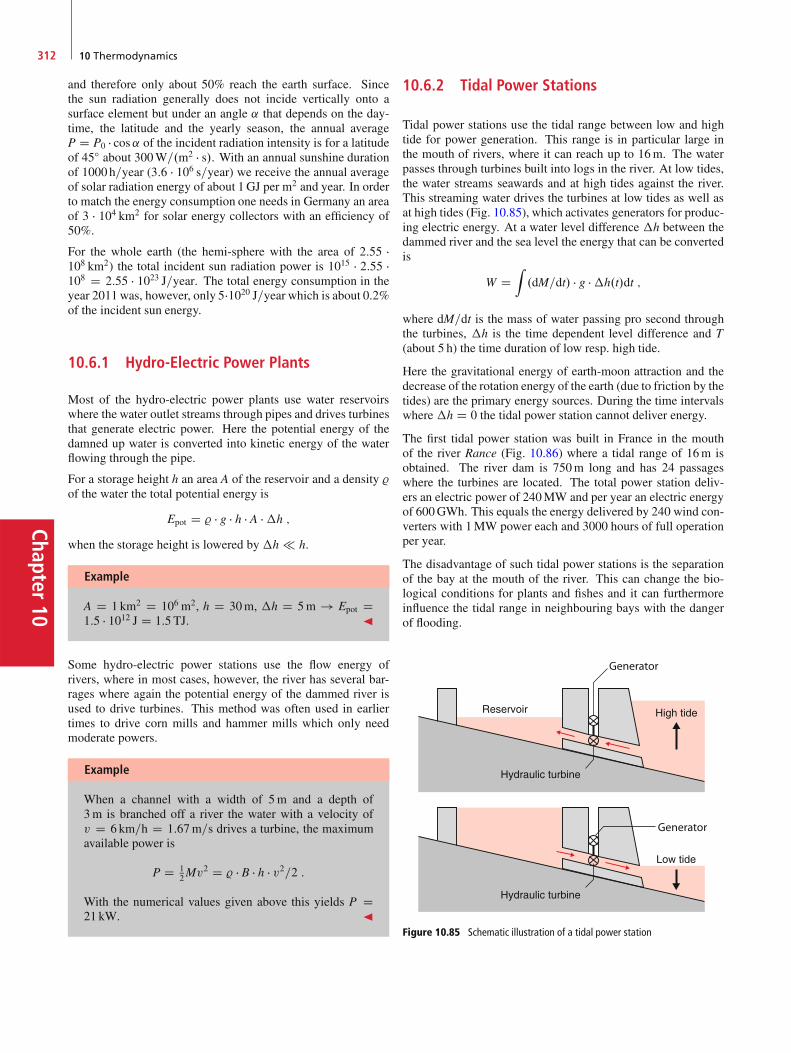
Chapter10
312 10 Thermodynamics
and therefore only about 50% reach the earth surface. Sincethe sun radiation generally does not incide vertically onto asurface element but under an angle ˛ that depends on the day-time, the latitude and the yearly season, the annual averageP D P0 � cos˛ of the incident radiation intensity is for a latitudeof 45ı about 300W=.m2 � s/. With an annual sunshine durationof 1000h=year (3:6 � 106 s=year) we receive the annual averageof solar radiation energy of about 1GJ per m2 and year. In orderto match the energy consumption one needs in Germany an areaof 3 � 104 km2 for solar energy collectors with an efficiency of50%.
For the whole earth (the hemi-sphere with the area of 2:55 �108 km2) the total incident sun radiation power is 1015 � 2:55 �108 D 2:55 � 1023 J=year. The total energy consumption in theyear 2011was, however, only 5�1020 J=year which is about 0.2%of the incident sun energy.
10.6.1 Hydro-Electric Power Plants
Most of the hydro-electric power plants use water reservoirswhere the water outlet streams through pipes and drives turbinesthat generate electric power. Here the potential energy of thedamned up water is converted into kinetic energy of the waterflowing through the pipe.
For a storage height h an area A of the reservoir and a density %of the water the total potential energy is
Epot D % � g � h � A ��h ;
when the storage height is lowered by�h h.
Example
A D 1 km2 D 106 m2, h D 30m, �h D 5m ! Epot D1:5 � 1012 J D 1:5 TJ. J
Some hydro-electric power stations use the flow energy ofrivers, where in most cases, however, the river has several bar-rages where again the potential energy of the dammed river isused to drive turbines. This method was often used in earliertimes to drive corn mills and hammer mills which only needmoderate powers.
Example
When a channel with a width of 5m and a depth of3m is branched off a river the water with a velocity ofv D 6 km=h D 1:67m=s drives a turbine, the maximumavailable power is
P D 12Mv
2 D % � B � h � v2=2 :
With the numerical values given above this yields P D21 kW. J
10.6.2 Tidal Power Stations
Tidal power stations use the tidal range between low and hightide for power generation. This range is in particular large inthe mouth of rivers, where it can reach up to 16m. The waterpasses through turbines built into logs in the river. At low tides,the water streams seawards and at high tides against the river.This streaming water drives the turbines at low tides as well asat high tides (Fig. 10.85), which activates generators for produc-ing electric energy. At a water level difference �h between thedammed river and the sea level the energy that can be convertedis
W DZ.dM=dt/ � g ��h.t/dt ;
where dM=dt is the mass of water passing pro second throughthe turbines, �h is the time dependent level difference and T(about 5 h) the time duration of low resp. high tide.
Here the gravitational energy of earth-moon attraction and thedecrease of the rotation energy of the earth (due to friction by thetides) are the primary energy sources. During the time intervalswhere �h D 0 the tidal power station cannot deliver energy.
The first tidal power station was built in France in the mouthof the river Rance (Fig. 10.86) where a tidal range of 16m isobtained. The river dam is 750m long and has 24 passageswhere the turbines are located. The total power station deliv-ers an electric power of 240MW and per year an electric energyof 600GWh. This equals the energy delivered by 240 wind con-verters with 1MW power each and 3000 hours of full operationper year.
The disadvantage of such tidal power stations is the separationof the bay at the mouth of the river. This can change the bio-logical conditions for plants and fishes and it can furthermoreinfluence the tidal range in neighbouring bays with the dangerof flooding.
Figure 10.85 Schematic illustration of a tidal power station
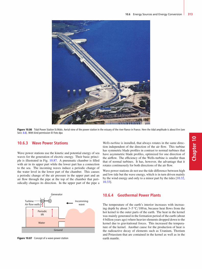
10.6 Energy Sources and Energy Conversion 313
Chap
ter10
Figure 10.86 Tidal Power Station St.Malo. Aerial view of the power station in the estuary of the river Rance in France. Here the tidal amplitude is about 8m (seeSect. 6.6). With kind permission © Foto dpa
10.6.3 Wave Power Stations
Wave power stations use the kinetic and potential energy of seawaves for the generation of electric energy. Their basic princi-ple is illustrated in Fig. 10.87. A pneumatic chamber is filledwith air in its upper part while the lower part has a connectionto the sea. The incoming waves induce a periodic change ofthe water level in the lower part of the chamber. This causesa periodic change of the air pressure in the upper part and anair flow through the pipe at the top of the chamber that peri-odically changes its direction. In the upper part of the pipe a
Generator
Ground
Water
Periodiclift
Air flow wellsTurbine Incomming
wave
Figure 10.87 Concept of a wave-power station
Wells-turbine is installed, that always rotates in the same direc-tion independent of the direction of the air flow. This turbinehas symmetric blade profiles in contrast to normal turbines thathave asymmetric blade profiles, optimized for one direction ofthe airflow. The efficiency of the Wells-turbine is smaller thanthat of normal turbines. It has, however, the advantage that itrotates continuously for both directions of the air flow.
Wave power stations do not use the tide difference between highand low tide but the wave energy, which is in turn driven mainlyby the wind energy and only to a minor part by the tides [10.32,10.33].
10.6.4 Geothermal Power Plants
The temperature of the earth’s interior increases with increas-ing depth by about 3–5 ıC=100m, because heat flows from thehot kernel to the outer parts of the earth. The heat in the kernelwas mainly generated in the formation period of the earth (about4 billion years ago) where heavier elements dropped down to thekernel due to gravitational forces. This increased the tempera-ture of the kernel. Another cause for the production of heat isthe radioactive decay of elements such as Uranium, Thoriumand Potassium that are contained in the kernel as well as in theearth mantle.
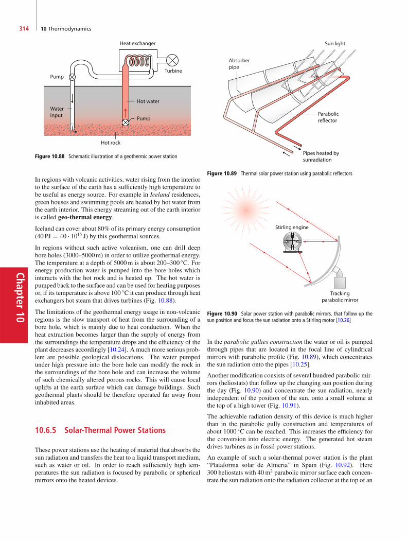
Chapter10
314 10 Thermodynamics
Hot rock
Hot water
Heat exchanger
Pump
Pump
Waterinput
Turbine
Figure 10.88 Schematic illustration of a geothermic power station
In regions with volcanic activities, water rising from the interiorto the surface of the earth has a sufficiently high temperature tobe useful as energy source. For example in Iceland residences,green houses and swimming pools are heated by hot water fromthe earth interior. This energy streaming out of the earth interioris called geo-thermal energy.
Iceland can cover about 80% of its primary energy consumption(40 PJ D 40 � 1015 J) by this geothermal sources.
In regions without such active volcanism, one can drill deepbore holes (3000–5000m) in order to utilize geothermal energy.The temperature at a depth of 5000m is about 200–300 ıC. Forenergy production water is pumped into the bore holes whichinteracts with the hot rock and is heated up. The hot water ispumped back to the surface and can be used for heating purposesor, if its temperature is above 100 ıC it can produce through heatexchangers hot steam that drives turbines (Fig. 10.88).
The limitations of the geothermal energy usage in non-volcanicregions is the slow transport of heat from the surrounding of abore hole, which is mainly due to heat conduction. When theheat extraction becomes larger than the supply of energy fromthe surroundings the temperature drops and the efficiency of theplant decreases accordingly [10.24]. A much more serious prob-lem are possible geological dislocations. The water pumpedunder high pressure into the bore hole can modify the rock inthe surroundings of the bore hole and can increase the volumeof such chemically altered porous rocks. This will cause localuplifts at the earth surface which can damage buildings. Suchgeothermal plants should be therefore operated far away frominhabited areas.
10.6.5 Solar-Thermal Power Stations
These power stations use the heating of material that absorbs thesun radiation and transfers the heat to a liquid transport medium,such as water or oil. In order to reach sufficiently high tem-peratures the sun radiation is focused by parabolic or sphericalmirrors onto the heated devices.
Absorberpipe
Parabolicreflector
Pipes heated bysunradiation
Sun light
Figure 10.89 Thermal solar power station using parabolic reflectors
Trackingparabolic mirror
Stirling engine
Figure 10.90 Solar power station with parabolic mirrors, that follow up thesun position and focus the sun radiation onto a Stirling motor [10.26]
In the parabolic gullies construction the water or oil is pumpedthrough pipes that are located in the focal line of cylindricalmirrors with parabolic profile (Fig. 10.89), which concentratesthe sun radiation onto the pipes [10.25].
Another modification consists of several hundred parabolic mir-rors (heliostats) that follow up the changing sun position duringthe day (Fig. 10.90) and concentrate the sun radiation, nearlyindependent of the position of the sun, onto a small volume atthe top of a high tower (Fig. 10.91).
The achievable radiation density of this device is much higherthan in the parabolic gully construction and temperatures ofabout 1000 ıC can be reached. This increases the efficiency forthe conversion into electric energy. The generated hot steamdrives turbines as in fossil power stations.
An example of such a solar-thermal power station is the plant“Plataforma solar de Almeria” in Spain (Fig. 10.92). Here300 heliostats with 40m2 parabolic mirror surface each concen-trate the sun radiation onto the radiation collector at the top of an
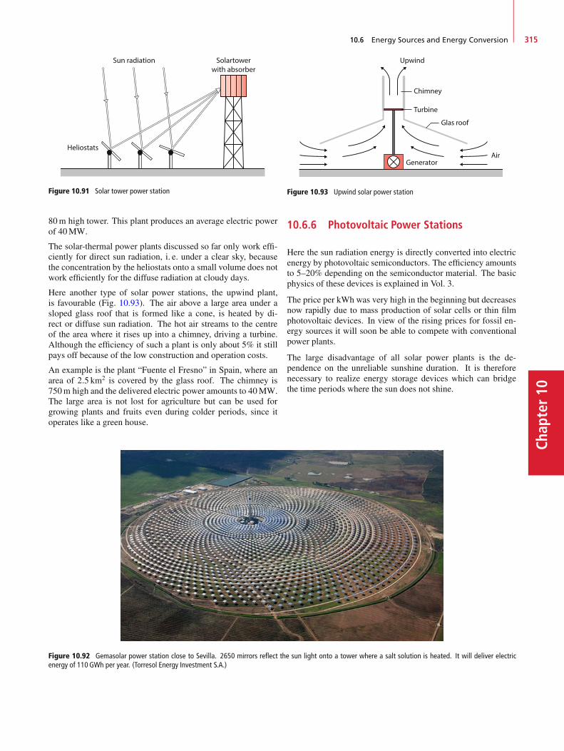
10.6 Energy Sources and Energy Conversion 315
Chap
ter10
Solartowerwith absorber
Sun radiation
Heliostats
Figure 10.91 Solar tower power station
80m high tower. This plant produces an average electric powerof 40MW.
The solar-thermal power plants discussed so far only work effi-ciently for direct sun radiation, i. e. under a clear sky, becausethe concentration by the heliostats onto a small volume does notwork efficiently for the diffuse radiation at cloudy days.
Here another type of solar power stations, the upwind plant,is favourable (Fig. 10.93). The air above a large area under asloped glass roof that is formed like a cone, is heated by di-rect or diffuse sun radiation. The hot air streams to the centreof the area where it rises up into a chimney, driving a turbine.Although the efficiency of such a plant is only about 5% it stillpays off because of the low construction and operation costs.
An example is the plant “Fuente el Fresno” in Spain, where anarea of 2:5 km2 is covered by the glass roof. The chimney is750m high and the delivered electric power amounts to 40MW.The large area is not lost for agriculture but can be used forgrowing plants and fruits even during colder periods, since itoperates like a green house.
Figure 10.92 Gemasolar power station close to Sevilla. 2650 mirrors reflect the sun light onto a tower where a salt solution is heated. It will deliver electricenergy of 110 GWh per year. (Torresol Energy Investment S.A.)
Upwind
Chimney
Turbine
Glas roof
AirGenerator
Figure 10.93 Upwind solar power station
10.6.6 Photovoltaic Power Stations
Here the sun radiation energy is directly converted into electricenergy by photovoltaic semiconductors. The efficiency amountsto 5–20% depending on the semiconductor material. The basicphysics of these devices is explained in Vol. 3.
The price per kWh was very high in the beginning but decreasesnow rapidly due to mass production of solar cells or thin filmphotovoltaic devices. In view of the rising prices for fossil en-ergy sources it will soon be able to compete with conventionalpower plants.
The large disadvantage of all solar power plants is the de-pendence on the unreliable sunshine duration. It is thereforenecessary to realize energy storage devices which can bridgethe time periods where the sun does not shine.
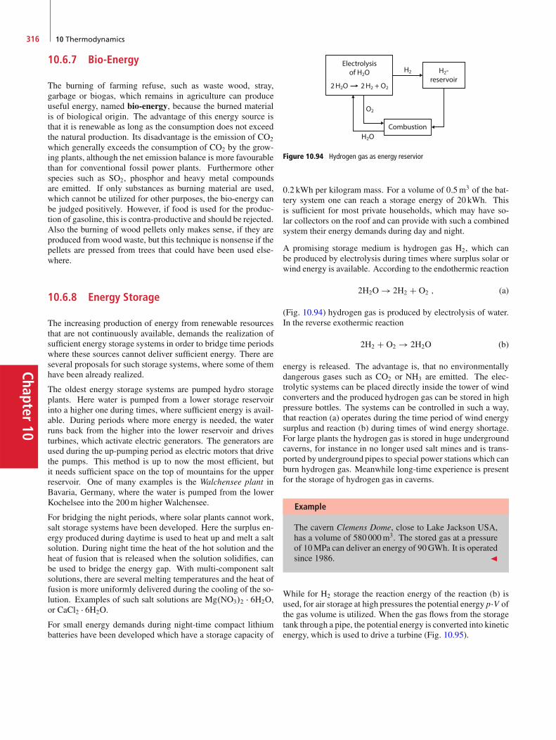
Chapter10
316 10 Thermodynamics
10.6.7 Bio-Energy
The burning of farming refuse, such as waste wood, stray,garbage or biogas, which remains in agriculture can produceuseful energy, named bio-energy, because the burned materialis of biological origin. The advantage of this energy source isthat it is renewable as long as the consumption does not exceedthe natural production. Its disadvantage is the emission of CO2
which generally exceeds the consumption of CO2 by the grow-ing plants, although the net emission balance is more favourablethan for conventional fossil power plants. Furthermore otherspecies such as SO2, phosphor and heavy metal compoundsare emitted. If only substances as burning material are used,which cannot be utilized for other purposes, the bio-energy canbe judged positively. However, if food is used for the produc-tion of gasoline, this is contra-productive and should be rejected.Also the burning of wood pellets only makes sense, if they areproduced from wood waste, but this technique is nonsense if thepellets are pressed from trees that could have been used else-where.
10.6.8 Energy Storage
The increasing production of energy from renewable resourcesthat are not continuously available, demands the realization ofsufficient energy storage systems in order to bridge time periodswhere these sources cannot deliver sufficient energy. There areseveral proposals for such storage systems, where some of themhave been already realized.
The oldest energy storage systems are pumped hydro storageplants. Here water is pumped from a lower storage reservoirinto a higher one during times, where sufficient energy is avail-able. During periods where more energy is needed, the waterruns back from the higher into the lower reservoir and drivesturbines, which activate electric generators. The generators areused during the up-pumping period as electric motors that drivethe pumps. This method is up to now the most efficient, butit needs sufficient space on the top of mountains for the upperreservoir. One of many examples is the Walchensee plant inBavaria, Germany, where the water is pumped from the lowerKochelsee into the 200m higher Walchensee.
For bridging the night periods, where solar plants cannot work,salt storage systems have been developed. Here the surplus en-ergy produced during daytime is used to heat up and melt a saltsolution. During night time the heat of the hot solution and theheat of fusion that is released when the solution solidifies, canbe used to bridge the energy gap. With multi-component saltsolutions, there are several melting temperatures and the heat offusion is more uniformly delivered during the cooling of the so-lution. Examples of such salt solutions are Mg.NO3/2 � 6H2O,or CaCl2 � 6H2O.
For small energy demands during night-time compact lithiumbatteries have been developed which have a storage capacity of
Electrolysisof H2O H2-
reservoir
CombustionH2O
O2
H2
2 H2O 2 H2 + O2
Figure 10.94 Hydrogen gas as energy reservior
0:2 kWh per kilogram mass. For a volume of 0:5m3 of the bat-tery system one can reach a storage energy of 20 kWh. Thisis sufficient for most private households, which may have so-lar collectors on the roof and can provide with such a combinedsystem their energy demands during day and night.
A promising storage medium is hydrogen gas H2, which canbe produced by electrolysis during times where surplus solar orwind energy is available. According to the endothermic reaction
2H2O ! 2H2 C O2 ; (a)
(Fig. 10.94) hydrogen gas is produced by electrolysis of water.In the reverse exothermic reaction
2H2 C O2 ! 2H2O (b)
energy is released. The advantage is, that no environmentallydangerous gases such as CO2 or NH3 are emitted. The elec-trolytic systems can be placed directly inside the tower of windconverters and the produced hydrogen gas can be stored in highpressure bottles. The systems can be controlled in such a way,that reaction (a) operates during the time period of wind energysurplus and reaction (b) during times of wind energy shortage.For large plants the hydrogen gas is stored in huge undergroundcaverns, for instance in no longer used salt mines and is trans-ported by underground pipes to special power stations which canburn hydrogen gas. Meanwhile long-time experience is presentfor the storage of hydrogen gas in caverns.
Example
The cavern Clemens Dome, close to Lake Jackson USA,has a volume of 580 000m3. The stored gas at a pressureof 10MPa can deliver an energy of 90GWh. It is operatedsince 1986. J
While for H2 storage the reaction energy of the reaction (b) isused, for air storage at high pressures the potential energy p�V ofthe gas volume is utilized. When the gas flows from the storagetank through a pipe, the potential energy is converted into kineticenergy, which is used to drive a turbine (Fig. 10.95).
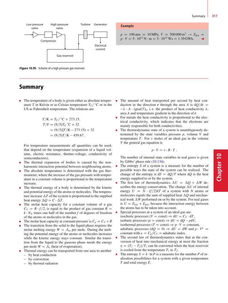
Summary 317
Chap
ter10
Low pressurevalve
High pressurevalve
Turbine Generator
Electricalcurrent
Compressor
Gas reservoir
Figure 10.95 Scheme of a high pressure gas reservior
Example
p D 100 atm D 10MPa, V D 500 000m3 ! Epot Dp � V D 5 � 1012 N � m D 5 � 1012 Ws D 1:39GWh. J
Summary
The temperature of a body is given either as absolute temper-ature T in Kelvin or as Celsius temperature TC= ıC or in theUS as Fahrenheit temperature. The relations are
T=K D TC=ıC C 273:15;
T=F D .9=5/TC ıC C 32
D .9=5/ŒT=K� 273:15/C 32
D .9=5/T=K� 459:67 :
For temperature measurements all quantities can be used,that depend on the temperature (expansion of a liquid vol-ume, electric resistance, thermo-voltage, conductivity ofsemiconductors).The thermal expansion of bodies is caused by the non-harmonic interaction potential between neighbouring atoms.The absolute temperature is determined with the gas ther-mometer, where the increase of the gas pressure with temper-ature in a constant volume is proportional to the temperatureincrease.The thermal energy of a body is determined by the kineticand potential energy of the atoms or molecules. The tempera-ture increase�T of the system is proportional to the suppliedheat energy �Q D C ��T .The molar heat capacity for a constant volume of a gasCV D R � f =2, is equal to the product of gas constant R Dk � NA times one half of the number f of degrees of freedomof the atoms or molecules in the gas.The molar heat capacity at constant pressure is Cp D CV CRThe transition from the solid to the liquid phase requires themolar melting energy W D �m per mole. During the melt-ing the potential energy of the atoms or molecules increaseswhile the kinetic energy stays constant. Similar the transi-tion from the liquid to the gaseous phase needs the energyper moleW D �e (heat of evaporation).Thermal energy can be transported from one area to another– by heat conduction– by convection– by thermal radiation
The amount of heat transported per second by heat con-duction in the direction r through the area A is dQ=dt D�� � A � .gradT/r, i. e. the product of heat conductivity �,area A and temperature gradient in the direction of r.For metals the heat conductivity is proportional to the elec-trical conductivity, which indicates that the electrons aremainly responsible for both conductivities.The thermodynamic state of a system is unambiguously de-termined by the state variables pressure p, volume V andtemperature T . For � moles of an ideal gas in the volumeV the general gas equation is
p � V D � � R � T :The number of internal state variables in real gases is givenby Gibbs’ phase rule (10.134).The entropy S of a system is a measure for the number ofpossible ways the state of the system can be realized. Thechange of the entropy is dS D dQ=T where dQ is the heatenergy supplied to or by the system.The first law of thermodynamics �U D �Q C �W de-scribes the energy conservation. The change �U of internalenergy U D N � .f =2/kT of a system with N atoms ormolecules equals the sum of supplied heat �Q and mechan-ical work �W performed on or by the system. For real gasesis U D Ekin C Epot, because the interaction energy betweenthe atoms has to be taken into account.Special processes in a system of an ideal gas are:isochoric processes (V D const) ) dU D CV � dT ,isobaric processes (p D const) ) dU D dQ � pdV,isothermal processes (T D const) ) p � V D constant,adiabatic processes (dQ D 0) ) dU D dW and p � V� Dconstant with � D Cp=CV D adiabatic index.The second law of thermodynamics states that at the con-version of heat into mechanical energy at most the fraction� D .T1 � T2/=T1 can be converted when the heat reservoiris cooled from the temperature T1 to T2.The entropy S D k � lnP is a measure for the number P of re-alization possibilities for a system with a given temperatureT and total energy E.

Chapter10
318 10 Thermodynamics
Reversible processes are ideal processes where a systempasses a cycle of processes and reaches its initial state with-out any losses. An example is the Carnot Cycle where thesystem passes through two isothermal and two adiabatic pro-cesses.For reversible processes the entropy remains constant. Forall irreversible processes the entropy increases and the freeenergy F D U � T � S decreases.The entropy S approaches zero for T ! 0 (third law of ther-modynamics).For real gases the Eigen-volume of the atoms and the inter-action between the atoms cannot be neglected as for idealgases. The equation of state p � V D � � R � T of ideal gases ismodified to the van derWaals equation .pCa=V2/�.V�b/ DR � T , where a=V2 denotes the internal pressure and b=4 theEigen-volume of the NA molecules per mole.
The heat of evaporation of a liquid� D T �dps=dT �.Vv�Vl/ isdue to the mechanical work necessary to enlarge the volumeVl of the liquid to the much larger volume Vv of the vapouragainst the external pressure and against the internal attrac-tive forces between the molecules. The second contributionis much larger than the first one.In a p.T/ phase diagram the liquid and gaseous phases areseparated by the vapour phase curve and the liquid and solidphase by the melting curve. The two curves intersect in thetriple point (Ttr; ptr) where all three phases can coexist.The vapour pressure of a liquid is lowered by addition ofsolvable substances, which increases the evaporation temper-ature. Also the melting temperature can be lowered.
Problems
10.1 Give a physically intuitive explanation, why the thermalexpansion coefficient for liquids is larger than that of solids.
10.2 Prove example 2 in Sect. 10.1.2.
10.3 A container with 1mol helium and a container of equalsize with 1mol nitrogen are heated with the same heat powerof 10W. Calculate after which time the temperature of the gasin the containers has risen from 20 to 100 ıC. The heat capac-ity of the containers is 10Ws=K. How long does it take, untilT D 1000 ıC is reached, when we assume that the vibrationaldegrees of freedom of N2 can be excited already at T D 500 ıC?All heat losses should be neglected.
10.4 Give a vivid and a mathematical justification for the timedependent temperature function T.t/ during the mixing experi-ment of Fig. 10.12.
10.5 A container (m D 0:1 kg) with 10mol air at room tem-perature rests on the ground. What is the probability that it liftsby itself 10 cm above ground? Such an event would cause acooling (conversion of thermal into potential energy). How largeis the decrease of the temperature? (Specific heat of the gas is.5=2/R, that of the container is 1 kJ=.kg � K/.)
10.6 A volume of 1 dm3 of helium under standard condi-tions (p0 D 1 bar, T0 D 0 ıC) is heated up to the temperatureT D 500K. What is the entropy increase for isochoric and forisobaric heating?
10.7 The critical temperature for CO2 (M D 44 g=mol) isTc D 304:2K and the critical pressure pc D 7:6 � 106 Pa, itsdensity at the critical point is % D 46 kg=m3. What are the vander Waals constants a and b?
10.8 What is the entropy increase �S1 when 1 kg water isheated from 0 to 50 ıC? Compare�S1 with the entropy increase�S2 when 0:5 kg water of 0 ıC is mixed with 0:5 kg of 100 ıC.
10.9 A power station delivers the mechanical work W1 whenwater vapour of 600 ıC drives a turbine and cools down to100 ıC.a) What is the Carnot efficiency?b) How many % of the output energy can one win, when the
water of 100 ıC is used for heating and cools down to 30 ıC?
10.10 A hot solid body (m D 1 kg, c D 470 J=.kg � K/,T D 300 ıC) is immersed into 10 kg of water at 20 ıC.a) What is the final temperature?b) What is the entropy increase?
10.11 Calculate the pressure that a wire with 1mm diameterexerts onto an ice block with a width of 10 cm (according toFig. 10.80) when both ends are connected with a massm D 5 kg.What is the increase of the melting temperature? What is theheat supplied to the ice block by the wire, if the outside temper-ature and the wire temperature are 300K‹ How much ice can bemelted per second by the wire?
10.12 Calculate from the diagram of Fig. 10.64b the theoreticalefficiency of the Otto-motor.
10.13 Show that for a periodically supplied heat at x D 0Eq. 10.42 is a solution of the Eq. 10.38b for one-dimensionalheat conduction.
10.14 What is the maximum power an upwind power plantcan deliver (area 5 km2, temperature below the glass roof T D50 ıC, height of the tower 100m, outside temperature 20 ıC atthe top of the chimney).
References 319
Chap
ter10
References
10.1. F.W.G. Kohlrausch, An Introduction to Physical Mea-surements, 2nd ed. (Univ. Toronto Libraries, Toronto,2011)
10.2a. J.V. Iribane, H.R. Cho, Atmospheric Physics. (D. Reidel,Dordrecht, 1980)
10.2b. D.G. Andrews, An Introduction to Atmospheric Physics.(Cambridge Univ. Press, Cambridge, 2010)
10.3. H. Haken, Synergetics. An Introduction. (Springer,Berlin, Heidelberg, 2014)
10.4. H. Haken, Synergetics. Introduction and Advanced Top-ics. (Springer, Heidelberg, 2004)
10.5. J.E. Parrot, A.D. Stuckes, Thermal Conductivity ofSolids. (Pion Ltd, London, 1975)
10.6. P. Dunn, D.A. Reay, Heatpipes, 2nd ed. (Pergamon, Ox-ford, 1978)
10.7. N. Rice, Thermal Insulation. A Building Guide. (NY Re-search Press, New York, 2015)
10.8. R.T. Bynum, Insulation Handbook. (McGrawHill, NewYork, 2000)
10.9. J. Fricke and W.L. Borst, Essentials of Energy Technol-ogy: Sources, Transport, Storage Conservation. (WileyVCH, Weinheim, 2014)
10.10. Ph. Warburg, Harvest the Sun. America’s Quest for a So-lar Powered Future. (Beacon Press, Boston, 2015)
10.11. M. Green, Third Generation Photovoltaics. AdvancedSolar Energy Conversion. Springer Series in Photonics,Vol. 12. (Springer, Berlin, Heidelberg, 2005)
10.12. S.A. Goudsmit, R. Clayborne, Time. (Time-Life Amster-dam, 1970)
10.13. S.C. Colbeck, Am. J. Phys. 63, 888 (1995)10.14. CRC handbook of Chemistry and Physics, 96th ed. (CRC
Press, Boca Raton, Florida, USA, 2015)10.15. http://cdn.intechopen.com/pdfs/20377/InTech-
Practical_application_of_electrical_energy_storage_system_in_industry.pdf
10.16. http://www2.hesston.edu/physics/201112/regenerativeenergy_cw/paper.html
10.17. https://en.wikipedia.org/wiki/Climate_change10.18. http://www.bounceenergy.com/blog/2013/05/wind-
energy-grid-part-3-future/, http://www.pasolar.org/index.asp?Type=B_BASIC&SEC=%7B9D644D34-AF8E-475C-A330-4396D09F454B%7D
10.19. https://en.wikipedia.org/wiki/World_energy_consumption
10.20. https://en.wikipedia.org/wiki/Electric_energy_consumption
10.21. https://en.wikipedia.org/wiki/Renewable_energy10.22. https://en.wikipedia.org/wiki/Tidal_power, https://en.
wikipedia.org/wiki/Rance_Tidal_Power_Station, http://www.darvill.clara.net/altenerg/tidal.htm
10.23. https://en.wikipedia.org/wiki/Wave_power, https://en.wikipedia.org/wiki/List_of_wave_power_stations
10.24. https://en.wikipedia.org/wiki/Geothermal_energy,https://en.wikipedia.org/wiki/Geothermal_electricity
10.25. https://en.wikipedia.org/wiki/Solar_thermal_energy10.26. http://www.volker-quaschning.de/articles/
fundamentals2/index_e.php, https://en.wikipedia.org/wiki/List_of_solar_thermal_power_stations
10.27. http://de.total.com/en-us/making-energy-better/worldwide-%20%20%20projects/sunpower-puts-total-cutting-edge-solar?gclid=CLKnluvxjckCFVZAGwod6mQFh
10.28. http://energy.gov/eere/fuelcells/hydrogen-storage,https://en.wikipedia.org/wiki/Hydrogen_storage
10.29. https://en.wikipedia.org/wiki/Energy_storage10.30. https://en.wikipedia.org/wiki/Renewable_energy10.31. BP, Workbook of historical data. Microsoft Excel docu-
ment10.32. http://www.darvill.clara.net/altenerg/wave.htm10.33. http://thinkglobalgreen.org/WAVEPOWER.html
Chap
ter11
Mechanical Oscillations andWaves 1111.1 The Free Undamped Oscillator . . . . . . . . . . . . . . . . . . . . . . 322
11.2 Mathematical Notations of Oscillations . . . . . . . . . . . . . . . . . 323
11.3 Superposition of Oscillations . . . . . . . . . . . . . . . . . . . . . . . 324
11.4 The Free Damped Oscillator . . . . . . . . . . . . . . . . . . . . . . . . 328
11.5 Forced Oscillations . . . . . . . . . . . . . . . . . . . . . . . . . . . . . 330
11.6 Energy Balance for the Oscillation of a Point Mass . . . . . . . . . . 333
11.7 Parametric Oscillator . . . . . . . . . . . . . . . . . . . . . . . . . . . . 334
11.8 Coupled Oscillators . . . . . . . . . . . . . . . . . . . . . . . . . . . . . 335
11.9 Mechanical Waves . . . . . . . . . . . . . . . . . . . . . . . . . . . . . 339
11.10 Superposition of Waves; Interference . . . . . . . . . . . . . . . . . . 352
11.11 Diffraction, Reflection and Refraction of Waves . . . . . . . . . . . . 354
11.12 Standing Waves . . . . . . . . . . . . . . . . . . . . . . . . . . . . . . . 359
11.13 Waves Generated by Moving Sources . . . . . . . . . . . . . . . . . . 363
11.14 Acoustics . . . . . . . . . . . . . . . . . . . . . . . . . . . . . . . . . . . 366
11.15 Physics of Musical Instruments . . . . . . . . . . . . . . . . . . . . . . 372
Summary . . . . . . . . . . . . . . . . . . . . . . . . . . . . . . . . . . . 376
Problems . . . . . . . . . . . . . . . . . . . . . . . . . . . . . . . . . . . 378
References . . . . . . . . . . . . . . . . . . . . . . . . . . . . . . . . . . 379
321© Springer International Publishing Switzerland 2017W. Demtröder, Mechanics and Thermodynamics, Undergraduate Lecture Notes in Physics, DOI 10.1007/978-3-319-27877-3_11

Chapter11
322 11 Mechanical Oscillations and Waves
Mechanical oscillations play an important role in basic sci-ences as well as for technical applications. Their significanceas sources of acoustic waves and for the realization of musi-cal performances, in sensors for hearing is obvious. Often theprevention of unwanted acoustic resonances of buildings andbridges represents a technical challenge. All these points jus-tify a more detailed study of the basic physics of oscillationsand waves.
Their mathematical treatment is in many aspects very similar tothat of electric oscillations and waves (see Vol. 2, Chap. 6). Theinvestigation of common features and differences between me-chanical and electro-magnetic oscillations and waves not onlyintensifies our knowledge of macroscopic oscillation phenom-ena but also gives a deeper insight into the microscopic structureof matter. (atomic and molecular vibrations in solids).
In this chapter we will discuss mechanical oscillations, wherematter is moved, and mechanical waves where this motion istransported by couplings between neighbouring layers of gases,liquids or solids. At the end of this chapter some interestingapplications of ultrasonics in medicine and of acoustics in musicare presented.
11.1 The Free Undamped Oscillator
In Chap. 2 the basic equations of motion for the simplifiedmodel of point masses were derived. In a similar way the basicfacts of mechanical oscillations can be best understood when westart with the idealized model of point masses before we proceedto oscillations of extended bodies.
A point mass m suspended by a spring has its equilibrium po-sition at x D 0 where the gravity force is just compensated bythe opposite restoring force of the spring. When the mass m isremoved from its equilibrium position by a small displacementx (Fig. 11.1) a restoring force occurs, which is, according toHooke’s Law (Sect. 6.2) proportional to x:
F D �D � x ;
where D is the spring constant that depends on the strength ofthe spring. This force drives the mass m back to its equilibriumposition x D 0. The one-dimensional equation of motion is then
m � d2x
dt2D �Dx : (11.1a)
With the abbreviation !20 D D=m this becomes
d2x
dt2C !2
0x D 0 : (11.1b)
This is the equation for the harmonic oscillator (which is called“harmonic” because its oscillation generates a “pure” sinusoidaltone at the frequency !0. Together with its overtones n � !0 itforms a superposition of tones that are felt by human ears asharmony).
Figure 11.1 Undamped harmonic oscillator
In Sect. 2.9.7 we had already derived the oscillation equation forthe simple pendulum, where we had found for small elongationsthe same equation R' C .g=L/' D 0 for the angle ' (Eq. 2.79b).
The equation (11.1) has the solution
x D c � e�t ; (11.2)
where c is an arbitrary constant. Inserting (11.2) into (11.1)gives the quadratic equation for the parameter �:
�2 C !20 D 0 ;
which has the two solutions
�1 D Ci � !0 and �2 D �i � !0 :
We therefore obtain the two solutions of (11.1)
x1.t/ D c1ei!0 t and x2.t/ D c2e
�i!0 t ;
which are linearly independent for !0 ¤ 0. The general solu-tion of the linear differential equation (11.1) is then the linearcombination of the two solutions
x.t/ D c1ei!0 t C c2e
�i!0 t : (11.3)
Since x.t/ must be a real function (not complex) it follows forthe complex constants c1 D c�
2 D c. The solution for the oscil-lation amplitude is then
x.t/ D cei!0 t C c�e�i!0 t with c D a C ib : (11.4a)
The real constants a and b can be determined from the initialconditions for the special oscillation problem.
Example
When the mass m in Fig. 11.1 passes at t D 0 with thevelocity v0 through the equilibrium position x D 0, weobtain from (11.4a): c� C c D 0 ) a D 0 and v0 Di � !0.c � c�/ D i!0 � 2ib D> b D v0=2!0. Therefore is
x.t/ D v0
!0sin!0t : J
Remark. The oscillating mass on a spring is only one exam-ple for a harmonic oscillator. Other examples are a mass thatoscillates on a parabolic air track, or the simple pendulum sus-pended by a string, or an electron in the lowest energy level ofthe hydrogen atom.

11.2 Mathematical Notations of Oscillations 323
Chap
ter11
11.2 Mathematical Notations ofOscillations
When we write the complex amplitudes c and c� in (11.4) aspolar representation
c D jcj � ei' ; c� D jcj � e�i' :
We obtain the representation
x.t/ D jcj �ei.!0 tC'/ C e�i.!0 tC'/� ; (11.4b)
that is equivalent to (11.4a).
According to Euler’s formula for complex numbers
eix D cos x C i � sin x :
We can write (11.4a) also in the form
x.t/ D C1 cos!0t C C2 sin!0t
with
(C1 D c C c�
C2 D i.c � c�/
):
(11.4c)
A forth equivalent representation is
x.t/ D A � cos.!0t C '/ : (11.4d)
The comparison with (11.4c) gives
C1 D A � cos' ; C2 D �A � sin') � tan ' D C2
C1and A D
qC21 C C2
2 :
All 4 representations (11.4a–d) for the solution of (11.1) areequivalent (Fig. 11.2). They represent a harmonic oscillationwith the frequency !0 and the amplitude A D 2jcj (Fig. 11.3).For our example above with the initial conditions x.0/ D 0 and.dx=dt/0 D v0 all forms (11.4a–d) give the solution
x.t/ D v0
!0sin.!0t/ ;
as can be immediately proved by inserting x.t/ into (11.4a–d).
Imaginary part
Real part
Figure 11.2 Relations betwenn different equivalent representations of har-monic oscillations
Figure 11.3 Period T , amplitude A and phase shift ' of a harmonic oscillation
Figure 11.4 Elongation x.t/, velocity Px.t/ and acceleration Rx.t/ of a harmonicoscillation
The argument (!0t C ') in the cosine function (11.4d), whichdetermines the momentary value of the elongation x.t/, is calledthe phase of the oscillation. The time origin x D 0 can be chosenin such a way that ' D 0. This reduces (11.4d) to
x.t/ D A � cos!0t : (11.4e)
After a time t D 2=!0 D T always the same value of x.t/ isreached. This means
x.t C T/ D x.t/ :
The time interval T is called the oscillation period, while thereciprocal � D 1=T is the oscillation frequency and ! D 2�is the circular frequency. The mass that experiences a restoringforce proportional to the displacement (x� x0) from the equilib-rium position x0 is called a harmonic oscillator.
In Fig. 11.4 the elongation x.t/ D A � cos.!t/, the velocity dx=dtand the acceleration d2x=dt2 are shown. The figure illustratesthat the acceleration always has the opposite phase as the elon-gation, i. e. x.t/ shows a phase shift of against d2x=dt2.
Example
x1.t/ D A � cos.!0t/ and x2.t/ D A � cos.!0 C '/ aretwo harmonic oscillators with the same frequency andthe same amplitude but with a phase shift ' against eachother. The maxima of the two oscillations are shiftedagainst each other by the time �t D '=!0 (Fig. 11.5).
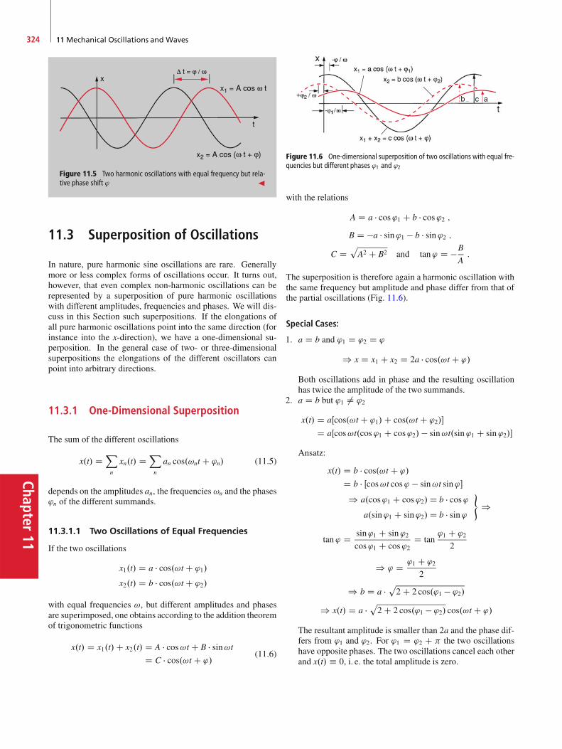
Chapter11
324 11 Mechanical Oscillations and Waves
Figure 11.5 Two harmonic oscillations with equal frequency but rela-tive phase shift ' J
11.3 Superposition of Oscillations
In nature, pure harmonic sine oscillations are rare. Generallymore or less complex forms of oscillations occur. It turns out,however, that even complex non-harmonic oscillations can berepresented by a superposition of pure harmonic oscillationswith different amplitudes, frequencies and phases. We will dis-cuss in this Section such superpositions. If the elongations ofall pure harmonic oscillations point into the same direction (forinstance into the x-direction), we have a one-dimensional su-perposition. In the general case of two- or three-dimensionalsuperpositions the elongations of the different oscillators canpoint into arbitrary directions.
11.3.1 One-Dimensional Superposition
The sum of the different oscillations
x.t/ DX
n
xn.t/ DX
n
an cos.!nt C 'n/ (11.5)
depends on the amplitudes an, the frequencies !n and the phases'n of the different summands.
11.3.1.1 Two Oscillations of Equal Frequencies
If the two oscillations
x1.t/ D a � cos.!t C '1/
x2.t/ D b � cos.!t C '2/
with equal frequencies !, but different amplitudes and phasesare superimposed, one obtains according to the addition theoremof trigonometric functions
x.t/ D x1.t/C x2.t/ D A � cos!t C B � sin!tD C � cos.!t C '/
(11.6)
Figure 11.6 One-dimensional superposition of two oscillations with equal fre-quencies but different phases '1 and '2
with the relations
A D a � cos'1 C b � cos'2 ;B D �a � sin '1 � b � sin '2 ;
C DpA2 C B2 and tan ' D �B
A:
The superposition is therefore again a harmonic oscillation withthe same frequency but amplitude and phase differ from that ofthe partial oscillations (Fig. 11.6).
Special Cases:
1. a D b and '1 D '2 D '
) x D x1 C x2 D 2a � cos.!t C '/
Both oscillations add in phase and the resulting oscillationhas twice the amplitude of the two summands.
2. a D b but '1 ¤ '2
x.t/ D aŒcos.!t C '1/C cos.!t C '2/�
D aŒcos!t.cos'1 C cos'2/ � sin!t.sin '1 C sin '2/�
Ansatz:
x.t/ D b � cos.!t C '/
D b � Œcos!t cos' � sin!t sin'�
) a.cos'1 C cos'2/D b � cos'a.sin'1 C sin'2/D b � sin '
))
tan ' D sin'1 C sin '2cos'1 C cos'2
D tan'1 C '2
2
) ' D '1 C '2
2
) b D a �p2 C 2 cos.'1 � '2/
) x.t/ D a �p2 C 2 cos.'1 � '2/ cos.!t C '/
The resultant amplitude is smaller than 2a and the phase dif-fers from '1 and '2. For '1 D '2 C the two oscillationshave opposite phases. The two oscillations cancel each otherand x.t/ � 0, i. e. the total amplitude is zero.
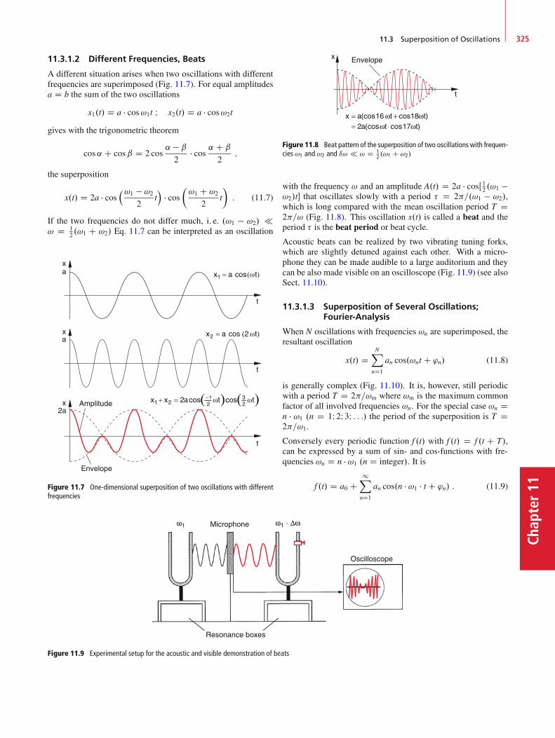
11.3 Superposition of Oscillations 325
Chap
ter11
11.3.1.2 Different Frequencies, Beats
A different situation arises when two oscillations with differentfrequencies are superimposed (Fig. 11.7). For equal amplitudesa D b the sum of the two oscillations
x1.t/ D a � cos!1t I x2.t/ D a � cos!2t
gives with the trigonometric theorem
cos˛ C cosˇ D 2 cos˛ � ˇ2
� cos ˛ C ˇ
2;
the superposition
x.t/ D 2a � cos�!1 � !2
2t
� cos�!1 C !2
2t
�: (11.7)
If the two frequencies do not differ much, i. e. .!1 � !2/ ! D 1
2 .!1 C !2/ Eq. 11.7 can be interpreted as an oscillation
Amplitude
Envelope
Figure 11.7 One-dimensional superposition of two oscillations with differentfrequencies
Microphone
Resonance boxes
Oscilloscope
Figure 11.9 Experimental setup for the acoustic and visible demonstration of beats
Envelope
Figure 11.8 Beat pattern of the superposition of two oscillations with frequen-cies !1 and !2 and ı! ! D 1
2 .!1 C !2/
with the frequency ! and an amplitude A.t/ D 2a � cosŒ 12 .!1 �!2/t� that oscillates slowly with a period � D 2=.!1 � !2/,which is long compared with the mean oscillation period T D2=! (Fig. 11.8). This oscillation x.t/ is called a beat and theperiod � is the beat period or beat cycle.
Acoustic beats can be realized by two vibrating tuning forks,which are slightly detuned against each other. With a micro-phone they can be made audible to a large auditorium and theycan be also made visible on an oscilloscope (Fig. 11.9) (see alsoSect. 11.10).
11.3.1.3 Superposition of Several Oscillations;Fourier-Analysis
When N oscillations with frequencies !n are superimposed, theresultant oscillation
x.t/ DNX
nD1
an cos.!nt C 'n/ (11.8)
is generally complex (Fig. 11.10). It is, however, still periodicwith a period T D 2=!m where !m is the maximum commonfactor of all involved frequencies !n. For the special case !n Dn � !1 .n D 1I 2I 3I : : :/ the period of the superposition is T D2=!1.
Conversely every periodic function f .t/ with f .t/ D f .t C T/,can be expressed by a sum of sin- and cos-functions with fre-quencies !n D n � !1 .n D integer/. It is
f .t/ D a0 C1X
nD1
an cos.n � !1 � t C 'n/ : (11.9)

Chapter11
326 11 Mechanical Oscillations and Waves
Figure 11.10 Superposition of five oscillations xn D a � sin.n!t/ with equalamplitudes An and frequencies!n D n �!1 (dashed curve) and!n D .2n�1/!1
(solid curve). The amplitude of the superposition has been reduced by a factor3:66
The oscillation a1 �cos!1t is the fundamental oscillation,the members with higher frequencies n�!1 are higher har-monics. In acoustics, they are called fundamental toneand overtones.
The partition of a periodic function into harmonics i. e. the rep-resentation of f .t/ as a Fourier-series is called Fourier analysis.Its general from is discussed in Sect. 13.4.
The experimental Fourier analysis can be performed with thevibrating reed frequency meter, shown in Fig. 11.11. It consistsof a series of flat springs with different lengths and resonancefrequencies ! D n �!1 .n D 1; 2; 3; : : :/. When they are excitedby a mechanical vibration their oscillation amplitude becomesmaximum, when the exciting frequency matches the resonancefrequency determined by the length of the spring.
The human inner ear embodies such vibrating springs in theform of thin hairs with different resonance frequencies. Their vi-brations are transformed into electric signals that are conductedto the brain (see Sect. 11.5 and 11.14). If the hairs are exposed
Stroboscobicillumination
Leaf spring
Figure 11.11 Reed frequency meter
5Sound source
Frequency filter
Microphone
Oscilloscope
Figure 11.12 Electrical detection of mechanical oscillation and Fourier-analysis with frequency filters
to excessive sound intensities, they can break and the ear can nolonger hear the corresponding frequencies.
In a more elegant way mechanical oscillations can be detectedand measured by microphones, which transform them into elec-trical signals that can be viewed for instance, on the screen of anoscilloscope. If the source emits several frequencies, they canbe selected by parallel-connected electrical filters (Fig. 11.12).that act as Fourier-analysers.
In Fig. 11.13 the Fourier-analysis of a periodic rectangular func-tion
f .t/ D(A for 0 < t < T
2
0 for T2 � t � T
)and f .t C T/ D f .t/ I
f .t/ D a0 C1X
nD1
an sin.n!t/ I ! D 2
T
a0 D A
2I a2n�1 D 2A
.2n � 1/I a2n D 0
is shown with the corresponding magnitude distribution of theamplitudes an.
Remark. Even an arbitrary not necessary periodic function canbe represented as a superposition of periodic functions. Instead

11.3 Superposition of Oscillations 327
Chap
ter11
Figure 11.13 Fourier-analysis of an equidistant sequence of rectangular pro-files
of the sum one obtains now the integral
f .t/ D1Z
0
Œa.!/ cos!t C b.!/ sin!t� d!
with the coefficients
a.!/ D 1
C1Z
�1f .t/ cos!tdt ; b.!/ D 1
C1Z
�1f .t/ sin!tdt :
11.3.2 Two-dimensional Superposition;Lissajous-Figures
When two oscillations with the same frequency ! and a phaseshift ',
x D a � cos.!t/ ; y D b � cos.!t C '/ ; (11.10)
which oscillate into directions that are orthogonal to each other,are superimposed, one obtains the two-dimensional representa-tion
x
aD cos!t I
y
bD cos!t cos' � sin!t sin '
D x
acos' � sin!t sin ' :
Rearrangement gives
sin!t � sin' D x
acos' � y
b
cos!t � sin ' D x
asin ' :
Elimination of time t by squaring and adding the two equationsyields
sin2 ' D x2
a2C y2
b2� 2xy
abcos' :
Figure 11.14 Trajectories y.x/ of the superposition x.t/C y.t/ with x.t/ Db � sin.!t C �'/ and y.t/ D a � sin!t for different values of the phase shift�'. a for a ¤ b and b for a D b . c Illustration of the functions y.t/ and x.t/for�' D =6
This can be rearranged into the ellipse equation for the motionof the oscillating point mass in the x–y-plane.
x2
a�2 C y2
b�2 � 2xy cos'
a�b� D 1 ; (11.11)
which describes an ellipse with axes tilted by the angle ' againstthe x- and y-axes. The length of the half axes a� D a � sin'and b� D b � sin ' depends on the amplitudes a and b of theoscillations and on the phase shift ' (Fig. 11.14).
For the special case ' D 0 the ellipse reduces to the straight liney D .b=a/x.
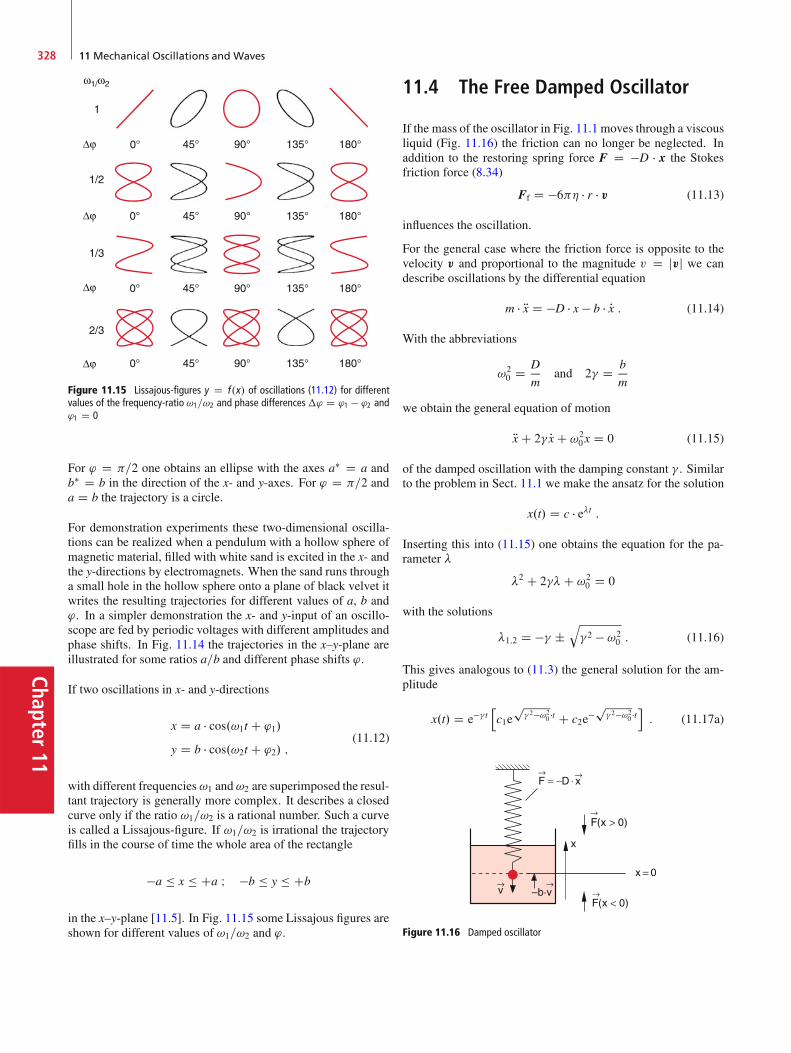
Chapter11
328 11 Mechanical Oscillations and Waves
Figure 11.15 Lissajous-figures y D f .x/ of oscillations (11.12) for differentvalues of the frequency-ratio !1=!2 and phase differences�' D '1 � '2 and'1 D 0
For ' D =2 one obtains an ellipse with the axes a� D a andb� D b in the direction of the x- and y-axes. For ' D =2 anda D b the trajectory is a circle.
For demonstration experiments these two-dimensional oscilla-tions can be realized when a pendulum with a hollow sphere ofmagnetic material, filled with white sand is excited in the x- andthe y-directions by electromagnets. When the sand runs througha small hole in the hollow sphere onto a plane of black velvet itwrites the resulting trajectories for different values of a, b and'. In a simpler demonstration the x- and y-input of an oscillo-scope are fed by periodic voltages with different amplitudes andphase shifts. In Fig. 11.14 the trajectories in the x–y-plane areillustrated for some ratios a=b and different phase shifts '.
If two oscillations in x- and y-directions
x D a � cos.!1t C '1/
y D b � cos.!2t C '2/ ;(11.12)
with different frequencies !1 and!2 are superimposed the resul-tant trajectory is generally more complex. It describes a closedcurve only if the ratio !1=!2 is a rational number. Such a curveis called a Lissajous-figure. If !1=!2 is irrational the trajectoryfills in the course of time the whole area of the rectangle
�a � x � Ca I �b � y � Cb
in the x–y-plane [11.5]. In Fig. 11.15 some Lissajous figures areshown for different values of !1=!2 and '.
11.4 The Free Damped Oscillator
If the mass of the oscillator in Fig. 11.1 moves through a viscousliquid (Fig. 11.16) the friction can no longer be neglected. Inaddition to the restoring spring force F D �D � x the Stokesfriction force (8.34)
Ff D �6� � r � v (11.13)
influences the oscillation.
For the general case where the friction force is opposite to thevelocity v and proportional to the magnitude v D jvj we candescribe oscillations by the differential equation
m � Rx D �D � x � b � Px : (11.14)
With the abbreviations
!20 D D
mand 2� D b
m
we obtain the general equation of motion
Rx C 2� Px C !20x D 0 (11.15)
of the damped oscillation with the damping constant � . Similarto the problem in Sect. 11.1 we make the ansatz for the solution
x.t/ D c � e�t :
Inserting this into (11.15) one obtains the equation for the pa-rameter �
�2 C 2��C !20 D 0
with the solutions
�1;2 D �� ˙q�2 � !2
0 : (11.16)
This gives analogous to (11.3) the general solution for the am-plitude
x.t/ D e�� thc1e
p�2�!2
0 �t C c2e�p�2�!2
0 �ti: (11.17a)
Figure 11.16 Damped oscillator

11.4 The Free Damped Oscillator 329
Chap
ter11
The time behaviour of x.t/ essentially depends on the ratio of
mean restoring force
mean friction forceD hjD � xji
hjb � Pxji
D m!20
px2
2�mp
Px2D !0
2�:
This means that it depends on the relative magnitude of !0 and� . We distinguish between the following three cases:
11.4.1 � < !0, i. e. weak damping
With the abbreviation !2 D !20 � �2 is
�1;2 D �� ˙p
�!2 D �� ˙ i! :
The general solution (11.17a) is then
x.t/ D e�� t �cei!t C c�e�i!t�
D Ae�� t cos.!t C '/ ;(11.17b)
where, as in Sect. 11.1
A D 2jcj and tan ' D � i.c � c�/c C c� D Imfcg
Refcg :
Equation 11.17b describes a damped oscillation, where the am-plitude A�e�� t decays exponentially. It is illustrated in Fig. 11.17for the initial conditions x.0/ D A and .dx=dt/.0/ D v0, forwhich the solution (11.17b) is
x.t/ D Ae�� t cos!t : (11.17c)
With v0 D �A � � we obtain
v.t/ D v0e�� t�cos!t C !
�sin!t
�: (11.17d)
Two successive maxima of the damped oscillation have the am-plitude ratio
x.t C T/
x.t/D e��T (11.18)
with the period T D 2=!.
The natural logarithm of the inverse ratio
ln
�x.t/
x.t C T/
�D � � T D ı
is called the logarithmic decrement.
After the time t D � D 1=� the envelope f .t/ D A � e�� t of theoscillation has decreased to 1=e of its initial value f .0/ D A.
x
Figure 11.17 Damped oscillation with damping constant � and oscillation pe-riod T for the initial conditions x.0/ D A (black curve) and x.0/ D 0 (redcurve)
The frequency ! Dq!20 � �2 of the damped oscillator is
for the same spring constant D slightly smaller than thatof the undamped oscillator. The frequency shift �! in-creases with increasing damping � .
Examples
1. �=!0 D 0:01 ) .!0 � !/ D 5 � 10�5 � !0; ı D 0:06,i. e. after about 16 oscillation periods the amplitudehas dropped to 1=e of its initial value, i. e. � D 16T .
2. �=!0 D 0:1 ) .!0 � !/ D 5 � 10�3!0; ı D 0:6,) � D 1:6T , i. e. after 1.6 oscillation periods the am-plitude has already decreased to 1=e. J
11.4.2 � > !0, i. e. strong Damping
The coefficients � (11.16) are now real.
�1;2 D �� ˙q�2 � !2
0 D �� ˙ ˛
with ˛ Dq�2 � !2
0
The general solution (11.17) is therefore
x.t/ D e�� t �c1e˛t C c2e�˛t� : (11.19a)
With the initial conditions x.0/ D 0 and dx=dt.0/ D v0 oneobtains c1 C c2 D 0 and c1 � c2 D v0. This gives the specialsolution
x.t/ D v0
2˛e�� t �e˛t � e�˛t� : (11.19b)
With the hyperbolic sine-function sinh.˛t/ D 1=2.e˛t � e�˛t/this can be written as
x.t/ D v0
˛e�� t sinh.˛t/ : (11.19c)

Chapter11
330 11 Mechanical Oscillations and Waves
Critical damping
Critical damping
Subcritical damping
Strong damping(creeping case)
Strong damping
Figure 11.18 Elongation x.t/ of the damped oscillation for critical damping(red curve) and super-critical damping (black curve, creeping case). Initial con-ditions: a x.0/ D 0; Px.0/ D v0; b x.0/ D A ; Px.0/ D 0
The “oscillation” (11.19c) consist of a single elongation, whichconverges slowly to zero for t ! 1 (Fig. 11.18a). This situa-tion is also called the “creep-case” because x.t/ creeps after itsmaximum very slowly towards zero.
For different initial conditions x.0/ D A and dx=dt.0/ D 0 thecoefficients ci become
c1 D ˛ C �
2˛A I c2 D ˛ � �
2˛A ;
which gives
x.t/ D A
˛e�� tŒ˛ cosh.˛t/C � sinh.˛t/� : (11.19d)
11.4.3 � D !0 (aperiodic limiting case)
The two parameters � (11.16) now become
�1 D �2 D � D �� :The general solution of the differential equation (11.15) musthave two independent integration constants. In order to findthese constants we try the ansatz
x.t/ D C.t/ � e�t (11.20)
with the time-dependent factor C.t/. Inserting this into (11.15)we obtain for the function C.t/ the equation
RC C .2�C 2�/ PC C .�2 C 2��C !20 /C D 0 :
For the solution � D �� D �!0 the two expressions in thebrackets become zero and our equation reduces to
d2C
dt2D 0 ! C D c1t C c2 :
The general solution (11.20) then becomes
x.t/ D .c1t C c2/e�� t : (11.21)
With the initial conditions x.0/ D 0, dx=dt.0/ D v0 this reducesto
x.t/ D v0te�� t ; (11.21a)
which is illustrated in Fig. 11.18a). The oscillation is de-generated to a single elongation, like in the creeping case(Sect. 11.4.2), it starts, however, with a linear rise and, after themaximum, it reaches zero faster than for the case in Sect. 11.4.2.The maximum is reached at t D 1=� . For t D 5=� the amplitudehas already decreased to x D 0:1xmax.
For different initial conditions x.0/ D A and dx=dt.0/ D 0 thesolution is
x.t/ D A.1 C � t/e�� t : (11.21b)
The amplitude starts at x D A and proceeds initiallywith horizontal slope until it decreases exponentially to zero(Fig. 11.18b).
11.5 Forced Oscillations
If the upper end of the spring in Fig. 11.16 is not kept at a fixedposition, but is moved up and down by a periodic external force(Fig. 11.19), this force is transferred through the spring onto themass m. The equation of motion is now
m � Rx D �Dx � bPx C F0 cos!t : (11.22a)
With the abbreviations
!20 D D
mI � D b
2mI K D F0
m;
this changes into the inhomogeneous differential equation
Rx C 2� Px C !20x D K � cos!t ; (11.22b)
which differs from the homogeneous equation (11.15) of thedamped free oscillator by the expression K � cos.!t/ of the ex-ternal force, which is independent of x.
The general solution of this inhomogeneous equation is the sumof the general solution (11.17a) of the homogeneous equation(11.15) with F D 0, and a special solution of the inhomoge-neous equation (11.22b). It therefore must have the form
x.t/ D A1e�� t � cos.!1t C '1/C A2 cos.!t C '/ ; (11.23a)
where !1 Dq!20 � �2 is the frequency of the free damped
oscillator (11.15) with weak damping.
After a sufficiently long time t � 1=� the amplitude A1 � e�� tbecomes so small that we can neglect it against the second termin (11.23a). This second term depends on the frequency ! ofthe periodic driving force, which enforces its frequency ! ontothe system (forced oscillation).
The second term in (11.23a) therefore represents the station-ary oscillation state while the first term gives the transientresponse valid for times t < 1=� .

11.5 Forced Oscillations 331
Chap
ter11
Excenter
Figure 11.19 Forced oscillation
11.5.1 Stationary State
We will at first discuss the stationary state of the forced oscilla-tion, where the transient response of the damped oscillation ofthe free oscillator has already decayed. We make the ansatz
x.t/ D A2 � cos.!t C '/ ; (11.23b)
which has the two free parameters amplitude A2 and phase 'of the forced oscillation. Inserting (11.23b) into (11.22b) giveswith the trigonometric addition theorem and after rearrangementof the summands the result
��!20 � !2
�A2 cos' � 2�A2! sin ' � K
�cos!t
� ��!20 � !2
�A2 sin' C 2�A2! cos'
�sin!t D 0 :
Since this equation must be valid for arbitrary times the twoprefactors of the time dependent terms cos!t and sin!t in thecornered brackets must be identical zero. This gives the twoequations
A2�!20 � !2
�cos' � 2A2�! sin ' � K D 0 : (11.24a)
�!20 � !2
�sin ' C 2�! cos' D 0 : (11.24b)
From (11.24b) we conclude
tan ' D � 2�!
!20 � !2
: (11.25)
The phase shift '.!/ of the forced oscillation with � > 0 againstthe enforcing oscillation increases for ! � !0 from 0 to �=2.For ! > !0 from �=2 to � (Fig. 11.20). It is negative, i. e.the forced oscillation lags behind the enforcing oscillation.
The phase shift '.!/ depends on the damping constant � andon the frequency difference !0 – ! between the eigen-frequency!0 of the free oscillator and the frequency ! of the driving force(Fig. 11.20).
For ! D 0 is ' D 0. For ! D !0 the phase shift ' reachesthe value ' D �=2, where d'=d! has its maximum value andconverges for ! ! 1 towards ' D � .
– /2Strong damping
Weak damping
Figure 11.20 Phase shift ' between forced oscillation and exciting oscillationfor different damping coefficients
When we solve (11.24a) for A2 cos' and A2 sin ' and insert(11.24b), we obtain
A2 sin' D � 2�!K
.!20 � !2/2 C .2�!/2
;
A2 cos' D .!20 � !2/K
.!20 � !2/2 C .2�!/2
:
Squaring both equations and adding the results gives
A2.!/ D F0=mq.!2
0 � !2/2 C .2�!/2: (11.26)
Note: With a complex Ansatz for the driving force we getinstead of the real equation (11.22) the complex equation forz D x C iy
Rz C 2� Pz C !20z D K � ei!t with z D x C iy : (11.27)
This equation allows a faster and more elegant way to the so-lution than the derivation (11.24)–(11.26). Inserting the Ansatzz D A � ei!t into (11.27) gives immediately the amplitude
A D K � .!20 � !2 � 2i�!/
.!20 � !2/2 C .2�!/2
D a C ib D jAj � ei' ; (11.27a)
with the real part
a D K.!20 � !2/
.!20 � !2/2 C .2�!/2
D A2 cos' ; (11.27b)
and the imaginary part
b D � 2K�!
.!20 � !2/2 C .2�!/2
D A2 sin ' : (11.27c)
With tan ' D b=a this allows the direct determination of thephase ' and the real amplitude jAj D p
a2 C b2 (Fig. 11.21).
This derivation uses the fact that for complex solutions of lineardifferential equations the real part as well as the imaginary partare solutions. It can be shown (see Probl. 11.3) that only theimaginary part b describes the consumption of energy, whichis supported by the driving force. The real part describes theperiodic acceptance and delivery of energy during the oscillationcycles.

Chapter11
332 11 Mechanical Oscillations and Waves
a
b
Figure 11.21 Complex representation of a forced oscillation with a D Re.A /and b D Im.A /
The amplitude of the forced oscillation depends on
the amplitude K D F0=m of the driving forcethe damping constant �the frequency difference .!0 � !/ between the eigen-frequency !0 of the free oscillator and the frequency ! ofthe driving force.
If we differentiate the radicand in (11.26) with respect to ! andset the derivative equal to zero, we obtain the minimum of thedenominator, i. e., the maximum of the amplitude A2.!/. Thisyields for the resonance frequency of the forced oscillator
!R Dq!20 � 2�2 : (11.27d)
This is not exactly the resonance frequency !1 D p!20 � �2 of
the free damped oscillator. The deviation is, however, small for� !0.
The resonance curve A2.!/ of the forced oscillation is shownin Fig. 11.22 for different values of the ratio �=!0 of dampingconstant and eigen-frequency !0. Note, that the curves are notsymmetric with respect to !0. and are also not centered aroundthe resonance frequency !R D p
!20 � �2 of the free damped
oscillator. The asymmetry increases with increasing dampingconstant.
We will now determine the half width (FWHM D full widthat half maximum) of the resonances. The amplitude A.!/ in(11.26) becomes maximum for the resonance frequency !R
in (11.27d), where the denominator in (11.26) has the value2�.!2
R C �2/1=2. The amplitude decreases to 1=2 of its maxi-mum value at the frequencies !1;2, when the radicand in (11.26)takes four times the value of the radicand for the resonance fre-quency !R.
Taking into account (11.27d) we obtain the condition
.!20 � !2
1;2/2 C .2�!1;2/
2 D 4 � Œ.!20 � !2
R/2 C .2�!2
1;2/2�
D 16�2.!2R C �2/ :
Solving for !1;2 gives
!1;2 D !2R ˙
q3!2
R C 3�2 :
Figure 11.22 a Resonance curve of forced oscillation for different damping.Note the shift of the maximum with increasing damping. b Quantitative be-haviour of '.!=!0/
The full half width �! D !1 � !2 is then
�! D�!2R C 2�
q3!2
R C 3�2�1=2
��!2R � 2� �
q3!2
R C 3�2�1=2
:
(11.27e)
The asymmetry of the curve A2.!/ and the shift of the maximumbecomes more obvious in Fig. 11.23, where the frequency scaleis compressed in order to show a larger frequency range.
For � !R is !21;2 � !2
R D .!1;2 C !R/ � .!1;2 � !R/ �2 � !R � 1=2�! and we can approximate the half width by
�! D 2�
!R
q3!2
R C 3�2 � 2� � p3 : (11.27f)
For � D 0 is �! D 0 and the amplitude is A2.!R/ D 1 (Res-onance disaster). The damping restricts the amplitude to suchfinite value, where the energy supplied per second by the exter-nal force just compensates the friction losses (see Sect. 11.15).
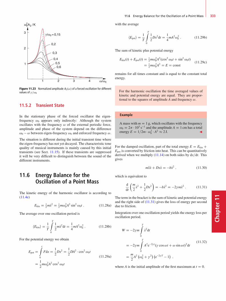
11.6 Energy Balance for the Oscillation of a Point Mass 333
Chap
ter11
Figure 11.23 Normalized amplitude A2.!/ of a forced oscillation for differentvalues of �=!0
11.5.2 Transient State
In the stationary phase of the forced oscillator the eigen-frequency !0 appears only indirectly: Although the systemoscillates with the frequency ! of the external periodic force,amplitude and phase of the system depend on the difference!0 � ! between eigen-frequency !0 and enforced frequency !.
The situation is different during the initial transient time wherethe eigen-frequency has not yet decayed. The characteristic tonequality of musical instruments is mainly caused by this initialtransients (see Sect. 11.15). If these transients are suppressedit will be very difficult to distinguish between the sound of thedifferent instruments.
11.6 Energy Balance for theOscillation of a Point Mass
The kinetic energy of the harmonic oscillator is according to(11.4e)
Ekin D 12mPx2 D 1
2m!20A
2 sin2 !0t : (11.28a)
The average over one oscillation period is
hEkini D 1
T
TZ
0
1
2mPx2dt D 1
4mA2!2
0 : (11.28b)
For the potential energy we obtain
Epot DxZ
0
Fdx D 1
2Dx2 D 1
2DA2 � cos2 !0t
D 1
2m!2
0A2 cos2 !0t
(11.29a)
with the average
hEpoti D 1
T
TZ
0
1
2Dx2dt D 1
4mA2!2
0 : (11.29b)
The sum of kinetic plus potential energy
Ekin.t/C Epot.t/ D 12m!
20A
2.cos2 !0t C sin2 !0t/
D 12m!
20A
2 D E D const(11.29c)
remains for all times constant and is equal to the constant totalenergy.
For the harmonic oscillation the time averaged values ofkinetic and potential energy are equal. They are propor-tional to the squares of amplitude A and frequency !.
Example
Amass with m D 1 g, which oscillates with the frequency!0 D 2 � 103 s�1 and the amplitude A D 1 cm has a totalenergy E D 1=2m � !2
0 � A2 � 2 J. J
For the damped oscillation, part of the total energy E D Ekin CEpot is converted by friction into heat. This can be quantitativelyderived when we multiply (11.14) on both sides by dx=dt. Thisgives
mRxPx C DxPx D �bPx2 ; (11.30)
which is equivalent to
d
dt
�m
2Px2 C 1
2Dx2
�D �bPx2 D �2�mPx2 : (11.31)
The term in the bracket is the sum of kinetic and potential energyand the right side of (11.31) gives the loss of energy per seconddue to friction.
Integration over one oscillation period yields the energy loss peroscillation period.
W D �2�m
TZ
0
Px2dt
D �2�m
TZ
0
A2e�2� t.� cos!t C ! sin!t/2dt
D m
2A2�!20 C �2
� �e�2�T � 1
�;
(11.32)
where A is the initial amplitude of the first maximum at t D 0.
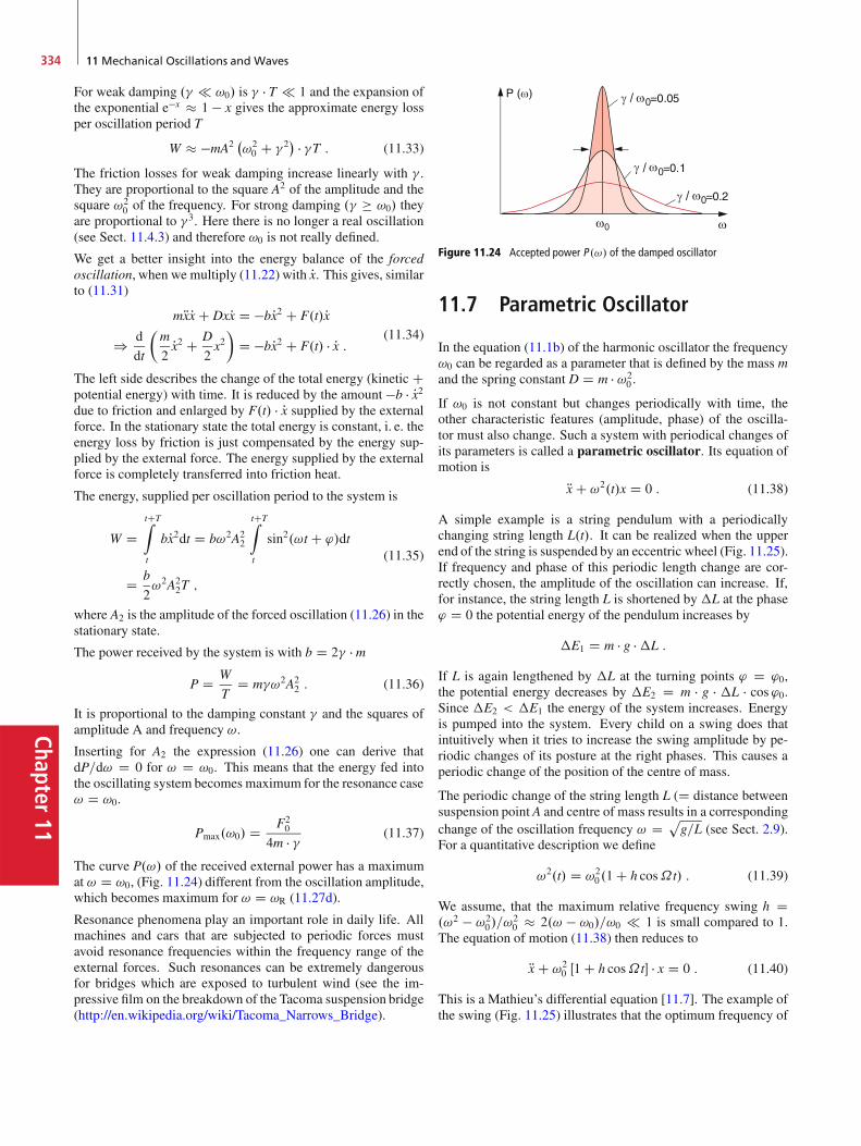
Chapter11
334 11 Mechanical Oscillations and Waves
For weak damping .� !0/ is � � T 1 and the expansion ofthe exponential e�x � 1 � x gives the approximate energy lossper oscillation period T
W � �mA2�!20 C �2
� � �T : (11.33)
The friction losses for weak damping increase linearly with � .They are proportional to the square A2 of the amplitude and thesquare !2
0 of the frequency. For strong damping .� � !0/ theyare proportional to �3. Here there is no longer a real oscillation(see Sect. 11.4.3) and therefore !0 is not really defined.
We get a better insight into the energy balance of the forcedoscillation, when we multiply (11.22) with Px. This gives, similarto (11.31)
mRxPx C DxPx D �bPx2 C F.t/Px) d
dt
�m
2Px2 C D
2x2�
D �bPx2 C F.t/ � Px : (11.34)
The left side describes the change of the total energy (kinetic Cpotential energy) with time. It is reduced by the amount �b � Px2due to friction and enlarged by F.t/ � Px supplied by the externalforce. In the stationary state the total energy is constant, i. e. theenergy loss by friction is just compensated by the energy sup-plied by the external force. The energy supplied by the externalforce is completely transferred into friction heat.
The energy, supplied per oscillation period to the system is
W DtCTZ
t
bPx2dt D b!2A22
tCTZ
t
sin2.!t C '/dt
D b
2!2A2
2T ;
(11.35)
where A2 is the amplitude of the forced oscillation (11.26) in thestationary state.
The power received by the system is with b D 2� � m
P D W
TD m�!2A2
2 : (11.36)
It is proportional to the damping constant � and the squares ofamplitude A and frequency !.
Inserting for A2 the expression (11.26) one can derive thatdP=d! D 0 for ! D !0. This means that the energy fed intothe oscillating system becomes maximum for the resonance case! D !0.
Pmax.!0/ D F20
4m � � (11.37)
The curve P.!/ of the received external power has a maximumat ! D !0, (Fig. 11.24) different from the oscillation amplitude,which becomes maximum for ! D !R (11.27d).
Resonance phenomena play an important role in daily life. Allmachines and cars that are subjected to periodic forces mustavoid resonance frequencies within the frequency range of theexternal forces. Such resonances can be extremely dangerousfor bridges which are exposed to turbulent wind (see the im-pressive film on the breakdown of the Tacoma suspension bridge(http://en.wikipedia.org/wiki/Tacoma_Narrows_Bridge).
Figure 11.24 Accepted power P .!/ of the damped oscillator
11.7 Parametric Oscillator
In the equation (11.1b) of the harmonic oscillator the frequency!0 can be regarded as a parameter that is defined by the mass mand the spring constant D D m � !2
0 .
If !0 is not constant but changes periodically with time, theother characteristic features (amplitude, phase) of the oscilla-tor must also change. Such a system with periodical changes ofits parameters is called a parametric oscillator. Its equation ofmotion is
Rx C !2.t/x D 0 : (11.38)
A simple example is a string pendulum with a periodicallychanging string length L.t/. It can be realized when the upperend of the string is suspended by an eccentric wheel (Fig. 11.25).If frequency and phase of this periodic length change are cor-rectly chosen, the amplitude of the oscillation can increase. If,for instance, the string length L is shortened by �L at the phase' D 0 the potential energy of the pendulum increases by
�E1 D m � g ��L :
If L is again lengthened by �L at the turning points ' D '0,the potential energy decreases by �E2 D m � g � �L � cos'0.Since �E2 < �E1 the energy of the system increases. Energyis pumped into the system. Every child on a swing does thatintuitively when it tries to increase the swing amplitude by pe-riodic changes of its posture at the right phases. This causes aperiodic change of the position of the centre of mass.
The periodic change of the string length L (D distance betweensuspension point A and centre of mass results in a correspondingchange of the oscillation frequency ! D p
g=L (see Sect. 2.9).For a quantitative description we define
!2.t/ D !20 .1 C h cos˝t/ : (11.39)
We assume, that the maximum relative frequency swing h D.!2 � !2
0/=!20 � 2.! � !0/=!0 1 is small compared to 1.
The equation of motion (11.38) then reduces to
Rx C !20 Œ1 C h cos˝t� � x D 0 : (11.40)
This is a Mathieu’s differential equation [11.7]. The example ofthe swing (Fig. 11.25) illustrates that the optimum frequency of
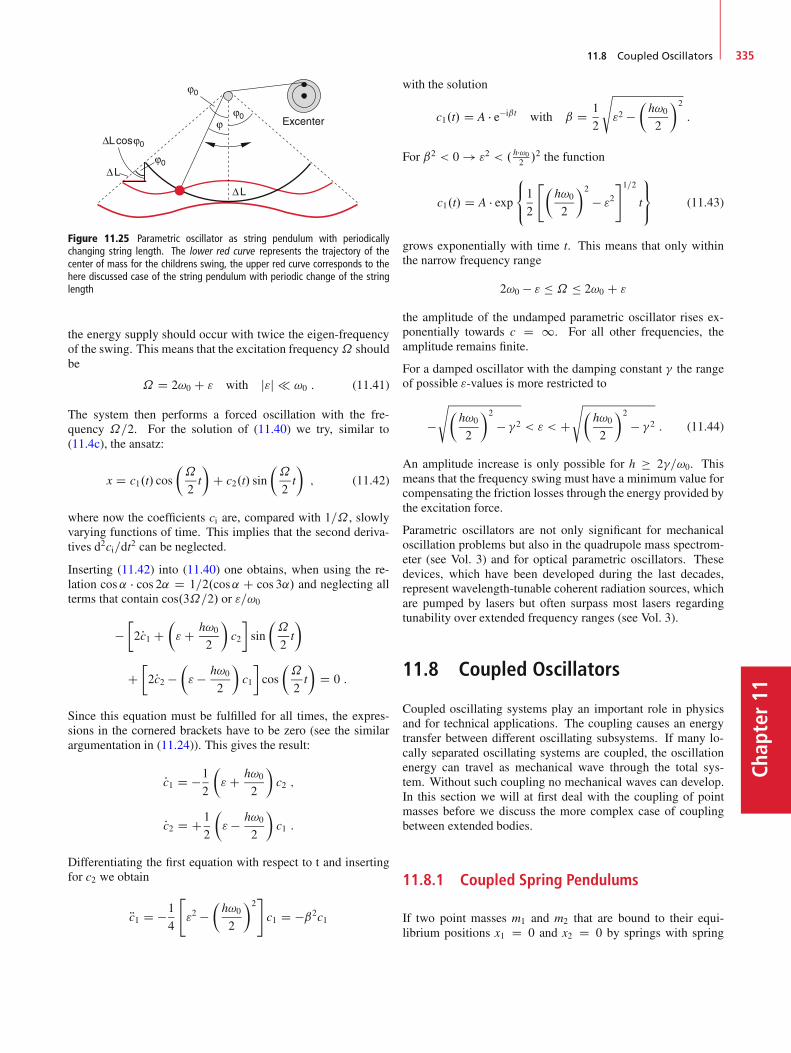
11.8 Coupled Oscillators 335
Chap
ter11
Excenter
Figure 11.25 Parametric oscillator as string pendulum with periodicallychanging string length. The lower red curve represents the trajectory of thecenter of mass for the childrens swing, the upper red curve corresponds to thehere discussed case of the string pendulum with periodic change of the stringlength
the energy supply should occur with twice the eigen-frequencyof the swing. This means that the excitation frequency˝ shouldbe
˝ D 2!0 C " with j"j !0 : (11.41)
The system then performs a forced oscillation with the fre-quency ˝=2. For the solution of (11.40) we try, similar to(11.4c), the ansatz:
x D c1.t/ cos
�˝
2t
�C c2.t/ sin
�˝
2t
�; (11.42)
where now the coefficients ci are, compared with 1=˝ , slowlyvarying functions of time. This implies that the second deriva-tives d2ci=dt2 can be neglected.
Inserting (11.42) into (11.40) one obtains, when using the re-lation cos˛ � cos 2˛ D 1=2.cos˛ C cos 3˛/ and neglecting allterms that contain cos.3˝=2/ or "=!0
��2Pc1 C
�"C h!0
2
�c2
�sin
�˝
2t
�
C�2Pc2 �
�" � h!0
2
�c1
�cos
�˝
2t
�D 0 :
Since this equation must be fulfilled for all times, the expres-sions in the cornered brackets have to be zero (see the similarargumentation in (11.24)). This gives the result:
Pc1 D �1
2
�"C h!0
2
�c2 ;
Pc2 D C1
2
�" � h!0
2
�c1 :
Differentiating the first equation with respect to t and insertingfor c2 we obtain
Rc1 D �1
4
""2 �
�h!0
2
�2#c1 D �ˇ2c1
with the solution
c1.t/ D A � e�iˇt with ˇ D 1
2
s
"2 ��h!0
2
�2
:
For ˇ2 < 0 ! "2 < . h�!02 /
2 the function
c1.t/ D A � exp8<
:1
2
"�h!0
2
�2
� "2#1=2
t
9=
; (11.43)
grows exponentially with time t. This means that only withinthe narrow frequency range
2!0 � " � ˝ � 2!0 C "
the amplitude of the undamped parametric oscillator rises ex-ponentially towards c D 1. For all other frequencies, theamplitude remains finite.
For a damped oscillator with the damping constant � the rangeof possible "-values is more restricted to
�s�
h!0
2
�2
� �2 < " < Cs�
h!0
2
�2
� �2 : (11.44)
An amplitude increase is only possible for h � 2�=!0. Thismeans that the frequency swing must have a minimum value forcompensating the friction losses through the energy provided bythe excitation force.
Parametric oscillators are not only significant for mechanicaloscillation problems but also in the quadrupole mass spectrom-eter (see Vol. 3) and for optical parametric oscillators. Thesedevices, which have been developed during the last decades,represent wavelength-tunable coherent radiation sources, whichare pumped by lasers but often surpass most lasers regardingtunability over extended frequency ranges (see Vol. 3).
11.8 Coupled Oscillators
Coupled oscillating systems play an important role in physicsand for technical applications. The coupling causes an energytransfer between different oscillating subsystems. If many lo-cally separated oscillating systems are coupled, the oscillationenergy can travel as mechanical wave through the total sys-tem. Without such coupling no mechanical waves can develop.In this section we will at first deal with the coupling of pointmasses before we discuss the more complex case of couplingbetween extended bodies.
11.8.1 Coupled Spring Pendulums
If two point masses m1 and m2 that are bound to their equi-librium positions x1 D 0 and x2 D 0 by springs with spring
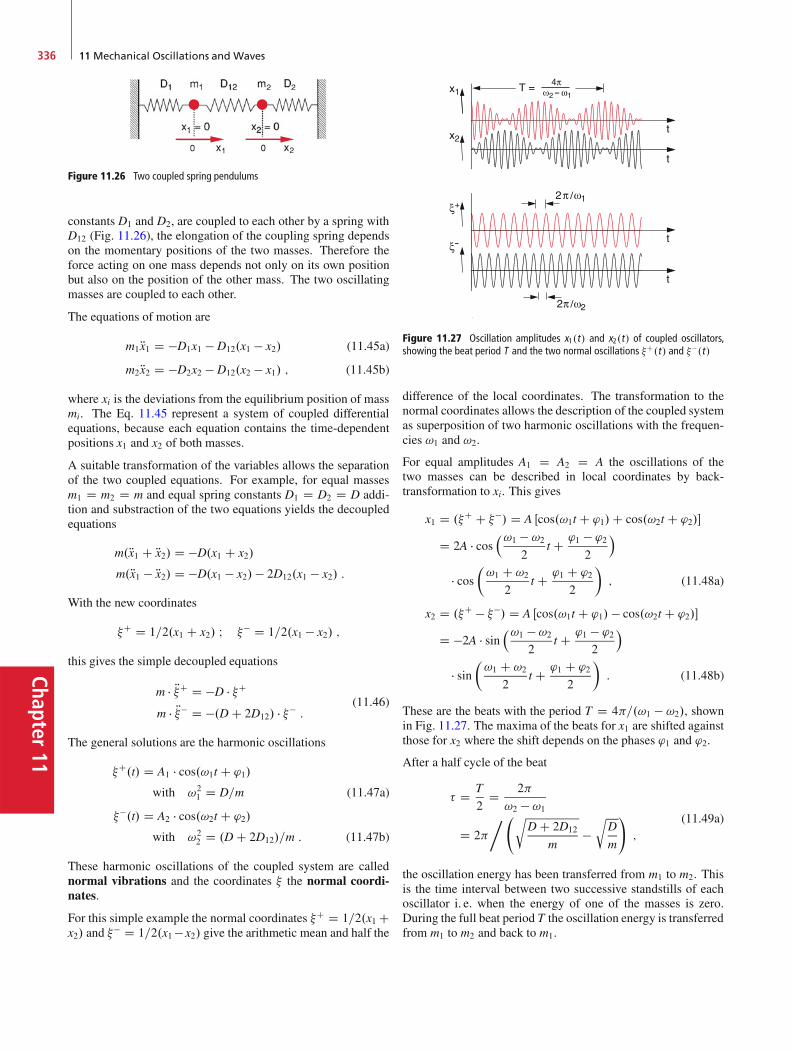
Chapter11
336 11 Mechanical Oscillations and Waves
Figure 11.26 Two coupled spring pendulums
constants D1 and D2, are coupled to each other by a spring withD12 (Fig. 11.26), the elongation of the coupling spring dependson the momentary positions of the two masses. Therefore theforce acting on one mass depends not only on its own positionbut also on the position of the other mass. The two oscillatingmasses are coupled to each other.
The equations of motion are
m1 Rx1 D �D1x1 � D12.x1 � x2/ (11.45a)
m2 Rx2 D �D2x2 � D12.x2 � x1/ ; (11.45b)
where xi is the deviations from the equilibrium position of massmi. The Eq. 11.45 represent a system of coupled differentialequations, because each equation contains the time-dependentpositions x1 and x2 of both masses.
A suitable transformation of the variables allows the separationof the two coupled equations. For example, for equal massesm1 D m2 D m and equal spring constants D1 D D2 D D addi-tion and substraction of the two equations yields the decoupledequations
m.Rx1 C Rx2/ D �D.x1 C x2/
m.Rx1 � Rx2/ D �D.x1 � x2/ � 2D12.x1 � x2/ :
With the new coordinates
�C D 1=2.x1 C x2/ I �� D 1=2.x1 � x2/ ;
this gives the simple decoupled equations
m � R�C D �D � �C
m � R�� D �.D C 2D12/ � �� :(11.46)
The general solutions are the harmonic oscillations
�C.t/ D A1 � cos.!1t C '1/
with !21 D D=m (11.47a)
��.t/ D A2 � cos.!2t C '2/
with !22 D .D C 2D12/=m : (11.47b)
These harmonic oscillations of the coupled system are callednormal vibrations and the coordinates � the normal coordi-nates.
For this simple example the normal coordinates �C D 1=2.x1 Cx2/ and �� D 1=2.x1 � x2/ give the arithmetic mean and half the
Figure 11.27 Oscillation amplitudes x1.t/ and x2.t/ of coupled oscillators,showing the beat period T and the two normal oscillations �C.t/ and ��.t/
difference of the local coordinates. The transformation to thenormal coordinates allows the description of the coupled systemas superposition of two harmonic oscillations with the frequen-cies !1 and !2.
For equal amplitudes A1 D A2 D A the oscillations of thetwo masses can be described in local coordinates by back-transformation to xi. This gives
x1 D .�C C ��/ D A Œcos.!1t C '1/C cos.!2t C '2/�
D 2A � cos�!1 � !2
2t C '1 � '2
2
� cos�!1 C !2
2t C '1 C '2
2
�; (11.48a)
x2 D .�C � ��/ D A Œcos.!1t C '1/ � cos.!2t C '2/�
D �2A � sin�!1 � !2
2t C '1 � '2
2
� sin�!1 C !2
2t C '1 C '2
2
�: (11.48b)
These are the beats with the period T D 4=.!1 � !2/, shownin Fig. 11.27. The maxima of the beats for x1 are shifted againstthose for x2 where the shift depends on the phases '1 and '2.
After a half cycle of the beat
� D T
2D 2
!2 � !1
D 2� r
D C 2D12
m�r
D
m
!;
(11.49a)
the oscillation energy has been transferred from m1 to m2. Thisis the time interval between two successive standstills of eachoscillator i. e. when the energy of one of the masses is zero.During the full beat period T the oscillation energy is transferredfrom m1 to m2 and back to m1.
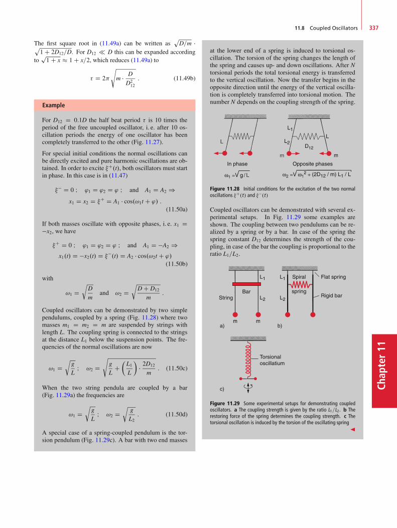
11.8 Coupled Oscillators 337
Chap
ter11
The first square root in (11.49a) can be written aspD=m �p
1 C 2D12=D. For D12 D this can be expanded accordingto
p1 C x � 1 C x=2, which reduces (11.49a) to
� D 2
sm � D
D212
: (11.49b)
Example
For D12 D 0:1D the half beat period � is 10 times theperiod of the free uncoupled oscillator, i. e. after 10 os-cillation periods the energy of one oscillator has beencompletely transferred to the other (Fig. 11.27).
For special initial conditions the normal oscillations canbe directly excited and pure harmonic oscillations are ob-tained. In order to excite �C.t/, both oscillators must startin phase. In this case is in (11.47)
�� D 0 I '1 D '2 D ' I and A1 D A2 )x1 D x2 D �C D A1 � cos.!1t C '/ :
(11.50a)
If both masses oscillate with opposite phases, i. e. x1 D�x2, we have
�C D 0 I '1 D '2 D ' I and A1 D �A2 )x1.t/ D �x2.t/ D ��.t/ D A2 � cos.!2t C '/
(11.50b)
with
!1 Dr
D
mand !2 D
rD C D12
m:
Coupled oscillators can be demonstrated by two simplependulums, coupled by a spring (Fig. 11.28) where twomasses m1 D m2 D m are suspended by strings withlength L. The coupling spring is connected to the stringsat the distance L1 below the suspension points. The fre-quencies of the normal oscillations are now
!1 Dr
g
LI !2 D
sg
LC�L1L
�� 2D12
m: (11.50c)
When the two string pendula are coupled by a bar(Fig. 11.29a) the frequencies are
!1 Dr
g
LI !2 D
rg
L2: (11.50d)
A special case of a spring-coupled pendulum is the tor-sion pendulum (Fig. 11.29c). A bar with two end masses
at the lower end of a spring is induced to torsional os-cillation. The torsion of the spring changes the length ofthe spring and causes up- and down oscillations. After Ntorsional periods the total torsional energy is transferredto the vertical oscillation. Now the transfer begins in theopposite direction until the energy of the vertical oscilla-tion is completely transferred into torsional motion. Thenumber N depends on the coupling strength of the spring.
Opposite phasesIn phase
L
L1
L2
(2D12 / m) L1 / L
Figure 11.28 Initial conditions for the excitation of the two normaloscillations �C.t/ and ��.t/
Coupled oscillators can be demonstrated with several ex-perimental setups. In Fig. 11.29 some examples areshown. The coupling between two pendulums can be re-alized by a spring or by a bar. In case of the spring thespring constant D12 determines the strength of the cou-pling, in case of the bar the coupling is proportional to theratio L1=L2.
StringBar
Rigid bar
Torsionaloscillatium
L1 L1
L2 L2
Flat springSpiral
spring
Figure 11.29 Some experimental setups for demonstrating coupledoscillators. a The coupling strength is given by the ratio L1=L2. b Therestoring force of the spring determines the coupling strength. c Thetorsional oscillation is induced by the torsion of the oscillating spring
J

Chapter11
338 11 Mechanical Oscillations and Waves
11.8.2 Forced Oscillations of Two CoupledOscillators
When the coupled oscillators in Fig. 11.26 are exposed to an ex-ternal periodic force F D F0 cos!t that acts on m1 (Fig. 11.30a)both masses are excited to forced oscillations, due to the cou-pling between m1 and m2. The equations of motion (11.45) thenbecome with m1 D m2 D m
mRx1 D �D1x1 � D12.x1 � x2/
� 2m� Px1 C F0 � cos!t (11.51a)
mRx2 D �D2x2 C D12.x1 � x2/
� 2m� Px2 ; (11.51b)
where � D b=2m is the damping constant.
For � D 0 and F0 D 0 we obtain Eq. 11.45 of the undampedcoupled oscillators. When we introduce again the normal coor-dinates
�C D x1 C x22
and �� D x1 � x22
:
We obtain after adding and subtracting the two equations for thecase D1 D D2 D D the decoupled equations
m R�C D �D�C � 2m� P�C C 12F0 cos!t ; (11.52a)
m R�� D �.D C 2D12/�� � 2m� P�� C 1
2F0 cos!t : (11.52b)
Each of these equations represents a forced oscillation. Thismeans that the two normal oscillations can be regarded as forcedoscillations with the eigen-frequencies
!1 Dp.D=m � �2/ I !2 D
p.D C D12=m � �2/ :
Excenter
Figure 11.30 Forced oscillation of coupled oscillators. a Coupling by springs;b coupling by a bar
B
B
Figure 11.31 Amplitudes A�1 (black curves), B1 (red curves) and A�
2 ; B2 of theamplitudes of coupled forced oscillators, that are driven by the force F0 � cos!t ,acting on pendulum 1
Their amplitudes can be determined from (11.52), where for �Cthe eigen-frequency is ! D !1 and for �� it is ! D !2.
When the exciting frequency ! is tuned one observes reso-nances at the frequencies !�
1 D pD=m � 2�2 and !�
2 Dp.D C 2D12/=m � 2�2 (see (11.27d).
For the oscillations of the two pendulums in Fig. 11.30b with
x1 D �C C �� D A1 cos!t C B1 � sin!tx2 D �C � �� D A2 cos ;
we obtain for the representation
xi D Ai � sin ' C Bi � cos'
the amplitudes A1, B1 and A2, B2. Art the frequency !�1 only the
oscillation �C contributes essentially, for !�2 only ��.
In Fig. 11.31 the amplitudes A�1 D 2.!2
1=K/ � A1 and A�2 D
2.!22=K/ � A2, are plotted, normalized to the driving force
F D K � ei!t D K.cos!t C i � sin!t/ ;
with K D F0=m (black curves) and B�i D 2.!2
i =K/Bi (redcurves).
Such coupled forced oscillations can be demonstrated by differ-ent arrangements. One example is shown in Fig. 11.30b, wheretwo spring pendulums are coupled by a rigid bar while m1 iscoupled to the external force driven by an excenter. The cou-pling strength between the two pendulums can be varied withthe height of the bar and the coupling to the external force bythe modulation amplitude of the excenter.

11.9 Mechanical Waves 339
Chap
ter11
11.8.3 Normal Vibrations
In nature one finds many examples of coupled vibrations. Thenumber N of coupled oscillations is not restricted to N D 2 butcan be large integers. For instance in a solid crystal all N atomsare coupled by electromagnetic forces interacting between theatoms. For a crystal with a volume of 1 cm3 is N D 1023. If oneatom is excited to vibrations, it transfers its excitation energy tomany atoms in the crystal.
We will at first consider the one-dimensional case of N atoms ona line, which are all coupled by springs with the same couplingconstant as illustrated for N D 5 in Fig. 11.32. The possible 5coupled oscillations are also shown.
Analogue to the Eq. 11.45 one obtains a system of 5 equations.They can be arranged in form of a matrix, where equal massesare assumed.
m �
0
BBBBBBB@
Rx1Rx2Rx3Rx4Rx5
1
CCCCCCCA
D
0
BBBBBBB@
�2D D 0 0 0
D �2D D 0 0
0 D �2D D 0
0 0 D �2D D
0 0 0 D �2D
1
CCCCCCCA
0
BBBBBBB@
x1
x2
x3
x4
x5
1
CCCCCCCA
: (11.53a)
The solutions of these equations give the frequencies !N .N D0; 1; 2; 3; 4/. The result is
!0 Dq.2 � p
3/D=m I !1 D pD=m I
!2 D p2D=m I !3 D p
3D=m I
!4 Dq.2 C p
3/D=m :
(11.53b)
Each of these 5 normal vibrations describes a state where allmasses perform harmonic oscillations with the same frequency!N .
Every arbitrary oscillation of the system can be always de-scribed as a superposition of normal vibrations.
Figure 11.32 Longitudinal oscillation of a linear chain of five equal masses
Figure 11.33 The three normal vibrations of a nonlinear triatomic moleculeAB2, where the center of mass remains at rest
Examples of oscillations where the masses do not move alonga line, are the vibrations of polyatomic molecules (see Vol. 3).They can be also described as superposition of normal vibra-tions, which can be deduced by the following considerations.
Each of the N atoms of a molecule has 3 degrees of freedomfor its motion. A molecule with N atoms therefore has 3N de-grees of freedom. If the molecule would be a rigid body (i. e.the atoms could not vibrate) its motion could be described as asuperposition of the translation of its centre of mass (3 degreesof freedom) and a rotation around this centre (3 degrees of free-dom, see Sect. 5.1). For the vibrations therefore 3N � 6 degreesof freedom are left. This is valid for nonlinear molecules. Linearmolecules cannot rotate around their axis (because the momentof inertia would be extremely small and therefore its rotationenergy extremely high (see Eq. 5.16b)).
In summary: Linear molecules with N atoms have 3N � 5 de-grees of freedom for their vibrations and therefore 3N�5 normalvibrations. Nonlinear molecules have 3N�6 vibrational degreesof freedom and 3N � 6 normal vibrations. Since translation androtation are already subtracted normal vibrations are those mo-tions of the nuclear frame of the molecule, where the centre ofmass does not move and the rotational angular momentum iszero.
In Fig. 11.33 the three normal vibrations of a triatomic bendmolecule are shown. For all three normal vibrations the centreof mass is locally fixed and the angular momentum is zero.
11.9 Mechanical Waves
When an oscillating point mass m1 is coupled with other neigh-bouring masses the oscillation energy is transported from m1 tothe neighbours. (Fig. 11.34). For a transport velocity v anda distance to the neighbouring masses �z the energy transportneeds the time�t D �z=v.
This spatial transport of oscillation energy is called a wave. Ex-amples for mechanical waves are water waves, acoustic wavesor pressure waves in solids, liquids or gases.
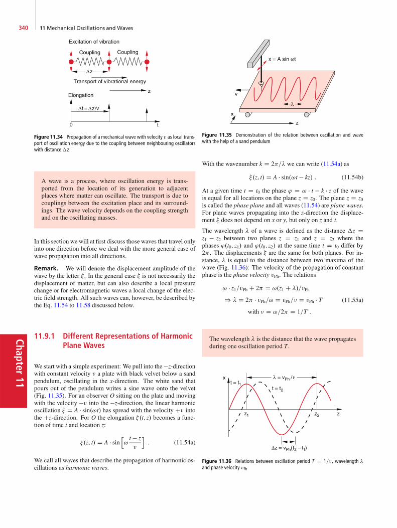
Chapter11
340 11 Mechanical Oscillations and Waves
Figure 11.34 Propagation of a mechanical wave with velocity v as local trans-port of oscillation energy due to the coupling between neighbouring oscillatorswith distance�z
A wave is a process, where oscillation energy is trans-ported from the location of its generation to adjacentplaces where matter can oscillate. The transport is due tocouplings between the excitation place and its surround-ings. The wave velocity depends on the coupling strengthand on the oscillating masses.
In this section we will at first discuss those waves that travel onlyinto one direction before we deal with the more general case ofwave propagation into all directions.
Remark. We will denote the displacement amplitude of thewave by the letter � . In the general case � is not necessarily thedisplacement of matter, but can also describe a local pressurechange or for electromagnetic waves a local change of the elec-tric field strength. All such waves can, however, be described bythe Eq. 11.54 to 11.58 discussed below.
11.9.1 Different Representations of HarmonicPlane Waves
We start with a simple experiment: We pull into the �z-directionwith constant velocity v a plate with black velvet below a sandpendulum, oscillating in the x-direction. The white sand thatpours out of the pendulum writes a sine wave onto the velvet(Fig. 11.35). For an observer O sitting on the plate and movingwith the velocity �v into the �z-direction, the linear harmonicoscillation � D A � sin.!t/ has spread with the velocity Cv intothe Cz-direction. For O the elongation �.t; z/ becomes a func-tion of time t and location z:
�.z; t/ D A � sinh!t � z
v
i: (11.54a)
We call all waves that describe the propagation of harmonic os-cillations as harmonic waves.
λ
Figure 11.35 Demonstration of the relation between oscillation and wavewith the help of a sand pendulum
With the wavenumber k D 2=� we can write (11.54a) as
�.z; t/ D A � sin.!t � kz/ : (11.54b)
At a given time t D t0 the phase ' D ! � t � k � z of the waveis equal for all locations on the plane z D z0. The plane z D z0is called the phase plane and all waves (11.54) are plane waves.For plane waves propagating into the z-direction the displace-ment � does not depend on x or y, but only on z and t.
The wavelength � of a wave is defined as the distance �z Dz1 � z2 between two planes z D z1 and z D z2 where thephases '.t0; z1/ and '.t0; z2/ at the same time t D t0 differ by2 . The displacements � are the same for both planes. For in-stance, � is equal to the distance between two maxima of thewave (Fig. 11.36): The velocity of the propagation of constantphase is the phase velocity vPh. The relations
! � z1=vPh C 2 D !.z1 C �/=vPh
) � D 2 � vPh=! D vPh=� D vPh � Twith � D !=2 D 1=T :
(11.55a)
The wavelength � is the distance that the wave propagatesduring one oscillation period T .
Figure 11.36 Relations between oscillation period T D 1=�, wavelength �and phase velocity vPh

11.9 Mechanical Waves 341
Chap
ter11
For an observer who moves with the phase velocity of the wave(he is, for example, always sitting on a maximum of the wave),the phase of the wave stays constant. For him is
d.!t � kz/
dtD 0 ) ! � k � dz
dtD 0 ) dz
dtD !
k:
The phase velocity in (11.55a) is then with � D !=2
vPh D !
kD � � � : (11.55b)
The phase velocity vPh is equal to the ratio of angular ve-locity ! and wave number k.
It depends on the coupling strength between neighbouringatoms. their density and on the mass of the oscillating atoms.
The following descriptions of plane waves propagating into thez-direction are equivalent:
�.z; t/ D A � sin.!t � kz/
D A � sin�2
�.vPh � t � z/
�
D A � sinh2vPh � t � z
�
i:
(11.56)
In Sect. 11.1 it was shown, that oscillations can be also de-scribed by complex functions. This means that the real part aswell as the imaginary part of the complex function
ei!t D cos!t C i � sin!tare solutions of the oscillation equation. In a similar way har-monic waves can be written in a complex form as
�.z; t/ D C � ei.!t�kz/ C C� � e�i.!t�kz/ : (11.57a)
This is equivalent to
�.z; t/ D A � cos.!t � kz/C B � sin.!t � kz/
with A D C C C� and B D i.C � C�/ :(11.57b)
Often only the complex amplitude is written as an abbreviatedversion:
�.z; t/ D C � ei.!t�kz/ : (11.57c)
The real and the imaginary part are then the representations ofthe real wave.
11.9.2 Summary
Each of the representations (11.56), (11.57) of a harmonic wavedescribes:
Figure 11.37 Illustration of a harmonic wave a as stationary oscillator �.zo ; t/at a fixed position z0, b as spatially periodic function �.z ; t0/ at a fixed time t0
at a fixed position z D z0 a periodic harmonic oscillation
�.t/ D A � sin.!t � kz0/ D A � sin.!t � '/ (11.58a)
with the period T D 2=! and the phase '.t D 0/ D k � z0(Fig. 11.37a),at a fixed time t D t0 a spatially period function
�.z/ D A � cos.!t0 � kz/ (11.58b)
with the wavelength � D 2=k and the initial phase '.z D0/ D ! � t0 (Fig. 11.37b).
11.9.3 General Description of ArbitraryWaves; Wave-Equation
The harmonic sine wave described so far, is only a special typeof a great variety of different wave forms. We will thereforediscuss a more general description of waves propagating intothe z-direction. The following consideration will lead us to sucha general description:
A physical quantity (for example pressure, temperature, me-chanical displacement, electrical field strength etc.) shouldexperience a local perturbation � as deviation from the equi-librium conditions. Due to the coupling with the neighbouringparticles this perturbation will propagate in space in the courseof time. We call this propagation process a wave. We will studyits characteristics at first for one-dimensional waves that propa-gate into the z-direction. A simple example is the deflection ofa string stretched in the z-direction at t D 0 (Fig. 11.38). In thecourse of time this deflection will propagate into the z-direction.
If the perturbation � occurs at the time t D 0 at the positionz D z0 it will propagate with the velocity v and reach at a later
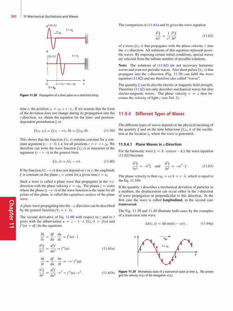
Chapter11
342 11 Mechanical Oscillations and Waves
z1 = z0 + v(t1 – t0)z0
(z0, t0)
Figure 11.38 Propagation of a short pulse on a stretched string
time t1 the position z1 D z0 C v � t1. If we assume that the formof the deviation does not change during its propagation into thez-direction, we obtain the equation for the time- and position-dependent perturbation � as
�.z1; t1/ D �.z1 � vt1; 0/ D �.z0; 0/ : (11.59)
This shows that the function �.z; t/ remains constant for a con-stant argument .z� v � t/, i. e. for all positions z D v � tC z0. Wetherefore can write the wave function �.z; t/ as functions of theargument .z � v � t/ in the general form
�.z; t/ D f .z � vt/ : (11.60)
If the function f .z�v �t/ does not depend on x or y, the amplitude� is constant on the plane z D const for a given time t D t0.
Such a wave is called a plane wave that propagates in the Cz-direction with the phase velocity v D vPh. The planes z D constwhere the phase .z�v � t/ of the wave function is the same for allpoints of this plane, is called the equiphase surface of the planewave.
A plane wave propagating into the�z-direction can be describedby the general function f .z C v � t/.The second derivative of Eq. 11.60 with respect to z and to tgives with the abbreviation u D z � v � t, �.z; t/ D f .u/ andf 0.u/ D df =du the equations
@�
@zD df
du� dudz
D f 0.u/ � 1
@2�
@z2D d2f
du2D f 00.u/ (11.61a)
@�
@tD df
du� @u@t
D �v � f 0.u/
@2�
@t2D d2f
du2� v2 D f 00.u/ � v2 : (11.61b)
The comparison of (11.61a and b) gives the wave equation
@2�
@z2D 1
v2@2�
@t2(11.62)
of a wave �.z; t/ that propagates with the phase velocity v intothe Cz-direction. All solutions of this equation represent possi-ble waves. By imposing certain initial conditions, special wavesare selected from the infinite number of possible solutions.
Note: The solutions of (11.62) are not necessary harmonicwaves and even not periodic waves. Also short pulses �.z; t/ thatpropagate into the z-direction (Fig. 11.38) can fulfil the waveequation (11.62) and are therefore also called “waves”.
The quantity � can be also the electric or magnetic field strength.Therefore (11.62) not only describes mechanical waves but alsoelectro-magnetic waves. The phase velocity v D c then be-comes the velocity of light c (see Vol. 2).
11.9.4 Different Types of Waves
The different types of waves depend on the physical meaning ofthe quantity � and on the time behaviour �.z0; t/ of the oscilla-tion at the location z0 where the wave is generated.
11.9.4.1 Plane Waves in z-Direction
For the harmonic wave � D A � cos.!t � kz/ the wave equation(11.62) becomes
@2�
@z2D �k2� and
@2�
@t2D �!2 � � : (11.63)
The phase velocity is then vPh D !=k D � � �, which is equal tothe Eq. 11.55b.
If the quantity x describes a mechanical deviation of particles ina medium, the displacement can occur either in the z-directionof wave propagation or perpendicular to this direction. In thefirst case the wave is called longitudinal, in the second casetransversal.
The Fig. 11.39 and 11.40 illustrate both cases by the examplesof a transverse sine wave
�x.z; t/ D AOx sin.kz � !t/ ; (11.64a)
Figure 11.39 Momentary state of a transversal wave at time t0. The arrowsgive the velocity Px.t0/ of the elongation x.t0/

11.9 Mechanical Waves 343
Chap
ter11
Figure 11.40 Longitudinal wave with elongation � of the particles and theirvelocities vz (arrows) in the propagation direction z. The lower part illustratesschematically the shifts of the oscillating particles at t D t0
with the amplitude �x D x � x0, where Ox is the unit vector inx-direction.
For the longitudinal wave we obtain
�z.z; t/ D BOz sin.kz � !t/ ; (11.64b)
where the displacement of the oscillating particles occurs in thepropagation direction of the wave.
We will see below, that the phase velocity vPh D !=k of thedifferent wave types generally will be different because therestoring forces that determine the oscillation frequency ! isdifferent for shear displacements and for compression. Thevelocity depends, of course, also on the medium, because thecoupling strength between neighbouring atoms may be differentfor different materials.
When the displacement of the particles in a transverse wave oc-curs in a fixed plane (for instance in the x-direction) the waveis linearly polarized (Fig. 11.41a). The wave (11.64a) is for ex-ample for A D const a transverse wave, linearly polarized inx-direction and propagating into the z-direction.
Figure 11.41 a Linear polarized wave; b elliptical polarized wave
When two oscillations
x D A sin.!t C '1/
y D B sin.!t C '2/
with '1 ¤ '2 are superimposed, an elliptical oscillation in thex–y-plane is generated (see Sect. 11.3). If such an oscillationpropagates into the z-direction, an elliptical polarized transversewave emerges (Fig. 11.41b) which becomes for A D B and'1 D '2 ˙ =2 a circular polarized wave. Any elliptically po-larized wave can be generated by superposition of two linearlypolarized waves with orthogonal polarization.
The complex representation of an elliptically polarized wave isfor equal phase velocity of the two linearly polarized waves
� D �1 C �2 D �AOx C BOyei�'� ei.!t�kz/ : (11.65)
The real part as well as the imaginary part give the amplitude �of the wave (Fig. 11.41b).
11.9.4.2 Plane Waves with Arbitrary PropagationDirection
When a plane wave propagates into an arbitrary direction wedescribe the propagation direction by the wave vector
k D fkx; ky; kzg : (11.66)
The absolute value k D jkj D 2=� is the wavenumber, alreadyintroduced in Sect. 11.9.1 (Fig. 11.42).
Since the equiphasic surfaces of a plane wave are planes perpen-dicular to the propagation direction k, the position vector r of apoint on this surface must obey the condition k � r D const. Thiscan be seen as follows: For the position vectors r1 and r2 of twopoints on the surface the difference r1�r2 must be a vector in thesurface. This implies: k � .r1 � r2/ D 0 ! k � r1 D k � r2 D const.
The representation of the plane harmonic wave is then
� D A sin.!t � k � r/ ; (11.67a)
because this ensures that for a fixed time all point on theequiphasic surface k � r D const have the same phase. The am-plitude vector A is perpendicular to k.
Figure 11.42 Plane wave with arbitrary propagation direction k
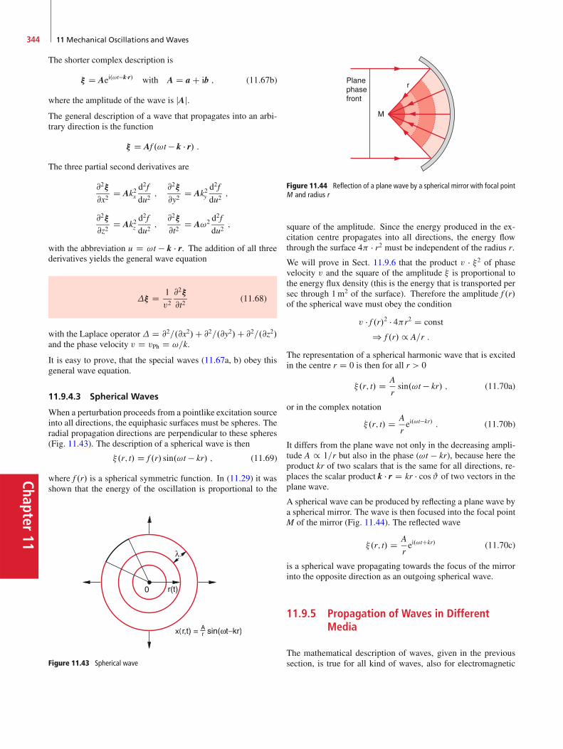
Chapter11
344 11 Mechanical Oscillations and Waves
The shorter complex description is
� D Aei.!t�k�r/ with A D a C ib ; (11.67b)
where the amplitude of the wave is jAj.The general description of a wave that propagates into an arbi-trary direction is the function
� D Af .!t � k � r/ :The three partial second derivatives are
@2�
@x2D Ak2x
d2f
du2;
@2�
@y2D Ak2y
d2f
du2;
@2�
@z2D Ak2z
d2f
du2;
@2�
@t2D A!2 d
2f
du2;
with the abbreviation u D !t � k � r. The addition of all threederivatives yields the general wave equation
�� D 1
v2@2�
@t2(11.68)
with the Laplace operator� D @2=.@x2/C @2=.@y2/C @2=.@z2/and the phase velocity v D vPh D !=k.
It is easy to prove, that the special waves (11.67a, b) obey thisgeneral wave equation.
11.9.4.3 Spherical Waves
When a perturbation proceeds from a pointlike excitation sourceinto all directions, the equiphasic surfaces must be spheres. Theradial propagation directions are perpendicular to these spheres(Fig. 11.43). The description of a spherical wave is then
�.r; t/ D f .r/ sin.!t � kr/ ; (11.69)
where f .r/ is a spherical symmetric function. In (11.29) it wasshown that the energy of the oscillation is proportional to the
Figure 11.43 Spherical wave
M
Planephasefront
r
Figure 11.44 Reflection of a plane wave by a spherical mirror with focal pointM and radius r
square of the amplitude. Since the energy produced in the ex-citation centre propagates into all directions, the energy flowthrough the surface 4 � r2 must be independent of the radius r.
We will prove in Sect. 11.9.6 that the product v � �2 of phasevelocity v and the square of the amplitude � is proportional tothe energy flux density (this is the energy that is transported persec through 1m2 of the surface). Therefore the amplitude f .r/of the spherical wave must obey the condition
v � f .r/2 � 4r2 D const
) f .r/ / A=r :
The representation of a spherical harmonic wave that is excitedin the centre r D 0 is then for all r > 0
�.r; t/ D A
rsin.!t � kr/ ; (11.70a)
or in the complex notation
�.r; t/ D A
rei.!t�kr/ : (11.70b)
It differs from the plane wave not only in the decreasing ampli-tude A / 1=r but also in the phase (!t � kr), because here theproduct kr of two scalars that is the same for all directions, re-places the scalar product k � r D kr � cos# of two vectors in theplane wave.
A spherical wave can be produced by reflecting a plane wave bya spherical mirror. The wave is then focused into the focal pointM of the mirror (Fig. 11.44). The reflected wave
�.r; t/ D A
rei.!tCkr/ (11.70c)
is a spherical wave propagating towards the focus of the mirrorinto the opposite direction as an outgoing spherical wave.
11.9.5 Propagation of Waves in DifferentMedia
The mathematical description of waves, given in the previoussection, is true for all kind of waves, also for electromagnetic
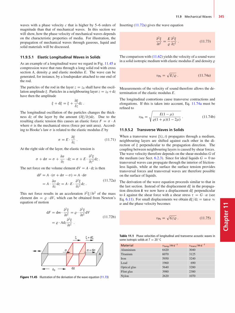
11.9 Mechanical Waves 345
Chap
ter11
waves with a phase velocity c that is higher by 5–6 orders ofmagnitude than that of mechanical waves. In this section wewill show, how the phase velocity of mechanical waves dependson the characteristic properties of media. For illustration, thepropagation of mechanical waves through gaseous, liquid andsolid materials will be discussed.
11.9.5.1 Elastic Longitudinal Waves in Solids
As an example of a longitudinal wave we regard in Fig. 11.45 acompression wave that runs through a long solid rod with crosssection A, density % and elastic modulus E. The wave can begenerated, for instance, by a loudspeaker attached to one end ofthe rod.
The particles of the rod in the layer z D z0 shall have the oscil-lation amplitude � . Particles in a neighbouring layer z D z0 Cdzhave then the amplitude
� C d� D � C @�
ızdz :
The longitudinal oscillation of the particles changes the thick-ness dz of the layer by the amount .@�=@z/dz. Due to theresulting elastic tension this causes an elastic force F D � � Awhere � is the mechanical stress (force per unit area). Accord-ing to Hooke’s law � is related to the elastic modulus E by
� D E � @�@z: (11.71)
At the right side of the layer, the elastic tension is
� C d� D � C @�
@z� dz D � C E � @
2�
@z2dz :
The net force on the volume element dV D A � dz is thendF D A � .� C d� � �/ D A � d�
D A � @�@z
dz D A � E � @2�
@z2dz :
(11.72a)
This net force results in an acceleration @2�=@t2 of the masselement dm D % � dV, which can be obtained from Newton’sequation of motion
dF D dm � @2�
@t2D % � @
2�
@t2dV
D % � Adz@2�
@t2:
(11.72b)
Figure 11.45 Illustration of the derivation of the wave equation (11.73)
Inserting (11.72a) gives the wave equation
@2�
@t2D E
%
@2�
@z2: (11.73)
The comparison with (11.62) yields the velocity of a soundwavein a solid isotropic mediumwith elastic modulusE and density %
vPh DpE=% : (11.74a)
Measurements of the velocity of sound therefore allows the de-termination of the elastic modulus E.
The longitudinal contortions cause transverse contractions andelongations. If this is taken into account, Eq. 11.74a must berefined to
vPh Ds
E.1 � /%.1 C /.1 � 2/
: (11.74b)
11.9.5.2 Transverse Waves in Solids
When a transverse wave �.z; t/ propagates through a medium,neighbouring layers are shifted against each other in the di-rection of � perpendicular to the propagation direction. Thecoupling between neighbouring layers is caused by shear forces.The wave velocity therefore depends on the shear-modulus G ofthe medium (see Sect. 6.2.3). Since for ideal liquids G D 0 notransversal waves can propagate through the interior of friction-less liquids, while at the surface the surface tension providestransversal forces and transversal waves are therefore possibleon the surface of liquids.
The derivation of the wave equation proceeds similar to that inthe last section. Instead of the displacement d� in the propaga-tion direction k we now have a displacement d� perpendicularto k against the shear force with a shear stress � D G � ˛ (seeEq. 6.11). For small displacements we obtain d�=dz D tan˛ �˛ and the phase velocity becomes
vPh DpG=% : (11.75)
Table 11.1 Phase velocities of longitudinal and transverse acoustic waves insome isotropic solids at T D 20 ıC
Material vlong=ms�1 vtrans=ms�1
Aluminium 6420 3040Titanium 6070 3125Iron 5950 3240Lead 1960 690Optical glas 5640 3280Flint glas 3980 2380Nylon 2620 1070
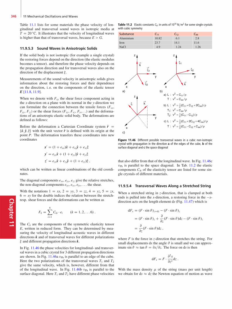
Chapter11
346 11 Mechanical Oscillations and Waves
Table 11.1 lists for some materials the phase velocity of lon-gitudinal and transversal sound waves in isotropic media atT D 20 ıC. It illustrates that the velocity of longitudinal wavesis higher than that of transversal waves, because E > G.
11.9.5.3 Sound Waves in Anisotropic Solids
If the solid body is not isotropic (for example a single crystal)the restoring forces depend on the direction (the elastic modulusbecomes a tensor). and therefore the phase velocity depends onthe propagation direction and for transversal waves also on thedirection of the displacement � .
Measurements of the sound velocity in anisotropic solids givesinformation about the restoring forces and their dependenceon the direction, i. e. on the components of the elastic tensorE [11.8, 11.9].
When we denote with Fxy the shear force component acting inthe x-direction on a plane with its normal in the y-direction wecan formulate the connection between the tensile forces (Fxx,Fyy, Fzz) or the shear forces (Fxy, Fxz, Fyx: : :) and the deforma-tions of an anisotropic elastic solid body. The deformations aredefined as follows:
Before the deformation a Cartesian Coordinate system Or DfOx; Oy; Ozg with the unit vector Or is defined with its origin at thepoint P. The deformation transfers these coordinates into newcoordinates
x0 D .1 C exx/Ox C exy Oy C exzOzy0 D eyx Ox C .1 C eyy/Oy C eyzOzz0 D ezx Ox C ezyOy C .1 C ezz/Oz ;
which can be written as linear combinations of the old coordi-nates.
The diagonal components exx, eyy, ezz give the relative stretches,the non-diagonal components exy, exz, eyx, : : : the shear.
With the notations 1 D xx, 2 D yy, 3 D zz, 4 D yz, 5 D zx,6 D xy for the double indices the relation between the stretch-resp. shear forces and the deformations can be written as
Fk D6X
iD1
Cki � ei .k D 1; 2; : : : 6/ :
The Ck are the components of the symmetric elasticity tensorE, written in reduced form. They can be determined by mea-suring the velocity of longitudinal acoustic waves in differentdirections k and of transversal waves for different polarizations� and different propagation directions k.
In Fig. 11.46 the phase velocities for longitudinal- and transver-sal waves in a cubic crystal for 3 different propagation directionsare shown. In Fig. 11.46a vPh is parallel to an edge of the cube.Here the two polarizations of the transversal waves T1 and T2give the same velocity, which is, however, different from thatof the longitudinal wave. In Fig. 11.46b vPh is parallel to thesurface diagonal. Here T1 and T2 have different phase velocities
Table 11.2 Elastic constants Cki in units of 1010 N=m2 for some single crystalswith cubic symmetry
Substance C11 C12 C44
Aluminium 10.82 6.1 2.8Iron 23.7 14.1 11.6NaCl 4.9 1.24 1.26
Figure 11.46 Different possible transversal waves in a cubic non-isotropiccrystal with propagation in the direction a of the edges of the cube, b of thesurface diagonal and c the space diagonal
that also differ from that of the longitudinal wave. In Fig. 11.46cvPh is parallel to the space diagonal. In Tab. 11.2 the elasticcomponents Cik of the elasticity tensor are listed for some sin-gle crystals of different materials.
11.9.5.4 Transversal Waves Along a Stretched String
When a stretched string in z-direction, that is clamped at bothends is pulled into the x-direction, a restoring force in the �x-direction acts on the length element ds (Fig. 11.47) which is
dFx D .F � sin#/zCdz � .F � sin#/zD .F � sin#/z C @
@z.F � sin#/dz � .F � sin#/z
D @
@z.F � sin#/dz ;
where F is the force in z-direction that stretches the string. Forsmall displacements dx the angle # is small and we can approx-imate sin# � tan# D @x=@z. The force on ds is then
dFx D F � @2x
@z2dz :
With the mass density of the string (mass per unit length)we obtain for ds � dz the Newton equation of motion as wave

11.9 Mechanical Waves 347
Chap
ter11
Figure 11.47 Illustration of the propagation of a transversal wave along astretched string
equation
� dz � @2x
@t2D F � @
2x
@z2dz : (11.76)
The velocity of the transversal wave propagating along the stringis then
vPh DpF= : (11.77)
The velocity of the transverse wave depends on the forcethat stretches the string and on the mass density , but noton the elastic modulus E as for longitudinal waves or fromthe torsion modulusG as for transverse waves in extendedsolid bodies.
11.9.5.5 Sound Waves in Gases
While in solids longitudinal waves (where the elastic modulusE determines the strength of the coupling) as well as transversewaves (where the shear modulus determines the coupling) arepossible, in gases only longitudinal waves can occur, becausethe shear modulus in gases is zero. In gas flows a viscosity(see Sect. 8.5) is indeed present that causes a coupling betweenneighbouring layers with different velocities. This couplingcauses, however, only damping effects and there is no restor-ing force, because this friction force is proportional to ru for aflow velocity u and not to du=dt as for restoring forces.
For longitudinal waves the local compression leads to pres-sure maxima and minima. We regard in Fig. 11.48 similar toSect. 11.9.5.1 a volume dV D A�dzwhich is traversed by a planelongitudinal wave in z-direction. The displacement amplitude atthe position z D z0 is again denoted by � . The displacement atz D z0 C dz is then
�.z0 C dz/ D �.z0/C @�
@zdz : (11.78a)
Figure 11.48 Propagation of a plane acoustic wave in gases
The volume dV changes then by
dV D A � @�@z
dz : (11.78b)
In an isothermal gas this volume change causes a pressurechange
dp D �pdV
VD �p
@�
@z: (11.79a)
The force on the volume element dV is F D grad p � dV. Thenet force (force in the direction of the pressure gradient) has thez-component
dFz D �A � dz � @@z.dp/ D pA � @
2�
@z2dz ; (11.79b)
that acts on the mass dm D % �dV D % �A �dz. Newton’s equationof motion is therefore
p � A � @2�
@z2D % � A � @
2�
@t2) @2�
@t2D p
%
@2�
@z2: (11.80)
This is the wave equation for the displacement � of particles in agas with density % and pressure p. The comparison with (11.62)gives the phase velocity of the longitudinal wave
vPh Dpp=% : (11.81a)
Introducing the compression modulusK the comparison of (6.9)and (11.79a) shows that the pressure p in (11.79a) can be re-placed by the compression modulus K. This gives anotherrelation for the phase velocity
vPh DpK=% : (11.81b)
From the gas equation (7.14) we get the relation
p
%D p � V
n � m D nkT
n � m D kT
m;
where n is the number of molecules with mass m in the volumeV. According to (7.29) the square root of the mean velocitysquare
phv2i D
r3kT
mDp3p=% D vPh � p
3 (11.81c)
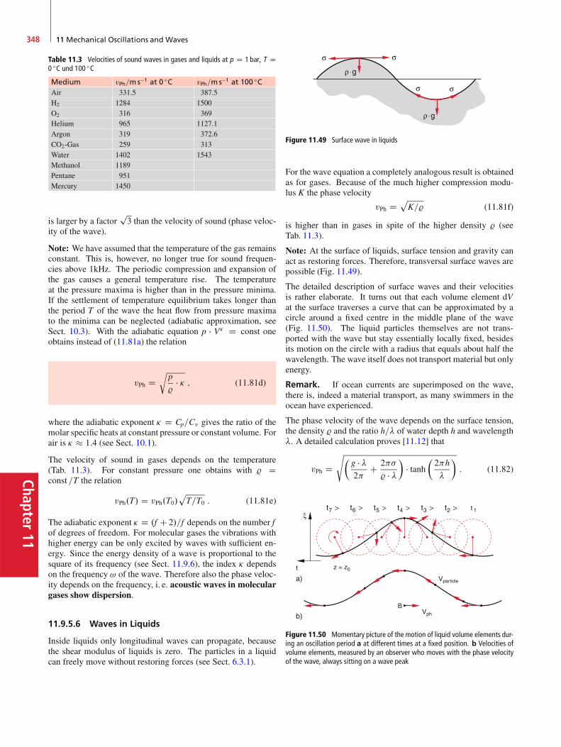
Chapter11
348 11 Mechanical Oscillations and Waves
Table 11.3 Velocities of sound waves in gases and liquids at p D 1 bar, T D0 ıC und 100 ıC
Medium vPh=ms�1 at 0 ıC vPh=ms�1 at 100 ıCAir 331.5 387.5H2 1284 1500O2 316 369Helium 965 1127.1Argon 319 372.6CO2-Gas 259 313Water 1402 1543Methanol 1189Pentane 951Mercury 1450
is larger by a factorp3 than the velocity of sound (phase veloc-
ity of the wave).
Note: We have assumed that the temperature of the gas remainsconstant. This is, however, no longer true for sound frequen-cies above 1kHz. The periodic compression and expansion ofthe gas causes a general temperature rise. The temperatureat the pressure maxima is higher than in the pressure minima.If the settlement of temperature equilibrium takes longer thanthe period T of the wave the heat flow from pressure maximato the minima can be neglected (adiabatic approximation, seeSect. 10.3). With the adiabatic equation p � V� D const oneobtains instead of (11.81a) the relation
vPh Dr
p
%� � ; (11.81d)
where the adiabatic exponent � D Cp=Cv gives the ratio of themolar specific heats at constant pressure or constant volume. Forair is � � 1:4 (see Sect. 10.1).
The velocity of sound in gases depends on the temperature(Tab. 11.3). For constant pressure one obtains with % Dconst =T the relation
vPh.T/ D vPh.T0/pT=T0 : (11.81e)
The adiabatic exponent � D .f C 2/=f depends on the number fof degrees of freedom. For molecular gases the vibrations withhigher energy can be only excited by waves with sufficient en-ergy. Since the energy density of a wave is proportional to thesquare of its frequency (see Sect. 11.9.6), the index � dependson the frequency ! of the wave. Therefore also the phase veloc-ity depends on the frequency, i. e. acoustic waves in moleculargases show dispersion.
11.9.5.6 Waves in Liquids
Inside liquids only longitudinal waves can propagate, becausethe shear modulus of liquids is zero. The particles in a liquidcan freely move without restoring forces (see Sect. 6.3.1).
Figure 11.49 Surface wave in liquids
For the wave equation a completely analogous result is obtainedas for gases. Because of the much higher compression modu-lus K the phase velocity
vPh DpK=% (11.81f)
is higher than in gases in spite of the higher density % (seeTab. 11.3).
Note: At the surface of liquids, surface tension and gravity canact as restoring forces. Therefore, transversal surface waves arepossible (Fig. 11.49).
The detailed description of surface waves and their velocitiesis rather elaborate. It turns out that each volume element dVat the surface traverses a curve that can be approximated by acircle around a fixed centre in the middle plane of the wave(Fig. 11.50). The liquid particles themselves are not trans-ported with the wave but stay essentially locally fixed, besidesits motion on the circle with a radius that equals about half thewavelength. The wave itself does not transport material but onlyenergy.
Remark. If ocean currents are superimposed on the wave,there is, indeed a material transport, as many swimmers in theocean have experienced.
The phase velocity of the wave depends on the surface tension,the density % and the ratio h=� of water depth h and wavelength�. A detailed calculation proves [11.12] that
vPh Ds�
g � �2
C 2�
% � ��
� tanh�2h
�
�: (11.82)
Figure 11.50 Momentary picture of the motion of liquid volume elements dur-ing an oscillation period a at different times at a fixed position. b Velocities ofvolume elements, measured by an observer who moves with the phase velocityof the wave, always sitting on a wave peak
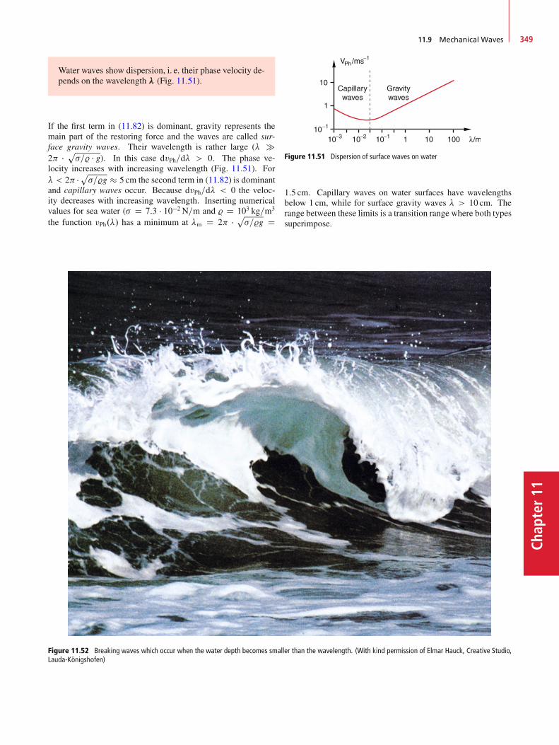
11.9 Mechanical Waves 349
Chap
ter11
Water waves show dispersion, i. e. their phase velocity de-pends on the wavelength (Fig. 11.51).
If the first term in (11.82) is dominant, gravity represents themain part of the restoring force and the waves are called sur-face gravity waves. Their wavelength is rather large (� �2 � p�=% � g). In this case dvPh=d� > 0. The phase ve-locity increases with increasing wavelength (Fig. 11.51). For� < 2 �p�=%g � 5 cm the second term in (11.82) is dominantand capillary waves occur. Because dvPh=d� < 0 the veloc-ity decreases with increasing wavelength. Inserting numericalvalues for sea water (� D 7:3 � 10�2 N=m and % D 103 kg=m3
the function vPh.�/ has a minimum at �m D 2 � p�=%g D
Figure 11.52 Breaking waves which occur when the water depth becomes smaller than the wavelength. (With kind permission of Elmar Hauck, Creative Studio,Lauda-Königshofen)
Capillarywaves
Gravitywaves
Figure 11.51 Dispersion of surface waves on water
1:5 cm. Capillary waves on water surfaces have wavelengthsbelow 1 cm, while for surface gravity waves � > 10 cm. Therange between these limits is a transition range where both typessuperimpose.
Chapter11
350 11 Mechanical Oscillations and Waves
11.9.6 Energy Density and Energy Transport ina Wave
In a mechanical wave mass elements dm D % � dV oscillate. Thekinetic and potential energy of this oscillation propagates withthe wave caused by the coupling between neighbouring masselements. It should be again stressed that no mass is trans-ported by the wave, but only the energy of the oscillation.
The kinetic energy of an oscillating mass element �m in thewave
� D A � cos.!t � kz/
is
Ekin D 12�m � P�2 D 1
2% ��V � A2!2 sin2.!t � kz/ :
The mean energy density, averaged over one oscillation periodis then
.Ekin=�V/ D 1
4%A2!2 : (11.83)
The potential energy of a mass element dm, that oscillates withthe amplitude � against the restoring force F D �D � � is withD D !2dm
Epot D ��Z
0
F.x/dx D 12D�
2
D 12DA
2 cos2.!t � kz/ :
(11.84)
The time average of the potential energy per volume element�V is then
Epot=�V D 14%A
2!2 D Ekin=�V : (11.85)
The total energy density W=�V D .Epot C Ekin/=�V of thewave is therefore
%e D W
�VD 1
2%A2!2 : (11.86)
Definition
The intensity I or energy flux density of a wave is theenergy that is transported per second through a unit areaperpendicular to the propagation direction of the wave.
Since the energy transport occurs with the wave velocity vPh theintensity can be written as the product
I D vPh � %e D 12vPh � %A2!2 : (11.87)
The intensity of a wave is proportional to the square A2 ofthe wave amplitude and the square !2 of its frequency.
11.9.7 Dispersion; Phase- and Group-Velocity
We have seen in the previous section that for some wave typesthe phase velocity vPh depends on the wavelength � of thewave (see for example Eq. 11.82). This phenomenon is calleddispersion. The relation between vPh and wavelength � resp.wavenumber k D 2=�
vPh D !
k(11.88a)
is the dispersion relation.
A well-known example is the dispersion of light waves in glass
vPh D c D !
kD !
k0n.!/; (11.88b)
where this relation is described by the wavelength-dependent re-fractive index n.�/ of the glass and c0 D !=k0 is the velocityof light waves in vacuum (see Vol. 2). If a parallel ray of whitelight passes through a glass prism it is diffracted into the differ-ent contributions of different wavelength, which are dispersedinto different directions. Behind the prism appears a band oflight with separated colours (rainbow).
For monochromatic harmonic waves (only one wavelength)there is a unique phase velocity vPh D !=k with ! D 2� D2vPh=�.
The situation is different for waves with many wavelengths orwith a broad continuous distribution over the interval ��, resp.the frequency interval �! D !m ˙ �!=2. A short pulsewith time duration�t contains a continuous frequency spectrumwithin the interval �! D 2=�t. If the different frequenciespropagate with different velocities the relative phases of the dif-ferent contributions change and therefore the time profile of thepulse is modified.
We regard in Fig. 11.53a an arbitrary perturbation �.t/, whichpropagates into the z-direction. According to the Fourier-theorem (see Sect. 11.3.1) the function �.t; z/ can be describedby a superposition of an infinite number of harmonic waves withfrequencies !
�.t; z/ D1Z
0
A.!/ � ei.!t�kz/d! (11.89a)
with amplitudes A.!/ that follow the frequency distributionshown in Fig 11.53b. The amplitudes A.!/ can be determinedby the inverse Fourier-transformation
A.!/ D 1
C1Z
�1�.t; z/e�i.!t�kz/dt : (11.89b)
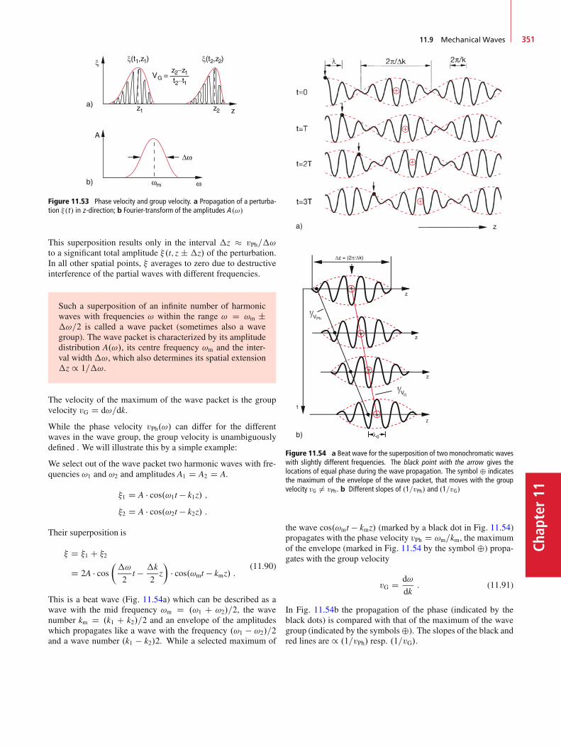
11.9 Mechanical Waves 351
Chap
ter11
Figure 11.53 Phase velocity and group velocity. a Propagation of a perturba-tion �.t/ in z-direction; b Fourier-transform of the amplitudes A .!/
This superposition results only in the interval �z � vPh=�!to a significant total amplitude �.t; z ˙�z/ of the perturbation.In all other spatial points, � averages to zero due to destructiveinterference of the partial waves with different frequencies.
Such a superposition of an infinite number of harmonicwaves with frequencies ! within the range ! D !m ˙�!=2 is called a wave packet (sometimes also a wavegroup). The wave packet is characterized by its amplitudedistribution A.!/, its centre frequency !m and the inter-val width �!, which also determines its spatial extension�z / 1=�!.
The velocity of the maximum of the wave packet is the groupvelocity vG D d!=dk.
While the phase velocity vPh.!/ can differ for the differentwaves in the wave group, the group velocity is unambiguouslydefined . We will illustrate this by a simple example:
We select out of the wave packet two harmonic waves with fre-quencies !1 and !2 and amplitudes A1 D A2 D A.
�1 D A � cos.!1t � k1z/ ;
�2 D A � cos.!2t � k2z/ :
Their superposition is
� D �1 C �2
D 2A � cos��!
2t � �k
2z
�� cos.!mt � kmz/ :
(11.90)
This is a beat wave (Fig. 11.54a) which can be described as awave with the mid frequency !m D .!1 C !2/=2, the wavenumber km D .k1 C k2/=2 and an envelope of the amplitudeswhich propagates like a wave with the frequency .!1 � !2/=2and a wave number .k1 � k2/2. While a selected maximum of
Figure 11.54 a Beat wave for the superposition of two monochromatic waveswith slightly different frequencies. The black point with the arrow gives thelocations of equal phase during the wave propagation. The symbol ˚ indicatesthe maximum of the envelope of the wave packet, that moves with the groupvelocity vG ¤ vPh. b Different slopes of .1=vPh/ and .1=vG/
the wave cos.!mt � kmz/ (marked by a black dot in Fig. 11.54)propagates with the phase velocity vPh D !m=km, the maximumof the envelope (marked in Fig. 11.54 by the symbol ˚) propa-gates with the group velocity
vG D d!
dk: (11.91)
In Fig. 11.54b the propagation of the phase (indicated by theblack dots) is compared with that of the maximum of the wavegroup (indicated by the symbols˚). The slopes of the black andred lines are / .1=vPh/ resp. .1=vG/.
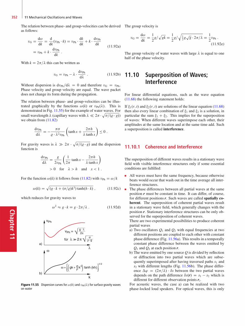
Chapter11
352 11 Mechanical Oscillations and Waves
The relation between phase- and group-velocities can be derivedas follows:
vG D d!
dkD d
dk.vPh � k/ D vPh � dk
dkC k � dvPh
dk
D vPh C k � dvPhdk
:
(11.92a)
With k D 2=� this can be written as
vG D vPh � � � dvPhd�
: (11.92b)
Without dispersion is dvPh=d� D 0 and therefore vG D vPh.Phase velocity and group velocity are equal. The wave packetdoes not change its form during the propagation.
The relation between phase- and group-velocities can be illus-trated graphically by the functions !.k/ or vPh.�/. This isdemonstrated in Fig. 11.55) for the example of water waves. Forsmall wavelength � (capillary waves with � 2 �p�=.% � g/)we obtain from (11.82)
dvPhd�
D � �
% � �2vPh�tanh x C 2h
� tanh x
�� 0 :
For gravity waves is � � 2 � p�=.% � g/ and the dispersionfunction is
dvPhd�
D g
2vPh
�1
2tanh x � 2h
� tanh x
�
> 0 for � > h and x < 1 :
For the function !.k/ it follows from (11.82) with vPh D !=k
!.k/ Dp.g � k C .�=%/k3/ tanh.h � k/ ; (11.92c)
which reduces for gravity waves to
!2 � g � k D g � 2=� : (11.92d)
(kh)
Figure 11.55 Dispersion curves for !.k / and vPh.�/ for surface gravity waveson water
The group velocity is
vG D d!
dkD 1
2g=pgk D 1
2g=q
12g
pg � 2=� D 1
2vPh :
(11.92e)
The group velocity of water waves with large � is equal to onehalf of the phase velocity.
11.10 Superposition of Waves;Interference
For linear differential equations, such as the wave equation(11.68) the following statement holds:
If �1.r; t/ and �2.r; t/ are solutions of the linear equation (11.68)then also every linear combination of �1 and �2 is a solution, inparticular the sum �1 C �2. This implies for the superpositionof waves: When different waves superimpose each other, theiramplitudes at the same location and at the same time add. Sucha superposition is called interference.
11.10.1 Coherence and Interference
The superposition of different waves results in a stationary wavefield with visible interference structures only if some essentialconditions are fulfilled:
All waves must have the same frequency, because otherwisebeats would occur that wash out in the time average all inter-ference structures.The phase differences between all partial waves at the sameposition r must be constant in time. It can differ, of course,for different positions r. Such waves are called spatially co-herent. The superposition of coherent partial waves resultin a stationary wave field, which generally changes with theposition r. Stationary interference structures can be only ob-served for the superposition of coherent waves.There are two experimental possibilities to produce coherentpartial wavesa) Two oscillators Q1 and Q2 with equal frequencies at two
different positions are coupled to each other with constantphase difference (Fig. 11.56a). This results in a temporallyconstant phase difference between the waves emitted byQ1 and Q2 at each position r.
b) The wave emitted by one source Q is divided by reflectionor diffraction into two partial waves which are subse-quently superimposed after having traversed paths s1 ands2 with different lengths (Fig. 11.56b). The phase differ-ence �' D .2=�/ � ıs between the two partial wavesdepends on the path difference ıs.r/ D s1 � s2 which isdifferent for different observation points ri.
For acoustic waves, the case a) can be realized with twophase-locked loud speakers. For optical waves, this is only
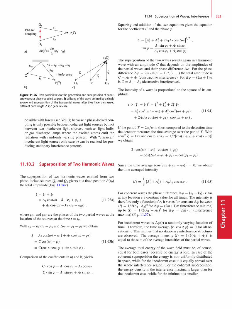
11.10 Superposition of Waves; Interference 353
Chap
ter11
Figure 11.56 Two possibilities for the generation and superposition of coher-ent waves; a phase-coupled sources; b splitting of the wave emitted by a singlesource and superposition of the two partial waves after they have transverseddifferent path length�s ; c general case
possible with lasers (see Vol. 3) because a phase-locked cou-pling is only possible between coherent light sources but notbetween two incoherent light sources, such as light bulbsor gas discharge lamps where the excited atoms emit theradiation with randomly varying phases. With “classical”incoherent light sources only case b) can be realized for pro-ducing stationary interference patterns.
11.10.2 Superposition of Two Harmonic Waves
The superposition of two harmonic waves emitted from twophase-locked sources Q1 and Q2 givers at a fixed position P.r0/the total amplitude (Fig. 11.56c)
� D �1 C �2
D A1 cos.!t � k1 � r0 C '01/
C A2 cos.!t � k2 � r0 C '02/ ;
(11.93a)
where '01 and '02 are the phases of the two partial waves at thelocation of the sources at the time t D t0.
With 'i D ki � r0 � '0i and �' D '1 � '2 we obtain
� D A1 cos.!t � '1/C A2 cos.!t � '2/D C cos.!t � '/D C.cos!t cos' C sin!t sin '/ :
(11.93b)
Comparison of the coefficients in a) and b) yields
C � cos' D A1 cos'1 C A2 cos'2
C � sin ' D A1 sin '1 C A2 sin '2 :
Squaring and addition of the two equations gives the equationfor the coefficient C and the phase '
C D �A21 C A2
2 C 2A1A2 cos�'�1=2
;
tan ' D A1 sin '1 C A2 sin'2A1 cos'1 C A2 cos'2
:
The superposition of the two waves results again in a harmonicwave with an amplitude C that depends on the amplitudes ofthe partial waves and their phase difference �'. For the phasedifference �' D 2m � .m D 1; 2; 3; : : :/ the total amplitude isC D A1 C A2 (constructive interference). For�' D .2mC 1/is C D A1 � A2 (destructive interference).
The intensity of a wave is proportional to the square of its am-plitude:
I / .�1 C �2/2 D �21 C �22 C 2�1�2
D A21 cos
2.!t C '1/C A22 cos
2.!t C '2/
C 2A1A2 cos.!t C '1/ � cos.!t C '2/ :
(11.94)
If the period T D 2=! is short compared to the detection timethe detector measures the time average over the period T . Withhcos2 xi D 1=2 and cos x � cos y D 1=2Œcos.xC y/C cos.x� y/�we obtain
2 � cos.!t C '1/ � cos.!t C '2/
D cos.2!t C '1 C '2/C cos.'1 � '2/ :
Since the time average hcos.2!t C '1 C '2/i D 0, we obtainthe time averaged intensity
hIi D 1
2
�A21 C A2
2
�C A1A2 cos�' : (11.95)
For coherent waves the phase difference �' D .k1 � k2/ � r hasat any location r a constant value for all times. The intensity istherefore only a function of r. it varies for constant�' betweenhIi D 1=2.A1�A2/
2 for�' D .2mC1/ (interference minima)up to hIi D 1=2.A1 C A2/
2 for �' D 2m � (interferencemaxima) (Fig. 11.57).
For incoherent waves is �'.t/ a randomly varying function oftime. Therefore, the time average hr � cos�'i D 0 for all lo-cations r. This implies that no stationary interference structuresare observed. The average intensity hIi D 1=2.A1 C A2/
2 isequal to the sum of the average intensities of the partial waves.
The average total energy of the wave field must be, of course,equal for both cases, because no energy is lost. In case of thecoherent superposition the energy is non-uniformly distributedin space, while for the incoherent case it is equally spread overthe whole interference region. For the coherent superposition,the energy density in the interference maxima is larger than forthe incoherent case, while for the minima it is smaller.

Chapter11
354 11 Mechanical Oscillations and Waves
a)
b)
BS1
M1 M2
BS2
Q
Figure 11.57 a Mean intensity I of the superpostion of two coherent wavesas a function of their phase different �'. b Experimental arrangement for theinterference of copropagation plane waves
Examples
1. Superposition of plane waves with equal frequenciesand equal amplitudes but different phases, propagat-ing both into the z-direction.
�1 D A � cos.!t � kz/ I�2 D A � cos.!t � kz C '/
Their superposition gives the total amplitude
� D �1 C �2 D 2A � cos.'=2/� cos.!t � kx C '=2/
D B.'/ � cos.!t � kx C '=2/ :
(11.96)
This is again a harmonic plane wave with a phase thatis equal to the mean value h'i D .1=2/ ' and an am-plitude B.'/ that depends on the phase difference�'.For �' D .2m C 1/ the total amplitude � is zero inthe whole superposition region. Where has the energygone?Figure 11.57b shows an experimental arrangementthat can realize the superposition described above(Mach-Zehnder Interferometer). The wave, emittedby the source Q is divided by the beam splitter BS 1into a reflected partial wave and a transmitted wave.
The reflected wave is again reflected by the mirrorsM1 and M2 and is then superimposed by beam split-ter BS 2 onto the first transmitted partial wave. Thephase difference between the two partial waves canbe adjusted by moving the mirrors up or down, thuschanging the path length difference between the twointerfering waves.
2. Superposition of two spherical waves, emitted by thesources Q1 and Q2 (Fig. 11.58).At the point P.r/ the phase difference is �' D k �.r1 � r2/. The interference maxima are located on thecurves for which �' D k � .r1 � r2/ D 2m � . Thisare hyperbolas (in Fig. 11.58 marked by dashed redcurves), where the two sourcesQ1 andQ2 are the focalpoints.
Figure 11.58 Superposition of the spherical waves emitted by twophase-coupled sources Q1 and Q2 J
When spherical waves, emitted by two phase-coupled sources,are superimposed, one observes hyperbolas as interferencestructures. The form of the hyperbolas depends on the distanced between Q1 and Q2.
11.11 Diffraction, Reflection andRefraction of Waves
The propagation direction and the local amplitude distributioncan be altered by reflection on surfaces, by refraction in mediawith a different refractive index or by diffraction at obstaclessuch as slits, apertures, or small objects in the path of the wave.All these processes can be described by Huygen’s principle,which was postulated by the Dutch scientist Christian Huygensaround 1600.

11.11 Diffraction, Reflection and Refraction of Waves 355
Chap
ter11
11.11.1 Huygens’s Principle
The propagation of waves in space can be described when eachpoint of a phase surface is considered as the source of a newspherical wave (secondary wave or elementary wave). Thesespherical waves propagate into all directions and superimpose(Fig. 11.59a). Assume that all elementary waves on a phase sur-face '.r0; t0/ are generated at the same time t0. They proceedduring the time�t over a distance r D vPh ��t. The tangent sur-face as the envelope of all spherical waves at the time t D t0C�tforms again a phase surface of the wave which has propagatedin space by the distance r D vPh ��t.
This principle that has been formulated more than 400 yearsago, can be explained by modern concepts of atomic physics.In case of sound waves which can propagates only in matter butnot in vacuum, all atoms on a phase surface are excited by theacoustic wave to oscillate in phase. They transfer their oscilla-tion energy to neighbouring atoms due to their mutual coupling.The oscillating atoms are the sources for the elementary waves.In isotropic media, the coupling is independent of the direction.This means that the phase velocity of the elementary waves isisotropic. Therefore, spherical waves are generated. In vac-
Isotropicmedium
a)
b)
Unisotropicmedium
Incidentwave
Transmittedwave
Phasefrontsfor reflectedwave
Phasefrontsin unisotropicmedium
Elementarywaves
Pasefronts
Figure 11.59 a Huygen’s principle. b Transmission of a wave in an unisotropicmedium. The phasefront is the tangent to the phasefronts of the elementarywaves
Q4
Q3
Q2
Q1k→
k→
Incidentplane wave
Surface of constantphase( )⊥
´
k→
´
Z=Z0 Z
α
Qi Qin = δ
Figure 11.60 Superposition of the spherical waves emitted by N sources lo-cated on a plane z D const
uum, there are no atoms, and therefore no sources for acousticwaves are present. This can be experimentally demonstrated byan electric alarm clock in a container that is evacuated. As soonas the air pressure in the container drops below a certain value,the alarm clock can no longer be heard.
In contrast to acoustic waves electromagnetic waves can alsopropagate through vacuum (otherwise we would not see the sunand the stars). Their propagation also follows Huygens’s princi-ple. This is explained in Vol. 2.
For the general case of non-isotropic media, the phase velocitydoes depend on the direction and the elementary waves have anelliptic envelope (Fig. 11.59b). The envelope to the ellipticalwaves at a time t D t0 C�t is a phase-plane that is tilted againstthe phase-plane of the incoming wave by an angle ˛.
Up to now we have considered the case of an infinite number ofsource points for the elementary waves with a continuous dis-tribution on the phase surface. We will now discuss the case ofN distinct sources on the phase-plane with a distance ı betweenadjacent source points Qi that are phase-locked to each other(Fig. 11.60). The phase difference between the different ele-mentary waves depends on the direction ˛ against the directionk0 of the incident plane wave.
The path difference of waves from adjacent points in the direc-tion ˛ is �s D ı � sin˛ and the corresponding phase difference
�' D 2
���s D k � ı sin˛ with k D 2
�: (11.97)
The superposition of all spherical waves emitted into the direc-tion ˛ from all N sources Qi that are located on the phase frontover a distance d D N � ı gives the total amplitude at the point P
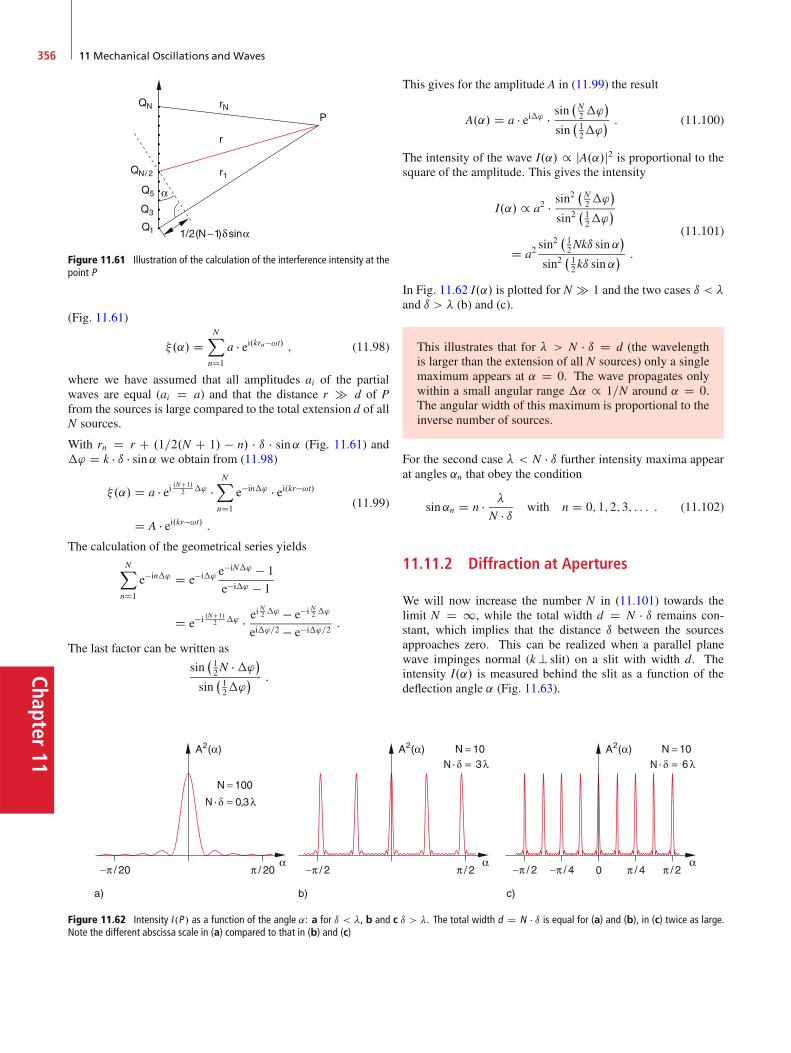
Chapter11
356 11 Mechanical Oscillations and Waves
Figure 11.61 Illustration of the calculation of the interference intensity at thepoint P
(Fig. 11.61)
�.˛/ DNX
nD1
a � ei.krn�!t/ ; (11.98)
where we have assumed that all amplitudes ai of the partialwaves are equal (ai D a) and that the distance r � d of Pfrom the sources is large compared to the total extension d of allN sources.
With rn D r C .1=2.N C 1/ � n/ � ı � sin˛ (Fig. 11.61) and�' D k � ı � sin˛ we obtain from (11.98)
�.˛/ D a � ei .NC1/2 �' �
NX
nD1
e�in�' � ei.kr�!t/
D A � ei.kr�!t/ :(11.99)
The calculation of the geometrical series yieldsNX
nD1
e�in�' D e�i�' e�iN�' � 1
e�i�' � 1
D e�i .NC1/2 �' � e
i N2 �' � e�i N2 �'
ei�'=2 � e�i�'=2:
The last factor can be written as
sin�12N ��'�
sin�12�'
� :
Figure 11.62 Intensity I .P / as a function of the angle ˛: a for ı < �, b and c ı > �. The total width d D N � ı is equal for (a) and (b), in (c) twice as large.Note the different abscissa scale in (a) compared to that in (b) and (c)
This gives for the amplitude A in (11.99) the result
A.˛/ D a � ei�' � sin�N2�'
�
sin�12�'
� : (11.100)
The intensity of the wave I.˛/ / jA.˛/j2 is proportional to thesquare of the amplitude. This gives the intensity
I.˛/ / a2 � sin2�N2�'
�
sin2�12�'
�
D a2sin2
�12Nkı sin˛
�
sin2�12kı sin˛
� :
(11.101)
In Fig. 11.62 I.˛/ is plotted for N � 1 and the two cases ı < �and ı > � (b) and (c).
This illustrates that for � > N � ı D d (the wavelengthis larger than the extension of all N sources) only a singlemaximum appears at ˛ D 0. The wave propagates onlywithin a small angular range �˛ / 1=N around ˛ D 0.The angular width of this maximum is proportional to theinverse number of sources.
For the second case � < N � ı further intensity maxima appearat angles ˛n that obey the condition
sin˛n D n � �
N � ı with n D 0; 1; 2; 3; : : : : (11.102)
11.11.2 Diffraction at Apertures
We will now increase the number N in (11.101) towards thelimit N D 1, while the total width d D N � ı remains con-stant, which implies that the distance ı between the sourcesapproaches zero. This can be realized when a parallel planewave impinges normal (k? slit) on a slit with width d. Theintensity I.˛/ is measured behind the slit as a function of thedeflection angle ˛ (Fig. 11.63).
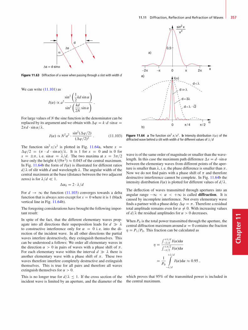
11.11 Diffraction, Reflection and Refraction of Waves 357
Chap
ter11
α
Δs = d⋅sinα
Δs
d
Figure 11.63 Diffraction of a wave when passing through a slot with width d
We can write (11.101) as
I.˛/ / a2sin2
�1
2kd sin˛
�
sin2�kd
2Nsin˛
� :
For large values ofN the sine function in the denominator can bereplaced by its argument and we obtain with�' D k �d �sin˛ D2d � sin˛=�.
I.˛/ / N2a2 � sin2.�'=2/
.�'=2/2: (11.103)
The function sin2 x=x2 is plotted in Fig. 11.64a, where x D�'=2 D . � d � sin˛/=�. It is 1 for x D 0 and is 0 forx D ˙ , i. e. sin˛ D �=d. The two maxima at x D 3=2have only the height 4=.92/ � 0:045 of the central maximum.In Fig. 11.64b the form of I.˛/ is illustrated for different ratiosd=� of slit width d and wavelength �. The angular width of thecentral maximum at the base (distance between the two adjacentzeros) is for �=d 1.
�˛0 D 2 � �=dFor d ! 1 the function (11.103) converges towards a deltafunction that is always zero except for x D 0 where it is 1 (blackvertical line in Fig. 11.64b).
The foregoing considerations have brought the following impor-tant result:
In spite of the fact, that the different elementary waves prop-agate into all directions their superposition leads for d � �to constructive interference only for ˛ D 0 i. e. into the di-rection of the incident wave. In all other directions the partialwaves interfere destructively, they extinguish themselves. Thiscan be understood a follows: We order all elementary waves inthe direction ˛ > 0 in pairs of waves with a phase shift of .For each elementary wave within the interval d � � there isanother elementary wave with a phase shift of . These twowaves therefore interfere completely destructive and extinguishthemselves. This is true for all pairs and therefore all wavesextinguish themselves for ˛ > 0.
This is no longer true for d=� � 1. If the cross section of theincident wave is limited by an aperture, and the diameter of the
Figure 11.64 a The function sin2 x=x2. b Intensity distribution I .˛/ of thediffracted wave behind a slit with width d for different values of �=d
wave is of the same order of magnitude or smaller than the wave-length. In this case the maximum path difference �s D d � sin˛between the elementary waves from different points of the aper-ture is smaller than �, i. e. the phase difference is smaller than .Now we do not find pairs with a phase shift of and thereforedestructive interference cannot be complete. In Fig. 11.64b theintensity distribution I.˛/ is plotted for different values of d=�.
The deflection of waves transmitted through apertures into anangular range �1 < ˛ < C1 is called diffraction. It iscaused by incomplete interference. Not every elementary wavefinds a partner with a phase delay�' D . Therefore a residualtotal amplitude remains even for ˛ ¤ 0. With increasing valuesof d=� the residual amplitudes for ˛ > 0 decreases.
When P0 is the total power transmitted through the aperture, thecentral diffraction maximum around ˛ D 0 contains the fraction� D P1=P0. This fraction can be calculated as
� DR C�=d
��=d I.˛/d˛R C=2
�=2 I.˛/d˛
D 1
P0
C�=dZ
��=dI.˛/d˛ � 0:95 ;
which proves that 95% of the transmitted power is included inthe central maximum.

Chapter11
358 11 Mechanical Oscillations and Waves
11.11.3 Summary
Without limiting boundaries waves propagate in isotropicmedia straightforward. Their propagation can be describedby Huygens’s principle where each phase front of the wavecan be regarded as an infinite number of sources that emitelementary waves, which interfere with each other. Ford � � this interference is always completely destructivefor deflection angles ˛ ¤ 0. Therefore the wave propagatesstraightforward.The intensity distribution I.˛/ as a function of the deflectionangel ˛ against the direction of the incident wave depends onthe ratio d=� of aperture diameter d and wavelength �.
11.11.4 Reflection and Refraction of Waves
When a wave passes through a boundary between two media,where the wave has different phase velocities, part of the waveis reflected and the transmitted part changes its direction. Thiscan be also described by Huygens’s principle.
We will show this at first for the reflection of a plane wave atthe plane boundary between two different media (Fig. 11.65).When the phase plane 'e D constant has reached the point A atthe time t D 0, an elementary spherical wave is emitted from A,which spreads out into the whole upper plane. When the samephase front has reached the point B at the time t0 D DB=vPh alsoan elementary spherical wave is emitted from B. Meanwhile thefirst elementary wave has propagated along the distance r DvPh � t0.The elementary waves emitted from points Pn between A andB have been excited at times tn D t0 � .APn/=AB and until thetime t0 they have travelled the distance rn D vPh � .t0 � tn/ DvPh.PnB=AB/. The tangent BE to all spheres of the elementarywaves at time t0 is the phase plane of the reflected wave. FromFig. 11.65 it can be seen that
AE D DB ) ^.ABE/ D ^.BAD/ D ˛ :
Figure 11.65 Explanation of the reflection law based on Huygen’s priciple
Figure 11.66 Derivation of the refraction law from Huygen’s principle
We name the angle ˛ between the wave vector ke of the incidentwave and the normal vector N of the reflecting plane the angleof incidence. We then can formulate the law of reflection:
When a plane wave is reflected at a plane boundary be-tween two media, the angle of reflection is equal to theangle of incidence.
For that part of the wave that penetrates into the medium 2(Fig. 11.66), the velocity v D v2 of the elementary waves isdifferent from the velocity v D v1 in medium 1. During thetime t0 D DB=v1, where the wave front in medium 1 travelsfrom D to B the elementary wave starting from A has travelledin medium 2 the distance AE D v2 � t0 D DB � v2=v1. This im-plies AE=DB D v2=v1. From the triangles ABD and AEB withthe same base length we conclude:
sin˛
sinˇD v1
v2: (11.104)
Equation 11.104 is Snellius’ refraction law (after the DutchAstronomer Willebrord Snellius van Royen 1580–1626, whopublished this law for the first time although it was known be-fore). It holds for arbitrary waves, not only for acoustic but alsofor light waves (see Vol. 2).
Reflection and refraction of waves can be substantiated by amore general law, called Fermat’s principle.
A wave always travels that path for which the runtime fora phase front between two points P1.x1; y1/ and P2.x2; y2/ isminimum. This is illustrated for the refraction of waves inFig. 11.67). The run-time T for a phase front from P1.x1; y1/to P2.x2; y2/ is
T D S1v1
C S2v2
D 1
v1
q.x � x1/2 C y21 C 1
v2
q.x2 � x/2 C y22 :
(11.105)

11.12 Standing Waves 359
Chap
ter11
Figure 11.67 Explanation of the refraction law with the Fermat principle
When we shift the point P.x; y/ along the boundary surface y D0, the run-time T changes by
dT
dxD .x � x1/=v1q
.x � x1/2 C y21
� .x2 � x/=v2q.x2 � x/2 C y22
:
If T should be minimum, the derivative dT=dx must be zero.This gives with sin ˛ D .x � x1/=s1 and sinˇ D .x2 � x/=s2 thecondition
sin˛
v1D sinˇ
v2; (11.106)
which is identical to Snellius’ law (11.104).
11.12 Standing Waves
Special superpositions of running waves result in stationary os-cillation patterns where certain points, lines or planes in spaceare always at rest, which means that here the oscillation ampli-tude is zero (nodes of oscillation). The pattern of nodes dependson the frequency and the boundary conditions. We will illustratethis by several examples.
Nodes
Oscillation maxima
Figure 11.68 a Standing wave as superposition of a wave propagating into the Cz-direction and the reflected wave running into the �z-direction. b Periodicmaxima and nodes of a standing wave
11.12.1 One-Dimensional Standing Waves
When a plane wave � D A � cos.!t C kz/ that propagates intothe �z-direction is reflected by a plane z D 0 (Fig. 11.68) thereflected wave � D A � cos.!t � kz/ propagates into the Cz-direction. For z > 0 the two waves superimpose and the totalwave field is
� D �1 C �2
D AŒcos.!t C kz/C cos.!t � kz C '/� ;(11.107)
where a phase jump ' at the reflection has been taken into ac-count. According to the addition theorem of the cos-functionsthis can be written as
� D 2A � cos�kz � '
2
� cos
�!t C '
2
: (11.108)
This represents an oscillation cos.!tC'=2/ with the amplitude2A � cos.k � z � '=2/ that depends periodically on the location z.It is called a standing wave. At the positions z D .�=4/Œ.2nC1/C'� the amplitude of the standing wave is zero. These zeropoints are the oscillation nodes. For z D .�=4/.2n C '/ theamplitude becomes maximum. It changes during one oscillationperiod T D 2=! from �2A to C2A. These maxima of thestanding wave are called the oscillation antinodes.
Note the difference to the running wave � D A � cos.!t � k � z/.Here the nodes and antinodes propagate with the velocity vPh D!=k into the Cz-direction, while for the standing wave they arefixed in place.
The spatial amplitude distribution of the standing wave and thepositions of the nodes and antinodes depend on the phase jumpat the reflection. We will discuss some special cases:
Reflection at a fixed end at z D 0 (Fig. 11.69a).This can be realized by a rope with its right end fixed to awall, while the left end is connected to an oscillator, for ex-ample a hand that shakes up and down. Since �.0/ D 0 itfollows from (11.108)
'=2 D ˙=2 ) ' D ˙ :
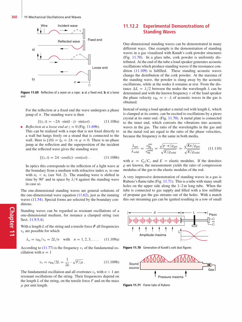
Chapter11
360 11 Mechanical Oscillations and Waves
Incident wave
Fixed end
Wire
Loose end
z
Reflected wave
Figure 11.69 Reflection of a wave on a rope: a at a fixed end, b at a looseend
For the reflection at a fixed end the wave undergoes a phasejump of . The standing wave is then
�.z; t/ D �2A � sin.k � z/ � sin.!t/ : (11.108a)Reflection at a loose end at z D 0 (Fig. 11.69b).This can be realized with a rope that is not fixed directly toa wall but hangs freely on a strand that is connected to thewall. Here is �.0/ D �0 D 2A ) ' D 0. There is no phasejump at the reflection and the superposition of the incidentand the reflected wave gives the standing wave
�.z; t/ D 2A � cos.kz/ � cos.!t/ : (11.108b)
In optics this corresponds to the reflection of a light wave atthe boundary from a medium with refractive index n1 to onewith n2 < n1 (see Vol. 2). The standing wave is shifted intime by 90ı and in space by �=4 against the standing wavein case a).
The one-dimensional standing waves are general solutions ofthe one-dimensional wave equation (11.62), just as the runningwaves (11.54). Special forms are selected by the boundary con-ditions.
Standing waves can be regarded as resonant oscillations of aone-dimensional medium, for instance a clamped string (seeSect. 11.9.5.4).
With a length L of the string and a tensile force F all frequencies�n are possible for which
�n D vPh=�n D 2L=n with n D 1; 2; 3; : : : : (11.109a)
According to (11.77) is the frequency �1 of the fundamental os-cillation with n D 1
�1 D vPh=2L D 1
2L�pF= : (11.109b)
The fundamental oscillation and all overtones �n with n > 1 areresonant oscillations of the string. Their frequencies depend onthe length L of the string, on the tensile force F and on the mass per unit length.
11.12.2 Experimental Demonstrations ofStanding Waves
One-dimensional standing waves can be demonstrated in manydifferent ways. One example is the demonstration of standingwaves in a gas visualized with Kundt’s cork-powder structures(Fig. 11.70). In a glass tube, cork powder is uniformly dis-tributed. At the end of the tube a loud speaker generates acousticoscillations which produce standing waves if the resonance con-dition (11.109) is fulfilled. These standing acoustic waveschange the distribution of the cork powder. At the maxima ofthe standing wave, the powder is slung away by the acousticoscillations, while at the nodes it remains at rest. From the dis-tance �L D �=2 between the nodes the wavelength � can bedetermined and with the known frequency � of the loud speakerthe phase velocity vPh D � � � of acoustic waves in the gas isobtained.
Instead of using a loud speaker a metal rod with length L, whichis clamped at its centre, can be excited to oscillations by a piezocrystal at its outer end. (Fig. 11.70). A metal plate is connectedto the inner end, which converts the vibrations into acousticwaves in the gas. The ratio of the wavelengths in the gas andin the metal rod are equal to the ratio of the phase velocities,because the frequency is the same in both media.
�gas
�solidD v
gasPh
vsolidPh
Dpp � �=%gaspE=%solid
DpK�=%gaspE=%solid
(11.110)
with � D Cp=Cv and E D elastic modulus. If the densities% are known, the measurement yields the ratio of compressionmodulus of the gas to the elastic modulus of the rod.
A very impressive demonstration of standing waves in a gas isRubens’s flame tube (Fig. 11.71). This is a tube with many smallholes on the upper side along the 1–2m long tube. When thetube is connected to gas supply and filled with a few millibarof propane gas the gas streams out of the holes. With a matchthis out streaming gas can be ignited resulting in a row of small
Amplitude maxima
Figure 11.70 Generation of Kundt’s cork dust figures
Pressure maxima
Soundsource
Gas
Figure 11.71 Flame tube of Rubens
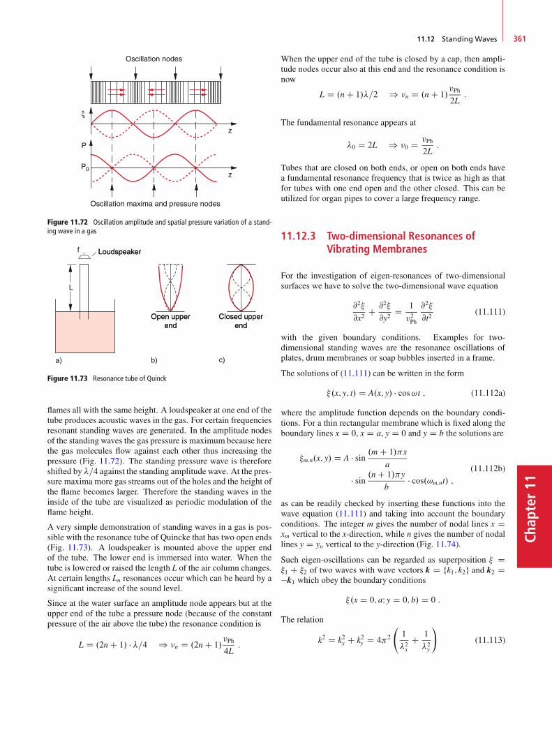
11.12 Standing Waves 361
Chap
ter11
Oscillation nodes
Oscillation maxima and pressure nodes
Figure 11.72 Oscillation amplitude and spatial pressure variation of a stand-ing wave in a gas
Loudspeaker
Open upperend
Closed upperend
Figure 11.73 Resonance tube of Quinck
flames all with the same height. A loudspeaker at one end of thetube produces acoustic waves in the gas. For certain frequenciesresonant standing waves are generated. In the amplitude nodesof the standing waves the gas pressure is maximum because herethe gas molecules flow against each other thus increasing thepressure (Fig. 11.72). The standing pressure wave is thereforeshifted by �=4 against the standing amplitude wave. At the pres-sure maxima more gas streams out of the holes and the height ofthe flame becomes larger. Therefore the standing waves in theinside of the tube are visualized as periodic modulation of theflame height.
A very simple demonstration of standing waves in a gas is pos-sible with the resonance tube of Quincke that has two open ends(Fig. 11.73). A loudspeaker is mounted above the upper endof the tube. The lower end is immersed into water. When thetube is lowered or raised the length L of the air column changes.At certain lengths Ln resonances occur which can be heard by asignificant increase of the sound level.
Since at the water surface an amplitude node appears but at theupper end of the tube a pressure node (because of the constantpressure of the air above the tube) the resonance condition is
L D .2n C 1/ � �=4 ) �n D .2n C 1/vPh
4L:
When the upper end of the tube is closed by a cap, then ampli-tude nodes occur also at this end and the resonance condition isnow
L D .n C 1/�=2 ) �n D .n C 1/vPh
2L:
The fundamental resonance appears at
�0 D 2L ) �0 D vPh
2L:
Tubes that are closed on both ends, or open on both ends havea fundamental resonance frequency that is twice as high as thatfor tubes with one end open and the other closed. This can beutilized for organ pipes to cover a large frequency range.
11.12.3 Two-dimensional Resonances ofVibrating Membranes
For the investigation of eigen-resonances of two-dimensionalsurfaces we have to solve the two-dimensional wave equation
@2�
@x2C @2�
@y2D 1
v2Ph
@2�
@t2(11.111)
with the given boundary conditions. Examples for two-dimensional standing waves are the resonance oscillations ofplates, drum membranes or soap bubbles inserted in a frame.
The solutions of (11.111) can be written in the form
�.x; y; t/ D A.x; y/ � cos!t ; (11.112a)
where the amplitude function depends on the boundary condi-tions. For a thin rectangular membrane which is fixed along theboundary lines x D 0, x D a, y D 0 and y D b the solutions are
�m;n.x; y/ D A � sin .m C 1/x
a
� sin .n C 1/y
b� cos.!m;nt/ ;
(11.112b)
as can be readily checked by inserting these functions into thewave equation (11.111) and taking into account the boundaryconditions. The integer m gives the number of nodal lines x Dxm vertical to the x-direction, while n gives the number of nodallines y D yn vertical to the y-direction (Fig. 11.74).
Such eigen-oscillations can be regarded as superposition � D�1 C �2 of two waves with wave vectors k D fk1; k2g and k2 D�k1 which obey the boundary conditions
�.x D 0; aI y D 0; b/ D 0 :
The relation
k2 D k2x C k2y D 42
1
�2xC 1
�2y
!(11.113)

Chapter11
362 11 Mechanical Oscillations and Waves
Nodeline Nodeline
Figure 11.74 Two-dimensional oscillation modes for a rectangular clamp ofthe membrane
between wave vector and wavelength gives for the eigen-frequencies ! D 2 � vPh=� the equation
!m;n D
vuut�
%
"�m C 1
a
�2
C�n C 1
b
�2#: (11.114)
Here we have assumed that the membrane is sufficiently thinthat torsion- and bending forces can be neglected. The onlyrestoring forces are then due to tensile stress � , which acts be-cause of the length change in x- and y-directions.
For a circular frame where the membrane is fixed the node lineshave circular symmetry. Therefore, polar coordinates are con-venient for the wave equation (11.111)
1
r
1
@r
�r@�
@r
�C 1
r2@2�
@'2D 1
vPh2
@2�
@t2: (11.115)
The solutions
�.r; '; t/ D �.r/ � �.'/ � cos!t
can be written as the product of three one-dimensional func-tions, analogous to (11.112a, b). For a radius R of the circularmembrane one obtains the solutions
�n;p.r; '; t/ D Jp�r � rn;p
R
� ŒA1 cos.p'/
C A2 sin.p'/� � cos.!n;pt/ ;(11.116)
where n and p are integers and Jp is the Bessel-function of or-der p. The frequency
!n;p D rn;pR
r�
(11.117)
is the resonance frequency of the standing wave with n radialcircular nodes and p azimuthal nodes along radial lines on acircular membrane with mass density (mass per unit area) andthe tensile stress � (Fig. 11.75) The dimensionless number rn;pis the n-th root of the Bessel function Jp.
Such two-dimensional standing waves can be demonstrated bydifferent means:
Figure 11.75 Oscillation modes of a circularly clamped membrane
Chladni’s Figures. A thin rectangular or circular dark metalplate is clamped at one point in the mid of the plate. It isuniformly powdered with colophony and then a violin bowis stroked along an edge of the plate, which excites two-dimensional resonant vibrations of the plate. On the nodallines the powder remains on the surface, while at all otherplaces it is removed by the vibration. The nodal lines ap-pear as bright lines on a dark background. Depending on thecontact pressure of the violin bow and on the velocity of thebowmotion different figures appear, which are typical for thesound of the violin (Fig. 11.76).Oscillations of lamellar soap bubbles. When a rectangu-lar or circular wire-frame with a handle is immersed intoa soap solution and then carefully lifted, a soap lamella isformed over the whole area within the wire frame, which canbe made visible by a proper illumination. by skilful move-ments of the frame different eigen-vibrations (11.112b) resp.(11.116) of the soap lamella can be excited. For a frame areaof 40 100 cm2 vibrational amplitudes up to 20 cm can berealized. (see the demonstration movie “Standing Waves” byEaling corporation [11.22]).
Figure 11.76 Oscillation modes of a quadratic metal plate, clamped in thecenter. The oscillations are excited by a violin bow, sweeping along the edges ofthe plate (Chladnic’s sound patterns)
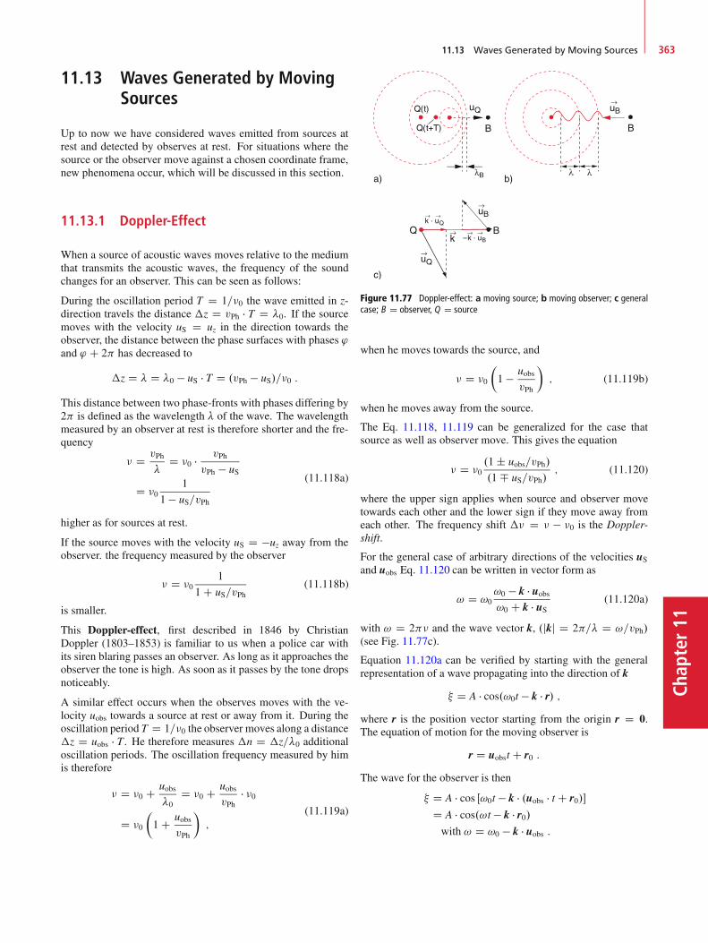
11.13 Waves Generated by Moving Sources 363
Chap
ter11
11.13 Waves Generated by MovingSources
Up to now we have considered waves emitted from sources atrest and detected by observes at rest. For situations where thesource or the observer move against a chosen coordinate frame,new phenomena occur, which will be discussed in this section.
11.13.1 Doppler-Effect
When a source of acoustic waves moves relative to the mediumthat transmits the acoustic waves, the frequency of the soundchanges for an observer. This can be seen as follows:
During the oscillation period T D 1=�0 the wave emitted in z-direction travels the distance �z D vPh � T D �0. If the sourcemoves with the velocity uS D uz in the direction towards theobserver, the distance between the phase surfaces with phases 'and ' C 2 has decreased to
�z D � D �0 � uS � T D .vPh � uS/=�0 :
This distance between two phase-fronts with phases differing by2 is defined as the wavelength � of the wave. The wavelengthmeasured by an observer at rest is therefore shorter and the fre-quency
� D vPh
�D �0 � vPh
vPh � uS
D �01
1 � uS=vPh
(11.118a)
higher as for sources at rest.
If the source moves with the velocity uS D �uz away from theobserver. the frequency measured by the observer
� D �01
1 C uS=vPh(11.118b)
is smaller.
This Doppler-effect, first described in 1846 by ChristianDoppler (1803–1853) is familiar to us when a police car withits siren blaring passes an observer. As long as it approaches theobserver the tone is high. As soon as it passes by the tone dropsnoticeably.
A similar effect occurs when the observes moves with the ve-locity uobs towards a source at rest or away from it. During theoscillation period T D 1=�0 the observer moves along a distance�z D uobs � T . He therefore measures �n D �z=�0 additionaloscillation periods. The oscillation frequency measured by himis therefore
� D �0 C uobs�0
D �0 C uobsvPh
� �0
D �0
�1 C uobs
vPh
�;
(11.119a)
Figure 11.77 Doppler-effect: a moving source; b moving observer; c generalcase; B D observer, Q D source
when he moves towards the source, and
� D �0
�1 � uobs
vPh
�; (11.119b)
when he moves away from the source.
The Eq. 11.118, 11.119 can be generalized for the case thatsource as well as observer move. This gives the equation
� D �0.1 ˙ uobs=vPh/
.1 uS=vPh/; (11.120)
where the upper sign applies when source and observer movetowards each other and the lower sign if they move away fromeach other. The frequency shift �� D � � �0 is the Doppler-shift.
For the general case of arbitrary directions of the velocities uSand uobs Eq. 11.120 can be written in vector form as
! D !0!0 � k � uobs!0 C k � uS (11.120a)
with ! D 2� and the wave vector k, .jkj D 2=� D !=vPh/(see Fig. 11.77c).
Equation 11.120a can be verified by starting with the generalrepresentation of a wave propagating into the direction of k
� D A � cos.!0t � k � r/ ;where r is the position vector starting from the origin r D 0.The equation of motion for the moving observer is
r D uobst C r0 :
The wave for the observer is then
� D A � cos Œ!0t � k � .uobs � t C r0/�
D A � cos.!t � k � r0/with ! D !0 � k � uobs :

Chapter11
364 11 Mechanical Oscillations and Waves
A similar expression can be derived when the source is moving.
Note: For light waves the Doppler-shift depends only on therelative velocity between source S and observer. This is differentfor sound waves, where the Doppler shift differs for the casewhen the source is moving from that for a moving observer.The reason for this difference is the fact that the propagation ofsound waves needs a medium and the motion of the source Sagainst this medium has another effect than the motion of theobserver. Only for u vPh the two Eq. 11.118 and 11.119converge because of 1=.1 � x/ � 1 C x for x 1.
The Doppler-effect can be already quantitatively demonstratedfor small velocities u. One acoustic source is mounted on aglider moving on an air-track while a second source with thesame frequency is at rest. Due to the Doppler-shift the superpo-sition of the two sound waves generates a beat signal which canreadily be measured, thus giving the Doppler-shift
�� D �0 � u
vPh:
Numerical Example
�0 D 5 kHz, vPh D 330m=s, u D 0:05m=s ) �� D0:75Hz. One hears a modulation of the 5 kHz frequencyat 0:75Hz. J
In another demonstration experiment the acoustic source ismounted at the swinging end of a long pendulum with lengthL. If the pendulum moves in the direction x of the line of sightthe frequency shift is
�� D �0 � uxvPh
D �0
vPh�p2g � L.1 � cos'/ :
With L D 10m the oscillation period is T D 6 s. With an elon-gation 'max D 10ı from the equilibrium position ' D 0 themaximum velocity of the acoustic source at ' D 0 is
umax Dp2g � L.1 � cos'max/ D p
2:9807 D 1:73m=s :
(Check this result by using the energy conservation during oneoscillation period!). At a frequency �0 D 5 kHz the fre-quency changes during one oscillation period from 4:974 kHzto 5:026 kHz. This can be measured by superimposing a soundwave with fixed frequency �0 and determining the beat fre-quency �0 � �.
11.13.2 Wave Fronts for Moving Sources
We consider a point-like acoustic source, which moves withthe velocity u into the z-direction. During its motion, it emitscontinuously spherical waves with frequency �0 (Fig. 11.78).According to the considerations in the last section the distancebetween two phase fronts that differ by �' D 2
�.˛/ D 1
�0.vPh � u � cos˛/ (11.121)
Shock front
z
z
Shock front
Figure 11.78 Generation of a shock front, if the velocity of the source S ap-proaches the velocity of sound
depends on the angle ˛ against the direction of the velocity uof the source. If the velocity u of the source reaches the veloc-ity vPh of the acoustic waves, the phase front distance becomes�.0/ D 0 (Fig. 11.78c). The amplitudes of the waves emittedat different times into the z-direction all superimpose in phaseresulting in a shock-wave with exceedingly large amplitude.
For u > vPh �.˛/ becomes zero for ˛ D arccos.vPh=u/. Theamplitudes of all waves emitted at different times all add up inphase at a cone with the opening angle ˇ D 90ı �˛. Accordingto (11.121) and Fig. 11.79 is cos˛ D vPh=u which gives
sinˇ D vPh
uD 1
M: (11.122)
This shock-wave cone is called Mach’s cone and the ratio M Du=vPh of source velocity to sound velocity is theMach number,named after the Austrian physicist Ernst Mach (1838–1916).
Such shock-wave cones can be observed as bow waves along aship on a lake, when the velocity u of the ship becomes largerthan the velocity vPh of water surface waves [11.16]. The sit-uation is here, however, more complex, because water surfacewaves show dispersion (see Sect. 11.9.7). The ship generates
Shock front
Figure 11.79 Calculation of the aperture angle of the Mach-cone
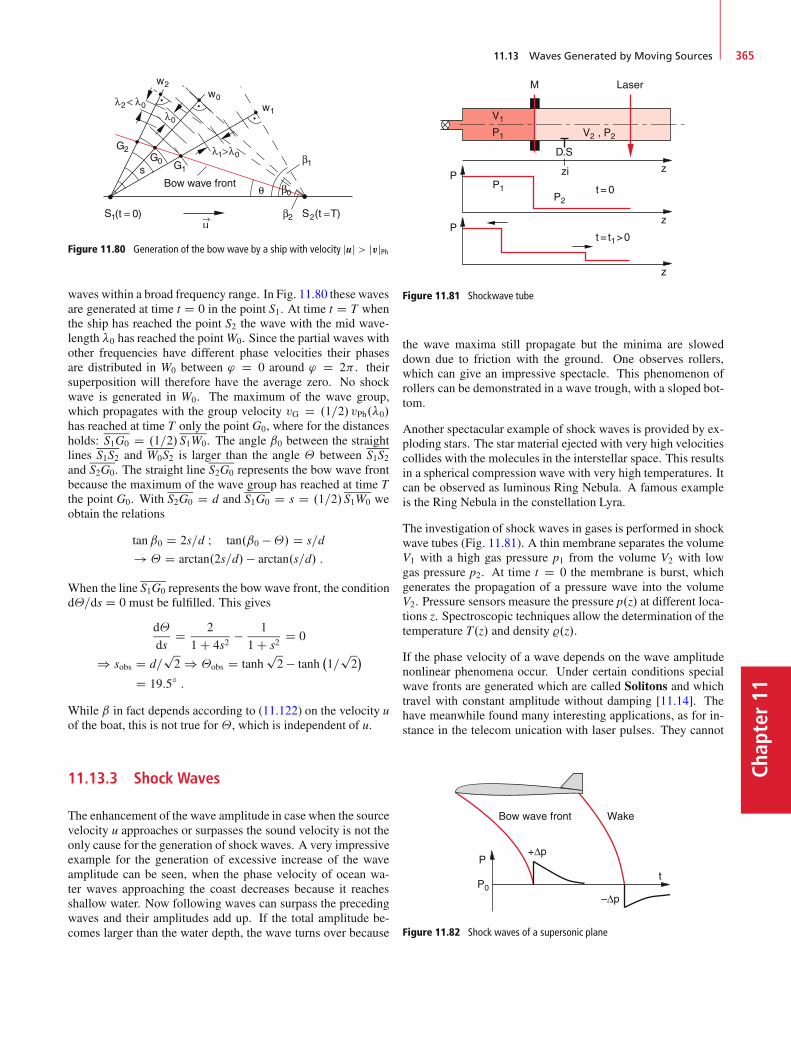
11.13 Waves Generated by Moving Sources 365
Chap
ter11
Bow wave front
Figure 11.80 Generation of the bow wave by a ship with velocity juj > jvjPh
waves within a broad frequency range. In Fig. 11.80 these wavesare generated at time t D 0 in the point S1. At time t D T whenthe ship has reached the point S2 the wave with the mid wave-length �0 has reached the pointW0. Since the partial waves withother frequencies have different phase velocities their phasesare distributed in W0 between ' D 0 around ' D 2 . theirsuperposition will therefore have the average zero. No shockwave is generated in W0. The maximum of the wave group,which propagates with the group velocity vG D .1=2/ vPh.�0/has reached at time T only the point G0, where for the distancesholds: S1G0 D .1=2/S1W0. The angle ˇ0 between the straightlines S1S2 and W0S2 is larger than the angle � between S1S2and S2G0. The straight line S2G0 represents the bow wave frontbecause the maximum of the wave group has reached at time Tthe point G0. With S2G0 D d and S1G0 D s D .1=2/S1W0 weobtain the relations
tanˇ0 D 2s=d I tan.ˇ0 ��/ D s=d
! � D arctan.2s=d/� arctan.s=d/ :
When the line S1G0 represents the bowwave front, the conditiond�=ds D 0 must be fulfilled. This gives
d�
dsD 2
1 C 4s2� 1
1 C s2D 0
) sobs D d=p2 ) �obs D tanh
p2 � tanh
�1=
p2�
D 19:5ı :
While ˇ in fact depends according to (11.122) on the velocity uof the boat, this is not true for �, which is independent of u.
11.13.3 Shock Waves
The enhancement of the wave amplitude in case when the sourcevelocity u approaches or surpasses the sound velocity is not theonly cause for the generation of shock waves. A very impressiveexample for the generation of excessive increase of the waveamplitude can be seen, when the phase velocity of ocean wa-ter waves approaching the coast decreases because it reachesshallow water. Now following waves can surpass the precedingwaves and their amplitudes add up. If the total amplitude be-comes larger than the water depth, the wave turns over because
M
Figure 11.81 Shockwave tube
the wave maxima still propagate but the minima are sloweddown due to friction with the ground. One observes rollers,which can give an impressive spectacle. This phenomenon ofrollers can be demonstrated in a wave trough, with a sloped bot-tom.
Another spectacular example of shock waves is provided by ex-ploding stars. The star material ejected with very high velocitiescollides with the molecules in the interstellar space. This resultsin a spherical compression wave with very high temperatures. Itcan be observed as luminous Ring Nebula. A famous exampleis the Ring Nebula in the constellation Lyra.
The investigation of shock waves in gases is performed in shockwave tubes (Fig. 11.81). A thin membrane separates the volumeV1 with a high gas pressure p1 from the volume V2 with lowgas pressure p2. At time t D 0 the membrane is burst, whichgenerates the propagation of a pressure wave into the volumeV2. Pressure sensors measure the pressure p.z/ at different loca-tions z. Spectroscopic techniques allow the determination of thetemperature T.z/ and density %.z/.
If the phase velocity of a wave depends on the wave amplitudenonlinear phenomena occur. Under certain conditions specialwave fronts are generated which are called Solitons and whichtravel with constant amplitude without damping [11.14]. Thehave meanwhile found many interesting applications, as for in-stance in the telecom unication with laser pulses. They cannot
Bow wave front Wake
Figure 11.82 Shock waves of a supersonic plane
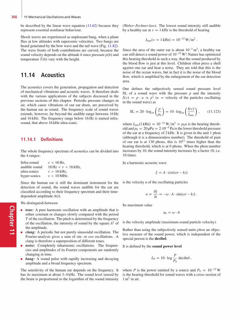
Chapter11
366 11 Mechanical Oscillations and Waves
be described by the linear wave equation (11.62) because theyrepresent essential nonlinear behaviour.
Shock waves are experienced as unpleasant bang, when a planeflies at low altitudes with supersonic velocities. Two bangs areheard generated by the bow wave and the tail wave (Fig. 11.82).The wave fronts of both contributions are curved, because thesound velocity depends on the altitude h since pressure p.h/ andtemperature T.h/ vary with the height.
11.14 Acoustics
The acoustics covers the generation, propagation and detectionof mechanical vibrations and acoustic waves. It therefore dealswith the various applications of the subjects discussed in theprevious sections of this chapter. Periodic pressure changes inair, which cause vibrations of our ear drum, are perceived bythe human ear as sound. The frequency scale of sound wavesextends, however, far beyond the audible range between 16Hzand 16 kHz. The frequency range below 16Hz is named infra-sound, that above 16 kHz ultra-sonic.
11.14.1 Definitions
The whole frequency spectrum of acoustics can be divided intothe 4 ranges:
Infra-sound � < 16Hz,audible sound 16Hz < � < 16 kHz,ultra-sonics � > 16 kHz,hyper-sonics � > 10MHz.
Since the human ear is still the dominant instrument for thedetection of sound, the sound waves audible for the ear areclassified according to their frequency spectrum and their time-dependent amplitude A.t/.
We distinguish between:
tone: A pure harmonic oscillation with an amplitude that iseither constant or changes slowly compared with the periodT of the oscillation. The pitch is determined by the frequencyof the oscillation, the intensity of sound by the square A2 ofthe amplitude.clang: A periodic but not purely sinusoidal oscillation. TheFourier-analysis gives a sum of sin- or cos oscillations. Aclang is therefore a superposition of different tones.noise: Completely inharmonic oscillations. The frequen-cies and amplitudes of its Fourier components are randomlychanging in time.bang: A sound pulse with rapidly increasing and decayingamplitude and a broad frequency spectrum.
The sensitivity of the human ear depends on the frequency. Ithas its maximum at about 3–4 kHz. The sound level sensed bythe brain is proportional to the logarithm of the sound intensity
(Weber–Fechner-law). The lowest sound intensity still audibleby a healthy ear at � D 1 kHz is the threshold of hearing
Imin.� D 1 kHz/ D 10�12 W=m2 :
Since the area of the outer ear is about 10�3 m2, a healthy earcan still detect a sound power of 10�15 W! Nature has optimizedthis hearing threshold in such a way, that the sound produced bythe blood flow is just at this level. Children often press a shellagainst one ear and hear a noise. They are told that this is thenoise of the ocean waves, but in fact it is the noise of the bloodflow, which is amplified by the enlargement of the ear detectionarea.
One defines the subjectively sensed sound pressure levelSL of a sound wave with the pressure p and the intensityI.�/ D p � u / p2 (u D velocity of the particles oscillatingin the sound wave) as
SL D 20 � log10�p
p0
�D 10 � log10
�I.�/
Imin
�; (11.123)
where Imin.1 kHz/ D 10�12 W=m2 D p0u is the hearing thresh-old and p0 D 20 µPa D 2�10�5 Pa is the lower threshold pressureof the ear at a frequency of 2 kHz. It is given in the unit 1 phon(although it is a dimensionless number). The threshold of painof our ear is at 130 phons, this is 1013 times higher than thehearing threshold, which is at 0 phons. When the phon numberincreases by 10, the sound intensity increases by a factor 10, i.e.10 times.
In a harmonic acoustic wave
� D A � cos.!t � kz/
is the velocity u of the oscillating particles
u D @�
@tD �! � A � sin.!t � kz/ :
Its maximum value
u0 D ! � A
is the velocity amplitude (maximum sound particle velocity).
Rather than using the subjectively sensed units phon an objec-tive measure of the sound power, which is independent of thespecial person is the decibel.
It is defined by the sound power level
LP D 10 � log P
P0decibel ;
where P is the power emitted by a source and P0 D 10�12 Wis the hearing threshold for sound waves with a cross section of1m2 in air.

11.14 Acoustics 367
Chap
ter11
Table 11.4 Examples of phon numbers for some acoustic sources
Low whisper 10 phonClear speech 50 phonJet plane at 100m distance � 120 phonDiscotheque 100–130 phonJack hammer at 1m distance 130 phon
Examples
An acoustic source that emits a power of 1W has a soundpower level of 10 � log 1012 D 120 decibel. The soundpower level at the hearing threshold 10�12 W is LP D 10 �log 1 D 0 decibel. A source S1 that emits 100 times thepower emitted by S2 differs by 20 decibels by a factor of100. If the decibel level increases by a factor of ten, thesound power also increases 10 fold (Tab. 11.4). J
The sound power is a characteristic property of the soundsource. It is independent of the distance, in contrast the soundpressure level and the sound intensity which decrease as 1=r2
with the distance r from the source.
11.14.2 Pressure Amplitude and EnergyDensity of Acoustic Waves
According to Eq. 11.79a and 11.80 the relation between thepressure p D p0 C �p in an acoustic wave in gases and theamplitude � is given by
@p
@zD �% � @
2�
@t2: (11.124)
With � D �0 � cos.!t � kz/ this gives
@p
@zD % � !2�0 cos.!t � kz/ : (11.125)
Integration over z yields with k D 2=�
p D �% � !2 � �2�0 � sin.!t � kz/C C :
The integration constant C is determined by the condition thatwithout the sound wave (� D 0) the pressure is p D p0, because�p D 0. This gives the equation for the pressure wave
p D p0 C�p0 � sin.!t � kz/ (11.126)
with the pressure amplitude
�p0 D �vPh%!�0 D �vPh%u0 ; (11.127)
where the relations vPh D !=k and u0 D .@�=@t/0 D ! � �0 havebeen used.
The mean energy density of the wave follows from (11.86) and(11.127) as
dW
dVD w D 1
2%!2�20 D 1
2
�p20% � v2Ph
: (11.128)
The relation between the energy density and the particle veloc-ity u in a sound wave can be derived as follows:
In a harmonic acoustic wave
� D �0 � cos.!t � kz/ ;
the velocity of the oscillating particles is
u D @�=@t D �! � �0 � sin.!t � kz/ :
Its maximum value is according to (11.127)
u0 D ! � A D �p0=.% � vPh/ ;and is named the acoustic particle velocity.
Inserting u0 into (11.128), the energy density can be written as
w D 1
2% � u20 ;
which is equal to the kinetic energy of the particles per unit vol-ume oscillating in the acoustic wave.
The energy flux density of the wave (intensity I with the dimen-sion W=m2 is then
I D vPh � dWdV
D 1
2
�p20% � vPh D 1
2vPh%u
20 : (11.129)
The total power P emitted by an acoustic source is equal to theintensity of the emitted wave, integrated over a closed surfacesurrounding the source
P DI
I � dA :
The sound pressure level is defined as
Lp D 10 log10
��p
�ps
�2
D 20 log10�p
�ps; (11.129a)
where �ps D 2 � 10�5 Pa D 2 � 10�10 bar is the sound pressureat the threshold of hearing.
Both quantities, the sound pressure level Lp and the sound powerlevel LP are relative quantities, giving the ratio of sound pressureto a given lower limit �ps, measured in decibel dB resp. theratio of sound power to the power at the threshold of hearing,also given in decibel (Tab. 11.5). They are a measure for thelogarithm of the ratios �p=�ps of sound pressures or P=Ps ofpower levels.

Chapter11
368 11 Mechanical Oscillations and Waves
Table 11.5 Sound power and sound power levels of some sound sources
Sound source Soundpower
Soundpower level
Rocket propulsion engine 106 W 180 dBJet propulsion engine 104 W 160 dBSirene 103 W 150 dBJack hammer 1W 120 dBLoud speech 10�3 W 90 dBNormal conversation 10�5 W 70 dBAverage apartment in quiet surrounding 10�7 W 50 dBWhisper 10�9 W 30 dBRustling of leaves 10�10 W 20 dBHearing threshold 10�12 W 0dB
Pain threshold
Hearing threshold
Figure 11.83 Frequency dependence of sound intensity I .�/ (measured in dB)compared with the phon numbers illustrated by the horizontal lines
Examples
1. The sound pressure level is 60 dB, when 20 �log.�p=�ps/ D 60 ) log.�p=�ps/ D 3 ) �p D103 ��ps D 2 � 10�2 Pa.
2. The sound power level is 80 dB if log.P=Ps/ D 8 )P D 108 � Ps D 10�4 W. J
The sensitivity of the ear depends on the frequency. Thereforethe curves of equal phon values as a function of frequency arenot horizontal lines in a diagram of sound power level againstfrequency (Fig. 11.83) but have a minimum at the frequency ofabout 4 kHz where the sensitivity is maximum.
11.14.3 Sound Generators
Sound waves can be generated by free or forced oscillations ofsolid bodies, which emit their oscillation energy into their sur-roundings. Examples are loud speakers, vibrating strings andtuning forks or vibrating membranes (Fig. 11.84). Also a gas
Compressedair
Figure 11.84 Different soundwave sources: a Hooter with n teeth of the ro-tation disc; b tuning fork; c vibrating string
Electrodes
Piezo disc
Acoustic wavein rod
Detector
Mounting
Figure 11.85 Piezo disc as acouctic source mounted on the end of a solid rod
stream, periodically interrupted, produces sound waves. It isused in hooters and in all wind instruments, such as trumpets,horns or flutes.
For the investigation of sound waves in solids and their prop-agation piezo-crystals can be used. They consist of materialsthat expand or contract if an external electric voltage is applied.If a disc of piezo material is attached to the end face of a rod(Fig. 11.85), application of an alternating voltage between thetwo end faces of the piezo disc produces mechanical oscillationof the disc, which propagate as acoustic waves through the rod.A second piezo disc at the other end of the rod serves as detectorof the acoustic waves. Measuring the phase difference betweenthe sound generation and the detection yields the sound velocitythrough the rod.
A commonly used acoustic source is the loudspeaker(Fig. 11.86), where a membrane is attached to a solenoid in apermanent magnet. If an electric current is send through thesolenoid, it becomes magnetic and is attracted or repelled in thefield of a permanent magnet, depending on its magnetic polarity(see Vol. 2). The attached membrane follows the movement ofthe solenoid which produces pressure waves that propagate asacoustic waves in the surrounding air.
11.14.4 Sound-Detectors
Besides the human ear, all devices, sensitive to pressurechanges, can be used as sound detectors. Examples for demon-
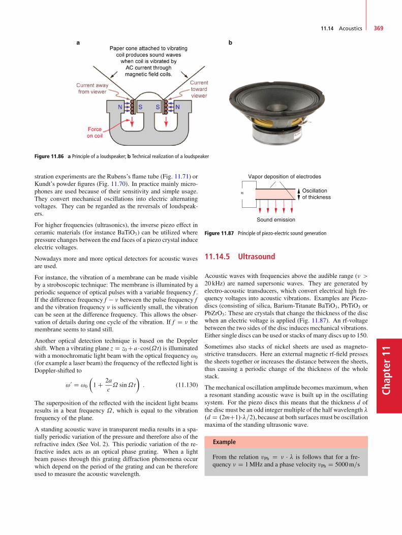
11.14 Acoustics 369
Chap
ter11
Figure 11.86 a Principle of a loudspeaker; b Technical realization of a loudspeaker
stration experiments are the Rubens’s flame tube (Fig. 11.71) orKundt’s powder figures (Fig. 11.70). In practice mainly micro-phones are used because of their sensitivity and simple usage.They convert mechanical oscillations into electric alternatingvoltages. They can be regarded as the reversals of loudspeak-ers.
For higher frequencies (ultrasonics), the inverse piezo effect inceramic materials (for instance BaTiO3) can be utilized wherepressure changes between the end faces of a piezo crystal induceelectric voltages.
Nowadays more and more optical detectors for acoustic wavesare used.
For instance, the vibration of a membrane can be made visibleby a stroboscopic technique: The membrane is illuminated by aperiodic sequence of optical pulses with a variable frequency f .If the difference frequency f � � between the pulse frequency fand the vibration frequency � is sufficiently small, the vibrationcan be seen at the difference frequency. This allows the obser-vation of details during one cycle of the vibration. If f D � themembrane seems to stand still.
Another optical detection technique is based on the Dopplershift. When a vibrating plane z D z0 Ca �cos.˝t/ is illuminatedwith a monochromatic light beam with the optical frequency !0
(for example a laser beam) the frequency of the reflected light isDoppler-shifted to
! 0 D !0
�1 C 2a
c˝ sin˝t
�: (11.130)
The superposition of the reflected with the incident light beamsresults in a beat frequency ˝ , which is equal to the vibrationfrequency of the plane.
A standing acoustic wave in transparent media results in a spa-tially periodic variation of the pressure and therefore also of therefractive index (See Vol. 2). This periodic variation of the re-fractive index acts as an optical phase grating. When a lightbeam passes through this grating diffraction phenomena occurwhich depend on the period of the grating and can be thereforeused to measure the acoustic wavelength.
Vapor deposition of electrodes
Oscillationof thickness
Sound emission
Figure 11.87 Principle of piezo-electric sound generation
11.14.5 Ultrasound
Acoustic waves with frequencies above the audible range (� >20 kHz) are named supersonic waves. They are generated byelectro-acoustic transducers, which convert electrical high fre-quency voltages into acoustic vibrations. Examples are Piezo-discs (consisting of silica, Barium-Titanate BaTiO3, PbTiO3 orPbZrO3: These are crystals that change the thickness of the discwhen an electric voltage is applied (Fig. 11.87). An rf-voltagebetween the two sides of the disc induces mechanical vibrations.Either single discs can be used or stacks of many discs up to 150.
Sometimes also stacks of nickel sheets are used as magneto-strictive transducers. Here an external magnetic rf-field pressesthe sheets together or increases the distance between the sheets,thus causing a periodic change of the thickness of the wholestack.
The mechanical oscillation amplitude becomes maximum, whena resonant standing acoustic wave is built up in the oscillatingsystem. For the piezo discs this means that the thickness d ofthe disc must be an odd integer multiple of the half wavelength �.d D .2mC1/��=2/, because at both surfaces must be oscillationmaxima of the standing ultrasonic wave.
Example
From the relation vPh D � � � is follows that for a fre-quency � D 1MHz and a phase velocity vPh D 5000m=s
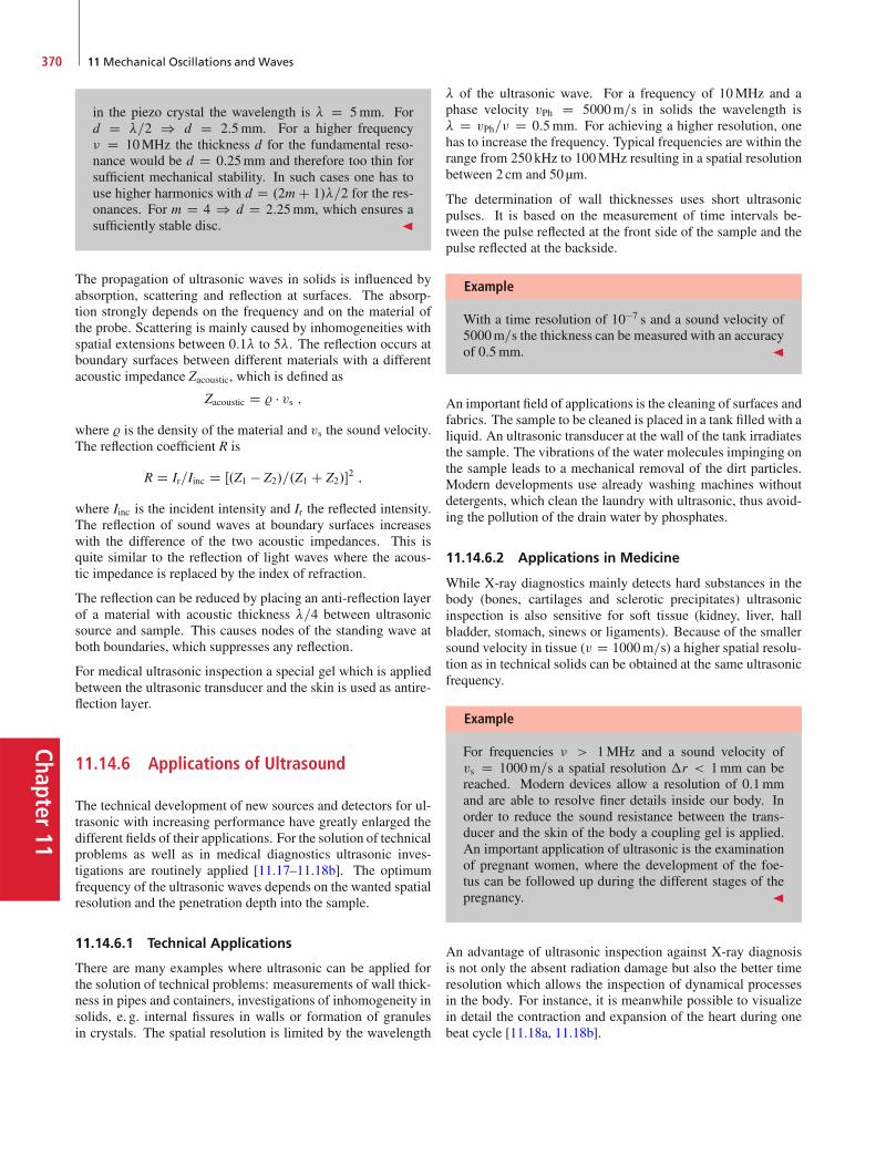
Chapter11
370 11 Mechanical Oscillations and Waves
in the piezo crystal the wavelength is � D 5mm. Ford D �=2 ) d D 2:5mm. For a higher frequency� D 10MHz the thickness d for the fundamental reso-nance would be d D 0:25mm and therefore too thin forsufficient mechanical stability. In such cases one has touse higher harmonics with d D .2m C 1/�=2 for the res-onances. For m D 4 ) d D 2:25mm, which ensures asufficiently stable disc. J
The propagation of ultrasonic waves in solids is influenced byabsorption, scattering and reflection at surfaces. The absorp-tion strongly depends on the frequency and on the material ofthe probe. Scattering is mainly caused by inhomogeneities withspatial extensions between 0:1� to 5�. The reflection occurs atboundary surfaces between different materials with a differentacoustic impedance Zacoustic, which is defined as
Zacoustic D % � vs ;where % is the density of the material and vs the sound velocity.The reflection coefficient R is
R D Ir=Iinc D Œ.Z1 � Z2/=.Z1 C Z2/�2 ;
where Iinc is the incident intensity and Ir the reflected intensity.The reflection of sound waves at boundary surfaces increaseswith the difference of the two acoustic impedances. This isquite similar to the reflection of light waves where the acous-tic impedance is replaced by the index of refraction.
The reflection can be reduced by placing an anti-reflection layerof a material with acoustic thickness �=4 between ultrasonicsource and sample. This causes nodes of the standing wave atboth boundaries, which suppresses any reflection.
For medical ultrasonic inspection a special gel which is appliedbetween the ultrasonic transducer and the skin is used as antire-flection layer.
11.14.6 Applications of Ultrasound
The technical development of new sources and detectors for ul-trasonic with increasing performance have greatly enlarged thedifferent fields of their applications. For the solution of technicalproblems as well as in medical diagnostics ultrasonic inves-tigations are routinely applied [11.17–11.18b]. The optimumfrequency of the ultrasonic waves depends on the wanted spatialresolution and the penetration depth into the sample.
11.14.6.1 Technical Applications
There are many examples where ultrasonic can be applied forthe solution of technical problems: measurements of wall thick-ness in pipes and containers, investigations of inhomogeneity insolids, e. g. internal fissures in walls or formation of granulesin crystals. The spatial resolution is limited by the wavelength
� of the ultrasonic wave. For a frequency of 10MHz and aphase velocity vPh D 5000m=s in solids the wavelength is� D vPh=� D 0:5mm. For achieving a higher resolution, onehas to increase the frequency. Typical frequencies are within therange from 250 kHz to 100MHz resulting in a spatial resolutionbetween 2 cm and 50 µm.
The determination of wall thicknesses uses short ultrasonicpulses. It is based on the measurement of time intervals be-tween the pulse reflected at the front side of the sample and thepulse reflected at the backside.
Example
With a time resolution of 10�7 s and a sound velocity of5000m=s the thickness can be measured with an accuracyof 0:5mm. J
An important field of applications is the cleaning of surfaces andfabrics. The sample to be cleaned is placed in a tank filled with aliquid. An ultrasonic transducer at the wall of the tank irradiatesthe sample. The vibrations of the water molecules impinging onthe sample leads to a mechanical removal of the dirt particles.Modern developments use already washing machines withoutdetergents, which clean the laundry with ultrasonic, thus avoid-ing the pollution of the drain water by phosphates.
11.14.6.2 Applications in Medicine
While X-ray diagnostics mainly detects hard substances in thebody (bones, cartilages and sclerotic precipitates) ultrasonicinspection is also sensitive for soft tissue (kidney, liver, hallbladder, stomach, sinews or ligaments). Because of the smallersound velocity in tissue (v D 1000m=s) a higher spatial resolu-tion as in technical solids can be obtained at the same ultrasonicfrequency.
Example
For frequencies � > 1MHz and a sound velocity ofvs D 1000m=s a spatial resolution �r < 1mm can bereached. Modern devices allow a resolution of 0:1mmand are able to resolve finer details inside our body. Inorder to reduce the sound resistance between the trans-ducer and the skin of the body a coupling gel is applied.An important application of ultrasonic is the examinationof pregnant women, where the development of the foe-tus can be followed up during the different stages of thepregnancy. J
An advantage of ultrasonic inspection against X-ray diagnosisis not only the absent radiation damage but also the better timeresolution which allows the inspection of dynamical processesin the body. For instance, it is meanwhile possible to visualizein detail the contraction and expansion of the heart during onebeat cycle [11.18a, 11.18b].
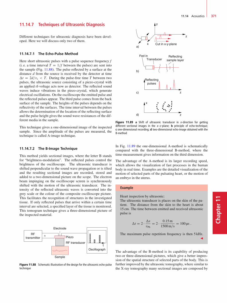
11.14 Acoustics 371
Chap
ter11
11.14.7 Techniques of Ultrasonic Diagnosis
Different techniques for ultrasonic diagnosis have been devel-oped. Here we will discuss only two of them.
11.14.7.1 The Echo-Pulse Method
Here short ultrasonic pulses with a pulse sequence frequency f(i. e. a time interval T D 1=f between the pulses) are sent intothe sample (Fig. 11.88). The pulse reflected by a surface at thedistance d from the source is received by the detector at time�t D 2d=vs < T . During the pulse-free time T between twopulses, the ultrasonic source consisting of a piezo-crystal withan applied rf-voltage acts now as detector. The reflected soundwaves induce vibrations in the piezo-crystal, which generateelectrical oscillations. On the oscilloscope the emitted pulse andthe reflected pulses appear. The third pulse comes from the backsurface of the sample. The heights of the pulses depends on thereflectivity of the surfaces. The time interval between the pulsesallows the determination of the location of the reflecting surfaceand the pulse height gives the sound wave resistances of the dif-ferent media in the sample.
This technique gives a one-dimensional image of the inspectedsample. Since the amplitude of the pulses are measured, thetechnique is called A-image technique.
11.14.7.2 The B-Image Technique
This method yields sectional images, where the letter B standsfor “brightness-modulation”. The reflected pulses control thebrightness of the oscilloscope. The ultrasonic transducer isshifted perpendicular to the sound wave propagation or is tiltedand the resulting sectional images are recorded, stored andadded to a two-dimensional picture on the scope. The electronbeam impinging on the oscilloscope screen is synchronouslyshifted with the motion of the ultrasonic transducer. The in-tensity of the reflected ultrasonic waves is converted into thegrey scale or the colour of the composite oscilloscope picture.This facilitates the recognition of structures in the investigatedtissue. If only reflected pulses that arrive within a certain timeinterval are selected, a specified layer of the tissue is monitored.This tomogram technique gives a three-dimensional picture ofthe inspected material.
RFtransmitter
Electrode
Piezo
Sample
RF transducer
Oscillograph
Figure 11.88 Schematic illustration of the design for the ultrasonic echo-pulsetechnique
Figure 11.89 a Shift of ultrasonic transducer in x-direction for gettingdifferent sectional images in the x–z-plane; b principle of echo-technique;c one-dimensional recording; d two-dimensional echo-image obtained with theB-method
In Fig. 11.89 the one-dimensional A-method is schematicallycompared with the three-dimensional B-method, where thetime-measurement gives information on the third dimension.
The advantage of the A-method is its larger recording speed,which allows the visualization of fast processes in the humanbody in real time. Examples are the detailed visualization of themotion of selected parts of the pulsating heart, or the motion ofan embryo in the uterus.
Example
Heart inspection by ultrasonic:The ultrasonic transducer is places on the skin of the pa-tient. The distance from the skin to the heart is about15 cm. The time between emitted and received ultrasonicpulse is
�t D 2 � �s
vPhD 2 � 0:15m
1500m=sD 100 µs :
The maximum pulse repetition frequency is then 5 kHz.J
The advantage of the B-method is its capability of producingtwo-or three-dimensional pictures, which give a better impres-sion of the spatial structure of selected parts of the body. This isfurther improved by the ultrasonic tomography, where similar tothe X-ray tomography many sectional images are composed by
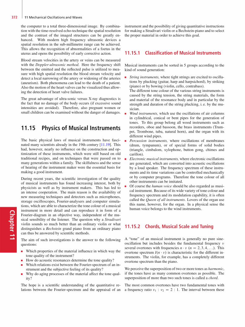
Chapter11
372 11 Mechanical Oscillations and Waves
the computer to a total three-dimensional image. By combina-tion with the time-resolved echo-technique the spatial resolutionand the contrast of the imaged structures can be greatly en-hanced. With modern high frequency ultrasonic devices aspatial resolution in the sub-millimetre range can be achieved.This allows the recognition of abnormalities of a foetus in theuterus and opens the possibility of early corrective action.
Blood stream velocities in the artery or veins can be measuredwith the Doppler-ultrasonic method. Here the frequency shiftbetween the emitted and the reflected pulse is utilized to mea-sure with high spatial resolution the blood stream velocity anddetect a local narrowing of the artery or widening of the arteries(aneurism). Both phenomena can lead to the death of a patient.Also the motion of the heart valves can be visualized thus allow-ing the detection of heart valve failures.
The great advantage of ultra-sonic versus X-ray diagnostics isthe fact that no damage of the body occurs (if excessive soundintensities are avoided). Therefore, also pregnant women orsmall children can be examined without the danger of damages.
11.15 Physics of Musical Instruments
The basic physical laws of musical instruments have fasci-nated many scientists already in the 19th century [11.19]. Thishad, however, nearly no influence on the construction and op-timization of these instruments, which were still based on oldtraditional recipes, and on techniques that were passed on tomany generations within a family. The skilfulness and the senseof hearing of the instrument maker were the essential basis formaking a good instrument.
During recent years, the scientific investigation of the qualityof musical instruments has found increasing interest, both byphysicists as well as by instrument makers. This has led toan intense cooperation. The main reason is the availability ofnew measuring techniques and detectors such as microphones,storage oscilloscopes, Fourier-analysers and computer simula-tions, which are able to characterize the tone colour of a musicalinstrument in more detail and can reproduce it in form of aFourier-diagram in an objective way, independent of the mu-sical sensibility of the listener. The question why a Stradivariviolin sounds so much better than an ordinary violin or whatdistinguishes a Bechstein grand piano from an ordinary pianocan thus be answered by scientific methods.
The aim of such investigations is the answer to the followingquestions:
Which properties of the material influence in which way thetone quality of the instrument?How do acoustic resonances determine the tone quality?Which relations exist between the Fourier-spectrum of an in-strument and the subjective feeling of its quality?Why do aging processes of the material affect the tone qual-ity?
The hope is a scientific understanding of the quantitative re-lations between the Fourier-spectrum and the appraisal of an
instrument and the possibility of giving quantitative instructionsfor making a Stradivari violin or a Bechstein-piano and to selectthe proper material in order to achieve this goal.
11.15.1 Classification of Musical Instruments
Musical instruments can be sorted in 5 groups according to thekind of sound generation:
String instruments, where tight strings are excited to oscilla-tions by plucking (guitar, harp and harpsichord), by striking(piano) or by bowing (violin, cello, contrabass).The different tone colour of the various string instruments iscaused by the string tension, the string materials, the formand material of the resonance body and in particular by thestrength and duration of the string plucking, i. e. by the mu-sician.Wind instruments, which use the oscillations of air columnsin cylindrical, conical or bent pipes for the generation oftones. To this group belong all wood instruments such asrecorders, oboe and bassoon, the brass instruments (Trum-pet, Trombone, tuba, natural horn), and the organ with itsdifferent wind pipes.Percussion instruments, where oscillations of membranes(drum, tympanum), or of special forms of solid bodies(triangle, cimbalom, xylophone, button gong, chimes andcarillon).Electronic musical instruments,where electronic oscillationsare generated, which are converted into acoustic oscillationsby a loud speaker. The frequency spectrum of these instru-ments and its time variations can be controlled mechanicallyor by computer programs. Therefore the tone colour of allother instruments can be imitated.Of course the human voice should be also regarded as musi-cal instrument. Because of its wide variety of tone colour andfrequency spectrum and its modulation capability, it is oftencalled the Queen of all instruments. Lovers of the organ usethis name, however, for the organ. In a physical sense thehuman voice belongs to the wind instruments.
11.15.2 Chords, Musical Scale and Tuning
A “tone” of an musical instrument is generally no pure sine-oscillation but includes besides the fundamental frequency �several overtones with frequencies n � � .n D 2; 3; 4; : : :/. Thisovertone spectrum I.n � �/ is characteristic for the different in-struments. The violin, for example, has a completely differentovertone spectrum than the piano.
We perceive the superposition of two or more tones as harmonic,if the tones have as many common overtones as possible. Thesuperposition of more than two such tones is called a chord.
The most common overtones have two fundamental tones witha frequency ratio �1 W �2 D 2 W 1. The interval between these
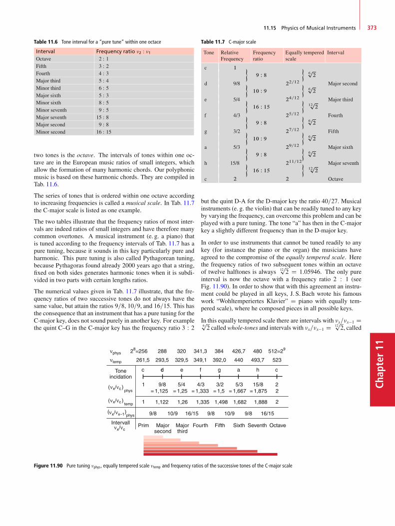
11.15 Physics of Musical Instruments 373
Chap
ter11
Table 11.6 Tone interval for a “pure tune” within one octace
Interval Frequency ratio �2 W �1Octave 2 : 1Fifth 3 : 2Fourth 4 : 3Major third 5 : 4Minor third 6 : 5Major sixth 5 : 3Minor sixth 8 : 5Minor seventh 9 : 5Major seventh 15 : 8Major second 9 : 8Minor second 16 : 15
two tones is the octave. The intervals of tones within one oc-tave are in the European music ratios of small integers, whichallow the formation of many harmonic chords. Our polyphonicmusic is based on these harmonic chords. They are compiled inTab. 11.6.
The series of tones that is ordered within one octave accordingto increasing frequencies is called a musical scale. In Tab. 11.7the C-major scale is listed as one example.
The two tables illustrate that the frequency ratios of most inter-vals are indeed ratios of small integers and have therefore manycommon overtones. A musical instrument (e. g. a piano) thatis tuned according to the frequency intervals of Tab. 11.7 has apure tuning, because it sounds in this key particularly pure andharmonic. This pure tuning is also called Pythagorean tuning,because Pythagoras found already 2000 years ago that a string,fixed on both sides generates harmonic tones when it is subdi-vided in two parts with certain lengths ratios.
The numerical values given in Tab. 11.7 illustrate, that the fre-quency ratios of two successive tones do not always have thesame value, but attain the ratios 9=8, 10=9, and 16=15. This hasthe consequence that an instrument that has a pure tuning for theC-major key, does not sound purely in another key. For examplethe quint C–G in the C-major key has the frequency ratio 3 W 2
Figure 11.90 Pure tuning �phys, equally tempered scale �temp and frequency ratios of the successive tones of the C-major scale
Table 11.7 C-major scale
Tone RelativeFrequency
Frequencyratio
Equally tempered scale
Interval
c
d
e
f
g
a
h
c
9/8
5/4
4/3
3/2
5/3
15/8
Major second
Major third
Fourth
Fifth
Major sixth
Major seventh
Octave
but the quint D-A for the D-major key the ratio 40=27. Musicalinstruments (e. g. the violin) that can be readily tuned to any keyby varying the frequency, can overcome this problem and can beplayed with a pure tuning. The tone “a” has then in the C-majorkey a slightly different frequency than in the D-major key.
In order to use instruments that cannot be tuned readily to anykey (for instance the piano or the organ) the musicians haveagreed to the compromise of the equally tempered scale. Herethe frequency ratios of two subsequent tones within an octaveof twelve halftones is always 12
p2 D 1:05946. The only pure
interval is now the octave with a frequency ratio 2 W 1 (seeFig. 11.90). In order to show that with this agreement an instru-ment could be played in all keys, J. S. Bach wrote his famouswork “Wohltemperiertes Klavier” D piano with equally tem-pered scale), where he composed pieces in all possible keys.
In this equally tempered scale there are intervals with �x=�x�1 D6p2 called whole-tones and intervals with �x=�x�1 D 12
p2, called

Chapter11
374 11 Mechanical Oscillations and Waves
Figure 11.91 Triads and their frequency-ratios
half-tones. In the C-major key the only half-tones are the inter-vals e–f and h–c, while all other intervals are whole-tones. Theonly really pure interval in the equally tempered scale is the oc-tave.
Since most instruments span a scale over several octaves, thetones in different octaves must be differently marked. Thisis done by defining the absolute frequency of a tone. Onechooses as standard tone the concert pitch “a” with a frequencyfa D 440Hz. All tones within the same octave as the concertpitch a are marked by the upper exponent 1 or by an upper apos-trophe ’. The C-major scale around the concert pitch a is then c’,d’, .e’, f’, g’, a’, h’. All tones in the octave above are marked bythe upper exponent 2 or by a double apostrophe ’’, etc. The oc-tave below the concert pitch are named as small octave, grandoctave and contra-octave. The lowest tone c on the piano hasthe frequency f D 32Hz, the next higher c has f D 65Hz. Thehighest c = c’’’’ has f D 4158Hz.
Consonant chores are a superposition of overtones with the samefundamental tone. Examples are shown in Fig. 11.91.
11.15.3 Physics of the Violin
The primary sound source of the violin is the string, clamped onboth sides, which is bowed by a violin bow. The vibration of thestring is transferred by a violin bridge and through the air to theresonance body of the violin. This resonance body has a specialform and is made of selected wood, which has been stored formany years in order to have the optimum resonance conditionfor the sound produced by bowing the strings.
When the violin bow is uniformly bowed over the string, thestring will be taken along with the moving bow at the touchpoint due to the static friction, until the restoring force of thedeflected string becomes larger than the static friction force.Now the string jumps back into its equilibrium position, be-cause the sliding friction is smaller than the static friction (see
Figure 11.92 Elongation �.t/ and velocity v.t/ D P�.t/ of the string at thelocation of the bow under a uniform bow stroke. a Strong; b medium; c weakpress-on string [11.20]
Sect. 5.6.2). The detailed motion of the string depends on theforce with which the bow is pressed against the string and onthe position of the touch point relative to the fix points of thestring (Fig. 11.92).
The oscillation of the string is therefore by no means a sine func-tion, it has a rich overtone spectrum (see Sect. 11.3.1). Thefundamental tone is determined by the length L of the string, itsmass per unit length and by its tensile force. From equation(11.77) we obtain for the phase velocity
vPh DpF= D � � � D 2�0 � L
) �0 D 1
2L
pF= :
(11.131)
Oscillation center
Time
Figure 11.93 Migration of the elongation kink along the violin string duringone oscillation period

11.15 Physics of Musical Instruments 375
Chap
ter11
Figure 11.94 Amplitudes an .t/ of fundamental tune and first overtune foruniform bow
The kink-shaped deflection of the string moves during one os-cillation period along the whole string, as shown in Fig. 11.93.The kink passes along the dashed curve, which represents a mo-mentary picture of a standing sine-wave with the wavelength� D 2L at the time of the maximum elongation.
The time-dependent deflection of the string can be described bythe Fourier series
�.x; t/ DX
n
an.t/ � sin nx
Lsin.n!t/ : (11.132)
The amplitudes a.t/ of the different overtones are not constant,even for a uniform bow motion but show a behaviour as illus-trated in Fig. 11.94.
Of particular importance for the sound of a violin is the reso-nance body. For a good violin, it has a broad resonance spectrumaround the maximum of the ear sensitivity. The wider the reso-nance spectrum is the more brilliant is the sound of the violin.For comparison, Fig. 11.95 shows the average values of the res-onance curves of ten Old Italian violins (upper curve) and thatof trivial violins. Significant differences in the range between1 kHz and 4 kHz are obvious.
Figure 11.95 Comparison of the frequency spectrum of an old Italian violin(above) and a cheap manufactured violin (below)
Figure 11.96 Holographic interferograms of the violin top (above) and bottom(below) for different frequencies. The patterns give mean elongations of thesurface, which differ between lines of equal elongation by �.� 0:6 µm/
With stroboscopic and holographic methods, the elongations ofthe cap (above) and the bottom (below) of the resonance bodycan be visualized for different frequencies. Such pictures showwhich part of the resonance body preferentially emits soundwave (Fig. 11.96).
11.15.4 Physics of the Piano
In the piano, a tone is generated by a key stroke, activating ahammer of felt that strikes a tense string. The sound of thegenerated tone depends on the material of the hammer and thecharacter of the string (thickness and tensile force) and on theresonance body. In Fig. 11.97 the amplitudes �.t/ of the trans-verse elongations are shown for three strings excited at differentfundamental frequencies. It shows that the duration ta of thehammer stroke is for low frequencies small compared with theoscillation period T D 1=�0. It furthermore illustrates that theoscillation strongly deviates from a sine function. For higherfrequencies, the stroke duration ta becomes comparable with theoscillation period.
The overtone spectrum of a C4 string with the fundamental fre-quency �1 D 262Hz, shown in Fig. 11.98, demonstrates that forhard strokes the overtone spectrum is much more pronouncedthan for soft strokes.
The frequencies of the overtones of the fundamental �1 arenot exactly at n � �1 (Fig. 11.99), because the acoustic ve-locity vPh depends on the frequency and since the frequency�.n/ D vPh=� D vPh.�/=L=n of the n-th harmonic is not equalto n � �1. The physical reason for this inharmonicity is the largerrigidity of thick strings (for low tones) compared with that ofthin strings for the higher tones. This inharmonicity essentiallyinfluences the sound of the piano tone.

Chapter11
376 11 Mechanical Oscillations and Waves
Figure 11.97 Transversal elongations �.t/ of three piano strings for differenttone frequencies. Relation between strike time of hammer ta and oscillationperiod T
kHz
Hard stroke
Normal stroke
Soft stroke
Figure 11.98 Frequency spectrum Lst.�/ of the C4-string (�0 D 262 Hz) of the piano under soft, normal und hard strokes
Overtone number n
Figure 11.99 Anharmonicity of overtunes n � �0 of the lowest piano string A.The real frequenciy of the overtunes is higher than n � �0 [11.21]
Summary
The free undamped one-dimensional oscillator performs aharmonic motion x D A � cos.!t C '/ that is determinedby its amplitude A, its circlar frequency ! D 2 � � and itsphase shift '. The total energy of the oscillation as the sumof kinetic and potential energy is constant in time.As long as the deviation from the equilibrium position issufficiently small, the restoring force is proportional to the
elongation and the oscillation amplitude is a linear functionof the restoring force. Such linear oscillations are mathemat-ically described by real sine-or cos-functions or by complexfunctions ei!t C e�i!t which, however, must be combined insuch a way that the total amplitude of the oscillation is al-ways real.
Summary 377
Chap
ter11
The superposition of different one-dimensional oscillationswith equal frequencies gives again an oscillation with thesame frequency but a phase ', that depends on the phasesof the superposed oscillations. For different frequencies thesuperposition is a more complicated oscillation with time de-pendent amplitude which is determined by the amplitudes,the phases and the frequencies of the different partial oscil-lations. The superposition can be reduced to the sum of thepartial oscillations by a Fourier-analysis.The superposition of oscillations in the x and the y-directiongives two-dimensional curves in the x–y-plane (Lissajous-figures). These are closed curves if the frequency ratio !1=!2
of the two frequencies are rational numbers.For a damped oscillator kinetic energy of the oscillationis transferred into other forms of energy, e. g. into heat offriction. For small damping the oscillation amplitude de-creases exponentially. For large friction no oscillation canbe realized. The amplitude decreases after a first elongationexponentially against zero.For a forced oscillation external energy is periodically fedinto the oscillating system. After an initial transient perioda stationary oscillation appears with the frequency of theexternal force. The losses of the damped system are justcompensated by the external energy supply. For the reso-nance case (exciting frequency D resonance frequency of thesystem) very large amplitudes are reached which might evendestroy the system (resonance disaster).For a parametric oscillator the oscillation parameters (ampli-tude, frequency or phase) are periodically changed. This isachieved by a periodic external energy supply. The paramet-ric oscillation characteristics depends on the ratio of excitingfrequency to resonance frequency of the system.A coupling between two independent oscillators leads to aperiodic energy exchange between the two oscillators. Theoscillation amplitudes change periodically, where the fre-quency of the modulation depends on the strength of thecoupling. The complicated motion of the system of N cou-pled oscillators with different frequencies can be alwaysreduced to the superposition of N normal vibrations.A wave is the propagation in space of a local perturbationof the equilibrium state. The propagation of a harmonic os-cillation gives a harmonic sine-wave. The propagation of amechanical wave is accomplished by the coupling of oscil-lating mass particles to its neighbouring particles.For transverse waves the elongation occurs perpendicular tothe propagation direction, for longitudinal waves in the prop-agation direction. Transverse wave can occur only in mediawith a shear modulusG ¤ 0. In the inside of liquids isG D 0and no transverse waves can appear. At the surface of liquidssurface tension and gravity act as restoring forces which canenable the propagation of transvers waves.The phase velocity vPh D !=k of a wave traveling througha medium depends on the properties of this medium. WhenvPh.�/ depends on the wavelength, the medium shows dis-persion.Longitudinal waves in solids have the phase velocity vPh DpE=%, which depends on the elasticity modulus E and den-
sity %, while for transverse waves vPh D pG=% depends on
the shear modulus G.In gases only longitudinal waves are possible. Their phasevelocity vPh D p
p=% depends on pressure and density of thegas.The phase velocity of transverse waves at liquid surfaces de-pends on the surface tension, on the depth of the liquid andon the wavelength. These waves show dispersion.The intensity of a wave I D .1=2/ vPh � % � A2 � !2 gives theenergy flux density measured in ŒW=m2�. It is proportionalto the squares of amplitude and frequency.A wave packet (D wave group) is generated by the superpo-sition of an infinite number of partial waves with frequenciesinside a spectral range �! around a mid-frequency !0. Itsgroup velocity vG D d!=dk gives the velocity of the maxi-mum Amax.!0/ of the amplitude distribution A.!/. In mediawith dispersion, group velocity and phase velocity are differ-ent.Huygens’ principle states that every point on a wave frontis the source of a spherical wave. The resultant wave is thesuperposition of all such elementary waves. This principleexplains all phenomena of the wave propagation, such as re-flection, refraction and diffraction.Two waves with equal frequencies are called coherent if theirsuperposition gives at every point within the superpositionregion a constant phase difference between the two waves.The superposition of coherent waves results in interferencestructures.Transverse waves can be realized with linear, circular or el-liptical polarization. For longitudinal waves there is only onetype because the oscillation direction is always in the propa-gation direction.All linear waves are solutions of the linear wave equation
�� D .1=v2/@2�=@t2
with v D vPh.Standing waves are generated by the superposition of run-ning waves under specific boundary conditions. They repre-sent spatially periodic stationary oscillation patterns.Shock waves are non-periodic waves where a short local per-turbation propagates as a singular steep pressure change.The energy of a sound wave in the volume�V
�W D .1=2/�p2=.% � v2Ph/ ��V
is proportional to the square of the pressure change�p.The energy density is �W=�V, the energy flux density (in-tensity) of a sound wave is I D vPh ��W=�V.Sound waves in gases are generated by oscillating solidbodies that transfer their oscillation energy partly to the sur-rounding gas. Examples are electro-strictive piezo materialsor loud speakers.Sound waves can be detected by membranes that are ex-cited to oscillations by the acoustic wave. If the oscillationsoccur in a magnetic field electric signals are generated (mi-crophone).
Chapter11
378 11 Mechanical Oscillations and Waves
Problems
11.1 An elastic spring is elongated by the force F D 1N by5 cm. What is the oscillation period T if a mass of 1 kg is at-tached to one end of the spring? The mass of the spring can beneglected.
11.2 A homogeneous steel wire with length L and mass Mis vertically suspended. At its lower end a mass m is attached.Now the upper suspension is shifted for a short moment in thehorizontal direction, causing a transvers wave pulse travellingdownwards. At the same time a steel ball is released from thesuspension point of the wire and falls down. Where does the ballovertake the wave pulse (air friction can be neglected). What isthe minimum value of the ratio m=M in order to realize the over-taking?
11.3 Show, that for a complex representation of a forced os-cillation only the imaginary part consumes energy. What is therole of the real part?
11.4 A soap bubble with radius R, wall thickness d and den-sity % performs radial oscillations due to the restoring force ofthe surface tension � . Calculate the oscillation period T as afunction of R, %, and � .
11.5 A plane longitudinal acoustic wave with the frequency� D 10 kHz and the amplitude A D 10�4 m propagates througha steel rod (E D 22 � 1010 N=m2, density % D 8 � 103 kg=m3).How large are the maximum tension � and the phase velocityvPh?
11.6 How large is the oscillation amplitude of a sound wavein air and the maximum velocity of the oscillating particles fora frequency � D 1 kHza) at the hearing threshold (0 dB)b) at the absolute threshold of pain (130 dB)?Compare the results with the mean free pathlength � in air andthe thermal velocity of the molecules at T D 300K.
11.7 A U-shaped tube with 2 cm inner diameter contains wa-ter with the mass 0:5 kg. When the water column in one branchis shortly pressed down by �z D 10 cm and then released, thewater column begins to oscillate. How large is the oscillationperiod and what are the maximum velocity and acceleration ofthe water? How large is the damping, if we use the values forthe viscosity � in Tab. 8.1.
11.8 A sound wave with a frequency of 2 kHz impinges verti-cally onto a sound-damping wall, which has, however, a verticalfree slit with 0:5m width. A pedestrian walks on the other sideof the wall parallel to the wall at a distance of 20m. Alongwhich path length can he receive more than 50% (5%) of thesound power incident onto the other side of the wall.
11.9 A plane sound wave impinges vertically onto a watersurface The sound velocities are: vair D 334m=s; vwater D1480m=s. Which fraction of the incident sound power is re-flected, which fraction propagates into the water? Compare alsothe intensities of the reflected and transmitted sound waves.
11.10 Two plane sound waves � D A � cos.800t � 2z/ and�2 D A � cos.630t � 1:5z/ superimpose. How looks the inter-ference pattern? What is the group velocity compared with thephase velocities of the partial waves?
11.11 What is the phase velocity of ocean waves with � D500m at a large water depth. Compare this result with waves ona lake with � D 0:5m, which are generated by throwing a stoneinto the water.
11.12 A string with length L D 1m, density % D 7:8 �103 kg=m3 and mass m D L is clamped on both ends. A ten-sile stress � D 3 � 1010N=m2 acts on the string. The string isdeflected in its mid by�r L. The form of the deflected stringcan be represented by a triangle. What are oscillation frequencyand oscillation period after ending the deflection.
11.13 A mass m D 2000 kg is suspended at the lower end of athin steel rope with L D 2m. What is the period of vertical os-cillations of the mass m? Compare the result with the horizontalpendulum oscillation of the mass m.
11.14 At the end of a thin laminated spring of length L D10 cm with the resonance frequency ! D 2 � 100 s�1 is a massm D 100 g attached. What is the frequency shift by this mass?
11.15 A buoy consisting of a cylindrical pipe with length Lfloats vertically in water. Without waves, the part a � L.a < 1/immerses in the water. What is the amplitude of the vertical os-cillation of the buoy, when sine waves with the total heights 2h(from the wave maximum to the minimum) with the period Tappear? Numerical example: a � L D 30m, h D 2m, T D 5 s.How large must L be that the wave maximum just reaches theupper peak of the buoy?
11.16 Prove that the spherical wave � D .A=r/ � ei.!t�kr/ is asolution of the wave equation�� D .1=v2Ph/@
2�=@t2.
11.17 The first tone of a police siren has the frequency �1 D390Hz, the second tone has �2 D 520Hz (the tone ratio is amajor fourth).a) At which speed of the approaching police car are both tones
higher by a whole tone (�01 D 1:12246��1, �0
2 D 1:12246��2).b) At which velocity has the observer to approach the police car
at rest, in order to hear the same tone shift?

References 379
Chap
ter11
11.18 A cube with mass m D 2 kg is at rest in the mid be-tween two springs with the spring constants D0 D 100N=m. Itcan slide on a horizontal rail (Fig. 11.100). The friction force isFf D f � m � g. The coefficient of the sliding friction is f1 D 0:3,that of the static friction f0 D 0:9.
Figure 11.100 To Probl. 11.18
a) According to which physical law do the amplitudes de-crease? (Hint: Consider the energy ratio at successivereversal points xn and xnC1 at opposite sides of the oscilla-tion.)
b) At which x-position comes the mass to a rest, if it has beenreleased at a position 22 cm away from the equilibrium posi-tion?
c) What is the time difference between two successive reversalpoints?
References
11.1. R. Bracewell, The Fourier Transform and its Applica-tions. (McGraw Hill, New York, 1999)
11.2. Ph. Dennery, A. Krtzywiki,Mathematics for Physicists.(Dover Publications, Mineola, New York, USA, 2012)
11.3. B.R. Martin, G.P. Shaw, Mathematics for Physicists.(John Wiley and Sons, Hoboken, N.J., USA, 2015)
11.4. K. Weltner et al., Mathematics for Physicists and Engi-neers. (Springer, Berlin, Heidelberg, 2014)
11.5. C.S. Lüdde, R.M. Dreizler, Theoretical Mechanics.(Springer, Berlin, Heidelberg 2010)
11.6. M. Tenenbaum, H. Pollard,Ordinary Differential Equa-tions. (Dover Publications, Mineola, USA, 1985)
11.7. R. Bronson, G. Costa, Schaum’s Outline of differentialEquations, 4th ed. (Mc GrawHill, New York, 2014)
11.8. N.W. Ashcroft, N.D. Mermin, Solid State Physics.(Cengage Learning Inc., Boston, MA, USA, 1976)
11.9. Ch. Kittel, Introduction to Solid State Physics. (JohnWiley and Sons, Hoboken, N.J., USA, 2004)
11.10. American Institute of Physics, Handbook, 3rd ed.(Mcgraw-Hill, Texas, USA, 1972)
11.11. CRC, Handbook of Chemistry and Physics, 96th ed.(CRC Press, Cleveland, Ohio, USA, 2015)
11.12. B. Le Mehauté, An Introduction to Hydrodynamics andWater Waves. (Springer, Berlin, Heidelberg, 1976)
11.13. G. Joos, I.M. Freeman, Theoretical Physics. (DoverPublications, Mineola, USA, 1986)
11.14. Th. Dauxoid, M. Peyrard, Physics of Solitons. (Cam-bridge Univ. Press, Cambridge, M.A., USA, 2006)
11.15. D. Ensminger, L.J. Bond, Ultrasonics: Fundamentals,Technologies and Applications, 3rd ed. (CRC Press,Cleveland, Ohio, USA, 2011)
11.16. F.S Crawford, Am. J. Phys. 52, 782 (1984)11.17. L.C. Lynnworth, Industrial Applications of Ultra-
sound. (IEEE Transactions of Sonics and Ultrasonic,Vol. 8U 22, March 1975)
11.18a. F.W. Kremkau, Diagnostic Utrasound: Principles andInstrumentation, 5th ed. (W.B. Saunders, Philadelphia,2001)
11.18b. F.W. Kremkau, Sonography: Principles and Applica-tions. (Saunders-Elsevier, New York, 2015)
11.19. N.H. Fletcher, Th.D. Rossing, The Physics of MusicalIntruments. (Springer, Berlin, Heidelberg, 2008)
11.20. B. Parker, Good Vibrations: The Physics of Mu-sic. (John Hopkins University Press, Baltimore, USA,2009)
11.21. A. Wood, The Physics of Music. (Read Books, 2008)11.22. https://www.amazon.co.uk/Definitive-Ealing-Studios-
Collection-DVD/dp
Chap
ter12
Nonlinear Dynamics andChaos 1212.1 Stability of Dynamical Systems . . . . . . . . . . . . . . . . . . . . . . 383
12.2 Logistic Growth Law; Feigenbaum-Diagram . . . . . . . . . . . . . . 386
12.3 Parametric Oscillator . . . . . . . . . . . . . . . . . . . . . . . . . . . . 388
12.4 Population Explosion . . . . . . . . . . . . . . . . . . . . . . . . . . . . 389
12.5 Systems with Delayed Feedback . . . . . . . . . . . . . . . . . . . . . 390
12.6 Self-Similarity . . . . . . . . . . . . . . . . . . . . . . . . . . . . . . . . 391
12.7 Fractals . . . . . . . . . . . . . . . . . . . . . . . . . . . . . . . . . . . . 392
12.8 Mandelbrot Sets . . . . . . . . . . . . . . . . . . . . . . . . . . . . . . . 393
12.9 Consequences for Our Comprehension of the Real World . . . . . . . 397
Summary . . . . . . . . . . . . . . . . . . . . . . . . . . . . . . . . . . . 397
Problems . . . . . . . . . . . . . . . . . . . . . . . . . . . . . . . . . . . 398
References . . . . . . . . . . . . . . . . . . . . . . . . . . . . . . . . . . 399
381© Springer International Publishing Switzerland 2017W. Demtröder, Mechanics and Thermodynamics, Undergraduate Lecture Notes in Physics, DOI 10.1007/978-3-319-27877-3_12

Chapter12
382 12 Nonlinear Dynamics and Chaos
In Chap. 2 we have discussed the motion of point masses underthe influence of forces. The equations of motion are linear dif-ferential equations. If the complete initial conditions are given,(e. g. location and velocity at time t D 0) the solution of the dif-ferential equation determines exactly the future fate of the pointmass (its location and velocity at future times t > 0), as long asthe forces and their changes with time are known.
For cases where the equation of motion has no analytical solu-tions and requires a numerical integration the accuracy of theresults is only limited by numerical uncertainties, which can beminimized by using sufficiently fast computers.
In such cases of exact predictions, the motion of a body or thetime development of a system are called strictly deterministic.For exact initial conditions, exact predictions of the future de-velopment are possible.
If small deviations of the initial conditions cause onlysmall changes of the future development of the system,we call the solutions of the equation of motion stable.
Examples of such stable solutions are the motion of the moonaround the earth, or of the earth around the sun. Small perturba-tion of the central gravitational force field by the influences ofthe other planets (or in case of the moon by the sun) lead onlyto small corrections of the trajectories of the earth or the moon,which can be calculated within the framework of perturbationtheory. As long as the solutions of the equation of motion arestable, such small corrections do not destroy the predictabilityof future positions and velocities.
Although we are accustomed in daily life to the normality ofstable solutions, there are numerous examples of unstable so-lutions, where tiny changes of the initial conditions result in acompletely different future development of a system, which thenlead to completely different final states.
A simple example is a ball, that is released from the point (x D0, z D h) and falls down. During its fall it hits a body with twosloped plain surfaces and a sharp edge at the top (Fig. 12.1). Ifthe initial point is only shifted by a tiny amount ıx to the right,the ball hits the right slope of the obstacle and is reflected to thepoint (x D x1, z D 0) while for ıx < 0 the ball hits the left sideand is deflected to the point (x D �x1, z D 0).
A second example is the parametric oscillator (see Sect. 11.7) asan oscillating system that is driven by an external periodic force.It can be realized, for instance, by a simple pendulum with astring length L D L0 C �L0 � cos.!t C ˛/ that is periodicallychanged and a large oscillation amplitude where the restoringforce m � g � sin ' can no longer approximated by m � g � ' (seeSect. 2.9.6), Eq. 2.79). The equation of motion of such a drivenpendulum
.L0 C�L0 cos.!t C ˛// R' C � P' C g � sin' D 0 (12.1)
is nonlinear. For certain regimes of the parameters �L0, ! and˛ (amplitude, frequency and phase of the external force) theamplitude grows until the angel ' exceeds the value . Then
Figure 12.1 The final location of the falling ball depends very sensitive on theinitial position around x D 0
the periodic pendulum motion changes into an irregular circu-lar motion where the function '.t/ shows a chaotic behaviour(Fig. 12.2).
Another example is the motion of a planet that moves in thegravitational field of two stars (double star system) that is quitecommon in the universe. Its trajectory depends critically on theinitial conditions. It can be stable, for instance, but for tinychanges of the initial conditions the motion of the planet be-comes unstable. It either leaves the system or it collides withone of the two stars.
A more difficile example is the motion of a body around theplanet Saturn in the range of the ring system. Here ranges forthe distances r to Saturn are found where the superposition ofthe gravitational forces by Saturn and by its inner moons leadsto unstable trajectories of the body while slightly different radiishow stable motions. The unstable ranges are those where thegaps in the ring system occurs. In the unstable ranges the ratioTb=Tm of the circulation periods of the body and of one of theinner moons equals the ratio p=q of small integers p and q. Avery small change of the initial radius r can convert a stabletrajectory into an unstable one.
Figure 12.2 Pendulum oscillations driven by an external force. a Small am-plitude in the stable linear range; b in the unstable range with large amplitude.The ordinate scale is in (b) 100 times larger than in (a)
12.1 Stability of Dynamical Systems 383
Chap
ter12
A similar phenomenon occurs in the asteroid belt between Marsand Jupiter, where the time-dependent gravitational attractionbetween asteroid and Jupiter leads for certain radii to unstableasteroid trajectories and causes the observed gaps in the asteroidbelt.
All of these examples correspond to equations of motion thatcontain at least one nonlinear term that is responsible for theunstable motion. For the example of the parametric pendulum,these are the nonlinear restoring force m � g � sin ' and the non-linear driving force. For certain ranges of the parameters a andb (a D ratio of the resonance frequency !0 to the driving fre-quency !, and b gives the ratio of the amplitudes of drivingforce to restoring force) the motion becomes unstable.
The solutions of linear equations have the following noteworthyproperty: They obey the superposition principle, which has beendemonstrated in Sect. 11.3 for the example of linear oscillations:If x1.t/ and x2.t/ are solutions of the linear equation, every linearcombination x.t/ D a � x1.t/C b � x2.t/ is also a solution.We will show that this superposition principle no longer holdsfor the solutions of nonlinear equations It is replaced by anotherprinciple: The scale invariance or self-similarity.
As was illustrated by the forgoing examples, for many parameterranges there are no stable solutions of nonlinear equations. Thismeans that even for very small changes of the initial conditionsthe time development of a system leads to completely differentfinal states. Since generally the initial states are not exactly de-fined (because of measuring uncertainties), the predictability isseverely limited for such systems.
Most processes in nature can be described only approximatelyby linearized equations, although in many cases an admirableaccuracy is reached (for example by prediction of moon- or so-lar eclipses). The exact equation of motion should contain thenonlinear terms. If these terms lead to unstable developmentsof the system, we called this a chaotic behaviour. Examples ofsuch chaotic behaviour can be for instance, found in Meteorol-ogy. They demonstrate that the difficulty to predict exactly theforthcoming weather is not an indication of the missing capabil-ity of the meteorologists but an inherent feature of the chaoticsystem.
In spite of these difficulties a lot of surprising statements canbe made about the solutions of nonlinear equations and thebehaviour of nonlinear systems. The investigation of chaoticsystems is the subject of Chaos Research, which can be onlyshortly discussed here. For a more extensive study of this fasci-nating field the reader is referred to the literature [12.1a–12.6b]
12.1 Stability of Dynamical Systems
A dynamical system changes with time, in contrast to a station-ary system, which has reached an equilibrium state that does nolonger change in time.
The dynamical system can be described by time-dependent pa-rameters �i.t/ .i D 1; 2; 3; : : :;N/. The quantities �.t/ can be, for
example, the coordinates xi.t/ and the velocities vi.t/ of a pointmass moving on its trajectory, or they characterize the time de-pendent state of a system of many particles, for instance pressurep.t/ and temperature T.t/. They can also describe the numberof subjects in a biological system where the population changeswith time.
If the state of a dynamical system at time t2 is unambiguouslydetermined by its state at the earlier time t1 < t2 we call thedynamics deterministic, in contrast to the stochastic or randomdynamics, where for the development of the system only proba-bilities can be given, no certain and unambiguous predictions.
When the state of a system at time t is characterized by the Nquantities
X.t/ D f�1.t/; �2.t/; : : : ; �N.t/g ; (12.2)
which we can condense in the vector X.t/, the change of thesystem in time is described by
PX.t/ D d�1.t/
dt;d�2.t/
dt; : : : ;
d�N.t/
dt
�: (12.3)
If the system converges towards a stationary (time-independent)state and reaches it in a finite time tf the condition
PX.tf/ D 0
must be fulfilled. If the stationary state is only reached at t D 1,the condition is
limt!1
PX.t/ D 0 :
An example for the first kind is the function
X.t/ D X0 C a � t2 for t < 0 and X D X0 for t > 0;
! PX.t/ D 2at for t < 0 and PX.t/ D 0 for t � 0 :
In many cases the system approaches a stationary state onlyasymptotically and reaches it for t D 1.
Example: The population of radioactive atoms, decaying with adecay constant � is
N D N0e��t ;
it approaches N.t D 1/ D 0 only after an infinite time.
Often the situation occurs that the state of a system does notchange continuously but in finite steps. An example is thenumber of living species in a biological population, where thebirth rate is not constant over the year but births happen onlyin spring. Such discrete dynamics can be described by finitedifference-equations compared to differential equations for con-tinuous dynamics. For example the number NnC1 of subjects inthe .n C 1/th generation is determined by the population in thenth generation and the birth- and death-rate:
NnC1 D Nn C Bn � Dn ; (12.4)
where the difference NnC1 � Nn, which is determined by thebirth- and death-rate, is not a continuous but discrete functionof time (see Sect. 12.2).
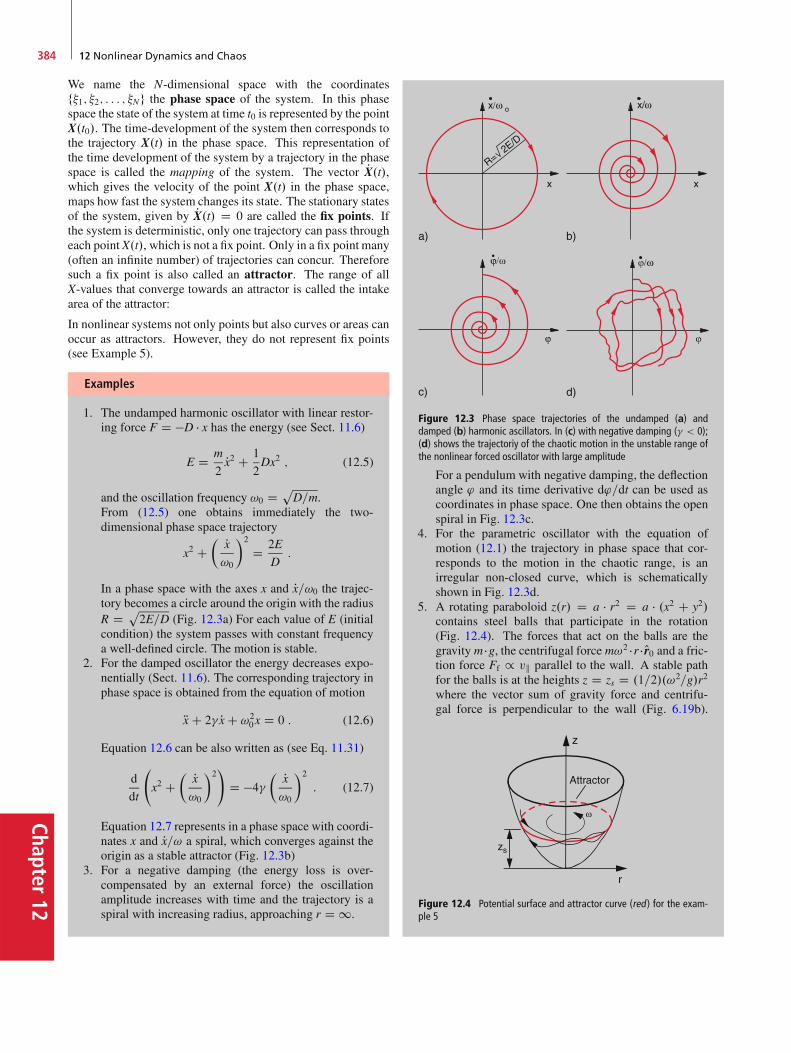
Chapter12
384 12 Nonlinear Dynamics and Chaos
We name the N-dimensional space with the coordinatesf�1; �2; : : : ; �Ng the phase space of the system. In this phasespace the state of the system at time t0 is represented by the pointX.t0/. The time-development of the system then corresponds tothe trajectory X.t/ in the phase space. This representation ofthe time development of the system by a trajectory in the phasespace is called the mapping of the system. The vector PX.t/,which gives the velocity of the point X.t/ in the phase space,maps how fast the system changes its state. The stationary statesof the system, given by PX.t/ D 0 are called the fix points. Ifthe system is deterministic, only one trajectory can pass througheach pointX.t/, which is not a fix point. Only in a fix point many(often an infinite number) of trajectories can concur. Thereforesuch a fix point is also called an attractor. The range of allX-values that converge towards an attractor is called the intakearea of the attractor:
In nonlinear systems not only points but also curves or areas canoccur as attractors. However, they do not represent fix points(see Example 5).
Examples
1. The undamped harmonic oscillator with linear restor-ing force F D �D � x has the energy (see Sect. 11.6)
E D m
2Px2 C 1
2Dx2 ; (12.5)
and the oscillation frequency !0 D pD=m.
From (12.5) one obtains immediately the two-dimensional phase space trajectory
x2 C� Px!0
�2
D 2E
D:
In a phase space with the axes x and Px=!0 the trajec-tory becomes a circle around the origin with the radiusR D p
2E=D (Fig. 12.3a) For each value of E (initialcondition) the system passes with constant frequencya well-defined circle. The motion is stable.
2. For the damped oscillator the energy decreases expo-nentially (Sect. 11.6). The corresponding trajectory inphase space is obtained from the equation of motion
Rx C 2� Px C !20x D 0 : (12.6)
Equation 12.6 can be also written as (see Eq. 11.31)
d
dt
x2 C
� Px!0
�2!
D �4�� Px!0
�2
: (12.7)
Equation 12.7 represents in a phase space with coordi-nates x and Px=! a spiral, which converges against theorigin as a stable attractor (Fig. 12.3b)
3. For a negative damping (the energy loss is over-compensated by an external force) the oscillationamplitude increases with time and the trajectory is aspiral with increasing radius, approaching r D 1.
Figure 12.3 Phase space trajectories of the undamped (a) anddamped (b) harmonic ascillators. In (c) with negative damping (� < 0);(d) shows the trajectoriy of the chaotic motion in the unstable range ofthe nonlinear forced oscillator with large amplitude
For a pendulum with negative damping, the deflectionangle ' and its time derivative d'=dt can be used ascoordinates in phase space. One then obtains the openspiral in Fig. 12.3c.
4. For the parametric oscillator with the equation ofmotion (12.1) the trajectory in phase space that cor-responds to the motion in the chaotic range, is anirregular non-closed curve, which is schematicallyshown in Fig. 12.3d.
5. A rotating paraboloid z.r/ D a � r2 D a � .x2 C y2/contains steel balls that participate in the rotation(Fig. 12.4). The forces that act on the balls are thegravity m �g, the centrifugal force m!2 �r � Or0 and a fric-tion force Ff / vk parallel to the wall. A stable pathfor the balls is at the heights z D zs D .1=2/.!2=g/r2
where the vector sum of gravity force and centrifu-gal force is perpendicular to the wall (Fig. 6.19b).
Attractor
Figure 12.4 Potential surface and attractor curve (red ) for the exam-ple 5
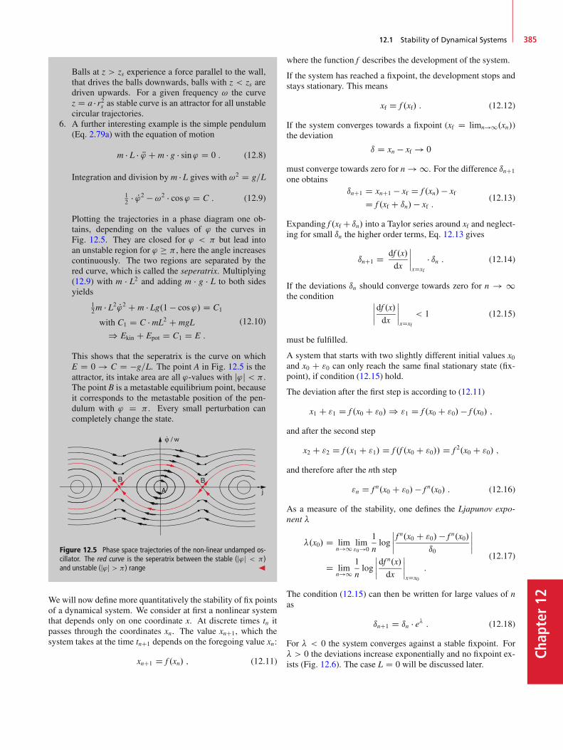
12.1 Stability of Dynamical Systems 385
Chap
ter12
Balls at z > zs experience a force parallel to the wall,that drives the balls downwards, balls with z < zs aredriven upwards. For a given frequency ! the curvez D a � r2s as stable curve is an attractor for all unstablecircular trajectories.
6. A further interesting example is the simple pendulum(Eq. 2.79a) with the equation of motion
m � L � R' C m � g � sin' D 0 : (12.8)
Integration and division by m � L gives with !2 D g=L
12 � P'2 � !2 � cos' D C : (12.9)
Plotting the trajectories in a phase diagram one ob-tains, depending on the values of ' the curves inFig. 12.5. They are closed for ' < but lead intoan unstable region for ' � , here the angle increasescontinuously. The two regions are separated by thered curve, which is called the seperatrix. Multiplying(12.9) with m � L2 and adding m � g � L to both sidesyields
12m � L2 P'2 C m � Lg.1 � cos'/ D C1
with C1 D C � mL2 C mgL
) Ekin C Epot D C1 D E :
(12.10)
This shows that the seperatrix is the curve on whichE D 0 ! C D �g=L. The point A in Fig. 12.5 is theattractor, its intake area are all '-values with j'j < .The point B is a metastable equilibrium point, becauseit corresponds to the metastable position of the pen-dulum with ' D . Every small perturbation cancompletely change the state.
Figure 12.5 Phase space trajectories of the non-linear undamped os-cillator. The red curve is the seperatrix between the stable (j'j < )and unstable (j'j > ) range J
We will now define more quantitatively the stability of fix pointsof a dynamical system. We consider at first a nonlinear systemthat depends only on one coordinate x. At discrete times tn itpasses through the coordinates xn. The value xnC1, which thesystem takes at the time tnC1 depends on the foregoing value xn:
xnC1 D f .xn/ ; (12.11)
where the function f describes the development of the system.
If the system has reached a fixpoint, the development stops andstays stationary. This means
xf D f .xf/ : (12.12)
If the system converges towards a fixpoint (xf D limn!1.xn/)the deviation
ı D xn � xf ! 0
must converge towards zero for n ! 1. For the difference ınC1
one obtainsınC1 D xnC1 � xf D f .xn/ � xf
D f .xf C ın/ � xf :(12.13)
Expanding f .xf C ın/ into a Taylor series around xf and neglect-ing for small ın the higher order terms, Eq. 12.13 gives
ınC1 D df .x/
dx
ˇ̌ˇ̌xDxf
� ın : (12.14)
If the deviations ın should converge towards zero for n ! 1the condition ˇ̌
ˇ̌df .x/dx
ˇ̌ˇ̌xDxf
< 1 (12.15)
must be fulfilled.
A system that starts with two slightly different initial values x0and x0 C "0 can only reach the same final stationary state (fix-point), if condition (12.15) hold.
The deviation after the first step is according to (12.11)
x1 C "1 D f .x0 C "0/ ) "1 D f .x0 C "0/ � f .x0/ ;
and after the second step
x2 C "2 D f .x1 C "1/ D f .f .x0 C "0// D f 2.x0 C "0/ ;
and therefore after the nth step
"n D f n.x0 C "0/ � f n.x0/ : (12.16)
As a measure of the stability, one defines the Ljapunov expo-nent �
�.x0/ D limn!1 lim
"0!0
1
nlog
ˇ̌ˇ̌ f
n.x0 C "0/ � f n.x0/
ı0
ˇ̌ˇ̌
D limn!1
1
nlog
ˇ̌ˇ̌df
n.x/
dx
ˇ̌ˇ̌xDx0
:
(12.17)
The condition (12.15) can then be written for large values of nas
ınC1 D ın � e� : (12.18)
For � < 0 the system converges against a stable fixpoint. For� > 0 the deviations increase exponentially and no fixpoint ex-ists (Fig. 12.6). The case L D 0 will be discussed later.
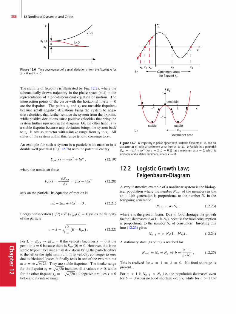
Chapter12
386 12 Nonlinear Dynamics and Chaos
Figure 12.6 Time development of a small deviation " from the fixpoint xf for� > 0 and � < 0
The stability of fixpoints is illustrated by Fig. 12.7a, where theschematically drawn trajectory in the phase space (x; Px) is therepresentation of a one-dimensional equation of motion. Theintersection points of the curve with the horizontal line Px D 0are the fixpoints. The points x1 and x3 are unstable fixpoints,because small negative deviations bring the system to nega-tive velocities, that further remove the system from the fixpoint,while positive deviations cause positive velocities that bring thesystem further upwards in the diagram. On the other hand is x2a stable fixpoint because any deviation brings the system backto x2. It acts as attractor with a intake range from x1 to x3. Allstates of the system within this range tend to converge to x2.
An example for such a system is a particle with mass m in adouble well potential (Fig. 12.7b) with the potential energy
Epot.x/ D �ax2 C bx4 ; (12.19)
where the nonlinear force
Fx.x/ D �dEpot
dxD 2ax � 4bx3 (12.20)
acts on the particle. Its equation of motion is
mRx � 2ax C 4bx3 D 0 : (12.21)
Energy conservation .1=2/mPx2CEpot.x/ D E yields the velocityof the particle
v D Px Dr
2
m
�E � Epot
�: (12.22)
For E D Epot ! Ekin D 0 the velocity becomes Px D 0 at theposition x D 0 because there is Epot.0/ D 0. However, this is nostable fixpoint, because small deviations bring the particle eitherto the left or the right minimum. If its velocity converges to zerodue to frictional losses, it finally rests in one of the two minimaat x D ˙pa=2b. They are stable fixpoints. The intake rangefor the fixpoint x1 D p
a=2b includes all x-values x > 0, whilefor the other fixpoint x2 D �pa=2b all negative x-values x < 0belong to its intake range.
Catchment areafor fixpoint x2
unstable
stable stable
Catchment area
Figure 12.7 a Trajectory in phase space with unstable fixpoints x1, x3 and anattractor at x2 with a catchment area from x1 to x3. b Particle in a potentialEpot D �ax2 C bx4 (for a D 2, b D 0:5) has a maximum at x D 0, which isunstable and a stable minimum, where Px ! 0
12.2 Logistic Growth Law;Feigenbaum-Diagram
A very instructive example of a nonlinear system is the biolog-ical population where the number NnC1 of the members in the.n C 1/th generation is proportional to the number Nn in theforegoing generation.
NnC1 D a � Nn ; (12.23)
where a is the growth factor. Due to food shortage the growthfactor a decreases to a.1�b �Nn/, because the food consumptionis proportional to the number Nn of consumers. Inserting thisinto (12.23) gives
NnC1 D a � Nn.1 � bNn/ : (12.24)
A stationary state (fixpoint) is reached for
NnC1 D Nn D Nst ) b D a � 1
a � Nst: (12.25)
This is realized for a D 1 ) b D 0. No food shortage ispresent.
For a < 1 is NnC1 < Nn i. e. the population decreases evenfor b D 0 when no food shortage occurs, while for a > 1 the
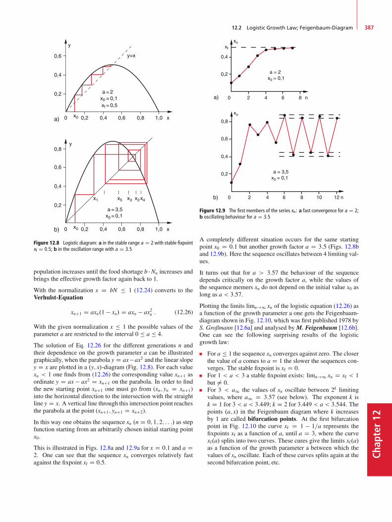
12.2 Logistic Growth Law; Feigenbaum-Diagram 387
Chap
ter12
Figure 12.8 Logistic diagram: a in the stable range a D 2 with stable fixpointxf D 0:5; b in the oscillation range with a D 3:5
population increases until the food shortage b �Nn increases andbrings the effective growth factor again back to 1.
With the normalization x D bN � 1 (12.24) converts to theVerhulst-Equation
xnC1 D axn.1 � xn/ D axn � ax2n : (12.26)
With the given normalization x � 1 the possible values of theparameter a are restricted to the interval 0 � a � 4.
The solution of Eq. 12.26 for the different generations n andtheir dependence on the growth parameter a can be illustratedgraphically, when the parabola y D ax�ax2 and the linear slopey D x are plotted in a .y; x/-diagram (Fig. 12.8). For each valuexn < 1 one finds from (12.26) the corresponding value xnC1 asordinate y D ax � ax2 D xnC1 on the parabola. In order to findthe new starting point xnC1 one must go from (xn; yn D xnC1)into the horizontal direction to the intersection with the straightline y D x. A vertical line through this intersection point reachesthe parabola at the point (xnC1; ynC1 D xnC2).
In this way one obtains the sequence xn .n D 0; 1; 2; : : :/ as stepfunction starting from an arbitrarily chosen initial starting pointx0.
This is illustrated in Figs. 12.8a and 12.9a for x D 0:1 and a D2. One can see that the sequence xn converges relatively fastagainst the fixpoint xf D 0:5.
Figure 12.9 The first members of the series xn : a fast convergence for a D 2;b oscillating behaviour for a D 3:5
A completely different situation occurs for the same startingpoint x0 D 0:1 but another growth factor a D 3:5 (Figs. 12.8band 12.9b). Here the sequence oscillates between 4 limiting val-ues.
It turns out that for a > 3:57 the behaviour of the sequencedepends critically on the growth factor a, while the values ofthe sequence memers xn do not depend on the initial value x0 aslong as a < 3:57.
Plotting the limits limn!1 xn of the logistic equation (12.26) asa function of the growth parameter a one gets the Feigenbaum-diagram shown in Fig. 12.10, which was first published 1978 byS. Großmann [12.6a] and analysed by M. Feigenbaum [12.6b].One can see the following surprising results of the logisticgrowth law:
For a � 1 the sequence xn converges against zero. The closerthe value of a comes to a D 1 the slower the sequences con-verges. The stable fixpoint is xf D 0.For 1 < a < 3 a stable fixpoint exists: limn!1 xn D xf < 1but ¤ 0.For 3 < a1 the values of xn oscillate between 2k limitingvalues, where a1 D 3:57 (see below). The exponent k isk D 1 for 3 < a < 3:449; k D 2 for 3:449 < a < 3:544. Thepoints .a; x/ in the Feigenbaum diagram where k increasesby 1 are called bifurcation points. At the first bifurcationpoint in Fig. 12.10 the curve xf D 1 � 1=a represents thefixpoints xf as a function of a, until a D 3, where the curvexf.a/ splits into two curves. These cures give the limits xf.a/as a function of the growth parameter a between which thevalues of xn oscillate. Each of these curves splits again at thesecond bifurcation point, etc.

Chapter12
388 12 Nonlinear Dynamics and Chaos
Figure 12.10 Feigenbaum diagram: Value of the fixpoint xf as a function of the control parameter a. The values ai give the bifurcation points a1 D 3:0;a2 D 3:449: : :; a3 D 3:544: : :; a4 D 3:564: : :
The system has therefore 2k attractors for all values of thegrowth parameter a in the range ak � a � akC1 between thebifurcation points ak and akC1.With increasing values of a the interval between two bifurca-tion points becomes smaller and smaller. The values of thebifurcation points of order k follow a geometrical sequence
ak D a1 � c � ı�k for k � 1 : (12.27)
For the distance�k D ak � ak�1 we obtain
�k D c � ı�k.ı � 1/ : (12.28)
The Feigenbaum-constant ıF D limn!1.�k=�kC1/ has thenumerical value
ıF � 4:669201660910: : : :
The sequence of bifurcation points converges against thelimit
a1 D limk!1
ak D 3:5699456: : : :
The Ljapunov exponent � is in the range 3 < a < a1 alwaysnegative, except at the bifurcation points where is � D 0.In the range a1 < a < 4 chaotic regions occur wherethe values of the fixpoints scatter randomly. Here is theLjapunov exponent � > 0 (Fig. 12.11) between these chaoticranges periodic windows appear where stable fixpoints oc-cur. The sequence xn oscillates between these fixpoints. TheLjapunov exponent � is negative in these windows. With in-creasing values of the growth parameter a the chaotic regionsmore and more displace the windows of stable regions.In the chaotic regions rational start values give fixpoints,while for irrational start values no convergence is possibleFor a D 4 the logistic equation
xnC1 D 4xn.1 � xn/ (12.29)
can be exactly solved and gives the solution
xn D sin2.2nx0/ ; (12.30)
where x0 is the start value.
Figure 12.11 The fixpoints of the logistic mapping for different values of theparameter a for illustration of the bifurcation
12.3 Parametric Oscillator
The equation of the undamped parametric oscillator, depicted inFig. 11.25 with the pendulum length
L.t/ D L0 ��L0 cos˝t (12.31)
and �L0=L0 1, can be written as
R' C !20
�1 C �L0
L0cos˝t
�sin ' D 0 ; (12.32)
where the approximations
1
LD 1
L0�1 � �L0
L0cos˝t
� 1
L0
�1 C �L0
L0cos˝t
�
have been used with the frequency
!2 D !20
�1 C �L0
L0cos˝t
�:
Introducing the abbreviations !20 D g=L0; ˛ D !2
0=˝2; ˇ D
�L0=L0 and � D ˝ � t the Eq. 12.32 converts into the Mathieu-equation
' 00 C ˛ .1 C ˇ cos �/ ' D 0 ; (12.33)

12.4 Population Explosion 389
Chap
ter12
Figure 12.12 Stable (white) and unstable (red ) ranges for the solutions of theMathieu equation
where ' 00 D d2'=d�2. The solutions of this linear differentialequation depend on the parameters ˛ and ˇ. There exist sta-ble solutions for certain ranges (˛; ˇ) which are shown as whiteareas in Fig. 12.12 while for the red areas (resonance ranges)unstable solutions exist, where ' increases unlimited.
The first instable range appears for ˛ D .1=4/, ! ˝ D 2!0.This is the parameter range which a child instinctively uses toenhance the oscillation amplitude of its swing by uplifting andlowering its centre of mass at the right moment twice per oscilla-tion period. Without damping the oscillation amplitude becomesinfinite in the red regions and the solutions of (12.33) lead touseless results.
The situation changes if we do not use the approximate linearequation but the exact nonlinear equation (12.32) for the so-lution of the problem. We start with the trivial case ' D 0,where the pendulum does not perform angular oscillations '.t/but only vertical periodic changes of the pendulum length L.t/.The mass m then executes vertical oscillations with the excitingfrequency˝ , where always ' D 0. This is true for ˛ < 1=4 andˇ 1. If for ˛ D 1=4 the amplitude exceeds a critical ampli-tude ˇc the oscillation becomes unstable and the vertical motionswitches into a '-oscillation (Fig. 12.13) with an amplitude thatdepends on the parameter ˇ. The frequency!0 of this '.t/ oscil-lation is one half of the exciting frequency ˝ .!0 D .1=2/˝/.At the bifurcation point B in Fig. 12.13 a doubling of the periodlength T occurs. When further increasing ˇ, more and more
Figure 12.13 The first bifurcation of the pendulum that oscillates initially onlyvertical. The abscissa ˇ D �L=L0 corresponds in the stability diagram ofFig. 12.12 a vertical line
Figure 12.14 Phase diagram of the parametrically driven pendulum a in thestable, b in the unstable region
bifurcation points are passed until the chaotic range is reachedwhere the motion of the pendulum becomes random. Here astatistic motion of vertical and angular oscillation takes place.The phase diagram of the regula and chaotic ranges is shown inFig. 12.14.
In the chaotic regime the motion is very sensitive to smallchanges of the initial conditions. Plotting '.t/ against t smallchanges of '.0/ or d'=dt.0/ result in large changes of �'.t/which can grow exponentially with time t [12.4].
12.4 Population Explosion
We will describe the growth of the world population by a simplemodel that allows in spite of its simplicity, a good insight intothe problem [12.5].
We will take zf.t/ as the female and zm.t/ as the male populationat time t. We denote the death rate of the females as af � zf andthat of the males as am � zm. The birth-rate is proportional to theproduct zf � zm. For the change of the population per unit timewe then obtain
Pzm D �amzm C bmzmzf ; (12.34a)
Pzf D �afzf C bfzfzm : (12.34b)
The “symbiosis”-terms bmzm � zf and bf � zf � zm cause the nonlin-earity of the equation and couple them with each other.
It turns out that birth rates and death rates do not differ muchbetween males and females. We therefore can approximateam D af D a and bm D bf D b. Furthermore the popula-tion statistics shows that the populations of males and femalesis approximately equal, i. e. zm � zf.
With these assumptions we obtain for the total population z Dzm C zf by addition of the two Eqs. 12.34a,b the nonlinear equa-tion
Pz D �a � z C b
2z2 : (12.35)
For b D 0 (zero birth-rate) we get the solution
z.t/ D z0e�at : (12.36)
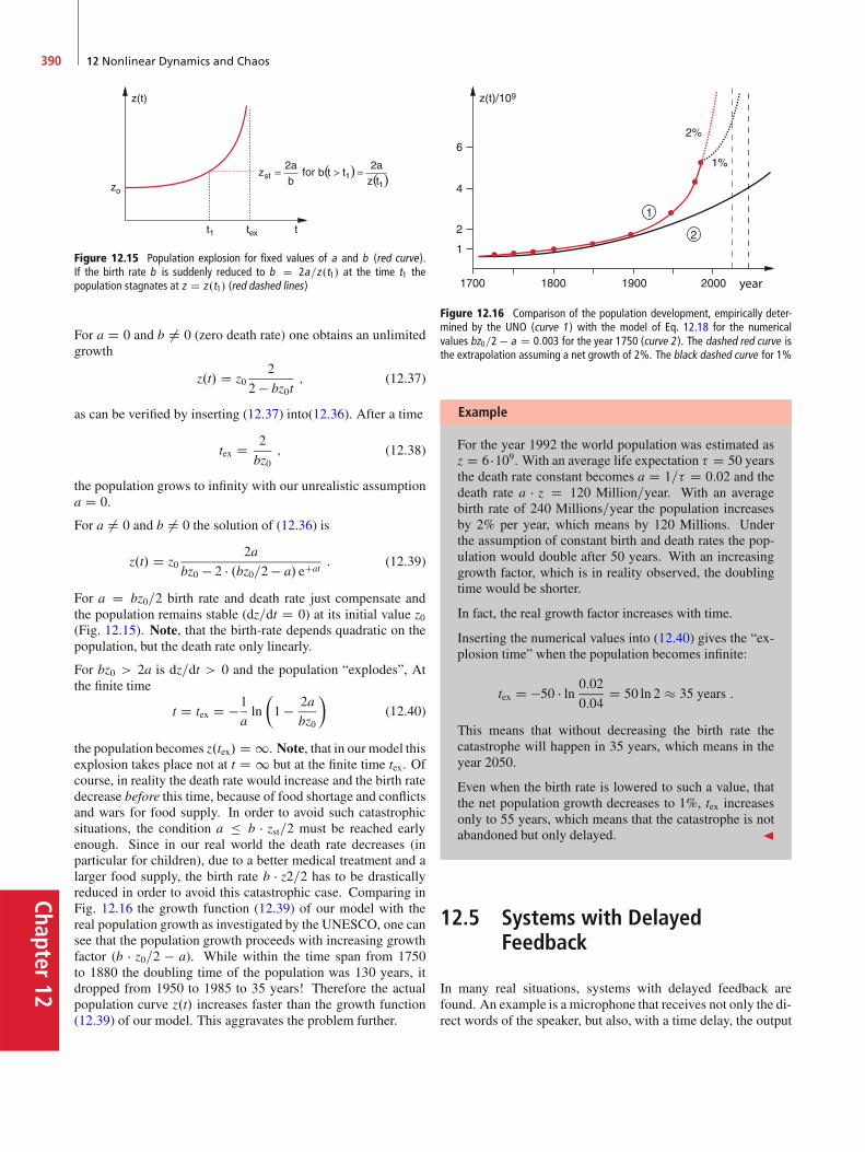
Chapter12
390 12 Nonlinear Dynamics and Chaos
Figure 12.15 Population explosion for fixed values of a and b (red curve).If the birth rate b is suddenly reduced to b D 2a=z.t1/ at the time t1 thepopulation stagnates at z D z.t1/ (red dashed lines)
For a D 0 and b ¤ 0 (zero death rate) one obtains an unlimitedgrowth
z.t/ D z02
2 � bz0t; (12.37)
as can be verified by inserting (12.37) into(12.36). After a time
tex D 2
bz0; (12.38)
the population grows to infinity with our unrealistic assumptiona D 0.
For a ¤ 0 and b ¤ 0 the solution of (12.36) is
z.t/ D z02a
bz0 � 2 � .bz0=2 � a/ eCat: (12.39)
For a D bz0=2 birth rate and death rate just compensate andthe population remains stable (dz=dt D 0) at its initial value z0(Fig. 12.15). Note, that the birth-rate depends quadratic on thepopulation, but the death rate only linearly.
For bz0 > 2a is dz=dt > 0 and the population “explodes”, Atthe finite time
t D tex D �1
aln
�1 � 2a
bz0
�(12.40)
the population becomes z.tex/ D 1. Note, that in our model thisexplosion takes place not at t D 1 but at the finite time tex. Ofcourse, in reality the death rate would increase and the birth ratedecrease before this time, because of food shortage and conflictsand wars for food supply. In order to avoid such catastrophicsituations, the condition a � b � zst=2 must be reached earlyenough. Since in our real world the death rate decreases (inparticular for children), due to a better medical treatment and alarger food supply, the birth rate b � z2=2 has to be drasticallyreduced in order to avoid this catastrophic case. Comparing inFig. 12.16 the growth function (12.39) of our model with thereal population growth as investigated by the UNESCO, one cansee that the population growth proceeds with increasing growthfactor (b � z0=2 � a). While within the time span from 1750to 1880 the doubling time of the population was 130 years, itdropped from 1950 to 1985 to 35 years! Therefore the actualpopulation curve z.t/ increases faster than the growth function(12.39) of our model. This aggravates the problem further.
year
Figure 12.16 Comparison of the population development, empirically deter-mined by the UNO (curve 1 ) with the model of Eq. 12.18 for the numericalvalues bz0=2 � a D 0:003 for the year 1750 (curve 2 ). The dashed red curve isthe extrapolation assuming a net growth of 2%. The black dashed curve for 1%
Example
For the year 1992 the world population was estimated asz D 6 �109. With an average life expectation � D 50 yearsthe death rate constant becomes a D 1=� D 0:02 and thedeath rate a � z D 120 Million=year. With an averagebirth rate of 240 Millions=year the population increasesby 2% per year, which means by 120 Millions. Underthe assumption of constant birth and death rates the pop-ulation would double after 50 years. With an increasinggrowth factor, which is in reality observed, the doublingtime would be shorter.
In fact, the real growth factor increases with time.
Inserting the numerical values into (12.40) gives the “ex-plosion time” when the population becomes infinite:
tex D �50 � ln 0:02
0:04D 50 ln 2 � 35 years :
This means that without decreasing the birth rate thecatastrophe will happen in 35 years, which means in theyear 2050.
Even when the birth rate is lowered to such a value, thatthe net population growth decreases to 1%, tex increasesonly to 55 years, which means that the catastrophe is notabandoned but only delayed. J
12.5 Systems with DelayedFeedback
In many real situations, systems with delayed feedback arefound. An example is a microphone that receives not only the di-rect words of the speaker, but also, with a time delay, the output
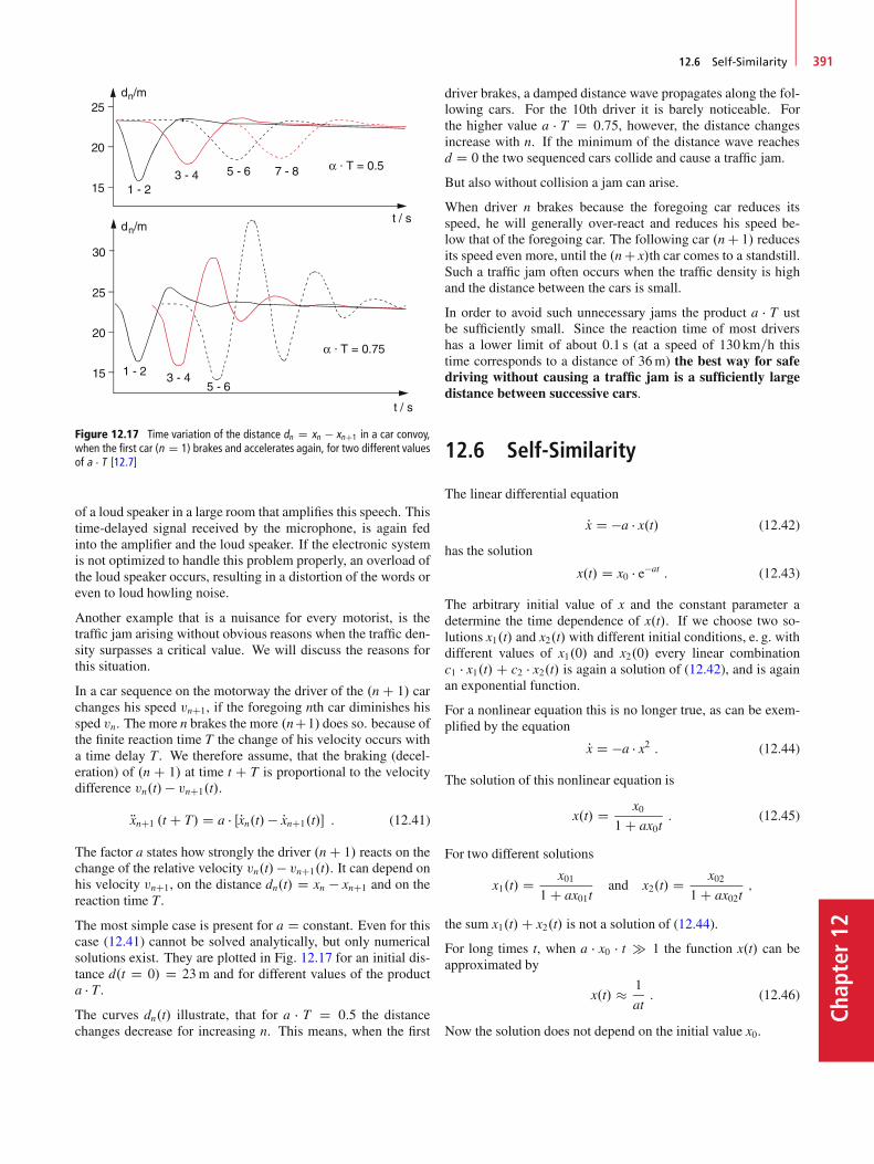
12.6 Self-Similarity 391
Chap
ter12
Figure 12.17 Time variation of the distance dn D xn � xnC1 in a car convoy,when the first car (n D 1) brakes and accelerates again, for two different valuesof a � T [12.7]
of a loud speaker in a large room that amplifies this speech. Thistime-delayed signal received by the microphone, is again fedinto the amplifier and the loud speaker. If the electronic systemis not optimized to handle this problem properly, an overload ofthe loud speaker occurs, resulting in a distortion of the words oreven to loud howling noise.
Another example that is a nuisance for every motorist, is thetraffic jam arising without obvious reasons when the traffic den-sity surpasses a critical value. We will discuss the reasons forthis situation.
In a car sequence on the motorway the driver of the .n C 1/ carchanges his speed vnC1, if the foregoing nth car diminishes hissped vn. The more n brakes the more .nC1/ does so. because ofthe finite reaction time T the change of his velocity occurs witha time delay T . We therefore assume, that the braking (decel-eration) of .n C 1/ at time t C T is proportional to the velocitydifference vn.t/ � vnC1.t/.
RxnC1 .t C T/ D a � ŒPxn.t/ � PxnC1.t/� : (12.41)
The factor a states how strongly the driver .n C 1/ reacts on thechange of the relative velocity vn.t/� vnC1.t/. It can depend onhis velocity vnC1, on the distance dn.t/ D xn � xnC1 and on thereaction time T .
The most simple case is present for a D constant. Even for thiscase (12.41) cannot be solved analytically, but only numericalsolutions exist. They are plotted in Fig. 12.17 for an initial dis-tance d.t D 0/ D 23m and for different values of the producta � T .The curves dn.t/ illustrate, that for a � T D 0:5 the distancechanges decrease for increasing n. This means, when the first
driver brakes, a damped distance wave propagates along the fol-lowing cars. For the 10th driver it is barely noticeable. Forthe higher value a � T D 0:75, however, the distance changesincrease with n. If the minimum of the distance wave reachesd D 0 the two sequenced cars collide and cause a traffic jam.
But also without collision a jam can arise.
When driver n brakes because the foregoing car reduces itsspeed, he will generally over-react and reduces his speed be-low that of the foregoing car. The following car .nC 1/ reducesits speed even more, until the .nC x/th car comes to a standstill.Such a traffic jam often occurs when the traffic density is highand the distance between the cars is small.
In order to avoid such unnecessary jams the product a � T ustbe sufficiently small. Since the reaction time of most drivershas a lower limit of about 0:1 s (at a speed of 130 km=h thistime corresponds to a distance of 36m) the best way for safedriving without causing a traffic jam is a sufficiently largedistance between successive cars.
12.6 Self-Similarity
The linear differential equation
Px D �a � x.t/ (12.42)
has the solution
x.t/ D x0 � e�at : (12.43)
The arbitrary initial value of x and the constant parameter adetermine the time dependence of x.t/. If we choose two so-lutions x1.t/ and x2.t/ with different initial conditions, e. g. withdifferent values of x1.0/ and x2.0/ every linear combinationc1 � x1.t/C c2 � x2.t/ is again a solution of (12.42), and is againan exponential function.
For a nonlinear equation this is no longer true, as can be exem-plified by the equation
Px D �a � x2 : (12.44)
The solution of this nonlinear equation is
x.t/ D x01 C ax0t
: (12.45)
For two different solutions
x1.t/ D x011 C ax01t
and x2.t/ D x021 C ax02t
;
the sum x1.t/C x2.t/ is not a solution of (12.44).
For long times t, when a � x0 � t � 1 the function x.t/ can beapproximated by
x.t/ � 1
at: (12.46)
Now the solution does not depend on the initial value x0.
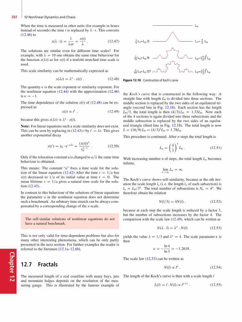
Chapter12
392 12 Nonlinear Dynamics and Chaos
When the time is measured in other units (for example in hoursinstead of seconds) the time t is replaced by � � t. This converts(12.46) to
x.� � t/ D 1
�atD x.t/
�: (12.47)
The solutions are similar even for different time scales! Forexample, with � D 10 one obtains the same time behaviour forthe function x.�t/ as for x.t/ if a tenfold stretched time scale isused.
This scale similarity can be mathematically expressed as
x.�t/ D �� � x.t/ : (12.48)
The quantity � is the scale exponent or similarity exponent. Forthe nonlinear equation (12.44) with the approximation (12.46)is � D �1.
The time dependence of the solution x.t/ of (12.48) can be ex-pressed as
x.t/ / t� ; (12.49)
because this gives x.�t/ / �� � x.t/.Note: For linear equations such a scale similarity does not exist.This can be seen by replacing in (12.43) t by t0 D �t. This givesanother exponential decay
x.t0/ D x0 � e�a�t D .x.t//�
x��10
: (12.50)
Only if the relaxation constant a is changed to a=� the same timebehaviour is obtained.
This means: The constant “a” fixes a time scale for the solu-tion of the linear equation (12.42) After the time t D 1=a hasx.t/ decreased to 1=e of its initial value at time t D 0. Themean lifetime � D 1=a gives a natural time scale for the solu-tion (12.43).
In contrast to this behaviour of the solutions of linear equationsthe parameter a in the nonlinear equation does not determinesuch a benchmark. An arbitrary time stretch can be always com-pensated by a corresponding change of the x-scale.
The self-similar solutions of nonlinear equations do nothave a natural benchmark.
This is not only valid for time-dependent problems but also formany other interesting phenomena, which can be only partlypresented in the next section. For further examples the reader isreferred to the literature [12.1a–12.6b].
12.7 Fractals
The measured length of a real coastline with many bays, jutsand mountain ledges depends on the resolution of the mea-suring gauge. This is illustrated by the famous example of
Figure 12.18 Construction of Koch’s curve
the Koch’s curve that is constructed in the following way: Astraight line with length L0 is divided into three sections. Themiddle section is replaced by the two sides of an equilateral tri-angle (second line in Fig. 12.18). Each section has the lengthL0=3, the total length is then .4=3/L0 D 1:33L0. Now eachof the 4 sections is again divided into three subsections and themiddle subsection is replaced by the two sides of an equilat-eral triangle (third line in Fig. 12.18). The total length is nowL D .16=9/L0 D .4=3/2L0 D 1:78L0.
This procedure is continued. After n steps the total length is
Ln D�4
3
�n
L0 : (12.51)
With increasing number n of steps, the total length Ln becomesinfinite.
limn!1 Ln D 1
The Koch’s curve shows self-similarity, because at the nth iter-ation the scale length ln (i. e. the length ln of each subsection) isln D L0=3n. The total number of subsections is Nn D 4n. Wetherefore obtain the relation
N.l=3/ D 4N.l/ ; (12.52)
because at each step the scale length is reduced by a factor 3,but the number of subsections increases by the factor 4. Thecomparison with the scale law (12.49), which can be written as
N.� � l/ D �� � N.l/ (12.53)
yields the value � D 1=3 and �� D 4. The scale parameter � isthen
� D � ln 4
ln 3D �1:2618 :
The scale law (12.53) can be written as
N.l/ / l� : (12.54)
The length of the Koch’s curve is then with a scale length l
L.l/ D l � N.l/ / l�C1 : (12.55)
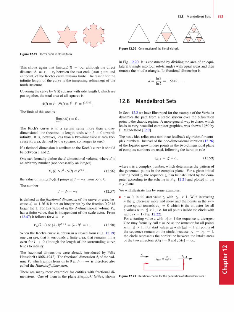
12.8 Mandelbrot Sets 393
Chap
ter12
Figure 12.19 Koch’s curve in closed form
This shows again that liml!0 L.l/ D 1, although the directdistance � D x1 � x2 between the two ends (start point andendpoint) of the Koch’s curve remains finite. The reason for theinfinite length of the curve is the increasing refinement of thetooth structure.
Covering the curve by N.l/ squares with side length l, which areput together, the total area of all squares is
A.l/ D l2 � N.l/ / l2 � l� D l0:7382 :
The limit of this area is
liml!0.A.l// D 0 :
The Koch’s curve is in a certain sense more than a one-dimensional line (because its length tends with l ! 0 towardsinfinity. It is, however, less than a two-dimensional area (be-cause its area, defined by the squares, converges to zero).
If a fictional dimension is attribute to the Koch’s curve it shouldbe between 1 and 2.
One can formally define the d-dimensional volume, where d isan arbitrary number (not necessarily an integer)
Vd.l/ / ld � N.l/ / ldC� ; (12.56)
the value of liml!0.Vd.l// jumps at d D �� from 1 to 0.
The number
d D df D �� (12.57)
is defined as the fractional dimension of the curve or area, be-cause df D 1:2618 is not an integer but by the fraction 0:2618larger the 1. For this value of df the df-dimensional volume Vdfhas a finite value, that is independent of the scale actor. From(12.47) it follows for d D ��
Vdf.� � l/ / .� � l/dfC� D .� � l/0 D 1 : (12.58)
When the Koch’s curve is drawn in a closed form (Fig. 12.19)one can see, that it surrounds a finite area, that remains finiteeven for l ! 0 although the length of the surrounding curvetends to infinity.
The fractional dimensions were already introduced by FelixHausdorff (1868–1942). The fractional dimension df of the vol-ume Vd which jumps from 1 to 0 at df D �� is therefore alsocalled the Hausdorff dimension.
There are many more examples for entities with fractional di-mensions. One of them is the plane Sierpinski lattice, shown
Figure 12.20 Construction of the Sierpinski-grid
in Fig. 12.20. It is constructed by dividing the area of an equi-lateral triangle into four sub-triangles with equal areas and thenremove the middle triangle. Its fractional dimension is
d D ln 3
ln 2D 1:5849 : : : :
12.8 Mandelbrot Sets
In Sect. 12.2 we have illustrated for the example of the Verhulstdynamics the path from a stable system over the bifurcationpoint to the chaotic regime. A more general way to chaos, whichleads to very beautiful computer graphics, was shown 1980 byB. Mandelbrot [12.9].
The basic idea relies on a nonlinear feedback algorithm for com-plex numbers. Instead of the one-dimensional iteration (12.26)of the logistic growth here points in the two-dimensional planeof complex numbers are used, following the iteration rule
znC1 D z2n C c ; (12.59)
where c is a complex number, which determines the pattern ofthe generated points in the complex plane. For a given initialstarting point z0 the sequence zn can be calculated by the com-puter according to the scheme in Fig. 12.21 and plotted in thex–y-plane.
We will illustrate this by some examples:
c D 0, initial start value z0 with jz0j < 1. With increasingn the zn decrease more and more and the points in the x–y-plane spiral towards z1 D 0 which is the attractor for allz-values with jzj < 1, i. e. for all points inside the circle withradius r D 1 (Fig. 12.22).For a starting value z with jzj > 1 the sequence zn diverges.One may formally call z D 1 as the attractor for all pointswith jzj > 1. For start values z0 with jz0j D 1 all points ofthe sequence remain on the circle, because jznj D jz0j D 1,the circle represents the borderline between the intake areasof the two attractors z.A1/ D 0 and z.A2/ D 1.
Figure 12.21 Iteration scheme for the generation of Mandelbrot sets
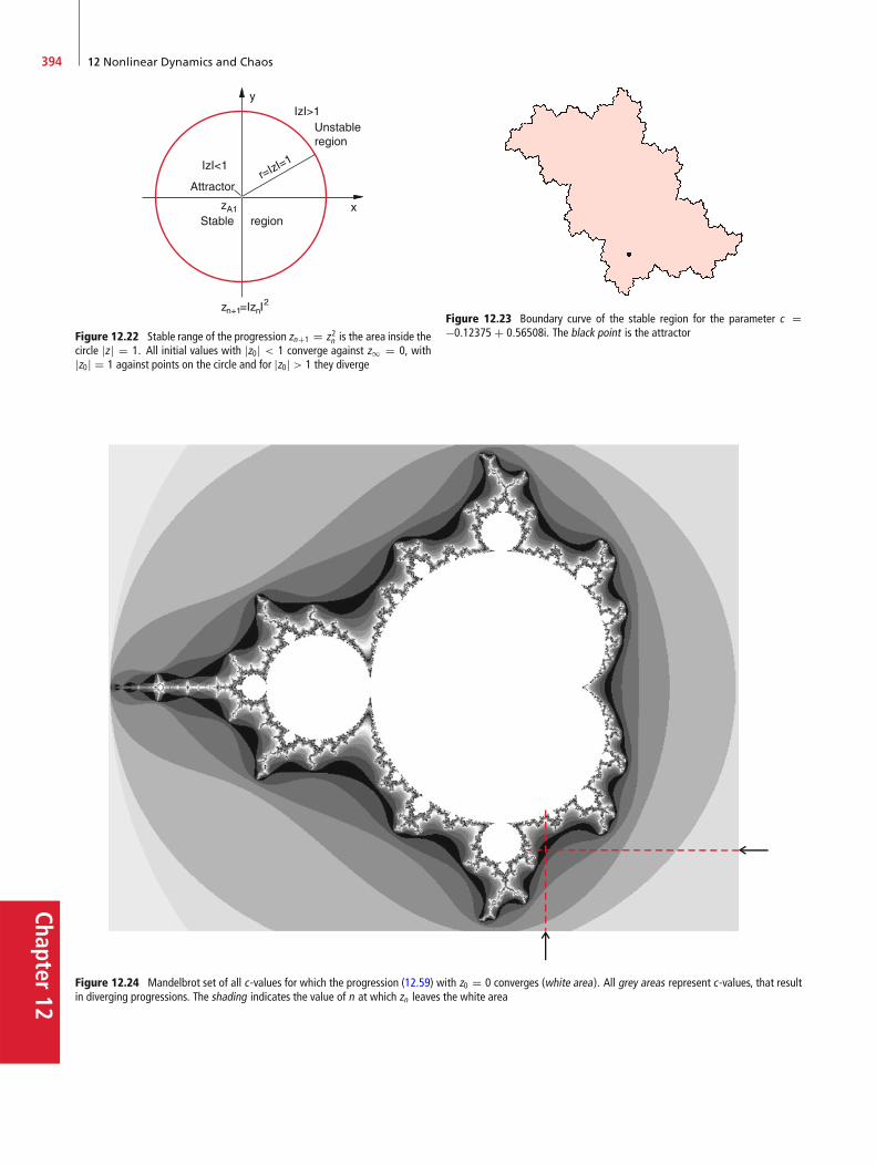
Chapter12
394 12 Nonlinear Dynamics and Chaos
Figure 12.22 Stable range of the progression znC1 D z2n is the area inside thecircle jz j D 1. All initial values with jz0j < 1 converge against z1 D 0, withjz0j D 1 against points on the circle and for jz0j > 1 they diverge
Figure 12.24 Mandelbrot set of all c-values for which the progression (12.59) with z0 D 0 converges (white area). All grey areas represent c-values, that resultin diverging progressions. The shading indicates the value of n at which zn leaves the white area
Figure 12.23 Boundary curve of the stable region for the parameter c D�0:12375 C 0:56508i. The black point is the attractor

12.8 Mandelbrot Sets 395
Chap
ter12
Figure 12.25 Strongly enlarged section of Fig. 12.24 around the intersection point of the two arrows, with an area of 1mm2 in Fig. 12.24
If we choose c ¤ 0 we get surprising sequences. For in-stance, starting with z0 D 0 the sequence (12.59) reads:
z1 D c I z2 D c2 C c Iz3 D .c2 C c/2 C c I : : : :
For c D 1 C i this gives:
z1 D 1 C i I z2 D 1 C 3i I z3 D �7 C 7i Iz4 D 1 � 97i I z5 D �9407 � 193i I : : : :
This shows that the points zn in the x–y-plane perform largejumps from one to the next iteration step and that the sequenceof our example diverges.
Also for c ¤ 0 there is a region in the complex plane where thesequence converges. The attractor is now generally not zero andthe borderline between stable and unstable regions is no longera circle but (Fig. 12.23) a more complicated curve. Similar tothe Koch’s curve the borderline shows self-similarity i. e. it hasa fractional structure. When it is magnified, every magnifiedsegment shows a similar structure as the non-magnified largersection. Such self-similar border curves are called Julia sets.
The Mandelbrot set consists of all numbers c of the sequence(12.59) with z0 D 0 that do not diverge. These are for instanceall values of c D a C ib with �2 < a < C1 and �1:5 <b < C1:5. In order to generate the Mandelbrot set, one has todesign a computer program that calculates for such sequencesthe border curves of the stable region.
Choosing, for instance, a rectangle �A � x � CA; �B � y �CB in the complex plane, one can find out for every value ofc D x C iy within this range, whether the sequence (12.59)converges or diverges. Now a certain colour is assigned toeach value of c, depending on the number of iterations beforethe points c leave the rectangle. In Fig. 12.24 the colours aresubstituted by different grey shades. The white areas are theMandelbrot set, imaging those zn values which lead to stablesequences. Enlarging the tiny region in Fig. 12.24 which liesaround the intersection of the two arrows, one gets the magni-fied Fig. 12.25.
The aesthetic beauty of such Mandelbrot sets becomes obviouswith coloured computer graphics (see Fig. 12.26 and [12.10a–12.13]).
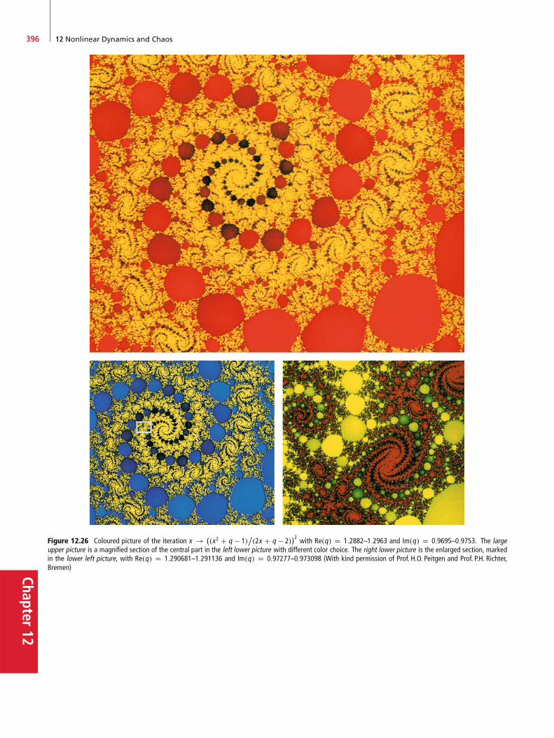
Chapter12
396 12 Nonlinear Dynamics and Chaos
Figure 12.26 Coloured picture of the iteration x ! �.x2 C q � 1/
ı.2x C q � 2/
�2 with Re.q/ D 1:2882–1:2963 and Im.q/ D 0:9695–0:9753. The largeupper picture is a magnified section of the central part in the left lower picture with different color choice. The right lower picture is the enlarged section, markedin the lower left picture, with Re.q/ D 1:290681–1:291136 and Im.q/ D 0:97277–0:973098 (With kind permission of Prof. H.O. Peitgen and Prof. P.H. Richter,Bremen)

Summary 397
Chap
ter12
12.9 Consequences forOur Comprehensionof the Real World
Until the end of the 19th century most physicists were con-vinced, that all processes in nature proceed strictly deterministicand that it is, at least in principle, possible to determine the ini-tial conditions of a system so accurately, that the future fateof the system can be exactly described for all times. This issubstantiated by the famous statement of Laplace, published in1776:
The momentary state of a system is obviously the consequence of thestate at an earlier moment. If we assume an intelligent creature thatis able to calculate at one moment all relations between the differentparts of the universe, it could predict all motions and all relations atall locations now and forever.
Such a Laplace demon would be able to predict the fate of allmankind if he knows the relevant data at a given time.
This strictly deterministic conception of the world arises thequestion: What can the free will of a human being change, ifeverything is already determined by initial conditions which wecannot influence? How much is a criminal responsible for hiscrime, if his future fate is already determined?
This strictly mechanistic conception has been shaken by two de-velopments: The nonlinear dynamics and the quantum theory.
Poicaré, who has performed important spade work in nonlineardynamics, wrote 1903:
A very tiny effect, which we even may not notice, causes a large ef-fect, that we cannot overlook. Then we say: This effect is accidental,because we have overlooked the real cause.
We see, that by no means the deterministic character of natureis questioned. This means that the principle of causality is ac-cepted. However, the assumption that the initial conditions canbe determined with sufficient accuracy, is no longer valid forinstable systems, because here tiny changes of the initial con-ditions can cause large deviations of the final states. Often theuncertainty of the measurement limits the accuracy of predic-tions for many cases in nonlinear dynamics.
Quantum mechanics adds another principle argument: The un-certainty principle (see Vol. 3) states that it is impossible todetermine exactly both the momentum and the position of aparticle simultaneously. The more accurate one quantity ismeasured, the larger is the uncertainty for the other quantity.this implies that the initial state of a system cannot be deter-mined with arbitrary accuracy, not only because of measurementerrors, but because of the principle quantum mechanical restric-tions.
For stable systems these small uncertainties have no big effect,but for unstable systems (chaotic systems) they can be disas-trous, because they principally limit the predictions of futurebehaviour.
These few considerations illustrate that investigations of non-linear phenomena bring about many new and surprising resultswhen leaving the approximations of basic linear equations. Thisresearch field has developed only recently and more and morescientists are now interested in its basic physics and possible ap-plications besides the gain of insight into the complexity of ourreal world [12.17–12.20].
There is in addition a psychological problem: How the spon-taneous human interference in natural phenomena changes thepredictability of processes and how spontaneous such interfer-ence really is, belongs into the field of psychology and cannotbe solved in Physics.
Summary
For phenomena described by nonlinear equations, the timedevelopment of the solutions often depends critically on theinitial conditions. Unstable solutions are those, where in-finitesimal small changes of the initial conditions cause largechanges of the final states.The dynamical development of a system can be representedby a curve in phase space.The development of a system described by the Verhulst equa-tion
xnC1 D a � xn � a � x2ndepends on the control parameter a. For certain values of athe solutions xf D limn!1.xn/ split into two possible values
(bifurcation). For larger values of a each of these two valuessplit again into two possible values. This splitting continuouswith increasing a, until the chaotic regime is reached whereno predictions of the final states are possible.Examples of applications of this equation are the populationexplosion, the parametric oscillator and the origin of trafficjams without identifiable causes, often caused by the delayedreaction of the driver.While for linear equations the superposition principle holds(i. e. with two independent solutions also their linear com-bination is a solution), this is no longer true for nonlinearequations. For special nonlinear equations the solutionsshow self-similarity.
Chapter12
398 12 Nonlinear Dynamics and Chaos
Self similarity is present, if
x.�t/ D ��x.t/ ) x.t/t� ;
where � is a positive or negative number, not necessary aninteger.The number � is the fractional dimension.For self-similar solutions of nonlinear equations a naturalscale is missing. An arbitrary stretching of time can be com-pensated by a corresponding change of the x-scale.
All complex numbers which are generated by the sequenceznC1 D z2n C c form a set in the complex plane. The set of allnon-divergent sequences with z0 D 0 generate the Mandel-brot set.Such sets can be graphically displayed by simple computerprograms.
Problems
12.1 A mass m is hold in its equilibrium position .0; 0/ in thex; y-plane by four springs with length L and restoring force con-stant k. aligned in the ˙x- and ˙y-directions.a) What is the equation of motion, when the mass m is dis-
placed in the Cx-direction?b) Bring this equation for x L in the form d2x=dt2 C ax C
bx3 D 0. How large are a and b?c) What is the oscillation frequency for bx3 a in the linear
approximation and how does it change in the nonlinear formof the equation in b)?
12.2 Show, that the nonlinear equation in Probl. 12.1b withthe initial conditions x.0/ D x0 and dx=dt.0/ D 0 has periodicalsolutions.
12.3a) Show that the non linear equation m d2x=dt2 D �k1x � k2x
with the initial conditions x.0/ D x0, .dx=dt/.0/ D 0 canbe transformed by the substitutions !2
0 D k1=m, y D x=x0,L� D !0L into the dimensionless form d2y=dL�2 C y C "y2
with " D x0k2=k1.b) Calculate for " D 0:1 the frequency shift against !0.
12.4 Determine the fix points for the system of differentialequations dx1=dt D �1x1 � �2x1x2.For which values of �1 and �2 are the fix points stable,metastable or unstable?
12.5 The equation of motion for the damped pendulum oscil-lation is R' C � P' C !2
0 sin' D 0 with !20 D g=L.
Determine the oscillation period T.'/ and calculate the ratiosT.'/=T.0/ for ' D =4, =2, .3=4/ and .
12.6a) What is the solution of the logistic growth function Pz.t/ D
az � bz2?b) After which time has the function z.t/ doubled for a D b?c) What is the limit for z.t ! 1/?
12.7 Determine the fixpoints xf and the Ljapunov exponent �of the logistic equation xnC1 D axn .1 � xn/ for a D 3:1 anda D 3:3.
12.8 Show, that the fractional dimension of the Sierpinski gridis d1 D 1:5849.
12.9 Determine fixpoints and attractor for the differentialequation in polar coordinates dr=dt D �r .�a C r2/ for a < 0and a > 0, d'=dt D !0 D const.
12.10 A particle with mass m moves in the potential Epot DEpot.x0/C a.x � x0/2 C b.x � x0/3.a) Determine the nonlinear equation of motion.b) Up to which amplitude xmax is the solution a harmonic oscil-
lation?
References 399
Chap
ter12
References
12.1a. J. Gleick, Chaos: Making a New Science. (PenguinBooks, New York, 2008)
12.1b. E. Lorenz, The Essence of Chaos. (University of Wash-ington Press, Washington, 1995)
12.2a. P. Bak, How Nature works: The Science of Self-organizes Criticality. (Copernicus Books, New York,1996)
12.2b. St.A. Kaufman, At Home in the Universe: The Searchfor the Laws of Self-Organization and Complexity. (Ox-ford University Press, Oxford, 1996)
12.3. F.D. Peat, J. Briggs, Timeless Wisdom from the Scienceof Change. (Harper Collins Publ., New York, 1999)
12.4. T. Mullin, The Nature of Chaos. (Clarendon Press,Watton-under-Edge, UK, 1995)
12.5. P. Bergé, K. Pomeau, Ch. Vidal, Order within Chaos.(John Wiley, New York, 1984)
12.6a. G.L. Baker, J.P. Gollub,Chaotic Dynamics. (CambridgeUniversity Press, Cambridge, 1996)
12.6b. M.J. Feigenbaum, J. Stat. Phys. 19, 25–52 (1978)12.7. W. Leutzbach, Introduction in to the Theory of Traffic
Flow. (Springer, New York, 1987)12.8. https://en.wikipedia.org/wiki/Self-similarity12.9. B.B. Mandelbrot, The Fractal Geometry of Nature.
(Freeman, San Francisco, 1982)12.10a. H.-O. Peitgen, P.H. Richter, The Beauty of Fractals.
(Springer, Berlin, Heidelberg, 1986)
12.10b. H.-O. Peitgen, Chaos: Bausteine der Ordnung.(Rowohlt, Hamburg, 1998)
12.11. See many articles in: Chaos: An Interdisciplinary Jour-nal of Nonlinear Science. (American Institut of Physics)
12.12. H.J. Korsch, H.J. Jodl, Chaos, A Program Collection forthe PC. (Springer, Berlin, Heidelberg, 1994)
12.13. H. Jürgens, H.O. Peitgen, D. Saupe (ed.), Chaos andFractals. (Springer, Berlin, Heidelberg, 1993)
12.14. St.H. Strogatz, Nonlinear Dynamics and Chaos: Appli-cations to Physics, Biology, Chemistry and Engineer-ing. (Westview Press, Boulder, Colorado, USA, 2014)
12.15. G. Mayer-Kress (ed.), Dimensions and Entropies inChaotic Systems. (Springer, Berlin, Heidelberg, 1986)
12.16. W.H. Steeb, A. Kunick, Chaos und Quantenchaos indynamischen Systemen, 2nd ed. (Bibliographisches In-stitut, Mannheim, 1994)
12.17. B. Kaye, Chaos and Complexity. (VCH, Weinheim,1993)
12.18. J. Parisi, St. Müller, W. Zimmermann (eds.), A Per-spective Look at Nonlinear Media. (Springer, Berlin,Heidelberg, 1998)
12.19. L. Lam, Nonlinear Physics for Beginners. (World Sci-entific, Singapore, 1998)
12.20. R. Gilmore, M. Lefrane, The Topology of Chaos. (WileyVCH, Weinheim, 2002)

Chap
ter13Supplement 13
13.1 Vector Algebra and Analysis . . . . . . . . . . . . . . . . . . . . . . . . 402
13.2 Coordinate Systems . . . . . . . . . . . . . . . . . . . . . . . . . . . . . 407
13.3 Complex Numbers . . . . . . . . . . . . . . . . . . . . . . . . . . . . . . 410
13.4 Fourier-Analysis . . . . . . . . . . . . . . . . . . . . . . . . . . . . . . . . 411
401© Springer International Publishing Switzerland 2017W. Demtröder, Mechanics and Thermodynamics, Undergraduate Lecture Notes in Physics, DOI 10.1007/978-3-319-27877-3_13
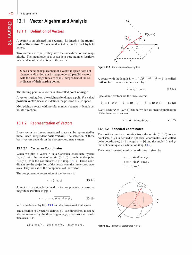
Chapter13
402 13 Supplement
13.1 Vector Algebra and Analysis
13.1.1 Definition of Vectors
A vector is an oriented line segment. Its length is the magni-tude of the vector. Vectors are denoted in this textbook by boldletters.
Two vectors are equal, if they have the same direction and mag-nitude. The magnitude of a vector is a pure number (scalar),independent of the direction of the vector.
Since a parallel displacement of a vector in space does notchange its direction nor its magnitude, all parallel vectorswith the same magnitude are equal, independent of the co-ordinates of their starting points.
The starting point of a vector is also called point of origin.
A vector starting from the origin and ending at a point P is calledposition vector, because it defines the position of P in space.
Multiplying a vector with a scalar number changes its length butnot its direction.
13.1.2 Representation of Vectors
Every vector in a three-dimensional space can be represented bythree linear independent basis vectors. The selection of thesebasis vectors depends on the chosen coordinate system.
13.1.2.1 Cartesian Coordinates
When we plot a vector r in a Cartesian coordinate system.x; y; z/ with the point of origin .0; 0; 0/ it ends at the pointP.x; y; z/ with the coordinates x; y; z (Fig. 13.1). These coor-dinates are the projection of the vector onto the three coordinateaxes. They are called the components of the vector.
The component representation of the vector r is
r D fx; y; zg : (13.1a)
A vector r is uniquely defined by its components, because itsmagnitude (written as jrj) is
r D jrj Dpx2 C y2 C z2 ; (13.1b)
as can be derived by Fig. 13.1 and the theorem of Pythagoras.
The direction of a vector is defined by its components. It can bealso represented by the three angles ˛; ˇ; � against the coordi-nate axes. It is
cos˛ D x=r ; cosˇ D y=r ; cos � D z=r :
Figure 13.1 Cartesian coordinate system
A vector with the length L D 1 .px2 C y2 C z2 D 1/ is called
unit vector. It is often represented by
Or D r=jrj D Oe : (13.1c)
Special unit vectors are the three vectors
Oe1 D f1; 0; 0g I Oe2 D f0; 1; 0g I Oe3 D f0; 0; 1g : (13.1d)
Every vector r D fx; y; zg can be written as linear combinationof the three basis vectors
r D xOe1 C yOe2 C zOe3 : (13.2)
13.1.2.2 Spherical Coordinates
The position vector r pointing from the origin .0; 0; 0/ to thepoint P.r; #; '/ is defined in spherical coordinates (also calledpolar coordinates) by its length r D jrj and the angles # and 'that define uniquely its direction (Fig. 13.2).
The conversion to Cartesian coordinates is given by
x D r � sin# � cos' ;y D r � sin# � sin ' ;z D r � cos# :
Figure 13.2 Spherical coordinates r , # , '

13.1 Vector Algebra and Analysis 403
Chap
ter13
Figure 13.3 Cylindrical coordinates %, ', z
13.1.2.3 Cylindrical Coordinates
The point P.%; '; z/ in Fig. 13.3 is defined in cylindrical coor-dinates .%; ':z/ by the vector r D f%; '; zg where % gives thedistance from the z-axis, z the distance from the x–y-plane and' the angle of the projection of r onto the x–y-plane against thex-axis. The conversion to Cartesian coordinates is:
x D % � cos' ;y D % � sin ' ;z D z :
The length of the vector r is
jrj Dp%2 C z2 :
The direction of r is defined by the angle ' and the ratio z=%.
13.1.3 Polar and Axial Vectors
The transformation x ! �x; y ! �y; z ! �z (mirror imagingof the coordinate system) transforms the position vector r !�r. Therefore r is called a polar vector.
Besides these polar vectors which are defined by their lengthand their direction, there are also vectors that define apart fromdirection and magnitude a sense of rotation.
Example
Magnitude and orientation of a surface element can becharacterized by the normal vector A perpendicular to thesurface element (Fig. 13.4). The magnitude of the vec-tor gives the area of the surface element and its directionthe orientation of the surface element. In order to defineuniquely on which of the two sides of the surface elementthe vector A starts, its direction is defined such, that itforms a right hand screw (like a corkscrew) when the sur-face element is counterclockwise circulated.
Figure 13.4 Surface normal vector A as axial vector, that is charac-terized by its direction of orientation. At the coordinate transformationr ! �r, A keeps its orientation as a right hand helix J
Under the coordinate transformation x ! �x, y ! �y, z ! �zthe sense of rotation of A is preserved, i. e. A ! CA but notA ! �A, i. e. A forms again a right-handed screw. Such vectorsare called axial vectors. Examples are the angular momentumvector L D r p (see Sect. 2.8 and 13.1.5.3).
13.1.4 Addition and Subtraction of Vectors
Definition
Vectors are added by adding their components (Fig. 13.5).The sum of the two vectors a D fa1; a2; a3g and b Dfb1; b2; b3g is the vector
c D a C b D fa1 C b1; a2 C b2; a3 C b3g : (13.3)
According to this rule each vector can be written as the sum ofits component vectors
a D fa1; a2; a3g D a1 Oe1 C a2 Oe2 C a3 Oe3 :
The graphical representation of vector addition shown inFig. 13.5, illustrates that the sum vector c is the diagonal in theparallelogram of the vectors a and b.
Figure 13.5 Addition of vectors

Chapter13
404 13 Supplement
Problem
Show that this graphical representation fulfils the rules ofvector addition. J
13.1.5 Multiplication of Vectors
13.1.5.1 Multiplication of a Vector with a Scalar
The vector a is multiplied by a scalar c by multiplying eachcomponent of a by c.
c � a D c � fa1; a2; a3g D fc � a1; c � a2; c � a3g ;jc � aj D jcj � jaj :
13.1.5.2 The Scalar Product
The scalar product of two vectors
a D fa1; a2; a3g and b D fb1; b2; b3gwith the angle ˛ between them is defined as the scalar
c D a � b D jaj � jbj � cos˛ : (13.4a)
It is the product of the projection jbj � cos˛ of b on a timesthe amount jaj of a. For ˛ D 90ı is the scalar product zero(Fig. 13.6).
Two vectors ¤ 0 are perpendicular to each other only iftheir scalar product is zero.
For the three unit vectors Oe1, Oe2, Oe3 hold the relationOei � Oek D ıik ;
where ıik is the Kronecker symbol which is defined by
ıik D(1 for i D k ;
0 for i ¤ k :
Figure 13.6 The scalar product a�b represents the area A D a�b D a �b �cos˛
The scalar product can be also expressed by the vector compo-nents. For
a D a1 Oe1 C a2 Oe2 C a3 Oe3 ;b D b1 Oe1 C b2 Oe2 C b3 Oe3 ;
(13.4b)
the scalar product becomes
a � b D .a1Oe1 C a2 Oe2 C a3 Oe3/ � .b1Oe1 C b2 Oe2 C b3 Oe3/ ;D a1b1 C a2b2 C a3b3 since Oei � Oek D ıik :
(13.5)
13.1.5.3 The Vector Product
Definition
The vector product of two vectors a and b is the vectorc D a b
that is perpendicular to a and b,that forms a right handed screw when a is rotated to-ward b on the shortest way,that has the magnitude jcj D jaj � jbj � sin˛, where ˛ isthe angle between a and b.
The vector c defines besides magnitude and direction also theorientation. It is therefore an axial vector.
Note, that
.a b/ D �.b a/ :
The absolute value jaj � jbj � sin˛ of the vector product a bis equal to the area of the parallelogram, formed by a and b(Fig. 13.7). The vector product can be therefore regarded asthe surface normal of the parallelogram generated by the twovectors a and b.
c D .a b/ is an axial vector, because under reflection of allcoordinates at the origin we have a ! �a; b ! �b ) c ! c(Fig. 13.7b).
For the unit vectors we get the relations:
Oe1 Oe2 D Oe3 ; Oe2 Oe3 D Oe1 ; Oe3 Oe1 D Oe2 :
Figure 13.7 The vectorial product as normal vector to the area ja bj

13.1 Vector Algebra and Analysis 405
Chap
ter13
We therefore get the component representation of the vectorproduct
.a b/ D fa2b3 � a3b2; a3b1 � a1b3; a1b2 � a2b1g : (13.6)
Check this relation by multiplication of the six vector compo-nents.
This component representation can be abbreviated by the sym-bolic determinant notation
c D
ˇ̌ˇ̌ˇ̌ˇ
Oe1 Oe2 Oe3a1 a2 a3b1 b2 b3
ˇ̌ˇ̌ˇ̌ˇ
(13.7)
D .a2b3 � a3b2/Oe1 C .a3b1 � a1b3/Oe2 C .a1b2 � a2b1/Oe3 :
13.1.5.4 Multiple Products
Scalar Products of a Polar and an Axial Vector
The dot product (scalar product) d D c.ab/ of the polar vectorc and the axial vector .a b/ gives a scalar number d that trans-forms into �c when all coordinates are reflected at the origin,because the axial vector .a b/ does not change its sign, whilethe scalar number c does. The number d is called a pseudo-scalar.
The product d D jcj � ja bj � cosˇ describes the volume of theparallel-epiped (oblique angled cuboid) which is formed by thevectors a, b and c (Fig. 13.8).
This scalar triple product can be written as a determinant
c � .a b/ D
ˇ̌ˇ̌ˇ̌ˇ
a1 a2 a3b1 b2 b3c1 c2 c3
ˇ̌ˇ̌ˇ̌ˇ: (13.8)
Vector Product of a Polar and an Axial Vector
d D c .a b/ :
Since the vector .a b/ is perpendicular to a and to b and thevector d is perpendicular to .a b/, d must lie in the plane of
Figure 13.8 Scalar triple products d D c � .a b/ represents the volume ofthe parallel-epiped generated by vectors a, b and c
a and b which we choose as the x–y-plane. It therefore can bedescribed as a linear combination of a and b.
d D x � a C y � b ; (x and y are real numbers) :
Inserting the components of a, b and c gives, following the rulesgiven above for the components,
x D c1b1 C c2b2 C c3b3 ;
y D �c1a1 � c2a2 � c3a3 :
These relations give the vector equation
c .a b/ D .c � b/a � .c � a/b : (13.9)
Since the vector product changes its sign when the sequence ofthe factors are interchanged, we get the relations
.a b/ c D �c .a b/ ;
.a b/ c ¤ a .b c/ ¤ .a c/ b :
Neither the commutative law nor the associative law are validfor the triple vector products.
From Eq. 13.9 follows
a .b c/C b .c a/C c .a b/ D 0 : (13.10)
Scalar Product of Two Axial Vectors
From the relations above we can conclude
.a b/ � .c d/ D .a � c/.b � d/ � .a � d/.b � c/ ; (13.11a)
.a b/2 D a2b2 � .a � b/2 : (13.11b)
13.1.6 Differentiation of Vectors
13.1.6.1 Vector-Fields
If it is possible to attribute to each space point P.x; y; z/ a vectora D fax; ay; azg the entity of all vectors a D a.x; y; z/ is calleda vector field. Each component of a is a function of the coordi-nates .x; y; z/:
ax D f1.x; y; z/ I ay D f2.x; y; z/ and az D f3.x; y; z/ :
This means that length and direction of the vector a depend onthe coordinates .x; y; z/. If the components depend additionallyon the time t, a.x; y; z/ represents a time-dependent vector field.If a does not depend on time, the field is called stationary orstatic.
Examples
1. The velocity of particles in a fluid, flowing througha pipe with locally variable cross section representsa vector field. If the pressure is time dependent, thevector field v D f.x; y; z; t/ is non-stationary.
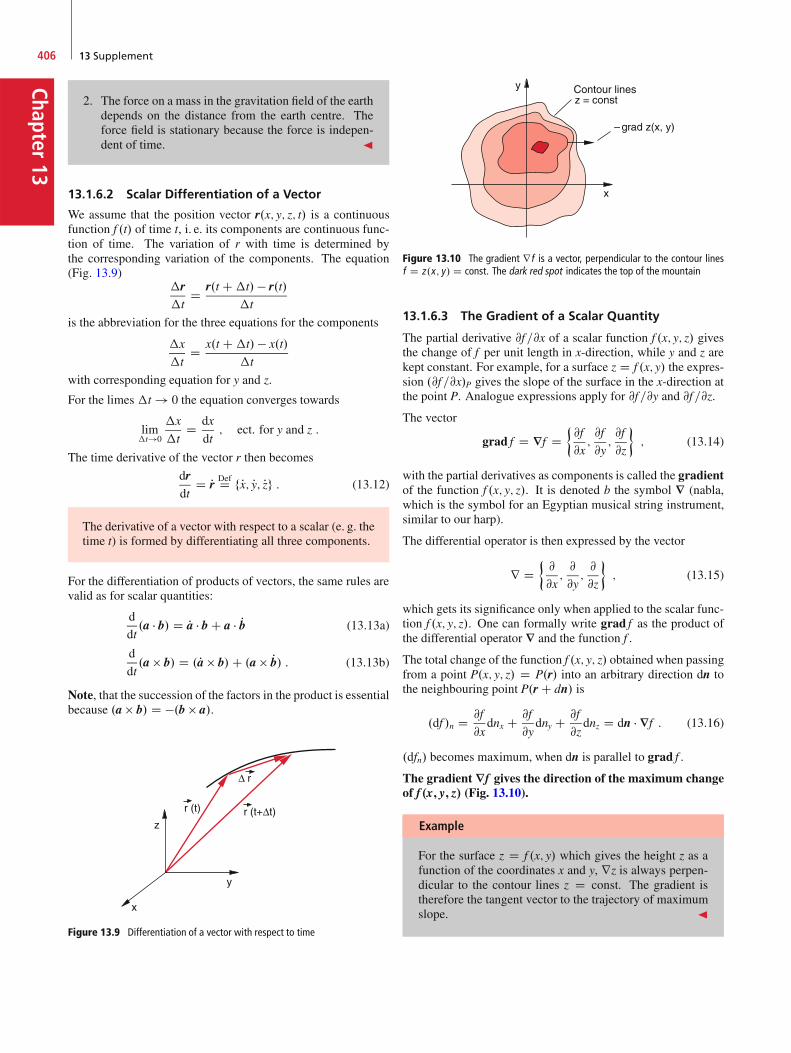
Chapter13
406 13 Supplement
2. The force on a mass in the gravitation field of the earthdepends on the distance from the earth centre. Theforce field is stationary because the force is indepen-dent of time. J
13.1.6.2 Scalar Differentiation of a Vector
We assume that the position vector r.x; y; z; t/ is a continuousfunction f .t/ of time t, i. e. its components are continuous func-tion of time. The variation of r with time is determined bythe corresponding variation of the components. The equation(Fig. 13.9)
�r�t
D r.t C�t/ � r.t/�t
is the abbreviation for the three equations for the components
�x
�tD x.t C�t/ � x.t/
�t
with corresponding equation for y and z.
For the limes �t ! 0 the equation converges towards
lim�t!0
�x
�tD dx
dt; ect. for y and z :
The time derivative of the vector r then becomes
drdt
D Pr DefD fPx; Py; Pzg : (13.12)
The derivative of a vector with respect to a scalar (e. g. thetime t) is formed by differentiating all three components.
For the differentiation of products of vectors, the same rules arevalid as for scalar quantities:
d
dt.a � b/ D Pa � b C a � Pb (13.13a)
d
dt.a b/ D .Pa b/C .a Pb/ : (13.13b)
Note, that the succession of the factors in the product is essentialbecause .a b/ D �.b a/.
Figure 13.9 Differentiation of a vector with respect to time
Figure 13.10 The gradient rf is a vector, perpendicular to the contour linesf D z.x; y/ D const. The dark red spot indicates the top of the mountain
13.1.6.3 The Gradient of a Scalar Quantity
The partial derivative @f =@x of a scalar function f .x; y; z/ givesthe change of f per unit length in x-direction, while y and z arekept constant. For example, for a surface z D f .x; y/ the expres-sion .@f =@x/P gives the slope of the surface in the x-direction atthe point P. Analogue expressions apply for @f =@y and @f =@z.
The vector
grad f D r f D @f
@x;@f
@y;@f
@z
�; (13.14)
with the partial derivatives as components is called the gradientof the function f .x; y; z/. It is denoted b the symbol r (nabla,which is the symbol for an Egyptian musical string instrument,similar to our harp).
The differential operator is then expressed by the vector
r D @
@x;@
@y;@
@z
�; (13.15)
which gets its significance only when applied to the scalar func-tion f .x; y; z/. One can formally write grad f as the product ofthe differential operator r and the function f .
The total change of the function f .x; y; z/ obtained when passingfrom a point P.x; y; z/ D P.r/ into an arbitrary direction dn tothe neighbouring point P.r C dn/ is
.df /n D @f
@xdnx C @f
@ydny C @f
@zdnz D dn � r f : (13.16)
.dfn/ becomes maximum, when dn is parallel to grad f .
The gradient r f gives the direction of the maximum changeof f.x; y; z/ (Fig. 13.10).
Example
For the surface z D f .x; y/ which gives the height z as afunction of the coordinates x and y, rz is always perpen-dicular to the contour lines z D const. The gradient istherefore the tangent vector to the trajectory of maximumslope. J
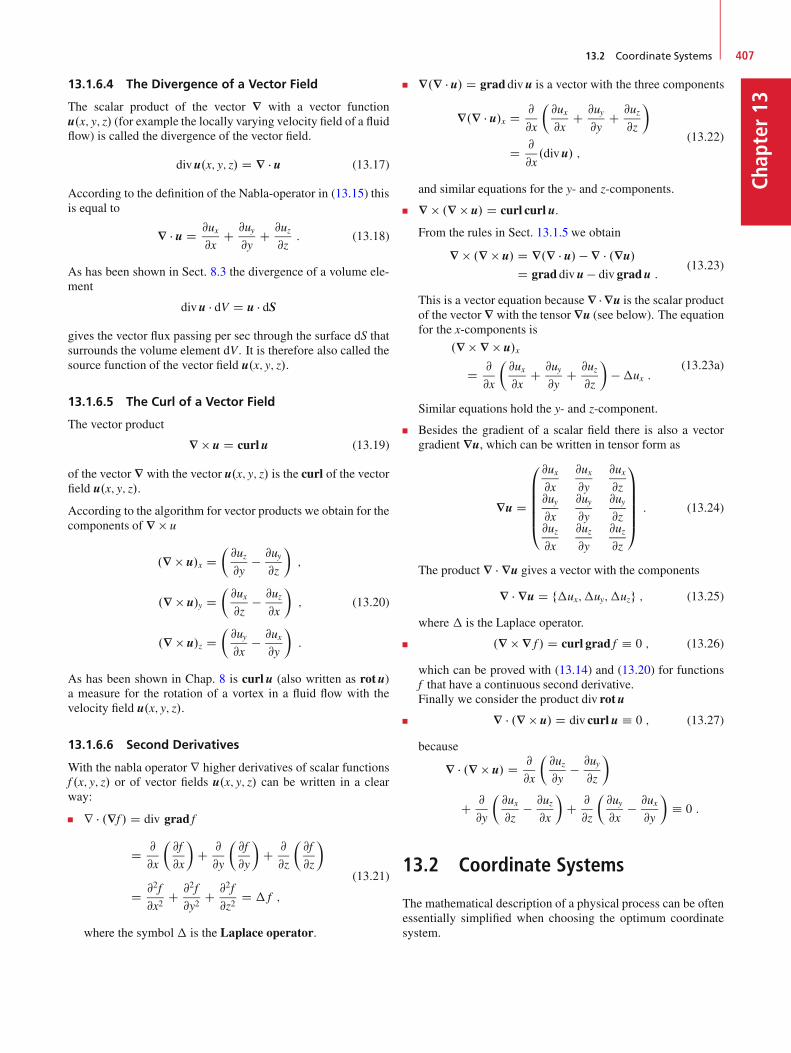
13.2 Coordinate Systems 407
Chap
ter13
13.1.6.4 The Divergence of a Vector Field
The scalar product of the vector r with a vector functionu.x; y; z/ (for example the locally varying velocity field of a fluidflow) is called the divergence of the vector field.
divu.x; y; z/ D r � u (13.17)
According to the definition of the Nabla-operator in (13.15) thisis equal to
r � u D @ux@x
C @uy@y
C @uz@z
: (13.18)
As has been shown in Sect. 8.3 the divergence of a volume ele-ment
divu � dV D u � dSgives the vector flux passing per sec through the surface dS thatsurrounds the volume element dV. It is therefore also called thesource function of the vector field u.x; y; z/.
13.1.6.5 The Curl of a Vector Field
The vector product
r u D curlu (13.19)
of the vector r with the vector u.x; y; z/ is the curl of the vectorfield u.x; y; z/.
According to the algorithm for vector products we obtain for thecomponents of r u
.r u/x D�@uz@y
� @uy@z
�;
.r u/y D�@ux@z
� @uz@x
�;
.r u/z D�@uy@x
� @ux@y
�:
(13.20)
As has been shown in Chap. 8 is curl u (also written as rotu)a measure for the rotation of a vortex in a fluid flow with thevelocity field u.x; y; z/.
13.1.6.6 Second Derivatives
With the nabla operator r higher derivatives of scalar functionsf .x; y; z/ or of vector fields u.x; y; z/ can be written in a clearway:
r � .r f / D div grad f
D @
@x
�@f
@x
�C @
@y
�@f
@y
�C @
@z
�@f
@z
�
D @2f
@x2C @2f
@y2C @2f
@z2D � f ;
(13.21)
where the symbol� is the Laplace operator.
r .r � u/ D grad div u is a vector with the three components
r .r � u/x D @
@x
�@ux@x
C @uy@y
C @uz@z
�
D @
@x.divu/ ;
(13.22)
and similar equations for the y- and z-components.
r .r u/ D curl curl u.
From the rules in Sect. 13.1.5 we obtain
r .r u/ D r.r � u/ � r � .ru/
D grad div u � div gradu :(13.23)
This is a vector equation because r � ru is the scalar productof the vector r with the tensor ru (see below). The equationfor the x-components is
.r r u/x
D @
@x
�@ux@x
C @uy@y
C @uz@z
���ux :
(13.23a)
Similar equations hold the y- and z-component.
Besides the gradient of a scalar field there is also a vectorgradient ru, which can be written in tensor form as
ru D
0
BBBBB@
@ux@x
@ux@y
@ux@z
@uy@x
@uy@y
@uy@z
@uz@x
@uz@y
@uz@z
1
CCCCCA: (13.24)
The product r � ru gives a vector with the components
r � ru D f�ux;�uy; �uzg ; (13.25)
where � is the Laplace operator.
.r r f / D curl grad f � 0 ; (13.26)
which can be proved with (13.14) and (13.20) for functionsf that have a continuous second derivative.Finally we consider the product div rotu
r � .r u/ D div curl u � 0 ; (13.27)
because
r � .r u/ D @
@x
�@uz@y
� @uy@z
�
C @
@y
�@ux@z
� @uz@x
�C @
@z
�@uy@x
� @ux@y
�� 0 :
13.2 Coordinate Systems
The mathematical description of a physical process can be oftenessentially simplified when choosing the optimum coordinatesystem.
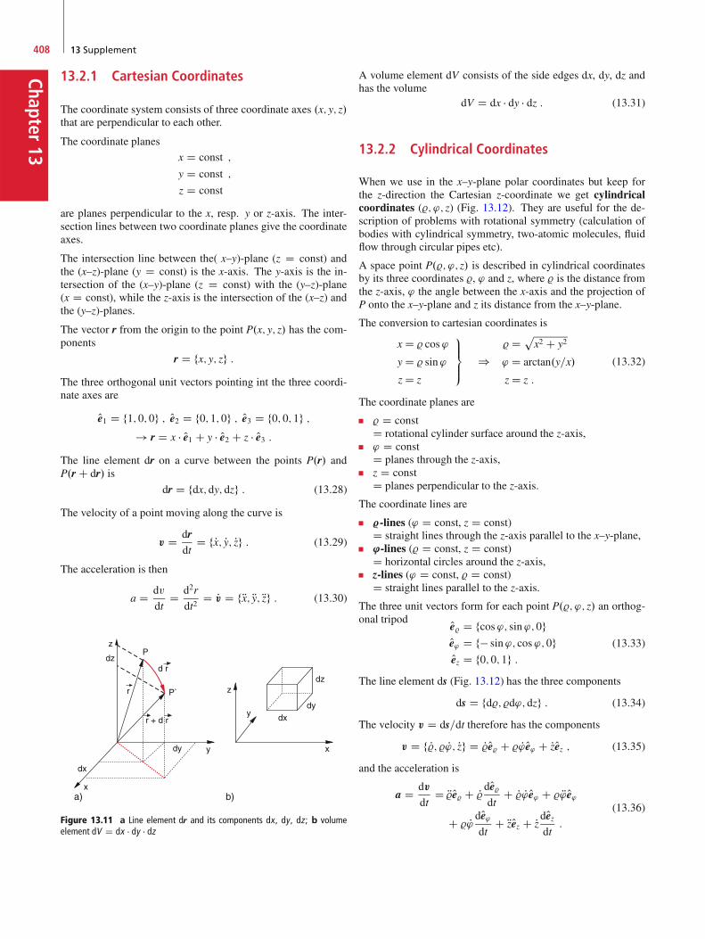
Chapter13
408 13 Supplement
13.2.1 Cartesian Coordinates
The coordinate system consists of three coordinate axes .x; y; z/that are perpendicular to each other.
The coordinate planes
x D const ;
y D const ;
z D const
are planes perpendicular to the x, resp. y or z-axis. The inter-section lines between two coordinate planes give the coordinateaxes.
The intersection line between the( x–y)-plane (z D const) andthe (x–z)-plane (y D const) is the x-axis. The y-axis is the in-tersection of the (x–y)-plane (z D const) with the (y–z)-plane(x D const), while the z-axis is the intersection of the (x–z) andthe (y–z)-planes.
The vector r from the origin to the point P.x; y; z/ has the com-ponents
r D fx; y; zg :The three orthogonal unit vectors pointing int the three coordi-nate axes are
Oe1 D f1; 0; 0g ; Oe2 D f0; 1; 0g ; Oe3 D f0; 0; 1g ;! r D x � Oe1 C y � Oe2 C z � Oe3 :
The line element dr on a curve between the points P.r/ andP.r C dr/ is
dr D fdx; dy; dzg : (13.28)
The velocity of a point moving along the curve is
v D drdt
D fPx; Py; Pzg : (13.29)
The acceleration is then
a D dv
dtD d2r
dt2D Pv D fRx; Ry; Rzg : (13.30)
Figure 13.11 a Line element dr and its components dx, dy, dz; b volumeelement dV D dx � dy � dz
A volume element dV consists of the side edges dx, dy, dz andhas the volume
dV D dx � dy � dz : (13.31)
13.2.2 Cylindrical Coordinates
When we use in the x–y-plane polar coordinates but keep forthe z-direction the Cartesian z-coordinate we get cylindricalcoordinates (%; '; z) (Fig. 13.12). They are useful for the de-scription of problems with rotational symmetry (calculation ofbodies with cylindrical symmetry, two-atomic molecules, fluidflow through circular pipes etc).
A space point P.%; '; z/ is described in cylindrical coordinatesby its three coordinates %, ' and z, where % is the distance fromthe z-axis, ' the angle between the x-axis and the projection ofP onto the x–y-plane and z its distance from the x–y-plane.
The conversion to cartesian coordinates is
x D % cos'
y D % sin'
z D z
9>=
>;)
%Dpx2 C y2
' D arctan.y=x/
z D z :
(13.32)
The coordinate planes are
% D constD rotational cylinder surface around the z-axis,' D constD planes through the z-axis,z D constD planes perpendicular to the z-axis.
The coordinate lines are
%-lines (' D const, z D const)D straight lines through the z-axis parallel to the x–y-plane,'-lines (% D const, z D const)D horizontal circles around the z-axis,z-lines (' D const, % D const)D straight lines parallel to the z-axis.
The three unit vectors form for each point P.%; '; z/ an orthog-onal tripod Oe% D fcos'; sin'; 0g
Oe' D f� sin'; cos'; 0gOez D f0; 0; 1g :
(13.33)
The line element ds (Fig. 13.12) has the three components
ds D fd%; %d'; dzg : (13.34)
The velocity v D ds=dt therefore has the components
v D f P%; % P'; Pzg D P%Oe% C % P' Oe' C PzOez ; (13.35)
and the acceleration is
a D dv
dtD R%Oe% C P%dOe%
dtC P% P' Oe' C % R' Oe'
C % P' dOe'dt
C RzOez C PzdOezdt
:
(13.36)
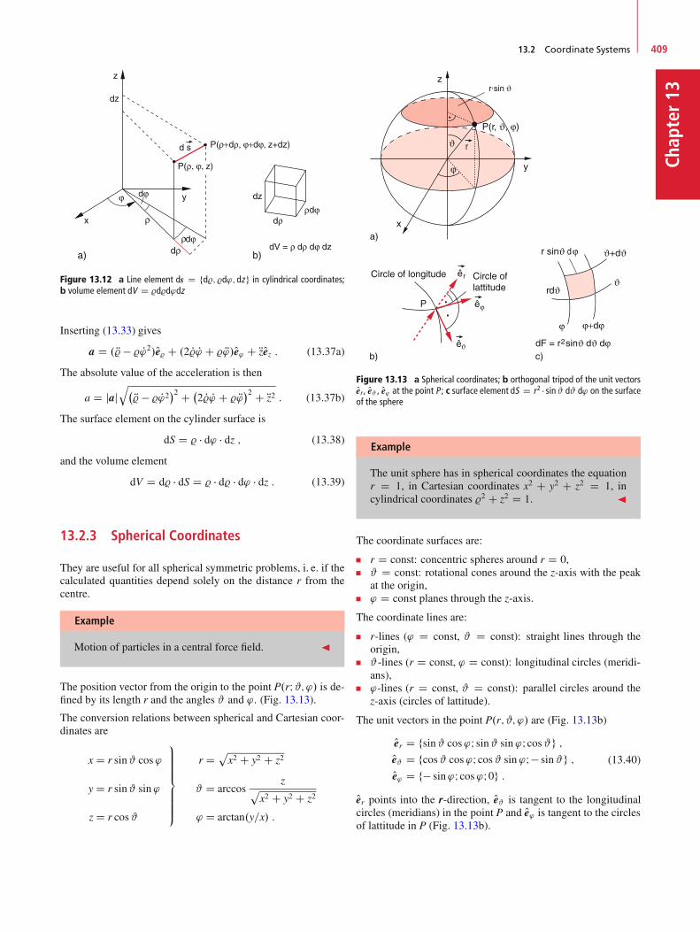
13.2 Coordinate Systems 409
Chap
ter13
Figure 13.12 a Line element ds D fd%; %d'; dzg in cylindrical coordinates;b volume element dV D %d%d'dz
Inserting (13.33) gives
a D . R%� % P'2/Oe% C .2 P% P' C % R'/Oe' C RzOez : (13.37a)
The absolute value of the acceleration is then
a D jajq� R% � % P'2
�2 C �2 P% P' C % R'�2 C Rz2 : (13.37b)
The surface element on the cylinder surface is
dS D % � d' � dz ; (13.38)
and the volume element
dV D d% � dS D % � d% � d' � dz : (13.39)
13.2.3 Spherical Coordinates
They are useful for all spherical symmetric problems, i. e. if thecalculated quantities depend solely on the distance r from thecentre.
Example
Motion of particles in a central force field. J
The position vector from the origin to the point P.rI#; '/ is de-fined by its length r and the angles # and '. (Fig. 13.13).
The conversion relations between spherical and Cartesian coor-dinates are
x D r sin# cos'
y D r sin# sin '
z D r cos#
9>>>>>>=
>>>>>>;
r Dpx2 C y2 C z2
# D arccosz
px2 C y2 C z2
' D arctan.y=x/ :
Figure 13.13 a Spherical coordinates; b orthogonal tripod of the unit vectorsOer , Oe# , Oe' at the point P ; c surface element dS D r2 � sin# d# d' on the surfaceof the sphere
Example
The unit sphere has in spherical coordinates the equationr D 1, in Cartesian coordinates x2 C y2 C z2 D 1, incylindrical coordinates %2 C z2 D 1. J
The coordinate surfaces are:
r D const: concentric spheres around r D 0,# D const: rotational cones around the z-axis with the peakat the origin,' D const planes through the z-axis.
The coordinate lines are:
r-lines (' D const, # D const): straight lines through theorigin,#-lines (r D const, ' D const): longitudinal circles (meridi-ans),'-lines (r D const, # D const): parallel circles around thez-axis (circles of lattitude).
The unit vectors in the point P.r; #; '/ are (Fig. 13.13b)
Oer D fsin# cos'I sin# sin 'I cos#g ;Oe# D fcos# cos'I cos# sin 'I � sin#g ;Oe' D f� sin'I cos'I0g :
(13.40)
Oer points into the r-direction, Oe# is tangent to the longitudinalcircles (meridians) in the point P and Oe' is tangent to the circlesof lattitude in P (Fig. 13.13b).
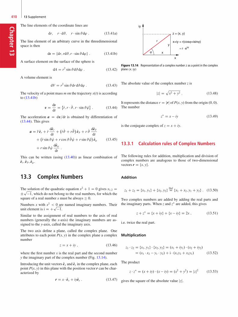
Chapter13
410 13 Supplement
The line elements of the coordinate lines are
dr; r � d#; r � sin#d' : (13.41a)
The line element of an arbitrary curve in the threedimensionalspace is then
ds D fdr; rd#; r � sin#d'g : (13.41b)
A surface element on the surface of the sphere is
dA D r2 sin#d#d' : (13.42)
A volume element is
dV D r2 sin#dr d#d' : (13.43)
The velocity of a point massm on the trajectory s.t/ is accordingto (13.41b)
v D dsdt
D ˚Pr; r � P#; r � sin# P' : (13.44)
The acceleration a D dv=dt is obtained by differentiation of(13.44). This gives
a D Rr Oer C Pr dOerdt
C �Pr P# C r R#� Oe# C r P# dOe#dt
C �Pr sin# P' C r cos# P# P' C r sin# R'� Oe'C r sin# P' dOe'
dt:
(13.45)
This can be written (using (13.40)) as linear combination ofOer; Oe# ; Oe' .
13.3 Complex Numbers
The solution of the quadratic equation x2 C 1 D 0 gives x1;2 D˙p�1, which do not belong to the real numbers, for which thesquare of a real number x must be always � 0.
Numbers x with x2 < 0 are named imaginary numbers. Theirunit element is i D Cp�1.
Similar to the assignment of real numbers to the axis of realnumbers (generally the x-axis) the imaginary numbers are as-signed to the y-axis, called the imaginary axis.
The two axis define a plane, called the complex plane. Oneattributes to each point P.x; y/ in the complex plane a complexnumber
z D x C iy ; (13.46)
where the first number x is the real part and the second numbery the imaginary part of the complex number (Fig. 13.14).
Introducing the unit vectors Oex and Oey in the complex plane, eachpoint P.x; y/ in this plane with the position vector r can be char-acterized by
r D x � Oex C iyOey : (13.47)
Figure 13.14 Representation of a complex number z as a point in the complexplane .x; iy/
The absolute value of the complex number z is
jzj Dpx2 C y2 : (13.48)
It represents the distance r D jrj of P.x; y/ from the origin .0;0/.The number
z� D x � iy (13.49)
is the conjugate complex of z D x C iy.
13.3.1 Calculation rules of Complex Numbers
The following rules for addition, multiplication and division ofcomplex numbers are analogous to those of two-dimensionalvectors r D fx; yg.
Addition
z1 C z2 D fx1; y1g C fx2; y2g DefD fx1 C x2; y1 C y2g : (13.50)
Two complex numbers are added by adding the real parts andthe imaginary parts. When z and z� are added, this gives
z C z� D fx C iyg C fx � iyg D 2x ; (13.51)
i.e. twice the real part.
Multiplication
z1 � z2 D fx1; y1g � fx2; y2g D .x1 C iy1/ � .x2 C iy2/
D .x1 � x2 � y1 � y2/C i � .x1y2 C x2y1/ (13.52)
The product
z � z� D .x C iy/ � .x � iy/ D .x2 C y2/ D jzj2 (13.53)
gives the square of the absolute value jzj.
13.4 Fourier-Analysis 411
Chap
ter13
Division
z1z2
D x1 C iy1x2 C iy2
:
Multiplication of numerator and denumerator with .x2 � iy2/gives
z1z2
D .x1 C iy1/ � .x2 � iy2/
x22 C y22
D .x1x2 C y1y2/C i.x2y1 � x1y2/
x22 C y22D a C ib :
This gives again a complex number with the real part
a D .x1x2 C y1y2/
x22 C y22
and the imaginary part
b D x2y1 � x1y2x22 C y22
:
13.3.2 Polar Representation
Often the representation of a complex number in polar coordi-nates r and ' is more convenient (Fig. 13.14).
Withx D r � cos' I y D r � sin'
we obtainz D x C iy D r.cos' C i sin '/ D r � ei'z� D x � iy D r � e�i'
) z � z� D r2 I jzj Dpx2 C y2 D r :
From Fig. 13.14 we see that
tan ' D iy
xD Im.z/
Re.z/) ' D arctan
Im.z/
Re.z/:
Note: The polar representation is not unambiguous, because allangles 'n D '0 C n � 2 .n D 1; 2; 3; : : :/ represent the samecomplex number z. The representation with n D 0 is called theprincipal value.
From z D r � ei' ) ln z D ln r C i.'0 C 2n/.
The polar representation facilitates multiplication and divisionof complex numbers
z1 � z2 D r1 � r2 � ei.'1C'2/
z1z2
D r1r2
� ei.'1�'2/ :
For arbitrary n one obtains
zn D .r � ei'/n D rn � ein' :
Complex numbers are raised to higher powers n by calculatuingthe n-th power of r and multiplying ' by n. In the same way wesee the relation
npz D z1=n D n
pr � ei'=n :
The general rule for complex numbers can be formulated as (seemathematics text books):
The set of complex numbers z D .x; y/ forms a bodywhich includes the real numbers .x; 0/ as subset.
13.4 Fourier-Analysis
In mathematical textbooks it is proved, that every continuouslydifferentiable function f .x/ can be written as infinite series ofbasis functions g.x/, if the g.x/ represent a complete set.
We choose as basis functions the trigonometric functions sin.nx/and cos.nx/ .n D 0; 1; 2; : : :/.
The Fourier-theorem states:
f .x/ D a02
C1X
nD1
�an cos.nx/C bn sin.nx/
�: (13.54)
(13.54) is called “Fourier-Series”. By multiplication of (13.54)with cos.mx/ or sin.mx/ respectively and integration over x fromx D 0 to x D 2 one obtains because of
2Z
0
cos.nx/ cos.mx/ dx D(0 for m ¤ n
for n D m ¤ 0
2Z
0
cos.nx/ sin.mx/ dx D 0 for m R n
2Z
0
sin.nx/ sin.mx/ dx D(0 for n ¤ m
for n D m ¤ 0
(13.55)
the coefficients an and bn as
a0 D b0 D 1
2Z
0
f .x/ dx I an D 1
2Z
0
f .x/ cos.nx/ dx I
bn D 1
2Z
0
f .x/ sin.nx/ dx :
(13.56)
It is therefore possible to determine the coefficients an, bn in theFourier-Series (13.54) by integration of f .x/.
Chapter13
412 13 Supplement
For x D ! � t the coefficients give the amplitudes of the contri-butions n! to the total function f .!; t/ (Fourier-Analysis) withx D !t and T D 2=! (13.55) transfers to
an D 2
T
TZ
0
f .t/ cos.n!t/dt ;
bn D 2
T
TZ
0
f .t/ sin.n!t/ dt :
(13.57)

Chap
ter14
Solutions of the Problems 1414.1 Chapter 1 . . . . . . . . . . . . . . . . . . . . . . . . . . . . . . . . . . . 414
14.2 Chapter 2 . . . . . . . . . . . . . . . . . . . . . . . . . . . . . . . . . . . 414
14.3 Chapter 3 . . . . . . . . . . . . . . . . . . . . . . . . . . . . . . . . . . . 418
14.4 Chapter 4 . . . . . . . . . . . . . . . . . . . . . . . . . . . . . . . . . . . 420
14.5 Chapter 5 . . . . . . . . . . . . . . . . . . . . . . . . . . . . . . . . . . . 423
14.6 Chapter 6 . . . . . . . . . . . . . . . . . . . . . . . . . . . . . . . . . . . 425
14.7 Chapter 7 . . . . . . . . . . . . . . . . . . . . . . . . . . . . . . . . . . . 426
14.8 Chapter 8 . . . . . . . . . . . . . . . . . . . . . . . . . . . . . . . . . . . 429
14.9 Chapter 9 . . . . . . . . . . . . . . . . . . . . . . . . . . . . . . . . . . . 431
14.10 Chapter 10 . . . . . . . . . . . . . . . . . . . . . . . . . . . . . . . . . . 433
14.11 Chapter 11 . . . . . . . . . . . . . . . . . . . . . . . . . . . . . . . . . . 436
14.12 Chapter 12 . . . . . . . . . . . . . . . . . . . . . . . . . . . . . . . . . . 441
413© Springer International Publishing Switzerland 2017W. Demtröder, Mechanics and Thermodynamics, Undergraduate Lecture Notes in Physics, DOI 10.1007/978-3-319-27877-3_14
Chapter14
414 14 Solutions of the Problems
14.1 Chapter 1
1.1 180 km=h.
1.2 The length measurement can be performed in differentways:For example the period of the earth’s rotation depends onthe moment of inertia and is therefore proportional to R�2.Independent measurements of length and time can decidethe question.
1.3 This is one, but not the only requirement for a length stan-dard. Similarly important is the accuracy of the compari-son between the length to be measured and the standard.
1.4 The length T of a day increases per year by 10�4 s. Therelative prolongation of a day per year is then
dT=T D a D 10�4
24 � 3600 D 1:1 � 10�9 :
a) Since the length of a day increases per year by 10�4 s, itis after 104 years longer by 1 s.b) How often must a leap second be inserted?The length of a day increases per day by ıt D10�4 s=365d D 2:74 � 10�8 s=d. The total time delay af-ter x days is
�t D ıt
xZ
0
n dn D 1
2ıt � n2ˇ̌x
0
D 12x
2ıt D 1 s ! x2 D 2
ıt
! x D 8600d D 23:5 years :
The distance xnC1 � xn D .2=aT0/1=2 � .pn C 1 � pn/
between two leap times becomes shorter and shorter andreaches for n � 1 the value 1=.aT0/1=2=
p2n.
1.5 1 light year D 9:46 � 1015 m ) T D 4:5 years. The dis-tance is 1.39 parsec, the angle 1=1:39 D 0:700.
1.6 L D 2 � 103 � tan.˛=2/ D 17:45m for ˛ D 1ı. For ˛ D1ı ˙ 10 ) L D 17:45 ˙ 0:29m.
1.7 Since the orbital speed of the earth varies during one rev-olution, the time between two culminations of the sunalso varies (see Fig. 1.22 and 1.23). Further reasons arevariations of the mass distribution inside the earth, whichchanges the moment of inertia, caused by magma flow,earth quakes and melting of glaciers.
1.8 The mass of a hydrogen atom is mH D 1:673 � 10�27 kg )N D 5:98 � 1026 =kg.
1.9 The mass of a H2O-molecules is mH2O D 3:0 � 10�26 kg;%H2O D 1 kg=litre; ) N D 3:0 � 1025 =litre.
1.10 The mass of the uranium nucleus is m.238U/ D 1:661 �238 � 10�27 kg. Its density is then % D m=.4 � 1
3r3/ D
1:4 � 1017 kg=m3.
1.11 From s D 1=2gt2 it follows for the falling time t Dp2s=g D 0:45 s.
�m D�P
.x � xi/2
n.n � 1/
�1=2D�40 � 0:0140 � 39
�1=2s
D 1:6 � 10�2 s
) �m=x D 1:6 � 10�2
0:45D 3:5% :
1.12 a) e�x2=2 D 0:5 ) x2 D 2 ln 2 ) x D p2 ln 2 � 1:177;
b) e�x2=2 D 0:1 ) x2 D 2 ln 10 ) x D p2 ln 10 � 2:156.
1.13 A D x � y2 ) @A=@x D 1 and @A=@y D �2y
�A D �.1000 � 10�3 � 1/2 C .30 � 3 � 10�3 � 60/2�1=2
D Œ1 C 29�1=2 � 5:5 :
1.14 Quartz clock �Tmax D 10�9 � 3:16 � 107 s � 0:03 s D30ms.Atomic Clock: �Tmax D 0:3 µs.
1.15 For the five points we obtain from (1.35) with n D 5:
a D 5 �P xiyi �PxiP
yi5 � .P x2i / � .P xi/2
D 5 � .3 C 6 C 20 C 25/ � 12 � 185 � .1 C 4 C 16 C 25/� 122
D 0:628 ;
b D .P
x2i / � .P yi/ � .P xi/ � .P xiyi/
5 � .P x2i / � .P xi/2
D 828 � 684
230 � 144D 2:093
) y D 0:628x C 2:093 I
�y Dr
0:430
n � 2D 0:38 :
Note, that here .n � 2/ instead of .n � 1/ has to be used,because already two values are determined by the equationy D ax C b.
�2a D 5 � �2
y
86D 0:006 ) �a D 0:077 ;
�2b D �2
y �P x2i86
D 0:102 � .1 C 4 C 16 C 25/
86D 0:055
) �b D 0:23 :
14.2 Chapter 2
2.1 a) The acceleration time t1 can be obtained from
v1 D v0 C at1
) t1 D v1 � v0a
D .100 � 80/m=s
3:6 � am=s2 D 4:27 s :
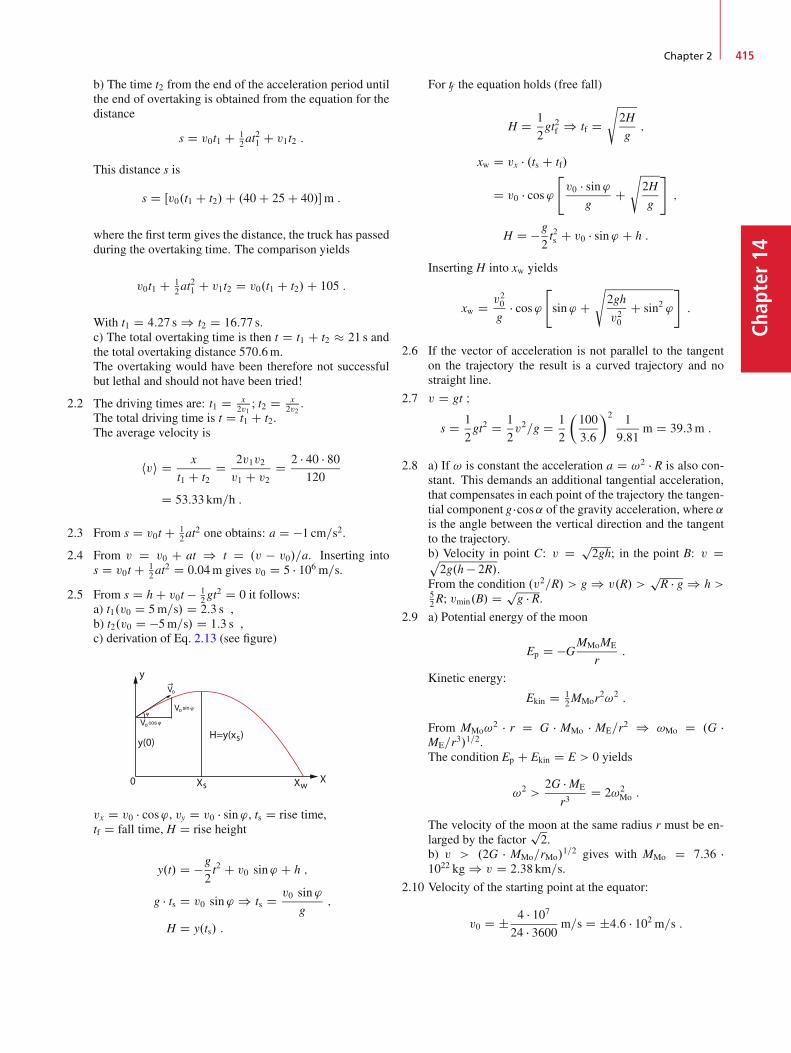
Chapter 2 415
Chap
ter14
b) The time t2 from the end of the acceleration period untilthe end of overtaking is obtained from the equation for thedistance
s D v0t1 C 12at
21 C v1t2 :
This distance s is
s D Œv0.t1 C t2/C .40 C 25 C 40/�m :
where the first term gives the distance, the truck has passedduring the overtaking time. The comparison yields
v0t1 C 12at
21 C v1t2 D v0.t1 C t2/C 105 :
With t1 D 4:27 s ) t2 D 16:77 s.c) The total overtaking time is then t D t1 C t2 � 21 s andthe total overtaking distance 570:6m.The overtaking would have been therefore not successfulbut lethal and should not have been tried!
2.2 The driving times are: t1 D x2v1
; t2 D x2v2
.The total driving time is t D t1 C t2.The average velocity is
hvi D x
t1 C t2D 2v1v2v1 C v2
D 2 � 40 � 80120
D 53:33 km=h :
2.3 From s D v0t C 12at
2 one obtains: a D �1 cm=s2.
2.4 From v D v0 C at ) t D .v � v0/=a. Inserting intos D v0t C 1
2at2 D 0:04m gives v0 D 5 � 106 m=s.
2.5 From s D h C v0t � 12gt
2 D 0 it follows:a) t1.v0 D 5m=s/ D 2:3 s ,b) t2.v0 D �5m=s/ D 1:3 s ,c) derivation of Eq. 2.13 (see figure)
XXXs w0
H=y(x )y(0) s
y
Vo cos ϕ
ϕVo
Vo
sin ϕ
→
vx D v0 � cos', vy D v0 � sin ', ts D rise time,tf D fall time, H D rise height
y.t/ D �g
2t2 C v0 sin' C h ;
g � ts D v0 sin ' ) ts D v0 sin '
g;
H D y.ts/ :
For tf the equation holds (free fall)
H D 1
2gt2f ) tf D
s2H
g;
xw D vx � .ts C tf/
D v0 � cos'"v0 � sin '
gCs
2H
g
#;
H D �g
2t2s C v0 � sin ' C h :
Inserting H into xw yields
xw D v20g
� cos'"sin ' C
s2gh
v20C sin2 '
#:
2.6 If the vector of acceleration is not parallel to the tangenton the trajectory the result is a curved trajectory and nostraight line.
2.7 v D gt I
s D 1
2gt2 D 1
2v2=g D 1
2
�100
3:6
�2 1
9:81m D 39:3m :
2.8 a) If ! is constant the acceleration a D !2 � R is also con-stant. This demands an additional tangential acceleration,that compensates in each point of the trajectory the tangen-tial component g �cos˛ of the gravity acceleration, where ˛is the angle between the vertical direction and the tangentto the trajectory.b) Velocity in point C: v D p
2gh; in the point B: v Dp2g.h � 2R/.
From the condition .v2=R/ > g ) v.R/ >pR � g ) h >
52R; vmin.B/ D p
g � R.2.9 a) Potential energy of the moon
Ep D �GMMoME
r:
Kinetic energy:
Ekin D 12MMor
2!2 :
From MMo!2 � r D G � MMo � ME=r2 ) !Mo D .G �
ME=r3/1=2.The condition Ep C Ekin D E > 0 yields
!2 >2G � ME
r3D 2!2
Mo :
The velocity of the moon at the same radius r must be en-larged by the factor
p2.
b) v > .2G � MMo=rMo/1=2 gives with MMo D 7:36 �
1022 kg ) v D 2:38 km=s.
2.10 Velocity of the starting point at the equator:
v0 D ˙ 4 � 10724 � 3600 m=s D ˙4:6 � 102 m=s :

Chapter14
416 14 Solutions of the Problems
Rocket equation (neglecting the vertical acceleration if g �T v0):
v D v0 C ve ln.m0=m/ :
With m0 D m C mx (mx D fuel mass) it follows:
ln�1 C mx
m
D .7:9 � 103 4:6 � 102/=.4:5 � 103/
) mx D 2103kg for a launch into the east direction andmx D 2705 kg into the west direction, if the mass of thefuel container is neglected.
2.11 .mv20=2/ >G�m�ME
R D mgR ) v0 >p2gR.
2.12 Because the velocity of the earth at the launch point is vE D463m=s. The initial velocity of the rocket is not zero butv0 D vE � cos 30ı D 400m=s. One wins the initial kineticenergy 1
2mv20 . For a vertical launch one would need the
escape velocity vE D p2gR D 11;200m=s (see (2.30)).
Therefore one only needs to accelerate from 400m=s until11;200m=s. This requires the kinetic energy�Ekin D 1
2m �.v2E � v20/. The relative energy saving is .1 � �E=E/ D0:004. One saves only 0.4%.
2.13 The total force is F D FA �m � g D g �r2.z � %w � h � %H/.For z D 2
3h ! F D 0 ,
) %H D 23%w :
The work is
W DıZ
zD2h=3
F dz DıZ
2h=3
gr2.z%w � h%H/ dz
D 29gr
2h2%w D 24:7 J :
Without water twice the work would be necessary.
2.14 Ekin.h1/ D 12mv
2.h1/ D 200N � m ,
mg.h2 � h1/ D Ekin.h/ ;
) h2 D Ekin.h1/
mgC h1 D 35:5m :
2.15 F D �Dx1 ) D D F1x1
D 400N=m.
W Dl0Z
0
Dx dx D 12Dl
20 D 128N � m :
2.16 The neutral point between earth and moon, where theopposite gravitational forces just compensate, has the dis-tance r2 from the earth and r1 from the moon. From F D 0it follows:
G � MMo
r21D G � ME
r22and r D r1 C r2
) r2 D r
1 C .MMo=ME/1=2D 3:84 � 108 m
1 C 0:11
� 3:46 � 108 m :
In order to reach the distance r1 for the earth the initialkinetic energy must be
1
2mv20 � G � MEm
r2Z
R
dr
r2:
SinceMMo D 0:012ME we can neglect the attraction by themoon at the start of the rocket. It follows:
v20 � 2G � ME
�1
R� 1
r2
�� 0:98 v20.1/ :
The energy saving is 2% compared with the case where thesecond escape velocity is required to reach r D 1.
2.17 a) m!2r D mG � ME=r2 ) r3 D G � ME=!2 ,
T D 2
!D 1 day D 24 � 3600 s
) ! D 7:2 � 10�5 s�1
) r D 4:25 � 107 m D 42;500 km :
b) The energy of the body in the geostationary orbit com-pared to a body resting on the earth surface is
E D Ekin C Ep D mv2
2C
rSZ
rDR
GmME
r2dr
D m!2r2S2
C GmME
�1
R� 1
rS
�
with rS D 42;500 km. It needs the energy supply
E D m�12 � !2rS C gR.1 � R=rS/
�:
c) In order to get the accuracy 0:1 km=day of its positionthe upper limit for the accuracy of the angular velocity is
�!
dayD 0:1
42;500D 2:4 � 10�6 per day :
The minimum relative stability has to be �!=! �2:4 � 10�6=2 D 3:8 � 10�7
Since !2 D G � ME=r3 ) �r=r D �2=3�!=! ) �r �10:6m.
2.18 Ep D �G �m � ME
rD �m � g � R
2
rwith R D radius of earth.
Ekin D CG � m � ME
2rD �1
2Ep ;
E D Ep C Ekin D �G � m � ME
2rD �Ekin :
2.19 Ep D mgL.1 � cos'/; Ekin D mv2
2D m
2L2 P'2;
E D Ekin C Ep :
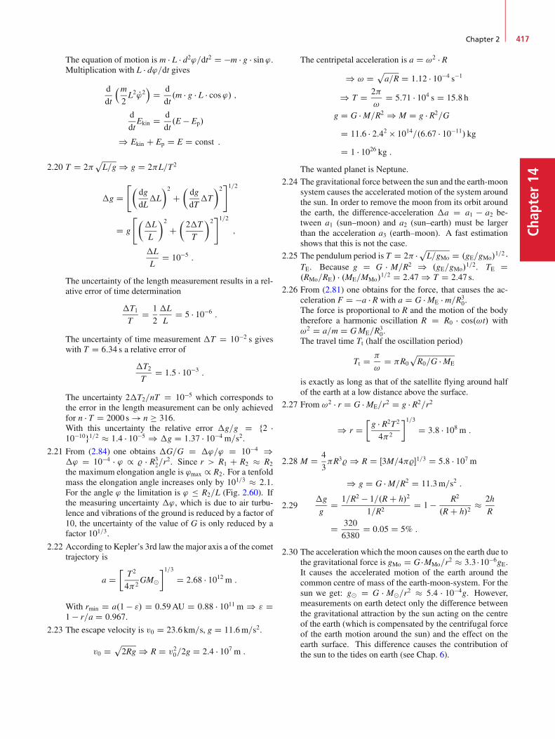
Chapter 2 417
Chap
ter14
The equation of motion is m � L � d2'=dt2 D �m � g � sin '.Multiplication with L � d'=dt gives
d
dt
�m2L2 P'2
D d
dt.m � g � L � cos'/ ;
d
dtEkin D d
dt.E � Ep/
) Ekin C Ep D E D const :
2.20 T D 2pL=g ) g D 2L=T2
�g D"�
dg
dL�L
�2
C�dg
dT�T
�2#1=2
D g
"��L
L
�2
C�2�T
T
�2#1=2
;
�L
LD 10�5 :
The uncertainty of the length measurement results in a rel-ative error of time determination
�T1T
D 1
2
�L
LD 5 � 10�6 :
The uncertainty of time measurement �T D 10�2 s giveswith T D 6:34 s a relative error of
�T2T
D 1:5 � 10�3 :
The uncertainty 2�T2=nT D 10�5 which corresponds tothe error in the length measurement can be only achievedfor n � T D 2000 s ! n � 316.With this uncertainty the relative error �g=g D f2 �10�10g1=2 � 1:4 � 10�5 ) �g D 1:37 � 10�4 m=s2.
2.21 From (2.84) one obtains �G=G D �'=' D 10�4 )�' D 10�4 � ' / % � R3
2=r2. Since r > R1 C R2 � R2
the maximum elongation angle is 'max / R2. For a tenfoldmass the elongation angle increases only by 101=3 � 2:1.For the angle ' the limitation is ' � R2=L (Fig. 2.60). Ifthe measuring uncertainty �', which is due to air turbu-lence and vibrations of the ground is reduced by a factor of10, the uncertainty of the value of G is only reduced by afactor 101=3.
2.22 According to Kepler’s 3rd law the major axis a of the comettrajectory is
a D�T2
42GMˇ
�1=3D 2:68 � 1012 m :
With rmin D a.1 � "/ D 0:59AU D 0:88 � 1011 m ) " D1 � r=a D 0:967.
2.23 The escape velocity is v0 D 23:6 km=s, g D 11:6m=s2.
v0 D p2Rg ) R D v20=2g D 2:4 � 107 m :
The centripetal acceleration is a D !2 � R) ! D
pa=R D 1:12 � 10�4 s�1
) T D 2
!D 5:71 � 104 s D 15:8 h
g D G � M=R2 ) M D g � R2=G
D 11:6 � 2:42 1014=.6:67 � 10�11/ kg
D 1 � 1026 kg :The wanted planet is Neptune.
2.24 The gravitational force between the sun and the earth-moonsystem causes the accelerated motion of the system aroundthe sun. In order to remove the moon from its orbit aroundthe earth, the difference-acceleration �a D a1 � a2 be-tween a1 (sun–moon) and a2 (sun–earth) must be largerthan the acceleration a3 (earth–moon). A fast estimationshows that this is not the case.
2.25 The pendulum period is T D 2 �pL=gMo D .gE=gMo/1=2 �
TE. Because g D G � M=R2 ) .gE=gMo/1=2. TE D
.RMo=RE/ � .ME=MMo/1=2 D 2:47 ) T D 2:47 s.
2.26 From (2.81) one obtains for the force, that causes the ac-celeration F D �a � R with a D G � ME � m=R3
0.The force is proportional to R and the motion of the bodytherefore a harmonic oscillation R D R0 � cos.!t/ with!2 D a=m D GME=R3
0.The travel time Tt (half the oscillation period)
Tt D
!D R0
pR0=G � ME
is exactly as long as that of the satellite flying around halfof the earth at a low distance above the surface.
2.27 From !2 � r D G � ME=r2 D g � R2=r2
) r D�g � R2T2
42
�1=3D 3:8 � 108 m :
2.28 M D 4
3R3% ) R D Œ3M=4%�1=3 D 5:8 � 107 m
) g D G � M=R2 D 11:3m=s2 :
2.29�g
gD 1=R2 � 1=.R C h/2
1=R2D 1 � R2
.R C h/2� 2h
R
D 320
6380D 0:05 D 5% :
2.30 The acceleration which the moon causes on the earth due tothe gravitational force is gMo D G �MMo=r2 � 3:3 �10�6gE.It causes the accelerated motion of the earth around thecommon centre of mass of the earth-moon-system. For thesun we get: gˇ D G � Mˇ=r2 � 5:4 � 10�4g. However,measurements on earth detect only the difference betweenthe gravitational attraction by the sun acting on the centreof the earth (which is compensated by the centrifugal forceof the earth motion around the sun) and the effect on theearth surface. This difference causes the contribution ofthe sun to the tides on earth (see Chap. 6).
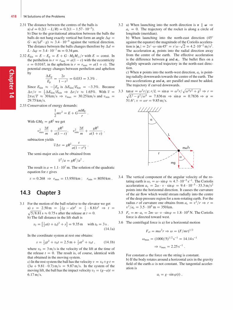
Chapter14
418 14 Solutions of the Problems
2.31 The distance between the centres of the balls isa) d D 0:2.1 � L=R/ D 0:2.1 � 1:57 � 10�5/.b) Due to the gravitational attraction between the balls theballs do not hang exactly vertical but form an angle �' DG � m=.d2 � g/ � 3:4 � 10�9 against the vertical direction.The distance between the balls changes therefore by�d DL ��' D 3:4 � 10�7 m D 0:34 µm.
2.32 Ekin D E � Ep D E C G � MEMˇ=r with E D const. Inthe perihelion is r D rmin D a.1 � "/ with the eccentricity" D 0:0167, in the aphelion is r D rmax D a.1 C "/. Thepotential energy changes between perihelion and aphelionby
�Ep
EpD 2"
1 � "2 D 0:033 D 3:3% :
Since Ekin � � 12Ep is �Ekin=Ekin D �3:3%. Because
�v=v D 12�Ekin=Ekin ) �v=v � 1:65%. With v D
2a=T � 30 km=s ) vmax D 30:25 km=s and vmin D29:75 km=s.
2.33 Conservation of energy demands:1
2mv2 D E C G
mME
r:
With GME D gR2 we get
v2max2E
mC gR2
a.1 � "/ ; v2min2E
mC gR2
a.1 C "/;
subtraction yields
v�v D gR2 "
a.1 � "2/ :
The semi-major axis can be obtained from
v2=a D gR2=a2 :
The result is a D 1:1 � 107 m. The solution of the quadraticequation for " gives
" D 0:268 ) rmax D 13;950 km I rmin D 8050 km :
14.3 Chapter 3
3.1 For the motion of the ball relative to the elevator we geta) s D 2:50m D 1
2 .g � a/t2 D 12 � 8:81t2 ) t Dp
5=8:81 s � 0:75 s after the release at t D 0.b) The fall distance in the lift shaft is
s2 D �12a.t C t0/
2 C s� D 9:35m with t0 D 3 s :
(14.1a)
In the coordinate system at rest one obtains:
s D 12gt
2 C v0t D 2:5m C 12at
2 C v0t ; (14.1b)
where v0 D 3m=s is the velocity of the lift at the time ofthe release t D 0. The result is, of course, identical withthat obtained in the moving system.c) In the rest system the ball has the velocity v D v0Cg�t D.3a C 9:81 � 0:7/m=s D 9:87m=s. In the system of themoving lift, the ball has the impact velocity v2 D .g�a/t D6:17m=s.
3.2 a) When launching into the north direction is v k ! )ac D 0. The trajectory of the rocket is along a circle oflongitude (meridian).b) When launching into the north-east direction (45ıagainst the equator) the magnitude of the Coriolis accelera-tion is jacj D 2v0 �! � sin 45ı D v0! �p2 D 4:2 �10�2 m=s2.The acceleration ac points into the radial direction awayfrom the centre of the earth. The effective accelerationis the difference between g and ac. The bullet flies on aslightly upwards curved trajectory in the north-east direc-tion.c) When v points into the north-west direction, ac is point-ing radially downwards towards the centre of the earth. Thetwo accelerations g and ac are parallel and must be added.The trajectory if curved downwards.
3.3 tan˛ D !2r=g; r=L D sin˛ D !2r=p!4r2 C g2 ) r Dp
L2 � g2=!4 D 7:836m ) sin˛ D 0:7836 ) ˛ D51:6ı; v D !r D 9:85m=s.
3.4 The vertical component of the angular velocity of the ro-tating earth is !s D ! � sin' � 4:7 � 10�5 s�1. The Coriolisacceleration ac D 2! � v � sin' D 9:4 � 10�5 � 33:3m=s2points into the horizontal direction. It causes the curvatureof the air flow which would stream radially into the centreof the deep pressure region for a non-rotating earth. For theradius r of curvature one obtains from ac D v2=r ) r Dv2=ac D 3:5 � 105 m D 350 km.
3.5 Fc D m � ac D 2m �! � v � sin' D 1:8 � 104 N. The Coriolisforce is directed toward west.
3.6 The centrifugal force is a) for a horizontal motion
Fcf D m!2r ) ! D .F=mr/1=2
!max D .1000=5/1=2 s�1 D 14:14 s�1
) �max D 2:25 s�1 :
For constant ! the force on the string is constant.b) If the body rotates around a horizontal axis in the gravityfield of the earth ! is not constant. The tangential acceler-ation is
at D g � sin '.t/ ;
Chapter 3 419
Chap
ter14
where ' is the angle between the radius vector r and thevertical z-axis. The angular velocity is then
! D !0 C .g=r/
'Z
0
sin'.t/ dt ;
where !0 D !.' D 0/ is the velocity at the upper point ofthe circle. The maximum value of ! is reached for ' D at the lowest point of the circle. The following relationshold:
!max D !0 C�gr
Z
0
sin '.t/dt
D !0 C�gr
.cos'/P'
ˇ̌ˇ̌0
:
(14.2)
With d'=dt D ! we obtain
! !max D !0 C g
.r � !0/C g
.r � !max/;
! !max D 1
2r
�r � !0 C g
!0
�
C 1
2
s
!20 C 6g
NC g2
N2!20
:
(14.3)
For !min the plus sign before the square root must be re-placed by a minus sign.The maximum force onto the string occurs at the lowerpoint %' D .The condition that the string does not break gives the rela-tion
F D m!2max � r C m � g � 1000N
! !max ��.1000=5� g/
r
�1=2D 13:8 s�1 :
The maximum allowed angular velocity !0 at the lowerpoint ' D 0 can be calculated either from (3) or from thelaw of energy conservation
12mv
20 D 1
2mv2max � 2mg � r with v D r � ! :
Inserting the numerical values gives
!0 D 12:3 s�1 :
The difference between the velocities in the upper andlower point is
12v
2min C 2rg D 1
2v2max ) !2
max � !2min D 4g
r:
3.7 At a radial velocity vr D 10m=s the ball needs 10�2 s toreach the outer edge of the disc. For a non-rotating discthe ball would fly on a straight line with the velocity v Dfvr; v'g in the lab system as well as in the system of the disc(which are identical for the non-rotating disc). It wouldreach the edge of the disc at the displacement R �' from theposition ' D 0 which can be obtained from R � ' D �t �v' D 0:05m at the angle ' D 0:05m=0:2m D 0:25 rad D14:8ı. When the disc rotates with ! D 2 � 10 s�1, itsedge turns during the time T D 0:01 s by R' D R!T D0:126m ) ' D 39ı. For a radial velocity (d'=dt D 0)the bullet would reach the edge at ' D �39ı. With v' D5m=s the bullet reaches the edge at ' D 14:5ı � 39ı D�24:5ı. From the point of view of the observer at rest thebullet flies on a straight line, but viewed by an observeron the disc it flies along a curved line with the tangentialacceleration
a' D 2vr � ! :The trajectory on the disc is a parabola. The velocity isv D fvr; v' � 2vr!tg where vr and v' are the velocitycomponents in the rest frame while vr and v' � 2vr!t arethe components in the system of the rotating disc.
3.8 The centrifugal acceleration is
acf D !2r D !2R cos' .R D earth radius/
D 3:7 � 10�9 � 6:37 � 106 m=s2D 2:36 � 10�2 m=s2 :
It is acting radially outwards, perpendicular to the angularvelocity !.The Coriolis acceleration is parallel to acf. Numerical val-ues: acf D 0:023m=s2, aC D 1:02m=s2. The Coriolisacceleration is for this case 44 times as large as the cen-trifugal force.
3.9 a) According to the Galilei-transformations is:
u0x D ux � vx D 0:5c � 1
3c D 16c
u0y D uy D 0:1 c
u0z D uz D 0 :
b) The Lorentz-transformations give:
u0x D 1
5c I u0y D 0:113c I u0
z D 0
) u0 D f0:2; 0:113; 0gc :
Chapter14
420 14 Solutions of the Problems
The relative errors of the Galilei transformations are with�u D uLo � uGa
�u0x
u0x
D 1=5 � 1=6
1=5D 1
6� 16:7% ;
�u0y
u0u
D 0:013
0:113� 11:5% ;
�u0z D 0 :
3.10 � D .1 � v2=c2/�1=2 D 2:785 ) L0 D L=� D 0:36L.
3.11 The nearest distance Earth–Neptune is (Tab. 2.1)
L D 28:8AU D 4:3 � 1012 m :
The travel time according to the measurement of the pilot:
T 0 D 2L
�vD 2L
v
p1 � v2=c2 D 1 d ¶ 8:64 � 104 s :
Resolving for v yields
v D 2L
.T2 C 4L2=c2/1=2D 0:94 � 108 m=s D 0:3c
) � D 1:048 :
Travel time according to the observers at rest on earth:
T D T 0� D 9:05 � 104sD 1 d C 1:41 � 104 s D 1 d C 1:15 h :
3.12 a) In the rest frame the observer O sits in the middle be-tween A and B. This is also true, when A, B and O movewith the same constant velocity v.b) When O0 moves with the velocity vx against the lengthAB, he measures the simultaneous arrival of the light pulsesfrom A and B at the point C, if C is away from A by.L=2/.1 � v=c/. C is therefore closer to A than to B.
3.13 v D 0:8c ) � D 5=3.The travelling time is according to B: T D 2L=v D10 years. According to A is T 0 D 2L=.v�/ D 6 years.The number of pulses sent by B is
N D f T D 1 � 10 D 10 :
Number of pulses sent by A:
N 0 D f T 0 D 6 :
Number of pulses received by A during the journey out:
N 01 D .L=v/.1 � ˇ/ D 5 � 0:2 D 1 :
On the journey back:
N 02 D .L=v/.1 C ˇ/ D 5 � 1:8 D 9 :
3.14 For C the two astronauts A and B meet after a distance x(in ly) with x D 0:8ct C 0:1ct D 0:9ct, when t is measuredin years.
) t D 8 years after the departure of B, ) x D 7:2 ly.For A the travelling time is t0A D 1=�A with �A D .1 �0:82/�1=2 D 1:67 ) t0A D 4:8 years.For B is t0B D 1=�B with �B D .1 � 0:92/�1=2 D 2:3 )t0B D 3:49 years.
14.4 Chapter 4
4.1 All particles move into the ˙x-direction, ) v D fvx; 0; 0g;jvj D v.The centre of mass velocity is
vCM D mv � 3mv
4mD �1
2v :
The particle velocity in the CM-system is
v1CM D v1 � vCM D 32v ;
v2CM D v2 � vCM D 12v :
a) Elastic collision:
v01CM D �v1CM D � 3
2v ;
v02CM D �v2CM D C 1
2v
)
) v01 D v0
1CM C vCM D �2v ;
v02 D v0
2CM C vCM D 0
)
) E0kin.m1/D m
2 v0 21 D 2mv2 ;
E0kin.m2/D 0 :
Before the collisions was
Ekin.m1/ D m
2v2 I Ekin.m2/ D 3
2mv2
)X
Ekin DX
E0kin :
b) Completely inelastic collision: The two particles stay to-gether after the collision. The total mass M D 4m moveswith the velocity vCM D v0
CM D � 12v
) E0kin D 4m
2v2CM D 1
2mv2 :
The rest .3=2/mv2 of the initial energy 2mv2 is transferredinto heat energy, ) 75% are converted into heat, only 25%remain as kinetic energy.
4.2 The momentum of the bullet: m2v) the velocity of wooden block C bullet is
v0 D m2v
Mwith M D m1 C m2 :
) Ekin D 12Mv
0 2 D 12m22
M v2
D Ep D MgL.1 � cos'0/
Chapter 4 421
Chap
ter14
) cos'0 D 1 � 1
2
m22
M2gLv2 D 1 � 0:196 D 0:804
) '0 D 36:5ı :
4.3 We assume that the incident proton moves into the Cx-direction.a) The momentum conservation for the x- and the y-directiondemands:
xW mv01 cos �1 C 2mv0
2 cos 45ı D mv1 (14.4a)
yW mv01 sin �1 D 2mv0
2 sin 45ı : (14.4b)
Division by m gives for (14.4b):
v01 D 2v0
2sin 45ı
sin �1:
Inserting in (14.4a) gives:
v02 D 1
2
v1
cos 45ı C sin 45ı= tan �1
D v1p2 .1 C cot �1/
;
v01 D v1
sin �1 C cos �1:
Energy conservation demands
v21 D v0 21 C 2v0 2
2
) 1 D 1
.sin �1 C cos �1/2C 1
.1 C cot �1/2
) tan �1 D 2 ) �1 D 63:435ı :
b) vCM D m1v1
m1 C m2with 2m1 D m2
) vCM D 13v1 D v0
CM :
c) v021 D v21�
1 C m2m1
2
"�m2
m1
�2
C 2m2
m1cos#1 C 1
#
D v214 C 4 cos 63:435ı C 1
9D 0:75 v21
) v01 D 0:866 v1 :
v022 D 1
2.v21 � v02
1 / D 1
20:25 v21 D 0:125 v21
) v02 D 0:35 v1 :
4.4 a) Energies in the Lab-system:
Ekin.m1/ D m
2
�v2x C v2y C v2z
�
D 1 � .9 C 4 C 1/ D 14Nm ;
Ekin.m2/ D 36Nm :
Velocity of the centre of mass:
vCM D 1
M
Xmi � vi
D ˚vxCM; vyCM; vzCM
D f0; 2; 2g m=s :
Relative velocities:
v1CM D v1 � vCM D f3; 0;�3gm=sv2CM D v2 � vCM D f�2; 0; 2gm=s
))
E.CM/kin .m1/ D m1
2v21CM D 18Nm ;
E.CM/kin .m2/ D m2
2v22CM D 12Nm :
b) The centre of mass momentum equals the momentum ofthe compound particles after the collision.
MvCM D M f0; 2; 2g kgm=s ;E0kin.M/ D M
2v2CM D 20Nm :
c) The fraction of the converted kinetic energy is
� D 1 � E0kin.M/
Ekin.m1/C Ekin.m2/D 50 � 20
50D 0:6 :
In the centre of mass system is ECMkin D 0. The total kinetic
energy is converted into heat.
4.5 We choose the x-axis as the direction of v1.a) Conservation of momentum for the x- and y-componentsyields:
m1v1x C m2v2x D m1v01x C m2v
02x ;
v1 D f4; 0gm=s I v01 D f2; 2gm=s I
v02 D f1;�1gm=s ) v2x D 0 ;
m1v1y C m2v2y D m1v01y C m2v
02y
0 C 2v2y D 2 � 2 � 1m=s ;) v2y D 0m=s
) v2 D f0; 0gm=s ;i. e. m2 was at rest before the collision.b) Energy conservation (4.17) gives:
Q D E0kin � Ekin
D 12
�m1v
0 21 C m2v
0 22 � m1v
21 � m2v
22
�
D �2Nm :
Ekin D 8Nm ) 25% of the initial energy is converted intoheat.The centre of mass velocity is
vCM D 1
M
˚m1v1x C m2v2xIm1v1y C m2v2y
D 13 f4; 0gm=s :
Chapter14
422 14 Solutions of the Problems
The energy of the centre of mass is
E.CM/kin D 12Mv
2CM D 2:66Nm :
For a completely inelastic collision the fraction Q D Ekin �E.CM/kin is converted into heat. Since the collision of our exam-ple is not a central collision, jQj is smaller. In the C-system37.5% are converted.c) Velocities in the CM-system:
v1CM D v1 � vCM D ˚83 ; 0
m=s ;
v01CM D v0
1 � vCM D ˚23 ; 2
m=s I
cos#1 D v1CM � v01CM
jv1CMjjv01CMj D 16=9
q649 � 40
9
D 0:316
) #1 D 71:578ı Iv2CM D ˚� 4
3 ;23
m=s I v0
2CM D ˚� 13 ;� 7
3
m=s
) #2 D 121:6ı :
4.6 Conservation of momentum gives
m1v01 C m2v
02 D m2v2 :
Conservation of energy gives:
m1v0 21 C m2v
0 22 D m2v
22 :
a) After the collision is v02 D �v0
1
) v02
�1 � m1
m2
�D v2 ; v0 2
2
�1 C m1
m2
�D v22
) m1=m2 D 3 :
b) The travel time for m1 resp. m2 until the left barrier are
t1 D 1:6m
v01
> t2 D 2:4m
v02
) v02
v01
> 1:5 :
Energy conservation demands with x D m1=m2
v0 22
v0 21
D v22v0 21
� x :
Using momentum conservation gives:
v02
v01
D 1
2.x � 1/ ) x > 4 :
c) The velocity of the CM is
vCM D v0CM D 1
3v2 :
The velocities in the lab-system are after the collision:
v01 D 2
3v2I v0
2 D �1
3v2 :
The two masses meet for the first time at x0 D 1:6m at thetime t1 D 0, for the second time t2 at the location x (x D 0is at the left wall). According to the calculation in a) themasses meet for the second time only after the reflection ofm1 at the left wall. It is:
t2 D x0 C x
v01
D 0:8 C x0 � x
v02
) x D 1:07m :
The two masses meet at x D 1:07m from the left wall afterm1 has suffered a reflection at the left wall and m2 at theright wall.
4.7 The velocity of the steel ball at the impact is
m1Lg D 12m1v
21 ) v1 D p
2gL D 4:43m=s :
The energy transferred to m2
�E D 4m1m2
M2E1 :
The steel ball has therefore the energy after the collision
E0kin D
�1 � 4
m1m2
M2
E1 D 4
9E1 :
It rises up to the heightH D L.1� cos'/ D 49L ) cos' D
59 ) ' D 56:15ı.
4.8 The distance between ball and lift is �s D 20m. The timeuntil the impact onto the ceiling of the lift is obtained from
12gt
21 C vt1 D �s D 20m ) t1 D 1:8 s :
During this time the lift has moved over the distance vt1 D3:6m. The impact point is therefore 26:4m below A.b) In the lab system the impact velocity of the ball is v1 Dgt1 D 17:66m=s. The centre of mass moves because M �m with the velocity vCM D v D 2m=s upwards. In thecentre of mass system (which is nearly identical with thesystem of the lift) the ball has the velocity v1CM D v1 CvCM D 19:66m=s downwards. After the completely elasticreflection at the lift ceiling the ball has the upward velocityv01CM D 19:66m=s.
In the Lab system is v01 D v0
1CM C vCM D 21:66m=s. Theball has won twice the velocity of the lift by the reflection atthe moving lift. It rises now by the distance �h1 D v02
1 =2gabove the impact point. Inserting the numerical values gives:�h1 D 23:9m. Its upper return point is then 2:5m below A.c) It hits the ceiling of the lift for a second time at the timet2. During the time �t D t2 � t1 the lift has moved upwardsby �h2 D v�t.The ball needs a rise time�t1 obtained from v.�h1/ D 0 Dv010g�t1 ) �t1 D v0
1=g D 2:2 s. Its drop time is �t2 D1:9 s which is obtained from
12g�t22 D �h1 � v.2:2 s C�t2/ :
This gives the time �t D �t1 C �t2 D 4:1 s ) �h2 D8:2m. The second impact occurs 8:2m above the first im-pact point, i. e. 18:2m below A.
Chapter 5 423
Chap
ter14
4.9 a) The ˛-particle should fly into the Cx-direction. For they-components of the momenta we get
0 D m1v01 sin 64
ı � m2v02 sin 51
ı
) v01
v02
D 4 � sin 51ı
sin 64ı D 3:46 since m2 D 4m1 :
b) E0kin.m1/
E0kin.m2/
D m1v0 21
m2v0 22
D 1
4� 3:462 � 3:0 :
4.10 E D cqm2
0c2 C p2 ;
with E D 6GeV and pc D 4GeV
) m0c2 D p
20GeV ;
) E0 D p20 C 25GeV D 6:71GeV :
With
E D mc2
E0 D m0c2
)) m0
mD 6:7
6D 1p1 � v2=c2
) v
cD 0:445 :
The two systems move with v D 0:445c against each other.
14.5 Chapter 5
5.1 When we cut a cone with full aperture angle 2˛ out of asphere we choose the origin of our coordinate system at thepeak of the cone. The z-axis is the symmetry axis. Then thecoordinates of the centre of mass are
xCM D yCM D 0 ;
zCM D 1
V
RZ
rD0
=2Z
#D=2�˛
2Z
'D0
r3 cos# sin# dr d# d'
D 1
V
4R4h1 � sin2
�2
� ˛i
D 1
V
4R4 sin2 ˛ :
The volume of the cone is V D 23R
3.1 � cos˛/. Then weget
zCM D 3
8R
�sin2 ˛
1 � cos˛
�D 3
8R.1 C cos˛/ :
5.2 a) ICM D 25MR2 D 9:7 � 1037 kgm2;
L D ICM! D 7:07 � 1033 kgm2 s�1
) Ecurl D 1
2ICM!
2 D 1
5MR2!2 D 2:57 � 1029 J :
b) The mass of the earth is for this case
ME D 4
3%1
R3
8C 4
3%2
�R3 � 1
8R3
�D 4
3%R3 :
With % D M=V D mean density
) %1 C 7%2 D 8% :
With %1 D 2%2
) %2 D 8
9% ; %1 D 16
9% :
The moment of inertia is therefore
ICM D 2
5� 43
0
@%1�R
2
�3 �R
2
�2
C%2"R3R2 �
�R
2
�3 �R2
�2#1
A
D 8
15
�%1
R5
32C %2
31
32R5
�
D 1
60R5
�16
9%C 31 � 8
9%
�
D 22
45R5% D 11
30MR2 D 0:367MR2 :
This should be compared with the moment of inertia ICM D.2=5/MR2 D 0:4MR2 D 9:72 � 1037 kgm2 of the homoge-neous earth.c) If all N D 5�109 adults on earth would run simultaneouslyon the equator eastwards their torque exerted on the earthwould be D D N �m �a �R D 5 �109 �70 �2 �6:37 �106 N � m D4:46 � 1018 Nm. This would lead to a relative decrease�!=! D �L=L of the earth rotation. Inserting the numeri-cal value for the angular momentum L
L D ICM! D 0:71 � 1034 kgm2=s
we get
�!=�t
!D 1
L
�L
�tD D
LD 6:3 � 10�16 s�1 ;
which is so small, that it falls below the detection limit.
5.3 a) I0 D 12MR2 D 5 � 10�4 kgm2
L D I0!0 D 12MR2!0 D 3:14 � 10�2 Nm s ;
E0curl D 1
2 I0!20 D 0:987Nm :
b) I D I0 C mR2 D .5 C 1/ � 10�4 kgm2 D 6 � 10�4 kgm2.The angular momentum does not change, because the bugfalls onto the disc parallel to the rotation axis.
) ! D L0I
D 5
6!0
Ecurl D 1
2I!2 D 5
6E0curl D 0:823Nm :
Chapter14
424 14 Solutions of the Problems
The energy difference �E D 0:164N � m is converted byfriction into heat energy, which is lost during the equaliza-tion of the tangential velocities of bug and disc (which arehere assumed to occur instantaneously).c)
!.r/ D 1
1 C mr2=I0!0
L.r/ D L0; independent of r ;
Ecurl D E0curl
1 C mr2=I0:
5.4 a) I DZ
V
r2% dV D 2H%0
RZ
rD0
�1 C
� rR
2�r3 dr
D 2%0H�1
4R4 C 1
6R4
�D 10
12%0HR
4
D 5
6%0R
2V :
The mass is M D RV % dV D 3
2%0HR2
) I D 5
9MR2 :
Numerical values: M D 18:85 kg, I D 0:105 kgm2.
b) a D g sin˛
1 C ICM=.MR2/D g sin 10ı
14=9
h D 12at
2 ) t D .2h=a/1=2 D 1:35 s :
5.5 For the isosceles triangle with height h and side length d thecentre of mass S D .xCM; yCM/ has the coordinates xCM D 0,yCM.˛/.The moments of inertia around the principal axes are
Ia D 2my2CM C m.h � yCM/2 ;
Ib D 2mx2 ;
Ic D m.h � yCM/2 C 2m.x2 C y2CM/ D Ia C Ib ;
x D d sin.˛=2/ D 0:204 nm ;
h D d cos.˛=2/ D 0:247 nm ;
yCM D 13h D 0:082 nm :
For the moments of inertia we get:
Ia D 0:93AMUnm2 ;
Ib D 1:91AMUnm2 ;
Ic D 2:85AMUnm2 :
1AMU D 1:67 � 10�27 kg .The rotational energy is then
Erot D L2
2Iwith L2 D l � .l C 1/„2 :
Where l D 1; 2; 3; : : : and „ D h=2 D 1:06 � 10�34 J � s isthe reduced Planck constant and it is the smallest unit of therotational angular momentum.This gives with 1 eV D 1:6 � 10�19 J
Ea D 2:2 � 10�5 eV ;
Eb D 1:1 � 10�5 eV ;
Ec D 0:73 � 10�5 eV :
5.6 The inertial moment of a rod with length L is
ICM D 112ML2 D 1:33 � 10�2 kgm2 :
The angular momentum of the bullet referred to the CM ofthe rod is
LB D jr pj D 12Lmv D 0:4Nm s :
The rotational velocity of the rod is
! D LBI
D LBICM C m.L=2/2
D 29:2 s�1 ) � D 4:65 s�1 :
) Erot D 12 I!
2 D 5:67Nm ;
Ekin D 12mv
2 D 200Nm ;
) Erot=Ekin D 2:8 � 10�2 D 2:8% :
97.1% of the kinetic energy of the bullet is lot as heat energy.Compare this with the case of a completely inelastic centralcollision of a bullet with mass m hitting a free massM. Herethe ratio
E0kin=Ekin D .m C M/v2CM
mv2(see Sect. 4.2.4) :
With vCM D m
M C mv ) E0
kin=Ekin � m
MD 0:01.
Question: Why is the transfer of kinetic energy of the bulletinto rotational energy more efficient?
Chapter 6 425
Chap
ter14
5.7 ICM D 1
2MR2 I D D ICM � d!
dt
) ! D !0 C 1
ICM
tZ
0
D dt0
D !0 C D0
ICM
tZ
0
e�at0dt0
D !0 C 2D0
aMR2
�1 � e�at
�:
For t ! 1 ) !.1/ D !0 C .2D0=aMR2/.Numerical example: !.t D 10 s/ D 136:4 s�1 (because!0 D 10 s�1).
5.8 Ekin D Erot C Etrans D 12 ICM!
20 C 1
2MR2!20
Ep D Mgh D Ekin
) h D !20
2Mg.ICM C MR2/ :
a) Full cylinder: ICM D 1
2MR2 ) h1 D 3
4
!20R
2
g.
b) Hollow cylinder: ICM D MR2 ) h2 D !20R
2
g.
Numerical example: h1 D 17:2 cm; h2 D 22:9 cm.
14.6 Chapter 6
6.1 Tensile strength in the height z above the end of the rope:
� D % � g � z :Relative elongation:
".z/ D 1
E�.z/ :
Total elongation
�L DLZ
0
".z/ dz D 1
E
LZ
0
�.z/ dz
D %g
E
LZ
0
z dz D %g
2EL2 :
a) %St D 7:7 � 103 kg=m3, E D 2 � 1011 N=m2 ) �L D15:3m.b) �% D %St � %W D 6:67 � 103 kg=m3 ) �L D 13:3m.c) The maximum tensile stress �max D % � g � L appears forz D L at the upper end of the rope. It should be smallerthan �tear D 8 � 108 N=m2
) L <�tear
%gD 104 m :
6.2 The maximum deflection is according to (6.23)
s D L3
3EIF with I D cross sectional moment of inertia :
a) I D 112d
3b D 4:2 � 10�6 m4 ) s D 0:4m.
b) I D 112 .b1d
31 � b2d
32/ D 7:8 � 10�6 m4
) s D 0:22m :
The two cross sectional areas area) 5 � 10�3 m2, b) 7:5 � 10�3 m2.Although the area in b) is only 1.5 times larger than ina) the double-T-profile has twice the stability in the z-direction and 10 times higher stability when bending intothe y-direction.
6.3 p.h D 10;000m/ � 108 Pa � 103 atm.F D 4r2 � p D 2:8 � 109 N. This force equals the weightof 2:8 � 105 tons.According to (6.9) is �V D �p � V=K. After Tab. 6.1 isK D 1=� D 1:56 � 1011 N=m2.
a) ) �V
VD � 1018
1:56 � 1011 D 6:4 � 10�4
) �r
rD 1
3
�V
V� 2:1 � 10�4 :
The radius of the solid sphere decreases by 0:3mm. Thiscan be also obtained in the following way: �V=V D �p �� and � D .3=E/.1 � 2/ ) �r=r D �p=E.1 � 2/.Inserting the numerical values for E and from Tab. 6.1one obtains the same results for �r=r.b) Compression of a hollow sphere with radius r and wallthickness d: Now the elastic back pressure during thecompression is missing since the inner sphere with radius(r � d) is a gas volume, where the compression modulusis smaller by 3 orders of magnitude. We therefore get ford r the pressure
p D � E
1 � 2
��r
r� �r
r � d
�� E
1 � 2
d�r
r2
) �r
r� � p
E
r
d.1 � 2/ :
For d D 0:2m and r D 1:5:m ) r=d D 7:5 ) �r=r1:5 �10�3. The compression is larger by a factor 7:5 comparedto the solid sphere.
6.4 The tangential force acting on the wave is
F D power
lenght/timeD 3 � 105
2R � 25 N D 3:8 � 104 N :
a) The torque acting on the axis is
D D FR D
2G
R4
L' ) ' D 2FL
GR3
D 1
G3:87 � 109 rad :
With G D 8 � 1010 N=m2 ) ' D 5:2 � 10�2 rad � 3ı.
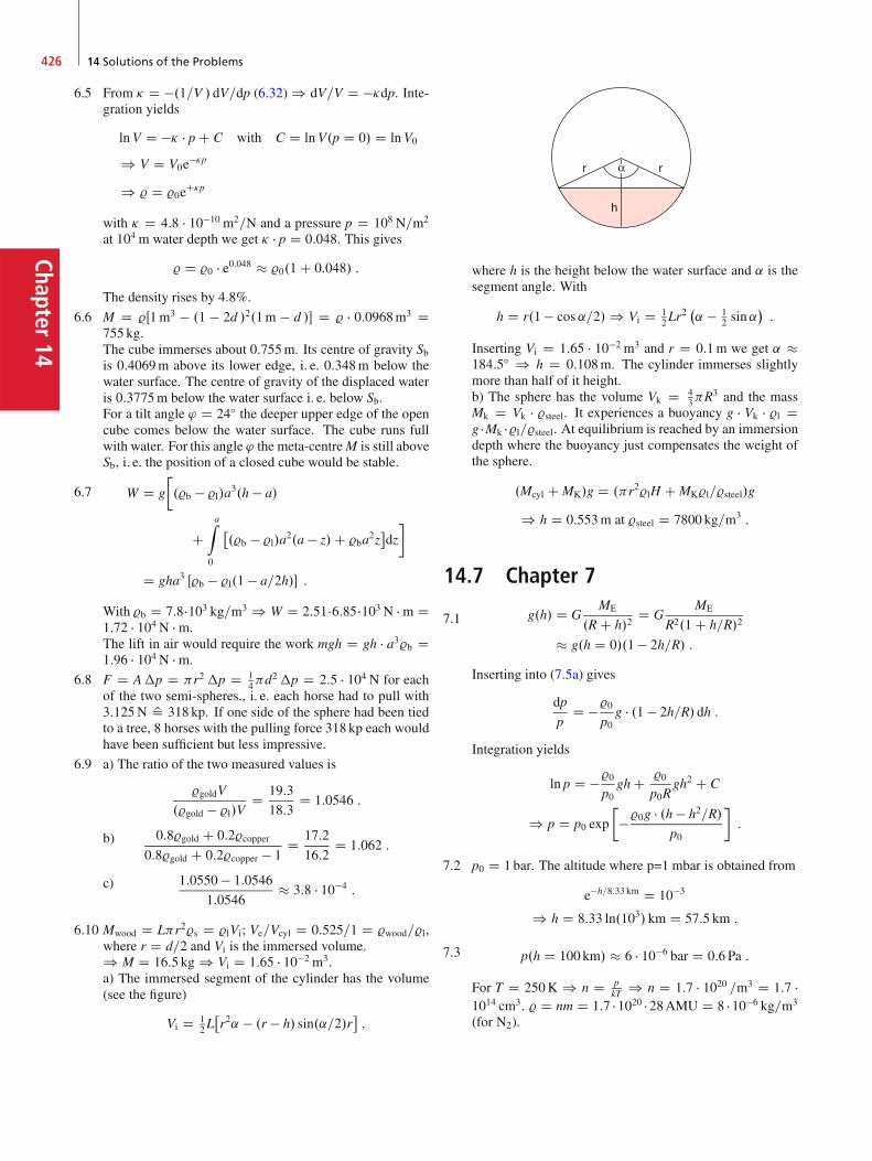
Chapter14
426 14 Solutions of the Problems
6.5 From � D �.1=V / dV=dp (6.32) ) dV=V D ��dp. Inte-gration yields
lnV D �� � p C C with C D lnV.p D 0/ D lnV0
) V D V0e��p
) % D %0eC�p
with � D 4:8 � 10�10 m2=N and a pressure p D 108 N=m2
at 104 m water depth we get � � p D 0:048. This gives
% D %0 � e0:048 � %0.1 C 0:048/ :
The density rises by 4.8%.
6.6 M D %Œ1m3 � .1 � 2d /2.1m � d /� D % � 0:0968m3 D755 kg.The cube immerses about 0:755m. Its centre of gravity Sbis 0:4069m above its lower edge, i. e. 0:348m below thewater surface. The centre of gravity of the displaced wateris 0:3775m below the water surface i. e. below Sb.For a tilt angle ' D 24ı the deeper upper edge of the opencube comes below the water surface. The cube runs fullwith water. For this angle ' the meta-centreM is still aboveSb, i. e. the position of a closed cube would be stable.
6.7 W D g
�.%b � %l/a3.h � a/
CaZ
0
�.%b � %l/a2.a � z/C %ba
2z�dz�
D gha3 Œ%b � %l.1 � a=2h/� :
With %b D 7:8�103 kg=m3 ) W D 2:51�6:85�103 N � m D1:72 � 104 N � m.The lift in air would require the work mgh D gh � a3%b D1:96 � 104 N � m.
6.8 F D A�p D r2�p D 14d
2�p D 2:5 � 104 N for eachof the two semi-spheres., i. e. each horse had to pull with3:125N ¶ 318 kp. If one side of the sphere had been tiedto a tree, 8 horses with the pulling force 318 kp each wouldhave been sufficient but less impressive.
6.9 a) The ratio of the two measured values is
%goldV
.%gold � %l/V D 19:3
18:3D 1:0546 :
b) 0:8%gold C 0:2%copper0:8%gold C 0:2%copper � 1
D 17:2
16:2D 1:062 :
c) 1:0550 � 1:0546
1:0546� 3:8 � 10�4 :
6.10 Mwood D Lr2%s D %lVi; Ve=Vcyl D 0:525=1 D %wood=%l,where r D d=2 and Vi is the immersed volume.) M D 16:5 kg ) Vi D 1:65 � 10�2 m3.a) The immersed segment of the cylinder has the volume(see the figure)
Vi D 12L�r2˛ � .r � h/ sin.˛=2/r
�;
where h is the height below the water surface and ˛ is thesegment angle. With
h D r.1 � cos˛=2/ ) Vi D 12Lr
2�˛ � 1
2 sin˛�:
Inserting Vi D 1:65 � 10�2 m3 and r D 0:1m we get ˛ �184:5ı ) h D 0:108m. The cylinder immerses slightlymore than half of it height.b) The sphere has the volume Vk D 4
3R3 and the mass
Mk D Vk � %steel. It experiences a buoyancy g � Vk � %l Dg �Mk �%l=%steel. At equilibrium is reached by an immersiondepth where the buoyancy just compensates the weight ofthe sphere.
.Mcyl C MK/g D .r2%lH C MK%l=%steel/g
) h D 0:553m at %steel D 7800 kg=m3 :
14.7 Chapter 7
7.1 g.h/ D GME
.R C h/2D G
ME
R2.1 C h=R/2
� g.h D 0/.1 � 2h=R/ :
Inserting into (7.5a) gives
dp
pD �%0
p0g � .1 � 2h=R/ dh :
Integration yields
ln p D �%0p0
gh C %0
p0Rgh2 C C
) p D p0 exp
��%0g � .h � h2=R/
p0
�:
7.2 p0 D 1 bar. The altitude where p=1 mbar is obtained from
e�h=8:33 km D 10�3
) h D 8:33 ln.103/ km D 57:5 km :
7.3 p.h D 100 km/ � 6 � 10�6 bar D 0:6 Pa :
For T D 250K ) n D pkT ) n D 1:7 � 1020 =m3 D 1:7 �
1014 cm3. % D nm D 1:7 � 1020 � 28AMU D 8 � 10�6 kg=m3
(for N2).

Chapter 7 427
Chap
ter14
7.4 The buoyancy GA D weight of the displaced air ) GA D%.h/gV D %0ge�1=8:33 � 3 � 103 m3 D 3:37 � 104 N.The mass of balloon C load C gas fill can be at most 3:44 �103 kg. The pressure of the fill gas is p.h/ D 0:887 p0 D8:87 � 104 Pa.The mass of the fill gasa) helium: %0 D 0:1785kg=m3 ) %.h/ D 0:1583 kg=m3
) mHe D 475 kg; ) mass of balloon C load can be atmost D 2965kg.b) H2: %0 D 0:09 kg=m3 ) %.h/ D 0:08 kg=m3 ) mH2 D240 kg ) mass of balloon C load should be smaller than3200 kg.
7.5 For h D 0 the pressure is p D p0 D 105 Pa and x D x0 D0:2m. According to the Boyle–Marriott law is
.p0 C %gh/Ax D p0Ax0
) h D ax0 � x
xwith a D p0
%gD 10:2m
) �h
�x� �a
x0x2< 0
) x Ds
ax0
ˇ̌ˇ̌�x
�h
ˇ̌ˇ̌ ;
with �x D 10�3 m and �h D 1m. The device is usabledown to a depth of 35m with an accuracy of ˙1m.
7.6 The number of particles that have passed at least the dis-tance x without collisions is according to (7.33)
N.x/ D N0e�x=� :
a) N.x � �/ D N0e�1 ) N.�/=N0 D 0:368 D 36:8%.b) N.x � 2�/ D N0e�2 ) N.2�/=N0 D 13:5%.
7.7 The probabilityW is
W Dv2Z
v1
f .v/ dv D 4pv3W
v2Z
v1
v2e�v2=v2Wdv
� 4v2pv3W
�ve�v2=v2W ;
with v D .v1 C v2/=2 D 950m=s and �v D .v1 �v2/ D 100m=s. For N2-molecules at T D 300K isvW D 422m=s.
) W D 4 � 9502 � 100p � 4223 � e�5:06 D 1:7 � 10�2 :
7.8 From (7.6) we obtain
lnp1p2
D %1
p1g�h :
The density is obtained from %1 D m � p1=.kT/ with m D0:71mN2 C 0:29mO2 as %1 D 1:24 kg=m3
) �h D 866m :
7.9 �v D v1 � v2 ) .�v/2 D v21 C v22 � 2v1v2 cos˛.a) Since the direction s of the velocity vectors are uni-
formly distributed the average values v21 D v22 D v2 andcos˛ D 0:
.�v/2 D 2v2 )q.�v/2 D p
2pv2 ;
�v D j�vj
Dq.vx1 � vx2/2 C .vy1 � vy2/2 C .vz1 C vz2/2
D �v2x1 C v2x2 C v2y1 C v2y2 C v2z1 C v2z2
� 2.vx1vx2 C vy1vy2 C vz1vz2/�1=2 I
with v2x D v2y D v2z D 13v
2 and vx D vy D vz D 0
) �v2 D 6 � 13v
2 D 2 � v2 :b) Here all absolute values v of the velocity v have thesame value ) �v D p
2v.
7.10 The molecular density at p D 105 Pa and T D 20 ıC isn D 2:5 � 1019=cm3
) �Ar D 1
n�D 10�25 � 107
2:5 � 1:5D 2:6 � 10�19 m2 D 26Å2 :
If both collision partners are moving, the mean time be-tween two collisions is � D �=�v where �v is the meanrelative velocity. We have the following numerical values:
�N2 D 31 � 10�16 cm2 ;
�vAr D p2v D 565m=s
) �Ar D �=�v D 2:6 � 10�10 s ;
�N2 D 1:8 � 10�10 s :
7.11 The density is (as in 7.10) n D 2:5 � 1019=cm3.
a) N D M
mHeD 0:1
6:68 � 10�27D 1:5 � 1025, where N is the
total number of the He-atoms in the container.b) �He�He D 10 � 10�16 cm2
) � D 1
n�D 4 � 10�7 m :
c) The sumP
i Si is:
X
i
Si DX
i
Nivi�t D Nv�t
D 1:5 � 1025 � 1260m for �t D 1 s
D 6:3 � 1019 light secondsD 2 � 1012 light years :
Chapter14
428 14 Solutions of the Problems
7.12 Assume, two atoms with velocities v1 and v2 pass the discat t D 0. Their arrival times at the detector are
t1 D L
v1I t2 D L
v2) �t D L
�v
v1v2
with �v D v1 � v2.If one atom passes the disc at the beginning of the openingtime �t0, the other atom at the end, the time differencebetween the arrival times at the detector is
�tmax D �t C�t0 :
The time spectrum N.t/ of the arriving atoms with the ve-locity distribution N.v/ D N � f .v/ can be obtained asfollows: With v D L=t and dv D �.L=t2/dt D .v=t/dtwe get the distribution function
f .v/ dv D 1
tvf
�L
t
�dt :
The function f .v/ / v2e�v2=v2W (see (7.30)) is then con-verted to
f .v; t/ / L3
t4e�L2=t2v2Wdt :
If the time profile of the velocity selector is g.t/ the timedependence of the detector signal is
S.t/ DC1Z
�1g.t0/ f .t � t0/ dt0 :
If the opening time�t0 of the selector were infinitely short(�t0 ! 0), the difference �t of the arrival times of theatoms at the detector (because of their different velocities)would be
�t D t2
L�v D L
v2W�v D 1
6002D 1:6ms :
Taking into account the finite opening time, the convolu-tion S.t/ gives a time profile with a half width �t which isfor a rectangular opening time profile g.t/with�t0 D 1msapproximately �t � 2:5ms.
7.13m
2v20 > G
MEm
R C h) v0 >
r2GME
R C h
) v0.h/ D v0.h D 0/
s1
1 C h=R
� v0.0/
�1 � 1
2h=R
�:
For h D 100 km, ) v0.h/ D 0:992v0.0/ D 11:1 km=s.a) If half of all molecules within the Maxwell distributionhas a velocity v > v
) v > v Dr
8kT
mD 11:1 km=s
) T D 1:6 � 105 K :
7.14 The density of the outside air in a height of 50m at T D300K is
% D %0e�%0gh=p0 ;
with %0 D 1:29 kg=m3, p0 D 105 N=m2 ) % D1:28 kg=m3.The exhaust gases must have a temperature T > T0.Because the pressure at the upper end of the smokestack isat the same temperature the same for the exhaust gases andthe outside air it follows
) %1=%2 D T2=T1 ) T2 D 452K :
For the outside air is p1 D p0e�%1gh=p0 and for the exhaustgases inside of the smokestack p2 D p0
0 � e�%2gh=p00 . With
p00 D p2.h D 0/ and p1.h/ D p2.h/ we obtain with the
approximation ex � 1 C x
p00 � %2gh D p0 � %1gh
) �p0 D p0 � p00 D �%gh
D .1:28 � 0:85/ � 9:81 � 50Pa D 211Pa :
7.15 %0.He/ D 0:178 kg=m3 at p0 D 1 bar.
) %He.1:5 bar/ D 0:267 kg=m3.
From mHe C mBal D V%Air )
V D mBal
%Air � %He.1:5 bar/
D 0:01
1:023m3 D 9:8 � 10�3 m3 :
7.16 a) 12m � hv2i D 3
2kT D 3:1 � 10�16 J ¶ 1:9 � 103 eV.The ionization energy of the H-atom is 13:5 eV. At a den-sity of 5 � 1029 =m3 the mean distance between the protonsis 1:25 � 10�10 m. The mean potential energy, due to theCoulomb repulsion, is Ep � 1:8 � 10�18 J which is smallcompared to the mean kinetic energy at a temperature of15 million Kelvin. This means that the matter in the cen-tral part of the sun can be safely regarded as ideal gas.
b) v Dr
8kT
mvp D 5:6 � 105 m=s;
vel D 2:4 � 107 m=s D 0:08 c.
c) p D nkT D 1 � 1014 Pa ¶ 109 atm.
7.17 MAtm D 4R2 � 1:013 � 105 N9:81m=s2
D 5:3 � 1018 kg.The comparison with the earth massME D 6�1024 kg showsthat MAtm � 10�6ME.
7.18 MB C %He � V D %Air � V) V D MB
%Air � %He :
a) h D 0, T D 300K ) pAir D 1 bar, pHe D 1:1 bar )%Air D 1:23 kg=m3, %He.p D 1:1 bar/ D 0:196 kg=m3
) V D 300 kg
.1:23 � 0:196/kg=m3D 290m3 :

Chapter 8 429
Chap
ter14
b) h D 20 km, T D 217K, p D 5:5 � 10�2 bar
) %Air D 0:9 kg=m3 ; %He.p D 0:055 bar/
D 0:042 kg=m3
) V D 300
0:09 � 0:042m3 D 6250m3 :
The balloon has to expand considerably. On the ground ithas only 5% of its maximum volume.
7.19 a) If the pressure at the upper end of the atmosphere (whichis here assumed to have a sharp edge) should be p1 D10 bar, the pressure at the bottom must be p0 D 11 bar.We assume as mean pressure
) %Air.p D 10:5 bar ;T D 300K/
D 1:23 � 10:5 kg=m3 D 12:9 kg=m3 ;
) % � g � h D 105 Pa
) h D 105
12:9 � 9:81m D 7:9 � 102 m ;
b) The density of solid air at T D 0K is % D 103 kg=m3.) h D 10m.
14.8 Chapter 8
8.1 a) The force acting on the area A is according to (8.41b)
Fw D cw%
2u2 � A :
Numerical values: A D 100m2, %L D 1:225 kg=m3, u D100 km=h D 27:8m=s.) F D 5:67 � 104 N. This corresponds to a weight of5.8 tons.b) For a simple estimation we assume that the streamlinesof the wind above the roof are following the roof profile.The air above the roof then passes through a path lengthS2 D 2 � 6m D 12m. In the same time the horizontalwind flow passes only a distance S1 D 2 � 6m � sin.˛=2/ D11:6m. The velocity is then u2 D 100 km=h � 12=11:6 D103:4 km=h D 28:7m=s. From the Bernoulli equation
p D p0 � 12% � u22 :
we can determine the pressure difference �p D p � p0.With p0 (pressure below the roof) D 105 N=m2 and 1
2%u22 D
531N=m2 the pressure p becomes p D .105 � 531/N=m2
and the difference 531N=m2. The force is F D A � �p.With A D 2Ly �6m � sin.˛=2/ D 96:7m2 effective roof area(projection onto a horizontal plane) we get
F D 531 � 96:7N D 5:1 � 104 N :
8.2 The buoyancy depends not only on the wing profile but alsoon the stalling angle (Fig. 8.43). When a plane flies upsidedown the buoyancy is much smaller but can be still largerthan zero if the stalling angle is correctly chosen.
8.3 The mean free path length � D 1=.n � �/ in liquids withtypical densities n D 3 � 1028 =m3 and � D 10�19 m2 )� D 3 � 10�10 m. The boundary layer where moleculesdiffuse from neighbouring layers is therefore very thin.The appearance of curls at large velocities is not caused bydiffusion but by macroscopic turbulence (Convection).
8.4 The following relations apply:
grad .a � b/ D .b � r / a C .a � r / b C a .r b/
C b .r a/
) grad .u � u/ D grad u2
D 2 � .u � r/ u C 2 � u .r u/ :
The last equation can be verified in component representa-tion. For the x-component the left hand side can be writtenas:
@
@x
�u2x C u2y C u2z
�
D 2ux@ux@x
C 2uy@uy@x
C 2uz@uz@x
:
(14.5)
For the components on the right hand side is
2
�ux@
@xC uy
@
@yC uz
@
@z
�ux
C 2�uy.curlu/z � uz.curlu/y
�:
(14.6)
The second bracket Œ � in Eq. 14.6 is in the component rep-resentation
uy
�@
@xuy � @
@yux
�� uz
�@
@zux � @
@xuz
�:
Inserting this into (14.5) the right hand side gives the sameexpression as the left hand side.Analogous results are obtained for the y- and z-component.
8.5 The pressure at the height h is
p.h/ D % � g � .H � h/C p0 :
At the exit of the pipe the Bernoulli equation yields
�p D p.h/� p0 D 12%u
2x
u2x D 2g.H � h/ :
The trajectory of the liquid stream is a parabola. The initialvelocity is
v D fux; uy D 0; uz D 0g :
The drop time can be obtained from h D .1=2/gt2 ) t Dp2h=g.
Chapter14
430 14 Solutions of the Problems
a) The point of impinge is
P D fxi D ux � t I y D z D 0g Dn2ph.H � h/; 0; 0
o:
The velocity at P is
v.P/ D fux; uz D gtgjvj D
qu2x C u2z D p
2gH :
This is the same velocity as for body falling vertically fromthe height H.b) According to the Hagen–Poiseuille Law is:
�dV
dtD �R2 dH
dtD r4
8�L�p
with �p D %gH C p0 � p0
) dH
dtD � r4
R2
%gH
8�L) H D H0e
�at
with H0 D H.t D 0/ and a D r4%g
8R2L � � .8.6 The probe in Fig. 8.10c measures the total pressure
p0 D p C 12%u
2 D %gh
D 103 � 9:81 � 1:5 � 10�1 Pa D 1470Pa :
The results of the measurements in Fig. 8.10a give p D10mbar D 103 Pa) 0:5%u2 D 470Pa ) u D 0:97m=s.
8.7 If the funnel is filled up to the height H the radius R of thewater surface is R D H � tan.˛=2/. The volume of the wateris then
V D 13R
2H D 13H
3 tan2.˛=2/ D 19H
3 ;
because tan2 30ı D 1=3.a) The reduction of the water volume per time unit is
dV
dtD dV
dH
dH
dtD 1
3H2 dH
dt:
On the other side the Hagen–Poiseuille Law demands
dV
dtD �r
4
8�L�p
with r D d=2 and �p D %gH
) dH
dtD �3
8
r4%g
�LH) H dH D �a dt
with a D 38
r4%g�L � 7:2 � 10�4 m2s2.
Integration gives:
H2 D �2at C H20
with H0 D H.t D 0/
) H DqH2
0 � 2at :
b) dM
dtD %
dV
dtD �1
3aH%
D �1
3a%
qH2
0 � 2at
) M.t/ D 19%
�H2
0 � 2at�3=2
:
c) The time when all of the water has streamed out of thefunnel (i. e. H.t/ D 0) is
T D H20=2a :
With H0 D 0:3m, r D 2:5 � 10�3 m, L D 0:2m, � D1:0 � 10�3 Pa s ) T D 62:5 s.d) With 4 litre water ) H0 D .9V=/1=3 D 0:225m.The time to fill the container with V D 4 l completely iswith a D 7:2 � 10�4 T D 35 s. If the outflowing water inthe funnel is continuously substituted by pouring water intothe funnel in order to keep the water level always constantat H D H0, the time to fill the 4 l container is obtained by:
V D 1
3aH0 � t
) t D 3 � 4 � 10�3
� 7:2 � 10�4 � 0:225 s D 23:6 s :
8.8 dV
dtD R4
8�L�p with �p D %g.�h C L sin˛/
D 1:5 � 10�4.0:1 C sin˛/m3=s:
The mean flow velocity is
u D 1
A
dV
dtD 1
r2dV
dtD 7:6.0:1 C sin˛/m=s :
The Reynold’s number is
Re D 2300 D %ruc�
:
This gives the critical velocity
uc D �Re
%rD 0:92m=s :
The inclination angle ˛ is then for u D uc
sin˛ D 0:021 ) ˛ D 1:2ı :
8.9 dV
dtD R4
8�L%g�h D 10�3 m3I �h D 20m
) R D�10�3 � 8�L%g ��h
�1=4
D 6 � 10�3 m D 6mm
) d D 1:2 cm
) u D 8:8m=s :

14.9 Chapter 9 431
Chap
ter14
This is already above the critical velocity, which means thatd has to be larger because the flow resistance is for u > uclarger than obtained from the Hagen–Poiseuille law.
8.10 The total force acting on the ball is
F D am D m�g � 6�rv with m� D .%K � %l/43r3
) dv
dtD m�
mg � 6�rv
m:
Rearrangement, division by m� and multiplication by myields
dv
g � .6�rv=m�/D m�
mdt ;
with the abbreviations
b D 6�r
gm� and c D gm�
m
) dv
1 � bvD c dt :
Integration gives
�1
bln.1 � bv/ D ct C C1
) v D 1
b
�1 � e�bC1e�bct
�:
Since v.0/ D v0 ) e�bC1 D 1 � v0b
) v.t/ D 1
b
�1 C .v0b � 1/e�bct
�
) z.t/ D 1
bt � v0b � 1
b2ce�bct :
8.11 Division of (8.36a)by % and applying the differential oper-ator rot D r onto both sides yields
@
@trotu C r .u � r/u
D �1
%r .rp/� r g C �
%r div gradu :
Nowwe use the relationsrrp D 0 andrr�.ru/ D 0.If the influence of gravity can be neglected () g D 0) weobtain with ˝ D rotu the relation
.u � r/u D 12grad u
2 � u rotu
D 12ru2 C .˝ u/ :
Vector multiplication with r gives with r r D 0
r .u � r/u D r .˝ u/ :
Then (8.36a) converts to
@˝
@tC r .˝ u/ D 0 :
14.9 Chapter 9
9.1 Through the capillary flows per second the air mass % �dV=dt / p � dV=dt. At the high pressure side this is p1 �dV1=dt and at the low pressure side p2 � dV2=dt. It is
p1dV1
dtD p2
dV2
dt:
The pumped-out volume is V2. According to Hagen–Poiseuille we get
p2dV
dtD R4
8�L.p1 � p2/
p1 C p22
with p1 D 105 Pa, p2 D 10�1 Pa
) p2dV
dtD 4:25 � 10�3 m3 Pa=s :
In order to maintain a pressure of 10�3 hPa D 10�1 Pa thethroughput of the vacuum pump must be at least dV=dt D4:25 � 10�2 m3=s D 42:5 l=s.
9.2 The force acting on each hemisphere is
F D ��d
2
�2
�p D 2:5 � 104 N :
One has to pull on each hemisphere with this force in orderto separate the two hemispheres.
9.3 For p D 10�5 hPa is n D 2:5 � 1017 =m3.
� D 6m ; � D �
v� 1:2 � 10�2 s for v D 500m=s
Z1 D n � � � vrel � n�p2 � v with � D 10�14 cm2
The number Z1 of collisions between the molecules is
Z1 � 180 s�1 :
The number Z2 of collisions per sec with the wall is
Z2 D 14nv � 3 � 1019 m�2s�1 :
Onto the whole container wall with A D 3:26m2 impinge9:8 � 1019 molecules per second ) Z1=Z2 D 1:8 � 10�18;P
si D n � V ��=� D n � V � v D 5 � 1019 m=s.9.4 The number of collisions per second and per m2 with the
wall is Z2 D 14n � v. At a pressure p D 10�7 hPa ) n D
2:5 � 1015 m�3. With v D 500m=s ) Z2 D 3 � 1017m�2 s�1.A complete monolayer on the wall is achieved for Z colli-sions, where
Z D 1m2
(surface area per molecule)
D 1
0:15 � 0:2 � 10�18D 3:3 � 1019 :
Since the number of wall colissions per sec and m2 isZ2 D 3 � 1017, it follows that after about 100 s the wall iscompletely covered by a monolayer.

Chapter14
432 14 Solutions of the Problems
9.5 The suction capacity dV=dt of a mechanical pump at thepressure p1 D 0:1 hPa must be equal to the suction capacityof the diffusion pump at the pressure p2 D 10�6 hPa.
p2 � 3000 l=s D p1.dV=dt/mech. pump
) dV
dtD p2
p1� 3000 l=s D 3 � 10�2 l=s D 0:1m3=h :
It is, however, advisable to use a larger mechanical pump.Because the diffusion pump reaches its full suction capac-ity already at a pressure of 10�4 hPa, where the mechanicalpump needs a suction capacity of dV=dt D 10�3 �3000 l=s D10m3=h in order to prevent the rise of the pressure p1 above10�1 hPa.
9.6 When passing through the gas the intensity of the electronbeam decreases according to I D I0e�n�� �x. The numberof produced ions is then equal to the difference .I0 � I/=q,where q D �e D �1:6 � 10�19 C is the electron charge. Forn � � � x 1 we obtain
I0 � I
eD I0
en�x
D 10�2
1:6 � 10�19� 2:5 � 1015 � 10�18 � 2 � 10�2 s�1
D 3 � 1012 ions=s :
The ion current is then 0:5 µA.
9.7 The mean free path length � at a pressure p D 10�2 hPa is� D 6 � 10�3 m (see Tab. 9.1) and therefore comparable tothe distance d D 1 cm between the hot wire and he wall.This case is between the limiting cases � � d and � d.For� � d we get from (7.49)
dW
dtD �F�T D 52mW :
For � D n1 � v .f =2/k D 4:4Nm�1 K�1 F D 2r1 � l D7:8 � 10�5 m2 und �T D 150K.For� d we obtain
dW
dtD � � F dt
dxD 60mW :
If we choose for� � d the average of the two values we get
dW
dt� 56mW :
The electric power input is
Pe D U � I D 1W :
Only 5.6% of the input power are transported by heat con-duction through the gas. The major part (94.4%) are lost dueto heat radiation and heat conduction through the mountings.
9.8 We assume that every molecule that hits the wall sticks therefor some time and then evaporates again. For a ball at rest
with a temperature equal to that of the gas the velocity dis-tribution of the evaporating molecules is equal to that ofthe impinging molecules. Therefore there is no net angularmomentum transfer. This is different for the rotating ball.Molecules that impinge onto a strip around the latitude #get the rotational velocity
u D ! � r � sin# ;while resting on the rotating sphere. We choose the z-axisinto the direction of the rotational axis. The velocity perpen-dicular to the rotational axis is for the impinging moleculesv? D .v2x C v2y /
1=2 and the evaporating molecules have thevelocity v0
? D .v2x C v2y C u2/1=2.The number of molecules impinging per sec onto the surfaceelement dA D 2r2 sin# d# (the grey strip in the Figure) isaccording to (7.47)
dN
dtD n
4v dA :
Each evaporating molecule wins the additional momentumm � u in tangential direction. The total number impinging ondA gets the additional momentum per sec
�p.#/ D n
4vmu dA
D n
4vm!r sin# � 2r2 sin# d# :
The torque transferred to the ball by these molecules is thenwith F D dp=dt
dD.#/ D n
2vm!r4 sin3 #d# :
Integration over all # gives with
C=2Z
�=2sin3 # d# D 4
3;
the torque
D D 23mv!nr
4
D 12Vspheremv!nr with V D M=%
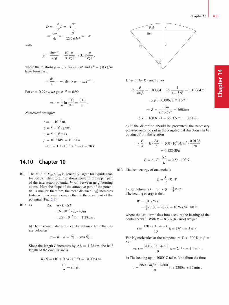
Chapter 10 433
Chap
ter14
D D � d
dtL D �I
d!
dt
) d!
dtD � D
.2=5/Mr2D �a!
with
a D 5nmv
4r%D 10
p
r%v� 3:18
p
r%v;
where the relations p D .1=3/n � m � v2 and v2 D .3kT/=mhave been used.
) d!
!D �a dt ) ! D !0e
�at :
For ! D 0:99!0 we get e�at D 0:99
) t D 1
aln
100
99D 0:01
a:
Numerical example:
r D 1 � 10�3 m;
% D 5 � 103 kg=m3;
v D 5 � 102 m=s;p D 10�3 hPa D 10�1 Pa
) a D 1:3 � 10�4 s�1 ) t D 78 s:
14.10 Chapter 10
10.1 The ratio of Ekin=Epot is generally larger for liquids thanfor solids. Therefore, the atoms move in the upper partof the interaction potential V.rik/ between neighbouringatoms. Here the slope of the attractive part of the poten-tial is smaller, therefore, the mean distance hriki increasesfaster with increasing energy than in the lower part of thepotential (Fig. 6.1).
10.2 a) �L D ˛ � L ��T
D 16 � 10�6 � 20 � 40mD 1:28 � 10�2 m D 1:28 cm :
b) The maximum distortion can be obtained from the fig-ure below as
x D R � d D R.1 � cosˇ/ :
Since the length L increases by �L D 1:28 cm, the halflength of the circular arc is
R � ˇ D .10 C 0:64 � 10�2/ D 10:0064m
10
RD sinˇ :
Division by R � sinˇ gives
) ˇ
sinˇD 1:00064 ) 1
1 � 16ˇ
2D 10:0064m
) ˇ D 0:00623 ¶ 3:57ı
) R D 10m
sin 3:57ı D 160:6m
) x D 160:6 � .1 � cos 3:57ı/ D 0:31m :
c) If the distortion should be prevented, the necessarypressure onto the rail in the longitudinal direction can beobtained from the relation
) F
AD E � �L
LD 200 � 109 N=m2 � 0:0128
20D 0:128GPa
F D A � E � �L
LD 2:56 � 106 N :
10.3 The heat energy of one mole is
Q D f
2� R � T :
a) For helium is f D 3 ) Q D 32R � T
The heating energy is then
W D 10 � tWs
D 32R.100 � 20/K C 10Ws=K � 80K ;
where the last term takes into account the heating of thecontainer wall. With R D 8:3 J=.K � mol/ we get
t D 120 � 8:31 C 800
10s D 180 s D 3min :
For N2-molecules at the temperature T > 300K is f D5=2.
) t D 200 � 8:31 C 800
10s D 246 s D 4:1min :
b) The heating up to 1000 ıC takes for helium the time
t D 980 � 3R=2 C 9800
10s � 2200 s � 37min I

Chapter14
434 14 Solutions of the Problems
for N2 is f in the range from 20–500 ıC f D 5; for T >500 ıC is f D 7=2.
dQ D U.T2/ � U.T1/ D R. 72T2 � 52T1/
D 2:89 � 104 J
) t D dQ
10s D 2:89 � 103 s D 48min :
10.4 If T is lower than the temperature TS of the surroundingthe temperature T will be approach TS by heat conduction.After the mixing the temperature Tm is above TS. Theheat losses are proportional to the temperature difference(T � TS). Therefore the temperature decline
dT=dt D �a � .T � TS/ :
The time-dependence of T.t/ after the mixture at t D t1 isthen
dT
T � TSD �a.t � t1/ ) T � TS D C e�a.t�t1/ :
If the mixing process occurs in a very short time at t D t1it is T.t D t1/ D Tm ) C D Tm � TS ) T.t/ DTS C .Tm � TS/ � e�a�.t�t1/.If the real measured temperature curve T.t/ is replacedby the dashed curve in Fig. 10.12b in such a way, that theareas A1 and A2 are equal, the true mixing temperature isobtained. The dashed curve represents the ideal case of aninfinitesimal short mixing process, where the heat lossesare zero during the mixing process.
10.5 1 Mole air (N2/O2-mixture) has a mass of about 29 g andcontains 6 � 1023 molecules. For the lift of the containerby 10 cm in the gravity field of the earth the energy
E D m � g � h D 0:129 kg � 9:81m=s2 � 0:1mD 0:13N � m
is required.The thermal energy of the gas at room temperature is
Egasth D .5=2/R � T D 6:2 � 103 N � m ;
and that of the container with the specific heat c is
Econtth D mC � c � T D 0:1 � 103 � 300
D 3 � 104 N � m) Etot D 3:6 � 104 N � m :
The energy additionally required for the lift is thereforevery small compared to the thermal energy. And thecooling after the lift would be only�T D 1�10�3 K. Nev-ertheless this lift is extremely improbable, not because ofenergetic reasons but because of statistical reasons:For the lift the z-component of the momentum must be atleast pz D m �v0z D m � p2gh ) pz > 0:18 kg � m=s. Themean velocity component hvzi of all molecules, which is
hvzi D 0 at thermal equilibrium, must be hvzi > v0 Dpz=mgas D 6:2m=s. The probability that a molecule has avelocity component vz > v0 is given by the integral
W.vz > v0/ D1Z
v0
e�v2z m=2kTdvz. C1Z
�1e�v2z m=2kTdvz :
With x2 D 12m � v2z =kT and x.v0/ 1 )
1Z
x0
D �x0Z
0
C1Z
0
with
x0Z
0
e�x2dx �x0Z
0
.1 � x2/dx D x0 � x303:
This gives with v0 D 6:2m=s ) W.vz > v0/ D 0:49.The probability that all 6 �1023 molecules have at the sametime the velocity component vz > v0 is then
W D 0:49�6�1023 < 10�10�23;
and therefore practically zero.
10.6 a) The entropy change�S for an isobaric temperature risefrom T0 D 273K to T1 D 500K is
�Sisobaric D �
�CV ln
T1T0
C R lnV1
V0
�;
where � D 1=22:4 is the mole fraction.With V1=V0 D T1=T0 for p D const and Cp D RCCV weobtain
�Sisobaric D �Cp ln.T1=T0/
with Cp D 21 J=.K � mol/
) �Sisobaric D 21
22:4ln
500
273D 0:57 J=K :
b) isochoric heating:
�Sisochoric D �CV lnT1T0
with CV D 12:7 J=.K � mol/
) �Sisochoric D 0:34 J=K :
10.7 WithM D % � V the critical mole volume is
Vc D 0:044 kg
%cD 0:044
46
D 9:56 � 10�4 m3 D 0:956 l :
The mole volume is compressed from 22:4 l at standardconditions of an ideal gas to 0:956 l.
Chapter 10 435
Chap
ter14
From the general gas equation of an ideal gas it follows:
Vc D RTcpc
D 0:33 � 10�3 m3 :
This shows that eigen-volume and internal pressure of areal gas around the critical point cause considerable devi-ations from the ideal gas. From Eq. 10.129 we obtain thevan-der-Waals constants
b D 1
3Vc ) b D 0:32 � 10�3 m3 ;
a D 3pcV2c ) a D 20:8N � m4 :
Under standard conditions (p D 1 bar, T D 273K) theinternal pressure is for 1 mole
a
V2D 4:1 � 104 N=m2
¶ 41% of normal pressure!
The eigen-volume of CO2 molecules is b=4 D 8 �10�5 m3
and the relative correction b=V D 0:32�10�3
22:4�10�3 D 1:4%.
10.8 �S1 D mcv ln323:15
273:15J=K
D 4:18 � 103 ln 1:183 J=KD 689 J=K I
�S2 D mcv lnT2m
T1T2
D 0:5 � 4:18 � 103 � ln 323:152
273:15 � 373:15D 49:62 J=K :
10.9 The theoretically possible maximum efficiency for T1 D600 ıC and T2 D 100 ıC is
� D T1 � T2T1
D 500K
873KD 0:57 :
The heat delivered at 100 ıC amounts therefore to 43%of the heat reveived at 600 ıC. When using the techniqueof “cogeneration of heat and mechanical power” the heatdelivered at 100 ıC can be partly used for heating of build-ings. The efficiency increase for cooling down to 30 ıC is
" D 100 � 30
373D 18:8% :
However, this saves only part of this efficiency increase,because when the additional heat energy available bycooling from 100 ıC down to 30 ıC can be used for driv-ing a gas-turbine connected to an electric generator, thiscan deliver additional electric power. The theoretical effi-ciency of the power station increases then from � D 57%to � D 570=873 D 0:65 D 65%. In order to prevent thewater vapour to condensate at temperatures below 100 ıCone has to decrease the pressure in the expansion cham-ber. This demands additions energy for the expansionagainst the external pressure.
10.10 a) m1c1.T1 � Tm/ D m2c2.Tm � T2/
) Tm D m1c1T1 C m2c2T2m1c1 C m2c2
:
Numerical values:
m1 D 1 kg; c1 D 470 J=.kg � K/;m2 D 10 kg; c2 D 4:17 � 103 J=.kg � K/
) Tm D 23:2 ıC ¶ 296:34K :
b)�S1 D Cmc ln
TmT1
D 1 � 470 ln 296:34
573:15D �310 J=K
�S2 D 10 � 4:1 � 103 ln 296:34
293:15D C445 J=K
�S D �S1 C�S2 D C135 J=K :
10.11 a) A massM D 2 �5 kg D 10 kg exerts a pressure onto thearea 0:1m � 10�3 m D 10�4 m2
p D 98
10�4N=m2 D 9:8 � 105 Pa :
Since the increase of the melting temperature Tm underthe pressure p at T D �8 ıC is given by dTm=dp D10�7 ıC =Pa the resulting temperature increase is dTm D10�7 � 9:8 � 105 ıC D 0:1 ıC. Ice at T D �8 ıC therforecannot melt solely due to the pressure.b) The heat conduction is, according to (10.35)
dQ
dtD � � A � dT
dx:
With A D r2 D � 0:25 � 10�6 m2 D 7:8 � 10�7 m2,dx D 5 cm D 0:05m, dT D 35 ıC D 35K and � D67W=m�1 � K�1, for steel we get
dQ=dt D 0:037W :
This heat energy flows into the horizontal part of the wireand in the surrounding volume of the ice. Since the sur-face 2rL of the wire with radius r and length L is largecompared to its volume, we can assume that nearly all ofthe heat energy flows into the ice. If the wire should meltthe ice, it has to increase the temperature up to Tm and inaddition it has to supply the heat of fusion. The energybalance requires:
dQ
dtD .cIce ��T C Wm/% � dV
dt:
This gives the velocity with which the wire melts throughthe ice block:
dz
dtD 1
L � d � % � dQ=dt
c ��T C Wm:
Chapter14
436 14 Solutions of the Problems
Inserting the numerical values gives: c D 2:1 kJ=.kg � K/,% D 0:9 � 103 kg=m3, L D 0:1m, d D 10�3 m, Wm D333 kJ=kg, �T D 8K.This finally yields the result:
dz
dtD 10�6 m=s :
The observed velocity is higher by one order of magni-tude. The reason for this is the heat, transferred directlyfrom the warm wire at the edges of the horizontal part intothe ice. This increases dQ=dt considerably.
10.12 During the compression of V1 to V2 < V1 the work sup-plied to the system is
dW1 DV2Z
V1
p dV :
With dS D dQ=T D 0 ) dQ D 0 )p � V� D const D C1 )
dW1 D �V2Z
V1
C1
V�dV D C1
� � 1
�1
V��12
� 1
V��11
�
D C1
.� � 1/ � V��12
�1 � 1
.V1=V2/��1
�:
During the transition 3 ! 4 the system delivers the work
dW2 D C2
� � 1
�1
V��11
� 1
V��12
�:
The gain of energy during one cycle is then
�W D C1 � C2
.� � 1/V��12
�1 � 1
.V1=V2/��1
�:
For the isochoric processes 2 ! 3 and 4 ! 1 is�W D 0.The heat energy supplied to the ssterm is for 1 mole
Q1 D CV.T.3/� T.1// :
For isentropic processes is dQ D 0, T � V��1 D const DC1 for the point 2 and C2 for the point 3.With � D Cp=CV ) .� � 1/ � CV D Cp � CV D R. Theefficiency then becomes
� D �W
Q1D 1 � 1
.V1=V2/��1:
Example: V1 D 10V2, � D 1:4 ) � D 0:6.Note that � does not depend on the temperature but onlyon the compression ration V1=V2.
10.13 We treat at first the stationary case with �T D 0
) T D T0 C .T1 � T0/e�˛1x
) @2T
@x2D ˛21.T1 � T0/e
�˛1x :(14.7)
The stationary heat conduction equation (10.38a) giveswith @T=@=t D 0
�
% � c@2T
@x2D h� � .T � T0/ :
Inserting of (14.7) yields
@2T
@x2D %ch�
�.T1 � T0/e
�˛1x
) ˛21 D %ch�
�) ˛1 D
r%ch�
�Dr% � hm � � :
For �T ¤ 0 ) T D T0 C .T1 � T0/e�˛1x C�Te�˛2x cos.!t � kx/,
@T
@tD ��T � e�˛2x � ! sin.!t � kx/ ;
@2T
@x2D ˛21.T1 � T0/e
�˛1x C .˛22 � k2/�Te�˛2x
� cos.!t � kx/ � 2˛2�Te�˛2x � k � sin.!t � kx/ :
Inserting into (10.38a) gives the stated relations by com-paring the coefficients of sin and cos.
14.11 Chapter 11
11.1 F D D � x. With F D 1N and x D 0:05m ) D D20N=m. ) T D 2
pm=D D 1:4 s.
11.2 a) Approximation m M D � L.Velocity of the transverse wave
vPh DpF= D
pmg= :
Running time of the wave over the distance z:
t1 D z
vPhD z
p=mg :
Falling time of the ball:
t2 Dp2z=g :
For t1 D t2 the ball overtakes the wave pulse.
) z D 2m= ;
) withM D � L this gives
z D 2m
ML :
This shows, that for m > M ) z > L the ball cannotovertake the wave.b) More accurate calculation for an arbitrary ratio m=M:For the distance z below the suspension point z D 0 theforce
F D .L � z/g C mg
Chapter 11 437
Chap
ter14
acts on the rope due to the weight of rope C mass m. Thephase velocity of the wave is
vPh.z/ D Œ.L � z C m=/g�1=2 :
It decreases with increasing z (due to the decreasingweight force) according to
dv
dzD � g
2v.z/:
Withdv
dtD dv
dz� dzdt
D � g
2vv D �g
2) v.t/ D v.z D 0/� 1
2gt :
The distance z that the wave propagates during the time tis then
z1.t/ D v0t � 14gt
2 :
The ball falls in this time the distance z2.t/ D 12gt
2.The meeting point is t at z1 D z2
) v0t1 � 1
4gt21 D 1
2gt21
) t1 D 4
3v0=g D 4
3
sL C m
g:
This gives the meeting point
zm D 1
2gt21 D 8
9
�L C m
�D 8
9L
�1 C m
M
�:
11.3 According to (11.36) the power supplied to the oscillatingsystem is
P D m � �!2A22
D�F20=m
� � � � !2
�!20 � !2
�2 C .2�!/2:
It is proportional to the square of the imaginary part bin equation (11.27c), because only the friction consumesenergy. The real part a in (11.27b) determines the phaseshift ', because tan' D b=a, but does not consume en-ergy. For b D 0 and ! ¤ !0 is ' D 0.For b D 0 and ! D !0 no stationary oscillation is pos-sible. The amplitude A of the forced oscillation increasesuntil A D 1 (resonance catastrophe). In this case energyis supplied by the exciter which increases the amplitudeuntil the oscillating system is destroyed.
11.4 The pressure at equilibrium is p D 4"=r with " D � .Changing the radius r changes the pressure by
dp D dp
drdr D �4"
r2dr :
Therefore the restoring force is
dF D 4r2 dp D �16" dr ) F D �16"r:
With the restoring constant D D 16" the oscillation pe-riod becomes
T D 2pm=D D 1
2
pm=" D r
p%d=ep
with the mass m D 4r2 � % � d and the thickness d of theskin of the soap bubble.(The small change of the air pressure inside the bubbledue to the small change of the volume is negligible).
11.5 The phase velocity is
vPh DpE=% D 5:2 � 103 m=s :
The wavelength is
� D vPh=� D 0:52m :
The maximum change of the length appears betweenmaxima and minima of the longitudinal wave. Thereforewe obtain
.�L=L/max D 2A=.�=2/ D 4A=�
) �L=L D 7:7 � 10�4
) �max D E
��L
L
�
maxD 1:7 � 108 N=m2 :
This is below the tensile strength by a factor 9.
11.6 The intensity of the sound wave is
I D 1
2
�p20%vPh
) �p0 D p2%vPhI :
At the hearing limit is I D 10�12 W=m2. With % D1:25 kg=m3, vPh D 300m=s is
�p0 D 2:74 � 10�5 N=m2 :
With �p0 D vPh � % � ! � �0 the oscillation amplitude be-comes
�0 D 1:2 � 10�11 m D 0:12Å :
The amplitude is therefore smaller as one atomic diame-ter. The acoustic particle velocity u0 is
u0 D !�0 D 7 � 10�8 m=s :
This is small compared to the thermal velocity hvi D 5 �102 m=s of the molecules.
11.7 a) The surface of the liquid at rest is z D 0 in both sidesof the U-tube. For a change�z D z0 � z D �z in one side

Chapter14
438 14 Solutions of the Problems
of the tube rises the liquid in the other side by Cz. Therestoring force is then for an ideal liquid (no friction)
F D �2z%gA D mRz
) z.t/ D �z sin
r2%gA
mt
!D �z sin!t
) ! D 3:5 s�1 ) T D 2
!D 1:8 s :
The velocity v is then
v D Pz D ! �z cos!t :
With �z D 0:1m is follows: vmax D ! ��z D 0:35m=s.The acceleration is
a D Rz D �!2�z sin!t ) amax D 1:23m=s2 :
b) Taking into account friction:According to Hagen–Poiseuille the velocity profile is
u.r/ D �p
4�L
�R2 � r2
�:
Defining a mean velocity u, averaged over the cross sec-tion � r2 we obtain with (8.31) and Ff D �p � r2 thefriction force on a liquid column of length L
Ff D 8�Lu with u D 1
R2
RZ
0
u.r/2r dr :
In the equation of motion
m � Rz � b � Pz � 2%gR2z D 0 :
With dz=dt D u, b D 8�L the damping constant
� D b=.2m/ D 4�L=m D 4 � 10�2 s�1 ;
where
L D m
%R2D 1:6m and � D 10�3 Pa � s
have been inserted. After the time � D 25 s the oscillationamplitude has decreased to 1=e of its initial value.
11.8 The intensity distribution of the wave, diffracted by theslit is
I.˛/ D I0sin2.d sin˛=�/
.d sin˛=�/2;
where ˛ is the diffraction angle.a) For I.˛/=I0 D 0:5 is
sin2 x
x2D 0:5 ) x � 1:4 ) sin˛ D 1:4�=.d / :
With � D c=� D 330=.2 � 103/ D 0:165m und d D0:5m ) sin˛ D 0:147 ) ˛ D 9:4ı
) �s D 2 � 20 � tan˛ D 6m :
b) For I.˛/=I0 D 0:05 ) x � 2:5 ) ˛ D 17:0ı
) �s D 10:9m :
11.9 Conservation of energy demands for the intensities of thewaves:
Ie D Ir C Id
with I D 12%vPhu
20 (u0 D sound particle velocity).
) 12%1vPh1u
20e D 1
2%1vPh1u20r C 1
2%2vPh2u20d :
With the wave resistance z D % � vPh this can be written asz1�u20e � u20r
� D z2u20d :
At the boundary is u0e C u0r D u0d
) u0r D u0ez1 � z2z1 C z2
and u0d D u0e2z1
z1 C z2
) Ir D 1
2z1u
20r D Ie
�z2 � z1z2 C z1
�2
D RIe ; R D reflection coefficient
Id D 1
2z2u
20d D 4Ie
z1z2.z1 C z2/2
D TIe ; T D transmission coefficient :
With the numerical values
%Air D 1:29 kg=m3 ; %Water D 103 kg=m3 ;
vAirPh D 334m=s ; vWaterPh D 1480m=s
we obtain
Z1 D 1:29 � 334 kg=.m2 � s/ ;Z2 D 103 � 1480 kg=.m2 � s/) R D 99:88% I T D 0:12% :
11.10 � D �1 C �2
D 2A cos
��!
2t � �k
2z
�cos .!mt � kmz/
D 2A cos.85t � 0:25z/ cos.715t � 1:75z/ I
v1Ph D !1
k1D 800
2m=s D 400m=s ;
v2Ph D !2
k2D 630
1:5m=s D 420m=s ;
vG D �!
�kD 170
0:5m=s D 340m=s :

Chapter 11 439
Chap
ter14
11.11 For large values of � the term 2�=.%�/ in equation(11.86) can be neglected. This gives
vPh Dr
g�
2tanh
2h
�:
For � D 500m and h > � is tanh.2h=�/� 1.
) vPh D 28m=s :
For � D 0:5m is g � �=2 � 0:78m2=s2 and with � D7:25 J=m2 is 2�=.% � �/ � 9:1 � 10�2 m2=s2
) vPh D 0:93m=s :
11.12 The frequency of the fundamental oscillation is
�0 D 1
2L
pF= D 1
2L
p�=% ;
�0 D 2L ) vPh D �0�0 Dp�=% :
With � D 3 � 1010 N=m2 D 3 � 104 N=mm2 und % D7:8 � 103 kg=m3, L D 1m
) �0 D 103 s�1
) T0 D 1
�0D 1ms
) �0 D 2m ; vPh D 2 � 103 m=s :
11.13 The weight m � g is compensated by the elastic restoringforce FE D r2E�L
L
m � g D �k�L with k D r2E=L :
) k D m � g�L
:
The oscillation period is
T D 2pm=k D 2
p�L=g :
It is independent of m as long as the mass of the rope isnegligible.With �L D 2 � 10�3 m ) T D 0:09 s.A pendulum with the length L has the oscillation periodT D 2
pL=g. In our example the period would be T D
2:84 s, i.e. 30 times as long.
11.14 A force F acting onto the end of the flat spring bends theend by a distance (see (6.20))
�s D � 4L3
Ed3bF
) F D �k�s with k D Ed3b
4L3:
The oscillation period of the spring without additionalmass is
!0 Dp4k=mF D 2
pk=mF :
Here the fourfold restoring force constant has to be in-serted because the mean deflection of the spring is
�s D 1
L
LZ
xD0
�s.x/ dx D 1
4�s.L/ :
With mF D % � b � d � L and k D Ed3b
4L3we obtain
!0 D d
L2pE=% :
The frequency deceases with 1=L3!With !0 D 2 � 100 s�1, L D 0:1m, E D 2 � 1011 N=m2
and % D 7:8 � 103 kg ) d D 0:63mm.If a mass m is attached to the end of the spring, the fre-quency becomes
! Dpk=.m C mF=4/
) !0
!D 2
s
m C mF=4
mF=4D 2
s
1 C 4m
mF:
11.15 Without waves the equilibrium position is given by:buoyancy D weight,
) aqL%l � g D m � g ) m D aLq%l :
If the buoy is immersed by �z below its equilibrium po-sition and then released it performs an oscillation becauseof the restoring force F D �q%lg�z
z D �z sin!0t with !20 D q%lg
mD g
aL:
If waves are present the water surface at the location ofthe buoy is
z D z0 C h � sin!0t with !0 D 2
Tand z0 D 0 :
The waves generate an additional periodic buoyancy
�FB D h � q � g � %l � sin!t ;which results in a forced oscillation
�z D A sin.!t C '/ :
The oscillation amplitude is then, according to (11.26)when we neglect friction
A.!/ D hg=.aL/
.!20 � !2/
:
Numerical values: a � L D 30m, h D 2m, T D 5 s )! D 1:25 s�1, !0 D 0:57 s�1 ) A.!/ D 0:525m.Without waves (plane water surface) the fraction .1�a/Lof the buoy are above the water surface, at the wave peakonly x D Œ.1� a/L� .2m � 0:525m/�. If the buoy shouldbe just under water at the wave peak we must set x D 0.This gives L D 32:475m.
Chapter14
440 14 Solutions of the Problems
11.16 The radial part of the Laplace-operator is
�r D 2
r
@
@rC @2
@r2:
If it is applied to � D .A=r/ei.kr�!t/, we obtain
�r� D�� 2
r3C ik
r2C 2
r3� 2ik
r2� k2
r
�Aei.kr�!t/
D �k2
rAei.kr�!t/ D �k2� ;
@2�
@t2D �!2� ) @2�
@t2D !2
k2�r� ) c D !
k:
11.17 a) � D �01
1 � u=vPh; From �=�0 D 1:12246
) uQ D vPh
�1 � 1
1:12246
�D 0:1091vPh
with vPh D 330m=s;
uQ � 36m=s D 130 km=h :
b) � D �0
�1 C uB
vPh
�) 1 C uB
vPhD 1:12246
) uB D 0:12246vPh � 145 km=h :
11.18 We choose x D 0 as equilibrium position. When the blockis shifted to an elongation x0 > 0, is potential energy is
Epot0 Dx0Z
0
2D0x dx D D0x20 :
a) After releasing the block it slides until the reverse pointx1 and loses on the way the energy by friction
Ef D f1mg.x0 � x1/ with x1 < 0 :
) D0x21 D D0x
20 � f1mg.x0 � x1/
) x1 D f1mg
D0� x0 < 0 :
The absolute values of the elongations are
jx1j D jx0j � f1mg=D0 :
For the general reverse points we obtain
jxnj D jxn�1j � f1mg=D0 D jxn�1j � 0:059m ;
jxnj D jx0j � nf1mg=D0 D jx0j � n � 0:059m :
The distances between the revers points decrease linearlywith n. The motion of the block is a damped, but notharmonic oscillation.
b) The block sticks at the nth reverse point, if here therestoring force is smaller than the static friction coeffi-cient.
) 2D0jxnj < f0 � m � g ) n >D0x0f1mg
� f02f1
:
Inserting the numerical values gives
n >100 � 0:220:3 � 2 � 9:81 � 0:9
2 � 0:3 D 2:3 ;
i. e. the block sticks at least at the 3rd reverse point, if itreaches it at all. In order to check this we determine itsstart energy at the 2nd reverse point:
Ep D D0x22 D D0.x0 � 2f1mg=D0/
2 :
It should be larger than the friction energy f1 � m � gjx3 �x2j, if it should reach the reverse point x3. Inserting thenumerical values gives: Ep.x1/ D 1:05N � m, f1 �m �gjx3�x2j D 0:346N � m. This proves that the block reaches x3but sticks there.c) The total energy is
E D 12D0x
20 D 1
2D0x2 C 1
2mv2 C f1 � mg � .x0 � x/
) v2 D .D0=m/�x20 � x2
�� 2f1g.x0 � x/ :
The block is released at x0. The time T at which it reachesx1 is
T Dt0Z
tD0
dt Ct1Z
t0
dt wheret0 D t.x D 0/t1 D t.x D x1/
�dx D v dt ) dt D �dx=v
) T D �0Z
x0
dx
v�
x1Z
0
dx
vD
x0Z
x1
dx
v:
Inserting of
v Dq.D0=m/.x20 � x2/ � 2f1g.x0 � x/
gives with the substitutions
z D .x0 � x/ ) x20 � x2 D .x0 � x/ � .x0 C x/
D z � .2x0 � z/ I dx D �dz
) x D x0 ) z D 0 I x D x1 ) z D z1 D x0 � x1
a D D0=m I b D 2 � a � x0 � 2f1g
T D0Z
zDz1
dz
.�az2 C bz/1=2:
The integral can be solved analytically and gives
T D � 1pa
�arcsin
�2az C b
b
�ˇ̌ˇ̌0
z1
:

Chapter 12 441
Chap
ter14
The revers point x1 can be obtained from
x1 D f1mg
D0� x0 < 0 :
With x0 D 0:22m ) x1 D �0:161m ) z1 D 0:22 C0:16 D 0:38m
) T D C 1pD0=m
�arcsin 1 � arcsin
�1 � 2az1
b
��:
14.12 Chapter 12
12.1 a) m � Rx C 2kx�1 C L
.L2 C x2/1=2
�D 0 :
b) m � Rx C 4kx � .k=L2/x3 D 0 :
c) m � Rx C 4kx D 0 I !0 D .4k=m/1=2 :
For x0=L D " is ! D !0 � K."/ � !0.1 � "2=2/, whereK."/ is the elliptical integral, that has been discussed inSect. 2.9.7).
12.2 Rx C ax C bx3 D 0 ; a; b > 0
v D dx
dt) d2x
dt2D dv
dtD dv
dx� dxdt
D vdv
dx
D 1
2
d.v2/
dx:
Inserting and integration over x and multiplication withthe factor 2 yields the equation
v2 C ax2 C b
2x4 D const D ax20 C b
2x40 D A :
The function v.x/ represents in an x-v-diagram a closedcurve (called phase-space trajectory) where x0 D x.t D0/ and v.t D 0/ D 0.
v.x/ D ˙�A � ax2 � b
2x4�1=2
;
which is periodically traversed. For v D 0 we obtain theintersection points of v.x/ with the x-axis
xm D ˙2
4�a
b˙s
a2
b2C 2A
b
3
51=2
:
The time for one circulation is obtained from
v D dx
dt) dt D dx
v.x/
) T D 4
xmZ
xD0
dx�A � ax2 � b
2x4�1=2 ;
because the path from x D 0 until xm is traversed in thetime T=4. The elliptical integral can be found in integraltables.
12.3 a) With y D x=x0 and t� D !0t we get
d2x
dt2D x0
d2y
dt2and dt D 1
!0dt�
) d2x
dt2D !2
0x0d2y
dt�2:
The differential equation then transformes into
d2y
dt�2C k1x0!20x0m
y C k2x20!20x0m
y2 D 0 :
This yields with !20 D k1=m and " D .k2=k1/x0
d2y
dt�2C y C "y2 D 0
with the initial conditions: y.0/ D 1 and Py.0/ D 0.b) With t� D ! � t we obtain the equations
d2y
dt�2C y C "y2 D 0 ; (14.8a)
d2y
dt2C !2y C "!2y2 D 0 ; (14.8b)
d2y
dt2C !2yŒ1 C "y� D 0 : (14.8c)
The last equation can be solved by series expansion withregard to ", because the term .1 C "/ can be regarded asperturbation term of the unperturbed equation with " D 0.

Chapter14
442 14 Solutions of the Problems
We make the ansatz
y.t; "/ D y0.t/C "y1.t/C "2y2.t/C : : :
! D !0 C "!1 C "2!2 C : : : :
Inserting this into the differential equation (14.8) and or-dering the term according to the power exponents of ",the different “coefficients” of "n have to be zero, if theequation should hold for arbitrary values of ".For the "-free terms with "0 one obtains the unperturbedequation for the oscillation
d2y0dt2
C !20y0 D 0 ) y0 D A0 � cos!0t :
For the term with "1 this gives
d2y1dt2
C !20.y
20 C y1/C 1!0!1y0 D 0 :
Inserting y0 from the previous equation we get
d2y1dt2
C !20.A
20 cos
2 !0t C y1/C 2!0y1A0 cos!t D 0 :
Proceeding to the quadratic term with "2 one obtains aftersome efforts
!."/ D !0
�1 � 5A2
12"2 C O."3/
�:
For " D 0:1 ) ! D !0.1 � 4:17 � 10�3A20/.
12.4 Fixpoints occur for dx=dt D 0. From the two equationsof the problem we get for the fix pointsa) F D .xF1; xF2/ D .0; 0/.b) F D .xF1; xF2/ D .�3=�2; �1=�2/.They are stable, if for an elongation�x from the fix pointthe conditions hold
Px1 > 0 for �xi < 0 I i D 1; 2 ;
x1 < 0 for �xi > 0 I i D 1; 2 :
If the stability condition only holds for one direction (forinstance x1 but not for x2) than the fix point is stable forshifts in the direction of x1 but not for a shift in the direc-tion of x2.In analogy to a saddle point on a curved surface this fixpoint is called saddle point. If the stability condition doesnot hold for both directions, the fix point is unstable.Which of the cases applies for x1 and x2 can be obtainedas follows:Addition of the two equations yields
Px1 C Px2 D �1x1 � �3x2 :
The stability depends on the sign of �1 and �3. That of �2is not significant.We distinguish between the 4 cases listed in the table. Thearrows indicate the motion of the point F D .0;0/ at a
�1 �3 F.0; 0/
> 0 < 0 Saddle
# F ! x1
"x2
> 0 < 0 Unstable
" F !
#
< 0 > 0 Stable
#! F
"
< 0 < 0 Saddle
"! F
#
displacement. If the arrows point towards F the fix pointF is stable against displacements in this direction, if theypoint away from F it is unstable in this direction.For the second fix point F D .�3=�2; �1=�2/ no stableposition exists. For .�1 > 0; �3 < 0/ and .�1 < 0; �3 >0/ saddle-points exist. For the other two possible cases Fmoves on an elliptical path.
12.5 In Sect. 2.9.7 it was shown that the oscillation period T ofthe undamped pendulum is given by
T D 2
T0F.'0/
with
F.'0/ D=2Z
0
d�p1 � sin2.'0=2/ sin2 �
:
As can be seen in tables of elliptical integrals [2.6a, 2.6b],is
F
�'0 D
4
�D 1:63 I F
�'0 D
2
�D 1:84 I
F
�'0 D 3
4
�D 2:4 I F
�'0 D
2
�D 1 :
The oscillation periods of the undamped pendulum arethen
T.'/ D a � T0 with
a D 1:038 for ' D =4 ;a D 1:17 for ' D =2 ;a D 1:53 for ' D 3
4
a D 1 for ' D :
For the last case the pendulum reaches the metastableposition in the upper reversal point where it could stay(without perturbation) infinitely long.The equation for the damped oscillation can be solvedonly approximately, when using the expansion sin ' D' � 1
6'3 C : : :
Chapter 12 443
Chap
ter14
The resulting equation
R' C !20' C � P' � !2
0
6'3 D 0
can be solved for the case �=!0 1 with the ansatz' D '0 C "'1 C : : :This gives the oscillation period
T D T04F.'0/q1 C 1
6A2
with T0 D 2q!20 � �2
;
where F.'0/ is again the elliptical integral and A D '.t D0/ the initial amplitude (see Probl. 12.2).
12.6z.t/ D
�b
aC�1
z0� b
a
�e�a.t�t0/
��1
with z.t D 0/ D z0, z.t ! 1/ D a=b.The doubling time for the case a D b:
T D 1
aln
2 � 2z01 � 2z0
:
This shows that z doubles for 0 < z0 < 0:5 within a finitetime, but for z0 D 0:5 only after an infinite time. Forz0 > 0:5 there is no doubling at all.
12.7 The numerical analysis of the equation
xnC1 D 3:1xn.1 � xn/
gives for x0 D 0:5
limn!1 x2n D 0:5580 : : : D xF1 ;
limn!1 x2nC1 D 0:7646 : : : D xF2 :
For x0 D 1=4 the two quantities xF1 and xF2 interchangetheir values remain, however, independent of the initialvalue x0.For a D 3:3 one obtains
xF1 D 0:4794 : : : ; xF2 D 0:8236 : : : :
The Ljapunov exponent is
� D limN!1
1
N
N�1X
iD0
lnjf 0.xi/j :
With f .xn/ D axn.1 � xn/ ) f 0.xn/ D a � 2axn
) � D ln a C 12 lnj1 � 2xF1j C 1
2 lnj1 � 2xF2j :
For a D 3:1 ) � D �0:264.
For a D 3:3 ) � D �0:619.
12.8 For each iteration the length of a triangle side is cut inhalves, but the number of sides becomes threefold larger.The total length therefore becomes
Ln D �32
�nL0 and N.L=2/ D 3N.L/ :
In Eq. 12.54 is � D 1=2 and �� D 3.
) � D � ln 3
ln 2) d D �� D 1:58496 : : : :
12.9 The condition for the boundary curve is: Pr D 0.
) .a � r2/r D 0 ) r1 D 0 ; r2 D pa :
The first solution r1 D 0 gives the stable fix point. Thesecond solution r2 D p
a and ' D !0t gives as boundarycurve a circle with radius
pa and centre r D 0, which is
traversed with constant angular velocity.
12.10F D �dV
dxD �2a.x � x0/ � 3b.x � x0/
2:
The equation of motion: F D mRx
) Rx C 2a � 6bx0m
x C 3b
mx2 C �2ax0 C 3bx20
mD 0
Rx C Ax C Dx2 C C D 0 :
Besides the minimum at x D x0, V.x/ has a maximum
dV
dxD 2a.x � x0/C 3b.x � x0/
2 D 0
) xmax D x0 � 2a
3b:
The maximum amplitude is then 2a=3b. For jx � x0j >2a=b no periodic motion is possible.

Index
AAbsolute error, 28Absolute humidity, 304Absolute temperature, 190, 254Absolute temperature scale, 255, 259Absolute zero, 295Absorptivity, 273Accelerated motion, 42Acceleration, 41Acceleration of a rocket, 55Acoustic particle velocity, 367Acoustics, 366Addition of forces, 47Addition of vectors, 403Adhesion tension, 168Adhesive force, 169Adiabatic cooling, 304Adiabatic index, 262Adiabatic process, 282, 309Aerodynamical buoyancy, 226Aerodynamical lift, 227Aerodynamics, 210, 226Aggregate state, 154Aggregation state, 301Ampere, 9, 25Anaxagoras, 6Anergy, 284Ångström, 18Angular momentum, 63, 105Angular momentum axis, 145Angular velocity, 44Anharmonicity of overtunes, 376Anomaly, 306Anomaly of water, 306Anti-reflection layer, 370Aperiodic limiting case, 330Arbitrary force fields, 53Archimedes, 6Archimedes’ principle, 165, 186Aristotle, 2, 6Arithmetic mean value, 28Astronomical unit AU, 18Astrophysics, 15Asymmetric top, 142Atmospheric pressure, 185Atomic clock, 22, 23Atomic model of thermal expansion, 257Atomic physics, 13Attractor, 384AU, 20Audible sound, 366Avogadro, 8Avogadro constant, 261Avogadro’s number, 24Axial vector, 403, 404
BBaffle, 245Ball bearing, 173Balloon flight, 186Bang, 366Barometric formula, 185, 204Basic Units, 16Basis vector, 402Bayard–Alpert tube, 250Beat, 325Beat pattern, 325Bénard instability, 266, 267Bending of balks, 159Bernoulli equation, 213Bifurcation of the pendulum, 389Bifurcation point, 387B-image technique, 371Bio-energy, 316Biological population, 386Biophysics, 14Black body, 274Black body radiation, 276Boiling, 303Boiling temperature, 306Bolometer, 197Bolt cracker, 258Boltzmann, 9, 188Boltzmann constant, 190Bound energy, 291Boundary layer, 217Bow wave, 365Boyle, 7Boyle–Mariotte’s law, 184Bragg, 9Brinell-hardness, 162Brown, Robert, 201Brownian motion, 8, 200Bunsen, 10Buoyancy, 165Buoyancy force, 165Burning time, 56
CCaesium atomic clock, 21, 22Caliper gauge, 19Candela, 25Capillarity, 170Capillary wave, 349Carnot, 8Carnot cycle, 283Cartesian coordinate, 402, 408Causality, 99Cavendish, Henry, 71Cavity radiation, 277Celsius, 8
Celsius scale, 255Celsius, Anders, 255Center of mass, 104, 130Center of mass system, 104Central collisions, 109Central force field, 48, 63, 76Centrifugal acceleration, 86Centrifugal potential, 69Centripetal-acceleration, 44Cgs-system, 56Chaos research, 15, 383Chemical equilibrium constant, 292Chemical potential, 292Chemical reaction, 292Chladni’s Figures, 362Chord, 372Circular motion, 40, 44Circular pendulum, 48Circulation, 221Circulation region, 221Clang, 366Clausius, 8, 188Clausius–Clapeyron equation, 302Closed system, 52, 104CODATA, 27Coefficient of performance, 296Coefficient of viscosity, 203Coherence, 352Coherent wave, 353Cohesion pressure, 304Collision, 107Collision cross section, 195Collision of two hard spheres, 116Collision rate with the wall, 239Collisional cross section, 195Collisional excitation, 114Complex representation of a forced oscillation,
332Complex systems, 2Component of the vector, 402Compressibility of a gas, 184Concept of Models, 3Condensation, 303Confidence range, 31Conic section, 67Conservation law, 123Conservation of angular momentum, 124Conservation of momentum, 123Conservative force field, 58, 61Constant forces, 53Constructive interference, 353Contact angle, 168Continuity equation, 213Control parameter, 388Convection, 266
445© Springer International Publishing Switzerland 2017W. Demtröder, Mechanics and Thermodynamics, Undergraduate Lecture Notes in Physics, DOI 10.1007/978-3-319-27877-3

446 Index
Coriolis force, 86Coriolis-acceleration, 86Cosmic velocity, 54Coulomb, 9Coulomb potential, 61Couple of forces, 132Coupled oscillators, 335Coupled spring pendulums, 335, 336Critical damping, 330Critical point, 303Critical pressure, 306Critical temperature, 303, 306Cryopump, 246Culmination of the sun, 21Curl of the vector field, 407curlF, 58Curvilinear integral, 57Cylindrical coordinate, 403, 408
DDalton, 7Damped oscillator, 328Damped temperature wave, 269Death-hurricane, 89Deceleration of the earth rotation, 179Decibel, 366Deductive method, 4Deep-pressure region, 89Definition of physics, 2Definition of the absolute temperature, 259Definition of the second, 21Deflection angle, 109, 115Deflection function, 116Deformation of a surface, 173Deformation of the earth crust, 180Deformation of the rotating earth, 175Degree of freedom, 132, 190Delayed feedback, 390Democritus, 6Density, 74Derivation of friction force, 218Derivation of the refraction law, 358Destructive interference, 353Determinant notation, 405Determination of g, 74Deterministic, 382Deterministic conception of the world, 397Deviation of g, 179Dewar, 275Diameter of atoms, 12Diesel engine, 297, 298Differentiation of vectors, 405Diffraction at apertures, 356Diffraction of a wave, 357Diffraction of waves, 354Diffusion, 198Diffusion coefficient, 199, 200, 203Diffusion pump, 244Dipole force field, 49Discus, 144Dispersion, 348, 350Dispersion curve, 352Dispersion of surface waves, 349Displacement amplitude, 347Distribution function, 30, 190, 193Divergence of the vector field, 407DNA, 14Doppler effect, 363
Doppler, Christian, 363Doppler-effect of the signal frequency, 98Doppler-ultrasonic method, 372Double glass window, 272Double Helix, 14Double star system, 382Double well potential, 386Dulong–Petit law, 264Dwarf planet, 68Dynamic viscosity, 217Dynamical system, 383
EEarth atmosphere, 204Earth deformation, 179Earth radius R, 74Echo-pulse method, 371Ecliptic pole, 149Effective potential, 68Efficiency factor, 230Efficiency of the Carnot engine, 284Einstein, 10Elastic collision, 108Elastic constants, 346Elastic hysteresis, 161Elastic longitudinal wave, 345Elastic modulus E, 156, 180Electric heat equivalent, 260Electrical filter, 326Electrical heat equivalent, 260Electrodynamics, 13Electron mass, 27Electron microscopy, 14Electronic musical instrument, 372Elementary cell, 154Elementary particle, 11, 12Elementary particle physics, 13Elevator experiment, 85Ellipse equation, 327Elliptical integrals, 67Elliptical polarized wave, 343Elongation kink, 374Emissivity, 273Emittance, 275Empedocles, 6Endothermic reactive collisions, 118Energy conservation, 56, 61, 124Energy consumption, 311Energy conversion, 309Energy density, 367Energy flux density, 344, 367Energy loss per oscillation period, 333Energy source, 309Energy storage, 316Energy transfer, 110, 112Energy transport in a wave, 350Ephemeris time, 21Equalization calculus, 32Equally tempered scale, 373Equation for an ellipse, 67Equation of a parabola, 67Equilibrium of forces, 48Equilibrium state, 293Equipartition Law, 190Equipotential surface, 48Equivalence principle, 53Ergoden hypothesis, 190Error distribution, 29
Error propagation, 31Escape velocity, 54Euler equation, 144, 212Euler, Leonhard, 212Exajoule, 311Exergy, 284Exothermic reactive collisions, 118Expansion coefficient, 256
FFahrenheit scale, 255Family tree of physics, 13Faraday, 9Feigenbaum constant, 388Feigenbaum diagram, 388Feigenbaum, Mitchell, 387Femtosecond, 23Fermat’s principle, 358Fermi, 18Fick’s Law, 200Fictitious force, 84Figure axis, 145Final pressure, 241First law of thermodynamics, 281Fix point, 384Flame tube of Rubens, 360Flow conductance, 240Flow resistance, 227, 241Flow resistance coefficent, 225Flow velocity u, 210Flux density, 194Force, 47Force concept, 50Force field, 48Forced oscillation, 330Forced oscillation of two coupled oscillators,
338Force-lines, 48Foucault pendulum, 88Fourier-analyser, 326Fourier-analysis, 325Four-momentum, 123Fractal, 392Fractional dimension, 393Free axis, 144Free body, 47Free damped oscillator, 328Free energy, 291Free enthalpy, 291, 292Free fall, 43Free particle, 51Free rotational axis, 143Free undamped oscillator, 322Frequency stabilized Laser, 23Fresnel, 9Friction, 171Friction vacuum gauge, 250Full cylinder, 135Fundamental oscillation, 326Fundamental tone, 326Fusion heat, 265
GGalilei transformation, 83Galilei, Galileo, 2, 6Gap in the ring system, 382Gas thermometer, 259Gaussian distribution, 30, 193

Index 447
Gedanken-experiment, 53, 121, 283General gas constant, 261General gas-equation, 190Generation of Mandelbrot sets, 393Geoid, 71, 175Geometrical moment of inertia, 160Geophysics, 15Geothermal energy, 314Geothermal power plant, 313Gibb’s chemical potential, 292Gibb’s phase rule, 307Gigahertz, 22Gigajoule, 311Gilbert, 9Gimbal mount, 148Giotto-space probe, 15Glide ratio, 228Global Positioning System, 19, 20Gluon, 11Goal of research, 2GPS, 19, 20Gradient, 62Gradient of a scalar quantity, 406Graphite surface, 16Gravitation, 64Gravitational constant, 66, 73Gravitational field, 69Gravitational field of a full sphere, 71Gravitational field of a hollow sphere, 70Gravitational field strength, 62Gravitational field-strength of a hollow sphere,
69Gravitational force, 54Gravitational force field, 49Gravitational torsion balance, 73Graviton, 11Gravity wave, 352Grazing elastic collision, 119Grimaldi, 8Group velocity, 350–352Group velocity of water, 352Growth function, 390Guggenheim square, 293Gyro-compass, 149
HHagen–Poiseuille Law, 219Half tone, 374Hamilton, 7Hardness, 162Hardness scale, 162Hardness test, 162Harmonic chord, 373Harmonic motion, 61Harmonic oscillator, 322, 323Harmonic plane wave, 340Hausdorff dimension, 393Hearing threshold, 366Heat capacity, 261Heat conduction, 198, 202, 267Heat conduction coefficient, 267Heat conduction in gases, 270Heat conduction manometer, 249Heat conductivity, 202, 203, 267Heat death, 292Heat engine, 284Heat of evaporation, 265, 302Heat pipe, 271
Heat pump, 285, 296Heat radiation, 273Heat transfer coefficient, 202Hektopascal, 185Helmholtz vorticity theorem, 222Helmholtz, Hermann von, 222Herpohodie cone, 146Hierarchy of Physics, 13High pressure gas reservior, 317High vacuum, 238Higher harmonics, 326Hollow cylinder, 135Holographic interferogram, 375Homogeneity of space, 124Homogeneity of time, 125Homogeneous body, 154Homogeneous force field, 50Hooke’s law, 156Hooter, 368Hot-air balloon, 186Huygens, 9Huygens’s principle, 355Hydraulic press, 164Hydrodynamic paradox, 215Hydrodynamics, 210Hydro-electric power plants, 312Hydrogen atom, 12Hydrophilic, 170Hydrophobic, 170Hydrostatic, 162Hydrostatic paradoxon, 165Hydrostatic pressure, 164Hyper-sonics, 366Hysteresis curve, 161
IIdeal gas, 188, 261Ideal liquid, 162, 211Illustration of twin paradox, 98Impact parameter, 64, 115, 195Impossibility statement, 295Inclination angle, 68Inclined plane, 48Incompressible liquid, 164Increase of entropy, 288Inductive method, 4Inelastic collision, 108, 113Inertia, 52Inertial ellipsoid, 140, 141Inertial force, 83, 84Inertial system, 82Inertial tensor, 140Infra-sound, 366Intake area, 384Intensity, 276, 367Interface, 168Interference, 352Internal friction, 216Internal pressure, 300Inversion temperature, 305, 306Ion physics, 13Ion-getter pump, 247Ionization detector, 198Ionization gauge, 249Ionosphere, 205Irradiance, 276Irreversible, 283Irreversible process, 290
Isentropic process, 287, 309Isobaric expansion coefficient, 280Isobaric process, 281, 309Isochoric pressure coefficient, 280Isochoric process, 281, 309Isoenthalpic process, 309Isothermal atmosphere, 186, 192Isothermal compressibility, 280Isothermal process, 282, 309Isotropic pressure, 163Isotropy of space, 125
JJohannes Kepler, 64Joule–Thomson effect, 304Julia set, 395
KKant, 16Karman vortex street, 225Kelvin, 8, 24, 259Kelvin scale, 259Kepler’s law, 64Key stroke, 375Kilogram, 23Kilohertz, 22Kilojoule, 311Kilowatt hour, 311Kinetic energy, 61Kinetic gas theory, 188Kirchhoff, 10Knudsen flow, 240Knudsen number, 240Koch’s curve, 392Krypton lamp, 17Kundt’s cork dust figures, 360k-value, 271
LLaboratory system, 104Lagrange, 7Laminar flow, 211, 216, 218Laminar flows in tubes, 219Langmuir–Taylor detector, 197Laplace demon, 397Laplace operator, 407Laser interferometer, 180Laue, 9Launch of a body, 54Lavoisier, 7, 8Law of Gay-Lussac, 259Law of gravity, 66Lenght scale, 93Length contraction, 95Length unit, 17Length unit 1m, 18Lepton, 11Lidar-technique, 20Lifetime of relativistic muons, 96Light intensity, 25Light year, 18Linde process, 305Linear chain, 264, 339Linear polarized wave, 343Line-integral, 57Lipershey, 7Liquefaction of air, 305Liquid, 155

448 Index
Liquid drop, 169Liquid manometer, 248Liquid surface, 163, 166Liquid thermometer, 254Lissajous-figures, 327, 328Ljapunov exponent, 385Logarithmic decrement, 329Logistic diagram, 387Logistic mapping, 388Long range order, 155Longitudinal wave, 342, 343Lorentz contraction, 94Lorentz transformation, 90, 91Loschmidt, 8Loudspeaker, 369Low vacuum, 238Lowering of the melting temperature, 307Luminosity unit, 25
MMach cone, 364Mach number, 364Mach, Ernst, 364Mach-Zehnder interferometer, 354Magneto-hydrodynamics, 210Magnitude of the vector, 402Magnus effect, 226Mandelbrot set, 393Mass, 52Mass flow density, 212Mass of the earth, 74Mass unit, 23, 26Mathematical notation of oscillations, 323Mathieu’s differential equation, 334Maximum deflection angle � , 109Maxwell, 9, 188Maxwell–Boltzmann velocity distribution, 193Maxwell’s Wheel, 138Mayer, 8Mayer, Julius Robert, 254McLeod vacuum meter, 248Mean density of sun, 74Mean free path, 196Mean free path length, 195Mean kinetic energy, 190Mean sun, 20Mean velocity v, 194Measurement, 73Measurement of elevations z, 175Measurement of G, 71Measurement of rolling friction, 173Mechanical heat equivalent, 260Mechanical pump, 242Mechanical work, 56Mechanics, 13Medical physics, 14Medium vacuum, 238Megahertz, 22Megajoule, 311Megaton, 24Melting curve, 306Membrane capacitor vacuum gauge, 249Membrane manometer, 248Mendelejew, 8Mercury droplet, 168Mesopause, 205Mesosphere, 205Meta-center, 166
Meteorology, 15Met-glasses, 16Meyer, 8Michelson, 10Microgram, 24Microhertz, 22Micrometer caliper, 19Micrometer screw, 19Migration of the north pole, 150Milligram, 24Millihertz, 22Minkowski-Diagram, 93Minkowski-force, 123Mks-system, 26Model of a point mass, 3Model of extended deformable bodies, 3Modern gravimeter, 75Modulus of shear, 158mol, 24Molar heat capacity, 262Molar quantity unit, 24Molar specific heat, 262, 263Molar volume V, 261Molecular beam, 196Molecular beam apparatus, 196Molecular physics, 13Molecular sieve, 247Molecules, 12Molecules at the walls, 239Moment of inertia, 134Moment of inertia of a sphere, 136Momentary rotation axis, 145Momentary velocity, 42Momentum, 51Momentum diagram, 109Mono-molecular film, 170Mono-molecular layer, 170Moon trajectory, 41Most probable value, 34Most probable velocity, 194Motion of a rigid body, 131Motion of the moon, 107Motion on a straight line, 40Mountaineer, 57Moving source, 364Musical instrument, 372
NNabla, 62Nanogram, 24Navier–Stokes equation, 220Neap tide, 177Nernst’s theorem, 294, 295Net energy flow, 202Neutral filament, 159New definition of the second, 22Newton, Isaac, 7Newton-diagram, 114Newtonian axiom, 51Newton’s first law, 51Newton’s law, 66Newton’s third law, 52Noise, 366Non-collinear collisions, 110Non-conservative Force Fields, 59Nonlinear triatomic molecule, 339Non-stationary flow, 210, 211Non-uniform expansion, 256
Normal acceleration, 45Normal coordinate, 336Normal vector, 403Normal vibration, 336, 339Normal zero surface, 71Normalized amplitude of a forced oscillation,
333Normalized statistical distribution, 30Nuclear fission, 16Nuclear physics, 13Nutation cone, 146Nutation period, 150
OOblate symmetric top, 142One-dimensional superposition, 324Optical frequency comb, 23Optics, 13Oscillation frequency, 323Oscillation modes of a quadratic metal plate, 362Oscillation of lamellar soap bubbles, 362Oscillation period, 323Osmosis, 307Osmotic pressure, 307Otto engine, 297, 298Overtone, 326Ozone layer, 205
PParabolic reflector, 314Parachute, 46Parametric oscillator, 334Parsec, 18Particle flux, 195Pascal, 164Path-independent work, 58Pendulum, 74Penning vacuum gauge, 250Percussion instrument, 372Permeable membrane, 308Perpetuum mobile, 281Perpetuum mobile of the second kind, 285, 286Petajoule, 311Pfeffer cell, 308Phase diagram, 303Phase space, 384Phase space trajectory, 384Phase velocity, 341Phase-coupled source, 353Philosophy, 16Phon number, 366Photovoltaic power station, 315Physical atmosphere, 185Physical law, 2Physics of liquids and gases, 13Piezo disc, 368Piezo-electric sound generation, 369Pikogram, 24Pitch of deflection, 160Pitot tube, 214Planck, 10Planet, 74Planetary motion, 64Planetary orbit, 66Planetary system, 49Plato, 6Pneumatic cigarette lighter, 282Point mass, 40

Index 449
Point of origin, 402Poisson number, 258Poisson-adiabatic equation, 282Polar vector, 403Polhodie, 146Population development, 390Population explosion, 389, 390Position vector, 40, 154, 402Potential barrier, 118Potential energy, 59Potential scattering, 116Power, 56Precession, 147Precession frequency, 147Pressure amplitude, 367Pressure drag coefficient, 225Pressure manometer, 214Primary energy, 311Principal moments of inertia, 141Projectile motion, 43Projectile parabola, 43Prolate symmetric top, 142Propagation direction, 343Propagation of waves, 344Pseudo-force, 84Pseudo-scalar, 405Pumping speed, 239, 240Pure tune, 373Pythagoras, 6
QQuantum electrodynamics, 10, 12Quark, 11Quartz Clock, 23
RRadial potential, 69Radian, 25Radiation density, 275Radiation power, 277Ram pressure, 213Range of actual lengths, 18Raoult’s law, 308Reactive collision, 108, 118Real gas, 299Rectilinear motion, 41Reduced mass, 105Reduction of vapour pressure, 308Reference point, 60Reflection coefficient, 370Reflection law, 358Refrigerator, 295, 296Relative humidity, 304Relative length change, 156Relative motion, 82Relativistic energy, 121Relativistic mass increase, 119Relativistic momentum, 120Resonance curve of forced oscillation, 332Resonant oscillation of the string, 360Rest-mass, 120Retardation, 50Reversible, 283Reversible collision process, 290Reversible process, 283Reynolds number, 229Rigid body, 130Rocket, 55
Roentgen, 9Rolling friction, 173Roots pump, 243Rotary oscillation, 139Rotary vane pump, 243Rotating ball vacuum gauge, 250Rotating earth, 175Rotating rotor, 232Rotating system, 85Rotating vane pump, 243Rotation axis, 145Rotation of a rigid body, 136Rotational degrees of freedom, 263Rotational inertia, 133rotF, 58Rotor blade of a wind converter, 232Rotor of a turbo pump, 244Rubens’s flame tube, 360
SSand pendulum, 340Saturation humidity, 304Saturn rocket, 55Scalar, 402Scalar differentiation of a vector, 406Scalar product, 404Scalar product of two axial vectors, 405Scalar triple product, 405Scale invariance, 383Scale parameter, 392Schrödinger, 10Second derivative, 407Second law of thermodynamics, 282Second moment of area, 160Second Newtonian Axiom, 51Secondary energy, 311Selfdiffusion coefficient, 203Self-similarity, 383, 391Shearing, 158Shock wave, 365Shockwave tube, 365Short range order, 155SI unit, 26Sidereal day, 20, 21Sierpinski lattice, 393Simple pendulum, 322Simultaneity, 90, 92SI-System, 26Sliding friction, 172Sloped plane, 48Snellius, 8Snellius’ refraction law, 358Soap bubble, 167Solar day, 20, 21Solar energy, 278Solar radiation collector, 278, 279Solar second, 20Solar system, 68Solar tower power station, 315Solar-thermal power station, 314Solid angle, 25Solid crystal, 154Solidstate physics, 13Solution, 307Sorption pump, 246Sound detector, 368Sound generator, 368Sound intensity, 367
Sound power, 367, 368Sound power level, 366, 368Sound pressure level, 367Sound wave, 346Sound wave in gases, 347Source strength, 213Space-time event, 99Special relativity, 92Specific evaporation energy, 271Specific heat cK, 260–262Specific heat of solids, 264Specific heat ratio, 262Specific surface energy, 167Speed of light, 18Spherical coordinate, 402, 409Spherical top, 143Spherical wave, 344Spinning top, 139Spring balance, 50, 179Spring model, 155Spring tide, 177Stability criterion, 166Stagnation pressure, 213Stand pipe, 214Standard, 17Standard atmosphere, 185, 205Standard deviation, 28Standard kilogram, 23Standard pressure, 185Standing wave, 359Static friction, 171Static friction coefficient , 171Static pressure, 213Stationary state, 331Statistical error, 27Steam engine, 297, 298Stefan–Boltzmann law, 277Steiner’s theorem, 134Stirling engine, 296, 297Stirling process, 297Stokes law, 220Stratosphere, 205Stream filament, 210Stream tube, 210Streamline, 210Streamline apparatus, 211Stretched string, 346String instrument, 372Strong damping, 329Sublimation, 307Sublimation curve, 307Substantial acceleration, 212Suction capacity, 239Sun radiation, 278Superelastic collision, 108Superposition of harmonic waves, 351Superposition of plane waves, 354Superposition of the spherical waves, 354Superposition of two spherical waves, 354Superposition of waves, 352Superposition principle, 383Supersonic plane, 365Surface roughness, 172Surface tension, 166, 167Surface wave, 348Symmetric top, 142Symmetry, 124Synergetics, 267

450 Index
System of units, 26Systematic error, 27
TTangential acceleration, 45Taylor expansion, 31Technical atmosphere, 185Technology, 15Temperature measurement, 254Temperature scale, 254Temperature unit, 24Temperature wave, 269Tensile stress, 156Terahertz, 22Terrajoule, 311Testing Newton’s law, 72Thales, 6Thermal diffusitivity, 268Thermal expansion, 256Thermal expansion coefficient, 259Thermal insulation, 271, 272Thermal power plant, 299Thermal radiation, 273Thermo couple, 254Thermodynamic engine, 295Thermodynamic potential, 292Thermodynamic system, 279Thermodynamic variable, 279Thermo-dynamical temperature scale, 259Thermodynamics, 8Thermometer, 254, 255Thermos bottle, 275Thermosphere, 205Thin disc, 134Thin rod, 135Third law of thermodynamics, 294Third Newtonian Axiom, 52Threshold of hearing, 366Tidal deformation, 175Tidal friction, 178, 179Tidal power station, 312Tide amplitude, 178Time arrow, 291Time dilatation, 96Time units, 20Time-dependent forces, 54Ton, 24Tone, 366Torque, 63Torque of the force, 63Torque strength, 222torr, 184Torricelli, 184Torricelli manometer, 185Torsion balance, 71
Torsion of a wire, 158Torsional oscillation, 337Torsional pendulum, 159Torsional rigidity, 139Traffic jam, 391Trajectory, 40Transient state, 333Translational temperature, 198Transport phenomena, 198Transvers contraction ratio , 180Transversal wave, 342Transverse contraction, 157Transverse contraction ratio, 157Transverse wave in solids, 345Tribology, 174Triple point, 24, 255, 303, 306, 307Triple point of water, 286Tropical year, 21Tropopause, 205Troposphere, 205Tuning fork, 368Tunnel microscope, 16Turbo-molecular pump, 244Turbulent flow, 211, 221Turntable, 139Twin-paradox, 97Two-dimensional oscillation mode, 362Tycho de Brahe, 64
UUltrahigh Vacuum, 238Ultra-sonics, 366Ultrasound, 369Uniform motion, 41Unisotropic crystal, 155Unit of angle, 25Unit of luminous intensity, 25Unit of the electric current, 25Unit of the force, 52Unit vector, 402Upwind solar power station, 315
VVan der Waals equation, 299, 300Van der Waals isotherms, 301van’t Hoff’s law, 308van’t-Hoff equation, 303Vapor pressure curve, 306Vapor pressure curve p, 301Vaporizer, 215Vapour pressure, 301Variance, 29, 30Vector, 402Vector field, 405Vector product, 404
Vector sum, 47Velocity, 41Velocity amplitude, 366Velocity distribution, 191Velocity field, 210Velocity of light, 89Velocity of sound waves, 348Velocity profile, 219Velocity selector, 196, 197Verhulst equation, 387Vibrating membrane, 361Violin, 374Viscosimeter, 220Viscosity, 198Viscosity of gases, 202, 203Volta, 9Volume expansion coefficient � , 258Volume flow rate, 239Vortex, 211, 221Vortex formation, 223Vortex kernel, 221Vortex line, 222Vortex tube, 222
WWater jet vacuum pump, 215Wave equation, 341, 342Wave in liquids, 348Wave power station, 313Wavelength, 340Weak damping, 329Weber–Fechner-law, 366Weightlessness, 87Wetting angle, 169Whole tone, 373Wiedemann–Franz law, 268Wind converter, 230Wind energy, 229Wind instrument, 372Work, 56Working hypothesis, 4World line, 93World population, 389
XX-unit, 18
YYoung, 9
ZZeolite, 247Zero point of the Fahrenheit temperature scale,
309Zero surface, 175
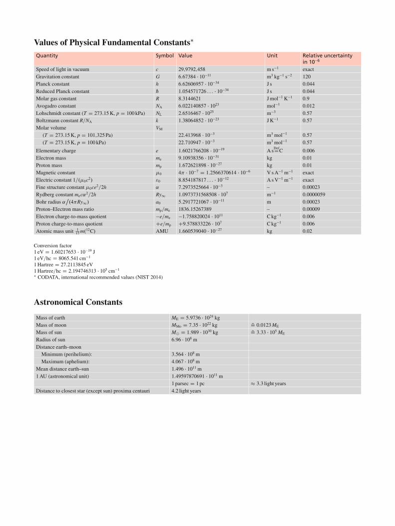
Values of Physical Fundamental Constants�
Quantity Symbol Value Unit Relative uncertaintyin 10�6
Speed of light in vacuum c 29;9792;458 m s�1 exactGravitation constant G 6:67384 � 10�11 m3 kg�1 s�2 120Planck constant h 6:62606957 � 10�34 J s 0:044Reduced Planck constant „ 1:054571726 : : : � 10�34 J s 0:044Molar gas constant R 8:3144621 Jmol�1 K�1 0:9Avogadro constant NA 6:022140857 � 1023 mol�1 0:012Lohschmidt constant (T D 273:15K, p D 100 kPa) NL 2:6516467 � 1025 m�3 0:57Boltzmann constant R=NA k 1:38064852 � 10�23 J K�1 0:57Molar volume VM
(T D 273:15K, p D 101;325 Pa) 22:413968 � 10�3 m3 mol�1 0:57(T D 273:15K, p D 100 kPa) 22:710947 � 10�3 m3 mol�1 0:57
Elementary charge e 1:6021766208 � 10�19 A sDefDC 0:006
Electron mass me 9:10938356 � 10�31 kg 0:01Proton mass mp 1:672621898 � 10�27 kg 0:01Magnetic constant 0 4 � 10�7 D 1:2566370614 � 10�6 V sA�1 m�1 exactElectric constant 1=.0c2/ "0 8:854187817 : : : � 10�12 A sV�1 m�1 exactFine structure constant 0ce2=2h ˛ 7:2973525664 � 10�3 – 0:00023Rydberg constant mec˛2=2h Ry1 1:0973731568508 � 107 m�1 0:0000059Bohr radius ˛
ı.4Ry1/ a0 5:2917721067 � 10�11 m 0:00023
Proton–Electron mass ratio mp=me 1836:15267389 – 0:00009Electron charge-to-mass quotient �e=me �1:758820024 � 1011 C kg�1 0:006Proton charge-to-mass quotient Ce=mp C9:578833226 � 107 C kg�1 0:006Atomic mass unit 1
12m.12C/ AMU 1:660539040 � 10�27 kg 0:02
Conversion factor1 eV D 1:60217653 � 10�19 J1 eV=hc D 8065:541 cm�1
1Hartree D 27:2113845 eV1Hartree=hc D 2:194746313 � 105 cm�1
� CODATA, international recommended values (NIST 2014)
Astronomical Constants
Mass of earth ME D 5:9736 � 1024 kgMass of moon MMo D 7:35 � 1022 kg ¶ 0:0123ME
Mass of sun Mˇ D 1:989 � 1030 kg ¶ 3:33 � 105 ME
Radius of sun 6:96 � 108 mDistance earth–moon
Minimum (perihelium): 3:564 � 108 mMaximum (aphelium): 4:067 � 108 m
Mean distance earth–sun 1:496 � 1011 m1AU (astronomical unit) 1:49597870691 � 1011 m
1 parsec D 1 pc � 3:3 light yearsDistance to closest star (except sun) proxima centauri 4:2 light years
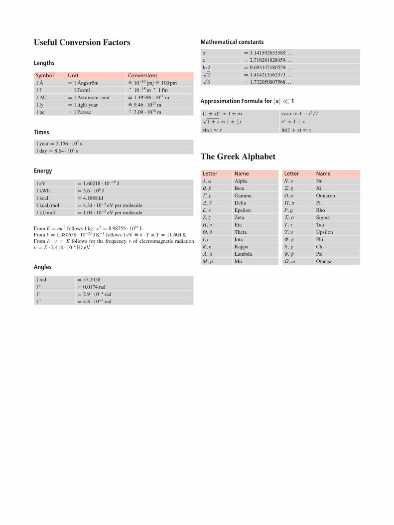
Useful Conversion Factors
Lengths
Symbol Unit Conversions1Å D 1Ångström ¶ 10�10 Œm� ¶ 100 pm1 f D 1 Fermi ¶ 10�15 m ¶ 1 fm1AU D 1Astronom. unit ¶ 1:49598 � 1011 m1 ly D 1 light year ¶ 9:46 � 1015 m1 pc D 1 Parsec ¶ 3:09 � 1016 m
Times
1 year D 3:156 � 107 s1 day D 8:64 � 104 s
Energy
1 eV D 1:60218 � 10�19 J1 kWh D 3:6 � 106 J1 kcal D 4:1868 kJ1 kcal=mol D 4:34 � 10�2 eV per molecule1 kJ=mol D 1:04 � 10�2 eV per molecule
From E D mc2 follows 1 kg � c2 D 8:98755 � 1016 J.From k D 1:380658 � 10�23 J K�1 follows 1 eV ¶ k � T at T D 11;604K.From h � � D E follows for the frequency � of electromagnetic radiation� D E � 2:418 � 1014 Hz eV�1
Angles
1 rad D 57:2958ı
1ı D 0:0174 rad10 D 2:9 � 10�4 rad100 D 4:8 � 10�6 rad
Mathematical constants
D 3:141592653589: : :e D 2:718281828459: : :ln 2 D 0:693147180559: : :p2 D 1:414213562373: : :p3 D 1:732050807568: : :
Approximation Formula for |x | � 1
.1 ˙ x/n � 1 ˙ nx cos x � 1 � x2=2p1 ˙ x � 1 ˙ 1
2 x ex � 1 C x
sin x � x ln.1 C x/ � x
The Greek Alphabet
Letter NameA; ˛ AlphaB; ˇ Beta�; � Gamma�; ı DeltaE; " EpsilonZ; � ZetaH; � Eta�; # ThetaI; � IotaK; � Kappa�; � LambdaM; Mu
Letter NameN; � Nu�; � XiO; o Omicron˘; PiP; % Rho˙; � SigmaT; � Tau$; � Upsilon˚; ' PhiX; � Chi(; Psi˝;! Omega
Related Documents