Wireless Sensor Networks Power Management Professor Jack Stankovic Department of Computer Science University of Virginia.

Wireless Sensor Networks

Power Management

Professor Jack StankovicDepartment of Computer

ScienceUniversity of Virginia

Critical Issue – Cross CutsCritical Issue – Cross Cuts

Problem StatementsProblem Statements

• Increase the lifetime of the system while meeting functional requirements.– Including communication coverage

• How to provide sensing coverage for a sensor network in a power-efficient way?

• MANET – how to maintain communication coverage

Questions?Questions?

• Will solar cells solve the problem?

• Will energy scavenging solve the problem?

• Will batteries just get much better?

QuestionsQuestions

• How do you define system lifetime?

• Can we solve the lifetime problem with high density?

Ideal:7 x 9 = 63 nodes

Per area Rotate

63 times increaseIn lifetime

Aging of System(with sleeping nodes)

Aging of System(with sleeping nodes)

After a certain amount of time, active nodes eventually die off.

Neighboring active nodes must detect this loss and issue help message(via wakeup) OR neighboring passive nodes must periodically wake upand detect loss and switch to active state.

Aging of System (cont.)

Aging of System (cont.)

Ideally, one node becomes activewhen only one node stops working.

Possible (more than likely?) thatmultiple nodes become active.

OutlineOutline

• Hardware layer• MAC layer - review• Routing layer – review• Localization and Clock Sync - review• Overarching power management

schemes– Sentry service– Tripwire service– Duty cycle– Differentiated surveillance

Power Management- Hardware layer

Power Management- Hardware layer

• Turn off/on– CPU – Memory– Sensors– Radio (most expensive)– Fully awake ………… Deep Sleep– Dynamic voltage scaling also possible

• SW ensures a node/components are awake when needed

Power Costs - Examples


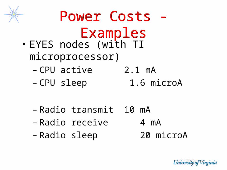
• EYES nodes (with TI microprocessor)– CPU active 2.1 mA– CPU sleep 1.6 microA

– Radio transmit 10 mA– Radio receive 4 mA– Radio sleep 20 microA



• Motes– ATmega 128 – six working modes with

different energy saving features• Most aggressive sleep can be very small %

of active working mode– Working – 8 mA– Sleep – 100 microA

– Radio• 10 microA sleeping• 7.5 mA Rcv• 12 mA Tx

Instructions and Modules Experimental Results

Instructions and Modules Experimental Results

Power Cost TradeoffPower Cost Tradeoff

• Communication versus calculation– Energy consumed for 1,000 basic

calculations is the same as for transmitting a single bit!

– Means: sending a 50 byte packet same energy cost as 400,000 instructions

– Implies: trade off calculation for messages

TinyOS Cost ResultsTinyOS Cost Results

MAC LayerMAC Layer

• Use overhearing (of wireless transmissions) and scheduling to reduce energy use– When a node hears another sending

RTS (not for me) it can go to sleep– Synchronized schedules (TDMA) – when

it is not my turn, listen then go to sleep

– Good algorithm can also reduce collisions!

MAC LayerMAC Layer

• 802.11 DCF doze mode

• S-MAC (pack all messages into awake period)

• B-MAC (duty cycle and CCA)

Routing LayerRouting Layer

• Use multiple routes to balance energy consumption– E.g., SPEED protocol

• Use data caching to minimize messages /energy– E.g., SEAD protocol (covered later)

• Adjust communication range to lowest possible to just reach neighbor– Many papers on this, but is this a good

idea? Not really, consider robustness

Routing LayerRouting Layer

• Use only good neighbors (high link quality)– Avoids need for re-transmissions

• Use data aggregation protocols– Directed diffusion– AIDA (not covered in this class)– …

• Piggyback state table updates

LocalizationLocalization

• Localization– How often?– Minimize messages– Long range beacons costly– Example:

• APIT costs long range beacons (higher power) but few messages

• Amorphous Localization costs - flooding• Walking GPS costs - receiving several

messages

Clock SyncClock Sync

• Clock Sync– Minimize messages to the number

needed for a particular sync accuracy

• Example: RBS – one time message and then all neighbors must exchange messages

• Example: TPSN – exchange 2 sync messages with parent node in spanning tree

• Example: Internet NTS protocol sends many messages to the time server

Two ViewpointsTwo Viewpoints

• Power Management in the Small– Individual protocols

• Power Management in the Large– Overarching protocols for additional

power savings• Sentry Service• Tripwire Management Service• Duty Cycle• Differential Surveillance

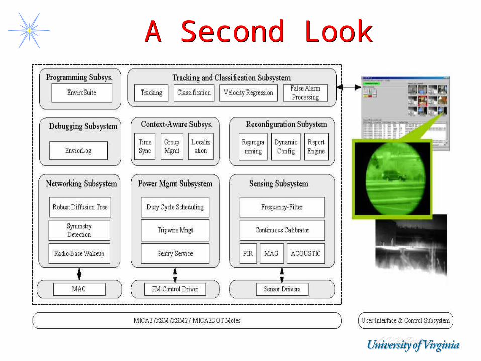
A Second LookA Second Look

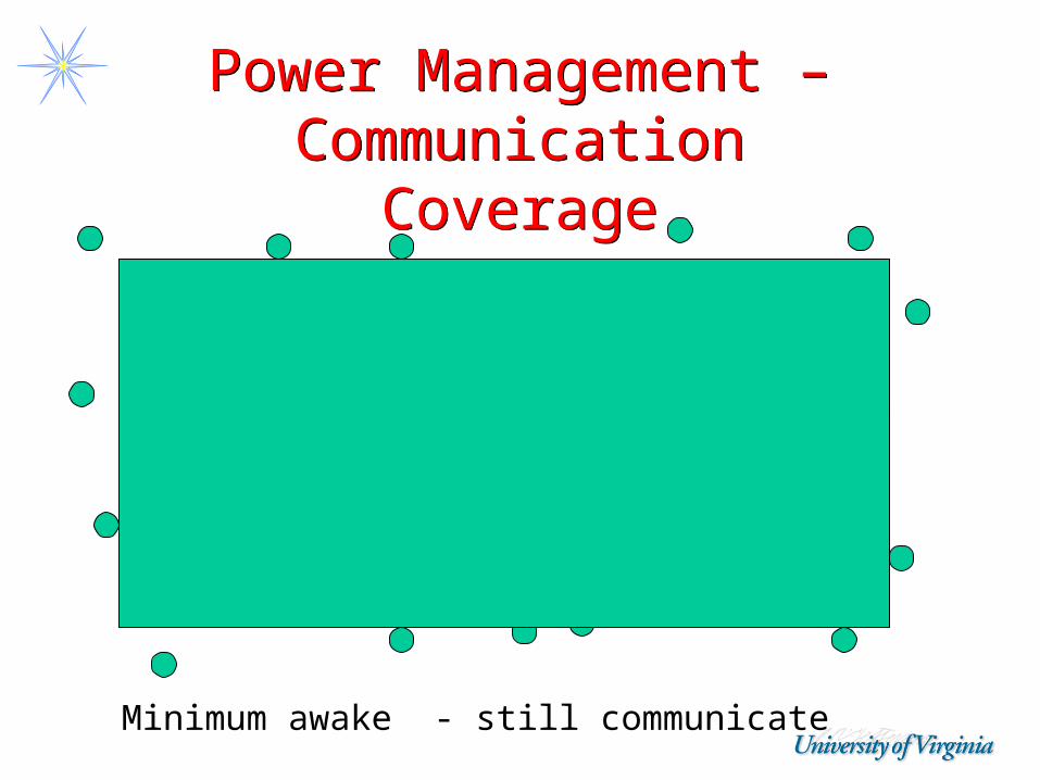
Power Management – Communication

Coverage

Power Management – Communication

Coverage

Minimum awake - still communicate

Sensing Coverage (r) First

Then 2r for Communication

Sensing Coverage (r) First

Then 2r for Communication

Power Management - Communication

Coverage

Power Management - Communication

CoverageComm. Range

Virtual Grid – one node awake per gridRotate

Power Management- Sensing Coverage

Power Management- Sensing Coverage

• 100% coverage• > 100% coverage

– FT– Higher quality/confidence sensing

• < 100% coverage (aggressive)– Use movement (temporal) of object to

compensate for less spatial coverage– Increased lifetime

Application ScenarioApplication Scenario• A small number of nodes stay awake• Most of the network sleeps• Rare events

Application ScenarioApplication Scenario• Awakened nodes detect an

event• Messages are sent to wake

up other nodes

Wake-Up Solution (1)Wake-Up Solution (1)

• Periodic wake-up– Each (non-awake) node has a

sleep/wakeup duty cycle based on local timer• Listen for stay awake message

– Most current systems use this technique

– Application dependent, often complicated, wastes energy• E.g., correct duty cycle depends on speed

of targets, sensing ranges, types of sensors, …

• May miss wakeup call

Awake Sleep


• Special low power hardware stand-by component that (always) listens for a wakeup beacon (not the full radio component)– PicoRadio– Uses extra energy (but not as much as

full radio component)


• Just-In-Time Wake-up Capability– A node does not wake up until it is

needed– It uses no active listening energy– Uses radio-triggered hardware that

extracts energy from the electromagnetic energy in the wakeup signal itself

– Proposed – not built for WSN

– Not RFID – they employ powerful readers to send strong radio signals

Just-in-Time Solution – Is it worth?

Just-in-Time Solution – Is it worth?

• Is there much energy to save?• How is energy consumed on a network

node?– Examine the distribution of consumed

energy on a node in a sensor network for vehicle tracking

• 10 events per day, each event lasts 2 minutes• Work/sleep current intensity: 20mA / 100uA• Note: Actual computation is more involved

Solution – Is it worth? Solution – Is it worth?

• Scheme I: Always-on (No power management)– The node is on and actively

sensing until it is out of power

– 1% of the energy is used to track vehicles, 99% is used in a peeking state (uselessly sensing for potential passing vehicles)

– Lifetime 3.3 days

Always-on

Waiting99%

Tracking1%

Energy wasted!!!

Solution – Is it worth? Solution – Is it worth?

• Scheme II: Rotation-based (Periodic wake-up)– Nodes are awakened

wirelessly by wake-up messages

– Duty cycle 4.7%– 21% of the energy is used

to track vehicles, 7% used in sleeping mode, and 72% is used in peeking state

– Lifetime 50 days

Rotation-based powermanagement

Wai ti ng72%

Sl eep7% Tracki ng

21%

Energy wasted!!!

Solution – Is it worth it? Solution – Is it worth it?

• Scheme III: Radio-triggered– Nodes keep sleeping until

events of interest happen– Nodes are awakened

wirelessly by wake-up messages

– 74% of the energy is used to track vehicles, 26% used in sleeping mode (minimal cpu energy)

– Lifetime – 178 days

Radio-triggered powermanagement

Tracki ng74%

Sl eep26%

Sentry-Based Power Management (SBPM)Sentry-Based Power Management (SBPM)

• Two classes of nodes: sentries and non-sentries

– Sentries are awake – Non-sentries can sleep

• Sentries – Provide coarse monitoring & backbone communication network– Sentries “wake up” non-sentries for finer sensing

• Sentry rotation– Even energy distribution– Prolong system lifetime

• Decentralized Algorithm–See photo

1

4

3

2

SBPMSBPM

• Basic Algorithm– Each node sets timer inversely

proportional to the amount of energy it has remaining

– Implies: node with most energy will declare itself a sentry FIRST

– Other nodes hearing sentry declare themselves as non-sentries

SBPM - IllustrationSBPM - IllustrationAll nodes are awake.

Base node declares itself first as a sentry and sends SENTRY_DECLARE message.

Communication at sensing range (ensure sensing coverage).

SBPM - IllustrationSBPM - Illustration

Other nodes send SENTRY_DECLARE message as backoff expires (function of remaining energy).


Other nodes send SENTRY_DECLARE message as backoff expires.

If backoff expires and heard from a sentry then just join one sentry (first, closest)

All sentries or attached toa sentry


Increase communication range – at least 2X

All sentries or attached toa sentry

New communication Range

Tripwire Service – Scaling to 1000s

Tripwire Service – Scaling to 1000s

10-N dormant sections

...

...

...

...

...

...

...

...

……

……

N Tripwire sections

...

...

...

...

...

.........

...

...

...

...

……

……

……

10 relays

Suggest N = 2

100M

1000m

Network partitioning• 2 tripwire sections• 8 dormant sections• 100 motes, 1 relay

per section• Size and number of

sections reconfigurable

• Rotate sections

Sentries• N% in tripwire

section• Rotate sentries

Creating SectionsCreating Sections

• How many sections?

• How to create sections?

• How (or do) base stations communicate?

• What if base station fails?

Network LifetimeNetwork Lifetime

0

10

20

30

40

50

60

70

Time (seconds)

En

erg

y(m

w)

Sentry

NonSentry

Initialization Duration = 5 minutes

Surveillance Duration = 1day

Without system rotation:NonSentry Life Time: 250 daysSentry LifeTime: 7 days

• Lifetime is determined by– Individual Mica 2 mote

consumption •Energy plot for a sentry node

•Energy plot for a sleep node

Summary -Power Management

Summary -Power Management

• Sentry Service – x% in a region are awake

• Tripwire – many regions to handle scale

• Within a Region - Area only wakeup (each region may be large)

Lifetime AnalysisLifetime Analysis

Network Life Time

Number of Tripwires (10 regions, 30% sentry, 7 day

life)

4 3 2 1

2 AA Batteries

50 days 70 days

105 days

210 days

4 AA Batteries

100 days 140 days

210 days

420 days

Sentry Duty CycleSentry Duty Cycle

• Sentry can also sleep based on– Sensing range– Speed of targets– Lifetime of events (static/moving)– Required probability of detection

– Use spatial properties to detect moving target/event• If first sentry is asleep what is the

probability that the second one will be too

Sentry Duty CycleSentry Duty Cycle

Sentry Duty-Cycle Scheduling

Sentry Duty-Cycle Scheduling

• A common period p and duty-cycle β is chosen for all sentries, while

starting times Tstart are randomly selected

Non-sentries

Sentries

Target TraceA

BC

DE

A

B

C

D

E

t

t

t

t

t

Awake Sleeping

p0 2p

Lifetime AnalysisLifetime Analysis Network Life Time

Number of Tripwires (10 regions, 30% sentry, 7

day life)

10 4 2 1

2 AA Batteries

Sentries Awake

21 days

50 days

105 days

210 days

Sentries with Duty Cycles

50 days

125 days

250 days

500 days

4 AA Batteries

Sentries Awake

42 days

100 days

210 days

420 days

Sentries with Duty Cycles

100 days

250 days

500 days

1000 days

Differentiated Surveillance

Differentiated Surveillance

> 100%

= 100%

< 100%

Most Important

Important

Less Important

Vehicles

Differentiated Surveillance Solution

Differentiated Surveillance Solution

DOC = 1 DOC = 2

DOC = Degree of CoverageDynamic

Design GoalsDesign Goals

• Provide energy efficient sensing coverage for a geographic area covered by sensor nodes– Extend system life

• Reduce total energy consumption• Reduce energy consumption variation

among nodes

– Provide differentiated surveillance service• Some areas more critical

Sensing Coverage = 100%

Sensing Coverage = 100%

Degree of Sensing CoverageDegree of Sensing Coverage

• Current solutions regard the sensing coverage to a certain geographic area as a binary True/False.

• It is possible that higher degree of sensing coverage is desired to obtain high detection confidence since individual nodes are not reliable.

0

1

2

F

T

T

r

AssumptionsAssumptions

• Each node knows its own location and nodes are not moving.

• Neighboring nodes are time synchronized.• The sensing area of a node is a circle with radius

r centered at the location of this node.• Radio radius is larger than 2r

< 2r

Basic Design Without Differentiation

Basic Design Without Differentiation

• Goal – find a work-sleep schedule for each node which achieves 100% Sensing coverage guarantee.

• Ideally we should decide the schedule for each point in the area, but it’s impossible because the number of points is infinite. What can we do?

For EACH POINT p in a certain geographic area, Guarantee that at ANY TIME, p is covered by at least one node’s sensing range.

Basic design with 100% sensing coverage

Basic design with 100% sensing coverage

• Solution – 100% Grid point sensing coverage– Divide whole network into virtual grids– For each grid point x, guarantee that x is covered by at

least one node’s sensing range at ANY time

r

Decide Working Schedule


• Schedule example

If we want to provide sensing coverage for point x, we can have either A or B or C awake.

B

A

C

Point x

Node A

Node B

Node C

Waking Sleeping

0 10030 70

10 60

5 45

time

Scheduling example for A, B and C



• Challenge: For each node, how to coordinate with other nodes and decide its own schedule?– Solution - Random Reference Point

Scheduling Algorithm



• Concepts– Initialization Phase

• In this phase, nodes find their own positions, synchronize time with neighboring nodes and decide their own working schedule.

– Sensing Phase• Nodes enter this phase after initialization phase and

choose to sense or sleep according to their schedule.

– Sensing Round - T• Sensing phase is divided into sensing rounds with

equal duration T. A node has the same schedule for each round.

Decide working schedule for sensing round T



• Concepts– A node’s working schedule is

determined by a four parameter tuple – (T, Ref, Tfront, Tend)• Ref: a random time reference point chosen

by a node within [0, T)• Tfront: the duration of time prior to Ref• Tend: the duration of time after Ref.• By this tuple, A node’s working period is

determined as follows:– [T*j + Ref – Tfront , T*j + Ref + Tend)At other times the node is sleeping.



• Solution – Random Reference Point Scheduling Algorithm1) Each node N chooses a “Reference Point (Ref)”

randomly from [0, 100) and broadcasts its Ref and position.e.g. T = 100, RefA = 40, RefB= 90, RefC = 20

2) For each grid point P in its own sensing area, N sorts all the Refs from nodes (including N) which can also sense P in ascending order.For A according to point P1, we have:Ref(1) = RefC = 20, Ref(2) = RefA = 40, Ref(3) = RefB = 90

B

A

C

Point P10 refC refA refB

20 40 90

100



3) Assuming RefN is the (i)th Ref, N’s four parameter tuple is computed as follows:• TfronN = (Ref(i)- Ref(i-1))/2, 1<i<M• TendN = (Ref(i+1)-Ref(i))/2, 1<i<MTfrontA = (Ref(2)-Ref(1))/2 = (40-20)/2 = 10TendA = (Ref(3)-Ref(2))/2 = (90-40)/2 = 25(T, RefA, TfrontA, TendA) = (100, 40, 10, 25)

4) N’s working period for point P (TwN(P)) is decided by:[T*j + RefN – TfrontN , T*j + RefN + TendN), j = 0, 1, 2, …

TwA(P1) = [100*j+40–10, 100*j+40+25) = [100*j+30, 100*j+65)

0

refC refA refBt

t20 40 90

30 65



5) Calculate the union of TwN(Px) for all grid points within N’s sensing area, choose this union as the final working period of N (TwN).

TwA(P1)TwA(P2)TwA(P3)

TwA(Pn)

TwA

.

.

.

0 1005 65

6545

5 50…

B

A

C

Point P1

Enhanced Design with Differentiation

Enhanced Design with Differentiation

• Goal– provide sensing coverage with DOC = a

• a > 1 or a < 1

• Solution– Extend 4-parameter tuple to 5-

parameter tuple (T, Ref, Tfront, Tend, a)– Determine a node’s working period as

follows:• [T*j + Ref – Tfront*a , T*j + Ref + Tend*a)

An ExampleAn Example

Schedule for Grid Point P1 (a=2)

(T, RefA, TfrontA, TendA, a) = (100, 40, 10, 25, 2)

(T, RefB, TfrontB, TendB, a) = (100, 90, 25, 15, 2)

(T, RefC, TfrontC, TendC, a) = (100, 20, 15, 10, 2)

TwA = [T*j + Ref – Tfront*2,T*j + Ref + Tend*2)

= [100*j + 20, 100*j + 90)

TwB = [100*j + 40, 100*j + 120)

TwC = [100*j -10, 100*j + 40)

A

refC refA refB

20 40 90

C

B

0

30 655

Multi-Round Extension for Energy Balancing

Multi-Round Extension for Energy Balancing

• Problem– Reference points are

selected randomly instead of uniformly, which results in big variation in Tw among nodes and big variation in power consumption

TwA

TwC

TwB

refCrefBrefA

Multi-Round Extension for Energy Balance

Multi-Round Extension for Energy Balance

• Multi-Round Extension– Instead of calculating a single schedule, calculate M

schedules for each node according to M independently selected random Refs for each node.

– At each round T in sensing phase, the nodes choose one schedule consecutively.

TwA1 TwA1TwA2 TwA3 TwA2 TwA3

SummarySummary

• Energy is key metric to minimize and will remain so for a long time

• Savings must be addressed at all levels in the system and for most protocols/services– Clock sync – don’t send too many messages to maintain

minimal clock drift– Localization – even one time costs have to be efficient

(avoid solutions with too many messages)

• Improved batteries• Solar • Energy scavenging• Better hardware (low power cpus, sensors, …)

SummarySummary

• Power Management in the Large

• Models can be used to estimate lifetime tradeoffs

• Fault tolerance might use heartbeat beacons -> energy cost

• Metrics– Total energy consumed per period X– Lifetime– Half-life– Energy consumption balance

Wireless Sensor Networks Power Management Professor Jack Stankovic Department of Computer Science University of Virginia.

Documents

neighboring active nodes

active state

energy cost

multiple nodes

active working modeworking

different energy

energy usewhen

energy scavenging