Wireless Network information Theory - CESGcesg.tamu.edu/.../prk_present/Wireless-Network-Information-Theory.pdfModel for wireless network information theory 33 ... Shannonʼs formulation

1/105

© June 30, 2009 , P. R. Kumar

Wireless Network information Theory

P. R. Kumar

Dept. of Electrical and Computer Engineering, and Coordinated Science Lab University of Illinois, Urbana-Champaign

Email: [email protected]: http://decision.csl.illinois.edu/~prkumar

This work is licensed under a Creative Commons Attribution-Noncommercial-No Derivative Works 3.0 Unported License. Based on a work at decision.csl.illinois.edu See last page and http://creativecommons.org/licenses/by-nc-nd/3.0/

2/105

© June 30, 2009 , P. R. Kumar

What is really the best way to operate wireless networks?

And what are the ultimate limits to information transfer over wireless

networks?

3/105

© June 30, 2009 , P. R. Kumar

Outline   Reappraising multi-hop transport 4   What is information theory? 11   Network information theory 22   Model for wireless network information theory 33   Results when absorption or relatively large path loss 45   Order optimality of multi-hop transport 65   The effect of fading 80   Low path loss 82   A quick survey of more recent results 94   Remarks 99   References 100

4/105

© June 30, 2009 , P. R. Kumar

Reappraising multi-hop transport

5/105

© June 30, 2009 , P. R. Kumar

Reappraising multi-hop transport

  Nodes fully decode packets at each stage   Treating interference as noise

  But why should nodes Decode and Forward?   Why not just Amplify and Forward?

Interference+

Noise Interference

+Noise

Interference+

Noise

S D R1 R2 R3

R

S

D

  Why should intermediate nodes be able to decode the packets?   Why go digital?

6/105

© June 30, 2009 , P. R. Kumar

Why treat interference as noise?

  Interference is not interference

Subtractloud

signal

Interference is information

  Packets do not destructively collide

  Why not use multi-user decoding?

  How much benefit can multi-user decoding give for wireless networks?

7/105

© June 30, 2009 , P. R. Kumar

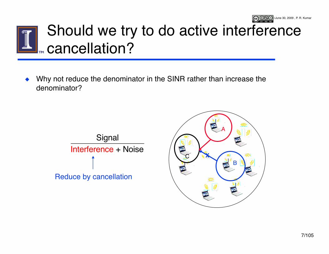
Should we try to do active interference cancellation?

  Why not reduce the denominator in the SINR rather than increase the denominator?

A

B C X

Reduce by cancellation

SignalInterference + Noise

8/105

© June 30, 2009 , P. R. Kumar

Why even take small hops?

  Why not use long range communication with multi-user decoding?

9/105

© June 30, 2009 , P. R. Kumar

In fact is the notion of spatial reuse appropriate for wireless networks?

  Spatial reuse of frequency

  If spatial reuse of frequency is the goal, then is a sharper path loss better for wireless networks?

0Distance

Attenuation

1r8

1r4

1r 8 better for wireless networks than 1

r 4 ?–  Is

–  Or worse?

  Are jungles better for wireless networking than deserts?

10/105

© June 30, 2009 , P. R. Kumar

Wireless networks are not wired networks …

“There are more things in heaven and earth, Horatio, Than are dreamt of in your philosophy.” — Hamlet

  Wireless networks are formed by nodes with radios –  There is no a priori notion of “links” –  Nodes simply radiate energy

  Nodes can cooperate in many complex ways

  So how should information be transported in wireless networks?   What should be the architecture of wireless networks?   What are the limits to information transfer?

–  Maxwell rather than Kirchoff

  Need an information theory to provide strategic guidance for wireless networks

11/105

© June 30, 2009 , P. R. Kumar

What is Information Theory?

12/105

© June 30, 2009 , P. R. Kumar

Model of communication

Information Source

Information Transmitter

Channel Receiver Information Sink

Noise

Message Received

signal Transmitted

Signal Message

13/105

© June 30, 2009 , P. R. Kumar

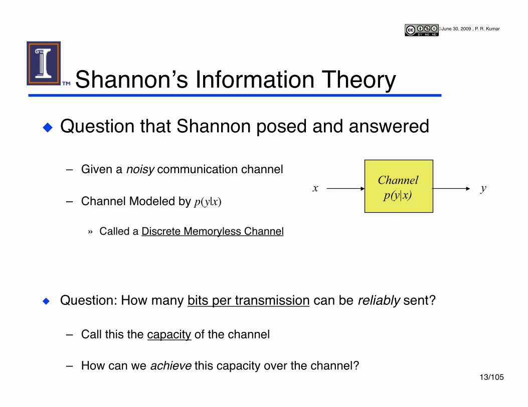
Shannonʼs Information Theory

  Question that Shannon posed and answered

–  Given a noisy communication channel

–  Channel Modeled by p(y|x)�

»  Called a Discrete Memoryless Channel

  Question: How many bits per transmission can be reliably sent?

–  Call this the capacity of the channel

–  How can we achieve this capacity over the channel?

Channel p(y|x) x y

14/105

© June 30, 2009 , P. R. Kumar

Shannonʼs formulation   There are a set of 2nR messages

1 2

4 6

7

3

2nR-1 2nR

5

  One message W in {1, 2, … , 2nR}is picked by the source out ofthese 2nR messages

  This is encoded as a codeword {X1, X2, … , Xn}

5

Channelp(y|x)

Xk Yk

  Xk is transmitted on the k-th transmission

  Yk is received on the k -th transmission

  So in n uses of the channel {X1, X2, … , Xn} is sent, and{Y1, Y2, … , Yn} is received

15/105

© June 30, 2009 , P. R. Kumar

Shannonʼs formulation

Channelp(y|x)

{X1,… , Xn} {Y1,… , Yn}

1 2

4 6

7

3

2nR-1 2nR

5 5

  There are a set of 2nR messages

  The receiver decodes {Y1, Y2, … , Yn} as W

  There are a set of 2nR messages   One message W in {1, 2, … , 2nR}

is picked by the source out ofthese 2nR messages

  This is encoded as a codeword {X1, X2, … , Xn}

  Xk is transmitted on the k-th transmission

  Yk is received on the k -th transmission

  So in n uses of the channel {X1, X2, … , Xn} is sent, and{Y1, Y2, … , Yn} is received

16/105

© June 30, 2009 , P. R. Kumar

Definition of Achievable Rate R   Let Perror = Prob(W ≠ W)   Suppose we can make Perror smaller than any ε we desire by

choosing n large   Then we say that the channel can support a Rate of R bits

per transmission   Overall scheme

–  Choose encoder E: {1, 2, … , 2nR} Xn –  Choose decoder D: Xn {1, 2, … , 2nR} –  Want Perror smaller than a desired ε –  Then we can “reliably transmit R bits per transmission”

D E

2nR messages

W W {X1, X2, … , Xn} {Y1, Y2, … , Yn} Channel p(y|x)

17/105

© June 30, 2009 , P. R. Kumar

Shannonʼs Answers   Capacity Theorem

–  Given Channel Model p(y|x)

  Capacity = Max I(X;Y) bits/transmission

–  Where is called the “mutual information”

–  This is the supremum of the achievable rates

  Shannonʼs architecture for digital communication

Channel p(y|x) x y

I(X;Y ) = p(x, y)x, y∑ log p(X,Y)

p(X )p(Y)⎛ ⎝ ⎜ ⎞

⎠ ⎟

p(x)

Channel Source decode(Decompression)

Decode Encodefor the

channel Source code

(Compression)

2nR messages 2nR messages

18/105

© June 30, 2009 , P. R. Kumar

Capacity of Gaussian Channel   Gaussian Channel

  Yi = Xi + Zi

  Zi ∼ N(0, σ2) –  Independent, identically distributed noise

  Power constraint P on transmissions:

  Capacity =

Channel p(y|x) x y

X Y +

Z ~ N(0,σ2) = Noise

1n

Xi2

i=1

n

∑ ≤ P

12

log 1+ Pσ 2

⎛⎝⎜

⎞⎠⎟ bits per transmission

19/105

© June 30, 2009 , P. R. Kumar

Capacity of Continuous AWGN Bandlimited Channel

  AWGN Noise Z(t) with Power Spectral Density

  Band Limited Channel [-W,+W]

  Power constraint P on signal transmitted:

  Capacity =

1T

X 2 (t)0

T

∫ ≤ P

W log 1+ PWN

⎛⎝⎜

⎞⎠⎟ bits per second

X(t) Y(t) +

Z(t) White Gaussian Noise with PSD N

-W +W

1

N2

20/105

© June 30, 2009 , P. R. Kumar

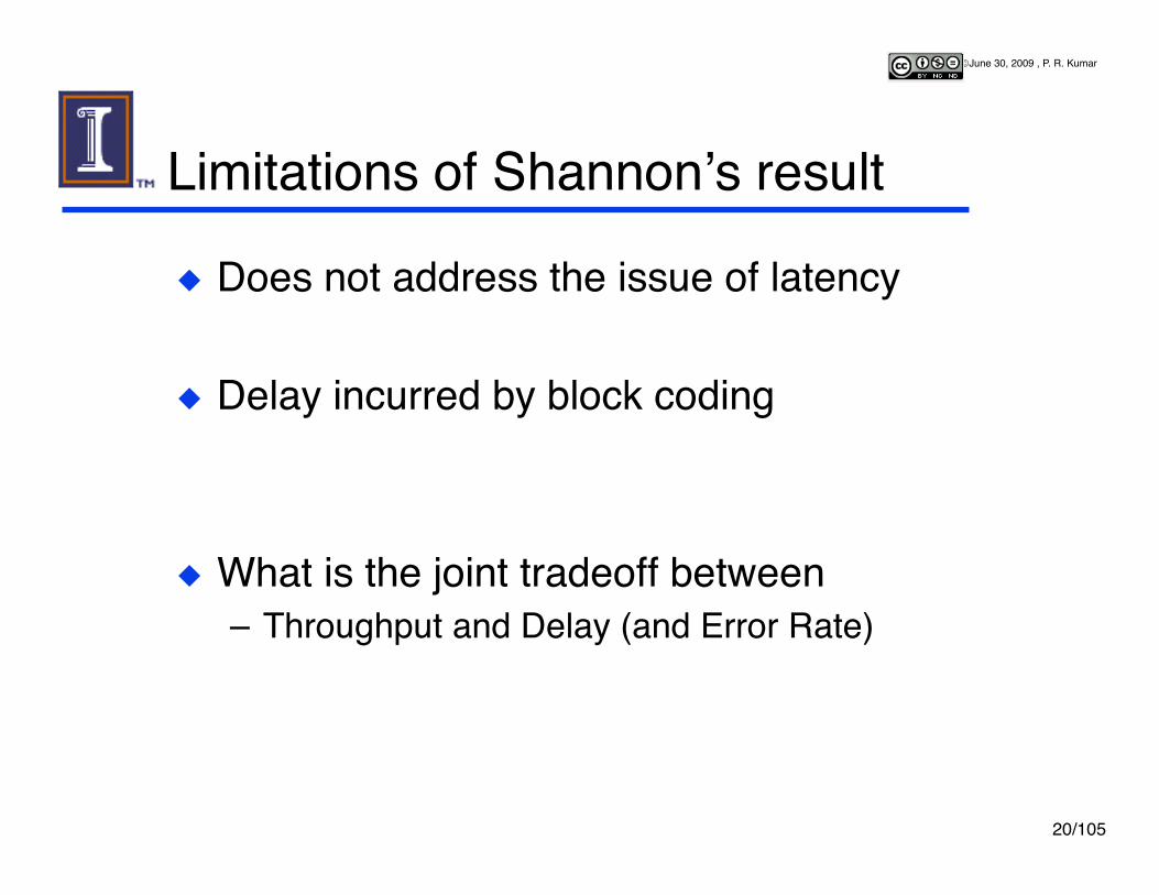
Limitations of Shannonʼs result

  Does not address the issue of latency

  Delay incurred by block coding

  What is the joint tradeoff between –  Throughput and Delay (and Error Rate)

21/105

© June 30, 2009 , P. R. Kumar

The classic references   C. E. Shannon, "A mathematical theory of communication", Bell

Syst. Tech. J.", Vol 27, pp. 379--423", 1948.

  C. E. Shannon, "Communication in the presence of noise", Proceedings of the IRE, vol. 37, pp. 10--21, 1949.

  C. E. Shannon and W. Weaver The Mathematical Theory of Information, University of Illinois Press, Urbana, 1949.

  R. G. Gallager, Information Theory and Reliable Communication, John Wiley and Sons, New York, 1968.

  T. Cover and J. Thomas, Elements of Information Theory, Wiley and Sons, New York, 19103.

22/105

© June 30, 2009 , P. R. Kumar

Network Information Theory

23/105

© June 30, 2009 , P. R. Kumar

23

The Multiple Access Channel   Model

–  Node 1 sends –  Node 2 sends –  The receiver receives generated as

  Senders and their Rates –  Message 1: –  Sends

–  Message 2: –  Sends

  Decoder: and

  What rate vectors are feasible?

24/105

© June 30, 2009 , P. R. Kumar

24

Solution   Capacity region:

All rate vectors satisfying

for some distribution are feasible

25/105

© June 30, 2009 , P. R. Kumar

25

Interpretation and coding strategy   At point A

A

Node 2 acts as a pure facilitator

26/105

© June 30, 2009 , P. R. Kumar

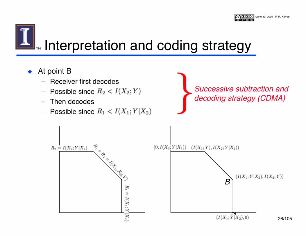
26

Interpretation and coding strategy   At point B

–  Receiver first decodes –  Possible since –  Then decodes –  Possible since

B

Successive subtraction and decoding strategy (CDMA)

27/105

© June 30, 2009 , P. R. Kumar

27

The Scalar Gaussian Broadcast Channel

  Goal –  To send to Receiver 1 –  To send to Receiver 2 –  Simultaneously –  Through one broadcast –  Power constraint

  Receiver 1 receives –  Decodes

  Receiver 2 receives –  Decodes

  What rate vectors are feasible?

28/105

© June 30, 2009 , P. R. Kumar

28

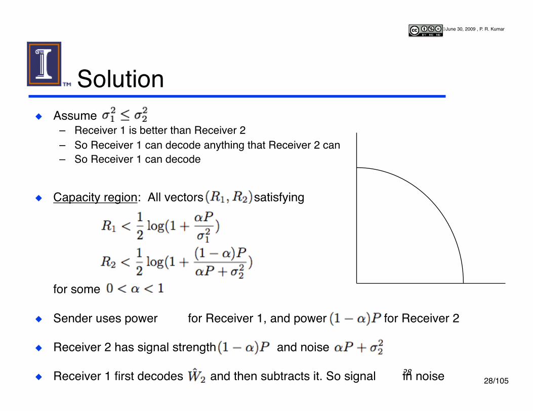
Solution   Assume

–  Receiver 1 is better than Receiver 2 –  So Receiver 1 can decode anything that Receiver 2 can –  So Receiver 1 can decode

  Capacity region: All vectors satisfying

for some

  Sender uses power for Receiver 1, and power for Receiver 2

  Receiver 2 has signal strength and noise

  Receiver 1 first decodes and then subtracts it. So signal in noise

29/105

© June 30, 2009 , P. R. Kumar

General broadcast channel   General Broadcast channel capacity unknown

–  Vector Gaussian channel capacity recently established

30/105

© June 30, 2009 , P. R. Kumar

30

Max Flow - Min Cut Theorem   Theorem (El Gamal Ph. D. Thesis)

Suppose is feasible vector of rates.

Then

  Example: Relay Channel

S Sc

X

X1,Y1

Y

31/105

© June 30, 2009 , P. R. Kumar

31

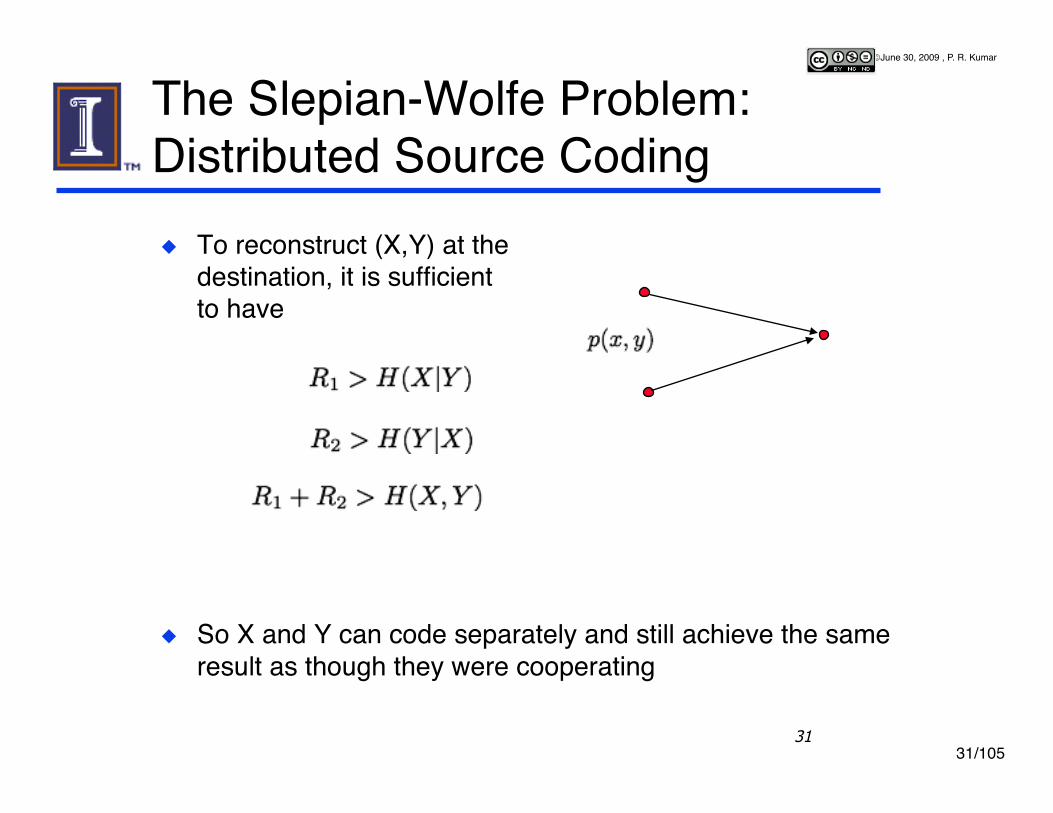
The Slepian-Wolfe Problem: Distributed Source Coding   To reconstruct (X,Y) at the

destination, it is sufficientto have

  So X and Y can code separately and still achieve the same result as though they were cooperating

32/105

© June 30, 2009 , P. R. Kumar

Network information theory

Gaussian broadcast channel

Unknowns

The simplest interference channel

  Networks being built (ad hoc networks, sensor nets) are much more complicated

Multiple access channel

Triumphs

The simplest relay channel

33/105

© June 30, 2009 , P. R. Kumar

Model for Wireless Network Information Theory

34/105

© June 30, 2009 , P. R. Kumar

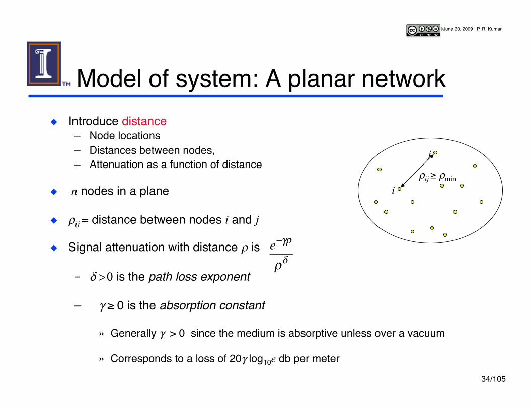
Model of system: A planar network   Introduce distance

–  Node locations –  Distances between nodes, –  Attenuation as a function of distance

  n nodes in a plane

  ρij = distance between nodes i and j�

  Signal attenuation with distance ρ is

–  δ > 0 is the path loss exponent

–  Gγ ≥ 0 is the absorption constant

»  Generally γ > 0 since the medium is absorptive unless over a vacuum

»  Corresponds to a loss of 20γ log10e db per meter

ρij ≥ ρmin i

j

�

e−γρ

ρδ

35/105

© June 30, 2009 , P. R. Kumar

�

CT = sup(R1,R2 ,…,Rn(n−1) )

Rii=1

n(n−1)∑ ⋅ ρi

�

ˆ W i = g j (y jT ,Wj )

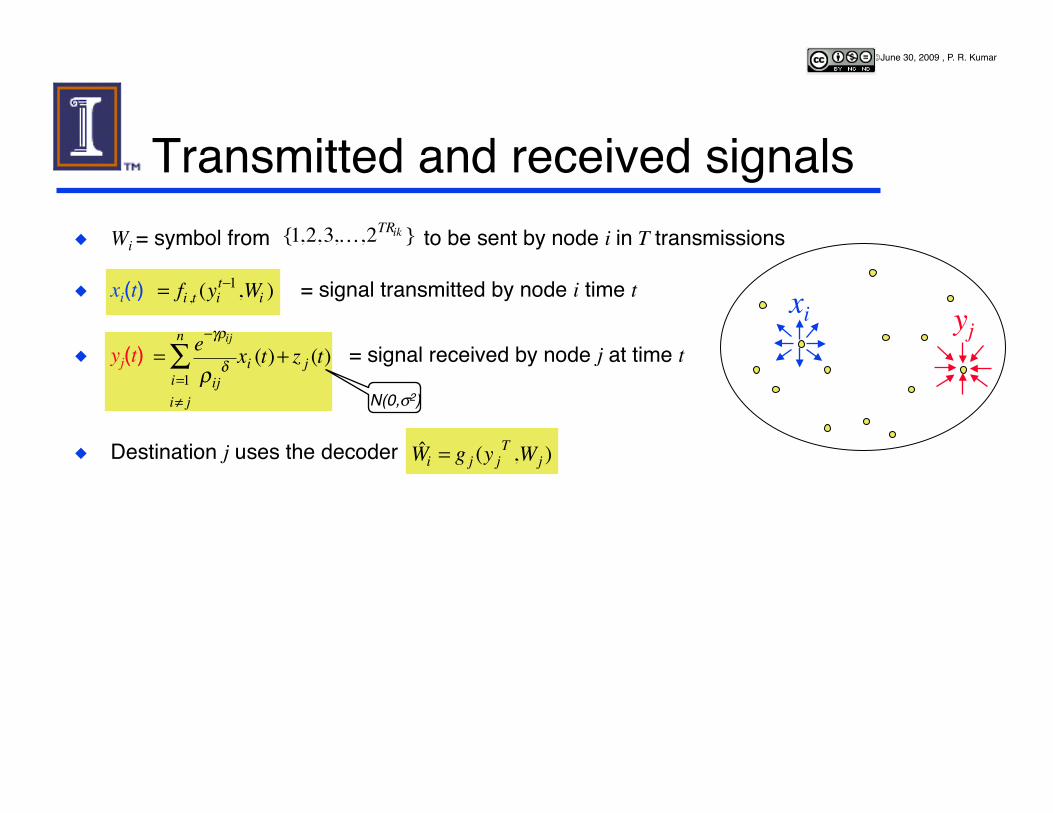
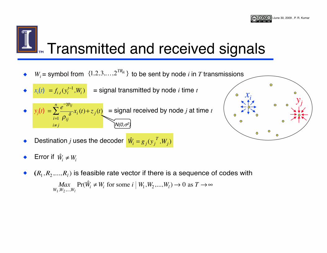
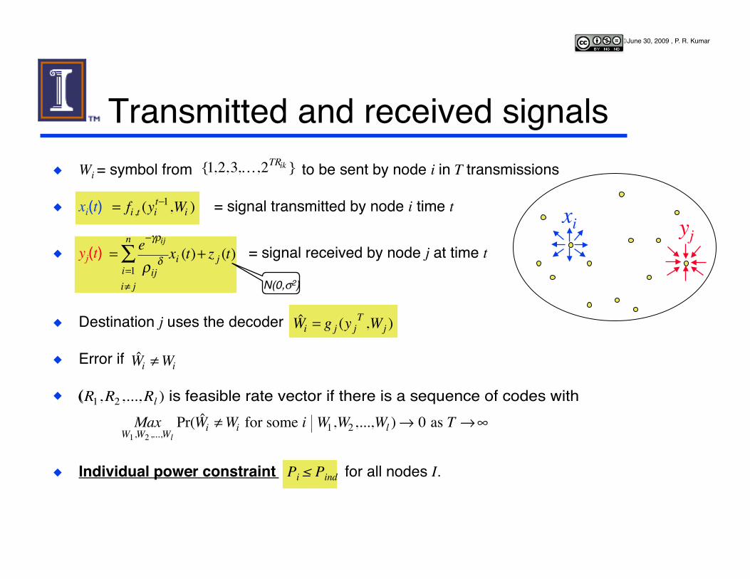
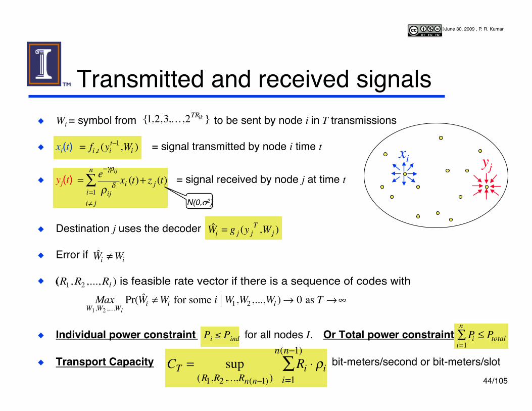
Transmitted and received signals

N(0,σ2) �

= fi ,t (yit−1,Wi )

�

{1,2,3,…,2TRik }

�

= e−γρij

ρijδ

i=1i≠ j

n

∑ xi (t)+ z j (t)

Pii=1

n∑ ≤ Ptotal

�

ˆ W i ≠Wi

�

(R1,R2,...,Rl ) is feasible rate vector if there is a sequence of codes with

�

MaxW1,W2 ,...,Wl

Pr( ˆ W i ≠Wi for some i W1,W2,...,Wl ) → 0 as T →∞

  Wi = symbol from to be sent by node i in T transmissions

  xi(t) = signal transmitted by node i time t�

  yj(t) = signal received by node j at time t

  Destination j uses the decoder

  Error if

  (

  Individual power constraint Pi ≤ Pind for all nodes I. or Total power constraint

  Transport Capacity bit-meters/second or bit-meters/slot

36/105

© June 30, 2009 , P. R. Kumar

�

CT = sup(R1,R2 ,…,Rn(n−1) )

Rii=1

n(n−1)∑ ⋅ ρi

�



N(0,σ2) �


�

= e−γρij

ρijδ

i=1i≠ j

n

∑ xi (t)+ z j (t)

Pii=1

n∑ ≤ Ptotal

�

ˆ W i ≠Wi

�


�

MaxW1,W2 ,...,Wl






  Error if

  (



�

{1,2,3,…,2TRik }

xi yj

37/105

© June 30, 2009 , P. R. Kumar

�

CT = sup(R1,R2 ,…,Rn(n−1) )

Rii=1

n(n−1)∑ ⋅ ρi

�



N(0,σ2) �


�

= e−γρij

ρijδ

i=1i≠ j

n

∑ xi (t)+ z j (t)

Pii=1

n∑ ≤ Ptotal

�

ˆ W i ≠Wi

�


�

MaxW1,W2 ,...,Wl






  Error if

  (



�

{1,2,3,…,2TRik }

xi yj

38/105

© June 30, 2009 , P. R. Kumar

�

CT = sup(R1,R2 ,…,Rn(n−1) )

Rii=1

n(n−1)∑ ⋅ ρi

�



N(0,σ2) �


�

= e−γρij

ρijδ

i=1i≠ j

n

∑ xi (t)+ z j (t)

Pii=1

n∑ ≤ Ptotal

�

ˆ W i ≠Wi

�


�

MaxW1,W2 ,...,Wl






  Error if

  (



�

{1,2,3,…,2TRik }

xi yj

39/105

© June 30, 2009 , P. R. Kumar

�

CT = sup(R1,R2 ,…,Rn(n−1) )

Rii=1

n(n−1)∑ ⋅ ρi

�



N(0,σ2) �


�

= e−γρij

ρijδ

i=1i≠ j

n

∑ xi (t)+ z j (t)

Pii=1

n∑ ≤ Ptotal

�

ˆ W i ≠Wi

�


�

MaxW1,W2 ,...,Wl






  Error if

  (



�

{1,2,3,…,2TRik }

xi yj

40/105

© June 30, 2009 , P. R. Kumar

�

CT = sup(R1,R2 ,…,Rn(n−1) )

Rii=1

n(n−1)∑ ⋅ ρi

�



N(0,σ2) �


�

= e−γρij

ρijδ

i=1i≠ j

n

∑ xi (t)+ z j (t)

Pii=1

n∑ ≤ Ptotal

�

ˆ W i ≠Wi

�


�

MaxW1,W2 ,...,Wl






  Error if

  (



�

{1,2,3,…,2TRik }

xi yj

41/105

© June 30, 2009 , P. R. Kumar

�

CT = sup(R1,R2 ,…,Rn(n−1) )

Rii=1

n(n−1)∑ ⋅ ρi

�



N(0,σ2) �


�

= e−γρij

ρijδ

i=1i≠ j

n

∑ xi (t)+ z j (t)

Pii=1

n∑ ≤ Ptotal

�

ˆ W i ≠Wi

�


�

MaxW1,W2 ,...,Wl






  Error if

  (



�

{1,2,3,…,2TRik }

xi yj

42/105

© June 30, 2009 , P. R. Kumar

�

CT = sup(R1,R2 ,…,Rn(n−1) )

Rii=1

n(n−1)∑ ⋅ ρi

�



N(0,σ2) �


�

= e−γρij

ρijδ

i=1i≠ j

n

∑ xi (t)+ z j (t)

Pii=1

n∑ ≤ Ptotal

�

ˆ W i ≠Wi

�


�

MaxW1,W2 ,...,Wl






  Error if

  (



�

{1,2,3,…,2TRik }

xi yj

43/105

© June 30, 2009 , P. R. Kumar

�

CT = sup(R1,R2 ,…,Rn(n−1) )

Rii=1

n(n−1)∑ ⋅ ρi

�



N(0,σ2) �


�

= e−γρij

ρijδ

i=1i≠ j

n

∑ xi (t)+ z j (t)

Pii=1

n∑ ≤ Ptotal

�

ˆ W i ≠Wi

�


�

MaxW1,W2 ,...,Wl






  Error if

  (

  Individual power constraint Pi ≤ Pind for all nodes I. Or Total power constraint


�

{1,2,3,…,2TRik }

xi yj

44/105

© June 30, 2009 , P. R. Kumar

�

CT = sup(R1,R2 ,…,Rn(n−1) )

Rii=1

n(n−1)∑ ⋅ ρi

�



xi yj

N(0,σ2) �


�

= e−γρij

ρijδ

i=1i≠ j

n

∑ xi (t)+ z j (t)

Pii=1

n∑ ≤ Ptotal

�

ˆ W i ≠Wi

�


�

MaxW1,W2 ,...,Wl






  Error if

  (

  Individual power constraint Pi ≤ Pind for all nodes I. Or Total power constraint


�

{1,2,3,…,2TRik }

45/105

© June 30, 2009 , P. R. Kumar

Results when there is absorption or a relatively large path loss

46/105

© June 30, 2009 , P. R. Kumar

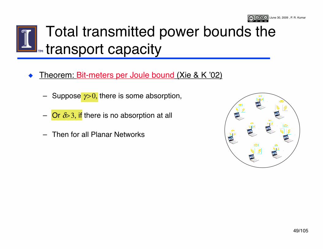
Total transmitted power bounds the transport capacity

  Theorem: Bit-meters per Joule bound (Xie & K ʼ02)

–  Suppose γ > 0, there is some absorption,

–  Or δ > 3, if there is no absorption at all

–  Then for all Planar Networks

  where

CT ≤ c1(γ ,δ ,ρmin )σ 2 ⋅Ptotal

c1(γ ,δ, ρmin) = 22δ +7

γ 2ρmin2δ +1

e−γρmin

2 (2 − e−γρmin

2 )

(1− e−γρmin

2 ) if γ > 0

= 22δ +5(3δ − 8)(δ − 2)2(δ − 3)ρmin

2δ −1 if γ = 0 and δ > 3

47/105

© June 30, 2009 , P. R. Kumar






  where


c1(γ ,δ, ρmin) = 22δ +7

γ 2ρmin2δ +1

e−γρmin


2 )

(1− e−γρmin

2 ) if γ > 0

= 22δ +5(3δ − 8)(δ − 2)2(δ − 3)ρmin

2δ −1 if γ = 0 and δ > 3

48/105

© June 30, 2009 , P. R. Kumar






  where


c1(γ ,δ, ρmin) = 22δ +7

γ 2ρmin2δ +1

e−γρmin


2 )

(1− e−γρmin

2 ) if γ > 0

= 22δ +5(3δ − 8)(δ − 2)2(δ − 3)ρmin

2δ −1 if γ = 0 and δ > 3

49/105

© June 30, 2009 , P. R. Kumar




–  Or δ> 3, if there is no absorption at all


  where


c1(γ ,δ, ρmin) = 22δ +7

γ 2ρmin2δ +1

e−γρmin


2 )

(1− e−γρmin

2 ) if γ > 0

= 22δ +5(3δ − 8)(δ − 2)2(δ − 3)ρmin

2δ −1 if γ = 0 and δ > 3

50/105

© June 30, 2009 , P. R. Kumar






  where


c1(γ ,δ, ρmin) = 22δ +7

γ 2ρmin2δ +1

e−γρmin


2 )

(1− e−γρmin

2 ) if γ > 0

= 22δ +5(3δ − 8)(δ − 2)2(δ − 3)ρmin

2δ −1 if γ = 0 and δ > 3

51/105

© June 30, 2009 , P. R. Kumar






  where


c1(γ ,δ, ρmin) = 22δ +7

γ 2ρmin2δ +1

e−γρmin


2 )

(1− e−γρmin

2 ) if γ > 0

= 22δ +5(3δ − 8)(δ − 2)2(δ − 3)ρmin

2δ −1 if γ = 0 and δ > 3

Energy cost of communicating one bit-meter in a sensor network

52/105

© June 30, 2009 , P. R. Kumar






  where


c1(γ ,δ, ρmin) = 22δ +7

γ 2ρmin2δ +1

e−γρmin


2 )

(1− e−γρmin

2 ) if γ > 0

= 22δ +5(3δ − 8)(δ − 2)2(δ − 3)ρmin

2δ −1 if γ = 0 and δ > 3

Energy cost of communicating one bit-meter in a wireless network

53/105

© June 30, 2009 , P. R. Kumar

O(n) upper bound on Transport Capacity

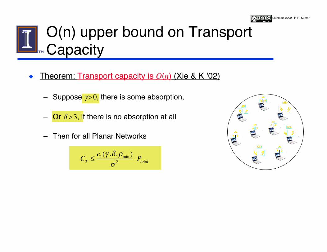
  Theorem: Transport capacity is O(n) (Xie & K ʼ02)




  Same as square root law based on treating interference as noise –  since area A grows like Ω(n)

  So multi-hop with decode and forward with interference treated as noise is order optimal architecture whenever Θ(n) can be achieved

CT ≤ c1(γ ,δ ,ρmin )Pindσ 2 ⋅n

Θ An( ) = Θ n( )

54/105

© June 30, 2009 , P. R. Kumar









Θ An( ) = Θ n( )

55/105

© June 30, 2009 , P. R. Kumar




–  Or δ> 3, if there is no absorption at all





Θ An( ) = Θ n( )

56/105

© June 30, 2009 , P. R. Kumar






  Same as square root law baseδ on treating interference as noise –  since area A grows like Ω(n)



Θ An( ) = Θ n( )

57/105

© June 30, 2009 , P. R. Kumar








Θ An( ) = Θ n( )


58/105

© June 30, 2009 , P. R. Kumar






  Same as square root law based on treating interference as noise –  since area A γγrows like Ω(n)



Θ An( ) = Θ n( )

Ptotal = Pind · n

59/105

© June 30, 2009 , P. R. Kumar









Θ An( ) = Θ n( )

Ptotal = Pind · n

60/105

© June 30, 2009 , P. R. Kumar









Θ An( ) = Θ n( )

Ptotal = Pind · n

61/105

© June 30, 2009 , P. R. Kumar









Θ An( ) = Θ n( )

Ptotal = Pind · n

62/105

© June 30, 2009 , P. R. Kumar

62

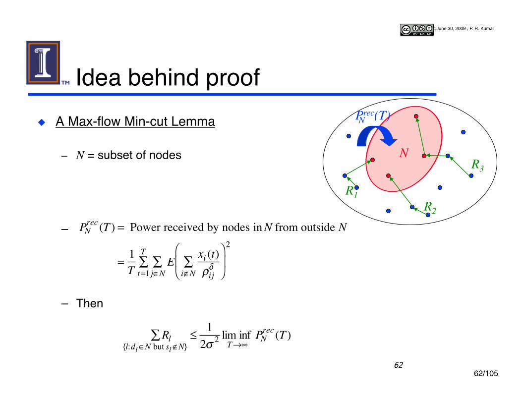
Idea behind proof   A Max-flow Min-cut Lemma

–  N = subset of nodes

– 

–  Then

Rl{l:dl∈N but sl∉N}

∑ ≤1

2σ 2 lim infT→∞

PNrec (T )

PNrec (T ) = Power received by nodes in N from outside N

=1T

Exi (t)ρijδ

i∉N∑

⎛

⎝ ⎜

⎞

⎠ ⎟

j∈N∑

t=1

T∑

2

Prec(T) N

R1 R2

R3 N

63/105

© June 30, 2009 , P. R. Kumar

63

To obtain power bound on transport capacity   Idea of proof

  Consider a number of cutsone meter apart

  Every source-destinationpair (sl,dl) with source ata distance ρl is cut by aboutρl cuts

  Thus

ρl

�

Rlρll∑ ≤ c Rl

{l is cut by Nk }∑

Nk∑ ≤ c

2σ 2 liminfT→∞

PNkrec(T ) ≤ cPtotal

σ 2Nk∑

64/105

© June 30, 2009 , P. R. Kumar

64


  Theorem




where

CT ≤ c1(γ ,δ ,ρmin)Pindσ 2

⋅n

c1(γ ,δ, ρmin) = 22δ +7

γ 2ρmin2δ +1

e−γρmin


2 )

(1− e−γρmin

2 ) if γ > 0

= 22δ +5(3δ − 8)(δ − 2)2(δ − 3)ρmin

2δ −1 if γ = 0 and δ > 3

65/105

© June 30, 2009 , P. R. Kumar

Order optimality of multi-hop transport

66/105

© June 30, 2009 , P. R. Kumar

66

  Random traffic

  Multihop can provide bits/second

–  for every source –  with probability →1 –  as the number of nodes n → ∞

  Nearly optimal since transport

capacity achieved is

Order optimality of multihop transport in a randomly chosen scenario

Ω 1n log n

⎛

⎝ ⎜ ⎜

⎞

⎠ ⎟ ⎟

Ω nlog n

⎛

⎝ ⎜ ⎜

⎞

⎠ ⎟ ⎟

67/105

© June 30, 2009 , P. R. Kumar

67

  Random traffic






Ω 1n log n

⎛

⎝ ⎜ ⎜

⎞

⎠ ⎟ ⎟

Ω nlog n

⎛

⎝ ⎜ ⎜

⎞

⎠ ⎟ ⎟

68/105

© June 30, 2009 , P. R. Kumar

68

  Random traffic






Ω 1n log n

⎛

⎝ ⎜ ⎜

⎞

⎠ ⎟ ⎟

Ω nlog n

⎛

⎝ ⎜ ⎜

⎞

⎠ ⎟ ⎟

69/105

© June 30, 2009 , P. R. Kumar

69

  Random traffic






Ω 1n log n

⎛

⎝ ⎜ ⎜

⎞

⎠ ⎟ ⎟

Ω nlog n

⎛

⎝ ⎜ ⎜

⎞

⎠ ⎟ ⎟

70/105

© June 30, 2009 , P. R. Kumar

70

  Random traffic






Ω 1n log n

⎛

⎝ ⎜ ⎜

⎞

⎠ ⎟ ⎟

Ω nlog n

⎛

⎝ ⎜ ⎜

⎞

⎠ ⎟ ⎟

71/105

© June 30, 2009 , P. R. Kumar

71

  Random traffic






Ω 1n log n

⎛

⎝ ⎜ ⎜

⎞

⎠ ⎟ ⎟

Ω nlog n

⎛

⎝ ⎜ ⎜

⎞

⎠ ⎟ ⎟

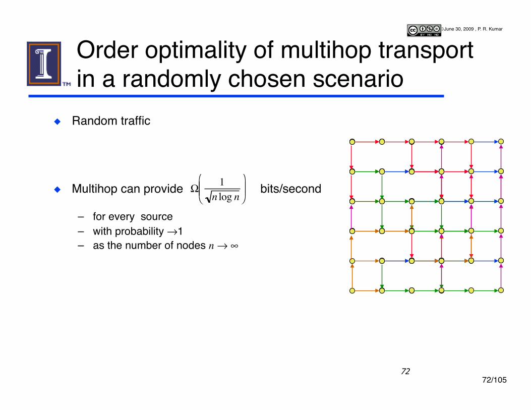
72/105

© June 30, 2009 , P. R. Kumar

72

  Random traffic






Ω 1n log n

⎛

⎝ ⎜ ⎜

⎞

⎠ ⎟ ⎟

Ω nlog n

⎛

⎝ ⎜ ⎜

⎞

⎠ ⎟ ⎟

73/105

© June 30, 2009 , P. R. Kumar

73

  Random traffic






Ω 1n log n

⎛

⎝ ⎜ ⎜

⎞

⎠ ⎟ ⎟

Ω nlog n

⎛

⎝ ⎜ ⎜

⎞

⎠ ⎟ ⎟

74/105

© June 30, 2009 , P. R. Kumar

74

  Random traffic





  So Random case ≈ Best Case


Ω 1n log n

⎛

⎝ ⎜ ⎜

⎞

⎠ ⎟ ⎟

Ω nlog n

⎛

⎝ ⎜ ⎜

⎞

⎠ ⎟ ⎟

75/105

© June 30, 2009 , P. R. Kumar

75

What can multihop transport achieve?

  Theorem

–  A set of rates (R1, R2, … , Rl) can besupported by multi-hop transport if

–  Traffic can be routed, possibly overmany paths, such that

–  No node has to relay more than

–  where is the longest distance of a hop

and

ρ

S e−2γρ Pind ρ 2δ

c3(γ ,δ ,ρmin)Pind+σ 2⎛

⎝ ⎜ ⎜

⎞

⎠ ⎟ ⎟

c3(γ ,δ ,ρmin) = 23+2δ e−γρmin

γρmin1+2δ if γ > 0

= 22+2δ

ρmin2δ (δ −1)

if γ = 0 and δ > 1

76/105

© June 30, 2009 , P. R. Kumar

76

Multihop transport can achieve Θ(n)   Theorem



–  Then in a regular planar network

where

CT ≥ S e−2γ Pindc2 (γ ,δ )Pind +σ 2

⎛

⎝ ⎜ ⎜

⎞

⎠ ⎟ ⎟ ⋅n

c2(γ ,δ ) = 4(1+4γ )e−2γ −4e−4γ

2γ (1− e−2γ ) if γ > 0

= 16δ 2 + (2π −16)δ −π(δ −1)(2δ −1)

if γ = 0 and δ >1

n sources each sendingover a distance n

77/105

© June 30, 2009 , P. R. Kumar

77

Optimality of multi-hop transport   Corollary

–  So if γ > 0 or δ > 3

–  And multi-hop achieves Θ(n)

–  Then it is optimal with respect to the transport capacity- up to order

  Example

78/105

© June 30, 2009 , P. R. Kumar

78

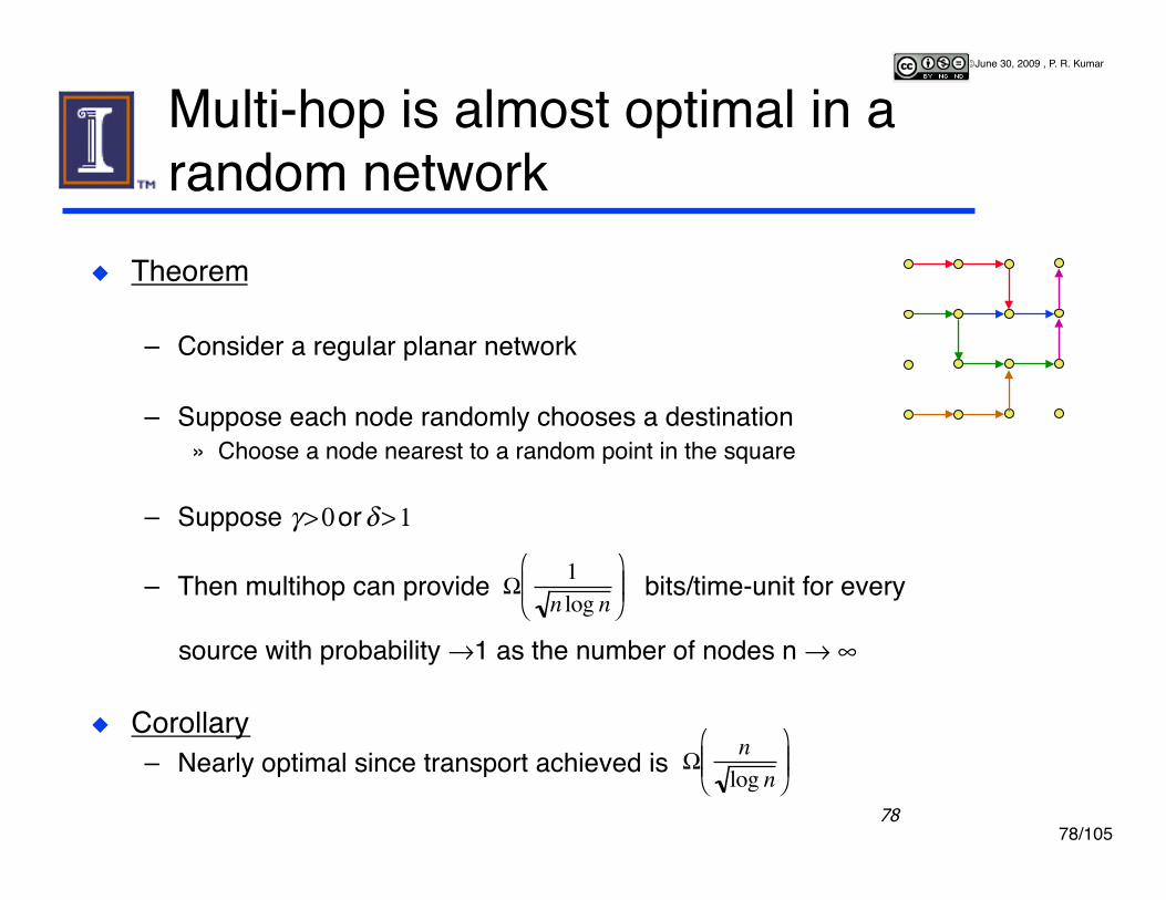
Multi-hop is almost optimal in a random network

  Theorem

–  Consider a regular planar network

–  Suppose each node randomly chooses a destination »  Choose a node nearest to a random point in the square

–  Suppose γ > 0 or δ > 1

–  Then multihop can provide bits/time-unit for every

source with probability →1 as the number of nodes n → ∞

  Corollary –  Nearly optimal since transport achieved is

Ω 1n log n

⎛

⎝ ⎜ ⎜

⎞

⎠ ⎟ ⎟

Ω nlog n

⎛

⎝ ⎜ ⎜

⎞

⎠ ⎟ ⎟

79/105

© June 30, 2009 , P. R. Kumar

79

Idea of proof for random source -destination pairs   Simpler than Gupta-Kumar since

cells are square and containone node each

  A cell has to relay traffic if a randomstraight line passes through it

  How many random straight linespass through cell?

  Use Vapnik-Chervonenkis theoryto guarantee that no cell is overloaded

80/105

© June 30, 2009 , P. R. Kumar

The effect of fading

81/105

© June 30, 2009 , P. R. Kumar

Large path loss: Effect of fading   n nodes located on the plane

–  Base-band model

–  Consider δ > 3 or γ > 0

–  Then even with full channel state information,

–  Even with iid unknown channel, for regular node locations,

there is a scheme yielding 81/23 (Xue, Xie and K ʻ03)

82/105

© June 30, 2009 , P. R. Kumar

82

What happens when the attenuation is very low?

83/105

© June 30, 2009 , P. R. Kumar

83

A feasible rate for the Gaussian multiple-relay channel

  Theorem

–  Suppose αij = attenuation from i to j�

–  Choose power Pik = power usedby i intended directly for node k

–  where

–  Then

is feasible

  Proof based on coding

αij

i

j

Pik i k

R < min1≤ j≤n

S1σ 2

αij Piki=0

k−1∑

⎛ ⎝ ⎜ ⎞

⎠ ⎟ 2

k=1

j∑

⎛

⎝ ⎜

⎞

⎠ ⎟

Pikk =i

M∑ ≤ Pi

84/105

© June 30, 2009 , P. R. Kumar

84

A group relaying version   Theorem

–  A feasible rate for group relaying

–  R < R < min1≤ j≤M

S1σ 2 αNiNj Pik / ni ⋅ni

i=0

k −1∑

⎛ ⎝ ⎜ ⎞

⎠ ⎟ 2

k =1

j∑

⎛

⎝ ⎜

⎞

⎠ ⎟

ni

85/105

© June 30, 2009 , P. R. Kumar

85

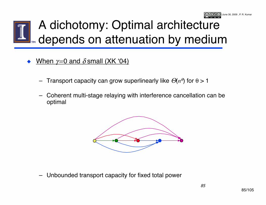
A dichotomy: Optimal architecture depends on attenuation by medium

  When γ = 0 and δ small (XK ʻ04)

–  Transport capacity can grow superlinearly like Θ(nθ) for θ > 1

–  Coherent multi-stage relaying with interference cancellation can be optimal

–  Unbounded transport capacity for fixed total power

86/105

© June 30, 2009 , P. R. Kumar

86

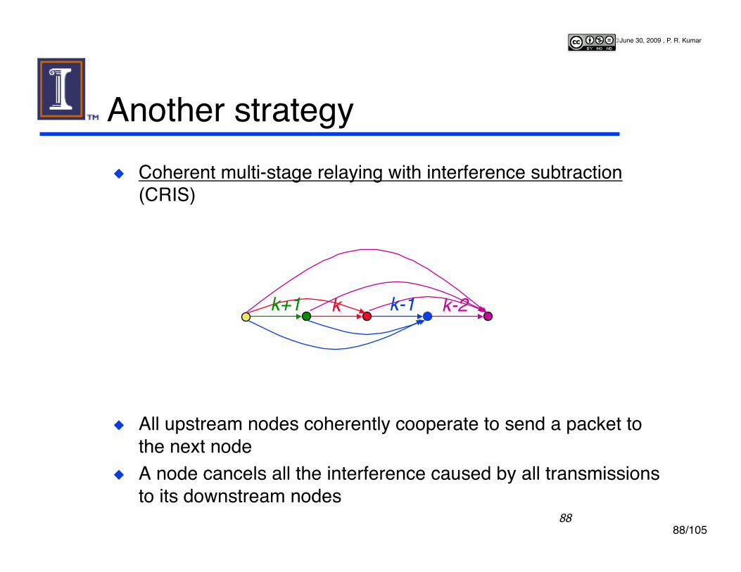
  Coherent multi-stage relaying with interference subtraction (CRIS)

  All upstream nodes coherently cooperate to send a packet to the next node

  A node cancels all the interference caused by all transmissions to its downstream nodes

Another strategy

k-1 k-2 k-3 k

k k-1 k-2 k+1

87/105

© June 30, 2009 , P. R. Kumar

87




Another strategy

k

k k+1

88/105

© June 30, 2009 , P. R. Kumar

88




Another strategy

k k-1 k-2 k+1

89/105

© June 30, 2009 , P. R. Kumar

89

Unbounded transport capacity can be obtained for fixed total power   Theorem

–  Suppose γ = 0, there is no absorption at all,

–  And δ < 3/2

–  Then CT can be unbounded in regular planar networkseven for fixed Ptotal

  Theorem –  If γ = 0 and δ < 1 in regular planar networks –  Then no matter how many many nodes there are –  No matter how far apart the source and destination are chosen

–  A fixed rate Rmin can be provided for the single-source destination pair

90/105

© June 30, 2009 , P. R. Kumar

90

Idea of proof of unboundedness   Linear case: Source at 0, destination at n

  Choose

  Planar case

Pik =P

(k − i)α kβ

0 1 i k n

Pik

Source Destination

Source 0 iq rq

Destination (i+1)q

iq-1

91/105

© June 30, 2009 , P. R. Kumar

91

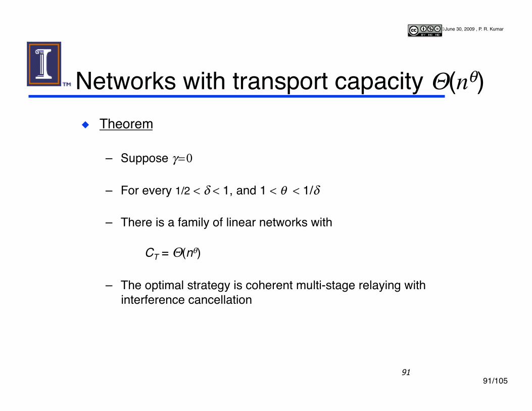
Networks with transport capacity Θ(nθ)   Theorem

–  Suppose γ = 0 �

–  For every 1/2 < δ < 1, and 1 < θ < 1/δ

–  There is a family of linear networks with

CT = Θ(nθ)

–  The optimal strategy is coherent multi-stage relaying with interference cancellation

92/105

© June 30, 2009 , P. R. Kumar

92

Idea of proof   Consider a linear network

  Choose

  A positive rate is feasible from source to destination for all n –  By using coherent multi-stage relaying with interference cancellation �

  To show upper bound –  Sum of power received by all other nodes from any node j is bounded –  Source destination distance is at most nθ

0 1 iθ kθ nθ

Pik

Source Destination

Pik =P

(k − i)α where 1<α < 3− 2θδ

93/105

© June 30, 2009 , P. R. Kumar

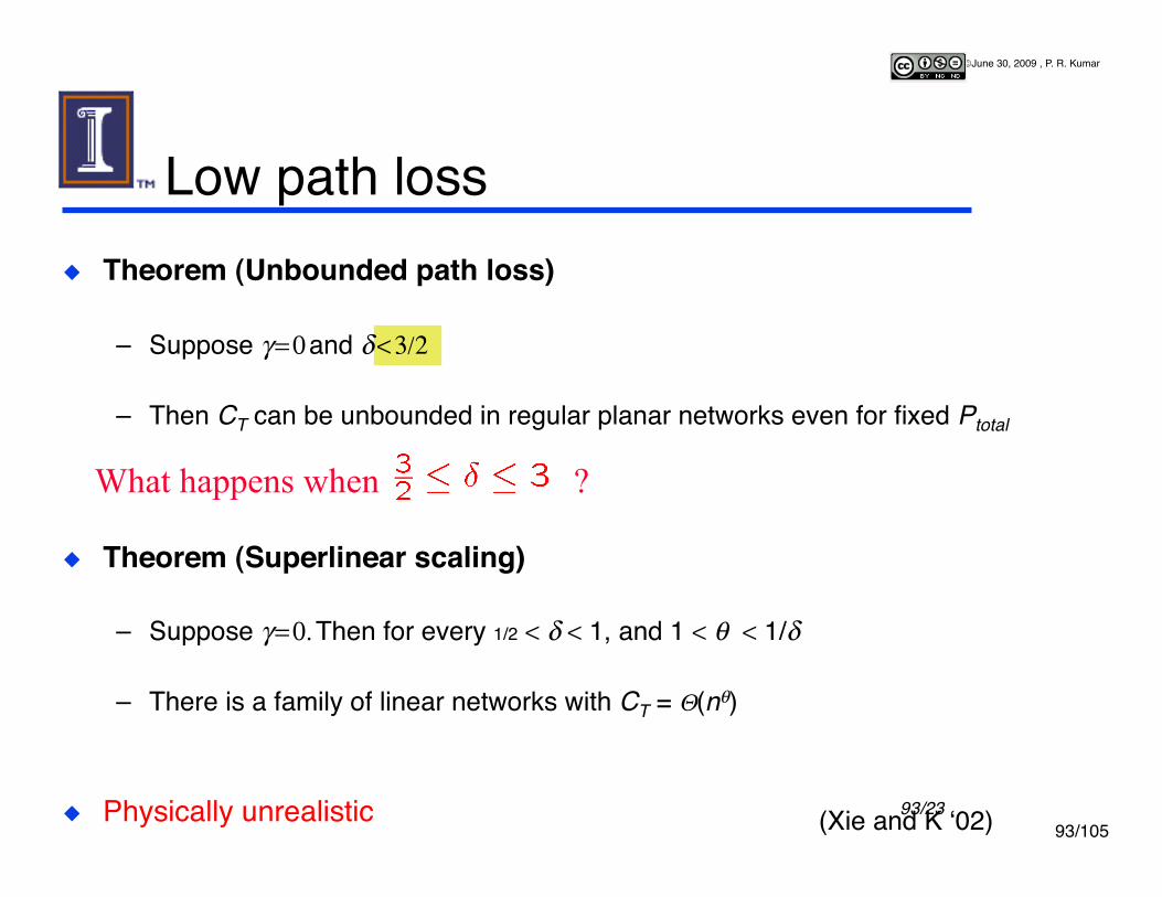
Low path loss   Theorem (Unbounded path loss)

–  Suppose γ = 0 and δ < 3/2�

–  Then CT can be unbounded in regular planar networks even for fixed Ptotal

  Theorem (Superlinear scaling)

–  Suppose γ = 0. Then for every 1/2 < δ < 1, and 1 < θ < 1/δ

–  There is a family of linear networks with CT = Θ(nθ)

  Physically unrealistic

What happens when ?

(Xie and K ʻ02) 93/23

94/105

© June 30, 2009 , P. R. Kumar

Recent work

95/105

© June 30, 2009 , P. R. Kumar

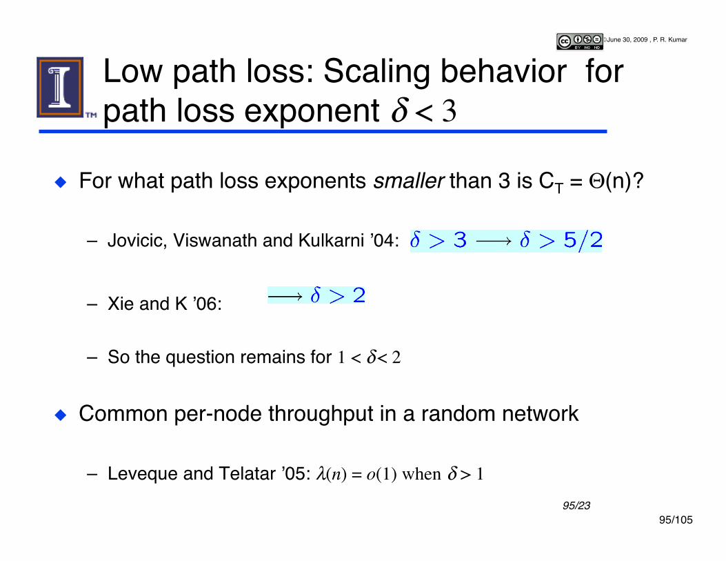
Low path loss: Scaling behavior for path loss exponent δ < 3

  For what path loss exponents smaller than 3 is CT = Θ(n)?

–  Jovicic, Viswanath and Kulkarni ʼ04:

–  Xie and K ʼ06:

–  So the question remains for 1 < δ < 2

  Common per-node throughput in a random network

–  Leveque and Telatar ʼ05: λ(n) = o(1) when δ > 1 95/23

96/105

© June 30, 2009 , P. R. Kumar

What is the scaling behavior in the range

96/23

1 < δ < 2

  Ozgur, Leveque and Tse ʼ07: Lower bound

  Based on cooperation -  Long range MIMO between blocks of nodes -  Intra-cluster cooperation -  Transmit and receive cooperation

-  Xie ʼ08: Exact study of pre-constant and shows it is o(1)   Niessen, Gupta and Shah ʻ08: Arbitrarily spaced nodes

nλ(n) ≥ cn2−δ −ε for 1 ≤ δ ≤32

nλ(n) ≥ c ' n for 32≤ δ ≤ 2

  Aeron and Saligrama ʼ07: How to achieve a total throughput of in a dense network Θ n2 /3( )

97/105

© June 30, 2009 , P. R. Kumar

Is “channel” the right model for massive cooperation?

  Franceschetti, Migliore, Minero ʼ08

  Number of information channels is only

  Scaling law per node

–  Limitation in spatial degrees of freedom –  Not based on empirical path-loss models and stochastic fading models –  Depends only on geometry

97/23

O n( )O

log2 nn

⎛⎝⎜

⎞⎠⎟

98/105

© June 30, 2009 , P. R. Kumar

Paper by Lloyd, Giovannetti and Maccone

98/23

99/105

© June 30, 2009 , P. R. Kumar

Remarks   Studied networks with arbitrary numbers of nodes

–  Explicitly incorporated distance in model »  Distances between nodes »  Attenuation as a function of distance »  Distance is also used to measure transport capacity

  Make progress by asking for less –  Instead of studying capacity region, study the transport capacity –  Instead of asking for exact results, study the scaling laws

»  The exponent is more important »  The preconstant is also important but is secondary - so bound it

–  Draw some broad conclusions »  Optimality of multi-hop when absorption or large path loss »  Optimality of coherent multi-stage relaying with interference cancellation when no

absorption and very low path loss

  Open problems abound –  What happens for intermediate path loss when there is no absorption –  The channel model is simplistic, …... –  …..

100/105

© June 30, 2009 , P. R. Kumar

References-1   C. E. Shannon, "A mathematical theory of communication", Bell Syst. Tech.

J.", Vol 27, pp. 379--423", 1948.   C. E. Shannon, "Communication in the presence of noise", Proceedings of

the IRE, vol. 37, pp. 10--21, 1949.   C. E. Shannon and W. Weaver The Mathematical Theory of Information,

University of Illinois Press, Urbana, 1949.   R. G. Gallager, Information Theory and Reliable Communication, John Wiley

and Sons, New York, 1968.   T. Cover and J. Thomas, Elements of Information Theory, Wiley and Sons,

New York, 19103.   R ~Ahlswede, ``Multi-way communication channels,ʼʼ in Proceedings of the

2nd Int. Symp. Inform. Theory (Tsahkadsor, Armenian S.S.R.), (Prague), pp. 23-52, Publishing House of the Hungarian Academy of Sciences, 1971.

  H. Liao, Multiple access channels. PhD thesis, University of Hawaii, Honolulu, HA, 1972. Department of Electrical Engineering.

  T. Cover, “Broadcast channels,” IEEE Trans. Inform. Theory, vol. 18, pp. 2-14, 1972.

101/105

© June 30, 2009 , P. R. Kumar

  P. Bergmans, ``Random coding theorem for broadcast channels with degraded components,'ʼ IEEE Trans. Inform. Theory, vol. 19, pp. 197—207, 1973.

  P. Bergmans, ``A simple converse for broadcast channels with additive white Gaussian noise,'ʼ IEEE Trans. Inform. Theory, vol.~20, pp. 279-280, 1974.

  E. C. Van der Meulen, “Three-terminal communication channels,” Adv. Appl. Prob., vol. 3, pp. 120-154, 1971.

  T. Cover and A.~E. Gamal, ``Capacity theorems for the relay channel,'ʼ IEEE Trans. Inform. Theory, vol.~25, pp.~572--584, 1979

  M. Franceschetti, J. Bruck, and L. J. Schulman, “A random walk model of wave propagation,” IEEE Trans. Antennas Propag., vol. 52, no. 5, pp. 1304–1317, May 2004.

  Liang-Liang Xie and P. R. Kumar, “New Results in Network Information Theory: Scaling Laws for Wireless Communication and Optimal Strategies for Information Transport,” Proceedings of 2002 IEEE Information Theory Workshop, Bangalore, India, pp. 24–25, October 20-25, 2002.

References-2

102/105

© June 30, 2009 , P. R. Kumar

References-3   Liang-Liang Xie and P. R. Kumar, “A Network Information Theory for

Wireless Communication: Scaling Laws and Optimal Operation,” IEEE Transactions on Information Theory, vol. 50, no. 5, pp. 748–767, May 2004.

  Piyush Gupta and P. R. Kumar, “Towards an Information Theory of Large Networks: An Achievable Rate Region,” IEEE Transactions on Information Theory, vol. 49, no. 8, pp. 1877–1894, August 2003.

  Liang-Liang Xie and P. R. Kumar, “An Achievable Rate for the Multiple-Level Relay Channel,” IEEE Transactions on Information Theory, vol. 51, no. 4, pp. 1348–1358, April 2005.

  Feng Xue and P. R. Kumar, Scaling Laws for Ad Hoc Wireless Networks: An Information Theoretic Approach. NOW Publishers, Delft, The Netherlands, 2006.

  Liang-Liang Xie and P. R. Kumar, “On the Path-Loss Attenuation Regime for Positive Cost and Linear Scaling of Transport Capacity in Wireless Networks,” Joint Special Issue of IEEE Transactions on Information Theory and IEEE/ACM Transactions on Networking on Networking and Information Theory, pp. 2313–2328, vol. 52, no. 6, June 2006.

103/105

© June 30, 2009 , P. R. Kumar

References-4

  Liang-Liang Xie and P. R. Kumar, “Multisource, multidestination, multirelay wireless networks,” IEEE Transactions on Information Theory, Special issue on Models, Theory and Codes for Relaying and Cooperation in Communication Networks, vol. 53, no. 10, pp. 3586–3595, October 2007.

  Feng Xue, Liang-Liang Xie, and P. R. Kumar, “The Transport Capacity of Wireless Networks over Fading Channels,” IEEE Transactions on Information Theory, vol. 51, no. 3, pp. 834–847, March 2005.

  O. Lévêque and I. E. Telatar, “Information-theoretic upper bounds on the capacity of large, extended ad hoc wireless networks,” IEEE Trans. Inf. Theory, vol. 51, no. 3, pp. 858–865, Mar. 2005.

  A. Jovicic, P. Viswanath and S. R. Kulkarni,. “Upper Bounds to Transport Capacity of Wireless Networks”,. IEEE Transactions on Information Theory, 50(11):2555--2565, 2004.

104/105

© June 30, 2009 , P. R. Kumar

References-5   S. Aeron, V. Saligrama, Wireless Ad-hoc networks: Strategies and scaling

laws in Fixed SNR regime, IEEE Trans. on Info Theory (to appear)   Ayfer Ozgür, Olivier Lévêque, and David N. C. Tse, Hierarchical

Cooperation Achieves Optimal Capacity Scaling in Ad Hoc Networks, in IEEE Transactions on Information Theory, vol. 53, no. 10, Oct 2007,

  Liang-Liang Xie, On Information-Theoretic Scaling Laws for Wireless Networks, arXiv:0809.1205v2 [cs.IT], 2008

  Urs Niesen, Piyush Gupta, and Devavrat Shah, On Capacity Scaling in Arbitrary Wireless Networks, to appear in IEEE Transactions on Information Theory arXiv:0711.2745v2 [cs.IT]

  Massimo Franceschetti, Marco D. Migliore, Paolo Minero, The Capacity of Wireless Networks: Information-theoretic and Physical Limits, Forty-Fifth Annual Allerton Conference Allerton House, UIUC, Illinois, September 26-28, 2007. IEEE Trans. on Information Theory, in press.

105/105

© June 30, 2009 , P. R. Kumar

http://decision.csl.illinois.edu/~prkumar/html_files/talks.html

Wireless Network information Theory - CESGcesg.tamu.edu/.../prk_present/Wireless-Network-Information-Theory.pdfModel for wireless network information theory 33 ... Shannonʼs formulation

Documents