Wirelength Estimation based on Rent Exponents of Partitioning and Placement 1 Xiaojian Yang, Elaheh Bozorgzadeh, and Majid Sarrafzadeh Synplicity Inc. Sunnyvale, CA 94086 [email protected] Computer Science Department University of California at Los Angeles Los Angeles, CA 90095 elib,[email protected] Abstract Wirelength estimation is one of the most important Rent’s rule applica- tions. Traditionally, the Rent exponent is extracted using recursive bipar- titioning. However, the obtained exponent may not be appropriate for the purpose of wirelength estimation. In this paper, we propose the concepts of partitioning-based Rent exponent and placement-based Rent exponent. The relationship between these two exponents is analyzed and empirically verified. Experiments on large industrial circuits show that for wirelength estimation, the Rent exponent extracted from placement is more appropriate than that from partitioning. 1 This work was supported by NSF under Grant #CCR-0090203. A preliminary version of this paper appeared in Proc. Int. Workshop on System-Level Interconnect Prediction, pp.25-31, April 2001. 1

Welcome message from author
This document is posted to help you gain knowledge. Please leave a comment to let me know what you think about it! Share it to your friends and learn new things together.
Transcript

Wirelength Estimation based on Rent Exponents ofPartitioning and Placement 1
Xiaojian Yang, Elaheh Bozorgzadeh, and Majid Sarrafzadeh
Synplicity Inc.Sunnyvale, CA 94086
Computer Science DepartmentUniversity of California at Los Angeles
Los Angeles, CA 90095elib,[email protected]
Abstract
Wirelength estimation is one of the most important Rent’s rule applica-tions. Traditionally, the Rent exponent is extracted using recursive bipar-titioning. However, the obtained exponent may not be appropriate for thepurpose of wirelength estimation. In this paper, we propose the conceptsof partitioning-based Rent exponent and placement-based Rent exponent.The relationship between these two exponents is analyzed and empiricallyverified. Experiments on large industrial circuits show that for wirelengthestimation, the Rent exponent extracted from placement is more appropriatethan that from partitioning.
1This work was supported by NSF under Grant #CCR-0090203. A preliminary version of thispaper appeared inProc. Int. Workshop on System-Level Interconnect Prediction, pp.25-31, April2001.
1

1 Introduction
Rent’s rule was first described by Landman and Russo in 1971 [1]. It relates the
number of external connections and the number of cells for a given block in a
partitioned circuit. Rent’s rule has been observed on many real designs. It has ex-
tensive applications in VLSI design. A priori wirelength estimation is one of the
most important applications of Rent’s rule. The classical work [2, 3] gives good
estimates for post layout interconnect wirelength. More recent work improves
the estimation by consideringoccupying probability [4] or recursively applying
Rent’s rule throughout an entire monolithic system [5]. Extension of basic wire-
length estimation, including routing utilization estimation [6], congestion estima-
tion [7], 3-D design performance analysis [8, 9], interconnect fan-out distribution
[10], are also of value for physical design automation tools.
Rent’s rule correlation is commonly presented byT � tGp, whereT andG
are the number of external nets and the number of cells for a block, respectively.
t is often called Rent coefficient, which is the average number of pins per cell.
The Rent exponent,p, is the feature parameter of the circuit. Hagen, et. al.,
studied Rent exponents of circuits by comparing different partitioning approaches
[11]. They proposed theintrinsic Rent exponent which indicates the minimum
Rent exponent obtained by an optimal partitioning method. Furthermore, it is
argued that the Rent exponent is a measure of partitioning approach. Smaller Rent
exponent means that the partitioning approach used to obtain this Rent exponent
is better. Other related work includes the proposal of Region III [12], the local
variation of the Rent exponent [13] and Rent exponent prediction [14].
One of the fundamental issues in Rent’s rule study is the extraction of the
Rent exponent from a given circuit. Traditionally, Rent exponents were obtained
by partitioning circuits and analyzing the partitioned subcircuits. In [1] a multi-
way partitioning algorithm is used to generate partitioning instances. For each
instance, the average subcircuit size and the average number of pins (external
nets) per subcircuit are calculated and the result represents a data point on a log-
log scale. A linear regression is then applied to find the slope of the fitted line,
2

which is the Rent exponent of the circuit. A similar strategy was employed in
[11].
In this paper we propose a different method of extracting the Rent exponent
for a given circuit, that is, achieving the Rent exponent from an existing place-
ment. This is to better understand the notion of Rent parameters, and is not to
suggest that the Rent parameters should be obtained from placement. The issue
of the Rent exponents in partitioning and placement was studied in [15, 16, 17].
In this work we try to evaluate the relationship between the Rent exponents from
empirical point of view. We argue that Rent exponents extracted from partition-
ing and placement are not identical. However, there exists a relationship between
these two exponents. We theoretically analyze and empirically evaluate this re-
lationship. All the experiments are conducted on mid-size or large benchmark
circuits in order to provide useful information close to real world. To take the
variety of placement tools into account, three recent placement tools (Capo [18],
Feng Shui [19] andDragon [20]) are used in this work. There is no doubt that ex-
tracting the Rent exponent from placement is much slower than from partitioning.
Furthermore, the Rent exponent is indeed useless after placement stage. However,
studies on this issue will provide a different point of view on Rent’s rule and its
applications.
The rest of the paper is organized as follows: Section 2 defines the Rent ex-
ponent for partitioning and placement. The relationship between two different
Rent exponents is analyzed. Section 3 presents experimental results to support the
claim in section 2. In section 4, wirelength estimation methods based on Rent’s
rule are evaluated. Section 5 gives the conclusion of the paper.
2 Rent Exponents for Partitioning and Placement
2.1 Extracting Rent Exponents
Conventional approaches of extracting the Rent exponent are based on partition-
ing. Analyzing an existing placement of a circuit, however, will give a new way
3

of measuring the Rent exponent. It is no surprise that the Rent exponents ob-
tained from two methods are different. Partitioning based extraction focuses on
the topological structure of the circuit, while placement based extraction concen-
trates on the geometrical information of the placed circuit. Figure 1, algorithm 1
and algorithm 2 explain the two different methods to extract the Rent exponent.
BipartitioningRecursively
...... ...Partitioning tree Partitioning Rent’s exponent
ToolPlacement ...
Placement Rent’s exponentPlacement
Figure 1: Rent exponent extraction from recursive bipartitioning (upper half) andplacement (lower half).
Algorithm 1 Extract-Rent-by-Partitioning(C)Input: Circuit C � �V�E�Output: Rent exponentp
1. Recursively bipartition the original circuits. At each recursive level, calculate the av-erage number of cells per partition and the average number of external nets over allpartitions. Save the data pair to�Gi�Ti� wherei is the depth of recursive partitioning.Partitioning stops when reaching a given depthn.
2. Apply linear regression on the log-log scaled data pairs:�Gk�Tk���Gk�1�Tk�1�� �����Gn�Tn� (k is a given number around 4-6)
3. Return the slope of the fitted line by linear regression.
In the first method Extract-Rent-by-Partitioning, a partitioning algorithm is
used to recursively bisection the original circuits. At each bisection level, aver-
age number of cells and average number of external nets for all subcircuits are
4

Algorithm 2 Extract-Rent-by-Placement(C)Input: CircuitC � �V�E�Output: Rent exponentp�
Place the circuit on two dimensional plane,for i� 1 to a given depthn do
Divide the core area into 2i regular regions;Each region contains a group of cells; Compute the average number of cells per groupand the average number of external nets over all cell groups.Save the data pair to�Gi�Ti�.
end forApply linear regression on the log-log scaled data pairs:�G k�Tk���Gk�1�Tk�1�� �����Gn�Tn� (k isa given number around 4-6 to skip Region II)Return the slope of the fitted line by linear regression
recorded. This pair of numbers form a point on a log-log plane. After achieving
enough points, a linear regression is performed to obtain the Rent exponent.
To extract the Rent exponent from placement, we first place the circuit using
existing placement tools. Then we divide the layout area into several regions and
analyze the subcircuit in each region. The average number of cells and average
number of external nets for all regions are recorded. This dividing step continues
to a given depth. Then we obtain the Rent exponent by linear regression on the
recorded points.
A detailed step of implementingExtract-Rent-by-Partitioning is as follows:
when a subcircuit is partitioned into two smaller subcircuits, the nets which con-
nect the outside cells are not considered. For multi-terminal nets, part of the net
will be reserved and the external pins are ignored.
We define the terms for partitioning-based Rent exponent and placement-based
Rent exponent:
Definition 1 For a given circuit and a bipartition approach, the partitioning Rent
exponent p is the output of the algorithm Extract-Rent-by-Partitioning().
Definition 2 For a given circuit and a wirelength optimized placement of the cir-
cuit, the placement Rent exponent p� is the output of the algorithm Extract-Rent-
by-Placement().
5

2.2 Relationship between Exponents
Since partitioning and placement are related problems, the partitioning Rent ex-
ponent and placement Rent exponent might also be related. Partitioning tends
to minimize the number of cut nets for two subcircuits, which in turn leads to a
small number of external nets for a subcircuit. While in a wirelength driven place-
ment, the cells which are tightly connected are placed closer. There is no effort on
reducing the crossing nets between two regions.
As shown in Figure 2, for a given subcircuit with sizeG1, the number of
external nets in placement is larger than that in partitioning. Two straight lines
represent linear regression results for partitioning and placement. Both lines share
the samey-intercept because the Rent coefficientt is fixed for a given circuit.
Therefore the slope of the line which is obtained by partitioning is smaller than
the slope of the other line, which is done by placement.
p � p�
log Glog G1
log t
T = t G
T = t G
p’
p
Placement Rent’s curve
Partitioning Rent’s curve
log T
Figure 2: Comparison between partitioning Rent exponent and placement Rentexponent
If the placement engine is a min-cut class approach, we can derive a relation-
ship between the two Rent exponents. Figure 3 illustrates two different biparti-
6

tioning problems. In figure 3(a), the partitioner only considers the interconnects
between cells of the subcircuit to be partitioned. We call this problempure bi-
partitioning problem. In Figure 3(b), external nets, which connect cells of this
subcircuit to other subcircuits, are also included into partitioning problem. This
is the bipartitioning problem withterminal propagation, which is normally used
in min-cut class placement tools, as shown in Figure 3(c). It is the difference be-
tween these two bipartitioning approaches which explains the difference between
partitioning Rent exponent and placement Rent exponent.
In the pure bipartitioning problem without terminal propagation, assuming the
sizes of the subcircuits after partitioning areG1 andG2. Let C be the number of
cut nets (figure 3(a)). For the bipartitioning process with terminal propagation, let
C� be the number of cut nets of bipartitioning. We haveC � � C because of the
effect of the external nets. According to Rent’s rule, from Figure 3(a), we obtain:
T1�C � T � tGp1� (1)
whereT is the total number of external nets for subcircuitG1. T1 is the number of
the external nets which arenot cut nets.t is Rent coefficient, the average number
of pins per cell.p is the partitioning Rent exponent.
We assume that all the nets are two-terminal nets. Applying Rent’s rule on the
original subcircuit before partitioning, we obtain:
T1�T2 � t�G1�G2�p (2)
For simplicity, we assume that in a balanced bipartitioning,G1 � G2 andT1 �
T2. From equation (1) and (2), we have:
T1 � 2p�1T
In the bipartitioning with terminal propagation (Figure 3(b)), there areT1 ex-
ternal nets connected to other subcircuits. These nets connect to cells that are
located either to the left or to the right of original circuit. The external nets con-
nected to the right side (T1�2 nets) will “drag” cells from left to right, thus they
7

G1 G2
C’
(a) (b)
G1 G2
C
2T’1
GT1 T2T’
(c)
Figure 3: Comparison between a pure partitioning (a) and a partitioning withterminal propagation in min-cut placement (b), (c). The former only considers theinternal nets, while the latter considers both internal nets and external nets.T1 andT2 are the number of external nets which are not cut nets for subcircuitG1 andG2,respectively.
8

may increase the cut nets of the partitioning. We assume that one such external
net increases the number of cut nets byα. α is a real number between 0 and 1. It
represents the possibility that an external net increases the number of cut nets by
one.
The same situation exists on the right subcircuit. Thus the result of partitioning
with terminal propagation will increase byαT1. Therefore for a partitioned subcir-
cuit, the number of external netsT � after terminal propagation based partitioning
is:
T � � T �αT1 � �1�α �2p�1�T
SinceT � tGp1 and T � � tGp�
1 (p and p� are partitioning Rent exponent and
placement Rent exponent, respectively), we have,
p�� p �logT �� logt
logG1� logT � logt
logG1
�log�T ��T �
logG1
�log�1�α �2p�1�
logG1
Thus we have,
p� � p�log�1�α �2p�1�
logG1(3)
whereG1 should be the number of cells in a subcircuit which corresponds to a
data point. In practice we setG1 to be�V ��25 to avoid the Rent’s rule region II2.
Equation (3) shows that the placement Rent exponent (p�) is larger than the
partitioning Rent exponent (p). It should be noted that the analysis is based on
some simplifications (e.g. two-teminal nets). The valid range of Equation (3)
is limited. For example, ifp is close either 0 or 1, the equation does not give
meaningful result. However, for ordinary circuits and ordinary partitioning Rent
exponents, this equation approximately derives a placement Rent exponent which
can be used for certain estimation purposes.2Region II corresponds to a few top-most levels of the partitioning or placement where the
number of cells and the number of external nets do not follow the Rent’s rule.
9

3 Experimental Validation
Equation (3) shows that we can derive placement Rent exponentp� from the par-
titioning Rent exponentp. The following experiments are conducted to evaluate
the relationship.
3.1 Derivation of placement Rent exponent
We experimentally extract both partitioning exponent and placement exponent for
a set of circuits. The circuits are chosen from MCNC and IBM-PLACE bench-
mark suits. IBM-PLACE benchmarks are obtained by modifying ISPD98 IBM
partitioning benchmark suits [21]. Experimental circuit sizes range from 21,000
cells to 210,000 cells. For partitioning Rent exponent, we use hMetis [22] as
the partitioning tool. Unbalance factor is set to 1% in each bipartitioning call.
For placement Rent exponent, three different placement tools are used to place
the circuit and placement Rent exponents are extracted from the placed circuits.
The placement tools used in this work areCapo [18], Feng Shui [19] andDragon
[20]. All of them are recent academic works and they all integrate multi-level hy-
pergraph partitioning, a breakthrough technique in VLSI/CAD partitioning prob-
lem. Capo and Feng Shui use recursively bipartitioning approach followed by
local improvement.Dragon employs both cut and wirelength minimization in hi-
erarchical placement flow. All experiments are performed on Sun workstations
with 400MHz CPU and 128M memory. The depths of both Extract-Rent-by-
partitioning and Extract-Rent-by-placement are set to be 14, i.e., 14 data points
are collected from partitioning or placement to do linear regression. The first 5
points are discarded in order to avoid effects caused by Rent’s rule region II. Thus
the linear regression is actually carried out on 9 data points for each circuit.
Figure 4 shows a sample extraction on ibm15 circuit. The lower line is the re-
sult of linear regression on data points collected by recursive bipartitioning. Three
upper lines are obtained from placement outputs byCapo, Feng Shui andDragon.
All the slopes of three upper lines are larger than the slope of the partitioning line,
10

2
3
4
5
6
7
8
9
10
2 4 6 8 10 12
log G
log
T
points extracted from recursivebipartitioning
points extracted from Capoplacement
points extracted from FengShui placement
points extracted from Dragonplacement
fitted line for partitioning
fitted line for Capo placement
fitted line for Feng Shuiplacement
fitted line for Dragonplacement
Figure 4: Rent’s rule fitted line based on partitioning and placement for bench-mark ibm15. The lower line is the result of linear regression on data points fromrecursive bipartitioning. Three upper lines are from placement outputs.
11

supporting the relationship between partitioning Rent exponent and placement
Rent exponent discussed in Section 2.
Table 1 shows the comparison between partitioning Rent exponentp, derived
placement Rent exponentp� which is obtained from Equation (3)3, and three real
placement Rent exponentsp�� extracted from outputs of three different placement
tools. Note that the Rent exponents produced by different placement tools are
not the same. However, they do not vary much for a given circuit. Comparing
with partitioning Rent exponentp, derived placement Rent exponentp� is closer
to real placement Rent exponents, partially supporting the theoretical relationship
between two Rent exponents. However, better derivation of placement Rent ex-
ponent requires the knowledge ofα in Equation (3).
ckt #cells #nets Partition Estimated Placement Rentp��
Rentp Placep� Capo Feng Shui Dragonavqs 21,854 22,124 0.449 0.529 0.535 0.526 0.521avql 25,114 25,384 0.449 0.527 0.536 0.520 0.522
golem3 99,932 143,379 0.556 0.624 0.615 0.600 0.575ibm11 68,119 78,843 0.608 0.682 0.693 0.682 0.667ibm12 69,026 75,157 0.648 0.723 0.708 0.694 0.683ibm13 81,018 97,574 0.600 0.672 0.689 0.668 0.648ibm14 147,088 147,605 0.622 0.690 0.679 0.650 0.663ibm15 157,861 183,684 0.599 0.665 0.669 0.630 0.640ibm16 181,633 188,324 0.609 0.690 0.674 0.627 0.651ibm17 182,359 186,764 0.645 0.712 0.704 0.650 0.671ibm18 210,323 201,560 0.600 0.664 0.658 0.615 0.632
Table 1: Comparison between partitioning Rent exponentp, derived placementRent exponentp� and real placement Rent exponentp�� extracted from three place-ment tools’ outputs
3.2 Range of α
In the above experiments we setα to be 1, which leads to a simplified model.
However, as defined in Section 2.2,α is a coefficient that indicates the effect of3We setα � 1 in experiments.
12

the external nets in partitioning. The larger this coefficient, the more cut nets
appear in partitioning with terminal propagation, the larger difference between
partitioning Rent exponent and placement Rent exponent.
Theoretically,α is a number between 0 and 1. the value ofα varies for differ-
ent circuits. For a given circuit, if we gradually increaseα from 0 to 1, we obtain
different placement Rent exponent based on Equation (3). Figure 5 illustrates an
example ofα’s effect for circuit ibm15. The solid curve in Figure 5 shows the
change of derived placement Rent exponent asα increases. The dashed line rep-
resents the average placement Rent exponent of three different placement Rent
exponents extracted by three placers. The intersection of the solid and the dashed
line corresponds toα � 0�65. This value is called the expected value ofα. It
means that if we setα in Equation (3) to be this value, the derived placement Rent
exponent is close to the real exponent extracted from placement outputs.
Applying the same approach on other circuits, we obtain the expected value
of α for every circuit. Table 2 shows the average placement Rent exponent and
the expectedα for all of 8 IBM-PLACE circuits. Expectedα varies for differ-
ent circuits, ranging from 0.38 to 0.98. In general, larger circuits tend to have a
smaller expectedα. How to obtain a properα is a non-trivial problem. There
could be multiple factors that affect expectedα, including percentage of multi-
terminal nets, quality of partitioning approach and the Rent coefficient (t). In the
following sections we still setα to be 1 for simplicity.
4 Wirelength Estimation
In Section 3 we have shown the difference between the partitioning Rent exponent
and the placement Rent exponent. In wirelength estimation, the total wirelength
or the average wirelength is a function of the Rent exponent. Different Rent expo-
nents can lead to different wirelength estimates. In order to obtain more accurate
wirelength estimates, aproper Rent exponent is required.
13

0 0.1 0.2 0.3 0.4 0.5 0.6 0.7 0.8 0.9 10.55
0.6
0.65
0.7p’ as a function of α for circuit ibm15
α
Ren
t exp
onen
tderived p’ as α changes average p’ from three placement outputs
Figure 5: Derived placement Rent exponent p’ as a function ofα (the solid curve).The dashed line reprensents the average placement Rent exponent of three differ-ent placement Rent exponents extracted by three placers. The intersection of solidand dashed lines corresponds toα � 0�65.
Circuit Partitioning Derived placement Average placement ExpectedαRent exponent Rent exponent Rent exponent
ibm11 0.608 0.680 0.681 0.98ibm12 0.648 0.723 0.695 0.55ibm13 0.600 0.674 0.668 0.93ibm14 0.622 0.690 0.664 0.55ibm15 0.599 0.665 0.646 0.65ibm16 0.609 0.673 0.651 0.57ibm17 0.645 0.708 0.675 0.38ibm18 0.600 0.664 0.635 0.48
Table 2: Partitioning Rent exponent, placement Rent exponent derived from Equa-tion, average placement Rent exponent by three placers, and the expectedα com-puted by these exponents.
14
4.1 Different Rent Exponents in Estimation
The authors in [11] show that the Rent exponent of a circuit depends on the par-
titioning approach from which it is derived. Similar situation exists in extracting
placement Rent exponent. If we use different placement algorithms, we will ob-
tain different placement Rent exponents. Likewise, it is expected that the place-
ment Rent exponents do not have much variation from different placement algo-
rithms.
In the wirelength estimation work [2, 4], the authors adopt a hierarchical place-
ment model and assume that Rent’s rule holds for all subcircuits at each hierar-
chical level. In [5] the wirelength distribution is derived from the number of in-
terconnects between gates that are a given distance away. In these approaches, the
partitioning Rent exponent and the placement Rent exponent are not distinguished
from each other. By definition, wirelength estimation requires the placement Rent
exponent. In the real world, however, wirelength is often estimated using par-
titioning Rent exponent since it can be obtained easily. In general, wirelength
estimates using the partitioning Rent exponent tend to under-estimate the total
wirelength. This can be observed by the following experiments.
In Section 3 we have obtained the partitioning Rent exponent and three place-
ment Rent exponents for each circuit. With these exponents, we estimate the total
wirelength based on existing wirelength distribution models. Both classic Do-
nath’s method [2] and the recent Davis’s distribution model [5]4 are used in this
work.
The estimation results are compared with real wirelength given by the global
router. Since we have three placement outputs, we also have three corresponding
global routing results. For simplicity, the number of rows in standard cell place-
ment is set to be the power of 2 (128 in the experiments). We also assume that the
grid in global routing is a square with unit width and unit height. For better com-
parison, the estimated total wirelength is scaled to the length in terms of global
routing grid units. Specifically, if the number of cells in a circuit isG, and the4We refer it as Davis’s model while the authors of [5] are J. A. Davis, V. K. De and J. Meindl.
15

global routing grid isn�n, then the scaled estimated wirelengthWL is,
WL �WL�n�G
whereWL� is the estimated wirelength.
Table 3 shows a comparison between the estimated wirelength and real wire-
length after global routing. For each circuit, two estimation methods (Donath’s
and Davis’s) are used on four Rent exponents (one partitioning Rent exponent and
three placement Rent exponents). Placements of circuit are obtained using three
different placement tools. For each placement output the corresponding global
routing result is reported.
It is generally believed that Donath’s classic work over-estimates the total
wirelength for most circuits. Therefore we focus on wirelength estimates by
Davis’s wirelength distribution model. From Table 3 we observe that the wire-
length estimates based on the partitioning Rent exponent are always smaller then
the real wirelength. While wirelength estimates based on the placement Rent
exponents are closer to the real results. This observation supports the previous as-
sumption that wirelength estimation should be based on placement Rent exponent
rather than partitioning Rent exponent.
4.2 Using Derived Placement Rent Exponent
The fact that placement Rent exponent is more appropriate suggests a new wire-
length estimation approach, as shown in Figure 6. For a given circuit, we first
extract its partitioning Rent exponent using traditional recursively bipartitioning.
Then placement Rent exponent is derived by the relationship between two ex-
ponents, which was discussed in Section 2.2. Now we can estimate wirelength
using existing models and derived placement Rent exponent. The motivation is to
exploit the advantage of partitioning Rent exponent (easy to be obtained), while
avoid its inaccuracy in estimating wirelength.
Table 4 shows the estimated total wirelength based on derived placement Rent
exponent, compared with real wirelength after placement and global routing. For
16

Partitioning Placementckt p est. WL est. WL placement p�� est. WL est. WL real WL
(Donath’s) (Davis’s) tool (Donath’s) (Davis’s)Capo 0.693 800 583 489
ibm11 0.608 562 442 Feng Shui 0.682 764 562 494Dragon 0.667 718 534 483Capo 0.708 1024 699 738
ibm12 0.648 798 572 Feng Shui 0.694 967 667 744Dragon 0.683 923 642 646Capo 0.689 937 675 676
ibm13 0.600 640 500 Feng Shui 0.668 856 627 716Dragon 0.648 786 586 605Capo 0.679 1273 935 913
ibm14 0.622 972 752 Feng Shui 0.650 1109 836 841Dragon 0.663 1180 879 822Capo 0.669 1482 1053 1242
ibm15 0.599 1062 807 Feng Shui 0.630 1227 905 1175Dragon 0.640 1288 940 1196Capo 0.674 1694 1192 1207
ibm16 0.609 1236 925 Feng Shui 0.627 1349 991 1090Dragon 0.651 1512 1086 1078Capo 0.704 2149 1429 1661
ibm17 0.645 1606 1123 Feng Shui 0.650 1646 1146 1651Dragon 0.671 1826 1247 1653Capo 0.658 1411 1056 1108
ibm18 0.600 1207 933 Feng Shui 0.615 1605 1173 1247Dragon 0.632 1300 989 1090
Table 3: Partitioning Rent exponentp and wirelength estimates by two estima-tion methods (Donath’s and Davis’s), comparing with placement exponentp �� bythree different placement tools (Capo, Feng Shui andDragon), and the wirelengthestimates based onp��. The final column is the real wirelength output by globalrouter. Both estimated and real WL (wirelength) are in 103 grid units of globalrouting.
17

BipartitioningPartitioning Rent
Exponent ( p )Recursively
Placement RentExponent ( p" )
Rent ExponentBased on Placement
Wirelength Estimation
WirelengthEstimated
Circuit
Derivation ofPlacement
Rent Exponent
Figure 6: A new approach for wirelength estimation. The difference betweenthis approach and previous ones is that it derives placement Rent exponent frompartitioning Rent exponent, and then uses this derived exponent to do estimation.
most circuits, wirelength estimates based on derived placement Rent exponent are
closer to real wirelength than those based on partitioning Rent exponent.
However, 100% accurate wirelength estimation does not exist. As shown in
Table 3, even the real placement Rent exponent does not always lead to an accurate
wirelength estimate. Wirelength estimates vary with different placement tools.
In addition, parameters in global routing (e.g. routing capacity) also affect total
wirelength. A good wirelength estimate is only meaningful in a given context. In
general there is noperfect wirelength estimation independent of place and route
tool.
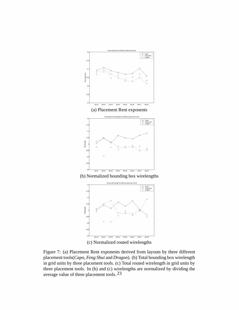
4.3 Placement Quality and Rent Exponent
In [11] the Rent exponent is regarded as a metric of quality of partitioning algo-
rithm. It is interesting to know whether there is a similar correlation between the
placement quality and the Rent exponent of placement. Previously the quality of
placement is measured by the total bounding box wirelength or the wirelength
after global routing. Therefore we compare placement wirelength and Rent expo-
nents for different placement tools.
Table 5 lists the Rent exponent, total bounding box wirelength and total routed
18

ckt partitioning derived placement estimated real WL (�103units)Rent exp.p Rent exp.p� WL by p� Capo Feng Shui Dragon
ibm11 0.608 0.682 558 489 494 483ibm12 0.648 0.723 734 738 744 646ibm13 0.600 0.672 641 676 716 605ibm14 0.622 0.690 977 913 841 822ibm15 0.599 0.665 1037 1242 1175 1196ibm16 0.609 0.690 1189 1207 1090 1078ibm17 0.645 0.712 1453 1661 1651 1653ibm18 0.600 0.664 1204 1108 1247 1090
Table 4: Partitioning Rent exponentp, derived placement Rent exponentp� andestimated total wirelength based onp�, comparing with the routed total wirelengthfrom three placement outputs.
wirelength for three placement approaches. For consistency, both bounding box
wirelength and routed wirelength is reported in grid units of global routing. The
global router is based on maze routing including rip-up and re-route. The capacity
of global routing edges is set to a value such that the number of nets which are
ripped-up and re-routed is less than 10% of the total nets. This is to reduce the
influence of the global routing on the placement.
placement Rent exponent total bounding box WL total routed WLckt (�103 grid units) (�103 grid units)
Capo Feng Shui Dragon Capo Feng Shui Dragon Capo Feng Shui Dragonibm11 0.693 0.682 0.667 435 442 423 489 494 483ibm12 0.708 0.694 0.683 655 654 567 738 744 646ibm13 0.689 0.668 0.648 505 510 487 676 716 605ibm14 0.679 0.650 0.663 827 759 740 913 841 822ibm15 0.669 0.630 0.640 951 882 890 1242 1175 1196ibm16 0.674 0.627 0.651 1025 972 961 1207 1090 1078ibm17 0.704 0.650 0.671 1483 1315 1364 1661 1651 1653ibm18 0.658 0.615 0.632 1088 953 967 1108 1247 1090
Table 5: Placement Rent exponents derived from layouts by three different place-ment tools, with the normalized total bounding box wirelength and normalizedtotal routed wirelength.
Figure 7 shows the comparison more clearly. For most circuits the smaller
Rent exponent relates to less total wirelength. Some other circuits show the con-
19

trary cases. However, the difference are relatively small in these cases. The cor-
relation exists for both bounding box wirelength and routed wirelength. Thus
we conclude that the Rent exponent of placement is a good metric of placement
quality.
5 Conclusion
Wirelength estimation for large circuits is a complex problem. A number of fac-
tors can affect the accuracy of estimating, including the approach to obtain the
Rent exponent, the placement algorithm used in the design flow and the quality
or parameters of the global router. In order to obtain accurate wirelength esti-
mates, designers ought to adjust estimation model and the Rent exponent extrac-
tion method according to the place and route tool they employ. Precise wirelength
estimation needs extensive experimental data as well as theoretical formulation.
Our work is a step toward understanding this process.
6 Acknowledgments
The authors wish to thank Dr. Dirk Stroobandt for his precious comments.
References[1] B. Landman and R. Russo. “ On a Pin Versus Block Relationship for Parti-
tions of Logic Graphs ”.IEEE Transactions on Computers, c-20:1469–1479,1971.
[2] W. E. Donath. “Placement and Average Interconnection Lengths of Com-puter Logic”. IEEE Transactions on Circuits and Systems, 26(4):272–277,April 1979.
[3] M. Feuer. “Connectivity of random logic”.IEEE Transactions on Comput-ers, C-31(1):29–33, Jan 1982.
[4] D. Stroobandt and J. Van Campenhout. “Accurate Interconnection LengthEstimations for Predictions Early in the Design Cycle”.VLSI Design, Spe-cial Issue on Physical Design in Deep Submicron, 10(1):1–20, 1999.
20

[5] J. A. Davis, V. K. De, and J. Meindl. “A Stochastic Wire-Length Distributionfor Gigascale Integration(GSI) - Part I: Derivation and Validation”.IEEETransactions on Electron Devices, 45(3):580–589, Mar 1998.
[6] P. Chong and R. K. Brayton. “Estimating and Optimizing Routing Utiliza-tion in DSM Design”. InInternational Workshop on System-Level Intercon-nect Prediction. ACM, April 1999.
[7] X. Yang, R. Kastner, and M. Sarrafzadeh. “Congestion Estimation DuringTop-down Placement”. InInternational Symposium on Physical Design,pages 164–169. ACM, April 2001.
[8] K. C. Saraswat, S. J. Souri, K. Banerjee, and P. Kapur. “Performance Analy-sis and Technology of 3-D ICs”. InInternational Workshop on System-LevelInterconnect Prediction, pages 85–90. ACM, April 2000.
[9] R. Zhang, K. Roy, C. K. Koh, and D. B. Janes. “Stochastic Wire-Length andDelay Distributions of 3-Dimensional Circuits”. InInternational Conferenceon Computer-Aided Design, pages 208–213. IEEE, November 2000.
[10] P. Zarkesh-Ha, J. A. Davis, W. Loh, and J. D. Meindl. “Prediction of In-terconnect Fan-Out Distribution Using Rent’s Rule”. InInternational Work-shop on System-Level Interconnect Prediction, pages 107–112. ACM, April2000.
[11] L. Hagen, A. B. Kahng, F. J. Kurdahi, and C. Ramachandran. “On the Intrin-sic Rent Parameter and Spectra-Based Partitioning Methodologies”.IEEETransactions on Computer Aided Design, 13(no.1):27–37, Jan 1994.
[12] D. Stroobandt. “On an Efficient Method for Estimating the InterconnectionComplexity of Designs and on the Existence of Region III in Rent’s Rule”. InProceedings of the Ninth Great Lakes Symposium on VLSI, pages 330–331.IEEE, March 1999.
[13] H. Van Marck, D. Stroobandt, and J. Van Campenhout. “Towards An Ex-tension of Rent’s Rule for Describing Local Variations in InterconnectionComplexity”. In Proceedings of the Fourth International Conference forYoung Computer Scientists, pages 136–141, 1995.
[14] P. Christie. “Managing Interconnect Resources”. InInternational Workshopon System-Level Interconnect Prediction, pages 1–51. ACM, April 2000.
[15] P. Christie and D. Stroobandt. “The Interpretation and Application of Rent’sRule”. IEEE Transactions on VLSI Systems, 8(6):639–648, 2000.
[16] P. Verplaetse, J. Dambre, D. Stroobandt, and J. Van Campenhout. “Onpartitioning vs. placement Rent properties”. InInternational Workshop onSystem-Level Interconnect Prediction, pages 33–40. ACM, March 2001.
21

[17] X. Yang, E. Bozorgzadeh, and M. Sarrafzadeh. “Wirelength Estimationbased on Rent Exponents of Partitioning and Placement”. InInternationalWorkshop on System-Level Interconnect Prediction, pages 25–31. ACM,April 2001.
[18] A. E. Caldwell, A. B. Kahng, and I. L. Markov. “Can Recursive BisectionAlone Produce Routable Placements?”. InDesign Automation Conference,pages 477–482. IEEE/ACM, June 2000.
[19] M. C. Yildiz and P. H. Madden. “Global Objectives for Standard Cell Place-ment”. InProceedings of the Great Lakes Symposium on VLSI, pages 68–72,March 2001.
[20] M. Wang, X. Yang, and M. Sarrafzadeh. “Dragon2000: Fast Standard-cellPlacement for Large Circuits”. InInternational Conference on Computer-Aided Design, pages 260–263. IEEE, 2000.
[21] C. J. Alpert. “The ISPD98 Circuit Benchmark Suite”. InInternational Sym-posium on Physical Design, pages 18–25. ACM, April 1998.
[22] G. Karypis, R. Aggarwal, V. Kumar, and S. Shekhar. “Multilevel Hyper-graph Partitioning: Application in VLSI Domain”. InDesign AutomationConference, pages 526–529. IEEE/ACM, 1997.
22
0.5
0.55
0.6
0.65
0.7
0.75
0.8
ibm11 ibm12 ibm13 ibm14 ibm15 ibm16 ibm17 ibm18
Rent exponents by different placement tools
Ren
t exp
onen
t
Capo Feng ShuiDragon
(a) Placement Rent exponents
0.8
0.85
0.9
0.95
1
1.05
1.1
1.15
1.2
ibm11 ibm12 ibm13 ibm14 ibm15 ibm16 ibm17 ibm18
Bounding box Wirelength by different placement tools
Wire
leng
th
Capo Feng ShuiDragon
(b) Normalized bounding box wirelengths
0.8
0.85
0.9
0.95
1
1.05
1.1
1.15
1.2
ibm11 ibm12 ibm13 ibm14 ibm15 ibm16 ibm17 ibm18
Routed Wirelength by different placement tools
Wire
leng
th
Capo Feng ShuiDragon
(c) Normalized routed wirelengths
Figure 7: (a) Placement Rent exponents derived from layouts by three differentplacement tools(Capo, Feng Shui andDragon). (b) Total bounding box wirelengthin grid units by three placement tools. (c) Total routed wirelength in grid units bythree placement tools. In (b) and (c) wirelengths are normalized by dividing theaverage value of three placement tools.23
Related Documents