WINDOWS: Finite Aperture Effects and Applications in ... · trol finite aperture effects can be found hi numer-ous disciplines. These include the following: i. Finite duration Impulse

p a p e r

WINDOWS: Finite Aperture Effects and Applications in SignalProcessing

1

fred harris,San Diego State University

1. INTRODUCTION:

Awindow is the aperture through we exam-ine the world. By necessity, any time orspatial signal we observe, collect, and

process must have bounded support. Similarly,any time or spatial signal we approximate, design,and synthesize must also have bounded support.Support is the range or width of the independentvariable (time, distance, or frequency) over whichthe dependent variable, say the signal, is non-zero. This finite support can be defined over mul-tiple dimensions, extending for instance, over aline, a plane, or a volume. Windows can be con-tinuous functions or discrete sequences definedover their appropriate finite supports.At the simplest level, a window can be considereda multiplicative operator that turns on the signalwithin the finite support and turns it off outsidethat same support. This operator effects the sig-nal's Fourier Transform in a number of undesiredways; the most significant of which is undesiredout-of-band side-lobe levels. The size and order ofthe discontinuities exhibited by the signal governsthe level and rate of attenuation of these spectralside-lobes. Other unwanted effects include spec-tral smearing and in-band ripple. The design andapplication of windows is directed to minimizing

or controlling the undesired artifacts of in-bandripple, out-of-band side-lobes, and spectralsmearing.Examples of the application of windows to con-trol finite aperture effects can be found hi numer-ous disciplines. These include the following:

i. Finite duration Impulse Response (FIR) FilterDesign:

Windows applied to a prototype filter's Impulse Response to control transition bandwidth, in-band and out-of-band side-lobe levels,

ii. Spectrum Analysis, Transforms of Sliding,Overlapped, Windowed Data:

Windows applied to observed time series to control Variance of Spectral Estimate while suppressing Spectral Leakage (additive bias).

iii. Power Spectra as Transform of WindowedCorrelation Functions:

Windows applied to sample correlation function to suppress segments of the sample correlation function exhibiting high bias and variance.

iv. Non Stationary Spectra and Model Estimates:Windows applied to delayed and overlapped collected time series to localize time

2

and spectral features (model parameters) of non-stationary signals.

v. Modulation Spectral Mask Control:Design of modulation envelope to control spectral side-lobe behavior.

vi. Synthetic Aperture RADAR (SAR):Windows applied to spatial series to con-trol Antenna Side-lobes

vii. Phased Array Antenna Shading Function:Window applied to spatial function to control Antenna Side-lobes

viii. Photolithography Apodizing Function:Smooth Transmission Function applied to optical aperture to control diffraction pattern side - lobes

We will discuss a subset of these applications laterin this chapter. For convenience and consistency,we will consider the window as being applied toa time domain signal. The window can, of course,be applied to any function with the same intentand goal. The common theme of these applica-tions is control of envelope smoothness in thetime domain to obtain desired properties in thefrequency domain.

2. WINDOWS IN SPECTRUM ANALYSIS:

A concept we now take for granted is that a signalcan be described in different coordinate systemsand that there is engineering value in examininga signal described in an alternate basis system.One basis system we find particularly useful is theset of complex exponentials, The attraction of thisbasis set is that complex exponentials are theeigen-functions and eigen-series of linear timeinvariant (LTI) differential and difference opera-tors respectively. Put in its simplest form, thismeans that when a sinewave is applied to an LTIfilter the steady state system response is a scaledversion of the same sinewave. The system canonly affect the complex amplitude (magnitudeand phase) of the sinewave but can never changeits frequency. Consequently complex sinusoids

have become a standard tool to probe anddescribe LTI systems. The process of describing asignal as a summation of scaled sinusoids is stan-dard Fourier transform analysis. The FourierTransform and Fourier Series, shown on the leftand right hand side of (1), permits us to describesignals equally well in both the time domain andthe frequency domain.

Since the complex exponentials have infinite sup-port, the limits of integration in the forward trans-form (time- to- frequency) are from minus to plusinfinity. As observed earlier, all signals of engi-neering interest have finite support, which moti-vates us to modify the limits of integration of theFourier transform to reflect this restriction. This isshown in (2) where Tsup and N define the finitesupports of the signal.

The two versions of the transform can be mergedin a single compact form if we use a finite supportwindow to limit the signal to the appropriatefinite support interval, as opposed to using the

dtethH tj∫+∞

∞−

−= ωω )()(

ωωπ

ω deHht tj∫+∞

∞−

+= )(21

∑+∞

∞−

−= tjenhH θθ )()(

θθπ

π

ο

θ deHnh nj∫+

−

+= )(21)(

(1)

dtethHT

tjSUP ∫ −=

sup

)()( ωω

ωωπ

ω deHth tjSUP

++∞

∞−∫= )(

21)(

∑ −=N

njSUP enhH θθ )()(

θθ θπ

π

deHnh njSUP

−+

−∫= )()(

(2)

3

limits of integration or limits of summation. Thisis shown in (3).

A natural question to ask when examining (3) ishow has limiting the signal extent with the multi-plicative window affected the transform of thesignal? The simple answer is related to the rela-tionship that multiplication of two functions (orsequences) in the time (or sequence) domain isequivalent to convolution of their spectra in thefrequency domain. As shown in (4), the transformof the windowed signal is the convolution of thetransform of the signal with the transform of thewindow.

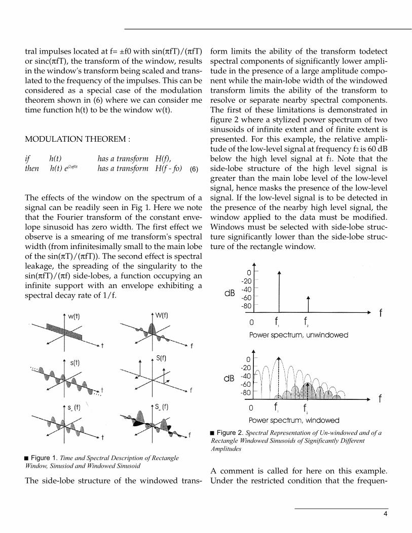
This relationship and its impact on spectral analy-sis can be dramatically illustrated by examiningthe Fourier transform of a single sinusoid on aninfinite support and on a finite support. Figure 1

shows the time and frequency representation ofthe rectangle window, of a sinusoid of infiniteduration, and of a finite support sinusoidobtained as a product of the previous two signals.Equations (5a) and (5b) describe the same signalsand their corresponding transforms.

As we can see, the transform of THe windowedsinusoid, being the convolution of a pair of spec-

dtethtwHH tjWSUP ∫

+∞

∞−

−⋅== ωωω )()()()(

ωωπ

ω deHth tjW

++∞

∞−∫= )(

21)(

∑+∞

∞−

−⋅== njWSUP enhnwHH θθθ )()()()(

θθπ

θπ

π

deHnh njW

−+

−∫= )(

21)( (3)

∫+∞

∞−

−⋅= λλλπ

ω dWHH w )()(21)(

∫+

−

−⋅=π

π

λλθλπ

θ dWHH w )()(21)(

ωπ

ω ω dethH tj∫+∞

∞−

−= )(21)(

ωπ

ω ω detwWT

T

tj∫+

−

−=2/

2/

)(21)(

∑+∞

∞−

−= njenhH θθ )()(

∑+

−

−=2/

2/)()(

N

N

njenwW θθ (4)

::0

22:1)(

<<−=

Otherwise

TtTtw

fTfTTfW

ππ )sin()( =

+∞<<∞−=

ttfAts :)2sin()( 0 φπ

)(2

)(2

|)( 00 ffeAffeAfS jj ++−= +− δδ ϕϕ

:)2sin()( 0 φπ −= tfAtsw

))(())(sin(

2

)(())(sin(

2)(

0

0

)0

0

TffTff

eAT

TffTff

eATfS

j

jw

++

+

−−

=

+

−

ππ

ππ

ϕ

ϕ

22TtT +<<−

(5a)

::0

22:1)(

<<−=

Otherwise

NnNnw

)21sin(

)2

sin()(

θ

θθ

N

TW =

+∞<<∞−=

tnAns :)sin()( 0 φθ

)(2

)(2

|)( 00 θθδθθδθ ϕϕ ++−= +− jj eAeAS

:)sin()( 0 φθ −= nAnsw

2)sin((

2)sin((

2)21sin((

)2

)sin((

2)(

0

0

)0

0

N

N

eAN

eAS jjw

θθ

θθ

θθ

θθθ ϕϕ

+

++

−

−= +−

22NnN +<<−

(5b)

4

tral impulses located at f= ±f0 with sin(πfT)/(πfT)or sinc(πfT), the transform of the window, resultsin the window's transform being scaled and trans-lated to the frequency of the impulses. This can beconsidered as a special case of the modulationtheorem shown in (6) where we can consider metime function h(t) to be the window w(t).

MODULATION THEOREM :

if h(t) has a transform H(f),then h(t) ej2πf0t has a transform H(f - fo)

The effects of the window on the spectrum of asignal can be readily seen in Fig 1. Here we notethat the Fourier transform of the constant enve-lope sinusoid has zero width. The first effect weobserve is a smearing of me transform's spectralwidth (from infinitesimally small to the main lobeof the sin(πT)/(πfT)). The second effect is spectralleakage, the spreading of the singularity to thesin(πfT)/(πf) side-lobes, a function occupying aninfinite support with an envelope exhibiting aspectral decay rate of 1/f.

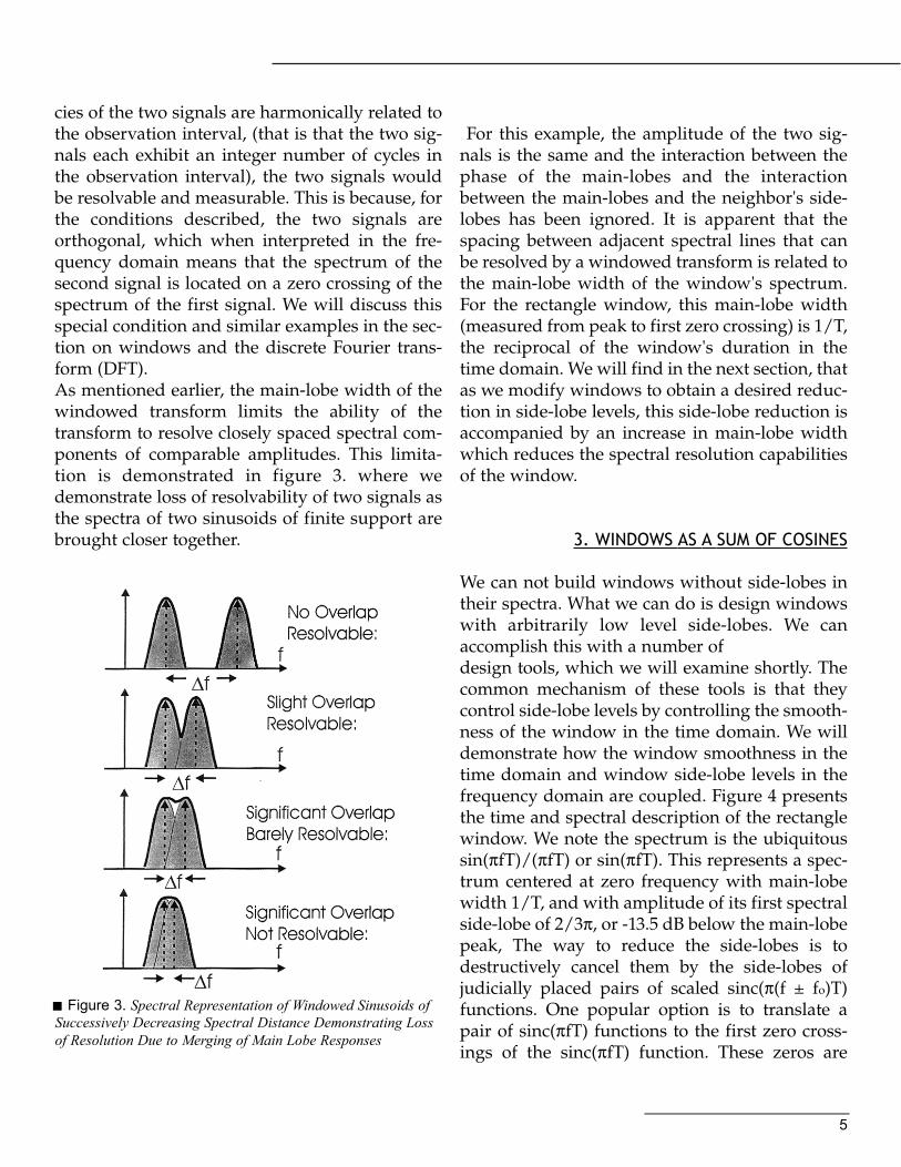
The side-lobe structure of the windowed trans-

form limits the ability of the transform todetectspectral components of significantly lower ampli-tude in the presence of a large amplitude compo-nent while the main-lobe width of the windowedtransform limits the ability of the transform toresolve or separate nearby spectral components.The first of these limitations is demonstrated infigure 2 where a stylized power spectrum of twosinusoids of infinite extent and of finite extent ispresented. For this example, the relative ampli-tude of the low-level signal at frequency f2 is 60 dBbelow the high level signal at f1. Note that theside-lobe structure of the high level signal isgreater than the main lobe level of the low-levelsignal, hence masks the presence of the low-levelsignal. If the low-level signal is to be detected inthe presence of the nearby high level signal, thewindow applied to the data must be modified.Windows must be selected with side-lobe struc-ture significantly lower than the side-lobe struc-ture of the rectangle window.

A comment is called for here on this example.Under the restricted condition that the frequen-

(6)

Figure 1. Time and Spectral Description of RectangleWindow, Sinusiod and Windowed Sinusoid

Figure 2. Spectral Representation of Un-windowed and of aRectangle Windowed Sinusoids of Significantly DifferentAmplitudes

5

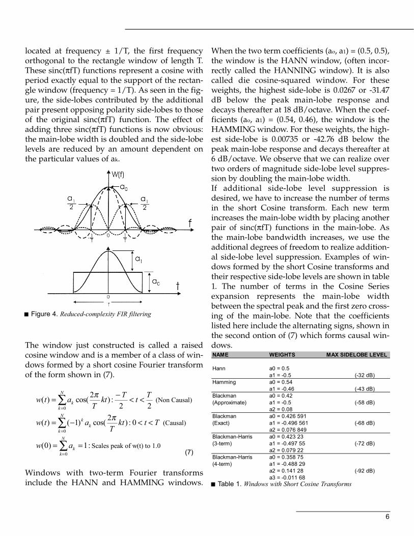
cies of the two signals are harmonically related tothe observation interval, (that is that the two sig-nals each exhibit an integer number of cycles inthe observation interval), the two signals wouldbe resolvable and measurable. This is because, forthe conditions described, the two signals areorthogonal, which when interpreted in the fre-quency domain means that the spectrum of thesecond signal is located on a zero crossing of thespectrum of the first signal. We will discuss thisspecial condition and similar examples in the sec-tion on windows and the discrete Fourier trans-form (DFT).As mentioned earlier, the main-lobe width of thewindowed transform limits the ability of thetransform to resolve closely spaced spectral com-ponents of comparable amplitudes. This limita-tion is demonstrated in figure 3. where wedemonstrate loss of resolvability of two signals asthe spectra of two sinusoids of finite support arebrought closer together.

For this example, the amplitude of the two sig-nals is the same and the interaction between thephase of the main-lobes and the interactionbetween the main-lobes and the neighbor's side-lobes has been ignored. It is apparent that thespacing between adjacent spectral lines that canbe resolved by a windowed transform is related tothe main-lobe width of the window's spectrum.For the rectangle window, this main-lobe width(measured from peak to first zero crossing) is 1/T,the reciprocal of the window's duration in thetime domain. We will find in the next section, thatas we modify windows to obtain a desired reduc-tion in side-lobe levels, this side-lobe reduction isaccompanied by an increase in main-lobe widthwhich reduces the spectral resolution capabilitiesof the window.

3. WINDOWS AS A SUM OF COSINES

We can not build windows without side-lobes intheir spectra. What we can do is design windowswith arbitrarily low level side-lobes. We canaccomplish this with a number ofdesign tools, which we will examine shortly. Thecommon mechanism of these tools is that theycontrol side-lobe levels by controlling the smooth-ness of the window in the time domain. We willdemonstrate how the window smoothness in thetime domain and window side-lobe levels in thefrequency domain are coupled. Figure 4 presentsthe time and spectral description of the rectanglewindow. We note the spectrum is the ubiquitoussin(πfT)/(πfT) or sin(πfT). This represents a spec-trum centered at zero frequency with main-lobewidth 1/T, and with amplitude of its first spectralside-lobe of 2/3π, or -13.5 dB below the main-lobepeak, The way to reduce the side-lobes is todestructively cancel them by the side-lobes ofjudicially placed pairs of scaled sinc(π(f ± fo)T)functions. One popular option is to translate apair of sinc(πfT) functions to the first zero cross-ings of the sinc(πfT) function. These zeros are

Figure 3. Spectral Representation of Windowed Sinusoids ofSuccessively Decreasing Spectral Distance Demonstrating Lossof Resolution Due to Merging of Main Lobe Responses

6

located at frequency ± 1/T, the first frequencyorthogonal to the rectangle window of length T.These sinc(πfT) functions represent a cosine withperiod exactly equal to the support of the rectan-gle window (frequency = 1/T). As seen in the fig-ure, the side-lobes contributed by the additionalpair present opposing polarity side-lobes to thoseof the original sinc(πfT) function. The effect ofadding three sinc(πfT) functions is now obvious:the main-lobe width is doubled and the side-lobelevels are reduced by an amount dependent onthe particular values of ak.

The window just constructed is called a raisedcosine window and is a member of a class of win-dows formed by a short cosine Fourier transformof the form shown in (7).

Windows with two-term Fourier transformsinclude the HANN and HAMMING windows.

When the two term coefficients (ao, a1) = (0.5, 0.5),the window is the HANN window, (often incor-rectly called the HANNING window). It is alsocalled die cosine-squared window. For theseweights, the highest side-lobe is 0.0267 or -31.47dB below the peak main-lobe response anddecays thereafter at 18 dB/octave. When the coef-ficients (ao, a1) = (0.54, 0.46), the window is theHAMMING window. For these weights, the high-est side-lobe is 0.00735 or -42.76 dB below thepeak main-lobe response and decays thereafter at6 dB/octave. We observe that we can realize overtwo orders of magnitude side-lobe level suppres-sion by doubling the main-lobe width.If additional side-lobe level suppression isdesired, we have to increase the number of termsin the short Cosine transform. Each new termincreases the main-lobe width by placing anotherpair of sinc(πfT) functions in the main-lobe. Asthe main-lobe bandwidth increases, we use theadditional degrees of freedom to realize addition-al side-lobe level suppression. Examples of win-dows formed by the short Cosine transforms andtheir respective side-lobe levels are shown in table1. The number of terms in the Cosine Seriesexpansion represents the main-lobe widthbetween the spectral peak and the first zero cross-ing of the main-lobe. Note that the coefficientslisted here include the alternating signs, shown inthe second ontion of (7) which forms causal win-dows.

Figure 4. Reduced-complexity FIR filtering

22:)2cos()(

0

TtTktT

atwN

kk <<−=∑

=

π (Non Causal)

TtktT

atwN

kk

k <<−=∑=

0:)2cos()1()(0

π (Causal)

∑=

==N

kkaw

0:1)0( Scales peak of w(t) to 1.0

(7)

NAME WEIGHTS MAX SIDELOBE LEVEL

Hann a0 = 0.5a1 = -0.5 (-32 dB)

Hamming a0 = 0.54a1 = -0.46 (-43 dB)

Blackman a0 = 0.42(Approximate) a1 = -0.5 (-58 dB)

a2 = 0.08Blackman a0 = 0.426 591(Exact) a1 = -0.496 561 (-68 dB)

a2 = 0.076 849Blackman-Harris a0 = 0.423 23(3-term) a1 = -0.497 55 (-72 dB)

a2 = 0.079 22Blackman-Harris a0 = 0.358 75(4-term) a1 = -0.488 29

a2 = 0.141 28 (-92 dB)a3 = -0.011 68

Table 1. Windows with Short Cosine Transforms

7

8

9

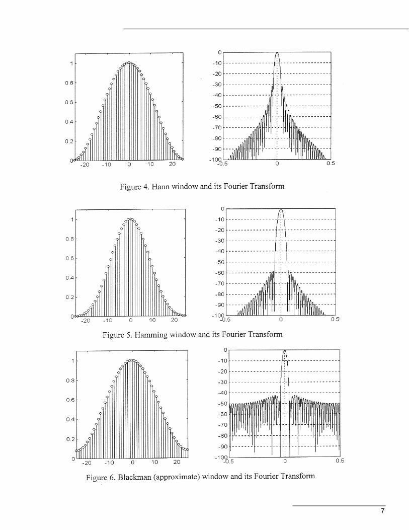
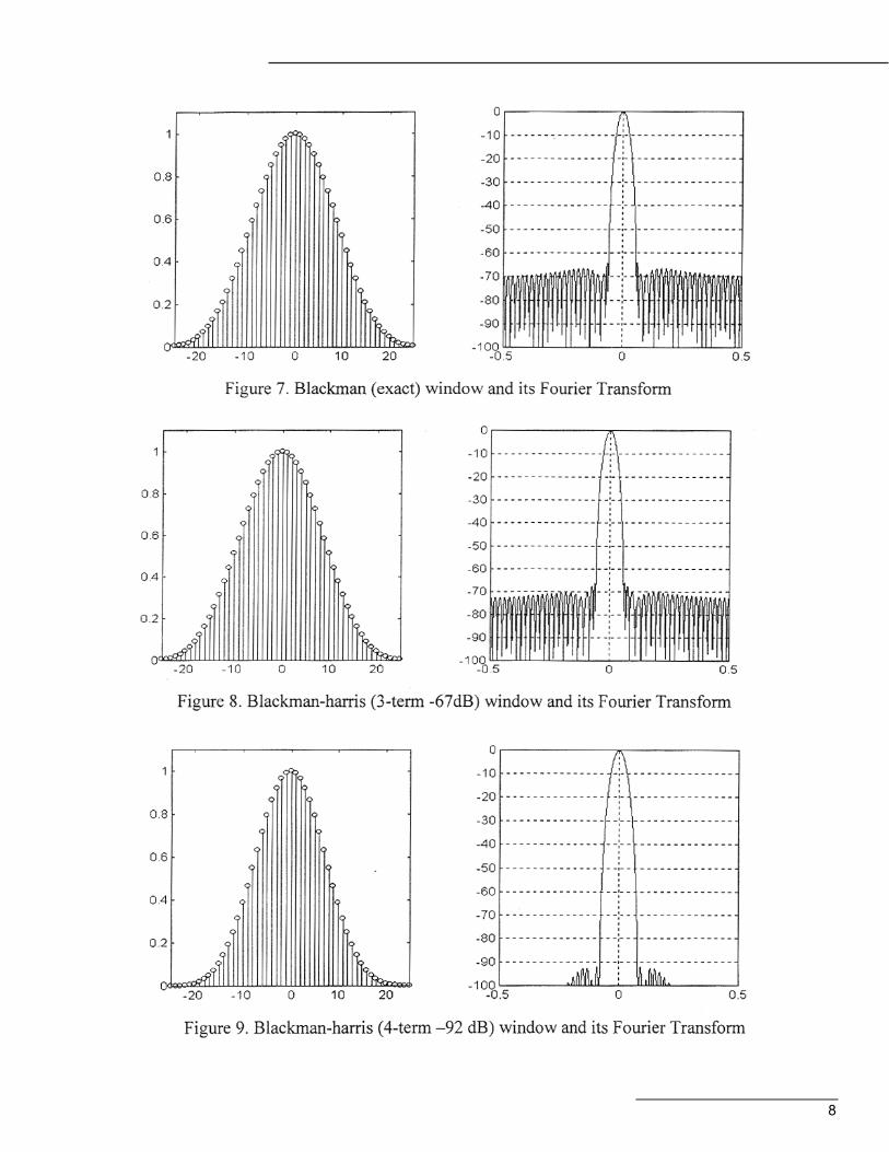
The time and frequency responses of the win-dows listed in Table-1 are presented in figures 4through 9. The windows contain 51 -samples, alength selected to permit us to see some detail intheir (1024) point Fourier Transforms. The appar-ent modulation of the spectral side-lobes is anartifact due to the sampling grid bracketing thespectral zero-crossings.

4. WINDOWS WITH ADJUSTABLE DESIGNPARAMETERS

We recognize that windows trade spectral main-lobe width for spectral side-lobe levels. A goodwindow achieves low side-lobe levels with mini-mum increase in main-lobe width. We now exam-ine two windows that can make this trade inaccord with an optimality criterion.

4.1 Dolph-Tchebyshev Window

The optimality criterion addressed by the Dolph-Tchebyshev window is that its Fourier transformexhibit the narrowest main-lobe width for a spec-ified (and selectable) side-lobe level. The Fouriertransform of this window exhibits equal ripple atthe specified side-lobe level. The FourierTransform of the window is a mapping of the N-th order algebraic Tchebyshev polynomial to theN-th order trigonometric Tchebyshev polynomialby the relationship TN(X) = COS(Nq). The Dolph-Tchebyshev window is defined in terms of uni-

formly spaced samples of its Fourier Transform.These samples are defined in (8).

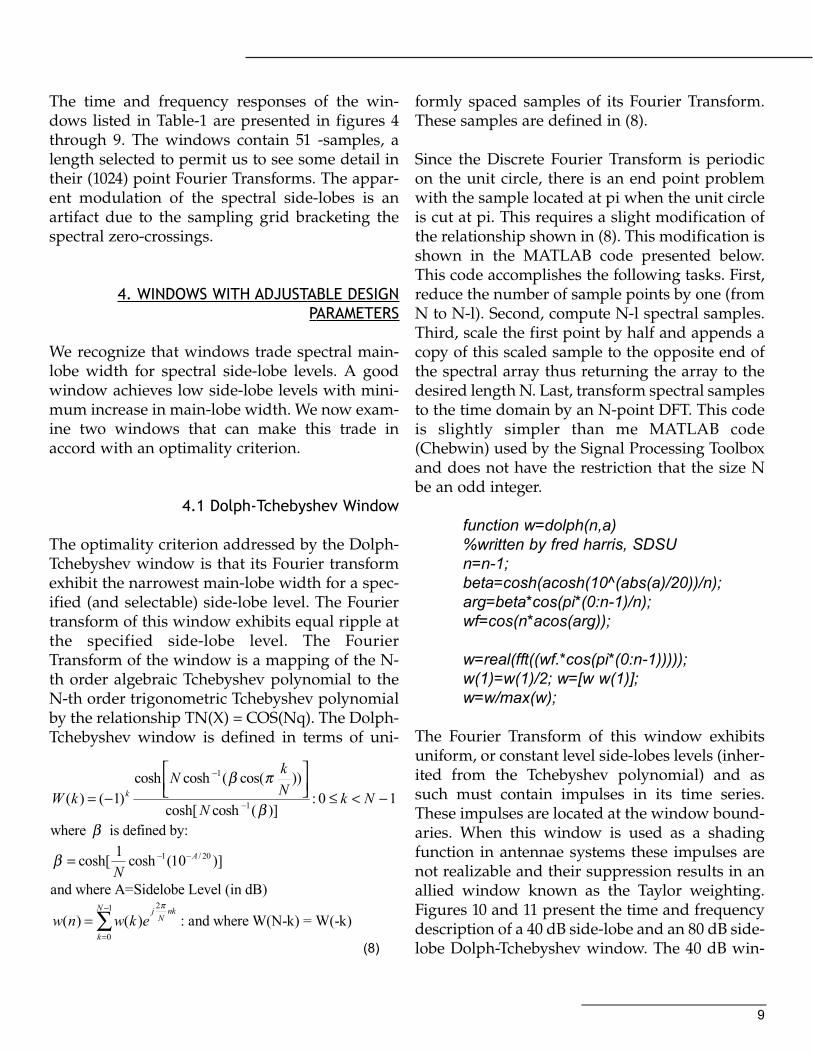
Since the Discrete Fourier Transform is periodicon the unit circle, there is an end point problemwith the sample located at pi when the unit circleis cut at pi. This requires a slight modification ofthe relationship shown in (8). This modification isshown in the MATLAB code presented below.This code accomplishes the following tasks. First,reduce the number of sample points by one (fromN to N-l). Second, compute N-l spectral samples.Third, scale the first point by half and appends acopy of this scaled sample to the opposite end ofthe spectral array thus returning the array to thedesired length N. Last, transform spectral samplesto the time domain by an N-point DFT. This codeis slightly simpler than me MATLAB code(Chebwin) used by the Signal Processing Toolboxand does not have the restriction that the size Nbe an odd integer.

function w=dolph(n,a)%written by fred harris, SDSUn=n-1;beta=cosh(acosh(10^(abs(a)/20))/n);arg=beta*cos(pi*(0:n-1)/n);wf=cos(n*acos(arg));

w=real(fft((wf.*cos(pi*(0:n-1)))));w(1)=w(1)/2; w=[w w(1)];w=w/max(w);

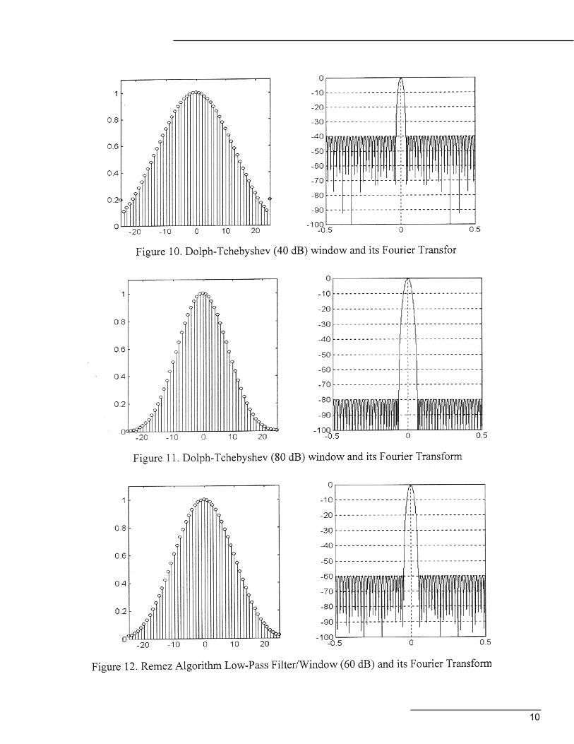
The Fourier Transform of this window exhibitsuniform, or constant level side-lobes levels (inher-ited from the Tchebyshev polynomial) and assuch must contain impulses in its time series.These impulses are located at the window bound-aries. When this window is used as a shadingfunction in antennae systems these impulses arenot realizable and their suppression results in anallied window known as the Taylor weighting.Figures 10 and 11 present the time and frequencydescription of a 40 dB side-lobe and an 80 dB side-lobe Dolph-Tchebyshev window. The 40 dB win-

10:)](coshcosh[

))cos((coshcosh)1()( 1

1

−<≤

−= −

−

NkN

NkN

kW k

β

πβ

where β is defined by:

)]10(cosh1cosh[ 20/1 A

N−−=β

and where A=Sidelobe Level (in dB)

∑−

=

=1

0

2

)()(N

k

nkN

jekwnw

π

: and where W(N-k) = W(-k)

(8)

10

11

dow is included to demonstrate the end pointimpulses. As an aside, the Tchebyshev, or equalripple behavior of the Dolph-Tchebyshev windowcan be obtained iteratively by the Remez (or theEqual-Ripple or Parks-Mclellan) Filter design rou-tine. For comparison, figure 12 presents a windowdesigned as a narrow-band filter with 60 dB side-lobes. The MATLAB call for this design was

ww=remez(50,[0 .001.047 0.5]/0.5,[11 0 0]).

The weights were scaled by ww(max) to set themaximum value of the window to unity. This fil-ter, by virtue of the equal-ripple side-lobes, alsoexhibits end point impulses.A comment on system performance is called for atthis point. Windows (and filters) with constantlevel side-lobes, while optimal in the sense ofequal ripple approximation, are sub-optimal interms of their integrated side-lobe levels. Thewindow (or filter) is used in spectral analysis toreduce signal bandwidth and then sample rate.The reduction in sample rate causes aliasing. Thespectral content in the side-lobes, (the out-of bandenergy) folds back to the in band interval andbecomes in-band interference. A measure of thisunexpected interference is integrated side-lobeswhich, for a given main-lobe width, is greaterwhen the side-lobes are equal-ripple. From a sys-tems viewpoint, the window (or filter) shouldexhibit 6-db per octave (1/0 rate of falloff of side-lobe levels. Faster rates of falloff actually increaseintegrated side-lobe levels due to an accompany-ing increase in close-in side-lobes as the remoteside-lobes are depressed (while holding main-lobe width and window length fixed). Systemdesigners should shv awav from equal-ripplewindows (and filters).

4.2 Gaussian window

A second window that exhibits a measure of opti-mality is the Gaussian or Weierstrass function. Adesired property of a window is that they be

smooth (usually) positive functions with FourierTransforms which approximate an impulse, (i.e.tall thin main lobe with low level side-lobes).From the uncertainty principle we know that wecannot simultaneously concentrate both a signaland its Fourier Transform. We can define themeasure of concentration (or width) as the func-tion's second central moments (i.e. moment ofinertia). With sT being the RMS time duration andwith sw being the RMS bandwidth (in Hz.) weknow these parameters must satisfy the uncer-tainty principle inequality shown in (9).

The equality constraint is achieved only by theGaussian function. Thus the Gaussian function,exhibiting a minimum time-bandwidth product,seems like a reasonable candidate for a window.Since windows span a finite support, when theGaussian is used as a window we must truncateor discard its tails. By restricting the window to afinite support the (truncated) Gaussian loses itsminimum time-bandwidth distinction. Never-the-less, the window enjoys wide usage by virtue ofits simplicity and (misplaced) reputation as aminimum time-bandwidth function. The sampledGaussian window is defined in (10) with theparameter a, the inverse of the standard devia-tion, controlling the effective time duration andthe effective spectral width.The sampled Gaussian window is defined in (10)with the parameter a, the inverse of the standarddeviation, controlling the effective time durationand the effective spectral width.

The Fourier Transform of this truncated windowis the convolution of the Gaussian transform witha Dirichlet kernel as indicated in (11). The convo-lution results in the formation of the spectral

21≥WTσσ

(9)

−+

2

2/21exp)(

Nnnw α

(10)

12

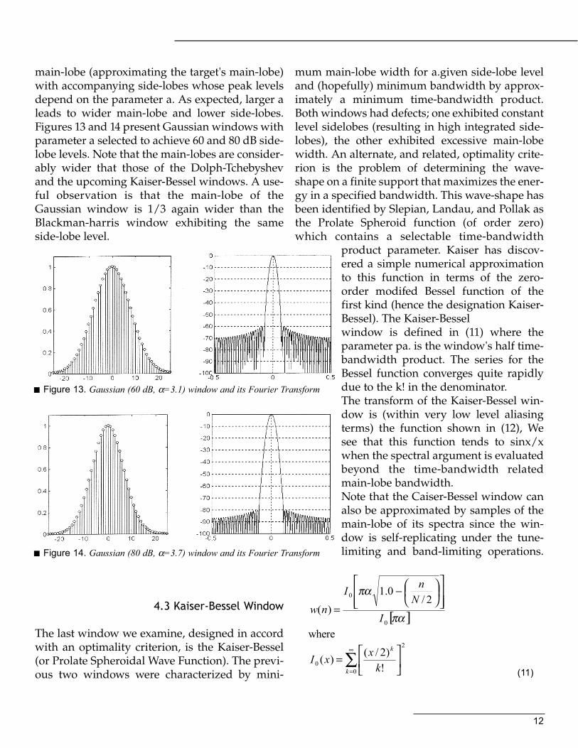
main-lobe (approximating the target's main-lobe)with accompanying side-lobes whose peak levelsdepend on the parameter a. As expected, larger aleads to wider main-lobe and lower side-lobes.Figures 13 and 14 present Gaussian windows withparameter a selected to achieve 60 and 80 dB side-lobe levels. Note that the main-lobes are consider-ably wider that those of the Dolph-Tchebyshevand the upcoming Kaiser-Bessel windows. A use-ful observation is that the main-lobe of theGaussian window is 1/3 again wider than theBlackman-harris window exhibiting the sameside-lobe level.

4.3 Kaiser-Bessel Window

The last window we examine, designed in accordwith an optimality criterion, is the Kaiser-Bessel(or Prolate Spheroidal Wave Function). The previ-ous two windows were characterized by mini-

mum main-lobe width for a.given side-lobe leveland (hopefully) minimum bandwidth by approx-imately a minimum time-bandwidth product.Both windows had defects; one exhibited constantlevel sidelobes (resulting in high integrated side-lobes), the other exhibited excessive main-lobewidth. An alternate, and related, optimality crite-rion is the problem of determining the wave-shape on a finite support that maximizes the ener-gy in a specified bandwidth. This wave-shape hasbeen identified by Slepian, Landau, and Pollak asthe Prolate Spheroid function (of order zero)which contains a selectable time-bandwidth

product parameter. Kaiser has discov-ered a simple numerical approximationto this function in terms of the zero-order modifed Bessel function of thefirst kind (hence the designation Kaiser-Bessel). The Kaiser-Besselwindow is defined in (11) where theparameter pa. is the window's half time-bandwidth product. The series for theBessel function converges quite rapidlydue to the k! in the denominator.The transform of the Kaiser-Bessel win-dow is (within very low level aliasingterms) the function shown in (12), Wesee that this function tends to sinx/xwhen the spectral argument is evaluatedbeyond the time-bandwidth relatedmain-lobe bandwidth.Note that the Caiser-Bessel window canalso be approximated by samples of themain-lobe of its spectra since the win-dow is self-replicating under the tune-limiting and band-limiting operations.

Figure 13. Gaussian (60 dB, α=3.1) window and its Fourier Transform

Figure 14. Gaussian (80 dB, α=3.7) window and its Fourier Transform

[ ]πα

πα

0

0 2/0.1

)(I

NnI

nw

−

=

where 2

00 !

)2/()( ∑∞

=

=

k

k

kxxI

(11)

13

14

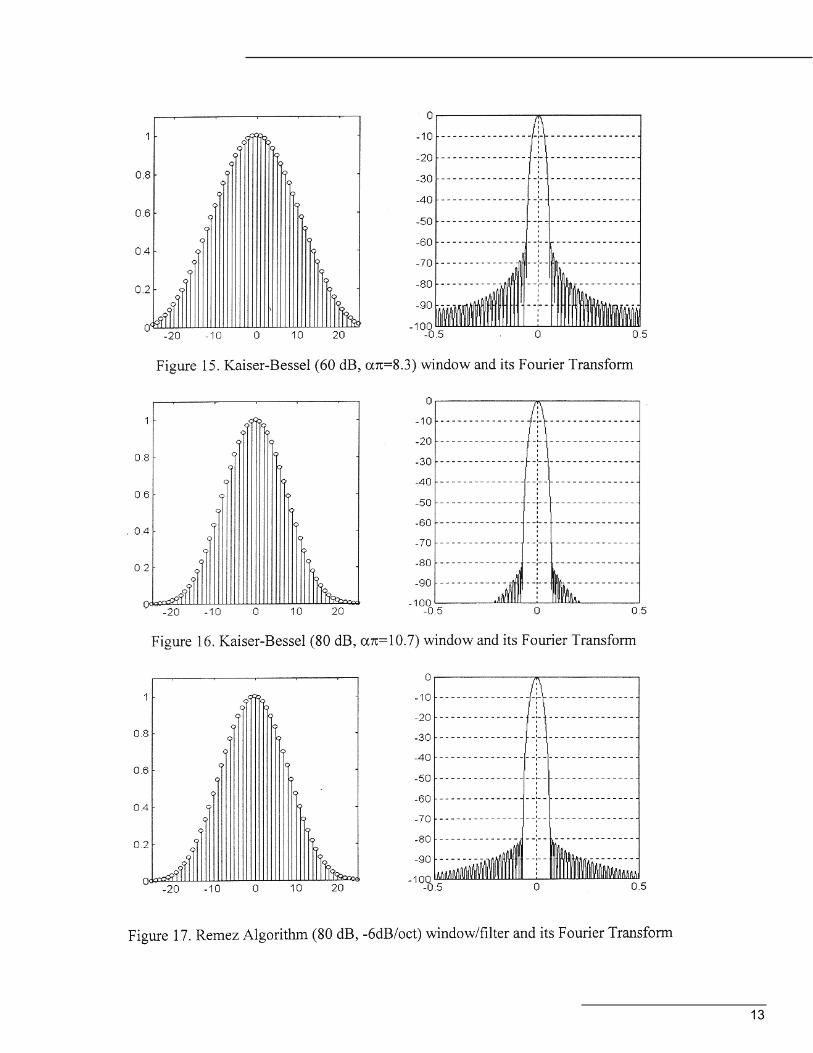
That is if w(n) and W(θ) are a Fourier Transformpair, then the band-limited version Rect(θ/απ)-W(θ) is a scaled version of (the envelope of) w(n)and the transform of theband-limited spectra is atime series consisting of the original time-limitedseriesw(n) with appended side-lobe tails. Timelimiting this new time series (truncating the tails)returns the pair back to their original relationship.

Figures 15 and 16 present the Kaiser-Bessel win-dow for parameter ap selected to achieve 60 and80 dB side-lobes. Compare the main-lobe widthsto those of the earlier windows. As commentedupon earlier, windows can be designed using theRemez Algorithm. When the penalty function ofthe Remez algorithm is made to increase linearlywith frequency the side-lobes fall inversely withfrequency (-6 dB/oct). Figure 17 presents a win-dow designed by a modified Remez algorithm.The call to the modified routine is of the form

Note that due to the reduced sidelobe slope thiswindow exhibits a narrower main-lobe widthcompared to a Kasier-Bessel with the same -80 dBside-lobe level.

5. SPECTRAL ANALYSIS AND WINDOW FIGURES OFMERIT

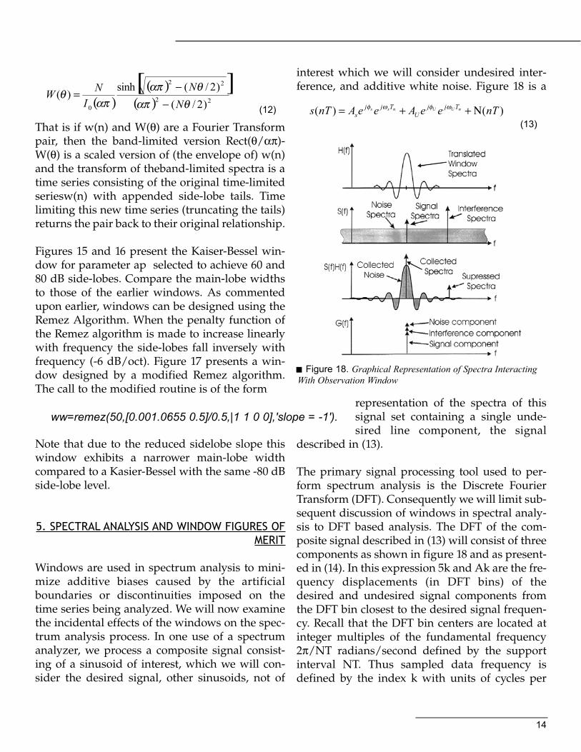
Windows are used in spectrum analysis to mini-mize additive biases caused by the artificialboundaries or discontinuities imposed on thetime series being analyzed. We will now examinethe incidental effects of the windows on the spec-trum analysis process. In one use of a spectrumanalyzer, we process a composite signal consist-ing of a sinusoid of interest, which we will con-sider the desired signal, other sinusoids, not of

interest which we will consider undesired inter-ference, and additive white noise. Figure 18 is a

representation of the spectra of thissignal set containing a single unde-sired line component, the signal

described in (13).

The primary signal processing tool used to per-form spectrum analysis is the Discrete FourierTransform (DFT). Consequently we will limit sub-sequent discussion of windows in spectral analy-sis to DFT based analysis. The DFT of the com-posite signal described in (13) will consist of threecomponents as shown in figure 18 and as present-ed in (14). In this expression 5k and Ak are the fre-quency displacements (in DFT bins) of thedesired and undesired signal components fromthe DFT bin closest to the desired signal frequen-cy. Recall that the DFT bin centers are located atinteger multiples of the fundamental frequency2π/NT radians/second defined by the supportinterval NT. Thus sampled data frequency isdefined by the index k with units of cycles per

( )( )[ ]

( ) 22

22

0 )2/()2/(sinh

)(θαπ

θαπαπ

θN

NI

NW−

−=

(12)

ww=remez(50,[0.001.0655 0.5]/0.5,|1 1 0 0],'slope = -1').

)()( nTeeAeeAnTs nUUnss TjjU

Tjjs Ν++= ωφωφ

(13)

Figure 18. Graphical Representation of Spectra InteractingWith Observation Window

15

interval or by the equivalent sampled data fre-quency of k(2π/N) radians/sample.

The three separate components of the DFT pre-sented in (14) are identified and shown in (15).

The signal component, S(k)DES SIG. of the DFT out-put is seen to preserve the complex amplitude ofthe input sinusoid but multiplies that amplitudeby a gain term we recognize as the DFT of thewindow. The DFT is evaluated at δk. the frequen-cy displacement of the input sinusoid from thenearest DFT bin. We note that the frequencyresponse of the window spectra centered at the k-lh bin and observed by the input sinusoid at fre-quency k+δk cvcles/interval is the same as thefrequency response of the window centered at DCand observed at frequency offset δk. When thedisplacement, dk, is zero this gain defaults to theDC (or zero frequency) response of the window.This gain is called the peak amplitude gain of thewindow and as shown in (16) is the sum of the

window weights. This sum is bounded by N (forthe rectangle window) and is aoN for the short

cosine transforms presented in sec-tion 3. For good windows, typical val-ues of peak amplitude gain is on theorder of 0.5*N through 0.35*N. Arelated gain term is called the peakpower gain of the window which is

also shown in (16).

The undesired component, S(k)UNDES SIG, of theDFT output is also seen to preserve the complexamplitude of the input sinusoid but multipliesthat amplitude by a gain term W(Dk). We recog-nize the gain term as the DFT of the window eval-uated at Dk, the frequency displacement of theundesired input sinusoid from the DFT bin ofinterest. This term is the spectral leakage term orout-of-band frequency response of the window. Itis our desire to control this term that motivated usto design and use good windows. When Dk isgreater than the window's main-lode width (3-to-6 bins) this term is the window's side-lobe levelswhich can be on the order of 0.01 *N through0.0001 *N.The component S(k)NOISE is the DFT of the inputnoise. We can assume that this noise-is zero meanand white with variance σ2N. Since the noise in arandom variable, so is it's DFT, so we are obligedto describe the DFT of the noise by its statistics.Two statistics of primary interest are, as shown in(17), the first and second moments.

We see that the DFT output variance, due to inputnoise, is a scaled version of the input noise vari-ance. The scale term is the sum of square of thewindow weights. This gain, shown in (18) istermed the peak noise power gain of the window.This of course is bounded by N (for the rectangle)

∑−

=

−=

1

0

2

)()()(N

n

nkN

jensnwkS

π

nkN

jkknN

juju

kknN

jN

n

SjS enNeeAeeAnw

ππϕδπ

ϕ2)(2)(21

0)]()[(

−∆++++−

=

++=∑ (14)

nkN

jkknN

jsjN

NsDESSIG eeeAnwkS

πδπϕ 2)(21

0)()(

−++−

=∑=

∑−

=

=1

0

2

)(N

n

Nj

knenwsjesA δφ π

)( kWeA sjs δφ=

nkN

jkknN

jujN

NuUNDESSIG eeeAnwkS

ππϕ 2)(21

0)()(

−∆++−

=∑=

∑−

=

∆=1

0

2

)(N

n

Nj

UU knenwjeA

πφ

)( kWeA ujU ∆= φ

nkN

jN

NNOISE ennwkS

π21

0)()()(

−−

=∑ ℵ=

(15)

Peak Signal Gain ∑−

=

=≡1

)()0(N

onnwW

Peak Signal Power Gain [ ]21

2 )()0( ∑−

=

=≡N

onnwW

(16)

16

and is on the order of (3/8) N for other windows.

5.1 Figures of Merit

The use of a window leads to conflicting effectson the output of the transform. The window isapplied to data to suppress out-of-band side-lobelevels: this is a desirable effect. The window con-trols side-lobes by smoothly discarding data nearthe boundaries of the observation interval. Thishas the effect of reducing the amplitude, henceenergy, of both signal and noise components pre-sented to the transform. Concurrently, theincreased bandwidth of the window's spectralmain-lobe (required to purchase the reduced side-lobe levels) permits additional noise into themeasurement.To facilitate comparison of different windows wedefine two performance measures related to theeffects of the window on both signal and noise.The first of these is equivalent noise bandwidth(ENBW). This parameter indicates the equivalentrectangular bandwidth of a filter with the same

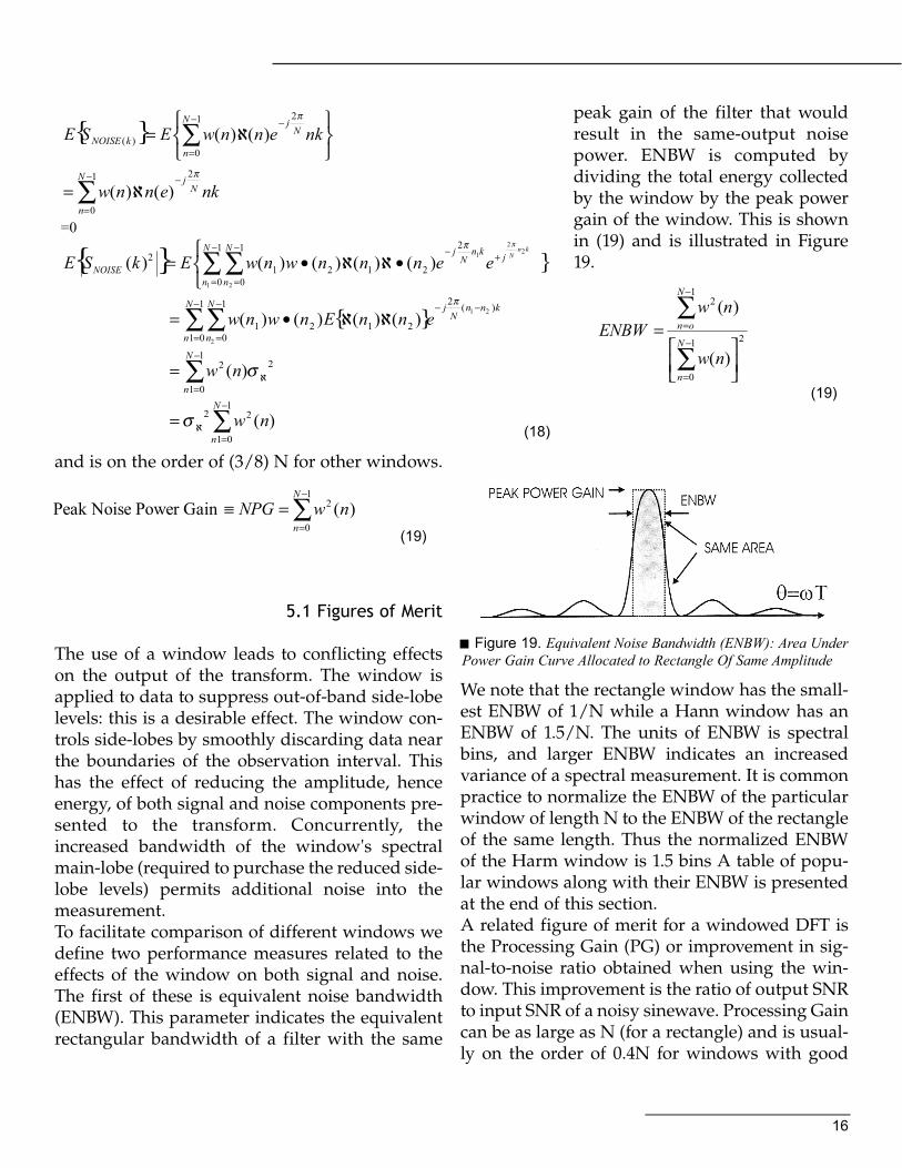
peak gain of the filter that wouldresult in the same-output noisepower. ENBW is computed bydividing the total energy collectedby the window by the peak powergain of the window. This is shownin (19) and is illustrated in Figure19.

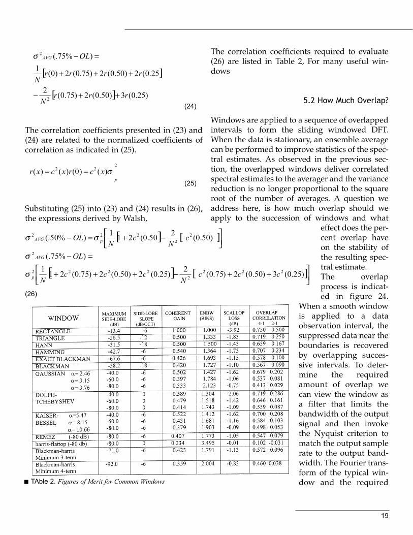
We note that the rectangle window has the small-est ENBW of 1/N while a Hann window has anENBW of 1.5/N. The units of ENBW is spectralbins, and larger ENBW indicates an increasedvariance of a spectral measurement. It is commonpractice to normalize the ENBW of the particularwindow of length N to the ENBW of the rectangleof the same length. Thus the normalized ENBWof the Harm window is 1.5 bins A table of popu-lar windows along with their ENBW is presentedat the end of this section.A related figure of merit for a windowed DFT isthe Processing Gain (PG) or improvement in sig-nal-to-noise ratio obtained when using the win-dow. This improvement is the ratio of output SNRto input SNR of a noisy sinewave. Processing Gaincan be as large as N (for a rectangle) and is usual-ly on the order of 0.4N for windows with good

{ }

ℵ= ∑−

=

−1

0

2

)( )()(N

n

Nj

kNOISE nkennwESEπ

nkennwN

n

Nj

∑−

=

−ℵ=

1

0

2

)()(π

=0

{ } }kn

NjknN

jN

n

N

nNOISE eennnwnwEkSE

22

1

1 2

2

212

1

0

1

01

2 )()()()()(ππ

+−−

=

−

=

•ℵℵ•

= ∑∑

{ } knnN

jN

n

N

nennEnwnw

)(2

212

1

01

1

01

21

2

)()()()(−−−

=

−

=

ℵℵ•= ∑∑π

21

01

2 )( ℵ

−

=∑= σnwN

n

)(1

01

22 nwN

n∑

−

=ℵ=σ

(18)

Peak Noise Power Gain )(1

0

2 nwNPGN

n∑

−

=

=≡

(19)

21

0

12

)(

)(

=

∑

∑−

=

−

=

N

n

N

on

nw

nwENBW

(19)

Figure 19. Equivalent Noise Bandwidth (ENBW): Area UnderPower Gain Curve Allocated to Rectangle Of Same Amplitude

17

side-lobe levels. As shown in (20), the processinggain is also equal to the reciprocal of the win-dow's ENBW.

5.1.1 Scalloping Loss

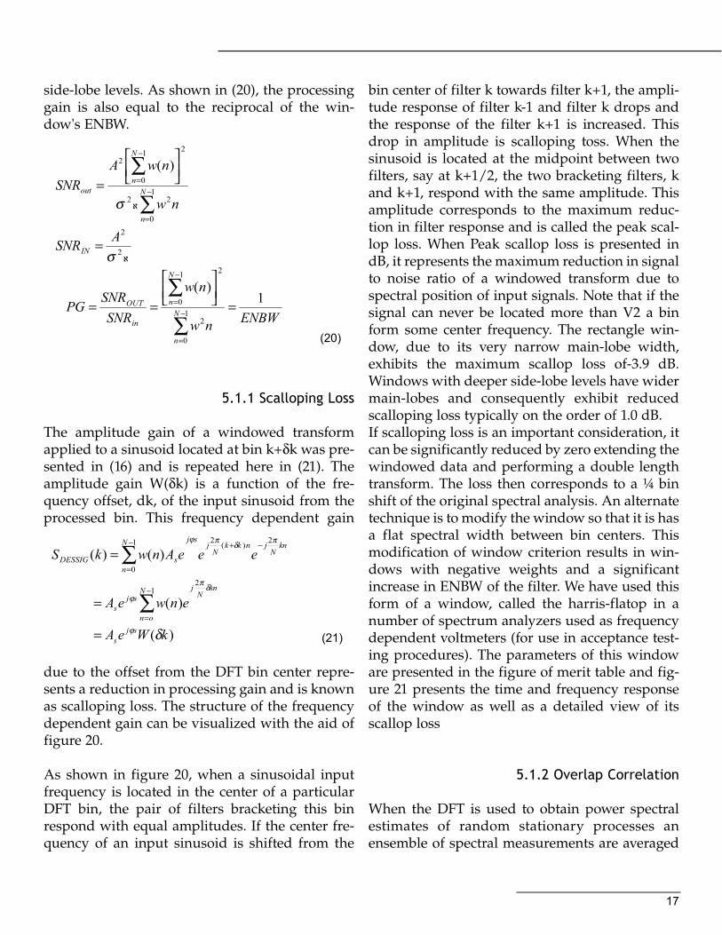
The amplitude gain of a windowed transformapplied to a sinusoid located at bin k+δk was pre-sented in (16) and is repeated here in (21). Theamplitude gain W(δk) is a function of the fre-quency offset, dk, of the input sinusoid from theprocessed bin. This frequency dependent gain

due to the offset from the DFT bin center repre-sents a reduction in processing gain and is knownas scalloping loss. The structure of the frequencydependent gain can be visualized with the aid offigure 20.

As shown in figure 20, when a sinusoidal inputfrequency is located in the center of a particularDFT bin, the pair of filters bracketing this binrespond with equal amplitudes. If the center fre-quency of an input sinusoid is shifted from the

bin center of filter k towards filter k+1, the ampli-tude response of filter k-1 and filter k drops andthe response of the filter k+1 is increased. Thisdrop in amplitude is scalloping toss. When thesinusoid is located at the midpoint between twofilters, say at k+1/2, the two bracketing filters, kand k+1, respond with the same amplitude. Thisamplitude corresponds to the maximum reduc-tion in filter response and is called the peak scal-lop loss. When Peak scallop loss is presented indB, it represents the maximum reduction in signalto noise ratio of a windowed transform due tospectral position of input signals. Note that if thesignal can never be located more than V2 a binform some center frequency. The rectangle win-dow, due to its very narrow main-lobe width,exhibits the maximum scallop loss of-3.9 dB.Windows with deeper side-lobe levels have widermain-lobes and consequently exhibit reducedscalloping loss typically on the order of 1.0 dB.If scalloping loss is an important consideration, itcan be significantly reduced by zero extending thewindowed data and performing a double lengthtransform. The loss then corresponds to a ¼ binshift of the original spectral analysis. An alternatetechnique is to modify the window so that it is hasa flat spectral width between bin centers. Thismodification of window criterion results in win-dows with negative weights and a significantincrease in ENBW of the filter. We have used thisform of a window, called the harris-flatop in anumber of spectrum analyzers used as frequencydependent voltmeters (for use in acceptance test-ing procedures). The parameters of this windoware presented in the figure of merit table and fig-ure 21 presents the time and frequency responseof the window as well as a detailed view of itsscallop loss

5.1.2 Overlap Correlation

When the DFT is used to obtain power spectralestimates of random stationary processes anensemble of spectral measurements are averaged

∑

∑−

=ℵ

−

=

= 1

0

22

21

0

2 )(

N

n

N

nout

nw

nwASNR

σ

ℵ= 2

2

σASNRIN

ENBWnw

nw

SNRSNR

PG N

n

N

n

in

OUT 1)(

1

0

2

21

0 =

==∑

∑−

=

−

=

(20)

knN

jnkkN

jsjN

nsDESSIG eeeAnwkS

πδπϕ 2)(21

0)()(

−+−

=∑=

knN

jN

on

sjs enweA

δπ

ϕ

21

)(∑−

=

=

)( kWeA sjs δϕ= (21)

18

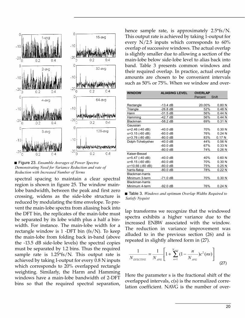
to reduce the variance of the estimates. When thesuccessive transforms are obtained from non-overlapped segments of the time series, the stan-dard deviation of the spectral estimates obtainedby simple averaging is reduced by the square-rootof the number of averages. For instance, averaging32 independent transforms will reduce the stan-dard deviation by a factor of 5.6 or 15. dB. Figure23 demonstrates the improvement in varianceobtained by the ensemble averaging of independ-ent transforms. We apply windows to data to sup-press artificial discontinuities at the data bound-aries. The window essentially discards the data inthe intervals nears near the boundaries. To avoidmissing data we overlap successive intervals andobtain what has been called the sliding windowedDFT. Typical values of interval overlap for succes-sive transforms is 75% and 50%. These overlapintervals are often called 4-to-l overlap and 2-to-loverlap respectively. The data collected from suc-

cessive overlapped and windowed trans-forms is not independent. Consequently, thedegree of variance reduction obtained byensemble averaging of spectra will be signif-icantly reduced.The variance reduction obtained by averag-ing correlated data can be easily determinedby examining the terms in the covariancematrix of the summation shown in (22).

When the entries in the summation of (22)are independent, the diagonal terms of thecovariance matrix are the only non zeroterms and the summation collapses toc(0)/N. When the collected data represents50% overlapped intervals, The matrixbecomes. banded and contains only the diag-onal terms and the first upper and lower offdiagonal terms. Gathering all the terms onthe three diagonals results in the summationshown in (23).

When the collected data represents 75%overlapped intervals. The matrix becomes

banded and contains only the diagonal terms andthe three upper and lower off diagonal terms.Gathering all the terms on the seven diagonalsresults in the summation shown in (24).

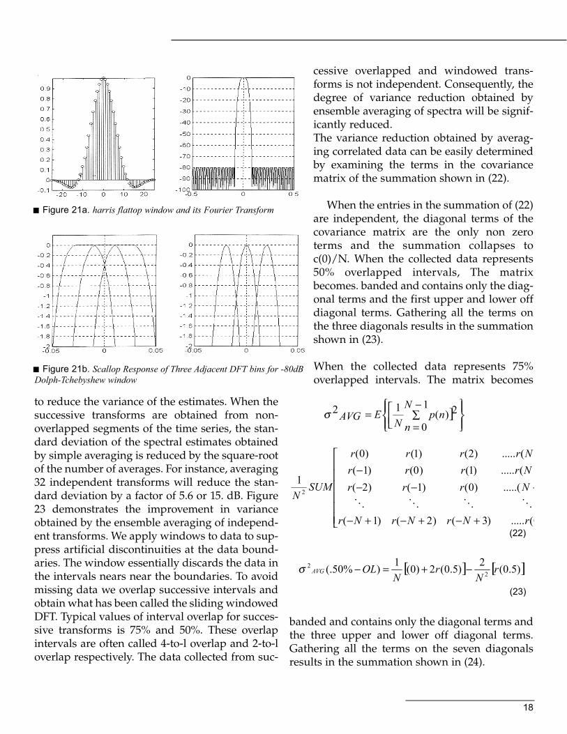
Figure 21a. harris flattop window and its Fourier Transform

Figure 21b. Scallop Response of Three Adjacent DFT bins for -80dBDolph-Tchebyshew window

]

∑−

== 2)(

1

0

12 npN

nNEAVGσ

+−+−+−

−−−−

0(.....)3()2()1(

.....()0()1()2((.....)1()0()1((.....)2()1()0(

12

rNrNrNr

NrrrNrrrrNrrrr

SUMN

OOOO

(22)

[ ] [ ])5.0(2)5.0(2)0(1)%50(. 22 r

Nr

NOLAVG −+=−σ

(23)

19

The correlation coefficients presented in (23) and(24) are related to the normalized coefficients ofcorrelation as indicated in (25).

Substituting (25) into (23) and (24) results in (26),the expressions derived by Walsh,

The correlation coefficients required to evaluate(26) are listed in Table 2, For many useful win-dows

5.2 How Much Overlap?

Windows are applied to a sequence of overlappedintervals to form the sliding windowed DFT.When the data is stationary, an ensemble averagecan be performed to improve statistics of the spec-tral estimates. As observed in the previous sec-tion, the overlapped windows deliver correlatedspectral estimates to the averager and the variancereduction is no longer proportional to the squareroot of the number of averages. A question weaddress here, is how much overlap should weapply to the succession of windows and what

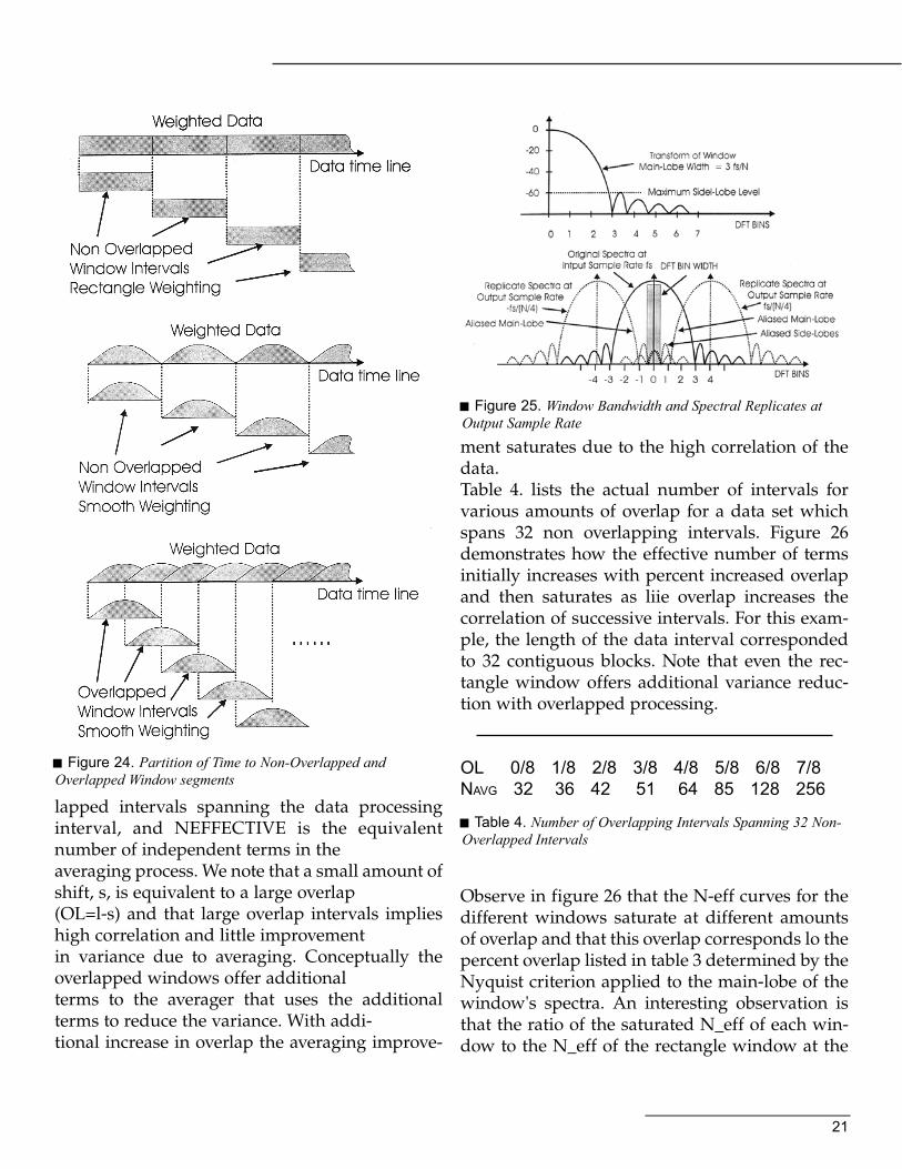
effect does the per-cent overlap haveon the stability ofthe resulting spec-tral estimate.The overlapprocess is indicat-ed in figure 24.

When a smooth windowis applied to a dataobservation interval, thesuppressed data near theboundaries is recoveredby overlapping succes-sive intervals. To deter-mine the requiredamount of overlap wecan view the window asa filter that limits thebandwidth of the outputsignal and then invokethe Nyquist criterion tomatch the output samplerate to the output band-width. The Fourier trans-form of the typical win-dow and the required

[ ]

[ ] )25.0(3)50.0(2)75.0(2

25.0(2)50.0(2)75.0(2)0(1)%75(.

2

2

rrrN

rrrrN

OLAVG

++−

+++

=−σ

(24)

222 )()0()()(

pxcrxcxr σ==

(25)

[ ] [ ]

−+=− )50.0(250.0(211)%50(. 2

2222 c

Nc

NOL pAVG σσ

[ ] [ ]

++−+++

=−

)25.0(3)50.0(2)75.0(2)25.0(2)50.0(2)75.0(211)%75(.

2222

2222

2

cccN

cccN

OL

p

AVG

σ

σ

(26)

TAble 2. Figures of Merit for Common Windows

20

spectral spacing to maintain a clear spectralregion is shown in figure 25. The window main-lobe bandwidth, between the peak and first zerocrossing, widens as the side-lobe structure isreduced by modulating the time envelope. To pre-vent the main-lobe spectra from aliasing back intothe DFT bin, the replicates of the main-lobe mustbe separated by its lobe width plus a half a bin-width. For instance. The main-lobe width for arectangle window is 1 -DFT bin (fs/N). To keepthe main-lobe from folding back in-band (abovethe -13.5 dB side-lobe levels) the spectral copiesmust be separated by 1.2 bins. Thus the requiredsample rate is 1.25*fs/N. This output rate isachieved by taking I-output for every 0.8 N inputswhich corresponds to 20% overlapped rectangleweighting. Similarly, the Harm and Hammingwindows have a main-lobe bandwidth of 2-DFTbins so that the required spectral separation,

hence sample rate, is approximately 2.5*fs/N.This output rate is achieved by taking 1-output forevery N/2.5 inputs which corresponds to 60%overlap of successive windows. The actual overlapis slightly smaller due to allowing a section of themain-lobe below side-lobe level to alias back intoband. Table 3 presents common windows andtheir required overlap. In practice, actual overlapamounts are chosen to be convenient intervalssuch as 50% or 75%. When we window and over-

lap transforms we recognize that the windowedspectra exhibits a higher variance due to theincreased ENBW associated with the window.The reduction in variance improvement wasalluded to in the previous section (26) and isrepeated in slightly altered form in (27).

Here the parameter s is the fractional shift of theoverlapped intervals, c(s) is the normalized corre-lation coefficient. NAVG is the number of over-

Figure 23. Ensamble Averages of Power SpectraDemonstrating Need for Variance Reduction and rate ofReduction with Increased Number of Terms

WINDOW ALIASING LEVEL OVERLAPPercent Shift

Rectangle -13.4 dB 20.00% 0.80 NTriangle -26.8 dB 52% 0.48 NHann -31.5 dB 56% 0.44 NHamming -42.7 dB 56% 0.44 NBlackman -58.2 dB 69% 0.31 NGaussianα=2.46 (-40 dB) -40.0 dB 70% 0.30 Nα=3.15 (-60 dB) -60.0 dB 76% 0.24 Nα=3.76 (-80 dB) -80.0 dB 83% 0.17 N Dolph-Tchebyshev -40.0 dB 44% 0.56 N

-60.0 dB 67% 0.33 N-80.0 dB 74% 0.26 N

Kaiser-Besselα=5.47 (-40 dB) -40.0 dB 40% 0.60 Nα=8.15 (-60 dB) -60.0 dB 70% 0.30 Nα=10.66 (-80 dB) -80.0 dB 75% 0.25 Nharris-flatop -80.0 dB 78% 0.22 NBlackman-harrisMinimum 3-term -71.0 dB 70% 0.30 NBlackman-harrisMinimum 4-term -92.0 dB 76% 0.24 N

Table 3. Windows and optimum Overlap Widths Required toSatisfy Nyquist

−+= ∑

=

AVGN

n AVGAVGEFECTIVE

nscN

nNN 1

2 )()1(111

(27)

21

lapped intervals spanning the data processinginterval, and NEFFECTIVE is the equivalentnumber of independent terms in theaveraging process. We note that a small amount ofshift, s, is equivalent to a large overlap(OL=l-s) and that large overlap intervals implieshigh correlation and little improvementin variance due to averaging. Conceptually theoverlapped windows offer additionalterms to the averager that uses the additionalterms to reduce the variance. With addi-tional increase in overlap the averaging improve-

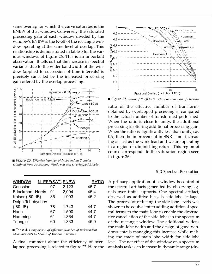
ment saturates due to the high correlation of thedata.Table 4. lists the actual number of intervals forvarious amounts of overlap for a data set whichspans 32 non overlapping intervals. Figure 26demonstrates how the effective number of termsinitially increases with percent increased overlapand then saturates as liie overlap increases thecorrelation of successive intervals. For this exam-ple, the length of the data interval correspondedto 32 contiguous blocks. Note that even the rec-tangle window offers additional variance reduc-tion with overlapped processing.

OL 0/8 1/8 2/8 3/8 4/8 5/8 6/8 7/8NAVG 32 36 42 51 64 85 128 256

Observe in figure 26 that the N-eff curves for thedifferent windows saturate at different amountsof overlap and that this overlap corresponds lo thepercent overlap listed in table 3 determined by theNyquist criterion applied to the main-lobe of thewindow's spectra. An interesting observation isthat the ratio of the saturated N_eff of each win-dow to the N_eff of the rectangle window at the

Figure 24. Partition of Time to Non-Overlapped andOverlapped Window segments

Figure 25. Window Bandwidth and Spectral Replicates atOutput Sample Rate

Table 4. Number of Overlapping Intervals Spanning 32 Non-Overlapped Intervals

22

same overlap for which the curve saturates is theENBW of that window. Conversely, the saturatedprocessing gain of each window divided by thewindow's ENBW is the N-eff of the rectangle win-dow operating at the same level of overlap. Thisrelationship is demonstrated in table 5 for the var-ious windows of figure 26. This is an importantobservation! It tells us that the increase in spectralvariance due to the wider bandwidth of the win-dow (applied to succession of time intervals) isprecisely cancelled bv the increased processinggain offered bv the overlap processing.

WINDOW N_EFF(SAT) ENBW RATIOGaussian 97 2.123 45.7B lackman- Harris 91 2,004 45.4Kaiser (-80 dB) 86 1.903 45.2Dolph-Tchebyshev(-80 dB) 78 1.743 44.7Hann 67 1.500 44.7Hamming 61 1.364 44.7Triangle 60 1.333 45.0

A final comment about the efficiency of over-lapped processing is related to figure 27. Here the

ratio of the effective number of transformsobtained by overlapped processing is comparedto the actual number of transformed performed.When the ratio is close to unity, the additionalprocessing is offering additional processing gain.When the ratio is significantly less than unity, say0.9, then the improvement in SNR is not increas-ing as fast as the work load and we are operatingin a region of diminishing return. This region ofcourse corresponds to the saturation region seenin figure 26.

5.3 Spectral Resolution

A primary application of a window is control ofthe spectral artifacts generated by observing sig-nals over finite supports. One spectral artifact,observed as additive bias, is side-lobe leakage.The process of reducing the side-lobe levels wasshown to be equivalent to adding additional spec-tral terms to the main-lobe to enable the destruc-tive cancellation of the side-lobes in the spectrumof the rectangle window. The additional widensthe main-lobe width and the design of good win-dows entails managing this increase while mak-ing the trade of main-lobe width for side-lobelevel. The net effect of the window on a spectrumanalysis task is an increase in dynamic range (due

Figure 26. Effective Number of Independant SamplesObtained from Processing Windowed and Overlapped Blocks

Table 4. Comparison of Effective Number of IndependentMeasurements to ENBW of Various Windows

Figure 27. Ratio of N_eff to N_actual as Function of Overlap

23

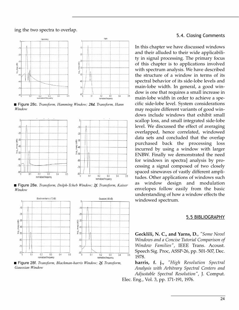
to side-lobe suppression) with a decrease in spec-tral resolution (due to main-lobe widening).The most demanding test of a windowed trans-form is its ability to resolve and detect two closelyspaced sinusoids of significantly different ampli-tudes. A more stringent test would be the samesignal in the presence of large levels of additivenoise, but that problem is addressed by ensembleaveraging which we examined in section 5.2. Wenow demonstrate the affect of the window on thedetection and measurement of two sine-waves ofamplitude 1.0 and 0.01 and of frequency 11.5 and16.0 cycles per interval respectively. The large sig-nal at frequency 10.5 cycles per interval is locatedbetween two DFT bins and splatters its spectralside-lobes throughout the remaining DFT bins. Areference point to compare the performance of thewindows is available in figure 26a. Here we seethe power spectrum of the two signals with thelarge signal moved to DFT bin 11(11 cycles pernterval). Since both signals are harmonically relat-ed to the observation interval there is no spectralsplatter between the DFT bins and the signals areperfectly resolvable (within additive and arith-metic noise effects). In figure 26b, we see thepower spectrum of the two signals after returningthe large signal to bin 11.5. As we can see, the side-lobe levels of the large signal almost covers themain-lobe of the small signal resulting in signifi-cant degradation of its detectability.The remaining figures of this example (26cthrough 26f) present the power spectra of thesame two signals processed with differentwindows. When the window used in thisdemonstration had selectable side-lobe levelsthey were selected to be 60 dB below peak.Note that the power spectra were not nor-malized for peak power level but rather werenormalized to peak power level of the rec-tangle window with bin centered signal. Thispermits us to see the reduction in peakamplitude response due to application of thewindow. Note in figure 26c the side-lobes ofthe Hamming window now-centered on thespectrum of the large signal, are spilling into

the spectrum and nearly covering the low levelsignal. By comparison, we see in figure 26d thatthe side-lobe structure of the Hann window failsquite rapidly and while not filling the entire spec-trum they spill into the spectral region occupiedby the smaller signal. In figure 26e we see that themain-lobe of the Dolph-Tchebyshev is sufficientlynarrow to permit excellent resolution of the twosignal spectra but that the side-lobes of the twosignals interact and cause incidental side-lobeamplitude modulation. This is one of the prob-lems with windows (and filters) that exhibit con-stant level side-lobes. Figure 26f shows the excel-lent performance of the Kaiser-Bessel windowand illustrates the window's ability to resolveclosely spaced signals of significantly differentamplitude levels. The spectral notch between thetwo spectral lines can be thought of as the win-dow's ability to accommodate additional resolu-tion stress (of reduced signal level or reducedspectral spacing). This window would have nodifficulty resolving these two signals even if theywere 80 dB apart (rather that the 40 dB of thisexample). Similarly, figure 28f illustrates the suc-cess of the Blackman-harris window in its abilityto resolve the two spectral lines. Finally, figure 26fdemonstrates that the Gaussian window resolvesthe two signals but the notch between the twospectral lines is not as deep as the former twoexamples. This reduction in resolution is due tothe wider main-lobe width of the window caus-

Figure 28a. Transform, Rectangle window; 28b. Transform, Rectangle window

24

ing the two spectra to overlap.5.4. Closing Comments

In this chapter we have discussed windowsand their alluded to their wide applicabili-ty in signal processing. The primary focusof this chapter is to applications involvedwith spectrum analysis. We have describedthe structure of a window in terms of itsspectral behavior of its side-lobe levels andmain-lobe width. In general, a good win-dow is one that requires a small increase inmain-lobe width in order to achieve a spe-cific side-lobe level. System considerationsmay require different variants of good win-dows include windows that exhibit smallscallop loss, and small integrated side-lobelevel. We discussed the effect of averagingoverlapped, hence correlated, windoweddata sets and concluded that the overlappurchased back the processing lossincurred by using a window with largerENBW. Finally we demonstrated the needfor windows in spectra] analysis by pro-cessing a signal composed of two closelyspaced sinewaves of vastly different ampli-tudes. Other applications of windows suchas window design and modulationenvelopes follow easily from the basicunderstanding of how a window effects thewindowed spectrum.

5.5 BIBLIOGRAPHY

Gecklili, N. C., and Yarns, D., "Some NovelWindows and a Concise Tutorial Comparison ofWindow Families", IEEE Trans. Acoust.Speech Sig. Proc, ASSP-26, pp. 501-507, Dec.1978.harris, f. j., "High Resolution SpectralAnalysis with Arbitrary Spectral Centers andAdjustable Spectral Resolution", J. Comput.

Elec. Eng., Vol. 3, pp. 171-191, 1976.

Figure 28c. Transform, Hamming Window; 28d. Transform, HannWindow

Figure 28e. Transform, Dolph-Tcheb Window; 2f. Transform, KaiserWindow

Figure 28f. Transform, Blackman-harris Window; 2f. Transform,Gaussian Window

25

harris, f.j., "On the Use of Windows for HarmonicAnalysis with the Discrete Fourier Transform' Proc.IEEE, 66, pp. 51-83, January 1978.harris, f. j.. "On Overlapped Fast FourierTransforms", International TelemeteringConference (ITC-78), pp 301-306, Los Angeles,CA, Nov. 14-16, 1978.harris, f. j., "The Discrete Fourier Transform Appliedto Time Domain Signal Processing", IEEECommunications Magazine, Vol. 20, No. 3, pp. 13-22, May 1982.Kaiser, J. F. and R.W. Schafer, "On the Use of thelo-Sinh Window for Spectrum Analysis", IEEE Trans.Acoust., Speech, Signal Proc., ASSP-28, pplOS,1980.Nuttal, A. H., ''Some Windows with Very GoodSidelobe Behavior", IEEE Trans. Acoust., Speech,Signal Proc., ASSP-29, pp. 84-87,1981.Ward. H. R.. "Properties of Dolph-ChebyshevWeighting Functions", IEEE Trans. Aerospace andElec. Syst., Vol. AES-9, No. 5, pp 785-786., Sept.1973.Welch, P. D., "The Use of Fast Fourier Transform forthe Estimation of Power Spectr: A Method Based onTime Averaging Over Short, Modified Periodograms",IEEE Trans., Audio Electrocaust., Vol. AU-15, pp70-73, June 1967