Windowed Cross–Correlation and Peak Picking for …people.virginia.edu/~smb3u/psych611/Peak20020108aReprint.pdf · Windowed Cross–Correlation and Peak Picking for the Analysis

Windowed Cross–Correlation and Peak Picking for theAnalysis of Variability in the Association Between Behavioral

Time Series

Steven M. BokerDepartment of Psychology

The University of Notre Dame

Minquan XuAmdocs St. Louis Development Center

Jennifer L. RotondoAugustana College

Kadija KingUniversity of Akron

January 16, 2002

AbstractCross–correlation and most other longitudinal analyses assume that the as-sociation between two variables is stationary. Thus, a sample of occasionsof measurement is expected to be representative of the association betweenvariables regardless of the time of onset or number of occasions in the sam-ple. We propose a method to analyze the association between two variableswhen the assumption of stationarity may not be warranted. The method re-sults in estimates of both the strength of peak association and the time lagwhen the peak association occurred for a range of starting values of elapsedtime from the beginning of an experiment.

This work was supported in part by NIA grant R29 AG14983 and a grant from the University of NotreDame. We also wish to thank David Parker, Melissa Sturge–Apple and Eric Covey whose assistance is greatlyappreciated in gathering the example data presented here. We also wish to express our thanks to ScottMaxwell, Kathy Eberhard and four anonymous reviewers who provided many helpful editorial comments.Some of the example data has previously appeared in Boker and Rotondo (in press). Correspondence maybe addressed to Steven M. Boker, Department of Psychology, The University of Notre Dame, Notre DameIndiana 46556, USA; email sent to [email protected]; or browsers pointed to http://www.nd.edu/˜ sboker. Ccode to calculate the windowed cross–correlation matrices and Splus code for the peak picking algorithm areavailable for free on this web site.

WINDOWED CROSS–CORRELATION AND PEAK PICKING 2

Introduction

Many psychological experiments involve data that are comprised of multiple observa-tions of the same variable over time. These data may be only a few waves of data in a panelstudy, from tens to hundreds of observations in a self–report journaling study or as manyas tens of thousands of observations per variable in psychophysiological time series such asEEG, EKG or motion capture studies. In most cases, multiple variables are being observed(or as it is sometimes expressed in the time series literature, sampled) at each occasion ofmeasurement. The data for which the methods in this article are appropriate include atleast 100 occasions of measurement on at least two variables for one or more participants.While data with fewer occasions of measurement could be used, the method’s usefulnesswould be reduced. The methods we propose use Pearson product moment correlations toestimate bivariate relationships between continuous variables. In addition, the algorithmspresented here are specific to data that have equal intervals of time between observations,although in principle they could be adapted to unequal intervals.

The reason multiple occasions of measurement are included in a research design isgenerally because one wishes to understand not only the relationship between multiplevariables at the same moment in time, but also the relationships between these variablesas they change over time. Thus the relationship between variables observed at the sameoccasion of measurement may only be part of the story. Variables observed at differentoccasions of measurement may also be related to one another. These relationships betweenvariables may have different strengths depending on the interval of time separating themeasurements. The structure of the way that this relationship between variables changesas the interval between occasions of measurement changes can be an extremely informativediagnostic as to the nature of the underlying processes that gave rise to the data.

A number of methods are in common use to model these relationships between mul-tiple variables at multiple occasions of measurement. These methods include, autocor-relation and cross-correlation, autoregressive and cross–lagged structural models (see e.g.Cook, Dintzer, & Mark, 1980; West & Hepworth, 1991), multivariate time series methodssuch as autoregressive moving average models (see e.g. Box, Jenkins, & Reinsel, 1994),cross–spectral or coherence analysis (Bloomfield, 1976; Warner, 1998), P–technique factoranalysis (e.g. Nesselroade & Ford, 1985), dynamic factor analysis (Molenaar, 1985), variousstructural equation model variants proposed by McArdle and colleagues (e.g. Hamagami,McArdle, & Cohen, 2000), and nonlinear methods such as mutual information (Abarbanel,1996; Boker, Schreiber, Pompe, & Bertenthal, 1998). Each of these methods uses relatedmethods in that they all estimate some set of linear or nonlinear relations between observa-tions separated by intervals of time while assuming that this structure remains constant overtime. This assumption of constant relations over time boils down to an assumption knownas stationarity (for discussions of stationarity and nonstationarity see Hendry & Juselius,2000; Shao & Chen, 1987). In order for a process to be stationary (formally known as weakstationarity) for any starting time, t, the expected value of the means, standard deviations,autocorrelations, frequency spectra, and cross correlations of a sample from the processmust be equal to the corresponding population values (Box et al., 1994; Ito, 1993). In otherwords, an assumption of stationarity implies that a set of statistical properties are assumedto hold across the entire length of time during which the psychological process was under


observation.With any simplifying assumption there are positive and negative consequences. There

are two main benefits in assuming that a multivariate time series is stationary. The first isthat one may conclude that any particular collection of occasions of measurement is repre-sentative of the whole behavior. Closely related, one may also conclude that all occasions ofmeasurement separated by some time interval, s, have a relationship which has an expectedvalue that does not change over the occasions of measurement in the experiment. Thusby assuming stationarity and making distribution assumptions, one may calculate means,covariances, regressions, and standard errors that may be concluded to be estimates ofcharacteristics of the behavior as a whole.

Although these positive consequences might seem to provide arguments in favor ofmaking an assumption of stationarity, it can be dangerous to make assumptions concerningdata based on the convenience or power of a statistical method. Sometimes the assumptionof stationarity is untenable. Traditional time series analyses use methods to remove non-stationarity so that the remaining stationary process can be analyzed, a process sometimesknown as prewhitening the time series data (see e.g. West & Hepworth, 1991). For instance,bivariate time series analysis will typically remove co–occuring trends and cycles in orderto examine the time–lagged relationship of the residuals of the two time series. However,many interesting behavioral phenomena are not only inherently nonstationary, but the veryreason that they are interesting lies in the nature of that nonstationarity. One phenomenonof wide interest to behavioral researchers is human communication in its various forms, in-cluding face to face verbal conversation, nonverbal cues in conversation, written language,and music production and perception. It is our contention that the process of human com-munication is an excellent example of when understanding nonstationarity may be essentialto understanding a behavioral phenomenon.

As an example, consider one form of human communication in which differing degreesof stationarity can be conveniently observed: the production and perception of music. Ifa musical composition were stationary, then there would be one function that, given aninterval of time s milliseconds, would give the expected value of the correlation between thelevel of air pressure at any one moment in time and the level of the air pressure s millisecondslater. The logical consequence is that this musical composition would be composed of asingle repeated waveform: essentially a single phrase played repeatedly without end bysome combination of instruments.

While there exist musical compositions that display this characteristic of unendingrepetition, most musical compositions evolve over their span. And while there may benearly repeating themes in a composition, new elements and relations between instrumentstend to be added as the musical piece progresses. Humans do not tend to produce musicthat is stationary. Musical compositions tend to contain both elements of predictability andelements of surprise (Jones, 1993). Over short time spans one may observe repetition of aphrase, but over longer time spans the composition will tend to evolve in unexpected ways.

Similarly, an interesting conversation does not involve endlessly repeated verbiage,but contains both redundancy and surprise. It has been long known that over short timespans a listener may be able to predict the next word a speaker will say, but over longertime spans the words tend to be relatively unpredictable (Aborn, Rubenstein, & Sterling,1959). Researchers in psycholinguistics, music perception, and auditory perception have


begun to realize that many of the relationships of interest in their data are nonstationary,and that the nature of that nonstationarity is a crucial topic for analysis (see e.g. Bregman,1990; Gregson & Harvey, 1992; Miller & Chomsky, 1963).

A related argument is advanced by Nesselroade and Featherman (1991) as appliedto lifespan development. They suggest that the intraindividual variability of a constructover occasions of measurement may be an important indicator in and of itself. For instancevariability in trial by trial performance has been used to help understand strategy learningin children (Siegler & Jenkens, 1989). Inherent in this argument is the notion that theremay be critical changes in this variability, that is nonstationarity, which may be predictiveof important outcomes. It is only a small step from Nesselroade and Featherman’s positionto suggest that nonstationarity in multivariate time series may itself prove to be a usefulvariable when addressing a variety of developmental questions.

In fact, the variability or nonstationarity of a variable may indicate only part of thestory. We propose that there may be interesting patterns of variability in the associationbetween variables. One consequence of this proposal is that variables may be nearly sta-tionary in short durations, but much less so over longer time spans. We will use this ideaof local stationarity in order to quantify variability in association.

Variability in a measure of association such as correlation may be important in orderto understand, in particular, how adaptable creatures such as ourselves behave when theenvironment is also adapting to us. In any interpersonal exchange, two or more individualsmay be adapting to one another and it therefore might be expected that the association be-tween the individuals’ behavior would show a pattern of variability that would be indicativeof the underlying adaptive process.

The use of nonstationarity of association as a variable in psychological research re-quires a method that can quantify fluctuations in the relationships between variables overtime. We propose a composite method, a few well–known steps and a simple algorithm,that can estimate time varying changes in patterns of bivariate predictability in a flexi-ble manner. We then apply the method to a data set from an experiment in non–verbalcommunication in order to illustrate its use in a real–world psychological context.

In order to create a method that would be able to quantify variability of association,we identified three criteria that needed to be fulfilled. The first criterion is that the methodmust be able to track changes in the time lag and strength of association between the twotime series over the course of the experiment. Suppose we measure two variables on multipleoccasions separated by equal intervals and resulting in two vectors of observations X andY. If an event in X occurs before a similar event in Y, we might reason that the event inX may have predicted the event Y. But later we may see an event in Y that appears topredict a later event in X. Such changes in lag and strength of maximum prediction can beindicative of an underlying dynamic relationship between the constructs that gave rise tothe data in X and Y. The variance of the time lag and variance of strength of associationwill give estimates of two types of nonstationarity in the bivariate time series.

Second, within some set bounds the method should estimate the interval of timebetween occasions of measurement at which a maximum association between two timeseries occurs and the strength of that association. The importance of finding a best lag ofassociation has been long been recognized (e.g. Cattell, 1963). Often, one is only interestedin the association between events that are separated by no more than some fixed bound


(a few seconds, a few minutes, a day, etc.), while events that occur outside this bound arelikely to be only spuriously related. Within that bounded interval of time, there may a lagbetween an event that occurs in time series X and a similar event that occurs in time seriesY. The method should give an estimate of the time lag between the event in X and theevent in Y as well as the strength of association between the two events.

Finally, the method should be flexible in the inherent tradeoff between the reliabilityof estimates of association between variables and the sensitivity to changes in the estimatesof association. As more occasions of measurement are used to create an aggregated estimateof association, longer durations of time will be aggregated. This will tend to lead to a moreaccurate estimate of association from a statistical standpoint, but will simultaneously reducethe sensitivity needed to measure short duration fluctuations in a process. At the presenttime, we see no way around this reliability–sensitivity tradeoff other than both decreasingthe interval of time between occasions of measurement and simultaneously increasing thenumber of occasions. The optimal tradeoff between sensitivity and reliability is likely tobe different for each experiment, since how quickly the predictive relationship betweenpsychological processes changes will be dependent on which processes are being studied,and each individual experiment may incorporate its own unique interval between occasionsof measurement. Thus, the method must allow flexibility in assigning parameters thatcontrol the associated reliability and sensitivity.

As an example, we examined the coordination between movements made by pairs ofindividuals engaged in conversation. Facial expression, eye contact, pupil dilation, posture,gesture, and inter-personal distance may potentially be considered as elements of non-verbal communication. We tracked individual’s hand and head motions during a 10 minuteconversation and examined the association between the overall velocity of two conversants’head movements and between the left hand of one conversant and the right hand of theother. Previous work has indicated that the pattern of association between two conversants’movements can be nonstationary (Rotondo & Boker, in press). The example conversationalexperiment tests the hypothesis that auditory interference in the form of amplified trafficnoise with a loudness equivalent to that of a subway train will change the structure ofthe coordination between two conversants’ movements. The proposed method allows anestimate of the nonstationarity in the conversants’ movements when noise is present asopposed to when noise is absent.

Cross–Correlation

A common method for estimating the association between events in two time seriesis cross–correlation, the correlation between two time varying stimuli or events over timeintervals that may or may not be coincident. Essentially, a vector of sequential occasionsof measurement is selected from each time series such that both vectors contain the samenumber of occasions and then the Pearson product moment correlation is calculated forthese two vectors. The vectors may or may not begin at the same occasion of measurement.The interval of time separating the beginning occasion of measurement for the two vectorsis the lag or offset. A vector of sequential measurements sampled from a time series is oftencalled a window.

Suppose we wish to cross correlate two time series each containing N observations X ={x1, x2, x3, . . . , xN} and Y = {y1, y2, y3, . . . , yN} with equal intervals of time, s, between


observations. If we assume stationarity and choose a positive lag of τ observations, thecross–correlation between X and Y at a lag τ is a function r of X, Y, and τ that can bedefined as

r(X,Y, τ) =1

N − τ

N−τ∑i=1

(xi −X)(yi+τ −Y)sd(X)sd(Y)

, (1)

where X and Y are the grand means and sd(X) and sd(Y) are the standard deviationsof X and Y respectively over all occasions of measurement. This is merely an ordinaryPearson correlation between the two time series lagged by τ observations (a time intervalcorresponding to τ times s, the sampling interval).

Variations of cross–correlation similar to Equation 1 are commonly used in psycho-logical research. For instance, cross–correlation has been used in theories in audition (e.g.Cherry, 1961; Licklider, 1959), of motion perception (e.g. Reichardt, 1961; Santen & Sper-ling, 1985), and of form detection and pattern recognition (e.g. Dodwell, 1971; Glass &Switkes, 1976; Dixon & Di Lolo, 1994). Most researchers assume the observed data comefrom stationary processes, where means and variances are constant over time. This yieldsmathematical tractability at the expense of possibly oversimplifying the model for the pro-cess of interest.

We will illustrate the use of cross–correlation with two example data sets, each con-taining data recorded using motion tracking equipment from the movements of pairs ofparticipants sampled at 80 Hz (80 occasions of measurement per second). The first data setis from two participants who were asked to dance while mimicking each others’ movementsand the second data set is from two participants engaged in conversation. We use thesetwo examples of coordinated behavior because the dancing behavior should be relativelystationary due to the repeating nature of the synchronizing auditory stimulus to which theparticipants were asked to dance. The coordination of head behavior from conversation hasbeen found to exhibit a great deal of nonstationarity in previous work in our lab (Rotondo,2000).

In the first data set, two individuals are dancing with one another while listening toa repeating rhythm. Dancer A is instructed to lead and dancer B is instructed to followdancer A’s movements as closely as possible. The movements that they make are likely to behighly synchronized with each other as well as being synchronized with the rhythm. Sincethe rhythm is repeating, the dancers are synchronizing with a stationary signal. Thus, wewould expect that there would be a stable pattern of cross–correlation over the whole trial.A plot of the average cross–correlation between two dancers’ movements as calculated usingEquation 1 is shown in Figure 1–a. There is a high degree of association between the twodancers’ movements at synchrony and at plus and minus 1600ms. The rhythm with whichthe dancers were synchronizing repeated every 1600ms, so this suggests that the dancerswere making movements in time with this rhythm such that their movements also tendedto repeat with the same cycle. These data are largely in conformance with an assumptionof stationarity, so the overall cross–correlational pattern is strong.

Now consider the coordination between head movements produced as two individualsconverse. It seems likely that these movements might not occur at exactly the same time.Sometimes conversant A would initiate a head movement that conversant B would respondto a short time later. Similarly, conversant B may sometimes make a head movement that


a.

Lag in Milliseconds

Cro

ss C

orre

latio

n

b.

Lag in Seconds

Cro

ss C

orre

latio

n

Figure 1. Overall lagged cross–correlations for (a) whole body movements of two individuals dancingduring a 40 second trial and (b) head movements of two individuals during a 5 minute dyadic conversation.

conversant A would later respond to. Thus the correlation between lagged observationsof position or orientation might turn out to be greater than that between synchronousobservations. But sometimes the response may be in the same direction as the stimulus,and sometimes it may be in the opposite direction. Thus it might be that over short timescales there could be a high degree of association, but due to nonstationarity, overall theremight be only low values of cross–correlation. Figure 1–b plots the overall cross–correlationbetween two conversants’ head movements. Only weak relationships are evident. Thiscould mean that there really is not much coordination in the conversation, or it could bethat there is short–term coordination along with nonstationarity. Standard methods whichassume stationarity cannot distinguish between these two possibilities.

Thus while a single measure of cross–correlation may give a good estimate of associ-ation between two behavioral time series, it may not give an estimate of the expected valueof that association in the same way as calculating a mean of numbers drawn from a normaldistribution. Instead, aggregating across the whole time series when global stationaritydoes not hold may be more akin to calculating the mean of a multimodal distribution. Infact, there may not be a stable expected value of association between two behavioral timeseries. The examination of patterns of change in the association between two time seriesmay be a legitimate area of inquiry in and of itself. For this reason, we now consider a moretemporally detailed analysis that can be calculated using many short cross–correlationalwindows in which the starting time of windows of observations is incremented or swept overthe whole data set.

Windowed Cross–Correlation

One way to examine how the strengths and lags of association between two timeseries are changing over time is to use only short intervals of data from each time series toestimate the association and then select these windows so that their starting points representincreasing elapsed time from the beginning of the experiment. This has the advantage ofonly making an assumption of local stationarity rather than assuming stationarity over the


whole time series.Using short, overlapping windows that cover the time series results in a moving esti-

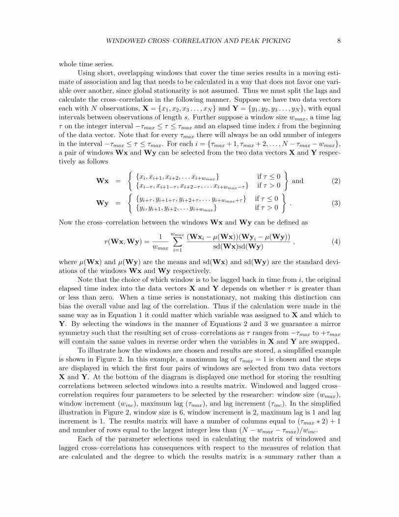
mate of association and lag that needs to be calculated in a way that does not favor one vari-able over another, since global stationarity is not assumed. Thus we must split the lags andcalculate the cross–correlation in the following manner. Suppose we have two data vectorseach with N observations, X = {x1, x2, x3 . . . , xN} and Y = {y1, y2, y3 . . . , yN}, with equalintervals between observations of length s. Further suppose a window size wmax, a time lagτ on the integer interval −τmax ≤ τ ≤ τmax and an elapsed time index i from the beginningof the data vector. Note that for every τmax there will always be an odd number of integersin the interval −τmax ≤ τ ≤ τmax. For each i = {τmax + 1, τmax + 2, . . . , N − τmax−wmax},a pair of windows Wx and Wy can be selected from the two data vectors X and Y respec-tively as follows

Wx =

{{xi, xi+1, xi+2, . . . xi+wmax} if τ ≤ 0{xi−τ , xi+1−τ , xi+2−τ , . . . xi+wmax−τ} if τ > 0

}and (2)

Wy =

{{yi+τ , yi+1+τ , yi+2+τ , . . . yi+wmax+τ} if τ ≤ 0{yi, yi+1, yi+2, . . . yi+wmax} if τ > 0

}. (3)

Now the cross–correlation between the windows Wx and Wy can be defined as

r(Wx,Wy) =1

wmax

wmax∑i=1

(Wxi − µ(Wx))(Wyi − µ(Wy))sd(Wx)sd(Wy)

, (4)

where µ(Wx) and µ(Wy) are the means and sd(Wx) and sd(Wy) are the standard devi-ations of the windows Wx and Wy respectively.

Note that the choice of which window is to be lagged back in time from i, the originalelapsed time index into the data vectors X and Y depends on whether τ is greater thanor less than zero. When a time series is nonstationary, not making this distinction canbias the overall value and lag of the correlation. Thus if the calculation were made in thesame way as in Equation 1 it could matter which variable was assigned to X and which toY. By selecting the windows in the manner of Equations 2 and 3 we guarantee a mirrorsymmetry such that the resulting set of cross–correlations as τ ranges from −τmax to +τmax

will contain the same values in reverse order when the variables in X and Y are swapped.To illustrate how the windows are chosen and results are stored, a simplified example

is shown in Figure 2. In this example, a maximum lag of τmax = 1 is chosen and the stepsare displayed in which the first four pairs of windows are selected from two data vectorsX and Y. At the bottom of the diagram is displayed one method for storing the resultingcorrelations between selected windows into a results matrix. Windowed and lagged cross–correlation requires four parameters to be selected by the researcher: window size (wmax),window increment (winc), maximum lag (τmax), and lag increment (τinc). In the simplifiedillustration in Figure 2, window size is 6, window increment is 2, maximum lag is 1 and lagincrement is 1. The results matrix will have a number of columns equal to (τmax ∗ 2) + 1and number of rows equal to the largest integer less than (N − wmax − τmax)/winc.

Each of the parameter selections used in calculating the matrix of windowed andlagged cross–correlations has consequences with respect to the measures of relation thatare calculated and the degree to which the results matrix is a summary rather than a


1

2

3

4

5

6

7

t

8

9

X Y

a

a b c

d

-1 0 +1

X Y

b

X Y

c

X Y

d

resultsmatrix

1

2

3

4

r(Wx,Wy)r(Wx,Wy)r(Wx,Wy)r(Wx,Wy)

Figure 2. Four pairs of windows selected from two data vectors, X and Y. Results of correlating eachpair of windows is stored into the results matrix whose columns represent the relative lag of the twowindows and whose rows represent the starting time of the window selected from X.

recapitulation of the data vectors. It is important to be guided in the selection of theseparameters by substantive theory as well as an exploration of a set of pilot data. In this waythese parameters can then be fixed and used to estimate windowed and lagged associationsin a second data set in a statistically testable manner.

The window size, wmax, (the number of observations in the data vectors Wx andWy) should be chosen to be small enough so that the assumption can be made of littlechange in lead–lag relationship within the number samples in the window. However, if thewindow size is too small, the reliability for the correlation estimate for each sample will bereduced. Choosing the window size involves confronting the reliability/sensitivity tradeoffdiscussed earlier. The analyst should make this choice based on substantive and theoreticconsiderations in order to optimize the method for her particular data.

The window increment, winc, is the number of samples between successive changes inthe window for the X vector as illustrated in Figures 2–c and d. The window increment istherefore also the amount of time that elapses between the correlations stored in successiverows in the results matrix. If the window increment is too short, there may be little changebetween successive rows in the results matrix, but if the window increment is too long,there may be so much change that successive rows in the results matrix will appear tobe unrelated. Short window increments also lead to large numbers of rows in the resultsmatrix. Thus one wishes to choose a window increment as long as possible, but not so longthat the relation between successive rows in the results matrix is lost.

The maximum lag, τmax is the maximum interval of time that separates the beginning


of the two windows selected from their respective data vectors. The greater the maximumlag, the greater the interval of time that can separate behaviors for which estimates ofcoordination can be obtained. However, large maximum lags will tend to lead to largenumbers of columns in the results matrix. It is thus up to the researcher to select the greatestinterval of time separating a behavior from participant X and behavior from participant Ythat would be considered to be of interest.

The lag increment, τinc, is the number of samples between successive changes in thewindow for the Y vector as shown by the difference between columns a and b in Figure 2.The lag increment is thus also the interval of time separating successive columns in theresults matrix. Short lag increments lead to little change between successive columns in theresults matrix, while long lag increments lead to apparently unrelated successive columns.The shorter the lag increments the more columns there will be in the results matrix. Thus,a good choice of lag increments will be the longest lag increment that still results in relatedchange between successive columns. In this way the size of the results matrix can beminimized while patterns in change in the lead–lag structure of the coordination of theconversants can still be examined.

An implementation written in portable C code of the windowed lagged cross–correlation algorithm is available on the web page http://www.nd.edu/˜ sboker. The codecan be compiled for MSDOS, Apple OS X, or most flavors of Unix. It inputs an ASCIItextfile with two columns of data outputs a results matrix as shown above and includescommand line options to control all the parameters discussed above.

Examples of the results of a windowed cross–correlation analysis applied to two ex-ample behavioral data sets are shown in Figure 3. In each of these graphs, the abscissa plotsthe lag of the two windows, the ordinate plots the elapsed time during the trial and the colorrepresents the value of the cross–correlation at each combination of lag and elapsed time.Thus, the rows and columns in these two graphs correspond to the rows and columns in theresults matrix from Figure 2 and the colors correspond to the values in the results matrix.Note that in these graphs, elapsed time increases as the value on the ordinate increases.Thus, the first row from the results matrix is the bottom row of the graph and the last rowof the results matrix is at the top of the graph. In this way the cross–correlations at anyparticular value of elapsed time are shown as the colors from a horizontal slice through thegraph.

The cross–correlations between two dancers’ movements are plotted in Figure 3–a.Note that after about 8 seconds into the trial, the pattern of cross–correlations becomesstable; that is each horizontal slice through the graph is much like the next horizontal slice.Thus, vertical stripes are formed when the associations between variables are stable overtime and therefore the association between the variables is stationary. When we observethe vertical stripes in Figure 3–a, it is evident that the pattern of association between thedancers’ movements becomes stationary shortly about 8 seconds after the beginning of thetrial.

On the other hand, the cross–correlations between the two conversants’ head motionsplotted in Figure 3–b does not show a pattern of vertical stripes of color. In fact, there arerelatively large changes between subsequent horizontal slices through the graph. Thus, thelags of the cross–correlational association between the two conversants’ head movementsare changing rapidly as elapsed time in the trial increases. This pattern of association is


1.0.8.6.4.2

-.2-.4-.6-.8-1.0

0

a.

Lag (s)

-2 -1 0 +1 +2

20

10

0

Ela

psed

Tim

e (

s)

b.

Lag (s)-2 -1 0 +1 +2

20

10

0

Ela

psed

Tim

e (

s)

CrossCorrelation

Figure 3. Density plots of windowed and lagged correlation result matrices from (a) 20 seconds of bodyvelocities during dyadic dance, and (b) from 25 seconds of head velocity during dyadic conversation.High positive values of correlation are red, zero values of correlation are green and high negative valuesof correlation are orange. For these plots, window size is 120 samples, window increment is 20 samples,maximum lag is 400 samples, lag increment is 10 samples, and sampling rate is 80 Hz.


nonstationary.Although the cross–correlations in Figure 3–b do not form vertical stripes, there does

seem to be some sort of pattern to the variability of this association. As elapsed timeincreases, it seems that the stripes mostly are diagonal from lower right to upper left. Thatis, the peak cross–correlations appear to change from positive to negative lags. In order tobe able to analyze patterns of change in the peak cross–correlation we have developed apeak picking algorithm that selects the peak correlation at each elapsed time according tosome flexible criteria. The next section introduces this peak picking method and presentsthe parameters for controlling the selection of peak cross–correlations.

The Peak Picking Algorithm

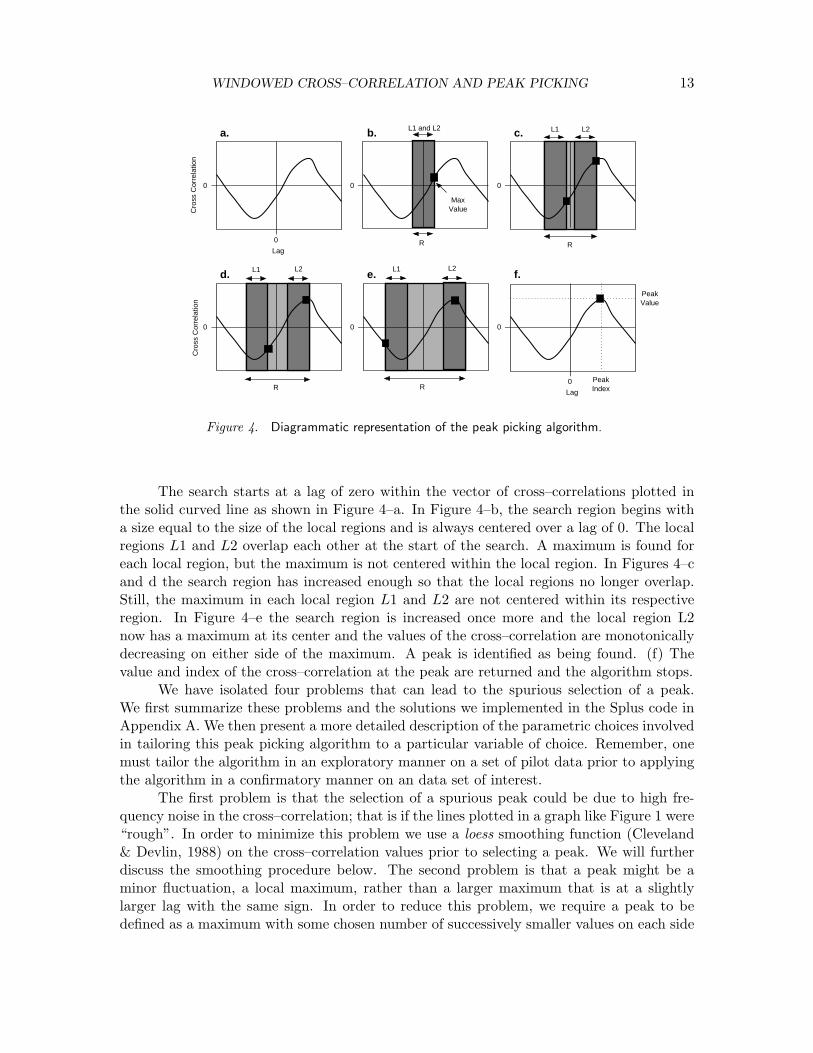
One possible way to estimate the time lag of the predictive association between twotime series is to find the peak cross–correlation that is closest to a lag of zero. For instance,suppose an event of duration one second occurs in data vector window Wx and a similarevent occurs two seconds later in data vector window Wy. In this case, we would expecta peak cross–correlation between the two windows at a lag of τ = 2/s where s is thesampling interval of the observations in the windows expressed in seconds. In order to findsuch a lag between two similar events a definition of what is meant by a “peak” will berequired. As is so often the case in data analysis, the best definition may depend on thecharacteristics of the phenomena and the design of the experiment. We have defined a peakto be a maximum value of cross–correlation centered in a local region in which values aremonotonically decreasing on each side of the peak. The analyst must define the size of thislocal region to be large enough so that spurious local noise is rejected, but small enough sothat meaningful peaks are not rejected.

We now describe the peak picking algorithm in specific terms and then will describeit diagrammatically so as to provide an intuitive understanding of both how the algorithmworks, and how changing its control parameter will affect the results obtained. A completeimplementation of the algorithm is provided in S–plus language source code in Appendix Aand is available for download from http://www.nd.edu/˜ sboker.

The peak picking algorithm operates on a vector, V, of cross–correlations (one rowfrom the results matrix shown in Figure 2) by starting at the element in this vector whoseindex, c, corresponds to a lag of zero. Since the lagged and windowed cross–correlationprocedure described above always generates a results matrix with an odd number of columns([τmax ∗2]+1), the initial value of c will be c = τmax +1. The output from the peak pickingalgorithm is two numbers, the lag of the selected peak relative to c and value of the cross–correlation at that peak. The control parameter that needs to be defined prior to startingthe algorithm is Lsize, the size of the local region that defines a peak. The algorithm isdescribed in general below and is enumerated in detail in Appendix B. A few additions tothis algorithm have been made in order to account for exceptional cases and are discussedseparately at the end of this section.

In Figure 4 we present the steps of the algorithm diagrammatically for an easy–to–find peak. In general, what happens is that the search region is incrementally increaseduntil finally a local region is centered over a peak; then the lag index at the peak and thevalue of the cross–correlation at the peak are returned.


Lag

0

0

00

a. b. c.

Lag

0

0

0 0

d. e. f.

PeakValue

PeakIndex

L1 and L2 L1

MaxValue

R

Cro

ss C

orre

latio

nC

ross

Cor

rela

tion

L2

L1 L2 L1 L2

R

R R

Figure 4. Diagrammatic representation of the peak picking algorithm.

The search starts at a lag of zero within the vector of cross–correlations plotted inthe solid curved line as shown in Figure 4–a. In Figure 4–b, the search region begins witha size equal to the size of the local regions and is always centered over a lag of 0. The localregions L1 and L2 overlap each other at the start of the search. A maximum is found foreach local region, but the maximum is not centered within the local region. In Figures 4–cand d the search region has increased enough so that the local regions no longer overlap.Still, the maximum in each local region L1 and L2 are not centered within its respectiveregion. In Figure 4–e the search region is increased once more and the local region L2now has a maximum at its center and the values of the cross–correlation are monotonicallydecreasing on either side of the maximum. A peak is identified as being found. (f) Thevalue and index of the cross–correlation at the peak are returned and the algorithm stops.

We have isolated four problems that can lead to the spurious selection of a peak.We first summarize these problems and the solutions we implemented in the Splus code inAppendix A. We then present a more detailed description of the parametric choices involvedin tailoring this peak picking algorithm to a particular variable of choice. Remember, onemust tailor the algorithm in an exploratory manner on a set of pilot data prior to applyingthe algorithm in a confirmatory manner on an data set of interest.

The first problem is that the selection of a spurious peak could be due to high fre-quency noise in the cross–correlation; that is if the lines plotted in a graph like Figure 1 were“rough”. In order to minimize this problem we use a loess smoothing function (Cleveland& Devlin, 1988) on the cross–correlation values prior to selecting a peak. We will furtherdiscuss the smoothing procedure below. The second problem is that a peak might be aminor fluctuation, a local maximum, rather than a larger maximum that is at a slightlylarger lag with the same sign. In order to reduce this problem, we require a peak to bedefined as a maximum with some chosen number of successively smaller values on each side


of it. The third problem is that a spurious peak might have a smaller value than a largerpeak with a somewhat larger lag of the opposite sign. To reduce this problem, we do notselect a peak with a lag of one sign when there are successively increasing values with anequal lag of the opposite sign. The fourth problem is that there may be no credible peakwithin a range of lags that is appropriate to the phenomena under study, for instance allcorrelations within the range of lags might be equal to one another. To solve this problem,we allow the search to terminate as having failed after searching within some appropriaterange and to return an indicator for missing values for the value and index of the peak. Allof these solutions are implemented in the Splus code in Appendix A.

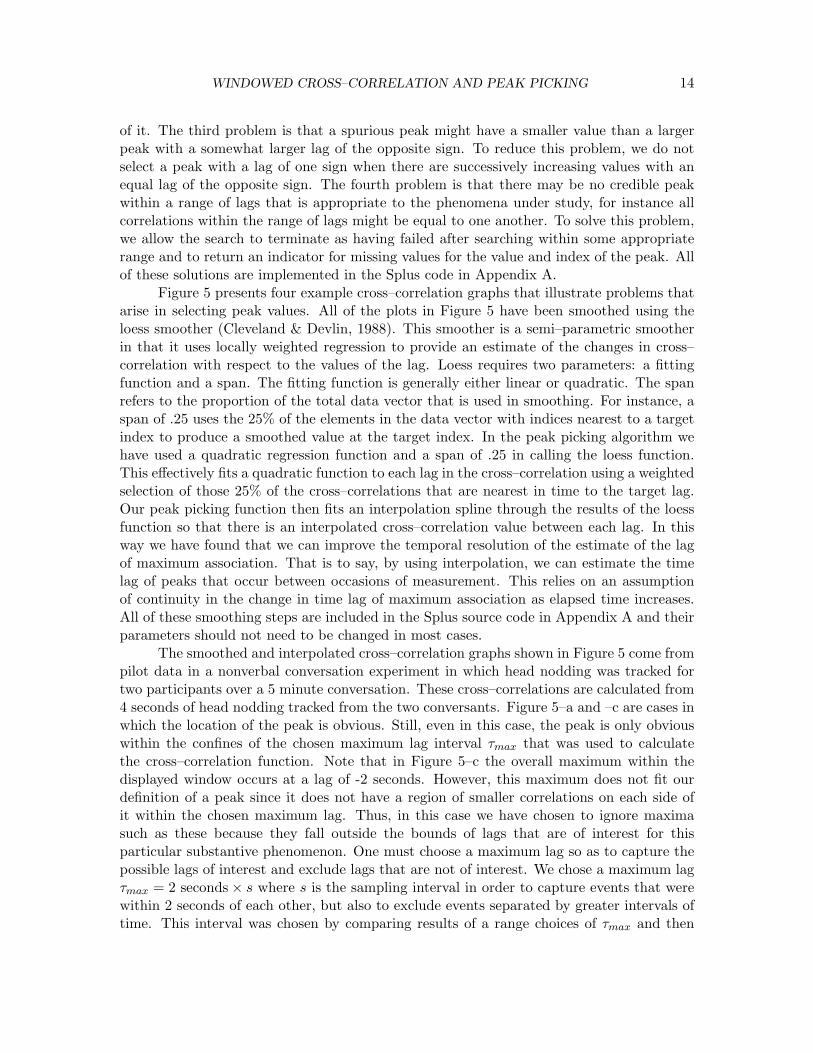
Figure 5 presents four example cross–correlation graphs that illustrate problems thatarise in selecting peak values. All of the plots in Figure 5 have been smoothed using theloess smoother (Cleveland & Devlin, 1988). This smoother is a semi–parametric smootherin that it uses locally weighted regression to provide an estimate of the changes in cross–correlation with respect to the values of the lag. Loess requires two parameters: a fittingfunction and a span. The fitting function is generally either linear or quadratic. The spanrefers to the proportion of the total data vector that is used in smoothing. For instance, aspan of .25 uses the 25% of the elements in the data vector with indices nearest to a targetindex to produce a smoothed value at the target index. In the peak picking algorithm wehave used a quadratic regression function and a span of .25 in calling the loess function.This effectively fits a quadratic function to each lag in the cross–correlation using a weightedselection of those 25% of the cross–correlations that are nearest in time to the target lag.Our peak picking function then fits an interpolation spline through the results of the loessfunction so that there is an interpolated cross–correlation value between each lag. In thisway we have found that we can improve the temporal resolution of the estimate of the lagof maximum association. That is to say, by using interpolation, we can estimate the timelag of peaks that occur between occasions of measurement. This relies on an assumptionof continuity in the change in time lag of maximum association as elapsed time increases.All of these smoothing steps are included in the Splus source code in Appendix A and theirparameters should not need to be changed in most cases.

The smoothed and interpolated cross–correlation graphs shown in Figure 5 come frompilot data in a nonverbal conversation experiment in which head nodding was tracked fortwo participants over a 5 minute conversation. These cross–correlations are calculated from4 seconds of head nodding tracked from the two conversants. Figure 5–a and –c are cases inwhich the location of the peak is obvious. Still, even in this case, the peak is only obviouswithin the confines of the chosen maximum lag interval τmax that was used to calculatethe cross–correlation function. Note that in Figure 5–c the overall maximum within thedisplayed window occurs at a lag of -2 seconds. However, this maximum does not fit ourdefinition of a peak since it does not have a region of smaller correlations on each side ofit within the chosen maximum lag. Thus, in this case we have chosen to ignore maximasuch as these because they fall outside the bounds of lags that are of interest for thisparticular substantive phenomenon. One must choose a maximum lag so as to capture thepossible lags of interest and exclude lags that are not of interest. We chose a maximum lagτmax = 2 seconds× s where s is the sampling interval in order to capture events that werewithin 2 seconds of each other, but also to exclude events separated by greater intervals oftime. This interval was chosen by comparing results of a range choices of τmax and then


max IndexFirstHeadVelCorInt2r5w10

Lag

-2000 -1000 0 1000 2000

-1.0

-0.5

0.0

0.5

1.0


Lag-2000 -1000 0 1000 2000

-1.0

-0.5

0.0

0.5

1.0


Lag-2000 -1000 0 1000 2000

-1.0

-0.5

0.0

0.5

1.0


Lag-2000 -1000 0 1000 2000

-1.0

-0.5

0.0

0.5

1.0

Lag (ms)

a.

Lag (ms)

Lag (ms) Lag (ms)

Cro

ss C

orre

latio

nC

ross

Cor

rela

tion

Cro

ss C

orre

latio

nC

ross

Cor

rela

tion

b.

c. d.

Figure 5. Four types of peaks found in cross–correlation graphs. (a) The peak is chosen at the dottedvertical line in an easy to find case. (b) An ambiguous case in which two small peaks are near lag zeroin which the algorithm chooses the larger peak even though it is farther from zero. (c) Sometimes thepeak is exactly at zero. (d) In some cases there may be no peak that fits the chosen parameters and sothe algorithm terminates and returns missing value indicators.

running the lagged windowed cross–correlation method on pilot data from a separate headmotion experiment. Greater values of τmax tended to obscure the correlational structure andsmaller values of τmax tended to produce results that were not smooth and thus containedmany spurious peaks. We tempered this decision with qualitative observations of humanhead nodding behavior which indicated that a 2 second range was not an unreasonable timeframe in which agreement nods could occur.

The pattern of cross–correlations in Figure 5–b contains two peaks, a small peak witha negative lag near a lag of zero and a larger peak with a positive lag somewhat fartherfrom lag zero. Such patterns can often occur when cross–correlations are calculated oncyclic phenomena. Since the increasing correlations for the positive lag within the searchregion become greater than the smaller peak before the smaller peak is identified as beingcentered in its local region, the local region switches to the positive lag and thus the largerpeak becomes identified. Therefore, the size of the local region is critical in identifyingwhich peak will be selected in cases like this. One must decide what temporal interval isof interest, since the size of the local region acts as a low pass filter, effectively removing


cyclic phenomena with frequencies greater than 1/Lsize where Lsize is the time interval ofthe local region.

The cross–correlations in Figure 5–d do not have a peak that fits our definition.Thus, the algorithm stops when it reaches τmax the maximum size that its search regioncan assume. The values that are returned for the peak index and peak value in this caseare codes for missing values, since no peak was identified. If the local region had been setto be smaller, there would have been several possible candidate peaks. However, we havechosen in this case to reject such small peaks by the choice of Lsize, the size of the localregion.

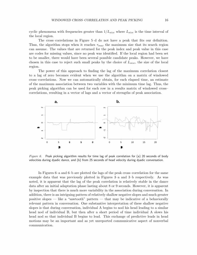
The power of this approach to finding the lag of the maximum correlation closestto a lag of zero becomes evident when we use the algorithm on a matrix of windowedcross–correlations. Now we can automatically obtain, for each elapsed time, an estimateof the maximum association between two variables with the minimum time lag. Thus, thepeak picking algorithm can be used for each row in a results matrix of windowed cross–correlations, resulting in a vector of lags and a vector of strengths of peak association.

Elapsed Time (sec)

0 5 10 15 20

-2-1

01

2

Elapsed Time (sec)0 5 10 15 20

-2-1

01

2

a.

Elapsed Time (sec)

Lag

(sec

)

b.

Elapsed Time (sec)

Lag

(sec

)

Figure 6. Peak picking algorithm results for time lag of peak correlation for (a) 20 seconds of bodyvelocities during dyadic dance, and (b) from 25 seconds of head velocity during dyadic conversation.

In Figures 6–a and 6–b are plotted the lags of the peak cross–correlation for the sameexample data that was previously plotted in Figures 3–a and 3–b respectively. As wasnoted, it is apparent that the lag of the peak correlation is relatively stable in the dancedata after an initial adaptation phase lasting about 8 or 9 seconds. However, it is apparentby inspection that there is much more variability in the association during conversation. Inaddition, there is an intriguing pattern of relatively shallow negative slopes and much greaterpositive slopes — like a “sawtooth” pattern — that may be indicative of a behaviorallyrelevant pattern in conversation. One substantive interpretation of these shallow negativeslopes is that during conversation, individual A begins to nod his head leading to a similarhead nod of individual B, but then after a short period of time individual A slows hishead nod so that individual B begins to lead. This exchange of predictive leads in headmotions may be an important and as yet unreported communicative aspect of nonverbalcommunication.


We next present an example of how this method can be put to use in an experimentalsetting. The example application uses motion capture data from our lab where we havebeen studying adaptive associations between individuals’ movements during conversation.

Example Application

Many researchers suggest there is a close relationship between posture, gesture andspeech (e.g. Condon & Ogston, 1966; Dittman & Llewellyn, 1969; Scheflen, 1964). Ac-cording to the functions posture and gesture serve, speech–related non–verbal cues havebeen divided by Ekman and Friesen (1969) into three main types: emblems, illustratorsand regulators. Emblems refer to those non-verbal acts that have a direct translation,such as nodding the head when meaning ”yes”. Their function is explicitly communicativeand is recognized as such. Illustrators are movements which are tied directly to speechand facilitate communication by amplifying and elaborating the verbal content of message;for instance, swinging ones arms when speaking of playing golf. Regulators are movementswhich guide and control the flow of conversation, influencing who is speaking and how muchis said. Instances of regulators include postural shifts and changes in gaze direction. Kendon(1981) argued that people may choose to use emblems in preference to speech, because incertain communicative contexts there may be distinct advantages in using gesture. Forinstance, since communication through posture and gesture is silent, environmental noisewould be unlikely to interfere with nonverbal communication whereas spoken language couldbecome difficult to understand in the presence of a loud sustained noise.

We hypothesize that when people are engaged in conversation in a noisy environment,they may use posture and gesture in a way that carries more informational content so todisambiguate their verbal communications. Higher informational content means that move-ments are less likely to be redundant and are more likely to be surprising to an interlocutor.Given this hypothesis, the association between two individuals’ movements in a noisy en-vironment would be expected to have greater variability in both time lag and maximumcorrelation than would the association between movements of the same individuals convers-ing in a quiet environment. We performed an experiment in order to test this hypothesisand used windowed cross–correlation and the peak picking algorithm to test whether therewas greater variability in interpersonal coordination when loud environmental noise waspresent.

Methods

Participants.Participants were 8 (4 dyads) female undergraduate senior students from Clark At-

lanta University who volunteered for the study and who were not compensated. Participantswere previously acquainted, having participated in a summer internship program with oneanother.

Apparatus.An Ascension Technologies MotionStar 16 sensor magnetic motion tracking system

was used to track the motions of participants. Each sensor is a cube approximately 3cm ona side and provides 3 dimensions of position and 3 dimensions of orientation informationsampled at 80 Hz with a resolution of approximately 1.5mm in position and 2 degrees of


arc in orientation. Eight sensors were placed on each individual: one on a the back of abaseball cap worn tightly on the head, one strapped just below each elbow using a neopreneand velcro around–the-limb strap, one held to the back of the back of each hand with anelastic weightlifting glove, one held to the sternum with a neoprene and velcro vest, and onestrapped just below each knee with a neoprene and velcro around–the–limb strap. Eachsensor was connected to the MotionStar system computer with a long cable. Thus eachindividual had a bundle of 8 cables that were gathered and positioned behind them in orderto provide the minimum of interference with movement.

Participants were seated approximately 2 meters from each other with the magnetictransmitter sitting to one side of them. Due to the relatively small size of the room (3.5m ×3.5m) the transmitter was so close to the individuals that the motion of the hands nearestthe transmitter was inaccurately recorded. Thus, we have only used head motion of eachparticipant and one hand from each participant (the left hand of one participant and righthand of the other) in our analysis.

Procedure.Participants were informed that they were in an experiment measuring “magnetic

fields during conversation” in order to minimize self–consciousness about their posture andgestures. Participants were not informed that the experiment would include the noisemanipulation In debriefing, no participant guessed that we were actually recording theirmovements. Participants were strapped into the sensors, and were asked to engage in a 5minute free conversation while seated about 2 meters apart from each other. The exper-imenter then left the room. During one half of the conversation the room was quiet andduring the other half of the conversation a loud (90db A-weighted) traffic noise was playedover loudspeakers located in two corners of the room. The order of the noise was counter-balanced so that for half the dyads the noise occurred in the first half of the conversationand for the other half of the dyads the noise occurred in the latter half of the conversation.The traffic noise had been recorded in stereo at a local street corner and included soundsof cars, trucks and motorcycles that were multitracked, time delayed and re-recorded withreverb so as to approximate the sound at a busy intersection in the downtown of a largecity. To give an intuitive understanding of the apparent loudness of the sound, the soundpressure in the room was equivalent to that present at a subway platform when a subwayis arriving.

Results

Since the stated hypothesis concerns the association between movements, we firstcalculated the velocity of the head and hands for each person for each sampled time duringthe experiment. Velocity was calculated for the head, Vhead, and one hand, Vhand, of eachparticipant for each time t as

V (t) =(

(xt+1 − xt−1

2S)2 + (

yt+1 − yt−1

2S)2 + (

zt+1 − zt−1

2S)2

)1/2

, (5)

where xt−1, yt−1, and zt−1 are the positions of the sensor in centimeters along the threespatial axes at at one sample prior to time t, and S is the interval of time between samples,S = 1/80 sec. The resulting velocity vectors (in cm/sec) for the head motions for each


participant from the whole session were then used as input to the windowed cross–correlationanalysis. The velocity vectors from the left hand of one participant and right hand of theother participant were cross–correlated in the same way.

We chose to analyze windows of 4 seconds of data since based on previous experiments(Boker & Rotondo, in press; Rotondo & Boker, in press) it seemed reasonable that theproduction and perception of a gesture or head nod would occur within 2 seconds of eachother. Thus the window size, wmax, was chosen to be wmax = 4 secs × 80 samples/sec =320 samples. We chose to increment the window by 1/8 second in order to be able to capturerapid changes in lead and lag, so winc was set to be 1/10 second × 80 samples/sec = 8samples. We set the maximum lag to be τmax = 2 secs×80 samples/sec = 160 samples andthe lag increment τinc = 1/10 second× 80 samples/sec = 8 samples.

The windowed cross–correlations were run separately on the portions of the conversa-tion with noise and without noise so that there would not be a set of windowed correlationsthat crossed the boundary between the noise and no noise conditions. The resulting ma-trices from the windowed cross–correlational analysis were submitted to the peak pickingalgorithm to calculate peak correlations nearest a lag of zero and their respective time lags.A loess smoothing span of .25 was used, producing a moderate amount of regression splinesmoothing of the cross–correlation data. The peak–picking algorithm was called with alocal region size Lsize = 4, which corresponds to 4 cross–correlation lags each of which wasτinc = 1/10 second. Thus the effective local region used for the peak picking was 0.4 secondsso cyclic movements faster than 2.5 cycles per second were rejected.

The mean and variance of the vector of peak correlation values and the associatedvector of lags were calculated for each dyad within each condition. Thus comparisons couldbe made between estimates of the overall amount of coordination between individuals in thetwo conditions. Similarly, the variability of the coordination magnitude and lag could alsobe compared across conditions. The resulting means and variances of the peak correlationvalues and their associated lags were used as dependent variables in univariate mixed modelregression analyses grouped by dyad and fit using the Splus software function nlme. A testfor order effects was made, but in no case did the order of the noise (first half versus latterhalf of the conversation) significantly predict any of the outcome variables so the orderpredictor variable was dropped from the analysis.

The mixed effects model was specified such that the intercept term was allowed tovary across dyads. The noise condition was dummy coded (0=silence and 1=noise) andused as a fixed predictor of the selected outcome variable as follows:

yij = b0j + b1xij + eij , (6)

where yij is the selected dependent variable for the ith noise condition during the jth dyadsession, xij is the ith noise condition during the jth dyad session, b0j is the intercept termfor the jth dyad session, b1 is the regression coefficient of noise predicting the selectedoutcome variable, and eij is a independent identically distributed random variable. Theresults of these analyses are presented in Tables 2 and 1.

Both the mean and variance of the peak correlation increased significantly when theenvironmental noise was present (Table 1). Thus individuals movements were more highlycorrelated in the presence of noise and at the same time there was more variability in thevalue of the peak association. Only the variance of the lag between individuals increased


Table 1: Noise condition predicting the mean and variance of the value of the peak windowedcross–correlation for head and one hand using four independent univariate mixed model regressionsgrouped by dyad. Noise was coded silence=0, noise=1. Asterisk indicates p < 0.05

Dependent Variable b SE ZHead

mean .041 .015 2.745*variance .009 .002 3.523*

Handmean .043 .011 3.843*

variance .012 .002 6.946*

Table 2: Noise condition predicting the mean and variance of the lag of the peak windowed cross–correlation for head and one hand using four independent univariate mixed model regressions groupedby dyad. Noise was coded silence=0, noise=1. Asterisk indicates p < 0.05

Dependent Variable b SE ZHead

mean .374 .331 1.131variance 5.091 1.241 4.102*

Handmean -.221 .287 -.767

variance 13.818 4.505 3.067*

significantly when noise was present (Table 2). Thus the predictive association betweenindividuals’ movements tended to have lags that were farther from synchrony (a lag of zero)when exposed to the environmental noise.

Discussion

The results supported the hypothesis of greater variability in the coordination betweenconversing individuals when in the presence of noise than when there was no interferingnoise. Thus, the variability of the time lag and value of peak association increased signifi-cantly for both the head and the hand in the presence of noise. No change was observed inthe mean value of the time lag of peak association, but this was expected. Since individualswere randomly assigned to chairs, there was no reason why one would expect individuals inchair A to behave differently than those in chair B and therefore there should be no changein the mean value of the lag of the peak cross–correlation across noise conditions.

However, there was a significant increase in the coordination between conversantswhen the noise was present. While this finding was not anticipated in the hypothesis, it isintriguing. It appears that individuals more closely coupled their movements to each otherwhen verbal communication became more difficult. These findings, while interesting, arefrom a small, and most likely nonrepresentative sample of individuals and thus may notgeneralize to the population of English language conversational dyads. We present these


results solely in order to illustrate the use of the methods.

General Discussion

The combination of the use of windowed cross–correlation with our peak pickingalgorithm allows the empirical estimation of variability in a fundamentally different waythan the usual examination of within–variable change over time. These methods allow theestimation of variability in the association between variables. The way in which the valueof the peak association between variables changes and the way in which the temporal lagchanges can be extremely informative as to the structure of adaptive relationships betweenindividuals or the predictive capacity exhibited between variables within an individual overtime.

We expect that methods such as those explicated here will become much more preva-lent as psychologists begin increasingly to use experimental designs that measure a set ofvariables on many occasions from a sample of individuals. Prime examples for the use ofthe methods described here are physiological measurements (i.e. EEG, EKG, GSR, singlecell recordings of neuron activation) taken over the course of an experiment, data fromjournaling studies in which individuals repeatedly self–report on several variables over anextended period of time, or motion capture experiments such as the example applicationreported above. Other psychological data such as longer daily diary studies with approxi-mately 100 occasions of measurment or more may also be amenable to exploratory analysiswith the methods presented here. In order for the algorithms to be useful, (a) each windowmust contain sufficient observations to reliably estimate the cross–correlations and (b) theremust be a sufficient number of windows in order to reliably estimate the pattern of changein the time lags and strength of association between the variables. Estimating the actualnumber of observations that are sufficient for (a) and (b) above requires a power calculationdependent on the hypothesized effect size and required significance level for each of (a) and(b).

Other methods have been developed for the analysis of nonstationary and nonlineartime series. These methods fall into four basic groups: (a) those that emphasize forwardprediction such as Kalman filtering, nonlinear prediction and mutual information; (b) thosethat emphasize system identification and description such as Lyapunov exponents, corre-lation dimension, and surrogate data; (c) those that emphasize graphical description andexploration such as state space plots and recurrence diagrams; and (d) those that emphasizenoise reduction (for introductions see Abarbanel, 1996; Heath, 2000; Kantz & Schreiber,1997). The windowed cross–correlation and peak picking method differs from these othertechniques in that its primarily goal is the analysis of the change in the association betweenvariables over time. The most closly related method known to the authors is an informationtransfer method proposed by Schreiber (2000) in which entropy is used as the measure ofassociation between the time series. Schreiber’s method differs substantially from ours inthat his method doesn’t attempt to estimate time–varying patterns of association betweenvariables.

The primary disadvantage to the windowed cross–correlation and peak picking anal-ysis is that it requires the analyst to choose several parameters in order to to appropriatelyestimate the changing pattern of association between variables. A preliminary sample ofdata must be used to tune these parameters prior to using the method for hypothesis test-


ing. We have found this process of exploration of preliminary samples to be illuminatingin its own right, and so now run pilots of our experiments so that we can adjust both theparameters and our hypotheses prior to gathering larger and inevitably more expensivesamples to test these revised hypothesis without adjusting the parameters of the windowedcross–correlation and peak picking algorithms.

The particular choices of parameters for the windowed cross–correlation and peakpicking algorithms used here apply only to the particular experimental paradigm presentedin the example analysis. However, the flexibility of choice in these parameters means thatthe algorithms are very general in the types of repeated measures data to which they maybe applied. Any continuous variable bivariate time series data in which an assumption ofstationarity in linear association between the variables might be invalid is a candidate foranalysis with these algorithms.

A second disadvantage is that the assumption of local stationarity may frequentlybe violated to some degree and this may produce downward bias in the estimates of themagnitude of the cross–correlations and the variances of the lags. While this remainsan unsolved problem with our method, it produces errors in the conservative direction;underestimating the magnitudes of effects.

A third disadvantage is one that plagues all modeling methods: an unobserved vari-able may be the cause of the associations estimated between the observed variables. Al-though this method estimates time lagged associations, this does not necessarily implycausality between the observed variables.

Finally, the methods presented here estimate peak correlations and their associatedlags but do not impose a testable model of the process that gave rise to the nonstationarityin the first place. An advance on these methods would be the creation of a multivariatemodel that would predict patterns of changes in peak cross–correlations among severalvariables in such a way that particular hypotheses concerning the short term dynamics ofthe processes involved could be rejected.

It seems unlikely that living, adapting individuals will always exhibit predictive as-sociations between variables that are stable and unchanging over time. And yet this isexactly the assumption that is generally made in order to provide a statistically tractableestimate of those associations. It seems much more likely that in adaptive relations betweenvariables sometimes person A will lead and person B will follow and sometimes the reverse;sometimes variable X will predict Y and sometimes the reverse; sometimes system J willdrive system K and sometimes the reverse. We propose that the time has come to developnew methods that are able to relax the assumption of unchanging structure over time in theassociation between variables. It is our expectation that the development of such methodswill lead to a deeper and more realistic understanding of human behavior.


Appendix A

# File name: peakPick.S# Author: Steven M. Boker, Minquan Xu# University of Notre Dame# Date: Feb 09, 2001

# input data structure(Splus object matrix):# rows: elapsed time# columns: cross correlations# output: a list of local peak indices and values

# Parameters:# ---------------------------------------------------------------------# tAllCor: Splus object matrix, this matrix is created from the output# file of windcross program using Splus function such as# "scan". ex. tAllCor <- matrix(scan("windcross.dat"), ncol=n, byrow=T),# where n is the number of columns in windcross.dat file.# Lsize: local search region, the value should be larger than 0 and# less than 1/2 length of one row# graphs: number of graphs to draw for one input data object, the# value should be larger than 0 and less than number of rows# of one input data object# pspan: see help(loess) for span# type: local maximum or local minimum, valid values are: "Min" and "Max"# tFileName: root characters for .eps file#---------------------------------------------------------------------

peakpick<- function(tAllCor, Lsize=8, graphs=0, pspan=.25,type="Max",tFileName="peak") {

#----------------check for validity of parameters -------------------colLen <- length(tAllCor[1,]) # col length --- number of columnsrowLen <- length(tAllCor[,1]) # row length --- number of rowstLsize <- floor((1/2)*colLen) # maximum local search region

if(Lsize<1 || Lsize>tLsize) { # Lsize too small or too largeerrorStr<- paste("Lsize should be >0 and <= ", tLsize, sep="")stop(errorStr) # print error message and stop the program

}if(graphs<0||graphs>rowLen) { # num of graphics to print is too small or large

errorStr <- paste("graphs should be >=0 and <= ", rowLen, sep="")stop(errorStr) # print error message and stop the program

}if(pspan<0 || pspan>1) { # invalid pspan value

stop("pspan should be >0 and <1\n") # print error message and stop}if(type!="Max"&&type!="Min"&&type!="max"&&type!="min"){ # only two types

stop("valid types are: max|Max or Min|min \n") # print message and stop}#-----------Initialization------------------------------------------------drawgraph <- 0 # graphics drawn


colLen <- length(tAllCor[1,]) # col lengthrowLen <- length(tAllCor[,1]) # row lengthxSequence <- seq(-(colLen-1), (colLen-1), by=1) # X axis for each graphmx<- rep(NA, (2*colLen-1)) #vector for keeping temp peak value for a row

#data points will be 2*colLen-1 after smoothtIndex <- rep(NA, rowLen) #vector of peak index---one peak index for each rowtValue <- rep(NA, rowLen) #vector of peak value---one peak value for each row

#------------- type == max or Max ---------------------------------------if(type=="Max"||type=="max") { #compute local maximum

for(rowNo in c(1: rowLen)) { #acess each row#eliminate missing valuemiss <- is.na(tAllCor[rowNo, ]) #a row is T is "NA" or F is not "NA"#initialize the position of NA in a rowmissposition <- 0for(mIndex in c(1:colLen)) { #evaluate an entire row

missposition <- mIndex #the position of NAif(miss[missposition]) break #find onemissposition <- missposition+1 #increase countif(missposition==colLen+1) break #No NA in this row

}#cat("missposition=", missposition, "\n")#if has missing valueif(missposition <= colLen) next #skip a row with NAelse { # no missing value

drawgraph <- drawgraph+1 #number of graph to drawtCor <- tAllCor[rowNo, ] #number of columns#smootht1 <- loess(tCor~c(1:colLen), degree=2,

span=pspan, )$fitted.values#data points is set to nt2 <- spline(c(1:colLen), t1, n=(2*colLen-1))$y

# show calculate progress# cat("row=", rowNo, "\n")#----- process a row --find max value and max index------windowWidth <- 0 # searched regionlookAhead <- 0 # look ahead data pointsfor(j in 1:(colLen-1)) { # search from 1 to colLen -1

windowWidth <- windowWidth+1 # increase search ed region# select the search region, the center of search region# is in the middle of t2, notice that t2 has 2*colLen-1# data points.tSelect <- (colLen - windowWidth):(colLen+windowWidth)mx[j] <- max(t2[tSelect], na.rm=T) # store temp max valueif(j==1) mmx <- mx[j] # mmx is final local max value#remember current maxelse { # if j != 1

if(mx[j]>mmx) { # new temp max value, only one# max value in tSelect

lookAhead <- 0 # set stop criterion = 0,


# the criterion is that if we find# Lsize data points less than current# max, then stop and the current max# value is the local maximum we wanted

mmx <- mx[j] # update new max value}

else if(mx[j]<=mmx) { # if other values are less than# current maximum# increase the count---how many neighbor data# point are less than current maximumlookAhead <- lookAhead+1if(lookAhead>=Lsize) break # meet criterion

}}#else

}#for j--max value and index for each row#use match function to find the indexIndex <- match(mmx, t2[tSelect])+tSelect[1]-1# tSelect[1] is the first index of the selected window

# relative position to the middle pointposition <- Index -colLen

#according to the local maximum definitionif (position >(colLen - Lsize - 1) ||

position < (-(colLen - Lsize -1))) { # failtIndex[rowNo] <- NAtValue[rowNo] <- NA

}else { # found a local maximum

tIndex[rowNo] <- positiontValue[rowNo] <-mmx

}

#draw plotsif(drawgraph <= graphs) {

# define graphic file nametepsfile <- paste(tFileName, "Max", rowNo, ".eps", sep="")# title of the graphtmain <- paste("max Index", tFileName, "r", rowNo,"w",

Lsize, sep="")# write to postscript formatpostscript(tepsfile, height=6.4, horizontal=F)

# draw borders and their labelsplot(c(-(colLen-1), (colLen-1)), c(-1,1), xlab="Lag",

ylab="Cross Correlation", main=tmain, type="n")

# draw the curvelines(xSequence, t2, type="l")

# draw the local maximum


lines(c(position,position), c(-1,1), type="l", lty=8)

# draw the axeslines(c(0,0), c(-1,1), type="l", lty=4)lines(c(-(colLen-1), (colLen-1)), c(0,0), type="l", lty=4)dev.off() # term off plot device to generate graph

} # if drawgraph} #else no missing value

} # for rowNo-- process each row#end of process a rowreturn(list(maxIndex=tIndex, maxValue=tValue))}#if type=max

#-------------------------------------------------------------------------------# type == Min or min#-------------------------------------------------------------------------------else if(type=="Min"||type=="min") {

for(rowNo in c(1: rowLen)) {#eliminate missing valuemiss <- is.na(tAllCor[rowNo, ])missposition <- 0for(mIndex in c(1:colLen)) {

missposition <- mIndex #the position of NAif(miss[missposition]) break #find onemissposition <- missposition+1if(missposition==colLen+1) break

}#cat("missposition=", missposition, "\n")#if has missing valueif(missposition <= colLen) next #skip a row with NA

else { # no missing valuedrawgraph <- drawgraph+1tCor <- tAllCor[rowNo, ]t1 <- loess(tCor~c(1:colLen), degree=2, span=pspan, )$fitted.valuest2 <- spline(c(1:colLen), t1, n=(2*colLen-1))$y# show calculate progress#cat("row=", rowNo, "\n")

#process a row --find max value and max index#-------------------------------------------------------------windowWidth <- 0lookAhead <- 0for(j in 1:(colLen-1)) {

windowWidth <- windowWidth+1tSelect <- (colLen - windowWidth):(colLen+windowWidth)mx[j] <- min(t2[tSelect], na.rm=T)if(j==1) mmx <- mx[j]#remember current maxelse {if(mx[j]<mmx) { #only one value in tSelect


lookAhead <- 0mmx <- mx[j]

}else if(mx[j]>=mmx) {

lookAhead <- lookAhead+1if(lookAhead>=Lsize) break

}}#else

}#for j--max value and index for each row#use match function to find the indexIndex <- match(mmx, t2[tSelect])+tSelect[1]-1position <- Index -colLen

if (position >(colLen - Lsize -1) ||position < (-(colLen -Lsize -1))) { # failtIndex[rowNo] <- NAtValue[rowNo] <- NA

}else {

tIndex[rowNo] <- positiontValue[rowNo] <-mmx

}

#draw first 10 plotsif(drawgraph <= graphs) {

tepsfile <- paste(tFileName, "Min", rowNo, ".eps", sep="")tmain <- paste("min Index", tFileName, "r",

rowNo,"w", Lsize, sep="")postscript(tepsfile, height=6.4, horizontal=F)plot(c(-(colLen-1), (colLen-1)), c(-1,1),

xlab="Lag", ylab="Cross Correlation",main=tmain, type="n")

lines(xSequence, t2, type="l")lines(c(position,position), c(-1,1), type="l", lty=8)lines(c(0,0), c(-1,1), type="l", lty=4)lines(c(-(colLen-1), (colLen-1)), c(0,0), type="l", lty=4)dev.off()

} # if drawgraph} #else no missing value

} # rowNo-- process each row#end of process a row#-----------------------------------------------------------------------

return(list(minIndex=tIndex, minValue=tValue))}#if type=mix

}


Appendix B

1. A search region size Rsize is defined as the smallest integer such that Rsize ≥(Lsize/2)

2. A search region R is defined as a sequential and increasing set of integers of sizeRsize centered on c, the index corresponding to a lag of zero between the two cross–correlateddata vectors as follows: R = {c−Rsize, . . . , c− 1, c, c + 1, . . . , , c + Rsize}.

3. Two local regions are defined: L1 as the first Lsize integers in R and and L2 asthe last Lsize integers in R.

4. The maximum value L1max of the cross–correlations in V with indices containedin the local search region L1 is calculated.

5. If the index of L1max is the center element of L1 and the values from V on eitherside of L1max are monotonically decreasing, then a peak has been found. In this case, thevalue L1max and its index are returned and the algorithm stops. Otherwise, the algorithmgoes to the next step.

6. The maximum value L2max of the cross–correlations in V with indices containedin the local search region L2 is calculated.

7. If the index of L2max is the center element of L2 and the values from V on eitherside of L2max are monotonically decreasing, then a peak has been found. In this case, thevalue L2max and its index are returned and the algorithm stops. Otherwise, the algorithmgoes to the next step.

8. Rsize is incremented by one and then if Rsize ≤ τmax the process is repeated fromstep 2.

9. If Rsize > τmax then no viable peak was found and the algorithm returns a missingvalue indicator for both the peak value and peak index and then stops.


References

Abarbanel, H. D. I. (1996). Analysis of observed chaotic data. New York: Springer–Verlag.

Aborn, M., Rubenstein, H., & Sterling, T. D. (1959). Sources of contextual constraint upon wordsin sentences. Journal of Experimental Psychology, 57, 171–180.

Bloomfield, P. (1976). Fourier analysis of time series. New York: Wiley-Interscience.

Boker, S. M., & Rotondo, J. L. (in press). Symmetry building and symmetry breaking in synchro-nized movement. In M. Stamenov & V. Gallese (Eds.), Mirror neurons and the evolution ofbrain and language. Amsterdam: John Benjamins.

Boker, S. M., Schreiber, T., Pompe, B., & Bertenthal, B. I. (1998). Nonlinear analysis of perceptual–motor coupling in the development of postural control. In H. Kantz, J. Kurths, & G. Mayer-Kress (Eds.), Nonlinear analysis of physiological data (pp. 251–270). Berlin: Springer Verlag.

Box, J. E. P., Jenkins, G. M., & Reinsel, G. C. (1994). Time series analysis: forecasting and control.Englewood Cliffs, NJ: Prentice Hall.

Bregman, A. S. (1990). Auditory scene analysis : the perceptual organization of sound. Cambridge,MA: MIT Press.

Cattell, R. B. (1963). The structuring of change by P–technique and incremental R–technique. InC. W. Harris (Ed.), Problems in measuring change (pp. 167–198). Madison, WI: University ofWisconsin Press.

Cherry, C. (1961). Two ears — but one world. Cambridge, MA, New York: MIT Press and Wiley.

Cleveland, W. S., & Devlin, S. J. (1988). Locally weighted regression: An approach to regressionanalysis by local fitting. Journal of the American Statistical Association, 83, 596–610.

Condon, W. S., & Ogston, W. D. (1966). Sound film analysis of normal pathological behaviorpatterns. Journal of Nervous and Mental Disease, 143, 338-347.

Cook, T. D., Dintzer, L., & Mark, M. M. (1980). The causal analysis of concomitant time series.In L. Bickman (Ed.), Applied social psychology annual (volume 1) (pp. 93–135). Beverly Hills:Sage.

Dittman, A. T., & Llewellyn, L. G. (1969). Body movement and speech rhythm in social conversa-tion. Journal of Personality and Social Psychology, 11, 98-106.

Dixon, P., & Di Lolo, V. (1994). Beyond visible persistence: An alternative account of temporalintegration and segregation in visual processing. Cognitive Psychology, 26, 33-63.

Dodwell, P. (1971). On the perceptual clarity. Psychological Review, 78, 275-289.

Ekman, P., & Friesen, W. V. (1969). The repertoire of nonverbal behaviour: categories, origins,usage and coding. Semiotica, 1, 49-98.

Glass, L., & Switkes, E. (1976). Pattern recognition in humans: Correlations which cannot beperceived. Perception, 5 (1), 67–72.

Gregson, R. A., & Harvey, J. P. (1992). Similarities of low-dimensional chaotic auditory attractorsequences to quasirandom noise. Perception & Psychophysics, 51 (3), 267–278.

Hamagami, F., McArdle, J., & Cohen, P. (2000). A new approach to modeling bivariate dynamicrelationships applied to evaluation of comorbidity amoung DSM–III personality disorder symp-toms. In V. J. Molfese (Ed.), Temperament and personality development across the life span.Mahwah, NJ: Lawrence Erlbaum Associates.


Heath, R. A. (2000). Nonlinear dynamics: Techniques and applications in psychology. Mahwah, NJ:Lawrence Erlbaum.

Hendry, D., & Juselius, K. (2000). Explaining cointegration analysis: Part 1. Energy Journal, 21,1-42.

Ito, K. (Ed.). (1993). Encyclopedic dictionary of mathematics. Cambridge, MA: MIT Press.

Jones, M. R. (1993). Dynamics of musical patterns: How do melody and rhythm fit together? InT. J. Tighe & W. J. Dowling (Eds.), Psychology and music: The understanding of melody andrhythm (pp. 67–92). Hillsdale, NJ: Lawrence Erlbaum Associates, Inc.

Kantz, H., & Schreiber, T. (1997). Nonlinear time series analysis. Cambridge: Cambridge UniversityPress.

Kendon, A. (1981). Geography of gesture. Semiotica, 37, 129-163.

Licklider, J. (1959). Three auditory theories. New York: McGraw-Hill.

Miller, G. A., & Chomsky, N. (1963). Finitary models of language users. In R. D. Luce, R. Bush,& E. Galanter (Eds.), Handbook of mathematical psychology (vol 2) (pp. 419–491). New York:Wiley.

Molenaar, P. C. M. (1985). A dynamic factor model for the analysis of multivariate time series.Psychometrika, 50, 181–202.

Nesselroade, J. R., & Featherman, D. L. (1991). Intraindividual variability in older adults’ depressionscores: Some implications for longitudinal research. In D. Magnusson, L. Bergman, G. Rudinger,& B. Torestad (Eds.), Stability and change: Methods and models for data treatment. London:Cambridge University Press.

Nesselroade, J. R., & Ford, D. H. (1985). P–technique comes of age: Multivariate, replicated,single–subject designs for research on older adults. Research on Aging, 7, 46–80.

Reichardt, W. (1961). Autocorrelation, a principle for the evaluation of sensory information by thecentral nervous system. Cambridge, MA, NEW York: MIT Press and Wiley.

Rotondo, J. L. (2000). Dominance and gender in conversational interaction. Unpublished doctoraldissertation, University of Notre Dame. (Unpublished doctoral dissertation)

Rotondo, J. L., & Boker, S. M. (in press). Behavioral synchronization in human conversationalinteraction. In M. Stamenov & V. Gallese (Eds.), Mirror neurons and the evolution of brainand language. Amsterdam: John Benjamins.

Santen, J. P. H. van, & Sperling, G. (1985). Elaborated Reichardt detectors. Journal of OpticalSociety of America, 2A, 300-320.

Scheflen, A. E. (1964). The significance of posture in communication systems. Psychiatry, 27,316-331.

Schreiber, T. (2000). Measuring information transfer. Physical Review Letters, 85 (2), 461–464.

Shao, X. M., & Chen. (1987). Normalized auto– and cross–covariance fucntions for neuronal spiketrain analysis. International Journal of Neuroscience, 34, 85-95.

Siegler, R. S., & Jenkens, E. (1989). How children discover new strategies. Hillsdale, NJ: LawrenceErlbaum Associates.

Warner, R. M. (1998). Spectral analysis of time–series data. New York: Guilford Press.

West, S. G., & Hepworth, J. T. (1991). Statistical issues in the study of temporal data: Dailyexperiences. Journal of Personality, 59 (3), 609–662.

Windowed Cross–Correlation and Peak Picking for …people.virginia.edu/~smb3u/psych611/Peak20020108aReprint.pdf · Windowed Cross–Correlation and Peak Picking for the Analysis

Documents