Progress in Aerospace Sciences 39 (2003) 467–510 Wind turbine wake aerodynamics L.J. Vermeer a, *, J.N. S^rensen b , A. Crespo c a Section Wind Energy, Faculty of Civil Engineering and Geosciences, Delft University of Technology, Stevinweg 1, 2628 CN Delft, The Netherlands b Fluid Mechanics Section, Department of Mechanical Engineering, Technical University of Denmark, DK-2800 Kgs. Lyngby, Denmark c Departamento de Ingenier ! ıa Energ ! etica y Fluidomec ! anica, ETS de Ingenieros Industriales, Universidad Polit ! ecnica de Madrid, Jos ! e Guti ! errez Abascal 2, E-28006 Madrid, Spain Abstract The aerodynamics of horizontal axis wind turbine wakes is studied. The contents is directed towards the physics of power extraction by wind turbines and reviews both the near and the far wake region. For the near wake, the survey is restricted to uniform, steady and parallel flow conditions, thereby excluding wind shear, wind speed and rotor setting changes and yawed conditions. The emphasis is put on measurements in controlled conditions. For the far wake, the survey focusses on both single turbines and wind farm effects, and the experimental and numerical work are reviewed; the main interest is to study how the far wake decays downstream, in order to estimate the effect produced in downstream turbines. The article is further restricted to horizontal axis wind turbines and excludes all other types of turbines. r 2003 Elsevier Ltd. All rights reserved. ARTICLE IN PRESS Contents 1. Introduction ........................................... 468 2. Overview ............................................. 469 3. Near wake experiments ...................................... 470 3.1. Global properties ...................................... 473 3.2. Flow visualisations ..................................... 473 3.3. Averaged data ....................................... 476 3.4. Detailed data ........................................ 476 3.4.1. Velocities ...................................... 477 3.4.2. Tip vortex properties ............................... 478 4. Near wake computations ..................................... 480 4.1. The Navier–Stokes equations ................................ 481 4.2. Vortex wake modelling ................................... 482 4.3. Generalized actuator disc models ............................. 484 4.4. Navier–Stokes methods ................................... 487 4.4.1. Turbulence modelling ............................... 488 4.4.2. Laminar–turbulent transition ........................... 488 *Corresponding author. Tel.: +31-15-2785166; fax: +31-15-2785347. E-mail addresses: [email protected] (L.J. Vermeer), [email protected] (J.N. S^rensen), crespo@enerflu.etsii.upm.es (A. Crespo). 0376-0421/$ - see front matter r 2003 Elsevier Ltd. All rights reserved. doi:10.1016/S0376-0421(03)00078-2

Welcome message from author
This document is posted to help you gain knowledge. Please leave a comment to let me know what you think about it! Share it to your friends and learn new things together.
Transcript
Progress in Aerospace Sciences 39 (2003) 467–510
ARTICLE IN PRESS
Contents
1. Intro
2. Over
3. Near
3.1.
3.2.
3.3.
3.4.
4. Near
4.1.
4.2.
4.3.
4.4.
*Correspondin
E-mail addres
(A. Crespo).
0376-0421/$ - see
doi:10.1016/S037
Wind turbine wake aerodynamics
L.J. Vermeera,*, J.N. S^rensenb, A. Crespoc
aSection Wind Energy, Faculty of Civil Engineering and Geosciences, Delft University of Technology, Stevinweg 1,
2628 CN Delft, The NetherlandsbFluid Mechanics Section, Department of Mechanical Engineering, Technical University of Denmark, DK-2800 Kgs. Lyngby, Denmark
cDepartamento de Ingenier!ıa Energ!etica y Fluidomec !anica, ETS de Ingenieros Industriales, Universidad Polit!ecnica de Madrid,
Jos!e Guti!errez Abascal 2, E-28006 Madrid, Spain
Abstract
The aerodynamics of horizontal axis wind turbine wakes is studied. The contents is directed towards the physics of
power extraction by wind turbines and reviews both the near and the far wake region. For the near wake, the survey is
restricted to uniform, steady and parallel flow conditions, thereby excluding wind shear, wind speed and rotor setting
changes and yawed conditions. The emphasis is put on measurements in controlled conditions. For the far wake, the
survey focusses on both single turbines and wind farm effects, and the experimental and numerical work are reviewed;
the main interest is to study how the far wake decays downstream, in order to estimate the effect produced in
downstream turbines. The article is further restricted to horizontal axis wind turbines and excludes all other types of
turbines.
r 2003 Elsevier Ltd. All rights reserved.
duction . . . . . . . . . . . . . . . . . . . . . . . . . . . . . . . . . . . . . . . . . . . 468
view . . . . . . . . . . . . . . . . . . . . . . . . . . . . . . . . . . . . . . . . . . . . . 469
wake experiments . . . . . . . . . . . . . . . . . . . . . . . . . . . . . . . . . . . . . . 470
Global properties . . . . . . . . . . . . . . . . . . . . . . . . . . . . . . . . . . . . . . 473
Flow visualisations . . . . . . . . . . . . . . . . . . . . . . . . . . . . . . . . . . . . . 473
Averaged data . . . . . . . . . . . . . . . . . . . . . . . . . . . . . . . . . . . . . . . 476
Detailed data . . . . . . . . . . . . . . . . . . . . . . . . . . . . . . . . . . . . . . . . 476
3.4.1. Velocities . . . . . . . . . . . . . . . . . . . . . . . . . . . . . . . . . . . . . . 477
3.4.2. Tip vortex properties . . . . . . . . . . . . . . . . . . . . . . . . . . . . . . . 478
wake computations . . . . . . . . . . . . . . . . . . . . . . . . . . . . . . . . . . . . . 480
The Navier–Stokes equations . . . . . . . . . . . . . . . . . . . . . . . . . . . . . . . . 481
Vortex wake modelling . . . . . . . . . . . . . . . . . . . . . . . . . . . . . . . . . . . 482
Generalized actuator disc models . . . . . . . . . . . . . . . . . . . . . . . . . . . . . 484
Navier–Stokes methods . . . . . . . . . . . . . . . . . . . . . . . . . . . . . . . . . . . 487
4.4.1. Turbulence modelling . . . . . . . . . . . . . . . . . . . . . . . . . . . . . . . 488
4.4.2. Laminar–turbulent transition . . . . . . . . . . . . . . . . . . . . . . . . . . . 488
g author. Tel.: +31-15-2785166; fax: +31-15-2785347.
ses: [email protected] (L.J. Vermeer), [email protected] (J.N. S^rensen), [email protected]
front matter r 2003 Elsevier Ltd. All rights reserved.
6-0421(03)00078-2
ARTICLE IN PRESS
5. Far wake experiments . . . . . . . . . . . . . . . . . . . . . . . . . . . . . . . . . . . . . . 489
5.1. Wind tunnel experiments . . . . . . . . . . . . . . . . . . . . . . . . . . . . . . . . . . 490
5.2. Field experiments . . . . . . . . . . . . . . . . . . . . . . . . . . . . . . . . . . . . . . 492
5.2.1. Fatigue and loads . . . . . . . . . . . . . . . . . . . . . . . . . . . . . . . . . 493
5.2.2. Anisotropy . . . . . . . . . . . . . . . . . . . . . . . . . . . . . . . . . . . . . 494
5.2.3. Atmospheric stability . . . . . . . . . . . . . . . . . . . . . . . . . . . . . . . 494
5.2.4. Coherence . . . . . . . . . . . . . . . . . . . . . . . . . . . . . . . . . . . . . 495
6. Far wake modelling . . . . . . . . . . . . . . . . . . . . . . . . . . . . . . . . . . . . . . . 495
6.1. Individual wakes . . . . . . . . . . . . . . . . . . . . . . . . . . . . . . . . . . . . . . 495
6.1.1. Kinematic models . . . . . . . . . . . . . . . . . . . . . . . . . . . . . . . . . 495
6.1.2. Field models . . . . . . . . . . . . . . . . . . . . . . . . . . . . . . . . . . . . 495
6.1.3. Boundary layer wake models . . . . . . . . . . . . . . . . . . . . . . . . . . . 495
6.1.4. Hybrid models . . . . . . . . . . . . . . . . . . . . . . . . . . . . . . . . . . . 496
6.2. Wind farm wake models . . . . . . . . . . . . . . . . . . . . . . . . . . . . . . . . . . 497
6.2.1. Single wake superposition . . . . . . . . . . . . . . . . . . . . . . . . . . . . . 497
6.2.2. Elliptic wake models . . . . . . . . . . . . . . . . . . . . . . . . . . . . . . . . 497
6.2.3. Parabolic wake models . . . . . . . . . . . . . . . . . . . . . . . . . . . . . . 497
6.2.4. CFD code calculations . . . . . . . . . . . . . . . . . . . . . . . . . . . . . . 498
6.2.5. Offshore wind farm wakes . . . . . . . . . . . . . . . . . . . . . . . . . . . . . 498
6.2.6. Generic wind farm wake models . . . . . . . . . . . . . . . . . . . . . . . . . 499
7. Far wake: engineering expressions . . . . . . . . . . . . . . . . . . . . . . . . . . . . . . . . 499
7.1. Velocity deficit . . . . . . . . . . . . . . . . . . . . . . . . . . . . . . . . . . . . . . . 499
7.2. Turbulence intensity . . . . . . . . . . . . . . . . . . . . . . . . . . . . . . . . . . . . 500
7.3. Wind farm wake expressions . . . . . . . . . . . . . . . . . . . . . . . . . . . . . . . . 500
8. Concluding remarks . . . . . . . . . . . . . . . . . . . . . . . . . . . . . . . . . . . . . . . 501
8.1. Near wake . . . . . . . . . . . . . . . . . . . . . . . . . . . . . . . . . . . . . . . . . 501
8.2. Far wake . . . . . . . . . . . . . . . . . . . . . . . . . . . . . . . . . . . . . . . . . . 501
Acknowledgements . . . . . . . . . . . . . . . . . . . . . . . . . . . . . . . . . . . . . . . . . . 502
References . . . . . . . . . . . . . . . . . . . . . . . . . . . . . . . . . . . . . . . . . . . . . . . 502
L.J. Vermeer et al. / Progress in Aerospace Sciences 39 (2003) 467–510468
1. Introduction
The conversion of wind energy to useful energy
involves two processes: the primary process of extracting
kinetic energy from wind and conversion to mechanical
energy at the rotor axis, and the secondary process of
the conversion into useful energy (mostly electrical, but
also mechanical for water pumps or chemical for water
desalination or hydrolyses). This paper concerns the
primary process: the extraction of kinetic energy from
the wind. The major field of science involved in this
process is aerodynamics, but it needs meteorology (wind
description) as input, and system dynamics for the
interaction with the structure. The latter is important
since all movement of the rotor blades, including
bending of the blades out of their plane of rotation,
induces apparent velocities that can influence or even
destabilize the energy conversion process. Aerodynamics
is the oldest science in wind energy: in 1915, Lanchester
[1] was the first to predict the maximum power output of
an ideal wind turbine. A major break-through was
achieved by Glauert [2], by formulating the blade
element momentum (BEM) method. This method,
extended with many ‘engineering rules’ is still the basis
for all rotor design codes. Recently, first results of
complete Navier–Stokes calculations for the most
simple wind turbine operational mode have been
reported. Progress is significant in the 30-year history
of modern wind energy. To name one example: a better
understanding of the aerodynamics improved the
efficiency of the primary process from 0.4 to 0.5 (out
of a maximum of 0.592). Nevertheless, many phenom-
ena are still not fully understood or quantified. This is
due to several aspects that are unique for wind turbine
aerodynamics:
* Although at present wind turbines are the biggest
rotating machines on earth (up to 110 m diameter so
each blade has approximately the size of the span
of a Boeing 777) they operate in the lowest part
of the earth boundary layer. Most aircraft try to
fly high enough to avoid turbulence and extreme
wind events, but for wind turbines steady wind is an
off-design condition. All aerodynamic phenomena

ARTICLE IN PRESSL.J. Vermeer et al. / Progress in Aerospace Sciences 39 (2003) 467–510 469
are essentially unsteady, which, however, is still
beyond the scope of current design knowledge.* The very successful ‘Danish concept’ for wind
turbines relies on stall for aerodynamic power
limitation in high wind speeds: the increase in drag
due to stall limits the torque produced at the rotor
axis. All other aerodynamic objects (except military
aircraft) avoid stall as much as possible because of
the associated high loads and the possible loss of
aerodynamic damping. Since many wind turbines
rely on stall, a thorough understanding of unsteady
(deep) stall is necessary.* The flow in the blade tip- and root region is three-
dimensional: for example, due to centrifugal and
coriolis forces the flow in the boundary layer at the
root is in spanwise direction, while the flow just
outside the layer is chordwise. This effect delays stall,
by which much higher lift is achieved compared to
two-dimensional data. The relevance of two-dimen-
sional data for wind turbine performance prediction
is very limited.
The aerodynamic research for wind turbines has
contributed significantly to the success of modern wind
energy. For most unsolved problems, engineering rules
have been developed and verified. All of these rules have
a limited applicability, and the need to replace these
rules by physical understanding and modelling is
increasing. This is one of the reasons that the worldwide
aerodynamic research on wind energy shows a shift
towards a more fundamental approach. ‘Back to basics’,
based on experiments in controlled conditions, is
governing most research programs. This paper contri-
butes to this by surveying all previous experiments and
analyses on the flow through the rotor. For an overview
on the technology development of wind turbines, see [3].
For a survey of the future R&D needs for wind energy,
see [4].
2. Overview
Wind turbine wakes have been a topic of research
from the early start of the renewed interest in wind
energy utilisation in the late 1970s. From an outsider’s
point of view, aerodynamics of wind turbines may seem
quite simple. However, the description is complicated,
by the fact that the inflow always is subject to stochastic
wind fields and that, for machines that are not pitch-
regulated, stall is an intrinsic part of the operational
envelope. Indeed, in spite of the wind turbine being one
of the oldest devices for exploiting the energy of the
wind (after the sailing boat), some of the most basic
aerodynamic mechanisms governing the power output
are not yet fully understood.
When regarding wakes, a distinct division can be
made into the near and far wake region. The near wake
is taken as the area just behind the rotor, where the
properties of the rotor can be discriminated, so
approximately up to one rotor diameter downstream.
Here, the presence of the rotor is apparent by the
number of blades, blade aerodynamics, including stalled
flow, 3-D effects and the tip vortices. The far wake is the
region beyond the near wake, where the focus is put on
the influence of wind turbines in farm situations, so
modelling the actual rotor is less important. Here, the
main attention is put on wake models, wake inter-
ference, turbulence models, and topographical effects.
The near wake research is focussed on performance and
the physical process of power extraction, while the far
wake research is more focussed on the mutual influence
when wind turbines are placed in clusters, like wind
farms. Then, the incident flow over the affected turbines
has a lower velocity and a higher turbulence intensity,
that make the power production decrease and increase
the unsteady loads. In the far wake the two main
mechanisms determining flow conditions are convection
and turbulent diffusion and in many situations a
parabolic approximation is appropriate to treat this
region. It is expected that sufficiently far downstream,
the deleterious effects of momentum deficit and in-
creased level of turbulence will vanish because of
turbulent diffusion of the wake.
For the near wake, the survey is restricted to the
uniform, steady and parallel flow conditions. Topics
which will not be addressed, but which contribute to the
complexity of the general subject, are: wind shear, rotor–
tower interaction, yawed conditions, dynamic inflow,
dynamic stall and aeroelastics, but these are not taken
along in this article. Furthermore, the emphasis is put on
measurements in controlled conditions. This is guided
by the realisation that, although there have been
attempts to tackle dynamic inflow and yawed related
topics, the basics of wind turbine aerodynamics is not
fully understood. For an overview of wind turbine rotor
aerodynamics in general, see [5] and for an overview of
unsteady wind turbine aerodynamic modelling, see [6].
Some field experiments are directed towards wake
measurements, but changes in wind force and wind
direction often obscure the effects of investigation. Most
recent field measurement campaigns are related to the
pressure distribution over the blade. These measure-
ments are done as an international cooperation project
as IEA Annex XVIII: ‘‘Enhanced Field Rotor Aero-
dynamic Database’’ see [7]. Because this topic is outside
the scope of this article, the mention will be restricted to
this and the focus will be on experiments under
controlled conditions (i.e. in the wind tunnel).
For the far wake, the survey focusses on both single
turbines and wind farm effects, which are modelled often
in a different way. Both analytical and experimental
ARTICLE IN PRESSL.J. Vermeer et al. / Progress in Aerospace Sciences 39 (2003) 467–510470
work is analysed. In the research work of the far wake
frequent reference is made to the near wake behaviour,
and consequently both are difficult to separate in a
review paper; the main reason is that the near wake
characteristics of the flow are initial conditions for the
far wake. In the study of the far wake the effect of wind
shear has to be retained, as it is an important mechanism
to explain some phenomena of interest. The article is
further restricted to horizontal axis wind turbines and
excludes all other types of turbines. Nevertheless,
sufficiently far downstream, the results for the far wake,
could be extended to other turbines if the overall drag of
the wind turbine that originates the wake is estimated
correctly.
3. Near wake experiments
In sharp contrast to the helicopter research (see [8]),
good near wake experiments are hard to find in wind
energy research. And also, unlike in helicopter industry,
there are only few financial resources available for
experiments, but the need for experimental data is
nevertheless well recognized (see also [9]).
Since the start of the wind energy revival, effort has
been put into experiments, both for single turbines and
wind farms. During the literature survey for this article,
a number of references to wind tunnel experiments have
been gathered, which are summarized in Table 1. These
experiments on the near wake will be assessed by several
criteria to evaluate the significance: model to tunnel area
ratio, Reynolds number, completeness of acquired data.
The properties to evaluate concern the feasibility to
make a comparison between the experimental data and
results from computational codes, so the fluid dynamics
must be representable for validation. The suitable rotor
properties thus are the aerofoil, the Reynolds number
and the wind tunnel environment (specifically the tunnel
to model area ratio).
The main focus will be on experiments in controlled
conditions, because these are capable of providing the
essential data for comparison with numerical simula-
tions. The drawback of wind tunnel experiments is the
effect of scaling on the representation of ‘‘real world’’
issues. On the other hand, the full-scale experiments
(which are mostly field experiments) are put at a
disadvantage by wind shear, turbulence, changing
oncoming wind in both strength and direction on the
exposure of physical phenomena.
Most experiments have been performed at rather low
Reynolds numbers (as related to blade chord and
rotational speed), only three cases with Reynolds
numbers exceeding 300,000 are known [10–12]. Running
a test at low Reynolds numbers shouldn’t be much of a
problem as long as an appropriate aerofoil section is
chosen, of which the characteristics are known for that
particular Reynolds range. In this way, the model test
does not resemble a full-scale turbine, but is still suitable
for comparison and verification with numerical models.
The same reasoning can be applied to the number of
blades: although the current standard in wind turbine
industry is to design three bladed wind turbines,
experiments on two (or even one) bladed models can
be very valuable.
Another aspect to consider is the model to tunnel area
ratio. This is especially important for closed tunnels, but
should also be taken into account for open-jet tunnels.
Because of the mutual dependency of rotor inflow and
wake structure, the performance of the rotor is
influenced by the possibility of free expansion of the
wake. As can be seen in the near wake experiments table,
there are a great diversity of models and tunnels. The
model to tunnel area ratio ranges from 1 to 125 (where
the size of the model is apparently very small) to 1 to 1
(where it is clear that there cannot be any undisturbed
expansion of the wake).
The most promising results are to be gained from
wind tunnel experiments on full-scale rotors. However,
these experiments tend to be very expensive, because of
both investments in the model and the required tunnel
size. There is only one known source: the NREL
Unsteady Aerodynamic Experiment in the NASA-Ames
wind tunnel (see [13,14]). In this case, the field test
turbine of NREL, with a diameter of 10 m; was placedin the 24:4 m� 36:6 m ð80 ft:� 120 ft:Þ NASA-Ames
wind tunnel; the model to tunnel area ratio is 1 to 10.8
and the Reynolds number was 1,000,000. Although
there was a considerable time to spend in the tunnel,
most emphasis was put on pressure distributions over
the blade and hardly any wake measurements were
performed. Nevertheless, a considerable amount of data
has been collected. This data will be the starting point
for an international cooperation project as IEA Annex
XX: ‘‘HAWT Aerodynamics and Models from Wind
Tunnel Measurements’’ to analyse the NREL data to
understand flow physics and to enhance aerodynamics
subcomponent models.
Within the European Union, a similar project to the
NREL experiment was started under the acronym
‘‘MEXICO’’ (model rotor experiments under controlled
conditions). In this project, a three bladed rotor
model of 4:5 m diameter will be tested in the DNW
(Deutsch-Niederl.andische Windanlage: the German-
Dutch Wind Tunnels) wind tunnel. For this experiment,
the tunnel will be operated with an open test section of
9:5 m� 9:5 m; the model to tunnel area ratio is 1–3.8
and the Reynolds number will be 600,000 at 75% radius.
One of the three rotor blades will be instrumented with
pressure sensors at five radial locations. In the measure-
ment campaign, also wake velocity measurements with
PIV (particle image velocimetry) are planned. In this
way, a correlation between the condition of the blade

ARTIC
LEIN
PRES
STable 1
Descriptive
name
TNO1 FFA NLR Cambridge VTEC MEL TUDelft1 TUDelft2 TUDelft3 Rome
Institute or
organization
TNO FFA NLR University of
Cambridge
Virginia
Polytechnic
Institute
MEL Delft University
of Technology
Delft University
of Technology
Delft University
of Technology
University of
Rome
Country Netherlands Sweden Netherlands UK USA Japan Netherlands Netherlands Netherlands Italy
Leading person P.E. Vermeulen P.H. Alfredsson O. de Vries M.B. Anderson M.A. Kotb H. Matsumiya L.J. Vermeer L.J. Vermeer L.J. Vermeer G. Guj
Framework National
research
programme
Basic research National
research
programme
Ph.D. Ph.D. Basic research Basic research Basic research Basic research
Years 1978 1979–1981 1979 1982 B1983 1987 1985–1987 1987–1992 1983–2002 1991
Facility Wind tunnel Wind tunnel Wind tunnel Wind tunnel Wind tunnel Wind tunnel Wind tunnel Wind tunnel Wind tunnel Wind tunnel
Size 2.65m by 1.2m 2.1m by 1.5m
octogonal
3m by 2m 9.2m by 6.5m 1.82m by 1.82m
(6 ft by 6 ft)
1.4m by 1.4m 2.24m diameter 2.24m diameter 2.24m diameter 0.39m diameter
Model to tunnel
area ratio
1 to 31.2 1 to 56 1 to 13.6 1 to 8.46 1 to 16.3 1 to 3.9 1 to 125 1 to 3.5 1 to 3.5 1 to 1.9
Model size 0.36m diameter 0.25m diameter 0.75m diameter 3m diameter 0.508m diameter 0.8m diameter 0.2m diameter 1.2m diameter 1.2m diameter 0.28m diameter
Number of
blades
2 2 2 2 3 2 2 2 2 1
Reynolds
number range
25,000–50,000 at
50% R
65,000 at the tip,
60,000 at 75% R
350,000 at
75% R
335,000 at
75%R
? # N/A 18,000 at the tip,
24,000 at 75% R
240,000 at the
tip, 175,000 at
75% R
240,000 at the
tip, 175,000 at
75%
45,000
Airfoil(s) G .o 804 #N/A NACA 0012 NACA 4412 Airplane
propeller (Zinger
20-6)
NACA 4415 curved plates NACA 0012 NACA 0012 NACA 0012
Chord Constant Tapered Tapered Tapered Tapered Tapered Tapered Constant Constant Constant
Tip chord 0.02m 0.025m 0.048m 0 #N/A 0.04m 0.0122m 0.08m 0.08m 0.03m
Pitch constant Twisted Twisted Twisted Twisted Twisted Twisted Twisted Twisted Constant
Design tip-speed
ratio
7.5 3.5 8 10 3 6 5 6 6 5
Solidity 0.071 0.14 0.0674 0.047 ? 0.11 0.08 0.059 0.059 0.068
Measurement
techniques
pitot-tube, hot
wires
hot wires pitot- and static-
pressure
Hot film, LDV 3-D yawhead
probe
LDV hot wires hot wires hot wires hot wires
Availability of
data
on microfiche in
report
Yes, on request Yes, on request Yes, on request
References [34,35] [16,17] [10] [11] [36–38] [52] [21–23] [15,56,57,24] [61–64,28,24] [58]
Type of work CP, CT,
averaged
velocity data,
turbulence
intensities
CP, CT,
averaged
velocity data,
flowviz, vortex
spirals
CP, CT,
averaged
velocities
CP, CT,
averaged
velocities,
detailed
velocities
CP, averaged
velocities
Detailed
velocities
CP, CT, detailed
velocities,
flowviz
CP, CT, detailed
velocities
Tip vortex
properties,
flowviz
Detailed
velocities
L.J
.V
ermeer
eta
l./
Pro
gress
inA
erosp
ace
Scien
ces3
9(
20
03
)4
67
–5
10
471

ARTIC
LEIN
PRES
STable 1 (continued)
Newcastle1 Newcastle2 Edinburgh Herriot-Watt1 Herriot-Watt2 NREL Mie UIUC Mexico Descriptive name
University of
Newcastle
University of
Newcastle
University of
Edinburgh
Herriot-Watt
University
Herriot Watt
University
NREL Mie University University of
Illinois at
Urbana-
Champaign
ECN Institute or
organization
Australia Australia UK UK UK USA Japan USA Netherlands Country
P.D. Clausen P.R. Ebert J. Whale I. Grant I. Grant M. Hand Y. Shimizu C.J. Fisichella H. Snel et. al. Leading person
National research
programme
Ph.D. Ph.D. Project Project Ph.D. Project Framework
1985–1988 B1992–1996 B1990–1996 B1996 B1996 1999 B2000 1997–2001 2000–2005 Years
Wind tunnel Wind tunnel Water tank Wind tunnel Wind tunnel Wind tunnel Wind tunnel Wind tunnel Wind tunnel Facility
0.26m diameter 0.25m diameter
octagonal
400mm by
750mm
octagonal 1.24m 2.13m by 1.61m 24.4m by 36.6m
(80 ft�120 ftNASA Ames)
1.8m diameter 1.52m by 1.52m 9.5m by 9.5m
(DNW)
Size
1 to 1.0 1 to 1.0 1 to 12.5 1 to 4.4 1 to 10.8 1 to 1.7 1 to 2.9 1 to 3.8 Model to tunnel
area ratio
0.26m diameter 0.25m diameter 0.175m diameter 0.9m diameter 1.0m diameter 10.08m diameter 1.4m diameter 1.0m diameter 4.5m diameter Model size
2 2 2 2 or 3 2 2 3 1, 2 or 3 3 Number of blades
210,000 at 75%R 255,000 at 75% R 6,400–16,000 ? ? 1,000,000 325,000 ? 600,000 at 75% R Reynolds number
range
NACA 4418 NACA 4418 flat plate NACA 4611 to
NACA 3712
NACA 4415 NREL S809 NACA 4415 Clark-Y DU91-W2-250,
RIS+A221,
NACA 64-418
Airfoil(s)
Constant Constant Tapered Tapered # N/A Tapered Tapered Constant Tapered Chord
0.058m 0.06m 0.01m # N/A 0.1m 0.356m 0.12 0.0457m 0.085m Tip chord
Constant Constant Constant Constant # N/A Twisted Twisted Twisted Twisted Pitch
4 4 6 6.7 # N/A 5 3 # N/A 6.5 Design tip-speed
ratio
0.2 0.17 0.091 ? ? 0.052 0.12 0.029, 0.058 or
0.087
0.085 Solidity
hot wires hot wires PIV PIV PIV, pressure taps Pressure taps LDV Hot film PIV Measurement
techniques
As charts in thesis After project
finish
Availability of
data
[53–55] [46–50] [40–42,44,45] [65] [65] [13,14] [12] [51] References
Detailed velocities CP, detailed
velocities
Detailed
velocities, tip
vortex properties
Tip vortex
properties
Tip vortex
properties
Flowviz CP, detailed
velocities, flowviz
CT, detailed
velocities, tip
vortex properties
CP, CT, detailed
velocities, tip
vortex properties
Type of work
L.J
.V
ermeer
eta
l./
Pro
gress
inA
erosp
ace
Scien
ces3
9(
20
03
)4
67
–5
10
472
ARTICLE IN PRESS
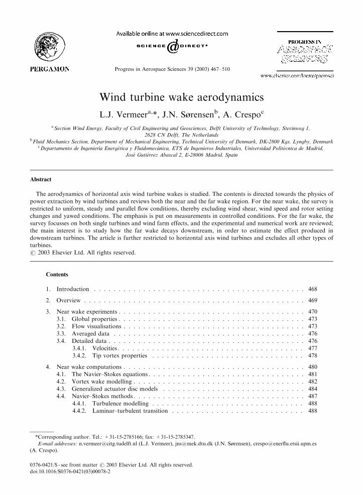
Fig. 1. Influence of pitch angle, ytip; on power coefficient (top)
and rotor drag coefficient (bottom) versus tip-speed ratio l(from [10]).
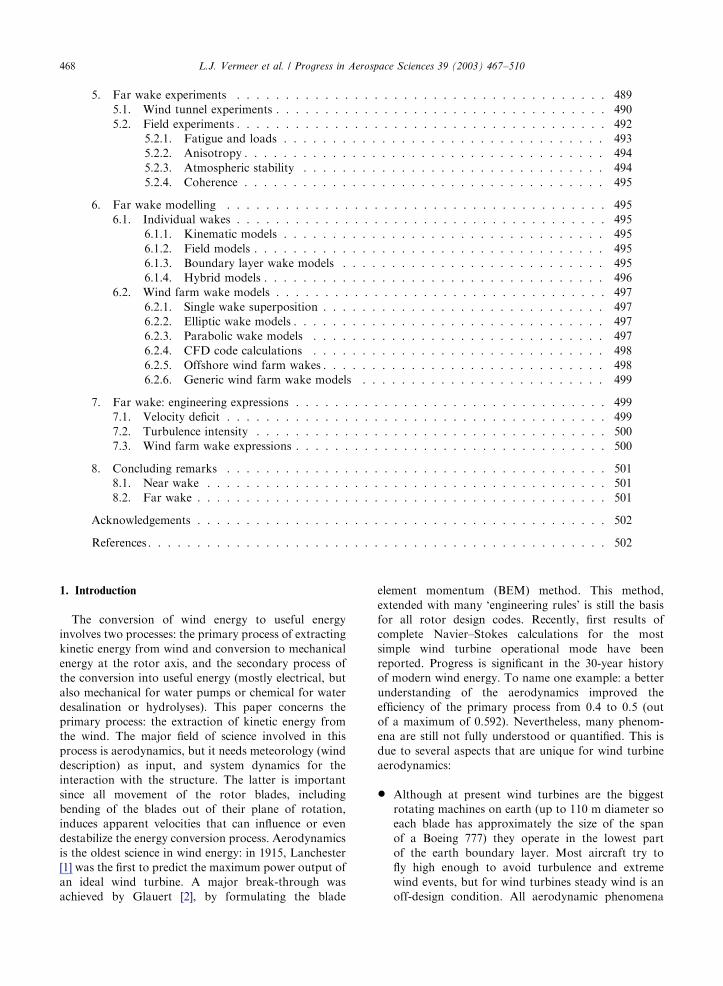
Fig. 2. Power coefficient as function of tip-speed ratio, l; withtip pitch angle, Y; as a parameter (from [15]).
L.J. Vermeer et al. / Progress in Aerospace Sciences 39 (2003) 467–510 473
circulation and the wake properties is expected to be
achieved.
3.1. Global properties
The operational conditions of a wind turbine are
described in a non-dimensional way with the CP–l and
CDax–l curves. The CP–l curve gives the power
coefficient against the tip-speed ratio, where CP is
defined as the power from the wind turbine divided by
the power available from the wind through the rotor
area, so CP ¼ P=12rV3
0pR2 and l is the rotor tip speed
divided by the oncoming wind speed, so l ¼ oR=V0
(similar to the reciprocal of the advance ratio in
helicopter terminology). The CDax–l curves gives the
axial force coefficient against the tip-speed ratio, where
CDaxis defined as the axial force on the total rotor
divided by the reference value, so CDax¼ Dax=12 rV2
0pR2:A lot of the references do give data for the global
properties of the rotor, but only for the configuration
parameters of the tests. Good practice would be to
thoroughly test the rotor before trying to experiment on
the wake, providing a proper documentation of the
rotor for later analysis. The curves given by de Vries [10]
(see Fig. 1) and Vermeer [15] (see Figs. 2 and 3) show
typical examples for two different rotor models.
3.2. Flow visualisations
Flow visualisation can give information, mostly
qualitative, about the flow in the vicinity of the rotor
and can reveal areas of attention. It can be done either in
the wake, trying to reveal rotor related flow patterns, or
on the blade, trying to reveal blade related flow pattern.
One of the first flow visualisation experiments is done
at FFA by Alfredsson [16,17]. Later by Anderson [11],
Savino [18], Anderson [19], Eggleston [20], Vermeer
[21–23] and [24], Hand [13] and Shimizu [12].
There is a distinction between two types of flow
visualisation with smoke: either the smoke can be
inserted into the flow from an external nozzle, so the
smoke is being transported with inflow velocity and
shows the cross section of the tip vortices (see Figs. 4–6),
or the smoke is ejected from the model (mostly near the
tip), so the smoke trails are being transported with the
local velocity and show a helix trace (see Fig. 7).
The FFA experiment by Alfredsson was originally set
out for wind farm effects, but was used later on for
deducing parameters for a single wake. In Fig. 4, as
much as six tip vortex cores can be counted, so for this
two-bladed rotor this means three full revolutions. The
visibility of these vortex cores is dependent on several
aspects: the quality of the wind tunnel with respect to
turbulence intensity, the quality of the smoke and
illumination, but also on the strength of the tip vortex
itself.
Also at TUDelft, similar smoke pictures were taken
by Vermeer [24] (see Fig. 6). Compared to the FFA
pictures, these appear rather poor, which might be due
to the turbulence level and the quality of the smoke
nozzle. Although the rotor model is really small (0:2 mdiameter), it has been used in the first phase of a long-
term wake research programme. With this model, the
initial measurements have been carried out and some
interesting observations have been made: when setting

ARTICLE IN PRESS
Fig. 3. Axial force coefficient as function of tip-speed ratio, l;with tip pitch angle, Y; as a parameter (from [15]).
Fig. 4. Flow visualisation with smoke, revealing the tip vortices
(from [16]).
Fig. 5. Flow visualisation with smoke, revealing smoke trails
being ‘sucked’ into the vortex spirals (from [16]).
Fig. 6. Flow visualisation experiment at TUDelft, showing two
revolutions of tip vortices for a two-bladed rotor (from [24]).
Fig. 7. Flow visualisation with smoke grenade in tip, revealing
smoke trails for the NREL turbine in the NASA-Ames wind
tunnel (from Hand [13]).
L.J. Vermeer et al. / Progress in Aerospace Sciences 39 (2003) 467–510474
the two blades at different pitch angles, the two tip
vortex spirals appear to have each their own path and
transport velocity. After a few revolutions, one tip
vortex catches up with the other and the two spirals
become entwined into one. Unluckily, there are no
recordings of this phenomena.
During the full scale experiment of NREL at the
NASA-Ames wind tunnel, also flow visualisation were
performed with smoke emanated from the tip (see
Fig. 7). With this kind of smoke trails, it is not clear
whether the smoke trail reveals the path of the tip vortex
or some streamline in the tip region. Also, these
experiments have been performed at very low thrust
values, so there is hardly any wake expansion.
A different set-up to visually reveal some properties of
the wake was utilised by Shimizu [12] with a tufts screen
(see Fig. 8).
Visualisation of the flow pattern over the blade is
mostly done with tufts. This is a well-known technique
and applied to both indoor and field experiments (see
[16–20,25–27]), however since blade aerodynamics is

ARTICLE IN PRESS
Fig. 9. Correlation between flow condition on the blade on
observed velocity pattern in the near wake for non-stalled
conditions (from [28]). The blade passages, recorded at 90� and
270� rotor azimuth angle, are steady.
L.J. Vermeer et al. / Progress in Aerospace Sciences 39 (2003) 467–510 475
a related subject, but beyond the scope of this article,
only one mention will be made of such an application.
Vermeer [28] has tried to correlate the flow pattern
visualised by tufts on the blade with near wake velocity
patterns, in order to get a better understanding of how
to interpret velocity signals. Especially, the location of
stall on the blade was the focus of this experiment. The
hot-wire probe was located at 65% radius and recorded
velocity traces over ten revolutions. There appeared to
be a great difference between attached flow (Fig. 9) and
stalled flow (Fig. 10). In attached flow, the velocity
changes associated with the blade passages (at 90� and
270� azimuth angle) are steady and the regions
associated with the remains of the boundary layer (just
after 0� and 180� azimuth angle) are relatively small, in
contrast to stalled flow, where the blade passages cause
changing magnitude (because of fluctuating circulation)
and the remains of the boundary layer is wide and
dominated by erratic fluctuations.
A novel technique of blade flow visualisation has been
devised by Corten [29–32] in the form of what he has
entitled stall-flags. The operational principle of the stall-
flags is shown in Figs. 11 and 12. The stall-flag basically
consists of a hinged flap and a retroreflector, fitted on a
sticker. These stickers have such a size that a few
hundred can be positioned on a full-scale rotor blade.
When the flow over the rotor blade is non-stalled, the
flap covers the reflector, where-as in stalled conditions,
the reflector will be uncovered.
Stall flags are suitable of surveying the stall behaviour
of full scale wind turbines on location. By installing a
powerful lightsource in the field (up to 500 m down-
stream of the turbine), the whole rotor area can be
illuminated, revealing all visible reflectors (see Fig. 13).
The stalling behaviour is recorded by a digital video
camera. Subsequently, the video frames are fed into the
computer, which can analyse automatically thousands of
frames, thanks to the binary character of the stall flag
Fig. 8. Flow visualisation by tufted grid method (from Shimizu
[12]).
signal. Statistical properties of the very dynamic process
of stalling can be derived, so that one can determine
whether the behaviour meets the design. If deviations
are notified, it can be derived from the data which
precise adaptations have to be made. The adaptations
are made by applying vortex generators or stall strips or
by pitching the blades slightly. Therefore the stall flag
technique can be seen as a diagnostic tool, which also
can prescribe the cure. An example of such diagnostics
was the analysis of the double stall problem, see [32].
As easy as it is to visualise the tip vortex, so hard it is
to do the same for the root vortex. Vermeer has tried to
visualise the root vortex of the TUDelft rotor model (see
[33]). In a total length of half an hour video material (at
25 frames/s), it is possible to locate a few frames on
which a clear root vortex is visible. This has several
causes: the root vortex is weaker than the tip vortex, the
attachment of the root of the blade to the hub and the
hub itself prevents a distinct vortex to be formed. As it is
hard to visualise the root vortex, getting experimental
data will be extremely difficult. This is regrettable,

ARTICLE IN PRESS
Fig. 11. The stall flag, consisting of a hinged flap and a reflector
(from [32], r Nature, with permission).
Fig. 12. Stall flags, showing the separated-flow area on an
aerofoil (from [32], r Nature, with permission).
Fig. 10. Correlation between flow condition on the blade on
observed velocity pattern in the near wake for stalled conditions
(from [28]). The blade passages, recorded at 90� and 270� rotor
azimuth angle, show changing magnitude.
Fig. 13. Recording of stall-flag signals from the NEG Micon
turbine in California (from [32], r Nature, with permission).
L.J. Vermeer et al. / Progress in Aerospace Sciences 39 (2003) 467–510476
because calculations have shown that including or
excluding the root vortex does make a lot of difference,
especially under yawed conditions.
3.3. Averaged data
Averaged data dealing with velocity distribution in
the wake is mostly used for attempts to analyse power
and thrust, which are the global properties of a wind
turbine, and do not reveal much about the physical
process of power extraction. The experiments have
mostly been carried out in the early years of wind
turbine research (up until 1983), with modest equipment
(Pitot tubes and pressure sensors), see [10,16,17,34–38].
Most data are shown at radius scale, including the rotor
model axis area, e.g. see Fig. 14. This is rather directed
towards wind farm research, but clearly shows the path
towards near wake research in which detailed data is
related to its spanwise location.
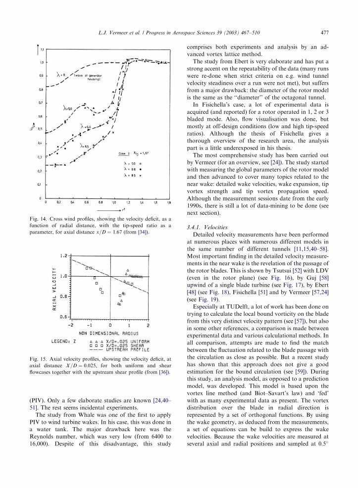
Wind profiles are also measured in non-uniform
flowfields (see [36] and Fig. 15) and even in atmospheric
boundary layers (see [39]).
3.4. Detailed data
Detailed wake data is acquired to provide a better
understanding of the underlying physics of wind turbine
aerodynamics. The experiments with detailed data are
done after 1982, when more sophisticated equipment
was employed. This section will be divided into two
parts, one concerning velocity measurements and one
concerning tip vortex properties. The experimental
equipment has changed to fast response pressure
sensors, hot wires (HW), laser doppler (LDV) and as a
latest promising development particle image velocimetry
ARTICLE IN PRESS
Fig. 14. Cross wind profiles, showing the velocity deficit, as a
function of radial distance, with the tip-speed ratio as a
parameter, for axial distance x=D ¼ 1:67 (from [34]).
Fig. 15. Axial velocity profiles, showing the velocity deficit, at
axial distance X=D ¼ 0:025; for both uniform and shear
flowcases together with the upstream shear profile (from [36]).
L.J. Vermeer et al. / Progress in Aerospace Sciences 39 (2003) 467–510 477
(PIV). Only a few elaborate studies are known [24,40–
51]. The rest seems incidental experiments.
The study from Whale was one of the first to apply
PIV to wind turbine wakes. In his case, this was done in
a water tank. The major drawback here was the
Reynolds number, which was very low (from 6400 to
16,000). Despite of this disadvantage, this study
comprises both experiments and analysis by an ad-
vanced vortex lattice method.
The study from Ebert is very elaborate and has put a
strong accent on the repeatability of the data (many runs
were re-done when strict criteria on e.g. wind tunnel
velocity steadiness over a run were not met), but suffers
from a major drawback: the diameter of the rotor model
is the same as the ‘‘diameter’’ of the octagonal tunnel.
In Fisichella’s case, a lot of experimental data is
acquired (and reported) for a rotor operated in 1, 2 or 3
bladed mode. Also, flow visualisation was done, but
mostly at off-design conditions (low and high tip-speed
ratios). Although the thesis of Fisichella gives a
thorough overview of the research area, the analysis
part is a little underexposed in his thesis.
The most comprehensive study has been carried out
by Vermeer (for an overview, see [24]). The study started
with measuring the global parameters of the rotor model
and then advanced to cover many topics related to the
near wake: detailed wake velocities, wake expansion, tip
vortex strength and tip vortex propagation speed.
Although the measurement sessions date from the early
1990s, there is still a lot of data-mining to be done (see
next section).
3.4.1. Velocities
Detailed velocity measurements have been performed
at numerous places with numerous different models in
the same number of different tunnels [11,15,40–58].
Most important finding in the detailed velocity measure-
ments in the near wake is the revelation of the passage of
the rotor blades. This is shown by Tsutsui [52] with LDV
(even in the rotor plane) (see Fig. 16), by Guj [58]
upwind of a single blade turbine (see Fig. 17), by Ebert
[48] (see Fig. 18), Fisichella [51] and by Vermeer [57,24]
(see Fig. 19).
Especially at TUDelft, a lot of work has been done on
trying to calculate the local bound vorticity on the blade
from this very distinct velocity pattern (see [57]), but also
in some other references, a comparison is made between
experimental data and various calculational methods. In
all comparison, attempts are made to find the match
between the fluctuation related to the blade passage with
the circulation as close as possible. But a recent study
has shown that this approach does not give a good
estimation for the bound circulation (see [59]). During
this study, an analysis model, as opposed to a prediction
model, was developed. This model is based upon the
vortex line method (and Biot–Savart’s law) and ‘fed’
with as many experimental data as present. The vortex
distribution over the blade in radial direction is
represented by a set of orthogonal functions. By using
the wake geometry, as deduced from the measurements,
a set of equations can be build to express the wake
velocities. Because the wake velocities are measured at
several axial and radial positions and sampled at 0:5�

ARTICLE IN PRESS
Fig. 16. Axial velocity component (at r=R ¼ 0:7) as a functionof rotor azimuth angle for several axial distances, both
upstream and downstream of the rotor (from [52]). Blade
passages are shown at 12p and 3
2p blade azimuth angle.
Fig. 17. Axial velocity in near wake, showing blade passage at
180�; as a function of rotor azimuth angle, for a single bladed
rotor model (from [58]).
Fig. 18. Comparison of axial (top) and tangential (bottom)
velocity patterns occurring at a blade passage (from [48]).
Fig. 19. Measured axial (top) and tangential (bottom) velocity
components as a function of rotor azimuth angle (from [24]).
The blades pass at 90� and 270� azimuth angle.
L.J. Vermeer et al. / Progress in Aerospace Sciences 39 (2003) 467–510478
azimuth angle, a highly overdetermined set of equations
is derived. By solving these equations with a least
squares method, the bound circulation can be calcu-
lated, and from this distribution the wake velocities can
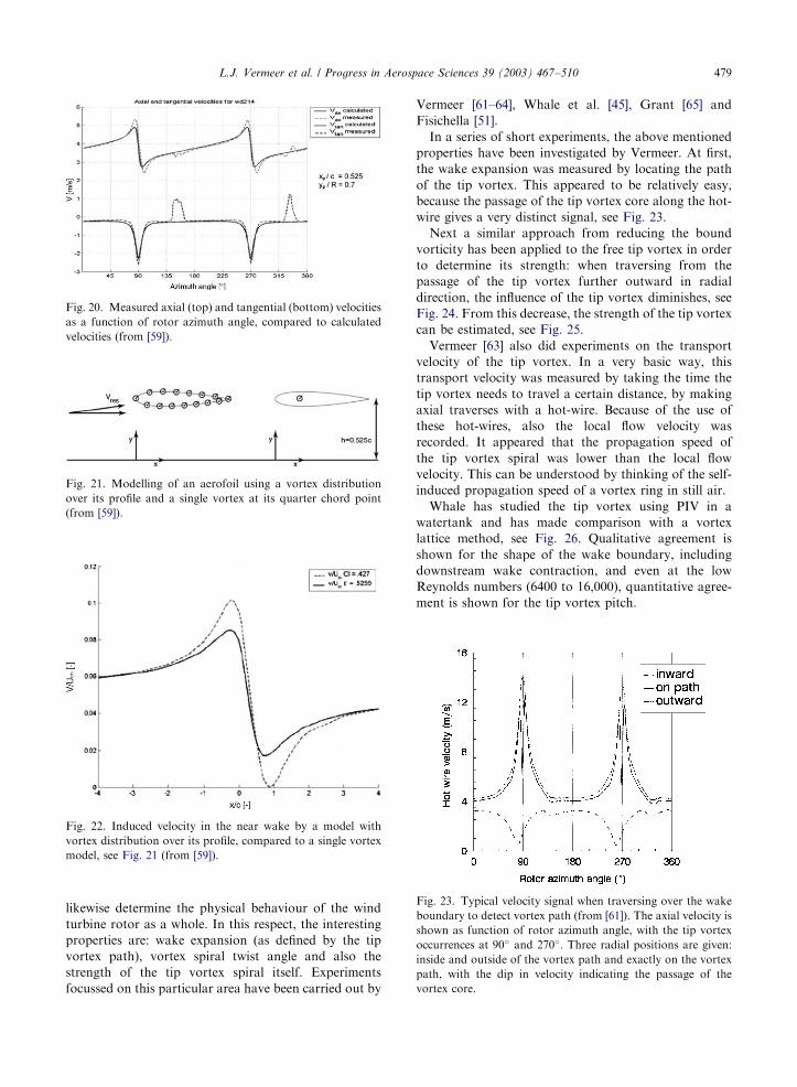
be compared with the measured ones (see Fig. 20).
One of the major findings was that the velocity
fluctuation caused by the blade passages can only
partially be attributed to the bound vorticity on the
blade, but when the measurement position is close to the
rotor blade, also the vorticity distribution over the
thickness of the blade has to be accounted for. A
simulation was done to compare a single line vortex (as
used in the study), with a vortex panel method (XFOIL,
see [60]) with a distribution of vortices over the contour
of the aerofoil, see Fig. 21. The vorticity distribution
results in a different velocity fluctuation and the
difference resembles the one from the analysis model,
see Figs. 22 and 20.
3.4.2. Tip vortex properties
Besides wake velocities, also the properties of the tip
vortices are worthwhile to investigate, because they
ARTICLE IN PRESS
Fig. 20. Measured axial (top) and tangential (bottom) velocities
as a function of rotor azimuth angle, compared to calculated
velocities (from [59]).
Fig. 21. Modelling of an aerofoil using a vortex distribution
over its profile and a single vortex at its quarter chord point
(from [59]).
Fig. 22. Induced velocity in the near wake by a model with
vortex distribution over its profile, compared to a single vortex
model, see Fig. 21 (from [59]).
Fig. 23. Typical velocity signal when traversing over the wake
boundary to detect vortex path (from [61]). The axial velocity is
shown as function of rotor azimuth angle, with the tip vortex
occurrences at 90� and 270�: Three radial positions are given:inside and outside of the vortex path and exactly on the vortex
path, with the dip in velocity indicating the passage of the
vortex core.
L.J. Vermeer et al. / Progress in Aerospace Sciences 39 (2003) 467–510 479
likewise determine the physical behaviour of the wind
turbine rotor as a whole. In this respect, the interesting
properties are: wake expansion (as defined by the tip
vortex path), vortex spiral twist angle and also the
strength of the tip vortex spiral itself. Experiments
focussed on this particular area have been carried out by
Vermeer [61–64], Whale et al. [45], Grant [65] and
Fisichella [51].
In a series of short experiments, the above mentioned
properties have been investigated by Vermeer. At first,
the wake expansion was measured by locating the path
of the tip vortex. This appeared to be relatively easy,
because the passage of the tip vortex core along the hot-
wire gives a very distinct signal, see Fig. 23.
Next a similar approach from reducing the bound
vorticity has been applied to the free tip vortex in order
to determine its strength: when traversing from the
passage of the tip vortex further outward in radial
direction, the influence of the tip vortex diminishes, see
Fig. 24. From this decrease, the strength of the tip vortex
can be estimated, see Fig. 25.
Vermeer [63] also did experiments on the transport
velocity of the tip vortex. In a very basic way, this
transport velocity was measured by taking the time the
tip vortex needs to travel a certain distance, by making
axial traverses with a hot-wire. Because of the use of
these hot-wires, also the local flow velocity was
recorded. It appeared that the propagation speed of
the tip vortex spiral was lower than the local flow
velocity. This can be understood by thinking of the self-
induced propagation speed of a vortex ring in still air.
Whale has studied the tip vortex using PIV in a
watertank and has made comparison with a vortex
lattice method, see Fig. 26. Qualitative agreement is
shown for the shape of the wake boundary, including
downstream wake contraction, and even at the low
Reynolds numbers (6400 to 16,000), quantitative agree-
ment is shown for the tip vortex pitch.

ARTICLE IN PRESS
Fig. 24. Azimuthal velocity plot outside the wake boundary,
showing the passage of the tip vortices at 90� and 270� azimuth
angle (from [62]). The parameter r is the radial coordinate
measured from the tip radius. The velocity peak associated with
the passage of the tip vortex decreases with increasing radial
distance.
Fig. 25. The value of the peak velocity associated with the
passage of the tip vortex (see Fig. 24), as a function of the
radial distance from the rotor tip, for several axial distances
(from [62]).
Fig. 26. Comparison of PIV measurements and ROVLM
computations of vorticity contour plots of the full wake of a
two-bladed flat-plate rotor (from [45]).
Fig. 27. Predicted and measured wake expansion for tip-speed
ratios 4 and 5 in head-on flow (from [65]).
L.J. Vermeer et al. / Progress in Aerospace Sciences 39 (2003) 467–510480
Grant [65] has used Laser sheet visualisation to
measure the behaviour of the vorticity trailing from
the turbine blade tips and the effect of wall interference
on wake development, for various conditions of turbine
yaw. Results were compared with a prescribed wake
model, see Fig. 27.
4. Near wake computations
Although there exists a large variety of methods for
predicting performance and loadings of wind turbines,
the only approach used today by wind turbine manu-
facturers is based on the blade element/momentum
(BEM) theory. A basic assumption in the BEM theory is
that the flow takes place in independent stream tubes
and that the loading is determined from two-dimen-
sional sectional aerofoil characteristics. The advantage
of the model is that it is easy to implement and use on a
computer, it contains most of the physics representing
rotary aerodynamics, and it has proven to be accurate
for the most common flow conditions and rotor

ARTICLE IN PRESSL.J. Vermeer et al. / Progress in Aerospace Sciences 39 (2003) 467–510 481
configurations. A drawback of the model is that it, to
a large extent, relies on empirical input which is not
always available. Even in the simple case of a rotor
subject to steady axial inflow, aerofoil characteristics
have to be implemented from wind tunnel measure-
ments. The description is further complicated if we look
at more realistic operating situations. Wind turbines are
subject to atmospheric turbulence, wind shear from the
ground effect, wind directions that change both in time
and in space, and effects from the wake of neighbouring
wind turbines. These effects together form the ordinary
operating conditions experienced by the blades. As a
consequence, the forces vary in time and space and
a dynamical description is an intrinsic part of the
aerodynamic analysis.
At high wind velocities, where a large part of the blade
operates in deep stall, the power output is extremely
difficult to determine within an acceptable accuracy. The
most likely explanation for this is that the flow is not
adequately modelled by static, two-dimensional aerofoil
data. When separation occurs in the boundary layer,
outward spanwise flow generated by centrifugal and
coriolis pumping tends to decrease the boundary layer
thickness, resulting in the lift coefficient being higher
than what would be obtained from wind tunnel
measurements on a non-rotating blade. Employing a
viscous-inviscid interaction technique it has been shown
by S^rensen [66] that the maximum lift may increase by
more than 30% due to the inclusion of rotational effects.
Later experiments of e.g. Butterfield [67], Ronsten [68],
and Madsen and Rasmussen [69] have confirmed this
result. To take into account the rotational effects, it is
common to derive synthesized three-dimensional aero-
foil data (see e.g. [70] or Chaviaropoulos and Hansen
[71]). If it turns out, however, that stall on a rotating
blade inherently is a three-dimensional process, it is
doubtful if general values for modifying two-dimen-
sional aerofoil characteristics can be used at high
winds. In all cases there is a need to develop three-
dimensional models from which parametrical studies
can be performed.
When the wind changes direction, misalignment with
the rotational axis occurs, resulting in yaw error. This
causes periodic variations in the angle of attack and
invalidates the assumption of axisymmetric inflow
conditions. Furthermore, it gives rise to radial flow
components in the boundary layer. Thus, both the
aerofoil characteristics and the wake are subject to
complicated three-dimensional and unsteady flow beha-
viour, which only in an approximate way can be
implemented in the standard BEM method. To take
into account yaw misalignment, modifications to the
BEM model have been proposed by e.g. Goankar and
Peters [72], Hansen [73], van Bussel [74] and Hasegawa
et al. [75]. But, again, a better understanding demands
the use of more representative models.
A full description of the global flow field around a
wind turbine is in principle possible by solving the
Navier–Stokes equations subject to unsteady inflow and
rotational effects. In practice, however, the capability of
present computer technology limits the number of mesh
points to a maximum of about 10 millions, which is not
always sufficient for a global description that includes
the boundary layer on the rotor as well as and the
shed vortices in the wake. As a consequence, various
models have been proposed, ranging from models based
on potential flow and vortex theory to CFD models
based on solving the Reynolds-averaged Navier–Stokes
equations.
In the following an overview of computational
methods for use in wind turbine aerodynamics will be
presented. The intention is not to give here an exhaustive
description of numerical techniques. Rather the pre-
sentation will concentrate on describing basic features of
models pertinent to the aerodynamics of horizontal-axis
wind turbines.
4.1. The Navier–Stokes equations
As basic mathematical model we consider the
Reynolds-averaged, incompressible Navier–Stokes
equations which, with ~VV denoting the Reynolds-
averaged velocity and P the pressure, in conservative
form are written as
@~VV
@tþr � ð~VV#~VV Þ
¼ 1
rrP þ nr � 1þ
nt
n
� �r~VV
h iþ ~ff ; ð1Þ
r � ~VV ¼ 0; ð2Þ
where t denotes time, r is the density of the fluid and n isthe kinematic viscosity. The Reynolds stresses are
modelled by the eddy-viscosity, nt; and a body force, ~ff ;is introduced in order to model external force fields, as
done in the generalized actuator disc model. These
equations constitute three transport equations, which
are parabolic in time and elliptic in space, and an
equation of continuity stating that the velocity is
solenoidal. The main difficulty of this formulation is
that the pressure does not appear explicitly in the
equation of continuity. The role of the pressure,
however, is to ensure the continuity equation be satisfied
at every time instant. A way to circumvent this problem
is to relate the pressure to the continuity equation by
introducing an artificial compressibility term into this
(see e.g. [76]). Thus, an artificial transport equation for
the pressure is solved along with the three momentum
equations, ensuring a solenoidal velocity field when a
steady state is achieved. The drawback of this method is
that only time-independent problems can be considered.
Another approach, the pressure correction method, is to

ARTICLE IN PRESSL.J. Vermeer et al. / Progress in Aerospace Sciences 39 (2003) 467–510482
relate the velocity and pressure fields through the
solution of a Poisson equation for the pressure. This is
obtained by taking the divergence of the momentum
equations, resulting in the following relation:
r2P ¼ rr � ½r � ð~VV#~VV Þ ntr~VV �; ð3Þ
which is solved iteratively along with the momentum
equations.
As an alternative to the ~VV P formulation of the
Navier–Stokes equations, vorticity based models may be
employed, see [77,78]. The vorticity, defined as the curl
of the time-averaged velocity
~oo ¼ r� ~VV ; ð4Þ
may be introduced as primary variable by taking the curl
of Eq. (1). This results in the following set of equations:
@~oo@t
þr� ð~oo� ~VV Þ
¼ nr2 1þnt
n
� �~oo
h iþr� ~ff þ Qo; ð5Þ
r � ~VV ¼ ~oo; r � ~VV ¼ 0; ð6Þ
where Qo contains some additional second order terms
from the curl operation. The equations can be for-
mulated in various ways. The Cauchy–Riemann part of
the equations, Eq. (6), may e.g. be replaced by a set of
Poisson equations
r2 ~VV ¼ r� ~oo: ð7Þ
If we consider Eq. (5) in an arbitrarily moving frame of
reference we get
@~oo�
@tþr� ð~oo� � ~VVÞ
¼ nr2 1þnt
n
� �~oo�
h iþr� ~ff þ Qo; ð8Þ
where the vorticity vector ~oo� refers to the inertial
system, i.e. ~oo� ¼ ~ooþ 2~OO; with ~OO ¼ ðOx;Oy;OzÞ denot-ing the angular velocity of the coordinate system.
The advantage of the vorticity–velocity formulation
over that of the primitive variables were discussed by
Speziale [79]. To summarize, these are: (1) Non-inertial
effects arising from a rotation or translation of the frame
of reference to an inertial frame enter the problem only
through the initial and boundary conditions, as demon-
strated in Eq. (8); (2) A solenoidal velocity field is
automatically ensured when solving Eq. (6), thus no
pressure–velocity coupling is needed; (3) The relation
between velocity and vorticity is linear. The disadvan-
tages, on the other hand, are that the Cauchy–Riemann
part of the equations are overdetermined, i.e. contains
more equations than unknowns, and when replacing this
by Eq. (7), three Poisson equations have to be solved
instead of the one for the pressure in the primitive
variables formulation. Another drawback of the model
is that the vorticity field must satisfy the solenoidal
constraint, r � ~oo ¼ 0; which follows directly from
Eq. (4). Finally, it should be mentioned that when the
formulation is employed to solve flow problems in
multiple-connected domains, for each hole in the
domain, the equations are subject to the following
integral constraint (see e.g. [80])
1
r
Il
rP dl ¼ I
l
@~VV
@tþr � ð~VV#~VV Þ
" #dl
þ nI
l
r � 1þnt
n
� �r~VV
h idl; ð9Þ
where l is an arbitrary circuit looping the inner body.
In a study by Hansen [81] it was concluded that the
vorticity–velocity formulation is not well suited to
handle high Reynolds number problems in complicated
domains, but is a valuable tool for simulations of basic
flow problems in Cartesian or cylindrical coordinates.
4.2. Vortex wake modelling
Vortex wake models denote a class of methods in
which the rotor blades and the trailing and shed vortices
in the wake are represented by lifting lines or surfaces.
At the blades the vortex strength is determined from the
bound circulation which is related to the local inflow
field. The global flow field is determined from the
induction law of Biot–Savart, where the vortex filaments
in the wake are convected by superposition of the
undisturbed flow and the induced velocity field. The
trailing wake is generated by spanwise variations of the
bound vorticity along the blade. The shed wake is
generated by the temporal variations as the blade
rotate. Assuming that the flow in the region outside
the trailing and shed vortices is curl-free, the overall flow
field can be represented by the Biot–Savart law. This is
most easily shown by decomposing the velocity in a
solenoidal part and a rotational part, using Helmholtz
decomposition:
~VV ¼ r� ~AA þrF; ð10Þ
where ð~AAÞ is a vector potential and F a scalar potential.
The vector potential automatically satisfies the con-
tinuity equation, Eq. (2), and from the definition of
vorticity, Eq. (4), we get
r2~AA ¼ ~oo: ð11Þ
In the absence of boundaries, this can be expressed as an
integral relation,
~AAð~XX Þ ¼1
4p
Z~oo0
j~XX ~XX 0jdVol; ð12Þ
where ~XX denotes the point where the potential is
computed and the integration is taken over the region
where the vorticity is non-zero, designated by Vol: Fromthe definition, Eq. (10), the resulting velocity field is
ARTICLE IN PRESSL.J. Vermeer et al. / Progress in Aerospace Sciences 39 (2003) 467–510 483
obtained by
~VV ð~XX Þ ¼ 1
4p
Zð~XX ~XX 0Þ � ~oo0
j~XX ~XX 0j3dVol; ð13Þ
which is the most usual form of the Biot–Savart law.
In its simplest form the wake is prescribed as a hub
vortex plus a spiralling tip vortex or as a series of ring
vortices. In this case the vortex system is assumed to
consists of a number of line vortices with vorticity
distribution
oð~XX Þ ¼ Gdð~XX ~XX 0Þ; ð14Þ
where G is the circulation, d is the Dirac delta function
and ~XX 0 is the curve defining the location of the vortex
lines. Combining this with Eq. (13) results in
~VV ð~XX Þ ¼ 1
4p
ZS
Gð~XX ~XX 0Þ
j~XX ~XX 0j3�
@~XX 0
@s0ds0; ð15Þ
where S is the curve defining the vortex line and s0 is the
parametric variable along the curve. Utilizing Eq. (15),
simple vortex models can be derived to compute quite
general flow fields about wind turbine rotors. In a study
of Miller [82], a system of vortex rings was used to
compute the flow past a heavily loaded wind turbine. It
is remarkable that in spite of the simplicity of the model,
it was possible to simulate the vortex ring/turbulent
wake state with good accuracy, as compared to the
empirical correction suggested by Glauert [2]. As a
further example, a similar simple vortex model devel-
oped by Øye [83] was used to calculate the relation
between thrust and induced velocity at the rotor disc of a
wind turbine, in order to validate basic features of the
streamtube-momentum theory. The model includes
effects of wake expansion, and, as in the model of
Miller, it simulates a rotor with an infinite number of
blades, with the wake being described by vortex rings.
From the model it was found that the axial induced
velocities at the rotor disc are smaller than those
determined from the ordinary streamtube–momentum
theory. Based on the results a correction to the
momentum method was suggested. Although the
correction is small, an important conclusion was that
the apparent underestimation of the power coefficient by
the momentum method is not primarily caused by its
lack of detail regarding the near wake, but is more likely
caused by the decay of the far wake. A similar approach
has been utilised by Wood and co-workers [84,85].
To compute flows about actual wind turbines it
becomes necessary to combine the vortex line model
with tabulated two-dimensional aerofoil data. This can
be accomplished by representing the spanwise loading
on each blade by a series of straight vortex elements
located along the quarter chord line. The strength of the
vortex elements are determined by employing the Kutta–
Joukowsky theorem on the basis of the local aerofoil
characteristics. As the loading varies along the span of
each blade the value of the bound circulation changes
from one filament to next. This is compensated for by
introducing trailing vortex filaments whose strengths
correspond to the differences in bound circulation
between adjacent blade elements. Likewise, shed vortex
filaments are generated and convected into the wake
whenever the loading undergoes a temporal variation.
While vortex models generally provide physically
realistic simulations of the wake structure, the quality
of the obtained results depends crucially on the input
aerofoil data. Indeed, in order to be of practical use,
aerofoil data has to be modified with respect to three-
dimensional effects and dynamic stall. In particular the
American NREL experiment in the wind tunnel at
NASA-Ames has demonstrated that, even though two-
dimensional aerofoil data exist, input aerofoil data are
the main source of uncertainty and errors in load
predictions, see [14].
In vortex models, the wake structure can either be
prescribed or computed as a part of the overall solution
procedure. In a prescribed vortex technique, the position
of the vortical elements is specified from measurements
or semi-empirical rules. This makes the technique fast to
use on a computer, but limits its range of application to
more or less well-known steady flow situations. For
unsteady flow situations and complicated wake struc-
tures free wake analysis becomes necessary. A free wake
method is more straightforward to understand and use,
as the vortex elements are allowed to convect and
deform freely under the action of the velocity field. The
advantage of the method lies in its ability to calculate
general flow cases, such as yawed wake structures and
dynamic inflow. The disadvantage, on the other hand, is
that the method is far more computing expensive than
the prescribed wake method, since the Biot–Savart law
has to be evaluated for each time step taken. Further-
more, free wake vortex methods tend to suffer from
stability problems owing to the intrinsic singularity in
induced velocities that appears when vortex elements are
approaching each other. This can to a certain extent be
remedied by introducing a vortex core model in which a
cut-off parameter models the inner viscous part of the
vortex filament. In recent years much effort in the
development of models for helicopter rotor flowfields
have been directed towards free-wake modelling using
advanced pseudo-implicit relaxation schemes, in order
to improve numerical efficiency and accuracy (e.g.
[86,87]).
To analyse wakes of horizontal axis wind turbines,
prescribed wake models have been employed by e.g.
Gould and Fiddes [88], Robison et al. [89], and Coton
and Wang [90], and free vortex modelling techniques
have been utilised by e.g. Afjeh and Keith [91] and
Simoes and Graham [92]. A special version of the free
vortex wake methods is the method by Voutsinas [93] in
which the wake modelling is taken care of by vortex

ARTICLE IN PRESSL.J. Vermeer et al. / Progress in Aerospace Sciences 39 (2003) 467–510484
particles or vortex blobs. Recently, the model of Coton
and co-workers [94] was employed in the NREL blind
comparison exercise [14], and the main conclusion from
this was that the quality of the input blade sectional
aerodynamic data still represent the most central issue to
obtaining high-quality predictions.
A generalisation of the vortex method is the so-called
boundary integral equation method (BIEM), where the
rotor blade in a simple vortex method is represented by
straight vortex filaments, the BIEM takes into account
the actual finite-thickness geometry of the blade. The
theoretical background for BIEMs is potential theory
where the flow, except at solid surfaces and wakes, is
assumed to be irrotational. In such a case the velocity
field can be represented by a scalar potential,
~VV ¼ rF; ð16Þ
where the velocity potential
F ¼ fN
þ f; ð17Þ
is decomposed into a potential fN
representing the free
stream velocity, and a perturbation potential f that
through the continuity equation, Eq. (2), can be
expressed as
r2f ¼@2f@x2
þ@2f@y2
þ@2f@z2
¼ 0: ð18Þ
Integrating this equation over discontinuity surfaces,
here denoted S; Green’s theorem yields
f ¼ 1
4p
ZS
s1
j~XX ~XX 0jdS
1
4p
ZS
m@
@n
1
j~XX ~XX 0jdS;
ð19Þ
where n is the coordinate normal to the wall, s is the
source distribution and m is the doublet distribution.
These represent the singularities at the border of the flow
domain, i.e. at solid surfaces and wakes. In a rotor
computation the blade surface is covered with both
sources and doublets while the wake only is represented
by doublets (see e.g. [95] or [96]). The circulation of the
rotor is obtained as an intrinsic part of the solution by
applying the Kutta condition on the trailing edge of the
blade. The main advantage of the BIEM is that complex
geometries can be treated without any modification of
the model. Thus, both the hub and the tower can be
modelled as a part of the solution. Furthermore, the
method does not depend on aerofoil data and viscous
effects can, at least in principle, be included by coupling
the method to a viscous solver. Within the field of wind
turbine aerodynamics, BIEMs has been applied by e.g.
Preuss et al. [97], Arsuffi [98] and Bareiss and Wagner
[99]. Up to now, however, only simple flow cases have
been considered.
A method in line with the BIEM is the asymptotic
acceleration potential method, developed originally
for helicopter aerodynamics by van Holten [100] and
later developed further to cope with wind turbines by
van Bussel [101]. The method is based on solving a
Poisson equation for the pressure, assuming small
perturbations of the mean flow. The model has been
largely used by van Bussel [101] to analyse various
phenomena within wind turbine aerodynamics. Compu-
tational efficiency and range of application of the
method corresponds to what is obtained by prescribed
vortex wake models.
4.3. Generalized actuator disc models
In fluid mechanics the actuator disc is defined as a
discontinuous surface or line on which surface forces act
upon the surrounding flow. In rotary aerodynamics the
concept of the actuator disc is not new. Indeed, the
actuator disc constitutes the main ingredient in the one-
dimensional momentum theory, as formulated by
Froude [102], and in the ‘classical’ BEM method by
Glauert [2]. Usually, the actuator disc is employed in
combination with a simplified set of equations and its
range of applicability is often confused with the
particular set of equations considered. In the case of a
horizontal axis wind turbine the actuator disc is given as
a permeable surface normal to the freestream direction
on which an evenly distribution of blade forces acts
upon the flow. In its general form the flow field is
governed by the unsteady, axisymmetric Euler or
Navier–Stokes equations, which means that no physical
restrictions need to be imposed on the kinematics of
the flow.
The first non-linear actuator disc model for heavily
loaded propellers was formulated by Wu [103].
Although no actual calculations were carried out, this
work demonstrated the opportunities for employing the
actuator disc on complicated configurations as e.g.
ducted propellers and propellers with finite hubs. Later
improvements, especially on the numerical treatment of
the equations, are due to e.g. [104,105], and recently
Conway [106,107] has developed further the analytical
treatment of the method. In the application of the
actuator disc concept for wind turbine aerodynamics,
the first non-linear model was suggested by Madsen
[108], who developed an actuator cylinder model to
describe the flow field about a vertical-axis wind turbine,
the Voight–Schneider or Gyro mill. This model has later
been adapted to treat horizontal axis wind turbines. A
thorough review of ‘classical’ actuator disc models for
rotors in general and wind turbines in particular can be
found in the dissertation by van Kuik [109]. Recent
developments of the method has mainly been directed
towards the use of Navier–Stokes equations.
In helicopter aerodynamics combined Navier–Stokes/
actuator disc models have been applied by e.g. Fejtek
and Roberts [110] who solved the flow about a
helicopter employing a chimera grid technique in

ARTICLE IN PRESSL.J. Vermeer et al. / Progress in Aerospace Sciences 39 (2003) 467–510 485
which the rotor was modelled as an actuator disk,
and Rajagopalan and Mathur [111] who modelled
a helicopter rotor using time-averaged momentum
source terms in the momentum equations.
In a numerical actuator disc model, the Navier–Stokes
(or Euler) equations, Eqs. (1)–(3) or Eqs. (5)–(7), are
typically solved by a second order accurate finite
difference/volume scheme, as in a usual CFD computa-
tion. However, the geometry of the blades and the
viscous flow around the blades are not resolved. Instead
the swept surface of the blades is replaced by surface
forces that act upon the incoming flow at a rate
corresponding to the period-averaged mechanical work
that the rotor extracts from the flow.
In the simple case of an actuator disc with constant
prescribed loading, various fundamental studies can
easily be carried out. Comparisons with experiments
have demonstrated that the method works well for
axisymmetric flow conditions and can provide useful
information regarding basic assumptions underlying the
momentum approach [112–115], turbulent wake states
occurring for heavily loaded rotors [115,116], and rotors
subject to coning [117,118].
When computing the flow past an actual wind turbine,
the aerodynamic forces acting on the rotor are
determined from two-dimensional aerofoil characteris-
tics, corrected for three-dimensional effects, using a
blade-element approach.
In Fig. 28, a cross-sectional element at radius r defines
the aerofoil in the ðy; zÞ plane. Denoting the tangential
and axial velocity in the inertial frame of reference as Vy
and Vz; respectively, the local velocity relative to the
rotating blade is given as
Vrel ¼ ðVy Or;VzÞ: ð20Þ
The angle of attack is defined as
a ¼ f g; ð21Þ
where f ¼ tan1ðVz=ðOr VyÞÞ is the angle between V rel
and the rotor plane and g is the local pitch angle. The
Fig. 28. Cross-sectional aerofoil element (from [119]).
distribution of surface forces, i.e. forces per unit rotor
area, is given by the following expression:
f 2D ¼dF
dA¼1
2rV2
relcBðCLeL þ CDeDÞ=ð2prÞ; ð22Þ
where CL ¼ CLða;ReÞ and CD ¼ CDða;ReÞ are the lift
and drag coefficients, respectively, c is the chord length,
B denotes the number of blades, and eL and eD denote
the unit vectors in the directions of the lift and the drag,
respectively. The lift and drag coefficients are deter-
mined from measured or computed two-dimensional
aerofoil data that are corrected for three-dimensional
effects. There are several reasons why it is necessary to
correct the aerofoil data. First, at separation rotational
effects limit the growth of the boundary layer, resulting
in an increased lift as compared to two-dimensional
characteristics. Various correction formulas for rota-
tional effects have been derived using quasi three-
dimensional approaches (see e.g. [120,71]). Next, the
aerofoil characteristics depend on the aspect ratio of the
blade. This is in particular pronounced at high
incidences where the finite aspect ratio drag coefficient,
CD; is much smaller than the corresponding one for an
infinite blade. As an example, for a flat plate at an
incidence a ¼ 90� the drag coefficient CD ¼ 2 for an
infinitely long plate, whereas for aspect ratios corre-
sponding to the geometry of a wind turbine blade CD
takes values in the range 1:2 1:3: In [121] it is stated
that the normal force from a flat plate is approximately
constant for 45�oao135�; indicating that in this range
both CL and CD have to be reduced equally. Hansen
[122] proposes to reduce CL and CD by an expression
that takes values in range from 0:6 to 1:0; depending onthe ratio between the distance to the tip and the local
chord length. It should be noticed, however, that this is
only a crude guideline and that most aerofoil data for
wind turbine use is calibrated against actual perfor-
mance and load measurements. This also explains why
most manufacturers of wind turbine blades are reluctant
to change well-tested aerofoil families. Yet a correction
concerns unsteady phenomena related to boundary layer
separation, referred to as dynamic stall. For aerofoils
undergoing large temporal variations of the angle of
attack, the dynamic response of the aerodynamic forces
exhibits hysteresis that changes the static aerofoil data.
Dynamic stall models have been developed and applied
on wind turbines by e.g. Øye [123] or Leishman and
Beddoes [124].
Computations of actual wind turbines employing
numerical actuator disc models in combination with a
blade-element approach have been carried out by e.g.
S^rensen et al. [112,113] and Masson et al. [125,126] in
order to study unsteady phenomena. Wakes from coned
rotors have been studied by Madsen and Rasmussen
[117], Masson [126], and Mikkelsen et al. [118], rotors
operating in enclosures such as wind tunnels or solar

ARTICLE IN PRESS
Fig. 31. Transient behaviour of the flapping moment for the
Tjæreborg wind turbine subjected to instantaneous blade pitch
changes (from [113]).
L.J. Vermeer et al. / Progress in Aerospace Sciences 39 (2003) 467–510486
chimneys were computed by Phillips and Schaffarczyk
[127], and Mikkelsen and S^rensen [128], and approx-
imate models for yaw have been implemented by
Mikkelsen and S^rensen [129] and Masson [126].
Finally, Masson and colleagues have devised techniques
for employing their actuator disc model to study the
wake interaction in wind farms and the influence of
thermal stratification in the atmospheric boundary layer
[126,130].
To demonstrate which kind of results can be achieved
using an numerical axisymmetric actuator disc model, in
Figs. 29 and 30 we show computed stream lines for the
flow field about the Tjæreborg wind turbine at two
different wind speeds. Noteworthy is the details of
unsteady flow behaviour that can be obtained at small
wind velocities. In fact, the streamline shown in Fig. 29
corresponds to the turbulent wake state. A main feature
of the numerical actuator disc technique is the possibility
of predicting transient and unsteady flow behaviour. For
wind turbines unsteady effects occurs when the wind
changes speed or direction, or when the rotor is subject
to blade pitching actions.
This is shown in Fig. 31 where measured and
computed time histories of the flapping moment of the
Tjæreborg machine are compared for a case in which the
pitch angle was changed in a sequence going from 0� to
2� and then back to 0�; with the value of 2� fixed in 30 s:In the calculations the pitch angle was changed
instantaneously, therefore a slight difference between
the two curves occurs in the initial and the final stage of
the sequence. The overall behaviour of the calculations,
Fig. 29. Flow field about the Tjæreborg wind turbine at a wind
speed of 6:5 m=s (from [113]).
Fig. 30. Flow field about the Tjæreborg wind turbine at a wind
speed of 10 m=s (from [113]).
however, is seen to be in excellent agreement with
measured data.
The main limitation of the axisymmetric assumption
is that the forces are distributed evenly along the
actuator disk, hence the influence of the blades is taken
as an integrated quantity in the azimuthal direction. To
overcome this limitation, an extended three-dimensional
actuator disc model has recently been developed by
S^rensen and Shen [119]. The model combines a three-
dimensional Navier–Stokes solver with a technique in
which body forces are distributed radially along each of
the rotor blades. Thus, the kinematics of the wake is
determined by a full three-dimensional Navier–Stokes
simulation whereas the influence of the rotating blades
on the flow field is included using tabulated aerofoil data
to represent the loading on each blade. As in the
axisymmetric model, aerofoil data and subsequent
loading are determined iteratively by computing local
angles of attack from the movement of the blades and
the local flow field. The concept enables one to study in
detail the dynamics of the wake and the tip vortices and
their influence on the induced velocities in the rotor
plane. The main motivation for developing the model is
to analyse and verify the validity of the basic assump-
tions that are employed in the simpler more practical
engineering models. In the following, we show some
numerical results from computations of a 500 kW
Nordtank wind turbine at a wind speed V0 ¼ 10 m=s;corresponding to a tip speed ratio of 5.8.
Fig. 32 depicts iso-vorticity contours illustrating the
downstream development of the wake vortices. The
bound vorticity of the blades is seen to be shed

ARTICLE IN PRESS
Fig. 34. Distribution of axial velocity at a wind speed of
10 m=s: The core of the tip vortices are marked by � (from
[119]).
L.J. Vermeer et al. / Progress in Aerospace Sciences 39 (2003) 467–510 487
downstream from the rotor in individual vortex tubes.
These vortices persist about 2 turns after which they
diffuse into a continuous vortex sheet.
Fig. 33 shows the distribution of the axial interference
factor, in the rotor plane. The three blades are seen as
lines with a high density of iso-lines, owing to the large
changes in induced velocity that takes place across the
blades. The number of iso-lines is 30 and the value
between two successive lines is equidistant. The values
range from 0:15 to 0.55, with peak values appearing
near the mid-section of the blades (with a positive value
on one side of the blade and a negative value on the
other).
The development of the axial velocity distribution in
the wake is depicted in Fig. 34. The velocity distribu-
tions are averaged in the azimuthal direction and plotted
at axial positions z=R ¼ 0; 1; 2 and 3: Outside the wakethe value of the axial velocity attains the one of the
undisturbed wind. A small overshoot is observed at
Fig. 32. Computed vorticity field showing the formation of the
wake structure about the Tjæreborg wind turbine at a wind
speed of 10 m=s (from [119]).
Fig. 33. Distribution of axial interference factor, a ¼1 Vz=Vo; in the rotor plane at a wind speed of 10 m=s (from[119]).
z=R ¼ 2: For all velocity profiles a distinct minimum
occurs at r ¼ 0: This is caused by the loading on the
inner part of the blade that is dominated by large drag
forces. The position of the tip vortices is inferred as dots
on the velocity profiles. As can be seen they are generally
located midway between the wake and the external flow
at the position where the gradient of the axial velocity
attains its maximum value.
4.4. Navier–Stokes methods
During the past two decades a strong research activity
within the aeronautical field has resulted in the devel-
opment of a series of Computational Fluid Dynamics
(CFD) tools based on the solution of the Reynolds-
averaged Navier–Stokes (RANS) equations. This re-
search has mostly been related to the aerodynamics of
fixed-wing aircraft and helicopters. Some of the experi-
ence gained from the aeronautical research institutions
has been exploited directly in the development of CFD
algorithms for wind turbines. Notably is the develop-
ment of basic solution algorithms and numerical
schemes for solution of the flow equations, grid
generation techniques and the modelling of boundary
layer turbulence. These elements together form the basis
of all CFD codes, of which some already exist as
standard commercial software. Looking specifically on
the aerodynamics of horizontal axis wind turbines, we
find some striking differences as compared to usual
aeronautical applications. First, as tip speeds generally
never exceeds 100 m=s; the flow around wind turbines is
incompressible. Next, the optimal operating condition
for a wind turbine always includes stall, with the upper
side of the rotor blades being dominated by large areas
of flow separation. This is in contrast to the cruise

ARTICLE IN PRESSL.J. Vermeer et al. / Progress in Aerospace Sciences 39 (2003) 467–510488
condition of an aircraft where the flow is largely
attached.
The research on CFD in wind turbine aerodynamics
has in Europe taken place mostly through the EU-
funded collaborate projects VISCWIND [131], VISCEL
[132] and the on-going project KNOW-BLADE. The
participants in these projects are Ris^; DTU, CRES,NTUA, VUB, FFA and DLR, who all have vast
experience in developing Navier–Stokes codes. Results
from the projects have been reported in e.g. [132–137].
In the US, three-dimensional computations of wind
turbine rotors employing Reynolds-averaged Navier–
Stokes equations have been carried out by Duque et al.
[138,139] and by Xu and Sankar [140,141], who utilised
a hybrid Navier–Stokes/full-potential/free wake method
in order to reduce computing time.
Recently, the American NREL experiment at NASA-
Ames [142] and the accompanying NREL/NWTC
Aerodynamics Blind Comparison test [14] have given a
lot of new insight into wind turbine aerodynamics and
revealed serious shortcomings in present day wind
turbine aerodynamics prediction tools. First, computa-
tions of the performance characteristics of the rotor by
methods based on blade element techniques were found
to be extremely sensitive to the input blade section
aerodynamic data [94,143]. Indeed, predicted values of
the distribution of the normal force coefficient deviated
from measurements by as much as 50%. Even at low
angles of attack, model predictions differed from
measured data by 15–20% [14]. Next, the computations
based on Navier–Stokes equations convincingly showed
that CFD has matured to become a tool for predicting
and understanding the flow physics of modern wind
turbine rotors. The Navier–Stokes computations by
S^rensen et al. [144] generally exhibited very good
agreement with the measurements, except at a wind
speed of 10 m=s: At this particular wind speed, onset of
flow separation is taking place. Hence, it is likely that
the introduction of a more physically consistent
turbulence modelling and the inclusion of a laminar/
turbulent transition model will improve the quality of
the results. In the following we give a short description
of basic elements and research areas that generally are
acknowledged to be of importance for CFD solutions of
wind turbine rotors.
4.4.1. Turbulence modelling
To model the Reynolds stresses various turbulence
models are available, ranging from simple algebraic
zero-equation models to two-equation transport models
and system of transport equations for the Reynolds
stresses. The turbulence modelling in itself has been an
important subject for many years and the research
activities within the field will probably continue for the
next many years to come. Along with laminar–turbulent
transition, turbulence modelling constitutes the most
critical part of the flow modelling, as they do not have a
universal validity, and for most practical applications,
various parameters have to be calibrated to empirical
data. Some of the most popular models are still the
Baldwin–Lomax zero-equation model [145] and the two-
equation k–e model [146], although they exhibit
problems in reproducing correctly stall characteristics
of aerofoils and rotor blades (see e.g. [147,148]). In the
past years refined one- and two-equation turbulence
models have been developed to cope with specific flow
features. In particular the k–oSST model developed by
Menter [149] has shown its capability to cope with
attached and lightly separated aerofoil flows, and today
this model is widely used for wind turbine computations
[144]. As an alternative to the Reynolds-averaged
methodology large eddy simulation (LES) techniques
have been widely explored in the past years. Although
LES gives a better physical representation of the eddy
dynamics in separated flows, it is still limited to flow
problems at moderate Reynolds numbers. As the RANS
equations fail to simulate massive separation, even when
simulations are performed in a time-true sense, and large
eddy simulations (LES) are unaffordable, hybrid LES/
RANS approaches, such as detached eddy simulation
(DES), represent an attractive compromise between
computing costs and accuracy. The idea behind hybrid
approaches is to combine fine-tuned RANS technology
in the boundary layers, and the simple power of LES in
the separated regions, see [150]. In the RANS regions,
the turbulence model has full control over the solution
through the eddy-viscosity based closure. In the LES
region, little control is left to the model, the larger eddies
are resolved both in space and time, and grid refinement
directly expands the range of scales in the solution. This
reduces considerably the computing costs as compared
to a full blown LES. The DES technique has recently
been applied on the NREL Phase VI wind turbine blade
under parked conditions by Johansen et al. [151].
4.4.2. Laminar–turbulent transition
Most computations of flows around rotor blades are
carried out assuming that the boundary layer is fully
turbulent everywhere. However, recent computational
results indicate that correct treatment of flow transition
is important for capturing the flow physics of aerofoils
and rotor blades during stall and post-stall. There are at
least two different forms of transition. If the incoming
flow is largely laminar, natural transition is encountered,
whereas for highly turbulent incoming flow or flow over
rough surfaces, such as often found in wind engineering,
the so-called bypass transition occurs. To predict free
transition, several engineering methods based on linear
stability analysis may be utilised. These range from
empirical one-step methods, such as the Michel criterion
[152], to methods based on solution to the Orr–
Sommerfeldt equations, such as the en database method

ARTICLE IN PRESSL.J. Vermeer et al. / Progress in Aerospace Sciences 39 (2003) 467–510 489
of Stock and Degenhart [153]. In principle a transition
prediction can take place by solving the RANS along
with the Orr–Sommerfeldt equations. However, this has
shown to be difficult and not very robust. Hence, most
efforts have been directed towards the use of integral
boundary layer methods to obtain integral boundary
layer parameters, such as momentum thickness and
shape parameter [137]. These are subsequently used as
input to the transition model. For bypass transition,
only empirical methods are presently available. Such
methods rely entirely on experimental data and for
bypass transition on aerodynamic configurations the
body of experimental knowledge is very limited.
Within the field of wind turbine aerodynamics,
transition models have for two-dimensional aerofoils
been examined by Johansen and S^rensen [154],
Brodeur and van Dam [155], Xu and Sankar [141],
and Michelsen and S^rensen [137]. By Johansen and
S^rensen [154], it was clearly demonstrated that transi-
tion prediction can be of utmost importance. For the
flow past a FX 66-196 VI aerofoil, an underprediction of
the lift coefficient of about 20% was obtained when
assuming fully turbulent flow, whereas the use of a
database method for transition prediction resulted in
predictions within 1% up to stall and a small over-
prediction of maximum lift of about 4%.
In three dimensions transition predictions involve a
number of additional complications that still remains
unsolved. The determination of the stagnation point is
not obvious, since it forms a line with an a priori
unknown position. The boundary layer equations are
more complex and involves cross-flow effects. Further,
they need to be integrated along the flow on the edge of
the boundary layer.
Fig. 35. Vertical turbulent velocity profile at different down-
stream distances. Comparison of experimental measurements in
wind tunnel and model calculations (from [156]).
5. Far wake experiments
The far wake is the region located downstream of the
near wake previously studied. As explained before, in
the near wake region, immediately downstream of the
rotor, vortex sheets, associated with the radial variation
in circulation along the blades, are shed from their
trailing edge, and roll up in a short downstream distance
forming tip vortices that describe helical trajectories, as
can be seen in Figs. 4–8 and 32. When the inclination
angle of the helix is small enough, the layer, in which the
tip vortices are located, can be interpreted as a
cylindrical shear layer which separates the slow moving
fluid in the wake from that on the outside. Because of
turbulent diffusion, the thickness of the shear layer
increases with downstream distance. Most of the
turbulence that makes the wake diffuse is, at this stage,
created by the shear in the wake, mainly in the shear
layer. However, the shear in the external atmospheric
flow also plays an important role, at least in the
redistribution of the generated turbulence. At a certain
distance downstream (about two to five diameters), the
shear layer reaches the wake axis. This marks the end of
the near wake region. After the near wake region, there
is a transition region leading to the far wake region,
where the wake is completely developed and, in the
hypothetical absence of ambient shear flow, it may be
assumed that the perturbation profiles of both velocity
deficit and turbulence intensity are axisymmetric, and
have self-similar distributions in the cross-sections of the
wake. This property of self-similarity is the basis of the
kinematic models describing wind turbine wakes. How-
ever, the presence of the ground and the shear of the
ambient flow invalidate the assumption of axial sym-
metry and, to some extent, the hypothesis of self-
similarity.
As already indicated, it is difficult to separate the
research work on the near and far wakes. A typical
example is shown in Fig. 35 from [156].
This figure represents the turbulent velocity profile in
vertical planes at different downstream stages. It can be
seen that in the annular shear layer of the near wake
there is a peak in turbulence, that is largest in the upper
part. Further downstream, the shear layer has diffused,
and the ring-like maxima shrinks to a single maximum,
that is located above the turbine axis; this upward
location is clearly a reminiscent phenomenon of the near
wake. The non-symmetric character of the turbulence
distribution in the shear layer, is clearly associated to the
non-symmetric character of the incident flow, and the
maximum of turbulence in the upper part, could no be
predicted with an analysis based on axial symmetry.
Other aspect to be considered, when relating the far and
near wakes, is that what is interpreted as turbulence in
Fig. 35, is, at least partially, ordered motion associated
to mean vorticity, in the previous analysis. It could be of

ARTICLE IN PRESS
Fig. 36. Mean velocity behind turbine in freestream (from [16]).
Fig. 37. Velocity deficit in boundary layer (from [39]).
L.J. Vermeer et al. / Progress in Aerospace Sciences 39 (2003) 467–510490
interest to see how the previous analysis should be
modified to take into account the non-symmetric effects,
and check, at least qualitatively, if this will result in
larger turbulence plus vorticity production in the upper
part of the shear layer. As it will be seen in the section on
far wake numerics, the analysis made by Smith and
Taylor [156], Fig. 35, and those of other authors [157],
based on eddy-diffusivity models, and parabolic approx-
imations, are comparatively easy, and even Crespo and
Hern!andez [157] were able to give a theoretical estima-
tion of the near wake peak; however, an analysis based
on solving the fully elliptic equations, with complicated
non-symmetric boundary conditions could be a formid-
able problem.
In this section, far wake measurements of both wind
tunnel and field experiments will be discussed. A
comparison of experimental and numerical results will
be made in the following sections. In general, the
conditions are better controlled in the wind tunnel
experiments and consequently a better agreement with
numerical results can be obtained. On the other hand,
the reproduction of many aspects of the real situation of
the atmospheric and environmental conditions is not
easy in wind tunnel experiments, and the size of the
models should be small enough to avoid blocking
effects. Helmis et al. [158] argue that the length of the
near wake region is overestimated in wind tunnel
experiments. H .ogstr .om et al. [159] indicate that wake
turbulence intensity may be higher than the correspond-
ing wind tunnel data by a factor of two, whereas velocity
deficit is higher in wind tunnel data. A general review of
the earlier experimental work on wind wakes prior to
1989 can be found, in [160], and regarding turbulence
characteristics in [161].
5.1. Wind tunnel experiments
Most of the wind tunnel experiments were carried out
before 1995. They were both for single wakes and for
clusters, and were based on model rotors and static
simulators. These measurements were on velocity
deficits (see Figs. 36 and 37) and on turbulence
characteristics (see Fig. 35 from [156]). Vermeulen and
Builtjes [162] and Builtjes [163] carried out wind tunnel
experiments on static simulators and investigated both
velocities and turbulence structure. They found inter-
esting results, confirmed by later research work, such as
the saturation of the turbulence, that reaches an
equilibrium value within the cluster, after several rows
of turbines. They also found that in the wakes there is a
shift in the turbulence energy spectrum towards higher
frequencies; this effect is confirmed by field experiments.
Similar experiments were made by Green [164]. Ross
and Ainslie [39] and Ross [165] carried out experiments
with rotating models in clusters, that were incorporated
to the analysis of Vermeulen and Builtjes [162]; they
were able to study the influence of the thrust coefficient
of the turbine on the equilibrium value of the added
turbulence.

ARTICLE IN PRESSL.J. Vermeer et al. / Progress in Aerospace Sciences 39 (2003) 467–510 491
Vermeulen and Builtjes [162] also measured the auto-
correlation function, for several locations in the cluster,
and compared it to the unperturbed upstream value.
They found very similar auto-correlation functions for
the perturbed flow, so that there is no difference between
the turbulence structure after the first row and after
multiple rows. This is probably because the typical size
of the auto-correlation for all the perturbed flows is
always the rotor diameter.
Several authors studied experimentally the influence
of different parameters, such as downstream distance:
[166,164,167,39], thrust coefficient of the wind turbine:
[168,164,167], ambient turbulence: [168–170] on the
added turbulence intensity. Some of these measurements
have been gathered by Quarton [161] and Crespo and
Hern!andez [157,171], that have developed analytical
correlations to estimate the added turbulence intensity in
the far wake, that will be presented later (Eqs. (26) and
(28)). The turbulence intensity decreases with down-
stream distance, and increases with the thrust coefficient,
but regarding the dependence with ambient turbulence,
the results are not consistent, even qualitatively. In
general, it is found that turbulence effects are more
persistent, and that the decay of the velocity deficit is
more rapid than the decay of turbulence intensity; this is
also observed in large field experiments. This result is
confirmed by field experiments: H^jstrup [172] and
H .ogstr .om et al. [159] found that turbulence effects are
noticeable even at 12D (diameters) and 10D down-
stream, respectively, whereas velocity defects are almost
negligible at those distances. The correlations given later
will also confirm these tendencies.
Smith [173] and Smith and Taylor [156] performed
wind tunnel experiments on two rotating models of
0:27 m diameter, one located directly downstream from
the other. The scale was 1/300, and they reproduced the
atmospheric surface layer with an equivalent full scale
roughness of 0:07 m; and a turbulence intensity of 9%.
Mean and turbulent velocity and shear stress profiles
were obtained at a number of locations behind the
downstream machine. Their measurements were com-
pared with the predictions of a model that is also
presented in [156], and obtained a reasonable agreement.
Smith and Taylor [156] observed that the maximum
turbulence intensity in the far wake is located above the
turbine axis, as can be seen in Fig. 35. This is probably
because the turbulence in the far wake ‘‘remembers’’
how it was originated in the ‘‘near wake’’. In the near
wake, turbulence production is more important in the
upper part of the shear layer where the velocity gradients
are more intense, and the eddy viscosity of the ambient
flow is larger. As can be observed in this and other wind
tunnel experiments [156,170,164,174–176] there is a well
defined annular peak of turbulence intensity in this
cylindrical shear layer, with its highest values in the
upper part. This is also observed in field experiments
and numerical models [156,177]. Crespo and Hern!andez
[157] gave a theoretical estimation of this peak, and
compared it with the previously mentioned experimental
results. The added turbulent kinetic energy turned out to
be Dk ¼ Du2=8; where Dk is the turbulent kinetic energy
created in the shear layer and Du is the velocity deficit in
the near wake. Within the same research program as
Smith [173], Hassan et al. [176] performed similar
experiments, but also included larger wind farms with
different lay-outs, some of them with 15 turbines. They
were the first ones to measure wind loads in wakes in a
wind tunnel. They found a substantial increase in the
dynamic loads when the turbines were within the array;
that is to be expected because of the higher turbulence;
however, they found the surprising result that the loads
for some downstream rows are smaller than in upstream
rows, where supposedly wake effects are more intense.
Another interesting result, also confirmed by field
experiments, is that highest loads do not occur when
the rotor is on the wake centre, but when is only
partially immersed.
A series of well planned experiments were carried out
by Talmon [178,167] that used a moving model in a
simulated atmospheric boundary layer; he investigated
the effect of the tower, nacelle and floor of the wind
tunnel on the wake. He found a downshift of the
maximum velocity deficit, oppositely to what happens
with the maximum turbulence intensity. These experi-
ments have been used by Luken and Vermeulen [179]
and Crespo et al. [180] to check the validity of their wake
models. In the numerical calculations of Crespo et al.
[180], it is shown that this downshift is mainly due to the
shear of the incoming flow and the presence of the
ground. Comparison of the measurements and model
results is shown in Fig. 38.
The superposition of several wakes was studied by
Smith and Taylor [156], who found that the wake of the
downstream machine recovers more rapidly than the one
upstream so that, at the same relative position, the
velocity deficit is smaller in the downstream machine
wake. This surprising behaviour may be explained by
the enhanced momentum diffusion due to the high
turbulence levels and shear stress profiles generated by
the upstream machine, that leads to a faster recovery in
the downstream machine. What is usually found when
there is superposition of wakes is that the rate of
decrease of wind velocity is smaller after crossing several
rows of wind turbines, and tends to reach an equilibrium
value, as can be seen in Ross and Ainslie [39], and in
field experiments and numerical models that will be
examined in the following sections.
The wake behaviour in complex terrain was studied
by Taylor and Smith [181] in the wind tunnel. The scale
was 1=1000; and the turbine was located at several
positions in a flat-topped hill 0:3 m high, and 0:6 m long.
A static simulator of 72 mm diameter was used for the
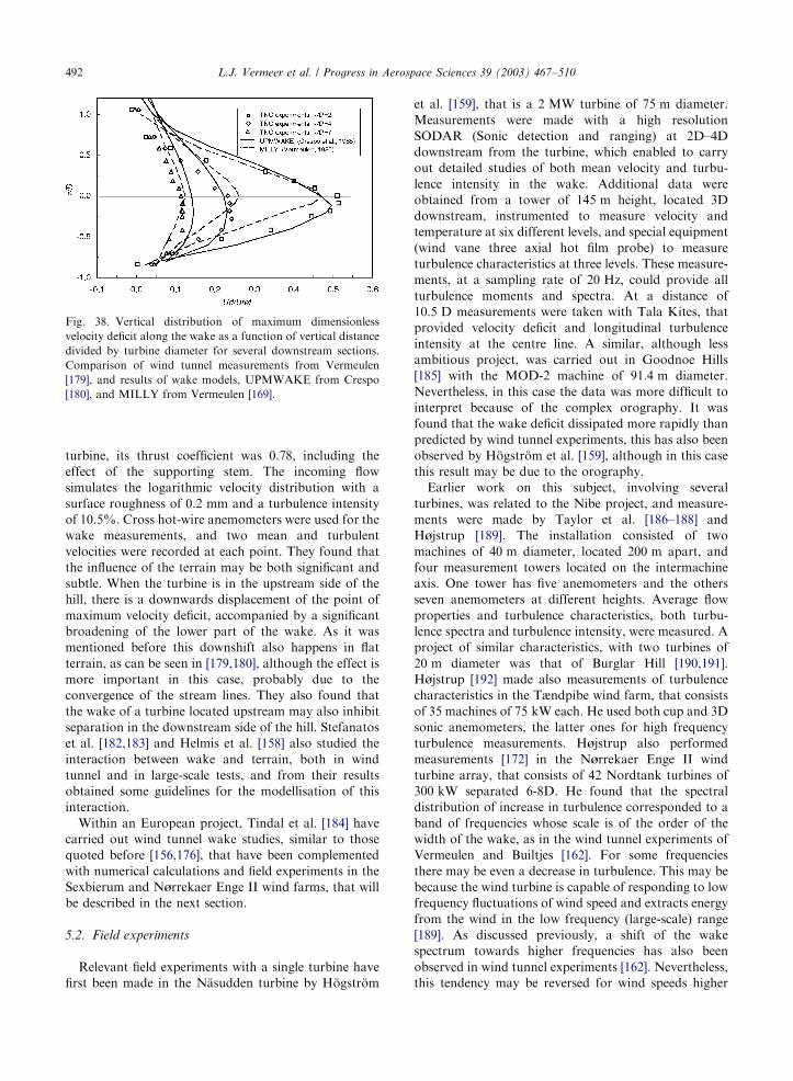
ARTICLE IN PRESS
Fig. 38. Vertical distribution of maximum dimensionless
velocity deficit along the wake as a function of vertical distance
divided by turbine diameter for several downstream sections.
Comparison of wind tunnel measurements from Vermeulen
[179], and results of wake models, UPMWAKE from Crespo
[180], and MILLY from Vermeulen [169].
L.J. Vermeer et al. / Progress in Aerospace Sciences 39 (2003) 467–510492
turbine, its thrust coefficient was 0.78, including the
effect of the supporting stem. The incoming flow
simulates the logarithmic velocity distribution with a
surface roughness of 0.2 mm and a turbulence intensity
of 10.5%. Cross hot-wire anemometers were used for the
wake measurements, and two mean and turbulent
velocities were recorded at each point. They found that
the influence of the terrain may be both significant and
subtle. When the turbine is in the upstream side of the
hill, there is a downwards displacement of the point of
maximum velocity deficit, accompanied by a significant
broadening of the lower part of the wake. As it was
mentioned before this downshift also happens in flat
terrain, as can be seen in [179,180], although the effect is
more important in this case, probably due to the
convergence of the stream lines. They also found that
the wake of a turbine located upstream may also inhibit
separation in the downstream side of the hill. Stefanatos
et al. [182,183] and Helmis et al. [158] also studied the
interaction between wake and terrain, both in wind
tunnel and in large-scale tests, and from their results
obtained some guidelines for the modellisation of this
interaction.
Within an European project, Tindal et al. [184] have
carried out wind tunnel wake studies, similar to those
quoted before [156,176], that have been complemented
with numerical calculations and field experiments in the
Sexbierum and N^rrekaer Enge II wind farms, that will
be described in the next section.
5.2. Field experiments
Relevant field experiments with a single turbine have
first been made in the N.asudden turbine by H .ogstr .om
et al. [159], that is a 2 MW turbine of 75 m diameter.
Measurements were made with a high resolution
SODAR (Sonic detection and ranging) at 2D–4D
downstream from the turbine, which enabled to carry
out detailed studies of both mean velocity and turbu-
lence intensity in the wake. Additional data were
obtained from a tower of 145 m height, located 3D
downstream, instrumented to measure velocity and
temperature at six different levels, and special equipment
(wind vane three axial hot film probe) to measure
turbulence characteristics at three levels. These measure-
ments, at a sampling rate of 20 Hz; could provide all
turbulence moments and spectra. At a distance of
10:5 D measurements were taken with Tala Kites, that
provided velocity deficit and longitudinal turbulence
intensity at the centre line. A similar, although less
ambitious project, was carried out in Goodnoe Hills
[185] with the MOD-2 machine of 91:4 m diameter.
Nevertheless, in this case the data was more difficult to
interpret because of the complex orography. It was
found that the wake deficit dissipated more rapidly than
predicted by wind tunnel experiments, this has also been
observed by H .ogstr .om et al. [159], although in this case
this result may be due to the orography.
Earlier work on this subject, involving several
turbines, was related to the Nibe project, and measure-
ments were made by Taylor et al. [186–188] and
H^jstrup [189]. The installation consisted of two
machines of 40 m diameter, located 200 m apart, and
four measurement towers located on the intermachine
axis. One tower has five anemometers and the others
seven anemometers at different heights. Average flow
properties and turbulence characteristics, both turbu-
lence spectra and turbulence intensity, were measured. A
project of similar characteristics, with two turbines of
20 m diameter was that of Burglar Hill [190,191].
H^jstrup [192] made also measurements of turbulence
characteristics in the Tændpibe wind farm, that consists
of 35 machines of 75 kW each. He used both cup and 3D
sonic anemometers, the latter ones for high frequency
turbulence measurements. H^jstrup also performed
measurements [172] in the N^rrekaer Enge II wind
turbine array, that consists of 42 Nordtank turbines of
300 kW separated 6-8D. He found that the spectral
distribution of increase in turbulence corresponded to a
band of frequencies whose scale is of the order of the
width of the wake, as in the wind tunnel experiments of
Vermeulen and Builtjes [162]. For some frequencies
there may be even a decrease in turbulence. This may be
because the wind turbine is capable of responding to low
frequency fluctuations of wind speed and extracts energy
from the wind in the low frequency (large-scale) range
[189]. As discussed previously, a shift of the wake
spectrum towards higher frequencies has also been
observed in wind tunnel experiments [162]. Nevertheless,
this tendency may be reversed for wind speeds higher

ARTICLE IN PRESSL.J. Vermeer et al. / Progress in Aerospace Sciences 39 (2003) 467–510 493
than that corresponding to the maximum power
coefficient, as measured by Papadopoulus et al. [193],
that made measurements in the wake of a single turbine
in the Samos Island wind farm. Velocity spectra were
also measured in the offshore Vindeby wind farm [194],
that consists of 11 machines of 450 kW which are
arranged in two rows, each machine and each row
separated by approximately 8D. Two instrumented
masts provide measurements of ambient and wake-flow
parameters. The geometry of the wind farm and the
instrumentation allowed for both single and multiple-
wake measurements. It was observed that there is a great
variation in the length scales of turbulence in the wake
region, probably because atmospheric stability, and in
particular the length scale in the wake is found to be
much smaller than in free flow. Tindal et al. [184] also
report, from wind tunnel experiments, that in the near
wake the turbulence length scale is reduced to a quarter
of the free stream value. H^jstrup and Courtney [195],
based on data from several wind farms, indicate that the
shear layers in the wake create turbulence at much
smaller length scales that those seen in free turbulence.
Probably what is observed is that the turbulence length
scale in the wake is related to the wake width, as
discussed previously in the wind tunnel experiments of
Vermeulen and Builtjes [162].
Kline [196] made measurements in a Howden wind
farm, in Altamont Pass in California, in a cluster of 75
turbines of 33m diameter. Emphasis was put in
estimating characteristics of gusts in wakes. Also, they
report measurements of horizontal shear at 2D (dia-
meters) and 6D downstream. Other measurements of
velocities and turbulence intensities were also made in
Altamont Pass in California [197,198] for clusters of
smaller wind turbines.
The Zeebrugge [199,200] wind farm became opera-
tional in 1987 and has 23 turbines of 22 m diameter.
Two fully equipped wind masts are installed so that
unperturbed wind conditions could be measured.
Recordings of 10 min data sets, including wind velocity
and direction, turbulence intensity, and power output
were obtained. The main purpose of the research was to
investigate power production and compare the measure-
ments with the results of different models. The effect of
other obstacles, such as LNG tanks in the harbour, had
to be included in the analysis.
In the Vindeby wind farm, within the ENDOW
(Efficient Development of Offshore Wind Farms)
project, measurements have been made using SODAR
instrumentation mounted on a boat [201]. This is an
interesting method to complement measurements in
wakes performed with fixed meteorological masts.
5.2.1. Fatigue and loads
The most important structural effect on a wind
turbine which is in the wake of a neighbouring machine
is fatigue, that is due to the combined effect of increased
turbulence, wind speed deficit and shear, and changes in
turbulence structure that cause dynamic loading, which
may excite the wind turbine structure. There is a need
for revision of the standards on wind turbine design and
safety, to adequately account for increased fatigue
loading in wind turbine clusters; this issue has been
addressed by Frandsen and Th^gersen [202]. Fatigue in
wind turbine clusters has already been reviewed in [203],
so that previous efforts will not be considered in much
detail. Earlier work on this subject was made in the Nibe
project [186,187] where special emphasis was put in
measuring the wake induced loads, because of its
implication in the fatigue life of the machine. Other
earlier measurements of loads were made by V^lund
[204] and Stiesdal [205], for machines that were 2 to 3D
apart. They found increases of the standard deviation of
the flapwise bending moment of the order of 100%
relative to the unobstructed case. Loads were largest
when the machine was exposed to half-wake conditions.
Stiesdal [205] introduced the concept of equivalent load,
that is the amplitude of a sinusoidal load with a fixed
frequency that would generate the same fatigue damage
as the actual (random) load; this concept provides a
more precise fatigue measurement than the standard
deviation. Measurements have been made on one wind
turbine in the experimental Alsvik wind farm in Sweden
[206], which has four machines sited so that the
instrumented unit is exposed to 5D, 7D or 9.5D single-
wake loads, depending on wind direction. The terrain is
smooth and the ambient turbulence low. The wind farm
layout is unique in offering many experimental possibi-
lities. It was found that under full-wake conditions the
equivalent load is increased by 10% at 9.5D and up to
45% at 5D. Their conclusion is that for low roughness
and low ambient turbulence sites, as occur in offshore
wind farms, the wake effects are very important for wind
turbine loads and fatigue. This is probably due to the
fact that under these conditions wakes are more
persistent, because diffusion due to ambient turbulence
is smaller in the sea. Similar results were reported by
Thomsen et al. [207] in the Kappel wind farm in
Denmark, that consists of 24 units of 400 kW; sited in a
row on a westerly shoreline, with 3.7D separations.
However, in a later paper Thomsen and S^rensen [208]
observe the same relative increase in fatigue loads for an
offshore wind farm and a land site wind farm. Frandsen
and Christensen [209] made measurements in the large
N^rrekaer Enge II wind turbine array in Denmark. Two
turbines in opposite corners of the wind farm were
instrumented to measure stresses in towers and blades.
There was a clear increase in the standard deviation of
the fluctuating load when the instrumented machine was
in the direct wake of a neighbouring machine, although
the integrated effect of wake and non-wake operation
was significantly smaller. Frandsen and Thomsen [210]
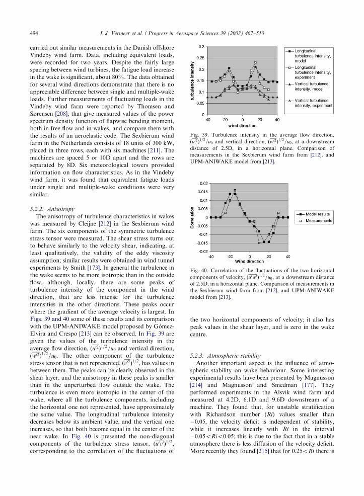
ARTICLE IN PRESS
Fig. 39. Turbulence intensity in the average flow direction,
ðu02Þ1=2=u0 and vertical direction, ðw02Þ1=2=u0; at a downstream
distance of 2.5D, in a horizontal plane. Comparison of
measurements in the Sexbierum wind farm from [212], and
UPM-ANIWAKE model from [213].
Fig. 40. Correlation of the fluctuations of the two horizontal
components of velocity, ðu0w0Þ1=2=u0; at a downstream distance
of 2.5D, in a horizontal plane. Comparison of measurements in
the Sexbierum wind farm from [212], and UPM-ANIWAKE
model from [213].
L.J. Vermeer et al. / Progress in Aerospace Sciences 39 (2003) 467–510494
carried out similar measurements in the Danish offshore
Vindeby wind farm. Data, including equivalent loads,
were recorded for two years. Despite the fairly large
spacing between wind turbines, the fatigue load increase
in the wake is significant, about 80%. The data obtained
for several wind directions demonstrate that there is no
appreciable difference between single and multiple-wake
loads. Further measurements of fluctuating loads in the
Vindeby wind farm were reported by Thomsen and
S^rensen [208], that give measured values of the power
spectrum density function of flapwise bending moment,
both in free flow and in wakes, and compare them with
the results of an aeroelastic code. The Sexbierum wind
farm in the Netherlands consists of 18 units of 300 kW;placed in three rows, each with six machines [211]. The
machines are spaced 5 or 10D apart and the rows are
separated by 8D. Six meteorological towers provided
information on flow characteristics. As in the Vindeby
wind farm, it was found that equivalent fatigue loads
under single and multiple-wake conditions were very
similar.
5.2.2. Anisotropy
The anisotropy of turbulence characteristics in wakes
was measured by Cleijne [212] in the Sexbierum wind
farm. The six components of the symmetric turbulence
stress tensor were measured. The shear stress turns out
to behave similarly to the velocity shear, indicating, at
least qualitatively, the validity of the eddy viscosity
assumption; similar results were obtained in wind tunnel
experiments by Smith [173]. In general the turbulence in
the wake seems to be more isotropic than in the outside
flow, although, locally, there are some peaks of
turbulence intensity of the component in the wind
direction, that are less intense for the turbulence
intensities in the other directions. These peaks occur
where the gradient of the average velocity is largest. In
Figs. 39 and 40 some of these results and its comparison
with the UPM-ANIWAKE model proposed by G !omez-
Elvira and Crespo [213] can be observed. In Fig. 39 are
given the values of the turbulence intensity in the
average flow direction, ðu02Þ1=2=u0 and vertical direction,
ðw02Þ1=2=u0: The other component of the turbulence
stress tensor that is not represented, ðv02Þ1=2; has values inbetween them. The peaks can be clearly observed in the
shear layer, and the anisotropy in these peaks is smaller
than in the unperturbed flow outside the wake. The
turbulence is even more isotropic in the center of the
wake, where all the turbulence components, including
the horizontal one not represented, have approximately
the same value. The longitudinal turbulence intensity
decreases below its ambient value, and the vertical one
increases, so that both become equal in the center of the
near wake. In Fig. 40 is presented the non-diagonal
components of the turbulence stress tensor, ðu0v0Þ1=2;corresponding to the correlation of the fluctuations of
the two horizontal components of velocity; it also has
peak values in the shear layer, and is zero in the wake
centre.
5.2.3. Atmospheric stability
Another important aspect is the influence of atmo-
spheric stability on wake behaviour. Some interesting
experimental results have been presented by Magnusson
[214] and Magnusson and Smedman [177]. They
performed experiments in the Alsvik wind farm and
measured at 4.2D, 6.1D and 9.6D downstream of a
machine. They found that, for unstable stratification
with Richardson number ðRiÞ values smaller than
0:05; the velocity deficit is independent of stability,
while it increases linearly with Ri in the interval
0:05oRio0:05; this is due to the fact that in a stable
atmosphere there is less diffusion of the velocity deficit.
More recently they found [215] that for 0:25oRi there is

ARTICLE IN PRESSL.J. Vermeer et al. / Progress in Aerospace Sciences 39 (2003) 467–510 495
a tendency for the deficit to decrease, which would
indicate more effective mixing.
5.2.4. Coherence
Coherence is another magnitude of interest, and is
defined as the absolute value of the normalized two-
point spectrum. It represents the degree to which two
wind speeds at points separated in space are alike in
their time histories. It could be useful to estimate the
duration of a gust whose size should be large enough to
engulf a rotor, and also to translate the spectra from an
Eulerian frame to a rotating frame as seen by the turbine
blades. H^jstrup [172] has made measurements in the
N^rrekaer Enge II wind farm, of the spectral coherence,
both vertical and lateral, in wakes of wind turbines. He
found that there is a small influence of the wake on
vertical coherence, and that the lateral coherence was
only modified in the near wake. Nevertheless, this result
may be influenced by the fact that in these experiments
the distances between the two points were small
compared to the size of the wake.
6. Far wake modelling
In this section the numerical research on the far wake
will be presented. Much of it has already been reviewed
by Crespo et al. [203], so that previous contributions in
this field will not be examined in much detail. The first
subsection will be dedicated to individual wakes in flat
terrain, that are easy to characterize with few para-
meters, and provide information of basic interest that
can be easily arranged. However, the usual situation of
practical interest, that will be discussed next, is that
many wind turbines are located in a wind farm with
irregular terrain, where the different wakes interact.
6.1. Individual wakes
6.1.1. Kinematic models
The first approach to study wind–turbine wakes was
introduced in a seminal paper by Lissaman [216] with a
so-called kinematic model. Kinematic models are based
on self-similar velocity deficit profiles obtained from
experimental and theoretical work on co-flowing jets.
The wake description starts after the wake has
expanded; and are assigned different types of transverse
velocity profiles for the near, transition and far wake
regions. Lissaman [216] and Voutsinas et al. [217] used
velocity profiles obtained from models on co-flowing jets
by Abramovich [218]. Vermeulen [169] used a Gaussian
type of profile quite similar to that of Abramovich [218],
and Katic et al. [219] simplified the problem further and
assumed a top-hat profile everywhere. The reference
value of the velocity deficit is usually obtained from
global momentum conservation, using as input the
thrust coefficient of the machine. The wake growth is
due to the added effects of the ambient turbulence and
the turbulence created by the shear in the wake.
Vermeulen [169] added another term: the turbulence
created by the turbine itself. Katic et al. [219] simply
assumed that the wake radius increases linearly with
downstream distance; the proportionality constant must
be adjusted by comparison with experiments. The
ground effect is simulated by imaging techniques.
Lissaman [216] included a symmetrical turbine and
added the velocity deficits of both the real and image
turbine, so that drag conservation is satisfied. Crespo
et al. [220] use an antisymmetric wake so that velocity
deficits are subtracted and give zero perturbation at the
ground. The differences in the results are not important,
and it is not clear which procedure is more appropriate.
6.1.2. Field models
The field models follow a different approach and
calculate the flow magnitudes at every point of the flow
field. The earlier models assumed axial symmetry, such
as the simple model proposed by Sforza et al. [221], that
used the linearized momentum equation in the main flow
direction, with constant advective velocity and a
constant eddy diffusivity. They made small-scale experi-
ments, and the agreement was reasonable, considering
the simplicity of the model. A more complete parabolic
model, EVMOD, was developed by Ainslie [222,223]
assuming an eddy viscosity method for turbulence
closure. The eddy viscosity is represented by a simple
analytical form based on Prandtl’s free shear layer
model, but which also includes a contribution from
ambient turbulence. This eddy viscosity is an average
value over a cross-section. At small downstream
distances, the eddy viscosity is modified by an empirical
filter function to account for the lack of equilibrium
between the mean velocity field and the developing
turbulence field. Several constants appear in the
problem, that are adjusted by comparison with parti-
cular experiments. The model is fairly simple and gives
reasonable results when compared with wind tunnel
experiments [179,224]. For large-scale experiments, the
results are corrected by taking into account meandering
effects. Nevertheless, some aspects such as the downshift
of the wake centreline, or the upward displacement of
the maximum turbulence intensity, can never be well
predicted by models with axial symmetry. To reproduce
such effects, models which retain three-dimensional
effects are needed.
6.1.3. Boundary layer wake models
Crespo et al. [220,225] developed the UPMWAKE
model in which the wind turbine is supposed to be
immersed in a nonuniform basic flow corresponding to
the surface layer of the atmospheric boundary layer. The
properties of the nonuniform incident flow over the

ARTICLE IN PRESSL.J. Vermeer et al. / Progress in Aerospace Sciences 39 (2003) 467–510496
wind turbine are modelled by taking into account
atmospheric stability, given by the Monin–Obukhov
length, and the surface roughness. The modelling of the
turbulent transport terms is based on the k–e method forthe closure of the turbulent flow equations, previously
presented. Finite-difference methods were used in the
discretization of the equations. A parabolic approxima-
tion was made and the equations were solved numeri-
cally by using an alternate-direction implicit (ADI)
method. The developed wake model is three-dimen-
sional and pressure variations in the cross-section have
to be retained in order to calculate transverse velocities.
Crespo and Hern!andez [226,225] and Crespo et al.
[180,227] compared UPMWAKE results with the results
of wind-tunnel experiments obtained by Luken et al.
[224] and those of field experiments using full-scale
machines [186]. The code can predict effects such as the
downward tilt of the wake centreline, as shown in
Fig. 38, the upward displacement of the point of
maximum added turbulence kinetic energy, as shown
in Fig. 35, or the different vertical and horizontal
growths of the wake width.
Another approach was followed by Taylor [228] and
Liu et al. [229], that retained Coriolis forces and
assumed that the pressure gradients were given by the
geostrophic wind. However, this assumption cannot be
justified because the length scale of the wake is not
sufficiently large for the Coriolis forces to play a
dominant role; indeed, they can be neglected, and the
pressure field will be that resulting from the momentum
conservation in the wake. If a parabolic approximation
is made, pressure variations across the wake can be
neglected in the momentum equation for the main flow
direction, but not for the momentum components in the
transverse direction, particularly when there is neither
axial nor two-dimensional symmetry. Taylor’s model
[228] was two-dimensional, and the equations were
linearized around a basic flow. Liu et al.’s model
[229] was three-dimensional, and included atmospheric
stability effects.
Smith and Taylor [156] and, in more detail, Taylor
[230] presented a non-symmetric two-equation
model that is in many ways similar to the three-equation
model of Crespo et al. [220]. They neglected transverse
velocities and just solve the momentum equation in
the axial direction. To model the turbulent viscosity
they use a k–L method, where the turbulent length
scale, L; is related to the width of the wake. The
comparison with their wind-tunnel experimental
results is very good, as can be seen in Fig. 35, although
a comparison with full-scale Nibe measurements
showed that the model overestimates the values of the
velocity deficit. They attributed this discrepancy to
meandering and obtained better agreement when they
corrected for this effect using the method proposed by
Ainslie [223].
Based on the model developed by Ainslie [223], the
company Garrad and Hassan has developed the code
EVFARM, described by Adams and Quarton [231]. The
code incorporates two alternative semi-empirical models
to calculate wake turbulence. Adams and Quarton [231]
use both EVFARM and UPMWAKE codes in combi-
nation with machine load predictive tools to provide a
method for fatigue load prediction. As part of this study,
a comprehensive validation of both codes is made using
the wind tunnel measurements of Hassan [232]. A better
agreement with experiments is found if a downstream
displacement of the origin is considered. In the initial
region of the wake some important discrepancies were
also observed between the results of UPMWAKE and
the Nibe measurements published by Taylor et al. [186].
On the other hand, by eliminating the boundary layer
approximation used in UPMWAKE, Crespo et al. [227]
proposed an elliptic model to deal simultaneously with
the axial pressure gradients and diffusion effects by
retaining both the axial and transverse diffusion terms.
Their model therefore describes both the evolution of
the expansion region and the diffusion processes in the
near wake. No fundamental differences between the
results of the elliptic and parabolic models were found,
and displacement of the origin was apparently not
necessary. Another reason for the discrepancies ob-
served between models and experiments in the near wake
may be the uncertainty involved in the radial distribu-
tion of the initial velocity deficit, that has been studied
by several authors, [230,233–235] and is discussed in
more detail in the first part of this review. Schepers [236]
found that, by using a Gaussian profile for the initial
velocity deficit, a significative improvement of the
agreement with experimental results is obtained.
6.1.4. Hybrid models
An alternative approach that requires less computing
capacity is the multi-parametric wake model of Voutsi-
nas et al. [237,238], which was further developed by
Cleijne et al. [235]. This model divides the wake into the
rotor region, the near wake region and the far wake
region, and applies a vortex particle method in the rotor
region, a field model in the near wake region, and, in the
far wake region, explicit self-similar expressions similar
to those used in the kinematic models. Different
assumptions are made to match the different regions.
The method was partially successful in simulating the
experimental results of the Nibe turbines given in Taylor
[188]. Later, Magnusson et al. [239] applied the model to
reproduce the experimental results of the Alsvik wind
farm. Explicit expressions for wake characteristics
obtained from this work were later applied to study
the noise emissions from wind farms [240].
All these models use a closure scheme, based on zero,
one or two equation models, to calculate the turbulence
transport terms, and assume an isotropic turbulence

ARTICLE IN PRESSL.J. Vermeer et al. / Progress in Aerospace Sciences 39 (2003) 467–510 497
field. Transport equations for the Reynolds stresses have
only been used occasionally. Ansorge et al. [241] used a
Reynolds-stress turbulence model based on the com-
mercial code PHOENICS and obtained reasonable
results. More recently G !omez-Elvira and Crespo [213]
have extended UPMWAKE by using an explicit
falgebraic model for the components of the turbulent
stress tensor. The constants of the new model, UPM-
ANIWAKE, have been adjusted, so that it will
reproduce the logarithmic layer of the basic flow and
the corresponding stress tensor. The new model has a
low computational cost, and its results are compared to
experimental data from the Sexbierum wind farm [212],
as can be seen in Figs. 39 and 40, previously commented,
and a reasonable agreement is obtained.
6.2. Wind farm wake models
6.2.1. Single wake superposition
A wind farm consists of many wind turbines whose
wakes can interact, and whose turbines may be affected
by the wakes of several machines located upstream.
Wind farm codes usually rely on the results of single
wake calculations, and make superposition assumptions
to take into account the combined effect of different
wakes. The linear superposition of the perturbations
created by wakes of different machines in a wind farm
model was first used by Lissaman [216] in a classical
paper, although this assumption fails for large perturba-
tions as it overestimates velocity deficits and could lead
to the absurd result of negative velocities when many
wakes superimpose. Instead, Katic et al. [219] assumed
linear superposition of the squares of the velocity
deficits. In this case, the cumulative effect, when there
are many wakes, will be smaller than that calculated for
linear superposition, and, in general, this assumption
provides better agreement with experimental results than
the linear superposition, although, apparently, there is
no physical reason for it. The corresponding code,
named PARK, was applied by Beyer et al. [242] for the
optimization of wind farm configurations using genetic
algorithms. As already mentioned, Smith and Taylor
[156] found, for a particular experimental configuration
of two machines in a row, that the wake velocity of the
downstream machine recovers more rapidly than the one
upstream. By making a number of crude assumptions
concerning the momentum transfer within the down-
stream wake that is imbedded in the upstream wake,
Smith and Taylor [156] were able to formulate a semi-
empirical superposition law that works quite well.
However, it is cumbersome and can only be applied
for the interaction of the wakes of two turbines in a row.
When there are many turbines in a line it has been
observed experimentally [200] that while the first turbine
produces full power, there is a significant decrease of
power in the second turbine, with practically no further
loss in successive machines. Based on these observations,
and on the results of the calculations of Crespo et al.
[227], Van Leuven [200] assumed in his farm model
(WINDPARK) that a given turbine is only affected by
the wake of the closest upstream turbine, obtaining good
agreement in comparison with measurements made at
the Zeebrugge wind farm.
6.2.2. Elliptic wake models
Crespo et al. [227] applied an elliptic model for
studying the interaction of the wakes from two turbines
in two configurations: abreast and in a line. There was
good agreement with experimental results, and, when
other superposition assumptions were compared, it was
found that the linear superposition worked well for the
two machines abreast, in which velocity deficits in the
interference region are small. However, for the two
turbines placed in a row the linear superposition
overestimated the velocity deficit, as was to be expected.
Recently, this model has been improved by Sotiropoulos
et al. [243] by a more detailed analysis of the rotor and
inclusion of terrain effects; the results are in fair
agreement with measurements in the Alsvik wind farm
[239] and in wind tunnel. When the results of the elliptic
model [227] are considered, it can be observed that the
truly elliptic effects, such as axial pressure variations,
only occur very close to the turbine, so that the
parabolic approximation may be a suitable approach
for studying wake interactions over most of the region
where this interaction occurs. Moreover, to extend the
fully elliptic code to a wind farm consisting of many
machines, besides consuming a lot of calculation time,
would require very powerful computers and would
therefore be of little practical interest for modelling
wind farms.
6.2.3. Parabolic wake models
Because of the above, Crespo et al. [244] have
developed a code, UPMPARK, extending the parabolic
UPMWAKE code for a single wake to the case of a park
with many machines. No assumptions are required
regarding the type of superposition or the type of wake
to be used, as all the wakes and their interactions are
effectively calculated by the code. In UPMPARK, the
conservation equations solved are the same as those for
the single wake code, UPMWAKE, as specified in
Crespo and Hern!andez [225], and turbulence is closed
using a k–e model. Adams and Quarton [231] extended
the UPMWAKE model to wind farms using a procedure
quite similar to that of UPMPARK; this extended code
has been incorporated in a wind farm design support
tool, named FYNDFARM (Fatigue Yield Noise Design
Farm) [245].
Usually wind farm models make the assumption that
the terrain is flat and that the unperturbed wind velocity
is uniform, an assumption which is not reasonable in

ARTICLE IN PRESS
Fig. 41. Example results from the ENDOW project: cross wind
profiles in vertical direction (from [256]).
Fig. 42. Example results form the ENDOW project: turbulence
in the wake (from [256]).
L.J. Vermeer et al. / Progress in Aerospace Sciences 39 (2003) 467–510498
many cases of interest since, as is well known, terrain
irregularities can be used to enhance or concentrate wind
power. For terrains that are moderately complex, the
simple procedure of adding the velocity perturbations of
the wake and terrain should give an approximate flow
field; this or equivalent procedures were applied in
[226,231,200]. In the Monteahumada wind farm the
velocity irregularities of the terrain and the velocity
deficit created by a single wake are both of a similar
order of magnitude; from its analysis it is shown, [246],
that, for a moderately irregular terrain, the linear
superposition of wake and terrain effects gives reason-
able results. More elaborated models to take into
account terrain effect on wakes are proposed by
Voutsinas et al. [247], Stefanatos et al. [182], Hemon
et al. [248], and Migoya et al. [249].
6.2.4. CFD code calculations
Numerical calculations using commercial CFD codes
were made by several authors, [241,250] to study wake
and terrain interaction for simple configurations, but
their extension to wind farms of typical size will be
computationally expensive. More recently, Chaviaro-
poulos and Douvikas, [251], and Ivanova and Nadyoz-
hina, [252], have developed their own in-house CFD
methods that deal simultaneously with terrain and wake
effects. In [252] the turbines are considered as distributed
roughness elements; this approach will be discussed
later. In [251] a k–o model for closure was used, the
numerical results were compared with experimental
measurements, and the accuracy of the simulation is
fair. The method was applied to sets of one and two
turbines and also seems to be computationally expensive
for conventional wind farms.
As mentioned previously Taylor and Smith [181],
Stefanatos et al. [182,183], and Helmis et al. [158] gave
some guidelines for the modellisation of the terrain–
wake interaction.
6.2.5. Offshore wind farm wakes
A related problem arises in offshore wind farms
where, when the wind blows from land to sea, there is an
internal boundary layer, whose development is super-
posed on that of the wakes, as mentioned by Crespo and
G !omez [253]. As the surface roughness of the sea is
usually much smaller than the corresponding roughness
on land, it is to be expected that wind velocity will be
greater and turbulence intensities lower than for
equivalent inland stations. Consequently, turbulent
diffusion of the wake will also be lower and wake
effects will probably be more persistent downstream.
Wake effects in offshore wind farms obtained from both
experiments and numerical models are reported by
Frandsen et al. [194], Crespo et al. [254,243] and their
effect on fatigue loading by Frandsen [255]. Recently,
within the ENDOW project, the performance of several
wake models in offshore wind farms has been evaluated
[256]. A total of seven models have been proposed
within the ENDOW project: an axisymmetric semi-
analytical engineering model (Ris^), an advanced code
based on computational fluid dynamics, that is coupled
to an aeroelastic model (Ris^), an analytical model
based on Taylor’s hypothesis for closure (Upsala
University), two axisymmetric models based on eddy-
viscosity assumption for turbulence closure (Garrad
Hassan, and Oldenburg University), a fully elliptic 3D
turbulent Navier–Stokes model with k–e assumption for
closure (Robert Gordon University, RGU), and a
modification of UPMWAKE made by ECN (Nether-
lands Energy Research Foundation) [236]. Comparisons
were made of the results of the different models and with
experimental results in Vindeby and Bockstigen wind
farms. In all cases large discrepancies appear in the near
wake region, see Figs. 41 and 42.
Compared to the Vindeby experimental results, all the
models overestimate the wake effects in the case of low
ambient turbulence (6%), and give acceptable results in
the case of higher ambient turbulence (8%). The 3D
models, ECN and RGU, predict downward shift of the
maximum velocity deficit, that is also confirmed by
experimental results, as previously mentioned, see
Fig. 38. The superposition of several wakes in double
and quintuple wake cases is being also examined within
the ENDOW project [257], and preliminary results point
out the importance of including correct values of the
ambient turbulence intensity. Another issue addressed
by ENDOW, is how to link wake models with atmo-
spheric boundary layer models; this is also in its

ARTICLE IN PRESS
Fig. 43. Local turbulence intensity at hub height, as function of
the distance from the leading edge of the wind farm, from [262].
Comparison with an analytical prediction for equilibrium
conditions in an infinitely large wind farm, from [202], see
Eq. (30).
L.J. Vermeer et al. / Progress in Aerospace Sciences 39 (2003) 467–510 499
preliminary stages, and it does not seem to contemplate
the superposition of wake and local terrain effects yet
[258]. This linking provides the input needed for the
wake models, assuming that the calculated atmospheric
conditions are uniform along the wind farm.
6.2.6. Generic wind farm wake models
Another approach to model wind farms is to
consider that the turbines behave as distributed rough-
ness elements. Several models were proposed by
Newman [259] and Bossanyi [260]. They assumed a
logarithmic wind profile for the unperturbed wind,
which includes ground roughness as a parameter. The
presence of the turbines increases the value of the
roughness. Frandsen [261] gave an explicit expression
relating the artificial surface roughness to the wind
turbine characteristics and its spacing within the
wind farm.
Recently, the distributed roughness model has been
used by Crespo el al. [262] to estimate how the large
offshore wind farms may change the local wind
climate, and how in turn this change of the climate
will affect the local behaviour of the wind farm. In
a first approach, the large wind farm is simulated
by an artificial roughness as proposed in [261]. An
internal boundary layer is considered that starts
developing at the leading edge of the farm until it
reaches, sufficiently far downstream (if the wind
farm is large enough), the top of the planetary
boundary layer, after that a new equilibrium region is
reached. This will occur in a large distance, so that
presumably, most of the wind farm will be immersed in
the developing internal boundary layer. From the
calculation of the internal boundary layer, the flow
conditions are obtained at a certain reference height,
these are then used as boundary conditions for
UPMPARK. In [262] a large wind farm has been
considered, that has 384 turbines of 1:5 MW rated
power each; the evolution of the local turbulence
intensity at hub height, as the distance from the leading
edge increases, is calculated, and is presented in Fig. 43.
A comparison is made with an equilibrium value
predicted by Frandsen and Thogersen [202], that will
be presented later in Eq. (30).
A different approach was used by Hegberg [263] that
analysed the equilibrium region by establishing a global
balance of Coriolis, pressure and drag forces.
Recent work on local wind climate, within and
downwind of large offshore wind turbine clusters, was
presented in a meeting for experts at the Ris^
Laboratory, that is reviewed by Frandsen and Barthel-
mie [264]. In this meeting, it was pointed out that the
new understanding of resistive flows can be obtained
from other areas of fluid dynamics, such as flow behind
buildings and in forest canopies [265].
7. Far wake: engineering expressions
7.1. Velocity deficit
In many cases it is of interest for the designer to have,
as an alternative to numerical models, analytical
expressions which can estimate the order of magnitude
and the tendencies of the most important parameters
characterising wake evolution. Regressions or correla-
tions of this type were obtained by different authors to
describe single wake behaviour, [226,224,159,266,215],
for the velocity deficit and the width of the wake. For
the velocity deficit in the far wake, these correlations are
usually of the type:
DV
Vhub¼ A
D
x
n
; ð23Þ
where Vhub is the incident wind velocity at hub height, x
is the downstream distance, D the wind–turbine radius,
and A and n are constants. In some cases, to extend the
range of validity of this equation to smaller values of x;its origin is displaced. The constant A will depend on
turbine characteristics, fundamentally on the thrust
coefficient, CT or the induced velocity factor, a; andwill increase with either of them. These constants are in
the range 1oAo3; and 0:75ono1:25; respectively. Ifwe consider an axisymmetric wake we can apply classical
results, see for example the book of Schlichting [267].
For the case of a turbulent wake that is diffusing
with zero ambient turbulence, n ¼ 2=3; [268], and
for a laminar wake, or equivalently when diffusion is
controlled by a constant ambient turbulent diffusivity,
n ¼ 1:Instead of using the non-dimensional distance, x=D;
Magnusson and Smedman, [266,215], expressed wake
diffusion as a function of the transport time t ¼ x=Vhub

ARTICLE IN PRESS
Fig. 44. Maximum, added hub height wake turbulence
measured in four different cases, compared with the three
correlations: (26), (28), and (29), with adjusted coefficients.
Wind velocities in the range 9 m=soUo11 m=s: The experi-
mental data were compiled by Ghaie (Personal communication
to Frandsen, 1997). Figure taken from [269].
L.J. Vermeer et al. / Progress in Aerospace Sciences 39 (2003) 467–510500
made dimensionless with t0; the transport time where thenear wake ends. Their correlation takes the form
DV
Vhub¼ C2 ln
t0
t
� �þ CT; ð24Þ
valid for t > t0; and for t0 in neutral atmosphere they
give
t0 ¼ C11
fln
H
z0
D
2H; ð25Þ
where H is the turbine height, z0 is the surface roughness
of the ground, f is the rotational frequency of the
turbine, and C1 and C2 are constants, taken respectively
equal to 1 and 0; 4; in [215].
7.2. Turbulence intensity
Correlations for turbulence intensity in the far wake
have been given in [224,162,159,161,171,157,266,268].
Crespo and Hern!andez [157,171], give the following
expression for the added turbulence intensity, created by
the turbine:
DI ¼ 0:73a0:83I0:0325N
D
x
0:32
: ð26Þ
The turbulence intensity, I ; is defined as the ratio of
the standard deviation of the wind velocity in the
average wind direction, divided by the average wind
velocity. It is assumed that the wind turbine creates an
additional turbulent kinetic energy that should be added
to the ambient one, consequently, DI will be,
DI ¼ffiffiffiffiffiffiffiffiffiffiffiffiffiffiffiffiffiI2 I2
N
q; ð27Þ
where IN; is the ambient turbulence intensity. This
expression was obtained by fitting with the numerical
results of UPMWAKE, and was validated by compar-
ison with experimental results, both of wind tunnel and
field experiments (many of them compiled by Quarton
[161]). A similar expression was proposed in [161],
obtained by fitting with experimental results:
DI ¼ 4:8C0:7T I0:68
N
xN
x
� �0:57ð28Þ
where the drag coefficient, CT; has been used instead of
the induced velocity factor a; and the diameter has been
substituted by the near wake length, xN ; that is of theorder of 1D–3D. Frandsen and Thogersen [202]
proposed the following correlation based on measure-
ments:
DI ¼1
1:5þ 0:3ðx=DÞffiffiffiffiffiffiffiffiffiffiVhub
p ; ð29Þ
where Vhub is related to CT: The decay with downstreamdistance is smaller in Eq. (26), x0:32; than in Eq. (28),
x0:57 and in Eq. (29), that for large values of x; will belike x1: In [159] a decay like x0:5 is obtained. In [268] it
is observed that the behaviour should be like x1=3; thiscorresponds to the classical situation of a wake
developing in an ambient with no turbulence [267]. If
only field experiments are used, in Eq. (28) the exponent
will be 0.37, whereas, from wind tunnel experiments
made at TNO [160], the behaviour is estimated to be like
x0:7: In any case it should be noticed that the decay of
turbulence intensity, DI ; is slower than the decay of the
velocity deficit, DV : Frandsen [269] has plotted the threecorrelations: (26), (28), and (29), with different coeffi-
cients, in order to fit to some experimental results. These
are shown in Fig. 44. It can be seen that the agreement
of the correlation of Crespo and Hern!andez [157],
Eq. (26), is appropriate for large distances, whereas that
of Quarton [161]), Eq. (28), gives a better fitting for
smaller distances.
7.3. Wind farm wake expressions
For wind turbine clusters Luken [160] proposed a
correlation for the equilibrium value of the turbulence
intensity reached in a row of turbines, using the
experimental results of Builtjes and Vermeulen [162],
in which the turbulence decayed like x1:64; x being the
distance between machines. Frandsen et al. [194]
presented correlations giving values of the average
velocity, turbulence intensity, turbulence scale and width
of the wake at different positions of each machine in a
row as functions of their operating characteristics. These
correlations are obtained by making the best fit with
numerical results from UPMPARK, and are validated
by comparison with measurements made in Vindeby
wind farm. Frandsen and Thogersen [202], based on the
distributed roughness model of Frandsen [261], con-
sidered the case of an infinitely large wind farm that
perturbs the whole boundary layer, and estimated the
value of the added turbulence intensity deep inside the

ARTICLE IN PRESSL.J. Vermeer et al. / Progress in Aerospace Sciences 39 (2003) 467–510 501
farm to be
DI ¼0; 36
1þ 0:2ffiffiffiffiffiffiffiffiffixrxf
p=D=
ffiffiffiffiffiffiCT
p ð30Þ
where xr is the separation of rows, and xf the separation
of files. This equation gives a maximum value of DI ¼0:36 that is equal to the one obtained by Crespo and
Hern!andez [157], for the annular peak of turbulence
intensity in the cylindrical shear layer formed in the near
wake. This correlation agrees well with the predictions
made in [262], as can be seen in Fig. 43.
The effect of atmospheric stability (expressed in terms
of the Richardson number) on velocity deficit decay was
taken into account in the correlation given by Magnus-
son and Smedman [177].
All these correlations have been compared with some
experimental results and show at least an acceptable
degree of agreement, although more work is needed to
carry out a full comparison both among these correla-
tions and with experimental results.
8. Concluding remarks
At a time when it is realised that the matter of interest
is really complicated, it is worthwhile to review the work
that has been done. Hopefully, this overview will
provide a point of departure for ‘plunging’ into the
subject.
8.1. Near wake
With regards to the near wake experiments, it can be
concluded that the wealth of experimental data for
helicopters is regrettably not present for wind turbines.
In this respect, it is not the quantity that matters,
because even when restricting to the uniform, static,
non-yawed case, there is a lot of experimental work done
on wind turbine near wakes. However, most of these
experiments tend to be fragmentarily carried out,
meaning they deal only with a limited set of rotor
properties. The experiments themselves certainly achieve
their own described goal. But most of them seem to be
individual and limited efforts. In a larger perspective, by
the great diversity in rotor models and wind tunnels, it is
extremely difficult to make a comparison between the
different experiments and trying to combine them to
gain an added value appears to be unfeasible.
The lack of an extensive data set with such basic
aerodynamic rotor properties is often felt as a large
deficiency, in both the scientific and the engineering
environment, for comparison with calculational codes.
So, initiatives like the measurement campaign by NREL
in the NASA-Ames wind tunnel and the EU-funded
‘‘MEXICO’’ project (with forthcoming measurements in
the DNW wind tunnel) are highly appreciated, but
definitely need to have a continuous follow-up.
Near wake computations can be carried out by
various numerical techniques, ranging from inviscid
lifting line/surface methods to viscous Navier–Stokes
based methodologies. Each method has its own advan-
tages and limitations. While e.g. prescribed vortex wake
methods are fast to run on a computer but leaves much
of the physics to a priori given assumptions, Navier–
Stokes based methods offer very detailed insight in the
flow behaviour but are very computing costly. There is
no doubt, however, that full-blown Navier–Stokes
simulations now are reaching a level where they
convincingly have matured to become the most im-
portant predictive tool for predicting and understanding
aerodynamics of modern wind turbines.
8.2. Far wake
With regards to far wake analysis, wind turbine wakes
have been extensively studied both experimentally and
analytically. Nevertheless, their knowledge is far from
being satisfactory. Many of the numerical models
proposed show an acceptable degree of agreement with
the experiments with which they are compared. How-
ever, the assumptions and coefficients that are chosen
are such that the agreement with some particular
experiments may be good, although the overall validity
has not been checked in more general situations. There
is a clear need for serious and conscious checks against
independent data, as it is made in the project ENDOW,
[256,257]. The models which depend on the least
simplifying assumptions are better suited in dealing with
different configurations and in reproducing wake devel-
opment in more detail. Some aspects of individual wake
modelling, such as near wake representation, influence
of atmospheric stability, appropriate turbulence model-
ling, or convergence problems, are still issues of active
research. Some of these aspects are more relevant to the
offshore wind farms, many of which are expected to be
installed in future. While greater emphasis used to be
directed to the estimation of velocity deficits and farm
efficiency in terms of energy production, research is
nowadays more oriented to other issues, such as
estimating magnitudes related to the structural and
fatigue behaviour, or fluctuations in the electrical energy
produced by machines affected by upstream wakes. For
this, it is necessary to know the turbulence character-
istics of the flow (turbulence intensity, correlations and
spectrum), and wind shear data. An issue of some
importance, and in which some progress has been made,
is the non-isotropic nature of the turbulence of ambient
atmospheric flow, in contrast to the more isotropic
turbulence in the wakes. One of the most important
difficulties that has not been treated satisfactorily is the
choice of appropriate input parameters to define

ARTICLE IN PRESSL.J. Vermeer et al. / Progress in Aerospace Sciences 39 (2003) 467–510502
ambient unperturbed flow, particularly in complicated
terrains. Usually, a comparison with wind tunnel
experiments is reasonably straightforward, but when
field experiments are used for comparison there are
many difficulties and effects like meandering, that have
not yet been satisfactorily modelled. The results
obtained from experimental and modelling studies for
terrains of varying roughness and the appearance of
internal boundary layers, such as those observed in large
wind farms located near the coast or offshore, should be
incorporated into the description of ambient flow. The
problem is that it is difficult to envisage general
solutions, and we will always be solving particular
problems that, at most, could only point to general
tendencies.
Acknowledgements
Thanks to everyone who has contributed to this
article: Gijs van Kuik for writing the introduction on
wind energy and proof-reading, Gerard van Bussel for
proof-reading and ‘‘restructuring advice’’, and Gustave
Corten for his help with the stall-flag pictures.
References
[1] Lanchester FW. A contribution to the theory of propul-
sion and the screw propeller. Trans Inst Naval Archi.
1915;57:98.
[2] Glauert H. Aerodynamic theory, vol. 4. Berlin, Germany:
Julius Springer: 1935. p. 169–360 (Chapter Division L).
[3] van Kuik G. 25 years of wind turbine technology
development. In: Watson R, editor. European Wind
Energy Conference 1997, IWEA, Slane, Ireland, 1997.
p. 21–4.
[4] Thor S-E, Weis-Taylor P. Long-term research and
development needs for wind energy for the time frame
2000–2020. Wind Energy 2002;5(1):73–5.
[5] Snel H. Review of the present status of rotor aero-
dynamics. Wind Energy 1998;1(S1):46–69.
[6] Leishman JG. Challenges in modelling the unsteady
aerodynamics of wind turbines. Wind Energy 2002;5
(2–3):85–132.
[7] Schepers JG, et al., Final report of IEA Annex XVIII:
enhanced field rotor aerodynamic database. Technical
report ECN-C–02-016, ECN, Petten, The Netherlands,
February 2002.
[8] Conlisk AT. Modern helicopter rotor aerodynamics.
Progr Aerospace Sci 2001;37(5):419–76.
[9] Landgrebe AJ, Cheney MC. Rotor wakes—key to
performance. In: Aerodynamics of Rotary Wings,
AGARD, Marseilles, France, 1972. p. 1/1–1/19.
[10] de Vries O. Wind-tunnel tests on a model of a two-bladed
horizontal axis wind turbine and evaluation of an
aerodynamic performance calculation method. Technical
report NLR TR 79071 L, NLR, Amsterdam, The
Netherlands, June 1979.
[11] Anderson MB, Milborrow DJ, Ross NJ. Performance
and wake measurements on a 3 m diameter horizontal
axis wind turbine. Comparison of theory, wind tunnel
and field test data. Technical report, University of
Cambridge, Department of Physics, Cavendish Lab.,
Cambridge, U.K., April 1982.
[12] Shimizu Y, Kamada Y. Studies on a horizontal axis wind
turbine with passive pitch-flap mechanism (performance
and flow analysis around wind turbine). J Fluids Eng
2001;123:516–22.
[13] Hand M, Simms D, Fingersh L, Jager D, Cotrell J,
Schreck S, Larwood S. Unsteady aerodynamics experi-
ment phase vi: Wind tunnel test configurations and
available data campaigns. Technical report NREL/TP-
500-29955, NREL, December 2001.
[14] Schreck S. The NREL full-scale wind tunnel experiment
introduction to the special issue. Wind Energy 2002;5
(2–3):77–84.
[15] Vermeer N. A new rotor model for aerodynamic
measurements in the improved open jet wind tunnel
(in dutch). In: National Wind Energy Conference 1990,
Lunteren, The Netherlands, 1990. p. 441–5.
[16] Alfredsson P-H, Dahlberg J- (A. A preliminary wind
tunnel study of windmill wake dispersion in various flow
conditions. Technical Note AU-1499, Part 7, FFA,
Stockholm, Sweden, September 1979.
[17] Alfredsson P-H, Dahlberg J- (A. Measurements of wake
interaction effects on power output from small wind
turbine models. Technical Note HU-2189, Part 5, FFA,
Stockholm, Sweden, June 1981.
[18] Savino JM, Nyland TW. Wind turbine flow visualization
studies. In: Proceedings of the Windpower ‘85 Con-
ference, Washington, DC: American Wind Energy
Association, 1985. p. 559–64.
[19] Anderson CG, Niven AJ, Jamieson P, Knight RR,
Milborrow DJ. Flow visualization on rotating blades.
In: 9th British Wind Energy Association Conference,
1987. p. 169–76.
[20] Eggleston DM, Starcher K. Comparative studies of the
aerodynamics of several wind turbines using flow
visualization. J Solar Energy Eng 1990;112:301–9.
[21] Vermeer NJ. Velocity measurements in the near wake of a
model rotor (in dutch). In: Fourth Dutch National Wind
Energy Conference, Noordwijkerhout, The Netherlands,
1988. p. 209–12.
[22] Vermeer NJ. Velocity measurements in the near wake of a
model rotor. In: European Wind Energy Conference
1989, Glasgow, UK, 1989. p. 532–5.
[23] Vermeer NJ, van Bussel GJW. Velocity measurements
in the near wake of a model rotor and comparison
with theoretical results. In: Fifteenth European
Rotorcraft Forum, Amsterdam, The Netherlands, 1989.
p. 20/1–20/14.
[24] Vermeer LJ. A review of wind turbine wake research at
TUDelft. In: A Collection of the 2001 ASME Wind
Energy Symposium Technical Papers. New York: ASME,
2001. p. 103–13.
[25] Wentz W, Ostawari C, Manor D, Snyder M. Horizontal
axis wind turbine wake and blade flow studies from model

ARTICLE IN PRESSL.J. Vermeer et al. / Progress in Aerospace Sciences 39 (2003) 467–510 503
tests. In: Fourth ASME Wind Energy Symposium.
Dallas, TX, 1985. p. 235–44.
[26] Butterfield CP. Aerodynamic pressure and flow-visualiza-
tion measurement from a rotating wind turbine blade.
In: Eighth ASME Wind Energy Symposium, ASME,
Houston, TX, 1989. p. 245–56.
[27] Dexin H, Ming C, Dahlberg J, Ronsten G. Flow
visualization on a rotating wind turbine blade. Technical
report FFA-TN 1993-28, FFA, Bromma, Sweden, June
1993.
[28] Vermeer LJ, Timmer WA. Identification of operational
aerofoil state by means of velocity measurements. In:
European Wind Energy Conference 1999, Nice, France,
1999. p. 168–71.
[29] Corten GP. Visualization of the stalled area on large wind
turbine blades. In: Zervos A. editor. 1996 European
Union Wind Energy Conference. G .oteborg, Sweden:
H.S. Stephens & Associates; 1996. p. 1055–8.
[30] Corten GP. The stall flag method: proof of concept. In:
Proceedings of the 17th ASME Wind Energy Symposium
held in conjunction with the 36th AIAA Aerospace
Meeting and Exhibit. New York: ASME, 1998. p. 31–43.
[31] Corten GP. Flow separation on wind turbine blades. PhD
thesis, Utrecht University, The Netherlands, January
2001.
[32] Corten GP, Veldkamp HF. Insects can halve wind-
turbine power. Nature 2001;412(6842):41–2.
[33] Vermeer LJ. Video recordings of root vortex flow
visualisation, unpublished video material, January 2002.
[34] Vermeulen P. A wind tunnel study of the wake of a
horizontal axis wind turbine. Technical report 78-09674,
TNO,’s Gravenhage, The Netherlands, September 1978.
[35] Vermeulen P. Studies of the wake structure of model wind
turbine generators. Technical report 79-012904, TNO,’s
Gravenhage, The Netherlands, November 1979.
[36] Kotb MA, Schetz JA. Windmill flowfield with non-
uniform approach flow. In: European Wind Energy
Conference, 1984. p. 500–5.
[37] Kotb MA, Schetz JA. Wind turbine blade mean and
turbulent flowfield measurements. In: European Wind
Energy Association Conference, 1986. p. 387–90.
[38] Kotb MA, Abdel Haq MM. A rigid wake model for a
horizontal axis wind turbine. Wind Eng 1992;16(2):
95–108.
[39] Ross JN, Ainslie JF. Wake measurements in clusters of
model wind turbines using laser doppler anemometry.
In: Proceedings of the Third BWEA Wind Energy
Conference, Cranfield, 1981. p. 172–84.
[40] Whale J, Anderson CG. An experimental investigation of
wind turbine wakes using particle image velocimetry. In:
1993 European Community Wind Energy Conference
and Exhibition, L .ubeck-Travem .unde, Germany, 1993.
p. 457–60.
[41] Helmis CG, Whale J, Papadopoulos KH, Anderson CG,
Asimakopoulos DN, Skyner DJ. A comparative labora-
tory and full-scale study of the near wake structure of a
wind turbine. In: Tsipouridis JL, editor. European Wind
Energy Conference 1994, Thessaloniki, Greece, 1994.
p. 465–71.
[42] Whale J, Papadopoulos KH, Anderson CG, Helmis CG,
Skyner DJ. A study of the near wake structure of a wind
turbine comparing measurements from laboratory and
full-scale experiments. Solar Energy 1996;56(6):621–33.
[43] Whale J, Bareiss R, Wagner S, Anderson CG. The wake
structure of a wind turbine rotor—comparison between
PIV measurements and free-wake calculations. In: Zervos
A. editor. Proceedings of the 1996 European Wind
Energy Conference. G .oteborg, Sweden: H.S. Stephens
& Associates; 1996. p. 695–8.
[44] Whale J. Investigating fundamental properties of wind
turbine wake structure using particle image velocimetry.
In: 10th IEA Symposium on Wind Turbine Aerody-
namics. Vienna: IEA, 1996.
[45] Whale J, Anderson CG, Bareiss R, Wagner S. An
experimental and numerical study of the vortex structure
in the wake of a wind turbine. J Wind Eng Ind Aerodyn
2000;84:1–21.
[46] Ebert PR, Wood DH. Three dimensional measurements
in the wake of a horizontal axis wind turbine. In:
Tsipouridis JL, editor. European Wind Energy Confer-
ence 1994, Thessaloniki, Greece, 1994. p. 460–4.
[47] Ebert PR. Aspects of the aerodynamics of horizontal axis
wind turbines, PhD thesis, Department of Mechanical
Engineering, University of Newcastle (N.S.W.), 1996.
[48] Ebert PR, Wood DH. The near wake of a model
horizontal-axis wind turbine: Part 1: experimental
arrangements and initial results. Renewable Energy
1997;12:225–43.
[49] Ebert PR, Wood DH. The near wake of a model
horizontal-axis wind turbine: Part 2: general features of
the three-dimensional flowfield. Renewable Energy
1999;18:513–34.
[50] Ebert PR, Wood DH. The near wake of a model
horizontal-axis wind turbine: Part 3: properties of the
tip and hub vortices. Renewable Energy 2001;22:461–72.
[51] Fisichella CJ. An improved prescribed wake analysis for
wind turbine rotors. PhD thesis, University of Illinois,
Urbana, Illinois, USA, April 2001.
[52] Tsustui Y, Matsumya H. Ldv measurements of flow field
around a wind turbine. In: Windpower 1987, 1987.
p. 381–6.
[53] Clausen PD, Wood DH. The phase and time dependence
of the wake of a wind turbine. In: 9th Australasian Fluid
Mechanics Conference, Auckland, New Zealand, 1986.
p. 416–9.
[54] Clausen PD, Piddington DM, Wood DH. An experi-
mental investigation of blade element theory for wind
turbines. Part 1. mean flow results. J Wind Eng Ind
Aerodyn 1987;25:189–206.
[55] Clausen PD, Wood DH. An experimental investigation of
blade element theory for wind turbines. Part 2. Phase-
locked averaged results. J Wind Eng Ind Aerodyn
1988;31:305–22.
[56] Vermeer N, van Bussel GJW. Velocity measurements in
the near wake of a model rotor and comparison with
theoretical results. In: European Community Wind
Energy Conference 1990, Madrid, Spain, 1990. p. 218–22.
[57] Vermeer LJ. Local circulation on rotating wind turbine
blades from velocity measurements in the wake of a
model rotor. In: British Wind Energy Association Annual
Wind Energy Conference 1992, Nottingham, UK, 1992.
p. 117–21.

ARTICLE IN PRESSL.J. Vermeer et al. / Progress in Aerospace Sciences 39 (2003) 467–510504
[58] Guj G, Terzitta M, Arsuffi G. Velocity measurements
upstream of a windmill rotor model. Wind Eng
1991;15(5):248–60.
[59] Mast EHM. Estimating the circulation distribution using
near wake velocity measurements, Master thesis WE-
03190, Section Wind Energy, Delft University of Tech-
nology, Delft, The Netherlands, March 2003.
[60] Drela M. XFOIL: an analysis and design system for low
Reynolds number airfoils. In: Conference on Low
Reynolds Number Airfoil Aerodynamics, University of
Notre Dame, 1989.
[61] Vermeer LJ. Measurements on the properties of the tip
vortex of a rotor model. In: Tsipouridis JL, editor.
European Wind Energy Conference 1994, Thessaloniki,
Greece, 1994. p. 805–8.
[62] Vermeer LJ, Briaire JJ, van Doorne C. How strong is a
tip vortex? In: British Wind Energy Association Annual
Wind Energy Conference 1995, Warwick, UK, 1995.
p. 59–64.
[63] Vermeer N. How fast is a tip vortex? In: Nineth IEA
Symposium on the Aerodynamics of Wind Turbines,
Stockholm, Sweden, 1995. p. 15–20.
[64] Vermeer N, van Bemmelen J, Over E. How big is a tip
vortex? In: Tenth IEA Symposium on the Aerodynamics
of Wind Turbines, Edinburgh, UK, 1996. p. 77–82.
[65] Grant I, et al. An experimental and numerical study of
the vortex laments in the wake of an operational,
horizontal-axis, wind turbine. J Wind Eng Ind Aerodyn
2000;85:177–89.
[66] S^rensen JN. Three-level, viscous-inviscid interaction
technique for the prediction of separated flow past
rotating wings. AFM report 86-07, Department
of Fluid Mechanics, The Technical University of
Denmark, 1986.
[67] Butterfield CP. Three-dimensional airfoil performance
measurements on a rotating wing. In: EWEC’89 Eur-
opean Wind Energy Conference and Exhibition, Peter
Peregrinus Ltd, 1989. p. 90–4.
[68] Ronsten G. Static pressure measurements on a rotating
and a non-rotating 2:375 m wind turbine blade—compar-
ison with 2d calculations. In: Hulle FV, Smulders P,
Dragt J, editors. Wind Energy: Technology and Imple-
mentation, Amsterdam EWEC ’91: Elsevier Science
Publishers, 1991. p. 214–20.
[69] Madsen HA, Rasmussen F. Measured airfoil character-
istics of three blade segments on a 19 m hawt rotor. In:
McAnulty K, editor. Proceedings of the Third IEA
Symposium on the Aerodynamics of Wind Turbines,
ETSU, Harwell, 1990. p. 7.1–7.13.
[70] Snel H. Scaling laws for the boundary layer flow on
rotating windturbine blades. In: McAnulty K, editor.
Proceedings of the Fourth IEA Symposium on the
Aerodynamics of Wind Turbines, ETSU, Harwell, 1991.
p. 5.1–5.20.
[71] Chaviaropoulos PK, Hansen MOL. Investigating three-
dimensional and rotational effects on wind turbine blades
by means of a quasi-3D Navier–Stokes solver. J Fluids
Eng 2000;197:330–6.
[72] Gaonkar GH, Peters DA. Effectiveness of current
dynamic-inflow models in hover and forward flight.
J Amer Helicopter Soc 1986;31(2):47–57.
[73] Hansen AC. Yaw dynamics of horizontal axis wind
turbines: final report. NREL Technical report 442-4822,
Nat Renewable Energy Lab, 1992.
[74] van Bussel GJW. Induced velocity distribution and axial
loads on yawed rotors. In: Tsipouridis JL, editor.
European Wind Energy Conference 1994, Thessaloniki,
Greece, 1994. p. 834–9.
[75] Hasegawa Y, Kkikuyama K, Tanimoto M, van
Bussel GJW. Calculation of yawed inflow effects on a
horizontal axis wind turbine rotor by an asymptotic
acceleration potential method. In: Zervos A. editor.
1996 European Union Wind Energy Conference. G-
.oteborg, Sweden: H.S. Stephens & Associates; 1996.
753–6.
[76] Peyret R, Taylor TD. Computational methods for fluid
flows. Berlin: Springer; 1983.
[77] Gatski TB, Grosch CE, Rose ME. The numerical
solution of the Navier–Stokes equations for 3-dimen-
sional unsteady incompressible flows by compact
schemes. J Comput Phys 1989;82:298–329.
[78] Hansen MOL, S^rensen JN, Shen WZ. vorticity-velocity
formulation of the 3D Navier–Stokes equations in
cylindrical co-ordinates. Int J Numer Methods Fluids
2003;41:29–45.
[79] Speziale CG. On the advantages of the vorticity-velocity
formulation of the equations of fluid dynamics. Report
CR-178076, ICASE 86/18, NASA Langley Research
Center, Hampton, 1986.
[80] Daube O, Guermond JL, Sellier A. Sur la formulation
vitesse-tourbillon des !equations de navier-stokes en!ecoulement incompressible. CR Acad Sci Paris 1991;
313(II):377–82.
[81] Hansen MOL. Vorticity-velocity formulation of the
navier-stokes equations for aerodynamic flows. PhD
dissertation AFM 94-07, Department of Fluid
Mechanics, Technical University of Denmark, 1994.
[82] Miller RH. The aerodynamic and dynamic analysis of
horizontal axis wind turbines. J Wind Eng Ind Aerodyn
1983;15:329–40.
[83] Øye S. A simple vortex model. In: McAnulty K, editor.
Proceedings of the Third IEA Symposium on the
Aerodynamics of Wind Turbines, ETSU, Harwell, 1990.
p. 4.1–5.15.
[84] Koh SG, Wood DH. Formulation of a vortex wake
model for horizontal-axis wind turbines. Wind Eng
1991;15(4):196–210.
[85] Wood DH. On wake modelling at high tip speed ratios.
Wind Eng 1992;16(5):291–303.
[86] Bagai A, Leishman JG. Rotor free-wake modeling using a
pseudoimplicit relaxation algorithm. J Aircraft 1995;
32(6):1276–85.
[87] Bhagwat M, Leishman JG. Accuracy of straight-line
segmentation applied to curvilinear vortex filaments.
J Amer Helicopter Soc 2001;46(2):166–9.
[88] Gould J, Fiddes SP. Computational methods for the
performance prediction of hawts. In: Hulle FV, Smulders
P, Dragt J, editors. Wind Energy: Technology and
Implementation. Amsterdam EWEC ’91: Elsevier Science
Publishers, 1991. p. 29–33.
[89] Robison DJ, Coton FN, Galbraith RAM, Vezza M.
Application of a prescribed wake aerodynamic prediction
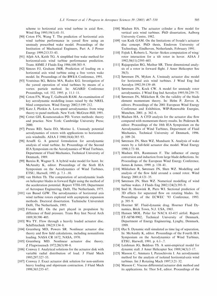
ARTICLE IN PRESSL.J. Vermeer et al. / Progress in Aerospace Sciences 39 (2003) 467–510 505
scheme to hotizontal axis wind turbine in axial flow.
Wind Eng 1995;19(1):41–51.
[90] Coton FN, Wang T. The prediction of horizontal axis
wind turbine performance in yawed flow using an
unsteady prescribed wake model. Proceedings of the
Institution of Mechanical Engineers, Part A. J Power
Energy 1999;213:33–43.
[91] Afjeh AA, Keith TG. A simplified free wake method for
horizontal-axis wind turbine performance prediction.
Trans ASME J Fluids Eng 1986;108:303–9.
[92] Simoes FJ, Graham JMR. Prediction of loading on a
horizontal axis wind turbine using a free vortex wake
model. In: Proceedings of the BWEA Conference, 1991.
[93] Voutsinas SG, Beleiss MA, Rados KG. Investigation of
the yawed operation of wind turbines by means of a
vortex particle method. In: AGARD Conference
Proceedings, vol. 552. 1995. p. 11.1–11.
[94] Coton FN, Wang T, Galbraith RAM. An examination of
key aerodynamic modelling issues raised by the NREL
blind comparison. Wind Energy 2002;5:199–212.
[95] Katz J, Plotkin A. Low-speed aerodynamics: from wing
theory to panel methods. New York: McGraw-Hill; 1991.
[96] Cottet GH, Koumoutsakos PD. Vortex methods: theory
and practice. New York: Cambridge University Press;
2000.
[97] Preuss RD, Suciu EO, Morino L. Unsteady potential
aerodynamics of rotors with applications to horizontal-
axis windmills. AIAA J 1980;18(4):385–93.
[98] Arsuffi G. A general formulation for aerodynamic
analysis of wind turbine. In: Proceedings of the Second
IEA Symposium on the Aerodynamics of Wind Turbines,
Department of Fluid Mechanics, Technical University of
Denmark, 1989.
[99] Bareiss R, Wagner S. A hybrid wake model for hawt. In:
McAnulty K, editor. Proceedings of the Sixth IEA
Symposium on the Aerodynamics of Wind Turbines,
ETSU, Harwell, 1993. p. 7.1–.10.
[100] van Holten Th. The computation of aerodynamic loads
on helicopter blades in forward flight using the method of
the acceleration potential. Report VTH-189, Department
of Aerospace Engineering, Delft, The Netherlands, 1975.
[101] van Bussel GJW. The aerodynamics of horizontal axis
wind turbine rotors explored with asymptotic expansion
methods. Doctoral dissertation. Technische Universiteit
Delft, The Netherlands, 1995.
[102] Froude RE. On the part played in propulsion by
difference of fluid pressure. Trans Roy Inst Naval Arch
1889;30:390–405.
[103] Wu TY. Flow through a heavily loaded actuator disc.
Schiffstechnik 1962;9:134–8.
[104] Greenberg MD, Powers SR. Nonlinear actuator disc
theory and flow field calculations, including nonuniform
loading. NASA CR 1672, NASA, 1970.
[105] Greenberg MD. Nonlinear actuator disc theory.
Z Flugwissensch 1972;20(3):90–8.
[106] Conway J. Analytical solutions for the actuator disk with
variable radial distribution of load. J Fluid Mech
1995;297:327–55.
[107] Conway J. Exact actuator disk solution for non-uniform
heavy loading and slipstream contraction. J Fluid Mech
1998;365:235–67.
[108] Madsen HA. The actuator cylinder a flow model for
vertical axis wind turbines. PhD dissertation, Aalborg
University Centre, 1982.
[109] van Kuik GAM. On the limitations of froude’s actuator
disc concept. PhD thesis, Eindoven University of
Technology, Eindhoven, Netherlands, February 1991.
[110] Fejtek I, Roberts L. Navier–Stokes computation of wing/
rotor interaction for a tilt rotor in hover. AIAA J
1992;30(11):2595–603.
[111] Rajagopalan RG, Mathur SR. Three dimensional analy-
sis of a rotor in forward flight. J Amer Helicopter Soc
38(3).
[112] S^rensen JN, Myken A. Unsteady actuator disc model
for horizontal axis wind turbines. J Wind Eng Ind
Aerodyn 1992;39:139–49.
[113] S^rensen JN, Kock CW. A model for unsteady rotor
aerodynamics. J Wind Eng Ind Aerodyn 1995;58:259–75.
[114] S^rensen JN, Mikkelsen R. On the validity of the blade
element momentum theory. In: Helm P, Zervos A,
editors. Proceedings of the 2001 European Wind Energy
Conference and Exhibition, WIP-Renewable Energies,
Munchen, 2001. p. 362–6.
[115] Madsen HA. A CFD analysis for the actuator disc flow
compared with momentum theory results. In: Pedersen B,
editor. Proceedings of the 10th IEA Symposium on the
Aerodynamics of Wind Turbines, Department of Fluid
Mechanics, Technical University of Denmark, 1996.
p. 109–24.
[116] S^rensen JN, Shen WZ, Munduate X. Analysis of wake
states by a full-field actuator disc model. Wind Energy
1998;1:73–88.
[117] Madsen HA, Rasmussen F. The influence of energy
conversion and induction from large blade deflections. In:
Proceedings of the European Wind Energy Conference,
James & James, 1999. p. 138–41.
[118] Mikkelsen R, S^rensen JN, Shen WZ. Modelling and
analysis of the flow field around a coned rotor. Wind
Energy 2001;4:121–35.
[119] S^rensen JN, Shen WZ. Numerical modelling of wind
turbine wakes. J Fluids Eng 2002;124(2):393–9.
[120] Snel H, Houwink R, Piers WJ. Sectional prediction of
3D effects for separated flow on rotating blades. In:
Proceedings of the ECWEC ’93 Conference, 1993.
p. 395–9.
[121] Hoerner SF. Fluid-dynamic drag. Hoerner Fluid Dy-
namics, Brick Town, N.J. USA, 1965.
[122] Hansen MOL. Polar for NACA 63-415 airfoil. Report
ET-AFM-9902, Technical University of Denmark,
Department of Energy Engineering, Lyngby, Denmark,
1999.
[123] Øye S. Dynamic stall simulated as time lag of separation,
In: McAnulty K, editor. Proceedings of the Fourth IEA
Symposium on the Aerodynamics of Wind Turbines,
ETSU, Harwell, 1991. p. 6.1–.7.
[124] Leishman JG, Beddoes TS. A semi-empirical model for
dynamic stall. J Amer Helicopter Soc 1989;34(3):3–17.
[125] Masson C, Ammara I, Paraschivoiu I. An aerodynamic
method for the analysis of isolated horizontal-axis wind
turbines. Int J Rotating Mach 1997;3:21–32.
[126] Masson C. Viscous differential/actuator disk method and
its applications. In: Thor S-E, editor. Proceedings of the

ARTICLE IN PRESSL.J. Vermeer et al. / Progress in Aerospace Sciences 39 (2003) 467–510506
15th IEA Symposium on the Aerodynamics of Wind
Turbines, FOI, Swedish Defence Research Agency, 2002.
p. 65–80.
[127] Phillips D, Schaffarczyk AP. Blade-element and actuator-
disk models for a shrouded wind-turbine. In: Thor S-E,
editor. Proceedings of the 15th IEA Symposium on the
Aerodynamics of Wind Turbines, FOI, Swedish Defence
Research Agency, 2002. p. 95–105.
[128] Mikkelsen R, S^rensen JN. Modelling of wind tunnel
blockage. In: Thor S-E, editor. Proceedings of the 15th
IEA Symposium on the Aerodynamics of Wind Turbines,
FOI, Swedish Defence Research Agency, 2001. p. 41–51.
[129] Mikkelsen R, S^rensen JN. Yaw analysis using a
numerical actuator disc model. In: Pedersen B, editor.
Proceedings of the 14th IEA Symposium on the Aero-
dynamics of Wind Turbines, Department of Fluid
Mechanics, Technical University of Denmark, 2000.
p. 53–9.
[130] Ammara I, Leclerc C, Masson C. A viscous three-
dimensional differential/actuator-disk method for aero-
dynamic analysis of wind farms. J Solar Energy—
T ASME 2002;124(4):345–56.
[131] S^rensen JN. VISCWIND viscous effects on wind turbine
blades. ET-AFM 9902, Department of Fluid Mechanics,
The Technical University of Denmark, 1999.
[132] Chaviaropoulos PK, Nikolaou IG, Aggelis K, S^rensen
NN, Montgomerie B, von Geyr H, Hansen MOL, Kang
S, Voutsinas S, Dyrmose SZ. Viscous and aeroelastic
effects on wind turbine blades: The VISCEL project. In:
Helm P, Zervos A, editors. Proceedings of the 2001
European Wind Energy Conference and Exhibition,
WIP-Renewable Energies, Munchen, 2001. p. 347–50.
[133] Hansen MOL, S^rensen JN, Michelsen JA, S^rensen
NN. A global Navier–Stokes rotor prediction model. In:
AIAA Paper 97-0970, 1997.
[134] S^rensen NN, Hansen MOL. Rotor performance predic-
tions using a Navier–Stokes method. In: AIAA Paper
98-0025, 1998.
[135] S^rensen NN, Michelsen JA. Aerodynamic predictions
for the unsteady aerodynamics experiment phase-ii rotor
at the national renewable energy laboratory. In: AIAA
Paper 2000-0037, 2000.
[136] Kang S, Hirsch C. Features of the 3D viscous flow
around wind turbine blades based on numerical solutions.
In: Helm P, Zervos A, editors. Proceedings of the 2001
European Wind Energy Conference and Exhibition,
WIP-Renewable Energies, Munchen, 2001. p. 495–8.
[137] Michelsen JA, S^rensen NN. Current developments in
Navier–Stokes modelling of wind turbine rotor flow. In:
Helm P, Zervos A, editors. Proceedings of the 2001
European Wind Energy Conference and Exhibition,
WIP-Renewable Energies, Munchen, 2001. p. 367–72.
[138] Duque EPN, van Dam CP, Hughes S. Navier–Stokes
simulations of the NREL combined experiment phase II
rotor. In: AIAA Paper 99-0037, 1999.
[139] Duque EPN, Johnson W, van Dam CP, Cortes R, Yee K.
Numerical predictions of wind turbine power and
aerodynamic loads for the NREL phase ii combined
experiment rotor. In: AIAA Paper 2000-0038, 2000.
[140] Xu G, Sankar LN. Computational study of horizontal
axis wind turbines. In: AIAA Paper 99-0042, 1999.
[141] Xu G, Sankar LN. Effects of transition, turbulence and
yaw on the performance of horizontal axis wind turbines.
In: AIAA Paper 2000-0048, 2000.
[142] Fingersh L, Simms D, Hand M, Jager D, Cortrell J,
Robinson M, Schreck S, Larwood S. Wind tunnel testing
of NREL’s unsteady aerodynamics experiment. In: AIAA
Paper 2001-0035, 2001.
[143] Tangler JL. The nebulous art of using wind tunnel
aerofoil data for predicting rotor performance. Wind
Energy 2002;5:245–57.
[144] S^rensen NN, Michelsen JA, Schreck S. Navier–Stokes
predictions of the NREL phase vi rotor in the nasa ames
80 ft� 120 ft wind tunnel. Wind Energy 2002;5:151–69.
[145] Baldwin BS, Lomax H. Thin layer approximation and
algebraic model for separated turbulent flows. AIAA
Paper 78-257.
[146] Launder BE, Spalding DB. The numerical computation
of turbulent flows. Comput Meth Appl Mech Eng
1974;3:269–89.
[147] Haase W, Brandsma F, Elsholz E, Lechziner M,
Schwamborn D. Euroval—an european initiative in
validation of cfd codes, Notes on numerical fluid
mechanics, vol. 42. Braunschweig: Vieweg; 1993.
[148] Haase W, Chaput E, Elsholz E, Lechziner M, Muller UR.
ECARP—european computational aerodynamic research
project: validation of cfd codes and assessment of
turbulence models, Notes on numerical fluid mechanics,
vol. 58. Braunschweig: Vieweg; 1997.
[149] Menter FR. Zonal two-equation model k–o models for
aerodynamic flows. In: AIAA Paper 93-2906, 1993.
[150] Spalart PR. Strategies for turbulence modelling and
simulations. Int J Heat Fluid Flow 2000;21:252–63.
[151] Johansen J, S^rensen NN, Michelsen JA, Schreck S.
Detached-eddy simulation of flow around the NREL
phase vi blade. Wind Energy 2002;5:185–97.
[152] Michel R. Etude de la transition sur les profiles d’aile:
Etablissement d’un critere de determination de point de
transition et calcul de la trainee de profile incompressible.
ONERA TR 1/1578A, 1951.
[153] Stock HW, Degenhart E. A simplified en method for
transition prediction in two-dimensional, incompressible
boundary layers. Zeitschrift f .ur Flugwissenschaften 13.
[154] Johansen J, S^rensen JN. Prediction of laminar/turbulent
transition in airfoil flows. J Aircraft 1999;36(4):731–4.
[155] Brodeur RR, van Dam CP. Transition prediction for a
two dimensional Navier–Stokes solver applied to wind-
turbine airfoils. In: AIAA Paper 2000-0047, 2000.
[156] Smith D, Taylor GJ. Further analysis of turbine wake
development and interaction data. In: Q.D.C., F. V. C,
editors. Proceedings of the 13th BWEA Wind Energy
Conference, Swansea, UK, 1991. p. 325–31.
[157] Crespo A, Hern!andez J. Turbulence characteristics in
wind-turbine wakes. J Wind Eng Ind Aerodyn
1996;61:71–85.
[158] Helmis CG, Papadopoulos KH, Asimakopoulos DN,
Papageorgas PG, Soilemes AT. An experimental
study of the near wake structure of a wind turbine
operating over complex terrain. Solar Energy 1995;
54(6):413–28.
[159] H .ogstrom U, Asimakopoulos DN, Kambezidis H,
Helmis CG, Smedman A. A field study of the wake

ARTICLE IN PRESSL.J. Vermeer et al. / Progress in Aerospace Sciences 39 (2003) 467–510 507
behind a 2 mw wind turbine. Atmos Environ
1988;22(4):803–20.
[160] Luken E. The wind loads of wind turbines in clusters—
literature survey. Report 89-160, TNO Division of
Technology for Society, 1989.
[161] Quarton DC. Characterization of wind turbine wake
turbulence and its implications on wind farm spacing.
Final Report ETSU WN 5096, Department of Energy of
the UK. Garrad-Hassan Contract, 1989.
[162] Vermeulen PEJ, Builtjes PJH. Turbulence measurements
in simulated wind turbine clusters. Report 82-03003,
TNO Division of Technology for Society, September
1982.
[163] Builtjes PJH. The interaction of windmill wakes. In:
Proceedings of the 2nd International Symposium on
Wind Energy Systems, BHRA Fluid Engineering,
Amsterdam, Netherlands, 1978. p. B5-49-58.
[164] Green DRR. Near wake wind tunnel studies. ETSU-WN-
5040/P1 Report, Loughborough University, March 1986.
[165] Ross JN. Measurements of velocity in wind tunnel
studies of windmill arrays using laser anemometry.
LM/Phys./133, Central Electricity Research Labora-
tories, July 1979.
[166] Green DRR, Alexander AJ. Measurement of velocity and
turbulence profiles in flow situations relevant to wind
turbine performance. Final Report on ETSU contract
E/5A/CON/5003/177/026, Loughborough University,
May 1985.
[167] Talmon AM. The wake of a horizontal axis wind turbine
model, measurements in uniform approach flow and in
a simulated boundary layer, Report 85-01021, TNO
Division of Technology for Society, August 1985.
[168] Milborrow DJ, Ross JN. The influence of turbulence and
rotor thrust on wind turbine wake characteristics.
Memorandum TPRD/L/AP/0098/M83, CERL, 1983.
[169] Vermeulen PEJ. An experimental analysis of wind turbine
wakes. In: Proceedings of the 3rd International Sympo-
sium on Wind Energy Systems. BHRA Fluid Engineer-
ing, Lyngby, Denmark, 1980. p. 431–50.
[170] Alfredson PH, Dahlberg J (A, Bark FH. Some properties
of the wake behind horizontal axis wind turbines. In:
Proceedings of the 3rd International Symposium onWind
Energy Systems, BHRA Fluid Engineering, Lyngby,
Denmark, 1980. p. 469–84.
[171] Crespo A, Hern!andez J. Analytical correlations for
turbulence characteristics in the wakes of wind turbines.
In: Garrad AD, Palz W, Scheller S, editors. Proceedings
of the 1993 European Community Wind Energy
Conference. Germany: Travem .unde; 1993. p. 436–9.
[172] H^jstrup J. Spectral coherence in wind turbine wakes.
J Wind Eng Ind Aerodyn 1999;80:137–46.
[173] Smith D. Multiple wake measurements and analysis. In:
Davies TD, Halliday JA, Palutikov JP, editors. Proceed-
ings of the 12th BWEA Wind Energy Conference. UK:
Norwich; 1990. p. 53–6.
[174] Papaconstantinou A, Bergeles G. Hot-wire measurements
of the flow field in the vicinity of a HAWG rotor. J Wind
Eng Ind Aerodyn 1988;31:133–6.
[175] Ainslie JF, Hassan U, Parkinson HG, Taylor GJ. A wind
tunnel investigation of the wake structure within small
wind turbine farms. Wind Eng 1990;14:24–8.
[176] Hassan U, Glendinning AG, Morgan CA. A wind tunnel
investigation of the wake structure and machine loads
within small wind turbine farms. In: Davies TD, Halliday
JA, Palutikov JP, editors. Proceedings of the 12th BWEA
Wind Energy Conference. Norwich, UK 1990. p. 47–52.
[177] Magnusson M, Smedman AS. Influence of atmospheric
stability on wind turbine wakes. Wind Eng 1994;
18(3):139–52.
[178] Talmon AM. A wind tunnel investigation into the effects
of tower and nacelle on wind turbine wake flow. Report
84-08479, TNO Division of Technology for Society, July
1984.
[179] Luken E, Vermeulen PEJ. Development of advanced
mathematical models for the calculation of wind
turbine wake-interaction effects. In: Palz W, Sesto E,
editors. Proceedings of EWEC’86, Rome, Italy, 1986.
p. 423–7.
[180] Crespo A, Hern!andez J, Fraga E, Andreu C. Experi-
mental validation of the UPM computer code to calculate
wind turbine wakes and comparison with other models.
J Wind Eng Ind Aerodyn 1988;27:77–88.
[181] Taylor GJ, Smith D. Wake measurements over complex
terrain. In: Quarton DC, Fenton VC, editors. Proceed-
ings of the 13th BWEA Wind Energy Conference,
Swansea, UK, 1991. p. 335–42.
[182] Stefanatos NC, Voutsinas SG, Rados KG, Zervos A. A
combined experimental and numerical investigation of
wake effects in complex terrain. In: Tsipouridis JL,
editor. Proceedings of EWEC’94, Thessaloniki, Greece,
1994. p. 484–90.
[183] Stefanatos NC, Morfiadakis EE, Glinou GL. Wake
measurements in complex terrain. In: Zervos A, Ehmann
H, Helm P, editors. Proceedings of the 1996 European
Union Wind Energy Conference, G .oteborg, Sweden,
1996. p. 773–7.
[184] Tindal AJ, Garrad AD, Schepers G, Bulder B, Hutting H,
Verheij F. Dynamic loads in wind farms. In: Garrad AD,
Palz W, Scheller S, editors. Proceedings of the 1993
European Community Wind Energy Conference,
Travem.unde, Germany, 1993. p. 477–80.
[185] Baker RW, Walker SN. Wake velocity deficit measure-
ments at the Goodnoe Hills MOD-2 Site. Report, Report
No. BPA 84-15, DOE/BP/29182-15, 1985.
[186] Taylor GJ, Milborrow DJ, McIntosh DN, Swift-Hook
DT. Wake measurements on the nibe windmills. In:
Garrad A, editor. Proceedings of the 7th BWEA Wind
Energy Conference, Oxford, UK, 1985. p. 67–73.
[187] Taylor GJ. Fluctuating loads on a wind turbine operating
in a wake. In: Galt J, editor. Proceedings of the 9th
BWEA Wind Energy Conference, Edinburgh, UK, 1987.
p. 55–62.
[188] Taylor GJ. Wake measurements on the nibe wind-
turbines in Denmark. Part 2: Data collection and
analysis. Final Report CEC Contract No. EN3-
W.0039.UK(H1), National Power, London, 1990.
[189] H^jstrup J. Wake measurements on the nibe wind-
turbines in Denmark. Appendix 1. Nibe wake 2. Final
Report CEC Contract no. EN3W.0039.UK(H1), Ris^;1990.
[190] Scott AM. Wake interaction studies on the HWP-300/22
and WEG MS-1 WTGs on Burgar Hill, Orkney. Report

ARTICLE IN PRESSL.J. Vermeer et al. / Progress in Aerospace Sciences 39 (2003) 467–510508
on UK DOEN Contract E/5A/CON/5039/1277, James
Howden and Co Ltd, 1987.
[191] Haines RS, Milborrow DJ, Page DI, Scott AD,
Stevenson WG, Taylor GJ. Wake interaction studies on
the HWP-300/22 and WEG MS-1 WTGs on Burgar Hill,
Orkney, UK. In: Palz W, Sesto E, editors. Proceedings of
EWEC’86, vol. 1, Rome, Italy, 1986. p. 453–8.
[192] H^jstrup J. Turbulence measurements in a wind farm. In:
Davies TD, Halliday JA, Palutikov JP, editors. Proceed-
ings of the 12th BWEA Wind Energy Conference,
Norwich, UK, 1990. p. 59–63.
[193] Papadopoulos KH, Helmis CG, Soilemes AT, Papageor-
gas PG, Asimakopoulos DN. Study of the turbulent
characteristics of the near-wake field of a medium sized
wind turbine operating in high wind conditions. Solar
Energy 1999;80:121–36.
[194] Frandsen S, Chac!on L, Crespo A, Enevoldsen P, G!omez-
Elvira R, Hern!andez J, H^jstrup J, Manuel F, Thomsen
K, S^rensen P. Measurements on and modelling of
offshore wind farms. Report Ris^-R-903(EN), Ris^; 1996.[195] H^jstrup J, Courtney MS. Turbulence in wind farms, In:
Garrad AD, Palz W, Scheller S, editors. Proceedings of
the 1993 European Community Wind Energy Confer-
ence, Travem .unde, Germany, 1993. p. 383–6.
[196] Kline J. Turbulence characteristics at Howden wind park
I. In: AWEA conference ‘‘windpower 88’’, Honolulu,
Hawaii, USA, 1988.
[197] Simon RL, Matson DF, Fuchs JM. Wake effects in a
Fayette 95-II5 wind turbine array, Report SERI/STR-
217-3186, Fayette Manufacturing Company, September
1987.
[198] Nierenberg R. Free flow variability and wake energy
deficit studies in the Altamont pass, California: results of
the DOE-AEC CFT program. In: AWEA conference
‘‘windpower 88’’, Honolulu, Hawaii, USA, 1988.
[199] Van Leuven J, Stevens D. The wind farm of Zeebrugge:
Experimental set-up. J Wind Eng Ind Aerodyn 1988;
27:139–44.
[200] Van Leuven J. The energetic effectiveness of a cluster of
wind turbines. PhD thesis, Universite Catholique de
Louvain, Institut des Sciences Naturelles Appliquees,
1992.
[201] Folkerts L, Barthelmie R, Sanderhof P, Ormel F, Eecen
P, Stobbe O. Sodar wind velocity measurements of
offshore wind turbine wakes. Wind Eng 2001;25(5):
301–6.
[202] Frandsen S, Th^gersen ML. Integrated fatigue loading
for wind turbines in wind farms by combining
ambient turbulence and wakes. Wind Eng 1999;23(6):
327–40.
[203] Crespo A, Hern!andez J, Frandsen S. A survey of
modelling methods for wind-turbine wakes and wind
farms. Wind Energy 1994;2:1–24.
[204] V^lund P. Loads on a horizontal axis wind turbine
operating in a wake. In: Van Hulle FJL, Smulders PT,
Dragt JB, editors. Proceedings of EWEC’91, Amsterdam,
Netherlands, 1991. p. 605–9.
[205] Stiesdal H. Wake loads on the Bonus 450 kW II turbine.
In: Clayton BR, editor. Proceedings of the 14th BWEA
Wind Energy Conference, Nottingham, UK, 1992.
p. 183–9.
[206] Dahlberg J (A, Poppen M, Thor SE. Load/fatigue effects
on a wind turbine generator in a wind farm. In: Van Hulle
FJL, Smulders PT, Dragt JB, editors. Proceedings of
EWEC’91, Amsterdam, Netherlands, 1991. p. 251–5.
[207] Thomsen K, Bindner H, Pedersen TF. Fatigue loads on a
pitch regulated wind turbine operating in a coastal wind
turbine array. Report Ris^-R-743(EN), Ris^; 1994.[208] Thomsen K, S^rensen P. Fatigue loads for wind turbines
operating in wakes. J Wind Eng Ind Aerodyn
1999;55(1):61–72.
[209] Frandsen S, Christensen CJ. Structural loads in
large wind farm arrays. In: Tsipouridis JL, editor.
Proceedings of EWEC’94, vol. III, Thessaloniki, Greece,
1994. p. 116–22.
[210] Frandsen S, Thomsen K. Change in fatigue and extreme
loading when moving wind farms offshore. Wind Eng
1997;21(3):197–214.
[211] Adams BM, Quarton JGDC, Schepers, Bulder B,
Dahlberg J (A, Morfiadakis E. Dynamic loads in wind
farms. In: Tsipouridis JL, editor. Proceedings of
EWEC’94, Thessaloniki, Greece, 1994. p. 756–61.
[212] Cleijne JW. Results of Sexbierum wind farm. Report
92-388, TNO-MT, Apeldoorn, Netherlands, 1992.
[213] G !omez-Elvira R, Crespo A. An explicit algebraic
turbulent model to reproduce the anisotropy of the
momentum turbulent flows in a wind turbine wake. In:
accepted for publication in Proceedings of EWEC’2003
Madrid, Spain, 2003.
[214] Magnusson M. Full-scale wake measurements at
Alsvik wind farm, Sweden. In: Tsipouridis JL, editor.
Proceedings of EWEC’94, Thessaloniki, Greece, 1994.
p. 472–7.
[215] Magnusson M, Smedman AS. Air flow behind wind
turbines. J Wind Eng Ind Aerodyn 1999;80:169–89.
[216] Lissaman PBS. Energy effectiveness of arbitrary arrays of
wind turbines. In: AIAA Paper 79-0114, 1979. p. 1–7.
[217] Voutsinas SG, Rados KG, Zervos A. On the analysis of
wake effects in wind parks. Journal of Wind Eng Ind
Aerodyn 1990;14(4):204–19.
[218] Abramovich GN. The theory of turbulent jets.
Cambridge, MA: MIT Press; 1963.
[219] Katic I, H^jstrup J, Jensen NO. A simple model for
cluster efficiency. In: Palz W, Sesto E, editor. Proceedings
of EWEC’86, Rome, Italy, 1986. p. 407–10.
[220] Crespo A, Manuel F, Moreno D, Fraga E, Hern!andez J.
Numerical analysis of wind turbine wakes. In: Bergeles G,
Chadjivassiliadis J, editors. Proceedings of the Delphi
Workshop on Wind Energy Applications, Delphi,
Greece, 1985. p. 15–25.
[221] Sforza PM, Sheering P, Smorto M. Three-dimensional
wakes of simulated wind turbines. AIAA J 1981;19(9):
1101–7.
[222] Ainslie JF. Development of an eddy viscosity model for
wind turbine wakes. In: Garrad A, editor. Proceedings of
the 7th BWEA Wind Energy Conference, Oxford, UK,
1985. p. 61–6.
[223] Ainslie JF. Calculating the field in the wake of wind
turbines. J Wind Eng Ind Aerodyn 1988;21:213–24.
[224] Luken E, Talmon A, Vermeulen PEJ. Evaluation of two
mathematical wind turbine wake models in various types
of flows. Report 86-07, TNO-MT, 1986.

ARTICLE IN PRESSL.J. Vermeer et al. / Progress in Aerospace Sciences 39 (2003) 467–510 509
[225] Crespo A, Hern!andez J. Numerical modelling of the flow
field in a wind turbine wake. In: Proceedings of the 3rd
Joint ASCE/ASME Mechanics Conference, Forum on
Turbulent Flows. ASME, FED-vol. 76, La Jolla, CA,
USA, 1989. p. 121–7.
[226] Crespo A, Hern!andez J. A numerical model of wind
turbine wakes and wind farms. In: Palz W, Sesto E,
editors. Proceedings of EWEC’86, vol. 2, Rome, Italy,
1986. p. 111–5.
[227] Crespo A, Manuel F, Hern!andez J. Numerical modelling
of wind turbine wakes. In: Palz W, editor. Proceedings
of the 1990 European Community Wind Energy
Conference, Madrid, Spain, 1990. p. 166–70.
[228] Taylor PA. On wake decay and row spacing for wecs
farms. In: Proceedings of the 3rd International Sympo-
sium on Wind Energy Systems, BHRA Fluid Engineer-
ing, Lyngby, Denmark, 1980. p. 451–68.
[229] Liu M, Vocke M, Myers T. Mathematical model for the
analysis of wind turbine wakes. Journal of Energy
1983;7(1):73.
[230] Taylor GJ. Development of an improved eddy viscosity
model. Wake and wind farm modelling. Final Report
TNO-Report 93-374, National Power, London, 1993.
[231] Adams BM, Quarton DC. Dynamic loads in wind farms.
Final Report, Joule Project JOU2-CT92-0094 (Edited by
Garrad Hassan, 1996).
[232] Hassan U. A wind tunnel investigation of the wake
structure within small wind farms. Report. ETSU Report
No. WN5113, Garrad-Hassan, 1993.
[233] Magnusson M. Near wake behaviour of wind turbines.
J Wind Eng Ind Aerodyn 1999;80:147–67.
[234] Zervos A, Huberson S, Hemon A. Three-dimensional free
wake calculation of wind turbine wakes. J Wind Eng Ind
Aerodyn 1988;27:65–76.
[235] Cleijne JW, Crespo A, Huberson S, Taylor GJ, Voutsinas
SG. Wake and wind farm modelling. Report 93-374,
TNO-MT, Apeldoorn, Netherlands, 1993.
[236] Schepers JG. ENDOW: Validation and improvement of
ECN’s wake model. ECN-C–03-034, ECN, March 2003.
[237] Voutsinas SG, Glekas JP, Zervos A. Investigation of the
effect of the initial velocity profile on the wake develop-
ment of a wind turbine. J Wind Eng Ind Aerodyn
1992;39:293–301.
[238] Voutsinas SG, Rados KG, Zervos A. On the effect of the
rotor geometry on the formation and the development of
its wake. J Wind Eng Ind Aerodyn 1992;39:283–91.
[239] Magnusson M, Rados KG, Voutsinas SG. A study of the
flow downstream of a wind turbine using measurements
and simulations. Wind Eng 1996;20(6):389–403.
[240] Pothou KP, Voutsinas SG, Huberson S, Kuhlmann M,
Rawlinson-Smith R. Investigation of noise emissions
from wind parks and their impact to the design of parks
by means of the noisepark software. In: Petersen EL,
Jensen PH, Rave K, Helm P, Ehmann H, editors.
Proceedings of the 1999 European Union Wind Energy
Conference, Nice, France, 1999. p. 97–100.
[241] Ansorge T, Fallen M, G .unther P, Ruh C, Wolfanger T.
Numerical simulation of wake-effects in complex terrain
and application of a Reynolds-stress turbulence model.
In: Tsipouridis J, editor. Proceedings of EWEC’94,
Thessaloniki, Greece, 1994. p. 448–53.
[242] Beyer HG, R .uger T, Sch.afer G, Waldl HP. Optimization
of wind farm configuration with variable number of
turbines. In: Zervos A, Ehmann H, Helm P, editors.
Proceedings of the 1996 European Union Wind Energy
Conference. G .oteborg, Sweden, 1996. p. 1073–6.
[243] Sotiropoulos DP, Koukas A, Stephanatos NC, Voutsinas
SG. Numerical investigation of wake effects in offshore
wind farms using a 3d navier-stokes solver. In: Petersen
EL, Jensen PH, Rave K, Ehmann HPH, editors.
Proceedings of the 1999 European Union Wind Energy
Conference. Nice, France, 1999. p. 254–7.
[244] Crespo A, Chac !on L, Hern!andez J, Manuel F, Grau JC.
UPMPARK: a parabolic 3D code to model wind farms,
In: Tsipouridis JL, editor. Proceedings of EWEC’94,
Thessaloniki, Greece, 1994. p. 454–9.
[245] Bulder BH. Fynd farm—a wind farm design support tool.
In: Proceedings of the European Wind Energy
Conference, Dublin Castle, Ireland, 1997. p. 246–8.
[246] Crespo A, Manuel F, Grau JC, Hern!andez J. Modeliza-
tion of wind farms in complex terrain. Application to the
monteahumada wind farm. In: Garrad AD, Palz W,
Scheller S, editors. Proceedings of the 1993 European
Community Wind Energy Conference, Travem .unde,
Germany, 1993. p. 436–9.
[247] Voutsinas SG, Rados KG, Zervos A. The effect of the
non-uniformity of the wind velocity field in the optimal
design of wind parks. In: Palz W, editor. Proceedings
of the 1990 European Community Wind Energy
Conference, Madrid, Spain, 1990. p. 181–5.
[248] Hemon A, Huberson S, Zervos A. Numerical study
of wind turbine operation in complex terrain.
In: Quarton DC, Fenton VC, editors. Proceedings of
the 13th BWEAWind Energy Conference, Swansea, UK,
1991. p. 343–50.
[249] Migoya E, Crespo A, Garc!ıa J, Moreno F, Jim!enez A.
Comparative study of the behaviour of several wind-
turbines in a wind farm. In: Proceedings of EWEC’2003
Madrid, Spain, 2003, Accepted for publication.
[250] G .unther P, Fallen M, Wolfanger T. Numerical wake
simulation of a hawt considering topography and using a
mesoscale turbulence model. In: Garrad AD, Palz W,
Scheller S, editors. Proceedings of the 1993 European
Community Wind Energy Conference, Travem .unde,
Germany, 1993. p. 448–50.
[251] Chaviaropoulos PK, Douvikas DI. Mean wind field
prediction over complex terrain in the presence of wind
turbines. In: Petersen EL, Jensen P, Rave K, Helm P,
Ehmann H, editors. Proceedings of the 1999 European
Union Wind Energy Conference, Nice, France, 1999.
p. 1208–11.
[252] Ivanova LA, Nadyozhina ED. Numerical simulation of
wind farm influence on wind flow. Wind Eng 2000;
24(4):257–70.
[253] Crespo A, G !omez-Elvira R. Effect of the proximity of
land on wind farm performance for offshore flow. In:
Proceedings of the European Seminar OWEMES’97,
La Magdalene, Sardinia, Italy, 1997. p. 33–41.
[254] Crespo A, Chac !on L, Manuel F, G !omez-Elvira R,
Hern!andez J. Modelization of offshore wind farms.
Effect of the surface roughness of the sea. In: Zervos A,
Ehmann H, Helm P (editors). Proceedings of the 1996

ARTICLE IN PRESSL.J. Vermeer et al. / Progress in Aerospace Sciences 39 (2003) 467–510510
European Union Wind Energy Conference, G .oteborg,
Sweden, 1996. p. 644–7.
[255] Frandsen S. Fatigue loading on offshore wind power
stations. In: Zervos H, Ehmann A, Helm P, editors.
Proceedings of the 1996 European Union Wind Energy
Conference, G .oteborg, Sweden, 1996. p. 990–4.
[256] Rados K, Larsen G, Barthelmie R, Schlez W, Lange B,
Schepers G, Hegberg T, Magnusson M. Comparison of
wake models with data for offshore windfarms. Wind
Eng 2001;25(5):271–80.
[257] Schlez W, Umana A, Barthelmie R, Larsen G, Rados K,
Lange B, Schepers G, Hegberg T. ENDOW: improve-
ment of wake models within offshore wind farms. Wind
Eng 2001;25(5):281–7.
[258] Schepers G, Barthelmie R, Rados K, Lange B, Schlez W.
Large offshore wind farms: linking wake models with
atmospheric boundary layer models. Wind Eng 2001;
25(5):307–16.
[259] Newman BG. Near wake behaviour of wind turbines.
Energy Conversion 1977;16:169–71.
[260] Bossanyi EA, Maclean C, Whittle GE, Dunn PD,
Lipman NH, Musgrove PJ. The efficiency of wind turbine
clusters. In: Proceedings of the 3rd International Sympo-
sium on Wind Energy Systems, BHRA Fluid Engineer-
ing, Lyngby, Denmark, 1980. p. 401–16.
[261] Frandsen S. On the wind speed reduction in the center of
large clusters of wind turbines. J Wind Eng Ind Aerodyn
1992;39:261–5.
[262] Crespo A, Frandsen S, G !omez-Elvira R, Larsen SE.
Modelization of a large wind farm, considering the
modification of the atmospheric boundary layer. In:
Petersen EL, Jensen PH, Rave K, Helm P, Ehmann H
(editors). Proceedings of the 1999 European Union Wind
Energy Conference, Nice, France, 1999. p. 1109–13.
[263] Hegberg T. The effect of large windfarms on the
atmospheric boundary layer. In: Proceedings of the Global
Wind Power Conference 2002, Paris, France, 2002.
[264] Frandsen S, Barthelmie R. Local wind climate whithin
and downwind of large offshore wind turbine clusters.
Wind Eng 2002;26(1):51–8.
[265] Hunt J, Eames I. The disappearance of laminar and
turbulent wakes in complex flows. J Fluid Mech 2002;
457:111–32.
[266] Magnusson M, Smedman AS. A practical method to
estimate wind turbine wake characteristics from turbine
data and routine wind measurements. Wind Eng 1996;
20(2):73–92.
[267] Schlichting H. Boundary layer theory. New York:
McGraw-Hill; 1968.
[268] Larsen GC, H^jstrup J, Madsen HA. Wind fields in
wakes. In: Zervos A, Ehmann H, Helm P, editors.
Proceedings of the 1996 European Union Wind Energy
Conference, G .oteborg, Sweden, 1996. p. 764–8.
[269] Frandsen S. Turbulence and turbulence-generated fatigue
loading in wind turbine clusters. Report in draft form
Ris^-R-1188(EN), Ris^; Roskilde, Denmark, 2003.
Related Documents