A n ati ona l l abo rat ory of the U.S . Depa rtment of Energy Office of Energy Efficiency & Renewable Energy National Renewable Energy Laboratory Innovation for Our Energy Future Wind Tunnel Tests of Parabolic Trough Solar Collectors March 2001–August 2003 N. Hosoya and J.A. Peterka Cermak Peterka Petersen, Inc. Fort Collins, Colorado R.C. Gee Solargenix Energy, LLC Raleigh, North Carolina D. Kearney Kearney & Associates Vashon, Washington Subcontract Report NREL/SR-550-32282 May 2008 NREL is operated by Midwest Research Institute ●Battelle Contract No. DE-AC36-99-GO10337

Welcome message from author
This document is posted to help you gain knowledge. Please leave a comment to let me know what you think about it! Share it to your friends and learn new things together.
Transcript

7/31/2019 Wind Tunnel Test
http://slidepdf.com/reader/full/wind-tunnel-test 1/243
A national laboratory of the U.S. Department of E
Office of Energy Efficiency & Renewable E
National Renewable Energy Laboratory
Innovation for Our Energy Future
Wind Tunnel Tests of Parabolic
Trough Solar Collectors
March 2001–August 2003
N. Hosoya and J.A. PeterkaCermak Peterka Petersen, Inc.Fort Collins, Colorado
R.C. Gee
Solargenix Energy, LLC Raleigh, North Carolina
D. KearneyKearney & AssociatesVashon, Washington
Subcontract Report
NREL/SR-550-32282
May 2008
NREL is operated by Midwest Research Institute ●Battelle Contract No. DE-AC36-99-GO10337
7/31/2019 Wind Tunnel Test
http://slidepdf.com/reader/full/wind-tunnel-test 2/243
National Renewable Energy Laboratory1617 Cole Boulevard, Golden, Colorado 80401-3393
303-275-3000 www.nrel.gov
Operated for the U.S. Department of EnergyOffice of Energy Efficiency and Renewable Energy
by Midwest Research Institute • Battelle
Contract No. DE-AC36-99-GO10337
Subcontract Report
NREL/SR-550-32282
May 2008
Wind Tunnel Tests of Parabolic
Trough Solar Collectors
March 2001–August 2003
N. Hosoya and J.A. PeterkaCermak Peterka Petersen, Inc.Fort Collins, Colorado
R.C. Gee
Solargenix Energy, LLC Raleigh, North Carolina
D. KearneyKearney & AssociatesVashon, Washington
NREL Technical Monitor: Mary Jane HalePrepared under Subcontract No. NAA-2-32439-01

7/31/2019 Wind Tunnel Test
http://slidepdf.com/reader/full/wind-tunnel-test 3/243
This publication was reproduced from the best available copySubmitted by the subcontractor and received no editorial review at NREL
NOTICE
This report was prepared as an account of work sponsored by an agency of the United States
government. Neither the United States government nor any agency thereof, nor any of their employees,makes any warranty, express or implied, or assumes any legal liability or responsibility for the accuracy,completeness, or usefulness of any information, apparatus, product, or process disclosed, or representsthat its use would not infringe privately owned rights. Reference herein to any specific commercialproduct, process, or service by trade name, trademark, manufacturer, or otherwise does not necessarilyconstitute or imply its endorsement, recommendation, or favoring by the United States government or anyagency thereof. The views and opinions of authors expressed herein do not necessarily state or reflectthose of the United States government or any agency thereof.
Available electronically at http://www.osti.gov/bridge
Available for a processing fee to U.S. Department of Energy
and its contractors, in paper, from:U.S. Department of EnergyOffice of Scientific and Technical InformationP.O. Box 62Oak Ridge, TN 37831-0062phone: 865.576.8401fax: 865.576.5728email: mailto:[email protected]
Available for sale to the public, in paper, from:U.S. Department of CommerceNational Technical Information Service5285 Port Royal RoadSpringfield, VA 22161
phone: 800.553.6847fax: 703.605.6900email: [email protected] online ordering: http://www.ntis.gov/ordering.htm
Printed on paper containing at least 50% wastepaper, including 20% postconsumer waste
7/31/2019 Wind Tunnel Test
http://slidepdf.com/reader/full/wind-tunnel-test 4/243
TABLE OF CONTENTS
1. INTRODUCTION .................................................................................................................. 1 1.1 Background and Scope of Parabolic Trough Wind Tunnel Test Program ......... 11.2 Wind Load Issues ................................................................................................ 2
2. TEST SETUP AND PROCEDURES ..................................................................................... 3 2.1 Boundary Layer Simulation Technique .............................................................. 3
2.2 Wind-Tunnel Models .......................................................................................... 42.2.1 Balance Model for Lift and Drag Force Measurements ............................. 5
2.2.2 Balance Model for Pitching Moment Measurements ................................. 7
2.2.3 Pressure Model............................................................................................ 8
2.2.4 Non-Instrumented Solar Collector Models ............................................... 122.3 Instrumentation ................................................................................................. 12
2.3.1 Signal Conditioner for High-Frequency Force and Moment Balances .... 12
2.3.2 CPP Multi-Pressure Measurement System ............................................... 132.4 Test Configurations and Matrix ........................................................................ 13
2.5 Test Procedures ................................................................................................. 252.6 Accuracy and Uncertainty of Test Results........................................................ 26
3. ANALYSIS METHODS ...................................................................................................... 29 3.1 Definition of Test Parameters ........................................................................... 29
3.1.1 Orientation of Solar Collector ................................................................... 29
3.1.2 Load Coefficients ...................................................................................... 30
3.1.3 Consideration for Load Cases for Structural Strength Design .................. 313.2 Particular Treatment of Pressure Data .............................................................. 32
3.2.1 Integration of Distributed Local Pressures ............................................... 32
3.2.2 Instantaneous Pressure Distributions ........................................................ 33
3.2.3 Interpolation of Point Pressures ................................................................ 344. RESULTS AND DISCUSSION ........................................................................................... 38
4.1 Boundary Layer Simulation .............................................................................. 38
4.2 Effects of Reynolds Number and Turbulence Intensity .................................... 394.3 Isolated Solar Collector..................................................................................... 41
4.3.1 Test Results ............................................................................................... 41
4.3.2 Flow Visualization .................................................................................... 46
4.4 Exterior Solar Collectors in Array Field ........................................................... 494.4.1 General Observations ................................................................................ 49
4.4.2 Effects of Wind Protective Fence Barrier and Torque Tube .................... 63
4.5 Interior Solar Collectors in Array Field ............................................................ 70
4.5.1 General Observations ................................................................................ 704.5.2 Effects of Torque Tube ............................................................................. 92
4.6 Loads on Deep Interior Solar Collectors .......................................................... 934.7 Wind Characteristics Within Array Field ....................................................... 100
4.8 Summary of Design Load Cases and Combinations....................................... 103
4.8.1 Structural Strength Design Loads ........................................................... 103
4.8.2 Local Peak Differential Design Pressures............................................... 1054.8.3 Instantaneous Differential Pressures ....................................................... 111
4.8.4 Example Calculations of Design Loads .................................................. 120
i
7/31/2019 Wind Tunnel Test
http://slidepdf.com/reader/full/wind-tunnel-test 5/243
4.9 Adjustment to Pressure Test Data ................................................................... 123
4.9.1 Adjustment Factor ................................................................................... 123
4.9.2 Effectiveness of the Adjustment Factors to Pressure Data ..................... 126
5. CONCLUDING REMARKS .............................................................................................. 132
6. REFERENCES ................................................................................................................... 133
7. APPENDICES ........................................................................................................................ 1 7.1 APPENDIX A - VALIDITY OF FULL-SCALE PREDICTION ................................ A1
7.2 APPENDIX B - LIST OF OVERALL LOAD DATA ................................................. B17.3 APPENDIX C - WIND CHARACTERISTICS SIMULATED IN A
WIND TUNNEL .......................................................................................................... C17.4 APPENDIX D - INSTANTANEOUS DIFFERENTIAL PRESSURE CONTOURS
FOR SELECTED TEST CONFIGURATIONS .......................................................... D1
7.5 APPENDIX E - TIME SERIES OF LOCAL PRESSURES ........................................ E1
ii
7/31/2019 Wind Tunnel Test
http://slidepdf.com/reader/full/wind-tunnel-test 6/243
LIST OF FIGURES
Figure 2-1 CPP aerodynamic wind tunnel ........................................................................ 4
Figure 2-2 Wind tunnel setup ........................................................................................... 5
Figure 2-3 Lift and drag force balance model .................................................................. 6Figure 2-4 Lift and drag force balance model assembly................................................... 6
Figure 2-5 Photograph of Pitching Moment Balance Model ............................................ 7
Figure 2-6 Pitching Moment Balance Model Assembly................................................... 8Figure 2-7 Pressure model ................................................................................................ 9
Figure 2-8 Pressure model assembly .............................................................................. 10
Figure 2-9 Coordinates of pressure taps ......................................................................... 11Figure 2-10 Collector field model................................................................................... 12
Figure 2-11a Test configurations for array field study, exterior field ............................ 15
Figure 2-12 Test matrix .................................................................................................. 17Figure 2-13 Test Configurations for Phase 4 .................................................................. 22
Figure 2-14 Test Configurations for Deep Interior Tests, (a) Yaw = 0 degrees ............. 23Figure 2-15 Photograph of Test Setup for Configuration I8 .......................................... 25
Figure 2-16a Typical statistical variation of mean load .................................................. 26Figure 3-1 Definition of coordinate system and key dimensions ................................... 30
Figure 3-2 Tributary areas assigned for differential pressure taps ................................. 33
Figure 3-3 Interpolation of point pressures ..................................................................... 34Figure 3-4 Example of mirror panel arrangement for interpolation of differential
pressures .................................................................................................... 36
Figure 4-1 Turbulent boundary layer simulated in wind tunnel ..................................... 39Figure 4-2 Sensitivity of load coefficients to Reynolds Number ................................... 40
Figure 4-3 Effects of turbulence intensity on horizontal force ....................................... 41
Figure 4-4a Loads on isolated solar collector with and without torque tube, balancestudy .......................................................................................................... 42Figure 4-5a Comparisons of balance and pressure results for isolated collector,
without torque tube ................................................................................... 45
Figure 4-6 Flow around isolated solar collector ............................................................. 48Figure 4-7 Loads on exterior collector for Configuration B1, collector in Row 1
at Module Position 4 (from edge), yaw = 0 degrees ................................. 50
Figure 4-8a Loads on exterior collector for Configuration B3 Collector in Row 1at Module Position 1 (at edge), yaw = 0 degrees ...................................... 51
Figure 4-9a Loads on exterior collector for Configuration B4, collector in Row 2
at Module Position 1 (at edge), yaw = 0 degrees ...................................... 53
Figure 4-10a Loads on exterior collector for Configuration B5, collector in Row 3at Module Position 1 (at edge), yaw = 0 degrees ...................................... 55
Figure 4-11 Pitching Moment of Exterior Collector (a) Configuration B1, Yaw = 0
degrees ...................................................................................................... 57Figure 4-12a Effect of row position along edge of array field, yaw = 0 degrees .......... 61
Figure 4-13 General flow patterns within array field ..................................................... 63
Figure 4-14a Loads on exterior collector with protective fence for Configuration D3,collector in Row 1 at Module Position 1 (at edge), yaw = 0 degrees ....... 64
Figure 4-15 Effect of wind protective fence ................................................................... 66
iii
7/31/2019 Wind Tunnel Test
http://slidepdf.com/reader/full/wind-tunnel-test 7/243
Figure 4-16 Effect of torque tube on collector in array field, Configurations B1
and E1, collector in Row 1 at Module Position 4 (from edge), yaw = 0
degrees ...................................................................................................... 67Figure 4-17 Effect of torque tube on collector in array field, Configurations B3
and E3, collector in Row 1 at Module Position 1 (at edge), yaw = 0
degrees ...................................................................................................... 68Figure 4-18 Effect of torque tube on collector in array field, Configurations B4
and E4, collector in Row 2 at Module Position 1 (at edge), yaw = 0 ....... 69
Figure 4-19a Loads on interior collector for Configuration C1, collector in Row 2at Module Position 4 (from edge), yaw = - 30 degrees ............................. 71
Figure 4-20a Loads on interior collector for Configuration C3, collector in Row 3
at Module Position 4 (from edge), yaw = - 30 degrees ............................. 74
Figure 4-21a Loads on interior collector for Configuration C5, collector in Row 5at Module Position 4 (from edge), yaw = - 30 degrees ............................. 77
Figure 4-22 Effect of row position at interior of array field, yaw = 0 degrees ............... 80
Figure 4-23 Pitching Moment of Interior Collector (a) Configuration C2, Yaw = 0
degrees ...................................................................................................... 81Figure 4-24 Wind flow within interior of array field ...................................................... 82
Figure 4-25a Loads on interior collector for Configuration C2, collector in Row 2at Module Position 2 (from edge), yaw = - 30 degrees ............................. 83
Figure 4-26a Loads on interior collector for Configuration C4, collector in Row 3
at Module Position 2 (from edge), yaw = - 30 degrees ............................. 86
Figure 4-27a Loads on interior collector for Configuration C6, collector in Row 5at Module Position 2 (from edge), yaw = - 30 degrees ............................. 89
Figure 4-28 Effect of torque tube on collector in array field, Configurations C5
and F5, yaw = 0 degrees ........................................................................... 92Figure 4-29 Effect of Row Position for Collectors at 4
thColumn, Yaw = 0 degrees ..... 94
Figure 4-30 Effect of Row Position for Collectors at 4th
Column, Yaw = 30 degrees ... 96
Figure 4-31 Effect of Row Position for Collectors at 8th Column, Yaw = 0 degrees ..... 97Figure 4-32 Effect of Row Position for Collectors at 8
thColumn, Yaw = 30 degrees ... 98
Figure 4-33 Effect of Row Position for Collectors at 12th
Column, Yaw = 30
degrees ...................................................................................................... 99
Figure 4-34 Mean Velocity and Turbulent Profiles Within Array Field (a) Pitch = 0deg ........................................................................................................... 101
Figure 4-35a Local peak differential pressure distribution, field exterior .................... 106
Figure 4-36 Vortex flow forming from corner of collector .......................................... 111Figure 4-37a Instantaneous differential pressure distribution with the largest local
peak, yaw = - 30 degrees ........................................................................ 112
Figure 4-38a Instantaneous differential pressure distribution with .............................. 116Figure 4-39 Comparison of Previous Balance and Pressure Data, (a) Horizontal
Force Component .................................................................................... 123
Figure 4-40 Comparison of Balance and Adjusted Pressure Data, ............................... 127Figure 4-41 Comparison of Balance and Adjusted Pressure Data ................................ 130
Figure 4-42 Comparison of Balance and Adjusted Pressure Data ................................ 131
iv
7/31/2019 Wind Tunnel Test
http://slidepdf.com/reader/full/wind-tunnel-test 8/243
LIST OF TABLES
Table 2-1 Test Configurations ........................................................................................ 14
Table 2-2 Estimated Uncertainty Associated with Mean Load Measurement ............... 28
Table 3-1 Influence Factors for Interpolation of Differential Pressures ......................... 37
Table 4-1 Summary of Load Cases and Load Combinations ....................................... 104Table 4-2 Summary of Peak Local Differential Pressures ............................................ 110
Table 4-3 Selected Summary of Instantaneous Differential Distribution with the
Largest Local Peak .................................................................................. 115Table 4-4 Differential Pressure Distributions Resulting in........................................... 119
Table 4-5 Design Pressure Conversion Factors for Different Mean Recurrence
Intervals................................................................................................... 122Table 4-6 Adjustment Factors to Be Applied to Previous Pressure Data ..................... 126
v

7/31/2019 Wind Tunnel Test
http://slidepdf.com/reader/full/wind-tunnel-test 9/243
LIST OF SYMBOLS
Cfx Horizontal force coefficient
Cfz Vertical force coefficient
Cmy Pitching moment coefficient
Cp Pressure coefficient
Cdp Differential pressure coefficient
fx Horizontal force
fz Vertical force
my Pitching moment
p Pressure
dp Differential pressure
H Top height of solar collector
Hc Height of collector pivot
L Horizontal length of solar collector
W Aperture width
n Mean velocity profile power law exponent
ps Static pressure in wind tunnel at reference height z ref
q Reference dynamic pressure
U Local mean velocity
U Hc Velocity at height of collector pivot
U R Reference velocity (=U Hc)
x , y Horizontal coordinates
z Vertical coordinate
ν Kinematic viscosity of approach flow
ρ Density of approach flow
σ u(z) Standard deviation of rms)(),( ′=
( )max Maximum value during data record
( )min
Minimum value during data record
( )mean Mean value during data record
( )rms Root mean square about the mean
vi

7/31/2019 Wind Tunnel Test
http://slidepdf.com/reader/full/wind-tunnel-test 10/243
1. INTRODUCTION
1.1 Background and Scope of Parabolic Trough Wind Tunnel TestProgram
Wind load estimates for parabolic trough solar collectors have relied largely on wind tunnel testssponsored by Sandia National Laboratories in the late 1970s and early 1980s, specifically Peterkaet al. (1980, 1992) and Randall et al. (1980, 1982). These tests involved wind-tunnelmeasurements in a boundary-layer wind tunnel at Colorado State University (CSU) performed by
current principals of Cermak Peterka Petersen, Inc. (CPP). The reports provided mean wind loadcoefficients for an isolated parabolic trough collector and for a collector within an array field.The wind loads were measured using a force balance to determine overall mean load. Noassessment for dynamically fluctuating load or peak load was made. Further, the measurementsdid not include the distribution of local pressures across the face of the collector. Measurements
of these missing elements are the primary contributions of this current study. The wind-tunneldata presented in this report was, in part, designed to augment these missing load components thatare of significance for designers of solar collectors. The study also includes examination of windloads on collectors located deep inside an array field for the purpose of extending design loaddata as a function of position.
The focus of the current study was the wind loads on a 26-ft (7.9-m) section of parabolic troughcollector with an aperture of 16.4 ft (5 m), supported with a minimum distance of collector toground of 1.2 ft (0.35 m). Two versions of the instrumented collector models were used for thewind-tunnel study: One was a model installed on a high frequency force balance to measureoverall fluctuating loads; the other was a pressure-tapped model primarily designed to obtain the
distribution of the pressureloads across the face of thecollector at 30 discretelocal points, but also to
measure overall loads on
the collectors. Thecollector was first studiedas an isolated unit to obtain
baseline loading. The
collector was then studiedat a variety of locations in acollector field. The effectsof a porous fence at theedge of the field were
included in some tests, because available docu-ments on other collectors
have shown beneficial shielding with protective fences of about 50% solidity. Testconfigurations and procedures for the study presented here are described in Section 2.
Parabolic trough solar field at 30
MWe lant at Kramer Junction
This report also presents investigative test results related to the effect of Reynolds Number onaerodynamic load coefficients of the solar collector since the curved surface of the paraboliccollector could potentially cause the measured load coefficients to be dependent on Reynolds
number (specifically affected by the test wind speed). The effect of turbulence intensity in theapproach flow was similarly of concern. Sandia Laboratories Report SAND 92-7009 (see Peterka
and Derickson, 1992) demonstrated a sensitivity to turbulence intensity for heliostats (see Figures
1
7/31/2019 Wind Tunnel Test
http://slidepdf.com/reader/full/wind-tunnel-test 11/243
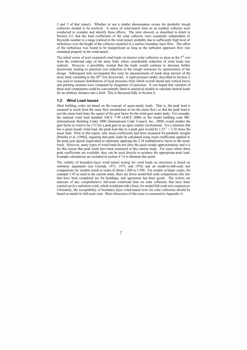
2 and 3 of that report). Whether or not a similar phenomenon occurs for parabolic troughcollectors needed to be resolved. A series of wind-tunnel tests on an isolated collector were
conducted to examine and identify these effects. The tests showed, as described in detail inSection 4.2, that the load coefficients of the solar collector were essentially independent of
Reynolds number in a range realized in the wind tunnel, probably due to sufficiently high level of turbulence over the height of the collector modeled in a surface boundary layer flow. The effect
of the turbulence was found to be insignificant as long as the turbulent approach flow wassimulated properly in the wind tunnel.
The initial series of tests examined wind loads on interior solar collectors as deep as the 5th
rowfrom the windward edge of the array field, where considerable reduction of wind loads wasrealized. However, a possibility existed that the loads would continue to decrease further downwind, leading to potential cost reduction in the trough structures by optimization of the
design. Subsequent tests investigated this issue by measurements of loads deep interior of thearray field, extending to the 20
throw downwind. A rigid pressure model, described in Section 2,
was used to measure distributions of local pressures from which overall lateral and vertical forcesand pitching moment were computed by integration of pressures. It was hoped that variation of
these load components could be conveniently fitted to analytical models to calculate desired loadsfor an arbitrary distance into a field. This is discussed fully in Section 4.
1.2 Wind Load Issues
Most building codes are based on the concept of quasi-steady loads. That is, the peak load is
assumed to result from the same flow mechanisms as for the mean flow, so that the peak load is just the mean load times the square of the gust factor for the wind gust under study. For example,the national wind load standard ASCE 7-98 (ASCE 2000) or the model building code IBC(International Building Code) 2000 (International Code Council, Inc., 2000) would predict thegust factor in wind to be 1.53 for a peak gust in an open country environment. For a structure that
has a quasi-steady wind load, the peak load due to a peak gust would be 1.532
= 2.34 times themean load. Prior to this report, only mean coefficients had been measured for parabolic troughs[Peterka et al. (1980)], requiring that peak loads be calculated using mean coefficients applied at
the peak gust speeds (equivalent to uniformly applying the 2.34 multiplicative factor to the meanload). However, many types of wind loads do not obey the quasi-steady approximation, and it is
for this reason that peak loads have been measured in this current study. For cases where these peak coefficients are available, they can be used directly to produce the appropriate peak load.
Example calculations are included in section 4.7.4 to illustrate this point.
The validity of boundary-layer wind tunnel testing for wind loads on structures is based onsimilarity arguments (see Cermak, 1971, 1975, and 1976) and on model-to-full-scale test
comparisons for models tested at scales of about 1:200 to 1:500. For models at larger scales, for example 1:45 as used in the current study, there are fewer model/full scale comparisons (the fewthat have been completed are for buildings, and agreement has been good). The writers areunaware of any comprehensive full-scale wind-load tests on solar collectors that have beencarried out in a turbulent wind, which would provide a basis for model/full-scale test comparison.
Ultimately, the acceptability of boundary-layer wind-tunnel tests for solar collectors should be based on model-to-full-scale tests. More discussion of this issue is contained in Appendix A.
2
7/31/2019 Wind Tunnel Test
http://slidepdf.com/reader/full/wind-tunnel-test 12/243
2. TEST SETUP AND PROCEDURES
Modeling of the aerodynamic loading on a structure requires special consideration of flow
conditions to obtain similitude between the model and the prototype. A detailed discussion of thesimilarity requirements and their wind-tunnel implementation can be found in Cermak (1971,
1975, 1976). In general, the requirements are that the model and prototype be geometricallysimilar, that the approach mean velocity at the model building site have a vertical profile shapesimilar to the full-scale flow, and that the Reynolds Number for the model and prototype be
equal.
These criteria are satisfied by constructing a scale model of the structure and its surroundings and by performing the tests in a wind tunnel specifically designed to model atmospheric boundary-layer flows. Reynolds Number similarity requires that the quantity UD/ ν (the ratio of flow inertiaforce to viscous force) be similar for model and prototype. Since ν, the kinematic viscosity of air,
is identical for both, Reynolds Numbers cannot be made equal with a reasonable wind velocity,for such a velocity would introduce unacceptable compressibility effects. However, for sufficiently high Reynolds Numbers (>2 x 10⁴) the pressure coefficient at any location on a blunt,
sharp-edged body becomes independent of the Reynolds Number. Thus, an exact equality of the
Reynolds Number is no longer required for similarity. On the other hand, the pressure coefficienton a streamlined body, such as a circular cylinder, is known to vary over the wide range of theReynolds number typically encountered at full (106 – 107) and model (5 x 10⁴) scales.
For streamlined bodies such as a circular cylinder or a sphere, on the other hand, it is known that
the load coefficients are highly dependent on the Reynolds Number above the typical range of theReynolds Number for wind-tunnel models. The main geometric features of the solar collectorsconsisted of reflective concentrator panels assembled in a thin parabolic shape; therefore, a
possible Reynolds Number effect that would invalidate the model test was addressed. A series of
preliminary tests as described in Section 4.2 indicated that the necessary Reynolds Number independence for the aerodynamic performance of the parabolic solar collectors could beadequately achieved in a wind tunnel. All model tests reported herein were performed at a
sufficiently high velocity to maintain the independence of Reynolds Number. That is, the modelReynolds number was sufficiently high such that the measured pressure and load coefficients
were essentially independent of the Reynolds number. As such the wind-tunnel data presented inthis report are directly applicable to full-scale parabolic solar collectors.
2.1 Boundary Layer Simulation Technique
The wind-tunnel test was performed in the boundary-layer wind tunnel in the Wind Engineering
Laboratory of CPP (Figure 2-1). This closed-circuit wind tunnel had a 68-ft-long test sectioncovered with roughness elements to reproduce at model scale the atmospheric windcharacteristics required for the model test. Some of these wind characteristics pertaining to windload are explained in Appendix C. The wind tunnel had a flexible roof, adjustable in height, tomaintain a zero pressure gradient along the test section and to minimize blockage effects.
The wind-tunnel floor upstream from the modeled area was covered with roughness elementsconstructed from 0.75-in. cubes. Spires and a low barrier were installed in the test sectionentrance to provide a thicker boundary layer than would otherwise be available, permitting asomewhat larger scale model. The spires, barrier, and roughness were designed to provide amodeled atmospheric boundary layer approximately 4 ft thick and a mean velocity power law
exponent and turbulence structure in the modeled atmospheric boundary layer similar to thatexpected in open country. Figure 2-2 is a photograph of the test section of the wind tunnel as
3

7/31/2019 Wind Tunnel Test
http://slidepdf.com/reader/full/wind-tunnel-test 13/243
modeled. The approach wind established for the model test is explained more fully in Section4.1.
Figure 2-1 CPP aerodynamic wind tunnel
2.2 Wind-Tunnel Models
Four types of wind-tunnel models of a parabolic trough solar collector were constructed for this
wind-tunnel study. They were (1) a light-weight model for measuring lift and drag dynamic windloads using a high-frequency force balance, (2) a light-weight model instrumented with a set of strain gages for direct measurement of pitching moment, (3) a rigid plastic model instrumentedwith pressure taps for measuring pressure distribution over the surface of the collector concentrator component, and (4), in the array field studies, a number of non-instrumented dummy
mock-ups surrounding the instrumented model. The instrumented models and the mock-ups wereconstructed at a scale of 1:45 based on the set of dimensions consistent with the SolargenixEnergy parabolic trough. These overall dimensions are identical to those of the LS-2 collector (Cohen, 1999) and are expected to result in non-dimensional load data applicable over a range of modest variations in parabolic trough configurations. The thickness and rear side details of the
concentrator component compared to an actual collector were not viewed as critical aspects of thewind test model configuration, with the possible exception of a torque tube, which is discussedlater in this report. In the following sections, the wind-tunnel models and construction techniqueare described.
4

7/31/2019 Wind Tunnel Test
http://slidepdf.com/reader/full/wind-tunnel-test 14/243
Figure 2-2 Wind tunnel setup
2.2.1 Balance Model for Lift and Drag Force Measurements
Both balance models1 consisted of all key features of a parabolic trough solar collector, including
a main parabolic concentrator module, support pylons, and the receiver and collector support pedestals. The main concentrator component was made of solid plastic, molded using stereolithography apparatus (SLA) technology. The concentrator model was 1/8 in. thick at the chordcenter and tapered to 1/16 in. thick at the top and bottom edges. The thickness was varied tomaintain stiffness near the location where the concentrator was fastened as well as to obtain
lightness in weight.
The model used for lift and drag measurements consisted of a pair of aluminum arms glued toeither side of the concentrator component, which was then attached to an aluminum pedestal with
setscrews for support and to permit the concentrator to rotate a full 360 degrees about thedesignated center of rotation. The arms also held a replica of the receiver made of a 1/16-in. OD
brass pipe and a removable torque tube replica at the back center of the concentrator module. A5/16-in. OD brass tube was used to model the torque tube for selected test runs. The aluminum
pedestals, or pylons, were slightly oversized for the model, compared to the actual support
pylons, in order to obtain sufficient rigidity required for measuring accurate dynamic windloading.
The entire solar collector model was mounted on a high-frequency force balance consisting of sets of strain-gage transducers, designed by CPP that measured horizontal force. The force
balance was coupled by FUTEK load cells, Model L2357, with a rated capacity of 2 lbs. tomeasure the vertical force.
1 A balance model is also referred to as a dynamic model since it is designed to measure fluctuating wind
load as well as mean load.
5

7/31/2019 Wind Tunnel Test
http://slidepdf.com/reader/full/wind-tunnel-test 15/243
A photograph of this balance model is given in Figure 2-3, and the assembly is illustrated inFigure 2-4.
Figure 2-3 Lift and drag force balance model
CPP High-Frequency Shear Balance (Details not shown)
CPP High-Frequency Moment Balance (Details not shown)
Center of Rotation of Moment Balance
Center of Rotation of
Solar Collector
Model Mounting Bracket
Receiver Torque Tube
Mounting Hole
Lift Force Transducer
Balance Model Assembly
Support
Ground Level
Figure 2-4 Lift and drag force balance model assembly
6

7/31/2019 Wind Tunnel Test
http://slidepdf.com/reader/full/wind-tunnel-test 16/243
2.2.2 Balance Model for Pitching Moment Measurements
The pitching moment balance model consisted of the parabolic module described above mounted
on a miniature torque transducer designed and built specifically for this purpose. The torquetransducer was made of an aluminum tube, and cantilevered out from a rigid aluminum reaction
post. The transducer was instrumented with 4 strain gages wired into a conventional Wheatstone bridge circuit for direct measurement of torsion about the principle axis of the tube. The parabolic module was mounted at the open end of the transducer, matching the pivot center, for
delivering overall pitching moment directly to the torque transducer.The torque transducer was essentially a thin-wall aluminum tube. It measured 1 inch in
length and 0.5 inch in OD with a wall thickness of 1/16 inch. These dimensions, particularly thewall thickness, were selected to obtain adequate sensitivity in the anticipated range of pitchingmoment while maintaining required stiffness for measurement of the wind load fluctuations. Atthe expected maximum load, the new transducer was designed to yield 2 µ-strains in the primaryshear direction.
A photograph of the balance model is given in Figure 2-5, and the assembly is illustrated inFigure 2-6.
Figure 2-5 Photograph of Pitching Moment Balance Model
7

7/31/2019 Wind Tunnel Test
http://slidepdf.com/reader/full/wind-tunnel-test 17/243
Balance Model Assembly
Aluminum Base Plate
Torque Transducer
with Strain Gages
Aluminum
Reaction Post
Aluminum Frame
Mounting Bolt
Figure 2-6 Pitching Moment Balance Model Assembly
2.2.3 Pressure Model
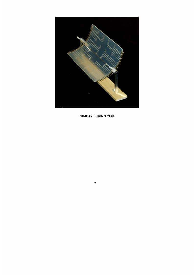
A pressure model was designed to measure the distribution of local pressures on the front and
back surfaces of the collector concentrator module. The model was made of a 1/5-in. plastic witha total of 60 pressure taps pre-installed using the SLA technique. Thirty pressure taps were
dedicated to measure pressures on the front surface, with thirty corresponding taps on the back surface. The pressure taps were laid out so that differential pressures across the collector concentrator could be numerically obtained by pairing the pressure taps on the front surface with
the corresponding taps on the back surface. The pressure taps were 1/32-in. diameter, and pressures sensed at these taps were routed to the sides of the model where plastic tubes directedthe pressure input to transducers mounted underneath the turntable.
Pressures over the concentrator modules can vary in space and time, because of spatial and
temporal variation in approach velocity (turbulence), the bluff geometry of the solar collector,and the wide range of the operational conditions. Surrounding solar collectors and wind barriersalso affect the pressure distributions. The variation of pressures near the corners and edges of the
solar collector can be very large. To capture the large pressure gradient anticipated, several pressure taps were placed near the extreme corners and edges of the model. It should be noted
that the number of the pressure taps incorporated in the model is probably the physical upper limitwithout overly distorting its geometry.
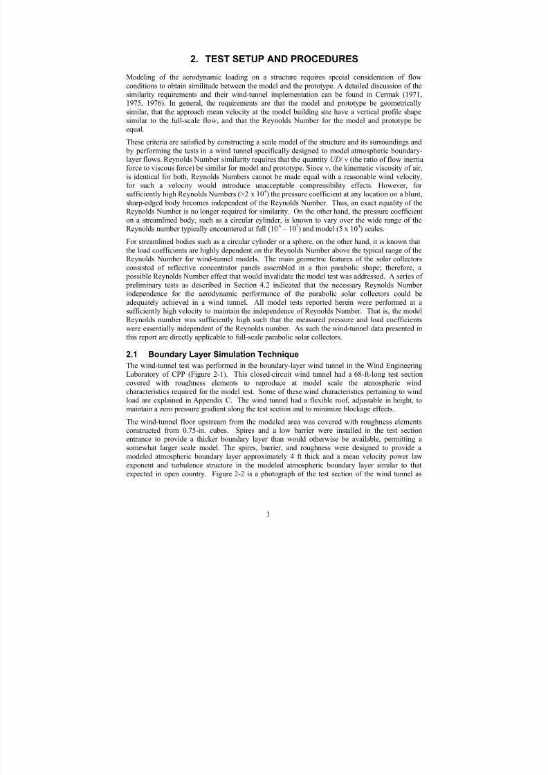
The concentrator component of the pressure model had overall dimensions identical to those of
the balance model counterpart except for somewhat larger thickness to accommodate the pressuretaps. The other model components including the support legs, arms, and receiver wereconstructed similarly, if not identically, to those for the balance model. Figure 2-7 shows a
photograph of the pressure model, and the pressure tap locations are schematically shown inFigure 2-8.
The exact locations of the pressure taps are given in Figure 2-9 using the local coordinate system projected on the vertical plane.
8
7/31/2019 Wind Tunnel Test
http://slidepdf.com/reader/full/wind-tunnel-test 18/243
Figure 2-7 Pressure model
9

7/31/2019 Wind Tunnel Test
http://slidepdf.com/reader/full/wind-tunnel-test 19/243
Pressure Model Assembly and Pressure Tap Numbers
Pressure Tap Access Holes
Front
Back
101 106
107 112
113 118
125
119 124
130
206 201
207 212
213218
219224
225 230
Figure 2-8 Pressure model assembly
10
7/31/2019 Wind Tunnel Test
http://slidepdf.com/reader/full/wind-tunnel-test 20/243
Back
206 201
207 212
213218
219224
225 230
z
y
Front
101 106
107 112
113 118
125
119 124
130
z
y
Front
Tap y, ft z, ft Tap y, ft z, ft Tap y, ft z, ft Tap y, ft z, ft Tap y, ft z, ft
101 -12.05 7.46 107 -12.05 3.95 113 -12.05 0.00 119 -12.05 -3.95 125 -12.05 -7.46
102 -7.26 7.46 108 -7.26 3.95 114 -7.26 0.00 120 -7.26 -3.95 126 -7.26 -7.46
103 -2.48 7.46 109 -2.48 3.95 115 -2.48 0.00 121 -2.48 -3.95 127 -2.48 -7.46
104 2.48 7.46 110 2.48 3.95 116 2.48 0.00 122 2.48 -3.95 128 2.48 -7.46
105 7.26 7.46 111 7.26 3.95 117 7.26 0.00 123 7.26 -3.95 129 7.26 -7.46
106 12.05 7.46 1 12 12.05 3.95 1 18 12.05 0.00 1 24 12.05 -3.95 1 30 12.05 -7.46
Back
Tap y, ft z, ft Tap y, ft z, ft Tap y, ft z, ft Tap y, ft z, ft Tap y, ft z, ft
201 12.05 7.02 2 07 12.05 3.54 213 11.67 0.00 219 12.05 -3.54 2 25 12.05 -7.02
202 6.70 7.58 208 6.70 4.10 214 6.70 0.00 220 6.70 -4.10 226 6.70 -7.58
203 1.83 7.58 209 1.83 4.10 215 1.83 0.00 221 1.83 -4.10 227 1.83 -7.58
204 -1.83 7.58 210 -1.83 4.10 2 16 -1.83 0.00 222 -1.83 -4.10 228 -1.83 -7.58
205 -6.70 7.58 211 -6.70 4.10 2 17 -6.70 0.00 223 -6.70 -4.10 229 -6.70 -7.58
206 -12.05 7.02 212 -12.05 3.54 218 -11.67 0.00 224 -12.05 -3.54 230 -12.05 -7.02
Figure 2-9 Coordinates of pressure taps
11

7/31/2019 Wind Tunnel Test
http://slidepdf.com/reader/full/wind-tunnel-test 21/243
2.2.4 Non-Instrumented Solar Collector Models
The test program called for multi-configuration wind-tunnel tests on solar collectors at different
locations within an array of collectors. To model a field of solar collectors, a number of non-instrumented collector models were constructed, which would surround the instrumented model.The non-instrumented models, also referred to as dummy mockups, were made with readily
available PVC pipes with a 6-in. OD cut in proper size. Several dummy units were attached to along aluminum shaft supported horizontally by specially made brackets to allow rotation of the
collectors about the pitch axis.
For the array field study, the solar collector models were laid out in rows with a spacingequivalent to 2.8 times the collector aperture. A typical arrangement of the non-instrumentedsolar collectors in a field is shown in Figure 2-10.
Figure 2-10 Collector field model
2.3 Instrumentation
2.3.1 Signal Conditioner for High-Frequency Force and Moment Balances
The data acquisition system for the balance tests included Honeywell Accudata amplifier/signalconditioners and IO Tech elliptic low-pass filters from which the output DC signals were fed intoa Metrabyte analog-to-digital converter (ADC) with +/-10 volt input range at a 12-bit resolution.The force and moment balances were statically calibrated prior to the wind-tunnel tests to obtain
calibration factors for conversion of the voltage output to loads in engineering units. These force
12
7/31/2019 Wind Tunnel Test
http://slidepdf.com/reader/full/wind-tunnel-test 22/243
and moment balance systems, with the collector model mounted, had inherent natural frequenciesof higher than 40 and 80 Hz, respectively, and were sufficient for measurement of dynamic loads.
2.3.2 CPP Multi-Pressure Measurement System
Pressure data on the solar collector were acquired using the CPP multi-pressure system (MPS).
The system features simultaneous signal samples from 512 individual pressure transducers at amaximum design rate of 500 samples per second per channel. When fully configured, the MPSwould consist of four 16-channel analog-to-digital converters with a 16-bit resolution and eight
64-channel multiplexers, both manufactured by IO Tech, connected to an IEEE488 controller onboard a desktop personal computer. For the present wind-tunnel study requiring 60 pressure
taps on the model, the system was configured with a single 16-bit ADC and a multiplexer for atotal capacity of 64 data channels. The differential pressure transducers used were DataInstruments Model XPC with a full-scale range of +/-0.14 psid (differential pressure) combined
with a signal amplifier that provided a gain of 50.
The wind pressure at the model exterior was transmitted to the pressure transducer using a two-
segment plastic tube. The plastic tube consisted of a 13-in. (1/32-in. ID) section and a 36-in.(1/16 in. ID) section joined together with a small brass coupler. The inherent frequency response
characteristics of the tube system were measured before the pressure tests so that a compensationdigital filter could be designed. The response correction filter was then incorporated in the dataacquisition software and applied to the measured pressure signals during the data collection.
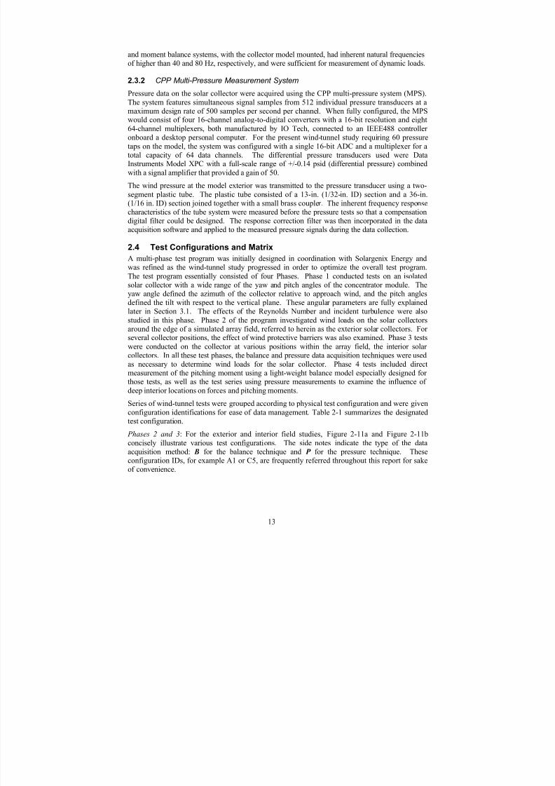
2.4 Test Configurations and Matrix
A multi-phase test program was initially designed in coordination with Solargenix Energy andwas refined as the wind-tunnel study progressed in order to optimize the overall test program.
The test program essentially consisted of four Phases. Phase 1 conducted tests on an isolatedsolar collector with a wide range of the yaw and pitch angles of the concentrator module. Theyaw angle defined the azimuth of the collector relative to approach wind, and the pitch anglesdefined the tilt with respect to the vertical plane. These angular parameters are fully explainedlater in Section 3.1. The effects of the Reynolds Number and incident turbulence were also
studied in this phase. Phase 2 of the program investigated wind loads on the solar collectorsaround the edge of a simulated array field, referred to herein as the exterior solar collectors. For several collector positions, the effect of wind protective barriers was also examined. Phase 3 tests
were conducted on the collector at various positions within the array field, the interior solar collectors. In all these test phases, the balance and pressure data acquisition techniques were used
as necessary to determine wind loads for the solar collector. Phase 4 tests included directmeasurement of the pitching moment using a light-weight balance model especially designed for those tests, as well as the test series using pressure measurements to examine the influence of
deep interior locations on forces and pitching moments.
Series of wind-tunnel tests were grouped according to physical test configuration and were given
configuration identifications for ease of data management. Table 2-1 summarizes the designatedtest configuration.
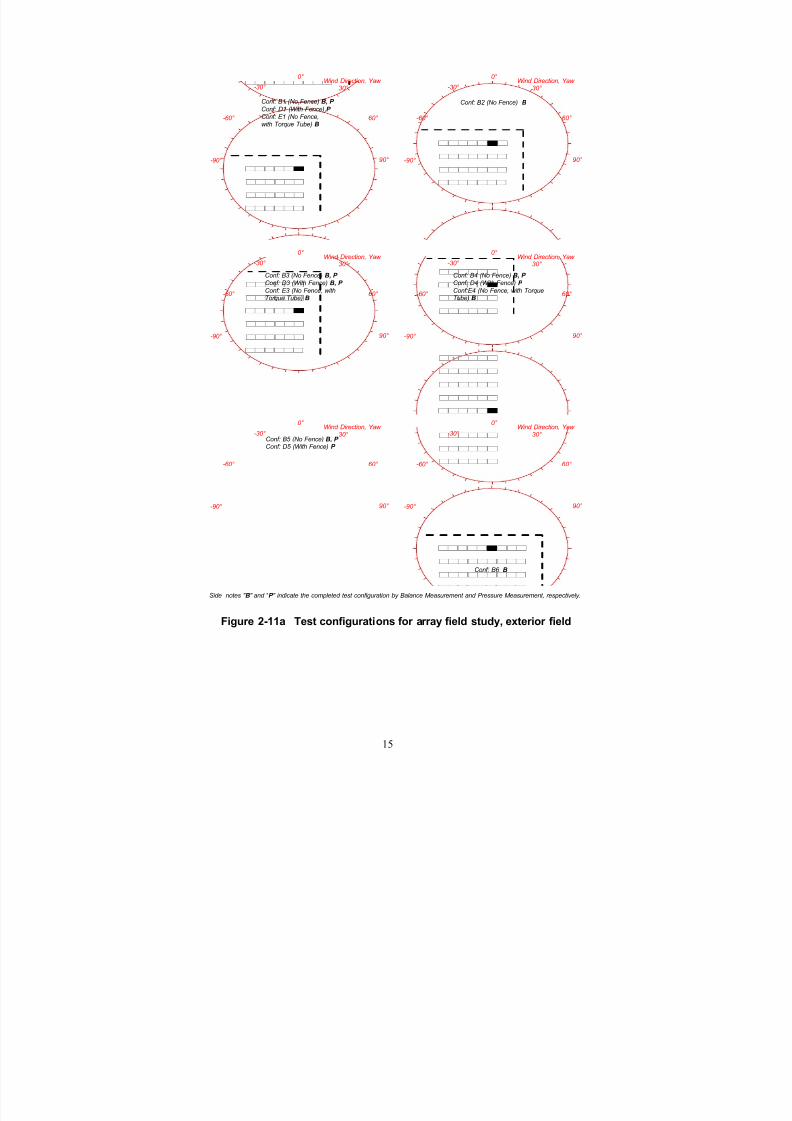
Phases 2 and 3: For the exterior and interior field studies, Figure 2-11a and Figure 2-11 b
concisely illustrate various test configurations. The side notes indicate the type of the dataacquisition method: B for the balance technique and P for the pressure technique. Theseconfiguration IDs, for example A1 or C5, are frequently referred throughout this report for sakeof convenience.
13

7/31/2019 Wind Tunnel Test
http://slidepdf.com/reader/full/wind-tunnel-test 23/243
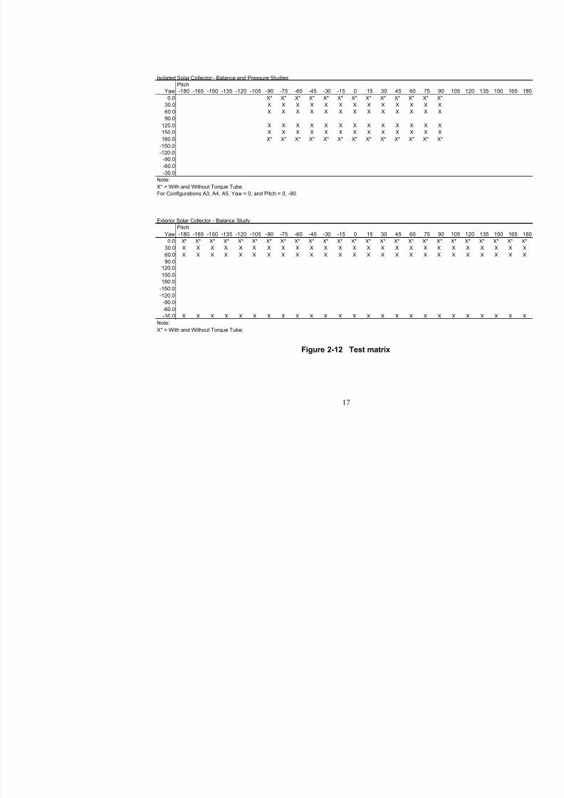
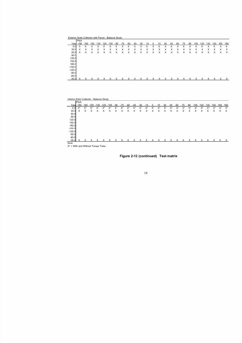
The ranges of the yaw and pitch angles varied depending on the test configurations. Figure 2-12 gives the combinations of these angles tested for different test configurations in the form of test
matrices.
Table 2-1 Test Configurations
Conf. Description A1 Single Collector in Nominal Roughness.
A2 Single Collector With Torque Tube in Nominal Roughness.
A3 Single Collector in Bare Floor.
A4 Single Collector in Smooth Roughness.
A5 Single Collector in Rough Roughness.
Bx Collector at Edge of Field. x = Position ID.
Cx Collector at Interior of Field. x = Position ID.
Dx Collector at Edge of Field With Protective Fence. x = Position ID.
Ex Collector at Edge of Field With Torque Tube. x = Position ID.
Fx Collector at Interior of Field with Torque Tube. x = Position ID.
14
7/31/2019 Wind Tunnel Test
http://slidepdf.com/reader/full/wind-tunnel-test 24/243
-90°
-60°
-30°
0°
30°
90°
60°
Wind Direction, Yaw
-90°
-60°
-30°
0°
30°
90°
60°
Wind Direction, Yaw
-90°
-60°
-30°
0°
30°
90°
60°
Wind Direction, Yaw
-90°
-60°
-30°
0°
30°
90°
60°
Wind Direction, Yaw
-90°
-60°
-30°
0°
30°
90°
60°
Wind Direction, Yaw
-90°
-60°
-30°
0°
30°
90°
60°
Wind Direction, Yaw
Conf: B1 (No Fence) B, P
Conf: D1 (With Fence) P Conf: E1 (No Fence,with Torque Tube) B
Conf: B2 (No Fence) B
Conf: B3 (No Fence) B, P Conf: D3 (With Fence) B, P
Conf: E3 (No Fence, withTorque Tube) B
Conf: B4 (No Fence) B, P Conf: D4 (With Fence) P
Conf:E4 (No Fence, with TorqueTube) B
Conf: B5 (No Fence) B, P Conf: D5 (With Fence) P
Conf: B6 B
Side notes " B" and " P " indicate the completed test configuration by Balance Measurement and Pressure Measurement, respectively.
Figure 2-11a Test configurations for array field study, exterior field
15

7/31/2019 Wind Tunnel Test
http://slidepdf.com/reader/full/wind-tunnel-test 25/243
be used directly for the pr esent solar collector data because (1) the ASCE wind speeds are givenas a 3-second gust speed rather than a mean speed adopted for the wind-tunnel test, and (2) the
ASCE wind speeds are referenced at an elevation of 33 ft rather than the collector pivot height of 9.35 ft. Thus, conversion of the ASCE wind speeds is necessary using the procedures explained
in ASCE 7-98. Conversion of a 50-year wind load is also explained in ASCE 7-98 for differentmean recurrence intervals and is presented here.
Conversion of ASCE Basic Wind Speed
Consider a solar collector site in California for which ASCE 7-98 (Figure 6-1) gives the basicwind speed of V = 85 mph. Using Figure C6-1, the corresponding hourly mean wind speed at 33
ft, U 33 is obtained as
U V 33 153 85 153 55 6= = =/ . / . . mph hourly mean .
Using values implied by Table 6-4 of ASCE 7-98, the mean wind s peed at the collector pivotheight, U Hc, is given as
.
The hourly mean wind speed of 46.4 mph is the design wind speed for the solar collectors in
California.
Design Wind Loads
Based on the design wind speed, the corresponding design pressure, q, is calculated by
q U hc= = =1
20 00256 46 4 551
2 2 ρ . ( . ) . psf .
Here, the constant 0.00256 is conveniently used to obtain the reference pressure in psf from the
wind speed in mph. As an example, we wish to determine the 50-year peak design loads on the
innermost-shielded solar collectors (Configuration C5) when that collector is oriented at a –60degree pitch angle (a downward-facing stow position). We note from Table 4.1 that the largest
peak vertical force, Load Case 3, is produced at this –60 degree pitch angle, at a yaw angle of 0degrees, so this orientation is of special interest to designers. Table 4.1 shows the peak Cfz is
2.754 and the corresponding Cfx value is 1.404, and the Cmy value is 0.107. Using equations(4.5) – (4.7):
Horizontal Force fx = qLWCfx = (5.51)(25.97)(16.40)(1.404) = 3,295 lbs
Vertical Force, fz = qLWCfz = (5.51)(25.97)(16.40)(2.754) = 6,463 lbs
Pitching Moment, my = qLW 2Cmy = (5.51)(25.97)(16.40)2(0.107) = 4,118 lb-ft.
Note that these loads are to be applied simultaneously to the structure because the wind-tunnel
results were obtained as a concurrent load combination from the time series data for which thevertical f orce was maximized.
Comparison to Design Loads Determined by Quasi-Steady Assumption
As pointed out in Section 1.2, the traditional approach to obtaining the structural design loads on
solar collectors has been based on the quasi-steady assumption. With this technique, themeasured mean load is scaled to follow the gust wind speed to provide the equivalent peak load.
The scale factor is known as the gust load factor, and ASCE 7-98 or the model building code IBC
121
7/31/2019 Wind Tunnel Test
http://slidepdf.com/reader/full/wind-tunnel-test 26/243
Isolated Solar Collector - Balance and Pressure Studies
Pitch
Yaw -180 -165 -150 -135 -120 -105 -90 -75 -60 -45 -30 -15 0 15 30 45 60 75 90 105 120
0.0 X* X* X* X* X* X* X* X* X* X* X* X* X*
30.0 X X X X X X X X X X X X X60.0 X X X X X X X X X X X X X
90.0
120.0 X X X X X X X X X X X X X
150.0 X X X X X X X X X X X X X
180.0 X* X* X* X* X* X* X* X* X* X* X* X* X*
-150.0
-120.0
-90.0
-60.0
-30.0
Note:
X* = With and Without Torque Tube.
For Configurations A3, A4, A5, Yaw = 0, and Pitch = 0, -90.
Exterior Solar Collector - Balance Study
Pitch
Yaw -180 -165 -150 -135 -120 -105 -90 -75 -60 -45 -30 -15 0 15 30 45 60 75 90 105 120
0.0 X* X* X* X* X* X* X* X* X* X* X* X* X* X* X* X* X* X* X* X* X*
30.0 X X X X X X X X X X X X X X X X X X X X X
60.0 X X X X X X X X X X X X X X X X X X X X X
90.0120.0
150.0
180.0
-150.0
-120.0
-90.0
-60.0
-30.0 X X X X X X X X X X X X X X X X X X X X X
Note:X* = With and Without Torque Tube.
Figure 2-12 Test matrix
17
7/31/2019 Wind Tunnel Test
http://slidepdf.com/reader/full/wind-tunnel-test 27/243
Exterior Solar Collector with Fence - Balance Study
Pitch
Yaw -180 -165 -150 -135 -120 -105 -90 -75 -60 -45 -30 -15 0 15 30 45 60 75 90 105 12
0.0 X X X X X X X X X X X X X X X X X X X X X30.0 X X X X X X X X X X X X X X X X X X X X X
45.0 X X X X X X X X X X X X X X X X X X X X X
90.0
120.0
150.0
180.0
-150.0
-120.0
-90.0
-60.0
-30.0 X X X X X X X X X X X X X X X X X X X X X
Interior Solar Collector - Balance Study
Pitch
Yaw -180 -165 -150 -135 -120 -105 -90 -75 -60 -45 -30 -15 0 15 30 45 60 75 90 105 12
0.0 X* X* X* X* X* X* X* X* X* X* X* X* X* X* X* X* X* X* X* X* X*
30.0 X X X X X X X X X X X X X X X X X X X X X
60.0
90.0
120.0
150.0
180.0
-150.0
-120.0
-90.0
-60.0
-30.0 X X X X X X X X X X X X X X X X X X X X X
Note:
X* = With and Without Torque Tube.
Figure 2-12 (continued) Test matrix
18

7/31/2019 Wind Tunnel Test
http://slidepdf.com/reader/full/wind-tunnel-test 28/243
Exterior Solar Collector - Pressure Study
Pitch
Yaw -180 -165 -150 -135 -120 -105 -90 -75 -60 -45 -30 -15 0 15 30 45 60 75 90 105 12
0.0 X X X X X X X X X X X X X30.0 X X X X X X X X X X X X X
45.0 X X X X X X X X X X X X X
90.0
120.0
150.0
180.0
-150.0
-120.0
-90.0
-60.0
-30.0 X X X X X X X X X X X X X
Exterior Solar Collector with Fence - Pressure Study
Pitch
Yaw -180 -165 -150 -135 -120 -105 -90 -75 -60 -45 -30 -15 0 15 30 45 60 75 90 105 120
0.0 X X X X X X X X X X X X X X X X X X X X X
30.0 X X X X X X X X X X X X X X X X X X X X X
45.0 X X X X X X X X X X X X X X X X X X X X X
90.0
120.0
150.0
180.0
-150.0
-120.0
-90.0
-60.0
-30.0 X X X X X X X X X X X X X X X X X X X X X
Figure 2-12 (continued) Test matrix
19

7/31/2019 Wind Tunnel Test
http://slidepdf.com/reader/full/wind-tunnel-test 29/243
20
Interior Solar Collector - Pressure Study
Pitch
Yaw -180 -165 -150 -135 -120 -105 -90 -75 -60 -45 -30 -15 0 15 30 45 60 75 90 105 12
0.0 X* X* X* X* X* X* X* X* X* X* X* X* X* X* X* X* X* X* X* X* X
30.0 X* X* X* X* X* X* X* X* X* X* X* X* X* X* X* X* X* X* X* X* X
60.0
90.0
120.0
150.0
180.0
-150.0
-120.0
-90.0
-60.0
-30.0 X* X* X* X* X* X* X* X* X* X* X* X* X* X* X* X* X* X* X* X* X
Note:
X* = With and Without Torque Tube.
Figure 2-12 (continued) Test matrix

7/31/2019 Wind Tunnel Test
http://slidepdf.com/reader/full/wind-tunnel-test 30/243
Phase 4: Figure 2-13 illustrates the configurations of the solar collectors tested for the additional pitching moment tests. These test configurations had been investigated in the Phase 2 and 3 tests,
and were repeated here for comparison purposes. The selection of the configurations was basedlargely on the test results from the earlier Phase that exhibited significant pitching moments. For
all the indicated configurations, the tests were conducted for a full rotation of the pitch angle atintervals of 15 degrees. (Refer to Figure 2-10 and Figure 2-13 that show the test setup for
Configuration C5 at a yaw angle of –30 degrees.)
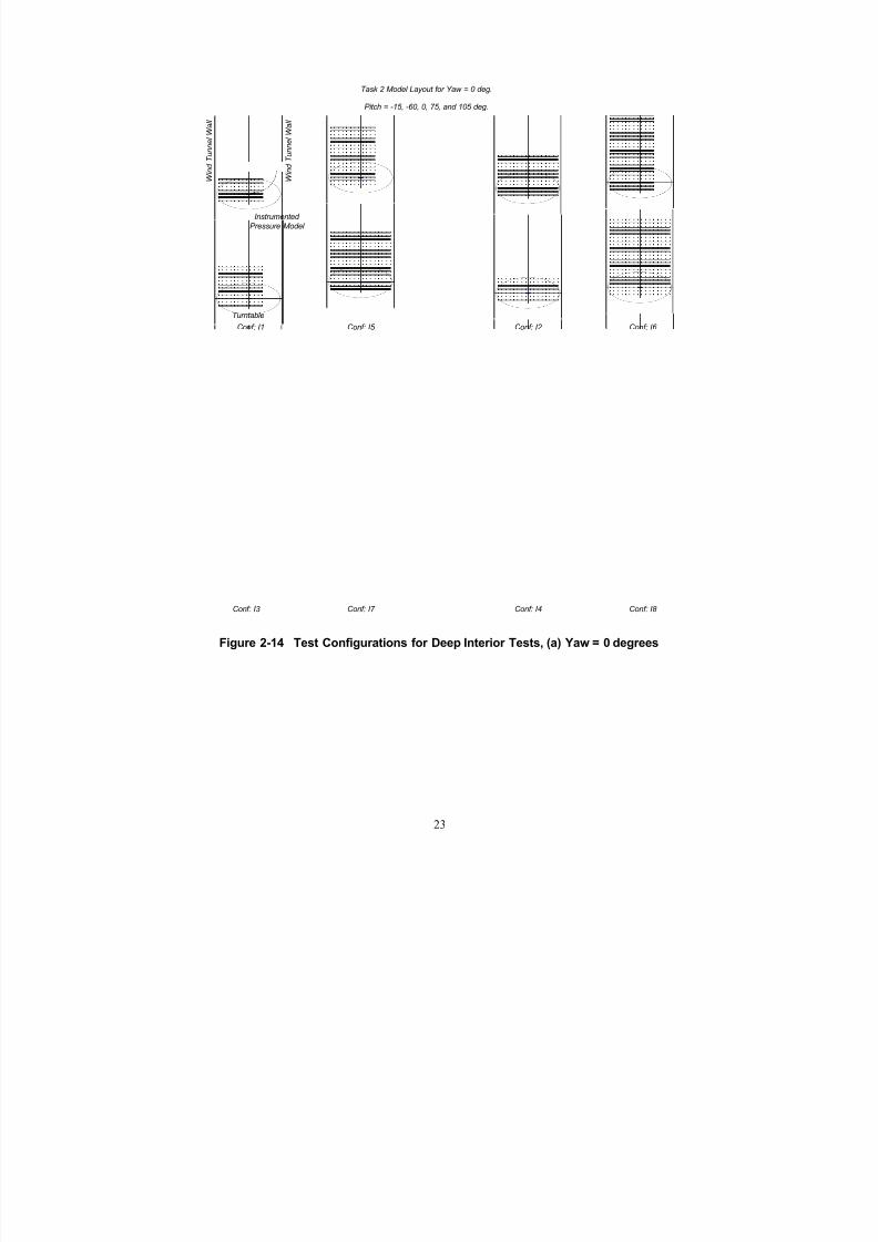
The test configurations for the deep interior tests are shown in Figure 2-14. The pressuredistribution over the collector concentrator was measured on the unit at the 5th, 10th, 15th and20th rows from the upwind edge of the array field for the yaw angle of 0 degrees (Figure2-14(a)). Two column positions, 4th and 8th from the open side edge, were also tested at thisyaw angle. At a yaw angle of 30 degrees (Figure 2-14(b)), the row positions of 5th, 10th and
15th, and the column positions of 4th, 8th and 12th were tested. A limited set of pitch angleswere of interest, including -15, -60, 0, 75 and 105 degrees, at which the Phase 3 wind-tunnel
study showed relatively large integrated wind loads. Note that Configurations I2 and I3 arenearly identical. To optimize the test program, Configuration I3 was eliminated from the test
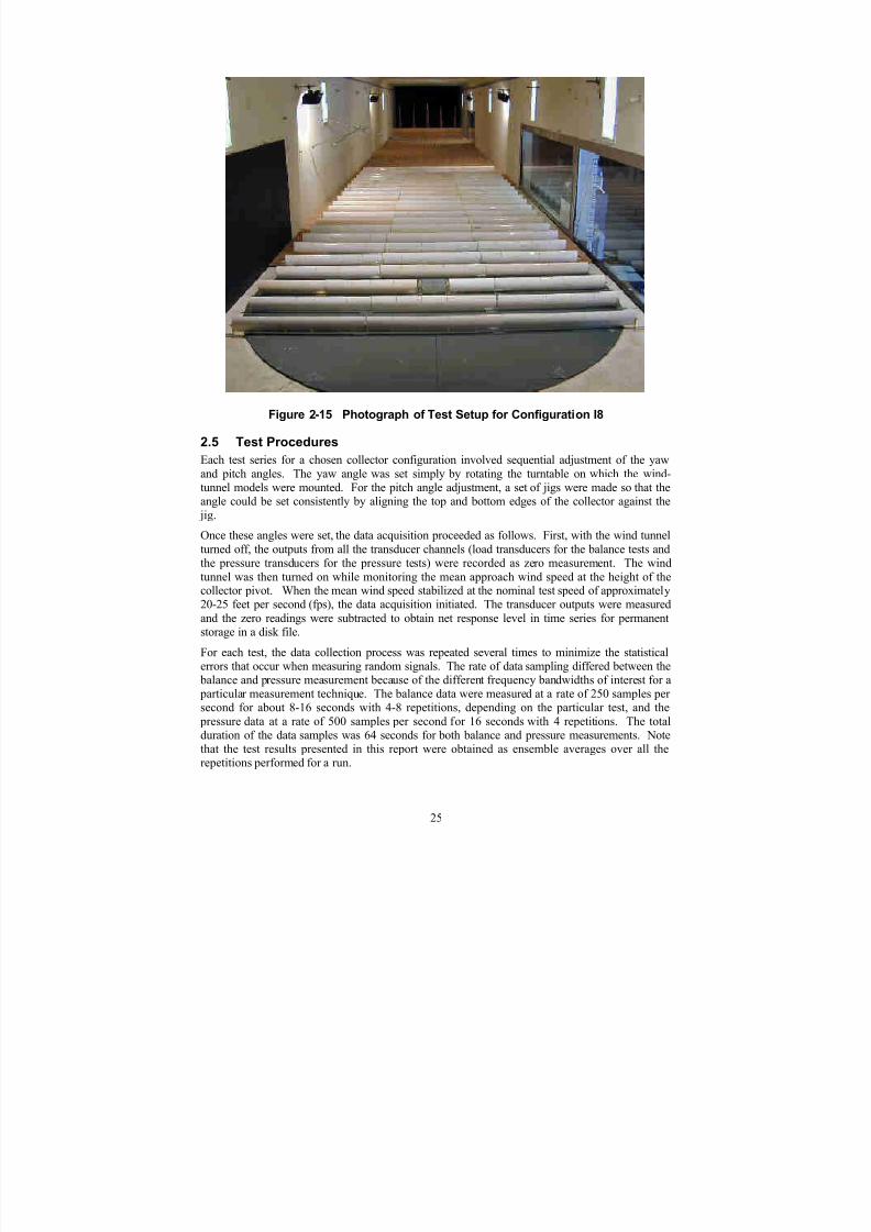
plan. In this report, the test results obtained for Configuration I2 also substitute for thosereferring to Configuration I3 for convenience. A photograph of one of the test setups,Configuration I8, is given in Figure 2-15.
21

7/31/2019 Wind Tunnel Test
http://slidepdf.com/reader/full/wind-tunnel-test 31/243
-90°
-60°
-30°
0°
30°
90°
60°
Wind Direction, Yaw
Conf: A1
-90°
-60°
-30°
0°
30°
90°
60°
Wind Direction, Yaw
Conf: B1
-90°
-60°
-30°
0°
30°
90°
60°
Wind Direction, Yaw
Conf: B2
-90°
-60°
-30°
0°
30°
90°
60°
Wind Direction, Yaw
Conf: B3
Task 1 Model Layout
Pitch = -180 to 180 deg. at 15 deg. increments
Instrumented Dynamic Model for Direct
Measurement of Pitching Moment
-90°
-60°
-30°
0°
30°
90°
60°
Wind Direction, Yaw
Conf: C5
-90°
-60°
-30°
0°
30°
90°
60°
Wind Direction, Yaw
Conf: C2
Figure 2-13 Test Configurations for Phase 4
22
7/31/2019 Wind Tunnel Test
http://slidepdf.com/reader/full/wind-tunnel-test 32/243
W i n d
T u n n e l W a l l
Turntable
Instrumented
Pressure Model
W i n d
T u n n e l W a l l
Task 2 Model Layout for Yaw = 0 deg.
Pitch = -15, -60, 0, 75, and 105 deg.
Conf: I1 Conf: I2
Conf: I3 Conf: I4
Conf: I5 Conf: I6
Conf: I7 Conf: I8
Figure 2-14 Test Configurations for Deep Interior Tests, (a) Yaw = 0 degrees
23

7/31/2019 Wind Tunnel Test
http://slidepdf.com/reader/full/wind-tunnel-test 33/243
Task 2 Model Layout for Yaw = 30 deg.
Pitch = -15, -60, 0, 75, and 105 deg.
Note: Configurations I2 and I3 are nearly identical. The test results for Conf. I2 substitute Conf. I3.
Conf: I1 Conf: I5
Conf: I2* Conf: I6
Conf: I3* Conf: I7
Conf: I10
Conf: I11
Conf: I9
Figure 2-14 Test Configurations for Deep Interior Tests, (b) Yaw = 30 degrees
24
7/31/2019 Wind Tunnel Test
http://slidepdf.com/reader/full/wind-tunnel-test 34/243
Figure 2-15 Photograph of Test Setup for Configuration I8
2.5 Test Procedures
Each test series for a chosen collector configuration involved sequential adjustment of the yaw
and pitch angles. The yaw angle was set simply by rotating the turntable on which the wind-tunnel models were mounted. For the pitch angle adjustment, a set of jigs were made so that the
angle could be set consistently by aligning the top and bottom edges of the collector against the jig.
Once these angles were set, the data acquisition proceeded as follows. First, with the wind tunnel
turned off, the outputs from all the transducer channels (load transducers for the balance tests andthe pressure transducers for the pressure tests) were recorded as zero measurement. The wind
tunnel was then turned on while monitoring the mean approach wind speed at the height of thecollector pivot. When the mean wind speed stabilized at the nominal test speed of approximately20-25 feet per second (fps), the data acquisition initiated. The transducer outputs were measured
and the zero readings were subtracted to obtain net response level in time series for permanentstorage in a disk file.
For each test, the data collection process was repeated several times to minimize the statistical
errors that occur when measuring random signals. The rate of data sampling differed between the balance and pressure measurement because of the different frequency bandwidths of interest for a particular measurement technique. The balance data were measured at a rate of 250 samples per second for about 8-16 seconds with 4-8 repetitions, depending on the particular test, and the
pressure data at a rate of 500 samples per second for 16 seconds with 4 repetitions. The totalduration of the data samples was 64 seconds for both balance and pressure measurements. Notethat the test results presented in this report were obtained as ensemble averages over all therepetitions performed for a run.
25

7/31/2019 Wind Tunnel Test
http://slidepdf.com/reader/full/wind-tunnel-test 35/243
2.6 Accuracy and Uncertainty of Test Results
Complete analysis of accuracy and uncertainty associated with load measurements performedwith a wind tunnel is no trivial matter. It would require, in general, sophisticated statisticalinvestigation on random processes as well as characterization of instruments used. Although anextensive effort might be prudent in many engineering practices, this section limits the analysis to
two readily identifiable sources of uncertainties: (1) the statistical variation of the measured meanloads and (2) the performance of the instruments.
Because fluctuations of wind loads are random in nature, determination of their true mean and
root mean square (standard deviation) theoretically requires infinitely long measurement duration.Although this is not possible, acceptable estimates of these quantities can be obtained by
cumulating the statistical results over several repeated measurements of reasonable length. As anexample, Figure 2-16a illustrates the variation of the mean loads measured by the force balanceon an isolated solar collector over repeated tests. The data were taken for 16 extendedmeasurements (compared to the nominal 8), and the overall means were assumed to represent thetrue values. All the load components asymptotically converge to the assumed true means as the
number of measurements increases. Figure 2-16 b shows a similar plot for a typical pressuremeasurement in a wind tunnel.
The load measurement instrument consisted of the force and pressure transducers, signalconditioner, and analog-to-digital converter. This equipment can be a source of measurementuncertainty because of, for example, non-linear response, instability, and limited resolution. A
careful calibration of the instrument revealed the response characteristics and the possible worsterror in the measured loads.
Variation o f Mean L oad With Number of Balan ce Measu reme nts
Configuration A1, Yaw = 0 deg., Pitch = -90 de g.
Numbe r of Measurements (Nom inally 8 for presen t balance study)
0 5 10 15 20
M e a n C o e f f i c i e n t
0.1
0.2
0.3
0.4
Cfx Cfz
Ass umed True Means
8
Δ = 0.011
Δ = 0.013
Variation o f Mean L oad With Number of Balan ce Measu reme nts
Configuration A1, Yaw = 0 deg., Pitch = -90 de g.
Numbe r of Measurements (Nom inally 8 for presen t balance study)
0 5 10 15 20
M e a n C o e f f i c i e n t
0.1
0.2
0.3
0.4
Cfx Cfz
Ass umed True Means
CfxCfx CfzCfz
Ass umed True Means
8
Δ = 0.011
Δ = 0.013
Figure 2-16a Typical statistical variation of mean loadmeasurement, balance study2
2 Figure 2-16a,b show how long the measurement should be to obtain a statistically accurate meanestimate. To do this, multiple measurements were repeated, each measurement with the equal
sample duration, and the means were computed from individual measurements. What is plottedin these Figures is the cumulative means with the increasing number of sample blocks. That is,the first (left-most) point represents the mean computed from the first sample block only. The
26

7/31/2019 Wind Tunnel Test
http://slidepdf.com/reader/full/wind-tunnel-test 36/243
Typical Variation of Mean Pressure With Number of
Measurements
Number of Measurements (4 for present pressure study)
0 5 10
M e a n C o e f f i c i e n t
-1.0
-0.5
0.0
0.5
Stagnation Region Separation Region
Assumed True Means
Δ = 0.0012
Δ = 0.0023
Figure 2-16b Typical statistical variation of mean loadmeasurement, pressure study
Table 2-2 summarizes the uncertainties in the mean load measurement caused by the above twosources and the combined effect. Note that the total errors were simply obtained as an algebraic
summation of the errors due to these two sources of uncertainty disregarding any statistical
second point was computed as an average of the means from the first and second sample blocks,effectively increasing the total sample duration. The third point is the average of the first three
sample blocks, and so forth. Obviously, the mean from the single sample block alone (the first point in the graph) has the largest uncertainty and deviates from the true mean the largest. Itseffect remains in the succeeding points, although should be gradually diminishing, because the
first mean is repeatedly used to compute the overall cumulative means. This is why the plot tendsto approach the true mean from its either side dictated by the inaccuracy of the very first mean
estimate. To be more precise, the y-axis of the graph should have been labeled “CumulativeMean Coefficient.”
Alternatively, we could have taken several measurements, each with different sample durations.If you plot the individual means from these measurements as a function of the sample duration,you would see that the mean fluctuates about the true mean with decreasing variation.
27

7/31/2019 Wind Tunnel Test
http://slidepdf.com/reader/full/wind-tunnel-test 37/243
correlation; they reflect the worst case. In average, it is reasonable to assume that the actual levelof uncertainty would be somewhat smaller than what is indicated. If these possible errors are
directly related to the largest measured mean overall loads, the uncertainties can be estimated as3% for the force and moment components for the balance study. For the pressure study, the
uncertainty of about 6% would result for all the load components. The instrument uncertainty(denoted as Source 2) shown in Table 2-2 was estimated as a combination of the worst cases that
could occur for each of the contributing load transducers, resulting in the higher level of uncertainty.
Table 2-2 Estimated Uncertainty Associated with Mean Load Measurement
fx fz my p+ p- fx fz my
Due to Source (1) 0.011 0.013 0.0042 0.0012 0.0023 0.0025 0.0035 0.00052
Due to Source (2) 0.0053 lbs. 0.0094 lbs. 0.0061 lb-in. 0.044 psf 0.044 psf 0.013 lbs. 0.018 lbs. 0.012 lb-in.
Equivalent load coef. 0.050 0.090 0.013 0.087 0.087 0.12 0.17 0.026
Total 0.061 0.103 0.017 0.088 0.089 0.13 0.18 0.026
Source (1) Statistical variation of random signal.
Source (2) Characteristics of instrumentation. The worst possible errors observed during static calibration are indicated.
Overall Load Component Pressure Component
28
7/31/2019 Wind Tunnel Test
http://slidepdf.com/reader/full/wind-tunnel-test 38/243
3. ANALYSIS METHODS
The chief objective of the present wind-tunnel study was to determine wind loads on parabolic
trough solar collectors that would provide guidelines for design. The wind load effects of interestfor the present study included the overall lateral force, vertical force, pitching moment about thecollector pivot axis, and pressure distributions over the concentrator surface. It is common
practice to present the wind loads measured in a wind tunnel in the form of load coefficientsdirectly applicable to full-scale structures through use of consistent scaling parameters. This
section describes the definition of the relevant test parameters and basic techniques involved inthe data analysis.
3.1 Definition of Test Parameters
3.1.1 Orientation of Solar Collector
Parabolic trough solar collectors are typically designed to follow the apparent motion of the sun by rotating about a one dimensional axis throughout the day. Because of this, wind loads exertedon the drive mechanism vary depending on the tilt angle of the collector, herein called the pitchangle. In addition, the incident angle of the approach wind relative to the span of the solar collector, or the yaw angle, causes the wind loads to vary. Thus, the orientation of the solar
collector, defined by the pitch and yaw angles is an important factor for evaluating theaerodynamic performance and structural design criteria of the collector. Figure 3-1 schematicallyshows the definition of the pitch and yaw angles established for the current wind-tunnel study, aswell as that of the overall loads and several characteristic dimensions of the solar collector. Itshould be noted that the two modes of operation for the solar collectors can be conveniently
distinguished by the sign of the pitch angle. That is, the positive and negative pitch angles implythe normal operation and stow modes, respectively.
29

7/31/2019 Wind Tunnel Test
http://slidepdf.com/reader/full/wind-tunnel-test 39/243
Key Dimensions
Ground Level
W = 16.40 ft
Hc = 9.32 ft
L = 25.97 ft
H = 17.52 ft
Wind
+ Yaw
Plan View
X
Y
Z up Torque Tube
(for selected tests only)
Receiver
Wind
+ Pitch
Side View
fx
fz
my
Definition of Coordinate System
0.65 ft
Figure 3-1 Definition of coordinate system and key dimensions
3.1.2 Load Coefficients
Wind load effects are characterized in terms of non-dimensional coefficients. The definitions of the load coefficients are:
30

7/31/2019 Wind Tunnel Test
http://slidepdf.com/reader/full/wind-tunnel-test 40/243
Horizontal Force, fx Cfx fx
qLW = (3.1)
Vertical Force, fz Cfz fz
qLW = (3.2)
Pitching Moment, my Cmymy
qLW =
2(3.3)
where fx, fz , and my are the aerodynamic loads (Figure 3-1), L is the span-wise length, and W isthe aperture width of the collector. The quantity, q, is the mean reference dynamic pressure
measured at the pivot height of the solar collector, Hc, as given by
q U =1
2
2 ρ (3.4)
Here U is the mean wind speed at the pivot height, and ρ is the density of air. Similarly, the pressure coefficient is expressed by
Cp p
q= (3.5)
where p is the local pressure relative to the undisturbed ambient static pressure. Because thecollector is essentially a curved thin plate composed of a number of reflective concentrator
panels, the net pressure between the opposing surfaces is of significance for the design load of thecollector structure. The net pressure, or the differential pressure coefficient, Cdp, is defined
herein as
Cdp p p
q
f = b−(3.6)
where p f and pb are the pressures on the front (reflective) side and the back side,respectively.
3.1.3 Consideration for Load Cases for Structural Strength Design
In general, parabolic trough solar collectors are either tracking the sun (normal operation) or assume a stationary downward-facing attitude called the “stow” position (at night or during
cloudy or very windy periods). During sunny periods with moderate and low winds, the solar collectors are in the normal operation mode, with the parabolic reflector rotated toward the sun.
Wind loads on the solar collectors during normal operation are a concern because deformation of the parabolic trough reflector surface can cause a loss of efficiency. During strong winds, wherethe structural strength might be a concern, the solar collectors are typically rotated to the “stow”mode with the concentrators facing down to limit wind loads and to prevent the reflective surface
from being damaged. Sufficient data were obtained in the wind-tunnel testing to provide loaddata for structural analysis in both operating modes.
Within a field of solar collectors, the largest wind loads experienced by an individual collector
module will vary depending on its position and the presence of a protective barrier. Applicationof the design loads appropriate for the exterior collector modules throughout the entire fieldwould result in over-design for most of the interior units, which in fact constitute the majority of
the field collector modules. On the other hand, use of the interior design loads on the exterior collector modules can expose those modules to higher risk of structural failure. To provide
31

7/31/2019 Wind Tunnel Test
http://slidepdf.com/reader/full/wind-tunnel-test 41/243
practical design criteria, different design load cases were determined separately for the exterior collector modules with and without a protective fence, various locations of interior modules, and
in particular the collector module denoted as Configuration C5 (Figure 2-13), which wasconsidered to be most representative for a large array field as a whole.
The load cases were derived as the loading condition that would maximize the individual overall
load components in either the positive or negative direction. Each load case specified the peak load for one component as primary and the simultaneous point-in-time load values for the other
two as extracted from the integrated pressure or balance time series data. For the structuralstrength design, applying the combination of all three load components is appropriate.
3.2 Particular Treatment of Pressure Data
While the balance tests were suited for measurement of overall loads on the solar collector,determination of the detailed load distribution required the pressure tests. The tests were
performed to measure instantaneous distribution of local pressures over the collector module at a
total of 60 locations. The results of the pressure tests were intended to allow finite elementanalysis, wherein wind forces imparted to the surfaces of a parabolic trough concentrator can be
used to determine the developed stresses and deformations of the concentrator (e.g., support
structure, parabolic-shaped mirrors, etc.). To serve this need, a number of unique pressuredistributions were determined based on several relevant load conditions. The analysis method for obtaining these pressure distributions is described in Section 3.2.2. In addition, the overall loadswere computed by integrating the distribution of the measured local pressures for comparisonwith the directly measured loads by the balance technique. The procedure is explained in thissection.
3.2.1 Integration of Distributed Local Pressures
Distribution of point pressures and differential pressures can be integrated over the parabolicconcentrator surface to numerically determine the total loads on the parabolic trough solar
collector. The resulting loads should approximate reasonably those measured directly using theforce balance. Some discrepancy can be expected because the measured pressure distribution is
discrete and the integration is, therefore, piecewise, whereas the total loads measured by the balance are, in principle, the result of true integration of continuously distributed pressures. Inaddition, the balance loads include the contribution due to not only the concentrator module itself,
but also other secondary structural elements such as the pylon supports and the receiver. Nevertheless, the comparison of the pressure and balance total loads is useful in confirming thevalidity and consistency of the test results in general and is discussed in Section 4. Here weexplain the technique used in the current study to determine the integral loads from the pressuredistribution data.
Because the pressure distribution measured on the pressure model is discrete, the integration isactually a weighted summation of point pressures:
. (3.14)Q wii
N
i=
=∑1 p
Here Q is the load effect of interest, pi is the surface pressure (or differential pressure at the taplocation I ), and N is the number of pressure taps. The quantity wi is the weight factor assigned atthe pressure tap location i. If, for example, the load effect to be obtained is force, the weightfactor typically represents the tributary area associated with the pressure tap. The weight factors
for calculation of the forces and pitching moment for all the pitch angles tested in the study aretabulated in a spreadsheet file on the CD-ROM provided to NREL as backup to this report (alsosee Appendix E).
32

7/31/2019 Wind Tunnel Test
http://slidepdf.com/reader/full/wind-tunnel-test 42/243
Figure 3-2 shows the tributary areas defined for the solar collector, as well as the differential pressure taps with the identification numbers. The boundaries indicated by dashed lines were
established to divide the distance between two adjacent pressure taps in half. The choice of thetributary areas is somewhat arbitrary, as long as each of these areas is exclusively assigned to a
particular tap, and the individual tributary areas collectively account for the entire exposed areaexerting the wind load. The pressure is usually assumed to be uniform within the tributary area.
For calculations of the horizontal and vertical forces, the effective tributary areas projected on thevertical and horizontal planes, respectively, were computed for different pitch angles, taking intoaccount the curvature of the concentrator. This was necessary to resolve the pressure load acting
perpendicular to the concentrator surface into the respective force components. The resultingeffective tributary areas were the weight factors that appear in Equation 3.14. For the pitchingmoment, the weight factors used were a combination of the tributary area and the effectivedistance about the axis of rotation.
5001 5002 5003 5004 5005 5006
5007 5008 5009 5010 5011 5012
5013 5014 5015 5016 5017 5018
5019 5020 5021 5022 5023 5024
5025 5026 5027 5028 5029 5030
Side View Frontal View
5001 - 5030 Differential Pressure Taps
Figure 3-2 Tributary areas assigned for differential pressure taps
3.2.2 Instantaneous Pressure Distributions
Simultaneous measurement of the pressure at all the tap locations permits realization of pressure
distributions at any given instant in time. In this wind-tunnel study, several conditions relevant tostructural design were identified in order to extract specific sets of pressure distributions from the
time series data stored in computer disk files. The extracted pressure distribution can be regardedas a snapshot of pressure pattern occurring when a specified condition is met. One of theconditions for the snapshot analysis was the occurrence of the peak local differential pressure at
any tap location. In this case, the time series of the differential pressures were computed for eachtap location shown in Figure 3-2, and the instantaneous pressure distribution was recorded when
the largest local differential pressure occurred regardless of the tap location. The other conditionswere associated with the occurrence of the integrated loads, described in the preceding section,exceeding a specified level, for example, the 80th percentile from minimum to maximum peaks.
33

7/31/2019 Wind Tunnel Test
http://slidepdf.com/reader/full/wind-tunnel-test 43/243
A number of snapshot pressure distributions were taken from different test configurations, andsome of the results are presented in sections 4.8.2 and 4.8.3.
3.2.3 Interpolation of Point Pressures
In order to apply the measured differential pressure distribution to the individual reflector panels
on the solar collector, spatial interpolation of these pressures may be necessary. This is becausethe pressure tap layout on the wind-tunnel model does not necessarily coincide with that of thereflector panels of the actual solar collector. This section provides a simple technique for
interpolating point pressures by a superposition of measured pressures in the vicinity of thedesired application point on the reflector panel. That is,
1
m
i
j
j j p pψ =
= ∑ , (3.15)
. (3.16)ψ j j
n
=∑ =
1
1
In this case, p j is the pressure measured at the pressure tap j, ψ j is the influence factor associatedwith the pressure tap, and m is the number of pressure taps contributing to the reflector panel.
Selection of the influence factorsψ j can be based on a common technique used in the finite
element analysis for obtaining an interior solution within a two-dimensional element. Toillustrate this, Figure 3-3 shows a case where the nodal point of the reflector panel is surrounded
by four pressure taps.
x
y
(x1, y
1) (x
2, y
2)
(x3, y
3)
Pressure Tap 1 Pressure Tap 2
Pressure Tap 3
Target Interior Node
(x, y)
(x4, y
4)
Pressure Tap 4
Figure 3-3 Interpolation of point pressures
In this example, the influence factors for each pressure tap location can be assumed to take the
following form based on the Pascal’s triangle:
(3.17) j j j j ja b x c y d xyψ = + + +
in which a j, b j, c j, and d j are the constants to be determined. The x and y are the coordinates of
the point at which the interpolated pressure is determined. For the solar collector, these
34
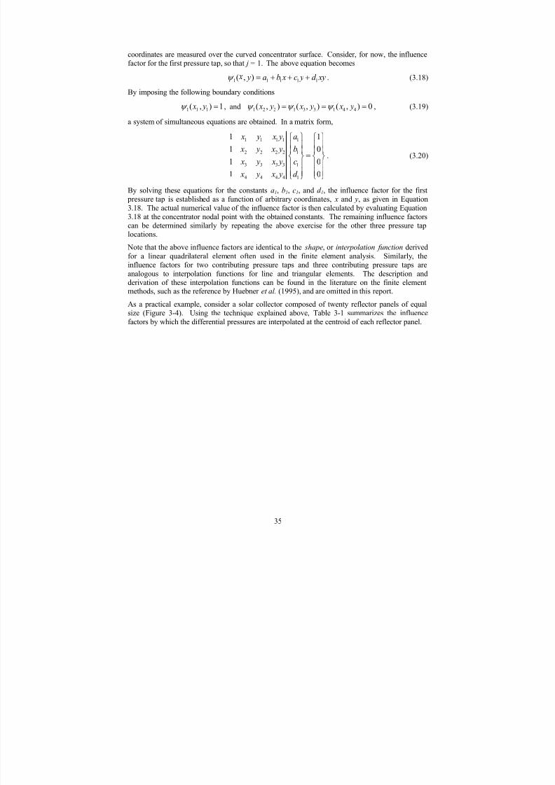
7/31/2019 Wind Tunnel Test
http://slidepdf.com/reader/full/wind-tunnel-test 44/243
coordinates are measured over the curved concentrator surface. Consider, for now, the influencefactor for the first pressure tap, so that j = 1. The above equation becomes
1 1 1 1( , ) 1 y a b x c y d xψ = + + + y . (3.18)
By imposing the following boundary conditions
, and1 1 1( , ) 1 x yψ = 1 2 2 1 3 3 1 4 4( , ) ( , ) ( , ) 0 x y x y x yψ ψ ψ = = = , (3.19)
a system of simultaneous equations are obtained. In a matrix form,
1 1 1 1 1
2 2 2 2 1
3 3 3 3 1
4 4 4 4 1
1 1
1 0
1 0
1 0
x y x y a
x y x y b
x y x y c
x y x y d
⎧ ⎫ ⎧ ⎫⎪ ⎪ ⎪ ⎪⎪ ⎪ ⎪ ⎪
=⎨ ⎬ ⎨ ⎬⎪ ⎪ ⎪ ⎪⎪ ⎪ ⎪ ⎪⎩ ⎭⎩ ⎭
. (3.20)
By solving these equations for the constants a1, b1, c1, and d 1, the influence factor for the first pressure tap is established as a function of arbitrary coordinates, x and y, as given in Equation
3.18. The actual numerical value of the influence factor is then calculated by evaluating Equation3.18 at the concentrator nodal point with the obtained constants. The remaining influence factorscan be determined similarly by repeating the above exercise for the other three pressure taplocations.
Note that the above influence factors are identical to the shape, or interpolation function derived
for a linear quadrilateral element often used in the finite element analysis. Similarly, theinfluence factors for two contributing pressure taps and three contributing pressure taps are
analogous to interpolation functions for line and triangular elements. The description andderivation of these interpolation functions can be found in the literature on the finite elementmethods, such as the reference by Huebner et al. (1995), and are omitted in this report.
As a practical example, consider a solar collector composed of twenty reflector panels of equalsize (Figure 3-4). Using the technique explained above, Table 3-1 summarizes the influence
factors by which the differential pressures are interpolated at the centroid of each reflector panel.
35

7/31/2019 Wind Tunnel Test
http://slidepdf.com/reader/full/wind-tunnel-test 45/243
5001 5002 5003 5004 5005 5006
5007 5008 5009 5010 5011 5012
5013 5014 5015 5016 5017 5018
5019 5020 5021 5022 5023 5024
5025 5026 5027 5028 5029 5030
M1 M2 M3 M4 M5
M6 M7 M8 M9 M10
M11 M12 M13 M14 M15
M16 M17 M18 M19 M20
Side View Frontal View
5001 - 5030 Differential Pressure Taps
M1 - 20 Assumed Mirror Modules
Figure 3-4 Example of reflector panel arrangement for interpolation of differential pressures
36
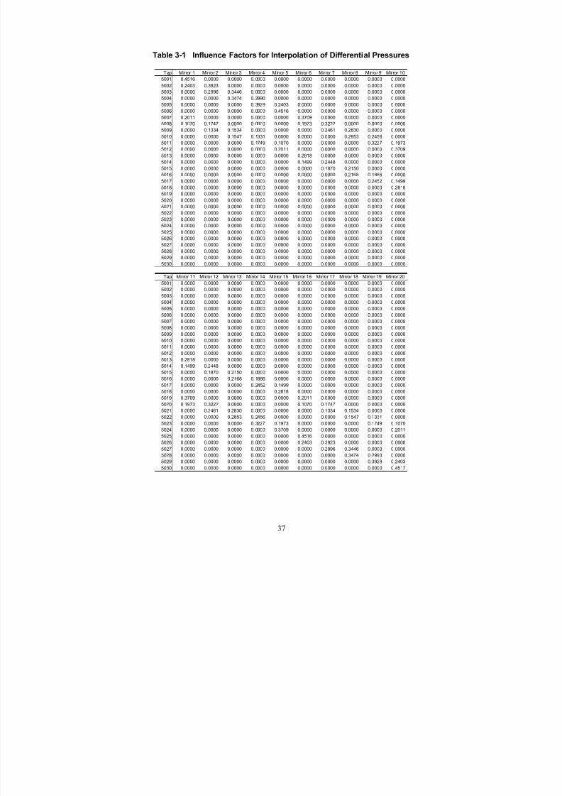
7/31/2019 Wind Tunnel Test
http://slidepdf.com/reader/full/wind-tunnel-test 46/243
Table 3-1 Influence Factors for Interpolation of Differential Pressures
Tap Mirror 1 Mirror 2 Mirror 3 Mirror 4 Mirror 5 Mirror 6 Mirror 7 Mirror 8 Mirror 9 Mirror 10
5001 0.4516 0.0000 0.0000 0.0000 0.0000 0.0000 0.0000 0.0000 0.0000 0.0000
5002 0.2403 0.3923 0.0000 0.0000 0.0000 0.0000 0.0000 0.0000 0.0000 0.0000
5003 0.0000 0.2996 0.3446 0.0000 0.0000 0.0000 0.0000 0.0000 0.0000 0.0000
5004 0.0000 0.0000 0.3474 0.2990 0.0000 0.0000 0.0000 0.0000 0.0000 0.0000
5005 0.0000 0.0000 0.0000 0.3929 0.2403 0.0000 0.0000 0.0000 0.0000 0.0000
5006 0.0000 0.0000 0.0000 0.0000 0.4516 0.0000 0.0000 0.0000 0.0000 0.0000
5007 0.2011 0.0000 0.0000 0.0000 0.0000 0.3709 0.0000 0.0000 0.0000 0.0000
5008 0.1070 0.1747 0.0000 0.0000 0.0000 0.1973 0.3222 0.0000 0.0000 0.0000
5009 0.0000 0.1334 0.1534 0.0000 0.0000 0.0000 0.2461 0.2830 0.0000 0.0000
5010 0.0000 0.0000 0.1547 0.1331 0.0000 0.0000 0.0000 0.2853 0.2456 0.0000
5011 0.0000 0.0000 0.0000 0.1749 0.1070 0.0000 0.0000 0.0000 0.3227 0.1973
5012 0.0000 0.0000 0.0000 0.0000 0.2011 0.0000 0.0000 0.0000 0.0000 0.3709
5013 0.0000 0.0000 0.0000 0.0000 0.0000 0.2818 0.0000 0.0000 0.0000 0.0000
5014 0.0000 0.0000 0.0000 0.0000 0.0000 0.1499 0.2448 0.0000 0.0000 0.0000
5015 0.0000 0.0000 0.0000 0.0000 0.0000 0.0000 0.1870 0.2150 0.0000 0.0000
5016 0.0000 0.0000 0.0000 0.0000 0.0000 0.0000 0.0000 0.2168 0.1866 0.0000
5017 0.0000 0.0000 0.0000 0.0000 0.0000 0.0000 0.0000 0.0000 0.2452 0.1499
5018 0.0000 0.0000 0.0000 0.0000 0.0000 0.0000 0.0000 0.0000 0.0000 0.2818
5019 0.0000 0.0000 0.0000 0.0000 0.0000 0.0000 0.0000 0.0000 0.0000 0.0000
5020 0.0000 0.0000 0.0000 0.0000 0.0000 0.0000 0.0000 0.0000 0.0000 0.0000
5021 0.0000 0.0000 0.0000 0.0000 0.0000 0.0000 0.0000 0.0000 0.0000 0.0000
5022 0.0000 0.0000 0.0000 0.0000 0.0000 0.0000 0.0000 0.0000 0.0000 0.00005023 0.0000 0.0000 0.0000 0.0000 0.0000 0.0000 0.0000 0.0000 0.0000 0.0000
5024 0.0000 0.0000 0.0000 0.0000 0.0000 0.0000 0.0000 0.0000 0.0000 0.0000
5025 0.0000 0.0000 0.0000 0.0000 0.0000 0.0000 0.0000 0.0000 0.0000 0.0000
5026 0.0000 0.0000 0.0000 0.0000 0.0000 0.0000 0.0000 0.0000 0.0000 0.0000
5027 0.0000 0.0000 0.0000 0.0000 0.0000 0.0000 0.0000 0.0000 0.0000 0.0000
5028 0.0000 0.0000 0.0000 0.0000 0.0000 0.0000 0.0000 0.0000 0.0000 0.0000
5029 0.0000 0.0000 0.0000 0.0000 0.0000 0.0000 0.0000 0.0000 0.0000 0.0000
5030 0.0000 0.0000 0.0000 0.0000 0.0000 0.0000 0.0000 0.0000 0.0000 0.0000
Tap Mirror 11 Mirror 12 Mirror 13 Mirror 14 Mirror 15 Mirror 16 Mirror 17 Mirror 18 Mirror 19 Mirror 20
5001 0.0000 0.0000 0.0000 0.0000 0.0000 0.0000 0.0000 0.0000 0.0000 0.0000
5002 0.0000 0.0000 0.0000 0.0000 0.0000 0.0000 0.0000 0.0000 0.0000 0.0000
5003 0.0000 0.0000 0.0000 0.0000 0.0000 0.0000 0.0000 0.0000 0.0000 0.0000
5004 0.0000 0.0000 0.0000 0.0000 0.0000 0.0000 0.0000 0.0000 0.0000 0.0000
5005 0.0000 0.0000 0.0000 0.0000 0.0000 0.0000 0.0000 0.0000 0.0000 0.0000
5006 0.0000 0.0000 0.0000 0.0000 0.0000 0.0000 0.0000 0.0000 0.0000 0.0000
5007 0.0000 0.0000 0.0000 0.0000 0.0000 0.0000 0.0000 0.0000 0.0000 0.00005008 0.0000 0.0000 0.0000 0.0000 0.0000 0.0000 0.0000 0.0000 0.0000 0.0000
5009 0.0000 0.0000 0.0000 0.0000 0.0000 0.0000 0.0000 0.0000 0.0000 0.0000
5010 0.0000 0.0000 0.0000 0.0000 0.0000 0.0000 0.0000 0.0000 0.0000 0.0000
5011 0.0000 0.0000 0.0000 0.0000 0.0000 0.0000 0.0000 0.0000 0.0000 0.0000
5012 0.0000 0.0000 0.0000 0.0000 0.0000 0.0000 0.0000 0.0000 0.0000 0.0000
5013 0.2818 0.0000 0.0000 0.0000 0.0000 0.0000 0.0000 0.0000 0.0000 0.0000
5014 0.1499 0.2448 0.0000 0.0000 0.0000 0.0000 0.0000 0.0000 0.0000 0.0000
5015 0.0000 0.1870 0.2150 0.0000 0.0000 0.0000 0.0000 0.0000 0.0000 0.0000
5016 0.0000 0.0000 0.2168 0.1866 0.0000 0.0000 0.0000 0.0000 0.0000 0.0000
5017 0.0000 0.0000 0.0000 0.2452 0.1499 0.0000 0.0000 0.0000 0.0000 0.0000
5018 0.0000 0.0000 0.0000 0.0000 0.2818 0.0000 0.0000 0.0000 0.0000 0.0000
5019 0.3709 0.0000 0.0000 0.0000 0.0000 0.2011 0.0000 0.0000 0.0000 0.0000
5020 0.1973 0.3222 0.0000 0.0000 0.0000 0.1070 0.1747 0.0000 0.0000 0.0000
5021 0.0000 0.2461 0.2830 0.0000 0.0000 0.0000 0.1334 0.1534 0.0000 0.0000
5022 0.0000 0.0000 0.2853 0.2456 0.0000 0.0000 0.0000 0.1547 0.1331 0.0000
5023 0.0000 0.0000 0.0000 0.3227 0.1973 0.0000 0.0000 0.0000 0.1749 0.1070
5024 0.0000 0.0000 0.0000 0.0000 0.3709 0.0000 0.0000 0.0000 0.0000 0.20115025 0.0000 0.0000 0.0000 0.0000 0.0000 0.4516 0.0000 0.0000 0.0000 0.0000
5026 0.0000 0.0000 0.0000 0.0000 0.0000 0.2403 0.3923 0.0000 0.0000 0.0000
5027 0.0000 0.0000 0.0000 0.0000 0.0000 0.0000 0.2996 0.3446 0.0000 0.0000
5028 0.0000 0.0000 0.0000 0.0000 0.0000 0.0000 0.0000 0.3474 0.2990 0.0000
5029 0.0000 0.0000 0.0000 0.0000 0.0000 0.0000 0.0000 0.0000 0.3929 0.2403
5030 0.0000 0.0000 0.0000 0.0000 0.0000 0.0000 0.0000 0.0000 0.0000 0.4517
37

7/31/2019 Wind Tunnel Test
http://slidepdf.com/reader/full/wind-tunnel-test 47/243
4. RESULTS AND DISCUSSION
Extensive wind-tunnel tests were conducted that involved measurements of overall loads on thesolar collectors using a high-frequency force balance and determination of detailed pressuredistributions on the collector concentrator. A number of test configurations were examined for different positions of the solar collector within a collector field for various combinations of yaw
and pitch angles, as well as for a few cases with an isolated solar collector. Because of thecontinuous interest by Solargenix and CPP in creating a comprehensive database, the totalnumber of test runs well exceeded that originally proposed. It is not the intent of this section to
present all of the test results in detail, but rather to present a review of the most importantfindings. The force and moment coefficient results of the overall loads obtained from the balance
measurements and by the integration of pressure distributions are tabulated in Appendix B for allthe tests conducted. In addition, the time series data of the measured pressure distributions for alltest configurations, described in Appendix E, have been recorded on a set of CD-ROMs that
provide backup data to this report.
Significant test conditions and results on the integrated overall loads on the isolated and fieldsolar collectors are presented in Sections 4.1 through 4.7 for a variety of test configurations.Sections 4.8 and 4.9 gives the summary of the structural design loads and the detailed differential
pressure distributions over the concentrator that can be used for the structural analysis of a parabolic trough collector. In addition, the use of these wind-tunnel test results for the structuraldesign is demonstrated in Section 4.8. The turbulent boundary layer simulated in the wind tunnel
is described in the next section.
4.1 Boundary Layer Simulation
One of the most important prerequisites for load measurements in a wind tunnel is modeling of anatmospheric boundary layer at the scale of the model. Several key characteristics of the boundarylayer are described in detail in Appendix C. In general, the vertical profiles of mean wind speed
and turbulence intensity are of particular significance for simulating wind loads. A representativesize of turbulent eddies, commonly denoted as a turbulence integral scale, also plays a roledepending on its relation to typical dimensions of a wind-tunnel model. The importance of exact
boundary layer simulation, however, tends to diminish for a structure surrounded by significantobjects that can dictate the local wind characteristics, such as a solar collector within a fieldconsisting of many adjacent units.
Figure 4-1 shows the mean wind velocity and turbulence intensity profiles simulated for thecurrent study. As seen, the modeled boundary layer profiles compare well with those suggested
by the well-recognized literature for winds over an open country exposure. It should be notedthat the designated model scale (1:45) was much larger than that for which the CPP wind tunnelwas primarily designed (1:200 to 1:500). For this reason, a series of wind measurements were
conducted before the load measurements to obtain the appropriate boundary layer flow. Theintegral scale of turbulence was also measured at the height of the collector pivot point and wasequivalent to about 70 ft at full scale. The suggested empirical values for an open country
boundary layer flow vary greatly, for example, 390 ft (Counihan 1975) and 150 ft (EngineeringScience Data Unit [ESDU] 1975). Although the simulated turbulence length scale was smaller
that those cited, it was considered acceptable because it is widely understood that the effect of thelength scale is generally insignificant if it is larger than the typical structure size.
38
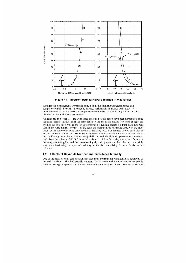
7/31/2019 Wind Tunnel Test
http://slidepdf.com/reader/full/wind-tunnel-test 48/243
Normalized Mean Wind Speed, U/Ur
0.0 0.5 1.0 1.5 2.0
F u l l - S c a l e E l e v a t i o n ,
f t
0
10
20
30
40
50
60
70
80
90
100
Local Turbulence Intensity, %
0 5 10 15 20 25 300
10
20
30
40
50
60
70
80
90
100
Simiu (1996)
Snyder (1981)
0.14 Power Law
Figure 4-1 Turbulent boundary layer simulated in wind tunnel
Wind profile measurements were made using a single hot-film anemometer mounted on acomputer-controlled vertical traverse and oriented horizontally transverse to the flow. Theinstrument was a TSI, Inc., constant-temperature anemometer (Model 1053b) with a 0.002-in.-diameter platinum-film sensing element.
As described in Section 3.1, the wind loads presented in this report have been normalized usingthe characteristic dimensions of the solar collector and the mean dynamic pressure of approach
wind at the collector pivot height. In determining the dynamic pressure, a Pitot static tube wasused in the wind tunnel. For most of the tests, the measurement was made directly at the pivotheight of the collector at some point upwind of the array field. For the deep interior array tests inPhase 4, however, it was not possible to measure the dynamic pressure at the same location due tothe significantly expanded size of the array field. Instead, the dynamic pressure was measured
well above the collector field (3 ft at model scale and 135 ft at full scale) where the influence of
the array was negligible, and the corresponding dynamic pressure at the collector pivot heightwas determined using the approach velocity profile for normalizing the wind loads on thecollector.
4.2 Effects of Reynolds Number and Turbulence Intensity
One of the most essential considerations for load measurements in a wind tunnel is sensitivity of the load coefficients with the Reynolds Number. This is because wind tunnel tests cannot exactlysimulate the high Reynolds typically encountered for full-scale structures. The mismatch is of
39

7/31/2019 Wind Tunnel Test
http://slidepdf.com/reader/full/wind-tunnel-test 49/243
particular concern for streamlined or curved shape structures because the load coefficients can behighly dependent on the Reynolds Number. A series of preliminary tests were conducted to test
the sensitivity of the wind load coefficients to the Reynolds Numbers.
Figure 4-2 shows the mean load coefficients at a pitch angle of -60 degrees with differentReynolds Numbers. The model Reynolds Numbers were calculated using the mean wind speed at
the collector pivot height and the aperture width as the reference quantities. As the figureindicates, the load coefficients are nearly invariant of the Reynolds Number for the range tested.
Yaw = 0, Pitch = -60 in 21 % Turbulent Flow
Reynolds Number
25000 30000 35000 40000 45000 50000 55000
M
e a n C o e f f i c i e n t
0.0
0.5
1.0
1.5
2.0
Cfx Cfz
Yaw = 0, Pitch = -60 in 21 % Turbulent Flow
Reynolds Number
25000 30000 35000 40000 45000 50000 55000
M
e a n C o e f f i c i e n t
0.0
0.5
1.0
1.5
2.0
Cfx CfzCfx Cfz
Figure 4-2 Sensitivity of load coefficients to Reynolds Number
Proper modeling of turbulence intensity is also important because it affects the fluctuations of theload, as well as the mean load to some extent. Figure 4-3 shows the effect of turbulence intensityon the mean horizontal load at a pitch angle of 0 degrees for a range of Reynolds Numbers. Theload coefficients are similar for all turbulence intensities simulated when the Reynolds Number exceeds 46,000. In this particular test, the small variations at the lower Reynolds Numbers are
probably due to poor signal-to-noise ratio or initial drift of the data acquisition instrument, rather than the aerodynamic behavior of the solar collector. The disparity of the load coefficients for different turbulence intensities is nominal, considering a slight variation of the velocity profiles toobtain the different turbulence levels over the height of the solar collector. The effect of theturbulence intensity is properly accounted for in the current study because the simulated turbulent
boundary layer is representative of a terrain exposure encountered in open country exposure as
intended. All data tests in this study, other than these shown in the above figures, were run at thetypical Reynolds Number of 50,000 in the turbulent boundary layer with 21% turbulence intensity
at the pivot height of 9.3 ft.
40

7/31/2019 Wind Tunnel Test
http://slidepdf.com/reader/full/wind-tunnel-test 50/243
Yaw = 0, Pitch = 0
Reynolds Number
20000 30000 40000 50000 60000 70000
M e a n C f x
0.0
0.5
1.0
1.5
2.0
8 % turb. 15 % turb. 21 % turb.
Figure 4-3 Effects of turbulence intensity on horizontal force
4.3 Isolated Solar Collector
4.3.1 Test Results Drag and Lift Force Tests (Phase 1 data): In practice, the solar collector is used in an array
consisting of a number of similar units, and the design wind loads should be determined for sucha configuration. However, loads on an isolated collector are informative for characterizing the
baseline performance. The isolated solar collector was tested with and without a torque tube (on
the back side of the collector concentrator, discussed in Section 2.2.1 and Figure 3-1). Figure4-4a shows the load coefficients for the isolated solar collector as a function of the pitch angle
obtained by the balance measurement. The yaw angle was 0 degrees, and the approach wind is perpendicular to the major axis (y axis) of the solar collector. For each of the collector configurations, two curves are plotted in the figure. The lines represent the mean loads, and thesymbols represent the peak maximum and minimum loads. Note that the test configurationrelative to the wind were duplicated at pitch angles of +90 and –90 degrees as a check for
repeatability. Refer to Section 3.1 for the definition of the overall load coefficients.
When the torque tube increases the load, for example, for Cfz at pitch = -105 degrees, the changein the peak loads is more notable than that of the mean loads. This implies that the torque tubecan affect the load fluctuations considerably. The effect of the torque tube is different, however,
for the collector in an array field, depending on the location in the field, as discussed in Sections4.4 and 4.5. Similar plots are presented in Figure 4-4 b for data obtained by the pressure modeltests. The load coefficients were computed by integrating the measured point pressures over the
41

7/31/2019 Wind Tunnel Test
http://slidepdf.com/reader/full/wind-tunnel-test 51/243
exposed area of the solar collector concentrator and by resolving the resulting load into thespecified load components.
The effect of the torque tube is more apparent for the vertical force, Cfz , than for the horizontalforce, Cfx. The torque tube does not necessarily worsen the wind loads, for example, the verticalforce component for a range of pitch angles from 45 to 90 degrees is notably reduced with the
torque tube. As far as the largest absolute load of the individual load components is concerned,the torque tube did not increase the load values.
Configurations A1 and A2 Balance (Isolated Collector w ithout andw ith Torque Tube), Yaw = 0
-180 -150 -120 -90 -60 -30 0 30 60 90 120 150 180
C f x
-1
0
1
2
3
4
-180 -150 -120 -90 -60 -30 0 30 60 90 120 150 180
C f z
-5
-4
-3
-2
-1
0
1
2
3
4
Pitch A ngle, deg.
Mean (w ithout Torque Tube) Max/Min (w ithout Torque Tube)
Mean (w ith Torque Tube) Max/Min (w ith Torque Tube)
Figure 4-4a Loads on isolated solar collector with and without torque tube,balance study
42
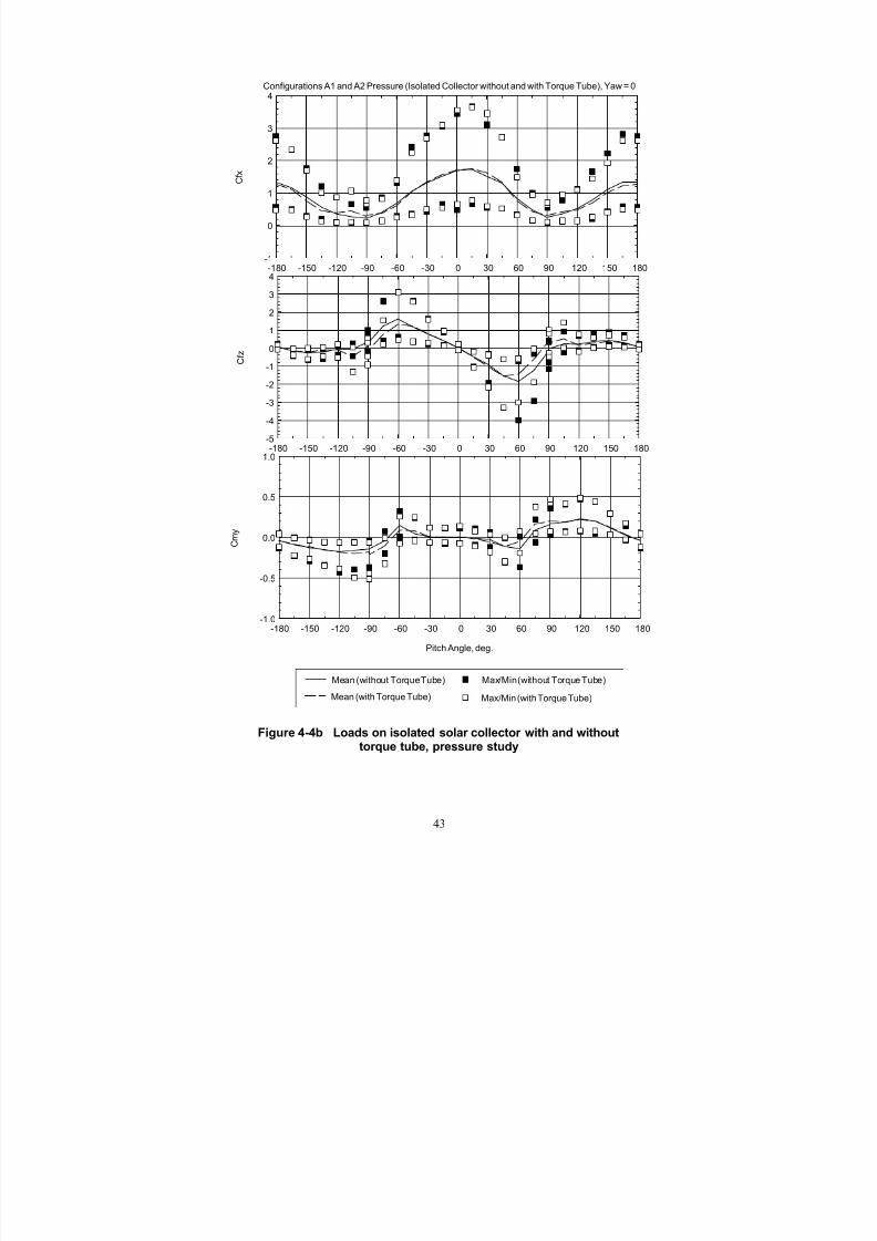
7/31/2019 Wind Tunnel Test
http://slidepdf.com/reader/full/wind-tunnel-test 52/243
Configurations A1 and A2 Pressure (Isolated Collector without and with Torque Tube), Yaw = 0
-180 -150 -120 -90 -60 -30 0 30 60 90 120 150 180
C f x
-1
0
1
2
3
4
-180 -150 -120 -90 -60 -30 0 30 60 90 120 150 180
C f z
-5
-4
-3
-2
-1
01
2
3
4
Pitch Angle, deg.
-180 -150 -120 -90 -60 -30 0 30 60 90 120 150 180
C m y
-1.0
-0.5
0.0
0.5
1.0
Mean (without Torque Tube) Max/Min (without Torque Tube)
Mean (with Torque Tube) Max/Min (with Torque Tube)
Figure 4-4b Loads on isolated solar collector with and withouttorque tube, pressure study
43

7/31/2019 Wind Tunnel Test
http://slidepdf.com/reader/full/wind-tunnel-test 53/243
Figure 4-5a and Figure 4-5 b compare the balance and pressure test results for the isolated solar collector tests. Note that in Figure 4-5a, the balance results from Phase 1 and 4 tests have been
combined. To aid comparison between the force components and among the various testconfigurations shown later, the plots have been produced using consistent scales. Note also that
in this and following figures, the balance results are consistently slightly larger than the pressureresults. The reason has to do with the discrete nature of the pressure taps; adjustment factors for
the pressure results are derived in Section 4-9.
44
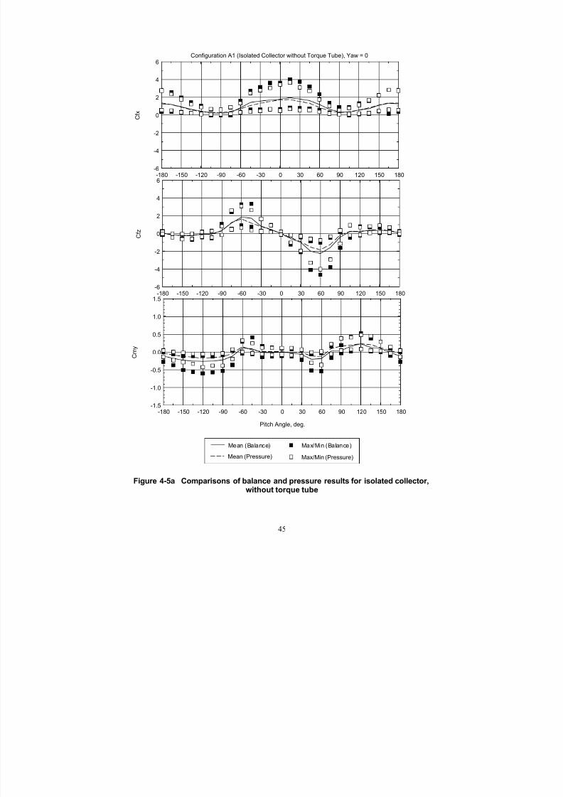
7/31/2019 Wind Tunnel Test
http://slidepdf.com/reader/full/wind-tunnel-test 54/243
Configuration A1 (Isolated Collector without Torque Tube), Yaw = 0
-180 -150 -120 -90 -60 -30 0 30 60 90 120 150 180
C f x
-6
-4
-2
0
2
4
6
-180 -150 -120 -90 -60 -30 0 30 60 90 120 150 180
C f z
-6
-4
-2
0
2
4
6
Pitch Angle, deg.
-180 -150 -120 -90 -60 -30 0 30 60 90 120 150 180
C m y
-1.5
-1.0
-0.5
0.0
0.5
1.0
1.5
Mean (Balance) Max/Min (Balance)
Mean (Pressure) Max/Min (Pressure)
Figure 4-5a Comparisons of balance and pressure results for isolated collector,without torque tube
45
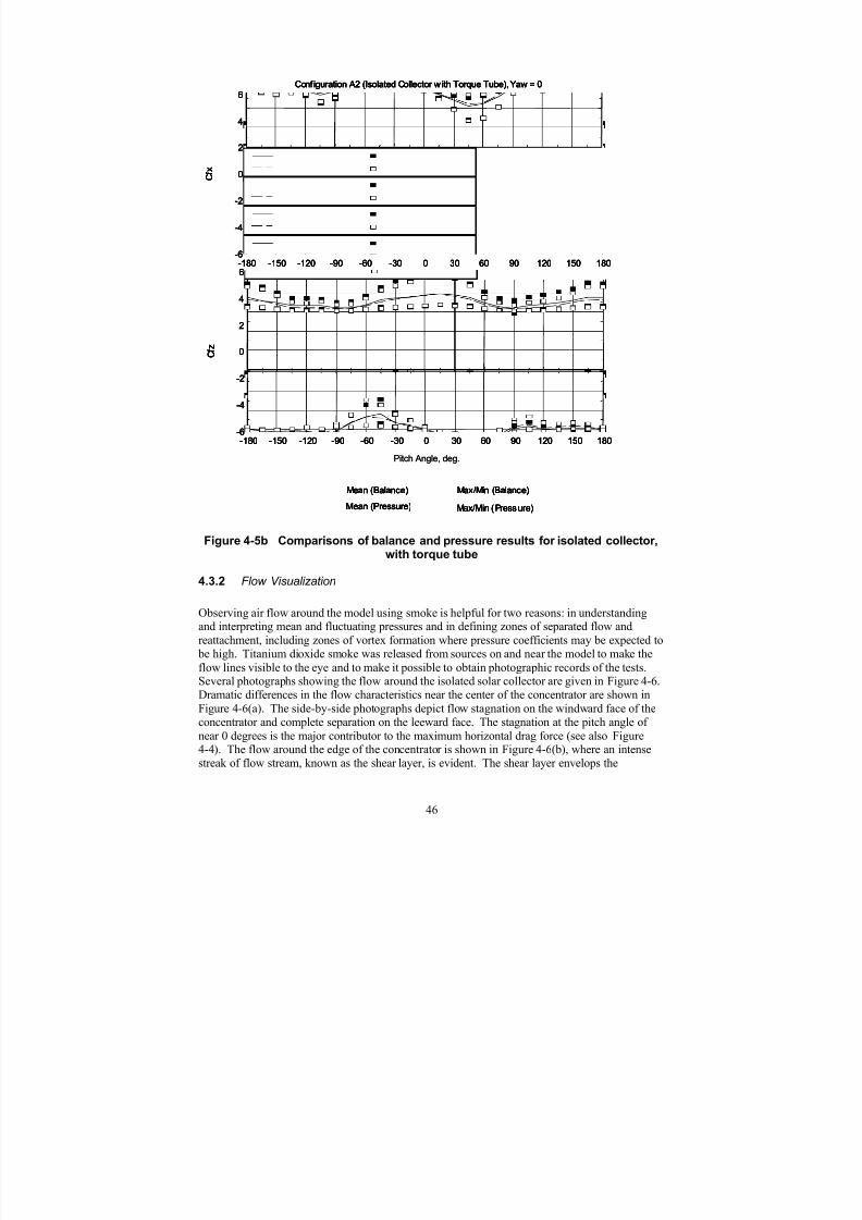
7/31/2019 Wind Tunnel Test
http://slidepdf.com/reader/full/wind-tunnel-test 55/243
Configuration A2 (Isolated Collector w ith Torque Tube), Yaw = 0
-180 -150 -120 -90 -60 -30 0 30 60 90 120 150 180
C f x
-6
-4
-2
0
2
4
6
-180 -150 -120 -90 -60 -30 0 30 60 90 120 150 180
C f z
-6
-4
-2
0
2
4
6
Pitch Angle, deg.
Mean (Balance) Max/Min (Balance)Mean (Pressure) Max/Min (Pressure)
Configuration A2 (Isolated Collector w ith Torque Tube), Yaw = 0
-180 -150 -120 -90 -60 -30 0 30 60 90 120 150 180
C f x
-6
-4
-2
0
2
4
6
-180 -150 -120 -90 -60 -30 0 30 60 90 120 150 180
C f z
-6
-4
-2
0
2
4
6
Mean (Balance) Max/Min (Balance)Mean (Pressure) Max/Min (Pressure)
Configuration A2 (Isolated Collector w ith Torque Tube), Yaw = 0
-180 -150 -120 -90 -60 -30 0 30 60 90 120 150 180
C f x
-6
-4
-2
0
2
4
6
-180 -150 -120 -90 -60 -30 0 30 60 90 120 150 180
C f z
-6
-4
-2
0
2
4
6
Pitch Angle, deg.
Mean (Balance) Max/Min (Balance)Mean (Pressure) Max/Min (Pressure)
Configuration A2 (Isolated Collector w ith Torque Tube), Yaw = 0
-180 -150 -120 -90 -60 -30 0 30 60 90 120 150 180
C f x
-6
-4
-2
0
2
4
6
-180 -150 -120 -90 -60 -30 0 30 60 90 120 150 180
C f z
-6
-4
-2
0
2
4
6
Mean (Balance) Max/Min (Balance)Mean (Pressure) Max/Min (Pressure)
Figure 4-5b Comparisons of balance and pressure results for isolated collector,with torque tube
4.3.2 Flow Visualization
Observing air flow around the model using smoke is helpful for two reasons: in understandingand interpreting mean and fluctuating pressures and in defining zones of separated flow and
reattachment, including zones of vortex formation where pressure coefficients may be expected to
be high. Titanium dioxide smoke was released from sources on and near the model to make theflow lines visible to the eye and to make it possible to obtain photographic records of the tests.Several photographs showing the flow around the isolated solar collector are given in Figure 4-6.Dramatic differences in the flow characteristics near the center of the concentrator are shown in
Figure 4-6(a). The side-by-side photographs depict flow stagnation on the windward face of theconcentrator and complete separation on the leeward face. The stagnation at the pitch angle of
near 0 degrees is the major contributor to the maximum horizontal drag force (see also Figure4-4). The flow around the edge of the concentrator is shown in Figure 4-6(b), where an intensestreak of flow stream, known as the shear layer, is evident. The shear layer envelops the
46

7/31/2019 Wind Tunnel Test
http://slidepdf.com/reader/full/wind-tunnel-test 56/243
separation zone, and its trajectory varies depending on the pitch angle. For example, at a pitchangle of 0 degrees (i.e., the photograph on the left) the shear layer is much elevated compared to
that at a pitch of 120 degrees (on the right), despite the similar height of the top edge of theconcentrator. Transition of the flow pattern is shown in Figure 4–6(c). Near the leading edge of
the concentrator, the flow seems to follow the curvature of the concentrator and eventuallyseparates from the surface around the center of the concentrator. Before separation, the flow
tends to accelerate, creating a zone of high negative pressure on the leeward face of theconcentrator. Combined with the near stagnant positive pressure on the windward face, both
pitch angles (-60 and +60 degrees) result in a significant vertical force, though of opposite sign.
47
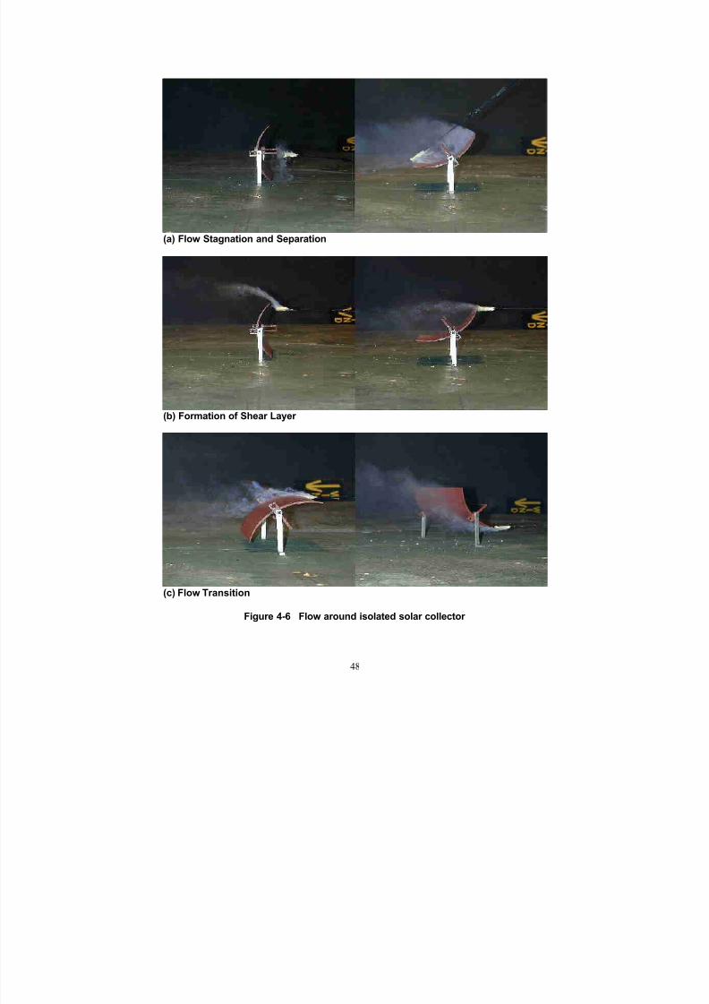
7/31/2019 Wind Tunnel Test
http://slidepdf.com/reader/full/wind-tunnel-test 57/243
(a) Flow Stagnation and Separation
(b) Formation of Shear Layer
(c) Flow Transition
Figure 4-6 Flow around isolated solar collector
48

7/31/2019 Wind Tunnel Test
http://slidepdf.com/reader/full/wind-tunnel-test 58/243
4.4 Exterior Solar Collectors in Array Field
4.4.1 General Observations
Figure 4-7 through Figure 4-10 show the Phase 2 test data on drag and lift load coefficients for
the collectors at the exterior edge of the array field and compare the balance and pressuremeasurement techniques. Figure 4-11 shows the Phase 4 pitching moment load coefficients for
selected collectors at the exterior edge of the array field, also comparing the balance and pressuremeasurement techniques.
Particular collector positions can be identified by the configuration ID and by referring to Figure2-11a. At a yaw of 0 degrees, the loads on the collectors in all module positions in the mostupwind row are similar for all pitch angles (e.g., see Figure 4-7 and Figure 4-8a). The collector at
the edge of the field shows a higher horizontal force at a yaw of 30 degrees (Figure 4-8 b) whenthe collector is near upright, while the vertical force and pitching moment are similar to those atyaw = 0 degrees. Some reduction of the loads is realized for the collectors along the field edge atthe row positions 2 and 3 because of upwind shielding (see Figure 4-9 and Figure 4-10).
Figure 4-12 illustrates the variation of the wind loads along the side edge of the array field. Therow position is measured from the upwind edge of the field with a position of 0, denoting anisolated collector. The pitch angles were selected separately for individual load components on
basis of significance. In general, differences in the loads become insignificant beyond a row position of 3.
49

7/31/2019 Wind Tunnel Test
http://slidepdf.com/reader/full/wind-tunnel-test 59/243
Configuration B1, Yaw = 0
-180 -150 -120 -90 -60 -30 0 30 60 90 120 150 180
C f x
-6
-4
-2
0
2
4
6
-180 -150 -120 -90 -60 -30 0 30 60 90 120 150 180
C f z
-6
-4
-2
0
2
4
6
Pitch A ngle, deg.
Mean (Balance) Max/Min (Balance)Mean (Pressure) Max/Min (Press ure)
Configuration B1, Yaw = 0
-180 -150 -120 -90 -60 -30 0 30 60 90 120 150 180
C f x
-6
-4
-2
0
2
4
6
-180 -150 -120 -90 -60 -30 0 30 60 90 120 150 180
C f z
-6
-4
-2
0
2
4
6
Pitch A ngle, deg.
Mean (Balance) Max/Min (Balance)Mean (Pressure) Max/Min (Press ure)
Figure 4-7 Loads on exterior collector for Configuration B1, collector in Row 1at Module Position 4 (from edge), yaw = 0 degrees
50
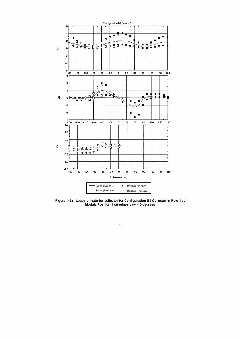
7/31/2019 Wind Tunnel Test
http://slidepdf.com/reader/full/wind-tunnel-test 60/243
Configuration B3, Yaw = 0
-180 -150 -120 -90 -60 -30 0 30 60 90 120 150 180
C f x
-6
-4
-2
0
2
4
6
-180 -150 -120 -90 -60 -30 0 30 60 90 120 150 180
C f z
-6
-4
-2
0
2
4
6
Pitch A ngle, deg.
-180 -150 -120 -90 -60 -30 0 30 60 90 120 150 180
C m y
-1.5
-1.0
-0.5
0.0
0.5
1.0
1.5
Mean (Balance) Max/Min (Balance)
Mean (Pressure) Max/Min ( Press ure)
Figure 4-8a Loads on exterior collector for Configuration B3 Collector in Row 1 atModule Position 1 (at edge), yaw = 0 degrees
51

7/31/2019 Wind Tunnel Test
http://slidepdf.com/reader/full/wind-tunnel-test 61/243
Configuration B3, Yaw = 30
-180 -150 -120 -90 -60 -30 0 30 60 90 120 150 180
C f x
-6
-4
-2
0
2
4
6
-180 -150 -120 -90 -60 -30 0 30 60 90 120 150 180
C f z
-6
-4
-2
0
2
4
6
Pitch A ngle, deg.
-180 -150 -120 -90 -60 -30 0 30 60 90 120 150 180
C m y
-1.5
-1.0
-0.5
0.0
0.5
1.0
1.5
Mean (Balance) Max/Min (Balance)
Mean (Pressure) Max/Min (Press ure)
Figure 4-8b Loads on exterior collector for Configuration B3, collector in Row 1at Module Position 1 (at edge), yaw = 30 degrees
52

7/31/2019 Wind Tunnel Test
http://slidepdf.com/reader/full/wind-tunnel-test 62/243
Configuration B4, Yaw = 0
-180 -150 -120 -90 -60 -30 0 30 60 90 120 150 180
C f x
-6
-4
-2
0
2
4
6
-180 -150 -120 -90 -60 -30 0 30 60 90 120 150 180
C f z
-6
-4
-2
0
2
4
6
Pitch A ngle, deg.
-180 -150 -120 -90 -60 -30 0 30 60 90 120 150 180
C m y
-1.5
-1.0
-0.5
0.0
0.5
1.0
1.5
Mean (Balance) Max/Min (Balance)
Mean (Pressure) Max/Min (Press ure)
Figure 4-9a Loads on exterior collector for Configuration B4, collector in Row 2at Module Position 1 (at edge), yaw = 0 degrees
53
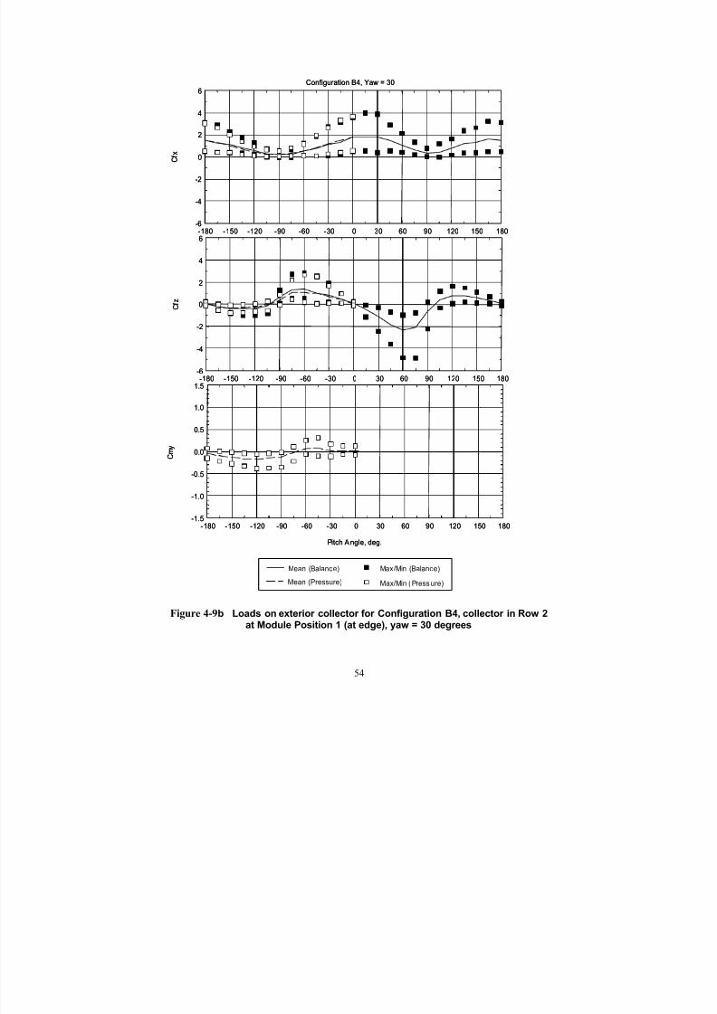
7/31/2019 Wind Tunnel Test
http://slidepdf.com/reader/full/wind-tunnel-test 63/243
Configuration B4, Yaw = 30
-180 -150 -120 -90 -60 -30 0 30 60 90 120 150 180
C f x
-6
-4
-2
0
2
4
6
-180 -150 -120 -90 -60 -30 0 30 60 90 120 150 180
C f z
-6
-4
-2
0
2
4
6
Pitch A ngle, deg.
-180 -150 -120 -90 -60 -30 0 30 60 90 120 150 180
C m y
-1.5
-1.0
-0.5
0.0
0.5
1.0
1.5
Mean (Balance) Max/Min (Balance)
Mean (Pressure) Max/Min (Press ure)
Figure 4-9b Loads on exterior collector for Configuration B4, collector in Row 2at Module Position 1 (at edge), yaw = 30 degrees
54

7/31/2019 Wind Tunnel Test
http://slidepdf.com/reader/full/wind-tunnel-test 64/243
Configuration B5, Yaw = 0
-180 -150 -120 -90 -60 -30 0 30 60 90 120 150 180
C f x
-6
-4
-2
0
2
4
6
-180 -150 -120 -90 -60 -30 0 30 60 90 120 150 180
C f z
-6
-4
-2
0
2
4
6
Pitch A ngle, deg.
-180 -150 -120 -90 -60 -30 0 30 60 90 120 150 180
C m y
-1.5
-1.0
-0.5
0.0
0.5
1.0
1.5
Mean (Balance) Max/Min (Balance)
Mean (Pressure) Max/Min (Press ure)
Figure 4-10a Loads on exterior collector for Configuration B5, collector in Row 3at Module Position 1 (at edge), yaw = 0 degrees
55

7/31/2019 Wind Tunnel Test
http://slidepdf.com/reader/full/wind-tunnel-test 65/243
Configuration B5, Yaw = 30
-180 -150 -120 -90 -60 -30 0 30 60 90 120 150 180
C f x
-6
-4
-2
0
2
4
6
-180 -150 -120 -90 -60 -30 0 30 60 90 120 150 180
C f z
-6
-4
-2
0
2
4
6
Pitch A ngle, deg.
-180 -150 -120 -90 -60 -30 0 30 60 90 120 150 180
C m y
-1.5
-1.0
-0.5
0.0
0.5
1.0
1.5
Mean (Balance) Max/Min (Balance)
Mean (Pressure) Max/Min (Press ure)
Figure 4-10b Loads on exterior collector for Configuration B5, collector in Row 3at Module Position 1 (at edge), yaw = 30 degrees
56

7/31/2019 Wind Tunnel Test
http://slidepdf.com/reader/full/wind-tunnel-test 66/243
Configuration B1, Yaw = 0
Pitch Angle, deg.
-180 -150 -120 -90 -60 -30 0 30 60 90 120 150 180
C m y
-1.5
-1.0
-0.5
0.0
0.5
1.0
1.5
Mean (Balance) Max/Min (Balance)
Mean (Pressure) Max/Min (Pressure)
Figure 4-11 Pitching Moment of Exterior Collector (a) Configuration B1, Yaw = 0 degrees
57
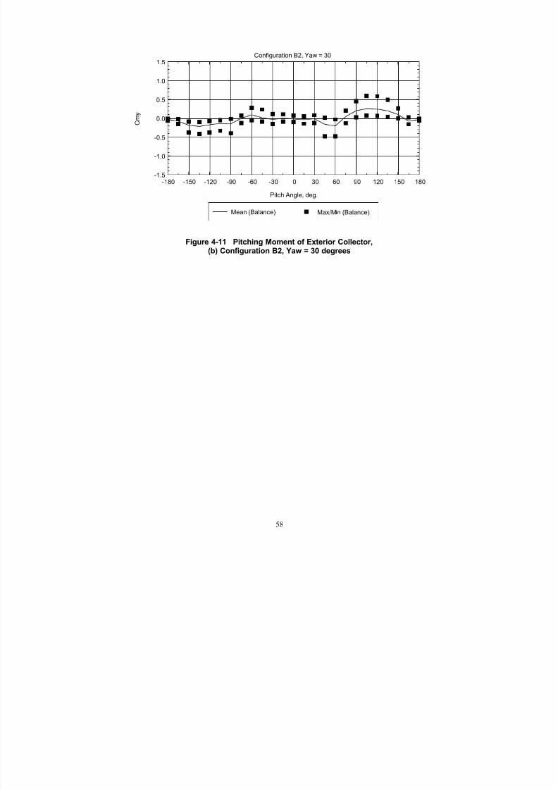
7/31/2019 Wind Tunnel Test
http://slidepdf.com/reader/full/wind-tunnel-test 67/243
Configuration B2, Yaw = 30
Pitch Angle, deg.
-180 -150 -120 -90 -60 -30 0 30 60 90 120 150 180
C m y
-1.5
-1.0
-0.5
0.0
0.5
1.0
1.5
Mean (Balance) Max/Min (Balance)
Figure 4-11 Pitching Moment of Exterior Collector,(b) Configuration B2, Yaw = 30 degrees
58

7/31/2019 Wind Tunnel Test
http://slidepdf.com/reader/full/wind-tunnel-test 68/243
Configuration B3, Yaw = 0
Pitch Angle, deg.
-180 -150 -120 -90 -60 -30 0 30 60 90 120 150 180
C m y
-1.5
-1.0
-0.5
0.0
0.5
1.0
1.5
Mean (Balance) Max/Min (Balance)Mean (Pressure) Max/Min (Pressure)
Figure 4-11 Pitching Moment of Exterior Collector,(c) Configuration B3, Yaw = 0 degrees
59
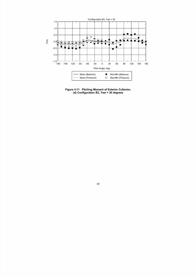
7/31/2019 Wind Tunnel Test
http://slidepdf.com/reader/full/wind-tunnel-test 69/243
Configuration B3, Yaw = 30
Pitch Angle, deg.
-180 -150 -120 -90 -60 -30 0 30 60 90 120 150 180
C m y
-1.5
-1.0
-0.5
0.0
0.5
1.0
1.5
Mean (Balance) Max/Min (Balance)Mean (Pressure) Max/Min (Pressure)
Figure 4-11 Pitching Moment of Exterior Collector,(d) Configuration B3, Yaw = 30 degrees
60

7/31/2019 Wind Tunnel Test
http://slidepdf.com/reader/full/wind-tunnel-test 70/243
Configurations A1, B3, B4, B5 and B6 Balance, Yaw = 0
0 1 2 3 4 5
C f x a t P i t c h =
0 d e g .
-6
-4
-2
0
2
4
6
0 1 2 3 4 5
C f z a t P i t c h = 6 0
d e g .
-6
-4
-2
0
2
4
6
Row Position
Mean (w i thout Torque Tube) Max /Min (w ithout Torque Tube)
Row Position = 0 denotes isolated c ollector
Configurations A1, B3, B4, B5 and B6 Balance, Yaw = 0
0 1 2 3 4 5
C f x a t P i t c h =
0 d e g .
-6
-4
-2
0
2
4
6
0 1 2 3 4 5
C f z a t P i t c h = 6 0
d e g .
-6
-4
-2
0
2
4
6
Row Position
Mean (w i thout Torque Tube) Max /Min (w ithout Torque Tube)
Row Position = 0 denotes isolated c ollector
Figure 4-12a Effect of row position along edge of array field,yaw = 0 degrees
61
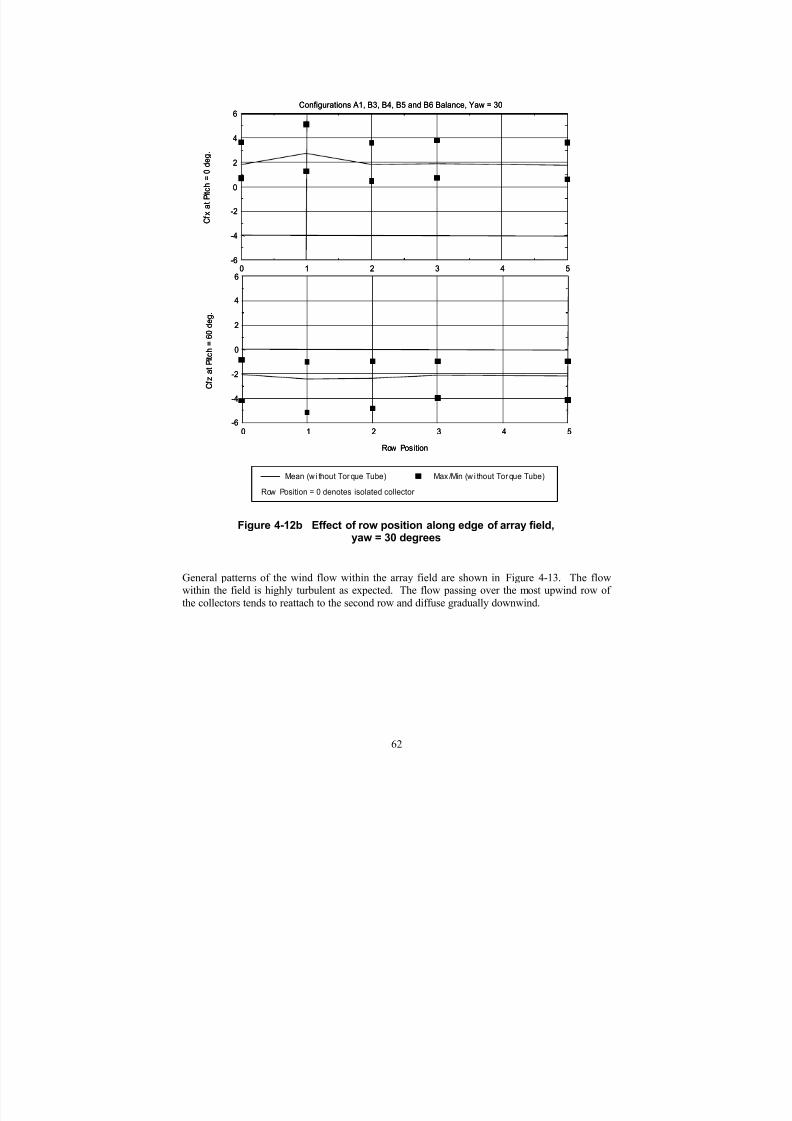
7/31/2019 Wind Tunnel Test
http://slidepdf.com/reader/full/wind-tunnel-test 71/243
Configurations A1, B3, B4, B5 and B6 Balance, Yaw = 30
0 1 2 3 4 5
C f x a t P i t c h = 0 d e g .
-6
-4
-2
0
2
4
6
0 1 2 3 4 5
C f z a t P i t c h = 6 0 d e g .
-6
-4
-2
0
2
4
6
Row Position
Mean (w i thout Torque Tube) Max /Min (w i thout Torque Tube)
Row Position = 0 denotes isolated collector
Configurations A1, B3, B4, B5 and B6 Balance, Yaw = 30
0 1 2 3 4 5
C f x a t P i t c h = 0 d e g .
-6
-4
-2
0
2
4
6
0 1 2 3 4 5
C f z a t P i t c h = 6 0 d e g .
-6
-4
-2
0
2
4
6
Row Position
Mean (w i thout Torque Tube) Max /Min (w i thout Torque Tube)
Row Position = 0 denotes isolated collector
Figure 4-12b Effect of row position along edge of array field,yaw = 30 degrees
General patterns of the wind flow within the array field are shown in Figure 4-13. The flowwithin the field is highly turbulent as expected. The flow passing over the most upwind row of
the collectors tends to reattach to the second row and diffuse gradually downwind.
62

7/31/2019 Wind Tunnel Test
http://slidepdf.com/reader/full/wind-tunnel-test 72/243
(a)
(b)
Figure 4-13 General flow patterns within array field
4.4.2 Effects of Wind Protective Fence Barrier and Torque Tube
Drastic reduction of the loads can be seen when a protective fence surrounds the collector field,as shown by comparing Figure 4-14 with Figure 4-8a and Figure 4-8 b. The effectiveness of thefence is more pronounced for the vertical force component.
63

7/31/2019 Wind Tunnel Test
http://slidepdf.com/reader/full/wind-tunnel-test 73/243
Configuration D3, Yaw = 0
-180 -150 -120 -90 -60 -30 0 30 60 90 120 150 180
C f x
-6
-4
-2
0
2
4
6
-180 -150 -120 -90 -60 -30 0 30 60 90 120 150 180
C f z
-6
-4
-2
0
2
4
6
Pitch A ngle, deg.
-180 -150 -120 -90 -60 -30 0 30 60 90 120 150 180
C m y
-1.5
-1.0
-0.5
0.0
0.5
1.0
1.5
Mean (Balance) Max/Min (Balance)
Mean (Pressure) Max/Min ( Press ure)
Figure 4-14a Loads on exterior collector with protective fence for ConfigurationD3, collector in Row 1 at Module Position 1 (at edge), yaw = 0 degrees
64

7/31/2019 Wind Tunnel Test
http://slidepdf.com/reader/full/wind-tunnel-test 74/243
Configuration D3, Yaw = 30
-180 -150 -120 -90 -60 -30 0 30 60 90 120 150 180
C f x
-6
-4
-2
0
2
4
6
-180 -150 -120 -90 -60 -30 0 30 60 90 120 150 180
C f z
-6
-4
-2
0
2
4
6
Pitch Angle, deg.
-180 -150 -120 -90 -60 -30 0 30 60 90 120 150 180
C m y
-1.5
-1.0
-0.5
0.0
0.5
1.0
1.5
Mean (Balance) Max/Min (Balance)
Mean (Pressure) Max/Min ( Pressure)
Figure 4-14b Loads on exterior collector with protective fence for ConfigurationD3, collector in Row 1 at Module Position 1, (at edge), yaw = 30 degrees
65

7/31/2019 Wind Tunnel Test
http://slidepdf.com/reader/full/wind-tunnel-test 75/243
The effect of the protective fence is apparent in the photographs shown in Figure 4-15, whichcompare the wind flows with and without the fence. With the porous protective fence in place,
the flow is more diffused.
The effect of the torque tube on the exterior collectors can be seen in Figure 4-16 through Figure4-18. In general, the influence of the torque tube is small, with the effect being most noticeable
on the vertical force, especially at a pitch angle of about 60 degrees.
Figure 4-15 Effect of wind protective fence
66

7/31/2019 Wind Tunnel Test
http://slidepdf.com/reader/full/wind-tunnel-test 76/243
Configurations B1 and E1 Balance, Y aw = 0
-180 -150 -120 -90 -60 -30 0 30 60 90 120 150 180
C f x
-6
-4
-2
0
2
4
6
-180 -150 -120 -90 -60 -30 0 30 60 90 120 150 180
C f z
-6
-4
-2
0
2
4
6
Pitch A ngle, deg.
Mean (w ithout Torque Tube) Max /Min (w i thout Torque Tube)
Mean (w ith Torque Tube) Max/Min (w ith Torque Tube)
Figure 4-16 Effect of torque tube on collector in array field, Configurations B1and E1, collector in Row 1 at Module Position 4 (from edge), yaw = 0 degrees
67

7/31/2019 Wind Tunnel Test
http://slidepdf.com/reader/full/wind-tunnel-test 77/243
Configurations B3 and E3 Balance, Y aw = 0
-180 -150 -120 -90 -60 -30 0 30 60 90 120 150 180
C f x
-6
-4
-2
0
2
4
6
-180 -150 -120 -90 -60 -30 0 30 60 90 120 150 180
C f z
-6
-4
-2
0
2
4
6
Pitch Angle, deg.
Mean (w i thout Torque Tube) Max /Min (w i thout Torque Tube)
Mean (w ith Torque Tube) Max/Min (w ith Torque Tube)
Figure 4-17 Effect of torque tube on collector in array field, Configurations B3and E3, collector in Row 1 at Module Position 1 (at edge), yaw = 0 degrees
68

7/31/2019 Wind Tunnel Test
http://slidepdf.com/reader/full/wind-tunnel-test 78/243
Configurations B4 and E4 Balance, Y aw = 0
-180 -150 -120 -90 -60 -30 0 30 60 90 120 150 180
C f x
-6
-4
-2
0
2
4
6
-180 -150 -120 -90 -60 -30 0 30 60 90 120 150 180
C f z
-6
-4
-2
0
2
4
6
Pitch A ngle, deg.
Mean (w i thout Torque Tube) Max /Min (w i thout Torque Tube)
Mean (w ith Torque Tube) Max/Min (w ith Torque Tube)
Figure 4-18 Effect of torque tube on collector in array field, Configurations B4and E4, collector in Row 2 at Module Position 1 (at edge), yaw = 0
69

7/31/2019 Wind Tunnel Test
http://slidepdf.com/reader/full/wind-tunnel-test 79/243
4.5 Interior Solar Collectors in Array Field
4.5.1 General Observations
Figure 4-19 through Figure 4-21 show the Phase 3 test data on drag and lift load coefficients,
obtained by both the balance and pressure measurements, for the solar collectors located interior of the array field. Figure 4-23 shows the Phase 4 pitching moment load coefficients for selected
collectors interior of the array field, also comparing the pressure measurement data whereavailable.
Figure 2-11(b) can be used to identify the positions of the collector within the field. For Configuration C1 (presented in Figure 4-19 a, b, and c), the solar collector of interest is located at
the second row from the windward field edge. Agreement between the two test methods (balanceand pressure data) is generally good. The largest difference is evident for the peak vertical force
component at a yaw angle of 75 degrees, shown in Figure 4-19 b. Compared with the collector
directly in front of this unit (Configuration B1 in Figure 4-7), considerable reduction of the wind
loads is noticed due to shielding.
The wind loads continue to decrease slightly for the collectors located further downwind,(Configurations C3 and C5 in Figure 4-20 and Figure 4-21. Patterns of the vertical force and
pitching moment are similar among the interior collectors, while some variations in the horizontalforce component can be observed. The effect of the row positions for these interior collectors isillustrated in Figure 4-22.
The pitching moment for the interior solar collectors are shown in Figure 4-23. No Phase3pressure data are available for Configuration C2 at a yaw angle of 0 degrees (Figure 4-23a).
70
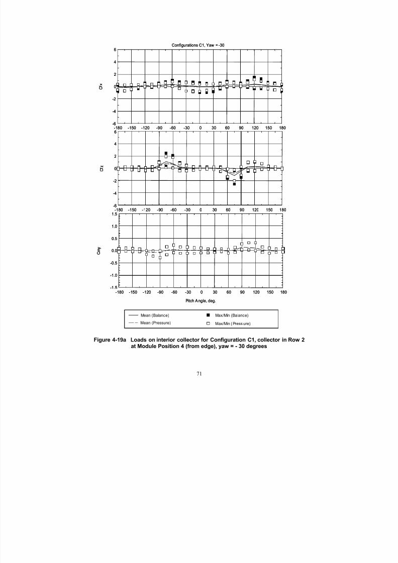
7/31/2019 Wind Tunnel Test
http://slidepdf.com/reader/full/wind-tunnel-test 80/243
Configurations C1, Yaw = -30
-180 -150 -120 -90 -60 -30 0 30 60 90 120 150 180
C f x
-6
-4
-2
0
2
4
6
-180 -150 -120 -90 -60 -30 0 30 60 90 120 150 180
C f z
-6
-4
-2
0
2
4
6
Pitch Angle, deg.
-180 -150 -120 -90 -60 -30 0 30 60 90 120 150 180
C m y
-1.5
-1.0
-0.5
0.0
0.5
1.0
1.5
Mean (Balance) Max/Min (Balance)
Mean (Pressure) Max/Min ( Press ure)
Figure 4-19a Loads on interior collector for Configuration C1, collector in Row 2at Module Position 4 (from edge), yaw = - 30 degrees
71

7/31/2019 Wind Tunnel Test
http://slidepdf.com/reader/full/wind-tunnel-test 81/243
Configurations C1, Yaw = 0
-180 -150 -120 -90 -60 -30 0 30 60 90 120 150 180
C f x
-6
-4
-2
0
2
4
6
-180 -150 -120 -90 -60 -30 0 30 60 90 120 150 180
C f z
-6
-4
-2
0
2
4
6
Pitch Angle, deg.
-180 -150 -120 -90 -60 -30 0 30 60 90 120 150 180
C m y
-1.5
-1.0
-0.5
0.0
0.5
1.0
1.5
Mean (Balance) Max/Min (Balance)
Mean (Pressure) Max/Min ( Press ure)
Figure 4-19b Loads on interior collector for Configuration C1, collector in Row 2at Module Position 4 (from edge), yaw = 0 degrees
72
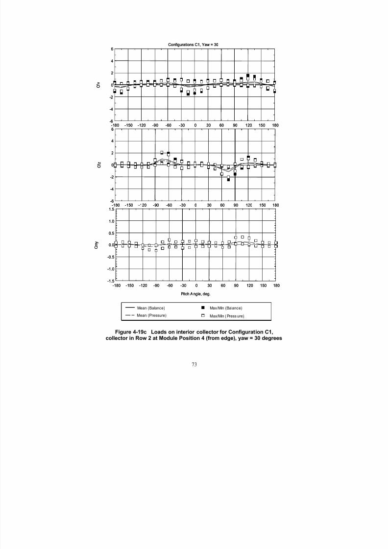
7/31/2019 Wind Tunnel Test
http://slidepdf.com/reader/full/wind-tunnel-test 82/243
Configurations C1, Yaw = 30
-180 -150 -120 -90 -60 -30 0 30 60 90 120 150 180
C f x
-6
-4
-2
0
2
4
6
-180 -150 -120 -90 -60 -30 0 30 60 90 120 150 180
C f z
-6
-4
-2
0
2
4
6
Pitch Angle, deg.
-180 -150 -120 -90 -60 -30 0 30 60 90 120 150 180
C m y
-1.5
-1.0
-0.5
0.0
0.5
1.0
1.5
Mean (Balance) Max/Min (Balance)
Mean (Pressure) Max/Min ( Press ure)
Figure 4-19c Loads on interior collector for Configuration C1,collector in Row 2 at Module Position 4 (from edge), yaw = 30 degrees
73
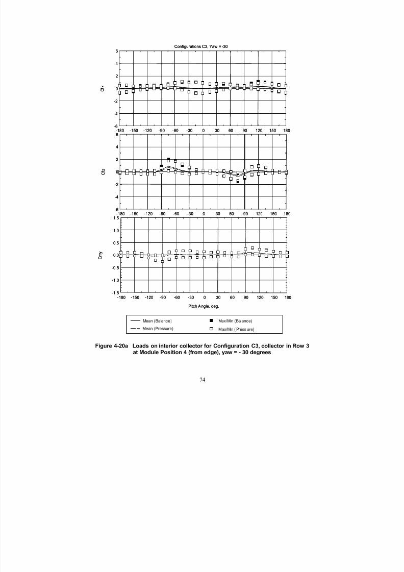
7/31/2019 Wind Tunnel Test
http://slidepdf.com/reader/full/wind-tunnel-test 83/243
Configurations C3, Yaw = -30
-180 -150 -120 -90 -60 -30 0 30 60 90 120 150 180
C f x
-6
-4
-2
0
2
4
6
-180 -150 -120 -90 -60 -30 0 30 60 90 120 150 180
C f z
-6
-4
-2
0
2
4
6
Pitch Angle, deg.
-180 -150 -120 -90 -60 -30 0 30 60 90 120 150 180
C m y
-1.5
-1.0
-0.5
0.0
0.5
1.0
1.5
Mean (Balance) Max/Min (Balance)
Mean (Pressure) Max/Min ( Press ure)
Figure 4-20a Loads on interior collector for Configuration C3, collector in Row 3at Module Position 4 (from edge), yaw = - 30 degrees
74
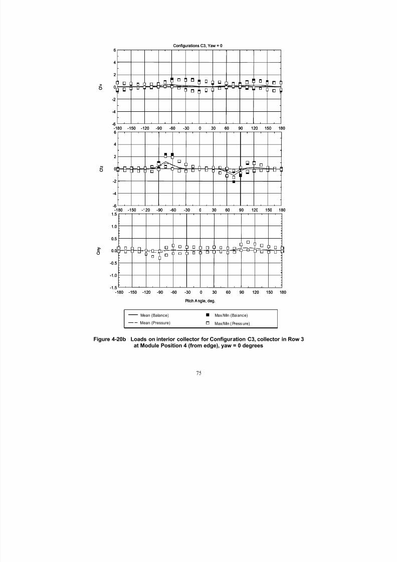
7/31/2019 Wind Tunnel Test
http://slidepdf.com/reader/full/wind-tunnel-test 84/243
Configurations C3, Yaw = 0
-180 -150 -120 -90 -60 -30 0 30 60 90 120 150 180
C f x
-6
-4
-2
0
2
4
6
-180 -150 -120 -90 -60 -30 0 30 60 90 120 150 180
C f z
-6
-4
-2
0
2
4
6
Pitch Angle, deg.
-180 -150 -120 -90 -60 -30 0 30 60 90 120 150 180
C m y
-1.5
-1.0
-0.5
0.0
0.5
1.0
1.5
Mean (Balance) Max/Min (Balance)
Mean (Pressure) Max/Min ( Press ure)
Figure 4-20b Loads on interior collector for Configuration C3, collector in Row 3at Module Position 4 (from edge), yaw = 0 degrees
75
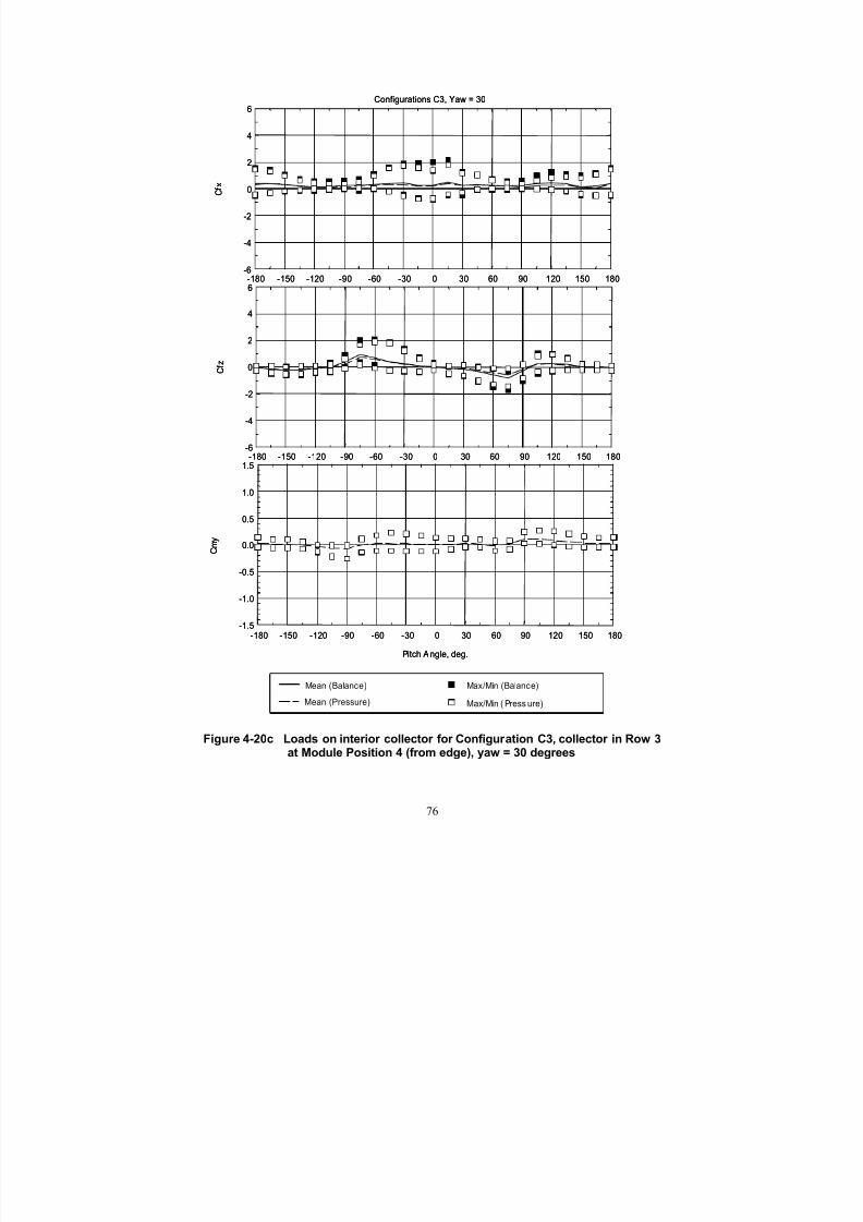
7/31/2019 Wind Tunnel Test
http://slidepdf.com/reader/full/wind-tunnel-test 85/243
Configurations C3, Yaw = 30
-180 -150 -120 -90 -60 -30 0 30 60 90 120 150 180
C f x
-6
-4
-2
0
2
4
6
-180 -150 -120 -90 -60 -30 0 30 60 90 120 150 180
C f z
-6
-4
-2
0
2
4
6
Pitch Angle, deg.
-180 -150 -120 -90 -60 -30 0 30 60 90 120 150 180
C m y
-1.5
-1.0
-0.5
0.0
0.5
1.0
1.5
Mean (Balance) Max/Min (Balance)
Mean (Pressure) Max/Min ( Press ure)
Figure 4-20c Loads on interior collector for Configuration C3, collector in Row 3at Module Position 4 (from edge), yaw = 30 degrees
76

7/31/2019 Wind Tunnel Test
http://slidepdf.com/reader/full/wind-tunnel-test 86/243
Configurations C5, Yaw = -30
-180 -150 -120 -90 -60 -30 0 30 60 90 120 150 180
C f x
-6
-4
-2
0
2
4
6
-180 -150 -120 -90 -60 -30 0 30 60 90 120 150 180
C f z
-6
-4
-2
0
2
4
6
Pitch Angle, deg.
-180 -150 -120 -90 -60 -30 0 30 60 90 120 150 180
C m y
-1.5
-1.0
-0.5
0.0
0.5
1.0
1.5
Mean (Balance) Max/Min (Balance)
Mean (Pressure) Max/Min ( Pressure)
Figure 4-21a Loads on interior collector for Configuration C5, collector in Row 5at Module Position 4 (from edge), yaw = - 30 degrees
77

7/31/2019 Wind Tunnel Test
http://slidepdf.com/reader/full/wind-tunnel-test 87/243
Configurations C5, Yaw = 0
-180 -150 -120 -90 -60 -30 0 30 60 90 120 150 180
C f x
-6
-4
-2
0
2
4
6
-180 -150 -120 -90 -60 -30 0 30 60 90 120 150 180
C f z
-6
-4
-2
0
2
4
6
Pitch Angle, deg.
-180 -150 -120 -90 -60 -30 0 30 60 90 120 150 180
C m y
-1.5
-1.0
-0.5
0.0
0.5
1.0
1.5
Mean (Balance) Max/Min (Balance)
Mean (Pressure) Max/Min ( Pressure)
Figure 4-21b Loads on interior collector for Configuration C5, collector in Row 5at Module Position 4 (from edge), yaw = 0 degrees
78
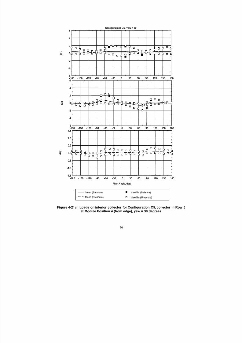
7/31/2019 Wind Tunnel Test
http://slidepdf.com/reader/full/wind-tunnel-test 88/243
Configurations C5, Yaw = 30
-180 -150 -120 -90 -60 -30 0 30 60 90 120 150 180
C f x
-6
-4
-2
0
2
4
6
-180 -150 -120 -90 -60 -30 0 30 60 90 120 150 180
C f z
-6
-4
-2
0
2
4
6
Pitch Angle, deg.
-180 -150 -120 -90 -60 -30 0 30 60 90 120 150 180
C m y
-1.5
-1.0
-0.5
0.0
0.5
1.0
1.5
Mean (Balance) Max/Min (Balance)
Mean (Pressure) Max/Min ( Pressure)
Figure 4-21c Loads on interior collector for Configuration C5, collector in Row 5at Module Position 4 (from edge), yaw = 30 degrees
79

7/31/2019 Wind Tunnel Test
http://slidepdf.com/reader/full/wind-tunnel-test 89/243
Configurations A1, B1, C1, C3 and C5 Balance, Yaw = 0
0 1 2 3 4 5
C f x a t P i t c h = 0 d
e g .
-6
-4
-2
0
2
4
6
C f z a t P i t c h = 6 0 d e g
.
-6
-4
-2
0
2
4
6
Row Position
0 1 2 3 4 5
Mean (w i thout Torque Tube) Max /Min (w i thout Torque Tube)
Row Position = 0 denotes isolated collector
Configurations A1, B1, C1, C3 and C5 Balance, Yaw = 0
0 1 2 3 4 5
C f x a t P i t c h = 0 d
e g .
-6
-4
-2
0
2
4
6
C f z a t P i t c h = 6 0 d e g
.
-6
-4
-2
0
2
4
6
Row Position
0 1 2 3 4 5
Mean (w i thout Torque Tube) Max /Min (w i thout Torque Tube)
Row Position = 0 denotes isolated collector
Figure 4-22 Effect of row position at interior of array field, yaw = 0 degrees
80
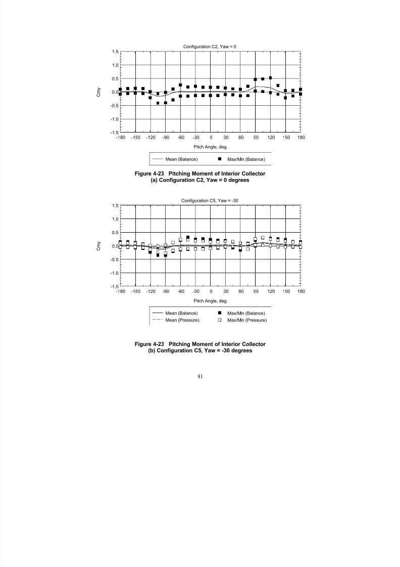
7/31/2019 Wind Tunnel Test
http://slidepdf.com/reader/full/wind-tunnel-test 90/243
Configuration C2, Yaw = 0
Pitch Angle, deg.
-180 -150 -120 -90 -60 -30 0 30 60 90 120 150 180
C m y
-1.5
-1.0
-0.5
0.0
0.5
1.0
1.5
Mean (Balance) Max/Min (Balance)
Figure 4-23 Pitching Moment of Interior Collector (a) Configuration C2, Yaw = 0 degrees
Configuration C5, Yaw = -30
Pitch Angle, deg.
-180 -150 -120 -90 -60 -30 0 30 60 90 120 150 180
C m y
-1.5
-1.0
-0.5
0.0
0.5
1.0
1.5
Mean (Balance) Max/Min (Balance)
Mean (Pressure) Max/Min (Pressure)
Figure 4-23 Pitching Moment of Interior Collector (b) Configuration C5, Yaw = -30 degrees
81

7/31/2019 Wind Tunnel Test
http://slidepdf.com/reader/full/wind-tunnel-test 91/243
Configuration C5, Yaw = 0
Pitch Angle, deg.
-180 -150 -120 -90 -60 -30 0 30 60 90 120 150 180
C m y
-1.5
-1.0
-0.5
0.0
0.5
1.0
1.5
Mean (Balance) Max/Min (Balance)
Mean (Pressure) Max/Min (Pressure)
Figure 4-23 Pitching Moment of Interior Collector (c) Configuration C5, Yaw = 0 degrees
A photograph of the flow in the deep interior of the array field is shown in Figure 4-24. Atapproximately the height of the concentrator pivot axis, the flow is very stagnant.
The Phase 3 balance test results on the interior solar collectors near the side edge of the arrayfield are given in Figure 4-25 through Figure 4-27, for Configurations C2, C4, and C6. In
general, the effect of the row position is similar to that for the collectors in the further interior.Some increase in the wind loads is seen, however, compared to the inner collectors.
Figure 4-24 Wind flow within interior of array field
82
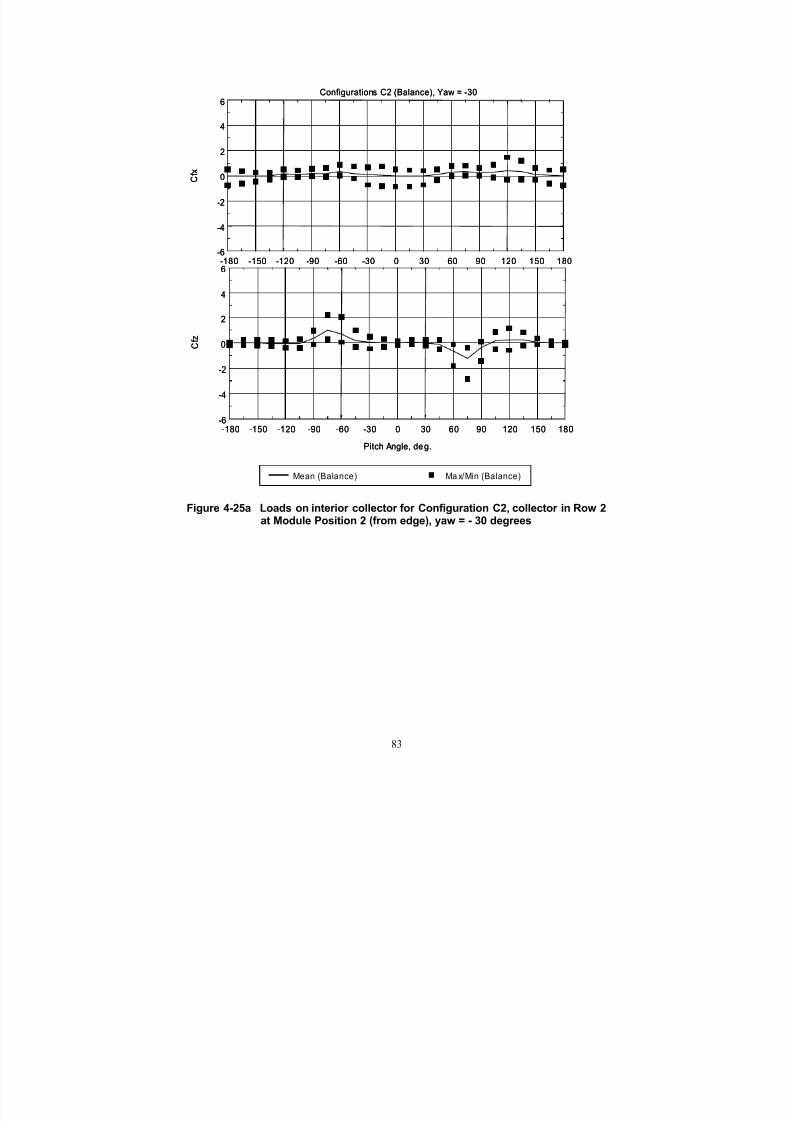
7/31/2019 Wind Tunnel Test
http://slidepdf.com/reader/full/wind-tunnel-test 92/243
Configurations C2 (Balance), Yaw = -30
-180 -150 -120 -90 -60 -30 0 30 60 90 120 150 180
C f x
-6
-4
-2
0
2
4
6
-180 -150 -120 -90 -60 -30 0 30 60 90 120 150 180
C f z
-6
-4
-2
0
2
4
6
Pitch Angle, deg.
Mean (Balance) Ma x/Min (Balance)
Configurations C2 (Balance), Yaw = -30
-180 -150 -120 -90 -60 -30 0 30 60 90 120 150 180
C f x
-6
-4
-2
0
2
4
6
-180 -150 -120 -90 -60 -30 0 30 60 90 120 150 180
C f z
-6
-4
-2
0
2
4
6
Pitch Angle, deg.
Mean (Balance) Ma x/Min (Balance)
Figure 4-25a Loads on interior collector for Configuration C2, collector in Row 2at Module Position 2 (from edge), yaw = - 30 degrees
83

7/31/2019 Wind Tunnel Test
http://slidepdf.com/reader/full/wind-tunnel-test 93/243
Con figurations C2 (Balance), Yaw = 0
-180 -150 -120 -90 -60 -30 0 30 60 90 120 150 180
C f x
-6
-4
-2
0
2
4
6
-180 -150 -120 -90 -60 -30 0 30 60 90 120 150 180
C f z
-6
-4
-2
0
2
4
6
Pitch Angle, deg.
Mean (Balance) Ma x/Min (Balance)
Con figurations C2 (Balance), Yaw = 0
-180 -150 -120 -90 -60 -30 0 30 60 90 120 150 180
C f x
-6
-4
-2
0
2
4
6
-180 -150 -120 -90 -60 -30 0 30 60 90 120 150 180
C f z
-6
-4
-2
0
2
4
6
Pitch Angle, deg.
Mean (Balance) Ma x/Min (Balance)
Con figurations C2 (Balance), Yaw = 0
-180 -150 -120 -90 -60 -30 0 30 60 90 120 150 180
C f x
-6
-4
-2
0
2
4
6
-180 -150 -120 -90 -60 -30 0 30 60 90 120 150 180
C f z
-6
-4
-2
0
2
4
6
Pitch Angle, deg.
Mean (Balance) Ma x/Min (Balance)
Con figurations C2 (Balance), Yaw = 0
-180 -150 -120 -90 -60 -30 0 30 60 90 120 150 180
C f x
-6
-4
-2
0
2
4
6
-180 -150 -120 -90 -60 -30 0 30 60 90 120 150 180
C f z
-6
-4
-2
0
2
4
6
Pitch Angle, deg.
Mean (Balance) Ma x/Min (Balance)
Figure 4-25b Loads on interior collector for Configuration C2,collector in Row 2 at Module Position 2 (from edge), yaw = 0 degrees
84

7/31/2019 Wind Tunnel Test
http://slidepdf.com/reader/full/wind-tunnel-test 94/243
Configurations C2 (Ba lance), Yaw = 3 0
-180 -150 -120 -90 -60 -30 0 30 60 90 120 150 180
C f x
-6
-4
-2
0
2
4
6
-180 -150 -120 -90 -60 -30 0 30 60 90 120 150 180
C f z
-6
-4
-2
0
2
4
6
Pitch Angle, deg.
Mean (Balance) Ma x/Min (Balance)
Con figurations C2 (Ba lance), Yaw = 3 0
-180 -150 -120 -90 -60 -30 0 30 60 90 120 150 180
C f x
-6
-4
-2
0
2
4
6
-180 -150 -120 -90 -60 -30 0 30 60 90 120 150 180
C f z
-6
-4
-2
0
2
4
6
Pitch Angle, deg.
Mean (Balance) Ma x/Min (Balance)
Con figurations C2 (Ba lance), Yaw = 3 0
-180 -150 -120 -90 -60 -30 0 30 60 90 120 150 180
C f x
-6
-4
-2
0
2
4
6
-180 -150 -120 -90 -60 -30 0 30 60 90 120 150 180
C f z
-6
-4
-2
0
2
4
6
Pitch Angle, deg.
Mean (Balance) Ma x/Min (Balance)
Con figurations C2 (Ba lance), Yaw = 3 0
-180 -150 -120 -90 -60 -30 0 30 60 90 120 150 180
C f x
-6
-4
-2
0
2
4
6
-180 -150 -120 -90 -60 -30 0 30 60 90 120 150 180
C f z
-6
-4
-2
0
2
4
6
Pitch Angle, deg.
Mean (Balance) Ma x/Min (Balance)
Figure 4-25c Loads on interior collector for Configuration C2,collector in Row 2 at Module Position 2 (from edge), yaw = 30 degrees
85

7/31/2019 Wind Tunnel Test
http://slidepdf.com/reader/full/wind-tunnel-test 95/243
Configurations C4 (Ba lance), Yaw = -30
-180 -150 -120 -90 -60 -30 0 30 60 90 120 150 180
C f x
-6
-4
-2
0
2
4
6
-180 -150 -120 -90 -60 -30 0 30 60 90 120 150 180
C f z
-6
-4
-2
0
2
4
6
Pitch Angle, deg.
Mean (Balance) Ma x/Min (Balance)
Configurations C4 (Ba lance), Yaw = -30
-180 -150 -120 -90 -60 -30 0 30 60 90 120 150 180
C f x
-6
-4
-2
0
2
4
6
-180 -150 -120 -90 -60 -30 0 30 60 90 120 150 180
C f z
-6
-4
-2
0
2
4
6
Pitch Angle, deg.
Mean (Balance) Ma x/Min (Balance)
Configurations C4 (Ba lance), Yaw = -30
-180 -150 -120 -90 -60 -30 0 30 60 90 120 150 180
C f x
-6
-4
-2
0
2
4
6
-180 -150 -120 -90 -60 -30 0 30 60 90 120 150 180
C f z
-6
-4
-2
0
2
4
6
Pitch Angle, deg.
Mean (Balance) Ma x/Min (Balance)
Configurations C4 (Ba lance), Yaw = -30
-180 -150 -120 -90 -60 -30 0 30 60 90 120 150 180
C f x
-6
-4
-2
0
2
4
6
-180 -150 -120 -90 -60 -30 0 30 60 90 120 150 180
C f z
-6
-4
-2
0
2
4
6
Pitch Angle, deg.
Mean (Balance) Ma x/Min (Balance)
Figure 4-26a Loads on interior collector for Configuration C4,collector in Row 3 at Module Position 2 (from edge), yaw = - 30 degrees
86

7/31/2019 Wind Tunnel Test
http://slidepdf.com/reader/full/wind-tunnel-test 96/243
Configurations C4 (Ba lance), Yaw = 0
-180 -150 -120 -90 -60 -30 0 30 60 90 120 150 180
C f x
-6
-4
-2
0
2
4
6
-180 -150 -120 -90 -60 -30 0 30 60 90 120 150 180
C f z
-6
-4
-2
0
2
4
6
Pitch Angle, deg.
Mean (Balance) Ma x/Min (Balance)
Con figurations C4 (Ba lance), Yaw = 0
-180 -150 -120 -90 -60 -30 0 30 60 90 120 150 180
C f x
-6
-4
-2
0
2
4
6
-180 -150 -120 -90 -60 -30 0 30 60 90 120 150 180
C f z
-6
-4
-2
0
2
4
6
Pitch Angle, deg.
Mean (Balance) Ma x/Min (Balance)
Con figurations C4 (Ba lance), Yaw = 0
-180 -150 -120 -90 -60 -30 0 30 60 90 120 150 180
C f x
-6
-4
-2
0
2
4
6
-180 -150 -120 -90 -60 -30 0 30 60 90 120 150 180
C f z
-6
-4
-2
0
2
4
6
Pitch Angle, deg.
Mean (Balance) Ma x/Min (Balance)
Con figurations C4 (Ba lance), Yaw = 0
-180 -150 -120 -90 -60 -30 0 30 60 90 120 150 180
C f x
-6
-4
-2
0
2
4
6
-180 -150 -120 -90 -60 -30 0 30 60 90 120 150 180
C f z
-6
-4
-2
0
2
4
6
Pitch Angle, deg.
Mean (Balance) Ma x/Min (Balance)
Figure 4-26b Loads on interior collector for Configuration C4,collector in Row 3 at Module Position 2 (from edge), yaw = 0 degrees
87

7/31/2019 Wind Tunnel Test
http://slidepdf.com/reader/full/wind-tunnel-test 97/243
Configurations C4 (Ba lance), Yaw = 3 0
-180 -150 -120 -90 -60 -30 0 30 60 90 120 150 180
C f x
-6
-4
-2
0
2
4
6
-180 -150 -120 -90 -60 -30 0 30 60 90 120 150 180
C f z
-6
-4
-2
0
2
4
6
Pitch Angle, deg.
Mean (Balance) Ma x/Min (Balance)
Con figurations C4 (Ba lance), Yaw = 3 0
-180 -150 -120 -90 -60 -30 0 30 60 90 120 150 180
C f x
-6
-4
-2
0
2
4
6
-180 -150 -120 -90 -60 -30 0 30 60 90 120 150 180
C f z
-6
-4
-2
0
2
4
6
Pitch Angle, deg.
Mean (Balance) Ma x/Min (Balance)
Con figurations C4 (Ba lance), Yaw = 3 0
-180 -150 -120 -90 -60 -30 0 30 60 90 120 150 180
C f x
-6
-4
-2
0
2
4
6
-180 -150 -120 -90 -60 -30 0 30 60 90 120 150 180
C f z
-6
-4
-2
0
2
4
6
Pitch Angle, deg.
Mean (Balance) Ma x/Min (Balance)
Con figurations C4 (Ba lance), Yaw = 3 0
-180 -150 -120 -90 -60 -30 0 30 60 90 120 150 180
C f x
-6
-4
-2
0
2
4
6
-180 -150 -120 -90 -60 -30 0 30 60 90 120 150 180
C f z
-6
-4
-2
0
2
4
6
Pitch Angle, deg.
Mean (Balance) Ma x/Min (Balance)
Figure 4-26c Loads on interior collector for Configuration C4,collector in Row 3 at Module Position 2 (from edge), yaw = 30 degrees
88
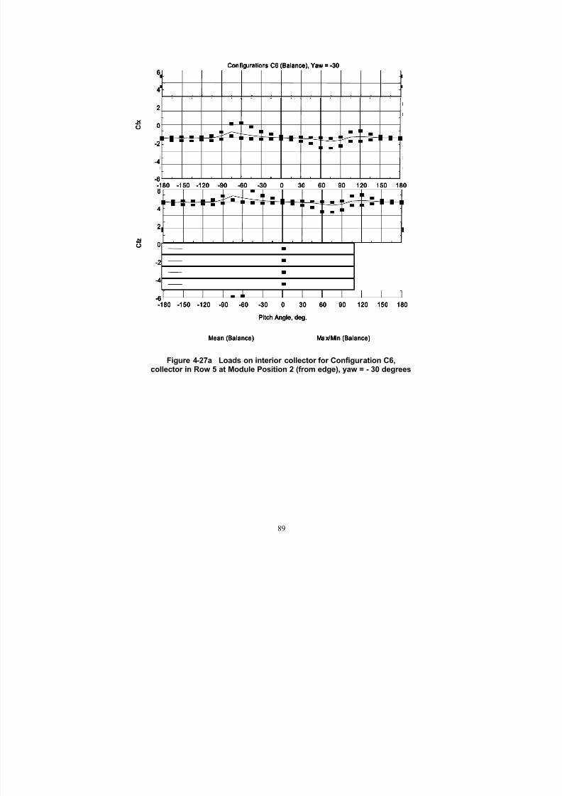
7/31/2019 Wind Tunnel Test
http://slidepdf.com/reader/full/wind-tunnel-test 98/243
Configurations C6 (Balance), Yaw = -30
-180 -150 -120 -90 -60 -30 0 30 60 90 120 150 180
C f x
-6
-4
-2
0
2
4
6
-180 -150 -120 -90 -60 -30 0 30 60 90 120 150 180
C f z
-6
-4
-2
0
2
4
6
Pitch Angle, deg.
Mean (Balance) Ma x/Min (Balance)
Con figurations C6 (Balance), Yaw = -30
-180 -150 -120 -90 -60 -30 0 30 60 90 120 150 180
C f x
-6
-4
-2
0
2
4
6
-180 -150 -120 -90 -60 -30 0 30 60 90 120 150 180
C f z
-6
-4
-2
0
2
4
6
Pitch Angle, deg.
Mean (Balance) Ma x/Min (Balance)
Con figurations C6 (Balance), Yaw = -30
-180 -150 -120 -90 -60 -30 0 30 60 90 120 150 180
C f x
-6
-4
-2
0
2
4
6
-180 -150 -120 -90 -60 -30 0 30 60 90 120 150 180
C f z
-6
-4
-2
0
2
4
6
Pitch Angle, deg.
Mean (Balance) Ma x/Min (Balance)
Con figurations C6 (Balance), Yaw = -30
-180 -150 -120 -90 -60 -30 0 30 60 90 120 150 180
C f x
-6
-4
-2
0
2
4
6
-180 -150 -120 -90 -60 -30 0 30 60 90 120 150 180
C f z
-6
-4
-2
0
2
4
6
Pitch Angle, deg.
Mean (Balance) Ma x/Min (Balance)
Figure 4-27a Loads on interior collector for Configuration C6,collector in Row 5 at Module Position 2 (from edge), yaw = - 30 degrees
89

7/31/2019 Wind Tunnel Test
http://slidepdf.com/reader/full/wind-tunnel-test 99/243
Configurations C6 (Ba lance), Yaw = 0
-180 -150 -120 -90 -60 -30 0 30 60 90 120 150 180
C f x
-6
-4
-2
0
2
4
6
-180 -150 -120 -90 -60 -30 0 30 60 90 120 150 180
C f z
-6
-4
-2
0
2
4
6
Pitch Angle, deg.
Mean (Balance) Ma x/Min (Balance)
Con figurations C6 (Ba lance), Yaw = 0
-180 -150 -120 -90 -60 -30 0 30 60 90 120 150 180
C f x
-6
-4
-2
0
2
4
6
-180 -150 -120 -90 -60 -30 0 30 60 90 120 150 180
C f z
-6
-4
-2
0
2
4
6
Pitch Angle, deg.
Mean (Balance) Ma x/Min (Balance)
Con figurations C6 (Ba lance), Yaw = 0
-180 -150 -120 -90 -60 -30 0 30 60 90 120 150 180
C f x
-6
-4
-2
0
2
4
6
-180 -150 -120 -90 -60 -30 0 30 60 90 120 150 180
C f z
-6
-4
-2
0
2
4
6
Pitch Angle, deg.
Mean (Balance) Ma x/Min (Balance)
Con figurations C6 (Ba lance), Yaw = 0
-180 -150 -120 -90 -60 -30 0 30 60 90 120 150 180
C f x
-6
-4
-2
0
2
4
6
-180 -150 -120 -90 -60 -30 0 30 60 90 120 150 180
C f z
-6
-4
-2
0
2
4
6
Pitch Angle, deg.
Mean (Balance) Ma x/Min (Balance)
Figure 4-27b Loads on interior collector for Configuration C6,collector in Row 5 at Module Position 2 (from edge), yaw = 0 degrees
90

7/31/2019 Wind Tunnel Test
http://slidepdf.com/reader/full/wind-tunnel-test 100/243
Configurations C6 (Ba lance), Yaw = 3 0
-180 -150 -120 -90 -60 -30 0 30 60 90 120 150 180
C f x
-6
-4
-2
0
2
4
6
-180 -150 -120 -90 -60 -30 0 30 60 90 120 150 180
C f z
-6
-4
-2
0
2
4
6
Pitch Angle, deg.
Mean (Balance) Ma x/Min (Balance)
Con figurations C6 (Ba lance), Yaw = 3 0
-180 -150 -120 -90 -60 -30 0 30 60 90 120 150 180
C f x
-6
-4
-2
0
2
4
6
-180 -150 -120 -90 -60 -30 0 30 60 90 120 150 180
C f z
-6
-4
-2
0
2
4
6
Pitch Angle, deg.
Mean (Balance) Ma x/Min (Balance)
Con figurations C6 (Ba lance), Yaw = 3 0
-180 -150 -120 -90 -60 -30 0 30 60 90 120 150 180
C f x
-6
-4
-2
0
2
4
6
-180 -150 -120 -90 -60 -30 0 30 60 90 120 150 180
C f z
-6
-4
-2
0
2
4
6
Pitch Angle, deg.
Mean (Balance) Ma x/Min (Balance)
Con figurations C6 (Ba lance), Yaw = 3 0
-180 -150 -120 -90 -60 -30 0 30 60 90 120 150 180
C f x
-6
-4
-2
0
2
4
6
-180 -150 -120 -90 -60 -30 0 30 60 90 120 150 180
C f z
-6
-4
-2
0
2
4
6
Pitch Angle, deg.
Mean (Balance) Ma x/Min (Balance)
Figure 4-27c Loads on interior collector for Configuration C6,collector in Row 5 at Module Position 2 (from edge), yaw = 30 degrees
91

7/31/2019 Wind Tunnel Test
http://slidepdf.com/reader/full/wind-tunnel-test 101/243
4.5.2 Effects of Torque Tube
The effect of the torque tube on the most interior solar collector is shown in Figure 4-28. As far
as the structural design loads are concerned, the torque tube caused no significant effect.
Configurations C5 and F5 Balance, Yaw = 0
-180 -150 -120 -90 -60 -30 0 30 60 90 120 150 180
C f x
-6
-4
-2
0
2
4
6
-180 -150 -120 -90 -60 -30 0 30 60 90 120 150 180
C f z
-6
-4
-2
0
2
4
6
Pitch Angle, deg.
Mean (w i thout Torque Tube) Max /Min (w i thout Torque Tube)
Mean (w ith Torque Tube) Max/Min (w ith Torque Tube)
Figure 4-28 Effect of torque tube on collector in array field,Configurations C5 and F5, yaw = 0 degrees
92

7/31/2019 Wind Tunnel Test
http://slidepdf.com/reader/full/wind-tunnel-test 102/243
4.6 Loads on Deep Interior Solar Collectors
In order to determine wind loads that can be regarded as representative for a majority of the solar collector modules within a large array field, tests were conducted on a collector module at various
row and column positions. Pressure distributions over the collector module concentrator were
measured, which were then integrated to yield the overall forces and pitch moment. Refer toSection 2.4 for the tested locations of the solar collector module within the array field.
At each row and column combination, the wind-tunnel test was performed for pitch angles of -15,-60, 0, 75 and 105 degrees, at which the Phase 3 wind-tunnel study showed relatively large wind
loads. For sake of clarity, however, this section selectively presents the test results based on thesignificance found for the individual overall load components exerted on the pivotal axis of the
collector concentrator. The following discussion deals with the lateral and vertical forces and the pitching moment at particular pitch angles of 0, -60 and 105 degrees, respectively. A completeset of the test results is found in Appendix B.
Variations of the mean and peak loads at different row positions are shown in Figure 4-29 for the4th column collectors at a yaw angle of 0 degrees. The Phase 3 pressure model test results, where
available, are included to show the load pattern on the collectors near the upwind edge of thearray field (1st through 4th rows). Note that at the 5th row position, both the Phase 3 and 4 test
results are plotted, showing a good repeatability in the mean load measurement, and some scatter in the peaks due to inherent statistical variability. For the lateral force, Cfx, at a pitch angle of 0degrees, the most drastic reduction is realized on the 2nd row collector, and the load tends to
recover somewhat for the collectors up to the 5 th row. No appreciable change in the lateral forceis evident for the collectors further downwind. The vertical force component, Cfz , at a pitch
angle of –60 degrees shows a similar trend, except that the recovery of the peak load is morevigorous. In fact, the positive peak on the interior collectors is nearly as large as that on thecollector at the field edge. The pitching moment component, Cmy, appears to decrease slowly
through the 5th row collector, and becomes independent of the row position downwind.
93

7/31/2019 Wind Tunnel Test
http://slidepdf.com/reader/full/wind-tunnel-test 103/243
0 5 10 15 20
C f z a
t P i t c h = - 6
0 d e
g .
-6
-4
-2
0
2
4
6
Collector at Column 4, Yaw = 0
0 5 10 15 20
C f x a
t P i t c h =
0 d e g .
-6
-4
-2
0
2
4
6
Row Position
0 5 10 15 20
C m y a
t P i t c h =
1 0 5 d e g .
-1.5
-1.0
-0.5
0.0
0.5
1.0
1.5
Mean Max/Min
Row Position = 0 denotes isolated collector
Figure 4-29 Effect of Row Position for Collectors at 4th Column, Yaw = 0 degrees
94
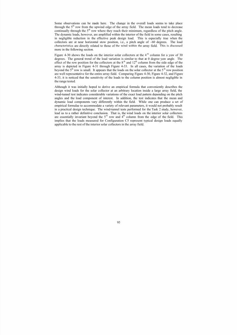
7/31/2019 Wind Tunnel Test
http://slidepdf.com/reader/full/wind-tunnel-test 104/243
Some observations can be made here. The change in the overall loads seems to take placethrough the 5
throw from the upwind edge of the array field. The mean loads tend to decrease
continually through the 5th
row where they reach their minimum, regardless of the pitch angle.The dynamic loads, however, are amplified within the interior of the field in some cases, resulting
in negligible reduction in the effective peak design load. This is especially true when thecollectors are at near horizontal stow position, i.e., a pitch angle of –60 degrees. The load
characteristics are directly related to those of the wind within the array field. This is discussedmore in the following section.
Figure 4-30 shows the loads on the interior solar collectors at the 4th
column for a yaw of 30degrees. The general trend of the load variation is similar to that at 0 degree yaw angle. Theeffect of the row position for the collectors at the 8 th and 12th column from the side edge of thearray is depicted in Figure 4-31 through Figure 4-33. In all cases, the variation of the loads
beyond the 5th
row is small. It appears that the loads on the solar collector at the 5th
row positionare well representative for the entire array field. Comparing Figure 4-30, Figure 4-32, and Figure4-33, it is noticed that the sensitivity of the loads to the column position is almost negligible inthe range tested.
Although it was initially hoped to derive an empirical formula that conveniently describes the
design wind loads for the solar collector at an arbitrary location inside a large array field, thewind-tunnel test indicates considerable variations of the exact load pattern depending on the pitch
angles and the load component of interest. In addition, the test indicates that the mean anddynamic load components vary differently within the field. While one can produce a set of
empirical formulae to accommodate a variety of relevant parameters, it would not probably resultin a practical design technique. The wind-tunnel tests performed for the Task 2 study, however,lead us to a rather definitive conclusion. That is, the wind loads on the interior solar collectors
are essentially invariant beyond the 5th
row and 4th
column from the edge of the field. Thisimplies that the loads measured for Configuration C5 represent typical design loads equallyapplicable to the rest of the interior solar collectors in the array field.
95
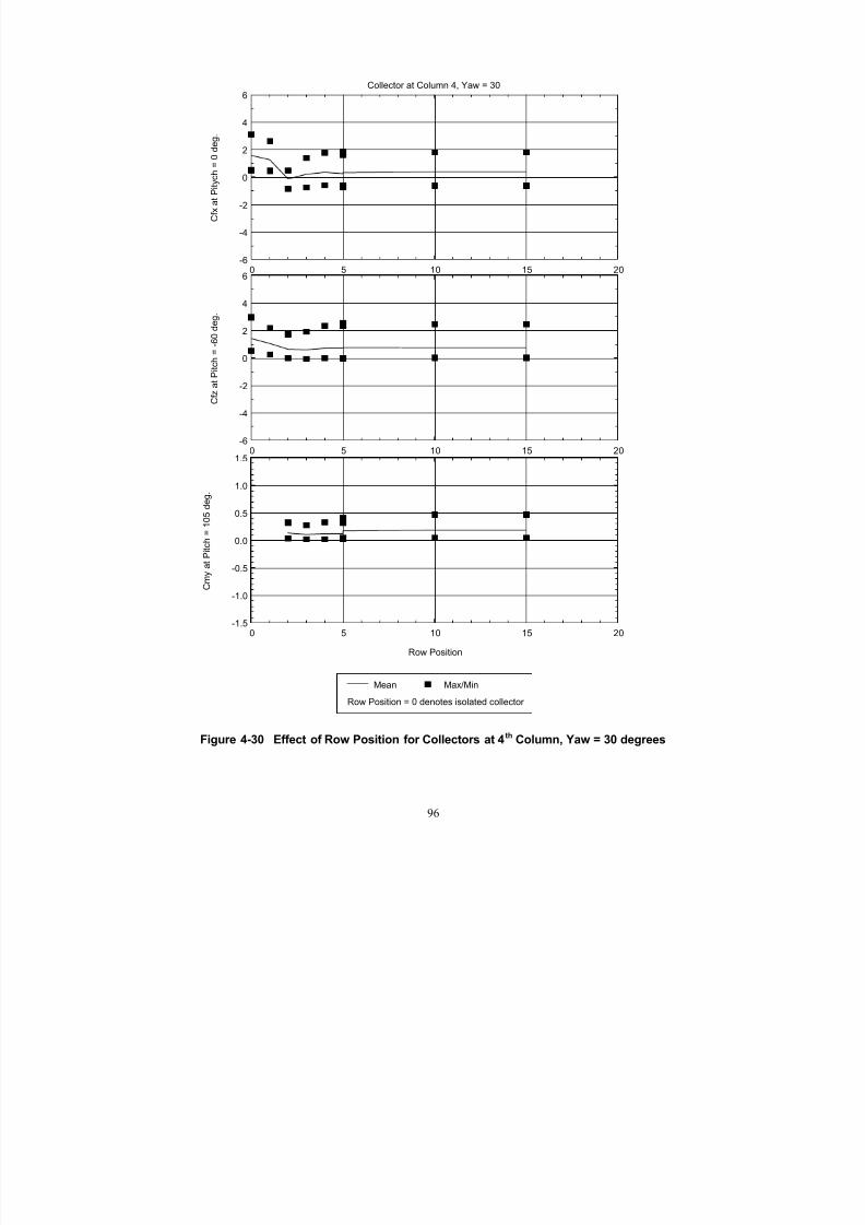
7/31/2019 Wind Tunnel Test
http://slidepdf.com/reader/full/wind-tunnel-test 105/243
0 5 10 15 20
C f z a t P i t c h = - 6 0 d e g .
-6
-4
-2
0
2
4
6
Collector at Column 4, Yaw = 30
0 5 10 15 20
C f x a t P i t y c h =
0 d e g .
-6
-4
-2
0
2
4
6
Row Position
0 5 10 15 20
C m y a t P i t c h = 1 0 5 d e g
.
-1.5
-1.0
-0.5
0.0
0.5
1.0
1.5
Mean Max/Min
Row Position = 0 denotes isolated collector
Figure 4-30 Effect of Row Position for Collectors at 4th Column, Yaw = 30 degrees
96
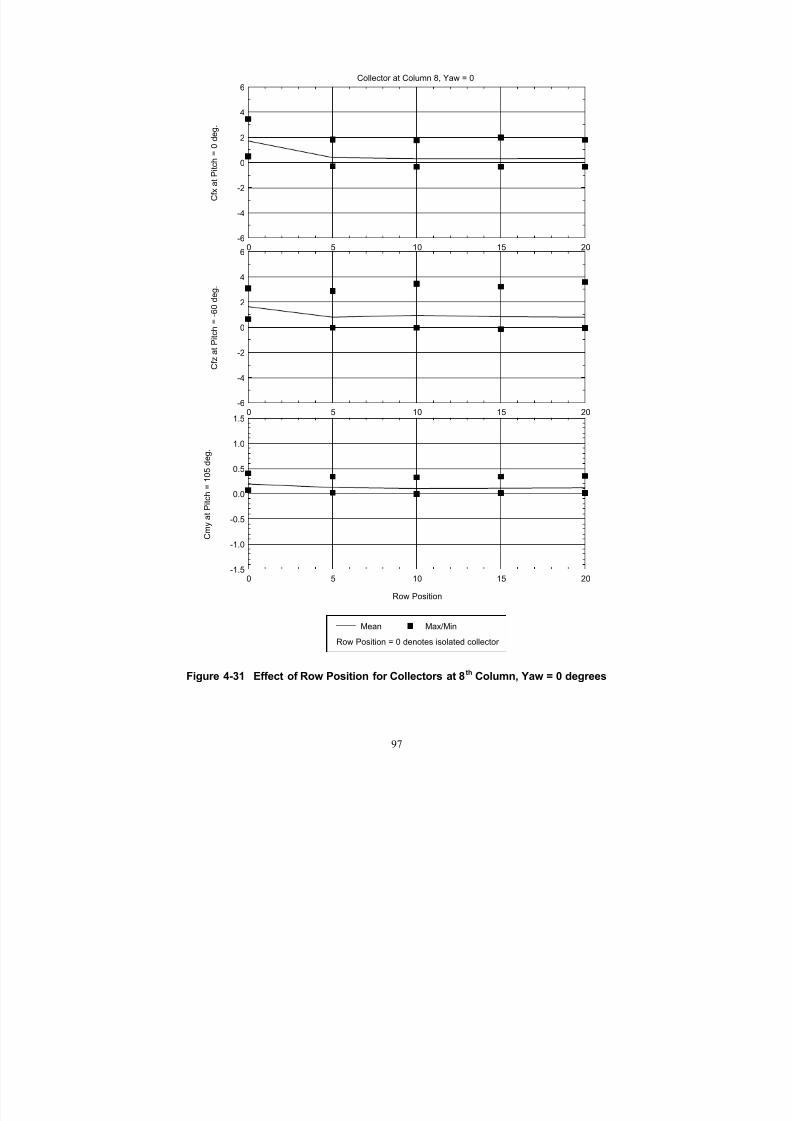
7/31/2019 Wind Tunnel Test
http://slidepdf.com/reader/full/wind-tunnel-test 106/243
0 5 10 15 20
C f z a t P i t c h = - 6 0 d e g .
-6
-4
-2
0
2
4
6
Collector at Column 8, Yaw = 0
0 5 10 15 20
C f x a t P i t c h =
0 d e g .
-6
-4
-2
0
2
4
6
Row Position
0 5 10 15 20
C m y a t P i t c h = 1 0 5 d e g
.
-1.5
-1.0
-0.5
0.0
0.5
1.0
1.5
Mean Max/Min
Row Position = 0 denotes isolated collector
Figure 4-31 Effect of Row Position for Collectors at 8th Column, Yaw = 0 degrees
97

7/31/2019 Wind Tunnel Test
http://slidepdf.com/reader/full/wind-tunnel-test 107/243
0 5 10 15 20
C f z a
t P i t c h = - 6
0 d
e g .
-6
-4
-2
0
2
4
6
Collector at Column 8, Yaw = 30
0 5 10 15 20
C f x a
t P i t c h =
0 d e g .
-6
-4
-2
0
2
4
6
Row Position
0 5 10 15 20
C m y a
t P i t c h =
1 0 5 d e g .
-1.5
-1.0
-0.5
0.0
0.5
1.0
1.5
Mean Max/Min
Row Position = 0 denotes isolated collector
Figure 4-32 Effect of Row Position for Collectors at 8th Column, Yaw = 30 degrees
98
7/31/2019 Wind Tunnel Test
http://slidepdf.com/reader/full/wind-tunnel-test 108/243
0 5 10 15 20
C f z a
t P i t c h = - 6
0 d e g .
-6
-4
-2
0
2
4
6
Collector at Column 12, Yaw = 30
0 5 10 15 20
C f x a
t P i t c h =
0 d e g .
-6
-4
-2
0
2
4
6
Row Position
0 5 10 15 20
C m y a
t P i t c h =
1 0 5
d e g .
-1.5
-1.0
-0.5
0.0
0.5
1.0
1.5
Mean Max/Min
Row Position = 0 denotes isolated collector
Figure 4-33 Effect of Row Position for Collectors at 12th Column, Yaw = 30 degrees
99
7/31/2019 Wind Tunnel Test
http://slidepdf.com/reader/full/wind-tunnel-test 109/243
4.7 Wind Characteristics Within Array Field
Vertical profiles of the mean wind speed and local turbulence intensity are given in Figure 4-34 (at the top and bottom, respectively) at various row positions within the array field. The
undisturbed velocity profiles approaching the array field are also shown at the far left of the
figure. All data were taken at a yaw angle of 0 degrees with the collectors rotated at pitch anglesof 0 (Figure 4-34 (a)) and –60 (Figure 4-34 (b)) degrees. The mean wind speeds have beennormalized relative to the speed at the collector pivot height of the approach wind. The figureclearly shows drastic reduction of the mean wind speed and increased turbulence intensity as the
wind initially enters the array field. The shapes of the mean and turbulence intensity profilesseem to become invariant beyond the 5
throw position. As expected, the mean wind speed over
the collector height is much smaller when the collectors are at upright position (Figure 4-34 (a))than at near stow position (Figure 4-34 (b)) due to increased blockage. Differences in the shapesof the turbulence intensity between the two collector positions are also noticeable.
The characteristics of the wind speed and turbulence intensity inside the array filed are consistentwith the resulting wind loads on the solar collectors described above. That is, the reduced mean
loads and increased dynamic loads. Little variation of the wind loads beyond the 5th
row position
is also well explained by the wind profiles.
100

7/31/2019 Wind Tunnel Test
http://slidepdf.com/reader/full/wind-tunnel-test 110/243
U / U H c
0 . 0
0 . 5
1 . 0
1 . 5
z / H c
0 5 1 0
1 5
U / U H c
0 . 0
0 . 5
1 . 0
1 . 5
U / U H c
0 . 0
0 . 5
1 . 0
1 . 5
U / U H c
0 . 0
0 . 5
1 . 0
1 . 5
U / U H c
0 . 0
0 . 5
1 . 0
1 . 5
2 . 0
T I , %
0
2 0
4 0
6 0
8 0
z / H c
0 5 1 0
1 5
T I , %
0
2 0
4 0
6 0
8 0
T I , %
0
2 0
4 0
6 0
8 0
T I , %
0
2 0
4 0
6 0
8 0
T I , %
0
2 0
4 0
6 0
8 0
1 0 0
R o w 1
R o w 5
R o w 1 0
R o w 1 5
R o w
2 0
R o w 1
R o w 5
R o w 1 0
R o w 1 5
R o w 2 0
Figure 4-34 Mean Velocity and Turbulent Profiles Within Array Field(a) Pitch = 0 deg
101

7/31/2019 Wind Tunnel Test
http://slidepdf.com/reader/full/wind-tunnel-test 111/243
U / U H c
0 . 0
0 . 5
1 . 0
1 . 5
z / H c
0 5 1 0
1 5
U / U H c
0 . 0
0 . 5
1 . 0
1 . 5
U / U H c
0 . 0
0 . 5
1 . 0
1 . 5
U / U H c
0
. 0
0 . 5
1 . 0
1 . 5
U / U H c
0 . 0
0 . 5
1 . 0
1 . 5
2 . 0
T I , %
0
2 0
4 0
6 0
8 0
z / H c
0 5 1 0
1 5
T I , %
0
2 0
4 0
6 0
8 0
T I , %
0
2 0
4 0
6 0
8 0
T I , %
0
2 0
4 0
6 0
8 0
T I , %
0
2 0
4 0
6 0
8 0
1 0 0
R o w 1
R o w 5
R o w 1 0
R o w 1 5
R o w 2 0
R o w 1
R o w 5
R o w 1 0
R o w 1 5
R o w 2 0
Figure 4-34 Mean Velocity and Turbulent Profiles Within Array Field(b) Pitch = - 60 deg
102
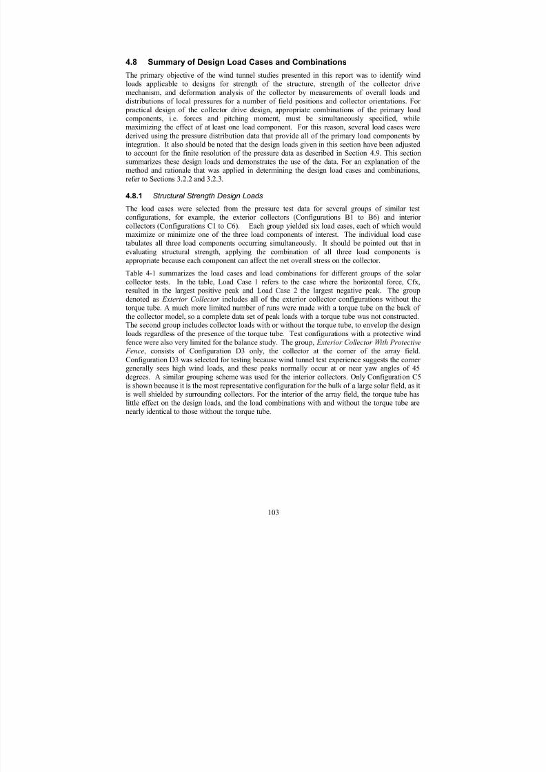
7/31/2019 Wind Tunnel Test
http://slidepdf.com/reader/full/wind-tunnel-test 112/243
4.8 Summary of Design Load Cases and Combinations
The primary objective of the wind tunnel studies presented in this report was to identify windloads applicable to designs for strength of the structure, strength of the collector drive
mechanism, and deformation analysis of the collector by measurements of overall loads and
distributions of local pressures for a number of field positions and collector orientations. For practical design of the collector drive design, appropriate combinations of the primary loadcomponents, i.e. forces and pitching moment, must be simultaneously specified, whilemaximizing the effect of at least one load component. For this reason, several load cases were
derived using the pressure distribution data that provide all of the primary load components byintegration. It also should be noted that the design loads given in this section have been adjustedto account for the finite resolution of the pressure data as described in Section 4.9. This sectionsummarizes these design loads and demonstrates the use of the data. For an explanation of themethod and rationale that was applied in determining the design load cases and combinations,
refer to Sections 3.2.2 and 3.2.3.
4.8.1 Structural Strength Design Loads
The load cases were selected from the pressure test data for several groups of similar testconfigurations, for example, the exterior collectors (Configurations B1 to B6) and interior
collectors (Configurations C1 to C6). Each group yielded six load cases, each of which wouldmaximize or minimize one of the three load components of interest. The individual load casetabulates all three load components occurring simultaneously. It should be pointed out that in
evaluating structural strength, applying the combination of all three load components isappropriate because each component can affect the net overall stress on the collector.
Table 4-1 summarizes the load cases and load combinations for different groups of the solar collector tests. In the table, Load Case 1 refers to the case where the horizontal force, Cfx,resulted in the largest positive peak and Load Case 2 the largest negative peak. The group
denoted as Exterior Collector includes all of the exterior collector configurations without thetorque tube. A much more limited number of runs were made with a torque tube on the back of
the collector model, so a complete data set of peak loads with a torque tube was not constructed.The second group includes collector loads with or without the torque tube, to envelop the designloads regardless of the presence of the torque tube. Test configurations with a protective wind
fence were also very limited for the balance study. The group, Exterior Collector With Protective Fence, consists of Configuration D3 only, the collector at the corner of the array field.
Configuration D3 was selected for testing because wind tunnel test experience suggests the corner generally sees high wind loads, and these peaks normally occur at or near yaw angles of 45degrees. A similar grouping scheme was used for the interior collectors. Only Configuration C5
is shown because it is the most representative configuration for the bulk of a large solar field, as itis well shielded by surrounding collectors. For the interior of the array field, the torque tube haslittle effect on the design loads, and the load combinations with and without the torque tube arenearly identical to those without the torque tube.
103

7/31/2019 Wind Tunnel Test
http://slidepdf.com/reader/full/wind-tunnel-test 113/243
Table 4-1 Summary of Load Cases and Load Combinations
(a) Exterior Collectors
Operational Mode (positove pitch angles)* Stow Mode (negative pitch angles)
Case Condition Conf. Yaw Pitch Cfx Cfz Cmy Case Condition Conf. Yaw Pitch Cfx Cfz Cmy
1 Max Cfx B3 30 0 5.097 -0.034 --- 1 Max Cfx B3 45 -15 5.117 1.550 0.114
2 Min Cfx B4 0 0 -1.242 -0.125 --- 2 Min Cfx B4 0 -15 -1.130 -0.404 -0.0653 Max Cfz B3 30 135 2.527 1.849 --- 3 Max Cfz B3 0 -60 1.647 3.952 0.364
4 Min Cfz B3 0 60 2.107 -5.256 --- 4 Min Cfz B4 30 -150 2.306 -0.927 -0.232
5 Max Cmy --- --- --- --- --- --- 5 Max Cmy B3 0 -60 1.410 3.709 0.419
6 Min Cmy --- --- --- --- --- --- 6 Min Cmy B3 0 -105 0.870 -0.231 -0.517
(b) Exterior Collectors With Protective Fence
Operational Mode (positove pitch angles)* Stow Mode (negative pitch angles)
Case Condition Conf. Yaw Pitch Cfx Cfz Cmy Case Condition Conf. Yaw Pitch Cfx Cfz Cmy
1 Max Cfx D3 45 15 2.900 -0.374 --- 1 Max Cfx D4 30 -15 4.033 1.026 -0.035
2 Min Cfx D3 30 60 -0.503 -0.264 --- 2 Min Cfx D4 -30 -15 -0.852 -0.278 -0.032
3 Max Cfz D3 45 135 1.705 1.030 --- 3 Max Cfz D5 30 -60 1.294 2.984 0.246
4 Min Cfz D3 45 60 1.175 -2.281 --- 4 Min Cfz D4 30 -135 1.481 -1.050 -0.202
5 Max Cmy --- --- --- --- --- --- 5 Max Cmy D5 30 -45 1.573 2.282 0.332
6 Min Cmy --- --- --- --- --- --- 6 Min Cmy D5 30 -105 0.849 -0.436 -0.468
(c) Interior Collectors Without Torque Tube
Operational Mode (positove pitch angles) Stow Mode (negative pitch angles)
Case Condition Conf. Yaw Pitch Cfx Cfz Cmy Case Condition Conf. Yaw Pitch Cfx Cfz Cmy
1 Max Cfx C5 30 15 2.264 -0.429 0.113 1 Max Cfx C7 0 -30 2.569 1.717 0.134
2 Min Cfx C1 0 0 -1.330 -0.148 -0.098 2 Min Cfx C1 30 -15 -1.374 -0.329 0.025
3 Max Cfz C1 0 120 1.433 1.362 0.370 3 Max Cfz C5 0 -60 1.404 2.754 0.107
4 Min Cfz C1 0 75 0 .712 -2.533 0.021 4 Min Cfz C5 30 -135 0 .859 -0.763 -0.045
5 Max Cmy C1 0 120 1.384 1.081 0.436 5 Max Cmy C5 30 -45 1.929 2.618 0.322
6 Min Cmy C1 0 0 -1.228 -0.236 -0.156 6 Min Cmy C5 0 -90 0.571 0.303 -0.378
(d) Interior Collectors With Torque Tube
Operational Mode (positove pitch angles) Stow Mode (negative pitch angles)
Case Condition Conf. Yaw Pitch Cfx Cfz Cmy Case Condition Conf. Yaw Pitch Cfx Cfz Cmy
1 Max Cfx F3 30 0 2.646 0.007 0.005 1 Max Cfx F3 30 -15 2.777 0.823 0.051
2 Min Cfx F3 0 0 -1.195 -0.081 -0.053 2 Min Cfx F3 0 -15 -1.475 -0.554 -0.102
3 Max Cfz F3 0 105 1.108 1.428 0.463 3 Max Cfz F3 30 -60 1.478 2.760 0.066
4 Min Cfz F3 30 60 1.148 -2.155 -0.055 4 Min Cfz F3 0 -90 0.783 -1.127 -0.518
5 Max Cmy F3 30 105 1.139 1.127 0.535 5 Max Cmy F3 30 -30 1.477 1.402 0.315
6 Min Cmy F3 30 0 0.157 -0.307 -0.203 6 Min Cmy F3 0 -90 0.950 -0.806 -0.629
(e) Interior Collectors - Configuration C5 only
Operational Mode (positove pitch angles) Stow Mode (negative pitch angles)
Case Condition Conf. Yaw Pitch Cfx Cfz Cmy Case Condition Conf. Yaw Pitch Cfx Cfz Cmy
1 Max Cfx C5 30 15 2.264 -0.429 0.113 1 Max Cfx C5 30 -45 2.209 2.721 0.239
2 Min Cfx C5 30 0 -0.858 -0.106 -0.070 2 Min Cfx C5 30 -15 -0.819 -0.220 0.000
3 Max Cfz C5 0 120 1.011 1.186 0.187 3 Max Cfz C5 0 -60 1.404 2.754 0.107
4 Min Cfz C5 30 75 0.456 -2.233 -0.091 4 Min Cfz C5 30 -135 0.859 -0.763 -0.045
5 Max Cmy C5 30 105 0.716 0.550 0.363 5 Max Cmy C5 30 -45 1.929 2.618 0.322
6 Min Cmy C5 30 75 0.244 -1.759 -0.145 6 Min Cmy C5 0 -90 0.571 0.303 -0.378
* Data available only by Phase 2 force balance study.
104

7/31/2019 Wind Tunnel Test
http://slidepdf.com/reader/full/wind-tunnel-test 114/243
4.8.2 Local Peak Differential Design Pressures
From all the pressure data taken, the largest local differential pressures were extracted
irrespective of the yaw or the pitch angle. The results are presented as a contour map in Figure
4-35, looking into the reflective side of the concentrator. The data are applicable to limitedsurface areas on the collector and are intended to provide a guideline for a mounting scheme for the individual reflector panels, for example. High pressures are typically concentrated around theedges of the collector because of flow separation or vortex formation from the corner (Figure
4-36) where the most wind damage, such as breakage of the reflector panels, is expected to occur.The results are also tabulated in Table 4-2.
The use of the local peak pressures given here for the structural design is inappropriate becausethese peak pressures do not occur simultaneously for the structural frames to react. Thedifferential pressure distributions suitable for the structural concerns are presented in the next
section.
105

7/31/2019 Wind Tunnel Test
http://slidepdf.com/reader/full/wind-tunnel-test 115/243
9.5
7.5 7.0 7.5
6.0 6.5
5.5
5.5 6.0 6.5
5.0
5.0
-4.5
-4.0
-4.5
-5.0
-4.0
-4.5
-3.5
-3.0
-2.5
Peak Positive
Peak Negative
Field Exterior
Figure 4-35a Local peak differential pressure distribution, field exterior
106

7/31/2019 Wind Tunnel Test
http://slidepdf.com/reader/full/wind-tunnel-test 116/243
6.5
6.0 5.5
5.0
4.5
6.0
4.0
4.5
5.0
4.0
4.5
-5.0
-4.0 -3.5
-4.5
-3.5
-4.0
-3.5
-4.0 -3.0
-2.5
Peak Positive
Peak Negative
Field Exterior with Protective Fence
Figure 4-35b Local peak differential pressure distribution,field exterior with protective fence
107

7/31/2019 Wind Tunnel Test
http://slidepdf.com/reader/full/wind-tunnel-test 117/243
6.5 6.0 5.5 6.0
6.5
5.0
4.5
4.0
4.5
5.0
3.5
4.0
-3.0
-4.0
-2.5
-4.0
-3.0
-4.0
-3.5 -5.0
-4.0
-5.0
Peak Positive
Peak Negative
Field Interior
Figure 4-35c Local peak differential pressure distribution,field interior
108

7/31/2019 Wind Tunnel Test
http://slidepdf.com/reader/full/wind-tunnel-test 118/243
6.0 5.5 6.0
6.5
5.0
4.5
4.0 4.0
4,5
3.5
-4.0
-3.0
-2.5
-3.5
-3.0
-3.5 -4.0
-3.5 -4.0
-5.0
Peak Positive
Peak Negative
Innermost Collector, Configuration C5
Figure 4-35d Local peak differential pressure distribution,innermost collector, Configuration C5
109
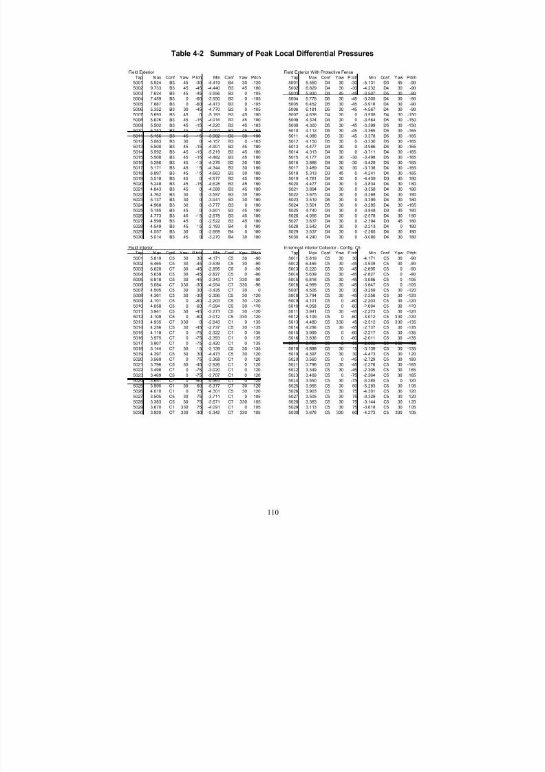
7/31/2019 Wind Tunnel Test
http://slidepdf.com/reader/full/wind-tunnel-test 119/243
Table 4-2 Summary of Peak Local Differential Pressures
Field Exterior Field Exterior With Protective Fence
Tap Max Conf Yaw Pitch Min Conf Yaw Pitch Tap Max Conf Yaw Pitch Min Conf Yaw Pitch
5001 5.924 B3 45 -30 -4.419 B4 30 -120 5001 5.550 D4 30 -30 -5.131 D3 45 -90
5002 9.733 B3 45 -45 -4.440 B3 45 180 5002 6.829 D4 30 -30 -4.232 D4 30 -90
5003 7.634 B3 45 -45 -3.956 B3 0 -105 5003 5.930 D4 45 -45 -3.507 D5 30 -90
5004 7.459 B3 0 -60 -3.950 B3 0 -105 5004 5.776 D5 30 -45 -3.305 D4 30 -90
5005 7.887 B3 0 -60 -4.473 B3 0 -105 5005 6.452 D5 30 -45 -3.918 D4 30 -905006 5.352 B3 30 -45 -4.770 B3 0 -105 5006 6.181 D5 30 -45 -4.567 D4 30 -90
5007 5.693 B3 45 0 -5.193 B3 45 180 5007 4.638 D4 30 0 -3.908 D4 30 -150
5008 5.626 B3 45 -15 -4.916 B3 45 180 5008 4.324 D4 30 0 -3.564 D5 30 -150
5009 5.502 B3 45 -15 -4.220 B3 45 -165 5009 4.300 D5 30 -45 -3.399 D5 30 -150
5010 5.252 B3 45 -15 -4.001 B3 45 -165 5010 4.112 D5 30 -45 -3.365 D5 30 -165
5011 5.156 B3 45 -15 -3.982 B3 30 180 5011 4.088 D5 30 -45 -3.378 D5 30 -165
5012 5.083 B3 30 0 -4.157 B3 0 -165 5012 4.150 D5 30 0 -3.230 D5 30 -165
5013 5.500 B3 45 -15 -4.901 B3 45 180 5013 4.477 D4 30 0 -3.966 D4 30 -165
5014 5.592 B3 45 -15 -5.219 B3 45 180 5014 4.313 D4 30 0 -3.711 D4 30 -165
5015 5.508 B3 45 -15 -4.482 B3 45 180 5015 4.177 D4 30 -30 -3.498 D5 30 -165
5016 5.286 B3 45 -15 -4.276 B3 30 180 5016 3.888 D4 30 -30 -3.429 D5 30 -165
5017 5.171 B3 45 -15 -4.344 B3 30 180 5017 3.489 D4 30 -30 -3.738 D4 30 -165
5018 6.897 B3 45 -15 -4.663 B3 30 180 5018 5.313 D3 45 0 -4.241 D4 30 -165
5019 5.518 B3 45 0 -4.977 B3 45 180 5019 4.781 D4 30 0 -4.459 D3 45 180
5020 5.248 B3 45 -15 -4.628 B3 45 180 5020 4.477 D4 30 0 -3.834 D4 30 180
5021 4.843 B3 45 0 -4.089 B3 45 180 5021 3.894 D4 30 0 -3.358 D4 30 180
5022 4.762 B3 30 0 -3.587 B3 30 180 5022 3.675 D4 30 0 -3.268 D4 30 180
5023 5.137 B3 30 0 -3.941 B3 30 180 5023 3.519 D5 30 0 -3.399 D4 30 180
5024 4.968 B3 30 0 -3.777 B3 0 180 5024 3.501 D5 30 0 -3.295 D4 30 -165
5025 5.185 B3 45 0 -3.601 B3 45 180 5025 4.740 D4 30 0 -3.848 D3 45 180
5026 4.773 B3 45 -15 -2.678 B3 45 180 5026 4.056 D4 30 0 -2.578 D4 30 180
5027 4.599 B3 45 0 -2.522 B3 45 180 5027 3.637 D4 30 0 -2.394 D3 45 180
5028 4.549 B3 45 -15 -2.193 B4 0 180 5028 3.542 D4 30 0 -2.213 D4 0 180
5029 4.557 B3 30 0 -2.669 B4 0 180 5029 3.537 D4 30 0 -2.265 D4 30 180
5030 5.014 B3 45 0 -3.270 B4 30 180 5030 4.240 D4 30 0 -3.080 D4 30 180
Field Interior Innermost Interior Collector - Config. C5
Tap Max Conf Yaw Pitch Min Conf Yaw Pitch Tap Max Conf Yaw Pitch Min Conf Yaw Pitch
5001 5.819 C5 30 30 -4.171 C5 30 -90 5001 5.819 C5 30 30 -4.171 C5 30 -90
5002 6.465 C5 30 -45 -3.539 C5 30 -90 5002 6.465 C5 30 -45 -3.539 C5 30 -90
5003 6.628 C7 30 -45 -2.895 C5 0 -90 5003 6.220 C5 30 -45 -2.895 C5 0 -90
5004 5.639 C5 30 -45 -2.827 C5 0 -90 5004 5.639 C5 30 -45 -2.827 C5 0 -90
5005 6.818 C5 30 -45 -3.343 C1 330 -90 5005 6.818 C5 30 -45 -3.086 C5 0 -105
5006 5.084 C7 330 -30 -4.054 C7 330 -90 5006 4.999 C5 30 -45 -3.847 C5 0 -105
5007 4.505 C5 30 30 -3.435 C7 30 0 5007 4.505 C5 30 30 -3.259 C5 30 -120
5008 4.361 C3 30 -30 -2.356 C5 30 -120 5008 3.794 C5 30 -45 -2.356 C5 30 -120
5009 4.101 C5 0 -60 -2.203 C5 30 -120 5009 4.101 C5 0 -60 -2.203 C5 30 -120
5010 4.058 C5 0 -60 -2.094 C5 30 -120 5010 4.058 C5 0 -60 -2.094 C5 30 -120
5011 3.941 C5 30 -45 -2.273 C5 30 -120 5011 3.941 C5 30 -45 -2.273 C5 30 -1205012 4.109 C5 0 -60 -3.012 C5 330 -120 5012 4.109 C5 0 -60 -3.012 C5 330 -120
5013 4.935 C7 330 0 -2.943 C1 0 135 5013 4.480 C5 330 45 -2.512 C5 330 -135
5014 4.256 C5 30 -45 -2.737 C5 30 -135 5014 4.256 C5 30 -45 -2.737 C5 30 -135
5015 4.118 C7 0 -75 -2.322 C1 0 135 5015 3.999 C5 0 -60 -2.217 C5 30 -135
5016 3.975 C7 0 -75 -2.393 C1 0 135 5016 3.836 C5 0 -60 -2.011 C5 30 -135
5017 3.907 C7 0 -75 -2.420 C1 0 135 5017 3.793 C5 0 -60 -2.058 C5 330 -135
5018 5.144 C7 30 15 -3.139 C5 30 -135 5018 4.888 C5 30 15 -3.139 C5 30 -135
5019 4.397 C5 30 30 -4.473 C5 30 120 5019 4.397 C5 30 30 -4.473 C5 30 120
5020 3.569 C7 0 -75 -3.368 C1 0 120 5020 3.560 C5 0 -45 -2.729 C5 30 180
5021 3.796 C5 30 -45 -2.926 C1 0 120 5021 3.796 C5 30 -45 -2.276 C5 30 -165
5022 3.498 C7 0 -75 -3.020 C1 0 120 5022 3.349 C5 30 -45 -2.305 C5 30 165
5023 3.469 C5 0 -75 -3.707 C1 0 120 5023 3.469 C5 0 -75 -2.364 C5 30 165
5024 3.651 C7 0 -60 -4.563 C1 0 120 5024 3.550 C5 30 -75 -3.285 C5 0 120
5025 3.995 C1 30 60 -5.377 C7 30 120 5025 3.955 C5 30 60 -5.283 C5 30 105
5026 4.010 C1 0 75 -4.301 C5 30 120 5026 3.903 C5 30 75 -4.301 C5 30 120
5027 3.505 C5 30 75 -3.711 C1 0 105 5027 3.505 C5 30 75 -3.329 C5 30 120
5028 3.383 C5 30 75 -3.671 C7 330 105 5028 3.383 C5 30 75 -3.144 C5 30 120
5029 3.670 C1 330 75 -4.091 C1 0 105 5029 3.113 C5 30 75 -3.618 C5 30 105
5030 3.920 C7 330 -30 -5.342 C7 330 105 5030 3.676 C5 330 60 -4.273 C5 330 105
110

7/31/2019 Wind Tunnel Test
http://slidepdf.com/reader/full/wind-tunnel-test 120/243
Figure 4-36 Vortex flow forming from corner of collector
4.8.3 Instantaneous Differential Pressures
Differential pressures over collector reflectors can cause the reflector to deflect, resulting in a loss
of efficiency because the reflected sunlight may move out of focus. Severe deflection of thecollector can also cause the reflector to break. To assess wind–induced reflector deflection andstructural failure, the relationship between the loading condition and the resulting reflector
deflection (and mechanical stresses) can be established through structural analysis, for exampleusing finite element modeling. Collector designs vary by manufacturer, and each structure can
respond differently to imposed loads. The pressure distribution data in this section are intended toenable this type of structural analysis. A very large number of pressure distributions have beenobtained during these tests. Presenting all the pressure distribution results in this report is neither
practical nor desirable. Accordingly, this section presents a limited number of the pressure testresults, shown as differential pressure distributions realized instantaneously ― in essence, a
“snapshot” extracted from the pressure time series data.
The results presented here are selected from the data taken for Configuration C5, because it isrepresentative of most of the collectors within the interior of the solar field. Figure 4-37 shows
the instantaneous pressure distributions that contained the largest differential pressure at any of the tap locations, for each of the three yaw angles tested. The numerical values of the differential
pressures are presented in Table 4-3.
111

7/31/2019 Wind Tunnel Test
http://slidepdf.com/reader/full/wind-tunnel-test 121/243
1.5
2.0
2.0
2.5 3.0
4.0 1.5
1.0 0.5
0.0
0.0
0.0
-0.5
-1.0
-1.5 -2.0
-2.5
-4.0
Peak Positive, Yaw = -30, Pitch = 45
Peak Negative, Yaw = -30, Pitch = 105
Figure 4-37a Instantaneous differential pressure distributionwith the largest local peak, yaw = - 30 degrees
112

7/31/2019 Wind Tunnel Test
http://slidepdf.com/reader/full/wind-tunnel-test 122/243
3.0
1.5 1.0
0.5
-0.5
-1.0
-1.5 -2.0
0.0
-4.0 -2.0
Peak Positive, Yaw = 0, Pitch = 0
Peak Negative, Yaw = 0, Pitch = 120
Figure 4-37b Instantaneous differential pressure distribution with thelargest local peak, yaw = 0 degrees
113

7/31/2019 Wind Tunnel Test
http://slidepdf.com/reader/full/wind-tunnel-test 123/243

7/31/2019 Wind Tunnel Test
http://slidepdf.com/reader/full/wind-tunnel-test 124/243
Table 4-3 Selected Summary of Instantaneous Differential Distributionwith the Largest Local Peak
Yaw = -30 Yaw = 0 Yaw = 30
Pk Pos Pk Neg Pk Pos Pk Neg Pk Pos Pk Neg
Tap 45 deg. 105 deg. 0 deg. 120 deg. 0 deg. 120 deg.
5001 1.450 0.070 3.275 -0.041 5.018 0.489
5002 1.473 -0.054 1.146 -0.245 1.586 0.295
5003 1.678 0.077 0.934 -0.197 0.479 -0.009
5004 1.834 0.208 0.374 -0.089 0.594 0.118
5005 1.582 0.263 0.311 -0.117 0.594 0.089
5006 2.103 0.170 0.365 -0.337 0.085 -0.044
5007 1.060 0.016 1.167 -0.399 0.741 0.365
5008 1.709 -0.082 0.725 -0.249 0.815 0.158
5009 1.794 0.056 0.368 -0.127 0.653 0.077
5010 1.683 0.154 0.344 -0.193 0.729 0.042
5011 1.579 0.111 0.340 -0.161 0.560 0.076
5012 1.907 0.029 0.354 -0.447 0.460 0.057
5013 4.480 0.007 0.249 -0.179 0.385 -0.345
5014 1.783 -0.373 0.383 -0.236 0.642 -0.152
5015 1.673 -0.358 0.386 -0.353 0.582 -0.406
5016 1.534 -0.303 0.389 -0.459 0.617 -0.503
5017 1.388 -0.167 0.385 -0.464 0.691 -0.356
5018 1.444 -0.412 0.205 0.182 0.840 -0.117
5019 0.508 -0.925 0.252 -1.438 0.363 -2.874
5020 1.245 -1.071 0.319 -0.992 0.628 -1.937
5021 1.231 -1.080 0.265 -0.894 0.684 -1.639
5022 1.275 -1.185 0.316 -1.023 0.559 -1.298
5023 1.230 -1.359 0.394 -1.109 0.497 -1.168
5024 1.041 -2.059 0.312 -1.270 0.311 -0.883
5025 -0.122 -1.088 0.239 -2.095 0.523 -5.283
5026 0.645 -1.290 0.233 -1.738 0.527 -2.8625027 0.501 -1.572 0.279 -1.609 0.556 -1.949
5028 0.658 -1.828 0.306 -2.123 0.561 -1.562
5029 0.782 -2.672 0.392 -2.501 0.597 -1.464
5030 0.874 -4.273 0.328 -4.175 0.282 -1.214
The largest pressure is in bold.
Pitch Angle Pitch Angle Pitch Angle
Additional pressure contours are presented in Appendix D for Configurations B1, C1, C3, C5 and D1.
Other pressure distributions of interest to the design engineer are those that, when integrated over the collector surface, result in specific overall load levels. Various load levels may be used toevaluate the deformation of the structure to optimize structural and economical impact due towind loads. This section presents instantaneous pressure distributions that resulted in the integralloads at the 80th percentile of their peak values. The choice of the load level was somewhat
arbitrary, however. Figure 4-38 shows the selected results for positive pitch angles. Thecorresponding tabulated data are given in Table 4-4.
115

7/31/2019 Wind Tunnel Test
http://slidepdf.com/reader/full/wind-tunnel-test 125/243
1.6
1.2
1.0
0.8
1.0
0.6
0.6
0.8
1.0
1.4
0.8
0.0
0.0
0.0
Positive 80th Percentile Level at Yaw = 30 deg., Pitch = 30 deg.
Negative 80th Percentile Level at Yaw = -30 deg., Pitch = 0 deg.
Figure 4-38a Instantaneous differential pressure distribution with
horizontal force at 80th percentile level of peak
116

7/31/2019 Wind Tunnel Test
http://slidepdf.com/reader/full/wind-tunnel-test 126/243
0.8
0.6 1.0
1.0
1.2
0.6
0.8
1.0 1.0
Positive 80th Percentile Level at Yaw = 30 deg., Pitch = 120 deg.
Negative 80th Percentile Level at Yaw = 30 deg., Pitch = 75 deg.
-0.2
-0.2
-0.4
-0.6
-0.8 -1.0
-0.6 -1.2
Figure 4-38b Instantaneous differential pressure distributionwith vertical force at 80th percentile level of peak
117
7/31/2019 Wind Tunnel Test
http://slidepdf.com/reader/full/wind-tunnel-test 127/243
0.2 0.2
0.4
0.2
0.0
-0.2
-0.4
-0.6
-0.8
-1.0 -1.2
-1.6
Positive 80th Percentile Level at Yaw = 30 deg., Pitch = 105 deg.
Negative 80th Percentile Level at Yaw = 30 deg., Pitch = 60 deg.
1.0
0.8
0.6
0.4
0.8
0.6
0.8 0.8
1.0
Figure 4-38c Instantaneous differential pressure distributionwith pitching moment at 80th percentile level of peak
118

7/31/2019 Wind Tunnel Test
http://slidepdf.com/reader/full/wind-tunnel-test 128/243
Table 4-4 Differential Pressure Distributions Resulting inOverall Loads at 80th Percentile of Respective Peaks
Yaw 30 Yaw -30 Yaw 30 Yaw 30 Yaw 30 Yaw 30
Pitch 30 Pitch 0 Pitch 120 Pitch 75 Pitch 105 Pitch 60
Tap Pos. Neg. Pos. Neg. Pos. Neg.5001 1.653 -0.143 -0.434 0.687 0.277 1.004
5002 1.198 -0.036 -0.185 0.711 0.075 0.666
5003 0.817 0.074 -0.235 0.776 0.184 0.418
5004 0.629 0.109 -0.144 0.786 0.217 0.312
5005 0.982 -0.149 -0.029 0.557 0.324 0.354
5006 0.721 -0.145 -0.054 0.412 0.029 0.289
5007 1.027 -0.013 -0.591 0.989 0.366 0.939
5008 0.895 -0.090 -0.194 1.062 0.244 0.741
5009 0.658 0.040 -0.191 1.117 0.397 0.579
5010 0.754 0.076 -0.154 1.013 0.538 0.554
5011 0.856 -0.041 -0.138 0.750 0.438 0.470
5012 0.689 -0.162 -0.134 0.600 0.289 0.419
5013 0.886 -0.186 -0.401 0.844 0.283 0.635
5014 0.835 -0.113 -0.536 1.090 0.312 0.7625015 0.642 -0.092 -0.502 1.144 0.135 0.712
5016 0.663 -0.001 -0.513 1.045 0.232 0.656
5017 0.759 -0.096 -0.449 0.907 0.193 0.621
5018 1.509 0.028 -0.475 1.252 0.048 1.002
5019 1.146 -0.080 -1.188 1.172 -0.630 0.964
5020 0.810 -0.015 -1.097 0.965 -0.290 0.736
5021 0.535 -0.164 -0.931 1.070 -0.685 0.684
5022 0.653 -0.143 -0.835 0.935 -0.575 0.651
5023 0.775 -0.075 -0.746 0.786 -0.426 0.658
5024 0.452 -0.027 -0.658 0.437 -0.472 0.397
5025 0.873 -0.050 -1.343 0.505 -1.803 0.636
5026 0.630 -0.157 -1.066 0.836 -1.298 1.053
5027 0.428 -0.069 -0.949 0.773 -1.083 0.907
5028 0.514 -0.089 -0.877 0.867 -1.024 0.921
5029 0.624 -0.036 -0.741 0.692 -0.938 0.897
5030 0.520 0.069 -0.559 0.452 -0.761 0.568
fz myfx
119

7/31/2019 Wind Tunnel Test
http://slidepdf.com/reader/full/wind-tunnel-test 129/243
4.8.4 Example Calculations of Design Loads
This section demonstrates the use of the current wind-tunnel test results to determine the wind
loads required by the designer. First, recall the definition of the load coefficients given in Section3.1:
Horizontal Force, fx Cfx fxqLW
= (4.1)
Vertical Force, fz Cfz fz
qLW = (4.2)
Pitching Moment, my Cmymy
qLW =
2(4.3)
and the mean reference dynamic pressure measured at the collector pivot height, Hc, of the solar collector as given by
q U = 12
2 ρ . (4.4)
Here U is the mean wind speed at the pivot height, and ρ is the density of air. The aboveequations can be rewritten to obtain the loads as
Horizontal Force, fx fx qLWCfx= (4.5)
Vertical Force, fz fz qLWCfz = (4.6)
Pitching Moment, my . (4.7)my qLW Cmy= 2
For the full-scale loads, the corresponding reference dimensions, L is 25.97 ft and W is 16.40 ft.In addition, the velocity reference elevation, Hc, is 9.35 ft. Note that these reference dimensionsmust be used consistently between the model and full-scale to properly calculate the loadsapplicable to the full-scale solar collector. To actually determine the full-scale loads, the designwind pressure, q, or equivalently, the design wind speed, U , must be also specified. An example
procedure is described next.
Specifying Design Wind Speed
Several available sources provide wind speed to be used for estimating design wind loads on civil
engineering structures and buildings. They include, but are not limited to, the current USstandard, ASCE 7-98, and regional wind load codes. Regional wind data are also available from
the National Climate Data Center (NCDC), but require considerable data analysis to determine a
rational design wind speed. For the example in this section, the wind map provided by ASCE 7-98 (Figure 6-1, pp. 34-38) is used because it is a widely accepted practice.
The ASCE 7-98 specifies design wind speeds as 3-sec gust speeds at an elevation of 33 ft for theentire United States in a form of a wind map. Except for hurricane-prone southern and eastern
coastal regions and Alaska, much of the United States plains have been zoned as 90-mph regions.Western states such as California, Oregon, and Washington have been zoned as 85 mph regions.These wind speeds are referred to as the basic wind speed that would result in 50-year recurrence
wind loads for structures in open countries. The ASCE-specified wind speeds, however, cannot
120

7/31/2019 Wind Tunnel Test
http://slidepdf.com/reader/full/wind-tunnel-test 130/243
be used directly for the present solar collector data because (1) the ASCE wind speeds are given
as a 3-second gust speed rather than a mean speed adopted for the wind-tunnel test, and (2) the
ASCE wind speeds are referenced at an elevation of 33 ft rather than the collector pivot height of
9.35 ft. Thus, conversion of the ASCE wind speeds is necessary using the procedures explained
in ASCE 7-98. Conversion of a 50-year wind load is also explained in ASCE 7-98 for different
mean recurrence intervals and is presented here.
Conversion of ASCE Basic Wind Speed
Consider a solar collector site in California for which ASCE 7-98 (Figure 6-1) gives the basic
wind speed of V = 85 mph. Using Figure C6-1, the corresponding hourly mean wind speed at 33
ft, U 33 is obtained as
U V 33 153 85 153 55 6= = =/ . / . . mph hourly mean .
Using values implied by Table 6-4 of ASCE 7-98, the mean wind speed at the collector pivot
height, U Hc, is given as
U U Hc
=
F
H
GI
K
J =
F
H
GI
K
J =33
1 7 1 7
9 32
33
55 69 32
33
46 4.
..
.
/ /
mph hourly mean .
The hourly mean wind speed of 46.4 mph is the design wind speed for the solar collectors in
California.
Design Wind Loads
Based on the design wind speed, the corresponding design pressure, q, is calculated by
q U hc= = =
1
20 00256 46 4 551
2 2 ρ . ( . ) . psf .
Here, the constant 0.00256 is conveniently used to obtain the reference pressure in psf from the
wind speed in mph. As an example, we wish to determine the 50-year peak design loads on the
innermost-shielded solar collectors (Configuration C5) when that collector is oriented at a –60degree pitch angle (a downward-facing stow position). We note from Table 4.1 that the largest
peak vertical force, Load Case 3, is produced at this –60 degree pitch angle, at a yaw angle of 0
degrees, so this orientation is of special interest to designers. Table 4.1 shows the peak Cfz is
2.754 and the corresponding Cfx value is 1.404, and the Cmy value is 0.107. Using equations
(4.5) – (4.7):
Horizontal Force fx = qLWCfx = (5.51)(25.97)(16.40)(1.404) = 3,295 lbs
Vertical Force, fz = qLWCfz = (5.51)(25.97)(16.40)(2.754) = 6,463 lbs
Pitching Moment, my = qLW 2Cmy = (5.51)(25.97)(16.40)2(0.107) = 4,118 lb-ft.
Note that these loads are to be applied simultaneously to the structure because the wind-tunnel
results were obtained as a concurrent load combination from the time series data for which thevertical force was maximized.
Comparison to Design Loads Determined by Quasi-Steady Assumption
As pointed out in Section 1.2, the traditional approach to obtaining the structural design loads on
solar collectors has been based on the quasi-steady assumption. With this technique, the
measured mean load is scaled to follow the gust wind speed to provide the equivalent peak load.
The scale factor is known as the gust load factor, and ASCE 7-98 or the model building code IBC
121

7/31/2019 Wind Tunnel Test
http://slidepdf.com/reader/full/wind-tunnel-test 131/243
2000 would predict the gust load factor to be 2.34 for a structure in open country. To illustratethis, the next example calculates the load combination using the mean load data for the
innermost-shielded solar collectors (Configuration C5) under the quasi-steady assumption. Tomake a direct comparison with the values calculated just above, we use the same assumptions for
pitch angle and yaw angle, -60 degrees and 0 degrees, respectively.
From Appendix B (pg. 8-51) and using the scale factor of 1.13 (see Section 4.9) it can be shownthat mean coefficients for a –60 degree pitch angle, with a yaw of 0 degrees, are: Cfx = 0.382, Cfy
= 0.742, and Cmy = 0.027.
Applying the gust factor, the design loads are calculated as:
Horizontal Force fx = (2.34)qLWCfx = (2.34)(5.51)(25.97)(16.40)(0.382) = 2,098 lbs
Vertical Force, fz = (2.34)qLWCfz = (2.34)(5.51)(25.97)(16.40)(0.742) = 4,075 lbs
Pitching Moment, my = (2.34)qLW 2Cmy = (2.34)(5.51)(25.97)(16.40)2(0.027) = 2,432 lb-ft.
The quasi-steady approach considerably underestimated the design loads for the interior solar collectors. Not all collector orientations and collector configurations will yield underestimates,
but this example is intended to illustrate the differences between these two approaches, as well as
the calculation methods. In wind tunnels, measurement of the mean loads is far easier thanmeasuring the peak loads, as done in the current wind-tunnel study, because the design of thewind-tunnel model, as well as necessary instrumentation, need not concern high frequency gustresponse due to turbulence. However, the estimate of the design load based on the quasi-steadyassumption has limited applicability to the realistic structural design, so generally the measured
peak coefficients should instead be used.
Design Loads for Other Mean Recurrence Intervals
The above examples demonstrates the use of the wind-tunnel results to determine the design windloads of the solar collector with the design wind speed provided by ASCE 7-98. The calculated
loads are expected to occur at an annual probability of 0.02, or once in 50 years. ASCE 7-98 alsotabulates a set of conversion factors to obtain the design loads for other mean recurrence
intervals. Table 4-5 is a summary of the conversion factors for most of the United States with the basic wind speed of 85 to 90 mph.
Table 4-5 Design Pressure Conversion Factors for Different Mean Recurrence Intervals
MRI, years 5 10 25 50 100 200 500
Conversion Factor 0.61 0.71 0.86 1 1.14 1.3 1.51
122

7/31/2019 Wind Tunnel Test
http://slidepdf.com/reader/full/wind-tunnel-test 132/243
4.9 Adjustment to Pressure Test Data
4.9.1 Adjustment Factor
Although the overall loads calculated by integration of the local pressure data generally agree
well with the directly measured balance results, a slight discrepancy is noted primarily due to the
degree of the finite resolution of the pressure distributions actually measured. A denser array of pressure tap measurements (were it physically possible) would likely result in better agreement.Before the pressure data can be used the discrepancy needs to be quantified. Figure 4-39 compares the balance and pressure results for the horizontal and vertical force components. The
comparisons are made for all of the essential statistical measures for completeness.
Mean Cfx
Pressure Data
-2 -1 0 1 2 3
B a l a n c e D a t a
-2
-1
0
1
2
3RMS Cfx
Pressure Data
0.0 0.1 0.2 0.3 0.4 0.5 0.6
B a l a n c e D a t a
0.0
0.1
0.2
0.3
0.4
0.5
0.6
Max Cfx
Pressure Data
-1 0 1 2 3 4 5
B a l a n c e D a t a
-1
0
1
2
3
4
5
Min Cfx
Pressure Data
-4 -3 -2 -1 0 1 2
B a l a n c e D a t a
-4
-3
-2
-1
0
1
2
Figure 4-39 Comparison of Balance and Pressure Data,(a) Horizontal Force Component
123

7/31/2019 Wind Tunnel Test
http://slidepdf.com/reader/full/wind-tunnel-test 133/243
Mean Cfy
Pressure Data
-2 -1 0 1 2 3
B a
l a n c e
D a t a
-2
-1
0
1
2
3RMS Cfy
Pressure Data
0.0 0.1 0.2 0.3 0.4 0.5 0.6
B a
l a n c e
D a t a
0.0
0.1
0.2
0.3
0.4
0.5
0.6
Max Cfy
Pressure Data
-1 0 1 2 3 4 5
B a
l a n c e
D a
t a
-1
0
1
2
3
4
5Min Cfy
Pressure Data
-4 -3 -2 -1 0 1 2
B a
l a n c e
D a
t a
-4
-3
-2
-1
0
1
2
Figure 4-39 Comparison of Balance and Pressure Data,(b) Vertical Force Component
124
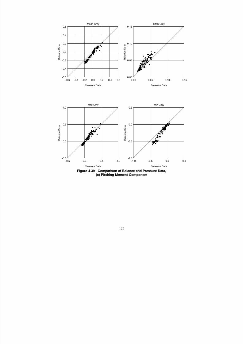
7/31/2019 Wind Tunnel Test
http://slidepdf.com/reader/full/wind-tunnel-test 134/243
Mean Cmy
Pressure Data
-0.6 -0.4 -0.2 0.0 0.2 0.4 0.6
B a l a n c e D a t
a
-0.6
-0.4
-0.2
0.0
0.2
0.4
0.6RMS Cmy
Pressure Data
0.00 0.05 0.10 0.15
B a l a n c e D a t
a
0.00
0.05
0.10
0.15
Max Cmy
Pressure Data
-0.5 0.0 0.5 1.0
B
a l a n c e D a t a
-0.5
0.0
0.5
1.0Min Cmy
Pressure Data
-1.0 -0.5 0.0 0.5
B
a l a n c e D a t a
-1.0
-0.5
0.0
0.5
Figure 4-39 Comparison of Balance and Pressure Data,
(c) Pitching Moment Component
125
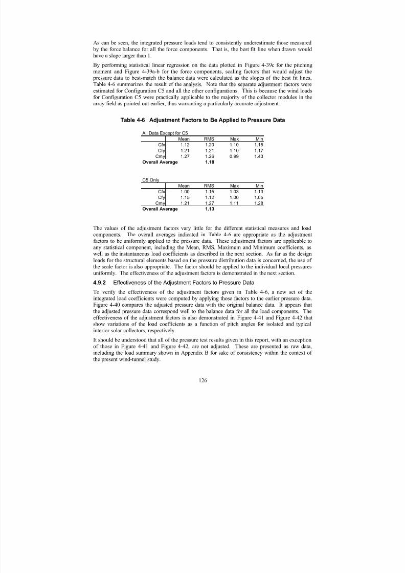
7/31/2019 Wind Tunnel Test
http://slidepdf.com/reader/full/wind-tunnel-test 135/243
As can be seen, the integrated pressure loads tend to consistently underestimate those measured by the force balance for all the force components. That is, the best fit line when drawn would
have a slope larger than 1.
By performing statistical linear regression on the data plotted in Figure 4-39c for the pitching
moment and Figure 4-39a-b for the force components, scaling factors that would adjust the
pressure data to best-match the balance data were calculated as the slopes of the best fit lines.Table 4-6 summarizes the result of the analysis. Note that the separate adjustment factors were
estimated for Configuration C5 and all the other configurations. This is because the wind loadsfor Configuration C5 were practically applicable to the majority of the collector modules in thearray field as pointed out earlier, thus warranting a particularly accurate adjustment.
Table 4-6 Adjustment Factors to Be Applied to Pressure Data
All Data Except for C5
Mean RMS Max Min
Cfx 1.12 1.20 1.10 1.15
Cfy 1.21 1.21 1.10 1.17
Cmy 1.27 1.26 0.99 1.43Overall Average 1.18
C5 Only
Mean RMS Max Min
Cfx 1.00 1.15 1.03 1.13
Cfy 1.15 1.12 1.00 1.05
Cmy 1.21 1.27 1.11 1.28
Overall Average 1.13
The values of the adjustment factors vary little for the different statistical measures and load
components. The overall averages indicated in Table 4-6 are appropriate as the adjustmentfactors to be uniformly applied to the pressure data. These adjustment factors are applicable toany statistical component, including the Mean, RMS, Maximum and Minimum coefficients, aswell as the instantaneous load coefficients as described in the next section. As far as the design
loads for the structural elements based on the pressure distribution data is concerned, the use of the scale factor is also appropriate. The factor should be applied to the individual local pressuresuniformly. The effectiveness of the adjustment factors is demonstrated in the next section.
4.9.2 Effectiveness of the Adjustment Factors to Pressure Data
To verify the effectiveness of the adjustment factors given in Table 4-6, a new set of theintegrated load coefficients were computed by applying those factors to the earlier pressure data.Figure 4-40 compares the adjusted pressure data with the original balance data. It appears that
the adjusted pressure data correspond well to the balance data for all the load components. Theeffectiveness of the adjustment factors is also demonstrated in Figure 4-41 and Figure 4-42 thatshow variations of the load coefficients as a function of pitch angles for isolated and typical
interior solar collectors, respectively.
It should be understood that all of the pressure test results given in this report, with an exception
of those in Figure 4-41 and Figure 4-42, are not adjusted. These are presented as raw data,including the load summary shown in Appendix B for sake of consistency within the context of
the present wind-tunnel study.
126
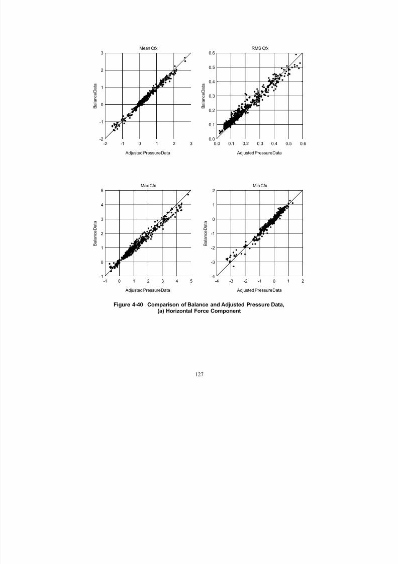
7/31/2019 Wind Tunnel Test
http://slidepdf.com/reader/full/wind-tunnel-test 136/243
Mean Cfx
Adjusted Pressure Data
-2 -1 0 1 2 3
B a l a n c e D a t a
-2
-1
0
1
2
3RMS Cfx
Adjusted Pressure Data
0.0 0.1 0.2 0.3 0.4 0.5 0.6
B a l a n c e D a t a
0.0
0.1
0.2
0.3
0.4
0.5
0.6
Max Cfx
Adjusted Pressure Data
-1 0 1 2 3 4 5
B a l a n c e D
a t a
-1
0
1
2
3
4
5Min Cfx
Adjusted Pressure Data
-4 -3 -2 -1 0 1 2
B a l a n c e D
a t a
-4
-3
-2
-1
0
1
2
Figure 4-40 Comparison of Balance and Adjusted Pressure Data,(a) Horizontal Force Component
127
7/31/2019 Wind Tunnel Test
http://slidepdf.com/reader/full/wind-tunnel-test 137/243
Mean Cfy
Adjusted Pressure Data
-2 -1 0 1 2 3
B a l a n c e D a t a
-2
-1
0
1
2
3RMS Cfy
Adjusted Pressure Data
0.0 0.1 0.2 0.3 0.4 0.5 0.6
B a l a n c e D a t a
0.0
0.1
0.2
0.3
0.4
0.5
0.6
Max Cfy
Adjusted Pressure Data
-1 0 1 2 3 4 5
B a l a n c e D a t a
-1
0
1
2
3
4
5Min Cfy
Adjusted Pressure Data
-4 -3 -2 -1 0 1 2
B a l a n c e D a t a
-4
-3
-2
-1
0
1
2
Figure 4-40 Comparison of Balance and Adjusted Pressure Data,(b) Vertical Force Component
128

7/31/2019 Wind Tunnel Test
http://slidepdf.com/reader/full/wind-tunnel-test 138/243
Mean Cmy
Adjusted Pressure Data
-0.5 0.0 0.5
N e w
B a
l a n c e D
a t a
-0.5
0.0
0.5RMS Cmy
Adjusted Pressure Data
0.00 0.05 0.10
N e w
B a
l a n c e D
a t a
0.00
0.05
0.10
Max Cmy
Adjusted Pressure Data
-0.5 0.0 0.5 1.0
N e w B
a l a n c e
D a
t a
-0.5
0.0
0.5
1.0Min Cmy
Adjusted Pressure Data
-1.0 -0.5 0.0 0.5
N e w B
a l a n c e
D a
t a
-1.0
-0.5
0.0
0.5
Figure 4-40 Comparison of Balance and Adjusted Pressure Data,(c) Pitching Moment Component
129

7/31/2019 Wind Tunnel Test
http://slidepdf.com/reader/full/wind-tunnel-test 139/243
Configuration A1, Yaw = 0
-180 -150 -120 -90 -60 -30 0 30 60 90 120 150 180
C f x
-6
-4
-2
0
2
4
6
-180 -150 -120 -90 -60 -30 0 30 60 90 120 150 180
C f z
-6
-4
-2
0
2
4
6
Pitch Angle, deg.
-180 -150 -120 -90 -60 -30 0 30 60 90 120 150 180
C m y
-1.5
-1.0
-0.5
0.0
0.5
1.0
1.5
Balance Mean (2001, 2002)
Balance Max/Min (2001, 2002)
Adjusted Pressure Mean (2001)
Adjusted Pressure Max/Min (2001)
Figure 4-41 Comparison of Balance and Adjusted Pressure Datafor Isolated Solar Collector
JAP note: Why blank page?
130

7/31/2019 Wind Tunnel Test
http://slidepdf.com/reader/full/wind-tunnel-test 140/243
Configuration C5, Yaw = 0
-180 -150 -120 -90 -60 -30 0 30 60 90 120 150 180
C f x
-6
-4
-2
0
2
4
6
-180 -150 -120 -90 -60 -30 0 30 60 90 120 150 180
C f z
-6
-4
-2
0
2
4
6
Pitch Angle, deg.
-180 -150 -120 -90 -60 -30 0 30 60 90 120 150 180
C m y
-1.5
-1.0
-0.5
0.0
0.5
1.0
1.5
Balance Mean (2001, 2002)
Balance Max/Min (2001, 2002)
Adjusted Pressure Mean (2001)
Adjusted Pressure Max/Min (2001)
Figure 4-42 Comparison of Balance and Adjusted Pressure Datafor Interior Solar Collector
131
7/31/2019 Wind Tunnel Test
http://slidepdf.com/reader/full/wind-tunnel-test 141/243
5. CONCLUDING REMARKS
Extensive wind-tunnel tests were conducted on parabolic trough solar collectors to determine
practical wind loads applicable to the structural design for stress and deformation, as well as thelocal component design for the concentrator reflectors. The overall dynamic loads andsimultaneous pressure distributions on the concentrator were measured using force balances and a
multi-pressure data acquisition system, respectively, in a boundary layer wind tunnel at CPP.Various test configurations were examined, including an isolated collector and solar field
collectors at different positions.
Significant test results are presented and discussed in detail. Overall, the wind-tunnel tests produced sufficient data that can be used by designers of the present and future for a variety of design practices.
Several recommendations can be made for future work. The validity of the wind-tunnel data is
particularly important. Ultimately, the acceptability of the test results should be based on model-
to-full-scale comparison, which requires measurement of wind loads on a full-scale solar collector. Should further wind tunnel prove useful, the pressure test model should attempt toincrease the pressure tap installation density to enhance the resolution of discrete pressuredistribution data.
132

7/31/2019 Wind Tunnel Test
http://slidepdf.com/reader/full/wind-tunnel-test 142/243
133
6. REFERENCES
ASCE 7-98 (2000), Minimum Design Loads for Buildings and Other Structures, Standard
ANSI/ASCE 7-98, American Society of Civil Engineers and American National StandardsInstitute, New York.
Cermak, J.E. (1971), “Laboratory Simulation of the Atmospheric Boundary Layer,” AIAAJournal, Vol. 9, September.
Cermak, J.E. (1975), “Applications of Fluid Mechanics to Wind Engineering,” A FreemanScholar Lecture, ASME Journal of Fluids Engineering, Vol. 97, No. 1, March.
Cermak, J.E. (1976), “Aerodynamics of Buildings,” Annual Review of Fluid Mechanics, Vol. 8, pp. 75 – 106.
Cohen, G.E., D.W. Kearney and G.J. Kolb (1999), Final Report on the Operation andMaintenance Improvement for Concentrating Solar Power Plants, Report SAND99-1290, Sandia
National Laboratories.
Counihan, J. (1975), “Adiabatic Atmospheric Boundary Layers: A Review and Analysis of Data
from the Period 1880-1972,” Atmos. Environ., Vol. 9, pp. 871 – 905.
Engineering Science Data Unit [ESDU], (1975), “Characteristics of Atmospheric Turbulence Near the Ground,” Item No. 75001, London, U.K.
Huebner, K.H., E.A. Thornton and T.G. Byrom, (1995), The Finite Element Method for Engineer,Third Edition, A Wiley-Interscience Publication, Jon Wiley & Sons, Inc., New York
International Code Council, Inc. (2000), International Building Code 2000 (IBC 2000), Falls
Church, VA.
Peterka, J. A. and R.G. Derickson (1992), Wind Load Design Methods for Ground-Based
Heliostats and Parabolic Dish Collectors, Report SAND 92-7009, Sandia National Laboratories.
Peterka, J. A., J. M. Sinou and J. E. Cermak (1980), Mean Wind Forces on Parabolic-Trough
Solar Collectors, Report SAND80-7023, Sandia National Laboratories.
Randall, D.E., D.D. McBride and R.E. Tate (1980), Steady-State Wind Loading on Parabolic-Trough Solar Collectors, Report SAND79-2134, Sandia National Laboratories.
Randall, D.E., R.E. Tate and D.A Powers (1982), Experimental Results of Pitching Moment Testson Parabolic-Trough Solar-Collector Array Configurations, Report SAND82-1569, Sandia
National Laboratories.
7/31/2019 Wind Tunnel Test
http://slidepdf.com/reader/full/wind-tunnel-test 143/243
7. APPENDICES
7.1 APPENDIX A - VALIDITY OF FULL-SCALE PREDICTION
Boundary-layer wind-tunnel testing for wind loads on structures has been an accepted practice for
many years. The first well-conducted test for a structure using modern understanding of wind/structure interaction was performed for the World Trade center in New York City,conducted in about 1963 at Colorado State University under the direction of Drs. Jack Cermak (a
principal of CPP, Inc.) and Alan Davenport. The wind load standard ANSI A58.1-1982 was
referenced by most U.S. building codes by the mid 1980's, and permitted properly conductedwind-tunnel tests to be used in lieu of local building code wind load provisions. This capabilitycontinues today, with most U.S. building codes referring to some version of ASCE 7, the nationalwind load standard, which permits wind tunnel testing to replace code provisions. Surveyreferences that discuss wind-tunnel modeling and its validity include Cermak (1971, 1975, 1976).
The basis for acceptance of wind-tunnel testing relied initially on early testing in aeronautical
wind tunnels which showed that non-dimensional load coefficients become invariant withincreasing Reynolds number. In the final analysis, comparisons of model and full-scale data have
provided confidence in the ability of boundary-layer wind tunnels to correctly model full-scalewind loads. There have been a number of model/full-scale comparisons that have shown that the
same non-dimensional wind load coefficients are obtained for models and full-scale structures. Afew of these are listed below. These references include Meroney (1980) for wind flow similarityover terrain, Dalgliesh et al (1980) for cladding loads on a high-rise building, Cermak and
Cochran (1992) for wind-tunnel simulation of a partial height boundary layer, Cochran andCermak (1993) for cladding and frame pressures on a low rise building, Cheung et al. (1996) for
cladding pressures and frame loads on a low-rise building, Cochran, Peterka and Derickson(1999) for wind speed similarity close to the roofs of low-rise buildings, Peterka and Hosoya, etal. (1998) for area-averaged pressures on a low-rise building.
For the current study, parabolic collectors have curved surfaces. Curved shapes such as cylindersare the shapes most sensitive to Reynolds number effects. For example, it is well-known thatautomobiles and airplanes must be modeled at near-full-scale Reynolds numbers to achieveacceptable accuracy. Both of these vehicle types are typically tested in uniform-flow,aeronautical-type wind tunnels with very low turbulence (typically less than 1 percent). For
stationary objects at the surface of the earth, the turbulence intensity is much larger, typicallygreater than 15-20 percent. The added turbulence decreases the Reynolds number effects by
inserting turbulence directly into the boundary layer on the object, increasing the effectiveReynolds number of the flow. Several proprietary studies by CPP, Inc. have demonstrated this
effect. Reynolds number tests on the solar collector models have shown no significant effect of Reynolds numbers over the range of Reynolds numbers that are permitted at model scale. On the
basis of available information, it is likely that Reynolds number effects are not significant for
determination of design wind loads on parabolic collectors using properly conducted boundary-layer wind tunnel tests. However, model to full scale comparisons for this geometry would be
valuable and should be considered for future funding.
A-1

7/31/2019 Wind Tunnel Test
http://slidepdf.com/reader/full/wind-tunnel-test 144/243
A-2
References
Cermak, J.E. (1971), “Laboratory Simulation of the Atmospheric Boundary Layer,” AIAA Jl.,
Vol. 9, September.Cermak, J.E. (1975), “Applications of Fluid Mechanics to Wind Engineering,” A Freeman
Scholar Lecture, ASME Journal of Fluids Engineering , Vol. 97, No. 1, March.
Cermak, J.E. (1976), “Aerodynamics of Buildings,” Annual Review of Fluid Mechanics, Vol. 8, pp. 75 B 106.
Cermak, J. E. and L. S. Cochran (1992), “Physical modeling of the atmospheric boundary layer,” Journal of Wind Engineering and Industrial Aerodynamics, Vol. 41-44, pp 935-946.
Cheung, J. C. K., Holmes, J. D., Melbourne, W. H., Lakshmanan, N., and Bowditch, P. (1996),
"Pressures on a 1/10 Scale Model of the Texas Tech Building,” Third International Colloquium on Bluff Body Aerodynamics & Applications BBAA, Blacksburg, Virginia, ppA IX 5 - A IX 8.
Cochran, L.S. and Cermak, J. E. (1992), “Full- and model-scale cladding pressures on the TexasTech University experimental building,” Journal of Wind Engineering and Industrial
Aerodynamics, Vol. 41-44, pp 1589-1600.Cochran, L. S., Peterka, J., and Derickson, R. (1999), “Roof Surface Wind Speed Distributions on
Low-Rise Buildings,” Architectural Science Review, Vol. 42, pp 151-160.Dalgliesh, W.A., J.T. Templin and K.R. Cooper, (1980), “Comparison of Wind Tunnel and Full-
Scale Building Surface Pressures with Emphasis on Peaks,” The Proceedings of the Fifth
International Conference in Wind Engineering, Fort Collins, Colorado, Vol. 1, pp553-565.
Meroney, R. N. (1980), “Wind-Tunnel Simulation of the Flow Over Hills and Complex Terrain,” Journal of Industrial Aerodynamics, Vol. 5, pp 297-321.
Peterka, J. N., Hosoya, N., Dodge, S., Cochran, L., and Cermak, J. E. (1998), “Area-average peak
pressures in a gable roof vortex region,” Journal of Wind Engineering and Industrial
Aerodynamics, Vol. 77-78, pp 205-215.

7/31/2019 Wind Tunnel Test
http://slidepdf.com/reader/full/wind-tunnel-test 145/243
B-1
7.2 APPENDIX B - LIST OF OVERALL LOAD DATA
This appendix section presents a list of overall load coefficients (Mean, RMS, Max and Min) measured by
the balance and surface integration of the local pressure data. For the integrated pressure loads, the
original local pressures as measured were used, and have not been adjusted to account for loss of resolutions due to the finite pressure tap layout on the wind-tunnel model (See Section 4.9).

7/31/2019 Wind Tunnel Test
http://slidepdf.com/reader/full/wind-tunnel-test 146/243
B-2
Phase 1, 2, and 3 Balance Data
Phase 1, 2, and 3 Balance Data
Uref
Run Conf fps Yaw Pitch Mean RMS Max Min Mean RMS Max Min
174 A1 10.6 0 0 1.529 0.442 2.927 0.557 0.048 0.091 0.309 -0.215
175 A1 12.3 0 0 1.499 0.463 3.009 0.451 0.049 0.081 0.329 -0.158
176 A1 14.1 0 0 1.473 0.435 3.011 0.499 0.042 0.072 0.313 -0.121
177 A1 16.4 0 0 1.588 0.463 3.295 0.519 0.038 0.069 0.324 -0.112
178 A1 17.8 0 0 1.614 0.472 3.400 0.594 0.032 0.068 0.332 -0.144
179 A1 17.7 0 0 1.788 0.442 3.564 0.748 0.031 0.065 0.328 -0.152
180 A1 19.1 0 0 1.795 0.511 3.546 0.671 0.025 0.069 0.351 -0.131
181 A1 20.7 0 0 1.757 0.499 3.688 0.695 0.021 0.067 0.339 -0.140
182 A1 22.1 0 0 1.767 0.475 3.745 0.525 0.014 0.070 0.513 -0.369
183 A1 10.5 0 -90 -0.133 0.148 0.359 -0.558 1.591 0.162 2.056 1.111
184 A1 12.3 0 -90 -0.097 0.157 0.467 -0.570 0.846 0.181 1.552 0.307
185 A1 1 4.5 0 -90 -0.079 0.154 0.380 -0.499 0.532 0.158 1.115 -0.003
186 A1 16.3 0 -90 0.003 0.157 0.528 -0.433 0.415 0.165 1.018 -0.145
187 A1 18.1 0 -90 0.033 0.143 0.496 -0.351 0.356 0.155 0.884 -0.146
188 A1 19.7 0 -90 0.069 0.135 0.546 -0.271 0.329 0.162 0.952 -0.171
189 A1 21.2 0 -90 0.113 0.135 0.577 -0.255 0.340 0.176 1.020 -0.239
190 A1 22.5 0 -90 0.120 0.134 0.593 -0.251 0.338 0.176 1.041 -0.194
207 A3 12.5 0 0 1.804 0.332 2.756 1.070 -0.015 0.082 0.192 -0.124
208 A3 14.7 0 0 1.776 0.328 2.896 0.984 -0.006 0.063 0.184 -0.180209 A3 16.9 0 0 1.678 0.348 2.758 0.818 -0.010 0.053 0.163 -0.137
210 A3 19.0 0 0 1.683 0.342 2.827 0.929 -0.010 0.051 0.193 -0.127
211 A3 21.4 0 0 1.654 0.359 2.949 0.761 -0.008 0.050 0.253 -0.302
212 A3 23.4 0 0 1.656 0.360 3.014 0.859 -0.008 0.048 0.193 -0.126
213 A3 25.1 0 0 1.647 0.371 3.069 0.851 -0.012 0.047 0.189 -0.130
214 A3 27.0 0 0 1.709 0.364 3.042 0.876 -0.010 0.049 0.199 -0.135
215 A3 12.7 0 -90 0.594 0.081 0.834 0.404 -0.053 0.106 0.309 -0.468
216 A3 15.0 0 -90 0.408 0.084 0.673 0.203 0.002 0.128 0.516 -0.366
217 A3 17.0 0 -90 0.291 0.082 0.568 0.089 0.041 0.120 0.514 -0.364
218 A3 19.3 0 -90 0.268 0.076 0.527 0.095 0.082 0.124 0.557 -0.325
219 A3 21.7 0 -90 0.252 0.079 0.545 0.062 0.119 0.127 0.639 -0.287
220 A3 23.7 0 -90 0.256 0.075 0.554 0.022 0.157 0.129 0.656 -0.514
221 A3 25.7 0 -90 0.262 0.073 0.523 0.074 0.170 0.135 0.755 -0.249
222 A3 27.3 0 -90 0.262 0.073 0.554 0.078 0.207 0.136 0.714 -0.233
223 A4 1 2.6 0 -90 -0.073 0.097 0.204 -0.316 0.099 0.117 0.494 -0.276
224 A4 1 4.4 0 -90 -0.171 0.089 0.124 -0.384 0.135 0.129 0.568 -0.338
225 A4 1 6.6 0 -90 -0.175 0.082 0.128 -0.371 0.157 0.124 0.543 -0.241226 A4 1 9.3 0 -90 -0.095 0.076 0.184 -0.285 0.181 0.131 0.645 -0.259
227 A4 2 1.4 0 -90 -0.067 0.077 0.193 -0.239 0.198 0.131 0.747 -0.211
228 A4 2 3.0 0 -90 -0.013 0.072 0.247 -0.194 0.215 0.133 0.756 -0.213
229 A4 24.8 0 -90 0.046 0.072 0.341 -0.118 0.240 0.140 0.799 -0.194
230 A4 26.6 0 -90 0.057 0.078 0.361 -0.126 0.270 0.143 0.843 -0.182
231 A4 12.3 0 0 1.031 0.349 2.121 0.256 0.903 0.076 1.122 0.710
232 A4 14.8 0 0 1.348 0.341 2.642 0.571 0.349 0.064 0.540 0.193
233 A4 16.8 0 0 1.435 0.374 2.736 0.630 0.192 0.056 0.395 0.032
234 A4 18.6 0 0 1.474 0.360 2.731 0.651 0.123 0.051 0.329 0.007
235 A4 21.1 0 0 1.550 0.355 2.774 0.770 0.081 0.049 0.265 -0.046
236 A4 22.9 0 0 1.592 0.365 3.074 0.760 0.055 0.049 0.256 -0.090
237 A4 25.3 0 0 1.592 0.366 2.880 0.755 0.041 0.047 0.235 -0.084
238 A4 26.3 0 0 1.628 0.398 3.080 0.753 0.031 0.049 0.245 -0.101
239 A2 23.2 0 0 1.720 0.509 3.910 0.598 -0.006 0.065 0.326 -0.174
Cfx Cfz

7/31/2019 Wind Tunnel Test
http://slidepdf.com/reader/full/wind-tunnel-test 147/243
B-3
Phase 1, 2, and 3 Balance Data
Uref
Run Conf fps Yaw Pitch Mean RMS Max Min Mean RMS Max Min
240 A2 22.7 0 15 1.851 0.498 3.828 0.745 -0.570 0.101 -0.324 -0.926
241 A2 22.8 0 30 1.765 0.487 3.658 0.762 -1.170 0.249 -0.651 -2.075
242 A2 23.3 0 45 1.482 0.401 2.980 0.632 -1.803 0.425 -0.930 -3.215
243 A2 22.8 0 60 0.971 0.287 2.073 0.346 -1.539 0.410 -0.713 -3.015
244 A2 22.9 0 75 0.531 0.206 1.367 0.096 -0.792 0.280 -0.220 -1.837245 A2 22.6 0 90 0.321 0.171 1.114 -0.094 0.144 0.150 0.704 -0.443
246 A2 23.1 0 -90 0.406 0.144 0.960 0.080 -0.272 0.201 0.278 -1.119
247 A2 23.0 0 -75 0.423 0.174 1.062 0.062 0.703 0.200 1.480 0.172
248 A2 22.6 0 -60 0.706 0.232 1.616 0.182 1.290 0.346 2.559 0.479
249 A2 22.7 0 -45 1.280 0.330 2.538 0.514 1.594 0.410 3.144 0.689
250 A2 22.7 0 -30 1.434 0.416 3.219 0.426 0.697 0.237 1.722 0.174
251 A2 22.9 0 -15 1.494 0.456 3.435 0.496 0.360 0.142 0.967 0.047
252 A2 23.1 180 -15 -1.159 0.362 -0.386 -2.597 -0.168 0.076 0.008 -0.438
253 A2 23.4 180 -30 -0.919 0.273 -0.328 -1.980 -0.211 0.083 -0.007 -0.522
254 A2 23.2 180 -45 -0.655 0.201 -0.217 -1.462 -0.147 0.061 0.016 -0.403
255 A2 23.2 180 -60 -0.637 0.180 -0.203 -1.381 -0.227 0.125 0.162 -0.737
256 A2 23.4 180 -75 -0.647 0.169 -0.253 -1.298 -0.651 0.209 -0.109 -1.458
257 A2 23.0 180 -90 -0.435 0.145 -0.121 -1.021 -0.199 0.184 0.441 -0.849
258 A2 22.9 180 90 -0.394 0.172 -0.014 -1.225 0.074 0.092 0.378 -0.362
259 A2 22.9 180 75 -0.637 0.195 -0.163 -1.510 0.331 0.111 0.788 0.031
260 A2 23.1 180 60 -0.791 0.229 -0.295 -1.753 0.062 0.077 0.387 -0.207
261 A2 22.7 180 45 -0.943 0.270 -0.365 -2.064 0.081 0.051 0.280 -0.089
262 A2 23.1 180 30 -1.199 0.333 -0.453 -2.438 0.144 0.049 0.319 0.015
263 A2 22.5 180 15 -1.516 0.406 -0.661 -3.019 0.138 0.048 0.330 0.004
264 A2 23.4 180 0 -1.483 0.375 -0.647 -2.950 0.037 0.031 0.140 -0.083
265 A1 22.7 180 0 -1.253 0.425 -0.366 -2.772 0.032 0.052 0.231 -0.159
266 A1 22.9 150 0 -1.137 0.388 -0.311 -2.558 0.061 0.046 0.218 -0.152
267 A1 22.8 120 0 -1.431 0.448 -0.433 -3.314 0.007 0.043 0.171 -0.174
268 A1 22.7 60 0 1.271 0.448 3.045 0.243 0.031 0.048 0.244 -0.108
269 A1 22.7 30 0 1.814 0.480 3.672 0.714 -0.020 0.038 0.146 -0.149
270 A1 22.7 0 0 1.757 0.482 3.609 0.648 -0.027 0.042 0.131 -0.175
271 A1 22.0 0 15 1.941 0.516 3.986 0.805 -0.595 0.162 -0.207 -1.225
272 A1 2 2.5 30 15 1.686 0.437 3.426 0.565 -0.510 0.137 -0.160 -1.073
273 A1 2 3.1 60 15 1.220 0.437 2.818 0.192 -0.394 0.142 -0.054 -0.931
274 A1 22.8 120 15 -1.327 0.441 -0.359 -2.869 0.246 0.101 0.628 0.008
275 A1 23.0 150 15 -1.198 0.392 -0.380 -2.676 0.291 0.086 0.622 0.095
276 A1 22.6 180 15 -1.297 0.396 -0.138 -2.803 0.287 0.087 0.612 0.066
277 A1 22.7 180 30 -1.069 0.309 -0.396 -2.171 0.311 0.092 0.643 0.047
278 A1 22.9 150 30 -1.248 0.343 -0.430 -2.491 0.430 0.111 0.817 0.168
279 A1 23.3 120 30 -1.264 0.378 -0.383 -2.602 0.461 0.139 0.952 0.142280 A1 2 3.3 60 30 1.069 0.424 2.580 0.124 -0.675 0.275 -0.083 -1.676
281 A1 2 2.7 30 30 1.682 0.439 3.441 0.727 -0.961 0.258 -0.415 -1.958
282 A1 22.8 0 30 1.780 0.482 3.739 0.762 -1.002 0.274 -0.422 -2.085
283 A1 22.6 0 45 1.604 0.435 3.190 0.696 -2.004 0.557 -0.845 -4.128
284 A1 2 2.7 30 45 1.455 0.410 3.071 0.581 -1.868 0.532 -0.749 -3.971
285 A1 2 2.7 60 45 0.664 0.310 1.806 0.000 -0.936 0.403 -0.149 -2.508
286 A1 22.8 120 45 -0.809 0.295 -0.098 -1.830 0.481 0.185 1.143 0.048
287 A1 22.6 150 45 -0.835 0.255 -0.079 -1.856 0.456 0.136 1.079 0.013
288 A1 22.6 180 45 -0.687 0.229 -0.142 -1.599 0.329 0.097 0.708 0.046
289 A1 22.9 180 60 -0.558 0.190 -0.115 -1.290 0.212 0.127 0.782 -0.223
Cfx Cfz

7/31/2019 Wind Tunnel Test
http://slidepdf.com/reader/full/wind-tunnel-test 148/243
B-4
Phase 1, 2, and 3 Balance Data
Uref
Run Conf fps Yaw Pitch Mean RMS Max Min Mean RMS Max Min
290 A1 22.4 150 60 -0.627 0.194 -0.181 -1.370 0.456 0.164 1.036 -0.023
291 A1 22.5 120 60 -0.654 0.222 -0.110 -1.490 0.452 0.180 1.166 -0.013
292 A1 2 2.6 60 60 0.385 0.211 1.155 -0.114 -0.778 0.385 0.006 -2.259
293 A1 2 2.5 30 60 1.083 0.291 2.106 0.437 -2.034 0.606 -0.819 -4.182
294 A1 22.7 0 60 1.166 0.304 2.342 0.542 -2.267 0.640 -1.033 -4.656295 A1 22.9 0 75 0.632 0.182 1.336 0.235 -1.610 0.540 -0.503 -3.775
296 A1 2 2.5 30 75 0.525 0.161 1.081 0.173 -1.429 0.493 -0.431 -3.146
297 A1 2 2.7 60 75 0.151 0.109 0.594 -0.142 -0.502 0.288 0.197 -1.710
298 A1 22.9 120 75 -0.240 0.125 0.097 -0.761 0.101 0.163 0.761 -0.540
299 A1 22.5 150 75 -0.281 0.136 0.067 -0.809 0.241 0.160 0.897 -0.444
300 A1 22.6 180 75 -0.297 0.118 0.001 -0.848 0.206 0.176 0.927 -0.474
301 A1 22.7 180 90 -0.244 0.116 0.035 -0.756 -0.311 0.241 0. 229 -1.515
302 A1 22.8 150 90 -0.274 0.119 0.022 -0.714 -0.502 0.291 0. 228 -1.754
303 A1 22.6 120 90 -0.354 0.098 -0.100 -0.755 -0.238 0.226 0. 364 -1.327
304 A1 2 2.8 60 90 0.001 0.090 0.358 -0.242 -0.201 0.215 0.423 -1.084
305 A1 22.2 30 90 0.397 0.124 0.882 0.114 -0.614 0.327 0.106 -1.999
306 A1 22.4 0 90 0.337 0.124 0.866 0.056 -0.430 0.273 0.145 -1.612
307 A1 22.6 0 -90 0.211 0.095 0.588 0.007 0.295 0.167 0.871 -0.278
308 A1 22.6 30 -90 0.264 0.112 0.728 0.025 0.467 0.151 1.030 -0.048
309 A1 2 2.6 60 -90 0.182 0.098 0.565 -0.079 0.203 0.122 0.758 -0.208
310 A1 22.6 120 -90 -0.086 0.106 0.155 -0.546 0.227 0.149 0.899 -0.219
311 A1 22.3 150 -90 -0.222 0.118 0.037 -0.645 0.512 0.162 1.162 -0.022
312 A1 22.2 180 -90 -0.189 0.107 0.030 -0.639 0.320 0.179 1.076 -0.180
313 A1 22.9 180 -75 -0.235 0.107 0.011 -0.638 -0.106 0.119 0.312 -0.556
314 A1 22.7 150 -75 -0.285 0.121 -0.010 -0.750 -0.131 0.133 0.252 -0.681
315 A1 22.5 120 -75 -0.333 0.121 -0.052 -0.801 -0.097 0.115 0.240 -0.577
316 A1 22.5 60 -75 0.098 0.100 0.510 -0.160 0.498 0.196 1.325 0.010
317 A1 22.6 30 -75 0.391 0.165 1.014 -0.035 1.090 0.286 2.280 0.484
318 A1 22.6 0 -75 0.255 0.145 0.850 -0.048 1.162 0.294 2.444 0.504
319 A1 22.7 0 -60 0.793 0.219 1.584 0.320 1.823 0.426 3.273 0.871
320 A1 22.4 30 -60 0.807 0.223 1.686 0.350 1.603 0.421 3.167 0.741
321 A1 22.8 60 -60 0.425 0.169 1.059 0.027 0.766 0.279 1.860 0.159
322 A1 22.3 120 -60 -0.347 0.184 0.097 -1.049 -0.402 0.155 -0.022 -1.032
323 A1 22.8 150 -60 -0.465 0.162 -0.126 -1.119 -0.274 0.126 0.076 -0.840
324 A1 22.3 180 -60 -0.434 0.151 -0.113 -1.035 -0.084 0.089 0.217 -0.425
325 A1 22.7 180 -45 -0.625 0.203 -0.219 -1.425 -0.263 0.097 -0.020 -0.677
326 A1 21.9 150 -45 -0.661 0.202 -0.215 -1.472 -0.287 0.104 -0.026 -0.719
327 A1 22.8 120 -45 -0.607 0.211 -0.089 -1.422 -0.376 0.135 -0.018 -0.875
328 A1 22.9 60 -45 0.613 0.242 1.612 0.057 0.905 0.308 2.189 0.253
329 A1 22.3 30 -45 1.244 0.333 2.524 0.508 1.673 0.459 3.323 0.635330 A1 22.4 0 -45 1.402 0.350 2.675 0.634 1.705 0.452 3.328 0.716
331 A1 22.5 0 -30 1.550 0.419 3.159 0.638 0.801 0.219 1.649 0.319
332 A1 22.6 30 -30 1.552 0.406 3.158 0.682 0.851 0.243 1.790 0.328
333 A1 22.6 60 -30 1.017 0.361 2.447 0.207 0.700 0.257 1.764 0.156
334 A1 22.7 120 -30 -0.692 0.275 -0.018 -1.761 -0.330 0.107 -0.085 -0.754
335 A1 22.8 150 -30 -0.856 0.269 -0.289 -1.904 -0.247 0.088 -0.054 -0.600
336 A1 22.8 180 -30 -0.913 0.276 -0.345 -1.942 -0.237 0.085 -0.059 -0.530
337 A1 22.6 180 -15 -1.166 0.358 -0.363 -2.544 -0.190 0.069 -0.040 -0.451
338 A1 22.6 150 -15 -1.070 0.341 -0.347 -2.348 -0.166 0.068 -0.028 -0.420
339 A1 22.4 120 -15 -1.103 0.347 -0.264 -2.465 -0.169 0.074 -0.011 -0.478
Cfx Cfz
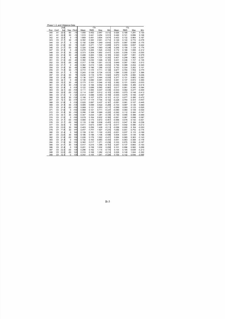
7/31/2019 Wind Tunnel Test
http://slidepdf.com/reader/full/wind-tunnel-test 149/243
B-5
Phase 1, 2, and 3 Balance Data
Uref
Run Conf fps Yaw Pitch Mean RMS Max Min Mean RMS Max Min
340 A1 22.0 60 -15 1.055 0.452 2.947 0.012 0.526 0.168 1.291 0.130
341 A1 22.8 30 -15 1.510 0.441 3.254 0.513 0.446 0.121 0.896 0.158
342 A1 22.5 0 -15 1.669 0.491 3.604 0.674 0.453 0.132 0.964 0.167
343 C5 21.7 30 -15 0.392 0.382 2.001 -0.714 0.129 0.144 0.772 -0.278
344 C5 21.7 0 -15 0.192 0.269 1.549 -0.643 0.070 0.087 0.599 -0.175345 C5 21.6 -30 -15 0.261 0.271 1.747 -0.659 0.073 0.093 0.657 -0.222
346 C5 21.7 -30 -30 0.324 0.249 1.560 -0.248 0.206 0.158 1.124 -0.174
347 C5 21.5 0 -30 0.270 0.265 1.524 -0.432 0.172 0.168 1.095 -0.212
348 C5 21.5 30 -30 0.373 0.304 1.852 -0.417 0.250 0.209 1.333 -0.255
349 C5 21.6 30 -45 0.408 0.263 1.594 -0.165 0.520 0.297 1.891 -0.079
350 C5 21.6 0 -45 0.366 0.264 1.737 -0.202 0.407 0.299 1.982 -0.207
351 C5 21.3 -30 -45 0.392 0.230 1.546 -0.160 0.431 0.246 1.727 -0.135
352 C5 22.0 -30 -60 0.317 0.158 1.051 -0.033 0.649 0.287 1.952 0.012
353 C5 21.7 0 -60 0.362 0.215 1.326 -0.053 0.756 0.389 2.454 -0.045
354 C5 21.6 30 -60 0.388 0.186 1.268 -0.022 0.763 0.324 2.262 0.101
355 C5 21.8 30 -75 0.210 0.126 0.711 -0.108 0.877 0.260 1.954 0.279
356 C5 21.7 0 -75 0.243 0.128 0.724 -0.033 1.096 0.300 2.327 0.368
357 C5 21.6 -30 -75 0.234 0.116 0.751 0.023 0.870 0.278 2.060 0.236
358 C5 21.8 -30 -90 0.136 0.077 0.444 -0.068 0.377 0.131 0.883 -0.063
359 C5 22.1 0 -90 0.146 0.080 0.491 -0.052 0.481 0.137 0.972 0.000
360 C5 22.2 30 -90 0.173 0.101 0.546 -0.103 0.382 0.121 0.853 -0.033
361 C5 21.5 30 -105 0.124 0.106 0.552 -0.163 -0.043 0.084 0. 259 -0.416
362 C5 21.9 0 -105 0.122 0.088 0.565 -0.063 0.017 0.081 0.340 -0.384
363 C5 22.1 -30 -105 0.111 0.084 0.447 -0.086 -0.033 0.082 0.277 -0.400
364 C5 22.0 -30 -120 0.114 0.087 0.512 -0.105 -0.063 0.073 0.148 -0.412
365 C5 21.4 0 -120 -0.013 0.088 0.493 -0.198 -0.045 0.075 0.165 -0.467
366 C5 22.0 30 -120 0.166 0.107 0.574 -0.121 -0.121 0.077 0. 085 -0.472
367 C5 22.1 30 -135 0.210 0.119 0.704 -0.142 -0.228 0.094 0. 014 -0.602
368 C5 21.8 0 -135 0.020 0.087 0.437 -0.167 -0.081 0.081 0.107 -0.445
369 C5 21.9 -30 -135 0.085 0.099 0.522 -0.208 -0.103 0.087 0.126 -0.464
370 C5 21.9 -30 -150 0.068 0.131 0.653 -0.317 -0.099 0.093 0.123 -0.505
371 C5 21.6 0 -150 0.068 0.121 0.711 -0.247 -0.090 0.084 0.109 -0.504
372 C5 21.8 30 -150 0.286 0.168 0.999 -0.220 -0.262 0.112 0. 045 -0.747
373 C5 22.1 30 -165 0.347 0.234 1.281 -0.345 -0.150 0.090 0. 088 -0.490
374 C5 21.5 0 -165 0.078 0.164 0.832 -0.355 -0.061 0.067 0.088 -0.387
375 C5 21.7 -30 -165 0.080 0.175 0.872 -0.467 -0.066 0.076 0.142 -0.431
376 C5 21.7 -30 180 0.133 0.188 0.938 -0.405 -0.012 0.047 0. 106 -0.236
377 C5 22.0 0 180 0.011 0.673 0.997 -0.319 -0.017 0.042 0. 090 -0.212
378 C5 22.0 30 180 0.403 0.256 1.428 -0.319 -0.058 0.055 0. 104 -0.253
379 C5 21.8 30 165 0.402 0.253 1.502 -0.270 0.056 0.051 0.252 -0.124380 C5 21.4 0 165 0.159 0.181 1.100 -0.283 -0.001 0.037 0. 115 -0.169
381 C5 22.0 -30 165 0.186 0.196 1.106 -0.446 0.004 0.041 0.139 -0.168
382 C5 21.8 -30 150 0.226 0.176 1.022 -0.431 0.084 0.065 0.363 -0.143
383 C5 21.8 0 150 0.192 0.163 0.993 -0.300 0.051 0.063 0.308 -0.178
384 C5 21.9 30 150 0.360 0.217 1.271 -0.236 0.103 0.075 0.399 -0.167
385 C5 21.7 30 135 0.417 0.215 1.395 -0.193 0.247 0.137 0.893 -0.153
386 C5 21.8 0 135 0.201 0.158 1.032 -0.258 0.101 0.096 0.582 -0.299
387 C5 22.3 -30 135 0.296 0.162 1.114 -0.170 0.144 0.105 0.639 -0.213
388 C5 22.0 -30 120 0.316 0.168 1.282 -0.214 0.228 0.148 1.044 -0.302
389 C5 22.2 0 120 0.202 0.155 1.041 -0.226 0.159 0.132 0.836 -0.566
Cfx Cfz
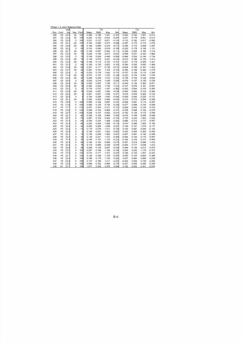
7/31/2019 Wind Tunnel Test
http://slidepdf.com/reader/full/wind-tunnel-test 150/243
B-6
Phase 1, 2, and 3 Balance Data
Uref
Run Conf fps Yaw Pitch Mean RMS Max Min Mean RMS Max Min
390 C5 22.4 30 120 0.389 0.196 1.441 -0.161 0.252 0.164 1.001 -0.214
391 C5 22.2 30 105 0.224 0.153 0.915 -0.257 0.231 0.179 0.931 -0.513
392 C5 22.5 0 105 0.231 0.127 0.871 -0.143 0.133 0.182 0.917 -0.590
393 C5 22.1 -30 105 0.164 0.080 0.473 -0.056 -0.297 0.175 0. 172 -1.078
394 C5 22.6 -30 90 0.168 0.089 0.516 -0.073 -0.258 0.172 0.208 -1.097395 C5 22.2 0 90 0.124 0.094 0.519 -0.159 -0.292 0.178 0.146 -1.131
396 C5 22.7 30 90 0.148 0.097 0.542 -0.112 -0.326 0.205 0. 195 -1.316
397 C5 22.3 30 75 0.229 0.106 0.613 -0.061 -0.908 0.231 -0. 323 -1.882
398 C5 2 2.0 0 75 0.158 0.059 0.458 -0.004 -0.664 0.204 -0.144 -1.734
399 C5 22.5 -30 75 0.149 0.072 0.421 -0.044 -0.612 0.186 -0. 135 -1.415
400 C5 22.2 -30 60 0.169 0.112 0.722 -0.101 -0.351 0.178 0.029 -1.221
401 C5 22.3 0 60 0.189 0.120 0.822 -0.105 -0.280 0.200 0.083 -1.469
402 C5 22.6 30 60 0.257 0.117 0.730 -0.070 -0.604 0.189 -0. 161 -1.423
403 C5 22.7 30 45 0.367 0.191 1.374 -0.124 -0.390 0.168 -0. 042 -1.279
404 C5 22.4 0 45 0.253 0.176 1.443 -0.131 -0.167 0.156 0.115 -1.240
405 C5 22.4 -30 45 0.252 0.187 1.276 -0.149 -0.223 0.154 0.091 -1.035
406 C5 22.2 -30 30 0.246 0.236 1.410 -0.352 -0.106 0.100 0.129 -0.634
407 C5 22.0 0 30 0.202 0.216 1.439 -0.252 -0.079 0.107 0.129 -0.720
408 C5 22.0 30 30 0.430 0.287 1.746 -0.311 -0.245 0.130 0. 053 -0.871
409 C5 22.6 30 15 0.384 0.325 1.745 -1.003 -0.107 0.076 0. 161 -0.591
410 C5 22.2 0 15 0.178 0.222 1.347 -0.362 -0.043 0.064 0.105 -0.405
411 C5 22.2 -30 15 0.225 0.267 1.552 -0.545 -0.062 0.064 0.103 -0.364
412 C5 22.2 -30 0 0.201 0.257 1.538 -0.471 0.016 0.045 0.262 -0.122
413 C5 22.5 0 0 0.184 0.258 1.640 -0.580 -0.009 0.040 0.220 -0.131
414 C5 22.1 30 0 0.362 0.402 2.006 -0.830 0.010 0.072 0.294 -0.208
415 F5 22.0 0 -165 0.085 0.162 0.887 -0.351 -0.056 0.081 0.114 -0.457
416 F5 21.6 0 -150 0.090 0.125 0.704 -0.256 -0.077 0.088 0.104 -0.508
417 F5 22.7 0 -135 0.053 0.093 0.471 -0.172 -0.080 0.082 0.108 -0.434
418 F5 22.2 0 -120 0.098 0.102 0.669 -0.121 -0.038 0.066 0.162 -0.379
419 F5 22.7 0 -105 0.228 0.127 0.823 -0.013 -0.162 0.135 0.172 -0.784
420 F5 22.1 0 -90 0.326 0.128 0.866 0.069 -0.016 0.199 0.495 -0.948
421 F5 22.7 0 -75 0.267 0.153 0.942 -0.105 0.730 0.223 1.623 0.035
422 F5 22.3 0 -50 0.356 0.235 1.469 -0.254 0.686 0.310 2.137 -0.067
423 F5 22.2 0 -45 0.352 0.264 1.838 -0.318 0.415 0.266 1.920 -0.192
424 F5 22.4 0 -30 0.282 0.265 1.638 -0.527 0.190 0.151 1.019 -0.177
425 F5 22.2 0 -15 0.179 0.276 1.511 -0.706 0.105 0.087 0.549 -0.142
426 F5 22.0 0 0 0.156 0.281 1.622 -0.662 0.035 0.045 0.300 -0.092
427 F5 22.1 0 15 0.109 0.249 1.483 -0.607 -0.007 0.061 0.140 -0.349
428 F5 22.2 0 30 0.138 0.221 1.312 -0.498 -0.064 0.105 0.175 -0.597
429 F5 22.5 0 45 0.196 0.192 1.174 -0.210 -0.164 0.163 0.107 -0.999430 F5 22.3 0 60 0.169 0.125 0.866 -0.076 -0.291 0.219 0.066 -1.472
431 F5 22.4 0 75 0.119 0.069 0.438 -0.070 -0.400 0.177 0.038 -1.412
432 F5 22.8 0 90 0.208 0.100 0.697 -0.048 0.096 0.136 0.514 -0.574
433 F5 23.2 0 105 0.297 0.166 1.194 -0.190 0.294 0.202 1.176 -0.373
434 F5 22.4 0 120 0.215 0.171 1.321 -0.275 0.166 0.152 1.091 -0.432
435 F5 22.1 0 135 0.126 0.168 1.105 -0.384 0.093 0.103 0.605 -0.369
436 F5 22.4 0 150 0.189 0.179 1.125 -0.322 0.037 0.064 0.266 -0.239
437 F5 2 2.2 0 165 0.137 0.189 1.211 -0.432 -0.004 0.050 0.159 -0.250
438 F5 2 2.2 0 180 0.089 0.182 0.990 -0.378 -0.027 0.055 0.085 -0.309
439 E1 22.1 0 180 1.677 0.356 3.078 0.849 0.192 0.052 0.351 -0.034
Cfx Cfz

7/31/2019 Wind Tunnel Test
http://slidepdf.com/reader/full/wind-tunnel-test 151/243
B-7
Phase 1, 2, and 3 Balance Data
Uref
Run Conf fps Yaw Pitch Mean RMS Max Min Mean RMS Max Min
440 E1 22.2 0 165 1.762 0.369 3.218 0.873 0.521 0.087 0.843 0.281
441 E1 22.5 0 150 1.610 0.332 2.859 0.813 0.644 0.108 1.061 0.333
442 E1 22.4 0 135 1.178 0.268 2.322 0.478 0.492 0.098 0.869 0.188
443 E1 22.2 0 120 0.899 0.266 2.019 0.185 0.252 0.155 1.104 -0.328
444 E1 22.5 0 105 0.665 0.237 1.837 0.072 0.698 0.280 2.021 -0.050445 E1 22.2 0 90 0.457 0.234 1.497 -0.130 0.460 0.206 1.278 -0.411
446 E1 22.9 0 75 0.731 0.222 1.673 0.224 -1.393 0.435 -0.562 -3.110
447 E1 22.4 0 60 0.869 0.232 1.768 0.323 -1.793 0.481 -0.773 -3.513
448 E1 22.4 0 45 1.458 0.346 2.752 0.704 -2.103 0.507 -1.041 -4.037
449 E1 22.5 0 30 1.989 0.411 3.732 1.016 -1.368 0.286 -0.703 -2.490
450 E1 22.2 0 15 2.138 0.455 4.320 1.065 -0.823 0.168 -0.437 -1.534
451 E1 22.5 0 0 2.104 0.434 4.080 1.071 0.024 0.038 0.155 -0.098
452 E1 22.4 0 -15 1.855 0.401 3.462 0.793 0.617 0.118 1.064 0.332
453 E1 22.3 0 -30 1.846 0.370 3.405 0.899 1.151 0.248 2.161 0.595
454 E1 22.6 0 -45 1.563 0.350 2.985 0.691 1.798 0.424 3.366 0.875
455 E1 22.6 0 -60 0.769 0.230 1.663 0.160 1.812 0.450 3.417 0.716
456 E1 22.6 0 -75 0.324 0.157 0.973 0.029 1.114 0.279 2.198 0.398
457 E1 23.2 0 -90 0.516 0.145 1.159 0.207 -0.231 0.221 0.360 -1.119
458 E1 2 2.5 0 -105 0.663 0.185 1.438 0.214 -0.713 0.239 0.032 -1.771
459 E1 2 2.7 0 -120 0.625 0.179 1.321 0.163 -0.175 0.126 0.220 -0.645
460 E1 2 2.4 0 -135 0.830 0.187 1.587 0.416 -0.083 0.063 0.127 -0.320
461 E1 2 2.4 0 -150 1.012 0.248 2.035 0.479 -0.129 0.071 0.030 -0.418
462 E1 2 2.5 0 -165 1.331 0.308 2.628 0.678 -0.087 0.069 0.066 -0.350
463 B1 22.9 -30 -165 0.965 0.254 2.009 0.410 -0.051 0.056 0. 085 -0.251
464 B1 2 2.6 0 -165 1.378 0.294 2.498 0.742 -0.096 0.061 0.030 -0.345
465 B1 22.4 30 -165 0.994 0.252 1.861 0.359 -0.107 0.053 0. 028 -0.324
466 B1 22.6 60 -165 0.418 0.167 1.075 -0.024 -0.033 0.037 0. 067 -0.165
467 B1 22.4 60 -150 0.237 0.130 0.754 -0.134 -0.089 0.050 0. 044 -0.303
468 B1 22.4 30 -150 0.792 0.181 1.519 0.378 -0.206 0.072 -0.033 -0.488
469 B1 22.3 0 -150 0.986 0.212 1.837 0.510 -0.258 0.076 -0. 098 -0.546
470 B1 22.2 -30 -150 0.720 0.203 1.473 0.255 -0.198 0.073 -0. 023 -0.479
471 B1 22.9 -30 -135 0.514 0.164 1.153 0.123 -0.175 0.071 0. 004 -0.448
472 B1 2 2.4 0 -135 0.661 0.171 1.288 0.273 -0.224 0.081 0.007 -0.534
473 B1 22.7 30 -135 0.605 0.155 1.216 0.245 -0.203 0.074 -0.017 -0.494
474 B1 22.4 60 -135 0.165 0.111 0.610 -0.121 -0.075 0.052 0. 078 -0.300
475 B1 23.1 60 -120 0.100 0.099 0.511 -0.155 -0.057 0.062 0. 146 -0.304
476 B1 22.4 30 -120 0.432 0.136 1.008 0.125 -0.119 0.080 0. 099 -0.449
477 B1 2 2.4 0 -120 0.473 0.147 1.028 0.147 -0.094 0.090 0.251 -0.442
478 B1 22.3 -30 -120 0.387 0.139 0.952 0.086 -0.140 0.076 0. 128 -0.451
479 B1 23.2 -30 -105 0.197 0.115 0.646 -0.065 -0.114 0.115 0.322 -0.620480 B1 2 2.7 0 -105 0.334 0.112 0.780 0.091 -0.096 0.136 0.466 -0.565
481 B1 22.7 30 -105 0.228 0.109 0.635 -0.047 -0.097 0.113 0. 318 -0.570
482 B1 22.4 60 -105 0.093 0.094 0.456 -0.163 -0.047 0.094 0. 213 -0.472
483 B1 2 2.3 60 -90 0.040 0.080 0.347 -0.163 0.192 0.109 0.641 -0.212
484 B1 22.2 30 -90 0.160 0.099 0.558 -0.059 0.525 0.164 1.190 0.007
485 B1 22.3 0 -90 0.274 0.101 0.704 0.063 0.545 0.200 1.408 -0.104
486 B1 22.3 -30 -90 0.183 0.116 0.657 -0.052 0.544 0.196 1.341 -0.084
487 B1 2 2.4 -30 -75 0.197 0.132 0.686 -0.094 1.422 0.414 2.923 0.492
488 B1 22.7 0 -75 0.221 0.139 0.744 -0.077 1.707 0.428 3.411 0.753
489 B1 22.4 30 -75 0.333 0.119 0.785 0.064 1.276 0.364 2.684 0.474
Cfx Cfz

7/31/2019 Wind Tunnel Test
http://slidepdf.com/reader/full/wind-tunnel-test 152/243
B-8
Phase 1, 2, and 3 Balance Data
Uref
Run Conf fps Yaw Pitch Mean RMS Max Min Mean RMS Max Min
490 B1 2 2.3 60 -75 0.074 0.072 0.367 -0.124 0.424 0.179 1.159 -0.007
491 B1 22.8 60 -60 0.142 0.096 0.549 -0.123 0.502 0.215 1.490 0.023
492 B1 22.6 30 -60 0.491 0.159 1.120 0.153 1.484 0.426 3.034 0.562
493 B1 22.2 0 -60 0.654 0.186 1.359 0.221 2.093 0.518 3.915 0.895
494 B1 22.5 -30 -60 0.508 0.175 1.223 0.139 1.555 0.481 3.431 0.526495 B1 22.3 -30 -45 1.037 0.279 2.138 0.361 1.534 0.414 3.036 0.606
496 B1 22.1 0 -45 1.367 0.319 2.583 0.638 1.792 0.448 3.429 0.851
497 B1 22.2 30 -45 0.965 0.255 2.030 0.416 1.360 0.385 2.832 0.565
498 B1 22.3 60 -45 0.376 0.142 0.954 -0.007 0.486 0.182 1.344 0.078
499 B1 22.3 60 -30 0.617 0.224 1.536 0.054 0.447 0.140 1.098 0.116
500 B1 22.2 30 -30 1.372 0.319 2.796 0.651 0.908 0.201 1.789 0.461
501 B1 22.0 0 -30 1.653 0.375 3.013 0.771 0.993 0.222 1.799 0.502
502 B1 22.3 -30 -30 1.316 0.331 2.632 0.446 0.818 0.201 1.600 0.308
503 B1 22.5 -30 -15 1.476 0.359 2.885 0.656 0.495 0.120 0.954 0.237
504 B1 22.2 0 -15 1.835 0.399 3.438 0.891 0.509 0.116 0.959 0.239
505 B1 22.2 30 -15 1.414 0.348 2.730 0.529 0.402 0.116 0.884 0.125
506 B1 22.5 60 -15 0.673 0.220 1.594 0.088 0.192 0.065 0.466 0.021
507 B1 22.7 60 0 0.681 0.245 1.728 0.084 0.009 0.029 0.124 -0.083
508 B1 22.2 30 0 1.530 0.367 2.930 0.581 -0.015 0.044 0.147 -0.166
509 B1 22.1 0 0 2.224 0.450 3.926 1.084 -0.038 0.038 0.098 -0.162
510 B1 22.1 -30 0 1.575 0.375 2.979 0.727 -0.012 0.043 0.176 -0.122
511 B1 22.4 -30 15 1.580 0.403 3.064 0.678 -0.475 0.120 -0. 188 -0.882
512 B1 22.3 0 15 2.217 0.468 3.963 1.193 -0.617 0.129 -0.306 -1.098
513 B1 2 2.4 30 15 1.688 0.364 3.120 0.806 -0.496 0.103 -0.229 -0.877
514 B1 2 2.7 60 15 0.697 0.262 1.701 0.089 -0.225 0.080 -0.028 -0.526
515 B1 22.4 60 30 0.568 0.226 1.505 0.015 -0.385 0.165 0.006 -1.078
516 B1 2 2.0 30 30 1.628 0.358 3.067 0.771 -1.143 0.258 -0.520 -2.206
517 B1 22.3 0 30 2.035 0.430 3.694 1.045 -1.409 0.304 -0.671 -2.557
518 B1 22.3 -30 30 1.558 0.393 3.091 0.679 -1.193 0.292 -0. 542 -2.349
519 B1 22.6 -30 45 1.234 0.356 2.584 0.473 -1.779 0.522 -0. 692 -3.717
520 B1 22.1 0 45 1.604 0.355 3.016 0.812 -2.236 0.508 -1.140 -4.289
521 B1 2 2.5 30 45 1.243 0.312 2.433 0.547 -1.767 0.464 -0.747 -3.468
522 B1 22.6 60 45 0.405 0.193 1.177 -0.056 -0.620 0.270 -0. 106 -1.672
523 B1 22.7 60 60 0.256 0.136 0.793 -0.109 -0.698 0.317 -0. 052 -1.968
524 B1 2 2.2 30 60 0.919 0.255 2.006 0.366 -2.302 0.673 -0.972 -5.119
525 B1 22.4 0 60 1.000 0.264 1.938 0.418 -2.767 0.712 -1.288 -5.196
526 B1 22.3 -30 60 0.869 0.264 1.895 0.301 -2.303 0.695 -0. 843 -4.797
527 B1 22.9 -30 75 0.573 0.179 1.230 0.155 -2.039 0.630 -0. 762 -4.236
528 B1 22.4 0 75 0.715 0.212 1.494 0.244 -2.528 0.779 -1.001 -5.205
529 B1 2 2.5 30 75 0.573 0.168 1.239 0.188 -1.997 0.609 -0.700 -4.309530 B1 2 2.2 60 75 0.133 0.102 0.551 -0.111 -0.618 0.312 0.052 -1.949
531 B1 2 2.7 60 90 0.041 0.078 0.352 -0.193 -0.134 0.194 0.328 -0.945
532 B1 22.8 30 90 0.282 0.111 0.745 0.013 -0.410 0.283 0.222 -1.630
533 B1 22.6 0 90 0.313 0.137 0.947 -0.001 -0.330 0.309 0.299 -1.664
534 B1 22.6 -30 90 0.271 0.125 0.818 -0.020 -0.473 0.314 0.206 -1.856
535 B1 22.5 -30 105 0.357 0.146 0.938 -0.012 0.323 0.193 1.005 -0.300
536 B1 22.6 0 105 0.502 0.148 1.215 0.134 0.236 0.223 1.282 -0.613
537 B1 22.3 30 105 0.274 0.130 0.895 -0.058 0.331 0.185 1.205 -0.279
538 B1 22.5 60 105 0.154 0.088 0.530 -0.106 0.184 0.132 0.754 -0.254
539 B1 22.7 60 120 0.165 0.113 0.719 -0.131 0.179 0.108 0.721 -0.112
Cfx Cfz

7/31/2019 Wind Tunnel Test
http://slidepdf.com/reader/full/wind-tunnel-test 153/243
B-9
Phase 1, 2, and 3 Balance Data
Uref
Run Conf fps Yaw Pitch Mean RMS Max Min Mean RMS Max Min
540 B1 2 2.1 30 120 0.556 0.182 1.295 0.119 0.338 0.143 1.018 -0.083
541 B1 22.4 0 120 0.819 0.218 1.649 0.307 0.377 0.144 1.052 -0.055
542 B1 22.4 -30 120 0.614 0.193 1.396 0.136 0.332 0.138 0.934 -0.157
543 B1 2 2.2 -30 135 0.915 0.244 1.817 0.334 0.505 0.116 0.972 0.184
544 B1 22.3 0 135 1.107 0.274 2.104 0.517 0.607 0.129 1.058 0.270545 B1 22.2 30 135 0.937 0.230 1.850 0.424 0.492 0.108 0.958 0.217
546 B1 22.6 60 135 0.314 0.149 0.956 -0.053 0.165 0.081 0.518 -0.056
547 B1 2 2.7 60 150 0.423 0.190 1.214 -0.020 0.231 0.077 0.522 0.044
548 B1 22.8 30 150 1.230 0.278 2.308 0.573 0.534 0.104 0.938 0.256
549 B1 22.5 0 150 1.523 0.328 2.765 0.743 0.673 0.116 1.094 0.372
550 B1 2 2.4 -30 150 1.286 0.334 2.499 0.527 0.554 0.120 0.988 0.268
551 B1 2 2.6 -30 165 1.266 0.330 2.537 0.493 0.424 0.080 0.725 0.219
552 B1 22.3 0 165 1.545 0.346 2.866 0.742 0.483 0.080 0.812 0.269
553 B1 22.3 30 165 1.473 0.309 2.609 0.812 0.391 0.074 0.675 0.200
554 B1 22.4 60 165 0.600 0.205 1.410 0.095 0.154 0.058 0.370 0.000
555 B1 2 2.5 60 180 0.551 0.194 1.291 0.055 0.086 0.031 0.195 -0.004
556 B1 2 2.3 30 180 1.300 0.274 2.255 0.625 0.144 0.040 0.259 -0.010
557 B1 22.3 0 180 1.568 0.339 2.886 0.837 0.158 0.045 0.316 -0.001
558 B1 22.3 -30 180 1.241 0.315 2.444 0.517 0.100 0.044 0.246 -0.060
559 B3 22.5 -30 -165 0.777 0.243 1.720 0.263 -0.049 0.058 0. 111 -0.478
560 B3 2 2.2 0 -165 1.415 0.360 2.791 0.619 -0.120 0.074 0.045 -0.409
561 B3 22.5 30 -165 1.776 0.420 3.447 0.833 -0.183 0.079 -0.009 -0.523
562 B3 22.4 60 -165 1.455 0.442 3.090 0.285 -0.210 0.085 0. 012 -0.536
563 B3 22.7 60 -150 1.017 0.333 2.170 0.127 -0.358 0.139 0. 029 -0.841
564 B3 22.4 30 -150 1.246 0.293 2.360 0.578 -0.358 0.112 -0.112 -0.813
565 B3 22.8 0 -150 1.005 0.266 2.003 0.430 -0.274 0.091 -0. 082 -0.604
566 B3 22.9 -30 -150 0.575 0.181 1.342 0.156 -0.154 0.064 -0. 003 -0.414
567 B3 23.0 -30 -135 0.444 0.146 1.041 0.121 -0.130 0.067 0. 061 -0.396
568 B3 22.6 0 -135 0.773 0.199 1.487 0.326 -0.258 0.090 -0. 028 -0.571
569 B3 22.2 30 -135 0.949 0.242 1.924 0.391 -0.420 0.131 -0.096 -0.970
570 B3 22.6 60 -135 0.718 0.266 1.632 0.007 -0.489 0.178 -0.019 -1.091
571 B3 22.5 60 -120 0.387 0.184 1.065 -0.061 -0.372 0.187 0. 089 -1.103
572 B3 22.2 30 -120 0.619 0.176 1.369 0.226 -0.402 0.165 0. 021 -1.127
573 B3 2 2.4 0 -120 0.454 0.144 1.038 0.140 -0.096 0.096 0.269 -0.485
574 B3 22.6 -30 -120 0.333 0.138 0.878 0.022 -0.118 0.082 0. 144 -0.440
575 B3 22.8 -30 -105 0.263 0.117 0.688 0.011 -0.109 0.110 0. 274 -0.565
576 B3 2 3.0 0 -105 0.368 0.108 0.793 0.108 -0.121 0.134 0.337 -0.690
577 B3 23.0 30 -105 0.354 0.122 0.822 0.075 -0.164 0.148 0. 356 -0.744
578 B3 22.8 60 -105 0.222 0.139 0.758 -0.150 -0.115 0.139 0. 356 -0.751
579 B3 2 2.3 60 -90 0.112 0.098 0.517 -0.138 0.262 0.148 0.958 -0.201580 B3 22.9 30 -90 0.247 0.110 0.694 0.011 0.579 0.183 1.323 0.009
581 B3 23.0 0 -90 0.286 0.098 0.679 0.067 0.381 0.191 1.162 -0.222
582 B3 23.0 -30 -90 0.231 0.114 0.679 -0.005 0.412 0.160 1.045 -0.078
583 B3 22.7 -30 -75 0.319 0.134 0.883 0.042 1.291 0.368 2.723 0.491
584 B3 22.7 0 -75 0.387 0.153 0.958 0.058 1.561 0.383 2.955 0.714
585 B3 22.2 30 -75 0.430 0.145 0.993 0.120 1.403 0.361 2.780 0.557
586 B3 22.7 60 -75 0.206 0.105 0.672 -0.044 0.608 0.246 1.613 0.007
587 B3 22.3 60 -60 0.379 0.177 1.114 -0.025 0.961 0.341 2.462 0.287
588 B3 22.4 30 -60 0.776 0.224 1.685 0.277 1.904 0.486 3.855 0.796
589 B3 23.0 0 -60 0.706 0.225 1.595 0.208 1.931 0.538 3.956 0.696
Cfx Cfz
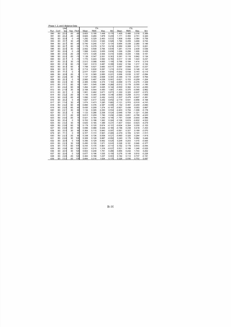
7/31/2019 Wind Tunnel Test
http://slidepdf.com/reader/full/wind-tunnel-test 154/243
B-10
Phase 1, 2, and 3 Balance Data
Uref
Run Conf fps Yaw Pitch Mean RMS Max Min Mean RMS Max Min
590 B3 22.5 -30 -60 0.603 0.190 1.448 0.178 1.405 0.466 3.318 0.389
591 B3 22.2 -30 -45 0.825 0.265 1.878 0.208 1.171 0.394 2.751 0.320
592 B3 22.9 0 -45 1.292 0.329 2.463 0.533 1.808 0.458 3.364 0.758
593 B3 22.7 30 -45 1.289 0.324 2.546 0.529 1.790 0.459 3.469 0.744
594 B3 22.7 60 -45 0.740 0.245 1.727 0.134 0.954 0.339 2.280 0.189595 B3 22.7 60 -30 1.178 0.379 2.731 0.218 0.950 0.308 2.172 0.201
596 B3 22.5 30 -30 2.002 0.508 3.784 0.839 1.261 0.318 2.439 0.536
597 B3 22.8 0 -30 1.568 0.403 3.055 0.656 1.026 0.256 1.935 0.439
598 B3 22.6 -30 -30 1.073 0.326 2.444 0.310 0.648 0.220 1.556 0.161
599 B3 22.5 -30 -15 1.128 0.347 2.551 0.363 0.391 0.116 0.842 0.134
600 B3 22.7 0 -15 1.770 0.443 3.592 0.783 0.517 0.128 1.020 0.237
601 B3 22.3 30 -15 2.512 0.588 4.693 1.106 0.768 0.184 1.414 0.319
602 B3 21.9 60 -15 1.541 0.513 3.487 0.388 0.552 0.184 1.217 0.104
603 B3 22.3 60 0 1.708 0.527 3.683 -0.077 0.097 0.060 0.351 -0.227
604 B3 22.1 30 0 2.714 0.630 5.097 1.274 -0.014 0.044 0.148 -0.142
605 B3 22.2 0 0 2.027 0.502 4.091 0.810 -0.002 0.039 0.163 -0.114
606 B3 22.8 -30 0 1.131 0.365 2.850 0.221 0.006 0.035 0.157 -0.094
607 B3 22.6 -30 15 1.147 0.350 2.608 0.341 -0.348 0.110 -0.057 -0.764
608 B3 22.3 0 15 2.060 0.497 4.038 0.961 -0.621 0.153 -0.259 -1.204
609 B3 2 2.3 30 15 2.385 0.550 4.374 1.104 -0.699 0.173 -0.276 -1.329
610 B3 2 2.1 60 15 1.601 0.545 3.588 0.269 -0.512 0.178 -0.055 -1.190
611 B3 2 2.2 60 30 1.264 0.491 3.025 0.142 -0.930 0.362 -0.143 -2.293
612 B3 2 1.9 30 30 2.168 0.544 4.493 1.001 -1.403 0.375 -0.595 -2.962
613 B3 22.1 0 30 1.901 0.462 3.671 0.873 -1.330 0.320 -0.637 -2.572
614 B3 22.2 -30 30 1.145 0.344 2.459 0.348 -0.900 0.258 -0.313 -1.850
615 B3 22.0 -30 45 1.090 0.337 2.452 0.433 -1.537 0.479 -0.607 -3.391
616 B3 22.2 0 45 1.657 0.417 3.252 0.652 -2.119 0.541 -0.856 -4.168
617 B3 2 2.4 30 45 1.674 0.423 3.285 0.693 -2.131 0.553 -0.918 -4.243
618 B3 2 2.2 60 45 0.890 0.376 2.387 0.089 -1.152 0.491 -0.200 -3.060
619 B3 2 2.5 60 60 0.430 0.209 1.274 -0.107 -0.921 0.436 0.053 -2.667
620 B3 2 2.1 30 60 1.134 0.305 2.293 0.504 -2.403 0.704 -1.006 -5.178
621 B3 22.2 0 60 1.123 0.286 2.208 0.524 -2.648 0.709 -1.321 -5.256
622 B3 22.1 -30 60 0.812 0.259 1.765 0.230 -2.095 0.651 -0.788 -4.520
623 B3 22.5 -30 75 0.521 0.184 1.240 0.145 -1.791 0.638 -0.655 -3.986
624 B3 22.4 0 75 0.763 0.198 1.562 0.324 -2.106 0.674 -0.832 -4.553
625 B3 2 2.2 30 75 0.620 0.185 1.389 0.231 -1.837 0.622 -0.623 -4.279
626 B3 2 2.8 60 75 0.179 0.120 0.674 -0.131 -0.634 0.354 0.200 -2.103
627 B3 2 2.8 60 90 0.096 0.088 0.426 -0.180 -0.196 0.238 0.418 -1.253
628 B3 22.5 30 90 0.364 0.115 0.840 0.087 -0.561 0.327 0.189 -2.070
629 B3 22.1 0 90 0.307 0.133 0.953 -0.005 -0.379 0.306 0.240 -1.913630 B3 2 2.3 -30 90 0.338 0.136 0.938 0.021 -0.460 0.320 0.264 -1.919
631 B3 22.6 -30 105 0.309 0.128 0.887 -0.002 0.240 0.176 0.962 -0.446
632 B3 22.9 0 105 0.356 0.129 0.942 0.025 0.209 0.203 1.015 -0.505
633 B3 2 2.3 30 105 0.450 0.155 1.071 0.043 0.328 0.181 0.946 -0.377
634 B3 22.2 60 105 0.244 0.135 0.861 -0.114 0.162 0.178 0.920 -0.494
635 B3 22.6 60 120 0.521 0.215 1.318 -0.027 0.521 0.189 1.248 -0.025
636 B3 22.5 30 120 0.843 0.248 1.791 0.266 0.855 0.242 1.744 0.202
637 B3 22.6 0 120 0.677 0.196 1.535 0.158 0.278 0.149 0.910 -0.228
638 B3 22.8 -30 120 0.463 0.168 1.237 0.063 0.182 0.112 0.737 -0.191
639 B3 2 2.2 -30 135 0.664 0.216 1.634 0.175 0.326 0.090 0.703 0.087
Cfx Cfz

7/31/2019 Wind Tunnel Test
http://slidepdf.com/reader/full/wind-tunnel-test 155/243
B-11
Phase 1, 2, and 3 Balance Data
Uref
Run Conf fps Yaw Pitch Mean RMS Max Min Mean RMS Max Min
640 B3 22.5 0 135 0.950 0.269 2.076 0.345 0.459 0.122 0.954 0.131
641 B3 22.3 30 135 1.398 0.354 2.710 0.552 0.941 0.240 1.849 0.353
642 B3 22.5 60 135 0.904 0.316 2.049 0.057 0.608 0.204 1.341 0.078
643 B3 22.7 60 150 1.343 0.475 3.119 0.211 0.640 0.184 1.317 0.202
644 B3 22.5 30 150 1.857 0.462 3.349 0.799 0.776 0.176 1.334 0.390645 B3 22.5 0 150 1.440 0.366 2.815 0.673 0.525 0.118 0.958 0.236
646 B3 2 2.6 -30 150 0.945 0.271 1.950 0.370 0.309 0.085 0.604 0.099
647 B3 2 2.6 -30 165 0.974 0.288 2.105 0.339 0.279 0.063 0.522 0.127
648 B3 22.3 0 165 1.629 0.419 3.100 0.712 0.396 0.092 0.722 0.169
649 B3 22.2 30 165 1.976 0.510 3.771 0.784 0.544 0.124 0.988 0.224
650 B3 21.8 60 165 1.658 0.528 3.614 0.401 0.425 0.125 0.927 0.129
651 B3 22.7 60 180 1.621 0.509 3.355 0.263 0.148 0.047 0.333 0.002
652 B3 2 2.4 30 180 1.931 0.451 3.537 0.910 0.134 0.051 0.304 -0.053
653 B3 22.4 0 180 1.573 0.392 3.023 0.688 0.072 0.046 0.223 -0.106
654 B3 22.3 -30 180 0.985 0.297 2.204 0.386 0.024 0.038 0.153 -0.115
655 E3 22.4 0 -180 1.458 0.420 3.216 0.449 0.114 0.057 0.305 -0.125
656 E3 2 2.3 0 -165 1.295 0.374 2.819 0.398 -0.103 0.077 0.087 -0.415
657 E3 2 2.2 0 -150 1.064 0.272 2.110 0.405 -0.173 0.084 0.012 -0.522
658 E3 2 2.6 0 -135 0.741 0.211 1.657 0.270 -0.074 0.070 0.126 -0.372
659 E3 2 2.7 0 -120 0.633 0.193 1.459 0.199 -0.222 0.146 0.266 -0.777
660 E3 22.0 0 -105 0.628 0.186 1.401 0.222 -0.706 0.242 -0. 085 -1.653
661 E3 22.0 0 -90 0.445 0.154 1.071 0.124 -0.137 0.224 0.499 -1.025
662 E3 22.5 0 -75 0.352 0.168 1.019 -0.042 0.909 0.229 1.830 0.173
663 E3 22.8 0 -60 0.737 0.231 1.566 0.169 1.599 0.399 2.919 0.725
664 E3 23.0 0 -45 1.233 0.359 2.671 0.302 1.709 0.450 3.257 0.524
665 E3 23.4 0 -30 1.488 0.417 3.154 0.404 1.036 0.242 1.950 0.464
666 E3 22.8 0 -15 1.724 0.487 3.896 0.604 0.602 0.137 1.165 0.290
667 E3 22.8 0 0 2.008 0.530 4.350 0.716 0.057 0.040 0.218 -0.068
668 E3 22.8 0 15 2.011 0.500 4.123 0.818 -0.591 0.157 -0.211 -1.184
669 E3 21.9 0 30 1.999 0.520 4.203 0.788 -1.110 0.288 -0.463 -2.266
670 E3 22.2 0 45 1.584 0.437 3.270 0.558 -1.897 0.525 -0.775 -3.812
671 E3 22.6 0 60 1.040 0.285 2.217 0.409 -1.849 0.524 -0.801 -3.826
672 E3 22.7 0 75 0.635 0.197 1.473 0.206 -1.000 0.356 -0.220 -2.308
673 E3 22.3 0 90 0.456 0.197 1.482 -0.001 0.408 0.189 1.072 -0.369
674 E3 22.4 0 105 0.568 0.236 1.628 -0.013 0.732 0.262 1.879 0.039
675 E3 22.9 0 120 0.795 0.257 1.969 0.180 0.196 0.149 0.871 -0.307
676 E3 22.5 0 135 1.000 0.318 2.587 0.250 0.349 0.103 0.950 0.004
677 E3 22.3 0 150 1.436 0.394 3.079 0.502 0.531 0.122 1.018 0.192
678 E3 22.5 0 165 1.536 0.417 3.213 0.544 0.397 0.087 0.726 0.157
679 E4 22.6 0 15 0.001 0.293 1.439 -1.152 0.038 0.053 0.238 -0.243680 E4 22.9 0 30 0.080 0.248 1.247 -0.909 -0.031 0.087 0.223 -0.504
681 E4 22.4 0 45 0.276 0.236 1.560 -0.579 -0.250 0.192 0.258 -1.212
682 E4 2 2.5 0 60 0.552 0.208 1.554 -0.034 -0.731 0.240 -0.179 -1.797
683 E4 22.5 0 75 0.480 0.161 1.124 0.123 -0.452 0.210 0.017 -1.358
684 E4 23.0 0 90 0.352 0.164 1.122 -0.053 0.270 0.149 0.818 -0.334
685 E4 22.4 0 105 0.485 0.318 2.123 -0.671 0.531 0.248 1.557 -0.130
686 E4 22.4 0 120 0.474 0.368 2.408 -0.914 0.200 0.252 1.271 -0.673
687 E4 22.6 0 135 0.341 0.307 1.854 -0.633 0.232 0.148 0.918 -0.277
688 E4 22.7 0 150 0.132 0.256 1.316 -0.775 0.099 0.078 0.428 -0.166
689 E4 22.9 0 165 0.085 0.226 1.046 -0.716 0.016 0.050 0.216 -0.177
Cfx Cfz

7/31/2019 Wind Tunnel Test
http://slidepdf.com/reader/full/wind-tunnel-test 156/243
B-12
Phase 1, 2, and 3 Balance Data
Uref
Run Conf fps Yaw Pitch Mean RMS Max Min Mean RMS Max Min
690 E4 2 2.3 0 180 0.016 0.261 1.283 -1.065 -0.053 0.050 0.102 -0.304
691 E4 22.5 0 -165 -0.043 0.262 1.169 -0.922 -0.040 0.075 0.168 -0.413
692 E4 22.5 0 -150 0.037 0.213 0.981 -0.695 -0.065 0.090 0.221 -0.433
693 E4 22.7 0 -135 0.000 0.162 0.762 -0.509 -0.088 0.092 0.180 -0.498
694 E4 22.6 0 -120 0.211 0.139 0.841 -0.192 -0.063 0.088 0.210 -0.433695 E4 2 2.7 0 -105 0.398 0.148 1.041 0.070 -0.397 0.176 0.043 -1.119
696 E4 22.5 0 -90 0.309 0.130 0.823 0.022 -0.130 0.180 0.415 -0.915
697 E4 22.3 0 -75 0.312 0.162 0.953 -0.098 0.558 0.183 1.249 -0.030
698 E4 22.4 0 -60 0.416 0.269 1.542 -0.193 0.904 0.287 2.151 0.287
699 E4 22.7 0 -45 0.328 0.245 1.440 -0.439 0.288 0.207 1.248 -0.299
700 E4 23.1 0 -30 0.206 0.269 1.523 -0.827 0.067 0.150 0.827 -0.474
701 E4 2 2.7 0 -15 -0.077 0.305 1.285 -1.289 0.006 0.101 0.480 -0.451
702 E4 22.4 0 0 -0.040 0.346 1.718 -1.417 0.027 0.060 0.311 -0.213
703 B4 22.8 -30 0 0.020 0.147 0.526 -0.765 0.035 0.037 0.194 -0.101
704 B4 22.1 0 0 -0.098 0.269 1.157 -1.242 0.029 0.057 0.296 -0.205
705 B4 22.0 30 0 1.796 0.528 3.613 0.460 0.094 0.044 0.268 -0.054
706 B4 22.9 60 0 1.338 0.500 3.236 0.207 0.040 0.052 0.250 -0.123
707 B4 22.5 60 -15 1.198 0.452 3.060 0.140 0.505 0.162 1.131 0.152
708 B4 22.6 30 -15 1.333 0.454 3.132 0.236 0.430 0.134 0.949 0.100
709 B4 2 2.2 0 -15 0.039 0.256 1.155 -1.068 -0.058 0.104 0.383 -0.483
710 B4 22.7 -30 -15 0.133 0.155 0.645 -0.722 0.012 0.056 0.216 -0.307
711 B4 22.6 -30 -30 0.121 0.154 0.671 -0.509 0.096 0.096 0.550 -0.318
712 B4 22.3 0 -30 0.072 0.237 1.407 -0.844 0.090 0.170 1.080 -0.515
713 B4 22.2 30 -30 1.145 0.419 2.732 0.137 0.831 0.277 1.939 0.192
714 B4 22.2 60 -30 1.108 0.377 2.602 0.237 0.780 0.284 1.878 0.169
715 B4 22.8 60 -45 0.649 0.228 1.491 0.067 0.968 0.315 2.160 0.252
716 B4 22.6 30 -45 0.745 0.298 1.914 0.109 0.993 0.419 2.610 0.093
717 B4 22.5 0 -45 0.289 0.198 1.310 -0.143 0.366 0.252 1.511 -0.209
718 B4 23.2 -30 -45 0.186 0.124 0.727 -0.252 0.209 0.150 0.912 -0.364
719 B4 2 3.1 -30 -60 0.178 0.132 0.795 -0.097 0.670 0.282 1.916 0.054
720 B4 22.9 0 -60 0.330 0.232 1.324 -0.107 1.108 0.406 2.861 0.284
721 B4 23.1 30 -60 0.512 0.182 1.252 0.120 1.350 0.397 2.853 0.493
722 B4 23.2 60 -60 0.555 0.164 1.221 0.152 0.904 0.319 2.270 0.172
723 B4 22.9 60 -75 0.166 0.114 0.596 -0.104 0.657 0.254 1.651 0.074
724 B4 23.3 30 -75 0.195 0.120 0.703 -0.061 1.327 0.332 2.687 0.538
725 B4 22.1 0 -75 0.285 0.147 0.841 -0.049 1.235 0.322 2.459 0.483
726 B4 23.3 -30 -75 0.284 0.116 0.782 0.045 0.901 0.308 2.138 0.253
727 B4 23.3 -30 -90 0.167 0.082 0.478 -0.015 0.292 0.131 0.818 -0.132
728 B4 23.2 0 -90 0.179 0.082 0.500 -0.017 0.400 0.144 1.041 -0.011
729 B4 23.0 30 -90 0.217 0.104 0.607 -0.043 0.626 0.188 1.329 0.107730 B4 2 2.6 60 -90 0.156 0.095 0.534 -0.091 0.276 0.142 0.862 -0.194
731 B4 23.0 60 -105 0.189 0.124 0.656 -0.127 -0.088 0.134 0. 325 -0.676
732 B4 22.9 30 -105 0.313 0.125 0.785 0.031 -0.151 0.162 0. 356 -0.848
733 B4 22.9 0 -105 0.198 0.088 0.627 -0.013 -0.023 0.109 0.392 -0.479
734 B4 22.9 -30 -105 0.106 0.080 0.439 -0.078 -0.057 0.094 0.293 -0.438
735 B4 23.0 -30 -120 0.047 0.073 0.370 -0.150 -0.050 0.071 0.176 -0.374
736 B4 23.3 0 -120 0.160 0.109 0.639 -0.099 -0.100 0.084 0.164 -0.463
737 B4 22.8 30 -120 0.604 0.186 1.315 0.194 -0.373 0.163 0. 032 -0.991
738 B4 23.2 60 -120 0.385 0.196 1.169 -0.073 -0.391 0.186 0. 103 -1.150
739 B4 23.3 60 -135 0.618 0.239 1.579 0.061 -0.407 0.163 -0.009 -1.027
Cfx Cfz

7/31/2019 Wind Tunnel Test
http://slidepdf.com/reader/full/wind-tunnel-test 157/243
B-13
Phase 1, 2, and 3 Balance Data
Uref
Run Conf fps Yaw Pitch Mean RMS Max Min Mean RMS Max Min
740 B4 22.7 30 -135 0.846 0.230 1.767 0.319 -0.425 0.132 -0.116 -0.958
741 B4 23.3 0 -135 0.002 0.148 0.725 -0.356 -0.135 0.094 0.137 -0.591
742 B4 23.1 -30 -135 0.017 0.074 0.340 -0.263 -0.026 0.062 0.214 -0.317
743 B4 22.7 -30 -150 -0.051 0.096 0.265 -0.482 0.014 0.055 0.240 -0.204
744 B4 23.1 0 -150 -0.030 0.181 0.754 -0.573 -0.050 0.090 0.204 -0.480745 B4 22.8 30 -150 1.123 0.308 2.318 0.388 -0.371 0.123 -0.069 -0.865
746 B4 22.4 60 -150 0.961 0.329 2.345 0.053 -0.370 0.133 -0.014 -0.899
747 B4 23.1 60 -165 1.131 0.399 2.691 0.066 -0.138 0.077 0. 068 -0.441
748 B4 23.2 30 -165 1.276 0.391 2.922 0.431 -0.217 0.090 0. 013 -0.578
749 B4 22.9 0 -165 0.053 0.231 1.084 -0.733 -0.088 0.067 0.127 -0.385
750 B4 23.2 -30 -165 0.020 0.117 0.395 -0.524 0.002 0.039 0.164 -0.186
751 B4 22.6 -30 180 -0.049 0.126 0.344 -0.658 0.003 0.028 0.112 -0.101
752 B4 22.5 0 180 -0.006 0.230 1.054 -0.763 -0.012 0.039 0.126 -0.169
753 B4 2 2.3 30 180 1.499 0.416 3.133 0.474 0.070 0.054 0.253 -0.119
754 B4 2 2.2 60 180 1.511 0.484 3.319 0.402 0.052 0.043 0.208 -0.099
755 B4 22.8 60 165 1.431 0.470 3.058 0.227 0.405 0.105 0.785 0.130
756 B4 22.3 30 165 1.625 0.451 3.221 0.484 0.335 0.108 0.682 0.067
757 B4 2 2.3 0 165 0.105 0.201 1.024 -0.653 -0.027 0.047 0.173 -0.173
758 B4 22.8 -30 165 0.030 0.122 0.407 -0.576 0.007 0.036 0.109 -0.125
759 B4 22.2 -30 150 0.028 0.111 0.499 -0.396 0.096 0.058 0.318 -0.077
760 B4 22.7 0 150 0.196 0.214 1.263 -0.481 0.117 0.077 0.478 -0.111
761 B4 22.3 30 150 1.306 0.421 2.662 0.377 0.551 0.173 1.107 0.147
762 B4 22.3 60 150 1.231 0.399 2.723 0.313 0.535 0.160 1.150 0.172
763 B4 2 2.7 60 135 0.852 0.310 1.993 -0.007 0.635 0.198 1.367 0.116
764 B4 21.8 30 135 1.171 0.346 2.392 0.341 0.754 0.228 1.509 0.222
765 B4 22.2 0 135 0.345 0.250 1.536 -0.325 0.222 0.145 0.895 -0.223
766 B4 21.8 -30 135 0.239 0.173 1.283 -0.303 0.174 0.123 0.818 -0.220
767 B4 22.9 -30 120 0.230 0.218 1.319 -0.510 0.178 0.209 1.082 -0.538
768 B4 22.2 0 120 0.387 0.291 1.964 -0.750 0.233 0.232 1.317 -0.617
769 B4 22.4 30 120 0.752 0.234 1.635 0.162 0.731 0.241 1.619 0.073
770 B4 2 2.4 60 120 0.574 0.211 1.465 0.017 0.499 0.191 1.277 -0.032
771 B4 22.6 60 105 0.231 0.130 0.781 -0.109 0.220 0.174 0.910 -0.401
772 B4 2 2.3 30 105 0.433 0.166 1.196 0.000 0.410 0.189 1.166 -0.311
773 B4 21.9 0 105 0.318 0.206 1.345 -0.501 0.124 0.212 0.958 -0.736
774 B4 22.2 -30 105 0.258 0.179 1.158 -0.345 0.175 0.194 0.943 -0.567
775 B4 22.1 -30 90 0.160 0.093 0.524 -0.070 -0.232 0.182 0.266 -1.114
776 B4 22.1 0 90 0.245 0.101 0.657 0.012 -0.242 0.171 0.267 -1.004
777 B4 21.8 30 90 0.335 0.115 0.828 0.057 -0.657 0.358 0.197 -2.210
778 B4 2 1.8 60 90 0.187 0.093 0.574 -0.061 -0.219 0.241 0.508 -1.252
779 B4 2 2.9 60 75 0.242 0.123 0.753 -0.061 -0.687 0.355 0.103 -2.146780 B4 2 1.7 30 75 0.640 0.180 1.347 0.216 -2.126 0.669 -0.780 -4.859
781 B4 22.2 0 75 0.578 0.156 1.148 0.224 -1.440 0.391 -0.601 -2.882
782 B4 21.8 -30 75 0.311 0.116 0.736 0.043 -1.106 0.366 -0. 328 -2.392
783 B4 22.0 -30 60 0.263 0.122 0.852 -0.096 -0.587 0.224 -0. 026 -1.621
784 B4 22.7 0 60 0.651 0.204 1.458 0.175 -1.219 0.377 -0.401 -2.713
785 B4 2 2.4 30 60 1.062 0.295 2.119 0.415 -2.331 0.680 -0.956 -4.819
786 B4 21.6 60 60 0.478 0.227 1.392 -0.049 -1.013 0.475 -0. 062 -2.931
787 B4 2 2.1 60 45 0.863 0.359 2.178 0.017 -1.090 0.467 -0.049 -2.844
788 B4 2 2.3 30 45 1.488 0.393 2.905 0.563 -1.827 0.488 -0.732 -3.622
789 B4 22.5 0 45 0.306 0.226 1.530 -0.297 -0.409 0.251 0.115 -1.646
Cfx Cfz

7/31/2019 Wind Tunnel Test
http://slidepdf.com/reader/full/wind-tunnel-test 158/243
B-14
Phase 1, 2, and 3 Balance Data
Uref
Run Conf fps Yaw Pitch Mean RMS Max Min Mean RMS Max Min
790 B4 22.5 -30 45 0.143 0.099 0.635 -0.237 -0.105 0.092 0.188 -0.505
791 B4 22.5 -30 30 0.099 0.127 0.549 -0.540 -0.016 0.058 0.199 -0.234
792 B4 22.2 0 30 0.158 0.217 1.347 -0.611 -0.058 0.115 0.207 -0.735
793 B4 2 1.9 30 30 1.798 0.519 3.861 0.381 -1.150 0.348 -0.285 -2.472
794 B4 2 1.7 60 30 1.219 0.478 2.998 0.102 -0.924 0.352 -0.155 -2.221795 B4 22.4 60 15 1.368 0.475 3.147 0.160 -0.375 0.159 0.001 -0.993
796 B4 2 2.2 30 15 1.840 0.501 3.969 0.561 -0.471 0.158 -0.085 -1.125
797 B4 22.0 0 15 0.104 0.242 1.355 -0.921 -0.032 0.055 0.154 -0.321
798 B4 2 2.5 -30 15 0.029 0.130 0.477 -0.720 0.027 0.037 0.165 -0.087
799 B5 22.8 -30 -165 -0.071 0.129 0.418 -0.563 0.013 0.030 0.110 -0.124
800 B5 22.3 0 -165 0.520 0.337 1.827 -0.204 -0.100 0.053 0.036 -0.312
801 B5 22.3 30 -165 1.416 0.384 3.029 0.610 -0.170 0.051 -0.023 -0.342
802 B5 22.7 60 -165 1.167 0.396 2.586 0.216 -0.158 0.042 -0.047 -0.324
803 B5 22.9 60 -150 0.900 0.316 1.949 0.108 -0.305 0.081 -0.052 -0.567
804 B5 22.3 30 -150 1.106 0.299 2.213 0.408 -0.300 0.074 -0.136 -0.576
805 B5 22.8 0 -150 0.393 0.267 1.436 -0.209 -0.148 0.076 0.033 -0.465
806 B5 22.8 -30 -150 0.014 0.099 0.418 -0.334 -0.007 0.042 0.150 -0.189
807 B5 22.8 -30 -135 0.001 0.087 0.341 -0.291 -0.016 0.049 0.150 -0.213
808 B5 22.2 0 -135 0.260 0.205 0.966 -0.223 -0.152 0.080 0.051 -0.455
809 B5 23.1 30 -135 0.782 0.226 1.638 0.246 -0.331 0.086 -0.090 -0.652
810 B5 21.9 60 -135 0.645 0.274 1.744 -0.081 -0.395 0.129 -0. 017 -0.870
811 B5 22.7 60 -120 0.367 0.191 1.182 -0.124 -0.319 0.131 0. 043 -0.873
812 B5 23.0 30 -120 0.675 0.174 1.396 0.250 -0.329 0.106 -0.029 -0.745
813 B5 22.3 0 -120 0.226 0.147 0.805 -0.095 -0.073 0.066 0.122 -0.364
814 B5 23.0 -30 -120 0.148 0.072 0.496 -0.061 -0.030 0.044 0.104 -0.241
815 B5 22.7 -30 -105 0.158 0.070 0.464 -0.017 -0.016 0.060 0.183 -0.286
816 B5 2 2.7 0 -105 0.126 0.091 0.484 -0.092 0.010 0.078 0.325 -0.321
817 B5 22.9 30 -105 0.238 0.136 0.693 -0.119 -0.143 0.118 0. 232 -0.579
818 B5 22.7 60 -105 0.175 0.129 0.669 -0.153 -0.065 0.097 0. 266 -0.485
819 B5 2 3.1 60 -90 0.118 0.095 0.471 -0.158 0.262 0.113 0.754 -0.090
820 B5 22.4 30 -90 0.226 0.123 0.700 -0.090 0.605 0.155 1.277 0.135
821 B5 22.6 0 -90 0.292 0.087 0.644 0.099 0.340 0.126 0.887 0.004
822 B5 2 3.1 -30 -90 0.261 0.084 0.574 0.061 0.217 0.090 0.574 -0.087
823 B5 23.3 -30 -75 0.267 0.115 0.766 0.026 0.653 0.222 1.595 0.166
824 B5 22.6 0 -75 0.400 0.150 0.994 0.088 0.907 0.244 1.932 0.419
825 B5 23.1 30 -75 0.291 0.124 0.732 -0.028 1.144 0.244 2.063 0.555
826 B5 23.0 60 -75 0.195 0.109 0.590 -0.099 0.556 0.197 1.349 0.086
827 B5 23.1 60 -60 0.515 0.173 1.221 0.092 0.839 0.273 1.985 0.258
828 B5 22.6 30 -60 0.644 0.209 1.406 0.154 1.144 0.370 2.470 0.334
829 B5 22.8 0 -60 0.556 0.286 1.668 0.020 1.027 0.414 2.690 0.195830 B5 2 2.7 -30 -60 0.451 0.146 1.149 0.121 0.518 0.233 1.649 -0.011
831 B5 22.9 -30 -45 0.320 0.163 1.223 -0.067 0.207 0.161 1.129 -0.155
832 B5 21.8 0 -45 0.788 0.371 2.332 0.004 0.791 0.405 2.430 -0.050
833 B5 22.7 30 -45 1.067 0.325 2.188 0.211 0.989 0.368 2.287 0.121
834 B5 22.7 60 -45 0.702 0.254 1.834 0.110 0.828 0.282 2.106 0.206
835 B5 22.8 60 -30 1.119 0.358 2.705 0.262 0.667 0.246 1.820 0.079
836 B5 22.9 30 -30 1.351 0.397 2.889 0.382 0.664 0.239 1.602 0.123
837 B5 22.6 0 -30 0.704 0.373 2.418 -0.097 0.390 0.250 1.558 -0.126
838 B5 22.3 -30 -30 0.129 0.185 1.139 -0.435 0.060 0.111 0.744 -0.309
839 B5 22.4 -30 -15 0.100 0.196 0.934 -0.630 0.032 0.074 0.393 -0.262
Cfx Cfz
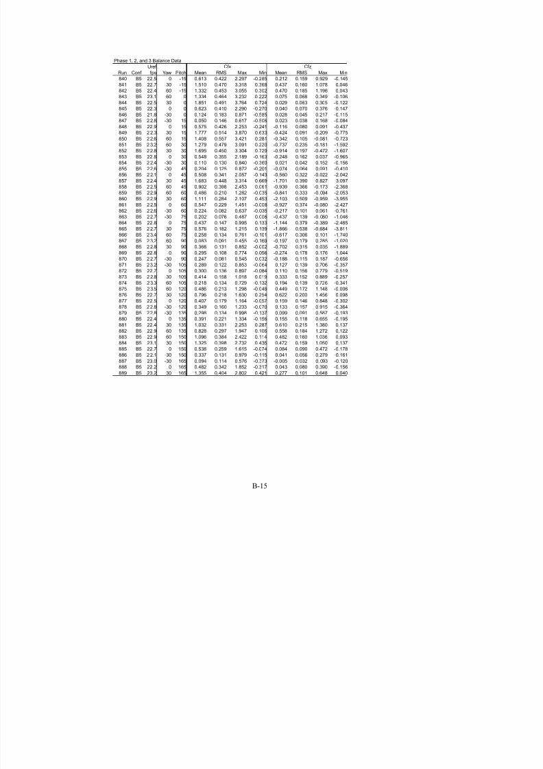
7/31/2019 Wind Tunnel Test
http://slidepdf.com/reader/full/wind-tunnel-test 159/243
B-15
Phase 1, 2, and 3 Balance Data
Uref
Run Conf fps Yaw Pitch Mean RMS Max Min Mean RMS Max Min
840 B5 22.5 0 -15 0.613 0.422 2.297 -0.285 0.212 0.159 0.929 -0.145
841 B5 22.7 30 -15 1.510 0.470 3.318 0.368 0.437 0.160 1.078 0.046
842 B5 22.4 60 -15 1.332 0.453 3.055 0.302 0.470 0.185 1.196 0.043
843 B5 23.1 60 0 1.334 0.464 3.232 0.222 0.075 0.068 0.349 -0.106
844 B5 22.5 30 0 1.851 0.491 3.764 0.724 0.029 0.063 0.305 -0.122845 B5 22.3 0 0 0.623 0.410 2.290 -0.270 0.040 0.070 0.376 -0.147
846 B5 21.8 -30 0 0.124 0.183 0.871 -0.585 0.028 0.045 0.217 -0.115
847 B5 2 2.8 -30 15 0.050 0.146 0.617 -0.506 0.023 0.038 0.168 -0.084
848 B5 22.9 0 15 0.575 0.426 2.253 -0.241 -0.116 0.080 0.091 -0.437
849 B5 2 2.3 30 15 1.777 0.514 3.870 0.633 -0.424 0.091 -0.209 -0.775
850 B5 2 2.6 60 15 1.408 0.557 3.421 0.281 -0.342 0.105 -0.081 -0.723
851 B5 2 3.2 60 30 1.279 0.479 3.091 0.220 -0.737 0.235 -0.181 -1.592
852 B5 2 2.8 30 30 1.695 0.450 3.304 0.729 -0.914 0.197 -0.472 -1.607
853 B5 22.8 0 30 0.548 0.355 2.189 -0.163 -0.248 0.162 0.037 -0.965
854 B5 2 2.4 -30 30 0.110 0.130 0.840 -0.360 0.021 0.042 0.152 -0.156
855 B5 22.6 -30 45 0.204 0.125 0.872 -0.201 -0.074 0.064 0.091 -0.410
856 B5 2 2.1 0 45 0.508 0.341 2.057 -0.143 -0.560 0.322 -0.022 -2.042
857 B5 2 2.4 30 45 1.683 0.448 3.314 0.669 -1.701 0.390 -0.827 -3.097
858 B5 2 2.5 60 45 0.902 0.398 2.453 0.061 -0.939 0.366 -0.173 -2.368
859 B5 22.9 60 60 0.486 0.210 1.282 -0.035 -0.841 0.333 -0. 094 -2.053
860 B5 2 2.9 30 60 1.111 0.284 2.107 0.453 -2.103 0.509 -0.959 -3.955
861 B5 2 2.5 0 60 0.547 0.229 1.451 -0.008 -0.927 0.374 -0.080 -2.427
862 B5 22.6 -30 60 0.224 0.082 0.637 -0.035 -0.217 0.101 0.061 -0.761
863 B5 22.7 -30 75 0.202 0.076 0.487 0.006 -0.437 0.139 -0. 060 -1.046
864 B5 22.8 0 75 0.437 0.147 0.995 0.133 -1.144 0.379 -0.389 -2.485
865 B5 2 2.7 30 75 0.576 0.182 1.215 0.139 -1.866 0.538 -0.684 -3.811
866 B5 2 3.4 60 75 0.258 0.134 0.761 -0.101 -0.617 0.306 0.101 -1.740
867 B5 2 3.2 60 90 0.083 0.091 0.455 -0.169 -0.197 0.179 0.285 -1.020
868 B5 2 2.8 30 90 0.366 0.131 0.852 -0.002 -0.702 0.315 0.035 -1.889
869 B5 22.8 0 90 0.295 0.108 0.774 0.056 -0.274 0.178 0.176 -1.044
870 B5 2 2.7 -30 90 0.247 0.081 0.545 0.032 -0.188 0.115 0.187 -0.656
871 B5 23.2 -30 105 0.289 0.122 0.853 -0.064 0.127 0.139 0.706 -0.357
872 B5 22.7 0 105 0.300 0.136 0.897 -0.084 0.110 0.156 0.779 -0.519
873 B5 2 2.8 30 105 0.414 0.158 1.018 0.019 0.333 0.152 0.889 -0.257
874 B5 23.3 60 105 0.218 0.134 0.729 -0.132 0.194 0.139 0.726 -0.341
875 B5 23.5 60 120 0.486 0.213 1.298 -0.048 0.449 0.172 1.148 -0.006
876 B5 22.7 30 120 0.796 0.218 1.630 0.254 0.622 0.200 1.456 0.098
877 B5 22.5 0 120 0.407 0.179 1.164 -0.057 0.159 0.146 0.848 -0.302
878 B5 22.8 -30 120 0.349 0.160 1.233 -0.070 0.133 0.157 0.915 -0.364
879 B5 22.8 -30 135 0.298 0.134 0.998 -0.137 0.099 0.091 0.587 -0.193880 B5 22.4 0 135 0.391 0.221 1.334 -0.156 0.155 0.118 0.655 -0.195
881 B5 22.4 30 135 1.032 0.331 2.253 0.287 0.610 0.215 1.380 0.137
882 B5 22.9 60 135 0.828 0.297 1.947 0.106 0.558 0.184 1.272 0.122
883 B5 22.9 60 150 1.096 0.384 2.422 0.114 0.482 0.160 1.036 0.093
884 B5 23.1 30 150 1.325 0.398 2.732 0.435 0.472 0.159 1.050 0.137
885 B5 22.7 0 150 0.538 0.259 1.615 -0.074 0.084 0.090 0.472 -0.178
886 B5 22.1 -30 150 0.337 0.131 0.979 -0.115 0.041 0.056 0.279 -0.161
887 B5 23.0 -30 165 0.094 0.114 0.576 -0.373 -0.005 0.032 0. 093 -0.120
888 B5 22.2 0 165 0.482 0.342 1.852 -0.317 0.043 0.080 0.390 -0.156
889 B5 23.2 30 165 1.355 0.404 2.802 0.421 0.277 0.101 0.648 0.040
Cfx Cfz

7/31/2019 Wind Tunnel Test
http://slidepdf.com/reader/full/wind-tunnel-test 160/243
B-16
Phase 1, 2, and 3 Balance Data
Uref
Run Conf fps Yaw Pitch Mean RMS Max Min Mean RMS Max Min
890 B5 22.9 60 165 1.315 0.429 2.802 0.224 0.293 0.109 0.709 0.031
891 B5 2 2.7 60 180 1.381 0.441 2.891 0.300 0.081 0.054 0.306 -0.052
892 B5 2 3.0 30 180 1.478 0.394 2.946 0.599 0.064 0.053 0.296 -0.100
893 B5 2 2.3 0 180 0.575 0.336 2.125 -0.129 -0.005 0.052 0.226 -0.148
894 B5 21.9 -30 180 0.053 0.132 0.550 -0.445 0.004 0.028 0.074 -0.102895 B6 22.9 -30 -180 0.118 0.184 1.022 -0.426 -0.007 0.027 0.073 -0.111
896 B6 22.6 0 -180 0.463 0.299 1.926 -0.126 -0.018 0.049 0.205 -0.176
897 B6 23.2 30 -180 1.396 0.391 2.795 0.565 0.059 0.057 0.274 -0.105
898 B6 22.9 60 -180 1.403 0.463 3.360 0.368 0.085 0.065 0.393 -0.069
899 B6 23.6 60 -165 1.218 0.385 2.693 0.215 -0.150 0.042 0. 007 -0.285
900 B6 22.9 30 -165 1.357 0.375 2.855 0.514 -0.155 0.047 -0.030 -0.334
901 B6 22.7 0 -165 0.368 0.265 1.450 -0.204 -0.095 0.050 0.042 -0.296
902 B6 22.9 -30 -165 0.115 0.162 0.855 -0.333 -0.052 0.042 0.081 -0.216
903 B6 22.4 -30 -150 0.072 0.130 0.645 -0.289 -0.073 0.061 0.097 -0.334
904 B6 22.8 0 -150 0.350 0.231 1.345 -0.108 -0.153 0.072 0.024 -0.466
905 B6 23.2 30 -150 0.998 0.283 2.066 0.338 -0.288 0.070 -0.103 -0.545
906 B6 23.3 60 -150 0.873 0.305 2.061 0.109 -0.308 0.082 -0.048 -0.616
907 B6 23.7 60 -135 0.605 0.233 1.521 -0.005 -0.357 0.112 -0. 034 -0.765
908 B6 23.2 30 -135 0.807 0.228 1.722 0.306 -0.328 0.089 -0.088 -0.681
909 B6 22.7 0 -135 0.268 0.190 1.143 -0.091 -0.148 0.078 0.046 -0.521
910 B6 23.0 -30 -135 0.085 0.099 0.510 -0.217 -0.084 0.057 0.102 -0.318
911 B6 23.0 -30 -120 0.077 0.087 0.487 -0.161 -0.042 0.052 0.151 -0.269
912 B6 22.8 0 -120 0.163 0.125 0.708 -0.099 -0.066 0.064 0.185 -0.340
913 B6 23.0 30 -120 0.566 0.175 1.282 0.168 -0.345 0.118 -0.018 -0.779
914 B6 23.2 60 -120 0.323 0.169 0.978 -0.124 -0.296 0.125 0. 098 -0.775
915 B6 23.1 60 -105 0.200 0.123 0.710 -0.091 -0.046 0.101 0. 298 -0.435
916 B6 23.2 30 -105 0.364 0.123 0.790 0.046 -0.131 0.119 0. 264 -0.536
917 B6 22.6 0 -105 0.169 0.098 0.600 -0.033 -0.003 0.078 0.271 -0.322
918 B6 23.1 -30 -105 0.128 0.079 0.451 -0.073 -0.027 0.063 0.230 -0.294
919 B6 23.1 -30 -90 0.194 0.083 0.560 -0.015 0.208 0.093 0.600 -0.144
920 B6 23.0 0 -90 0.195 0.088 0.559 -0.009 0.268 0.112 0.845 -0.047
921 B6 23.4 30 -90 0.183 0.103 0.518 -0.067 0.592 0.154 1.273 0.157
922 B6 2 3.7 60 -90 0.144 0.089 0.515 -0.078 0.259 0.125 0.879 -0.098
923 B6 23.6 60 -75 0.184 0.102 0.578 -0.083 0.571 0.216 1.620 0.115
924 B6 23.3 30 -75 0.260 0.120 0.725 -0.029 1.143 0.292 2.208 0.493
925 B6 23.2 0 -75 0.456 0.157 1.130 0.143 0.894 0.268 1.967 0.326
926 B6 23.0 -30 -75 0.279 0.107 0.700 0.041 0.626 0.201 1.569 0.156
927 B6 23.0 -30 -60 0.216 0.124 0.794 -0.061 0.442 0.208 1.462 -0.179
928 B6 23.5 0 -60 0.510 0.250 1.458 0.033 0.983 0.411 2.596 0.139
929 B6 23.1 30 -60 0.452 0.171 1.067 0.049 1.170 0.373 2.419 0.334930 B6 23.3 60 -60 0.342 0.132 0.853 0.019 0.735 0.257 1.832 0.193
931 B6 23.5 60 -45 0.743 0.237 1.689 0.139 0.827 0.279 1.891 0.183
932 B6 23.4 30 -45 0.884 0.292 2.041 0.171 1.008 0.357 2.385 0.159
933 B6 23.0 0 -45 0.655 0.362 2.068 -0.025 0.748 0.422 2.435 -0.029
934 B6 22.8 -30 -45 0.326 0.185 1.225 -0.120 0.284 0.188 1.270 -0.110
935 B6 23.1 -30 -30 0.337 0.232 1.465 -0.242 0.173 0.151 0.949 -0.168
936 B6 22.7 0 -30 0.529 0.365 2.104 -0.296 0.369 0.264 1.470 -0.179
937 B6 23.3 30 -30 1.281 0.370 2.654 0.095 0.727 0.244 1.651 0.103
938 B6 23.6 60 -30 1.000 0.334 2.330 0.209 0.690 0.250 1.637 0.117
939 B6 23.5 60 -15 1.226 0.434 3.103 0.236 0.428 0.169 1.290 -0.182
Cfx Cfz

7/31/2019 Wind Tunnel Test
http://slidepdf.com/reader/full/wind-tunnel-test 161/243
B-17
Phase 1, 2, and 3 Balance Data
Uref
Run Conf fps Yaw Pitch Mean RMS Max Min Mean RMS Max Min
940 B6 23.4 30 -15 1.548 0.483 3.392 0.482 0.413 0.156 1.029 0.066
941 B6 22.6 0 -15 0.486 0.355 2.121 -0.278 0.132 0.133 0.761 -0.161
942 B6 22.3 -30 -15 0.310 0.271 1.564 -0.400 0.063 0.103 0.641 -0.202
943 B6 22.5 -30 0 0.204 0.247 1.390 -0.453 0.006 0.050 0.297 -0.148
944 B6 22.4 0 0 0.470 0.386 2.306 -0.351 0.019 0.069 0.388 -0.149945 B6 23.0 30 0 1.729 0.503 3.637 0.594 0.054 0.066 0.339 -0.116
946 B6 23.3 60 0 1.392 0.474 3.216 0.236 0.088 0.078 0.448 -0.107
947 B6 2 3.7 60 15 1.414 0.478 3.381 0.249 -0.311 0.088 -0.027 -0.675
948 B6 2 3.2 30 15 1.789 0.468 3.566 0.638 -0.374 0.077 -0.150 -0.646
949 B6 22.5 0 15 0.554 0.378 2.369 -0.174 -0.096 0.065 0.085 -0.385
950 B6 22.3 -30 15 0.156 0.213 1.288 -0.446 -0.024 0.038 0.132 -0.187
951 B6 22.4 -30 30 0.153 0.188 1.058 -0.364 -0.044 0.049 0.107 -0.242
952 B6 22.7 0 30 0.535 0.363 2.195 -0.197 -0.246 0.147 0.027 -0.876
953 B6 2 3.4 30 30 1.752 0.468 3.541 0.704 -0.840 0.181 -0.378 -1.475
954 B6 2 3.5 60 30 1.289 0.455 3.085 0.154 -0.666 0.204 -0.123 -1.397
955 B6 2 3.5 60 45 0.913 0.354 2.173 0.099 -0.947 0.347 -0.153 -2.195
956 B6 2 3.2 30 45 1.641 0.417 3.205 0.623 -1.707 0.394 -0.653 -3.173
957 B6 22.6 0 45 0.565 0.338 2.020 -0.125 -0.606 0.335 0.035 -1.957
958 B6 22.8 -30 45 0.242 0.159 1.102 -0.195 -0.132 0.091 0.079 -0.633
959 B6 22.9 -30 60 0.192 0.105 0.742 -0.073 -0.234 0.117 0.061 -0.893
960 B6 2 3.2 0 60 0.522 0.266 1.470 -0.053 -0.919 0.415 -0.041 -2.438
961 B6 2 3.3 30 60 1.201 0.298 2.328 0.481 -2.205 0.513 -0.965 -4.156
962 B6 23.5 60 60 0.506 0.226 1.382 -0.010 -0.858 0.357 -0.069 -2.253
963 B6 2 3.5 60 75 0.249 0.122 0.720 -0.067 -0.605 0.282 0.135 -1.645
964 B6 2 3.7 30 75 0.585 0.159 1.157 0.206 -1.812 0.487 -0.654 -3.459
965 B6 23.5 0 75 0.440 0.163 1.027 0.082 -1.090 0.419 -0.174 -2.577
966 B6 22.9 -30 75 0.151 0.075 0.413 -0.053 -0.344 0.120 0.003 -0.944
967 B6 23.3 -30 90 0.174 0.081 0.485 -0.065 -0.234 0.122 0.131 -0.752
968 B6 23.6 0 90 0.213 0.107 0.650 -0.019 -0.342 0.202 0.084 -1.270
969 B6 2 3.5 30 90 0.336 0.105 0.756 0.071 -0.808 0.303 -0.069 -2.053
970 B6 2 3.7 60 90 0.137 0.083 0.474 -0.096 -0.244 0.188 0.295 -0.989
971 B6 23.4 60 105 0.241 0.134 0.807 -0.153 0.208 0.146 0.812 -0.319
972 B6 2 3.3 30 105 0.493 0.155 1.090 0.105 0.351 0.159 0.978 -0.218
973 B6 23.4 0 105 0.268 0.126 0.827 -0.082 0.103 0.143 0.679 -0.418
974 B6 23.0 -30 105 0.282 0.117 0.846 -0.078 0.117 0.136 0.748 -0.422
975 B6 22.9 -30 120 0.290 0.128 0.896 -0.093 0.145 0.122 0.703 -0.298
976 B6 22.6 0 120 0.271 0.177 1.092 -0.145 0.148 0.136 0.795 -0.266
977 B6 22.9 30 120 0.766 0.236 1.611 0.204 0.616 0.215 1.410 0.050
978 B6 23.4 60 120 0.511 0.215 1.414 -0.034 0.474 0.177 1.238 -0.011
979 B6 23.5 60 135 0.808 0.283 1.941 0.116 0.546 0.174 1.266 0.088980 B6 23.1 30 135 1.099 0.317 2.236 0.345 0.605 0.203 1.343 0.143
981 B6 23.1 0 135 0.393 0.213 1.383 -0.118 0.123 0.108 0.662 -0.224
982 B6 22.8 -30 135 0.299 0.133 0.933 -0.134 0.097 0.081 0.463 -0.202
983 B6 22.8 -30 150 0.220 0.146 0.873 -0.224 0.035 0.051 0.262 -0.132
984 B6 22.9 0 150 0.399 0.275 1.620 -0.211 0.105 0.099 0.552 -0.136
985 B6 23.2 30 150 1.221 0.371 2.529 0.438 0.461 0.152 1.010 0.136
986 B6 23.4 60 150 1.173 0.408 2.568 0.175 0.495 0.172 1.094 0.091
987 B6 2 3.6 60 165 1.313 0.424 2.797 -0.040 0.337 0.120 0.934 0.006
988 B6 23.0 30 165 1.435 0.425 3.108 0.541 0.300 0.117 0.810 0.065
989 B6 22.4 0 165 0.543 0.292 1.749 -0.094 0.057 0.079 0.407 -0.134
Cfx Cfz
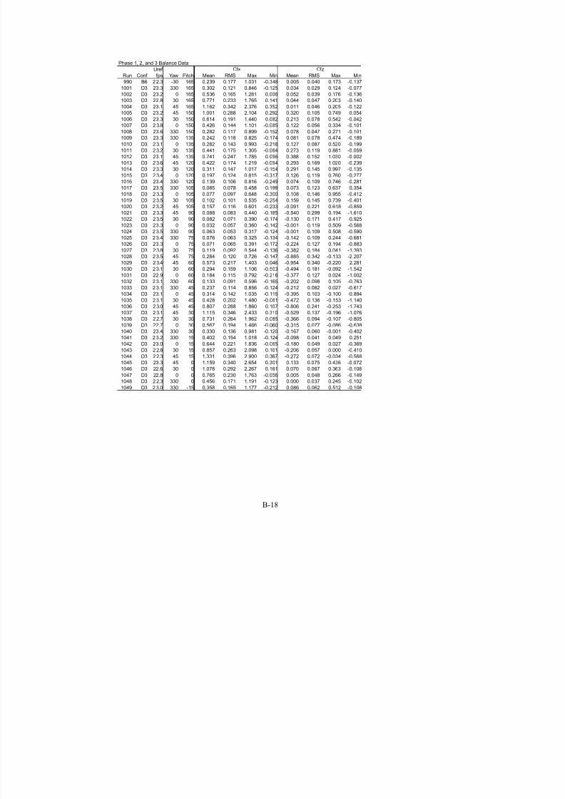
7/31/2019 Wind Tunnel Test
http://slidepdf.com/reader/full/wind-tunnel-test 162/243
B-18
Phase 1, 2, and 3 Balance Data
Uref
Run Conf fps Yaw Pitch Mean RMS Max Min Mean RMS Max Min
990 B6 22.3 -30 165 0.239 0.177 1.031 -0.348 0.005 0.040 0.173 -0.137
1001 D3 23.3 330 165 0.302 0.121 0.846 -0.125 0.034 0.029 0.124 -0.077
1002 D3 23.2 0 165 0.536 0.165 1.281 0.006 0.052 0.039 0.176 -0.136
1003 D3 22.8 30 165 0.771 0.233 1.765 0.141 0.044 0.047 0.203 -0.140
1004 D3 23.1 45 165 1.162 0.342 2.376 0.352 0.011 0.046 0.205 -0.1221005 D3 23.2 45 150 1.001 0.288 2.104 0.292 0.320 0.105 0.749 0.054
1006 D3 23.3 30 150 0.614 0.191 1.440 0.082 0.213 0.078 0.542 -0.042
1007 D3 2 3.8 0 150 0.426 0.144 1.101 -0.085 0.122 0.056 0.334 -0.101
1008 D3 23.6 330 150 0.282 0.117 0.899 -0.152 0.078 0.047 0.271 -0.101
1009 D3 23.3 330 135 0.242 0.118 0.825 -0.174 0.081 0.078 0.474 -0.189
1010 D3 2 3.1 0 135 0.282 0.143 0.993 -0.218 0.127 0.087 0.520 -0.199
1011 D3 23.2 30 135 0.441 0.175 1.305 -0.064 0.273 0.119 0.881 -0.059
1012 D3 23.1 45 135 0.741 0.247 1.785 0.096 0.388 0.152 1.030 -0.002
1013 D3 23.6 45 120 0.422 0.174 1.219 -0.094 0.293 0.169 1.020 -0.239
1014 D3 23.3 30 120 0.311 0.147 1.017 -0.154 0.291 0.145 0.997 -0.135
1015 D3 2 3.4 0 120 0.197 0.124 0.815 -0.317 0.126 0.119 0.760 -0.277
1016 D3 23.4 330 120 0.139 0.106 0.816 -0.249 0.074 0.109 0.746 -0.281
1017 D3 23.5 330 105 0.085 0.078 0.458 -0.199 0.073 0.123 0.637 -0.354
1018 D3 2 3.3 0 105 0.077 0.097 0.648 -0.300 0.108 0.146 0.955 -0.412
1019 D3 23.5 30 105 0.102 0.101 0.535 -0.254 0.159 0.145 0.739 -0.401
1020 D3 23.2 45 105 0.157 0.116 0.601 -0.233 -0.091 0.221 0.618 -0.859
1021 D3 23.3 45 90 0.088 0.083 0.440 -0.185 -0.540 0.299 0.194 -1.610
1022 D3 23.5 30 90 0.082 0.071 0.390 -0.174 -0.130 0.171 0.417 -0.925
1023 D3 23.3 0 90 0.032 0.057 0.360 -0.142 -0.001 0.119 0.509 -0.568
1024 D3 23.5 330 90 0.063 0.053 0.317 -0.124 -0.001 0.109 0.508 -0.590
1025 D3 23.4 330 75 0.076 0.063 0.325 -0.134 -0.142 0.109 0.244 -0.681
1026 D3 23.3 0 75 0.071 0.065 0.391 -0.172 -0.224 0.127 0.194 -0.883
1027 D3 23.8 30 75 0.119 0.092 0.544 -0.136 -0.382 0.184 0.041 -1.393
1028 D3 23.5 45 75 0.284 0.120 0.726 -0.147 -0.885 0.342 -0.133 -2.207
1029 D3 23.4 45 60 0.573 0.217 1.403 0.046 -0.954 0.340 -0.220 -2.281
1030 D3 23.1 30 60 0.294 0.159 1.106 -0.503 -0.494 0.181 -0.092 -1.542
1031 D3 22.9 0 60 0.184 0.115 0.792 -0.216 -0.377 0.127 0.024 -1.002
1032 D3 23.1 330 60 0.133 0.091 0.596 -0.165 -0.202 0.098 0.105 -0.763
1033 D3 23.1 330 45 0.237 0.114 0.856 -0.124 -0.212 0.082 0.027 -0.617
1034 D3 23.1 0 45 0.314 0.142 1.035 -0.115 -0.395 0.103 -0.100 -0.894
1035 D3 23.1 30 45 0.428 0.202 1.480 -0.061 -0.472 0.136 -0.153 -1.140
1036 D3 23.0 45 45 0.807 0.288 1.860 0.107 -0.806 0.241 -0.253 -1.743
1037 D3 23.1 45 30 1.115 0.346 2.433 0.310 -0.529 0.137 -0.196 -1.076
1038 D3 22.7 30 30 0.731 0.264 1.962 0.085 -0.366 0.094 -0.107 -0.805
1039 D3 22.7 0 30 0.567 0.194 1.466 -0.060 -0.315 0.077 -0.086 -0.6381040 D3 23.4 330 30 0.330 0.136 0.981 -0.120 -0.167 0.060 -0.001 -0.402
1041 D3 23.2 330 15 0.402 0.154 1.018 -0.124 -0.098 0.041 0.049 -0.251
1042 D3 23.0 0 15 0.644 0.221 1.836 -0.065 -0.180 0.049 0.027 -0.369
1043 D3 2 2.8 30 15 0.857 0.263 2.098 0.101 -0.206 0.057 0.000 -0.410
1044 D3 22.3 45 15 1.331 0.396 2.900 0.367 -0.272 0.072 -0.034 -0.568
1045 D3 23.3 45 0 1.159 0.340 2.654 0.301 0.133 0.075 0.436 -0.072
1046 D3 22.6 30 0 1.078 0.292 2.267 0.161 0.070 0.067 0.363 -0.108
1047 D3 22.8 0 0 0.765 0.230 1.763 -0.056 0.005 0.048 0.266 -0.149
1048 D3 2 2.3 330 0 0.456 0.171 1.191 -0.123 0.000 0.037 0.245 -0.102
1049 D3 23.0 330 -15 0.358 0.165 1.177 -0.212 0.086 0.062 0.512 -0.108
Cfx Cfz
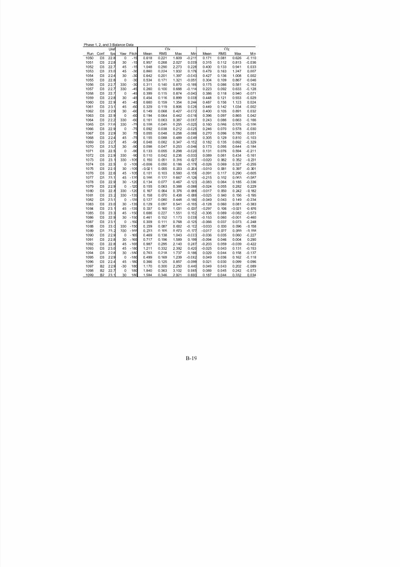
7/31/2019 Wind Tunnel Test
http://slidepdf.com/reader/full/wind-tunnel-test 163/243
B-19
Phase 1, 2, and 3 Balance Data
Uref
Run Conf fps Yaw Pitch Mean RMS Max Min Mean RMS Max Min
1050 D3 22.8 0 -15 0.618 0.221 1.609 -0.211 0.171 0.081 0.626 -0.110
1051 D3 2 2.8 30 -15 0.957 0.268 2.027 0.009 0.315 0.112 0.813 -0.036
1052 D3 22.7 45 -15 1.048 0.290 2.273 0.226 0.400 0.133 0.941 0.033
1053 D3 23.0 45 -30 0.860 0.224 1.932 0.176 0.479 0.163 1.247 0.007
1054 D3 2 2.4 30 -30 0.642 0.201 1.397 -0.043 0.427 0.136 1.008 0.0021055 D3 22.8 0 -30 0.534 0.171 1.321 -0.051 0.304 0.109 0.867 -0.046
1056 D3 22.7 330 -30 0.311 0.140 0.870 -0.186 0.175 0.086 0.581 -0.163
1057 D3 22.7 330 -45 0.260 0.100 0.688 -0.114 0.223 0.092 0.633 -0.128
1058 D3 22.7 0 -45 0.399 0.115 0.874 -0.043 0.386 0.118 0.940 -0.071
1059 D3 2 2.8 30 -45 0.454 0.116 0.899 0.008 0.448 0.121 0.933 -0.029
1060 D3 22.9 45 -45 0.660 0.159 1.354 0.244 0.487 0.156 1.123 0.024
1061 D3 2 3.1 45 -60 0.329 0.119 0.806 0.026 0.449 0.142 1.034 -0.002
1062 D3 2 2.9 30 -60 0.149 0.068 0.427 -0.072 0.400 0.105 0.891 0.032
1063 D3 22.9 0 -60 0.194 0.064 0.442 -0.016 0.396 0.097 0.865 0.042
1064 D3 22.2 330 -60 0.161 0.063 0.387 -0.067 0.243 0.086 0.663 -0.166
1065 D3 22.6 330 -75 0.108 0.045 0.255 -0.025 0.160 0.066 0.525 -0.106
1066 D3 22.9 0 -75 0.092 0.038 0.212 -0.025 0.246 0.070 0.578 -0.030
1067 D3 22.9 30 -75 0.055 0.048 0.258 -0.088 0.270 0.096 0.780 -0.051
1068 D3 22.4 45 -75 0.155 0.088 0.489 -0.049 0.305 0.129 0.810 -0.103
1069 D3 22.7 45 -90 0.048 0.082 0.347 -0.152 0.182 0.135 0.692 -0.329
1070 D3 23.2 30 -90 0.098 0.047 0.253 -0.046 0.173 0.095 0.644 -0.184
1071 D3 22.5 0 -90 0.133 0.055 0.298 -0.020 0.131 0.076 0.594 -0.211
1072 D3 22.9 330 -90 0.110 0.042 0.236 -0.033 0.089 0.061 0.434 -0.161
1073 D3 23.1 330 -105 0.150 0.051 0.316 -0.027 -0.020 0.062 0.352 -0.231
1074 D3 22.5 0 -105 -0.006 0.050 0.186 -0.178 -0.026 0.069 0.327 -0.255
1075 D3 22.9 30 -105 -0.021 0.055 0.203 -0.204 -0.010 0.081 0.397 -0.301
1076 D3 22.6 45 -105 0.101 0.103 0.560 -0.156 -0.091 0.117 0.290 -0.605
1077 D3 23.1 45 -120 0.166 0.122 0.667 -0.126 -0.215 0.102 0.063 -0.587
1078 D3 22.9 30 -120 0.134 0.077 0.467 -0.123 -0.083 0.064 0.185 -0.336
1079 D3 22.9 0 -120 0.155 0.063 0.388 -0.088 -0.024 0.055 0.282 -0.229
1080 D3 22.8 330 -120 0.167 0.064 0.376 -0.066 -0.017 0.050 0.242 -0.182
1081 D3 23.2 330 -135 0.158 0.070 0.438 -0.088 -0.025 0.040 0.156 -0.195
1082 D3 23.1 0 -135 0.127 0.080 0.448 -0.180 -0.049 0.043 0.149 -0.234
1083 D3 23.0 30 -135 0.129 0.097 0.541 -0.195 -0.128 0.060 0.081 -0.383
1084 D3 23.1 45 -135 0.337 0.160 1.031 -0.037 -0.297 0.106 -0.021 -0.676
1085 D3 23.3 45 -150 0.686 0.227 1.551 0.152 -0.306 0.089 -0.082 -0.573
1086 D3 22.9 30 -150 0.461 0.152 1.173 0.008 -0.153 0.060 -0.001 -0.460
1087 D3 23.1 0 -150 0.309 0.111 0.768 -0.125 -0.066 0.037 0.073 -0.248
1088 D3 23.0 330 -150 0.239 0.087 0.602 -0.102 -0.033 0.030 0.096 -0.158
1089 D3 23.2 330 -165 0.233 0.105 0.673 -0.177 -0.017 0.027 0.069 -0.1581090 D3 22.9 0 -165 0.469 0.138 1.043 -0.003 -0.036 0.035 0.060 -0.227
1091 D3 22.8 30 -165 0.717 0.196 1.589 0.199 -0.094 0.046 0.004 -0.290
1092 D3 22.8 45 -165 0.987 0.295 2.140 0.267 -0.203 0.059 -0.039 -0.422
1093 D3 23.0 45 -180 1.211 0.332 2.392 0.420 -0.025 0.043 0.131 -0.153
1094 D3 22.8 30 -180 0.763 0.218 1.737 0.186 0.029 0.044 0.158 -0.137
1095 D3 22.9 0 -180 0.499 0.169 1.239 -0.062 0.049 0.036 0.162 -0.118
1096 D3 22.4 45 -180 0.366 0.125 0.857 -0.099 0.021 0.030 0.099 -0.096
1097 B2 22.9 -30 180 1.170 0.300 2.250 0.440 0.049 0.043 0.202 -0.089
1098 B2 22.7 0 180 1.840 0.363 3.102 0.965 0.089 0.045 0.242 -0.073
1099 B2 23.1 30 180 1.584 0.346 2.921 0.693 0.187 0.044 0.332 0.034
Cfx Cfz
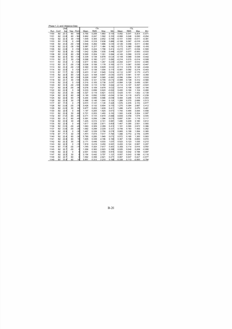
7/31/2019 Wind Tunnel Test
http://slidepdf.com/reader/full/wind-tunnel-test 164/243
B-20
Phase 1, 2, and 3 Balance Data
Uref
Run Conf fps Yaw Pitch Mean RMS Max Min Mean RMS Max Min
1100 B2 23.1 60 180 0.755 0.259 1.863 0.130 0.052 0.041 0.204 -0.071
1101 B2 22.8 60 -165 0.662 0.247 1.582 0.100 -0.066 0.046 0.050 -0.254
1102 B2 22.4 30 -165 1.549 0.305 2.652 0.789 -0.151 0.059 -0.011 -0.381
1103 B2 22.9 0 -165 1.549 0.318 2.838 0.889 -0.168 0.067 -0.016 -0.426
1104 B2 23.0 -30 -165 0.946 0.262 1.886 0.340 -0.126 0.058 0.011 -0.3601105 B2 22.9 -30 -150 0.697 0.217 1.494 0.183 -0.172 0.065 -0.026 -0.416
1106 B2 22.8 0 -150 0.945 0.224 1.798 0.412 -0.215 0.071 -0.034 -0.500
1107 B2 22.8 30 -150 1.042 0.256 1.935 0.448 -0.237 0.077 -0.063 -0.533
1108 B2 22.8 60 -150 0.569 0.204 1.351 0.064 -0.145 0.069 0.019 -0.441
1109 B2 22.5 60 -135 0.339 0.138 0.878 -0.024 -0.159 0.068 0.039 -0.442
1110 B2 22.7 30 -135 0.598 0.180 1.277 0.092 -0.214 0.075 -0.014 -0.508
1111 B2 23.0 0 -135 0.677 0.165 1.267 0.259 -0.204 0.077 0.012 -0.495
1112 B2 22.7 -30 -135 0.536 0.156 1.178 0.165 -0.171 0.067 0.030 -0.447
1113 B2 23.3 -30 -120 0.360 0.128 0.829 0.022 -0.113 0.078 0.148 -0.434
1114 B2 22.6 0 -120 0.477 0.138 1.004 0.115 -0.081 0.092 0.274 -0.443
1115 B2 22.7 30 -120 0.403 0.142 0.945 0.014 -0.112 0.087 0.179 -0.473
1116 B2 22.5 60 -120 0.223 0.108 0.647 -0.083 -0.073 0.061 0.157 -0.350
1117 B2 22.8 60 -105 0.226 0.097 0.585 -0.061 -0.096 0.094 0.171 -0.533
1118 B2 23.1 30 -105 0.254 0.121 0.705 -0.072 -0.089 0.109 0.312 -0.580
1119 B2 23.0 0 -105 0.316 0.105 0.738 0.067 -0.084 0.128 0.456 -0.591
1120 B2 22.5 -30 -105 0.306 0.110 0.782 0.022 -0.114 0.107 0.267 -0.522
1121 B2 22.9 -30 -90 0.278 0.109 0.678 0.022 0.414 0.158 1.025 -0.184
1122 B2 22.8 0 -90 0.233 0.099 0.620 -0.022 0.400 0.190 1.104 -0.280
1123 B2 23.0 30 -90 0.327 0.119 0.821 -0.003 0.425 0.151 1.002 -0.139
1124 B2 22.5 60 -90 0.190 0.092 0.552 -0.064 0.154 0.115 0.673 -0.239
1125 B2 22.6 60 -75 0.204 0.095 0.586 -0.059 0.484 0.206 1.418 -0.003
1126 B2 22.8 30 -75 0.496 0.146 1.044 0.124 1.268 0.370 2.688 0.513
1127 B2 22.6 0 -75 0.633 0.143 1.136 0.325 1.576 0.405 3.153 0.677
1128 B2 2 2.8 -30 -75 0.426 0.132 0.904 0.130 1.270 0.394 2.687 0.412
1129 B2 2 2.5 -30 -60 0.877 0.202 1.639 0.411 1.486 0.472 3.270 0.481
1130 B2 22.6 0 -60 1.197 0.205 1.925 0.673 1.740 0.494 3.444 0.558
1131 B2 22.6 30 -60 0.721 0.203 1.493 0.192 1.593 0.438 3.204 0.597
1132 B2 2 3.2 60 -60 0.271 0.133 0.819 -0.066 0.659 0.256 1.678 0.045
1133 B2 23.1 60 -45 0.591 0.206 1.394 0.075 0.697 0.261 1.718 0.117
1134 B2 22.6 30 -45 1.425 0.315 2.741 0.681 1.480 0.409 3.180 0.612
1135 B2 22.8 0 -45 1.617 0.328 2.871 0.808 1.467 0.390 2.931 0.565
1136 B2 2 2.5 -30 -45 1.063 0.309 2.289 0.412 1.181 0.395 2.672 0.386
1137 B2 2 2.6 -30 -30 1.062 0.299 2.229 0.321 0.706 0.183 1.455 0.262
1138 B2 22.9 0 -30 1.497 0.339 2.756 0.578 0.885 0.199 1.594 0.385
1139 B2 22.2 30 -30 1.803 0.424 3.512 0.784 1.088 0.253 2.106 0.4891140 B2 22.4 60 -30 0.790 0.285 1.949 0.072 0.572 0.185 1.300 0.083
1141 B2 22.8 60 -15 1.005 0.339 2.196 0.169 0.367 0.106 0.693 0.072
1142 B2 22.3 30 -15 2.171 0.446 4.033 1.057 0.523 0.123 1.035 0.210
1143 B2 22.5 0 -15 1.919 0.419 3.450 0.981 0.493 0.124 0.957 0.207
1144 B2 2 2.8 -30 -15 1.290 0.354 2.617 0.451 0.359 0.114 0.816 0.092
1145 B2 22.7 -30 0 1.358 0.383 2.923 0.388 0.025 0.040 0.208 -0.090
1146 B2 22.3 0 0 2.001 0.442 3.593 0.915 0.022 0.042 0.198 -0.097
1147 B2 22.5 30 0 2.154 0.442 3.757 1.121 0.007 0.043 0.188 -0.116
1148 B2 22.7 60 0 1.092 0.358 2.621 0.271 0.067 0.047 0.227 -0.077
1149 B2 22.8 60 15 0.951 0.313 2.210 0.198 -0.339 0.113 -0.063 -0.794
Cfx Cfz

7/31/2019 Wind Tunnel Test
http://slidepdf.com/reader/full/wind-tunnel-test 165/243
B-21
Phase 1, 2, and 3 Balance Data
Uref
Run Conf fps Yaw Pitch Mean RMS Max Min Mean RMS Max Min
1150 B2 22.8 30 15 1.947 0.460 3.704 0.893 -0.698 0.159 -0.339 -1.293
1151 B2 22.8 0 15 2.001 0.463 3.830 1.007 -0.711 0.155 -0.348 -1.301
1152 B2 22.8 -30 15 1.399 0.395 2.869 0.546 -0.524 0.144 -0.198 -1.051
1153 B2 23.1 -30 30 1.287 0.359 2.731 0.428 -1.039 0.280 -0.355 -2.178
1154 B2 22.8 0 30 1.841 0.442 3.753 0.841 -1.354 0.313 -0.644 -2.6841155 B2 22.8 30 30 1.608 0.408 3.284 0.667 -1.183 0.282 -0.540 -2.445
1156 B2 22.6 60 30 0.846 0.298 1.997 -0.133 -0.638 0.222 -0.092 -1.470
1157 B2 22.8 60 45 0.586 0.241 1.488 0.030 -0.859 0.340 -0.121 -2.163
1158 B2 22.6 30 45 1.238 0.355 2.747 0.399 -1.877 0.501 -0.713 -3.950
1159 B2 23.1 0 45 1.439 0.373 2.878 0.614 -2.110 0.519 -0.958 -4.150
1160 B2 22.6 -30 45 1.190 0.349 2.515 0.463 -1.710 0.523 -0.660 -3.648
1161 B2 22.6 -30 60 0.835 0.274 1.826 0.223 -2.232 0.682 -0.845 -4.732
1162 B2 22.8 0 60 1.050 0.260 1.977 0.474 -2.735 0.670 -1.340 -5.212
1163 B2 23.0 30 60 0.912 0.265 1.851 0.245 -2.309 0.630 -0.927 -4.563
1164 B2 23.1 60 60 0.383 0.169 1.055 -0.027 -0.856 0.395 -0.092 -2.480
1165 B2 22.7 60 75 0.153 0.114 0.564 -0.180 -0.572 0.304 0.082 -1.817
1166 B2 23.0 30 75 0.486 0.173 1.152 0.044 -1.818 0.584 -0.644 -4.008
1167 B2 22.7 0 75 0.610 0.185 1.251 0.157 -2.275 0.692 -0.901 -4.744
1168 B2 23.0 -30 75 0.514 0.177 1.226 0.117 -1.934 0.633 -0.650 -4.345
1169 B2 22.8 -30 90 0.285 0.117 0.760 -0.018 -0.528 0.314 0.155 -1.942
1170 B2 22.8 0 90 0.279 0.128 0.821 -0.038 -0.440 0.319 0.187 -2.230
1171 B2 23.1 30 90 0.324 0.136 0.852 -0.058 -0.491 0.323 0.224 -1.855
1172 B2 22.9 60 90 0.170 0.089 0.501 -0.099 -0.210 0.195 0.306 -0.958
1173 B2 22.8 60 105 0.178 0.123 0.679 -0.188 0.180 0.143 0.765 -0.379
1174 B2 23.2 30 105 0.367 0.154 1.025 -0.072 0.362 0.192 1.122 -0.416
1175 B2 23.1 0 105 0.391 0.140 0.942 0.024 0.220 0.215 1.153 -0.543
1176 B2 22.8 -30 105 0.374 0.139 0.919 0.014 0.270 0.193 1.084 -0.412
1177 B2 22.7 -30 120 0.528 0.186 1.229 0.075 0.283 0.125 0.809 -0.143
1178 B2 22.9 0 120 0.671 0.198 1.443 0.170 0.330 0.138 0.961 -0.159
1179 B2 22.8 30 120 0.679 0.195 1.411 0.115 0.448 0.149 1.031 0.012
1180 B2 23.4 60 120 0.394 0.158 1.065 -0.018 0.324 0.142 0.908 -0.024
1181 B2 2 2.8 60 135 0.517 0.204 1.288 -0.025 0.362 0.130 0.852 0.063
1182 B2 22.5 30 135 1.028 0.268 2.085 0.368 0.566 0.133 1.130 0.219
1183 B2 23.0 0 135 0.946 0.265 2.014 0.315 0.462 0.121 0.942 0.130
1184 B2 2 2.4 -30 135 0.821 0.244 1.755 0.257 0.371 0.106 0.771 0.080
1185 B2 2 2.9 -30 150 0.975 0.281 2.031 0.353 0.388 0.096 0.749 0.154
1186 B2 22.6 0 150 1.365 0.328 2.596 0.630 0.533 0.114 0.947 0.244
1187 B2 22.8 30 150 1.399 0.320 2.601 0.643 0.560 0.116 1.004 0.266
1188 B2 22.8 60 150 0.715 0.240 1.624 0.090 0.297 0.100 0.687 0.050
1189 B2 22.9 60 165 0.765 0.280 1.930 0.161 0.178 0.073 0.513 0.0101190 B2 22.8 30 165 1.474 0.340 2.824 0.656 0.334 0.077 0.630 0.132
1191 B2 22.4 0 165 1.497 0.391 3.051 0.641 0.334 0.077 0.632 0.119
1192 B2 2 2.6 -30 165 1.173 0.299 2.238 0.449 0.237 0.063 0.478 0.056
1193 C4 22.2 -30 180 -0.105 0.145 0.509 -0.645 -0.011 0.037 0.073 -0.171
1194 C4 22.8 0 180 0.043 0.200 0.898 -0.631 -0.025 0.043 0.107 -0.202
1195 C4 22.3 30 180 1.132 0.301 2.301 0.373 -0.039 0.049 0.099 -0.229
1196 C4 22.4 30 165 0.879 0.267 1.939 0.140 0.166 0.062 0.414 -0.005
1197 C4 22.5 0 165 0.107 0.212 1.029 -0.668 -0.003 0.056 0.215 -0.194
1198 C4 22.1 -30 165 -0.043 0.144 0.589 -0.584 -0.014 0.040 0.106 -0.165
1199 C4 22.4 -30 150 0.062 0.139 0.608 -0.476 0.017 0.056 0.213 -0.212
Cfx Cfz
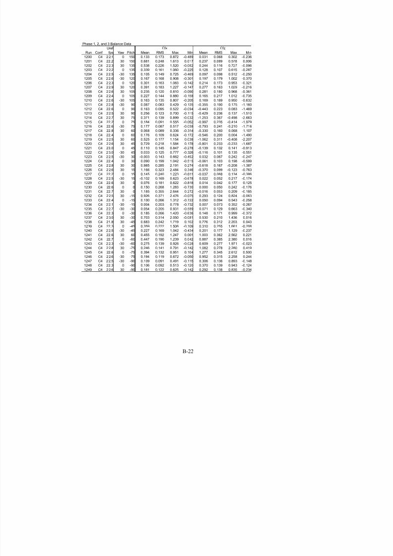
7/31/2019 Wind Tunnel Test
http://slidepdf.com/reader/full/wind-tunnel-test 166/243
B-22
Phase 1, 2, and 3 Balance Data
Uref
Run Conf fps Yaw Pitch Mean RMS Max Min Mean RMS Max Min
1200 C4 2 2.1 0 150 0.133 0.173 0.872 -0.489 0.031 0.068 0.302 -0.236
1201 C4 22.2 30 150 0.681 0.248 1.613 0.017 0.237 0.089 0.578 0.006
1202 C4 22.3 30 135 0.538 0.226 1.520 -0.062 0.244 0.116 0.727 -0.096
1203 C4 2 2.2 0 135 0.339 0.161 1.060 -0.225 0.128 0.107 0.615 -0.287
1204 C4 22.5 -30 135 0.105 0.149 0.725 -0.469 0.097 0.098 0.512 -0.2501205 C4 22.6 -30 120 0.167 0.168 0.908 -0.301 0.197 0.179 1.002 -0.370
1206 C4 2 2.3 0 120 0.301 0.163 1.083 -0.142 0.214 0.173 0.953 -0.321
1207 C4 22.9 30 120 0.391 0.183 1.227 -0.147 0.277 0.163 1.029 -0.216
1208 C4 22.6 30 105 0.235 0.120 0.810 -0.090 0.281 0.180 0.968 -0.361
1209 C4 2 2.4 0 105 0.227 0.144 0.880 -0.158 0.165 0.217 1.012 -0.735
1210 C4 22.6 -30 105 0.163 0.135 0.807 -0.205 0.169 0.189 0.950 -0.632
1211 C4 22.8 -30 90 0.087 0.083 0.429 -0.135 -0.355 0.190 0.175 -1.160
1212 C4 22.6 0 90 0.163 0.095 0.522 -0.094 -0.443 0.223 0.083 -1.469
1213 C4 22.5 30 90 0.256 0.123 0.700 -0.115 -0.429 0.236 0.137 -1.510
1214 C4 22.7 30 75 0.371 0.139 0.899 -0.032 -1.253 0.367 -0.498 -2.663
1215 C4 22.2 0 75 0.184 0.091 0.555 -0.052 -0.997 0.235 -0.414 -1.979
1216 C4 22.6 -30 75 0.177 0.087 0.517 -0.058 -0.793 0.241 -0.210 -1.716
1217 C4 22.8 -30 60 -0.068 0.089 0.336 -0.314 -0.330 0.160 0.068 -1.107
1218 C4 22.4 0 60 0.176 0.109 0.624 -0.172 -0.546 0.200 0.004 -1.490
1219 C4 22.5 30 60 0.525 0.177 1.154 0.038 -1.062 0.311 -0.408 -2.207
1220 C4 22.6 30 45 0.729 0.218 1.584 0.178 -0.801 0.233 -0.233 -1.687
1221 C4 23.0 0 45 0.110 0.145 0.847 -0.278 -0.139 0.132 0.141 -0.913
1222 C4 23.0 -30 45 0.033 0.125 0.777 -0.326 -0.116 0.101 0.135 -0.551
1223 C4 22.5 -30 30 -0.003 0.143 0.662 -0.492 0.032 0.067 0.242 -0.247
1224 C4 22.4 0 30 0.090 0.199 1.042 -0.515 -0.061 0.103 0.198 -0.599
1225 C4 22.8 30 30 0.985 0.285 2.191 0.274 -0.618 0.167 -0.208 -1.387
1226 C4 22.6 30 15 1.166 0.323 2.484 0.346 -0.370 0.099 -0.123 -0.763
1227 C4 22.2 0 15 0.145 0.240 1.223 -0.611 -0.037 0.068 0.134 -0.386
1228 C4 22.5 -30 15 -0.102 0.169 0.623 -0.678 0.022 0.052 0.217 -0.174
1229 C4 22.6 -30 0 -0.076 0.181 0.622 -0.818 0.014 0.042 0.177 -0.125
1230 C4 22.6 0 0 0.150 0.268 1.283 -0.730 0.000 0.050 0.242 -0.176
1231 C4 22.7 30 0 1.185 0.355 2.644 0.272 -0.016 0.053 0.209 -0.185
1232 C4 22.5 30 -15 0.926 0.371 2.476 -0.075 0.293 0.124 0.824 -0.063
1233 C4 22.4 0 -15 0.100 0.266 1.312 -0.722 0.050 0.094 0.543 -0.258
1234 C4 22.1 -30 -15 0.004 0.203 0.778 -0.732 0.007 0.073 0.352 -0.267
1235 C4 22.7 -30 -30 0.054 0.205 0.931 -0.589 0.071 0.129 0.663 -0.340
1236 C4 22.3 0 -30 0.185 0.266 1.420 -0.636 0.148 0.171 0.999 -0.372
1237 C4 2 3.0 30 -30 0.703 0.314 2.050 -0.081 0.530 0.210 1.436 0.016
1238 C4 21.8 30 -45 0.683 0.242 1.719 0.102 0.776 0.312 2.203 0.043
1239 C4 22.3 0 -45 0.359 0.222 1.506 -0.109 0.310 0.255 1.661 -0.2081240 C4 22.5 -30 -45 0.227 0.169 1.042 -0.434 0.201 0.177 1.129 -0.237
1241 C4 22.6 30 -60 0.455 0.192 1.247 0.001 1.003 0.362 2.562 0.221
1242 C4 22.7 0 -60 0.447 0.190 1.239 0.042 0.887 0.385 2.380 0.016
1243 C4 22.3 -30 -60 0.275 0.139 0.926 -0.028 0.609 0.277 1.971 -0.023
1244 C4 2 2.8 30 -75 0.246 0.141 0.791 -0.142 1.082 0.278 2.280 0.419
1245 C4 22.6 0 -75 0.394 0.132 0.951 0.104 1.277 0.345 2.612 0.500
1246 C4 22.6 -30 -75 0.194 0.119 0.672 -0.050 0.952 0.315 2.258 0.244
1247 C4 22.5 -30 -90 0.109 0.091 0.491 -0.115 0.306 0.136 0.893 -0.148
1248 C4 22.3 0 -90 0.106 0.092 0.513 -0.120 0.370 0.139 0.943 -0.124
1249 C4 22.6 30 -90 0.181 0.122 0.625 -0.142 0.292 0.138 0.835 -0.234
Cfx Cfz
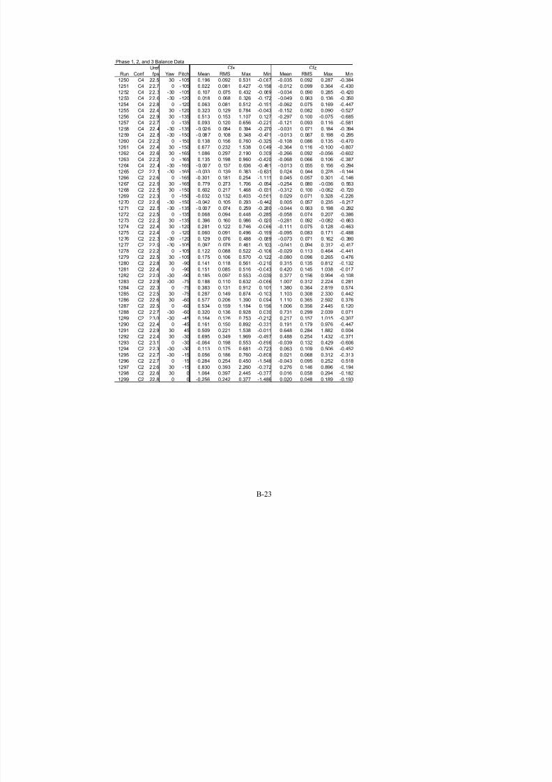
7/31/2019 Wind Tunnel Test
http://slidepdf.com/reader/full/wind-tunnel-test 167/243
B-23
Phase 1, 2, and 3 Balance Data
Uref
Run Conf fps Yaw Pitch Mean RMS Max Min Mean RMS Max Min
1250 C4 22.5 30 -105 0.196 0.092 0.531 -0.067 -0.035 0.092 0.287 -0.384
1251 C4 22.7 0 -105 0.022 0.081 0.427 -0.158 -0.012 0.099 0.364 -0.430
1252 C4 22.3 -30 -105 0.107 0.075 0.432 -0.069 -0.034 0.090 0.285 -0.420
1253 C4 22.6 -30 -120 0.018 0.068 0.326 -0.172 -0.049 0.063 0.136 -0.350
1254 C4 22.8 0 -120 0.063 0.081 0.512 -0.151 -0.062 0.075 0.169 -0.4471255 C4 22.4 30 -120 0.323 0.129 0.784 -0.043 -0.152 0.082 0.090 -0.527
1256 C4 22.9 30 -135 0.513 0.153 1.107 0.127 -0.297 0.100 -0.075 -0.685
1257 C4 22.7 0 -135 0.093 0.120 0.656 -0.221 -0.121 0.093 0.116 -0.581
1258 C4 22.4 -30 -135 -0.026 0.084 0.394 -0.270 -0.031 0.071 0.184 -0.394
1259 C4 22.8 -30 -150 -0.087 0.108 0.348 -0.471 -0.013 0.067 0.198 -0.295
1260 C4 22.2 0 -150 0.138 0.156 0.760 -0.325 -0.108 0.086 0.135 -0.470
1261 C4 22.4 30 -150 0.677 0.232 1.538 0.049 -0.364 0.116 -0.100 -0.807
1262 C4 22.6 30 -165 1.086 0.297 2.190 0.309 -0.266 0.092 -0.056 -0.602
1263 C4 22.2 0 -165 0.135 0.198 0.960 -0.420 -0.068 0.066 0.106 -0.387
1264 C4 22.4 -30 -165 -0.007 0.137 0.636 -0.491 -0.013 0.055 0.156 -0.294
1265 C2 22.1 -30 -165 -0.033 0.139 0.383 -0.631 0.024 0.044 0.228 -0.144
1266 C2 22.6 0 -165 -0.301 0.181 0.254 -1.111 0.045 0.057 0.301 -0.146
1267 C2 22.9 30 -165 0.779 0.273 1.706 -0.054 -0.254 0.080 -0.036 -0.553
1268 C2 22.5 30 -150 0.602 0.217 1.468 -0.031 -0.312 0.100 -0.062 -0.720
1269 C2 22.3 0 -150 -0.032 0.132 0.403 -0.561 0.029 0.071 0.328 -0.226
1270 C2 22.6 -30 -150 -0.042 0.105 0.293 -0.442 0.005 0.057 0.235 -0.217
1271 C2 22.5 -30 -135 -0.007 0.074 0.259 -0.280 -0.044 0.063 0.198 -0.292
1272 C2 22.5 0 -135 0.068 0.094 0.448 -0.285 -0.058 0.074 0.207 -0.386
1273 C2 22.2 30 -135 0.396 0.160 0.986 -0.020 -0.281 0.092 -0.082 -0.663
1274 C2 22.4 30 -120 0.281 0.122 0.746 -0.066 -0.111 0.075 0.128 -0.463
1275 C2 22.4 0 -120 0.060 0.091 0.496 -0.199 -0.095 0.083 0.171 -0.488
1276 C2 22.3 -30 -120 0.129 0.076 0.488 -0.089 -0.073 0.071 0.162 -0.390
1277 C2 22.9 -30 -105 0.097 0.078 0.461 -0.103 -0.041 0.094 0.312 -0.417
1278 C2 22.2 0 -105 0.122 0.088 0.522 -0.106 -0.029 0.113 0.464 -0.441
1279 C2 22.5 30 -105 0.175 0.106 0.570 -0.122 -0.080 0.096 0.265 -0.476
1280 C2 22.8 30 -90 0.141 0.118 0.561 -0.210 0.315 0.135 0.812 -0.132
1281 C2 22.4 0 -90 0.151 0.085 0.516 -0.043 0.420 0.145 1.038 -0.017
1282 C2 22.0 -30 -90 0.185 0.097 0.553 -0.039 0.377 0.156 0.994 -0.108
1283 C2 22.9 -30 -75 0.188 0.110 0.632 -0.066 1.007 0.312 2.224 0.281
1284 C2 22.3 0 -75 0.383 0.131 0.912 0.101 1.380 0.364 2.819 0.574
1285 C2 2 2.5 30 -75 0.287 0.149 0.874 -0.103 1.103 0.308 2.330 0.442
1286 C2 22.6 30 -60 0.577 0.206 1.390 0.094 1.110 0.365 2.592 0.376
1287 C2 22.5 0 -60 0.534 0.159 1.184 0.156 1.006 0.356 2.445 0.120
1288 C2 2 2.7 -30 -60 0.320 0.136 0.928 0.030 0.731 0.299 2.039 0.071
1289 C2 23.0 -30 -45 0.164 0.126 0.753 -0.212 0.217 0.157 1.015 -0.3071290 C2 22.4 0 -45 0.161 0.150 0.892 -0.331 0.191 0.179 0.976 -0.447
1291 C2 22.9 30 -45 0.509 0.221 1.538 -0.011 0.648 0.284 1.882 -0.004
1292 C2 22.4 30 -30 0.695 0.349 1.969 -0.497 0.488 0.254 1.432 -0.371
1293 C2 23.1 0 -30 -0.064 0.198 0.553 -0.896 -0.039 0.132 0.429 -0.606
1294 C2 22.3 -30 -30 0.113 0.175 0.681 -0.723 0.063 0.109 0.506 -0.452
1295 C2 22.7 -30 -15 0.056 0.186 0.760 -0.808 0.021 0.068 0.312 -0.313
1296 C2 22.7 0 -15 -0.284 0.254 0.450 -1.548 -0.043 0.095 0.252 -0.518
1297 C2 22.6 30 -15 0.830 0.393 2.260 -0.372 0.276 0.146 0.896 -0.194
1298 C2 22.6 30 0 1.064 0.397 2.445 -0.377 0.016 0.058 0.294 -0.182
1299 C2 22.8 0 0 -0.256 0.242 0.377 -1.486 0.020 0.048 0.189 -0.193
Cfx Cfz

7/31/2019 Wind Tunnel Test
http://slidepdf.com/reader/full/wind-tunnel-test 168/243
B-24
Phase 1, 2, and 3 Balance Data
Uref
Run Conf fps Yaw Pitch Mean RMS Max Min Mean RMS Max Min
1300 C2 22.7 -30 0 -0.033 0.163 0.504 -0.821 0.017 0.040 0.153 -0.149
1301 C2 22.7 -30 15 -0.041 0.149 0.472 -0.846 0.045 0.043 0.204 -0.117
1302 C2 23.0 0 15 -0.178 0.193 0.418 -1.082 0.067 0.046 0.255 -0.062
1303 C2 22.9 30 15 0.789 0.352 1.970 -0.240 -0.224 0.103 0.054 -0.569
1304 C2 22.7 30 30 0.655 0.316 1.806 -0.264 -0.356 0.173 0.097 -0.9771305 C2 22.5 0 30 -0.035 0.158 0.572 -0.803 0.051 0.059 0.296 -0.132
1306 C2 22.4 -30 30 -0.023 0.142 0.426 -0.725 0.009 0.057 0.230 -0.188
1307 C2 22.7 -30 45 0.077 0.109 0.515 -0.326 -0.087 0.096 0.221 -0.478
1308 C2 22.4 0 45 0.110 0.120 0.667 -0.386 -0.111 0.105 0.270 -0.583
1309 C2 22.5 30 45 0.533 0.209 1.275 -0.064 -0.712 0.246 -0.105 -1.647
1310 C2 22.7 30 60 0.461 0.150 0.998 0.067 -1.133 0.273 -0.489 -2.232
1311 C2 23.0 0 60 0.320 0.123 0.813 -0.043 -0.857 0.244 -0.171 -1.832
1312 C2 23.1 -30 60 0.273 0.117 0.802 -0.017 -0.640 0.237 -0.114 -1.815
1313 C2 22.8 -30 75 0.319 0.122 0.837 0.035 -1.210 0.396 -0.385 -2.858
1314 C2 22.7 0 75 0.383 0.120 0.819 0.075 -1.511 0.361 -0.648 -2.852
1315 C2 22.5 30 75 0.420 0.133 0.945 0.040 -1.219 0.330 -0.555 -2.491
1316 C2 23.2 30 90 0.166 0.114 0.605 -0.171 -0.290 0.200 0.192 -1.439
1317 C2 22.6 0 90 0.202 0.095 0.584 -0.036 -0.446 0.246 0.110 -1.524
1318 C2 22.8 -30 90 0.226 0.094 0.615 -0.008 -0.366 0.216 0.122 -1.430
1319 C2 23.0 -30 105 0.251 0.144 0.912 -0.159 0.171 0.189 0.883 -0.511
1320 C2 2 2.9 0 105 0.240 0.180 1.050 -0.248 0.164 0.248 1.115 -0.859
1321 C2 22.6 30 105 0.349 0.140 0.912 -0.051 0.300 0.186 1.007 -0.378
1322 C2 22.8 30 120 0.405 0.183 1.225 -0.095 0.282 0.180 1.060 -0.290
1323 C2 2 2.7 0 120 0.384 0.282 1.576 -0.429 0.267 0.276 1.334 -0.677
1324 C2 22.8 -30 120 0.394 0.232 1.473 -0.305 0.226 0.228 1.165 -0.567
1325 C2 22.7 -30 135 0.308 0.187 1.215 -0.257 0.229 0.142 0.848 -0.183
1326 C2 2 2.4 0 135 0.277 0.215 1.305 -0.280 0.248 0.168 1.038 -0.226
1327 C2 22.3 30 135 0.620 0.212 1.456 0.034 0.274 0.124 0.760 -0.095
1328 C2 22.4 30 150 0.648 0.236 1.517 -0.131 0.197 0.086 0.511 -0.097
1329 C2 2 2.4 0 150 0.097 0.152 0.731 -0.491 0.111 0.085 0.493 -0.157
1330 C2 23.0 -30 150 0.115 0.121 0.611 -0.296 0.094 0.069 0.369 -0.105
1331 C2 22.6 -30 165 0.066 0.140 0.478 -0.615 0.020 0.046 0.194 -0.146
1332 C2 22.6 0 165 -0.020 0.157 0.508 -0.803 0.004 0.049 0.192 -0.197
1333 C2 22.8 30 165 0.628 0.293 1.563 -0.800 0.119 0.066 0.354 -0.260
1334 C2 22.8 30 180 0.776 0.307 1.813 -0.240 -0.033 0.043 0.110 -0.184
1335 C2 22.9 0 180 -0.128 0.177 0.391 -0.919 -0.019 0.034 0.109 -0.130
1336 C2 22.6 -30 180 -0.038 0.137 0.487 -0.748 -0.006 0.031 0.089 -0.138
1337 C6 22.7 -30 180 0.104 0.204 1.040 -0.473 -0.027 0.040 0.076 -0.205
1338 C6 21.8 0 180 0.461 0.274 1.660 -0.303 -0.071 0.060 0.100 -0.313
1339 C6 22.3 30 180 0.965 0.290 2.027 0.253 -0.025 0.044 0.109 -0.2071340 C6 22.5 30 -165 0.965 0.283 2.118 0.261 -0.269 0.093 -0.057 -0.638
1341 C6 22.3 0 -165 0.325 0.200 1.183 -0.203 -0.142 0.086 0.047 -0.547
1342 C6 22.4 -30 -165 0.088 0.170 0.740 -0.353 -0.095 0.072 0.096 -0.375
1343 C6 22.4 -30 -150 0.056 0.134 0.644 -0.324 -0.069 0.084 0.152 -0.424
1344 C6 22.8 0 -150 0.190 0.159 0.862 -0.212 -0.166 0.099 0.078 -0.594
1345 C6 22.9 30 -150 0.697 0.224 1.670 0.110 -0.336 0.113 -0.079 -0.842
1346 C6 23.0 30 -135 0.481 0.160 1.119 0.081 -0.287 0.103 -0.041 -0.749
1347 C6 22.3 0 -135 0.137 0.111 0.703 -0.130 -0.161 0.089 0.049 -0.611
1348 C6 22.5 -30 -135 0.086 0.091 0.514 -0.186 -0.097 0.078 0.134 -0.457
1349 C6 23.1 -30 -120 0.058 0.074 0.400 -0.143 -0.048 0.066 0.163 -0.346
Cfx Cfz

7/31/2019 Wind Tunnel Test
http://slidepdf.com/reader/full/wind-tunnel-test 169/243
B-25
Phase 1, 2, and 3 Balance Data
Uref
Run Conf fps Yaw Pitch Mean RMS Max Min Mean RMS Max Min
1350 C6 22.6 0 -120 0.079 0.096 0.504 -0.187 -0.095 0.080 0.177 -0.454
1351 C6 22.7 30 -120 0.347 0.121 0.792 0.018 -0.143 0.078 0.108 -0.458
1352 C6 23.1 30 -105 0.200 0.108 0.616 -0.136 -0.019 0.090 0.310 -0.391
1353 C6 22.5 0 -105 0.083 0.093 0.515 -0.112 0.005 0.098 0.364 -0.440
1354 C6 23.0 -30 -105 0.101 0.077 0.461 -0.072 -0.032 0.083 0.295 -0.4071355 C6 22.7 -30 -90 0.111 0.088 0.475 -0.105 0.322 0.134 0.831 -0.196
1356 C6 22.8 0 -90 0.085 0.092 0.468 -0.149 0.319 0.141 0.918 -0.131
1357 C6 22.5 30 -90 0.213 0.117 0.681 -0.127 0.365 0.139 0.951 -0.088
1358 C6 2 3.1 30 -75 0.298 0.140 0.823 -0.082 1.032 0.281 2.095 0.362
1359 C6 22.5 0 -75 0.366 0.133 0.885 0.074 1.279 0.339 2.634 0.508
1360 C6 22.6 -30 -75 0.226 0.113 0.671 -0.014 0.900 0.285 2.103 0.269
1361 C6 22.6 -30 -60 0.327 0.157 1.152 -0.017 0.605 0.299 2.247 -0.026
1362 C6 22.6 0 -60 0.543 0.235 1.667 0.064 1.030 0.482 3.308 0.071
1363 C6 22.8 30 -60 0.441 0.182 1.201 0.007 0.889 0.340 2.332 0.135
1364 C6 22.9 30 -45 0.640 0.252 1.694 0.028 0.763 0.305 2.068 0.084
1365 C6 22.7 0 -45 0.684 0.299 2.166 0.042 0.621 0.353 2.424 -0.101
1366 C6 22.3 -30 -45 0.327 0.215 1.446 -0.148 0.366 0.242 1.665 -0.121
1367 C6 22.6 -30 -30 0.297 0.243 1.386 -0.372 0.179 0.152 0.913 -0.197
1368 C6 22.3 0 -30 0.649 0.323 2.171 -0.089 0.305 0.211 1.315 -0.150
1369 C6 2 2.4 30 -30 0.743 0.326 2.170 -0.055 0.493 0.205 1.428 0.009
1370 C6 2 3.0 30 -15 1.046 0.367 2.459 0.139 0.282 0.118 0.801 -0.008
1371 C6 22.0 0 -15 0.712 0.374 2.419 -0.143 0.124 0.122 0.738 -0.201
1372 C6 22.0 -30 -15 0.264 0.292 1.486 -0.495 0.066 0.099 0.562 -0.198
1373 C6 22.3 -30 0 0.197 0.265 1.325 -0.503 0.001 0.049 0.235 -0.148
1374 C6 22.7 0 0 0.443 0.337 1.828 -0.434 -0.009 0.055 0.229 -0.212
1375 C6 22.5 30 0 1.185 0.374 2.798 0.242 0.007 0.055 0.254 -0.203
1376 C6 22.7 30 15 1.075 0.332 2.494 0.256 -0.319 0.099 -0.073 -0.726
1377 C6 22.3 0 15 0.455 0.328 1.959 -0.295 -0.135 0.094 0.081 -0.608
1378 C6 22.3 -30 15 0.174 0.228 1.177 -0.508 -0.060 0.062 0.127 -0.338
1379 C6 22.3 -30 30 0.169 0.202 1.206 -0.334 -0.088 0.093 0.122 -0.555
1380 C6 22.8 0 30 0.395 0.263 1.678 -0.197 -0.224 0.139 0.049 -0.903
1381 C6 22.4 30 30 0.944 0.293 2.264 0.205 -0.562 0.162 -0.193 -1.294
1382 C6 23.1 30 45 0.756 0.237 1.687 0.172 -0.888 0.266 -0.258 -1.957
1383 C6 22.8 0 45 0.295 0.205 1.265 -0.131 -0.363 0.226 0.050 -1.506
1384 C6 22.7 -30 45 0.240 0.149 0.963 -0.132 -0.193 0.132 0.082 -0.841
1385 C6 22.5 -30 60 0.141 0.103 0.630 -0.156 -0.358 0.190 0.043 -1.470
1386 C6 22.5 0 60 0.161 0.123 0.775 -0.133 -0.442 0.251 0.053 -1.708
1387 C6 22.4 30 60 0.548 0.175 1.181 0.077 -1.233 0.353 -0.451 -2.587
1388 C6 22.7 30 75 0.373 0.136 0.898 -0.015 -1.283 0.372 -0.532 -2.662
1389 C6 22.6 0 75 0.101 0.093 0.484 -0.155 -0.696 0.223 -0.128 -1.6831390 C6 22.7 -30 75 0.146 0.068 0.429 -0.055 -0.558 0.202 -0.080 -1.509
1391 C6 22.5 -30 90 0.109 0.070 0.407 -0.063 -0.329 0.178 0.123 -1.194
1392 C6 22.8 0 90 0.060 0.070 0.382 -0.121 -0.303 0.182 0.133 -1.292
1393 C6 2 2.8 30 90 0.319 0.114 0.763 0.002 -0.516 0.233 0.049 -1.415
1394 C6 22.7 30 105 0.283 0.132 0.859 -0.123 0.349 0.184 1.040 -0.305
1395 C6 2 2.6 0 105 0.148 0.120 0.701 -0.201 0.144 0.183 0.852 -0.652
1396 C6 22.7 -30 105 0.190 0.122 0.773 -0.168 0.145 0.184 0.862 -0.561
1397 C6 22.5 -30 120 0.223 0.155 1.010 -0.286 0.182 0.167 1.038 -0.472
1398 C6 2 2.5 0 120 0.233 0.156 1.037 -0.224 0.173 0.161 0.919 -0.366
1399 C6 22.5 30 120 0.427 0.185 1.205 -0.072 0.278 0.164 1.071 -0.309
Cfx Cfz

7/31/2019 Wind Tunnel Test
http://slidepdf.com/reader/full/wind-tunnel-test 170/243
B-26
Phase 1, 2, and 3 Balance Data
Uref
Run Conf fps Yaw Pitch Mean RMS Max Min Mean RMS Max Min
1400 C6 22.9 30 135 0.582 0.211 1.401 0.005 0.264 0.111 0.722 -0.052
1401 C6 2 2.6 0 135 0.311 0.155 1.021 -0.204 0.119 0.105 0.564 -0.287
1402 C6 22.5 -30 135 0.217 0.148 0.925 -0.241 0.105 0.098 0.575 -0.269
1403 C6 22.7 -30 150 0.148 0.151 0.832 -0.349 0.030 0.050 0.231 -0.151
1404 C6 2 2.5 0 150 0.430 0.204 1.343 -0.219 0.065 0.073 0.344 -0.1891405 C6 22.5 30 150 0.687 0.252 1.594 0.013 0.241 0.082 0.545 -0.009
1406 C6 22.4 30 165 0.781 0.270 1.832 0.104 0.163 0.060 0.397 0.011
1407 C6 2 2.5 0 165 0.470 0.217 1.422 -0.108 0.015 0.057 0.226 -0.175
1408 C6 22.5 -30 165 0.088 0.168 0.989 -0.400 -0.006 0.038 0.127 -0.141
1409 C1 22.5 -30 -165 -0.147 0.152 0.285 -0.748 0.031 0.043 0.191 -0.147
1410 C1 22.8 0 -165 -0.317 0.150 0.119 -0.992 0.049 0.050 0.261 -0.111
1411 C1 22.9 30 -165 -0.438 0.224 0.256 -1.369 0.049 0.067 0.312 -0.196
1412 C1 22.0 30 -150 -0.136 0.158 0.369 -0.725 0.020 0.083 0.300 -0.273
1413 C1 23.3 0 -150 -0.074 0.115 0.311 -0.568 0.008 0.060 0.245 -0.243
1414 C1 22.7 -30 -150 -0.092 0.105 0.237 -0.497 0.009 0.056 0.206 -0.188
1415 C1 22.7 -30 -135 -0.014 0.079 0.333 -0.300 -0.040 0.063 0.181 -0.356
1416 C1 22.5 0 -135 0.087 0.090 0.441 -0.209 -0.070 0.068 0.156 -0.361
1417 C1 22.7 30 -135 0.096 0.108 0.500 -0.293 -0.091 0.071 0.178 -0.377
1418 C1 22.7 30 -120 0.148 0.102 0.547 -0.150 -0.077 0.064 0.112 -0.383
1419 C1 22.7 0 -120 0.114 0.099 0.560 -0.154 -0.073 0.075 0.163 -0.408
1420 C1 22.4 -30 -120 0.136 0.082 0.546 -0.085 -0.076 0.068 0.143 -0.408
1421 C1 22.9 -30 -105 0.057 0.083 0.377 -0.160 -0.037 0.083 0.290 -0.376
1422 C1 22.2 0 -105 0.068 0.089 0.485 -0.164 -0.002 0.105 0.406 -0.455
1423 C1 23.2 30 -105 0.193 0.093 0.553 -0.084 -0.021 0.082 0.280 -0.357
1424 C1 22.9 30 -90 0.204 0.100 0.565 -0.082 0.420 0.126 0.901 -0.003
1425 C1 23.0 0 -90 0.113 0.092 0.445 -0.121 0.547 0.155 1.098 0.134
1426 C1 21.5 -30 -90 0.218 0.092 0.586 -0.015 0.429 0.155 1.070 -0.026
1427 C1 2 2.4 -30 -75 0.273 0.123 0.825 0.005 1.049 0.321 2.438 0.353
1428 C1 22.4 0 -75 0.317 0.126 0.814 0.020 1.275 0.315 2.466 0.530
1429 C1 2 1.9 30 -75 0.224 0.125 0.707 -0.111 0.991 0.261 2.012 0.370
1430 C1 2 2.1 30 -60 0.320 0.143 0.941 -0.069 0.801 0.267 2.001 0.132
1431 C1 22.4 0 -60 0.450 0.140 1.007 0.090 0.903 0.296 2.088 0.192
1432 C1 2 2.1 -30 -60 0.388 0.140 1.069 0.048 0.757 0.283 2.113 0.078
1433 C1 22.1 -30 -45 0.217 0.144 0.799 -0.239 0.222 0.158 0.918 -0.308
1434 C1 21.8 0 -45 0.158 0.135 0.692 -0.355 0.152 0.155 0.810 -0.444
1435 C1 21.8 30 -45 0.246 0.174 0.829 -0.285 0.312 0.187 0.999 -0.303
1436 C1 22.3 30 -30 -0.025 0.261 0.921 -1.004 0.012 0.161 0.606 -0.607
1437 C1 22.0 0 -30 -0.091 0.196 0.553 -0.942 -0.033 0.123 0.428 -0.581
1438 C1 21.8 -30 -30 0.115 0.187 0.740 -0.689 0.070 0.109 0.514 -0.374
1439 C1 21.7 -30 -15 0.165 0.197 0.771 -0.670 0.022 0.069 0.285 -0.2671440 C1 22.1 0 -15 -0.318 0.237 0.334 -1.481 -0.057 0.081 0.188 -0.468
1441 C1 22.1 30 -15 -0.371 0.328 0.688 -1.532 -0.021 0.118 0.380 -0.417
1442 C1 21.8 30 0 -0.291 0.314 0.747 -1.402 0.069 0.075 0.335 -0.179
1443 C1 21.8 0 0 -0.305 0.233 0.320 -1.470 0.019 0.042 0.176 -0.184
1444 C1 21.8 -30 0 -0.016 0.191 0.644 -0.893 0.034 0.045 0.224 -0.130
1445 C1 21.8 -30 15 -0.064 0.175 0.475 -0.911 0.037 0.040 0.188 -0.083
1446 C1 22.0 0 15 -0.205 0.192 0.312 -1.182 0.054 0.036 0.211 -0.024
1447 C1 22.0 30 15 -0.184 0.242 0.602 -1.125 0.096 0.064 0.360 -0.102
1448 C1 22.2 30 30 0.138 0.182 0.779 -0.566 -0.051 0.088 0.216 -0.413
1449 C1 22.5 0 30 -0.068 0.143 0.405 -0.797 0.038 0.052 0.257 -0.124
Cfx Cfz
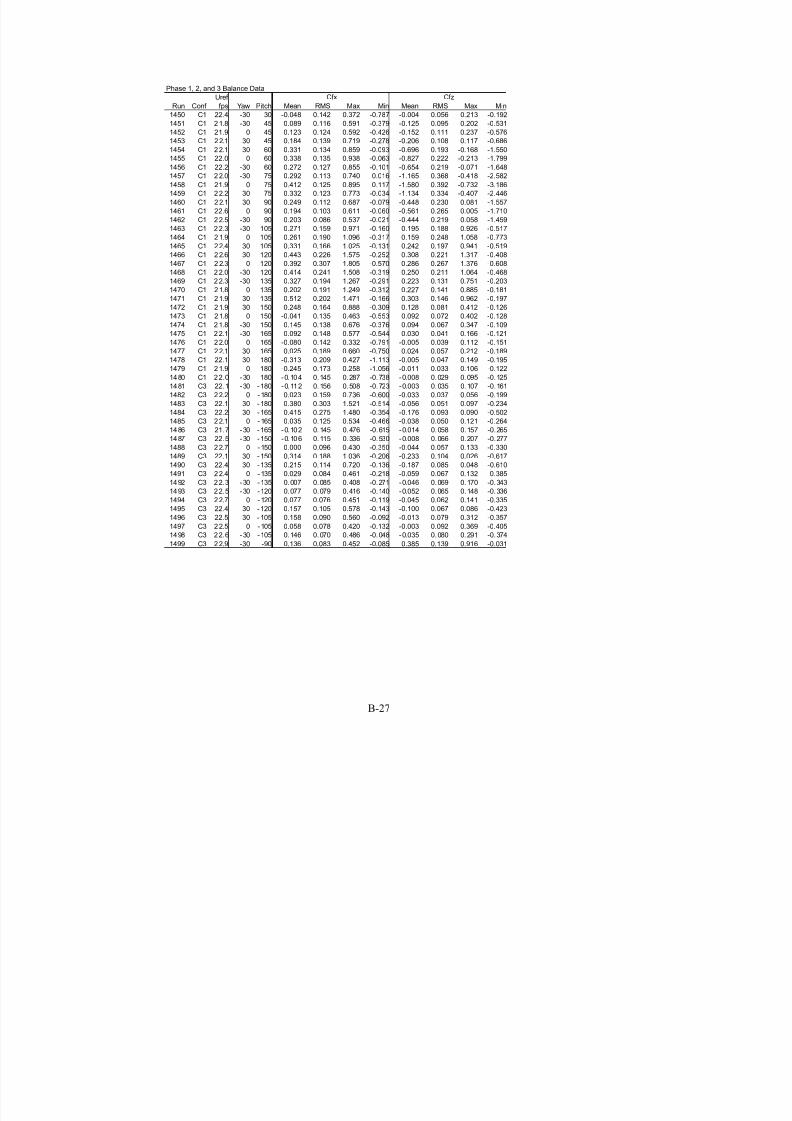
7/31/2019 Wind Tunnel Test
http://slidepdf.com/reader/full/wind-tunnel-test 171/243
B-27
Phase 1, 2, and 3 Balance Data
Uref
Run Conf fps Yaw Pitch Mean RMS Max Min Mean RMS Max Min
1450 C1 22.4 -30 30 -0.048 0.142 0.372 -0.787 -0.004 0.056 0.213 -0.192
1451 C1 21.8 -30 45 0.089 0.116 0.591 -0.379 -0.125 0.095 0.202 -0.531
1452 C1 21.9 0 45 0.123 0.124 0.592 -0.426 -0.152 0.111 0.237 -0.576
1453 C1 22.1 30 45 0.184 0.139 0.719 -0.278 -0.206 0.108 0.117 -0.686
1454 C1 22.1 30 60 0.331 0.134 0.859 -0.093 -0.696 0.193 -0.168 -1.5501455 C1 22.0 0 60 0.338 0.135 0.938 -0.063 -0.827 0.222 -0.213 -1.799
1456 C1 22.2 -30 60 0.272 0.127 0.855 -0.101 -0.654 0.219 -0.071 -1.648
1457 C1 22.0 -30 75 0.292 0.113 0.740 0.016 -1.165 0.368 -0.418 -2.582
1458 C1 21.9 0 75 0.412 0.125 0.895 0.117 -1.580 0.392 -0.732 -3.186
1459 C1 22.2 30 75 0.332 0.123 0.773 -0.034 -1.134 0.334 -0.407 -2.446
1460 C1 22.1 30 90 0.249 0.112 0.687 -0.079 -0.448 0.230 0.081 -1.557
1461 C1 22.6 0 90 0.194 0.103 0.611 -0.060 -0.561 0.265 0.005 -1.710
1462 C1 22.5 -30 90 0.203 0.086 0.537 -0.021 -0.444 0.219 0.058 -1.459
1463 C1 22.3 -30 105 0.271 0.159 0.971 -0.160 0.195 0.188 0.926 -0.517
1464 C1 2 1.9 0 105 0.261 0.190 1.096 -0.317 0.159 0.248 1.058 -0.773
1465 C1 22.4 30 105 0.331 0.166 1.025 -0.131 0.242 0.197 0.941 -0.519
1466 C1 22.6 30 120 0.443 0.226 1.575 -0.252 0.308 0.221 1.317 -0.408
1467 C1 2 2.3 0 120 0.392 0.307 1.805 -0.570 0.286 0.267 1.376 -0.608
1468 C1 22.0 -30 120 0.414 0.241 1.508 -0.319 0.250 0.211 1.064 -0.468
1469 C1 22.3 -30 135 0.327 0.194 1.267 -0.291 0.223 0.131 0.751 -0.203
1470 C1 2 1.8 0 135 0.202 0.191 1.249 -0.312 0.227 0.141 0.885 -0.181
1471 C1 21.9 30 135 0.512 0.202 1.471 -0.166 0.303 0.146 0.962 -0.197
1472 C1 21.9 30 150 0.248 0.164 0.888 -0.309 0.128 0.081 0.412 -0.126
1473 C1 21.8 0 150 -0.041 0.135 0.463 -0.553 0.092 0.072 0.402 -0.128
1474 C1 21.8 -30 150 0.145 0.138 0.676 -0.376 0.094 0.067 0.347 -0.109
1475 C1 22.1 -30 165 0.092 0.148 0.577 -0.544 0.030 0.041 0.166 -0.121
1476 C1 22.0 0 165 -0.080 0.142 0.332 -0.791 -0.005 0.039 0.112 -0.151
1477 C1 22.1 30 165 0.025 0.189 0.660 -0.750 0.024 0.057 0.212 -0.189
1478 C1 22.1 30 180 -0.313 0.209 0.427 -1.113 -0.005 0.047 0.149 -0.195
1479 C1 21.9 0 180 -0.245 0.173 0.258 -1.056 -0.011 0.033 0.106 -0.122
1480 C1 22.0 -30 180 -0.104 0.145 0.287 -0.738 -0.008 0.029 0.095 -0.125
1481 C3 22.1 -30 -180 -0.112 0.156 0.508 -0.723 -0.003 0.035 0.107 -0.161
1482 C3 22.2 0 -180 0.023 0.159 0.736 -0.600 -0.033 0.037 0.056 -0.199
1483 C3 22.1 30 -180 0.380 0.303 1.521 -0.514 -0.056 0.051 0.097 -0.234
1484 C3 22.2 30 -165 0.415 0.275 1.480 -0.354 -0.176 0.093 0.090 -0.502
1485 C3 22.1 0 -165 0.035 0.125 0.534 -0.466 -0.038 0.050 0.121 -0.264
1486 C3 21.7 -30 -165 -0.102 0.145 0.476 -0.615 -0.014 0.058 0.157 -0.265
1487 C3 22.5 -30 -150 -0.106 0.115 0.336 -0.530 -0.008 0.066 0.207 -0.277
1488 C3 22.7 0 -150 0.000 0.096 0.430 -0.350 -0.044 0.057 0.133 -0.330
1489 C3 22.1 30 -150 0.314 0.188 1.036 -0.206 -0.233 0.104 0.026 -0.6171490 C3 22.4 30 -135 0.215 0.114 0.720 -0.136 -0.187 0.085 0.048 -0.610
1491 C3 22.4 0 -135 0.029 0.084 0.461 -0.218 -0.059 0.067 0.132 -0.385
1492 C3 22.3 -30 -135 0.007 0.085 0.408 -0.271 -0.046 0.069 0.170 -0.343
1493 C3 22.5 -30 -120 0.077 0.079 0.416 -0.140 -0.052 0.065 0.148 -0.336
1494 C3 22.7 0 -120 0.077 0.076 0.451 -0.119 -0.045 0.062 0.141 -0.335
1495 C3 22.4 30 -120 0.157 0.105 0.578 -0.143 -0.100 0.067 0.086 -0.423
1496 C3 22.5 30 -105 0.158 0.090 0.560 -0.092 -0.013 0.079 0.312 -0.357
1497 C3 22.5 0 -105 0.058 0.078 0.420 -0.132 -0.003 0.092 0.369 -0.405
1498 C3 22.6 -30 -105 0.146 0.070 0.486 -0.048 -0.035 0.080 0.291 -0.374
1499 C3 22.9 -30 -90 0.136 0.083 0.452 -0.085 0.385 0.139 0.916 -0.031
Cfx Cfz

7/31/2019 Wind Tunnel Test
http://slidepdf.com/reader/full/wind-tunnel-test 172/243
B-28
Phase 1, 2, and 3 Balance Data
Uref
Run Conf fps Yaw Pitch Mean RMS Max Min Mean RMS Max Min
1500 C3 22.9 0 -90 0.178 0.085 0.525 -0.031 0.491 0.145 1.089 0.064
1501 C3 22.2 30 -90 0.241 0.108 0.620 -0.049 0.421 0.133 0.928 -0.022
1502 C3 2 2.5 30 -75 0.250 0.122 0.730 -0.113 0.937 0.253 2.022 0.389
1503 C3 22.6 0 -75 0.321 0.121 0.865 0.063 1.157 0.294 2.353 0.422
1504 C3 2 2.5 -30 -75 0.267 0.107 0.725 0.030 0.896 0.272 2.020 0.2471505 C3 2 2.5 -30 -60 0.304 0.132 0.951 0.008 0.550 0.236 1.750 0.031
1506 C3 22.0 0 -60 0.410 0.181 1.318 0.049 0.655 0.333 2.326 -0.017
1507 C3 2 2.6 30 -60 0.351 0.174 1.122 -0.039 0.719 0.298 2.116 0.122
1508 C3 22.5 30 -45 0.405 0.241 1.563 -0.153 0.400 0.269 1.825 -0.159
1509 C3 21.8 0 -45 0.266 0.184 1.184 -0.223 0.178 0.191 1.180 -0.323
1510 C3 22.3 -30 -45 0.189 0.155 0.955 -0.220 0.186 0.163 1.053 -0.219
1511 C3 22.4 -30 -30 0.098 0.201 0.984 -0.531 0.037 0.117 0.614 -0.325
1512 C3 22.0 0 -30 0.203 0.224 1.235 -0.441 0.056 0.138 0.725 -0.369
1513 C3 21.8 30 -30 0.460 0.327 1.907 -0.384 0.274 0.232 1.347 -0.303
1514 C3 22.2 30 -15 0.290 0.383 1.939 -0.739 0.082 0.147 0.737 -0.350
1515 C3 21.7 0 -15 0.185 0.235 1.213 -0.586 0.015 0.080 0.435 -0.274
1516 C3 22.0 -30 -15 -0.019 0.231 1.023 -0.749 0.007 0.076 0.413 -0.248
1517 C3 21.9 -30 0 -0.030 0.207 0.902 -0.802 0.021 0.044 0.227 -0.133
1518 C3 22.3 0 0 0.054 0.200 0.911 -0.724 0.000 0.038 0.215 -0.132
1519 C3 22.1 30 0 0.291 0.401 2.000 -0.828 0.009 0.072 0.334 -0.209
1520 C3 22.3 30 15 0.497 0.364 2.153 -0.434 -0.124 0.093 0.082 -0.581
1521 C3 21.8 0 15 0.043 0.179 0.833 -0.613 0.010 0.041 0.167 -0.151
1522 C3 22.4 -30 15 -0.026 0.167 0.612 -0.642 0.022 0.050 0.221 -0.131
1523 C3 21.9 -30 30 0.071 0.149 0.784 -0.443 0.016 0.065 0.206 -0.265
1524 C3 22.2 0 30 0.036 0.140 0.593 -0.536 0.009 0.057 0.221 -0.217
1525 C3 22.3 30 30 0.254 0.229 1.267 -0.421 -0.155 0.108 0.116 -0.682
1526 C3 22.1 30 45 0.326 0.157 1.060 -0.105 -0.349 0.146 -0.011 -1.102
1527 C3 22.4 0 45 0.156 0.104 0.753 -0.182 -0.062 0.085 0.188 -0.397
1528 C3 22.5 -30 45 0.164 0.114 0.734 -0.167 -0.132 0.100 0.130 -0.675
1529 C3 22.6 -30 60 0.194 0.088 0.654 -0.058 -0.366 0.156 0.008 -1.202
1530 C3 22.6 0 60 0.148 0.094 0.518 -0.135 -0.516 0.170 -0.052 -1.184
1531 C3 22.0 30 60 0.246 0.113 0.726 -0.103 -0.592 0.171 -0.135 -1.446
1532 C3 22.3 30 75 0.210 0.095 0.534 -0.071 -0.831 0.204 -0.295 -1.683
1533 C3 22.2 0 75 0.197 0.082 0.535 -0.018 -1.041 0.247 -0.430 -2.090
1534 C3 22.7 -30 75 0.238 0.071 0.518 0.034 -0.752 0.206 -0.221 -1.573
1535 C3 22.3 -30 90 0.161 0.078 0.474 -0.050 -0.313 0.174 0.158 -1.061
1536 C3 22.8 0 90 0.145 0.088 0.497 -0.083 -0.326 0.182 0.132 -1.087
1537 C3 22.3 30 90 0.265 0.108 0.637 -0.046 -0.295 0.187 0.154 -1.058
1538 C3 22.6 30 105 0.357 0.139 0.991 -0.045 0.263 0.189 1.037 -0.493
1539 C3 2 2.4 0 105 0.184 0.150 0.838 -0.249 0.163 0.207 0.934 -0.5881540 C3 22.7 -30 105 0.295 0.135 0.901 -0.067 0.175 0.184 0.880 -0.489
1541 C3 22.4 -30 120 0.309 0.164 1.106 -0.153 0.181 0.168 0.983 -0.348
1542 C3 2 2.5 0 120 0.240 0.171 1.116 -0.294 0.193 0.174 1.080 -0.384
1543 C3 22.2 30 120 0.428 0.180 1.259 -0.107 0.288 0.183 1.020 -0.321
1544 C3 22.6 30 135 0.370 0.176 1.122 -0.177 0.201 0.126 0.717 -0.173
1545 C3 2 2.4 0 135 0.265 0.158 0.996 -0.254 0.150 0.112 0.663 -0.261
1546 C3 22.5 -30 135 0.321 0.150 1.012 -0.231 0.121 0.111 0.677 -0.242
1547 C3 22.5 -30 150 0.175 0.148 0.833 -0.391 0.022 0.056 0.222 -0.178
1548 C3 2 2.3 0 150 0.182 0.151 0.855 -0.456 0.007 0.059 0.215 -0.248
1549 C3 22.2 30 150 0.139 0.199 0.956 -0.462 0.027 0.066 0.291 -0.190
Cfx Cfz
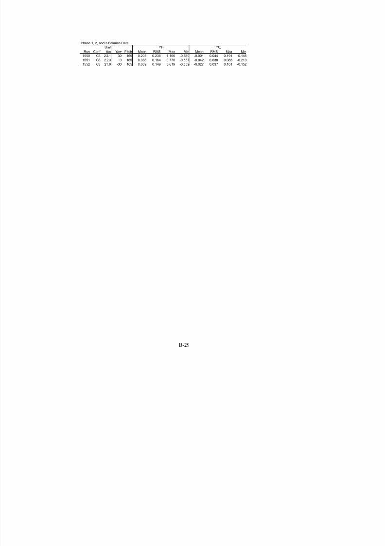
7/31/2019 Wind Tunnel Test
http://slidepdf.com/reader/full/wind-tunnel-test 173/243
B-29
Phase 1, 2, and 3 Balance Data
Uref
Run Conf fps Yaw Pitch Mean RMS Max Min Mean RMS Max Min
1550 C3 22.1 30 165 0.205 0.238 1.166 -0.510 -0.001 0.044 0.191 -0.145
1551 C3 22.3 0 165 0.088 0.164 0.770 -0.567 -0.042 0.038 0.083 -0.210
1552 C3 21.9 -30 165 0.009 0.149 0.619 -0.559 -0.027 0.037 0.101 -0.152
Cfx Cfz

7/31/2019 Wind Tunnel Test
http://slidepdf.com/reader/full/wind-tunnel-test 174/243
B-30
Phase 4 Balance Data
Phase 4 Balance Data
Uref
Run Conf fps Yaw Pitch Mean RMS Max Min
4 A1 25.1 0 180 -0.122 0.034 -0.013 -0.282
5 A1 25.3 0 - 165 -0.181 0.046 -0.061 -0.372
6 A1 25.5 0 - 150 -0.238 0.056 -0.112 -0.5067 A1 25.4 0 - 135 -0.256 0.067 -0.119 -0.567
8 A1 25.6 0 - 120 -0.270 0.075 -0.109 -0.606
9 A1 25.7 0 - 105 -0.258 0.065 -0.126 -0.574
10 A1 25.4 0 -90 -0.233 0.067 -0.092 -0.535
11 A1 25.8 0 -75 -0.119 0.053 0.027 -0.371
12 A1 24.9 0 -60 0.105 0.046 0.295 -0.044
13 A1 25.1 0 -45 0.085 0.062 0.407 -0.064
14 A1 25.5 0 -30 -0.025 0.035 0.169 -0.149
15 A1 25.1 0 -15 -0.027 0.024 0.115 -0.133
16 A1 25.2 0 0 -0.014 0.001 -0.010 -0.016
17 A1 25.3 0 15 -0.033 0.023 0.068 -0.130
18 A1 25.7 0 30 -0.076 0.033 0.058 -0.224
19 A1 25.0 0 45 -0.002 0.002 0.004 -0.008
20 A1 25.2 0 60 -0.092 0.040 -0.044 -0.230
21 A1 24.9 0 75 0.020 0.036 0.151 -0.163
22 A1 25.4 0 90 0.035 0.037 0.191 -0.031
23 A1 25.0 0 105 0.156 0.057 0.415 0.01624 A1 24.9 0 120 0.001 0.001 0.005 -0.002
25 A1 25.2 0 135 0.124 0.067 0.384 0.011
26 A1 24.8 0 150 0.096 0.045 0.284 -0.003
27 A1 25.4 0 165 -0.020 0.023 0.105 -0.096
28 B1 25.0 0 165 -0.050 0.023 0.062 -0.122
29 B1 2 4.9 0 150 -0.067 0.003 -0.054 -0.072
30 B1 25.1 0 135 0.186 0.059 0.423 0.055
31 B1 24.6 0 120 0.246 0.078 0.577 0.072
32 B1 25.4 0 105 0.192 0.063 0.472 0.040
33 B1 24.8 0 90 0.184 0.064 0.446 0.034
34 B1 25.1 0 75 -0.002 0.039 0.140 -0.210
35 B1 25.1 0 60 -0.254 0.072 -0.078 -0.569
36 B1 24.8 0 45 -0.213 0.057 -0.055 -0.484
37 B1 25.1 0 30 -0.096 0.036 0.021 -0.247
38 B1 25.0 0 15 -0.043 0.022 0.068 -0.130
39 B1 25.1 0 0 -0.028 0.023 0.064 -0.116
40 B1 25.0 0 -15 -0.027 0.021 0.072 -0.097
41 B1 25.5 0 -30 -0.056 0.022 0.053 -0.14742 B1 25.1 0 -45 0.012 0.036 0.242 -0.092
43 B1 24.9 0 -60 0.133 0.061 0.396 -0.033
44 B1 24.9 0 -75 -0.016 0.032 0.072 -0.177
45 B1 25.2 0 -90 -0.200 0.060 -0.067 -0.481
46 B1 25.2 0 -105 -0.246 0.064 -0.109 -0.536
47 B1 25.4 0 -120 -0.270 0.066 -0.133 -0.568
48 B1 24.9 0 -135 -0.253 0.055 -0.119 -0.502
49 B1 24.8 0 -150 -0.239 0.047 -0.102 -0.476
50 B1 25.1 0 -165 -0.189 0.036 -0.082 -0.363
51 B1 2 5.1 0 180 -0.141 0.027 -0.055 -0.253
52 B1 25.0 0 150 0.089 0.041 0.268 -0.004
53 C5 2 3.7 0 -165 -0.003 0.021 0.107 -0.071
Cmy

7/31/2019 Wind Tunnel Test
http://slidepdf.com/reader/full/wind-tunnel-test 175/243
B-31
Phase 4 Balance Data
Uref
Run Conf fps Yaw Pitch Mean RMS Max Min
54 C5 24.1 -30 -165 0.024 0.026 0.149 -0.063
55 C5 24.0 -30 -150 0.014 0.024 0.115 -0.074
56 C5 2 4.1 0 -150 -0.005 0.020 0.119 -0.094
57 C5 2 4.1 0 -135 -0.003 0.017 0.087 -0.083
58 C5 24.8 -30 -135 -0.007 0.020 0.064 -0.10059 C5 25.0 -30 -120 -0.063 0.029 -0.004 -0.233
60 C5 24.7 0 -120 -0.060 0.029 -0.003 -0.235
61 C5 24.9 0 -105 -0.142 0.052 -0.052 -0.384
62 C5 24.9 -30 -105 -0.129 0.046 -0.042 -0.353
63 C5 25.2 -30 -90 -0.119 0.048 -0.022 -0.354
64 C5 24.4 0 -90 -0.141 0.054 -0.034 -0.431
65 C5 25.0 0 -75 -0.027 0.056 0.147 -0.278
66 C5 24.7 -30 -75 -0.017 0.043 0.124 -0.207
67 C5 2 4.8 -30 -60 0.023 0.040 0.204 -0.149
68 C5 24.3 0 -60 0.018 0.048 0.277 -0.180
69 C5 23.3 0 -45 0.018 0.048 0.289 -0.157
70 C5 2 4.4 -30 -45 0.024 0.050 0.314 -0.138
71 C5 2 4.3 -30 -30 0.021 0.042 0.251 -0.112
72 C5 23.3 0 -30 0.005 0.039 0.224 -0.156
73 C5 22.9 0 -15 0.004 0.032 0.208 -0.163
74 C5 2 4.7 -30 -15 0.017 0.039 0.262 -0.097
75 C5 25.4 -30 0 0.026 0.040 0.233 -0.081
76 C5 23.8 0 0 -0.004 0.026 0.181 -0.095
77 C5 23.9 0 15 0.006 0.022 0.143 -0.089
78 C5 24.9 -30 15 0.025 0.035 0.203 -0.084
79 C5 24.8 -30 30 0.038 0.030 0.190 -0.047
80 C5 24.0 0 30 0.007 0.022 0.145 -0.067
81 C5 24.5 0 45 0.009 0.019 0.122 -0.071
82 C5 25.1 -30 45 0.012 0.021 0.143 -0.073
83 C5 2 5.5 -30 60 -0.014 0.021 0.086 -0.167
84 C5 24.9 0 60 -0.004 0.021 0.096 -0.127
85 C5 25.2 0 75 -0.008 0.022 0.082 -0.122
86 C5 2 5.4 -30 75 -0.006 0.021 0.093 -0.121
87 C5 25.5 -30 90 0.080 0.028 0.206 -0.004
88 C5 24.9 0 90 0.083 0.030 0.205 0.002
89 C5 25.0 0 105 0.112 0.045 0.320 -0.002
90 C5 25.3 -30 105 0.120 0.038 0.292 0.020
91 C5 24.9 -30 120 0.095 0.037 0.280 0.006
92 C5 24.8 0 120 0.076 0.039 0.289 -0.014
93 C5 24.2 0 135 0.029 0.036 0.224 -0.06894 C5 24.5 -30 135 0.068 0.038 0.263 -0.031
95 C5 24.6 -30 150 0.053 0.035 0.217 -0.044
96 C5 23.9 0 150 0.018 0.033 0.198 -0.057
97 C5 23.8 0 150 0.024 0.033 0.195 -0.047
98 C5 24.6 -30 150 0.057 0.036 0.231 -0.038
99 C5 24.5 -30 165 0.035 0.031 0.164 -0.042
100 C5 23.4 0 165 0.001 0.023 0.137 -0.064
101 C5 23.8 0 180 -0.004 0.020 0.118 -0.067
102 C5 24.3 -30 180 0.020 0.028 0.145 -0.059
103 A1 25.5 0 0 -0.010 0.024 0.098 -0.114
Cmy

7/31/2019 Wind Tunnel Test
http://slidepdf.com/reader/full/wind-tunnel-test 176/243
B-32
Phase 4 Balance Data
Uref
Run Conf fps Yaw Pitch Mean RMS Max Min
104 A1 25.7 0 45 -0.208 0.058 -0.060 -0.522
105 A1 25.4 0 60 -0.192 0.070 -0.039 -0.545
106 A1 25.5 0 120 0.226 0.073 0.527 0.070
107 B3 25.1 0 165 0.007 0.028 0.135 -0.063
108 B3 24.9 30 150 0.114 0.040 0.278 0.008109 B3 25.1 0 150 0.108 0.042 0.290 0.010
110 B3 25.2 30 165 -0.022 0.025 0.080 -0.106
111 B3 25.2 30 135 0.240 0.073 0.560 0.064
112 B3 25.4 0 135 0.231 0.067 0.527 0.085
113 B3 25.6 0 120 0.227 0.068 0.519 0.075
114 B3 24.8 30 120 0.211 0.064 0.457 0.067
115 B3 25.3 30 105 0.257 0.078 0.584 0.088
116 B3 25.2 0 105 0.189 0.059 0.496 0.051
117 B3 25.1 0 90 0.193 0.062 0.476 0.050
118 B3 25.4 30 90 0.248 0.069 0.536 0.077
119 B3 25.3 30 75 -0.066 0.040 0.085 -0.251
120 B3 25.3 0 75 -0.002 0.043 0.164 -0.228
121 B3 25.6 0 60 -0.191 0.068 -0.014 -0.537
122 B3 25.7 30 60 -0.124 0.060 0.047 -0.419
123 B3 2 5.9 30 45 -0.443 0.074 -0.257 -0.834
124 B3 25.5 0 45 -0.277 0.078 -0.064 -0.633
125 B3 25.5 0 30 -0.051 0.031 0.085 -0.227
126 B3 25.1 30 30 -0.082 0.035 0.054 -0.212
127 B3 25.2 30 15 0.027 0.025 0.146 -0.075
128 B3 25.4 0 15 -0.016 0.026 0.110 -0.106
129 B3 25.3 0 0 0.009 0.024 0.135 - 0.073
130 B3 25.4 30 0 -0.037 0.023 0.055 -0.128
131 B3 2 5.3 30 -15 -0.011 0.026 0.078 -0.115
132 B3 25.7 0 -15 0.004 0.023 0.095 -0.086
133 B3 25.0 0 -30 -0.004 0.028 0.136 -0.106
134 B3 2 5.3 30 -30 -0.030 0.039 0.193 -0.164
135 B3 25.4 30 -45 0.095 0.054 0.328 -0.056
136 B3 25.3 0 -45 0.047 0.047 0.286 -0.096
137 B3 25.0 0 -60 0.134 0.053 0.353 -0.024
138 B3 25.7 30 -60 0.085 0.043 0.273 -0.053
139 B3 2 6.0 30 -75 -0.084 0.047 0.039 -0.281
140 B3 25.6 0 -75 -0.066 0.050 0.060 -0.288
141 B3 25.4 0 -90 -0.193 0.058 -0.062 -0.504
142 B3 25.4 30 -90 -0.202 0.068 -0.056 -0.475
143 B3 25.3 30 -105 -0.259 0.067 -0.109 -0.545144 B3 25.5 0 -105 -0.235 0.066 -0.094 -0.527
145 B3 26.8 0 -120 -0.237 0.067 -0.093 -0.555
146 B3 26.1 30 -120 -0.234 0.059 -0.100 -0.512
147 B3 26.7 30 -135 -0.244 0.058 -0.108 -0.520
148 B3 26.6 0 -135 -0.240 0.059 -0.104 -0.506
149 B3 27.0 0 -150 -0.207 0.046 -0.079 -0.387
150 B3 26.2 30 -150 -0.223 0.050 -0.087 -0.464
151 B3 26.2 30 -165 -0.188 0.041 -0.068 -0.393
152 B3 26.5 0 -165 -0.169 0.037 -0.062 -0.334
153 B3 26.0 0 180 -0.087 0.028 0.043 -0.204
Cmy

7/31/2019 Wind Tunnel Test
http://slidepdf.com/reader/full/wind-tunnel-test 177/243
B-33
Phase 4 Balance Data
Uref
Run Conf fps Yaw Pitch Mean RMS Max Min
154 B3 26.5 30 180 -0.106 0.030 0.003 -0.224
155 B2 25.2 30 165 -0.078 0.023 0.031 -0.157
156 B2 25.1 30 150 0.101 0.039 0.269 0.000
157 B2 24.9 30 135 0.199 0.070 0.490 0.046
158 B2 25.3 30 120 0.243 0.080 0.588 0.065159 B2 25.5 30 105 0.254 0.076 0.598 0.079
160 B2 25.6 30 90 0.202 0.061 0.454 0.030
161 B2 25.5 30 75 0.045 0.034 0.208 -0.132
162 B2 2 5.1 30 60 -0.203 0.066 -0.033 -0.478
163 B2 25.0 30 45 -0.161 0.060 0.009 -0.477
164 B2 25.3 30 30 -0.011 0.024 0.084 -0.128
165 B2 25.0 30 15 -0.042 0.021 0.055 -0.144
166 B2 25.1 30 0 -0.019 0.020 0.077 -0.097
167 B2 25.6 30 -15 0.002 0.023 0.107 -0.090
168 B2 2 5.5 30 -30 -0.031 0.027 0.114 -0.149
169 B2 25.7 30 -45 0.014 0.039 0.236 -0.087
170 B2 25.1 30 -60 0.092 0.044 0.275 -0.046
171 B2 2 5.7 30 -75 -0.005 0.027 0.074 -0.126
172 B2 25.6 30 -90 -0.148 0.061 -0.016 -0.396
173 B2 25.4 30 -105 -0.137 0.041 -0.047 -0.333
174 B2 25.4 30 -120 -0.174 0.045 -0.075 -0.372
175 B2 25.8 30 -135 -0.216 0.047 -0.105 -0.415
176 B2 25.4 30 -150 -0.189 0.041 -0.090 -0.380
177 B2 25.0 30 -165 -0.022 0.004 -0.009 -0.040
178 B2 25.2 30 180 -0.018 0.003 -0.006 -0.032
179 B2 25.5 30 180 -0.037 0.007 -0.010 -0.068
180 B2 25.4 30 -165 -0.079 0.016 -0.024 -0.147
181 B3 2 5.2 30 45 -0.043 0.013 -0.007 -0.101
182 B3 25.0 30 120 0.240 0.066 0.504 0.072
183 B3 2 5.8 30 45 -0.257 0.059 -0.100 -0.571
184 B3 24.8 30 30 -0.049 0.050 0.136 -0.242
185 B3 25.3 30 15 -0.064 0.027 0.043 -0.164
186 C2 25.4 0 165 -0.056 0.026 0.061 -0.153
187 C2 25.2 0 150 -0.066 0.032 0.050 -0.223
188 C2 25.3 0 135 0.031 0.041 0.231 -0.090
189 C2 25.0 0 120 0.156 0.072 0.523 -0.028
190 C2 25.5 0 105 0.183 0.070 0.479 0.013
191 C2 25.1 0 90 0.188 0.061 0.462 0.032
192 C2 25.4 0 75 0.041 0.039 0.210 -0.141
193 C2 25.1 0 60 -0.012 0.027 0.097 -0.148194 C2 25.3 0 45 0.011 0.025 0.113 -0.112
195 C2 24.9 0 30 0.008 0.023 0.148 -0.095
196 C2 24.7 0 15 0.017 0.026 0.169 -0.136
197 C2 25.1 0 0 0.017 0.030 0.173 -0.130
198 C2 25.3 0 -15 0.008 0.031 0.172 -0.139
199 C2 24.9 0 -30 0.013 0.034 0.207 -0.128
200 C2 25.6 0 -45 0.001 0.037 0.179 -0.155
201 C2 25.5 0 -60 0.024 0.046 0.256 -0.159
202 C2 25.5 0 -75 -0.039 0.052 0.105 -0.295
203 C2 2 6.0 0 -90 -1.277 0.048 -1.169 -1.510
204 C2 2 5.4 0 -90 -0.140 0.049 -0.020 -0.403
205 C2 25.5 0 -105 -0.174 0.050 -0.069 -0.416
206 C2 2 5.4 0 - 120 -0.075 0.024 0.005 -0.214
207 C2 25.5 0 -135 0.008 0.020 0.120 -0.061
208 C2 25.4 0 -150 0.015 0.022 0.135 -0.052
209 C2 25.6 0 -165 0.012 0.020 0.121 -0.055
210 C2 24.8 0 180 0.001 0.019 0.093 -0.087
Cmy

7/31/2019 Wind Tunnel Test
http://slidepdf.com/reader/full/wind-tunnel-test 178/243
B-34
Phase 1, 2, and 3 Integrated Pressure Data
Phase 1, 2, and 3 Integrated Pressure Data
Uref
Run Conf fps Yaw Pitch Mean RMS Max Min Mean RMS Max Min Mean RMS Max Min
1 A1 24.8 0 0 1.683 0.433 3.436 0.479 0.005 0.031 0.165 -0.113 0.004 0.021 0.109 -0.074
2 A1 24.9 30 0 1.567 0.425 3.129 0.510 0.009 0.029 0.172 -0.084 0.006 0.019 0.114 -0.056
3 A1 24.8 60 0 1.179 0.353 2.657 0.340 0.013 0.024 0.147 -0.072 0.009 0.016 0.097 -0.0474 A1 24.9 120 0 -1.083 0.336 -0.279 -2.385 0.050 0.025 0.165 -0.044 0.033 0.017 0.109 -0.029
5 A1 24.6 150 0 -1.242 0.326 -0.500 -2.562 0.060 0.032 0.229 -0.084 0.040 0.021 0.152 -0.056
6 A1 24.6 180 0 -1.334 0.373 -0.562 -2.737 0.061 0.032 0.207 -0.065 0.040 0.021 0.137 -0.043
7 A1 24.1 180 15 -1.331 0.359 -0.579 -2.811 0.311 0.083 0.684 0.127 -0.029 0.024 0.037 -0.140
8 A1 24.8 150 15 -1.229 0.324 -0.421 -2.607 0.298 0.079 0.632 0.114 -0.020 0.020 0.036 -0.124
9 A1 24.7 120 15 -1.173 0.364 -0.116 -2.755 0.290 0.089 0.695 0.025 -0.016 0.018 0.045 -0.100
10 A1 24.6 60 15 1.078 0.348 2.607 0.117 -0.309 0.104 -0.037 -0.778 -0.013 0.017 0.071 -0.097
11 A1 24.7 30 15 1.514 0.402 3.321 0.572 -0.421 0.112 -0.148 -0.953 -0.010 0.019 0.101 -0.103
12 A1 24.7 0 15 1.724 0.462 3.666 0.670 -0.479 0.131 -0.195 -1.015 -0.011 0.022 0.110 -0.094
13 A1 24.6 0 30 1.513 0.398 3.105 0.542 -0.924 0.242 -0.319 -1.931 -0.029 0.022 0.065 -0.121
14 A1 24.6 30 30 1.350 0.380 2.848 0.439 -0.838 0.234 -0.278 -1.782 -0.033 0.021 0.055 -0.127
15 A1 24.8 60 30 0.921 0.309 2.257 0.234 -0.628 0.215 -0.156 -1.608 -0.055 0.028 0.047 -0.192
16 A1 24.8 120 30 -0.997 0.338 -0.255 -2.256 0.426 0.147 1.000 0.113 -0. 086 0.033 0.005 -0.217
17 A1 25.1 150 30 -1.128 0.293 -0.513 -2.217 0.467 0.117 0.933 0.208 -0. 106 0.036 -0.031 -0.273
18 A1 24.9 180 30 -1.102 0.280 -0.433 -2.221 0.431 0.107 0.888 0.157 -0. 118 0.038 -0.031 -0.285
19 A1 24.7 180 45 -0.785 0.200 -0.196 -1.661 0.356 0.093 0.787 0.067 -0. 201 0.056 -0.045 -0.444
20 A1 24.8 150 45 -0.844 0.203 -0.330 -1.593 0.445 0.109 0.879 0.153 -0. 187 0.051 -0.055 -0.39521 A1 24.7 120 45 -0.708 0.227 -0.188 -1.684 0.428 0.138 1.044 0.092 -0. 131 0.045 -0.024 -0.321
22 A1 24.9 60 45 0.649 0.240 1.629 0.115 -0.785 0.300 -0.127 -2.002 -0.064 0.035 0.033 -0.211
23 A1 24.5 30 45 1.167 0.314 2.492 0.475 -1.404 0.377 -0.543 -3.076 -0.111 0.037 -0.002 -0.312
24 A1 24.3 0 45 1.302 0.357 2.715 0.525 -1.545 0.422 -0.624 -3.295 -0.114 0.037 -0.007 -0.310
25 A1 24.4 0 60 0.826 0.228 1.730 0.345 -1.857 0.537 -0.751 -4.018 -0.141 0.053 0.008 -0.369
26 A1 24.6 30 60 0.701 0.197 1.647 0.172 -1.510 0.451 -0.353 -3.618 -0.098 0.044 0.031 -0.309
27 A1 25.0 60 60 0.350 0.132 0.903 0.054 -0.667 0.290 -0.055 -1.914 -0.020 0.029 0.062 -0.167
28 A1 24.6 120 60 -0.458 0.149 -0.054 -1.035 0.377 0.134 0.954 -0.084 -0.138 0.046 -0 .020 -0.307
29 A1 24.5 150 60 -0.588 0.147 -0.226 -1.188 0.416 0.126 1.057 0.052 -0. 199 0.056 -0.080 -0.419
30 A1 24.4 180 60 -0.519 0.141 -0.156 -1.121 0.215 0.087 0.673 -0.134 -0.226 0.064 -0 .077 -0.473
31 A1 24.4 180 75 -0.354 0.101 -0.108 -0.782 0.228 0.133 0.931 -0.243 -0.187 0.054 -0 .068 -0.407
32 A1 24.6 150 75 -0.360 0.094 -0.094 -0.759 0.343 0.127 0.927 -0.192 -0.171 0.046 -0 .056 -0.370
33 A1 24.8 120 75 -0.246 0.094 -0.005 -0.688 0.179 0.122 0.826 -0.280 -0.127 0.047 -0 .006 -0.347
34 A1 2 4.7 60 75 0.180 0.069 0.487 0.010 -0.442 0.222 0.130 -1.495 0.039 0.019 0.131 -0.062
35 A1 24.7 30 75 0.400 0.107 0.833 0.143 -1.088 0.357 -0.235 -2.532 0.069 0.027 0.195 -0.106
36 A1 2 4.6 0 75 0.478 0.138 1.007 0.158 -1.262 0.430 -0.324 -2.931 0.089 0.030 0.220 -0.057
37 A1 24.9 0 90 0.238 0.072 0.575 0.065 -0.182 0.179 0.327 -1.135 0.158 0.048 0.380 0.043
38 A1 24.4 30 90 0.271 0.072 0.581 0.090 -0.356 0.218 0.208 -1.297 0.179 0.048 0.385 0.059
39 A1 24.9 60 90 0.128 0.048 0.362 -0.001 -0.140 0.155 0.319 -0.946 0.085 0.032 0.240 -0.001
40 A1 24.7 120 90 -0.152 0.058 0.010 -0.416 -0.135 0.159 0.387 -0.798 -0. 100 0.038 0.006 -0.275
41 A1 25.0 150 90 -0.260 0.068 -0.095 -0.530 -0.191 0.190 0.388 -1.121 -0.172 0.045 -0 .063 -0.351
42 A1 24.7 180 90 -0.252 0.071 -0.079 -0.539 -0.038 0.152 0.421 -0.786 -0.167 0.047 -0 .052 -0.357
43 A1 24.7 180 -15 -1.159 0.306 -0.496 -2.348 -0.166 0.059 -0.033 -0.438 0.092 0.028 0.231 0.002
44 A1 25.0 150 -15 -1.066 0.295 -0.327 -2.396 -0.147 0.056 -0.015 -0.419 0.089 0.028 0.216 0.002
45 A1 25.1 120 -15 -0.752 0.240 -0.126 -1.710 -0.115 0.046 0.022 -0.322 0.056 0.022 0.160 -0.012
46 A1 25.3 60 -15 1.135 0.344 2.604 0.356 0.348 0.110 0.853 0.087 0.028 0.025 0.170 -0.050
47 A1 24.4 30 -15 1.507 0.385 3.133 0.486 0.420 0.112 0.887 0.133 0.010 0.019 0.113 -0.067
48 A1 24.2 0 -15 1.508 0.385 3.043 0.647 0.408 0.111 0.895 0.155 0.002 0.020 0.112 -0.081
49 A1 24.6 0 -30 1.311 0.335 2.780 0.429 0.766 0.201 1.631 0.232 0.005 0.020 0.122 -0.067
50 A1 24.3 30 -30 1.295 0.334 2.631 0.310 0.773 0.201 1.592 0.182 0.014 0.020 0.130 -0.053
Cfx Cfz Cmy

7/31/2019 Wind Tunnel Test
http://slidepdf.com/reader/full/wind-tunnel-test 179/243
B-35
Phase 1, 2, and 3 Integrated Pressure Data
Uref
Run Conf fps Yaw Pitch Mean RMS Max Min Mean RMS Max Min Mean RMS Max Min
51 A1 24.6 60 -30 0.975 0.300 2.262 0.165 0.673 0.215 1.569 0.091 0.063 0.035 0.230 -0.041
52 A1 24.7 120 -30 -0.540 0.179 -0.047 -1.261 -0.201 0.075 0.014 -0.506 0.063 0.027 0.185 -0.005
53 A1 24.7 150 -30 -0.774 0.227 -0.249 -1.699 -0.249 0.086 -0.058 -0.612 0.113 0.034 0.268 0.033
54 A1 24.6 180 -30 -0.878 0.244 -0.302 -1.765 -0.285 0.092 -0.082 -0.647 0.127 0.035 0.287 0.028
55 A1 24.3 180 -45 -0.562 0.163 -0.203 -1.219 -0.233 0.085 -0.031 -0.610 0.154 0.043 0.338 0.05456 A1 25.0 150 -45 -0.514 0.154 -0.129 -1.235 -0.232 0.083 -0.022 -0.604 0.132 0.040 0.339 0.034
57 A1 24.9 120 -45 -0.364 0.129 -0.037 -0.924 -0.219 0.085 0.011 -0.607 0. 068 0.027 0.190 0.004
58 A1 24.9 60 -45 0.672 0.235 1.697 0.117 0.806 0.297 2.088 0.077 0.063 0.036 0.235 -0.041
59 A1 24.8 30 -45 1.068 0.267 2.113 0.403 1.290 0.340 2.602 0.468 0.104 0.045 0.284 -0.013
60 A1 24.4 0 -45 1.053 0.293 2.431 0.369 1.153 0.322 2.621 0.382 0.047 0.031 0.244 -0.032
61 A1 24.2 0 -60 0.680 0.167 1.316 0.304 1.616 0.402 3.069 0.638 0.145 0.044 0.326 0.006
62 A1 24.6 30 -60 0.631 0.169 1.317 0.227 1.410 0.375 2.956 0.532 0.105 0.039 0.274 -0.042
63 A1 24.8 60 -60 0.373 0.143 0.951 0.062 0.701 0.291 1.932 0.059 0.019 0.030 0.172 -0.093
64 A1 24.8 120 -60 -0.226 0.088 -0.022 -0.627 -0.158 0.071 0.031 -0.522 0. 077 0.032 0.220 0.005
65 A1 24.5 150 -60 -0.340 0.103 -0.071 -0.788 -0.140 0.073 0.093 -0.470 0. 149 0.045 0.365 0.044
66 A1 24.3 180 -60 -0.350 0.110 -0.106 -0.869 -0.061 0.060 0.156 -0.380 0. 181 0.053 0.430 0.067
67 A1 24.5 180 -75 -0.269 0.087 -0.075 -0.654 -0.054 0.080 0.263 -0.438 0. 162 0.051 0.392 0.055
68 A1 24.6 150 -75 -0.233 0.076 -0.058 -0.584 -0.072 0.074 0.196 -0.472 0. 137 0.041 0.331 0.046
69 A1 24.5 120 -75 -0.145 0.061 0.015 -0.420 -0.051 0.060 0.193 -0.400 0. 084 0.034 0.225 0.007
70 A1 24.7 60 -75 0.160 0.069 0.471 0.015 0.383 0.182 1.305 -0.054 -0.037 0.023 0.032 -0.136
71 A1 2 4.6 30 -75 0.352 0.110 0.881 0.128 1.010 0.270 2.303 0.395 -0.052 0.035 0.063 -0.216
72 A1 24.5 0 -75 0.397 0.118 0.869 0.136 1.212 0.310 2.589 0.442 -0.046 0.036 0.072 -0.196
73 A1 24.6 0 -90 0.216 0.067 0.551 0.072 0.330 0.128 0.985 -0.174 -0.143 0.044 -0.048 -0.364
74 A1 24.7 30 -90 0.212 0.070 0.525 0.063 0.330 0.108 0.802 -0.113 -0.140 0.046 -0.041 -0.347
75 A1 24.8 60 -90 0.099 0.045 0.365 0.003 0.105 0.079 0.541 -0.174 -0.066 0.030 -0.002 -0.242
76 A1 24.6 120 -90 -0.097 0.054 0.015 -0.391 0.093 0.085 0.563 -0.255 0. 064 0.036 0.258 -0.010
77 A1 24.8 150 -90 -0.200 0.069 -0.020 -0.530 0.275 0.098 0.730 -0.108 0. 132 0.045 0.351 0.013
78 A1 24.8 180 -90 -0.213 0.069 -0.066 -0.579 0.262 0.119 0.794 -0.172 0. 141 0.045 0.383 0.044
79 A2 24.0 0 -90 0.276 0.088 0.669 0.078 0.116 0.115 0.548 -0.425 -0.183 0.058 -0.052 -0.443
80 A2 2 3.9 0 -75 0.370 0.105 0.831 0.143 0.736 0.187 1.543 0.225 -0.110 0.046 -0.005 -0.326
81 A2 24.1 0 -60 0.607 0.172 1.388 0.248 1.316 0.367 3.085 0.451 0.088 0.032 0.256 -0.073
82 A2 23.9 0 -45 1.038 0.272 2.233 0.328 1.204 0.320 2.585 0.357 0.077 0.034 0.251 -0.039
83 A2 23.8 0 -30 1.340 0.346 2.683 0.503 0.783 0.207 1.602 0.274 0.005 0.021 0.121 -0.064
84 A2 24.3 0 -15 1.560 0.406 3.088 0.553 0.426 0.118 0.949 0.130 0.005 0.020 0.123 -0.068
85 A2 23.8 0 0 1.707 0.477 3.546 0.652 0.011 0.033 0.209 -0.108 0.007 0.022 0.138 -0.072
86 A2 24.2 0 15 1.747 0.446 3.651 0.770 -0.502 0.127 -0.209 -1.078 -0.022 0.022 0.079 -0.111
87 A2 23.8 0 30 1.620 0.427 3.448 0.599 -1.035 0.268 -0.386 -2.170 -0.057 0.024 0.035 -0.178
88 A2 23.9 0 45 1.328 0.364 2.717 0.523 -1.568 0.431 -0.621 -3.311 -0.113 0.038 0.000 -0.298
89 A2 24.1 0 60 0.750 0.193 1.486 0.326 -1.454 0.407 -0.580 -3.024 -0.051 0.033 0.076 -0.190
90 A2 23.5 0 75 0.428 0.126 0.949 0.155 -0.643 0.263 -0.050 -1.881 0.163 0.045 0.375 0.04591 A2 24.1 0 90 0.302 0.086 0.643 0.101 0.360 0.134 0.988 -0.283 0.200 0.057 0.425 0.067
92 A2 25.0 180 90 -0.306 0.086 -0.116 -0.704 0.267 0.134 0.791 -0.480 -0.203 0.057 -0 .077 -0.465
93 A2 24.9 180 75 -0.423 0.114 -0.150 -0.949 0.508 0.173 1.395 0.024 -0. 184 0.051 -0.064 -0.415
94 A2 24.8 180 60 -0.470 0.133 -0.147 -1.097 0.150 0.096 0.756 -0.191 -0.219 0.063 -0 .083 -0.484
95 A2 24.5 180 45 -0.687 0.182 -0.275 -1.434 0.264 0.075 0.584 0.015 -0. 198 0.058 -0.080 -0.441
96 A2 25.0 180 30 -1.008 0.245 -0.405 -1.924 0.368 0.091 0.738 0.105 -0. 122 0.037 -0.032 -0.297
97 A2 25.1 180 15 -1.221 0.329 -0.505 -2.620 0.271 0.074 0.594 0.068 -0. 036 0.023 0.022 -0.172
98 A2 24.8 180 0 -1.268 0.340 -0.477 -2.603 0.060 0.030 0.182 -0.067 0.040 0.020 0.121 -0.044
99 A2 24.8 180 -15 -1.116 0.305 -0.477 -2.344 -0.161 0.059 -0.030 -0.387 0.088 0.026 0.222 0.005
100 A2 25.0 180 -30 -0.753 0.215 -0.264 -1.694 -0.232 0.082 -0.018 -0.599 0.116 0.032 0.265 0.034
Cfx Cfz Cmy
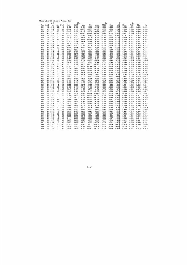
7/31/2019 Wind Tunnel Test
http://slidepdf.com/reader/full/wind-tunnel-test 180/243
B-36
Phase 1, 2, and 3 Integrated Pressure Data
Uref
Run Conf fps Yaw Pitch Mean RMS Max Min Mean RMS Max Min Mean RMS Max Min
101 A2 24.3 180 -45 -0.450 0.136 -0.134 -1.012 -0.113 0.060 0.050 -0.427 0. 158 0.044 0.350 0.059
102 A2 24.1 180 -60 -0.387 0.110 -0.093 -0.866 -0.119 0.095 0.203 -0.543 0. 183 0.050 0.385 0.066
103 A2 24.0 180 -75 -0.440 0.131 -0.117 -1.064 -0.474 0.172 0.032 -1.310 0. 200 0.058 0.490 0.060
104 A2 24.2 180 -90 -0.319 0.100 -0.093 -0.779 -0.149 0.142 0.300 -0.928 0. 211 0.066 0.516 0.061
105 D1 24.8 0 180 0.553 0.120 1.071 0.118 0.055 0.026 0.121 -0.112 -0. 037 0.017 0.074 -0.080106 D1 24.6 30 180 0.417 0.110 0.859 0.001 0.044 0.021 0.108 -0.080 -0.029 0.014 0.053 -0.071
107 D1 24.9 45 180 0.311 0.115 0.824 -0.142 0.030 0.021 0.100 -0.071 -0.020 0.014 0.047 -0.066
108 D1 24.3 -30 180 0.392 0.108 0.878 -0.011 0.034 0.021 0.103 -0.092 -0.023 0.014 0.061 -0.068
109 B1 24.8 -30 180 1.031 0.234 1.910 0.453 0.068 0.025 0.173 -0.035 -0. 045 0.017 0.023 -0.114
110 B1 25.1 45 180 0.857 0.209 1.787 0.321 0.067 0.023 0.169 -0.028 -0.044 0.015 0.019 -0.112
111 B1 24.4 30 180 1.114 0.241 2.162 0.460 0.084 0.025 0.181 -0.014 -0.055 0.017 0.009 -0.120
112 B1 24.3 0 180 1.393 0.292 2.785 0.697 0.099 0.028 0.230 -0.023 -0.065 0.018 0.015 -0.152
113 B1 25.1 45 -165 0.721 0.187 1.642 0.208 -0.083 0.035 0.032 -0.289 -0. 070 0.020 -0.004 -0.156
114 B1 24.6 30 -165 0.922 0.211 1.854 0.396 -0.103 0.042 0.018 -0.319 -0. 092 0.021 -0.020 -0.186
115 B1 24.5 0 -165 1.179 0.257 2.250 0.508 -0.139 0.048 -0.034 -0.347 -0. 113 0.024 -0.025 -0.221
116 B1 24.6 -30 -165 0.879 0.227 1.808 0.329 -0.107 0.044 0.007 -0.309 -0.082 0.022 -0 .001 -0.182
117 D1 24.4 -30 -165 0.304 0.093 0.714 -0.038 -0.034 0.025 0.049 -0.196 -0.030 0.014 0.053 -0.080
118 D1 24.8 0 -165 0.452 0.102 1.006 0.077 -0.044 0.029 0.043 -0.269 -0.049 0.018 0.064 -0.110
119 D1 24.4 30 -165 0.311 0.107 0.765 -0.080 -0.027 0.027 0.075 -0.185 -0.036 0.015 0.043 -0.085
120 D1 24.5 45 -165 0.166 0.130 0.719 -0.341 -0.010 0.032 0.108 -0.168 -0.022 0.015 0.040 -0.068
121 D1 24.8 45 -150 0.128 0.096 0.581 -0.323 -0.028 0.048 0.184 -0.246 -0.026 0.014 0.045 -0.080
122 D1 24.2 30 -150 0.237 0.076 0.585 -0.089 -0.068 0.035 0.106 -0.257 -0.039 0.014 0.038 -0.096
123 D1 24.3 0 -150 0.305 0.073 0.628 -0.025 -0.080 0.034 0.054 -0.297 -0.055 0.016 0.026 -0.108
124 D1 24.4 -30 -150 0.209 0.071 0.528 -0.068 -0.060 0.033 0.072 -0.249 -0.035 0.014 0.036 -0.082
125 B1 24.6 -30 -150 0.647 0.170 1.436 0.152 -0.181 0.059 -0.025 -0.448 -0.111 0.031 -0 .012 -0.256
126 B1 24.7 0 -150 0.840 0.187 1.598 0.261 -0.236 0.066 -0.076 -0.535 -0. 143 0.030 -0.034 -0.269
127 B1 24.3 30 -150 0.730 0.171 1.559 0.307 -0.212 0.064 -0.044 -0.507 -0.120 0.027 -0 .045 -0.269
128 B1 25.2 45 -150 0.562 0.143 1.142 0.125 -0.168 0.052 -0.012 -0.374 -0.090 0.024 -0 .018 -0.206
129 B1 24.9 45 -135 0.359 0.093 0.717 0.114 -0.144 0.051 0.002 -0.365 -0. 101 0.026 -0.025 -0.203
130 B1 25.0 30 -135 0.466 0.114 0.918 0.190 -0.180 0.056 -0.023 -0.420 -0.134 0.033 -0 .050 -0.287
131 B1 24.8 0 -135 0.549 0.136 1.122 0.238 -0.194 0.061 -0.038 -0.474 -0. 166 0.041 -0.070 -0.339
132 B1 24.6 -30 -135 0.446 0.121 0.982 0.163 -0.155 0.056 0.009 -0.375 -0.136 0.038 -0 .043 -0.317
133 D1 24.6 -30 -135 0.120 0.051 0.379 -0.074 -0.043 0.038 0.126 -0.255 -0.036 0.012 0.024 -0.087
134 D1 24.6 0 -135 0.172 0.053 0.393 -0.037 -0.058 0.039 0.125 -0.243 -0.053 0.014 0.017 -0.109
135 D1 24.3 30 -135 0.138 0.055 0.369 -0.088 -0.057 0.042 0.144 -0.266 -0.038 0.013 0.031 -0.089
136 D1 24.6 45 -135 0.088 0.060 0.323 -0.139 -0.035 0.050 0.167 -0.237 -0.025 0.012 0.033 -0.066
137 D1 24.4 45 -120 0.044 0.039 0.289 -0.112 -0.016 0.052 0.258 -0.323 -0.020 0.010 0.026 -0.071
138 D1 24.1 30 -120 0.071 0.040 0.263 -0.113 -0.027 0.051 0.255 -0.250 -0.032 0.011 0.028 -0.085
139 D1 24.8 0 -120 0.086 0.043 0.291 -0.097 -0.023 0.052 0.274 -0.306 -0.042 0.012 0.020 -0.093
140 D1 24.6 -30 -120 0.061 0.037 0.225 -0.091 -0.018 0.048 0.240 -0.240 -0.029 0.010 0.018 -0.079141 B1 25.5 -30 -120 0.288 0.083 0.617 0.072 -0.075 0.048 0.098 -0.314 -0.140 0.039 -0 .046 -0.299
142 B1 24.9 0 -120 0.372 0.102 0.823 0.116 -0.085 0.056 0.135 -0.356 -0. 185 0.050 -0.070 -0.394
143 B1 25.3 30 -120 0.308 0.084 0.695 0.097 -0.103 0.050 0.057 -0.357 -0. 143 0.038 -0.052 -0.300
144 B1 25.4 45 -120 0.230 0.073 0.543 0.054 -0.093 0.046 0.059 -0.325 -0. 101 0.031 -0.029 -0.237
145 B1 25.6 45 -105 0.141 0.056 0.399 0.004 -0.028 0.061 0.167 -0.335 -0. 085 0.029 -0.019 -0.209
146 B1 24.9 30 -105 0.208 0.067 0.529 0.030 -0.065 0.072 0.216 -0.434 -0. 122 0.035 -0.031 -0.290
147 B1 25.4 0 -105 0.260 0.082 0.715 0.072 -0.054 0.081 0.311 -0.489 -0. 157 0.048 -0.053 -0.402
148 B1 25.3 -30 -105 0.205 0.070 0.525 0.036 -0.062 0.072 0.224 -0.466 -0.120 0.038 -0 .038 -0.290
149 D1 24.1 -30 -105 0.032 0.025 0.172 -0.080 -0.004 0.061 0.315 -0.291 -0.020 0.010 0.021 -0.077
150 D1 24.3 0 -105 0.048 0.028 0.180 -0.070 -0.016 0.061 0.316 -0.285 -0.028 0.011 0.015 -0.079
Cfx Cfz Cmy

7/31/2019 Wind Tunnel Test
http://slidepdf.com/reader/full/wind-tunnel-test 181/243
B-37
Phase 1, 2, and 3 Integrated Pressure Data
Uref
Run Conf fps Yaw Pitch Mean RMS Max Min Mean RMS Max Min Mean RMS Max Min
151 D1 25.2 30 -105 0.030 0.023 0.185 -0.074 0.000 0.055 0.323 -0.292 -0.019 0.008 0.018 -0.076
152 D1 24.7 45 -105 0.016 0.023 0.150 -0.071 0.023 0.056 0.302 -0.248 -0.014 0.009 0.019 -0.061
153 D1 24.6 45 -90 0.011 0.014 0.111 -0.057 0.071 0.059 0.478 -0.248 -0.008 0.009 0.038 -0.074
154 D1 24.6 30 -90 0.020 0.013 0.109 -0.041 0.085 0.057 0.374 -0.206 -0.014 0.009 0.027 -0.072
155 D1 24.3 0 -90 0.034 0.015 0.119 -0.030 0.108 0.064 0.508 -0.184 -0.022 0.010 0.020 -0.079156 D1 24.7 -30 -90 0.024 0.014 0.103 -0.052 0.091 0.059 0.459 -0.188 -0.016 0.009 0.034 -0.068
157 B1 25.1 -30 -90 0.163 0.060 0.433 0.027 0.354 0.123 0.985 -0.066 -0. 108 0.039 -0.018 -0.287
158 B1 25.1 0 -90 0.203 0.067 0.508 0.061 0.411 0.138 1.090 -0.064 -0.135 0.044 -0.040 -0.336
159 B1 24.9 30 -90 0.153 0.058 0.422 0.024 0.392 0.114 0.950 -0.025 -0.101 0.038 -0.016 -0.279
160 B1 25.7 45 -90 0.102 0.047 0.343 -0.002 0.281 0.091 0.796 -0.051 -0. 067 0.031 0.001 -0.227
161 B1 25.2 45 -75 0.162 0.069 0.501 0.002 0.566 0.198 1.589 0.097 -0.007 0.022 0.076 -0.108
162 B1 24.9 30 -75 0.253 0.094 0.646 0.069 0.901 0.265 1.954 0.251 -0.007 0.027 0.082 -0.126
163 B1 25.2 0 -75 0.340 0.108 0.812 0.118 1.197 0.301 2.538 0.488 -0.012 0.033 0.093 -0.162
164 B1 24.8 -30 -75 0.266 0.100 0.759 0.046 0.960 0.287 2.339 0.261 -0.006 0.031 0.114 -0.142
165 D1 24.5 -30 -75 0.046 0.016 0.122 -0.018 0.201 0.067 0.562 -0.124 0.005 0.010 0.057 -0.059
166 D1 24.5 0 -75 0.069 0.018 0.170 -0.001 0.307 0.077 0.728 -0.072 0. 008 0.011 0.080 -0.060
167 D1 24.7 30 -75 0.043 0.015 0.120 -0.033 0.195 0.069 0.541 -0.155 0.006 0.010 0.068 -0.057
168 D1 24.6 45 -75 0.028 0.015 0.103 -0.034 0.128 0.063 0.442 -0.188 0.004 0.010 0.054 -0.056
169 D1 24.5 45 -60 0.091 0.040 0.259 -0.085 0.186 0.084 0.503 -0.238 0.010 0.013 0.077 -0.062
170 D1 24.4 30 -60 0.132 0.041 0.336 -0.025 0.284 0.088 0.725 -0.078 0.018 0.013 0.112 -0.046
171 D1 24.5 0 -60 0.207 0.046 0.406 0.040 0.438 0.095 0.831 0.040 0.026 0.013 0.107 -0.057
172 D1 24.5 -30 -60 0.137 0.043 0.388 -0.034 0.303 0.091 0.801 -0.194 0.022 0.014 0.117 -0.078
173 B1 24.7 -30 -60 0.487 0.146 1.179 0.099 1.156 0.345 2.703 0.242 0.103 0.038 0.270 -0.007
174 B1 24.7 0 -60 0.622 0.158 1.314 0.264 1.425 0.383 3.012 0.528 0.115 0.045 0.316 -0.009
175 B1 2 4.5 30 -60 0.441 0.128 0.966 0.130 1.044 0.302 2.194 0.266 0.093 0.035 0.244 -0.017
176 B1 2 4.9 45 -60 0.287 0.101 0.888 0.078 0.669 0.235 2.052 0.156 0.057 0.028 0.212 -0.034
177 B1 24.7 45 -45 0.489 0.165 1.324 -0.018 0.603 0.221 1.739 -0.099 0.053 0.033 0.230 -0.048
178 B1 2 4.7 30 -45 0.811 0.228 1.909 0.193 1.016 0.287 2.370 0.192 0.096 0.043 0.308 -0.019
179 B1 24.6 0 -45 1.074 0.248 2.255 0.354 1.168 0.281 2.554 0.352 0.044 0.026 0.198 -0.035
180 B1 24.3 -30 -45 0.888 0.254 1.986 0.212 1.040 0.307 2.393 0.247 0.071 0.039 0.253 -0.027
181 D1 23.9 -30 -45 0.317 0.094 0.688 -0.071 0.351 0.101 0.739 -0.103 0.016 0.017 0.114 -0.061
182 D1 23.8 0 -45 0.460 0.100 0.833 0.013 0.482 0.106 0.956 -0.033 0.010 0.016 0.132 -0.064
183 D1 23.8 30 -45 0.335 0.092 0.766 -0.049 0.385 0.103 0.827 -0.059 0.023 0.018 0.141 -0.062
184 D1 24.0 45 -45 0.203 0.080 0.502 -0.093 0.225 0.092 0.574 -0.143 0.011 0.016 0.106 -0.054
185 D1 24.0 45 -30 0.310 0.129 0.866 -0.163 0.195 0.082 0.607 -0.175 0.009 0.015 0.129 -0.065
186 D1 23.8 30 -30 0.522 0.134 1.160 -0.016 0.308 0.082 0.811 -0.057 0.004 0.018 0.152 -0.058
187 D1 23.4 0 -30 0.679 0.149 1.282 0.129 0.388 0.087 0.832 0.039 -0.002 0.016 0.132 -0.065
188 D1 24.1 -30 -30 0.448 0.127 0.908 -0.049 0.271 0.077 0.588 -0.064 0.007 0.014 0.110 -0.049
189 B1 24.6 -30 -30 1.072 0.266 2.271 0.437 0.663 0.165 1.390 0.262 0.025 0.015 0.101 -0.026
190 B1 24.6 0 -30 1.350 0.278 2.626 0.630 0.807 0.172 1.569 0.361 0.016 0.015 0.113 -0.040191 B1 2 4.6 30 -30 1.102 0.245 2.112 0.372 0.678 0.151 1.312 0.239 0.024 0.020 0.148 -0.046
192 B1 2 4.6 45 -30 0.781 0.218 1.894 0.215 0.523 0.155 1.258 0.128 0.041 0.027 0.176 -0.027
193 B1 2 5.4 45 -15 0.864 0.259 1.963 0.186 0.257 0.083 0.647 0.063 0.016 0.018 0.127 -0.033
194 B1 2 4.4 30 -15 1.177 0.291 2.476 0.436 0.342 0.093 0.749 0.120 0.017 0.021 0.127 -0.049
195 B1 24.5 0 -15 1.578 0.329 2.857 0.730 0.451 0.102 0.875 0.190 0.018 0.017 0.095 -0.038
196 B1 24.9 -30 -15 1.186 0.281 2.254 0.471 0.359 0.092 0.722 0.135 0.026 0.018 0.116 -0.030
197 D1 24.0 -30 -15 0.550 0.156 1.257 0.023 0.154 0.046 0.465 -0.035 0.004 0.014 0.139 -0.045
198 D1 24.7 0 -15 0.765 0.166 1.456 0.142 0.192 0.045 0.433 -0.001 -0. 008 0.013 0.089 -0.060
199 D1 24.7 30 -15 0.519 0.150 1.077 -0.049 0.136 0.042 0.335 -0.045 -0.002 0.014 0.101 -0.045
200 D1 24.6 45 -15 0.334 0.149 0.902 -0.175 0.109 0.043 0.293 -0.111 0.013 0.014 0.095 -0.049
Cfx Cfz Cmy

7/31/2019 Wind Tunnel Test
http://slidepdf.com/reader/full/wind-tunnel-test 182/243
B-38
Phase 1, 2, and 3 Integrated Pressure Data
Uref
Run Conf fps Yaw Pitch Mean RMS Max Min Mean RMS Max Min Mean RMS Max Min
201 D1 24.6 45 0 0.333 0.150 0.945 -0.191 0.012 0.023 0.169 -0.068 0.008 0.015 0.112 -0.045
202 D1 24.9 30 0 0.489 0.152 1.166 -0.100 -0.017 0.019 0.114 -0.078 -0.011 0.012 0.076 -0.052
203 D1 24.4 0 0 0.823 0.169 1.526 0.196 -0.021 0.018 0.156 -0.081 -0.014 0.012 0.103 -0.053
204 D1 24.1 -30 0 0.540 0.153 1.162 -0.053 -0.011 0.018 0.131 -0.068 -0.007 0.012 0.086 -0.045
205 B1 24.7 -30 0 1.308 0.314 2.836 0.271 0.006 0.027 0.130 -0.079 0.004 0.018 0.086 -0.052206 B1 24.9 0 0 1.752 0.375 3.516 0.866 0.007 0.029 0.152 -0.081 0.004 0.019 0.101 -0.053
207 B1 2 4.6 30 0 1.266 0.303 2.618 0.454 -0.002 0.030 0.131 -0.105 -0.002 0.020 0.086 -0.070
208 B1 2 4.8 45 0 0.956 0.253 1.892 0.293 -0.010 0.023 0.102 -0.081 -0.006 0.015 0.067 -0.053
209 C1 24.4 30 0 -0.143 0.170 0.460 -0.844 0.062 0.044 0.256 -0.106 0. 041 0.029 0.169 -0.070
210 C1 23.9 0 0 -0.226 0.172 0.228 -1.127 0.007 0.030 0.121 -0.200 0.005 0.020 0.080 -0.132
211 C1 24.1 -30 0 -0.042 0.138 0.376 -0.757 0.025 0.029 0.162 -0.137 0.016 0.019 0.107 -0.091
212 C1 23.9 -30 15 -0.005 0.117 0.394 -0.619 0.015 0.030 0.155 -0.107 0.009 0.016 0.076 -0.093
213 C1 24.4 0 15 -0.147 0.134 0.236 -0.950 0.042 0.025 0.190 -0.025 0. 002 0.017 0.068 -0.113
214 C1 24.2 30 15 -0.095 0.154 0.491 -0.843 0.064 0.044 0.244 -0.104 0.024 0.024 0.128 -0.074
215 C1 24.2 30 30 0.092 0.129 0.648 -0.470 -0.032 0.072 0.209 -0.329 0.012 0.016 0.096 -0.057
216 C1 24.2 0 30 -0.042 0.102 0.321 -0.653 0.034 0.043 0.239 -0.153 0. 006 0.014 0.067 -0.089
217 C1 24.4 -30 30 0.043 0.095 0.414 -0.409 -0.019 0.045 0.173 -0.203 0.003 0.012 0.065 -0.076
218 C1 24.7 -30 45 0.132 0.077 0.480 -0.182 -0.130 0.079 0.143 -0.486 0.001 0.013 0.071 -0.051
219 C1 24.3 0 45 0.110 0.086 0.530 -0.255 -0.094 0.081 0.218 -0.496 0. 008 0.013 0.074 -0.045
220 C1 24.3 30 45 0.181 0.090 0.662 -0.140 -0.182 0.086 0.103 -0.623 0.000 0.015 0.079 -0.053
221 C1 24.3 30 60 0.290 0.086 0.779 0.041 -0.572 0.166 -0.068 -1.484 -0.023 0.019 0.066 -0.105
222 C1 24.8 0 60 0.303 0.093 0.839 0.008 -0.582 0.175 -0.053 -1.645 -0.019 0.020 0.068 -0.121
223 C1 24.9 -30 60 0.279 0.088 0.694 0.035 -0.545 0.173 -0.107 -1.364 -0.020 0.018 0.050 -0.102
224 C1 24.7 -30 75 0.268 0.077 0.605 0.093 -0.852 0.252 -0.280 -2.020 0.026 0.022 0.128 -0.074
225 C1 24.9 0 75 0.341 0.081 0.692 0.162 -1.023 0.253 -0.446 -2.147 0. 043 0.022 0.140 -0.065
226 C1 24.8 30 75 0.265 0.071 0.594 0.097 -0.860 0.245 -0.265 -2.014 0.022 0.021 0.122 -0.090
227 C1 2 5.4 30 90 0.183 0.055 0.452 0.057 -0.217 0.146 0.154 -1.015 0.121 0.036 0.299 0.038
228 C1 24.9 0 90 0.192 0.057 0.509 0.063 -0.153 0.137 0.222 -0.964 0.127 0.038 0.337 0.042
229 C1 24.7 -30 90 0.188 0.052 0.415 0.054 -0.262 0.156 0.214 -1.122 0.125 0.034 0.274 0.036
230 C1 25.1 -30 105 0.251 0.086 0.672 0.017 0.237 0.140 0.975 -0.311 0.119 0.037 0.315 0.026
231 C1 24.8 0 105 0.295 0.104 0.772 0.011 0.251 0.163 1.013 -0.428 0.145 0.045 0.367 0.037
232 C1 2 4.8 30 105 0.271 0.089 0.740 0.039 0.271 0.136 0.970 -0.262 0.127 0.039 0.322 0.037
233 C1 25.0 30 120 0.335 0.146 1.037 -0.058 0.269 0.173 1.046 -0.308 0.103 0.035 0.280 0.007
234 C1 24.8 0 120 0.364 0.177 1.261 -0.184 0.251 0.190 1.154 -0.449 0. 125 0.047 0.369 -0.001
235 C1 24.5 -30 120 0.314 0.148 1.135 -0.137 0.235 0.168 1.096 -0.425 0.102 0.038 0.317 0.009
236 C1 24.7 -30 135 0.255 0.126 0.887 -0.140 0.195 0.103 0.733 -0.132 0.028 0.025 0.153 -0.075
237 C1 24.7 0 135 0.278 0.157 1.120 -0.191 0.241 0.125 0.888 -0.148 0. 017 0.030 0.173 -0.072
238 C1 24.7 30 135 0.337 0.130 0.969 -0.106 0.234 0.108 0.809 -0.143 0.048 0.024 0.172 -0.046
239 C1 24.4 30 150 0.172 0.111 0.639 -0.316 0.084 0.063 0.350 -0.129 0.009 0.019 0.099 -0.068
240 C1 24.5 0 150 0.093 0.105 0.610 -0.324 0.117 0.067 0.420 -0.097 -0.036 0.021 0.060 -0.121241 C1 24.5 -30 150 0.103 0.098 0.545 -0.314 0.085 0.060 0.361 -0.134 -0.014 0.022 0.093 -0.105
242 C1 24.3 -30 165 0.054 0.114 0.473 -0.546 0.032 0.037 0.184 -0.113 -0.011 0.016 0.069 -0.079
243 C1 24.5 0 165 -0.010 0.111 0.440 -0.568 0.029 0.038 0.207 -0.138 -0.020 0.016 0.062 -0.098
244 C1 24.2 30 165 0.047 0.131 0.603 -0.484 0.014 0.043 0.188 -0.142 -0.001 0.017 0.086 -0.066
245 C1 24.3 30 180 -0.241 0.152 0.265 -0.884 -0.005 0.027 0.100 -0.127 0.003 0.018 0.084 -0.066
246 C1 24.0 0 180 -0.151 0.116 0.213 -0.783 -0.004 0.018 0.079 -0.098 0.003 0.012 0.065 -0.052
247 C1 23.8 -30 180 -0.009 0.111 0.376 -0.517 0.002 0.021 0.083 -0.122 -0.001 0.014 0.081 -0.055
248 C1 24.2 -30 -15 -0.004 0.157 0.522 -0.804 0.012 0.058 0.240 -0.319 0.009 0.020 0.112 -0.108
249 C1 24.2 0 -15 -0.184 0.173 0.305 -1.076 -0.033 0.061 0.151 -0.399 0.010 0.019 0.092 -0.112
250 C1 24.5 30 -15 -0.184 0.225 0.598 -1.164 -0.002 0.077 0.271 -0.362 0.030 0.030 0.152 -0.114
Cfx Cfz Cmy

7/31/2019 Wind Tunnel Test
http://slidepdf.com/reader/full/wind-tunnel-test 183/243
B-39
Phase 1, 2, and 3 Integrated Pressure Data
Uref
Run Conf fps Yaw Pitch Mean RMS Max Min Mean RMS Max Min Mean RMS Max Min
251 C1 24.4 30 -30 -0.043 0.168 0.860 -0.741 0.016 0.108 0.553 -0.518 0.023 0.026 0.143 -0.132
252 C1 24.2 0 -30 -0.070 0.149 0.465 -0.816 -0.018 0.095 0.389 -0.536 0.013 0.022 0.121 -0.113
253 C1 24.5 -30 -30 0.076 0.147 0.685 -0.687 0.058 0.097 0.464 -0.430 0.008 0.022 0.140 -0.110
254 C1 24.3 -30 -45 0.134 0.098 0.562 -0.278 0.153 0.113 0.734 -0.423 0.009 0.023 0.154 -0.105
255 C1 23.9 0 -45 0.150 0.117 0.692 -0.308 0.162 0.135 0.876 -0.474 0. 006 0.028 0.180 -0.129256 C1 24.5 30 -45 0.135 0.094 0.635 -0.191 0.159 0.108 0.672 -0.314 0.011 0.023 0.117 -0.095
257 C1 24.7 30 -60 0.288 0.091 0.778 0.053 0.625 0.202 1.715 -0.004 0. 042 0.031 0.201 -0.096
258 C1 24.8 0 -60 0.392 0.124 0.953 0.102 0.841 0.273 2.045 0.121 0.054 0.037 0.224 -0.083
259 C1 24.7 -30 -60 0.291 0.106 0.816 0.038 0.629 0.236 1.753 0.043 0. 041 0.033 0.219 -0.080
260 C1 25.0 -30 -75 0.204 0.084 0.601 0.036 0.794 0.237 1.903 0.113 0. 006 0.034 0.159 -0.166
261 C1 24.9 0 -75 0.267 0.091 0.704 0.077 1.057 0.261 2.241 0.379 0.011 0.037 0.151 -0.152
262 C1 2 4.8 30 -75 0.187 0.074 0.661 0.044 0.755 0.219 2.130 0.228 0.010 0.031 0.123 -0.149
263 C1 24.8 30 -90 0.122 0.048 0.368 0.009 0.341 0.098 0.785 -0.018 -0.081 0.032 -0.006 -0.243
264 C1 25.3 0 -90 0.151 0.051 0.428 0.029 0.454 0.121 0.964 0.093 -0. 100 0.034 -0.019 -0.283
265 C1 25.0 -30 -90 0.137 0.056 0.425 0.011 0.325 0.119 0.930 -0.071 -0.091 0.037 -0.007 -0.281
266 C1 24.8 -30 -105 0.135 0.054 0.397 0.010 -0.028 0.063 0.219 -0.309 -0.082 0.028 -0 .022 -0.219
267 C1 25.2 0 -105 0.159 0.061 0.527 0.014 -0.004 0.077 0.342 -0.394 -0.101 0.033 -0.024 -0.285
268 C1 25.1 30 -105 0.120 0.047 0.386 0.008 -0.010 0.059 0.218 -0.328 -0.075 0.024 -0.017 -0.205
269 C1 24.9 30 -120 0.125 0.052 0.442 -0.012 -0.066 0.054 0.118 -0.365 -0.050 0.016 -0 .005 -0.154
270 C1 24.9 0 -120 0.149 0.058 0.488 -0.008 -0.072 0.062 0.141 -0.436 -0.061 0.018 -0.005 -0.154
271 C1 24.8 -30 -120 0.126 0.053 0.440 -0.009 -0.072 0.052 0.117 -0.353 -0.049 0.017 -0 .003 -0.152
272 C1 24.5 -30 -135 0.064 0.056 0.338 -0.125 -0.052 0.051 0.131 -0.297 -0.006 0.013 0.064 -0.052
273 C1 24.8 0 -135 0.061 0.055 0.357 -0.154 -0.045 0.051 0.150 -0.325 -0.008 0.013 0.065 -0.062
274 C1 24.6 30 -135 0.074 0.064 0.353 -0.175 -0.063 0.057 0.145 -0.331 -0.005 0.014 0.060 -0.071
275 C1 24.8 30 -150 -0.164 0.111 0.272 -0.613 0.058 0.064 0.302 -0.184 0.021 0.017 0.110 -0.040
276 C1 24.5 0 -150 -0.070 0.072 0.158 -0.441 0.016 0.043 0.203 -0.162 0.014 0.012 0.080 -0.022
277 C1 24.2 -30 -150 -0.011 0.085 0.302 -0.421 -0.007 0.049 0.232 -0.222 0.008 0.014 0.088 -0.039
278 C1 24.6 -30 -165 -0.099 0.106 0.277 -0.667 0.008 0.034 0.188 -0.155 0.012 0.014 0.101 -0.034
279 C1 24.4 0 -165 -0.181 0.103 0.104 -0.761 0.028 0.031 0.209 -0.108 0.013 0.012 0.088 -0.040
280 C1 24.4 30 -165 -0.348 0.167 0.219 -1.021 0.063 0.049 0.286 -0.129 0.019 0.020 0.114 -0.048
281 C3 24.2 30 -165 0.399 0.237 1.314 -0.325 -0.130 0.061 0.065 -0.405 0.015 0.021 0.107 -0.057
282 C3 24.0 0 -165 0.022 0.108 0.615 -0.365 -0.024 0.037 0.086 -0.243 0.012 0.015 0.103 -0.037
283 C3 23.7 -30 -165 -0.046 0.119 0.506 -0.532 0.001 0.039 0.137 -0.231 0.008 0.015 0.097 -0.044
284 C3 23.9 -30 -150 -0.027 0.092 0.387 -0.365 -0.015 0.057 0.175 -0.273 0.018 0.014 0.095 -0.031
285 C3 24.3 0 -150 0.028 0.077 0.547 -0.239 -0.038 0.049 0.113 -0.348 0.013 0.014 0.084 -0.025
286 C3 24.3 30 -150 0.331 0.157 0.998 -0.135 -0.215 0.083 0.043 -0.553 0.013 0.021 0.104 -0.058
287 C3 24.4 30 -135 0.197 0.091 0.626 -0.088 -0.177 0.076 0.063 -0.517 -0.009 0.016 0.052 -0.077
288 C3 24.2 0 -135 0.036 0.056 0.399 -0.162 -0.046 0.054 0.127 -0.362 0.004 0.011 0.066 -0.052
289 C3 24.5 -30 -135 0.028 0.064 0.316 -0.170 -0.044 0.058 0.140 -0.309 0.007 0.012 0.061 -0.046
290 C3 24.1 -30 -120 0.077 0.050 0.388 -0.050 -0.054 0.052 0.103 -0.351 -0.027 0.015 0.012 -0.112291 C3 24.3 0 -120 0.066 0.048 0.456 -0.053 -0.033 0.052 0.130 -0.378 -0.027 0.014 0.013 -0.140
292 C3 24.5 30 -120 0.114 0.053 0.413 -0.025 -0.079 0.053 0.098 -0.360 -0.039 0.016 0.004 -0.133
293 C3 25.1 30 -105 0.095 0.048 0.394 -0.014 0.002 0.055 0.204 -0.290 -0.061 0.025 -0.010 -0.219
294 C3 24.7 0 -105 0.119 0.057 0.444 -0.014 0.008 0.071 0.338 -0.383 -0.078 0.032 -0.012 -0.246
295 C3 24.5 -30 -105 0.099 0.050 0.412 -0.012 -0.018 0.060 0.204 -0.345 -0.060 0.026 -0 .010 -0.213
296 C3 25.1 -30 -90 0.127 0.051 0.400 0.017 0.223 0.091 0.658 -0.121 -0.084 0.034 -0.011 -0.265
297 C3 24.7 0 -90 0.148 0.053 0.448 0.036 0.317 0.107 0.786 -0.093 -0. 098 0.035 -0.024 -0.296
298 C3 25.0 30 -90 0.124 0.049 0.398 0.019 0.224 0.082 0.625 -0.124 -0.082 0.032 -0.013 -0.264
299 C3 24.8 30 -75 0.203 0.074 0.527 0.051 0.733 0.208 1.682 0.212 -0. 004 0.032 0.113 -0.139
300 C3 24.7 0 -75 0.247 0.092 0.713 0.077 0.949 0.237 2.050 0.368 0.005 0.039 0.127 -0.184
Cfx Cfz Cmy
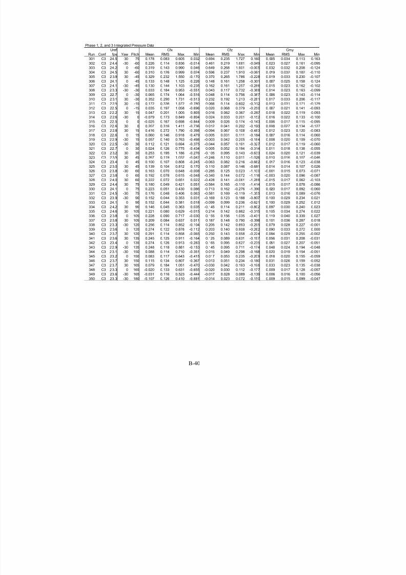
7/31/2019 Wind Tunnel Test
http://slidepdf.com/reader/full/wind-tunnel-test 184/243
B-40
Phase 1, 2, and 3 Integrated Pressure Data
Uref
Run Conf fps Yaw Pitch Mean RMS Max Min Mean RMS Max Min Mean RMS Max Min
301 C3 24.5 -30 -75 0.178 0.083 0.605 0.032 0.694 0.235 1.727 0.160 0. 005 0.034 0.113 -0.163
302 C3 24.4 -30 -60 0.226 0.114 0.836 -0.014 0.461 0.219 1.681 -0.049 0.023 0.027 0.161 -0.095
303 C3 24.2 0 -60 0.319 0.143 0.990 0.046 0.649 0.268 1.901 -0.005 0.032 0.032 0.208 -0.124
304 C3 24.5 30 -60 0.310 0.126 0.999 0.024 0.596 0.237 1.910 -0.061 0. 019 0.032 0.182 -0.110
305 C3 23.9 30 -45 0.329 0.232 1.550 -0.170 0.370 0.265 1.786 -0.228 0.019 0.033 0.230 -0.107306 C3 24.1 0 -45 0.133 0.148 1.125 -0.226 0.148 0.161 1.258 -0.301 0. 007 0.025 0.158 -0.124
307 C3 24.1 -30 -45 0.130 0.144 1.103 -0.235 0.162 0.161 1.257 -0.286 0.015 0.023 0.162 -0.102
308 C3 23.3 -30 -30 0.033 0.184 0.953 -0.551 0.043 0.117 0.732 -0.388 0.014 0.023 0.163 -0.099
309 C3 22.7 0 -30 0.065 0.174 1.064 -0.516 0.048 0.114 0.756 -0.387 0. 006 0.023 0.143 -0.114
310 C3 23.1 30 -30 0.352 0.290 1.731 -0.513 0.232 0.192 1.213 -0.281 0.017 0.033 0.206 -0.117
311 C3 22.5 30 -15 0.172 0.336 1.572 -0.780 0.066 0.114 0.602 -0.312 0.013 0.031 0.171 -0.129
312 C3 22.5 0 -15 0.035 0.197 1.058 -0.696 0.020 0.068 0.379 -0.250 0. 007 0.021 0.141 -0.093
313 C3 22.2 -30 -15 -0.047 0.201 1.005 -0.805 0.016 0.062 0.367 -0.287 0.018 0.022 0.119 -0.093
314 C3 22.6 -30 0 -0.079 0.173 0.849 -0.804 0.024 0.033 0.201 -0.152 0.016 0.022 0.133 -0.100
315 C3 22.5 0 0 -0.025 0.167 0.698 -0.844 0.009 0.026 0.174 -0.143 0.006 0.017 0.115 -0.095
316 C3 22.6 30 0 0.207 0.316 1.411 -0.736 0.012 0.041 0.202 -0.193 0.008 0.027 0.134 -0.127
317 C3 22.8 30 15 0.416 0.272 1.790 -0.398 -0.094 0.067 0.108 -0.483 0.012 0.023 0.120 -0.083
318 C3 22.6 0 15 0.060 0.146 0.918 -0.479 -0.005 0.031 0.111 -0.184 0. 007 0.016 0.114 -0.060
319 C3 22.9 -30 15 0.057 0.140 0.763 -0.498 -0.003 0.042 0.205 -0.184 0.008 0.020 0.109 -0.070
320 C3 22.5 -30 30 0.112 0.121 0.694 -0.375 -0.044 0.057 0.191 -0.327 0.012 0.017 0.119 -0.060
321 C3 22.7 0 30 0.024 0.126 0.775 -0.434 0.005 0.052 0.194 -0.314 0.011 0.018 0.138 -0.055
322 C3 23.2 30 30 0.253 0.195 1.186 -0.276 -0.105 0.095 0.143 -0.633 0.024 0.020 0.121 -0.039
323 C3 23.5 30 45 0.267 0.119 1.032 -0.042 -0.246 0.110 0.011 -1.026 0.010 0.016 0.107 -0.046
324 C3 23.4 0 45 0.100 0.107 0.808 -0.245 -0.063 0.082 0.216 -0.662 0. 017 0.016 0.123 -0.038
325 C3 23.0 -30 45 0.139 0.104 0.812 -0.170 -0.110 0.087 0.146 -0.681 0.014 0.014 0.107 -0.026
326 C3 23.8 -30 60 0.163 0.070 0.648 -0.008 -0.285 0.125 0.023 -1.100 -0.001 0.015 0.073 -0.071
327 C3 23.8 0 60 0.192 0.078 0.615 -0.048 -0.340 0.144 0.072 -1.116 -0.003 0.020 0.096 -0.087
328 C3 24.0 30 60 0.222 0.072 0.651 0.022 -0.428 0.141 -0.061 -1.288 -0.015 0.017 0.062 -0.103
329 C3 24.4 30 75 0.180 0.049 0.421 0.051 -0.584 0.165 -0.110 -1.414 0.015 0.017 0.078 -0.086
330 C3 24.1 0 75 0.223 0.051 0.430 0.086 -0.713 0.162 -0.276 -1.390 0. 020 0.017 0.092 -0.060
331 C3 24.5 -30 75 0.176 0.048 0.406 0.063 -0.581 0.169 -0.119 -1.355 0.013 0.016 0.089 -0.076
332 C3 23.9 -30 90 0.152 0.044 0.353 0.031 -0.169 0.123 0.188 -0.807 0.100 0.029 0.234 0.021
333 C3 24.1 0 90 0.152 0.044 0.381 0.018 -0.099 0.099 0.236 -0.621 0.100 0.029 0.252 0.012
334 C3 2 4.2 30 90 0.146 0.045 0.363 0.035 -0.145 0.114 0.211 -0.802 0.097 0.030 0.240 0.023
335 C3 24.6 30 105 0.221 0.080 0.629 -0.015 0.214 0.142 0.862 -0.315 0.105 0.034 0.274 0.022
336 C3 2 3.8 0 105 0.228 0.090 0.717 -0.030 0.155 0.156 1.035 -0.431 0.119 0.040 0.339 0.027
337 C3 23.8 -30 105 0.209 0.084 0.637 -0.011 0.187 0.148 0.790 -0.398 0.101 0.036 0.287 0.018
338 C3 23.3 -30 120 0.256 0.114 0.852 -0.104 0.205 0.142 0.893 -0.295 0.079 0.028 0.227 -0.001
339 C3 2 3.6 0 120 0.274 0.122 0.878 -0.112 0.203 0.140 0.908 -0.262 0.090 0.033 0.272 0.000
340 C3 23.7 30 120 0.291 0.114 0.858 -0.065 0.250 0.143 0.958 -0.224 0.084 0.029 0.255 -0.002341 C3 23.6 30 135 0.245 0.125 0.911 -0.164 0.125 0.089 0.631 -0.197 0.056 0.031 0.208 -0.031
342 C3 23.4 0 135 0.274 0.126 0.913 -0.283 0.165 0.095 0.627 -0.235 0. 051 0.027 0.207 -0.051
343 C3 22.9 -30 135 0.248 0.118 0.881 -0.153 0.145 0.095 0.711 -0.174 0.048 0.024 0.194 -0.048
344 C3 23.1 -30 150 0.088 0.114 0.710 -0.351 0.015 0.049 0.298 -0.168 0.020 0.019 0.154 -0.051
345 C3 23.2 0 150 0.083 0.117 0.643 -0.415 0.017 0.053 0.235 -0.209 0. 018 0.020 0.155 -0.059
346 C3 23.7 30 150 0.115 0.134 0.807 -0.367 0.013 0.051 0.234 -0.180 0.031 0.026 0.159 -0.052
347 C3 23.7 30 165 0.079 0.184 1.051 -0.470 -0.030 0.042 0.193 -0.196 0.033 0.023 0.135 -0.038
348 C3 23.3 0 165 -0.020 0.133 0.631 -0.655 -0.020 0.030 0.112 -0.177 0.009 0.017 0.128 -0.057
349 C3 23.6 -30 165 -0.031 0.116 0.523 -0.444 -0.017 0.028 0.089 -0.139 0.006 0.016 0.100 -0.056
350 C3 23.3 -30 180 -0.107 0.126 0.410 -0.681 -0.014 0.023 0.072 -0.150 0.009 0.015 0.099 -0.047
Cfx Cfz Cmy
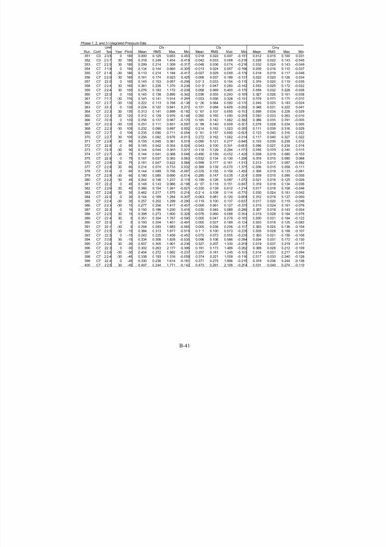
7/31/2019 Wind Tunnel Test
http://slidepdf.com/reader/full/wind-tunnel-test 185/243
B-41
Phase 1, 2, and 3 Integrated Pressure Data
Uref
Run Conf fps Yaw Pitch Mean RMS Max Min Mean RMS Max Min Mean RMS Max Min
351 C3 23.5 0 180 0.000 0.125 0.653 -0.453 -0.018 0.022 0.047 -0.151 0.012 0.015 0.100 -0.031
352 C3 23.7 30 180 0.318 0.249 1.454 -0.419 -0.042 0.033 0.068 -0.216 0.028 0.022 0.143 -0.045
353 C7 22.5 30 180 0.299 0.214 1.309 -0.317 -0.048 0.036 0.074 -0.216 0.032 0.024 0.143 -0.049
354 C7 21.9 0 180 0.134 0.144 0.865 -0.305 -0.013 0.024 0.057 -0.166 0.009 0.016 0.110 -0.037
355 C7 21.8 -30 180 0.110 0.214 1.184 -0.417 -0.027 0.029 0.069 -0.176 0.018 0.019 0.117 -0.046356 C7 22.0 -30 165 0.161 0.174 0.923 -0.425 0.008 0.037 0.189 -0.131 0.022 0.020 0.126 -0.034
357 C7 22.0 0 165 0.145 0.153 0.957 -0.298 0.013 0.033 0.194 -0.115 0. 016 0.020 0.119 -0.035
358 C7 22.4 30 165 0.381 0.226 1.370 -0.238 0.019 0.047 0.260 -0.142 0.053 0.025 0.172 -0.022
359 C7 22.4 30 150 0.276 0.183 1.172 -0.238 0.058 0.069 0.400 -0.170 0.058 0.032 0.228 -0.026
360 C7 22.0 0 150 0.145 0.138 0.895 -0.342 0.036 0.055 0.293 -0.189 0. 027 0.026 0.161 -0.038
361 C7 22.2 -30 150 0.145 0.141 0.914 -0.266 0.033 0.056 0.328 -0.151 0.029 0.023 0.175 -0.032
362 C7 22.7 -30 135 0.222 0.113 0.768 -0.138 0.126 0.084 0.580 -0.170 0.045 0.025 0.183 -0.024
363 C7 22.3 0 135 0.224 0.122 0.841 -0.272 0.121 0.088 0.629 -0.252 0. 048 0.031 0.222 -0.041
364 C7 22.3 30 135 0.313 0.141 0.899 -0.192 0.167 0.107 0.695 -0.193 0.069 0.034 0.228 -0.029
365 C7 22.3 30 120 0.312 0.129 0.976 -0.146 0.260 0.165 1.090 -0.299 0.093 0.033 0.263 -0.010
366 C7 22.0 0 120 0.256 0.122 0.987 -0.129 0.185 0.142 1.062 -0.382 0. 086 0.035 0.291 -0.005
367 C7 22.3 -30 120 0.251 0.111 0.831 -0.097 0.199 0.140 0.959 -0.307 0.078 0.028 0.224 0.005
368 C7 22.3 -30 105 0.232 0.090 0.697 0.002 0.214 0.162 1.023 -0.355 0.111 0.039 0.316 0.029
369 C7 2 2.7 0 105 0.235 0.090 0.711 -0.054 0.161 0.157 0.990 -0.505 0.123 0.040 0.316 0.022
370 C7 22.7 30 105 0.256 0.092 0.676 -0.013 0.272 0.162 1.062 -0.314 0.117 0.040 0.327 0.022
371 C7 2 2.8 30 90 0.155 0.045 0.361 0.019 -0.090 0.121 0.277 -0.840 0.103 0.030 0.239 0.012
372 C7 22.6 0 90 0.145 0.042 0.354 0.024 -0.043 0.100 0.341 -0.600 0.096 0.027 0.234 0.016
373 C7 22.8 -30 90 0.144 0.044 0.363 0.022 -0.118 0.129 0.294 -1.073 0.095 0.029 0.240 0.015
374 C7 22.7 -30 75 0.144 0.041 0.368 0.046 -0.490 0.159 -0.052 -1.426 0.008 0.018 0.080 -0.103
375 C7 22.8 0 75 0.167 0.037 0.363 0.063 -0.532 0.134 -0.130 -1.256 0. 016 0.015 0.090 -0.068
376 C7 22.9 30 75 0.181 0.047 0.422 0.068 -0.599 0.177 -0.161 -1.513 0.013 0.017 0.087 -0.092
377 C7 22.9 30 60 0.214 0.074 0.733 0.032 -0.389 0.139 -0.070 -1.375 -0.006 0.015 0.058 -0.111
378 C7 22.6 0 60 0.144 0.089 0.756 -0.087 -0.225 0.155 0.159 -1.452 0. 008 0.019 0.123 -0.081
379 C7 22.9 -30 60 0.180 0.085 0.690 -0.014 -0.285 0.147 0.035 -1.204 0.009 0.015 0.095 -0.055
380 C7 22.2 -30 45 0.244 0.146 1.237 -0.119 -0.199 0.126 0.097 -1.072 0.021 0.016 0.125 -0.026
381 C7 22.2 0 45 0.148 0.143 0.966 -0.198 -0.107 0.118 0.151 -0.847 0. 019 0.018 0.134 -0.036
382 C7 22.6 30 45 0.366 0.154 1.261 -0.021 -0.330 0.139 0.012 -1.214 0.017 0.018 0.108 -0.046
383 C7 22.8 30 30 0.462 0.217 1.575 -0.216 -0.214 0.108 0.114 -0.770 0.030 0.024 0.161 -0.042
384 C7 22.0 0 30 0.144 0.169 1.284 -0.307 -0.063 0.081 0.120 -0.658 0. 012 0.018 0.127 -0.050
385 C7 22.4 -30 30 0.257 0.202 1.299 -0.290 -0.119 0.100 0.137 -0.637 0.017 0.020 0.119 -0.046
386 C7 22.3 -30 15 0.277 0.256 1.417 -0.457 -0.050 0.061 0.127 -0.375 0.015 0.024 0.161 -0.076
387 C7 22.3 0 15 0.150 0.186 1.230 -0.416 -0.030 0.045 0.089 -0.285 0. 007 0.018 0.143 -0.054
388 C7 22.5 30 15 0.398 0.273 1.600 -0.328 -0.076 0.060 0.088 -0.394 0.019 0.028 0.164 -0.076
389 C7 22.4 30 0 0.351 0.304 1.767 -0.590 0.000 0.047 0.279 -0.185 0.000 0.031 0.184 -0.122
390 C7 22.5 0 0 0.193 0.204 1.401 -0.491 0.005 0.027 0.189 -0.124 0.003 0.018 0.125 -0.082391 C7 22.1 -30 0 0.258 0.293 1.683 -0.565 0.005 0.038 0.206 -0.157 0. 003 0.025 0.136 -0.104
392 C7 22.5 -30 -15 0.384 0.313 1.677 -0.519 0.111 0.100 0.573 -0.236 0.005 0.028 0.168 -0.107
393 C7 22.5 0 -15 0.242 0.225 1.458 -0.452 0.070 0.073 0.505 -0.238 0. 003 0.021 0.156 -0.106
394 C7 22.8 30 -15 0.334 0.306 1.828 -0.535 0.096 0.106 0.586 -0.284 0.004 0.031 0.172 -0.130
395 C7 22.4 30 -30 0.507 0.305 1.901 -0.236 0.327 0.207 1.330 -0.258 0.019 0.037 0.219 -0.117
396 C7 22.3 0 -30 0.302 0.263 2.177 -0.396 0.191 0.173 1.489 -0.262 0. 009 0.028 0.212 -0.109
397 C7 22.6 -30 -30 0.404 0.272 1.682 -0.237 0.257 0.181 1.245 -0.195 0.014 0.031 0.217 -0.094
398 C7 22.4 -30 -45 0.338 0.193 1.316 -0.059 0.374 0.221 1.599 -0.116 0.017 0.033 0.240 -0.126
399 C7 22.4 0 -45 0.330 0.236 1.614 -0.181 0.371 0.275 1.856 -0.215 0. 019 0.036 0.244 -0.136
400 C7 22.5 30 -45 0.407 0.244 1.771 -0.142 0.473 0.291 2.106 -0.254 0.031 0.040 0.274 -0.110
Cfx Cfz Cmy

7/31/2019 Wind Tunnel Test
http://slidepdf.com/reader/full/wind-tunnel-test 186/243
B-42
Phase 1, 2, and 3 Integrated Pressure Data
Uref
Run Conf fps Yaw Pitch Mean RMS Max Min Mean RMS Max Min Mean RMS Max Min
401 C7 22.5 30 -60 0.353 0.159 1.175 0.026 0.704 0.318 2.358 -0.026 0. 031 0.037 0.207 -0.122
402 C7 22.6 0 -60 0.354 0.175 1.205 0.005 0.725 0.349 2.413 -0.016 0.037 0.038 0.245 -0.113
403 C7 23.1 -30 -60 0.296 0.141 1.058 0.021 0.599 0.276 2.103 -0.015 0.028 0.035 0.235 -0.120
404 C7 22.9 -30 -75 0.204 0.090 0.716 0.029 0.801 0.244 2.041 0.173 0. 007 0.039 0.130 -0.181
405 C7 22.7 0 -75 0.258 0.104 0.835 0.003 1.017 0.259 2.272 0.210 0.010 0.045 0.151 -0.198406 C7 22.9 30 -75 0.241 0.094 0.783 0.068 0.831 0.239 1.973 0.225 -0. 012 0.039 0.111 -0.229
407 C7 22.9 30 -90 0.119 0.051 0.371 0.006 0.376 0.110 0.921 -0.005 -0.079 0.034 -0.004 -0.245
408 C7 23.0 0 -90 0.128 0.053 0.433 0.016 0.514 0.135 1.168 0.065 -0. 085 0.035 -0.010 -0.286
409 C7 23.0 -30 -90 0.112 0.056 0.384 -0.007 0.391 0.141 1.072 -0.040 -0.074 0.037 0.004 -0.254
410 C7 22.6 -30 -105 0.097 0.057 0.434 -0.009 -0.021 0.062 0.183 -0.413 -0.059 0.029 -0 .007 -0.219
411 C7 23.0 0 -105 0.103 0.059 0.498 -0.026 0.012 0.067 0.317 -0.345 -0.068 0.033 -0.006 -0.282
412 C7 22.7 30 -105 0.121 0.055 0.487 0.010 -0.024 0.060 0.247 -0.398 -0.073 0.029 -0.018 -0.261
413 C7 22.7 30 -120 0.164 0.062 0.484 -0.010 -0.128 0.061 0.077 -0.429 -0.052 0.019 -0 .006 -0.154
414 C7 22.6 0 -120 0.058 0.051 0.325 -0.086 -0.036 0.055 0.169 -0.298 -0.021 0.014 0.019 -0.100
415 C7 22.8 -30 -120 0.092 0.059 0.426 -0.057 -0.077 0.060 0.116 -0.416 -0.027 0.017 0.013 -0.122
416 C7 22.9 -30 -135 0.111 0.089 0.618 -0.134 -0.116 0.078 0.096 -0.529 0.002 0.013 0.059 -0.066
417 C7 22.8 0 -135 0.068 0.064 0.422 -0.123 -0.067 0.062 0.118 -0.381 -0.001 0.011 0.064 -0.049
418 C7 22.9 30 -135 0.246 0.095 0.676 -0.007 -0.222 0.087 0.011 -0.606 -0.011 0.016 0.068 -0.082
419 C7 22.6 30 -150 0.230 0.141 0.796 -0.251 -0.168 0.088 0.108 -0.598 0.020 0.022 0.143 -0.055
420 C7 22.3 0 -150 0.099 0.096 0.635 -0.220 -0.069 0.064 0.108 -0.452 0.007 0.016 0.092 -0.043
421 C7 22.4 -30 -150 0.123 0.135 0.812 -0.253 -0.101 0.080 0.108 -0.473 0.017 0.017 0.105 -0.040
422 C7 22.4 -30 -165 0.048 0.175 0.821 -0.467 -0.048 0.055 0.106 -0.305 0.022 0.020 0.113 -0.042
423 C7 22.3 0 -165 0.099 0.119 0.690 -0.350 -0.034 0.043 0.105 -0.272 0.005 0.017 0.105 -0.044
424 C7 22.5 30 -165 0.200 0.196 1.020 -0.357 -0.094 0.065 0.110 -0.389 0.026 0.023 0.140 -0.048
425 D3 22.7 45 180 1.023 0.266 2.103 0.281 -0.019 0.033 0.091 -0.169 0.012 0.022 0.112 -0.060
426 D3 22.5 30 180 0.752 0.197 1.731 0.199 0.020 0.039 0.126 -0.182 -0.013 0.026 0.121 -0.084
427 D3 22.8 0 180 0.518 0.134 1.152 0.069 0.038 0.030 0.125 -0.147 -0. 025 0.020 0.097 -0.082
428 D3 22.6 -30 180 0.260 0.100 0.719 -0.136 0.024 0.023 0.086 -0.117 -0.016 0.015 0.078 -0.057
429 D3 22.6 -30 -165 0.189 0.090 0.593 -0.179 -0.019 0.028 0.075 -0.200 -0.021 0.015 0.071 -0.065
430 D3 22.7 0 -165 0.421 0.120 0.977 -0.027 -0.049 0.039 0.084 -0.294 -0.041 0.021 0.073 -0.108
431 D3 22.7 30 -165 0.668 0.166 1.586 0.170 -0.126 0.057 -0.009 -0.453 -0.034 0.025 0.074 -0.112
432 D3 22.7 45 -165 0.915 0.254 1.995 0.270 -0.219 0.073 -0.017 -0.533 -0.017 0.021 0.068 -0.096
433 D3 22.7 45 -150 0.622 0.185 1.377 0.181 -0.311 0.106 -0.056 -0.712 -0.028 0.021 0.059 -0.117
434 D3 22.6 30 -150 0.447 0.124 1.135 0.004 -0.184 0.075 -0.002 -0.578 -0.043 0.024 0.083 -0.128
435 D3 22.7 0 -150 0.280 0.081 0.654 -0.011 -0.079 0.042 0.076 -0.342 -0.047 0.018 0.055 -0.103
436 D3 22.5 -30 -150 0.133 0.067 0.439 -0.148 -0.031 0.034 0.112 -0.301 -0.026 0.014 0.072 -0.077
437 D3 22.5 -30 -135 0.087 0.056 0.321 -0.140 -0.027 0.043 0.198 -0.231 -0.028 0.014 0.041 -0.078
438 D3 22.6 0 -135 0.163 0.063 0.491 -0.111 -0.063 0.050 0.160 -0.349 -0.047 0.016 0.048 -0.116
439 D3 22.6 30 -135 0.243 0.085 0.732 -0.025 -0.156 0.076 0.076 -0.607 -0.041 0.020 0.059 -0.126
440 D3 22.6 45 -135 0.387 0.136 1.120 0.012 -0.312 0.121 0.043 -0.882 -0.035 0.021 0.067 -0.142441 D3 22.2 45 -120 0.201 0.096 0.659 -0.019 -0.195 0.111 0.104 -0.752 -0.051 0.023 0.012 -0.159
442 D3 22.7 30 -120 0.110 0.054 0.418 -0.065 -0.080 0.070 0.196 -0.463 -0.037 0.015 0.027 -0.115
443 D3 22.6 0 -120 0.079 0.047 0.312 -0.107 -0.018 0.060 0.268 -0.328 -0.039 0.013 0.022 -0.095
444 D3 22.8 -30 -120 0.045 0.039 0.225 -0.096 -0.005 0.051 0.240 -0.261 -0.024 0.010 0.024 -0.068
445 D3 22.2 -30 -105 0.028 0.026 0.162 -0.093 0.007 0.062 0.436 -0.257 -0.019 0.010 0.022 -0.068
446 D3 22.7 0 -105 0.048 0.031 0.217 -0.085 -0.015 0.072 0.357 -0.382 -0.028 0.012 0.025 -0.090
447 D3 22.6 30 -105 0.047 0.035 0.253 -0.070 0.003 0.080 0.370 -0.408 -0.031 0.014 0.012 -0.109
448 D3 22.6 45 -105 0.111 0.067 0.442 -0.040 -0.049 0.099 0.284 -0.561 -0.063 0.030 0.003 -0.211
449 D3 22.7 45 -90 0.091 0.051 0.352 -0.049 0.079 0.114 0.583 -0.412 -0.060 0.034 0.032 -0.233
450 D3 22.6 30 -90 0.040 0.023 0.214 -0.042 0.121 0.091 0.603 -0.317 -0.027 0.015 0.028 -0.141
Cfx Cfz Cmy

7/31/2019 Wind Tunnel Test
http://slidepdf.com/reader/full/wind-tunnel-test 187/243
B-43
Phase 1, 2, and 3 Integrated Pressure Data
Uref
Run Conf fps Yaw Pitch Mean RMS Max Min Mean RMS Max Min Mean RMS Max Min
451 D3 23.0 0 -90 0.035 0.018 0.145 -0.060 0.104 0.075 0.576 -0.219 -0.023 0.012 0.040 -0.096
452 D3 22.2 -30 -90 0.022 0.015 0.128 -0.060 0.091 0.062 0.556 -0.204 -0.014 0.010 0.040 -0.084
453 D3 22.8 -30 -75 0.038 0.016 0.131 -0.032 0.187 0.073 0.583 -0.182 0.008 0.011 0.067 -0.065
454 D3 22.6 0 -75 0.066 0.019 0.161 -0.019 0.281 0.082 0.680 -0.138 0. 006 0.013 0.072 -0.077
455 D3 22.7 30 -75 0.083 0.026 0.232 -0.005 0.273 0.097 0.772 -0.199 -0.006 0.017 0.057 -0.122456 D3 22.4 45 -75 0.133 0.053 0.402 0.012 0.255 0.115 0.714 -0.245 -0.042 0.036 0.045 -0.206
457 D3 22.4 45 -60 0.252 0.089 0.733 0.019 0.424 0.137 1.053 -0.080 -0.004 0.035 0.113 -0.165
458 D3 22.5 30 -60 0.180 0.050 0.406 0.006 0.388 0.112 0.808 -0.051 0. 025 0.019 0.112 -0.089
459 D3 22.3 0 -60 0.176 0.046 0.385 0.006 0.387 0.100 0.849 -0.087 0.027 0.017 0.142 -0.066
460 D3 22.5 -30 -60 0.123 0.045 0.375 -0.057 0.265 0.092 0.804 -0.197 0.017 0.015 0.125 -0.079
461 D3 22.7 -30 -45 0.241 0.089 0.592 -0.097 0.254 0.094 0.696 -0.145 0.006 0.017 0.131 -0.064
462 D3 22.4 0 -45 0.368 0.099 0.813 -0.053 0.390 0.110 0.914 -0.174 0. 010 0.021 0.164 -0.092
463 D3 22.3 30 -45 0.378 0.103 0.775 -0.056 0.440 0.122 1.001 -0.103 0.029 0.024 0.205 -0.083
464 D3 2 2.2 45 -45 0.427 0.142 1.205 0.046 0.491 0.153 1.248 0.004 0.030 0.032 0.161 -0.109
465 D3 22.5 45 -30 0.679 0.201 1.578 0.114 0.478 0.147 1.181 -0.015 0. 049 0.035 0.233 -0.085
466 D3 22.6 30 -30 0.634 0.160 1.283 0.033 0.397 0.109 0.898 -0.084 0. 018 0.027 0.183 -0.093
467 D3 22.6 0 -30 0.552 0.146 1.113 -0.064 0.323 0.094 0.749 -0.174 0. 002 0.023 0.173 -0.107
468 D3 22.6 -30 -30 0.335 0.129 1.074 -0.224 0.195 0.080 0.683 -0.193 0.001 0.017 0.136 -0.066
469 D3 22.4 -30 -15 0.388 0.142 1.036 -0.416 0.101 0.043 0.384 -0.167 -0.002 0.014 0.132 -0.068
470 D3 22.4 0 -15 0.690 0.185 1.515 -0.010 0.178 0.058 0.495 -0.058 -0.004 0.019 0.122 -0.075
471 D3 2 2.6 30 -15 0.909 0.218 1.796 0.187 0.260 0.071 0.612 0.006 0.011 0.022 0.171 -0.069
472 D3 23.0 45 -15 0.918 0.247 2.089 0.228 0.300 0.092 0.706 -0.013 0. 035 0.031 0.198 -0.086
473 D3 23.0 45 0 1.158 0.307 2.564 0.319 0.034 0.038 0.258 -0.081 0.023 0.025 0.170 -0.054
474 D3 23.1 30 0 0.935 0.236 2.165 0.006 0.005 0.034 0.204 -0.105 0.004 0.022 0.135 -0.069
475 D3 23.0 0 0 0.681 0.186 1.531 0.008 -0.010 0.025 0.191 -0.086 -0.007 0.016 0.126 -0.057
476 D3 22.7 -30 0 0.357 0.145 0.971 -0.136 -0.003 0.019 0.153 -0.061 -0.002 0.013 0.101 -0.040
477 B3 22.3 -30 0 1.105 0.354 2.814 0.304 0.038 0.030 0.225 -0.052 0.025 0.020 0.149 -0.034
478 B3 22.8 0 0 1.832 0.462 3.696 0.671 0.039 0.034 0.231 -0.070 0.026 0.023 0.153 -0.046
479 B3 22.9 30 0 2.245 0.504 4.477 0.956 0.016 0.031 0.178 -0.089 0.010 0.021 0.118 -0.059
480 B3 22.7 45 0 2.290 0.500 4.319 1.077 0.022 0.033 0.170 -0.102 0.014 0.022 0.113 -0.068
481 B3 2 2.6 45 -15 2.205 0.498 4.337 0.911 0.670 0.156 1.327 0.244 0.050 0.029 0.197 -0.032
482 B3 2 2.8 30 -15 2.262 0.470 4.075 1.114 0.667 0.140 1.222 0.315 0.039 0.022 0.140 -0.039
483 B3 22.5 0 -15 1.668 0.422 3.647 0.382 0.493 0.130 1.093 0.113 0.030 0.020 0.116 -0.034
484 B3 22.3 -30 -15 1.058 0.348 2.576 0.282 0.328 0.112 0.849 0.088 0.029 0.017 0.122 -0.023
485 B3 22.6 -30 -30 0.937 0.299 2.296 0.210 0.586 0.184 1.411 0.128 0.026 0.015 0.121 -0.026
486 B3 22.6 0 -30 1.412 0.356 2.943 0.579 0.855 0.217 1.840 0.340 0.023 0.019 0.122 -0.067
487 B3 2 2.8 30 -30 1.826 0.417 3.378 0.858 1.097 0.250 2.027 0.502 0.024 0.025 0.142 -0.078
488 B3 2 2.5 45 -30 1.644 0.389 3.378 0.631 1.048 0.245 2.128 0.406 0.056 0.041 0.266 -0.065
489 B3 2 3.0 45 -45 1.026 0.275 2.224 0.416 1.287 0.352 2.832 0.502 0.122 0.047 0.346 -0.008
490 B3 2 2.6 30 -45 1.201 0.296 2.468 0.537 1.409 0.367 2.878 0.609 0.097 0.051 0.331 -0.016491 B3 22.5 0 -45 1.150 0.290 2.371 0.396 1.242 0.313 2.616 0.406 0.043 0.026 0.218 -0.040
492 B3 22.9 -30 -45 0.797 0.253 1.870 0.198 0.887 0.283 2.175 0.230 0.042 0.026 0.223 -0.034
493 B3 22.8 -30 -60 0.524 0.164 1.303 0.120 1.261 0.402 3.094 0.343 0.117 0.047 0.340 -0.025
494 B3 22.8 0 -60 0.676 0.188 1.405 0.250 1.587 0.461 3.349 0.556 0.138 0.054 0.355 -0.021
495 B3 2 3.4 30 -60 0.644 0.165 1.288 0.187 1.478 0.383 2.871 0.438 0.120 0.042 0.312 -0.020
496 B3 2 2.9 45 -60 0.569 0.170 1.321 0.200 1.231 0.371 2.843 0.374 0.081 0.039 0.273 -0.076
497 B3 22.6 45 -75 0.289 0.099 0.721 0.076 0.835 0.261 1.964 0.177 -0.042 0.032 0.075 -0.177
498 B3 22.8 30 -75 0.355 0.114 0.838 0.121 1.098 0.290 2.259 0.427 -0.039 0.038 0.085 -0.227
499 B3 22.4 0 -75 0.387 0.119 0.944 0.062 1.323 0.330 2.755 0.337 -0.021 0.040 0.123 -0.203
500 B3 23.0 -30 -75 0.292 0.114 0.780 0.011 1.087 0.332 2.654 0.368 -0.001 0.034 0.136 -0.143
Cfx Cfz Cmy
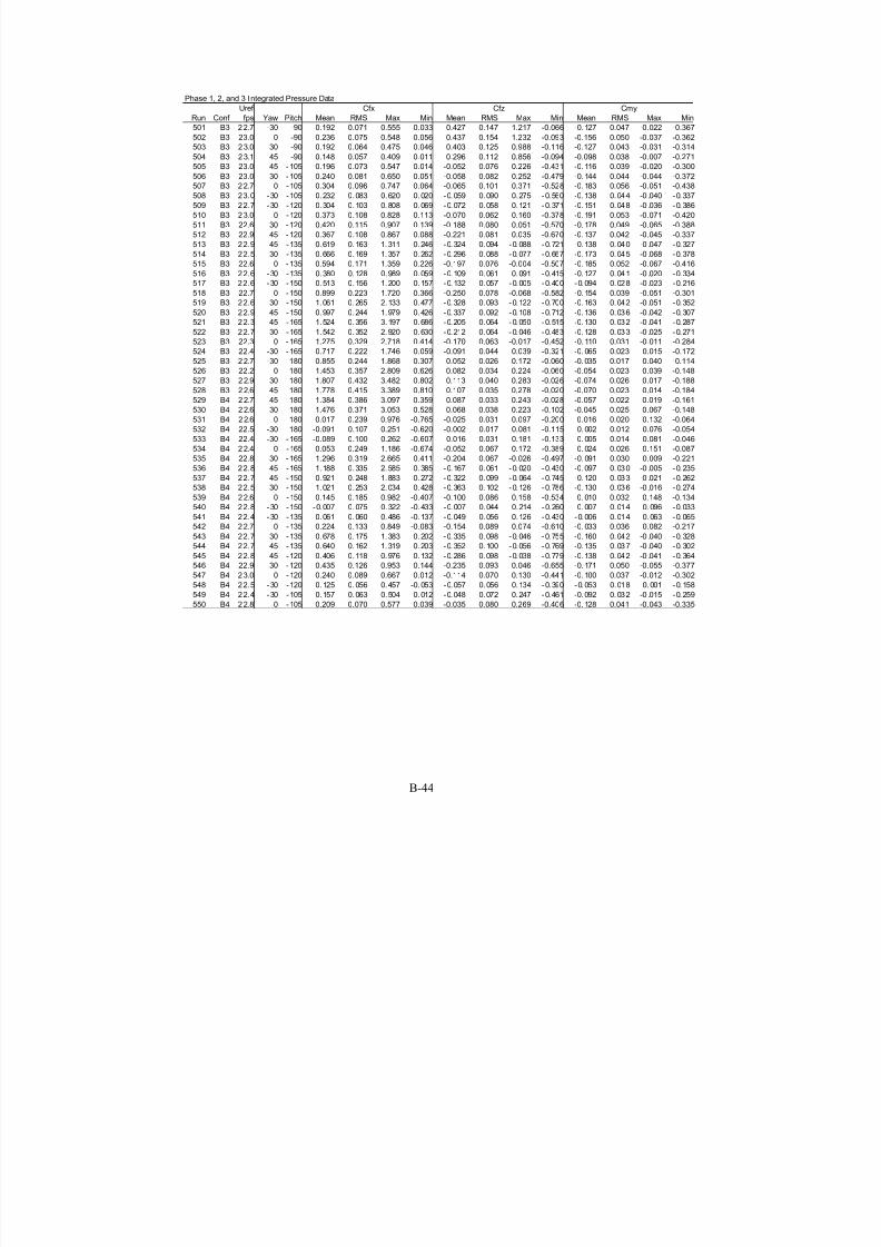
7/31/2019 Wind Tunnel Test
http://slidepdf.com/reader/full/wind-tunnel-test 188/243

7/31/2019 Wind Tunnel Test
http://slidepdf.com/reader/full/wind-tunnel-test 189/243
B-45
Phase 1, 2, and 3 Integrated Pressure Data
Uref
Run Conf fps Yaw Pitch Mean RMS Max Min Mean RMS Max Min Mean RMS Max Min
551 B4 22.6 30 -105 0.244 0.082 0.698 0.052 -0.059 0.084 0.256 -0.560 -0. 146 0.044 -0.045 -0.370
552 B4 22.7 45 -105 0.199 0.071 0.517 0.041 -0.052 0.072 0.211 -0.428 -0. 118 0.038 -0.030 -0.296
553 B4 22.7 45 -90 0.151 0.061 0.411 0.015 0.244 0.109 0.770 -0.176 -0.100 0.040 -0.010 -0.272
554 B4 22.6 30 -90 0.189 0.067 0.538 0.039 0.367 0.119 0.877 -0.080 -0.125 0.044 -0.026 -0.356
555 B4 22.9 0 -90 0.217 0.068 0.549 0.055 0.319 0.118 0.843 -0.086 -0.144 0.045 -0.036 -0.363556 B4 22.6 -30 -90 0.169 0.062 0.497 0.027 0.241 0.112 0.818 -0.231 -0. 112 0.041 -0.018 -0.328
557 B4 22.4 -30 -75 0.238 0.100 0.728 0.043 0.710 0.246 1.931 0.175 -0.030 0.040 0.106 -0.244
558 B4 22.5 0 -75 0.357 0.114 0.894 0.113 0.884 0.241 2.162 0.300 -0.077 0.049 0.095 -0.302
559 B4 22.6 30 -75 0.318 0.101 0.837 0.091 1.053 0.269 2.189 0.417 -0.023 0.037 0.108 -0.222
560 B4 22.9 45 -75 0.266 0.089 0.645 0.041 0.778 0.244 1.719 0.079 -0.037 0.037 0.090 -0.181
561 B4 2 2.9 45 -60 0.540 0.147 1.169 0.188 1.140 0.308 2.468 0.373 0.068 0.034 0.230 -0.074
562 B4 2 2.9 30 -60 0.505 0.151 1.174 0.134 1.078 0.339 2.647 0.197 0.067 0.037 0.257 -0.058
563 B4 22.7 0 -60 0.452 0.199 1.322 0.044 0.810 0.332 2.345 0.003 0.009 0.042 0.203 -0.146
564 B4 22.7 -30 -60 0.223 0.107 0.799 -0.003 0.453 0.216 1.600 -0.139 0. 022 0.032 0.184 -0.125
565 B4 22.7 -30 -45 0.121 0.096 0.746 -0.212 0.147 0.114 0.851 -0.299 0. 012 0.023 0.135 -0.115
566 B4 2 2.4 0 -45 0.224 0.166 1.152 -0.197 0.254 0.198 1.367 -0.327 0.014 0.036 0.212 -0.163
567 B4 2 2.8 30 -45 0.819 0.305 1.970 0.096 0.985 0.390 2.504 0.033 0.078 0.051 0.318 -0.101
568 B4 2 2.7 45 -45 0.904 0.258 1.961 0.315 1.111 0.326 2.384 0.339 0.097 0.042 0.283 -0.029
569 B4 2 2.4 45 -30 1.253 0.347 2.534 0.430 0.793 0.234 1.783 0.241 0.040 0.039 0.243 -0.069
570 B4 2 2.5 30 -30 1.185 0.364 2.633 0.298 0.707 0.224 1.697 0.115 0.013 0.028 0.181 -0.106
571 B4 2 2.5 0 -30 0.091 0.221 1.319 -0.575 0.055 0.151 0.829 -0.475 0.001 0.037 0.200 -0.185
572 B4 22.6 -30 -30 0.054 0.125 0.544 -0.565 0.043 0.081 0.422 -0.387 0. 007 0.019 0.129 -0.085
573 B4 22.5 -30 -15 0.019 0.139 0.504 -0.706 0.014 0.049 0.234 -0.277 0. 005 0.016 0.096 -0.091
574 B4 22.9 0 -15 -0.036 0.239 1.236 -0.958 -0.011 0.090 0.393 -0.424 -0. 001 0.031 0.144 -0.161
575 B4 2 2.4 30 -15 1.491 0.427 3.302 0.423 0.416 0.123 0.940 0.097 0.011 0.022 0.121 -0.065
576 B4 2 2.7 45 -15 1.535 0.424 3.198 0.464 0.437 0.126 0.947 0.114 0.016 0.021 0.145 -0.052
577 B4 22.6 45 0 1.681 0.441 3.562 0.642 0.016 0.029 0.190 -0.131 0.011 0.019 0.125 -0.087
578 B4 22.4 30 0 1.771 0.494 3.683 0.546 0.018 0.036 0.194 -0.114 0.012 0.024 0.128 -0.075
579 B4 23.0 0 0 -0.006 0.249 1.130 -1.133 0.009 0.040 0.223 -0.205 0.006 0.027 0.148 -0.136
580 B4 2 2.7 -30 0 0.009 0.129 0.453 -0.777 0.005 0.024 0.140 -0.146 0.003 0.016 0.092 -0.096
581 D4 22.8 -30 0 0.028 0.128 0.632 -0.607 0.009 0.023 0.160 -0.133 0. 006 0.015 0.106 -0.088
582 D4 22.2 0 0 0.112 0.223 1.191 -0.587 0.015 0.035 0.249 -0.138 0.010 0.023 0.165 -0.091
583 D4 22.2 30 0 1.317 0.504 3.374 0.299 0.028 0.040 0.258 -0.130 0.019 0.026 0.170 -0.086
584 D4 22.4 45 0 0.848 0.383 2.664 0.019 0.025 0.042 0.245 -0.132 0.016 0.028 0.162 -0.087
585 D4 22.7 45 -15 0.681 0.348 2.733 -0.083 0.204 0.107 0.809 -0.083 0.014 0.028 0.176 -0.097
586 D4 22.6 30 -15 1.050 0.437 2.896 0.038 0.290 0.121 0.794 -0.044 0. 006 0.028 0.141 -0.114
587 D4 22.6 0 -15 0.081 0.218 1.594 -0.555 0.029 0.079 0.511 -0.260 0. 005 0.025 0.181 -0.115
588 D4 22.2 -30 -15 0.041 0.134 0.653 -0.612 0.015 0.049 0.289 -0.296 0.003 0.016 0.125 -0.112
589 D4 22.0 -30 -30 0.070 0.127 0.827 -0.499 0.045 0.084 0.598 -0.362 0.003 0.019 0.145 -0.093
590 D4 22.8 0 -30 0.086 0.163 0.900 -0.496 0.055 0.112 0.663 -0.387 0. 003 0.025 0.129 -0.139591 D4 22.5 30 -30 0.785 0.352 2.317 -0.031 0.516 0.241 1.635 -0.091 0.036 0.042 0.261 -0.100
592 D4 22.6 45 -30 0.570 0.297 1.976 -0.173 0.365 0.199 1.382 -0.187 0.021 0.034 0.207 -0.090
593 D4 22.4 45 -45 0.398 0.228 1.699 -0.030 0.470 0.285 2.160 -0.121 0.034 0.039 0.267 -0.079
594 D4 22.5 30 -45 0.563 0.273 1.769 0.004 0.670 0.331 2.146 -0.055 0. 050 0.044 0.254 -0.106
595 D4 22.2 0 -45 0.073 0.104 0.627 -0.250 0.080 0.119 0.777 -0.324 0. 003 0.023 0.139 -0.126
596 D4 22.3 -30 -45 0.049 0.088 0.583 -0.368 0.060 0.093 0.595 -0.440 0.005 0.018 0.120 -0.101
597 D4 22.2 -30 -60 0.045 0.047 0.336 -0.159 0.095 0.095 0.583 -0.385 0.006 0.017 0.109 -0.111
598 D4 22.6 0 -60 0.088 0.069 0.601 -0.071 0.168 0.126 0.987 -0.257 0. 005 0.021 0.112 -0.122
599 D4 22.5 30 -60 0.403 0.193 1.358 -0.097 0.688 0.313 2.333 -0.119 -0.004 0.037 0.194 -0.164
600 D4 22.5 45 -60 0.255 0.142 1.197 -0.030 0.515 0.261 2.077 -0.059 0.024 0.030 0.191 -0.127
Cfx Cfz Cmy

7/31/2019 Wind Tunnel Test
http://slidepdf.com/reader/full/wind-tunnel-test 190/243
B-46
Phase 1, 2, and 3 Integrated Pressure Data
Uref
Run Conf fps Yaw Pitch Mean RMS Max Min Mean RMS Max Min Mean RMS Max Min
601 D4 22.3 45 -75 0.150 0.087 0.601 0.001 0.428 0.191 1.509 -0.082 -0.022 0.040 0.089 -0.210
602 D4 22.1 30 -75 0.241 0.114 0.803 0.033 0.473 0.196 1.552 -0.007 -0.073 0.052 0.058 -0.323
603 D4 22.5 0 -75 0.064 0.036 0.354 -0.020 0.189 0.099 0.733 -0.202 -0.008 0.023 0.058 -0.185
604 D4 22.4 -30 -75 0.036 0.029 0.261 -0.046 0.118 0.092 0.697 -0.327 -0.003 0.019 0.064 -0.140
605 D4 22.3 -30 -90 0.024 0.030 0.228 -0.048 0.082 0.082 0.464 -0.294 -0.016 0.020 0.032 -0.151606 D4 22.7 0 -90 0.039 0.036 0.300 -0.041 0.115 0.090 0.578 -0.396 -0.026 0.024 0.027 -0.199
607 D4 22.5 30 -90 0.162 0.080 0.526 -0.010 0.134 0.116 0.722 -0.366 -0.107 0.053 0.007 -0.348
608 D4 22.3 45 -90 0.099 0.067 0.492 -0.040 0.179 0.116 0.748 -0.327 -0.066 0.044 0.026 -0.326
609 D4 22.7 45 -105 0.141 0.090 0.614 -0.032 -0.056 0.101 0.285 -0.594 -0.080 0.046 0.005 -0.323
610 D4 22.7 30 -105 0.212 0.106 0.673 -0.020 -0.069 0.109 0.341 -0.643 -0.124 0.054 -0 .011 -0.363
611 D4 22.7 0 -105 0.042 0.050 0.475 -0.061 0.027 0.084 0.376 -0.449 -0.032 0.024 0.023 -0.251
612 D4 22.6 -30 -105 0.022 0.037 0.298 -0.071 0.028 0.066 0.309 -0.296 -0.019 0.017 0.016 -0.151
613 D4 22.2 -30 -120 0.021 0.048 0.339 -0.148 0.001 0.057 0.264 -0.324 -0.012 0.013 0.036 -0.112
614 D4 22.6 0 -120 0.050 0.057 0.419 -0.155 -0.017 0.064 0.227 -0.387 -0.023 0.016 0.046 -0.137
615 D4 22.8 30 -120 0.311 0.130 0.816 0.018 -0.204 0.102 0.085 -0.606 -0.111 0.047 -0.014 -0.306
616 D4 22.3 45 -120 0.220 0.116 0.807 -0.037 -0.126 0.094 0.138 -0.577 -0.085 0.044 0.003 -0.318
617 D4 22.6 45 -135 0.359 0.173 1.087 0.025 -0.208 0.113 0.045 -0.696 -0.071 0.040 0.010 -0.249
618 D4 22.3 30 -135 0.559 0.207 1.339 0.099 -0.376 0.133 -0.030 -0.890 -0.086 0.043 0.033 -0.269
619 D4 22.5 0 -135 0.076 0.086 0.612 -0.180 -0.063 0.074 0.144 -0.505 -0.006 0.017 0.087 -0.097
620 D4 22.5 -30 -135 0.021 0.064 0.390 -0.250 -0.018 0.057 0.212 -0.344 -0.001 0.012 0.069 -0.058
621 D4 22.2 -30 -150 0.011 0.089 0.439 -0.394 -0.014 0.050 0.214 -0.279 0.004 0.015 0.095 -0.043
622 D4 22.3 0 -150 0.102 0.130 0.813 -0.253 -0.074 0.078 0.133 -0.522 0.008 0.019 0.108 -0.059
623 D4 22.7 30 -150 0.872 0.298 2.001 0.133 -0.408 0.132 -0.072 -0.879 -0.055 0.036 0.054 -0.206
624 D4 22.5 45 -150 0.567 0.255 1.645 0.072 -0.233 0.112 -0.001 -0.738 -0.054 0.035 0.041 -0.233
625 D4 22.2 45 -165 0.705 0.308 2.145 0.006 -0.131 0.070 0.032 -0.450 -0.037 0.032 0.052 -0.182
626 D4 22.3 30 -165 1.108 0.395 2.607 0.237 -0.246 0.084 -0.042 -0.611 -0.033 0.034 0.068 -0.186
627 D4 22.5 0 -165 0.061 0.160 0.903 -0.479 -0.046 0.055 0.100 -0.392 0.019 0.020 0.136 -0.037
628 D4 22.3 -30 -165 -0.031 0.104 0.398 -0.522 0.003 0.035 0.148 -0.210 0.003 0.016 0.111 -0.043
629 D4 22.4 -30 180 -0.029 0.116 0.547 -0.559 -0.004 0.021 0.069 -0.136 0.003 0.014 0.090 -0.046
630 D4 22.5 0 180 0.089 0.171 0.933 -0.539 -0.026 0.031 0.056 -0.192 0.017 0.020 0.127 -0.037
631 D4 22.4 30 180 1.177 0.402 2.699 0.177 -0.009 0.040 0.170 -0.184 0.006 0.027 0.122 -0.113
632 D4 22.6 45 180 0.753 0.328 2.151 0.048 0.009 0.038 0.176 -0.142 -0.006 0.025 0.094 -0.116
633 B5 22.7 -30 0 -0.027 0.140 0.633 -0.577 0.018 0.028 0.162 -0.101 0.012 0.019 0.107 -0.067
634 B5 23.1 0 0 0.529 0.390 2.590 -0.317 0.020 0.040 0.291 -0.142 0.013 0.027 0.193 -0.094
635 B5 22.6 30 0 1.733 0.487 3.584 0.564 0.014 0.034 0.201 -0.113 0.009 0.023 0.133 -0.074
636 B5 23.1 45 0 1.686 0.422 3.485 0.626 0.011 0.028 0.151 -0.105 0.007 0.018 0.100 -0.070
637 B5 2 3.2 45 -15 1.619 0.402 3.286 0.666 0.461 0.117 0.982 0.182 0.018 0.019 0.126 -0.058
638 B5 2 2.9 30 -15 1.483 0.413 3.207 0.379 0.416 0.120 0.930 0.084 0.012 0.021 0.129 -0.057
639 B5 2 2.8 0 -15 0.517 0.350 2.227 -0.357 0.155 0.109 0.703 -0.237 0.010 0.031 0.176 -0.136
640 B5 22.4 -30 -15 -0.018 0.166 0.880 -0.678 0.016 0.055 0.340 -0.269 0. 013 0.020 0.108 -0.080641 B5 22.4 -30 -30 0.032 0.154 0.947 -0.456 0.045 0.097 0.733 -0.296 0. 015 0.021 0.143 -0.092
642 B5 2 2.5 0 -30 0.543 0.347 2.385 -0.275 0.352 0.232 1.588 -0.274 0.022 0.039 0.209 -0.130
643 B5 2 3.1 30 -30 1.200 0.355 2.653 0.328 0.716 0.215 1.603 0.159 0.013 0.025 0.160 -0.079
644 B5 2 3.0 45 -30 1.269 0.344 2.875 0.372 0.802 0.234 1.841 0.184 0.040 0.039 0.249 -0.071
645 B5 2 3.0 45 -45 0.927 0.248 1.975 0.378 1.144 0.321 2.461 0.405 0.101 0.045 0.295 -0.035
646 B5 2 3.1 30 -45 0.848 0.304 2.131 0.071 1.007 0.385 2.678 0.063 0.074 0.049 0.320 -0.059
647 B5 2 2.6 0 -45 0.518 0.308 2.047 -0.179 0.605 0.382 2.569 -0.279 0.041 0.051 0.314 -0.111
648 B5 22.7 -30 -45 0.154 0.146 0.943 -0.169 0.191 0.166 1.188 -0.241 0. 017 0.025 0.165 -0.090
649 B5 22.8 -30 -60 0.242 0.128 0.973 0.019 0.505 0.252 1.843 -0.031 0.029 0.030 0.184 -0.100
650 B5 23.1 0 -60 0.543 0.248 1.469 0.071 1.024 0.439 2.749 0.137 0.028 0.043 0.252 -0.131
Cfx Cfz Cmy

7/31/2019 Wind Tunnel Test
http://slidepdf.com/reader/full/wind-tunnel-test 191/243
B-47
Phase 1, 2, and 3 Integrated Pressure Data
Uref
Run Conf fps Yaw Pitch Mean RMS Max Min Mean RMS Max Min Mean RMS Max Min
651 B5 2 3.0 30 -60 0.530 0.174 1.272 0.134 1.145 0.403 2.841 0.259 0.075 0.044 0.269 -0.068
652 B5 2 3.1 45 -60 0.551 0.144 1.218 0.218 1.208 0.319 2.680 0.428 0.084 0.036 0.269 -0.035
653 B5 23.1 45 -75 0.262 0.087 0.628 0.077 0.857 0.251 1.902 0.234 -0.021 0.038 0.114 -0.168
654 B5 2 2.7 30 -75 0.294 0.099 0.730 0.089 1.098 0.267 2.245 0.403 0.000 0.038 0.121 -0.164
655 B5 22.7 0 -75 0.391 0.133 0.979 0.096 0.987 0.273 2.343 0.348 -0.081 0.057 0.102 -0.331656 B5 23.2 -30 -75 0.210 0.094 0.776 0.036 0.704 0.248 2.036 0.132 -0.013 0.038 0.113 -0.216
657 B5 23.1 -30 -90 0.137 0.058 0.451 0.013 0.291 0.114 0.806 -0.132 -0. 091 0.038 -0.009 -0.298
658 B5 2 2.9 0 -90 0.209 0.074 0.590 0.042 0.435 0.139 1.089 0.007 -0.138 0.049 -0.028 -0.391
659 B5 22.9 30 -90 0.163 0.057 0.479 0.026 0.565 0.141 1.199 0.122 -0.108 0.038 -0.017 -0.317
660 B5 23.1 45 -90 0.140 0.055 0.391 0.019 0.389 0.132 1.162 -0.054 -0.093 0.036 -0.013 -0.259
661 B5 23.0 45 -105 0.203 0.074 0.648 -0.034 -0.001 0.077 0.308 -0.454 -0.130 0.039 -0 .014 -0.356
662 B5 23.0 30 -105 0.263 0.088 0.700 0.068 -0.009 0.088 0.358 -0.502 -0. 166 0.047 -0.064 -0.390
663 B5 23.0 0 -105 0.180 0.076 0.561 0.019 0.041 0.081 0.385 -0.328 -0.122 0.044 -0.034 -0.333
664 B5 22.9 -30 -105 0.107 0.054 0.366 -0.027 0.018 0.066 0.265 -0.326 -0.072 0.027 -0 .008 -0.198
665 B5 22.8 -30 -120 0.067 0.059 0.455 -0.089 -0.037 0.060 0.178 -0.392 -0.026 0.017 0.015 -0.152
666 B5 22.8 0 -120 0.198 0.114 0.683 -0.044 -0.093 0.081 0.148 -0.484 -0. 083 0.048 0.009 -0.290
667 B5 22.8 30 -120 0.427 0.121 0.911 0.125 -0.208 0.090 0.064 -0.576 -0. 176 0.048 -0.063 -0.392
668 B5 22.8 45 -120 0.395 0.117 0.888 0.126 -0.256 0.092 0.009 -0.709 -0. 141 0.043 -0.045 -0.340
669 B5 22.9 45 -135 0.570 0.164 1.349 0.173 -0.299 0.098 -0.051 -0.744 -0.127 0.038 -0 .030 -0.297
670 B5 22.8 30 -135 0.617 0.167 1.349 0.221 -0.283 0.091 -0.046 -0.706 -0.156 0.042 -0 .047 -0.346
671 B5 22.5 0 -135 0.276 0.155 0.994 -0.117 -0.158 0.093 0.113 -0.623 -0. 055 0.044 0.045 -0.257
672 B5 22.5 -30 -135 0.014 0.066 0.377 -0.219 -0.022 0.060 0.200 -0.335 0. 004 0.012 0.061 -0.050
673 B5 22.2 -30 -150 -0.028 0.092 0.439 -0.466 0.002 0.055 0.229 -0.296 0. 008 0.014 0.084 -0.036
674 B5 22.8 0 -150 0.370 0.246 1.589 -0.289 -0.161 0.101 0.131 -0.694 -0. 030 0.040 0.080 -0.212
675 B5 22.7 30 -150 0.940 0.263 2.051 0.303 -0.325 0.106 -0.077 -0.779 -0.125 0.035 -0 .014 -0.278
676 B5 22.7 45 -150 0.868 0.261 1.937 0.273 -0.297 0.102 -0.070 -0.725 -0.117 0.037 -0 .011 -0.282
677 B5 22.6 45 -165 1.219 0.349 2.755 0.341 -0.171 0.064 -0.016 -0.513 -0.100 0.031 -0 .006 -0.243
678 B5 22.8 30 -165 1.295 0.351 2.845 0.469 -0.197 0.070 -0.026 -0.499 -0.096 0.031 -0 .003 -0.244
679 B5 22.8 0 -165 0.429 0.293 1.671 -0.243 -0.091 0.064 0.084 -0.381 -0. 015 0.032 0.116 -0.159
680 B5 22.9 -30 -165 -0.053 0.112 0.374 -0.618 0.004 0.035 0.178 -0.156 0. 006 0.013 0.076 -0.038
681 B5 22.2 -30 180 -0.031 0.117 0.473 -0.525 -0.004 0.019 0.063 -0.122 0. 002 0.013 0.081 -0.042
682 B5 22.7 0 180 0.438 0.339 1.966 -0.308 0.001 0.039 0.168 -0.166 -0.001 0.026 0.110 -0.111
683 B5 22.7 30 180 1.410 0.364 2.885 0.472 0.074 0.038 0.247 -0.127 -0.049 0.025 0.084 -0.164
684 B5 22.4 45 180 1.359 0.380 2.913 0.409 0.095 0.034 0.269 -0.041 -0.063 0.022 0.027 -0.178
685 D5 22.9 45 180 0.574 0.199 1.540 0.070 0.012 0.030 0.147 -0.117 -0.008 0.020 0.077 -0.097
686 D5 22.7 30 180 1.028 0.400 2.654 0.042 0.018 0.050 0.242 -0.143 -0.012 0.033 0.095 -0.160
687 D5 22.6 0 180 0.322 0.235 1.420 -0.207 -0.014 0.030 0.084 -0.184 0.009 0.020 0.122 -0.056
688 D5 22.3 -30 180 -0.002 0.122 0.612 -0.455 -0.003 0.020 0.068 -0.135 0.002 0.014 0.090 -0.045
689 D5 22.3 -30 -165 -0.021 0.122 0.584 -0.600 -0.003 0.039 0.154 -0.191 0.006 0.014 0.075 -0.044
690 D5 22.4 0 -165 0.285 0.219 1.542 -0.256 -0.078 0.063 0.054 -0.431 0.001 0.020 0.095 -0.079691 D5 22.2 30 -165 1.015 0.398 2.662 0.013 -0.195 0.083 0.020 -0.544 -0.050 0.041 0.095 -0.249
692 D5 22.7 45 -165 0.530 0.186 1.484 0.030 -0.099 0.051 0.040 -0.351 -0.028 0.021 0.055 -0.156
693 D5 23.0 45 -150 0.399 0.147 1.224 0.007 -0.164 0.073 0.059 -0.575 -0.038 0.021 0.036 -0.171
694 D5 22.4 30 -150 0.801 0.318 2.086 0.061 -0.329 0.134 -0.001 -0.850 -0.076 0.045 0.058 -0.265
695 D5 22.5 0 -150 0.204 0.166 1.102 -0.205 -0.113 0.090 0.101 -0.610 -0.003 0.020 0.093 -0.118
696 D5 22.5 -30 -150 0.010 0.099 0.565 -0.385 -0.016 0.059 0.195 -0.351 0.006 0.013 0.078 -0.038
697 D5 22.7 -30 -135 0.035 0.079 0.466 -0.221 -0.040 0.069 0.191 -0.357 0.003 0.012 0.059 -0.064
698 D5 22.1 0 -135 0.140 0.123 0.770 -0.131 -0.105 0.097 0.119 -0.638 -0.017 0.021 0.052 -0.135
699 D5 23.0 30 -135 0.526 0.220 1.365 0.020 -0.294 0.129 0.022 -0.803 -0.109 0.054 0.022 -0.335
700 D5 22.6 45 -135 0.256 0.108 0.908 -0.026 -0.148 0.078 0.077 -0.602 -0.051 0.025 0.034 -0.226
Cfx Cfz Cmy

7/31/2019 Wind Tunnel Test
http://slidepdf.com/reader/full/wind-tunnel-test 192/243
B-48
Phase 1, 2, and 3 Integrated Pressure Data
Uref
Run Conf fps Yaw Pitch Mean RMS Max Min Mean RMS Max Min Mean RMS Max Min
701 D5 22.8 45 -120 0.154 0.073 0.647 -0.018 -0.092 0.076 0.128 -0.562 -0.058 0.026 0.009 -0.225
702 D5 23.1 30 -120 0.326 0.139 0.946 0.034 -0.179 0.102 0.102 -0.637 -0.128 0.055 -0.015 -0.379
703 D5 22.7 0 -120 0.091 0.092 0.644 -0.113 -0.056 0.085 0.174 -0.540 -0.034 0.029 0.027 -0.213
704 D5 22.4 -30 -120 0.055 0.065 0.460 -0.115 -0.037 0.064 0.190 -0.382 -0.019 0.019 0.025 -0.153
705 D5 22.5 -30 -105 0.053 0.051 0.342 -0.052 0.011 0.064 0.357 -0.347 -0.036 0.026 0.014 -0.183706 D5 22.7 0 -105 0.065 0.065 0.470 -0.082 0.014 0.075 0.337 -0.431 -0.044 0.034 0.017 -0.243
707 D5 23.0 30 -105 0.220 0.110 0.737 -0.015 -0.077 0.116 0.266 -0.696 -0.128 0.058 -0 .010 -0.397
708 D5 23.1 45 -105 0.092 0.051 0.429 -0.028 -0.024 0.079 0.284 -0.484 -0.055 0.025 0.002 -0.233
709 D5 22.9 45 -90 0.066 0.040 0.344 -0.007 0.165 0.093 0.563 -0.433 -0.044 0.026 0.005 -0.228
710 D5 22.5 30 -90 0.173 0.082 0.566 -0.005 0.149 0.134 0.799 -0.443 -0.114 0.054 0.004 -0.374
711 D5 22.8 0 -90 0.072 0.056 0.421 -0.021 0.086 0.090 0.559 -0.314 -0.047 0.037 0.014 -0.279
712 D5 22.6 -30 -90 0.053 0.045 0.374 -0.025 0.081 0.075 0.399 -0.292 -0.035 0.030 0.016 -0.247
713 D5 22.9 -30 -75 0.069 0.049 0.441 -0.018 0.212 0.114 0.850 -0.140 -0.008 0.026 0.070 -0.193
714 D5 22.4 0 -75 0.107 0.074 0.567 -0.009 0.239 0.144 1.108 -0.164 -0.027 0.034 0.055 -0.240
715 D5 23.1 30 -75 0.233 0.111 0.793 -0.017 0.640 0.259 1.856 -0.050 -0.039 0.044 0.101 -0.278
716 D5 22.9 45 -75 0.103 0.041 0.363 0.007 0.418 0.158 1.288 -0.053 0. 005 0.025 0.112 -0.134
717 D5 22.6 45 -60 0.208 0.075 0.782 -0.020 0.426 0.153 1.455 -0.056 0.022 0.021 0.128 -0.101
718 D5 22.8 30 -60 0.378 0.177 1.151 -0.051 0.772 0.374 2.529 -0.253 0.039 0.042 0.281 -0.129
719 D5 23.0 0 -60 0.170 0.117 0.874 -0.032 0.296 0.199 1.439 -0.139 0. 000 0.025 0.125 -0.154
720 D5 22.7 -30 -60 0.096 0.075 0.560 -0.085 0.195 0.134 0.927 -0.236 0.009 0.020 0.095 -0.102
721 D5 22.3 -30 -45 0.091 0.116 0.794 -0.289 0.119 0.126 0.895 -0.262 0.013 0.020 0.135 -0.095
722 D5 22.6 0 -45 0.224 0.180 1.181 -0.160 0.247 0.208 1.433 -0.267 0. 011 0.029 0.199 -0.108
723 D5 22.4 30 -45 0.538 0.273 2.001 -0.064 0.650 0.347 2.398 -0.166 0.052 0.049 0.281 -0.085
724 D5 22.7 45 -45 0.300 0.120 0.884 -0.076 0.340 0.149 1.130 -0.165 0.019 0.026 0.171 -0.090
725 D5 23.1 45 -30 0.398 0.181 1.316 -0.071 0.252 0.130 0.943 -0.103 0.013 0.027 0.172 -0.073
726 D5 23.1 30 -30 0.716 0.401 2.388 -0.211 0.452 0.254 1.455 -0.248 0.022 0.036 0.214 -0.103
727 D5 22.8 0 -30 0.316 0.254 1.644 -0.268 0.208 0.173 1.153 -0.224 0. 014 0.030 0.205 -0.107
728 D5 22.7 -30 -30 0.047 0.136 0.829 -0.424 0.047 0.086 0.564 -0.310 0.011 0.018 0.121 -0.091
729 D5 22.8 -30 -15 0.029 0.157 0.819 -0.562 0.025 0.052 0.351 -0.225 0.011 0.017 0.118 -0.064
730 D5 23.0 0 -15 0.421 0.292 1.793 -0.256 0.127 0.092 0.583 -0.139 0. 009 0.025 0.174 -0.080
731 D5 22.8 30 -15 0.960 0.446 2.795 -0.078 0.275 0.130 0.810 -0.056 0.012 0.030 0.176 -0.092
732 D5 23.1 45 -15 0.567 0.222 1.687 -0.077 0.173 0.083 0.628 -0.087 0.013 0.026 0.191 -0.062
733 D5 22.9 45 0 0.675 0.226 1.959 -0.020 0.020 0.038 0.245 -0.084 0.013 0.025 0.162 -0.056
734 D5 23.1 30 0 1.133 0.480 3.194 -0.064 0.028 0.043 0.251 -0.134 0.018 0.029 0.166 -0.088
735 D5 23.0 0 0 0.405 0.295 2.022 -0.285 0.017 0.031 0.209 -0.107 0.011 0.021 0.139 -0.071
736 D5 22.8 -30 0 0.004 0.152 0.937 -0.616 0.018 0.025 0.154 -0.111 0. 012 0.017 0.102 -0.073
737 F3 20.0 -30 180 -0.159 0.151 0.491 -0.740 -0.024 0.033 0.081 -0.197 0. 016 0.022 0.130 -0.054
738 F3 20.2 0 180 -0.030 0.150 0.709 -0.655 -0.030 0.034 0.053 -0.232 0. 020 0.023 0.154 -0.035
739 F3 20.1 30 180 0.537 0.305 1.880 -0.340 -0.053 0.045 0.102 -0.298 0. 035 0.030 0.197 -0.068
740 F3 20.3 30 165 0.166 0.207 1.048 -0.526 -0.031 0.044 0.179 -0.197 0. 048 0.032 0.212 -0.056741 F3 20.3 0 165 -0.020 0.163 0.760 -0.827 -0.031 0.043 0.116 -0.252 0. 016 0.025 0.164 -0.061
742 F3 20.1 -30 165 -0.027 0.147 0.687 -0.592 -0.034 0.036 0.139 -0.191 0. 017 0.025 0.158 -0.049
743 F3 20.3 -30 150 0.107 0.145 0.833 -0.378 0.016 0.064 0.318 -0.222 0. 027 0.026 0.186 -0.052
744 F3 19.9 0 150 0.114 0.144 0.797 -0.609 0.033 0.068 0.328 -0.267 0.019 0.027 0.205 -0.081
745 F3 20.4 30 150 0.224 0.185 1.123 -0.345 0.035 0.066 0.328 -0.191 0.054 0.036 0.227 -0.050
746 F3 20.0 30 135 0.348 0.153 1.113 -0.150 0.207 0.114 0.750 -0.211 0.066 0.040 0.279 -0.060
747 F3 19.9 0 135 0.282 0.141 0.948 -0.235 0.189 0.116 0.741 -0.230 0.044 0.031 0.227 -0.054
748 F3 20.4 -30 135 0.254 0.139 0.993 -0.271 0.147 0.114 0.756 -0.320 0. 050 0.032 0.253 -0.070
749 F3 20.1 -30 120 0.307 0.142 1.100 -0.104 0.240 0.180 1.321 -0.406 0. 096 0.037 0.346 -0.001
750 F3 20.3 0 120 0.300 0.139 0.979 -0.159 0.226 0.175 1.175 -0.349 0.097 0.037 0.296 -0.020
Cfx Cfz Cmy

7/31/2019 Wind Tunnel Test
http://slidepdf.com/reader/full/wind-tunnel-test 193/243
B-49
Phase 1, 2, and 3 Integrated Pressure Data
Uref
Run Conf fps Yaw Pitch Mean RMS Max Min Mean RMS Max Min Mean RMS Max Min
751 F3 20.4 30 120 0.395 0.149 1.125 -0.043 0.334 0.186 1.273 -0.239 0.116 0.043 0.346 0.001
752 F3 2 0.4 30 105 0.364 0.115 0.999 0.060 0.374 0.182 1.314 -0.214 0.169 0.052 0.453 0.037
753 F3 20.3 0 105 0.358 0.129 0.939 0.051 0.397 0.238 1.491 -0.304 0.161 0.053 0.409 0.035
754 F3 20.3 -30 105 0.350 0.122 1.008 0.046 0.366 0.198 1.430 -0.329 0.161 0.053 0.448 0.047
755 F3 2 0.1 -30 90 0.295 0.078 0.623 0.106 0.047 0.156 0.625 -0.718 0.195 0.052 0.412 0.070756 F3 20.6 0 90 0.279 0.078 0.604 0.098 0.335 0.134 0.949 -0.317 0.185 0.051 0.400 0.065
757 F3 20.2 30 90 0.290 0.075 0.597 0.088 0.063 0.148 0.631 -0.691 0.192 0.050 0.395 0.059
758 F3 20.2 30 75 0.275 0.068 0.615 0.106 -0.704 0.207 -0.164 -1.719 0.055 0.026 0.163 -0.057
759 F3 2 0.1 0 75 0.292 0.069 0.605 0.120 -0.619 0.172 -0.153 -1.373 0.081 0.030 0.202 -0.054
760 F3 20.5 -30 75 0.235 0.063 0.517 0.088 -0.599 0.192 -0.099 -1.504 0. 047 0.025 0.156 -0.081
761 F3 20.1 -30 60 0.214 0.088 0.784 -0.011 -0.387 0.163 0.009 -1.500 -0. 005 0.019 0.100 -0.098
762 F3 19.6 0 60 0.291 0.099 0.829 0.005 -0.539 0.189 -0.008 -1.590 -0.011 0.021 0.091 -0.122
763 F3 20.1 30 60 0.338 0.107 0.979 0.082 -0.637 0.203 -0.142 -1.827 -0. 017 0.023 0.079 -0.133
764 F3 20.1 30 45 0.430 0.177 1.408 -0.045 -0.428 0.183 0.023 -1.396 0.001 0.021 0.103 -0.106
765 F3 2 0.4 0 45 0.086 0.112 0.930 -0.258 -0.057 0.094 0.209 -0.785 0.014 0.017 0.117 -0.044
766 F3 20.6 -30 45 0.168 0.113 0.897 -0.153 -0.141 0.100 0.119 -0.750 0. 012 0.015 0.109 -0.038
767 F3 19.7 -30 30 0.031 0.151 1.086 -0.534 0.015 0.071 0.251 -0.495 0.019 0.022 0.177 -0.072
768 F3 20.4 0 30 0.002 0.151 0.888 -0.549 0.016 0.062 0.247 -0.342 0.010 0.021 0.132 -0.070
769 F3 19.9 30 30 0.311 0.252 1.591 -0.425 -0.149 0.127 0.202 -0.835 0.018 0.026 0.163 -0.085
770 F3 19.8 30 15 0.553 0.377 2.175 -0.673 -0.134 0.095 0.147 -0.594 0.009 0.029 0.154 -0.122
771 F3 2 0.3 0 15 -0.041 0.188 0.855 -0.867 0.023 0.040 0.204 -0.194 0.008 0.022 0.148 -0.118
772 F3 20.3 -30 15 -0.056 0.183 0.732 -0.786 0.039 0.052 0.237 -0.165 0. 015 0.026 0.125 -0.072
773 F3 20.0 -30 0 -0.071 0.210 0.734 -0.869 0.017 0.045 0.215 -0.158 0.011 0.030 0.142 -0.104
774 F3 20.1 0 0 -0.025 0.230 1.202 -1.013 0.008 0.033 0.249 -0.190 0.005 0.022 0.165 -0.126
775 F3 20.4 30 0 0.461 0.410 2.243 -0.763 -0.007 0.051 0.235 -0.260 -0.005 0.034 0.156 -0.172
776 F3 20.1 30 -15 0.445 0.417 2.353 -0.941 0.125 0.144 0.767 -0.442 0.004 0.040 0.227 -0.160
777 F3 1 9.8 0 -15 0.031 0.248 1.214 -1.250 0.019 0.086 0.506 -0.483 0.007 0.026 0.214 -0.118
778 F3 19.8 -30 -15 -0.078 0.248 1.067 -1.024 -0.003 0.080 0.387 -0.375 0. 012 0.030 0.139 -0.118
779 F3 20.5 -30 -30 0.001 0.205 1.232 -0.605 0.024 0.129 0.893 -0.396 0. 013 0.027 0.163 -0.113
780 F3 1 9.9 0 -30 0.044 0.209 1.125 -0.737 0.036 0.137 0.759 -0.567 0.006 0.029 0.174 -0.164
781 F3 20.3 30 -30 0.438 0.355 2.143 -0.480 0.289 0.243 1.471 -0.295 0.021 0.042 0.267 -0.124
782 F3 19.9 30 -45 0.430 0.279 1.717 -0.272 0.475 0.319 1.985 -0.260 0.021 0.043 0.234 -0.184
783 F3 2 0.1 0 -45 0.131 0.172 1.139 -0.433 0.146 0.186 1.220 -0.547 0.007 0.033 0.180 -0.174
784 F3 20.3 -30 -45 0.150 0.167 1.139 -0.256 0.181 0.186 1.418 -0.310 0. 015 0.030 0.214 -0.148
785 F3 20.0 -30 -60 0.320 0.147 1.018 0.011 0.606 0.255 1.771 -0.051 0.017 0.037 0.187 -0.189
786 F3 20.6 0 -60 0.338 0.151 1.240 0.033 0.647 0.267 2.250 -0.011 0.020 0.041 0.183 -0.204
787 F3 2 0.3 30 -60 0.443 0.185 1.353 0.056 0.809 0.311 2.339 0.109 0.014 0.043 0.195 -0.185
788 F3 20.2 30 -75 0.327 0.111 0.800 0.085 0.920 0.235 2.061 0.212 -0.051 0.056 0.096 -0.316
789 F3 20.3 0 -75 0.312 0.114 0.919 0.061 0.869 0.249 2.150 0.109 -0.050 0.065 0.130 -0.359
790 F3 20.3 -30 -75 0.296 0.109 0.828 0.094 0.842 0.237 1.916 0.150 -0.045 0.058 0.107 -0.328791 F3 20.7 -30 -90 0.245 0.085 0.661 0.043 0.023 0.145 0.480 -0.816 -0. 162 0.057 -0.029 -0.437
792 F3 20.4 0 -90 0.299 0.101 0.805 0.074 -0.075 0.158 0.356 -0.955 -0.198 0.067 -0.049 -0.533
793 F3 20.7 30 -90 0.249 0.079 0.655 0.054 0.056 0.136 0.495 -0.564 -0.165 0.052 -0.035 -0.434
794 F3 20.3 30 -105 0.191 0.070 0.537 0.046 -0.121 0.094 0.161 -0.553 -0. 101 0.034 -0.028 -0.271
795 F3 20.3 0 -105 0.239 0.091 0.780 0.044 -0.200 0.123 0.218 -0.857 -0. 119 0.043 -0.029 -0.365
796 F3 20.6 -30 -105 0.164 0.071 0.591 0.009 -0.083 0.098 0.252 -0.655 -0.090 0.034 -0 .022 -0.281
797 F3 20.0 -30 -120 0.062 0.053 0.368 -0.103 -0.009 0.060 0.240 -0.301 -0.033 0.018 0.012 -0.132
798 F3 20.1 0 -120 0.086 0.060 0.454 -0.088 -0.014 0.064 0.283 -0.347 -0. 045 0.020 0.011 -0.171
799 F3 20.1 30 -120 0.134 0.062 0.519 -0.037 -0.066 0.061 0.169 -0.440 -0. 055 0.021 0.001 -0.169
800 F3 19.9 30 -135 0.289 0.130 0.973 -0.131 -0.263 0.111 0.069 -0.842 -0. 012 0.022 0.089 -0.127
Cfx Cfz Cmy

7/31/2019 Wind Tunnel Test
http://slidepdf.com/reader/full/wind-tunnel-test 194/243
B-50
Phase 1, 2, and 3 Integrated Pressure Data
Uref
Run Conf fps Yaw Pitch Mean RMS Max Min Mean RMS Max Min Mean RMS Max Min
801 F3 20.2 0 -135 0.050 0.076 0.415 -0.198 -0.065 0.073 0.151 -0.428 0. 007 0.016 0.100 -0.046
802 F3 20.3 -30 -135 -0.001 0.084 0.451 -0.291 -0.021 0.078 0.254 -0.443 0.010 0.015 0.080 -0.061
803 F3 19.6 -30 -150 -0.067 0.120 0.460 -0.539 0.010 0.069 0.245 -0.318 0. 017 0.020 0.123 -0.048
804 F3 20.2 0 -150 0.026 0.099 0.528 -0.310 -0.043 0.061 0.152 -0.395 0. 016 0.019 0.109 -0.047
805 F3 19.6 30 -150 0.385 0.204 1.248 -0.256 -0.240 0.106 0.098 -0.668 0. 010 0.026 0.146 -0.091806 F3 20.2 30 -165 0.681 0.306 1.998 -0.318 -0.187 0.080 0.096 -0.524 0. 003 0.029 0.177 -0.097
807 F3 20.1 0 -165 0.032 0.135 0.730 -0.531 -0.030 0.045 0.123 -0.304 0. 014 0.022 0.140 -0.057
808 F3 20.1 -30 -165 -0.054 0.159 0.654 -0.692 0.006 0.049 0.190 -0.243 0. 006 0.024 0.143 -0.058
809 F7 21.8 -30 -165 0.127 0.173 0.901 -0.329 -0.061 0.055 0.100 -0.299 0. 018 0.022 0.116 -0.051
810 F7 21.8 0 -165 0.108 0.129 0.914 -0.338 -0.039 0.047 0.082 -0.295 0. 006 0.019 0.102 -0.050
811 F7 22.2 30 -165 0.286 0.216 1.152 -0.507 -0.123 0.068 0.133 -0.404 0. 030 0.028 0.158 -0.058
812 F7 22.3 30 -150 0.257 0.155 0.890 -0.278 -0.182 0.084 0.128 -0.493 0. 019 0.024 0.120 -0.064
813 F7 22.3 0 -150 0.083 0.098 0.707 -0.190 -0.058 0.060 0.099 -0.406 0. 005 0.016 0.103 -0.048
814 F7 22.0 -30 -150 0.089 0.130 0.713 -0.319 -0.081 0.074 0.158 -0.417 0. 017 0.017 0.087 -0.048
815 F7 22.6 -30 -135 0.124 0.093 0.616 -0.113 -0.128 0.080 0.115 -0.555 0. 002 0.014 0.075 -0.060
816 F7 22.1 0 -135 0.082 0.076 0.515 -0.109 -0.078 0.070 0.103 -0.493 -0. 002 0.012 0.057 -0.059
817 F7 22.1 30 -135 0.279 0.107 0.722 -0.064 -0.242 0.094 0.085 -0.635 -0. 017 0.018 0.067 -0.098
818 F7 22.9 30 -120 0.140 0.054 0.444 -0.012 -0.085 0.052 0.114 -0.367 -0.052 0.018 -0 .002 -0.147
819 F7 22.4 0 -120 0.062 0.053 0.359 -0.067 -0.024 0.050 0.160 -0.270 -0. 028 0.018 0.014 -0.125
820 F7 22.3 -30 -120 0.078 0.055 0.402 -0.090 -0.047 0.052 0.181 -0.319 -0.029 0.018 0.014 -0.139
821 F7 22.7 -30 -105 0.123 0.064 0.518 -0.014 -0.046 0.083 0.245 -0.526 -0.071 0.030 -0 .012 -0.257
822 F7 22.5 0 -105 0.165 0.077 0.556 0.022 -0.106 0.094 0.183 -0.564 -0. 087 0.037 -0.020 -0.264
823 F7 22.5 30 -105 0.152 0.067 0.620 0.009 -0.054 0.085 0.226 -0.651 -0. 088 0.033 -0.022 -0.296
824 F7 22.3 30 -90 0.193 0.066 0.526 0.039 0.078 0.132 0.570 -0.514 -0.128 0.044 -0.026 -0.348
825 F7 22.7 0 -90 0.236 0.084 0.620 0.058 -0.058 0.133 0.344 -0.736 -0.156 0.055 -0.038 -0.410
826 F7 22.4 -30 -90 0.185 0.071 0.508 0.002 0.017 0.126 0.438 -0.630 -0. 123 0.047 -0.002 -0.336
827 F7 22.7 -30 -75 0.224 0.087 0.672 0.071 0.557 0.168 1.324 0.095 -0.048 0.049 0.073 -0.287
828 F7 2 2.5 0 -75 0.256 0.092 0.690 0.060 0.589 0.178 1.398 -0.013 -0.063 0.056 0.076 -0.322
829 F7 22.7 30 -75 0.262 0.088 0.696 0.071 0.598 0.161 1.321 0.015 -0.065 0.049 0.059 -0.305
830 F7 22.1 30 -60 0.362 0.153 1.036 -0.014 0.662 0.261 1.887 -0.052 0.012 0.036 0.151 -0.156
831 F7 2 2.4 0 -60 0.291 0.149 1.062 -0.002 0.522 0.251 1.970 -0.075 0.006 0.036 0.151 -0.149
832 F7 22.3 -30 -60 0.267 0.131 1.023 -0.009 0.490 0.214 1.788 -0.021 0. 009 0.034 0.164 -0.146
833 F7 22.2 -30 -45 0.321 0.218 1.511 -0.125 0.360 0.241 1.727 -0.177 0. 019 0.031 0.187 -0.136
834 F7 2 2.0 0 -45 0.306 0.221 1.607 -0.151 0.336 0.246 1.831 -0.190 0.014 0.032 0.246 -0.125
835 F7 22.2 30 -45 0.433 0.248 1.504 -0.063 0.511 0.290 1.807 -0.116 0.037 0.037 0.228 -0.101
836 F7 22.3 30 -30 0.495 0.327 2.309 -0.447 0.342 0.224 1.597 -0.299 0.032 0.037 0.247 -0.102
837 F7 2 2.4 0 -30 0.275 0.224 1.449 -0.385 0.181 0.147 0.977 -0.279 0.013 0.026 0.175 -0.108
838 F7 22.0 -30 -30 0.385 0.294 1.834 -0.451 0.258 0.194 1.243 -0.366 0. 020 0.032 0.185 -0.122
839 F7 22.0 -30 -15 0.415 0.363 2.078 -0.522 0.140 0.126 0.746 -0.187 0. 019 0.033 0.208 -0.086
840 F7 2 1.7 0 -15 0.261 0.239 1.529 -0.476 0.086 0.079 0.549 -0.149 0.010 0.022 0.154 -0.085841 F7 22.1 30 -15 0.340 0.369 2.038 -0.712 0.124 0.127 0.760 -0.306 0.021 0.034 0.204 -0.134
842 F7 22.1 30 0 0.256 0.353 1.862 -0.897 0.029 0.048 0.268 -0.162 0.019 0.032 0.177 -0.107
843 F7 22.2 0 0 0.214 0.219 1.445 -0.390 0.011 0.027 0.182 -0.106 0.007 0.018 0.120 -0.070
844 F7 2 1.9 -30 0 0.324 0.336 1.843 -0.549 0.021 0.040 0.281 -0.146 0.014 0.026 0.186 -0.097
845 C5 22.0 -30 0 0.143 0.261 1.625 -0.575 0.019 0.034 0.210 -0.143 0. 012 0.022 0.139 -0.095
846 C5 21.5 0 0 0.164 0.224 1.236 -0.591 0.010 0.030 0.213 -0.129 0.006 0.020 0.141 -0.085
847 C5 22.3 30 0 0.247 0.321 1.609 -0.759 0.016 0.044 0.264 -0.165 0.011 0.029 0.175 -0.109
848 C5 21.8 30 -15 0.244 0.333 1.835 -0.725 0.087 0.114 0.631 -0.300 0.014 0.030 0.179 -0.124
849 C5 21.7 0 -15 0.207 0.222 1.478 -0.524 0.063 0.068 0.516 -0.188 0. 005 0.021 0.150 -0.102
850 C5 21.9 -30 -15 0.246 0.283 1.692 -0.642 0.082 0.090 0.635 -0.303 0.010 0.025 0.176 -0.123
Cfx Cfz Cmy
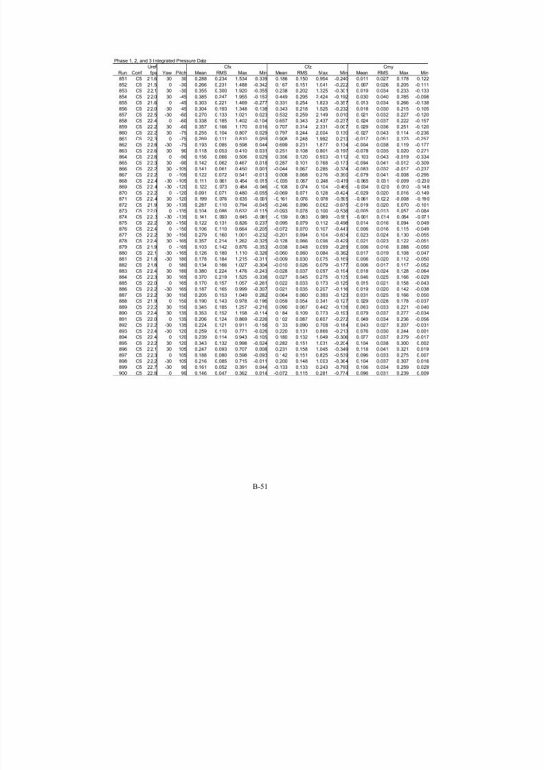
7/31/2019 Wind Tunnel Test
http://slidepdf.com/reader/full/wind-tunnel-test 195/243
B-51
Phase 1, 2, and 3 Integrated Pressure Data
Uref
Run Conf fps Yaw Pitch Mean RMS Max Min Mean RMS Max Min Mean RMS Max Min
851 C5 21.6 -30 -30 0.288 0.234 1.534 -0.339 0.186 0.150 0.954 -0.240 0.011 0.027 0.178 -0.122
852 C5 21.5 0 -30 0.266 0.231 1.488 -0.342 0.167 0.151 1.041 -0.222 0. 007 0.026 0.205 -0.111
853 C5 22.1 30 -30 0.355 0.300 1.920 -0.355 0.238 0.202 1.325 -0.301 0.019 0.034 0.233 -0.133
854 C5 22.0 30 -45 0.385 0.247 1.955 -0.152 0.449 0.295 2.424 -0.192 0.030 0.040 0.285 -0.098
855 C5 21.6 0 -45 0.303 0.221 1.469 -0.277 0.331 0.254 1.823 -0.357 0. 013 0.034 0.266 -0.138856 C5 22.0 -30 -45 0.304 0.193 1.348 -0.138 0.343 0.218 1.525 -0.232 0.018 0.030 0.215 -0.105
857 C5 22.5 -30 -60 0.270 0.133 1.021 0.023 0.532 0.259 2.149 0.010 0. 021 0.032 0.227 -0.120
858 C5 22.4 0 -60 0.338 0.185 1.402 -0.104 0.657 0.343 2.437 -0.237 0. 024 0.037 0.222 -0.157
859 C5 22.2 30 -60 0.357 0.166 1.170 0.016 0.707 0.314 2.331 -0.007 0. 029 0.036 0.251 -0.120
860 C5 22.2 30 -75 0.255 0.104 0.807 0.029 0.797 0.244 2.004 0.130 -0. 027 0.043 0.114 -0.236
861 C5 22.3 0 -75 0.269 0.111 0.810 0.059 0.908 0.248 1.992 0.213 -0.017 0.051 0.123 -0.257
862 C5 22.8 -30 -75 0.193 0.085 0.598 0.044 0.699 0.231 1.877 0.134 -0.004 0.038 0.119 -0.177
863 C5 22.6 -30 -90 0.118 0.053 0.410 -0.031 0.251 0.108 0.801 -0.197 -0.078 0.035 0.020 -0.271
864 C5 22.8 0 -90 0.156 0.066 0.506 0.029 0.356 0.120 0.903 -0.112 -0. 103 0.043 -0.019 -0.334
865 C5 22.3 30 -90 0.142 0.062 0.467 0.018 0.287 0.101 0.768 -0.173 -0.094 0.041 -0.012 -0.309
866 C5 22.2 30 -105 0.141 0.061 0.450 0.001 -0.044 0.067 0.285 -0.374 -0.083 0.032 -0.017 -0.237
867 C5 22.2 0 -105 0.122 0.072 0.541 -0.013 0.008 0.068 0.276 -0.390 -0.079 0.041 -0.008 -0.295
868 C5 22.4 -30 -105 0.111 0.061 0.454 -0.015 -0.035 0.067 0.248 -0.419 -0.065 0.031 -0 .009 -0.230
869 C5 22.4 -30 -120 0.122 0.073 0.484 -0.046 -0.108 0.074 0.104 -0.466 -0.034 0.020 0.010 -0.148
870 C5 22.2 0 -120 0.091 0.071 0.480 -0.055 -0.069 0.071 0.128 -0.424 -0.029 0.020 0.016 -0.149
871 C5 22.4 30 -120 0.199 0.076 0.635 -0.001 -0.161 0.076 0.078 -0.595 -0.061 0.022 -0 .008 -0.190
872 C5 21.9 30 -135 0.287 0.110 0.794 -0.045 -0.246 0.096 0.062 -0.675 -0.019 0.020 0.070 -0.101
873 C5 22.0 0 -135 0.104 0.086 0.632 -0.115 -0.093 0.078 0.100 -0.538 -0.005 0.013 0.057 -0.084
874 C5 22.3 -30 -135 0.141 0.093 0.645 -0.081 -0.139 0.083 0.089 -0.551 -0.001 0.014 0.054 -0.071
875 C5 22.2 -30 -150 0.122 0.131 0.826 -0.237 -0.095 0.079 0.112 -0.498 0.014 0.016 0.094 -0.049
876 C5 22.4 0 -150 0.106 0.110 0.664 -0.205 -0.072 0.070 0.107 -0.443 0.006 0.016 0.115 -0.049
877 C5 22.2 30 -150 0.279 0.160 1.001 -0.232 -0.201 0.094 0.104 -0.634 0.023 0.024 0.130 -0.055
878 C5 22.4 30 -165 0.357 0.214 1.262 -0.325 -0.128 0.066 0.096 -0.429 0.021 0.023 0.122 -0.051
879 C5 21.9 0 -165 0.103 0.142 0.876 -0.353 -0.038 0.048 0.099 -0.289 0.006 0.016 0.088 -0.050
880 C5 22.1 -30 -165 0.126 0.180 1.110 -0.326 -0.060 0.060 0.084 -0.362 0.017 0.019 0.108 -0.047
881 C5 21.8 -30 180 0.178 0.184 1.215 -0.311 -0.009 0.030 0.075 -0.169 0.006 0.020 0.112 -0.050
882 C5 21.8 0 180 0.134 0.166 1.027 -0.304 -0.010 0.026 0.079 -0.177 0.006 0.017 0.117 -0.052
883 C5 22.4 30 180 0.380 0.224 1.476 -0.243 -0.028 0.037 0.097 -0.194 0.018 0.024 0.128 -0.064
884 C5 22.3 30 165 0.370 0.219 1.525 -0.338 0.027 0.045 0.275 -0.135 0.046 0.025 0.166 -0.029
885 C5 22.0 0 165 0.170 0.157 1.057 -0.261 0.022 0.033 0.173 -0.125 0. 015 0.021 0.158 -0.043
886 C5 22.2 -30 165 0.187 0.165 0.999 -0.307 0.021 0.035 0.207 -0.116 0.019 0.020 0.142 -0.038
887 C5 22.2 -30 150 0.205 0.153 1.049 -0.282 0.064 0.060 0.393 -0.123 0.031 0.025 0.166 -0.050
888 C5 21.9 0 150 0.190 0.143 0.978 -0.196 0.059 0.054 0.341 -0.127 0. 029 0.028 0.178 -0.037
889 C5 22.2 30 150 0.345 0.185 1.257 -0.216 0.090 0.067 0.442 -0.136 0.063 0.033 0.221 -0.040
890 C5 22.4 30 135 0.353 0.152 1.158 -0.114 0.184 0.109 0.773 -0.193 0.079 0.037 0.277 -0.034891 C5 22.0 0 135 0.206 0.124 0.869 -0.226 0.102 0.087 0.607 -0.272 0. 049 0.034 0.236 -0.056
892 C5 22.2 -30 135 0.224 0.121 0.911 -0.158 0.133 0.090 0.708 -0.184 0.043 0.027 0.207 -0.031
893 C5 22.4 -30 120 0.259 0.110 0.771 -0.026 0.220 0.131 0.866 -0.213 0.076 0.030 0.244 0.001
894 C5 22.4 0 120 0.239 0.114 0.943 -0.105 0.180 0.132 1.049 -0.306 0. 077 0.037 0.279 -0.017
895 C5 22.2 30 120 0.343 0.132 0.998 -0.024 0.282 0.151 1.031 -0.204 0.104 0.038 0.300 0.002
896 C5 2 2.1 30 105 0.247 0.093 0.707 0.008 0.231 0.158 1.045 -0.349 0.118 0.041 0.321 0.019
897 C5 2 2.3 0 105 0.188 0.080 0.598 -0.093 0.142 0.151 0.825 -0.539 0.096 0.033 0.275 0.007
898 C5 22.2 -30 105 0.216 0.085 0.715 -0.011 0.200 0.148 1.003 -0.364 0.104 0.037 0.307 0.016
899 C5 22.7 -30 90 0.161 0.052 0.391 0.044 -0.133 0.133 0.243 -0.793 0.106 0.034 0.259 0.029
900 C5 22.8 0 90 0.146 0.047 0.362 0.014 -0.072 0.115 0.281 -0.774 0.096 0.031 0.239 0.009
Cfx Cfz Cmy

7/31/2019 Wind Tunnel Test
http://slidepdf.com/reader/full/wind-tunnel-test 196/243
B-52
Phase 1, 2, and 3 Integrated Pressure Data
Uref
Run Conf fps Yaw Pitch Mean RMS Max Min Mean RMS Max Min Mean RMS Max Min
901 C5 2 3.0 30 90 0.159 0.051 0.429 0.024 -0.115 0.124 0.267 -0.819 0.105 0.034 0.284 0.016
902 C5 22.5 30 75 0.204 0.056 0.536 0.071 -0.700 0.228 -0.166 -1.976 0.011 0.022 0.097 -0.129
903 C5 23.0 0 75 0.117 0.035 0.328 0.018 -0.392 0.153 0.028 -1.263 0.007 0.017 0.082 -0.094
904 C5 22.7 -30 75 0.140 0.045 0.374 0.042 -0.512 0.185 -0.080 -1.485 0.002 0.020 0.075 -0.116
905 C5 22.6 -30 60 0.238 0.101 0.776 0.008 -0.394 0.175 -0.011 -1.319 0.006 0.018 0.099 -0.083906 C5 22.4 0 60 0.160 0.106 0.775 -0.025 -0.241 0.179 0.071 -1.263 0. 012 0.018 0.108 -0.076
907 C5 22.4 30 60 0.310 0.099 0.752 0.080 -0.586 0.192 -0.127 -1.468 -0.017 0.020 0.077 -0.119
908 C5 22.6 30 45 0.441 0.165 1.352 0.021 -0.413 0.155 -0.035 -1.321 0.013 0.020 0.120 -0.069
909 C5 22.1 0 45 0.182 0.159 1.083 -0.124 -0.141 0.133 0.110 -1.035 0. 019 0.018 0.132 -0.035
910 C5 22.2 -30 45 0.291 0.175 1.397 -0.079 -0.242 0.151 0.061 -1.235 0.023 0.020 0.157 -0.029
911 C5 22.3 -30 30 0.309 0.215 1.369 -0.208 -0.131 0.102 0.138 -0.709 0.027 0.022 0.164 -0.033
912 C5 22.3 0 30 0.169 0.181 1.351 -0.298 -0.075 0.088 0.146 -0.711 0. 013 0.019 0.147 -0.044
913 C5 22.3 30 30 0.523 0.249 1.734 -0.055 -0.250 0.125 0.027 -0.914 0.030 0.028 0.168 -0.055
914 C5 22.3 30 15 0.412 0.282 2.003 -0.414 -0.080 0.062 0.096 -0.432 0.020 0.028 0.160 -0.079
915 C5 22.0 0 15 0.174 0.196 1.428 -0.332 -0.034 0.047 0.099 -0.364 0. 008 0.018 0.132 -0.066
916 C5 22.4 -30 15 0.243 0.229 1.530 -0.403 -0.039 0.052 0.095 -0.349 0.016 0.022 0.149 -0.056
Cfx Cfz Cmy

7/31/2019 Wind Tunnel Test
http://slidepdf.com/reader/full/wind-tunnel-test 197/243
B-53
Phase 4 Integrated Pressure Data
Phase 4 Integrated Pressure Data
Uref
Run Conf fps Yaw Pitch Mean RMS Max Min Mean RMS Max Min Mean RMS Max Min
1 I1 25.7 0 105 0.229 0.088 0.702 -0.040 0.164 0.146 0.856 -0.453 0.118 0.038 0.336 0.020
2 I1 25.4 0 75 0.143 0.037 0.361 0.035 -0.444 0.142 -0.037 -1.150 0.015 0.017 0.102 -0.081
3 I1 25.3 0 0 0.199 0.230 1.517 -0.554 0.009 0.029 0.228 -0.142 0.006 0.019 0.151 -0.0944 I1 25.2 0 -15 0.259 0.246 1.635 -0.352 0.081 0.082 0.525 -0.177 0.007 0.024 0.167 -0.087
5 I1 25.2 0 -60 0.350 0.195 1.585 -0.014 0.702 0.376 3.220 -0.122 0.032 0.041 0.315 -0.133
6 I4 25.6 0 0 0.277 0.271 1.704 -0.329 0.011 0.030 0.206 -0.113 0.007 0.020 0.136 -0.075
7 I4 25.9 0 -15 0.383 0.315 1.991 -0.297 0.112 0.098 0.677 -0.192 0.006 0.024 0.170 -0.105
8 I4 25.6 0 -60 0.438 0.227 1.454 -0.032 0.892 0.451 3.145 -0.034 0.044 0.047 0.329 -0.137
9 I4 25.5 0 105 0.211 0.092 0.753 0.010 0.161 0.139 0.994 -0.409 0.107 0.043 0.340 0.014
10 I4 25.4 0 75 0.115 0.052 0.442 0.009 -0.393 0.194 -0.010 -1.612 0.006 0.021 0.103 -0.097
11 I3 25.4 0 75 0.117 0.054 0.522 0.004 -0.397 0.207 0.054 -1.625 0.007 0.023 0.147 -0.142
12 I3 2 5.8 0 105 0.196 0.092 0.714 -0.095 0.150 0.145 0.930 -0.490 0.099 0.043 0.339 -0.008
13 I3 25.5 0 -60 0.403 0.219 1.478 -0.022 0.813 0.433 2.940 -0.072 0.038 0.049 0.314 -0.149
14 I3 25.9 0 -15 0.364 0.313 1.992 -0.425 0.109 0.101 0.694 -0.267 0.007 0.026 0.193 -0.113
15 I3 26.1 0 0 0.254 0.269 1.674 -0.371 0.010 0.030 0.230 -0.113 0.007 0.020 0.152 -0.075
16 I2 25.2 0 0 0.260 0.275 1.654 -0.404 0.010 0.031 0.207 -0.132 0.007 0.021 0.137 -0.087
17 I2 25.3 0 -15 0.324 0.300 1.947 -0.497 0.097 0.096 0.683 -0.221 0.007 0.026 0.199 -0.118
18 I2 25.4 0 -60 0.392 0.215 1.438 -0.050 0.791 0.424 2.977 -0.118 0.037 0.045 0.306 -0.153
19 I2 25.3 0 75 0.112 0.054 0.452 -0.002 -0.380 0.196 0.090 -1.550 0.007 0.022 0.110 -0.102
20 I2 25.4 0 105 0.199 0.089 0.665 -0.039 0.133 0.143 0.862 -0.503 0.104 0.042 0.314 0.00821 I1 25.5 30 105 0.338 0.103 0.838 0.071 0.268 0.143 0.896 -0.252 0.170 0.049 0.404 0.049
22 I1 25.4 30 75 0.220 0.052 0.430 0.079 -0.617 0.164 -0.210 -1.467 0.035 0.020 0.121 -0.062
23 I1 25.5 30 -60 0.367 0.184 1.271 -0.021 0.739 0.347 2.558 -0.044 0.034 0.042 0.243 -0.138
24 I1 25.4 30 -15 0.322 0.319 1.901 -0.625 0.119 0.115 0.741 -0.275 0.021 0.033 0.206 -0.117
25 I1 25.3 30 0 0.323 0.307 1.853 -0.585 0.020 0.046 0.292 -0.170 0.013 0.031 0.193 -0.113
26 I2 25.1 30 0 0.388 0.322 1.823 -0.619 0.024 0.050 0.275 -0.181 0.016 0.033 0.182 -0.120
27 I2 25.1 30 -15 0.337 0.327 1.993 -0.617 0.126 0.118 0.759 -0.235 0.023 0.035 0.208 -0.115
28 I2 2 5.2 30 -60 0.363 0.187 1.286 -0.015 0.735 0.359 2.469 0.005 0.035 0.041 0.267 -0.126
29 I2 25.1 30 75 0.230 0.052 0.466 0.084 -0.664 0.166 -0.182 -1.653 0.033 0.020 0.123 -0.090
30 I2 25.3 30 105 0.368 0.114 0.957 0.049 0.301 0.156 1.117 -0.227 0.184 0.055 0.467 0.044
31 I8 25.5 0 105 0.220 0.094 0.708 -0.037 0.158 0.130 0.817 -0.387 0.113 0.046 0.350 0.008
32 I8 25.7 0 75 0.122 0.054 0.421 -0.010 -0.414 0.197 0.040 -1.640 0.007 0.021 0.103 -0.128
33 I8 25.8 0 -60 0.394 0.246 1.738 -0.027 0.779 0.491 3.575 -0.085 0.032 0.048 0.365 -0.186
34 I8 26.1 0 -15 0.345 0.292 1.864 -0.367 0.102 0.092 0.583 -0.155 0.006 0.024 0.143 -0.089
35 I8 25.9 0 0 0.306 0.290 1.790 -0.340 0.010 0.030 0.214 -0.106 0.006 0.020 0.142 -0.070
36 I7 26.4 0 0 0.291 0.267 1.979 -0.357 0.009 0.029 0.255 -0.109 0.006 0.019 0.169 -0.072
37 I7 26.3 0 -15 0.383 0.314 1.840 -0.335 0.112 0.099 0.621 -0.169 0.006 0.024 0.171 -0.103
38 I7 25.6 0 -60 0.412 0.239 1.502 -0.056 0.826 0.484 3.206 -0.162 0.037 0.049 0.325 -0.162
39 I7 25.9 0 75 0.127 0.054 0.457 0.016 -0.439 0.197 -0.049 -1.687 0.006 0.022 0.121 -0.129
40 I7 26.2 0 105 0.207 0.091 0.685 -0.030 0.153 0.139 0.892 -0.425 0.106 0.043 0.342 0.011
41 I6 2 5.6 0 105 0.201 0.085 0.727 -0.051 0.150 0.137 0.927 -0.366 0.102 0.040 0.326 -0.004
42 I6 25.4 0 75 0.123 0.052 0.437 0.019 -0.402 0.198 -0.040 -1.607 0.010 0.021 0.104 -0.133
43 I6 25.4 0 -60 0.449 0.257 1.652 -0.007 0.923 0.535 3.457 -0.061 0.048 0.055 0.363 -0.146
44 I6 25.3 0 -15 0.385 0.307 2.016 -0.297 0.114 0.098 0.632 -0.129 0.007 0.024 0.162 -0.101
45 I6 25.5 0 0 0.290 0.250 1.736 -0.353 0.009 0.029 0.200 -0.102 0.006 0.019 0.132 -0.067
46 I5 25.1 0 0 0.282 0.230 1.598 -0.289 0.021 0.030 0.218 -0.100 0.014 0.020 0.144 -0.066
47 I5 25.2 0 75 0.201 0.043 0.420 0.070 -0.626 0.150 -0.104 -1.405 0.021 0.020 0.097 -0.096
48 I5 25.0 0 105 0.237 0.088 0.734 -0.035 0.192 0.147 0.986 -0.419 0.119 0.038 0.336 0.017
49 I5 25.0 0 -15 0.366 0.269 1.979 -0.417 0.112 0.089 0.717 -0.241 0.009 0.025 0.236 -0.119
50 I5 25.0 0 -60 0.389 0.205 1.532 -0.031 0.778 0.397 2.870 -0.058 0.035 0.042 0.286 -0.138
Cfx Cfz Cmy

7/31/2019 Wind Tunnel Test
http://slidepdf.com/reader/full/wind-tunnel-test 198/243
B-54
Phase 4 Integrated Pressure Data
Uref
Run Conf fps Yaw Pitch Mean RMS Max Min Mean RMS Max Min Mean RMS Max Min
51 I5 24.9 0 0 0.373 0.261 1.813 -0.303 0.007 0.029 0.221 -0.120 0.004 0.019 0.146 -0.079
52 I11 25.4 30 -60 0.322 0.189 1.296 -0.078 0.664 0.376 2.686 -0.118 0.035 0.041 0.283 -0.129
53 I11 25.2 30 -15 0.361 0.288 1.755 -0.364 0.119 0.102 0.644 -0.149 0.014 0.028 0.173 -0.084
54 I11 25.2 30 75 0.127 0.046 0.410 0.019 -0.472 0.198 -0.023 -1.607 0.000 0.020 0.086 -0.135
55 I11 25.5 30 105 0.275 0.099 0.761 0.018 0.202 0.142 0.886 -0.351 0.141 0.049 0.391 0.02356 I11 25.3 30 0 0.346 0.269 1.754 -0.287 0.021 0.039 0.228 -0.092 0.014 0.026 0.151 -0.061
57 I10 24.7 30 0 0.372 0.270 1.709 -0.260 0.024 0.040 0.272 -0.104 0.016 0.027 0.180 -0.069
58 I10 24.7 30 -15 0.412 0.308 1.944 -0.342 0.135 0.104 0.690 -0.166 0.016 0.027 0.177 -0.094
59 I10 25.2 30 -60 0.341 0.205 1.292 -0.073 0.681 0.388 2.636 -0.078 0.030 0.041 0.278 -0.146
60 I10 25.1 30 75 0.123 0.044 0.367 0.008 -0.471 0.191 0.082 -1.642 -0.002 0.019 0.075 -0.122
61 I10 25.3 30 105 0.264 0.097 0.761 0.011 0.197 0.137 0.994 -0.343 0.135 0.049 0.373 0.029
62 I9 2 5.5 30 105 0.247 0.089 0.771 -0.003 0.190 0.141 0.955 -0.383 0.125 0.041 0.358 0.018
63 I9 25.7 30 75 0.138 0.036 0.333 0.031 -0.449 0.143 -0.036 -1.286 0.011 0.018 0.085 -0.105
64 I9 25.1 30 -60 0.301 0.186 1.215 -0.073 0.585 0.351 2.342 -0.161 0.021 0.038 0.243 -0.144
65 I9 25.1 30 -15 0.221 0.208 1.265 -0.343 0.073 0.077 0.565 -0.188 0.009 0.023 0.197 -0.084
66 I9 25.1 30 0 0.194 0.204 1.299 -0.270 0.008 0.030 0.227 -0.091 0.006 0.020 0.150 -0.060
67 I7 25.3 30 0 0.389 0.271 1.720 -0.272 0.025 0.042 0.235 -0.099 0.017 0.028 0.155 -0.065
68 I7 25.4 30 -15 0.380 0.287 1.972 -0.338 0.126 0.104 0.710 -0.162 0.016 0.028 0.185 -0.098
69 I7 25.4 30 -60 0.347 0.205 1.336 -0.024 0.684 0.381 2.803 -0.028 0.028 0.039 0.250 -0.130
70 I7 25.6 30 75 0.120 0.040 0.384 0.014 -0.452 0.163 0.001 -1.341 -0.001 0.019 0.086 -0.111
71 I7 25.4 30 105 0.261 0.094 0.703 0.006 0.187 0.129 0.837 -0.336 0.135 0.047 0.352 0.032
72 I6 2 5.1 30 105 0.232 0.097 0.799 -0.005 0.165 0.152 0.930 -0.405 0.120 0.045 0.413 0.023
73 I6 25.4 30 75 0.133 0.043 0.385 0.021 -0.490 0.180 -0.065 -1.634 0.001 0.020 0.072 -0.130
74 I6 25.4 30 -60 0.330 0.183 1.289 -0.044 0.664 0.348 2.298 -0.061 0.031 0.039 0.242 -0.133
75 I6 25.3 30 -15 0.425 0.298 1.896 -0.243 0.144 0.110 0.680 -0.131 0.019 0.030 0.183 -0.075
76 I6 25.1 30 0 0.392 0.286 1.872 -0.238 0.029 0.045 0.259 -0.102 0.019 0.030 0.171 -0.067
77 I5 25.3 30 0 0.451 0.297 2.071 -0.490 0.030 0.043 0.246 -0.105 0.020 0.029 0.163 -0.069
78 I5 25.3 30 -15 0.420 0.272 1.730 -0.385 0.140 0.100 0.652 -0.152 0.017 0.028 0.183 -0.076
79 I5 25.3 30 -60 0.308 0.174 1.164 -0.025 0.598 0.320 2.227 -0.010 0.022 0.035 0.186 -0.123
80 I5 25.5 30 75 0.138 0.038 0.342 0.034 -0.493 0.169 -0.053 -1.510 0.004 0.019 0.077 -0.104
81 I5 25.6 30 105 0.273 0.094 0.758 0.021 0.194 0.136 0.948 -0.397 0.141 0.045 0.359 0.041
Cfx Cfz Cmy

7/31/2019 Wind Tunnel Test
http://slidepdf.com/reader/full/wind-tunnel-test 199/243
C-1
7.3 APPENDIX C - WIND CHARACTERISTICS SIMULATED IN A WIND TUNNEL
This section describes some of the primary parameters associated with winds in a thermally neutral
atmospheric boundary layer that are commonly simulated in a wind tunnel for proper measurement of
wind loads on a scaled model. These parameters specify mean, or time-averaged, and turbulencecharacteristics of winds which can then be related to the surface roughness of the field site.
C.1 Mean Wind Speed Characteristics
C.1.1. Power Law
Historically, the expression, which describes the mean wind profile over the height of the atmospheric
boundary layer, is the power law proposed by Hellman (1916). The power law is given by
U z U z
z R
R
( ) =F H G
I K J
α
(C.1)
where U is the mean wind speed, z is the height above the ground, and α is the power-law exponent
dependent on roughness of terrain and averaging time of measurements. The height z R is the reference
height, commonly 10 meters or 33 ft, and U R represents the wind speed at the reference height.
The power-law exponent is obtained by a linear regression of wind data measured at different heights on a
log-log basis as illustrated in Figure C-1(a). Recommended values of power-law exponent are tabulated
in Table C-1.
Table C-1 Recommended values of power-law exponent
Davenport (1965) ASCE A58.1 (1982)
Coastal Areas - 1/10 (0.10)
Open Terrain 0.16 1/7 (0.14)
Suburban Terrain 0.28 1/4.5 (0.22)
Center of Large City 0.4 1/3 (0.33)
C.1.2. Logarithmic LawAnother commonly used expression, particularly in micrometeorological practice, is the logarithmic law
that was developed from the similarity theory of a boundary layer flow over a flat plate. Because it has an
approximate theoretical basis, meteorologists regard the logarithmic law as a more suitable representation
of strong wind profiles than the power law in the lower atmosphere, say up to 50 meters. It is given by
U z u
k
z
z o( ) ln*
=F H G
I K J
(C.2)
in which u* is the shear velocity, z o is the aerodynamic roughness length, and k is the von Karman’s
constant, approximately 0.4. The shear velocity may be interpreted as a fluid velocity which would cause
a normal stress (i.e., dynamic pressure) equivalent to one half, in magnitude, of the shear stress occurring

7/31/2019 Wind Tunnel Test
http://slidepdf.com/reader/full/wind-tunnel-test 200/243
C-2
over a solid surface, and the roughness length as a height at which the fluid velocity in Equation 6.2
vanishes due to friction.
The roughness length, z o, is obtained by a regression on a linear-log basis as shown in Figure C-1(b).Values of z o corresponding to different types of surface roughness have been reported from various
sources, however considerable scatter exists from experiment to experiment. The variability is generallyattributed to local flow inhomogeneities that cannot be easily accounted for, and to some extent, the factthat the estimate of z o is extremely susceptible to accuracy involving wind speed measurements due to
extrapolation in the regression technique.
Typical roughness lengths for various types of terrain are given in Table C-2.
Table C-2 Typical surface roughness lengths, Simiu et al. (1996) Type of Surface zo (cm)
Sand 0.01-0.1
Snow surface 0.1-0.6
Mown grass (~0.01 m) 0.1-1
Low grass, steppe 1-4Fallow field 2-3
High grass 4-10
Palmetto 10-30
Pine forest 90-100
Sparsely built-up suburbs 20-40
Densly built-up suburbs 80-120
Center of large cities 200-300

7/31/2019 Wind Tunnel Test
http://slidepdf.com/reader/full/wind-tunnel-test 201/243
C-3
U/U(33 ft)
1
E l e v a t i o n ,
f t
10
100
20.90.80.70.60.5
Power-law
exponent
U/U(33 ft)
0.0 0.5 1.0 1.5
E l e v a t i o n ,
f t
0.01
0.1
1
10
100
Roughness length, z o
Figure C-1 Regression of wind speed data
C.2. Turbulence Characteristics
C.2.1. Local Turbulence Intensity
Of all the statistical measures of atmospheric turbulence, the turbulence (gustiness) intensity is thesimplest parameter. It is defined for the longitudinal component as
I z z
U z u
u( )( )
( )=
σ (C.3)
where I u is the local turbulence intensity and σ u(z) is the standard deviation of the velocity fluctuations in
the longitudinal direction at height z. Vertical and lateral turbulence intensity may be similarly defined.
Turbulence intensity can be estimated using several different available empirical equations. Lumley and
Panofsky (1964) suggests
I z Ck
z
z
u
o
( )
ln
=
F H G
I K J
(C.4)
where C is the constant that varies approximately from 2.0 to 2.5 depending on the roughness length z o,
see Simiu and Scanlan (1996). For a lower surface layer below a height of 100 m, Snyder (1981)

7/31/2019 Wind Tunnel Test
http://slidepdf.com/reader/full/wind-tunnel-test 202/243
C-4
proposed the following formula.
I z z
z z
u
o
o
( )
ln
ln
=
F H G
I K J
F H G
I K J
α
30
(C.5)
in which the heights are measured in full-scale meters, and α is the power-law exponent.
When a mean wind speed is relatively high, say above 20 mph, lateral turbulence intensity may beapproximated by the standard deviation of wind direction fluctuations. It can be shown that
I z z
v ( )( )
=
πσ θ
180. (C.6)
Here, I v is the lateral turbulence intensity and σ θ is the standard deviation of wind direction fluctuations
measured in degrees. The magnitude of lateral turbulence intensity is somewhat smaller than longitudinalcomponent. For example, empirical equations for velocity power spectral densities proposed by Kaimal
(1972), described below, imply that that
I z
I z
v
u
( )
( ).= 0 63. (C.7)
C.2.2 . Power Spectral Density
Velocity fluctuations of atmospheric turbulence are a random process, and turbulence can be regarded as
a combination of fluid motions by eddies of various sizes, each associated with a unique periodicity.
Contributions by these eddies to the total turbulence kinetic energy are conveniently described by a power
spectral density function. Power spectral densities of atmospheric turbulence are known to depend on the
measurement height, and commonly characterized by several distinct regions as illustrated in Figure C-2after Hinze (1975). Referring to the Figure, the inertial sub-range of turbulence is often considered to be
of particular significance as far as wind loads on civil engineering structures are concerned. This is
because structural natural frequencies typically fall in the inertial sub-range and the resulting quasi-steady
or resonance excitation is controlled by characteristics of this spectral range.

7/31/2019 Wind Tunnel Test
http://slidepdf.com/reader/full/wind-tunnel-test 203/243
C-5
S(n)
Frequency n , Hz
Inertial sub-range
Largest
eddies of
permanent
character
Energy-containnig
eddies
n ~ 0.2 n ~ 0.01 n ~ 2
Note: Frequency values are nominal, and vary depending on wind speed and height.
Figure C-2 A form of atmospheric turbulence spectrum, Hinze (1975)
Techniques to obtain a power spectrum density are readily available in a number of sources such as theone by Bendat and Piersol (1971), which involve a Fourier transform of velocity time series. Adescription of those techniques is beyond the scope of this report, and is omitted here. There are alsoseveral empirical equations for longitudinal atmospheric turbulence developed from field measurements.One of the earliest models was proposed by Davenport (1965), and subsequently adopted in the National
Building Code of Canada (1980), which is given by
nS n
u
x
x
( ).
( )*
/2
2
2 4 34 0
1=
+(C.8)
where S is the power spectral density, n is the frequency in Hz, and x is defined as
xn
U =
1200
10( )(C.9)
in which U (10) is the mean wind speed in meters per second at z = 10 m. It should be noted thatDavenport’s model does not account for the dependence of spectra on height. A more elaborate modelwas suggested by Kaimal (1972) as
nS z n
u
f
f
( , )
( )*
/2
200
1 50=
+ 5 3(C.10)
in which f is typically known as the reduced frequency defined by
f nz
U z =
( ). (C.11)

7/31/2019 Wind Tunnel Test
http://slidepdf.com/reader/full/wind-tunnel-test 204/243
C-6
Kaimal also proposed a model for the lateral turbulence spectrum as follows.
nS z n
u
f
f
v( , )
( . )*
/2
15
1 9 5=
+5 3
. (C.12)
To illustrate some of the noteworthy properties of a power spectral density, consider time series of wind
velocity fluctuations u(t ). Then
σ u
S n dn2
0=
∞
z ( ) (C.13)
and
RT
u t u t dt S n n dnuT T
T
( ) lim ( ) ( ) ( )cos( )τ τ = + =→∞ −
∞
π τ z z 1
22
0(C.14)
where Ru(τ ) is the auto-covariance function of the original velocity time series. Applying the spectral property in Equation (C.13) to the Kaimal’s longitudinal and lateral spectrum models above, it can be
shown that
(C.15)σ u
u2 6=*
2
for the longitudinal turbulence, and
σ v
u2 45
19=
*
2 (C.16)
for the lateral turbulence. Equations (I.15) and (I.16) yield
I z
I z
U z
U z
v
u
v
u
( )
( )
( )
( ).= =
σ
σ
0 63 (C.17)
as mentioned in the previous section.
C.2.3. Integral Length Scale
Integral scales of turbulence represent the average size of turbulence eddies in three orthogonal directions
associated with the longitudinal, lateral and vertical components of fluctuating velocity, i.e. a total of 9
scales to be considered. The most frequently evaluated length scale for characterization of winds and
load effects on standing structures is the longitudinal length scale associated with the longitudinal
turbulence. Formally, the longitudinal integral length scale is defined as
L R xux
u
u u=
∞
dxz 1
2 1 20
σ
( ) (C.18)
where Ru1u2( x) is the cross-covariance of the longitudinal turbulence components u1 and u2 measured at
two separate points in space with the longitudinal distance of x. However, a simplified approximation to
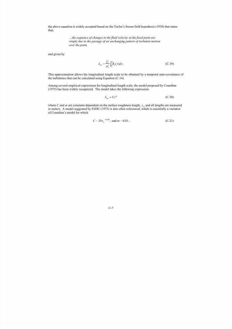
7/31/2019 Wind Tunnel Test
http://slidepdf.com/reader/full/wind-tunnel-test 205/243
C-7
the above equation is widely accepted based on the Taylor’s frozen field hypothesis (1938) that states
that;
…the sequence of changes in the fluid velocity at the fixed point are
simply due to the passage of an unchanging pattern of turbulent motion
over the point,
and given by
LU
R d ux
u
u=
∞
z σ
τ τ 2 0
( ) . (C.19)
This approximation allows the longitudinal length scale to be obtained by a temporal auto-covariance of
the turbulence that can be calculated using Equation (C.14).
Among several empirical expressions for longitudinal length scale, the model proposed by Counihan
(1975) has been widely recognized. The model takes the following expression.
(C.20) L Cz uxm
=
where C and m are constants dependent on the surface roughness length, z o, and all lengths are measuredin meters. A model suggested by ESDU (1975) is also often referenced, which is essentially a variation
of Counihan’s model for which
. (C.21)C z mo=−
25 0 350 063.
., and =

7/31/2019 Wind Tunnel Test
http://slidepdf.com/reader/full/wind-tunnel-test 206/243
C-8
References
American National Standard A58.1-1982, Minimum Design Loads for Buildings and Other Structures,American National Standard Institute, Inc., New York, 1982.
J. S. D. Bendat and A.G. Piersol, Random Data: Analysis and Measurement Procedures, A Wiley-
Interscience Publication, John Wiley & Sons, Inc., New York, 1971.
J. Counihan, “Adiabatic Atmospheric Boundary Layers: A Review and Analysis of Data from the Period1880-1972,” Atmos. Environ., 9 (1975), 871-905.
A. G. Davenport, “The Relationship of Wind Structure to Wind Loading,” in Proceedings of the
Symposium on Wind Effects on Buildings and Structures, Vol. 1, National Physical Laboratory,Teddington, U.K., Her Majesty’s Stationery Office, London, 1965, pp.53-102.
A. G. Davenport, “The Spectrum of Horizontal Gustiness Near the Ground in High Winds,” J. Royal
Meterol. Soc., 87 (1961) 194-211.
ESDU , “Characteristics of Atmospheric Turbulence Near the Ground,” Item No. 75001, EngineeringScience Data Unit, London, U.K., 1975.
National Building Code of Canada 1980, National Research Council of Canada, Associate Committee of the National Building Code, NRCC No. 17724, Ottawa, Canada, 1980.
G. Hellman, “Uber die Bewegung der Luft in den untersten Schichten der Atmospare,” Meteoro. Z ., 34(1916) 273.
J. O. Hinze, Turbulence, 2nd ed., McGraw-Hill Book Company, New York, 1975.
J. C. Kaimal et al., “Spectral Characteristics of Surface-Layer Turbulence,” J. Royal Meteorol. Soc., 98
(1972) 563-589.
J. L. Lumley and H. A. Panofsky, The Structure of Atmospheric Turbulence, John Wiley & Sons, Inc., New York, 1964.
E. Simiu and R. H. Scanlan, Wind Effects on Structures, 3rd ed., A Wiley-Interscience Publication, JohnWiley & Sons, Inc., New York, 1996.
D. H. Slade, editor, Meteorology and Atomic Energy 1968, Technical Information Center, U.S.Department of Energy, 1968.
W. H. Snyder, “Guideline for Fluid Modeling of Atmospheric Diffusion,” Report No. EPA600/8-81-009,USEPA, Environmental Services Research Laboratory, Office of Research and development, ResearchTriangle Park, New Jersey, 1981.
Taylor, G. I., “The Spectrum of Turbulence,” Proceedings of the Royal Soc., A164 (1938), 476-490.

7/31/2019 Wind Tunnel Test
http://slidepdf.com/reader/full/wind-tunnel-test 207/243
D-1
7.4 APPENDIX D - INSTANTANEOUS DIFFERENTIAL PRESSURE CONTOURSFOR SELECTED TEST CONFIGURATIONS

7/31/2019 Wind Tunnel Test
http://slidepdf.com/reader/full/wind-tunnel-test 208/243
D-2
Pitch: 0 deg.Peak Positive Differential
Pitch: 0 deg.Peak Negative Differential
Operational Mode, Yaw: -30 deg.
Configuration B1
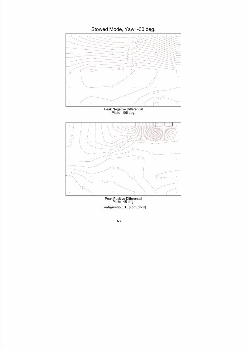
7/31/2019 Wind Tunnel Test
http://slidepdf.com/reader/full/wind-tunnel-test 209/243
D-3
Stowed Mode, Yaw: -30 deg.
Pitch: -105 deg.Peak Negative Differential
Peak Positive DifferentialPitch: -45 deg.
Configuration B1 (continued)

7/31/2019 Wind Tunnel Test
http://slidepdf.com/reader/full/wind-tunnel-test 210/243
D-4
Pitch: 0 deg.Peak Positive Differential
Peak Negative DifferentialPitch: 0 deg.
Operational Mode, Yaw: 0 deg.
Configuration B1 (continued)
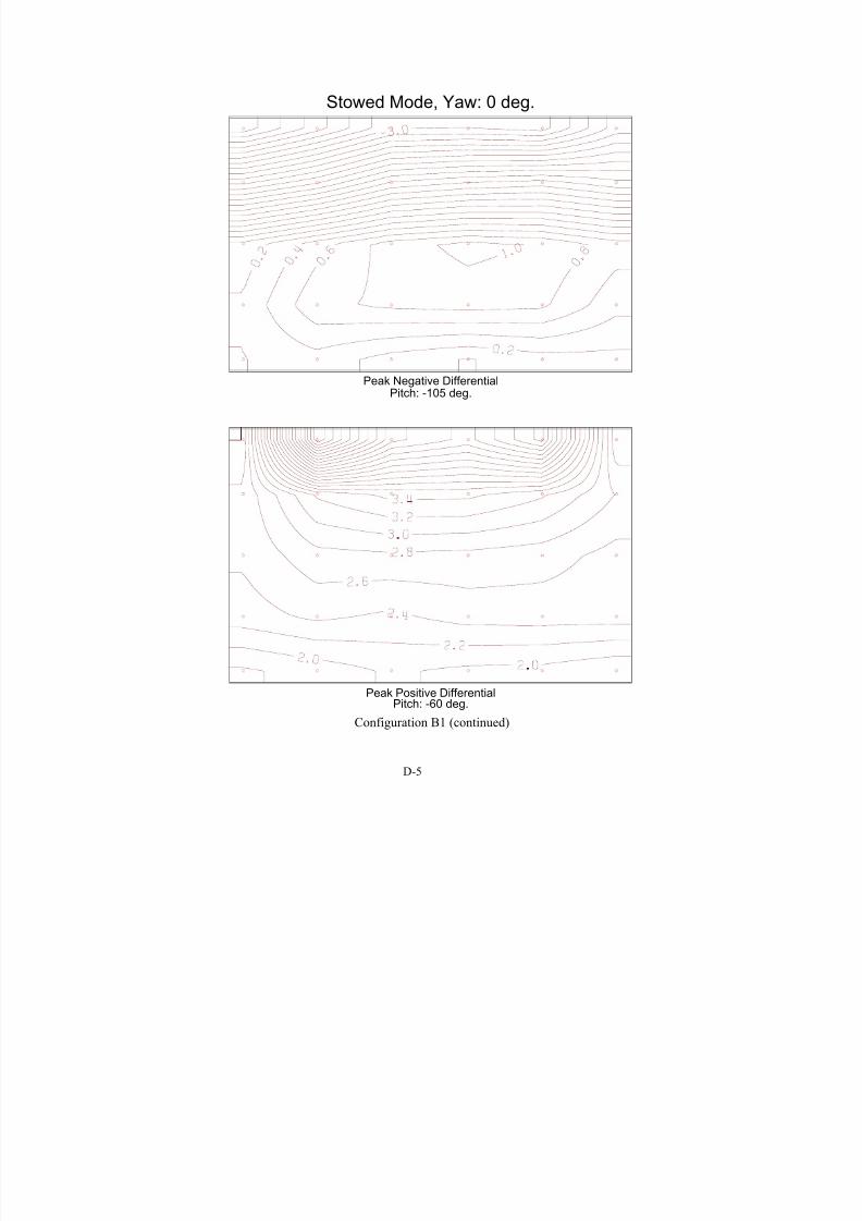
7/31/2019 Wind Tunnel Test
http://slidepdf.com/reader/full/wind-tunnel-test 211/243
D-5
Pitch: -60 deg.Peak Positive Differential
Peak Negative DifferentialPitch: -105 deg.
Stowed Mode, Yaw: 0 deg.
Configuration B1 (continued)
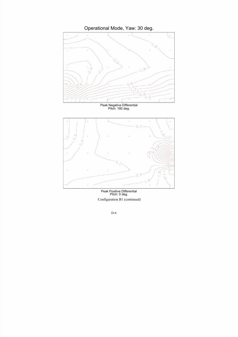
7/31/2019 Wind Tunnel Test
http://slidepdf.com/reader/full/wind-tunnel-test 212/243
D-6
Pitch: 0 deg.Peak Positive Differential
Peak Negative DifferentialPitch: 180 deg.
Operational Mode, Yaw: 30 deg.
Configuration B1 (continued)

7/31/2019 Wind Tunnel Test
http://slidepdf.com/reader/full/wind-tunnel-test 213/243
D-7
Pitch: -45 deg.Peak Positive Differential
Peak Negative DifferentialPitch: -90 deg.
Stowed Mode, Yaw: 30 deg.
Configuration B1 (continued)
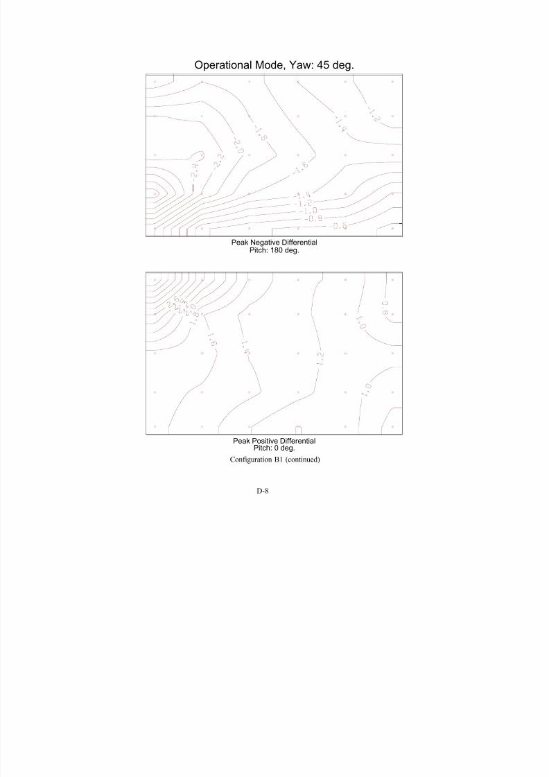
7/31/2019 Wind Tunnel Test
http://slidepdf.com/reader/full/wind-tunnel-test 214/243
D-8
Pitch: 0 deg.Peak Positive Differential
Pitch: 180 deg.Peak Negative Differential
Operational Mode, Yaw: 45 deg.
Configuration B1 (continued)

7/31/2019 Wind Tunnel Test
http://slidepdf.com/reader/full/wind-tunnel-test 215/243
D-9
Pitch: -45 deg.Peak Positive Differential
Pitch: -105 deg.Peak Negative Differential
Stowed Mode, Yaw: 45 deg.
Configuration B1 (continued)

7/31/2019 Wind Tunnel Test
http://slidepdf.com/reader/full/wind-tunnel-test 216/243
D-10
Pitch: 75 deg.Peak Positive Differential
Pitch: 120 deg.Peak Negative Differential
Operational Mode, Yaw: -30 deg.
Configuration C1
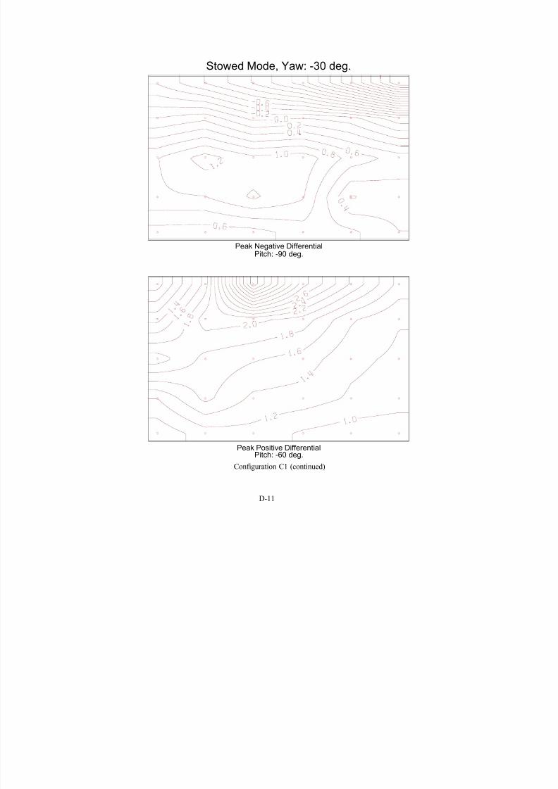
7/31/2019 Wind Tunnel Test
http://slidepdf.com/reader/full/wind-tunnel-test 217/243
D-11
Stowed Mode, Yaw: -30 deg.
Pitch: -90 deg.Peak Negative Differential
Peak Positive DifferentialPitch: -60 deg.
Configuration C1 (continued)
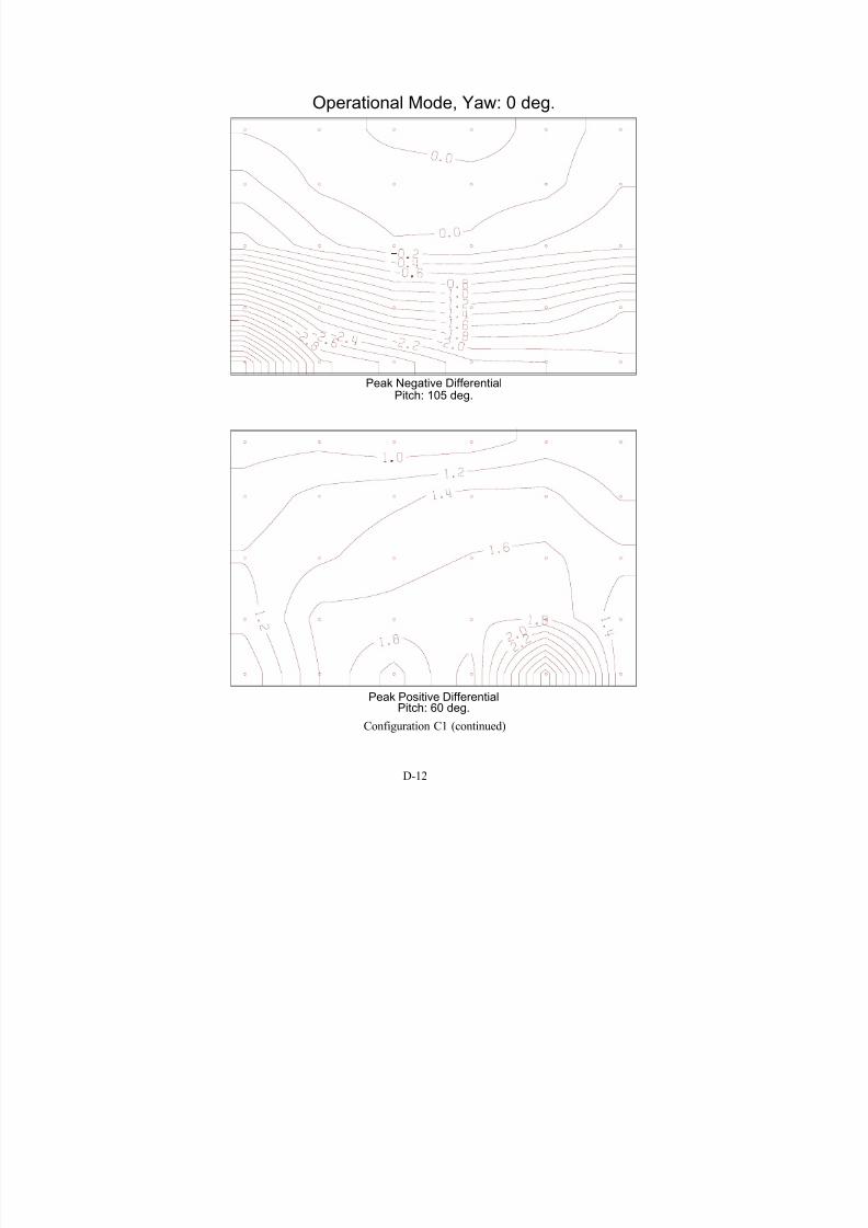
7/31/2019 Wind Tunnel Test
http://slidepdf.com/reader/full/wind-tunnel-test 218/243
D-12
Pitch: 60 deg.Peak Positive Differential
Peak Negative DifferentialPitch: 105 deg.
Operational Mode, Yaw: 0 deg.
Configuration C1 (continued)

7/31/2019 Wind Tunnel Test
http://slidepdf.com/reader/full/wind-tunnel-test 219/243
D-13
Pitch: -60 deg.Peak Positive Differential
Peak Negative DifferentialPitch: -90 deg.
Stowed Mode, Yaw: 0 deg.
Configuration C1 (continued)

7/31/2019 Wind Tunnel Test
http://slidepdf.com/reader/full/wind-tunnel-test 220/243
D-14
Pitch: 60 deg.Peak Positive Differential
Peak Negative DifferentialPitch: 105 deg.
Operational Mode, Yaw: 30 deg.
Configuration C1 (continued)
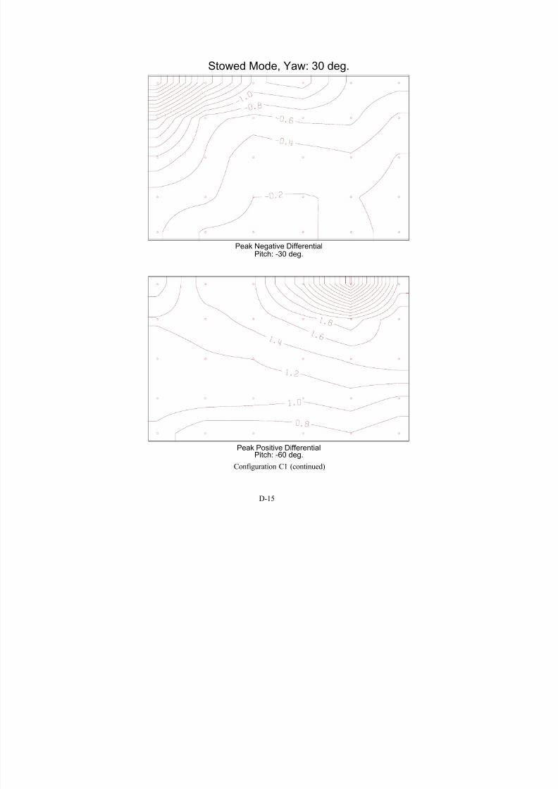
7/31/2019 Wind Tunnel Test
http://slidepdf.com/reader/full/wind-tunnel-test 221/243
D-15
Pitch: -60 deg.Peak Positive Differential
Peak Negative DifferentialPitch: -30 deg.
Stowed Mode, Yaw: 30 deg.
Configuration C1 (continued)

7/31/2019 Wind Tunnel Test
http://slidepdf.com/reader/full/wind-tunnel-test 222/243
D-16
Pitch: 30 deg.Peak Positive Differential
Pitch: 105 deg.Peak Negative Differential
Operational Mode, Yaw: -30 deg.
Configuration C3
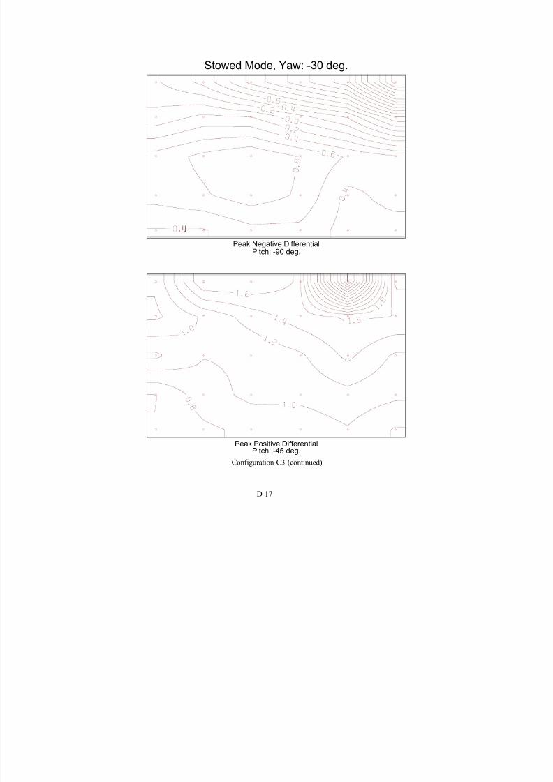
7/31/2019 Wind Tunnel Test
http://slidepdf.com/reader/full/wind-tunnel-test 223/243
D-17
Stowed Mode, Yaw: -30 deg.
Pitch: -90 deg.Peak Negative Differential
Peak Positive DifferentialPitch: -45 deg.
Configuration C3 (continued)

7/31/2019 Wind Tunnel Test
http://slidepdf.com/reader/full/wind-tunnel-test 224/243
D-18
Pitch: 60 deg.Peak Positive Differential
Peak Negative DifferentialPitch: 105 deg.
Operational Mode, Yaw: 0 deg.
Configuration C3 (continued)

7/31/2019 Wind Tunnel Test
http://slidepdf.com/reader/full/wind-tunnel-test 225/243
D-19
Pitch: -60 deg.Peak Positive Differential
Peak Negative DifferentialPitch: -90 deg.
Stowed Mode, Yaw: 0 deg.
Configuration C3 (continued)
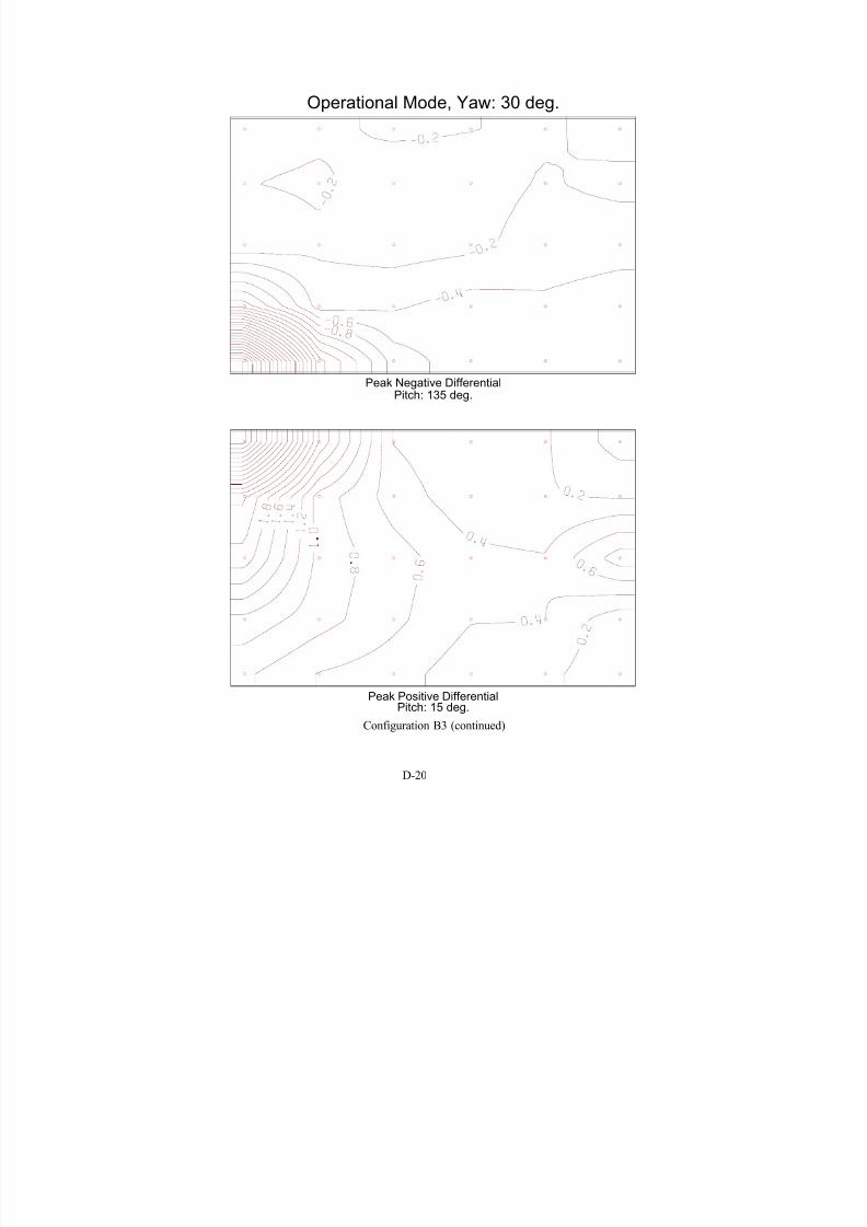
7/31/2019 Wind Tunnel Test
http://slidepdf.com/reader/full/wind-tunnel-test 226/243
D-20
Pitch: 15 deg.Peak Positive Differential
Peak Negative DifferentialPitch: 135 deg.
Operational Mode, Yaw: 30 deg.
Configuration B3 (continued)

7/31/2019 Wind Tunnel Test
http://slidepdf.com/reader/full/wind-tunnel-test 227/243
D-21
Pitch: -30 deg.Peak Positive Differential
Peak Negative DifferentialPitch: -90 deg.
Stowed Mode, Yaw: 30 deg.
Configuration C3 (continued)

7/31/2019 Wind Tunnel Test
http://slidepdf.com/reader/full/wind-tunnel-test 228/243
D-22
Pitch: 45 deg.Peak Positive Differential
Peak Negative DifferentialPitch: 105 deg.
Operational Mode, Yaw: -30 deg.
Configuration C5

7/31/2019 Wind Tunnel Test
http://slidepdf.com/reader/full/wind-tunnel-test 229/243
D-23
Pitch: -60 deg.Peak Positive Differential
Peak Negative DifferentialPitch: -105 deg.
Stowed Mode, Yaw: -30 deg.
Configuration C5 (continued)
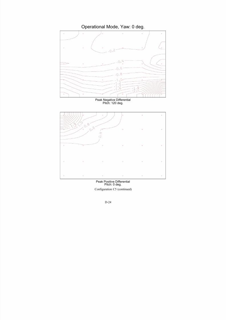
7/31/2019 Wind Tunnel Test
http://slidepdf.com/reader/full/wind-tunnel-test 230/243
D-24
Pitch: 0 deg.Peak Positive Differential
Pitch: 120 deg.Peak Negative Differential
Operational Mode, Yaw: 0 deg.
Configuration C5 (continued)
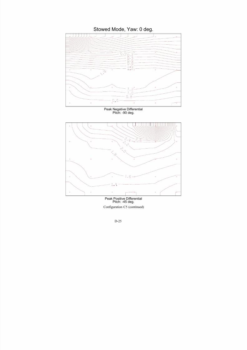
7/31/2019 Wind Tunnel Test
http://slidepdf.com/reader/full/wind-tunnel-test 231/243
D-25
Stowed Mode, Yaw: 0 deg.
Pitch: -90 deg.Peak Negative Differential
Peak Positive DifferentialPitch: -45 deg.
Configuration C5 (continued)
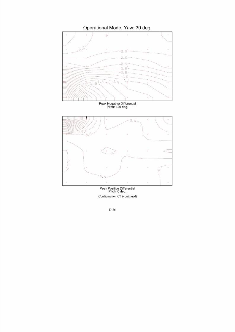
7/31/2019 Wind Tunnel Test
http://slidepdf.com/reader/full/wind-tunnel-test 232/243
D-26
Pitch: 0 deg.Peak Positive Differential
Peak Negative DifferentialPitch: 120 deg.
Operational Mode, Yaw: 30 deg.
Configuration C5 (continued)

7/31/2019 Wind Tunnel Test
http://slidepdf.com/reader/full/wind-tunnel-test 233/243
D-27
Pitch: -45 deg.Peak Positive Differential
Peak Negative DifferentialPitch: -90 deg.
Stowed Mode, Yaw: 30 deg.
Configuration C5 (continued)

7/31/2019 Wind Tunnel Test
http://slidepdf.com/reader/full/wind-tunnel-test 234/243
D-28
Pitch: 0 deg.Peak Positive Differential
Pitch: 0 deg.Peak Negative Differential
Operational Mode, Yaw: -30 deg.
Configuration D1
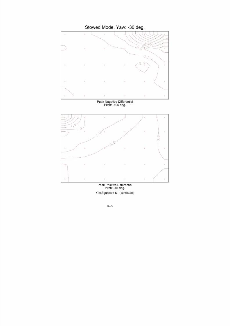
7/31/2019 Wind Tunnel Test
http://slidepdf.com/reader/full/wind-tunnel-test 235/243
D-29
Stowed Mode, Yaw: -30 deg.
Pitch: -105 deg.Peak Negative Differential
Peak Positive DifferentialPitch: -45 deg.
Configuration D1 (continued)
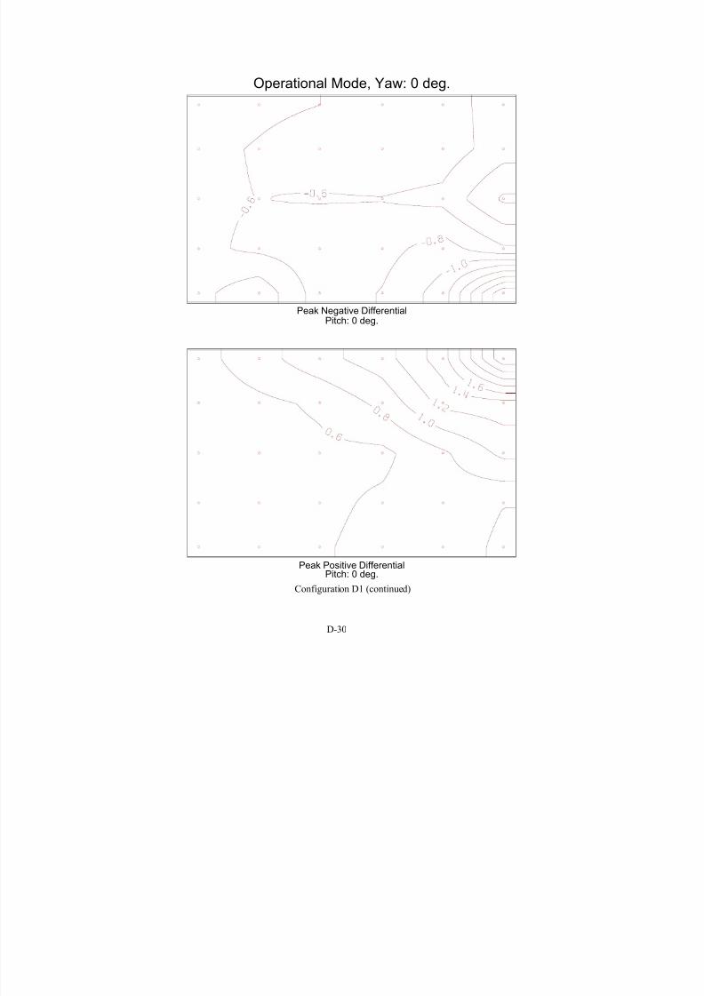
7/31/2019 Wind Tunnel Test
http://slidepdf.com/reader/full/wind-tunnel-test 236/243
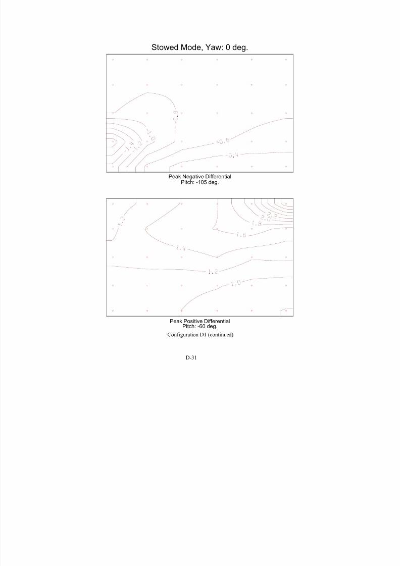
7/31/2019 Wind Tunnel Test
http://slidepdf.com/reader/full/wind-tunnel-test 237/243
D-31
Pitch: -60 deg.Peak Positive Differential
Peak Negative DifferentialPitch: -105 deg.
Stowed Mode, Yaw: 0 deg.
Configuration D1 (continued)

7/31/2019 Wind Tunnel Test
http://slidepdf.com/reader/full/wind-tunnel-test 238/243
D-32
Pitch: 0 deg.Peak Positive Differential
Peak Negative DifferentialPitch: 180 deg.
Operational Mode, Yaw: 30 deg.
Configuration D1 (continued)

7/31/2019 Wind Tunnel Test
http://slidepdf.com/reader/full/wind-tunnel-test 239/243
D-33
Pitch: -45 deg.Peak Positive Differential
Peak Negative DifferentialPitch: -90 deg.
Stowed Mode, Yaw: 30 deg.
Configuration D1 (continued)
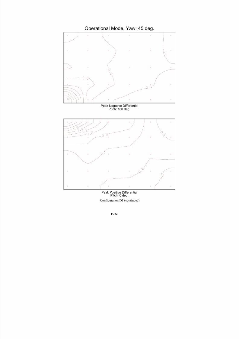
7/31/2019 Wind Tunnel Test
http://slidepdf.com/reader/full/wind-tunnel-test 240/243
D-34
Pitch: 0 deg.Peak Positive Differential
Pitch: 180 deg.Peak Negative Differential
Operational Mode, Yaw: 45 deg.
Configuration D1 (continued)
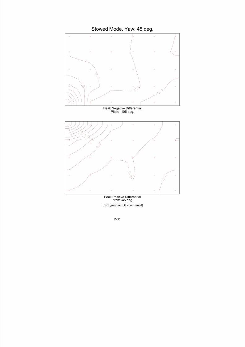
7/31/2019 Wind Tunnel Test
http://slidepdf.com/reader/full/wind-tunnel-test 241/243
D-35
Pitch: -45 deg.Peak Positive Differential
Pitch: -105 deg.Peak Negative Differential
Stowed Mode, Yaw: 45 deg.
Configuration D1 (continued)

7/31/2019 Wind Tunnel Test
http://slidepdf.com/reader/full/wind-tunnel-test 242/243
7.5 APPENDIX E - TIME SERIES OF LOCAL PRESSURES
A set of CD-ROMs provided to NREL as backup to this report contains the time series of local pressure coefficients measured on the model of the solar collector concentrator. The pressure
values have been adjusted to approximate the directly measured force and moment balance loadswhen integrated. The weight factors for pressure integrations are provided in a spreadsheet file
(INTEGRATE.XLS), also found on the CD-ROM.
Data Filename Convention
The following data file naming convention is used.cccP-rrr.DAT
where
ccc : Test configuration, I1 – I11.
rrr : Run number.
Data File Format and Contents
The data are stored in printable ASCII format. Each data file contains a brief header
followed by series of instantaneous local pressure coefficients. A typical data file might look likethis (description of the data lines in parentheses):
Run 1 (Unique run number)
Config I1 (Test configuration ID)
Yaw (deg.) .0 (Yaw angle)
Pitch (deg.) 105.0 (Pitch angle)
Uref (fps) 25.69 (Reference wind speed at pivot height)
Qref (psf) .6270 (Reference pressure at pivot height)
Sample Rate (Hz) 500.0 (Number of samples per second per channel)
No. Samples 8192 (Number of samples per segment block)
No. Segments 4 (Number of segment blocks)
(Blank line)
130 129 128 (Pressure Tap Number)
(Blank line)
-.0207 -.1248 -.3266 (1st data point)
-.4157 -.4448 -.5087 (2nd data point)
-.3385 -.3933 -.3903
. . .
. . .
. . .
. . .
. . .
-.8503 -.9533 -.9259
-1.5147 -1.0938 -1.1680 (8192nd data point of 1st segment)
(Blank line separating segment blocks)
-.0989 -.1662 -.1522
-.4142 -.3249 -.4434
-.2717 -.3196 -.3241
. . .
. . .
. . .
(End of File)
E-1

7/31/2019 Wind Tunnel Test
http://slidepdf.com/reader/full/wind-tunnel-test 243/243
REPORT DOCUMENTATION PAGEForm Approved
OMB No. 0704-0188
The public reporting burden for this collection of information is estimated to average 1 hour per response, including the time for reviewing instructions, searching existing data sources,gathering and maintaining the data needed, and completing and reviewing the collection of information. Send comments regarding this burden estimate or any other aspect of thiscollection of information, including suggestions for reducing the burden, to Department of Defense, Executive Services and Communications Directorate (0704-0188). Respondentsshould be aware that notwithstanding any other provision of law, no person shall be subject to any penalty for failing to comply with a collection of information if it does not display acurrently valid OMB control number.
PLEASE DO NOT RETURN YOUR FORM TO THE ABOVE ORGANIZATION. 1. REPORT DATE (DD-MM-YYYY)
May 2008
2. REPORT TYPE
Subcontract Report
3. DATES COVERED (From - To)
March 2001- August 2003
5a. CONTRACT NUMBER
DE-AC36-99-GO103375b. GRANT NUMBER
4. TITLE AND SUBTITLE
Wind Tunnel Tests of Parabolic Trough Solar Collectors
5c. PROGRAM ELEMENT NUMBER
Related Documents