Wind Power Dynamic Behaviour - Chalmers

Här finns utrymme att lägga in en bild.

Wind Power Dynamic Behaviour Real Case Study on Linderödsåsen Wind Farm Master of Science Thesis MATS WANG-HANSEN Department of Energy and Environment Division of Electric Power Engineering CHALMERS UNIVERSITY OF TECHNOLOGY Göteborg, Sweden, 2008

Tänk bara på att anpassa så att nedersta textraden ligger kvar i nederkant.

0 0.5 1 1.5 2−4

−2

0

2

4

6

8

10

12

Time [sec]

P &

Q [M

W &

MV

Ar]

0 0.5 1 1.5 2−4

−2

0

2

8

10

4

6

12

Time [sec]

P &

Q [M

W &

MV

Ar]

Power

Reactive power

Power

Reactive power

DFIG 1001−1701 (WTG−PCC) PMSG 1001−1701 (WTG−PCC)

Wind Power Dynamic Behaviour Real Case Study on Linderödsåsen Wind Farm

M. WANG-HANSEN

Project supervisor:

N. R. Ullah, Electric Power Engineering

Project examiner:

Dr. Tuan Le, Electric Power Engineering

Department of Energy and Environment

CHALMERS UNIVERSITY OF TECHNOLOGY

Göteborg, Sweden 2008

Wind Power Dynamic Behaviour Real Case Study on Linderödsåsen Wind Farm MATS G. WANG-HANSEN © MATS G. WANG-HANSEN, 2008. Department of Energy and Environment Chalmers University of Technology SE-412 96 Göteborg Sweden Telephone + 46 (0)31-772 1000 Cover: [2,5 MW Wind turbine generator and DFIG & PMSG 400 kV fault response. Photo & graphics by Mats Wang-Hansen] Göteborg, Sweden 2008

Abstract Rapid wind power development has led to a shift from small generators to large generators and from single distributed units to large centralised clusters of generators commonly known as wind farms. This substantial structural difference has invoked power system stability issues related to wind power. Large, centralised power plants of conventional types have always been forced by regulation to stay online and support the grid during voltage dips, but for wind farms no such regulation have historically existed. In 2005, the Swedish transmission system operator (TSO) acknowledged the forthcoming need for regulation and issued a new grid code including connection requirements for wind power generation. The new grid code describes different fault scenarios in the high voltage network which generators are supposed to ride through without disconnection. The new grid code applies to all facilities commissioned or rebuilt after 2006. In this study, the grid code scenarios are simulated, and the resulting wind power dynamic behaviour is examined to establish the implications of the grid code for wind farm grid connections in Sweden. HS Kraft’s planned wind farm at Linderödsåsen in southern Sweden is considered to be of relevant proportions (90 MW) and is chosen as a real case study. A PSS/E model of the wind farm is subjected to the fault scenarios described in the grid code, and the resulting voltages at the different busses in the test system are monitored along with wind turbine generator (WTG) active and reactive power response. The two dominating WTG technologies, doubly fed induction generator (DFIG) and permanent magnet synchronous generator (PMSG), are compared and evaluated both from a wind farm developer perspective, and from a grid owner/TSO perspective. Additionally, low voltage ride through (LVRT) settings from three large WTG manufacturers are compared with the simulated residual voltages at the WTG transformer high side to determine their degree of compliance with the grid code. All simulation results show WTG high side residual voltages that are within the LVRT capabilities of the wind turbines at offer for the planned wind farm investigated. A wind farm consisting of PMSG turbines run in reactive power injection mode experience higher residual voltages at the transformer high side than a farm consisting of DFIG turbines. But the DFIG turbine farm experience higher residual voltage than normal mode run PMSG-turbine farm. Both DFIG and PMSG technologies deliver more reactive current when operating at low speeds due to the limited current carrying capabilities of the DC-link converters. The collector network layout is of minor importance to the residual voltage level at the wind turbine transformer high side, and the DFIG LVRT-actions cause considerable stress to its mechanical drive train. Keywords: Wind power, Wind farm, Grid code, LVRT, DFIG, PMSG, Dynamic behaviour.

1

Table of contents Abbreviations Notation 1 Introduction………………………………………………………………………5 1.1 Background 5 1.2 Objective 7 2 Power system stability…………………………………………………………...8 2.1 Stability classes 8 2.2 Different fault types 9 2.3 Grid code 10 3 Wind power fundamentals……………………………………………………..12 3.1 Design and development overview 12 3.2 Generator technology 15 3.3 Wind speed dynamics 16 3.4 WTG fault response 18 3.4.1 DFIG 18 3.4.2 PMSG 20 4 Linderödsåsen wind farm……………………………………………………...21 4.1 Project specifications 21 4.2 Existing transmission network 21 4.3 Wind turbine candidates 22 4.3.1 Enercon 23 4.3.2 GE Energy 24 4.3.3 Vestas 25 4.3.4 Nordex 25 5 Modelling ……………………………………………………………………….26 5.1 Grid model 26 5.1.1 Line model 27 5.1.2 Load model 27 5.1.3 Transformer model 27 5.1.4 Strong network connection point model 28 5.2 Collector network model 28 5.3 WTG model 28 5.3.1 DFIG 28 5.3.2 PMSG 30 5.4 Wind speed model 30

5.5 Full model diagram 31

2

6 Simulation………………………………………………………………….........32 6.1 PSS/E 32

6.2 Base case power flow simulations 32 6.3 Dynamic simulation 33 6.3.1 Grid code scenarios 33 6.3.2 Experimental simulation plan 34 6.3.3 Dynamic simulation settings 34

7 Results…………………………………………………………………………...35

7.1 Base case 35 7.2 DFIG scenarios 40

7.3 DFIG versus PMSG 43 7.4 Different control modes 46

8 Result summary…………………………………………………………...........48 9 Discussion……………………………………………………………………….49 10 Conclusions……………………………………………………………………...51 11 Future work……………………………………………………………………..53 12 References…………………………………………………………………….....54 13 Appendix………………………………………………………………………...56 A PMSG model documentation 56 B Matlab PSS/E output channel converter program 59

3

Abbreviations A AG Annular generator D DFAG Doubly fed asynchronous generator DFIG Doubly fed induction generator DFIM Doubly fed induction machine H HS Kraft Wind power developer based in Malmö I IGBT Insulated gate bipolar transistor L LVRT Low voltage ride through M MVA Mega Volt Ampere (Unit for apparent power) MVAr Mega Volt Ampere reactive (Unit for reactive power) MW Mega Watt (Unit for active power) P P Active power [MW] PCC Point of common coupling PMSG Permanent magnet synchronous generator PSS/E Power system simulator for engineers developed by PTI/Siemens Q Q Reactive power [MVAr] S SvK Svenska Kraftnät (Swedish TSO) T TSO Transmission system operator TSR Tip speed ratio W WTG Wind turbine generator Z ZVRT Zero voltage ride through Notation Cp Power coefficient of the wind turbine rotor λ Tip speed ratio β Blade pitch angle φ Phase (An electrical conductor)

4

1 Introduction

1.1 Background Wind power has become one of the preferred alternatives for new energy production in Sweden and wind power projects for grid connection are growing both in size and numbers. The Swedish Energy authority has announced a development goal of 30 TWh annual wind energy output within 2020, which is more than 20 % of the annual Swedish electrical energy consumption of 130 TWh. This prospective growth implies that wind power will also play a major role in the power system dynamics. To secure a future-proof development of the Swedish power system, respect has to be paid to this rapidly increasing fraction of wind power. In Denmark, the wind energy fraction of total energy production has been significant for a few years already and history has shown that wind turbines have had tendencies to disconnect from the grid during network faults. Due to the disconnection issues, Denmark formed regulations governing wind power grid connections relatively early, but in Sweden such regulations have been non-existent and consequently wind turbine dynamic fault behaviour has been neglected. The introduction of larger wind farms with power plant-like proportions able to influence power system stability have however changed the way transmission system operators (TSO’s) and grid owners look at wind turbine disconnection issues in Sweden. The low voltage ride through (LVRT) –performance has gone from being a concern for the wind power owners themselves, (to ensure that turbine equipment survived voltage deviations) to be an area of large interest for both TSO’s and subtransmission network owners [1], [2]. The power system legislation in Sweden is prepared by the national TSO Svenska Kraftnät (SvK) which, in a response to the lack of wind power regulations, in 2005 issued a document with a new set of grid-connection rules including all types of power-generating facilities. The purpose of this document, known as the Swedish grid code, is simply to ensure a stable power system operation where power is delivered to the customers in a reliable and efficient manner. Generators are regulated by the grid code to stay online and contribute to stability in the grid during faults and other abnormal conditions that may lead to tripping of major power system components. The extent of support expected from the different power sources vary according to their natural limitations. For instance, wind power units can not be expected to ramp up production under normal circumstances, since the turbines exploit the full energy potential of the wind at any given time. (It is unreasonable to ask for a regulated increase in wind strength.) Conventional synchronous generators generally have the electromechanical prerequisites needed for severe fault ride through, and their performances are therefore more strictly regulated in the grid code than other types of generators.

5

Even though generators should comply with regulations and stay connected as long as possible during grid faults, their fault ride through capability will always be limited regardless of generator type. Some faults are of such a severe character that it is unreasonable to demand that generators stay connected, and this limit is exactly what is specified in the grid code. For a certain fault with certain durability the generators have to stay connected. If the voltage dips below this predefined level and/or if the dip is of a longer duration, the tripping of generators are tolerable, but nevertheless unwanted from a power system stability perspective. The strain that such faults cause on wind turbine generators (WTG’s) can be very large, foremost due to their mechanical structure including power transmission with high gear ratios and comparatively soft shafts. There are several reasons why WTG’s has to trip relatively fast during severe faults, but common to all reasons for disconnection are the risk of causing irreversible damage to electrical or mechanical parts in the turbine. During faults, internal generator currents and voltages increase dramatically and both electric and mechanical torque is altered. It is therefore of great importance to ensure that the generator type to be used in a certain facility has physical properties that can withstand the deviations in current and voltage that is expected in that specific facility during a dimensioning fault in the grid. For this reason, generators have to be developed in conjunction with grid code-rules so that increased fault performance of the generator hardware and software can be built in to suit the fault conditions prescribed in the regulation. It is important to stress that fault-conditions vary greatly throughout the network. In strong parts of the grid, voltage dips are rare due to the relatively weather-secure power line gates, but on the other hand, dips propagate at full amplitude due to low resistivity lines and few transformers between the generation facility and the prescribed fault-sites. In weaker parts of the grid the remaining voltage during faults in the subtransmission network will generally be higher since the fault current contribution from the wind farm will flow through larger impedance, raising the remaining voltage level. Linderödsåsen wind farm is situated centrally in a high capacity subtransmission network with low impedance and will therefore experience relatively low terminal voltage at its generators during severe transmission and subtransmission network faults. Historical proof of wind power playing a major role in power system stability is found in measurements from the Danish transmission system during the winter storm Gudrun on January 8th 2005. Wind power supplying more than half of western Denmark’s consumer load (2100 MW) was disconnected over a period of 10 hours (fastest rate of disconnection was 600 MW/h) due to hurricane force winds. The DC-Link between Denmark and Norway experienced a power reversal, from transmitting 950 MW from Denmark to Norway before the disconnection, to transmitting 1000 MW from Norway to Denmark after the disconnection [3]. This kind of power flow change is obviously an important aspect for a transmission system operator, and changes on this power order would be even more challenging if caused by instantaneous disconnection as a result of voltage dips in the transmission system.

6

A more enlightening wind power stability observation was done in Sweden in February 2008 when the newly commissioned offshore wind farm Lillgrund stayed connected through a severe subtransmission fault, while nearby thermal generation was tripped by under voltage protection [4]. This episode indicates that wind power connection stability has come a long way in few years, and that wind power is gradually adapting to power system requirements for reliable operation. The anticipated adaption of wind power to the grid is related to the increased regulating possibilities for wind turbines, such as variable speed drives and aerodynamically efficient pitching mechanisms together with better generator and converter technology. All planned connections of new wind farms to the power system still have to be examined for case specific problems to ensure that they will comply with the grid code. 1.2 Objective The main objective of this study is to analyse the dynamic behaviour of HS-Kraft’s planned wind farm at Linderödsåsen in Skåne. A reduced equivalent network-model for the area in question and a theoretical model of the wind farm including turbines and collector network is used as a starting point for further analysis. Fault-scenarios, outlined in the Swedish TSO’s grid code, that represent the theoretical ride-through criteria for the wind farm will be identified and documented. The different fault scenarios will be simulated and the resulting voltage dips at the wind turbine transformer high side will be compared with typical turbine protection relay-settings. This comparison will establish the ride through capability and other stability aspects of the planned wind farm layout. Since the wind farm has yet to be built and several system dimensioning factors are not yet decided, a secondary objective is to find out how different types of turbines will affect the stability-performance of the wind farm. The doubly fed induction generator (DFIG) will be compared with the permanent synchronous generator (PMSG). The main computer software analysis-tool used in the study is Siemens power system simulator PSS/E, which is renowned in the power industry for its ability to perform complex power system computations with clear and accurate results.

7

2 Power system stability Power system stability can be divided into subgroups relating to operation and disturbances of different nature and on different timescales. A short guide of stability definitions is provided in this chapter. The main stability-issue is traditionally a generators ability to stay connected through severe voltage dips and frequency deviations, thereby supporting a struggling network. If successful, the continuous operation of one generator will help other generators to stay synchronised after severe faults, or at least not worsen the situation. The description “lost generator synchronization” have to be tweaked a bit to appear meaningful for new wind power generating technologies. The different types of wind turbine generators included in this work can never loose synchronism, traditionally speaking, due to their natural variable speed capabilities which means they are not synchronized to the grid in the first place. Nevertheless, wind turbine generators can still dysfunction in other ways during transient disturbances and the equal consequence as that of a synchronous generator loosing synchronism with the grid is the disconnection of a wind turbine during a fault. For wind turbine generators, their ability to stay connected during faults is referred to as their “ride through capability”. Whether faults lead to lost synchronism for conventional generators, or tripping of other types of generators, the impact on the total system stability is mainly dependent on the total amount of power tripped. If a huge cluster of generators is tripped, it does not matter whether it consists of conventional generators or new wind turbine generators, active power supply will decrease and the power flow in the system will change dramatically. Voltages in all nodes will be affected and frequency excursions can occur. The bottom line is that all types of generators have transient behaviour that can affect power system stability.

2.1 Stability classes Power system stability is a complex area of knowledge that include many classes and sub-divisions of phenomena. Stability can be divided into the following four classes: Voltage stability, Long-term Stability, Mid-term Stability and Transient stability [5]. Stability issues are referred to on different timescales and are therefore simulated and measured with different approaches. Voltage stability is understood as the long term operating point of the system, were the goal is to maintain node voltages within reasonable limits at all times, that is, all possible load and generation scenarios. Transient stability, which is the area of focus in this work, is understood as voltage deviations with a timescale of tens to hundreds of milliseconds and with resulting dynamic oscillations lasting several seconds or in some cases even minutes. Between the two extremes explained lies Mid- and Long-term stability that cover large voltage and frequency excursions lasting from minutes to tens of minutes concerning larger system weaknesses.

8

Mechanical dynamics in machines and physical faults in the grid such as different types of short circuits are typically investigated on a transient timescale. Electrical engineers have, over time, shaped a sharper definition of transient stability as; angle stability between grid-interconnected synchronous generators. This definition has historically covered the major share of transient timescale stability issues. One problem though, with this relatively old definition, is that it does not include short time stability issues for new type of large scale generation technology such as DFIG’s or PMSG’s with full power converters, which are commonly found in wind turbines. A more suitable definition of transient stability for all types of generation would be; immunity against large, fast disturbances in voltage. 2.2 Different fault types The different faults that can occur in a three phase system are the following; Shunt faults (short-circuits) Single line-to-ground fault (SLG) Double line-to-ground fault (2LG) Three phase short circuit grounded (3φ G) Line-to-line fault (LL) Three phase short circuit (3φ ) Series faults (interruptions) One-line-open (1 LO) Two-line-open (2LO) Three-line-open (3LO) SLG is by far the most frequent fault type, but looking at the remaining voltage in the undisturbed phases also the least severe fault type. Even 2LG and LL-faults are more common than the very rare 3φ G-fault often referred to as a bolted three phase fault. The 3φ G-fault is nevertheless the most interesting benchmark for stability testing due to its severity from a remaining voltage point of view. A 3φ G-fault causes high amplitude fault currents and affect torques in machines more than any other fault. The series faults are of different nature since no short circuit current is involved, and they are therefore not as interesting for this type of work. In general, electrical systems have to be designed to withstand theoretically possible faults even though they are statistically rare. The reason for this seemingly over-cautious principle is the potentially very costly effects of one single power system collapse. Instability in one area can quickly spread and cause instability in large parts of a country’s power system, thereby causing partial collapse. The whole society relies on delivered electricity, and multiple large industries will suffer great economic losses by one single outage. The issue of cautiousness also relates to safety and security from a

9

societal point of view. Emergency shutdown of nuclear reactors involves a certain risk of malfunction, as do the starting up of UPS-units (power backup) in hospitals and other institutions where people’s lives are power dependent. The choice of fault type during simulations therefore has to represent the most challenging situation the system may experience theoretically, even though the actual statistics show that other less severe fault types are much more common in the system [6]. 2.3 Grid code Until 2006, there were no regulations governing the connection of wind power to the electrical grid in Sweden. The reasoning for the absence of regulations was simply that wind power units historically had been non-influent on power system stability as they were usually installed in weak-grid locations, alone and with relatively low power ratings. As the turbines grew rapidly in both size and numbers, the Swedish transmission operator Svenska Kraftnät (SvK) took the initiative to form regulations for connection of electricity producing facilities. The finished document was released in 2005 and named SvKFS 2005:2. Grid connection requirements for wind farms of all sizes are specified in SvKFS 2005:2, upon which this study is conducted. The analysis focus on the low voltage fault ride through part of the regulations as described for a medium size wind farm rating between 25 and 100 MW in total. There are two different fault scenarios [7]: SvKFS 2005:2, scenario 1 “The wind turbine generators are supposed to stay connected during a three-phase fault reducing the voltage to 25 % at the closest bus in the meshed 400 kV grid. The duration of the fault is 0.25 seconds, where after the voltage resumes and remains at a steady 90% level.”

10

Figure 1 Prescribed voltage profile for the 400 kV fault SvKFS 2005:2, scenario 2 “The wind farm shall, with sustained grid-connection, ride through variations in the voltage caused by instantaneously cleared faults in the connecting meshed network”. The second scenario is less explicit and clear. It is also case-specific and will therefore be explained in the chapter on the projected wind farm. Generally the connected meshed network is the network that the wind farm is connected directly to and the fault details will be explained later. Responsibility for compliance with the grid code lies fully with the wind farm developer. When asked if the project developer needs to establish documentation or perform live testing on the facility prior to grid connection, SvK replied the following: “According to SvKFS 2005:2 chapter 8, SvK has the right to demand construction documentation from the wind farm owner. The connection itself is a settlement between the wind farm owner and the local power network owner. SvK will in practice not demand any documentation in order to make statements prior to the connection. If however it becomes clear that the wind farm owner fail to comply with the Grid code he will have to expect to take the full responsibility for his breach of the rules.” The regulations work in the same way as normal law, you will not be suspected for a crime before you have done something wrong [8].

11

3 Wind power fundamentals Wind power has certain distinctive properties which should be assessed to create a basic understanding of wind turbine development. Technology related issues for choice of turbines for specific projects will be gone through in this chapter, as well as different dynamic aspects of wind farm connection for grid studies.

3.1 Design and development overview Wind turbine generators have evolved dramatically over the last decades. From having small towers and rotors with induction generators in sub-kilowatt ratings, they now have large towers and rotors and are equipped with variable speed drives of different kinds rating several megawatts. Old and small induction generator turbines were often equipped with passive stalling blades which meant that there were not many tuneable parameters to optimize the production and the electrical behaviour during operation. Generators experienced large start-up currents, high and relatively uncontrolled torques and were sources of flicker emission. During wind fluctuations the rotor would occasionally act as a large fan drawing power from the grid and with poor aerodynamics on top of that, the overall turbine efficiency was not particularly good.

Plate 1 Wind turbine size development [9] The larger turbines of today are being equipped with new generator technology that has come a long way from the simple induction generators. All available generator technologies are constantly developing, and the world market is currently led by doubly

12

fed induction generators (DFIG’s). The DFIG is also referred to in literature as the doubly fed asynchronous machine DFAG, or doubly fed induction machine (DFIM). Synchronous generators with full power converters are relatively new on the market but conquering new market shares. Even large annular (direct driven multi pole) generators are used in some of the synchronous generator powered wind turbines and direct drive market leader Enercon is showing the way. To a large extent, wind turbines are developed to suit a certain set of conditions, taking into account the following design-determining site-specific variables: Average wind speed and median wind strength, regular turbulence due to local topography and vegetation, maximum wind force during extreme weather events and acceptable noise emission levels. A wind turbine designed with a particular set of conditions in mind but deployed in a completely different environment could therefore be a poor economic investment or the conditions could even prove fatal to the turbine hardware. Large rotors with small generators and a high gear ratio are suitable for low average wind areas, whereas large generators with comparatively small rotor diameters are aimed at higher wind strength sites. The optimal tip speed ratio (TSR) of the turbine, (the quotient between tip speed and true wind speed), is closely related to the number of rotor blades and their chord. Multiple blade rotors reach their optimal efficiencies at lower TSR, but since manufacturing cost is proportional to the number of blades, the overall system economy for utility size turbines is regarded better with two or three blades, fairly long chord and TSR in the range of 6-11 [10]. Few blades combined with shorter chords result in high optimal TSR and consequently these rotors create more noise, which could be problematic in populated areas. Especially for two-blade design, the noise issue, structural resonance phenomena and a need for relatively laminar low turbulence winds, mean that they will probably only be considered for future offshore or remote area projects. Since turbines are shadowing each other there is a clear lower limit to the distance between them that determines how many turbines of a certain size that can be installed in a given area. The wind speed recovery from one turbine to the next depends on the wind speed itself. In strong winds recovery is faster than in light winds, and recovery is especially faster during winds exceeding the turbine optimal efficiency operation point due to the mere fact that the blade pitching mechanism sheets out the blades and lets through more of the incoming wind energy. Normally turbines are placed with 5 turbine diameters spacing perpendicular to the predominant wind direction on site and with 5 - 10 turbine diameters spacing in the predominant wind direction. When rotors grow larger, there is also an increased effect of varying wind over the rotor plane. The average wind strength will be higher at the top of a revolution and lower at the bottom. This variance cause additional strain on the drive train and could be mitigated by having smaller rotors in high wind, rough topography areas.

13

The extra power in wind gusts during high winds is radical. The power in the wind is proportional to the cube of the wind speed and consequently, wind gusting from 11 to 12 m/s gives an absolute power increase 6.5 times as large as the power increase when the wind is gusting from 4 to 5 m/s. The above outlined design-factors are rudimental to how the theoretically perfect wind turbine for a certain site is designed, and what economical yields it will produce during its lifecycle. If space were unlimited, installation and maintenance were free and grid issues were of no concern, one would probably build turbines solely after these criteria because it would offer the best return on investment. Additional factors always complicate the build and investment strategy and it could be better to invest in more expensive units, i.e. units with relatively large and technologically robust generators that are more tolerant to grid disturbances, rough wind conditions and other unforeseen events. In any real life wind farm project, space is also limited and the wind resource is to be exploited with the best economy possible. Looking closer at the hardware details it is not only the generators that have changed over the last years, aerodynamic rotor blade design has to. The new generation of blades are much longer and have complex twisted profiles that are continuously pitch angle controlled from the rotor hub. The pitch control systems allows for fast reduction in aerodynamic power when needed, as in case of electrical interruptions. DFIG and PMSG pitch control algorithms are similar since the pitch mechanism is a general aerodynamic optimization question.

14

3.2 Generator technology 3.2.1 DFIG

Power electronic

converter

DFIG

Gear

Plate 2 Schematic figure of a DFIG wind turbine In this type of turbine, the rotor-speed is raised through a gearbox and the high-speed shaft is connected to a doubly fed asynchronous generator. The introduction of the DFIG has opened up possibilities for a large variable speed range unheard of with older technology. The variable speed operation is achieved through converter modulation of the rotor voltage. The mechanical speed (rounds per second) of the rotor shaft plus the rotor field speed will always equal the speed of the grid controlled field in the stator which have a steady 50 Hz frequency. The magnitude of the converter modulated active rotor current controls the voltage, and the phase angle controls the reactive power. This way the VAR control is decoupled from the active power operation point of the turbine. Variable speed allows the generator to follow the optimal Tip speed ratio (TSR) in a major range of the generation window. From 30 % below synchronous speed to 30 % above synchronous speed, the direction of active power in the DC- link changes from rotor-converter to converter-rotor. At the reversing point of the DC-link current, the generator is in synchronous operation and the current in the rotor circuit becomes a dc-current. The reversal of the DC-link also means that the fraction of power output from the stator ranges between 70 % and 130 % of the total power, and the rest is transmitted either way through the converter feeding the rotor. A crow bar with resistors grounded on the downside is connected between the rotor and the rotor side converter, which function will be explained later. The generating voltage usually lie around 660 to 690 Volts and generators normally have four or six poles.

15

3.2.2 PMSG

Power electronic

converterSG/IG

Gear

Plate 3 Synchronous generator with full power converters The permanent magnet synchronous generator (PMSG) has been used in thermal and hydropower plants for years, but is relatively new in wind power context. In a conventional PMSG, the frequency of the stator is directly coupled to the rotor-speed, which leaves no room for variable speed operation. However, a solution enabling variable speed operation emerged when the DC-link back-to-back converter topology was introduced in conjunction with the generator. This solution could not be deployed until the late nineties when power electronic converters reached higher power ratings due to fast development of insulated gate bipolar transistors (IGBT’s). The high power IGBT’s allow for a turbine design where 100 % of the generated power flows through the DC-link connected to the generator-side and the grid-side converters. The PMSG setups either utilize a low speed annular generator (direct drive) -type, or a conventional high-speed generator. The mechanical moving parts in the direct drive type are reduced to a minimum but it needs many poles in order to raise the generating frequency and is therefore often referred to as a multi-pole generator. The more traditional high-speed PMSG utilizes a gearbox that can be of either parallel axis or planetary type to raise the rpm of the driveshaft. The rotor circuits in both types are excited with permanent magnets and the converters control the reactive power output by voltage modulation. The full power DC-link effectively decouples the generator dynamics from the grid in both the direct drive and the high-speed drive cases.

3.3 Wind speed dynamics In contrast to most other electrical generation which have a more or less constant input power from its prime mover, wind power has natural dynamics on the mechanical side of the generator. Wind gusts and lulls create varying torque on the driveshaft and consequently varying electrical power.

16

The mechanical power available from the low speed rotor shaft in a wind turbine varies with air density and most importantly wind speed according to:

Pmech =12ρπR2Cp (λ,β)vw

3

Where ρ is air density, λ is tip speed ratio and β is the pitch angle of the blades. This formula is derived from the well-known equation for the kinetic energy of moving mass. Note the cubic relation between wind speed and power that magnifies any change in wind strength. The following diagrams are showing wind behaviour during 24 hours of low pressure passage in the summer at the south-west cost of Sweden.

Figure 2 a) Wind strength, b) Wind direction [11] The variation in both strength and direction is large and the timeframe is also fairly long, but the relatively large and fast changes in strength and direction put a perspective on the variable nature of the wind.

17

The controllers in a turbine are constantly working to adapt the electrical torque to equal the mechanical power input from the driveshaft to ensure smooth and efficient turbine operation. This control action will, as all control action, have some response time and the resulting action will in case of large wind gradients result in damped oscillation. Oscillations in wind turbines are further facilitated by relatively soft drive trains compared to the likes of conventional generators, allowing for more twist in the mechanical drive train acting as an energy storing spring. Depending on the natural turbulence in the wind, the rotor will have more or less input dynamics to compensate for. Open and flat areas experience less disturbed airflows than forestal or hilly terrain and local low-pressure systems provide more uneven wind than the more stable gradient winds. Common to all types of changes in wind strength and direction is a timescale of seconds or longer, which is relatively slow compared to the transient dynamics of electrical equipment [12]. 3.4 WTG fault response When faults occur in the grid, any wind turbine generator equipped with power electronics will show a distinctive combination of passive and active response in the grid connection point. This combined response, which can be observed as changes in currents, voltages and phase angles, vary significantly between different generator technologies and is a result of different equivalent electric circuits and different control systems. 3.4.1 DFIG Wind turbines of DFIG-type show behaviour close to that of the traditional induction machine due to their technical similarities. There are however to significant differences: One; when bypass resistors in the crow bar is connected resistance can no longer be neglected, and two; The DFIG slip can be far from zero, whereas the induction machine always operate close to zero slip. There are also some clear differences due to the controllability of the rotor current in a DFIG, since the electrical torque is no longer governed by the slip. The physical properties of the stator in the DFIG remain the same, but the rotor circuit is fed from the generator side converter, by which the rotor current is fully dictated. When the voltage drops at the generator terminals, the rotor current from the converter increases in a compensation effort to stabilize the active power output from the turbine and together with the passive response of the stator-circuit, the resulting transient currents can reach 5 pu. The transient currents in the stator have DC components that induce alternating currents in the rotor with the rotor frequency. These currents interfere with the control strategy of the converter and also charge the DC-link to unacceptable voltage levels harmful for the converter. This situation can not last very long without any controlling action or a special design to cope with the situation. LVRT-strategies can be implemented either on the stator or the rotor side of the generator. Over-sizing of the converter

18

transistors will ensure that the set point for controlling action can be delayed, but does not change the physical situation very much[13],[14],[15]. For converter protection reasons, as a part of any fault ride through system, a crow bar is connected between the rotor and the rotor-side converter. If the rotor voltage exceeds a certain threshold, current thyristors (not included in the plate 2 schematic) in the crowbar will be activated and the current will pass through resistors, which are grounded on the downside. This action will prevent to high rotor currents and excessive DC-link voltage. The resulting voltage amplitude in the rotor circuit is determined by the crow bar resistors. Low fault currents are wanted, but high resistor values that effectively limit the current will at the same time cause high converter voltage. The choice is therefore a trade-off between high rotor currents or high voltage at the converter terminals and the most important of these factors for fast regain of controlled operation, is the current. The crow bar resistors also act as an active power sink, burning off active power to mitigate rotor over-speeding. During the time the crow bar is activated, the generator works as a conventional induction generator with high rotor resistance. Several different chains of events can follow a crow bar action, and those are effectively the different LVRT-strategies. One possibility is to overrate the IGBT modules in the converter to allow for an extended, voltage tolerance of the DC-link, another is the possibility to disconnect the rotor side converter but not the grid side converter and a third is to disconnect the stator and continue the active operation of both converters and the DC-link. Different hardware options and various control strategies could also be deployed in each principal system solution. The main goal of the LVRT-systems regardless of principal system solution is instantaneous resumed active operation for the wind turbine after grid fault clearance. A so called chopper resistor (dump load) could be added on the DC-link with a similar function to that of the rotor side crow bar, reducing the DC-link voltage. The chopper facilitates a voltage-raising action from the converter terminals in order to keep the rotor currents low during the fault ride through and thereby enabling a faster regain of the control of the rotor current after faults. Opinions amongst scientists still differ regarding the detailed reactive behaviour of the DFIG during faults, which might just be the result of the different generator systems available. E.g. researcher Istvan Erlich changed his opinion about the DFIG reactive power response during a fault from writing that the DFIG consumes reactive power during a fault in 2006 [16], to supplying reactive power in 2007 [14]. However, the whole DFIG-turbine including the DC-link is most often regarded as a net reactive power injector during faults.

19

3.4.2 PMSG The PMSG have a completely different behaviour from the DFIG due to the full power converter link. The fault response of this kind of generator is determined by the size and rating of the grid side converter alone, and is therefore completely decoupled from the currents and voltages in the generator itself. The behaviour of the converter is very simple and straight forward since the current levels and phase angles are actually adjustable to suit customized criteria. The only adaption to the transient disturbance that the turbine still has to carry out is a reduction in input mechanical power on its primary driveshaft to avoid acceleration. The difference in mechanical input power and electrical output power cause acceleration of the rotor, and is stored as kinetic energy in the total mass of the complete drive train. During very short time intervals the resulting surplus of active energy could be burned off in dump load resistors. Immediately when a fault occurs in the grid and the voltage dips on the converter terminals, the converter will modulate an output voltage matching the grid-voltage to prevent higher currents than nominal from flowing through the converter. The most obvious result from this action is the safety benefits for the whole DC-link, which never has to carry high currents and the related risk of hardware damage. More interesting though, from a power system perspective, is the theoretically resulting low voltage in the wind farm point of common coupling due to the lack of reactive current injection if PMSG turbines are not operated in Q-injection mode. Injection of reactive current into the network both supports the voltage and facilitates fast location of faults in the network. Proper function of protection systems in the grid is dependent on large initial fault currents clearly overshooting the thresholds for relay operation. Consequently, low reactive current injections could result in longer lasting grid faults. This is however mostly a concern for the network owner, since the requirements on the duration of wind turbine LVRT is limited. The PMSG’s are often equipped with different modes of operation to enable a reactive current injection. Operation in such a mode provides a solution to the problem, but the question is at what expense for the wind farm owner. If additional investment cost and increased steady state operation losses are the consequences, other incentives will have to be introduced by the network owner or the TSO for the wind farm owner to run the WTG’s in Q-injection mode.

20

4 Linderödsåsen wind farm In this real case study, a wind farm with a nominal power rating close to 90 MW was modelled and connected to the existing 130 kV-network in southern Sweden. 4.1 Project specifications The land based Linderödsåsen wind farm project is planned to deploy 36 turbines rated at approximately 2.5 MW power, and the wind farm will cover an area of around 12 square kilometres when finished. The site for the planned wind farm is located in southern Sweden at a relatively high plateau (highest point 195 m above sea level) with short distances to three coastlines facing east, south and west. This particular location provides for reliable winds and good prospective energy yields. When considering turbine types, the mean wind strength is of great importance and from the initial wind speed measurements it is clear that this site has stronger winds than normally would be expected at an inland site. The terrain on the plateau is fairly flat and already contains roads suited for transport of construction equipment and for power cabling. No significant topographical shadow or turbulence effects are expected due to the relatively flat surrounding nature. (There are no large mountains or ridges between the site and any of the three coast lines mentioned.)

4.2 Existing transmission network The map shows the geographical position of the wind farm and the subtransmission network in southern Sweden. The network has a nominal voltage of 135 kV, is meshed on the bases of an N-1 criterion and owned and operated by Eon Sweden.

21

Plate 4 The transmission grid in the area around the planned wind farm. Blue; 135 kV- lines, Red; 50 kV-lines [4] The project site is located between Tollarp in the north and Huaröd in the south, with the 135 kV-line touching the southern edge of the planned wind farm area. The connection point to the 135 kV network is in the south corner of the wind farm area, numerous small roads can be seen in the map.

4.3 Wind turbine candidates There are several possible turbine suppliers for this project. Several of the turbines at offer basically share the market leading DFIG technology, while Enercon and GE offer two variants of the PMSG full power converter setup.

22

4.3.1 Enercon Enercon offers a direct driven synchronous generator with full power converter technology. The blades are pitch regulated and the turbine has a large range of variable speed. The nacelle is relatively large and heavy due to the annular generator. It is equipped with a LVRT-scheme. Rotor diameter: 82 m Rated wind speed: 12 m/s Power rating: 2.0 MW Terminal voltage: 400 V

Figure 3 Enercon LVRT limits. The red line shows the maximum depth and duration of a fault to be handled by its LVRT-system [17].

23

4.3.2 GE Energy GE offers a variable speed PMSG-turbine with planetary gear and a full power converter. The turbine can basically be operated at any speed, since its pitch regulation and nominal generator output are the only limiting factors. This type of turbine is relatively new and represents GE Winds latest development to meet higher demands from grid operators and is available with the additional feature; LVRT/ZVRT (Low voltage ride-through/Zero voltage ride through). Rotor diameter: 100 m Rated wind speed: 13.5 m/s Power rating: 2.5 MW Terminal voltage: 690 V

Figure 4 GE Energy LVRT limits. The red line shows the maximum depth and duration of a fault to be handled by its LVRT-system [18].

24

4.3.3 Vestas Vestas offers a 4 pole variable speed DFIG generator with slip rings. The blades are pitch regulated and the variable speed range is 40 % below nominal to nominal. Up 30 % of the generated power (the slip power) is handled through the converter/DC-link. Rotor diameter: 80 m / 90 m Rated wind speed: 14.5 / 13.5 m/s Power rating: 2.0 MW Terminal voltage: 690 V Converter voltage: 480 V

Figure 5 Vestas LVRT limits. The solid line shows the maximum depth and duration of a fault to be handled by its LVRT-system [19]. 4.3.4 Nordex Nordex offers a 6 pole variable speed DFIG generator with slip rings. The gearbox is a two-stage planetary variant with one spur-gear stage or differential gearbox. The blades are pitch regulated and the variable speed range is 740-1300 rpm. Rotor diameter: 90 m Rated wind speed: 13 m/s (H/S) 14 m/s (L/S) Power rating: 2.5 MW Terminal voltage: 660 V Nordex’s relay protection limits are not available.

25

5 Modelling The different parts of the system setup used for simulation are represented here, along with justification for the particular choice of model concept in each case.

5.1 Grid model The Nordic power system, which the wind farm will effectively be connected to, is off course to large of a system to represent in this study-setup. The study system is instead kept as small and straight forward as possible representing only the major loads, subtransmission lines and the connection point to the 400 kV transmission network. The layout of the simulation grid is a dynamic reduction of the power system performed by engineers Dan Andersson and Niklas Stråth at the subtransmission grid owner Eon. The resulting equivalent network is a four bus network reduced from the existing 135 kV-network in southern Sweden. The strong network connection point is in reality the downside of the 400 kV substation in Sege, Malmö. In this way the 400 kV / 135 kV transformer does not have to be represented in the simulation software PSS/E. The names for the two other 135 kV busses, Hörby and Åhus, and their respective loads are consistent with real life busses and loads.

Figure 6 Reduced model of the 135 kV subtransmission network for dynamic simulations. The wind farm will be attached to bus 1701 Maltes.2.

26

5.1.1 Line model The power lines and cables are modelled and represented in PSS/E as pi-sections with series resistance and reactance and shunted capacitive line charging. Impedance values for the different branches of the 22 kV and the 135 kV systems are as follows:

Line Z-base [Ω ] Resistance [pu] Reactance [pu] Charging [pu] WTG-PCC 0.484 1.54959 1.11570 0.00039 Maltesholm-Hörby

18.225 0.06946 0.38402 0.00095

Maltesholm-Åhus

18.225 0.07345 0.40775 0.00101

Sege-Hörby 18.225 0.05377 0.53772 0.00000 Sege-Åhus 18.225 0.04280 0.42798 0.00000 Sege-Fault 1 18.225 0.01756 0.17558 0.00000

Table 1 Power line impedances

5.1.2 Load model There are two loads in the system and they are both kept constant during all simulations. The reason for keeping them constant is the low sensitivity in the analysis to changes in load size, as well as to keep the number of simulations reasonable. One of the loads is located in Hörby and consumes 20 MW power and 9 MVAr reactive power. The other load is located in Åhus and consumes 34 MW power and 20 MVAr reactive power. Both loads are in reality a combination of motor load and resistive load. In the dynamic simulations the loads are therefore modelled according to the following characteristics: Active power: 50 % constant active current and 50 % constant conductance. Reactive power: 50 % constant reactive current and 50 % constant susceptance. 5.1.3 Transformer model The developer is emphasising the importance of reliability and failsafe operation, which leads to the redundant choice of two smaller parallel transformers in stead of one large transformer for the network connection. The resulting preferred transformer connection is two times 40 MVA, 22 kV / 135 kV, represented in PSS/E as regular two winding transformers. No tap changers are included in the simulation model, which is justified by their relatively long operation response times compared to the timescale of the transient dynamics to be studied.

27

5.1.4 Strong network connection point The connection point where the closest meshed 400 kV bus is situated is represented as a classical generator in PSS/E, GENCLS. This representation is basically that of a very strong network with unlimited moment of inertia and short circuit capacity. The Strong network-bus, which is a virtual bus representation of Sege, is also used as the swing bus in the simulations as this is the power absorbing/injecting bus in reality. 5.2 Collector network model The collector network model is based on real distances and roads in the project, but simplified and equalled for all the turbine clusters for the sake of simplicity. Basic map material including topography and roads in the area was used to establish a reasonable representation of the collector network. The Project study resulted in a 22 kV radially fed collector network with parallel feeders to each turbine cluster for redundancy. It is assumed that 15 MW of power can bee connected to one collector bus which resulted in a chosen cable dimension of 3×240 with the following impedance values: 2mm R = 0.125 [ ] km/Ω

lX = 0.090 [ ] km/ΩB = 0.0000315 [ ] kmS / This cable has a maximum power rating of 15 MW which means that all the power from the 6 turbines in one cluster could be fed through one single of the parallel cables should the other one fail. 15 MW corresponds to 6 turbines of 2.5 MW rated power, which again means that there will be 6 clusters of turbines to reach the planned number of 36 wind turbines. However, a 2.5 MW turbine was not available in PSS/E, and 4 times 3.6 MW was used instead. The new total power rating becomes 14.4 MW for one cluster, and a wind farm total output of 86.4 MW. 5.3 WTG model Two sets of simulations are performed, one with a DFIG model and one with a PMSG full power converter model. The choice of models is described here. 5.3.1 Doubly fed induction generator (DFIG) The DFIG-generator is a well proven wind turbine technology serving as benchmark technology for asynchronous generators and an industry standard currently accounting for 70 % of total world wide installed wind capacity.

28

When searching for an adequate model to represent the DFIG generator it is important to bear in mind what type of phenomena the study is aimed to discover. For the most detailed generator response it would be important to consider rotor and stator magnetic fluxes in addition to the electromechanical coupling. A “full order” model with detailed representation of both rotor and stator magnetic fluxes will represent initial (very short timescale) response of the turbine that will other ways not be considered. Reduced order models could neglect stator flux dynamics, or even neglect both rotor and stator flux dynamics and instead utilize an algebraic representation of the response. The algebraic model response is instantaneous and therefore highly controlled. The question is what degree of model detail that is necessary for acquiring a reasonable turbine response during grid faults. It should be remembered that the different turbine manufacturers have different solutions and that the DFIG generator model chosen for the simulations in this study is different from all of them. The main purpose of the model is therefore to show the principle DFIG-response to grid faults [12]. Collection of generator data from the different turbine manufacturers is difficult and actual generator parameters acquired from the manufacturers are often not allowed for publication due to business sensitivity reasons. This fact limits the degree of details in the DFIG model, but the main fault behaviour mechanisms are generally known, and simulations can be cross-checked with other studies for reasonable response. PSS/E 29 has a wind power extension application with a built-in model of the GE DFIG turbines rated 1.5 and 3.6 MW. Considering size, the GE 3.6 MW model was chosen and used as a reference generator for all the DFIG variants. The GE 3,6MW DFIG is a reduced order two-mass model, it does not include the above mentioned rotor and stator fluxes details, but have instead an algebraic representation of rotor and stator. This setup is considered sufficient for acquiring the main outline of the DFIG fault response and provides the bases for discussions on change in behaviour with different LVRT-solutions. The impedance of the step-up transformer is included in the PSS/E wind turbine application; hence no extra modelling is required for the transformer. The mechanical part of the turbine is represented in the model with pitch controller systems also set to react upon faults [20], [21]. The planned WTG cluster of six 2.5 MW turbines is instead represented as four 3.6 MW turbines amounting to a comparable 14.4 MW instead of the originally planned 15 MW per cluster. (To avoid confusion, one should keep in mind that GE’s model in PSS/E is a DFIG, whereas their turbine at offer for the project is a synchronous generator with a full power converter.) The DFIG model is set to control the power factor at bus 1001 (WTG high side 22 kV) to 1. A power factor equal to 1 at the substation high-side (37377 Maltesholm) would have been better, but was not possible to implement in PSS/E. However this difference is not a deciding factor for the outcome of the simulations.

29

5.3.2 Permanent magnet synchronous generator (PMSG) Full power converter equipped WTG’s have a significantly different transient behaviour than their DFIG opponents. The back to back converter/inverter topology effectively decouples the generator dynamics from the grid. Sub-transient and transient reactances are normally sought in synchronous generators in order to determine generator performance during grid faults, but these parameters are not predicting the response of PMSG’s with full power converters. The maximum currents delivered to the grid are strictly limited by the converter-link to around 1.0pu of the nominal grid-side converter rating and are therefore no real challenge for the generator itself to handle. One positive result of this characteristic is the mild influence grid faults consequently have on the generator itself. Even numerous low-voltage ride-troughs will for this reason not cause excessive wear and tear on the turbine hardware. Enercon are releasing a dynamic model in PSS/E representing their PMSG-turbine, which is due in January 2009. Even though their model is not known in detail, one can reasonably assume that it is the power converter in the turbine that dictates its behaviour during grid disturbances. This assumption makes for a straight forward understanding of the dynamic response and thus facilitates the build-up of a representative (user-written) model in PSS/E. The model used for the simulations consists of a negative load, which resembles that of a converter. P and Q injections are decoupled and the model could be simulated either in normal mode controlling the reactive output to zero in the connection point, or in a Q-injection mode enabling reactive power injection during grid faults. No turbine mechanical representation is included in the model, so generator torques and pitching mechanisms can not be evaluated. GE Energy have however performed such simulations and the results are presented in their modelling documentation for the future release of their wind power application [21]. The simulations show that turbine-specific parameters are very little influenced by a transient LVRT-action.

5.4 Wind speed model Wind-strength will vary throughout the wind farm area both in time and in space as it covers almost 12 square kilometres. The turbulent boundary layer close to the Earths surface consists of curls of different size, strength and lifetimes. These variations in wind-strength cause input power fluctuations on different timescales. Large turbulence curls can have minutes as timescales, while smaller ones can have a lifespan of seconds or tens of seconds. These variations can interfere with the dynamics of the power system since power system oscillations often occur on a timescale in the range of 0.5 to 10 Hertz. Despite this fact, the wind is assumed to be constant during all simulations since the main focus of the study is the difference in response between points of operation, different turbines types, and different control modes. Additionally, the possible interference of the

30

wind is not crucial since the transient timescale investigated is even shorter than the shortest of the wind dynamics. When wind strength is considered constant, there is two possible ways of representing the input on the primary driveshaft; constant power or constant torque. The constant power model is chosen due to its stable numerical nature compared to constant torque when represented in a simulation program [12]. 5.5 Full model diagram

Figure 6 The full simulation setup including wind turbines generators. The power flow values in the figure correspond to 100 % wind power production.

31

6 Simulation 6.1 PSS/E PSS/E is a simulation tool representing the fundamental frequency of the power system, 50 Hz. It operates with a positive sequence network representation of the network system. The DC component of transient currents is neglected in simulations, but will always be there in reality. The PSS/E software package is updated several times a year, and due to compatibility issues with the wind power application version 29 was chosen over the newer version 30. During the time of this work PSS/E has even released version 31, which is supposed to have an extended wind power application included in the software suit [6]. 6.2 Base case power flow simulations The aim of the power flow simulations is to ensure that the modelled system agree well with sub-transmission grid owner Eons own simulations, and that the system is in steady state operation with healthy parameter levels prior to fault appliance. First the reduced network equivalent of the 135 kV network is simulated merely with a bus bar at the wind farm connection point, as to see what initial voltage conditions this position in the network will experience during a bolted three phase fault in the connection point between the 135 kV and the 400 kV systems, (the bus called Sege in the case). The results for the simulation of the network with no wind farm connected correlate well between Eons and this study, and the voltage in Maltesholm dips to 0.49 pu in both cases. From that point, the representation of the wind farm is added. The wind farm consists of two identical parallel 40 MVA transformers, twelve 6 km long 22 kV collector cables and six times four turbines rated 3.6 MW each. In the first simulations the turbines are clustered together in 6 units, each consisting of four identical DFIG turbines. Secondly, the DFIG turbines are switched with PMSG full power converter models, six times 14.4 MW. To enable power flow simulations with DFIG turbines installed, the IPLAN program gewinda.irf has to be executed prior to the power flow solver. Gewinda.irf adds the wind turbines to the case, which prior to the execution only contains collector busses with no generators attached. PMSG generators are represented as negative loads in the load flow case. High and low wind production, 30 % and 100 % of rated power, is simulated for both DFIG and PMSG turbines, which means that there are four different load flow cases. The size of the loads in Hörby and Åhus is kept constant during all simulations.

32

6.3 Dynamic simulations Once the steady state power flow cases are solved, the particular choice of fault location and fault type is determined, and the dynamic simulation procedures and settings are gone through. 6.3.1 Grid code scenarios In this particular wind farm project it is quite clear, as mentioned in chapter two, that the “connecting meshed network” referred to in the grid code document is the 135 kV-network which the wind farm is connecting directly to, but the specification of the “instantaneously cleared fault” is less legible and could be of random nature. For the sake of clarity I will elaborate on the different possible scenarios for an “instantaneously cleared fault”, and what intentions Svenska Kraftnät (SvK) had when they formulated this part of the regulations. E.g. one of the faults cleared by normal relay and breaker operation in the investigated network is the tripping of a faulted branch (37377 Maltesholm – 37215 Hörby). If the fault on this particular branch is occurring close to bus 37215 Hörby, the circuit breaker on that bus will trip first and, due to selectivity consideration, the circuit breaker in Maltesholm will not trip until 0.4 seconds have passed. This fault is thus possibly more severe both in size and duration than the 400 kV-fault. The question arises whether or not this fault is classified as instantaneously cleared. Since breakers are functioning normally one could argue that it is, but on the other hand, one can argue that 0.4 seconds is to long time for the tripping to be considered as instantaneous. When asked for a clear interpretation, SvK stated the following: “A fault tripped after 0.4 seconds is not considered as instantaneously cleared. Instantaneously cleared faults should be interpreted as faults cleared on the order of 0.1 seconds. Whether or not the connecting network do have instantaneous tripping is not an issue for SvK to interfere with, but in those cases where instantaneous tripping do exist, the wind farm is supposed to stay connected” [8]. The answer from SvK leads to the selection of two different faults that should be simulated for all the load flow cases and compared with the connection requirements. SvKFS 2005:2, scenario 1; is as specified in chapter two, a 250ms 25 % remaining voltage fault at the closest 400 kV bus, and will be referred to as the 400 kV fault. SvKFS 2005:2, scenario 2; is a 150ms bolted three phase fault on the 135 kV-bus 37377 Maltesholm and will be referred to as the 135 kV fault.

33

6.3.2 Experimental simulation plan Simulation Generator type Production

level Fault type Control mode

@ bus 1001 1 DFIG 30 % 400 kV Pf = 1 2 DFIG 30 % 135 kV Pf = 1 3 DFIG 100 % 400 kV Pf = 1 4 DFIG 100 % 135 kV Pf = 1 5 PMSG 30 % 400 kV Pf = 1 6 PMSG 30 % 135 kV Pf = 1 7 PMSG 100 % 400 kV Pf = 1 8 PMSG 100 % 135 kV Pf = 1 9 DFIG 30 % 400 kV Voltage

controlled 10 PMSG 30 % 400 kV Q-injection

mode Table 2 Experimental simulation scenarios combining different turbines, production levels, fault types and control modes. Numerous simulations have been performed, and the above outlined simulation plan is a grinded down version with the most relevant simulations in a structured manner. 6.3.3 Dynamic simulation settings The time-step used in the simulation is 10ms. Both the DFIG and the PMSG model is set to control the power factor at buses 1001 through 1006 (WTG high sides 22 kV) to 1. A power factor equal to 1 at the substation high-side (37377 Maltesholm) would have been better, but is not possible to implement in PSS/E. However this difference is not a deciding factor for the outcome of the simulations. On the background outlined in chapter 2, bolted three phase faults are chosen for all simulations, instead of a mix of single line faults, line to line faults and three phase faults. The faults are applied manually and removed either by tripping of the connecting power line, (valid for the 400 kV fault), or by fault clearing (valid for the 135 kV fault). All simulations are run 250ms before faults are applied for easy identification of pre-fault parameter levels. The main output channels from the simulation for both DFIG and PMSG is voltage, angle, P and Q measured on the same set of busses. Since the DFIG is represented including a model for the mechanical part of the turbine, it is possible to monitor mechanical dynamics such as blade pitch, mechanical and electrical torque and rotor speed. The PMSG model is merely a converter model, and thus introduces no possibility for choosing channels with mechanical dynamic output.

34

7 Results The result section is divided in four major parts. The first part called base case simulation consists of simulations with DFIG turbines running at 100 % power and inception of the 400 kV fault. The second part is a comparison between the different DFIG production and fault-scenarios, the third part is a comparison between the various DFIG and PMSG simulations and the fourth and final part is a comparison of the different control modes for both DFIG and PMSG. 7.1 Base case

0 0.5 1 1.5 20.5

0.6

0.7

0.8

0.9

1

1.1

Time [sec]

Vol

tage

[pu]

DFIG 100% production, 400kV faultmonitored at bus 1001 (WTG high side)

0 0.5 1 1.5 2

10

15

20

25

Time [sec]

Ang

le [d

egre

es]

bus 1001 (WTG high side)

bus 1701 (PCC)

Figure 7.1 a) Voltage at bus 1701 (PCC), b) angle at buses 1701 and 1001 (WTGhs)

35

The figure shows the voltage at the WTG transformer high side during the 400 kV fault. The voltage immediately drops to 0.59 pu after fault inception and continues, albeit at a slower rate, down to 0.53 pu before the fault is cleared and the voltage instantaneously resume to 0.95 pu. The voltage then levels out towards the pre-fault voltage in few seconds. Small angle-oscillations could be seen throughout the post-fault period.

0 0.5 1 1.50.4

0.5

0.6

0.7

0.8

0.9

1

1.1

Time [sec]

Vol

tage

[pu]

WTG (generator termials)

bus 1001 (WTG high side)

bus 1701 (PCC)

bus 10000 (strong network)

Figure 7.2 Voltage dip at different positions in the modeled system during 100 % wind power production and the 400 kV fault. The voltage dip is propagating through the network, loosing depth as it approaches the WTG. The largest steps in the dip-depth occurs when the dip passes through the transformers and could be seen as the amplitude difference between bus 10000 and 1701 and between 1001 and WTG terminals. The amplitude difference between the two cable-ends in the collector network, bus1701 and bus1001, is small. The initial voltage drop difference is larger (0.15 pu) than the later difference (0.9 pu) due to the decaying reactive current contribution from the wind turbines. The voltage level at the WTG high side bus and the voltage in the PCC is almost equal despite the 6 km long collector cables between the two buses. This result implies that the length and layout of the collector network is of minor importance for the severity of voltage dips at the turbine terminals.

36

What does matter though is the number of transformers between the fault in the 400 kV network and the wind farm, which is also clear from the results.

0 0.5 1 1.5 2−5

0

5

10

15

Time [sec]

Pow

er &

VA

R [M

VA

]

0 0.5 1 1.5 2

−40

−20

0

20

40

60

80

Time [sec]

Pow

er &

VA

R [M

VA

]

0 0.5 1 1.5 2−40

−20

0

20

40

60

80

Time [sec]

Pow

er &

VA

R [M

VA

]

0 0.5 1 1.5 2−100

−50

0

50

100

150

Time [sec]

Pow

er &

VA

R [M

VA

]

1001 − 1701 (WTG − PCC) 37377 − 37215 (Maltesholm − Hörby)

PowerReactive power

Total wind farm output37377 − 37230 (Maltesholm − Åhus)

Figure 7.3 Power flow in the simulation system during the fault a) WTG-PCC, b) Maltesholm-Hörby, c) Maltesholm-Åhus, d) Total wind farm output from Maltesholm transformer high side. Prior to the fault, the active power output from the whole wind farm is 85 MW, during the fault, the power initially decreases to 40 MW and then stabilizes at 55 MW before the fault is cleared and the power resumes with an overshoot up to 115 MW. The Mirrored characteristics of the P & Q output is a sign of the controlled converter action only limited by the nominal current rating of the converter. When active power output increases, reactive power decreases and vice versa. An interesting aspect of the converter control is the algorithm for prioritization of active or reactive current in the first stages of the fault, as the chain of events will be affected. If reactive current is prioritized, the voltage at the terminals will be higher, and as a consequence the active power output will also increase without the need for more active current. If, on the other hand active current is prioritized in the early stages, reactive current injection will suffer, terminal voltage will be lower and so will the active power output.

37

0 0.5 1 1.5−3

−2

−1

0

1

2

3

Time [sec]

Rea

ctiv

e po

wer

[MV

Ar]

0.2 0.3 0.4 0.51.5

2

2.5

3

Time [sec]

Rea

ctiv

e po

wer

[MV

Ar]

30%

100%

400kV fault

Figure 7.4 a) Q output from WTG, b) Q-details The figure shows the Q-transmission from the collector-bus 1001 to the PCC-bus 1701 from 2 WTG’s. Prior to the fault, the reactive power is negative in the 100 % production case. The absolute maximum reactive power output during the fault is in the range of 1.25 MVAr per WTG. There is a clear difference in reactive power output from low to high production. During 30 % production, the converter has extra capacity to supply reactive power since the active power output is low. As a result, the reactive current decay is very slow which supports the voltage for the full duration of the fault. Whereas the 100 % production case supplies more active power during the fault and thus have a rapid reactive power decay allowing the voltage to fall further. Since the DFIG is modelled and simulated without the active function of the crow bar and an LVRT system, the response of the turbine appear more controlled than it is in reality. The converter rating defines both active and reactive power output at all times. The reactive current contribution seems to be peaking in the very firs stages of the dip in the simulations, but that is merely a result of the algebraic model with instantaneous response, suppressing the initial high transient currents and not considering crow bar activation. In reality, the crow bar is activated after a few milliseconds and it then takes some 50ms for the initial transient currents to decay and for the crow bar to be deactivated again and the LVRT system to fulfil its job of regaining rotor current control. It is not until this point that the DFIG actually becomes a reactive power contributor to the grid. There is even one more aspect of this issue, not covered by the simulation model. When the DFIG is running in sub-synchronous speed, the slip is positive and it will behave like an induction motor load during crow bar activation, drawing both active and reactive power from the grid until rotor current control is regained and the crow bar is deactivated.

38

Figure 7.5 a) Pitch angle, b) Torque, c) Speed, d) Mechanical power. The longer simulation shows the larger timescale dynamics including the aerodynamic effects. The initial speed increase is trigging a pitching operation, and when the fault is cleared the turbine is retarded by the electric torque exceeding the input torque which is still reduced by the increased pitch angle. After the sudden retardation the pitching operation reverse its direction, sheeting in the blades and the rotor gradually regain speed to reach the steady operation after approximately 10 seconds. The pitch angle graph in the results show instantaneous pitch angle response and consequently instantaneously changed torque on the low speed shaft connected directly to the blades. Instantaneous reaction does not reflect reality; instead delay times of at least 100ms are expected since the blades weigh in at around 10 tons each and are equipped with relatively small pitch motors [22]. Prolonged delay times means that the input low speed power will be the same throughout all the faults simulated here. This instantaneous pitch response has a dampening effect on the mechanical dynamics since torque and pitch angle has a strong relation, as have mechanical torque and electrical output at the turbine terminals. However, it should be noted that the total pitching impact on the simulation results is small due to the much faster electromechanical dynamics.

39

7.2 DFIG scenarios

0 0.5 1 1.50.2

0.4

0.6

0.8

1

1.2

Time [sec]

Vol

tage

[pu]

0 0.5 1 1.50.2

0.4

0.6

0.8

1

1.2

Time [sec]

Vol

tage

[pu]

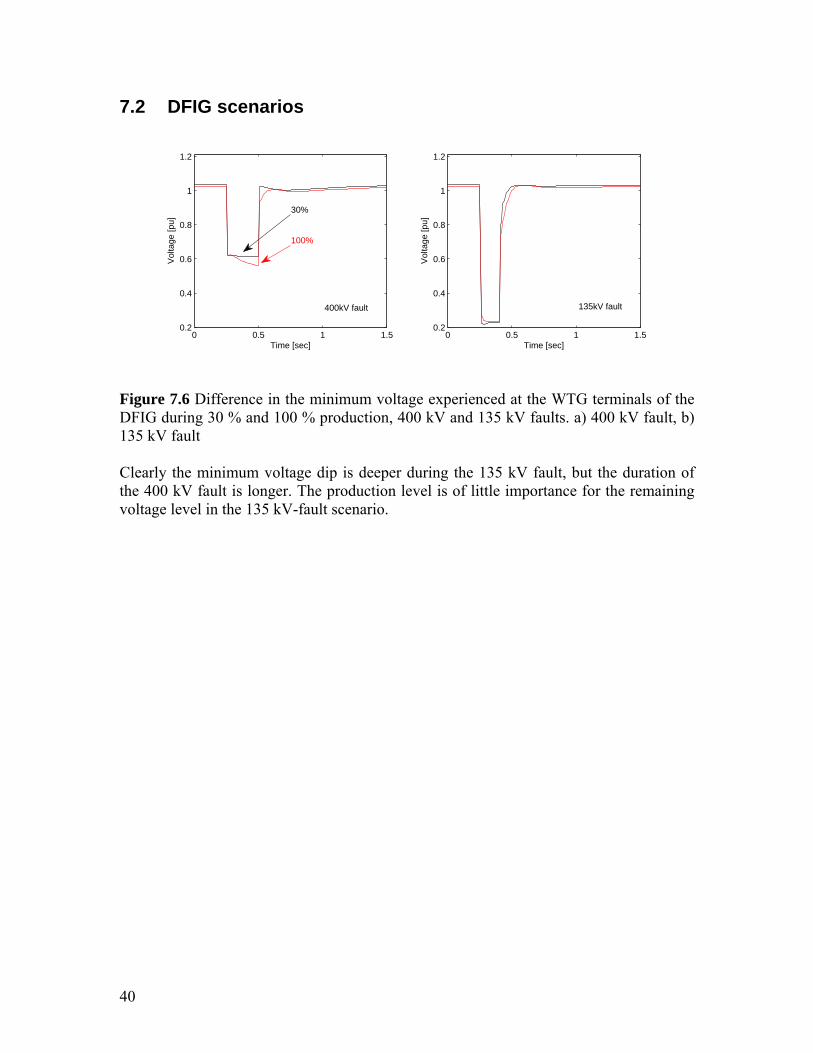
400kV fault 135kV fault

30%

100%

Figure 7.6 Difference in the minimum voltage experienced at the WTG terminals of the DFIG during 30 % and 100 % production, 400 kV and 135 kV faults. a) 400 kV fault, b) 135 kV fault Clearly the minimum voltage dip is deeper during the 135 kV fault, but the duration of the 400 kV fault is longer. The production level is of little importance for the remaining voltage level in the 135 kV-fault scenario.

40

0 0.5 1 1.5 2

0.2

0.4

0.6

0.8

1

1.2

Time [sec]

Vol

tage

[pu]

0 0.5 1 1.5 20

20

40

60

80

100

Time [sec]

Ang

le [d

egre

es]

0 0.5 1 1.5 2

0.2

0.4

0.6

0.8

1

1.2

Time [sec]

Vol

tage

[pu]

0 0.5 1 1.5 20

20

40

60

80

100

Time [sec]

Ang

le [d

egre

es]

135kV fault400kV fault

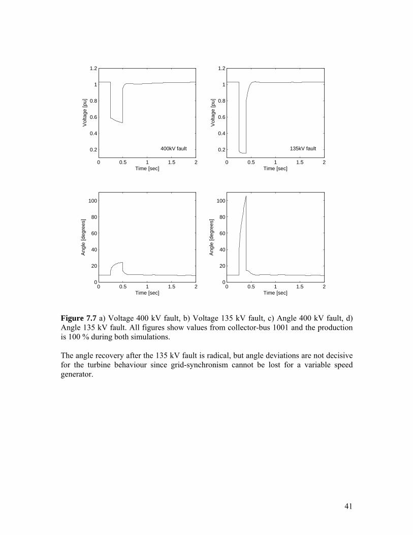
Figure 7.7 a) Voltage 400 kV fault, b) Voltage 135 kV fault, c) Angle 400 kV fault, d) Angle 135 kV fault. All figures show values from collector-bus 1001 and the production is 100 % during both simulations. The angle recovery after the 135 kV fault is radical, but angle deviations are not decisive for the turbine behaviour since grid-synchronism cannot be lost for a variable speed generator.

41

0 0.5 1 1.5 2 2.5 30.185

0.19

0.195

0.2

0.205

0.21

0.215

0.22

Time [sec]

LS s

peed

[pu]

0 0.5 1 1.5 2 2.5 3−0.5

0

0.5

1

1.5

2

2.5

Time [sec]

Mec

hani

cal p

ower

[pu]

100% prod

400kV

135kV

Figure 7.8 Comparison of 400 kV versus 135 kV fault and 100 % production. a) Speed, b) Mechanical power Both speed and mechanical power oscillations are far greater in the 135 kV fault case. Mechanical power increases from below zero (-0.25 pu) to more than 200 % (2.25 pu) of rated value in approximately 150ms during the first oscillation. For a 2.5 MW turbine, which is the approximate turbine size planned for this project, this will result in 2.5 MW × 2.5 pu = 6.25 MW = 8378 hp of power-change in 150ms. That is the equal to a top fuel dragster with 8000 hp rocketing of a starting line.

42

7.3 DFIG versus PMSG

0 0.5 1 1.50.4

0.5

0.6

0.7

0.8

0.9

1

1.1

1.2

Time [sec]

Vol

tage

[pu]

0 0.5 1 1.50.4

0.5

0.6

0.7

0.8

0.9

1

1.1

1.2

Time [sec]

Vol

tage

[pu]

DFIG

PMSG

0 0.5 1 1.50

0.2

0.4

0.6

0.8

1

1.2

Time [sec]

Vol

tage

[pu]

0 0.5 1 1.50

0.2

0.4

0.6

0.8

1

1.2

Time [sec]

Vol

tage

[pu]

DFIGPMSG

Figure 7.9 a) Voltage 30 % production 400 kV fault, b) voltage 100 % production 400 kV fault, c) Voltage 30 % production 135 kV fault, d) voltage 100 % production 135 kV fault. The performance of the DFIG and PMSG is compared when the PMSG runs in normal mode, i.e. Pf =1. The resulting voltage dip becomes much lower with the PMSG for both production levels and both faults, but the voltage recovery is on the other hand faster for the PMSG in all simulations. The reactive current contribution is the crucial factor determining the remaining voltage in the connection point, and the mechanisms behind the size of the reactive current contribution should therefore be assessed closer in the discussion chapter.

43

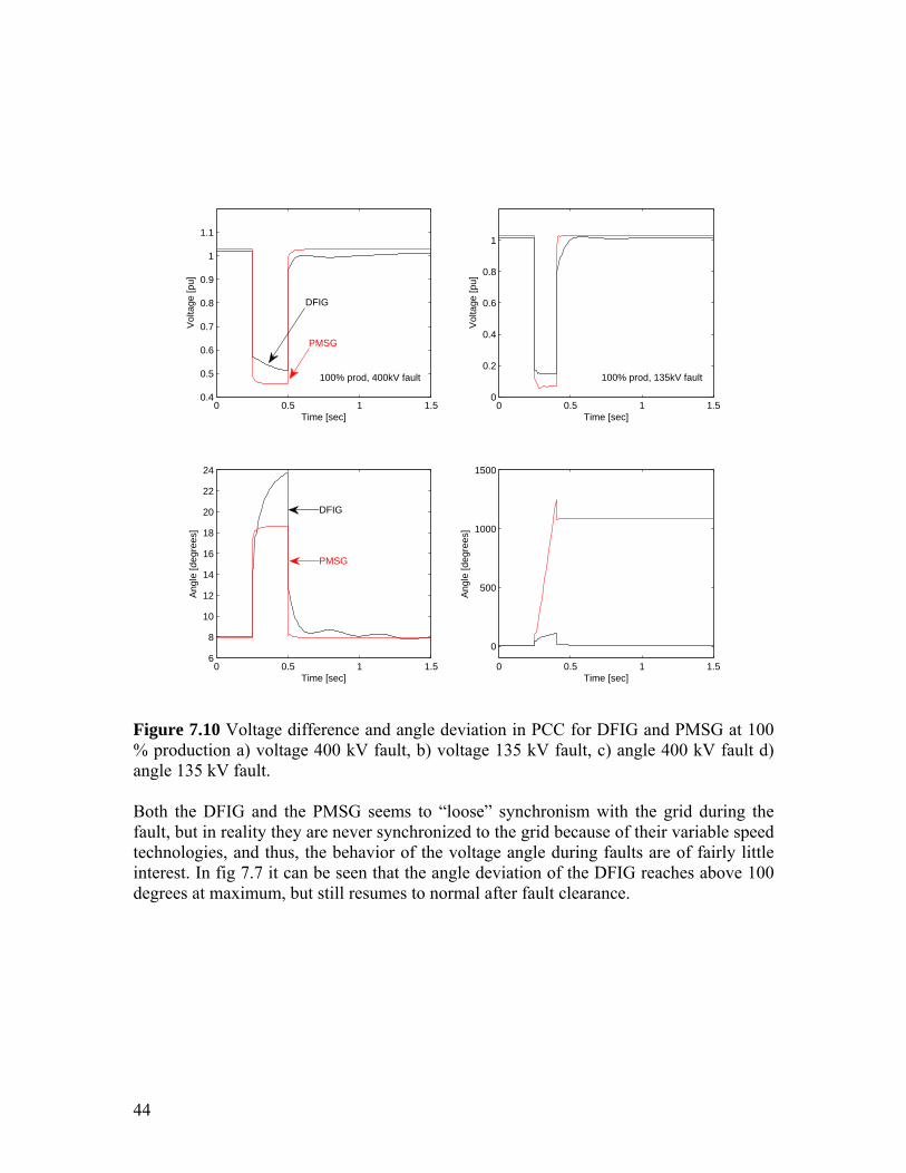
0 0.5 1 1.50.4

0.5

0.6

0.7

0.8

0.9

1

1.1

Time [sec]

Vol

tage

[pu]

0 0.5 1 1.56

8

10

12

14

16

18

20

22

24

Time [sec]

Ang

le [d

egre

es]

0 0.5 1 1.50

0.2

0.4

0.6

0.8

1

Time [sec]

Vol

tage

[pu]

0 0.5 1 1.5

0

500

1000

1500

Time [sec]

Ang

le [d

egre

es]

DFIG

DFIG

PMSG

PMSG

100% prod, 400kV fault 100% prod, 135kV fault

Figure 7.10 Voltage difference and angle deviation in PCC for DFIG and PMSG at 100 % production a) voltage 400 kV fault, b) voltage 135 kV fault, c) angle 400 kV fault d) angle 135 kV fault. Both the DFIG and the PMSG seems to “loose” synchronism with the grid during the fault, but in reality they are never synchronized to the grid because of their variable speed technologies, and thus, the behavior of the voltage angle during faults are of fairly little interest. In fig 7.7 it can be seen that the angle deviation of the DFIG reaches above 100 degrees at maximum, but still resumes to normal after fault clearance.

44

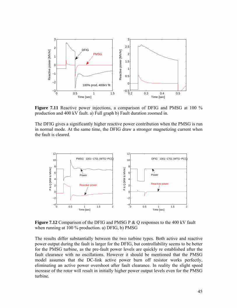
0 0.5 1 1.5−3

−2

−1

0

1

2

3

Time [sec]

Rea

ctiv

e po

wer

[MV

Ar]

0.2 0.3 0.4 0.5−0.5

0

0.5

1

1.5

2

2.5

3

Time [sec]

Rea

ctiv

e po

wer

[MV

Ar]

DFIGPMSG

100% prod, 400kV flt

Figure 7.11 Reactive power injections, a comparison of DFIG and PMSG at 100 % production and 400 kV fault. a) Full graph b) Fault duration zoomed in. The DFIG gives a significantly higher reactive power contribution when the PMSG is run in normal mode. At the same time, the DFIG draw a stronger magnetizing current when the fault is cleared.

0 0.5 1 1.5 2−4

−2

0

2

4

6

8

10

12

Time [sec]

P &

Q [M

W &

MV

Ar]

0 0.5 1 1.5 2−4

−2

0

2

4

6

8

10

12

Time [sec]

P &

Q [M

W &

MV

Ar]

DFIG 1001−1701 (WTG−PCC)PMSG 1001−1701 (WTG−PCC)

Power

Reactive power

Power

Reactive power

Figure 7.12 Comparison of the DFIG and PMSG P & Q responses to the 400 kV fault when running at 100 % production. a) DFIG, b) PMSG The results differ substantially between the two turbine types. Both active and reactive power output during the fault is larger for the DFIG, but controllability seems to be better for the PMSG turbine, as the pre-fault power levels are quickly re established after the fault clearance with no oscillations. However it should be mentioned that the PMSG model assumes that the DC-link active power burn off resistor works perfectly, eliminating an active power overshoot after fault clearance. In reality the slight speed increase of the rotor will result in initially higher power output levels even for the PMSG turbine.

45

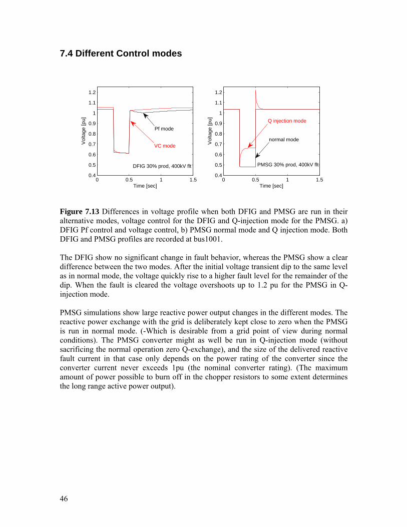
7.4 Different Control modes

0 0.5 1 1.50.4

0.5

0.6

0.7

0.8

0.9

1

1.1

1.2

Time [sec]

Vol

tage

[pu]

0 0.5 1 1.50.4

0.5

0.6

0.7

0.8

0.9

1

1.1

1.2

Time [sec]

Vol

tage

[pu]

Q injection mode

normal mode

DFIG 30% prod, 400kV flt PMSG 30% prod, 400kV flt

Pf mode

VC mode

Figure 7.13 Differences in voltage profile when both DFIG and PMSG are run in their alternative modes, voltage control for the DFIG and Q-injection mode for the PMSG. a) DFIG Pf control and voltage control, b) PMSG normal mode and Q injection mode. Both DFIG and PMSG profiles are recorded at bus1001. The DFIG show no significant change in fault behavior, whereas the PMSG show a clear difference between the two modes. After the initial voltage transient dip to the same level as in normal mode, the voltage quickly rise to a higher fault level for the remainder of the dip. When the fault is cleared the voltage overshoots up to 1.2 pu for the PMSG in Q-injection mode. PMSG simulations show large reactive power output changes in the different modes. The reactive power exchange with the grid is deliberately kept close to zero when the PMSG is run in normal mode. (-Which is desirable from a grid point of view during normal conditions). The PMSG converter might as well be run in Q-injection mode (without sacrificing the normal operation zero Q-exchange), and the size of the delivered reactive fault current in that case only depends on the power rating of the converter since the converter current never exceeds 1pu (the nominal converter rating). (The maximum amount of power possible to burn off in the chopper resistors to some extent determines the long range active power output).

46

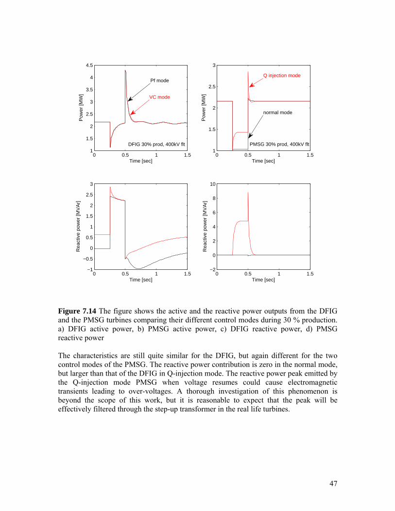
0 0.5 1 1.51

1.5

2

2.5

3

3.5

4

4.5

Time [sec]

Pow

er [M

W]

0 0.5 1 1.5−1

−0.5

0

0.5

1

1.5

2

2.5

3

Time [sec]

Rea

ctiv

e po

wer

[MV

Ar]

0 0.5 1 1.51

1.5

2

2.5

3

Time [sec]

Pow

er [M

W]

0 0.5 1 1.5−2

0

2

4

6

8

10

Time [sec]

Rea

ctiv

e po

wer

[MV

Ar]

normal mode

Pf mode

VC mode

PMSG 30% prod, 400kV fltDFIG 30% prod, 400kV flt

Q injection mode

Figure 7.14 The figure shows the active and the reactive power outputs from the DFIG and the PMSG turbines comparing their different control modes during 30 % production. a) DFIG active power, b) PMSG active power, c) DFIG reactive power, d) PMSG reactive power The characteristics are still quite similar for the DFIG, but again different for the two control modes of the PMSG. The reactive power contribution is zero in the normal mode, but larger than that of the DFIG in Q-injection mode. The reactive power peak emitted by the Q-injection mode PMSG when voltage resumes could cause electromagnetic transients leading to over-voltages. A thorough investigation of this phenomenon is beyond the scope of this work, but it is reasonable to expect that the peak will be effectively filtered through the step-up transformer in the real life turbines.

47

8 Result summary The voltage dip originating in the 400 kV transmission network gradually decrease in depth as it approach the wind farm through power lines and transformers, from 0.48 pu in Sege to around 0.60 pu at the WTG terminals (depending on the setup). The dip is of almost equal amplitude in the wind farm point of common connection and at the wind turbine transformer high side, but differs significantly between the WTG terminals and the WTG transformer high side in case of successful reactive power injection. The resulting voltage level in the PCC is, for the various simulations, spread around the 0.49 pu-value obtained in the no-wind farm base case scenario simulation. This spread in voltage levels indicates that the reactive current injection differ substantially between the simulations of the different scenarios. The instantaneous voltage drop at the DFIG terminals is similar for both low and high production, but the voltage continues to fall at a fairly steep rate throughout the fault when the turbine runs at full power. The PMSG on the other hand shows similar response characteristics throughout the duration of the voltage dip at both low and high production. Voltage recovery after fault clearance is fast for both the DFIG and PMSG at both points of operation and during both faults, but the PMSG is the better performer in this aspect. The reactive power injection is larger from the DFIG than the normal mode PMSG, but slightly lower than the Q-injection mode PMSG. The 135 kV fault at the Maltesholm transformer station high side cause a lower dip, (0.2 pu), than the 400 kV fault and the resulting mechanical dynamics in the DFIG turbine consequently show higher amplitude fluctuations. The rotor-speed of the DFIG increase during both faults, the pitch mechanism is activated and the rotor is retarded below pre-fault speed when regular voltage level resumes after fault clearance, but stabilises in ten seconds after a slight speed-overshoot around 5 seconds. The active power output decrease to about half the initial value during 400 kV faults and overshoot the nominal value when voltage resumes at the WTG terminals.

48

9 Discussion

The results show that the fault behaviour of the two turbine types DFIG and PMSG is substantially different. The DFIG simulations show a higher voltage level close to the turbine compared to the PMSG turbine running in normal mode, but that result is flipped once the PMSG is run in Q-injection mode. Mechanical dynamic output channels, introduced only in the DFIG simulations, should be interpreted with special attention to the model assumptions as explained in the results section. Nevertheless, regardless of the accuracy of the input power mechanisms modelled, the rate of power change shows that the mechanical stress on DFIG turbines during LVRT is considerable. The turbine hardware is more sensitive to the depth of a voltage dip than its duration, as it functions like a force impulse hitting harder with higher amplitude. Vestas clearly state, in the user guide for their wind turbine, that the maximum number of low voltage ride troughs is once per week throughout the technical lifetime of the turbine. Ride through systems can also influence steady state power loss, an aspect of no interest for the simulation response, but which should be considered when choosing WTG’s for wind farm projects. In total, the reactive power output from the DFIG simulations is probably a bit optimistic, especially in the first stages of the voltage dip. This observation was to some extent expected since the supplier of the model is also selling the turbine modelled. It would be interesting to test the sensitivity of the model to change in the different generator and converter parameters. Officially there is little room for such evaluation of the different manufacturers LVRT solutions, since any internal machine parameter acquired from a manufacturer is confidential. For the PMSG, the LVRT systems are not very complicated since no transient rotating mechanical dynamics are directly coupled to the fault voltage. Basically the only challenge that remains for the PMSG is the long term active power surplus experienced during a fault when the electrical power is smaller than the mechanical power. DC-link dump loads (choppers) are used to mitigate this problem together with fast emergency pitching systems, but these kinds of systems still has to disconnect for faults of longer duration due to chopper resistor thermal limits. It could be confirmed that different LVRT-strategies exist, and that some are technically and/or strategically better than others, but only time can tell exactly how well the different strategies work in practice compared to their cost. Obviously, over-dimensioning of electrical components and over-engineering of turbine solutions result in technically superior turbines, but they also turn out more expensive. The challenge is to find the best compromise of investment and performance for the conditions expected at a certain site. Earlier experience with operation of turbines in similar environments will probably prove useful in this context.

49

As seen in the simulations, during successful operation, wind farms contribute to fault currents hence keeping up the voltage at the connection point, thereby preventing their own relays from initializing disconnecting actions. A paradoxal perspective though, is that the reactive current injection also helps the voltage level in the closest meshed 400 kV-node where the fault is applied. This means that the same physical fault which prior to the wind farm connection caused a voltage dip to 25 % now will be less severe. The mitigated voltage dip is clearly a power system stability enhancement, but at the same time means that a new and more severe physical fault (lower fault impedance) have to be introduced to again reach the standardized fault level of 25 % in the 400 kV-node. The paradox is that by contributing to grid stability, the wind turbines have to withstand even worse faults in the network than the original 25 % dips with no wind farm connected.

50

10 Conclusions The wind farm project planned for Linderödsåsen in southern Sweden have successfully been modelled together with a reduced network model of Eons 135 kV subtransmission network. The simulation setup described has served as a platform for dynamic performance comparison of different wind turbine generator technologies and grid code aspects in general, and has facilitated grid code compliance investigation of the planned Linderödsåsen wind farm in particular. The zero-controlled reactive fault current contribution from the PMSG, when run in normal mode, result in low residual voltages in the whole system during faults, especially close to the turbine. On the low voltage side of the wind farm point of common coupling (PCC) the difference can exceed 0.10 pu when compared with a DFIG or a PMSG Q-injection mode setup. This result is more of an issue for the TSO than for the wind farm operator, since the PMSG turbines will have no problems staying connected even tough the voltage profile is more severe. The responsibility regarding this issue lies fully with the TSO as long as the requirement of no wind farm tripping has been met by the producing facility. The voltage threshold for turbine disconnection is low and of much longer duration for the PMSG turbine than the DFIG, and consequently it has no problems staying connected to the grid in either Q-injection mode or normal mode. This means that the performance of the PMSG is largely chosen by the wind farm owner and could be set to suit any criteria within a broad spectre of voltage levels, trip times and Q-injection levels. Mechanical dynamics have only been evaluated for the DFIG turbines, and the stress levels are shown to exceed 200 % of the rated mechanical power values. It is known that the mechanical stress during faults is larger on the DFIG turbines, and details of the PMSG turbine mechanical dynamics have not been investigated as they are known to be of minor magnitude and importance. Regardless of simulation setup, it is clear that the resulting voltage levels at the wind turbine terminals are tolerable for all the wind turbines at offer for Linderödsåsen Wind Farm. The wind turbine manufacturers investigated argue that they can provide wind turbine generators that will meet the operational challenges introduced by the grid code. And the simulations compared with the LVRT –protection settings provided, suggest that they do. The manufacturers can deliver different turbine options with or without low voltage ride-through options, but it could seriously be doubted that the simpler versions will be able to ride through the grid code prescribed voltage dips, and such versions can therefore not be recommended for this wind farm project. The worst case simulation voltage curves could be used as reference to decide the choice of voltage levels and triggering times for the wind turbine protection relays in Linderödsåsen Wind Farm. The two different Q-modes of the PMSG and the magnitude of Q injected by the DFIG determine the remaining voltage level close to the wind farm during voltage dips. Other

51

generators or machines located close to the farm could trip during the same fault, and does so more easily if the voltage dip is lower. If turbine configurations capable of delivering large reactive currents are chosen, circuit breakers in close proximity of the wind turbine have to be rated accordingly. The Linderödsåsen wind farm project will have to meet the regulations from the national TSO Svenska Kraftnät, but at the same time make a system beneficiary trade-off between regulation compliance, investment cost and maintenance cost related to the mechanical stress on the turbines. And finally the economics of the various low voltage ride through systems will have to be weighed into the full economic picture of the turbine solutions offered from the different manufacturers.

52

11 Future work A documented possible islanding operation scenario for the wind farm, described in detail by Eon, would be interesting to look further into. It would be regarded as system beneficial if the wind farm could be run in such a way that the local load still would be served and the active power output could be regulated according to the local needs during this scenario. A detailed survey of the models possible to use for comparison of different turbine manufacturers would be very interesting. During this work it proved difficult to gather enough technical information from the wind turbine manufacturers to easily compare turbines on equal bases. A full WTG representation with pitching systems and converter control algorithms is complex and requires much work to fully go through, but one could focus on developing one model based on one of the current commercial DFIG’s with LVRT solution. Turbine modelling for computer simulation is moving on, and PSS/E will be updated with new models in short time, (new models from both Enercon and GE Energy have due release in January 09), including representation of GE’s PMSG full power converter turbine. Simulations with new updated models will always be relevant and 5th order model simulations including rotor and stator fluxes and crow bar operation could be a step towards less uncertainty for the DFIG reactive power output results. Measurements of real life fault behaviour at the wind farm once in operation would be very interesting to look into to see how well the simulations correlate with the real network and wind farm behaviour.

53

12 References [1] Yvonne Coughlan, Paul Smith, Alan Mullane and Mark O’Malley, Wind Turbine

Modelling for Power System Stability Analysis – A System Operator Perspective, IEEE Transactions on power systems, vol. 22, no.3, august 2007.

[2] I.Erlich and F. Shewarega, Insert Impact of Large-Scale Wind Power Generation

on the Dynamic Behaviour of Interconnected Systems, 2007 iREP Symposium- Bulk Power System Dynamics and Control – VII, Revitalizing Operational Reliability, August 19-24, 2007, Charleston, SC, USA.

[3] J.O. Tande, K. Uhlen, Impact of integrating wind power in the Norwegian power

system Sintef Energy Research, technical report April 2006 [4] D. Andersson, Eon, Personal communication Mars 4, 2008. [5] P. Kundur, Power System Stability and Control, McGraw-Hill, Inc. 1994 [6] V. Akhmatov, Analysis of Dynamical Behaviour of Electric Power Systems with

Large Amount of Wind Power, PhD Thesis, Electric Power Engineering, Örsted-DTU, Technical University of Denmark, April 2003.

[7] Affärsverket svenska kraftnäts författningssamling, Affärsverket svenska kraftnäts

föreskrifter och allmänna råd om driftsäkerhetsteknisk utformning av produktionsanläggningar, SvKFS 2005:2, 9 december 2005.

[8] S. Arnborg. Senior Engineer at Svenska Kraftnät, Personal communication May

16, 2008. [9] J.Beurskens, Eon [10] K.Y. Maalawi and M.A. Badr, A practical approach for selecting optimum wind

rotors, Mechanical Engineering Department, National Research Center, Dokki, Cairo, Egypt, Renewable energy, ISSN 0960-1481, 2003, vol. 28 no.5.

[11] Onsala Space Observatory, Real time 24-hour wind strength and direction,

http://www.oso.chalmers.se/~weather/. [12] T. Ackermann, Wind Power in Power Systems, John Wiley & Sons, Ltd 2005.

reprinted 2007.

54

[13] J. Morren, S. W. H. de Haan, Short-Circuit Current of Wind Turbines With Doubly Fed Induction Generator, IEEE Transactions on energy conversion, vol. 22, No. 1, March 2007.

[14] I. Erlich,J. Kretschmann, J. Fortmann, S. Mueller-Enghard & H. Wrede, Modelling of Wind Turbines Based on Doubly-Fed Induction Generators for Power System Studies, IEEE Transactions on energy conversion, vol. 22, No. 3, August 2007.

[15] A. Dittrich & A. Stoev, Comparison of fault ride through strategies for wind

turbines with DFIM Generator, Power Electronics and Applications, 2005 European Conference on 11-14 September 2005.

[16] I. Erlich & F. Shewarega, Interaction of Large Wind Power Generation Plants

with the Power System, Power and Energy Conference, 2006. PECon ’06. IEEE International, November 28-29, 2006.

[17] Enercon Product leaflet. [18] GE Energy Product leaflet. [19] Vestas Product leaflet. [20] Siemens Power Transmission & Distribution, Inc., PSS/E Wind Modeling User

Guide, Issue 1.0.0 March 2005. [21] GE Energy, Modelling of GE Wind Turbine-Generators for Grid Studies, Version

4.1, January 2008.

55

13 Appendix A PMSG model documentation

56

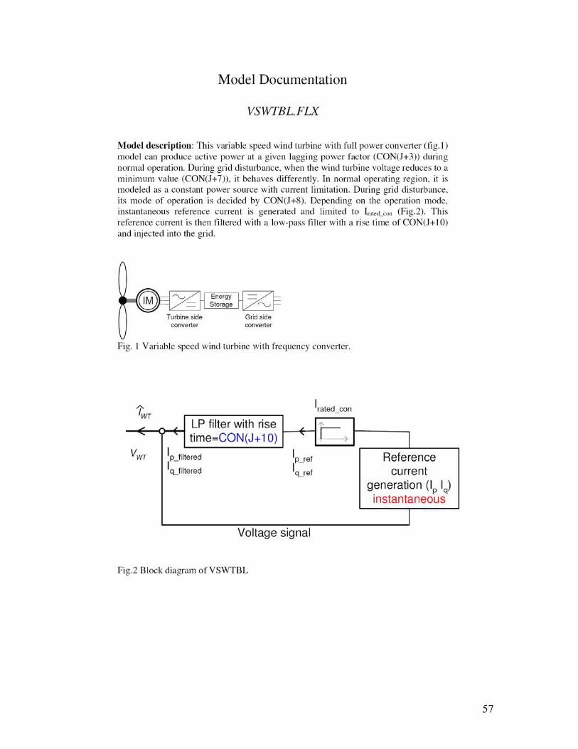
57

58

59

B Matlab PSS/E output channel converter program This matlab program converts the PSS/E output channel files to the matlab matrix format. One example of the resulting straight forward matlab plotting is also provided. % function out=psse2matl % From a PSSE/24 result file to a Matlab Matrix. % The first column is time clc; close l; alclear; channels=[]; data=[]; antal=[]; titel=[]; [filename,path]=uigetfile('*.out','PSSE .out files') fid=fopen(filename); setstr(fread(fid,4,'char')'); setstr(fread(fid,4,'char')'); setstr(fread(fid,4,'char')'); antal=fread(fid,1,'float32'); disp(['Total Channels:',num2str(antal)]) fread(fid,1,'float32'); channels=setstr(fread(fid,[32, antal] ,'char'))'; disp(channels) titel=setstr(fread(fid,[60, 2] ,'char'))'; disp(titel) data=fread(fid,Inf,'float32'); tider=(size(data,1)-2)/(antal+2); resultat=reshape(data(1:tider*(antal+2)),antal+2,tider)'; out=resultat(:,2:size(resultat,2)); fclose(fid); % % time=out(:,1); t=time; c2=out(:,2); %Voltage at 1001 c3=out(:,3); %Angle at 1001 c4=out(:,4); %Voltage at 1701 c5=out(:,5); %Angle at 1701 c6=out(:,6); %Voltage at 10000 c7=out(:,7); %Angle at 10000 c8=out(:,8); %P 1001-1701 c9=out(:,9); %Q 1001-1701 c10=out(:,10); %P 37377-37215 Hörby c11=out(:,11); %Q 37377-37215 Hörby c12=out(:,12); %P 37377-37230 Åhus c13=out(:,13); %Q 37377-37230 Åhus c14=out(:,14); %Pitch angle at 91001 c15=out(:,15); %LS shaft torque at 91001 c16=out(:,16); %LS shaft rotor speed at 91001 c17=out(:,17); %LS shaft Mechanical power at 91001

60

c18=out(:,18); %WTG terminal voltage % DFIG, 30% prod, 400kV figure (1) subplot(2,2,1) plot(t,c18,'k'); hold on xlabel('Time [sec]') ylabel('Voltage [pu]') figure (2) subplot(2,2,1) plot(t,c2,'k'); hold on xlabel('Time [sec]') ylabel('Voltage [pu]') figure (6) subplot(2,2,1) plot(t,c9,'r'); hold on xlabel('Time [sec]') ylabel('Reactive power [MVA]') subplot(2,2,2) plot(t,c9,'r'); hold on xlabel('Time [sec]') ylabel('Reactive power [MVA]') figure (9) subplot(2,2,1) plot(t,c2,'k') hold on xlabel('Time [sec]') ylabel('Voltage [pu]') figure (10) subplot(2,2,1) plot(t,c8,'k') hold on xlabel('Time [sec]') ylabel('Power [MW]') subplot(2,2,2) plot(t,c8,'k') hold on xlabel('Time [sec]') ylabel('Power [MW]') figure (13) subplot(2,2,1) plot(t,c8,'k') hold on

61

xlabel('Time [sec]') ylabel('power [MW]') subplot(2,2,3) plot(t,c9,'k') hold on xlabel('Time [sec]') ylabel('Reactive power [MVA]')

62