William Kirk · Naseer Shahzad Fixed Point Theory in Distance Spaces

Welcome message from author
This document is posted to help you gain knowledge. Please leave a comment to let me know what you think about it! Share it to your friends and learn new things together.
Transcript
William Kirk · Naseer Shahzad
Fixed Point Theory in Distance Spaces
Fixed Point Theory in Distance Spaces


William Kirk • Naseer Shahzad
Fixed Point Theoryin Distance Spaces
123

William KirkDepartment of MathematicsUniversity of IowaIowa City, IA, USA
Naseer ShahzadDepartment of MathematicsKing Abdulaziz UniversityJeddah, Saudi Arabia
ISBN 978-3-319-10926-8 ISBN 978-3-319-10927-5 (eBook)DOI 10.1007/978-3-319-10927-5Springer Cham Heidelberg New York Dordrecht London
Library of Congress Control Number: 2014948344
Mathematics Subject Classification (2000): 54H25, 51K10, 54C05, 47H09
© Springer International Publishing Switzerland 2014This work is subject to copyright. All rights are reserved by the Publisher, whether the whole or part ofthe material is concerned, specifically the rights of translation, reprinting, reuse of illustrations, recitation,broadcasting, reproduction on microfilms or in any other physical way, and transmission or informationstorage and retrieval, electronic adaptation, computer software, or by similar or dissimilar methodologynow known or hereafter developed. Exempted from this legal reservation are brief excerpts in connectionwith reviews or scholarly analysis or material supplied specifically for the purpose of being enteredand executed on a computer system, for exclusive use by the purchaser of the work. Duplication ofthis publication or parts thereof is permitted only under the provisions of the Copyright Law of thePublisher’s location, in its current version, and permission for use must always be obtained from Springer.Permissions for use may be obtained through RightsLink at the Copyright Clearance Center. Violationsare liable to prosecution under the respective Copyright Law.The use of general descriptive names, registered names, trademarks, service marks, etc. in this publica-tion does not imply, even in the absence of a specific statement, that such names are exempt from therelevant protective laws and regulations and therefore free for general use.While the advice and information in this book are believed to be true and accurate at the date of pub-lication, neither the authors nor the editors nor the publisher can accept any legal responsibility for anyerrors or omissions that may be made. The publisher makes no warranty, express or implied, with respectto the material contained herein.
Printed on acid-free paper
Springer is part of Springer Science+Business Media (www.springer.com)

Abstract. Traditionally, a large body of metric fixed point theory has been couchedin a functional analytic framework. This aspect of the theory has been written aboutextensively. This survey treats the purely metric aspects of the theory—specifically resultsthat do not depend on any algebraic structure of the underlying space. The focus is on (I)metric spaces satisfying additional geometric conditions, (II) metric spaces with geodesicstructures, and (III) semimetric spaces satisfying relaxed versions of the triangle inequality.


Preface
Mathematicians interested in topology typically give an abstract set a“topological structure” consisting of a collection of subsets of the given set todetermine when points are “near” each other. People interested in geometryneed a more rigid notion of nearness. This usually begins with assigning asymmetric “distance” to each two points of a set, resulting in the notion ofa semimetric. With the addition of the triangle inequality, one passes to ametric space. This will be our point of departure.
There are four classical fixed point theorems against which metric ex-tensions are usually checked. These are, respectively, the Banach contractionmapping principle, Nadler’s well-known set-valued extension of that theorem,the extension of Banach’s theorem to nonexpansive mappings, and Caristi’stheorem. These comparisons form a significant component of this survey.
This exposition is divided into three parts. In Part I we discuss someaspects of the purely metric theory, especially Caristi’s theorem and its rela-tives. Among other things, we discuss these theorems in the context of theirlogical foundations. We omit a discussion of the well-known Banach Con-traction Principle and its many generalizations in Part I because this topicis well known and has been reviewed extensively elsewhere (see, e.g., [117]).In Part II we discuss classes of spaces which, in addition to having a met-ric structure, also have geometric structure. These specifically include thegeodesic spaces, length spaces, and CAT(0) spaces. In Part III we turn todistance spaces that are not necessarily metric. These include certain dis-tance spaces which lie strictly between the class of semimetric spaces and theclass of metric spaces, as well as other spaces whose distance properties donot fully satisfy the metric axioms.
We make no attempt to explain all aspects of the topics we cover nor topresent a compendium of all known facts, especially since the theory continuesto expand at a rapid rate. Any attempt to provide the latest tweak on thevarious theorems we discuss would surely be outdated before reaching print.Our objective rather is to present a concise accessible document which canbe used as an introduction to the subject and its central themes. We includeproofs selectively, and from time to time we mention open problems. Thematerial in this exposition is collected together here for the first time. Those
VII

VIII PREFACE
wishing to investigate these topics deeper are referred to the original sources.We have attempted to include details in those instances where the sources arenot readily available. This might be the case, for example, when the source isin a conference proceedings. Also some results appear here for the first time.
Many of the concepts introduced here have found interesting applications.Indeed some were motivated by attempts to address both mathematical andapplied problems. Other concepts we discuss are more formal in nature andhave yet to find any serious application; indeed some may never. Howeverour hope is that this discussion will suggest directions for those interested infurther research in this area.
The first author lectured on portions of the material covered in thismonograph to students and faculty at King Abdulaziz University. He wishesto thank them for providing an attentive and critical audience. Both authorsexpress their gratitude to Rafa Espínola for calling attention to a number ofoversights in an earlier draft of this manuscript.
Iowa City, IA, USA William KirkJeddah, Saudi Arabia Naseer Shahzad

Contents
Preface VII
Contents IX
Part I. Metric Spaces 1
Chapter 1. Introduction 3
Chapter 2. Caristi’s Theorem and Extensions 72.1. Introduction 72.2. A Proof of Caristi’s Theorem 92.3. Suzuki’s Extension 112.4. Khamsi’s Extension 112.5. Results of Z. Li 162.6. A Theorem of Zhang and Jiang 18
Chapter 3. Nonexpansive Mappings and Zermelo’s Theorem 193.1. Introduction 193.2. Convexity Structures 19
Chapter 4. Hyperconvex Metric Spaces 23
Chapter 5. Ultrametric Spaces 255.1. Introduction 255.2. Hyperconvex Ultrametric Spaces 275.3. Nonexpansive Mappings in Ultrametric Spaces 285.4. Structure of the “Fixed Point Set” of Nonexpansive Mappings 305.5. A Strong Fixed Point Theorem 315.6. Best Approximation 35
Part II. Length Spaces and Geodesic Spaces 37
Chapter 6. Busemann Spaces and Hyperbolic Spaces 396.1. Convex Combinations in a Busemann Space 42
Chapter 7. Length Spaces and Local Contractions 477.1. Local Contractions and Metric Transforms 54
IX
X CONTENTS
Chapter 8. The G-Spaces of Busemann 618.1. A Fundamental Problem in G-Spaces 63
Chapter 9. CAT(0) Spaces 659.1. Introduction 659.2. CAT(κ) Spaces 669.3. Fixed Point Theory 709.4. A Concept of “Weak” Convergence 819.5. Δ-Convergence of Nets 839.6. A Four Point Condition 869.7. Multimaps and Invariant Approximations 899.8. Quasilinearization 93
Chapter 10. Ptolemaic Spaces 9510.1. Some Properties of Ptolemaic Geodesic Spaces 9610.2. Another Four Point Condition 98
Chapter 11. R-Trees (Metric Trees) 9911.1. The Fixed Point Property for R-Trees 10011.2. The Lifšic Character of R-Trees 10211.3. Gated Sets 10511.4. Best Approximation in R-Trees 10611.5. Applications to Graph Theory 109
Part III. Beyond Metric Spaces 111
Chapter 12. b-Metric Spaces 11312.1. Introduction 11312.2. Banach’s Theorem in a b-Metric Space 11512.3. b-Metric Spaces Endowed with a Graph 11612.4. Strong b-Metric Spaces 12112.5. Banach’s Theorem in a Relaxedp Metric Space 12412.6. Nadler’s Theorem 12512.7. Caristi’s Theorem in sb-Metric Spaces 12812.8. The Metric Boundedness Property 129
Chapter 13. Generalized Metric Spaces 13313.1. Introduction 13313.2. Caristi’s Theorem in Generalized Metric Spaces 13613.3. Multivalued Mappings in Generalized Metric Spaces 139
Chapter 14. Partial Metric Spaces 14114.1. Introduction 14114.2. Some Examples 14314.3. The Partial Metric Contraction Mapping Theorem 14314.4. Caristi’s Theorem in Partial Metric Spaces 144

CONTENTS XI
14.5. Nadler’s Theorem in Partial Metric Spaces 14814.6. Further Remarks 152
Chapter 15. Diversities 15315.1. Introduction 15315.2. Hyperconvex Diversities 15515.3. Fixed Point Theory 155
Bibliography 159
Index 173
Part I
Metric Spaces
CHAPTER 1
Introduction
At the outset we adopt the classical terminology of W.A. Wilson [216].(The term “semimetric space” (halb-metrischer Raume) is likely due to KarlMenger [153].)
Definition 1.1. Let X be a set and let d : X ×X → R be a mappingsatisfying for each x, y ∈ X:
I. d (x, y) ≥ 0, and d (x, y) = 0 ⇔ x = y;II. d (x, y) = d (y, x) .
Then the pair(X, d) is called a semimetric space.
In such a space, convergence of sequences is defined in the usual way:A sequence {xn} ⊆ X is said to converge to x ∈ X if limn→∞ d (xn, x) = 0.Also a sequence is said to be Cauchy if for each ε > 0 there exists N ∈ N suchthat m,n ≥ N ⇒ d (xm, xn) < ε. The space (X, d) is said to be complete ifevery Cauchy sequence has a limit.
With such a broad definition of distance, three problems are immediatelyobvious: (i) There is nothing to assure that limits are unique (thus the spaceneed not be Hausdorff ); (ii) a convergent sequence need not be a Cauchysequence; (iii) the mapping d (x, ·) : X → R need not even be continuous.These facts preclude an effective topological theory in such a general setting.
With the introduction of the triangle inequality problems (i)–(iii) aresimultaneously eliminated.
VI. (Triangle Inequality) With X and d as in Definition 1.1 assume alsothat for each x, y, z ∈ X:
d (x, y) ≤ d (x, z) + d (z, y) .
Definition 1.2. A pair (X, d) satisfying Axioms I, II, and VI is calleda metric space.
A metric space (X, d) is said to be metrically convex (or Menger convex)if given any two points p, q ∈ X there exists a point z ∈ X, p = z = q, suchthat
d (p, z) + d (z, q) = d (p, q) .
© Springer International Publishing Switzerland 2014W. Kirk, N. Shahzad, Fixed Point Theory in Distance Spaces,DOI 10.1007/978-3-319-10927-5__1
3

4 1. INTRODUCTION
Karl Menger was a pioneer in the axiomatic study of distance spaces, and hewas the first to discover the following fact.
Theorem 1.1 ([153]). Any two points of a complete and metrically con-vex metric space are the endpoints of at least one metric segment.
See [28, p. 41] for a proof of this theorem due to N. Aronszajn. Mengerbased the original proof of his classical result on transfinite induction. A proofbased on Caristi’s theorem is given in [113].
In his study [216], Wilson introduced three axioms in addition to I andII which are weaker than VI. These are the following:
III. For each pair of (distinct) points x, y ∈ X there is a number rx,y > 0such that for every z ∈ X
rx,y ≤ d (x, z) + d (z, y) .
IV. For each point x ∈ X and each k > 0 there is a number rx,k > 0such that if y ∈ X satisfies d (x, y) ≥ k then for every z ∈ X
rx,k ≤ d (x, z) + d (z, y) .
V. For each k > 0 there is a number rk > 0 such that if x, y ∈ X satisfyd (x, y) ≥ k then for every z ∈ X
rk ≤ d (x, z) + d (z, y) .
Obviously if Axiom V is strengthened to rk = k, then the space becomesmetric. W.A. Wilson asserts in [216] that E.W. Chittenden [53] has shown(using an equivalent definition) that a semimetric space satisfying Axiom Vis always metrizable. (We have not independently verified this assertion.)
Axiom III in a semimetric space (X, d) is equivalent to the assertion thatthere do not exist distinct points x, y ∈ X and a sequence {zn} ⊆ X such thatd (x, zn) + d (y, zn) → 0 as n → ∞. Thus, as Wilson observes, the followingis self-evident.
Proposition 1.1. In a semimetric space Axiom III implies that limitsare unique.
For r > 0, let U (p; r) = {x ∈ X : d (x, p) < r} . Then Axiom III is alsoequivalent to the assertion that X is Hausdorff in the sense that given anytwo distinct points x, y ∈ X there exist positive numbers rx and ry such thatU (x; rx) ∩ U (y; ry) = ∅.
Definition 1.3. Let (X, d) be a semimetric space. Then the distancefunction d is said to be continuous if for any sequences {pn} , {qn} ⊆ X,limn→∞ d (pn, p) = 0 and limn→∞ d (qn, q) = 0 ⇒ limn→∞ d (pn, qn) =d (p, q) .

1. INTRODUCTION 5
A point p in a semimetric space X is said to be an accumulation pointof a subset E of X if given any ε > 0, U (p; ε) ∩ E = ∅. A subset of asemimetric space is said to be closed if it contains each of its accumulationpoints. A subset of a semimetric space is said to be open if its complementis closed. With these definitions, if X is a semimetric space with continuousdistance function, then U (p; r) is an open set for each p ∈ X and r > 0 andmoreover, X is a Hausdorff topological space [28, p. 11].
Remark 1.1. Some authors call a space satisfying Axioms I and II asymmetric space, and reserve the term semimetric space for symmetric spaceswith continuous distance function. We use the classical definition in thismonograph.
CHAPTER 2
Caristi’s Theorem and Extensions
2.1. Introduction
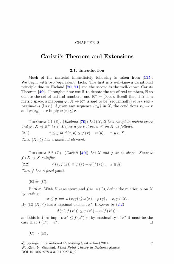
Much of the material immediately following is taken from [115].We begin with two “equivalent” facts. The first is a well-known variationalprinciple due to Ekeland [70, 71] and the second is the well-known CaristiTheorem [49]. Throughout we use R to denote the set of real numbers, N todenote the set of natural numbers, and R
+ = [0,∞). Recall that if X is ametric space, a mapping ϕ : X → R
+ is said to be (sequentially) lower semi-continuous (l.s.c.) if given any sequence {xn} in X, the conditions xn → xand ϕ (xn) → r imply ϕ (x) ≤ r.
Theorem 2.1 (E). (Ekeland [70]) Let (X, d) be a complete metric spaceand ϕ : X → R
+ l.s.c. Define a partial order ≤ on X as follows:
(2.1) x ≤ y ⇔ d (x, y) ≤ ϕ (x)− ϕ (y) , x, y ∈ X.
Then (X,≤) has a maximal element.
Theorem 2.2 (C). (Caristi [49]) Let X and ϕ be as above. Supposef : X → X satisfies
(2.2) d (x, f (x)) ≤ ϕ (x)− ϕ (f (x)) , x ∈ X.
Then f has a fixed point.
(E) ⇒ (C).
Proof. With X,ϕ as above and f as in (C), define the relation ≤ on Xby setting
x ≤ y ⇐⇒ d (x, y) ≤ ϕ (x)− ϕ (y) , x, y ∈ X.
By (E) (X,≤) has a maximal element x∗. However by (2.2)
d (x∗, f (x∗)) ≤ ϕ (x∗)− ϕ (f (x∗)) ,
and this in turn implies x∗ ≤ f (x∗) so by maximality of x∗ it must be thecase that f (x∗) = x∗. �
(C) ⇒ (E) .
© Springer International Publishing Switzerland 2014W. Kirk, N. Shahzad, Fixed Point Theory in Distance Spaces,DOI 10.1007/978-3-319-10927-5__2
7

8 2. CARISTI’S THEOREM AND EXTENSIONS
Proof. Assume X,ϕ, and ≤ are as in (E), and assume (X,≤) does nothave a maximal element. Then for each x ∈ X there exists yx ∈ X suchthat x < yx. Define f : X → X by setting f (x) = yx. Then by (2.1)d (x, yx) ≤ ϕ (x)− ϕ (yx) ; hence
d (x, f (x)) ≤ ϕ (x)− ϕ (f (x)) , x ∈ X.
By (C) f has a fixed point x∗. But by assumption x∗ < f (x∗), which is acontradiction. �
Thus it is easy to see that (E) ⇔ (C) . However to a logician these tworesults are not equivalent. In particular the implication (C) ⇒ (E) invokesthe Axiom of Choice (AC). In fact, N. Brunner [42] has shown that anyproof of (E) requires at least the basic axioms of Zermelo–Fraenkel (ZF) plusa form of the Axiom of Choice called the Axiom of Dependent Choice (DC),whereas R. Mańka [143] has shown that (C) holds within (ZF). So from apurely logical point of view the two theorems are not equivalent. (DC) isstrictly weaker than (AC) but strictly stronger than the Axiom of CountableChoice.
Brézis and Browder derive Ekeland’s Theorem from an order princi-ple (see Theorem 2.4 below) which requires only ZFDC. They then deriveCaristi’s Theorem as in the implication (E) ⇒ (C) above. Hence Choiceis invoked at this step. However in [87] it is shown that Caristi’s theo-rem can be derived directly from the order principle of Brézis and Browderwithout recourse to Ekeland’s Theorem. We give a similar proof below (seeTheorem 2.3).
In the chart below we list the authors of some of the early proofs ofCaristi’s theorem, the methods, and the axioms used. See Sect. 13.2 for aquick proof using Zorn’s Lemma.
Author Method AxiomsCaristi (1976) [49] Transfinite Induction ZFACWong (1976) [217] Transfinite Induction ZFACKirk (1976) [113] Zorn’s Lemma ZFACBrøndsted (1976) [38] Zorn’s Lemma ZFACBrowder (1976) [39] Mathematical Induction ZFDCBrézis–Browder (1976) [34] Mathematical Induction ZFDCPenot (1976) [169] ZFDCSiegel (1977) [202] ZFDCPasicki (1978) [167] ZFACMańka (1988) [144] ZFGoebel–Kirk (1990) [87] ZFDC

2.2. A PROOF OF CARISTI’S THEOREM 9
It is interesting that to this day Caristi’s Theorem continues to be“generalized” (see, e.g., [32, 206]). Indeed Caristi’s name appears in thetitles of over one hundred papers. It would be a huge undertaking to see howmany of the literally dozens of generalizations and/or extensions of Caristi’sTheorem can be obtained without at least assuming DC. At the same timemany “extensions” of Caristi’s theorem turn out to be consequences of Caristi’stheorem. The next section provides an illustration of this very fact.
2.2. A Proof of Caristi’s Theorem
The paper [32] uses as its point of departure the following definitionintroduced in Kirk and Saliga [126]. (The idea has also been credited to [52].However the talk in which this definition was introduced, and on which [126]is based, was delivered at the meeting of the World Congress of NonlinearAnalysts in Catania, Sicily, July, 2000.)
Definition 2.1. Let X be a metric space. A mapping ϕ : X → R is saidto be [sequentially ] lower semicontinuous from above (l.s.c.a.) if given any net[sequence] {xα} in X, whenever xα → x and {ϕ (xα)} → r is nonincreasing(ϕ (xα) ↘ r), then ϕ (x) ≤ r.
It is shown in [126] that this weaker lower semicontinuity suffices forCaristi’s Theorem, a fact which leads directly to another proof of theDowning–Kirk [63] extension of Caristi’s Theorem.
Theorem 2.3 ([126]). Suppose (X, d) is complete, suppose ϕ : X → R isbounded below and lower semicontinuous from above, and suppose f : X → Xis an arbitrary mapping satisfying
(2.3) d (x, f (x)) ≤ ϕ (x)− ϕ (f (x))
for all x ∈ X. Then f has a fixed point.
We shall derive this theorem from the following order principle due toBrézis and Browder [34].
Theorem 2.4 (Brézis–Browder Order Principle). Let (X,�) be a par-tially ordered set, and for x ∈ X, set S (x) = {y ∈ X : x � y} . Supposeψ : X → R satisfies:
(a) x � y and x = y ⇒ ψ (x) < ψ (y) ;(b) for any increasing sequence {xn} in X such that ψ (xn) ≤ C < ∞
for all n there exists some y ∈ X such that xn � y for all n;(c) for each x ∈ X, ψ (S (x)) is bounded above.
Then for each x ∈ X there exists x∗ ∈ S (x) such that x∗ is maximal in(X,�) , that is, S (x∗) = {x∗} .
Proof of Theorem 2.3. Let � denote the Brøndsted order in X. Thusfor x, y ∈ X, x � y ⇔ d (x, y) ≤ ϕ (x) − ϕ (y) . Now let ψ = −ϕ. Thencondition (a) of Theorem 2.4 is obvious, and condition (c) follows from the

10 2. CARISTI’S THEOREM AND EXTENSIONS
fact that ϕ is bounded below. To see that (b) holds, suppose {xn} is anincreasing sequence in (X,�) which satisfies ψ (xn) ≤ C < ∞ for all n ∈ N.Then {ϕ (xn)} is a decreasing sequence in R, so there exists r ∈ R such thatlimn→∞ ϕ (xn) = r. Since {ϕ (xn)} is decreasing, for any m > n,
limm,n→∞
d (xn, xm) ≤ limm,n→∞
[ϕ (xn)− ϕ (xm)] = 0.
Therefore {xn} is a Cauchy sequence in X. Hence there exists x ∈ X suchthat limn→∞ xn = x. Since ϕ (xn) ↘ r, ϕ (x) ≤ r and it follows that
d (xn, x) ≤ limm→∞
d (xn, xm) ≤ limm→∞
[ϕ (xn)− ϕ (xm)]
= ϕ (xn)− r ≤ ϕ (xn)− ϕ (x) .
Therefore x is an upper bound for {xn} in (X,�) , proving (b) of Theorem 2.4.By Theorem 2.4 (X,�) has a maximal element, say x∗. Since condition (2.3)implies x∗ � f (x∗) it must be the case that f (x∗) = x∗. �
Theorem 2.3 contains the following theorem due to Downing andKirk [63].
Theorem 2.5. Suppose (X, d) and (Y, ρ) are complete metric spaces, letf : X → Y be a closed mapping, and let φ : X → R be lower semicontinuousand bounded below. Let g : X → X satisfy
max {d (x, g (x)) , cρ (f (x) , f (g (x)))} ≤ φ (f (x))− φ (f (g (x)))
for some constant c > 0 and all x ∈ X. Then g has a fixed point.
Proof. Introduce the metric D on X by setting
D (x, y) = max {d (x, y) , cρ (f (x) , f (y))}for all x, y ∈ X. It is easy to check that (X,D) is a complete metric space.Now let ϕ := φ ◦ f, and define
x � y ⇔ D (x, y) ≤ ϕ (x)− ϕ (y)
for x, y ∈ X. Now suppose {xn} is decreasing in (X,�) . Then {ϕ (xn)} isdecreasing, so there exists r ∈ R such that limn→∞ ϕ (xn) = r. Also
limm,n→∞
D (xn, xm) = limm,n→∞
max {d (xn, xm) , cρ (f (xn) , f (xm))} = 0,
and this implies that both {xn} and {f (xn)} are Cauchy sequences in (X, d)and (Y, ρ) , respectively. Hence there exist x ∈ X, y ∈ Y such thatlimn→∞ xn = x and limn→∞ f (xn) = y. Since f is a closed mapping, f (x) =y. Also, since φ is lower semicontinuous we have
ϕ (x) = φ (y) ≤ limn→∞
φ ◦ f (xn) = limn→∞
ϕ (xn) .
This shows that ϕ is lower semicontinuous from above. Therefore Theorem 2.3can be applied directly to the complete metric space (X,D) .Since D (x, g (x)) ≤ ϕ (x)− ϕ (g (x)) , we conclude g has a fixed point. �
2.4. KHAMSI’S EXTENSION 11
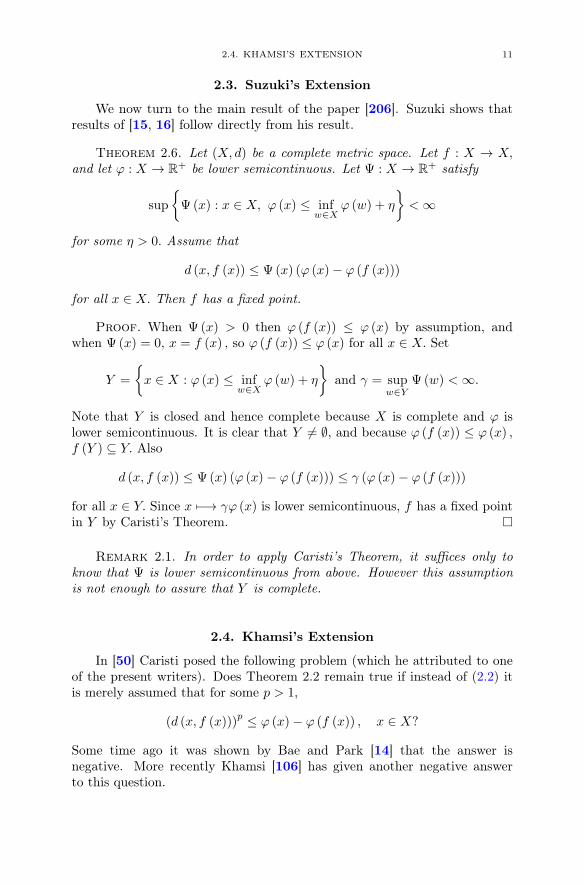
2.3. Suzuki’s Extension
We now turn to the main result of the paper [206]. Suzuki shows thatresults of [15, 16] follow directly from his result.
Theorem 2.6. Let (X, d) be a complete metric space. Let f : X → X,and let ϕ : X → R
+ be lower semicontinuous. Let Ψ : X → R+ satisfy
sup
{Ψ(x) : x ∈ X, ϕ (x) ≤ inf
w∈Xϕ (w) + η
}< ∞
for some η > 0. Assume that
d (x, f (x)) ≤ Ψ(x) (ϕ (x)− ϕ (f (x)))
for all x ∈ X. Then f has a fixed point.
Proof. When Ψ(x) > 0 then ϕ (f (x)) ≤ ϕ (x) by assumption, andwhen Ψ(x) = 0, x = f (x) , so ϕ (f (x)) ≤ ϕ (x) for all x ∈ X. Set
Y =
{x ∈ X : ϕ (x) ≤ inf
w∈Xϕ (w) + η
}and γ = sup
w∈YΨ(w) < ∞.
Note that Y is closed and hence complete because X is complete and ϕ islower semicontinuous. It is clear that Y = ∅, and because ϕ (f (x)) ≤ ϕ (x) ,f (Y ) ⊆ Y. Also
d (x, f (x)) ≤ Ψ(x) (ϕ (x)− ϕ (f (x))) ≤ γ (ϕ (x)− ϕ (f (x)))
for all x ∈ Y. Since x �−→ γϕ (x) is lower semicontinuous, f has a fixed pointin Y by Caristi’s Theorem. �
Remark 2.1. In order to apply Caristi’s Theorem, it suffices only toknow that Ψ is lower semicontinuous from above. However this assumptionis not enough to assure that Y is complete.
2.4. Khamsi’s Extension
In [50] Caristi posed the following problem (which he attributed to oneof the present writers). Does Theorem 2.2 remain true if instead of (2.2) itis merely assumed that for some p > 1,
(d (x, f (x)))p ≤ ϕ (x)− ϕ (f (x)) , x ∈ X?
Some time ago it was shown by Bae and Park [14] that the answer isnegative. More recently Khamsi [106] has given another negative answerto this question.

12 2. CARISTI’S THEOREM AND EXTENSIONS
Example. ([106]) Let p > 1, let xn :=∑n
i=1
1
i, and let X = {xn : n ∈ N} .
Then X is a closed (discrete) subset of R+ and is therefore complete. (If m >
n, then d (xn, xm) ≥ 1
m.) Define f : X → X by taking f (xn) = xn+1 for all
n ≥ 1. Now define ϕ (xn) =∑∞
i=n+1
1
ip. Then
(d (xn, f (xn)))p
=1
(n+ 1)p
=
∞∑i=n+1
1
ip−
∞∑i=n+2
1
ip
= ϕ (xn)− ϕ (xn+1)
= ϕ (xn)− ϕ (f (xn)) .
Clearly f is fixed point free. Also note that ϕ is continuous (because X isdiscrete) and f is even nonexpansive.
Khamsi then turns to the question of whether there exist positive func-tions η : R+ → R
+ with the property that if f : X → X (X complete)satisfies
η (d (x, f (x))) ≤ ϕ (x)− ϕ (f (x)) , x ∈ X,
for some lower semicontinuous ϕ : X → R+, then f has a fixed point. He
gives an affirmative answer in the form of the following theorem.The standing assumptions are these: η : R+ → R
+ is nondecreasing,continuous, and such that there exists c > 0 and δ0 > 0 such that for anyt ∈ [0, δ0] , η (t) ≥ ct. Because η is continuous, there exists ε0 > 0 such thatη−1 ([0, ε0]) ⊂ [0, δ0] .
Theorem 2.7. Suppose X is a complete metric space and ϕ : X → R+
lower semicontinuous. Define the relation ≺ on X by setting
x ≺ y ⇔ η (d (x, y)) ≤ ϕ (y)− ϕ (x) , x, y ∈ X,
where η is as above. Then (X,≺) has a minimal element x∗ (i.e., x ≺ x∗ forx ∈ X ⇒ x = x∗).
Proof. ([106]) Set ϕ0 = inf {ϕ (x) : x ∈ X}. For any ε > 0, set
Xε = {x ∈ X : ϕ (x) ≤ ϕ0 + ε} .Since ϕ is lower semicontinuous, Xε is a closed nonempty subset of X. (Thisuses the fact that ϕ is lower semicontinuous. Suppose {xn} ⊂ Xε and xn → x.Then ϕ (xn) ≤ ϕ0 + ε, so ϕ (x) ≤ ϕ0 + ε i.e., x ∈ Xε.) Also, if x, y ∈ Xε andif x ≺ y, then
η (d (x, y)) ≤ ϕ (y)− ϕ (x)
which impliesϕ0 ≤ ϕ (x) ≤ ϕ (y) ≤ ϕ0 + ε.

2.4. KHAMSI’S EXTENSION 13
Hence η (d (x, y)) ≤ ε. In particular, if x, y ∈ Xε0 and x ≺ y, then
c (d (x, y)) ≤ η (d (x, y)) ≤ ϕ (y)− ϕ (x) .
Now on Xε0 define the new relation ≺∗ by
x ≺∗ y ⇔ d (x, y) ≤ 1
cϕ (y)− 1
cϕ (x) , x, y ∈ Xε0 .
Clearly (Xε0 ,≺∗) is a partial order with all the necessary assumptions forsecuring, via Zorn’s Lemma, an element x∗ ∈ Xε0 which is minimal relativeto ≺∗ .
Now let x ∈ X satisfy x ≺ x∗. Then η (d (x, x∗)) ≤ ϕ (x∗) − ϕ (x) , soϕ (x) ≤ ϕ (x∗) ≤ ϕ0 + ε0, i.e., x ∈ Xε0 . As before, η (d (x, x∗)) ≤ ε0 and thisimplies
cd (x, x∗) ≤ η (d (x, x∗)) ≤ ϕ (x∗)− ϕ (x) .
Since x∗ is minimal in (Xε0 ,≺∗) we have x = x∗. �
The following is Theorem 3 of [106].
Theorem 2.8. Let X be a complete metric space and let f : X → X bea mapping such that for all x ∈ X
η (d (x, f (x))) ≤ ϕ (x)− ϕ (f (x)) ,
where η and ϕ are as in Theorem 2.7. Then f has a fixed point.
Proof. Define the relation ≺ as in Theorem 2.7. Obviously f (x) ≺ xfor any x ∈ X. In particular, if x∗ is a minimal element in (X,≺) , it mustbe the case that f (x∗) = x∗. �
We now turn to a variant of Khamsi’s Theorem.
Theorem 2.9. Suppose X is a complete metric space and suppose ϕ :X → R
+ is bounded below and sequentially lower semicontinuous from above.Define the relation ≺ on X by setting
x ≺ y ⇔ η (d (x, y)) ≤ ϕ (x)− ϕ (y) , x, y ∈ X,
where η is as in Theorem 2.7. Then (X,≺) has a maximal element x∗ (i.e.,x∗ ≺ x for x ∈ X ⇒ x = x∗).
Proof. Set ϕ0 = inf {ϕ (x) : x ∈ X} . For any ε > 0, set
Xε = {x ∈ X : ϕ (x) ≤ ϕ0 + ε} .If x, y ∈ Xε and if x ≺ y, then
η (d (x, y)) ≤ ϕ (x)− ϕ (y)
which impliesϕ0 ≤ ϕ (y) ≤ ϕ (x) ≤ ϕ0 + ε.
Hence η (d (x, y)) ≤ ε. In particular, if x, y ∈ Xε0 and x ≺ y, then
cd (x, y) ≤ η (d (x, y)) ≤ ϕ (x)− ϕ (y) .

14 2. CARISTI’S THEOREM AND EXTENSIONS
Now on Xε0 we define the new relation ≺∗ by
x ≺∗ y ⇔ d (x, y) ≤ 1
cϕ (x)− 1
cϕ (y) , x, y ∈ Xε0 .
Set ψ := −1
cϕ and define x ≤ y ⇔ d (x, y) ≤ ψ (y)−ψ (x) . We now show that
(Xε0 ,≤) has a maximal element. (Notice that we are not assuming Xε0 iscomplete.) Condition (a) of Theorem 2.4 is obvious, and condition (c) followsfrom the fact that ϕ is bounded below. To see that (b) holds, suppose {xn} isan increasing sequence in (Xε0 ,≤) which satisfies ψ (xn) ≤ C < ∞ for all n.Then {ϕ (xn)} is a decreasing sequence in R, so there exists r ∈ R such thatlimn→∞ ϕ (xn) = r. Since for any m > n,
limm,n→∞
cd (xn,xm) ≤ limm,n→∞
[ϕ (xn)− ϕ (xm)] = 0.
It follows that {xn} is a Cauchy sequence in X, and since X is completethere exists x ∈ X such that limn xn = x. Since ϕ (xn) ↘ r and ϕ is lowersemicontinuous from above, ϕ (x) ≤ r. However xn ∈ Xε0 ⇒ ϕ (xn) ≤ ϕ0+ε0.Therefore r ≤ ϕ0 + ε; hence ϕ (x) ≤ ϕ0 + ε0, and so x ∈ Xε0 . It follows that
cd (xn, x) = limm→∞
cd (xn, xm) ≤ limm→∞
[ϕ (xn)− ϕ (xm)]
= ϕ (xn)− r ≤ ϕ (xn)− ϕ (x) .
Thus x is an upper bound for {xn} in (Xε0 ,≤) . By Theorem 2.4, there existsa maximal element x∗ in (Xε0 ,≤) , and in turn x∗ is a maximal element in(Xε0 ,≺∗) .
Now let x ∈ X satisfy x∗ ≺ x. Then η (d (x, x∗)) ≤ ϕ (x∗) − ϕ (x) , soϕ (x) ≤ ϕ (x∗) ≤ ϕ0 + ε0, i.e., x ∈ Xε0 . As before, η (d (x, x∗)) ≤ ε0 and thisimplies
cd (x, x∗) ≤ η (d (x, x∗)) ≤ ϕ (x∗)− ϕ (x) .
Since x∗ is maximal in (Xε0 ,≺∗) we have x = x∗. �Since the Brézis–Browder order principle does not require Zorn’s Lemma,
the preceding result yields a more “constructive” proof of a slight generaliza-tion of Khamsi’s Theorem.
Corollary 2.1. Suppose X is a complete metric space and supposeϕ : X → R is bounded below and sequentially lower semicontinuous fromabove. Define the relation ≺ on X by setting
x ≺ y ⇔ η (d (x, y)) ≤ ϕ (y)− ϕ (x) , x, y ∈ X,
where η is as above. Then (X,≺) has a minimal element x∗.Proof. An element x∗ ∈ X is maximal in X relative to the relation
x ≺ y ⇔ η (d (x, y)) ≤ ϕ (x)− ϕ (y) , x, y ∈ X,
if and only if x∗ is minimal in X relative to the relation
x ≺ y ⇔ η (d (x, y)) ≤ ϕ (y)− ϕ (x) , x, y ∈ X.
�

2.4. KHAMSI’S EXTENSION 15
Theorem 2.10. Let (X, d) be a complete metric space. Let f : X → X,and let ϕ : X → R
+ be lower semicontinuous from above. Let Ψ : X → R+
satisfy
sup
{Ψ(x) : x ∈ X, ϕ (x) ≤ inf
w∈Xϕ (w) + ε
}< ∞
for some ε > 0. Introduce the relation ≺ on X by setting
x ≺ y ⇔ η(d (x, y)) ≤ Ψ(x) (ϕ (x)− ϕ (y))
for all x, y ∈ X. Then there is an element x∗ ∈ X that is maximal relativeto ≺ .
Proof. First notice that x ≺ y ⇒ ϕ (y) ≤ ϕ (x) for all x, y ∈ X. Letϕ0 = infw∈X ϕ (w) , and set
Y = {x ∈ X : ϕ (x) ≤ ϕ0 + ε} and γ = supw∈Y
Ψ(w) < ∞.
Now letXε =
{x ∈ X : ϕ (x) ≤ ϕ0 + γ−1ε
}and introduce the relation ≺∗ on Xε by setting
x ≺∗ y ⇔ η(d (x, y)) ≤ Ψ(x) (ϕ (x)− ϕ (y)) .
which in turn implies
ϕ0 ≤ ϕ (y) ≤ ϕ (x) ≤ ϕ0 + γ−1ε.
In particular ϕ (x)− ϕ (y) ≤ γ−1ε. Let ε′0 = min {ε, ε0} . Thus if x, y ∈ Xε′0 ,
η(d (x, y)) ≤ Ψ(x) (ϕ (x)− ϕ (y)) ≤ γ(γ−1)ε′0 ≤ ε0. In particular
cd (x, y) ≤ η(d (x, y)) ≤ Ψ(x) (ϕ (x)− ϕ (y)) ≤ γ (ϕ (x)− ϕ (y)) .
Now let φ := −γ
cϕ and introduce the new partial order ≤ on Xε0 by setting
x ≤ y ⇔ d (x, y) ≤ φ (y)− φ (x) .
It is now possible to complete the proof exactly as in the proof of Theorem 2.9.�
Observe that by taking Ψ to be the identity mapping one recoversKhamsi’s theorem.
Corollary 2.2. Let (X, d) be a complete metric space. Let f : X → X,and let ϕ : X → R
+ be lower semicontinuous from above. Let Ψ : X → R+
satisfy
sup
{Ψ(x) : x ∈ X, ϕ (x) ≤ inf
w∈Xϕ (w) + ε
}< ∞
for some ε > 0. Assume that
η (d (x, f (x))) ≤ Ψ(x) (ϕ (x)− ϕ (f (x)))
for all x ∈ X. Then f has a fixed point.
16 2. CARISTI’S THEOREM AND EXTENSIONS
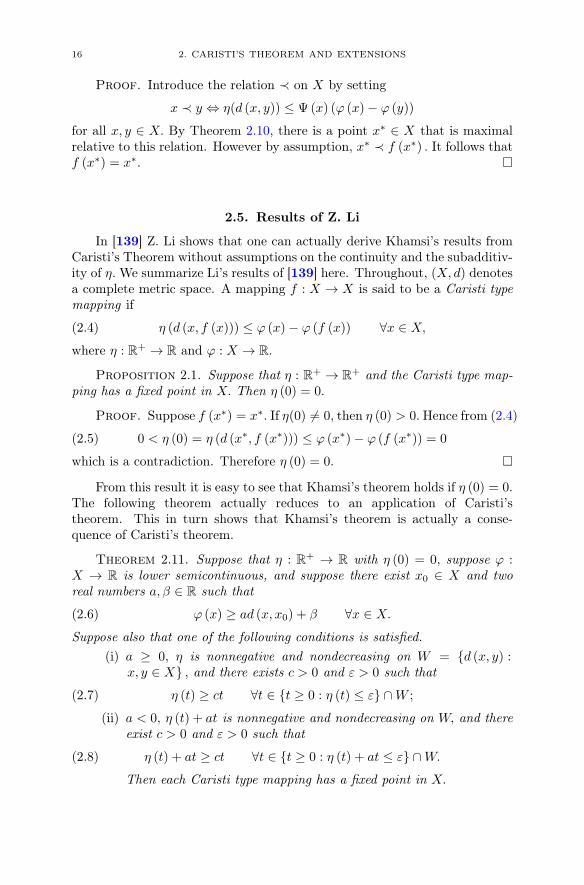
Proof. Introduce the relation ≺ on X by setting
x ≺ y ⇔ η(d (x, y)) ≤ Ψ(x) (ϕ (x)− ϕ (y))
for all x, y ∈ X. By Theorem 2.10, there is a point x∗ ∈ X that is maximalrelative to this relation. However by assumption, x∗ ≺ f (x∗) . It follows thatf (x∗) = x∗. �
2.5. Results of Z. Li
In [139] Z. Li shows that one can actually derive Khamsi’s results fromCaristi’s Theorem without assumptions on the continuity and the subadditiv-ity of η. We summarize Li’s results of [139] here. Throughout, (X, d) denotesa complete metric space. A mapping f : X → X is said to be a Caristi typemapping if
(2.4) η (d (x, f (x))) ≤ ϕ (x)− ϕ (f (x)) ∀x ∈ X,
where η : R+ → R and ϕ : X → R.
Proposition 2.1. Suppose that η : R+ → R+ and the Caristi type map-
ping has a fixed point in X. Then η (0) = 0.
Proof. Suppose f (x∗) = x∗. If η(0) = 0, then η (0) > 0. Hence from (2.4)
(2.5) 0 < η (0) = η (d (x∗, f (x∗))) ≤ ϕ (x∗)− ϕ (f (x∗)) = 0
which is a contradiction. Therefore η (0) = 0. �
From this result it is easy to see that Khamsi’s theorem holds if η (0) = 0.The following theorem actually reduces to an application of Caristi’stheorem. This in turn shows that Khamsi’s theorem is actually a conse-quence of Caristi’s theorem.
Theorem 2.11. Suppose that η : R+ → R with η (0) = 0, suppose ϕ :X → R is lower semicontinuous, and suppose there exist x0 ∈ X and tworeal numbers a, β ∈ R such that
(2.6) ϕ (x) ≥ ad (x, x0) + β ∀x ∈ X.
Suppose also that one of the following conditions is satisfied.(i) a ≥ 0, η is nonnegative and nondecreasing on W = {d (x, y) :
x, y ∈ X} , and there exists c > 0 and ε > 0 such that
(2.7) η (t) ≥ ct ∀t ∈ {t ≥ 0 : η (t) ≤ ε} ∩W ;
(ii) a < 0, η (t) + at is nonnegative and nondecreasing on W, and thereexist c > 0 and ε > 0 such that
(2.8) η (t) + at ≥ ct ∀t ∈ {t ≥ 0 : η (t) + at ≤ ε} ∩W.
Then each Caristi type mapping has a fixed point in X.
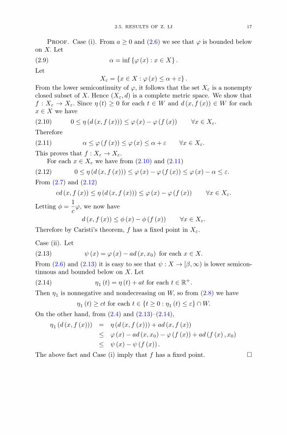
2.5. RESULTS OF Z. LI 17
Proof. Case (i). From a ≥ 0 and (2.6) we see that ϕ is bounded belowon X. Let
(2.9) α = inf {ϕ (x) : x ∈ X} .Let
Xε = {x ∈ X : ϕ (x) ≤ α+ ε} .From the lower semicontinuity of ϕ, it follows that the set Xε is a nonemptyclosed subset of X. Hence (Xε, d) is a complete metric space. We show thatf : Xε → Xε. Since η (t) ≥ 0 for each t ∈ W and d (x, f (x)) ∈ W for eachx ∈ X we have
(2.10) 0 ≤ η (d (x, f (x))) ≤ ϕ (x)− ϕ (f (x)) ∀x ∈ Xε.
Therefore
(2.11) α ≤ ϕ (f (x)) ≤ ϕ (x) ≤ α+ ε ∀x ∈ Xε.
This proves that f : Xε → Xε.For each x ∈ Xε we have from (2.10) and (2.11)
(2.12) 0 ≤ η (d (x, f (x))) ≤ ϕ (x)− ϕ (f (x)) ≤ ϕ (x)− α ≤ ε.
From (2.7) and (2.12)
cd (x, f (x)) ≤ η (d (x, f (x))) ≤ ϕ (x)− ϕ (f (x)) ∀x ∈ Xε.
Letting φ =1
cϕ, we now have
d (x, f (x)) ≤ φ (x)− φ (f (x)) ∀x ∈ Xε.
Therefore by Caristi’s theorem, f has a fixed point in Xε.
Case (ii). Let
(2.13) ψ (x) = ϕ (x)− ad (x, x0) for each x ∈ X.
From (2.6) and (2.13) it is easy to see that ψ : X → [β,∞) is lower semicon-tinuous and bounded below on X. Let
(2.14) η1 (t) = η (t) + at for each t ∈ R+.
Then η1 is nonnegative and nondecreasing on W, so from (2.8) we have
η1 (t) ≥ ct for each t ∈ {t ≥ 0 : η1 (t) ≤ ε} ∩W.
On the other hand, from (2.4) and (2.13)–(2.14),
η1 (d (x, f (x))) = η (d (x, f (x))) + ad (x, f (x))
≤ ϕ (x)− ad (x, x0)− ϕ (f (x)) + ad (f (x) , x0)
≤ ψ (x)− ψ (f (x)) .
The above fact and Case (i) imply that f has a fixed point. �
18 2. CARISTI’S THEOREM AND EXTENSIONS
2.6. A Theorem of Zhang and Jiang
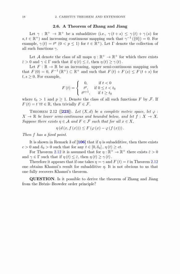
Let γ : R+ → R
+ be a subadditive (i.e., γ (t+ s) ≤ γ (t) + γ (s) fors, t ∈ R
+) and increasing continuous mapping such that γ−1 ({0}) = 0. Forexample, γ (t) = tp (0 < p ≤ 1) for t ∈ R
+). Let Γ denote the collection ofall such functions γ.
Let A denote the class of all maps η : R+ → R+ for which there exists
ε > 0 and γ ∈ Γ such that if η (t) ≤ ε, then η (t) ≥ γ (t) .Let F : R → R be an increasing, upper semi-continuous mapping such
that F (0) = 0, F−1 (R+) ⊂ R+ and such that F (t) + F (s) ≤ F (t+ s) for
t, s ≥ 0. For example,
F (t) =
⎧⎨⎩
0, if t < 0tp, if 0 ≤ t < t0
tp+1, if t ≥ t0
where t0 > 1 and p ≥ 1. Denote the class of all such functions F by F . IfF (t) = t ∀t ∈ R, then trivially F ∈ F .
Theorem 2.12 ([223]). Let (X, d) be a complete metric space, let ϕ :X → R be lower semi-continuous and bounded below, and let f : X → X.Suppose there exists η ∈ A and F ∈ F such that for all x ∈ X,
η (d (x, f (x))) ≤ F (ϕ (x)− ϕ (f (x))) .
Then f has a fixed point.
It is shown in Remark 3 of [106] that if η is subadditive, then there existsc > 0 and δ0 > 0 such that for any t ∈ [0, δ0] , η (t) ≥ ct.
For Theorem 2.12 it is assumed that for η : R+ → R+ there exists ε > 0
and γ ∈ Γ such that if η (t) ≤ ε, then η (t) ≥ γ (t) .Therefore it appears that if one takes η = γ and F (t) = t in Theorem 2.12
one obtains Khamsi’s result for subadditive η. It is not obvious to us thatone fully recovers Khamsi’s theorem.
QUESTION. Is it possible to derive the theorem of Zhang and Jiangfrom the Brézis–Browder order principle?

CHAPTER 3
Nonexpansive Mappings and Zermelo’sTheorem
3.1. Introduction
An extension of a theorem attributed variously to Zermelo, Bourbaki, andKneser provides the basis for Mańka’s proof that Caristi’s theorem holds inZF. In the sequel we shall simply refer to this theorem as Zermelo’s theorem.This theorem should NOT be confused with the celebrated well-orderingtheorem also due to Zermelo, which is equivalent to the Axiom of Choice.See A.3 and A.9 of [107] for a brief discussion of constructive aspects ofmathematics.
Theorem 3.1 (Zermelo [222]). Let (E,≤) be a partially ordered set andlet f : E → E satisfy x ≤ f (x) ∀x ∈ E. Suppose every chain in (E,≤) has aleast upper bound. Then f has a fixed point in E. In fact, given x ∈ E it ispossible to construct x∗ ∈ E so that x ≤ x∗ and f (x∗) = x∗.
For a constructive (ZF) proof of this theorem see [67, p. 9], [221, p. 504],or [107, p. 284].
3.2. Convexity Structures
In this section we prove an abstract metric fixed theorem for nonexpan-sive mappings that contains many known theorems as special cases. Ourproof is constructive in that it only relies on Zermelo’s theorem. We firstneed some definitions and we start with a concept inspired by observationsof J.-P. Penot in [169].
Definition 3.1. A convexity structure in a metric space (X, d) is a familyΣ of subsets of X such that ∅, X ∈ Σ and Σ is closed under arbitraryintersections. The structure Σ is said to be [countably ] compact if every[countable] subfamily of Σ which has the finite intersection property hasnonempty intersection.
Given a convexity structure Σ in a metric space (X, d) , we adopt thefollowing notation: For D ∈ Σ and x ∈ X, set:
rx (D) = sup {d (x, y) : y ∈ D} ;rX (D) = inf {rx (D) : x ∈ X} ;r (D) = inf {rx (D) : x ∈ D} .
© Springer International Publishing Switzerland 2014W. Kirk, N. Shahzad, Fixed Point Theory in Distance Spaces,DOI 10.1007/978-3-319-10927-5__3
19

20 3. NONEXPANSIVE MAPPINGS AND ZERMELO’S THEOREM
Definition 3.2. A convexity structure Σ in X is said to be normal ifgiven D ∈ Σ, diam (D) > 0 ⇒ r(D) < diam (D) .
A subset A of a metric space X is said to be admissible if A is theintersection of closed balls centered at points of X. Thus
A =⋂i∈I
{B (xi; ri) : xi ∈ X, ri ≥ 0} .
The set of all admissible subsets of X is denoted by A (X) . Of particular in-terest in metric fixed point theory is the convexity structure A (X) consistingof all admissible sets in X. Given any bounded set A ⊆ X we set
cov (A) :=⋂
{D : D ∈ Σ and D ⊇ A} .
Clearly cov (A) ∈ A (X) , and thus A = cov (A) ⇔ A ∈ A (X) .
Examples of convexity structures
1. Let Σ be the family of all closed and convex subsets of a given closedconvex subset of a Banach space X.
2. Let Σ = A (B) where B is the unit ball in a Banach space X.3. Let Σ = A (X) where X is a bounded metric space.4. Let Σ = A (K) where K is a closed convex subset of a complete
CAT(0) space (see Chap. 9).
Examples of compact convexity structures
5. The same as Example 1, but with K weakly compact.6. The same as Example 2, but with B the unit ball in a dual Banach
space.7. The same as Example 3, but with X a hyperconvex metric space
(see the next chapter).8. The same as Example 4.
Examples of convexity structures that are compact and normal
9. The same as Example 5, but with K possessing normal structure[110].
10. The same as Example 6, but with B possessing normal structure.12. The same as Example 7.13. The same as Example 4.
We now derive the following theorem as an application of Zermelo’stheorem (Theorem 3.1). This provides a constructive proof of the originaltheorem of Kirk [110] for nonexpansive mappings. The original proof issomewhat shorter, but it uses Zorn’s Lemma. (Recall that a mapping f of ametric space (X, d) into itself is nonexpansive if d (f (x) , f (y)) ≤ d (x, y) forall x, y ∈ X.) This proof, taken from [115], was inspired by one given by B.Fuchssteiner in [85].
3.2. CONVEXITY STRUCTURES 21
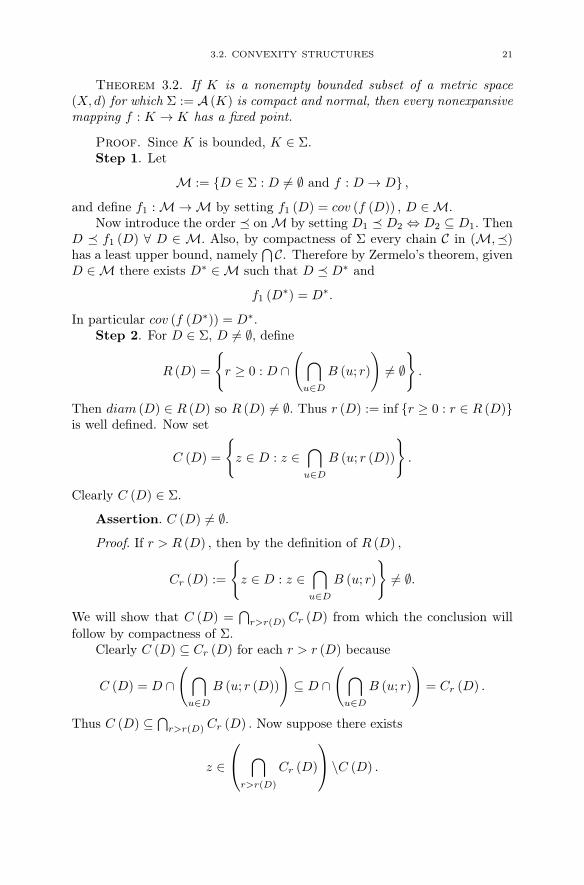
Theorem 3.2. If K is a nonempty bounded subset of a metric space(X, d) for which Σ := A (K) is compact and normal, then every nonexpansivemapping f : K → K has a fixed point.
Proof. Since K is bounded, K ∈ Σ.Step 1. Let
M := {D ∈ Σ : D = ∅ and f : D → D} ,
and define f1 : M → M by setting f1 (D) = cov (f (D)) , D ∈ M.Now introduce the order � on M by setting D1 � D2 ⇔ D2 ⊆ D1. Then
D � f1 (D) ∀ D ∈ M. Also, by compactness of Σ every chain C in (M,�)has a least upper bound, namely
⋂C. Therefore by Zermelo’s theorem, given
D ∈ M there exists D∗ ∈ M such that D � D∗ and
f1 (D∗) = D∗.
In particular cov (f (D∗)) = D∗.Step 2. For D ∈ Σ, D = ∅, define
R (D) =
{r ≥ 0 : D ∩
( ⋂u∈D
B (u; r)
)= ∅}.
Then diam (D) ∈ R (D) so R (D) = ∅. Thus r (D) := inf {r ≥ 0 : r ∈ R (D)}is well defined. Now set
C (D) =
{z ∈ D : z ∈
⋂u∈D
B (u; r (D))
}.
Clearly C (D) ∈ Σ.
Assertion. C (D) = ∅.Proof. If r > R (D) , then by the definition of R (D) ,
Cr (D) :=
{z ∈ D : z ∈
⋂u∈D
B (u; r)
}= ∅.
We will show that C (D) =⋂
r>r(D) Cr (D) from which the conclusion willfollow by compactness of Σ.
Clearly C (D) ⊆ Cr (D) for each r > r (D) because
C (D) = D ∩( ⋂
u∈D
B (u; r (D))
)⊆ D ∩
( ⋂u∈D
B (u; r)
)= Cr (D) .
Thus C (D) ⊆⋂
r>r(D) Cr (D) . Now suppose there exists
z ∈
⎛⎝ ⋂
r>r(D)
Cr (D)
⎞⎠ \C (D) .

22 3. NONEXPANSIVE MAPPINGS AND ZERMELO’S THEOREM
Then there exists u ∈ D such that d (z, u) > r (D) ; hence, there exists r′
such that d (z, u) > r′ > r (D) . But d (z, u) > r′ implies z /∈ Cr′ (D)—acontradiction.
Given D ∈ M, construct D∗ as in Step 1. It is now possible to definef2 : M → M by setting f2 (D) = C (D∗) . As in Step 1, by Zermelo’stheorem there exists D∗∗ ∈ M such that f2 (D
∗∗) = D∗∗. This implies thatC (D∗∗) = D∗∗. However since Σ is normal, diam (D∗∗) > 0 ⇒ C (D∗∗) is aproper subset of D∗∗. Therefore D∗∗ must be a singleton consisting of a fixedpoint of f. �
We now give a proof of Theorem 3.2 which mimics the Zorn Lemma proofin the original paper of Kirk [110]. This more abstract approach, inspiredby observations of Penot [169], is self-contained and somewhat quicker.
Alternate Proof. Since A(K) is compact, an application of Zorn’sLemma yields the existence of a set D ∈ A(K) which is minimal with respectto being nonempty and mapped into itself by f. Also, cov(f(D)) ⊆ D andf : cov(f(D)) → cov(f(D)), so minimality of D implies
D = cov(f(D)).
Now assume diam(D) > 0 and choose r so that r(D) < r < diam(D). Itfollows that the set
C = {x ∈ D : D ⊆ B(x; r)} = ∅.
Also one can quickly check that
C =⋂x∈D
B(x; r)⋂
D.
This proves that C ∈ A(K). Now let z ∈ C. Then if x ∈ D
d(f(z), f(x)) ≤ d(x, z) ≤ r.
Therefore f(x) ∈ B(f(z); r) for every x ∈ D; hence, f(D) ⊆ B(f(z); r)from which cov(f(D)) ⊆ B(f(z); r). But D = cov(f(D)), so D ⊆ B(f(z); r).This proves that f(z) ∈ C. Hence f : C → C. However if z, w ∈ C, thend(z, w) ≤ r, so diam(C) ≤ r < diam(D). This proves that C is a propersubset of D. Since C ∈ A(K) and f : C → C this contradicts the minimalityof D. We thus conclude that diam(D) = 0, so D consists of a single pointwhich must be a fixed point of f. �
Remark 3.1. In [114] it is shown that countable compactness of Σ issufficient for the validity of Theorem 3.2. However it has since been shownby Kulesza and Lim [136] that if (X, d) a bounded metric space for whichA (X) is countable compact and normal, then A (X) is in fact compact. See[107, p. 109] for full details.

CHAPTER 4
Hyperconvex Metric Spaces
We only briefly discuss this topic because metric fixed point theory inthese spaces has been discussed extensively elsewhere (see, e.g., [72] or [107,Chapter 4]). However, since some of the spaces we discuss below are hyper-convex (in particular the so-called R-trees) we touch on a few of the relevantproperties of these spaces.
A metric space M is said to be injective if it has the following extensionproperty: Whenever Y is a subspace of a metric space X and f : Y → Mis nonexpansive, then f has a nonexpansive extension f : X → M. Thisfact has several nice consequences. For example, suppose M is injective andsuppose M is a subspace of a metric space X. Then since the identity mappingI : M → M is nonexpansive then I can be extended to a nonexpansivemapping R : X → M. Since R is a retraction of X onto M we have thefollowing.
Theorem 4.1. An injective metric space is a nonexpansive retract of anymetric space in which it is metrically embedded.
In light of the above it is clear that an injective metric space must becomplete because it is a nonexpansive retract (hence a closed subspace) ofits own completion.
Definition 4.1. A metric space (X, d) is said to be hyperconvex if forany indexed class of closed balls B(xi; ri), i ∈ I, of X which satisfy
d(xi, xj) ≤ ri + rj i, j ∈ I,
it is necessarily the case that⋂i∈I
B(xi; ri) = ∅.
It is easy to see that a hyperconvex metric space X is always complete.Also if x, y ∈ X then there exists z ∈ X such that d (x, z)+d (z, y) = d (x, y) .Thus X is Menger convex. Therefore by Menger’s theorem each two pointsof X are the endpoints of a metric segment.
Of particular relevance is the fact that hyperconvex spaces are injective.Indeed, the following well-known theorem is due to Aronszajn and Panitch-pakdi [12].
© Springer International Publishing Switzerland 2014W. Kirk, N. Shahzad, Fixed Point Theory in Distance Spaces,DOI 10.1007/978-3-319-10927-5__4
23
24 4. HYPERCONVEX METRIC SPACES
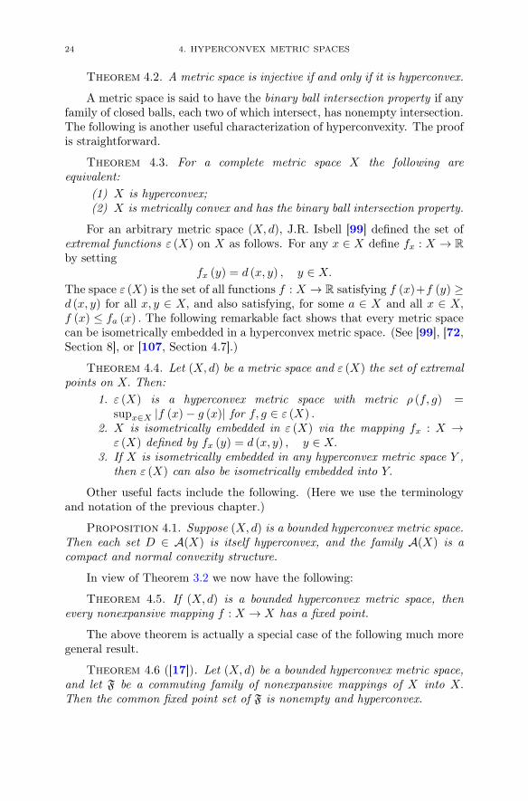
Theorem 4.2. A metric space is injective if and only if it is hyperconvex.
A metric space is said to have the binary ball intersection property if anyfamily of closed balls, each two of which intersect, has nonempty intersection.The following is another useful characterization of hyperconvexity. The proofis straightforward.
Theorem 4.3. For a complete metric space X the following areequivalent:
(1) X is hyperconvex;(2) X is metrically convex and has the binary ball intersection property.
For an arbitrary metric space (X, d), J.R. Isbell [99] defined the set ofextremal functions ε (X) on X as follows. For any x ∈ X define fx : X → R
by settingfx (y) = d (x, y) , y ∈ X.
The space ε (X) is the set of all functions f : X → R satisfying f (x)+f (y) ≥d (x, y) for all x, y ∈ X, and also satisfying, for some a ∈ X and all x ∈ X,f (x) ≤ fa (x) . The following remarkable fact shows that every metric spacecan be isometrically embedded in a hyperconvex metric space. (See [99], [72,Section 8], or [107, Section 4.7].)
Theorem 4.4. Let (X, d) be a metric space and ε (X) the set of extremalpoints on X. Then:
1. ε (X) is a hyperconvex metric space with metric ρ (f, g) =supx∈X |f (x)− g (x)| for f, g ∈ ε (X) .
2. X is isometrically embedded in ε (X) via the mapping fx : X →ε (X) defined by fx (y) = d (x, y) , y ∈ X.
3. If X is isometrically embedded in any hyperconvex metric space Y ,then ε (X) can also be isometrically embedded into Y.
Other useful facts include the following. (Here we use the terminologyand notation of the previous chapter.)
Proposition 4.1. Suppose (X, d) is a bounded hyperconvex metric space.Then each set D ∈ A(X) is itself hyperconvex, and the family A(X) is acompact and normal convexity structure.
In view of Theorem 3.2 we now have the following:
Theorem 4.5. If (X, d) is a bounded hyperconvex metric space, thenevery nonexpansive mapping f : X → X has a fixed point.
The above theorem is actually a special case of the following much moregeneral result.
Theorem 4.6 ([17]). Let (X, d) be a bounded hyperconvex metric space,and let F be a commuting family of nonexpansive mappings of X into X.Then the common fixed point set of F is nonempty and hyperconvex.
CHAPTER 5
Ultrametric Spaces
5.1. Introduction
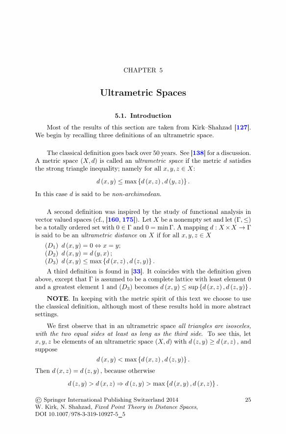
Most of the results of this section are taken from Kirk–Shahzad [127].We begin by recalling three definitions of an ultrametric space.
The classical definition goes back over 50 years. See [138] for a discussion.A metric space (X, d) is called an ultrametric space if the metric d satisfiesthe strong triangle inequality; namely for all x, y, z ∈ X:
d (x, y) ≤ max {d (x, z) , d (y, z)} .
In this case d is said to be non-archimedean.
A second definition was inspired by the study of functional analysis invector valued spaces (cf., [160, 175]). Let X be a nonempty set and let (Γ,≤)be a totally ordered set with 0 ∈ Γ and 0 = minΓ. A mapping d : X×X → Γis said to be an ultrametric distance on X if for all x, y, z ∈ X
(D1) d (x, y) = 0 ⇔ x = y;(D2) d (x, y) = d (y, x) ;(D3) d (x, y) ≤ max {d (x, z) , d (z, y)} .A third definition is found in [33]. It coincides with the definition given
above, except that Γ is assumed to be a complete lattice with least element 0and a greatest element 1 and (D3) becomes d (x, y) ≤ sup {d (x, z) , d (z, y)} .
NOTE. In keeping with the metric spirit of this text we choose to usethe classical definition, although most of these results hold in more abstractsettings.
We first observe that in an ultrametric space all triangles are isosceles,with the two equal sides at least as long as the third side. To see this, letx, y, z be elements of an ultrametric space (X, d) with d (z, y) ≥ d (x, z) , andsuppose
d (x, y) < max {d (x, z) , d (z, y)} .Then d (x, z) = d (z, y) , because otherwise
d (z, y) > d (x, z) ⇒ d (z, y) > max {d (x, y) , d (x, z)} .
© Springer International Publishing Switzerland 2014W. Kirk, N. Shahzad, Fixed Point Theory in Distance Spaces,DOI 10.1007/978-3-319-10927-5__5
25

26 5. ULTRAMETRIC SPACES
We use the notation B (x; r) to denote the closed ball
B (x; r) = {y ∈ X : d (x, y) ≤ r} ,where r ≥ 0 (with B (x; 0) = {x}) and we observe that alwaysdiam (B (x; r)) ≤ r.
Another characteristic property of ultrametric spaces is the following:
(5.1) α ≤ β and B (x;α) ∩B (y;β) = ∅ ⇒ B (x;α) ⊆ B (y;β) .
Moreover if α = d (x, y) , B (x;α) = B (y;α) .
Definition 5.1. An ultrametric space (X, d) is said to be sphericallycomplete if every chain of balls in X has nonempty intersection.
Remark 5.1. An immediate consequence of (5.1) is the fact that ∩F = ∅for any family F of closed balls in a spherically complete ultrametric spacewhich has the property that each two members of F intersect.
Ultrametric spaces1 and hyperconvex metric spaces share many commonproperties, yet they are quite different in very distinctive ways. The moststriking similarity has to do with the injective extension property; the moststriking difference is likely the fact that while hyperconvex metric spaces arealways metrically convex, ultrametric spaces never are.
An ultrametric space (M,d) is said to have the extension property (EP)if given any ultrametric space (X, ρ) and any subspace Y of X, every nonex-pansive mapping f : Y → M has a nonexpansive extension f ′ : X → M.
The following characterization of spherical completeness is found in [175].
Theorem 5.1. An ultrametric space is spherically complete if and onlyif it has the extension property.
Proof. (⇒) Suppose (M,d) is spherically complete, let (X, ρ) be anultrametric space, let Y be a subspace of X, and suppose f : Y → M isnonexpansive. Let z ∈ X with z /∈ Y and let Y ′ = Y ∪ {z}. We first showthat f has a nonexpansive extension f ′ : Y ′ → M.
Now let F = {B(f(y); ρ(y, z)) : y ∈ Y }. We assert that each two membersof F intersect. Indeed, suppose y1, y2 ∈ Y with ρ(y1, z) ≤ ρ(y2, z). Thenz ∈ B(y1; ρ(y1, z)) ∩B(y2; ρ(y2, z)) so by (5.1)
B(y1; ρ(y1, z)) ⊆ B(y2; ρ(y2, z)).
Therefore d(f(y1), f(y2)) ≤ ρ(y1, y2) ≤ ρ(y2, z), so f(y1) ∈ B(f(y2); ρ(y2, z)).Since M is spherically complete, ∩F = ∅, so let p ∈ ∩F and define f ′(z) = p.Then if f ′(y) = f(y) for each y ∈ Y, d(f ′(z), f ′(y)) ≤ ρ(z, y) and f ′ is
1Ultrametrics arise naturally in the study of non-archimedean analysis; in particular inthe study of normed vector spaces over non-archimedean valuation fields (see [156, 160,213]).

5.2. HYPERCONVEX ULTRAMETRIC SPACES 27
a nonexpansive extension of f to Y ′. The proof of this implication is nowcompleted by using Zorn’s lemma as in the extension theorem of Aronszajnand Panitchpakdi.
(⇐) Now assume (M,d) has the extension property but is not sphericallycomplete. Then there exists a decreasing family {B(xi; ri)}i∈I of closed ballsin M for which
⋂i∈I
B(xi; ri) = ∅. Let M ′ = M ∪{p} where p /∈ M and define
a metric ρ on M ′ as follows. Set ρ(p, p) = 0, ρ(x, y) = d(x, y) if x, y ∈ M ;otherwise for x ∈ M set ρ(x, p) = ρ(p, x) = d(x, xj) where x /∈ B(xj ; rj). Byassumption such j ∈ I must exist. To see that ρ is well defined, notice thatif x /∈ B(xk; rk) then, since these balls are nested, d(xj , xk) < d(x, xj). Thusd(x, xj) = d(x, xk).
By the extension property, the identity mapping on M has an extensionf ′ : M ′ → M. Also if xi /∈ B(xj ; rj), it must be the case that B(xj ; rj) ⊆B(xi; ri). Thus
d(f ′(p), xi) = d(f ′(p), f ′(xi)) ≤ ρ(p, xi) = d(xi, xj) ≤ ri,
and f ′(p) ∈⋂i∈I
B(xi; ri). This contradicts the original assumption and com-
pletes the proof. �
5.2. Hyperconvex Ultrametric Spaces
An ultrametric space X in the terminology of [33] is said to be hyper-convex if it satisfies the following two conditions (where Γ is assumed to bea complete lattice with least element 0 and a greatest element 1):
(H1) For any family {B (xi; γi)}i∈I of balls
B (xi; γi) ∩B(xj ; γj
)= ∅ ∀ i, j ∈ I ⇒
⋂i∈I
B (xi; γi) = ∅.
(H2) For all x, y ∈ X and γ1, γ2 ∈ Γ :
d (x, y) ≤ sup {γ1, γ2} ⇒ ∃ z ∈ X such that d (x, z) ≤ γ1 andd (z, y) ≤ γ2 (i.e., B (x; γ1) ∩B (y; γ2) = ∅).
We first observe that in the classical setting the second condition is re-dundant. Indeed, in any classical ultrametric space,
d (x, y) ≤ max {γ1, γ2} ⇔ B (x; γ1) ∩B (y; γ2) = ∅.Consider balls B (x; γ1) and B (y; γ2) with d (x, y) ≤ max {γ1, γ2} . Thereare two cases: If γ1 ≤ γ2, then x ∈ B (x; γ1)∩ B (y; γ2) . On the otherhand if γ2 ≤ γ1, then y ∈ B (x; γ1)∩ B (y; γ2) . In either case B (x; γ1)∩B (y; γ2) = ∅. Conversely, suppose B (x; γ1)∩ B (y; γ2) = ∅ and let z ∈B (x; γ1)∩ B (y; γ2) . Then d (x, z) ≤ γ1 and d (y, z) ≤ γ2. By the ultrametrictriangle inequality, d (x, y) ≤ max {d (x, z) , d (y, z)} ≤ max {γ1, γ2} .
Accordingly, we say that an ultrametric space is a classical hyperconvexultrametric space if it satisfies (H1).

28 5. ULTRAMETRIC SPACES
A hyperconvex ultrametric space is never hyperconvex in the metricsense. This is because a hyperconvex metric space is always complete, andeach two points are joined by a metric segment. In contrast, as we haveseen, each three distinct points of an ultrametric space are the vertices of anisosceles triangle.
Next observe that if B (x; γ) ⊆ B (y; δ), then
d (x, y) ≤ δ ≤ sup {γ, δ} .Hence any descending collection of balls in a classical hyperconvex ultra-metric space has nonempty intersection by (5.1), so we conclude that if anultrametric space is hyperconvex then it is spherically complete.
Now suppose X is a spherically complete ultrametric space and suppose
{B (xi; γi)}i∈I
is a family of balls in X satisfying d (xi, xj) ≤ max{γi, γj
}. Since the real
numbers are linearly ordered, it follows that {B (xi; γi)}i∈I is a nested chain;hence by spherical completeness
⋂i∈I B (xi; γi) = ∅.
Theorem 5.2. A classical ultrametric space is hyperconvex in the senseof (H1 ) if and only if it is spherically complete.
Since it is well known that hyperconvex metric spaces are injective, theabove fact suggests that spherically complete ultrametric spaces should alsobe injective. This is indeed the case. Following [175] we say that an ultra-metric space (X, d) has the extension property (EP) if for every ultrametricspace (X, ρ) and any subspace Y of X, any nonexpansive mapping f : Y → Xhas a nonexpansive extension f ′ : X → X. The following is a special case ofTheorem 1.3 of [175].
Theorem 5.3. Let (X, d) be an ultrametric space. Then the followingare equivalent:
(1) (X, d) is spherically complete;(2) (X, d) has (EP ).
Corollary 5.1. Let Y be a spherically complete subspace of an ultra-metric space X. Then Y is a nonexpansive retract of X.
Proof. The identity mapping I : Y → Y has a nonexpansive extensionr : X → Y. �
5.3. Nonexpansive Mappings in Ultrametric Spaces
Suppose (X, d) is an ultrametric space and f : X → X a mapping.We say that ball B := B (x; r) is minimal f -invariant if f : B → B andd (u, f (u)) = r for all u ∈ B. The following theorem was first proved in [170]using Zorn’s Lemma. Here we give a constructive proof that seems to be
5.3. NONEXPANSIVE MAPPINGS IN ULTRAMETRIC SPACES 29
more illuminating. Specifically, the fact that the conclusion holds in everyball of the form B (x, d (x, f (x))) seems to be a new observation.
Theorem 5.4 (cf., [170]). Suppose (X, d) is a spherically complete ul-trametric space and suppose f : X → X is nonexpansive. Then every ball ofthe form
B (x; d (x, f (x)))
contains either a fixed point of f or a minimal f -invariant ball.
Proof. ([127]) Let z ∈ X, let r = d (z, f (z)) and let u ∈ B (z; r) . Weassert that f (u) ∈ B (z; r) and d (u, f (u)) ≤ d (z, f (z)) . To see this we lookat two cases. (i) If d (u, z) < r, then, since d (f (z) f (u)) ≤ d (z, u) , by isosce-les triangles it must be the case that d (z, f (u)) = r, andagain by isosceles triangles d (u, f (u)) = r. (ii) If d (z, u) = r, then by isosce-les triangles, either d (z, f (u)) = r and d (u, f (u)) ≤ r or d (z, f (u)) < rand d (u, f (u)) = r. Thus in either case, f (u) ∈ B (z; r) and d (u, f (u)) ≤ r.Therefore every ball in X of the form B (z; d (z, f (z))) is invariant under f.
Now let x ∈ X. We shall show that B := B (x, d (x, f (x))) contains eithera fixed point of f or a minimal f -invariant ball. We proceed by induction.Let x1 = x, let r1 = d (x1, f (x1)) , and set
μ1 = inf {d (x, f (x)) : x ∈ B (x1; r1)} .
Now let {εn} be a sequence of positive numbers such that limn→∞ εn = 0. Ifμ1 = r1, then B = B (x1; r1) is either a singleton or a minimal f -invariantball, and we are finished. If r1 > 0 and μ1 < r1 select x2 ∈ B (x1; r1) so that
r2 := d (x2, f (x2)) < min {r1, μ1 + ε1} .
Having defined xn ∈ X, let
μn = inf {d (x, f (x)) : x ∈ B (xn; rn)} .
As seen above when n = 1, if μn = rn or rn = 0 we are finished. Otherwiseselect xn+1 ∈ B (xn; rn) so that
rn+1 := d (xn+1, f (xn+1)) < min {rn, μn + εn} .
Either this process terminates and the conclusion follows after a finite numberof steps, or {B (xn; rn)}∞n=1 is a nested sequence of nontrivial balls. In thelatter case, since X is spherically complete,
∞⋂n=1
B (xn; rn) = ∅.
Since {rn} is decreasing, r := limn→∞ rn exists. Also {μn} is nondecreasingand bounded above, so μ := limn→∞ μn also exists. Let x∗ ∈ ∩∞
n=1B (xn; rn) .Then for each n,
d (x∗, f (x∗)) ≤ max {d (x∗, xn) , d (xn, f (x∗))} ≤ rn.
30 5. ULTRAMETRIC SPACES
Moreover, x∗ ∈ B (xn+1; rn+1) ∀n ⇒μn ≤ d (x∗, f (x∗)) ≤ r ≤ rn+1 ≤ μn + εn.
Letting n → ∞ we see that d (x∗, f (x∗)) = μ = r. On the other hand,
inf {d (x, f (x)) : x ∈ B (x∗; d (x∗, f (x∗)))} ≥ μn,
and this implies
r ≥ inf {d (x, f (x)) : x ∈ B (x∗; d (x∗, f (x∗)))} ≥ μ = r.
If r > 0, B (x∗; d (x∗, f (x∗))) is a minimal f -invariant ball contained in B.If r = 0, x∗ is a fixed point of f. �
Remark 5.2. The above proof requires only that descending sequencesof closed balls have nonempty intersection.
Remark 5.3. If B (x; r) is a minimal f -invariant ball, then
d(fn (x) , fn+1 (x)
)= r
for all n ∈ N.
Corollary 5.2 (cf., [174]). Suppose (X, d) is a spherically completeultrametric space and suppose f : X → X is strictly contractive (d(f(x),f(y)) < d (x, y) when x = y). Then f has a unique fixed point.
Notice that in Corollary 5.2 the fixed point of f must lie in every ballof the form B (x; d (x, f (x))) for x ∈ X. Hence these balls are nested, andconsequently
{x∗} =⋂x∈X
B (x; d (x, f (x))) ,
where f (x∗) = x∗. Also, if x ∈ X and x = x∗, then d (x∗, f (x)) < d (x∗, x) ⇒d (x∗, x) = d (x, f (x)) . This suggests a method for approximating the fixedpoint of a strictly contractive mapping.
5.4. Structure of the “Fixed Point Set” of Nonexpansive Mappings
In this section we examine the nature of the “fixed point set” under theassumptions of Theorem 5.4.
Theorem 5.5. Suppose (X, d) is a spherically complete ultrametric spaceand suppose f : X → X is nonexpansive. Let
M = {x ∈ X : ∃ r ≥ 0 such that d (u, f (u)) = r ∀u ∈ B (x; r)} .Then M is spherically complete, and hence a nonexpansive retract of X.

5.5. A STRONG FIXED POINT THEOREM 31
Proof. Let B (xi; γi) be a descending collection of closed balls centeredat points xi ∈ M. Then for each i there exists ri ≥ 0 such that d (u, xi) ≤ ri ⇒d (u, f (u)) = ri. Since X is spherically complete, B :=
⋂i∈I B (xi; γi) = ∅. If
γi ≤ ri for some i, then the collection of balls all eventually lie in B (xi; ri) ,and so B ⊆ B (xi; ri) ⊆ M. So, suppose ri < γi for each i. Let x ∈ B. Thend (f (x) , f (xi)) ≤ d (x, xi) ≤ γi. Also,
d (f (x) , xi) ≤ max {d (f (x) , f (xi)) , d (f (xi) , xi)} ≤ max {γi, ri} = γi.
Thus f : B → B. But B is itself spherically complete. So B ∩M = ∅. Thisproves that M is spherically complete. The fact that M is a nonexpansiveretract of X follows from Corollary 5.1. �
With f and M as in Theorem 5.5, suppose x ∈ M, and suppose there ex-ists r > 0 such that f : B (x; r) → B (x; r) and d (u, f (u)) = r ∀ u ∈ B (x; r) .Then d (u, x) < r ⇒ d (f (u) , x) = r. Moreover, since d
(fn (x) , fn+1 (x)
)= r
for all n ∈ N, by isosceles triangles we have d (x, fn (x)) < r ⇒d(x, fn+1 (x)
)= r for any n ∈ N. The simple example below shows that
this behavior is typical.
Example. Let X = {a, b, c, d} with d (x, x) = 0 for all x ∈ X; d (a, b) =d (c, d) = 1/2; d (a, c) = d (a, d) = d (b, c) = d (b, d) = 1; d (y, x) = d (x, y) forall x, y ∈ X. Then (X, d) is a spherically complete ultrametric space. Definef (a) = c; f (c) = a; f (b) = d; f (d) = b. Then f is nonexpansive, f does nothave any fixed points, and M = X.
Remark 5.4. Under the assumptions of Theorem 5.5, if z ∈ X satisfiesd (z, f (z)) = inf {d (x, f (x)) : x ∈ X} , then
d (u, f (u)) = d (z, f (z))
for all u ∈ B (z; d (z, f (z))) .
Suppose x, y ∈ M with d (x, f (x)) = r1 and d (y, f (y)) = r2. If B (x; r1)∩B (y; r2) = ∅, then d (x, y) := d > max {r1, r2} . By isosceles triangles,
d (f (x) , f (y)) = d.
On the other hand if B (x; r1)∩B (y; r2) = ∅, then r1 = r2. Thus if x, y ∈ M,either d (x, f (x)) = d (y, f (y)) = r and d (x, y) ≤ r or
d (x, y) > max {d (x, f (x)) , d (y, f (y))}and d (x, y) = d (f (x) , f (y)) .
5.5. A Strong Fixed Point Theorem
The existence part of the following theorem is Theorem 1 of [179].The proof given there is indirect and also relies on Zorn’s Lemma. As inTheorem 5.4, we give a more constructive proof here, one that also showsf : X → X has a fixed point in every ball of the form B (x; d (x, f (x))) . The
32 5. ULTRAMETRIC SPACES
assumption that f is strictly contracting on orbits [178] means that f (x) = ximplies d
(f2 (x) , f (x)
)< d (f (x) , x) for each x ∈ X.
Theorem 5.6. Let (X, d) be a spherically complete ultrametric space, letf : X → X, and assume the following properties are satisfied:
(1 ) If z = f (z) and d (x, f (z)) ≤ d(f2 (z) , f (z)
), then
d (x, f (x)) ≤ d (z, f (z)) .
(2 ) f is strictly contracting on orbits.Then f has a fixed point in every ball of the form B (x; d (x, f (x))) .
Proof. Choose x ∈ X. We shall show that B (x; d (x, f (x))) containsa fixed point of f . Let Ω denote the set of all countable ordinals and letx1 = x. We proceed by transfinite induction. Let β ∈ Ω and assume xα hasbeen defined for all α < β, where {B (xα; d (xα, f (xα)))}α<β is a descendingchain of balls and {d (xα, f (xα))}α<β a descending chain of real numbers. Ifxα′ = f (xα′) for some α′ < β, take xα′ = xβ . Otherwise, if β = α + 1, takexβ = f (xα) . If β is a limit ordinal, choose
xβ ∈⋂α<β
B (xα; d (xα, f (xα))) .
We may now assume that xα = f (xα) for all α < β; otherwise xβ is afixed point of f in B (x; d (x; f (x))) and there is nothing more to prove.Suppose β = α+1. Then by (2) we have d (xβ , f (xβ)) = d
(f (xα) , f
2 (xα))<
d (xα, f (xα)) . Since
f (xα) ∈ B (xβ ; d (xβ , f (xβ))) ∩B (xα; d (xα, f (xα))) ,
it must be the case that
B (xβ ; d (xβ , f (xβ))) = B (xα+1; d (xα+1, f (xα+1))) ⊂ B (xα; d (xα, f (xα))) .
If β is a limit ordinal, then xβ ∈⋂
α<β B (xα; d (xα, f (xα))) , and inparticular
xβ ∈ B (xα+1; d (xα+1, f (xα+1))) = B(f (xα) ; d
(f (xα) , f
2 (xα)))
.
Thus d (xβ , f (xα)) ≤ d(f (xα) , f
2 (xα)). Since we are assuming xα = f (xα) ,
condition (1) implies
d (xβ , f (xβ)) ≤ d (xα, f (xα))
for each α < β. Also
xβ ∈ B (xβ ; d (xβ , f (xβ))) ∩⋂α<β
B (xα; d (xα, f (xα)))
so it must be the case that xβ ∈ B (xβ ; d (xβ , f (xβ))) ⊆ B (xα; d (xα, f (xα)))for each α < β; hence
B (xβ ; d (xβ , f (xβ))) ⊆⋂α<β
B (xα; d (xα, f (xα))) .

5.5. A STRONG FIXED POINT THEOREM 33
We have thus defined xα for all α ∈ Ω. Moreover the transfinite sequence
{d (xα, f (xα))}α∈Ω
is nonincreasing. Also, by (2), d (xα, f (xα)) > 0 implies
0 ≤ d (xα+1, f (xα+1)) = d(f (xα) , f
2 (xα))< d (xα, f (xα)) .
Observe that xα = f (xα) is not possible for all α ∈ Ω because otherwise itfollows from α′ < α that d (xα′ , f (xα′)) > d (xα, f (xα)) . Then, since Ω hascofinal type ω1, the transfinite sequence {d (xα, f (xα))}α∈Ω of real positivenumbers ( = 0) would be of coinitial type ω1, whereas the coinitial type of{r ∈ R : r > 0} is countable. �
We now have the following extension of Corollary 5.2.
Corollary 5.3. Let (X, d) be a spherically complete ultrametric space.Suppose f : X → X is nonexpansive and strictly contracting on orbits. Thenf has a fixed point.
Proof. If f is nonexpansive on X, if z = f (z) for z ∈ X, and ifd (x, f (z)) ≤ d
(f2 (z) , f (z)
), then, since d
(f2 (z) , f (z)
)≤ d (f (z) , z) ,
Condition (1) of Theorem 5.6 holds. �
The above corollary shows that every strictly contractive mappingdefined on a spherically complete ultrametric space has a unique fixed point.In fact, the following is true.
Proposition 5.1. Let (X, d) be an ultrametric space. Then the followingare equivalent:
(a) X is spherically complete.(b) Every strictly contractive mapping f : X → X has a fixed point.
Proof. (a) ⇒ (b): This is a special case of Corollary 5.3.(b) ⇒ (a): (cf., Lemma 2 (b) in [180]). Assume that X is not spherically
complete. Then there is a strictly decreasing family {B (aι; γι)}ι<λ of ballssuch that
⋂ι<λ (B (aι; γι)) = ∅. We may further assume λ is a limit ordinal
and that {γι}ι<λ is strictly decreasing. Set Bι = B (aι; γι) for ι < λ. Foreach x ∈ X there is a smallest ordinal κ (x) < λ such that x /∈ Bκ(x). Definef : X → X by setting f (x) = aκ(x).
To see that f is strictly contractive, let x, y ∈ X with x = y. If κ (x) =κ (y), then
d (f (x) , f (y)) = d(aκ(x), aκ(y)
)= 0 < d (x, y) .
Now suppose κ (x) < κ (y) . Then Bκ(y) ⊂ Bκ(x); thus, x /∈ Bκ(x) and y ∈Bκ(x). Hence
d (x, y) > γκ(x) ≥ d(aκ(x), aκ(y)
)= d (f (x) , f (y)) .
Thus f is strictly contractive. Clearly f has no fixed point. �

34 5. ULTRAMETRIC SPACES
Remark 5.5. Implicit in the proof of Theorem 5.6 is a transfinite methodfor “approximating” the fixed points of f. Let (X, d) be spherically completeand f : X → X strictly contractive. Then f has a unique fixed point z inX. Now let x ∈ X and construct the transfinite sequence {xα} as follows.Let Ω denote the set of all countable ordinals and let x1 = x. We proceedby transfinite induction. Let β ∈ Ω and assume xα has been defined for allα < β, where {B (xα; d (xα, f (xα)))}α<β is a descending chain of balls and{d (xα, f (xα))}α<β a descending chain of real numbers. If xα′ = f (xα′)
for some α′ < β take xα′ = xβ . Otherwise, if β is not a limit ordinal, sayβ = α+ 1, take xβ = f (xα) . If β is a limit ordinal and
⋂α<β
B (xα; d (xα, f (xα))) = {z} ,
define xβ = z. Otherwise choose
xβ ∈⋂α<β
B (xα; d (xα, f (xα))) \ {z} .
This sequence must eventually be constant. Let μ be the smallest ordinalsuch that xμ+1 = xμ. If μ is not a limit ordinal, then the transfinite se-quence terminates at xμ, and xμ = f (xμ) = z. If μ is a limit ordinal, then⋂
γ<μ B (xγ ; d (xγ , f (xγ))) = {z} . See [181] for more details.
We now state two facts which are special cases of more abstract resultsproved elsewhere. An ultrametric space (X, d) is said to be an immediateextension of an ultrametric space (Y, d) if Y ⊆ X and if for each x ∈ X andevery y ∈ Y with y = x there exists y′ ∈ Y such that d (y′, x) < d (y, x) .
Theorem 5.7 ([177]). Every ultrametric space (X, d) has an immediateextension which is spherically complete. (This space is called the sphericalcompletion of X.)
Theorem 5.8 ([176]). Let Y be a subspace of a spherically completemetric space (X, d) , and suppose f : Y → Y is strictly contractive. Thenthere exists f ′ : X → X such that f ′ is strictly contractive and extends f.
Remark 5.6. Most of the results described in this chapter hold in moreabstract settings where the distance function d takes values in an ordered setΓ. In some cases, especially when Γ is totally ordered, the arguments parallelthe ones given here and in other cases more technical arguments are needed.Although we emphasize the metric approach here, it is only appropriate tomention the more general approach. We follow the terminology of [180].
Definition 5.2. Let (Γ,≤) be an ordered set with smallest element 0,and let X be a nonempty set. A mapping d : X × X → Γ is called anultrametric distance function if for all x, y, z ∈ X

5.6. BEST APPROXIMATION 35
(d 1) d (x, y) = 0 ⇔ x = y;(d 2) d (x, y) = d (y, x) ;(d 3) d (x, y) ≤ γ and d (y, z) ≤ γ ⇒ d (x, z) ≤ γ for all γ ∈ Γ.
In this setting (X, d,Γ) is called an ultrametric space and d (x, y) is calledthe ultrametric distance between x and y. If Γ is totally ordered, then (d 3)becomes
(d 3′) d (x, z) ≤ max {d (x, y) , d (y, z)} .Several examples are discussed in [180], some where Γ is totally ordered
and others where Γ is not totally ordered.
5.6. Best Approximation
A subspace A of a metric space is said to be an almost nonexpansiveretract of X if for any λ > 1 there exists a retraction rλ of X onto A suchthat rλ is λ-Lipschitz, i.e., d (rλ (x) , rλ (z)) ≤ λd (x, z) for all x, z ∈ X.
Theorem 5.9. A metric space X is ultrametric if and only if every closedsubset A of X is an almost nonexpansive retract of X.
One implication of this result is Theorem 2.9 of [37]. The other implica-tion is alluded to in the lecture notes [N. Brodskiy, Asymptotic Dimension ofGroups], which are based on [37]. An analysis of the proof of Theorem 2.9of [37] leads to the following.
Theorem 5.10. Suppose K is a spherically complete subspace of an ultra-metric space X, and suppose f : K → X satisfies d (f (x) , f (y)) ≤ kd (x, y)for each x, y ∈ K, where k ∈ (0, 1) . Then for any μ > 1 there exists x∗ ∈ Ksuch that
d (f (x∗) , x∗) ≤ μdist (f (x∗) ,K) .
Proof. Given k ∈ (0, 1) , choose λ > 1 so that kλ < 1, and choose δ > 1so that δ ≤ μ and δ2 < λ. As seen in the proof of Theorem 2.9 of [37] it ispossible to define an order ≺ on X such that for every nonempty boundedsubset C of X the restricted order ≺|C is a well-order. Define a retractionr : X → K as follows. For x ∈ X let Bx = {b ∈ K : d (x, b) ≤ δdist (x,K)}and take r (x) to be the point of Bx which is minimal with respect to ≺ . Itis shown in the proof of Theorem 2.9 of [37] that r is λ-Lipschitz. For x ∈ K,set g (x) = r ◦ f (x) . Then g : K → K, and moreover for each x, y ∈ K,
d (g (x) , g (y)) = d (r ◦ f (x) , r ◦ f (y))
≤ λd (f (x) , f (y))
≤ kλd (x, y) ,
so by Corollary 5.2 g has a unique fixed point x∗ in K. Since x∗ = r◦f (x∗) ∈Bf(x∗) we have
d (f (x∗) , x∗) = d (f (x∗) , r ◦ f (x∗)) ≤ δdist (f (x∗) ,K) ≤ μdist (f (x∗) ,K) .
�

36 5. ULTRAMETRIC SPACES
The following is a consequence of results of [147]. For the sake of com-pleteness we give the simple proof. Recall that a subspace Y of a metricspace X is proximinal in X if for any z ∈ X there exists y ∈ Y such thatd (z, y) = dist (z, Y ) .
Theorem 5.11. Let Y be a spherically complete subspace of an ultramet-ric space (X, d) . Then Y is proximinal in X.
Proof. Let z ∈ X\Y , and let d = dist (z, Y ) . Choose xn ∈ Y so thatdn := d (xn, z) ≤ d + 1
n and so that {dn} is nonincreasing. Then m > n ⇒d (xn, xm) = dn. Hence {xn, xn+1, · · ·} ⊂ B (xn; dn)∩ Y. So {B (xn; dn)} is adescending sequence of nonempty balls in Y. Since Y is spherically complete,there exists x ∈ ∩∞
n=1B (xn; dn) ∩ Y. Clearly d (x, z) = d. �Theorem 5.12. Let Y be a spherically complete subspace of an ultramet-
ric space X, and let x∗ ∈ X\Y. Suppose f : X → X is a mapping for whichf (x∗) = x∗. Also assume that f is nonexpansive on Y ∪ {x∗} and that Y isf -invariant. Then f has a fixed point in Y which is a nearest point of x∗ inY, or Y contains a minimal f -invariant set, each point of which is a nearestpoint to x∗ in Y.
Proof. Let d = dist (x∗, Y ) and let Z = B (x∗; d)∩Y. By Theorem 5.11,Z is nonempty. Let y ∈ Z. Then
dist (x∗, Y ) ≤ d (x∗, f (y))
≤ d (x∗, y)
= dist (x∗, Y ) .
This implies that Z is f -invariant. Now let y ∈ Z. Since
d (y, f (y)) ≤ max {d (y, x∗) , d (f (y) , x∗)} = d,
it must be the case that
B (y; d (y, f (y))) ∩ Y ⊆ B (x∗; d) .
Therefore B (y; d (y, f (y))) ∩ Y ⊆ Z, and
f (B (y; d (y, f (y))) ∩ Y ) ⊆ B (y; d (y, f (y))) ∩ Y.
By Theorem 5.4, B (y; d (y, f (y))) ∩ Y contains either a fixed point y∗ of fwhich is in Z, or a minimal f -invariant ball which necessarily lies in Z. �
Corollary 5.4. Let Y be a spherically complete subspace of an ultra-metric space X and suppose f : X → X is a mapping having a fixed pointx∗ ∈ X\Y . Assume that f is strictly contractive on Y ∪ {x∗} and Y isf -invariant. Then there exists a unique fixed point y∗ of f which is a nearestpoint of x∗ in Y .
Proof. Let d = dist (x∗, Y ) and let Z = B (x∗; d) ∩ Y. As we haveseen, Z = ∅ and f : Z → Z. If y∗ ∈ Z and f (y∗) = y∗, then we have thecontradiction dist (x∗, Y ) ≤ d (x∗, f (y∗)) < d (x∗, y∗) = dist (x∗, Y ) . �

Part II
Length Spaces and GeodesicSpaces

CHAPTER 6
Busemann Spaces and Hyperbolic Spaces
We begin with the fundamental definitions. These are taken from [166].
Definition 6.1. Let X be a metric space. A geodesic path (or simply ageodesic) in X is a path γ : [a, b] → X, where γ is an isometry. A geodesic rayis an isometry γ : R+ → X, and a geodesic line is an isometry γ : R → X.
Definition 6.2. Let E be a vector space. A subset X ⊂ E is said to beaffinely convex if for all x, y ∈ X the affine segment [x, y] := {(1− t)x+ ty :t ∈ [0, 1]} is contained in X.
Definition 6.3. Let E be a vector space and let C be an affinely convexsubset of E. Then a function f : C → R is said to be convex if for everyx, y ∈ C and every t ∈ [0, 1] ,
f ((1− t)x+ ty) ≤ (1− t) f (x) + tf (y) .
Definition 6.4. A metric space X is said to be a geodesic space if giventwo arbitrary points of X there exists a geodesic path that joins them.
A Busemann space (also known as a Busemann convex space) is a ge-odesic metric space X such that for any two geodesics γ : [a, b] → X andγ′ : [a′, b′] → X, the map Dγ,γ′ : [a, b]× [a′, b′] → R defined by
Dγ,γ′ (t, t′) = d (γ (t) , γ′ (t′))
is convex. Equivalently, let [x0, x1] and [x′0, x
′1] be two geodesic segments
in X. For every t ∈ [0, 1] let xt be the point on [x0, x1] satisfying d (x0, xt) =td (x0, x1) and let x′
t be the point on [x′0, x
′1] satisfying d (x′
0, x′t) = td (x′
0, x′1) .
Thend (xt, x
′t) ≤ (1− t) d (x0, x
′0) + td (x1, x
′1) .
The following two conditions are necessary and sufficient conditions fora geodesic metric space X to be a Busemann space.
(1) Let [x0, x1] and [x0, x′1] be two geodesic segments in X having a
common initial point x0, and let m and m′ be their respective mid-points. Then
d (m,m′) ≤ 1
2[d (x0, x1) + d (x0, x
′1)] .
© Springer International Publishing Switzerland 2014W. Kirk, N. Shahzad, Fixed Point Theory in Distance Spaces,DOI 10.1007/978-3-319-10927-5__6
39

40 6. BUSEMANN SPACES AND HYPERBOLIC SPACES
(2) Let [x0, x1] and [x′0, x
′1] be two geodesic segments in X, and let m
and m′ be their respective midpoints. Then
d (m,m′) ≤ 1
2[d (x0, x1) + d (x′
0, x′1)] .
In a Busemann space the geodesic joining any two points is unique. Tosee this, let [x0, x1] and [x′
0, x′1] be two geodesic segments in X. For every
t ∈ [0, 1] let xt be the point on [x0, x1] satisfying d (x0, xt) = td (x0, x1) andlet x′
t be the point on [x′0, x
′1] satisfying d (x′
0, x′t) = td (x′
0, x′1) . Then
d (xt, x′t) ≤ (1− t) d (x0, x
′0) + td (x1, x
′1) .
From this we see that if x0 = x′0 and x1 = x′
1, then it follows that xt = x′t
for all t ∈ [0, 1] .
Definition 6.5 ([133]). (X, d,W ) is called a hyperbolic space if (X, d)is a metric space and W : X ×X × [0, 1] → X is a function satisfying
(i) ∀x, y, z ∈ X and ∀λ ∈ [0, 1] , d (z,W (x, y, λ)) ≤ (1− λ) d (z, x) +λd (z, y) ;
(ii) ∀x, y ∈ X and ∀λ1, λ2 ∈ [0, 1] , d (W (x, y, λ1) ,W (x, y, λ2)) =|λ1 − λ2| d (x, y) ;
(iii) ∀x, y ∈ X and ∀λ ∈ [0, 1] , W (x, y, λ) = W (y, x, 1− λ) ;(iv) ∀x, y, z, w ∈ X and ∀λ ∈ [0, 1] , d (W (x, z, λ) ,W (y, w, λ)) ≤ (1− λ)
d (x, y) + λd (z, w) .
If only condition (i) is satisfied, then (X, d,W ) is a convex metric spacein the sense of Takahashi (cf., [208]). We shall use (X, d) for (X, d,W )when there is no ambiguity. All four conditions imply that the space is aBusemann space. Conditions (i)–(iii) are equivalent to (X, d,W ) being aspace of hyperbolic type in the sense of [86]. For these spaces we have thefollowing very useful fact.
Theorem 6.1. Let (X, d) be a metric space of hyperbolic type and let Kbe a bounded subset of X. Suppose f : K → X is nonexpansive. Fix α ∈ (0, 1)and define g : K → X by taking g (x) to be the point of [x, f (x)] satisfying
d (x, g (x)) = αd (x, f (x)) , x ∈ K.
Then if {gn (x)} ⊂ K for x ∈ K, g is asymptotically regular at x. In partic-ular, if f : K → K, then inf {d (x, f (x)) : x ∈ K} = 0.
In what immediately follows we only use condition (i). We shall adoptthe customary notation and write W (x, y, λ) = (1 − λ)x ⊕ λy, and we shallsay a subset K of X is convex if x, y ∈ K ⇒ (1 − λ)x ⊕ λy ∈ K for allλ ∈ [0, 1]. Recall that a mapping f from a topological space X into a metricspace M is said to be r-continuous for r > 0 if each point x ∈ X has aneighborhood Ux such that diam (f (Ux)) ≤ r.
Theorem 6.2 ([122]). Let (X, d) be a compact Busemann space(or, more generally, a Takahashi convex space) and suppose f : X → X

6. BUSEMANN SPACES AND HYPERBOLIC SPACES 41
is r-continuous. Then there exists a continuous mapping f : X → X suchthat d
(f (x) , f (x)
)≤ r for each x ∈ X. In particular, if X has the fixed point
property for continuous mappings, there exists x0 ∈ X such thatd (x0, f (x0)) ≤ r.
For x1, x2 ∈ X and a1, a2 ∈ [0, 1] satisfying a1 + a2 = 1, let a1x1 ⊕ a2x2
denote the unique point of X for which
d (x1, a1x1 ⊕ a2x2) = a2d (x1, x2) and d (x2, a1x1 ⊕ a2x2) = a1d (x1, x2) .
Now for a1, a2, a3 ∈ [0, 1] with a1 + a2 + a3 = 1, and an ordered triple(x1, x2, x3) ∈
∏3i=1 X, define a1x1⊕a2x2⊕a3x3 = x3 if a3 = 1. Otherwise set
a1x1 ⊕ a2x2 ⊕ a3x3 = a3x3 ⊕ (1− a3)
[a2
1− a3x2 ⊕
a11− a3
x1
].
Since the metric d is convex, for each x ∈ X,
d
(x, a3x3 ⊕ (1− a3)
[a2
1− a3x2 ⊕
a11− a3
x1
])
≤ a3d (x, x3) + (1− a3) d
(x,
a21− a3
x2 ⊕a1
1− a3x1
)
≤ a3d (x, x3) + a2d (x, x2) + a1d (x, x1) .
Having defined a1x1 ⊕ a2x2 ⊕ a3x3 ⊕ · · · ⊕ an−1xn−1 for (x1, · · ·, xn−1) ∈∏n−1i=1 X, {ai}n−1
i=1 ⊂ [0, 1] , and∑n−1
i=1 ai = 1, suppose (x1, · · ·, xn) ∈∏n
i=1 X,{ai}ni=1 ⊂ [0, 1] , and
∑ni=1 ai = 1, and set
a1x1 ⊕ a2x2 ⊕ a3x3 ⊕ · · · ⊕ anxn = xn if an = 1.
Otherwise set
a1x1 ⊕ a2x2 ⊕ a3x3 ⊕ · · · ⊕ anxn
= anxn ⊕ (1− an)
[a1
1− anx1 ⊕
a21− an
x2 ⊕ · · · ⊕ an−1
1− anxn−1
].
We now adopt the notation
a1x1 ⊕ a2x2 ⊕ a3x3 ⊕ · · · ⊕ anxn =
n∑i=1
−−→aixi.
Observe that with this convention we have for all x ∈ X,
d
(x,
n∑i=1
−−→aixi
)≤
n∑i=1
aid (x, xi) .
Proof of Theorem 6.2. Since f is r-continuous, for each x ∈ X thereexists rx > 0 such that diam (f (U (x; rx))) ≤ ε, where U (x; rx) denotesthe open ball centered at x with radius rx. Since X is compact there ex-ists a finite set {x1, · · ·, xj} ⊆ X such that X ⊆ ∪j
i=1U (xi; rxi/2) . Let
r = inf (rxi: 1 ≤ i ≤ j). We now have the following: If x, y ∈ X and

42 6. BUSEMANN SPACES AND HYPERBOLIC SPACES
d (x, y) ≤ r/2, then there exists 1 ≤ i ≤ j such that x, y ∈ U (xi; rxi) .
Hence d (f (x) , f (y)) ≤ r.Again using the fact that X is compact, there exists A = {a1, · · ·, an} ⊆
X such that X ⊆ ∪ni=1Ui where Ui = U (ai; r/2), i = 1, · · ·, n. Then {Ui} is
a finite open covering of X so there exists a partition of unity {φi}ni=1 of X
dominated by the family {Ui} .Now define the function f : X → X as follows: f (x) =
∑ni=1
−−−−−−−−→φi (x) f (ai)
for each x ∈ X. Since each of the functions φi is continuous, f is continuous.Then for x ∈ X,
d(f (x) , f (x)
)= d
(f (x) ,
n∑i=1
−−−−−−−−→φi (x) f (ai)
)
≤n∑
i=1
φi (x) d (f (x) , f (ai)) .
Since φi (x) = 0 if x ∈ Ui while d (f (x) , f (ai)) ≤ r if x ∈ Ui, we haved(f (x) , f (x)
)≤ r. �
6.1. Convex Combinations in a Busemann Space
We now summarize the results of [9]. Throughout this section X denotesa complete Busemann space. We take as our point of departure the approachof the previous section, but with the goal of defining the convex combinationof a finite set of points of X that is independent of the order in which theyare chosen. This procedure suggests two new ways to define the convex hullof a subset of X. We discuss this in more detail at the end of the section. Ourmotivation is to try to find a more analytic approach to the study of convexhulls of subsets of Busemann spaces. At this point it appears that we havebeen only partially successful.
We proceed by induction. Having defined a1x1 ⊕ a2x2 for {x1, x2} ⊂ Xand {a1, a2} ⊂ [0, 1] with a1+a2 = 1, we now proceed by induction. Supposek > 2 and suppose a1x1⊕···⊕ak−1xk−1 has been defined, regardless of order,for all sets of k − 1 points of X and all {a1, · · ·, ak−1} ⊂ [0, 1] satisfying∑k−1
i=1 ai = 1. Now consider a k-tuple: {x1, x2, · · ·, xk} ⊂ X and suppose{a1, · · ·, ak} ⊂ [0, 1] satisfies
∑ki=1 ai = 1. By the inductive assumption we
may further assume that {a1, · · ·, ak} ⊂ (0, 1) . Now set

6.1. CONVEX COMBINATIONS IN A BUSEMANN SPACE 43
x11 = a1x1 ⊕ (1− a1)
(a2
1− a1x2 ⊕
a31− a1
x3 ⊕ · · · ⊕ ak1− a1
xk
)
x12 = a2x2 ⊕ (1− a2)
(a1
1− a2x1 ⊕
a31− a2
x3 ⊕ · · · ⊕ ak1− a2
xk
)
x13 = a3x3 ⊕ (1− a3)
(a1
1− a3x1 ⊕
a21− a3
x2 ⊕ · · · ⊕ ak1− a3
xk
)
...
x1k = akxk ⊕ (1− ak)
(a1
1− akx1 ⊕
a21− ak
x2 ⊕ · · · ⊕ ak−1
1− akxk−1
)
In general, let
xn1 = a1x
n−11 ⊕ (1− a1)
(a2
1− a1xn−12 ⊕ a3
1− a1xn−13 ⊕ · · · ⊕ ak
1− a1xn−1k
)
xn2 = a2x
n−12 ⊕ (1− a2)
(a1
1− a2xn−11 ⊕ a3
1− a2xn−13 ⊕ · · · ⊕ ak
1− a2xn−1k
)
xn3 = a3x
n−13 ⊕ (1− a3)
(a1
1− a3xn−11 ⊕ a2
1− a3xn−12 ⊕ · · · ⊕ ak
1− a3xn−1k
)
...
xnk = akx
n−1k ⊕ (1− ak)
(a1
1− akxn−11 ⊕ a2
1− akxn−12 ⊕ · · · ⊕ ak−1
1− akxn−1k−1
)
We now estimate d(xni , x
nj
), i < j. By iterated use of (i) we obtain
d(xni , x
nj
)≤
k∑i=1
aid(xn−1i , xn
j
)
≤k∑
i=1
ai
k∑j=1
ajd(xn−1i , xn−1
j
)
=
k∑i,j=1
aiajd(xn−1i , xn−1
j
)
≤ 2
⎡⎣ k∑i,j=1(i<j)
aiaj
⎤⎦ diam ({xn−1
1 , xn−12 , xn−1
3 , · · ·, xn−1k
}).
In general for i, j ∈ {1, · · ·, k} , i < j,
d(xni , x
nj
)≤ 2
⎡⎣ k∑i,j=1(i<j)
aiaj
⎤⎦ diam ({xn−1
1 , xn−12 , xn−1
3 , · · ·, xn−1k
}),

44 6. BUSEMANN SPACES AND HYPERBOLIC SPACES
and we conclude
diam ({xn1 , x
n2 , x
n3 , · · ·, xn
k})
≤ 2
⎡⎣ k∑i,j=1(i<j)
aiaj
⎤⎦ diam ({xn−1
1 , xn−12 , xn−1
3 , · · ·, xn−1k
})
It remains to show that if {a1, a2, · · ·, an} ⊂ (0, 1) and∑k
i=1 ai = 1, then
2k∑
i,j=1(i<j)
aiaj < 1.
However
2k∑
i,j=1(i<j)
aiaj = a1
⎛⎝ k∑
j=2
aj
⎞⎠+ a2
⎛⎝ k∑
j=1,j �=2
aj
⎞⎠+ · · ·+ ak
⎛⎝k−1∑
j=1
aj
⎞⎠
= a1 (1− a1) + a2 (1− a2) + · · ·+ ak (1− ak)
=
k∑i=1
ai −k∑
i=1
a2i = 1−k∑
i=1
a2i < 1.
Letting
δ = 2k∑
i,j=1(i<j)
aiaj ,
we now have
diam ({xn1 , x
n2 , x
n3 , · · ·, xn
k}) ≤ δdiam({
xn−11 , xn−1
2 , xn−13 , · · ·, xn−1
k
})with δ < 1. It follows that
(6.1) diam ({xn1 , x
n2 , x
n3 , · · ·, xn
k}) ≤ δndiam ({x1, x2, x3, · · ·, xk}) .Now let conv (F ) denote the closed convex hull of a subset F ⊂ X in the
usual sense. Thus conv (F ) denotes the closure of the set
(6.2) conv (F ) =
∞⋃n=0
Fn,
where F0 = F and for n ≥ 1 the set Fn consists of all points in the space whichlie on geodesics which have endpoints in Fn−1. With this definition it is clearvia (i) that diam (F ) = diam (F1) = diam (F2) = · · · = diam (conv (F )) .
By construction, the set {xn1 , x
n2 , x
n3 , · · ·, xn
k} lies in the convex hull of theset{xn−11 , xn−1
2 , xn−13 , · · ·, xn−1
k
}; thus
conv {xn1 , x
n2 , x
n3 , · · ·, xn
k} ⊂ conv{xn−11 , xn−1
2 , xn−13 , · · ·, xn−1
k
}.
Now, from inequality (6.1), we conclude that
diam (conv {xn1 , x
n2 , x
n3 , · · ·, xn
k}) ≤ δndiam (conv {x1, x2, x3, · · ·, xk}) .
6.1. CONVEX COMBINATIONS IN A BUSEMANN SPACE 45
We can now apply Cantor’s intersection theorem to the closures of the de-scending sequence of sets
{conv {xn1 , x
n2 , x
n3 , · · ·, xn
k}}∞n=1
and conclude that for 1 ≤ j ≤ k, each of the sequences{xnj
}∞n=1
is a Cauchysequence, and all of these sequences converge to a common limit, which wedenote a1x1 ⊕ · · · ⊕ akxk.
As in the approach of [122], with this definition we have the followingestimate: If x, x1, · · ·, xn ∈ X, then
d (x, a1x1 ⊕ · · · ⊕ akxk) ≤k∑
i=1
aid (x, xi) .
If ai ≡1
k, then we have another definition of the mean point (or “barycen-
ter”)x1 ⊕ · · · ⊕ xk
kanalogous to the one given in [98]. In this case,
2k∑
i,j=1(i<j)
aiaj =k − 1
k
and for each x ∈ X,
d
(x,
x1 ⊕ · · · ⊕ xk
k
)≤ 1
k
k∑i=1
d (x, xi) .
Remark 6.1. If X is a closed subset of a strictly convex Banach space,then the iterative process described above for defining the convex combinationterminates at the first step. It is also known that X is isometric to a convexsubset of a normed space if and only if affine functions on X separate points(see Theorem 1.1 in [94]).
Remark 6.2. We will use the notation co (F ) to denote the collectionof all convex combinations of finite subsets of F as defined above. All thatis clear at this point is that co (F ) is contained in conv (F ) . It is probablyasking too much to expect the two sets to coincide. A third approach might beto set F0 = F and for n ≥ 1, set Fn = co (Fn−1). It is now possible to definea new concept of “convex hull” of F by taking the union of the sets co (Fn) .In general this “convex hull” lies between co (F ) and conv (F ) .

CHAPTER 7
Length Spaces and Local Contractions
In general, a path in a metric space (X, d) is a continuous image of theunit interval I = [0, 1] ⊂ R. If S ≡ f (I) is a path, then its length is defined as
� (S) = sup(xi)
N−1∑i=0
d (f (xi) , f (xi+1))
where (xi) := (0 = x0 < x1 < · · · < xN = 1) is any partition of [0, 1] .If � (S) < ∞, then the path is said to be rectifiable.
A metric space (X, d) is said to be a length space if the distance betweeneach two points x, y of X is the infimum of the lengths of all rectifiable pathsjoining them. In this case, d is said to be a length metric (also known asinner metric or intrinsic metric).
A length space X is called a geodesic space if there is a path S joiningeach two points x, y ∈ X for which � (S) = d (x, y) . Such a path is often calleda metric segment (or a geodesic, as in the previous chapter) with endpointsx and y. There is a simple criterion which assures the existence of metricsegments.
Another criterion is given in [158]. (Recall that a Hausdorff topologicalspace X is said to be locally compact if each point has a neighborhood thatis contained in a compact subspace of X.)
Theorem 7.1. If X is a complete metric space, locally compact at allexcept possibly one of its points, and any pair of points has a path of finitelength joining them, then any pair of points has a shortest path joining them.
There is an analog of Menger’s criterion for length spaces.
Definition 7.1 ([93]). A metric space (X, d) is said to satisfy property(A) if given any two points x, y ∈ X, any two numbers b, c ≥ 0 such thatb+ c = d (x, y) , and any ε > 0,
(A) B (x; b+ ε) ∩B (y; c+ ε) = ∅.The proof of Theorem 1 of [93] yields the following fact.
Theorem 7.2. If a complete metric space (X, d) satisfies property (A) ,then each two points of X can be joined by a rectifiable path. (Thus X hasan intrinsic metric.)
© Springer International Publishing Switzerland 2014W. Kirk, N. Shahzad, Fixed Point Theory in Distance Spaces,DOI 10.1007/978-3-319-10927-5__7
47

48 7. LENGTH SPACES AND LOCAL CONTRACTIONS
The following is also known.
Theorem 7.3. Let K be a bounded convex subset of a Busemann con-vex space and let f : K → K be nonexpansive. Then inf {d (x, f (x)) : x∈ K} = 0.
The question of whether there is an analog of this result for length spacesis complicated by the fact that it is not clear how to define Busemann con-vexity for length spaces. One way to circumvent this difficulty is by passingto a metric space ultrapower of the underlying space. There are many waysto do this. If (X, d) is a complete metric space, then X can be isometricallyembedded in a Banach space E. It is now possible to identify X with its im-age in E. (The fact that one can do this is a classical result. In fact, E can betaken to be the space of all real valued continuous functions defined on X.)
Now let E denote the Banach space ultrapower of E relative to some non-trivial ultrafilter U over N in the usual sense (see, e.g., [4] for details). Thusthe elements of E are equivalence classes of bounded sequences x := [(xn)]in E, where (un) ∈ [(xn)] if and only if limU ‖un − xn‖ = 0. Next take
X :={x = [(xn)] ∈ E : xn ∈ X for each n ∈ N
}.
Then for x, y ∈ X, set ρ (x, y) = limU ‖xn − yn‖ = limU d (xn, yn) . Onecan now say that a length space X is Busemann convex if and only if someultrapower
(X, ρ)
of X is Busemann convex in the usual sense.
Theorem 7.4. A complete metric space (X, d) is a length space if andonly if every nontrivial ultrapower X of X is a geodesic space.
Proof. Let p, q ∈ X and α = (1/2) ρ (p, q) . Let {εn} ⊂ (0,∞) withεn → 0. The fact that X is a length space assures the existence of a se-quence {mn} ⊂ B (p;α+ εn) ∩B (q;α+ εn). If m = [(mn)], then ρ (p, m) =
ρ (q, m) = (1/2) ρ (p, q) . Since X is complete, X is a geodesic space by thecriterion of Menger. On the other hand, if X is a geodesic space, then it iseasy to verify that X satisfies Property (A); hence, X is a length space byTheorem 7.2. �
Theorem 7.5. Let K be a bounded Busemann convex length space andlet f : K → K be nonexpansive. Then inf {d (x, f (x)) : x ∈ K} = 0.
Proof. By assumption there is a nontrivial ultrapower X of X that isBusemann convex. Define f : X → X by setting f (x) = [f (x)] = f (x).
Then f is also nonexpansive, so inf{d(x, f (x)
): x ∈ X
}= 0. Thus given
ε > 0 there exists x ∈ X such that d(x, f (x)
)= limU d (xn, f (xn)) < ε.
This implies the existence of x ∈ X for which d (x, f (x)) < ε. �
(In the statement of the preceding result in [121] the boundedness as-sumption is inadvertently omitted.)

7. LENGTH SPACES AND LOCAL CONTRACTIONS 49
It is also shown in [158] that if (X, d) is a complete metric space whichhas the property that each two of its points can be joined by a rectifiable path,and if � is the length metric on X, then (X, �) is also complete. However thislatter fact was proved earlier by Hu and Kirk [97]. It is implicit in the proofof the following theorem and stated as a corollary in [97]. (It is not true thatif X is compact, then (X, �) is compact—consider the radial metric on anappropriate subset of the unit disc in R
2.)
Definition 7.2. A mapping f defined on a metric space (X, d) is saidto be a local radial contraction if there exists k ∈ (0, 1) such that d (f (x) ,f (u)) ≤ kd (x, u) for u in some neighborhood Ux of x. (It follows that anylocal radial contraction is continuous.)
Theorem 7.6. Let (X, d) be a complete metric space and f : X → X alocal radial contraction. Suppose for some x0 ∈ X the points x0 and f (x0)are joined by a path of finite length. Then the sequence {fn (x0)} convergesto a fixed point of f.
Rakotch proved the above theorem in [182] under the slightly strongerassumption that f is locally contractive in the sense that there exists k ∈(0, 1) such that each point of x ∈ X has a neighborhood Ux such thatd (f (u) , f (v)) ≤ kd (u, v) for all u, v ∈ Ux.
The original proof of Theorem 7.6 in [97] was based on the followingclaim of Holmes in [96].
Proposition 7.1 ([96]). Let (X, d) be a compact metric space and sup-pose f : X → X is a local radial contraction. Then there exist numbersk ∈ (0, 1) and β > 0 such that d (f (x) , f (y)) ≤ kd (x, y) for all x, y ∈ Xsuch that d (x, y) ≤ β.
However G. Jungck has given an example in [103] which shows that thisproposition is false. At the same time, Jungck has shown that the followingis true.
Proposition 7.2 ([103]). Let (X, d) be a metric space and g : X → X alocal radial contraction with contraction constant k ∈ (0, 1) . If α : [0, 1] → Xis a path of finite length � (α) , then g (α) is also a path of finite length.Moreover � (g (α)) ≤ k� (α) .
Using Jungck’s proposition the proof given in [97] carries over withoutessential change. We give the details.
Proof of Theorem 7.6. Consider the space X consisting of all thosepoints of X that can be joined to x0 by a rectifiable path and assign thelength metric � to X. We complete the proof by showing:
(1) f : X → X;(2) f is a contraction mapping on
(X, �);
(3)(X, �)
is complete.

50 7. LENGTH SPACES AND LOCAL CONTRACTIONS
The conclusion will then follow from Banach’s Theorem, i.e., f has a uniquefixed point in X.
Let y ∈ X and let α be a rectifiable path joining x0 and y. ByProposition 7.2 the restriction of f to α maps α into a path β joining f (x0)and f (y) with the property that � (β) ≤ k� (α) . By assumption there is arectifiable path γ joining x0 and f (x0) . Thus β∪γ is a rectifiable path joiningx0 and f (y) . This proves (1). (2) is also a consequence of Proposition 7.1.
At this point it is possible to complete the proof by observing that{fn (x0)} is a Cauchy sequence in
(X, �). Since d (fn (x0) , f
m (x0)) ≤� (fn (x0) , f
m (x0)), it follows that {fn (x0)} is also a Cauchy sequence in(X, d) . By completeness of (X, d) , there exists x∗ ∈ X such thatlimn→∞ d (fn (x0) , x
∗) = 0, and since f is continuous, f (x∗) = x∗.We now turn to (3). Let {xn} be a Cauchy sequence in
(X, �). Since
� (x, y) ≥ d (x, y) it follows that {xn} is also a Cauchy sequence in (X, d) ;hence, there exists x ∈ X such that d (xn, x) → 0. We complete the proof byshowing that x ∈ X and � (xn, x) → 0.
Let {εi} be a sequence of positive numbers for which∑∞
i=1 εi < ∞.
Since {xn} is Cauchy in(X, �), there exist positive integers {Ni} such that
m,n ≥ Ni ⇒ � (xn, xm) ≤ εi. It is now possible to choose a subsequence {xn}of {xn} such that � (xn, xn+1) < εn, n = 1, 2, · · ·. For each n there is a pathαn :[
1n+1 ,
1n
]→(X, d)
joining xn and xn+1 with length less than εn. Define
α : [0, 1] → X by taking
α (t) =
{αn (t) if t ∈
[1
n+1 ,1n
],
x if t = 0.
Clearly α is continuous on (0, 1]. To see that α is continuous at 0, let ti ↓ 0.
Then given any N ∈ N and i sufficiently large, ti ∈[
1n+1 ,
1n
]for some n ≥ N.
It follows that
d (α (ti) , x) ≤ d
(α
(1
n+ 1
), x
)+ d
(α
(1
n+ 1
), α (ti)
)
≤ d (xn, x) + εn.
From this it follows that limi→∞ d (α (ti) , x) = 0. This proves continuity ofα at 0. Also � (α) ≤
∑∞i=1 εi.
Notice that
� (xn, x) ≤∞∑i=n
� (xi, xi+1) ≤∞∑i=n
εi.
Therefore limn→∞ � (xn, x) = 0. Since {xn} is a subsequence of the Cauchysequence {xn} in
(X, �), it follows that limn→∞ � (xn, x) = 0, and we are
finished. �
Implicit in the above proof is the following fact.

7. LENGTH SPACES AND LOCAL CONTRACTIONS 51
Theorem 7.7. Let (X, d) be a complete metric space, and suppose eachtwo points of X can be joined by a rectifiable path. Then (X, �) is also com-plete, where � is the length metric on X induced by d. Consequently everylocal radial contraction f : X → X has a unique fixed point x∗, and moreoverlimn→∞ fn (x) = x∗ for each x ∈ X.
An example is given in [97] (see Example 7.2 in the next section) showsthat Theorem 7.6 is false if x0 and g (x0) are merely assumed to be joined byan arbitrary path rather than a rectifiable path. Also an earlier example in[182] shows that the fixed point in Theorem 7.6 need not be unique, even ifthe space is connected.
Proposition 7.3 ([10]). A connected open subset of a geodesic space hasa path metric.
Proof. Let U be a connected open subset of a geodesic space and letx ∈ U. Let
U0 = {y ∈ U : x and y can be joined by a rectifiable path} .If y ∈ U, then some open ball centered at y also lies in U, and any pointin this ball is clearly in U0. So U0 is an open subset of U. Suppose U0 is aproper subset of U and let u ∈ U\U0. Then some open ball centered at u liesin U, and this ball must necessarily lie in U\U0. This would mean that U isthe union of two disjoint open sets, which is clearly impossible because U isconnected. Hence U0 = U. �
In the following theorem, U denotes the closure of U.
Theorem 7.8 ([10]). Let U be a connected open subset of a completegeodesic space (X, d), suppose f : U → U is a local radial contraction, andsuppose f can be extended to a continuous mapping f : U → U. Then f hasa fixed point in U, and moreover {fn (x)} converges to x∗ for each x ∈ U.
Proof. Let � be the path metric on U. In view of proof of Theorem 7.6f is a contraction mapping on (U, �) . Let x ∈ U. By a standard argument{fn (x)} is a Cauchy sequence in (U, �) . This in turn implies that {fn (x)} is aCauchy sequence in (U, d) . Hence {fn (x)} converges to some point x∗ ∈ U.Since f is continuous, we conclude f (x∗) = x∗. Moreover if k is the con-traction constant for f and if y ∈ U , then � (fn (x) , fn (y)) ≤ kn� (x, y) . Itfollows that limn→∞ � (fn (x) , fn (y)) = 0 and so {fn (y)} converges to x∗.Finally, if for some x ∈ U the segment [x, f (x)] lies in U, then we have theestimate
d (fn (x) , x∗) ≤ � (fn (x) , x∗) ≤ kn
1− k� (x, f (x)) =
kn
1− kd (x, f (x)) .
�

52 7. LENGTH SPACES AND LOCAL CONTRACTIONS
Example 7.1. At this point it is probably natural to wonder whetherthe closure of a connected open subset of a Banach space always has a pathmetric. The answer is no. An example can be given in R
2. Let ε ∈ (0, 1/2)and R the open rectangle with vertices (0, 0) , (0, 1 + ε) , (1, 1 + ε) , (1, 0) .Delete the closed strip centered on the segment joining (1/2, 0) to (1/2, 1)of width 1/6. Then delete the closed strip centered on the segment joining(1/3, 1 + ε) to (1/3, ε) of width 1/12. In general delete the closed strip centeredon the segment joining (1/2n, 0) and (1/2n, 1) of width 1/ [2n (2n+ 1)] anddelete the closed strip centered on the segment joining (1/ (2n+ 1) , 1 + ε) and(1/ (2n+ 1) , ε) of width 1/ [(2n+ 1) (2n+ 2)] . Now let U be the points of Rremaining after the closed strips have been deleted. Clearly U is a connectedopen set in R
2. However the point (0, 1/2) is in the closure of U, but no pathof finite length can join any point of U to (0, 1/2) .
Theorem 7.9 ([10]). Let D be the closure of a connected open set ina Banach space, and suppose D is rectifiably pathwise connected. Then anylocal radial contraction f : D → D has a unique fixed point.
Theorem 7.10 ([10]). Let U be a connected open set in a Banach spaceX, and suppose the intersection of every line in X with U consists of atmost finitely many open intervals. Then U is rectifiably pathwise connected.Consequently every local radial contraction f : U → U has a unique fixedpoint.
Proof. Let x, y ∈ U . For z ∈ U, the line L (z, x) passing through z andx intersects U in a finite number of open intervals. Consequently there is ametric segment [u, x] lying on this line with [u, x] ⊂ U and u ∈ U. Similarlythere is a metric segment [v, y] ⊂ U with v ∈ U. By Proposition 7.3 thereis a rectifiable path α joining u and v. It follows that α ∪ [u, x] ∪ [v, y] is arectifiable path joining x and y. The result now follows from Theorem 7.9. �
It is not difficult to think of very elaborate examples of open sets inBanach spaces which satisfy the criteria of Theorem 7.10. In fact a moregeneral formulation is true.
Theorem 7.11 ([10]). Let U be a connected open set in a Banach space,and suppose for each x ∈ U, there exists z ∈ U such that the interval (x, z)lies in U . Then U is rectifiably pathwise connected.
The following result is Theorem 1 in Holmes [96].
Theorem 7.12. Let (X, d) be a connected and locally connected metricspace and let f be a homeomorphism of X onto X which is a local radialcontraction. Then there is a metric ρ on X, topologically equivalent to d,such that f is a contraction on (X, ρ).
Holmes also asserts in a corollary in [96] that completeness of (X, ρ)follows from completeness of (X, d) . This in turn would imply that f has a

7. LENGTH SPACES AND LOCAL CONTRACTIONS 53
fixed point if (X, d) is complete. However, in view of the example given inthe next section (Example 7.2), either the theorem is false or the assertionof the corollary is false.
The following lemma is central to the proof of Theorem 7.12.
Lemma 7.1 ([96]). If fn is a contraction on (X, d) and if f is continuous,then for each k, 0 < k < 1, there exists a metric ρ on X, equivalent to d,such that f is a k-contraction on (X, ρ) .
The proof applies the following theorem of P. Meyers [154]. (Holmesneglects to mention that f is continuous, but it is obvious from his proofthat this assumption is necessary.)
Theorem 7.13. Let (X, d) be a metric space. Suppose f : X → X iscontinuous and satisfies:
(i) there exists x∗ ∈ X such that f (x∗) = x∗;(ii) fn (x) → x∗ as n → ∞ for all x ∈ X;(iii) there is an open neighborhood U of x∗ such that fn (U) → {x∗}
as n → ∞ (i.e., for any open neighborhood V of x∗ there is ann(V ) > 0 such that fn (U) ⊂ V for all n ≥ n(V )).
Then for each k ∈ (0, 1) there is a metric ρ on X such that f is ak-contraction on (X, ρ) . Moreover if (X, d) is complete, then so is (X, ρ) .
Proof of Lemma 7.1. We proceed to show that (i), (ii), (iii) holdunder the assumptions of Lemma 7.1.
If the contraction mapping fn does not have a fixed point, then by theBanach Contraction Principle we may adjoin a point x∗ to X which will bethe unique fixed point of fn. In either case f i (x) → x∗ as i → ∞ for eachx ∈ X and conditions (i) and (ii) are fulfilled. To see this, observe thatfn (f (x∗)) = f (fn (x∗)) = f (x∗) . Thus f (x∗) is a fixed point of fn. Sincethe fixed point of fn is unique, we must have f (x∗) = x∗. So (i) is true. Butwhy is (ii) true? Because i ∈ N ⇒i = nj + t for some 0 ≤ t ≤ n − 1, so forx ∈ X
f i (x) = fnj+t (x) = fnj(f t (x)
)→ x∗ as i → ∞.
Note that fnj converges to x∗ uniformly on the finite set
S :={x, f (x) , · · ·, fn−1 (x)
}.
For (iii) set V = B (x∗; 1) and let λ be the contraction constant of fn. Thenif v ∈ V and j ∈ N,
d(fnj (v) , fnj (x∗)
)≤ λjd (v, x∗)
so fnj (V ) ⊂ B(x∗;λj
). Set U = ∩n−1
i=0 f−i (V ). Now notice that since f is
continuous, U is a neighborhood of x∗, and, if 0 ≤ t < n,
fnj+t (U) ⊂ fnj (V ) ⊂ B(x∗;λj
)and condition (iii) is fulfilled. �

54 7. LENGTH SPACES AND LOCAL CONTRACTIONS
Remark 7.1. In [201] it is shown that if (X, d) is a metric space andif f : X → X is a contraction with constant λ, then for any λ such thatλ1/n < k < 1 there is a metric ρ on X such that f is a k-contraction on(X, ρ) . Moreover if f is uniformly continuous on (X, d) and if d is complete,then so is ρ.
Implicit in Lemma 7.1 is the following fact.
Theorem 7.14. Let X be a complete metric space and f : X → X amapping for which fN is a contraction for some N ∈ N. Then f has aunique fixed point x∗ and limn→∞ fn (x) = x∗ for each x ∈ X.
This is actually a special case of a more general topological result whichhas been known for some time. We prove the metric case here.
Theorem 7.15. Let X be a metric space, let x∗ ∈ X, and let f : X → Xbe a mapping for which g := fN satisfies limn→∞ gn (x) = x∗ for each x ∈ X.Then limn→∞ fn (x) = x∗ for each x ∈ X.
Proof. Let ε > 0 and let x ∈ X. By assumption there exists N1 ∈ N
such that j ≥ N1 ⇒ d(f jN (x) , x∗) ≤ ε. Similarly there exists N2 ∈ N such
that j ≥ N2 ⇒ d(f jN (f (x)) , x∗) = d
(f jN+1 (x) , x∗) ≤ ε. In general, for
each i ∈ {0, · · ·, n− 1} there exists Ni ∈ N such that j ≥ Ni ⇒d(f jN(f i (x)
), x∗) = d
(f jN+i (x) , x∗) ≤ ε.
Finally, there exists N ∈ N such that n ≥ N ⇒ n = jN + i for some j ≥max {N1, · · ·, Nn−1} and i ∈ {0, · · ·, n− 1} . Thus n ≥ N ⇒ d (fn (x) , x∗)≤ ε. �
Corollary 7.1. Let X be a complete metric space and f : X → X amapping for which fN is an asymptotic contraction for some N ∈ N. Thenf has a unique fixed point x∗ and limn→∞ fn (x) = x∗ for each x ∈ X.
Corollary 7.2. Let X be a complete metric space for which each twopoints can be joined by a rectifiable path, and suppose f : X → X is amapping for which fN is a local radial contraction for some N ∈ N. Then fhas a unique fixed point x∗, and limn→∞ fn (x) = x∗ for each x ∈ X.
7.1. Local Contractions and Metric Transforms
We now turn to a special case of a classical concept due to L.M.Blumenthal (see [28, p. 130]). We call strictly increasing concave functionφ : R+ → R for which φ (0) = 0 a metric transform. It is known (see Exer-cise 5 in [28, p. 26]) that if (X, d) is a metric space and if ρ (x, y) = φ (d (x, y))for each x, y ∈ X for such a function φ, then (X, ρ) is also a metric space.Blumenthal had introduced this concept earlier in [27] to show that the met-ric transform φ (X) of any metric space X, where φ (t) = tα, 0 < α ≤ 1
2 , hasthe Euclidean four point property, i.e., each four points of φ (X) are isometricto a quadruple of points in three-dimensional Euclidean space.
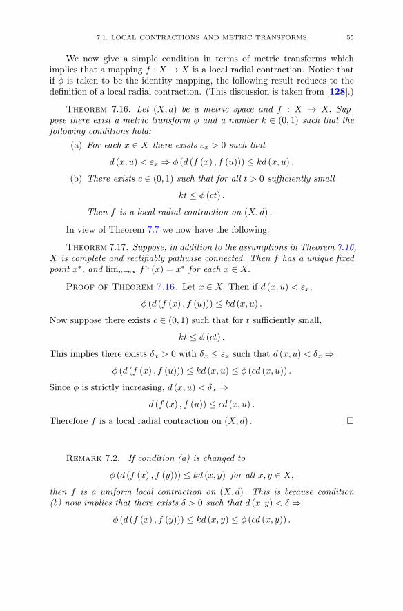
7.1. LOCAL CONTRACTIONS AND METRIC TRANSFORMS 55
We now give a simple condition in terms of metric transforms whichimplies that a mapping f : X → X is a local radial contraction. Notice thatif φ is taken to be the identity mapping, the following result reduces to thedefinition of a local radial contraction. (This discussion is taken from [128].)
Theorem 7.16. Let (X, d) be a metric space and f : X → X. Sup-pose there exist a metric transform φ and a number k ∈ (0, 1) such that thefollowing conditions hold:
(a) For each x ∈ X there exists εx > 0 such that
d (x, u) < εx ⇒ φ (d (f (x) , f (u))) ≤ kd (x, u) .
(b) There exists c ∈ (0, 1) such that for all t > 0 sufficiently small
kt ≤ φ (ct) .
Then f is a local radial contraction on (X, d) .
In view of Theorem 7.7 we now have the following.
Theorem 7.17. Suppose, in addition to the assumptions in Theorem 7.16,X is complete and rectifiably pathwise connected. Then f has a unique fixedpoint x∗, and limn→∞ fn (x) = x∗ for each x ∈ X.
Proof of Theorem 7.16. Let x ∈ X. Then if d (x, u) < εx,
φ (d (f (x) , f (u))) ≤ kd (x, u) .
Now suppose there exists c ∈ (0, 1) such that for t sufficiently small,
kt ≤ φ (ct) .
This implies there exists δx > 0 with δx ≤ εx such that d (x, u) < δx ⇒
φ (d (f (x) , f (u))) ≤ kd (x, u) ≤ φ (cd (x, u)) .
Since φ is strictly increasing, d (x, u) < δx ⇒
d (f (x) , f (u)) ≤ cd (x, u) .
Therefore f is a local radial contraction on (X, d) . �
Remark 7.2. If condition (a) is changed to
φ (d (f (x) , f (y))) ≤ kd (x, y) for all x, y ∈ X,
then f is a uniform local contraction on (X, d) . This is because condition(b) now implies that there exists δ > 0 such that d (x, y) < δ ⇒
φ (d (f (x) , f (y))) ≤ kd (x, y) ≤ φ (cd (x, y)) .

56 7. LENGTH SPACES AND LOCAL CONTRACTIONS
Remark 7.3. If f : X → X is onto and satisfies the following expansivetype condition: there exists k ∈ (0, 1) such that
d (f (x) , f (y)) ≥ k−1φ (d (x, y)) for all x, y ∈ X,
then f−1 is a uniform local contraction on (X, d) . This is because f−1 existsand satisfies
φ(d(f−1 (x) , f−1 (y)
))≤ kd (x, y) for all x, y ∈ X.
Condition (b) of Theorem 7.16 might appear to be too restrictive. How-ever we now list several examples of nontrivial metric transforms for whichthe condition holds.
(i) φ (t) =t
1 + t. Let k ∈ (0, 1) and select c ∈ (k, 1) . Then
kt ≤ φ (ct) ⇔ kt ≤ ct
1 + ct⇔
k ≤ c
1 + ct⇔ t ≤ c− k
ck.
Since c > k, condition (b) follows.(ii) φ (t) = tβ , for β ∈ (0, 1) . Then for any c, k ∈ (0, 1)
t ≤ φ (ct)
k⇔ t ≤ (ct)
β
k,
and condition (b) holds for t ≤ 1.
(iii) φ (t) = sin
(t
1 + t
). Let k ∈ (0, 1) , and set h (t) =
t
1 + t. We know
that if c ∈ (k, 1) and if t ≤ c− k
ck, then
kt ≤ h (ct) .
In particular, take k′ ∈ (k, 1) , then choose c ∈ (k′, 1) . The same
argument as in (ii) shows that if t ≤ c− k′
ck′, then
kt < k′t ≤ h (ct) .
Thus if t is sufficiently small,
kt ≤ sin k′t ≤ sin (h (ct)) = φ (ct) .
(iv) φ (t) = p tan−1 t for fixed p > 1. Let k ∈ (0, 1) . Then kt ≤ φ (ct) ⇔tan
(kt
p
)≤ ct. Let f (t) = ct − tan
(kt
p
). Then f (0) = 0 and
f ′ (t) = c − k
psec2(kt
p
)> 0 ⇔ sec2
(kt
p
)<
pc
k. If c ∈ (0, 1) is
chosen so thatpc
k> 1, then f ′ (t) > 0 for t > 0 sufficiently small.
This implies that f (t) > 0 for t > 0 sufficiently small, and this inturn implies that condition (b) holds.
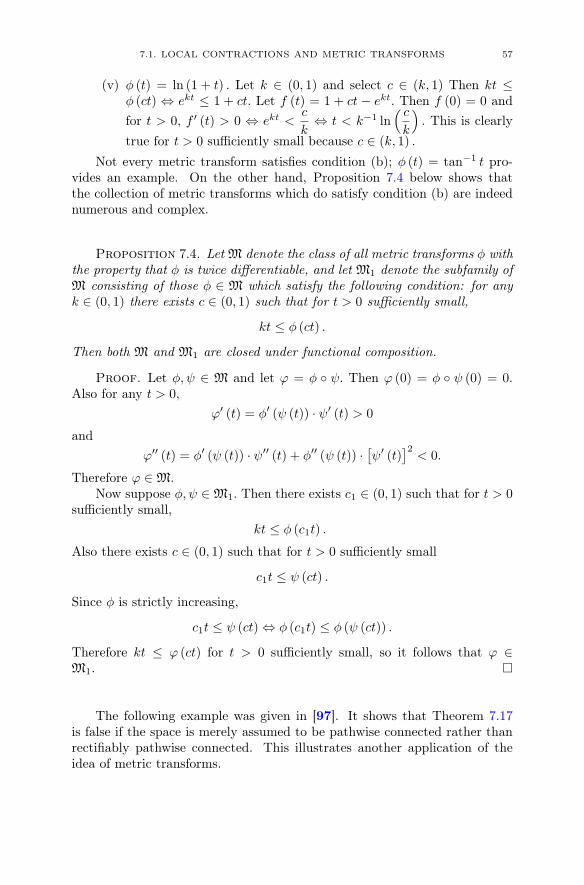
7.1. LOCAL CONTRACTIONS AND METRIC TRANSFORMS 57
(v) φ (t) = ln (1 + t) . Let k ∈ (0, 1) and select c ∈ (k, 1) Then kt ≤φ (ct) ⇔ ekt ≤ 1 + ct. Let f (t) = 1 + ct − ekt. Then f (0) = 0 andfor t > 0, f ′ (t) > 0 ⇔ ekt <
c
k⇔ t < k−1 ln
( ck
). This is clearly
true for t > 0 sufficiently small because c ∈ (k, 1) .
Not every metric transform satisfies condition (b); φ (t) = tan−1 t pro-vides an example. On the other hand, Proposition 7.4 below shows thatthe collection of metric transforms which do satisfy condition (b) are indeednumerous and complex.
Proposition 7.4. Let M denote the class of all metric transforms φ withthe property that φ is twice differentiable, and let M1 denote the subfamily ofM consisting of those φ ∈ M which satisfy the following condition: for anyk ∈ (0, 1) there exists c ∈ (0, 1) such that for t > 0 sufficiently small,
kt ≤ φ (ct) .
Then both M and M1 are closed under functional composition.
Proof. Let φ, ψ ∈ M and let ϕ = φ ◦ ψ. Then ϕ (0) = φ ◦ ψ (0) = 0.Also for any t > 0,
ϕ′ (t) = φ′ (ψ (t)) · ψ′ (t) > 0
andϕ′′ (t) = φ′ (ψ (t)) · ψ′′ (t) + φ′′ (ψ (t)) ·
[ψ′ (t)
]2< 0.
Therefore ϕ ∈ M.Now suppose φ, ψ ∈ M1. Then there exists c1 ∈ (0, 1) such that for t > 0
sufficiently small,kt ≤ φ (c1t) .
Also there exists c ∈ (0, 1) such that for t > 0 sufficiently small
c1t ≤ ψ (ct) .
Since φ is strictly increasing,
c1t ≤ ψ (ct) ⇔ φ (c1t) ≤ φ (ψ (ct)) .
Therefore kt ≤ ϕ (ct) for t > 0 sufficiently small, so it follows that ϕ ∈M1. �
The following example was given in [97]. It shows that Theorem 7.17is false if the space is merely assumed to be pathwise connected rather thanrectifiably pathwise connected. This illustrates another application of theidea of metric transforms.

58 7. LENGTH SPACES AND LOCAL CONTRACTIONS
Example 7.2. Let (βn)∞n=−∞ be a strictly increasing doubly infinite
sequence in (0, 1) . For x, y ∈ R+, set
(7.1) ρ (x, y) =
⎧⎨⎩
|x− y|βn if x, y ∈ [n, n+ 1] ;
|x− (n+ 1)|βn + (p− 1) + |(n+ p)− y|βn+p
if x ∈ [n, n+ 1] , y ∈ [n+ p, n+ p+ 1] , p ∈ N.
We first observe that (R+, ρ) is a metric space (see Proposition 7.5 below).
Now define f : R+ → R
+ by setting f (x) = x + 1. This mapping is ahomeomorphism which is a local contraction for any k ∈ (0, 1) . To see this,suppose x, y ∈ [n, n+ 1] . Then
ρ (f (x) , f (y)) = |x− y|βn+1 ≤ k |x− y|βn = kρ (x, y)
if and only if |x− y|βn+1−βn ≤ k. Since βn+1 −βn > 0, this is always true if|x− y| is sufficiently small; indeed
ρ (x, y) = |x− y|βn ≤ kβn/(βn+1−βn) ⇔ |x− y|βn+1−βn ≤ k.
To deal with the case x = n > 0, merely take a neighborhood of x with radiusless than min
{kβn/(βn+1−βn), kβn+1/(βn+2−βn+1)
}.
Notice that the mapping of the above example is even locally contractivein the sense of Rakotch [182], but it is fixed point free. We note also thatthe space (R+, ρ) is topologically equivalent to R
+ with its usual metric. Inparticular (R+, ρ) is complete, connected, and locally connected.
The technique of the example is a special case of “gluing” of metric spaces(see, e.g., [36, p. 67]). Specifically, we use the following fact, which is a specialcase of Lemma 5.34 of [36].
Proposition 7.5. Suppose (M1, d1) and (M2, d2) are metric spaces withM1 ∩M2 = {u} . For x, y ∈ X := M1 ∪M2 set
ρ (x, y) = di (x, y) if x, y ∈ Mi, i = 1, 2;
ρ (x, y) = d1 (x, u) + d2 (u, y) if x ∈ M1, y ∈ M2.
Then (X, ρ) is a metric space.
We now observe that for each n ∈ Z and βn ∈ (0, 1) , the metric trans-form φn (t) = tβn induces a metric on the interval [n, n+ 1] . The metricspace (R+, ρ) is obtained by simply “gluing” the consecutive intervals at theircommon endpoints and applying Proposition 7.5 inductively. This results inthe metric defined by (7.1).
Remark. A theorem which appears to be a slight extension ofTheorem 7.16 has recently been announced. A mapping ϕ : R+ → R
+ issaid to be metric preserving if for all metric spaces (X, d) , ϕ ◦ d is a metric
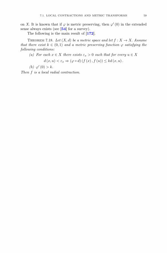
7.1. LOCAL CONTRACTIONS AND METRIC TRANSFORMS 59
on X. It is known that if ϕ is metric preserving, then ϕ′ (0) in the extendedsense always exists (see [54] for a survey).
The following is the main result of [172].
Theorem 7.18. Let (X, d) be a metric space and let f : X → X. Assumethat there exist k ∈ (0, 1) and a metric preserving function ϕ satisfying thefollowing conditions:
(a) For each x ∈ X there exists εx > 0 such that for every u ∈ X
d (x, u) < εx ⇒ (ϕ ◦ d) (f (x) , f (u)) ≤ kd (x, u) .
(b) ϕ′ (0) > k.
Then f is a local radial contraction.

CHAPTER 8
The G-Spaces of Busemann
Here we digress somewhat, although fixed point theory in geodesic spacesis an important underlying factor. A finitely compact (recall, this meansbounded closed sets are compact) geodesically connected (metrically convex)metric space (R, d) which has the geodesic extension property (see Defini-tion 9.3 below) and for which such extension is unique is called a G-space.This definition is due to Busemann [46]. Precisely, to every point p ∈ Rthere corresponds a number ρp > 0 such that if x, y ∈ U
(p; ρp)
(the openball) with x = y, there exists a point z ∈ R for which
d (x, y) + d (y, z) = d (x, z) ,
and moreover, the conditions d (x, y)+d (y, z1) = d (x, z1), d (x, y)+d (y, z2) =
d (x, z2) , and d (y, z1) = d (y, z2) ⇒ z1 = z2. A mapping ψ of a G-space R
onto a G-space R is called a local isometry if for every p ∈ R, there existsa number ηp > 0 such that ψ maps U
(p; ηp)
isometrically onto U(p; ηp).
When such a mapping exists the space R is said to be a covering space of theG-space R and ψ a covering map. It is shown in [46] that every G-space has auniversal (simply connected) covering space which is unique up to isometries(and which is, itself, a G-space). In particular, if R is the universal coveringspace of R with Ω : R → R a covering map, then the fundamental group ofR may be realized as the group of those motions Ψ (surjective isometries) ofR onto R for which Ω ◦Ψ = Ω.
An isometry of a G-space onto itself is called a motion. It is known thata local isometry of a noncompact G-space R onto itself is a motion if thefundamental group of R is not isomorphic with a proper subgroup of itself[46, p. 174]. Without this hypothesis on the fundamental group the assertionmay or may not be true. It is true for a cylinder with a locally Euclideanmetric but it is false for a cylinder with a locally hyperbolic metric. This leadsto the problem (see [46, p. 405, (27)]) of finding conditions under which localisometries are motions, in particular conditions which apply to an ordinarycylinder. A response to this problem is given in [108]. To discuss this furtherwe need some fundamental properties of local isometries.
Let φ denote a locally isometric mapping of a G-space(R, d)
onto aG-space (R, d) . The following properties of φ are found in Busemann [46,pp. 167–170].
© Springer International Publishing Switzerland 2014W. Kirk, N. Shahzad, Fixed Point Theory in Distance Spaces,DOI 10.1007/978-3-319-10927-5__8
61

62 8. THE G-SPACES OF BUSEMANN
(1) If x (τ) , α ≤ τ ≤ β, is a curve in R and if φ (x (τ)) = x (τ)is a geodesic segment in R, then x (τ) is a geodesic segment andd (x (α) , x (β)) = d (x (α) , x (β)) .
(2) For a given curve x (τ) , α ≤ τ ≤ β, in R and a given point a ∈ Rsuch that φ (a) = x (α) there is exactly one curve x (τ) in R suchthat φ (x (τ)) = x (τ) with x (α) = a.
(3) Given p ∈ R there is a number ρ (p) > 0 such that if p1, p2 ∈ Rsatisfy p1 = p2 and φ (p1) = φ (p2) = p, then d (p1, p2) ≥ 2ρ (p) .
(4) The number of points of R that are mapped into a given point ofR is at most countable, and is the same for different points of R.
(5) If φ is one-to-one, then φ is an isometry.(6) If a, b ∈ R and if φ (a) = a, there is exactly one point b ∈ R such
that φ(b)= b and d
(a, b)= d (a, b) .
The following is immediate from the definition of a local isometry.
(7) If φ is a locally isometric mapping of R onto itself, then φn is also,n = 1, 2, · · ·.
Theorem 8.1 ([108]). A locally isometric mapping of a G-space ontoitself which has a fixed point is a motion.
Proof. Let φ (p) = p, and suppose φ is not a motion. Then by (5) φis not one-to-one so by (4) there is a point p1 ∈ R with p1 = p such thatφ (p1) = p. By (6) there is a point p2 ∈ R such that φ (p2) = p1 and such thatd (p, p2) = d (p, p1). Proceeding by induction obtain a sequence {pn} ⊂ Rsuch that φ (pn+1) = pn and d (p, pn) = d (p, p1) , n = 1, 2, · · ·.
If n < m, then φn (pn) = p while φn (pm) = pm−n. Since
d(p, pm−n) = d (p, p1) > 0,
we see that pm−n = p. Therefore φn (pn) = φn (pm) and it follows thatpn = pm. By (7) φn, for each positive integer n, is a locally isometric mappingof R onto itself, so by (3) d (pi, pj) ≥ 2ρ (p) if i = j. Since the sequence {pn}is bounded, this contradicts the finite compactness of R. �
Theorem 8.2. A locally isometric mapping φ of a G-space (R, d) ontoitself is a motion if and only if there exists a motion ψ of R such that forsome point p ∈ R, ψ ◦ φ (p) = p.
Proof. The necessity is trivial. The sufficiency is established byobserving that ψ ◦ φ is a locally isometric mapping with a fixed point p.Thus by Theorem 8.1 ψ ◦ φ is a motion, and hence one-to-one. Therefore φis one-to-one, and by (5) also a motion. �
The group of motions of a G-space are said to be transitive if given anytwo points of the space there is a motion of the space that maps one into theother. Among two-dimensional G-spaces, it is known that the cylinder (andtorus) with a Minkowskian metric has a transitive group of motions. Thusthe following is an immediate consequence of Theorem 8.2.
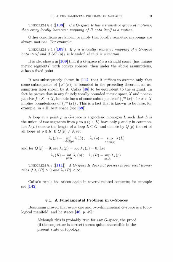
8.1. A FUNDAMENTAL PROBLEM IN G-SPACES 63
Theorem 8.3 ([108]). If a G-space R has a transitive group of motions,then every locally isometric mapping of R onto itself is a motion.
Other conditions are known to imply that locally isometric mappings arealways motions. For example:
Theorem 8.4 ([109]). If φ is a locally isometric mapping of a G-spaceonto itself and if {φn (p)} is bounded, then φ is a motion.
It is also shown in [109] that if a G-space R is a straight space (has uniquemetric segments) with convex spheres, then under the above assumptions,φ has a fixed point.
It was subsequently shown in [112] that it suffices to assume only thatsome subsequence of {φn (x)} is bounded in the preceding theorem, an as-sumption later shown by A. Całka [48] to be equivalent to the original. Infact he proves that in any finitely totally bounded metric space X and nonex-pansive f : X → X, boundedness of some subsequence of {fn (x)} for x ∈ Ximplies boundedness of {fn (x)} . This is a fact that is known to be false, forexample, in a Hilbert space (see [68]).
A loop at a point p in G-space is a geodesic monogon L such that L isthe union of two segments from p to q (q ∈ L) have only p and q in common.Let λ (L) denote the length of a loop L ⊂ G, and denote by Q (p) the set ofall loops at p ∈ R. If Q (p) = ∅, set
λi (p) = infL∈Q(p)
λ (L) ; λs (p) = supL∈Q(p)
λ (L)
and for Q (p) = ∅, set λi (p) = ∞; λs (p) = 0. Let
λi (R) = infp∈R
λi (p) ; λs (R) = supp∈R
λs (p) .
Theorem 8.5 ([111]). A G-space R does not possess proper local isome-tries if λi (R) > 0 and λs (R) < ∞.
Całka’s result has arisen again in several related contexts; for examplesee [142].
8.1. A Fundamental Problem in G-Spaces
Busemann proved that every one and two-dimensional G-space is a topo-logical manifold, and he states [46, p. 49]:
Although this is probably true for any G-space, the proof(if the conjecture is correct) seems quite inaccessible in thepresent state of topology.

64 8. THE G-SPACES OF BUSEMANN
We do not know the current state of this conjecture. However it was soonestablished for the case of three dimensions by B. Krakus [134], and in a sur-prising more recent development,2 P. Thurston [209] established Busemann’sconjecture for four dimensions.
Theorem 8.6 (Berestovskii [21]). Busemann G-spaces of dimension n ≥5 having Aleksandrov curvature bounded above3 are n-manifolds.
A Comment About Dimension. There are various notions ofdimension in topology (see, e.g., [69]). The one Busemann is referring tothe classical “Menger-Urysohn” dimension. The axioms are:(MU1) dimX = −1 ⇔ X = ∅;(MU2) dimX ≤ n, n ∈ N, if for every point x ∈ X and each neighborhood
Vx of x there exists an open set U ⊂ X such that
x ∈ U ⊂ Vx and dimFrU ≤ n− 1;
(MU3) dimX = n if dimX ≤ n and dimX > n − 1, i.e., dimX is not≤ n− 1;
(MU4) dimX = ∞ if dimX > n ∀n ∈ N.
In the realm of separable metric spaces (e.g., G-spaces) this concept ofdimension coincides with the notion of “covering” dimension. See [22] for arecent survey of all known results on the topology of Busemann G-spaces offinite dimension.
2The reviewer of this paper states in [188]: “Without any doubt this is one of thenicest papers in geometric topology of the 1990’s.”
3A metric space is said to have Alexandrov curvature ≤ κ if it is locally a CAT(κ)space. CAT(κ) spaces are defined in the next chapter.

CHAPTER 9
CAT(0) Spaces
9.1. Introduction
A substantial part of the discussion in this chapter is taken from twosurvey articles [118, 119]. These articles motivated a substantial resurgenceof the study of metric fixed point theory in spaces of non-positive curvature.The study of spaces of non-positive curvature originated with the discoveryof hyperbolic spaces, the work of J. Hadamard at the beginning of the lastcentury, and the work of E. Cartan in the 1920s. The idea of what it means fora geodesic metric space to have non-positive curvature (or, more generally,curvature bounded above by a real number κ) goes back to the work ofH. Busemann and A.D. Alexandrov in the 1950s. Of particular importanceto the revival of interest in this topic are the lectures which Mikhael Gromovgave in 1981 at the Collège de France in Paris (see [36, p. VIII]). In theselectures Gromov explained the main features of global Riemannian geometryessentially by basing his account wholly on the so-called CAT(0) inequality.
It is shown in [118] that many of the standard ideas and methods ofnonlinear analysis and Banach space theory carry over to the class of spacesGromov calls CAT(0) spaces. (The letters C, A, and T stand for Cartan,Alexandrov, and Toponogov.) A metric space X is said to be a CAT(0) spaceif it is geodesically connected, and if every geodesic triangle in X is at least as“thin” as its comparison triangle in the Euclidean plane. We make this precisebelow. However it is this latter property, known as the CAT(0) inequality,that encapsulates the concept of non-positive curvature in Riemannian ge-ometry and allows one to reflect the same concept in a much wider setting.We shall almost invariably assume completeness as well. Complete CAT(0)spaces are often called Hadamard spaces. CAT(0) spaces have a remarkablynice geometric structure. One can see almost immediately that in such spacesangles exist in a strong sense, the distance function is convex, one has bothuniform convexity and orthogonal projection onto convex subsets, etc. Also,because of their generality, CAT(0) spaces arise in a wide variety of contexts.In CAT(0) spaces the nonexpansive mappings arise naturally in the study ofisometries or, more generally, local isometries.
© Springer International Publishing Switzerland 2014W. Kirk, N. Shahzad, Fixed Point Theory in Distance Spaces,DOI 10.1007/978-3-319-10927-5__9
65

66 9. CAT(0) SPACES
In [186], Reich and Shafrir introduced a class of “hyperbolic” metricspaces which they proposed as “an appropriate background for the study ofnonlinear operator theory in general, and of iterative processes for nonexpan-sive mappings in particular.” The observations in this chapter should serveto reinforce that assessment. Within the hyperbolic framework, the CAT(0)spaces might be viewed as an analog to the Hilbert spaces in the classicaltheory of nonlinear analysis. However such an analogy could be misleading.CAT(0) spaces include all R-trees, and these spaces bear little resemblanceto Hilbert spaces.
A fundamental source for much of our exposition is the recent book [36]by M.R. Bridson and A. Haefliger, and one should look there for things notspecifically attributed here to other sources. A more elementary treatmentof many of these ideas can be found in the recent text of Burago et al. [45].Many results, most of which are found in [36], are stated here without proof.
Several new results concerning fixed point theorems in CAT(0) spaces arealso discussed and proofs of a few new results are included. We also indicatehow some new fixed point theorems in R-trees have applications to graphtheory.
9.2. CAT(κ) Spaces
Denote by Mnκ the following classical metric spaces:
(1) if κ = 0, then Mn0 is the Euclidean space R
n;(2) if κ > 0, then Mn
κ is obtained from the sphere Sn by multiplying
the spherical distance by 1/√κ;
(3) if κ < 0, then Mnκ is obtained from the hyperbolic space H
n bymultiplying the hyperbolic distance by 1/
√−κ.
A geodesic triangle Δ(x1, x2, x3) in a geodesic metric space (X, d) con-sists of three points in X (the vertices of Δ) and a geodesic segment betweeneach pair of vertices (the edges of Δ). A comparison triangle for geodesictriangle Δ(x1, x2, x3) in (X, d) is a triangle Δ(x1, x2, x3) := Δ (x1, x2, x3)in M2
κ such that dR2 (xi, xj) = d (xi, xj) for i, j ∈ {1, 2, 3} . If κ > 0 it isfurther assumed that the perimeter of Δ(x1, x2, x3) is less than 2Dκ, whereDκ denotes the diameter of M2
κ . Such a triangle always exists.A geodesic metric space is said to be a CAT(κ) space if all geodesic
triangles of appropriate size satisfy the following CAT(κ) comparison axiom.
CAT(κ): Let Δ be a geodesic triangle in X and let Δ ⊂ M2κ be a com-
parison triangle for Δ. Then Δ is said to satisfy the CAT(κ) inequality if forall x, y ∈ Δ and all comparison points x, y ∈ Δ,
d (x, y) ≤ d (x, y) .
Complete CAT(0) spaces are often called Hadamard spaces. These spacesare of particular relevance to this study.

9.2. CAT(κ) SPACES 67
Definition 9.1. A metric space X is said to be of curvature ≤ 0 if it islocally a CAT(0) space. In this case X is said to be non-positively curved.
The significance of the above definition lies in the fact that it provides agood notion of an upper bound on curvature in an arbitrary geodesic space.In fact, classical theorems in differential geometry show that if a Riemannianmanifold is sufficiently smooth (e.g., C3), then it has curvature in the abovesense if and only if its sectional curvatures are ≤ κ. This is a result due toAlexandrov [8] in general, and to E. Cartan [51] in the case κ = 0. It shouldbe noted that nonpositively curved spaces play a significant role in manybranches of mathematics. See, e.g., B. Kleiner’s review [132] of [36].
To continue with the terminology of [36], the metric on a space X is saidto be convex if X is a geodesic space and all geodesics c1 : [0, a1] → X andc2 : [0, a2] → X with c1 (0) = c2 (0) satisfy the inequality
d (c1 (ta1) , c2 (ta2)) ≤ td (c1 (a1) , c2 (a2))
for all t ∈ [0, 1] . X is said to be locally convex if every point has a neigh-borhood in which the induced metric is convex. If the metric space is locallyconvex, then in particular X is locally contractible, and therefore X has auniversal covering space X. This means that X is simply connected and thereis a local isometry p : X → X. In fact the space X is unique up to an isometry.
Theorem 9.1 ((Cartan–Hadamard Theorem) [36, p. 193]). Let X be acomplete and connected metric space.
(1) If the metric on X is locally convex, then the induced length metricon the universal covering space X is (globally) convex.
(2) If X is of curvature ≤ 0, then X is of CAT(0) .
Thus if a complete simply connected length space is locally convex andhas curvature ≤ 0, it is a CAT(0) space.
The CAT(0) inequality may be stated in the following equivalent butformally weaker form.
Proposition 9.1 (cf., [36, p. 161]). A geodesic metric space is a CAT(0)space if and only if the following condition holds: For every geodesic triangleΔ(p, q, r) in X and every point x ∈ [q, r] the following inequality is satisfiedby the comparison point x ∈ [q, r] ⊂ Δ(p, q, r) ⊂ R
2 :
d (p, x) ≤ d (p, x) .
We now collect some further properties of CAT(κ) spaces. These are allfound in [36].
Proposition 9.2. Let X be a CAT(κ) space.(1) There is a unique geodesic segment joining each pair of points x, y ∈
X (provided d (x, y) < Dκ if κ > 0), and this geodesic segmentvaries continuously with its endpoints.

68 9. CAT(0) SPACES
(2) Every local geodesic in X of length at most Dκ is a geodesic.(3) The balls in X of radius smaller that Dκ/2 are convex.(4) The balls in X of radius less than Dκ are contractible.(5) Approximate midpoints are close to midpoints. Specifically, for
every λ < Dκ and ε > 0 there exists δ = δ (κ, λ, ε) such that ifm is the midpoint of a geodesic segment [x, y] ⊂ X with d (x, y) ≤ λand if
max {d (x,m′) , d (y,m′)} ≤ 1
2d (x, y) + δ,
then d (m,m′) < ε.
Theorem 9.2. The following relations hold:(1) If X is a CAT(κ) space, then it is a CAT(κ′) space for every κ′ ≥ κ.(2) If X is a CAT(κ′) space for every κ′ > κ, then it is a CAT(κ) space.(3) X is a CAT(κ) space for all κ if and only if X is an R-tree.
One consequence of (1) is that any result proved for CAT(0) spaces auto-matically carries over to CAT(κ) spaces for κ < 0, and especially to R-trees.(See Chap. 11 for the definition of an R-tree.)
The following is another important observation.
Proposition 9.3 ([36, p. 176]). If X is a CAT(0) space, then the dis-tance function d : X ×X → R is convex.
This means that given any pair of geodesics c : [0, 1] → X and c′ [0, 1] →X parametrized proportional to arc length, the following inequality holds forall t ∈ [0, 1] :
d (c (t) , c′ (t)) ≤ (1− t) d (c (0) , c′ (0)) + td (c (1) , c′ (1)) .
We now turn to a generalization of Jung’s theorem. (This result alsoholds for spaces of curvature bounded below.) We use rad (S) to denote theusual Chebyshev radius of S relative to the underlying space X:
rad (S) = inf {ρ > 0 : S ⊆ B (x; ρ) for some x ∈ X} .We also need to introduce the function snκ : R → R, defined by
snκ (x) :=
⎧⎨⎩
sin (√κx) /
√κ if κ > 0,
x if κ = 0,sinh(√
−κx)/√−κ if κ < 0.
Theorem 9.3 ([137]). Let X be a complete CAT(κ) space and S anonempty bounded subset of X. Then there exists a unique x ∈ X such thatS ⊆ B (x; rad (S)) , where
snκ (rad (S)) ≤√2snκ
(diam (S)
2
).

9.2. CAT(κ) SPACES 69
In particular (cf., [47]), if S is a bounded subset of a complete CAT(0)space, then
rad (S) ≤√2
2diam (S) .
This of course coincides with the well-known Hilbert space estimate.
While many reformulations of the CAT(κ) condition concern the geom-etry of triangles, there is also a useful reformulation involving the geometryof quadrilaterals. Let (x1, x2, x3, x4) be a 4-tuple of point of a metric spaceX. A subembedding of this 4-tuple in M2
κ is a 4-tuple (x1, y1, x2, y2) of pointsof M2
κ such that d (xi, yj) = d (xi, yj) for i, j ∈ {1, 2}, and
d (x1,x2) ≤ d (x1, x2) and d (y1, y2) ≤ d (y1, y2) .
X is said to satisfy the CAT(κ) 4-point condition if every 4-tuple of points
(x1, y1, x2, y2)
in X for which
d (x1, y1) + d (y1, x2) + d (x2, y2) + d (y2, x1) < 2Dκ
has a subembedding in M2κ .
Proposition 9.4. Let X be a complete metric space. Then the followingconditions are equivalent.
(1) X is a CAT(κ) space.(2) X satisfies the CAT(κ) 4-point condition and every pair of points
x, y ∈ X with d (x, y) < Dκ has approximate midpoints.
Finally we observe that if x, y1, y2 are points of a CAT(0) space and if y0is the midpoint of the segment [y1, y2], then the CAT(0) inequality implies
(9.1) d (x, y0)2 ≤ 1
2d (x, y1)
2+
1
2d (x, y2)
2 − 1
4d (y1, y2)
2
because equality holds in the Euclidean metric. In fact (cf., [36, p. 163]), ageodesic metric space is a CAT (0) space if and only if it satisfies inequality(9.1) (which is known as the CN inequality of Bruhat and Tits [41]). Usingthis inequality it is easy to see that if X1 and X2 are CAT(0) spaces, thenX1 ×X2 is also a CAT(0) space, where the metric on X1 ×X2 is given by
d ((x1, x2) , (y1, y2))2= d (x1, y1)
2+ d (x2, y2)
2.
Also if d (x, y1) = d (x, y2) = 1 and d (y1, y2) ≥ ε, then (9.1) gives
d (x, y0) ≤√
1− ε2
4
70 9. CAT(0) SPACES
and so one has the usual Euclidean modulus of convexity in CAT(0) spaces.In particular, d (x, y1) ≤ R, d (x, y2) ≤ R, and d (y1, y2) ≥ r imply
d (x, y0) ≤(1− δ
( rR
))R,
where δ (ε) :=
√1− ε2
4.
An extremely useful property of CAT(0) is the nearest point projection.Crucial to the proof of this fact, and useful in other contexts as well, is theconcept of “angle” in a metric space. Let X be a metric space, and let c :[0, a] → X and c′ : [0, a′] → X be two geodesics with c (0) = c′ (0) . Given t ∈(0, a] and t′ ∈ (0, a′] we consider the comparison triangle Δ (c (0) , c (t) , c′ (t′))and the comparison angle ∠c(0) (c (t) , c
′ (t′)) . The (Alexandrov) angle be-tween the geodesic paths c and c′ is the number ∠c,c′ ∈ [0, π] defined by:
∠c,c′ = lim supt,t′→0
∠c(0) (c (t) , c′ (t′)) = lim
ε→0sup
0<t,t′<ε∠c(0) (c (t) , c
′ (t′)) .
Proposition 9.5 ([36, p. 176]). Let X be a CAT(0) space, and let C bea convex subset of X which is complete in the induced metric. Then:
(1) for every x ∈ X there exists a unique point P (x) ∈ C such that
d (x, P (x)) = dist (x,C) ;
(2) if x′ belongs to the geodesic segment [x, P (x)] , then P (x′) = P (x) ;(3) given x /∈ C and y ∈ C, if y = P (x) then ∠P (x) (x, y) ≥ π/2;(4) the map x �→ P (x) is a nonexpansive retraction of X onto C; the
map H : X × [0, 1] → X associating with (x, t) the point at dis-tance td (x, P (x)) from x on the geodesic segment [x, P (x)] is acontinuous homotopy from the identity map of X to P.
9.3. Fixed Point Theory
We now come to one of the central topics of this monograph. From thepreceding section it is easy to see that CAT(0) spaces share many proper-ties of uniformly convex Banach spaces. For example, closed convex setsare uniquely proximinal, descending sequences of nonempty bounded closedconvex sets have nonempty intersection, and “asymptotic center” techniquesapply. As we have seen, CAT(0) spaces also enjoy certain Hilbert space prop-erties: For example, nearest point projections onto closed convex sets arenonexpansive, and a notion of angle is present for which a law of cosines ap-plies. Also the family of all bounded closed convex subsets of a given CAT(0)space is normal in the sense described in Chap. 3. Thus the following theoremis immediate.
Theorem 9.4. Suppose K is a nonempty bounded closed convex subsetof a complete CAT(0) space and suppose f : K → K is nonexpansive. Thenthe set of fixed points of f is nonempty, closed, and convex.

9.3. FIXED POINT THEORY 71
We begin with some general notation. Let S be a subset of a completeCAT(0) space X. Then for each x, y ∈ S there is a unique geodesic [x, y] ⊂ Xjoining x and y. We denote by G1 (S) the union of all geodesic segmentsin X with endpoints in S. Then S is convex if G1 (S) = S. The CAT(0)inequality ensures that rad (G1 (S)) = rad (S) . For n ≥ 2, define inductivelyGn (S) = G1 (Gn−1 (S)) . The convex hull of S is defined to be the set
convS =∞⋃
n=1
Gn (S) ,
convS denotes its closure. From this we conclude that rad (convS) = rad (S)for every bounded S ⊂ X.
One of the fundamental theorems in fixed point of nonexpansive map-pings is the demiclosedness theorem due to F. Browder [40]. This theoremasserts that if K is a closed and convex subset of a uniformly convex Banachspace X, and if f : K → X is nonexpansive, then I − f is demiclosedon K, that is, if {uj} is a sequence in K which converges weakly to u ∈X and if {(I − f) (uj)} converges strongly (in norm) to w, then w ∈ Kand (I − f) (u) = w. One important corollary of this theorem is that ifinf {‖x− f (x)‖ : x ∈ K} = 0, then f has a fixed point in K when K isbounded. In the absence of a weak topology, an analog of this theorem can-not even be formulated in a complete CAT(0) space. However the corollarycan be formulated in such a setting, and indeed, it turns out to be true.
We need some notation. Given a mapping f : K → X where K is asubset of a metric space X, and a number ε > 0, the ε-fixed point set of f isthe set
Fε (f) = {x ∈ K : d (x, f (x)) ≤ ε} .We take the following lemma as a point of departure.
Lemma 9.1 ([36, p. 286]). Let X be a CAT(0) space. Fix x, y ∈ X withd (x, y) = 2r and let m be the midpoint of the geodesic segment [x, y] . Ifm′ is a point such that d (m′, x) ≤ r (1 + ε) and d (m′, y) ≤ r (1 + ε) , thend (m,m′) ≤ r
√ε2 + 2ε.
A slight modification of the argument given in [36] for Lemma 9.1 leadsto the following result.
Lemma 9.2. Let K be a bounded subset of a CAT(0) space X, supposef : K → X is nonexpansive, and suppose x, y ∈ Fε (f) with d (x, y) = r. Letm ∈ [x, y] ∩K. Then f (m) ∈ Fφ(ε) (f) , where φ (ε) =
√ε2 + 2rε.
Proof. Let m be the point of [x, y] with distance αr from x, and supposem ∈ K. Then if m′ = f (m) ,
d (x,m′) ≤ d (x, f (x)) + d (f (x) , f (m))
≤ d (x, f (x)) + d (x,m)
≤ ε+ αr.

72 9. CAT(0) SPACES
Similarly d (y,m′) ≤ ε+ (1− α) r. At least one of the angles ∠m (m′, x) and∠m (m′, y) is greater than or equal to π/2. If ∠m (m′, x) ≥ π/2, then in thecomparison triangle Δ(m,m′, x) the angle at m is also greater than or equalto π/2. By the law of cosines
(ε+ αr)2 ≥ d (x,m′)
2 ≥ (αr)2+ d (m,m′)
2.
Similarly, if ∠m (m′, y) ≥ π/2,
(ε+ (1− α) r)2 ≥ d (y,m′)
2 ≥ ((1− α) r)2+ d (m,m′)
2.
Therefore
d (m, f (m))2= d (m,m′)
2 ≤ max{ε2 + 2αrε, ε2 + 2 (1− α) rε
}≤ ε2 + 2rε.
�Theorem 9.5. Let K be a bounded closed convex subset of a complete
CAT(0) space X. Suppose f : K → X is a nonexpansive mapping for which
inf {d (x, f (x)) : x ∈ K} = 0.
Then f has a fixed point in K.
Proof. Let x0 ∈ X be fixed and define
r0 = inf {r > 0 : inf {d (x, f (x)) : x ∈ B (x0; r) ∩K} = 0} .Obviously r0 < ∞, and if r0 = 0, then x0 ∈ K and f (x0) = x0 by continuityof f. So we suppose r0 > 0. Now choose {xn} ⊂ K so that d (xn, f (xn)) → 0and d (x0, xn) → r0. Since any convergent subsequence of {xn} would havea fixed point of f as its limit, we may suppose there exist ε > 0 and sub-sequences {uj} and {vj} of {xn} such that d (uj , vj) ≥ ε. Passing again
to subsequences if necessary we may also suppose d (x0, uj) ≤ r0 +1
jand
d (x0, vj) ≤ r0+1
j. Let mj be the midpoint of the segment [uj , vj ] and let mj
be the point corresponding to mj on the comparison triangle Δ(x0, uj , vj) .Then by the CAT(0) inequality
d (x0,mj) ≤ d (x0, mj) ≤
√(r0 +
1
j
)2
−(ε2
)2.
Clearly d (x0,mj) ≤ r∗ < r0 for j sufficiently large. On the other hand, byLemma 9.2, d (mj , f (mj)) → 0 as j → ∞. This contradicts the definitionof r0. �
Essentially the same proof gives the following result.
Theorem 9.6. Let U be a connected bounded open set in a completeCAT(0) space X, and let f : U → X be nonexpansive. Then the followingalternative holds:

9.3. FIXED POINT THEORY 73
(a) f has a fixed point in U, or;(b) inf {d (x, f (x)) : x ∈ ∂U} ≤ inf {d (x, f (x)) : x ∈ U} .Proof. Assume there exists z ∈ U such that
d (z, f (z)) < ξ := inf {d (x, f (x)) : x ∈ ∂U} .Then if m ∈ [z, f (z)] ∩ U,
d (m, f (m)) ≤ d (m, f (z)) + d (f (z) , f (m))
≤ d (m, f (z)) + d (z,m)
= d (z, f (z)) .
This proves that the segment [z, f (z)] not only lies in U but in fact it isbounded away from ∂U. Consequently if one defines g : U → X by takingg (x) to be the midpoint of the segment [x, f (x)] for each x ∈ U, the sequence{gn (z)} lies in U. Moreover by Theorem 6.1, d
(gn (z) , gn+1 (z)
)→ 0. Thus
inf {d (x, f (x)) : x ∈ U} = 0. The argument now follows the preceding one.All one needs to observe is that if ε > 0 is chosen so that
√ε2 + 2rε ≤ δ <
ξ, where r = diam (U) , and if m ∈ [u, v] ∩ U , where u, v ∈ Fε (f) , thend (m, f (m)) ≤ δ. Hence [u, v]∩∂U = ∅. Thus the points mk as defined in thepreceding argument all lie in U. �
Remark 9.1. It is shown in [119] that Theorem 9.6 holds under theweaker assumption that f : U → X is continuous on U and locally nonex-pansive on D.
We next consider the approximate fixed point property. A subset K ofa metric space is said to have the approximate fixed point property (for non-expansive mappings) if given any nonexpansive f : K → K, inf {d (x, f (x)) :x ∈ K} = 0. To characterize this concept, we need some more definitions.
Definition 9.2 ([197]). Let X be a metric space. A curve γ : [0,∞) →X is said to be directional (with constant b) if there is b ≥ 0 such that
t− s− b ≤ d (γ (s) , γ (t)) ≤ t− s
for all t ≥ s ≥ 0. A subset of X is said to be directionally bounded if it doesnot contain a directional curve.
Definition 9.3. A geodesic metric space X is said to have the geodesicextension property if for every local geodesic c : [a, b] → X, with a = b, thereexists ε > 0 and a local geodesic c′ : [a, b+ ε] → X such that c′ |[a,b]= c.
Lemma 9.3 ([36, p. 298]). If X is a CAT (0) space, then X has thegeodesic extension property if and only if every non-constant geodesic c :[a, b] → X can be extended to a line c : R → X.

74 9. CAT(0) SPACES
(If a complete CAT(0) space is homeomorphic to a finite dimensionalmanifold, then it always has the geodesic extension property.)
In [185] it is shown that a reflexive Banach space has the approximatefixed point property if and only if it is directionally bounded (i.e., its inter-section with any line is bounded), and in [197] Shafrir proved that a closedconvex subset of a complete hyperbolic metric space has the approximatefixed point property for nonexpansive mappings if and only if it is direc-tionally bounded. As an immediate corollary of Shafrir’s result, a closedconvex subset of a complete CAT(0) space with the geodesic extension prop-erty has the approximate fixed point property if and only if it is directionallybounded. However in this case the stronger assertion of Reich’s result is true.(One should also compare this result to Theorem 32.2 of [88], which statesthat the same result holds for the complex Hilbert ball with a hyperbolicmetric. In fact, in this setting the approximate fixed point property actuallyimplies the fixed point property.)
Theorem 9.7. A closed convex subset of a complete CAT(0) space withthe geodesic extension property has the approximate fixed point property fornonexpansive mappings if and only if it does not contain a geodesic ray.
Proof. In view of Shafrir’s result it need only be shown that if a closedconvex set in a complete CAT(0) space X is geodesically bounded then it isdirectionally bounded. So, suppose K is a closed convex set in X and supposeK contains a directional curve γ. We show that this implies K contains ageodesic ray.
Let xn = γ (n) , n = 0, 1, 2, · · ·, and fix an arbitrary ρ > b, where b is thedirectional constant associated with γ. For each n ≥ ρ, let yn be the point ofgeodesic segment [x0, xn] with distance ρ from x0. Now suppose m > n ≥ ρ,and let αn,m be the comparison angle ∠x0
(xn, xm) in R2. By the law of
cosines
cos (αn,m) =d (x0, xn)
2+ d (x0, xm)
2 − d (xn, xm)2
2d (x0, xn) d (x0, xm).
Using the inequalities
n− b ≤ d (x0, xn) ≤ n;
m− b ≤ d (x0, xm) ≤ m;
m− n ≥ d (xn, xm) ,
9.3. FIXED POINT THEORY 75
we have
cos (αn,m) ≥ (n− b)2+ (m− b)
2 − (m− n)2
2nm
=n
2m
[(n− b)
2
n2
]+
m
2n
[(m− b)
2
m2
]− (m− n)
2
2nm
=n
2m+
m
2n− (m− n)
2
2nm− b
n− b
m+
b2
nm
= 1− b
(1
n+
1
m− b
nm
).
Thus cos (αn,m) → 1 as m,n → ∞; hence αn,m → 0. If yn, ym are therespective points of the comparison triangle Δ(x0, xn, xm) corresponding toyn, ym, then by the CAT(0) inequality d (yn, ym) ≤ d (yn, ym) . The fact thatαn,m → 0 as m,n → ∞ implies that {yn} , hence {yn} , is a Cauchy sequence.Since ρ > b is arbitrary it now follows that the sequence {[x0, xn]} of geodesicsegments converges to a geodesic ray issuing from x0. �
It has been known for some time that a nonempty closed convex subsetof a Hilbert space has the fixed point property for nonexpansive mappingsif and only if it is bounded (Ray’s theorem [183]). In view of this it mightbe tempting to conjecture that a closed convex subset of a complete CAT(0)space has the fixed point property if and only if it is bounded. However this isfalse. In [73] it is shown that a closed convex subset of an R-tree has the fixedpoint property for nonexpansive mappings if (and only if) it is geodesicallybounded. The question of whether there is a class of CAT(0) spaces for whichRay’s theorem holds is taken up in [76]. An affirmative answer is given viathe introduction of the following concept:
Definition 9.4. Let (X, d) be an unbounded geodesic space. Then X issaid to have the property of the far unbounded set (property U for short) if forany closed convex unbounded set Y ⊂ X, either Y is geodesically unbounded,or for each closed convex unbounded set K ⊆ Y and x ∈ K there exists aclosed convex unbounded subset K1 of K such that
dist (x,K1) := inf {d (x, y) : y ∈ K1} ≥ 1.
One of the central results of [76] asserts that if (X, d) is a completeCAT(0) space possessing property U, then a closed convex subset Y of Xhas the fixed point property for nonexpansive mappings if and only if itis bounded. (It is also shown in [76] that any reflexive Banach space hasproperty U.)
We now turn to a method for approximating fixed points of nonexpansivemappings in CAT(0) spaces. Let K be a bounded closed convex subset of acomplete CAT(0) space and suppose f : K → K is nonexpansive. Fix x0 ∈ K,

76 9. CAT(0) SPACES
and define the mapping ft : K → K by taking ft (u) , t ∈ (0, 1) , to be thepoint of [x0, f (u)] at distance td (x0, f (u)) from x0. Then by convexity ofthe metric
d (ft (u) , ft (v)) ≤ td (u, v) ,
so ft is a contraction mapping of K into K. Since K is complete, Banach’scontraction mapping theorem assures the existence of a unique point xt suchthat:
(9.2) xt ∈ [x0, f (xt)] and d (x0, xt) = td (x0, f (xt)) .
This fact can be used to prove the following theorem. For an analog ofthis result in the Hilbert ball, see Theorem 24.1 of [88].
Theorem 9.8. Let K be a bounded closed convex subset of a completeCAT(0) space X, let f : K → K be nonexpansive, fix x0 ∈ K, and for eacht ∈ [0, 1) let xt be the point of [x0, f (xt)] satisfying (9.2). Then limt→1− xt
converges to the unique fixed point of f which is nearest x.
Proof. Fix 0 < j < l ≤ 1 and consider Δ(x0, f (xj) , f (xl)
), the com-
parison triangle of Δ(x0, f (xj) , f (xl)) in R2. For convenience we take x0 to
be the origin. By the CAT(0) inequality we have∥∥f (xl)− f (xj)∥∥ = d (f (xl) , f (xj)) ≤ d (xl, xj)
≤ ‖xl − xj‖ =∥∥j−1f (xl)− l−1f (xj)
∥∥ .It is now possible to follow the argument of Halpern [91] step-by-step. Specif-ically, we have xj = jf (xj) and xl = lf (xl) . Let d = xl − xj . Then
〈l−1 (xj + d)− j−1xj , l−1 (xj + d)− j−1xj〉 =
∥∥l−1 (xj + d)− j−1xj
∥∥2=∥∥l−1xl − j−1xj
∥∥2=∥∥f (xl)− f (xj)
∥∥≤ ‖d‖2 .
Thus(l−1 − j−1
)2 ‖xj‖2 +(l−1)2 ‖d‖2 + 2〈
(l−1 − j−1
)l−1xj , d〉 ≤ ‖d‖2
from which(l−1 − j−1
)2 ‖xj‖2 +(l−2 − 1
)‖d‖2 ≤ 2
(j−1 − l−1
)l−1〈xj , d〉.
In particular 〈xj , d〉 ≥ 0. Now observe that
‖xl‖2 = 〈xj + d, xj + d〉 = ‖xj‖2 + ‖d‖2 + 2〈xj , d〉.
Therefore
(9.3) ‖xl‖2 ≥ ‖xj‖2 + ‖xj − xl‖2 .

9.3. FIXED POINT THEORY 77
Now let {ki} satisfy 0 < k1 < k2 < · · · < 1 with ki → 1 as i → ∞. Since thesequence
{‖xki
‖2}
is monotone increasing and bounded, it follows that
d(xki
, xkj
)2 ≤∥∥xki
− xkj
∥∥2 ≤ ‖xki‖2 −∥∥xkj
∥∥2 → 0 as i, j → ∞.
Thus {xki} converges to some point x∗ ∈ K. However
d (xki, f (xki
)) = (1− ki) d (x0, f (xki))
and by continuity
d (x∗, f (x∗)) = limki→1−
(1− ki) d (x0, f (xki)) = 0.
Therefore x∗ is a fixed point of f.Now let p be any other fixed point of f. By repeating the preceding
argument taking xl = x1 = p, we conclude from (9.3) that
d (x0, p)2= ‖p‖2 ≥ ‖xki
‖2 + ‖xki− p‖2
≥ ‖xki‖2 + d (xki
, p)2
= k2i d (x0, xki)2+ d (xki
, p)2,
from which (letting ki → 1−)
d (x0, p)2 ≥ d (x0, x
∗)2 + d (x∗, p)2 .
This proves that x∗ is the unique fixed point of f which is nearest x0. �
As a consequence of the above result, if fix (f) denotes the fixed pointset of f, then given any x ∈ K,
limt→1−
xt = Px ∈ fix (f) ,
where the mapping P defined by x �→ Px is the nearest point projection ofK onto fix (f) . Since the nearest point projection of CAT(0) space X ontoany complete convex subset of X is nonexpansive, P is nonexpansive. Thusfix (f) is a nonexpansive retract of X.
In a Banach space context, the fact that in Theorem 9.8 is true outsideHilbert space, and indeed in any uniformly smooth space (except that thelimit is a certain retraction different from the nearest point projection), isproved in Reich [184].
Remark 9.2. In fact, it is possible to show that the mapping P is firmlynonexpansive in the sense of Theorem 27.2 of [88].
We now give two homotopy invariance results in the spirit of Frigon [84].In these results intK and ∂K denote, respectively, the interior and boundaryof K.

78 9. CAT(0) SPACES
Theorem 9.9. Let K be a closed convex subset of a complete CAT(0)space X with intK = ∅. Suppose f, g : K → X are contraction mappings,and suppose h : [0, 1]×K → X is a homotopy satisfying
(a) h (0, ·) = g; h (1, ·) = f (·) ;(b) h (t, ·) is a contraction mapping with constant k ∈ (0, 1) for each
t ∈ [0, 1] ;(c) For any ε > 0 there exists δ > 0 such that for x ∈ K and t, s ∈ [0, 1] ,
|t− s| < δ ⇒ d (h (t, x) , h (s, x)) < ε;(d) x = h (t, x) for each x ∈ ∂K and t ∈ [0, 1] .
Then f has a fixed point in K if and only if g has a fixed point in K.
Proof. Assume that G has a fixed point, and let
E = {t ∈ [0, 1] : x = h (t, x) for some x ∈ K} .The theorem is proved by showing that E is both open and closed. If E isnot open, then there exists t ∈ E and {tn} ⊂ [0, 1] \E such that tn → t.Now let P be the nearest point projection of X onto K. Define the mappingsh (t, ·) : X → X by setting h (t, x) = h (t, P (x)) . Then the mappings h (t, ·)are contraction mappings with constant k. In particular there exist pointsxn ∈ X such that xn = h (tn, xn) . Thus
d (xn, x) = d (h (tn, P (xn)) , h (t, P (x)))
≤ d (h (tn, P (xn)) , h (tn, P (x))) + d (h (tn, P (x)) , h (t, P (x)))
≤ kd (xn, x) + d (h (tn, P (x)) , h (t, P (x))) ,
from which
d (xn, x) ≤ (1− k)−1
d (h (tn, P (x)) , h (t, P (x))) .
By (c) it must be the case that xn = h (tn, P (xn)) → x. However {xn} is inthe complement of K and x is in the interior of K. This contradiction provesthat E is open.
To prove that E is closed, assume {tn} ⊂ E with tn → t /∈ E. The sameargument as the one just given leads to the conclusion that xn → x with{xn} in the interior of K and x in the complement of K. �
Theorem 9.10. Let K be a bounded closed convex subset of a completeCAT(0) space X with intK = ∅. Suppose f : K → X is a nonexpansivemapping, and suppose h : [0, 1]×K → X is a homotopy satisfying
(a) h (0, ·) has a fixed point;(b) h (1, ·) = f (·) ;(c) For each t ∈ [0, 1), h (s, ·) is a kt-contraction mapping for each
s ∈ [0, t);(d) For any ε > 0 there exists δ > 0 such that for x ∈ K and t, s ∈ [0, 1] ,
|t− s| < δ ⇒ d (h (t, x) , h (s, x)) < ε;(e) x = h (t, x) for each x ∈ ∂K and t ∈ [0, 1] .
Then f has a fixed point in K.

9.3. FIXED POINT THEORY 79
Proof. Select {tn} ⊂ (0, 1) with tn → 1. By Theorem 9.9, for each nthere exists xn ∈ K such that xn = h (tn, xn) . Thus
d (xn, f (xn)) = d (h (tn, xn) , h (1, xn)) ,
and by (c) we conclude d (xn, f (xn)) → 0. The result now follows fromTheorem 9.5. �
Remark 9.3. It is possible to prove that Theorems 9.5–9.6 hold in uni-formly convex metric spaces by routinely modifying the arguments given here.However it does not appear that the same can be said of Theorems 9.7–9.9.In particular, it is not known whether Theorems 9.8 and 9.9 even hold in auniformly convex Banach space. On the other hand, as we have already noted,Theorem 9.7 holds in any reflexive Banach space but it fails in nonreflexivespaces.
QUESTION. It remains open whether any of the preceding resultsextend to spaces of non-positive curvature. There appear to be serious ob-stacles to carrying out such extensions.
We close this section with a theorem which invokes the Leray–Schauderboundary condition. For this we will use the following continuation principledue to A. Granas.
Theorem 9.11 ([89]). Let U be a domain (i.e., connected open set) in acomplete metric space X, let f, g : U → X be two contraction mappings, andsuppose there exists h : U × [0, 1] → X such that
(a) h (·, 1) = f, h (·, 0) = g;(b) h (x, t) = x for every x ∈ ∂U and t ∈ [0, 1] ;(c) there exists k < 1 such that d (h (x, t) , h (y, t)) ≤ kd (x, y) for every
x, y ∈ U and t ∈ [0, 1] ;(d) there exists a constant α ≥ 0 such that for every x ∈ U and t, s ∈
[0, 1] ,d (h (x, t) , h (x, s)) ≤ α |s− t| .
Then f has a fixed point if and only if g has a fixed point.
We will also need the following lemma due to Crandall and Pazy.
Lemma 9.4 ([56]). Let {zn} be a subset of a Hilbert space H and let {rn}be a sequence of positive numbers. Suppose
〈zn − zm, rnzn − rmzm〉 ≤ 0, for m = 1, 2, · · ·.Then if rn is strictly decreasing ‖zn‖ is increasing. If ‖zn‖ is bounded,limn→∞ zn exists.
Theorem 9.12. Let U be a bounded connected open set in a completeCAT(0) space X, and suppose f : U → X is nonexpansive. Suppose thereexists p ∈ U such that x /∈ [p, f (x)) for all x ∈ ∂U. Then f has a fixed pointin U.

80 9. CAT(0) SPACES
When X is a Hilbert space, Theorem 9.12 holds under the even weakerassumption that f is a lipschitzian pseudocontractive mapping. This hasbeen known for some time (see [187]). Our proof is patterned after Precup’sHilbert space proof [173] for nonexpansive mappings. We observe here thatthe CAT(0) inequality is sufficient.
Proof of Theorem 9.12 [120]. Let t ∈ (0, 1) and for u ∈ U let ft (u)be the point of the segment [p, f (u)] with distance td (p, f (u)) from p. Letx, y ∈ U and consider the comparison triangle Δ = Δ (p, x, y) of Δ(p, x, y)in R
2. If ft (x) and ft (y) denote the respective comparison points of ft (x)and ft (y) in Δ, then by the CAT(0) inequality,
d (ft (x) , ft (y)) ≤∥∥ft (x)− ft (y)
∥∥ = t ‖x− y‖ = td (x, y) .
Therefore ft is a contraction mapping of U → X. Moreover, if B (p; r) ⊂ U,then ft : U → B (p; r) for t sufficiently small. Thus ft has a fixed pointfor t sufficiently small. Now let λ ∈ (0, 1) . We apply Theorem 9.11 to showthat fλ has a fixed point. Define the homotopy h : U × [0, 1] → X bysetting h (x, t) = fλt (x) . Then h (·, 1) = fλ and h (·, 0) is a constant map. Ifh (x, t) = x for some x ∈ ∂U and t ∈ [0, 1], then fλt (x) = x and x ∈ [p, f (x)).Since this is not possible, condition (b) of Theorem 9.11 holds. Condition (c)holds upon taking k to be λ. Finally,
d (h (x, t) , h (x, s)) ≤ |s− t| d (p, f (x)) ,
for all t, s ∈ [0, 1] , and since U is bounded condition (d) holds. Therefore,by Theorem 9.11, fλ has a unique fixed point, and it follows that ft has aunique fixed point xt for each t ∈ (0, 1) .
Now denote by xn, n ∈ N, the point xt for t = 1 − 1/n. For m,n ∈ N,m,n > 1, consider the comparison triangle Δ = Δ
(0, f (xm) , f (xn)
)of
Δ(p, f (xm) , f (xn)) in R2, and let xm, xn denote the respective comparison
points of xm, xn. Then, using the fact that f is nonexpansive in conjunctionwith the CAT(0) inequality,∥∥f (xm)− f (xn)
∥∥ = d (f (xn) , f (xm)) ≤ d (xn, xm) ≤ ‖xn − xm‖ .
Consequently, if rm = (m− 1)−1 and rn = (n− 1)
−1,
〈rnxn − rmxm, xn − xm〉= 〈f (xn)− f (xm) , xn − xm〉 − ‖xn − xm‖2 ≤ 0.
Since {rn} is strictly decreasing, {xn} converges by Lemma 9.4. Sinced (xn, xm) ≤ d (xn, xm) , {xn} converges as well, necessarily to a fixed pointof f. �
Remark 9.4. It is noteworthy that in the preceding result the domain Uis not assumed to be convex nor is there any compactness assumption. See[11] for an interesting extension of Theorem 9.12 to continuous mappingswith compact range.
9.4. A CONCEPT OF “WEAK” CONVERGENCE 81
9.4. A Concept of “Weak” Convergence
In 1976 T.C. Lim [141] introduced a concept of convergence in a generalmetric space setting which he called strong Δ-convergence. We show herethat CAT(0) spaces provide a natural framework for Lim’s concept, andthat in such a setting Δ-convergence shares many properties of the usualnotion of weak convergence in Banach spaces. As a consequence Kirk andPanyanak were able to show in [124] that many Banach space concepts andresults which involve weak convergence can be extended to a CAT(0) setting.We discuss those results here. (We should also mention that in [135] T.Kuczumow introduced an identical notion of convergence in Banach spaces,which he calls “almost convergence”.)
Throughout, X denotes a complete CAT(0) space. Let {xn} be a boundedsequence in X and for x ∈ X set
r (x, {xn}) = lim supn→∞
d (x, xn) .
The asymptotic radius r ({xn}) of {xn} is given by
r ({xn}) = inf {r (x, {xn}) : x ∈ X} ,and the asymptotic center A ({xn}) of {xn} is the set
A ({xn}) = {x ∈ X : r (x, {xn}) = r ({xn})} .It is known [60] that in a CAT(0) space, A({xn})) consists of exactly onepoint.
We now turn to the study of Lim’s concept in CAT(0) spaces.
Definition 9.5. A sequence {xn} in X is said to Δ-converge to x ∈ Xif x is the unique asymptotic center of {un} for every subsequence {un} of{xn}. In this case we write Δ-limn→∞ xn = x and call x the Δ-limit of {xn} .
Next recall that a bounded sequence {xn} in X is said to be regularif r ({xn}) = r ({un}) for every subsequence {un} of {xn} . It is knownthat every bounded sequence in a Banach space has a regular subsequence[87, p. 166]. The proof is metric in nature and carries over to the presentsetting without change. Since every regular sequence Δ-converges, we seeimmediately that every bounded sequence in X has a Δ-convergent subse-quence.
Notice that given {xn} ⊂ X such that {xn} Δ-converges to x and giveny ∈ X with y = x,
lim supn→∞
d(xn, x) < lim supn→∞
d(xn, y).
Thus X satisfies a condition which is known in Banach space theory as theOpial property.
82 9. CAT(0) SPACES
Remark 9.5. Every bounded closed convex subset K of X is Δ-closedin the sense that it contains the Δ-limits of all of its Δ-convergent sequences(see Proposition 2.1 in [61]). The following fact is a consequence of this.
Proposition 9.6. If a sequence {xn} in X Δ-converges to x ∈ X, then
x ∈∞⋂k=1
conv{xk, xk+1, . . .},
where conv(A) =⋂{B : B ⊇ A and B is closed and convex} .
Proposition 9.7. Let K be a closed convex subset of X, and let f : K →X be a nonexpansive mapping. Then the conditions {xn} Δ-converges to xand d(xn, f(xn)) → 0, imply x ∈ K and f(x) = x.
Proof. Since
lim supn→∞
d(f(x), xn) ≤ lim supn→∞
[d(f(x), f(xn)) + d(xn, f(xn))] = r(x, (xn)),
it must be the case that f(x) = x by uniqueness of asymptotic centers. �
Notice that Theorem 9.5 is a corollary to the above proposition.
We have seen that CAT(0) spaces satisfy the Opial property. We nowshow that they also satisfy what is known in Banach space theory as theKadec–Klee property. For a bounded sequence {xn} in a metric space wedenote
sep {xn} := inf {d(xn, xm) : n = m} .
Theorem 9.13. (Kadec–Klee Property) Let p ∈ X, and let ε > 0. Thenthere exists δ > 0 such that d(p, x) ≤ 1− δ for every sequence {xn} ⊂ X suchthat d(p, xn) ≤ 1, sep {xn} > ε and Δ-limn→∞ xn = x.
Proof. For convenience, and without loss of generality, we assumed(p, xn) ≡ 1. By passing to a subsequence if necessary we may supposed(xn, x) ≥
ε
2for all n. Let �(p, x, xn) be a comparison triangle for �(p, x, xn)
in R2. Then x is the asymptotic center of {xn} relative to the segment [p, x],
and lim supn d(x, xn) = r({xn}). For each n, let un be the point of the seg-ment [p, x] which is nearest to xn, and let un be the point of the segment [p, x]for which d(p, un) = d(p, un) and d(un, x) = d(un, x). Let θn = �p(x, xn). Bypassing to subsequences again we may suppose {un} converges to u ∈ [p, x],
{un} converges to u ∈ [p, x], and θn → θ. Since d(xn, x) = d(xn, x) ≥ε
2> 0
it must be the case that θ > 0. If d(p, x) = d(p, x) ≤ cos θ, take δ = 1− cos θ.
Otherwise d(p, x) > cos θ from which �un(p, xn) =
π
2and d(p, un) = cos θn.

9.5. Δ-CONVERGENCE OF NETS 83
This implies d(p, u) = cos θ and cos θ = limn→∞ cos θn can be estimated interms of ε. In this case, we have (using the CAT(0) inequality),
r({xn}) = lim supn→∞
d(x, xn)
= lim supn→∞
d(x, xn)
≥ lim supn→∞
d(un, xn)
= lim supn→∞
d(u, xn)
≥ lim supn→∞
d(u, xn).
Thus r(u, {xn}) ≤ r({xn}). This implies that u = x by uniqueness of theasymptotic center. Hence u = x. But d(p, u) = d(p, u) ≤ cos θ < 1. We thusconclude that in either case d(p, u) ≤ 1− δ, where δ is positive and dependson ε. �
9.5. Δ-Convergence of Nets
The notion of Δ-convergence readily extends to nets. We begin by sum-marizing the results of [125]. A relation ≤ is said to be a partial order on aset S, and (S ≤) is said to be a partially ordered set if for each a, b, c ∈ S
(i) a ≤ a;(ii) a ≤ b and b ≤ a ⇒ a = b;(iii) a ≤ b and b ≤ c ⇒ a ≤ c.
Definition 9.6. A directed set is a partially ordered set (S ≤) for whichthe following condition holds:
(iv) For each a, b ∈ S there exists c ∈ S such that a ≤ c and b ≤ c.
Recall that a net in a set S is a mapping φ : I → S where I is a directedset. For α ∈ I we adopt the notation φ = {xα}α∈I (and when there is noconfusion simply {xα}) where it is understood that φ (α) = xα. If G ⊆ Sand {xα} is a net in S, then {xα} is said to be eventually in G if there existsα0 ∈ I such that α ≥ α0 ⇒ xα ∈ G. If S is a topological space, then the net{xα} is said to converge to p ∈ S if {xα} is eventually in each neighborhoodof p.
Definition 9.7. A net {xα} in a set S is an ultranet (or universal net)if, given any subset G of S, {xα} is either eventually in G or eventually inS\G.
If φ : I → S is a net in S and if ψ : J → I, where J is a directed set,then φ ◦ ψ is a subnet of φ if the following condition holds:For each α ∈ I there exists j0 ∈ J such that ψ (j) ≥ α for all j ≥ j0. It isclear from this definition that a subnet of an ultranet is also an ultranet.
The following fact is a remarkable consequence of the Axiom of Choice.See, e.g., [4] for further details.

84 9. CAT(0) SPACES
Proposition 9.8. Every net in a set S has a subnet which is an ultranet.
Some other facts are pertinent to our discussion.
Proposition 9.9. If S is compact in some (Hausdorff) topology, and if{xα}α∈I is an ultranet in S, then {xα} converges to some p ∈ S.
Proof. The proof is by contradiction. Suppose not. Then each pointp ∈ S has a neighborhood U (p) such that {xα} is eventually in S\U (p) .Since the family {U (p)}p∈S is an open cover of the compact set S, thereexist p1, · · ·, pn ∈ S such that S ⊆ ∪n
i=1U (pi) . For each i ∈ {1, · · ·, n} thereexists αi ∈ I such that α ≥ αi ⇒ xα ∈ S\U (pi) . However by (iv) thereexists α ∈ I such that α ≥ αi for i = 1, · · ·, n. This implies that xα does notexist—a contradiction. �
Proposition 9.10. Let S1 and S2 be sets, and let {xα} be an ultranetin S1. Then if f : S1 → S2 is an arbitrary mapping, {f (xα)} is an ultranetin S2.
Proof. Let G ⊂ S2 and let
f−1 (G) = {x ∈ S1 : f (x) ∈ G} .Then {xα} is either eventually in f−1 (G) , in which case {f (xα)} is even-tually in G, or {xα} is eventually in S1\f−1(G), in which case {f (xα)} iseventually in S2\G. �
Proposition 9.11. Let X be a metric space and let {xα} be a boundedultranet in X. Then for each p ∈ X, {d (xα, p)} converges.
Proof. Define f : X → R by setting f (x) = d (x, p). By Proposition9.10, {d (xα, p)} is an ultranet in a bounded closed subset of R. By Proposi-tion 9.9 {d (xα, p)} converges. �
We define the notions of asymptotic radius and asymptotic center for netanalogous to the way they are defined for sequences. Specifically: Let (X, d)be a metric space and let K be a subset of X. Let I be a directed set, andlet {xα}α∈I be a bounded net in X. For y ∈ X, set
ry ({xα}) = limα
{sup {d (y, xβ) : β ≥ α}} ;
rK ({xα}) = inf {ry {xα} : y ∈ K} ;AK ({xα}) = {x ∈ K : rx ({xα}) = rK ({xα})} .
The number rK ({xα}) is called the asymptotic radius of {xα} relative to Kand the (possibly empty) set is called the asymptotic center of {xα} in K.
9.5. Δ-CONVERGENCE OF NETS 85
A net {xα} is said to be regular if each of its subnets has the sameasymptotic radius, and {xα} is said to be uniform if each of its subnets hasthe same asymptotic center.
Proposition 9.12 ([125]). Let {xα} be a bounded ultranet in a metricspace X. Then {xα} is uniform.
Proof. For each y ∈ X {d (y, xα)} is a bounded ultranet in R. Thereforelimα d (y, xα) := ϕ (y) exists. If {xβ} is a subnet of {xα} , then {d (y, xβ)}is an ultranet subnet of {d (y, xα)} ; hence limβ d (y, xβ) = ϕ (y) . It followsthat every subnet of {xα} has the same asymptotic radius; hence the sameasymptotic center. �
Now let K be a closed convex subset of a complete CAT(0) space (X, d).Let {xα}α∈I be a bounded net in K with asymptotic radius r. Then AK({xα})consists of exactly one point. To see this, let ε > 0. By assumption thereexists x ∈ K and α0 ∈ I such that d (x, xα) ≤ r + ε for α ≥ α0. Therefore
Cε =⋃α∈I
⎛⎝⋂
β≥α
B (xβ ; r + ε)
⎞⎠ = ∅.
Since Cε, being the union of an ascending chain of convex sets, is convex, theclosure Cε of Cε is also convex. It follows that
C :=⋂ε>0
Cε = ∅.
The fact that this intersection consists of a single point follows from the CNinequality (9.1). Specifically, if u, v ∈ C and u = v and if m is the midpointof the segment [u, v], then by (9.1)
d (m,xα)2 ≤ d (u, xα)
2+ d (v, xα)
2
2− 1
4d (u, v)
2
This implies rm ({xα})2 < rK ({xα})2—a contradiction.
Definition 9.8. Let (X, d) be a complete CAT(0) space. A boundednet {xα} in X is said to Δ-converge to z ∈ X if z is the unique asymptoticcenter of every subnet of {xα} .
Now let {xα} be a bounded net in a complete CAT(0) space. Then{xα} has a subnet which is an ultranet. Since every ultranet is uniform, itΔ-converges to some z ∈ X. Thus we have the following:
Proposition 9.13. Every bounded net in a complete CAT(0) space hasa Δ-convergent subnet.
86 9. CAT(0) SPACES
The preceding fact can be reformulated as follows (cf., Theorem 3 of[141]).
Proposition 9.14. Every bounded closed convex set in a completeCAT(0) is Δ-compact.
9.6. A Four Point Condition
In this section (X, d) always denotes a complete CAT(0) space, and weassume that X satisfies the following seemingly mild geometric condition.
(Q4) For points x, y, p, q ∈ X,
d (x, p) < d (x, q)d (y, p) < d (y, q)
}⇒ d (m, p) ≤ d (m, q)
for any point m on the segment [x, y] .
This condition was introduced in [124], and it is easy to see that it holdsin many CAT(0) spaces, including Hilbert spaces and R-trees. This conditionhas been studied more deeply by Espínola and Fernández-León in [74]. Theyshow in particular that any CAT(0) space of constant curvature satisfies (Q4),but any CAT(0) gluing of two such spaces of different constant curvature failsthe (Q4) condition.
As we observed above (Proposition 9.6), if a sequence {xn} in XΔ-converges to x ∈ X, then
x ∈∞⋂k=1
conv{xk, xk+1, . . .},
and, as is the case for weak convergence in a Banach space, it is natural toask when
{x} =
∞⋂k=1
conv{xk, xk+1, . . .}.
A positive answer is given by Ahmadi Kakavandi in [1], where it is shownthat the following strengthening of condition (Q4) is sufficient.
(Q4) For points x, y, p, q ∈ X,
d (x, p) ≤ d (x, q)d (y, p) ≤ d (y, q)
}⇒ d (m, p) ≤ d (m, q)
for any point m on the segment [x, y] .
We now discuss another ultrapower technique. (See Chap. 7 for a pre-vious discussion.) Assume that K is a bounded closed convex subset of acomplete CAT(0) space X. Let U be a nontrivial ultrafilter on the naturalnumbers N. Fix p ∈ X, and let XU denote the metric space ultrapower of X

9.6. A FOUR POINT CONDITION 87
over U relative to p. In this case the elements of XU consist of equivalenceclasses x := [(xi)]i∈N for which
limU
d(xi, p) < ∞,
with (ui) ∈ [(xi)] if and only if limU d(xi, ui) = 0. It is known that XU is alsoa CAT(0) space [36, p. 187]. We use x to denote the class [(xi)] with xi ≡ x,
and X denotes the canonical isometric embedding of X in XU .The following ultrapower characterization of Δ-convergence can be found
in [61].
Proposition 9.15. A regular sequence (xn) ⊂ X Δ-converges to x ∈ Xif and only if for any nontrivial ultrafilter U over N, x is the unique point ofX which is nearest to x := [(xn)] in the ultrapower XU .
Proof. (⇒) Suppose x is the asymptotic center of {xn} , and supposedU (y, x) ≤ dU (x, x) for some y ∈ X. Choose a subsequence {un} of {xn}such that
limn→∞
d (y, un) = lim infn→∞
d (y, xn) .
Using the fact that {xn} is regular we have
limn→∞
d (y, un) ≤ limU
d (y, xn)
= dU (y, x)
≤ dU (x, x)
≤ lim supn→∞
d (x, xn)
= r ({xn})= lim sup
n→∞d (x, un) .
Thus limn→∞ d (y, un) ≤ lim supn→∞
d (x, un) , and y = x by uniqueness of the
asymptotic center.
(⇐) Suppose x is the unique point of X which is nearest to x := [(xn)] ,and suppose y is the asymptotic center of {xn} . Then by the implication(⇒) y is the unique point of X which is nearest to x, whence x = y; thusx = y. �
Proposition 9.16. Suppose X satisfies (Q4) , and suppose {xn} and{yn} both Δ-converge to p ∈ X. Suppose mn ∈ [xn, yn] satisfies d (xn,mn) =λd (xn, yn) for fixed λ ∈ (0, 1) . Then {mn} also Δ-converges to p.
Proof. We pass to the ultrapower XU of Proposition 9.15. Thus p is theunique point of X which is nearest to both x and y. Then some subsequenceof {mn} , which we again denote by {mn} , Δ-converges to q, and q is theunique point of X which is nearest to m. We pass to corresponding subse-quences of {xn} and {yn} and relabel as at the outset. Assume q = p. ThendU (x, p) < dU (x, q) and dU (y, p) < dU (y, q) , while dU (m, q) < dU (m, p) .

88 9. CAT(0) SPACES
It follows that one can choose n so that d (xn, p) < d (xn, q), d (yn, p) <d (yn, q) , and d (mn, q) < d (mn, p) . This contradicts condition (Q4) . Thusevery subsequence of the original sequence {mn} Δ-converges to p, and so{mn} itself Δ-converges to p. �
It is also shown in [124] that the approach of Kirk–Sims in [131] carriesover to CAT(0) spaces which satisfy (Q4) , provided one makes certain minoradjustments. If K is a closed convex subset of a Banach space X, a continuousmapping f : K → X is said to be locally almost nonexpansive (LANE) if foreach x ∈ K and ε > 0 there exists a weak neighborhood Ux of x such that foru, v ∈ Ux, ‖f(u)− f(v)‖ ≤ ‖u− v‖+ ε. The concept is due to R. Nussbaum[162]. He proved that if X is uniformly convex and if f : K → X is a LANEmapping, then I − f is demiclosed on K, in the sense that the conditions{xn} ⊂ K converges weakly to x ∈ X and limn→∞ ‖(I − f)(xn)− y‖ = 0 ⇒x ∈ K and x− f(x) = y.
It is not even possible to formulate the above result, as stated, in aCAT(0) setting. However it is possible to use the notion of Δ-convergence toformulate a precise analogue.
Definition 9.9. Let K be a closed convex subset of a complete CAT(0)space. A continuous mapping f : K → X is said to be locally almost nonex-pansive (LANE ) if for each x ∈ K and ε > 0 the following condition holds: If{un} , {vn} are two sequences in K which Δ-converge to x, then there existsN ∈ N such that
(9.4) d(f(un), f(vn)) ≤ d(un, vn) + ε whenever n ≥ N.
It is now possible to follow the approach of [131]. Let
KU = {x = [(xi)] : xi ∈ K for each i} .Assume f : K → X is a LANE mapping. For x = [(xi)] ∈ KU , definef : KU → XU by setting
f(x) = [(f(xi))].
For each x ∈ K, let
Wx ={x = [(xi)] ∈ KU : Δ- lim
Uxi = x
}.
If {xn}Δ-converges to x and {yn}Δ-converges to y, then x and y are theunique points of X which are nearest x and y, respectively. Since the near-est point projection from XU onto X is nonexpansive by Proposition 9.5,d (x, y) = dU (x, y) ≤ dU (x, y) . It follows that the sets Wx are closed, andby Proposition 9.16 they are also convex. The remaining details follow as in[131] and lead to the following analog of Proposition 9.7.
9.7. MULTIMAPS AND INVARIANT APPROXIMATIONS 89
Theorem 9.14 (cf., [203]). Let K be a closed convex subset of a com-plete CAT(0) space X, suppose X satisfies (Q4) , and let f : K → X be acontinuous LANE mapping. Then the conditions {xn} Δ-converges to x and
limn→∞
d(xn, f(xn)) = 0
imply x ∈ K and f(x) = x.
A question posed in [124] is whether every CAT(0) space satisfies (Q4).This question is answered negatively in [74]. Among other things it is alsoshown that Proposition 9.16 holds under a somewhat weaker assumption than(Q4), a fact which answers negatively another question posed in [124].
9.7. Multimaps and Invariant Approximations
Let (X, d) be a metric space, let 2X be the family of all subsets of Xand let CB (X) be the family of nonempty bounded closed subsets of X. ForA ∈ CB (X) and ε > 0, let
Nε (A) = {y ∈ X : dist (y,A) ≤ ε} .
The Hausdorff–Pompeiu metric H on CB (X) is defined as follows:
H (A,B) = max
{supa∈A
dist (a,B) , supb∈B
dist (b, A)
}.
This can be written in a more geometrical form as follows:
H (A,B) = inf {ε > 0 : A ⊆ Nε (B) and B ⊆ Nε (A)} .
A set-valued mapping T : X → CB (X) is said to be nonexpansive if
H (T (x) , T (y)) ≤ d (x, y) for all x, y ∈ X.
The following is the fundamental fixed point theorem for set-valued mappingsin a CAT(0) space.
Theorem 9.15. Suppose (X, d) is a complete CAT(0) , let K be a boundedclosed convex subset of X, and suppose T : K → 2K is a nonexpansive set-valued mapping whose values are nonempty compact subsets of K. Then Thas a fixed point.
Proof. Since asymptotic centers of bounded sequences are unique inCAT(0) spaces, it is possible to follow the standard proof of the Banach spaceanalog of this theorem in a uniformly convex space (cf., [87, p. 165]). �
As an application of this theorem we obtain the following results ofShahzad and Markin [199]. In this result the mappings f : X → X andT : X → 2X are said to commute if for all x ∈ X, T (x) = ∅ and f (T (x)) ⊂T (f (x)) .

90 9. CAT(0) SPACES
Theorem 9.16. Let (X, d) be a complete bounded CAT(0) space and letf : X → X be nonexpansive. Suppose T : X → 2X is a nonexpansivemapping whose values are compact and convex. If the mappings f and Tcommute, then there exists x∗ ∈ X such that x∗ = f (x∗) ∈ T (x∗) .
Proof. By Theorem 9.4, f has a nonempty fixed point set A in Xwhich is closed and convex. Since f and T commute, T (x) is invariant underf for all x ∈ A. Since T (x) is also closed bounded and convex, it is also aCAT(0) space, so again by Theorem 9.4, f has a fixed point in T (x) . ThusT (x) ∩ A = ∅ for each x ∈ A. Now consider the mapping T ′ : A → 2A
defined by T ′ (x) = T (x) ∩ A, x ∈ A. We claim that T ′ is nonexpansive.Indeed, if u ∈ T ′ (x) for some x ∈ A, let v be the unique closest pointto u in T (y) for some y ∈ A. Then d (u, v) = infw∈T (y) d (u,w) . Howeverd (u, f (v)) = d (f (u) , f (v)) ≤ d (u, v) . Since v is the unique closest pointto u in T (y) and since f (v) ∈ T (y) it must be the case that v = f (v) .Therefore v ∈ T (y) ∩A = T ′ (y) . Since the argument is symmetric in x andy, it follows that
H (T ′ (x) , T ′ (y)) ≤ H (T (x) , T (y)) ≤ d (x, y) for all x, y ∈ A.
By Theorem 9.15, T ′ has a fixed point x∗. Thus x∗ ∈ T ′ (x∗) = T (x∗) ∩ A,whence x∗ = f (x∗) ∈ T (x∗) . �
Theorem 9.17. Suppose K is a closed bounded convex subset of a com-plete CAT(0) space (X, d). Suppose f : K → K and T : K → 2X are nonex-pansive with T taking compact convex values, and suppose T (x)∩K = ∅ foreach x ∈ K. If the mappings f and T commute (i.e., f(T (x)∩K) ⊂ T (f(x))∩K for all x ∈ K), then there exists x∗ ∈ X such that x∗ = f (x∗) ∈ T (x∗) .
Proof. As in the previous theorem the mapping f has a nonemptyclosed convex fixed point set A in K. By the definition of commuting map-pings, f (y) ∈ T (f (x)) ∩K = T (x) ∩K for y ∈ T (x) ∩K and x ∈ A, andtherefore T (x) ∩ K is invariant under f for each x ∈ A. It follows that fhas a fixed point in T (x) ∩K, so T (x) ∩ A = ∅ for each x ∈ A. Now defineT ′ (x) = T (x) ∩A, x ∈ A and complete the proof as in Theorem 9.16. �
The following is one of the main results of Shahzad [198]. Let ∂KCdenote the relative boundary of C ⊂ K with respect to K.
Theorem 9.18. Let K be a closed bounded convex subset of a completeCAT(0) space X and f a nonexpansive self-mapping of K. Then for anyclosed convex subset C of K such that f (∂KC) ⊂ C we have Pfix(f) (C) ⊂ C.
Proof. Fix u ∈ C, and define the mapping ft : Y → K by taking ft(x)to be the point of [u, f(x)] at distance td(u, f(x)) from u. Then by convexityof the metric
d(ft(x), ft(y)) ≤ td(x, y)
9.7. MULTIMAPS AND INVARIANT APPROXIMATIONS 91
for all x, y ∈ C. This shows that ft : C → K is a contraction. Let PC
be the proximinal nonexpansive retraction of K into C. Then PCft is acontraction self-mapping of C. By the Banach Contraction Principle, thereexists a unique fixed point yt ∈ C of PCft. Thus
d(ftyt, yt) = inf{d(ftyt, z) : z ∈ C}.Since f(∂KC) ⊂ C, we have ft(∂KC) ⊂ C and so we have ft(yt) = yt ∈[u, f(yt)]. Note that A = Fix(f) is nonempty closed bounded convex byTheorem 9.4. Now Theorem 9.8 guarantees that limt→1− yt converges tothe unique fixed point of f which is nearest u. As a result, limt→1− yt =PA(u) ∈ C. Since X is a CAT(0) space, PA is nonexpansive and PA(C) ⊂ C.
�
Remark 9.6. Let K be a closed bounded convex subset of a completeCAT(0) space X and f : K → X a nonexpansive mapping. Then there existsan element x∗ ∈ K such that
d(f(x∗), x∗) = d(f(x∗),K).
To see this, let PK be the proximinal nonexpansive retraction of X into K.Then PK ◦f is a nonexpansive self-mapping of K and so has a fixed point x∗.Hence
d(f(x∗), x∗) = d(f(x∗),K).
The following is one of the invariant approximation results of Shahzadand Markin [199].
Theorem 9.19. Suppose K is a closed convex subset of a completeCAT(0) space (X, d) with int(K) nonempty. Suppose f : X → X andT : X → 2X are nonexpansive mappings with T taking compact convex val-ues, and suppose f (∂K) ⊂ K and T (∂K) ⊂ K. If the mappings f andT commute and y ∈ fix(f) ∩ fix(T ), then there exists x∗ ∈ X such thatd (y, x∗) = d (y,K) and x∗ = f (x∗) ∈ T (x∗) .
Proof. Let PK (y) = B (y; d (y,K))∩K = x∗ be the unique closest pointto y ∈ K. Then the point x∗ must lie in ∂ (K). Otherwise, if x∗ ∈ int (K), forε > 0 sufficiently small there is a ball B (x∗; ε) that is contained in int (K).Since B (x∗; ε) is a closed and convex set, let w denote the unique closestpoint in B (x∗; ε) to y. Thus d (y, w) < d (y, x∗), which is a contradiction.Since d (y, f (x∗)) ≤ d (y, x∗) and f (x∗) ∈ K, the uniqueness of x∗ impliesx∗ = f (x∗). Again, since y ∈ T (y), we have B (y; d (y,K)) ∩ T (x∗) = ∅.Since T (x∗) ⊂ K, this implies x∗ ∈ T (x∗). Thus x∗ is the required point. �
We now turn to an extension of Theorem 9.15. For convenience andbrevity we again work in an ultrapower setting and follow the approach of[61]. Assume that K is a bounded closed convex subset of a complete CAT(0)

92 9. CAT(0) SPACES
space X. Let U be a nontrivial ultrafilter on the natural numbers N. Fix p ∈X, and let XU denote the metric space ultrapower of X over U relative to p.A nonexpansive set-valued mapping T : K → CB (X) induces a nonexpansiveset-valued mapping T defined on K as follows:
T (x) ={u∈ XU : ∃ a representative (un) of u with un ∈T (xn) for each n
}.
To see that T is nonexpansive (and hence well-defined), let x, y ∈ KU ,with x = [(xn)] and y = [(yn)] . Then
H(T (x) , T (y)
)≤ lim
UH (T (xn) , T (yn))
≤ limU
d (xn, yn)
= dU (x, y) .
The following fact will be needed (see, e.g., [105]).
(9.5) If S ⊆ K is compact, then S = S.
Theorem 9.20. Let K be a closed convex subset of a complete CAT(0)space X, and let T : K → 2X be a nonexpansive mapping whose values arenonempty compact subsets of X. Suppose dist (xn, T (xn)) → 0 for somebounded sequence {xn} ⊂ K. Then T has a fixed point.
Proof. By passing to a subsequence we may suppose {xn} is regularand hence Δ-converges to some point x ∈ X. By Proposition 9.15 x is theunique point of X which is nearest to x := [(xn)] . Since x ∈ K, x ∈ K. Also,x must lie in an r-neighborhood of T (x) for r = H
(T (x) , T (x)
). Since
T (x) is compact, dist(x, T (x)
)= dU (x, u) for some u ∈ T (x) . But since
T (x) ⊂ X, if u = x we have the contradiction
dU (x, u) > dU (x, x) ≥ H(T (x) , T (x)
)= r.
Therefore x = u ∈ T (x) . However T (x) = T (x) , so by (9.5) this in turnimplies x ∈ T (x) . �
Remark 9.7. Convexity of K is needed in the preceding argument onlyto assure that the asymptotic center of {xn} lies in K. The theorem actu-ally holds under the weaker assumption that K is closed and contains theasymptotic centers of all of its regular sequences.

9.8. QUASILINEARIZATION 93
9.8. Quasilinearization
Let (X, d) be a metric space. Berg and Nikolaev in [26] introduced theconcept of quasilinearization in metric spaces. Formally denote a pair (a, b)
in X ×X by−→ab and call it a vector. Quasilinearization is defined as a map
〈·, ·〉 : X ×X → X ×X → R defined by
(9.6) 〈−→ab,−→cd〉 = 1
2
(d2 (a, d) + d2 (b, c)− d2 (a, c)− d2 (b, d)
).
It is easily seen that 〈−→ab,−→cd〉 = 〈−→cd,−→ab〉, 〈−→ab,−→cd〉 = −〈−→ba,−→cd〉 and
〈−→ax,−→cd〉+ 〈−→xb,−→cd〉 = 〈−→ab,−→cd〉for all a, b, c, d, x ∈ X, because
〈−→ax,−→cd〉 = 1
2
(d2 (a, d) + d2 (x, c)− d2 (a, c)− d2 (x, d)
)and
〈−→xb,−→cd〉 = 1
2
(d2 (x, d) + d2 (b, c)− d2 (x, c)− d2 (b, d)
).
It is known [26] that a geodesically connected metric space is a CAT(0) spaceif and only if it satisfies the Cauchy–Schwarz inequality:
〈−→ab,−→cd〉 ≤ d (a, b) d (c, d) .
Using the concept of quasilinearization, the authors in [2] introduceanother notion of “weak” convergence in complete CAT(0) spaces.
Definition 9.10. Let (X, d) be a complete CAT(0) space. A sequence{xn} in X is said to w-converge to x ∈ X if for each y ∈ X,limn→∞〈−−→xxn,
−→xy〉 = 0.
It is obvious that convergence in the metric implies w-convergence, and itis easy to check that w-convergence implies Δ-convergence (see Proposition2.5 in [2]). It is shown in [1] that the converse is not true. However thefollowing result provides an explicit relationship between w-convergence andΔ-convergence.
Theorem 9.21 ([1]). Let (X, d) be a complete CAT(0) space. Then asequence {xn} in X Δ-converges to x ∈ X if and only if for each y ∈ X,
lim supn→∞
〈−−→xxn,−→xy〉 ≤ 0.
Remark 9.8. Let (X, d) be a metric space. One can define a weakertopology Tw on X by taking Tw to be the weakest topology on X for whichthe function z �→ d (x, z) − d (y, z) is continuous, and Tc to be the weakesttopology on X for which metrically closed sets are Tc-closed. In view of thefollowing result, it appears that the latter definition has greater relevance forCAT(0) spaces. N. Monod has made the following observation in [157].
94 9. CAT(0) SPACES
Theorem 9.22. Let (X, d) be a complete CAT(0) space, and K ⊆ X abounded closed convex set. Then K is compact in the topology Tc.
Finally we call attention to the following result of Dehghan and Rooin[59]. In this theorem PK denotes the nearest point projection of X onto K.
Theorem 9.23. Let K be a convex subset of a CAT (0) space X. Letx ∈ X and y ∈ K. Then y = PK (x) if and only if
〈−→xy,−→yu〉 ≥ 0 for all u ∈ K.

CHAPTER 10
Ptolemaic Spaces
A metric space (X, d) is said to be ptolemaic if it satisfies the Ptolemyinequality:
d (x, y) d (z, p) ≤ d (x, z) d (y, p) + d (x, p) d (y, z)
for all x, y, z, p ∈ X.
It is known [196] that a normed space is an inner product space if and onlyif it is ptolemaic. Also, for each normed space (X, ‖·‖) there is a constantC ∈ [1, 2] such that
‖x− y‖ ‖z − p‖ ≤ C (‖x− z‖ ‖y − p‖+ ‖x− p‖ ‖y − z‖)
for all x, y, z, p ∈ X.The smallest constant Cp (X) for which the above inequality holds is
called the Ptolemy constant of the space X. Among other things, it is knownthat if X is a Banach space for which Cp (X) <
(1 +
√3)/2, then X has
uniform normal structure.In is also known [44] that CAT(0) spaces are ptolemaic. However a
geodesic ptolemaic space is not necessarily a CAT(0) space. In fact suchspaces need not even be uniquely geodesic, hence not necessarily Busemannspaces. On the other hand, a metric space is CAT(0) if and only if it isptolemaic and Busemann convex (see Foertsch et al. [82]).
The metric of a ptolemaic geodesic space is always convex. To see this,let u = (1− t) y + tz. Then d (u, y) = td (y, z) and d (u, z) = (1− t) d (y, z) .Now apply the ptolemaic inequality as follows:
d (x, (1− t) y + tz) d (y, z) ≤ d (x, y) d ((1− t) y + tz, z)
+d (x, z) d ((1− t) y + tz, y) = (1− t) d (x, y) d (y, z) + td (x, z) d (y, z) .
We say that X admits a continuous midpoint map if there exists anm : X ×X → X such that
d (x,m (x, y)) = d (y,m (x, y)) =d (x, y)
2
and for x, y ∈ X, the conditions xn → x and yn → y imply m (xn, yn) →m (x, y) . It is also shown in [82] that a ptolemaic geodesic space with acontinuous midpoint map is uniquely geodesic.
© Springer International Publishing Switzerland 2014W. Kirk, N. Shahzad, Fixed Point Theory in Distance Spaces,DOI 10.1007/978-3-319-10927-5__10
95

96 10. PTOLEMAIC SPACES
10.1. Some Properties of Ptolemaic Geodesic Spaces
Theorem 10.1. ([83]) Let X be a ptolemaic geodesic space with a con-tinuous midpoint map. Then X is strictly convex.
Definition 10.1. Let X be a geodesic space. We say that X admits auniformly continuous midpoint map if there exists a map m : X × X → Xsuch that
d (x,m (x, y)) = d (y,m (x, y)) =d (x, y)
2for all x, y ∈ X,
and for n ∈ N and the conditions xn, x′n, yn, y
′n ∈ X with limn→∞ d (xn, x
′n) =
0 and limn→∞ d (yn, y′n) = 0 imply limn→∞ d (m (xn, yn) ,m (x′
n, y′n)) = 0.
Every Busemann space admits a uniformly continuous midpoint map,but the converse is not true (see [75]).
A geodesic space (X, d) is said to be reflexive if every descending sequenceof nonempty bounded closed convex subsets of X has nonempty intersection.The following is the main result of [75].
Theorem 10.2. A complete geodesic ptolemaic space (X, d) with a uni-formly continuous midpoint map is reflexive.
As a consequence of the above, if K is a nonempty, bounded, closed, andconvex subset of X, then every nonexpansive mapping T : K → K has anonempty closed and convex fixed point set.
Definition 10.2. A geodesic metric space (X, d) is said to be uniformlyconvex if for any r > 0 and any ε ∈ (0, 2], there exists δ ∈ (0, 1] such that forall a, x, y ∈ X with d (x, a) ≤ r, d (y, a) ≤ r and d (x, y) ≥ εr it is the casethat
d (m, a) ≤ (1− δ) r,
where m denotes the midpoint of any geodesic segment [x, y].
QUESTION. A natural question to raise at this point is whether acomplete geodesic ptolemaic space with a uniformly continuous midpoint mapis a uniformly convex metric space.
The following is Theorem 1.1 of [82].
Theorem 10.3. Let X be an arbitrary Ptolemy space. Then X can beisometrically embedded into a complete geodesic Ptolemy space X.
Proof. ([82]) Explicitly construct the complete geodesic Ptolemy met-ric space X as follows. First, add midpoints to X in order to obtain aPtolemy metric space U (X) which has the midpoint property. Then pass toan ultraproduct of U (X) .
Let Σ denote the set of unordered tuples in X. Formally,
Σ = {{x1, x2} ⊂ X : x1, x2 ∈ X} ,that is Σ consists of all subsets of X with one or two elements.

10.1. SOME PROPERTIES OF PTOLEMAIC GEODESIC SPACES 97
On Σ define a metric via
d ({x1, x2} , {y1, y2})
=
{14 [d (x1, y1) + d (x1, y2) + d (x2, y1) + d (x2, y2)] if {x1, x2} = {y1, y2}
0 otherwise
for all {x1, x2} , {y1, y2} ∈ Σ. This indeed defines a metric on Σ. In order toverify this, one has to prove the triangle inequality
d ({x1, x2} , {y1, y2}) ≤ d ({x1, x2} , {z1, z2}) + d ({z1, z2} , {y1, y2})for all {x1, x2} , {y1, y2} , {z1, z2} ∈ Σ. If two of the triples coincide, thevalidity of the inequality is evident, and otherwise it just follows by repeatedapplication of the triangle inequality:
14 [d (x1, y1) + d (x1, y2) + d (x2, y1) + d (x2, y2)]
≤ 14 [d (x1, z1) + d (z1, y1) + d (x1, z2) + d (z2, y2)
+d (x2, z1) + d (z1, y1) + d (x2, z2) + d (z2, y2)].
At this point notice that if x, y ∈ X, x = y, then {x, y} is a midpoint ofx and y in M (X) because
d ({x, x} , {x, y}) =1
4[d (x, x) + d (x, y) + d (x, x) + d (x, y)]
=1
2d (x, y)
= d ({y, y} , {x, y}) .Moreover it is asserted in [82] that the space M (X) := (Σ, d) is Ptolemy,
that is, it satisfies
d ({x1, x2} , {y1, y2}) d ({z1, z2} , {u1, u2})≤ d ({x1, x2} , {z1, z2}) d ({y1, y2} , {u1, u2})
+d ({x1, x2} , {u1, u2}) d ({y1, y2} , {z1, z2}) .Once again, the validity of this inequality is evident if two of the tuplescoincide, and otherwise it follows by applying the Ptolemy inequality in X16 times. [We take the authors’ word for this.]
Note further that X isometrically embeds into M (X) via x �→ {x, x} .Thus it is possible to identify X with a subset of M (X) .
Now define M0 (X) := X, and Mn+1 (X) := M (Mn (X)) , and setU (X) =
⋃∞n=0 M
n (X) . From the above, this space is a Ptolemy metric space.Moreover, it has the midpoint property. Namely, each pair x, y ∈ U (X) isin some Mn (X) and {x, y} ∈ Mn+1 (X) is a midpoint of x and y. By pass-ing to an ultraproduct X of U (X) over some nontrivial ultrafilter U , oneobtains a complete Ptolemy metric space which has the midpoint property.By Menger’s Theorem, X is a geodesic space. �
98 10. PTOLEMAIC SPACES
10.2. Another Four Point Condition
Here is a quote from Foertsch et al. [82].Finally, we want to draw the reader’s attention to a recentjoint work of Berg and Nikolaev. In [26] the authors consideranother four point condition, which one derives from thePtolemy inequality by replacing the products of distancesthrough the sums of their squares. Especially in light of ourTheorem 1.1, it seems remarkable to us, that such a variantof the Ptolemy inequality indeed forces a geodesic space tobe CAT(0) .
The four point condition referred above is the following quadrilateralinequality condition.
d2 (x, y) + d2 (z, p)
≤ d2 (x, z) + d2 (y, p) + d2 (x, p) + d2 (y, z)(10.1)
for all x, y, z, p ∈ X. Specifically, the following is Theorem 6 of [26]:
Theorem 10.4. A geodesically connected metric space X is a CAT(0)space if and only if it satisfies the quadrilateral inequality condition.

CHAPTER 11
R-Trees (Metric Trees)
R-trees are a very special class of CAT(0) spaces. There are manyequivalent definitions of R-trees. Here are two of them.
Definition 11.1. An R-tree is a metric space X such that for every xand y in X there is a unique arc between x and y and this arc is isometricto an interval in R (i.e., is a geodesic segment).
Definition 11.2. An R-tree is a metric space X such that(i) there is a unique geodesic segment denoted by [x, y] joining each
pair of points x and y in X; and(ii) [y, x] ∩ [x, z] = {x} ⇒ [y, x] ∪ [x, z] = [y, z] .
The following is an immediate consequence of (i) and (ii).(iii) If x, y, z ∈ X, there exists a point w ∈ X such that [x, y] ∩ [x, z] =
[x,w] (whence by (i), [x,w] ∩ [z, w] = {w}).
Standard examples of R-trees include the “radial” and “river” metrics onR
2. For the radial metric, consider all rays emanating from the origin in R2.
Define the radial distance dr between x, y ∈ R2 as follows:
dr (x, y) = d (x, 0) + d (0, y) .
(Here d denotes the usual Euclidean distance and 0 denotes the origin.) Forthe river metric ρ, if two points x, y are on the same vertical line, defineρ (x, y) = d (x, y) . Otherwise define ρ (x, y) = |x2| + |y2|+ |x1 − y1| , wherex = (x1, x2) and y = (y1, y2) .
Much more subtle examples exist; e.g., the real tree of Dress and Ter-halle [66].
The concept of an R-tree goes back to a 1977 article of J. Tits [210]. Theidea has also been attributed to A. Dress [64], who first studied the conceptin 1984 and called it T -theory.
Bestvina in [25] observes that much of the importance of R-trees stemsfrom the fact that in many situations a sequence of negatively curvedobjects (manifolds, groups) gives rise (in some sense “converges”) to an R-treetogether with a group acting on it by isometries. There are applications in
© Springer International Publishing Switzerland 2014W. Kirk, N. Shahzad, Fixed Point Theory in Distance Spaces,DOI 10.1007/978-3-319-10927-5__11
99

100 11. R-TREES (METRIC TREES)
biology and computer science as well. The relationship with biology stemsfrom the construction of phylogenetic trees [195]. Concepts of “string match-ing” are also closely related with the structure of R-trees [19].
The following theorem yields a characterization of hyperconvex CAT(0)spaces.
Theorem 11.1 ([116]). For a metric space X the following are equiva-lent: (i) X is a complete R-tree; (ii) X is hyperconvex and has unique metricsegments.
It is known that a complete R-tree is a complete CAT(0) space [36,p. 167]. On the other hand, a CAT(0) space has unique metric segments. Ifit is also hyperconvex, then by Theorem 11.1 it must be a complete R-tree.Thus we have:
Theorem 11.2. A CAT(0) space is hyperconvex if and only if it is acomplete R-tree.
A proof that a complete R-tree is injective is given in [137]. Sinceinjective spaces are known to be hyperconvex [12] this also gives (i) ⇒ (ii).Another proof that (i) ⇒ (ii) is given in Aksoy and Maurizi [6]. Their proofis based on an interesting four point property of metric trees.
Definition 11.3. A metric space (X, d) is said to satisfy the four pointproperty if for each set of four points x, y, z, w ∈ X the following holds:
d (x, y) + d (u,w) ≤ max {d (x, u) + d (y, w) , d (x,w) + d (y, u)} .Since one obtains the triangle inequality by taking u = w, the four point
property is a stronger condition. Dress shows in [64] that a metric space isa complete R-tree if and only if it is complete, connected, and satisfies thefour point property.
11.1. The Fixed Point Property for R-Trees
G.S. Young, Jr. proved the following result in 1946. He notes explicitlyin [220] that compactness is not needed.
Theorem 11.3 ([219]). Let X be an arcwise connected Hausdorff spacewhich is such that every monotone increasing sequence of arcs is containedin an arc. Then X has the fixed point property (for continuous maps).
In [151], J.C. Mayer and L.G. Oversteegen proved that for a separablemetric space (X, d) the following are equivalent:
1. X is an R-tree.2. X is locally arcwise connected and uniquely arcwise connected met-
ric space.If a complete R-tree is geodesically bounded, it is easy to see that everymonotone increasing sequence of arcs is contained in an arc. In view of this,we have the following.

11.1. THE FIXED POINT PROPERTY FOR R-TREES 101
Theorem 11.4. A complete geodesically bounded R-tree has the fixedpoint property for continuous maps.
Although the validity of Theorem 11.4 goes back to Young’s 1946 result,a more constructive metric approach might be of interest. The followingproof is taken from [120].
Proof of Theorem 11.4. For u, v ∈ X let [u, v] denote the (unique)metric segment joining u and v and let [u, v) = [u, v] \ {v} . We associate witheach point x ∈ X a point ϕ (x) as follows. For each t ∈ [x, f (x)] , let ξ (t) bethe point of X for which
[x, f (x)] ∩ [x, f (t)] = [x, ξ (t)] .
(It follows from the definition of an R-tree that such a point always exists.)If ξ (f (x)) = f (x), take ϕ (x) = f (x) . Otherwise it must be the case thatξ (f (x)) ∈ [x, f (x)). Let
A = {t ∈ [x, f (x)] : ξ (t) ∈ [x, t]} ;B = {t ∈ [x, f (x)] : ξ (t) ∈ [t, f (x)]} .
Clearly A ∪ B = [x, f (x)] . Since ξ is continuous, both A and B are closed.Also A = ∅ as f (x) ∈ A. However the fact that f (t) → f (x) as t → ximplies B = ∅ (because t ∈ A implies d (f (t) , f (x)) ≥ d (t, x)). Thereforethere exists a point ϕ (x) ∈ A ∩ B. If ϕ (x) = x, then f (x) = x and we aredone. Otherwise x = ϕ (x) and
[x, f (x)] ∩ [x, f (ϕ (x))] = [x, ϕ (x)] .
Now let x0 ∈ X, and let xn = ϕn (x0) . Assuming the process doesnot terminate upon reaching a fixed point of f , by construction the points{x0, x1, x2, · · ·} are collinear and thus lie on a subset of X which is isometricwith a subset of the real line, i.e., on a geodesic. Since X does not contain ageodesic of infinite length, it must be the case that
∞∑i=0
d (xi, xi+1) < ∞,
and hence {xn} is a Cauchy sequence. Suppose limn→∞ xn = x∗. Then bycontinuity
limn→∞
f (xn) = f (x∗) ,
and in particular {f (xn)} is a Cauchy sequence. However, by construction,
d (f (xn) , f (xn+1)) = d (f (xn) , xn+1) + d (xn+1, f (xn+1)) .
Since limn→∞ d (f (xn) , f (xn+1)) = 0, it follows that limn→∞ d (f (xn) , xn+1)= d (f (x∗) , x∗) = 0 and f (x∗) = x∗. �

102 11. R-TREES (METRIC TREES)
11.2. The Lifšic Character of R-Trees
We now turn to the Lifšic character of R-trees. (The present discussionis taken from [130].) Balls in X are said to be c-regular if the following holds:For each k < c there exist μ, α ∈ (0, 1) such that for each x, y ∈ X and r > 0with d (x, y) ≥ (1− μ) r, there exists z ∈ X such that
(11.1) B (x; (1 + μ) r)⋂
B (y; k (1 + μ) r) ⊂ B (z;αr) .
The Lifšic character κ (X) of X is defined as follows:
κ (X) = sup {c ≥ 1 : balls in X are c-regular} .A mapping f : X → X is said to be eventually k-lipschitzian if there
exists n0 ∈ N such that d (fn (x) , fn (y)) ≤ kd (x, y) for all x, y ∈ X andn ≥ n0. The Lifšic character is fundamental in metric fixed point theorybecause of the following result.
Theorem 11.5 ([140]). Let (X, d) be a complete metric space. Thenevery eventually k-lipschitzian mapping f : X → X with k < κ (X) has afixed point if it has a bounded orbit.
Proof. (Except for the final paragraph, this is identical to the proofgiven in [87, p. 172].) If κ (X) = 1, then fn is a contraction mapping forsufficiently large n and there is nothing to prove. So, suppose κ (X) > 1. Foreach x ∈ X, set
r (x) = inf {r > 0 : B (x; r) contains an orbit of f} .Now let k < κ (X) , and let μ, α ∈ (0, 1) be the numbers associated with k inthe definition of k-regular balls. Then given any x ∈ X there is an integerm ∈ N such that
d (x, fm (x)) ≥ (1− μ) r (x)
and there is also a point y ∈ X such that
d (x, fn (y)) ≤ (1 + μ) r (x) , n = 1, 2, · · ·.Since the balls are k-regular, there exists z ∈ X such that
D := B (x; (1 + μ) r (x)) ∩B (fm (x) ; k (1 + μ) r (x)) ⊆ B (z;αr (x)) .
Next observe that for m sufficiently large,
d (fm (x) , fn (y)) ≤ kd(x, fn−m (y)
)≤ k (1 + μ) r (x)
for all n > m. This shows that {fn (y)}n>m is contained in D, and hence inB (z;αr (x)) . This in turn implies that
r (z) ≤ αr (x) .
Also, for any u ∈ D,
d (z, x) ≤ d (z, u) + d (u, x)
≤ αr (x) + (1 + μ) r (x)
= Ar (x) ,
where A = α+ 1 + μ.

11.2. THE LIFŠIC CHARACTER OF R-TREES 103
By setting x = x0 and z = z (x0) , it is possible to define a sequence {xn}with xn+1 = z (xn) , where z (xn) is defined via the above procedure. Thusr (xn) ≤ αnr (x0) and d (xn, xn+1) ≤ Ar (xn) ≤ αnr (x0) . This proves that{xn} is a Cauchy sequence which has limit, say x∗. Now choose N ∈ N sothat both fN and fN+1 are lipschitzian. Since B (x∗; ε) contains an orbit off for any ε > 0, there exists a sequence {yn} also converging to x∗ for whichlimn→∞ d
(fN (yn) , f
N+1 (yn))= 0. It follows that fN (x∗) = fN+1 (x∗) ;
hence fN (x∗) is a fixed point of f. �The Lifšic character is known for many classical Banach spaces. For a
Hilbert space it is√2. The following is proved in [60].
Theorem 11.6. If (X, d) is a complete CAT(0) space, then κ (X) ≥√2.
Moreover, if X is an R-tree, κ (X) = 2.
Another proof of the second statement is given in [3, Theorem 3.16]; alsoa characterization of compact R-trees in terms of metric segments is foundthere.
In view of Theorem 11.5, if X is a complete bounded CAT(0) space, thenevery eventually k-lipschitzian mapping f : X → X with k <
√2 has a fixed
point. The corresponding fact for a complete R-tree is the following.
Theorem 11.7. Let X be a complete R-tree and let f : X → X beeventually uniformly k-lipschitzian for k < 2, and assume that f has boundedorbits. Then f has a fixed point.
For a direct proof of this result (and related facts), see [5]. The signif-icance of the above result lies in the fact that the mapping is not assumedto be continuous. A remarkably stronger result holds if f is assumed to becontinuous. (Throughout we use O (x) to denote the orbit of a mappingf : X → X at a point x ∈ X; thus O (x) =
{x, f (x) , f2 (x) , · · ·
}.)
Theorem 11.8. Let (X, d) be a complete R-tree. Suppose f : X → Xis continuous and has bounded orbits, and suppose for all n ∈ N sufficientlylarge,
(11.2) d (fn (x) , fn (y)) ≤ knd (x, y)
for all x, y ∈ X, with lim supn→∞ kn < ∞. Then some bounded convex subsetof X is f -invariant; hence f has a fixed point.
This will be an immediate consequence of Theorem 11.4 and the followingresult.
Theorem 11.9 ([130]). Let (X, d) be an R-tree. Suppose f : X → Xis continuous and has bounded orbits, and suppose for all n ∈ N sufficientlylarge,
(11.3) d (fn (x) , fn (y)) ≤ knd (x, y)
for all x, y ∈ X, with lim supn→∞ kn < ∞. Then some bounded subtree of Xis f -invariant.

104 11. R-TREES (METRIC TREES)
Proof. Fix x ∈ X and choose m ∈ N and k > 0 with lim supn→∞ kn < kso that d (fn (u) , fn (v)) ≤ kd (u, v) for all u, v ∈ [x, f (x)] and n ≥ m. LetY =
⋃∞i=1 f
i ([x, f (x)]) . Since each f i ([x, f (x)]) is an arcwise connectedsubset of X, Y is an arcwise connected subset of X; hence Y itself is anR-tree which is clearly f -invariant. We show that Y is bounded.
Let ξ (z) = sup {d (z, fn (z)) : n ≥ m} for each z ∈ [x, f (x)] . By assump-tion ξ (z) < ∞ for each z ∈ [x, f (x)] . If z, w ∈ [x, f (x)], then
d (w, fn (w)) ≤ d (w, z) + d (z, fn (z)) + d (fn (z) , fn (w))
≤ d (w, z) + ξ (z) + kd (z, w)
for each n ≥ m. Thus ξ (w) ≤ ξ (z) + (1 + k) d (z, w) . Reversing the roles ofz and w, we conclude
|ξ (z)− ξ (w)| ≤ (1 + k) d (z, w)
for all z, w ∈ [x, f (x)] . Thus ξ is continuous, and since [x, f (x)] is compact,
ξ := sup {ξ (z) : z ∈ [x, f (x)]} < ∞.
Now for 1 ≤ i < m, let βi = sup{d(z, f i (z)
): z ∈ [x, f (x)]
}and let
β = max {βi : i = 1, · · ·,m− 1} .Since f is continuous, β < ∞. Also, by construction, given y ∈ Y there is atleast one point z ∈ [x, f (x)] such that y ∈ O (z) . It follows that d (z, y) ≤ β+ξ. Therefore Y is bounded. Specifically, Y ⊂ B (x; γ), where γ = d (x, f (x))+β + ξ. �
Since a nonexpansive mapping satisfies (11.2) for kn ≡ 1, we have thefollowing corollary.
Corollary 11.1 (Theorem 4.5 (i) of [73]). A nonexpansive mapping ofa complete R-tree into itself with bounded orbits always has a fixed point.
Remark 11.1. Under the assumptions of Theorem 11.8 it is enough toassume that one orbit of f is bounded. Indeed, the following is true.
Proposition 11.1. Let (X, d) be a metric space and suppose f : X → Xhas a bounded orbit. Suppose that for all n sufficiently large,
d (fn (x) , fn (y)) ≤ knd (x, y)
for all x, y ∈ X. Suppose also that lim supn→∞ kn < ∞. Then all orbits of fare bounded.
Proof. Assume there exist x ∈ X and r > 0 such that O (x) ⊂ B (x; r) .Choose k > 0 so that lim supn→∞ kn < k. Then if y ∈ X it is possible tochoose m ∈ N so that for all n ≥ m,
d (fn (x) , fn (y)) ≤ kd (x, y) .
Then for n ≥ m,
d (x, fn (y)) ≤ d (x, fn (x)) + d (fn (x) , fn (y)) ≤ r + kd (x, y) .

11.3. GATED SETS 105
This proves that {fn (y)}n≥m ⊂ B (x; γ), where γ = r + kd (x, y) . Let
γ′ = max{d(x, f i (y)
): i = 1, · · ·,m− 1
}.
Then O (y) ⊂ B (x; γ∗) , where γ∗ = max {γ, γ′} . Since y is arbitrary, allorbits of f are bounded. �
11.3. Gated Sets
Many of the ideas discussed above, especially those in R-trees, can becouched in a more abstract framework. A subset Y of a metric space X issaid to be gated [65] if for any point x /∈ Y there exists a unique point xY ∈ Y(called the gate of x in Y ) such that for any z ∈ Y,
d (x, z) = d (x, xY ) + d (xY , z) .
Obviously gated sets in a complete geodesic space are always closed andconvex.
It is known [65] that gated subsets of a complete geodesic space X areproximinal nonexpansive retracts of X. Specifically, if A is a gated subsetof X, then the mapping that associates with each point x in X its gatein A (i.e., the gate-map, or “nearest point map”) is nonexpansive. Severalother properties of gated sets can be found, for example, in [212, p. 98]. Inparticular it can be easily shown by induction that the family of gated setsin a complete geodesic space X has the Helly property. Thus if S1, · · ·, Sn isa collection of pairwise intersecting gated sets in X, then ∩n
i=1Si = ∅.
The gated subsets of an R-tree are precisely its closed and convex subsets.Thus the following results apply to R-trees.
Proposition 11.2 ([73]). Let (X, d) be a complete geodesic space, andlet {Hα}α∈Λ be a collection of nonempty gated subsets of X which is directeddownward by set inclusion. If X (or more generally, some Hα) does notcontain a geodesic ray, then ∩α∈ΛHα = ∅.
Proposition 11.3 ([73]). Let (X, d) be a complete geodesic space, andlet {Hn} be a descending sequence nonempty gated subsets of X. If {Hn} hasa bounded selection, then ∩∞
n=1Hn = ∅.
The following is given in [146].
Theorem 11.10. Let (X, d) be a complete R-tree and K a closed convexsubset of X. Then IK (x) is a closed convex set for each x ∈ K, where IK (x)is the metrically inward set of K at x defined by
IK (x) = {z ∈ X : z = x or ∃ y ∈ X, y �= x such that d(x, z) = d(x, y) + d(y, z)}.Remark 11.2. In a complete R-tree X, if K is a gated subset of X, then
IK(x) is also gated for each x ∈ K.

106 11. R-TREES (METRIC TREES)
11.4. Best Approximation in R-Trees
Ky Fan’s classical best approximation theorem [81] asserts that if Kis a nonempty compact convex subset of a normed linear space X and iff : K → X is continuous, then there exists a point x∗ ∈ K such that
‖x∗ − f (x∗)‖ = inf {‖x− f (x∗)‖ : x ∈ K} .Over the years this theorem has been extended in various ways. See, e.g.,Singh et al. [204] for a discussion.
There have been two recent approaches to best approximation for set-valued mappings in R-trees. In [123] Fan’s best approximation theorem isextended to upper semicontinuous mappings in an R-tree. The proof given in[123] is constructive—a modification of the proof of Theorem 11.4—althoughas we note below there is a nice topological approach. A second approachis found in [145], where it is shown that a lower semicontinuity assumptionalso suffices.
We begin with the approach of [123]. Once again we assume that thespace X is geodesically bounded, that is, we assume that X does not containa geodesic of infinite length.
Theorem 11.11. Suppose X is a closed convex subset of a complete R-tree Y , and suppose X is geodesically bounded. Let T : X → 2Y be an uppersemicontinuous mapping whose values are nonempty closed convex subsets ofX. Then there exists a point x∗ ∈ X such that
dist (x∗, T (x∗)) = infx∈X
dist (x, T (x∗)) .
For a subset B of a metric space Y, Nε (B) = {x ∈ Y : dist (x,B) ≤ ε} .We will need the following lemma.
Lemma 11.1. Under the assumptions of Theorem 11.11, let f be thenearest point selection of T. Then if tn → t, either f (tni
) → f (t) for somesubsequence {tni
} of {tn} , or for n sufficiently large, f (t) ∈ [tn, f (tn)] .
Proof. Suppose {f (tn)} is bounded away from f (t) , say d (f (tn) , f (t))≥ ε > 0 for all n. By upper semicontinuity of T there exists ρ > 0 such that
d (tn, t) < ρ ⇒ T (tn) ⊂ Nε (T (t)) .
Hence there exists a point un ∈ T (t) such that d (f (tn) , un) < ε. Sincef (t) ∈ [t, un], it follows that f (t) ∈ [t, f (tn)] . Therefore for n sufficientlylarge any segment joining tn to a point of T (t) must pass through f (t) ,whence f (t) ∈ [tn, f (tn)] . �
Proof of Theorem 11.11. For u, v ∈ X we let [u, v] denote the(unique) metric segment joining u and v and let [u, v) = [u, v] \ {v} . For

11.4. BEST APPROXIMATION IN R-TREES 107
each x ∈ X, let f (x) be the nearest point selection of T. Thus f (x) ∈ T (x)and
d (x, f (x)) = dist (x, T (x)) .
We associate with each point x ∈ X a point ϕ (x) as follows. For eacht ∈ [x, f (x)] ∩X, let ξ (t) be the point of X for which
[x, f (x)] ∩ [x, f (t)] = [x, ξ (t)] .
(It follows from the definition of an R-tree that such a point always exists.)If ξ (f (x)) = f (x), take ϕ (x) = f (x) . Otherwise it must be the case thatξ (f (x)) ∈ [x, f (x)). Let
A = {t ∈ [x, f (x)] ∩X : ξ (t) ∈ [x, t]} ;B = {t ∈ [x, f (x)] ∩X : ξ (t) ∈ [t, f (x)]} .
Clearly A ∪B = [x, f (x)] ∩X.Now let t ∈ [x, f (x)] ∩X and let ε > 0. Choose ρ > 0 so that
d (t, t′) < ρ ⇒ T (t′) ⊂ Nε (T (t)) .
Then it is easy to see that either d (f (t) , f (t′)) < ε or f (t) ∈ [t′, f (t′)] .One can use the above fact to show that both A and B are closed. Also
A = ∅ as f (x) ∈ A. The fact that B = ∅ also follows from the above uponletting t → x. Therefore there exists a point ϕ (x) ∈ A ∩ B. If ϕ (x) = x,then f (x) = x and we are done. Otherwise x = ϕ (x) and
[x, f (x)] ∩ [x, f (ϕ (x))] = [x, ϕ (x)] .
Now let x0 ∈ X, and let xn = ϕn (x0) . If the process terminates, theneither one has reached a fixed point of T, or one has reached a point x∗ forwhich [x∗, f (x∗)] ∩X = {x∗} . In the latter case, clearly
dist (x∗, T (x∗)) = infx∈X
dist (x, T (x∗)) .
So we assume the process does not terminate. The points {x0, x1, x2, · · ·}have been constructed so that they lie on a geodesic. Since X does notcontain a geodesic of infinite length, it must be the case that
∞∑i=0
d (xi, xi+1) < ∞,
and hence that {xn} is a Cauchy sequence. Suppose limn→∞ xn = x∗. Byconstruction
(11.4) d (f (xn) , xn+1) + d (xn+1, x∗) + d (x∗, f (x∗)) = d (f (xn) , f (x∗)) .
We now invoke Lemma 11.1. Clearly (11.4) precludes the possibility thatf (x∗) ∈ [xn, f (xn)] for n sufficiently large. On the other hand, if limi→∞f (xni
) = f (x∗) for some subsequence {xni} of {xn} , then (11.4) implies
d (x∗, f (x∗)) = 0, whence x∗ ∈ T (x∗) . �

108 11. R-TREES (METRIC TREES)
As we remarked above, there is a nice topological approach to Theorem11.11. Let X be a connected Hausdorff space. A point p ∈ X separatesu, v ∈ X if u and v are contained in disjoint open subsets of X\ {p} . If e ∈ Xit is possible to define a relation Γe on X × X in the following way. (HereΔ(X ×X) denotes the diagonal in X ×X.)
Γe = ({e×X}) ∪Δ(X ×X) ∪ {(x, y) : x separates e from y} .It is known [214] that Γe is a partial order.
A connected Hausdorff space X is said to satisfy property D(3) if thefollowing condition holds: If A and B are disjoint closed connected subsetsof X, then there exists z ∈ X such that z separates A and B.
Over 50 years ago L.E. Ward, Jr. proved the following result.Theorem 11.12 ([214]). Suppose X is a connected Hausdorff space that
satisfies property D(3) . Suppose also that there exists e ∈ X such that, relativeto Γe, each chain in X has a maximal element and a minimal element. LetT : X → 2X be an upper semicontinuous mapping whose values are nonemptyclosed connected subsets of X. Then T has a fixed point.
As we show below, Theorem 11.11 is an easy consequence of Ward’stheorem.
Another Proof of Theorem 11.11 ([123]). Since an R-tree is aCAT(0) space, the nearest point map P of Y onto X is nonexpansive byProposition 9.5. Hence the map P ◦ T : X → 2X is upper semicontinuousand has a fixed point x∗ by Theorem 11.12. Thus there exists y ∈ T (x∗)such that P (y) = x∗. However since P is the nearest point map, it must bethe case that P (y) = x∗ for all y ∈ T (x∗) . If x∗ ∈ T (x∗) we are finished.Otherwise, choose y1 ∈ T (x∗) such that d (x∗, y1) = dist (x∗, T (x∗)) . Thenif x ∈ X and x = x∗,
dist (x∗, T (x∗)) = d (x∗, y1) < d (x, x∗) + d (x∗, y1) = dist (x, T (x∗)) .
�
In fact, the following extension of Theorem 11.12 actually gives a topo-logical version of Fan’s best approximation theorem. In this theorem
xΓe := {z ∈ X : x ≤ z}where x ≤ z means (x, z) ∈ Γe.
Theorem 11.13 ([123]). Suppose Y is a connected Hausdorff space thatsatisfies property D(3) and suppose X is a closed and connected subset of Y.Suppose also that there exists e ∈ X such that, relative to Γe, each chain inX has a maximal element and a minimal element. Let T : X → 2Y be an

11.5. APPLICATIONS TO GRAPH THEORY 109
upper semicontinuous mapping whose values are nonempty closed connectedsubsets of Y. Then either T has a fixed point, or there exists x ∈ ∂X suchthat T (x) ⊂ xΓe\ {x}.
The following KKM principle for trees is also proved in [123]. It canalso be used to give yet another proof of Theorem 11.11. In this theorem,convY (F ) denotes the intersection of all closed convex subsets of Y thatcontain F.
Theorem 11.14 ([123]). Suppose X is a closed convex subset of a com-plete R-tree Y, and suppose G : X → 2Y has nonempty closed values. Supposealso that for each finite F ⊂ X,
convY (F ) ⊂⋃x∈F
G (x) .
Then {G (x)}x∈X has the finite intersection property. Moreover, if X isgeodesically bounded,
⋂x∈X G (x) = ∅.
We now turn to the results of Markin [145]. Let X be a topologicalspace, Y a metric space, and T : X → 2Y a mapping with nonempty values.T is said to be almost lower semicontinuous if given ε > 0, for each x ∈ Xthere is a neighborhood U (x) of x such that
⋂y∈U(x) Nε (T (y)) = ∅. It is easy
to check that a mapping which is lower semicontinuous in the usual sense isalso almost lower semicontinuous.
Theorem 11.15 ([145]). Suppose X is a closed convex subset of a com-plete R-tree Y , and suppose X is geodesically bounded. Let T : X → 2Y bean almost lower semicontinuous mapping whose values are nonempty boundedclosed convex subsets of Y . Then there exists a point x∗ ∈ X such that
dist (x∗, T (x∗)) = infx∈X
dist (x, T (x∗)) .
The proof of Theorem 11.15 is based on Proposition 11.3 and the follow-ing selection theorem for R-trees.
Theorem 11.16 ([145]). Let X be a paracompact topological space, Y acomplete R-tree, and T : X → 2Y an almost lower semicontinuous mappingwhose values are nonempty bounded closed convex subsets of Y. Then T hasa continuous selection.
11.5. Applications to Graph Theory
A graph is an ordered pair (V,E) where V is a set and E is a binaryrelation on V (E ⊆ V × V ) . Elements of E are called edges. We are concernedhere with (undirected) graphs that have a “loop” at every vertex (i.e., (a, a) ∈E for each a ∈ V ) and no “multiple” edges. Such graphs are called reflexive.In this case E ⊆ V × V corresponds to a reflexive (and symmetric) binaryrelation on V.
110 11. R-TREES (METRIC TREES)
For a graph G = (V,E) a map f : V → V is edge-preserving if (a, b) ∈E ⇒ (f (a) , f (b)) ∈ E. For such a mapping we simply write f : G →G. There is a standard way of metrizing connected graphs; let each edgehave length one and take distance d (a, b) between two vertices a and b tobe the length of the shortest path joining them. With this metric edge-preserving mappings become precisely the nonexpansive mappings. (Keep inmind that in a reflexive graph an edge-preserving map may collapse edgesbetween distinct points since loops are allowed.)
We now turn to the classical Fixed Edge Theorem and show how it is aconsequence of Theorem 11.4.
Theorem 11.17 ([161]). Let G be a reflexive graph that is connected,contains no cycles, and contains no infinite paths. Then every edge-preservingmap of G into itself fixes an edge.
Proof ([73]). Suppose f : G → G is edge-preserving. Since a connectedgraph with no cycles is a tree, one can construct from the graph G an R-treeX by identifying each (nontrivial) edge with a unit interval of the real lineand assigning the shortest path distance to any two points of X. It is easy tosee that with this metric X is complete. One can now extend f affinely oneach edge to the corresponding unit interval, and the resulting mapping f isa nonexpansive (hence continuous) mapping of X → X. Thus f has a fixedpoint z by Theorem 11.4. Moreover, since X has unique metric segments andf is nonexpansive, the fixed point set F of f is convex (and closed). It followsfrom this that either F contains a vertex of G, or z is the midpoint of a unitinterval of X in which case f must leave the corresponding edge fixed. �
An application of Baillon’s theorem [17] about commuting families ofnonexpansive mappings in hyperconvex metric space tells us even more. Fordetails, see [73].
Theorem 11.18 ([73]). Let G be a reflexive graph that is connected,contains no cycles, and contains no infinite paths. Suppose F is a commutingfamily of edge-preserving mappings of G into itself. Then either :
(a) there is a unique edge in G that is left fixed by each member of F; or(b) some vertex of G is left fixed by each member of F.
It is likely that the above result is known in a more abstract framework.This seems to be a natural in a metric space context.

Part III
Beyond Metric Spaces

CHAPTER 12
b-Metric Spaces
12.1. Introduction
In 1993 another axiom for semimetric spaces, which is weaker than thetriangle inequality, was put forth by Czerwik [58] with a view of generaliz-ing the Banach contraction mapping theorem. This same relaxation of thetriangle inequality is also discussed in Fagin et al. [79], who call this newdistance measure nonlinear elastic matching (NEM). The authors of that pa-per remark that this measure has been used, for example, in [55] for trade-mark shapes and in [152] to measure ice floes. Later Q. Xia [218] used thissemimetric distance to study the optimal transport path between probabilitymeasures. Xia has chosen to call these spaces quasimetric spaces, which isthe term used in the book by Heinonen [92].
Definition 12.1 ([18, 58]). A semimetric space (X, d) is said to be ab-metric space (or quasimetric space) if there exists s ≥ 1 such that for eachx, y, z ∈ X,
(12.1) d (x, y) ≤ s [d (x, z) + d (z, y)] .
Obviously a b-metric space for s = 1 is precisely a metric space. We notealso that these spaces are called s-relaxedt metric spaces in [78]. We mentiontwo examples. Other examples are found in the papers cited.
Example 12.1 ([31]). Let p ∈ (0, 1) , and let
X = �p (R) :=
{x = {xn} ⊂ R :
∞∑n=1
|xn|p < ∞}.
For x, y ∈ X, set d (x, y) = (∑∞
n=1 |xn − yn|p)1/p . Then (X, d) is a b-metricspace with s = 21/p.
The next example follows from the fact that if a and b are positive realnumbers and β > 1, then (
a+ b
2
)β
≤ aβ + bβ
2
and this in turn follows from the fact that the real valued function x �→ xβ
is convex.
© Springer International Publishing Switzerland 2014W. Kirk, N. Shahzad, Fixed Point Theory in Distance Spaces,DOI 10.1007/978-3-319-10927-5__12
113
114 12. b-METRIC SPACES
Example 12.2 ([218]). Suppose (X, d) is a metric space. Let β > 1,
λ ≥ 0, and μ > 0, and for x, y ∈ X define J (x, y) = λd (x, y) + μd (x, y)β.
Typically J is not a metric on X. However (X, J) is a b-metric space withs = 2β−1. Indeed, for any z ∈ X,
J (x, y) = λd (x, y) + μd (x, y)β
≤ λ [d (x, z) + d (z, y)] + μ [d (x, z) + d (z, y)]β
≤ λ [d (x, z) + d (z, y)] + 2β−1μ[d (x, z)
β+ d (z, y)
β]
≤ 2β−1 [J (x, z) + J (z, y)] .
Definition 12.2 ([78]). A semimetric space (X, d) is said to have themetric boundedness property if there exists a metric ρ on X and positiveconstants s1 and s2 such that for each x, y ∈ X,
s1ρ (x, y) ≤ d (x, y) ≤ s2ρ (x, y) .
By adjusting the metric ρ to s−11 ρ it is clear that we may assume s1 = 1,
in which case d is said to be s2-metric bounded.It is immediate that the metric boundedness property implies that the
semimetric is a b-metric, since in this case for each x, y, z ∈ X,
d (x, y) ≤ s2ρ (x, y)
≤ s2 [ρ (x, z) + ρ (z, y)]
≤ s2 [d (x, z) + d (z, y)] .
It is also noted by Fagin et al. in [78] that while the converse is not true,rather surprisingly the converse is true if one replaces the relaxed triangleinequality (12.1) in the definition of a b-metric with the relaxed polygonalinequality, which asserts that there is a constant s ≥ 1 such that for all n ∈ N
and x, y, x1, · · ·, xn−1 ∈ X,
d (x, y) ≤ s [d (x, x1) + d (x1, x2) + · · ·+ d (xn−1, y)] .
This leads to the following definition.
Definition 12.3 ([78]). An s-relaxedp metric is a semimetric space(X, d) for which d satisfies the relaxed polygonal inequality, that is,
d (x, y) ≤ s [d (x, x1) + d (x1, x2) + · · ·+ d (xn−1, y)]
for all x, x1, · · ·, xn−1, y ∈ X.
We discuss these facts further in Sect. 12.8.
Since every b-metric space is a semimetric space, we adopt the termi-nology and notation of Chap. 1. Also it is easy to see that any b-metric
space satisfies Wilson’s Axiom V by simply defining rk to bek
sand thus,
according to Wilson, they are metrizable. See [78] for a further discussion ofmetrizability of b-metric spaces.
12.2. BANACH’S THEOREM IN A b-METRIC SPACE 115
12.2. Banach’s Theorem in a b-Metric Space
Theorem 12.1. Let (X, d) be a complete semimetric space which satisfiesWilson’s Axiom III (see Chap. 1), suppose k ∈ (0, 1) , and suppose f : X →X satisfies
d (f (x) , f (y)) ≤ kd (x, y)
for all x, y ∈ X. Suppose some orbit O (x) :={x, f (x) , f2 (x) , · · ·
}is bounded.
Then f has a unique fixed point x∗ ∈ X, and limn→∞ fn (u) = x∗ for eachu ∈ X.
Proof. Let ε > 0 and let M = diam (O (x)) . Choose m ∈ N so thatki ≤ ε/M for i ≥ m. Then if j > i ≥ m,
d(f i (x) , f j (x)
)≤ kmd
(f i−m (x) , f j−m (x)
)≤ kmM ≤ ε.
This proves that {fn (x)} is a Cauchy sequence. Therefore there existsx∗ ∈ X such that limn→∞ fn (x) = x∗, and by Proposition 1.1, x∗ is unique.Since f is continuous, it follows that f (x∗) = x∗. Moreover if u ∈ X,d(fn (u) , x∗) = d (fn (u) , fn (x∗)) ≤ knd (u, x∗) → 0, so limn→∞fn (u) = x∗. �
In a b-metric space the assumption that O (x) is bounded may be dropped.As we noted above a b-metric space satisfies Wilson’s Axiom III. Indeed, thefollowing is essentially Theorem 1 of [58].
Theorem 12.2. Let (X, d) be a complete b-metric space with constants > 1, and suppose f : X → X satisfies
d (f (x) , f (y)) ≤ ϕ (d (x, y))
for each x, y ∈ X, where ϕ : [0,∞) → [0,∞) is increasing and satisfies
limn→∞
ϕn (t) = 0
for each t > 0. Then f has a unique fixed point x∗ ∈ X, and limn→∞ fn (x) =x∗ for each x ∈ X.
Proof. (cf., [58]) First we observe that the assumptions on ϕ implythat
limt→0+
ϕ (t) = 0,
so f is continuous. Now let x ∈ X and let ε > 0 be arbitrary. Choose n ∈ N
so that ϕn (ε) < ε/2s. Put g = fn and for each m ∈ N set xm = gm (x) .Then
d (xm+1, xm) = d (gm (gx) , gm (x)) ≤ ϕnm (d (g (x) , x))
so limm→∞ d (xm+1, xm) = 0.Now choose m ∈ N so that d (xm+1, xm) < ε/2s and let u ∈ B (xm; ε) .
Thend (g (u) , g (xm)) ≤ ϕn (d (u, xm)) ≤ ϕn (ε) < ε/2s
116 12. b-METRIC SPACES
andd (g (xm) , xm) = d (xm+1, xm) < ε/2s.
By the relaxed triangle inequality,
d (g (u) , xm) ≤ s [d (g (u) , g (xm)) + d (g (xm) , xm)]
< s[ ε2s
+ε
2s
]= ε.
Therefore g : B (xm; ε) → B (xm; ε) . It follows that if j, t ≥ m,
d (xt, xj) ≤ s [d (xt, xm) + d (xm, xj)]
≤ 2sε.
This proves that {xm} is a Cauchy sequence, so there exists x∗ ∈ X suchthat limm→∞ xm = x∗. Also, continuity of f implies continuity of g, so
x∗ = limm→∞
xm = limx→∞
xm+1 = limm→∞
g (xm) = g (x∗) .
Sinced (g (x∗) , g (y∗)) ≤ ϕn (d (x∗, y∗)) < d (x∗, y∗)
if x∗ = y∗, it is clear that g has exactly one fixed point. Also, since
d (x∗, gm (x)) = d (gm (x∗) , gm (x)) ≤ ϕnm (d (x∗, x)) → 0 as m → ∞,
{gm (x)} converges to x∗ for all x ∈ X. However, by continuity of f,
f (x∗) = limm→∞
f (xm) = limm→∞
f (gm (x)) = limm→∞
gm (f (x)) = x∗.
Therefore x∗ is also the unique fixed point of f. Finally, since for any x ∈ Xand r ∈ {0, 1, · · ·, n− 1} ,
fnm+r (x) = gm (fr (x)) → x∗ as m → ∞,
it follows that limm→∞ fm (x) = x∗. �
Remark. Theorem 12.2 reveals the extent to which the Banach contrac-tion mapping theorem does NOT depend on the triangle inequality.
12.3. b-Metric Spaces Endowed with a Graph
The material in this section is taken from [193], motivated in turn byideas introduced by Jachymski in [100]. We refer to [29, 193] for furtherdiscussion and citations.
Throughout (X, d) denotes a b-metric space with coefficient s ≥ 1 andΔ is the diagonal of the cartesian product X × X. G is a directed graphsuch that the set V (G) of its vertices coincides with X, and the set E(G) ofits edges contains all loops, i.e., E(G) ⊇ Δ. Assume that G has no paralleledges (i.e., multiple edges). We assign to each edge having vertices x and ya unique element d(x, y).
We will also use the following concept introduced by Matkowski [148,p. 68] in his well-known generalization of Banach’s contraction mappingprinciple.
12.3. b-METRIC SPACES ENDOWED WITH A GRAPH 117
Let ϕ : R+ → R+. Consider the following properties:
(i)ϕ t1 ≤ t2 =⇒ ϕ(t1) ≤ ϕ(t2), ∀t1, t2 ∈ R+;
(ii)ϕ ϕ(t) < t for t > 0;(iii)ϕ ϕ(0) = 0;(iv)ϕ limn→∞ ϕn(t) = 0 for all t ≥ 0;(v)ϕ
∑∞n=0 ϕ
n(t) converges for all t > 0.It is easily seen that: (i)ϕ and (iv)ϕ imply (ii)ϕ; (i)ϕ and (ii)ϕ imply
(iii)ϕ.We recall that a function ϕ satisfying (i)ϕ and (iv)ϕ is said to be a
comparison function. A function ϕ satisfying (i)ϕ and (v)ϕ is known as (c)-comparison function. Any (c)-comparison function is a comparison functionbut converse may not be true. For example, ϕ(t) = t
1+t ; t ∈ R+ is a compar-
ison function but not a (c)-comparison function. On the other hand, defineϕ(t) = t
2 ; 0 ≤ t ≤ 1 and ϕ(t) = t − 12 ; t > 1, then ϕ is a (c)-comparison
function. For details on ϕ contractions we refer the readers to [23, 191].Berinde [24] took further step to investigate ϕ contractions when the
framework was taken to be a b-metric space and for some technical reasonshe had to introduce the notion of b-comparison function in particular heobtained some estimations for rate of convergence [24].
Now, we introduce the following definition.
Definition 12.4. We say that a mapping f : X → X is a b-(ϕ,G)contraction if for all x, y ∈ X:
(12.2) (f (x) , f (y)) ∈ E(G) whenever (x, y) ∈ E(G);
(12.3) d(f (x) , f (y)) ≤ ϕ(d(x, y)) whenever (x, y) ∈ E(G),
where ϕ : R+ → R+ is a comparison function.
Remark 12.1. A mapping f : X → X is called a Banach G-contractionif (i) ∀x, y ∈ X((x, y) ∈ E(G) ⇒ (f (x) , f (y)) ∈ E(G)), (ii) ∃k ∈ (0, 1)such that ∀x, y ∈ X, (x, y) ∈ E(G) ⇒ d(f (x) , f (y)) ≤ kd(x, y). Note that aBanach G-contraction is a b-(ϕ,G) contraction.
Example 12.3. Any constant mapping f : X → X is a b-(ϕ,G) contrac-tion for any graph G with V (G) = X.
Example 12.4. Any self-mapping f on X is trivially a b-(ϕ,G1) con-traction, where G1 = (V (G), E(G)) = (X,Δ).
Example 12.5. Let X = R and define d : X × X → R by d(x, y) =|x − y|2. Then d is a b-metric on X with s = 2. Further, set f (x) = x
2 ,for all x ∈ X. Then f is a b-(ϕ,G0) contraction with ϕ(t) = t/4 and G0 =(X,X ×X). Note that d is not a metric on X.
Definition 12.5. Sequences {xn} and {yn} in X are said to be equivalentsequences if limn→∞ d(xn, yn) = 0, and if each of them is a Cauchy sequencethen they are called Cauchy equivalent.

118 12. b-METRIC SPACES
As an immediate consequence of Definition 12.5, we get the followingfact.
Remark 12.2. Let {xn} and {yn} be equivalent sequences in X. (i) If{xn} converges to x, then {yn} also converges to x and vice versa. (ii) {yn}is a Cauchy sequence whenever {xn} is a Cauchy sequence and vice versa.
Now we recollect some preliminaries from graph theory which we needfor the sequel. Let G = (V (G), E(G)) be a directed graph. By letter G wedenote the undirected graph obtained from G by ignoring the direction ofedges. If x and y are vertices in a graph G, then a path in G from x to y oflength l is a sequence {xi}li=0 of l + 1 vertices such that x0 = x, xl = y and(xi−1, xi) ∈ E(G) for i = 1, · · · , l. A graph G is called connected if there isa path between any two vertices. G is weakly connected if G is connected.For a graph G such that E(G) is symmetric and x is a vertex in G, thesubgraph Gx consisting of all edges and vertices which are contained in somepath beginning at x is known as a component of G containing x. So thatV (Gx) = [x]G, where [x]G is the equivalence class of a relation R defined onV (G) by the rule: yRz if there is a path in G from y to z. Clearly, Gx isconnected. A graph G is known as (C)-graph in X [7] if for any sequence{xn} in X with xn −→ x and (xn, xn+1) ∈ E(G) for n ∈ N then there existsa subsequence {xnj
} of {xn} such that (xnj, x) ∈ E(G) for j ∈ N.
Proposition 12.1. Let f : X → X be a b-(ϕ,G) contraction, whereϕ : R+ → R
+ is a comparison function. Then:
(i) f is a b-(ϕ, G)
contraction and also a b-(ϕ,G−1
)contraction;
(ii) [x0]G is f -invariant, and f |[x0]Gis a b-
(ϕ, Gx0
)contraction pro-
vided x0 ∈ X is such that f (x0) ∈ [x0]G .
Proof. (i) This is immediate from the symmetry of a b-metric(ii) Let x ∈ [x0]G. Then there is a path x = z0, z1, · · ·, zl = x0 from
x to x0. Since f is a b-(ϕ,G) contraction, (f (zi−1) , f (zi)) ∈ E (G)for all i = 1, 2, · · ·, l. Thus f (x) ∈ [f (x0)]G = [x0]G . Suppose(x, y) ∈ E
(Gx0
). Then again since f is a b-(ϕ,G) contraction,
(f (x) , f (y)) ∈ E (G) . But [x0]G is f -invariant, so we concludethat (f (x) , f (y)) ∈ E
(Gx0
). Condition (12.3) is satisfied auto-
matically as Gx0is a subgraph of G.
�
Henceforth we assume that the coefficient of the b-comparison functionis at least as large as the coefficient s of the b-metric.
12.3. b-METRIC SPACES ENDOWED WITH A GRAPH 119
Lemma 12.1. Let f : X → X be a b-(ϕ,G) contraction, where ϕ : R+ →R
+ is a comparison function. Then given any x ∈ X and y ∈ [x]G , thesequences {fn (x)} and {fn (y)} are equivalent.
Proof. Assume x ∈ X and y ∈ [x]G . Then there exists a path {xi}li=0
in G from x to y with x0 = x, xl = y0 and (xi−1, xi) ∈ E(G). From
Proposition 12.1 f is a b-(ϕ, G)
contraction. Therefore
(fn (xi−1) , fn (xi)) ∈ E
(G)⇒
d (fn (xi−1) , fn (xi)) ≤ ϕ
(d(fn−1 (xi−1) , f
n−1 (xi)))
for all n ∈ N and i = 1, 2, · · ·, l. Hence
(12.4) d (fn (xi−1) , fn (xi)) ≤ ϕn (d (xi−1, xi))
for all n ∈ N and i = 1, 2, · · ·, l. We observe that {fn (xi)}li=0 is a path in Gfrom fn (x) to fn (y) . Using (12.1) and (12.4) we have
d (fn (x) , fn (y)) ≤l∑
i=1
sid (fn (xi−1) , fn (xi))
≤l∑
i=1
siϕn (d (xi−1, xi)) .
Letting n → ∞, we obtain d (fn (x) , fn (y)) → 0. �Proposition 12.2. Let f : X → X be a b-(ϕ,G) contraction, where
ϕ : R+ → R+ is a comparison function. Suppose f (z0) ∈ [z0]G for some
z0 ∈ X. Then {fn (z0)} is a Cauchy sequence.
Proof. Since f (z0) ∈ [z0]G , let {yi}ri=0 be a path from z0 to f (z0) .Then following the argument in the previous lemma we arrive at theconclusion
d(fn (z0) , f
n+1 (z0))≤
r∑i=1
siϕn (d (yi−1, yi)) for each n ∈ N.
Let m > n ≥ 1. Then from the above inequality it follows that for p ≥ 1,
d(fn (z0) , f
n+p (z0))
≤ sd(fn (z0) , f
n+1 (z0))
(12.5)
+s2d(fn+1 (z0) , f
n+2 (z0))
+ · · ·+spd(fn+p−1 (z0) , f
n+p (z0))
≤ 1
sn−1
⎡⎣n+p−1∑
j=n
sjd(f j (z0) , f
j−1 (z0))⎤⎦
≤ 1
sn−1
⎡⎣ r∑
i=1
sin+p−1∑j=n
sjϕj (d (yi−1, yi))
⎤⎦ .

120 12. b-METRIC SPACES
Denoting for each i = 1, 2, · · ·, r
Sin =
n∑j=0
sjϕj (d (yi−1, yi)) , n ≥ 1,
relation (12.5) becomes
(12.6) d(fn (z0) , f
n+p (z0))≤ 1
sn−1
[r∑
i=1
[Sin+p−1 − Si
n−1
]].
Since ϕ is a b-comparison function, for each i = 1, 2, · · ·, r,∞∑j=0
sjϕj (d (yi−1, yi)) < ∞.
Then corresponding to each i, there is a real number Si such that
limn→∞
Sin = Si.
In view of this (12.6) gives d (fn (z0) , fn+p (z0)) → 0 as n → ∞. This proves
that {fn (z0)} is a Cauchy sequence in X. �
Definition 12.6 (cf., [192]). Let f : X → X, let y ∈ X and suppose thesequence {fn (y)} in X is such that fn (y) → x∗ with (fn (y) , fn+1 (y)) ∈E(G) for n ∈ N. We say that a graph G is (Cf )-graph if there exists asubsequence {fnk (y)} and a natural number p such that (fnk (y) , x∗) ∈ E(G)for all k ≥ p. We say that a graph G is an (Hf )-graph if fn (y) ∈ [x∗]Gfor n ≥ 1; then r(fn (y) , x∗) → 0 (as n → ∞), where r(fn (y) , x∗) =∑Mn
i=1 sid(zi−1, zi) ; {zi}Mn
i=0, is a path from fn (y) to x∗ in G.
Obviously every (C)-graph is a (Cf )-graph for any self-mapping f onX, but an example is given in [193] showing that the converse may nothold. Examples are also given in [193] showing that for a given f notions of(Cf )-graph and (Hf )-graph are independent even if f is identity map.
We now come to the main result of this section. Recall that a mappingf : X → X is called a Picard operator in the terminology of [171] if f has aunique fixed point x∗ ∈ X and limn→∞ fn (x) = x∗ for each x ∈ X.
Theorem 12.3. Let (X, d) be a complete b-metric space and f be ab-(ϕ,G) contraction, where ϕ is b-comparison function. Assume d is con-tinuous and there is z0 in X for which (z0, f (z0)) is an edge in G. Then thefollowing assertions hold:
1. If G is a (Cf )-graph, then f has a unique fixed point x∗ ∈ [z0]G andfor any y ∈ [z0]G, fn (y) → x∗. Further if G is a weakly connected,then f is Picard operator.
2. If G is a weakly connected (Hf )-graph, then f has a unique fixedpoint x∗ ∈ X and for any y ∈ X, fn (y) → x∗.
12.4. STRONG b-METRIC SPACES 121
Proof. (1) It follows from Proposition 12.2 that {fn (z0)} is a Cauchysequence in X. Since X is complete, there exists x∗ ∈ X such thatlimn→∞ fn (z0) = x∗. Since
(fn (z0) , f
n+1 (z0))∈ E (G) for all
n ∈ N, and G is a (Cf ) graph, there exists a subsequence {fnj (z0)}of {fn (z0)} and p ∈ N such that (fnj (z0) , x
∗) ∈ E (G) for all j ≥ p.Observe that
(z0, f (z0) , f
2 (z0) , · · ·, fni (z0) , · · ·, fnp (z0) , x∗) is a
path in G. Therefore x∗ ∈ [z0]G . Condition (12.3) now implies
d(fnj+1 (z0) , f (x∗)
)≤ ϕ (d (fnj (z0) , x
∗)) < d (fnj (z0) , x∗) for each j ≥ n0.
Since d is continuous, letting j → ∞ we obtain limj→∞ fnj (z0) =f (x∗) . Since {fnj (z0)} is a subsequence of {fn (z0)}, we concludethat f (x∗) = x∗. Finally, if y ∈ [z0]G, it follows from Lemma 12.1that limn→∞ fn (y) = x∗.
(2) Let G be a weakly connected (H)f -graph. From Proposition 12.2,fn (z0) → x∗ and thus r (fn (z0) , x
∗) → 0 as n → ∞. Now, for eachn ∈ N, let {yni } be a path in G from fn (z0) to x∗ (i = 0, 1, · · ·,Mn) ,with y0 = x∗ and ynMn
= fn (z0) . Then
d (x∗, f (x∗)) ≤ s[d(x∗, fn+1 (z0)
)+ d(fn+1 (z0) , f (x∗)
)]
≤ s
[d(x∗, fn+1 (z0)
)+
Mn∑i=1
sid(f(yni−1
), f (yni )
)]
≤ s
[d(x∗, fn+1 (z0)
)+
Mn∑i=1
siϕ(d(yni−1, y
ni
))]
< s
[d(x∗, fn+1 (z0)
)+
Mn∑i=1
sid(yni−1, y
ni
)]
= s[d(x∗, fn+1 (z0)
)+ r (fn (z0) , x
∗)].
Letting n → ∞, the above inequality yields f (x∗) = x∗. Let y ∈[z0]G = X be arbitrary. Then from Lemma 12.1 and Remark 12.2it is easily seen that limn→∞ fn (y) = x∗. �
12.4. Strong b-Metric Spaces
It is easy to see that the distance function in a b-metric space need notbe continuous. In fact if {qn} ⊂ X and if limn→∞ qn = q, then for any p ∈ Xall that can be said is that
s−1d (p, q) ≤ lim infn→∞
d (p, qn) ≤ lim supn→∞
d (p, qn) ≤ sd (p, q) .
In general limn→∞ d (p, qn) = d (p, q) ⇔ s = 1. Indeed, open balls in suchspaces need not be open sets. This prompts us to suggest a strengthening ofthe notion of b-metric spaces which remedies this defect.
122 12. b-METRIC SPACES
Definition 12.7. A semimetric space (X, d) is said to be a strong b-metric space (an sb-metric space for short) if there exists s ≥ 1 such that foreach p, q, r ∈ X
(12.7) d (p, q) ≤ d (q, r) + sd (p, r) .
Proposition 12.3. A semimetric space (X, d) is an sb-metric space ifand only if there exists s ≥ 1 such that for each p, q, r, t ∈ X,
(12.8) |d (p, q)− d (r, t)| ≤ s [d (p, r) + d (q, t)] .
Proof. Suppose (X, d) is an sb-metric space with constant s ≥ 1. Thenthere exists s ≥ 1 such that for all p, q, r, t ∈ X
d (p, q) ≤ d (p, r) + sd (q, r)
≤ d (r, t) + sd (p, t) + sd (q, r)
from whichd (p, q)− d (t, r) ≤ s [d (p, t) + d (q, r)] .
A similar argument shows that
d (t, r)− d (p, q) ≤ s [d (t, p) + d (r, q)] ;
hence|d (p, q)− d (t, r)| ≤ s [d (p, r) + d (q, t)] .
Thus an sb-metric space satisfies (12.8). The converse is trivial. �Remark 12.3. It is interesting to note that if s = 1 in inequality (12.8),
then the resulting inequality is precisely the triangle inequality. This is becausethe relation |d (p, q)− d (r, t)| ≤ d (p, r) + d (q, t) implies (upon taking t = r)d (p, q) ≤ d (p, r) + d (q, r) . Thus the triangle inequality holds. Conversely, ifthe triangle inequality is valid in (X, d), then
|d (p, q)− d (r, t)| = |d (p, q)− d (q, r) + d (q, r)− d (r, t)|≤ |d (p, q)− d (q, r)|+ |d (q, r)− d (r, t)|≤ d (p, r) + d (q, t) .
Remark 12.4. While the concept of an sb-metric space is appealing onthe surface, it would be nice to know whether there are interesting (natural)examples of such spaces.
Remark 12.5. In view of Proposition 12.3, sb-metric spaces are preciselyquasimetric spaces which satisfy condition (2.6 ) of Xia [218].
To see that the distance function in an sb-metric space is continuous inthe sense of Definition 1.3 we apply Proposition 12.3. Let {pn} , {qn} ⊆ X,and suppose
limn→∞
d (pn, p) = 0 and limn→∞
d (qn, q) = 0.
Then (12.8) implies
|d (p, q)− d (pn, qn)| ≤ s [d (p, pn) + d (q, qn)]

12.4. STRONG b-METRIC SPACES 123
from which limn→∞ d (pn, qn) = d (p, q) . An important consequence of thisfact is that open balls are always open sets in an sb-metric space.
While the triangle inequality is not always needed in metric fixed pointtheory, continuity of the distance function is extremely useful. Of course itwould be possible to just assume one has a b-metric space with a continuousdistance function. This is commonly done (see, e.g., [31, 193]). However cod-ifying both facts with inequality (12.8) seems both more elegant and more inkeeping with our “distance” approach. This formulation has other advantagesas well. Notably, sb-metric spaces satisfy the relaxed polygonal inequality.This in turn assures that the Cauchy summation criterion for convergenceof sequences holds. As we shall see, many fixed point theorems require onlythis latter fact.
Proposition 12.4. If a semimetric space (X, d) is an sb-metric space,then it is an s-relaxedp metric space.
Proof. Suppose X is an sb-metric space and let {pn} ⊆ X. We assertthat for any n, j ∈ N, j ≥ 1
(12.9) d (pn, pn+j) ≤ d (pn, pn+1) + s
n+j−1∑i=n+1
d (pi, pi+1) .
The proof is by induction on j. Clearly (12.9) holds for j = 1 and, bydefinition of an sb-metric space, for j = 2. Assume that for j ≥ 2 and n ∈ N,
(12.10) d (pn, pn+j) ≤ d (pn, pn+1) + s
n+j−1∑i=n+1
d (pi, pi+1) .
Then by (12.8)
|d (pn, pn+j+1)− d (pn, pn+j)| ≤ sd (pn+j , pn+j+1) .
This along with the inductive assumption gives
d (pn, pn+j+1) ≤ d (pn, pn+j) + sd (pn+j , pn+j+1)
≤ d (pn, pn+1) + s
n+j−1∑i=n+1
d (pi, pi+1) + sd (pn+j , pn+j+1)
= d (pn, pn+1) + s
n+j∑i=n+1
d (pi, pi+1) .
This completes the induction.At the same time, since d(pn, pn+1) ≤ sd(pn, pn+1), this implies that
d(pn, pn+j) ≤ s
n+j−1∑i=n
d(pi, pi+1).
124 12. b-METRIC SPACES
Taking pn = x, pn+j = y and xk = pn+k, k = 1, · · ·, j − 1, we have
d (x, y) ≤ s [d (x, x1) + d (x1, x2) + · · ·+ d (xj−1, y)] .
�Proposition 12.5. Let {pn} be a sequence in an sb-metric space and
suppose∞∑i=1
d (pi, pi+1) < ∞.
Then {pn} is a Cauchy sequence.
Proof. This is immediate from the relaxed polygonal inequality. Ifε > 0 there exists N ∈ N such that n ≥ N implies
n+j∑i=n
d(pi, pi+1) ≤ ε.
Thus for all j, n ∈ N with n sufficiently large,
d (pn, pn+j+1) ≤ s
n+j∑i=n
d (pi, pi+1) ≤ sε.
�
12.5. Banach’s Theorem in a Relaxedp Metric Space
The Cauchy convergence criterion yields a quick proof of the Banachcontraction mapping theorem in s-relaxedp metric spaces. However, as wenote above, Czerwik has shown that this theorem actually holds in a b-metricspace.
Theorem 12.4. Let (X, d) be a complete s-relaxedp metric space, supposek ∈ (0, 1), and suppose f : X → X satisfies
(12.11) d (f (x) , f (y)) ≤ kd (x, y)
for all x, y ∈ X. Then f has a unique fixed point x∗, and moreover the Picarditerates {fn (x)} converge to x∗ for all x ∈ X.
Proof. Define ϕ : X → R by setting ϕ (x) = (1− k)−1
d (x, f (x)) forx ∈ X. Then
d (x, f (x))− kd (x, f (x)) ≤ d (x, f (x))− d(f (x) , f2 (x)
).
Hence
d (x, f (x)) ≤ (1− k)−1 [
d (x, f (x))− d(f (x) , f2 (x)
)]= ϕ (x)− ϕ (f (x)) .
Therefore∞∑i=0
d(f i (x) , f i+1 (x)
)=
∞∑i=0
[ϕ(f i (x)
)− ϕ(f i+1 (x)
)]< ∞.

12.6. NADLER’S THEOREM 125
By the relaxed polygonal inequality {fn (x)} is a Cauchy sequence. Since Xis complete {fn (x)} converges to a point x∗ ∈ X, and since f is continuous,f (x∗) = x∗. Uniqueness follows from (12.11) and the fact that d (x, y) = 0 ⇔x = y. �
Theorem 12.4 extends readily to set-valued contraction. Let (X, d) be ansb-metric space, and let CB (X) be the collection of all nonempty boundedclosed subsets of X. Define the Hausdorff distance Hab on CB (X) in the usualway (see Sect. 9.7). The following is a generalization of Nadler’s set-valuedcontraction mapping theorem in metric spaces. With the aid of Proposi-tion 12.5 Nadler’s original proof of [159] carries over with only minor change.We include the details.
12.6. Nadler’s Theorem
Theorem 12.5. Let (X, d) be a complete s-relaxedp metric space, and letCB (X) be the collection of all nonempty bounded closed subsets of X endowedwith the Hausdorff sb-metric Hsb. Let k ∈ (0, 1) and suppose T : X → CB (X)satisfies
(12.12) Hsb (T (x) , T (y)) ≤ kd (x, y)
for all x, y ∈ X. Then there exists x∗ ∈ X such that x∗ ∈ T (x∗) .
Proof. Select x0 ∈ X and x1 ∈ T (x0) . Since x1 lies in an Hsb (T (x0) ,T (x1)) neighborhood of T (x1), there exists x2 ∈ T (x1) such that
d (x1, x2) ≤ Hsb (T (x0) , T (x1)) + k.
Similarly there exists x2 ∈ T (x2) such that
d (x2, x3) ≤ Hsb (T (x1) , T (x2)) + k2.
Continuing in this manner one obtains a sequence {xn} with xi+1 ∈ T (xi)such that
d (xi, xi+1) ≤ Hsb (T (xi−1) , T (xi)) + ki
≤ kd (xi−1, xi) + ki
≤ k[Hsb (T (xi−2) , T (xi−1)) + ki−1
]+ ki
≤ k2d (xi−2, xi−1) + 2ki
≤ · · ·≤ kid (x0, x1) + iki.
It follows that∞∑i=0
d (xi, xi+1) ≤ d (x0, x1)
∞∑i=0
ki +
∞∑i=0
iki < ∞

126 12. b-METRIC SPACES
so by the relaxed polygonal inequality {xn} is a Cauchy sequence. Since Xis complete, there exists x∗ ∈ X such that limn→∞ xn = x∗. By (12.12)
limn→∞
Hsb (T (xn) , T (x∗)) ≤ k limn→∞
d (xn, x∗) = 0.
Since xn ∈ T (xn−1) , limn→∞ dist (xn, T (x∗)) = 0 and since T (x∗) is closed,it follows that x∗ ∈ T (x∗) . �
Remark. In [57] Czerwik obtains the same result as Theorem 12.5 forb-metric spaces, but with the further restriction that k ≤ s−1.
The proof of Ostrowski’s stability result [165] also carries over to thesb-setting with only very minor modification of his original proof.
Theorem 12.6. Let (X, d) be a complete sb-metric space with s > 1. Letf : X → X be a contraction mapping with Lipschitz constant k ∈ (0, 1) , andsuppose x∗ is the unique fixed point of f. Let {εn} be a sequence of positivenumbers for which limn→∞ εn = 0. Let y0 ∈ X and suppose {yn} ⊂ Xsatisfies
d (yn+1, f (yn)) ≤ εn, n ∈ N.
Then limn→∞ yn = x∗.
Proof. Let m ∈ N. Then
d(fm+1 (y0) , ym+1
)≤ d (f (fm (y0)) , f (ym)) + sd (f (ym) , ym+1)
≤ kd (fm (y0) , ym) + sεm
≤ kd(f(fm−1 (y0)
), f (ym−1)
)+skd (f (ym−1) , ym) + sεm
≤ k2d(fm−1 (y0) , ym−1
)+ skεm−1 + sεm
...
≤m∑i=0
km−isεi.
Therefore
d (ym+1, x∗) ≤ d
(ym+1, f
m+1 (y0))+ sd(fm+1 (y0) , x
∗)
≤m∑i=0
km−isεi + sd(fm+1 (y0) , x
∗) .Now let ε > 0. Since limn→∞ εn = 0, there exists N ∈ N such that for m > N,sεm ≤ ε. Thus
m∑i=0
km−isεi = sN∑i=0
km−iεi +m∑
i=N+1
km−isεi
≤ km−NN∑i=0
kN−isεi + ε
m∑i=N+1
km−i.

12.6. NADLER’S THEOREM 127
Hence limm→∞∑m
i=0 km−isεi ≤ ε
∑∞i=0 k
i, and since ε > 0 is arbitrary, itfollows that limm→∞
∑mi=0 k
m−isεi = 0. Since limm→∞ sd(fm+1 (y0) , x
∗) =0, we conclude that limm→∞ ym+1 = x∗. �
It is only fair to point out that some results seem to require the fulluse of the triangle inequality. In this connection we mention an interestingextension of Nadler’s theorem due to Dontchev and Hager [62] using theconcept of the excess from a set A to a set B in a metric space. Let (X, d)be a metric space, and for A ⊆ X and x ∈ X, set
dist (x,A) = inf {d (x, a) : a ∈ A} .The excess δ from A to the set B ⊆ X is given by
δ (B,A) = sup {dist (x,A) : x ∈ B} .The following generalization of Nadler’s theorem is used in [62] to prove aninverse mapping theorem for set-valued mappings T from a complete metricspace X to a linear space Y with a translation invariant metric. We provethe original version of this theorem here. Another proof is given in the recentpaper [20], where it is pointed out that this “local” version does in fact includeNadler’s original theorem.
Theorem 12.7. Let (X, d) be a complete metric space and suppose Tmaps X into the nonempty closed subsets of X. Let x0 ∈ X and supposer ∈ R
+ and k ∈ [0, 1) satisfy(a) dist (x0, T (x0)) < r (1− k) ;(b) δ (T (x1) ∩B (x0; r) , T (x2)) ≤ kd (x1, x2) for all x1, x2 ∈ B (x0; r) .
Then T has a fixed point in B (x0; r) .
Proof ([62]). By assumption (a) there exists x1 ∈ T (x0) such thatd (x1, x0) < r (1− k) . Proceeding by induction, suppose that there existsxj+1 ∈ T (xj) ∩B (x0; r) such that
d (xj+1, xj) < r (1− k) kj
for j = 1, 2, · · ·, n− 1. By assumption (b)
dist (xn, T (xn)) ≤ δ (T (xn−1) ∩B (x0; r) , T (xn)) ≤ kd (xn, xn−1) < r (1− k) kn.
This implies that there exists xn+1 ∈ T (xn) such that
d (xn+1, xn) < r (1− k) kn.
However (and here we make full use of the triangle inequality)
d (xn+1, x0) ≤n∑
j=0
d (xj+1, xj) < r (1− k)
n∑j=0
kj < r.
Hence xj+1 ∈ T (xj) ∩B (x0; r). This completes the induction.For n > m we now have
d (xn, xm) ≤n−1∑j=m
d (xj+1, xj) < r (1− k)
n−1∑j=m
kj < rkm.

128 12. b-METRIC SPACES
Thus {xj} is a Cauchy sequence which converges to some x∗ ∈ B (x0; r) . Byassumption (b)
dist (xn, T (x∗)) ≤ δ (T (xn−1) ∩B (x0; r) , T (x∗)) ≤ kd (x∗, xn−1) .
The triangle inequality now implies that
dist (x∗, T (x∗)) ≤ d (x∗, xn) + dist (xn, T (x∗)) ≤ d (xn, x∗) + kd (xn−1, x
∗) .
Since the latter term approaches 0 as n → ∞, and since T (x∗) is closed, itfollows that x∗ ∈ T (x∗) . �
We conclude with two questions.
QUESTION. Does Theorem 12.7 hold under the weaker sb-metricassumption?
QUESTION. Is every sb-metric space X dense in a complete sb-metricspace X ′? If so, then every contraction mapping f : X → X extendsto a contraction mapping f ′ : X ′ → X ′ which has a unique fixed point.Ostrowski’s theorem then would provide a method for approximating thisfixed point.
12.7. Caristi’s Theorem in sb-Metric Spaces
The following is Theorem 2.4 of [31]. It is derived from a version ofEkeland’s variational principle in b-metric spaces.
Theorem 12.8. Let (X, d) be a complete b-metric space, (with s > 1)such that the b-metric d is continuous and let ψ : X → R be lower semicon-tinuous. Suppose f : X → X satisfies
(12.13) d (u, v) + sd (u, f (u)) ≥ d (f (u) , v)
and
(12.14)s2
s− 1d (u, f (u)) ≤ ψ (u)− ψ (f (u))
for all u, v ∈ X. Then f has a fixed point.
This quickly yields Caristi’s theorem for sb-metric spaces.
Corollary 12.1. Let (X, d) be a complete sb-metric space (with s > 1)and let ϕ : X → R be lower semicontinuous and bounded below. Supposef : X → X satisfies
d (x, f (x)) ≤ ϕ (x)− ϕ (f (x))
for all x ∈ X. Then f has a fixed point.

12.8. THE METRIC BOUNDEDNESS PROPERTY 129
Proof. Continuity of the distance functions comes from the fact that dis an sb-metric. Also, taking q = t in (12.8) we obtain
|d (p, t)− d (r, t)| ≤ sd (p, r)
for each p, r, t ∈ X. Thus
d (r, t) + sd (p, r) ≥ d (p, t)
for each p, r, t ∈ X, and it follows upon taking p = f (u) , t = v, and r = u,that
d (u, v) + sd (u, f (u)) ≥ d (f (u) , v)
for each u, v ∈ X, so (12.13) holds. Finally, taking ψ =s2
s− 1ϕ, we obtain
(12.14). �
Remark 12.6. We do not know whether Caristi’s theorem fully extendsto b-metric spaces. However, as we show in Chap. 14, it does extend to partialmetric spaces.
12.8. The Metric Boundedness Property
We now discuss the relation between b-metric spaces, relaxedp metricspaces, and metric boundedness. Recall that a semimetric space (X, d) iss-metric bounded (for s ≥ 1) if there is a metric ρ on X such that for allx, y ∈ X,
ρ (x, y) ≤ d (x, y) ≤ sρ (x, y) .
Theorem 12.9 ([78]). Let (X, d) be a semimetric space. Then (X, d) isan s-relaxedp metric if and only if (X, d) is s-metric bounded.
Proof. (⇒) Assume (X, d) is an s-relaxedp metric. Define ρ by taking
(12.15) ρ (x, y) = min�
min{x0,x1,···,x�:x0=x;x�=y}
�−1∑i=0
d (xi, xi+1)
for each x, y ∈ X.We first show that ρ is a metric. Since d (x, x) = 0 it follows from (12.15)
that ρ (x, x) = 0. Now suppose x, y ∈ X with x = y. By the relaxed polygonalinequality for s we know that in expression (12.15)
d (x, y) ≤ s
�−1∑i=0
d (xi, xi+1) .
Therefore
ρ (x, y) ≥ 1
sd (x, y) ,

130 12. b-METRIC SPACES
and since d (x, y) > 0 it follows that ρ (x, y) > 0. Symmetry of ρ is immediatefrom the definition. Finally ρ satisfies the triangle inequality because for anyx, y, z ∈ X,
ρ (x, y) = min�
min{x0,x1,···,x�:x0=x;x�=y}
�−1∑i=0
d (xi, xi+1)
≤ min�1
min{y0,y1,···,y�1
:y0=x;y�1=z}
�1−1∑i=0
d (yi, yi+1)
+min�2
min{z0,z1,···,z�2 :z0=z;z�2=y}
�2−1∑i=0
d (zi, zi+1)
= ρ (x, z) + ρ (z, y) .
To see that (X, d) is s-metric bounded, by (12.15) it follows easily thatρ (x, y) ≤ d (x, y), and also by (12.15) and the relaxed polygonal inequality,d (x, y) ≤ sρ (x, y) .
(⇐) Now assume (X, d) is s-metric bounded. Then there is a metric ρon X such that for all x, y ∈ X,
ρ (x, y) ≤ d (x, y) ≤ sρ (x, y) .
Therefore d (x, x) = 0. If x = y, then d (x, y) ≥ ρ (x, y) > 0. To see that dsatisfies the relaxed polygonal inequality, let x, x1, · · ·, xn−1, y ∈ X. Then
d (x, y) ≤ sρ (x, y)
≤ s [ρ (x, x1) + ρ (x1, x2) + · · ·+ ρ (xn−1, y)] (since ρ is a metric)
≤ s [d (x, x1) + d (x1, x2) + · · ·+ d (xn−1, y)] (since ρ (·, ·) ≤ d (·, ·) ).
Since d is semimetric by assumption, it follows that (X, d) is an s-relaxedp
metric. �
Having shown that the notions of an s-relaxedp metric space and metricboundedness are equivalent, we compare these concepts to the concept of a b-metric space. Every s-relaxedp metric space is a b-metric space by definition.We see below that the converse is not true.
Theorem 12.10 ([78]). There is a b-metric space that is not ans-relaxedp metric for any s.
Proof. Let X = [0, 1] and define d on X by setting d (x, y) = (x− y)2.
Clearly (X, d) is a semimetric space. To see that (X, d) is a b-metric space,let x, y, z ∈ X and set α = d (x, z) , β = d (z, y) and γ = d (x, y) . Then
12.8. THE METRIC BOUNDEDNESS PROPERTY 131
√γ ≤ √
α +√β since |· − ·| is the standard metric on X. Therefore γ ≤
α+ β + 2√αβ. But
√αβ ≤ α+ β
2. It follows that
d (x, y) ≤ 2 [d (x, z) + d (z, y)] .
So d is b-metric with constant 2.Now let n be an arbitrary positive integer and let xi =
i
nfor 1 ≤ i ≤ n−1.
Then
d (0, x1) + d (x1, x2) + · · ·+ d (xn−1, 1) = n
(1
n
)2
=1
n.
Since n is arbitrary it is clear that there can be no constant s such that
d (0, 1) ≤ s [d (0, x1) + d (x1, x2) + · · ·+ d (xn−1, 1)] .
�

CHAPTER 13
Generalized Metric Spaces
13.1. Introduction
We now turn to a concept introduced by A. Branciari. This class of spaceshas received significant attention lately, although at this point it remainsunclear whether the concept has any significant applications.
Definition 13.1 ([35]). Let X be a nonempty set and d : X × X →[0,∞) a mapping such that for all x, y ∈ X and all distinct points u, v ∈ X,each distinct from x and y :
(i) d (x, y) = 0 ⇔ x = y;(ii) d (x, y) = d (y, x) ;(iii) d (x, y) ≤ d (x, u) + d (u, v) + d (v, y) (quadrilateral inequality).
Then X is called a generalized metric space (g.m.s.).
Proposition 13.1. If (X, d) is a generalized metric space which satisfiesWilson’s Axiom III (see Chap. 1), then the distance function is continuousat distinct points.
Proof. Suppose {pn} , {qn} ⊆ X satisfy
limn→∞
d (pn, p) = 0 and limn→∞
d (qn, q) = 0,
where p = q. Also assume that for n arbitrarily large, pn = p and qn = q. Inview of Axiom III, we may also assume that for n sufficiently large, pn = qn.Then
d (p, q) ≤ d (p, pn) + d (pn, qn) + d (qn, q)
andd (pn, qn) ≤ d (pn, p) + d (p, q) + d (q, qn) .
Together these inequalities imply
lim infn→∞
d (pn, qn) ≥ d (p, q) ≥ lim supn→∞
d (pn, qn) .
Thus limn→∞ d (pn, qn) = d (p, q) . �
Proposition 2 of [129] asserts that the distance function is continuous.However, to get full continuity of d it would be necessary to show that iflimn→∞ d (pn, p) = 0 and limn→∞ d (qn, p) = 0, then limn→∞ d (pn, qn) = 0.While this is a trivial consequence of the triangle inequality, the quadrilateral
© Springer International Publishing Switzerland 2014W. Kirk, N. Shahzad, Fixed Point Theory in Distance Spaces,DOI 10.1007/978-3-319-10927-5__13
133
134 13. GENERALIZED METRIC SPACES
inequality alone is not strong enough to assure this. However the followingobservation shows that the quadrilateral inequality implies a weaker but use-ful form of distance continuity. (This is a special case of Proposition 1 of[211]. Also see Lemma 1.10 of [102].)
Proposition 13.2. Suppose {qn} is a Cauchy sequence in a generalizedmetric space X and suppose limn→∞ d (qn, q) = 0. Then limn→∞ d (p, qn) =d (p, q) for all p ∈ X. In particular, {qn} does not converge to p if p = q.
Proof. If qn = p for arbitrarily large n, it must be the case that p = q.So we may also assume that eventually p = qn. Also eventually qn = q;otherwise the result is trivial. So by passing to a subsequence we may assumethat qn = qm = q and qn = qm = p for all n,m ∈ N with n = m. Then bythe quadrilateral inequality,
d (p, q) ≤ d (p, qn) + d (qn, qn+1) + d (qn+1, q)
andd (p, qn) ≤ d (p, q) + d (q, qn+1) + d (qn+1, qn) .
Since {qn} is a Cauchy sequence, limn→∞ d (qn, qm) = 0. Therefore
lim supn→∞
d (p, qn) ≤ d (p, q) ≤ lim infn→∞
d (p, qn) .
�
We now come to Branciari’s extension of Banach’s contraction mappingtheorem. Although in his proof Branciari makes the erroneous assertion thata generalized metric space is a Hausdorff topological space with a neighbor-hood basis given by
B ={B (x; r) : x ∈ S, r ∈ R
+\{0}},
with the aid of Proposition 13.2, Branciari’s proof carries over with onlyminor change. The assertion in [194] that the space needs to be Hausdorffis superfluous, a fact first noted by Turinici in [211].
Theorem 13.1 ([35]). Let (X, d) be a complete generalized metric space,and suppose the mapping f : X → X satisfies d (f (x) , f (y)) ≤ kd (x, y) forall x, y ∈ X and fixed k ∈ (0, 1) . Then f has a unique fixed point x∗, andlimn→∞ fn (x) = x∗ for each x ∈ X.
Proof. It is possible to prove this theorem by following the proof givenby Branciari up to the point of showing that {fn (x)} is a Cauchy sequencefor each x ∈ X. We give the details. Let x ∈ X and consider the sequence{fn (x)} . If f i (x) = x for some i ∈ N, then
d (x, f (x)) = d(f i (x) , f i+1 (x)
)≤ kid (x, f (x))
and it follows that f (x) = x. Thus either f has a fixed point or fn (x) =fm (x) if m = n.

13.1. INTRODUCTION 135
We assert that for each y ∈ X
(a) d(y, f2n (y)
)≤∑2n−3
i=0 kid (y, f (y)) + k2n−2d(y, f2 (y)
)for n =
2, 3, 4, · · ·;(b) d
(y, f2n+1 (y)
)≤∑2n
i=0 kid (y, f (y)) for n = 0, 1, 2, · · ·.
The proof is by mathematical induction. To see that (a) is true, for n = 2one has
d(y, f4 (y)
)≤ d (y, f (y)) + d
(f (y) , f2 (y)
)+ d(f2 (y) , f4 (y)
)≤ d (y, f (y)) + kd (y, f (y)) + k2d
(y, f2 (y)
).
Now let n0 ∈ N and suppose that (a) holds for all n ∈ N such that 2 ≤ n ≤ n0.Then
d(y, f2n0+2 (y)
)≤ d (y, f (y)) + d
(f (y) , f2 (y)
)+ d(f2 (y) , f2n0+2 (y)
)≤ d (y, f (y)) + kd (y, f (y)) + k2d
(y, f2n0 (y)
)≤ d (y, f (y)) + kd (y, f (y))
+k2
[2n0−3∑i=0
kid (y, f (y)) + k2n0−2d(y, f2 (y)
)]
=
2n0−1∑i=0
kid (y, f (y)) + k2n0d(y, f2 (y)
).
To see that (b) is true, for n = 0 one has d (y, f (y)) = d (y, f (y)) . Nowsuppose (b) holds for some n0 ∈ N and all n ∈ N with 0 ≤ n ≤ n0. Then forn0 + 1,
d(y, f2n0+3 (y)
)≤ d (y, f (y)) + d
(f (y) , f2 (y)
)+ d(f2 (y) , f2n0+3 (y)
)≤ d (y, f (y)) + kd (y, f (y)) + k2d
(y, f2n0+1 (y)
)≤ d (y, f (y)) + kd (y, f (y))
+k22n0∑i=0
kid (y, f (y))
=
2n0+2∑i=0
kid (y, f (y)) .
It now follows that for all n,m ∈ N
d(fn (x) , fn+2m (x)
)≤ knd
(x, f2m (x)
)
≤ kn2m−2∑i=0
ki max{d (x, f (x)) , d
(x, f2 (x)
)}
≤ kn
1− kmax{d (x, f (x)) , d
(x, f2 (x)
)}.
136 13. GENERALIZED METRIC SPACES
Also
d(fn (x) , fn+2m+1 (x)
)≤ knd
(x, f2m+1 (x)
)
≤ kn2m∑i=0
ki max{d (x, f (x)) , d
(x, f2 (x)
)}
≤ kn
1− kmax{d (x, f (x)) , d
(x, f2 (x)
)}.
Thus for all n,m ∈ N
d (fn (x) , fm (x)) ≤ kn
1− kmax{d (x, f (x)) , d
(x, f2 (x)
)}.
Therefore {fn (x)} is a Cauchy sequence, and by completeness of X there ex-ists x∗ ∈ X such that limn→∞ fn (x) = x∗. But limn→∞ d
(fn+1 (x) , f (x∗)
)≤
k limn→∞ d (fn (x) , x∗) = 0, so
limn→∞
fn+1x = f (x∗) .
In view of Proposition 13.2, f (x∗) = x∗. �
13.2. Caristi’s Theorem in Generalized Metric Spaces
We begin with an examination of an easy proof of Caristi’s originaltheorem in a complete metric space to illustrate why it fails in a general-ized metric space. This proof is based on Zorn’s Lemma (in contrast to themore constructive and more general approaches discussed earlier in Chap. 2).
Theorem 13.2 (Caristi). Let (X, d) be a complete metric space. Letf : X → X a mapping, and ϕ : X → R
+ a lower semicontinuous function.Suppose
(13.1) d (x, f (x)) ≤ ϕ (x)− ϕ (f (x)) , x ∈ X.
Then f has a fixed point.
Proof. Introduce the Brøndsted partial order on X by setting x �y ⇔ d (x, y) ≤ ϕ (x) − ϕ (y) . Let I be a totally ordered set and let {xγ}γ∈I
be a chain in (X,�) . Then α ≤ β ⇒ xα � xβ ⇔ d (xα, xβ) ≤ ϕ (xα) −ϕ (xβ) . Therefore {ϕ (xγ)}γ∈I is decreasing. Since ϕ is bounded below,limγ ϕ (xγ) = r. This implies limα,β d (xα, xβ) = 0; hence {xγ}γ∈I is a Cauchynet. Since X is complete, there exists x ∈ X such that limγ xγ = x. Thus forα ∈ I,
d (xα, x) = limγ
d (xα, xγ)
≤ limγ
(ϕ (xα)− ϕ (xγ))
= ϕ (xα)− r
≤ ϕ (xα)− ϕ (x) .

13.2. CARISTI’S THEOREM IN GENERALIZED METRIC SPACES 137
Therefore xα � x for each α ∈ I, so x is an upper bound for the chain{ϕ (xγ)}γ∈I . By Zorn’s Lemma, (X,�) has a maximal element x∗. But con-dition (13.1) implies x∗ � f (x∗) , so it must be the case that x∗ = f (x∗) . �
The above argument fails in the setting of a generalized metric spacebecause it is not possible to conclude that (X,�) is transitive in such a space.In a metric space, transitivity follows directly from the triangle inequality.
The assertion in [129] that Caristi’s Theorem holds in generalized metricspaces is based on the false assertion that if {pn} is a sequence in a general-ized metric space (X, d) which satisfies
∑∞i=1 d (pi, pi+1) < ∞, then {pn} is a
Cauchy sequence. As we have seen in Proposition 12.5 this property is validin sb-metric spaces, and with this additional assumption it is likely Caristi’stheorem holds in a generalized metric space. However, as the following exam-ple shows, generalized metric spaces do not enjoy this Cauchy criterion. Thisexample is a modification of Example 1 of [101]. See also [129] for details.
Example 13.1. Let X := N, and define the function d : N × N → R byputting, for all m,n ∈ N,
d (n+ 1, n) = d (n, n+ 1) :=1
2n;
d (n, n) = 0;
d (n,m) = d (m,n) := 1 if m > n and m− n is even;
d (n,m) = d (m,n) :=m∑i=n
d (i, i+ 1) if m > n and m− n is odd.
To see that (X, d) is a generalized metric space, let xn = n (n ∈ N) , supposem,n ∈ N with m > n and suppose p, q ∈ N are distinct with q > p and p = nand q = m. We now show that
(13.2) d (xn, xm) ≤ d (xn, xp) + d (xp, xq) + d (xq, xm) .
If one of the three numbers |n− p| , q − p or |q −m| is even, then, since
d (xn, xm) ≤ 1,
clearly (13.2) holds. If all the three numbers are odd, then, since m − n =(m− q) + (q − p) + (p− n) , it follows that m− n is odd and
d (xn, xm) =
m∑i=n
d (xi, xi+1) .
There are four cases to consider:(i) n < p < q < m(ii) p < n < q < m(iii) n < p < m < q(iv) p < n < m < q
138 13. GENERALIZED METRIC SPACES
If (i) holds, then
d (xn, xm) =
m∑i=n
d (xi, xi+1)
=
p∑i=n
d (xi, xi+1) +
q∑i=p
d (xi, xi+1) +
m∑i=q
d (xi, xi+1)
= d (xn, xp) + d (xp, xq) + d (xq, xm) .
In the other three cases
d (xn, xm) < d (xn, xp) + d (xp, xq) + d (xq, xm) .
Therefore (X, d) is a generalized metric space. Also (X, d) is complete becauseany Cauchy sequence in X must eventually be constant. Notice that if m,n ∈N and m > n, then in order for d (xn, xm) to be small for large n, m − nmust be odd, because if m − n is even, d (xn, xm) = 1. However if {xnk
} isa subsequence of {xn}, then |ni − nj | cannot be odd for all sufficiently largei, j. (Suppose ni > nj > nk. If ni − nj is odd and if nj − nk is odd, thenni −nk is even.) Thus d
(xni
, xnj
)= 1 for arbitrarily large i, j. On the other
hand, the Cauchy summation criterion fails, because∑∞
i=1 d (xi, xi+1) < ∞,and clearly {xn} is not a Cauchy sequence.
Remark 13.1. Caristi’s Theorem fails in the above example. Let f (n) =
n+1 for n ∈ N, and define ϕ : N → R by setting ϕ (n) =2
n. Obviously f has
no fixed points and, because the space is discrete, ϕ is continuous. On theother hand, f satisfies Caristi’s condition:
d (n, f (n)) ≤ ϕ (n)− ϕ (f (n)) .
To see this, we need to show that1
2n≤ 2
n− 2
n+ 1=
2
n (n+ 1).
This is equivalent to the assertion that
(13.3) 2n+1 ≥ n (n+ 1) .
The proof is by induction. If n = 1,
22 = 4 > 2,
and for n = 2,23 > 2 · 3.
Assume (13.3) holds for n ∈ N, n ≥ 2. Then
2n+2 = 2(2n+1)
≥ 2n (n+ 1)
= (n+ n) (n+ 1)
≥ (n+ 1) (n+ 2) .

13.3. MULTIVALUED MAPPINGS IN GENERALIZED METRIC SPACES 139
13.3. Multivalued Mappings in Generalized Metric Spaces
In the study of metric fixed point theory it is customary to investi-gate multivalued analogs of theorems first established for single-valued map-pings. In view of Theorem 13.1 it is appropriate to see if Nadler’s theoremfor multivalued contraction mappings holds in generalized metric spaces.The starting point entails the Hausdorff metric H defined on the familyof nonempty bounded closed subsets CB (X) of a given metric space (X, d)(see Sect. 9.7). It is well known that H is a metric on CB (X) , and that(CB (X) , H) is complete if and only if (X, d) is complete. However Kadelburgand Radenović have noted in [104] that an analogous construction is not pos-sible in a generalized metric space.
Example 13.2 ([104]). Let X = {a, b, c} and let d : X × X → R bedefined as follows: d(a, b) = 4; d (a, c) = d (b, c) = 1; d (x, x) = 0 for x ∈ X,and d (x, y) = d (y, x) for x, y ∈ X. The triangle inequality only need bechecked when x = y in which case it is trivial. Thus (X, d) is a generalizedmetric space which is obviously not a metric space.Now let H be the Hausdorff metric on CB (X), and consider the quadrilateral({a} , {b} , {a, c} , {c}) . It is easy to see that
H ({a} , {b}) = 4 > 1+1+1 = H ({a} , {a, c})+H ({a, c} , {c})+H ({c} , {b}) .Hence the quadrilateral inequality is not satisfied, so (CB (X) , H) is not ageneralized metric space.

CHAPTER 14
Partial Metric Spaces
14.1. Introduction
The topic of this section has its origins in the study of theoretical computerscience. In 1992, S.G. Matthews [149] introduced the notion of a “partialmetric space” with the aim of providing a quantitative mathematical modelsuitable for programming verification. See [150, 200] for further discussion.Among other things, Matthews proved a partial metric version of the cele-brated Banach fixed point theorem which has become an appropriate quanti-tative fixed point technique to capture the meaning of recursive denotationalspecifications in programming languages. This is a class of distance spaces forwhich the triangle inequality is strengthened but for which Wilson’s AxiomI (see Chap. 1) is relaxed. Thus these spaces are neither metric spaces norsemimetric spaces.
We begin with the relevant definitions. A partial metric [149] on a setX is a function ρ : X ×X → R
+ such that for all x, y, z ∈ X:(i) x = y ⇔ ρ (x, x) = ρ (x, y) = ρ (y, y) ;(ii) ρ (x, x) ≤ ρ (x, y) ;(iii) ρ (x, y) = ρ (y, x) ;(iv) ρ (x, z) ≤ ρ (x, y) + ρ (y, z)− ρ (y, y) .
How does a partial metric differ from a metric? Suppose ρ (x, y) = 0.Then by (ii) and (iii), ρ (x, x) = ρ (y, y) = ρ (x, y) = 0, so by (i) x = y. Notice,however, that in general it is not the case that if x = y, then ρ (x, y) = 0.On the other hand, if one assumes that ρ (x, x) = 0 for each x ∈ X, then thespace (X, ρ) is a metric space in the usual sense.
Some other pertinent facts about partial metrics (see, e.g., [149, 163,164] for details):
1. Each partial metric ρ on X induces a T0 topology T (ρ) on X whichhas as a base the family of open balls {Uρ (x; ε) : x ∈ X, ε > 0} ,where Uρ (x; ε) = {y ∈ X : ρ (x, y) < ρ (x, x) + ε} . (Originally, thedefinition was taken as Uρ (x; ε) = {y ∈ X : ρ (x, y) < ε} . Withthis definition, open balls could be empty. Notice that by thedefinition given here it is always the case that x ∈ Uρ (x; ε) foreach ε > 0.) Also, given any two distinct points in X, there is
© Springer International Publishing Switzerland 2014W. Kirk, N. Shahzad, Fixed Point Theory in Distance Spaces,DOI 10.1007/978-3-319-10927-5__14
141

142 14. PARTIAL METRIC SPACES
a ball containing one that does not contain the other. To seethis, suppose x, y ∈ X with x = y. Then by (i) and (ii), eitherρ (x, x) < ρ (x, y) or ρ (y, y) < ρ (x, y) . Suppose ρ (x, x) < ρ (x, y) .
Let ε =ρ (x, y)− ρ (x, x)
2. Then ρ (x, y) > ε + ρ (x, x), so x ∈
Uρ (x; ε) and y /∈ Uρ (x; ε) . Observe that a sequence {xn} in a par-tial metric space (X, ρ) converges to a point x ∈ X with respect toT (ρ) if and only if ρ (x, x) = limn→∞ ρ (x, xn) ; in symbols we may
write xnT (ρ)→ x.
2. If ρ is a partial metric on X, then the function ρs : X ×X → R+
given by
ρs (x, y) = 2ρ (x, y)− ρ (x, x)− ρ (y, y) , x, y ∈ X,
is a metric on X. First note that ρs (x, y) ≥ 0 for all x, y ∈ X by(ii). Also, observe that for x, y, z ∈ X:(a) ρs (x, y) = 0 ⇔ x = y. To see this, suppose x = y. Then
ρs (x, x) = 2ρ (x, x) − ρ (x, x) − ρ (x, x) = 0. Now supposeρs (x, y) = 0. Then 2ρ (x, y)−ρ (x, x)−ρ (y, y) = 0. If ρ (x, x) =ρ (y, y) , then ρ (x, x) = ρ (x, y) = ρ (y, y) and by (i) x = y. Sup-pose ρ (y, y) < ρ (x, x) . Then ρ (x, y) < ρ (x, x) , contradicting(ii).
(b) ρs (x, y) = 2ρ (x, y)−ρ (x, x)−ρ (y, y) and ρs (y, x) = 2ρ (y, x)−ρ (y, y)− ρ (x, x) , so ρs (x, y) = ρs (y, x) by (iii).
(c) ρs (x, z) ≤ ρs (x, y) + ρs (y, z) ⇔2ρ (x, z)− ρ (x, x)− ρ (z, z)≤ [2ρ (x, y)− ρ (x, x)− ρ (y, y)] + [2ρ (y, z)− ρ (y, y)−ρ (z, z)] ⇔2ρ (x, z) ≤ 2ρ (x, y) + 2ρ (y, z) − 2ρ (y, y) , which is precisely(iv).
3. A sequence {xn} in (X, ρ) is a Cauchy sequence if limn,m→∞ ρ (xn,xm) exists and is finite.
4. Remark. A sequence {xn} is a Cauchy sequence in (X, ρ) if andonly if it is a Cauchy sequence in the metric space (X, ρs) .
5. A partial metric space (x, ρ) is said to be complete if every Cauchysequence {xn} in X converges, with respect to T (ρ), to a pointx ∈ X for which limn,m→∞ ρ (xn, xm) = ρ (x, x) .
6. Remark. It is well known that a partial metric space (X, ρ) iscomplete if and only the metric space (X, ρs) is complete. More-over, given a sequence {xn} in (X, ρ) and x ∈ X one has limn→∞ρs (x, xn) = 0 if and only if ρ (x, x) = limn→∞ ρ (x, xn) = limn,m→∞ρ (xn, xm).
7. As mentioned in [200], the success of partial metrics in ComputerScience lies in the fact that every partial metric ρ induces a partial
14.3. THE PARTIAL METRIC CONTRACTION MAPPING THEOREM 143
order ≤ρ on X (x ≤ρ y ⇔ ρ(x, y) = ρ(x, x)) in such a way thatincreasing sequences of elements have supremum with respect to ≤ρ
and converge to it with respect the partial metric topology T (ρ).
14.2. Some Examples
1. Let Sω be the set of all infinite sequences in R. For all such sequencesx = {xi} and y = {yi} , let dS (x, y) = 2−j , where j is the largestnumber (possibly ∞) such that xi = yi for all i < j. It can be shownthat (Sω, dS) is a metric space. Now add to Sω the set S∗ of allfinite sequences. Then (Sω ∪ S∗, dS) is a partial metric space, anddS (x, x) = 0 if x is a finite sequence, while dS (x, x) = 0 if x is aninfinite sequence.
2. Let ρ (a, b) = max {a, b} for a, b ∈ R+. Then (R+, ρ) is a partial
metric space.3. Let I be the collection of nonempty closed bounded intervals in R.
For [a, b] , [c, d] ∈ I, let ρ ([a, b] , [c, d]) = max {b, d} − min {a, c} .Then (I, ρ) is a partial metric space.
14.3. The Partial Metric Contraction Mapping Theorem
Theorem 14.1 ([149]). Let (X, ρ) be a complete partial metric space andsuppose for some k ∈ [0, 1), f : X → X satisfies
ρ (f (x) , f (y)) ≤ kρ (x, y) for all x, y ∈ X.
Then there exists a unique x∗ ∈ X such that x∗ = f (x∗) and ρ (x∗, x∗) = 0.
Proof. Suppose u ∈ X. Then for each n, j ∈ N,
ρ(fn+j+1 (u) , fn (u)
)≤ ρ
(fn+j+1 (u) , fn+j(u)
)+ ρ(fn+j (u) , fn(u)
)− ρ(fn+j (u) , fn+j (u)
)≤ kn+jρ (f (u) , u) + ρ
(fn+j (u) , fn (u)
).
Thus for each n, j ∈ N
ρ(fn+j+1 (u) , fn (u)
)≤ kn+jρ (f (u) , u) + kn+j−1ρ (f (u) , u) + ρ
(fn+j−1 (u) , fn (u)
)≤ · · ·≤(kn+j + kn+j−1 + · · ·+ kn
)ρ (f (u) , u) + ρ (fn (u) , fn (u))
≤(kn+j + kn+j−1 + · · ·+ kn
)ρ (f (u) , u) + knρ (u, u)
= kn(1− kj+1
1− k
)ρ (f (u) , u) + knρ (u, u)
= kn[(
1− kj+1
1− k
)ρ (f (u) , u) + ρ (u, u)
]
≤ kn[(
ρ (f (u) , u)
1− k
)+ ρ (u, u)
].

144 14. PARTIAL METRIC SPACES
Therefore, if m > n, we see that
ρ (fm (u) , fn (u)) ≤ kn[(
ρ (f (u) , u)
1− k
)+ ρ (u, u)
].
It follows thatlim
m,n→∞ρ (fm (u) , fn (u)) = 0.
Thus for all m ∈ N,
ρs (fm (u) , fn (u)) ≤ 2ρ (fm (u) , fn (u)) → 0 as n → ∞.
Therefore {fn (u)} is a Cauchy sequence in (X, ρs) . Since (X, ρ) is complete,so is (X, ρs) and the sequence {fn (u)} converges to some x∗ ∈ X with respectto the metric ρs. Therefore
ρ (x∗, x∗) = limn→∞
ρ (fn (u) , x∗) = limn,m→∞
ρ (fn (u) , fm (u)) = 0.
Also
ρ (f (x∗) , x∗) ≤ ρ(f (x∗) , fn+1 (u)
)+ ρ
(fn+1 (u) , x∗)− ρ
(fn+1 (u) , fn+1 (u)
)
≤ kρ (x∗, fn (u)) + ρ(fn+1 (u) , x∗) .
Letting n → ∞ we see that ρ (f (x∗) , x∗) = 0. We now have ρ (x∗, x∗) =ρ (f (x∗) , x∗) = 0 and by (ii) ρ (f (x∗) , f (x∗)) ≤ ρ (f (x∗) , x∗) = 0, so by (i)x∗ = f (x∗) .
Now suppose there exists y∗ ∈ X such that y∗ = f (y∗). Then
ρ (x∗, y∗) = ρ (f (x∗) , f (y∗)) ≤ kρ (x∗, y∗) .
Since k < 1 we conclude ρ (x∗, y∗) = 0 and so x∗ = y∗. Thus the fixed pointis unique. �
14.4. Caristi’s Theorem in Partial Metric Spaces
In order to give an appropriate notion of a Caristi mapping in the frame-work of partial metric spaces Romaguera [189] proposes two alternatives.Throughout, (X, ρ) is a partial metric space with associated metric space(X, ρs) .
(ρ-C) A mapping f : X → X is called a ρ-Caristi mapping if there existsa function ϕ : X → R
+ which is lower semicontinuous for ρ and for which
ρ (x, f (x)) ≤ ϕ (x)− ϕ (f (x)) for all x ∈ X.
(ρs-C) A mapping f : X → X is called a ρs-Caristi mapping if thereexists a function ϕ : X → R
+ which is lower semicontinuous for ρs and forwhich
ρ (x, f (x)) ≤ ϕ (x)− ϕ (f (x)) for all x ∈ X.
It is clear that every ρ-Caristi mapping is a ρs-Caristi mapping, but theconverse need not be true. [Suppose ϕ is lower semicontinuous for ρ. This

14.4. CARISTI’S THEOREM IN PARTIAL METRIC SPACES 145
means that xnT (ρ)→ x and ϕ (xn) → r ⇒ ϕ (x) ≤ r. However xn
ρs
→ x ⇒xn
T (ρ)→ x. To see this, suppose xnρs
→ x and let ε > 0. Then there existsn0 ∈ N such that
n ≥ n0 ⇒ ρs (xn, x) = 2ρ (x, xn)− ρ (x, x)− ρ (xn, xn) ≤ ε.
But by (ii), ρ (x, xn) − ρ (x, x) ≤ 2ρ (x, xn) − ρ (x, x) − ρ (xn, xn) . Hence
n ≥ n0 ⇒ xn ∈ Uρ (x; ε) , i.e., xnT (ρ)→ x.]
In a first attempt to generalize Kirk’s characterization of metric com-pleteness to the partial metric framework, one could conjecture that a partialmetric space is complete if and only if every ρ-Caristi mapping has a fixedpoint. However the following example shows that this conjecture is false.
Example ([189]). On the set N of natural numbers construct the partialmetric ρ given by
ρ (n,m) = max
{1
n,1
m
}, n,m ∈ N.
Properties (i)–(iii) of the definition of a partial metric are trivial. To see that(iv) holds, suppose n,m, p ∈ N. We need to show that
ρ (n, p) ≤ ρ (n,m) + ρ (m, p)− ρ (m,m) .
However max
{1
n,1
p
}≤ max
{1
n,1
m
}+ max
{1
m,1
p
}. Case (1). Suppose
n ≤ p. Then the left side is1
n, while max
{1
n,1
m
}≥ 1
nand max
{1
m,1
p
}−
1
m≥ 0. Case (2). Suppose p ≤ n. Then the left side is
1
pwhile max
{1
m,1
p
}≥
1
pand max
{1
n,1
m
}− 1
m≥ 0. Thus (iv) holds.
Notice that if m > n,
ρs (n,m) = 2ρ (n,m)− ρ (n, n)− ρ (m,m)
= 2max
{1
n,1
m
}− 1
n− 1
m
=2
n− 1
n− 1
m
=1
n− 1
m.
Thus {n}nεN is a Cauchy sequence in (N, ρs) . However {n}nεN does not havea limit, and so (N, ρs) , hence (N, ρ), is not complete. Also there are nofixed-point free ρ-Caristi mappings defined on N.

146 14. PARTIAL METRIC SPACES
Indeed, let f : N → N and suppose there is a lower semicontinuousmapping ϕ from (N, T (ρ)) into R
+ such that
ρ (n, f (n)) ≤ ϕ (n)− ϕ (f (n)) .
If 1 < f (1) , ρ (1, f (1)) = 1 = ρ (1, 1) . This means that f (1) ∈ Uρ (1; ε) forany ε > 0, so ϕ (1) ≤ ϕ (f (1)) by lower semicontinuity of ϕ. (It is possible tothink of it this way. The set {x ∈ N : ϕ (x) ≤ ϕ (f (1))} is closed. Obviously1 is in the closure of this set. Another point of view: Define {xn} by setting
xn ≡ f (1) . Then f (1) ∈ Uρ (1; ε) for any ε > 0 means xnT (ρ)→ 1. On the other
hand, ϕ (xn) ≡ ϕ (f (1)) → ϕ (f (1)) .) Since ρ (1, f (1)) ≤ ϕ (1) − ϕ (f (1)) ,we conclude ρ (1, f (1)) = 0, which contradicts ρ (1, f (1)) = 1. We concludetherefore that there does not exist a fixed-point free ρ-Caristi mapping fromN → N.
Definition 14.1 ([189]). A sequence {xn}n∈Nin a partial metric space
(X, ρ) is called 0-Cauchy if limn,m→∞ ρ (xn, xm) = 0. The space (X, ρ) is saidto be 0-complete if every 0-Cauchy sequence in X converges, with respect toT (ρ) , to a point x ∈ X for which ρ (x, x) = 0. Of course, every completepartial metric space is 0-complete but the converse is not true in general.
It is known that the fixed point property for Caristi maps characterizesmetric completeness. Specifically, if (X, d) is a metric space, a mapping f :X → X is said to be a Caristi mapping if there exists a lower semicontinuousmapping ϕ : X → R which is bounded below and for which
d (x, f (x)) ≤ ϕ (x)− ϕ (f (x))
for every x ∈ X.
Theorem 14.2 ([113]). A metric space (X, d) is complete if and only ifevery Caristi mapping f : X → X has a fixed point.
Subsequently there have been several similar characterizations of com-pleteness (see, e.g., [215, 207], and papers cited in [189]). In particular,it is known [30] that a normed linear space is complete if and only if everycontraction mapping defined on the space has a fixed point.
We now discuss Romaguera’s paper [189] in which an analog ofTheorem 14.2 is given for partial metric spaces.
Lemma 14.1. Let (X, ρ) be a partial metric space. Then for each x ∈ Xthe function ρx : X → R
+ defined by ρx (y) = ρ (x, y) is lower semicontinuousfor (X, ρs) .
14.4. CARISTI’S THEOREM IN PARTIAL METRIC SPACES 147
Proof. Assume that limn→∞ ρs (yn, y) = 0. Then, since ρs (yn, y) =2ρ (yn, y)− ρ (yn, yn)− ρ (y, y) and ρ (y, y) ≤ ρ (y, yn) ,
ρx (y) ≤ ρx (yn) + ρ (yn, y)− ρ (yn, yn)
= ρx (yn) + ρs (yn, y)− ρ (yn, y) + ρ (y, y)
≤ ρx (yn) + ρs (yn, y) .
Since ρ (y, y) ≤ ρ (y, yn) we have ρx (y) ≤ lim infn→∞ ρx (yn) . �
The main result of [189] is the following:
Theorem 14.3. A partial metric space (X, ρ) is 0-complete if and onlyif every ρs-Caristi mapping has a fixed point.
Proof. ([189]) Suppose that (X, ρ) is 0-complete, and let f be a ρs-Caristi mapping on X. Then there exists a ρs-lower semicontinuous functionϕ : X → R
+ for which
ρ (x, f (x)) ≤ ϕ (x)− ϕ (f (x)) for all x ∈ X.
For each x ∈ X set
Ax := {y ∈ X : ρ (x, y) ≤ φ (x)− φ (y)} .f (x) ∈ Ax ⇒ Ax = ∅. Moreover Ax is closed in the metric space (X, ρs) sincethe mapping y �→ ρ (x, y) + φ (y) is lower semicontinuous in (X, ρs) .
Now fix x0 ∈ X and choose x1 ∈ Ax0so that φ (x1) < infy∈Ax0
φ (y)+2−1.Clearly Ax1
⊆ Ax0. Hence for each x ∈ Ax1
we have
ρ (x1, x) ≤ φ (x1)− φ (x) ≤ infy∈Ax0
φ (y) + 2−1 − φ (x)
≤ φ (x) + 2−1 − φ (x) = 2−1.
Continuing in this manner it is possible to construct a sequence {xn} in Xsuch that the associated {Axn
} of closed subsets of (X, ρs) satisfies(i) Axn+1
⊆ Axnand xn+1 ∈ Axn
for all n ∈ N;(ii) ρ (xn, x) ≤ 2−n for all x ∈ Axn
, n ∈ N.
Since ρ (xn, xn) ≤ ρ (xn, xn+1) and, by (i) and (ii), ρ (xn, xm) ≤ 2−n
for all m > n, it follows that limn,m→∞ ρ (xn, xm) = 0. Therefore {xn}is a 0-Cauchy sequence in (X, ρ). Since (X, ρ) is 0-complete, there existsx∗ ∈ X such that limn→∞ ρ (x∗, xn) = ρ (x∗, x∗) = 0, and thus limn→∞ρs (x∗, xn) = 0. Therefore x∗ ∈ ∩n∈NAxn
.To see that x∗ = f (x∗) , note that
ρ (xn, f (x∗)) ≤ ρ (xn, x∗) + ρ (x∗, f (x∗))
≤ φ (xn)− φ (x∗) + φ (x∗)− φ (f (x∗)) ,
for all n ∈ N. Consequently f (x∗) ∈ ∩n∈NAxn, so by (ii) ρ (xn, f (x∗)) <
2−n for all n ∈ N. Since ρ (x∗, f (x∗)) ≤ ρ (x∗, xn) + ρ (xn, f (x∗)) and
148 14. PARTIAL METRIC SPACES
limn→∞ ρ (x∗, xn) = 0, it follows that ρ (x∗, f (x∗)) = 0. Henceρs (x∗, f (x∗)) = 0, and since ρs (x∗, f (x∗)) ≤ 2ρ (x∗, f (x∗)) we concludethat f (x∗) = x∗.
For the converse, suppose that there is a 0-Cauchy sequence {xn} ofdistinct points in (X, ρ) which is not convergent in (X, ρs). Select a sub-sequence {yn} if {xn} for which ρ (yn, yn+1) < 2−n for all n ∈ N. LetA := {yn : n ∈ N} , and define f : X → X by setting f (x) = y0 if x ∈ X\Aand f (yn) = yn+1 for all n ∈ N. Also note that A is closed in (X, ρs) .
Now define φ : X → R+ by setting φ (x) = ρ (x, y0) + 1 if x ∈ X\A
and φ (yn) = 2−n for all n ∈ N. Then φ (yn+1) < φ (yn) for all n ∈ N, andφ (y0) ≤ φ (x) for all x ∈ X\A. From this fact and Lemma 14.1 we concludethat φ is lower semicontinuous on (X, ρs) . Moreover, for each x ∈ X\A,
ρ (x, f (x)) = ρ (x, y0) = φ (x)− φ (y0) = φ (x)− φ (f (x)) ,
and for each yn ∈ A,
ρ (yn, f (yn)) = ρ (yn, yn+1) < 2−(n+1)
= φ (yn)− φ (yn+1)
= φ (yn)− φ (f (yn)) .
Therefore f is a Caristi ρs-mapping which has no fixed point. �
14.5. Nadler’s Theorem in Partial Metric Spaces
Following [13] we introduce the notion of a partial Hausdorff metric. Let(X, ρ) be a partial metric space and let CBρ (X) be the family of all nonemptybounded T (ρ)-closed subsets of (X, ρ) . (Here a set A in X is bounded if thereexists x0 /∈ X and M ≥ 0 such that for all a ∈ A, ρ (x0, a) ≤ ρ (a, a) +M .)
Now for A,B ∈ CBρ (X) and x ∈ X, set
distρ (x,A) = inf {ρ (x, a) : a ∈ A} ;δρ (A,B) = sup {distρ (a,B) : a ∈ A} ;δρ (B,A) = sup {distρ (b, A) : b ∈ B} .
Finally, let Hρ (A,B) = max {δρ (A,B) , δρ (B,A)} . It is easy to check that
distρ (x,A) = 0 ⇒ distρs (x,A) = 0,
where distρs (x,A) = inf {ρs (x, a) : a ∈ A} .
The following is the main result of [13].
Theorem 14.4. Let (X, ρ) be a complete partial metric space, and sup-pose T : X → CBρ (X) satisfies for some k ∈ (0, 1) and all x, y ∈ X :
Hρ (T (x) , T (y)) ≤ kρ (x, y) .
Then T has a fixed point (i.e., for some x∗ ∈ X, x∗ ∈ T (x∗)).

14.5. NADLER’S THEOREM IN PARTIAL METRIC SPACES 149
We should remark that this theorem, while true, requires the assumptionthat CBρ (X) = ∅ to be meaningful. In [190] Romaguera gives an exampleof a complete partial metric space (X, ρ) for which CBρ (X) = ∅.
Before proving the theorem, we make some preliminary observations,which are taken from [13]. Throughout (X, ρ) denotes a partial metric space.
Proposition 14.1. For A,B,C ∈ CBρ (X) :
(i) δρ (A,A) = sup {ρ (a, a) : a ∈ A} ;(ii) δρ (A,A) ≤ δρ (A,B) ;(iii) δρ (A,B) = 0 ⇒ A ⊆ B;(iv) δρ (A,B) ≤ δρ (A,C) + δρ (C,B)− infc∈C {ρ (c, c)} .
Proof. (i) Let A ∈ CBρ (X) . Since a is in the closure of A if and onlyif distρ (a,A) = ρ (a, a),
δρ (A,A) = sup {distρ (a,A) : a ∈ A} = sup {ρ (a, a) : a ∈ A} .(ii) Let a ∈ A. Since ρ (a, a) ≤ ρ (a, b) for all b ∈ B, it follows that
ρ (a, a) ≤ distρ (a,B) ≤ δρ (A,B) . From (i) we conclude that
δρ (A,A) = sup {ρ (a, a) : a ∈ A} ≤ δρ (A,B) .
(iii) Suppose that δρ(A,B) = 0. Then distρ (a,B) = 0 for all a ∈ A.From (i) and (ii) it follows that ρ (a, a) ≤ δρ (A,B) = 0 for alla ∈ A. Hence distρ (a,B) = ρ (a, a) for all a ∈ A. Thus a is in theclosure of B for all a ∈ A and, since B is closed, A ⊆ B.
(iv) Let a ∈ A, b ∈ B, c ∈ C. Since
ρ (a, b) ≤ ρ (a, c) + ρ (c, b)− ρ (c, c) ,
it follows that
distρ (a,B) ≤ ρ (a, c) + distρ (c,B)− ρ (c, c) ;
whencedistρ (a,B) + ρ (c, c) ≤ ρ (a, c) + δρ (C,B) .
Since c ∈ C is arbitrary,
distρ(a,B) + infc∈C
ρ (c, c) ≤ distρ (a,C) + δρ (C,B) .
Since a ∈ A is arbitrary, it follows that
δρ (A,B) ≤ δρ (A,C) + δρ (C,B)− infc∈C
ρ (c, c) .
�
Proposition 14.2. For all A,B,C ∈ CBρ (X)
(H1) Hρ (A,A) ≤ Hρ (A,B) ;(H2) Hρ (A,B) = Hρ (B,A) ;(H3) Hρ (A,B) ≤ Hρ (A,C) +Hρ (C,B)− infc∈C ρ (c, c) .
150 14. PARTIAL METRIC SPACES
Proof. From (ii) of Proposition 14.1 we have
Hρ (A,A) = δρ (A,A) ≤ δρ (A,B) ≤ Hρ (A,B) .
(H2) is obvious from the definition of Hρ. Using (iv) of Proposition 14.1 wehave
Hρ (A,B) = max {δρ (A,B) , δρ (B,A)}
≤ max
{δρ (A,C) + δρ (C,B)− infc∈C ρ (c, c) ,δρ (B,C) + δρ (C,A)− infc∈C ρ (c, c)
}
= max {δρ (A,C) + δρ (C,B) , δρ (B,C) + δρ (C,A)}− inf
c∈Cρ (c, c)
≤ max {δρ (A,C) , δρ (C,A)}+max {δρ (C,B) , δρ (B,C)}− inf
c∈Cρ (c, c)
= Hρ (A,C) +Hρ (C,B)− infc∈C
ρ (c, c) .
�Corollary 14.1. For A,B ∈ CBρ (X) ,
Hρ (A,B) = 0 ⇒ A = B.
Proof. Suppose Hρ (A,B) = 0. Then by definition, δρ (A,B) =δρ (B,A) = 0. By (iii) of Proposition 14.1, A ⊆ B and B ⊆ A; henceA = B. �
Remark 14.1. An example given in [13] shows that in general the con-verse of the above corollary is not true.
Lemma 14.2. Let A,B ∈ CBρ (X) . Then for any h > 1 and a ∈ A thereexists b = b (a) ∈ B such that
(14.1) ρ(a, b) ≤ hHρ (A,B) .
Proof. Suppose A = B. Then by (i) of Proposition 14.1
Hρ (A,B) = Hρ (A,A) = δρ (A,A) = supx∈A
ρ (x, x) .
However since h > 1, if a ∈ A
ρ (a, a) ≤ supx∈A
ρ (x, x) = Hρ (A,B) ≤ hHρ (A,B) .
Consequently b = a satisfies (14.1).Now suppose A = B, and suppose there exists a ∈ A such that ρ (a, b) >
hHρ (A,B) for all b ∈ B. This implies that inf {ρ (a, y) : y ∈ B} ≥ hHρ (A,B) .Thus distρ (a,B) ≥ hHρ (A,B) . However
Hρ (A,B) ≥ δρ (A,B) = supx∈A
distρ(x,B) ≥ distρ (a,B) ≥ hHρ (A,B) .
Since A = B, Corollary 14.1 implies Hρ (A,B) > 0, and this is acontradiction. �

14.5. NADLER’S THEOREM IN PARTIAL METRIC SPACES 151
Proof of Theorem 14.4. ([13]) Let x0 ∈ X and x1 ∈ T (x0) . FromLemma 14.2 there exists x2 ∈ T (x1) such that ρ (x1, x2) ≤ 1√
kHρ (T (x0) ,
T (x1)) . SinceHρ (T (x0) , T (x1)) ≤ kρ (x0, x1) ,
it follows that ρ (x1, x2) ≤√kρ(x0, x1). Similarly there exists x3 ∈ T (x2)
such that
ρ (x2, x3) ≤1√kHρ (T (x1) , T (x2)) ≤
√kρ (x1, x2) .
Inductively, there exists a sequence {xn} ⊂ X such that
xn+1 ∈ T (xn) and ρ (xn+1, xn) ≤√kρ (xn, xn−1) for all n ≥ 1.
By (iv) of the definition of a partial metric, for any n,m ∈ N,
ρ (xn, xn+m) ≤ ρ (xn, xn+1) + ρ (xn+1, xn+2) + · · ·+ ρ (xn+m−1, xn+m)
≤(√
k)n
ρ (x0, x1) +(√
k)n−1
ρ (x0, x1) +
· · ·+(√
k)n+m−1
ρ (x0, x1)
=
((√k)n
+(√
k)n+1
+ · · ·+(√
k)n+m−1
)ρ (x0, x1)
≤
(√k)n
1−√kρ (x0, x1) → 0 as n → ∞.
Thus for all m ∈ N,
ρs (xn, xn+m) ≤ 2ρ (xn, xn+m) → 0 as n → ∞.
Therefore {xn} is a Cauchy sequence in (X, ρs) . Since (X, ρ) is complete, asnoted earlier so is (X, ρs) and the sequence {xn} converges to some x∗ ∈ Xwith respect to the metric ρs. Therefore
(14.2) ρ (x∗, x∗) = limn→∞
ρ (xn, x∗) = lim
n,m→∞ρ (xn, xm) = 0.
Since Hρ (T (xn) , T (x∗)) ≤ kρ (xn, x∗) it follows that limn→∞ Hρ (T (xn) ,
T (x∗)) = 0. However xn+1 ∈ T (xn) ; hence
distρ (xn+1, T (x∗)) ≤ δρ (T (xn) , T (x∗)) ≤ Hρ (T (xn) , T (x∗))
and it follows that limn→∞ distρ (xn+1, T (x∗)) = 0. On the other hand
distρ (x∗, T (x∗)) ≤ ρ (x∗, xn+1) + distρ (xn+1, T (x∗)) .
Letting n → ∞ and using (14.2) it follows that distρ (x∗, T (x∗)) = 0.
Therefore ρ (x∗, x∗) = distρ (x∗, T (x∗)) and since T (x∗) is closed, x∗ ∈
T (x∗) . �

152 14. PARTIAL METRIC SPACES
14.6. Further Remarks
Recently it has been shown that many fixed point results proved in thecontext to partial metric framework can be obtained from their correspondingmetric counterparts (see [90, 95]). Specifically, it was proved in [95] thatevery partial metric ρ on a nonempty set X induces a metric dρ on X suchthat T (ρs) ⊆ T (dρ), where
dρ (x, y) =
{0 if x = yρ (x, y) if x = y
.
Moreover, (X, dρ) is complete if and only if (X, ρ) is 0-complete.Taking these facts into account, it was pointed out in [90] that a wide
class of generalized contractive mappings in the partial metric context areat the same time generalized contractive mappings in the metric setting aswell, so the existence and uniqueness of fixed point results for such mappingscan be deduced from those results given for the same kind of mappings inthe metric case. As a particular case of this observation one sees that if amapping f : X → X satisfies the contractive condition
(14.3) ρ (f (x) , f (y)) ≤ kρ (x, y)
for all x, y ∈ X and some k ∈ [0, 1), then
dρ (f (x) , f (y)) ≤ kdρ (x, y)
for all x, y ∈ X. Therefore if the partial metric space (X, ρ) is 0-completeand if f : X → X satisfies (14.3) the existence and uniqueness of a fixedpoint of f follows from the classical Banach contraction mapping theorem.However, as noted in [200], Theorem 14.1 provides a property of such a fixedpoint that cannot be deduced in the metric context and that is essential inDenotational Semantics. Specifically, if x∗ is the fixed point of the mappingf , then ρ (x∗, x∗) = 0. As a result, the classical fixed point results do notinvalidate totally the new ones in the partial metric framework. As noted in[200], this is especially true of the following result.
Theorem 14.5 ([200]). Let (X, ρ) be a 0-complete partial metric space,let f : X → X be monotone relative to the partial order ≤ρ, and supposex0 ∈ X satisfies x0 ≤ f (x0) . If there exists k ∈ [0, 1) such that
ρ (fn (x0) , fn (x0)) ≤ kρ
(fn−1 (x0) , f
n−1 (x0))
for all n ∈ N, then f has a fixed point x∗ ∈ X such that1) x∗ is the unique fixed point of f in {z ∈ X : x0 ≤ρ z} .2) x∗ is the supremum of {fn (x0)}n∈N
in (X,≤ρ) and maximal in(X,≤ρ) .
3) The sequence {fn (x0)}n∈Nconverges to x∗ with respect to T (ρs) .
4) ρ (x∗, x∗) = 0.

CHAPTER 15
Diversities
15.1. Introduction
A generalization of metric spaces called “diversities” has been introducedby Bryant and Tupper in [43]. It is shown there that remarkable analogiesexist between hyperconvex metric spaces and diversities, especially involvingthe “tight span” (otherwise called the injective or hyperconvex envelop).
Definition 15.1. Let X be a set, and let (X) denote the collection offinite subsets of X. A diversity is a pair (X, δ) , where δ : (X) → R satisfiesfor all A,B,C ∈ (X):
(D1) δ (A) ≥ 0, and δ (A) = 0 if and only if |A| ≤ 1;(D2) if B = ∅, δ (A ∪ C) ≤ δ (A ∪B) + δ (B ∪ C) .
A diversity (X, δ) is said to be bounded if there exist M ∈ R such thatδ (A) ≤ M for all A ∈ (X).
Motivation for the use of the term diversity stems from the appear-ance of special cases of the definition in work on phylogenetic and ecologicaldiversities [80, 155, 168, 205].
The following are among examples of diversities given in [43].1. Diameter diversity : Let (X, d) be a metric space. For all A ∈ (X) ,
let
δ (A) = max {d (a, b) : a, b ∈ A} = diam (A) .
Then (X, δ) is a diversity called the diameter diversity.2. Phylogenetic diversity : Let (T, d) be an R-tree and let μ be the
one-dimensional Hausdorff measure on it. In this case, μ ([a, b]) =d (a, b) for a, b ∈ T. If A ⊆ T,
conv (A) =⋃
a,b∈A
[a, b] .
For A ∈ (T ), set
δt (A) = μ (conv (A)) .
© Springer International Publishing Switzerland 2014W. Kirk, N. Shahzad, Fixed Point Theory in Distance Spaces,DOI 10.1007/978-3-319-10927-5__15
153

154 15. DIVERSITIES
Then δt defines a diversity on T called the R-tree (or real tree)diversity on T. Finally, a diversity (X, δ) is called a phylogeneticdiversity if it can be embedded in an R-tree diversity for some com-plete R-tree (T, d) .
Following [43] we now list some basic properties of diversities.
Proposition 15.1. Let (X, δ) be a diversity. Then:1. δ is monotone, that is, δ (A) ≤ δ (B) for A,B ∈ (X) with A ⊆ B.2. δ induces a metric d : X × X → R on X defined by d (x, y) =
δ ({x, y}) for x, y ∈ X.3. For A,B ∈ (X), if A ∩B = ∅, then δ (A ∪B) ≤ δ (A) + δ (B) .
Proof. 1. For any A ∈ (X) and b ∈ X, then by (D2) (takingC = ∅) we have
δ (A) ≤ δ (A ∪ {b}) + δ {b} = δ (A ∪ {b}) .
The result now follows by induction. Let A ∈ (X) , n > 1, and{b1, · · ·, bn} ∈ (X) , and assume
δ (A) ≤ δ (A ∪ {b1, · · ·, bn−1}) .
Again by (D2)
δ (A) ≤ δ (A ∪ {b1, · · ·, bn−1})≤ δ (A ∪ {b1, · · ·, bn−1} ∪ {bn})= δ (A ∪ {b1, · · ·, bn}) .
2. We have d (x, y) = 0 if and only if x = y by (D1) . Symmetry of dis clear. The triangle inequality follows from (D2):
d (x, z) = δ ({x, z}) ≤ δ ({x, y}) + δ ({y, z}) = d (x, y) + d (y, z)
for all x, y, z ∈ X.3. Since A ∩B = ∅, (D2) implies
δ (A ∪B) ≤ δ (A ∪ (A ∩B)) + δ (B ∪ (A ∩B)) = δ (A) + δ (B) .
�We remark in particular that statements 1 and 2 in the above proposition
imply the following: If A ∈ (X) and z ∈ X, then
δ (A) ≤ δ (A ∪ {z}) ≤∑a∈A
δ ({z, a}) =∑a∈A
d (z, a) .

15.3. FIXED POINT THEORY 155
15.2. Hyperconvex Diversities
Definition 15.2. 1. Given diversities (Y1, δ1) and (Y2, δ2), a map-ping f : Y1 → Y2 is said to be nonexpansive if for all A ⊆ (Y1)
δ2 (f (A)) ≤ δ1 (A) ,
and f is said to be an embedding if it is one-to-one and δ2 (f (A)) =δ1 (A) for all A ∈ (Y1) .
2. A diversity is injective if it satisfies the following property: givenany pair of diversities (Y1, δ1) , (Y2, δ2) and embedding π : Y1 → Y2
and a nonexpansive map f : Y1 → X there is a nonexpansive mapg : Y2 → X such that f = g ◦ π.
3. A diversity (X, δ) is said to be hyperconvex if for all r : (X) → R
such that
δ
( ⋃A∈A
A
)≤∑A∈A
r (A)
for all finite A ⊆ (X) there is a z ∈ X such that δ ({z} ∪ Y ) ≤ r (Y )for all finite Y ⊆ X.
It is worth noting that if (X, δ) is a hyperconvex diversity and d is itsinduced metric, then (X, d) is complete (see Proposition 3.10 of [77]). It isalso proved in [77] that (X, d) need not be hyperconvex.
The following is the diversity counterpart of the fundamental result ofAronszajn and Panitchpakdi’s result of hyperconvex metric spaces(see Theorem 4.2 of Chap. 4).
Theorem 15.1. A diversity is injective if and only if it is hyperconvex.
15.3. Fixed Point Theory
As we have observed earlier, any bounded hyperconvex metric space hasthe fixed point property for nonexpansive mappings. However it has beenshown in [77] that if (X, δ) is a hyperconvex diversity for which its inducedmetric space (X, d) is bounded, then (X, d) need not have the fixed pointproperty for nonexpansive mappings. However if the diversity δ is bounded,then (X, d) does have the fixed point property for nonexpansive mappings.Indeed, the following is Theorem 4.2 of [77].
Theorem 15.2. Let (X, δ) be a bounded and hyperconvex diversity withinduced metric space (X, d) and suppose f : X → X is nonexpansive relativeto d. Then f has a fixed point.
For a bounded subset A of a metric space (X, d) let rx (A) denote theChebyshev radius of A relative to x ∈ X, that is
rx (A) = inf {r ≥ 0 : A ⊆ B (x; r)}
156 15. DIVERSITIES
Recall also that
cov (A) :=⋂
{D : D is a closed ball, and D ⊇ A} .
For the proof of the theorem we will need the simple fact that rx (A) =rx (cov (A))
Proof of Theorem 15.2. ([77]) Let
U = {A ⊆ X : A = ∅, A = cov (A) , f (A) ⊆ A} .Our first objective is to show that U has a minimal element. First, since δ isa bounded diversity, (X, d) is a bounded metric space. Thus U = ∅ becauseX ∈ U . Now let {Ai}i∈I be a decreasing chain in U ordered by set inclusion.We shall show that ∩i∈IAi = ∅.
Notice that for each admissible subset A of X,
A =⋂x∈X
B (x; rx (A)) .
For each x ∈ X and i, j ∈ I, Ai ⊆ Aj if i ≥ j; hence rx (Ai) ≤ rx (Aj) . Henceit is possible to define
r (x) = inf {rx (Ai) : i ∈ I} .Notice that if r (x) = 0 for some x ∈ X, then x ∈ ∩i∈IAi, so we assumer (x) > 0 for each x. Let {y1, · · ·, yn} be a finite collection of points of X andlet ε > 0. Then for each k ∈ {1, · · ·, n} there exist i (k) such that
ryk
(Ai(k)
)≤ r (yk) + ε.
We may further assume that Ai(1) ⊆ Ai(2) ⊆ · · · ⊆ Ai(n). Hence
ryk
(Ai(1)
)≤ r (yk) + ε.
Taking any a ∈ Ai(1) we have d (yk, a) ≤ ryk
(Ai(1)
)≤ r (yk) + ε, and thus
δ ({y1, · · ·, yn}) ≤n∑
k=1
δ ({yk, a}) =n∑
k=1
d (yk, a) ≤n∑
k=1
r (yk) + nε.
Since ε > 0 is arbitrary,
δ ({y1, · · ·, yn}) ≤n∑
k=1
r (yk)
for any finite collection {y1, · · ·, yn} of point in X. Therefore for a given finitecollection {x1, · · ·, xm} ⊆ X we can set
r ({x1, · · ·, xm}) =m∑i=1
r (xk) .
It now follows from the hyperconvexity of (X, δ) that there exists z ∈ X suchthat
δ ({z} ∪ {y1, · · ·, yn}) ≤n∑
i=1
r (yi)

15.3. FIXED POINT THEORY 157
for all finite collections {y1, · · ·, yn} of points of X. In particular this impliesd (z, x) ≤ r (x) for all x ∈ X. Hence z ∈ Ai for each i and it follows that
z ∈⋂i∈I
Ai.
It is now immediate that ∩i∈IAi ∈ U . It now follows from Zorn’s lemma thatU contains an element A which is minimal with respect to set inclusion. Wemay suppose this element is not a singleton; otherwise it would be a fixedpoint of f.
Since A is minimal and f (A) ⊆ A, it follows that A = cov (f (A)) ; thus
A =⋂x∈X
B (x; rx (f (A))) .
Define
d = supn>1
supx1,···,xn∈X
δ ({x1, · · ·, xn})
n.
Since (X, δ) is bounded, there exists N ∈ N for which this supremum isattained. Choose ε > 0 so that ε ≤ d
N . Then there exist {y1, · · ·, yN} ⊆ Asuch that
δ ({y1, · · ·, yN})N
> d− ε,
so it follows that
δ ({y1, · · ·, yN}) > (N − 1) d.
From Property 2 of diversities
n∑i=2
d (y1, yi) ≥ δ ({y1, · · ·, yN}) > (N − 1) d.
It is now possible to select two points, say x, y, in {y1, · · ·, yN} such thatd (x, y) > d.
Now set A′ := A ∩(⋂
a∈A B (a; d)). We now show that A′ is nonempty.
First, since A is an admissible set,
A =⋂x∈X
B (x; rx (A)) .
Consider the function ρ : X → R defined by
ρ (x) =
{d if x ∈ A and rx (A) > d,rx (A) otherwise.

158 15. DIVERSITIES
Let {y1, · · ·, yn} be a finite subset of X, and order these points in such away that for some i ∈ {0, 1, · · ·, n}, yi ∈ A and ρ (yj) = d if j ≤ i andρ (yj) = ryj
(A) if j > i. Then
δ ({y1, · · ·, yi}) ≤ supx1,···,xi∈A
δ ({x1, · · ·, xi})
= isupx1,···,xi∈A δ ({x1, · · ·, xi})
i≤ id,
and for j > i+ 1,
ρ (yj) = ryj(A) ≥ d (yj , y1) = δ ({yj , y1}) .
Now proceed as follows (if i = 0, take y0 (in place of y1) to be any point of A)
δ ({y1, · · ·, yn}) ≤ δ ({y1, · · ·, yi}) +n∑
j=i+1
δ ({y1, yj})
≤ i · d+n∑
j=i+1
ryj(A)
=
n∑k=1
ρ (yk) .
Now for {x1, · · ·, xn} ⊆ X, define
ρ ({x1, · · ·, xn}) =n∑
k=1
ρ (xk) .
By the hyperconvexity of the diversity δ there exists z ∈ X such thatd (z, a) ≤ d for any a ∈ A. In particular z ∈ ∩a∈AB (a; d) . Moreover, forany x ∈ X, d (z, x) ≤ ρ (x) ≤ rx (A) . This implies z ∈ A; hence z ∈ A′.This proves that A′ = ∅. Now, since rx (A) = rx (f (A)) we conclude that A′
is f -invariant. On the other hand, A′ = A because, as shown above, thereexist two points, x, y ∈ A such that d (x, y) > d while diam (A′) ≤ d. Thiscontradiction shows that A must be a singleton consisting of a fixed pointfor f. �
QUESTION. We end with a final question. The authors mention in[77] the pattern of the above proof follows the original proof given by Kirkin [110]. As we have seen earlier (see Theorem 3.2) Kirk’s theorem also hasa constructive proof based on a theorem of Zermelo which avoids an appealto the Axiom of Choice. This raises the question of whether it is possible togive a more constructive proof Theorem 15.2.

Bibliography
[1] B. Ahmadi Kakavandi, Weak topologies in complete CAT(0) metricspaces. Proc. Am. Math. Soc. 141(3), 1029–1039 (2013)
[2] B. Ahmadi Kakavandi, M. Amini, Duality and subdifferential forconvex functions on complete CAT(0) metric spaces. Nonlinear Anal.73(10), 3450–3455 (2010)
[3] A.G. Aksoy, M.S. Borman, A.L. Westfall, Compactness and measuresof noncompactness in metric trees, in Banach and Function Spaces II(Yokohama Publ., Yokohama, 2008), pp. 277–292
[4] A.G. Aksoy, M.A. Khamsi, Nonstandard Methods in Fixed Point The-ory. With an introduction by W. A. Kirk. Universitext (Springer, NewYork, 1990)
[5] A.G. Aksoy, M.A. Khamsi, Fixed points of uniformly lipschitzianmappings in metric trees. Sci. Math. Jpn. 65(1), 31–41 (2007)
[6] A.G. Aksoy, B. Maurizi, Metric trees, hyperconvex hulls and extensions.Turkish J. Math. 32(2), 219–234 (2008)
[7] S.M.A. Aleomraninejad, Sh. Rezapour, N. Shahzad, Some fixed pointresults on a metric space with a graph. Topol. Appl. 159(3), 659–663(2012)
[8] A.D. Alexandrov, Die innere Geometrie der konvexen Flächen(Akademie-Verlag, Berlin, 1955) (in German)
[9] M.A. Alghamdi, W.A. Kirk, N. Shahzad, Remarks on convex combi-nations in geodesic spaces. J. Nonlinear Convex Anal. 15(1), 49–59(2014)
[10] M.A. Alghamdi, W.A. Kirk, N. Shahzad, Locally nonexpansive map-pings in geodesic and length spaces. Topol. Appl. 173, 59–73 (2014)
[11] D. Ariza-Ruiz, C. Li, G. López-Acedo, The Schauder fixed point theo-rem in geodesic spaces. J. Math. Anal. Appl. 417(1), 345–360 (2014)
[12] N. Aronszajn, P. Panitchpakdi, Extension of uniformly continuoustransformations and hyperconvex metric spaces. Pacific J. Math. 6,405–439 (1956)
[13] H. Aydi, M. Abbas, C. Vetro, Partial Hausdorff metric and Nadler’sfixed point theorem on partial metric spaces. Topol. Appl. 159(14),3234–3242 (2012)
[14] J.S. Bae, S. Park, Remarks on the Caristi-Kirk fixed point theorem.Bull. Korean Math. Soc. 19(2), 57–60 (1983)
© Springer International Publishing Switzerland 2014W. Kirk, N. Shahzad, Fixed Point Theory in Distance Spaces,DOI 10.1007/978-3-319-10927-5
159

160 BIBLIOGRAPHY
[15] J.S. Bae, Fixed point theorems for weakly contractive multivaluedmaps. J. Math. Anal. Appl. 284(2), 690–697 (2003)
[16] J.S. Bae, E.W. Cho, S.H. Yeom, A generalization of the Caristi-Kirk fixed point theorem and its applications to mapping theorems.J. Korean Math. Soc. 31(1), 29–48 (1994)
[17] J.B. Baillon, Nonexpansive mapping and hyperconvex spaces, in FixedPoint Theory and Its Applications (Berkeley, CA, 1986). ContemporaryMathematics, vol. 72 (American Mathematical Society, Providence,1988), pp. 11–19
[18] I.A. Bakhtin, The contraction mapping principle in almost metricspace. Funct. Anal. [Ul′yanovsk. Gos. Ped. Inst., Ul′yanovsk] 30,26–37 (1989) (Russian)
[19] I. Bartolini, P. Ciaccia, M. Patella, String matching with metric treesusing approximate distance, in String Processing and Information Re-trieval. Lecture Notes in Computer Science, vol. 2476 (Springer, Berlin,2002), pp. 271–283
[20] G. Beer, A.L. Dontchev, The weak Ekeland variational principle andfixed points. Nonlinear Anal. 102, 91–96 (2014)
[21] V.N. Berestovskiı, Busemann spaces with upper-bounded Aleksandrovcurvature (in Russian). Algebra i Analiz 14(5), 3–18 (2002) [Englishtransl. in St. Petersburg Math. J. 14(5), 713–723 (2003)]
[22] V.N. Berestovskiı, D.M. Halverson, D. Repovš. Locally G-homogeneousBusemann G-spaces. Differ. Geom. Appl. 29(3), 299–318 (2011)
[23] V. Berinde, Contractii Generalizate si Aplicatii, vol. 22 (Editura CubPress, Baia Mare, 1997) (in Romanian)
[24] V. Berinde, Generalized contractions in quasimetric spaces, in Semi-nar on Fixed Point Theory, Babes-Bolyai Univ., Cluj-Napoca. Preprint93-3 (1993), pp. 3–9
[25] M. Bestvina, R-trees in topology, geometry, and group theory, in Hand-book of Geometric Topology (North-Holland, Amsterdam, 2002), pp.55–91
[26] I.D. Berg, I.G. Nikolaev, Quasilinearization and curvature of Aleksan-drov spaces. Geom. Dedicata 133, 195–218 (2008)
[27] L.M. Blumenthal, Remarks concerning the Euclidean four-point prop-erty. Ergebnisse Math. Kolloq. Wien 7, 7–10 (1936)
[28] L.M. Blumenthal, Theory and Applications of Distance Geometry, 2ndedn. (Chelsea Publishing, New York, 1970)
[29] F. Bojor, Fixed point of φ-contraction in metric spaces endowed witha graph. An. Univ. Craiova Ser. Mat. Inform. 37(4), 85–92 (2010)
[30] J.M. Borwein, Completeness and the contraction principle. Proc. Am.Math. Soc. 87(2), 246–250 (1983)
[31] M. Bota, A. Molnár, C. Varga, On Ekeland’s variational principle inb-metric spaces. Fixed Point Theory 12(2), 21–28 (2011)
BIBLIOGRAPHY 161
[32] A. Bottaro Aruffo, G. Bottaro, Some variational results using general-izations of sequential lower semicontinuity. Fixed Point Theory Appl.2010, 21 pp. (2010). Art. ID 323487
[33] S. Bouamama, D. Misane, Hyperconvex ultrametric spaces and fixedpoint theory. New Zealand J. Math. 34(1), 25–29 (2005)
[34] H. Brézis, F.E. Browder, A general principle on ordered sets in nonlin-ear functional analysis. Adv. Math. 21(3), 355–364 (1976)
[35] A. Branciari, A fixed point theorem of Banach-Caccioppoli type ona class of generalized metric spaces. Publ. Math. Debrecen 57(1–2),31–37 (2000)
[36] M. Bridson, A. Haefliger, Metric Spaces of Non-positive Curvature(Springer, Berlin/Heidelberg/New York, 1999)
[37] N. Brodskiy, J. Dydak, J. Higes, A. Mitra, Dimension zero at all scales.Topol. Appl. 154(14), 2729–2740 (2007)
[38] A. Brøndsted, Fixed points and partial orders. Proc. Am. Math. Soc.60, 365–366 (1976)
[39] F.E. Browder, On a theorem of Caristi and Kirk, in Fixed Point Theoryand Its Applications (Proc. Sem., Dalhousie Univ., Halifax, NS, 1975)(Academic, New York, 1976), pp. 23–27
[40] F.E. Browder, Semicontractive and semiaccretive nonlinear mappingsin a Banach space. Bull. Am. Math. Soc. 74, 660–665 (1968)
[41] F. Bruhat, J. Tits, Groupes réductifs sur un corps local. I. Données radi-cielles valuées. Inst. Hautes Études Sci. Publ. Math. 41, 5–251 (1972)(in French)
[42] N. Brunner, Topologische maximalprinzipien. Math. Logik Grundlag.Math. 33(2), 135–139 (1987) (in German)
[43] D. Bryant, P.F. Tupper, Hyperconvexity and tight-span theory fordiversities. Adv. Math. 231(6), 3172–3198 (2012)
[44] S.M. Buckley, K. Falk, D.J. Wraith, Ptolemaic spaces and CAT(0).Glasgow Math. J. 51(2), 301–314 (2009)
[45] D. Burago, Y. Burago, S. Ivanov, A Course in Metric Geometry. Grad-uate Studies in Mathematics, vol. 33 (American Mathematical Society,Providence, 2001)
[46] H. Busemann, The Geometry of Geodesics (Academic, New York, 1955)[47] S.V. Buyalo, Geodesics in Hadamard Spaces. Algebra i Analiz 10(2),
93–123 (1998) (Russian); translation in St. Petersburg Math. J. 10(2),293–313 (1999)
[48] A. Całka, On conditions under which isometries have bounded orbits.Colloq. Math. 48(2), 219–227 (1984)
[49] J. Caristi, Fixed point theorems for mappings satisfying inwardnessconditions. Trans. Am. Math. Soc. 215, 241–251 (1976)
[50] J. Caristi, Fixed point theory and inwardness conditions, in Ap-plied Nonlinear Analysis (Proceedings of Third International Con-ference, University of Texas, Arlington, TX, 1978) (Academic, NewYork/London, 1979), pp. 479–483

162 BIBLIOGRAPHY
[51] E. Cartan, Leçons sur la Géometrié des Espaces de Riemann, 2nd edn.(Gauthier-Villars, Paris, 1951) (in French)
[52] Y. Chen, Y.J. Cho, L. Yang, Note on the results with lower semi-continuity. Bull. Korean Math. Soc. 39(4), 535–541 (2002)
[53] E.W. Chittenden, On the equivalence of écart and voisinage. Trans.Am. Math. Soc. 18(2), 161–166 (1917)
[54] P. Corazza, Introduction to metric preserving functions. Am. Math.Mon. 106(4), 309–323 (1999)
[55] G. Cortelazzo, G. Mian, G. Vezzi, P. Zamperoni, Trademark shapesdescription by string matching techniques. Pattern Recognit. 27(8),1005–1018 (1994)
[56] M. Crandall, A. Pazy, Semi-groups of nonlinear contractions and dissi-pative sets. J. Funct. Anal. 3, 376–418 (1969)
[57] S. Czerwik, Nonlinear set-valued contraction mappings in b-metricspaces. Atti Sem. Mat. Fis. Univ. Modena 46(2), 263–276 (1998)
[58] S. Czerwik, Contraction mappings in b-metric spaces. Acta Math.Inform. Univ. Ostraviensis 1, 5–11 (1993)
[59] H. Dehghan, J. Rooin, Metric projection and convergencetheorems for nonexpansive mappings in Hadamard spaces.arXiv:1410.1137[math.FA] (2014)
[60] S. Dhompongsa, W.A. Kirk, B. Sims, Fixed points of uniformly lips-chitzian mappings. Nonlinear Anal. 65(4), 762–772 (2006)
[61] S. Dhomponga, W.A. Kirk, B. Panyanak, Nonexpansive set-valuedmappings in metric and Banach spaces. J. Nonlinear Convex Anal.8(1), 35–45 (2007)
[62] A.L. Dontchev, W.W. Hager, An inverse mapping theorem for set-valued maps. Proc. Am. Math. Soc. 121(2), 481–489 (1994)
[63] D. Downing, W.A. Kirk, A generalization of Caristi’s theorem withapplications to nonlinear mapping theory. Pacific J. Math. 69(2),339–346 (1977)
[64] A. Dress, Trees, tight extensions of metric trees, and the cohomologicaldimension of certain groups: a note on combinatorial properties ofmetric spaces. Adv. Math. 53(3), 321–402 (1984)
[65] A. Dress, R. Scharlau, Gated sets in metric spaces. Aequationes Math.34(1), 112–120 (1987)
[66] A. Dress, W.F. Terhalle, The real tree. Adv. Math. 120(2), 283–301(1996)
[67] N. Dunford, J.T. Schwartz, Linear Operators, Part I: General Theory(Wiley Interscience, New York, 1957)
[68] M. Edelstein, On non-expansive mappings of Banach spaces. Proc.Camb. Philos. Soc. 60, 439–447 (1964)

BIBLIOGRAPHY 163
[69] R. Engelking, Theory of Dimensions Finite and Infinite (HeldermannVerlag, Lemgo, 1995)
[70] I. Ekeland, Sur les problèmes variationnels. C. R. Acad. Sci. Paris Sér.A-B 275, A1057–A1059 (1972)
[71] I. Ekeland, On the variational principle. J. Math. Anal. Appl. 47,324–353 (1974)
[72] R. Espínola, M.A. Khamsi, Introduction to hyperconvex spaces, inHandbook of Metric Fixed Point Theory (Kluwer Academic Publish-ers, Dordrecht, 2001), pp. 391–435.
[73] R. Espínola, W.A. Kirk, Fixed point theorems in R-trees with applica-tions to graph theory. Topol. Appl. 153(7), 1046–1055 (2006)
[74] R. Espínola, A. Fernández-León, CAT(κ) spaces, weak convergence andfixed points. J. Math. Anal. Appl. 353(1), 410–427 (2009)
[75] R. Espínola, A. Nicolae, Geodesic Ptolemy spaces and fixed points.Nonlinear Anal. 74(1), 27–34 (2011)
[76] R. Espínola, B. Piątek, The fixed point property and unbounded setsin CAT(0) spaces. J. Math. Anal. Appl. 408(2), 638–654 (2013)
[77] R. Espínola, B. Piątek, Diversities, hyperconvexity and fixed points.Nonlinear Anal. 95, 229–245 (2014)
[78] R. Fagin, R. Kumar, D. Sivakumar, Comparing top k lists. SIAM J.Discrete Math. 17(1), 134–160 (2003)
[79] R. Fagin, L. Stockmeyer, Relaxing the triangle inequality in patternmatching. Int. J. Comput. Vis. 30(3), 219–231 (1998)
[80] D.P. Faith, Conservation evaluation and phylogenetic diversity. Biol.Conserv. 61, 1–10 (1992)
[81] K. Fan, Extensions of two fixed point theorems of F. E. Browder. Math.Z. 112, 234–240 (1969)
[82] T. Foertsch, A. Lytchak, V. Schroeder, Nonpositive curvature and thePtolemy inequality. Int. Math. Res. Not. 2007(22), 15 pp. (2007).Article ID rnm100. Erratum to: “Nonpositive curvature and thePtolemy inequality”. Int. Math. Res. Not. IMRN 2007(24), 1 pp. Art.ID rnm160
[83] T. Foertsch, V. Schroeder, Group actions on geodesic Ptolemy spaces.Trans. Am. Math. Soc. 363(6), 2891–2906 (2011)
[84] M. Frigon, On continuation methods for contractive and nonexpansivemappings, in Recent Advances on Metric Fixed Point Theory (Seville,1995), Ciencias, vol. 48 (University of Sevilla, Seville, 1996), pp. 19–30
[85] B. Fuchssteiner, Iterations and fixpoints. Pacific J. Math. 68(1), 73–80(1977)
[86] K. Goebel, W.A. Kirk, Iteration processes for nonexpansive mappings,in Topological methods in nonlinear functional analysis (Toronto, Ont.,1982), Contemporary Mathematics, vol. 21 (American MathematicalSociety, Providence, 1983), pp. 115–123
164 BIBLIOGRAPHY
[87] K. Goebel, W.A. Kirk, Topics in Metric Fixed Point Theory.Cambridge Studies in Advanced Mathematics, vol. 28 (CambridgeUniversity Press, Cambridge, 1990)
[88] K. Goebel, S. Reich, Uniform Convexity, Hyperbolic Geometry, andNonexpansive Mappings (Marcel Dekker, New York/Basel, 1984)
[89] A. Granas, Continuation methods for contractive maps. Topol. Meth-ods Nonlinear Anal. 3(2), 375–379 (1994)
[90] R.H. Haghi, Sh. Rezapour, N. Shahzad, Be careful on partial metricfixed point results. Topol. Appl. 160(3), 450–454 (2013)
[91] B. Halpern, Fixed points of nonexpanding maps. Bull. Am. Math. Soc.73, 957–961 (1967)
[92] J. Heinonen, Lectures on Analysis on Metric Spaces. Universitext(Springer, New York, 2001)
[93] S.K. Hildebrand, H.W. Milnes, Minimal arcs in metric spaces.J. Austral. Math. Soc. 19(4), 426–430 (1975)
[94] P. Hitzelberger, A. Lytchak, Spaces with many affine functions. Proc.Am. Math. Soc. 135(7), 2263–2271 (2007)
[95] P. Hitzler, A. Seda, Mathematical Aspects of Logic Programming Se-mantics (Chapman & Hall/CRC Studies in Informatics Series, CRCPress, 2010)
[96] R.D. Holmes, Fixed points for local radial contractions (Proc. Sem.,Dalhousie Univ., Halifax, NS, 1975). (Academic, New York, 1976), pp.79–89
[97] T. Hu, W.A. Kirk, Local contractions in metric spaces. Proc. Am.Math. Soc. 68(1), 121–124 (1978)
[98] P.N. Ivanshin, Properties of two selections in metric spaces of nonpos-itive curvature. Asian-Eur. J. Math. 1(3), 383–395 (2008)
[99] J.R. Isbell, Six theorems about injective metric spaces. Comment.Math. Helv. 39, 65–76 (1964)
[100] J. Jachymski, The contraction principle for mappings on a metric spacewith a graph. Proc. Am. Math. Soc. 136(4), 1359–1373 (2008)
[101] J. Jachymski, J. Matkowski, T. Świątkowski, Nonlinear contractions onsemimetric spaces. J. Appl. Anal. 1(2), 125–134 (1995)
[102] M. Jleli, B. Samet, The Kannan’s fixed point theorem in a cone rect-angular metric space. J. Nonlinear Sci. Appl. 2(3), 161–167 (2009)
[103] G. Jungck, Local radial contractions – a counter-example. Houston J.Math. 8(4), 501–506 (1982)
[104] Z. Kadelburg, S. Radenović, On generalized metric spaces: a survey.TWMS J. Pure Appl. Math. 5(1), 3–13 (2014)
[105] M.A. Khamsi, On asymptotically nonexpansive mappings in hypercon-vex metric spaces. Proc. Am. Math. Soc. 132(2), 365–373 (2004)
[106] M.A. Khamsi, Remarks on Caristi’s fixed point theorem. NonlinearAnal. 71(1–2), 227–231 (2009)
BIBLIOGRAPHY 165
[107] M.A. Khamsi, W.A. Kirk, An Introduction to Metric Spaces and FixedPoint Theory. Pure and Applied Mathematics (Wiley-Interscience,New York, 2001)
[108] W.A. Kirk, On locally isometric mappings of a G-space on itself. Proc.Am. Math. Soc. 15, 584–586 (1964)
[109] W.A. Kirk, Isometries in G-spaces. Duke Math. J. 31, 539–541 (1964)[110] W.A. Kirk, A fixed point theorem for mappings which do not increase
distances. Am. Math. Mon. 72, 1004–1006 (1965)[111] W.A. Kirk, A theorem on local isometries. Proc. Am. Math. Soc. 17,
453–455 (1966)[112] W.A. Kirk, On conditions under which local isometries are motions.
Colloq. Math. 22, 229–232 (1971)[113] W.A. Kirk, Caristi’s fixed point theorem and metric convexity. Colloq.
Math. 36(1), 91–86 (1976)[114] W.A. Kirk, An abstract fixed point theorem for nonexpansive map-
pings. Proc. Am. Math. Soc. 82, 640–642 (1981)[115] W.A. Kirk, History and methods of metric fixed point theory, in
Antipodal Points and Fixed Points. Lecture Notes Series, vol. 28 (SeoulNational University, Seoul, 1995), pp. 21–54
[116] W.A. Kirk, Hyperconvexity of R-trees. Fund. Math. 156(1), 67–72(1998)
[117] W.A. Kirk, Contraction mappings and extensions, in Handbook ofMetric Fixed Point Theory (Kluwer Academic Publishers, Dordrecht,2001), pp. 1–34
[118] W.A. Kirk, Geodesic geometry and fixed point theory, in Seminar ofMathematical Analysis (Malaga/Seville, 2002/2003). Colecc. Abierta,vol. 64 (Univ. Sevilla Secr. Publ., Seville, 2003), pp. 195–225
[119] W.A. Kirk, Geodesic geometry and fixed point theory. II, in Interna-tional Conference on Fixed Point Theory and Applications (YokohamaPubl., Yokohama, 2004), pp. 113–142
[120] W.A. Kirk, Fixed point theorems in CAT(0) spaces and R-trees. FixedPoint Theory Appl. 2004(4), 309–316 (2004)
[121] W.A. Kirk, Approximate fixed points of nonexpansive maps. FixedPoint Theory 10(2), 275–288 (2009)
[122] W.A. Kirk, Remarks on approximate fixed points. Nonlinear Anal.75(12), 4632–4636 (2012)
[123] W.A. Kirk, B. Panyanak, Best approximation in R-trees. Numer. Funct.Anal. Optim. 28(5–6), 681–690 (2007)
[124] W.A. Kirk, B. Panyanak, A concept of convergence in geodesic spaces.Nonlinear Anal. 68(12), 3689–3696 (2008)
[125] W.A. Kirk, S. Massa, Remarks on asymptotic and Chebyshev centers.Houston J. Math. 16(3), 357–363 (1990)

166 BIBLIOGRAPHY
[126] W.A. Kirk, L.M. Saliga, The Brézis-Browder order principle and ex-tensions of Caristi’s theorem, Proceedings of the Third World Congressof Nonlinear Analysts, Part 4 (Catania, 2000). Nonlinear Anal. 47(4),2765–2778 (2001)
[127] W.A. Kirk, N. Shahzad, Some fixed point results in ultrametric spaces.Topol. Appl. 159(15), 3327–3334 (2012)
[128] W.A. Kirk, N. Shahzad, Remarks on metric transforms and fixed-pointtheorems. Fixed Point Theory Appl. 2013, 11 pp. (2013)
[129] W.A. Kirk, N. Shahzad, Generalized metrics and Caristi’s theorem.Fixed Point Theory Appl. 2014, 3 pp. (2014)
[130] W.A. Kirk, N. Shahzad, Uniformly lipschitzian mappings in R-trees. J.Nonlinear Convex Anal. (to appear)
[131] W.A. Kirk, B. Sims, An ultrafilter approach to locally almost nonex-pansive maps. Nonlinear Anal. 63, e1241–e1251 (2005)
[132] B. Kleiner, Lectures on spaces of nonpositive curvature byW. Ballmann; Metric spaces of non-positive curvature by Martin R.Bridson and André Haefliger; Geometry of nonpositively curved mani-folds by Patrick B. Eberlein. Bull. Am. Math. Soc. 39, 273–279 (2002,in Review)
[133] U. Kohlenbach, Some logical metatheorems with applications in func-tional analysis. Trans. Am. Math. Soc. 357(1), 89–128 (2005)
[134] B. Krakus, Any 3-dimensional G-space is a manifold. Bull. Acad. Polon.Sci. Sér. Sci. Math. Astronom. Phys. 16, 737–740 (1968)
[135] T. Kuczumow, An almost convergence and its applications. Ann. Univ.Mariae Curie-Skłodowska Sect. A 32, 79–88 (1978)
[136] J. Kulesza, T.C. Lim, On weak compactness abd countable weak com-pactness in fixed point theory. Proc. Am. Math. Soc. 124, 3345–3349(1996)
[137] U. Lang, V. Schroeder, Jung’s theorem for Alexandrov spaces of cur-vature bounded above. Ann. Glob. Anal. Geom. 15(3), 263–275 (1997)
[138] A. Lemin, On ultrametrization of general metric spaces. Proc. Am.Math. Soc. 131(3), 979–989 (2003)
[139] Z. Li, Remarks on Caristi’s fixed point theorem and Kirk’s problem.Nonlinear Anal. 73(12), 3751–3755 (2010)
[140] E.A. Lifšic, A fixed point theorem for operators in strongly convexspaces. Voronež. Gos. Univ. Trudy Mat. Fak. Vyp. (Sb. Stateı po Ne-lineınym Operator. Uravn. i Priložen) 16, 23–28 (1975, Russian)
[141] T.C. Lim, Remarks on some fixed point theorems. Proc. Am. Math.Soc. 60, 179–182 (1976)
[142] B. Lins, Asymptotic behavior of nonexpansive mappings in finite di-mensional normed spaces. Proc. Am. Math. Soc. 137(7), 2387–2392(2009)
[143] R. Mańka, Some forms of the axiom of choice. Jbuch. Kurt-Gödel-Ges.,Wien 1, 24–34 (1988)
BIBLIOGRAPHY 167
[144] R. Mańka, On generalized methods of successive approximations. Non-linear Anal. 72(3–4), 1438–1444 (2010)
[145] J.T. Markin, Fixed points, selections and best approximation for mul-tivalued mappings in R-trees. Nonlinear Anal. 67(9), 2712–2716 (2007)
[146] J. Markin, N. Shahzad, Fixed point theorems for inward mappings inR-trees. J. Nonlinear Convex Anal. 16 (2015) (in press)
[147] J. Martínez-Maurica, M.T. Pellón, Non-archimedean Chebyshevcenters. Nederl. Akad. Wetensch. Indag. Math. 49(4), 417–421 (1987)
[148] J. Matkowski, Integrable solutions of functional equations. Disserta-tiones Math. (Rozprawy Mat.) 127, 68 pp. (1975)
[149] S.G. Matthews, Partial metric topology, in Papers on General Topol-ogy and Applications (Flushing, NY, 1992). Annals of the New YorkAcademy of Sciences, vol. 728 (New York Academy of Sciences, NewYork, 1994), pp. 183–197
[150] S.G. Matthews, An extensional treatment of lazy data flow dead-lock. Topology and completion in semantics (Chartres, 1993). Theor.Comput. Sci. 151(1), 195–205 (1995)
[151] J.C. Mayer, L.G. Oversteegen, A topological characterization of R-trees. Trans. Am. Math. Soc. 320(1), 395–415 (1990)
[152] R. McConnell, R. Kwok, J. Curlander, W. Kober, S. Pang, Ψ-S corre-lation and dynamic time warping: two methods for tracking ice floes.IEEE Trans. Geosci. Remote Sens. 29(6), 1004–1012 (1991)
[153] K. Menger, Untersuchungen über allgemeine Metrik. Math. Ann.100(1), 75–163 (1928) (in German)
[154] P.R. Meyers, A converse to Banach’s contraction theorem. J. Res. Nat.Bur. Stand. Sect. B 71B, 73–76 (1967)
[155] B. Minh, S. Klaere, A. von Haeseler, Taxon selection under split diver-sity. Syst. Biol. 58(6), 586–594 (2009)
[156] A.F. Monna, Analyse Non-archimedienne (Springer, Berlin/ Hiedel-berg/New York, 1970) (in French)
[157] N. Monod, Supperrigidity for irreducible lattices and geometric split-ting. J. Am. Math. Soc. 19(4), 781–814 (2006)
[158] J. Mycielski, On the existence of a shortest arc between two points ofa metric space. Houston J. Math. 20(3), 491–494 (1994)
[159] S.B. Nadler Jr., Multivalued contraction mappings. Pacific J. Math.30, 475–488 (1969)
[160] L. Narici, E. Beckenstein, G. Bachman, Functional Analysis and Valu-ation Theory (Marcel Dekker, New York, 1971)
[161] R. Nowakowski, I. Rival, Fixed-edge theorem for graphs with loops. J.Graph Theory 3(4), 339–350 (1979)
[162] R.D. Nussbaum, Degree theory for local condensing mappings. J. Math.Anal. Appl. 37, 741–766 (1972)

168 BIBLIOGRAPHY
[163] S. Oltra, S. Romaguera, E.A. Sánchez-Pérez, Bicompleting weightablequasi-metric spaces and partial metric spaces. Rend. Circ. Mat.Palermo (2) 51(1), 151–162 (2002)
[164] S. Oltra, O. Valero, Banach’s fixed point theorem for partial metricspaces. Rend. Istid. Math. Univ. Trieste 36(1–2), 17–26 (2004)
[165] M.A. Ostrowski, The round-off stability of iterations. Z. Angew. Math.Mech. 47, 77–81 (1967)
[166] A. Papadopoulos, Metric Spaces, Convexity and Nonpositive Curva-ture. IRMA Lectures in Mathematics and Theoretical Physics, vol. 6(European Mathematical Society (EMS), Zürich, 2005)
[167] L. Pasicki, A short proof of the Caristi theorem. Comment. Math. PraceMat. 20(2), 427–428 (1977/1978)
[168] L. Pachter, D. Speyer, Reconstructing trees from subtree weights. Appl.Math. Lett. 17(6), 615–621 (2004)
[169] J.-P. Penot, A short constructive proof of Caristi’s fixed piont theorem.Publ. Math. Univ. Paris 10, 1–3 (1976)
[170] C. Petalas, T. Vidalis, A fixed point theorem in non-archimedean vectorspaces. Proc. Am. Math. Soc. 118(3), 819–821 (1993)
[171] A. Petrusel, I.A. Rus, Fixed point theorems in ordered L-spaces. Proc.Am. Math. Soc. 134(2), 411–418 (2006)
[172] P. Pongsriiam, I. Termwuttipong, On metric preserving functions andfixed point theorems. Fixed Point Theory Appl. 2014, 14 pp. (2014)
[173] R. Precup, Continuation results for mappings of contractive type.Semin. Fixed Point Theory Cluj-Napoca 2, 23–40 (2001)
[174] S. Priess-Crampe, Der Banachsche Fixpunktsatz für ultrametrischeRäume. Results Math. 18(1–2), 178–186 (1990) (in German)
[175] S. Priess-Crampe, Some results of functional analysis for ultrametricspaces and valued vector spaces. Geom. Dedicata 58(1), 79–90 (1995)
[176] S. Priess-Crampe, Remarks on some theorems of functional analysis, inUltrametric Functional Analysis. Contemporary Mathematics, vol. 384(American Mathematical Society, Providence, 2005), pp. 235–246
[177] S. Priess-Crampe, P. Ribenboim, Generalized ultrametric spaces II.Abh. Math. Sem. Univ. Hamburg 67, 19–31 (1997)
[178] S. Priess-Crampe, P. Ribenboim, The common point theorem forultrametric spaces. Geom. Dedicata 72(1), 105–110 (1998)
[179] S. Priess-Crampe, P. Ribenboim, Fixed point and attractor theoremsfor ultrametric spaces. Forum Math. 12(1), 53–64 (2000)
[180] S. Priess-Crampe, P. Ribenboim, Ultrametric dynamics. Illinois J.Math. 55(1), 287–303 (2011)
[181] S. Priess-Crampe, P. Ribenboim, The approximation to a fixed point.J. Fixed Point Theory Appl. 14(1), 41–53 (2013)
[182] E. Rakotch, A note on α-locally contractive mappings. Bull. Res. Coun-cil Israel Sect. F 10F, 188–191 (1962)

BIBLIOGRAPHY 169
[183] W.O. Ray, The fixed point property and unbounded sets in Hilbertspace. Trans. Am. Math. Soc. 258(2), 531–537 (1980)
[184] S. Reich, Strong convergence theorems for resolvents of accretive oper-ators in Banach spaces. J. Math. Anal. Appl. 75(1), 287–292 (1980)
[185] S. Reich, The almost fixed point property for nonexpansive mappings.Proc. Am. Math. Soc. 88(1), 44–46 (1983)
[186] S. Reich, I. Shafrir, Nonexpansive iterations in hyperbolic spaces.Nonlinear Anal. 15(6), 537–558 (1990)
[187] J. Reinermann, R. Schöneberg, Some results and problems in thefixed point theory for nonexpansive and pseudocontractive mappings inHilbert space, in Fixed Point Theory and Its Applications (Proc. Sem.,Dalhousie Univ., Halifax, NS, 1975) (Academic, New York, 1976), pp.187–196
[188] D. Repovš, Mathematical Reviews (American Mathematical Society,Providence, 1997) [97m:57030]
[189] S. Romaguera, A Kirk type characterization of completeness for partialmetric spaces. Fixed Point Theory Appl. 2010, 6 pp. (2010). ArticleID 493298
[190] S. Romaguera, On Nadler’s fixed point theorem for partial metricspaces. Math. Sci. Appl. E-Notes 1, 7 pp. (2013)
[191] I.A. Rus, Generalized Contractions and Applications (Cluj UniversityPress, Cluj-Napoca, 2001)
[192] M. Samreen, T. Kamran, Fixed point theorems for integralG-contractions. Fixed Point Theory Appl. 2013, 11 pp. (2013)
[193] M. Samreen, T. Kamran, N. Shahzad, Some fixed point theorems inb-metric spaces endowed with graph. Abstr. Appl. Anal. 2013, 9 pp.(2013). Article ID 967132
[194] I.R. Sarma, J.M. Rao, S.S. Rao, Contractions over generalized metricspaces. J. Nonlinear Sci. Appl. 2(3), 180–182 (2009)
[195] C. Semple, Phylogenetics. Oxford Lecture Series in Mathematics andIts Applications (Oxford University Press, Oxford, 2003)
[196] I.J. Schoenberg, A remark on M. M. Day’s characterization of inner-product spaces and a conjecture of L. M. Blumenthal. Proc. Am. Math.Soc. 3, 961–964 (1952)
[197] I. Shafrir, The approximate fixed point property in Banach and hyper-bolic spaces. Israel J. Math. 71(2), 211–223 (1990)
[198] N. Shahzad, Fixed point results for multimaps in CAT(0) spaces. Topol.Appl. 156(5), 997–1001 (2009)
[199] N. Shahzad, J. Markin, Invariant approximations for commuting map-pings in CAT(0) and hyperconvex spaces. J. Math. Anal. Appl. 337(2),1457–1464 (2008)
[200] N. Shahzad, O. Valero, On 0-complete partial metric spaces and quan-titative fixed point techniques. Abstr. Appl. Anal. 2013, 11 pp. (2013).Art. ID 985095
170 BIBLIOGRAPHY
[201] S. Shirali, Maps for which some power is a contraction. Math. Commun.15(1), 139–141 (2010)
[202] J. Siegel, A new proof of Caristi’s fixed point theorem. Proc. Am. Math.Soc. 66(1), 54–56 (1977)
[203] B. Sims, H.K. Xu, Locally almost nonexpansive mappings. Commun.Appl. Nonlinear Anal. 8(3), 81–88 (2001)
[204] S.P. Singh, B. Watson, P. Srivastava, Fixed Point Theory and BestApproximation: The KKM-Map Principle (Kluwer, Dordrecht, 1997)
[205] M.A. Steel, Phylogenetic diversity and the Greedy algorithm. Syst.Biol. 54(4), 527–529 (2005)
[206] T. Suzuki, Generalized Caristi’s fixed point theorems by Bae andothers. J. Math. Anal. Appl. 302(2), 502–508 (2005)
[207] T. Suzuki, A generalized Banach contraction principle that character-izes metric completeness. Proc. Am. Math. Soc. 136(5), 1861–1869(2008)
[208] W. Takahashi, A convexity in metric space and nonexpansive mappings.I. Kodai Math. Sem. Rep. 22, 142–149 (1970)
[209] P. Thurston, 4-Dimensional Busemann G-spaces are 4-manifolds. Dif-fer. Geom. Appl. 6(3), 245–270 (1996)
[210] J. Tits, A “theorem of Lie-Kolchin” for trees, in Contributions to Algebra(collection of papers dedicated to Ellis Kolchin) (Academic, New York,1977), pp. 377–388
[211] M. Turinici, Functional contractions in local Branciari metric spaces.ROMAI J. 8(2), 189–199 (2012)
[212] M. van de Vel, Theory of Convex Structures (North Holland, Amster-dam, 1993)
[213] A.C.M. van Rooij, Non-archimedean Functional Analysis (MarcelDekker, New York/Basel, 1978)
[214] L.E. Ward Jr., Recent developments in dendritic spaces and related top-ics, in Studies in Topology (Proc. Conf., Univ. North Carolina, Char-lotte, NC, 1974; dedicated to Math. Sect. Polish Acad. Sci.) (Academic,New York, 1975), pp. 601–647
[215] J.D. Weston, A characterization of metric completeness. Proc. Am.Math. Soc. 64(1), 186–188 (1977)
[216] W.A. Wilson, On semi-metric spaces. Am. J. Math. 53(2), 361–373(1931)
[217] C.S. Wong, On a fixed point theorem of contractive type. Proc. Am.Math. Soc. 57(2), 283–284 (1976)
[218] Q. Xia, The geodesic problem in quasimetric spaces. J. Geom. Anal.19(2), 452–479 (2009)
[219] G.S. Young, The introduction of local connectivity by change of topol-ogy. Am. J. Math. 68, 479–494 (1946)
[220] G.S. Young, Fixed-point theorems for arcwise connected continua.Proc. Am. Math. Soc. 11, 880–884 (1960)
BIBLIOGRAPHY 171
[221] E. Zeidler, Nonlinear Functional Analysis and its Applications I: FixedPoint Theorems (Springer, Berlin, 1986)
[222] E. Zermelo, Neuer Beweis für die Möglichkeit einer Wohlordnung.Math. Ann. 65(1), 107–128 (1907) (in German)
[223] G. Zhang, D. Jiang, On the fixed point theorems of Caristi type. FixedPoint Theory 14(2), 523–529 (2013)
Index
Aadmissible set, 20asymptotic center, 81asymptotic radius, 81
Bb-metric space, 113
strong b-metric space, 122
CCaristi’s theorem, 7CAT(0) space, 65CN inequality, 69convexity structures, 19
compact, 19normal, 20
Ddelta-convergence, 81diversity, 153
Eedge-preserving mapping, 110eventually lipschitzian mapping, 102
GG-space, 61gated set, 105generalized metric space, 133geodesic space, 39
Busemann space, 39length space, 47
graph, 109reflexive, 109
LLifsic character, 102local isometry, 61local radial contraction, 49
Mmetric boundeness property, 114metric preserving function, 58metric space, 3
hyperconvex, 23injective, 23
metric space ultrapower, 48metric transform, 54
Nnet, 83nonexpansive mapping, 20
Oorder principle , 9
Ppartial metric, 141ptolemaic space, 95
Qquasilinearization, 93quasimetric space, 113
RR-tree (metric tree), 99rectifiable path, 47regular sequence, 81relaxed polygonal inequality, 114
Ssemimetric space, 3
Uultrametric space, 25
extension property, 26hyperconvex, 27spherically complete, 26
ultranet, 83
ZZermelo’s theorem, 19
© Springer International Publishing Switzerland 2014W. Kirk, N. Shahzad, Fixed Point Theory in Distance Spaces,DOI 10.1007/978-3-319-10927-5
173
Related Documents