Wikner (2014) On decoupling points and ... - SSWM.info

Full Terms & Conditions of access and use can be found athttp://www.tandfonline.com/action/journalInformation?journalCode=tpmr20

Production & Manufacturing ResearchAn Open Access Journal

ISSN: (Print) 2169-3277 (Online) Journal homepage: http://www.tandfonline.com/loi/tpmr20

On decoupling points and decoupling zones

Joakim Wikner

To cite this article: Joakim Wikner (2014) On decoupling points and decoupling zones, Production& Manufacturing Research, 2:1, 167-215

To link to this article: https://doi.org/10.1080/21693277.2014.898219

© 2014 The Author(s). Published by Taylor &Francis

Published online: 03 Apr 2014.

Submit your article to this journal

Article views: 5180

View related articles

View Crossmark data

Citing articles: 6 View citing articles

On decoupling points and decoupling zones

Joakim Wiknera,b*

aDepartment of Management and Engineering, Linköping University, Linköping, Sweden; bSchoolof Engineering, Jönköping University, Jönköping, Sweden

(Received 4 July 2013; accepted 23 February 2014)

In a market with demand surplus, it is possible to compete with standard productsavailable in finished goods inventory. Sooner or later, the products will be sold andmass production can prevail. Competition is however increasing and to strike a com-petitive balance between cost efficiency and market responsiveness, it is becomingever more important to establish a competitive level of customer-order-based man-agement (COBM). This paper outlines a framework for this management approachbased on content, represented by four key decision categories, and an overview of aprocess for applying the content. The content is based on a generic decision-baseddecoupling theory that is used for deriving the decision categories; flow driving, flowdifferentiation and flow delimitation. The derivation of these decision categories isbased on analysis of strategic lead-times. Thereafter, the decision category flow trans-parency is included as the fourth content cornerstone of the framework. A process isthen outlined for application of the framework. A basic bill-of-material is used as anillustration of applying the framework for COBM.

Keywords: decoupling points; postponement; decision-making; decision categories;operations strategy

1. Introduction

Decoupling points (see e.g. Blackstone, 2008) have played a crucial role in productionand logistics management since the infancy of materials management. The objective ofdecoupling points, usually associated with stock points, has traditionally been to discon-nect the material flow into sub-flows and thus enabling more focused and localflow-management. It is well known that if the flow is not decoupled, it becomes moresensitive to disturbances since the disturbances then easily propagate through large partsof the flow due to the dependencies (Goldratt & Cox, 1984). Managing this combinationof uncertainties (referred to as fluctuations by Goldratt and Cox) and dependencies isthe key challenge to flow management. In isolation, local uncertainties can be handledby probability theory and dependencies without uncertainties are suitable for tools fromoptimization theory. However, when uncertainties are combined with dependencies,these tools are challenging to apply.

Henry Ford showed the potential of tightly coupled flows under certainty when hedeveloped the Ford production system (Ford & Crowther, 1988). A major drawback ofthis type of system is its inability to handle variations in volume or mix, which can beseen as disturbances that affect the continuous one-piece flow. GM and other companies

*Email: [email protected]

© 2014 The Author(s). Published by Taylor & Francis.This is an open-access article distributed under the terms of the Creative Commons Attribution License http://creativecommons.org/licenses/by/3.0/, which permits unrestricted use, distribution, and reproduction in any medium, provided the original work is properlycited. The moral rights of the named author(s) have been asserted.

Production & Manufacturing Research: An Open Access Journal, 2014Vol. 2, No. 1, 167–215, http://dx.doi.org/10.1080/21693277.2014.898219

introduced frequent changes to the product lines which forced the system developed byFord beyond its limits (Jones, 2001). Ford realized that one way to handle this challengewas to introduce a functional organization and stock points to decouple and reduce thedependency between different steps of the flow. GM went down a similar path but to alarger extent using arguments from cost accounting for decoupling the flow and thisapproach was adopted by many western companies for decades (Waddell & Bodek,2005). This approach was also intrinsically connected to materials management systemssuch as material requirements planning (MRP). MRP is basically a system that isdesigned to maintain a target stock level, i.e. safety stock level, at the decoupling pointsof the materials flow. In general, this approach to decoupling points was indiscriminateto prioritizing different decoupling points even if the introduction of master schedulingand VAX-profiles provided some support (see e.g. Plossl, 1985, p. 177). The letters V,A, and X represent different types of material profiles, where the ‘waist’ of the profileis associated with a suitable level for performing master scheduling. The waist does notonly provide an indication of suitable level for master scheduling but is also associatedwith the decoupling of customer-order-driven flow from forecast-driven flow (see e.g.Smith, 1989, p. 193), and hence a strategic location for inventory.

The importance of positioning decoupling points was further highlighted by the the-ory of constraints (TOC) (Goldratt, 1990) that emphasizes the importance of constraintsfor positioning of decoupling points. This approach proposes a design that can handledisturbances and dependencies by carefully positioning and dimensioning a combinationof capacity buffers and material buffers. TOC uses time buffers, which are not inthemselves decoupling points but rather an abstraction of flow segments related to non-constraints where the detailed flow analysis is replaced by earliest start time and latestfinishing time for the time buffer (Stein, 1996). As a consequence, the time buffer willresult in a physical buffer and hence a decoupling point. The most critical decouplingpoint is related to the bottleneck of the system. This is a different perspective comparedto the VAX approach, which is material based. Olhager and Wikner (1998) showed howthese two perspectives can be combined in support of master scheduling but providedlimited support in terms of how to operationally combine them.

At the same time as MRP was established, Ford’s original approach was furtherdeveloped by Toyota that created Toyota production system (TPS) (see e.g. Ōno, 1988).TPS is the backbone of lean, which is a system that from a flow management perspec-tive uses small decoupling points, referred to as supermarkets and FIFO-lanes, to handleproduct-mix demand uncertainties, and continuous improvement to reduce supply uncer-tainties. In all these approaches described above, the focus is on managing operationaland tactical decoupling points (Wikner, Johansson, & Persson, 2009) when planningand controlling the materials flow. The lean approach also carries many similarities tothe system simplification approach developed by the Cardiff group (see e.g. Wikner,Naim, & Towill, 1992). Both the lean and the Cardiff system approach emphasize sim-plification through elimination of unnecessary activities, i.e. waste. Lean is mainly con-cerned about waste at an operational level whereas the system’s approach is concernedwith waste at a structural level by creating effective control structures. The concept con-trol structures as used here focuses on decision-making for creating effective flowswhereas the lean approach has mainly been successful as an approach for creating effi-cient flows. The control structures of the system’s approach can be described in termsof three components related to feedback and feed forward of information, and keydecoupling points. These decoupling points are here referred to as strategic decouplingpoints (Wikner et al., 2009) due to their critical impact on competitiveness. In addition,

168 J. Wikner

there are tactical decoupling points related to items and item stock points, and opera-tional decoupling points related to queues and buffers in the flow. Below the focus isexclusively on strategic decoupling points even if they are referred to simply as decou-pling points.

The interest in decoupling points has developed in parallel streams of research relatedto, e.g. lead-time relation (see e.g. Mather, 1984; Shingo, 1989), decoupling point (see e.g.Hoekstra & Romme, 1992), customer order decoupling point (CODP) (see e.g. Bertrand,Wortmann, & Wijngaard, 1990), postponement (see e.g. Schmenner, 2001; van Hoek,2001), order penetration point (Sharman, 1984), supply chain segmentation (see e.g. vander Veeken & Rutten, 1998), customization (see e.g. Graca, Hendry, & Kingsman, 1999),services (Fließ & Kleinaltenkamp, 2004; Wikner, 2012b) and leagility (Naim & Gosling,2011; Naylor, Naim, & Berry, 1999). These different streams emphasize slightly differentaspects of decoupling points but a fundamental property is the explicit focus on customersfrom a lead-time perspective. The main focus has been on the customer as the driver ofthe process but the literature on postponement (see e.g. García-Dastugue & Lambert,2007), as well as the literature on CODP (see e.g. Hoekstra & Romme, 1992; Olhager &Östlund, 1990) have emphasized product differentiation as a separate aspect. Even if thesestreams have many similar properties, they have also to a large extent developed in paral-lel. They do however provide the decision-maker with a similar kind of decision support.In addition, a discussion on ‘multiple decoupling points’ has emerged in this context (seee.g. Banerjee, Sarkar, & Mukhopadhyay, 2011) where these issues are targeted to someextent but with a disperse foundation. An overall common structure is therefore neededthat highlights key decisions related to decoupling points and thus enabling thedevelopment of a more cohesive theory related to decoupling points. The intention here isto identify a set of decision categories that outline the key decisions to be made whendeveloping a competitive strategy for customer-order-based management (COBM), whichhere is defined as:

Customer-order based management (COBM) is a management approach that emphasizesthe individual customer’s demand as a key input to flow-based decision making in the sup-ply network.

COBM is a management approach and based on decision-making from a generic pro-cess perspective in contrast to, e.g. customer-order-based production (Borgström &Hertz, 2011), customer-driven strategy (Wallace, 1992), and customer-driven manufac-turing (Berry, Hill, & Klompmaker, 1995; Wortmann, Muntslag, & Timmermans, 1997)that are explicitly targeting manufacturing. In complex decision-making, the sheer num-ber of options makes the situation difficult to embrace for the decision-maker and thedecision problem must be organized in a structured manner. One approach is to identifyso-called decision categories by disintegrating the decision problem in relatively inde-pendent categories. One of the earliest, and probably the most referenced set of decisioncategories, was defined by Hayes and Wheelwright (1984). They divided decisions intostructural and infrastructural decision categories based on a rather resource-orientedapproach in that it focuses on the preconditions in terms of invested capital for thevalue-adding flow rather than the core properties of the value-adding flow per se. Witha more process-oriented and lead-time-based approach, the focus shifts from differentfunctional areas of the business to how and where customer value is created byprocesses in the flow. From a supply perspective, this approach puts the customer infocus and the extent of customer influence on supply management is here referred to as

Production & Manufacturing Research: An Open Access Journal 169

decisions concerning the level of COBM that should be implemented. High level ofCOBM means that the customer can be offered a product that to a large extent is uniqueand may consist of services, but at the same time it also means that the customer mustwait for delivery, i.e. for demand to be fulfilled. In contrast to this, a low level ofCOBM implies little customer influence, and that products are standardized goods withthe possibility to be delivered with short lead-time.

In some cases, the decision on level of COBM is simplified to a decision aboutpositioning of the CODP. This may be a sufficient description of the decision problemin some cases, but in many others it provides a too simplistic picture of the decision forsegmentation of the supply chain from a customer perspective. Competition from low-cost countries has also put increasing pressure on companies in other countries to bemore customers oriented. COBM is appropriate in this context as it involves more expli-cit customer focus both in terms of understanding specific customer requirements andcooperation with customers in different contexts. In this way, COBM rewards closenessto customers from a geographical perspective (due to costs and lead-times) as well ascultural/social perspective (due to the higher level of interaction between the parties)wherefore local suppliers, with high level of COBM, have advantages in this contextcompared to traditional goods focused providers.

Presently, there is very limited support available in terms of comprehensive frame-works concerning decision support for COBM. One reason is probably that COBMexists in a borderland between different challenges related to traditional manufacturingas well as service, distribution, and engineering activities. Due to these circumstances, itis interesting and important to investigate the challenges facing decision-makers inCOBM to identify similarities and differences between these different types of busi-nesses, and how synergies can be exploited to improve our ability to understand andmanage these kinds of enterprises. It is also important to avoid adopting assumptionsfrom specific industries. By keeping the approach focused on fundamental and genericconcepts, the result can be employed in different kinds of industries. A consequence ishowever that industry-specific properties of importance may have to be added to theresulting framework.

The purpose of this paper is therefore to outline a framework that captures keyaspects of COBM and in particular the role of lead-times and decoupling points from adecision-maker’s perspective. As outlined above, the real-world relevance of this pur-pose is based on that the different widely applied management approaches all wouldbenefit from a more explicit recognition of COBM. The research objectives targeted inthis paper are therefore focusing on the foundation of flow-based COBM:

� Define a generic framework for lead-time-based analysis of strategic decouplingpoints.

� Identify the lead-times of strategic importance for decoupling.� Outline key decision categories of a flow-based framework for COBM.

To achieve these objectives, the paper initially identifies the so-called logical entitieswhich are defined from a management perspective. Decision domains are then intro-duced and used to define decoupling points and resource-based and process-baseddecoupling zones which are positioned using strategic lead-times. Thereafter, more gen-eral compounded decision domains are established. Based on this flow-based theory, thethree decision categories flow driving, flow differentiation, and flow delimitation aredefined based on strategic lead-times. These decision categories are complemented with

170 J. Wikner

flow transparency and altogether they constitute the four decision categories of theframework for COBM. Finally, the process for applying the content is outlined.

2. Research approach

The framework for COBM outlined below is the result of many lines of research relatedto both a deductive theoretical approach to theory development and an inductive empiri-cal approach to both theory development and theory testing.

The theoretical baseline is a set of concepts developed in the literature related todecoupling points such as the CODP, postponement, customization, and leagility. Theliterature has mainly focused on the application of decoupling points in different areasand not so much on conceptual development. In particular, discussions on positioningof decoupling points (see e.g. Hoekstra & Romme, 1992) have gained much interest butless effort has been spent on investigating the more fundamental aspects of decouplingpoints and common properties of different kinds of decoupling. This is also the gap tar-geted here and the main contribution lies in the holistic perspective on decouplingpoints and the explicit flow-based approach.

The literature provided a set of theoretical concepts that were used in two researchprojects involving 5-6 companies. As the number of concepts used in the projectsincreased, a more general theoretical foundation of the decoupling-based concepts wasestablished resulting in the generic framework presented below. The generic frameworkwas then used as a platform for defining decoupling-oriented concepts providing a com-prehensive and conceptual identification of COBM. The resulting framework for COBMtherefore rests on a combined theoretical and empirical foundation. The actual casesfrom the research projects are rather complex and still not each covering all aspects ofthe framework. Hence, a fictitious example is used below that provides an opportunityto illustrate the application of the framework without introducing the complexity of thereal cases.

3. Management perspectives

Cost efficiency has for many decades been the most important driver for enterprisedevelopment. This approach has turned out to result in focus on local efficiency wherecustomers’ needs are of lesser importance. The development of lean thinking (see e.g.Womack & Jones, 1996) as a framework for flow-based enterprise management hashowever put the customer in focus and as a consequence the enterprise’s ability to cre-ate customer value becomes decisive. In this context, time is maybe the most importantresource and the time that is available should be used to create customer value, other-wise the time is considered as wasted. This puts strain on the management system sincetime should be used for value creation at the same time as uncertainties must be consid-ered. Before the importance of time in terms of lead-times is discussed, the context oflead-times is defined from a system’s perspective.

3.1. Transformation-based system perspective

A lead-time analysis is performed in some kind of context in terms of a system’s per-spective. The context can, for example, be different aggregation levels or hierarchicalcontrol structures. The analysis performed here is however more management orientedand based on the transformation process.

Production & Manufacturing Research: An Open Access Journal 171

Analysis of supply chains is often based on the interaction between different actors(see e.g. Harland, 1996). The actors may however be viewed from different perspectives(Wikner, 2012a). From an overall perspective, the actors are usually companies (legalentities) and the challenges are handled within business management. These legal enti-ties interact through e.g. customer orders and purchase orders. In this way, the legal per-spective handles issues associated with who is ultimately funding different types oftransactions, i.e. who is acting as the sponsor of transformation, see Figure 1.

The financial and contractual dimension, represented by the legal perspective, ishowever only a reflection of processes being performed by resources at the physicalentities in terms of geographical places or organizational units such as departments, pro-duction sites or distribution centres. To define actors from this perspective as physicalentities is important when analysing localization issues or how different units collaboratefrom a production perspective. This also involves how different strategies for managingthe supply chain are applied related to e.g. leagility and postponement. The managementapproach is therefore focused on logistics activities in a broad sense, including produc-tion, and can be referred to as supply chain management. A physical entity is hence avalue-adding node in a physical network that performs transformation in terms of form,place or time and is associated with type of transformation.

The division into physical entities is not that obvious from an enterprise manage-ment perspective since the business information systems, such as ERP systems, nowoffer the possibility to manage multiple physical units as one integrated network, whichmay also be referred to as a virtual supply chain (Chandrashekar & Schary, 1999). Theidea of virtual supply chains dates back to virtual inventory management and e.g. differ-ent types of base stock systems (see e.g. Clark & Scarf, 1960) which is interesting sinceinventory management in essence is concerned with the management of tactical decou-pling points. The concept of virtual supply chains is emphasizing a transient propertywith short-term orientation as supply chains may change frequently based on marketrequirements. In contrast, the framework introduced here makes no assumption on shortterm vs. long term but rather emphasizes a structural management perspective. The keyproperty here is that this type of network, from a planning and control perspective, is asystem of multiple geographically or organizationally dispersed units that are managedas one entity and it is here referred to as a logical entity. Logical entities are not con-cerned with the type of transformation that is performed but defines the flow in terms ofprocesses and objects and is thus associated with a generic transformation of input tooutput from a process management perspective. The concept logical entity is a funda-mental construct of COBM and is hence explicitly defined here:

A logical entity is a network of one or more physical entities that from a management per-spective can be considered as one integrated network, offering the same level of controlla-bility in all its parts.

The three perspectives legal, physical, and logical are summarized in Figure 1.

3.2. Legal and logical entities

The three system’s perspectives introduced above can be combined in different ways. Acompany (legal perspective) can be divided into manufacturing and distribution/transpor-tation with different functional belongings (physical perspective) but due to integratedbusiness information systems, they can be managed as one virtual integrated unit

172 J. Wikner

(logical perspective). In particular, it is important to separate between the legal perspec-tive and the logical perspective when performing flow analysis. Even if the economicconsequences of the transformation in the flow is related to the legal entities, the mis-sion for effective flow is created by considering the parts of the flow that can be man-aged as an integrated unit, i.e. as a logical entity. Figure 2 illustrates this with fourfundamental configurations that can be identified by combining legal entities with logi-cal entities. More general networks may of course contain multiple legal and logicalentities but this would basically be a generalization of the simple configurations ofFigure 2.

The configuration with one legal entity and one logical entity corresponds to twolegal entities and two logical entities since in both cases there is one logical entity perlegal entity, i.e. each company can be managed as one integrated system. This is proba-bly the most common scenario since legal entities with one production unit usually canbe managed as one integrated system and hence constitutes one logical entity. Whenthere is one logical entity for two legal entities, it means that the two legal entities areintegrated and managed as one unit. If, on the other hand, one legal entity has two logi-cal entities, it corresponds to a situation where one legal entity has not been able toestablish one integrated control approach but instead is divided in, e.g. different depart-ments that are managed as separate, non-integrated units.

Below, the point of departure is different logical entities. How these logical entitiesrelate to legal entities is of less importance for this framework since the focus here ison efficient and effective flows rather than who is responsible for different parts of theflow and economic evaluation of the flow. An implicit assumption below is thereforethat one logical entity may correspond to a part of a legal entity, a complete legal entityor a multiple legal entities that are managed as one unit. Since the logical entity isdefined from a flow and control perspective, it is also important for flow-based deci-sion-making. By defining the specific preconditions that are valid for decision-making

Figure 2. Four fundamental configurations of legal entities (actors) and logical entities.

Figure 1. System perspective, transformation association and management approach.

Production & Manufacturing Research: An Open Access Journal 173

in different parts of the logical entity, the key decision categories for COBM can beidentified.

4. Framework for flow-based decision-making

Flow is a general concept that basically implies a ‘change’, or in other words a transfor-mation, and a rate of transformation. The transformation can take place in the form,place, or time dimension (see e.g. Bucklin, 1965). Being a rate-based concept meansthat flow is closely associated to time and understanding implications of time in thiscontext is critical. A detailed flow analysis does however require a more elaborate viewin terms of the types of flow involved. Depending on the context of the analysis, differ-ent types of flow are significant but in most cases the five types identified by Forrester(1958) (information, materials, money, manpower, and capital equipment) suffice. At ahigher level of abstraction, the concept of flow can be defined from a customer perspec-tive as:

A flow represents the value-adding for customers through a set of transformation processes.

In this case, the concept of flow is used to represent that value adding is taking place,where value is added in a number of transformation processes (of course also non-valueadding activities may be included but the emphasis is on value adding) which is in thespirit of, e.g. swift and even flow (Schmenner & Swink, 1998) and simplified materialflow (Childerhouse & Towill, 2003). In every such process, a number of flow-baseddecisions are made that are decisive for how value adding is performed. The detaileddesign of the processes and the value-added flow may of course vary but here a com-mon denominator is that for illustrative purposes, the flow direction is assumed to befrom left to right and that the flow rate is directly or indirectly based on customerdemand. The flow may hence be associated with materials flow but it is important toalso recognize that the suggested framework does not exclude services since service canbe defined as a process-based concept (Vargo & Lusch, 2004).

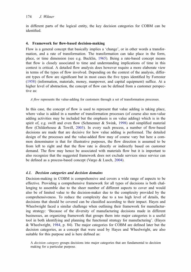
4.1. Decision categories and decision domains

Decision-making in COBM is comprehensive and covers a wide range of aspects to beeffective. Providing a comprehensive framework for all types of decisions is both chal-lenging to assemble due to the sheer number of different aspects to cover and wouldalso be of limited value to the decision-maker due to the complexity provided by thecomprehensiveness. To reduce the complexity due to a too high level of details, thedecisions that should be covered can be classified according to their impact. Hayes andWheelwright faced a similar challenge when outlining their framework for manufactur-ing strategy: ‘Because of the diversity of manufacturing decisions made in differentbusinesses, an organizing framework that groups them into major categories is a usefultool in both identifying and planning the functional strategy for manufacturing’. (Hayes& Wheelwright, 1984, p. 84). The major categories for COBM are defined later but thedecision categories, as a concept that were used by Hayes and Wheelwright, are alsosuitable for this purpose and is here defined as:

A decision category groups decisions into major categories that are fundamental to decisionmaking for a particular purpose.

174 J. Wikner

The scope of a decision category (DC) is based on some fundamental aspect of deci-sion-making, which is here referred to as a decision criterion. Thus, decision categoriesare a way of classifying decisions and the decision criterion is what the classification isbased on:

A decision criterion is a standard on which a decision may be based.

To manage an enterprise involves making numerous decisions of different character butall related to transformation processes. Some decisions are of more simple character anddo not affect the flow to a large extent while others are of decisive importance to theperformance of the process, such as initiating a process or not. Effective process man-agement therefore requires that the critical decisions can be isolated and classified toenable the design and application of a management framework with decision categories.These categories should then be applicable on a wide spectrum of processes with similarpreconditions. In support of this classification of processes, the concept of decisiondomain is introduced:

A decision domain is characterized by consistent preconditions for decision making relatedto a specific decision criterion.

A decision domain thus identifies what is common to a number of processes from adecision perspective and can hence be perceived as sub-categories within a DC (Wheel-wright, 1984). A decision domain might, for example, define that the processes relatedto a decision domain are performed based on that a customer order has been receivedand hence that the process can be classified as customer-order-driven. This decisiondomain would then belong to the DC ‘flow driving’ and be based on the decision crite-rion ‘flow driver’ with the property ‘driven by customer order’ (see e.g. Figure 20 foran overview of decision categories). From this perspective, it would be reasonable toillustrate a decision domain as if the processes are within a decision domain. But forpractical reasons, this relation is illustrated with a decision domain whose extensionalong the flow determines the processes associated with a particular decision domain, asshown in Figure 3. This means that the processes U1 and U2 in Figure 3 are classifiedas belonging to Upstream decision domain (from a flow perspective) and processes D1and D2 as belonging to Downstream decision domain.

Figure 3. Relation between processes, resources and decision domains.

Production & Manufacturing Research: An Open Access Journal 175

Resources that perform processes have a relation to decision domains that follow adifferent pattern compared to processes. Since a resource can perform more than oneprocess, it can also be related to more than one decision domain. Resource R1 inFigure 3 is, for example, related to both process U1 and process D2. Process U1 maybe forecast-driven and process D2 customer-order-driven wherefore they are classifieddifferently in terms of the DC flow driving. But, since both these processes areperformed by the same resource, the capacity of the resource is required by both fore-cast-driven and customer-order-driven processes. As Figure 3 shows, a decision domainis here illustrated by a rectangle with rounded corners and with black text on grey back-ground. Processes are depicted with traditional arrows, resources with rectangles withrounded corners and white text on dark background.

4.2. Decision domains and decoupling points

The analysis above defines decision domains as a collecting concept for processes witha specific property in common. The decision domains can be relatively independent ofeach other in the sense that they can be based on different decision criteria that high-lights different process perspectives, such as focusing on credit risk or representing dis-assembly decisions. From a flow perspective, it is of particular interest to focus ondecision criteria that separates the flow into two separate parts. A specific example ofthis is processes that are customer-order-driven and processes that are forecast-driven.For the DC flow driving, these processes are completely different but still they are con-nected to the same decision criterion, i.e. what decides that a process is initiated. Froma flow perspective these two decision domains can be seen as being in a sequence inthe flow and characterized as one upstream decision domain and one downstream deci-sion domain that from a decision perspective are disconnected from each other.

The decision criterion is decisive for the type of property that can be classified aseither upstream or downstream. To emphasize this difference, a decoupling point isintroduced that indicates that the decoupled decision domains are related to the samedecision criterion:

A decoupling point separates decisions that are made under different consistent propertiesrelated to a specific decision criterion.

The decision domains are disjunctive in the sense that they represent completely differ-ent properties, such as forecast-driven or customer-order-driven, considering the samedecision criterion. This relation is depicted in Figure 4 where a general decoupling pointis illustrated with an ellipse which symbolically connects the two decision domains ofthe DC.

Figure 4. Decision domains with disjunctive properties.

176 J. Wikner

However, in many cases, the decision support is not homogenous and based on onlyone property at each side of the decoupling point. In some cases, the transition is notinstantaneous along the flow, i.e. an upstream property is not changed to a downstreamproperty at one point, but rather can be seen as a gradual transition consisting of a mixof properties from each side of the decoupling point of Figure 4. A process driver may,for example, be a combination of forecast and customer order. This type of mixed prop-erties is here associated with a hybrid decision domain, see Figure 5. It is then logicalto model this as three decision domains and consequently two decoupling points foreach DC.

Hybrid decision domains represent more complex decision-making where the crite-rion has mixed properties. In some cases, it can be an advantage to use both decouplingpoints but this approach also increases the complexity. An alternative is to emphasizeonly one decoupling point and this is a useful approach when the decision criterion isintrinsically linked to one of the decision domains. A typical example is the flow drivercriterion of COBM, which is customer focused and hence the logical place to decoupleis upstream of the customer-order-driven decision domain. This domain is customerfocused, whereas the other decision domains also have other properties. Since the focusbelow is on COBM, only decoupling point 1 will be considered and below simply bedenoted ‘decoupling point’. The mixed properties that the hybrid decision domain relateto represent, from a flow perspective, a transition from the properties valid upstream tothe properties valid downstream of the hybrid decision domain. This transition with ahybrid decision domain can be seen as a zone that decouples the two single-propertydecision domains.

Decoupling points by definition mean, as described above, that different precondi-tions exist upstream and downstream from the decoupling point. From a material flowperspective, this type of discontinuity corresponds to that the preconditions for the flowchanges significantly which leads to disturbances of the flow. Different kinds of buffersare used to reduce the impact of these disturbances. Capacity buffers, related toresources, offer interesting possibilities since they increase the capability to be agile inprocesses performed to, e.g. customer order or backorders at stock points. A drawbackwith capacity buffers is however that they do not provide instant reaction but requires alead-time before a result can be delivered (since the capacity is used to perform somekind of transformation which takes time). The material buffers do not have this draw-back since they provide immediate availability of what is demanded even if this type ofbuffer provides less flexibility since decisions, about what to include in the material buf-fer, are made before the requirement is identified. In this way, the material buffer is amore lead-time responsive type of buffer that is suitable in relation to decoupling points.The capacity buffer does, however, provide important support downstream from the

Figure 5. Decision domains and strategic decoupling points.

Production & Manufacturing Research: An Open Access Journal 177

decoupling point as it enables the resources to be more flexible. The material buffer ishere referred as a stock point and later illustrated in the figures by a black trianglepointing downwards representing physical inventory in the flow.

The significance of so-called discontinuities can be reduced, or even eliminated, byintroducing decoupling zones that enable a softer transition from the conditions at theupstream decision domain to the conditions at the downstream decision domain. If dis-continuities are completely eliminated, there is also no need for a corresponding bufferat a stock point.

4.3. Decision domains and decoupling zones

Decoupling points are positioned at an instantaneous transition along the flow fromupstream property to downstream property. This represents a ‘black or white’ scenariowhich in some cases is too simplistic. The transition may be gradual and hence repre-sents a zone with different ‘shades of grey’ related to the hybrid decision domain asdescribed above.

A decoupling zone covers decisions that are made under mixed properties related to one ormore decision criteria.

There are mainly two different perspectives that require these ‘shades of grey’. The firstperspective is the gradual transition from upstream property to downstream property andit is here called process-based decoupling zone since it exists along one individual flowand corresponds to one single decision domain. The other perspective exists when mul-tiple flows are considered in parallel, from an aggregate perspective, and is in particularrelated to when one resource is involved across multiple flows at the same time. Thisscenario has its roots in how resources are positioned in relation to decision domains inFigure 3 and is therefore here referred to as resource-based decoupling zone that corre-sponds to an aggregation of two or more different decision domains.

4.3.1. Process-based decoupling zones

The concept decoupling zone refers to a mix of different properties related to decisiondomains. In case there is a gradual transition along a flow, a number of attributes relatedto the property can be affected. The properties can, for example, be associated withuncertainty or certainty concerning customer orders. The certainty can however be basedon different types of attributes related to the customer order such as requested deliverydate or requested quantity. When deciding on the number of attributes to use, a balancebetween the complexity of using many attributes and not challenging the relevance ofthe attributes, by using too few, must be established. In this framework for COBM, twoattributes are used for each DC related to a process-based decoupling zone, but from amore general perspective, one or more than two attributes can also be used.

A process-based decoupling zone is based on the gradual transition between two propertiesof one decision criterion related to one flow.

The process-based decoupling zone (PB-DZ) is in Figure 6 illustrated by a rectangleplaced above the hybrid decision domain. The zone is expanded to a two-dimensionalsurface that represents two attributes that each can take values on a scale from upstream

178 J. Wikner

to downstream property. The end-points (the corners) where the attributes have the same‘value’ represent the limit of upstream and downstream decision domain, respectively.Based on the definition of decision domain and how it is related to processes means thatthere are now, at least, three types of processes along the flow; in Figure 6, this is illus-trated with the processes U1, H1 and N1. At the beginning of the flow (on the left inthe figure), the upstream property is of relevance to decisions. When the flow reachesthe PB-DZ, the decision preconditions correspond to the lower left corner of the two-dimensional surface. The flow through the PB-DZ corresponds to that the preconditionschange as the value of the two different attributes changes along a trajectory from thelower left corner to the upper right corner of the surface, i.e. when the decoupling pointis reached. Thereafter, the downstream property is relevant for decision-making until theend of the flow is reached.

4.3.2. Resource-based decoupling zones

From a resource perspective, it looks different compared to the process perspective sinceresources can be connected to multiple decision domains with different properties asshown in Figure 3. This multi-property load on a resource is related to resource-baseddecoupling zones.

A resource-based decoupling zone is based on the intersection between different propertiesof one decision criteria across one or more flows.

In Figure 7, this is illustrated with the two flows, Flow A and Flow B, where each con-sists of two processes related to one upstream and one downstream decision domain,respectively, and thus has one decoupling point each. One individual flow is thereforerelatively simple from a process perspective with two basic decision domains both based

Figure 6. Process-based decoupling zone along one flow.

Production & Manufacturing Research: An Open Access Journal 179

on the decision criterion in question. In Figure 7, one resource is identified and fromthe resource’s perspective, the situation is more complex since it is involved in processDA and process UB, i.e. two processes that are related to different decision domainswith different properties. This type of scenario is here referred to as a resource-baseddecoupling zone (RB-DZ) and could, for example, mean that some of the load on theresource is forecast-driven (based on UB) and some is customer-order-driven (based onDA). This means that the load analysis becomes considerably more complex comparedto when only UA and UB or only DA and DB are involved, where the preconditionswould be more homogenous what concerns the actual DC. Note that the assumption isthat the same decision criterion is in focus for all processes, i.e. they belong to the sameDC. In addition, the individual flows may not contain a process-based decoupling zonebut in aggregation a resource-based decoupling zone can be identified. In case thedecoupling points of the individual flows are positioned at the same place also, theaggregate would not contain a decoupling zone and the decoupling point could bereferred to as a ‘resource-based decoupling point’.

The aggregation discussed above is across multiple flows. The corresponding situa-tion can occur in the case of aggregation in time where, for example, weeks are used astime periods rather than days. With a resolution of days, a more detailed analysis can beperformed resulting in that resources are either loaded with forecast-driven or customer-order-driven activities. Using the aggregation level of weeks on the other hand mightresult in a mix of different types of load for a particular resource since the timing ofload cannot be determined as exactly as in the case of time periods based on days. Also,resource aggregation may create a similar problem as individual resources are notloaded, but instead groups of resources are loaded. Hence aggregation in terms of flows(i.e. products), time, or resources can generate similar challenges from a capacityrequirement perspective.

In summary, the capacity requirement for a resource may be created by seven differ-ent combinations of processes related to three different decision domains of one singledecision criterion. Note that Figure 7 is based on that each flow consists of two decisiondomains whereas Table 1 is based on the existence of also a hybrid decision domain,i.e. PB-DZ. In Table 1, these combinations are illustrated and the first three cases (type1–3) in the table are based on one decision domain each with capacity requirement from

Figure 7. Resource-based decoupling zone across multiple flows.

180 J. Wikner

the respective decision domain. Three of the combinations originate in the combinationof two types of decision domains. Capacity requirement type 7, finally, is based on threedifferent types of decision domains, i.e. one resource would be used in processes ofthree different decision domains. The example of Figure 7 can, based on this, beclassified as a resource with capacity requirement type 5 since the capacity requirementsoriginate from a upstream DD and a downstream DD.

For both the PB-DZ and the RB-DZ, the ‘length’ of each decision domain is impor-tant since it determines the position of both decoupling point and decoupling zone. Thedecision domain is based on one decision criterion; for example, flow driver, whichmeans that the length of the decision domain and the priority of the chosen decision cri-terion are different sides of the same coin. The definition of important decision catego-ries for COBM can therefore be based on the identification of important lead-times.

4.4. Positioning of decoupling point and decoupling zone

The extension of decision domains have so far been based on a relative perspective. Adecoupling point has been identified that separates the flow into two distinct partsrelated to one decision domain each. In addition, a hybrid decision domain may be posi-tioned between these two decision domains resulting in a sequence of three decisiondomains along the flow. Identifying the decision domains is a first step but it is alsoimportant to determine the actual extension of each decision domain and as a conse-quence also the position of the decoupling point and the decoupling zone.

A useful measure for the extension would operationalize the concepts introduced sofar. A number of candidates exist for acting as a point of reference such as the physicalextension of the flow, organizational properties such as functions involved, or costaspects related to e.g. resource ownership. It is however important to have a baselinethat is absolute in the sense that it is not something that can easily be manipulated tosuit different purposes. It should rather be something that can act as a point of referencethat is important and transparent to all concerned interest parties. Considering the his-tory of operations and supply chain management, a number of cases have shown thatthe key resource to manage is time as time lost can never be recovered. In addition,time has also been shown to be a key driver of competitiveness. Henry Ford was one ofthe first to explicitly highlight time as one of the pillars of his management philosophy(Ford & Crowther, 1988) and time has continued to play a key role in, e.g. Time-basedmanagement (Stalk & Hout, 1990), BPR (Hammer & Champy, 1993) and lean thinking(Womack & Jones, 1996). Presently, the main proponent of time as a key resource isprobably lean in all its flavours such as lean thinking, lean production, lean services,lean administration, etc. At the core of all these, lean ‘flavours’ is the continuous

Table 1. The seven different types of capacity requirement.

Upstream DD Hybrid DD Downstream DD

Capacity requirements type 1 XCapacity requirements type 2 XCapacity requirements type 3 XCapacity requirements type 4 X XCapacity requirements type 5 X XCapacity requirements type 6 X XCapacity requirements type 7 X X X

Production & Manufacturing Research: An Open Access Journal 181

improvement to reduce waste, and waste is basically different incarnations of lost time.For example value stream mapping (Rother & Shook, 1998), the most highlighted partof the analysis is the timeline capturing the total lead-time as well as the value addingand non-value adding time. From a time perspective, the timeline positions the differentparts of the value stream in relation to the customer, i.e. the end-point of the valuestream.

The decision criterion and the related decision domains provide a conceptual divi-sion of the flow from a decision perspective. The decision in itself and what it involvesare important to define the decision situation, but the timing of the decision is absolutelycritical in defining the preconditions for the decision-maker. The timing is defined inrelation to when the result of the sub-flow, corresponding to the decision domain, isrequired. With this as a point of departure, three lead-times can be defined as ofFigure 8, related to one decision domain each: upstream (US), hybrid (H), and down-stream (DS). Accumulating these lead-times the total lead-time for the flow i (Fi) isobtained, where: FLTi = USLTi + HLTi + DSLTi. The decoupling zone highlighted here isrelated to a decision domain and hence of type PB-DZ. The RB-DZ can be positionedin a similar way based on that the decoupling zone is related to an intersection of a setof flows. DSLT would in this case correspond to DSLT ¼ min

i2FlowsfDSLTig where Flows

is the set of all flows where the resource is involved. In a corresponding way the lead-time of the RB-DZ can be defined as: HLT ¼ max

i2FlowsfHLTi þ DSLTig � DSLT. USLT

can then finally be defined as: USLT ¼ maxi2Flows

fFLTig � HLT� DSLT.

Based on the argument earlier, where the second decoupling point was consideredas of less interest, the decoupling point upstream of the hybrid decision domain is notanalysed further. The positioning of the decoupling point is hence based on the lead-time of the downstream decision domain, DSLT, in relation to a reference lead-timesuch as the total flow lead-time, FLT. The position of the decoupling point can hence beexpressed in two different ways:

� The lead-time DSLT, which is useful in e.g. analysis based on the time-phasedbill-of-material to calculate the position of the decoupling point. This is the ‘abso-lute’ lead-time expressed in suitable time units.

� The ‘relative’ lead-time results in a percentage and expresses how long a lead-timeis in relation to a ‘benchmark’ lead-time and in particular we are interested in thefraction of the benchmark lead-time that is related to downstream property. For posi-tioning of the decoupling point the key lead-time is the relation between the lead-times DSLT and FLT, which is called the DSLT:FLT relation. If DSLT:FLT = 1 thenthe decoupling point is at the beginning of the flow. If DSLT:FLT << 1

Figure 8. Decision domains and lead-times.

182 J. Wikner

(or DSLT:FLT = 0) then the decoupling point is at the end of the flow and finally ifDSLT:FLT < 1 the decoupling point is positioned within the flow.

The ‘relative’ lead-time is measured in relation to a reference value and is thus of morepractical use in COBM. From a general perspective it can be defined as:

A lead-time relation is a ratio of two strategic lead-times.

Positioning of the decoupling point also provides information about the extension of theupstream and the downstream decision domains in case there is no hybrid decisiondomain. If also a hybrid decision domain is present additional lead-time analysis isrequired to position also this decision domain. This additional analysis can be based oneither USLT or HLT. Once the decoupling point and decoupling zones are positioned,the different decision categories can be combined resulting in compounded decisiondomains.

4.5. Compounded decision domains

In an actual decision situation, multiple decision criteria may be important to considerat the same time. Still each decision criterion can be defined separately as in Figure 9where this is illustrated on the left side with decision criteria 1 and 2. In most cases, thedifferent decision criteria are independent of each other and capturing different aspectsof the challenges facing the decision-maker. Therefore the two decision criteria may bemodelled as two separate dimensions as shown on the right of Figure 9. The resultingfour decision domains are referred to as compounded decision domains (CDD):

A compounded decision domain covers the intersection of two decision domains related totwo separate decision criteria.

Each CDD is a combination of upstream (U) and/or downstream (D) decision domainsbased on decision criteria 1 or 2. For example, D1, D2 is a CDD where the decision cri-terion is a combination of decision criteria D1 and D2. Depending on the actual deci-sion criteria used some of the combinations might not be possible, or at least notcompetitive, and hence a strategy for that CDD might not be necessary. However, froma generic point of view all CDDs are assumed to be valid and hence all possible CDDsare included.

Figure 9. Example of compounded decision domains.

Production & Manufacturing Research: An Open Access Journal 183

The CDDs add complexity since they introduce a multi-dimensional perspective ondecision domains. The example in Figure 9 is based on two flows with decouplingpoints only. By also including decoupling zones there are some more challenging issuesto consider.

4.5.1. Compounded decision domains and process-based decoupling zones

The concept of CDD can easily be expanded to also include hybrid decision domainsand PB-DZs. The example of Figure 9 represents the possible combinations when nohybrid decision domains are included. By allowing hybrid decision domains eachdimension would be extended to three blocks and in total nine CDDs would be includedon the right in Figure 9. This scenario, with nine CDDs, is somewhat similar to theanalysis of the resource-based decoupling zone of Table 1 (with seven possible combi-nations). It is however important to note that in this case the two dimensions are basedon different criteria whereas in Table 1 the two dimensions were based on the same cri-terion. Since the CDD here is based on two criteria the type 7 case cannot occur andthe criteria are different for types 4–6 which means that it would result in another threetypes (for example, U1, D2 does not correspond to D1,U2 when different criteria areused). In summary there would be four CDDs only involving upstream and downstreamdecision domains and an additional five that include at least one hybrid decisiondomain. This would result in three decision domains in each dimension of Figure 9 and,consequently, in total nine different CDDs (cf. Figure 16 for an example).

4.5.2. Compounded decision domains and resource-based decoupling zones

The CDDs creates additional complexity in terms of RB-DZs since the number ofpossible combinations increases significantly. The example of Figure 7 resulted in oneadditional scenario (totally three) compared to when one flow was analysed. Thenumber of possible combinations of decision domains, CðNumber of flows;Number of decision domains per flowÞ affecting a resource when each flow can bedivided into n different decision domains is a combinatorial problem. For the case inFigure 7, which is based on that the decision domains belong to the same DC, thenumber of combinations would be: COneDCð2; 2Þ ¼ 2þ 1 ¼ 3 different combinations ofdecision domains. In case each flow would contain a hybrid decision domain the num-ber of combinations would be: COneDCð2; 3Þ ¼ 3þ 3þ 1 ¼ 7 different combinations (asshown in Table 1). When the CDDs are introduced the possible combinations for aresource to be involved in more than one decision domain increases dramatically forRB-DZs. Consider, for example, the case introduced above in Figure 9 with two dimen-sions and two decision domains in each dimension resulting in a total of four CDDs.One case could be that a resource is acting in the CDD U1, U2 for one flow and theCDD D1, D2 in the other flow. By definition the RB-DZ is related to when a resourceis involved in two CDDs of different properties which means that if a resource isinvolved in CDD U1, U2 of two different flows it is not defined as a RB-DZ. For thiscase with two flows with four CDDs each there are a total of CTwoDCsð2; 4Þ ¼ 12 possi-ble combinations. Introducing PB-DZs in each flow of course increases the complexityfurther and the number of combinations fast becomes hard to manage. It is thereforeimportant to identify the critical intersections and to exclude the less important from theanalysis.

184 J. Wikner

4.6. Summary of framework for flow based decision-making

The generic framework for decoupling points and decoupling zones provides the meansfor identifying some key decision categories related to supply chain and operations man-agement. In summary, the generic framework for flow based decision-making containsten key concepts (which have been explicitly defined above):

(1) Logical entities are the platform for decisions on flow based management.(2) Flow provides the point of reference for identifying lead-time based decision

categories.(3) Decision categories are defined based on decision criteria.(4) Decision criteria are used to define decision domains within a decision

category.(5) Decision domains for the same decision criteria are separated by decoupling

points.(6) Decoupling points are positioned at the interface between two decision

domains.(7) Decoupling zones correspond to mixed properties in a decoupling point sce-

nario.(8) Process-based or resource-based perspective can be applied on decoupling

zones.(9) Lead-time relations position decoupling points/zones and decision domains.(10) Compounded decision domains reflect the complexity of an actual decision

problem.

The generic framework with these ten key concepts is next used to define threelead-time relations and thereafter four decision categories for COBM.

5. Lead-time based flow analysis

Lead-time analysis is used in different contexts to e.g. reduce lead-times, identify wastesor simply to identify the magnitude of the lead-times. This type of lead-time analysiscan be categorized as ‘absolute’ lead-time analysis since focus is on the length of thelead-times. It is however ‘relative’ lead-time analysis that is of main interest as an indi-cator of positioning of decoupling points and decoupling zones since it involves therelation between different lead-times. Before these lead-time relations can be defined itis necessary to identify the key ‘strategic’ lead-times.

5.1. Lead-time definitions

Balancing the requirements and availability of material and capacity of operations areimportant challenges in logistics flow. Common to these challenges is that timing is ofcritical importance. The relationship between available capacity and capacity require-ments should be investigated with respect to a timeline and also the balancing ofdemand and supply of materials requires a time-phased approach (however less signifi-cant in a rate-based context). The comprehension of lead-times and how they should bemanaged is therefore of utmost importance to enterprise management.

The standard item lead-times (L) are fundamental, but even more important from acompetitiveness perspective are the five strategic lead-times (Wikner, 2011). From a

Production & Manufacturing Research: An Open Access Journal 185

supply perspective the cumulative lead-time (Blackstone, 2008) is critical since it repre-sents the lead-time of the product including all items. The cumulative lead-time is thensplit in two parts representing items provided by the logical entity in focus (internallead-time) and items provided by the upstream logical entities (external lead-time).Another key aspect is the level of possible customization involved and this is herereferred to as adapt from a supply perspective. Customization is based on customerrequirements and adapt may hence also be seen as based on customer requirements froma demand perspective. Finally, a key aspect from a customer perspective is also therequested delivery lead-time as it also frequently defines a key characteristic of the orderwinners.

Five strategic lead-times (referred to as SEIAD based on their variable names) areinvestigated here and further elaborated on below:

� Supply lead-time (S) is the cumulative lead-time for the product through thewhole (extended) logical entity.

� External lead-time (E) can in many cases be seen as related to the (purchased)component and is therefore usually associated with purchase orders.

� Internal lead-time (I) corresponds to the controllable part of the bill-of-materialand is usually associated with the own provisioning lead-time.

� Adapt lead-time (A) is related to the customer order but based on when the supplyperformed is actually customer order unique. The possible level of customizationis related to a supply perspective (AS) and the requested level of customization isrelated to a demand perspective (AD). This lead-time could also be referred to asthe customization lead-time but to avoid confusion with different types of custom-ization strategies the more neutral term adapt is used. The adapt lead-time isimportant in e.g. the context of mass customization but it is also a key componentin other cases such as e.g. postponement strategies.

� Delivery lead-time (D) is based on market requirements for delivery and directlyassociated with demand/customer order.

5.2. Example: lead-times and time-phasing

The different types of lead-times defined above are related to each other and a simpleexample is introduced as an illustration of the theory. Some of the concepts introducedhere have also been applied on actual cases (Bäckstrand et al., 2013) but in general,actual bill-of-material that can be used as an illustration of several concepts are rathercomplex. The sheer complexity of the bill-of-material in these cases and their area ofapplication diverge the focus from the illustration of the concepts. The example intro-duced below is therefore fictitious and designed to be simple but still sufficient to illus-trate the key concepts used here. The example is shown in Figure 10 in terms of atraditional material based bill-of-material (product structure) to the left and a time-phased bill-of-material to the right (see e.g. Bäckstrand & Wikner, 2013; Clark, 1979;Wikner & Rudberg, 2005b). The material based bill-of-material includes where-usedrelations and lead-times. For example, item Y consists of item X and item U, and item Yhas a lead-time (LY) of 3 periods. On the right in Figure 10 this bill-of-material isinstead represented by a time-phased bill-of-material where the horizontal distancebetween two filled circles corresponds to each item’s lead-time (L). In this case thesupply lead-time S = 12 periods (the cumulative lead-time for the bill-of-material) and

186 J. Wikner

the delivery lead-time to the customer is given as D = 6 periods. (The estimation of thedelivery lead-time D will be more elaborated on later, see e.g. Figure 18). Since it is theadaptation of Z that constitutes a customer order unique solution, the demand adaptslead-time AD = 2 periods and Y is customer unique. From an engineering and productionperspective it would be possible to also make item U customer order unique whichmeans that the supply adapt lead-time AS,U = 9 periods. The items V and Q, finally, arepurchased in a traditional way from suppliers. These two items represent the end of twobranches with an external lead-time (E). An internal lead-time (I) can then be calculatedfor each branch of the bill-of-material. The set Leafs is assumed to contain all N itemsthat are at the lowest level of each branch and would in many cases correspond topurchase items. In the example of Figure 10 it would mean that N ¼ 2 andLeaf ¼ fV ;Qg. For the branch of item V the cumulative lead-time isSV ¼ EV þ IV ¼ 2þ 8 and for item Q the cumulative lead-time isSQ ¼ EQ þ IQ ¼ 3þ 9. The branch with the longest cumulative lead-time is also equalto the supply lead-time S ¼ max

n2LeaffSn ¼ En þ Ing. A more elaborate analysis can also be

performed where a S is defined for each item in the bill-of-material (Bäckstrand &Wikner, 2013). This approach provides the opportunity to identify for each item if it iswithin D and can be customer-order-driven, or if it is longer than D and must beforecast-driven.

5.3. Lead-time context

If only one branch of the product structure in Figure 10 is considered, a network with-out different branches is obtained and this can be labelled as a ‘linear’ chain. Using theterminology introduced above the chain may be referred to as consisting of two logicalentities, one focal entity (‘focal’ refers to the unit that is in focus for the analysis) andone supplying entity, i.e. two logical entities in sequence and with an implicit entity rep-resented by a customer. The context of this analysis is therefore a triad consisting of acustomer entity and two logical entities representing the supply. Each one of the logicalentities can be illustrated with the entity’s strategic lead-times SEIAD resulting in

Figure 10. Example: Material-based and lead-time-based bill-of-materials.

Production & Manufacturing Research: An Open Access Journal 187

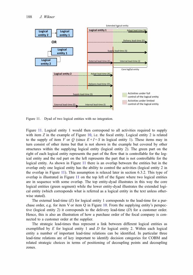
Figure 11. Logical entity 1 would then correspond to all activities required to supplywith item Z in the example of Figure 10, i.e. the focal entity. Logical entity 2 is relatedto the supply of item V or Q (since E + I = S in logical entity 1). These items may inturn consist of other items but that is not shown in the example but covered by otherstructures within the supplying logical entity (logical entity 2). The green part on theright of each logical entity represents the part of the flow that is controllable for the log-ical entity and the red part on the left represents the part that is not controllable for thelogical entity. As shown in Figure 11 there is an overlap between the entities but in theoverlap only one logical entity has the ability to control the activities (logical entity 2 inthe overlap in Figure 11). This assumption is relaxed later in section 6.3.2. This type ofoverlap is illustrated in Figure 11 on the top left of the figure where two logical entitiesare in sequence with some overlap. The top entity-dyad illustrates in this way the corelogical entities (green segment) while the lower entity-dyad illustrates the extended logi-cal entity (which corresponds what is referred as a logical entity in the text unless other-wise stated).

The external lead-time (E) for logical entity 1 corresponds to the lead-time for a pur-chase order, e.g. for item V or item Q in Figure 10. From the supplying entity’s perspec-tive (logical entity 2) it corresponds to the delivery lead-time (D) for a customer order.Hence, this is also an illustration of how a purchase order of the focal company is con-nected to a customer order at the supplier.

The strategic lead-times thus represent a link between different logical entities asexemplified by E for logical entity 1 and D for logical entity 2. Within each logicalentity a number of important lead-time relations can be identified. In particular threelead-time relations are of key important to identify decision categories for COBM andrelated strategic choices in terms of positioning of decoupling points and decouplingzones.

Figure 11. Dyad of two logical entities with no integration.

188 J. Wikner

5.4. Lead-time relations

Five different strategic lead-times were identified above and referred to as SEIAD. Intotal 20 different lead-time relations, between two different lead-times, can be identifiedbased on SEIAD as shown in Table 2 (based on Bäckstrand, 2012) (excluding the rela-tion between lead-times of the same type, i.e. the diagonal of Table 2). There are someoverlaps between these lead-times when a supply network is investigated since thedelivery lead-time D for a supplier corresponds to the external lead-time E for that itemat the customer. Note, however, that the analysis performed here is based on one logicalentity. Since the focus here is on COBM the emphasis is on customer facing lead-times(see Figure 11), i.e. A, D, S, and I (lead-time relations related to E are therefore indi-cated with n/a in Table 2 and since S = E + I, the E-based relations may be derivedbased on I-based relations if necessary). The lead-time relations above the diagonal arethe inverse of the lead-time relations below the diagonal and only one relation of each‘pair’ is included. As a general rule the relation where we normally would expect thesmaller value in the numerator is included and the other is indicated by a ‘×’ in Table 2.In total there are hence six potential lead-time relations left to investigate: D:S, A:D, I:S,A:I, A:S, and D:I.

In a lead-time relation one lead-time is used as a point of reference and the relationthen shows how long the other lead-time is in relation to the reference lead-time. Thelead-time relations further investigated are mainly related to D since the delivery lead-timeD is the fundamental lead-time from customers’ perspective. Note that the I:S relation andthe I:A-relation are multiple relations since there are N pieces of I lead-times (one for eachbranch of the bill-of-material) and hence also N pieces of I:S relations. In case of the A:Irelations it is even more complex since there may also be multiple A lead-times, and inaddition A may be supply based or demand based. The A:I relation could be of some inter-est as it can be used to analyse if customization affects more than the focal entity. Thisinformation is, however, implicitly provided by the I:S-relation in combination with theA:D-relation when the compounded decision domains are introduced. In a similar fashionthe A:S relation represents how customization affects supply but it is less exact comparedto the A:I-relation and is hence not included. The D:I relation, finally, could provide someinteresting information on if customer-order-driven flow impacts suppliers but this infor-mation can also be obtained from compounded decision domains which are describedlater. The three remaining lead-time relations are of key importance to identify importantdecision categories for COBM and they are highlighted in Table 2 as bold and italic. As aresult there are three lead-time relations that connects the two aspects of supply (I and S),the two aspects of demand (A and D, in particular if AD is assumed), and finally the keylink between supply and demand (D and S).

Table 2. Lead-time relations.

Production & Manufacturing Research: An Open Access Journal 189

5.4.1. D:S-relation

The fundamental lead-time relation is based on the delivery lead-time (D) in relation tothe supply lead-time (S). If the customers can accept to wait longer than it takes thesupplier to provide the product it becomes possible to perform all provisioning activitiesat the request of a customer. If, on the other hand, the customer cannot accept to waitthe time it takes to perform the activities at least some of these activities must be per-formed on speculation about future customer orders. This lead-time relation has receivedrelatively large attention in both practical application and literature (Shingo, 1989) (orig-inally published in Japanese in 1981) and is usually seen as the earliest reference on thiseven if Shingo used the denotation ‘relation of D:P’. This relation was introduced to abroader audience by Mather (1984) who observed the potential of this concept. Matherdid however note that D:P could be mixed up with DP, which at that time was widelyused as an acronym for ‘data processing’. To reduce the risk for this confusion he sug-gested that it would be better to call it the P:D relation (or P:D ratio as Mather calledit). Unfortunately the numerical result of the P:D relation does not provide an intuitivesense of how large part of P that is customer-order-driven. Due to this the original rela-tion D:P, as defined by Shingo, is used here as a point of departure.

Initially (Shingo, 1989) referred to P as the product lead-time but it has also beenassociated with production lead-time. Today supply is used as a terminology for alltypes of activities related to the provisioning of goods and hence S is here used insteadof P. Both Shingo (1989) and Mather (1984) used D as an abbreviation for deliverylead-time and this is also used here. Note that D implies that activities within D may beperformed to customer order. It is, however, not a requirement but should be seen as an‘option’ to provide to customer order. If the products are standardized and delivered fre-quently the activities may also be performed on speculation with reasonable risk taking.This option is sometimes not fully used by for instance production engineering reasonswhere it is suitable to produce a quantity that deviates from an individual customerorder. Some standard examples of the D:S-relation are:

� D << S: Basically all activities must be performed on speculation (corresponds tothe strategy Make-to-Stock, MTS).

� D < S: Some activities are performed on speculation (corresponds to the strategyAssemble-to-Order, ATO).

� D ≈ S: All activities can be performed on commitment (corresponds to the strategyMake-to-Order, MTO, Purchase-and-Make-to-Order, PMTO, or Engineer-to-Order,ETO, depending on if engineering activities are included or not).

5.4.2. A:D-relation

The relation between adapt lead-time (A) and delivery lead-time (D) is relating twoaspects of demand to each other. The distinction made here is based on how large partof D that is actually related to a part of the lead-time that is customer order unique, A.This relation highlights that even if the flow is customer-order-driven it is not necessar-ily also tailor made for that particular customer. The D:S relation shows what is cus-tomer-order-driven and therefore also that there is an ‘option’ for providing somethingcustomer order unique. A more detailed approach could also, as mentioned earlier, dif-ferentiate if A is what is actually possible from a supply perspective (AS) or if A isrelated to what is required by the customer (AD) (Bäckstrand & Wikner, 2013). From a

190 J. Wikner

supply perspective the different branches of the bill-of-material may provide differentopportunities for customization and hence As should also be defined for each and everybranch of the bill-of-material. In summary AD represent the market requirements and As

the opportunities available from a supply perspective. Hence the difference correspondsto the options available for responding to new market requirements due to e.g. increas-ing competition. In this context A is however assumed to represent the customers’requirements. The A:D relation shows to what extent the provider has decided to exer-cise the ‘option’ to provide something customer unique:

� A <<D: Basically all activities are standardized.� A =D: Customer-order-driven activities are also customized.� A >D: Some forecast-driven activities are customer order adapted (a high risk

strategy that usually should be avoided).

The connection between customer adaptation and customer-order-driven flow hasmany facets covering e.g. that it is not necessary for a product to first be completelyengineered and then produced. It may also involve, for example, engineering adaptationswhere some semi-finished goods are in stock when engineering adaptations are made.This can be described as a two dimensional problem where engineering and productionactivities can be combined in different ways (Wikner & Rudberg, 2005a).

5.4.3. I:S-relation

In contrast to the D:S and A:D relation, which are based on demand, the I:S relation iscompletely based on the supply side. The internal lead-time (I) represents the lead-timeperformed within control of the focal logical entity and the supply lead-time (S) repre-sents the cumulative lead-time of the system in question. In the case of traditional rela-tions to the suppliers, where integration is low and purchase order and customer orderare the foundation for cooperation, this means that if I is much smaller than S, basicallyall activities within S are performed by suppliers upstream in the flow. But, the supplierplays a less important role in the supply chain in case the total lead-time S is short andI therefore relatively long. Also here three cases are of particular interest and note thatin this case there is a lead-time relation for each ‘branch’, cf. Figure 10:

� Ik = Sk: Basically all activities of the k-branch are performed by the core logicalsystem.

� Ik < Sk: Some activities of the k-branch are outsourced to a supplier.� Ik << Sk: Basically all activities of the k-branch are outsourced to a supplier (the

extended logical entity).

Based on the three lead-time relations defined above it is possible to define andposition three decoupling points and three process-based decoupling zones that consti-tute three decision categories and thus also the core of the flow based framework forCOBM.

5.5. Example: Lead-time relations

Going back to the example of Figure 10 a set of lead-time relations can be calculatedand used to classify both the whole product and the individual items. In this case the

Production & Manufacturing Research: An Open Access Journal 191

D:S relation is analysed and in particular the item based D:S relations are analysed. Theindented bill-of-material of Table 3, based on Figure 10, includes the item based D:Srelations in the rightmost column. Sk is calculated for each item based on the cumulativelead-time for that particular item. For item X the cumulative lead-time SX = 2 + 3 + 1 = 6periods which is the same as the delivery lead-time according to Figure 10 (D=6).Consequently the item based D:Sk relation is one which means that item X can beproduced based on customer order.

According to the introduction of the example, item Z is customer order unique andY is customer unique. Both of these items are within the delivery lead-time whichmeans that they can be produced based on customer order. Since they are unique for thecustomer they are not suitable for speculation even if recurring customer orders wouldmake it possible to speculate on Y since it is unique for the customer and is hence thesame for different customer orders from the customer, The items W, V, U, and Q allhave a D:Sk relation < 1 and must be made to forecast and thus requires speculation.Item X finally is interesting since it has a D:Sk relations = 1 indicating that is should becustomer order driven but at the same time it is a standard item used for all types ofcustomer. In this case the D:Sk relation should be interpreted as a standard item with anoption to produce either to customer order or to forecast, i.e. on speculation. This dis-cussion is summarized in Table 4.

6. Customer-order based management

The different lead-time relations introduced above each represents a way of dividing theflow into two parts with different preconditions. The interface between these two typesof flow involves a discontinuity along the flow in the sense that the preconditionschange significantly when the flow crosses that point, which also corresponds to theinterface between two decision domains. Each one of the lead-time relations identifiedas important in Table 2 corresponds to such an interface and is of critical importance asdecision support for COBM. The three decision categories covered by this analysis areflow driving, flow differentiation and flow delimitation. In addition the DC flow trans-parency, with a slightly different approach, is introduced below.

Table 3. Example: Item-based D:S relations.

Item (k) Make/buy Lk Sk D:Sk

Z Make 2 2 6/2 = 3Y Make 3 5 1.2X Make 1 6 1W Make 2 8 0.75V Buy 2 10 0.6U Make 3 9 0.67Q Buy 4 12 0.5

Table 4. Example: classification using item-based D:Sk relations

Category Item

Requires speculation W, V, U, QPossible to speculate on XNot suitable for speculation Y, Z

192 J. Wikner

6.1. Decision category: flow driving

Flow driving refers to what it is that decides if a process should be initiated or not. Inthe case of flow driving, it is assumed that a high level of certainty of the driver isdefined from a customer perspective. The decoupling point that separates certain fromuncertain flow driving is referred to as the CODP (see e.g. Giesberts & van der Tang,1992) and based on the D:S-relation, see Table 2. Downstream from the CODP demandis certain in terms of a ‘perfect’ customer order where what (in terms of form/place) thecustomer wants and when the customer wants delivery is determined. The hybrid deci-sion domain here represents that there is some knowledge of what will be demandedbut that some information is missing for complete certainty. This domain corresponds tothe concept customer order decoupling zone (CODZ), introduced by Wikner & Rudberg(2005b). The starting point of the flow in Figure 12 is Source, which represents what isbeyond the extended logical entity, and Sink, which is the end point (usually also corre-sponding to a customer) of the logical entity.

6.1.1. Customer order decoupling point

The interest in the CODP gained ground when different so called hybrid strategies (seee.g. Sun, Ji, Sun, & Wang, 2008) came into focus. The pure make-to-stock (MTS) andmake-to-order (MTO) strategies were employed in different companies, but as customerrequested short delivery lead-times in combination with customization the assemble-to-order (ATO) strategy was highlighted (Wemmerlöv, 1984). The ATO strategy can bedescribed as a combination of MTS with MTO where MTS is applied upstream fromthe CODP and MTO downstream. In this context, the CODP is usually seen as identicalto a physical stock point. This material-based approach to decoupling points has a longtradition in the literature. There are a number of ‘local’ publications in e.g. industrymagazines in different countries but the two publications usually quoted as the originsof this concept are Hoekstra & Romme (1992), originally published in 1985 in Dutchand Sharman (1984). Sharman referred to the concept as order penetration point (OPP)since it is a measure of how far deep into the supply process (from a lead-time perspec-tive) that the actual customer order penetrates. The CODP has been used in many con-texts and is also known as e.g. decoupling point (Hoekstra & Romme, 1992), customerorder point (COP) (Mason-Jones & Towill, 1999; Olhager & Östlund, 1990), OPP(Sharman, 1984), supply stream decision point (Hines & Rich, 1997), material

Figure 12. DC for customer-order based management – flow driving.

Production & Manufacturing Research: An Open Access Journal 193

decoupling point (Mason-Jones & Towill, 1999) and push-pull boundary (Chopra &Meindl, 2004). In the postponement literature, the CODP corresponds to time postpone-ment relating to the time when the customer order actually drives the activities (Pagh &Cooper, 1998). This explicit focus on the physical stock point (see e.g. Banerjee et al.,2011; Sun et al., 2008) as the CODP is the dominant perspective in the literature buthere the CODP is first and foremost seen as something related to decision-making inline with Wikner and Rudberg (2005b) and the CODP is therefore defined as:

The customer order decoupling point (CODP) separates decisions about initiating flowbased on speculation on future customer orders from commitment against actual customerorders.

The CODP is based on the D:S-relation, where D indicates the part of the flow wherethe (future) customer’s demand is known. In Figure 12, the decision-based aspect of theCODP is indicated with a diamond (quadrangle). The stock point (black triangle in Fig-ure 12) corresponding to the CODP constitutes a buffer between the speculation-drivendecision domain and the commitment-driven decision domain. The CODP buffer is thusa safety stock for uncertainty in demand. The material in the CODP buffer is replen-ished based on speculation (forecast), i.e. an estimation of future demand for materialsin the stock point has been done. The commitment-driven withdrawals represent realdemand and the dimensioning of the CODP buffer is therefore based on the deviationbetween forecasted withdrawals and actual withdrawals which is in line with how safetystocks usually are calculated. It is however important to observe that the ‘real’ demandused in dimensioning should reflect the demand that the commitment-driven process candeliver. If there is capacity to handle variations in demand downstream, the pressure onthe material availability in the CODP buffer increases, but if the capacity downstream isnot that flexible it is also a constraint for how much the withdrawals can vary. TheCODP hence play a critical role in order promising and this is further discussed in e.g.Fleischmann and Meyr (2004); Rudberg and Wikner (2004). Dimensioning of theCODP buffer should therefore be based on the flexibility that the flow downstream fromthe CODP can offer. Product mix variations can, however, increase demand on the buf-fer even if the volume is stable. Another interpretation of this scenario is that flowupstream from the CODP is goods based but downstream also can involve services(Fließ & Kleinaltenkamp, 2004). In this context, the CODP has also been called the ser-vice decoupling point (Wikner, 2012b).

6.1.2. Customer order decoupling zone

The CODZ involves a mix of uncertainty and certainty about customer orders’ timing.Downstream from CODZ the flow is driven by customer orders and upstream fromCODZ the flow is driven by a market-based forecast. Within the CODZ, the flow driveris uncertain to some extent depending on either partial customer order information (pro-cess-based CODZ) or aggregate capacity requirements for resources where some of thematerials are forecast-driven and some are customer-order-driven (resource-basedCODZ).

The customer order decoupling zone (CODZ) covers decisions about initiating flow basedon a compromise of speculation and commitment on customer orders.

194 J. Wikner

For process-based CODZ, the certainty increases along the flow (Wikner & Rudberg,2005b) and the level of certainty can then be defined by two dimensions based onigure 6:

� Spatial dimension (what?): On a scale from uncertain to certain about what thecustomer wants (in terms of form and place).

� Temporal dimension (when?): On a scale from uncertainty to certainty of whenthe customer wants delivery.

Resource-based CODZ is based on that the level of certainty can vary depending onto what extent resources are involved in a combination of speculation-driven and com-mitment-driven decision domains. This type of CODZ has been noticed in different con-texts such as the assortment hybridity (Giesberts & Tang, 1992). The mixed load onresources can be created both as a consequence of that customers with different demandin terms of D purchase the same product and that different products are loading thesame resource but with different flow drivers. If the customers request different deliverylead-times, a backlog profile can be created where the resource-based CODZ representsthe time horizon where some customer orders are known, but not all, and hence theresources performing the corresponding activities operate under mixed load. This couldalso be referred to as customer-based CODZ. Correspondingly, different products maycreate a mixed load on resources which means that the aggregate could be referred to asproduct-based CODZ. But, for simplicity, both these types of mixed load are associatedwith the concept resource-based CODZ. In both these cases, there is a challenge interms of how to schedule the flow on the resources. For example, the forecast-drivenflow can generate a levelled first loading and then being complemented with customer-order-driven load, or the customer-order-driven flow may be prioritized and first loadedon the resources and thereafter the forecast-driven flow can be used to level out the loadon the resources.

6.2. Decision category: flow differentiation

Flow driving concerns the driver of the process but provides no information about thelevel of customization involved, which is a separate issue (see e.g. García-Dastugue &Lambert, 2007; Hoekstra & Romme, 1992; Mason-Jones, Naylor, & Towill, 2000;Olhager & Östlund, 1990; Wikner & Wong, 2007). For decisions about customization,the point of departure is flow differentiation, which means the level of uniqueness interms of form and place. A completely unique process is adapted for a specific customerorder and is limited, from a flow perspective, by the customer adaptation decouplingpoint (CADP) related to the A:D-relation. Generic processes are upstream from CADPand provide standard products and therefore lack connection to specific customers interms of form and place at this stage. The customer adaptation decoupling zone (CADZ)corresponds to some degree of adaptation, such as when the flow is customer unique,i.e. the product is customer unique, but not customer order unique, in terms of design(Wikner & Bäckstrand, 2012). The CADZ may hence extend upstream from the CODZsince speculation may be performed even on customer unique materials if the customerorders are recurring. A more comprehensive discussion on these issues, from acustomization aspect, can be found in Graca et al. (1999). These concepts are illustratedin Figure 13.

Production & Manufacturing Research: An Open Access Journal 195

6.2.1. Customer adaptation decoupling point

The CADP is based on the A:D relation (Bäckstrand & Wikner, 2013; Wikner, 2012a)and represents the interface between flow of standard products and customer orderadapted products (indicated with a pentagon in Figure 13). As mentioned above, theA:D-relation can be defined from a demand perspective or a supply perspective. Whenthe decoupling point and decoupling zone for customer adaptation are defined, thedemand perspective is assumed but in most cases the discussion is equally valid for thesupply perspective.

The customer adaptation decoupling point (CADP) separates decisions about differentiatingflow based on standardization for a market of different customers from adaptation againstactual customer orders.

The requirement for a stock point positioned at the CADP is in this case not as obviousas in the case of the CODP. It is, however, important to note that upstream from CADPthere is recurring need for the same product which enables some speculation (it is hereassumed that CADP is positioned downstream from CODP since it otherwise wouldresult in speculation on customer order unique products, which is not recommended). Ifit is possible to perform standard activities between the CODP and the CADP to cus-tomer order there might be a lot-sizing buffer of standard products positioned at theCADP as a stock point. This can be useful when it is preferable to supply with largerquantities (due to e.g. long set-up time) than the customer order that initiated the batchrequires (a lot-sizing method other than lot-for-lot is used). This type of lot-sizing inven-tory replenishement can also be created in other places upstream from CADP but CADPindicates the last point in the flow where this type of inventory should occur.

6.2.2. Customer adaptation decoupling zone

The CADZ (Wikner & Bäckstrand, 2012) is a hybrid between what is generic from acustomer perspective and what is unique from a customer order perspective. This com-promise means that the flow is customer unique but not unique for a single customerorder. This distinction between what is customer unique and what is customer orderunique is in many cases of decisive importance when it is combined with the decisionto speculate since it can be a reasonable decision for customer unique products but

Figure 13. DC for customer-order based management – flow differentiation.

196 J. Wikner

basically not for customer order unique products. In general, the CADZ is based on theA:D-relation and can be defined as:

The customer adaptation decoupling zone (CADZ) covers decisions about differentiatingflow based on a compromise of standardization and adaptation for customer orders.

As indicated in the general decoupling theory, the decoupling zones can be of twotypes: process-based or resource-based. Adaptation of a product can be performed inmany different aspects related to both form properties of product, including the serviceperformed, and the actual location, place, of the product. For process-based CADZ, twokey dimensions for flow differentiation can hence be identified in line with Figure 6:

� Form dimension (product): On a scale from generic form (standard product) tounique form (customer order unique product).

� Place dimension (location): On a scale from generic place (e.g. central distributionsite) to a unique place (e.g. the customer’s site or a specific delivery point/site).

Within the process-based CADZ the product is not completely standard but hassome characteristics that only is of interest to some customers which means that theproduct can be adapted in the meaning customer unique but not customer order unique(Wikner & Bäckstrand, 2012). The CADZ hence provides a more detailed view of cus-tomization where one level of customization is product related in the sense that it isunique for a particular customer, whereas customization for a particular customer orderis unique for that particular customer order. In some cases, only the form dimension isapplied since it could be argued that place is only unique once the product is in thehands of the customer. Unless form and place uniqueness are handled separately, theform uniqueness may then be dominated by the place uniqueness.

For resource-based CADZ, it means that one resource is involved in multiple pro-cesses that have different characters in terms of differentiation. This can create a numberof challenges from a capability perspective since standard products usually have cost asan order winner, and customer order adapted products usually have order winnersrelated to delivery speed or delivery precision. This of course also affects the loadingchallenge indirectly since products with focus on delivery precision have other require-ments on the process compared to products of standard character which can be kept ininventory.

6.2.3. Product differentiation

Customer adaptation (or customization) as a concept is part of the wider concept ofproduct differentiation since the latter by definition is not explicitly connected to cus-tomer demand but covers products in general, including customer generic products. Alsofor the flow upstream from the CODZ, a number of important decisions may be maderelated to what in the TOC (see e.g. Blackstone, 2008) are known as control pointsrelated to diverging flows which means that one particular material or component maybe used for different purposes due to supply-based differentiation. A set of standardcomponents can be assembled to a wide range of products based on forecast andavailable inventory for each product. Hence, the decision to use the components for aparticular product is in this case also resulting in differentiation since different variantscould be created by the standard components (see e.g. Hoekstra & Romme, 1992). Note

Production & Manufacturing Research: An Open Access Journal 197

however that the differentiation in this case is based on supply aspects and not relatedto a particular customer. The subject can therefore be divided into demand-based andsupply-based differentiation:

Demand-based differentiation is based on customer requirements as above, whichmeans that the product (the result from a process) in some sense is customer adapted.The customer unique flow is related to the CADZ in Figure 13 and the customer orderunique flow is related to the flow downstream from the CADP.

� Customer adaptation type A: Customer order unique product: Properties arerelated to requirements that are unique for a specific customer order of one-timecharacter, wherefore the product is difficult, and maybe even impossible, to sell ata later time.

� Customer adaptation type B: Customer unique product: Properties that are relatedto requirements that are unique for a particular customer but covered by recurringcustomer orders. This type of products provide some opportunity for speculationsince it is a recurring customer.

Supply-based differentiation is independent of specific customer requirements and istherefore only related to customer generic product (standard products). In Figure 13, thiscorresponds to the flow upstream from the CADZ but may in some instances also be anadditional cause of differentiation in the CADZ due to the design of the product interms of the process-based CADZ or due to mixing different flows in terms of resource-based CADZ. Note that CADPS represents potential customer-based differentiation,whereas supply-based differentiation is independent of customer requirements. Supply-based differentiation is therefore an important concept, but not in focus for COBM asoutlined here.

� Standard products can be sold to a market consisting of multiple customers. Prod-uct differentiation in this case is related to that material changes in terms of formor place to be part of different types of customer generic products.

6.3. Decision category: flow delimitation

The third flow-based DC complements the other two in the sense that flow driving isrelated to why and when a flow is initiated and flow differentiation is related todecisions about the uniqueness of the flow. The remaining issue, according to theanalysis of Table 2, is how the flow is managed and this DC is here referred to as flowdelimitation. This DC is based on the extension of the logical entities and is related tothe I:S-relation and the level of finiteness that can be applied in managing the flow. Thedecoupling point is defined from a control perspective but is despite this referred to asthe purchase order decoupling point (PODP), (Wikner et al., 2009). Since the PODP isrelated to the I:S-relation it is important to remember that since there might be multipleI:S-relations, there might correspondingly also be multiple PODPs related to one product(see e.g. Figure 10 with IV and IQ). The background to this name is that what is referredto as ‘external’ and ‘uncontrollable’ frequently is also related to suppliers and hencerelated to purchase orders (note that this is however not necessary). The analogy withCODP and customer order also supports the naming of the decoupling point in theframework. Somewhat simplified, processes performed by the focal company (same as

198 J. Wikner

focal logical entity in this case) can be considered as controllable as only own resourcesare involved. Processes performed by suppliers can in a corresponding fashion be con-sidered as uncontrollable. In some cases, the customer can control parts of the supplier’sresources (for example, when capacity is ‘purchased’) or depending on divided responsi-bility so that all the own resources can be controlled as one entity. Correspondingly, asupplier may have influence on some of the customers flow through vendor-managedinventory (VMI), which would move the PODP downstream compared to the situationbefore VMI was implemented. Wikner and Bäckstrand (2011) provide an overview ofdifferent configurations. Since controllability cannot unambiguously be related to cus-tomer/supplier interface the controllable decision domain is referred to as ‘Internal’ andthe uncontrollable decision domain as ‘External’.

Also in this case, a hybrid decision domain can be identified. Supply of materialand capacity can vary between finite and infinite. If material and capacity can be ana-lysed as finite resources there is full controllability but this is not always possible toachieve. The hybrid decision domain, where resources to some extent can be managedas finite, are in Figure 14 represented by the purchase order decoupling zone (PODZ).

6.3.1. Purchase order decoupling point

The PODP is indicated with a hexagon in Figure 14 and is based on the I:S-relation.The interface between the decision domains is in this case based on the controllabilityof the process which means that the PODP can be defined in line with CODP andCADP:

The purchase order decoupling point (PODP) separates decisions about delimiting flowbased on what is external to the logical entity from what is internal and hence controllable.

The PODP is based on the I:S relation and the interface is in this case based on the flowdelimitation and therefore also the controllability. Upstream from PODP is another logi-cal entity that ‘owns’ the controllability but downstream the flow is controllable fromthe focal logical entity’s perspective. Since the flow upstream from the PODP is notcontrollable for the focal entity, it can also involve some uncertainty considering thesupply to the stock point indicated in Figure 14 at the PODP. To handle this uncertainty,either safety lead-time is used, which results in some stock since materials are delivered

Figure 14. DC for customer-order based management – flow delimitation.

Production & Manufacturing Research: An Open Access Journal 199

before there is a requirement, or a traditional safety stock is used with a physical quan-tity. In combination with CODP, the PODP creates different preconditions for supplierinteraction (Wikner & Bäckstrand, 2011).

6.3.2. Purchase order decoupling zone

Planning and control of materials flow has traditionally been divided into planning andcontrol for manufacturing and for materials supply (basically purchased materials). Thisdelimitation along the flow is becoming less significant and focus is more and more oncreating a holistic and integrated management approach to the whole flow independentof, if it covers one department or multiple integrated actors in a supply network. In thiscontext, the logical entities play a crucial role since they are defined from a managementand control perspective. The activities that are included in the core logical entity, seeFigure 11, are controllable and finite principles considering resource constraints can beapplied. The upstream activities are considered as non-controllable which means thatinfinite control principles can be applied where a lead-time is given but the availabilityof resources in terms of materials and capacity is unknown to the core logical entity.The delimitation between these domains is not always that obvious but different degreesof finite can exist, which is also what defines the PODZ.

The purchase order decoupling zone (PODZ) covers decisions about delimiting flow basedon a compromise on what is external and what is internal to the logical entity.

Two key dimensions for flow control can be identified and they are applied in manycontexts related to planning and control. For example, in MRPII, materials are plannedusing a time-phased approach and then a capacity evaluation is performed based onthese plans (Wight, 1984). In rate-based approaches, capacity is usually planned firstthrough e.g. line balancing and then the product mix and required materials are sched-uled as needed and replenished using pull systems (see e.g. Duggan, 2012). At an over-all level, most techniques for planning and control are emphasizing these twodimensions:

� Material dimension (transformed resources): On a scale from infinite to finitematerials and with focus on availability of materials at stock points.

� Capacity dimension (transforming resources): On a scale from infinite to finitecapacity and with focus on availability of capacity at resources.

For CODZ and CADZ, it is obvious that there is a process-based and a resource-based variant of the decoupling zone. For PODZ, it is however not as intuitive toidentify these two perspectives since resources play such a key part in this DC oncontrollability. But, also in this case the two types of decupling zones can be identified.

Process-based PODZ represents a scenario where the possibility to apply finitetechniques gradually increases along the flow. In general, it is assumed that the moredownstream the more information about the resources is available to the logical entity.It is, for example, possible to apply finite scheduling in the own production (at least intheory, in practice all information might not be available due to e.g. technical reasons)but in the parts that involve suppliers, the information about availability might be lim-ited and the only given information might be the planned lead-times. For the receivinglogical entity, it means that the supplier is upstream from PODP and hence classified as

200 J. Wikner

infinite. It could however be that the availability of some of the capacity at the supplieris known and hence it would be possible to consider as finite, which would correspondto being inside a process-based PODZ, where some of the capacity can be finite sched-uled or that the capacity can be finite scheduled to some degree.

The resource-based PODZ is an aggregate of multiple flows that consumes the sameresource. In most cases, all load would be treated in the same way meaning for instancethat if a resource is scheduled using finite capacity all load would have to compete forthis capacity using some kind of priority as a base line but when the maximum capacityis reached more capacity is only added as an exception. An example of this scenario iswhen different customers have different priority. Normally, the resources are finitescheduled but in some cases fast delivery is highest priority and by using, e.g. overtimethe extra capacity can be provided to secure delivery reliability. In this way, the resourceis managed as finite for some flows/customers and as infinite for other flows/customers.

6.4. Decision domains for customer-order-based management

With flow-based decision-making as a point of departure, three different decision cate-gories have been identified above with support from analysis of lead-time relations.Three different sets of decision domains have been identified together with three decou-pling points and related decoupling zones. The four strategic lead-times S, I, A, and Dhave been used to position the decoupling points and therefore also decoupling zonesfrom a flow perspective. To be able to decide the starting point of the zones require fur-ther information which either can be based on the first decision domain in the flow orsimply the length of the decoupling zones, which is included in Figure 15 as CODZlead-time, CADZ lead-time or PODZ lead-time. From a planning and control perspec-tive, it can also be observed that the supply lead-time S corresponds to the planningtime fence (PTF) if master scheduling (Blackstone, 2008) is applied at the level of thedelivery object and defines how far into the future that flow is a constraint according toplanned lead-times. Note however that sometimes a master schedule is used at lowerlevels in the flow such as at the CODP, and in this case the PTF would cover the time

Figure 15. Decision domains for three decoupling points and three decoupling zones.

Production & Manufacturing Research: An Open Access Journal 201

span from the CODP to the beginning of the flow, i.e. the PTF would at the CODP beset to PTF = S–D. If there are several branches in the product structure, such as in theexample of Figure 10, PTF is related to the longest branch in terms of lead-time. PTF isalso referred to as frozen time fence, since firm planned order is used within PTF. Cor-respondingly, the demand time fence (DTF) that also can be used for planning and con-trol of delivery objects (Blackstone, 2008) is associated with the CODP since DTFindicates the part of the flow that, from a lead-time perspective, is customer-order-drivenwith no respect to forecast. DTF is also used in master scheduling. All deliveries withinDTF must be related to customer order to make it possible for all customer-order-drivenactivities to be performed within the delivery lead-time. In case master scheduling isapplied at the CODP, the DTF would be positioned at time zero since the master sche-dule then would be applied in a MTS-scenario.

The three decoupling points and the three decoupling zones can therefore be sum-marized as:

� CODP: D:S relation, safety stock for uncertain demand, DTF.� CODZ: Process-based: Different levels of certainty between uncertain and certain

for the attributes what and when. Resource-based: Mixed load for resources basedon forecast-driven and customer-order-driven flows.

� CADP: A:D relation, last point in flow with lot-sizing inventory.� CADZ: Process-based: Different levels of uniqueness between customer generic

and customer order unique for the attributes form and place. Resource-based: Thesame resource is involved with different levels of customization.

� PODP: I:S relation, safety stock for uncertain supply.� PODZ: Process-based: Different levels of controllability between infinite and finite

for the attributes material and capacity. Resource-based: Different levels of finite-ness are applied to different load-generating activities for the same resource.

Decoupling points thus mean that the preconditions for decision-making can varydepending on which part of the logical entity that is considered. This more sophisticateddescription of the decision problem is modelled in Figure 15 in terms of three decisioncategories with three decision domains each. The resource-based decoupling zones arehowever not explicitly illustrated in Figure 15.

So far the three decision categories have been analysed individually, but in practicea combination of multiple decision categories are usually relevant and the compoundeddecision domains are suitable to use for this purpose in COBM.

6.5. Compounded decision domains for customer-order-based management

The three decision perspectives related to flow driving, flow differentiation and flowdelimitation are important but do not exist in isolation from each other. In some deci-sion situations, one of these could dominate the others which may then be less impor-tant and therefore neglected. From a more general perspective, the context of thedecision in a specific situation is based on a combination of different decision domains.A flow decision may, for example, be based on a certain requirement (flow driver is acustomer order) for a standard product (flow uniqueness is standard in terms of standardproduct from stock) and own resources are used (flow control can be performed interms of finite material and finite capacity for delivery from finished goods inventory).

202 J. Wikner

Since the three different types of decision domains, based on lead-time relations, arenot mutually dependent, in terms of what they represent, they can be considered as threeseparate dimensions as shown in Figure 15. By combining these three dimensions ofdecision domains, eight compounded decision domains (CDD) can be identified if onlydecoupling points are included (on the left of Figure 16) or a total of 27 CDD if alsodecoupling zones are included (on the right of Figure 16). This approach is based onFigure 9. A CDD can be used to identify risk levels for different process configurations.In the case with eight CDD, the CDDs 1, 2, 3 and 6 (as indicated in Figure 16), repre-sent scenarios that are well-established scenarios with relatively low risk. CDDs 5 and 7represent a slightly higher level of risk when uncontrollable parts of the flow (e.g. a tra-ditional supplier) are involved in the customer-order-driven part of the flow (which alsocan be customer order unique). CDDs 4 and 8, finally, have high risk since a customerorder unique flow is performed on speculation.

To make it easier to reference to individual CDDs in the more complex model with27 CDDs, to the right in Figure 16, a typology is introduced to be able to refer to oneindividual CDD where the first dimension (x-axis, to the right) represents flow driving,the second dimension (y-axis, upwards) flow differentiation and the third dimension(z-axis, outwards) flow delimitation. The example above with a certain demand for stan-dard products supplied by own resources would then be represented by CDD (3,1,3),i.e. the cube to the right, furthest down and at the front, which is a CDD with low risk.

The three light yellow CDDs correspond to the standard cases with own productionof standard products to forecast (1,1,3) and customer order (3,1,3), respectively, and tomake something customized to customer order (3,3,3). The slightly darker CDDs at theback on the right (3,1,1) and (3,3,1) are CDDs with medium risk in the sense that thisis about standard products but the supply is performed by resources that are outside thecontrol of the logical entity (e.g. being performed by a supplier). CDDs (1,3,1), (1,3,2)and (1,3,3) are CDDs with high risk since they involve customer order unique produc-tion under speculation, which obviously should be avoided. The remaining CDDsinclude one or more zones and require a more thorough analysis to be evaluated. Thepresent knowledge about these CDDs is simply not so developed in neither the literaturenor in practical application. A further complicating factor is that the decoupling zones

Figure 16. Compounded decision domains.

Production & Manufacturing Research: An Open Access Journal 203

can be of two types, i.e. process-based or resource-based. Above the decoupling zonesincluded were process-based. As discussed in the section on CDDs and RB-DZs, thecomplexity would increase even further if RB-DZs were included since intersections ofthe 27 different CDDs would then be involved.

6.6. Decision category: flow transparency

The lead-time-based decoupling points define different decision categories in terms ofdecision domains as outlined above. A complementary type of DC is based on the shar-ing of information. This type of decoupling point does not define the decision situationor how the information may be used but indicates if a specific type of information isavailable as decision support. If there is a need for information that the owner of theinformation cannot, or does not want to, share this is indicated in the flow by an infor-mation-based decoupling point. From a flow perspective, there are in particular twotypes of information that are in focus: information about demand and information aboutsupply.

Sharing of demand information upstream in the flow is sometimes associated withsharing sales information such as point-of-sales data. From a more general perspective,all types of sales information are involved related to, e.g. customer orders, direct sales,delivery schedules and call-offs. The sharing of demand information upstream is limitedby the demand information decoupling point (DIDP), which corresponds to informationdecoupling point according to Mason-Jones and Towill (1999). The DIDP should bepositioned upstream from the CODZ, or upstream from the CODP if no CODZ is pres-ent (Olhager, Selldin, & Wikner, 2006), as shown in Figure 17.

The demand information decoupling point (DIDP) constrains the transparency upstream ofdemand information.

If DIDP was positioned downstream from the CODP, it would mean that parts of thecustomer-order-driven flow would not have access to information about the customerorder which would obviously be problematic. This could, however, occur if the CODPis positioned at a supplier who is not allowed to take part of the customer order infor-mation directly but only after it has been ‘filtered’ by the logical entity in direct contactwith the customer. Considering also the CODZ, the DIDP should be positionedupstream of CODZ, if it is included in the analysis, since the CODZ indicate that some

Figure 17. DC for customer-order-based management – flow transparency.

204 J. Wikner

of the process driving is based on customer order. DIDP therefore highlights the inter-face between the part of the flow where all requested demand information is availableand the part where different types of filter have been applied to the demand informa-tion.

Sharing of supply information downstream, i.e. downstream units having access toinformation of an upstream state, in the flow, enables for decision-makers to have infor-mation available regarding supply resources, such as available capacity and/or the usageof capacity. The will to share information may also in this case be limited. The userrequesting the information is sometimes not allowed to take part of it and this constraintin information sharing is indicated by the supply information decoupling point (SIDP),see Figure 17.

The supply information decoupling point (SIDP) constrains the transparency downstream ofsupply information

Since PODP marks a limit in the flow what concerns the possibility to control the flow,it also means that SIDP cannot be positioned downstream from PODP as indicated inFigure 17. If PODZ is also considered, the SIDP should be positioned upstream ofPODZ since the PODZ indicates that some information on availability is required. Alsonote that since the general case can consist of multiple PODPs there would also be cor-responding multiple SIDPs.

In both the case with demand information and the case with supply information, itis about the availability of information. The actual use of information is instead relatedto the decision domains or CDDs in combination with resource-based decoupling zones.

6.7. Example: decision categories

A fictitious product Z was introduced in Figure 10 in terms of a time-phased bill-of-material. Strategic lead-times were identified for the product and later some of the lead-time relations were analysed, see e.g. Table 3. Continuing on this example, someaspects of COBM can be illustrated. As a first step, a representative order book isassembled. In this example, the representative order book consists of 15 customerorders. The order book is sorted according to the requested delivery lead-time and illus-trated as a time-phased order book in Figure 18. An alternative would be to use thepromised delivery lead-time but to actually reflect the market requirements the requesteddelivery lead-time is preferable. The customer orders are positioned horizontally, wherethe requested delivery lead-time corresponds to the orange part at the right of each bar.The delivery lead-times vary between 6 periods and 10 periods. Consequently, all activi-ties during the last 6 periods of the supply lead-time can be customer-order-driven andthe CODP is positioned at D = 6 periods. During the time from 6 periods to 10 periodsbefore delivery, the activities can be based on a compromise of forecast and actual cus-tomer orders. This corresponds to a resource-based CODZ which extends from theCODP and 10–6 = 4 periods upstream. Production of V, W and U may hence be pro-duced/purchased based on a combination of forecast and customer orders.

Product Z is customized for individual customer orders at the last stage which meansthat CADPD is positioned two periods upstream. In addition, Y is unique for differentcustomers which means that a CADZD is positioned across the item Y. Items V and Qare purchased items, which here corresponds to the respective PODP since the productis assumed to be produced in one logical entity. The information about the activities

Production & Manufacturing Research: An Open Access Journal 205

and resource load at the supplier of Q is limited, wherefore the SIDPQ is positioned atthe PODPQ. The supplier of V provides load information but still is independent, where-fore this supplier is positioned within PODZV. Demand information (i.e. point of sales

Figure 18. Example: the time-phased bill-of-material in relation to the time-phased order book.

Figure 19. Example: the time-phased bill-of-material with decoupling points and decouplingzones.

206 J. Wikner

data) is provided to the supplier of V which is indicated by the position of DIDP whichis upstream from V. The supplier of Q does however not receive demand information asthe DIDP is positioned downstream from the supplier. In this case, only one DIDP isused but in some cases it might be necessary to have multiple DIDP depending on howthe provision of demand information is differentiated between different suppliers. Usingthe notation introduced above, the example could be illustrated as in Figure 19.

At this stage, it is also possible to categorize all items according to CDDs. Based onFigure 19, each item can be categorized in relation to the decoupling points as shown inTable 5. Item Y for instance is positioned downstream from the CODP and is hence cus-tomer order driven. It is also customer unique which corresponds to a position withinthe CADZ and finally it is manufactured and downstream of the PODPs which corre-spond to internal supply. In summary, this corresponds to CDD (3,2,3). It is importantto note that each item is classified based on the most upstream position of the item andhow it is related to the decoupling points. Finally, the information decoupling points areincluded in the two columns on the right. Each item is then categorized as beingupstream (US) or downstream (DS) in relation to SIDPs and DIDP.

7. Framework for customer-order-based management

Decision categories with decision domains related to lead-time relations and also decou-pling points and decoupling zones are the core elements of the framework for COBM.This type of components of a strategy framework is usually referred to as the content(Leong, Snyder, & Ward, 1990). To operationalize the content, it is necessary to identifyhow the content is supposed to be applied and this is usually referred to as the workprocess or simply process.

7.1. COBM framework: content

The framework’s different decision categories, i.e. its content, have been defined andexemplified above. Figure 20 summarizes the most important elements of the four deci-sion categories. Three of the decision categories in Figure 20 are decision based and ofsimilar structure. The DC Flow transparency is of information character and has in thisway a more supportive function, but nevertheless it is covering decisions about level oftransparency and hence also about positioning of two decoupling points. Flow transpar-ency is also absolute in the sense that it is based on lead-times, whereas the other deci-sion categories are relative since they are based on lead-time relations.

The four decision categories of Figure 20 represent the core aspects of the COBMframework as it is defined here. The purpose of the approach is to highlight that by

Table 5. Example: CDD classification of the items (columns ordered in line with Figure 20).

Item (i) Driving Differentiat. Delimitation CDD SIDP DIDP

Z Customer order Customer order Internal (3,3,3) DS DSY Customer order CADZ Internal (3,2,3) DS DSX Customer order Standard Internal (3,1,3) DS DSW CODZ Standard Internal (2,1,3) DS DSV CODZ Standard PODZ (2,1,2) DS DSU CODZ Standard Internal (2,1,3) DS DSQ Forecast Standard External (1,1,1) US US

Production & Manufacturing Research: An Open Access Journal 207

identifying the different decision domains, positioning decoupling points and decouplingzones, and consequently identifying the CDDs, an appropriate approach to flow manage-ment can be outlined. The procedure for applying this type of approach is then referredto as the process of the framework.

7.2. COBM framework: process

A complete process for analysing COBM is relatively comprehensive with a large num-ber of alternative activities depending on the specific circumstance in the particular case.The processes below are only outlined to provide the general idea and are based onWikner (2012a). A more comprehensive process for supplier interaction applied inindustrial cases is presented in (Bäckstrand, 2012; Bäckstrand et al., 2013). There aremainly two scenarios that are of interest and they are based on the analysis of a presentstate and the design of a future state, respectively. In both cases, the point of departureis usually the analysis of one product family, i.e. one value stream, at a time.

7.2.1. Analysing a present state

When analysing a present state, the objective is usually to investigate if the used controlmodel is suitable for the present preconditions. The process can be summarized in sevensteps:

(1) Identify the strategic lead-times S, As, D and the relevant Is.(2) Analyse lead-time relations.(3) Position the strategic decoupling points and use decoupling zones when suitable.(4) Analyse the positioning of the information decoupling points SIDP and DIDP.(5) Identify which CDDs that are applicable.(6) Evaluate the concerned supplier/customer relations from a CDD perspective.

Figure 20. Key content in the framework for customer-order-based management.

208 J. Wikner

(7) Decide/evaluate the appropriate approach for managing the flow based on identi-fied CDDs and resource-based decoupling zones.

When this process is finished, a set of CDDs have been identified for the logicalentity. This output supports the decision-maker in applying the appropriate approach formanaging the enterprise. Each CDD has its particular characteristics and hence require aparticular management approach. In this sense, the output can be seen as a foundationfor ‘plan for every CDD’ in a similar fashion as ‘plan for every part’ that is frequentlyapplied to select the appropriate approach for planning and control.

7.2.2. Example: analysing a present state

The fictitious example used above can be seen as representing a present state and hencealso matching the outlined process for analysing a present state.

(1) The strategic lead-times were identified and illustrated in Figure 10.(2) Lead-time relations were analysed in Tables 3 and 4.(3) Position of the strategic decoupling points and decoupling zones was illustrated

in Figures 18 and 19.(4) SIDPs and DIDP were positioned in Figure 19.(5) CDDs were identified in Table 5.(6) The relation with the two suppliers were briefly discussed based on Figure 19

and Table 5.(7) The CDDs were identified in Table 5 and provides the foundation for managing

flow since items are categorized according to driving, differentiation and delimi-tation of flow. The details of flow management are however not within the scopeof this paper.

7.2.3. Designing a future state

Design of a future state involves a completely different challenge compared to analysisof a present state. Instead of focusing on a present state this process is about innova-tively designing a future flow in the best possible way. This can of course involve manytypes of scenarios, such as designing new flows when new products are introduced,which involves the largest degrees of freedom, to designing a desired future state for anexisting value stream with existing products and resources. At an overall level, the pro-cess has similar properties for most alternative scenarios. Also, in this case, the processcan be summarized in seven steps:

(1) Identify customer value and requirements on the delivery lead-time D and cust-omizations (related to AD).

(2) Position the CODP and decide the length of CODZ to handle variations in therequirement(s) for D.

(3) Position CADPs and decide the length of CADZs to highlight potential differ-ences between standard, customer unique and customer order unique.

(4) Position the PODPs that are required to identify where the control possibilitiesare limited, e.g. supplier interfaces.

(5) When required, decide on the length of the respective PODZs.

Production & Manufacturing Research: An Open Access Journal 209

(6) Position the information decoupling points SIDP and DIDP.(7) Decide on the appropriate approach for managing the flow based on identified

CDDs and resource-based decoupling zones.

Designing a future state obviously provides more degrees of freedom. It is a greatopportunity to balance efficiency and effectiveness and consequently to establish com-petitive advantage by carefully positioning decoupling points and decoupling zones.

8. Discussion

Producing standard products to a mass market is still the main business for many com-panies. In these cases, the main competitive advantage is through cost efficiency andthis has accelerated the trend for outsourcing based on finding the supplier that can pro-vide the lowest possible cost. An alternative avenue is to differentiate the offering to themarket. Differentiation can be based on increasing the variety of standard products butunless the variety is large the possibility of fulfilling individual customer needs is lim-ited. Instead, different approaches for customization and servitization have developedover time to support this type of agility. Some activities are performed in the time spanbetween the customer order is received and the delivery is performed and this is the tar-get scenario for the framework developed here. Strategic decoupling points are animportant concept for understanding the implications of these trends but so far the dif-ferent perspectives have mainly been covered separately in the literature. In most casesthe focus has been on the process driver which also can be seen as the origin of decou-pling point analysis. The interest in a more integrated approach has however increasedand in particular ‘multiple decoupling points’ (see e.g. Banerjee et al., 2011; Sun et al.,2008) has been used as a keyword. In addition, a number of CODP-based extensionshave evolved over time. The most extensively explored is the different aspects of cus-tomization. Even in the early literature on CODP, such as Hoekstra and Romme (1992),this aspect was thoroughly investigated and many have followed. In parallel, the post-ponement literature provided an integrated approach to these two perspectives (see e.g.Pagh & Cooper, 1998). The CODP itself has been extended with the introduction ofCODZ (Wikner & Rudberg, 2005b). Engineering has mainly been seen as occurringupstream from manufacturing but later these were treated as two separate dimensions(Giesberts & Tang, 1992; Wikner & Rudberg, 2005a). In addition, purchasing has beensuggested as an additional dimension (Wallin, Rungtusanatham, & Rabinovich, 2006;Wikner & Bäckstrand, 2011). The resources and planning & control and order promis-ing perspective has also been used in some cases (Giesberts & Tang, 1992; Rudberg &Wikner, 2004), and also implications for reverse logistics (Wikner & Tang, 2008) andservices (Fließ & Kleinaltenkamp, 2004) have been included. The list above is not all-inclusive but still all these aspects are introduced more or less separately and not basedon an integrative approach and on a common platform.

The frameworks outlined here provide both a common platform, in terms of theframework for flow-based decision-making, which is a general framework that can beused for many purposes, and the COBM framework, which provides an integratedapproach to all these aspects of extending the CODP in terms of, e.g., multiple decou-pling points. The generic framework for flow-based decision-making is related to thefirst research objective and outlines the fundamental aspects of COBM in terms of 10key concepts. The concepts provide the building blocks of the decision categories forCOBM. The second research objective resulted in the identification of SEIAD, the five

210 J. Wikner

strategic lead-times. Three of the decision categories are defined based on these strategiclead-times and each involves a lead-time relation, a decoupling point, decoupling zonesand a strategic stock point. In addition, a DC related to transparency is included whichresulted in a total of four decision categories which correspond to the third researchobjective. Figure 21 provides a lead-time-based overview of these four decision catego-ries. Note however that the compounded decision domains and the resource-baseddecoupling zones are not explicitly represented in Figure 21. These two aspects arerelated to the intersection between multiple flows and different decision categories,respectively.

In addition to supporting the design of the flow, the COBM framework has alsoproved itself to be very useful for communication between different functions within acompany and for communication with suppliers. Financial information is readilyexpressed using cost accounting terminology, engineering information in terms of prod-uct design and material selection, quality information in six sigma-based terminology,etc. Logistics have however had more difficulties in providing a comprehensive pictureof the implications of different types of decisions on logistics-related issues (also includ-ing manufacturing). The COBM framework highlights strategic lead-times and strategicdecoupling points and decoupling zones based on a time-phased bill-of-material and atime-phased order book. In combination they provide a comprehensive picture that high-lights implications of lead-times. For example, a lead-time reduction that moves theCODP upstream in the bill-of-material has more important implications than a lead-timereduction that does not affect the position of the CODP. In a similar way, the procure-ment of focusing on low cost might extend the lead-time and thus changes a purchase-to-order to a purchase-to-forecast scenario. If this is also within the CADZ, it will beeven more critical since customer unique material should preferably not be purchased toforecast.

Figure 21. Lead-time-based summary of content for customer-order-based management.

Production & Manufacturing Research: An Open Access Journal 211

The COBM framework rests on a generic foundation independent of, e.g., industryand product portfolio. Some level of customer order influence on the flow obviouslymakes the approach more relevant. The application can, however, be demanding duringsome circumstances. An important challenge is if the context is very dynamic, the stra-tegic lead-times and consequently the position of decoupling points and decouplingzones may be dynamic, i.e. their position may change over time. In this type of situa-tion, it would be necessary to either re-evaluate the positioning according to the decisioncategories, or to prepare for a number of scenarios with predefined configuration ofCOBM for each scenario. Another challenge is when the demand is not easily classifiedas customer order or forecast. In some cases, the contracts may stipulate some flexibilityfor the customer depending on the time horizon. The PB-CODZ might be suitable tohandle this but still it can be difficult to actually position the CODP. This is even moreaccentuated in rate-based environments where the rate is set for an extensive timeperiod.

9. Conclusions

The COBM framework has been derived using a three-layer approach, where the gen-eric framework consisting of 10 key concepts provides the foundational constructs. Thefirst level of instantiation is represented by the COBM framework consisting of content(see Figure 20) and process. The second level of instantiation is represented by theexample used throughout the text, which is an instantiation of the COBM framework.The example highlights some detailed aspects of the framework but the implications ofapplying the framework are important also at a more general management perspective.Enterprise development with emphasis on operational efficiency has played a centralrole for many years in improving industrial productivity. Lean production has been akey enabler in this context and also introduced more emphasis on the customer. A costefficient internal flow is however only the first step towards improved competitiveness.To reach a higher level of competitiveness, it is important to also develop the effective-ness, which is here referred to as the strategic efficiency, to provide the right precondi-tions for the operational flow through improved interaction. The flow-based COBMframework introduced here can hopefully provide increased understanding of, and sup-port for, how strategic efficiency may be established.

The suggested COBM framework provides numerous opportunities for furtherresearch related to theory development, as well as industrial applications. In particular,three areas are being developed further:

� Strategic decoupling and supply chain strategies connects the logical entities tothe physical entities and focus on how common supply chain strategies can beinterpreted in terms of the COBM framework.

� Strategic decoupling points and supplier/customer interactions connects the logi-cal entities to the legal entities and focuses on how supplier/customer interactionscan be interpreted in terms of the COBM framework.

� Strategic decoupling points and implementation establishes a method for how toimplement competitive COBM and thus also how to best position decouplingpoints and decoupling zones.

212 J. Wikner

AcknowledgementsThe development of the COBM framework has been partly supported by six companies based onthe project KOPeration, covering the alignment of key aspects of purchasing strategy with opera-tions strategy, and the project KOPtimera, focusing on the evaluation of positioning of decouplingpoints and decoupling zones. The projects are funded by the Swedish Knowledge foundation(KKS) and by the participating companies.

ReferencesBäckstrand, J. (2012). A method for customer-driven purchasing: Aligning supplier interaction

and customer-driven manufacturing. Jönköping: School of Engineering, Jönköping University.Bäckstrand, J., Johansson, E., Wikner, J., Andersson, R., Carlsson, B., Kornebäck, F., … Spaak,

B. (2013). A method for customer-driven purchasing. Paper presented at the 20th EurOMAConference, Dublin, Ireland.

Bäckstrand, J., & Wikner, J. (2013). Time-phasing and decoupling points as analytical tools forpurchasing. Paper presented at the IEEE International Conference on Industrial Engineeringand Engineering Management, Bangkok, Thailand.

Banerjee, A., Sarkar, B., & Mukhopadhyay, S. K. (2011). Multiple decoupling point paradigms ina global supply chain syndrome: A relational analysis. International Journal of ProductionResearch, 50, 3051–3065.

Berry, W. L., Hill, T. J., & Klompmaker, J. E. (1995). Customer-driven manufacturing. Interna-tional Journal of Operations & Production Management, 15, 4–15.

Bertrand, J. W. M., Wortmann, J. C., & Wijngaard, J. (1990). Production control: A structuraland design oriented approach. Amsterdam: Elsevier.

Blackstone, J. H. (Ed.). (2008). APICS dictionary (12th ed.). Athens, GA: APICS.Borgström, B., & Hertz, S. (2011). Supply chain strategies: Changes in customer order-based

production. Journal of Business Logistics, 32, 361–373.Bucklin, L. P. (1965). Postponement, speculation and the structure of distribution channels. Jour-

nal of Marketing Research, 2, 26–31.Chandrashekar, A., & Schary, P. B. (1999). Toward the virtual supply chain: The convergence of

IT and organization. International Journal of Logistics Management, 10, 27–39.Childerhouse, P., & Towill, D. R. (2003). Simplified material flow holds the key to supply chain

integration. Omega, 31, 17–27.Chopra, S., & Meindl, P. (2004). Supply chain management: Strategy, planning, and operation

(2nd ed.). Upper Saddle River, NJ: Prentice Hall.Clark, J. T. (1979). Capacity management. Proceedings of the 22nd APICS Annual International

Conference.Clark, A. J., & Scarf, H. (1960). Optimal policies for a multi-echelon inventory problem. Manage-

ment Science, 6, 475–490.Duggan, K. J. (2012). Creating mixed model value streams: Practical lean techniques for building

to demand. New York, NY: CRC Press.Fleischmann, B., & Meyr, H. (2004). Customer orientation in advanced planning. In H. Dyckhoff,

R. Lackes, J. Reese, & G. Fandel (Eds.), Supply chain management and reverse logistics(pp. 297–321). Berlin: Springer.

Fließ, S., & Kleinaltenkamp, M. (2004). Blueprinting the service company: Managing service pro-cesses efficiently. Journal of Business Research, 57, 392–404.

Ford, H., & Crowther, S. (1988). Today and tomorrow. Cambridge, MA: Productivity Press.Forrester, J. W. (1958). Industrial dynamics. Harvard Business Review, 36, 37–66.García-Dastugue, S. J., & Lambert, D. M. (2007). Interorganizational time-based postponement in

the supply chain. Journal of Business Logistics, 28, 57–81.Giesberts, P. M. J., & van der Tang, L. (1992). Dynamics of the customer order decoupling point:

Impact on information systems for production control. Production Planning & Control, 3,300–313.

Goldratt, E. M. (1990). What is this thing called theory of constraints and how should it be imple-mented? Croton-on-Hudson, NY: North River Press.

Goldratt, E. M., & Cox, J. (1984). The goal: Excellence in manufacturing. Croton-on-Hudson,NY: North River Press.

Production & Manufacturing Research: An Open Access Journal 213

Graca, A., Hendry, L., & Kingsman, B. (1999). Competitive advantage, customisation and a newtaxonomy for non make-to-stock companies. International Journal of Operations & Produc-tion Management, 19, 349–371.

Hammer, M., & Champy, J. (1993). Reengineering the corporation: A manifesto for business rev-olution. New York, NY: HarperBusiness.

Harland, C. M. (1996). Supply chain management: Relationships, chains and networks. BritishJournal of Management, 7, S63–S80.

Hayes, R. H., & Wheelwright, S. C. (1984). Restoring our competitive edge: Competing throughmanufacturing. New York, NY: Wiley.

Hines, P., & Rich, N. (1997). The seven value stream mapping tools. International Journal ofOperations & Production Management, 17, 46–64.

Hoekstra, S., & Romme, J. (Eds.) (1992). Integral logistic structures: Developing customer-ori-ented goods flow. New York, NY: Industrial Press.

Jones, D. T. (2001). The lean transformation. In D. H. Taylor & D. Brunt (Eds.), Manufacturingoperations and supply chain management: The Lean approach (pp. 17–24). London:Thomson Learning.

Leong, G. K., Snyder, D. L., & Ward, P. T. (1990). Research in the process and content of manu-facturing strategy. Omega, 18, 109–122.

Mason-Jones, R., Naylor, B., & Towill, D. R. (2000). Engineering the leagile supply chain. Inter-national Journal of Agile Management Systems, 2, 54–61.

Mason-Jones, R., & Towill, D. R. (1999). Using the information decoupling point to improve sup-ply chain performance. International Journal of Logistics Management, 10, 13–26.

Mather, H. (1984). Attack your P:D ratio. Paper presented at the APICS Conference.Naylor, B. J., Naim, M. M., & Berry, D. (1999). Leagility: Integrating the lean and agile manufac-

turing paradigms in the total supply chain. International Journal of Production Economics,62, 107–118.

Naim, M. M., & Gosling, J. (2011). On leanness, agility and leagile supply chains. InternationalJournal of Production Economics, 131, 342–354.

Olhager, J., & Östlund, B. (1990). An integrated push-pull manufacturing strategy. EuropeanJournal of Operational Research, 45, 135–142.

Olhager, J., Selldin, E., & Wikner, J. (2006). Decoupling the value chain. International Journal ofValue Chain Management, 1, 19–32.

Olhager, J., & Wikner, J. (1998). A framework for integrated material and capacity based masterscheduling. In D. Andreas & A. Kimms (Eds.), Beyond manufacturing resource planning(MRP II): Advanced models and methods for production planning (pp. 3–20). Berlin:Springer-Verlag.

Ōno, T. (1988). Toyota production system: Beyond large-scale production. Cambridge, MA:Productivity Press.

Pagh, J. D., & Cooper, M. C. (1998). Supply chain postponement and speculation strategies: Howto choose the right strategy. Journal of Business Logistics, 19, 13–33.

Plossl, G. W. (1985). Production and inventory control: Principles and techniques (2nd ed.).Englewood Cliffs, NJ: Prentice-Hall.

Rother, M., & Shook, J. (1998). Learning to see: Value stream mapping to add value and elimi-nate muda. Brookline, MA: Lean Enterprise Institute.

Rudberg, M., & Wikner, J. (2004). Mass customization in terms of the customer order decouplingpoint. Production Planning & Control, 15, 445–458.

Schmenner, R. W. (2001). History of technology, manufacturing, and the industrial revolution: Arejoinder. Production and Operations Management, 10, 103–106.

Schmenner, R. W., & Swink, M. L. (1998). On theory in operations management. Journal ofOperations Management, 17, 97–113.

Sharman, G. (1984). The rediscovery of logistics. Harvard Business Review, 62, 71–79.Shingo, S.(1989). A study of the Toyota production system from an industrial engineering view-

point (rev. ed.). Cambridge, MA: Productivity Press.Smith, S. B. (1989). Computer-based production and inventory control. Englewood Cliffs, NJ:

Prentice-Hall.Stalk, G., & Hout, T. M. (1990). Competing against time: How time-based competition is reshaping

global markets. New York, NY: Free Press.

214 J. Wikner

Stein, R. E. (1996). Re-engineering the manufacturing system: Applying the theory of constraints.New York, NY: M. Dekker.

Sun, X. Y., Ji, P., Sun, L. Y., & Wang, Y. L. (2008). Positioning multiple decoupling points in asupply network. International Journal of Production Economics, 113, 943–956.

Vargo, S. L., & Lusch, R. F. (2004). The four service marketing myths. Journal of ServiceResearch, 6, 324–335.

van der Veeken, D. J. M, & Rutten, W. G. M. M. (1998). Logistics service management: Opportu-nities for differentiation. International Journal of Logistics Management, 9, 91–98.

Waddell, W., & Bodek, N. (2005). Rebirth of American industry: A study of lean management.Vancouver, WA: PCS Press.

Wallace, T. F. (1992). Customer-driven strategy: Winning through operational excellence. EssexJunction, VT: Oliver Wight.

Wallin, C., Rungtusanatham, M. J., & Rabinovich, E. (2006). What is the “right” inventory man-agement approach for a purchased item? International Journal of Operations & ProductionManagement, 26, 50–68.

van Hoek, R. I. (2001). The rediscovery of postponement a literature review and directions forresearch. Journal of Operations Management, 19, 161–184.

Wemmerlöv, U. (1984). Assemble-to-order manufacturing: Implications for materials management.Journal of Operations Management, 4, 347–368.

Wheelwright, S. C. (1984). Manufacturing strategy: Defining the missing link. Strategic Manage-ment Journal, 5, 77–91.

Wight, O. W. (1984). Manufacturing resource plannig: MRP II (rev. ed.). Essex Junction, VT:Wiley.

Wikner, J. (2011). Ledtidsbaserat ramverk för kundorderstyrning [in Swedish] [Lead-time basedframework for customer-order based management]. Paper presented at the 13th Plan Confer-ence on research and application, Norrköping, Sweden.

Wikner, J. (2012a). Grad av kundorderstyrning [Level of customer-order based management]. InG. Hultén (Ed.), Inköp & Logistik (pp. 5.1/1–5.1/25). Stockholm: Bonnier.

Wikner, J. (2012b). A service decoupling point framework for logistics, manufacturing, andservice operations. International Journal of Services Sciences, 4, 330–357.

Wikner, J., & Bäckstrand, J. (2011). Aligning operations strategy and purchasing strategy. Paperpresented at the EurOMA Conference, Cambridge, UK. Retrieved from: http://urn.kb.se/resolve?urn=urn:nbn:se:hj:diva-17224

Wikner, J., & Bäckstrand, J. (2012). Decoupling points and product uniqueness impact onsupplier relations. Paper presented at the 4th World Conference P&OM, Amsterdam.

Wikner, J., Johansson, E., & Persson, T. (2009). Process based inventory classification. Paperpresented at the The 21st Annual Nofoma Conference, Jönköping, Sweden.

Wikner, J., Naim, M. M., & Towill, D. R. (1992). The system simplification approach in under-standing the dynamic behaviour of a manufacturing supply chain. Journal of Systems Engi-neering, 2, 164–178.

Wikner, J., & Rudberg, M. (2005a). Integrating production and engineering perspectives on thecustomer order decoupling point. International Journal of Operations & Production Manage-ment, 25, 623–641.

Wikner, J., & Rudberg, M. (2005b). Introducing a customer order decoupling zone in logisticsdecision-making. International Journal of Logistics Research and Applications, 8, 211–224.

Wikner, J., & Tang, O. (2008). A structural framework for closed-loop supply chains. Interna-tional Journal of Logistics Management, 19, 344–366.

Wikner, J., & Wong, H. (2007, September 17–19). Postponement based on the positioning of thedifferentiation and decoupling points. In J. Olhager & P. Fredrik (Eds.), International IFIP TC5, WG 5.7 Conference on Advances in Production Management Systems (APMS 2007)(Vol. 246, pp. 143–150). Linköping: Springer-Verlag.

Womack, J. P., & Jones, D. T. (1996). Lean thinking: Banish waste and create wealth in your cor-poration. New York, NY: Simon & Schuster.

Wortmann, J. C., Muntslag, D. R., & Timmermans, P. J. M. (1997). Customer-driven manufacturing(1st ed.). London: Chapman & Hall.

Production & Manufacturing Research: An Open Access Journal 215