Wiener-Hopf techniques for the analysis of the time-dependent behavior of queues

Welcome message from author
This document is posted to help you gain knowledge. Please leave a comment to let me know what you think about it! Share it to your friends and learn new things together.
Transcript
Wiener-Hopf techniques for the analysis of thetime-dependent behavior of queues

The research presented in this thesis was carried out at the Stochastic Operations ResearchGroup, Faculty of Electrical Engineering, Mathematics and Computer Science, Universityof Twente, The Netherlands.
Samenstelling promotiecommissie:
Voorzitter en secretaris:Prof. dr. ir. A.J. Mouthaan University of TwentePromotor:Prof. dr. ir. J.H.A. de Smit University of TwenteAssistent promotor:Dr. ir. W.M. Nawijn University of TwenteLeden:Prof. dr. R.J. Boucherie University of TwenteProf. dr. A. Bagchi University of TwenteProf. dr. ir. O.J. Boxma Technical University of EindhovenProf. dr. H.C. Tijms Free University of AmsterdamProf. dr. R.K. Sembiring Institut Teknologi Bandung
Printed by Print Partners Ipskamp
ISBN 978-90-365-2494-0

Wiener-Hopf techniques for the analysis of thetime-dependent behavior of queues
PROEFSCHRIFT
ter verkrijging vande graad van doctor aan de Universiteit Twente,
op gezag van de rector magnificus,prof. dr. W.H.M. Zijm
volgens besluit van het College voor Promotiesin het openbaar te verdedigen
op woensdag 18 april 2007 om 15.00 uur
door
Rieske Hadianti
geboren op 13 februari 1969te Bandung, Indonesia

Dit proefschrift is goedgekeurd door:
Prof.dr.ir. J.H.A. de Smit (promotor)Dr.ir. W.M. Nawijn (assistent-promotor)
Contents
1 Introduction 11.1 Focus of the thesis . . . . . . . . . . . . . . . . . . . . . . . . . . . . . . . 21.2 Methodology . . . . . . . . . . . . . . . . . . . . . . . . . . . . . . . . . . 21.3 Finding the steady-state distributions . . . . . . . . . . . . . . . . . . . . . 41.4 Finding the time-dependent distributions . . . . . . . . . . . . . . . . . . . 61.5 Organization of the thesis . . . . . . . . . . . . . . . . . . . . . . . . . . . 7
2 Some Mathematical Preliminaries 92.1 Contours and Identities . . . . . . . . . . . . . . . . . . . . . . . . . . . . . 92.2 Analytic Function and Analytic Continuation . . . . . . . . . . . . . . . . 112.3 Wiener-Hopf factorization . . . . . . . . . . . . . . . . . . . . . . . . . . . 112.4 Numerical inversions . . . . . . . . . . . . . . . . . . . . . . . . . . . . . . 14
2.4.1 Numerical inversion algorithm for Laplace transforms . . . . . . . . 152.4.2 Numerical inversion algorithm for generating functions . . . . . . . 16
3 The Single Server GI/G/1 queue 173.1 Introduction . . . . . . . . . . . . . . . . . . . . . . . . . . . . . . . . . . . 173.2 Notations and definitions . . . . . . . . . . . . . . . . . . . . . . . . . . . . 193.3 The distribution of actual waiting times . . . . . . . . . . . . . . . . . . . 193.4 The distribution of the virtual waiting time . . . . . . . . . . . . . . . . . 213.5 Number of customers at arrival epochs . . . . . . . . . . . . . . . . . . . . 243.6 Number of customers in continuous time . . . . . . . . . . . . . . . . . . . 283.7 The systems GI/Kn/1 and Km/G/1 . . . . . . . . . . . . . . . . . . . . . 32
3.7.1 The system GI/Kn/1 . . . . . . . . . . . . . . . . . . . . . . . . . . 323.7.2 The system Km/G/1 . . . . . . . . . . . . . . . . . . . . . . . . . . 383.7.3 Examples . . . . . . . . . . . . . . . . . . . . . . . . . . . . . . . . 44
4 The GI/Hm/s queue 554.1 Introduction . . . . . . . . . . . . . . . . . . . . . . . . . . . . . . . . . . . 554.2 Notations and definitions . . . . . . . . . . . . . . . . . . . . . . . . . . . . 574.3 Wiener-Hopf factorization . . . . . . . . . . . . . . . . . . . . . . . . . . . 584.4 Steady state results . . . . . . . . . . . . . . . . . . . . . . . . . . . . . . . 704.5 The actual waiting time . . . . . . . . . . . . . . . . . . . . . . . . . . . . 714.6 The virtual waiting time . . . . . . . . . . . . . . . . . . . . . . . . . . . . 734.7 The queue length at arrival epochs . . . . . . . . . . . . . . . . . . . . . . 75
v
vi CONTENTS
4.7.1 The queue length at arrival epochs for γ < s . . . . . . . . . . . . . 754.7.2 The queue length at arrival epochs for γ ≥ s . . . . . . . . . . . . . 77
4.8 The total number of customers at arrival epochs . . . . . . . . . . . . . . . 804.8.1 The total number of customers at arrival epochs for γ < s . . . . . 814.8.2 The total number of customers at arrival epochs for γ ≥ s . . . . . 82
4.9 Queue length in continuous time . . . . . . . . . . . . . . . . . . . . . . . . 844.9.1 Queue length in continuous time for γ < s . . . . . . . . . . . . . . 884.9.2 Queue length in continuous time for γ ≥ s . . . . . . . . . . . . . . 89
4.10 The total number of customers in continuous time . . . . . . . . . . . . . . 904.11 Numerical Examples . . . . . . . . . . . . . . . . . . . . . . . . . . . . . . 92
4.11.1 Numerical results on the phase vectors . . . . . . . . . . . . . . . . 934.11.2 Numerical results on some distributions of interest . . . . . . . . . . 93
5 Markovian Fluid Flow Model 1015.1 Introduction . . . . . . . . . . . . . . . . . . . . . . . . . . . . . . . . . . . 1015.2 System of Wiener-Hopf-type equations . . . . . . . . . . . . . . . . . . . . 1035.3 Solution of the system of Wiener-Hopf equations . . . . . . . . . . . . . . . 1065.4 The steady state buffer content at transition epochs . . . . . . . . . . . . . 1135.5 The buffer content in continuous time . . . . . . . . . . . . . . . . . . . . . 116
5.5.1 The steady state buffer content in continuous time . . . . . . . . . 1165.5.2 Inversions for Time-dependent Buffer Content . . . . . . . . . . . 1215.5.3 Relaxation time for distribution of buffer content . . . . . . . . . . 124
5.6 Algorithm and numerical results . . . . . . . . . . . . . . . . . . . . . . . . 1265.6.1 Algorithm . . . . . . . . . . . . . . . . . . . . . . . . . . . . . . . . 1275.6.2 Results . . . . . . . . . . . . . . . . . . . . . . . . . . . . . . . . . . 127
6 Semi - Markovian Fluid Flow Model 1336.1 Introduction . . . . . . . . . . . . . . . . . . . . . . . . . . . . . . . . . . . 1336.2 System of Wiener-Hopf type equations . . . . . . . . . . . . . . . . . . . . 1366.3 Solution of the system of Wiener-Hopf equations . . . . . . . . . . . . . . . 1386.4 Inverse transformation . . . . . . . . . . . . . . . . . . . . . . . . . . . . . 1566.5 The steady-state distribution of the buffer content . . . . . . . . . . . . . . 161
6.5.1 The steady-state distribution of buffer content at transition epochs 1626.5.2 The steady-state distribution of the buffer content in continuous time 164
6.6 Numerical examples . . . . . . . . . . . . . . . . . . . . . . . . . . . . . . . 1686.6.1 Hyper-exponential case . . . . . . . . . . . . . . . . . . . . . . . . . 1696.6.2 Hypo-exponential case . . . . . . . . . . . . . . . . . . . . . . . . . 178
A Appendix 185A.1 Cauchy’s Integral Formula . . . . . . . . . . . . . . . . . . . . . . . . . . . 185A.2 Some Limit Theorems . . . . . . . . . . . . . . . . . . . . . . . . . . . . . 185A.3 Some inversion formulas . . . . . . . . . . . . . . . . . . . . . . . . . . . . 186A.4 Characteristics of the zeros of a function . . . . . . . . . . . . . . . . . . . 186A.5 Some results from the Theory of Matrices . . . . . . . . . . . . . . . . . . 187A.6 The proof of Lemma 5.3.3 . . . . . . . . . . . . . . . . . . . . . . . . . . . 191
CONTENTS vii
A.7 The proof of Lemma 5.4.1 . . . . . . . . . . . . . . . . . . . . . . . . . . . 192A.8 The proof of Lemma 5.5.1 . . . . . . . . . . . . . . . . . . . . . . . . . . . 192A.9 The proof of Lemma 6.3.4 . . . . . . . . . . . . . . . . . . . . . . . . . . . 194A.10 Analyticity of Z(1, φ, η, v) at φ = γi(η) for i = 1, · · · , Km . . . . . . . . . . 195
Bibliography 197
Index 201
Summary 203
Ringkasan 205
Acknowledgment 207
About the author 209

Chapter 1
Introduction
This thesis studies the (numerical) analysis of the time-dependent behavior of somequeueing systems based on the Wiener-Hopf factorization technique. The latter techniquebasically is used to solve Wiener-Hopf integral equations, and is discussed extensively inthe books by Corduneanu[19] and Zabreyko[44]. The probabilistic interpretation of theseequations is studied by Asmussen[9]. Cohen[18] gives an introduction to the use of Wiener-Hopf equations in queueing theory. This technique is known as a powerful analytic toolfor analyzing queueing systems.
To obtain the time-dependent distributions of interest, first we specify the initial work-load and then we derive the (systems of) transformed Wiener-Hopf integral equation(s).The (system of) equation(s) is(are) then solved by applying the Wiener-Hopf factoriza-tion technique. This approach is motivated by the thesis by Regterschot[38], where theWiener-Hopf factorization technique is applied to study the steady-state behavior of somequeueing systems.
For a queueing system with a non-zero initial workload, the (system of) transformedWiener-Hopf integral equation(s) contains a term that is related to the initial workload.The solution of the (system of) equation(s) requires a decomposition of the latter term.The need of this decomposition is the main difference between the analysis for the steady-state behavior (in [38]) and the analysis of the time-dependent behavior in the presentthesis.
Transform techniques are well known techniques in the analysis of queueing systems.The moments of the time-dependent distribution can be obtained easily by differentiatingthe transform. The cumulative distribution function and the probability density functioncan be obtained by inverting the transform. We use the Wiener-Hopf factorization and thedecomposition in analyzing the time-dependent behavior of some queueing systems, sincethis approach will give us explicit expressions for the transforms of the time-dependentdistributions of interest which are easy to differentiate in order to obtain the moments.Moreover, the explicit expressions for the transforms enable us to perform numerical inver-sion in order to obtain the cumulative distribution functions and the probability densityfunctions.
There are many papers in which the transform technique is used to analyze the time-dependent behavior of queueing systems. Papers by Bertsimas et. al.[13, 12] and Tanaka
1
2 Introduction
et. al[42] are a few examples. Most authors give the time-dependent behavior in theform of transforms or in the moments of the distributions of interest. The numericalinversion for obtaining cumulative distribution functions or probability density functionsare rarely attempted, because it is considered difficult. Fortunately, there are some effortsto develop effective numerical inversion algorithms so that numerical inversion can be easilyunderstood and performed. In particular, the algorithms proposed by Abate & Whitt[3, 2]and Abate, Choudhury, & Whitt[1] are very easy to perform and enable us to do carefulerror analysis. These effective numerical inversion algorithms and the explicit expressionsfor the transforms guide us in analyzing the time-dependent distributions of interest, whichthis thesis is about.
1.1 Focus of the thesis
We focus our analysis on two types of queueing systems: the classical queueing systemsand the fluid flow models. In the classical queueing systems the customers are treatedindividually. We study two classes of queuing systems: the single server GI/G/1 system,and the multi server GI/Hm/s system.
To investigate the applicability of our approach to the problems in the areas of computersystem modelling and telecommunication system modelling, we study fluid flow modelssince these models are often used in those areas. The fluid flow model is a queueing systemwhere the input traffic of the system is treated as if it is a fluid, flowing continuously intoa buffer, which drains at a constant rate. The input flow is modulated by a (continuous-time) stochastic process, and the input flow rate is constant between transitions of theunderlying jump process.
The first fluid flow model studied is the Markovian fluid flow model, where the inputflow is modulated by a (continuous-time) Markov chain. The second one is the semi-Markovian fluid flow model, a generalization of the Markovian fluid flow model, where theinter-jump time of the underlying process has a non-exponential distribution.
1.2 Methodology
For the GI/G/1 system, we consider the process (Wn, Tn), n = 1, 2, · · · defined onthe state space R+ × R+, in which Tn is an increasing time sequence generated by theinput process and Wn is the actual waiting time of the nth customer who arrives at timeTn.
For Re(φ) ≥ 0 and (|r| ≤ 1, Re(η) > 0, v ≥ 0) or (|r| < 1, Re(η) ≥ 0, v ≥ 0), weintroduce the generating functions
Z(r, φ, η, v) =∞∑
n=1
rnE(e−φWn−ηTn|C0 = v
), (1.1)
where C0 denotes the initial number of customers. For this system, we have a boundaryvalue problem on the imaginary axis Re(φ) = 0 characterized by the equation
Z(r, φ, η, v)(1 − rG(φ, η)) = rZ0(φ, η, v) + V (r, φ, η, v), (1.2)
1.2 Methodology 3
in which Z0(φ, η, v) is a function induced by the initial conditions defined for Re(φ) ≥ 0,Re(η) ≥ 0, v ≥ 0, and, V (z, φ, η, v) is a function defined for Re(φ) ≤ 0 and (|r| ≤ 1,Re(η) > 0, v ≥ 0) or (|r| < 1, Re(η) ≥ 0, v ≥ 0).
For the GI/Hm/s system and the fluid flow models, we consider the process (Wn, Tn,Xn), n = 1, 2, · · · defined on the state space R+ × R+ × S, with S a finite set, in whichTn is an increasing time sequence generated by the input process, Wn can be thought ofas workload of the system at time Tn and Xn represents the state at time Tn of a certainstochastic process. In the GI/Hm/1 system, this process is the service process. In the fluidflow models, this process is the underlying (semi-)Markov process, which we then denoteby the Jt,≥ 0.
Let 1(A) be the indicator function of the event A. Introducing the generating functions
Zij(r, φ, η, v) =∞∑
n=1
rnE(e−φWn−ηTn1(Xn = j)|X1 = i,W1 = v
), i, j ∈ S, (1.3)
for Re(φ) ≥ 0 and (|r| ≤ 1, Re(η) > 0, v ≥ 0) or (|r| < 1, Re(η) ≥ 0, v ≥ 0), one is ledto solve a boundary value problem on the imaginary axis Re(φ) = 0 characterized by a(matrix) equation of the following form
Z(r, φ, η, v)(I − rG(φ, η)) = rZ0(φ, η, v) + V(r, φ, η, v), (1.4)
in which Z0(φ, η, v) is a (matrix) function induced by the initial conditions defined forRe(φ) ≥ 0, Re(η) ≥ 0 and, V(z, φ, η, v) is a (matrix) function defined for Re(φ) ≤ 0 and(|r| ≤ 1, Re(η) > 0, v ≥ 0) or (|r| < 1, Re(η) ≥ 0, v ≥ 0).
The equations (1.2) and (1.4) are (a system of) Wiener-Hopf integral equations. In thekernel H(r, φ, η) = I − rG(φ, η), I is the identity matrix and G is such that G(0, 0) is astochastic (transition) matrix.
Two steps are necessary to solve (1.2) and (1.4) for Z as a function of φ. In the firststep a Wiener-Hopf factorization of the kernel H has to be found such that
H(r, φ, η) = H+(r, φ, η)H−(r, φ, η) (1.5)
where H+(r, φ, η) is non-singular for Re(φ) > 0 and satisfies the properties A+, that is, itis analytic for Re(φ) > 0 and continuous and bounded for Re(φ) ≥ 0 and H−(r, φ, η), isnon-singular for Re(φ) ≤ 0 and satisfies the properties A− that is analytic for Re(φ) < 0and continuous and bounded for Re(φ) ≤ 0. Having found such a factorization, (1.2) or(1.4) and (1.5) gives on Re(φ) = 0 the boundary equation
Z(r, φ, η, v)H+(r, φ, η)
=rZ0(φ, η, v)H−(r, φ, η)−1 + V(r, φ, η, v)H−(r, φ, η)−1.(1.6)
The left-hand side satisfies the properties A+ while the second term on the right satisfiesthe properties A−. Now the first term on the right involving Z0(φ, η, v) neither satisfies A+
nor A−. In the second step we, therefore, have to find a decomposition such that
rZ0(φ, η, v)H−(r, φ, η)−1 = K+(r, φ, η, v) + K−(r, φ, η, v), (1.7)
4 Introduction
in which K+(r, φ, η, v) satisfies properties A+ and K−(r, φ, η, v) satisfies properties A−.From (1.2) or (1.4) and (1.7) we then obtain on Re(φ) = 0
Z(r, φ, η, v)H+(r, φ, η) − K+(r, φ, η, v)
=K−(r, φ, η, v) + V(r, φ, η, v)H−(r, φ, η)−1,(1.8)
in which the function on the left satisfies the properties A+ and the function on the rightsatisfies properties A−. Hence, by analytic continuation we can define a bounded entirefunction on the whole φ-plane, which by Liouville’s theorem must be a matrix independentof φ, say C(r, η, v). This finally gives, apart from the determination of C(r, η, v), the(formal) solution
Z(r, φ, η, v) =(C(r, η, v) + K+(r, φ, η, v)
)H+(r, φ, η)−1, (1.9)
for Re(φ) ≥ 0 and (|r| ≤ 1, Re(η) > 0, v ≥ 0) or (|r| < 1, Re(η) ≥ 0, v ≥ 0). With thissolution we are able to determine the time-dependent distributions of interest.
It should be noted that, for the models we study in this thesis, the solution Z(r, φ, η, v)is a rational (matrix) function in φ. Then, it is possible to invert Z(r, φ, η, v) with respectto the variable φ analytically.
1.3 Finding the steady-state distributions
Since information on numerical steady state results is desirable when studying numericalsolutions to time-dependent equations, we derive the steady state results for all models inthis thesis, although most of these results are already known or have been derived in [38]or in de Smit[24, 21, 23].
For the GI/G/1 system, if the process Wn converges (weakly) to a random variableW, then the steady-state distribution of W can be found by applying Abel’s limit theoremfor generating functions to (1.9). More precisely, the expression for the transform Z(φ) =E[e−φW |C0 = v
]can be obtained by evaluating limz↑1(1 − z)Z(z, φ, 0, v) that is
Z(φ) = E[e−φW |C0 = v
]= lim
z↑1(1 − z)Z(z, φ, 0, v).
Since the function Z(φ) is a rational function, we then can invert this transform analyticallyto obtain the distribution function of W.
Similarly, for the other queueing systems we study in this thesis, if the process Wn, Xnconverges (weakly) to a random vector (W,X), then the steady-state distribution of (W,X)can be found similarly from (1.9). Then, for i, j = 1, 2, . . . , N, Re(φ) ≥ 0,
Zij(φ) = E(e−φW1(X = j)|X1 = i,W1 = v
)
= limz↑1
(1 − z)Zij(z, φ, 0, v).
It is shown that if Wn, Xn converges (weakly) to a random vector (W,X), the functionZij(φ) is independent of i and we later use the notation Zj(φ) instead of Zij(φ). The explicitexpression for the distribution function
Fj(x) = PW ≤ x, X = j, j = 1, 2, . . . , N,
1.3 Finding the steady-state distributions 5
then can be obtained by inverting Zj(φ) analytically.
Let Vt be the workload of the system at time t ≥ 0, and let Nt be the number oftransitions of the underlying (semi-)Markov process up to time t. For the fluid flow models,if at time t the underlying (semi-)Markov process is in state j, the input flow rate is assumedto be rj so that the workload Vt satisfies the relation
Vt = [WNt − rj(t − TNt)]+, (1.10)
where x+ = max0, x. The transform
Z∗ij(φ, η, v) =
∫ ∞
0
e−ηtE[e−φVt1(Jt = j)|X1 = i, V1 = v
]dt (1.11)
can be obtained in terms of Zij(φ, η, v) through a simple analysis of the process (Vt, Jt), t ≥0 and a contour integration. If the weak limit of (Vt, Jt), t ≥ 0 exists and is denotedby (V, J), then the transform
Z∗j (φ) = E
[e−φV 1(J = j)
](1.12)
can be obtained by applying Abel’s limit theorem to Z∗ij(φ, η, v), and inverting it analyti-
cally will yield the distribution function
F ∗j (x) = PV ≤ j, 1(J = j).
Moreover, for the classical queueing system GI/G/1 the workload Vt satisfies the rela-tion
Vt = [WNt + VNt − (t − TNt)]+. (1.13)
The relation (1.13), in a similar way as for the fluid flow models, leads to an expression forthe transform
Z∗(φ, η, v) =
∫ ∞
0
e−ηtE[e−φVt |C0 = v] dt (1.14)
in terms of Z(1, φ, η, v). Similarly, we also can derive expressions for the transforms
U(r, s, v) =∞∑
n=0
rnE[sCn|C0 = v]
and∫∞
0e−ηtE[sC∗
t ] dt, where Cn and C∗t denote the number of customers in the system
just before the arrival of the nth customer and the number of customers in the system attime t, respectively. By applying Abel’s limit theorem to these transforms, we obtain thedistributions of the number of customers at arrival epochs as well as in continuous times.For the GI/Hm/s system, the distributions of the queue length at arrival epochs and incontinuous time are studied in a similar way.
6 Introduction
1.4 Finding the time-dependent distributions
It should be noted that the decomposition step in the procedure described in section1.2 is essentially due to the presence of the rZ0(φ, η, v) term in (1.2) and (1.4) and ischaracteristic for finding the transforms of time-dependent probability distributions. Thiscan be seen from (1.2) and (1.4), with η = 0, when one applies Abel’s limit theorem toequation (1.2) and (1.4), under the provision that Wn or Wn, Xn converges weakly asn → ∞, since multiplying (1.2) and (1.4) by (1 − r) the term involving rZ0(φ, η, v) willtend to zero as one takes the limit for r ↑ 1.
The time-dependent distributions of interest can be obtained by inverting their mul-tidimensional transforms numerically as proposed by Abate, Choudhury and Whitt[1],Choudhury, Lucantoni and Whitt[16], and Moorthy[35, 36]. The numerical inversion al-gorithm in [1] is based on the connection between the Laguere-series representation of thefunction one wants to obtain and its multidimensional Laplace transform. To accelerate theconvergence, the algorithm is complemented by the scaling technique, which for invertingthe one dimensional transform is effective (see Choudhury, Lucantoni and Whitt[16]).
The transforms we derive in this thesis are not all multidimensional Laplace transform.For example, to obtain the time-dependent distribution of the workload at arrival epochs,Wn, we have to invert the transform Z(r, φ, 0, v) which is the generating function of theLaplace transform of Wn. The numerical inversion algorithms in [1, 16, 35, 36] can not beapplied directly to the transform Z(r, φ, 0, v). In obtaining time distributions of interest, inthis thesis we use a different approach. Noting that the transform Z(r, φ, η, v) is a rational(matrix) function in φ, first we apply an analytic inversion to the transforms. The resultis not a rational function anymore, so then we apply numerical inversion.
In the fluid flow models, we assume that the inter-jump times of the underlying processhave a common distribution where its Laplace-Stieltjes transform is a rational function. Itfollows that the kernel H(r, φ, η) is a rational function in the variable φ. The location ofthe zeros and the poles of H(r, φ, η) in the complex plane φ will guide us in finding thefactors H+(r, φ, η) and H−(r, φ, η), and the Wiener-Hopf factorization used will give usrational factors in φ. Furthermore, the expression of Z(r, φ, η) in (1.9) with respect to thevariable φ consists of some rational functions and multiplication of rational functions andexponential functions. This enable us to invert Z(r, φ, η) analytically with respect to thevariable φ. Let z(r, x, η) be the result of this inversion.
The time-dependent distribution of the workload at transition epochs can be obtainedby inverting the generating function z(r, 0, x). We then apply the numerical inversion al-gorithm proposed in Abate and Whitt[3] to invert z(r, η, x) since z(r, η, x) is not a simplefunction to be inverted analytically.
The time-dependent distribution of the workload can be obtained in a similar way.Notice that in obtaining this distribution, the analytical inversion will yield a Laplace-Stieltjes transform which is also not simple to be inverted analytically. The numericalinversion algorithm for inverting the Laplace transform in [3] can be applied to obtain thedistribution.
For the classical queueing systems we study in this thesis, the rationality of the ker-nel H(r, φ, η) is ensured if the inter-arrival times or the service times have a rational
1.5 Organization of the thesis 7
Laplace-Stieltjes transform. The GI/Hm/s system has this characteristic so that the time-dependent distributions of interest can be obtained by applying the same technique as forthe fluid flow models. For the GI/G/1 system, we restrict our analysis to the special casesGI/Km/1 and Km/G/1. This restriction is not too strong since the set of distributionswith rational Laplace-Stieltjes transform is dense in the distribution space so that any sin-gle server queueing system can be approximated by the GI/Km/1 system or the Km/G/1system.
As mentioned above the numerical inversion is the last crucial step in obtaining thetime-dependent distributions. The numerical inversion algorithms proposed in [1] are veryuseful for inverting the time-dependent distribution functions (more explanation on thealgorithms can be found in section 2.4).
1.5 Organization of the thesis
This thesis is organized as follows. After the introduction, in chapter 2 we recall someresults from complex function theory and some isolated lemmas and introduce notationthat will be used in the sequel. Moreover, we give a brief introduction on the Wiener-Hopf factorization and its application. This chapter also presents the numerical inversionalgorithms in [3] and an explanation of how we set the accuracy. In chapter 3 we apply theWiener-Hopf factorization technique to study the time-dependent behavior of the systemGI/G/1. In chapter 4 we apply the technique to study the system GI/Hm/s. In bothchapters, we successfully obtain the time-dependent distributions of the actual waitingtimes, the virtual waiting times, the number of customers at arrival epochs as well asin continuous time. In chapter 4 we also obtain the time dependent distributions of thequeue length at arrival epochs as well as in continuous time. In chapter 5 we study thetime-dependent buffer content in the Markovian Fluid Flow Model. The generalization ofthis model to the semi-Markovian case is studied in chapter 6.

8 Introduction
Chapter 2
Some Mathematical Preliminaries
In this chapter, we give some preliminaries that are needed for the analysis in chapter3 until chapter 6. We begin with section 2.1, which gives us definitions on some contoursand identities, and followed by a short discussion of the analytic continuation in section2.2. In section 2.3 we give a short introduction to Wiener-Hopf factorization, which playsa key role in solving the main systems of equations we derive in chapters 3 - 6. We end thischapter by giving the numerical algorithms used for inverting Laplace-Stieltjes transformsand generating functions.
2.1 Contours and Identities
In this thesis, we will often consider the following contours.
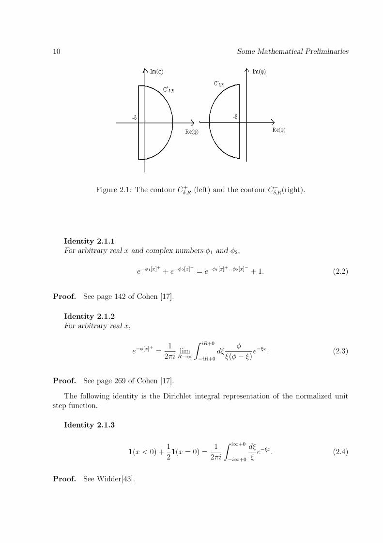
Definition 2.1.1For R > δ ≥ 0, C+
δ,R is the closed contour consisting of
1. the part of the line Re(φ) = −δ, running from −δ + i√
R2 − δ2 to−δ − i
√R2 − δ2 and
2. the part of circle |φ| = R, running counterclockwise from−δ − i
√R2 − δ2 to −δ + i
√R2 − δ2.
C−δ,R is the closed contour consisting of
1. the part of the line Re(φ) = −δ, running from −δ − i√
R2 − δ2 to−δ + i
√R2 − δ2 and
2. the part of circle |φ| = R, running counterclockwise from−δ + i
√R2 − δ2 to −δ − i
√R2 − δ2.
The definition is illustrated by figure 2.1.
For derivations, we use some identities of which the proof can be found in the book byCohen [17]. First, we introduce the notations
[x]+ = max(0, x), [x]− = min(0, x), −∞ < x < ∞. (2.1)
9
10 Some Mathematical Preliminaries
Figure 2.1: The contour C+δ,R (left) and the contour C−
δ,R(right).
Identity 2.1.1For arbitrary real x and complex numbers φ1 and φ2,
e−φ1[x]+ + e−φ2[x]− = e−φ1[x]+−φ2[x]− + 1. (2.2)
Proof. See page 142 of Cohen [17].
Identity 2.1.2For arbitrary real x,
e−φ[x]+ =1
2πilim
R→∞
∫ iR+0
−iR+0
dξφ
ξ(φ − ξ)e−ξx. (2.3)
Proof. See page 269 of Cohen [17].
The following identity is the Dirichlet integral representation of the normalized unitstep function.
Identity 2.1.3
1(x < 0) +1
21(x = 0) =
1
2πi
∫ i∞+0
−i∞+0
dξ
ξe−ξx. (2.4)
Proof. See Widder[43].
2.2 Analytic Function and Analytic Continuation 11
2.2 Analytic Function and Analytic Continuation
In chapters 3-6 we will consider some analytic functions that satisfy a certain property,which is formulated in the following.
Definition 2.2.1We say a function f satisfies property A+ if f(φ) is(i) analytic on Re(φ) > 0,(ii) continuous and bounded on Re(φ) ≥ 0,
and we say it satisfies property A+ if, in addition, it is(iii) bounded away from 0 on Re(φ) ≥ 0.
We say a function f satisfies property A− if f(φ) is(i) analytic on Re(φ) < 0,(ii) continuous and bounded on Re(φ) ≤ 0,
and we say it satisfies property A− if, in addition, it is(iii) bounded away from 0 on Re(φ) ≤ 0.
Next, we recall a theorem called the principle of analytic continuation. We will use thistheorem in proving some main theorems in this thesis.
Theorem 2.2.1Let an analytic function f1(z) be defined in a region Ω1 and let Ω2 be another region
which has a certain subregion ω, but only this one, in common with Ω1. Then, if a functionf2(z) exists which is analytic in Ω2 and coincides with f1(z) in ω, there can only be onesuch function. f1(z) and f2(z) are called analytic continuations of each other.
Proof. See Knopp [30].
2.3 Wiener-Hopf factorization
The technique to solve the problems in this thesis is based on Wiener-Hopf factorization.In this section we recall some definitions and some theorems about this factorization andits application to the problems in chapters 3 until chapter 6.
Let f, g and k0 be functions of bounded variation on the real line (−∞,∞), wheref and h have non-negative support, i.e. f(t) = k0(t) = 0 for t < 0. The function fdefines a Stieltjes measure df(.) on the positive half-axis [0,∞) which is used to defineRiemann-Stieltjes integrals. The integral equation for f,
f(t) −∫ +∞
0−
g(t − y)df(y) = k0(t), t ≥ 0, (2.5)
is called the Wiener-Hopf integral equation. Since f(t) = 0 for t < 0 we may extend thisequation to the negative half-axis by introducing a function
k(t) =
−∫ +∞
0−g(t − y)df(y), t < 0,
k0(t), t ≥ 0.
(2.6)
12 Some Mathematical Preliminaries
So we get the extended Wiener-Hopf integral equation
f(t) −∫ +∞
0−g(t − y)df(y) = k(t), −∞ < t < ∞. (2.7)
By introducing the Laplace-Stieltjes transforms
F (φ) =
∫ +∞
0−
e−φtdf(t), Re(φ) ≥ 0,
G(φ) =
∫ +∞
−∞
e−φtdg(t), Re(φ) = 0,
K(φ) =
∫ 0−
−∞
e−φtdk(t), Re(φ) ≤ 0, and
K0(φ) =
∫ +∞
0−e−φtdk0(t), Re(φ) ≥ 0,
and applying transforms to equation (2.7) gives the transformed Wiener-Hopf equation
F (φ)(1 − G(φ)) = K0(φ) + K(φ), Re(φ) = 0, (2.8)
where F (φ) and K0(φ) satisfy the property A+ and K(φ) satisfies the property A−. Theequation (2.8) can be solved using a factorization method applied to the symbol of (2.8)
H(φ) = 1 − G(φ).
The factorization is referred to as Wiener-Hopf factorization since it is connected to theWiener-Hopf technique in the theory of integral equations. This technique is about towrite a complex valued function H(φ), which is bounded and continuous on Re(φ) = 0with limφ→i∞ H(φ) = limφ→−i∞ H(φ) = 1, in the form
H(φ) = H+(φ)H−(φ), Re(φ) = 0, (2.9)
where H+(φ) satisfies property A+ and H−(φ) satisfies property A−.We shall only consider factorizations with
H+(+i∞) = H+(−i∞) = H−(+i∞) = H−(−i∞) = 1.
Since both factors are bounded at infinity and analytic in their respective half-planesRe(φ) > 0 and Re(φ) < 0 they are bounded in the closed half-planes Re(φ) ≥ 0 andRe(φ) ≤ 0 respectively. We impose the condition that H(φ) does not vanish on theimaginary axis, i.e.
H(φ) 6= 0, Re(φ) = 0. (2.10)
This condition implies that H+(φ) and H−(φ) can not vanish on the imaginary axisRe(φ) = 0. The factorization (2.9) is regular if at least one of the factors H+(φ) andH−(φ) does not vanish in the half-plane of analyticity. It is canonical if both factorsH+(φ) and H−(φ) do not vanish in their half-planes of analyticity, so that
H+(φ) 6= 0, Re(φ) ≥ 0, and
H−(φ) 6= 0, Re(φ) ≤ 0.(2.11)
The existence of the canonical factorization (2.11) is given by the following theorem.
2.3 Wiener-Hopf factorization 13
Theorem 2.3.1 (Scalar factorization theorem)A function H(φ) = 1 − G(φ) admits a canonical factorization if and only if
• H(φ) 6= 0, Re(φ) = 0,
• one of the following is satisfied
1. the number of zeros of H(φ) in Re(φ) > 0 is equal to the number of poles ofH(φ) in Re(φ) > 0,
2. the number of zeros of H(φ) in Re(φ) < 0 is equal to the number of poles ofH(φ) in Re(φ) < 0.
The canonical factorization is unique. Moreover we have
H+(φ) = 1 +
∫ +∞
0
e−φtdC(t), Re(φ) ≥ 0, and
H−(φ) = 1 +
∫ 0
−∞
e−φtdC(t), Re(φ) ≤ 0,
where C(t) is a function of bounded variation on the real line.
Proof. See Corduneanu [19] and Regterschot [38].
The conditions 1 and 2 in Theorem 2.3.1 can be verified by Rouche’s theorem. If ina half-plane the number of zeros is not equal to the number of poles then there exists afactorization as well. However it is not canonical and not necessarily unique. For moredetails see Corduneanu [19] and Zabreyko [44].
In chapters 4-6, we are dealing with some systems of transformed Wiener-Hopf equa-tions. The necessary and sufficient conditions for these systems to admit a canonicalfactorization is ensured in Bart, Gohberg, and Kaashoek[10]. The conditions involve thedet H(φ) instead of H(φ), and we can use a generalization of Rouche’s theorem, given inde Smit [21], to verify the conditions.
If the canonical factors for the symbol of (2.8) exist then we have
F (φ)H+(φ) = K0(φ)/H−(φ) + K(φ)/H−(φ), Re(φ) = 0. (2.12)
Now the left hand-side satisfies property A+ and the last term of the right hand-sidesatisfies property A−. We then try to find a decomposition of K0(φ)/H−(φ), i.e. we lookfor two functions C+(φ) and C−(φ) such that
• C+(φ) satisfies property A+,
• C−(φ) satisfies property A−,
• K0(φ)/H−(φ) = C+(φ) + C−(φ).
14 Some Mathematical Preliminaries
With this decomposition we have from (2.12)
F (φ)H+(φ) − C+(φ) = C−(φ) + K(φ)/H−(φ). (2.13)
At this point we invoke Liouville’s theorem.
Theorem 2.3.2 (Liouville’s theorem)A function analytic and bounded in the whole complex plane is constant.
Proof. See page 451 of Apostol[5].
From (2.13) it now follows by analytic continuation that it is possible to define a functionequal to the left hand-side of (2.13) for Re(φ) ≥ 0 and equal to the right hand-side of (2.13)for Re(φ) ≤ 0. It now follows from Liouville’s theorem that
F (φ)H+(φ) − C+(φ) = constant, Re(φ) ≥ 0, (2.14)
and
C−(φ) + K(φ)/H−(φ) = constant, Re(φ) ≤ 0, (2.15)
where the constant is determined by the known value, c say, at the origin, so
c = F (0)H+(0) − C+(0) = C−(0) + K(0)/H−(0). (2.16)
Since the factorization is unique we now have
Theorem 2.3.3If the function H(φ) = 1 − G(φ) admits a canonical factorization, then equation (2.8)
has the unique solution
F (φ) =(C+(φ) + F (0)H+(0) − C+(0)
)/H+(φ), Re(φ) ≥ 0, (2.17)
and
K(φ) =(F (0)H+(0) − K+(0) − C−(φ)
)H−(φ), Re(φ) ≤ 0. (2.18)
Proof. Equations (2.17) and (2.18) are obtained directly by substituting (2.16) into(2.14) and (2.15).
2.4 Numerical inversions
In this section we discuss the numerical inversions for the Laplace transforms and proba-bility generating functions proposed in Abate & Whitt[3].
2.4 Numerical inversions 15
2.4.1 Numerical inversion algorithm for Laplace transforms
Given the Laplace transform
f(s) =
∫ ∞
0
e−stf(t)dt, Re(s) ≥ 0, (2.19)
where f is a function on the positive real line, we want to invert (2.19) to obtain thefunction f. The analytical formula for this function is given by
f(t) =1
2π
∫ ∞
−∞
e−ituf(u)du, t ∈ R+, (2.20)
but often the integral in (2.20) is difficult to evaluate analytically. A numerical inversionis then appropriate. The numerical inversion is based on the integral (2.20), in which theintegral is evaluated numerically by using the trapezoidal rule. It yields an approximationfor f(t) in terms of the alternating series
f(t) ≈ eA/2
2tRe(f)
(A
2t
)+
eA/2
t
∞∑
k=1
(−1)kRe(f)
(A + 2kπi
2t
), (2.21)
where real number A and integer numbers m and n are parameters to control the accuracy.The series is then approximated by the Euler sum
E(t,m, n) =m∑
k=0
(m
k
)2−mSn+k(t) (2.22)
where
Sn(t) =n∑
k=0
(−1)kak(t), (2.23)
with
a0(t) = f
(A
2t
)/2, (2.24)
ak(t) = Re(f)
(A + 2kπi
2t
), k ≥ 1, (2.25)
so that
f(t) ≈ eA/2
tE(t,m, n). (2.26)
In [3] it is shown that |E(t,m, n)−E(t,m, n+1)| can be used for estimating the errordue to the approximation formula (2.26). It is indicated that to obtain accuracy to 10−7,we can set A = 19.1, m = 11, and n = 15.
16 Some Mathematical Preliminaries
2.4.2 Numerical inversion algorithm for generating functions
Suppose that
g(z) =∞∑
j=0
zjP (X = j) =∞∑
j=0
zjpj, |z| ≤ 1, (2.27)
the probability generating function of a random variable with non-negative integer valuesX, is given. The analytical formula for pj = P (X = j) is
pj =1
2πi
∫
Cr
g(z)
zj+1dz, (2.28)
where Cr is the circle with center at origin and of radius r, 0 < r < 1, and the integrationis taken counter clockwise. Let z = reiu. Substituting this to (2.28) we obtain
pj =1
2πi
∫ 2π
0
g(reiu)
(reiu)j+1ireiudu
=1
2πrj
∫ 2π
0
g(reiu)e−ijudu
=1
2πrj
∫ 2π
0
(Re(g(reiu)) + iIm(g(reiu))
)(cos(ju) − i sin(ju)) du.
(2.29)
Since pj is a real number, then
pj =1
2πrj
∫ 2π
0
(cos(ju)Re(g(reiu)) + sin(ju)Im(g(reiu))
)du. (2.30)
The trapezoidal rule with step size π/j is then applied to approximate the integral in(2.30), and yields
pj ≈π
2πjrj
[g(r) + g(−r)
2+
2j−1∑
k=1
cos(kπ)Re(g(reikπ/j)) +
2j∑
k=1
sin(kπ)Im(g(reikπ/j))
]
=1
2jrj
2j∑
k=1
(−1)kRe(g(reikπ/j)),
and with some algebra we obtain
pj ≈1
2jrj
[g(r) + g(−r) + 2
j−1∑
k=1
(−1)kRe(g(reikπ/j))
]. (2.31)
Denote the right hand side of (2.31) by pj. In [3] it is proven that for 0 < r < 1 and j ≥ 1,
|pj − pj| ≤r2j
1 − r2j.
But for practical purposes, we can think of the error bound as r2j since r2j
1−r2j is approxi-
mately equal to r2j when r2j is small. Hence, to have accuracy to 10−γ, we let r = 10−γ/2j.
Chapter 3
The Single Server GI/G/1 queue
3.1 Introduction
We consider a single server queueing system with renewal input and infinite waitingroom in which customers are served in order of arrival, i.e. with first come - first served(FCFS) discipline. We choose t = T0 = 0 at the arrival epoch of an arbitrary customer. Weassume that this customer finds upon his arrival C0 other customers in the system, whichare numbered 1, 2, . . . , C0 in order of their arrival. These customers will be referred to asspecial customers. For convenience we assume that the first special customer enters serviceat t = 0. The service times of the special customers will be denoted by X1, X2, . . . , XC0 .After the arrival at time T0 subsequent customers arrive at time epochs T1, T2, . . .. Theinter-arrival times are denoted by An = Tn − Tn−1, n = 1, 2, . . . and the service time of thenth customer is denoted by Bn, n = 0, 1, . . .. By assumption An constitutes a sequenceof independent identically distributed (i.i.d.) nonnegative random variables with
F (x) = P (An ≤ x)
F (0+) = 0
E(An) = α < ∞.
Also Bn are i.i.d. nonnegative random variables and we denote
G(x) = P (Bn ≤ x)
with G(0+) = 0
E(Bn) = β < ∞.
We assume that the probability distribution of An, n = 1, 2, · · · , is non-lattice. Moverover,we assume that An, Bn and Xi, i = 1, 2, . . . , C0 are three independent families ofrandom variables. As usual, the traffic intensity ρ is defined by β/α.
We are interested in the steady state (if it exists) and time dependent probabilitydistributions of the actual waiting time of the nth customer, the virtual waiting time attime t and, the number of customers in the system at arrival epochs and in continuous time.
17
18 The Single Server GI/G/1 queue
These system characteristics have been investigated by Cohen[17], Bertsimas et al. [13] andBertsimas & Nakazato[12], under the assumption C0 = 0.
In [13] the analysis is done by solving a Hilbert factorization problem. Two special casesof the problem, i.e. the cases in which either the probability distribution of the inter-arrivaltimes or the service times has a rational Laplace transform are solved explicitly, yieldingsimple closed-form expressions for the Laplace transforms of the waiting time distributionand the busy period distribution. Algorithmically, the approach offers a method for findingthese distributions through numerical inversion, which is claimed to be very tractable.
The two special cases mentioned above are also studied in de Smit[24] for the steadystate. Wiener-Hopf factorization is used to analyze the problem, and as a result, theLaplace-Stieltjes transforms of the steady-state distribution of waiting time of nth customerand the distribution of the virtual waiting time are obtained.
Furthermore, in [12] another special case of the model is considered. This special caseis the MGEL/MGEM/1 queue, that is the queueing model in which the inter-arrival timesand the service times have a mixed generalized Erlang distribution. The authors use themethod of stages, and give closed-form expressions for the Laplace transforms of the queuelength distribution and the waiting time distribution. Some examples of the distributionsof the busy period, the queue length, and the waiting time are given, obtained throughnumerical inversion of the Laplace transforms.
For the analysis of the present model, we use the same method as in [24]. To findthe distribution function of the waiting time of the nth arbitrary customer, Wiener-Hopffactorization is used. Later we will see that this factorization must be followed by adecomposition of a certain function since in our model we have a non-zero waiting timefor the customer who arrives at t = 0. For the two special cases studied in [13], which wedenote by GI/Kn/1 and Km/G/1, an explicit factorization can be found. This gives usan explicit expression for the generating function of the Laplace-Stieltjes transform of thedistribution of the actual waiting time of the nth customer. Based on this result, we couldderive an explicit expression for the Laplace-Stieltjes transform of the virtual waiting time.
For the study of the number of customers in the system, we derive a general expressionfor the Laplace-Stieltjes transform of the time-dependent expectation of the number of cus-tomers using contour integration. For the systems GI/Kn/1 and Km/G/1, the expressionfor the Laplace-Stieltjes transforms can be determined explicitly. The explicit expressionsfor the transforms enable us to perform a numerical inversion of these transforms to obtainthe time-dependent distributions/expectations of interest. We apply the numerical inver-sion algorithm proposed in [3], and the numerical results can be found in the end of thischapter.
This chapter is organized as follows. After giving some notations and definitions insection 3.2, we will study the probability distribution of the actual waiting time of the nthcustomer in section 3.3. Then in section 3.4 we derive the probability distribution of thevirtual waiting time. Based upon some results in sections 3.3 and 3.4, we subsequentlystudy the number of customers at arrival epochs in section 3.5 and for continuous time insection 3.6. A more detailed study of these distributions for the queueing models GI/Kn/1and Km/G/1, can be found in section 3.7. In section 3.7.3 we give some examples of thedistributions obtained by numerical inversion. For the systems with traffic intensity ρ < 1
3.2 Notations and definitions 19
we give the distributions in steady state as well as in transient state and, for the systemswith ρ > 1, we give the time dependent distribution of the number of customers at time tand its behavior as t increases.
3.2 Notations and definitions
We denote the actual waiting time of nth customer by Wn and the virtual waitingtime at time t by Vt. If C0 = γ, then W0 =
∑γi=1 Xi. We assume that the Xi have finite
positive mean and, that their probability distribution is non-lattice and has a rationalLaplace-Stieltjes transform of the following form
P(φ) = E[e−φXi
]=
P (φ)∏k
i=1(φ + wi), (3.1)
Consequently,
E[e−φW0|C0 = γ
]=
P γ(φ)∏k
i=1(φ + wi)γ, (3.2)
where Re(wi) > 0, i = 1, 2, . . . , k, and in which P (φ) is a polynomial of degree k − 1 orless. We assume that the coefficient of φd, where d is the degree of P (φ), is unity.
Let the L-S transforms of the distribution functions of the inter-arrival and servicetimes be denoted by
A(φ) =
∫ ∞
0
e−φxF (dx), Re(φ) ≥ 0
and
B(φ) =
∫ ∞
0
e−φxG(dx), Re(φ) ≥ 0,
respectively. We assume that there exists a δ > 0 such that A(φ) and B(φ) can be continuedanalytically into the region Re(φ) > −δ.
3.3 The distribution of actual waiting times
Since the service discipline is FCFS, the actual waiting times satisfy the recurrencerelation
Wn+1 = [Wn + Bn − An+1]+ n = 0, 1, . . . .
Let for (|r| < 1, Re(φ) ≥ 0, Re(η) ≥ 0, γ ≥ 0), or (|r| ≤ 1, Re(φ) ≥ 0, Re(η) > 0, γ ≥ 0), or(|r| ≤ 1, Re(φ) > 0, Re(η) ≥ 0, γ ≥ 0),
Z(r, φ, η, γ) =∞∑
n=0
rnE[e−φWn−ηTn|C0 = γ
],
and let
V (r, φ, η, γ) =∞∑
n=0
rn+1E[(
1 − e−φ[Wn+Bn−An−1]−)
e−ηTn+1|C0 = γ],
for (|r| < 1, Re(φ) ≤ 0, Re(η) ≥ 0, γ ≥ 0) or (|r| ≤ 1, Re(φ) ≤ 0, Re(η) > 0, γ ≥ 0).
20 The Single Server GI/G/1 queue
Theorem 3.3.1For (|r| < 1, Re(φ) = 0, Re(η) ≥ 0, γ ≥ 0) or (|r| ≤ 1, Re(φ) = 0, Re(η) > 0, γ ≥ 0),
Z(r, φ, η, γ)1 − rA(η − φ)B(φ) =P γ(φ)
∏ki=1(φ + wi)γ
+ V (r, φ, η, γ). (3.3)
Proof. By using the identity 2.1.1 with φ1 = φ2 = φ, that is
e−φx+
= e−φx + 1 − e−φx−
(3.4)
we have for Re(φ) = 0, Re(η) ≥ 0, and γ ≥ 0,
E[e−φWn+1−ηTn+1 |C0 = γ
]
= E[e−φ[Wn+Bn−An+1]+−ηTn+1 |C0 = γ
]
= E[e−φ[Wn+Bn−An+1]−ηTn+1|C0 = γ
]
+E[(
1 − e−φ[Wn+Bn−An+1]−)
e−ηTn+1|C0 = γ]
= E[e−φWn−ηTn|C0 = γ
]E[e−φBn−(η−φ)An+1|C0 = γ
]
+E[(
1 − e−φ[Wn+Bn−An+1]−)
e−ηTn+1|C0 = γ],
using the independence assumptions and the fact that Tn+1 = Tn + An+1. If we multiplyby rn+1 and sum over n this yields for Re(φ) = 0 and (|r| < 1, Re(η) ≥ 0, γ ≥ 0) or(|r| ≤ 1, Re(η) > 0, γ ≥ 0),
Z(r, φ, η, γ) − E[e−φW0 |C0 = γ
]= rZ(r, φ, η, γ)A(η − φ)B(φ) + V (r, φ, η, γ)
noting that T0 = 0 and using the independence of the service times and inter-arrival timesand, we get (3.3), using (3.2).
It can be shown, see Cohen[17], that for fixed (|r| < 1, Re(η) ≥ 0) or (|r| ≤ 1, Re(η) >0), the function 1 − rA(η − φ)B(φ) can be factorized, i.e. for Re(φ) = 0,
1 − rA(η − φ)B(φ) = K+(r, φ, η)K−(r, φ, η), (3.5)
where, in the complex φ plane, K+(r, φ, η) satisfies conditions A+ and K−(r, φ, η) satisfiesconditions A−. Then, from (3.3) we obtain for fixed (|r| < 1, Re(η) ≥ 0, γ ≥ 0) or(|r| ≤ 1, Re(η) > 0, γ ≥ 0) and Re(φ) = 0,
Z(r, φ, η, γ)K+(r, φ, η) =P γ(φ) [K−(r, φ, η)]
−1
∏ki=1(φ + wi)γ
+ V (r, φ, η, γ)[K−(r, φ, η)
]−1. (3.6)
In the complex φ plane, the left-hand side of (3.6) satisfies conditions A+ and the secondterm of the right-hand side satisfies conditions A−. Suppose we can decompose the firstterm of the right hand side of (3.6) into two functions C+ and C− such that for Re(φ) = 0,
P γ(φ)∏k
i=1(φ + wi)γ
[K−(r, φ, η)
]−1= C+(r, φ, η, γ) + C−(r, φ, η, γ), (3.7)
3.4 The distribution of the virtual waiting time 21
where C+(r, φ, η, γ) satisfies A+ and C−(r, φ, η, γ) satisfies A−. We then have the followingsolution of (3.3).
Theorem 3.3.2For (|r| < 1, Re(φ) ≥ 0, Re(η) ≥ 0, γ ≥ 0), or (|r| ≤ 1, Re(φ) ≥ 0, Re(η) > 0, γ ≥ 0), or
(|r| ≤ 1, Re(φ) > 0, Re(η) ≥ 0, γ ≥ 0),we have
Z(r, φ, η, γ) =[C+(r, φ, η, γ) + C−(r, 0, η, γ)
] [K+(r, φ, η)
]−1. (3.8)
Proof. From (3.6) and (3.7) we have
Z(r, φ, η, γ)K+(r, φ, η) − C+(r, φ, η, γ) = C−(r, φ, η, γ)
+ V (r, φ, η, γ)[K−(r, φ, η)
]−1.
(3.9)
The left-hand side of (3.9) satisfies A+ and the right-hand side satisfies A−. By analyticcontinuation in the complex φ plane, we can define an entire function which is equal to theleft-hand side for Re(φ) ≥ 0 and equal to the right-hand side for Re(φ) ≤ 0. This entirefunction is bounded, and hence by Liouville’s theorem, it is a constant. So, for Re(φ) ≥ 0
Z(r, φ, η, γ)K+(r, φ, η) − C+(r, φ, η, γ) = Z(r, 0, η, γ)K+(r, 0, η) − C+(r, 0, η, γ)
= C−(r, 0, η, γ) + 0,(3.10)
with (|r| ≤ 1, Re(η) > 0, γ ≥ 0) or (|r| < 1, Re(η) ≥ 0, γ ≥ 0), which proves the theorem.
If ρ < 1 and both
K+(1, φ, 0) = limr↑1
K+(r, φ, 0) and K−(1, φ, 0) = limr↑1
K−(r, φ, 0)
exist for Re(φ) ≥ 0, then from (3.8), in using Abel’s theorem, the Laplace-Stieltjes trans-form of the steady-state waiting time distribution for Re(φ) ≥ 0 is given by
Z(φ) = limr↑1
(1 − r)Z(r, φ, 0, γ)
=
[limr↑1
(1 − r)[C+(r, φ, 0, γ) + C−(r, 0, 0, γ)
]] [K+(1, φ, 0)
]−1.
(3.11)
The explicit expression for Z(φ) can then be found once we have explicit expressions forK+(r, φ, η), K−(r, φ, η), C+(r, φ, η, γ), and C−(r, φ, η, γ).
3.4 The distribution of the virtual waiting time
Let the number of arrivals in the interval (0, t] be denoted by
Nt = supn = 1, 2, . . . | Tn ≤ t
22 The Single Server GI/G/1 queue
and let
Ut = WNt + BNt − (t − TNt).
Then the virtual waiting time Vt is given by Vt = U+t . Notice that the sample paths of Vt
are right-continuous. By the law of total probability we have for Re(φ) ≥ 0, γ ≥ 0,
E[e−φUt|C0 = γ
]= E
[e−φ[WNt+BNt−(t−TNt )]|C0 = γ
]
=∞∑
n=0
E[e−φ(WNt+BNt−(t−TNt ))1(Tn ≤ t < Tn+1)|C0 = γ
]
=∞∑
n=0
∫ t
0
e+φ(t−u)1 − F (t − u)E(e−φBn
)
.duE[e−φWn1(Tn ≤ u)|C0 = γ
]
= B(φ)∞∑
n=0
∫ t
0
e+φ(t−u)1 − F (t − u)
.duE[e−φWn1(Tn ≤ u)|C0 = γ
],
(3.12)
where 1(A) denotes the indicator function of the event A.
Hence, for Re(η) > Re(φ) ≥ 0, γ ≥ 0, we find
∫ ∞
0
e−ηtE[e−φUt|C0 = γ
]dt
=B(φ) − A(η − φ)B(φ)
η − φ
∞∑
n=0
E[e−φWn−ηTn|C0 = γ
]
=B(φ) − A(η − φ)B(φ)
η − φZ(1, φ, η, γ).
(3.13)
Then, by using identity (3.4), we have for Re(η) > 0, Re(φ) = 0, γ ≥ 0,
Z∗(φ, η, γ) =
∫ ∞
0
e−ηtE[e−φVt|C0 = γ
]dt
=B(φ) − A(η − φ)B(φ)
η − φZ(1, φ, η, γ) +
1
η
−∫ ∞
0
e−ηtE[e−φU−
t |C0 = γ]dt.
(3.14)
We now decompose the term B(φ)−A(η−φ)B(φ)η−φ
Z(1, φ, η, γ), i.e. we determine two functions
D+(φ, η, γ) and D−(φ, η, γ) such that for Re(φ) = 0
B(φ) − A(η − φ)B(φ)
η − φZ(1, φ, η, γ) = D+(φ, η, γ) + D−(φ, η, γ), (3.15)
3.4 The distribution of the virtual waiting time 23
where in the complex φ plane, D+(φ, η, γ) satisfies A+ and D−(φ, η, γ) satisfies A−. Forthis purpose, we first notice from equation (3.3), that for Re(φ) ≥ 0, Re(η) > 0, γ ≥ 0,
B(φ) − A(η − φ)B(φ)
η − φZ(1, φ, η, γ) =
B(φ)Z(1, φ, η, γ)
η − φ− Z(1, φ, η, γ)
η − φ
+P (φ)γ
(η − φ)∏k
i=1(φ + wi)γ+
V (1, φ, η, γ)
(η − φ).
(3.16)
By defining the function
F (φ, η, γ) = B(φ)Z(1, φ, η, γ) − Z(1, φ, η, γ) +P γ(φ)
∏ki=1(φ + wi)γ
, (3.17)
for Re(φ) ≥ 0, Re(η) > 0, γ ≥ 0, we can choose
D+(φ, η, γ) =F (φ, η, γ) − F (η, η, γ)
(η − φ)(3.18)
and
D−(φ, η, γ) =F (η, η, γ)
(η − φ)+
V (1, φ, η, γ)
(η − φ)(3.19)
With this decomposition, we have the following result.
Theorem 3.4.1For Re(η) ≥ 0, Re(φ) ≥ 0, γ ≥ 0,
Z∗(φ, η, γ) = D+(φ, η, γ) +F (η, η, γ)
η. (3.20)
Proof. With the decomposition (3.15) we can rewrite (3.14) as
Z∗(φ, η, γ) − D+(φ, η, γ) = D−(φ, η, γ) +1
η
−∫ ∞
0
e−ηtE[e−φU−
t |C0 = γ]dt,
(3.21)
where in the complex φ plane the left-hand side of (3.21) satisfies A+ and the right-handside satisfies A−. By analytic continuation, we can define an entire function which is equalto the left-hand side for Re(φ) ≥ 0 and equal to the right-hand side for Re(φ) < 0. Thisentire function is bounded, and hence by Liouville’s theorem, it is a constant. Therefore,
Z∗(φ, η, γ) − D+(φ, η, γ) = Z∗(0, η, γ) − D+(0, η, γ)
= D−(0, η, γ) +1
η− 1
η
=F (η, η, γ)
η,
(3.22)
24 The Single Server GI/G/1 queue
and we get (3.20).
If ρ < 1 and if the distribution function of the inter-arrival times F is non-lattice, thenthe steady-state virtual waiting time distribution exists. Let
Z∗(φ) = limt→∞
E[e−φVt|C0 = γ
].
From Abel’s theorem for Laplace transforms, we obtain
Z∗(φ) = limη↓0
ηZ∗(φ, η, γ)
= limη↓0
η
[D+(φ, η, γ) +
F (η, η, γ)
η
]
= limη↓0
η
(η − φ)
[B(φ)Z(1, φ, η, γ) − Z(1, φ, η, γ) +
P γ(φ)∏k
i=1(φ + wi)γ
]
− limη↓0
φ
(η − φ)F (η, η, γ)
=1 − B(φ)
φlimη↓0
ηZ(1, φ, η, γ) − limη↓0
1 − B(η)
η· lim
η↓0ηZ(1, η, η, γ)
= 1 − ρ + ρ1 − B(φ)
βφZ(φ),
(3.23)
a well known relation for the GI/G/1 queue that relates the L-S transforms of the proba-bility distributions of the virtual and actual waiting time.
3.5 Number of customers at arrival epochs
Let Cn be the number of customers in the system at T−n , i.e. just before the arrival of
the nth customer. It is clear that
C0 ≤ j =
impossible event , j = 0, 1, . . . , C0 − 1
Ω , j = C0, C0 + 1, . . . ,
where Ω is the sure event. Furthermore, for n = 1, 2, . . . , j,
Cn ≤ j =
∑C0−(j−n)i=1 Xi < Tn
, j = 1, 2, . . . , C0
Ω , j = C0 + 1, C0 + 2, . . . , &
n = 1, 2, . . . , j − C0
∑C0−(j−n)i=1 Xi < Tn
, j = C0 + 1, C0 + 2, . . . , &
n = j − C0 + 1, j − C0 + 2, . . . , j
3.5 Number of customers at arrival epochs 25
and
Cn+j+1 ≤ j = Tn + Wn + Bn < Tn+j+1 n = 0, 1, . . . .
Theorem 3.5.1For |r| < 1, |s| < 1, γ ≥ 0,
U(r, s, γ) =∞∑
n=0
rnE[sCn|C0 = γ
]
=rsγ+1
(1 − rs)+ sγ
+(1 − s)
2πi
∫ i∞+0
−i∞+0
dξ
ξ
srA(−ξ)P (ξ)[P γ(ξ) − sγ
∏ki=1(ξ + wi)
γ]
X1(r, ξ)X2(s, ξ)∏k
i=1(ξ + wi)γ
+ (1 − s)r
2πi
∫ i∞+0
−i∞+0
dξ
ξ(1 − rsA(−ξ))−1A(−ξ)B(ξ)Z(r, ξ, 0, γ),
(3.24)
where
X1(r, s, ξ) = 1 − srA(−ξ),
and
X2(s, ξ) = P (ξ) − sk∏
i=1
(ξ + wi).
Proof. For |r| < 1, |s| < 1, γ ≥ 0,
∞∑
n=0
rnE[sCn|C0γ
]
= (1 − s)∞∑
n=0
rn
∞∑
j=0
sjP (Cn ≤ j)
= (1 − s)∞∑
j=γ
sj + (1 − s)∞∑
j=γ+1
j−γ∑
n=1
rnsj
+ (1 − s)∞∑
n=1
n+γ−1∑
j=n
rnsjP
γ−(j−n)∑
i=1
Xi < Tn
+ (1 − s)∞∑
j=0
∞∑
n=0
rn+j+1sjP (Tn + Wn + Bn < Tn+j+1|C0 = γ).
(3.25)
We use the identity 2.1.3, that is
1(x < 0) +1
21(x = 0) =
1
2πi
∫ i∞+0
−i∞+0
dξ
ξe−ξx
26 The Single Server GI/G/1 queue
to obtain
P
γ−(j−n)∑
i=1
Xi < Tn
=
1
2πi
∫ i∞+0
−i∞+0
dξ
ξE[e−ξ(
∑γ−(j−n)i=1 Xi−Tn)
]
=1
2πi
∫ i∞+0
−i∞+0
dξ
ξE[e−ξ(
∑γ−(j−n)i=1 Xi)
]An(−ξ)
(3.26)
and
P (Tn + Wn + Bn < Tn+j+1|C0 = γ)
=1
2πi
∫ i∞+0
−i∞+0
dξ
ξE[e−ξ(Tn+Wn+Bn−Tn+j+1)|C0 = γ
]
=1
2πi
∫ i∞+0
−i∞+0
dξ
ξE[e−ξWn|C0 = γ
]B(ξ)Aj+1(−ξ),
(3.27)
taking into account the independence assumptions. By substituting (3.26) and (3.27) into(3.25) we obtain for |r| < 1, |s| < 1, γ ≥ 0,
∞∑
n=1
rnE[sCn|C0 = γ
]
=(1 − s)∞∑
n=1
n+γ−1∑
j=n
rnsj 1
2πi
∫ i∞+0
−i∞+0
dξ
ξE[e−ξ(
∑γ−(j−n)i=1 Xi)
]An(−ξ)
+rsγ+1
(1 − rs)+ sγ
+ (1 − s)1
2πir
∫ i∞+0
−i∞+0
dξ
ξ(1 − rsA(−ξ))−1A(−ξ)B(ξ)Z(r, ξ, 0, γ).
(3.28)
Since the r.v.’s Xi, i = 1, . . . , γ, are independent the first term of the right-hand sideof (3.28) can be written as
(1 − s)∞∑
n=1
n+γ−1∑
j=n
rnsj 1
2πi
∫ i∞+0
−i∞+0
dξ
ξE[e−ξX1
](γ−j+n)An(−ξ)
=(1 − s)
2πi
∫ i∞+0
−i∞+0
dξ
ξPγ(ξ)
∞∑
n=1
n+γ−1∑
j=n
(rA(−ξ)P(ξ))n
(s
P(ξ)
)j
=(1 − s)
2πi
∫ i∞+0
−i∞+0
dξ
ξPγ(ξ)
srA(−ξ)
1 − srA(−ξ)
γ−1∑
j=0
(s
P(ξ)
)j
=(1 − s)
2πi
∫ i∞+0
−i∞+0
dξ
ξ
rA(−ξ)P(ξ)s [Pγ(ξ) − sγ]
(1 − srA(−ξ)) (P(ξ) − s)
=(1 − s)
2πi
∫ i∞+0
−i∞+0
dξ
ξ
srA(−ξ)P (ξ)[P γ(ξ) − sγ∏k
i=1(ξ + wi)γ]
(1 − srA(−ξ))(P (ξ) − s∏k
i=1(ξ + wi))∏k
i=1(ξ + wi)γ.
(3.29)
3.5 Number of customers at arrival epochs 27
By inserting (3.29) into (3.28), the proof is completed.
The generating function of the nth moment of number of customers at arrival epochscan be derived from (3.24). For the first moment one obtains the following relation. For|r| < 1, γ ≥ 0,
U(r, γ) =∞∑
n=0
rnE [Cn|C0 = γ]
=γ
1 − r+
r
(1 − r)2
− r
2πi
∫ i∞+0
−i∞+0
dξ
ξ
A(−ξ)
1 − rA(−ξ)
γ∑
j=1
Pj(ξ)
− r
2πi
∫ i∞+0
−i∞+0
dξ
ξ[1 − rA(−ξ)]−1A(−ξ)B(ξ)Z(r, ξ, 0, γ).
(3.30)
The first integral can be evaluated using contour integration leading to the followingtheorem.
Theorem 3.5.2For r < 1, γ ≥ 0, and wi 6= wj for i 6= j
U(r, γ) =γ +r
(1 − r)2
− r
γ∑
j=1
1
(j − 1)!
k∑
i=1
dj
dξj
[A(−ξ)P (ξ)j
ξ(1 − rA(−ξ))∏k
n=1,n 6=i(ξ + wn)j
]
ξ=−wi
− r
2πi
∫ i∞+0
−i∞+0
dξ
ξ[1 − rA(−ξ)]−1 A(−ξ)B(ξ)Z(r, ξ, 0, γ).
(3.31)
Proof. We want to evaluate the first integral in (3.29) using Cauchy’s residue theorem.Consider a closed contour consisting of the line segment [−iR + δ, iR + δ], δ > 0, parallelto the imaginary axis in the complex ξ plane and a left semi-circle ΓR closing the contour.The integrand has a simple pole at ξ = 0 and in view of (3.1) has poles in ξ = −wi, i =1, 2, . . . , k, each of which occurs with orders j = 1, 2, . . . , γ, since wi 6= wj(i 6= j) byassumption. Observe that 1 − rA(−ξ) 6= 0 within the closed contour.
The residue at ξ = 0 equals γ1−r
, since P(0) = 1 and A(0) = 1. The residue at ξ = −wi,
aij say, corresponding to P(ξ)j, cf. (3.1), equals
aij =1
(j − 1)!
dj
dξj
A(−ξ)P (ξ)j
ξ(1 − rA(−ξ))∏k
n=1n6=i
(ξ + wn)j
ξ=−wi
.
Hence, letting f(ξ) denote the integrand of the integral, we obtain
∫ i∞+0
−i∞+0
f(ξ)dξ +
∫
ΓR
f(ξ)dξ =rγ
1 − r+ r
γ∑
j=1
k∑
i=1
aij
28 The Single Server GI/G/1 queue
Now observe that
|γ∑
j=1
P(ξ)| = O
(1
|ξ|
)as |ξ| → ∞
and |A(−ξ)| ≤ M for Re(ξ) < δ.
Hence
limR→∞
∫
ΓR
f(ξ)dξ = 0
and the assertion follows after some simple calculations.
Theorem 3.5.2 will be used in section 3.7 where an explicit expression for the lastintegral in the right-hand side of (3.31) is derived.
The process Cn, n = 0, 1, . . . is regenerative with the same regeneration points asthe process Wn, n = 0, 1, . . ., because the events Cn = 0 and Wn = 0 are identical.Therefore Cn converges weakly to a random variable C iff ρ < 1. By using Abel’s theoremand (3.11), we have for ρ < 1,
E[sC]
=(1 − s)
2πi
∫ i∞+0
−i∞+0
dξ
ξ(1 − sA(−ξ))−1A(−ξ)B(ξ)Z(ξ),
and
E[C] = − 1
2πi
∫ i∞+0
−i∞+0
dξ
ξ(1 − A(−ξ))−1A(−ξ)B(ξ)Z(ξ). (3.32)
In section 3.7, where we have an explicit expression for A(−ξ) or B(ξ), the integral can becalculated, and we will get a closed-form expression for E[C].
3.6 Number of customers in continuous time
Let C∗t be the number of customers at time t. The process (C∗
t ) is defined to be left-continuous. Then by partitioning the event C∗
t ≤ j with respect to the number ofcustomers that enter the system in (0, t], we have for j = 0, 1, . . . , C0,
C∗t ≤ j =
C0⋃
n=C0−j+1
n∑
i=1
Xi < t,Nt = j − C0 − 1 + n
∪
∞⋃
n=C0+1
Tn−C0−1 + Wn−C0−1 + Bn−C0−1 < t,Nt = j − C0 − 1 + n
=
C0⋃
n=C0−j+1
n∑
i=1
Xi < t, Tj−C0−1+n ≤ t < Tj−C0+n
∪
∞⋃
n=0
Tn + Wn + Bn < t, Tj+n ≤ t < Tj+n+1,
3.6 Number of customers in continuous time 29
and for j = C0 + 1, C0 + 2, . . . ,
C∗t ≤ j = Nt ≤ j − C0 − 1∪
C0⋃
n=1
n∑
i=1
Xi < t,Nt = j − C0 − 1 + n
∪
∞⋃
n=C0+1
Tn−C0−1 + Wn−C0−1 + Bn−C0−1 < t,Nt = j − C0 − 1 + n
= t < Tj−C0
∪C0⋃
n=1
n∑
i=1
Xi < t, Tj−C0−1+n ≤ t < Tj−C0+n
∪∞⋃
n=0
Tn + Wn + Bn < t, Tj+n ≤ t < Tj+n+1.
This leads to
∫ ∞
0
e−ηtE[sC∗
t |C0 = γ]dt
= (1 − s)∞∑
j=0
sj
∫ ∞
0
e−ηtP (C∗t ≤ j|C0 = γ) dt
= (1 − s)
γ∑
j=0
sj
γ∑
n=γ+1−j
∫ ∞
0
e−ηtP
(n∑
i=1
Xi < t, Tj−γ−1+n ≤ t < Tj−γ+n
)dt
+ (1 − s)
γ∑
j=0
sj
∞∑
n=0
∫ ∞
0
e−ηtP (Tn + Wn + Bn < t, Tj+n ≤ t < Tj+n+1) dt
+ (1 − s)∞∑
j=0
sj+γ+1
∫ ∞
0
e−ηtP (t < Tj+1) dt
+ (1 − s)∞∑
j=0
sj+γ+1
γ∑
n=1
∫ ∞
0
e−ηtP
(n∑
i=1
Xi < t, Tj+n ≤ t < Tj+n+1
)dt
+ (1 − s)∞∑
j=γ+1
sj
∞∑
n=0
∫ ∞
0
e−ηtP (Tn + Wn + Bn < t, Tj+n ≤ t < Tj+n+1) dt,
for |s| < 1, γ ≥ 0.
Upon combining the first and fourth term and the second and fifth term one obtains for
30 The Single Server GI/G/1 queue
|s| < 1, γ ≥ 0,
∫ ∞
0
e−ηtE[sC∗t |C0 = γ]dt
= (1 − s)
[∞∑
j=0
sj+γ+1
∫ ∞
0
e−ηtP (Tj+1 > t)dt
+∞∑
j=0
sj
∞∑
n=0
∫ ∞
0
e−ηtP (Tn + Wn + Bn < t, Tj+n ≤ t < Tj+n+1|C0 = γ)dt
+
γ∑
n=1
∞∑
j=0
sj+γ−n+1
∫ ∞
0
e−ηtP (n∑
i=1
Xi < t, Tj ≤ t < Tj+1)dt
].
(3.33)
By using the identity 2.1.3 on page 10 it follows that for Re(η) > Re(ξ) > 0, γ ≥ 0,
∫ ∞
0
e−ηtE[sC∗
t |C0 = γ]dt
=sγ+1
η− (1 − s)
sγ+1
η
A(η)
(1 − sA(η))
+ (1 − s)∞∑
j=0
sj
∞∑
u=0
1
2πi
∫ i∞+0
−i∞+0
dξ
ξ
∫ ∞
0
e−ηt
∫ t
u=0
1 − F (t − u)
duE[e−ξ(Tn−t+Wn+Bn)1(Tn+j ≤ u)|C0 = γ]dt
+ (1 − s)
γ∑
n=1
∞∑
j=0
sj+γ−1+n 1
2πi
∫ i∞+0
−i∞+0
dξ
ξ
∫ ∞
0
e−ηt
∫ t
u=0
1 − F (t − u)
duE[e−ξ(∑n
i=1 Xi−t)1(Tj ≤ u)]dt
=sγ+1
η− (1 − s)
sγ+1
η
A(η)
1 − sA(η)
+ (1 − s)∞∑
j=0
sj
∞∑
n=0
1
2πi
∫ i∞+0
−i∞+0
dξ
ξ
1 − A(η − ξ)
η − ξB(ξ)
∫ ∞
0
e−(η−ξ)uduE
(e−ξ(Tn+Wn)1(Tn+j ≤ u)|C0 = γ)
+(1 − s)
2πi
γ∑
n=1
∞∑
j=0
sj+γ−1+n
∫ i∞+0
−i∞+0
dξ
ξ
1 − A(η − ξ)
η − ξE(e−ξ
∑ni=1 Xi)Aj(η − ξ)
=sγ+1
η− (1 − s)
sγ+1
η
A(η)
1 − sA(η)
+(1 − s)
2πi
∫ i∞+0
−i∞+0
dξ
ξ
1 − A(η − ξ)
η − ξB(ξ)
Z(1, ξ, η, γ)
1 − sA(η − ξ)
+(1 − s)
2πi
∫ i∞+0
−i∞+0
dξ
ξ· 1 − A(η − ξ)
η − ξ· sγP(ξ)
1 − sA(η − ξ)· 1 − sγP(ξ)γ
1 − sP(ξ).
(3.34)
3.6 Number of customers in continuous time 31
The Laplace transform of the nth moments of C∗t can be derived from (3.34). For the
first moment we obtain, with Re(η) > Re(ξ) > 0, γ ≥ 0,∫ ∞
0
e−ηtE [C∗t |C0 = γ] dt =
γ + 1
η+
A(η)
η(1 − A(η))
− 1
2πi
∫ i∞+0
−i∞+0
dξ
ξ
B(ξ)Z(1, ξ, η, γ)
(η − ξ)
− 1
2πi
∫ i∞+0
−i∞+0
dξ
ξ
P(ξ)
η − ξ· 1 − P(ξ)γ
1 − P(ξ).
(3.35)
Since B(ξ),P(ξ) and Z(1, ξ, η, γ) are regular functions in the right half-plane Re(ξ) > 0and, moreover |P(ξ)| < 1 for Re(ξ) > 0, and noting also that the integrands tends to zerosufficiently fast for |ξ| → ∞ if Re(ξ) > 0, it follows from contour integration that forRe(η) > 0, γ ≥ 0,
∫ ∞
0
e−ηtE [C∗t |C0 = γ] dt =
γ + 1
η+
A(η)
η(1 − A(η))
− B(η)Z(1, η, η, γ)
η− 1
ηP(η)
1 − P(η)γ
1 − P(η).
(3.36)
The process C∗t , t ≥ 0 is regenerative with the same regeneration epochs as Vt, t ≥
0. Consequently, (C∗t ) converges for t → ∞ to a stationary random variable C∗ iff ρ < 1
and the interarrival time distribution is non-lattice. We find from (3.34) for |s| < 1,
E[sC∗]
=(1 − s)
2πi
∫ i∞+0
−i∞+0
dξ
ξlimη↓0
ηB(ξ)(1 − A(η − ξ))Z(1, ξ, η, γ)
(η − ξ)(1 − sA(η − ξ)). (3.37)
Since we have assumed that there exists a δ > 0 such that B(φ) can be continued analyti-cally into the region Re(δ) > −δ, then the same applies to Z(1, φ, η, γ). Notice that
limη↓0
(1 − A(η))
η(1 − sA(η))limη↓0
ηZ(1, 0, η, γ)
= limη↓0
−A′(η)
(1 − sA(η)) − sηA′(η)limη↓0
ηZ(1, 0, η, γ)
=α
(1 − s)limη↓0
ηZ(1, 0, η, γ).
(3.38)
Now we have for |s| < 1,
E[sC∗]
= α limη↓0
ηZ(1, 0, η, γ)
+(1 − s)
2πi
∫ i∞−0
−i∞−0
dξ
ξlimη↓0
ηB(ξ)(1 − A(η − ξ))Z(1, ξ, η, γ)
(η − ξ)(1 − sA(η − ξ)),
(3.39)
and it yields
E[C∗] = − 1
2πi
∫ i∞−0
−i∞−0
dξ
ξ
B(ξ)
ξlimη↓0
ηZ(1, ξ, η, γ). (3.40)
Here we also need the expression for limη↓0 ηZ(1, ξ, η) to analyze the integral in (3.40). Forthis reason, the further study will be done in section 3.7.
32 The Single Server GI/G/1 queue
3.7 The systems GI/Kn/1 and Km/G/1
In this section, we study the two special cases of GI/G/1 in which either the inter-arrival time distribution or the service time distribution has a rational Laplace-Stieltjestransform. For these cases, the factorization of (3.5) can be done easily, and it yieldsexplicit expressions for (3.11),(3.23), (3.32), and (3.40).
3.7.1 The system GI/Kn/1
The Laplace-Stieltjes transform of the service time for this model has the form
B(φ) =B1(φ)∏n
i=1(φ + µi),
where Re(µi) > 0, i = 1, 2, . . . , n, and B1(φ) is a polynomial of degree (n− 1) or less. Nowwe have
1 − rA(η − φ)B(φ) =
∏ni=1(φ + µi) − rA(η − φ)B1(φ)∏n
i=1(φ + µi). (3.41)
For δ > 0, consider the contour C−δ,R in the complex φ plane. For |r| < 1 and Re(η) ≥ 0
or |r| ≤ 1 and Re(η) > 0 with φ ∈ C−δ,R, then for R large enough
|rA(η − φ)B1(φ)| < |n∏
i=1
(φ + µi)| with |φ| = R,Re(φ) < 0.
Moreover, since for Re(φ) = −δ and Re(η) ≥ 0
|rA(η − φ)B(φ)| ≤ |r|A(Re(η − φ))B(Re(φ))
≤ |r|A(δ)B(−δ).
SinceA(δ)B(−δ) = 1 + α(1 − ρ)δ + o(δ), δ ↓ 0, ρ = β/α
it follows that
|rA(η − φ)B1(φ)| < |n∏
i=1
(φ + µi)| with Re(φ) = −δ
for |r| < 1 or |r| = 1, ρ < 1. Hence, by Rouche’s theorem the function (3.40) has exactlyn zeros λi(r, η), i = 1, 2, . . . , n in the left half-plane Re(φ) < 0 if (|r| < 1, Re(η) ≥ 0) or(|r| = 1, ρ < 1, Re(η) ≥ 0). These zeros are continuous in r for |r| ≤ 1, so that
limr↑1
λi(r, η) = λi(1, η).
It follows that
1 − rA(η − φ)B(φ) = K+(r, φ, η)K−(r, φ, η), Re(φ) = 0,
3.7 The systems GI/Kn/1 and Km/G/1 33
with
K−(r, φ, η) =
∏ni=1(φ + µi) − rA(η − φ)B1(φ)∏n
i=1(φ − λi(r, η))(3.42)
and
K+(r, φ, η) =n∏
i=1
(φ − λi(r, η))
(φ + µi). (3.43)
It is clear that K+(r, φ, η) satisfies A+ and K−(r, φ, η) satisfies A−. For the decompositionindicated in (3.7) we impose the following condition.
Condition 3.7.1−wi and λj(r, η), i = 1, 2, . . . , k, j = 1, 2, . . . , n, are all distinct.
We expand (3.2) into partial fractions
P γ(φ)∏k
i=1(φ + wi)γ=
k∑
i=1
γ∑
j=1
qij
(φ + wi)j(3.44)
where
qij =1
(γ − j)!
dγ−j
dφγ−j
[P γ(φ)
∏kn=1,n 6=i(φ + wn)γ
]
φ=−wi
(3.45)
Notice that∑k
1
∑γ1 qij/w
ji = 1, since P(0) = 1.
Let
h(j)i (r, η) =
1
j!
dj
dφj
[K−(r, φ, η)
]−1 |φ=−wi(3.46)
where h(0)i (r, η) = [K−(r,−wi, η)]−1.
To find the decomposition for C+(r, φ, η, γ) and C−(r, φ, η, γ), see (3.7), we now choose
C−(r, φ, η, γ) =k∑
i=1
γ∑
j=1
qij
(φ + wi)j
[K−(r, φ, η)
]−1 −j−1∑
l=0
h(l)i (r, η)(φ + wi)
l
(3.47)
and
C+(r, φ, η, γ) =k∑
i=1
γ∑
j=1
j−1∑
l=0
qijh
(l)i (r, η)
(φ + wi)j−l. (3.48)
Since K−(r, φ, η) satisfies A− in the φ plane, it is readily seen that as a function of φ,C+(r, φ, η, γ) satisfies A+ and C−(r, φ, η, γ) satisfies A−.
34 The Single Server GI/G/1 queue
The actual waiting time
From (3.8), (3.43), (3.47) and (3.48) we have for (|r| < 1, Re(φ) ≥ 0, Re(η) ≥ 0, γ ≥ 0, ),or (|r| ≤ 1, Re(φ) ≥ 0, Re(η) > 0, γ ≥ 0), or (|r| ≤ 1, Re(φ) > 0, Re(η) ≥ 0, γ ≥ 0),
Z(r, φ, η, γ) =n∏
i=1
(φ + µi)
(φ − λi(r, η))
k∑
j=1
γ∑
l=1
l−1∑
m=0
qjl
h(m)j (r, η)
(φ + wj)l−m
+n∏
i=1
(φ + µi)
(φ − λi(r, η))C−(r, 0, η, γ).
(3.49)
To find the distribution of actual waiting times Wn, we consider the function Z(r, φ, η, γ)for η = 0. This function is a rational function in φ, so that we can invert it analytically toobtain the generating function
G(r, x, γ) =∞∑
m=0
rmP (Wm ≤ x|C0 = γ), |r| < 1, x ≥ 0, γ ≥ 0. (3.50)
For this inversion, let us define
pi =
∏nj=1(λi(r, 0) + µj)
λi(r, 0)∏n
j=1,j 6=i(λi(r, 0) − λj(r, 0)), (3.51)
Then by using (A.3) and (3.51) we have for |r| < 1, x ≥ 0,
G(r, x, γ) =1
(1 − r)+
n∑
i=1
pi
(C−(r, 0, 0, γ) + C+(r, λi(r, 0), 0, γ)
)eλi(r,0)x
+k∑
i=1
γ∑
j=1
j−1∑
m=0
q−1ij h
(m)i (r, η)
l−m∑
l=1
Φl(−wi)xl−m−1e−wjx
(j − m − l)!(l − 1)!,
(3.52)
where
Φl(φ) =∂l−1
∂φl−1
(1
φK+(r, φ, 0)
)−1
.
By a numerical inversion of (3.52), we get the distribution function P (Wn ≤ x).
For ρ < 1, we consider the steady-state distribution of the waiting times. For thispurpose, let
λi(1) = limr↑1
λi(r) = limr↑1
λi(r, 0), i = 1, . . . , n,
where the existence of the limit is discussed on page 32.By definition we see that for j = 1, 2, . . . , k,
limr↑1
(1 − r)(K−(r,−wj, η)
)−1= 0.
3.7 The systems GI/Kn/1 and Km/G/1 35
That implieslimr↑1
(1 − r)C+(r, φ, 0, γ) = 0.
Moreover, since∑k
1
∑γ1 qij/w
ji = 1,
limr↑1
(1 − r)C−(r, 0, 0, γ) =n∏
i=1
−λi(1)
µi
.
Then from (3.11) and by using Abel’s theorem we have
Z(φ) = limm→∞
E[e−φWm|C0 = γ
]=
n∏
i=1
(φ + µi)(−λi(1))
µi(φ − λi(1)), Re(φ) ≥ 0. (3.53)
This result is in accordance with a result in [24].
The virtual waiting time
By inserting (3.17) into (3.49), we have for this system
F (φ, η, γ) =B1(φ)∏n
i=1(φ − λi(1, η))
[k∑
i=1
γ∑
j=1
j−1∑
l=0
qijh
(l)i (1, η)
(φ + wi)j−l
]
+B1(φ)∏n
i=1(φ − λi(1, η))C−(1, 0, η, γ)
−n∏
i=1
(φ + µi)
(φ − λi(1, η))
[k∑
i=1
γ∑
j=1
j−1∑
l=0
qijh
(l)i (1, η)
(φ + wi)j−l
]
−n∏
i=1
(φ + µi)
(φ − λi(1, η))C−(1, 0, η, γ) +
P (φ)γ
∏ki=1(φ + wi)γ
.
(3.54)
Then, by inserting (3.54) and (3.18) into (3.20) we obtain for (Re(φ) ≥ 0, Re(η) > 0, γ ≥ 0)or (Re(φ) > 0, Re(η) ≥ 0, γ ≥ 0),
Z∗(φ, η, γ) =B1(φ)
(η − φ)∏n
i=1(φ − λi(1, η))
[k∑
i=1
γ∑
j=1
j−1∑
l=0
qijh
(l)i (1, η)
(φ + wi)j−l
]
+B1(φ)
(η − φ)∏n
i=1(φ − λi(1, η))C−(1, 0, η, γ)
− 1
(η − φ)
n∏
i=1
(φ + µi)
(φ − λi(1, η))
[k∑
i=1
γ∑
j=1
j−1∑
l=0
qijh
(l)i (1, η)
(φ + wi)j−l
]
− 1
(η − φ)
n∏
i=1
(φ + µi)
(φ − λi(1, η))C−(1, 0, η, γ)
+P (φ)γ
(η − φ)∏k
i=1(φ + wi)γ− F (η, η, γ)
(η − φ)+
F (η, η, γ)
η.
(3.55)
36 The Single Server GI/G/1 queue
Again, we get a rational function in φ that allows us to invert it with respect to this variableanalytically to find an explicit expression for the Laplace transform
z(x, η, γ) =
∫ ∞
0
e−ηtP (Vt ≤ x|C0 = γ)dt, x ≥ 0, Re(η) ≥ 0, γ ≥ 0. (3.56)
By defining
si(η) =B1(λi(1, η))
λi(1, η)(η − λi(1, η))∏n
j=1,j 6=i(λi(1, η) − λj(1, η))
and
ti(η) =
∏nj=1(λi(1, η) + µj)
λi(1, η)(η − λi(1, η))∏n
j=1,j 6=i(λi(1, η) − λj(1, η)),
we have for x ≥ 0, Re(η) ≥ 0, γ ≥ 0,
z(x, η, γ) =1
η+
n∑
i=1
(si(η) − ti(η))(C+(1, λi(1, η, γ), η) + C−(1, 0, η, γ))eλi(1,η)x
+k∑
i=1
γ∑
j=1
j−1∑
l=0
qijh(l)i (1, η)
j−l∑
m=1
Φ1m(−wi, η)xj−l−me−wix
(j − l − m)!(m − 1)!
−k∑
i=1
γ∑
j=1
j−1∑
l=0
qijh(l)i (1, η)
j−l∑
m=1
Φ2m(−wi, η)xj−l−me−wix
(j − l − m)!(m − 1)!
+k∑
i=1
γ∑
j=1
Φ3ij(−wi, η, γ)xγ−je−wix
(γ − j)!(j − 1)!,
(3.57)
where
Φ1m(φ, η) =∂m−1
∂φm−1
[B1(φ)
φ(η − φ)∏n
m=1(φ − λm(1, η))
],
Φ2m(φ, η) =∂m−1
∂φm−1
[1
φ(η − φ)
n∏
i=1
(φ + µi)
(φ − λi(1, η))
],
Φ3ij(φ, η, γ) =∂lj−1
∂φj−1
[P (φ)γ
φ(η − φ)∏n
m=1,m6=i(φ + wm)γ
].
The Laplace-Stieltjes transform of the probability distribution function of the virtualwaiting time in steady state is easily found from (3.23) by substituting the expression forZ(φ) in (3.53) obtaining for Re(φ) ≥ 0,
Z∗(φ) = 1 − ρ + Z(φ)1 − B(φ)
αφ
= 1 − ρ +n∏
i=1
(−λi(1))
(µi)(φ − λi(1))
(∏n
j=1(φ + µj) − B1(φ))
αφ,
(3.58)
3.7 The systems GI/Kn/1 and Km/G/1 37
as given in de Smit[24]. By inverting the Laplace-Stieltjes transform (3.58) we obtain theprobability distribution function of the virtual waiting time in steady state. As a result,we have for x ≥ 0,
P (V ≤ x) =1 − ρ +1
α
n∏
j=1
(−λj(1))
µj
n∑
i=1
(∏n
j=1(λi(1) + µj) − B1(λi(1)))eλi(1)x
λi(1)2∏
j=1,j 6=i(λi(1) − λj(1))
+1
α
(n∑
i=1
1
µi
− B′1(0)∏ni=1 µi
).
(3.59)
Number of customers at arrival epochs
For the queueing system under consideration, the integral in the third term of (3.31)would be
∫ i∞+0
−i∞+0
dξ
ξ(1 − rA(−ξ))−1A(−ξ)B(ξ)Z(r, ξ, 0, γ)
=
∫ i∞+0
−i∞+0
dξ
ξ
A(−ξ)B1(ξ) [C+(r, ξ, 0, γ) + C−(r, 0, 0, γ)]
(1 − rA(−ξ))∏n
i=1(ξ − λi(r, 0))
= 2πi
n∑
i=1
A(−λi(r, 0))B1(λi(r, 0)) [C+(r, λi(r, 0), 0, γ) + C−(r, 0, 0, γ)]
λi(r, 0)(1 − rA(−λi(r, 0)))∏n
j=1,j 6=i(λi(r, 0) − λj(r, 0))
+ 2πik∑
i=1
∂γ
∂ξγ
(A(−ξ)B1(ξ)pi (K
−(1,−wi, 0))−1
ξ(1 − rA(−ξ))∏n
j=1(ξ − λj(1, 0))
)∣∣∣∣∣ξ=−wi
∣∣∣∣∣ξ=−wi
∣∣∣∣∣ξ=−wi
.
(3.60)
If we substitute this into (3.31) we obtain for |r| ≤ 1, γ ≥ 0,
U(r, γ) =γ +r
(1 − r)2
− r
γ∑
j=1
1
(j − 1)!
k∑
i=1
dj
dξj
[A(−ξ)P (ξ)j
ξ(1 − rA(−ξ))∏k
n=1,n 6=i(ξ + wn)j
]
ξ=−wi
− rn∑
i=1
A(−λi(r, 0))B1(λi(r, 0)) [C+(r, λi(r, 0), 0, γ) + C−(r, 0, 0, γ)]
λi(r, 0)(1 − rA(−λi(r, 0)))∏n
j=1,j 6=i(λi(r, 0) − λj(r, 0))
−k∑
i=1
∂γ
∂ξγ
(A(−ξ)B1(ξ)pi (K
−(1,−wi, 0))−1
ξ(1 − rA(−ξ))∏n
j=1(ξ − λj(1, 0))
)∣∣∣∣∣ξ=−wi
∣∣∣∣∣ξ=−wi
∣∣∣∣∣ξ=−wi
,
(3.61)
and if we invert it we get E[Cn], n = 0, 1, · · · . Meanwhile, from (3.32), the expectation ofsteady-state number of customers at arrival epochs is
E[C] = −1 −n∑
i=1
A(−λi(1))B1(λi(1))[C+(1, λi(1), 0, γ) + C−(1, 0, 0, γ)
]
λi(1)(1 − A(−λi(1)))∏n
j=1,j 6=i(λi(1) − λj(1))
−k∑
i=1
∂γ
∂ξγ
(B1(ξ)piK
−(1,−wi, 0)−1
ξ(1 − A(−ξ))∏n
j=1(ξ − λj(1, 0))
)∣∣∣∣∣ξ=−wi
∣∣∣∣∣ξ=−wi
∣∣∣∣∣ξ=−wi
.
(3.62)
38 The Single Server GI/G/1 queue
Number of customers in continuous time
To get the explicit expression for the expected number of customers in continuous timein steady-state, we consider the following.
limη↓0
ηZ(1, φ, η, γ) = limη↓0
η
[n∏
i=1
(φ + µi)
(φ − λi(1, η))
k∑
j=1
pj[K−]
−1(1,−wj, η)
(φ + wj)γ
+n∏
i=1
(φ + µi)
(φ − λi(1, η))C−(r, 0, η, γ)
]
= limη↓0
ηn∏
i=1
(φ + µi)
(φ − λi(1, η))
∏ni=1 −λi(1, η)∏n
i=1 µi(1 − A(η))
=n∏
i=1
(φ + µi)(−λi(1, 0))
µi(−A′(0))(φ − λi(1, 0))
=1
α
n∏
i=1
(φ + µi)(−λi(1, 0))
µi(φ − λi(1, 0)).
(3.63)
If we substitute this into (3.40) we obtain
E[C∗]
= − 1
2πiα
∫ i∞−0
−i∞−0
dξ
ξ2B1(ξ)
n∏
i=1
−λi(1, 0)
(ξ − λi(1, 0))µi
= −n∏
i=1
(−λi(1))
αµi
[B′
1(0)∏n
i=1(−λi(1)) −∏ni=1 µi
∑ni=1
∏nj=1,j 6=i(−λj(1))
∏ni=1(−λi(1))2
].
(3.64)
3.7.2 The system Km/G/1
The Laplace-Stieltjes transform of the inter-arrival times for this model has the form
A(φ) =A1(φ)∏m
i=1(φ + λi),
where Re(λi) > 0, i = 1, 2, . . . ,m, and A1(φ) is a polynomial of degree (m − 1) or less.Now we have
1 − rA(η − φ)B(φ) =
∏mi=1(η − φ + λi) − rA1(η − φ)B(φ)∏m
i=1(η − φ + λi). (3.65)
With a similar proof as for the case GI/Kn/1, it can be shown that for (|r| < 1, Re(η) ≥ 0)or (|r| = 1, ρ < 1, Re(η) ≥ 0), the numerator of (3.65) has exactly m zeros in the righthalf-plane Re(φ) > 0, which we denote by µ1(r, η), µ2(r, η), . . . , µm(r, η), so that
1 − rA(η − φ)B(φ) = K+(r, φ, η)K−(r, φ, η), Re(φ) = 0,
3.7 The systems GI/Kn/1 and Km/G/1 39
with
K+(r, φ, η) =
∏mi=1(η − φ + λi) − rA1(η − φ)B(φ)∏m
i=1(φ − µi(r, η)),
and
K−(r, φ, η) =m∏
i=1
(φ − µi(r, η))
(η − φ + λi).
It is clear that K+(r, φ, η) satisfies A+ and K−(r, φ, η) satisfies A−. We will need the partialfractions expansion
P (φ)γ
∏ki=1(φ + wi)γ
[K−(r, φ, η)
]−1=
P (φ)γ
∏ki=1(φ + wi)γ
m∏
i=1
(η − φ + λi)
(φ − µi(r, η))
= P (φ)γ
∏mj=1(η − φ + λj)
∏k+mi=1 (φ − ai(r, η))li
=k+m∑
i=1
li∑
j=1
eij(r, η, γ)
(φ − ai(r, η))li−j+1,
(3.66)
where
ai(r, η) =
−wi for i = 1, . . . k,
µi−k(r, η) for i = k + 1, . . . , k + m,
li =
γ for i = 1, . . . k,
1 for i = k + 1, . . . , k + m.
If we denote by
R(φ, η, γ) = P (φ)γ
m∏
j=1
(η − φ + λj)
and
Q(φ, η) =k+m∏
i=1
(φ − ai(r, η))li ,
then the functions eij(r, η) satisfy
eij(r, η, γ) =1
(j − 1)!
∂j−1
∂φj−1(φ − ai(r, η))li
R(φ, η, γ)
Q(φ, η)
∣∣∣∣∣φ=ai(r,η)
∣∣∣∣∣φ=ai(r,η)
∣∣∣∣∣φ=ai(r,η)
. (3.67)
We now choose the following decomposition in (3.7)
C+(r, φ, η, γ) =k∑
i=1
γ∑
j=1
eij(r, η, γ)
(φ + wi)γ−j+1,
and
C−(r, φ, η, γ) =k+m∑
i=k+1
eij(r, η, γ)
φ − µi−k(r, η).
It is clear that C+(r, φ, η, γ) satisfies A+ and C−(r, φ, η, γ) satisfies A−.
40 The Single Server GI/G/1 queue
The actual waiting time
From (3.8) we have for (|r| < 1, Re(φ) ≥ 0, Re(η) ≥ 0, γ ≥ 0), or (|r| ≤ 1, Re(φ) ≥0, Re(η) > 0, γ ≥ 0), or (|r| ≤ 1, Re(φ) > 0, Re(η) ≥ 0, γ ≥ 0),
Z(r, φ, η, γ) =
[k∑
i=1
γ∑
j=1
eij(r, η)
(φ + wi)γ+ C−(r, 0, η, γ)
]
.
[ ∏mi=1(φ − µi(r, η))∏m
i=1(η − φ + λi) − rA1(η − φ)B(φ)
].
(3.68)
This function, in general, is not rational. Hence, we can not derive an explicit expressionfor the generating function G(r, x, γ) from (3.68). We just can get the generating functionsof the kth moments of Wn by differentiating the function Z(r, φ, 0, γ) with respect to thevariable φ.
For ρ < 1, we consider the steady-state distribution of the waiting times. For thispurpose, we need to study the behavior of the zeros µi(r, η) for r ↑ 1 and η = 0. Takeδ > 0 and consider the contour C+
δ,R. Then for R large enough |A(−φ)B(φ)| < 1 on thesemi-circle |φ| = R,Re(φ) < 0, whereas on Re(φ) = −δ,
|A(−φ)B(φ)| ≤ |A(δ)B(−δ)| = (1 − αδ + o(δ))(1 + βδ + o(δ))
= 1 − αδ(1 − ρ) + o(δ), δ ↓ 0.
Hence, |A(−φ)B(φ)| < 1 on Re(φ) = −δ if o(δ)/δ < α(1 − ρ), which will hold for ρ < 1and δ small enough. With the aid of Rouche’s theorem, we now see that for ρ < 1,1−A(−φ)B(φ) has a simple zero at the origin, which we denote by µ1(1, 0), and has m−1zeros in the right half-plane Re(φ) ≥ 0, which we denote by µ2(1, 0), . . . , µm(1, 0). Sincethe µi(r, 0) are continuous functions in r for |r| ≤ 1, we may write µi(1, 0) = limr↑1 µi(r, 0),i = 1, . . . ,m.
By definition, we see that
limr↑1
(1 − r)C+(r, φ, 0, γ)K+(r, φ, 0)−1 = 0.
Moreover,
limr↑1
(1 − r)C−(r, 0, 0, γ)K+(r, φ, 0)−1
= limr↑1
(1 − r)
−ak+1(r, 0)e(k+1)1(r, 0, γ)K+(r, φ, 0)−1
= limr↑1
(1 − r)
−µ1(r, 0)e(k+1)1(r, 0, γ)K+(r, φ, 0)−1.
(3.69)
To determine this limit, we use the fact 1− rA(−µ1(r, 0))B(µ1(r, 0)) = 0, from which it isreadily verified that
µ′1(1, 0) = 1/(β − α). (3.70)
3.7 The systems GI/Kn/1 and Km/G/1 41
Moreover, from the definition of eij(r, η, γ) in (3.67) we see that
limr↑1
e(k+1)1(r, 0, γ) =
∏mi=1 λi∏m
i=2(−µi(1, 0)),
which shows that this limit is independent of γ. By combining this result with (3.70) weobtain
limr↑1
(1 − r)C−(r, 0, 0, γ)K+(r, φ, 0)−1 = (β − α)
∏mi=1 λi∏m
i=2(−µi(1, 0))K+(1, φ, 0)−1.
Then from (3.11) we have for Re(φ) ≥ 0,
Z(φ) = φ(β − α)
(m∏
i=2
µi(1, 0) − φ
µi(1, 0)
) ∏mi=1 λi∏m
i=1(λi − φ) − A1(−φ)B(φ)(3.71)
in accordance with a result in de Smit[24].
The virtual waiting time
For this system we have for Re(φ) ≥ 0, Re(η) ≥ 0, γ ≥ 0,
F (φ, η, γ) =
[k∑
i=1
γ∑
j=1
eij(1, η, γ)
(φ + wi)γ+ C−(1, 0, η, γ)
]
.
[ ∏mi=1(φ − µi(1, η))∏m
i=1(η − φ + λi) − A1(η − φ)B(φ)
]B(φ)
−[
k∑
i=1
γ∑
j=1
eij(1, η)
(φ + wi)γ+ C−(1, 0, η, γ)
]
.
[ ∏mi=1(φ − µi(1, η))∏m
i=1(η − φ + λi) − A1(η − φ)B(φ)
]+
P (φ)γ
∏ki=1(φ + wi)γ
,
(3.72)
so that for Re(φ) ≥ 0, Re(η) ≥ 0, γ ≥ 0,
Z∗(φ, η, γ) =
[k∑
i=1
γ∑
j=1
eij(1, η, γ)
(φ + wi)γ+ C−(1, 0, η, γ)
]
.
[ ∏mi=1(φ − µi(r))∏m
i=1(η − φ + λi) − A1(η − φ)B(φ)
]B(φ)
η − φ
−[
k∑
i=1
γ∑
j=1
eij(1, η, γ)
(φ + wi)γ+ C−(1, 0, η, γ)
]
.
[ ∏mi=1(φ − µi(1, η))∏m
i=1(η − φ + λi) − A1(η − φ)B(φ)
]1
(η − φ)
+P (φ)γ
(η − φ)∏k
i=1(φ + wi)γ− F (η, η, γ)
(η − φ)+
F (η, η, γ)
η.
(3.73)
42 The Single Server GI/G/1 queue
The time-dependent distribution of the virtual waiting time can be obtained by invertingthis transfom.
The Laplace-Stieltjes transform of the steady-state probability distribution of the vir-tual waiting time follows from (3.23) and (3.71) and is given by
Z∗(φ) = 1 − ρ + Z(φ)1 − B(φ)
αφ
= 1 − ρ +(β − α)
α
(m∏
i=2
µi(1, 0) − φ
µi(1, 0)
) ∏mi=1 λi(1 − B(φ))∏m
i=1(λi − φ) − A1(−φ)B(φ),
(3.74)
for Re(φ) ≥ 0, ρ < 1. This result is an accordance with a result in de Smit[24].
The number of customers at arrival epochs
The last integral on the right hand side of (3.31) for the system under considerationbecomes
∫ i∞+0
−i∞+0
dξ
ξ(1 − rA(−ξ))−1A(−ξ)B(ξ)Z(r, ξ, 0, γ)
=
∫ i∞+0
−i∞+0
dξ
ξ
B(ξ)Z(1, ξ, 0, γ)∏m
i=1(−ξ + λi)∏mi=1(−ξ + λi) − rA1(−ξ)
.
(3.75)
We have discussed on page 38 that µi(r, 0), i = 1, 2, · · · ,m, are the zeroes of the denomi-nator of (3.75). Then (3.75) becomes
2πi
m∑
i=1
B(µi(r, 0))Z(1, µi(r, 0), 0, γ)∏m
j=1(−µi(r, 0) + λj)∏mj=1,j 6=i(µi(r, 0) − µj(r, 0))
.
If we substitute this into (3.31), then we obtain the explicit expression for the generatingfunction of the expectations E[Cn|C0 = γ], n = 0, 1, . . . , which for |r| < 1, γ ≥ 0, is givenby
U(r, γ) =γ +r
(1 − r)2
− r
γ∑
j=1
1
(j − 1)!
k∑
i=1
dj
dξj
[A(−ξ)P (ξ)j
ξ(1 − rA(−ξ))∏k
n=1,n 6=i(ξ + wn)j
]
ξ=−wi
− rm∑
i=1
B(µi(r, 0))Z(1, µi(r, 0), 0, γ)∏m
j=1(−µi(r, 0) + λj)∏mj=1,j 6=i(µi(r, 0) − µj(r, 0))
.
(3.76)
3.7 The systems GI/Kn/1 and Km/G/1 43
The number of customers in continuous time
For the system under consideration we have the following relations.
limη↓0
ηZ(1, φ, η, γ)
= limη↓0
η
[k∑
i=1
γ∑
j=1
eij(1, η, γ)
(φ + wi)γ+ C−(1, 0, η, γ)
]
.
[ ∏mi=1(φ − µi(1, η))∏m
i=1(η − φ + λi) − A1(η − φ)B(φ)
]
= 0 + limη↓0
ηC−(1, 0, η, γ)
∏mi=1(φ − µi(1, η))∏m
i=1(η − φ + λi) − A1(η − φ)B(φ)
= limη↓0
(η
k+m∑
i=k+1
ei1(1, η, γ)
−µi−k(1, η)
) ∏mi=1(φ − µi(1, η))∏m
i=1(η − φ + λi) − A1(η − φ)B(φ)
= limη↓0
ηe(k+1)1(1, η, γ)
−µ1(1, η)
∏mi=1(φ − µi(1, η))∏m
i=1(η − φ + λi) − A1(η − φ)B(φ).
(3.77)
To determine this limit, we need to differentiate the equation
1 − A(η − µ1(1, η))B(µ1(1, η)) = 0.
It is readily verified that
limη↓0
µ′1(1, η) =
α
α − β. (3.78)
By using l’Hopital’s rule we obtain
limη↓0
ηZ(1, φ, η, γ) =1
αZ(φ). (3.79)
If we substitute (3.79) into (3.40), we obtain
E[C∗]
=(α − β)
2πiα
∏mi=1 λi∏m
i=2 µi(1, 0)
∫ i∞−0
−i∞−0
dξ
ξB(ξ)
∏mi=2(µi(1, 0) − ξ)∏m
i=1(λi − ξ) − A1(−ξ)B(ξ).
(3.80)
It is clear that ξ = 0 is a pole of the integrand of order 2. Then for ρ < 1 and since theprobability distribution of An is non-lattice,
E[C∗] =c(β − α)
α
∏mi=1 λi∏m
i=2 µi(1, 0), (3.81)
where c is the residue of
B(ξ)
ξ
∏mi=2(µi(1, 0) − ξ)∏m
i=1(λi − ξ) − A1(−ξ)B(ξ)
at ξ = 0.
44 The Single Server GI/G/1 queue
3.7.3 Examples
In this section we give some examples of time-dependent distributions of the waitingtimes and the number of customers. To get all distribution functions and expectationsof interest, we apply the numerical inversion algorithms proposed in [3] to the relatedtransforms.
We suppose in all examples that the number of special customers in the system isC0 = γ. The service time of these special customers is exponentially distributed with mean23. So that
E[e−φW0
]=
(1.5
φ + 1.5
)γ
.
1. The system H2/M/1We suppose that the inter-arrival times have a H2 distribution with Laplace-Stieltjestransform
A(φ) =(15 + 4φ)
(3 + φ)(5 + φ),
and the service times have an exponential distribution with the Laplace-Stieltjestransform
B(φ) =6
φ + 6.
Note that the traffic intensity ρ = 1524
. This system is a special case of the GI/Kn/1system, so we will follow the analysis in sub-section 3.7.1 in order to obtain thedistributions of interest.
The Wiener-Hopf type equation (3.41) for this system is
1 − rA(η − φ)B(φ) =(3 + η − φ)(5 + η − φ)(φ + 6) − 6r(15 + 4(η − φ))
(3 + η − φ)(5 + η − φ)(φ + 6). (3.82)
For η = 0 and r ↑ 1 the numerator of (3.82) has exactly one zero in the left half-planeRe(φ) < 0, that is λ(1, 0) = −2.162.
The steady-state distribution function of the actual waiting time, from (3.53), is
P (W ≤ x) = −λ(1, 0)
6+
λ(1, 0) + 6
6
(1 − eλ(1,0)x
).
After following the analysis in sub-section 3.7.1, the distribution function P (Wn ≤ x)for fixed n can be obtained by inverting the generating function (3.52) numerically,where we apply the numerical algorithm proposed in [3]. The behavior of Wn forsome values of n is shown in figure 3.1.
The steady-state distribution function of the virtual waiting time follows from (3.58),
P (V ≤ x) = 1 − ρ + ρ(1 − eλ(1,0)x
).
The distribution function P (Vt ≤ x) for fixed t is obtained by inverting the Laplacetransform (3.57) numerically. The behavior of the distribution function of Vt for somevalues of t is shown in figure 3.2.
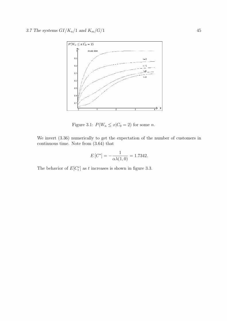
3.7 The systems GI/Kn/1 and Km/G/1 45
Figure 3.1: P (Wn ≤ x|C0 = 2) for some n.
We invert (3.36) numerically to get the expectation of the number of customers incontinuous time. Note from (3.64) that
E [C∗] = − 1
αλ(1, 0)= 1.7342.
The behavior of E[C∗t ] as t increases is shown in figure 3.3.
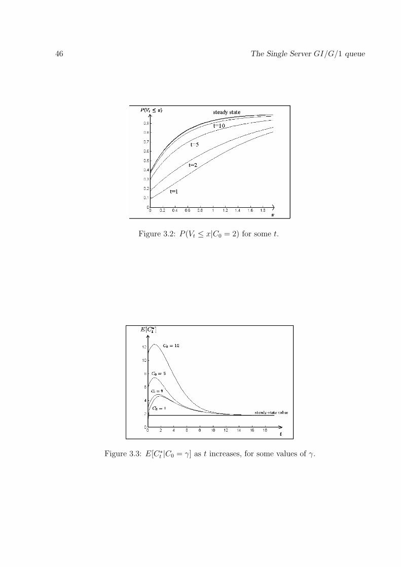
46 The Single Server GI/G/1 queue
Figure 3.2: P (Vt ≤ x|C0 = 2) for some t.
Figure 3.3: E[C∗t |C0 = γ] as t increases, for some values of γ.
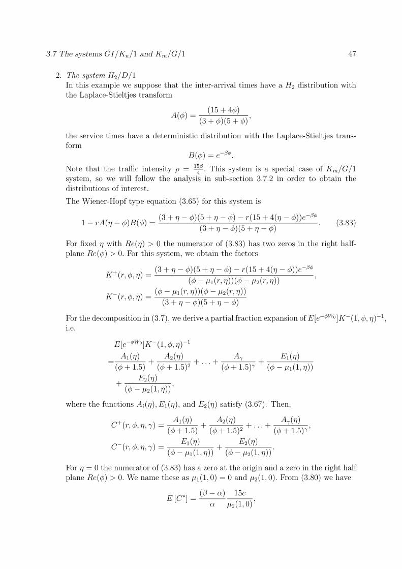
3.7 The systems GI/Kn/1 and Km/G/1 47
2. The system H2/D/1In this example we suppose that the inter-arrival times have a H2 distribution withthe Laplace-Stieltjes transform
A(φ) =(15 + 4φ)
(3 + φ)(5 + φ),
the service times have a deterministic distribution with the Laplace-Stieltjes trans-form
B(φ) = e−βφ.
Note that the traffic intensity ρ = 15β4
. This system is a special case of Km/G/1system, so we will follow the analysis in sub-section 3.7.2 in order to obtain thedistributions of interest.
The Wiener-Hopf type equation (3.65) for this system is
1 − rA(η − φ)B(φ) =(3 + η − φ)(5 + η − φ) − r(15 + 4(η − φ))e−βφ
(3 + η − φ)(5 + η − φ). (3.83)
For fixed η with Re(η) > 0 the numerator of (3.83) has two zeros in the right half-plane Re(φ) > 0. For this system, we obtain the factors
K+(r, φ, η) =(3 + η − φ)(5 + η − φ) − r(15 + 4(η − φ))e−βφ
(φ − µ1(r, η))(φ − µ2(r, η)),
K−(r, φ, η) =(φ − µ1(r, η))(φ − µ2(r, η))
(3 + η − φ)(5 + η − φ)
For the decomposition in (3.7), we derive a partial fraction expansion of E[e−φW0 ]K−(1, φ, η)−1,i.e.
E[e−φW0 ]K−(1, φ, η)−1
=A1(η)
(φ + 1.5)+
A2(η)
(φ + 1.5)2+ . . . +
Aγ
(φ + 1.5)γ+
E1(η)
(φ − µ1(1, η))
+E2(η)
(φ − µ2(1, η)),
where the functions Ai(η), E1(η), and E2(η) satisfy (3.67). Then,
C+(r, φ, η, γ) =A1(η)
(φ + 1.5)+
A2(η)
(φ + 1.5)2+ . . . +
Aγ(η)
(φ + 1.5)γ,
C−(r, φ, η, γ) =E1(η)
(φ − µ1(1, η))+
E2(η)
(φ − µ2(1, η)).
For η = 0 the numerator of (3.83) has a zero at the origin and a zero in the right halfplane Re(φ) > 0. We name these as µ1(1, 0) = 0 and µ2(1, 0). From (3.80) we have
E [C∗] =(β − α)
α
15c
µ2(1, 0),
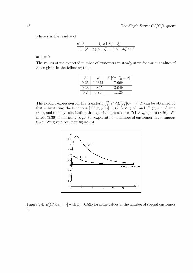
48 The Single Server GI/G/1 queue
where c is the residue of
e−βξ
ξ
(µ2(1, 0) − ξ)
(3 − ξ)(5 − ξ) − (15 − 4ξ)e−βξ
at ξ = 0.
The values of the expected number of customers in steady state for various values ofβ are given in the following table.
β ρ E [C∗|C0 = 2]0.25 0.9375 7.9690.23 0.825 3.0490.2 0.75 1.125
The explicit expression for the transform∫∞
0e−ηtE[C∗
t |C0 = γ]dt can be obtained byfirst substituting the functions [K+(r, φ, η)]−1, C+(r, φ, η, γ), and C−(r, 0, η, γ) into(3.9), and then by substituting the explicit expression for Z(1, φ, η, γ) into (3.36). Weinvert (3.36) numerically to get the expectation of number of customers in continuoustime. We give a result in figure 3.4.
Figure 3.4: E[C∗t |C0 = γ] with ρ = 0.825 for some values of the number of special customers
γ.
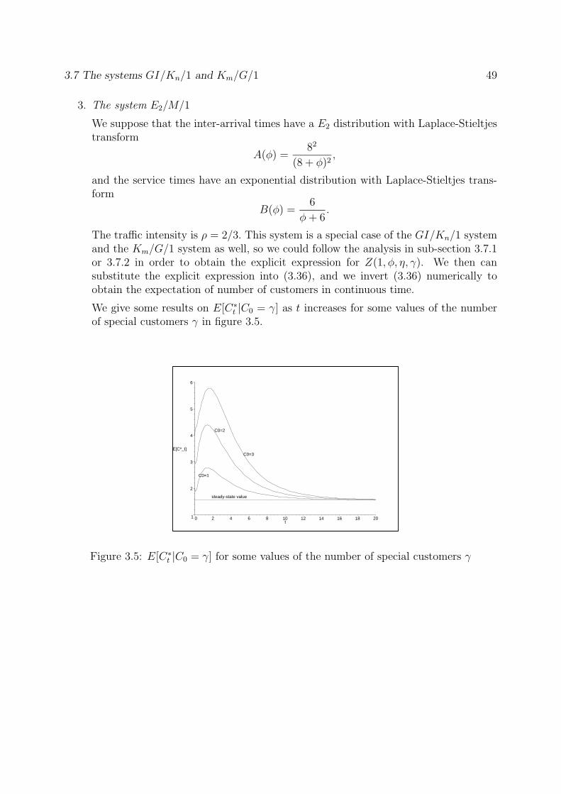
3.7 The systems GI/Kn/1 and Km/G/1 49
3. The system E2/M/1
We suppose that the inter-arrival times have a E2 distribution with Laplace-Stieltjestransform
A(φ) =82
(8 + φ)2,
and the service times have an exponential distribution with Laplace-Stieltjes trans-form
B(φ) =6
φ + 6.
The traffic intensity is ρ = 2/3. This system is a special case of the GI/Kn/1 systemand the Km/G/1 system as well, so we could follow the analysis in sub-section 3.7.1or 3.7.2 in order to obtain the explicit expression for Z(1, φ, η, γ). We then cansubstitute the explicit expression into (3.36), and we invert (3.36) numerically toobtain the expectation of number of customers in continuous time.
We give some results on E[C∗t |C0 = γ] as t increases for some values of the number
of special customers γ in figure 3.5.
C0=2
C0=1
steady-state value
C0=3
1
2
3
4
5
6
E[C*_t]
0 2 4 6 8 10 12 14 16 18 20t
Figure 3.5: E[C∗t |C0 = γ] for some values of the number of special customers γ
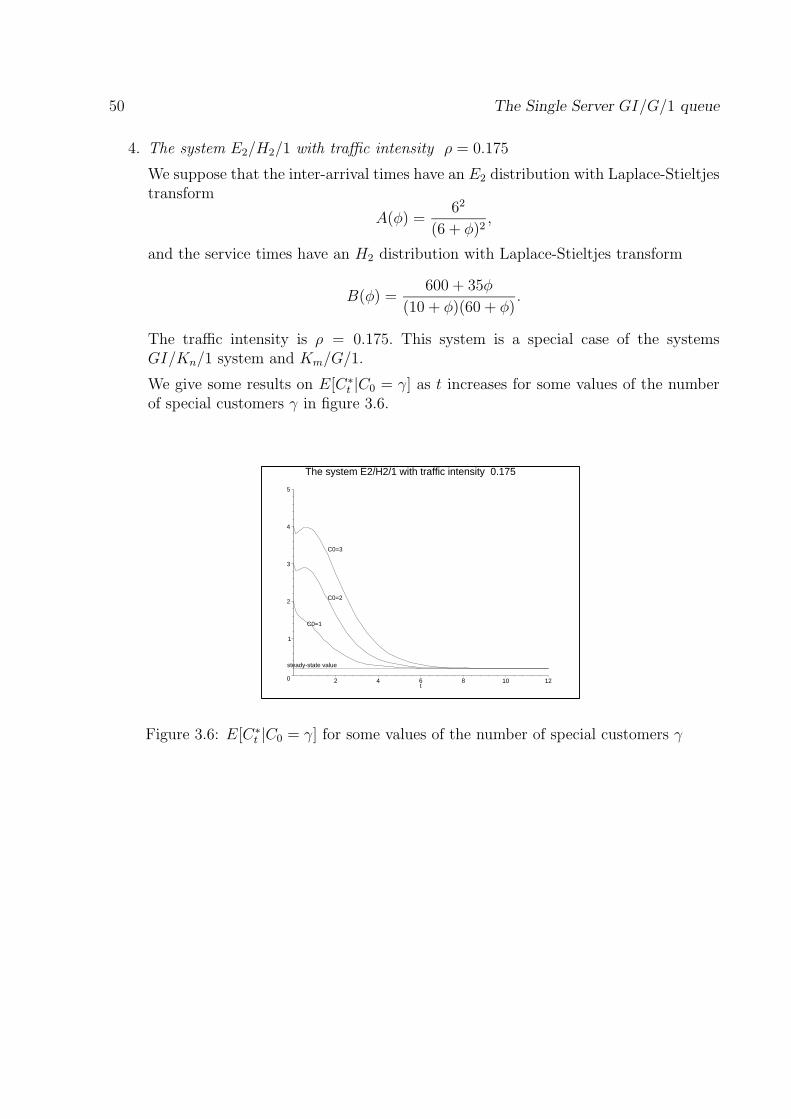
50 The Single Server GI/G/1 queue
4. The system E2/H2/1 with traffic intensity ρ = 0.175
We suppose that the inter-arrival times have an E2 distribution with Laplace-Stieltjestransform
A(φ) =62
(6 + φ)2,
and the service times have an H2 distribution with Laplace-Stieltjes transform
B(φ) =600 + 35φ
(10 + φ)(60 + φ).
The traffic intensity is ρ = 0.175. This system is a special case of the systemsGI/Kn/1 system and Km/G/1.
We give some results on E[C∗t |C0 = γ] as t increases for some values of the number
of special customers γ in figure 3.6.
steady-state value
C0=1
C0=2
C0=3
0
1
2
3
4
5
2 4 6 8 10 12t
The system E2/H2/1 with traffic intensity 0.175
Figure 3.6: E[C∗t |C0 = γ] for some values of the number of special customers γ
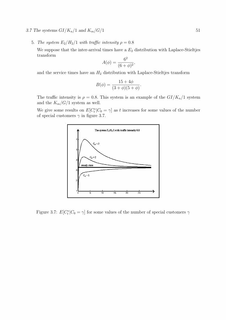
3.7 The systems GI/Kn/1 and Km/G/1 51
5. The system E2/H2/1 with traffic intensity ρ = 0.8
We suppose that the inter-arrival times have a E2 distribution with Laplace-Stieltjestransform
A(φ) =62
(6 + φ)2,
and the service times have an H2 distribution with Laplace-Stieltjes transform
B(φ) =15 + 4φ
(3 + φ)(5 + φ).
The traffic intensity is ρ = 0.8. This system is an example of the GI/Kn/1 systemand the Km/G/1 system as well.
We give some results on E[C∗t |C0 = γ] as t increases for some values of the number
of special customers γ in figure 3.7.
Figure 3.7: E[C∗t |C0 = γ] for some values of the number of special customers γ
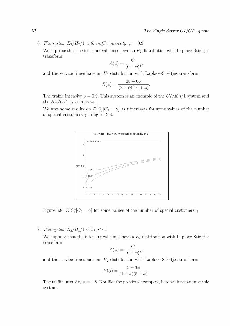
52 The Single Server GI/G/1 queue
6. The system E2/H2/1 with traffic intensity ρ = 0.9
We suppose that the inter-arrival times have an E2 distribution with Laplace-Stieltjestransform
A(φ) =62
(6 + φ)2,
and the service times have an H2 distribution with Laplace-Stieltjes transform
B(φ) =20 + 6φ
(2 + φ)(10 + φ).
The traffic intensity ρ = 0.9. This system is an example of the GI/Kn/1 system andthe Km/G/1 system as well.
We give some results on E[C∗t |C0 = γ] as t increases for some values of the number
of special customers γ in figure 3.8.
C0=2
C0=3
C0=1
steady-state value
2
4
6
8
10
E[C*_t]
0 2 4 6 8 10 12 14 16 18 20 22 24 26 28 30 32t
The system E2/H2/1 with traffic intensity 0.9
Figure 3.8: E[C∗t |C0 = γ] for some values of the number of special customers γ
7. The system E2/H2/1 with ρ > 1
We suppose that the inter-arrival times have a E2 distribution with Laplace-Stieltjestransform
A(φ) =62
(6 + φ)2,
and the service times have an H2 distribution with Laplace-Stieltjes transform
B(φ) =5 + 3φ
(1 + φ)(5 + φ).
The traffic intensity ρ = 1.8. Not like the previous examples, here we have an unstablesystem.
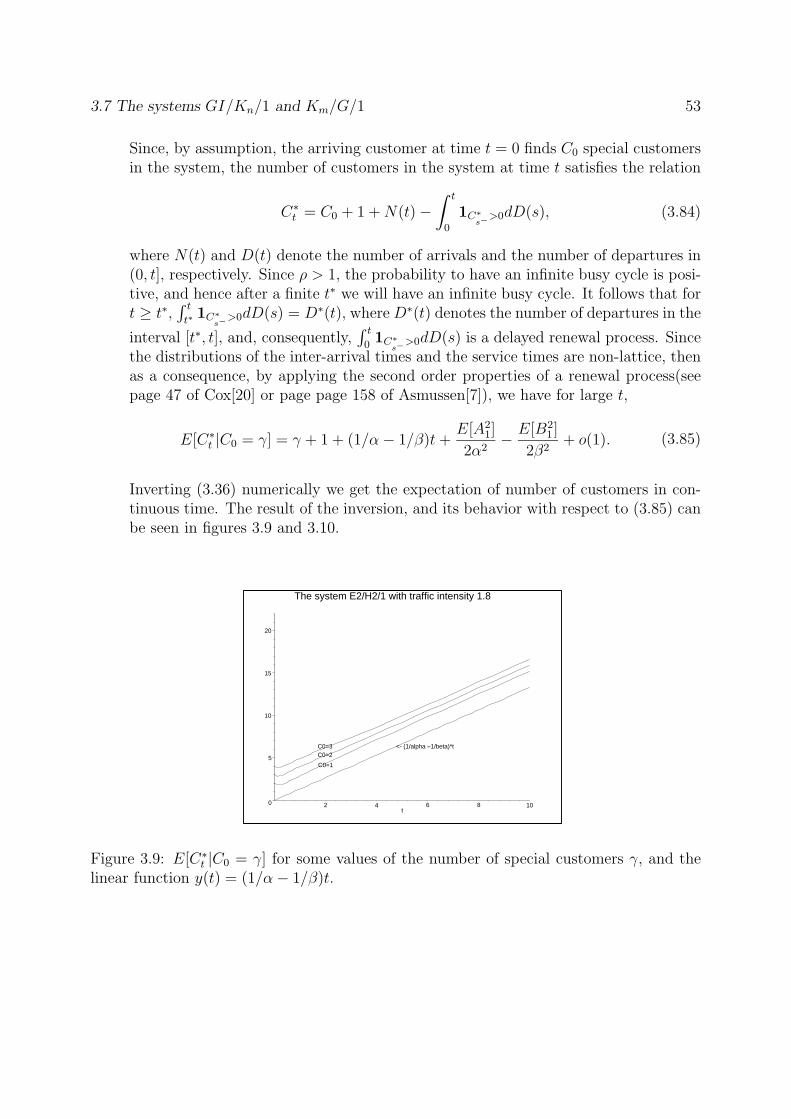
3.7 The systems GI/Kn/1 and Km/G/1 53
Since, by assumption, the arriving customer at time t = 0 finds C0 special customersin the system, the number of customers in the system at time t satisfies the relation
C∗t = C0 + 1 + N(t) −
∫ t
0
1C∗
s−>0dD(s), (3.84)
where N(t) and D(t) denote the number of arrivals and the number of departures in(0, t], respectively. Since ρ > 1, the probability to have an infinite busy cycle is posi-tive, and hence after a finite t∗ we will have an infinite busy cycle. It follows that fort ≥ t∗,
∫ t
t∗1C∗
s−>0dD(s) = D∗(t), where D∗(t) denotes the number of departures in the
interval [t∗, t], and, consequently,∫ t
01C∗
s−>0dD(s) is a delayed renewal process. Since
the distributions of the inter-arrival times and the service times are non-lattice, thenas a consequence, by applying the second order properties of a renewal process(seepage 47 of Cox[20] or page page 158 of Asmussen[7]), we have for large t,
E[C∗t |C0 = γ] = γ + 1 + (1/α − 1/β)t +
E[A21]
2α2− E[B2
1 ]
2β2+ o(1). (3.85)
Inverting (3.36) numerically we get the expectation of number of customers in con-tinuous time. The result of the inversion, and its behavior with respect to (3.85) canbe seen in figures 3.9 and 3.10.
C0=3 <- (1/alpha –1/beta)*t
C0=1
C0=2
0
5
10
15
20
2 4 6 8 10t
The system E2/H2/1 with traffic intensity 1.8
Figure 3.9: E[C∗t |C0 = γ] for some values of the number of special customers γ, and the
linear function y(t) = (1/α − 1/β)t.
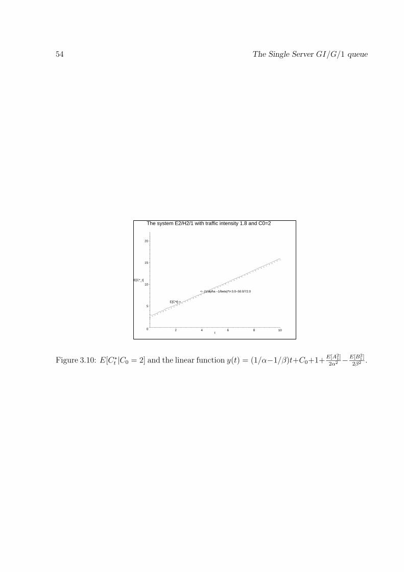
54 The Single Server GI/G/1 queue
E[C*t]->
<- (1/alpha –1/beta)*t+3.0–50.0/72.0
0
5
10
15
20
E[C*_t]
2 4 6 8 10t
The system E2/H2/1 with traffic intensity 1.8 and C0=2
Figure 3.10: E[C∗t |C0 = 2] and the linear function y(t) = (1/α−1/β)t+C0+1+
E[A21]
2α2 −E[B21 ]
2β2 .
Chapter 4
The GI/Hm/s queue
4.1 Introduction
In this chapter we consider the many server queue GI/Hm/s, which is described asfollows. Customers arrive at epochs T1, T2, . . . with T1 = 0. The customer arriving at Tn iscalled the nth customer. The inter-arrival time between the (n−1)th and the nth customeris denoted by An = Tn − Tn−1, and the service time of the nth customer is denoted byBn, n = 1, 2, . . . . There are s servers and the service discipline is first come, first served.We assume that An, n = 1, 2, . . . are i.i.d with common distribution function F and meanα, Bn, n = 1, 2, . . . are i.i.d with a common hyper-exponential distribution
G(x) =
∑mi=1 pi(1 − exp(−bix)), x ≥ 0
0, x < 0,
where∑m
i=1 pi = 1, bi > 0, bi 6= bj, i 6= j. Furthermore, we assume that the sequences An
and Bn are independent.The customer who arrives at T1 finds upon his arrival C0 other customers in the system.
We call these customers special customers, who we assume are numbered, describing theirpriority for service, from 1 up to C0. The service of (some of) the special customers hasjust begun at T1. Furthermore we assume that these customers have a common exponentialservice time with rate w, where w = bj for a fixed j, 1 ≤ j ≤ m, and its distribution functionis denoted by I(x).
Let Wn be the actual waiting time of the nth customer and Wn,i, i = 1, 2, . . . , s, theservice backlog or workload of the ith server just before the arrival of the nth customer,i.e., if the nth and subsequent customers would not enter the system then the ith serverwould become idle at time Tn + Wn,i. Since the queue discipline is first come, first served,we may assume that in front of each server there is a separate queue and that an arrivingcustomer joins the queue of the server with the smallest workload. In the case when thereare several servers with smallest workload, the arriving customer will select one of them atrandom. We also assume that this discipline holds for the special customers. Hence,
Wn = min1≤i≤s
Wn,i, n = 1, 2, . . . .
55
56 The GI/Hm/s queue
The study of this type of queue for C0 = 0 has been done by de Smit [21, 22, 23]. In[21], using the Wiener-Hopf factorization method, the author studied some distributions ofinterest, such as the actual waiting time Wn, the queue length at server i at time Tn−, thenumber of customers in the system at time Tn−, and the number of customers in the systemduring the kth busy period. All the distributions are given in terms of Laplace-Stieltjestransforms.
In [23], the investigation in [21] is extended to the study of the system in continuoustime. The results are expressions for the distributions of the virtual waiting time and thelength of the busy period.
A numerical solution for the system GI/H2/s has been studied in [22]. The study isbased on the Laplace-Stieltjes transforms of the distributions of interest derived in [21] and[23]. A numerical inversion algorithm is given, and some examples in this paper show thatthe algorithm has been successfully implemented to obtain good results.
In this chapter we try to extend the analysis in the papers mentioned above by assuminga non-zero initial number of customers. We are interested in those distributions, whichfor C0 = 0 have been studied in [21] and [23], such as the distribution of actual waitingtimes, the distribution of virtual waiting times, the queue length distribution, and thedistribution of the total number of customers. We consider the Markov process
(Wn, Tn,Xn), n = 1, 2, . . .,
where Xn is the phase vector at Tn−, which will be defined in the next section. Werefer to the derivation in [23] to obtain the system of Wiener-Hopf equations of the jointdistribution of Wn, Tn and Xn. The system of equations we derive here is a generalizationof what has been obtained in [21]. We solve this system of equations by first factorizing itssymbol, and then decomposing a certain vector. We then obtain an explicit expression forthe transform of the joint distribution of (Wn, Tn,Xn), n = 1, 2, · · · , which directly givesus the generating function of the waiting time of nth customer. The limiting distributionof the waiting time can be obtain by applying Abel’s limit theorem, and the distributionof the waiting time of nth customer can be obtained by inverting the generating functionnumerically.
The transforms of the virtual waiting time, the queue length , and the total numberof customers can be derived from the transform of of joint distribution of (Wn, Tn,Xn),n = 1, 2, · · · . We show in sections 4.7, 4.8, 4.9 and 4.10, how the expressions for thetransforms depend on the initial number of customers. The steady-state distributions ofthe distributions can be derived by applying Abel’s limit theorem, and the time-dependentdistributions can be obtained by inverting the transforms numerically. We apply the nu-merical inversion algorithm proposed in [3], and the results of the inversion can be foundin section 4.11.
This chapter is organized as follow. In section 4.2 we recall some definitions and nota-tions from [21]. In section 4.3 we derive the system of Wiener-Hopf equations, and thenwork out the factorization and the decomposition. The explicit expression for the Laplace-Stieltjes transform of the distribution of the actual waiting time can be found in section4.5, and for the virtual waiting times can be found in section 4.6. The study of the dis-tribution of the queue length at arrival epochs is done in section 4.7 and the distribution
4.2 Notations and definitions 57
of total number of customers at arrival epochs is given in section 4.8. For the system incontinuous time, the distributions of the queue length and the total number of customersare studied in section 4.9 and 4.10, respectively. Finally in section 4.11 some numericalexamples for those distributions are given.
4.2 Notations and definitions
We denote the Laplace-Stieltjes transform of F by A(φ), i.e.,
A(φ) =
∫ ∞
0
e−φxdF (x), Re(φ) ≥ 0.
The mean of service time is denoted by β, thus
β =m∑
i=1
pi
bi
.
The relative traffic intensity ρ is defined by
ρ =β
αs.
Suppose that x = (x1, . . . , xm) and y = (y1, . . . , ym) are two arbitrary m− dimensionalvectors. The inner product of vectors x and y is denoted by xy = x1y1 + . . . + xmym. Wewrite x ≤ y if x1 ≤ y1, · · · , xm ≤ ym. The vector (x1, . . . , xi ± 1, xi+1, . . . , xm) is denotedby x ± 1i and vector (x1 ± y1, . . . , xm ± ym) by x ± y.
Let Rkm be the class of m-dimensional vectors which have nonnegative integer compo-
nents and for which x1 = x1 + · · ·+xm = k. Rkm contains
(m + k − 1
k
)elements, see page
36 of Feller[26]. For brevity, we shall write c(k) instead of
(m + k − 1
k
).
δij is the Kronecker delta, i.e. δij = 0, i 6= j, δjj = 1. 1(A) is the indicator function ofthe event A. For real a we denote a+ = max(0, a) and a− = min(0, a).
If M is an m×n−dimensional matrix, we denote by Mx the xth column of M, and byMx the xth row of M.
We defineUn,i = Wn,i − Wn, i = 1, . . . , s.
Note that an arriving customer joins the queue with smallest workload, we see that Un,i,if non-zero, is the remaining service time at Tn + Wn of the last customer who joinedthe queue of server i before Tn. If this customer is of type j, this remaining service timeis exponentially distributed with parameter bj. We then say that at time Tn− server iis in phase j. Let Xn,i be the number of servers that at Tn− are in phase i; the vectorXn = (Xn,1, . . . , Xn,m) is called the phase vector of the system at time Tn− and we seethat Xn ∈ ⋃s−1
k=0 Rkm. Given Xn, those Un,i that are strictly positive and Wn are mutually
independent, and (Wn, Tn,Xn), n = 1, 2, . . . is a vector Markov process.
58 The GI/Hm/s queue
Let X∗n be the phase vector at time Tn, i.e. X∗
n = Xn +1i if the nth customer is of typei. Observe that X∗
n ∈ ⋃sk=1 Rk
m. Let us define
Vn = min(2)(Un,1, . . . , Un,s, Bn),
where min(2)(x1, . . . , xk) is the smallest but one element of (x1, . . . , xk). Let Yn be thephase vector corresponding to (Un,1, . . . , Un,s, Bn) that are not equal to 0 or Vn. If X∗
n = xwith x1 < s then Vn = Wn = 0 and Yn = x; if X∗
n = x with x1 = s it follows from Lemma1 of Appendix 1 in de Smit [21] that Yn = x − 1j with probability xjbj/xb.
For readability, in this chapter we write all vectors and matrices in bold or with baraccent.
4.3 Wiener-Hopf factorization
In this section we will derive the system of Wiener-Hopf equations governing theLaplace-Stieltjes transform of the joint distribution of Wn, Tn, and Xn. To obtain a so-lution for this system we use Wiener-Hopf factorization and a decomposition.
We recall that the first customer upon his arrival finds C0 other customers in the system.There are two possible cases for C0 to be considered.
1. C0 < s.This means that at T1 at least one server is idle so that W1 = 0, and we assumeX1 = (x1, . . . , xm). It is clear that for this case X1 ∈
⋃s−1k=0 Rk
m.
2. C0 ≥ s.This means that at T1 all servers are busy so that W1 > 0. Since by assumptionthe service times of the special customers are i.i.d and have a common exponentialdistribution with rate w, the distribution of W1 will be the convolution of exponentialdistributions with rate w. To illustrate this, let us consider the example described byfigure 4.1.
In this example, we denote by Bi the service time of the ith special customer. Wesee that
E(exp(−φW1)) =
(w
φ + w
)2
,
andX1,j = 4,
noting that w = bj.
In general, our assumption on the service times of the special customers leads to thefollowing condition.
Condition 4.3.1For Re(φ) ≥ 0,
E(exp(−φW1)) =
(w
φ + w
)a
,
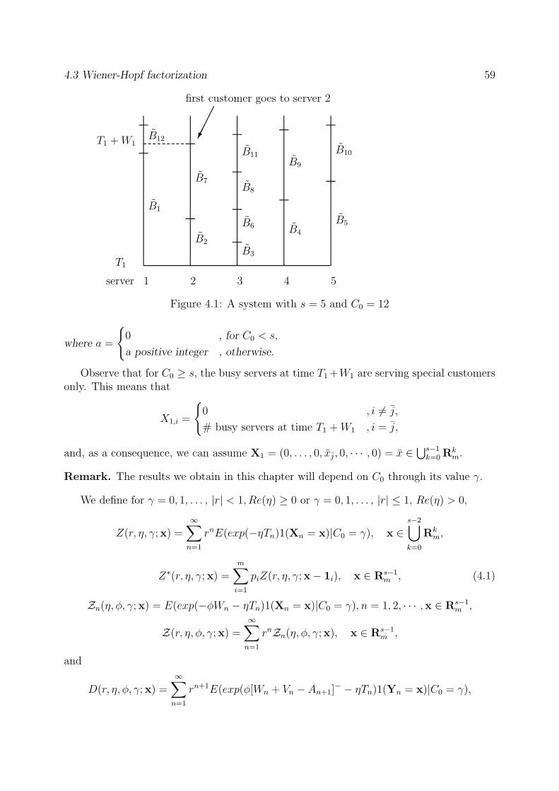
4.3 Wiener-Hopf factorization 59
B1
B12
B2
B7
first customer goes to server 2
B3
B6
B8
B11
B4
B9
B5
B10
server 1 2 3 4 5
T1
T1 + W1
Figure 4.1: A system with s = 5 and C0 = 12
where a =
0 , for C0 < s,
a positive integer , otherwise.
Observe that for C0 ≥ s, the busy servers at time T1 +W1 are serving special customersonly. This means that
X1,i =
0 , i 6= j,
# busy servers at time T1 + W1 , i = j,
and, as a consequence, we can assume X1 = (0, . . . , 0, xj, 0, · · · , 0) = x ∈ ⋃s−1k=0 Rk
m.
Remark. The results we obtain in this chapter will depend on C0 through its value γ.
We define for γ = 0, 1, . . . , |r| < 1, Re(η) ≥ 0 or γ = 0, 1, . . . , |r| ≤ 1, Re(η) > 0,
Z(r, η, γ;x) =∞∑
n=1
rnE(exp(−ηTn)1(Xn = x)|C0 = γ), x ∈s−2⋃
k=0
Rkm,
Z∗(r, η, γ;x) =m∑
i=1
piZ(r, η, γ;x − 1i), x ∈ Rs−1m , (4.1)
Zn(η, φ, γ;x) = E(exp(−φWn − ηTn)1(Xn = x)|C0 = γ), n = 1, 2, · · · ,x ∈ Rs−1m ,
Z(r, η, φ, γ;x) =∞∑
n=1
rnZn(η, φ, γ;x), x ∈ Rs−1m ,
and
D(r, η, φ, γ;x) =∞∑
n=1
rn+1E(exp(φ[Wn + Vn − An+1]− − ηTn)1(Yn = x)|C0 = γ),
60 The GI/Hm/s queue
x ∈ Rs−1m , Re(φ) ≥ 0.
With the assumptions on X1 and W1 we obtain the system of Wiener-Hopf equationsgiven in the following theorem. This is a generalization of Theorem 2.1 in de Smit[21].
Let (x
y; z
)=
m∏
i=1
xi!
yi!zi!(xi − yi − zi)!
and let b = (b1, b2, · · · , bm).
Theorem 4.3.1For x = (x1, . . . , xm) ∈ Rk
m, k = 0, 1, . . . , s − 2;
Z(r, η, γ;x)
= rm∏
i=1
δxi,xi+ rA(η + xb)
m∑
i=1
piZ(r, η, γ;x − 1i)
+s−2∑
l=k+1
∑
y∈Rlm
∑
ννν≤y−x
(y
x;ννν
)(−1)ννν1rA(η + xb + νb)
m∑
i=1
piZ(r, η, γ;y − 1i)
+∑
y∈Rs−1m
∑
ννν≤y−x
(y
x;ννν
)(−1)ννν1D(r, η,xb + νb, γ;y),
(4.2)
and for x ∈ Rs−1m , Re(φ) = 0,
Z(r, η, φ, γ;x)
[1 − r
m∑
j=1
pj(xj + 1)bj
φ + xb + bj
A(η − φ)
]
= rA(η − φ)m∑
i=1
piZ(r, η, γ;x − 1i)
+ rA(η − φ)m∑
j=1
m∑
i=1,i6=j
piZ(r, η, φ, γ;x + 1j − 1i)(xj + 1)bj
φ + xb + bj
+ rZ1(φ, γ;x) + Z(r, η, 0, γ;x) − D(r, η,−φ, γ;x),
(4.3)
while for x ∈ Rs−1m ,
Z(r, η, 0, γ;x) = D(r, η,xb, γ;x), (4.4)
and the vector Z1(φ, γ), by letting X1 = (x1, . . . , xm), has elements
Z1(φ, γ;x) =
0 , if γ < s − 1,∏mi=1 δxi,xi
, if γ = s − 1,∏m
i=1 δxi,xi
(w
φ+w
)a
, if γ ≥ s,
where a is a positive integer less than s, as described in Condition 4.3.1.
4.3 Wiener-Hopf factorization 61
Proof. We can follow the proof of Theorem 2.1 in de Smit [21] to obtain the equations(4.2), (4.3) and (4.4). It remains to determine the expression for Z1(φ, γ;x), x ∈ Rs−1
m .For x ∈ Rs−1
m ,
Z1(φ, γ;x) = E(exp(−φW1)1(X1 = x)|C0 = γ).
For γ = 0, X1 ∈ ⋃s−2k=0 Rk
m so that 1(X1 = x) = 0. It follows that Z1(φ, γ;x) = 0, so thatfor γ = 0 the equation (4.3) is precisely the same as the equation (2.2) in de Smit[23]. Forγ = s − 1, W1 = 0 so that Z1(φ, γ;x) = 1 if and only if x = X1. For γ ≥ s, we use the
condition 4.3.1 so that Z1(φ, γ;x) =∏m
i=1 δxi,xi
(w
φ+w
)a
.
Define the c(s − 1) × c(s − 1)-dimensional matrix H(r, η, φ) with elementsHx,y(r, η, φ),x,y ∈ Rs−1
m , as
Hx,x(r, η, φ) = 1 − rA(η − φ)m∑
j=1
pj(xj + 1)bj
φ + xb + bj
Hx,x+1j−1i(r, η, φ) = −rA(η − φ)pi
(xj + 1)bj
φ + xb + bj
, i 6= j, xi > 0,
Hx,y(r, η, φ) = 0, otherwise.
(4.5)
Let Z(r, η, φ, γ), D(r, η, φ, γ),Z∗(r, η, γ) and Z1(φ, γ) be the c(s − 1)−dimensional columnvectors with elements Z(r, η, φ, γ;x),D(r, η, φ, γ;x), Z∗(r, η, γ;x) and Z1(φ, γ;x) respec-tively. Equation (4.3) can then be written in the matrix form:
H(r, η, φ)Z(r, η, φ, γ)
=rA(η − φ)Z∗(r, η, γ) + rZ1(φ, γ) + Z(r, η, 0, γ) − D(r, η,−φ, γ).(4.6)
The system (4.6) can be solved by factorizing its symbol H(r, η, φ) and then decomposingthe vector rH−1(r, η, φ)Z1(φ, γ). The factorization is similar to the one in [21]. The resultis given in Theorem 4.3.3, and after that we discuss the decomposition. First, we recall atheorem from [21] that is needed for the factorization.
Theorem 4.3.2Let N(r, η) be the total order of the zeros of detH(r, η, φ) in the left half-plane
Re(φ) < 0. If 0 < |r| < 1 and Re(η) ≥ 0, or 0 < |r| ≤ 1 and Re(η) > 0, or r = 1, η = 0and ρ < 1 and if some conditions on H(r, η, φ) are satisfied, then N(r, η) = c(s). For|r| < 1 detH(r, η, φ) 6= 0 on Re(φ) = 0; for ρ < 1 detH(1, η, φ) has a simple zero at φ = 0and has no zero elsewhere on the imaginary axis.
Proof. See [21].
We denote the zeros of detH(r, η, φ) in the left half-plane Re(φ) < 0 by µx(r, η),x ∈ Rs
m. These zeros are continuous functions of r in [0, 1]. We impose the followingcondition.
62 The GI/Hm/s queue
Condition 4.3.2For (|r| < 1, Re(η) ≥ 0) or (|r| ≤ 1, Re(η) > 0), all zeros µx(r, η) are of order 1.
This condition and the conditions mentioned in the Theorem 4.3.2 are almost alwayssatisfied (see [21] for more explanation).
For y ∈ Rsm let By be a non-zero c(s − 1)−dimensional column vector satisfying
H(r, η, µy(r, η))By = 0, (4.7)
and let B be the c(s − 1) × c(s)−dimensional matrix whose column vectors are the By.Moreover we introduce the following matrices:
the c(s) × c(s)−dimensional matrix L with elements
Lx,y =∑
i|xi>0
piBx−1i,y1
µy(r, η) + xb, x ∈ Rs
m,y ∈ Rsm;
the c(s) × c(s − 1)−dimensional matrix M with elements
Mx,y =m∑
i=1
piδx,y+1i, x ∈ Rs
m,y ∈ Rs−1m ;
the c(s) × c(s)−dimensional matrix J(η, φ) with elements
Jx,x(η, φ) =1
φ − µx(r, η), x ∈ Rs
m,
Jx,y(η, φ) = 0, x ∈ Rsm,y ∈ Rs
m,x 6= y;
and the c(s − 1) × c(s − 1)−identity matrix I.
We shall assume that the following condition holds.
Condition 4.3.3detL 6= 0.
If Condition 4.3.3 holds the c(s)× c(s−1)−dimensional matrix C is determined by theset of linear equations
LC = M. (4.8)
Note that the matrices B,L, and C depend on r and η. For notational convenience, wesuppress this dependence. We define the c(s−1)× c(s−1) dimensional matrices K(r, η, φ)and H−(r, η, φ) by
K(r, η, φ) = I + BJ(η, φ)C, (4.9)
and
H−(r, η, φ) = H(r, η, φ)K(r, η, φ) = H(r, η, φ) + H(r, η, φ)BJ(η, φ)C. (4.10)
The following theorem gives the factors of matrix H(r, η, φ), which exist if a numberof conditions hold. de Smit [21] argues that these conditions are almost always satisfiedand their exclusion does not cause any serious practical restriction, because they can beapproximated arbitrarily closely by cases for which the conditions are satisfied.
4.3 Wiener-Hopf factorization 63
Theorem 4.3.3If conditions 4.3.2 and 4.3.3 and other conditions on detH(r, φ) hold then
1.
detK(r, η, φ) =∏
x∈Rsm
(φ + xb
φ − µx(r, η)
),
detH−(r, η, φ) is bounded away from 0 for Re(φ) ≤ 0;
2. For Re(φ) = 0,
H(r, η, φ) = H−(r, η, φ)H+(r, η, φ)
where H+(r, φ, η) = K(r, η, φ)−1 satisfies property A+ and is non-singular inRe(φ) > 0, and H−(r, φ, η) satisfies property A− and is non-singular in Re(φ) < 0.
Proof. See [21].
With the factorization above we can write (4.6), for Re(φ) = 0, as
H+(r, η, φ)Z(r, η, φ, γ) =H−(r, η, φ)−1[rA(η − φ)Z∗(r, η, γ) + Z(r, η, 0, γ)]
+ H−(r, η, φ)−1[−D(r, η,−φ, γ) + rZ1(φ, γ)].(4.11)
From Theorem 4.3.3 we see that H−(r, η, φ)−1 satisfies A+. Moreover, from the expressionfor Z1(φ, γ) in Theorem 4.3.1 we see that for γ < s, the vector Z1(φ, γ) has the same prop-erty as H−(r, η, φ)−1. It follows that the vector rH−(r, η, φ)−1Z1(φ, γ) in (4.11) satisfiesA+. For γ ≥ s, Z1(φ, γ) does not satisfy A−, so that we have to decompose the vec-tor rH−(r, η, φ)−1Z1(φ, γ), i.e. we need to determine c(s − 1)-dimensional column vectorsZ+
1 (r, η, φ, γ) and Z−1 (r, η, φ, γ) with elements Z+
1 (r, η, φ, γ;x) and Z−1 (r, η, φ, γ;x),x ∈
Rs−1m , respectively, such that
rH−(r, η, φ)−1Z1(φ, γ) = Z+1 (r, η, φ, γ) + Z−
1 (r, η, φ, γ), (4.12)
where Z+1 (r, η, φ, γ) satisfies A+ and Z−
1 (r, η, φ, γ) satisfies A−.Although the decomposition is needed only for the case (γ ≥ s and X1 ∈ Rs−1
m ), in thefollowing we give the expressions for Z+
1 (r, η, φ, γ) and Z−1 (r, η, φ, γ) for all cases, in order
to formulate the general solution for (4.6).Notice that for γ ≥ s − 1, the elements Z1(φ, γ; x) of Z1(φ, γ) are equal to zero except
for x = x, where x is the phase vector at time T1. It follows that the ’xth’ element ofrH−(r, η, φ)−1Z1(φ, γ) for γ ≥ s − 1 is given by
rH−x,x(r, η, φ)−1Z1(φ, γ; x).
Let
h(j)(r, η) =1
j!
dj
dφjH−
x,x(r, η, φ)−1∣∣∣φ=−w
and h(0)(r, η) = H−x,x(r, η,−w)−1.
For γ < s − 1, the vector rH−(r, η, φ)−1Z1(φ, γ) is the vector zero.
64 The GI/Hm/s queue
Lemma 4.3.1For γ ≥ s and x ∈ Rs−1
m , the elements of the column vectors Z+1 (r, η, φ, γ) and
Z−1 (r, η, φ, γ) are given by
Z−1 (r, η, φ, γ;x) =
rwa
(φ + w)a
[H−
x,x(r, η, φ)−1 −a−1∑
j=0
h(j)(r, η)(φ + w)j
],
Z+1 (r, η, φ, γ;x) = rwa
a−1∑
j=0
h(j)(r, η)
(φ + w)a−j,
for γ = s − 1 and x ∈ Rs−1m ,
Z−1 (r, η, φ, γ;x) = rH−
x,x(r, η, φ)−1,
Z+1 (r, η, φ, γ;x) = 0,
and for γ < s − 1 and x ∈ Rs−1m ,
Z−1 (r, η, φ, γ;x) = 0,
Z+1 (r, η, φ, γ;x) = 0,
With the factorization given by Theorem 4.3.3 and the decomposition in Lemma 4.3.1we obtain the solution of the system (4.3) that is given in the following theorem.
Theorem 4.3.4If all conditions mentioned before hold, then for 0 < |r| < 1, Re(φ) ≥ 0,
Z(r, η, φ, γ)
=K(r, η, φ)K(r, η, 0)−1Z(r, η, 0, γ) + K(r, η, φ)[Z+1 (r, η, φ, γ) − Z+
1 (r, η, 0, γ)].(4.13)
Proof. From (4.11), (4.12) and (4.3.1) we have for Re(φ) = 0,
H+(r, η, φ)Z(r, η, φ, γ) − Z+1 (r, η, φ, γ)
=H−(r, η, φ)−1[rA(η − φ)Z∗(r, η, γ) + Z(r, η, 0, γ) − D(r, η,−φ, γ)]
+ Z−1 (r, η, φ, γ).
(4.14)
The left-hand side of (4.14) satisfies A+; the right-hand side of (4.14) satisfies A−. Byanalytic continuation we can define an entire function that is equal to the left-hand sidefor Re(φ) ≥ 0 and equal to the right-hand side for Re(φ) ≤ 0. But this entire function isbounded and hence a constant by Liouville’s theorem. So for Re(φ) ≤ 0,
H−(r, η, φ)−1[rA(η − φ)Z∗(r, η, γ) + Z(r, η, 0, γ) − D(r, η,−φ, γ)]
+ Z−1 (r, η, φ, γ) = H+(r, η, 0)Z(r, η, 0, γ) − Z+
1 (r, η, 0, γ).(4.15)
Moreover, for Re(φ) ≥ 0,
H+(r, η, φ)Z(r, η, φ, γ) − Z+1 (r, η, φ, γ) = H+(r, η, 0)Z(r, η, 0, γ) − Z+
1 (r, η, 0, γ), (4.16)
4.3 Wiener-Hopf factorization 65
which yields
Z(r, η, φ, γ) =H+(r, η, φ)−1H+(r, η, 0)Z(r, η, 0, γ)
+ H+(r, η, φ)−1[Z+
1 (r, η, φ, γ) − Z+1 (r, η, 0, γ)
]
and using part 2 of the Theorem 4.3.3 we get (4.13). This completes the proof.
Equation (4.13) gives us an expression for Z(r, η, φ, γ) that depends on Z(r, η, 0, γ). Tofind an expression for Z(r, η, 0, γ), we let
S(r, η, φ) = H−(r, η, φ)H+(r, η, 0), Re(φ) ≤ 0.
From (4.15) we have for Re(φ) ≤ 0,
D(r, η,−φ, γ) =rA(η − φ)Z∗(r, η, γ) + Z(r, η, 0, γ) − S(r, η, φ)Z(r, η, 0, γ)
+ H−(r, η, φ)[Z−
1 (r, η, φ, γ) + Z+1 (r, η, 0, γ)
],
(4.17)
so that for x ∈ Rkm, k = 0, 1, · · · , s − 1;y ∈ Rs−1
m ,
D(r, η,xb, γ;y)
=rA(η + xb)Z∗(r, η, γ;y) + Z(r, η, 0, γ;y)
−∑
w∈Rs−1m
Sy,w(r, η,−xb)Z(r, η, 0, γ;w)
+∑
w∈Rs−1m
H−y,w(r, η,−xb)
[Z−
1 (r, η,−xb, γ;w) + Z+1 (r, η, 0, γ;w)
].
(4.18)
Choosing x = y and using (4.4) we have for y ∈ Rs−1m ,
∑
w∈Rs−1m
Sy,w(r, η,−yb)Z(r, η, 0, γ;w)
=rA(η + yb)Z∗(r, η, γ;y) + Z2(r, η,−yb, γ;y),
(4.19)
where
Z2(r, η, φ, γ;y)
=∑
w∈Rs−1m
H−y,w(r, η, φ)
[Z−
1 (r, η, φ, γ;w) + Z+1 (r, η, 0, γ;w)
],y ∈ Rs−1
m . (4.20)
Define the c(s − 1) × c(s − 1)−dimensional matrix Q(r, η) by
Qx,y(r, η) = H−x,y(r, η,−xb), x ∈ Rs−1
m ,y ∈ Rs−1m .
Condition 4.3.4For (|r| < 1, Re(η) ≥ 0) or (|r| ≤ 1, Re(η) > 0), detQ(r, η) 6= 0.
66 The GI/Hm/s queue
We assume that Condition 4.3.4 is satisfied. Let
R(r, η) = Q(r, η)H+(r, η, 0).
Then, for x ∈ Rs−1m ,
Z(r, η, 0, γ;x)
=∑
y∈Rs−1m
(R(r, η))−1x,y [rA(η + yb)Z∗(r, η, γ;y) + Z2(r, η,−yb, γ;y)] . (4.21)
If we substitute (4.21) into (4.13) we get an explicit expression for Z(r, η, φ, γ;x), x ∈ Rs−1m .
In the following, we will derive an explicit expression for Z(r, η, γ;x), x ∈ ⋃s−2k=0 Rk
m by firstdetermining expression for D(r, η,−φ, γ;x), x ∈ Rs−1
m .Define
G(r, η, φ) = (I − S(r, η, φ))R(r, η)−1,
then from (4.18) we have for Re(φ) ≤ 0,x ∈ Rs−1m ,
D(r, η,−φ, γ;x)
=rA(η − φ)Z∗(r, η, γ;x) + Z2(r, η, φ, γ;x)
+∑
y∈Rs−1m
Gx,y(r, η, φ) [rA(η + yb))Z∗(r, η − yb, γ;y) + Z2(r, η, φ, γ;y)] .(4.22)
Substitution into (4.2) yields for x ∈ Rkm, k = 0, 1, · · · , s − 2;
Z(r, η, γ;x) =s−3∑
l=(k−1)+
∑
y∈Rlm
Z(r, η, γ;y)rm∑
i=1
pic1(η;x,y + 1i)
+∑
y∈Rs−2m
Z(r, η, γ;y)rm∑
i=1
pi[c1(η;x,y + 1i) + c2(r, η;x,y + 1i)]
+ c3(r, η, γ;x),
(4.23)
where
c1(η;x,y) =∑
ν≤y−x
(y
x; ν
)(−1)ν1A(η + xb + νb)
c2(r, η;x,y) =∑
z∈Rs−1m
∑
ν≤z−x
(z
x; ν
)(−1)ν1Gz,y(r, η,−xb − νb)A(η + yb),
and
1. For γ ≥ s and X1 ∈ Rs−1m ,
c3(r, η, γ;x) =∑
z∈Rs−1m
c2(r, η,x, z)Z2(r, η,−zb, γ; z)/A(η + zb)
+∑
y∈Rs−1m
∑
ν≤y−x
(y
x; ν
)(−1)ν1Z2(r, η,−xb − νb;y),
4.3 Wiener-Hopf factorization 67
2. For γ < s − 1 or (γ ≥ s and X1 /∈ Rs−1m ), Z−
1 (r, η, φ, γ) and Z+1 (r, η, φ, γ) turn out
be zero and this implies Z2(r, η, φ, γ;y) = 0,∀y ∈ Rs−1m , so that
c3(r, η, γ;x) = r
m∏
i=1
δxi,xi,
3. For γ = s − 1, Lemma 4.3.1 implies that Z2(r, η, φ, γ;y) = r∏m
i=1 δxi,yi. Notice that
in this case X1 ∈ Rs−1m , so that r
∏mi=1 δxi,xi
= 0. We then have
c3(r, η, γ;x) =r∑
y∈Rs−1m
∑
ν≤y−x
(y
x; ν
)(−1)ν1Gy,x(r, η,−xb − νb)
+ r∑
ν≤x−x
(x
x; ν
)(−1)ν1.
Let the
(m + s − 2
s − 2
)×(
m + s − 2s − 2
)-dimensional matrix T(r, η) with elements
Tx,y(r, η), x ∈s−2⋃
k=0
Rkm, y ∈
s−2⋃
k=0
Rkm,
are defined by
Tx,y(r, η) =
r∑m
i=1 pic1(η;x,y + 1i) , for x ∈ Rkm,
y ∈ Rlm, with
(1 ≤ k ≤ s − 2;
k − 1 ≤ l ≤ s − 3)
or
k = 0; 0 ≤ l ≤ s − 3,
rm∑
i=1
pi[c1(η;x,y + 1i) + c2(r, η;x,y + 1i)] , for x ∈ Rkm,
k = 0, . . . , s − 2;
y ∈ Rs−2m ,
0 , otherwise.
Let I be the
(m + s − 2
s − 2
)×(
m + s − 2s − 2
)identity matrix, Z(r, η, γ) be the
(m + s − 2
s − 2
)-
dimensional column vector with elements Z(r, η, γ;x), x ∈ ⋃s−2k=0 Rk
m, and c3(r, η, γ) be
the
(m + s − 2
s − 2
)-dimensional column vector with elements c3(r, η;x), x ∈ ⋃s−2
k=0 Rkm. With
these definitions (4.23) becomes
(I − T(r, η))Z(r, η, γ) = c3(r, η, γ), (4.24)
68 The GI/Hm/s queue
which is a generalization of the system (3.19) in de Smit [21].
We have studied the system of equations of the time-dependent transforms Z(r, η, γ;x),x ∈ ⋃s−2
k=0 Rkm and Z(r, η, 0, γ;x),x ∈ Rs−1
m , which we derive in (4.24) and (4.21). In therest of this chapter all time-dependent probability distributions of interest are derived interms of these transforms. We need to impose the following condition in order to have anunique solution of the systems (4.24) and (4.21).
Condition 4.3.5For (|r| < 1, Re(η) ≥ 0) or (|r| ≤ 1, Re(η) > 0), det(I − T(r, η)) 6= 0.
We end this section with stating a theorem that will be used later in section 4.6. Thetheorem is a generalization to Theorem 1 in de Smit [23].
Theorem 4.3.5For γ ≥ s,X1 ∈ Rs−1
m , we have for Re(φ) ≥ 0 and Re(η) > 0
∞∑
n=1
E(exp(−φ(Wn + Vn) − ηTn)1(Yn = y)|C0 = γ)
=m∑
n=1
piZ(1, η, γ;y − 1i) +∑
x∈Rsm
(V1(1, η, γ;x)
(φ − µx(1, η))−
a∑
i=1
ai(x)V2(1, η;x)
(φ + w)a−i+1
)
.
(m∑
j=1
(yj + 1)bjLy+1j ,x
), y ∈ Rs−1
m ,
(4.25)
and
∞∑
i=1
E(exp(−φ(Wn + Vn) − ηTn)|C0 = γ)
=s−2∑
k=1
∑
y∈Rkm
m∑
i=1
piZ(1, η, γ;y − 1i)
+∑
x∈Rsm
(V1(1, η, γ;x)
(φ − µx(1, η))−
a∑
i=1
ai(η,x)V2(1, η;x)
(φ + w)a−i+1
)
.
1
A(η − µx(1, η))
∑
y∈Rs−1m
By,x
,
(4.26)
where
ai(η, x) =1
(i − 1)!lim
φ→−w
∂i−1
∂φi−1
1
(φ − µx(1, η))
=(−1)i−1
(i − 1)!(−w − µx(1, η))−i,
(4.27)
4.3 Wiener-Hopf factorization 69
and V1(r, η;x) and V2(r, η;x), x ∈ Rsm, respectively, are defined as
V1(r, η, γ;x) = [CK(r, η, 0)−1Z(r, η, 0, γ)]x − [CZ+1 (r, η, 0, γ)]x (4.28)
+V2(1, η;x)
(µx(1, η) + w)a,
V2(r, η;x) = rwa∑
v∈Rs−1m
Cx,v
[H−(r, 0,−w)−1
]v,x
, (4.29)
otherwise, we have for y ∈ Rs−1m , Re(φ) ≥ 0 and Re(η) > 0,
∞∑
n=1
E(exp(−φ(Wn + Vn) − ηTn)1(Yn = y)|C0 = γ)
=m∑
n=1
piZ(1, η, γ;y − 1i) +∑
x∈Rsm
V (1, η, γ;x)
(φ − µx(1, η))
(m∑
j=1
(yj + 1)bjLy+1j ,x
),
(4.30)
and
∞∑
i=1
E(exp(−φ(Wn + Vn) − ηTn)|C0 = γ)
=s−1∑
k=1
∑
y∈Rkm
m∑
i=1
piZ(1, η, γ;y − 1i)
+∑
x∈Rsm
V (1, η, γ;x)
(φ − µx(1, η))
1
A(η − µx(1, η))
∑
y∈Rs−1m
By,x
,
(4.31)
where Bx,y is defined in (4.7).
Proof. The proof of (4.25) and (4.26) is similar to the proof of Theorem 1 in [23] andwill be omitted. We use Theorem 16.20 in Apostol [5] for the derivation of ai(η,x).
For γ < s or (γ ≥ s and X1 /∈ Rs−1m ), by our choice of Z+
1 (r, η, φ) and Z−1 (r, η, φ) we
haveV1(1, η, γ;x)
(φ − µx(1, η))−
a∑
i=1
ai(x)V2(1, η;x)
(φ + w)a−i+1=
V (1, η, γ;x)
(φ − µx(1, η)),
where the column vector V (r, η, γ) with components V (r, η, γ,x),x ∈ Rsm is defined as
V(r, η, γ) = CK(r, η, 0)−1Z(r, η, 0, γ). (4.32)
In this case, equation (4.25) becomes equation (4.30), and equation (4.26) becomes equation(4.31).
The equations (4.30) and (4.31) are precisely the same as equations (2.4) and (2.5) inTheorem 1 in [23], where the GI/Hm/s system with γ = 0 is studied.
70 The GI/Hm/s queue
4.4 Steady state results
Before we study some distributions of interest, in this section we study the phase vectorsand some related transforms in steady state.
For ρ < 1 we define for x ∈ Rkm, k = 0, 1, · · · , s − 2;
X(x) = limn→∞
P (Xn = x)
and for x ∈ Rs−1m ,
X ∗(x) = limn→∞
m∑
i=1
piP (Xn = x − 1i)
X (φ;x) = limn→∞
E(exp(−φWn)1(Xn = x))
∆(φ;x) = limn→∞
E(exp(φ[Wn + Vn − An+1]−)1(Yn = x)).
Let X ∗, X (φ) and ∆(φ) be the c(s − 1)-dimensional column vectors with elements X ∗(x),X (φ;x), and ∆(φ;x) respectively, and write H(φ) = H(1, 0, φ),K(φ) = K(1, 0, φ). From(4.2) and
s−2∑
k=0
∑
x∈Rkm
Z(r, η, γ;x) +∑
x∈Rs−1m
Z(r, η, 0, γ;x) =r
1 − rA(η), (4.33)
we have for x ∈ Rkm, k = 0, 1, · · · , s − 2;
X(x) = limr↑1
(1 − r)Z(r, 0, 0;x) = limη↓0
(1 − A(η))Z(1, η, 0;x),
and for x ∈ Rs−1m ,
X ∗(x) = limr↑1
(1 − r)m∑
i=1
piZ(r, 0, 0;x − 1i) = limη↓0
(1 − A(η))Z(1, η, 0;x − 1i),
X (φ;x) = limr↑1
(1 − r)Z(r, 0, φ, 0;x) = limη↓0
(1 − A(η))Z(1, η, φ, 0;x),
and∆(φ;x) = lim
r↑1(1 − r)D(r, 0, φ, 0;x) = lim
η↓0(1 − A(η))D(1, η, φ, 0;x),
so that (4.6) implies
H(φ)X (φ) = A(−φ)X ∗ + X (0) − ∆(−φ).
From (4.13) we obtain the solution of (4.3) in steady state.
Theorem 4.4.1If ρ < 1 and appropriate generalizations of Conditions 3.3 - 3.6 as well as Condition
3.6’ in [21] hold for r = 1 then for Re(φ) ≥ 0,
X (φ) = K(φ)K(0)−1X (0). (4.34)
4.5 The actual waiting time 71
Proof. It is clear that
limr↑1
(1 − r)K(r, η, φ)[Z+1 (r, η, φ, 0) −Z+
1 (r, η, 0, 0)] = 0.
Then by applying Abel’s theorem into (4.13) we get (4.34).
Let X be the
(m + s − 2
s − 2
)-dimensional column vector with elements X(x), x ∈ ⋃s−2
k=0 Rkm.
Equation (4.24) becomes(I − T(1, 0))X = 0, (4.35)
and we have the normalizing condition
s−2∑
k=0
∑
x∈Rkm
X(x) +∑
x∈Rs−1m
X (0;x) = 1. (4.36)
If we apply Abel’s theorem to the function in (4.21) then we have for x ∈ Rs−1m ,
X (0;x) =∑
y∈Rs−1m
R(1, 0)−1x,yA(yb)X ∗(x). (4.37)
So that we can write (4.36) as
s−3∑
k=0
∑
x∈Rkm
X(x) +∑
x∈Rs−2m
X(x)
1 +
∑
y∈Rs−1m
m∑
i=1
piR(1, 0)−1y,x+1i
A(xb + bi)
= 1. (4.38)
We then impose the following condition.
Condition 4.4.1The matrix I − T(1, 0) has rank
(m + s − 2
s − 2
)− 1.
Since equation (4.38) is not a linear combination of the equations in the system (4.35),then, if the Condition 4.4.1 holds, system (4.35) plus the equation (4.38) has rank
(m + s − 2
s − 2
),
so that X(x),x ∈ ⋃s−2k=0 Rk
m can be obtained from (4.35) and (4.36). Moreover, X (0;x),x ∈ Rs−1
m can be obtained from equation (4.37).
4.5 The actual waiting time
In this section we derive the distribution of the actual waiting of the nth customer andthe distribution of the actual waiting time in steady state.
72 The GI/Hm/s queue
For |r| < 1, Re(φ) ≥ 0, by conditioning on the phase vector at time 0 we have
∞∑
n=1
rnE(exp(−φWn)|C0 = γ) =s−2∑
k=0
∑
x∈Rkm
Z(r, 0, γ;x) +∑
x∈Rs−1m
Z(r, 0, φ, γ;x)
=r
1 − r+∑
x∈Rs−1m
[Z(r, 0, φ, γ;x) −Z(r, 0, 0, γ;x)].
The expression for the function Z(r, 0, φ, γ;x) or Z(r, 0, 0, γ;x) can be obtained from (4.13)by setting η (and φ) equal to 0. Then by using (4.9), after some simple calculations, wehave for γ ≥ s,X1 ∈ Rs−1
m , |r| < 1, and Re(φ) ≥ 0,
∞∑
n=1
rnE(exp(−φWn)|C0 = γ)
=r
1 − r−(Z+
1 (r, 0, 0, γ))t
1 +∑
x∈Rsm
ex(r, 0, γ)φ + fx(r)
φ − µx(r, 0)
+ wa
(Z+
1 (r, 0, 0))t
1
(φ + w)a+
a∑
i=1
gi(r)
(φ + w)a−i+1,
(4.39)
where the c(s)-dimensional column vectors e(r, η, γ) and f(r) with elements ex(r, η) andfx(r), respectively, are given by
e(r, η, γ) = E(r, η)K(r, η, 0)−1Z(r, η, 0, γ) (4.40)
fx(r) =
[1
(w + µx(r, 0))a− 1
wa
]Bt
x1V2(r, 0;x), (4.41)
with the c(s) × c(s − 1)-dimensional matrix E(r, η) is defined as
Ex,y(r, η) =1
µx(r, η)Cx,y
∑
z∈Rs−1m
Bz,x, (4.42)
the l−dimensional column vector g(r) with elements gi(r) is given by
gi(r) =∑
y∈Rsm
ai(0,y)Bty1V2(r, 0;y),
where the function V2(r, 0;y) is defined in (4.29), and the function ai(η,y) is defined in(4.27).
For γ < s or (γ ≥ s,X1 /∈ Rs−1m ), it turns out that fx(r) = 0,x ∈ Rs
m, and gi(r) = 0,for i = 1, 2, · · · , l, so that the equation (4.39) becomes
∞∑
n=1
rnE(exp(−φWn)|C0 = γ) =r
1 − r+∑
x∈Rsm
ex(r, 0, γ)φ
φ − µx(r, 0), (4.43)
which for γ = 0 is identical to equation (4.1) in [21].
4.6 The virtual waiting time 73
If ρ < 1 let W be the actual waiting time in steady state. Then by applying Abel’stheorem to (4.39) or (4.43) we have for Re(φ) ≥ 0,
E(exp(−φW )) = 1 +∑
x∈Rsm
ex
φ
φ − µx
, (4.44)
where µx = µx(1, 0), and the c(s)-dimensional column vector e with elements ex is givenby e = EK(0)−1X (0), with E = E(1, 0), and X (0) is given in section 4.4. This resultcoincides with (4.3) in de Smit [21].
4.6 The virtual waiting time
Let Nt be the number of customers arriving during [0, t] and let W ∗t be the virtual
waiting time. Then
W ∗t = [WNt + VNt + TNt − t]+ . (4.45)
Since
E(exp(−φ(Wn + Vn + Tn − t))1(Nt = n)|C0 = γ)
=
∫ t
0
exp(φ(t − u))(1 − F (t − u))duE(exp(−φ(Wn + Vn))1(Tn ≤ u)|C0 = γ),
then by using (4.26) we have for γ ≥ s, X1 ∈ Rs−1m , and Re(η) > Re(φ) ≥ 0,
∫ ∞
0
exp(−ηt)E(exp(−φ(WNt + VNt + TNt − t))|C0 = γ)dt
=1 − A(η − φ)
η − φ
∞∑
n=1
E(exp(−φ(Wn + Vn) − ηTn)|C0 = γ)
=1 − A(η − φ)
η − φ
s−1∑
k=1
∑
y∈Rkm
m∑
i=1
piZ(1, η, γ;y − 1i)
+1 − A(η − φ)
η − φ
∑
x∈Rsm
(V1(1, η, γ;x)
φ − µx(1, η)−
a∑
i=1
ai(x)V2(1, η;x)
(φ + w)a−i+1
)
.
1
A(η − µx(1, η))
∑
y∈Rs−1m
By,x
.
(4.46)
Using the identity
exp(−φx+) =1
2πi
∫ i∞+0
−i∞+0
dξ
ξ
φ
φ − ξexp(−ξx), Re(φ) > Re(ξ) > 0,
74 The GI/Hm/s queue
which holds for any real x, and Theorem 16.20 in Apostol[5], we find for γ ≥ s, X1 ∈ Rs−1m ,
and Re(η) > 0, Re(ξ) ≥ 0,∫ ∞
0
exp(−ηt)E(exp(−φW ∗t )|C0 = γ)dt =
1
η+∑
x∈Rsm
nx(η, γ)φ
φ − µx(1, η)
+a∑
i=1
oi(η)φ
(φ + w)2(a−i),
(4.47)
where
nx(η) =1 − A(η − µx(1, η))
(η − µx(1, η))A(η − µx(1, η))
V1(1, η;x)
µx(1, η)
∑
y∈Rs−1m
By,x
oi(η) =
∏a−ij=1 −2(j − 1)
(a − i)!
∑
x∈Rsm
ai(x)V2(1, η;x)
A(η − µx(1, η))
∑
y∈Rs−1m
By,x
.∂a−i
∂ξa−i
(1 − A(η − ξ))
ξ(η − ξ)
∣∣∣∣∣
∣∣∣∣∣
∣∣∣∣∣ξ=−w
.
Furthermore, for γ < s or (γ ≥ s,X1 /∈ Rs−1m ), we have
∫ ∞
0
exp(−ηt)E(exp(−φW ∗t )|C0 = γ)dt =
1
η+∑
x∈Rsm
nx(η, γ)φ
φ − µx(1, η), (4.48)
where
nx(η, γ) =1 − A(η − µx(1, η))
(η − µx(1, η))A(η − µx(1, η))
V (1, η, γ;x)
µx(1, η)
∑
y∈Rs−1m
By,x
=1 − A(η − µx(1, η))
(η − µx(1, η))A(η − µx(1, η))ex(1, η, γ),
and the function ex(r, η, γ) is defined in (4.40).
For ρ < 1, let W ∗ be the virtual waiting time in steady state. Then by applying Abel’stheorem to (4.47) we obtain for Re(φ) ≥ 0,
E(exp(−φW ∗)) = 1 +∑
x∈Rsm
nx
φ
φ − µx
, (4.49)
with
nx =(A(−µx) − 1)
αµxA(−µx)
V (x)
µx
∑
y∈Rs−1m
By,x =(A(−µx) − 1)
αµxA(−µx)ex,
where the vector V with components V(x),x ∈ Rsm is given by
V = CK−1(1, 0, 0)X (0).
This result coincides with (3.4) in de Smit [23].
4.7 The queue length at arrival epochs 75
4.7 The queue length at arrival epochs
Let Qn be the number of waiting customers just before the arrival epoch Tn. To analyzeits probability distribution, we first determine the events related to the events
Qn ≤ j, n = 1, 2, · · · .
The events for γ < s are different from those for γ ≥ s. Hence, we split up the study intotwo different cases.
4.7.1 The queue length at arrival epochs for γ < s
For γ < s, let c = s−γ. Then up to Tc there is no queue in the system, and the randomvariable Qn fulfills the following expressions,
Qn ≤ j = Ω, 1 ≤ n ≤ c + j + 1,
Qc+j+1+n ≤ j = Tc+n + Wc+n < Tc+j+1+n, n = 1, 2, · · · ,
where Ω is the sure event. Since
E(qQn) = (1 − q)∞∑
j=0
qjP (Qn ≤ j), (4.50)
we have for γ < s and |r| < 1, |q| < 1,
∞∑
n=1
rnE(qQn|C0 = γ)
=∞∑
j=0
c+j+1∑
n=1
qj(1 − q)rn
+∞∑
j=0
∞∑
n=1
qj(1 − q)rc+j+1+nP (Tc+n + Wc+n < Tc+j+1+n).
(4.51)
Since G(x) is continuous, then by using the identity
1(x < 0) +1
21(x = 0) =
1
2πi
∫ i∞+0
−i∞+0
dξ
ξexp(−ξx), (4.52)
76 The GI/Hm/s queue
we rewrite (4.51) as
∞∑
n=1
rnE(qQn|C0 = γ)
=1 − q
1 − r
[r
1 − q− rc+2
1 − qr
]
+∞∑
j=0
∞∑
n=1
qj(1 − q)rc+j+1+n 1
2πi
∫ i∞+0
−i∞+0
dξ
ξAj+1(−ξ)E(exp(−ξWc+n)|C0 = γ)
=1 − q
1 − r
[r
1 − q− rc+2
1 − qr
]
+∞∑
j=0
qj(1 − q)rj+1 1
2πi
∫ i∞+0
−i∞+0
dξ
ξAj+1(−ξ)
∞∑
n=1
rnE(exp(−ξWn)|C0 = γ)
−∞∑
j=0
qj(1 − q)rj+1 1
2πi
∫ i∞+0
−i∞+0
dξ
ξAj+1(−ξ)
c∑
n=1
rnE(exp(−ξWn)|C0 = γ).
(4.53)
Since γ < s then Wn = 0, n = 1, 2, · · · , c. As a consequence, the last integral in (4.53)is equal to
∑cn=1 rn. The other integral can be analyzed by first interchanging the order
of the first summation and the integration so that the summation can be replaced by asimpler term, and then expressing the term
∑∞n=1 rnE(exp(−ξWn)|C0 = γ) in terms of
(4.43). It yields for γ < s and |r| < 1, |q| < 1,
∞∑
n=1
rnE(qQn|C0 = γ) =1 − q
1 − r
[r
1 − q− rc+2
1 − qr
]+
r2(1 − q)
(1 − r)(1 − qr)
+∑
x∈Rsm
(1 − q)rA(−µx(r, 0))ex(r, 0, γ)
1 − qrA(−µx(r, 0))
− r2(1 − rc)(1 − q)
(1 − r)(1 − qr)
=r
1 − r+∑
x∈Rsm
(1 − q)rA(−µx(r, 0))ex(r, 0, γ)
1 − qrA(−µx(r, 0)),
(4.54)
where ex(r, 0, γ) is defined in (4.40).
If ρ < 1 let Q be distributed according to the stationary queue-length distribution.Using Abel’s limit theorem it follows from (4.54) that for |q| ≤ 1,
E(qQ) = 1 +∑
x∈Rsm
ex
(1 − q)A(−µx)
1 − qA(−µx), (4.55)
where ex and µx are defined as in (4.44). Equation (4.55) coincides with (4.5) in deSmit [21].
4.7 The queue length at arrival epochs 77
The generating function of the kth moment of Qn can also be derived from (4.54). Forγ < s, the generating function of the first moment is given in the following equation,
∞∑
n=1
rnE(Qn|C0 = γ) = −∑
x∈Rsm
rA(−µx(r, 0))ex(r, 0, γ)
1 − rA(−µx(r, 0)). (4.56)
If ρ < 1 then it follows from (4.55) in the usual way that
E(Q) = −∑
x∈Rsm
ex
A(−µx)
1 − A(−µx), (4.57)
where ex and µx are defined as in (4.44).
4.7.2 The queue length at arrival epochs for γ ≥ s
For γ ≥ s, at time T1 we already find a queue, since at this epoch all servers can serveonly the first s special customers, and the rest is waiting for service. Let Wn be the waitingtime of the nth special customer. The random variable Qn satisfies the relations
Q1 ≤ j =
impossible event , for j = 0, 1, · · · , C0 − s − 1,
Ω , for j = C0 − s, C0 − s + 1, · · · ,
Q2 ≤ 0 = Tn−j−1 + Wn−j−1 < Tn,
for j = 1, 2, · · · , C0
Qn ≤ j =
WC0+n−j−1 < Tn , for n = 2, 3, · · · , j + 1,
Tn−j−1 + Wn−j−1 < Tn , for n = j + 2, j + 3, · · · ,
and for j = C0 + 1, C0 + 2, · · · ,
Qn ≤ j =
Ω , for n = 2, 3, · · · , j − C0 + 1,
WC0+n−j−1 < Tn , for n = j − C0 + 2, · · · , j + 1,
Tn−j−1 + Wn−j−1 < Tn , for n = j + 2, j + 3, · · · .
78 The GI/Hm/s queue
Since G(x) and I(x) are continuous, it follows by using the identity (4.52), that for γ ≥ sand |r| < 1, |q| < 1,
∞∑
n=1
rnE(qQn|C0 = γ)
= (1 − q)r∞∑
j=γ−s
qj + (1 − q)
γ∑
j=0
qj
∞∑
n=2
rnP (Qn ≤ j)
+ (1 − q)∞∑
j=γ+1
qj
∞∑
n=2
rnP (Qn ≤ j)
(4.58)
By exploring the events Qn ≤ j as we did above, we then obtain for γ ≥ s and |r| < 1,|q| < 1,
∞∑
n=1
rnE(qQn|C0 = γ)
= rqγ−s + (1 − q)
γ∑
j=1
qj
j+1∑
n=2
rnP (Wγ+n−j−1 < Tn)
+ (1 − q)
γ∑
j=0
qj
∞∑
n=j+2
rnP (Tn−j−1 + Wn−j−1 < Tn)
+ (1 − q)
[∞∑
j=γ+1
qj
j−γ+1∑
n=2
rn +∞∑
j=γ+1
qj
j+1∑
n=j−γ+2
rnP (Wγ+n−j−1 < Tn)
]
+ (1 − q)∞∑
j=γ+1
qj
∞∑
n=j+2
rnP (Tn−j−1 + Wn−j−1 < Tn)
= rqγ−s + (1 − q)r2
∞∑
j=γ+1
qj (1 − rj−γ)
(1 − r)
+ (1 − q)r∞∑
j=0
(qr)j 1
2πi
∫ i∞+0
−i∞+0
dξ
ξ
∞∑
n=1
rnAj+1(−ξ)E(exp(−ξWn)|C0 = γ)
+ (1 − q)
γ∑
j=1
qj 1
2πi
∫ i∞+0
−i∞+0
dξ
ξ
j+1∑
n=2
rnAn−1(−ξ)E(exp(−ξWγ+n−j−1))
+ (1 − q)r1−γ
∞∑
j=γ+1
(qr)j 1
2πi
∫ i∞+0
−i∞+0
dξ
ξ
γ∑
n=1
rnAn−γ+j(−ξ)E(exp(−ξWn)).
(4.59)
Since we assume that all the special customers have a common exponential service timewith rate w and are served first come first serve, then the departure process of the specialcustomers is a Poisson process with rate sw. It follows that for n = s + 1, s + 2, · · · , C0,
E[e−ξWn
]=
(sw
sw + ξ
)n−s
.
4.7 The queue length at arrival epochs 79
If we substitute this into (4.59) and if we express∑∞
n=1 rnE(exp(−ξWn)| C0 = γ) in termsof (4.43), by applying a contour integration we then obtain for γ ≥ s and |r| < 1, |q| < 1,
∞∑
n=1
rnE(qQn|C0 = γ)
= rqγ−s + (1 − q)r2
∞∑
j=γ+1
qj (1 − rj−γ)
(1 − r)
+r2(1 − q)
(1 − r)(1 − qr)+∑
x∈Rsm
(1 − q)rA(−µx(r, 0))ex(r, 0, γ)
1 − qrA(−µx(r, 0))
+ (1 − q)
γ+1−s∑
j=1
qj(sw)d(j − 1 , 0 )
+ (1 − q)
γ+1−s∑
j=1
qj(sw)γ+1−j−s(γ − s − j − 1)!d1(j)
+ (1 − q)r2−γ
(1 − r)
[(qr)γ−s+2 − (qr)γ+1
(1 − qr)− rs−γ(qr2)γ−s+2 − (qr2)γ+1
(1 − qr2)
]
+ (1 − q)rs−γ
γ∑
j=γ+2−s
(qr)j[(sw)s+1−γd(γ − s − 1, 0) + (sw)s+1(γ − 1)!d2(j)
]
+ (1 − q)r2−γ (1 − rs+1)
(1 − r)
(qr)γ+1
(1 − qr)+ (1 − q)r2−γ+s (1 − rγ−s−1)
(1 − r)
(qr)γ+1
(1 − qr),
(4.60)
where
d(j, ξ) =
j−1∑
n=0
(sw)j−1−n(rA(−ξ)sw)n, (4.61)
d1(j) =∂γ−s−j−1(A(−ξ)d(j − 1 , ξ)/ξ)
∂ξγ−s−j−1
∣∣∣ξ=−sw
, (4.62)
and
d2(j) =∂γ−1(As+1−γ+j(−ξ)d(γ − s + 1 , ξ)/ξ)
∂ξγ−1
∣∣∣ξ=−sw
. (4.63)
The generating function of the kth moment of Qn can also be derived from (4.60). Forγ ≥ s, the generating function of the first moment is given in the following equation. For
80 The GI/Hm/s queue
|r| < 1,
∞∑
n=1
rnE(Qn|C0 = γ) = r(γ − s) − r2
∞∑
j=γ+1
(1 − rj−γ)
1 − r− r2
(1 − r)2
+∑
x∈Rsm
rA(−µx(r, 0))ex(r, 0, γ)
1 − rA(−µx(r, 0))− (sw)
γ+1−s∑
j=1
d(j − 1, 0)
−γ+1−s∑
j=1
(sw)γ+1−j−s(γ − s − j − 1)!d1(j)
− r4−s − r3
(1 − r)2+
r6−s − r4+γ
(1 − r)(1 − r2)
− rs−γ
γ∑
j=γ+2−s
(r)j(sw)s+1−γd(γ − s − 1, 0)
− rs−γ
γ∑
j=γ+2−s
(r)j(sw)s+1(γ − 1)!d2(j)
− r3(1 − rs+1) + r3+s(1 − rγ−s−1)
(1 − r)2.
(4.64)
If ρ < 1, then from (4.64) in the usual way we can obtain the expression for E(Q),which coincides with (4.57).
4.8 The total number of customers at arrival epochs
Let Cn be the number of customers in the system just before the arrival epoch Tn. Wehave that
P (Cn = k|C0 = γ) =∑
x∈Rkm
P (Xn = x|C0 = γ), k = 0, 1, · · · , s − 2
P (Cn = s − 1|C0 = γ) =∑
x∈Rs−1m
limφ→∞
Zn(0, φ, γ;x),
P (Cn = s|C0 = γ) = P (Qn = 0|C0 = γ) −s−1∑
k=0
P (Cn = k|C0 = γ),
P (Cn = k|C0 = γ) = P (Qn = k − s|C0 = γ), k = s + 1, s + 2, · · · ;
4.8 The total number of customers at arrival epochs 81
so that we have for |r| < 1, |q| ≤ 1,
∞∑
n=1
rnE(qCn|C0 = γ) =s−2∑
k=0
(qk − qs)∑
x∈Rkm
Z(r, 0, γ;x)
+ qs−1(1 − q) limφ→∞
∑
x∈Rs−1m
Z(r, 0, φ, γ;x)
+ qs
∞∑
n=1
rnE(qQn|C0 = γ).
(4.65)
4.8.1 The total number of customers at arrival epochs for γ < s
Let 1 be the c(s − 1)-dimensional row vector with all components equal to 1. FromTheorem 4.13 and Lemma 4.3.1 it follows that
limφ→∞
∑
x∈Rs−1m
Z(r, 0, φ, γ;x) = 1K(r, 0, 0)−1Z(r, 0, 0, γ).
If we substitute this into (4.65), then by using (4.54) we obtain for C0 = γ < s,|r| < 1, |q| < 1,
∞∑
n=1
rnE(qCn|C0 = γ)
=s−2∑
k=0
(qk − qs)∑
x∈Rkm
Z(r, 0, γ;x) + qs−1(1 − q)1K(r, 0, 0)−1Z(r, 0, 0, γ)
+ qs r
1 − r+ qs
∑
x∈Rsm
(1 − q)rA(−µx(r, 0))ex(r, 0, γ)
1 − qrA(−µx(r, 0).
(4.66)
For ρ < 1, Cn weakly converges to a random variable C. Then for |q| < 1,
E(qC) =s−2∑
k=0
(qk − qs)∑
x∈Rkm
Z(x) + qs−1(1 − q)1K(0)−1X (0)
+ qs
1 +
∑
x∈Rsm
ex
(1 − q)A(−µx)
1 − qA(−µx)
,
(4.67)
where ex and µx are defined as in (4.44). The equation (4.67) coincides with (4.9) in [21].
The generating function of the kth moment of Cn can be derived from (4.66). Forγ < s, the generating function of the first moment is given by the following expression.

82 The GI/Hm/s queue
For |r| < 1,
∞∑
n=1
rnE(Cn|C0 = γ) =s−2∑
k=0
(k − s)∑
x∈Rkm
Z(r;x) − 1K−1(r, 0, 0)Z(r, 0, 0, γ)
+ sr
1 − r−∑
x∈Rsm
(rA(−µx(r, 0))ex(r, 0, γ)
1 − rA(−µx(r, 0)).
(4.68)
If ρ < 1 then we have
E(C) =s−2∑
k=0
(k − s)∑
x∈Rkm
Z(x) − 1K−1(0)X (0) + s
−∑
x∈Rsm
ex
A(−µx)
1 − A(−µx),
(4.69)
where ex and µx are defined as in (4.44).
4.8.2 The total number of customers at arrival epochs for γ ≥ s
Let 1 be the c(s − 1)-dimensional row vector with all components equal to 1. FromTheorem 4.13 and Lemma 4.3.1 it follows that
limφ→∞
∑
x∈Rs−1m
Z(r, 0, φ, γ;x) = 1K(r, 0, 0)−1Z(r, 0, 0, γ) − 1Z+1 (r, 0, 0, γ).
4.8 The total number of customers at arrival epochs 83
If we substitute this into (4.65), then by using (4.54) we obtain for γ ≥ s, |r| < 1, |q| < 1,
∞∑
n=1
rnE(qCn|C0 = γ)
=s−2∑
k=0
(qk − qs)∑
x∈Rkm
Z(r, 0, γ;x) + qs−1(1 − q)1K(r, 0, 0)−1Z(r, 0, 0, γ)
+ qs−1(1 − q)1Z+1 (r, 0, 0, γ) + rqγ + (1 − q)qsr2
∞∑
j=γ+1
qj (1 − rj−γ)
1 − r
+r2(1 − q)qs
(1 − r)(1 − qr)+ qs
∑
x∈Rsm
(1 − q)rA(−µx(r, 0))ex(r, 0, γ)
1 − qrA(−µx(r, 0))
+ (1 − q)qs
γ+1−s∑
j=1
qj(sw)d(j − 1 , 0 )
+ (1 − q)qs
γ+1−s∑
j=1
qj(sw)γ+1−j−s(γ − s − j − 1)!d1(j)
+ (1 − q)qs r2−γ
(1 − r)
[(qr)γ−s+2 − (qr)γ+1
1 − qr− rs−γ(qr2)γ−s+2 − (qr2)γ+1
1 − qr2
]
+ (1 − q)qsrs−γ
γ∑
j=γ+2−s
(qr)j(sw)s+1−γd(γ − s − 1, 0)
+ (1 − q)qsrs−γ
γ∑
j=γ+2−s
(qr)j(sw)s+1(γ − 1)!d2(j)
+ (1 − q)qsr2−γ (1 − rs+1)
(1 − r)
(qr)γ+1
(1 − qr)+ (1 − q)r2−γ+s (1 − rγ−s−1)
(1 − r)
(qr)γ+1
(1 − qr),
(4.70)
where the functions d, d1, and d2 are defined in (4.61) - (4.63).
The generating function of the kth moment of Cn can be derived from (4.70). Forγ ≥ s, the generating function of the first moment is given by the following expression.
84 The GI/Hm/s queue
For |r| < 1,
∞∑
n=1
rnE(Cn|C0 = γ) =s−2∑
k=0
(k − s)∑
x∈Rkm
Z(r;x) − 1K−1(r, 0, 0)Z(r, 0, 0, γ)
− 1Z+1 (r, 0, 0, γ) + γr − r2
∞∑
j=γ+1
(1 − rj−γ)
1 − r
− r2
(1 − r)2−∑
x∈Rsm
(rA(−µx(r, 0))ex(r, 0, γ)
(1 − rA(−µx(r, 0))
−γ+1−s∑
j=1
(sw)d(j − 1, 0) + (sw)γ+1−j−s(γ − s − j − 1)!d1(j)
− r4−s − r3
(1 − r)2+
r6−s − r4+γ
(1 − r)(1 − r2)
− rs−γ
γ∑
j=γ+2−s
(r)j(sw)s+1−γd(γ − s − 1, 0)
− rs−γ
γ∑
j=γ+2−s
(r)j(sw)s+1(γ − 1)!d2(j)
− r3(1 − rs+1) + r3+s(1 − rγ−s−1)
(1 − r)2.
(4.71)
If ρ < 1 then from (4.71) in the usual way we obtain the expression for E(C), whichcoincides with (4.69).
4.9 Queue length in continuous time
Let Q∗t be the queue length at time t. Its sample functions are considered to be left
continuous. By conditioning on the number of arrivals up to time t we have for j > γ and
4.9 Queue length in continuous time 85
t > 0,
P (Q∗t ≤ j)
= P (Nt ≤ j − γ) +∞∑
n=1
P (Q∗t ≤ j,Nt = n + j − γ)
= P (Tj−γ+1 > t) +
γ∑
n=1
P (Wn < t, Tn+j−γ ≤ t < Tn+j−γ+1)
+∞∑
n=1
P (Tn + Wn < t, Tn+j ≤ t < Tn+j+1)
= 1 − P (Tj−γ+1 ≤ t) +
∫ t
0
1 − F (t − u)du
γ∑
n=1
P (Wn < t, Tn+j−γ ≤ u)
+
∫ t
0
1 − F (t − u)du
∞∑
n=1
P (Tn + Wn < t, Tn+j ≤ u).
(4.72)
Since G(x) is absolutely continuous, and we assume that the function F (x) is continuous,(4.72) becomes
P (Q∗t ≤ j) = 1 − P (Tj−γ+1 ≤ t)
+1
2πi
∫ i∞+0
−i∞+0
dξ
ξ
∫ t
0
1 − F (t − u)
.du
γ∑
n=1
E(exp(−ξ(Wn − t))1(Tn+j−γ ≤ u))
+1
2πi
∫ i∞+0
−i∞+0
dξ
ξ
∫ t
0
1 − F (t − u)
.du
∞∑
n=1
E(exp(−ξ(Tn + Wn − t))1(Tn+j ≤ u)).
(4.73)
For j = 0, we obtain
P (Q∗t = 0) =
∞∑
n=1
P (Q∗t = 0, Nt = n) =
∞∑
n=1
P (Tn + Wn < t, Tn ≤ t < Tn+1),
and for 0 < j ≤ γ,
86 The GI/Hm/s queue
P (Q∗t ≤ j)
=∞∑
n=1
P (Q∗t ≤ j,Nt = n)
=
j∑
n=1
P (Wγ−j+n < t, Tn ≤ t < Tn+1)
+∞∑
n=j+1
P (Tn−j + Wn−j < t, Tn ≤ t < Tn+1)
=
∫ t
0
1 − F (t − u)du
γ∑
n=γ−j+1
P (Wn < t, Tn−γ+j ≤ u)
+
∫ t
0
1 − F (t − u)du
∞∑
n=1
P (Tn + Wn < t, Tn+j ≤ u)
=1
2πi
∫ i∞+0
−i∞+0
dξ
ξ
∫ t
0
1 − F (t − u)du
γ∑
n=γ−j+1
E(e−ξ(Wn−t1(Tn−γ+j ≤ u))
+1
2πi
∫ i∞+0
−i∞+0
dξ
ξ
∫ t
0
1 − F (t − u)du
∞∑
n=1
E(e−ξ(Tn+Wn−t)1(Tn+j ≤ u)).
(4.74)
4.9 Queue length in continuous time 87
Since E(qQ∗t ) = (1 − q)
∑∞j=0 qjP (Q∗
t ≤ j), we have for |q| ≤ 1,
E(qQ∗t |C0 = γ)
= (1 − q)
γ∑
j=1
qj 1
2πi
∫ i∞+0
−i∞+0
dξ
ξ
∫ t
0
1 − F (t − u)
.du
γ∑
n=γ−j+1
E(e−ξ(Wn−t)1(Tn−γ+j ≤ u))
+ (1 − q)
γ∑
j=0
qj 1
2πi
∫ i∞+0
−i∞+0
dξ
ξ
∫ t
0
1 − F (t − u)
.du
∞∑
n=1
E(e−ξ(Tn+Wn−t)1(Tn+j ≤ u)|C0 = γ)
+ (1 − q)∞∑
j=γ+1
qj(1 − P (Tj−γ+1 ≤ t))
+ (1 − q)∞∑
j=γ+1
qj 1
2πi
∫ i∞+0
−i∞+0
dξ
ξ
∫ t
0
1 − F (t − u)
.du
γ∑
n=1
E(e−ξ(Wn−t)1(Tn+j−γ ≤ u))
+ (1 − q)∞∑
j=γ+1
qj 1
2πi
∫ i∞+0
−i∞+0
dξ
ξ
∫ t
0
1 − F (t − u)
.du
∞∑
n=1
E(e−ξ(Tn+Wn−t)1(Tn+j ≤ u)|C0 = γ).
(4.75)
88 The GI/Hm/s queue
4.9.1 Queue length in continuous time for γ < s
If γ < s, it is clear that Wn = 0, n = 1, 2, · · · , γ. Then from (4.75)∫ ∞
0
exp(−ηt)E(qQ∗t |C0 = γ)dt
=(1 − q)
[γ∑
j=1
qj 1 − A(η)
η
j∑
n=1
An−1(η)
+
γ∑
j=0
qj
2πi
∫ i∞+0
−i∞+0
dξ
ξ
1 − A(η − ξ)
(η − ξ)
∞∑
n=1
E(exp(−ηTn − ξWn)|C0 = γ)Aj(η − ξ)
+∞∑
j=γ+1
qj
(1
η− Aj−γ(η)
η+
(1 − A(η))
η
γ∑
n=1
An+j−γ−1(η)
+1
2πi
∫ i∞+0
−i∞+0
dξ
ξ
1 − A(η − ξ)
(η − ξ)
∞∑
n=1
E(exp(−ηTn − ξWn)|C0 = γ)Aj(η − ξ)
)].
(4.76)
From (4.33), (4.13), (4.9) and Lemma 4.3.1, we have that for γ < s,
∞∑
n=1
E(exp(−ηTn − ξWn)|C0 = γ) =1
1 − A(η)+∑
x∈Rsm
ex(1, η, γ)ξ
ξ − µx(1, η),
where ex(r, η, γ) is defined in (4.40). Substituting this into (4.76), then by applying contourintegration we obtain for γ < s, |q| ≤ 1, Re(η) > 0,
∫ ∞
0
exp(−ηt)E(qQ∗t |C0 = γ)dt
=(1 − q)
[γ∑
j=1
qj 1 − A(η)
η
j∑
n=1
An−1(η) +(1 − qγ+1Aγ+1(η))
η(1 − qA(η))
+∑
x∈Rsm
ex(1, η)(1 − A(η − µx(1, η))) (1 − qγ+1Aγ+1(η − µx(1, η)))
(η − µx(1, η))(1 − qA(η − µx(1, η)))
+∑
x∈Rsm
ex(1, η)(1 − A(η − µx(1, η))) qγ+1Aγ+1(η − µx(1, η))
(η − µx(1, η))(1 − qA(η − µx(1, η)))
+qγ+1
η(1 − q)− qγ+1A(η)
η(1 − qA(η))+
qγ+1∑γ
n=1 An(η)
η(1 − qA(η))+
qγ+1Aγ+1(η)
η(1 − qA(η))
].
(4.77)
For ρ < 1, |q| ≤ 1, let Q∗ be the queue length in continuous time in steady state. We findfrom (4.77) in the usual way
E(qQ∗
) = 1 +∑
x∈Rsm
ex
(1 − q)(1 − A(−µx))
−µx(1 − qA(−µx)), (4.78)
in accordance to equation (3.9) in [23].
4.9 Queue length in continuous time 89
4.9.2 Queue length in continuous time for γ ≥ s
If γ ≥ s, it is clear that Wn = 0 for n = 1, 2, · · · , s, and Wn > 0 for n = s + 1, · · · , γ.It follows that
γ∑
j=1
qj
∫ t
0
1 − F (t − u)du
γ∑
n=γ−j+1
P (Wn < t, Tn−γ+j ≤ u)
=
γ−s−1∑
j=1
qj
∫ t
0
1 − F (t − u)du
γ∑
n=γ−j+1
P (Wn < t, Tn−γ+j ≤ u)
+
γ∑
j=γ−s
qj
∫ t
0
1 − F (t − u)du
γ∑
n=γ−j+1
P (Tn−γ+j ≤ u),
(4.79)
and
∫ t
0
1 − F (t − u)du
γ∑
n=1
P (Wn < t, Tn−γ+j ≤ u)
=
∫ t
0
1 − F (t − u)du
s∑
n=1
P (Tn−γ+j ≤ u)
+
∫ t
0
1 − F (t − u)du
γ∑
n=s+1
P (Wn < t, Tn−γ+j ≤ u).
(4.80)
Furthermore we have from (4.33), (4.13), (4.9) and Lemma 4.3.1, that for γ ≥ s,
∞∑
n=1
E(exp(−ηTn − ξWn)|C0 = γ) =1
1 − A(η)+∑
x∈Rsm
ex(1, η, γ)ξ
(ξ − µx(1, η))
+ 1K(1, η, ξ)[Z+1 (1, η, ξ, γ) − Z+
1 (1, η, 0, γ)].
(4.81)
90 The GI/Hm/s queue
If we substitute (4.79), (4.80), and (4.81) into (4.75), then similar to the case γ < s, weobtain for γ ≥ s, |q| ≤ 1, Re(η) > 0,
∫ ∞
0
exp(−ηt)E(qQ∗t |C0 = γ)dt
=(1 − q)
[γ∑
j=γ−s
qj 1 − A(η)
η
j∑
n=1
An−1(η)
+
γ−s−1∑
j=1
qj
(1 − A(η)
η
γ∑
n=γ−j+1
(sw
sw + η
)n−s
An−γ+j−1(η)
)
+1
η(1 − qA(η))+
qγ+1
η(1 − q)− qγ+1A(η)
η(1 − qA(η))+
qγ+1∑s
n=1 An(η)
η(1 − qA(η))
+∑
x∈Rsm
ex(1, η)(1 − A(η − µx(1, η))) (1 − qγ+1Aγ+1(η − µx(1, η)))
(η − µx(1, η))(1 − qA(η − µx(1, η)))
+∑
x∈Rsm
ex(1, η)(1 − A(η − µx(1, η))) qγ+1A(η − µx(1, η))
(η − µx(1, η))(1 − qA(η − µx(1, η)))
+∞∑
j=γ+1
qj
(1 − A(η)
η
γ∑
n=s+1
(sw
sw + η
)n−s
An−γ+j−1(η)
)].
(4.82)
If ρ < 1, |q| ≤ 1, then from (4.77) in the usual way we obtain the expression for E(qQ),which coincides with (4.78).
4.10 The total number of customers in continuous
time
Let C∗t be the number of customers at time t, which we consider to be a left-continuous
process. Observe that
P (C∗t = s − 1|C0 = γ) = P (W ∗
t = 0|C0 = γ) −s−2∑
j=0
P (C∗t = l|C0 = γ), (4.83)
P (C∗t = s|C0 = γ) = P (Q∗
t = 0|C0 = γ) − P (W ∗t = 0|C0 = γ) (4.84)
P (C∗t = l|C0 = γ) = P (Q∗
t = l − s|C0 = γ), l = s + 1, s + 2, · · · . (4.85)
4.10 The total number of customers in continuous time 91
To find the P (C∗t = l|C0 = γ) for l = 0, 1, · · · , s − 2, we can use the same derivation as in
section 3.3 in [23]. It yields for γ < s, Re(η) > 0, l = 0, 1, 2, · · · , s − 2;
∫ ∞
0
exp(−ηt)P (C∗t = l|C0 = γ)dt
=∑
x∈Rlm
s−1∑
k=l
∑
y∈Rkm
∑
ν≤y−x
(y
x; ν
)(−1)ν11 − A(η + xb + νb)
η + xb + νb
.
m∑
i=1
piZ(1, η, γ;y − 1i) −∑
y∈Rs−1m
∑
ν≤y−x
(y
x; ν
)(−1)ν1
.∑
z∈Rsm
V (1, η, γ, z)
xb + νb + µz(1, η)
m∑
j=1
(yj + 1)bjLy+1j ,z
.
1 − A(η + xb + νb)
η + xb + νb− 1 − A(η − µz(1, η))
η − µz(1, η)
],
(4.86)
where the function V (1, η, z) is defined in (4.32). Moreover, for γ ≥ s, Re(η) > 0, l =0, 1, 2, · · · , s − 2;
∫ ∞
0
exp(−ηt)P (C∗t = l|C0 = γ)dt
=∑
x∈Rlm
s−1∑
k=l
∑
y∈Rkm
∑
ν≤y−x
(y
x; ν
)(−1)ν11 − A(η + xb + νb)
η + xb + νb
.
m∑
i=1
piZ(1, η, γ;y − 1i) −∑
y∈Rs−1m
∑
ν≤y−x
(y
x; ν
)(−1)ν1
m∑
j=1
(yj + 1)bjLy+1j ,z
.
∑
z∈Rsm
(V1(1, η, γ, z)
−xb − νb − µz(1, η)−
a∑
i=1
ai(x)V2(1, η;x)
(−xb − νb + w)a−i+1
)
.(1 − A(η + xb + νb))
(η + xb + νb)+∑
z∈Rsm
(xb + νb)
µz(1, η)(xb + νb + µz(1, η))
.(1 − A(η − µz(1, η)))
η − µz(1, η)V1(1, η, γ; z) +
∑
z∈Rsm
a∑
i=1
(xb + νb)ai(z)V2(1, η; z)
.1
(i − 1)!lim
ξ→−w
∂i−1
∂ξi−1
(1 − A(η − ξ))
ξ(xb + νb + ξ)(η − ξ)
)].
(4.87)
An inversion of the transforms (4.86) and (4.87) will yield P (C∗t = l|C0 = γ) for l =
0, 1, · · · , s − 2. The probabilities for l = s − 1 and l = s can be obtained from (4.83) and(4.84) with help of (4.47), (4.48), and (4.77).
92 The GI/Hm/s queue
For ρ < 1, we have for l = 0, 1, 2, · · · , s − 2;
P (C∗ = l)
=∑
x∈Rlm
s−1∑
k=l
∑
y∈Rkm
∑
ν≤y−x
(y
x; ν
)(−1)ν11 − A(xb + νb)
α(xb + νb)
m∑
i=1
piZ(y − 1i)
−∑
y∈Rs−1m
∑
ν≤y−x
(y
x; ν
)(−1)ν1
∑
z∈Rsm
V (z)
−xb − νb − µz
.m∑
j=1
(yj + 1)bjLy+1j ,z
[(1 − A(xb + νb))
α(xb + νb)
(1 − A(−µz))
αµz
]],
(4.88)
in accordance with equation (3.14) in [23]. The probabilities P (C∗ = l) for l = s − 1 andl = 2 can be obtained from the steady-state version of (4.83) and (4.84), i.e.
P (C∗ = s − 1|C0 = γ) = P (W ∗ = 0|C0 = γ) −s−2∑
j=0
P (C∗ = l|C0 = γ), (4.89)
P (C∗ = s|C0 = γ) = P (Q∗ = 0|C0 = γ) − P (W ∗ = 0|C0 = γ), (4.90)
where P (W ∗ = 0|C0 = γ) and P (Q∗ = 0|C0 = γ) can be obtained from the inversion of(4.49) and (4.78).
4.11 Numerical Examples
In this section, we give some examples of the distributions of interest studied in theprevious sections. We restrict ourselves to the model GI/H2/s in which, as in [22], theelements of
⋃s−2k=0 Rk
2 = (i, j)|i ≥ 0, j ≥ 0, i + j ≤ s − 2 are numbered by using the oneto one correspondence
(i, j) → i + 1 + (s + i + j + 1)(s − i − j − 2)/2,
and the elements in Rs−12 = (j − 1, s − j)|j = 1, · · · , s are numbered by the one to one
correspondence (j − 1, s − j) → j.In particular we consider the system M/H2/s for s = 2, in which the service time
distribution function G is given by
G(x) =
0.7(1 − exp(−2.5x)) + 0.3(1 − exp(−1.5x)) , x ≥ 0,
0 , x < 0.(4.91)
The mean of the service time is then given by 24/50. The Laplace-Stieltjes transform ofthe inter-arrival time is given by
A(φ) =1.5
φ + 1.5
thus the inter-arrival time has an exponential distribution with mean 2/3. The trafficintensity is 0.72.
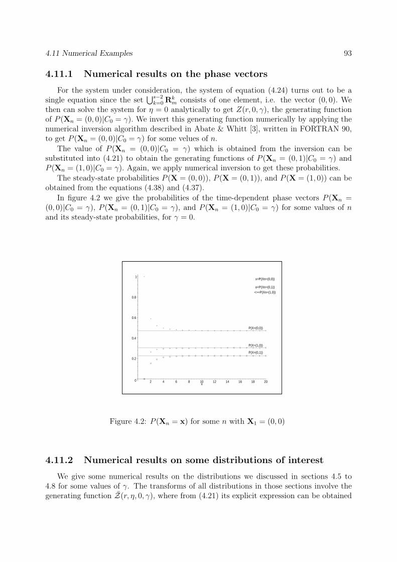
4.11 Numerical Examples 93
4.11.1 Numerical results on the phase vectors
For the system under consideration, the system of equation (4.24) turns out to be asingle equation since the set
⋃s−2k=0 Rk
m consists of one element, i.e. the vector (0, 0). Wethen can solve the system for η = 0 analytically to get Z(r, 0, γ), the generating functionof P (Xn = (0, 0)|C0 = γ). We invert this generating function numerically by applying thenumerical inversion algorithm described in Abate & Whitt [3], written in FORTRAN 90,to get P (Xn = (0, 0)|C0 = γ) for some velues of n.
The value of P (Xn = (0, 0)|C0 = γ) which is obtained from the inversion can besubstituted into (4.21) to obtain the generating functions of P (Xn = (0, 1)|C0 = γ) andP (Xn = (1, 0)|C0 = γ). Again, we apply numerical inversion to get these probabilities.
The steady-state probabilities P (X = (0, 0)), P (X = (0, 1)), and P (X = (1, 0)) can beobtained from the equations (4.38) and (4.37).
In figure 4.2 we give the probabilities of the time-dependent phase vectors P (Xn =(0, 0)|C0 = γ), P (Xn = (0, 1)|C0 = γ), and P (Xn = (1, 0)|C0 = γ) for some values of nand its steady-state probabilities, for γ = 0.
P(X=(0,1))
<>=P(Xn=(1,0))
o=P(Xn=(0,1))
x=P(Xn=(0,0))
P(X=(1,0))
P(X=(0,0))
0
0.2
0.4
0.6
0.8
1
2 4 6 8 10 12 14 16 18 20x
Figure 4.2: P (Xn = x) for some n with X1 = (0, 0)
4.11.2 Numerical results on some distributions of interest
We give some numerical results on the distributions we discussed in sections 4.5 to4.8 for some values of γ. The transforms of all distributions in those sections involve thegenerating function Z(r, η, 0, γ), where from (4.21) its explicit expression can be obtained
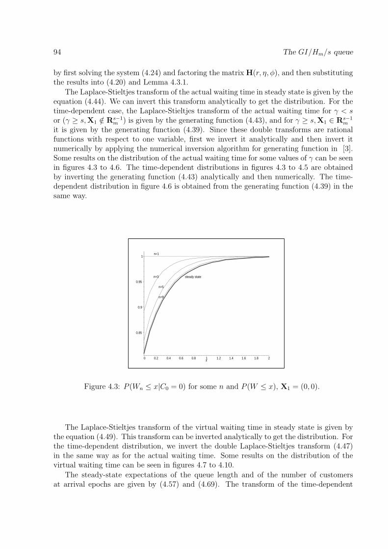
94 The GI/Hm/s queue
by first solving the system (4.24) and factoring the matrix H(r, η, φ), and then substitutingthe results into (4.20) and Lemma 4.3.1.
The Laplace-Stieltjes transform of the actual waiting time in steady state is given by theequation (4.44). We can invert this transform analytically to get the distribution. For thetime-dependent case, the Laplace-Stieltjes transform of the actual waiting time for γ < sor (γ ≥ s,X1 /∈ Rs−1
m ) is given by the generating function (4.43), and for γ ≥ s,X1 ∈ Rs−1m
it is given by the generating function (4.39). Since these double transforms are rationalfunctions with respect to one variable, first we invert it analytically and then invert itnumerically by applying the numerical inversion algorithm for generating function in [3].Some results on the distribution of the actual waiting time for some values of γ can be seenin figures 4.3 to 4.6. The time-dependent distributions in figures 4.3 to 4.5 are obtainedby inverting the generating function (4.43) analytically and then numerically. The time-dependent distribution in figure 4.6 is obtained from the generating function (4.39) in thesame way.
n=3
n=1
steady state
n=9
n=5
0.85
0.9
0.95
1
0 0.2 0.4 0.6 0.8 1 1.2 1.4 1.6 1.8 2x
Figure 4.3: P (Wn ≤ x|C0 = 0) for some n and P (W ≤ x), X1 = (0, 0).
The Laplace-Stieltjes transform of the virtual waiting time in steady state is given bythe equation (4.49). This transform can be inverted analytically to get the distribution. Forthe time-dependent distribution, we invert the double Laplace-Stieltjes transform (4.47)in the same way as for the actual waiting time. Some results on the distribution of thevirtual waiting time can be seen in figures 4.7 to 4.10.
The steady-state expectations of the queue length and of the number of customersat arrival epochs are given by (4.57) and (4.69). The transform of the time-dependent
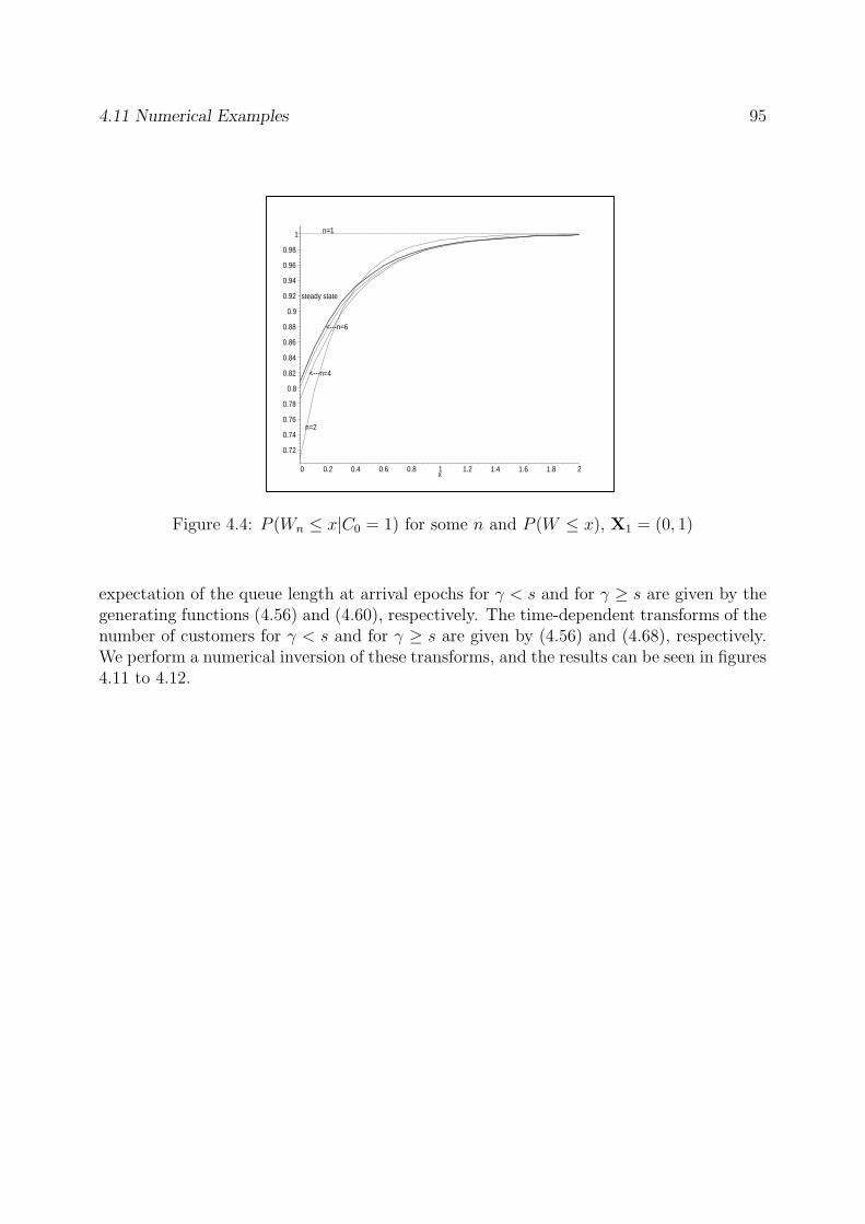
4.11 Numerical Examples 95
<---n=6
n=2
<---n=4
steady state
n=1
0.72
0.74
0.76
0.78
0.8
0.82
0.84
0.86
0.88
0.9
0.92
0.94
0.96
0.98
1
0 0.2 0.4 0.6 0.8 1 1.2 1.4 1.6 1.8 2x
Figure 4.4: P (Wn ≤ x|C0 = 1) for some n and P (W ≤ x), X1 = (0, 1)
expectation of the queue length at arrival epochs for γ < s and for γ ≥ s are given by thegenerating functions (4.56) and (4.60), respectively. The time-dependent transforms of thenumber of customers for γ < s and for γ ≥ s are given by (4.56) and (4.68), respectively.We perform a numerical inversion of these transforms, and the results can be seen in figures4.11 to 4.12.
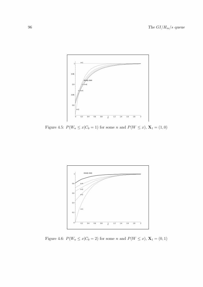
96 The GI/Hm/s queue
steady state
<---n=4
<---n=6
n=2
n=1
0.8
0.85
0.9
0.95
1
0 0.2 0.4 0.6 0.8 1 1.2 1.4 1.6 1.8 2x
Figure 4.5: P (Wn ≤ x|C0 = 1) for some n and P (W ≤ x), X1 = (1, 0)
n=3
n=4
n=1
n=2
steady state
0
0.2
0.4
0.6
0.8
1
0.2 0.4 0.6 0.8 1 1.2 1.4 1.6 1.8 2x
Figure 4.6: P (Wn ≤ x|C0 = 2) for some n and P (W ≤ x), X1 = (0, 1)
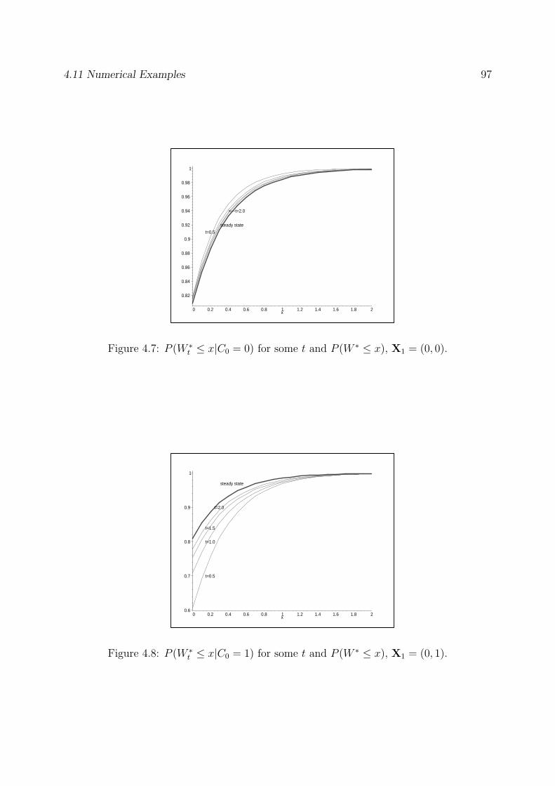
4.11 Numerical Examples 97
t=0.5
<---t=2.0
steady state
0.82
0.84
0.86
0.88
0.9
0.92
0.94
0.96
0.98
1
0 0.2 0.4 0.6 0.8 1 1.2 1.4 1.6 1.8 2x
Figure 4.7: P (W ∗t ≤ x|C0 = 0) for some t and P (W ∗ ≤ x), X1 = (0, 0).
t=2.0
t=1.5
t=1.0
steady state
t=0.5
0.6
0.7
0.8
0.9
1
0 0.2 0.4 0.6 0.8 1 1.2 1.4 1.6 1.8 2x
Figure 4.8: P (W ∗t ≤ x|C0 = 1) for some t and P (W ∗ ≤ x), X1 = (0, 1).
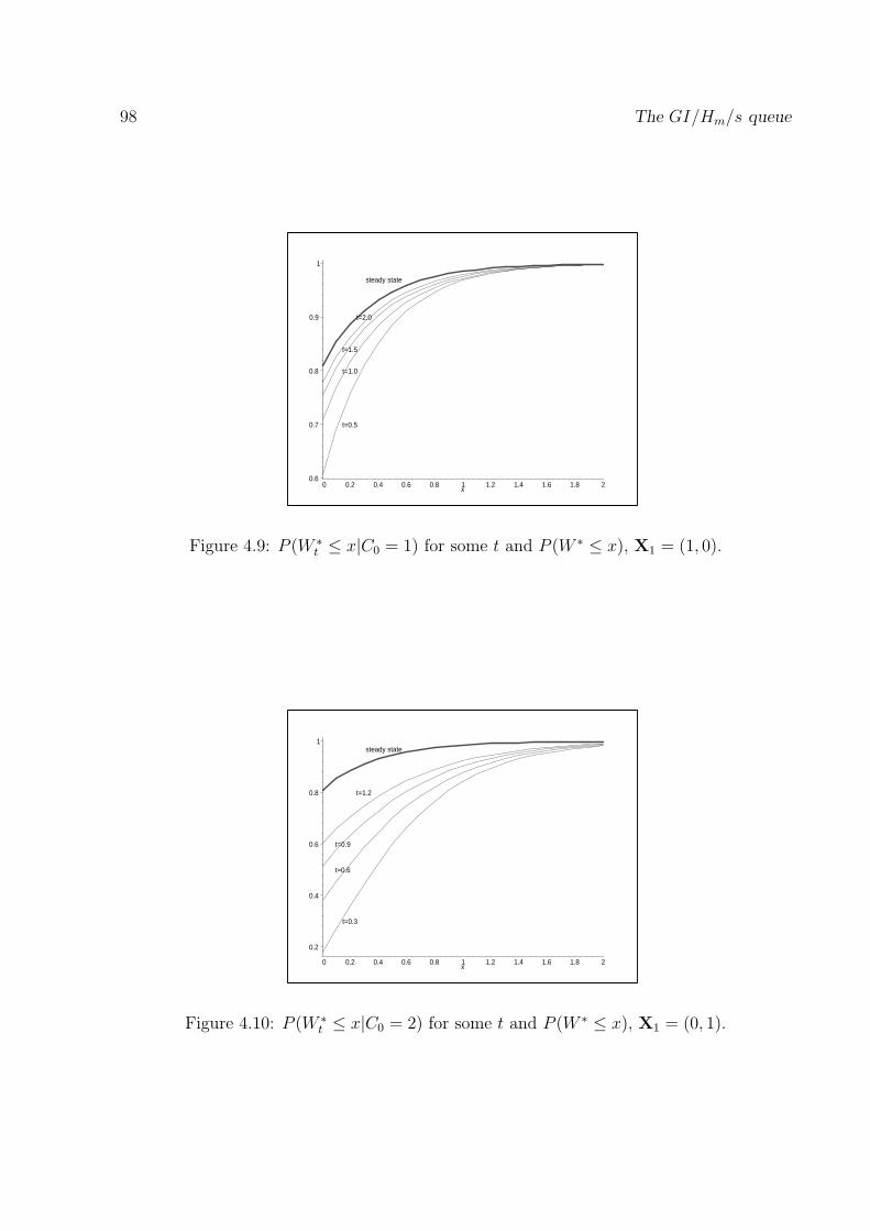
98 The GI/Hm/s queue
t=2.0
t=1.5
t=1.0
steady state
t=0.5
0.6
0.7
0.8
0.9
1
0 0.2 0.4 0.6 0.8 1 1.2 1.4 1.6 1.8 2x
Figure 4.9: P (W ∗t ≤ x|C0 = 1) for some t and P (W ∗ ≤ x), X1 = (1, 0).
t=0.6
t=1.2
t=0.9
t=0.3
steady state
0.2
0.4
0.6
0.8
1
0 0.2 0.4 0.6 0.8 1 1.2 1.4 1.6 1.8 2x
Figure 4.10: P (W ∗t ≤ x|C0 = 2) for some t and P (W ∗ ≤ x), X1 = (0, 1).
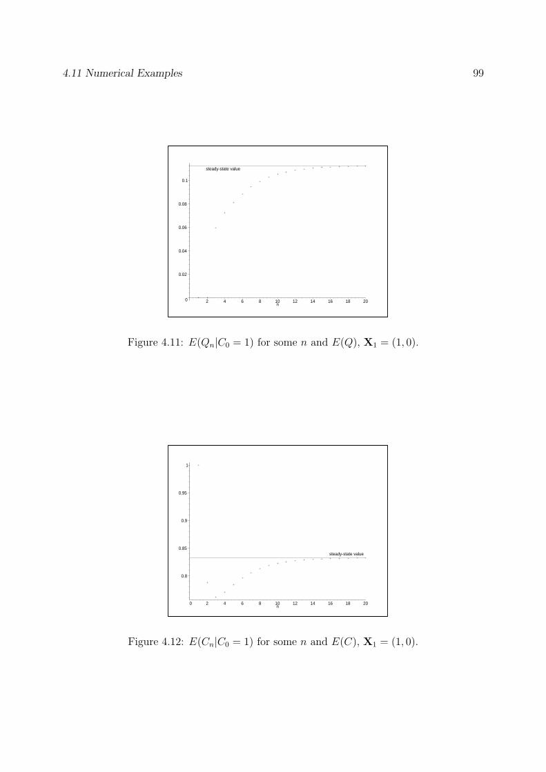
4.11 Numerical Examples 99
steady-state value
0
0.02
0.04
0.06
0.08
0.1
2 4 6 8 10 12 14 16 18 20n
Figure 4.11: E(Qn|C0 = 1) for some n and E(Q), X1 = (1, 0).
steady-state value
0.8
0.85
0.9
0.95
1
0 2 4 6 8 10 12 14 16 18 20n
Figure 4.12: E(Cn|C0 = 1) for some n and E(C), X1 = (1, 0).

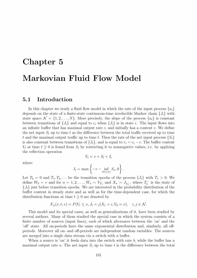
Chapter 5
Markovian Fluid Flow Model
5.1 Introduction
In this chapter we study a fluid flow model in which the rate of the input process atdepends on the state of a finite-state continuous-time irreducible Markov chain Jt withstate space N = 1, 2, . . . , N. More precisely, the slope of the process at is constantbetween transitions of Jt and equal to ci when Jt is in state i. The input flows intoan infinite buffer that has maximal output rate c, and initially has a content v. We definethe net input St up to time t as the difference between the total traffic received up to timet and the maximal output traffic up to time t. Then the rate of the net input process Stis also constant between transitions of Jt, and is equal to ri = ci − c. The buffer contentVt at time t ≥ 0 is found from St by restricting it to nonnegative values, i.e. by applyingthe reflection operation
Vt = v + St + It
where
It = max
−v − inf
0≤ν≤tSν , 0
.
Let T0 = 0 and T1, T2, . . . be the transition epochs of the process Jt with T1 > 0. Wedefine W0 = v and for n = 1, 2, . . . , Wn = VTn and Xn = JT−
n, where T−
n is the state ofJt just before transition epochs. We are interested in the probability distribution of thebuffer content in steady state and as well as for the time-dependent case, for which thedistribution functions at time t ≥ 0 are denoted by
Fij(x, t, v) = P (Vt ≤ x, Jt = j|X1 = i, V0 = v), i, j ∈ N .
This model and its special cases, as well as generalizations of it, have been studied byseveral authors. Many of them studied the special case in which the system consists of afinite number of sources (input lines), each of which alternates between the ’on’ and the’off’ state. All on-periods have the same exponential distribution and, similarly, all off-periods. Moreover all on- and off-periods are independent random variables. The sourcesare merged into a single data stream via a switch with a buffer.
When a source is ’on’ it feeds data into the switch with rate b, while the buffer has amaximal output rate a. The net input St up to time t is the difference between the total
101
102 Markovian Fluid Flow Model
traffic received up to time t and at, i.e. the maximal output traffic up to time t. We seethat this system is a special case of the fluid flow model, where Jt is the number of activesources at time t and ri = ib − a is the net input rate when there are i active sources.Moreover we see that Jt is a Birth and Death process.
This special case has been studied by Anick, Mitra, and Sondhi(AMS) [4], and Kosten [31].They determined the distribution function of the buffer content in steady state by derivingthe Kolmogorov forward equations for the Markov chain (Vt, Jt), t ≥ 0 and analyzingthis system of equations. Furthermore, in [4] and [31], G(u), -the steady-state probabilitythat the buffer content exceeds a certain level u- is studied. In AMS [4] an asymptoticformula for G(u), is given, of the form Ce−αu, where C is a constant and α is a positiveparameter. An approximation method to calculate G(u) is also given in this paper. In [31]the same asymptotic formula for G(u) is derived, and a simulation method is used to findthe constant C.
The model in which Jt is a general Markov chain has been studied by Regterschot [38],Asmussen [8], Rogers [40], and Pacheco & Prabhu [37]. The first three authors consider themodel with an initially empty buffer, and the last ones studied the non-empty case. Witha decomposition method, Asmussen [8] proved that the steady state distribution of thebuffer content is of phase type and proposed an algorithm to compute its phase generatorU. Regterschot [38], Rogers [40] and Pacheco & Prabhu [37] use Wiener-Hopf factorizationof a certain matrix. As a main result, they obtain the steady state distribution functionof the buffer content. In [38], an explicit formula for the steady state distribution functionis obtained not only for continuous time but also at transition epochs. Furthertmore, anexplicit formula for G(u) is given.
The transient behavior of the buffer content for the present model is studied by Tanakaet al. [42]. They refer to the model as Markov modulated input rate(MMIR) model, sincethe input is generated by a Markov modulated process. The Laplace transform of thejoint distribution of the buffer content and the state of the input process is derived. Byanalyzing the properties of the eigenvalues and eigenvectors of a certain matrix they foundan explicit expression for this transform.
In solving the present problem, we use the same technique as in [38] but we givesome corrections for the factorization. In section 5.2 we consider the process (Wn, Tn,Xn) and derive Wiener-Hopf type equations for the transform of the joint distribution of(Wn, Tn, Xn). Then in section 5.3, we solve this system of equation with Wiener-Hopffactorization, which boils down to finding some eigenvalues and eigenvectors of a certainmatrix and solving some matrix equations. The factorization is similar to the one in [38]but since we have initially a non-empty buffer we need to decompose a certain matrix asan additional step to complete the solution. In section 5.4 we derive an explicit expressionfor the steady state distribution function of the buffer content at transition epochs byconsidering the process (Wn, Xn). This result is found from the generating function oftransforms in section 5.3 using Abel’s limit theorem, and with the factorization we obtainan explicit expression for the steady state distribution function after we analytically invertits transform. In section 5.5 we derive the double Laplace transform of the time-dependentdistribution function of the buffer content and again after a limiting operation we get theLaplace transform of the steady state distribution. The explicit expression for the steady
5.2 System of Wiener-Hopf-type equations 103
state distribution can be found by inverting this transform, as shown in subsection 5.5.1.Since the double Laplace transform consists of terms involving multiplication of exponentialand rational terms in one variable only, to get the time-dependent distribution of the buffercontent we first invert it analytically. The result of this analytical inversion can be foundin subsection 5.5.2, and it shows a structure quite similar to the one in [42].
We study the behavior of the time-dependent distribution of Vt as t increases, byreferring to the relaxation time (see Blanc and van Doorn[14]), a measure of the speedof convergence to the steady-state distribution. In Tanaka, et al.[42], the analysis endswith a conjecture stating that the relaxation time for the present model depends on thegenerator of the underlying Markov chain, but not on the rates of the input flow. We studythe relaxation time in subsection 5.5.3, and show that the relaxation time also depends onthe net input rates ri, i ∈ N .
We implement the numerical inversion algorithm proposed in Abate and Whitt[3] toget the desired distributions. Some examples for these distributions can be found in section5.6.
We will use the following notations: x+ = max(0, x), and x− = min(0, x). 1 is theindicator function, 1 is the N -dimensional column vector with all components equal to 1,1i is the K-dimensional column vector with i-th component 1 and all other componentequal to 0, where K is an integer defined in section 5.2. I is the identity matrix, Ikl is thek × l-matrix with elements δij, where δij is Kronecker’s delta, i.e., δij = 0, for i 6= j, andδjj = 1. If A is an N ×N -dimensional matrix, the i-th column of A is denoted by Ai, andthe i-th row of A is denoted by Ai.
5.2 System of Wiener-Hopf-type equations
Let Q be the infinitesimal generator of the Markov chain Jt with elements Qij, and let Pbe the transition probability matrix of Xn with elements Pij. We assume that the matrixQ is indecomposable. Define qi = −Qii =
∑i6=j Qij, i, j ∈ N . Let q = diag(q1, . . . , qN) be
the N × N dimensional diagonal matrix with elements qi. It follows that
P = q−1(Q + q).
The stationary probabilities limt→∞ P (Jt = i) are denoted by πi, i ∈ N and π denotesthe N− dimensional row vector with components πi. We assume that
∑Ni=1 πiri < 0 to
ensure stability. The stationary probabilities limn→∞ P (Xn = i) are denoted by γi, i ∈ Nand γγγ denotes the N -dimensional row vector with components γi. It follows that
γi =πiqi
πq1πq1πq1, i = 1, 2, · · · , N. (5.1)
The traffic intensity ρ, i.e. the ratio of the average input rate and the maximal output rate, is ρ =
∑Ni=1 πici/c.
We assume that for i ∈ N , ci 6= c so that ri 6= 0 for i ∈ N . Let R− = i|ri <0, i = 1, . . . , N and R+ = i|ri > 0, i = 1, . . . , N. Suppose that |R−| = K. This impliesthat |R+| = N − K. Let r = diag(r1, . . . , rN). Without loss of generality, suppose thatR− = 1, 2, . . . , K.
104 Markovian Fluid Flow Model
Let T0 = 0 and T1, T2, . . . be the transition epochs of the process Jt with T1 > 0, andlet An = Tn − Tn−1 be the inter-jump time, n = 1, 2, . . .. Define Rn =
∑k rk1Xn = k,
we then have the relation
Wn+1 = [Wn + Rn+1An+1]+.
Define for Re(η) ≥ 0, Re(φ) ≥ 0,
Z0i (φ, η, v) = E
(e−φW1−ηT11 (X1 = i)|X1 = i, V0 = v
), (5.2)
and define for (|z| < 1, Re(η) ≥ 0, Re(φ) ≥ 0) or (|z| ≤ 1, Re(η) > 0, Re(φ) ≥ 0) or(|z| ≤ 1, Re(η) ≥ 0, Re(φ) > 0)
Zij(z, φ, η, v) =∞∑
n=1
znE(e−φWn−ηTn1 (Xn = j)|X1 = i, V0 = v
).
Define for Re(φ) ≤ 0,
Vij(z, φ, η, v) =∞∑
n=1
zn+1E((
1 − e−φ[Wn+Rn+1An+1]−)
e−η(Tn+An+1)1 (Xn = j)|X1 = i, V0 = v),
and for Re(φ) = 0,
Gij(φ, η) = E(e−(rjφ+η)An+11 (Xn+1 = j)|Xn = i
).
Let Z(z, φ, η, v),V(z, φ, η, v) and G(φ, η) be N×N− matrices with elements Zij(z, φ, η, v),Vij(z, φ, η, v) and Gij(φ, η) respectively. We then obtain the following system of Wiener-Hopf equations.
Theorem 5.2.1For Re(φ) = 0 and (|z| ≤ 1, Re(η) > 0) or (|z| < 1, Re(η) ≥ 0) we have
Z(z, φ, η, v)(I − zG(φ, η)) = zZ0(φ, η, v) + V(z, φ, η, v), (5.3)
where
Z0(φ, η, v) = diag(Z01(φ, η, v), Z0
2(φ, η, v), . . . , Z0N(φ, η, v))
with
Z0i (φ, η, v) =
e−φv qi
φri+η+qi, if ri > 0
qi
φri+η+qi
[e−φv − e(η+qi)v/ri
]+ qie
(η+qi)v/ri
η+qi, if ri < 0.
(5.4)
Proof. By the identity
e−φx+
= e−φx + 1 − e−φx−
5.2 System of Wiener-Hopf-type equations 105
we have for Re(φ) = 0, Re(η) ≥ 0
E(e−φWn+1−ηTn+11 (Xn+1 = j)|X1 = i, V0 = v
)
= E(e−φ[Wn+Rn+1An+1]+e−η(Tn+An+1)1 (Xn+1 = j)|X1 = i, V0 = v
)
= E(e−φ(Wn+Rn+1An+1)e−η(Tn+An+1)1 (Xn+1 = j)|X1 = i, V0 = v
)
+E((
1 − e−φ[Wn+Rn+1An+1]−)
e−η(Tn+An+1)1 (Xn+1 = j)|X1 = i, V0 = v)
= E(e−φWn−ηTn−(φRn+1+η)An+11 (Xn+1 = j)|X1 = i, V0 = v
)
+E((
1 − e−φ[Wn+Rn+1An+1]−)
e−η(Tn+An+1)1 (Xn+1 = j)|X1 = i, V0 = v)
.
(5.5)
Moreover
E(e−φWn−ηTn−(φRn+1+η)An+11 (Xn+1 = j)|X1 = i, V0 = v
)
=N∑
k=1
E(e−φWn−ηTn1 (Xn = k)|X1 = i, V0 = v
)
.E(e−(φRn+1+η)An+11 (Xn+1 = j)|Xn = k
)
=N∑
k=1
E(e−φWn−ηTn1 (Xn = k)|X1 = i, V0 = v
)
.E(e−(φrj+η)An+1)1 (Xn+1 = j)|Xn = k
)
=N∑
k=1
E(e−φWn−ηTn1 (Xn = k)|X1 = i, V0 = v
)Gkj(φ, η).
Substituting this into (5.5) we get
E(e−φWn+1−ηTn+11 (Xn+1 = j)|X1 = i, V0 = v
)
=N∑
k=1
E(e−φWn−ηTn1 (Xn = k)|X1 = i, V0 = v
)Gkj(φ, η)
+E((
1 − e−φ[Wn+Rn+1An+1]−)
e−η(Tn+An+11 (Xn+1 = j)|X1 = i, V0 = v)
If we multiply by zn+1 and sum over n this yields for (Re(φ) = 0, Re(η) ≥ 0, |z| < 1) or(Re(φ) = 0, Re(η) > 0, |z| ≤ 1),
Zij(z, φ, η, v) − zδijZ0i (φ, η, v) = z
N∑
k=1
Zik(z, φ, η, v)Gkj(φ, η) + Vij(z, φ, η, v)
and we get equation (5.3). It remains to verify the expression for Z0i (φ, η, v). To this end
106 Markovian Fluid Flow Model
we note that
Z0i (φ, η, v) = E
(e−φW1−ηT11 (X1 = i)|X1 = i, V0 = v
)
=
∫ ∞
0
E(e−φ[v+riT1]+−ηT1|T1 = u
)qie
−qiudu
=
∫ ∞
0
e−φ[v+riu]+−ηuqie−qiudu.
So, for ri < 0,
Z0i (φ, η, v) =
∫ −v/ri
0
e−φv−(φri+η)uqie−qiudu +
∫ ∞
−v/ri
e−ηuqie−qiudu
= e−φvqi
[−e(φri+η+qi)v/ri + 1
φri + η + qi
]+
qie(η+qi)v/ri
η + qi
,
and for ri > 0,
Z0i (φ, η, v) =
∫ ∞
0
e−φv−(φri+η)uqie−qiudu
= e−φv qi
φri + η + qi
.
The system (5.3) is the generalization of the system in [38], and will be solved byapplying the Wiener-Hopf factorization technique.
5.3 Solution of the system of Wiener-Hopf equations
In order to solve the system (5.3) we first factorize the symbol
H(z, φ, η) = I − zG(φ, η), (5.6)
i.e. for Re(φ) = 0, we try to find a factorization
H(z, φ, η) = H+(z, φ, η)H−(z, φ, η)
where
H+(z, φ, η) is analytic for Re(φ) > 0, and continuous and bounded forRe(φ) ≥ 0, and non-singular in Re(φ) > 0.
H−(z, φ, η) is analytic for Re(φ) < 0, and continuous and bounded forRe(φ) ≤ 0, and non-singular in Re(φ) < 0.
5.3 Solution of the system of Wiener-Hopf equations 107
In Arjas [6], the probabilistic interpretation of these factors is given.
To find H+(z, φ, η) and H−(z, φ, η) first we consider the following .
With the definition of q and r we can write the matrix G(φ, η) as
G(φ, η) = q−1(Q + q)q(q + φr + ηI)−1 = Pq(q + φr + ηI)−1. (5.7)
Let αi(η) = (η + qi)/ri, i = 1, 2, . . . , N. Define N × N−dimensional matrices
ααα(η) = diag(α1(η), . . . , αN(η)),
ααα = ααα(0) = diag
(q1
r1
, . . . ,qN
rN
),
L(z, φ, η) = φI + ααα(η) − zααα − zr−1Q,
and
M(φ, η) = ααα(η) + φI.
It follows thatH(z, φ, η) = ααα−1L(z, φ, η)αααM−1(φ, η). (5.8)
From (5.8) we have that
detL(z, φ, η) = detH(z, φ, η) detM(φ, η). (5.9)
Proposition 5.3.11. The poles of detH(z, φ, η) are the zeros of detM(φ, η),
2. The zeros of detL(z, φ, η) are the zeros of detH(z, φ, η).
Proof. It is clear that the zeros of detM(φ, η) are −α1(η), −α2(η), · · · ,−αN(η). Fori = 1, · · · , K these zeros lie in the right half-plane Re(φ) > 0 and for i = K + 1, · · · , Nthey lie in the left half-plane Re(φ) < 0.
Since detL(z, φ, η) does not have any pole, it follows from (5.9) that the poles ofdetH(z, φ, η) are the zeros of detM(φ, η). This proves part 1 of the proposition.
It also follows from (5.9) that the zeros of detL(z, φ, η) are the zeros of detH(z, φ, η) orthe zeros of detM(φ, η). Since from (5.6) and (5.7) we see that detH(z, φ, η) has exactly Npoles, then detL(z, φ, η) does not have any zero in common with detM(φ, η). This provespart 2 of the proposition.
Based on the proposition, we consider the following lemma, which has been proven in [38].We rewrite the proof of part 2 since some intermediate results in this proof will be used insection 5.4 and thereafter.
108 Markovian Fluid Flow Model
Lemma 5.3.1With respect to φ,
1. for (z, η) 6= (1, 0), detL(z, φ, η) has K zeros in the right half-plane Re(φ) > 0 and hasN − K zeros in the left half-plane Re(φ) < 0, and detL(z, φ, η) 6= 0 on the imaginaryaxis Re(φ) = 0.
2. detL(1, φ, 0) has K − 1 zeros in the right half- plane Re(φ) > 0 and a simple zero atφ = 0, and has N − K zeros in the left half-plane Re(φ) < 0.
Proof. See [38] for the proof of part 1.Let µ1(z, η), · · · , µK(z, η) be the zeros of detL(z, φ, η) in the right half-plane Re(φ) > 0,
and let µK+1(z, η), · · · , µN(z, η) be the zeros of detL(z, φ, η) in the left half-planeRe(φ) < 0. We consider the situation for η = 0. Now,
L(z, φ, 0) = φI + (1 − z)(r−1Q + ααα) − r−1Q.
Define the matrix L∗(z, φ) as a matrix obtained from L(z, φ, 0) by adding all columns tothe first column so that
L∗i1(z, φ) = φ + (1 − z)αi, i = 1, 2, . . . , N.
Since L∗i1(1, 0) = 0, i = 1, 2, . . . , N, we have detL∗(1, 0) = detL(1, 0, 0) = 0. With the
implicit function theorem we can define the function µ(z) uniquely by µ(1) = 0 and
detL∗(z, µ(z)) = detL(z, µ(z), 0) = 0.
We consider this function for z close to 1, so
µ(z) = −(1 − z)µ′(1) + o(1 − z), z ↑ 1.
It follows that
L(z, µ(z), 0) = (1 − z)(ααα − µ′(1)I) − zr−1Q + o(1 − z), z ↑ 1
andL∗
i1(z, µ(z)) = (1 − z)(αi − µ′(1)) + o(1 − z), z ↑ 1.
Since detL∗(z, µ(z)) = 0, we have
0 = limz↑1
1
1 − zdetL∗(z, µ(z)) = detLo,
where for i ∈ N , j ∈ N ,Lo
ij = −r−1i Qij,
andL
i1 = αi − µ′(1). (5.10)
5.3 Solution of the system of Wiener-Hopf equations 109
Since detLo = 0 and πr(r−1Q) = 0, we have
N∑
i=1
πiriLoi1 = 0,
or with (5.10)
µ′(1) =N∑
i=1
πiqi/N∑
i=1
πiri = πq1/πr1
so that
µ(z) = −(1 − z)πq1
πr1+ o(1 − z), z ↑ 1. (5.11)
For z ↑ 1 one of the K zeros of detL(z, µ(z), 0) in the right half-plane Re(φ) > 0 tends to0 if and only if
∑Ni=1 πiri = πr1 < 0. The latter condition corresponds to traffic intensity
ρ < 1.
We next impose the following condition.
Condition 5.3.1For (z, η) = (1, 0) and |z| ≤ 1, Re(η) > 0, −α1(η), . . . ,−αN(η) and µ1(z, η), . . . , µN(z, η)
are all distinct, possibly with the exception of a set of isolated points.
For i = 1, . . . , N let Ei(z, η) be a (non unique) nonzero column vector satisfying
L(z, µi(z, η), η)Ei(z, η) = 0, (5.12)
and let E(z, η) be the N ×N -matrix with ith column Ei(z, η). Let D(z, η) be the N × K-matrix with elements
Dij(z, η) = Eij(z, η) + ηq−1i Eij(z, η) + α−1
i Eij(z, η)µj(z, η), (5.13)
i ∈ N ; j ∈ R−; we then have
D(z, η) = (I + ηq−1)E(z, η)INK + ααα−1E(z, η)INKdiag(µ1(z, η), . . . , µK(z, η)).
From (5.8) it follows that for i ∈ R−,
H(z, µi(z, η), η)Di(z, η)
=ααα−1L(z, µi(z, η), η)αααM−1(µi(z, η), η)ααα−1(ααα(η) + µi(z, η)I)Ei(z, η)
=0.
(5.14)
The matrix D(z, η) we define here corrects the corresponding matrix in [38], which wronglydoes not satisfy (5.14).
Let S(z, η) be the K × K-matrix with elements
Sij(z, η) = α−1i Eij(z, η), i, j ∈ R−;
110 Markovian Fluid Flow Model
soS(z, η) = (IKNααα−1INK)(IKNE(z, η)INK). (5.15)
We now impose the following condition.
Condition 5.3.2For (z, η) = (1, 0) and 0 < |z| ≤ 1, Re(η) > 0, detS(z, η) 6= 0.
Define the K × N -matrix C(z, η) by
C(z, η) = S−1(z, η)IKN .
Hence, from (5.15) we have
C(z, η) = (IKNE(z, η)INK)−1IKNααα.
Notice that the last N−K columns of C(z, η) are equal zero. Now, define the N×N -matrixK(z, φ, η) by
K(z, φ, η) = I + D(z, η)diag
(1
φ − µ1(z, η), . . . ,
1
φ − µK(z, η)
)C(z, η). (5.16)
We now can prove the following factorization theorem.
Theorem 5.3.1If Conditions 5.3.1 and 5.3.2 are satisfied, then for (|z| < 1, Re(η) ≥ 0) or (|z| ≤ 1,
Re(η) > 0),
1. detK(z, φ, η) =∏K
i=1
(φ+αi(η)
φ−µi(z,η)
)
2. for Re(φ) = 0H(z, φ, η) = H+(z, φ, η)H−(z, φ, η)where
(a) H−(z, φ, η) = K−1(z, φ, η),
(b) H+(z, φ, η) = H(z, φ, η)K(z, φ, η),
(c) H+(z, φ, η) is analytic for Re(φ) > 0, and continuous and bounded forRe(φ) ≥ 0, and non-singular in Re(φ) > 0,
H−(z, φ, η) is analytic for Re(φ) < 0, and continuous and bounded forRe(φ) ≤ 0, and non-singular in Re(φ) < 0.
Proof. Although we have different expressions for the matrices D(z, η), S(z, η) andC(z, η), the proof is essentially the same as the proof of Theorem 4.2 in [38].
Now, by multiplying both sides of (5.3) by K(z, φ, η) and by using (5.6) we obtain
5.3 Solution of the system of Wiener-Hopf equations 111
Z(z, φ, η, v)H(z, φ, η)K(z, φ, η) = zZ0(φ, η, v)K(z, φ, η) + V(z, φ, η, v)K(z, φ, η), (5.17)
where from part 2.c of Theorem 5.3.1 we have that the left-hand side of (5.17) is analytic inRe(φ) > 0 and bounded and continuous in Re(φ) ≥ 0, and the last term of the right-handside is analytic in Re(φ) < 0 and bounded and continuous in Re(φ) ≤ 0.
To obtain a standard Wiener-Hopf decomposition for (5.17) we decompose the firstterm of the right-hand side of (5.17), i.e. we determine matrix functions K+ and K− suchthat for Re(φ) = 0,
Z0(φ, η, v)K(z, φ, η) = K+(z, φ, η, v) + K−(z, φ, η, v) (5.18)
where
K+(z, φ, η, v) is analytic for Re(φ) > 0, and continuous and bounded forRe(φ) ≥ 0,
K−(z, φ, η, v) is analytic for Re(φ) < 0, and continuous and bounded forRe(φ) ≤ 0.
Lemma 5.3.2If conditions 5.3.1 and 5.3.2 are satisfied then for Re(φ) ≥ 0,
K+ij (z, φ, η, v)
= δijZ0i (φ, η, v) +
K∑
k=1
Dik(z, η)Z0
i (φ, η, v) − Z0i (µk(z, η), η, v)
φ − µk(z, η)Ckj(z, η)
(5.19)
and
K−ij (z, φ, η, v) =
K∑
k=1
Dik(z, η)Z0
i (µk(z, η), η, v)
φ − µk(z, η)Ckj(z, η) (5.20)
if (|z| < 1, Re(η) ≥ 0) or (|z| ≤ 1, Re(η) > 0).
Proof.
• For i = 1, 2, · · · , N and j = 1, 2, · · · , N, it is clear from (5.19) and (5.20) that
K−ij (z, φ, η, v) + K+
ij (z, φ, η, v)
=δijZ0i (φ, η, v) +
K∑
k=1
Dik(z, η)Z0
i (φ, η, v)
φ − µk(z, η)Ckj(z, η)
so that, by using (5.16), (5.18) is satisfied.
112 Markovian Fluid Flow Model
• Since by definition µk(z, η) for k = 1, 2, · · · , K lies in the right half-plane Re(φ) > 0,K−
ij (z, φ, η, v) is analytic for Re(φ) < 0, and continuous for Re(φ) ≤ 0, taking intoaccount the properties of C(z, η) and D(z, η). Furthermore, it is bounded on the lefthalf-plane Re(φ) ≤ 0 since for i = 1, 2, · · · , K, the functions
Dik(z, η)Z0i (µk(z, η), η, v)Ckj(z, η)
and 1/(φ − µk(z, η)) are bounded.
• For i = 1, 2, · · · , N, j = 1, 2, · · · , N and l = 1, 2, · · · , K,
limφ→µl(z,η)
(φ − µl(z, η))K+ij (z, φ, η, v)
= limφ→µl(z,η)
(φ − µl(z, η))δijZ0i (φ, η, v) +
[lim
φ→µl(z,η)(φ − µl(z, η))
K∑
k=1
Dik(z, η)Z0
i (φ, η, v) − Z0i (µk(z, η), η, v)
φ − µk(z, η)Ckj(z, η)
]
=0,
consequently, K+ij (z, φ, η, v) does not have any pole in the right half-plane Re(φ) > 0,
taking into account the properties of C(z, η) and D(z, η). We can conclude thatK+(z, φ, η, v) is analytic for Re(φ) > 0, and continuous for Re(φ) ≥ 0. Furthermore,it is bounded in the right half-plane Re(φ) ≥ 0 since for i = 1, 2, · · · , N, the functionsZ0
i (φ, η, v), from (5.4), are bounded in the right half-plane Re(φ) ≥ 0.
Theorem 5.3.2If conditions 5.3.1 and 5.3.2 are satisfied then for Re(φ) ≥ 0, with (|z| < 1, Re(η) ≥ 0)
or (|z| ≤ 1, Re(η) > 0),
Z(z, φ, η, v)H(z, φ, η)K(z, φ, η) = zK+(z, φ, η, v) + zK−(z, 0, η, v) (5.21)
Proof. From (5.17) and (5.18) we have for Re(φ) = 0
Z(z, φ, η, v)H(z, φ, η)K(z, φ, η) − zK+(z, φ, η, v)
=zK−(z, φ, η, v) + V(z, φ, η, v)K(z, φ, η)(5.22)
where the left-hand side is analytic in Re(φ) > 0 and continuous in Re(φ) ≥ 0. Further-more, by definitions of Z(z, φ, η, v) and K+(z, φ, η, v) and from part 2.c of Theorem 5.3.1,it is bounded in Re(φ) ≥ 0. The right-hand side is analytic in Re(φ) < 0 and continuous inRe(φ) ≤ 0. By definitions of V(z, φ, η, v), K(z, φ, η) and K−(z, φ, η, v), it is also boundedin Re(φ) ≤ 0. Thus we can define an entire function which is equal to the left-hand side forRe(φ) ≥ 0 and equal to the right-hand side for Re(φ) ≤ 0. This entire function is bounded,and hence by Liouville’s theorem, it is a constant. Hence, for Re(φ) ≥ 0,
Z(z, φ, η, v)H(z, φ, η)K(z, φ, η) − zK+(z, φ, η, v)
= Z(z, 0, η, v)H(z, 0, η)K(z, 0, η) − zK+(z, 0, η, v).(5.23)
5.4 The steady state buffer content at transition epochs 113
Using (5.22) with φ = 0 and noting that V(z, 0, η, v) = 0, it follows from (5.23) that
Z(z, φ, η, v)H(z, φ, η)K(z, φ, η) = zK+(z, φ, η, v) + zK−(z, 0, η, v).
This proves the theorem.
From (5.21) we can find an explicit expression for Z(z, φ, η, v) once we find the explicitexpressions for K(z, φ, η)−1 and H+(z, φ, η)−1, which are given in the following lemma.
Lemma 5.3.3For (|z| < 1, Re(η) ≥ 0, Re(φ) ≥ 0) or (|z| ≤ 1, Re(η) > 0, Re(φ) ≥ 0) or
(|z| ≤ 1, Re(η) ≥ 0, Re(φ) > 0)
K−1(z, φ, η) = I − D(z, η)C(z, η)M−1(φ, η) (5.24)
and
H+(z, φ, η)−1 = [H(z, φ, η)K(z, φ, η)]−1
= [M(φ, η) − D(z, η)C(z, η)] α−1
N∑
i=1
Ei(z, η)Ei(z, η)−1
(φ − µi(z, η))ααα.
(5.25)
Proof. See Appendix A.6.
The equation (5.21) and Lemma 5.3.3 will give us an explicit expression for Z(z, φ, η, v)and we can use it to study the distribution of the buffer content.
5.4 The steady state buffer content at transition epochs
In this section we will derive the steady state distribution function of the buffer contentat transition epochs of the process Jt which exists for traffic intensity ρ < 1.
The process (Wn, Xn) is regenerative where for any i ∈ N the state (0, i) can beseen as the regenerative state. Since Q is indecomposable, all states of the process Jtcommunicate with each other. It follows that the return times of the process (Wn, Xn)are aperiodic so that limn→∞ PWn ≤ x,Xn = j|X1 = i, V0 = v for x ≥ 0 exists. If thislimit is zero then no limiting distribution exists, otherwise (Wn, Xn) converges weakly toa stationary random vector (W,X). From (5.19) and (5.20) we see that
114 Markovian Fluid Flow Model
limz↑1
(1 − z)K+ij (z, φ, 0, v) + (1 − z)K−
ij (z, 0, 0, v)
= limz↑1
(1 − z)δijZ0i (φ, η, v) − lim
z↑1(1 − z)
K∑
k=1
Dik(z, 0)Z0
i (µk(z, 0), 0, v)
µk(z, 0)Ckj(z, 0)
+ limz↑1
(1 − z)K∑
k=1
Dik(z, 0)Z0
i (φ, η, v) − Z0i (µk(z, 0), η, v)
φ − µk(z, 0)Ckj(z, 0)
= − Di1(1, 0)Z0i (µ1(1, 0), 0, v) lim
z↑1
(1 − z)
µ1(z, 0)C1j(1, 0)
= − Di1(1, 0) limz↑1
(1 − z)
µ1(z, 0)C1j(1, 0).
(5.26)
Since H(1, 0, 0) = I − G(0, 0) = I − P and H(1, 0, 0)D1(1, 0) = 0, we may put
E1(1, 0) = D1(1, 0) = 1.
We also may put E−11 (1, 0) = (πππr1)−1πππr.
From the proof of Lemma 5.3.1 we have
limz↑1
(1 − z)
µ1(z, 0)=
−πππr1πππq1
, if πππr1 < 0;
0 , if πππr1 ≥ 0(5.27)
Hence, if and only if πππr1 < 0, or ρ < 1, the vector (Wn, Xn) converges weakly to(W,X). If Condition 5.3.1 and Condition 5.3.2 are satisfied we have
C1(1, 0) = (IKNE(1, 0)INK)−11 IKNα
so C1i(1, 0) < 0, i ∈ R−; and C1i(1, 0) = 0, i ∈ R+. Denote µi = µi(1, 0), i ∈ N with µ1 = 0and D = D(1, 0),C = C(1, 0) and E = E(1, 0); H(φ) = H(1, φ, 0), and K(φ) = K(1, φ, 0).From (5.16) it follows that
K(φ) = I + Ddiag
(0,
1
φ − µ2
, . . . ,1
φ − µN
)C.
Now let
H+(φ) =
H(φ)K(φ) + 1φH(φ)D1C1, φ 6= 0,
H(0)K(0) + H′(0)D1C1, φ = 0,
(5.28)
and let Z(φ) be the N × N−dimensional matrix with elements
Zij(φ) = E(e−φW1 (X = j)|X1 = i
)
= limz↑1
(1 − z)Zij(z, φ, 0), j = 1, 2, . . . , N.
5.4 The steady state buffer content at transition epochs 115
From (5.21), (5.26), and (5.27) we now have for Re(φ) ≥ 0,
Z(φ)H+(φ) =πrπrπr1
πqπqπq1D1C1
=πrπrπr1
πqπqπq1U,
(5.29)
where U is an N×N−dimensional matrix with rows C1. The equation (5.29) confirms thatthe steady-state distribution of the buffer content does not depend on the initial condition.
Let Zi(φ) be the N− dimensional row vector with components Zji(φ). From (5.29) and(5.25) we have for Re(φ) ≥ 0,
Zi(φ) =πrπrπr1
πqπqπq1C1H
+(φ)−1
=πrπrπr1
πqπqπq1(IKNEINK)−1
1 IKNααα ((ααα + φI) − DC)ααα−1
N∑
j=1
EjE−1j
φ − µj
ααα.(5.30)
The explicit expression for Zi(φ) can be obtain by using the following lemma.
Lemma 5.4.1For (|z| < 1, Re(η) ≥ 0, Re(φ) ≥ 0) or (|z| ≤ 1, Re(η) > 0, Re(φ) ≥ 0) or
(|z| ≤ 1, Re(η) ≥ 0, Re(φ) > 0) and for i = 1, · · · , K,
Ci(z, η) [M(φ, η) − D(z, η)C(z, η)] = (φ − µi(z, η))Ci(z, η). (5.31)
Proof. See appendix A.7.
For z = 1 and η = 0, (5.31) yields
Ci [ααα + φI + φI − DC] = (φ − µi)Ci.
Then by using the orthogonality property of the vectors Ei, i ∈ N and our setting
E−11 (1, 0) = (πππr1)−1πππr
as is explained on page 114, (5.30) can be rewritten as in the following expression. ForRe(φ) ≥ 0,
Zi(φ) =πrπrπr1
πqπqπq1(φ − µ1)(IKNEINK)−1
1 IKN
N∑
j=1
EjE−1j
φ − µj
ααα
=πrπrπr1
πqπqπq1φ(IKNEINK)−1
1 IKN
N∑
j=1
EjE−1j
φ − µj
ααα
=πrπrπr1
πqπqπq1
E−1
1 ααα + φ(IKNEINK)−11 IKN
N∑
j=K+1
EjE−1j
φ − µj
ααα
= γγγ +πrπrπr1
πqπqπq1VVV
N∑
j=K+1
EjE−1j ααα − πrπrπr1
πqπqπq1VVV
N∑
j=K+1
−µj
φ − µj
EjE−1j ααα,
(5.32)
116 Markovian Fluid Flow Model
where
VVV = (IKNEINK)−11 IKN
and γγγ is given by (5.1). The equation (5.32) shows us that the steady-state distribution ofbuffer content at transition epochs is a mixture of exponentials and a concentration at 0.Let F(x) be the N -dimensional row vector with components
Fj(x) = P (W ≤ x,X = j), j ∈ N .
Then equation (5.32) yields
F(x) = γγγ +πrπrπr1
πqπqπq1VVV
N∑
j=K+1
EjE−1j eµjxα. (5.33)
This result can also be found in [38].
5.5 The buffer content in continuous time
In this section we consider the buffer content in continuous time. In the first part wewill derive the steady state distribution function of this buffer content, and in the secondpart we consider the time dependent distribution.
5.5.1 The steady state buffer content in continuous time
If Jt = j then
Vt = [WNt + rj(t − TNt)]+
where Nt is the number of transitions of the process Jt during [0, t]. Consequently, forRe(φ) ≥ 0,
E(e−φVt1(Jt = j)|X1 = i, V0 = v
)
= E(e−φ[W0+rj(t−T0)]+1 (T0 ≤ t < T1, Jt = j)|X1 = i, V0 = v
)
+∞∑
n=1
E(e−φ[Wn+rj(t−Tn)]+1(Tn ≤ t < Tn+1, Jt = j)|X1 = i, V0 = v
).
(5.34)
5.5 The buffer content in continuous time 117
The last term on the right can be written as
∞∑
n=1
E(e−φ[Wn+rj(t−Tn)]+1(Tn ≤ t < Tn+1, Jt = j)|X1 = i, V0 = v
)
=∞∑
n=1
N∑
l=1
E(e−φ[Wn+rj(t−Tn)]+1(Tn ≤ t < Tn+1, Xn = l, Xn+1 = j)|X1 = i, V0 = v
)
=∞∑
n=1
N∑
l=1
∫ t
0
P (An+1 > t − u,Xn+1 = j|Xn = l)
.duE(e−φ[Wn+rj(t−Tn)]+1(Tn ≤ u,Xn = l)|X1 = i, V0 = v
)
=∞∑
n=1
N∑
l=1
∫ t
0
Plje−qj(t−u)
.duE(e−φ[Wn+rj(t−Tn)]+1(Tn ≤ u,Xn = l)|X1 = i, V0 = v
).
(5.35)
From the identity (see page 269 of [17])
e−φx+
=1
2πi
∫ i∞+0
−i∞+0
dξ
ξ
φ
φ − ξe−ξx, Re(φ) > Re(ξ) > 0,
where the path of integration is a line parallel to the imaginary axis, we have
E(e−φ[Wn+rj(t−Tn)]+1(Tn ≤ u,Xn = l)|X1 = i, V0 = v
)
=1
2πi
∫ i∞+0
−i∞+0
dξ
ξ
φ
φ − ξe−ξrjtE
(e−ξWn+rjξTn1(Tn ≤ u,Xn = l)
|X1 = i, V0 = v) , Re(φ) > Re(ξ) > 0.
(5.36)
Combining (5.34), (5.35), and (5.36) yields for Re(η+qj +ξrj) > 0 and Re(φ) > Re(ξ) > 0,∫ ∞
0
e−ηtE(e−φVt1(Jt = j)|X1 = i, V0 = v
)dt
=1
2πi
∫ i∞+0
−i∞+0
dξ
ξ
φ
φ − ξe−ξv
∫ ∞
0
e−(η+ξrj)tE (1(t < T1, Jt = j)|X1 = i, V0 = v) dt
+∞∑
n=1
N∑
l=1
1
2πi
∫ i∞+0
−i∞+0
dξ
ξ
φ
φ − ξ
∫ ∞
0
e−ηt
.
∫ t
0
Plje−qj(t−u)e−ξrjtduE
(e−ξWn+rjξTn1(Tn ≤ u,Xn = l)|X1 = i, V0 = v
)dt
=1
2πi
∫ i∞+0
−i∞+0
dξ
ξ
φ
φ − ξe−ξv δij
η + ξrj + qj
+∞∑
n=1
N∑
l=1
1
2πi
∫ i∞+0
−i∞+0
dξ
ξ
φ
φ − ξE(e−ξWn−ηTn1(Xn = l)|X1 = i, V0 = v
)
.Plj(η + qj + ξrj)−1.
(5.37)
118 Markovian Fluid Flow Model
If Z∗(φ, η, v) is the N × N -dimensional matrix with elements
Z∗ij(φ, η, v) =
∫ ∞
0
e−ηtE(e−φVt1(Jt = j)|X1 = i, V0 = v
)dt, (5.38)
then, for Re(φ) > Re(ξ) > 0, Re(η) > 0, and maxj∈N Re(η + qj + ξrj) > 0 we have
Z∗(φ, η, v)
=1
2πi
∫ i∞+0
−i∞+0
dξ
ξ
φ
φ − ξ
(Z(1, ξ, η, v)P + e−ξv
)(ηI + ξr + q)−1.
(5.39)
From (5.7) and the fact that the matrix (ηI + ξr + q)−1 is diagonal, we can write forRe(ξ) > 0, Re(η) > 0,
P(ηI + ξr + q)−1 = G(ξ, η)q−1.
Moreover, from (5.6) it follows for Re(ξ) > 0, Re(η) > 0,
P(ηI + ξr + q)−1 = q−1 − H(1, ξ, η)q−1.
Multiply both sides by Z(1, ξ, η, v), then by using (5.21) we have for Re(ξ) > 0, Re(η) > 0,
Z(1, ξ, η, v)P(ηI + ξr + q)−1
=Z(1, ξ, η, v)q−1 − Z(1, ξ, η, v)H(1, ξ, η)q−1
=Z(1, ξ, η, v)q−1 − K+(1, ξ, η, v)K−1(1, ξ, η)q−1 − K−(1, 0, η, v)K−1(1, ξ, η)q−1.
(5.40)
Notice that the inverse of the matrix K(1, ξ, η) for Re(ξ) > 0, Re(η) > 0 exists due to part1 of Theorem 5.3.1. By using (5.18) we obtain from (5.40),
Z(1, ξ, η, v)P(ηI + ξr + q)−1
= Z(1, ξ, η, v)q−1 − Z0(ξ, η, v)K(1, ξ, η)K−1(1, ξ, η)q−1
+K−(1, ξ, η, v)K−1(1, ξ, η)q−1 − K−(1, 0, η, v)K−1(1, ξ, η)q−1
= Z(1, ξ, η, v)q−1 − Z0(ξ, η, v)q−1 + K−(1, ξ, η, v)K−1(1, ξ, η)q−1
−K−(1, 0, η, v)K−1(1, ξ, η)q−1, Re(ξ) > 0, Re(η) > 0.
Insertion into (5.39) yields for Re(φ) > 0, Re(η) > 0,
Z∗(φ, η, v) =1
2πi
∫ i∞+0
−i∞+0
dξ
ξ
φ
φ − ξ
(Z(1, ξ, η, v)q−1 − Z0(ξ, η, v)q−1
)
+1
2πi
∫ i∞+0
−i∞+0
dξ
ξ
φ
φ − ξK−(1, ξ, η, v)K−1(1, ξ, η)q−1
− 1
2πi
∫ i∞+0
−i∞+0
dξ
ξ
φ
φ − ξK−(1, 0, η, v)K−1(1, ξ, η)q−1
+1
2πi
∫ i∞+0
−i∞+0
dξ
ξ
φ
φ − ξe−ξv(ηI + ξr + q)−1.
(5.41)
5.5 The buffer content in continuous time 119
Since the elements of matrices Z(1, ξ, η, v) and Z0(ξ, η, v) satisfy A+(see page 11 for thedefinitions of A+ and A−), then the first integral in the right hand-side of (5.41) can beevaluated through the residue at ξ = φ. The elements of matrices
K−(1, ξ, η, v)K−1(1, ξ, η) and K−(1, 0, η, v)K−1(1, ξ, η)
satisfy A−, so we can evaluate the second and the third integral through the residue at φ =0, and yields the same results. It follows that the second and the third integrals will cancel.The last integral can be evaluated by using contour integration and Cauchy’s residuetheorem. We recall that the jth diagonal elements of the diagonal matrix (ηI + ξr + q)−1
has a pole at ξ = −(η + qj)/rj. For j ∈ R− this pole lies in the right half-plane Re(ξ) > 0,and for j ∈ R+ this pole lies in the left half-plane Re(ξ) < 0. If we evaluate the integral
1
2πi
∫ i∞+0
−i∞+0
dξ
ξ
φ
φ − ξe−ξv(ηI + ξr + q)−1
through the residue in the right half-plane of the contour of integration, then we obtainfor Re(φ) ≥ 0, Re(η) ≥ 0,
1
2πi
∫ i∞+0
−i∞+0
dξ
ξ
φ
φ − ξe−ξv(ηI + ξr + q)−1 = r−1diag
(Z1
1(φ, η, v), · · · , Z1N(φ, η, v)
),
where
Z1i (φ, η, v) =
(αi(η)e−φv + φeαi(η)v)/(αi(η)(φ + αi(η))), for i = 1, · · · , K,
e−φv/(φ + αi(η)), for i = K + 1, · · · , N.
LetZ1(φ, η, v) = diag
(Z1
1(φ, η, v), · · · , Z1N(φ, η, v)
).
From (5.4) it is clear that
r−1Z1(φ, η, v) = Z0(φ, η, v)q−1,
so that if we substitute the results of integrations in (5.41) we obtain for Re(φ) ≥ 0, Re(η) ≥0,
Z∗(φ, η, v) = Z(1, φ, η, v)q−1. (5.42)
The process (Vt, Jt), t ≥ 0 is regenerative, where the regeneration points are theepochs at which the process enters a state (0, i) for some fixed i ∈ N . Since the timesbetween regeneration points are non-arithmetic,
limt→∞
E(exp(−φVt)1(Jt = i)|X1 = j, V0 = v)
exists, independent of initial conditions. Denote this limit by Z∗i (φ) and let Z∗(φ) be
the N−dimensional row vector with components Z∗i (φ). Similar to the proof given for the
120 Markovian Fluid Flow Model
process (Wn, Xn), we can conclude that (Vt, Jt) converges weakly to a random vector(V, J) if and only if πrπrπr1 < 0.
To get the steady-state transform Z∗(φ), in the following we apply Abel’s theorem forLaplace transforms (see Appendix). From (5.21), (5.20), and (5.19), we have for Re(φ) ≥ 0,
limη↓0
ηZ∗(φ, η, v) = limη↓0
ηZ(1, φ, η, v)q−1
= limη↓0
η[K+(1, φ, η, v) + K−(1, 0, η, v)
][H(1, φ, η)K(1, φ, η)]−1
= limη↓0
ηK−(1, 0, η, v) [H(1, φ, η)K(1, φ, η)]−1 .
(5.43)
From (5.25) it is clear that
limη↓0
[H(1, φ, η)K(1, φ, η)]−1 = H+(φ)−1,
where H+(φ) is defined in (5.28). To evaluate limη↓0 ηK−(1, 0, η, v) we first prove (theproof can be done in a similar way as the proof of Lemma 5.3.1)
limη↓0
η
µ1(1, η)=
−πrπrπr1 , if πrπrπr1 < 0,
0 , if πrπrπr1 ≥ 0.(5.44)
Then, by our setting D1(1, 0) = E1(1, 0) = 1 as explained on page 114,
limη↓0
ηK−ij(1, 0, η, v) = lim
η↓0η
K∑
k=1
Dik(1, η)Z0
i (µk(1, η), η, v)
−µk(1, η)Ckj(1, η)
= limη↓0
η
−µ1(1, η)Di1(1, η)Z0
i (µ1(1, η), η, v)C1j(1, η)
=
−πr1πr1πr1C1j , if πrπrπr1 < 0,
0 , if πrπrπr1 ≥ 0,
(5.45)
or
limη↓0
ηK−(1, 0, η, v) =
−πr1πr1πr1U , if πrπrπr1 < 0,
0 , if πrπrπr1 ≥ 0,(5.46)
where U is the N × N -dimensional matrix with rows C1. It follows that
limη↓0
ηZ∗(φ, η, v) =
−πr1πr1πr1UH+(φ)−1 , if πrπrπr1 < 0,
0 , if πrπrπr1 ≥ 0,(5.47)
which confirms that limt→∞ E(exp(−φVt)1(Jt = i)|X1 = j, V0 = v) does not depend onthe initial conditions. From (5.47) and (5.29) we can conclude that for Re(φ) ≥ 0,
Z∗(φ) = πqπqπq1Z(φ)q−1, (5.48)
which is again the Laplace-Stieltjes transform of a mixture of exponentials and a concen-tration at 0.
5.5 The buffer content in continuous time 121
The distribution functions
F ∗i (x) = P (V ≤ x, J = i), i ∈ N ,
can be obtained by inverting the entry in the i-th column of Z∗(φ), which yields
F ∗i (x) =
πππ + πrπrπr1V
N∑
j=K+1
EjE−1j eµjxr−1
i
. (5.49)
These results can also be found in [38].
5.5.2 Inversions for Time-dependent Buffer Content
In the previous subsection, we have derived the Laplace transform of the steady statedistribution of the buffer content. An explicit expression for the distribution has beengiven by inverting the transform.
Now, we are interested in the distribution function of the buffer content at time t ≥ 0 foran initial buffer content V0 = v, i.e. Fij(x, t, v), for i, j ∈ N . The double Laplace transformof these distributions is defined in (5.38), where the expressions for these transforms isgiven in matrix form by equation (5.42), that is for Re(φ) ≥ 0, Re(η) > 0,
Z∗(φ, η, v) =Z(1, φ, η, v)q−1
=(K+(1, φ, η, v) + K−(1, 0, η, v))[H(1, φ, η)K(1, φ, η)]−1q−1,(5.50)
where the latter expression is obtained from Theorem 5.3.2. We will show below that(5.50) holds for Re(φ) > 0 and Re(η) ≥ 0. We have to invert the transform in (5.50)to get the distribution functions. From (5.50) we see that the expression for Z∗(φ, η, v)involves the matrices K−(1, φ, η, v) and [H(1, φ, η)K(1, φ, η)]−1 which are rational in φ andthe irrational diagonal matrix Z0(φ, η, v) with its diagonal elements that can be rewrittenas
Z0i (φ, η, v) =
(αiαi(η)e−φv + αiφeαi(η)v)/(αi(η)(φ + αi(η))), if ri < 0
e−φv/(φ + αi(η)), if ri > 0,
so that
Z0(φ, η, v)
=diag(α1(η)e−φv + φeα1(η)v
α1(η), · · · ,
αK(η)e−φv + φeαK(η)v
αK(η), e−φv, · · · , e−φv)
.αααM(φ, η)−1
(5.51)
From (5.51) we see that the irrational property of the matrices Z0(φ, η, v) is caused bythe exponential factors e−φv. This allows us to just consider the rational parts of Z∗(φ, η, v)in φ, and we can apply an analytic inversion of Z∗(φ, η, v) with respect to φ, since theinversion of a term like e−φuf(φ) is f(x− u)H(x− u), where f(x) is the inverse of Laplacetransform f(φ) and H(x) is the Heaviside function.
122 Markovian Fluid Flow Model
After the inversion with respect to φ, we get the Laplace-Stieltjes transform
∫ ∞
0
e−ηtdxFij(x, t, v)dt. (5.52)
Since we are interested in the distribution functions, we then derive the Laplace transform
ξij(x, η, v) =
∫ ∞
0
e−ηtFij(x, t, v)dt. (5.53)
The transform (5.53) in general is not a rational function in η. Hence, we invert (5.53)numerically to get the desired distribution functions.
For brevity, we suppress the dependency of E(1, η) and µi = µi(1, η), i ∈ N on thevariable η, and in the rest of this chapter we write E and µi instead of E(1, η) and
µi = µi(1, η), i ∈ N .
Let
Z0(φ, η,v)
=diag(α1(η)e−φv + φeα1(η)v
α1(η), · · · ,
αK(η)e−φv + φeαK(η)v
αK(η), e−φv, · · · , e−φv).
(5.54)
Lemma 5.5.1From (5.50), Lemma 5.3.3, (5.20), (5.19), and (5.54) we obtain for Re(φ) ≥ 0,
Re(η) > 0,
Z∗(φ, η, v) =Z0(φ, η,v)N∑
l=1
ElE−1l
(φ − µl)αααq−1
−K∑
l=1
1
µl
Z0(µl, η,v)ElCl(1, η)q−1
−K∑
l=1
1
µl
Z0(µl, η,v)ElCl(1, η)ααα−1
N∑
l1=1
µl1El1E−1
l1
(φ − µl1)αααq−1.
(5.55)
Proof. See Appendix A.8.
5.5 The buffer content in continuous time 123
For k = 1, 2, . . . , K, by using the orthogonality property of the vectors Ei, i ∈ N , we have
limφ→µk
(φ − µk)K∑
l=1
1
µl
Z0(µk, η,v)ElCl(1, η)ααα−1
N∑
l1=1
µl1El1E−1
l1
(φ − µl1)αααq−1
= limφ→µk
(φ − µk)K∑
l=1
1
µl
Z0(µk, η,v)El[(IKN EINK)−1
]lIKN
N∑
l1=1
µl1El1E−1
l1
(φ − µl1)αααq−1
=Z0(µk, η,v)EkE−1k αααq−1
+ limφ→µk
(φ − µk)K∑
l=1
1
µl
Z0(µl, η,v)El[(IKN EINK)−1
]lIKN
N∑
l1=K+1
µl1El1E−1
l1
(φ − µl1)αααq−1
=Z0(µk, η,v)EkE−1k αααq−1.
Now (5.55) yields for k = 1, 2, . . . , K,
limφ→µk
(φ − µk)Z∗(φ, η, v) = 0,
or Z∗(φ, η, v) has no pole at µk for k = 1, 2, . . . , K.
Inverting (5.55) with respect to the variable φ, we obtain the expression for ξij(x, η, v)which is given in the following theorem.
Theorem 5.5.1If conditions 5.3.1 and 5.3.2 are satisfied, then for i ∈ R−, Re(η) > 0,
ξij(x, η, v) = − 1
rj
N∑
l=1
(ElE−1l )ij
µl
(1 − eµl(x−v)
)H(x − v)
+1
rj
N∑
l=K+1
eαi(η)v
αi(η)(ElE−1
l )ijeµlx
− 1
rj
K∑
l=1
(ElE−1l )ij
µl
eµl(x−v)
− 1
rj
N∑
l1=K+1
K∑
l=1
(e−µlv
µl
+eαi(η)v
αi(η)
)(ElCl(1, η)ααα−1El1E−1
l1
)ij
eµl1x,
(5.56)
124 Markovian Fluid Flow Model
and for i ∈ R+,
ξij(x, η, v) = − 1
rj
N∑
l=1
(ElE−1l )ij
µl
(1 − eµl(x−v)
)H(x − v)
− 1
rj
K∑
l=1
(ElE−1l )ij
µl
eµl(x−v)
− 1
rj
N∑
l1=K+1
K∑
l=1
e−µlv
µl
(ElCl(1, η)ααα−1El1E−1
l1
)ij
eµl1x.
(5.57)
We can check that for all j = 1, 2, · · · , N, if we take the limit ηξij(x, η, v) for η ↓ 0,then we get the steady-state distribution function F ∗
i (x) given by (5.49).To get the distribution functions
Fij(x, t, v), i, j ∈ N ,
we invert the transforms (5.56) and (5.57) numerically, for which we use the algorithm in[3].
5.5.3 Relaxation time for distribution of buffer content
In this subsection we study the relaxation time, a measure of the speed of convergenceof the time-dependent distribution to the steady-state distribution.
We refer to [14] for the definition of the relaxation time T (Fij(x, v)) of the functionFij(x, v), as
T (Fij(x, v))
= infT : |P (Vt ≤ x, Jt = j|X1 = i, V0 = v) − P (V ≤ x, J = j)| = O(e−t/T ) (5.58)
for all x ≥ 0.If T ∗ = T (Fij(x, v)) is the relaxation time of the function Fij(x, v) for fixed i, j, v, then
P (Vt ≤ x, Jt = j|X1 = i, V0 = v) − P (V ≤ x, J = j) = e−t/T ∗
g(t),
where g(t) = O(eεt)(t → ∞) for all ε > 0, i.e. g(t) is a function increasing slower thanexponential. The behavior of the function
P (Vt ≤ x, Jt = j|X1 = i, V0 = v) − P (V ≤ x, J = j)
for t → ∞ depends upon the singularities of the Laplace transform ξij(x, η, v) in the lefthalf-plane Re(η) < 0 (see page 238 of Doetsch[25], page 148–156 of Schouten[41], and page40 of Widder[43]). In general, for t → ∞
P (Vt ≤ x, Jt = j|X1 = i, V0 = v) − P (V ≤ x, J = j) ≈ eath(t),
5.5 The buffer content in continuous time 125
where h(t) = O(eεt) for all ε > 0, and a is the real part of singular point of ξij(x, η, v)which is closest to the imaginary axis. This means that T ∗ = −a−1.
From expressions (5.56) we see that the function ξij(x, η, v) for i ∈ R− has a pole atη = −qi, for which αi(η) = 0, and some poles ηl, l ∈ N , for which µl(1, ηl) = 0. Moreover,from (5.57), for i ∈ R+, the poles are ηl, l ∈ N , for which µl(1, ηl) = 0. It is readily verifiedfrom the definition of L(z, φ, η) that in this case ηl for l ∈ N are exactly the eigenvaluesof the matrix Q.
The other possible singular points of ξij(x, η, v) are the branch points of µl(1, η). If ηis a branch point of ξij(x, η, v), then from (5.12),
det(µ(1, η)I + ηr−1 − r−1Q) = 0, (5.59)
anddµ(det(µ(1, η)I + ηr−1 − r−1Q)) = 0. (5.60)
For some values of ri, i ∈ N , the singular point of ξij(x, η, v) which is closest to theimaginary axis could be a branch point of µl(1, η), l ∈ N , and for other values of ri, i ∈ N ,such a singular point could be the pole η = −qi. This means that the relaxation timedepends on the matrix Q and indeed also on the net input rates ri. This shows that theconjecture in [42], which states that the relaxation time depends only on the generator Q,is false. For an illustration, consider the following example.
Example 5.5.1
Consider a system in which the generator of the underlying Markov chain is
Q =
(−q1 q1
q2 −q2
)=
(−4 45 −5
),
and the maximal output rate c = 1. The poles of the function ξij(x, η, v), which are alsothe eigenvalues of the generator Q, are η = −q1 = −4 and η = −9, the latter is the onlynon-zero eigenvelue of Q. The system of equations (5.59) and (5.60) gives us the branchpoints
η1 =−r1q2 + r2q1 + 2
√−r1r2q1q2
r1 − r2
and
η2 =−r1q2 + r2q1 − 2
√−r1r2q1q2
r1 − r2
.
For r1 = −1.5, r2 = 0.975, these branch points are η1 = −8.976425 and η2 = −0.2357.The singular point closest to the imaginary axis is the branch point η = −0.2357, so thatthe relaxation time is 1
0.2357.
One could think that the dependence of the relaxation time on the matrix Q andthe input rates ri can be converted to solely a dependence on the traffic intensity ρ. Theexamples in section 5.6 show that for fixed Q, the relaxation time is decreasing when thetraffic intensity is decreasing. It turns out that this dependence can not be interpreted as asimple dependence in the sense that the traffic intensity is the only variable that determines
126 Markovian Fluid Flow Model
the value of the relaxation time, since for the same value of the traffic intensity the typeof the singular point can be different and yields different relaxation times as shown in thefollowing example.
Example 5.5.2
We consider two systems in which N = 2 and the generator of the underlying Markovchain is
Q =
(−q1 q1
q2 −q2
),
where the values of q1 and q2 for the systems are given in the table below. Both systemshave the same traffic intensity, ρ = 0.2857.
q1 q2 r1 r2 ρ
type of thesinglular pointclosest to theimaginary axis
relaxationtime
1.0 6.0 -1.0 1.0 0.2857 pole 1.0
0.5 1.0555 -2.0 2.0 0.2857 branch point 19.498
5.6 Algorithm and numerical results
In this section we give some examples of the probability distribution of the buffercontent in continuous time for the model in which the underlying Markov Chain is
Q =
−4 1 1 1 11 −5 2 0 23 3 −9 1 21 2 1 −8 43 2 1 0 −6
.
The linear system for the stationary probabilities πππQ = 0, πππ1 = 1 yields
π1 = 0.399,
π2 = 0.255,
π3 = 0.126,
π4 = 0.058,
π5 = 0.222.
We choose the input rates ci, i ∈ N and the maximal output rate c such that condition
N∑
i=1
πiri =N∑
i=1
πi(ci − c) < 0
is satisfied. The traffic intensity is given by ρ =∑N
i=1 πici/c.
5.6 Algorithm and numerical results 127
5.6.1 Algorithm
The steady-state distribution function of the buffer content is given explicitly by (5.49),and the time-dependent distribution function of the buffer content
Fij(x, t, v) = P (Vt ≤ x, Jt = j|X1 = i, V0 = v)
for i ∈ R−, can be obtained by inverting (5.56) and (5.57)numerically.In evaluating the functions(5.49), (5.56), and (5.57) in some points of z and η, first we
need to determine the matrix E(z, η) since all the functions mentioned above contain theterm Ei(z, η)Ei(z, η)−1 for some i = 1, 2, · · · , N. As discussed on page 109, Ei(z, η), theith column of matrix E(z, η), is a nonzero column vector satisfying
L(z, µi(z, η), η)Ei(z, η) = 0,
or, from (5.9), µi(z, η) and Ei(z, η) is an eigen vector of the matrix −ααα(η) + zααα + zr−1Qwhich is associated to the eigen value µi(z, η). If condition 5.3.1 is fulfilled, the eigen spaceof the eigen value µi(z, η) for i = 1, 2, · · · , N, has dimension one. This means that wecan choose any eigen vector associated with the eigen value µi(z, η) for the column vectorEi(z, η), since the other eigen vectors are just the multiplication of Ei(z, η) with somepositive scalar. Choosing another eigen vector for Ei(z, η) will give us the same value ofEi(z, η)Ei(z, η)−1.
The approximation value of Fij(x, t, v) in [3] is given by
Fij(x, t, v) ≈ eA/2
t
m∑
k=0
(m
k
)2−mSn+k(t), (5.61)
where
Sn(t) =n∑
k=0
(−1)kak(t), (5.62)
and
a0(t) = ξij(x,A/2t, v)/2 (5.63)
ak(t) = Re(ξij(x, (A + 2kπi)/2t, v)), k ≥ 1. (5.64)
A,m, and n are the parameters to control the error bound. The setting of these parametersvalues is discussed in [3]. As an illustration, to set the error bound of order 10−7 we canchoose A = 19.1,m = 11, and n = 15.
5.6.2 Results
We give some numerical inversion results for the time-dependent distribution function
Fij(x, t, v) = P (Vt ≤ x, Jt = j|X1 = i, v = v0)
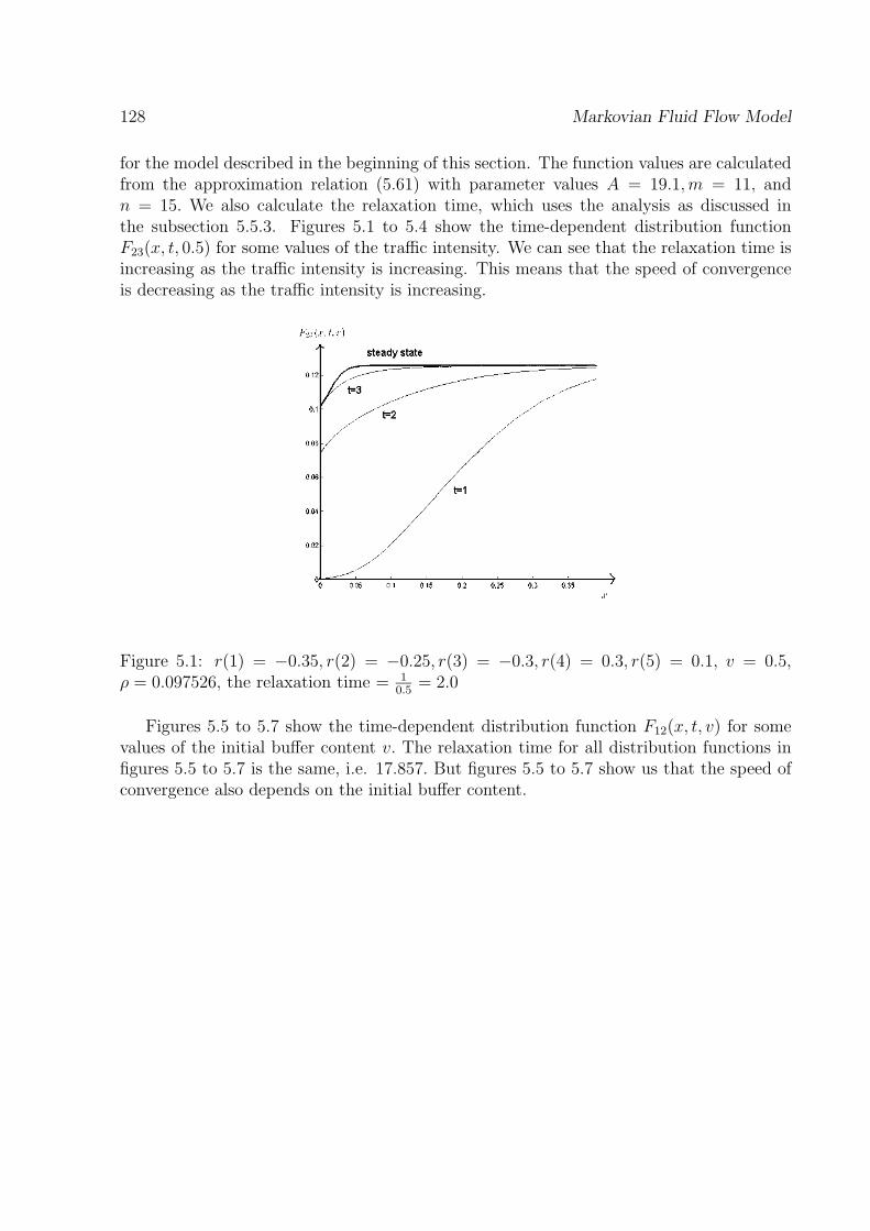
128 Markovian Fluid Flow Model
for the model described in the beginning of this section. The function values are calculatedfrom the approximation relation (5.61) with parameter values A = 19.1,m = 11, andn = 15. We also calculate the relaxation time, which uses the analysis as discussed inthe subsection 5.5.3. Figures 5.1 to 5.4 show the time-dependent distribution functionF23(x, t, 0.5) for some values of the traffic intensity. We can see that the relaxation time isincreasing as the traffic intensity is increasing. This means that the speed of convergenceis decreasing as the traffic intensity is increasing.
Figure 5.1: r(1) = −0.35, r(2) = −0.25, r(3) = −0.3, r(4) = 0.3, r(5) = 0.1, v = 0.5,ρ = 0.097526, the relaxation time = 1
0.5= 2.0
Figures 5.5 to 5.7 show the time-dependent distribution function F12(x, t, v) for somevalues of the initial buffer content v. The relaxation time for all distribution functions infigures 5.5 to 5.7 is the same, i.e. 17.857. But figures 5.5 to 5.7 show us that the speed ofconvergence also depends on the initial buffer content.
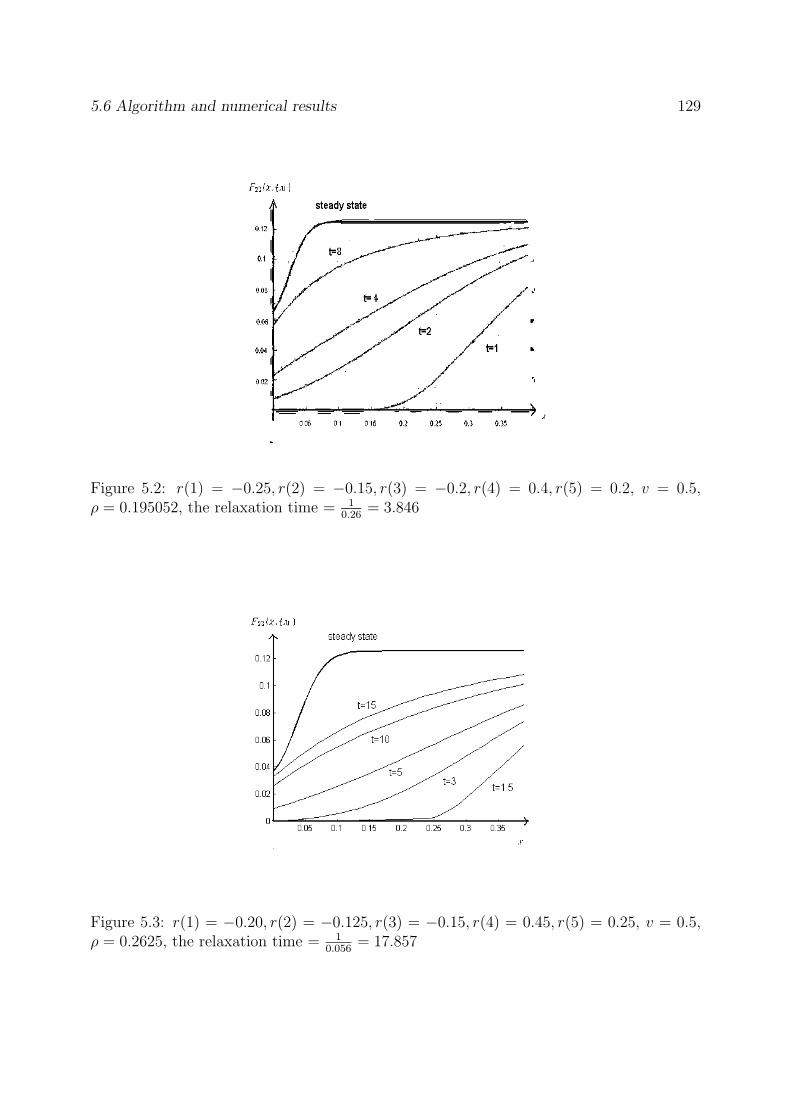
5.6 Algorithm and numerical results 129
Figure 5.2: r(1) = −0.25, r(2) = −0.15, r(3) = −0.2, r(4) = 0.4, r(5) = 0.2, v = 0.5,ρ = 0.195052, the relaxation time = 1
0.26= 3.846
Figure 5.3: r(1) = −0.20, r(2) = −0.125, r(3) = −0.15, r(4) = 0.45, r(5) = 0.25, v = 0.5,ρ = 0.2625, the relaxation time = 1
0.056= 17.857
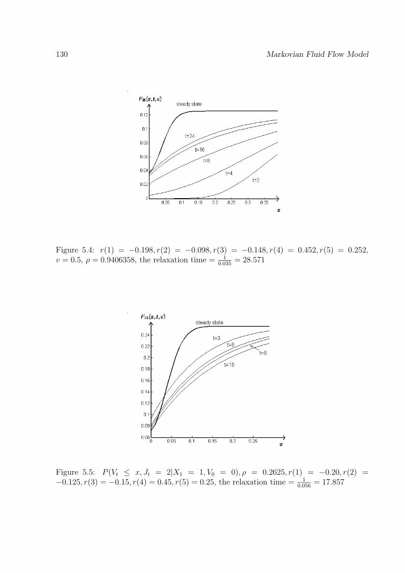
130 Markovian Fluid Flow Model
Figure 5.4: r(1) = −0.198, r(2) = −0.098, r(3) = −0.148, r(4) = 0.452, r(5) = 0.252,v = 0.5, ρ = 0.9406358, the relaxation time = 1
0.035= 28.571
Figure 5.5: P (Vt ≤ x, Jt = 2|X1 = 1, V0 = 0), ρ = 0.2625, r(1) = −0.20, r(2) =−0.125, r(3) = −0.15, r(4) = 0.45, r(5) = 0.25, the relaxation time = 1
0.056= 17.857
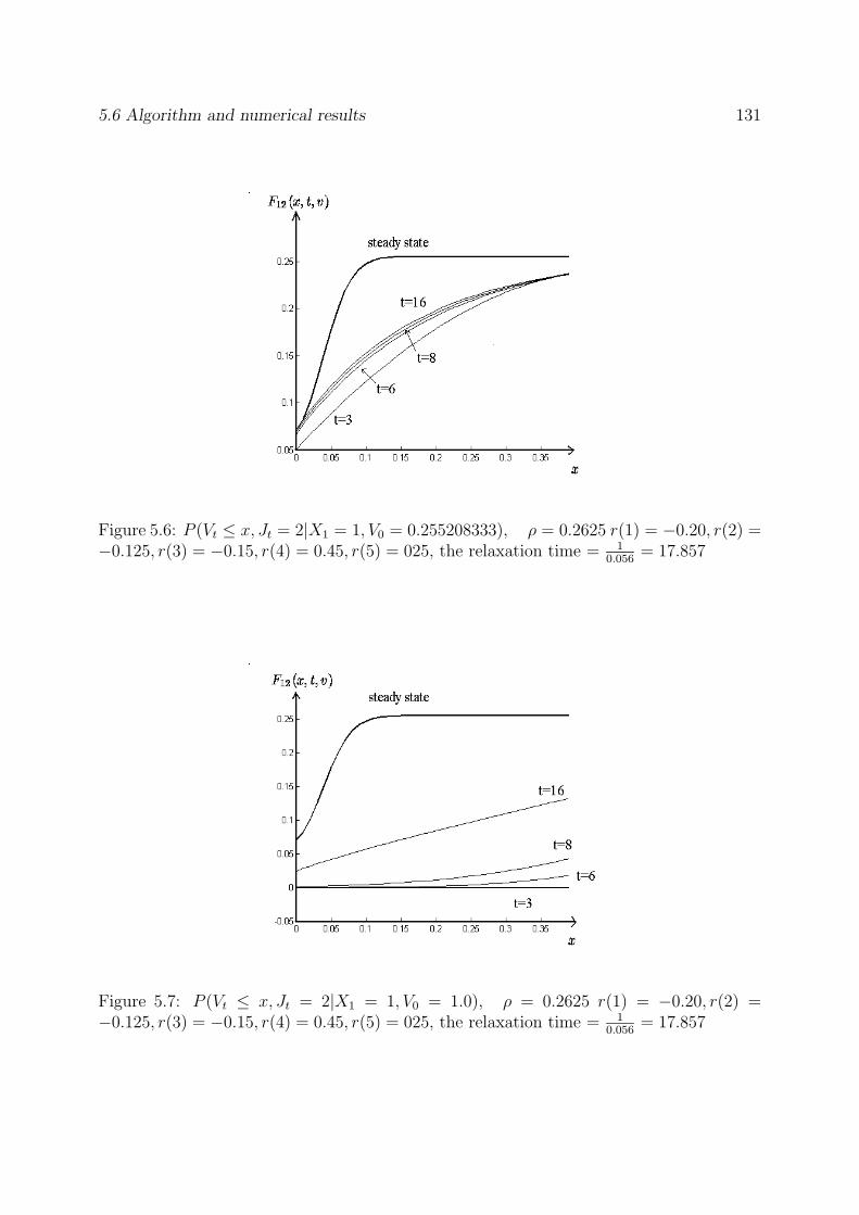
5.6 Algorithm and numerical results 131
Figure 5.6: P (Vt ≤ x, Jt = 2|X1 = 1, V0 = 0.255208333), ρ = 0.2625 r(1) = −0.20, r(2) =−0.125, r(3) = −0.15, r(4) = 0.45, r(5) = 025, the relaxation time = 1
0.056= 17.857
Figure 5.7: P (Vt ≤ x, Jt = 2|X1 = 1, V0 = 1.0), ρ = 0.2625 r(1) = −0.20, r(2) =−0.125, r(3) = −0.15, r(4) = 0.45, r(5) = 025, the relaxation time = 1
0.056= 17.857

Chapter 6
Semi - Markovian Fluid Flow Model
6.1 Introduction
In this chapter we study a generalization of the model considered in chapter 5. Let(An, Xn), n ≥ 0 be a Markov renewal sequence with the property that for n = 1, 2, · · · ,
P (An+1 ≤ x,Xn+1 = j|A1, · · · , An, X1, · · · , Xn−1, Xn = i)
=P (An+1 ≤ x,Xn+1 = j|Xn = i),
in which the latter conditional probability does not depend on n and will be denoted asHij(x). Let Tn =
∑ni=1 Ai, for n = 1, 2, · · · , T0 = 0, and for t ≥ 0, let
Nt = supn|Tn ≤ t.
Now, consider the semi-Markov process Jt, t ≥ 0 where
Jt = XNt+1.
We see that at Tn the process Jt, t ≥ 0 jumps from one state to the next state andXn = JT−
n.
The structure of the fluid flow model we study in this chapter is similar to the structureof the model in chapter 5. Let N = 1, 2, . . . , N be the state space of the Markov chainXn, n ≥ 0. We assume that this process is irreducible and aperiodic. The slope at ofthe input process is constant between transitions of Jt and is equal to ci when Jt is instate i. The input flows into an infinite buffer that has maximal output rate c, and initiallyhas a content v. It follows that the rate of the net input process is also constant betweentransitions of Jt, and is equal to ri = ci − c. We define the buffer content at time t as Vt,with the assumption that V0 = v > 0. Let Wn = VTn , n = 0, 1, . . . . It is clear that W0 = v.
Let Hj, j ∈ N be the time the process Jt spends in state j before making a transitioninto a different state. In this chapter we assume that for j ∈ N , Hj is hyper-exponentiallydistributed or hypo-exponentially distributed(see Riska[39]). In other words, for j ∈ N , Hj
is a mixture of m exponential distributions or the distribution of the sum of m independentexponentially distributed random veriables, m ≥ 2. Let M = 1, 2, · · · ,m. It follows that
133
134 Semi - Markovian Fluid Flow Model
for i, j ∈ N , n = 1, 2, · · · , the Laplace-Stieltjes transform
Hij(φ) =
∫ ∞
0
e−φxdHij(x)
=
∫ ∞
0
e−φxdPAn+1 ≤ x|Xn = i,Xn+1 = jPXn+1 = j|Xn = i,
can be expressed as
Hij(φ) = Pijhj(φ)∏m
k=1(φ + µjk)
= Pij
∑mk=1 ajkµjk
∏ml=1,l 6=k(φ + µjl)∏m
k=1(φ + µjk), j 6= i,
(6.1)
where for i, j ∈ N , k ∈ M, the constants Pij, µjk and ajk are described as follows.
• Pij is the transition probability Pij = PXn+1 = j|Xn = i,
• µjk > 0 are assumed to be distinct,
• Case 1 For j ∈ N , Hj is hyper-exponentially distributed. Then the constantsajk > 0 do not have to be dependent on µjk, and satisfy
∑mk=1 ajk = 1.
Case 2 For j ∈ N , Hj is hypo-exponentially distributed. Then
ajk =m∏
l=1, l 6=k
µjl
(−µjk + µjl). (6.2)
Notice that for this case, the function hj(φ) can be written in the simpler form
hj(φ) =m∏
k=1
µjk. (6.3)
Our assumption in (6.1) is a generalization of the corresponding Laplace-Stieltjes trans-form in chapter 5 which has the form
Hij(φ) =
Qij
qi
qj
φ+qj, i 6= j,
0 , i = j,
where Qij is the (i, j)th element of the infinitesimal generator of the process Jt, t ≥ 0,and qi = −Qii.
With the assumption on Hij(φ) above, the symbol of Wiener-Hopf-type equations isstill a rational matrix in φ, and each element of this matrix has only simple poles. Withthis property, this matrix can be factorized by the Wiener-Hopf factorization technique aswe apply in chapter 5. For more general models in which the times between transitions arenot hyper-exponential or hypo-exponential, but Hij(φ) is still a rational function of φ, the
6.1 Introduction 135
Wiener-Hopf factorization technique still can be used to solve the problem. If the symbolof Wiener-Hopf-type equations has some poles of order more than one, the construction offactors of the symbol will be different from what we did in section 5.3 and it needs a morecomplicated analysis.
We are interested in the probability distribution of the buffer content in steady stateas well as in the time-dependent case, in which the distribution functions at time t ≥ 0 aredenoted by
Fij(x, t, v) = P (Vt ≤ x, Jt = j|X1 = i, V0 = v), i, j ∈ N .
Although most fluid flow models studied so far have a Markovian underlying process,Kulkarni[32] has suggested an analysis of the semi-Markovian fluid flow models. It isassumed that the analysis is going to be rather hard, and indeed, most papers that study thesemi-Markovian fluid flow models, i.e. Kella and Whitt[29], Gautam et al.[27], Asmussen[8],Boxma et al.[15], and Latouche and Takine[34], focus the analysis on special cases of themodels.
The steady-state distribution of the buffer content of the present semi-Markovian fluidflow model is studied in [27]. The upper and lower bounds for the steady-state distributionare derived, and discussion on some examples and applications in telecommunication net-works can be found in this paper. In [34], the study is focused on the semi-Markovian fluidflow model in which the intervals during which the input rate is negative(positive) havean exponential distribution. The structure of the steady-state buffer content distributionis studied by applying the Markov-renewal approach developed earlier in the context ofquasi-birth-and-death processes and of Markovian fluid queues. In [15], a model is studiedin which the underlying semi-Markov process has three states where at least one of theperiods in a state has a general distribution and the others have exponential distributions.The distribution of the buffer content, the distribution of the busy period and the distri-bution of the maximal buffer content during a busy period, in steady-state, are obtainedby establishing relations between the fluid flow models and ordinary queues with instanta-neous input, and by using level crossing theory. The approach is an extension of the one in[29], which only uses the relations between the fluid flow models and ordinary queues withinstantaneous input. A more general model, in which the period the underlying processJi spends in a state has a general phase-type distribution, is studied in [8]. In the latterpaper the steady-state distribution of the buffer content is derived.
As in chapter 5, in section 6.2 we consider the process (Wn, Tn, Xn) and derive Wiener-Hopf type equations for the transform of the joint distribution of (Wn, Tn, Xn). Thesystem of equations we obtain for the present model is similar to the system in chapter5. The only difference is that the expression for its symbol is a more general rationalfunction, since now we are dealing with a more general transform Hij(φ) . In section6.3 we solve this system of equations with Wiener-Hopf factorization, which based on theminimal representation of polynomial matrices (see Gohberg et al [28] for the explanation ofthe minimal representation) . By using the characteristic of the minimal representation, weobtain an explicit expression for the transform of (Wn, Tn, Xn). The double transform ofthe buffer content in continuous time can be derived from the transform of (Wn, Tn, Xn),and this double transform with respect to one transform variable is a closed form, so that
136 Semi - Markovian Fluid Flow Model
we can invert it analytically to obtain the Laplace-Stieljes transform of the buffer content incontinuous time, as we do in section 6.4. To obtain the time-dependent distribution of thebuffer content in continuous time, we invert its Laplace-Stieltjes transform numerically.The steady-state distribution can be obtained by applying Abel’s limit theorem to thetransform. We show that the steady-state distribution function has a similar structure asfor the Markovian case we studied in chapter 5.
We implement the numerical inversion algorithm given in [3] to get the time-dependentdistribution functions, and the results can be found in section 6.6. The behavior of the time-dependent distributions we obtained from the numerical inversion confirms our conjecturein chapter 5, that the speed of convergence of the time-dependent distributions to thesteady-state distribution depends on the transition matrix P, the distribution of Hj, j ∈ N ,the initial buffer content v, and the net input rates ri, i ∈ N .
We will use the following notations: x+ = max(0, x), and x− = min(0, x). 1 is theindicator function, 1 is the N -dimensional column vector with all components equal to 1,1i is the K-dimensional column vector with i-th component 1 and all other componentequal to 0, where K is an integer defined in section 5.2. I is the identity matrix, Ikl isthe k × l-matrix with elements δij, where δij is Kronecker’s delta, i.e., δij = 0, for i 6= j,and δjj = 1. If A is an N × N -dimensional matrix, the i-th column of A is denoted byAi, and the i-th row of A is denoted by Ai. If A(i), i = 1, · · · ,m are N × N -dimensionalmatrices with elements A(i)jk, we denote by
∑mi=1 A(i) the N × N -dimensional matrix
with elements∑m
i=1 A(i)jk, and we denote by∏m
i=1 A(i) the N × N -dimensional matrixwhere the (j, k)th element is given by the multiplication of A(i)jk for i = 1, 2, · · · ,m.
6.2 System of Wiener-Hopf type equations
Let P be the transition probability matrix of the Markov chainXn with elementsPij. We assume that the Markov chain Xn is irreducible and positive recurrent. Thestationary probabilities limn→∞ P (Xn = i) are denoted by pi, i ∈ N , and p denotes the N -dimensional row vector with components pi. From (6.1) we see that the times between tran-sitions of Jt are non-arithmetic so that limt→∞ P (Jt = i), i ∈ N exists. The stationaryprobabilities limt→∞ P (Jt = i) are denoted by πi, i ∈ N and πππ denotes the N -dimensionalrow vector with components πi.
We assume that∑N
i=1 πiri < 0 to ensure stability. The traffic intensity ρ, i.e. the ratio
of the average input rate and the maximal output rate , is ρ =∑N
i=1 πici/c.
We assume that for i ∈ N , ci 6= c so that ri 6= 0 for i ∈ N . Let
R− = i|ri < 0, i = 1, . . . , N and R+ = i|ri > 0, i = 1, . . . , N.
Let |R−| = K. This implies that |R+| = N − K. Let r = diag(r1, . . . , rN). Without loss ofgenerality, suppose that R− = 1, 2, . . . , K.
Define for Re(η) ≥ 0, Re(φ) ≥ 0, v ≥ 0,
Z0i (φ, η, v) = E
(e−φW1−ηT11 (X1 = i)|X1 = i, V0 = v
), (6.4)
6.2 System of Wiener-Hopf type equations 137
and define for (|z| < 1, Re(η) ≥ 0, Re(φ) ≥ 0) or (|z| ≤ 1, Re(η) > 0, Re(φ) ≥ 0) or(|z| ≤ 1, Re(η) ≥ 0, Re(φ) > 0)
Zij(z, φ, η, v) =∞∑
n=1
znE(e−φWn−ηTn1 (Xn = j)|X1 = i, V0 = v
).
Define for Re(φ) ≤ 0,
Vij(z, φ, η, v) =∞∑
n=1
zn+1E((
1 − e−φ[Wn+Rn+1An+1]−)
e−η(Tn+An+1)1 (Xn = j)|X1 = i, V0 = v),
and for Re(φ) = 0,
Gij(φ, η) = E(e−(rjφ+η)An+11 (Xn+1 = j)|Xn = i
).
Let Z(z, φ, η, v),V(z, φ, η, v) and G(φ, η) be N × N -matrices with elements Zij(z, φ, η, v),Vij(z, φ, η, v) and Gij(φ, η) respectively.
The assumption given in equation (6.1) yields
Gij(φ, η) = Pijhj(φrj + η)∏m
k=1(φrj + η + µjk)= Pij
m∑
k=1
ajkµjk
(φrj + η + µjk),
where the constants ajk satisfy the conditions explained on page 134. We then obtain thefollowing system of Wiener-Hopf-type equations in matrix notation.
Theorem 6.2.1For Re(φ) = 0 and (|z| ≤ 1, Re(η) > 0) or (|z| < 1, Re(η) ≥ 0) we have
Z(z, φ, η, v)(I − zG(φ, η)) = zZ0(φ, η, v) + V(z, φ, η, v), (6.5)
whereZ0(φ, η, v) = diag(Z0
1(φ, η, v), Z02(φ, η, v), . . . , Z0
N(φ, η, v)),
with
Z0i (φ, η, v) =
e−φv hi(φri + η)∏mk=1(φri + η + µik)
, if ri > 0,
m∑
k=1
aikµik
[e−φv − e(η+µik)v/ri
(φri + η + µik)+
e(η+µik)v/ri
(η + µik)
], if ri < 0.
(6.6)
Proof. For the proof of (6.5), see the proof of Theorem 5.2.1. To get the expression forZ0
i (φ, η, v), we recall that
Z0i (φ, η, v) = E
(e−φW1−ηT11(X1 = i)|X1 = i, V0 = v
)
=
∫ ∞
0
E(e−φ[v+riT1]+−ηT1|T1 = u
)dPT1 ≤ u|X1 = i.
138 Semi - Markovian Fluid Flow Model
Since T1 = A1, it follows from our assumption in (6.1) that for ri < 0 and v ≥ 0,
Z0i (φ, η, v) =
∫ −v/ri
0
E(e−φv−(φri+η)T1|T1 = u
)dPA1 ≤ u|X1 = i
+
∫ ∞
−v/ri
E(e−ηT1|T1 = u
)dPA1 ≤ u|X1 = i
=m∑
k=1
aikµik
[e−φv − e(η+µik)v/ri
]
(φri + η + µik)
+m∑
k=1
aikµike(η+µik)v/ri
(η + µik),
and for ri > 0 and v ≥ 0,
Z0i (φ, η, v) =
∫ ∞
0
E(e−φv−(φri+η)T1|T1 = u
)dPA1 ≤ u|X1 = i
= e−φv hi(φri + η)∏mk=1(φri + η + µik)
.
The system in Theorem 6.2.1 will be solved by the Wiener-Hopf factorization method.
6.3 Solution of the system of Wiener-Hopf equations
The system (6.5) can be solved by factorizing the symbol
H(z, φ, η) = I − zG(φ, η), (6.7)
i.e. for Re(φ) = 0,
H(z, φ, η) = H+(z, φ, η)H−(z, φ, η)
where
H+(z, φ, η) is analytic for Re(φ) > 0, and continuous and bounded forRe(φ) ≥ 0, and non-singular in Re(φ) > 0.
H−(z, φ, η) is analytic for Re(φ) < 0, and continuous and bounded forRe(φ) ≤ 0, and non-singular in Re(φ) < 0.
To find H+(z, φ, η) and H−(z, φ, η) first we consider the following. Let
r = diag(r1, r2, · · · , rN).
6.3 Solution of the system of Wiener-Hopf equations 139
We then can write the matrix G(φ, η) as
G(φ, η) = Ph(φ, η)(µµµ1 + φr + ηI)−1(µµµ2 + φr + ηI)−1 · · · (µµµm + φr + ηI)−1, (6.8)
whereh(φ, η) = diag(h1(φr1 + η), · · · , hN(φrN + η)), (6.9)
with hj(φ) defined on page 134, and µµµi = diag(µ1i, µ2i, · · · , µNi), i ∈ M.Let
αij(η) = (η + µij)/ri, i ∈ N , j ∈ M,
and letαij = αij(0), i ∈ N , j ∈ M.
Define N × N -dimensional matrices
αααi(η) = diag(α1i(η), . . . , αNi(η)), i ∈ M,
αααi = diag(α1i, . . . , αNi), i ∈ M,
M(φ, η) = (ααα1(η) + φI)(ααα2(η) + φI) · · · (αααm(η) + φI), (6.10)
L(z, φ, η) = M(φ, η) − zPr−mh(φ, η), (6.11)
where rm = rr · · · r︸ ︷︷ ︸m
and r−m = (rm)−1. It follows that
H(z, φ, η) = L(z, φ, η)M−1(φ, η). (6.12)
Furthermore,detL(z, φ, η) = detH(z, φ, η) detM(φ, η). (6.13)
Proposition 6.3.11. The poles of detH(z, φ, η) are the zeros of detM(φ, η),
2. The zeros of detL(z, φ, η) are the zeros of detH(z, φ, η).
Proof. It is clear that detM(φ, η) has Nm zeros, i.c. −α11(η), · · · ,−α1m(η), −α21(η), · · · ,−α2m(η), · · · , −αN1, . . . ,−αNm(η). Since by definition ri < 0, 1 ≤ i ≤ K, the first Kmof these lie in the right half-plane Re(φ) > 0 and the (N − K)m others lie in the lefthalf-plane Re(φ) < 0.
From (6.7), (6.9), (6.1), and (6.8) we see that detH(z, φ, η) has exactly Nm poles.Since detL(z, φ, η) does not have any pole, it follows from (6.13) that the Nm poles ofdetH(z, φ, η) are the zeros of detM(φ, η). This proves part 1 of the proposition.
It also follows from (6.13) that the zeros of detL(z, φ, η) are the zeros of detH(z, φ, η)or the zeros of detM(φ, η). We then can conclude that detL(z, φ, η) does not have anyzero in common with detM(φ, η). This proves part 2 of the proposition.
Based on the proposition, we consider the following lemmas.
140 Semi - Markovian Fluid Flow Model
Lemma 6.3.1With respect to φ, for (|z| ≤ 1, Re(η) > 0) or (|z| < 1, Re(η) ≥ 0) , detL(z, φ, η) has
Km zeros in the right half- plane Re(φ) > 0 and has (N − K)m zeros in the left half-planeRe(φ) < 0.
Proof. We first study the characteristics of zeros and poles of detH(z, φ, η). Notice thatthe (i, j)th element of zG(φ, η) is given by
zPij
m∑
k=1
ajkµjk
(φrj + η + µjk),
so that (|z| ≤ 1, Re(η) > 0) or (|z| < 1, Re(η) ≥ 0) ,
N∑
j=1
|zG(φ, η)ij| =N∑
j=1
|z|Pij
∣∣∣∣∣
m∑
k=1
ajkµjk
φrj + η + µjk
∣∣∣∣∣. (6.14)
We then consider the following cases, that follows from our assumption on the time theprocess Jt spends in a state before making a transition into a different state.
Case 1 For j ∈ N , Hj is hyper-exponentially distributed. On Re(φ) = 0, with(|z| ≤ 1, Re(η) > 0) or (|z| < 1, Re(η) ≥ 0) , it is clear that for j ∈ N , k ∈ M,
∣∣∣∣µjk
φrj + η + µjk
∣∣∣∣ < 1. (6.15)
Let d0 = (|η| + 2 maxj∈N ,k∈M
|µjk|)/ minj∈N
|rj|. Then on |φ| = d with d > d0, the inequality
(6.15) is also satisfied. Since∑m
k=1 ajk = 1, it follows that on C+0,d(C
−0,d),
N∑
j=1
|zG(φ, η)ij| =N∑
j=1
|z|Pij
m∑
k=1
ajk
∣∣∣∣µjk
φrj + η + µjk
∣∣∣∣
<N∑
j=1
Pij
m∑
k=1
ajk
= 1.
Due to Theorem A.4.2 (generalization of Rouche’s theorem) it follows that on C+0,d(C
−0,d),
the number of zeros and the number of poles inside C+0,d (C−
0,d) of detH(z, φ, η) arethe same. From part 1 of Proposition 6.3.1 we can conclude that detH(z, φ, η) hasKm poles in the right half- plane Re(φ) > 0 and has (N − K)m poles in the lefthalf-plane Re(φ) < 0. It follows that detH(z, φ, η) has Km zeros in the right half-plane Re(φ) > 0 and has (N − K)m zeros in the left half-plane Re(φ) < 0. TheLemma for case 1 then can be proven by using part 2 of Proposition 6.3.1.
6.3 Solution of the system of Wiener-Hopf equations 141
Case 2 For j ∈ N , Hj is hypo-exponentially distributed. For this case, we usethe expression for hj(φ, η) given by (6.3), that is
hj(φ, η) =m∏
k=1
µjk.
On Re(φ) = 0, with (|z| ≤ 1, Re(η) > 0) or (|z| < 1, Re(η) ≥ 0) , it is clear that forj ∈ N , k ∈ M, ∣∣∣∣∣
m∏
k=1
µjk
(φrj + η + µjk)
∣∣∣∣∣ < 1. (6.16)
Let d0 = (|η| + 2 maxj∈N ,k∈M
|µjk|)/ minj∈N
|rj|. Then on |φ| = d with d > d0, the inequality
(6.16) is also satisfied so that on C+0,d(C
−0,d),
N∑
j=1
|zG(φ, η)ij| =N∑
j=1
|z|Pij
∣∣∣∣∣
m∏
k=1
µjk
(φrj + η + µjk)
∣∣∣∣∣
<N∑
j=1
Pij
= 1.
Case 2 of the lemma now follows by using the same argument as in the proof ofCase 1.
Let γi(z, η), i = 1, · · · , Km be the zeros of detL(z, φ, η) in the right half-planeRe(φ) > 0 and let γi(z, η), i = Km + 1, · · · , Nm be the zeros in the left half-planeRe(φ) < 0. The following lemma concerns the behavior of the zeros of detL(z, φ, 0) asz ↑ 1.
Lemma 6.3.2For z ↑ 1 one of the Km zeros of detL(z, φ, 0) in the right half-plane Re(φ) > 0 tends
to 0 if and only if∑N
i=1 πiri = πr1 < 0.
Proof. Let γ1(z, 0) be a zero of detL(z, φ, 0). Then by Proposition 6.3.1 we also havedetH(z, γ1(z, 0), 0) = 0. Let, moreover, v(z) be a non-zero column vector with elementsv1(z), · · · , vN(z), satisfying H(z, γ1(z, 0), 0)v(z) = 0. Since G(0, 0) = P, it follows thatdetH(1, 0, 0) = 0. So we may choose γ1(z, 0) such that γ1(1, 0) = 0, and since
H(1, 0, 0)1 = 0
we may assume that v(1) = 1. Noting that P is irreducible it follows that detH(1, φ, 0)has a simple zero at φ = 0. Consequently, the function γ1(z, 0) can not have a branch pointat z = 1 and, therefore, is differentiable at z = 1.
142 Semi - Markovian Fluid Flow Model
From H(z, γ1(z, 0), 0)v(z) = 0 we have for i = 1, 2, · · · , N,
N∑
j=1
(δij − zGij(γ1(z, 0), 0))vj(z) = 0.
Differentiating this equation and letting z tend to 1 yields
dvi(z)
dz
∣∣∣z=1
−N∑
j=1
Pijdvj(z)
dz
∣∣∣z=1
−N∑
j=1
Pijvj(1)
[1 − rj
m∑
k=1
ajk
µjk
dγ1(z, 0)
dz
∣∣∣z=1
]
= 0.
With our assumption v(1) = 1, this can be written as
dvi(z)
dz
∣∣∣z=1
−N∑
j=1
Pijdvj(z)
dz
∣∣∣z=1
−N∑
j=1
Pij +N∑
j=1
Pijrj
m∑
k=1
ajk
µjk
dγ1(z, 0)
dz
∣∣∣z=1
= 0.
Multiplying this equation with pi, where pi is the stationary distribution of P, andsumming over all i we get
dγ1(z, 0)
dz
∣∣∣z=1
=1
N∑
j=1
pjrj
m∑
k=1
ajk
µjk
.
Noting that
πj =
pj
m∑
k=1
ajk
µjk
N∑
i=1
pi
m∑
k=1
aik
µik
,
we can now write for z ↑ 1,
γ1(z, 0) = −(1 − z)dγ1(z, 0)
dz
∣∣∣z=1
+ o(1 − z),
= −(1 − z)
(N∑
j=1
πjrj
)(N∑
j=1
pj
m∑
k=1
ajk
µjk
)+ o(1 − z).
This zero lies in the right half-plane Re(φ) > 0 and tends to the origin if and only if∑Nj=1 πjrj < 1.
We next impose the following condition.
Condition 6.3.1For Re(η) ≥ 0, −α11(η), . . . ,−αNm(η) and γ1(z, η), . . . , γNm(z, η) are all distinct.
6.3 Solution of the system of Wiener-Hopf equations 143
Similar to Condition 5.3.1, Condition 6.3.1 is needed to obtain the canonical factoriza-tion of H(z, φ, η). To find the factors, we first define some index sets.
A = 1, 2, · · · , N × 1, 2, · · · ,m,
B = 1, 2, · · · , Nm,and
Rm− = 1, 2, · · · , Km.We define a map tm from B to A
tm : l 7−→(⌊
l − 1
m
⌋+ 1, l − m
⌊l − 1
m
⌋),
where bac denotes the largest integer less or equal to a. This map defines a one to onecorrespondence from B to A, with inverse t−1
m : (i, j) → m(i − 1) + j. Notice that thisinverse gives an enumeration of the set A. We also define the map
tK : l 7−→⌊
l − 1
K
⌋+ 1,
which defines a function from Rm− to 1, 2, · · · ,m. We will use this function to divideRm− into m sets with cardinality K.
For i ∈ B, let Ei(z, η) be a non-unique nonzero column vector satisfying
L(z, γi(z, η), η)Ei(z, η) = 0, (6.17)
and let E(z, η) be the N × Nm-matrix with ith column is Ei(z, η).
For |z| ≤ 1, Re(η) ≥ 0, let D(z, η) be the N × Km-matrix with elements
Dij(z, η)
=(αi1(η) + γj(z, η))(αi2(η) + γj(z, η)) · · · (αim(η) + γj(z, η))Eij(z, η),
i ∈ N ; j ∈ Rm−. The ith column of matrix D(z, η) satisfies
Di(z, η) = M(γi(z, η), η)Ei(z, η). (6.18)
It follows that for i ∈ Rm−,
H(z, γi(z, η), η)Di(z, η) = L(z, γi(z, η), η)M−1(γi(z, η), η)M(γi(z, η), η)Ei(z, η)
= 0.(6.19)
For i ∈ N , |z| ≤ 1, Re(η) ≥ 0, define the K × Km-matrix iS(z, η) with elements
iSjk(z, η) =m∏
l=1,l 6=i
(αjl(η) + γk(z, η))Ejk(z, η), j ∈ R−, k ∈ Rm−. (6.20)
144 Semi - Markovian Fluid Flow Model
Let S(z, η) be the Km × Km-dimensional matrix so that its j-th row is the j −⌊
j−1K
⌋-th
row of matrix tK(j)S(z, η), or
S(z, η) =
1S(z, η)2S(z, η)
...mS(z, η)
.
We impose the following condition.
Condition 6.3.2detS(z, η) 6= 0 for z 6= 0 and Re(η) ≥ 0.
Let C0 be the Km × N -dimensional matrix defined by
C0 =
IKN
IKN...
IKN
,
where IKN is the K × N -dimensional matrix defined on page 136. Define the Km × N -matrix C(z, η) by
C(z, η) = S−1(z, η)C0, |z| ≤ 1, Re(η) ≥ 0. (6.21)
Notice that the last N − K columns of C(z, η) are equal zero. Now, define for (|z| < 1,Re(η) ≥ 0, Re(φ) ≥ 0) or (|z| ≤ 1, Re(η) > 0, Re(φ) ≥ 0) or (|z| ≤ 1, Re(η) ≥ 0,Re(φ) > 0), the N × N -matrix K(z, φ, η) by
K(z, φ, η) = I + D(z, η)diag
(1
φ − γ1(z, η), . . . ,
1
φ − γKm(z, η)
)C(z, η). (6.22)
We now give the explicit factorization theorem.
Theorem 6.3.1If Condition 6.3.1 and 6.3.2 are satisfied then for (|z| < 1, Re(η) ≥ 0) or
(|z| ≤ 1, Re(η) > 0) ,
1. detK(z, φ, η) =Km∏
i=1
(φ + αtm(i)(η)
φ − γi(z, η)
),
2. for Re(φ) = 0H(z, φ, η) = H+(z, φ, η)H−(z, φ, η)where
(a) H−(z, φ, η) = K−1(z, φ, η)
(b) H+(z, φ, η) = H(z, φ, η)K(z, φ, η)
6.3 Solution of the system of Wiener-Hopf equations 145
(c) H+(z, φ, η) is analytic for Re(φ) > 0, and continuous and bounded forRe(φ) ≥ 0, and non-singular in Re(φ) > 0,
H−(z, φ, η) is analytic for Re(φ) < 0, and continuous and bounded forRe(φ) ≤ 0, and non-singular in Re(φ) < 0.
Proof.By rearranging the diagonal elements of matrix M−1(φ, η) into its partial fractions we havethat
H+(z, φ, η) = H(z, φ, η)K(z, φ, η)
= K(z, φ, η) − zPh(φ, η)r−m
N∑
i=1
1Ti 1i∏m
j=1(φ + αij(η))K(z, φ, η)
= K(z, φ, η) − zPh(φ, η)r−m
N∑
i=1
m∑
j=1
Aij(η)IijITij
(φ + αij(η))K(z, φ, η),
(6.23)
where
• Aij(η), i = 1, 2, · · · , N, j = 1, 2, · · · ,m are constants not depending on φ,
• 1i is the N−dimensional row vector with ith component 1 and all other componentsequal to 0,
• Iij is the N×Nm-matrix with (i, (j−1)N +i) -th element 1 and all other componentsequal to 0.
Moreover, for l ∈ Rm− with tm(l) = (i1, i2) we have using (6.22), (6.18), (6.21), and(6.20),
ITi1i2
K(z,−αi1i2(η), η)
= ITi1i2
− ITi1i2
Km∑
j=1
Dj(z, η)Cj(z, η)/(αi1i2(η) + γj(z, η))
= ITi1i2
− 1T(i2−1)N+i1
Km∑
j=1
∏mk=1(αi1k(η) + γj(z, η))
(αi1i2(η) + γj(z, η))Ei1j(z, η)Cj(z, η)
= ITi1i2
− 1T(i2−1)N+i1
Km∑
j=1
i2Si1j(z, η)S−1j (z, η)C0IKN
= ITi1i2
− 1T(i2−1)N+i1
1i1
= ITi1i2
− ITi1i2
= 0,
where 1i is the Km-dimensional row vector with ith component 1 and all other componentsequal to 0. This yields for l ∈ Rm−,
limφ→−αtm(l)
(φ + αtm(l))H+(z, φ, η) = 0,
146 Semi - Markovian Fluid Flow Model
and this shows that H+(z, φ, η) has no pole at φ = −αtm(l), l ∈ Rm−.As in the proof of Theorem 5.3.1 in chapter 5 we can show that
detK(z, φ, η) =Km∏
i=1
(φ + αtm(i)(η)
φ − γi(z, η)
),
which proves part 1 of the theorem.We see from (6.22) that
H+(z, φ, η) = H(z, φ, η) + H(z, φ, η)Km∑
j=1
Dj(z, η)Cj(z, η)
(φ − γj(z, η)),
so from (6.7), Condition 6.3.1, and (6.19) it follows that for i ∈ Rm−,
limφ→γi(z,η)
(φ − γi(z, η))H+(z, φ, η) = H(z, γi(z, η), η)Di(z, η)Ci(z, η) = 0,
which proves part 2 of the theorem.
With this result we can write for the system (6.5)
Z(z, φ, η, v)H(z, φ, η)K(z, φ, η) = zZ0(φ, η, v)K(z, φ, η) + V(z, φ, η, v)K(z, φ, η), (6.24)
where the left-hand side is analytic in Re(φ) > 0 and bounded and continuous inRe(φ) ≥ 0, and the last term of the right-hand side is analytic in Re(φ) < 0 and boundedand continuous in Re(φ) ≤ 0.
Next we decompose the first term of the right-hand side, we determine functions K+ andK− such that i.e. for Re(φ) = 0,
Z0(φ, η, v)K(z, φ, η) = K+(z, φ, η, v) + K−(z, φ, η, v) (6.25)
where
K+(z, φ, η, v) is analytic for Re(φ) > 0, and continuous and bounded forRe(φ) ≥ 0,
K−(z, φ, η, v) is analytic for Re(φ) < 0, and continuous and bounded forRe(φ) ≤ 0.
Lemma 6.3.3If Conditions 6.3.1 and 6.3.2 are satisfied then for Re(φ) ≥ 0,
K+ij (z, φ, η, v)
= δijZ0i (φ, η, v) +
Km∑
k=1
Dik(z, η)Z0
i (φ, η, v) − Z0i (γk(z, η), η, v)
φ − γk(z, η)Ckj(z, η)
6.3 Solution of the system of Wiener-Hopf equations 147
(6.26)
and for Re(φ) ≤ 0,
K−ij (z, φ, η, v) =
Km∑
k=1
Dik(z, η)Z0
i (γk(z, η), η, v)
φ − γk(z, η)Ckj(z, η) (6.27)
if (|z| < 1, Re(η) ≥ 0) or (|z| ≤ 1, Re(η) > 0) .
Proof. Since by definition the zeroes γk(z, η), i = 1, 2, · · · , Km all lie in the right half-plane Re(φ) ≥ 0, it is clear that for i, j ∈ N , K−
ij (z, φ, η, v) does not have any pole in theleft half-plane Re(φ) < 0.
For l = 1, 2, · · · , Km it follows from (6.18), (6.20) and Condition 6.3.1 that
limφ→γl(z,η)
(φ − γl(z, η))K+ij (z, φ, η, v)
= limφ→γl(z,η)
(φ − γl(z, η))δijZ0i (φ, η, v)
+ limφ→γl(z,η)
(φ − γl(z, η))Km∑
k=1
Dik(z, η)Z0
i (φ, η, v) − Z0i (γk(z, η), η, v)
φ − γk(z, η)Ckj(z, η)
= limφ→γl(z,η)
(φ − γl(z, η))δijZ0i (φ, η, v),
where the expression for Z0i (φ, η, v) is given by (6.6). It follows that for l = 1, 2, · · · , Km,
i, j ∈ N ,lim
φ→γl(z,η)(φ − γl(z, η))K+
ij (z, φ, η, v) = 0,
thus K+ij (z, φ, η, v) is analytic in the right half-plane Re(φ) > 0.
Theorem 6.3.2If conditions 6.3.1 and 6.3.2 are satisfied then for Re(φ) ≥ 0,
Z(z, φ, η, v)H(z, φ, η)K(z, φ, η) = zK+(z, φ, η, v) + zK−(z, 0, η, v) (6.28)
if (|z| < 1, Re(η) ≥ 0) or (|z| ≤ 1, Re(η) > 0) .
Proof. See the proof of Theorem 5.3.2 in chapter 5.
In section 6.4 we will study the distribution of the buffer content. We will see that theexpression for the distribution functions of interest can be obtained once we find an explicitexpression for Z(1, φ, η, v), which can be easily found by multiplying both sides of (6.28)with H+(z, φ, η)−1 = [H(z, φ, η)K(z, φ, η)]−1 . Lemma 6.3.5 below gives us an expressionfor H+(z, φ, η)−1, and in the following we first define some vectors and matrices that willbe used in the lemma.
148 Semi - Markovian Fluid Flow Model
By definition,H(z, φ, η)−1 = M(φ, η)L(1, φ, η)−1.
To obtain an explicit expression for L(1, φ, η)−1, first we rewrite the matrix L(1, φ, η) as
L(1, φ, η) = φmI +m−1∑
i=0
φiLi(η).
Due to theorem A.5.1 on page 189 in the appendix, the expression for L(1, φ, η)−1 is givenby
L(1, φ, η)−1 = P1(φI − CL(η))−1R1, (6.29)
where
P1 = (I 0 · · ·0), R1 =
0...0I
,
and the (first) companion matrix of L(1, φ, η) is defined by
CL =
0 I 0 · · · 0
0 0 I · · · ......
......
... I−L0(η) −L1(η) −L2(η) · · · −Lm−1(η)
.
Letγγγ(η) = diag(γ1(1, η), · · · , γNm(1, η)),
and letE(η) = (e1(η) · · · eNm(η)),
where ei(η) is the eigenvector that corresponds to the eigenvalue γi(1, η) of CL (note thatthe eigenvalues of CL are also the zeros of detL(1, φ, η)). If condition 6.3.1 is satisfied, the
rank of E(η) is Nm, and we can write
γγγ(η) = E(η)−1CL(η)E(η).
It follows that
L(1, φ, η)−1 =E(η)(φI − γγγ(η))−1Y(η)
=Nm∑
i=1
Ei(η),Yi(η)
(φ − γi(1, η)),
(6.30)
whereE(η) = P1E(η), Y(η) = E(η)−1R1,
with Ei(η)(Yi(η)) denoting the ith column(row) of matrix E(η)(Y(η)). It can be easilyshown that the matrix Ei(η) is the same as E(1, η) defined on page 143. For brevity, inthe rest of this chapter we will use the notation Ei(η) instead of E(1, η).
6.3 Solution of the system of Wiener-Hopf equations 149
To obtain an explicit expression for K(z, φ, η)−1, define for Re(φ) ≥ 0, Re(η) ≥ 0, theKm × Km-matrix X(φ, η) by
X(φ, η) = φI − diag(γ1(1, η), . . . , γKm(1, η)) + C(1, η)D(1, η), (6.31)
where I is the Km × Km identity matrix.
Lemma 6.3.4For Re(φ) ≥ 0, Re(η) ≥ 0,
X(φ, η)−1 = S(1, η)−1(φI + ααα(η))−1S(1, η), (6.32)
where
ααα(η) = diag(α11(η), α21(η), · · · , αK1(η), α12(η), · · · , αK2(η), · · · , αKm(η)). (6.33)
Proof. See page 194 in the appendix.
Now we have the explicit expression for H+(1, φ, η)−1 which is given in the followinglemma.
Lemma 6.3.5If Conditions 6.3.1 and 6.3.2 are satisfied then for Re(φ) ≥ 0, Re(η) > 0,
H+(1, φ, η)−1
=(I − D(1, η)S(1, η)−1(φI + ααα(η))−1C0
)M(φ, η)
Nm∑
k=1
Ek(η)Yk(η)
(φ − γk(1, η)).
(6.34)
Proof. If Conditions 6.3.1 and 6.3.2 are satisfied then from (6.12) and (6.30) we obtainfor Re(φ) ≥ 0, Re(η) > 0,
H(1, φ, η)−1 = M(φ, η)Nm∑
i=1
Ei(η)Yi(η)
(φ − γi(1, η)). (6.35)
Moreover, from (6.22), (A.10) in the appendix, and (6.32) we also have for Re(φ) ≥ 0,Re(η) > 0,
K(1, φ, η)−1
=I − D(1, η)X(φ, η)−1C(1, η)
=I − D(1, η)S(1, η)−1(φI + ααα(η))−1S(1, η)C(1, η)
=I − D(1, η)S(1, η)−1(φI + ααα(η))−1C0. (6.36)
Since H+(1, φ, η)−1 = K(1, φ, η)−1H(1, φ, η)−1, then from (6.36) and (6.35) we obtain(6.34), and it proves the lemma.
150 Semi - Markovian Fluid Flow Model
In order to have closed-form expressions for the Laplace-Stieltjes transforms of probabilitydistributions of interest, in the following we will rewrite the rational matrix Z(1, φ, η, v) ina form so that in each element the degree of the numerator is less than the degree of thedenominator. In doing so, we note that for every positive integer n,
n∏
k=1
(φ + ak) =n∑
k=0
φkck, (6.37)
where the coefficients cn−k are given by
cn = 1, (6.38)
cn−k =∑
l1,l2,··· ,lk∈Cnk
k∏
j=1
alj , (6.39)
where Cnk is the set of combinations of k elements out of 1, 2, · · · , n, k = 1, 2, · · · , n.
Besides the rearrangement (6.37), we also should consider the following lemma.
Lemma 6.3.6For l = 1, · · · ,m − 1,
Nm∑
k=1
φlEk(η)Yk(η)
(φ − γk(1, η))=
Nm∑
k=1
γk(1, η)lEk(η)Yk(η)
(φ − γk(1, η)),
and
Nm∑
k=1
φmEk(η)Yk(η)
(φ − γk(1, η))= I +
Nm∑
k=1
γk(1, η)mEk(η)Yk(η)
(φ − γk(1, η)).
Proof. The matrices E(η) and Y(η) have the property (see page 52 of Gohberg et al.[28]for the proof) that
E(η)γγγkY(η) =
0 , for k = 0, · · · ,m − 2,
I , for k = m − 1,
so that
Nm∑
k=1
φEk(η)Yk(η)
(φ − γk(1, η))=
Nm∑
k=1
(φ − γk(1, η) + γk(1, η))Ek(η)Yk(η)
(φ − γk(1, η))
=Nm∑
k=1
Ek(η)Yk(η) +Nm∑
k=1
γk(1, η)Ek(η)Yk(η)
(φ − γk(1, η))
=Nm∑
k=1
γk(1, η)Ek(η)Yk(η)
(φ − γk(1, η)).
6.3 Solution of the system of Wiener-Hopf equations 151
Furthermore, we can prove by induction that for l = 1, · · · ,m − 1,
Nm∑
k=1
φlEk(η)Yk(η)
(φ − γk(1, η))=
Nm∑
k=1
γk(1, η)lEk(η)Yk(η)
(φ − γk(1, η)).
For l = m, it follows that
Nm∑
k=1
φmEk(η)Yk(η)
(φ − γk(1, η))= φ
Nm∑
k=1
φm−1Ek(η)Yk(η)
(φ − γk(1, η))
= φ
Nm∑
k=1
γk(1, η)m−1Ek(η)Yk(η)
(φ − γk(1, η))
= I +Nm∑
k=1
γk(1, η)mEk(η)Yk(η)
(φ − γk(1, η)).
With the explicit expression for H+(1, φ, η)−1 given by (6.34), together with (6.37) andLemma 6.3.6, we are halfway to an explicit expression for Z(1, φ, η, v).
From (6.28) we obtain Re(φ) ≥ 0, Re(η) > 0,
Z(1, φ, η, v) =(K+(1, φ, η, v) + K−(1, 0, η, v)
)H+(1, φ, η)−1.
Now, using (6.25) and by definition of K−ij (1, φ, η, v), K+(1, φ, η, v) + K−(1, 0, η, v) can be
rewritten as
Z0(φ, η, v)K(φ, η, v) − φ
Km∑
i=1
Z0(γi(1, η), η, v)Di(1, η)Ci(1, η)
γi(1, η)(φ − γi(1, η)),
so that by multiplying with H+(1, φ, η)−1, as given by (6.34), yields for Re(φ) ≥ 0,Re(η) > 0,
Z(1, φ, η, v)
=Z0(φ, η, v)M(φ, η)Nm∑
i=1
Ei(η)Yi(η)
(φ − γi(1, η))
− φKm∑
i=1
Z0(γi(1, η), η, v)Di(1, η)Ci(1, η)
γi(1, η)(φ − γi(1, η))
(I − D(1, η)X(φ, η)−1C(1, η)
)
.M(φ, η)Nm∑
k=1
Ek(η)Yk(η)
(φ − γk(1, η)).
(6.40)
Using (6.31) we see that
Ci(1, η)(I − D(1, η)X−1(φ, η)C(1, η)
)
=Ci(1, η) − (Ci(1, η)D(1, η) + (φ − γi(1, η))1i)X−1(φ, η)C(1, η)
+ (φ − γi(1, η))1iX−1(φ, η)C(1, η)
=Ci(1, η) − Ci(1, η) − (φ − γi(1, η))1iX−1(φ, η)C(1, η)
=(φ − γi(1, η))1iX−1(φ, η)C(1, η),
(6.41)
152 Semi - Markovian Fluid Flow Model
and by substituting this to (6.40) and by using (6.32) we obtain for Re(φ) ≥ 0, Re(η) > 0,
Z(1, φ, η, v)
=Z0(φ, η, v)M(φ, η)Nm∑
k=1
Ek(η)Yk(η)
(φ − γk(1, η))
− φKm∑
i=1
Z0(γi(1, η), η, v)Di(1, η)(S(1, η)−1)i
γi(1, η)
[φI + ααα(η)
]−1
C0M(φ, η)
.
Nm∑
k=1
Ek(η)Yk(η)
(φ − γk(1, η)).
(6.42)
In Appendix A.10 we check that Z(1, φ, η, v) is indeed analytic in the right half-planeRe(φ) ≥ 0.
In the following we will use the rearrangement (6.37) and Lemma 6.3.7 to rewrite theright hand-side of (6.42) so that in each term, the degree of the numerator is less than thedegree of the denominator.
For j = 1, · · · ,m, define the map
θj : M\ j 7→ 1, 2, · · · ,m − 1,
where
θj(k) =
k , k ≤ j − 1,
k − 1 , k > j.
For brevity, we will often write by θj = k for θj(l) = k, l ∈ M \ j.
We first consider the matrix
Z0(φ, η, v)M(φ, η)Nm∑
k=1
Ek(η)Yk(η)
(φ − γk(1, η)).
From (6.6) and (6.10) we obtain for Re(φ) ≥ 0, Re(η) ≥ 0,
Z0(φ, η, v)M(φ, η) =A0(η)M(φ, η) +m∑
j=1
Aj(φ, η)Mj(φ, η), (6.43)
where
A0(η) = diag
(m∑
k=1
a1kµ1keα1k(η)v
r1α1k(η), · · · ,
m∑
k=1
aKkµKkeαKk(η)v
rKαKk(η), 0, · · · , 0
),
and for j = 1, · · · ,m,
Aj(φ, η) = diag
(a1jµ1je1j(φ, η)
r1
, · · · ,aNjµNje1N(φ, η)
rN
),
6.3 Solution of the system of Wiener-Hopf equations 153
with
eij(φ, η) =
e−φv − eαij(η)v, for j ≤ K,e−φv, for j > K.
and
Mj(φ, η) =m−1∏
θj=1
(φI + αααθj(η)), j = 1, 2, · · · ,m.
By using the rearrangement (6.37), we can write
M(φ, η) =m∑
l=0
φlM0l(η), (6.44)
where
M0m(η) = I, (6.45)
M0(m−k)(η) =∑
l1,l2,··· ,lk∈Cmk
k∏
j=1
αααlj(η), (6.46)
where Cmk is the set of combinations of k elements out of 1, 2, · · · ,m, k = 1, 2, · · · ,m.
We also can write
Mj(φ, η) =m−1∑
k=0
φkMjk(η), (6.47)
where for j = 1, · · · ,m, k = 0, · · · ,m−1, the matrices Mjk(η) are N×N -diagonal matriceswhose diagonal elements are defined in the following.
Since the ith diagonal element of Mj(φ, η) is∏m−1
θj=1(φ + αiθj(η)), we can rewrite this
element as∑m−1
k=0 φkc(η, i, j, k), in which the coefficients c(η, i, j, k), according to (6.38) -(6.39), are given by
c(η, i, j,m − 1) = 1, (6.48)
c(η, i, j,m − 1 − k) =∑
l1,l2,··· ,lk∈Θjk
k∏
j=1
αilj(η), (6.49)
where Θjk is the set of combinations of k elements out of M\j, k = 1, 2, · · · ,m− 1. For
j ∈ M, k = 0, · · · ,m−1, we then can define Mjk(η) as the N ×N -diagonal matrices withits ith diagonal element equal c(η, i, j, k).
154 Semi - Markovian Fluid Flow Model
From (6.43), (6.44), (6.47), and Lemma 6.3.6 we then obtain for Re(φ) ≥ 0, Re(η) > 0,
Z0(φ, η, v)M(φ, η)Nm∑
k=1
Ek(η)Yk(η)
(φ − γk(1, η))
=A0(η)m∑
l=0
M0l(η)Nm∑
k=1
φlEk(η)Yk(η)
(φ − γk(1, η))
+m∑
l=1
Al(φ, η)m−1∑
k1=1
Mlk1(η)Nm∑
k2=1
φk1Ek2(η)Yk2(η)
(φ − γk2(1, η))
=A0(η) + A0(η)m∑
l=0
M0l(η)Nm∑
k=1
γk(1, η)lEk(η)Yk(η)
(φ − γk(1, η))
+m∑
l=1
Al(φ, η)m−1∑
k1=1
Mlk1(η)Nm∑
k2=1
γk1k2
Ek2(η)Yk2(η)
(φ − γk2(1, η)).
(6.50)
We now rewrite the rational matrix
(φI + ααα(η))−1C0M(φ, η)Nm∑
k=1
Ek(η)Yk(η)
(φ − γk(1, η))
which is part of the second term of the right hand-side of (6.42).By definition, we can write
C0M(φ, η) =
IKNM(φ, η)IKNM(φ, η)
...IKNM(φ, η)
,
so that by rearrangement (6.37),
(φI + ααα(η))−1C0M(φ, η) =
IKN(φI + ααα1)−1M(φ, η)
IKN(φI + ααα2)−1M(φ, η)
...IKN(φI + αααm)−1M(φ, η)
=
IKNM1(η)
IKNM2(η)...
IKNMm(η)
=
IKN
∑m−1k=0 M1k(η)
IKN
∑m−1k=0 M2k(η)
...
IKN
∑m−1k=0 Mmk(η)
. (6.51)
6.3 Solution of the system of Wiener-Hopf equations 155
Define Km × N -dimensional matrices:
Lm−1(η) =
IKN
IKN...
IKN
= C0, (6.52)
Ll(η) =
IKNM1l(η)IKNM2l(η)
...IKNMml(η)
, l = 0, 1, · · · ,m − 2, (6.53)
where the matrices Mjl(η) are defined on page 153. With the definition of Ll(η), l =0, · · · ,m − 1 above, we obtain the following lemma.
Lemma 6.3.7For Re(φ) ≥ 0, Re(η) > 0,
(φI + ααα(η))−1C0M(φ, η)Nm∑
k=1
Ek(η)Yk(η)
(φ − γk(1, η))=
m−1∑
l=0
Ll(η)Nm∑
k=1
γk(1, η)lEk(η)Yk(η)
(φ − γk(1, η)). (6.54)
Proof. From (6.51) we have
(φI + ααα(η))−1C0M(φ, η)Nm∑
k=1
Ek(η)Yk(η)
(φ − γk(1, η))=
m−1∑
l=0
Ll(η)Nm∑
k=1
φlEk(η)Yk(η)
(φ − γk(1, η)).
By using Lemma 6.3.6, we then obtain (6.54).
From (6.75), (6.50), and (6.51) we obtain an explicit expression for Z(1, φ, η, v), whichwe write in the following theorem.
Theorem 6.3.3If Conditions 6.3.1 and 6.3.2 are satisfied then for Re(φ) ≥ 0, Re(η) > 0,
Z(1, φ, η, v) =A0(η) + A0(η)m∑
l=0
M0l(η)Nm∑
k=1
γk(1, η)lEk(η)Yk(η)
(φ − γk(1, η))
+m∑
l=1
Al(φ, η)m−1∑
k1=0
Mlk1(η)Nm∑
k2=1
γk1k2
Ek2(η)Yk2(η)
(φ − γk2(1, η))
− A(η)C0 − A(η)m−1∑
l=0
Ll(η)Nm∑
k=1
γk(1, η)l+1Ek(η)Yk(η)
(φ − γk(1, η)),
(6.55)
where
A(η) =Km∑
i=1
Z0(γi(1, η), η, v)Di(1, η)(S(1, η)−1)i
γi(1, η).
With this theorem, it is easy to obtain closed-form Laplace-Stieltjes transforms of theprobability distributions of interest, which will be derived in the sections 6.4 and 6.5.
156 Semi - Markovian Fluid Flow Model
6.4 Inverse transformation
In this section we consider the distribution functions Fij(x, t, v), for i, j ∈ N , of thebuffer content at time t ≥ 0 for initial buffer content V0 = v.
If Jt = j then Vt, the buffer content at time t, satisfies the relation
Vt = [WNt + rj(t − TNt)]+,
where Nt is the number of transitions of the process Jt during (0, t]. Consequently, forRe(φ) ≥ 0,
E(e−φVt1(Jt = j)|X1 = i, V0 = v
)
=E(e−φ[W0+rj(t−T0)]+1(T0 ≤ t < T1, Jt = j)|X1 = i, V0 = v
)
+∞∑
n=1
E(e−φ[Wn+rj(t−Tn)]+1(Tn ≤ t < Tn+1, Jt = j)|X1 = i, V0 = v
),
(6.56)
where
∞∑
n=1
E(e−φ[Wn+rj(t−Tn)]+1(Tn ≤ t < Tn+1, Jt = j)|X1 = i, V0 = v
)
=∞∑
n=1
N∑
l=1
E(e−φ[Wn+rj(t−Tn)]+1(Tn ≤ t < Tn+1, Xn = l, Xn+1 = j)
|X1 = i, V0 = v)
=∞∑
n=1
N∑
l=1
∫ t
0
P (An+1 > t − u,Xn+1 = j|Xn = l)
.duE(e−φ[Wn+rj(t−Tn)]+1(Tn ≤ u,Xn = l)|X1 = i, V0 = v
)
=∞∑
n=1
N∑
l=1
∫ t
0
Plj
m∑
k=1
ajke−µjk(t−u)
.duE(e−φ[Wn+rj(t−Tn)]+1(Tn ≤ u,Xn = l)|X1 = i, V0 = v
).
(6.57)
From the identity(see page 269 of [17])
e−φx+
=1
2πi
∫ i∞+0
−i∞+0
dξ
ξ
φ
φ − ξe−ξx, with x real, Re(φ) > Re(ξ) > 0,
where the path of integration is a line parallel to the imaginary axis, we have
E(e−φ[Wn+rj(t−Tn)]+1(Tn ≤ u,Xn = l)|X1 = i, V0 = v
)
=1
2πi
∫ i∞+0
−i∞+0
dξ
ξ
φ
φ − ξe−ξrjtE
(e−ξWn+rjξTn1(Tn ≤ u,Xn = l)
|X1 = i, V0 = v)
(6.58)
6.4 Inverse transformation 157
and
E(e−φ[W0+rj(t−T0)]+1(T0 ≤ t < T1, Jt = j)|X1 = i, V0 = v
)
=1
2πi
∫ i∞+0
−i∞+0
dξ
ξ
φ
φ − ξe−ξ(v+rjt)E (1(t < T1, Jt = j)|X1 = i, V0 = v).
(6.59)
Combining (6.56), (6.57),(6.58) and (6.59) yields∫ ∞
0
e−ηtE(e−φVt1(Jt = j)|X1 = i, V0 = v
)dt
=1
2πi
∫ i∞+0
−i∞+0
dξ
ξ
φ
φ − ξe−ξv
∫ ∞
0
e−ηt−ξrjtP (t < T1, Jt = j|X1 = i, V0 = v) dt
+∞∑
n=1
N∑
l=1
1
2πi
∫ i∞+0
−i∞+0
dξ
ξ
φ
φ − ξ
∫ ∞
0
e−ηt
∫ t
0
Plj
m∑
k=1
ajke−µjk(t−u)e−ξrjt
.duE(e−ξWn+rjξTn1(Tn ≤ u,Xn = l)|X1 = i, V0 = v
)dt
=1
2πi
∫ i∞+0
−i∞+0
dξ
ξ
φ
φ − ξe−ξv
∫ ∞
0
e−ηt−ξrjt
m∑
k=1
ajke−µjktδijdt
+∞∑
n=1
N∑
l=1
1
2πi
∫ i∞+0
−i∞+0
dξ
ξ
φ
φ − ξE(e−ξWn−ηTn1(Xn = l)|X1 = i, V0 = v
)
.Plj
m∑
k=1
ajk/(η + µjk + ξrj)
=1
2πi
∫ i∞+0
−i∞+0
dξ
ξ
φ
φ − ξe−ξvδij
m∑
k=1
ajk
(rjξ + µjk + η)
+N∑
l=1
1
2πi
∫ i∞+0
−i∞+0
dξ
ξ
φ
φ − ξZil(1, ξ, η, v)Plj
m∑
k=1
ajk
(η + µjk + ξrj).
(6.60)
For Re(φ) ≥ 0, Re(η) > 0, let
Z∗ij(φ, η, v) =
∫ ∞
0
e−ηtE(e−φVt1(Jt = j)|X1 = i, V0 = v
)dt. (6.61)
We evaluate the integrals in (6.60) by considering the poles of the integrands in theright half-plane Re(φ) > 0. It follows that for Re(φ) ≥ 0, Re(η) > 0, j ∈ R−,
Z∗ij(φ, η, v) =
δij
rj
m∑
k=1
ajk
[αjk(η)e−φv + φeαjk(η)v
]
αjk(η)(φ + αjk(η))
+1
rj
N∑
l=1
Zil(1, φ, η, v)Plj
m∑
k=1
ajk
(φ + αjk(η))
+1
rj
N∑
l=1
m∑
k=1
Zil(1,−αjk(η), η, v)Pljφ
(φ + αjk(η))
ajk
αjk(η),
(6.62)
158 Semi - Markovian Fluid Flow Model
and for j ∈ R+,
Z∗ij(φ, η, v) =
1
rj
e−φvδij
m∑
k=1
ajk
(φ + αjk(η))
+1
rj
N∑
l=1
Zil(1, φ, η, v)Plj
m∑
k=1
ajk
(φ + αjk(η)).
(6.63)
It is easy to see that for k = 1, 2, · · · ,m, −αjk(η) is not a pole of Z∗ij(φ, η, v) as a function
of φ in the domain Re(φ) > 0.
By substituting the explicit expression for Zil(1, φ, η, v) given by (6.55), we can invertZ∗
ij(φ, η, v) analytically to obtain the Laplace-Stieltjes transform
ξij(x, η, v) =
∫ ∞
0
e−ηtFij(x, t, v)dt, Re(η) ≥ 0, i, j ∈ N . (6.64)
The expressions for ξi,j(x, η, v), i, j ∈ N given in Theorem 6.4.1 below are obtainedby contour integration through the inversion formula for Laplace-Stieltjes transform, seeLemma A.3.1 in the appendix. Since the only singularities of Z∗
ij(φ, η, v) in (6.62) and (6.63)are simple poles, the result of this contour integration is obtained from the correspondingresidues.
From (6.55) and (A.10) we see that the poles of Zij(1, φ, η, v) in the left half-planeRe(φ) < 0 are γl(1, η), l = Km+1, Km+2, · · · , Nm. The −αik(η), k = 1, 2, · · · ,m, whichare the poles of Z0
i (φ, η, v) in the left half-plane Re(φ < 0) for i ∈ R+, are not poles ofZij(1, φ, η, v) since the factor 1/
∏mk=1(φ + αik(η)) of Z0
i (φ, η, v) in Zij(1, φ, η, v) will becancelled when multiplying Z0(φ, η, v) by M(φ, η).
From (6.62) and (6.63), it can be seen that for j ∈ R−, the poles of Z∗ij(1, φ, η, v) are
the poles of Zil(1, φ, η, v), l = 1, 2, · · · , N, and for j ∈ R+, the poles of Z∗ij(φ, η, v) are the
poles of Zil(1, φ, η, v), l = 1, 2, · · · , N, and φ = −αjk(η), k = 1, 2, · · · ,m.
Define for l1 = Km + 1, · · · , Nm, the N × N -matrix
U l1il (η) =
[A(η)
m−1∑
l2=0
Ll2(η)γl2l1El1(η)Yl1(η)
]
il
. (6.65)
We denote by Bkj (η) the kth diagonal element of the matrix Bj(η). Then by using all poles
of Z∗ij(φ, η, v), and by using the expression for Z0
i (φ, η, v) given in Theorem 6.2.1, we obtainafter length but straightforward calculations, taking into account the above arguments, thefollowing theorem.
6.4 Inverse transformation 159
Theorem 6.4.1If Condition 6.3.1 and 6.3.2 are satisfied, then for x ≥ 0, Re(η) > 0,
ξij(x, η, v)
= − 1
rj
Nm∑
l1=Km+1
N∑
l2=1
Ai0(η)
m∑
l3=0
Mi0l3
(η)γl3−1l1
(1, η)(El1(η)Yl1(η)
)il2
Pl2j
.
m∑
k=1
ajk
(γl1(1, η) + αjk(η))(1 − eγl1
x)
− 1
rj
Nm∑
l1=Km+1
N∑
l2=1
m∑
l3=1
ail3µil3
ri
m−1∑
l4=0
Mil3l4
(η)γl4−1l1
(1, η)(El1(η)Yl1(η)
)il2
.Pl2j
m∑
k=1
ajk
(γl1(1, η) + αjk(η))
(1 − eγl1
(x−v))H(x − v)
+1
rj
Nm∑
l1=Km+1
N∑
l2=1
m∑
l3=1
ail3µil3eαil3
(η)
ri
m−1∑
l4=0
Mil3l4
(η)γl4−1l1
(1, η)(El1(η)Yl1(η)
)il2
.Pl2j
m∑
k=1
ajk
(γl1(1, η) + αjk(η))(1 − eγl1
x)
+1
rj
Nm∑
l1=Km+1
N∑
l2=1
U l1il2
(η, v)Plj
m∑
k=1
ajk
(γl1(1, η) + αjk(η))
(1 − eγl1
(1,η)x),
(6.66)
for i, j ∈ R−,
ξij(x, η, v)
= − 1
rj
Nm∑
l1=Km+1
N∑
l2=1
m∑
l3=1
Ail3(η)
m−1∑
l4=1
Mil3l4
(η)γl4−1l1
(1, η)(El1(η)Yl1(η)
)il2
.Pl2j
m∑
k=1
ajk
(γl1(1, η) + αjk(η))
(1 − eγl1
(x−v))H(x − v)
+1
rj
Nm∑
l1=Km+1
N∑
l2=1
U l1il2
(η, v)Plj
m∑
k=1
ajk
(γl1(1, η) + αjk(η))
(1 − eγl1
(1,η)x),
(6.67)
160 Semi - Markovian Fluid Flow Model
for i ∈ R+ and j ∈ R−,
ξij(x, η, v)
=δij
rj
m∑
k=1
ajk
αjk(η)
(1 − e−αjk(η)(x−v)
)H(x − v)
− 1
rj
Nm∑
l1=Km+1
N∑
l2=1
Ai0(η)
m∑
l3=0
Mi0l3
(η)γl3−1l1
(1, η)(El1(η)Yl1(η)
)il2
Pl2j
.
m∑
k=1
ajk
(γl1(1, η) + αjk(η))(1 − eγl1
x)
− 1
rj
Nm∑
l1=Km+1
N∑
l2=1
m∑
l3=1
ail3µil3
ri
m−1∑
l4=0
Mil3l4
(η)γl4−1l1
(1, η)(El1(η)Yl1(η)
)il2
.Pl2j
m∑
k=1
ajk
(γl1(1, η) + αjk(η))
(1 − eγl1
(x−v))H(x − v)
− 1
rj
Nm∑
l1=Km+1
N∑
l2=1
m∑
l3=1
ail3µil3eαil3
(η)
ri
m−1∑
l4=0
Mil3l4
(η)γl4−1l1
(1, η)(El1(η)Yl1(η)
)il2
.Pl2j
m∑
k=1
ajk
(γl1(1, η) + αjk(η))(1 − eγl1
x)
+1
rj
Nm∑
l1=Km+1
N∑
l2=1
U l1il2
(η, v)Plj
m∑
k=1
ajk
(γl1(1, η) + αjk(η))
(1 − eγl1
(1,η)x),
(6.68)
for i ∈ R− and j ∈ R+,
ξij(x, η, v)
=δij
rj
m∑
k=1
ajk
αjk(η)
(1 − e−αjk(η)(x−v)
)H(x − v)
− 1
rj
Nm∑
l1=Km+1
N∑
l2=1
m∑
l3=1
Ail3(η)
m−1∑
l4=1
Mil3l4
(η)γl4−1l1
(1, η)(El1(η)Yl1(η)
)il2
.Pl2j
m∑
k=1
ajk
(γl1(1, η) + αjk(η))
(1 − eγl1
(x−v))H(x − v)
+1
rj
Nm∑
l1=Km+1
N∑
l2=1
U l1il2
(η, v)Plj
m∑
k=1
ajk
(γl1(1, η) + αjk(η))
(1 − eγl1
(1,η)x).
(6.69)
for i, j ∈ R+.
To get the distribution functions
Fij(x, t, v), i, j ∈ N ,
we can do a numerical inversion with respect to η of (6.66) - (6.69).
6.5 The steady-state distribution of the buffer content 161
6.5 The steady-state distribution of the buffer con-
tent
We have derived an explicit expression for the Laplace-Stieltjes transform ξij(x, η, v)in Theorem 6.4.1. In this section we will use Abel’s limit theorem to get the steady-statedistribution of the buffer content if it exists. It is clear that the steady-state distributionof the buffer content in continuous time exists if it exists at transition epochs. The follow-ing theorem states the necessary and sufficient condition for the existence of the limitingdistribution of the buffer content at transition epochs.
Theorem 6.5.1The process (Wn, Vn), n = 0, 1, · · · weakly converges to (W,V ) if and only if
N∑
j=1
πjrj < 0.
Proof. The process (Wn, Xn) is regenerative where for any i ∈ N the state (0, i)can be seen as the regenerative state. Since the process Xn is assumed to have alimiting distribution, the return times of the process (Wn, Xn) are aperiodic so thatlimn→∞ PWn ≤ x,Xn = j|X1 = i, V0 = v for x ≥ 0 exists. If this limit is zero then nolimiting distribution exists, otherwise (Wn, Xn) converges weakly to a stationary randomvector (W,X).
From (6.26), (6.27) and Lemma 6.3.2 we see that if and only if∑N
i=1 πiri < 1, for φ 6= 0,
limz↑1
(1 − z)K+ij (z, φ, 0, v) + (1 − z)K−
ij (z, 0, 0, v)
= limz↑1
(1 − z)δijZ0i (φ, 0, v) − lim
z↑1(1 − z)
Km∑
k=1
Dik(z, 0)Z0
i (γk(z, 0), 0, v)
γk(z, 0)Ckj(z, 0)
+ limz↑1
(1 − z)Km∑
k=1
Dik(z, 0)Z0
i (φ, 0, v) − Z0i (γk(z, 0), 0, v)
φ − γk(z, 0)Ckj(z, 0)
= − Di1(1, 0)Z0i (γ1(1, 0), 0, v) lim
z↑1
(1 − z)
γ1(z, 0)C1j(1, 0)
= − Di1(1, 0) limz↑1
(1 − z)
γ1(z, 0)C1j(1, 0),
(6.70)
where
limz↑1
(1 − z)
γ1(z, 0)= − 1(∑N
j=1 πjrj
)(∑Nj=1 pj
∑mk=1
ajk
µjk
) 6= 0,
so that
limn→∞
E(e−φWn1(Xn = j)|X1 = i,W0 = v
)= lim
z↑1(1 − z)Zij(z, φ, 0, v) 6= 0.
162 Semi - Markovian Fluid Flow Model
It follows that limn→∞ PWn ≤ x,Xn = j|X1 = i, V0 = v 6= 0. We then can conclude thatif∑N
j=1 πjrj < 0, the process (Wn, Xn) converges weakly to a stationary random vector(W,X).
In the following subsection, we will derive the distribution function P (W ≤ x,X = j),which from Theorem 6.5.1 exists if and only if
∑Nj=1 πjrj < 0. Then in subsection 6.5.2 we
will derive the distribution function of the steady-state buffer content in continuous timebased on the result in subsection 6.5.1.
6.5.1 The steady-state distribution of buffer content at transitionepochs
LetEi = Ei(1, 0), and γi = γi(1, 0), i = 1, 2, · · · , Nm.
By Lemma 6.3.2 we know that γ1 = 0. Let Y = Y(0), D = D(1, 0) and C = C(1, 0). SinceH(1, 0, 0) = I − G(0, 0) = I − P and H(1, 0, 0)D1(1, 0) = 0, we may put D1(1, 0) = 1. Itfollows that Ei1 = 1∏m
j=1 αij,
S1(1, 0) = (1
α11
,1
α21
, · · · ,1
αK1
,1
α12
,1
α22
, · · · ,1
αK2
, · · · ,1
α1m
, · · · ,1
αKm
)t.
Let
V1 =1
ddz
γ1(z, 0)∣∣z=1
=N∑
j=1
pjrj
m∑
k=1
ajk
µjk
.
We also may put
Y1 =1
V1
p,
where p is the stationary probability distribution vector of the Markov chain Xn.Let for Re(φ) ≥ 0,
H(φ) = H(1, φ, 0),
K(φ) = I + Ddiag
(0,
1
φ − γ2
, . . . ,1
φ − γNm
)C.
Moreover, let for Re(φ) ≥ 0,
X(φ) = X(φ, 0),
M(φ) = M(φ, 0),
S = S(1, 0),
S−1 = S(1, 0)−1,
and
H+(φ) =
H(φ)K(φ) + 1φH(φ)D1C1, if φ 6= 0,
H(0)K(0) + H′(0)D1C1, if φ = 0.
6.5 The steady-state distribution of the buffer content 163
The matrix H+(φ) is the limit of H+(z, φ, 0) for z ↑ 1. Let Z(φ) be the N×N−dimensionalmatrix with elements
Zij(φ) = E(e−φW1(X = j)|X1 = i,W0 = v
)
= limz↑1
(1 − z)Zij(z, φ, 0, v), j = 1, 2, . . . , N.
From Theorem 6.3.2 and (6.70) we now have for Re(φ) ≥ 0,
Z(φ)H+(φ) =1
ddz
γ1(z, 0)∣∣z=1
D1C1
= V1U,
(6.71)
where U is an N ×N−dimensional matrix with rows C1. This shows that Zij(φ) does notdepend on i and v.
From (6.71), if Conditions 6.3.1 and 6.3.2 are satisfied, we can find a closed formexpression for the Laplace-Stieltjes transform of the probability distribution in steady stateof the buffer content at transition epochs.
Let Z(φ) be the N− dimensional row vector with components Zj(φ), j = 1, 2, · · · , N.From (6.71) we obtain for Re(φ) ≥ 0, using Lemma 6.3.1, Lemma 6.3.2, and Theorem6.3.1, and (6.34),
Z(φ) = V1C1H+(φ)−1
= V1C1
[I − DX(φ)−1C
]M(φ)
Nm∑
k=1
EkYk
(φ − γk)
(6.72)
We can show, in a similar way as for the derivation of (6.41), that for Re(φ) ≥ 0,
C1
[I − DX(φ)−1C
]= φ11S
−1(φI + ααα(0)
)−1
C0 = φS−11
(φI + ααα(0)
)−1
C0. (6.73)
By substituting (6.73) into (6.72), and by letting
V2 = V1S−11 ,
we obtain for Re(φ) ≥ 0,
Z(φ) =V2φ (φI + ααα(0))−1 C0M(φ)Nm∑
k=1
EkYk
(φ − γk). (6.74)
By using Lemma 6.3.7, and setting η = 0, we then obtain for Re(φ) ≥ 0,
Z(φ) =V2L0(0)Nm∑
k=1
φEkYk
(φ − γk)+
m−1∑
l=1
Ll(0)Nm∑
k=1
φγlkE
kYk
(φ − γk). (6.75)
Noting thatV2L0(0)E1Y1 = V1Y1 = p
164 Semi - Markovian Fluid Flow Model
andφγl
kEkYk
(φ − γk)= γl
kEkYk +
γl+1k EkYk
(φ − γk),
where∑Nm
k=1 γlkE
kYk = 0, l = 0, · · · ,m − 2 and∑Nm
k=1 γm−1k EkYk = I, we then obtain for
Re(φ) ≥ 0,
Z(φ) =p + V2L0(0)Nm∑
k=2
EkYk + V2L0(0)Nm∑
k=2
γkEkYk
(φ − γk)
+ V2
m−1∑
l=1
Ll(0)
[Nm∑
k=1
γlkE
kYk +Nm∑
k=1
γl+1k EkYk
(φ − γk)
]
=p + V2L0(0)Nm∑
k=2
EkYk + V2L0(0)Nm∑
k=2
γkEkYk
(φ − γk)
+ V2C0 + V2
m−1∑
l=1
Ll(0)Nm∑
k=2
γl+1k EkYk
(φ − γk).
(6.76)
In a similar way as on page 195 in Appendix A.10, we can check that for j = 1, 2, · · · , Km,limφ→γj
(φ − γj)Z(φ) = 0, or Z(φ) is analytic in the right half-plane Re(φ) ≥ 0.The equation (6.75) shows us that we have a closed-form Laplace-Stieltjes transform
for the steady-state buffer content at transition epochs. By inverting the j-th element of(6.75), we obtain for x ≥ 0, j = 1, 2, · · · , N,
P (W ≤ x,X = j)
= pj +Nm∑
k=Km+1
[V2L0(0)EkYk
]jeγkx −
Nm∑
k=Km+1
[V2
m−2∑
l=1
Ll(0)γlkE
kYk
]
j
+Nm∑
k=Km+1
[V2
m−1∑
l=1
Ll(0)γlkE
kYk
]
j
eγkx,
(6.77)
which shows us that the steady-state distribution of the buffer content at transition epochsis a mixture of exponentials and a concentration at 0. This structure is the same as thestructure of the corresponding distribution in chapter 5.
6.5.2 The steady-state distribution of the buffer content in con-tinuous time
The process (Vt, Jt), t ≥ 0 is regenerative, where the regeneration points are theepochs at which the process leaves a state (0, i) for some i ∈ N . Since the times betweenregeneration points are non-arithmetic and have finite expectation as can be inferred fromTheorem 6.5.1 and the finite means of inter-jump times of Jt, the process (Vt, Jt), t ≥ 0converges weakly to a random vector (V, J). Let
Z∗i (φ) = lim
t→∞E(e−φVt1(Jt = i)
),
6.5 The steady-state distribution of the buffer content 165
which is independent of initial conditions and will be determined using Abel’s limit theo-rem.
Lemma 6.5.1
d
dηγ1(1, η)
∣∣η=0
= −
N∑
j=1
pj
m∑
k=1
ajk
µjk
N∑
j=1
pjrj
m∑
k=1
ajk
ηjk
= − 1N∑
j=1
πjrj
.
Proof. By the same argument as in the proof of Lemma 6.3.2 it is seen that there is avector v(η) with v(0) = 1 such that for i = 1, 2, · · · , N,
N∑
j=1
(δij − Gij(γ1(1, η), η))vj(η) = 0.
It is readily verified from this equation using the same procedure as in Lemma 6.3.2 that
d
dηγ1(1, η)
∣∣η=0
= −
N∑
i=1
pi
N∑
j=1
d
dηGij(0, η)
∣∣η=0
N∑
i=1
pi
N∑
j=1
d
dφGij(φ, 0)
∣∣φ=0
and the result follows from the definition of G.
Let V3 = −∑Nj=1 πjrj. Similar to the derivation of (6.70) we have
limη↓0
ηZil(1, φ, η, v) = −V3V(φ)l, (6.78)
where the N−dimensional row vector V(φ) is defined by
V(φ) = φS−11
m−1∑
l=0
Ll(0)Nm∑
k=1
γlkE
kYk
(φ − γk).
The expression (6.78) shows that limη↓0 ηZil(φ, η, v) does not depend on i and v.
166 Semi - Markovian Fluid Flow Model
By applying Abel’s limit theorem to (6.62) and (6.63), relation (6.78) yields for Re(φ) ≥0, j ∈ R−,
Z∗j (φ) = lim
η↓0ηZ∗
ij(φ, η, v)
=1
rj
N∑
l=1
limη↓0
ηZil(1, φ, η, v)Plj
m∑
k=1
ajk
(φ + αjk(η))
+1
rj
N∑
l=1
m∑
k=1
limη↓0
ηZil(1,−αjk(η), η, v)Pljφ
(φ + αjk(η))
ajk
αjk(η)
= − V3
rj
N∑
l=1
V(φ)lPlj
m∑
k=1
ajk
(φ + αjk)
− V3
rj
N∑
l=1
m∑
k=1
V(−αjk)lPljφ
(φ + αjk)
ajk
αjk
,
(6.79)
and for j ∈ R+,
Z∗j (φ) = lim
η↓0ηZ∗
ij(φ, η, v)
=1
rj
N∑
l=1
limη↓0
ηZil(1, φ, η, v)Plj
m∑
k=1
ajk
φ + αjk(η)
= − V3
rj
N∑
l=1
V (φ)lPlj
m∑
k=1
ajk
φ + αjk
.
(6.80)
Noting that
V (φ)l =
[S−1
1 L0(0)Nm∑
k=1
φEkYk
(φ − γk)
]
l
+[S−1
1 C0
]l+
[m−1∑
l=1
S−11 Ll(0)
Nm∑
k=1
γl+1k EkYk
(φ − γk)
]
l
=Yil +
[S−1
1 L0(0)Nm∑
k=2
φEkYk
(φ − γk)
]
l
+[S−1
1 C0
]l
+
[m−1∑
l=1
S−11 Ll(0)
Nm∑
k=1
γl+1k EkYk
(φ − γk)
]
l
where Y1l = pl
V1and
− V3
rjV1
N∑
l=1
plPlj
m∑
k=1
ajk
φ + αjk
= − V3
rjV1
pj
m∑
k=1
ajk
φ + αjk
,
6.5 The steady-state distribution of the buffer content 167
we then obtain for Re(φ) ≥ 0, j ∈ R−,
Z∗j (φ)
= − V3pj
rjV1
m∑
k=1
ajk
φ + αjk
− V3
rj
N∑
l=1
[S−1
1 C0
]lPlj
m∑
k=1
ajk
φ + αjk
− V3
rj
N∑
l=1
[S−1
1 L0(0)Nm∑
k1=2
φEk1Yk1
(φ − γk1)
]
l
Plj
m∑
k2=1
ajk2
(φ + αjk2)
− V3
rj
N∑
l=1
[m−1∑
l1=1
S−11 Ll(0)
Nm∑
k1=2
γl1+1k1
Ek1Yk1
(φ − γk1)
]
l
Plj
m∑
k2=1
ajk2
(φ + αjk2)
− V3
rj
N∑
l=1
m∑
k=2
V(−αjk)lPljφ
(φ + αjk)
ajk
αjk
,
(6.81)
and for Re(φ) ≥ 0, j ∈ R+,
Z∗j (φ)
= − V3pj
rjV1
m∑
k=1
ajk
φ + αjk
− V3
rj
N∑
l=1
[S−1
1 C0
]lPlj
m∑
k=1
ajk
φ + αjk
− V3
rj
N∑
l=1
[S−1
1 L0(0)Nm∑
k1=2
φEk1Yk1
(φ − γk1)
]
l
Plj
m∑
k2=1
ajk2
(φ + αjk2)
− V3
rj
N∑
l=1
[m−1∑
l1=1
S−11 Ll(0)
Nm∑
k1=2
γl1+1k1
Ek1Yk1
(φ − γk1)
]
l
Plj
m∑
k2=1
ajk2
(φ + αjk2).
(6.82)
Like in subsection 6.5.1, we get a closed form Laplace-Stieltjes transform of the steady-state buffer content in continuous time. By inverting (6.81) and (6.82) we obtain forx ≥ 0, j = 1, 2, · · · , N,
P (V ≤ x, J = j)
= − V3pj
rjV1
m∑
k=1
ajk
αjk
− V3
rj
N∑
l=1
[S−1
1 C0
]lPlj
m∑
k=1
ajk
αjk
− V3
rj
Nm∑
k1=Km+1
N∑
l=1
[S−1
1 L0(0)Ek1Yk1
]lPlj
m∑
k2=1
ajk2
(γk1 + αjk2)eγk1
x
+V3
rj
N∑
l=1
[m−1∑
l1=1
S−11 Ll(0)
Nm∑
k1=2
γl1k1
Ek1Yk1
]
l
Plj
m∑
k2=1
ajk2
αjk2
− V3
rj
Nm∑
k1=Km+1
N∑
l=1
[m−1∑
l1=1
S−11 Ll(0)γl1
k1Ek1Yk1
]
l
Plj
m∑
k2=1
ajk2
(γk1 + αjk2)eγk1x.
(6.83)
168 Semi - Markovian Fluid Flow Model
Since V1 = −(
N∑
j=1
πjrj
)(m∑
i=1
pi
m∑
k=1
aik
µik
)and πj =
pj
m∑
k=1
ajk
µjk
N∑
i=1
pi
m∑
k=1
aik
µik
, then
V3pj
rjV1
m∑
k=1
ajk
αjk
= πj.
It should also be noted that, since γ1 = 0,
V3
rj
N∑
l=1
[m−1∑
l1=1
S−11 Ll(0)
Nm∑
k1=2
γl1k1
Ek1Yk1
]
l
Plj
m∑
k2=1
ajk2
αjk2
=V3
rj
N∑
l=1
[m−1∑
l1=1
S−11 Ll(0)
Nm∑
k1=1
γl1k1
Ek1Yk1
]
l
Plj
m∑
k2=1
ajk2
αjk2
=V3
rj
N∑
l=1
S−11 C0Plj
m∑
k2=1
ajk2
αjk2
,
so that the second and the fifth term of the right-hand side of (6.83) are cancelled.
Equation (6.83) can thus be written as follows. For x ≥ 0, j = 1, 2, · · · , N,
P (V ≤ x, J = j)
=πj −V3
rj
Nm∑
k1=Km+1
N∑
l=1
[S−1
1 L0(0)Ek1Yk1
]lPlj
m∑
k2=1
ajk2
(γk1 + αjk2)eγk1
x
− V3
rj
Nm∑
k1=Km+1
N∑
l=1
[m−1∑
l1=1
S−11 Ll(0)γl1
k1Ek1Yk1
]
l
Plj
m∑
k2=1
ajk2
(γk1 + αjk2)eγk1x,
(6.84)
which shows us that the steady-state distribution of the buffer content in continuous timeis a mixture of exponentials and a concentration at 0. This structure is the same as thestructure of such distribution of the Markovian fluid flow model studied in chapter 5, andaggrees the structure of such distribution of the semi-Markovian fluid flow model in [8].
6.6 Numerical examples
In this section we give some examples of the probability distribution of the buffercontent in continuous time for two semi-Markovian fluid flow models, where:
• N = 5,
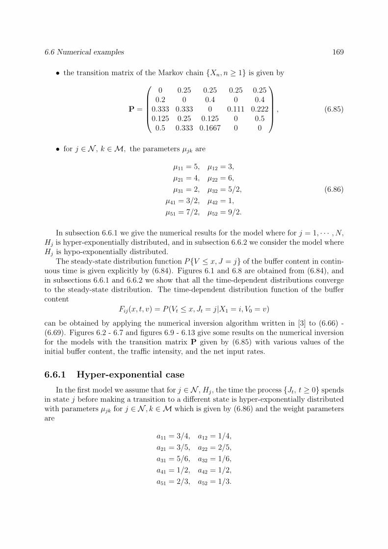
6.6 Numerical examples 169
• the transition matrix of the Markov chain Xn, n ≥ 1 is given by
P =
0 0.25 0.25 0.25 0.250.2 0 0.4 0 0.4
0.333 0.333 0 0.111 0.2220.125 0.25 0.125 0 0.50.5 0.333 0.1667 0 0
, (6.85)
• for j ∈ N , k ∈ M, the parameters µjk are
µ11 = 5, µ12 = 3,
µ21 = 4, µ22 = 6,
µ31 = 2, µ32 = 5/2,
µ41 = 3/2, µ42 = 1,
µ51 = 7/2, µ52 = 9/2.
(6.86)
In subsection 6.6.1 we give the numerical results for the model where for j = 1, · · · , N,Hj is hyper-exponentially distributed, and in subsection 6.6.2 we consider the model whereHj is hypo-exponentially distributed.
The steady-state distribution function PV ≤ x, J = j of the buffer content in contin-uous time is given explicitly by (6.84). Figures 6.1 and 6.8 are obtained from (6.84), andin subsections 6.6.1 and 6.6.2 we show that all the time-dependent distributions convergeto the steady-state distribution. The time-dependent distribution function of the buffercontent
Fij(x, t, v) = P (Vt ≤ x, Jt = j|X1 = i, V0 = v)
can be obtained by applying the numerical inversion algorithm written in [3] to (6.66) -(6.69). Figures 6.2 - 6.7 and figures 6.9 - 6.13 give some results on the numerical inversionfor the models with the transition matrix P given by (6.85) with various values of theinitial buffer content, the traffic intensity, and the net input rates.
6.6.1 Hyper-exponential case
In the first model we assume that for j ∈ N , Hj, the time the process Jt, t ≥ 0 spendsin state j before making a transition to a different state is hyper-exponentially distributedwith parameters µjk for j ∈ N , k ∈ M which is given by (6.86) and the weight parametersare
a11 = 3/4, a12 = 1/4,
a21 = 3/5, a22 = 2/5,
a31 = 5/6, a32 = 1/6,
a41 = 1/2, a42 = 1/2,
a51 = 2/3, a52 = 1/3.
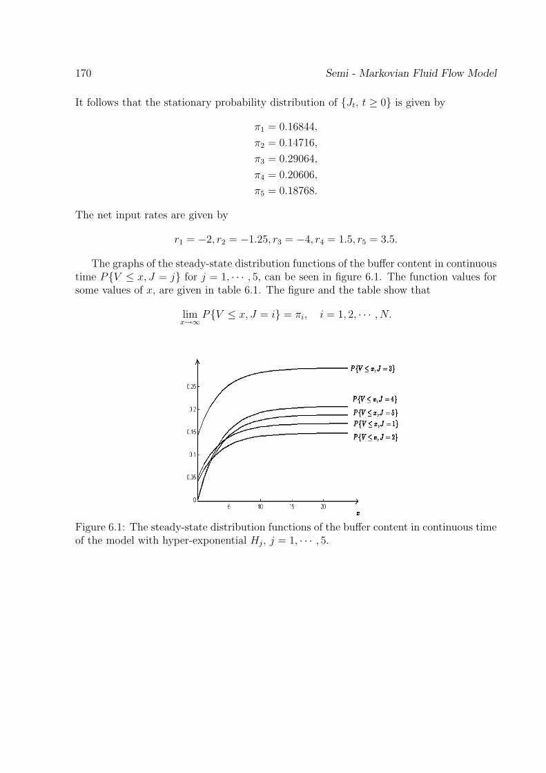
170 Semi - Markovian Fluid Flow Model
It follows that the stationary probability distribution of Jt, t ≥ 0 is given by
π1 = 0.16844,
π2 = 0.14716,
π3 = 0.29064,
π4 = 0.20606,
π5 = 0.18768.
The net input rates are given by
r1 = −2, r2 = −1.25, r3 = −4, r4 = 1.5, r5 = 3.5.
The graphs of the steady-state distribution functions of the buffer content in continuoustime PV ≤ x, J = j for j = 1, · · · , 5, can be seen in figure 6.1. The function values forsome values of x, are given in table 6.1. The figure and the table show that
limx→∞
PV ≤ x, J = i = πi, i = 1, 2, · · · , N.
Figure 6.1: The steady-state distribution functions of the buffer content in continuous timeof the model with hyper-exponential Hj, j = 1, · · · , 5.
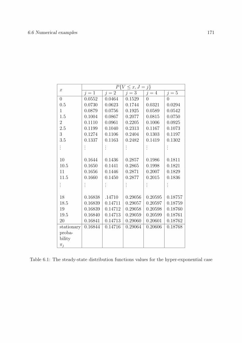
6.6 Numerical examples 171
PV ≤ x, J = jx
j = 1 j = 2 j = 3 j = 4 j = 50 0.0552 0.0464 0.1529 0 00.5 0.0730 0.0623 0.1744 0.0321 0.02941 0.0879 0.0756 0.1925 0.0589 0.05421.5 0.1004 0.0867 0.2077 0.0815 0.07502 0.1110 0.0961 0.2205 0.1006 0.09252.5 0.1199 0.1040 0.2313 0.1167 0.10733 0.1274 0.1106 0.2404 0.1303 0.11973.5 0.1337 0.1163 0.2482 0.1419 0.1302...
......
......
...
10 0.1644 0.1436 0.2857 0.1986 0.181110.5 0.1650 0.1441 0.2865 0.1998 0.182111 0.1656 0.1446 0.2871 0.2007 0.182911.5 0.1660 0.1450 0.2877 0.2015 0.1836...
......
......
...
18 0.16838 .14710 0.29056 0.20595 0.1875718.5 0.16839 0.14711 0.29057 0.20597 0.1875919 0.16839 0.14712 0.29058 0.20598 0.1876019.5 0.16840 0.14713 0.29059 0.20599 0.1876120 0.16841 0.14713 0.29060 0.20601 0.18762stationaryproba-bilityπj
0.16844 0.14716 0.29064 0.20606 0.18768
Table 6.1: The steady-state distribution functions values for the hyper-exponential case
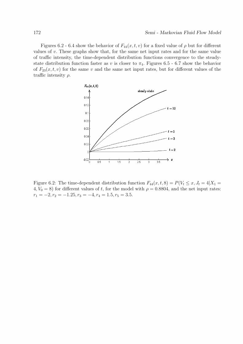
172 Semi - Markovian Fluid Flow Model
Figures 6.2 - 6.4 show the behavior of F44(x, t, v) for a fixed value of ρ but for differentvalues of v. These graphs show that, for the same net input rates and for the same valueof traffic intensity, the time-dependent distribution functions convergence to the steady-state distribution function faster as v is closer to π4. Figures 6.5 - 6.7 show the behaviorof F23(x, t, v) for the same v and the same net input rates, but for different values of thetraffic intensity ρ.
Figure 6.2: The time-dependent distribution function F44(x, t, 8) = P (Vt ≤ x, Jt = 4|X1 =4, V0 = 8) for different values of t, for the model with ρ = 0.8804, and the net input rates:r1 = −2, r2 = −1.25, r3 = −4, r4 = 1.5, r5 = 3.5.
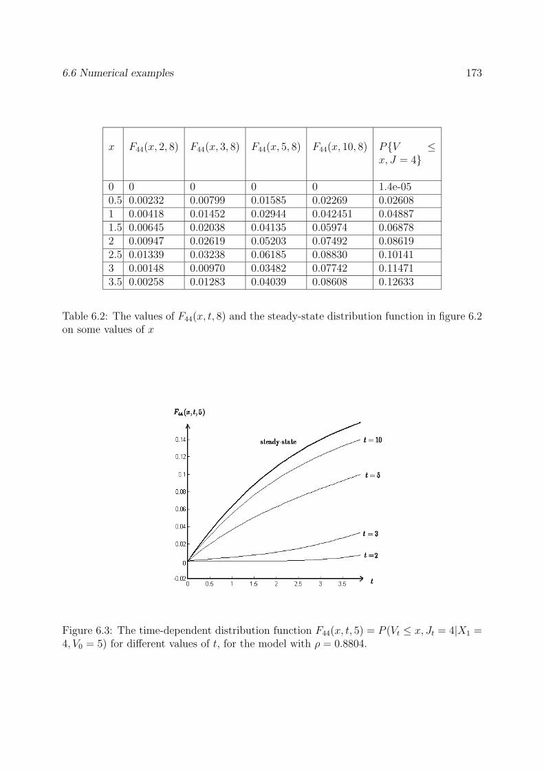
6.6 Numerical examples 173
x F44(x, 2, 8) F44(x, 3, 8) F44(x, 5, 8) F44(x, 10, 8) PV ≤x, J = 4
0 0 0 0 0 1.4e-050.5 0.00232 0.00799 0.01585 0.02269 0.026081 0.00418 0.01452 0.02944 0.042451 0.048871.5 0.00645 0.02038 0.04135 0.05974 0.068782 0.00947 0.02619 0.05203 0.07492 0.086192.5 0.01339 0.03238 0.06185 0.08830 0.101413 0.00148 0.00970 0.03482 0.07742 0.114713.5 0.00258 0.01283 0.04039 0.08608 0.12633
Table 6.2: The values of F44(x, t, 8) and the steady-state distribution function in figure 6.2on some values of x
Figure 6.3: The time-dependent distribution function F44(x, t, 5) = P (Vt ≤ x, Jt = 4|X1 =4, V0 = 5) for different values of t, for the model with ρ = 0.8804.
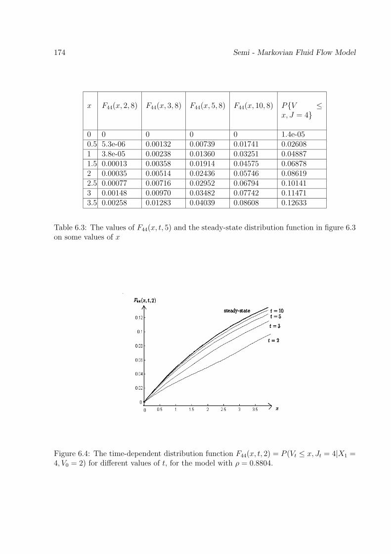
174 Semi - Markovian Fluid Flow Model
x F44(x, 2, 8) F44(x, 3, 8) F44(x, 5, 8) F44(x, 10, 8) PV ≤x, J = 4
0 0 0 0 0 1.4e-050.5 5.3e-06 0.00132 0.00739 0.01741 0.026081 3.8e-05 0.00238 0.01360 0.03251 0.048871.5 0.00013 0.00358 0.01914 0.04575 0.068782 0.00035 0.00514 0.02436 0.05746 0.086192.5 0.00077 0.00716 0.02952 0.06794 0.101413 0.00148 0.00970 0.03482 0.07742 0.114713.5 0.00258 0.01283 0.04039 0.08608 0.12633
Table 6.3: The values of F44(x, t, 5) and the steady-state distribution function in figure 6.3on some values of x
Figure 6.4: The time-dependent distribution function F44(x, t, 2) = P (Vt ≤ x, Jt = 4|X1 =4, V0 = 2) for different values of t, for the model with ρ = 0.8804.

6.6 Numerical examples 175
Figure 6.5: The time-dependent distribution function F23(x, t, 3) = P (Vt ≤ x, Jt = 3|X1 =2, V0 = 3) for different values of t, for the model with ρ = 0.82, and the net input rates:r1 = −2, r2 = −1.25, r3 = −4, r4 = 1.5, r5 = 3.5.
x F23(x, 2, 3) F23(x, 4, 3) F23(x, 5, 3) F23(x, 10, 3) PV ≤x, J = 3
0 0.15585 0.15815 0.15662 0.15034 0.177450.5 0.17947 0.17956 0.17776 0.17075 0.199591 0.20032 0.19790 0.19587 0.18829 0.216931.5 0.21872 0.21362 0.21138 0.20338 0.230702 0.23493 0.22708 0.22466 0.21637 0.241762.5 0.24906 0.23857 0.23600 0.22755 0.250683 0.26115 0.24836 0.24566 0.23717 0.257933.5 0.27125 0.25667 0.25387 0.24543 0.26383
Table 6.4: The values of F23(x, t, 3) and the steady-state distribution function in figure 6.5on some values of x
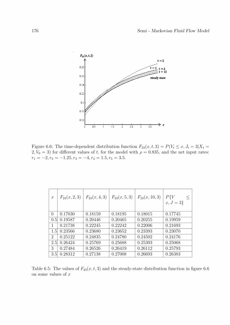
176 Semi - Markovian Fluid Flow Model
Figure 6.6: The time-dependent distribution function F23(x, t, 3) = P (Vt ≤ x, Jt = 3|X1 =2, V0 = 3) for different values of t, for the model with ρ = 0.835, and the net input rates:r1 = −2, r2 = −1.25, r3 = −4, r4 = 1.5, r5 = 3.5.
x F23(x, 2, 3) F23(x, 4, 3) F23(x, 5, 3) F23(x, 10, 3) PV ≤x, J = 3
0 0.17030 0.18159 0.18195 0.18015 0.177450.5 0.19587 0.20446 0.20465 0.20255 0.199591 0.21738 0.22245 0.22242 0.22006 0.216931.5 0.23566 0.23680 0.23652 0.23393 0.230702 0.25122 0.24835 0.24780 0.24502 0.241762.5 0.26424 0.25769 0.25688 0.25393 0.250683 0.27484 0.26526 0.26419 0.26112 0.257933.5 0.28312 0.27138 0.27008 0.26693 0.26383
Table 6.5: The values of F23(x, t, 3) and the steady-state distribution function in figure 6.6on some values of x
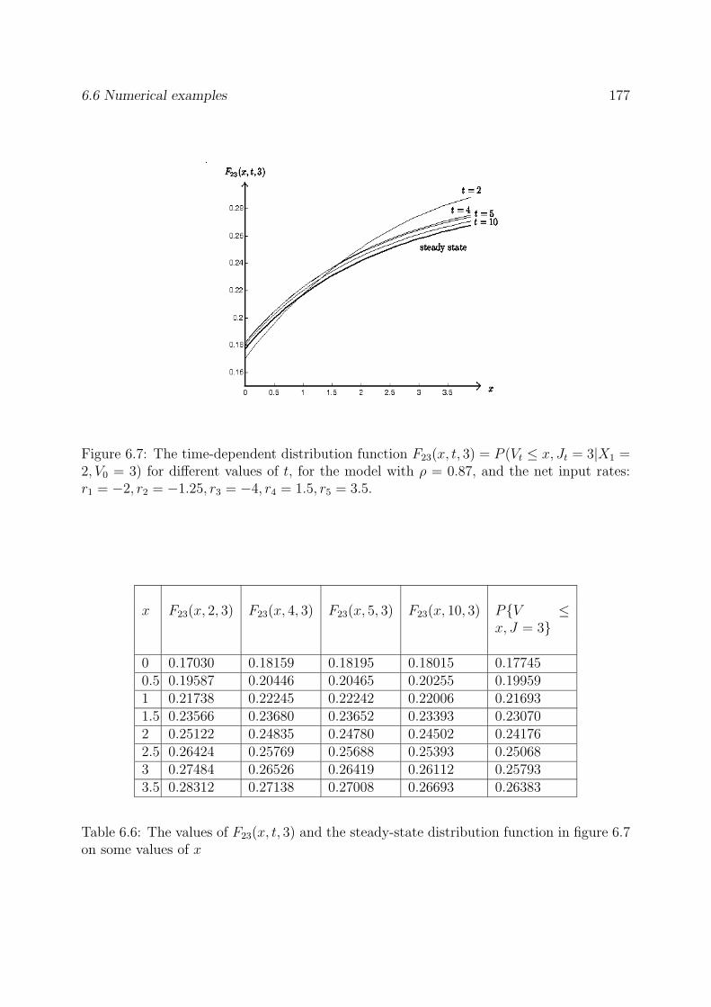
6.6 Numerical examples 177
Figure 6.7: The time-dependent distribution function F23(x, t, 3) = P (Vt ≤ x, Jt = 3|X1 =2, V0 = 3) for different values of t, for the model with ρ = 0.87, and the net input rates:r1 = −2, r2 = −1.25, r3 = −4, r4 = 1.5, r5 = 3.5.
x F23(x, 2, 3) F23(x, 4, 3) F23(x, 5, 3) F23(x, 10, 3) PV ≤x, J = 3
0 0.17030 0.18159 0.18195 0.18015 0.177450.5 0.19587 0.20446 0.20465 0.20255 0.199591 0.21738 0.22245 0.22242 0.22006 0.216931.5 0.23566 0.23680 0.23652 0.23393 0.230702 0.25122 0.24835 0.24780 0.24502 0.241762.5 0.26424 0.25769 0.25688 0.25393 0.250683 0.27484 0.26526 0.26419 0.26112 0.257933.5 0.28312 0.27138 0.27008 0.26693 0.26383
Table 6.6: The values of F23(x, t, 3) and the steady-state distribution function in figure 6.7on some values of x
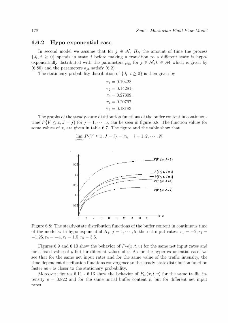
178 Semi - Markovian Fluid Flow Model
6.6.2 Hypo-exponential case
In second model we assume that for j ∈ N , Hj, the amount of time the processJt, t ≥ 0 spends in state j before making a transition to a different state is hypo-exponentially distributed with the parameters µjk for j ∈ N , k ∈ M which is given by(6.86) and the parameters ajk satisfy (6.2).
The stationary probability distribution of Jt, t ≥ 0 is then given by
π1 = 0.19428,
π2 = 0.14281,
π3 = 0.27309,
π4 = 0.20797,
π5 = 0.18183.
The graphs of the steady-state distribution functions of the buffer content in continuoustime PV ≤ x, J = j for j = 1, · · · , 5, can be seen in figure 6.8. The function values forsome values of x, are given in table 6.7. The figure and the table show that
limx→∞
PV ≤ x, J = i = πi, i = 1, 2, · · · , N.
Figure 6.8: The steady-state distribution functions of the buffer content in continuous timeof the model with hypo-exponential Hj, j = 1, · · · , 5, the net input rates: r1 = −2, r2 =−1.25, r3 = −4, r4 = 1.5, r5 = 3.5.
Figures 6.9 and 6.10 show the behavior of F52(x, t, v) for the same net input rates andfor a fixed value of ρ but for different values of v. As for the hyper-exponential case, wesee that for the same net input rates and for the same value of the traffic intensity, thetime-dependent distribution functions convergence to the steady-state distribution functionfaster as v is closer to the stationary probability.
Moreover, figures 6.11 - 6.13 show the behavior of F52(x, t, v) for the same traffic in-tensity ρ = 0.822 and for the same initial buffer content v, but for different net inputrates.
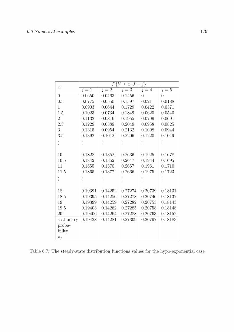
6.6 Numerical examples 179
PV ≤ x, J = jx
j = 1 j = 2 j = 3 j = 4 j = 50 0.0650 0.0463 0.1456 0 00.5 0.0775 0.0550 0.1597 0.0211 0.01881 0.0903 0.0644 0.1729 0.0422 0.03711.5 0.1023 0.0734 0.1849 0.0620 0.05402 0.1132 0.0816 0.1955 0.0799 0.06912.5 0.1229 0.0889 0.2049 0.0958 0.08253 0.1315 0.0954 0.2132 0.1098 0.09443.5 0.1392 0.1012 0.2206 0.1220 0.1049...
......
......
...
10 0.1828 0.1352 0.2636 0.1925 0.167810.5 0.1842 0.1362 0.2647 0.1944 0.169511 0.1855 0.1370 0.2657 0.1961 0.171011.5 0.1865 0.1377 0.2666 0.1975 0.1723...
......
......
...
18 0.19391 0.14252 0.27274 0.20739 0.1813118.5 0.19395 0.14256 0.27278 0.20746 0.1813719 0.19399 0.14259 0.27282 0.20753 0.1814319.5 0.19403 0.14262 0.27285 0.20758 0.1814820 0.19406 0.14264 0.27288 0.20763 0.18152stationaryproba-bilityπj
0.19428 0.14281 0.27309 0.20797 0.18183
Table 6.7: The steady-state distribution functions values for the hypo-exponential case
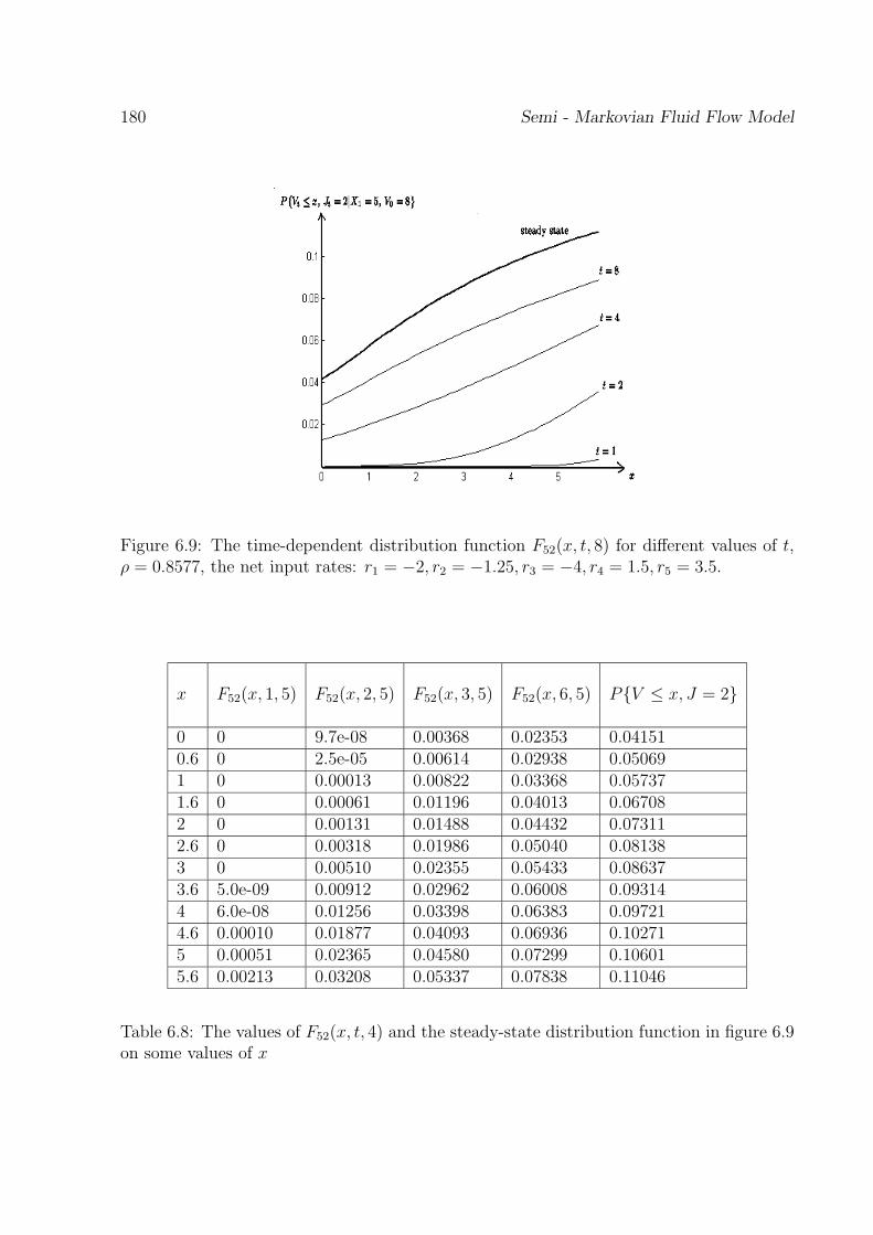
180 Semi - Markovian Fluid Flow Model
Figure 6.9: The time-dependent distribution function F52(x, t, 8) for different values of t,ρ = 0.8577, the net input rates: r1 = −2, r2 = −1.25, r3 = −4, r4 = 1.5, r5 = 3.5.
x F52(x, 1, 5) F52(x, 2, 5) F52(x, 3, 5) F52(x, 6, 5) PV ≤ x, J = 2
0 0 9.7e-08 0.00368 0.02353 0.041510.6 0 2.5e-05 0.00614 0.02938 0.050691 0 0.00013 0.00822 0.03368 0.057371.6 0 0.00061 0.01196 0.04013 0.067082 0 0.00131 0.01488 0.04432 0.073112.6 0 0.00318 0.01986 0.05040 0.081383 0 0.00510 0.02355 0.05433 0.086373.6 5.0e-09 0.00912 0.02962 0.06008 0.093144 6.0e-08 0.01256 0.03398 0.06383 0.097214.6 0.00010 0.01877 0.04093 0.06936 0.102715 0.00051 0.02365 0.04580 0.07299 0.106015.6 0.00213 0.03208 0.05337 0.07838 0.11046
Table 6.8: The values of F52(x, t, 4) and the steady-state distribution function in figure 6.9on some values of x
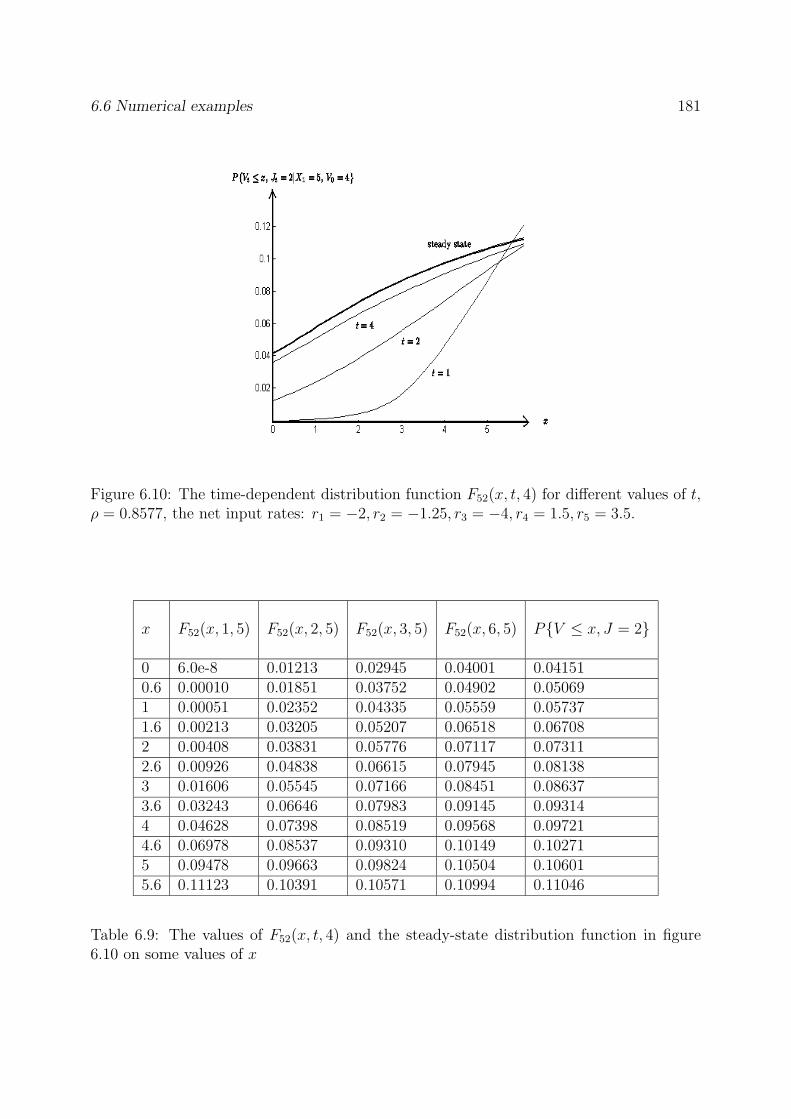
6.6 Numerical examples 181
Figure 6.10: The time-dependent distribution function F52(x, t, 4) for different values of t,ρ = 0.8577, the net input rates: r1 = −2, r2 = −1.25, r3 = −4, r4 = 1.5, r5 = 3.5.
x F52(x, 1, 5) F52(x, 2, 5) F52(x, 3, 5) F52(x, 6, 5) PV ≤ x, J = 2
0 6.0e-8 0.01213 0.02945 0.04001 0.041510.6 0.00010 0.01851 0.03752 0.04902 0.050691 0.00051 0.02352 0.04335 0.05559 0.057371.6 0.00213 0.03205 0.05207 0.06518 0.067082 0.00408 0.03831 0.05776 0.07117 0.073112.6 0.00926 0.04838 0.06615 0.07945 0.081383 0.01606 0.05545 0.07166 0.08451 0.086373.6 0.03243 0.06646 0.07983 0.09145 0.093144 0.04628 0.07398 0.08519 0.09568 0.097214.6 0.06978 0.08537 0.09310 0.10149 0.102715 0.09478 0.09663 0.09824 0.10504 0.106015.6 0.11123 0.10391 0.10571 0.10994 0.11046
Table 6.9: The values of F52(x, t, 4) and the steady-state distribution function in figure6.10 on some values of x
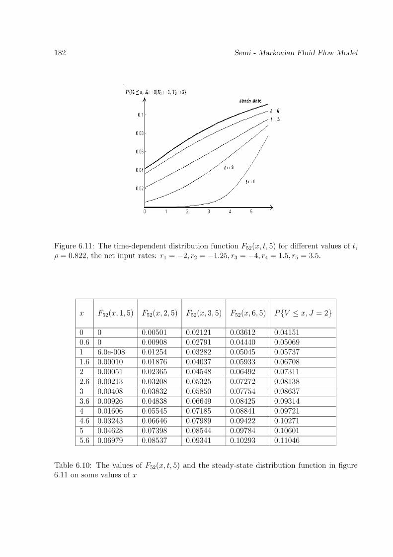
182 Semi - Markovian Fluid Flow Model
Figure 6.11: The time-dependent distribution function F52(x, t, 5) for different values of t,ρ = 0.822, the net input rates: r1 = −2, r2 = −1.25, r3 = −4, r4 = 1.5, r5 = 3.5.
x F52(x, 1, 5) F52(x, 2, 5) F52(x, 3, 5) F52(x, 6, 5) PV ≤ x, J = 2
0 0 0.00501 0.02121 0.03612 0.041510.6 0 0.00908 0.02791 0.04440 0.050691 6.0e-008 0.01254 0.03282 0.05045 0.057371.6 0.00010 0.01876 0.04037 0.05933 0.067082 0.00051 0.02365 0.04548 0.06492 0.073112.6 0.00213 0.03208 0.05325 0.07272 0.081383 0.00408 0.03832 0.05850 0.07754 0.086373.6 0.00926 0.04838 0.06649 0.08425 0.093144 0.01606 0.05545 0.07185 0.08841 0.097214.6 0.03243 0.06646 0.07989 0.09422 0.102715 0.04628 0.07398 0.08544 0.09784 0.106015.6 0.06979 0.08537 0.09341 0.10293 0.11046
Table 6.10: The values of F52(x, t, 5) and the steady-state distribution function in figure6.11 on some values of x
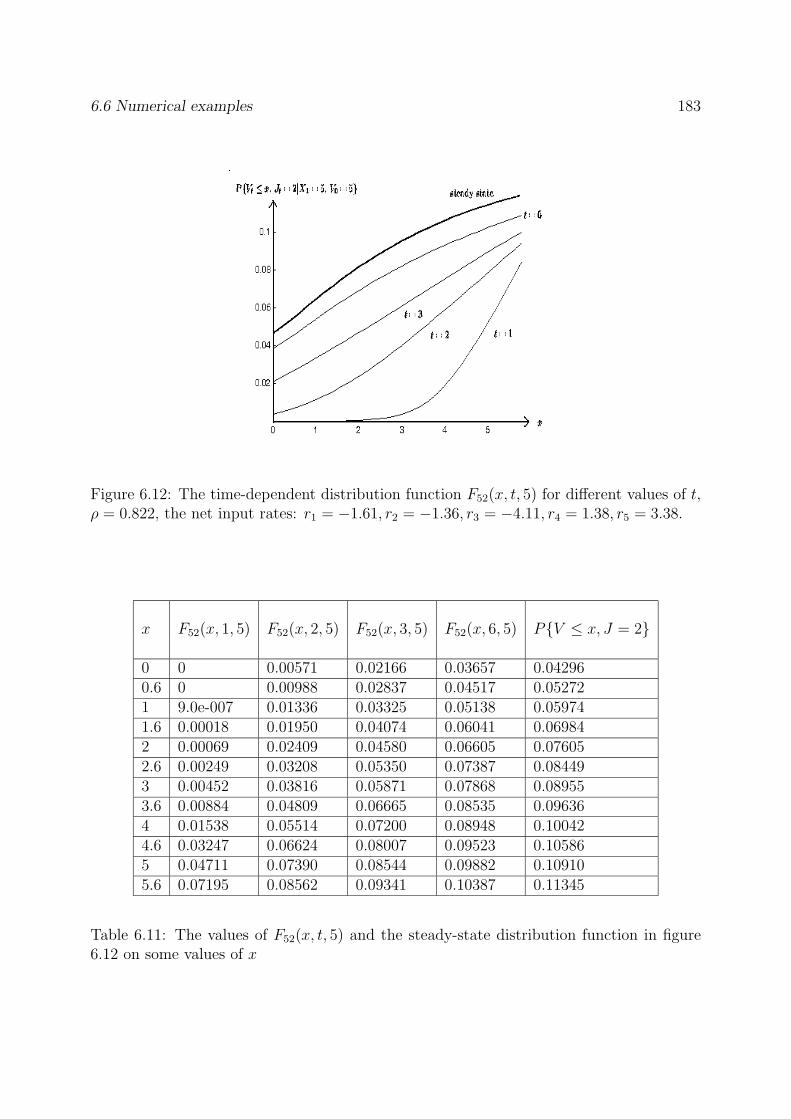
6.6 Numerical examples 183
Figure 6.12: The time-dependent distribution function F52(x, t, 5) for different values of t,ρ = 0.822, the net input rates: r1 = −1.61, r2 = −1.36, r3 = −4.11, r4 = 1.38, r5 = 3.38.
x F52(x, 1, 5) F52(x, 2, 5) F52(x, 3, 5) F52(x, 6, 5) PV ≤ x, J = 2
0 0 0.00571 0.02166 0.03657 0.042960.6 0 0.00988 0.02837 0.04517 0.052721 9.0e-007 0.01336 0.03325 0.05138 0.059741.6 0.00018 0.01950 0.04074 0.06041 0.069842 0.00069 0.02409 0.04580 0.06605 0.076052.6 0.00249 0.03208 0.05350 0.07387 0.084493 0.00452 0.03816 0.05871 0.07868 0.089553.6 0.00884 0.04809 0.06665 0.08535 0.096364 0.01538 0.05514 0.07200 0.08948 0.100424.6 0.03247 0.06624 0.08007 0.09523 0.105865 0.04711 0.07390 0.08544 0.09882 0.109105.6 0.07195 0.08562 0.09341 0.10387 0.11345
Table 6.11: The values of F52(x, t, 5) and the steady-state distribution function in figure6.12 on some values of x
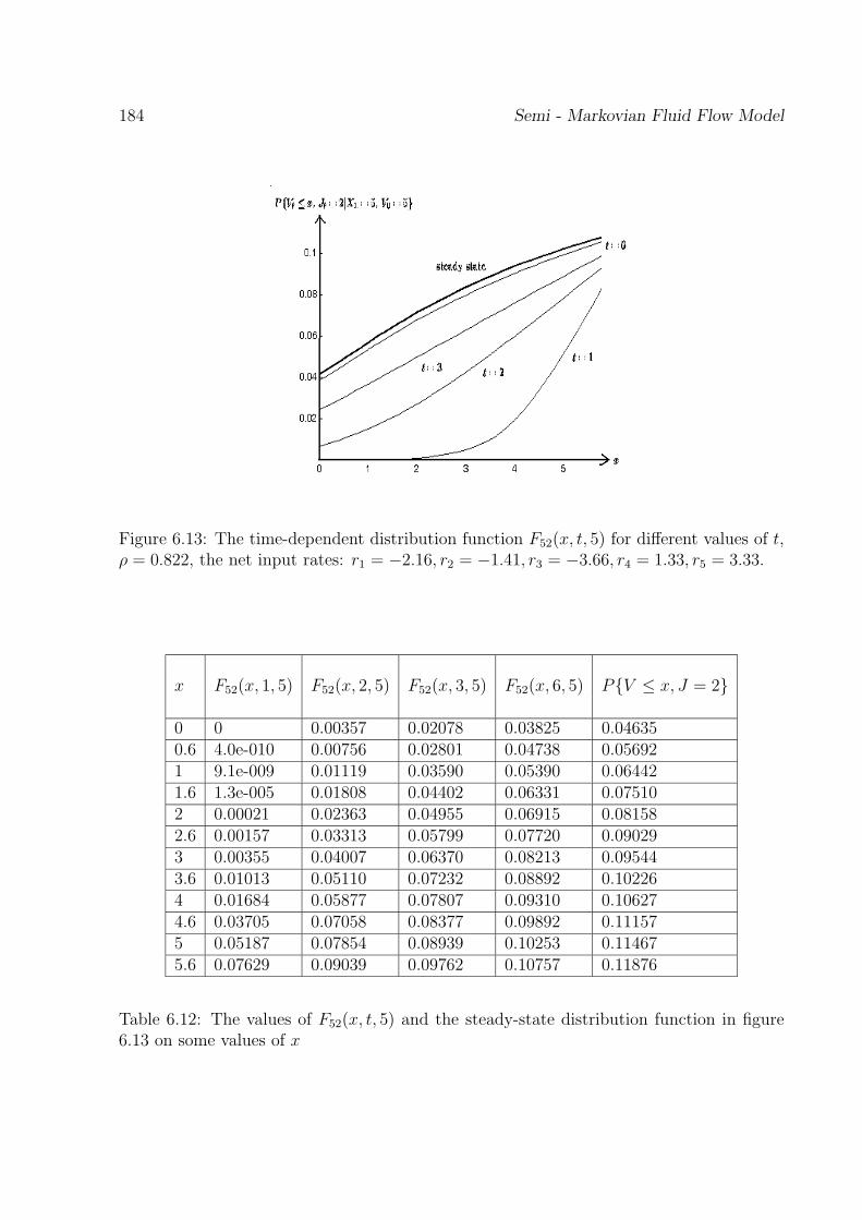
184 Semi - Markovian Fluid Flow Model
Figure 6.13: The time-dependent distribution function F52(x, t, 5) for different values of t,ρ = 0.822, the net input rates: r1 = −2.16, r2 = −1.41, r3 = −3.66, r4 = 1.33, r5 = 3.33.
x F52(x, 1, 5) F52(x, 2, 5) F52(x, 3, 5) F52(x, 6, 5) PV ≤ x, J = 2
0 0 0.00357 0.02078 0.03825 0.046350.6 4.0e-010 0.00756 0.02801 0.04738 0.056921 9.1e-009 0.01119 0.03590 0.05390 0.064421.6 1.3e-005 0.01808 0.04402 0.06331 0.075102 0.00021 0.02363 0.04955 0.06915 0.081582.6 0.00157 0.03313 0.05799 0.07720 0.090293 0.00355 0.04007 0.06370 0.08213 0.095443.6 0.01013 0.05110 0.07232 0.08892 0.102264 0.01684 0.05877 0.07807 0.09310 0.106274.6 0.03705 0.07058 0.08377 0.09892 0.111575 0.05187 0.07854 0.08939 0.10253 0.114675.6 0.07629 0.09039 0.09762 0.10757 0.11876
Table 6.12: The values of F52(x, t, 5) and the steady-state distribution function in figure6.13 on some values of x

Appendix A
Appendix
A.1 Cauchy’s Integral Formula
Theorem A.1.1 (Cauchy’s integral formula)Let f be an analytic function on a open set Ω, an let γ be any circuit which is homo-
morphic to a point in Ω. Then for any point z in Ω which is not on the graph of γ wehave
n(γ, z)f(z) =1
2πi
∫
γ
f(w)
w − zdw, (A.1)
where n(γ, z) is called the winding number of γ with respect to z.
We refer to Apostol [5] for the definition of n(γ, z). If γ(t) has domain [a, b], then n(γ, z)gives us the number of times the point γ(t) winds around the point z as t varies over theinterval [a, b]. For example, if γ is a positively oriented circle given by γ(θ) = z + reiθ,where 0 ≤ θ ≤ 2π, then the winding number is 1. For the proof see also [5].
A.2 Some Limit Theorems
Theorem A.2.1 (Abel’s theorem for power series)If∑∞
n=0 anrn converges for |r| < 1 and limn→∞ an = a, then
limr↑1
(1 − r)∞∑
n=0
anrn = a.
Proof. See Feller [26].
Theorem A.2.2 (Abel’s theorem for Laplace transforms)If∫∞
0a(t)dt is convergent then
∫∞
0e−φta(t)dt is uniformly convergent for Re(φ) ≥ 0
and
limφ→0
∫ ∞
0
e−φta(t)dt =
∫ ∞
0
a(t)dt, |arg(φ)| ≤ θ <1
2π.
185
186 Appendix
If∫∞
0a(t)dt is convergent for Re(φ) ≥ 0 and a(t) has a limit for t → ∞ then
limt→∞
a(t) = limφ→0
φ
∫ ∞
0
e−φta(t)dt, |arg(φ)| ≤ θ <1
2π.
Proof. See Doetsch [25].
A.3 Some inversion formulas
The following inversion formula can be found from Widder[43], page 69.
Lemma A.3.1Let F be the distribution function of a non-negative random variable with Laplace-
Stieltjes transform f ∗(φ). Then for x > 0,
F (x+) + F (x−)
2=
1
2πi
∫ c+i∞
c−i∞
eφx
φf ∗(φ)dφ, c > 0. (A.2)
For rational Laplace-Stieltjes transforms, we refer to Bateman & Erdelyi [11] for theinversion formula. Let
g(φ) =
∫ ∞
0
e−φtf(t)dt =Q(φ)
P (φ),
whereP (φ) = (φ − a1)
m1(φ − a2)m2 · · · (φ − an)mn
and Q(φ) is a polynomial of degree m1 + m2 + · · ·+ mn or less, ai 6= aj for i 6= j. Then theinverse is given by
f(t) =n∑
k=1
mk∑
l=1
Φkl(ak)tmk−1eakt
(mk − l)!(l − 1)!(A.3)
with
Φkl(φ) =∂l−1
∂φl−1
(Q(φ)
Pk(φ)
)
and
Pk(φ) =P (φ)
(φ − ak)mk.
A.4 Characteristics of the zeros of a function
Information on the location of zeros of a function is needed in order to get a uniqueWiener-Hopf factorization(see subsection 2.3).
Theorem A.4.1 (Rouche’s Theorem)Let f and g be analytic in D and let γ be a simply closed path which is null homologous
in D and which satisfies
|f(ζ) − g(ζ)| < |g(ζ)| for all ζ ∈ γ.
Then f and g have the same number of zeros inside γ.
A.5 Some results from the Theory of Matrices 187
Proof. See Apostol [5].For the queueing systems in chapters 4-6, the functions we consider are actually the
determinants of certain polynomial matrices. The generalization of Rouche’s theorem forthose determinants is given in de Smit [21].
Theorem A.4.2 (Generalization of Rouche’s Theorem)Let A(φ) = (aij(φ)) and B(φ) = (bij(φ)) be complex n × n−matrices, where B(φ) is
diagonal. The elements aij and bij, 1 ≤ i ≤ n, 1 ≤ j ≤ n, are meromorphic functions ina simply connected region S in which T is the set of all poles of these functions. C isa rectifiable closed Jordan curve in S − T. NA[NA+B] is the number of zeros inside C ofdetB(φ)[det(A(φ)+B(φ))] and PA[PA+B] is the number of poles inside C(poles and zerosof higher order are counted according to this order). If
(i) |bii(φ)| >∑n
j=1 |aij(φ)| on C for all i = 1, · · · , n
or(ii)A(φ) is decomposable on C and |bii(φ)| ≥∑n
j=1 |aij(φ)| on C,
for all i = 1, · · · , n with strict inequality for at least one i,
then on Cdet(A(φ) + B(φ)) 6= 0,
detB(φ) 6= 0,
andNA+B − PA+B = NB − PB.
A.5 Some results from the Theory of Matrices
The following lemma concerns the inverse of a simple constant matrix. An N × N -dimensional matrix A is called a simple matrix if it has N eigenvalues which are all distinct.
Lemma A.5.1Let A0 be a simple N×N -dimensional matrix. Let x1,x2, . . . ,xN be the right eigenvec-
tors corresponding to eigenvalues a1, a2, . . . , aN . If x−1i denotes the i-th row of the matrix
X−1 =(x1x2 . . .xN
)−1
then the inverse of matrix φI − A0, where φ is a complex number, is given by
(φI − A0)−1 =
N∑
i=1
xix−1i
(φ − ai).
Proof. Let yi, i = 1, 2, · · · , n be the left eigenvectors of A0. Let
X = [x1x2 . . .xn],
Y = [y1y2 . . .yn],
188 Appendix
andU = diag(a1, a2, . . . , an).
ThenA0X = XU and YtA0 = UYt.
Since A0 is simple, then X is nonsingular . Hence,
X−1A0 = UX−1. (A.4)
It follows that the rows of X−1 are the left eigenvectors of A0. Hence, Y can be chosen sothat Yt = X−1 or
YtX =
y1t
y2t
...ynt
[x1x2 . . .xn] = I
oryitxj = δij, i, j = 1, 2, . . . , n.
Define for i = 1, 2, . . . , n the constituent matrices
Gi = xiyti
where yti denotes the i-th row of the matrix Yt. According to these relations, we see that
the constituent matrices have the following properties;
1.∑n
i=1 Gi = I
2. GiGj = 0, i 6= j, i, j = 1, 2, . . . , n
3. G2i = Gi, i = 1, 2, . . . , n.
Now, from (A.4) we have
(φI − A0) = (φI − XUY)
=
φI − [x1x2 . . .xn]
a1yt1
a2yt2
...any
tn
=
(a
n∑
i=1
Gi −n∑
i=1
aiGi
)
=n∑
i=1
(φ − ai)Gi.
Define
B =n∑
l=1
Gl
(φ − al).
A.5 Some results from the Theory of Matrices 189
Then by the properties of Gi,
(φI − A0)B =n∑
i=1
n∑
l=1
(φ − ai)
(φ − al)GiGl =
n∑
i=1
G2i = I.
We can conclude that
B =n∑
l=1
Gl
(φ − al)= (φI − A0)
−1.
In chapter 6 we need to invert some matrix polynomials or sometimes known as φ-matrices of degree l, l ≥ 2 of the form
A(φ) =l∑
i=0
φiAi, (A.5)
where A0,A1, · · · ,Al are N×N -matrices of complex numbers independent of φ. If Al = IN ,the N × N -identity matrix, then the matrix polynomial is said to be monic, and (A.5)becomes
A(φ) = φlIN +l−1∑
i=0
φiAi. (A.6)
The complex number φ0 is called an eigenvalue of the monic matrix polynomial A(φ) ofform (A.6) if there are N -dimensional vectors x0,x1, · · · ,xk, for some k ≥ 0 with x0 6= 0,so that for i = 0, 1, · · · , k,
i∑
p=0
1
p!A(p)(φ0)xi−p = 0, (A.7)
where A(p)(φ) denotes the pth derivative of A(φ) with respect to φ. The sequence ofvectors x0,x1, · · · ,xk is called a Jordan chain of length k +1 of A(φ) corresponding to theeigenvalue φ0. The vector x0 is called an eigenvector and the subsequent vectors x1, · · · ,xk
are called generalized eigenvectors. The monic polynomial of form (A.6) has exactly Nleigenvalues when counted with multiplicities. The set
σ(A) = φ0|φ0 is the eigenvalue of A(φ)
is called the spectrum of A(φ). It is clear that σ(A) contains at most lN elements.For φ /∈ σ(A), the inverse of the monic matrix polynomial A(φ) in (A.6) can be
expressed in terms of the so called standard triple of A(φ). The theorem in the followingand some explanations after that will explain the standard triple of A(φ) precisely.
Theorem A.5.1For every φ /∈ σ(A),
A−1(φ) = P1(φINl − CA)−1R1,
190 Appendix
where
P1 = (IN 0 · · ·0), R1 =
0...0IN
,
and
CA =
0 IN 0 · · · 0
0 0 IN · · · ......
......
... IN
−A0 −A1 −A2 · · · −Al−1
,
which is called the (first) companion matrix of A(φ).
Proof. See page 58 of Gohberg[28].
Any three matrices (U,T,V) are said to be admissible for A(φ) if they are of sizeN × lN, lN × lN, and lN × N, respectively. Any admissible triple (U,T,V) which issimilar to the triple (P1,CA,R1) in Theorem A.5.1 above is said to be a standard triplefor A(φ). The similarity of those triples means that there is a non singular matrix S sothat
U = PS, T = S−1CAS, V = S−1R1.
The following theorem is a generalization of Theorem A.5.1, in the sense that the inverseof the monic matrix polynomial A(φ) can be expressed by any standard triple of A(φ).
Theorem A.5.2If (U,T,V) is a standard triple for A(φ) and φ /∈ σ(A), then
A−1(φ) = U(φINl − T )−1V. (A.8)
Proof. See [28].
In chapter 6 we use the representation of L(1, φ, η)−1 in form of (A.8), where U =
E(1, η) and T = diag(γ1(1, η), · · · , γNm(1, η)). The matrix
UUT
...UTl−1
is nonsingular, and
the third matrix V can be defined by
V =
UUT
...UTl−1
−1
00...
IN
.
A.6 The proof of Lemma 5.3.3 191
The standard triple (U,T,V) of the monic polynomial matrix (A.5) has the property(see page 52 of [28] for the proof) that
UTiV =
0 , for i = 0, · · · , l − 2,
IN , for i = l − 1.
A.6 The proof of Lemma 5.3.3
If B and A are n × n-dimensional nonsingular matrices, X is an n × r-dimensionalmatrix, R is an r × r-dimensional nonsingular matrix, and Y is an r × n-dimensionalmatrix such that
B = A + XRY,
then it is easy to prove(see [33]) that
B−1 = A−1 − A−1X(R−1 + YA−1X)−1YA−1. (A.9)
If we apply this result to the matrix K(1, φ, η) defined in (5.16), we get
K(1, φ, η)−1 = I − D(1, η)X(φ, η)−1C(1, η) (A.10)
where
X(φ, η) =diag(φ − µ1(1, η), . . . , φ − µK(1, η)) + C(1, η)D(1, η)
=φI + (IKNE(1, η)INK)−1IKNα(I + ηq−1)E(1, η)INK .
The inverse of X(φ, η), by using the same relation, is
1
φI − 1
φ(IKNE(1, η)INK)−1IKNααα(η)M(φ, η)−1E(1, η)INK .
If we substitute this into (A.10) we get
K(1, φ, η)−1 =I − 1
φD(1, η)C(1, η)
[I −ααα−1ααα(η)M(φ, η)−1E(1, η)INKC(1, η)
]
=I − D(1, η)C(1, η)M(φ, η)−1,
and we get (5.24). Since the last N − K columns of C(1, η) are zero, it is clear thatK−1(1, φ, η) is analytic in the left half-plane Re(φ) < 0.
Moreover, from equation (5.8) we get
H−1(1, φ, η) = M(φ, η)ααα−1L−1(1, φ, η)ααα. (A.11)
Since for i ∈ N µi and Ei satisfy the equation (5.12), then by Condition 5.3.1 and LemmaA.5.1 we have
L−1(1, φ, η) =N∑
i=1
EiE−1i
(φ − µi), (A.12)
and if we substitute this into (A.11) we get (5.25).
192 Appendix
A.7 The proof of Lemma 5.4.1
LetEEE(z, η) = (IKNE(z, η)INK)−1IKN .
Then by the various definitions,
M(φ, η) − D(z, η)C(z, η)
=φI + ααα(η) − (I + ηqqq−1)E(z, η)INKEEE(z, η)ααα
−ααα−1E(z, η)INKdiag(µ1(z, η), · · · , µK(z, η))EEE(z, η)ααα
=φI + ααα(η) − (I + ηqqq−1)
(IK 0A 0
)ααα
−ααα−1
K∑
k=1
µk(z, η)Ek(z, η)EEEk(z, η)ααα,
where IK is K × K-dimension identity matrix and A is (N − K) × K-dimension matrixwith elements
Aij = (E(z, η)INK)K+iEEEj(z, η).
It follows that
Ci(z, η) [M(φ, η) − D(z, η)C(z, η)]
=EEEi(z, η)ααα (φI + ααα(η)) − EEEi(z, η)ααα(η)
(IK 0A 0
)ααα
− EEEi(z, η)K∑
k=1
µk(z, η)Ek(z, η)EEEk(z, η)ααα
=φEEEi(z, η)ααα + EEEi(z, η)αααααα(η) − EEEi(z, η)ααα(η)
(IK 0A 0
)ααα
− µi(z, η)EEEi(z, η)ααα.
(A.13)
The second and the third term of the last equation in (A.13) will cancel since the lastN − K elements of EEEi(z, η) are zero. We then can conclude that
Ci(z, η) [M(φ, η) − D(z, η)C(z, η)] = (φ − µi(z, η))Ci(z, η).
A.8 The proof of Lemma 5.5.1
From Lemma 5.3.3 now we have
K−1(1, φ, η)H−1(1, φ, η) = (M(φ, η) − D(1, η)C(1, η))ααα−1
N∑
i=1
EiE−1i
(φ − µi)ααα, (A.14)
A.8 The proof of Lemma 5.5.1 193
and based on this result we will derive the expression for Z∗(φ, η, v).
By definition, we have
K+(1, φ, η, v) + K−(1, 0, η, v)
=Z0(φ, η, v)K(1, φ, η, v) −(K−(1, φ, η, v) − K−(1, 0, η, v)
)
=Z0(φ, η, v)K(1, φ, η, v) − φ
K∑
i=1
Z0(µi, η, v)Di(1, η)Ci(1, η)
µi(φ − µi),
so that
(K+(1, φ, η, v) + K−(1, 0, η, v)
)K(1, φ, η, v)−1H(1, φ, η)−1
=Z0(φ, η, v)H(1, φ, η)−1
− φK∑
i=1
Z0(µi, η, v)Di(1, η)Ci(1, η)
µi(φ − µi)K(1, φ, η, v)−1H(1, φ, η)−1.
(A.15)
By combining (A.15) with Lemma 5.4.1 and (A.14), we obtain
(K+(1, φ, η, v) + K−(1, 0, η, v)
)K−1(1, φ, η, v)H−1(1, φ, η)
=Z0(φ, η, v)M(φ, η)ααα−1
N∑
l=1
ElE−1l
(φ − µl)ααα
− φK∑
l1=1
Z0(µl1 , η, v)
µl1
M(µl1 , η)ααα−1El1Cl1(1, η)ααα−1
N∑
l2=1
El2E−1l2
(φ − µl2)ααα
=Z0(φ, η, v)M(φ, η)ααα−1
N∑
l=1
ElE−1l
(φ − µl)ααα
−K∑
l=1
Z0(µl, η, v)
µl
M(µl, η)ααα−1ElCl(1, η)
−K∑
l=1
Z0(µl, η, v)
µl
M(µl, η)ααα−1ElCl(1, η)ααα−1
N∑
l1=1
El1E−1l1
(φ − µl1)ααα.
(A.16)
If we substitute (A.16) into (5.42) then we get (5.55).
194 Appendix
A.9 The proof of Lemma 6.3.4
By the definitions of C(1, η) and D(1, η) we have for Re(η) ≥ 0,
C(1, η)D(1, η)
=S(1, η)−1C0D(1, η)
=S(1, η)−1C0
(M(γ1(1, η), η)E1(1, η) · · ·M(γKm(1, η), η)EKm(1, η)
),
where the (i, j)th element of
M(γ1(1, η), η)E1(1, η) · · ·M(γKm(1, η), η)EKm(1, η)
is equalm∏
k=1
(γj(1, η) + αik(η))Eij(1, η),
so that
C0
(M(γ1(1, η), η)E1(1, η) · · ·M(γKm(1, η), η)EKm(1, η)
)
=S(1, η)γγγ(1, η) + ααα(η)S(1, η),
where
γγγ(1, η) = diag(γ1(1, η), · · · , γKm(1, η))
and
ααα(η) = diag(α11(η), α21(η), · · · , αK1(η), α12(η), · · · , αK2(η), · · · , αKm(η)).
It follows that
X(φ, η) = φI − γγγ(η) + C(1, η)D(1, η)
= φI − S(1, η)−1S(1, η)γγγ(1, η) + S(1, η)−1S(1, η)γγγ(1, η)
+ S(1, η)−1ααα(η)S(1, η)
= φI + S(1, η)−1ααα(η)S(1, η),
and
X(φ, η)−1 = S(1, η)−1(φI + ααα(η))−1S(1, η), (A.17)
and it proves the lemma.
A.10 Analyticity of Z(1, φ, η, v) at φ = γi(η) for i = 1, · · · , Km 195
A.10 Analyticity of Z(1, φ, η, v) at φ = γi(η) for i =
1, · · · , Km
We see that for l = 1, 2, · · · , Km,
limφ→γl(1,η)
(φ − γl(1, η))Z(1, φ, η, v)
=Z0(γl(1, η), η, v)M(γl(1, η), η)El(η)Yl(η)
− γl(1, η)Km∑
i=1
Z0(γi(1, η), η, v)Di(1, η)
γi(1, η)1iX
−1(γl(1, η), η)C(1, η)M(γl(1, η), η)
=Z0(γl(1, η), η, v)M(γl(1, η), η)El(η)Yl(η)
− γl(1, η)Km∑
i=1
Z0(γi(1, η), η, v)Di(1, η)
γi(1, η)1iX
−1(γl(1, η), η)C(1, η)Dl(1, η)Yl(η)
.El(η)Yl(η),
using Dl(1, η) = M(γl(1, η), η)El(η). Eliminating C(1, η)Dl(1, η) using (6.31) we obtainfor Re(η) > 0,
limφ→γl(1,η)
(φ − γl(1, η))Z(1, φ, η, v)
=Z0(γl(1, η), η, v)M(γl(1, η), η)El(η)Yl(1, η)
− γl(1, η)Km∑
i=1
Z0(γi(1, η), η, v)Di(1, η)
γi(1, η)1iX
−1(γl(1, η), η)
(C(1, η)Dl(1, η) + (γl(1, η) − γl(1, η))1Tl )Yl(η)
=Z0(γl(1, η), η, v)M(γl(1, η), η)El(η)Yl(η)
− γl(1, η)Km∑
i=1
Z0(γi(1, η), η, v)Di(1, η)
γi(1, η)1i1
Tl Yl(η)
=0
(A.18)
or Z(1, φ, η, v) has no poles at γl(1, η) for l = 1, 2, . . . , Km.

Bibliography
[1] J. Abate, G. L. Choudhury, and W. Whitt. Numerical inversion of multidimensionalLaplace transforms by the Laguerre method. Performance Evaluation, 31:229–243,1998.
[2] J. Abate and W. Whitt. Numerical inversion of probability generating functions.Operation Research Letters, 12:245–251, 1992.
[3] J. Abate and W. Whitt. The Fourier-series method for inverting transforms of prob-ability distributions. Queueing Systems, 10:5–88, 1992.
[4] D. Anick, D. Mitra, and M. M. Sondhi. Stochastic theory of a data-handling systemwith multiple sources. The Bell System Technical Journal, 61:1871 – 1894, 1982.
[5] T. M. Apostol. Mathematical Analysis. Addison-Wesley Publishing Company, Read-ing, Massachusetts, second edition, 1974.
[6] E. Arjas. On a fundamental identity in the theory of semi-Markov processes. Advancesin Applied Probability, 4(2):271–284, 1972.
[7] S. Asmussen. Applied Probability and Queues. John Wiley and Sons, 1987.
[8] S. Asmussen. Stationary distributions for fluid flow models with or without Browniannoise. Communication in Statistics, Stochastic Models, 11(1):21–49, 1995.
[9] S. Asmussen. A probabilistic look at the Wiener-Hopf equation. SIAM, 40(2):189–201,1998.
[10] H. Bart, I. Gohberg, and M. A. Kaashoek. Minimal Factorization of Matrix andOperator Functions. Birkhauser Verlag, Bessel, 1979.
[11] H. Bateman and A. Erdelyi. Tables of Integral Transforms: based, in part, on notesleft by Harry Bateman. Mc Graw-Hill, New York, 1954.
[12] D. Bertsimas and D. Nakazato. Transient and busy period analysis of the GI/G/1queue : The method of stages. Queueing Systems, 10:153–184, 1992.
[13] D. J. Bertsimas, J. Keilson, D. Nakazato, and H. Zhang. Transient and busy periodanalysis of the GI/G/1 queue as a Hilbert factorization problem. Journal of AppliedProbability, 28:873–885, 1991.
197
198 BIBLIOGRAPHY
[14] J. P. C. Blanc and E. A. van Doorn. Relaxation times for queueing systems. In J. W.de Bakker, editor, Proceeding CWI Symposium, pages 139–162, Amsterdam, 1986.North-Holland.
[15] O. J. Boxma, D. Perry, and F. A. van der Duyn Schouten. Fluid queues and mountainprocesses. Probability in the Engineering and Informational Sciences, 13:407–427,1999.
[16] G. L. Choudhury, D. M. Lucantoni, and W. Whitt. Multidimensional transforminversion with applications to the transient M/G/1 queue. The Annals of AppliedProbability, 4:719–740, 1994.
[17] J. W. Cohen. The Single Server Queue. North-Holland Publishing Company, Ams-terdam, 1969.
[18] J. W. Cohen. The Wiener-Hopf technique in applied probability. In J. Gani, editor,Perspectives in Probability and Statistics, pages 145–156. Applied Probability Trust,1975.
[19] C. Corduneanu. Integral Equations and Stability of Feedback Systems. Academic Press,New York, 1973.
[20] D. R. Cox. Renewal Theory. John Wiley and sons, 1962.
[21] J. H. A. de Smit. The queue GI/M/s with customers of different types or the queueGI/Hm/s. Advances in Applied Probability, 15:392–419, 1983.
[22] J. H. A. de Smit. A numerical solution for the multiserver queue with hyper-exponential service times. Operations Research Letters, 2(5):217–224, 1984.
[23] J. H. A. de Smit. The queue GI/Hm/s in continuous time. Journal of AppliedProbability, 22(1):214–222, 1985.
[24] J. H. A. de Smit. Explicit Wiener-Hopf factorizations for the analysis of multidimen-sional queues. In J. H. Dshalalow, editor, Advances in Queueing: Theory, Methodsand Open Problems, pages 293–309. CRC Press Inc., 1995.
[25] G. Doetsch. Introduction to the Theory and Application of the Laplace Transformation.Springer-Verlag, Berlin, 1970.
[26] W. Feller. An Introduction to Probability Theory and Its Applications, volume I. Wiley,New York, second edition, 1960.
[27] N. Gautam, V. G. Kulkarni, Z. Palmowski, and T. Rolski. Bounds for fluid modelsdriven by semi-markov inputs. Prob.Eng.Inf.Sci, 18(4):429–475, 1999.
[28] I. Gohberg, P. Lancaster, and L. Rodman. Matrix Polynomials. Academic Press, NewYork, 1982.
BIBLIOGRAPHY 199
[29] O. Kella and W. Whitt. A storage model with a two-state random environment.Operations Research, S40:S257–S262, 1992.
[30] K. Knopp. Theory of Functions, volume I. Dover Publications, New York, 1945.
[31] L. Kosten. Liquid models for a type of information buffer problems. Delft ProgressReport 11, Delft University of Technology, Delft, The Netherlands, 1986.
[32] V. G. Kulkarni. Fluid models for single buffer system. In J. H. Dshalalow, editor,Frontiers in Queueing, pages 321–338. CRC Press, Boca Raton, 1997.
[33] P. Lancaster. Theory of Matrices. Academic Press Incorporation, London, 1969.
[34] G. Latouche and T. Takine. Markov-renewal fluid queues. Journal of Applied Proba-bility, 41(3):746757, 2004.
[35] M. V. Moorthy. Inversion of two-dimensional Laplace transform-expansion by La-guerre series. Z. Angew. Math. Phys, 46:793–806, 1995.
[36] M. V. Moorthy. Numerical inversion of two-dimensional Laplace transform-Fourierseries representation. Applied Numerical Mathematics, 17:119–127, 1995.
[37] A. Pacheco and N. U. Prabhu. A Markovian storage model. Technical Report 1079,School of Operation Research and Industrial Engineering College of Engineering Cor-nell University, Ithaca, New York, 1993.
[38] G. J. K. Regterschot. Wiener-Hopf Factorization Techniques in Queueing Models.PhD thesis, University of Twente, The Netherlands, 1987.
[39] A. Riska. Aggregate Matrix-analytic Techniques and their Applications. PhD thesis,Department of Computer Science, Williamsburg, Virginia, December 2002.
[40] L. C. G. Rogers. Fluid models in queueing theory and Wiener-Hopf factorization ofMarkov chains. The Annals of Applied Probability, 4(2):390–413, 1994.
[41] J. P. Schouten. Operatorenrechnung. Springer-Verlag, Berlin, 1961.
[42] T. Tanaka, O. Hashida, and Y. Takahashi. Transient analysis of fluid model for ATMstatistical multiplexer. Performance Evaluation, 23:145–162, 1995.
[43] D. V. Widder. The Laplace Transform. Princeton University Press, Princeton, 1946.
[44] P. P. Zabreyko. Integral Equations-a reference text. Noordhoff, Leiden, The Nether-lands, 1975.

Index
C+δ,R, 9
C−δ,R, 9
GI/G/1 queue, 17GI/Kn/1 queue, 18Km/G/1 queue, 18actual waiting times, 19number of customers, 24
at arrival epochs, 24in continuous time, 28
special customes, 17virtual waiting times, 21
GI/Hm/s queue, 55actual waiting time, 55, 72number of customers, 56
at arrival epochs, 80in continuous time, 90
queue length, 56at arrival epochs, 75in continuous time, 84
special customers, 55steady-state results, 70virtual waiting time, 73
x+, 10x−, 10
A+ property, 3, 11A− property, 3, 11
Abel’s theorem, 185for Laplace transforms, 185for power series, 185
analytic continuation, 11
Cauchy’s integral formula, 185
Euler sum, 15
fluid flow model, 2, 101Markovian, 101
semi-Markovian, 133
generating function, 2numerical inversion, 16
Laplace-Stieltjes transform, 12numerical inversion, 15
Liouville’s theorem, 14, 21, 64, 112
Markovian fluid flow modelbuffer content, 101
at transition epochs, 113in continuous time, 116time-dependent distribution, 121
relaxation time, 124matrix polynomials, 189
admissible triple, 190eigenvalue, 189eigenvector, 189generalized eigenvector, 189Jordan chain, 189monic, 189standard triple, 189, 190
Rouche’s theorem, 186generalization, 187
Semi-Markovian fluid flow modelbuffer content, 133, 156
steady-state distribution, 161time-dependent distribution function,
135, 160
Wiener-Hopf factorization, 1, 11, 18, 56,58, 102, 134, 135, 138, 204
canonical, 12Wiener-Hopf integral equation, 11transformed Wiener-Hopf equation, 3,
20, 60, 104, 137
201

Summary
In this thesis we study the time-dependent behavior of queueing systems. The study isfocused on the queueing systems:
1. the GI/G/1 system,
2. the GI/Hm/s system,
3. the Markovian Fluid Flow Model, the fluid flow model that is modulated by a Markovprocess,
4. the Semi-Markovian Fluid Flow Model, a generalization of the Markovian Fluid FlowModel.
In general, the time-dependent behavior of queueing systems is much influenced by theinitial server(s)’s work load. This leads us to consider the queueing systems with non-zeroinitial server(s)’s work load. In the GI/G/1 system and the GI/Hm/s system this meansthat in the beginning there exist a number of (special) customers to serve. In the last twosystems, initially the buffer has non-zero content.
The technique that is used to analyze the behavior of the queueing systems studied inthis thesis is based on the Wiener-Hopf factorization. A brief discussion on the Wiener-Hopf factorization is given in chapter 2, where we also give the conditions on the existenceof uniqueness of the factorization. In this chapter we also give some preliminaries that weneed for the analysis in the rest chapters.
The first major step in the analysis is the derivation of the (system of) transformedWiener-Hopf equation(s). Wiener-Hopf factorization is then applied to its symbol. Sincethe queueing systems we consider have a non-zero initial working load, the Wiener-Hopffactorization should be followed by a decomposition on a certain (matrix) function. TheWiener-Hopf factorization and the decomposition yields a (formal) solution of the (systemof) equation(s).
If the stability condition is fulfilled, then the steady-state distributions of interest can bedetermined by applying Abel’s limit theorem to the solution of the (system of) equation(s).
In chapter 3 we study the system GI/G/1 with non-zero initial number of customers.We get the explicit factorizations for two special systems, the systems GI/Kn/1 andKm/G/1. These results give explicit expressions for the Lapace-Stieltjes transform of ac-tual waiting times and virtual waiting times. Then, by applying a contour integration, weget the expectation of number of customers at arrival epochs and in continuous times as
203
204 Summary
well. At the end of this chapter we give numerical results to illustrate the behavior of thesystem as it tends to the steady-state.
In chapter 4 we study the system GI/Hm/s with non-zero initial number of customers.As in chapter 3, the Wiener-Hopf factorization gives explicit expressions for the Lapace-Stieltjes transform of actual waiting times and virtual waiting times. Then, the distribu-tions of the queue length and the number of customers in the system are derived, both atarrival epochs and in continuous time. At the end of this chapter we again give numericalresults.
In chapter 5 we study the Markovian Fluid Flow Model, the fluid flow model in whichthe rate of data that flow into the buffer depends on the state of a Markov process. TheWiener-Hopf factorization gives us an explicit expression for the Laplace-Stieltjes transformof buffer content at transition epochs of the underlying Markov process. From this we canderive the distribution of the buffer content in continuous times. We conclude this chapterwith some numerical results.
In chapter 6 we study a generalization of the model of chapter 5. The times be-tween transitions of the underlying Markov process are not assumed to be exponentiallydistributed anymore but are assumed to be either hyper-exponentially distributed or hypo-exponentially distributed. With this assumption, the symbol of Wiener-Hopf-type equa-tions is still a rational matrix in φ, and each element of this matrix has only simple poles.This matrix can be factorized by the Wiener-Hopf factorization technique as we apply inchapter 5. We have obtained the distribution of the buffer content and the correspondingnumerical results.
Ringkasan
Thesis ini membahas perilaku pada waktu tertentu(time-dependent behavior) dan per-ilaku pada keadaan steady state dari beberapa sistem antrian. Pembahasan perilaku-perilaku tersebut difokuskan pada sistem-sistem antrian:
1. Sistem antrian GI/G/1,
2. Sistem antrian GI/Hm/s,
3. Markovian Fluid Flow Models, yaitu model-model fluid flow yang berlandaskan padasuatu proses Markov,
4. Semi-Markovian Fluid Flow Models, yang merupakan perumuman dari MarkovianFluid Flow Models.
Secara umum, perilaku suatu sistem antrian pada suatu selang waktu yang terbatasakan sangat dipengaruhi oleh keadaan awal sistem antrian tersebut: apakah pada keadaaanawal (para) pelayan yang ada sedang sibuk melayani (para) pelanggan atau tidak. Lan-dasan pikiran ini mendorong kita untuk memandang sistem-sistem antrian di atas denganbeban kerja dari (para) pelayan pada awal pengamatan yang tidak nol. Ini berarti dalamdua sistem antrian pertama, sistem GI/G/1 dan GI/Hm/s, pada awal pengamatan ter-dapat sejumlah pelanggan dalam antrian. Sedangkan pada dua sistem terakhir, hal iniberarti pada awal pengamatan kita mempunyai buffer yang berisi.
Teknik yang dipakai untuk menentukan perilaku antrian - antrian yang dibahas dalamthesis ini adalah suatu teknik berdasarkan faktorisasi Wiener-Hopf. Penjelasan tentangfaktorisasi Wiener-Hopf kami berikan di bab 2, di mana pada bab tersebut kami jugamembahas kondisi-kondisi agar eksistensi dari ketunggalan faktorisasi Wiener-Hopf ini di-jamin. Di bab yang sama kami juga menampilkan penjelasan singkat tentang beberapateori dasar yang dipakai dalam menganalisa sistem-sistem antrian yang dibahas di thesisini.
Jika kondisi kestabilan dipenuhi, maka distribusi-distribusi peluang yang menjadi per-hatian pada keadaan steady state dapat diturunkan dengan cara menerapkan teorema limitAbel pada solusi dari sistem persamaan Wiener-Hopf. Hasilnya kemudian kita inversi se-cara analitik unutk mendapatkan distribusi yang kita inginkan.
Untuk sistem-sistem antrian di thesis ini, transformasi Laplace-Stieltjes ganda yangterturunkan merupakan fungsi rasional terhadap salah satu peubahnya. Hal ini memu-ngkinkan kita melakukan inversi secara analitik untuk mendapatkan transformasi Laplace-Stieltjes tunggal. Pada transformasi tunggal inilah, yang tidak lagi berupa fungsi rasional,
205
206 Ringkasan
kita dapat melakukan inversi secara numerik untuk melihat kelakuan sistem antrian padasaat - saat tertentu.
Di bab 3 dibahas sistem antrian GI/G/1 dengan jumlah pelanggan pada saat awal tidaksama dengan nol. Kita dapatkan faktor-factor eksplisit untuk dua kasus khusus sistemini, yaitu sistem-sistem GI/Kn/1 dan Km/G/1. Hasil ini memberikan ekspresi eksplisittransformasi Laplace-Stieltjes dari distribusi waktu tunggu sebenarnya juga waktu tungguvirtual. Sesudah itu, dengan teknik integral garis kita dapatkan ekspektasi dari jumlahpelanggan pada sistem pada titik-titik kedatangan pelanggan dan untuk waktu-waktu yangkontinu. Di akhir bab ditampilkan hasil perhitungan numerik untuk memberikan ilustrasitentang kelakuan sistem mulai awal pengamatan sampai dicapai keadaan steady state.
Di bab 4 dibahas sistem antrian GI/Hm/s dengan jumlah pelanggan pada awal penga-matan tidak sama dengan nol. Dengan menerapkan teknik faktorisasi Wiener-Hopf yangdilengkapi kita dapatkan ekspresi eksplisit transformasi Laplace-Stieltjes dari distribusiwaktu tunggu sebenarnya juga waktu tunggu virtual. Sesudah itu, diturunkan distribusidari panjang antrian juga banyaknya pelanggan pada sistem, keduanya dilihat pada titik-titik kedatangan pelanggan juga untuk waktu yang kontinu. Di akhir bab ditampilkanhasil perhitungan numerik untuk memberikan ilustrasi tentang kelakuan sistem mulai awalpengamatan sampai dicapai keadaan steady state.
Bab 5 berisi pembahasan tentang Markovian Fluid Flow Model, yaitu model fluid flowdimana aliran data yang masuk ke dalam buffer berdasarkan pada keadaan dari suatuproses Markov. Penerapan teknik faktorisasi Wiener-Hopf yang dilengkapi menghasilkanekspresi eksplisit transformasi Laplace-Stieltjes dari isi buffer pada titik-titik transisi prosesMarkov yang mendasari proses aliran data. Dari hasil ini kita juga bisa mendapatkandistribusi untuk isi buffer pada waktu yang kontinu. Hasil perhitungan numerik diberikandi akhir bab untuk memberi ilustrasi tentang distribusi peluang dari isi buffer mulai saatawal sistem berjalan sampai keadaan steady state dicapai.
Bab 6 mempelajari perumuman dari model di bab 5. Di bab ini, waktu antar transisidari proses Markov yang mendasari aliran data yang masuk ke buffer tidak lagi diasumsikanberdistribusi eksponensial, tetapi dibuat/diasumsikan memiliki distribusi hyper-exponentialatau hypo-exponential. Dengan asumsi ini, matriks dari simbol Wiener-Hopf masih meru-pakan matriks rasional dengan elemen-elemen yang mempunyai pole yang berorde satu.Karena itu, teknik faktorisasi dan dekomposisi seperti di bab 5 masih bisa digunakan un-tuk menyelesaikan sistem persamaan Wiener-Hopf dari model di bab ini. Distribusi dariisi buffer didapatkan dengan teknik ini, dan hasil numerik untuk distribusi ini diberikan diakhir bab.

Acknowledgement
Praise be to Allah, the Cherister and Sustainer of the Worlds.
A few years ago, having this thesis finished seemed to be one and only one compliment inmy life. As times went by, I realized that having many people who gave me encouragement,advices, and assistance in finishing this thesis is a more worthily compliment in my life.For that, I would like to express my gratitude.
I would like to begin with my promotor Prof. J. H. A. de Smit. He showed that healways had time for me, and I knew that he always tried to get best solutions for myproblems. Thank you very much for your supervision.
I am indebted to Dr. Wim Nawijn for all help he gave. One day he offered me toread the draft of this thesis, and he really did it. With a great patience, he sent me manye-mails, faxes and air mails for correcting mathematical aspect and my English. I reallyappreciated it.
Many thanks to Prof. E. van Groessen, who had supported me in finishing this thesisin many ways. His enthusiasm in solving a problem has inspired me to go through until Ireally finished this thesis.
I am grateful to Prof Adriaan van den Burg(Delft University of Technology), Mr. P.Althuis(CICAT) and Mr. D. Jellema(CICAT), who had managed the financial support Igot in the first four years of my research.
Many thank to the members of my thesis committee: Prof. R.J. Boucherie, Prof. A.Bagchi, Prof. O.J. Boxma, Prof. H.C. Tijms, and Prof. R.K. Sembiring, for the commentsand the support.
Many thanks to my husband, Saladin, and my sons, Essa and Wira, who have beenencouraging me to do my best, and helping me to be a good wife and a good mother.
Many thanks to my senior colleagues at Departemen Matematika ITB: Prof. R. K.Sembiring, Prof. M. Ansjar and Prof. Edy Soewono, who have guided me since I was astudent.
Many thanks to Dini Heres and J.C.W. van Ommeren for helping managing the Latexfile of this thesis. Many thanks to Erik van Doorn and Werner Scheindhardt for thevaluable ideas and advices. Many thanks to all friends at TWRC building especially forSjoerd Baas, Sri Nurdiati, Anja Tanke, Ineke van Eijkern-Moraal and Frits van Beckum.I am also grateful to Family Eisinger, Family Kruger, and Family Proost. Their supportduring my stay in Enschede made me feel at home.
Last but not least, to my family in Bandung and Klaten, terima kasih atas segala doadan dorongannya. Saya dedikasikan tesis ini untuk anda semuanya.
207


About the author
Rieske Hadianti was born in Bandung, Indonesia, on 13 February 1969. She finishedher study in mathematics at Institut Teknologi Bandung, in Bandung. In 1992 she startedher graduate study in mathematics at Institut Teknologi Bandung, and she finished it in1994. Her interest in mathematics has sent her in 1996 to University of Twente to dodoctoral research in Queuing Theory under supervision of Prof. J.H.A. de Smit. Due toserious illness she got, she went back to Bandung in 2000 and from then she has beenjoining Faculty of Mathematics and Natural Sciences, Institut Teknologi Bandung as anacademic staff.
Now, she is a member of Industrial and Financial Mathematics Group at the faculty.She has been performing some research on the application of queueing theory in Perfor-mance Analysis of Cellular Mobile Communication Networks.
209
Related Documents


![arxiv.org · arXiv:0803.3486v2 [math.QA] 22 Aug 2008 NEW TECHNIQUES FOR POINTED HOPF ALGEBRAS NICOLAS ANDRUSKIEWITSCH AND FERNANDO FANTINO´ Abstract. We present techniques that allow](https://static.cupdf.com/doc/110x72/5f7ee9b5fc4492603729ef17/arxivorg-arxiv08033486v2-mathqa-22-aug-2008-new-techniques-for-pointed-hopf.jpg)


