Why is Timing Perverse?

WHY IS TIMING PERVERSE? ∗

JUAN CARLOS MATALLÍNa, DAVID MORENOb and ROSA RODRÍGUEZb

a Finance and Accounting Department. Universidad Jaume I b Department of Business Administration. Universidad Carlos III

September, 2009

ABSTRACT The paper analyzes why traditional returns-based tests of market timing ability suggest that mutual fund managers possess no timing (or even perverse) ability. Our explanation is based on asymmetric correlation, which establishes that asset correlations are less strong in bull markets than in bear markets. This variation in stock correlations could mechanically lead to a variation in measured stock (and hence portfolio) betas in down versus up markets. For a portfolio of stocks whose betas increase (decrease) in down (up) markets, the estimated timing coefficient would be negative (positive). The paper investigates the sources of the mechanical variation in betas that would potentially result in spurious inference about timing ability.

∗ We are grateful to participants in the II International Risk Management Conference (Venice), XI Congreso Hispano-Italiano de Matemática Financiera y Actuarial (Badajoz), XV Foro de Finanzas (Mallorca), Universidad Carlos III Seminar Series, University of Zaragoza, for helpful comments and suggestions on a previous version of this paper. The contents of this paper are the sole responsibility of the authors. David Moreno acknowledges financial support from Ministerio de Ciencia y Tecnología grant SEJ2007-67448. Rosa Rodríguez acknowledges financial support from Ministerio de Ciencia y Tecnología grant SEJ2006-09401. Juan Carlos Matallín also acknowledges financial support from Generalitat Valenciana grant GV/2007/097 and Ministerio de Ciencia y Tecnología grant SEJ2007-67204/ECON.

2

1. Introduction

Market timing refers to the portfolio manager’s ability to anticipate future market movements and

to optimally allocate funds among different assets by modifying the portfolio risk. Analyzing this

ability requires looking at the variations in the asset holdings of each portfolio and relating them to

the changes in the market for the same period of time. In many cases, portfolio holdings are not

available or the frequency is too low. For this reason, the financial literature has developed

parametric models, using only the available data on net asset value, to measure market timing

ability (such as the Treynor and Mazuy (1966) or the Henriksson and Merton (1981) models).

Return-based measures of market timing are obtained by comparing the return of the mutual fund

with the return of a passive portfolio that replicates the beta risk or investment style. In this context,

a positive (negative) value in the timing parameter implies that the portfolio beta increases

(decreases) in upward markets and/or decreases (increases) in downward markets.

The empirical evidence indicates that managers do not time the market. In general, the

parameter that measures market timing takes negative rather than positive values1. However, it does

not seem likely that informed managers time the market in precisely the opposite way. Several

authors have analyzed this puzzle and offer various explanations. Firstly, Ferson and Warther

(1996) and Ferson and Schadt (1996) indicate that traditional measures of market timing are based

on unconditional models and that a conditional approach would assess market timing ability

correctly. Secondly, according to Warther (1995), Ferson and Warther (1996), and Edelen (1999)

investors’ inflows anticipate upward markets. Thus, if fund managers do not allocate these inflows

quickly, portfolio cash holdings increase, thus reducing the beta of the fund and generating

negative market timing. Thirdly, Bollen and Busse (2001) suggest measuring market timing with

higher frequency data. Thus, using daily fund returns they conclude that market timing tests are

1 Treynor and Mazuy (1966), Grinblatt and Titman (1989), Coggin et al. (1993), Wenchi-Kao et al. (1998), Volkman (1999), Edelen (1999), Becker et al. (1999), Patro (2001), Fung et al. (2002), Cesari and Panetta (2002), Jiang (2003) and Holmes and Faff (2004) among others.

3

more powerful and that mutual funds exhibit positive timing ability.2 Fourthly, Jagannathan and

Korajczyk (1986) propose that evidence of market timing in mutual funds is driven by the

asymmetry of the assets the fund holds. They find that mutual funds can show evidence of perverse

market timing due to the nonlinear payoff structure of options and option-like securities. If the

average stock in a mutual fund is less (more) option-like than the average stock in the market

proxy, an artificial negative (positive) market timing parameter is generated. Finally, Matallín-Sáez

(2006) proposes assessing market timing ability by adding a benchmark that proxies small caps, in

an attempt to avoid the negative bias caused by omitting relevant benchmarks. In the same line of

study, Comer (2006), for the case of hybrid mutual funds, proposes including bond indices to avoid

spurious timing.

The above-mentioned studies have explored biases in the returns-based measures of market

timing ability. Within this context, we propose an alternative hypothesis to explain why the

parameter measuring market timing ability of professional investors might become negative. Our

study is based on a well-known fact about asset returns in the literature: namely, as shown by

empirical evidence in Login and Solnik (2001), Ang and Bekaert (2002), Ang and Chen (2002) and

Campbell, Koedijk and Kofman (2002), among others, stocks move more closely together in down

markets than in up markets, in such a way that asset correlations are less strong in bull markets than

in bear markets. This phenomenon is called asymmetric correlation. However, it must be noted that

higher correlations among the stocks in the market do not imply directly higher betas. To illustrate

this fact, assume an upward market with only two assets, an aggressive stock with a beta greater

than one and a defensive stock with a beta below one. In the extreme case that the correlation

between the two assets in down markets were so high that assets behaved identically, the beta of

the two assets would be the same, with a value of one. In this example, the increase of the

correlation in a downward state does not imply an increase in beta for all assets. The beta for the

aggressive stock has decreased while that of the defensive stock has increased. Thus, the increase

2 Goetmann et al. (2000) propose an adjustment that mitigates this problem without the need to collect daily timer returns.

4

of some betas in downwards markets could explain why some stocks could mechanically exhibit a

negative timing parameter, and therefore generate a negative timing ability if they were included in

an unmanaged portfolio.

The goal of this paper is to analyze the sources of the (mechanical) variation in stocks’

betas across up and down markets that would potentially result in spurious inference about timing

ability. We measure the changes in the beta by conditioning the estimates to upward and downward

markets and relating them to the timing parameter. Thus, negative (positive) market timing implies

that the difference between the downside beta and the upside beta is positive (negative).

The paper’s main conclusion is that two key factors contribute to variation in estimated

betas and hence estimated timing ability. The first factor is labeled the mean covariance shift,

which is related to the change in the average pair-wise stock covariance across all stocks (in up

versus down markets) relative to the change in the benchmark (market) portfolio’s variance in the

two market states. When the increase in the average covariance in the down market state is higher

than the increase in the market variance in such a state, the measured beta in the down state will be

higher than that in the up state. This would be reflected in a negative measure of timing ability. The

paper shows that the mean covariance shift affects all stocks, and that it is only relevant when the

benchmark used is a value-weighted index.

The second factor is termed the covariance dispersion map and does not affect all stocks in

the same way. It is related to the difference of a stock’s covariances from the average covariance of

the whole market. These differences provide a dispersion map of covariances that defines the betas

of the stocks in a market. Stocks that covary less (more) than the mean covariance show negative

(positive) differences and hence lower (higher) betas. In general, the distribution of these

differences in down markets becomes more concentrated around the mean than the theoretical

distribution expected for no beta variation. The absolute value of the differences is therefore lower

than expected, so stocks with negative (positive) differences in up markets increase (diminish) their

5

differences as compared to those expected, with the result that stocks with lower (higher) betas tend

to show a negative (positive) timing bias component.

The joint effect of the two factors leads us to conclude that stocks with a lower beta in up

markets have a greater potential to mechanically experience an increase in their betas in down

markets. These stocks play an important role in generating perverse timing not only in a passive

portfolio of stocks, but also in decreasing this estimated parameter in an active portfolio when a

manager has varying levels of ability to forecast the market risk premium.

This paper makes two main contributions to the financial literature. First, we provide an

alternative explanation for the perverse market timing ability found in the literature in recent years

which affects both passively and actively managed portfolios. Second, we identify which assets are

responsible for this bias in traditional models used to measure timing ability.

The remainder of the paper is organized as follows. Section 2 gives an empirical view of

perverse timing. Section 3 presents the theoretical framework explaining changes in stocks’ betas

across up and down markets. Section 4 provides empirical evidence for the statements of our

model. Section 5 analyzes the effect of this change on beta in an actively managed portfolio and

measures the potential bias generated on the estimated market timing parameter. Summaries and

conclusions are presented in Section 6.

2. Preliminary empirical evidence

The quadratic models proposed by Treynor and Mazuy (1966) (hereinafter TM) and the Henriksson

and Merton (1981) (hereinafter HM) are the most popular parametric models used by academics

and professionals to measure timing3. The TM model establishes that managers may gradually vary

3 Although some other models have been proposed in the literature (e.g. Daniel et al. (1997), Chen and Liang (2007)) the TM and HM models are the most popular and most frequently used.

6

the portfolio’s beta according to the market return, increasing beta for up markets and decreasing it

for down markets. To capture the convex relation between the return of the portfolio and the

market return, the model is given by

PtBtPBtPBPtPt rrr εγβα +++= 2 , [1]

where rPt indicates the excess return of the portfolio P, rBt is the excess return on the benchmark,

βPB the beta of the portfolio with respect to the benchmark, and γP is the parameter associated with

market timing. If managers have timing ability, γP must be positive and implicitly, the beta for up

(down) markets will therefore be higher (lower) than the corresponding beta for down (up)

markets. The HM model does not assume that the portfolio manager can progressively change the

portfolio beta as the market risk premium changes. Rather, it assumes that the portfolio manager

can only forecast two different market states (bear and bull) and therefore the manager will have

two different betas. To incorporate this idea into the market model a dummy variable is added

tpBttpBtpptp rDrr ,,,, ][ εββα +++= 10 , [2]

where Dt equals zero if rBt is positive and -1 if it is negative. When the risk premium is negative,

equation [2] becomes

tpBtppptp rr ,,,, ][ εββα +−+= 10 , [3]

and indicates that the manager has market timing abilities and reduces the beta of the portfolio. If

managers have timing ability, the β1,p parameter must again be positive and the beta for down

markets will be lower than the beta for up markets.

7

Both models assume that variations in beta are caused only by market timing activities

(changes in the stocks’ weights in the portfolio or changes in the proportions invested in cash and

risky assets). Therefore, if we estimate a HM or TM model for an individual stock, representing

100% of a passive portfolio, we would expect the market timing parameter to be zero, because the

individual stock has no timing. It is possible that a value other than zero may arise without the

manager modifying the systematic risk of the portfolio prior to changes in the market return, but it

should not be statistically significant.

To empirically document these preliminary ideas on artificial timing we use daily returns

for 760 US stocks from January-1980 to December-2005 from CRSP NYSE/AMEX and NASDAQ

files and a market capitalization weighted index (VW). The data of daily capitalization are obtained

from the CRSP files4.

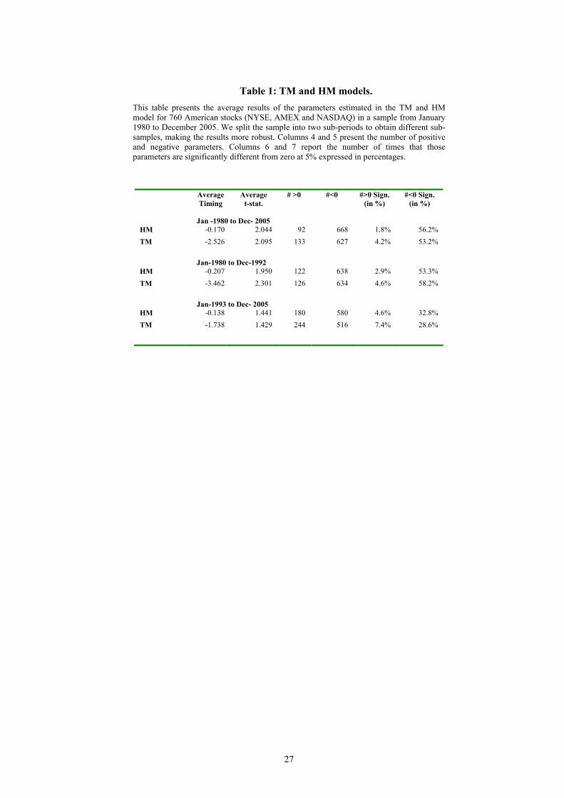
Table 1 presents a summary of the results of estimating the TM and HM models for the 760

individual stocks. We split the full sample period into two sub-samples, thus making results more

robust. We report the mean of the timing parameter in the TM and HM models, the mean t-

statistics, the number of negative and positive parameters, and the percentages of times that these

parameters are significantly different from zero at the 5% level expressed in percentages. Given

that we report average results of the 760 estimations, the estimated value for the timing parameter

would be the same as if we had an equally weighted portfolio in which the 760 stocks were

passively managed. The figures confirm the existence of perverse market timing, as the average

timing parameter is equal to -2.526 for the TM model and -0.17 for the HM model in the full

sample, and similar negative values are obtained for the sub-samples5. However, more important

than the negative value is its statistical significance, on average, and if we worked with an equally

4 In order to avoid putting too much weight on very extreme observations, we have excluded 10/19/87 and 10/21/87 from the data set as they are extremely anomalous values that could bias the results. 5 If we split the sample into five sub-samples the market timing parameter is again negative, on average. Results are available upon request from the authors.

8

weighted portfolio of all those assets the t-statistic would be even higher. Thus some evidence of

negative timing appears without active management.

[Table 1]

The results presented on the right side of Table 1 are also of note. These show the number

of stocks with a negative or positive value for the market timing parameter and the percentage of

stocks with a statistically significant parameter. Assuming that this value could be different from

zero, we should expect a similar number of positive and negative values, but we observe in column

5 that there are more negative values. In addition, the percentage of stocks with a positive and

significant parameter ranges from 1.8% to 7.4%, while the percentage of stocks with a negative and

statistically significant timing parameter is on average around 50%, suggesting that if we add these

latter stocks to a portfolio, even if managers do not actively manage, automatic perverse timing

would appear. Consequently, in the next section we develop a theoretical framework that explains

the sources of these automatic variations in betas that cause many stocks to increase the beta in

down markets, and identifies which stocks these are.

To verify the robustness of our results to different data frequencies, we repeat the analysis

in Table 1 using weekly and monthly data and, instead of only considering the classical two-factor

TM and HM models, we add the Fama-French (FF) factors (SMB and HML) and Carhart’s factor

(WML). The results are very similar, evidencing negative market timing parameter in all cases, but

are slightly reduced in monthly data or when FF factors are considered. For a weekly frequency,

the proportion of stocks with a positive and statistically significant timing is 1.7% in the HM and

2.2% in the TM two-factor models, and the proportion of stocks with a statistical and negative

timing parameter is much higher, at around 43% for both models. The timing parameter for an

equally-weighted portfolio holding all the stocks is also negative (-0.28 and -2.08 in the HM and

TM models, respectively) and clearly significant (the t-statistic is -7.7 and -7.6, respectively).

When monthly data are used, the timing parameter for an equally-weighted portfolio is also

9

negative for both HM and TM models (-0.468 and -2.06) and statistically significant. When SMB,

HML and WML are included in the models we still found clear evidence of negative bias in the

market timing parameter, as the timing parameter for an equally-weighted portfolio holding all the

stocks was negative and statistically significant in all frequencies.

3. Stock beta variation

We begin by writing the excess return of a benchmark as the weighted average of the individual

stock excess returns using the portfolio holdings as weights6

∑=

=N

jjjBB rwr

1 [4]

and the variance of the benchmark as the weighted sum of the individual stocks’ variances, vj, and

covariances, kij, with all other stocks

∑∑∑= ≠=

+=N

i

N

ijjBiBij

N

jjBjB wwkwvv

11

2 . [5]

Using [4] and [5], the beta of a stock s using the benchmark B, is given by

∑∑∑

∑

≠

≠

+

+= N

i

N

ijjBiBij

N

jjBj

N

sjjBsjsBs

sB

wwkwv

wkwv

2β . [6]

We can rewrite the beta of a stock s in [6] as

( )

B

N

sjjBsjsBssBsB

sB v

wdwdwkwv ∑≠

++−+=

1β , [7]

6 We assume that weights hold constant over time to simplify the development of the model.

10

where v denotes the average of the variance and of all stocks, k the average of all covariances and

variables dj and dij are the differences between the variance or covariance of the stock from the

average of all the stocks in the market.

∑=

=N

jjv

Nv

1

1, [8]

∑∑= ≠−

=N

s

N

sjsjk

NNk

1)1(1

, [9]

vvd jj −= , [10]

kkd ijij −= . [11]

The numerator of [7] indicates that the beta of a stock depends on four components: (i) the

average variance of all existing stocks weighted by the size of the stock; (ii) the average covariance

between all stocks weighted by the size of the rest of the stocks; (iii) the distance of the variance of

this particular stock from the average variance, weighted by its size, and (iv) the sum of the

distances of the covariances between s and the rest of stocks with respect to the average covariance,

weighted by the size of each stock in the benchmark.

We can draw some conclusions from [7]. First, the lower the size of the stock in the

benchmark, the higher the effect of the covariances on the beta, and the lower the effect of the

variances on the beta will be. Generally, wsB will take values close to zero in a well-diversified

benchmark and the most relevant components are therefore (ii) and (iv). Likewise, (1-wsB) will take

values close to one, and the value of component (ii) will then be similar for all the stocks. Thus, the

differences in the beta for two stocks are basically due to the values dsj in component (iv). In

general, the beta would be higher (lower) for those stocks with positive (negative) values of dsj, that

is, covariances higher (lower) than the average of all assets.

11

In this paper we analyze the sources of variations in the beta of a stock by comparing the

downside and the upside beta. We define the variation in the beta of a stock j as the difference

between the beta conditioned on downward markets ( jBβ ′ ) and that conditioned on upward markets

( jBβ )

jBjBjB βββ −′=∆ . [12]

To do that, we need to define some additional variables. Let cB be the relative variation of

the variance of the benchmark, when we compare it from up, Bv , to down, Bv′ , markets

B

BB v

vc′

= . [13]

In addition, we define cv as the variation of the average variances and ck, as the variation of

the average covariances, from down to up markets defined as

vv

cv

′= [14]

kkck

′= . [15]

Using the definition of [7] for down markets (where variables are denoted by ') and for up

markets, and considering [13] - [15] we can express the increase in beta [12] as

( ) ( )( ) ( )

B

N

sj

N

sjjBBsjjBsjsBBsssBBksBBv

sB v

wcdwdwcddwcckwccv

′

−+−+−−+−

=∆∑ ∑

≠ ≠, ,''1

β

[16]

12

Equation [16] shows that we can explain the sources of the variation in a stock’s beta from

up to down markets as a function of four components. We denoted these four components as PI,

PII, PIII and PIV, corresponding to

PI = ( ) sBBv wccv − ,

PII = ( )( )sBBk wcck −− 1 ,

PIII = ( ) sBBss wcdd −' ,

PIV = ∑ ∑≠ ≠

−N

sj

N

sjjBBsjjBsj wcdwd

, ,' .

PI and PIII are related to variances and are both multiplied by the relative size of the stock

in the benchmark. Because the relative size of any stock in a well-diversified benchmark is very

small, we suggest that both addends will be close to zero. They would be relevant, for the increase

in beta, only if the stock has a high weight in the benchmark, as expected for selective value-

weighted market indices with a low number of stocks. PII and PIV of [16] are related to

covariances. As they are weighted by the relative size of the rest of the stocks in the benchmark,

they will be the main components to explain the beta variation, and therefore market timing.

We termed PII the mean covariance shift. Given the empirical evidence that stocks move

more closely together in down markets, then ck would be higher than 1, and if this increase in the

average covariance is higher (lower) than the increase in the average market variance, then PII will

be positive (negative), contributing to a generalized increment (decline) of the beta for all stocks in

down markets and causing evidence of negative (positive) timing. It is important to note that this

increment is practically the same for all stocks, regardless of their characteristics.

Lastly, we termed PIV the covariance dispersion map because it depends on the

differences of the stock’s covariances from the mean covariance of all assets in the market. It must

be noted that PIV does not affect all stocks in the same way and therefore it explains why they may

13

show positive or negative evidence of market timing. Thus, for any stock s, PIV does not add

artificial timing if the weighted sum of differences for down markets is equal to cB times the

weighted sum for up markets ( )∑∑ = jBBsjjBsj wcdwd ' . Thus, the value of

∑ jBBsj wcd provides a necessary theoretical covariance dispersion map for no change in beta due

to the PIV. Given that in bull states the volatility of the market is usually lower than in bear states,

cB should be higher than one, and then to match the theoretical dispersion map that gives a null

PIV, stocks should increase the absolute value of their differences in down markets. Nevertheless,

there are no theoretical reasons to assume this could happen. On the contrary, it seems more logical

to suppose that if stocks move more closely together in down markets the absolute value of the

differences should decrease in down states. Let us suppose the extreme case: if stocks moved

extremely closely together in down markets, such that assets behave identically (they will have

identical covariances) the absolute value of the differences will fall to zero ( )0' =∑ jBsj wd and

therefore, the PIV will take a positive (negative) value when ∑ jBsjwd is negative (positive). It

therefore seems clear that PIV could mechanically contribute to a negative (positive) timing for

stocks with lower (higher) betas in up markets.

Therefore, the effect of PIV is that the assets that covary with other assets below the

average will show an increase in beta that together with the increase generated by PII will produce

an increase in beta, and therefore negative artificial timing. The assets that covary more than the

average will show a reduction in beta due to PIV. The negative value of this part plus the positive

effect of PII will produce an increase or decrease in beta.

4. Empirical results

In this section we test the statements made about equation [16] by explaining the artificial variation

in the asset’s beta in the different states of the market. Given that in [12] we defined the variation

of the beta of a stock ∆βsB as the difference between the downside beta and the upside beta, we

14

must define downward and upward markets. The financial literature presents several alternatives.

Henriksson and Merton (1981) define downward (upward) markets as periods where the excess

market returns are negative (positive), while Ang and Chen (2002), define downward (upward)

markets as periods in which the returns are below (above) their mean. Our empirical work follows

the Henriksson and Merton definition. We also performed the empirical work using Ang and

Chen’s and other alternative definitions with very similar results.

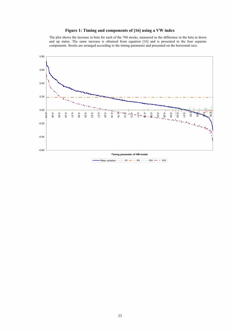
To test whether the stocks with a negative timing parameter in the estimation of a timing

model are those that automatically increase beta in down markets as opposed to up markets, in

Figure 1 we represent the increases in the stock’s beta according to [16]. The horizontal axis shows

the estimated value of the timing for each stock, from the HM model, arranged from negative to

positive values7. This value was estimated for the full sample period, using the VW index as the

benchmark. The plot shows the total variation in betas (∆βjB) and in addition each of the four parts

of [16], divided by the market variance in down markets so that the sum of the four components

matches the increase in beta. The figure presents a negative relationship between timing and the

beta increment, indicating that assets with negative timing are those in which the beta automatically

increases in down markets because of assets moving closely together, thus explaining the perverse

timing found when stocks are included in a portfolio without any active management.

[Figure 1]

As we suggested in the previous section, PI and PIII are not particularly important to

explain the variation in beta, which is approximately zero in the graph. The main parts are PII, the

mean covariance shift, and PIV, the covariance dispersion map. We can also observe that the mean

covariance shift component is practically equal for all assets (note the straight line). Recall that this

is a consequence of the fact that the mean covariance of the assets has increased from up to down

7 This graph was also calculated using a TM rather than a HM parameter with very similar results, which due to space restrictions are not presented here.

15

markets and the increase is higher that that noted in the variance of the benchmark. The figure also

shows that PIV takes a different value for each asset. Some stocks have a positive PIV and others a

negative value. But the path is similar to the total increase in beta. However, once we sum the PIV

and PII components, the line representing the total increase in beta jumps to the right, evidencing a

higher number of stocks with an automatic increase in beta in down markets than those whose beta

decreases, as reported in Table 1.

To ensure that the above results are robust to different time periods we repeated the

estimation, splitting the sample period into 2 and 5 sub-periods. Results, not presented for the sake

of brevity, are essentially the same.

Figure 1 also shows that the mean covariance shift component is positive in our sample,

favoring the increase in beta in down markets and causing the negative timing. The numerical

values of this component are interesting and are given for different time periods. Thus, Table 2

presents the values of some variables of [16]. We report the average stock’s standard deviation,

variance, covariance and correlations in down and up markets, the variance in the benchmark, and

the variations in the average stock’s variance (cv), in the market variance (cB), in the mean

covariance (ck) and in the mean correlation (cρ) when comparing down and up markets. We also

present the values for the two sub-samples. In parentheses we report the p-value for the t-test

showing that stocks in the bear and bull markets have the same mean variance (in row 3), the same

mean covariance (in row 6), and the same mean correlation coefficient (in row 9).

[Table 2]

Table 2 shows, first, that the difference, ck – cB, clearly obtains a positive value in the three

samples considered due to an increase in the mean covariance for down markets, higher than the

increase in the market variance in such down states, generating a positive mean covariance shift.

Second, we can not reject the null hypothesis of equally mean variance of the assets in up and

16

down markets; the variance of the individual stocks therefore does not change. But we observe that

the mean covariance in down and up markets changes statistically. This latter result corroborates

the increase in the correlations in down markets reported in the asymmetric correlations literature.

Moreover, the increase in the covariances of the stocks in down markets without changes in the

variances generates an increase in the variance of the market in down states and a cB greater than

one in all sub-samples.

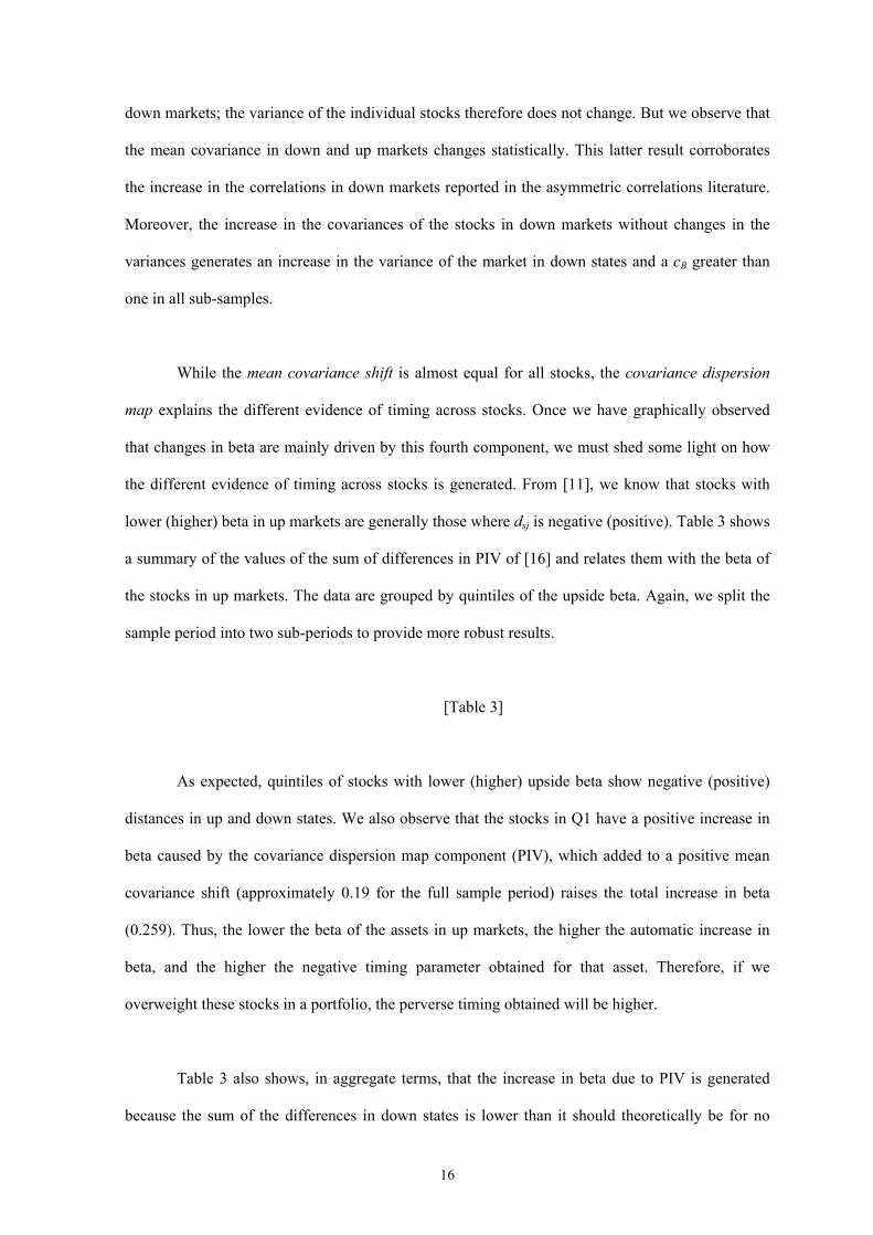
While the mean covariance shift is almost equal for all stocks, the covariance dispersion

map explains the different evidence of timing across stocks. Once we have graphically observed

that changes in beta are mainly driven by this fourth component, we must shed some light on how

the different evidence of timing across stocks is generated. From [11], we know that stocks with

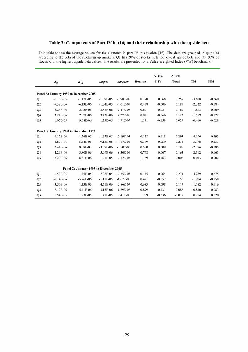
lower (higher) beta in up markets are generally those where dsj is negative (positive). Table 3 shows

a summary of the values of the sum of differences in PIV of [16] and relates them with the beta of

the stocks in up markets. The data are grouped by quintiles of the upside beta. Again, we split the

sample period into two sub-periods to provide more robust results.

[Table 3]

As expected, quintiles of stocks with lower (higher) upside beta show negative (positive)

distances in up and down states. We also observe that the stocks in Q1 have a positive increase in

beta caused by the covariance dispersion map component (PIV), which added to a positive mean

covariance shift (approximately 0.19 for the full sample period) raises the total increase in beta

(0.259). Thus, the lower the beta of the assets in up markets, the higher the automatic increase in

beta, and the higher the negative timing parameter obtained for that asset. Therefore, if we

overweight these stocks in a portfolio, the perverse timing obtained will be higher.

Table 3 also shows, in aggregate terms, that the increase in beta due to PIV is generated

because the sum of the differences in down states is lower than it should theoretically be for no

17

changes in beta. In other words, the weighted sum of the differences in down markets decreases for

the higher quintiles and becomes less negative for the lower quintiles compared to the same

variables in up markets. However it is interesting to analyze whether there was a real variation in

the dispersion map of covariances, as noted in Section 3, or whether the distances in up and down

markets did not change, and the effect of PIV was only caused by the positive and larger than one

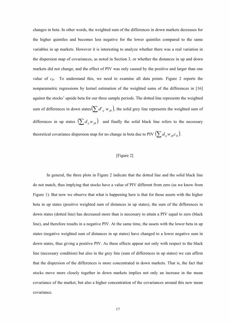
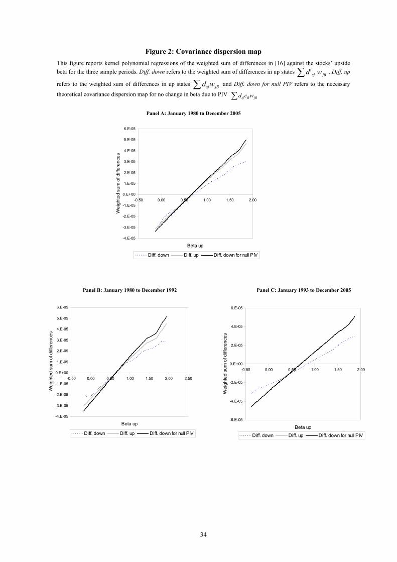
value of cB. To understand this, we need to examine all data points. Figure 2 reports the

nonparametric regressions by kernel estimation of the weighted sums of the differences in [16]

against the stocks’ upside beta for our three sample periods. The dotted line represents the weighted

sum of differences in down states ( )∑ jBsj wd ' , the solid grey line represents the weighted sum of

differences in up states ( )∑ jBsj wd and finally the solid black line refers to the necessary

theoretical covariance dispersion map for no change in beta due to PIV ( )∑ BjBsj cwd .

[Figure 2]

In general, the three plots in Figure 2 indicate that the dotted line and the solid black line

do not match, thus implying that stocks have a value of PIV different from zero (as we know from

Figure 1). But now we observe that what is happening here is that for those assets with the higher

beta in up states (positive weighted sum of distances in up states), the sum of the differences in

down states (dotted line) has decreased more than is necessary to attain a PIV equal to zero (black

line), and therefore results in a negative PIV. At the same time, the assets with the lower beta in up

states (negative weighted sum of distances in up states) have changed to a lower negative sum in

down states, thus giving a positive PIV. As these effects appear not only with respect to the black

line (necessary condition) but also in the grey line (sum of differences in up states) we can affirm

that the dispersion of the differences is more concentrated in down markets. That is, the fact that

stocks move more closely together in down markets implies not only an increase in the mean

covariance of the market, but also a higher concentration of the covariances around this new mean

covariance.

18

4.1. The Equally Weighted Index Case

Although using an equally weighted benchmark to estimate the performance of mutual

funds is not very common, it would be interesting to know what happens to the variation in betas in

such a case. First, considering that the variance of an equally weighted benchmark, vB, is

( )NkNv 11−+ , expression [11] is now given by

B

N

sjsjs

sB v

ddN

+

+=∑

≠

1

1β . [17]

Thus, if the benchmark used is an EW, then the sum of PI and PII equals zero in [16] and

the variation in beta is caused by two components only

( ) ( )

B

N

sjBsjsjBss

sEW v

cddcddN

′

−+−

=∆∑

≠,''1

β . [18]

Ceteris paribus if we compare the result in an EW and a VW index, we can affirm that the

evidence of negative timing will be higher with a VW benchmark, since the mean covariance shift

effect disappears in the case of an EW. Recall that this component was positive and increased the

beta of all stocks in down markets.

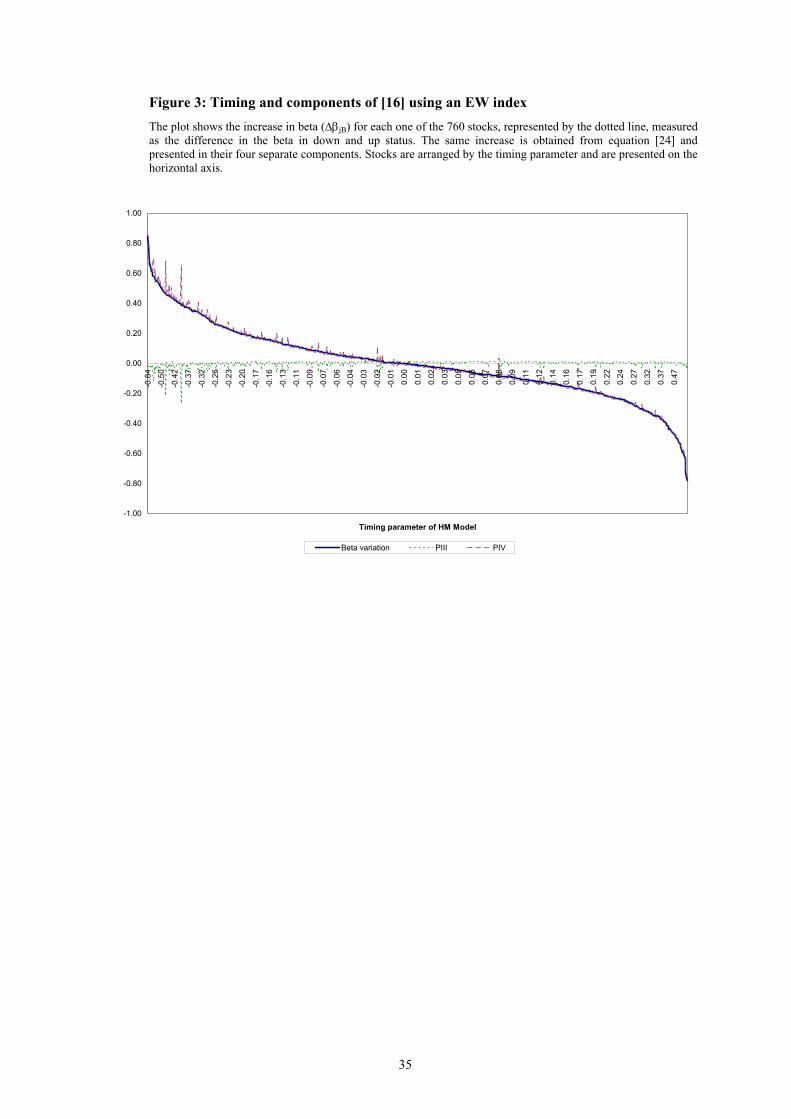
From [18] and similarly to [16], the first addend, PIII, will have a lower influence on the

variation of beta since it is only related to the distances to the variance of stock s, while the

importance will lie in the second addend, PIV, related to the rest of the distances to the covariance.

Figure 3 plots the increase in beta from up to down markets and the components of these increases

when the benchmark used is the EW index, following the two components PIII and PIV presented

in [16]. In this case, as the third component, PIII, has a low impact, the most significant component

19

is the fourth one. This PIV captures the specific effect of the covariance of each asset on the rest of

the assets and explains practically all the variation in beta.

[Figure 3]

Moreover, the plot indicates that the variation in betas sums to zero for all assets and the average

timing will be zero. To understand this, we need to express the variation in the beta of a portfolio P

as the weighted sum of the variation in the betas of the N stocks held in the portfolio

jP

N

jjBPB w∑

=

∆=∆1

ββ . [19]

Obviously, in a portfolio which mimics the composition of the benchmark (wjP = wjB) the

beta is always equal to one, and the increment in beta is equal to zero, verifying the following

expression

01

=∑=

jB

N

jjB wβ∆ . [20]

In addition, equation [20] easily shows how the weighted sum of the variation of the all

assets’ beta in a market, comparing down and up markets, should be equal to zero. Specifically,

when the benchmark is an equally weighted portfolio, the sum of these variations will be equal to

zero,

01

=∑=

N

jjEWβ∆ . [21]

However, a portfolio holding a set of assets could give a negative or positive parameter in

the assessment of the market timing ability, depending on the assets chosen.

20

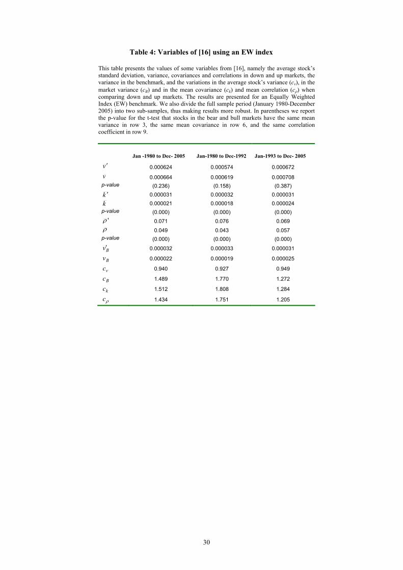
Table 4 shows some figures used in [16] when the benchmark is an EW portfolio. As in the

above sections, we find that assets are more correlated in down markets, and the fact that the mean

covariance of the markets and the variance of the benchmark in the different states changes

significantly. Thus, p-values for the test of equal covariance are lower than 0.05 and cB is clearly

greater than 1. Moreover, it should be noted that the differences in the mean variance and mean

covariances of the stocks in Table 4 as compared to the figures in Table 2 are only due to the fact

that the benchmark—in this case the EW index—is also used to separate down and up states, but

there is no change in the stocks and the sample period used.

[Table 4]

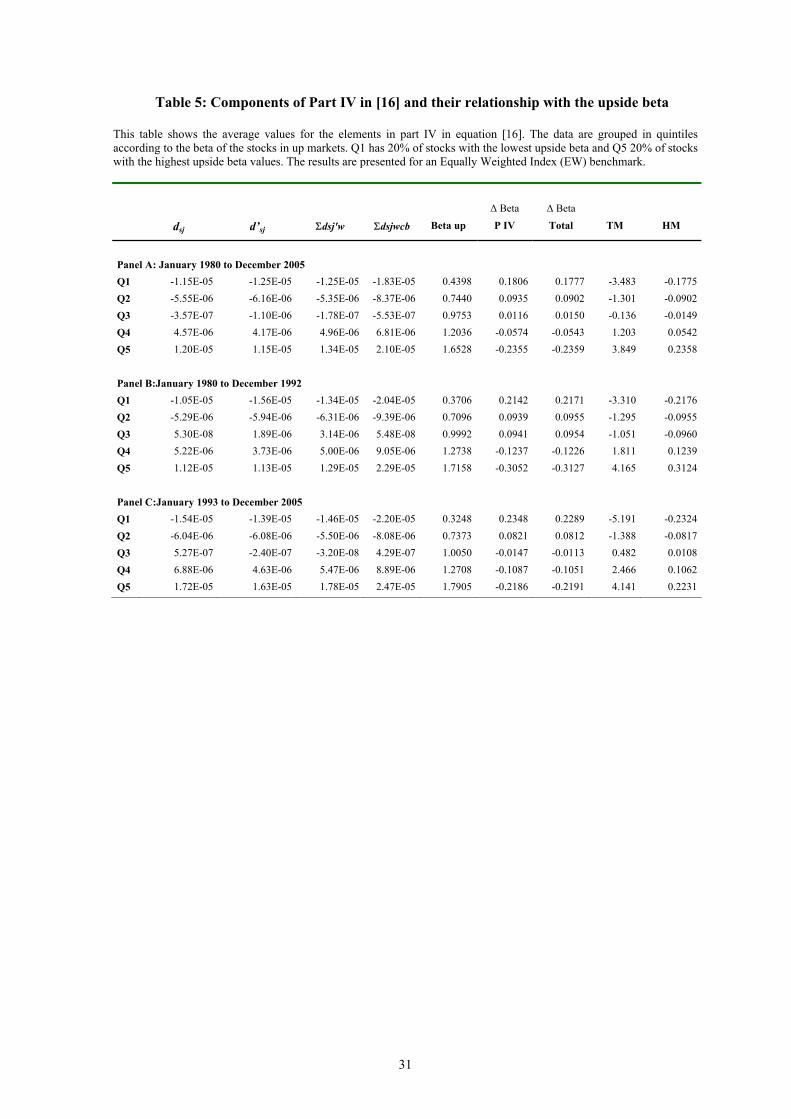
Finally, a comparison of the first two columns and the fifth column on the right in Table 5

shows how stocks with lower (higher) beta in up markets have negative (positive) differences, as

observed in [17]. The third and fourth columns show how the sum of the differences in down

markets is generally lower in absolute terms than the sum of the differences expected for a null

PIV. As in the case of the VW index analyzed in the previous section, this result implies that stocks

with lower (higher) betas for up markets increase (decrease) their beta for down markets, thus

mechanically evidencing negative (positive) timing. The table shows how the beta variation is

fundamentally due to the covariance dispersion map effect. Table 5 also illustrates an average

timing of zero using five quintiles both in HM and TM models, since we are considering all stocks

in the market.

[Table 5]

21

5. Market timing bias in an actively managed portfolio

As demonstrated in the previous section, an automatic and mechanical movement in stocks’ betas

occurs just because stocks move more closely together in down states. This will cause a negative

timing parameter in individual stocks or in a passive portfolio holding those stocks, generating a

negative bias (the difference between the estimated timing parameter and the manager’s real timing

ability, in these passive portfolios equal to zero). However, we have not yet analyzed the effect of

that change in betas if a portfolio is actively managed and the manager has positive market timing

abilities.

In this section we generate artificial portfolio returns under the null hypothesis of a positive

and perfect market timing ability in order to study what effect this bias may have when the

manager has real timing abilities. We generate various active portfolios that are rebalanced in each

time period to achieve a specific timing ability based on the HM model. Thus, we assume a

manager who has made a perfect forecast of the future market risk premium (RM-Rf). If he forecasts

a positive risk premium, then the portfolio’s beta will be βp = K0. If the estimation is such that the

risk premium is negative, he will reduce beta in K1, where the beta of the portfolio is βp = K0-K1.

Based on our previous results, the hypothesis is that managers that overweight the portfolio

with stocks with lower beta in up markets, and therefore stocks with a more highly increased beta

in down markets (as seen in Table 3), will be those that artificially obtain a negative bias. To test

this hypothesis, we rank all the stocks by their upside beta. The first quintile (Q1) contains 20% of

the stocks with the minimum value for the upside beta, and the fifth quintile (Q5) contains 20% of

stocks with the highest upside beta. To simplify this exercise, we assume that the manager, in each

simulation, chooses assets by creating two equally weighted portfolios based on 15 randomly

selected stocks from Q1 and a further 15 stocks from Q5. He is using these different sets of 15

22

stocks as two individual portfolios, and is allocating a proportion w and 1-w in each one, to achieve

the desired beta (βpt) in each time period.8

Next, we run the HM timing model on the daily data generated under our hypothesis and

evaluate whether bias on the timing parameters appears, and its significance. It should be noted that

if stocks did not move more closely together in down markets, and therefore, there were no

automatic change in beta between up and down states, in this simulation we should observe that the

estimated market timing parameter from the conventional HM model (β1) should equal the

theoretical timing ability (the value of k1 used in each simulation)9.

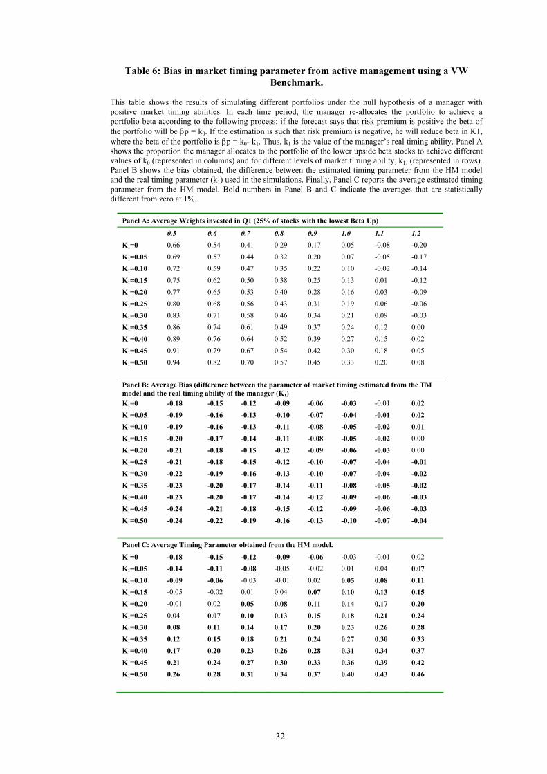
Table 6 shows the results of this simulation using a value-weighted index as a benchmark.

Panel A shows the proportion the manager allocates to the portfolio of the lower upside beta stocks

to achieve different values of k0 (represented in columns) and for different levels of market timing

ability, k1, (represented in rows). Panel B shows the bias obtained, the difference between the

estimated timing parameter from the HM model and the real timing parameter (k1) used in the

simulations. Finally, Panel C presents the average estimated timing parameter from the HM model.

In Panel B and C numbers in bold indicate the averages that are statistically different from zero at

1%.

[Table 6]

We can highlight several findings from Table 6. Firstly, Panel B provides evidence of a

negative and significant bias in measuring the market timing ability in portfolios of managers with

8 Note that with this simplification we can achieve the desired beta from an analytical expression only, without the need for any specific optimization procedure. For example, assume that we choose a set of 5 stocks from each quintile. The betas for the stocks chosen from quintile 1 are β1=0.2; β2=0.3; β3=0.25; β4=0.4; β5=0.33. The betas for the stocks from the fifth quintile are β1=1.1; β2=0.7; β3=0.55; β4=0.6; β5=0.8. We then generate an equally-weighted portfolio from stocks in Q1 (βQ1=0.296) and from Q5 (βQ5=0.75). Now, assume that for this simulation k0=0.5 and K1=0.1, and the risk-premium in the next time period is 0.01, then βp should be 0.5. We can then compute the proportion that should be invested in portfolio Q1 and portfolio Q5, just by knowing that 0.5 is the weighted sum of the betas of the two portfolios held, and then w equals 0.55. 9 Note that the bias found in this paper is completely different from the bias pointed out by Goetzmann et al. (2000) due to estimating the HM model using monthly returns of a daily timer. In our simulation we found a downward bias based on daily returns of a daily timer; there is therefore no difference between frequencies.

23

different levels of ability to forecast the market risk premium. This confirms our hypothesis that the

estimated parameter, in the traditional parametric market timing models, will be reduced with

respect to the true ability due to the higher correlation presented among stocks in down markets.

This could be biasing the empirical results found in the literature on mutual fund managers.

Secondly, we also confirm our hypothesis that portfolios that overweight the stocks with a low

upside beta (in this case the stocks in Q1) obtain a more negative bias, regardless of the manager’s

true ability to time the market. We can observe how for the same level of real market timing ability

(k1) as we move to the left side of Table 6, Panel A shows the increase in the proportion invested in

stocks with lower upside beta and Panel B reports the increase in the bias. Thirdly, Panel C clearly

shows that the estimated market timing parameter will be negative and statistically significant for a

manager without timing abilities (k1=0) in 9 out of 10 cases presented. Moreover, a manager would

need to have a real market timing ability equal to or higher than 0.3 to be sure that the estimated

market timing parameter from the traditional models shows us that he has timing abilities, in other

words a positive and statistically significant value. Therefore, if we assume for example a positive

timing ability of 0.10, even if the manager has the ability to forecast the market direction depending

on the proportion invested in stocks with lower and higher upside beta, the estimated parameter

will be negative and significant, zero, or positive and significant. Finally, we also observe that the

bias increases as the real ability (k1) increases. Again, the reason for this depends on the type of

stocks held in the portfolio. As k1 increases, the manager needs to hold a higher proportion of

stocks from Q1 to reduce the beta of the portfolio in a down state. Conclusions are identical if the

benchmark used is an EW index.

6. Summary and Conclusions

Traditional market timing measures based on nonlinear regressions of realized fund returns against

market returns indicate that, on average, sophisticated and informed mutual funds managers have

null or negative timing ability. However, this does not seem to be a reliable result. To solve this

puzzle, some authors have pointed out that the negative value might be due to a misspecification of

24

the model or some other reasons. In this article, we have proposed an additional explanation for the

negative timing parameter found in the literature on mutual fund managers.

Our explanation rests on prior empirical evidence from the literature that stocks move more

closely together in down markets. We found that because of this movement, stocks’ betas will

change automatically and mechanically, causing the negative or positive value of the timing

parameter. We demonstrate that this variation, and therefore also the timing, is basically explained

by two components: the mean covariance shift and the covariances dispersion map. Empirically,

both are related to the fact that in down markets stocks move more jointly than in up markets. The

first component is only relevant when the benchmark used is a value weighted index. In downward

markets the covariances between stocks increase more than the variance of the market, with the

main result that all stocks’ betas increase in down states, implying a negative timing for all stocks

due to this component. The second component affects any type of benchmark and explains why

different stocks may finally show positive or negative timing. Stocks with lower (higher)

covariances as compared to the average of the market in upward markets show lower (higher) betas

for up markets. In general the distances from the mean covariance of the market are shorter than the

distances in upward markets implying a more concentrated map of covariances. Thus, the

covariances are closer to the mean and the dispersion is lower than the dispersion expected for no

changes in the beta. In short, stocks with lower (higher) betas in up markets have a higher potential

to increase (decrease) their beta in down markets and therefore evidence of negative (positive)

timing is found.

Finally, we perform a simulation to test whether this automatic change in betas in managers

with positive market timing abilities biases the estimated timing parameter. We found that this bias

is more negative, as the stocks with lower beta in up markets are over weighted in the portfolio and

distort the empirical evidence found on the evaluation of market timing ability among mutual funds

managers in the previous literature.

25

References

Ang, A. and J. Chen, 2002. Asymmetric correlations of equity portfolios. Journal of Financial Economics 63,

443-494.

Ang, A., and G. Bekaert. 2002. International Asset Allocation with Regime Shifts. Review of Financial

Studies, vol. 15, no. 4 ,1137-1187.

Becker, C., Ferson, W., Myers, D.H., and Schill, M.J. 1999. Conditional market timing with benchmark

investors. Journal of Financial Economics 52, 119-148.

Bollen, N. and Busse, J.A. 2001. On the timing ability of mutual fund managers. Journal of Finance 56,

1075-1094.

Campbell, R., Koedijk, K., and Kofman, P., 2002. Increased Correlation in Bear Markets, Financial Analysts

Journal, 58 (1):, 87-94.

Cesari, R. and F. Panetta, 2002. The performance of Italian equity funds. Journal of Banking and Finance 26,

99-126.

Coggin, T.D., Fabozzi, F.J. and Rahman, S. 1993. The investment performance of U.S. equity pension fund

managers: An empirical investigation. Journal of Finance 48, 1039-1055.

Comer, G., 2006. Hybrid mutual funds and market timing performance. Journal of Business 79, 771-797.

Chen, Y. and Liang , B. .2007. Do Market Timing Hedge Funds Time the Market? Journal of Financial and

Quantitative Analysis, 42 (4), 827-856.

Daniels, K., Grinblattm, M., Titman S.,and Wermers, R.. 1997, Measuring Mutual Fund Performance with

Characteristic-Based Benchmarks”, Journal of Finance, 52(3), 1035-1058.

Edelen, R.M., 1999. Investor flows and the assessed performance of open-end mutual funds. Journal of

Financial Economics 53, 439-466.

Ferson, W.E. and Schadt, R.,1996. Measuring fund strategy and performance in changing economic

conditions. Journal of Finance 51, 425-461.

Ferson, W.E. and Warther, V.A., 1996. Evaluating fund performance in a dynamic market. Financial Analyst

Journal 52, 20-28.

Fung, H., Xu, E. and Yau, J., 2002. Global hedge funds: risk, return, and market timing. Financial Analyst

Journal 58, 19-30.

Grinblatt, M. and Titman, S., 1989. Portfolio performance evaluation: Old issues and new insights. Review of

Financial Studies 2, 93-421.

Henriksson, R.D. and Merton, R.C.,1981. On Market Timing and Investment Performance. II. Statistical

Procedures For Evaluating Forecasting Skills, Journal of Business 54 (4), 513-534.

Holmes, K. and Faff, R., 2004. Stability, Asymmetry and Seasonality of Fund Performance: An analysis of

Australian Multisector Managed Funds. Journal of Business Finance & Accounting, 33 (3&4) 539-

78.

Jagannathan, R. and Korajczyk, R.,1986. Assessing the Market Timing Performance of Managed Portfolios.

Journal of Business 59, 217-236.

Jiang, W., 2003. A nonparametric test of market timing, Journal of Empirical Finance 10, 399-425.

Kon, S.J., 1983. The market-timing performance of mutual fund managers, Journal of Business 56, 323-347.

26

Longin F. and B. Solnik, 2001. Extreme correlation of international equity markets, Journal of Finance 56,

649-676.

Matallín-Sáez, J.C., 2006. Seasonality, market timing and performance amongst benchmarks and mutual fund

evaluation. Journal of Business Finance & Accounting 33, 1484-1507.

Patro, D., 2001. Measuring performance of international closed-end funds. Journal of Banking and Finance

25, 1741-1767.

Treynor, J.L. and Mazuy, K., 1966. Can Mutual Funds Outguess The Market?. Harvard Business Review, 44

(4), 131-136.

Volkman, D., 1999. Market volatility and Perverse Timing Performance of Mutual Fund Managers. Journal

of Financial Research 22 (4) 449-70.

Warther, V., 1995. Aggregate mutual fund flows and security returns. Journal of Financial Economics 39,

209-235.

Wenchi-Kao G.L., Cheng and K. Chan, 1998. International Mutual Fund Selectivity and Market Timing

During Up and Down Conditions, Financial Review 33 (2) 127-44.

27

Table 1: TM and HM models. This table presents the average results of the parameters estimated in the TM and HM model for 760 American stocks (NYSE, AMEX and NASDAQ) in a sample from January 1980 to December 2005. We split the sample into two sub-periods to obtain different sub-samples, making the results more robust. Columns 4 and 5 present the number of positive and negative parameters. Columns 6 and 7 report the number of times that those parameters are significantly different from zero at 5% expressed in percentages.

Average Timing

Average t-stat.

# >0 #<0 #>0 Sign. (in %)

#<0 Sign. (in %)

Jan -1980 to Dec- 2005

HM -0.170 2.044 92 668 1.8% 56.2% TM -2.526 2.095 133 627 4.2% 53.2%

Jan-1980 to Dec-1992

HM -0.207 1.950 122 638 2.9% 53.3% TM -3.462 2.301 126 634 4.6% 58.2%

Jan-1993 to Dec- 2005

HM -0.138 1.441 180 580 4.6% 32.8% TM -1.738 1.429 244 516 7.4% 28.6%

28

Table 2: Variables of [16]

This table presents the values of some variables from [16]. Thus, we present the average stock's standard deviation, variance, covariances and correlations in down and up markets, the variance in the benchmark, and the variations in the average stock’s variance (cv), in the market variance (cB) and in the mean covariance (ck) and mean correlation (cρ) when comparing down and up markets. The results are presented for a Value Weighted Index (VW) benchmark. We also divide the full sample period (January 1980-December 2005) into two sub-samples, thus making results more robust. In parentheses we report the p-value for the t-test that stocks in the bear and bull markets have the same mean variance in row 3, the same mean covariance in row 6, and the same correlation coefficient in row 9.

Jan -1980 to Dec- 2005 Jan-1980 to Dec-1992 Jan-1993 to Dec- 2005

v ′ 0.000635 0.000580 0.000686

v 0.000667 0.000623 0.000711 p-value (0.330) (0.186) (0.551)

k ′ 0.000036 0.000034 0.000038

k 0.000026 0.000023 0.000029 p-value (0.000) (0.000) (0.000)

'ρ 0.079 0.081 0.081 ρ 0.057 0.051 0.065 p-value (0.000) (0.000) (0.000)

Bv′ 0.000043 0.000043 0.000042

Bv 0.000040 0.000038 0.000042

vc 0.951 0.931 0.965

Bc 1.074 1.152 1.003

kc 1.388 1.482 1.310

ρc 1.398 1.597 1.250

29

Table 3: Components of Part IV in (16) and their relationship with the upside beta

This table shows the average values for the elements in part IV in equation [16]. The data are grouped in quintiles according to the beta of the stocks in up markets. Q1 has 20% of stocks with the lowest upside beta and Q5 20% of stocks with the highest upside beta values. The results are presented for a Value Weighted Index (VW) benchmark.

∆ Beta ∆ Beta dsj d’sj Σdsj'w Σdsjwcb Beta up P IV Total TM HM

Panel A: January 1980 to December 2005 Q1 -1.10E-05 -1.17E-05 -1.69E-05 -1.98E-05 0.190 0.068 0.259 -3.818 -0.260Q2 -5.38E-06 -6.13E-06 -1.04E-05 -1.01E-05 0.418 -0.006 0.185 -2.322 -0.184Q3 2.25E-06 2.05E-06 -3.32E-06 -2.41E-06 0.601 -0.021 0.169 -1.813 -0.169Q4 3.21E-06 2.87E-06 3.43E-06 6.27E-06 0.811 -0.066 0.123 -1.559 -0.122Q5 1.03E-05 9.08E-06 1.23E-05 1.91E-05 1.131 -0.158 0.029 -0.410 -0.028 Panel B: January 1980 to December 1992 Q1 -9.12E-06 -1.26E-05 -1.67E-05 -2.19E-05 0.128 0.118 0.293 -4.106 -0.293Q2 -2.87E-06 -5.34E-06 -9.13E-06 -1.17E-05 0.369 0.059 0.233 -3.178 -0.233Q3 2.41E-06 8.58E-07 -3.09E-06 -3.50E-06 0.560 0.009 0.185 -2.276 -0.185Q4 4.26E-06 3.80E-06 5.99E-06 6.30E-06 0.798 -0.007 0.163 -2.312 -0.163Q5 8.29E-06 6.81E-06 1.41E-05 2.12E-05 1.169 -0.163 0.002 0.033 -0.002

Panel C: January 1993 to December 2005 Q1 -1.53E-05 -1.45E-05 -2.08E-05 -2.35E-05 0.135 0.064 0.274 -4.279 -0.275Q2 -5.14E-06 -5.76E-06 -1.11E-05 -8.67E-06 0.491 -0.057 0.156 -1.914 -0.158Q3 3.50E-06 1.13E-06 -4.71E-06 -5.86E-07 0.683 -0.098 0.117 -1.182 -0.116Q4 7.12E-06 5.41E-06 3.15E-06 8.69E-06 0.899 -0.131 0.086 -0.830 -0.083Q5 1.54E-05 1.23E-05 1.41E-05 2.41E-05 1.269 -0.236 -0.017 0.214 0.020

30

Table 4: Variables of [16] using an EW index This table presents the values of some variables from [16], namely the average stock’s standard deviation, variance, covariances and correlations in down and up markets, the variance in the benchmark, and the variations in the average stock’s variance (cv), in the market variance (cB) and in the mean covariance (ck) and mean correlation (cρ) when comparing down and up markets. The results are presented for an Equally Weighted Index (EW) benchmark. We also divide the full sample period (January 1980-December 2005) into two sub-samples, thus making results more robust. In parentheses we report the p-value for the t-test that stocks in the bear and bull markets have the same mean variance in row 3, the same mean covariance in row 6, and the same correlation coefficient in row 9.

Jan -1980 to Dec- 2005 Jan-1980 to Dec-1992 Jan-1993 to Dec- 2005

v ′ 0.000624 0.000574 0.000672

v 0.000664 0.000619 0.000708 p-value (0.236) (0.158) (0.387)

k ′ 0.000031 0.000032 0.000031

k 0.000021 0.000018 0.000024 p-value (0.000) (0.000) (0.000)

'ρ 0.071 0.076 0.069 ρ 0.049 0.043 0.057 p-value (0.000) (0.000) (0.000)

Bv′ 0.000032 0.000033 0.000031

Bv 0.000022 0.000019 0.000025

vc 0.940 0.927 0.949

Bc 1.489 1.770 1.272

kc 1.512 1.808 1.284

ρc 1.434 1.751 1.205

31

Table 5: Components of Part IV in [16] and their relationship with the upside beta

This table shows the average values for the elements in part IV in equation [16]. The data are grouped in quintiles according to the beta of the stocks in up markets. Q1 has 20% of stocks with the lowest upside beta and Q5 20% of stocks with the highest upside beta values. The results are presented for an Equally Weighted Index (EW) benchmark.

∆ Beta ∆ Beta dsj d’sj Σdsj'w Σdsjwcb Beta up P IV Total TM HM

Panel A: January 1980 to December 2005 Q1 -1.15E-05 -1.25E-05 -1.25E-05 -1.83E-05 0.4398 0.1806 0.1777 -3.483 -0.1775Q2 -5.55E-06 -6.16E-06 -5.35E-06 -8.37E-06 0.7440 0.0935 0.0902 -1.301 -0.0902Q3 -3.57E-07 -1.10E-06 -1.78E-07 -5.53E-07 0.9753 0.0116 0.0150 -0.136 -0.0149Q4 4.57E-06 4.17E-06 4.96E-06 6.81E-06 1.2036 -0.0574 -0.0543 1.203 0.0542Q5 1.20E-05 1.15E-05 1.34E-05 2.10E-05 1.6528 -0.2355 -0.2359 3.849 0.2358 Panel B:January 1980 to December 1992 Q1 -1.05E-05 -1.56E-05 -1.34E-05 -2.04E-05 0.3706 0.2142 0.2171 -3.310 -0.2176Q2 -5.29E-06 -5.94E-06 -6.31E-06 -9.39E-06 0.7096 0.0939 0.0955 -1.295 -0.0955Q3 5.30E-08 1.89E-06 3.14E-06 5.48E-08 0.9992 0.0941 0.0954 -1.051 -0.0960Q4 5.22E-06 3.73E-06 5.00E-06 9.05E-06 1.2738 -0.1237 -0.1226 1.811 0.1239Q5 1.12E-05 1.13E-05 1.29E-05 2.29E-05 1.7158 -0.3052 -0.3127 4.165 0.3124 Panel C:January 1993 to December 2005 Q1 -1.54E-05 -1.39E-05 -1.46E-05 -2.20E-05 0.3248 0.2348 0.2289 -5.191 -0.2324Q2 -6.04E-06 -6.08E-06 -5.50E-06 -8.08E-06 0.7373 0.0821 0.0812 -1.388 -0.0817Q3 5.27E-07 -2.40E-07 -3.20E-08 4.29E-07 1.0050 -0.0147 -0.0113 0.482 0.0108Q4 6.88E-06 4.63E-06 5.47E-06 8.89E-06 1.2708 -0.1087 -0.1051 2.466 0.1062Q5 1.72E-05 1.63E-05 1.78E-05 2.47E-05 1.7905 -0.2186 -0.2191 4.141 0.2231

32

Table 6: Bias in market timing parameter from active management using a VW Benchmark.

This table shows the results of simulating different portfolios under the null hypothesis of a manager with positive market timing abilities. In each time period, the manager re-allocates the portfolio to achieve a portfolio beta according to the following process: if the forecast says that risk premium is positive the beta of the portfolio will be βp = k0. If the estimation is such that risk premium is negative, he will reduce beta in K1, where the beta of the portfolio is βp = k0- k1. Thus, k1 is the value of the manager’s real timing ability. Panel A shows the proportion the manager allocates to the portfolio of the lower upside beta stocks to achieve different values of k0 (represented in columns) and for different levels of market timing ability, k1, (represented in rows). Panel B shows the bias obtained, the difference between the estimated timing parameter from the HM model and the real timing parameter (k1) used in the simulations. Finally, Panel C reports the average estimated timing parameter from the HM model. Bold numbers in Panel B and C indicate the averages that are statistically different from zero at 1%.

Panel A: Average Weights invested in Q1 (25% of stocks with the lowest Beta Up)

0.5 0.6 0.7 0.8 0.9 1.0 1.1 1.2 K1=0 0.66 0.54 0.41 0.29 0.17 0.05 -0.08 -0.20 K1=0.05 0.69 0.57 0.44 0.32 0.20 0.07 -0.05 -0.17 K1=0.10 0.72 0.59 0.47 0.35 0.22 0.10 -0.02 -0.14 K1=0.15 0.75 0.62 0.50 0.38 0.25 0.13 0.01 -0.12 K1=0.20 0.77 0.65 0.53 0.40 0.28 0.16 0.03 -0.09 K1=0.25 0.80 0.68 0.56 0.43 0.31 0.19 0.06 -0.06 K1=0.30 0.83 0.71 0.58 0.46 0.34 0.21 0.09 -0.03 K1=0.35 0.86 0.74 0.61 0.49 0.37 0.24 0.12 0.00 K1=0.40 0.89 0.76 0.64 0.52 0.39 0.27 0.15 0.02 K1=0.45 0.91 0.79 0.67 0.54 0.42 0.30 0.18 0.05 K1=0.50 0.94 0.82 0.70 0.57 0.45 0.33 0.20 0.08 Panel B: Average Bias (difference between the parameter of market timing estimated from the TM model and the real timing ability of the manager (K1) K1=0 -0.18 -0.15 -0.12 -0.09 -0.06 -0.03 -0.01 0.02 K1=0.05 -0.19 -0.16 -0.13 -0.10 -0.07 -0.04 -0.01 0.02 K1=0.10 -0.19 -0.16 -0.13 -0.11 -0.08 -0.05 -0.02 0.01 K1=0.15 -0.20 -0.17 -0.14 -0.11 -0.08 -0.05 -0.02 0.00 K1=0.20 -0.21 -0.18 -0.15 -0.12 -0.09 -0.06 -0.03 0.00 K1=0.25 -0.21 -0.18 -0.15 -0.12 -0.10 -0.07 -0.04 -0.01 K1=0.30 -0.22 -0.19 -0.16 -0.13 -0.10 -0.07 -0.04 -0.02 K1=0.35 -0.23 -0.20 -0.17 -0.14 -0.11 -0.08 -0.05 -0.02 K1=0.40 -0.23 -0.20 -0.17 -0.14 -0.12 -0.09 -0.06 -0.03 K1=0.45 -0.24 -0.21 -0.18 -0.15 -0.12 -0.09 -0.06 -0.03 K1=0.50 -0.24 -0.22 -0.19 -0.16 -0.13 -0.10 -0.07 -0.04

Panel C: Average Timing Parameter obtained from the HM model.

K1=0 -0.18 -0.15 -0.12 -0.09 -0.06 -0.03 -0.01 0.02 K1=0.05 -0.14 -0.11 -0.08 -0.05 -0.02 0.01 0.04 0.07 K1=0.10 -0.09 -0.06 -0.03 -0.01 0.02 0.05 0.08 0.11 K1=0.15 -0.05 -0.02 0.01 0.04 0.07 0.10 0.13 0.15 K1=0.20 -0.01 0.02 0.05 0.08 0.11 0.14 0.17 0.20 K1=0.25 0.04 0.07 0.10 0.13 0.15 0.18 0.21 0.24 K1=0.30 0.08 0.11 0.14 0.17 0.20 0.23 0.26 0.28 K1=0.35 0.12 0.15 0.18 0.21 0.24 0.27 0.30 0.33 K1=0.40 0.17 0.20 0.23 0.26 0.28 0.31 0.34 0.37 K1=0.45 0.21 0.24 0.27 0.30 0.33 0.36 0.39 0.42 K1=0.50 0.26 0.28 0.31 0.34 0.37 0.40 0.43 0.46

33

Figure 1: Timing and components of [16] using a VW index The plot shows the increase in beta for each of the 760 stocks, measured as the difference in the beta in down and up status. The same increase is obtained from equation [16] and is presented in the four separate components. Stocks are arranged according to the timing parameter and presented on the horizontal axis.

-0.60

-0.40

-0.20

0.00

0.20

0.40

0.60

0.80

-0.73

-0.49

-0.40

-0.34

-0.31

-0.28

-0.25

-0.23

-0.21

-0.20

-0.18

-0.16

-0.14

-0.12

-0.11

-0.10

-0.09

-0.07

-0.06

-0.04

-0.03

-0.01

0.02

0.05

0.08

0.16

Timing parameter of HM model

Beta variation PI PII PIII PIV

34

Figure 2: Covariance dispersion map This figure reports kernel polynomial regressions of the weighted sum of differences in [16] against the stocks’ upside beta for the three sample periods. Diff. down refers to the weighted sum of differences in up states ∑ jBsj wd ' , Diff. up

refers to the weighted sum of differences in up states ∑ jBsjwd and Diff. down for null PIV refers to the necessary

theoretical covariance dispersion map for no change in beta due to PIV ∑ jBBsj wcd

Panel A: January 1980 to December 2005

-4.E-05

-3.E-05

-2.E-05

-1.E-05

0.E+00

1.E-05

2.E-05

3.E-05

4.E-05

5.E-05

6.E-05

-0.50 0.00 0.50 1.00 1.50 2.00

Beta up

Wei

ghte

d su

m o

f diff

eren

ces

Diff. down Diff. up Diff. down for null PIV

Panel B: January 1980 to December 1992 Panel C: January 1993 to December 2005

-6.E-05

-4.E-05

-2.E-05

0.E+00

2.E-05

4.E-05

6.E-05

-0.50 0.00 0.50 1.00 1.50 2.00

Beta up

Wei

ghte

d su

m o

f diff

eren

ces

Diff. down Diff. up Diff. down for null PIV

-4.E-05

-3.E-05

-2.E-05

-1.E-05

0.E+00

1.E-05

2.E-05

3.E-05

4.E-05

5.E-05

6.E-05

-0.50 0.00 0.50 1.00 1.50 2.00 2.50

Beta up

Wei

ghte

d su

m o

f diff

eren

ces

Diff. down Diff. up Diff. down for null PIV

35

Figure 3: Timing and components of [16] using an EW index

The plot shows the increase in beta (∆βjB) for each one of the 760 stocks, represented by the dotted line, measured as the difference in the beta in down and up status. The same increase is obtained from equation [24] and presented in their four separate components. Stocks are arranged by the timing parameter and are presented on the horizontal axis.

-1.00

-0.80

-0.60

-0.40

-0.20

0.00

0.20

0.40

0.60

0.80

1.00

-0.8

4

-0.5

0

-0.4

2

-0.3

7

-0.3

2

-0.2

6

-0.2

3

-0.2

0

-0.1

7

-0.1

6

-0.1

3

-0.1

1

-0.0

9

-0.0

7

-0.0

6

-0.0

4

-0.0

3

-0.0

2

-0.0

1

0.00

0.01

0.02

0.03

0.05

0.06

0.07

0.08

0.09

0.11

0.12

0.14

0.16

0.17

0.19

0.22

0.24

0.27

0.32

0.37

0.47

Timing parameter of HM Model

Beta variation PIII PIV