Why is productivity so dispersed? - CERIBA · Why is productivity so dispersed? Rachel Griffith IFS, ... have achieved collected as part of the firm’s balanced scorecard performance

1

Why is productivity so dispersed? Rachel Griffith

IFS, UCL and AIM

Jonathan Haskel Queen Mary, University of London, AIM, CEPR and IZA

Andy Neely

Cranfield and AIM

June 2006

Abstract

Many papers have documented wide variations in productivity even in narrowly defined industries. Some have argued that this primarily reflects measurement problems due to, for example, comparing across different products. Others argue this reflects persistent differences in performance due, for example, to management. This paper looks at productivity differences not within an industry but within a firm. We use data on productivity of different branches within lines of business of a major UK-based wholesaler. Using these productivity data for comparisons is, we argue, more likely to compare like with like than comparing between firms. We document sustained differences in productivity even between branches within the same line of business. We also discuss to what extent they are correlated with differences in management and find that differences in management “account” for around 40% of the difference in productivity.

Acknowledgements Financial support for this research comes from the ESRC/EPSRC Advanced Institute of Management Research, grant number RES-331-25-0030 DN: OTHER ESRC REFS HERE?. This work contains statistical data from ONS which is Crown copyright and reproduced with the permission of the controller of HMSO and Queen's Printer for Scotland. The use of the ONS statistical data in this work does not imply the endorsement of the ONS in relation to the interpretation or analysis of the statistical data. This work uses research datasets which may not exactly reproduce National Statistics aggregates.

Correspondence

Rachel Griffith, IFS, 7 Ridgmount Street, London WC1E 7AE, [email protected]; Jonathan Haskel, Queen Mary, University of London, Economics Dept, London E1 4NS, [email protected]; Andy Neely, Cranfield School of Management, Cranfield, MK43 0AL, [email protected].

2

I Introduction

A long-standing empirical puzzle in economics is why we see so much persistent

variation in productivity, even within very narrowly defined industries. Economic

theory suggests that in well functioning markets poor performing firms should be

unviable, and therefore exit.

When comparing productivity at a more aggregate level, for example between

countries or broadly defined industries, the measured gap (say between the UK and

the US) may be due to different circumstances in each countries: the skills base, the

regulatory environment and the industry mix. Productivity variation between

industries may be explained, for example, by different technology and different levels

of competition. But the wide and persistence differences that exist across

establishments even within very narrowly defined industries remains a puzzle.1

For example, Syverson (2004) computes the ratio of productivity at the 90th percentile

(very good performing firm) to the 10th percentile (very poor performing firm) within

very narrowly defined manufacturing industries in the US in 1997.2 The average of

these ratios is over 4: in other words, the top firms are over 4 times as productive as

the bottom firms. Criscuolo, Haskel and Martin (2003) perform a similar calculation

for UK manufacturing in 2000 and find that the top firms are over 5 times as

productive as the bottom firms.

Does persistence in such variation matter? One view is that it is illusory: simply an

indicator that we do not measure productivity very well. There are a whole host of

difficulties in measuring productivity - government industrial classifications may not

accurately capture firms that are undertaking similar activities or competing in the

same markets and we may be mis-measuring inputs or outputs. Alternatively,

productivity variation may reflect real differences in productivity. If it does, we need

to understand why variation persists and crucially whether it is the same firms that

1 See, for example, Baily et al. (1992), Bartelsman and Doms (2000), Bernard and Jensen (1995), Davis and Haltiwanger (1991), Davis, Haltiwanger and Schuh (1996), Disney et al. (2003), Dunne, Roberts and Samuelson (1989) and Foster, Haltiwanger and Krizan (2002). 2 Industries are classified into 1,2,3 etc. digit divisions, with the divisions becoming finer and finer. This study uses 443 four-digit US manufacturing industries. Some examples of four digit US manufacturing industries are, for example, manufactured ice, dog and cat food, animal foods excluding dogs and cats.

3

consistently underperform, or whether firms move in and out of bad performance, for

example, do firms start a poor performers but then move up as they gain more

experience. This latter situation would be one where there is productivity dispersion,

but where it is quite consistent with a vigourous market.

In this paper we aim to shed light on these issues by looking at productivity

differences within a single firm. We focus on the retail/wholesale industry. Recent

attention has focused this sector as it accounts for close to 20% of the UK’s aggregate

productivity gap with the US.3 There is a wide dispersion in productivity in this sector,

with the firm at the 90th decile having just under 5 times higher productivity than the

firm at the 10th percentile. The firm that we look at is a national firm with many

hundreds of establishments located through the United Kingdom operating in the

wholesaling of building and plumbing equipment. Even within this narrowly defined

(4-digit) industry, when we look across firms in the UK we see that the firm at the

90th percentile is around 2.7 times more productive than the firm at the 10th

percentile.

These calculations are for firms within the same industry. In this paper we compare

branches within the same firm. By doing so, we can be more certain that we are

comparing “like for like” - branches sell basically the same thing - and we can control

for many other forms of measurement error (the data are all collected in a similar way

within the firm). When we do this we still find substantial variation in sales per

worker and profit before income tax in these establishments, with the best performing

establishment having about five times larger sales per employee than the worst

performing.

This variation appears to be persistent. While some poor performing branches

improve, most branches remain in their relative position over years. This leaves us

with a new puzzle - why do these differences in performance persist? There are a

large number of candidate reasons (which we enumerate below). One topical theory is

that differences in productivity might at least partly be explained by differences in

management. We investigate the role that local branch managers have on performance

using data on management from the firm itself. These data are scores that branches

3 See, inter alia, Inklaar, O’Mahony and Timmer (2003), and Griffith, Harrison, Haskel and Sako (2005).

4

have achieved collected as part of the firm’s balanced scorecard performance

monitoring programme (they score for example communication with staff, employee

satisfaction, customer service, etc.). We find a strong correlation between this score

and productivity. Of course, this correlation does not imply causation. Indeed it

might reflect the sorting of managers between branches – good branch managers are

asked to manage the better branches which achieve high levels of performance both

on the balanced scorecard metrics and the productivity metrics.

What are the quantitative effects that we find? A movement of a firm from the lower

to the upper quartile management scores “accounts” for about 40% of the inter-

quartile differences in productivity. In their study, using data on externally assessed

management scores between firms Bloom and Van Reenen (2006) find that

management “accounts” for around 33% of inter-quartile differences in their

productivity measure. We comment more on these differences below.

The rest of this paper proceeds as follows. The next section discusses the observed

productivity spreads in the wholesaling industry and in our firm. Section 3

investigates how much of this variation differences in management can explain.

Section 4 concludes.

II Productivity trends

We start by briefly reviewing what the existing literature shows in terms of

productivity dispersion. Table 1 summarises a number of papers.

[Table 1 here]

The first row shows the Syverson (1993) result referred to above - labour productivity

in US manufacturing industries. The second row shows the spread of total factor

productivity (TFP). The third row shows that the labour productivity variation also

shows up in UK manufacturing. One reason for this might be that labour productivity

varies due to different employment of other inputs, most notably capital and other

materials. We would expect, for example, that workers producing pencils are

working with very different capital to workers producing aircraft. To control for this,

the second and fourth rows in table 1 shows dispersion in TFP.4 The dispersion still

4 TFP, total factor productivity, generalises the single factor (labour) productivity measure and so is a multi-factor productivity measure. Rather than dividing by just labour input, it allows productivity to

5

remains. The final row shows dispersion in both manufacturing and services, which

is in fact larger than that in manufacturing.

Why does such variation exist? One view is that one is not comparing like with like.

Firms might be selling such different products that comparing pencils and aircraft,

even adjusting for other inputs, is not appropriate. Since comparisons are often made

within 4 digit industries, this view has less force, but it is clear that there are still some

significant differences between firms even within the same 4 digit industries.. One

reason for these differences is the use of different technologies. If capital is well

measured this could be controlled for, but measurement problems in capital are legion,

and controlling for capital does not control for other factors. Additional complexity is

added when one considers that there are other – often called intangible - assets, that

are poorly measured. These intangible assets include organisational, reputation and

managerial capital that may account for productivity differences.

II.i Productivity in wholesaling

How do we measure productivity in this paper? As in much of the literature, our basic

measure is output over labour inputs. We have two output measures: sales and sales

minus the costs of goods sold (this differs from value-added in that several other

intermediate goods are not deducted). We measure labour inputs using the wage bill,

since we do not have accurate measures of numbers employed in all branches in all

periods. This is not quite LP as conventionally measured, but the use of wages has the

advantage of controlling for the quality of labour, which might plausibly vary

between stores. We use nominal sales. This means that a branch that sells more of a

good with a higher markup will appear more productive than one selling a product

that is priced nearer to cost. We do not have information on the branch specific

composition of sales, or prices charged. However, the branches within each division

of the firm carry very similar products, and over a year it is likely that the mix of

goods sold will even out. In any case, it will be much more comparable then when

looking across different firms selling quite different goods.

be affected by labour, captial and material inputs, with each input weighted by its share in total costs. Such weighting is appropriate from an economic or index number point of view.

6

Whilst we focus on the productivity spread within the firm, at the outset it is useful to

compare the firm with other firms in the same industry. We focus on the two largest

divisions of the wholesaler which sell building and plumbing materials. We compare

these with data from the ARD (see data appendix) for the industries SIC 5153 and

5154, which are respectively “wholesale of wood, construction materials and sanitary

equipment”, and “wholesale of hardware, plumbing and heating equipment and

supplies”.

[Figure 1 here]

Figure 1 compares the distribution of productivity within branches of each division of

the firm with the distribution of productivity in establishments within the relevant

industry. The top graph in the top panel, headed “Plumb: Company” is a histogram of

productivity for the plumb division of the company and the lower graph in the top

panel headed “Plumb: Industry” is for the 4 digit industry. The lower panel is the

analogous graph for the Building materials industry. A number of points stand out.

There is a wide spread of productivity within both the firm and within these narrowly

defined industries. The 90/10 ratio is about 3 to 1 within each industry. There is a

similar spread even within the company and even within the different divisions of the

company. Note that the company spread is smaller, about 2 to 1, and that the

company average is above that of the industry.

[Table 2 here]

Table 2 sets out some further details about the distribution of productivity within the

industry and firm. This shows the dispersion in productivity as measured by the ratio

of productivity in the 90th to the 10th percentile. As the sectors become more

disaggregated, the dispersion falls. The branches within the company are less

dispersed than for the sector as a whole, but even at this quite disaggregated level

productivity is still very dispersed. In 2003, the branch at the 90th percentile was more

than twice as productive as that at the 10th percentile in plumb and 1.5 times as

productive in build.

II.ii How do establishments move in the productivity distribution?

As we emphasised above, whether or not persistent dispersion in productivity is a

cause for concern depends on whether it is the same branches or firms that are

7

persistently poor performers, or whether individuals move around the distribution.

Consider the analogy to the personal income distribution - if some people spend their

whole life poor this may be a cause for concern, whereas if everyone is poor for a few

years (say when they are a student) but then move up the distribution, this is of much

less concern. How persistent is a branch’s position in the cross-section productivity

distribution over time?

To examine changes over time in the distribution we first look at how the average

level of productivity evolves for branches at a certain point in the distribution. This is

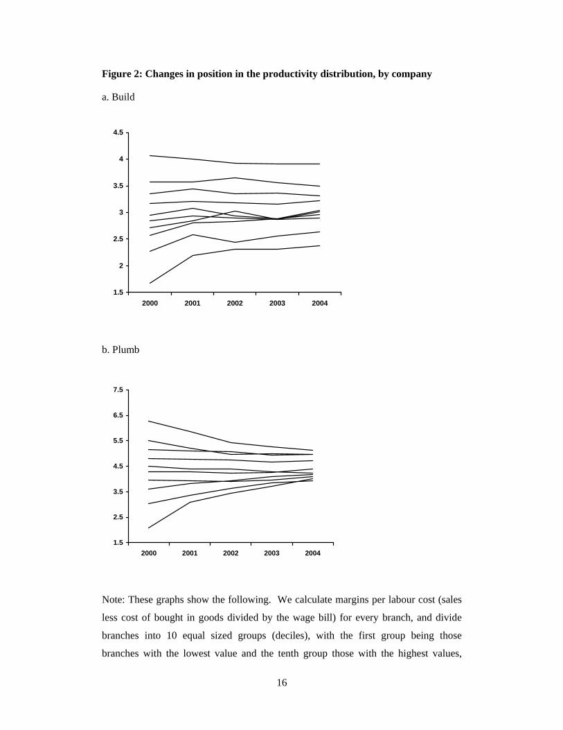
set out in Figure 2.

[Figure 2 here]

Consider the upper panel for build. We take all branches in the build division that

exist in 2000 and rank them by their position in the productivity distribution in 2000.

We then split the plants into ten equal size groups (deciles) and calculate the average

productivity of each decile. The graph then shows the average productivity, in each

year, of the same group of plants according to their membership in the initial year

deciles. The graph shows that the ranking of the plants is quite stable. The group of

plants in the top decile, those who start with the highest average, end up with the

highest average productivity, although slightly lower than where they started. The

group in the lowest decile end up still at the lowest point, but their average

productivity has risen. The middle groups tend to stay as they are, suggesting that the

position in the productivity distribution is quite persistent, but that neither the highest

nor the lowest productivity levels are sustained; the highest levels cannot be

maintained and the lowest levels improve towards the middle. The lower panel shows

the same picture for plumb division and shows a similar pattern, although there is

more convergence.

A second way to assess persistence is by looking at transition matrices. Figure 3 sets

these out in diagrammatic form.

[Figure 3 here]

To construct these we start by allocating all branches in the build division to their

productivity ranking deciles in 2000. We then calculate which decile these firms end

up in 2004 and allocate them to the appropriate point in the figure. For example, a

firm in the top decile in 2000 which is also in the top decile in 2004 would be in the

8

very top right hand cell. In the figure the diameter of the dot corresponds to the

number of firms in that cell. A zero in 2000 indicates that the branch was opened after

2000, and a zero in 2004 indicates that the branch shut down before 2004. As the

figure shows, there is a concentration of branches (i.e. the widest dots) in the 10/10

and 1/1 cells, indicating that firms in the 10th and 1st decile tend to stay there. Indeed

there is somewhat of a concentration of firms along the diagonal and near diagonal,

indicating persistence in performance. Entry and exit tend to be into and from the

lowest deciles.

It is slightly difficult to compare these results with others, since other studies have

mostly been for manufacturing and have used labour productivity data. Haskel and

Martin (2002) look at gross output per person averaged over three year intervals for

the 1980 and 1990s in UK manufacturing, and find that nearly half of firms tend to

stay where they are in the productivity distribution. For example, 48% of firms who

were in the bottom quintile of the productivity distribution were still there three years

later: likewise 50% of firms in the top quintile were still there three years later.

Finally, we can partition the variance of productivity into that part that is due to

branches having permanently different levels of productivity, and that part that is due

to productivity in individual branches fluctuating over time (around their own mean).

These two effects are commonly termed the between and with variance respectively.

In both divisions the between variation is about twice the within variation. Thus, the

bulk of the variation in productivity is due to the fact that some branches are

permanently more productivity than other branches.

III The role of management

So far we have shown that there is persistent variation in productivity even when we

compare very similar branches where issues of measure error are likely to be minimal.

As we stated earlier, there are potentially a large number of reasons why this might be

true. One reason that we are interested in investigating here is what role the

management skills of the branch manager might play.

Because we are looking with a firm we cannot investigate the role of management

overall. A few papers consider this. Bloom and Van Reenen (2006) use a survey of

company management practice where they ask a series of questions on practice each

with a scale of 1 to 5. Then then normalizing the practice to mean zero and standard

9

deviation one and take the unweighted average across all normalised scores as the

measure of overall managerial practice. Womack et al (1990) and Oliver et al (1996)

compare the quality and productivity performance of firms in the automotive industry,

arguing that performance variations can be traced back to management practices and

the adoption of lean thinking principles.

In our study, an important question is how to measure the quality of management. A

commonly used framework distinguishes between input, process and outcome

measures. Input measures include classic measures of human capital such as skill

levels, educational qualifications, attainment and experience. Process measures, such

as those used by Bloom and Van Reenen (2006), focus on the management processes

used in the organisation – e.g. the extent to which targets are set, incentives are

available, lean manufacturing methods are adopted, etc. Outcome measures focus on

the outcomes of management – e.g. customer satisfaction, employee satisfaction,

operational performance, etc. Clearly performance in terms of outcome measures

cannot solely be attributed to management, but for the purpose of this paper we

assume that management has significant influence over performance outcomes.

Hence we use a series of performance outcome measures as a proxy for management,

assuming that better performance in terms of outcomes is correlated with better

management.

To measure the performance of its branches the firm has adopted a balanced scorecard

(Kaplan and Norton, 1992). The balanced scorecard is a widely used measurement

framework, which consists of four perspectives – financial, customer, internal and

innovation and learning. In essence the balanced scorecard is designed to provide a

“balanced” view of an organisation’s performance by looking at it from a variety of

perspectives. Individual firms using the balanced scorecard are encouraged to select

those performance measures that are most appropriate for their context. In this case

the firm involved had 17 performance measures on its balanced scorecard. Together

these 17 measures reflect all of the important dimensions of performance for the

business. Six of the measures directly contain sales and/or labour cost and so we

exclude these for the purpose of our calculations. The remaining 11 measures cover

issues such as customer satisfaction, stock availability and operational standards (see

Table 3). For each of these measures the firm has set targets. A traffic light reporting

system is used (green for excellent, amber for acceptable and red for unacceptable).

10

To measure management performance we calculate how well each individual branch

performs against the targets defined by the business. Hence, the best performing

managers will operate in branches that are in the green zone for all of their measures,

while the worst performing managers will operate in branches that are in the red zone

for all of their measures.

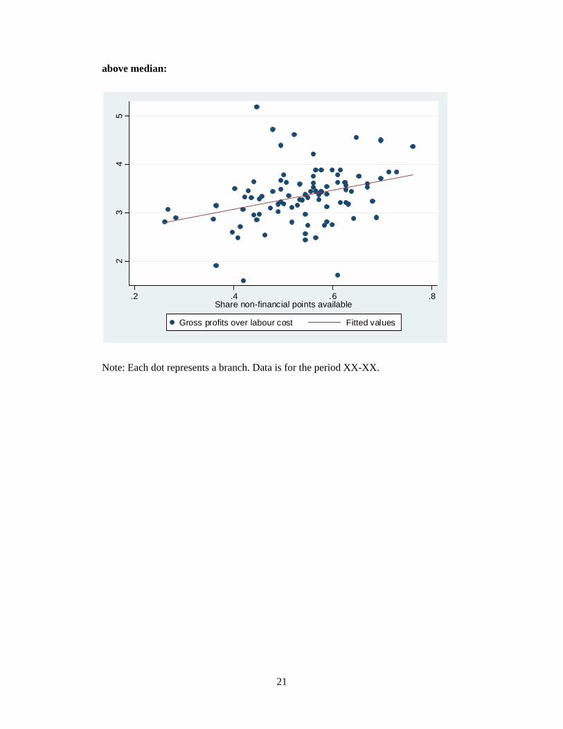
Figure 4 shows a plot of the branch’s average performance on the 11 measures over

the calendar year 2003 against the branches’ productivity performance over the same

period. We see a clear positive correlation between the two.

[Figure 4 here]

This graph shows a correlation between two variables and not causation. It might be

that managers are assigned to stores depending on store performance. Suppose for

example the best managers are assigned to the worst performing branches. Then we

would expect a negative relation (at first) between management scores and

performance, followed by a positive relation, but only for those initially poorly

performing branches. Thus in Figure 5 we split branches into those that had higher

than median productivity in the two preceding years (2000-2001) and those that were

below median. In both cases, we see a positive relationship here as well.

[Figure 5 here]

How do these data compare with other findings? Bloom and Van Reenen (2006)

control for other factors besides management (capital, materials etc.) and find that a

movement from the lower to the upper quartile of management scores between firms

(0.971 points) is associated with an increase in TFP of around 5%. In their actual

data, the difference in TFP between the lower quartile and upper quartile of the firms

is 31.9%. Hence management “accounts” for around 33% of inter-quartile differences

in their productivity measure. In our data, a movement of a firm from the lower to the

upper quartile management scores (0.15 points) is associated with an increase in our

productivity measure of 0.32 points. The difference between the upper and lower

quartile of productivity is 0.79 points. Thus our management differences “account”

for about 40% of the inter-quartile differences in productivity. This is remarkably

close to the Bloom and van Reenen number. A few points are worth making. First,

our measure of productivity does not correct for materials and capital in the way that

the Bloom study does. To the extent that better managed firms have more capital then

11

we might overstate the fraction of (total factor) productivity accounted for by

management. Second, our data is a much more like-for-like comparison of output

than the Bloom and Van Reenen (2006) sample. To the extent that their cross-section

comparison is obscured by comparisons of firms with different products they might

overstate the contribution of management to TFP.5

IV Summary and conclusions

This paper has used a new data set to compare productivity not between firms in an

industry but within a firm. We argue this comparison is more of a “like-for-like”

comparison then other work since different firms likely produce different goods. We

document a persistent productivity spread, not unlike that observed in the between

firm work. We then relate this spread to management measures and find that the

differences in management account for around 40% of the observed productivity

spread. This correlation cannot of course inform us about the causal effect of

management on productivity but it does suggest the relation is worth further

investigation.

5 If competition is not perfect and better managers are able to achieve higher mark-ups then the measured productivity in the better firms might reflect, in part, higher prices rather than more output.

12

V References

Baily, N, Hulten, C and Campbell, D (1992) "Productivity Dynamics in Manufacturing Plants", Brookings Papers on Economic Activity, Microeconomics, 187-267

Bartelsman, Eric and Mark Doms, (2000) "Understanding Productivity: Lessons from Longitudinal Microdata", Journal of Economic Literature, XXXVIII, 569-94.

Bernard, Andrew and Jensen, Brad (1995), “Exporters, Jobs, and Wages in US Manufacturing: 1976-1987”, Brookings Papers on Economic Activity. Microeconomics, 1

Bloom, N. and Van Reenen, J. 2006. 'Measuring and Explaining Management Practices Across Firms and Countries'. CEPR Discussion Paper no. 5581. London, Centre for Economic Policy Research. http://www.cepr.org/pubs/dps/DP5581.asp.

Criscuolo, C., Haskel, J. and Martin, R., (2003), “Building the evidence base for productivity policy using business data linking”, Economic Trends 600 Nov, p./39-49.

Davis, Steven J and John C. Haltiwanger. (1991) "Wage Dispersion between and within U.S. Manufacturing Plants, 1963-86", Brookings Papers on Economic Activity, Microeconomics, 115-80

Davis, Steven J, Haltiwanger, John C. and Scott Schuh (1996) Job Creation and Destruction, MIT Press

Disney, R., Haskel, J., and Heden, Y. (2003) "Restructuring and Productivity Growth in UK Manufacturing", Economic Journal, 113(489), 666-694

Dunne, T., Roberts M. J., and Samuelson L., (1989) "The Growth and Failure of U.S. Manufacturing Plants", Quarterly Journal of Economics, 104(4):671-98.

Foster, L, Haltiwanger, J and Krizan, C (2002) "The Link Between Aggregate and Micro Productivity Growth: Evidence from Retail Trade", NBER Working Paper, #9120.

Griffith, R., Harrison, R., Haskel, J., & Sako, M., The UK Productivity Gap & The Importance Of The Service Sectors, AIM report 2003.

Haskel, Jonathan and Ralf Martin (2002), "The UK Manufacturing Productivity Spread", CeRiBA working paper, www.ceriba.org.uk

Robert Inklaar, Mary O'Mahony and Marcel Timmer, (2003), “ICT and Europe's Productivity Performance. Industry-level growth account comparisons with the United States”, National Institute of Economic and Social Research, working paper < http://www.niesr.ac.uk/research/epke/confppt/Industry_growth_accounts.pdf>

Kaplan, R.S. and Norton, D.P. “The Balanced Scorecard—Measures That Drive Performance,” Harvard Business Review, 70/1 (January/February 1992): 71-79.

Oliver, N., Delbridge, R. and Lowe, J. (1996) "Lean production practices and manufacturing performance: international comparisons in the autocomponents industry." British Journal of Management, 7(Special Issue): S29-S44

Oulton, Nicholas, 1998."Competition and the Dispersion of Labour Productivity amongst UK Companies," Oxford Economic Papers, Oxford University Press, vol. 50(1), pages 23-38, January.

Syverson, Chad (2004), “Market Structure and Productivity: A Concrete Example” Journal of Political Economy, vol 112(61), pp. 1181-22

Womack, J.P., Jones, D.T. and Roos, D. (1990), The Machine that Changed the World, Rawson Associates, New York, NY.

13

VI Data appendix

ARD data

The ARD data is a sample of the business register, the Interdepartmental Business

Register (IDBR) (the register is a file of the addresses of all UK business , complied

using a combination of tax records, information lodged at Companies House, Dun and

Bradstreet data and information built up from other surveys). The IDBR holds

information on the structure of the enterprise/enterprise group, i.e. the addresses of the

relevant enterprise and shops and their industries. It holds some employment and

some output records. The Annual Business Inquiry (ABI) is the annual survey on

inputs and outputs and the ARD consists of the panel micro-level information

obtained from the ABI. To reduce compliance costs however, the ABI is not a Census

of all shops. This is in two regards. First, an enterprise with many shops may decide

to report information for a number of shops combined (a “reporting unit”). In practice,

most reporting units by number are shops, since by number most firms are single shop

chains, but most employment is in firms with many shops and in practice the

“reporting units” of the multi-shop firms are the whole chain of shops. Second, all

reporting units above a certain employment (currently 250) are all sent an ABI form.

Smaller reporting units are sampled by size-region-industry bands.6 To match the

ARD data with the company data we use sales as defined in the ARD and sales less

cost of bought in goods. Note the latter is not value added as measured on the ARD

since that also subtracts off other intermediates inputs such as heating and lighting etc.

Labour costs are measured in the ARD as wage bill plus employer taxes.

Employment usually refers to December and sales and costs data are typically for the

calendar year. We use the closest four digit industry for comparison with our chain

level data. However, it is important to note that the ARD data is by firm, not by store.

Thus productivity differences between firms likely mask differences between stores.

6 The employment size bands are 1-9, 10-19, 20-49, 50-99, 100-249, the regions are England and Wales combined, Scotland and Northern Ireland. Within England and Wales industries are stratified at 4 digit level, NI is at two digit level and Scotland is at a hybrid 2/3/4 digit level (oversampling in Scotland and NI is by arrangement with local executives). See Partington (2001).

14

Firm data

Figure 1: Comparing productivity in the firm with the industry

050

050

0 10 20

Company

Industry

Plumb

Plumb

Percentnormal gp_lc

Perc

ent

value added per labour cost

Graphs by plumbmark

050

050

0 10 20

Company

Industry

Build

Build

Percentnormal gp_lc

Per

cent

value added per labour cost

Graphs by buildmark

15

16

Figure 2: Changes in position in the productivity distribution, by company

a. Build

b. Plumb

Note: These graphs show the following. We calculate margins per labour cost (sales

less cost of bought in goods divided by the wage bill) for every branch, and divide

branches into 10 equal sized groups (deciles), with the first group being those

branches with the lowest value and the tenth group those with the highest values,

1.5

2

2.5

3

3.5

4

4.5

2000 2001 2002 2003 2004

1.5

2.5

3.5

4.5

5.5

6.5

7.5

2000 2001 2002 2003 2004

17

according to the measure in 2000. Each line is the average of margins per labour cost

for that group of branches, as it evolves over time. The top panel does this for all

branches in the Build brand and the bottom for all in the Plumb brand.

Source: Company data

18

Figure 3: Transition matrices, productivity by brand

Note: These graphs compare where each branch is in the productivity distribution in

2000 (on the horizontal axis) and in 2004 (on the vertical axis). We calculate margins

per labour cost (sales less cost of bought in goods divided by the wage bill) for every

branch, and divide branches into 10 equal sized groups (deciles), with the first group

being those branches with the lowest value and the tenth group those with the highest

values. We do this in 2000 and 2004. Zero in 2000 indicates branches that open

between 2000 and 2004, zero in 2004 indicates branches that closed between 2000

and 2004. The size of the dot indicates the number of branches in that cell.

01

23

45

67

89

1020

04 d

ec

0 1 2 3 4 5 6 7 8 9 102000 dec

Build

01

23

45

67

89

1020

04 d

ec

0 1 2 3 4 5 6 7 8 9 102000 dec

Plumb

19

Figure 4: management and productivity

Note: Each dot represents a branch. Data is for the period XX-XX.

01

23

45

.2 .4 .6 .8Share non-financial points available

Gross profits over labour cost Fitted values

20

Figure 5: management and productivity (split by prior performance)

below median:

Note: Each dot represents a branch. Data is for the period XX-XX.

01

23

4

.2 .3 .4 .5 .6 .7Share non-financial points available

Gross profits over labour cost Fitted values

21

above median:

Note: Each dot represents a branch. Data is for the period XX-XX.

23

45

.2 .4 .6 .8Share non-financial points available

Gross profits over labour cost Fitted values

22

Table 1: productivity dispersion

Standard

deviation

90th/10th

percentile

Syverson (2004) All US manufacturing, log (va/emp), 1997

0.40 4.12

log TFP, 1997 0.34 2.68

Criscuolo, Haskel and Martin (2003)

UK, manufacturing, log(go/emp), 2000

0.87 5.21

TFP, 2000 0.18 1.57

Oulton (1998) UK, all econ, log(sales/emp) 1.05 -

UK, wholesale Notes: Crisculo et al and Syverson data are averages of deviations within four-digit industries.

Table 2: 90/10 ratio

2000 2001 2002 2003 National 6.44 5.46 9.71 9.55 51 6.66 5.42 5.14 4.76 515 5.09 4.39 4.38 3.65 5153_4 3.01 2.76 2.98 2.73 5153 3.01 2.74 3.01 2.65 5154 3.14 2.62 3.08 2.87 Company ALL 2.25 2.10 2.16 2.09 BUILDER 1.69 1.65 1.63 1.57 PLUMB 2.11 1.95 2.07 1.94

23

Table 3: Management measures

Customer measures

Customer Satisfactionb

Score achieved via an external survey

Customer Retention

[(No. of Customers retained in rolling 12 months to current month – No. of Customer retained in rolling 12 months to last month) / No. of Customers retained in rolling 12 months to last month] x 100

Sales Mix [(Sales of Selected SPGs This Year to Date – Sales of Selected SPGs Last Year to Date) / Sales of Selected LLSPGs Last Year to Date] x 100

Availability of Stock Range

(Sum of Number of Days where Stock Ins for your MBR are equal to or greater than 90% / Number of Trading Days) x 100

Internal measures

Operational Efficiency

Stock/Debtors/Labour/Transport – Yes/No against individual targets: Stock 40 days, Debtors 0.5% against Sales, Labour 10% against Ex-Stock Sales, Transport 8% against Delivered Sales, where 25% is awarded per point

Operational Standards (Score from Operational Standards Check List / Total possible score from Operational Standards) x 100

Inter-company Co-operation

[(Number of Customers trading with foreign Branches This YTD – Number of Customers trading with foreign Branches Last YTD) / Number of Customers trading with foreign Branches LYTD] x 100

People measures

Staff retention (Number of voluntary leavers on a rolling 12 month basis / Average head count in rolling 12 months) x 100

Employee satisfaction (The number of people who indicate they are satisfied at work / average number of employees over the period) x 100

Communication (Number of people who feel they have been made aware of businesses activities / Average number of employees over the period) x 100 (By Region)

Supplier measures

Spend with Approved Suppliers

(Purchases from preferred Suppliers This Year To Date / Total purchases from Suppliers This Year To Date) x 100