Why is Bangladesh Outperforming Kenya

Why is Bangladesh Outperforming Kenya

A Comparative Study of Growth and its Causes since the 1960s John Roberts and Sonja Fagernäs Economic and Statistics Analysis Unit

September 2004

ESAU Working Paper 5

Overseas Development Institute London

The Economics and Statistics Analysis Unit has been established by DFID to undertake research, analysis and synthesis, mainly by seconded DFID economists, statisticians and other professionals, which advances understanding of the processes of poverty reduction and pro-poor growth in the contemporary global context, and of the design and implementation of policies that promote these objectives. ESAU’s mission is to make research conclusions available to DFID, and to diffuse them in the wider development community. ISBN: 0 85003 701 8 Economics and Statistics Analysis Unit Overseas Development Institute 111 Westminster Bridge Road London SE1 7JD © Overseas Development Institute 2004 All rights reserved. Readers may quote from or reproduce this paper, but as copyright holder, ODI requests due acknowledgement.

iii

Contents

Acknowledgements viii Acronyms viii Executive Summary ix Chapter 1: Introduction 1 PART I. SETTING THE SCENE: APPROACH TO THE QUESTION 3 Chapter 2: A Tale of Two Countries: Politics, People and Geography 3 2.1 Politics and institutions 3 2.2 Demography 4 2.3 Geography 4 Chapter 3: The Literature on Growth 6 3.1 Potentially causal factors 7 3.2 Implications for methodology 9 3.3 Summary 9 PART II. ECONOMIC AND SOCIAL OUTCOMES 10 Chapter 4: Growth and Economic Change 1960-2000 10 4.1 Brief economic history 10 4.2 Income and GDP 11 4.3 Income distribution 13 4.4 Sector shares and sector growth 13 4.5 Expenditure of GDP and resource gap 20 4.6 Summary 24 Chapter 5: Trade and External Financing 25 5.1 Role of exports 25 5.2 Terms of trade 30 5.3 Exchange and trade policies 31 5.4 Foreign Direct Investment 34 5.5 Financing the resource gap and balance-of-payments management 34 5.6 Summary 38 Chapter 6: Social Outcomes, Public Services and Public Expenditure 40 6.1 Health 40 6.2 Education 42 6.3 Public expenditure 43 6.4 Summary 44 Chapter 7: Conclusion of Part II. What could be the causes of the economic and social outcomes? 46 PART III. ASSESSMENT 48 Chapter 8: Productivity: the evidence from growth accounting 49 8.1 Summary 50 Chapter 9: Determinants of Growth and Investment – Econometric Evidence 52 9.1 Growth equations 52 9.2 Investment equations 53 9.3 Summary 54

iv

Chapter 10: Macroeconomic and Structural Policies 55 10.1 Structural reforms 55 10.2 Fiscal policies 57 10.3 Inflation 60 10.4 Financial depth 62 10.5 Financial sector 63 10.6 Macroeconomic volatility 63 10.7 Summary 65 Chapter 11: Institutional and Governance Factors 67 11.1 Corruption 67 11.2 Democracy and civil liberties 68 11.3 Regulation and bureaucracy 69 11.4 External assessments of the business environment 70 11.5 Business and politics 70 11.6 Summary 72 Chapter 12: Competition and competitiveness in the business environment 73 12.1 Labour costs 73 12.2 Transport costs 76 12.3 Summary 78 Chapter 13: Factors in Divergent Agricultural Performance 79 13.1 Bangladesh 79 13.2 Kenya 80 13.3 Summary 82 Chapter 14: Conclusions 83 14.1 Key outcomes 83 14.2 Explanations: Summary of the story line 83 14.3 Some implications 86 14.4 Success easier to explain than failure? 87 Bibliography 88 Annex 1: What Do Time Series Regressions Reveal about Growth Differences in Kenya and Bangladesh? 92 1. Introduction 92 2. Data description 93 3. Results for Bangladesh 96 4. Results for Kenya 100 5. Conclusions 104

Figures

Fig. 4.1 Bangladesh and Kenya: Real GDP 1960-2001 11 Fig. 4.2 Bangladesh and Kenya: Real per capita GDP 12 Fig. 4.3 Bangladesh and Kenya: Per capita GDP at current PPP prices 12 Fig. 4.4 Bangladesh: Sector shares of GDP at factor cost 1960-2001 14 Fig. 4.5 Kenya: Sector shares in GDP at factor cost 1960-2001 14 Fig. 4.6 Bangladesh and Kenya: Real value added in agriculture and industry 16

v

Fig. 4.7 Bangladesh and Kenya: Manufacturing value-added as a share of GDP 1960-2001 (current prices) 17

Fig. 4.8 Bangladesh and Kenya: Indices of manufacturing value-added 1960-2001 (constant prices) 17

Fig. 4.9 Kenya: Fruit and vegetable exports (3-year moving averages) 20 Fig. 4.10 Bangladesh: Consumption and savings as share of GDP 1960-2001 21 Fig. 4.11 Kenya: Consumption and savings as share of GDP 1960-2001 21 Fig. 4.12 Bangladesh: Savings, investment and resource gap 1960-2001 22 Fig. 4.13 Kenya: Savings, investment and resource gap 1960-2001 22 Fig. 4.14 Bangladesh and Kenya: Stock of physical capital (at constant prices) 23 Fig. 5.1 Bangladesh and Kenya: Trade/GDP ratios 26 Fig. 5.2 Bangladesh and Kenya: Real exports (1980=100) 26 Fig. 5.3 Bangladesh and Kenya: Exports as a share of GDP (current prices) 26 Fig. 5.4 Bangladesh and Kenya: Exports as a share of GDP (constant prices) 27 Fig. 5.5 Kenya's share of world exports of coffee and tea 27 Fig. 5.6 Kenya: Unit value of coffee and tea exports 27 Fig. 5.7 Kenya: Shares of merchandise exports 1980-2000 28 Fig. 5.8 World and Bangladesh exports of jute products 1970-2000 29 Fig. 5.9 Bangladesh: Shares of merchandise exports 1980-2000 30 Fig. 5.10 Bangladesh and Kenya: Net barter terms of trade 1966-2000 31 Fig. 5.11 Bangladesh and Kenya: Real exchange rates 1964-2001 32 Fig. 5.12 Bangladesh: Resource gap and current financing (percentages of GDP) 35 Fig. 5.13 Bangladesh: Current account long-term financing (percentages of GDP) 36 Fig. 5.14 Kenya: Resource gap and current financing (percentages of GDP) 36 Fig. 5.15 Kenya: Financing of the current account deficit (percentages of GDP) 37 Fig. 5.16 Bangladesh: External debt 38 Fig. 5.17 Kenya: External debt 38 Fig. 6.1 Bangladesh and Kenya: Educated labour force average number of years of schooling of population over 15 42 Fig. 10.1 Bangladesh and Kenya: Domestic revenues and expenditures as shares of GDP 57 Fig. 10.2 Bangladesh and Kenya: Overall budget balance (shares of GDP) 57 Fig. 10.3 Bangladesh and Kenya: Domestic financing of the fiscal deficit (shares of GDP) 58 Fig. 10.4 Bangladesh and Kenya: Domestic debt outstanding as share of GDP 59 Fig. 10.5a Bangladesh and Kenya: Nominal interest rates - Discount and Treasury Bills 60 Fig. 10.5b Bangladesh and Kenya: Nominal interest rates - Lending and deposit 60 Fig. 10.6a Bangladesh: Money supply growth and inflation 61 Fig. 10.6b Kenya: Money supply growth and inflation 61 Fig. 10.7 Bangladesh and Kenya: Financial depth 62 Fig. 10.8 Bangladesh and Kenya: Indicators of macroeconomic volatility 64

vi

Fig. 12.1 Bangladesh and Kenya: Labour costs in manufacturing 1969-97 74 Fig. 12.2 Labour productivity in Bangladesh and Kenya: Gross output per worker 75 Fig. 12.3 Bangladesh and Kenya: Comparative unit labour costs 75 Fig. 12.4 Bangladesh and Kenya: Freight and insurance margin on imports 77 Fig. 13.1 Bangladesh and Kenya: Crop production indices 79 Fig. A1 Capital stock (ln(K/L)) and GDP (ln(Y/L)) in Bangladesh 97 Fig. A2 Exports (ln(X/Y)) in Bangladesh 97 Fig. A3 Growth (Dln(Y/L)) and change in the capital stock (Dln(K/L)) in Kenya 101

Tables

Table 4.1 Comparative growth performance 12 Table 4.2 Relative price effect on sector shares in GDP 14 Table 4.3 Sector shares in growth at constant prices 1964-2001 15 Table 4.4 Annual growth rates of value added at constant prices by sector and by decade 16 Table 4.5 Total, private and public gross capital formation 23 Table 5.1 Foreign direct investment shares in capital formation 34 Table 6.1 Demographic, health and education indicators 1960-2000 41 Table 6.2 Working-age populations 1960-2000 41 Table 6.3 Public expenditure on education 43 Table 6.4 Shares of budget expenditure by sector and function and budget expenditure as share of GDP 43 Table 8.1 Annual GDP growth decomposed by contributions of capital, labour, years of schooling and total factor productivity 50 Table 9.1 Growth regressions: significant variables 52 Table 9.2 Investment regressions: significant variables 54 Table 11.1 Business cost indicators 68 Table 11.2 Corruption Perception Index scores 68 Table 11.3 Governance indicators 1996-2002 69 Table A1a Results for Dickey-Fuller tests for Bangladesh 95 Table A1b Results for Dickey-Fuller tests for Kenya 95 Table A2 Results for the Johansen Trace test 96 Table A3 Regression results for Bangladesh 98 Table A4 Correlation coefficients between explanatory variables used in models 2 and 3 for Bangladesh 99 Table A5 Investment regression for Bangladesh 100 Table A6 Regression results for Kenya 102 Table A7 Correlation coefficients between explanatory variables used in model (2) for Kenya 102 Table A8 Investment regression for Kenya 104

vii

Boxes

Box 4.1 Industry and manufacturing in Bangladesh and Kenya: Export-oriented acceleration vs. home-market-oriented deceleration 17 Box 4.2 Bangladesh: Birth of an export-oriented garment industry 19 Box 4.3 Kenya: Origins and growth of horticulture exports 19 Box 5.1 Bangladesh and Kenya: A tale of two trade diversions 33 Box 10.1 Bangladesh and Kenya: Structural reforms 56 Box 11.1 Business and politics: Two models of corruption and competition 71

viii

Acknowledgements

The authors are grateful to Adrian Wood, Chief Economist of DFID, for having inspired, advised and encouraged this research project. They also express their deep thanks to David Bevan, St. John’s College, Oxford for his detailed and perceptive review of the draft of the working paper, and for the contributions and suggestions of colleagues in ODI and DFID.

Acronyms

AGOA Africa Growth and Opportunity Act COMESA Common Market of Eastern and Southern Africa EAC East Africa Community EPZ Export Processing Zone EU European Union FDI Foreign Direct Investment GDP Gross Domestic Product GNI Gross National Income HIV-AIDS Human Immunodeficiency Virus-Acquired Immunodeficiency

Syndrome ICA Investment Climate Assessment (World Bank) IFIs International Financial Institutions IMF International Monetary Fund M2 Broad Money Supply PPP Purchasing Power Parity SOE State-owned Enterprise TFP Total Factor Productivity UNESCO United Nations Educational, Scientific and Cultural Organisation VAT Value Added Tax WDI World Development Indicators

ix

Executive Summary

This paper compares and contrasts the growth performances of Bangladesh and Kenya over the period 1960-2000. It seeks to establish the reasons why Kenya’s initially rapid growth in per capita income began to falter in the 1980s, and turned negative in the 1990s, and why that of Bangladesh has recently risen consistently, after a period of decline in the 1970s. It also seeks, by comparing developments in these two countries of similar per capita income, poverty and social indicators, to throw light of more general interest on growth processes in low-income developing countries. It asks, in particular, how and why the economic performances of two countries with similar reputations for corruption have diverged.

Main conclusions

The paper draws the conclusion that no simple explanations suffice to explain the divergences in the two countries’ performance. Political and institutional factors have impinged on production incentives both directly, by shaping the perceptions and expectations of investors and producers, and indirectly via their influence on the conduct of those facets of economic policy to which producers and investors are most responsive. In the 1960s and 1970s Kenya’s rate of GDP growth was close to 7% p.a., significantly faster than the average of a little over 2% p.a. achieved in the same period by Bangladesh. In the 1980s and 1990s the order was reversed, with Bangladesh’s economy growing at nearly 4.5% and Kenya’s at only 3% p.a. Over the most recent decade the difference widened as Kenya’s growth rate sank to 2% p.a. In terms of per capita income Kenya was poorer than Bangladesh in the 1960s, then overtook it in the 1970s, but is now some $60 poorer. Bangladesh’s mediocre performance in the 1960s and 1970s can be ascribed in large part to the political circumstances first of its subordinate position as the East Wing of Pakistan and then of the turbulence that accompanied and followed its struggle for independence. Its subsequent and unexpected economic revival and expansion reflected the benefits from the point of view of enterprise development of relative economic and political stability and predictability, restraint in public expenditure, progressive (if tardy) economic liberalisation and trade and exchange policies that maintained external competitiveness. Bangladesh made significant (if still inadequate) progress in human capital development at low cost. These conditions facilitated the accumulation of indigenous private sector capital in the very successful export-oriented garment industry, and the implementation of a ‘Green Revolution’ in rice production. They enabled Bangladesh to survive the decline of the world market for its former staple exports, jute and jute textiles, and to redeploy its resources in line with its comparative advantage. Producers’ incentives were sufficiently strong for them to overcome the well documented deficiencies of the business environment; namely, extensive corruption, an inefficient bureaucracy, power shortages and poor infrastructure. Kenya’s overall commendable growth record in the first two decades of independence is associated with simultaneous progress on several fronts. In agriculture production of maize for the home market increased with the wide adoption of hybrids, export-oriented production of coffee and tea expanded and horticulture began. Manufacturing grew with foreign investment for import substitution, taking advantage of the markets in the neighbouring East African Community countries. Tourism emerged as a major foreign-exchange earner. And there was a major expansion in public services, requiring large continuing fiscal outlays. With external financial support, Kenya weathered the storm of the oil crises and other terms-of-trade shocks of the 1970s without loss of momentum. Kenya’s growth momentum faltered in the 1980s and was lost in the 1990s as the result of a combination of factors which tarnished the country’s image as a location for business expansion

x

and as a growing force in commodity exports. These factors included inept macroeconomic management, episodes of inflationary instability, mounting public debt, the botched implementation of (extensive) economic liberalisation and institutional reforms, the effects of physical insecurity on tourism, worsening corruption at all levels and the extension of cronyism in the formal private sector. Import competition, following liberalisation in the 1990s, contributed to the decline of manufacturing industries formerly established behind protective barriers. Agricultural marketing liberalisation was followed by faltering maize and coffee production as producer incentives weakened. The disorderly macroeconomic adjustment of the 1990s - accompanied by falling public expenditure, declining real wages and worsening services - was made more painful because some external financiers withheld their support.

Methodology

The method of enquiry adopted in the paper is eclectic. Taking its cue from the empirical literature on the causes of growth, the paper makes pair-wise comparisons covering a range of possible influences on growth performance - sectoral, macroeconomic, fiscal, external, institutional and geographical. Econometric methods are used to help identify significant factors and turning points. Factors common to both countries are not explored in depth.

Comparative performance

Salient points of economic difference and similarity have been: • Savings, investment and public expenditure. Bangladesh’s domestic savings were very low

for many years, and have only risen towards 20% of GDP in the later 1990s. Public expenditure as a share of GDP has been uncharacteristically low for a low income country. Investment has risen above 15% of GDP only since 1990. Some two-thirds of it, however, have been in the private sector. In Kenya, rates of saving and investment have been high by the standard of low-income countries, though both have fallen sharply in the 1990s. The share of public expenditure in GDP has been exceptionally high for a low income country. Some 40% of investment expenditure has been in the public sector.

• Trade. In both countries the share of exports in GDP declined in the 1960s. The decline

persisted until the late 1980s in Kenya. Kenya lost world market share for its coffee exports, but was able to increase its presence in export markets for tea and horticultural products. Bangladesh’s export decline was reversed in the 1970s, in spite of the shrinking market for jute and jute products. In the 1990s there was rapid real export growth, notably through the expansion of exports of garments. Both countries have liberalised their trade and exchange policies. Both accepted IMF Article VIII (current account convertibility) obligations in 1994. Bangladesh remains more protectionist and restrictive on payments. However, the legacy of its pre-independence association with Pakistan left Bangladesh with a specialisation in export-oriented activity - the manufacture of textile products - for which it had comparative advantage. In Kenya, regional free trade, initially with the East African Community and now with COMESA, encouraged diversification into manufacturing where it has no international competitiveness. Under the influence of exports of manufactures, Bangladesh’s economy has become steadily more open to trade since the mid-1970s. Kenya’s economy, in contrast, experienced a declining trend in its trade/GDP ratio from the 1960s which lasted until the late 1980s.

• External financing. Bangladesh’s resource gap shrank from 10% of GDP circa 1980 to 5% of

GDP in 2000. It has been financed by an inflow of remittances which increased steadily to some 4% of GDP by 2000, and by concessional financing from donors, which has recently diminished

xi

from 6-8% to around 2% of GDP. Bangladesh’s external debt is very largely concessional. Kenya’s resource gap has also at times been very large – close to 10% of GDP in the period 1978-81 – and was still in excess of 5% of GDP in the late 1990s. Remittance inflows were insignificant until 1995, since when they have amounted to almost 5% of GDP. Kenya borrowed heavily on non-concessional (as well as concessional) terms to finance its public expenditure in the 1970s and 1980s, raising its debt-service/export ratio to a peak of nearly 40%, and precipitating payments difficulties. Inflows of aid and other sources of external finance have been volatile, leading to large swings in foreign-exchange reserves.

• Human resources. Bangladesh has a population more than four times the size of Kenya’s, but

it has a lower dependency ratio as population growth has been slower. Population growth rates have fallen decisively in both countries to less than 2% p.a. Enrolments in education and rates of child mortality have improved in both countries, but Bangladesh’s indicators, formerly worse than Kenya’s, are now superior, following rapid recent improvement. In Kenya life expectancy began to decline in the 1990s, but the labour force remains better educated than in Bangladesh, thanks to an earlier lead in school enrolments. Labour force skills – measured by the average number of years of schooling of the working-age population – have increased in both countries by 6.25% p.a.

Causal factors

The most prominent factors explaining the divergent patterns of GDP growth and international competitiveness have been: • Factor accumulation. The accumulation of physical and human capital has played a

significant part in promoting growth in both countries, but not consistently so throughout the period. In Bangladesh physical capital accumulation (or the absence of it) significantly explains the pace of growth at all times, but human capital accumulation contributed detectably and unambiguously only prior to 1980. In Kenya physical – but not human - capital accumulation affected the rate of growth over the whole period, and particularly in the first half; in more recent years both physical and human capital played a significant role but one which was weakened by the adverse effects of shocks and instability on growth. Empirical evidence indicates that investment in physical capital has risen when domestic savings have been higher. In Bangladesh, inward remittances have also raised investment. In Kenya, investment has been lower at times of high interest rates and falling terms of trade.

• Total factor productivity growth also varied between sub-periods: it was high in Kenya before 1980, and positive in Bangladesh after 1980, but at other times it was nil or negative. Marginal returns to factors were positive at times, but negative at others. In other words, there were forces at work, other than factor accumulation, affecting growth outcomes.

• Macroeconomic policies and management. Although both countries have pursued similar

structural adjustment policies of hesitant domestic market liberalisation, more thoroughgoing liberalisation of trade and payments and real exchange-rate depreciation, differences in macroeconomic and fiscal management have been profound. From the late 1970s to the mid-1990s Bangladesh followed policies of low public expenditure, low taxation and minimal domestic borrowing. Inflation fell in the 1980s and has remained low in the 1990s. Interest rates remained steady and fairly low. Kenya’s macroeconomic management has been more erratic. Public expenditure, taxation and employment have been high. The large public payroll raised formal sector wage levels. There has been continuous domestic financing of the fiscal deficit, at times on a very large scale, causing prolonged episodes of relatively high inflation (over 15%) and high and variable nominal interest rates.

xii

Econometric evidence indicates the positive contribution of price stability to growth in both countries – and the negative effect of inflation.

• Exports. Fitted growth equations show that export expansion has contributed to economic growth in Bangladesh throughout the period. In Kenya it had no significant effect on aggregate growth during the early period of fast growth, when the real export/GDP ratio was falling, and has only exerted a weak influence on growth during the more recent period of inferior performance.

• Institutional and governance factors. Both countries are now once again multi-party

democracies, having experienced periods of authoritarian rule. Kenya has been politically more stable and less prone to acts of violence than Bangladesh. The quality of public institutions has declined over the years in Kenya, and confidence in them has fallen as corrupt practice has become more pervasive. In Bangladesh institutional effectiveness has never been high, but in some respects there has been strengthening. Corrupt practice has become institutionalised and predictable. Respected civil society organisations have complemented the action of public services. Surveys of local business opinion rate governance less negatively in Bangladesh than they do in Kenya.

• Competition. Cronyism and rent-seeking have characterised government-business relations in Kenya. This has raised entry barriers, diminished competition in business life and impaired international competitiveness. In Bangladesh, indigenous private enterprises have been predominantly small- or medium-scale. They have grown quickly in number – as in the ready-made garment sector - and have behaved competitively. This has increased the flexibility of the economy, and its ability to respond positively to external and internal income-earning opportunities.

• Labour and transport costs. Labour costs in manufacturing have been lower in Bangladesh

than in Kenya. In Kenya, formal sector wage rates and labour costs in US$ terms rose in the 1970s and 1980s due to growing public-service employment, but then declined in the 1990s. There was no equivalent increase in Bangladesh. International sea freight transport costs have, until the late 1990s, been markedly higher in Kenya than Bangladesh. Inland road haulage rates remain higher, because haulage is more cartelised, in Kenya than in Bangladesh.

• Agriculture. Bangladesh’s long stagnant farm sector experienced accelerating growth starting in the later 1980s, due in large part to the widespread and successful implementation of Green Revolution technology, accompanied by the liberalisation of prices, input supply and marketing. Kenyan farmers raised maize yields in the 1970s and 1980s by adopting hybrid varieties, but have had no successor productivity-enhancing technology. Poorly designed and implemented marketing reforms contributed to falling maize and coffee output in the 1990s. Tea and horticultural exports, however, have continued to expand.

Implications

The paper, while noting that context specificity precludes firm prescriptions, draws some policy implications from the two countries’ experiences. These include the importance of (a) patience and consistency in policy choice and implementation: maintaining stable and predictable macroeconomic and enterprise-related policies long enough for investor confidence to build and to overcome negative presumptions; (b) prioritising and fostering those institutions which support competition and competitive market conditions; and (c) tackling the logistical and fiscal impediments and distortions which prevent countries playing to their comparative advantage in trade.

1

Growth Theory has no particular bearing on underdevelopment economics. J. Hicks, in Capital and Growth

Even the past was unpredictable, when it began. D. Rumsfelt

Chapter 1: Introduction

Contrary to the expectations entertained by most observers in the 1970s, Bangladesh is now comfortably out-performing Kenya in terms of per capita income in international prices, income growth, education and health. This paper sets out to explore the reasons why Kenya, from a very promising start in the 1960s, has experienced instability and declining performance in subsequent decades, and how Bangladesh, from unpropitious beginnings in the 1970s, has been able, in the course of the 1990s, to set itself on a path of solid growth and stability. One reason for comparing these two countries is their superficial similarity in per capita income and economic structure. Both are low-income countries, with per capita GNIs, according to the World Bank Atlas, of between $300 and $400. Both remain predominantly rural, with, until quite recently, a preponderance of agricultural produce in their exports. Another reason for comparing them is that both have reputations for official corruption and institutional dysfunction, and thus for low standards of governance. A strongly held contemporary view is that institutional factors are fundamental to explaining developing countries’ performance and their chances of achieving the Millennium Development Goals. A third reason for making the comparison is that Kenya lies in sub-Saharan Africa, a region dogged with development problems – although it has relatively well-performing neighbours – while Bangladesh is in South Asia, close to the (formerly) very fast growing ‘tiger’ countries of South-East Asia, and next door to India whose economic performance has markedly improved. ‘Neighbourhood’ effects may have affected outcomes. The paper concentrates on explanations for differences in economic growth – GDP and national income. It will note in passing differential trends in income poverty and in improvements in the standard education and health indicators. It does not, however, seek causes for these trends other than average income and public expenditure, the influence of which on poverty and social outcomes is known to be only partial. The paper’s approach is both descriptive and analytical, being guided by the eclectic body of theory and observation that has grown up around the topic of growth. Numerous facets of the economic circumstances and performance of the two countries over the period 1960-2000 are reviewed with a view to describing differences in outcomes, and to identifying possibly significant differences in environment and policy. These include the composition of GDP, savings, investment, macroeconomic and trade performance, and evidence on governance and market characteristics, and on relative production costs in the two countries, that might influence investment decisions. An underlying assumption in the analysis is that developing countries with competitive, low-cost and predictable ‘enabling’ environments conducive to private factor accumulation and entrepreneurship are best able to adapt and realise their (changing) comparative advantage in a global market of changing tastes and expenditure patterns. In assessing possible explanations for divergent performance, factors which have affected both countries similarly and simultaneously are discounted. Attention is instead focused on those other factors which affect the two countries in significantly different ways or degrees. Econometric tests are, where possible, applied to data on these factors. Where these are not possible, or when tests prove inconclusive, the conclusions reached rest on partial analysis based on well-established priors about factors favourable to growth. There are inherent problems about establishing statistically significant differences between countries unless there are long and stable time series to which reference can be made at appropriate junctures. As long time series data are often not available, it is not possible to calculate the relative strengths of all the pertinent causes of divergence. The broad conclusions reached are that:

2

• neither country has had a stable growth model; • factor accumulation is a proximate explanation for some of the two countries’ growth, at some

times, but not in all periods; • export growth is another, strong, proximate driver of growth in some periods; • Kenya’s deteriorating performance, relative to Bangladesh, may be better explained by a

combination of worsening institutional performance and the impact on enterprise of greater macroeconomic instability, of higher interest rates, taxes, wages and transport costs, and of a less competitive domestic market;

• Bangladesh, for all its institutional and management shortcomings, has reaped the harvest of prudent macroeconomic management, and of labour costs, interest rates and taxes low enough to offset the costs to enterprise of public sector inefficiency and corruption;

• the effect of institutional quality on growth is context-specific and hard to generalise; however, strengthening institutions most relevant to enterprise and a competitive business environment may merit priority.

The remainder of the paper is organised as follows. Part I is an introduction to the two countries’ politics and geography (Chapter 2), and to the recent literature on growth which helps to identify the array of possible causes of differential performance, thus setting the agenda for the rest of the paper (Chapter 3). Part II reviews the two countries’ economic and social outcomes in some detail, charting the progress of the two economies over four decades in respect of their GDPs and the sector composition thereof, savings and investment (Chapter 4), external transactions (Chapter 5) and social outcomes (Chapter 6). Part III presents an assessment of the causes of divergent performance in the two countries, starting with measures of their total factor productivity (Chapter 8), then proceeding to consideration of the econometric evidence (Chapter 9), macroeconomic management (Chapter 10), institutions and governance (Chapter 11), competition and production costs (Chapter 12) and factors in agricultural growth (Chapter 13). Chapter 14 draws conclusions from the evidence, with a review of significant policy and institutional differences and of differences in production costs and competitiveness.

3

PART I. SETTING THE SCENE: APPROACH TO THE QUESTION

Chapter 2: A Tale of Two Countries: Politics, People and Geography

2.1 Politics and institutions

Both Bangladesh and Kenya were democracies after independence, with a presidential regime in Kenya and a parliamentary constitution in Bangladesh. Both abandoned multi-party democracy for a time, and have now returned to it. Bangladesh. Prior to independence in 1971, Bangladesh was the East Wing of Pakistan whose federal government determined its fiscal, structural and trade policies. The Pakistani economy was expanding, and its macroeconomic policies avoided inflation and excessive indebtedness. However, the East Wing grew more slowly in the 1960s (3.6% p.a.) than the West Wing. As a major source of export earnings (from jute and jute products), it was disadvantaged by an overvalued exchange rate and protectionist trade policies, causing trade diversion to its disadvantage. After independence, the country was plunged into three years of political turmoil and violence which caused a sharp fall in growth, from which it recovered progressively in the later 1970s, leaving per capita income in 1980 well down from its 1970 level. From 1975 to 1991 Bangladesh was under authoritarian military rule, after which it reverted to parliamentary democracy. Politics then settled into a pattern of intense personal and party rivalries, with the two main parties taking turns to succeed each other after often disruptive and violent election campaigns. The rival parties possess similar ideologies and pursue similar policies, but the nature of political life has inhibited long-term, strategic planning. Bangladesh is culturally homogeneous, with 98% of the population Bengali-speaking, and 86% Muslim. Since the restoration of democracy the Supreme Court has asserted its independence of the administration, but lower courts are venal and subject to administrative influence. Citizens have, in practice, only limited judicial protection from official abuse of their individual and civil rights. Kenya. Prior to independence in 1963, economic life in Kenya was disrupted by the Mau Mau rebellion. But the seeds of post-independence growth and stability had been sown. Kenya inherited a rich and diversified agricultural sector, with complementary smallholder and commercial farm sectors. At independence smallholders were freed from regulatory restraints on their production of cash crops, and many settlers’ commercial farms were transferred to local private ownership. For a number of years Kenya was a one-party state, with formal multi-party democracy restored only in 1992. Until 2002 it experienced no change of government, except for a presidential succession. Civil order has been strictly maintained, with only momentary exceptions, in spite of a high degree of ethno-linguistic fractionalism and religious diversity. The political economy has been stable, apart from a short-lived insurrection in the 1980s, which the government of President Moi overcame with external support. It has, however, been dominated by an increasingly self-serving clientelistic élite, which grew more deeply entrenched in power after Kenya became a one-party state. The independence of the judiciary and the effectiveness of the courts in protecting civil rights and providing the means of redress have diminished since independence, and the judiciary has been subject to political influence. Some freedom of expression has persisted, however, even in the years of one-party rule, permitting some criticism of the administration and of official corruption.

4

Kenya was the commercial, manufacturing and financial hub of the East African Community,1 whose external tariff gave it the benefit of trade diversion in favour of its industries. Private investment, including inward investment, was encouraged, particularly in manufacturing and tourism, but only under much stricter conditions in the sensitive agriculture sector. These advantages were whittled away after 1980, partly because of the demise of the EAC in 1977, but also for other more fundamental reasons to do with mounting external investor and donor concern about political stability, macroeconomic policy and management, governance and the business environment. The policy adopted in the 1970s2 of allowing ministers and senior officials to pursue private business interests while in office created incentives favouring an anti-competitive, ‘crony’ capitalism. After a decade of falling per capita income, President Moi retired in 2002 at the end of his term in office, and was replaced, following free elections, by President Kibaki who restored multi-party democracy, and committed himself to economic reform and the repression of corruption. Kenya is one of the 41 Highly Indebted Poor Countries, but also one of the small minority of this group whose external indebtedness is regarded as sustainable, i.e. the present value of its debt-service obligations is calculated by the international financial institutions (IFIs) to be less than 150% of its export earnings.

2.2 Demography

Kenya has a population a quarter the size of that of Bangladesh; it now numbers 31 million, while Bangladesh’s population is 134 million. Population growth in Kenya has been 1% p.a. faster on average than in Bangladesh since 1960 (see Table 4.1). The dependency ratio3 rose in both countries in the 1960s and 1970s, but has fallen sharply in the 1980s and 1990s. It remains higher in Kenya (Table 6.1). Fertility rates have fallen markedly in both countries between 1960 and 2000, from 7 to 3 in Bangladesh, and from 8 to 4 in Kenya. Population density is much greater in predominantly fertile Bangladesh (925 persons per km2) than in Kenya (53 persons per km2) where much of the surface area is arid or semi-arid. The equivalent of some two-thirds of Bangladesh’s land area is classed as arable and available for annual crops; as against only some 6-7% in Kenya. The ratios of population to cultivable land (1.7:1) are thus much closer than the crude population densities. Bangladesh has also invested heavily in land-increasing technology (tubewells), thanks to which it has increased its cropping intensity to 1.8. Both countries have urbanised apace, with the urban share of the population in Kenya (34%) now exceeding that in Bangladesh (26%). These data suggest that Kenya may be losing the comparative advantage it once had in agriculture, though its exports are still predominantly agricultural. It has increased its cropped area, but in doing so has farmed areas of low and erratic rainfall with low expected returns. Bangladesh’s exports are mostly manufactured, as they have always been. Most of the growth in employment in both countries has been in urban-based and other off-farm activities.

2.3 Geography

Both countries have coastal locations, and should therefore be similarly favoured in terms of international sea-borne transport. Kenya has the locational advantage of having a significant economic hinterland; the COMESA countries take some 50% of its exports. Kenya also lies astride a busy airline corridor linking Europe and southern Africa, which confers advantageous airfreight

1 The East Africa Community, comprising Kenya, Tanzania and Uganda, was created prior to these countries’ independence. Its institutions included a common market with internal free trade, a common currency and common post, telecommunications and air and rail transport corporations. 2 Following the report of the Ndegwa Commission of 1971. 3 Ratio of the population aged 15-64 to the total population.

5

rates. Bangladesh has neither of these geographical advantages, lying, as it does, at some distance from the busy liner route between Suez and Singapore. The major potential advantage of proximity to the large and growing Indian market has not been exploited because of formal and administrative trade barriers. Kenya’s relative geographical disadvantage lies in its relatively costly inland transport, to which institutional factors also contribute (cf. Chapter 12). In Bangladesh, distances inland are shorter than in Kenya, and there is competition between road, rail and waterway transporters of freight. Episodic natural disasters visit both countries – cyclones and floods in Bangladesh and droughts in Kenya. The governments of both countries have to mount disaster prevention and emergency relief expenditure programmes, towards which substantial donor contributions are generally provided. Disaster proneness is not a likely cause of performance difference. Bangladesh, unlike Kenya, possess mineral wealth in the form of natural gas. Nineteen fields, with an estimated recoverable reserve of 25 trillion cubic feet, are under exploitation, and new fields continue to be discovered. In the 1990s gas output first slowed, then accelerated at the end of the decade, giving an average growth of some 7.5% p.a. To date, however, use of this resource has been largely devoted to the production of power and fertiliser, and exports have been prohibited. It has made a helpful but minor contribution to GDP.

6

Chapter 3: The Literature on Growth

Easterly (2002) has characterised the quest for the causes of growth in developing countries as ‘elusive’. Many theories – some with sound micro-foundations, others ad hoc and eclectic – have been tested on the data, and many researchers have found justification for their particular theories in their empirical results. This activity has intensified since the publication in 1991 of the Summers and Heston data set (Summers and Heston, 1991). Early conclusions were based on flawed econometric methodology, for example taking as explanatory variables economic, political and social features which are endogenous to the growth process. These flaws have been progressively overcome, for example by identifying instrumental variables whose exogeneity is beyond doubt. But this has only made it harder to account for growth in terms of tangible concepts and operational policies. The literature leads to the general conclusion that the causes of growth are multiple, varying in mix from case to case, and non-deterministic. However, the literature also identifies factors that are probably conducive, sooner or later, to economic growth, especially if available in combination. Read in this way, it sets the agenda for the enquiry in this paper. The empirical study of growth started with specifications based on Solow’s neo-classical model which explained income in terms of the accumulation of capital, labour and skills, on which marginal returns, in equilibrium, are stable and equal to marginal cost. Growth unexplained by accumulation derives from ‘total factor productivity’ whose increase is due to shared autonomous technical progress and to country-specific incentive and exogenous factors. It has subsequently become an eclectic area of enquiry. Competing theories have been propounded, are tested, and are often found to have some prima facie validity. Empirical testing is, however, fraught with methodological problems, such as the endogeneity of many explanatory variables used and the multi-collinearity and spurious correlations between time series, the ambiguity of the results of cross-country analyses, and the ordinal character of (subjective) indices of the quality of governance. The accumulation of physical and human capital is endogenous to the growth process, because it responds to perceptions of economic opportunity and advantage. But it can only be a proximate cause of growth. The fundamental sources of economic growth are thus to be sought in truly exogenous characteristics, such as the quality of countries’ institutions and their geographical location – whether close to or far from external markets, and whether in zones prone to adverse climates and ill-health. The testing of growth theories has relied on the econometric assessment of cross-country or panel data evidence. Conclusions drawn from cross-country studies, at best, offer insights into average past relationships to be found in (large) samples of countries; they are not reliable as indicators of actual causal or coincident relationships in particular countries. For this, country-level time series evidence has to be studied. Part III of this paper uses results from time-series growth and investment regressions. However, the explanatory power of time series analysis is diminished by the need to eliminate spurious correlation between variables. This is done by working with data in first differences, which has the effect of masking trends which may have genuinely causal significance. If real relationships are unstable, time series analysis may yield no usable results. These difficulties do not make pair-wise comparisons impossible, but they constrain them, forcing the analysis to rely heavily on analytical priors about causal factors and directions of causality. The usable methodology is thus more forensic than statistical – using systematic evidence-based description, and building a plausible case from circumstantial evidence. This has, broadly been the practice of authors of previous pair-wise comparison studies.4

4 e.g. Bevan et al. (1999)

7

3.1 Potentially causal factors

Whatever its limitations, the literature on growth is a valuable quarry from which to extract information on factors which have been found, in the analysis of different data sets, to have causal effects on growth. A useful starting point is Barro’s paper on the determinants of economic growth of 1996 (Barro, 1996). Barro starts from a conventional neo-classical framework of analysis, based on profit and welfare maximisation, which explains growth in terms of an equilibrium level (or steady state) of per capita output, and of the gap between it and the current level of income. Using panel data for some 100 countries, he finds that the equilibrium level of income for each country can be estimated from an array of choice and environmental variables, including savings and investment rates, labour force growth, education, economic policies and institutions, and governance variables.5 He finds that male secondary and higher education, life expectancy, fertility rates, the terms of trade, and indices of democracy and the rule of law all have significantly positive impacts on per capita GDP growth, and that inflation and government consumption (excluding expenditure on education and health) have significantly negative impacts. These same factors have impacts of the same sign on investment expenditure. The interpretation placed on the role of investment is that it is both caused by, and a cause of, growth. The magnitude of its effect is thus difficult to disentangle empirically. The expectation in neo-classical models, confirmed in Barro’s econometric tests, is that, after controlling for factors determining the level of steady state income, the lower a country’s initial level of income is, the faster it will grow. The theoretical reason for this process of conditional convergence is that, at the outset, poorer countries are lacking in some critical factors which, once supplied, have exceptionally high returns during the catch-up period. However, Pritchett, observing the persistent divergence between growth rates among developing countries, only a minority of which are manifestly ‘converging’, argues that several models are needed to explain the diversity of experience, including models of arrested growth and of stagnation (Pritchett, 2001). Ghura and Hadjimichael (1996), using panel data for 29 sub-Saharan African countries, estimate a neo-classical growth function including human capital, augmented by an array of economic policy, governance and state variables. Their results appear to confirm conditional convergence. They demonstrate the clear positive effects on growth of private investment, low fiscal deficits, low inflation, structural reforms and external competitiveness. They also show the negative effects of adverse movements in the terms of trade, and climatic shocks. Ghura and Hadjimichael reach a conclusion, of great relevance for the present paper, that macroeconomic policy works through its impact on the volume and efficiency of investment. In another paper (Ghura and Hadjimichael, 1995), the same authors identify low inflation, low uncertainty, low debt and effective financial intermediation as positive factors in promoting private saving and investment. Some authors advise strongly against the traditional assumption of economists that the accumulation of factors of production – land, physical capital, labour, skills, knowledge and organisation – holds the key to growth. Easterly and Levine (2001) argue that factor accumulation tends to be persistent and progressive through time, while growth is erratic; countries whose factor accumulation records are similar have divergent growth records. Pritchett makes the same point in respect of human capital whose steady rates of accumulation cannot explain fluctuations in growth (Pritchett, 2004). Easterly and Levine, and other authors, starting from the proposition that the key to understanding growth lies in explaining increases in total factor productivity, have found alternative policy and institutional variables that also have statistically significant impacts on growth These include 5 Barro recognises that many of his explanatory variables are endogenous, and would, using OLS, show bias and inconsistency in their estimated coefficients. He overcomes this problem by using lagged or instrumental variables.

8

‘openness’6, public expenditure on infrastructure (Easterly and Rebelo, 1993), and bureaucratic effectiveness (Mauro, 1995) – with a positive impact; and high government expenditure (Schmidt-Hebbel et al., 1996), corruption (ibid.), expropriation risk (Acemoglu et al., 2001), the foreign exchange black market premium, fiscal and current account deficits (Ghura and Hadjimichael, 1996), and macroeconomic instability (El Badawi and Schmidt-Hebbel, 1999) – with negative impacts. There are also a variety of additional social, institutional, and geographical state variables that are found to have significantly negative effects on growth outcomes. These include ethno-linguistic divisions, natural resource abundance,7 distance from external markets (Gallup et al., 1999; Redding and Venables, 2000), high transport costs, tropical climate, and the incidence of disease, especially malaria (Sachs and Malaney, 2002). The instability of the international economic environment facing countries has also been found to exert a significantly negative influence on growth (Guillaumont et al., 1997). Rodrik et al. have sought to establish a hierarchy of ‘deep’ growth-inducing factors – those which are truly exogenous to contemporary economic and social systems, either because they are bestowed by nature or because they are predetermined by long historical antecedents (Rodrik et al., 2002; Rodrik, 2003). They conclude that institutional quality, proxied by a composite index of the rule of law and property rights, exerts a more powerful influence over (PPP) per capita income growth than economic geography (distance from the equator) or openness (trade/GDP ratio) variables. Rodrik also argues that starting growth may be quite easily achieved through a few, context-specific, measures, and certainly does not require a whole panoply of growth-inducing policies and institutions. It may only require a more favourable attitude on the part of government to the private sector, and the removal of the most egregious impediments to enterprise. Sustaining growth, however, requires the incorporation into domestic policies and institutions of ‘higher order economic principles’ – respect for property rights and contracts, sound money, fiscal solvency and market-oriented incentives. These are likely to require proficient and impartial bureaucracies, independent judiciaries and a capacity for the beneficial regulation of markets (Rodrik, 2003). In one particular respect this literature is deficient. There have been few successful attempts to identify key complementarities and combinations of factors that may have generated positive externalities and increasing returns at particular junctures and in particular sectors. Yet, as Easterly (2002) convincingly argues – albeit on anecdotal evidence – growth episodes often feature fortuitous combinations of circumstances, occurring in an adequately enabling environment, that trigger profitable entrepreneurial activity. The specific chain of events taken by Easterly to illustrate his point is the emergence and swift expansion of the export-oriented garment industry in Bangladesh in the 1980s (see Box 4.2). These conclusions drawn from empirical studies offer little precise guidance on how to identify the key variables that are likely to account for the performance differences between Bangladesh and Kenya. They do not signpost any compact set of variables for particular attention. Rather, they suggest an eclectic approach which casts the net wide and considers a large number of variables to see where significant differences may lie.

6 Sachs and Warner (1995a) define an index of policy openness based on whether countries have ‘socialist’ trade regimes, and the incidence of high tariffs and quantitative restrictions. Other authors measure openness simply by the trade/GDP ratio. 7 Sachs and Warner (1995b) demonstrate that mineral-resource rich countries are prone to Dutch Disease (currency overvaluation) which inhibits the development of traded goods sectors with growth-enhancing knowledge externalities.

9

3.2 Implications for methodology

Some potentially causal factors are by nature relatively unchanging ‘state’ variables which condition the growth process, but cannot explain changes of trend. For the purposes of identifying sources of divergence, long-range background factors, such as institutional quality or ethno-linguistic diversity, will be relevant only if the performances of the two countries diverge systematically over a long period. If, on the other hand, as will be apparent in Chapter 4, the performance curves intersect (with Kenya performing better in an earlier period, and Bangladesh in a later period), the key sources of divergence have to be sought in shorter-range, proximate, state and policy variables. For our present purposes it does not matter if causal factors are endogenous, though as far as possible the key triggers for changes in outcomes will be identified.

3.3 Summary

The growth literature notes that growth rates tend to be unstable. It suggests that a wide range of causal factors may be at work in the growth process. Some of these are common to all countries, such as the advance of knowledge and technical progress. Others are: • endogenous to the growth process but largely pre-determined, such as the accumulation of

physical and human capital; or • policy-determined and subject to short-term fluctuation, such as macroeconomic stability and

the trade regime; or • related to political and institutional realities which tend to evolve only slowly, such as

democracy, political stability, ethno-linguistic divisions, the rule of law, administrative culture and corruption, or

• exogenous but short-term, e. g. climatic or term-of-trade shocks; or • unchanging or slowly changing state variables, such as geographical location and the

prevalence of disease. This paper looks at all of these, but concentrates on those factors which have changed in ways which, prima facie, alter economic performance.

10

PART II. ECONOMIC AND SOCIAL OUTCOMES

Chapter 4: Growth and Economic Change 1960-2000

This chapter sets out the facts of the economic performance of the two countries – with regard to the growth of their GDP and its sector shares, the breakdown of the expenditure of GDP, and the gap for financing between domestic savings and investment. The following chapter continues the story on the side of the external sector. The presentation leaves open questions about significance and causality which are discussed in Part III.

4.1 Brief economic history

Bangladesh. Prior to its independence in 1971, as the East Wing of Pakistan, Bangladesh’s fiscal, structural and trade policies were determined by the federal government. The Pakistani economy as a whole was expanding, and macroeconomic policies favoured low inflation and avoided an excessive accumulation of domestic and external debt. However, the exchange rate was overvalued, and imports were subject to licensing and payments controls. The East Wing was a larger source of export earnings (from jute) than the West Wing. The protectionist trade regime raised the cost of its imports, diverting their source from cheaper supplies on the world market to more expensive West Wing suppliers. By means of this mechanism a measure of subsidy was provided by the East to the West. The East Wing was also considered to receive a lower share of public expenditure than was warranted by its larger population. The East Wing’s real GDP grew more slowly than that of the West Wing, at some 3.6% p.a. in the 1960s, largely due to expansion in non-traded production. With the disincentive of an overvalued exchange rate, export growth was minimal, and the share of trade in GDP fell. The struggle for independence and the domestic insecurity and political instability that ensued brought about a sharp fall in GDP and exports in the years 1971-1973. There was serious macroeconomic instability, with the GDP deflator rising by 40-70% p.a. between 1973 and 1976. The already low rate of investment fell further and there was a drastic fall in savings. Productive and infrastructural assets deteriorated. The government of the newly independent Bangladesh tightened economic controls and nationalised productive assets belonging to Pakistani entrepreneurs. These included the main sources of foreign exchange, namely, the jute mills and the marketing of raw jute. In the turbulent circumstances of the immediate post-independence years nationalised assets deteriorated under politically influenced, short-termist management. Substantial external assistance, including food aid, amounting to 10-15% of GDP covered the wide current account deficit, stabilising the economy somewhat, reviving investment, initiating economic recovery, and releasing the government from immediate pressure to pursue structural reforms. Political life stabilised in the late 1970s and per capita income growth resumed. In the 1980s the government started to take a longer-term and more comprehensive approach to economic management and reform. It initiated policies of liberalisation and institutional reform, the implementation of which began slowly, but accelerated in the first half of the 1990s. In these it received persistent, if critical, support from the international financial institutions and a number of bilateral donors. Kenya. After independence in 1963 Kenya pursued simultaneous policies of continuing the development of export-oriented commodity production (coffee and tea) and of import substitution behind tariff barriers and import-licensing controls. Private investment, including inward investment, was encouraged, particularly in manufacturing and tourism, but under much

11

stricter conditions in the sensitive agriculture sector. Macroeconomic and fiscal management in the early years was consistent with price stability and moderation in the uptake of public debt. This policy mix favoured economic growth for a while, but led to mounting economic rigidities and distortions which prevented ease of adjustment to the terms-of-trade shocks – oil price shocks in 1973 and 1979 and the coffee price spike of 1976-7, in the 1970s. These were aggravated by rising, poorly controlled, public expenditure commitments. The increase in expenditure associated with a short-lived increase in revenues arising from high coffee export prices in 1976-7 led directly to mounting macroeconomic difficulties in the 1980s. In the later 1980s and 1990s the government undertook wide-ranging economic reforms which liberalised the trade, exchange, investment and financial sector regimes and privatised some state-owned enterprises. However, the incentive for growth potential of these measures was impaired by erratic implementation, contradictory policy signals, growing corruption and cronyism and macroeconomic instability. These points are elaborated in later chapters. The supply side of the economy, therefore, entered the 1990s maladjusted and weakened. Growth performance was then further impaired in the later 1990s by the severe adjustment policies applied by the government to cope with terms-of-trade deterioration at a time when external donors had reduced their support in protest against corruption.

4.2 Income and GDP

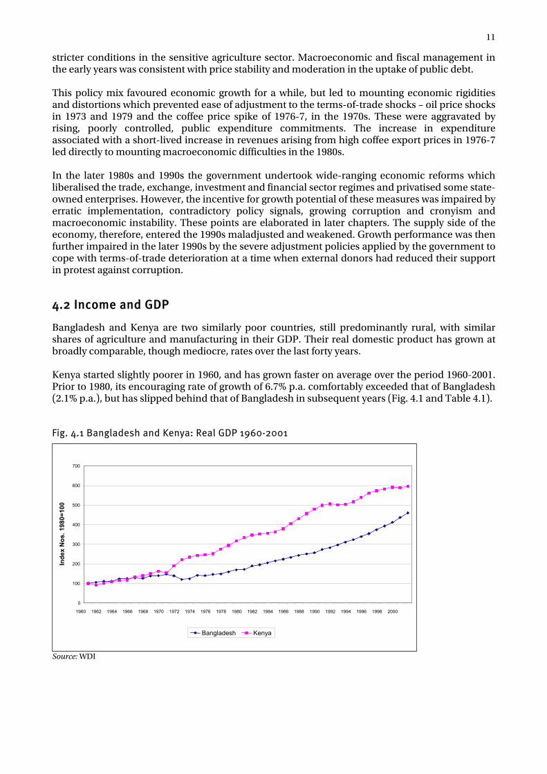
Bangladesh and Kenya are two similarly poor countries, still predominantly rural, with similar shares of agriculture and manufacturing in their GDP. Their real domestic product has grown at broadly comparable, though mediocre, rates over the last forty years. Kenya started slightly poorer in 1960, and has grown faster on average over the period 1960-2001. Prior to 1980, its encouraging rate of growth of 6.7% p.a. comfortably exceeded that of Bangladesh (2.1% p.a.), but has slipped behind that of Bangladesh in subsequent years (Fig. 4.1 and Table 4.1).

Fig. 4.1 Bangladesh and Kenya: Real GDP 1960-2001

Source: WDI

0

100

200

300

400

500

600

700

1960 1962 1964 1966 1968 1970 1972 1974 1976 1978 1980 1982 1984 1986 1988 1990 1992 1994 1996 1998 2000

Inde

x N

os. 1

980=

100

Bangladesh Kenya

12

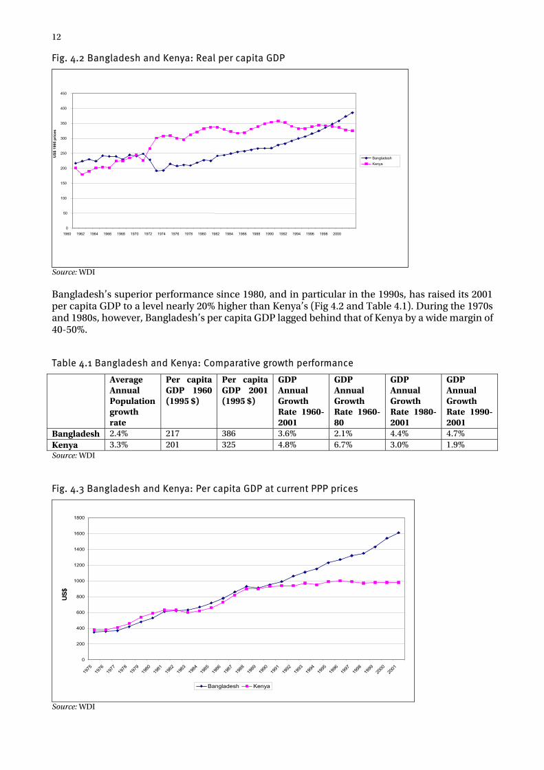
Fig. 4.2 Bangladesh and Kenya: Real per capita GDP

Source: WDI Bangladesh’s superior performance since 1980, and in particular in the 1990s, has raised its 2001 per capita GDP to a level nearly 20% higher than Kenya’s (Fig 4.2 and Table 4.1). During the 1970s and 1980s, however, Bangladesh’s per capita GDP lagged behind that of Kenya by a wide margin of 40-50%.

Table 4.1 Bangladesh and Kenya: Comparative growth performance

Average Annual Population growth rate

Per capita GDP 1960 (1995 $)

Per capita GDP 2001 (1995 $)

GDP Annual Growth Rate 1960-2001




Bangladesh 2.4% 217 386 3.6% 2.1% 4.4% 4.7% Kenya 3.3% 201 325 4.8% 6.7% 3.0% 1.9% Source: WDI

Fig. 4.3 Bangladesh and Kenya: Per capita GDP at current PPP prices

0

200

400

600

800

1000

1200

1400

1600

1800

1975

1976

1977

1978

1979

1980

1981

1982

1983

1984

1985

1986

1987

1988

1989

1990

1991

1992

1993

1994

1995

1996

1997

1998

1999

2000

2001

US$

Bangladesh Kenya

Source: WDI

0

50

100

150

200

250

300

350

400

450

1960 1962 1964 1966 1968 1970 1972 1974 1976 1978 1980 1982 1984 1986 1988 1990 1992 1994 1996 1998 2000

US$

199

5 pr

ices

Bangladesh Kenya

13

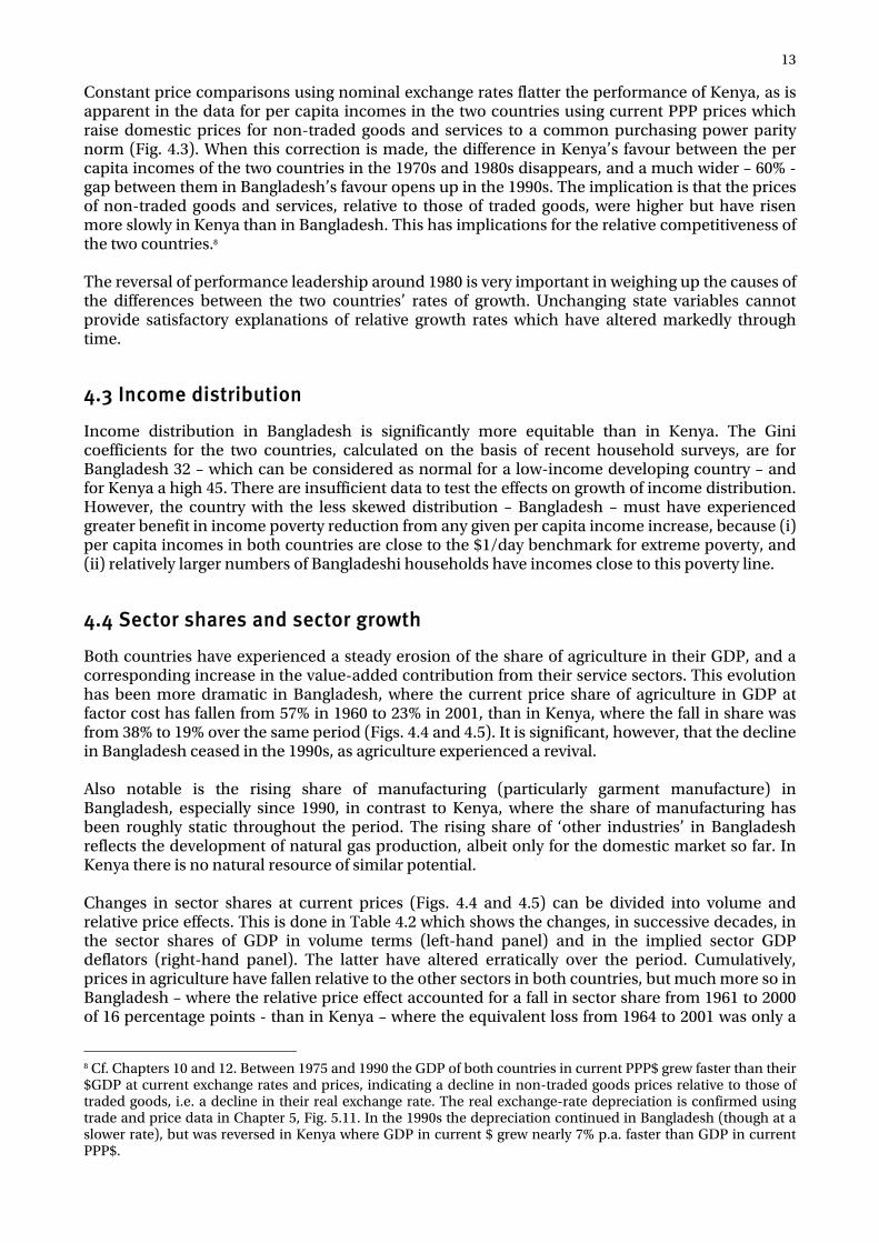
Constant price comparisons using nominal exchange rates flatter the performance of Kenya, as is apparent in the data for per capita incomes in the two countries using current PPP prices which raise domestic prices for non-traded goods and services to a common purchasing power parity norm (Fig. 4.3). When this correction is made, the difference in Kenya’s favour between the per capita incomes of the two countries in the 1970s and 1980s disappears, and a much wider – 60% - gap between them in Bangladesh’s favour opens up in the 1990s. The implication is that the prices of non-traded goods and services, relative to those of traded goods, were higher but have risen more slowly in Kenya than in Bangladesh. This has implications for the relative competitiveness of the two countries.8 The reversal of performance leadership around 1980 is very important in weighing up the causes of the differences between the two countries’ rates of growth. Unchanging state variables cannot provide satisfactory explanations of relative growth rates which have altered markedly through time.

4.3 Income distribution

Income distribution in Bangladesh is significantly more equitable than in Kenya. The Gini coefficients for the two countries, calculated on the basis of recent household surveys, are for Bangladesh 32 – which can be considered as normal for a low-income developing country – and for Kenya a high 45. There are insufficient data to test the effects on growth of income distribution. However, the country with the less skewed distribution – Bangladesh – must have experienced greater benefit in income poverty reduction from any given per capita income increase, because (i) per capita incomes in both countries are close to the $1/day benchmark for extreme poverty, and (ii) relatively larger numbers of Bangladeshi households have incomes close to this poverty line.

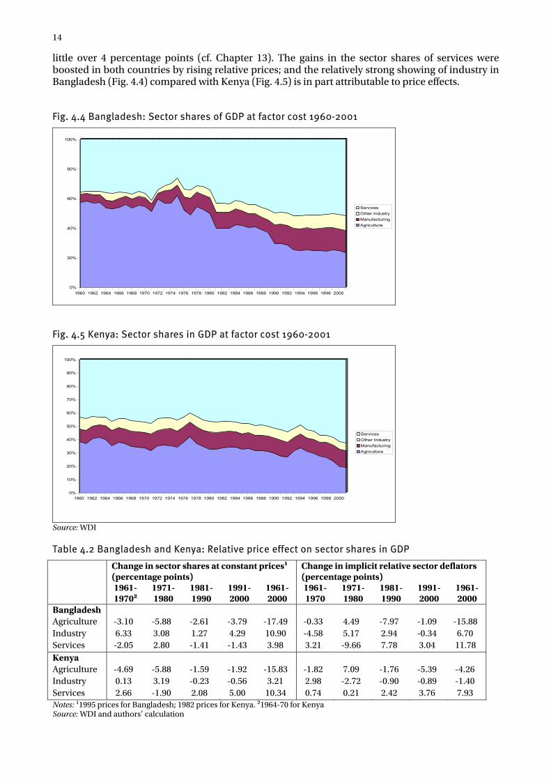
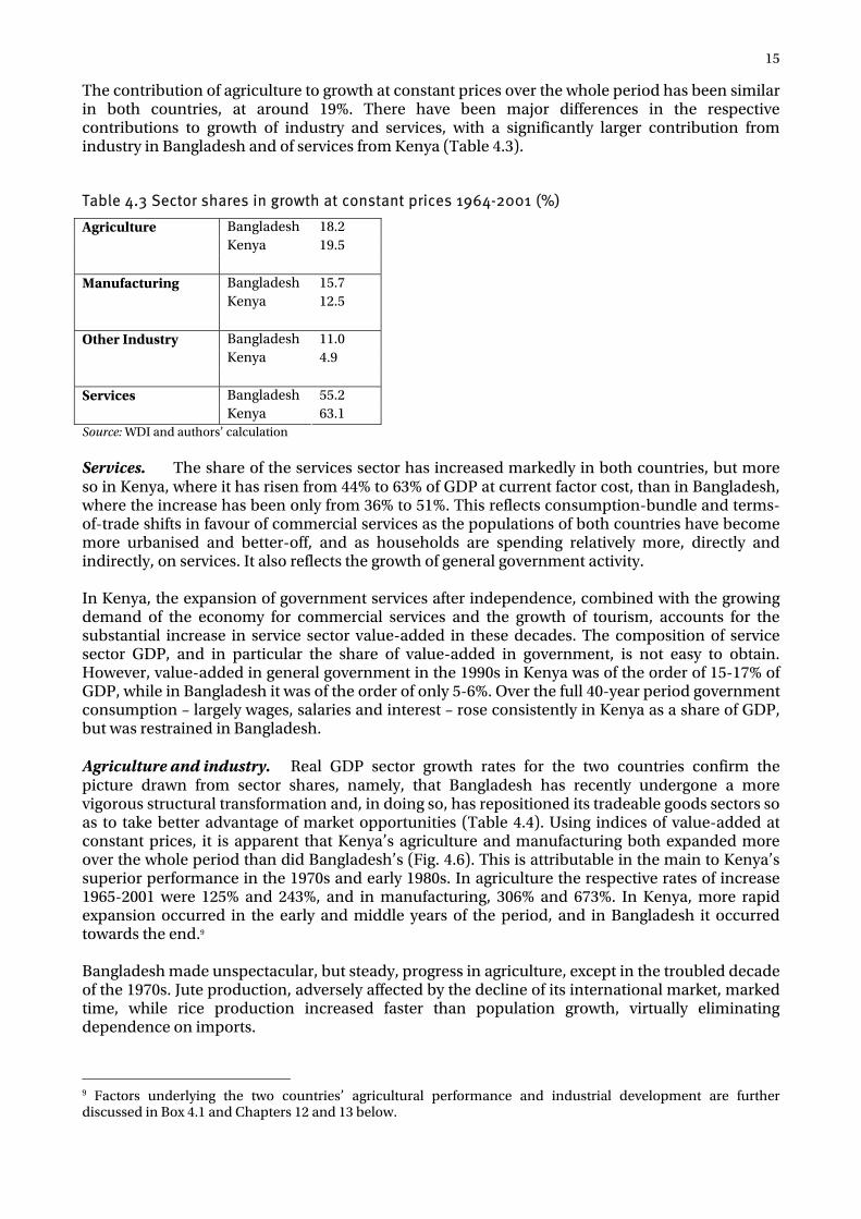
4.4 Sector shares and sector growth

Both countries have experienced a steady erosion of the share of agriculture in their GDP, and a corresponding increase in the value-added contribution from their service sectors. This evolution has been more dramatic in Bangladesh, where the current price share of agriculture in GDP at factor cost has fallen from 57% in 1960 to 23% in 2001, than in Kenya, where the fall in share was from 38% to 19% over the same period (Figs. 4.4 and 4.5). It is significant, however, that the decline in Bangladesh ceased in the 1990s, as agriculture experienced a revival. Also notable is the rising share of manufacturing (particularly garment manufacture) in Bangladesh, especially since 1990, in contrast to Kenya, where the share of manufacturing has been roughly static throughout the period. The rising share of ‘other industries’ in Bangladesh reflects the development of natural gas production, albeit only for the domestic market so far. In Kenya there is no natural resource of similar potential. Changes in sector shares at current prices (Figs. 4.4 and 4.5) can be divided into volume and relative price effects. This is done in Table 4.2 which shows the changes, in successive decades, in the sector shares of GDP in volume terms (left-hand panel) and in the implied sector GDP deflators (right-hand panel). The latter have altered erratically over the period. Cumulatively, prices in agriculture have fallen relative to the other sectors in both countries, but much more so in Bangladesh – where the relative price effect accounted for a fall in sector share from 1961 to 2000 of 16 percentage points - than in Kenya – where the equivalent loss from 1964 to 2001 was only a

8 Cf. Chapters 10 and 12. Between 1975 and 1990 the GDP of both countries in current PPP$ grew faster than their $GDP at current exchange rates and prices, indicating a decline in non-traded goods prices relative to those of traded goods, i.e. a decline in their real exchange rate. The real exchange-rate depreciation is confirmed using trade and price data in Chapter 5, Fig. 5.11. In the 1990s the depreciation continued in Bangladesh (though at a slower rate), but was reversed in Kenya where GDP in current $ grew nearly 7% p.a. faster than GDP in current PPP$.

14

little over 4 percentage points (cf. Chapter 13). The gains in the sector shares of services were boosted in both countries by rising relative prices; and the relatively strong showing of industry in Bangladesh (Fig. 4.4) compared with Kenya (Fig. 4.5) is in part attributable to price effects.

Fig. 4.4 Bangladesh: Sector shares of GDP at factor cost 1960-2001

0%

20%

40%

60%

80%

100%

1960 1962 1964 1966 1968 1970 1972 1974 1976 1978 1980 1982 1984 1986 1988 1990 1992 1994 1996 1998 2000

ServicesOther IndustryManufacturingAgriculture

Fig. 4.5 Kenya: Sector shares in GDP at factor cost 1960-2001

0%

10%

20%

30%

40%

50%

60%

70%

80%

90%

100%

1960 1962 1964 1966 1968 1970 1972 1974 1976 1978 1980 1982 1984 1986 1988 1990 1992 1994 1996 1998 2000

ServicesOther IndustryManufacturingAgriculture

Source: WDI

Table 4.2 Bangladesh and Kenya: Relative price effect on sector shares in GDP

Change in sector shares at constant prices1 (percentage points)

Change in implicit relative sector deflators (percentage points)

1961-19702

1971-1980

1981-1990

1991-2000

1961-2000

1961-1970

1971-1980

1981-1990

1991-2000

1961-2000

Bangladesh Agriculture -3.10 -5.88 -2.61 -3.79 -17.49 -0.33 4.49 -7.97 -1.09 -15.88 Industry 6.33 3.08 1.27 4.29 10.90 -4.58 5.17 2.94 -0.34 6.70 Services -2.05 2.80 -1.41 -1.43 3.98 3.21 -9.66 7.78 3.04 11.78 Kenya Agriculture -4.69 -5.88 -1.59 -1.92 -15.83 -1.82 7.09 -1.76 -5.39 -4.26 Industry 0.13 3.19 -0.23 -0.56 3.21 2.98 -2.72 -0.90 -0.89 -1.40 Services 2.66 -1.90 2.08 5.00 10.34 0.74 0.21 2.42 3.76 7.93 Notes: 11995 prices for Bangladesh; 1982 prices for Kenya. 21964-70 for Kenya Source: WDI and authors’ calculation

15

The contribution of agriculture to growth at constant prices over the whole period has been similar in both countries, at around 19%. There have been major differences in the respective contributions to growth of industry and services, with a significantly larger contribution from industry in Bangladesh and of services from Kenya (Table 4.3).

Table 4.3 Sector shares in growth at constant prices 1964-2001 (%)

Bangladesh 18.2 Agriculture Kenya 19.5

Bangladesh 15.7 Manufacturing Kenya 12.5

Bangladesh 11.0 Other Industry Kenya 4.9

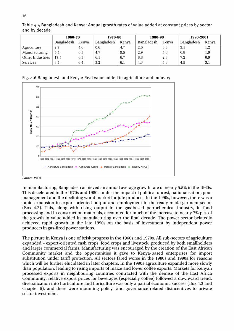
Bangladesh 55.2 Services Kenya 63.1 Source: WDI and authors’ calculation Services. The share of the services sector has increased markedly in both countries, but more so in Kenya, where it has risen from 44% to 63% of GDP at current factor cost, than in Bangladesh, where the increase has been only from 36% to 51%. This reflects consumption-bundle and terms-of-trade shifts in favour of commercial services as the populations of both countries have become more urbanised and better-off, and as households are spending relatively more, directly and indirectly, on services. It also reflects the growth of general government activity. In Kenya, the expansion of government services after independence, combined with the growing demand of the economy for commercial services and the growth of tourism, accounts for the substantial increase in service sector value-added in these decades. The composition of service sector GDP, and in particular the share of value-added in government, is not easy to obtain. However, value-added in general government in the 1990s in Kenya was of the order of 15-17% of GDP, while in Bangladesh it was of the order of only 5-6%. Over the full 40-year period government consumption – largely wages, salaries and interest – rose consistently in Kenya as a share of GDP, but was restrained in Bangladesh. Agriculture and industry. Real GDP sector growth rates for the two countries confirm the picture drawn from sector shares, namely, that Bangladesh has recently undergone a more vigorous structural transformation and, in doing so, has repositioned its tradeable goods sectors so as to take better advantage of market opportunities (Table 4.4). Using indices of value-added at constant prices, it is apparent that Kenya’s agriculture and manufacturing both expanded more over the whole period than did Bangladesh’s (Fig. 4.6). This is attributable in the main to Kenya’s superior performance in the 1970s and early 1980s. In agriculture the respective rates of increase 1965-2001 were 125% and 243%, and in manufacturing, 306% and 673%. In Kenya, more rapid expansion occurred in the early and middle years of the period, and in Bangladesh it occurred towards the end.9 Bangladesh made unspectacular, but steady, progress in agriculture, except in the troubled decade of the 1970s. Jute production, adversely affected by the decline of its international market, marked time, while rice production increased faster than population growth, virtually eliminating dependence on imports.

9 Factors underlying the two countries’ agricultural performance and industrial development are further discussed in Box 4.1 and Chapters 12 and 13 below.

16

Table 4.4 Bangladesh and Kenya: Annual growth rates of value added at constant prices by sector and by decade

1960-70 1970-80 1980-90 1990-2001 Bangladesh Kenya Bangladesh Kenya Bangladesh Kenya Bangladesh Kenya Agriculture 2.7 4.6 0.6 4.7 2.6 3.3 3.1 1.2 Manufacturing 5.4 6.3 4.7 9.5 2.9 4.8 6.8 1.9 Other Industries 17.5 6.3 6.1 6.7 8.8 2.3 7.2 0.9 Services 3.4 6.4 3.2 6.1 4.3 4.8 4.5 3.1

Fig. 4.6 Bangladesh and Kenya: Real value added in agriculture and industry

0

100

200

300

400

500

600

700

1960 1962 1964 1966 1968 1970 1972 1974 1976 1978 1980 1982 1984 1986 1988 1990 1992 1994 1996 1998 2000

Inde

x N

os. 1

965=

100

Agriculture Bangladesh Agriculture Kenya Industry Bangladesh Industry Kenya

Source: WDI In manufacturing, Bangladesh achieved an annual average growth rate of nearly 5.5% in the 1960s. This decelerated in the 1970s and 1980s under the impact of political unrest, nationalisation, poor management and the declining world market for jute products. In the 1990s, however, there was a rapid expansion in export-oriented output and employment in the ready-made garment sector (Box 4.2). This, along with rising output in the gas-based petrochemical industry, in food processing and in construction materials, accounted for much of the increase to nearly 7% p.a. of the growth in value-added in manufacturing over the final decade. The power sector belatedly achieved rapid growth in the late 1990s on the basis of investment by independent power producers in gas-fired power stations. The picture in Kenya is one of brisk progress in the 1960s and 1970s. All sub-sectors of agriculture expanded – export-oriented cash crops, food crops and livestock, produced by both smallholders and larger commercial farms. Manufacturing was encouraged by the creation of the East African Community market and the opportunities it gave to Kenya-based enterprises for import substitution under tariff protection. All sectors fared worse in the 1980s and 1990s for reasons which will be further elucidated in later chapters. In the 1990s agriculture expanded more slowly than population, leading to rising imports of maize and lower coffee exports. Markets for Kenyan processed exports in neighbouring countries contracted with the demise of the East Africa Community, relative export prices for beverages (especially coffee) followed a downward trend, diversification into horticulture and floriculture was only a partial economic success (Box 4.3 and Chapter 5), and there were mounting policy- and governance-related disincentives to private sector investment.

17

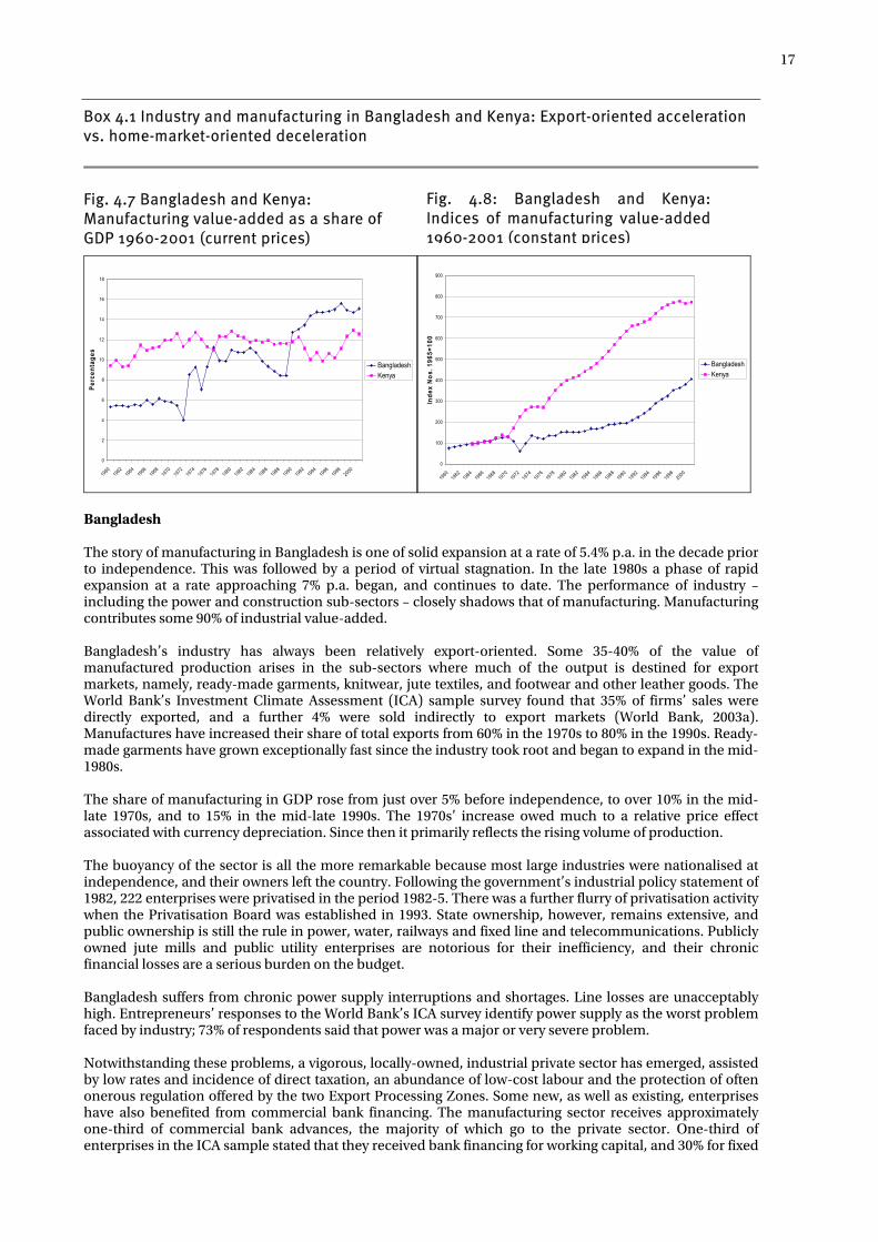
Box 4.1 Industry and manufacturing in Bangladesh and Kenya: Export-oriented acceleration vs. home-market-oriented deceleration

Fig. 4.7 Bangladesh and Kenya: Manufacturing value-added as a share of GDP 1960-2001 (current prices)

0

2

4

6

8

10

12

14

16

18

1960

196219

6419

661968

1970

197219

7419

761978

1980

198219

841986

198819

901992

1994

199619

9820

00

Perc

enta

ges

BangladeshKenya

0

100

200

300

400

500

600

700

800

900

1960

1962

19641966

1968

1970

1972

197419

7619

7819

801982

198419

8619

8819

901992

199419

9619

982000

Inde

x N

os. 1

965=

100

BangladeshKenya

Bangladesh The story of manufacturing in Bangladesh is one of solid expansion at a rate of 5.4% p.a. in the decade prior to independence. This was followed by a period of virtual stagnation. In the late 1980s a phase of rapid expansion at a rate approaching 7% p.a. began, and continues to date. The performance of industry – including the power and construction sub-sectors – closely shadows that of manufacturing. Manufacturing contributes some 90% of industrial value-added. Bangladesh’s industry has always been relatively export-oriented. Some 35-40% of the value of manufactured production arises in the sub-sectors where much of the output is destined for export markets, namely, ready-made garments, knitwear, jute textiles, and footwear and other leather goods. The World Bank’s Investment Climate Assessment (ICA) sample survey found that 35% of firms’ sales were directly exported, and a further 4% were sold indirectly to export markets (World Bank, 2003a). Manufactures have increased their share of total exports from 60% in the 1970s to 80% in the 1990s. Ready-made garments have grown exceptionally fast since the industry took root and began to expand in the mid-1980s. The share of manufacturing in GDP rose from just over 5% before independence, to over 10% in the mid-late 1970s, and to 15% in the mid-late 1990s. The 1970s’ increase owed much to a relative price effect associated with currency depreciation. Since then it primarily reflects the rising volume of production. The buoyancy of the sector is all the more remarkable because most large industries were nationalised at independence, and their owners left the country. Following the government’s industrial policy statement of 1982, 222 enterprises were privatised in the period 1982-5. There was a further flurry of privatisation activity when the Privatisation Board was established in 1993. State ownership, however, remains extensive, and public ownership is still the rule in power, water, railways and fixed line and telecommunications. Publicly owned jute mills and public utility enterprises are notorious for their inefficiency, and their chronic financial losses are a serious burden on the budget. Bangladesh suffers from chronic power supply interruptions and shortages. Line losses are unacceptably high. Entrepreneurs’ responses to the World Bank’s ICA survey identify power supply as the worst problem faced by industry; 73% of respondents said that power was a major or very severe problem. Notwithstanding these problems, a vigorous, locally-owned, industrial private sector has emerged, assisted by low rates and incidence of direct taxation, an abundance of low-cost labour and the protection of often onerous regulation offered by the two Export Processing Zones. Some new, as well as existing, enterprises have also benefited from commercial bank financing. The manufacturing sector receives approximately one-third of commercial bank advances, the majority of which go to the private sector. One-third of enterprises in the ICA sample stated that they received bank financing for working capital, and 30% for fixed

Fig. 4.8: Bangladesh and Kenya: Indices of manufacturing value-added 1960-2001 (constant prices)

18

asset purchases - high proportions compared with other low-income developing countries. Foreign direct investment played an insignificant role until the later 1990s when there was an influx, mainly into the natural gas, power and mobile telecommunications sectors, which absorbed over half the total. Even so, relative magnitudes were modest compared with other countries: the average annual inflow was of the order of $400 million, i.e. just under 1% of GDP. This belated interest in Bangladesh as a destination for FDI has been encouraged by deregulation: by the late 1990s the government had abolished the former requirements for prior approval and limits on foreign equity shares, profit remittances and capital repatriation. Kenya In Kenya, there was rapid expansion of manufacturing in the period up to 1980, when the economy as a whole was growing fast, reaching nearly 10% p.a. in the 1970s. After 1980 the rate of expansion declined - to below 5% p.a. in the 1980s and below 2% p.a. in the 1990s. The share of manufacturing in GDP has remained little changed at around 13% for two decades. The largest sub-sector is food, beverages and tobacco, accounting for some 50% of the value of manufacturing output, and 33% of value-added. This sub-sector includes the export-oriented processing of horticultural produce which started to expand strongly in the late 1990s. It is followed in importance by the petroleum refining and chemical industries which together contribute 20% to the value of output and 10% to value-added, and by light engineering industries which produce some 12% of the value of output, and 15% of value-added. These broad sub-sectoral shares have remained unchanged for many years, though there has been a turnover of enterprises within them. The primary market for Kenyan manufactures has always been the home market. The regional market is important too, particularly for the sale of petroleum products, refined in Mombasa and distributed up-country to Uganda by pipeline. Manufactures dominate sales to other African countries. The revival of the economies of neighbouring states, and the reduction of tariff barriers among countries in the COMESA and East Africa Co-operation groupings, help to explain the rise in the share of manufactures in total exports from a little over 10% in the period up to 1990 to 20-25% in recent years. The slow decline in manufactured exports after 1996 is due to supply-side and domestic cost factors. Surveys of manufacturing in 1993, 1994, 1995 and 2000 under the auspices of the World Bank-sponsored Regional Programme for Enterprise Development (World Bank, 2003b) have revealed some negative recent characteristics of Kenyan manufacturing, namely; • slowed growth in the 1990s, due to slack demand and worsening power supply shortages • a low value-added ratio • relatively high labour costs per worker • low labour productivity, declining in the 1990s, resulting in high and increasing unit labour costs • employment which has ceased to expand • static total factor productivity. Other problems highlighted have been the high cost of power, water supply, credit and transport. There have been a number of improvements in the regulatory environment: • prices have been largely decontrolled since 1988 • licensing has been streamlined – with licences delivered within a statutory 30 days • generous allowances against tax are provided, allowing many firms to escape direct taxation, and • 23 Export Processing Zones have been established since 1990. One indication of Kenya’s manufacturing potential has been the recent dramatic rise of the garment manufacturing industry in response to the US’s Africa Growth and Opportunity Act 1999 (AGOA). New garment manufacturing enterprises have sprung up – as in other African countries - taking advantage of the facilities in the EPZs. There are doubts, however, about whether these enterprises will survive the intensification of competition that is expected following the lifting of Multifibre Agreement quota restrictions on the exports of major international suppliers at the end of 2004. Most manufacturing activity is in the private sector. The public sector share in manufacturing employment has hovered at close to 20% since the 1970s, but has fallen more recently to around 16%. The power sector, however, remains in the public sector, defying initiatives to privatise it. Privatisation has proceeded slowly

19

but erratically, covering inter alia a formerly major publicly-owned dairy enterprise. Medium to large-scale manufacturing enterprises have been relatively favoured with advances by the commercial banks; some 28-30% of bank loans have recently been directed to manufacturing, well in excess of the sector’s share of GDP (16%). In the years of rapid expansion prior to 1980 manufacturing used to be a favoured destination for foreign investment, as well as for investment by the local Asian community. FDI in this sector, as in others, has waned in recent years.

Box 4.2 Bangladesh: Birth of an export-oriented garment industry (see Rhee, 1990)

In 1978 Nurul Qader, a former senior government official, and then agent for a project funded by a foreign government, had a chance encounter with executives from the Daewoo company at which he expressed the desire to collaborate with the Korean company in garment production. At the time Daewoo was still a significant exporter of mass-produced clothing. A technical collaboration agreement was concluded in 1979 between Qader’s new Desh Garment Company and Daewoo, which provided for the training of 130 Desh production workers, and a handful of engineers, in Daewoo’s factory in Pusan, and for follow-up technical services. At the same time Qader was able to arrange with the Bangladeshi government for manufacture-in-bond status for his new factory (several years before the Chittagong EPZ was created in 1983), and to obtain public authority for suppliers’ credit financing for his import requirements and working capital from local banks. Daewoo initially guaranteed credits extended to Desh through back-to-back letters of credit. The Desh Company made rapid technical and commercial strides, relinquishing its technical services agreement with Daewoo in 1981, yet steadily increasing the unit value of its products. In 1986-7 it was exporting garments to the value of $5 million. Most of the staff trained by Daewoo soon left the Desh Company to set up their own garment manufacturing enterprises. They were not the only garment sector entrepreneurs at the time. In 1979 there had been only a few garment factories in Bangladesh, but by 1985, when the United States imposed quotas on Bangladeshi garment exports, there were over 700 such factories. Case studies reveal powerful positive pecuniary external economies from the activities of pioneering firms. The externalities were both technical – production and business skills were rapidly replicated and extended by training and/or poaching – and financial – local (public sector) commercial banks, having seen success, provided financing for working capital and fixed assets.

Box 4.3 Kenya: Origins and growth of horticulture exports (see Minot and Ngigi, 2003)

In the late 1940s two British companies set up pineapple canning factories in Kenya to supply the UK market. Under the 1954 Swynnerton Plan smallholder farmers started to be supplied with pineapple planting material, and were guaranteed a market. By the early 1960s smallholders were supplying 75% of the canning factories’ input. After independence the government established an export levy-funded Horticultural Crop Development Authority to promote and facilitate smallholder horticulture, but not to manage it or to market produce. However, rapid expansion of the sector had to await investment by multinational companies, led by Del Monte which established a nucleus estate for pineapple production in 1968. Processing was dominated by joint ventures between foreign companies and state enterprises – such as Kenya Fruit Processing, the world’s largest exporter of passion fruit juice in the early 1970s. Rapid expansion of export-oriented horticulture occurred in the mid- to late 1970s, the mid-1980s and the mid- to late 1990s, led in the 1970s by pineapple product export, and in the 1980s by exports of fresh vegetables (especially French beans), flowers and, to a lesser extent, fruit – taking advantage of the emergence of air freight capacity serving European markets. Kenyan horticulture is exportable duty-free to the European Union under the Lomé Convention and the Cotonou Agreement. The simultaneous rapid expansion of tourism also created a domestic market for fresh produce. Smallholders were prominent in the expansion of fresh produce output; in the 1990s they were still responsible for growing some 55-60% of fruit and vegetable exports.

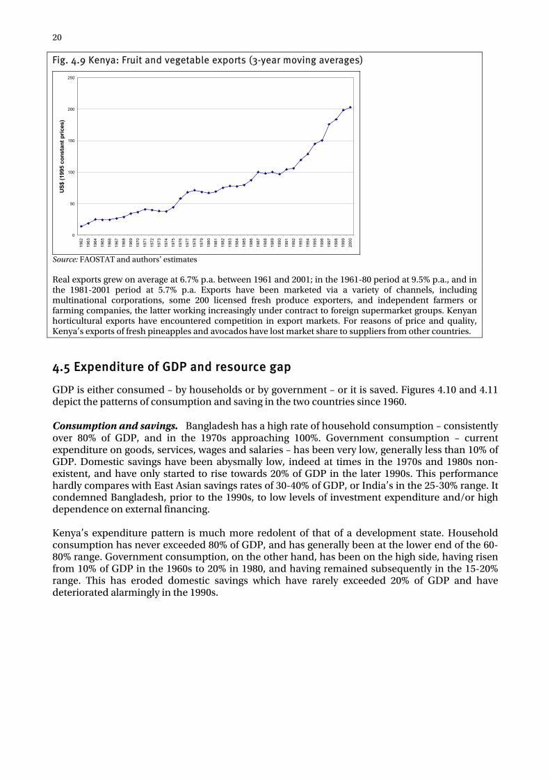
20

Fig. 4.9 Kenya: Fruit and vegetable exports (3-year moving averages)

0

50

100

150

200

25019

62

1963

1964

1965

1966

1967

1968

1969

1970

1971

1972

1973

1974

1975

1976

1977

1978

1979

1980

1981

1982

1983

1984

1985

1986

1987

1988

1989

1990

1991

1992

1993

1994

1995

1996

1997

1998

1999

2000

US$

(199

5 co

nsta

nt p

rices

)

Source: FAOSTAT and authors’ estimates Real exports grew on average at 6.7% p.a. between 1961 and 2001; in the 1961-80 period at 9.5% p.a., and in the 1981-2001 period at 5.7% p.a. Exports have been marketed via a variety of channels, including multinational corporations, some 200 licensed fresh produce exporters, and independent farmers or farming companies, the latter working increasingly under contract to foreign supermarket groups. Kenyan horticultural exports have encountered competition in export markets. For reasons of price and quality, Kenya’s exports of fresh pineapples and avocados have lost market share to suppliers from other countries.

4.5 Expenditure of GDP and resource gap

GDP is either consumed – by households or by government – or it is saved. Figures 4.10 and 4.11 depict the patterns of consumption and saving in the two countries since 1960. Consumption and savings. Bangladesh has a high rate of household consumption – consistently over 80% of GDP, and in the 1970s approaching 100%. Government consumption – current expenditure on goods, services, wages and salaries – has been very low, generally less than 10% of GDP. Domestic savings have been abysmally low, indeed at times in the 1970s and 1980s non-existent, and have only started to rise towards 20% of GDP in the later 1990s. This performance hardly compares with East Asian savings rates of 30-40% of GDP, or India’s in the 25-30% range. It condemned Bangladesh, prior to the 1990s, to low levels of investment expenditure and/or high dependence on external financing. Kenya’s expenditure pattern is much more redolent of that of a development state. Household consumption has never exceeded 80% of GDP, and has generally been at the lower end of the 60-80% range. Government consumption, on the other hand, has been on the high side, having risen from 10% of GDP in the 1960s to 20% in 1980, and having remained subsequently in the 15-20% range. This has eroded domestic savings which have rarely exceeded 20% of GDP and have deteriorated alarmingly in the 1990s.

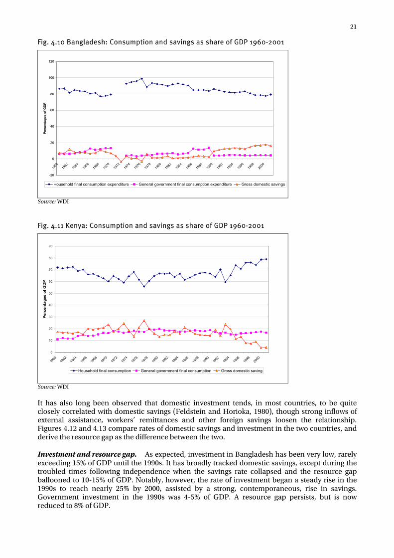
21

Fig. 4.10 Bangladesh: Consumption and savings as share of GDP 1960-2001

-20

0

20

40

60

80

100

120

1960

1962

1964

1966

1968

1970

1972

1974

1976

1978

1980

1982

1984

1986

1988

1990

1992

1994

1996

1998

2000

Perc

enta

ges

of G

DP

Household final consumption expenditure General government final consumption expenditure Gross domestic savings

Source: WDI

Fig. 4.11 Kenya: Consumption and savings as share of GDP 1960-2001

0

10

20

30

40

50

60

70

80

90

1960

1962

1964

1966

1968

1970

1972

1974

1976

1978

1980

1982

1984

1986

1988

1990

1992

1994

1996

1998

2000

Perc

enta

ges

of G

DP

Household final consumption General government final consumption Gross domestic saving

Source: WDI It has also long been observed that domestic investment tends, in most countries, to be quite closely correlated with domestic savings (Feldstein and Horioka, 1980), though strong inflows of external assistance, workers’ remittances and other foreign savings loosen the relationship. Figures 4.12 and 4.13 compare rates of domestic savings and investment in the two countries, and derive the resource gap as the difference between the two. Investment and resource gap. As expected, investment in Bangladesh has been very low, rarely exceeding 15% of GDP until the 1990s. It has broadly tracked domestic savings, except during the troubled times following independence when the savings rate collapsed and the resource gap ballooned to 10-15% of GDP. Notably, however, the rate of investment began a steady rise in the 1990s to reach nearly 25% by 2000, assisted by a strong, contemporaneous, rise in savings. Government investment in the 1990s was 4-5% of GDP. A resource gap persists, but is now reduced to 8% of GDP.

22

Fig. 4.12 Bangladesh: Savings, investment and resource gap 1960-2001

-20

-15

-10

-5

0

5

10

15

20

25

1960

1962

1964

1966

1968

1970

1972

1974

1976

1978

1980

1982

1984

1986

1988

1990

1992

1994

1996

1998

2000Sh

ares

of G

DP

(%)

Savings Investment Resource gap

Source: WDI In Kenya, the higher rate of savings has sustained a relatively high rate of investment – in the range 20-30% in the 1970s, but falling to 15-25% in the 1980s, and declining sharply in the 1990s to below 15%. Investment by general government (excluding the wider public sector) has been a low proportion of the total, fluctuating in the range 3-6% of GDP, though falling to 2% in the late 1990s. Kenya’s resource gap has been narrower than that of Bangladesh, usually of the order of 5% of GDP, though it has recently widened to 10% with the collapse of domestic savings that occurred in the 1990s. A characteristic of Kenya is the year-to-year volatility of savings and investment.

Fig. 4.13 Kenya: Savings, investment and resource gap 1960-2001

-15

-10

-5

0

5

10

15

20

25

30

35

1960

1962

1964

1966

1968

1970

1972

1974

1976

1978

1980

1982

1984

1986

1988

1990

1992

1994

1996

1998

2000

Shar

es o

f GD

P (5

)

Savings Investment Resource gap

Source: WDI As is to be expected, Kenya’s high public expenditure rate is reflected in its relatively high public sector share in total investment expenditure, which been in the 40-50% range (Table 4.5). In Bangladesh, the public sector share of investment outlays has been more modest – in the 30-40% range, despite extensive nationalisation of infrastructural and industrial enterprises at independence. Its policies and institutions, though not explicitly pro-private sector, have managed

23

to avoid crowding private investors out of capital markets and the business development scene. The two countries’ public-private splits in gross capital formation converged in the 1990s as Bangladesh stepped up its public expenditure programmes, and Kenya practised fiscal restraint.

Table 4.5 Total, private and public gross capital formation as percentages of GDP (at market prices)

1976-80 1981-85 1986-90 1991-95 1996-2000 B'desh Kenya B'desh Kenya B'desh Kenya B'desh Kenya B'desh Kenya GFCF 11.81 24.03 16.93 19.77 16.55 20.05 17.92 18.56 21.50 16.75 Private n.a. 12.89 12.10 11.03 10.42 11.58 11.25 10.54 14.73 10.48 Public n.a. 11.14 4.83 8.74 6.30 8.47 6.67 8.02 6.77 6.27 Sources: WDI, Osmani et al., GOK Statistical Abstract (various issues) and author’s estimates By making assumptions about possible initial levels of each country’s real stock of physical capital, and about the average rate of depreciation of physical capital,10 it is possible to construct approximate indices of the growth of the volume of physical capital in them both in the period under review, using the ‘perpetual inventory’ method. This is done in Fig. 4.14.

Fig. 4.14 Bangladesh and Kenya: Stock of physical capital (at constant prices)

0

20

40

60

80

100

120

140

160

180

200

1960

1962

1964

1966

1968

1970

1972

1974

1976

1978

1980

1982

1984

1986

1988

1990

1992

1994

1996

1998

2000

Inde

x N

os. (

1990

=100

)

Bangladesh Kenya

Source: WDI and authors’ estimates It emerges that Bangladesh accumulated physical capital in the 1960s, and again from 1980 onwards with increasing vigour, but experienced some loss of capital during the post-independence troubles in the 1970s. In Kenya, the period of rapid accumulation was from the late 1960s to the early 1980s, after which net fixed capital formation faltered. These capital stock estimates will be used in Part III to establish the significance of capital accumulation in explaining growth.

10 The assumptions are that: 5% of the inherited stock of capital is retired each year; gross capital formation from national income accounts data is added each year to the inherited stock; and initial 1960 capital stock/GDP ratios were in a steady state, assuming that 1960 rates of investment had been typical of previous years and that GDP had been growing previously at 3% in real terms.

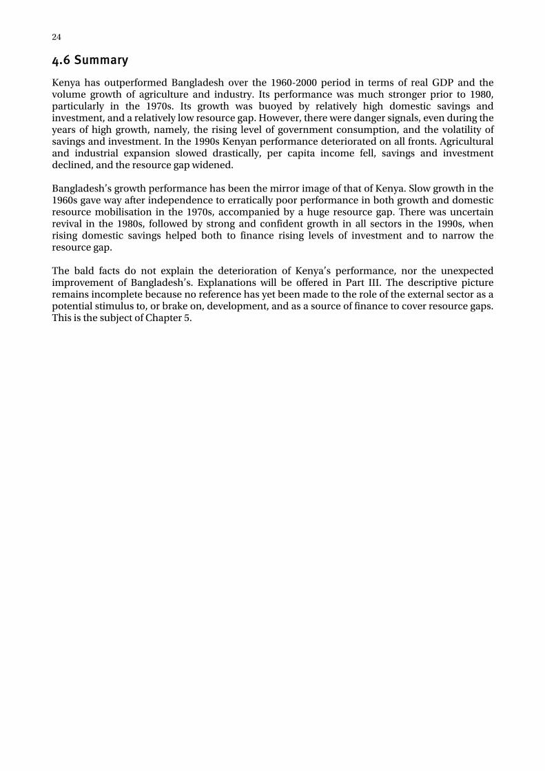
24

4.6 Summary

Kenya has outperformed Bangladesh over the 1960-2000 period in terms of real GDP and the volume growth of agriculture and industry. Its performance was much stronger prior to 1980, particularly in the 1970s. Its growth was buoyed by relatively high domestic savings and investment, and a relatively low resource gap. However, there were danger signals, even during the years of high growth, namely, the rising level of government consumption, and the volatility of savings and investment. In the 1990s Kenyan performance deteriorated on all fronts. Agricultural and industrial expansion slowed drastically, per capita income fell, savings and investment declined, and the resource gap widened. Bangladesh’s growth performance has been the mirror image of that of Kenya. Slow growth in the 1960s gave way after independence to erratically poor performance in both growth and domestic resource mobilisation in the 1970s, accompanied by a huge resource gap. There was uncertain revival in the 1980s, followed by strong and confident growth in all sectors in the 1990s, when rising domestic savings helped both to finance rising levels of investment and to narrow the resource gap. The bald facts do not explain the deterioration of Kenya’s performance, nor the unexpected improvement of Bangladesh’s. Explanations will be offered in Part III. The descriptive picture remains incomplete because no reference has yet been made to the role of the external sector as a potential stimulus to, or brake on, development, and as a source of finance to cover resource gaps. This is the subject of Chapter 5.

25

Chapter 5: Trade and External Financing

Trade can promote growth and welfare gains by widening market opportunities for both purchasers and suppliers, increasing the purchasing power of income for the former, and allowing the latter to expand their output, in line with their comparative advantage, well beyond the limits of demand in the domestic market. Some developing countries have achieved spectacular export growth by entering large and growing external markets on an initially small scale with competitively priced products, and then expanding their sales rapidly over sustained periods, and raising their market share. This strategy has contributed powerfully to GDP growth in some countries, directly – as export-oriented sectors expand and produce more value-added, indirectly – with the purchase of domestically produced inputs, and via the induced effect of the expenditure of wage income on consumer goods and services in the domestic market. However, export production is endogenous to the growth process: it is critically dependent on costs and the incentive environment in which it takes place. If the environment is favourable, production for export has an accelerator effect on growth – being both a consequence and cause of growth-generating processes, and a transmission belt in these processes. Also of great significance for growth, especially in open economies, are the stability and predictability of trade and exchange policies, flows of external financing, and relationships with external donors and creditors. Erratic behaviour in any of these gives, a priori, negative signals to investors about economic prospects and undermines confidence. This chapter outlines the comparative facts about trade performance by Bangladesh and Kenya over the last forty years – their supply of exportable goods and services, their external markets, terms of trade, and trade and exchange policies. It also covers the role of inward remittances, inward investment flows and the question of ‘capital flight’, official external financing, external debt, and balance-of-payments management.

5.1 Role of exports

A significant difference between the two countries lies in the fact that Bangladesh’s economy has become more ‘open’, i.e. its trade/GDP ratio has increased, especially in the 1990s, while Kenya became more closed prior to 1980, though it has raised its trade/GDP ratio subsequently. This is depicted in Fig. 5.1. Much of this difference is related to relative export performance, shown in Figs. 5.2-5.4. Kenya, the smaller country, has always been the more open to external trade. The sum of its exports and imports has fluctuated in the range 50-85% of GDP, but has remained for the most part in the 60-70% range (Fig. 5.1). The volume of exports has only grown slowly (Fig. 5.2), lagging behind GDP growth during the years of rapid economic expansion in the 1960s and 1970s, leading to a decline in its constant price export/GDP ratio (Fig. 15). This decline is not so evident in current prices because of a temporary increase in export prices in the later 1970s. Kenya’s traditional exports – coffee and tea – expanded in volume pari passu up until the mid-1980s, after which tea continued to grow, rising from 3% of world exports in 1963 to 16% by 1993, but coffee exports began to decline, from an average of 2.75% of world exports in the 1980s to below 2% in the later 1990s (Fig. 5.5). Supply-side factors underlay these developments (cf. Chapter 13). Export earnings from beverages were buoyed up in the 1980s by sharply higher prices (Fig. 5.6), but real unit values have subsequently followed a declining trend.

26

Fig. 5.1 Bangladesh and Kenya: Trade/GDP ratios

0

10

20

30

40

50

60

70

80

90

1960 1962 1964 1966 1968 1970 1972 1974 1976 1978 1980 1982 1984 1986 1988 1990 1992 1994 1996 1998 2000

Per

cent

ages

BangladeshKenya

Source: WDI

Fig. 5.2 Bangladesh and Kenya: Real exports (1980=100)

0

100

200

300

400

500

600

700

800

900

1000

1960 1962 1964 1966 1968 1970 1972 1974 1976 1978 1980 1982 1984 1986 1988 1990 1992 1994 1996 1998 2000

Inde

x N

os.

BangladeshKenya

Source: WDI

Fig. 5.3 Bangladesh and Kenya: Exports as a share of GDP (current prices)

Source: WDI

0 5

10

15

20

25

30

35

40

45

50

1960 1962 1964 1966 1968 1970 1972 1974 1976 1978 1980 1982 1984 1986 1988 1990 1992 1994 1996 1998 2000

Perc

enta

ges

BangladeshKenya

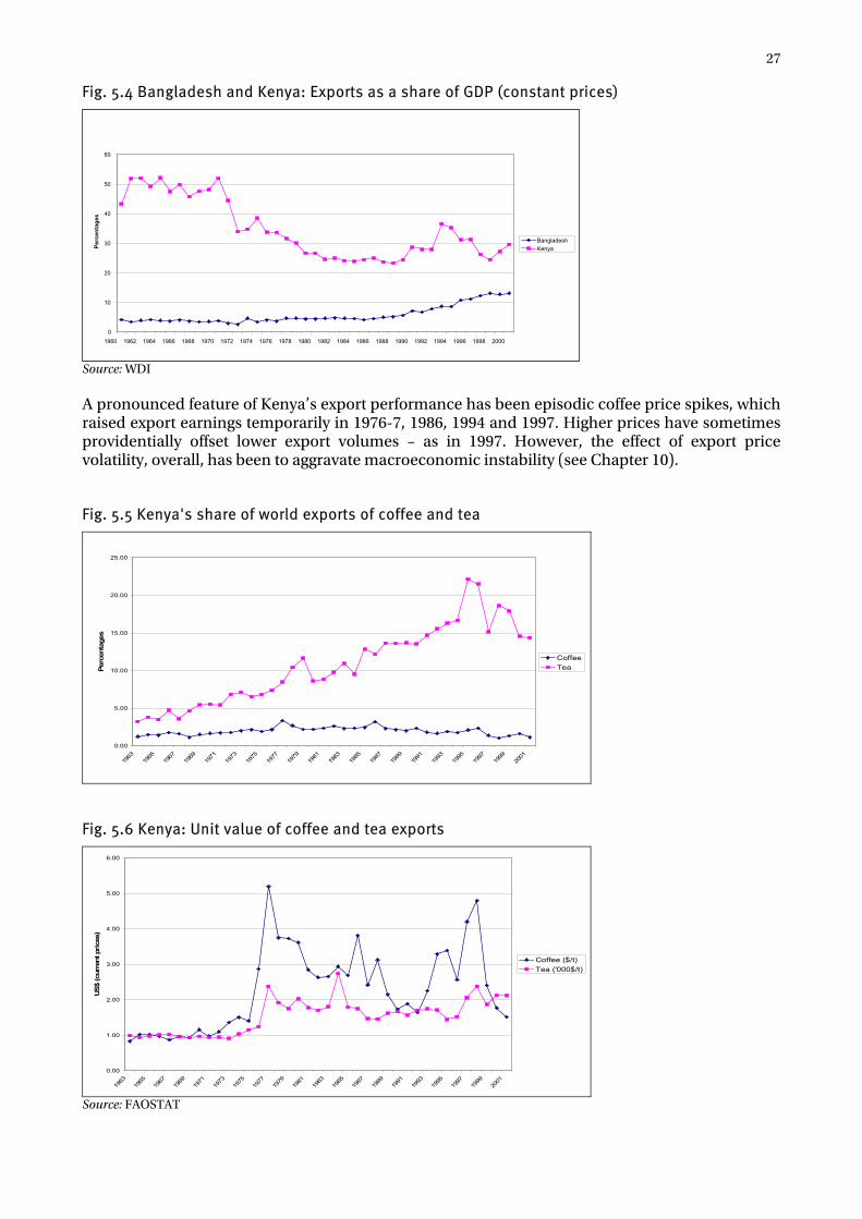
27

Fig. 5.4 Bangladesh and Kenya: Exports as a share of GDP (constant prices)

Source: WDI A pronounced feature of Kenya’s export performance has been episodic coffee price spikes, which raised export earnings temporarily in 1976-7, 1986, 1994 and 1997. Higher prices have sometimes providentially offset lower export volumes – as in 1997. However, the effect of export price volatility, overall, has been to aggravate macroeconomic instability (see Chapter 10).

Fig. 5.5 Kenya's share of world exports of coffee and tea

0.00

5.00

10.00

15.00

20.00

25.00

1963

1965

1967

1969

1971

1973

1975

1977

1979

1981

1983

1985

1987

1989

1991

1993

1995

1997

1999

2001

Perc

enta

ges

CoffeeTea

Fig. 5.6 Kenya: Unit value of coffee and tea exports

0.00

1.00

2.00

3.00

4.00

5.00

6.00

1963

1965

1967

1969

1971

1973

1975

1977

1979

1981

1983

1985

1987

1989

1991

1993

1995

1997

1999

2001

US$

(cur

rent

pric

es)

Coffee ($/t)Tea ('000$/t)

Source: FAOSTAT

0

10

20

30

40

50

60

1960 1962 1964 1966 1968 1970 1972 1974 1976 1978 1980 1982 1984 1986 1988 1990 1992 1994 1996 1998 2000

Perc

enta

ges

BangladeshKenya

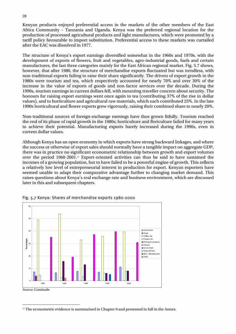
28

Kenyan products enjoyed preferential access in the markets of the other members of the East Africa Community – Tanzania and Uganda. Kenya was the preferred regional location for the production of processed agricultural products and light manufactures, which were promoted by a tariff policy favourable to import substitution. Preferential access to these markets was curtailed after the EAC was dissolved in 1977. The structure of Kenya’s export earnings diversified somewhat in the 1960s and 1970s, with the development of exports of flowers, fruit and vegetables, agro-industrial goods, fuels and certain manufactures, the last three categories mainly for the East African regional market. Fig. 5.7 shows, however, that after 1980, the structure of merchandise exports fluctuated but was trendless, with non-traditional exports failing to raise their share significantly. The drivers of export growth in the 1980s were tourism and tea, which respectively accounted for nearly 70% and over 30% of the increase in the value of exports of goods and non-factor services over the decade. During the 1990s, tourism earnings in current dollars fell, with mounting traveller concern about security. The honours for raising export earnings went once again to tea (contributing 37% of the rise in dollar values), and to horticulture and agricultural raw materials, which each contributed 25%. In the late 1990s horticultural and flower exports grew vigorously, raising their combined share to nearly 20%. Non-traditional sources of foreign-exchange earnings have thus grown fitfully. Tourism reached the end of its phase of rapid growth in the 1980s; horticulture and floriculture failed for many years to achieve their potential. Manufacturing exports barely increased during the 1990s, even in current dollar values. Although Kenya has an open economy in which exports have strong backward linkages, and where the success or otherwise of export sales should normally have a tangible impact on aggregate GDP, there was in practice no significant econometric relationship between growth and export volumes over the period 1960-2001.11 Export-oriented activities can thus be said to have sustained the incomes of a growing population, but to have failed to be a powerful engine of growth. This reflects a relatively low level of entrepreneurial interest in production for export. Kenyan exporters have seemed unable to adapt their comparative advantage further to changing market demand. This raises questions about Kenya’s real exchange rate and business environment, which are discussed later in this and subsequent chapters.

Fig. 5.7 Kenya: Shares of merchandise exports 1980-2000

0

10

20

30

40

50

60

1980 1985 1990 1995 2000

Perc

enta

ges

HorticultureSugarCoffee, teaFlowers etcPetroleum productsCementIron & SteelRoad vehiclesMisc. ManufacturesOther

Source: Comtrade

11 The econometric evidence is summarised in Chapter 9 and presented in full in the Annex.

29

Bangladesh has spectacularly outperformed Kenya in export volume growth since the mid-1980s. Unlike Kenya, it has become more open to external trade, particularly in the 1990s (Fig. 5.1). Its trade performance has been a straightforward case of diversification out of exports of raw materials and traditional manufactures into exports of non-traditional manufactured goods. Prior to 1976 Bangladesh’s export/GDP ratio was falling in current prices (Fig. 5.3) for reasons of exchange-rate overvaluation and declining export prices. Thereafter, the structural change to non-traditional exports began to take effect, albeit at first only gradually. Raw jute, the source of 30% of export earnings in the mid-1960s, now accounts for approximately 5%. Always the major player, Bangladesh is now the only significant exporter of raw jute, supplying over 90% of world exports. Export volumes have halved in the period 1965-2000 and relative prices have fallen. Raw jute is now dwarfed, among agricultural exports, by tea. The export market for manufactured jute products has similarly contracted in volume and unit value. Bangladesh has done well to sustain a level of export earnings from jute products of $400-500 million per annum in nominal terms since the late 1970s, when the size of the market contracted in nominal terms by 25% (Fig. 5.8). Manufactures are now predominant in Bangladesh’s exports. Textiles and clothing alone account for over 80% of merchandise exports, and all manufactures for 90% (Fig. 5.9). Textiles and clothing have always been the largest (30-40%) segment of manufactured exports, but their composition has radically changed in response to changing patterns of demand, away from jute textiles to ready-made clothing. Exports have become highly concentrated in the garment sector, and are now significantly less diversified than formerly. Bangladesh’s share of the world clothing trade more than trebled between 1990 and 1998 – rising from 0.54 % to 1.61% – and its share of trade in textiles and clothing more than doubled – from 0.42% to 1.03% (Spinanger, 2001). Its rising market penetration has been facilitated by the Multifibre Agreement under which the industrialised countries have been allowed to impose quota restrictions on imports of textiles and clothing from the main exporting countries, including China, India and Pakistan. Bangladesh’s exports have been exempt from such quota restrictions, and have also entered the EU market duty-free since 1996. The rebalancing of Bangladesh’s exports has been both market-led and consistent with the comparative advantage of a populous country with low wage (and employment) costs, and diminishing opportunities for employment in agriculture. Bangladesh has maintained a competitive exchange rate (see below and Fig. 5.11).

Fig. 5.8 World and Bangladesh exports of jute products 1970-2000

0

200

400

600

800

1000

1200

1400

1600

1970

1971

1972

1973

1974

1975

1976

1977

1978

1979

1980

1981

1982

1983

1984

1985

1986

1987

1988

1989

1990

1991

1992

1993

1994

1995

1996

1997

1998

1999

2000

US$

mill

ion

World Bangladesh

Source: FAO

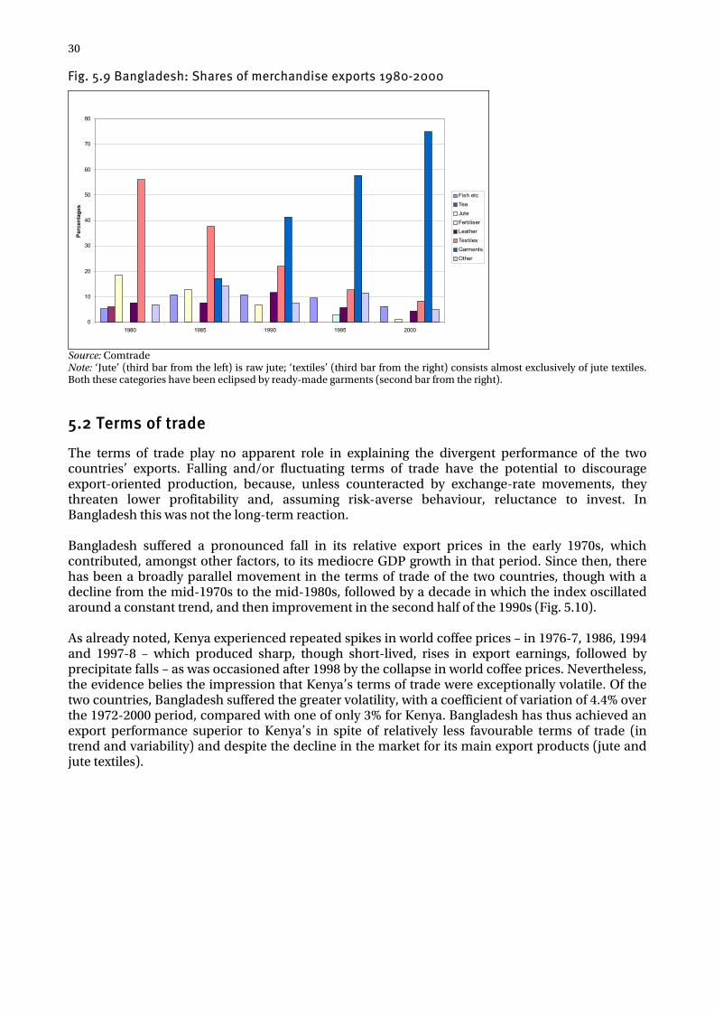
30

Fig. 5.9 Bangladesh: Shares of merchandise exports 1980-2000

0

10

20

30

40

50

60

70

80

1980 1985 1990 1995 2000

Per

cent

ages

Fish etcTeaJuteFertiliserLeatherTextilesGarmentsOther

Source: Comtrade Note: ‘Jute’ (third bar from the left) is raw jute; ‘textiles’ (third bar from the right) consists almost exclusively of jute textiles. Both these categories have been eclipsed by ready-made garments (second bar from the right).

5.2 Terms of trade

The terms of trade play no apparent role in explaining the divergent performance of the two countries’ exports. Falling and/or fluctuating terms of trade have the potential to discourage export-oriented production, because, unless counteracted by exchange-rate movements, they threaten lower profitability and, assuming risk-averse behaviour, reluctance to invest. In Bangladesh this was not the long-term reaction. Bangladesh suffered a pronounced fall in its relative export prices in the early 1970s, which contributed, amongst other factors, to its mediocre GDP growth in that period. Since then, there has been a broadly parallel movement in the terms of trade of the two countries, though with a decline from the mid-1970s to the mid-1980s, followed by a decade in which the index oscillated around a constant trend, and then improvement in the second half of the 1990s (Fig. 5.10). As already noted, Kenya experienced repeated spikes in world coffee prices – in 1976-7, 1986, 1994 and 1997-8 – which produced sharp, though short-lived, rises in export earnings, followed by precipitate falls – as was occasioned after 1998 by the collapse in world coffee prices. Nevertheless, the evidence belies the impression that Kenya’s terms of trade were exceptionally volatile. Of the two countries, Bangladesh suffered the greater volatility, with a coefficient of variation of 4.4% over the 1972-2000 period, compared with one of only 3% for Kenya. Bangladesh has thus achieved an export performance superior to Kenya’s in spite of relatively less favourable terms of trade (in trend and variability) and despite the decline in the market for its main export products (jute and jute textiles).

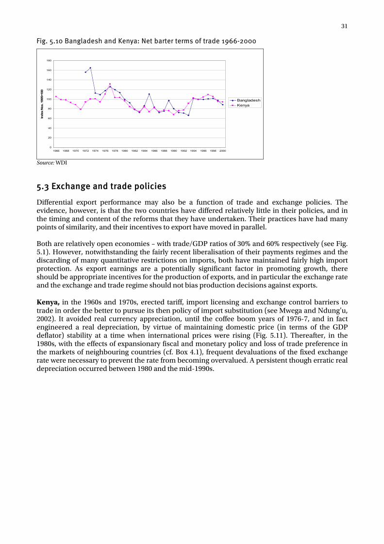
31

Fig. 5.10 Bangladesh and Kenya: Net barter terms of trade 1966-2000

0

20

40

60

80

100

120

140

160

180

1966 1968 1970 1972 1974 1976 1978 1980 1982 1984 1986 1988 1990 1992 1994 1996 1998 2000

Inde

x N

os. 1

995=

100

BangladeshKenya

Source: WDI

5.3 Exchange and trade policies

Differential export performance may also be a function of trade and exchange policies. The evidence, however, is that the two countries have differed relatively little in their policies, and in the timing and content of the reforms that they have undertaken. Their practices have had many points of similarity, and their incentives to export have moved in parallel. Both are relatively open economies – with trade/GDP ratios of 30% and 60% respectively (see Fig. 5.1). However, notwithstanding the fairly recent liberalisation of their payments regimes and the discarding of many quantitative restrictions on imports, both have maintained fairly high import protection. As export earnings are a potentially significant factor in promoting growth, there should be appropriate incentives for the production of exports, and in particular the exchange rate and the exchange and trade regime should not bias production decisions against exports. Kenya, in the 1960s and 1970s, erected tariff, import licensing and exchange control barriers to trade in order the better to pursue its then policy of import substitution (see Mwega and Ndung’u, 2002). It avoided real currency appreciation, until the coffee boom years of 1976-7, and in fact engineered a real depreciation, by virtue of maintaining domestic price (in terms of the GDP deflator) stability at a time when international prices were rising (Fig. 5.11). Thereafter, in the 1980s, with the effects of expansionary fiscal and monetary policy and loss of trade preference in the markets of neighbouring countries (cf. Box 4.1), frequent devaluations of the fixed exchange rate were necessary to prevent the rate from becoming overvalued. A persistent though erratic real depreciation occurred between 1980 and the mid-1990s.

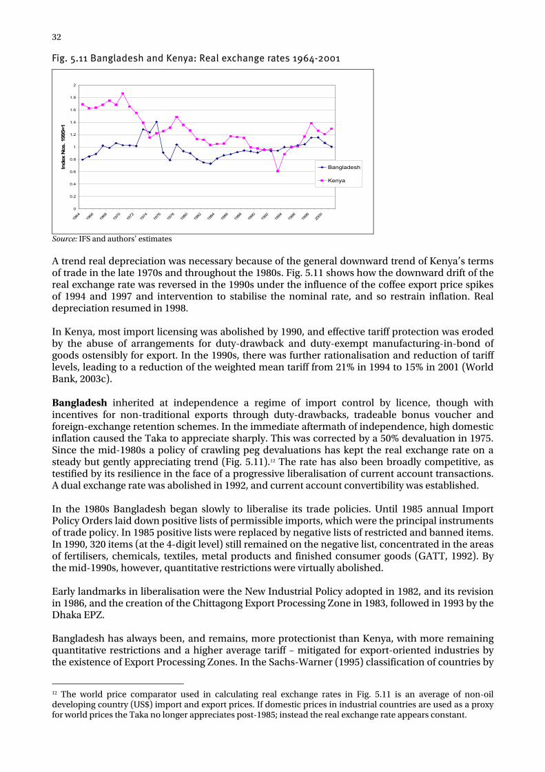
32

Fig. 5.11 Bangladesh and Kenya: Real exchange rates 1964-2001

0

0.2

0.4

0.6

0.8

1

1.2

1.4

1.6

1.8

2

1964

1966

1968

1970

1972

1974

1976

1978

1980

1982

1984

1986

1988

1990

1992

1994

1996

1998

2000

Inde

x N

os. 1

995=

1

Bangladesh

Kenya

Source: IFS and authors’ estimates A trend real depreciation was necessary because of the general downward trend of Kenya’s terms of trade in the late 1970s and throughout the 1980s. Fig. 5.11 shows how the downward drift of the real exchange rate was reversed in the 1990s under the influence of the coffee export price spikes of 1994 and 1997 and intervention to stabilise the nominal rate, and so restrain inflation. Real depreciation resumed in 1998. In Kenya, most import licensing was abolished by 1990, and effective tariff protection was eroded by the abuse of arrangements for duty-drawback and duty-exempt manufacturing-in-bond of goods ostensibly for export. In the 1990s, there was further rationalisation and reduction of tariff levels, leading to a reduction of the weighted mean tariff from 21% in 1994 to 15% in 2001 (World Bank, 2003c). Bangladesh inherited at independence a regime of import control by licence, though with incentives for non-traditional exports through duty-drawbacks, tradeable bonus voucher and foreign-exchange retention schemes. In the immediate aftermath of independence, high domestic inflation caused the Taka to appreciate sharply. This was corrected by a 50% devaluation in 1975. Since the mid-1980s a policy of crawling peg devaluations has kept the real exchange rate on a steady but gently appreciating trend (Fig. 5.11).12 The rate has also been broadly competitive, as testified by its resilience in the face of a progressive liberalisation of current account transactions. A dual exchange rate was abolished in 1992, and current account convertibility was established. In the 1980s Bangladesh began slowly to liberalise its trade policies. Until 1985 annual Import Policy Orders laid down positive lists of permissible imports, which were the principal instruments of trade policy. In 1985 positive lists were replaced by negative lists of restricted and banned items. In 1990, 320 items (at the 4-digit level) still remained on the negative list, concentrated in the areas of fertilisers, chemicals, textiles, metal products and finished consumer goods (GATT, 1992). By the mid-1990s, however, quantitative restrictions were virtually abolished. Early landmarks in liberalisation were the New Industrial Policy adopted in 1982, and its revision in 1986, and the creation of the Chittagong Export Processing Zone in 1983, followed in 1993 by the Dhaka EPZ. Bangladesh has always been, and remains, more protectionist than Kenya, with more remaining quantitative restrictions and a higher average tariff – mitigated for export-oriented industries by the existence of Export Processing Zones. In the Sachs-Warner (1995) classification of countries by

12 The world price comparator used in calculating real exchange rates in Fig. 5.11 is an average of non-oil developing country (US$) import and export prices. If domestic prices in industrial countries are used as a proxy for world prices the Taka no longer appreciates post-1985; instead the real exchange rate appears constant.

33

‘openness’, Bangladesh was rated ‘not-open’ on the grounds of its black market exchange-rate premium in 1970 and 1980 (eliminated since 1992) and the number of quota restrictions on intermediate and capital goods imports, in the period 1985-8. Radical trade policy reform in the 1990s, however, has brought the weighted average tariff down from 88% in 1989 to 21% in 2001, and reduced the range of tariff rates (World Bank, 2003c).13

Box 5.1 Bangladesh and Kenya: A tale of two trade diversions

Customs unions bring about welfare-reducing trade diversion when their common external tariffs cause union members to purchase their imports from within the union at higher prices than the tariff-free prices of imports from outside the union. Members with resource endowments giving them ‘extreme’ comparative advantage (for example in the production of raw materials or unskilled labour-intensive products for external markets) tend to suffer welfare loss because the prices of their imports from within the union rise. Countries with ‘intermediate’ resource endowments, where pre-union costs of production are closer to those of the rest of the world, typically gain when they enter customs unions with countries with ‘extreme’ factor endowments, because their producers are able to displace imports from the rest of the world into these countries (Venables, 2003). Bangladesh. Before its independence in 1971, Bangladesh was in a customs union with the West Wing of Pakistan. There was free trade between the two Wings, and imports from the rest of the world were restricted by licence and prohibition, and subject to tariffs which, for some manufactures such as textiles, clothing and beverages, were high. Purchases of foreign exchange for current account purposes such as import financing were subject to exchange controls, and there was a parallel market premium for the purchase of foreign exchange. There were export incentives for the exporters of non-traditional exports, notably manufactures. These took the form of ‘bonus vouchers’ which entitled exporters to retain for their own use a share of the foreign-exchange proceeds of their export sales, or to sell it to other, authorised, parties. In the 1950s and 1960s export sales from the East Wing (Bangladesh) were more important as a source of foreign exchange for Pakistan than West Wing exports. Exports from the East Wing consisted predominantly of raw jute, which was extensively used at the time as a raw material for the production of textiles for packaging and for carpet backing. The East Wing also attracted investment into the local production of jute textiles which, before Partition in 1948, had been concentrated in the neighbourhood of Calcutta in what became, after Partition, West Bengal. Much of the investment in jute mills came from West Wing-based entrepreneurs. Bangladesh’s exports of raw jute did not benefit from the export earnings retention scheme, but jute textile exports were beneficiaries of the scheme. Before 1971, the effects of trade policies affecting the East Wing were to: • cause a deterioration in the terms of trade of the East Wing - because Pakistani trade protection, combined

with free trade between the two Wings, diverted the source of (mainly manufactured) imports into the East Wing from lower-cost regional and international sources to the West Wing, where high-cost manufacturing was developing fast behind the shield of protectionist trade policy; and

• press producers in the East Wing to concentrate their activities in areas of their (then) comparative advantage, namely, jute and jute textiles - where effective rates of protection were low or negative.

Kenya. From independence in 1963 until 1977, Kenya was in a customs (and currency) union with Tanzania and Uganda - the other members of the East Africa Community (EAC). The average external tariff was moderately high (30%, except for capital goods (0%) and luxuries (75%)). Exchange controls, introduced in 1967, were initially limited. There was a gradual increase thereafter in import duties and licensing requirements. Trade within the Community was not restricted by tariffs, quantitative or exchange controls. For climatic and logistical reasons, Kenya had become, before independence, the main regional centre for light manufacturing and a hub for transport services. The EAC trade policy regime encouraged inward investment into import-substitution activities, which were largely concentrated in Kenya, where agglomeration benefits were largest and transport and communication costs least, and where there was a labour force with some production, administrative and commercial skills. A diverse range of manufacturing activities was thus created in the time of the Community, including food processing, textiles and clothing, oil refining, paper and printing, metallurgy, light engineering, vehicle assembly, chemicals and plastic goods. Over 70% of the EAC output of manufactures was produced in Kenya, a significant proportion of which was exported to neighbouring countries.

13 GATT (1992) reports that the import-weighted statutory rate of customs duty in 1983 was only 42% (with an effective rate of 24%). The apparent rise in the weighted average tariff in the 1980s is likely to have been due to the replacement of quota restrictions and import prohibitions by (high) nominal rates of duty.

34

When the EAC was dissolved in 1977 Kenyan producers lost part of their home market, particularly in Tanzania, which proceeded to pursue its own policy of highly protected import substitution. The effects of this were masked for a short time by the 1976-7 coffee price boom which raised export earnings and increased incomes and expenditure in the domestic economy. However, the boom was short-lived and, in its aftermath, Kenya experienced acute balance-of-payments problems – aggravated by unsustainably high levels of government expenditure. The barter terms of trade fell by 44% from a peak in 1977 to a trough in 1983. Enterprises which had grown up to serve customers in EAC countries were ill placed to divert their production to other external markets because their costs remained high until the full effects of the 50% devaluation of the Kenya Shilling between 1980 and 1984 were realised. In aggregate, the volume of exports remained unchanged for a decade, from 1975 to 1985. The EAC customs union had had the effect of encouraging investment in sectors in many of which Kenya had no comparative advantage vis-à-vis markets other than those of East Africa. Labour costs were too high and productivity was too low for Kenya to compete as an exporter of cheap manufactures. The welfare benefits of trade diversion working in the Kenyans’ favour prior to 1977 were thus bought at the expense of some structural rigidity in facing the challenge of seeking external markets after the demise of the EAC However, it cannot be argued that the exporters’ focus on the regional market was a total aberration. The markets of the East African region are now growing again, and have continued to be very important for Kenyan producers. The markets of the COMESA countries (which now exclude Tanzania) still take 50% of their exports. Kenya’s success in exporting clothing to the United States under the African Growth and Opportunity Act is symptomatic of emerging patterns of advantage in manufactures.

5.4 Foreign Direct Investment

Foreign direct investment has played a minimal role in financing investment in both countries, in spite of fiscal incentive policies deployed by both the governments to attract it (Table 5.1). In Bangladesh the share of FDI in gross investment expenditure never exceeded 1% until the late 1990s, when it rose to 1.5-2.5%. This intensification of activity in the later 1990s was related to improved opportunities in the natural gas and related sectors. In Kenya the FDI share fell from 3.5% in the 1970s to a little over 1% in the 1990s, in spite of incentive packages more generous than those of Bangladesh (Sen, 2002).

Table 5.1 Bangladesh and Kenya: Foreign direct investment shares in capital formation (%)

1970s 1980s 1990s Bangladesh 0.18 0.10 0.61 Kenya 3.55 2.03 1.13 Source: WDI

5.5 Financing the resource gap and balance-of-payments management

Chapter 4 described how Bangladesh’s savings-investment resource gap exceeded 10% of GDP in the mid-1970s but has narrowed to some 6% in the late 1990s, while Kenya’s formerly modest gap of around 5% of GDP has widened in recent years. There are important differences in how the two countries managed to finance their gaps with inflows on their current and capital accounts (Figs. 5.12-5.15). The resource gap is identical to the gap between exports and imports of goods and non-factor services, and is equal to the balance-of-payments current account balance plus or minus factor service and current transfer payments to and from the country. For our present purposes, current transfers are defined to include workers’ remittances, but exclude grants of official aid (which are treated as a source of finance for the current account). Figs. 5.12 and 5.14 show how the two countries’ resource gaps are related to their current account gaps. The difference between the resource gap plus net factor payments abroad (below the line) and inward remittances plus other

35

current transfers (above the line) equals the current account gap, the financing of which is shown in Figs. 5.13 and 5.15. This financing takes the form of official grants and loans and private lending, and direct and portfolio investment.

Fig. 5.12 Bangladesh: Resource gap and current financing (percentages of GDP)

-12.00%

-10.00%

-8.00%

-6.00%

-4.00%

-2.00%

0.00%

2.00%

4.00%

6.00%

1976 1977 1978 1979 1980 1981 1982 1983 1984 1985 1986 1987 1988 1989 1990 1991 1992 1993 1994 1995 1996 1997 1998 1999 2000

Resource gap Net factor income Remittances Other Crnt transfers

Source: IMF, Balance of Payments Statistics In Bangladesh the net inflow of factor service and transfer payments has been positive and rising strongly because of (a) the large inflow of remittances from Bangladeshis working abroad and (b) low debt-service and profit remittances out of the country (Fig 5.12). By the late 1990s net private transfer inflows offset over 70% of the resource gap – in stark contrast to the situation in the late 1970s and early 1980s when they offset only about 20%. The implication of these favourable developments is that the current account deficit before grants, which amounted to 8-9% of GDP in 1978-80, has fallen steadily to less than 2% of GDP in 1995-2000. The main sources of official and private long-term finance – grants, net loans and direct and portfolio investment – are identified in Fig. 5.13, which shows that (a) these capital account and financial inflows have consistently exceeded the country’s financing needs since the mid-1980s, and (b) the financing has been almost exclusively official, and concessional. Inward private investment only began to play a noticeable role in the later 1990s, but it has been dwarfed, in terms of the volume of resources provided, by official flows. The balance-of-payments data underlying Fig. 5.13 imply that non-governmental investors in Bangladesh have been net acquirers of foreign assets, even in years when, as in the early 1990s, foreign-exchange reserves were falling. It is implausible that Bangladeshis were investing abroad on the scale implied, and it is therefore likely that some current account outflows are under-recorded. The general picture of sufficiency of official financing (on concessional terms) is nevertheless plausible; and explains how Bangladesh managed to avoid serious external indebtedness and onerous debt-service charges.

36

Fig. 5.13 Bangladesh: Current account long-term financing (percentages of GDP)

-12.00%

-10.00%

-8.00%

-6.00%

-4.00%

-2.00%

0.00%

2.00%

4.00%

6.00%

8.00%

10.00%

1976 1977 1978 1979 1980 1981 1982 1983 1984 1985 1986 1987 1988 1989 1990 1991 1992 1993 1994 1995 1996 1997 1998 1999 2000

Current acct.before grants Grants Official LT loans Private LT Loans Direct & portfolio invt. ∆Reserves E&O

Source: IMF, Balance of Payments Statistics In Kenya a somewhat similar pattern of events can be observed, with a resource gap, large at times, as in the 1988-91 period, and since 1995 offset by recently rising inflows of private transfers (Fig. 5.14). This explains the diminishing current account deficit (before grants) seen in Fig. 5.15. A major difference from Bangladesh is that Kenya has also had to finance consistently significant factor income outflows, consisting of profit remittances and debt-service payments. Kenya’s current account deficit (before grants) has been smaller, relative to GDP, than that of Bangladesh, though with episodic spikes, such as in the late 1970s and late 1980s. The financing of periodically high deficits was also on less favourable terms. Fig. 5.15 shows that there has been greater use of private external financing than in Bangladesh, and also that official financing by way of grants and net lending, though significant in the late 1970s and late 1980s, tapered off sharply in the 1990s, when official net flows were negative in some years. Unlike Bangladesh, Kenya was creditworthy for commercial credits, and until the 1980s used to receive some official lending on non-concessional terms. Therein lay the cause of its indebtedness, its relatively high debt-service payments, and its HIPC status.

Fig. 5.14 Kenya: Resource gap and current financing (percentages of GDP)

-15.00%

-10.00%

-5.00%

0.00%

5.00%

10.00%

1975 1976 1977 1978 1979 1980 1981 1982 1983 1984 1985 1986 1987 1988 1989 1990 1991 1992 1993 1994 1995 1996 1997 1998 1999

Resource gap Net factor income Other Crnt transfers

Source: IMF, Balance of Payments Statistics

37

Fig. 5.15 Kenya: Financing of the current account deficit (percentages of GDP)

-20.00%

-15.00%

-10.00%

-5.00%

0.00%

5.00%

10.00%

15.00%

20.00%

1975 1977 1979 1981 1983 1985 1987 1989 1991 1993 1995 1997 1999

Current acct.before grants Grants Official LT loans (net) Direct & portfolio invt.Private LT Loans (net) ∆Reserves Errors & Omissions

Source: IMF, Balance of Payments Statistics and authors’ estimates The differences between the modes of financing the balance of payments are immediately apparent in Figs. 5.17 and 5.18 which illustrate the composition of the two countries’ external debt. Bangladesh’s debt has always been and remains essentially concessional. Kenya’s, on the other hand, has always had a large non-concessional component, amounting to 60% of total debt outstanding in 1990. Debt-service payments due from Kenya reached a peak of nearly 40% of the value of exports of goods and services in the early 1990s, though they have since diminished thanks to severe restraint in the uptake of new non-concessional debt. In Bangladesh, more prudent financing has kept debt-service payments for the most part well below 30% of the value of exports of goods and services. Both countries experienced balance-of-payments management difficulties in the 1970s, precipitated by terms-of-trade declines caused by oil price increases and falling export prices. In Kenya these persisted into the 1980s and 1990s. Bangladesh coped through IMF- and donor-assisted adjustment and financing programmes. Kenya progressively lost the confidence of the IMF and donors because of its lax adherence to the terms of previous programmes and mounting concern about corruption and malpractice, including the accounting for and use of official foreign-exchange reserves. For a while, Kenya was able to borrow commercially, short-term, to overcome its foreign-exchange liquidity difficulties, but by the early 1990s mounting debt-service obligations blocked further recourse to commercial borrowing. The liquidity crisis of 1994 provoked a sharp exchange-rate depreciation (see Fig. 5.11) and payments arrears, and precipitated a first application to the Paris Club for official debt rescheduling. Drought and the fall in coffee prices after their 1997 spike caused Kenya to incur further payments arrears, and to apply again (in 2000) for official debt rescheduling from the Paris Club.

38

Fig. 5.16 Bangladesh: External debt

0

2000

4000

6000

8000

10000

12000

14000

16000

18000

1972

1973

1974

1975

1976

1977

1978

1979

1980

1981

1982

1983

1984

1985

1986

1987

1988

1989

1990

1991

1992

1993

1994

1995

1996

1997

1998

1999

2000

2001

US$

Mill

ion

(cur

rent

pric

es)

Official concessional Official non-concessional Private Short term

Source: Global Development Finance

Fig. 5.17 Kenya: External debt

0

1000

2000

3000

4000

5000

6000

7000

8000

9000

1970

1971

1972

1973

1974

1975

1976

1977

1978

1979

1980

1981

1982

1983

1984

1985

1986

1987

1988

1989

1990

1991

1992

1993

1994

1995

1996

1997

1998

1999

2000

2001

US$

mill

ion

(cur

rent

pric

es)

Official concessional Official non-concessional Private Short term

Source: Global Development Finance

5.6 Summary

This chapter has demonstrated contrasting trends in the trade and balance-of-payments performance of Bangladesh and Kenya. The main observations of importance to the theme of this paper are the following: Exports. Bangladesh’s poor export performance in the 1970s and 1980s was transformed in the 1990s by outstanding export growth, driven by ready-made garments which, by 2000, accounted for 80% of exports. As a result, the economy became more open. The new manufactured export lines were consistent with comparative advantage, and replaced jute and jute products, the world market for which was shrinking and prices falling. Kenya’s exports grew strongly in the 1970s and for a time in the 1980s, but their overall rate of expansion declined sharply in the 1990s. Early diversification away from traditional tea and coffee

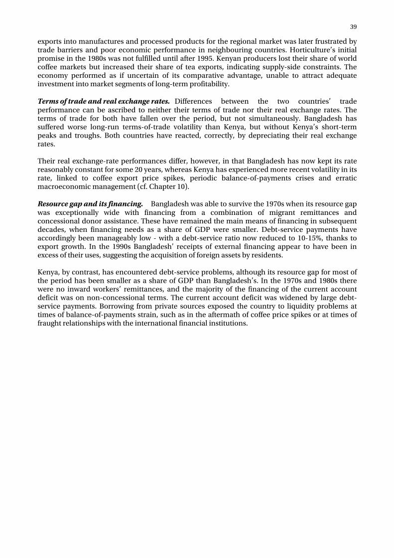
39

exports into manufactures and processed products for the regional market was later frustrated by trade barriers and poor economic performance in neighbouring countries. Horticulture’s initial promise in the 1980s was not fulfilled until after 1995. Kenyan producers lost their share of world coffee markets but increased their share of tea exports, indicating supply-side constraints. The economy performed as if uncertain of its comparative advantage, unable to attract adequate investment into market segments of long-term profitability. Terms of trade and real exchange rates. Differences between the two countries’ trade performance can be ascribed to neither their terms of trade nor their real exchange rates. The terms of trade for both have fallen over the period, but not simultaneously. Bangladesh has suffered worse long-run terms-of-trade volatility than Kenya, but without Kenya’s short-term peaks and troughs. Both countries have reacted, correctly, by depreciating their real exchange rates. Their real exchange-rate performances differ, however, in that Bangladesh has now kept its rate reasonably constant for some 20 years, whereas Kenya has experienced more recent volatility in its rate, linked to coffee export price spikes, periodic balance-of-payments crises and erratic macroeconomic management (cf. Chapter 10). Resource gap and its financing. Bangladesh was able to survive the 1970s when its resource gap was exceptionally wide with financing from a combination of migrant remittances and concessional donor assistance. These have remained the main means of financing in subsequent decades, when financing needs as a share of GDP were smaller. Debt-service payments have accordingly been manageably low - with a debt-service ratio now reduced to 10-15%, thanks to export growth. In the 1990s Bangladesh’ receipts of external financing appear to have been in excess of their uses, suggesting the acquisition of foreign assets by residents. Kenya, by contrast, has encountered debt-service problems, although its resource gap for most of the period has been smaller as a share of GDP than Bangladesh’s. In the 1970s and 1980s there were no inward workers’ remittances, and the majority of the financing of the current account deficit was on non-concessional terms. The current account deficit was widened by large debt-service payments. Borrowing from private sources exposed the country to liquidity problems at times of balance-of-payments strain, such as in the aftermath of coffee price spikes or at times of fraught relationships with the international financial institutions.

40

Chapter 6: Social Outcomes, Public Services and Public Expenditure

This chapter outlines health and education outcomes in Bangladesh and Kenya, and presents evidence on the size, effectiveness and efficiency of public expenditure in improving social outcomes and economic services. Social outcomes and the provision of public utilities and transport and communications infrastructure are important both as direct sources of individual and collective welfare and also as means of raising output and sustaining economic growth. Public expenditure may also have negative, deadweight, effects on economic performance. The chapter also introduces the complex topic of governance in the two countries as background to consideration in Part III of whether institutional factors have contributed to the divergence in performance.

6.1 Health

Life expectancy has increased in both countries over the 1960-2000 period – from 40 years to over 60 in Bangladesh, and from 45 to a peak of 57 in Kenya (Table 6.1). It has recently begun to fall in Kenya under the influence of HIV-AIDS.14. Under-five mortality, another key health indicator, fell consistently in both countries up to 1990, and has continued to fall dramatically in Bangladesh – to 77 per 1000 live births in 2000, from 254 in 1960. In Kenya, it rose by 25% from 97 per 1000 in 1990 to 122 in 2000, also on account of HIV-AIDS. Were it not for this epidemic, Kenya would probably have maintained its lead over Bangladesh in health indicators. Has HIV-AIDS been a cause of Kenya’s deteriorating growth performance, given the vulnerability to the disease of working adults? As a first approximation, this can be assessed in terms of the size of the working-age (15-64) population. Table 6.2 shows that the average rate of growth of the working-age population between 1960 and 2000 has been 0.8 of a percentage point higher in Kenya than in Bangladesh. It also shows that the share of the total population in the junior (15-24) and senior (25-59) working-age groups fell somewhat in the 1960s and 1970s, especially in Kenya, but has risen in the 1980s and 1990s, again especially in Kenya. The prima facie evidence, therefore, is that dependency ratios have fallen in both countries, and that labour supply has been increasing faster than population, in spite of AIDS. Relative to previous decades, Kenya’s economy should not therefore have decelerated in the 1990s on this account. This is not to deny that the high prevalence of AIDS in Kenya, which has continued since the late 1980s, has increased morbidity and labour turnover, especially among educated, skilled and professional personnel, and that this has reduced productivity below its without-AIDS level.15

14 UNAIDS estimates 190,000 deaths from AIDS in 2001 in Kenya, compared with 650 in Bangladesh. 15 UNAIDS’ official estimate is that, in 2001, 13,000 adults were living with HIV-AIDS in Bangladesh, and that 2.3 million (15% of the adult population) were living with it in Kenya (UNAIDS 2002). However, UNAIDS is now reported to have revised its estimate of the prevalence rate down to 9.4%. Recent preliminary evidence from the Kenya Demographic and Health Survey suggests that the actual prevalence rate may be lower still (6.7%) (The Economist, 17 January 2004).

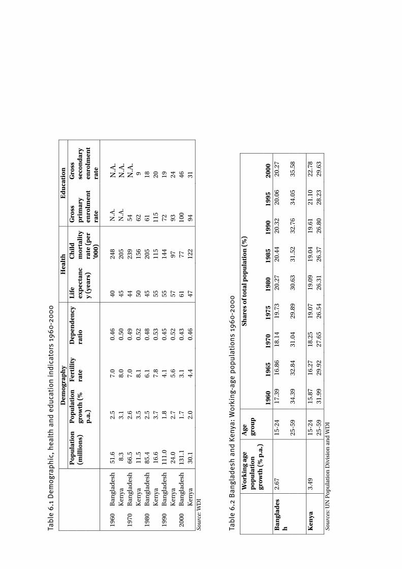
Tab

le 6

.1 D

emog

rap

hic

, h

ealt

h a

nd

ed

uca

tion

ind

icat

ors

196

0-2

00

0

Dem

ogra

phy

Hea

lth

E

duca

tion

Pop

ula

tion

(m

illi

ons)

P

opu

lati

on

grow

th (

%

p.a.

)

Fert

ilit

y ra

te

Dep

ende

ncy

ra

tio

Life

ex

pect

anc

y (y

ears

)

Ch

ild

mor

tali

ty

rate

(pe

r '0

00)

Gro

ss

prim

ary

enro

lmen

t ra

te

Gro

ss

seco

nda

ry

enro

lmen

t ra

te

1960

B

angl

ades

h

51.

6

2.5

7.

0

0.46

4

0 24

8 N

.A.

N.A

.

Ken

ya

8.

3

3.1

8.

0

0.50

4

5 20

5 N

.A.

N.A

. 19

70

Ban

glad

esh

6

6.5

2.

6

7.0

0.

49

44

239

54

N.A

.

Ken

ya

11.

5

3.5

8.

1

0.52

5

0 15

6 6

2

9 19

80

Ban

glad

esh

8

5.4

2.

5

6.1

0.

48

45

205

61

18

K

enya

1

6.6

3.

7

7.8

0.

53

55

115

115

20

1990

B

angl

ades

h

111.

0

1.8

4.

1

0.45

5

5 14

4 7

2 1

9

Ken

ya

24.

0

2.7

5.

6

0.52

5

7 9

7 9

3 2

4 20

00

Ban

glad

esh

13

1.1

1.

7

3.1

0.

43

61

77

100

46

K

enya

3

0.1

2.

0

4.4

0.

46

47

122

94

31

Sou

rce:

WD

I Ta

ble

6.2

Ban

glad

esh

an

d K

enya

: W

ork

ing-

age

pop

ula

tion

s 19

60

-20

00

W

orki

ng

age

popu

lati

on

grow

th (

% p

.a.)

Age

gr

oup

Shar

es o

f tot

al p

opu

lati

on (

%)

19

60

1965

19

70

1975

19

80

1985

19

90

1995

20

00

Ban

glad

esh

2.

67

15-2

4 1

7.39

1

6.86

1

8.14

1

9.73

2

0.27

2

0.44

2

0.32

2

0.06

2

0.27

25-5

9 3

4.39

3

2.84

3

1.04

2

9.89

3

0.63

3

1.52

3

2.76

3

4.05

3

5.58

K

enya

3.

49

15-2

4 1

5.87

1

6.27

1

8.25

1

9.07

1

9.09

1

9.04

1

9.61

2

1.10

2

2.78

25

-59

31.

99

29.

92

27.

65

26.

54

26.

31

26.

37

26.

80

28.

23

29.

63

Sou

rces

: UN

Pop

ula

tion

Div

isio

n a

nd

WD

I

42

6.2 Education

The two countries have also swapped places in their educational performance (Table 6.1). In 1980 Kenya had a slight lead in secondary school enrolment, and a pronounced lead in primary enrolments – with a gross enrolment ratio of 115, compared with Bangladesh’s 61. By 2000, however, Bangladesh had gross and net enrolment ratios in primary education of 100 and 89 respectively, well in advance of corresponding ratios in Kenya - 94 and 68.5. This effort has been translated recently into higher primary school completion rates in Bangladesh (70%) than in Kenya (58%) (UNESCO, 2002). Kenya maintains a lead in adult literacy and has a more educated labour force, thanks to earlier investment in primary education. In 2000 adult literacy rates in Kenya and Bangladesh were respectively 82.4% and 40%, and adult Kenyans had 4.2 years of schooling compared with only 2.6 in Bangladesh (Fig. 6.1). Bangladesh is catching up, however, and may in due course, if recent school enrolment figures can be believed, have as educated and skilled a workforce as Kenya. Recent research has cast doubt on the effectiveness of Kenya’s education, in view of the low quality provided, falling real wages and the diminishing probability that school leavers will find formal sector jobs.1

Fig. 6.1 Bangladesh and Kenya: Educated labour force average number of years of schooling of population over 15

0

0.5

1

1.5

2

2.5

3

3.5

4

4.5

5

1960 1965 1970 1975 1980 1985 1990 1995 2000

Year

s

Bangladesh Kenya

Source: Barro and Lee (2000) The most striking contrast between the two countries lies in the amount of public expenditure devoted to education – and specifically to primary education. Bangladesh’s recently superior performance has been achieved at a cost, in public expenditure relative to GDP, 70% less than the price paid in Kenya for all education services, and 75% less than the cost to Kenya of primary education services (Table 6.3). On the basis of this rough comparison, Bangladesh’s primary education is more than four times as cost-effective as that of Kenya.

1 King (2003) refers to mounting doubts about returns to primary education in Kenya and other African countries.

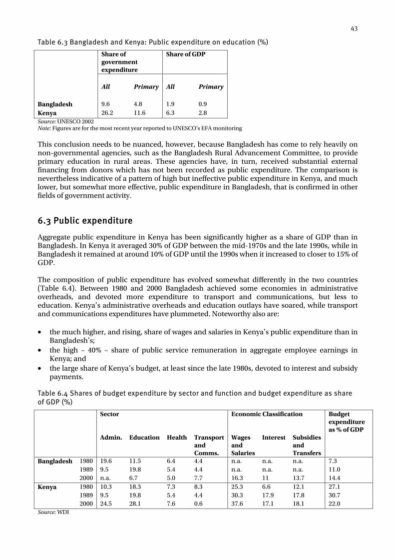
43

Table 6.3 Bangladesh and Kenya: Public expenditure on education (%)

Share of government expenditure

Share of GDP

All Primary All Primary Bangladesh 9.6 4.8 1.9 0.9 Kenya 26.2 11.6 6.3 2.8 Source: UNESCO 2002 Note: Figures are for the most recent year reported to UNESCO's EFA monitoring This conclusion needs to be nuanced, however, because Bangladesh has come to rely heavily on non-governmental agencies, such as the Bangladesh Rural Advancement Committee, to provide primary education in rural areas. These agencies have, in turn, received substantial external financing from donors which has not been recorded as public expenditure. The comparison is nevertheless indicative of a pattern of high but ineffective public expenditure in Kenya, and much lower, but somewhat more effective, public expenditure in Bangladesh, that is confirmed in other fields of government activity.

6.3 Public expenditure

Aggregate public expenditure in Kenya has been significantly higher as a share of GDP than in Bangladesh. In Kenya it averaged 30% of GDP between the mid-1970s and the late 1990s, while in Bangladesh it remained at around 10% of GDP until the 1990s when it increased to closer to 15% of GDP. The composition of public expenditure has evolved somewhat differently in the two countries (Table 6.4). Between 1980 and 2000 Bangladesh achieved some economies in administrative overheads, and devoted more expenditure to transport and communications, but less to education. Kenya’s administrative overheads and education outlays have soared, while transport and communications expenditures have plummeted. Noteworthy also are: • the much higher, and rising, share of wages and salaries in Kenya’s public expenditure than in

Bangladesh’s; • the high – 40% – share of public service remuneration in aggregate employee earnings in

Kenya; and • the large share of Kenya’s budget, at least since the late 1980s, devoted to interest and subsidy

payments.

Table 6.4 Shares of budget expenditure by sector and function and budget expenditure as share of GDP (%)

Sector Economic Classification Budget expenditure as % of GDP

Admin. Education Health Transport and Comms.

Wages and Salaries

Interest Subsidies and Transfers

Bangladesh 1980 19.6 11.5 6.4 4.4 n.a. n.a. n.a. 7.3 1989 9.5 19.8 5.4 4.4 n.a. n.a. n.a. 11.0 2000 n.a. 6.7 5.0 7.7 16.3 11 13.7 14.4 Kenya 1980 10.3 18.3 7.3 8.3 25.3 6.6 12.1 27.1 1989 9.5 19.8 5.4 4.4 30.3 17.9 17.8 30.7 2000 24.5 28.1 7.6 0.6 37.6 17.1 18.1 22.0 Source: WDI

44

Revenues mobilised in Kenya have also been much larger as a share of GDP (25-30%) than has been in the case in Bangladesh (8-10% of GDP). The deadweight effect on production incentives of direct taxes is generally believed to be greater than the effect of broad-based expenditure taxes like value-added tax, now introduced in both countries. Kenya’s revenue from direct taxes was as high as 10% of GDP in the mid-1990s, though it has recently declined to 7%; in Bangladesh the share of direct tax revenue in GDP has been 1-1.5%. In Kenya, public sector employment began to exert a strong influence on the labour market as early as the 1960s. By 1974 the public sector already employed 330,000, 40% of waged employees. Public sector employment expanded at 5-6% p.a. in the 1970s and at over 4% in the 1980s, i.e. faster than total wage employment, taking its share in the later 1980s to half of the formal sector labour market (with a maximum of 715,000 employees in 1991). The civil service and public education and health services alone accounted for 30% of employment in 1990. The public sector’s market share declined in the 1990s, back to 40%. In Bangladesh, public service employment has been relatively on a more modest scale, at least until the mid-1990s. Public services employed only 10% of waged employees in 1990/1. However, with the growth of public expenditure that occurred thereafter, their share rose swiftly to 20% in 1995/6 and to 22% by the end of the decade. The implications for wage levels of public sector leadership in the wage market are considered in Part III. In the 1990s the effectiveness of Kenya’s public services was seriously compromised by a combination of falling domestic revenues, diminished external financing and the pre-emption of available resources by high interest, subsidy and personal remuneration payments. Real non-wage outlays on operations and maintenance were severely compressed. Infrastructure and public utility services deteriorated markedly (World Bank, 2003b: Chapter 6). In Bangladesh, public expenditure restraint was relaxed in the 1990s, and fruitful efforts were made to remedy former deficiencies in public service provision, notably in road transport and power supply. The construction of the Jamuna road bridge removed an important transport bottleneck. Kenya’s overall budget balance was in constant deficit until the mid-1990s, giving rise to an accumulation of domestic as well as foreign debt and to interest charges amounting to 18% of public expenditure (Table 6.4). Bangladesh avoided domestic financing until the later 1990s, when a large deficit of 5% of GDP emerged, around half of which was domestically financed. The implications of this are explored in Part III.

6.4 Summary

Bangladesh lagged behind Kenya in social sector outcomes until 1990. Thereafter, it overtook Kenya in respect of both health indicators (life expectancy and child mortality) and education (enrolment and primary completion). Kenya’s working-age population remains, however, more literate and better educated than Bangladesh’s by a wide margin. Kenya is much more seriously affected by HIV-AIDS than Bangladesh. However, in spite of rising mortality among adults of working age, its dependency ratio is lower now than it was before the spread of the pandemic, and its working-age population cohorts continue to grow. Bangladesh achieved its rapidly improving social sector outcomes on the basis of a level of public expenditure relative to GDP on education services of one-quarter to one-third that of Kenya. Even taking account of the prominent role of NGOs in providing its education services, this indicates far higher levels of allocative and technical efficiency in public expenditure in Bangladesh than in

45

Kenya. Public expenditure as a share of GDP in Bangladesh is, by developing country standards, very low; in Kenya it is high. Bangladesh has been able to devote a rising share of its budget to infrastructure, though the share allocated to education has fallen. Kenya’s allocation to education has risen, but a high proportion of outlays is used to pay wages and salaries, leaving little for educational materials. Infrastructural expenditure in Kenya has contracted catastrophically. A large (35%) share of Kenya’s budget is devoted to interest and subsidy payments. The inescapable conclusion is that public expenditure has been deployed with reasonable economy, efficiency and effectiveness in the production of public services needed by the real economy in Bangladesh, but that it has been increasingly wasteful, misdirected and ineffective in Kenya.

46

Chapter 7: Conclusion of Part II. What could be the causes of the economic and social outcomes?

The preceding chapters have depicted a fairly consistent picture of overall strong performance by Kenya, though with periodic setbacks, in the period up to the mid-1980s, but of predominantly poor or very poor performance thereafter. By the 1990s per capita incomes were falling, savings and investment rates were declining, debt service was (for a time) unsustainably high, public services were deteriorating and education and health indicators were in retreat. The reverse pattern is observable in Bangladesh, where the decade following independence was troubled and the incomes of many fell, but where the foundations of growth laid in the 1980s bore significant fruit in the 1990s in the form of rising per capita income, improving agriculture, increasing rates of savings and investment, fast rising exports, a stronger balance of payments, a reduced debt-service ratio and sharply improving social sector indicators. Unchanging state variables, such as geography or socio-political structures, are unlikely to explain this reversal of tendencies satisfactorily. As discussed in Chapter 5, it is also hard to ascribe relative performance to long-run movements in the terms of trade, because both countries experienced similar shocks, with Bangladesh suffering more volatility than Kenya. There is a prima facie case for seeking causal linkages, as suggested by neo-classical models, between factor accumulation and GDP growth, because of the approximate coincidence of periods of faster accumulation (of at least physical capital) and faster growth. There is also reason to explore possible causal links between export growth and GDP growth, again because some coincidence in timing and export growth has been seen in the Asian Tiger economies to be a powerful stimulus to domestic economic activity. Chapter 4 noted the deceleration in the expansion of agricultural output in Kenya, in contrast to its acceleration in Bangladesh (a point explored further in Chapter 13). The question arises, therefore, whether these trends were outcomes of endogenous factors, or whether they should be treated as shocks in their own right, and thus as among the primary causes of growth. The major role of manufactures in Bangladesh’s exports, and in diversifying exports away from declining market segments towards expanding ones, has also been noted. The large-scale development of new product lines calls for the application of skill, know-how and finance, which are more likely to come together in environments favourable to enterprise and risk-taking. Enterprise development also occurred in Kenya, but without lasting effects on sector shares, other than in services. There is therefore a question as to whether there were material differences between the two countries in terms of business environment, private sector development policies, cost structures and financial sector capability. Rapid export growth helps, inter alia, to relieve balance-of-payments constraints, and thus to facilitate macroeconomic management, obviating short-term measures to reduce domestic expenditure. Chapter 5 has shown that Kenya has experienced episodic commodity export price spikes, and has been prone to balance-of-payments crises. This raises the possibility that Kenya’s growth was reduced by (short-run) terms-of-trade volatility, as well as by the medium- to long-term volatility which both countries experienced. Short-term volatility favoured the accumulation of external debt and debt-service obligations. Kenya had to compress public expenditure severely in the 1990s to cope with its indebtedness. The question of whether macroeconomic management has had a bearing on performance is an important one. Macroeconomic policies have a systemic, and often lagged, impact on the investment climate, and on the environment for business and enterprise, through the confidence they engender (or undermine) in prospects for growth and the outlook for exchange rates, prices, wages and interest rates, and the availability of credit. Reputation among international investors is based in large part on external perceptions of the stability of macroeconomic conditions.

47

Governance factors and the functioning of public institutions also bulk large in the shaping of investor perceptions, and in the timing and magnitude of decisions on enterprise expansion. High transaction costs, high transport and communications costs, regulatory uncertainty and administrative delay can offset locational advantage and other facets of comparative advantage. They can help to explain otherwise inexplicable differences in development performance. However, it is not easy to track changes through time in these variables, on which evidence is patchy and episodic, nor to relate them statistically to fluctuations in performance. The treatment of these aspects is perforce impressionistic. These are the main issues arising from the presentation of outcomes in Part II of this paper, which are now to be investigated in Part III.

48

PART III. ASSESSMENT

The final part of this paper assesses the evidence presented above, and seeks to find a balanced causal interpretation of it. Part of the assessment is formal, but there are strict limits to number of hypotheses that can be tested by means of the econometric analysis of time series data. Long time series are simply not available on some factors identified above as potentially significant, particularly in respect of governance and institutions, investor perceptions, and business costs. A distinction is required between potential causal factors which are endogenous to the growth process, and thus at best only proximate causes, and those which are contextual, pre-determined or exogenous. The stocks of human and physical capital – the standard arguments in growth equations used in the ‘augmented’ Solow tradition – are par excellence endogenous, since they depend on decisions of governments, enterprises and individuals, and on incentives created by policies and economic performance. Their efficiency, or rate of return, is nevertheless not pre-ordained, and calls for examination. Chapter 8 uses growth accounting to draw initial conclusions from evidence on total factor productivity growth in the two countries. Growth accounting is a crude technique with well-known limitations. Chapter 9 presents conclusions from a more sophisticated approach to the data – time series analysis. Variables – both endogenous and exogenous - are identified which seem to have had a significant effect on growth and investment outcomes, at least in particular time periods. Econometric evidence, however, cannot capture the full array of potentially causal factors, nor explain how they affected outcomes. To complete the picture, therefore, the paper makes use of some of the literature conclusions reviewed in Chapter 3 about the effects of institutional, macroeconomic and microeconomic features of the policy environment on business decisions on production and enterprise expansion to draw conclusions of a more intuitive nature. Chapters 10, 11 and 12 compare aspects of the macroeconomic policies and institutional and business environments of the two countries in a search for cost-related causes of recent divergences between them in investment and private sector growth. The agriculture sector – smaller relatively than formerly, but still large in both countries - lies to an extent outside the mainstream. Smallholders, and even commercial farmers, are less influenced than other producers by macroeconomic policies and other general features of the business environment, and they are much more affected by sector-specific policies and institutions. Chapter 13 sets out reasons for divergent performance in the two countries in agriculture.

49

Chapter 8: Productivity: the evidence from growth accounting

The search for the reasons for divergence in performance begins with the accumulation of factors of production in the two countries, namely, created physical capital, labour, and human capital (skills, health, etc.). Chapter 3 rehearsed the economists’ traditional view that economic growth requires the accumulation of physical capital and the deployment of increased amounts of labour and skill, and gave examples of empirical evidence in support of this view. Economies are generally thought to require investment in productive and infrastructural assets to maintain the momentum of growth, to adapt to changing market circumstances and demand, and to introduce new, productivity-enhancing, technology. Chapter 3 also noted the empirical observation that growth has been much more volatile than stocks of productive assets, implying that human and physical capital are only part of the story of economic growth (Easterly, 2001; Easterly and Levine, 2002; Pritchett 2004). Their accumulation is endogenous to the growth process, depending on expectations about returns and the availability of financing, and returns on them are highly variable and context-specific. Small amounts of capital expenditure may lead to dramatic productivity growth, if it promotes learning about process or product improvement or if it embodies factor-augmenting technology. Large outlays, in circumstances unfavourable to efficiency and innovation, may be wholly unproductive. This chapter uses growth accounting to discover, as a first approximation, how much of growth in Bangladesh and Kenya can be accounted for by physical and human capital accumulation, and what has been the size of the total factor productivity residual. A high residual, as found in some studies of the East Asian ‘miracle’ countries, would suggest increasing factor productivity from experience and learning-by-doing; a low or negative residual suggests static or falling productivity.2 Practitioners of growth accounting often assume that the income shares of capital, labour and skill are one-third each. This procedure is adopted here. The model of growth assumed in these calculations is Cobb-Douglas with constant returns to scale.3 This implies that GDP is exhausted when each factor of production is rewarded at its marginal product. Applying this procedure to the Bangladesh and Kenya cases – assuming factor shares of one-third each for capital, labour and years of education – yields the results shown in Table 8.1. They indicate that TFP growth: • contributed 24% to Kenya’s GDP growth prior to 1980 and 10% over the whole 1960-2000

period, and 15% to Bangladesh’s GDP growth after 1980 (17% in the 1990s); it thus made a positive contribution during the sub-periods when the two economies were performing relatively well, but

2 Onjala (2002) has applied this procedure to Kenyan data. Pritchett (2004) notes that growth accounting in developing countries commonly produces estimates of TFP which are unrealistically low, given that they have been adopting low-cost, productivity-enhancing technical innovations already pioneered elsewhere. Low TFP estimates may, however, reflect the waste of accumulated factors, such as may occur in dysfunctional policy environments. 3 With two factors of production, capital (K) and labour (L), and autonomous technical progress (A), a Cobb-Douglas production function is written as Y= AKαLβ . With constant returns to scale α+β=1. Taking proportionate rates of change, the function takes the form: dY/Y = dA/A + αdK/K + βdL/L, i.e. the rate of growth of output is equal to the sum of the rates of growth of the factors of production weighted by their elasticities, plus the rate of growth of autonomous productivity, or total factor productivity. With constant returns to scale, and if factor prices are equal to their marginal products, the elasticity parameters are also factor shares. This can be seen by setting the marginal product of labour equal to the (real) wage: ∂Y/∂L = βY/L = w, so that β = w.L/Y (the share of labour remuneration in output) = ∂Y/∂L.L/Y (the elasticity of output with respect to labour).

50

• was strongly negative for Bangladesh during the period up to and including its immediate post-independence troubles, and in Kenya in the 1990s.

These results would not alter qualitatively if assumptions about factor shares were somewhat different. They confirm prior knowledge about the economic performance of the two countries – strong for Kenya before 1980, and strengthening for Bangladesh after 1980 - and about its likely effect on rates of return to factors. Negative TFP residuals indicate negative aggregate returns at the margin to factor accumulation. Negative returns are more likely to affect labour and human capital, stocks of which cannot adjust in the short run to deteriorating economic environments, than physical capital which depreciates and which investors can stop accumulating. It was seen in Chapter 4 that investment in Bangladesh was very low in the troubled 1970s, and was falling fast as a share of GDP in Kenya in the 1990s, when real skilled and unskilled wages were falling quickly, as evidence of over-supply of labour with and without education.

Table 8.1 Annual GDP growth decomposed by contributions of capital (K), labour (L), years of schooling (H) and total factor productivity (%)

Bangladesh GDP K L H TFP 1960-2000 3.53 1.15 0.75 2.18 -0.55 1960-1979 2.03 1.07 0.62 2.49 -2.16 1980-2000 4.37 1.39 0.91 1.42 0.66 1990-2000 4.70 1.48 1.03 1.36 0.82 Kenya GDP K L H TFP 1960-2000 4.86 1.13 1.11 2.09 0.52 1960-1979 6.71 1.88 0.99 2.20 1.64 1980-2000 3.09 0.51 1.14 1.66 -0.22 1990-2000 2.04 0.49 1.09 1.75 -1.29 Source: WDI Note: The annual growth rates of capital (K), the labour force (L) and of years of schooling in the population over 15 (H) are divided by 3, reflecting the one-third share assumed for each factor. The analysis also shows that stocks of educated manpower, starting from a low base, were increasing faster in both countries than stocks of physical capital, and, over the whole period, faster than GDP. This suggests that both countries should have been promoting more education-using industries and technologies. At least in periods of low GDP growth, neither economy was making fully effective use of its rising stock of educated manpower. There is no similar evidence of wasteful accumulation of physical capital, or of diminishing returns on it. In Bangladesh the estimated stock of physical capital grew more or less pari passu with GDP, and in Kenya capital grew on average more slowly than output – with full period arc elasticities of output with respect to capital stock in the two countries of 1 and 1.6 respectively. The average rates of investment in both countries were low (cf. Figs. 4.9 and 4.10). Efficiency in factor use is, however, an intermediate outcome of the growth process, not a primary cause. To understand the respective roles of factor accumulation and other contextual influences in driving growth a more flexible and comprehensive empirical model is required. This is the subject of Chapter 9.

8.1 Summary

In a conventional growth accounting framework, factor accumulation is seen to have accounted for most of the growth of GDP in both countries. Total factor productivity growth was, however, positive and made a significant contribution to GDP growth in periods when GDP was growing satisfactorily. It was negative in other periods, suggesting a wasteful accumulation of factors –

51

specifically labour and human capital – and growth process failures caused by other contextual circumstances.

52

Chapter 9: Determinants of Growth and Investment – Econometric Evidence

The growth accounting model used in the previous chapter makes highly restrictive assumptions about the causes of growth and the characteristics of the production function. This chapter used empirical evidence from time series analyses to identify the significant determinants of growth, and to attribute to them orders of magnitude of relative importance. Details of the data, their characteristics, estimation methodology and results are reported in the Annex. This chapter summarises the findings, assesses their reliability and significance, and draws conclusions relevant to the examination later on in the paper of macroeconomic, microeconomic and institutional factors.

9.1 Growth equations

The dependent variable used in the growth equations is the growth of GDP per worker. The independent variables tested for their significance and explanatory power include not only physical and human capital, but also exports and indicators of the macroeconomic policy environment – inflation, public expenditure, domestic and external debt – and of the external trading environment – terms of trade. The data are used in first difference form, to obviate the spurious correlations typical of time series analysis. Regressions using first differences yield evidence of short-run relationships. An error correction model is also applied in some equations to identify longer-term relationships. Most of the explanatory variables are endogenous to the growth process. This is the case with physical and human capital formation, which tends to increase when expected returns improve, and vice versa. It is also true of exports, especially when these are supply-constrained, and to a degree of macroeconomic outcomes such as inflation and debt. However, the contemporary values of these variables are often pre-determined by events in previous periods. To mitigate bias in the values of estimated coefficients arising from their endogeneity, lagged or pre-determined values of independent variables are used where significant. The main valid results are summarised in Table 9.1 which identifies those variables, for each country and time period, whose coefficients in the estimating equations are significantly different from zero. Variables with some explanatory power but with coefficients insignificantly different from zero are omitted from this table. Variables that have ‘wrong’, i.e. counter-intuitive, signs or where coefficients are not robust, are shown in parentheses, because the interpretation of results with respect to them is unclear.

Table 9.1 Bangladesh and Kenya: Growth regressions: significant variables

Time period Variables Bangladesh 1964-2000 Exports (+), Human capital (+), Physical capital (+) 1963-1982 Exports (+), Human capital (+), Physical capital (+) 1978-2000 Physical capital (+), Human capital (+), Exports (+, long-run

relation), Real exchange rate (-), [Inflation (+)] Kenya 1963-2000 Physical capital (+), Inflation (-) 1963-1982 Physical capital (+), Inflation (-) 1972-2000

Human capital (+), Physical capital (+), Inflation (-), Terms of trade (+), External debt (-), Fiscal deficit (-), Exports (+)

Note: [ ] significant coefficients with ambiguous or wrong signs

53

Physical capital. The regression results show that physical capital formation has been a very strong determinant of growth in Bangladesh for the whole period, and for the two sub-periods. A long-run relationship is found from the late 1970s onwards when capital stock is positively associated with GDP (with an elasticity of 0.45). In Kenya changes in the stock of physical capital have also been significant in both periods, but they exerted a far stronger effect on growth (with an elasticity of 0.85) up to the early 1980s, when the economy was expanding satisfactorily, than in the later period. Human capital. In Bangladesh human capital is positively linked to growth over the whole period, including the first sub-period of poor performance. It seems also to have been a positive factor in the second sub-period.4 In Kenya changes in human capital seem, after controlling for other variables, to have contributed positively to growth, but only from 1973 onwards, not for the whole period. Exports. In Bangladesh changes in export performance are significantly and positively linked to growth, both over the whole period and during each sub-period. The relationship was somewhat stronger in the 1960s and 1970s, when overall performance was poor, than in the 1980s and 1990s. In the latter period, however, a long-run positive relationship is also found between exports and GDP. In Kenya exports have exerted a significant effect on growth only in the second sub-period, and then only weakly. This can be related to the observation in Chapter 5 that Kenya’s trade/GDP ratio was declining for much of the period of rapid growth prior to 1980. Macroeconomic variables. Macroeconomic variables have been of greater consequence in Kenya than in Bangladesh. Inflation had a significant and strong negative effect on growth throughout the period and in each sub-period. External debt appears, as expected, to have had a significant, negative, impact on performance in the 1980s and 1990s when Kenya’s burden of debt became onerous. Overall increases in budget deficits, both current and lagged, are also shown to exert a strong influence on growth – reflecting their impact on the domestic economy via the prospect of higher domestic financing, causing higher interest rates and/or higher taxation. In Bangladesh, the regression results throw little light on the impact of macroeconomic variables. They attribute a counter-intuitive positive coefficient to the inflation variable in the period 1978-2000, when inflation was falling and incomes growing, but reveal no statistically significant effect from the hyperinflation of the 1970s, when incomes were falling. Terms of trade. Consistent with expectations, negative terms-of-trade shocks have borne down on growth, but significantly so only in Kenya. And real exchange-rate appreciation has hampered growth, but significantly so only in the post-1978 period in Bangladesh. These growth equations contribute to understanding the reasons for the two countries’ divergent performance, and help to identify intermediate causal factors more clearly, but they do not tell the whole story. The results point in particular to the need for further investigation of the determinants of investment expenditure, and thus of physical capital formation, and of export production. Investment determinants are the subject of the remainder of this chapter, and incentives for export production of later chapters on industry and agriculture.

9.2 Investment equations

The hypotheses tested in the time series regressions on aggregate investment are that investment expenditure is determined by domestic savings (Feldstein and Horioka, 1980), domestic interest rates, workers’ remittances, the terms of trade and aid. The volume of inflows of FDI, as mentioned earlier, has been minor, except in the early years in Kenya. Breaks or inflections in the time series

4 This conclusion is not supported by all variants of the regression model because of high correlation between it and another variable.

54

make it impossible to generate valid regression results for the whole period since 1960, or for the first half of the period, in either country. The satisfactory results obtained (on first-differenced data) are summarised in Table 9.2, and reported in full in the Annex.

Table 9.2 Bangladesh and Kenya: Investment regressions: significant variables

Time period Variables Bangladesh 1967-2000 Domestic savings (+), Remittances (+)

Kenya 1972-2000 Domestic savings (+), Treasury Bill rate (-), Terms of trade (+)

Domestic savings are found, as expected, to be significant regressors in both countries. In Kenya, movements in the terms of trade and in lending rates have also exerted significant influence with the expected sign. Remittance inflows into Bangladesh also appear to have had a highly significant effect in raising rates of aggregate investment; there is no evidence that this factor has increased investment in Kenya. In Kenya, where interest rates rose sharply after liberalisation of the financial sector, it is interesting and plausible to find that higher Treasury bill rates had a significant negative effect on investment outlays. Movements in the terms of trade have also had a significant impact on the rate of investment in Kenya. The investment equations take the causal story a further step forward. They point once more to the importance of macroeconomic management in understanding performance differences. Aggregate domestic savings are heavily affected by countries’ budgetary operations, and by the extent (and sign) of their fiscal savings. Macroeconomic and fiscal management also underlies inflation, debt and interest-rate outcomes, and affects private investors’ willingness to invest, and migrant workers’ willingness to remit their earnings.

9.3 Summary

The data support an ‘augmented Solow’ view of Bangladesh and Kenya, in which growth is a function, in addition to capital accumulation, of exports and key features of the macroeconomic context. Physical capital has been significant in both countries throughout the 1960-2000 period, but strongly so in Kenya only in the first half of the period. Human capital contributed unambiguously to Bangladesh’s growth in the first half of the period, though not so clearly in the second. In Kenya it has contributed to growth only in the second half. Exports have played a supportive role throughout in Bangladesh, but in Kenya only more recently. Macroeconomic factors have had a significant impact on growth outcomes in Kenya; but there is much less evidence for this in Bangladesh. Investment in both countries is found, predictably, to be driven by domestic savings (which are reduced by fiscal deficits). Other significant factors have been remittance inflows in Bangladesh, and changes in terms of trade and interest rates in Kenya. Time series evidence does not tell the whole story, and yields some ambiguous results. Nevertheless, it points to the need to deepen the analysis of the macroeconomic outcomes in both countries, and of the evolution of incentives for investment and export production.

55

Chapter 10: Macroeconomic and Structural Policies

Features of the macroeconomic context have been shown in the previous chapter to be important empirically in explaining economic growth. The growth equations highlighted the importance of inflation and debt as factors affecting Kenya’s performance, implying that fiscal management has played a role, at least in Kenya. Earlier chapters have touched on their theoretical importance. Macroeconomic and structural policies, and outcomes, can affect, for good or ill: • price signals and incentives for productive enterprise, such as may arise from the magnitude

and structure of taxation, pricing and regulatory policies and other market distortions, and the operation of the public sector,

• the provision of public goods, • the distribution of income, • the costs of capital, labour and other inputs used by enterprises, and • investment decisions in the enterprise sector of policy-induced instability, unpredictability

and uncertainty about future economic prospects. This chapter compares and contrasts the structural and macroeconomic policies and performance of the two countries with reference to these themes. It asks whether institutional, fiscal and monetary policies have helped or hindered the countries’ economies in becoming more responsive to market forces and opportunities. It begins with a thumbnail sketch of the evolution of economic policies, and of relationships with the IFIs.

10.1 Structural reforms

Chapter 4 outlined the evolution of economic policy, and how the two countries came to undertake similar structural reforms. The reforms are summarised in Box 10.1. In Bangladesh post-independence state controls were extensive, and liberalising reforms were for many years piecemeal and gradual. The impetus of reform began to accelerate only in the 1990s. However, once reforms were undertaken they were rarely reversed and, with the exception of SOE reforms, they achieved general credibility. This credibility was reinforced by a cautious fiscal stance and prudent budget management, leading to a stable macroeconomic environment – even if the quantity and quality of public services left much to be desired – and low indebtedness. With low domestic inflation Bangladesh avoided currency overvaluation, although it continued to fix the rate of exchange, and it remained free from serious balance-of-payments crises. Fiscal caution was only relaxed towards the end of the 1990s (see below). Bangladesh retained the confidence and support of the IFIs and international donors, albeit with reservations and criticisms, throughout most of the post-independence period. Aid inflows were substantial in the 1970s and 1980s, but declined in the 1990s as the pace of economic growth accelerated. In Kenya, for much of the 1970s and 1980s, the government incurred excessive domestic and foreign debt, the service costs of which progressively displaced other public expenditure. The government’s increasingly erratic management of the macroeconomy undermined the positive incentive potential of the structural reforms. The reforms reduced controls on prices, crop marketing and investment, liberalised trade and external current account payments, established export processing schemes, floated the currency, liberalised and strengthened the supervision of the financial sector, and privatised certain enterprises. Most of these reforms were implemented only in the early 1990s (Box 10.1), by which time negative expectations about economic prospects had taken root. When interest rates were liberalised, as part of financial sector reform, government borrowing drove up the rates on Treasury Bills to levels at which private borrowing from banks was crowded out.

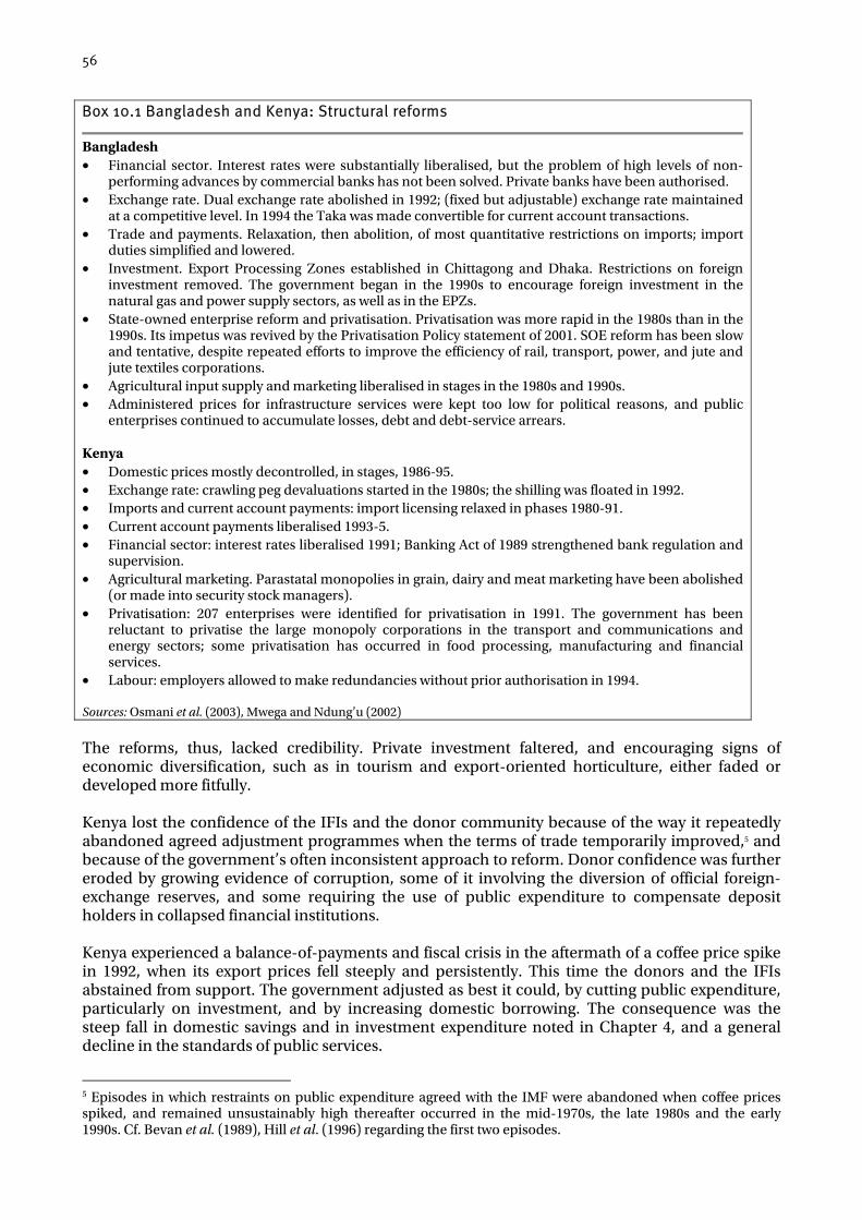
56

Box 10.1 Bangladesh and Kenya: Structural reforms

Bangladesh • Financial sector. Interest rates were substantially liberalised, but the problem of high levels of non-

performing advances by commercial banks has not been solved. Private banks have been authorised. • Exchange rate. Dual exchange rate abolished in 1992; (fixed but adjustable) exchange rate maintained

at a competitive level. In 1994 the Taka was made convertible for current account transactions. • Trade and payments. Relaxation, then abolition, of most quantitative restrictions on imports; import

duties simplified and lowered. • Investment. Export Processing Zones established in Chittagong and Dhaka. Restrictions on foreign

investment removed. The government began in the 1990s to encourage foreign investment in the natural gas and power supply sectors, as well as in the EPZs.

• State-owned enterprise reform and privatisation. Privatisation was more rapid in the 1980s than in the 1990s. Its impetus was revived by the Privatisation Policy statement of 2001. SOE reform has been slow and tentative, despite repeated efforts to improve the efficiency of rail, transport, power, and jute and jute textiles corporations.

• Agricultural input supply and marketing liberalised in stages in the 1980s and 1990s. • Administered prices for infrastructure services were kept too low for political reasons, and public

enterprises continued to accumulate losses, debt and debt-service arrears. Kenya • Domestic prices mostly decontrolled, in stages, 1986-95. • Exchange rate: crawling peg devaluations started in the 1980s; the shilling was floated in 1992. • Imports and current account payments: import licensing relaxed in phases 1980-91. • Current account payments liberalised 1993-5. • Financial sector: interest rates liberalised 1991; Banking Act of 1989 strengthened bank regulation and

supervision. • Agricultural marketing. Parastatal monopolies in grain, dairy and meat marketing have been abolished

(or made into security stock managers). • Privatisation: 207 enterprises were identified for privatisation in 1991. The government has been

reluctant to privatise the large monopoly corporations in the transport and communications and energy sectors; some privatisation has occurred in food processing, manufacturing and financial services.

• Labour: employers allowed to make redundancies without prior authorisation in 1994. Sources: Osmani et al. (2003), Mwega and Ndung’u (2002) The reforms, thus, lacked credibility. Private investment faltered, and encouraging signs of economic diversification, such as in tourism and export-oriented horticulture, either faded or developed more fitfully. Kenya lost the confidence of the IFIs and the donor community because of the way it repeatedly abandoned agreed adjustment programmes when the terms of trade temporarily improved,5 and because of the government’s often inconsistent approach to reform. Donor confidence was further eroded by growing evidence of corruption, some of it involving the diversion of official foreign-exchange reserves, and some requiring the use of public expenditure to compensate deposit holders in collapsed financial institutions. Kenya experienced a balance-of-payments and fiscal crisis in the aftermath of a coffee price spike in 1992, when its export prices fell steeply and persistently. This time the donors and the IFIs abstained from support. The government adjusted as best it could, by cutting public expenditure, particularly on investment, and by increasing domestic borrowing. The consequence was the steep fall in domestic savings and in investment expenditure noted in Chapter 4, and a general decline in the standards of public services.

5 Episodes in which restraints on public expenditure agreed with the IMF were abandoned when coffee prices spiked, and remained unsustainably high thereafter occurred in the mid-1970s, the late 1980s and the early 1990s. Cf. Bevan et al. (1989), Hill et al. (1996) regarding the first two episodes.

57

10.2 Fiscal policies

The implications for growth of high public expenditure are ambiguous, both theoretically and in the empirical evidence. In theory, public expenditure, if well conceived and well applied, should complement private expenditure, in both investment and consumption, raising private rates of return and consumers’ welfare. However, if inefficiently financed and poorly applied, it distorts private investment and consumption choices, and may introduce uncertainty into the business climate. As seen in Chapter 9, econometric tests of the impact of public expenditure – particularly government consumption – on growth often find that higher expenditure leads to lower growth. The fiscal stances of the two countries over three decades are compared in Figs. 10.1-10.3.

Fig. 10.1 Bangladesh and Kenya: Domestic revenues and expenditures as shares of GDP

0

5

10

15

20

25

30

35

40

1969

1970

1971

1972

1973

1974

1975

1976

1977

1978

1979

1980

1981

1982

1983

1984

1985

1986

1987

1988

1989

1990

1991

1992

1993

1994

1995

1996

1997

1998

1999

2000

2001

Perc

enta

ges

of G

DP

Bangladesh: Current revenue, excluding grants Bangladesh: Expenditure, totalKenya: Current revenue, excluding grants Kenya: Expenditure, total

Fig. 10.2 Bangladesh and Kenya: Overall budget balance (shares of GDP)

-12

-10

-8

-6

-4

-2

0

2

4

1969

1970

1971

1972

1973

1974

1975

1976

1977

1978

1979

1980

1981

1982

1983

1984

1985

1986

1987

1988

1989

1990

1991

1992

1993

1994

1995

1996

1997

1998

1999

2000

2001

Perc

enta

ges

of G

DP

Bangladesh overall budget balance Kenya overall budget balance

Source: WDI

58

The salient points of difference are: • aggregate public expenditure in Kenya has been significantly higher than in Bangladesh, with

respective averages of 30% of GDP between the mid-1970s and the late 1990s, and around 10% of GDP until the 1990s rising later to 15%. The public service employment implications for the two countries were reviewed in Chapter 6.

• revenues mobilised in Kenya have similarly been much larger (25-30% of GDP) than in Bangladesh (8-10%).

• Kenya’s overall budget balance was, until the mid-1990s, in continuous deficit. The deficit was exceptionally high in 1985-7, at 8-12% of GDP. Bangladesh’s budget was in rough balance or only modest deficit until the early 1990s, with a large deficit of 5% of GDP emerging only in the later 1990s.

• Kenya financed its deficit in large part domestically, giving rise to an accumulation of domestic debt; in Bangladesh, there was no domestic financing until the later 1990s, when domestic borrowing rose to 3% of GDP (Figs. 10.3 and 10.4). The external financing consequences of the deficits were discussed in Chapter 5: Kenya incurred substantial non-concessional debt, but Bangladesh’s external finance was made up of grants or concessional credits.

• The amplitude of the fluctuations in Kenya’s fiscal deficit has been greater than in the case of Bangladesh, indicating a more erratic (and shock-prone) fiscal environment in Kenya.

Fig. 10.3 Bangladesh and Kenya: Domestic financing of the fiscal deficit (shares of GDP)

-6

-4

-2

0

2

4

6

8

10

12

14

1970

1971

1972

1973

1974

1975

1976

1977

1978

1979

1980

1981

1982

1983

1984

1985

1986

1987

1988

1989

1990

1991

1992

1993

1994

1995

1996

1997

1998

1999

2000

2001

Perc

enta

ges

of G

DP

Kenya domestic financing Bangladesh domestic financing

Source: WDI Kenya’s fiscal operations have thus been more inflationary and debt-creating, and also more creative of public service employment. They have therefore had the potential for exerting a more distorting effect on labour and capital markets than the more modestly proportioned operations of the Bangladesh government. The effects on the labour market are covered in the next chapter. Taxation. Bangladesh’s revenue mobilisation effort is one of the lowest among developing countries while, for a low-income country, Kenya’s is among the highest. High levels of revenue mobilisation are likely to give rise to higher deadweight costs in terms of distortions and reductions of production incentives, and rewards for corrupt practice. High rates of tax not only introduce a wedge between social and private returns to investment, but also make business decisions more policy-dependent. Uncertainty about future tax rates may, of itself, lead to deferred investment decisions and inefficient portfolio choices, including a preference for capital flight over domestic investment. In Kenya, though not in Bangladesh, incentive-reducing taxes on business

59

and personal incomes are a major revenue source. Kenya’s revenue from direct taxes was as high as 10% of GDP in the mid-1990s, though it has latterly declined to 7%; in Bangladesh the share of direct tax revenue in GDP has been 1-1.5%. Both countries, however, derive 17-20% of their revenues from transaction-cost-raising fees and charges. These potential problems can be mitigated if tax policy is efficient and transparent, and if tax rates are predictable. Both countries have made progress since 1990 in improving the efficiency of their tax structures, notably by introducing VAT. However, distorting taxes on trade are still important in both countries. Kenya’s tax structure is somewhat more efficient than that of Bangladesh, but Kenya’s high rates increase the relative costs of doing business in that country, decrease the local incentive to save, and are an element in making Kenya a less attractive destination for investment. Domestic public debt. The Kenyan government borrowed heavily on the domestic money market in the 1970s and 1980s, in many years refinancing with domestic debt its net reimbursements of external debt. Fig. 10.4, constructed by cumulating the domestic financing of both countries’ budgets since 1970 (1973 in the case of Bangladesh), shows that Kenya’s domestic debt increased to nearly 30% of GDP in 1990 and 1991, before falling to 20% of GDP after the fiscal austerity of the late 1990s. In Bangladesh, in contrast, recorded domestic borrowing was negative in many years from the late 1970s through into the early 1990s. The situation changed only in the mid-1990s when the government abandoned its traditional fiscal restraint and embarked on an expansionary fiscal policy.

Fig. 10.4 Bangladesh and Kenya: Domestic debt outstanding as share of GDP

-10

-5

0

5

10

15

20

25

30

35

1970

1971

1972

1973

1974

1975

1976

1977

1978

1979

1980

1981

1982

1983

1984

1985

1986

1987

1988

1989

1990

1991

1992

1993

1994

1995

1996

1997

1998

1999

2000

2001

Perc

enta

ges

Bangladesh Kenya

Source: WDI and authors’ calculation The economic significance of domestic debt depends on how it is financed, whether by inflationary borrowing from the banking system or through funded debt instruments the emission of which is likely to raise interest rates, and may thus crowd other borrowers out of the loans market. Bangladesh’s recently issued public debt has been largely in the form of bonds held outside the banking system. In Kenya there has been extensive use of Treasury Bills to finance the fiscal deficit, some held by the central bank (thus tantamount to money creation), but a great majority held in commercial banks where they tend, subject to the monetary authorities’ varying regulations, to crowd out borrowing by non-banks.

60

Fig. 10.5a Bangladesh and Kenya: Nominal interest rates - Discount and Treasury Bills

0

10

20

30

40

50

60

1969

1970

1971

1972

1973

1974

1975

1976

1977

1978

1979

1980

1981

1982

1983

1984

1985

1986

1987

1988

1989

1990

1991

1992

1993

1994

1995

1996

1997

1998

1999

2000

2001

Perc

enta

ge ra

tes

B'desh discount Kenya T Bill

Fig. 10.5b Bangladesh and Kenya: Nominal interest rates - Lending and deposit

0

5

10

15

20

25

30

35

40

1969

1970

1971

1972

1973

1974

1975

1976

1977

1978

1979

1980

1981

1982

1983

1984

1985

1986

1987

1988

1989

1990

1991

1992

1993

1994

1995

1996

1997

1998

1999

2000

2001

Perc

enta

ge ra

tes

B'desh deposit B'desh lending Kenya deposit Kenya lending

Source: WDI Kenya’s high deficits in the 1980s and early 1990s, and its substantial domestic borrowing in the recently liberalised short-term Treasury Bill market, had a dramatic effect on local interest rates, sending the Treasury Bill rate up to 50% in 1993, and local commercial bank lending rates to over 30% in the period 1992-7 (Figs. 10.54a and b). In Bangladesh, financial sector liberalisation also occurred, but with a much less dramatic effect on interest rates. Commercial bank lending rates have barely exceeded 15%. In real terms, the difference between interest rates in the two countries is less marked. Nevertheless, for borrowers, high nominal rates, combined with uncertainty about the future course of prices, are a disincentive to borrow for all but short-term purposes.

10.3 Inflation

Figs. 10.6a and b trace the history of inflation, measured by the GDP deflator, relating it to the growth in the supply of broad money (M2). The relationship has been unstable; in both countries

61

inflation has been influenced by non-monetary factors such as export prices and domestic supply shortages as well as by growth in the money supply. Bangladesh (Fig. 10.6a) experienced hyperinflation for three years following independence, caused primarily by supply-side dislocation and shortages. Greater price stability was restored in the 1980s, when the annual rise in the GDP deflator averaged 10%, and volatility was much reduced. In the 1990s both inflation and its year-to-year fluctuations fell further, with annual increases in the GDP deflator of only 2% at the end of the decade. In Kenya, average annual inflation has risen from below 5% for most of the 1960s to over 15% in the 1980s and 1990s. In explaining economic performance average rates have had less significance than the highly inflationary episodes to which Kenya has been prone. One such occurred in the early 1970s, and was associated with a coffee price spike and its ramifications in the domestic economy.

Fig. 10.6a Bangladesh: Money supply growth and inflation

-40

-20

0

20

40

60

80

1967

1968

1969

1970

1971

1972

1973

1974

1975

1976

1977

1978

1979

1980

1981

1982

1983

1984

1985

1986

1987

1988

1989

1990

1991

1992

1993

1994

1995

1996

1997

1998

1999

2000

2001

Ann

ual R

ates

M2 GDP Deflator

Fig. 10.6b Kenya: Money supply growth and inflation

-20

-10

0

10

20

30

40

50

60

1967

1968

1969

1970

1971

1972

1973

1974

1975

1976

1977

1978

1979

1980

1981

1982

1983

1984

1985

1986

1987

1988

1989

1990

1991

1992

1993

1994

1995

1996

1997

1998

1999

2000

2001

Ann

ual R

ates

M2 GDP Deflator

Source: WDI

62

Another, more serious, episode occurred in the early 1990s, culminating in 1994 in a rise in the GDP deflator of nearly 40%, and in the consumer price index of 70%. This was policy-induced. The government reacted to the spike in interest rates in 1993 (Fig. 10.5a) by reducing its sales of Treasury Bills and monetising its deficit. The years immediately prior to the inflationary spike had seen exceptional growth in broad money (Fig. 10.6b). The following year, 1994 also saw a sharp rise in domestic financing of the fiscal deficit (Fig. 10.3), resulting from a shortfall in external financing. This coincided with a coffee price spike (Fig. 5.6) which further added to domestic liquidity. Inflation and money supply growth were subsequently brought under control, as the budget was brought into balance and domestic financing curbed (Figs. 10.2 and 10.3), but confidence in the government’s macroeconomic management ability was eroded. Its task in the later 1990s was complicated by slow economic growth, a falling revenue/GDP ratio, another coffee price spike followed by a drought, low external financing and a falling M2/GDP ratio (see below). Its initial success in reducing inflation was not sustained.

10.4 Financial depth

The evidence on inflation, fiscal deficit monetisation and money supply growth summarised in Figs. 10.3 and 10.6a and b does not suggest a simple money supply mechanism underlying inflation and macroeconomic instability in either country. The reason is that major changes in the demand for money were taking place in both Bangladesh and Kenya. Fig. 10.7 shows that Kenya’s M2/GDP ratio rose from 5% at independence to 25% in the late 1960s. It fluctuated in the range 25-30% until the 1990s when it rose briefly to 45% of GDP, before falling to below 40% in 2000. Holdings of liquid liabilities rose in periods of high coffee prices, and declined as a share of GDP when prices fell. This level of demand for money is high by the standards of many developing countries, where the broad money/GDP ratio is commonly less than 20%, and until 2000, it was much higher than in Bangladesh. It reveals a degree of, albeit fluctuating, confidence in the value of the Kenya shilling, and a willingness to hold monetary instruments for both transactions and savings purposes. This was not the case in Bangladesh until the mid-1980s, when confidence in the future of the Bangladeshi economy and its currency strengthened, and a steady rise in the M2/GDP ratio began.

Fig. 10.7 Bangladesh and Kenya: Financial depth

0

5

10

15

20

25

30

35

40

45

50

1960 1962 1964 1966 1968 1970 1972 1974 1976 1978 1980 1982 1984 1986 1988 1990 1992 1994 1996 1998 2000

M2/

GD

P R

atio

s (%

)

Bangladesh Kenya

Source: WDI The higher the M2/GDP ratio, the greater the scope for seignorage, and thus the greater the scope for non-inflationary growth in the money supply and for deficit monetisation. However, the course

63

of growth in demand for money in Kenya has been volatile, giving rise to a greater likelihood of unexpected inflationary outcomes complicating the task of macroeconomic management. In Bangladesh, in contrast, the ratio of broad money to GDP, initially low (only 8%), has grown more or less steadily, in particular since 1980, to reach 35% by 2001. This stable progression of the demand for money has facilitated macroeconomic management and contributed to relative price stability, even during the 1995-2000 period when fiscal deficits were rising.

10.5 Financial sector

Macroeconomic policies have not been solely to blame for high interest rates on bank advances. The other cause has been the high incidence in both countries (as in many other developing countries) of non-performing loans on the balance sheets of commercial banks. In Kenya there has been a history of poor supervision, imprudent bank lending and bank failure, starting with the crisis over the insolvency of non-bank financial intermediaries in the mid-1980s. In subsequent years some nationalised commercial banks also required recapitalisation by the government. Threats to financial sector solvency have continued to recur. The non-performing share of bank advances stood at 30% in mid-1999, and at 41% in June 2001 (8.8% of GDP). In Bangladesh there is a similarly long history of distress in the banking system, calling for similar measures of support from the government. The share of non-performing loans in total advances has varied since 1995 between 30% and 45%. Responsibility for non-performing loans in both countries has been shared between (a) the failure of state enterprises and parastatals to service their bank debt – often because government controls on prices and tariffs undermine their profitability –, and (b) abusive and corrupt relationship lending by banks to their own officers or to politically well-connected personalities. From the perspective of economic performance the significance of non-performing loans on this scale lies in the implication of resource misallocation; banks are lending money to unprofitable operations, and governments have to divert public expenditure to recapitalise financial institutions that should have been profitable. The availability of loanable resources for viable enterprises is thereby reduced. In practical terms, the existence of non-performing loans raises the cost of advances to sound borrowers, because banks increase the spread between deposit and lending rates to cover their losses on unsound advances. The spread in Kenya 15 percentage points in 1995, and was still 13 percentage points in 2001 (Fig. 10.5b). In Bangladesh the spread in 2001 was a more modest 7 percentage points (Fig. 10.5a). Resource misallocation through dysfunctions in financial intermediation would be greater in one country than the other if the relative size of financial intermediation were greater in one than the other. A useful proxy measure of this is the ratio of liquid liabilities of the banking system (M2) to GDP, in other words financial depth. For most of the period, as noted above, there has been greater financial depth in Kenya than in Bangladesh. For most of the 1971-2001 period, therefore, there has been greater scope for resource misallocation through ill-considered bank lending in Kenya than in Bangladesh (Fig. 10.7). Now, however, the danger is equally large in the two countries, making it equally important in each to heal the running sore of poor bank lending practice.

10.6 Macroeconomic volatility

Inflation, taxation, the level of interest rates and the availability of credit all have very obvious and direct effects on the climate for investment and on business confidence, and thus on the prospects for growth. Instability and unpredictability in the policy environment may have a similar and lasting effect.

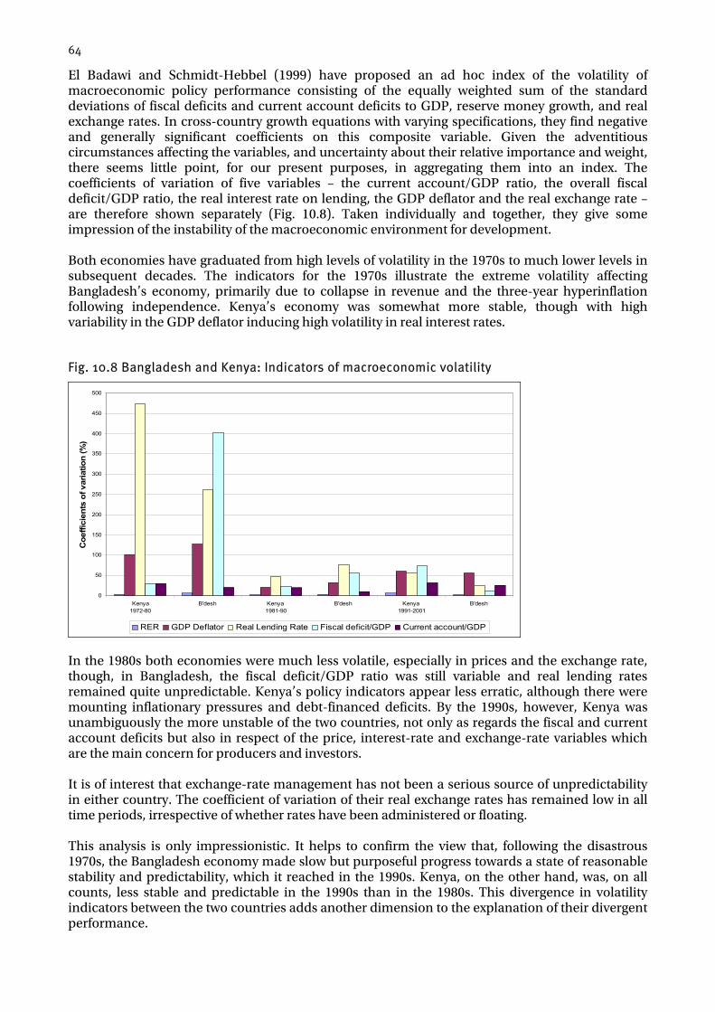
64

El Badawi and Schmidt-Hebbel (1999) have proposed an ad hoc index of the volatility of macroeconomic policy performance consisting of the equally weighted sum of the standard deviations of fiscal deficits and current account deficits to GDP, reserve money growth, and real exchange rates. In cross-country growth equations with varying specifications, they find negative and generally significant coefficients on this composite variable. Given the adventitious circumstances affecting the variables, and uncertainty about their relative importance and weight, there seems little point, for our present purposes, in aggregating them into an index. The coefficients of variation of five variables – the current account/GDP ratio, the overall fiscal deficit/GDP ratio, the real interest rate on lending, the GDP deflator and the real exchange rate – are therefore shown separately (Fig. 10.8). Taken individually and together, they give some impression of the instability of the macroeconomic environment for development. Both economies have graduated from high levels of volatility in the 1970s to much lower levels in subsequent decades. The indicators for the 1970s illustrate the extreme volatility affecting Bangladesh’s economy, primarily due to collapse in revenue and the three-year hyperinflation following independence. Kenya’s economy was somewhat more stable, though with high variability in the GDP deflator inducing high volatility in real interest rates.

Fig. 10.8 Bangladesh and Kenya: Indicators of macroeconomic volatility

0

50

100

150

200

250

300

350

400

450

500

Kenya1972-80

B'desh Kenya 1981-90

B'desh Kenya 1991-2001

B'desh

Coe

ffici

ents

of v

aria

tion

(%)

RER GDP Deflator Real Lending Rate Fiscal deficit/GDP Current account/GDP In the 1980s both economies were much less volatile, especially in prices and the exchange rate, though, in Bangladesh, the fiscal deficit/GDP ratio was still variable and real lending rates remained quite unpredictable. Kenya’s policy indicators appear less erratic, although there were mounting inflationary pressures and debt-financed deficits. By the 1990s, however, Kenya was unambiguously the more unstable of the two countries, not only as regards the fiscal and current account deficits but also in respect of the price, interest-rate and exchange-rate variables which are the main concern for producers and investors. It is of interest that exchange-rate management has not been a serious source of unpredictability in either country. The coefficient of variation of their real exchange rates has remained low in all time periods, irrespective of whether rates have been administered or floating. This analysis is only impressionistic. It helps to confirm the view that, following the disastrous 1970s, the Bangladesh economy made slow but purposeful progress towards a state of reasonable stability and predictability, which it reached in the 1990s. Kenya, on the other hand, was, on all counts, less stable and predictable in the 1990s than in the 1980s. This divergence in volatility indicators between the two countries adds another dimension to the explanation of their divergent performance.

65

10.7 Summary

This chapter has added chapter and verse to the bald suggestion, in the growth and investment regressions, that macroeconomic variables have been significant determinants of performance, at least in some time periods. It has provided complementary information on how policy variables have performed, and their likely impact. The analysis is predicated on the widely held assumptions that growth depends on enterprise development, and that enterprises expand and flourish best when macroeconomic conditions (prices, wages, exchange rates, retail interest rates) and policies (credit, money market interest rates, exchange rates) are stable and predictable. It is also based on the belief that business confidence is a lagged function of cumulative perceptions of the policy environment, so that confidence building requires persistence if perceptions are to alter substantially. The main conclusions drawn are that: • reform programmes and structural policies do little to explain performance divergences;

institutional and structural policy reforms in Bangladesh and Kenya followed broadly similar paths, and were similarly affected by implementation delays; however, policy reversals did more to impair the credibility of Kenya’s reforms than of Bangladesh’s;

• Bangladesh has had low taxes and low public expenditures; Kenya has had high tax revenues and high levels of expenditure. High expenditure in Kenya has, as argued in Chapter 6, exerted upward pressure on wages. High taxes have been a factor in discouraging and distorting enterprise expansion decisions, reducing the ratio of private investment to GDP (Table 4.5) and the flow of inward investment, and encouraging rent-seeking. The deadweight cost of taxation in Bangladesh has been less;

• Kenya’s persistently (relatively) high and increasingly variable rate of inflation in the 1980s and 1990s helped to further erode investor confidence. The converse has applied in Bangladesh, where hyperinflation in the 1970s was followed in the 1980s and 1990s by first moderate and then low and stable inflation;

• relatively low interest rates in Bangladesh helped to build up investor confidence, in spite of the ‘risk premium’ included in retail lending rates because of the high incidence of non-performing loans. Kenya’s high recourse to domestic funding for its high fiscal deficits led to higher nominal interest rates, especially after financial sector liberalisation;

• Kenya’s conduct of macroeconomic affairs has been more volatile and erratic than that of Bangladesh, especially in the 1990s, contributing to the greater unpredictability of Kenya as an environment for enterprise development; and

• Kenya’s repeated disagreements with the IFIs, leading to the loss of their financial support, have sent adverse signals to investors. Although the IFIs disapproved of many aspects of Bangladesh’s economic management on the institutional and structural front, this did not deter the expansion plans of domestic investors.

The Bangladeshi government started in the later 1990s to pursue policies of fiscal expansion with rising indebtedness that put at risk this confidence-inspiring inheritance. Real interest rates began to rise, increasing the possibility that investment will be crowded out. In the very recent past, however, it has taken steps to restore macroeconomic balance. Macroeconomic management performance has no simple, straightforward and immediate impact on economic growth. Growth was high in Kenya, but low in Bangladesh, in the volatile 1970s. Persistent imbalances and instability, however, erode confidence and shorten the time-horizons of investors’ decisions. An important part of the difference in performance between the two countries is thus attributable to features of their respective macroeconomic and investment climate characteristics. However, these alone do not suffice to explain the varying patterns of supply-side response in the two countries. The remaining chapters of this paper are devoted to other – microeconomic and institutional - features of the business environment, with a view to further

66

illuminating the question of why business investment has increased in Bangladesh, but fallen in Kenya, since the early 1990s.

67

Chapter 11: Institutional and Governance Factors

The previous chapter identified a number of features of macroeconomic outcomes and policies with significance in explaining differing economic performance. Chapter 6 discussed the enlargement of the government payroll and the public sector in Kenya, and the nationalisation of productive assets at independence in Bangladesh. The present chapter asks whether there are features of the two countries’ institutional environment and governance that could add further dimensions to the explanation. In particular, it asks whether there is evidence of institutional deterioration in Kenya of a kind that could have a bearing on enterprise and growth, and whether there are signs of institutional strengthening in Bangladesh which run parallel with the improvement in its macroeconomic management. The main focus of attention will be on the evidence that can be gleaned from comparative surveys of the opinions of key informants, many in business and in the private sector. For completeness, however, the assessment begins with the issues of corruption and the strength of democratic institutions, both of which, as seen in Chapter 9, are significant variables in cross-country growth equations. As will be seen, the evidence is ambiguous, though suggestive of an anti-competition bias in the business-government game in Kenya.

11.1 Corruption

Both Kenya and Bangladesh have acquired poor reputations for governance in respect of the endemic corruption of their public life, and the overall inefficiency and ineffectiveness of their public expenditures and public services. Moore et al. (2003) paint a very negative picture of governance and public life in Bangladesh, featuring corruption at many levels, disjuncture between formal and actual governmental processes, official arbitrariness, lack of oversight and political accountability, illegal funding of political parties, and a pervasive need to use ‘intermediaries’ (politicians, thugs, fixers, personal connections) to access public services of any kind. Political parties are less and less inclined to prevent their supporters from preying on society. These observations seem to betoken a deterioration of institutional quality arising from the interplay of economic forces, governmental controls and political self-interest, and seem to preclude the pro-poor developmental outcomes that are in practice observed (Chapters 4 and 6). But they are not wholly corroborated by other evidence reviewed below. Both countries have reverted in the course of the 1990s from authoritarian – one-party or military – rule to political pluralism. As noted in other countries like South Korea, this transition may be accompanied by a worsening of predation of the enterprise sector by political leaders and their party followers, caused by the need to mobilise funding to finance election campaigns as well as the funds required to maintain and enrich the party (or military) cadres (cf. Kang, 2003). The World Bank’s Investment Climate Assessment of Bangladesh (World Bank, 2003a) confirms the view that corrupt payments are widespread and endemic, and significantly impair the conduct of business. The Assessment, based on business surveys, shows that 58% of firms consider that corruption is a ‘major’ or ‘severe’ constraint on their activities. The only other constraint named by more than half the respondents was erratic electricity supply (73%). Rather less than 50% complained about tax administration and financing costs. The same source reports that corrupt payments cost firms 2.5% of turnover (see Table 11.1). Though there is no equivalent investment climate survey of Kenya, Transparency International have conducted a country-specific survey of the incidence, severity and frequency of corruption in the country, based on interviews with samples of micro- and small-scale enterprises, corporations and individuals. Some two-thirds of respondents’ interactions with public institutions were found

68

to involve bribery, or the threat of negative consequences if no bribe is paid. Bribe paying, if costs are shared between households and enterprises, may add 15% to the cost of living of households, and increase the cost of doing business for enterprises by 1.4%. The police, the municipal authorities and the judiciary were found to be among the most corrupt government institutions, and the Kenya Ports Authority (responsible for operating the port of Mombasa) was the most corrupt parastatal. The two countries occupy almost adjacent positions at the bottom of Transparency International’s most recent (2002) survey of perceptions of corruption and corruptibility among politicians and public officials (Table 11.2).

Table 11.1 Bangladesh and Kenya: Business cost indicators

Bangladesh Kenya Starting a business - registration and compliance cost (US$ in 2003)

$272 $194

- number of procedures 7 11 - time taken (weeks) 30 61 Employment law - index of complexity 50 34 Contract enforcement - complexity index 51 44 - cost (%GNI) 270 50 Credit - interest rate spread % 6.22 12.94 - private credit as % GDP 24.28 25.69 Corruption cost 2.5% of

revenue ª up to 2.8% of turnover b

Notes: a/ Investment Climate Assessment tables, World Bank; b/ Transparency International, Kenya

Table 11.2 Corruption Perception Index scores

Bangladesh Kenya CPI score (out of 10) 1.2 (Standard Deviation: 0.7) 1.9 (Standard Deviation: 0.3) Rank (out of 102) 102 96 Source: Transparency International These scores and assessments are subjective – based on polling the opinions of key informants – and do not reflect rigorous pair-wise comparisons. They nevertheless serve to place the two countries in the same league of the most corrupt among the countries covered in the survey. It is not possible to conclude that differing degrees or kinds of pervasiveness of corruption in public life and the conduct of enterprises account for differing economic performance. Both countries suffer impairments to their economic life that are similar in type and extent.

11.2 Democracy and civil liberties

Freedom House constructs indices of political rights and civil liberties covering all years since 1972, the former attributing better scores to functioning democratic institutions and worse scores to arbitrary and authoritarian regimes, and the latter measuring the protection given to individuals’ human rights and political freedoms.

69

Bangladesh scored badly on the political register during its years under military rule (scores of 3-7 out of 7), but much better since the restoration of multi-party rule (scores of 2-3 out of 7). For civil liberties its scores have all along been mediocre (4-5 out of 7). Kenya’s scores for political rights have been, for most years, even worse than those of Bangladesh (5-7 out of 7), with some deterioration after the 1970s. For civil liberties the two countries have been roughly on a par. This offers some evidence that institutions concerned with participation and ‘voice’ were growing stronger, post-1990, in Bangladesh but not in Kenya, but that this improvement did not extend to institutions charged with upholding the rule of law and individual rights. Freedom House’s indices, on their own, seem not to offer a convincing explanation for divergent economic performance, especially in view of the rise in political violence and economic disruption that has followed the restoration of political democracy in Bangladesh.

11.3 Regulation and bureaucracy

A more comprehensive set of governance indicators for nearly 200 countries has been computed by Kaufman et al. (2003) from 25 secondary sources (each of which has compiled indices based on surveys of informed opinion using multiple individual variables). Six composite indicators are calculated – covering the rule of law, corruption control, institutional accountability and effectiveness, regulation and political stability. All of these facets of governance are prima facie of potential importance in encouraging wealth-creating activity in the private sector. The indicators for Bangladesh and Kenya only cover the most recent six-year period 1996-2002. They are reproduced in Table 11.3. The negative index numbers shown for both countries signify that their quality of governance is perceived by informants to be below the worldwide mean6. Larger numbers indicate worse perceptions.

Table 11.3 Bangladesh and Kenya: Governance indicators 1996-2002

1996 1998 2000 2002 Bangladesh Kenya Bangladesh Kenya Bangladesh Kenya Bangladesh Kenya Rule of law -0.65 -0.73 -0.72 -1.02 -0.68 -1.02 -0.78 -1.04 Control of corruption

-0.43 -0.98 -0.40 -0.92 -0.64 -1.08 -1.12 -1.05

Voice and accountability

-0.31 -0.45 -0.17 -0.77 -0.34 -0.84 -0.57 -0.58

Government effectiveness

-0.57 -0.50 -0.36 -0.88 -0.45 -0.71 -0.53 -0.85

Regulatory quality

-0.53 -0.48 -0.08 -0.18 -0.02 -0.11 -1.05 -0.50

Political stability

-0.41 -0.23 -0.44 -1.07 -0.56 -1.00 -0.61 -0.86

Source: Kaufman et al. (2003) The scores in Table 11.3 lend weight to the impression that, by the second half of the 1990s, Bangladesh’s institutional performance had come to dominate that of Kenya. Bangladesh’s scores are better than Kenya’s in all six years in respect of the rule of law and accountability, in all years except 2002 in respect of efforts to control corruption, and in all years except 1996 in respect of government effectiveness and political stability. The exception to the generally less unfavourable perception of institutional quality in Bangladesh concerns regulatory quality. This is a key variable for enterprises because it directly affects decisions on establishment and expansion, and the costs of carrying on business. There is no consistency, from one year to another, in perceptions about which country performs better on this variable. The administration of regulations in both countries is erratic, inconsistent, corrupt and the source of delays and uncertainty. 6 The indicators are normalised, with a mean of zero and a standard deviation of 1.

70

The recent investment climate surveys which generated the evidence summarised in Table 11.1 suggest that delays in receiving authorisation to establish new enterprises in Kenya are twice as long (60 weeks) as in Bangladesh (30 weeks), though in both countries they are excessive. On the other hand, compliance costs for establishment are reported to be higher in Bangladesh than in Kenya ($272 compared with $194), as are the costs of complying with labour regulations. It is hard to say how much reliance should be placed on these average figures, which doubtless mask a wide dispersion in actual experience. Uncertainty about regulatory costs and delays adds to the deterrent effect on business of maladministration. The tentative conclusion from this fragmentary evidence is that the quality of relevant governance institutions remains poor in both countries, but that it has improved somewhat in Bangladesh since the chaotic 1970s, but has declined relatively in Kenya. It also suggests that developments in institutional quality have occurred across a broad front, thus increasing the likelihood that business intentions have been coloured by them.

11.4 External assessments of the business environment

The impression of relative institutional improvement in Bangladesh and relative deterioration in Kenya is, however, not confirmed by all surveys, particularly those which canvass the views of external investors. The International Composite Risk Guide gives the two countries almost identical scores for the combined political, financial and economic risks that external investors face. The Fraser Institute’s indicators of economic freedoms and institutional effectiveness for enterprise rate the Kenyan business environment more highly than that of Bangladesh, placing Kenya in 51st place out of 123 countries, and Bangladesh in 91st place. Kenya scores more highly in this source for its legal structure and protection of property rights, and for the liberality of its regulation of enterprises’ transactions with foreigners, and of its employment and financial sector regulations.

11.5 Business and politics

Governance scores derived from surveys of business opinion are implicitly predicated on the assumption that business has an arms-length relationship with government and administration, and is the mere passive victim of predatory practice and maladministration. In short, they assume a non-co-operative game. However, this is not a complete representation of business-government relationships, particularly in the presence of ‘crony capitalism’. Crony capitalism can be defined as a set of collusive relationships between members of the political leadership of a country and certain powerful elements in the business community whereby business contributes in various ways to the enrichment of political leaders, in exchange for the adoption of policies which ensure the profitability of business. These policies may include trade protection, preferences in public procurement and barriers to the entry of business competitors. Crony capitalism implies that a co-operative game is played by political and business élites at the expense of non-players, and at the cost of economic welfare. Crony capitalism, where it exists, is likely to favour monopolies, producer and supplier cartels and restrictive business practices, and to be inimical to competition and to market entry. It is likely to raise costs and prices, and to reduce competitive pressures for improvements in efficiency and for innovation. If unbridled, it is thus likely to damage a country’s international competitiveness, adaptability and responsiveness to external (as well as internal) market forces. This paper is unable to draw on any systematic comparative assessment of business-government relationships in Bangladesh and Kenya. However, there are signs and reports that a more competitive business environment has existed for many years in Bangladesh than in Kenya, and that this can be related to different opportunities for, and approaches to, rent-seeking by

71

politicians, and to different structures in the business communities of the two countries. Box 11.1 offers a schematic representation of how this may have come about.

Box 11.1 Business and politics: Two models of corruption and competition

Kenya Government interest Many years of government by the KANU élite have entrenched patrimonial attitudes towards state and parastatal institutions, and towards the private sector. These attitudes have been reinforced by strong clientelism arising from Kenya’s multi-ethnic character, from the politics of ethnic coalitions, and from the need, in the interests of political stability and unity, for the main ethnic groups to derive tangible benefit from the actions of ‘their’ government members. The élite has enriched itself and its clienteles by: • obtaining public office, in the government, in parastatals and in co-operatives, • using these positions to become directly involved in private sector business, often as sleeping partners or

managers in Asian or foreign-owned private enterprises (Hinbara, 1994), • taking bribes for public procurement contracts, and for licences and permits granted to enterprises, • ensuring that well-connected enterprises enjoy sufficient protection from domestic and foreign competition

to remain profitable, and, on occasion • obtaining exemptions from quotas and duties in order to import products at prices which undercut high-

cost, protected, domestic suppliers. The policy mix that has best served the élite has been pro-enterprise, but with a bias towards interventionism and discretion, and against ease of entry and competition. With the restoration of pluralist, multi-party, politics, the governing élite has also required a higher level of funding than previously for Party campaigns and for inducements to the electorate. Business interest The local enterprise scene has been dominated by diversified, conglomerate, Asian enterprises, politically precarious, but with strong family networks. These enterprises have had an interest in: • preserving the high degree of monopoly they have built up in many domestic markets, and • seeking political protection by co-opting the political élite into their business empires, enabling them to

share in the profits of monopoly or oligopoly. Neither set of actors has a perceived interest in promoting a vigorously competitive domestic private sector by minimising barriers to entry. Bangladesh Government interest At Partition, in 1948, most of the Hindu landlords and urban mercantile classes left the East Wing of the new Pakistan. At independence in 1971 West Wing merchants and entrepreneurs also left. The Muslim Bengali presence in medium- to large-scale private enterprise was weak. The post-independence governments in Bangladesh were economically nationalist in outlook, their first wish being to free the country from the ‘yoke’ of what was perceived to be the exploitative economic power of non-nationals. Nationalisation was the means of bringing inherited or abandoned productive, financial and mercantile assets under national control. The policy was not to expropriate the indigenous private sector, but rather to encourage it with low barriers to entry, low taxes and credit facilities. This encouraged competition between a growing number of small- and medium-scale indigenous enterprises. There were also limited rents available in the private sector for the ruling élite to exploit. There was next to no foreign investment, even in the EPZs, and public officials had insignificant bargaining power for favours vis-à-vis any investors who did come. The élite therefore sought rents from the expenditure of aid, and by exploiting positions in the public service and the wider public sector. It had, however, to share these with a poorly paid and often turbulent public sector workforce. The slow progress of privatisation in the 1980s can thus be seen as in part reflecting the reluctance of bureaucrats and the political élite to relinquish the personal advantages they derived from managing a monopolistic public sector, given the limited scope they then saw for prospering in the private sector.

72

Under military rule the government was financially frugal, with low capital expenditures, which limited the scope for bribery in public procurement. Public officials became extortionate in their administration of fees payable and permits required by the private sector, which contradicted, without totally upsetting, the government’s objective of developing indigenous enterprise. Business interest In the immediate post-independence period there were no dominant Bangladeshi business groups or ‘houses’, nor any established and influential foreign-owned enterprises. There were no business interests large or wealthy enough to forge ‘crony capitalist’ relationships with the new political leaders in Dhaka. The private sector remains characterised by increasing numbers of small- and medium-sized enterprises. 7 Small- and medium-scale indigenous enterprises could only flourish by seeking profitable opportunities in the interstices between the operations of public sector monopolies. They found these in import substitution, construction, a variety of distribution and other service trades, by looking for export markets (cf. Box 4.3) and, with the advance of market liberalisation, in agricultural marketing. These enterprises sought - and received - protection against competition from imports, but they were not large enough, nor did they enjoy sufficient market power, to seek to entrench market dominance at the expense of new entrants.

11.6 Summary

Institutional and governance variables offer only limited and ambiguous explanations for differing economic performance in the two countries, both of which are notorious for their corruption. With regard to the indicators with the greatest relevance to the development of enterprise and wealth creation, the similarities between the two countries are more striking than the differences. Evidence based on surveys of key domestic informants in both countries suggests that Bangladeshi institutions and administrative practices are seen in a somewhat more favourable light than those of Kenya, but the perceptions of external investors about the strength of legal institutions and the quality of regulation of the business environment come to the conclusion that Kenya is to be preferred to Bangladesh. More significant to understanding economic performance is the relationship between the formal business sector and government, and its implications for the degree of competition between enterprises. For historical reasons the business environment has been and remains more competitive in Bangladesh than in Kenya. Evidence for the effect of this on transport costs is presented in Chapter 12.

7 Moore et al. (2003) characterise the structure and corruption threat from the private sector as follows: “… there are few very large (transnational) firms, and little involvement of the private sector in large scale mineral exploitation [so] there are no strong reasons to fear that support for business organisations might tip the balance of power too much towards business as a whole. The politics of business are characteristically pluralist: business organisations spend more time and effort competing with each other … than they do promoting the general interest of business. Provided the structure of production and ownership in the private sector remains relatively diverse, supporting business is unlikely to threaten political pluralism. … It seems very likely that the newer, emerging, business sector will be less engaged in corrupt activities and relations with the state than is much of the older private sector. Many are export oriented …[and] have less incentive or opportunity to be corrupt because they are neither heavily engaged in providing goods or services to government agencies, nor very dependent on import protection.”

73

Chapter 12: Competition and competitiveness in the business environment

Chapter 10 presents evidence that Kenya has had higher (direct) taxes, higher interest rates, a larger government presence in the labour market and a more volatile macroeconomic environment for enterprise than Bangladesh. Chapter 11 adduces evidence that the ‘transaction costs’ of corruption are probably of the same order of magnitude, but that, in the view of key local informants at least, government and judicial institutions may function less unfavourably for enterprise in Bangladesh than in Kenya. This chapter looks further into the costs of doing business in the two countries with a view to reinforcing the evidence for saying that Bangladesh has been the more favourable location for business expansion. It focuses on the relative costs for enterprise in the two countries of labour and transport, and on the extent of competition in domestic markets for goods and services.

12.1 Labour costs

Labour markets in developing countries tend to be even more segmented than those in developed countries, and the preponderance of the informal sector in employment8 in which labour rates are unrecorded makes it difficult to paint a valid overall picture of labour costs. The most complete data available pertain to the formal manufacturing sector, which includes the garment sector which has become very important in Bangladesh’s export trade and is expanding in that of Kenya (cf. Chapter 4), and the processed food sector which is important in Kenya’s exports to COMESA markets. In these sectors labour costs typically constitute 30-50% of total production costs. Employment costs in manufacturing provide, at least in a first approximation, a proxy for labour costs in the production and marketing of merchandise exports, almost all of which involve formal sector operations at some stage. These costs are influenced by public service remunerations, because most employment in both sectors is urban, and because clerical and administrative occupations in manufacturing, at least, call for the same skills as similar occupations in public administration. Evidence from the two countries supports three propositions leading to the conclusion that Bangladesh has had substantially lower labour costs. These are that Bangladeshi manufacturing has had: • lower monthly labour costs per employee, • higher average labour productivity, and • lower unit labour costs. Labour costs per employee. Fig. 12.1 compares the costs per employee in manufacturing in Bangladesh and Kenya from the late 1960s to the late 1990s in constant US$ (at 1995 prices). Domestic labour costs (including wages and other benefits in cash and kind) have been converted into dollars at the official exchange rate, and deflated by an index of the prices of manufactured goods in world trade. The graph shows that labour costs per employee in manufacturing in Bangladesh have fluctuated trendlessly between $500 and $1000 p.a. over the period, while in Kenya annual average labour costs have fallen dramatically from nearly $4000 to a little more than $1000. In Kenya they have followed more or less the same pattern as the real exchange rate (Fig. 5.11), with temporary increases during successive coffee booms. The reason for the similarity of the two time profiles is that both reflect the rapid depreciation of the nominal exchange rate, and

8 A labour force survey of Kenya shows that small-scale agriculture and the non-farm informal sector employ 70% of the employed labour force (Government of Kenya, Statistical Abstract).

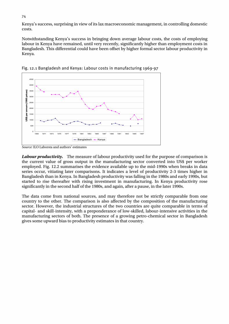
74

Kenya’s success, surprising in view of its lax macroeconomic management, in controlling domestic costs. Notwithstanding Kenya’s success in bringing down average labour costs, the costs of employing labour in Kenya have remained, until very recently, significantly higher than employment costs in Bangladesh. This differential could have been offset by higher formal sector labour productivity in Kenya.

Fig. 12.1 Bangladesh and Kenya: Labour costs in manufacturing 1969-97

0

500

1000

1500

2000

2500

3000

3500

4000

4500

1969 1971 1973 1975 1977 1979 1981 1983 1985 1987 1989 1991 1993 1995 1997

US$

per

ann

um (1

995

pric

es)

Bangladesh Kenya

Source: ILO Laborsta and authors’ estimates Labour productivity. The measure of labour productivity used for the purpose of comparison is the current value of gross output in the manufacturing sector converted into US$ per worker employed. Fig. 12.2 summarises the evidence available up to the mid-1990s when breaks in data series occur, vitiating later comparisons. It indicates a level of productivity 2-3 times higher in Bangladesh than in Kenya. In Bangladesh productivity was falling in the 1980s and early 1990s, but started to rise thereafter with rising investment in manufacturing. In Kenya productivity rose significantly in the second half of the 1980s, and again, after a pause, in the later 1990s. The data come from national sources, and may therefore not be strictly comparable from one country to the other. The comparison is also affected by the composition of the manufacturing sector. However, the industrial structures of the two countries are quite comparable in terms of capital- and skill-intensity, with a preponderance of low-skilled, labour-intensive activities in the manufacturing sectors of both. The presence of a growing petro-chemical sector in Bangladesh gives some upward bias to productivity estimates in that country.

75

Fig. 12.2 Labour productivity in Bangladesh and Kenya: Gross output per worker

0

1000

2000

3000

4000

5000

6000

7000

8000

1979 1980 1981 1982 1983 1984 1985 1986 1987 1988 1989 1990 1991 1992 1993 1994 1995 1996

US$

p.a

. at

cur

rent

pric

es

Bangladesh Kenya Sources: Published national statistics and authors’ estimates

Unit labour costs. Indices of current unit labour costs, following ILO methodology, are calculated by dividing current total labour costs in manufacturing by value-added in manufacturing at constant prices. The rationale for adopting this approach is that data on value-added at constant prices are more readily available than data on the value of gross output, and that real value-added is a good proxy indicator for growth in the volume of output. The evidence thus generated on unit labour costs in the two countries (Fig. 12.3) confirms the evidence in Fig. 12.1 on labour costs per employee. It shows that Bangladesh has enjoyed a very substantial cost advantage over Kenya, but that this advantage has been eroded by recent gains in Kenya’s competitiveness.

Fig. 12.3 Bangladesh and Kenya: Comparative unit labour costs

0

0.1

0.2

0.3

0.4

0.5

0.6

0.7

0.8

0.9

1970 1971 1972 1973 1974 1975 1976 1977 1978 1979 1980 1981 1982 1983 1984 1985 1986 1987 1988 1989 1990 1991 1992

Ann

ual l

abou

r cos

ts in

cur

rent

US$

per

uni

t of m

anuf

actu

ring

valu

e ad

ded

in 1

995

$

Kenya Bangladesh Sources: Published national statistics and authors’ estimates Kenya’s high labour costs in the 1970s and 1980s, and their decline in the 1990s, are almost certainly explicable by the trends in formal sector employment in government, industry and commerce, and their consequential effects on real wages. Total wage employment was expanding in the 1970s and 1980s by some 3.5% p.a., but its expansion slowed in the 1990s to 1.7% p.a. In the 1970s there was excess demand for labour with some education and experience. Wages rose, and productivity was low. In the 1980s with the rise in productivity, wage increases slowed as the stock of human capital – workers with some schooling - rose. By the 1990s, slower economic growth combined with the momentum of expansion in education had created a situation of excess supply.

76

The downward pressure on formal sector real wages was led by the public sector, where the budgetary situation was constrained and where employment was contracting. In Bangladesh, the supply of labour to the formal sector was elastic, with no upward pressure on real wages, up to the 1990s. The restoration of democracy was accompanied by freedom of trade union action, which became vigorous and often politically motivated. Labour costs have therefore tended to rise in the 1990s. The upward pressure on wages has been reinforced by the growth of government service employment since 1995, and by subsequent revisions of civil service pay structures and scales.

12.2 Transport costs

Transport costs are an important element in the total cost of imported goods, and in the cost of producing, marketing and delivering exports. High international transport costs are a particular disadvantage for enterprises producing goods for export which incorporate heavy and bulky imported inputs, because their margins are squeezed by the high cost of their purchases and the low factory-gate value of their sales. They predispose a country to import substitution, and against export production. High domestic transport costs, similarly, reduce the profitability of exports, particularly of bulky commodity exports. International transport costs. Chapter 2 briefly discussed the respective locations of Bangladesh and Kenya relative to their markets and sources of supply, noting that Kenya was closer geographically to its main commodity markets (Europe and North America) and to its markets for processed goods (Africa) than is the case for Bangladesh. However, geography notwithstanding, external transport costs have for many years been lower in Bangladesh than in Kenya. This point is illustrated in Fig. 12.4 which compares the insurance and freight margin on the value of imports entering the two countries since the mid-1970s. For most of this time the insurance and freight margin in Bangladesh has been approximately 11.5% of the value of imports, while in Kenya it has been of the order of 15-16%. Only in the late 1990s has there been a sharp reduction in Kenya’s external transport costs, under the combined effect of falls in world shipping rates and in the premium charged for conveying goods to Kenya. The excess cost of freight and insurance borne by the two countries on their sea-borne merchandise trade can be roughly estimated as a share of GDP. Aggregate estimates of the insurance and freight margin on overseas export sales are not so easy to compile. However, the margin on import purchases may be used as an indicator of the margin on outbound traffic as well. In Kenya’s case, imports and exports have amounted to some 65% of GDP (Fig. 5.1). However, some 35% of exports are sold to other African countries and mostly transported overland. Allowing for this, and assuming that Kenya is a price-taker in non-African international trade, so that the full burden of the freight and insurance margin falls on domestic importers and exporters, it is easy to calculate that, when the margin was still 15%, the total cost of freight and insurance on ship-borne trade was 8.2% of GDP.9 This is 3-4% of GDP higher than it could have been if Kenyan shippers and ports were providing a competitive service. In the case of Bangladesh, where the value of trade has been 25-30% of GDP and the freight and insurance margin 11-12% of the value of the merchandise transported, and making the same elasticity assumptions, the total margin has represented a charge of 3% to GDP, of which only about 0.8% of GDP could have been saved by more efficient logistical practice.

9 0.15*(0.35 + 0.65*0.30) = 0.82 (Imports, 35% of GDP, are mostly ship-borne. 65% of exports, 30% of GDP, are also ship-borne).

77

Fig. 12.4 Bangladesh and Kenya: Freight and insurance margin on imports

0

2

4

6

8

10

12

14

16

18

20

1975 1977 1979 1981 1983 1985 1987 1989 1991 1993 1995 1997 1999

Perc

enta

ge o

f FO

B C

ost o

f Im

ports

Bangladesh Kenya

Source: IMF, Balance of Payments Statistics The main reason for high overseas transport costs is the delay and other costs incurred in loading and unloading goods at ports. Bangladesh’s main port, Chittagong, and Kenya’s sole port, Mombasa, both have reputations for delay, inefficiency and corruption, the costs of which are ultimately borne by shippers and importers. A survey of the costs of using ports in South and South-East Asia found that the cost of moving a container through the main Bangladeshi port of Chittagong was twice as high or more as in other ports in the region.10 The evidence suggests that these problems are even worse in Kenya. Domestic transport. For inland transport Bangladesh has the advantage of shorter distances and more effective competition between modes – road, rail and waterway. However, it also has the disadvantage of annual monsoon floods that interrupt communications on many routes. The railways of both Bangladesh and Kenya are state-owned and loss-making. Tariffs are not reliable guides to costs. Bangladesh’s more extensive network carries a higher share of inland freight, but in both countries road transport has for a long time overtaken rail as the preferred mode for conveying general cargo. In both countries road haulage is predominantly in the private sector. There are no satisfactory data on the costs of road transport because private hauliers adjust their rates to the pressure of demand. However, there is outline evidence that the costs of haulage are significantly lower in Bangladesh than in Kenya. For the purposes of this paper quotations were sought (in December 2003 – January 2004) from haulage companies in Dhaka and Nairobi for the carriage of a standard container of general cargo from Chittagong to Dhaka in the first case and from Mombasa to Nairobi in the second. The best quotations received (from multinational companies) were: • Chittagong to Dhaka: US$ 187, i.e. $ 0.75 per km. • Mombasa to Nairobi: US$ 525, i.e. $ 1.17 per km. This very limited sampling suggests that road haulage rates for general cargo in Bangladesh could currently be some 35% cheaper than in Kenya. Comparisons of road haulage costs in Africa and South Asia typically find that like-for-like haulage rates are much higher in Africa than Asia inter alia because of the even worse state of the roads, the predatory practices of officialdom in Africa which requires transporters to pay bribes at road blocks, and the often non-competitive structure of the road haulage sector in African economies.

10 World Bank (2002) states that the cost of moving a container through Chittagong is $600 compared with norms of $150-300 in neighbouring ports.

78

The high cost of overland transport and handling in Kenya is attested by evidence that overland transport charges on Uganda’s exports and imports, which transit Kenya and are shipped from Mombasa, are as high as or higher than the charges they bear for ocean freight to or from Europe (Milner et al., 2000).11 In Kenya the road haulage industry, prior to the 2001 election, included firms closely associated with senior government figures, and it was heavily cartelised to protect the interests of powerful shareholders. The state of the roads, which deteriorated steadily in the course of the 1990s with falling real public expenditure on maintenance, was another factor raising transport costs. An assessment by the World Bank is that, as early as 1993, 46% of the network was in poor condition, and only 12% in good condition. In Bangladesh, in common with other countries in South Asia, the haulage sector is competitive, with bureaucratic and rent-seeking barriers to entry sufficiently low to permit the licensing of numerous ‘public carriers’. The poor state of Bangladeshi roads offsets some of the advantage of the competitive supply of transport services. However, there has been no deterioration equivalent to that experienced in Kenya. The comparison between the structures of the road haulage industries of the two countries offers an illustration in microcosm of the proposition advanced in Box 11.1 that the production of important non-traded goods and services in Bangladesh takes place in a more competitive environment than their equivalents in Kenya. The costs and prices of local inputs into the production of exports are accordingly lower. This has contributed to the price competitiveness and expansionary vigour of Bangladeshi exports, notably in ready-made garments.

12.3 Summary

Labour costs per employee have been lower, and labour productivity has been higher, in the manufacturing sector in Bangladesh than in manufacturing in Kenya. Unit labour costs have thus been lower. Relative costs in manufacturing are symptomatic of relative costs in the wider formal sector, and in export-oriented activities. However, with falling formal real wages in Kenya, the margin of advantage for Bangladesh is being eroded. International and internal transport costs have also been lower in Bangladesh than in Kenya, though the international cost advantage seems to have come to an end in recent years. This evidence, combined with evidence presented earlier of higher tax and interest rates in Kenya, confirms the impression that, though business costs have been unnecessarily high and confidence-sapping in both countries, they have been relatively higher, and uncertainties relatively greater, in Kenya than in Bangladesh. Production costs have been lower in Bangladesh than in Kenya not only because of more prudent macroeconomic policies but also because the business environment has been more competitive, thus lowering the costs of locally supplied goods and services.

11 On exports the implicit tax paid is 10.6% for overland transport and 11% for sea freight. On imports the implicit duty paid is 19.6% for overland transport and 13.6% for ocean freight. The data relate to 1994.

79

Chapter 13: Factors in Divergent Agricultural Performance

Agriculture in Kenya has a strong export-oriented character, which has grown stronger. Agriculture in Bangladesh has increasingly focused on satisfying the needs of the domestic market. Indices of crop production in the two countries (Fig. 13.1) indicate (as does the constant price sector GDP estimates, cf. Table 4.4 and Fig 4.6) that Kenya’s agriculture grew strongly and consistently until the late 1970s, but became erratic thereafter, and stagnated in the 1990s. Bangladesh’s agricultural output experienced a setback after 1969, returned to slow growth in the mid-1970s and 1980s, and grew faster in the 1990s. Over the 40-year period 1961-2001 Kenyan and Bangladeshi crop production averaged 2.7% p.a. and 1.9% p.a. growth respectively.

Fig. 13.1 Bangladesh and Kenya: Crop production indices

0

50

100

150

200

250

300

350

1961

1963

1965

1967

1969

1971

1973

1975

1977

1979

1981

1983

1985

1987

1989

1991

1993

1995

1997

1999

2001

Inde

x N

os. 1

961=

100

Bangladesh Kenya

Source: WDI

13.1 Bangladesh

The recent comparative success of Bangladeshi agriculture has much in common with other Green Revolution success stories elsewhere in South Asia. It has involved the application of the complex of technologies associated with the increasingly general use of high-yielding varieties. Bangladesh is a country of smallholder farmers, nearly 60% of whom are owner-operators, the bulk of the remainder being share-croppers. A high proportion of the land area has been under cultivation for a long time. The net cropped area has in fact declined over the last forty years (from 8.4 million ha to 7.7 million ha) with urban expansion. However, the gross cropped area (double counting land cultivated more than once in a year) has increased, thanks to an increase in cropping intensity from 150% in the 1960s to 190% currently. In the 1970s Bangladesh suffered a chronic food deficit which was met by imports of rice and wheat. Since the 1980s it has been broadly self-sufficient in food, and latterly it has been in surplus. This has been achieved by reducing the area used for the cultivation of jute, the market for which has drastically declined, and by dramatically expanding cultivation of rice and wheat in the dry boro season using Green Revolution technology. Three-quarters of the cultivated area is now under rice, the production of which has doubled since 1970. The main elements of Green Revolution technology have been: • shallow tubewells, with mechanised pumpsets (with a total command area of 3.3 million ha in

2000)

80

• the development, dissemination and use of certified high-yielding variety seeds (which farmers have freely replicated)

• the application of fertiliser • the increasing practice of mechanised cultivation, and • price incentives. The technology has been actively and successfully promoted by the government since the late 1970s, with the support of international donors. It has been implemented on 95% of the area under rice cultivation in the boro season, 49% in the aman (monsoon) season and 35% in the aus (summer) season. The technology has required finance for farmers’ fixed investment and for their procurement of seasonal inputs. An estimated 20% of farm households receive credit from microfinance sources. Technological change has been accompanied and complemented by policy changes which have improved the profitability of farming, in particular of cereal production. Until the early 1980s the government kept agricultural prices low in order to hold down consumer prices. Cereals marketing was state-controlled in respect of both prices and movement. In the 1980s government grain procurement prices were raised to levels that more than covered production costs, and general price subsidies for consumers were replaced with targeted subsidies. Later private trade was permitted, both for the import and distribution of fertiliser and machinery and for produce marketing. Universal subsidies for rice rations were replaced by targeted subsidies between 1991 and 1993, and private grain imports were permitted in 1994. (The government retains an exclusive role in the distribution of certified seed, with a view to maintaining its integrity and reliability.) In the post-liberalisation period, since the mid-1990s, farm-gate prices for rice have fluctuated around a constant trend, and have not kept up with the 5% p.a. rise in consumer prices. The terms of trade for rice farmers have thus declined somewhat. However, the jute/rice price ratio has been generally (and sometimes strongly) favourable to rice – whereas in neighbouring India it has been strongly favourable to jute – thus providing an incentive for a progressive conversion of land under jute to rice cultivation.

13.2 Kenya12

Kenya’s agriculture, like the agro-climatic zones in which it flourishes, is very diverse. Kenya’s climate is unpredictable, and prone to episodes of drought. Kenya has introduced no new land-augmenting farm technology since hybrid maize came into general use by large farmers in the 1970s and by small farmers in the 1980s. Investment in irrigation schemes has been largely unproductive, leaving the overwhelming bulk of agriculture rainfed. However, the regions of the country suitable for rainfed farming are fairly limited, the bulk of the surface area being arid or semi-arid, with at best unreliable rainfall. Though the cultivated area has expanded, increases have occurred in areas of decreasing potential and increasing risk of crop failure. Fundamental questions have been raised about whether resources devoted to farming in such areas can promote pro-poor growth (Dorward et al., 2004). In terms of market output, for which data are most readily available, by far the largest element is the production of commercial crops destined for export markets, notably coffee and tea, pyrethrum, sisal, pineapples and other horticultural crops, and cut flowers. The value of the output of these crops has fluctuated since the 1970s at between 50% and 65% of the total gross value of agricultural output, depending on prices and production levels. From the mid-1960s to the mid-1980s there were steady increases in the value of the output of beverage crops, based on smallholder production supported by marketing and processing

12 Omiti (2003); Mosley (1994).

81

facilities operated by parastatal institutions whose origins pre-dated the country’s independence, but which continued to provide a satisfactory service both for existing producers and new producers entering the field. In the 1970s horticulture and floriculture expanded rapidly (Box 4.3), taking advantage of the domestic tourist market and of growing cargo capacity on commercial aircraft to export fresh perishable produce to European markets. The momentum of export-oriented agriculture faltered in the 1980s. Coffee production reached a plateau in 1986-9 at around 110,000 tonnes of annual output – some three times that of twenty years earlier – before declining somewhat in the 1990s. Horticulture marked time in the 1980s and early 1990s, before experiencing a significant revival in the years after 1995. Only tea continued on a virtually uninterrupted path of output expansion. There was a roughly parallel development in the cereal and other food crops sector, where the main marketed product is maize. Kenya was formerly more than self-sufficient in maize, but has latterly had to resort to commercial imports to feed its growing, and increasingly urban, population. The sharply, if unsteadily, upward trend in marketed production observed in the 1960s and 1970s came to an end after the mid-1980s, when output reached a plateau and then proceeded to decline. The volume of domestic maize marketed in the late 1990s (0.2-0.22 million tonnes p.a.) was only 40% of the level of the mid-1980s (0.6 million tonnes p.a.). The introduction of hybrids resulted in an increase in maize yields averaging 2.5% p.a. between the early 1960s and the mid-1980s. The successful cultivation of hybrids owed much to the timely provision of seed and fertiliser, and of credit to finance their purchase (Mosley, 1994). By the late 1980s 70% of the maize produced was hybrid. Thereafter technical progress stalled in the absence of any successor land- or labour-augmenting technology. In the important livestock sector, too, there was a halt to the momentum of growth in the 1990s. Milk production has barely grown since the late 1980s, and there are increasing imports of dried milk for reconstitution. There is no fully satisfactory explanation for the worsening in the 1990s of agricultural performance in all sub-sectors except tea and horticulture. Price factors evidently played a role. The analysis of national accounts data in Chapter 4 showed the value-added deflator for agriculture falling strongly, relative to those of other sectors, in the 1990s – having risen strongly in the 1970s and remained more or less unchanged in the 1980s (Table 4.2). This inter-sectoral terms-of-trade decline (not wholly consistent with other evidence on real producer prices) would have induced some displacement of labour and other factors of production from agriculture to the pursuit of activities in other sectors. The 1990s deterioration in performance cannot, however, be blamed entirely on price factors. The serious fall in international coffee prices did not occur until the late 1990s, well after the fall in output had set in. Officially recorded producer prices of cereals have tended to rise, relative to consumer prices and to the GDP deflator, at least until 2001. Only in the case of sugar, the domestic production of which is protected and inefficient, is there clear evidence of falling real producer prices. This was caused by growing import competition from other COMESA countries. The prices of agricultural outputs relative to inputs fell in the later 1990s, but the two had previously moved approximately in tandem. Nevertheless, the ratio of value-added to gross output in the agricultural sector remains high (90%) and largely unaffected by the vagaries of markets. Some sources (Kimenyi (2002); also Dorward et al. (2004)) attribute the deteriorating agricultural performance to unsatisfactory reforms in marketing institutions which have lessened production incentives by precipitately unbundling formerly linked transactions (e.g., covering inputs supply, credit and marketing), thus raising producers’ transaction costs. Kenya’s production and marketing parastatals were under sustained attack from the IFIs throughout the 1980s, mainly because they were increasingly inefficient and loss-making, and requiring heavy financing by

82

public sector banks which had the effect of crowding out lending to other sectors. Agricultural marketing by parastatals in Kenya, unlike some other countries, was not primarily an instrument for taxing farmers, because farm interests were always strongly represented in government. The effect of the liberalisation of marketing which occurred in the 1990s, removed a prop sustaining farm-gate prices, and eroded former certainties about returns from crop production. The domestic marketing of maize, formerly the statutory preserve of the National Cereals and Produce Board, was fully liberalised between 1988 and 1993, allowing the progressive entry of private merchants into the wholesale trade. The inability of poorly financed private sector marketing channels to store grain intra-seasonally may also have eroded the de facto farm-gate prices of food crops. Post-harvest gluts have left farmers unable to delay their sales, and forced to sell at disadvantageously low prices. Producer prices are maintained above import parity by tariffs and occasional quantitative restrictions on imports. They leaped by a factor of three on liberalisation in 1993, but since then have increased by some 10% less than consumer prices. Reform in the tea sector is regarded as having been a success, building on existing institutions which were efficient and supportive of producers in both the estate and smallholder sectors (World Bank, 2003b). The Kenya Tea Development Authority was converted from a parastatal to a farmer-owned corporation in 2000. It has a long history of service to the smallholder sector for which it provides inputs and operates tea factories, but it no longer has a monopoly of marketing. Its costs have been contained, giving farmers attractive farm-gate prices. In the coffee sector the 1993 reform liberalised processing, milling and brokering, but retained prescriptive co-operative marketing channels. The role of co-operative societies was enlarged to include the delivery of inputs and services to smallholders, as well as their licensing and the processing and sale of their production. Following the reform, co-operatives’ charges increased, and farmers’ share of sales proceeds fell from 70% to 30% (ibid.). The agricultural reforms, like many others at the time, were poorly prepared, explained, and executed. The resultant uncertainty and institutional vacuum discouraged investment and competition, preventing the rapid formation of efficient new institutions, and leaving farmers with the worst of both worlds.

13.3 Summary

Bangladesh has achieved a belated Green Revolution in food crop agriculture, which was prepared in the 1980s and has borne fruit since the 1990s. Publicly sponsored investment in irrigation and new crop varieties, and the liberalisation of marketing, prices and input supply, were factors in recent success. Technical progress and investment created conditions for agricultural growth in Kenya in the earlier decades, but the benefits of these had largely run their course by the 1990s. Structural reform in crop marketing was then mishandled, leading to worsening incentives for producing coffee and maize. Reforms in the tea sector were better designed and have contributed to the continuing increase in Kenya’s share of the world tea market.

83

Chapter 14: Conclusions

14.1 Key outcomes

In its quest for explanations of the differences in economic performance between Bangladesh and Kenya, this paper has been eclectic. It has cast the net wide, recognising that the empirical literature on growth has found many factors – social, institutional and political, as well as strictly economic – to have explanatory significance. The paper also takes a long-term – 40-year – look at developments, to ensure that it does not mistake temporary episodes for longer-term trends. The evidence reviewed in the paper shows that Kenya’s economy started somewhat poorer than that of Bangladesh, but grew much faster until about 1980, though at an increasingly erratic rate. After 1980, its real per capita income ceased to rise and, by 1990, was on a declining trend. Bangladesh experienced serious disruption to its economic life during its independence struggle and in the troubles that followed it, but resumed real per capita income growth in the late 1970s which it has been able to sustain, and increase, to date. Evidence on income distribution suggests that Bangladesh’s recent growth has been poverty-reducing – in the sense that the numbers of the absolutely poor have fallen - and that Kenya’s recent economic decline has increased the poverty headcount rate. Underlying these trends in aggregate GDP there has been sustained diversification in Bangladesh out of agriculture into manufacturing and other industries, as well as into the (mainly non-traded) service sector. This diversification has been propelled by the country’s large, and unexpected, success in export-oriented garment manufacture, and to a lesser extent to by the emergence of natural gas-based manufacturing industry. Agriculture, nevertheless, expanded faster in the 1990s than previously: the cultivated area increased as cropping intensity rose, new technologies were adopted and domestically produced food replaced imports. In Kenya, there has been diversification into services, including tourism and the expanded government sector, and, within agriculture, into horticulture, but the development of the non-traditional traded goods and services sectors slowed in the 1980s, limiting the scope for export-led growth. There has been no recent land-augmenting or yield-increasing technical progress on a scale comparable to Bangladesh’s Green Revolution. Export volumes, in aggregate, stagnated in the 1990s, though tea continued to expand and horticulture/floriculture experienced a brisk revival.

14.2 Explanations: Summary of the story line

The story of this paper is that the causes of economic growth in the two countries have been multiple and varying, with episodic and transitory factors acting against a background of more slowly evolving, deep-seated, structural and institutional characteristics, some of which have altered perceptions and reputation with lagged and cumulative effects. Performance has been path-dependent, fed by perceptions and expectations formed in earlier times, and adjusting slowly to new realities and opportunities. The productivity-enhancing benefits of new technologies in agriculture have taken a decade or more to be diffused. As in an accelerator model, changes in perception affect willingness to save and to invest in wealth-creating activity, with self-reinforcing effect. Wealth creation depends on enterprise, whose growth is most likely to occur in enterprise-friendly environments, and where it is able to take advantage of opportunities in external markets. The degree of macroeconomic stability has been an important element conditioning investor behaviour. The quest for explanations of differences in performance has been somewhat simpler than a full-scale explanation of the performance of each country, because common characteristics have been discounted. Thus, the implications for growth of structural adjustment measures, the reputation for corruption, and the terms-of-trade volatility that both countries have shared have not been explored in any depth. The search for explanations has taken as its intellectual starting point the

84

‘augmented Solow’ model growth literature. In this, the proximate determinants of growth - human and physical capital and technical progress - are themselves determined by policy, institutional, social and geographical factors and by access to external support. The empirical assessment of these factors is constrained by the limitations of time series analysis and data availability. The results point to varying patterns of causation, with the importance of causal factors altering in intensity between time periods and across the two countries. Factor accumulation. The econometric analysis of time series data identifies significant positive causal relationships between GDP and the accumulation of physical and human capital; however, these vary between the two countries and between time periods. In Bangladesh they had a significant impact in both the 1960s and 1970s, and in the years of faster growth thereafter. In Kenya, physical capital accumulation made a stronger impact before 1980 than thereafter, while human capital accumulation took on significance mainly after 1980. In Bangladesh capital formation has been driven by domestic savings and the receipt of workers’ remittances, while in Kenya domestic savings and the terms of trade seem to have been the main determinants. The paper does not model the causes of human capital formation, but this was evidently due to the combined effect of rising supply of, and demand for, schooling. Total factor productivity growth was high in Kenya prior to 1980, but not thereafter. In Bangladesh, it was positive, but not so high, only after 1980. It was driven, in both cases, by technical progress and investment in agriculture and by investment in industry. External shocks. Both countries have suffered severely from adverse external terms-of-trade shocks. For Bangladesh the decline in the prices of and market for jute and jute products has been more or less monotonic, and the country successfully reallocated resources into boro rice and export-oriented garment production. Kenya’s shocks featured episodic coffee price spikes, followed by sharp price declines, to which macroeconomic policy reacted ineptly, causing growth-depressing destabilisation. Bangladesh’s agricultural success is all the more commendable in the light of evidence that its domestic inter-sectoral terms of trade shifted much more strongly against agriculture (in favour of services and industry) than was the case in Kenya. In Kenya mounting external debt has also weighed negatively on economic performance. Trade outcomes and policies. The econometric evidence confirms the intuition that the impressive export growth achieved in Bangladesh has promoted economic growth. In Kenya, the contribution of a disappointing export performance has been ambiguous and at best limited. Bangladesh, with prima facie comparative advantage in labour-intensive manufacturing, succeeded not only with export-orienting manufacturing but also with efficient import substitution in foodgrain production. Kenya, with prima facie comparative advantage in export-oriented agriculture, has been out-competed in export markets for coffee and in the home market for maize and rice. Per contra, it has been successful in tea and horticultural exports. Its exports of processed and manufactured goods have succeeded only fitfully. Trade outcomes have thus been driven by real exchange-rate and domestic supply-side factors, as well as by relative factor abundance. There is little to distinguish the two countries’ policies of liberalising their once highly protectionist policies and setting up export processing zones to encourage inward and local export-oriented investment. Bangladesh, however, has retained more payments restrictions. Trade policies in Bangladesh have consistently created incentives for patterns of sectoral growth in line with comparative advantage – substituting for imports of rice and promoting exports of simple manufactures. In Kenya, trade policies have sent out more mixed signals, including incentives to supply processed goods and manufactures to the regional East African market, and a (diminishing) element of bias against the production of higher-value agricultural and processed goods for the world market. Macroeconomic and fiscal policies. The econometric analysis confirms the importance of macroeconomic factors – such as inflation, the real exchange rate, debt and interest rates - in both

85

countries, but does not permit a full exploration of their ramifications and consequences. The fuller story is as follows. Bangladesh, after going through hyperinflation linked to shortages and a collapse in revenues after independence, was able to pursue policies of realistic exchange rates, falling inflation, fiscal restraint and low domestic indebtedness for a period of almost 20 years, thus building up business confidence in the conduct of macroeconomic affairs. Low tax rates and low levels of public expenditure were, on balance, beneficial to enterprise, even though public services were limited in scope, venal and of poor quality. In the 1990s rates of saving and investment rose strongly. These advantages are now in danger of being eroded by rising public expenditure financed by mounting indebtedness, and accompanied by increasing public employment and higher public service labour costs. However, any negative repercussions for growth of these recent developments have yet to be felt. Kenya increased public expenditure and public sector employment in the decade after independence, and continued to expand the government sector as a share of GDP until the 1990s. It increased rates of taxation, and incurred burdens of external and domestic debt which continued to mount until the early 1990s. High public employment drove up formal sector wage rates. Macroeconomic management became increasingly unstable and erratic, with instability aggravated by the inept management of the domestic consequences of episodic coffee price spikes. The early 1990s witnessed episodes of exceptionally high inflation and nominal interest rates, which were followed by steep falls in the rates of saving and investment as the government sought to adjust its fiscal stance to declining receipts and low growth. Real wages declined in an overstaffed public sector, and public service standards deteriorated. Investor confidence was undermined by worsening macroeconomic management, deteriorating services and the knowledge that the IFIs had lost patience with the government. By the 1990s, net foreign direct investment virtually came to a halt. Institutional and governance factors. The clear contrast between the two countries’ conduct of macroeconomic and fiscal affairs is not replicated in their governance and institutional development. Both countries are considered by the respondents to surveys of informed opinion to be highly corrupt, with unaccountable governments and administrations and judiciaries subject to executive influence. There was, however, a marked deterioration in institutional performance in Kenya in the 1980s and 1990s at a time when attempts at reform were yielding some improvements in Bangladesh. The behaviour of public institutions towards enterprise has been more predictable in Bangladesh. Moreover, ‘cronyism’ in business-government relationships has been evident and persistent in Kenya, increasing barriers to entry, reducing competition in the formal sector, and raising costs; in Bangladesh there has been less cronyism and more competition. Competition and business costs. The picture is completed by partial evidence suggesting that, at least until the recent past, labour costs in the formal sector and sea-borne and inland transport costs have been markedly lower in Bangladesh than in Kenya, indicating a lower real exchange rate. Lower inland transport costs are symptomatic of a more competitive business environment in Bangladesh than in Kenya. Neighbourhood effects. Bangladesh’s formal trade and investment ties with neighbouring India have been surprisingly weak. However, its Green Revolution parallels developments in West Bengal agriculture, and its diversification into export-oriented garment manufacture was inspired and assisted technically by East Asian examples. Kenya’s neighbours offered little inspiration - and closing markets – in the 1970s and 1980s, and the trade and investment benefits for Kenya of their economic revival in the 1990s have been overshadowed by the country’s domestic problems.

86

14.3 Some implications

Context specificity. Evidence from the two countries lends weight to the view that development drivers, appropriate development strategies, and the impact of governance and institutional characteristics are context-specific. In Kenya, policy environment volatility was worse in the 1970s, but demonstrably more damaging to performance in the 1990s. Sound fiscal policy, a key element in Rodrik’s ‘higher order economic principles’ for growth (Rodrik, 2003), was missing in the former period, but growth was high and reasonably sustained. Bangladesh’s widely condemned maladministration, political thuggery and pervasive corruption did not prevent constructive state intervention to promote the wide adoption of Green Revolution technology in agriculture and the emergence of a vigorous, export-oriented indigenous private manufacturing sector. This leads to the uncomfortable conclusion that there is a wide margin of a priori indeterminacy about policy and institutional priorities. Patience and credibility. Economic success often involves a long haul and much patience, especially in countries where business confidence is low. Policies must remain predictable and supportive of competitive enterprise, and should strive to ensure stable macroeconomic and funding conditions, offsetting the effects of shocks as best they can. It matters less, in the long run, that reforms should be speedy than that they should be well conceived, well understood and implemented progressively and with determination. Government should send trusted, respected, signals, and foster their credibility. Governance and institutions. The two-country comparison supports the contention that institutions are important, but that some institutions are more important than others, in explaining economic performance. Institutions supporting competition and competitive domestic markets, fostering innovation, cost reduction and export orientation, deserve particular attention. The comparison also suggests that perceptions of institutional deterioration and the fear of institutional capriciousness and unpredictability may exert a more harmful effect on the willingness of enterprises to undertake expansion than the low quality of institutions per se. Comparative advantage and logistics. It is by no means inevitable that countries will play to their inherent comparative advantage in external trade. Their success in trade is heavily contingent on domestic policies, and the domestic business environment, including transport and communications and transactions costs. Infrastructural and logistical costs can seriously undermine competitiveness and/or reduce producer incomes, especially in export-oriented activities. Kenya demonstrates how high logistical costs are a particular impediment to the confident expansion of export-oriented agriculture. Both countries would have been better-off had they not had poor roads, inefficient ports and railways and unreliable power supplies. There are well-known institutional and technical approaches to solving problems in these areas, including market-based solutions. A supportive business environment is never more important than when the parameters of comparative advantage change, and producers have to invest to develop new skills and new product lines. Policies which burden enterprises with high taxes and interest rates discourage investment; those which raise labour and transport and communications costs also have anti-export bias effects equivalent to tariffs and exchange-rate overvaluation. Kenya also illustrates the textbook objection to regional trade integration initiatives by countries in the South, namely, that they encourage investment by some participants in sectors without long-run international comparative advantage and with limited growth prospects in the regional market. Macroeconomic stability and fiscal restraint. The most eloquent lesson of the two-country comparison is that macroeconomic stability and fiscal restraint pay dividends in the longer run. In virtually all the time series – of output, incomes, savings, investment, prices, interest rates, exports

87

– progress in Kenya has been more volatile and uncertain than in Bangladesh. This is attributable in the main to erratic and inconsistent policies, whose effects, compounded by visible IFI disenchantment, have been cumulatively corrosive of business confidence. Once destroyed, confidence re-building requires patience and perseverance. Bangladesh recovered from exceptional instability in the 1970s, but it was not until the 1990s that its modest rate of private investment in GDP began to rise decisively. The performance comparison also conveys a warning about the dangers of large government, as practised in Kenya. Without strict rules of accountability, large expenditure programmes are conducive to more wasteful use of resources. Public expenditure programmes create vested interests with political voice. They are easier to increase than to cut. When resources contract, commitment to large expenditure programmes causes crises in macroeconomic management, and distorts expenditures (for example, by raising the share of personal remunerations as other outlays are cut), undermining their effectiveness. High public employment raises real wages, and high public debt crowds out private investment. Neither Bangladesh nor Kenya has yet mastered the art of raising levels of public expenditure so as to improve the provision of essential public services, without impairing macroeconomic and long-term development prospects. Precariousness of economic performance. The two countries illustrate the proposition that economic growth in poor developing countries is much more erratic than in middle- and high-income countries. The investor confidence on which success in periods of expansion is based is fragile, and is easily eroded by adverse shocks, especially persistent ones. An accumulation of adverse experiences - of governance, corruption, macroeconomic mismanagement, terms of trade, etc. - drives investors towards a ‘tipping point’ at which they lose confidence and dismantle their expansion plans. It may take a long accumulation of favourable experiences before these plans are reinstated. The only safe strategy for the government of a country which is performing well is to strive to maintain and improve on all relevant aspects of its ‘enabling environment’.

14.4 Success easier to explain than failure?

This study exemplifies the proposition that it is easier to explain development success than development failure by reference to standard models. Bangladesh’s modest success over twenty years is largely explicable by reference to standard notions and nostrums – incentives for factor accumulation, reasonable fiscal and macroeconomic stability and predictability, effective, market-oriented, state intervention in agriculture to co-ordinate Green Revolution adoption, and policies and institutions which, despite pervasive dysfunctionality, created an environment in which competitive local enterprise could flourish and expand. Explaining Kenya’s relative failure over these years is altogether more difficult by reference to standard economic models. Macroeconomic mismanagement and ineptly executed reforms have been surface phenomena. Rodrik’s socio-political model of policy failure and arrested growth in shock-prone, ethnically fragmented, societies comes much closer to an understanding of the root causes:

Deep social divisions provide an incentive to governments to delay needed adjustments and take on excessive levels of foreign debt, in the expectation that other social groups can be made to pay for the eventual costs. … [If shocks are not properly managed] the economy can be paralyzed for years as inadequate adjustment condemns the country to foreign exchange bottlenecks, import compression, debt crises, and bouts of high inflation (Rodrik, 2000: 8).

The Kenyan government’s numerous Sessional Papers on economic policy in these years display a lucid understanding of the issues, and of the required policy measures. The politicians were just unable to implement them.

88

Bibliography

Açemoglu, D., Johnson, S. and Robinson, J.A. (2001) ‘The Colonial Origins of Comparative Development: An Empirical Investigation’, American Economic Review Vol. 91 (5). Adam, C. and O’Connell, S. (1997) Aid, Taxation and Development: Analytical Perspectives on Aid Effectiveness in Sub-Saharan Africa, Queen Elizabeth House, Oxford. Ahmed, Nasiruddin (2003) ‘Trade Liberalisation and Endogenous Growth in Bangladesh: An Empirical Investigation’, Applied Economics Vol. 35. Barro, R. (1996) Determinants of Economic Growth: A Cross Country Empirical Study, NBER Working Paper 5698, National Bureau of Economic Research, Cambridge, MA. Barro, R. and Lee, J. (2000) International Data on Educational Attainment: Updates and Implications, Working Paper No. 42 and Human Capital Updated Files, Harvard Centre for International Development, Harvard University, Cambridge, MA. Bevan, D., Collier, P. and Gunning J-W. (1989) ‘Fiscal Response to a Temporary Trade Shock: The Aftermath of the Kenyan Coffee Boom’, World Bank Economic Review Vol. 3 (3). Bevan, D., Collier, P. and Gunning J-W. (1999) Nigeria and Indonesia: Political Economy of Poverty, Equity and Growth, World Bank Comparative Study, Washington, DC. Dorward, A., Kydd, J., Morrison, J. and Urey, I. (2004) ‘A Policy Agenda for Pro-Poor Agricultural Growth’, World Development Vol. 32(1). Easterly, W. (2001) The Elusive Quest for Growth: Economists’ Adventures and Misadventures in the Tropics, MIT Press, Cambridge, MA. Easterly, W. and Levine, R. (2001) It’s not Factor Accumulation: Stylised Facts and Growth Models, World Bank Working Paper, World Bank, Washington, DC. Easterly, W. and Rebelo, S. (1993) ‘Fiscal Policy and Economic Growth: An Empirical Investigation’, Journal of Monetary Economics Vol. 32. El Badawi, I. and Schmidt-Hebbel, K. (1999) ‘Macroeconomic Policies, Instability and Growth in the World’, Journal of African Economies Vol. 7, Supp. 2. Enders, W. (1995) Applied Econometric Time Series, J. Wiley & Sons, Chichester. Feldstein, M. and Horioka, C. (1980) ‘Domestic Savings and International Capital Flows’, Economic Journal Vol. 90(358). Fischer, S. (1993) ‘The Role of Macroeconomic Factors in Economic Growth’, Journal of Monetary Economics Vol. 32. Gallup, L., Sachs, J. and Mellinger, A. (1999) Geography and Economic Development, NBER Working Paper No. 6849, National Bureau of Economic Research, Cambridge, MA. GATT (1992) Trade Policy Review – Bangladesh, Vol. 1, GATT, Geneva. Ghura, D. and Hadjimichael, M. (1995) Public Policies and Private Savings and Investment in Sub-Saharan Africa: An Empirical Investigation, IMF Working Paper WP/95/19, International Monetary Fund, Washington, DC.

89

Ghura. D. and Hadjimichael, M. (1996) Growth in Sub-Saharan Africa, IMF Staff Papers Vol. 43(3). Government of Bangladesh, Bureau of Statistics (various years) Monthly Bulletin, Dhaka. Government of Bangladesh, Bureau of Statistics (various years) Statistical Yearbook of Bangladesh, Dhaka. Government of Kenya, Central Bureau of Statistics (various years) Statistical Abstract, Nairobi. Guillaumont, P., Guillaumont, S. and Brun, F. (1997) How Instability Lowers African Growth, Centre d’Études et de Recherches sur le Développement International, Université d’Auvergne. Hausman, R. and Rodrik, D. (2003) ‘Economic Development as Self-Discovery’, Journal of Development Economics Vol. 72. Hill, C. B., Kletzer, K. M. and Shah, A. A. (1996) ‘The Effects of Public Expenditures on Kenya’s Macroeconomy’ in H. Bruton and C. B. Hill (eds) The Evaluation of Public Expenditure in Africa, World Bank Economic Development Institute Report No. 16270, World Bank, Washington, DC. Hinbara, D. (1994) Kenyan Capitalists, the State and Development, Lynne Rienner, Boulder, CO. International Monetary Fund (1998) Bangladesh: Selected Issues, IMF, Washington, DC. International Monetary Fund (2000) Bangladesh: Recent Economic Developments, IMF, Washington, DC. International Monetary Fund (2002) Kenya: Selected Issues and Statistical Appendix, Country Report 04/84, IMF, Washington, DC. Joyeux, R. (2001) ‘How to Deal with Structural Breaks in Practical Cointegration Analysis’, Macquarie University, Sydney, mimeo. Kang, D. (2003) Crony Capitalism: Corruption and Development in South Korea and the Philippines, Cambridge Studies in Comparative Politics, Cambridge, UK. Kaufman, D., Kraay, A. and Mastruzzi, M. (2003) Governance Matters III: Governance Indicators for 1996-2002, World Bank, Washington, DC. Kimenyi, M. S. (2002) Agriculture, Economic Growth and Poverty Reduction, Occasional Paper No. 3, Kenya Institute for Public Policy Research and Analysis, Nairobi. King, K. (2003) Retargeting Schools, Skills and Jobs in Kenya: Quantity, Quality and Outcomes, University of Edinburgh Centre of African Studies, mimeo. Mauro, P. (1995) ‘Corruption and Growth’, Quarterly Journal of Economics, Vol. 110(3). Minot, N. and Ngigi, M. (2003) Are Horticultural Exports a Replicable Success Story? Evidence from Kenya and Côte d’Ivoire, Conference Paper No. 7, INWent, IFPRI, NEPAD and CTA Conference on Successes in African Agriculture, Pretoria. Moore, M., Kochanek, S., Blair, H. and Hobley, M. (2003) Politics and the Drivers of Pro-poor Change in Bangladesh, Institute of Development Studies, University of Sussex. Mosley, P. (1994) ‘Pricing and Capital Market Constraints to the African Green Revolution: A Study of Maize and Sorghum Yields in Kenya, Malawi and Zimbabwe 1960-91’, in G.A. Cornia and G.K.

90

Helleiner (eds) From Adjustment to Development in Africa: Conflict, Controversy, Convergence, Consensus?, UNICEF, New York. Mwega, F.M. and Ndungu’u, N.S. (2002) Explaining African Economic Growth Performance: The Case of Kenya, International Development Research Centre, Nairobi. Omiti, J. (2003) ‘Effects of Liberalisation of Agricultural Markets on Small-Scale Farmers and Local Food Production in Kenya’, EcoNews Africa, Nairobi. Onjala, J.O. (2002) Total Factor Productivity in Kenya: Links with Trade Policy, AERC Research Paper 118, Nairobi. Osmani, S.R., Mahmud, W., Sen, B., Dagdeviren, H. and Seth, A. (2002) The Macroeconomics of Poverty Reduction: The Case Study of Bangladesh, UNDP (Asia-Pacific Regional Programme on the Macroeconomics of Poverty Reduction), New York. Patillo, C., Poirson, H. and Ricci, I. (2002) ‘External Debt and Growth’, Finance and Development Vol. 39(2), June. Pritchett, L. (2001) A Toy Collection, a Socialist Star and a Democratic Dud? Growth Theory, Vietnam and the Philippines, Kennedy School of Government, Harvard University, Cambridge, MA. Pritchett, L. (2004) Does Learning to Add Add up? The Returns to Schooling in Aggregate Data, Kennedy School of Government, Harvard University, Cambridge, MA. Redding, S. and Venables, A. (2000) Economic Geography and International Inequality, CEPR Discussion Paper No. 2568, Centre for Economic and Policy Research, London. Rhee, Y.H. (1990) ‘The Catalyst Model of Development: Lessons from Bangladesh’s Success with Garment Exports’, World Development Vol. 18 (2). Rodrik, D. (2000) Development Strategies for the Next Century, February, paper prepared for presentation at the Conference on ‘Developing Economies in the 21st Century’, Institute for Developing Economies, Japan External Trade Organization, in Chiba, Japan, 26-27th January. Rodrik, D., Subramanian, A., and Trebbi, F. (2002) Institutions Rule: The Primacy of Institutions Over Geography and Integration in Economic Development, CEPR Discussion Paper No. 3643, Centre for Economic and Policy Research, London. Rodrik, D. (2003) Growth Strategies, John F. Kennedy School of Government, Harvard University, working draft for publication in the Handbook of Economic Growth. Sachs, J.D. and Malaney, P. (2002) ‘The Economic and Social Burden of Malaria’, Nature Insight Vol. 415 (6872). Sachs, J.D. and Warner, A.M. (1995a) Economic Convergence and Economic Policies, NBER Working Paper No. 5039, National Bureau of Economic Research, Cambridge, MA. Sachs, J.D. and Warner, A.M. (1995b) Natural Resource Abundance and Economic Growth, Development Discussion Paper 517, Harvard Institute for International Development, Cambridge, MA. Schmidt-Hebbel, K., Servén, L. and Solimano, A. (1996) ‘Savings and Investment: Paradigms, Puzzles, Policies’, World Bank Research Observer Vol. 11 (1).

91

Schneider, B. (2001) Measuring Capital Flight: Estimates and Interpretations, Overseas Development Institute, London. Sen, K. (2002) Globalisation and Employment in Bangladesh and Kenya, Discussion Paper No. 7, University of East Anglia School of Development Studies. Spinanger, D. (2001) Beyond Eternity: What Will Happen when ATC Gives Way to MFN Principles beyond 2004, Kiel Institute of World Economics, Kiel, Germany. Summers, R. and Heston, A. (1991) ‘The Penn World Tables Mark 5: An Expanded Set of International Comparisons 1950-1988’, Quarterly Journal of Economics Vol. 106(2). UNAIDS (2002) Report on the Global HIV/AIDS Epidemic, UNAIDS, Geneva. UNESCO (2002) Is the World on Track?, Education for All Global Monitoring Report, Paris. Venables, A.J. (2003) ‘Winners and Losers from Regional Trade Integration Agreements’, The Economic Journal Vol. 113. World Bank (2002) Bangladesh 2020: A Long-Run Perspective Study, World Bank, Washington, DC. World Bank (2003a) Improving the Investment Climate in Bangladesh, Pilot Investment Climate Assessment, World Bank, Washington, DC. World Bank (2003b) Kenya: A Policy Agenda to Restore Growth, World Bank, Washington, DC. World Bank (2003c) World Development Indicators, World Bank, Washington, DC, 2003 Edition.

92

Annex 1: What Do Time Series Regressions Reveal about Growth Differences in Kenya and Bangladesh?

1. Introduction

This annex reports on the results of time series analysis used to assess whether factor accumulation, trade or macroeconomic policies have had an impact on GDP growth or investment in the two countries over the period 1960-2000. Separate ordinary least squares (OLS) regressions are performed for both countries.13 This study has highlighted that there appear to be two distinct periods in the growth performance of the two countries and that different factors may explain the growth in these two periods. Because relationships can change during the forty-year period, regressions are carried out both for the entire period, and also for two sub-periods, as the time series analysis might otherwise result in an unstable model. The problem with using sub-periods is the shortness of the series, which limits the scope of analysis and degrees of freedom as well as the range of tests that can be carried out. Quarterly data would have improved the quality of the analysis considerably, but unfortunately these were not available. The benefit of modelling for two sub-periods is that, for the latter sub-period, data are available for more explanatory variables, which may increase reliability. The goal in the growth regressions is to test an augmented Solow growth model including factor accumulation (capital and human capital) and a number of other explanatory variables, such as exports and policy indicators (see Chapter 3 for the literature on factors found to influence growth, for example, Barro, 1996). GDP, capital and human capital are expressed per worker. The models are therefore estimating the factors influencing changes in GDP per worker or productivity. Exports and many of the policy variables are expressed as ratios of GDP. Separate investment regressions are also performed for both countries, but this analysis is kept brief, as in this case the models were not entirely robust and there were some problems with diagnostic tests. The results are presented to give some indication of possible differences in the determinants of investment between the two countries. The methodology used to arrive at the best regression is ‘general to specific’, which starts by including all possible explanatory variables and gradually limits the model to those that are statistically significant. For this reason, the final regression models shown may not include the same variables for the two countries or for different time periods. As the analysis relies on annual data, restricting the number of variables to those that are statistically significant also saves degrees of freedom, which can improve accuracy. Section 2 describes the variables used and their time series properties, section 3 reports the results for Bangladesh, section 4 those for Kenya, and section 5 compares and concludes. As this piece of analysis already constitutes an annex, results are not reported in great detail and only the most important test results are shown. Although the regressions rely on relatively short time series, some quite clear differences emerge. The main conclusions are: • Capital accumulation: Changes in the capital stock have had a strong positive impact on

growth in Bangladesh throughout the years. In Kenya they have also had a significantly positive impact in both periods, but the impact has been smaller during the period of worse economic performance.

• Human capital has promoted growth in Kenya only in the latter period of worse economic performance, whereas in Bangladesh it appears to have contributed to growth throughout the years, even though this finding is sensitive to model specification.

13 The regressions are performed with Stata 8 and Eviews.

93

• In Bangladesh exports have promoted growth throughout the years, whereas in Kenya export growth is associated with growth only in the latter sub-period.

• Macroeconomic and external factors such as the terms of trade, interest rates and external debt have had more impact on growth and investment in Kenya than in Bangladesh.

2. Data description

The following variables are used in this analysis (these abbreviations will be used in the results tables): Y/L = GDP per worker, in constant 1995 prices, source: WDI K/L = Capital stock per worker (assumes 5% depreciation), in constant 1995 prices, source: WDI and authors’ estimates

H/L = Human capital (total years of schooling of labour force) per worker, source: Barro and Lee (2000)

X/Y = Exports of goods and services per GDP (percentage), source: WDI

TOT = Terms of trade (index, 1995 = 100), source: WDI

RER = Real exchange rate (1995 = 1), source: IFS and authors’ estimates

M2/Y = Money (M2) per GDP, financial depth, source: WDI

INFL = Percentage change in GDP deflator, source: WDI EDEBT = Total external debt outstanding and disbursed per GDP, source: Global Development

Finance DDEBT = Total domestic debt outstanding per GDP, source: WDI and authors’ calculation BUDGET = Overall budget balance per GDP, excluding grants, source: IFS R = Nominal lending rate, source: IFS

R_b = Treasury bill rate, source: IFS I/Y = Total investment per GDP, source: WDI

S/Y = Total domestic savings per GDP, source: WDI

WR/Y = Net workers remittances (from abroad) per GDP, source: WDI

AID/Y = Total aid (ODA) per GDP, source: WDI Of the variables listed above, all except R, R_b, S/Y, I/Y and WR/Y are used in the growth regressions. The remaining variables are only used in the investment regressions. Final models only include variables with statistically significant coefficients. As mentioned, GDP, capital stock and human capital are expressed per worker. The policy variables used are those that are most likely to have affected growth or economic uncertainty. These, as well as exports, are measured as shares of GDP to relate them to the size of the economy. Money (liquid liabilities) as a share of GDP (M2/Y) can be considered an indicator of financial depth. Increases in financial depth are often associated with economic growth (see Chapter 10). As already mentioned in Chapter 10, changes in the GDP deflator and changes in M2/Y are not strongly correlated in either country. If unpredictable and rising, inflation gives rise to economic uncertainty. The real exchange rate (RER) is an indicator of competitiveness. Terms of trade affect growth by altering real incomes, but terms-of-trade volatility can also increase uncertainty and may impair investment. In our data current terms of trade and exports are not highly correlated in Kenya, but are somewhat more so in Bangladesh. The overall budget deficit, measured as a share of GDP (BUDGET) may induce a negative impact on growth through several mechanisms; the deficit may be monetised, increasing the risk of inflation; it may be funded through the issuance of domestic debt instruments, exerting upward pressure on interest rates; or it may be financed externally. Budget deficit was included as an explanatory variable in the growth regressions only for Kenya, as for Bangladesh the time series available was too short. Both the stocks of external and domestic debt are included separately for Kenya (as a share of GDP). A build-up of non-concessional external debt, if large enough, or if too fast, causes an

94

outflow of service payments and is likely to erode investor confidence. External debt for Bangladesh has been mainly concessional and therefore the build-up of debt is less likely to have an impact on growth (Chapter 10). In a cross-country analysis, Pattillo et al. (2002) find an empirical U-relation between external debt (measured as stock or net present value) and growth and a critical turning point after which the contribution of debt to growth becomes negative. At low initial levels of borrowing, the impact on growth is likely to be positive. As debt ratios rise, additional debt slows growth. The growth regression models control for changes in the capital stock, which means that if the macroeconomic variables affect growth primarily via changes in investment, the effects may not appear in the regressions. Partly for this reason, simple investment regressions are also carried out for both countries. There are, however, other channels such as total factor productivity via which economic policy can affect growth. As is common procedure in time series analysis, prior to carrying out regressions, the order of integration is determined for each time series. The assumptions of a classical regression model require that the series for both the dependent and explanatory variables are stationary. If they are non-stationary their mean and/or variance are time-dependent. In practice this means that there is no long-run mean to which the variable converges. If the regression variables are non-stationary, the regression is likely to be spurious, and the results have no economic meaning. Because variables are non-stationary, estimates for coefficients are not consistent and normal tests of statistical inference do not hold, (see, for example, Enders, 1995). Primarily, the Dickey-Fuller test (or its augmented version) is used to determine stationarity. Lag length and whether to include a trend and constant in the test regression is determined on the basis of statistical significance and therefore the form of the test regression can vary for each variable. The null-hypothesis of the Dickey-Fuller regressions is that of a unit root (that corresponds to non-stationarity). The Dickey-Fuller test is, however, not appropriate for variables where the error term does not have a constant variance. Therefore, the Phillips-Perron test is also used to confirm the results for some variables such as TOT, RER and BUDGET.14 In all cases, the 95% significance level is used to reject or accept the null hypothesis. Variables integrated of order x, should be differenced x times (x = number of roots) to make them stationary before performing a regression. As there may be structural breaks in the series, unit root test results may not hold for the entire period. For both countries tests were carried out for a couple of different periods. Breaking the sample limits the number of observations and thereby the degrees of freedom and efficiency, but the results remained unchanged. Tables A1a and A1b below show, for both countries, the years for which the data are available, the type of test regression used, the critical values for rejecting a unit root and whether the series is stationary or not. Most variables are tested in logarithmic form, except those that take negative values, such as BUDGET and S/Y.15

14 Certain economic time series exhibit periods of volatility followed by periods of tranquillity. For instance, for Bangladesh, terms of trade (TOT), real exchange rate (RER) as well as the BUDGET exhibit volatility. An ARCH(1) or GARCH(1,1) based measure was constructed to capture both terms of trade and real exchange rate volatility (as both seemed to exhibit either type of process). ARCH refers to autoregressive conditional heteroskedasticity, which implies that the variance of the error term is not constant, but depends on the error term of previous periods. These measures were, however, not significant in the growth regressions and are not discussed further. The Phillips-Perron test for a unit root entails less rigid assumptions about the distribution of the error terms than the Dickey-Fuller test. 15 R, R_b, S/Y, I/Y and WR/Y are only used in the investment regressions and are tested in non-logarithmic form. This is because the investment regressions are performed with variables in non-logarithmic form, as savings or net remittances take a negative value in several years.

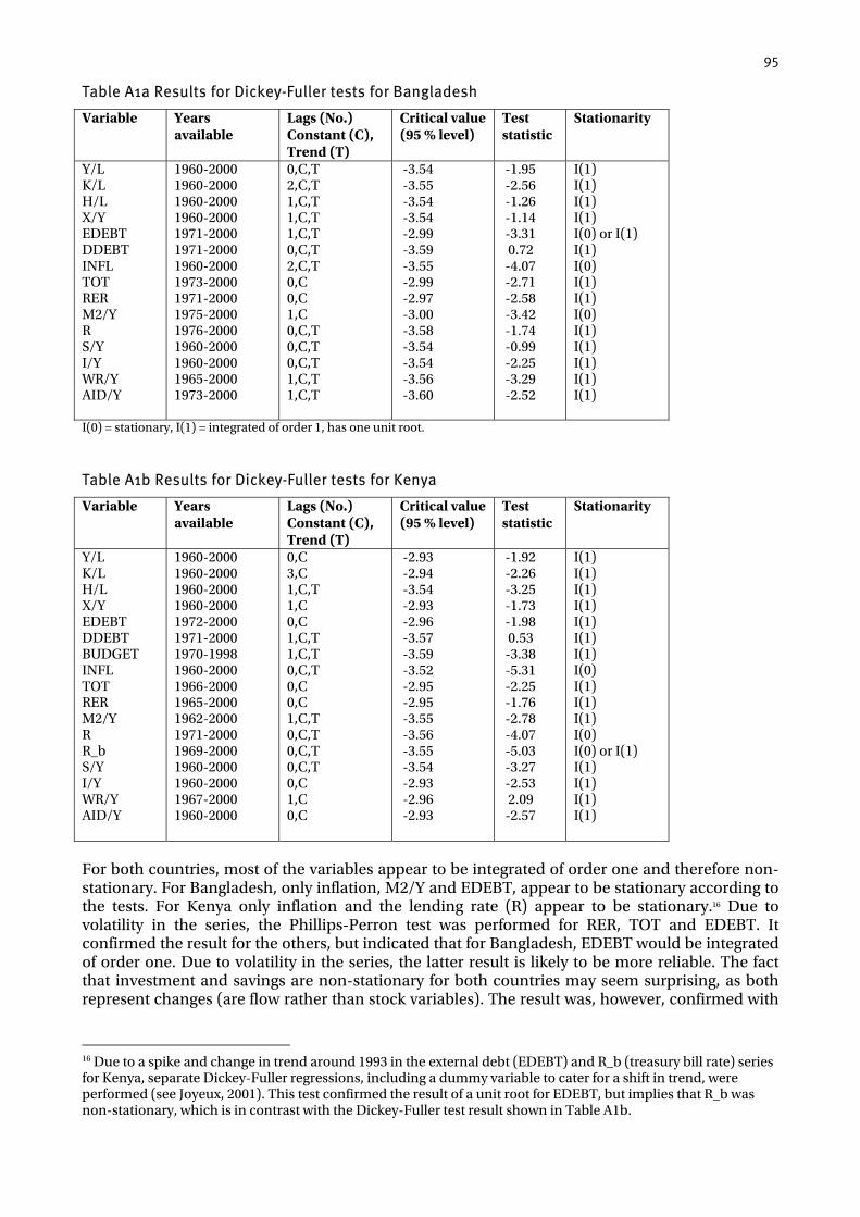
95

Table A1a Results for Dickey-Fuller tests for Bangladesh

Variable Years available

Lags (No.) Constant (C), Trend (T)

Critical value (95 % level)

Test statistic

Stationarity

Y/L K/L H/L X/Y EDEBT DDEBT INFL TOT RER M2/Y R S/Y I/Y WR/Y AID/Y

1960-2000 1960-2000 1960-2000 1960-2000 1971-2000 1971-2000 1960-2000 1973-2000 1971-2000 1975-2000 1976-2000 1960-2000 1960-2000 1965-2000 1973-2000

0,C,T 2,C,T 1,C,T 1,C,T 1,C,T 0,C,T 2,C,T 0,C 0,C 1,C 0,C,T 0,C,T 0,C,T 1,C,T 1,C,T

-3.54 -3.55 -3.54 -3.54 -2.99 -3.59 -3.55 -2.99 -2.97 -3.00 -3.58 -3.54 -3.54 -3.56 -3.60

-1.95 -2.56 -1.26 -1.14 -3.31 0.72 -4.07 -2.71 -2.58 -3.42 -1.74 -0.99 -2.25 -3.29 -2.52

I(1) I(1) I(1) I(1) I(0) or I(1) I(1) I(0) I(1) I(1) I(0) I(1) I(1) I(1) I(1) I(1)

I(0) = stationary, I(1) = integrated of order 1, has one unit root.

Table A1b Results for Dickey-Fuller tests for Kenya

Variable Years available

Lags (No.) Constant (C), Trend (T)

Critical value (95 % level)

Test statistic

Stationarity

Y/L K/L H/L X/Y EDEBT DDEBT BUDGET INFL TOT RER M2/Y R R_b S/Y I/Y WR/Y AID/Y

1960-2000 1960-2000 1960-2000 1960-2000 1972-2000 1971-2000 1970-1998 1960-2000 1966-2000 1965-2000 1962-2000 1971-2000 1969-2000 1960-2000 1960-2000 1967-2000 1960-2000

0,C 3,C 1,C,T 1,C 0,C 1,C,T 1,C,T 0,C,T 0,C 0,C 1,C,T 0,C,T 0,C,T 0,C,T 0,C 1,C 0,C

-2.93 -2.94 -3.54 -2.93 -2.96 -3.57 -3.59 -3.52 -2.95 -2.95 -3.55 -3.56 -3.55 -3.54 -2.93 -2.96 -2.93

-1.92 -2.26 -3.25 -1.73 -1.98 0.53 -3.38 -5.31 -2.25 -1.76 -2.78 -4.07 -5.03 -3.27 -2.53 2.09 -2.57

I(1) I(1) I(1) I(1) I(1) I(1) I(1) I(0) I(1) I(1) I(1) I(0) I(0) or I(1) I(1) I(1) I(1) I(1)

For both countries, most of the variables appear to be integrated of order one and therefore non-stationary. For Bangladesh, only inflation, M2/Y and EDEBT, appear to be stationary according to the tests. For Kenya only inflation and the lending rate (R) appear to be stationary.16 Due to volatility in the series, the Phillips-Perron test was performed for RER, TOT and EDEBT. It confirmed the result for the others, but indicated that for Bangladesh, EDEBT would be integrated of order one. Due to volatility in the series, the latter result is likely to be more reliable. The fact that investment and savings are non-stationary for both countries may seem surprising, as both represent changes (are flow rather than stock variables). The result was, however, confirmed with

16 Due to a spike and change in trend around 1993 in the external debt (EDEBT) and R_b (treasury bill rate) series for Kenya, separate Dickey-Fuller regressions, including a dummy variable to cater for a shift in trend, were performed (see Joyeux, 2001). This test confirmed the result of a unit root for EDEBT, but implies that R_b was non-stationary, which is in contrast with the Dickey-Fuller test result shown in Table A1b.

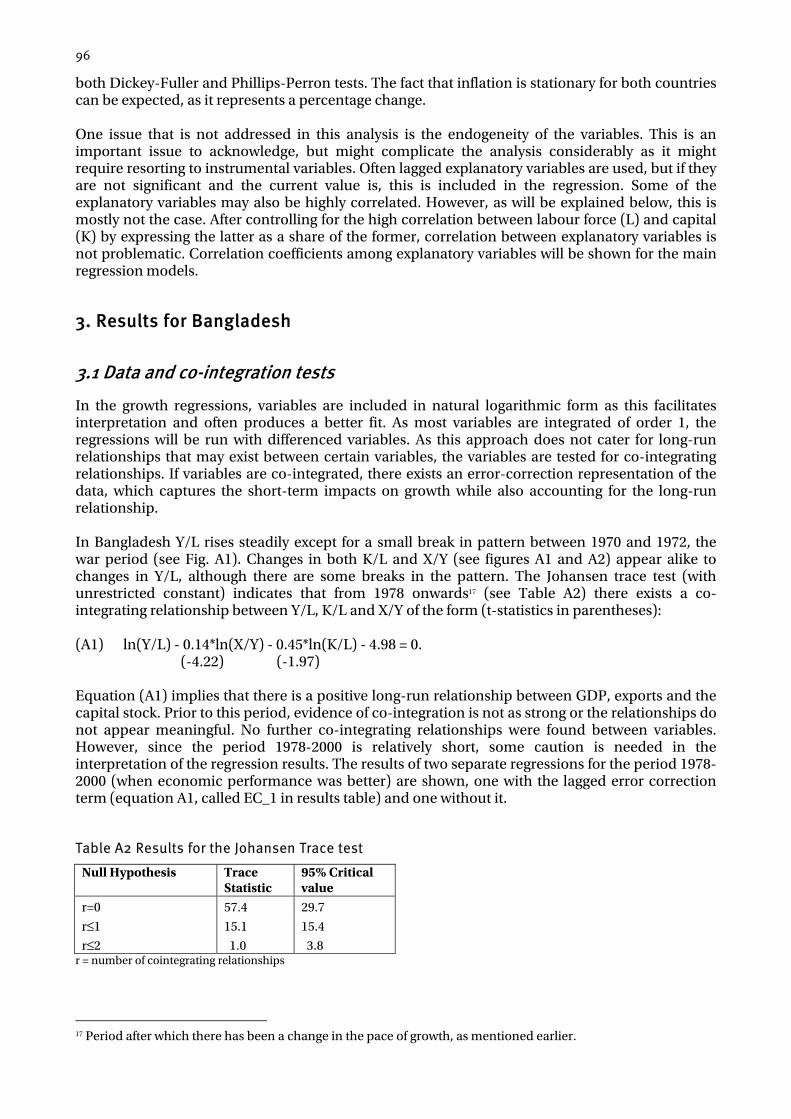
96

both Dickey-Fuller and Phillips-Perron tests. The fact that inflation is stationary for both countries can be expected, as it represents a percentage change. One issue that is not addressed in this analysis is the endogeneity of the variables. This is an important issue to acknowledge, but might complicate the analysis considerably as it might require resorting to instrumental variables. Often lagged explanatory variables are used, but if they are not significant and the current value is, this is included in the regression. Some of the explanatory variables may also be highly correlated. However, as will be explained below, this is mostly not the case. After controlling for the high correlation between labour force (L) and capital (K) by expressing the latter as a share of the former, correlation between explanatory variables is not problematic. Correlation coefficients among explanatory variables will be shown for the main regression models.

3. Results for Bangladesh

3.1 Data and co-integration tests

In the growth regressions, variables are included in natural logarithmic form as this facilitates interpretation and often produces a better fit. As most variables are integrated of order 1, the regressions will be run with differenced variables. As this approach does not cater for long-run relationships that may exist between certain variables, the variables are tested for co-integrating relationships. If variables are co-integrated, there exists an error-correction representation of the data, which captures the short-term impacts on growth while also accounting for the long-run relationship. In Bangladesh Y/L rises steadily except for a small break in pattern between 1970 and 1972, the war period (see Fig. A1). Changes in both K/L and X/Y (see figures A1 and A2) appear alike to changes in Y/L, although there are some breaks in the pattern. The Johansen trace test (with unrestricted constant) indicates that from 1978 onwards17 (see Table A2) there exists a co-integrating relationship between Y/L, K/L and X/Y of the form (t-statistics in parentheses): (A1) ln(Y/L) - 0.14*ln(X/Y) - 0.45*ln(K/L) - 4.98 = 0. (-4.22) (-1.97) Equation (A1) implies that there is a positive long-run relationship between GDP, exports and the capital stock. Prior to this period, evidence of co-integration is not as strong or the relationships do not appear meaningful. No further co-integrating relationships were found between variables. However, since the period 1978-2000 is relatively short, some caution is needed in the interpretation of the regression results. The results of two separate regressions for the period 1978-2000 (when economic performance was better) are shown, one with the lagged error correction term (equation A1, called EC_1 in results table) and one without it.

Table A2 Results for the Johansen Trace test

Null Hypothesis Trace Statistic

95% Critical value

r=0 57.4 29.7

r≤1 15.1 15.4

r≤2 1.0 3.8 r = number of cointegrating relationships

17 Period after which there has been a change in the pace of growth, as mentioned earlier.

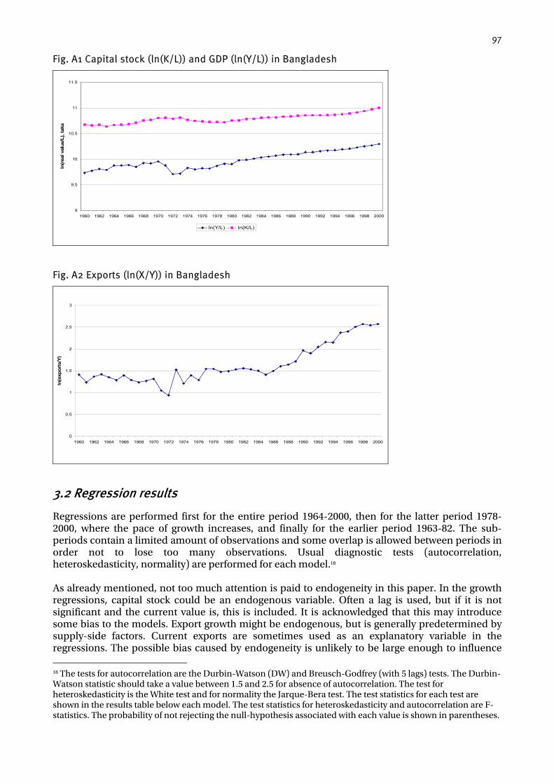
97

Fig. A1 Capital stock (ln(K/L)) and GDP (ln(Y/L)) in Bangladesh

9

9.5

10

10.5

11

11.5

1960 1962 1964 1966 1968 1970 1972 1974 1976 1978 1980 1982 1984 1986 1988 1990 1992 1994 1996 1998 2000

ln(r

eal v

alue

/L),

taka

ln(Y/L) ln(K/L)

Fig. A2 Exports (ln(X/Y)) in Bangladesh

0

0.5

1

1.5

2

2.5

3

1960 1962 1964 1966 1968 1970 1972 1974 1976 1978 1980 1982 1984 1986 1988 1990 1992 1994 1996 1998 2000

ln(e

xpor

ts/Y

)

3.2 Regression results

Regressions are performed first for the entire period 1964-2000, then for the latter period 1978-2000, where the pace of growth increases, and finally for the earlier period 1963-82. The sub-periods contain a limited amount of observations and some overlap is allowed between periods in order not to lose too many observations. Usual diagnostic tests (autocorrelation, heteroskedasticity, normality) are performed for each model.18 As already mentioned, not too much attention is paid to endogeneity in this paper. In the growth regressions, capital stock could be an endogenous variable. Often a lag is used, but if it is not significant and the current value is, this is included. It is acknowledged that this may introduce some bias to the models. Export growth might be endogenous, but is generally predetermined by supply-side factors. Current exports are sometimes used as an explanatory variable in the regressions. The possible bias caused by endogeneity is unlikely to be large enough to influence 18 The tests for autocorrelation are the Durbin-Watson (DW) and Breusch-Godfrey (with 5 lags) tests. The Durbin-Watson statistic should take a value between 1.5 and 2.5 for absence of autocorrelation. The test for heteroskedasticity is the White test and for normality the Jarque-Bera test. The test statistics for each test are shown in the results table below each model. The test statistics for heteroskedasticity and autocorrelation are F-statistics. The probability of not rejecting the null-hypothesis associated with each value is shown in parentheses.

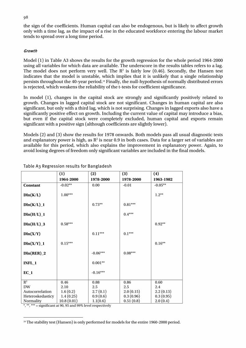
98

the sign of the coefficients. Human capital can also be endogenous, but is likely to affect growth only with a time lag, as the impact of a rise in the educated workforce entering the labour market tends to spread over a long time period.

Growth

Model (1) in Table A3 shows the results for the growth regression for the whole period 1964-2000 using all variables for which data are available. The underscore in the results tables refers to a lag. The model does not perform very well. The R2 is fairly low (0.46). Secondly, the Hansen test indicates that the model is unstable, which implies that it is unlikely that a single relationship persists throughout the 40-year period.19 Finally, the null-hypothesis of normally distributed errors is rejected, which weakens the reliability of the t-tests for coefficient significance. In model (1), changes in the capital stock are strongly and significantly positively related to growth. Changes in lagged capital stock are not significant. Changes in human capital are also significant, but only with a third lag, which is not surprising. Changes in lagged exports also have a significantly positive effect on growth. Including the current value of capital may introduce a bias, but even if the capital stock were completely excluded, human capital and exports remain significant with a positive sign (although coefficients are slightly lower). Models (2) and (3) show the results for 1978 onwards. Both models pass all usual diagnostic tests and explanatory power is high, as R2 is near 0.9 in both cases. Data for a larger set of variables are available for this period, which also explains the improvement in explanatory power. Again, to avoid losing degrees of freedom only significant variables are included in the final models.

Table A3 Regression results for Bangladesh

(1) (2) (3) (4) 1964-2000 1978-2000 1978-2000 1963-1982 Constant -0.02** 0.00 -0.01 -0.05** Dln(K/L) 1.00*** 1.2** Dln(K/L)_1 0.73** 0.81*** Dln(H/L)_1 0.4*** Dln(H/L)_3 0.58*** 0.92** Dln(X/Y) 0.11*** 0.1*** Dln(X/Y)_1 0.15*** 0.16** Dln(RER)_2 -0.06*** 0.08*** INFL_1 0.001** EC_1 -0.16*** R2 0.46 0.88 0.86 0.60 DW 2.10 2.5 2.5 2.4 Autocorrelation 1.6 (0.2) 2.7 (0.1) 2.0 (0.15) 2.2 (0.13) Heteroskedasticy 1.4 (0.25) 0.9 (0.6) 0.3 (0.96) 0.3 (0.95) Normality 10.8 (0.01) 1.1(0.6) 0.51 (0.8) 2.0 (0.4) *, **, *** = significant at 90, 95 and 99% level respectively

19 The stability test (Hansen) is only performed for models for the entire 1960-2000 period.

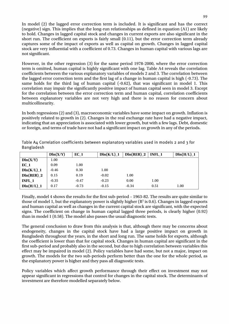
99

In model (2) the lagged error correction term is included. It is significant and has the correct (negative) sign. This implies that the long-run relationships as defined in equation (A1) are likely to hold. Changes in lagged capital stock and changes in current exports are also significant in the short run. The coefficient on exports is fairly small (0.11), but the error correction term already captures some of the impact of exports as well as capital on growth. Changes in lagged capital stock are very influential with a coefficient of 0.73. Changes in human capital with various lags are not significant. However, in the other regression (3) for the same period 1978-2000, where the error correction term is omitted, human capital is highly significant with one lag. Table A4 reveals the correlation coefficients between the various explanatory variables of models 2 and 3. The correlation between the lagged error correction term and the first lag of a change in human capital is high (-0.73). The same holds for the third lag of human capital (-0.62), that was significant in model 1. This correlation may impair the significantly positive impact of human capital seen in model 3. Except for the correlation between the error correction term and human capital, correlation coefficients between explanatory variables are not very high and there is no reason for concern about multicollinearity. In both regressions (2) and (3), macroeconomic variables have some impact on growth. Inflation is positively related to growth in (2). Changes in the real exchange rate have had a negative impact, indicating that an appreciation is associated with lower growth, but with a few lags. Debt, domestic or foreign, and terms of trade have not had a significant impact on growth in any of the periods.

Table A4 Correlation coefficients between explanatory variables used in models 2 and 3 for Bangladesh

Dln(X/Y) EC_1 Dln(K/L)_1 Dln(RER)_2 INFL_1 Dln(H/L)_1 Dln(X/Y) 1.00 EC_1 0.09 1.00 Dln(K/L)_1 -0.46 0.30 1.00

Dln(RER)_2 0.15 0.19 -0.02 1.00

INFL_1 -0.35 -0.47 -0.23 0.00 1.00

Dln(H/L)_1 0.17 -0.73 -0.15 -0.34 0.51 1.00

Finally, model 4 shows the results for the first sub-period – 1963-82. The results are quite similar to those of model 1, but the explanatory power is slightly higher (R2 is 0.6). Changes in lagged exports and human capital as well as changes in the current capital stock are significant, with the expected signs. The coefficient on change in human capital lagged three periods, is clearly higher (0.92) than in model 1 (0.58). The model also passes the usual diagnostic tests. The general conclusion to draw from this analysis is that, although there may be concerns about endogeneity, changes in the capital stock have had a large positive impact on growth in Bangladesh throughout the years, in the short and long run. The same holds for exports, although the coefficient is lower than that for capital stock. Changes in human capital are significant in the first sub-period and probably also in the second, but due to high correlation between variables this effect may be impaired in model (2). Policy variables have had some, but not a major, impact on growth. The models for the two sub-periods perform better than the one for the whole period, as the explanatory power is higher and they pass all diagnostic tests. Policy variables which affect growth performance through their effect on investment may not appear significant in regressions that control for changes in the capital stock. The determinants of investment are therefore modelled separately below.

100

Investment

The analysis of the determinants of investment is less rigorous than that of growth, as estimating a well-performing model proved more difficult and there were some problems with the diagnostic tests. There may also be similar concerns with endogeneity to those in the growth regressions, for instance between investment and savings. However, in order to obtain some indication of the possible determinants and differences in them between the two countries, a single regression is performed for both Bangladesh and Kenya. The results for Bangladesh are shown below in Table A5. In this model the variables are not in logarithmic form, since the savings variable takes a negative value in some years. Including all variables in non-logarithmic form may therefore facilitate interpretation. As most variables have a unit root, variables were included in first differences. One might expect variables such as S/Y, I/Y and R (interest rate) to be co-integrated, but the Johansen test confirms that this is not the case. The regression results are shown for 1966-2000, the entire period for which data are available. The results (Table A5) indicate that both savings and remittances have promoted investment, although savings are only significant at the 90% level. The coefficient on remittances (WR/Y) is much higher than on savings (S/Y), as remittances per GDP are much smaller in absolute value. AID/Y and macroeconomic variables were not significant. Changes in lagged GDP are not significant, but are included as a control variable that reduces a bias indicated by diagnostic tests. The model is still not entirely reliable, as the null hypothesis for normally distributed errors is rejected at the 95% level, but it does pass other diagnostic tests. The R2 is fairly low. The regression is only performed for total investment due to lack of data on private investment.

Table A5 Investment regression for Bangladesh

Dependent variable: D(I/Y) 1966-2000

Constant 0.5 D(Y)_1 0.0 D(S/Y) 0.2* D(WR/Y) 77** R2 0.48 DW 2.3 Autocorrelation 0.64 (0.63) Heteroskedasticity 0.76 (0.68) Normality 8.28 (0.02)

4. Results for Kenya

4.1 Data

As was the case for Bangladesh, most of the variables for Kenya are integrated of order 1 (see Table A1b) and therefore variables are used mostly in differenced form in the regressions. Graphical illustrations show that many of the variables to be used in the regressions either have a variable pattern through time (TOT, X/Y) or change clearly at a certain point. There may also be breakpoints in the data, where relationships change. However, if these changes in the pattern of Y/L coincide with those in other variables, the relationships are likely to hold. Figures of the

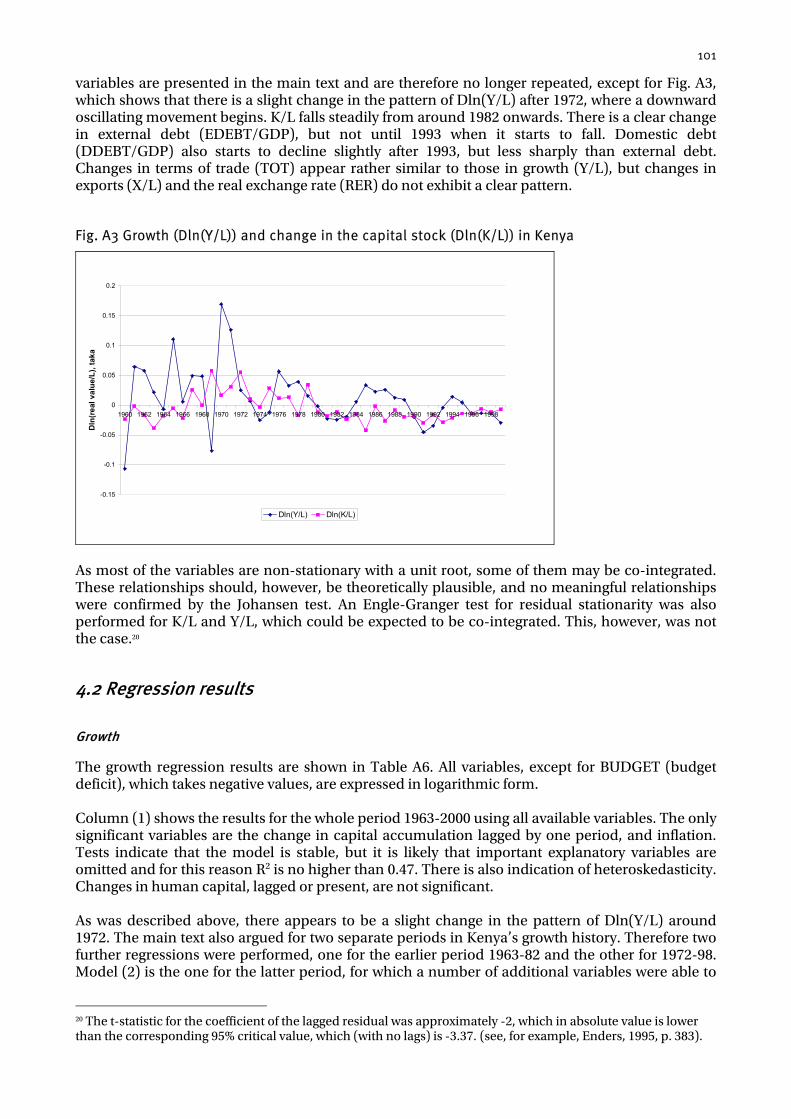
101

variables are presented in the main text and are therefore no longer repeated, except for Fig. A3, which shows that there is a slight change in the pattern of Dln(Y/L) after 1972, where a downward oscillating movement begins. K/L falls steadily from around 1982 onwards. There is a clear change in external debt (EDEBT/GDP), but not until 1993 when it starts to fall. Domestic debt (DDEBT/GDP) also starts to decline slightly after 1993, but less sharply than external debt. Changes in terms of trade (TOT) appear rather similar to those in growth (Y/L), but changes in exports (X/L) and the real exchange rate (RER) do not exhibit a clear pattern.

Fig. A3 Growth (Dln(Y/L)) and change in the capital stock (Dln(K/L)) in Kenya

-0.15

-0.1

-0.05

0

0.05

0.1

0.15

0.2

1960 1962 1964 1966 1968 1970 1972 1974 1976 1978 1980 1982 1984 1986 1988 1990 1992 1994 1996 1998

Dln

(rea

l val

ue/L

), ta

ka

Dln(Y/L) Dln(K/L)

As most of the variables are non-stationary with a unit root, some of them may be co-integrated. These relationships should, however, be theoretically plausible, and no meaningful relationships were confirmed by the Johansen test. An Engle-Granger test for residual stationarity was also performed for K/L and Y/L, which could be expected to be co-integrated. This, however, was not the case.20

4.2 Regression results

Growth

The growth regression results are shown in Table A6. All variables, except for BUDGET (budget deficit), which takes negative values, are expressed in logarithmic form. Column (1) shows the results for the whole period 1963-2000 using all available variables. The only significant variables are the change in capital accumulation lagged by one period, and inflation. Tests indicate that the model is stable, but it is likely that important explanatory variables are omitted and for this reason R2 is no higher than 0.47. There is also indication of heteroskedasticity. Changes in human capital, lagged or present, are not significant. As was described above, there appears to be a slight change in the pattern of Dln(Y/L) around 1972. The main text also argued for two separate periods in Kenya’s growth history. Therefore two further regressions were performed, one for the earlier period 1963-82 and the other for 1972-98. Model (2) is the one for the latter period, for which a number of additional variables were able to

20 The t-statistic for the coefficient of the lagged residual was approximately -2, which in absolute value is lower than the corresponding 95% critical value, which (with no lags) is -3.37. (see, for example, Enders, 1995, p. 383).

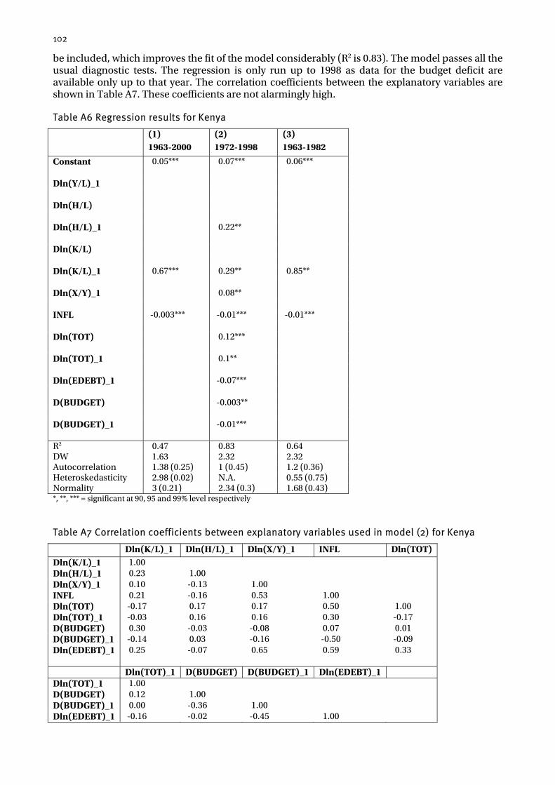
102

be included, which improves the fit of the model considerably (R2 is 0.83). The model passes all the usual diagnostic tests. The regression is only run up to 1998 as data for the budget deficit are available only up to that year. The correlation coefficients between the explanatory variables are shown in Table A7. These coefficients are not alarmingly high.

Table A6 Regression results for Kenya

(1) (2) (3) 1963-2000 1972-1998 1963-1982

Constant 0.05*** 0.07*** 0.06*** Dln(Y/L)_1 Dln(H/L) Dln(H/L)_1 0.22** Dln(K/L) Dln(K/L)_1 0.67*** 0.29** 0.85** Dln(X/Y)_1 0.08** INFL -0.003*** -0.01*** -0.01*** Dln(TOT) 0.12*** Dln(TOT)_1 0.1** Dln(EDEBT)_1 -0.07*** D(BUDGET) -0.003** D(BUDGET)_1 -0.01*** R2 0.47 0.83 0.64 DW 1.63 2.32 2.32 Autocorrelation 1.38 (0.25) 1 (0.45) 1.2 (0.36) Heteroskedasticity 2.98 (0.02) N.A. 0.55 (0.75) Normality 3 (0.21) 2.34 (0.3) 1.68 (0.43) *, **, *** = significant at 90, 95 and 99% level respectively

Table A7 Correlation coefficients between explanatory variables used in model (2) for Kenya

Dln(K/L)_1 Dln(H/L)_1 Dln(X/Y)_1 INFL Dln(TOT) Dln(K/L)_1 1.00 Dln(H/L)_1 0.23 1.00 Dln(X/Y)_1 0.10 -0.13 1.00 INFL 0.21 -0.16 0.53 1.00 Dln(TOT) -0.17 0.17 0.17 0.50 1.00 Dln(TOT)_1 -0.03 0.16 0.16 0.30 -0.17 D(BUDGET) 0.30 -0.03 -0.08 0.07 0.01 D(BUDGET)_1 -0.14 0.03 -0.16 -0.50 -0.09 Dln(EDEBT)_1 0.25 -0.07 0.65 0.59 0.33 Dln(TOT)_1 D(BUDGET) D(BUDGET)_1 Dln(EDEBT)_1 Dln(TOT)_1 1.00 D(BUDGET) 0.12 1.00 D(BUDGET)_1 0.00 -0.36 1.00 Dln(EDEBT)_1 -0.16 -0.02 -0.45 1.00

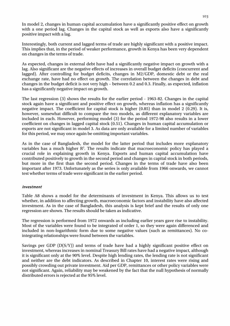
103

In model 2, changes in human capital accumulation have a significantly positive effect on growth with a one period lag. Changes in the capital stock as well as exports also have a significantly positive impact with a lag. Interestingly, both current and lagged terms of trade are highly significant with a positive impact. This implies that, in the period of weaker performance, growth in Kenya has been very dependent on changes in the terms of trade. As expected, changes in external debt have had a significantly negative impact on growth with a lag. Also significant are the negative effects of increases in overall budget deficits (concurrent and lagged). After controlling for budget deficits, changes in M2/GDP, domestic debt or the real exchange rate, have had no effect on growth. The correlation between the changes in debt and changes in the budget deficit is not very high – between 0.2 and 0.3. Finally, as expected, inflation has a significantly negative impact on growth. The last regression (3) shows the results for the earlier period - 1963-82. Changes in the capital stock again have a significant and positive effect on growth, whereas inflation has a significantly negative impact. The coefficient for capital stock is higher (0.85) than in model 2 (0.29). It is, however, somewhat difficult to compare the two models, as different explanatory variables are included in each. However, performing model (3) for the period 1972-98 also results in a lower coefficient on changes in lagged capital stock (0.51). Changes in human capital accumulation or exports are not significant in model 3. As data are only available for a limited number of variables for this period, we may once again be omitting important variables. As in the case of Bangladesh, the model for the latter period that includes more explanatory variables has a much higher R2. The results indicate that macroeconomic policy has played a crucial role in explaining growth in Kenya. Exports and human capital accumulation have contributed positively to growth in the second period and changes in capital stock in both periods, but more in the first than the second period. Changes in the terms of trade have also been important after 1973. Unfortunately as the series is only available from 1966 onwards, we cannot test whether terms of trade were significant in the earlier period.

Investment

Table A8 shows a model for the determinants of investment in Kenya. This allows us to test whether, in addition to affecting growth, macroeconomic factors and instability have also affected investment. As in the case of Bangladesh, this analysis is kept brief and the results of only one regression are shown. The results should be taken as indicative. The regression is performed from 1972 onwards as including earlier years gave rise to instability. Most of the variables were found to be integrated of order 1, so they were again differenced and included in non-logarithmic form due to some negative values (such as remittances). No co-integrating relationships were found between the variables. Savings per GDP (D(S/Y)) and terms of trade have had a highly significant positive effect on investment, whereas increases in nominal Treasury Bill rates have had a negative impact, although it is significant only at the 90% level. Despite high lending rates, the lending rate is not significant and neither are the debt indicators. As described in Chapter 10, interest rates were rising and possibly crowding out private investment. Aid per GDP, remittances or other policy variables were not significant. Again, reliability may be weakened by the fact that the null hypothesis of normally distributed errors is rejected at the 95% level.

104

Table A8 Investment regression for Kenya

Dependent variable: D(I/Y) 1972-2000

Constant -0.2 D(S/Y) 0.36*** D(TOT)_1 0.21*** DR_b_1 -0.1* R2 0.63 DW 2.4 Autocorrelation 0.8 (0.55) Heteroskedasticity 1 (0.48) Normality 8.1 (0.02)

5. Conclusions

Changes in the capital stock have been a significant determinant of growth in Bangladesh and Kenya in both periods, but in the latter the impact has been larger in the earlier period when growth was higher. In Kenya human capital has contributed significantly to growth only in the latter period. In Bangladesh its impact is clearly positive in the first period. It is also significant in the second, but, due to correlation between variables, the result depends on the model specification. The effect of human capital on growth is generally difficult to trace in time series analysis, as it may only reveal itself in the long run. However, no long-run co-integrating relationship was found between growth and human capital. In Bangladesh exports have promoted growth throughout the years and there is evidence of both a short- and a long-run relation. In Kenya export growth had a positive impact on GDP growth only in the latter sub-period of worse performance. Macroeconomic and external factors such as the debt and terms of trade have had a stronger impact on growth in Kenya than in Bangladesh. No clear relationship was found between aid and growth in either country, as the estimated coefficients were not robust, but varied in magnitude and sign with changes in model specification. The analysis of investment may be less reliable than that of growth, because error terms are not normally distributed and, for Bangladesh, the explanatory power of the model is not very high. However, although the results may be questionable, policy factors (interest rates and terms of trade) are again found to be influential in Kenya, but insignificant in Bangladesh. In Bangladesh remittances have clearly promoted investment. Aid was insignificant in both cases. For both countries, the growth model for the second sub-period is likely to be more accurate, as it has been possible to include more variables and these equations exhibit greater explanatory power. The regressions for the earlier sub-period may be subject to omitted variable bias. Although the growth regressions rely on relatively short time series, they perform quite well and some clear differences are observed in the determinants of growth in the two countries.

Why is Bangladesh Outperforming Kenya

Documents