Why Are Semiconductor Price Indexes Falling So Fast ...

Why Are Semiconductor Price Indexes Falling So Fast? Industry Estimates and Implications for Productivity Measurement

Ana Aizcorbe

WP2005-07

September 1, 2005

The views expressed in this paper are solely those of the author and not necessarily those of the U.S. Bureau of Economic Analysis

or the U.S. Department of Commerce.

Why Are Semiconductor Price Indexes Falling So Fast?

Industry Estimates and Implications for Productivity Measurement

Ana Aizcorbe

Bureau of Economic Analysis

March 2002

Revised June 2005

JEL Codes: D42, L63, O47

* I thank Steve Oliner and Dan Sichel for many useful discussions and extremely

helpful comments and Tim Bresnahan for his comments at the CRIW

workshop at the 2002 NBER Summer Institute. I am also grateful to J. Chiang, Nile

Hatch, Bart Hobijn, Sam Kortum, David Lebow, Kevin Stiroh, Jack Triplett, Philip

Webre and the anonymous referees for useful comments. Kevin Krewell (MicroDesign

Resources) kindly provided the data on Intel’s operations and Christopher Schildt and

Sarah Rosenfeld provided excellent research assistance. The views expressed in this

paper are solely mine and should not attributed to the Bureau of Economic Analysis or its

staff. Contact Information: Ana Aizcorbe, [email protected] Bureau of Economic

Analysis, 1441 L Street, NW, Washington, DC 20230; Voice: (202)606-9985; FAX:

(202)606-5310

3

Why Are Semiconductor Price Indexes Falling So Fast?

Industry Estimates and Implications for Productivity Measurement

Ana Aizcorbe

A B S T R A C T

By any measure, price deflators for semiconductors fell at a staggering pace over

much of the last decade, pulled down by steep declines in the deflator for the

microprocessor (MPU) segment. These rapid price declines are typically attributed to

technological innovations that lower constant-quality manufacturing costs through either

increases in the quality of the devices or decreases in costs. However, Intel’s dominance

in the microprocessor market raises the possibility that those price declines could also

reflect changes in Intel’s profit margins.

This paper uses industry estimates on Intel’s operations to decompose a price

index for Intel’s MPUs into three components: quality improvements, reductions in

costs, and changes in markups. The decomposition suggests that 1) virtually all of the

declines in a price index for Intel’s chips can be attributed to quality increases associated

with product innovation, rather than declines in the cost per chip. Of course, these

increases in quality pushed down constant-quality costs. However, cost per chip did not

play a role in generating the observed price declines in the MPU price index, as cost

increases associated with the introduction of new, higher quality chips more than offset

cost reductions associated with learning economies. With regard to markups, the sizable

4

decline in Intel's markups from 1993-99 only accounted for about 6 percentage points of

the average 24 percent decline per quarter in a price index for Intel’s chips

Consistent with the inflection point that Jorgenson(2000) noted in the overall

price index for semiconductors, the Intel price index falls faster after 1995 than in the

earlier period but, again, the decomposition attributes virtually all of the inflection point

to an acceleration in quality increases.

5

1. Introduction

By any measure, price deflators for semiconductors fell at a staggering pace over

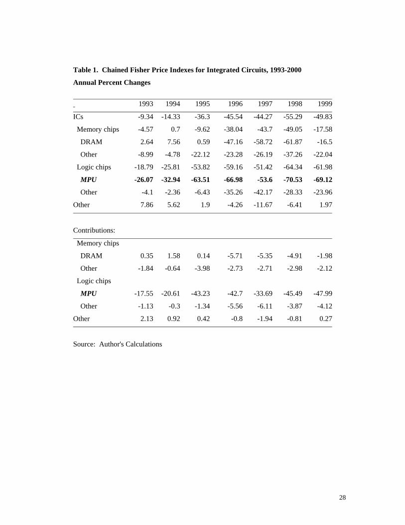
much of the last decade. As shown in the top panel of table 1, Fisher price indexes for

integrated circuits—ICs, a broad class of semiconductor devices that includes logic and

memory chips—fell an average of 36 percent each year from 1993 to 1999. As shown in

the bottom panel, those price declines were generated primarily by sharp declines in the

price index for microprocessors—MPUs, the logic chips that serve as the central

processing unit in PCs.

The price deflator for ICs fell even faster in the second half of the decade, pushed

down by faster declines in the MPU price index. Jorgenson (2000) noted the acceleration

and hypothesized that the development and deployment of semiconductors could have

been a key driver in the economy-wide resurgence in economic growth that began in the

mid-1990s. Empirical work based on macroeconomic growth models supported his

hypothesis by showing that the semiconductor industry accounted for nearly three-fourths

of the acceleration in multifactor productivity that occurred over the 1990s.TP

1PT

These sharp declines are typically attributed to the rapid rate of product

innovation that characterizes this sector (See, for example, Triplett (2004)). Informal

measures of quality change suggest that quality change is the primary driver behind the

price declines typically seen for these devices (Aizcorbe, Corrado, and Doms (2000)).

Indeed, the industry is credited with one of the fastest rates of product innovation and

technical change within manufacturing, as chipmakers generate wave after wave of ever-

more powerful chips for prices not much higher than those of existing chips.

6

At the same time that the quality of MPUs is increasing, manufacturers are also

getting better at producing them and the attendant reductions in the manufacturing cost

per chip could also have contributed to the observed declines in the price index. As is

well known, the semiconductor production process is subject to important learning

economies along several dimensions (See, for example, Gruber (1994) and Hatch and

Mowery (1998)). Most of the empirical literature on learning by doing in the

semiconductor industry has focused on memory chips—a homogeneous commodity good

sold in fairly competitive markets. For MPUs, Intel’s dominance of the market has

generated large markups so that cost savings from learning-by-doing may not necessarily

be passed along to consumers in the form of lower prices.

The presence of large markups, in and of itself, has potential implications for

price measurement: while quality increases and reductions in cost per chip are associated

with increases in productivity, changes in markups are not. Over the 1990s, Intel’s

markups shrank as increased competition from its rivals and weaker-than-expected

demand for personal computers in 1995 and beyond put downward pressure on prices.

This decline in Intel’s markup could have potentially distorted standard price indexes

because those indexes implicitly assume perfect competition.TP

2PT So, for example, falling

markups could lead one to incorrectly interpret the resulting price decline as a

productivity improvement.TP

3PT Although it is unlikely that Intel’s markups fell sufficiently

fast to explain much of the absolute price declines over the decade, those declines may,

nonetheless, have had a nontrivial effect on the acceleration that began in 1995.

To better understand the trend and inflection point in semiconductor prices, this

paper decomposes movements in the constant-quality price index into changes in the

7

index associated with productivity growth and those associated with markups. A further

decomposition of the productivity-related component into quality change—owing to

rapid rates of product innovation—vs. changes in cost per chip—perhaps related to

learning-by-doing—is also done. This is useful for predicting the likely effect of future

developments in the industry to changes on the price index and productivity. Moreover,

understanding the link between learning-by-doing—a phenomenon thought to be

important for other semiconductor devices—and productivity in the MPU segment is also

of interest.

The decomposition suggests that virtually all of the price declines in the Intel

price index can be attributed to quality increases associated with product innovation

rather than declines in cost per chip; increases in quality obviously pushed down

constant-quality prices, but cost per chip do not seem to have played a role in generating

the observed price declines because cost reductions associated with learning were more

than offset by cost increases associated with the introduction of new, higher-quality

chips. Although markups from Intel’s MPU segment shrank substantially from 1993-99,

those declines accounted for only about 6 percentage points of the average 24 percent per

quarter decline in its price index. Similarly, changes in quality were the primary driver

behind the inflection point seen in 1995.

The paper is organized as follows. Section 2 uses industry estimates of chip-level

prices to show that both the absolute declines and the inflection point in the MPU price

index reflect large quality increases. Section 3 uses cost estimates to explore the

contributions of changes in the cost per chip and markups to the observed declines in the

MPU price index. Section 4 concludes.

8

2. Measuring Changes in the Average Quality of Intel’s MPUs

"Discussions of "quality" in price indexes often place the term in quotation marks and

few authors have attempted to provide a rigorous definition."TP

4PT

The difference between a constant-quality index and an average price series is

often interpreted as an informal measure of quality both by practitioners in industry and

by researchers interested in price measurement.TP

5PT The idea is that if a price index holds

quality constant and an average price series does not, then the average price can be stated

as the sum of a constant-quality index and a quality measure. As in Raff and Trajtenberg

(1997), the identity is:

(1) dln (average price) ≡ dln (constant-quality price index) + dln (quality)

The problem in numerically implementing this notion is that while theory tells us how

to measure constant-quality prices, it does not tell us how to measure the average price

series. Should it be an arithmetic average or a geometric average? Should the weights be

fixed or variable? Does it matter? TP

PT

UInterpreting Informal Measures of Quality Change

The paradigm that comes to mind when thinking about quality change is the

framework implicitly used by the Bureau of Labor Statistics (BLS) to hold quality

constant when replacing one good in their basket with another. Chart 1 shows the general

9

idea. The chart shows price profiles for two chips, with chip 2 replacing chip 1 at time

t=1. The change in the price per chip from t=0 to t=2 may be stated as the product of the

price changes over the life of each chip and the gap in prices of the new and exiting chip.

In terms of the diagram, the change in the price per chip is the ratio of the last price for

chip 2 (PB2,2 B ) and the first price for chip 1 (PB1,0 B). That ratio may be written as:

(2) P B2,2 B / PB1,0B = ( PB2,2B / PB2,1 B ) ( PB2,1 B / PB1,1 B ) ( PB1,1 B / PB1,0 B ).

This change in the price per chip could be viewed as a constant-quality price index only

in the hypothetical case where the two chips are of equal quality; in that case, price per

chip is all that matters. Alternatively, one can allow the chips to be of different quality

and assume that any price difference at t=1 is the market’s valuation of these quality

differences. In this view, one obtains a constant-quality price index by measuring price

changes that occur over the life of each chip--shown in bold in (2)--and excluding the gap

in the two prices at t=1. The middle term is the gap between the average price measure

on the left-hand side and the matched-model index--the product of the two bold terms on

the right.

Taking logs and rearranging terms, the average price change from t=0 to t=2 is the

sum of three terms. The first two terms make up the constant-quality index and the third

measures quality change:

(2’) ln(PB2,2 B / PB1,0B) = [ ln( PB2,2 B / PB2,1 B ) + ln( PB1,1 B / PB1,0 B ] + ln( PB2,1 B / PB1,1 B )

10

Note that the valuation of quality change is independent of any changes in the underlying

costs or markups. Market prices are viewed as a signal of the markets’ valuation of the

different chips so that the price differentials reflect quality differentials.

This seems like a sensible way to value quality change and is, in fact, the

assumption implicit in MM methods. In general, though, there are many chips that

coexist in the market, and turnover is characterized by new and existing goods

overlapping for some period of time. Loosely speaking, if one thinks of the logged prices

in (2’) as averages, then the matched-model index still measures price change over the

lives of goods existing in both periods, but quality change is measured as a difference of

(logged) means: average prices with entry (the change in an average price series) and

average prices without entry (the change in the matched-model index).

A geometric mean index provides a simple example to illustrate the point. A

matched-model geometric mean of price change over the period t, t-1 (in logged form--

lnPP

GEOPBt,t-1 B) is an arithmetic mean of logged price relatives for the goods that exist in both

periods:

(3) lnIP

GEOPBt,t-1 B = ΣB m∈match(t)B ( ln PBm,t B - ln PBm,t-1 B) /MBt B

where models that exist in both periods are denoted match(t) and the number of such

models at time t is denoted MBt.B To see how this index handles quality change, consider

an example where a new good enters at time t. In that case, the geometric mean can be

restated as a combination of two terms: TP

6PT,

(4) lnIP

GEOPBt,t-1 B = [ ΣB m∈all(t) B( ln PBm,t B ) /NBt B - ΣB m∈all(t-1)B( B Bln PBm,t-1 B) /NBt-1 B ]

11

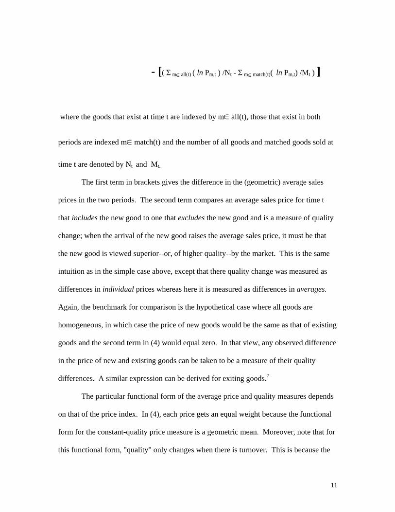
- [( ΣB m∈all(t) B( ln PBm,t B ) /NBt B - ΣB m∈match(t)B( B Bln PBm,t B) /M Bt B ) ]

where the goods that exist at time t are indexed by m∈all(t), those that exist in both

periods are indexed m∈match(t) and the number of all goods and matched goods sold at

time t are denoted by NBt B and M Bt. B

The first term in brackets gives the difference in the (geometric) average sales

prices in the two periods. The second term compares an average sales price for time t

that includes the new good to one that excludes the new good and is a measure of quality

change; when the arrival of the new good raises the average sales price, it must be that

the new good is viewed superior--or, of higher quality--by the market. This is the same

intuition as in the simple case above, except that there quality change was measured as

differences in individual prices whereas here it is measured as differences in averages.

Again, the benchmark for comparison is the hypothetical case where all goods are

homogeneous, in which case the price of new goods would be the same as that of existing

goods and the second term in (4) would equal zero. In that view, any observed difference

in the price of new and existing goods can be taken to be a measure of their quality

differences. A similar expression can be derived for exiting goods. TP

7PT

The particular functional form of the average price and quality measures depends

on that of the price index. In (4), each price gets an equal weight because the functional

form for the constant-quality price measure is a geometric mean. Moreover, note that for

this functional form, "quality" only changes when there is turnover. This is because the

12

weights in the index are fixed (at 1/N) and any changes in the relative importance (in

terms of sales, say) of one good relative to another are not counted as quality change.

In contrast, superlative indexes do capture changes in the relative importance of

goods by weighting each good’s price change by its share in nominal output. For one

such superlative index—the Tornquist—one can apply the same logic used above to show

that the Tornquist price index captures quality changes that result from both turnover—

differences in means with and without the new good—and from mix-shift among existing

goods—changes in the relative importance of existing goods. The only difference is that,

in the Tornquist, all measures use expenditure weights.

To see this, consider a matched-model Tornquist price index:

(5) lnIP

TORNPBt,t-1 B = ΣB m∈match(t)B B BωBm,t B ( ln PBm,t B - ln PBm,t-1 B)

where, as before, ΣB m∈match(t) Bdenotes a summation taken over goods available in both

periods and each ωBm,t B is an average of the time t-1 and time t expenditure weights: ωBm,t B =

½(wP

MMPB mtB+wP

MMPB mt-1 B), where wP

MMPBmt B = PBmtBQBmtB/ΣBm=match(t) BPBmtBQBmt B .

Again, consider the simple case where a new good enters at time t. In this

decomposition, average prices are weighted geometric means with weights that either

sum over all goods (wP

ALLPB mt B = PBmt BQBmt B/ΣB m∈all(t)BPBmtBQBmtB ) or over just the matched models

(wP

MMPBmt B = PBmt BQBmt B/ΣBm=match(t) BPBmtBQBmt B ). One decomposition that splits out quality change

from changes in average prices is:

(6) lnIP

TORNPBt,t-1 B = [ ΣBm∈all(t) B wP

ALLPB it B ln PBm,t B - ΣB m∈all(t-1)B wP

ALLPB it-1 B ln PBm,t-1 B ]

13

- [ ΣBm∈all(t) B wP

ALLPB it B ln PBm,t B - ΣB m∈match(t)B wP

MMPB it B ln PBm,t B ]

- [ ΣBm∈match(t) B ln PBm,t B (wP

MMPB it B - ωBm,t B ) ]

- [ ΣBm∈match(t) B ln PBm,t-1 B (ωBm,t B - wP

MMPB it-1 B ) ]

As before, the first term measures the difference in the average prices and the remaining

terms measure quality change. The second term measures quality change associated with

entry by comparing the average prices with and without the new good; it strips out any

changes in the average price that arise from the entry of the new (higher-quality) good.

In the absence of entry, all goods are matched in both periods and the term equals zero.

The last two terms capture changes in the quality measure that occur as the

relative importances of goods change over time. These terms strip out any changes in

average price that arises from changes in the composition of expenditures. For example,

suppose all the underlying prices are unchanged from time t-1 to time t but that

expenditures shift owing to changes in the market’s perception of the relative quality of

goods. The last two terms will capture this as a change in quality by changing the

weights associated with each good’s price.

Note that if goods’ expenditure shares are equal in both periods, then ωBm,t B=wP

MMPB

itB=wP

MMPB it-1 B and these two terms equal zero. Also, note that if there is no turnover and

goods’ relative importances are constant, then the Tornquist index reduces to a difference

in (weighted) average prices—the first term.

UIntel Price Data and Calculations

14

The decomposition in (6) is done using data on Intel’s MPU pricing that were

obtained from MicroDesign Resources (MDR)—the industry’s primary source for data

on Intel’s operations. The data are quarterly observations on prices, unit shipments, and

revenues for Intel’s microprocessors at a high level of product detail. MDR estimates

prices by taking Intel’s published list prices and making any needed adjustments for

volume discounts. They also estimate unit shipments and revenue data using Intel’s 10K

reports and the World Semiconductor Trade Statistics data published by the

Semiconductor Industry Association (see Aizcorbe, Corrado and Doms(2000)) for a

fuller description of the data).

Chart 2 uses price profiles for Intel’s desktop chips introduced from 1993 to 1998

to illustrate two features of these profiles that are characteristic of microprocessors and

other semiconductors.TP

8PT First, there is a high degree of turnover in this segment as new,

faster chips are brought to the market. Second, prices fall steeply over the life of each

chip; prices typically start at between $600 to $1000 at introduction--substantially higher

than the prices of existing chips. By the time the chip exits the market, its price has fallen

to under $100. The steepness of these profiles could reflect demand- or supply-driven

forces. On the demand side, the profiles are consistent with the view that users are

initially willing to pay high prices for new chips but as the introduction of the new

(better) chip nears, they are less willing to do so and prices of the incumbent chips fall.TP

9PT

On the supply side, these profiles are consistent with the view that prices over the life of

the chip are pulled down by declining costs as firms find ways to produce each chip at

lower cost.

15

Because most price indexes are essentially functions of weighted averages of

price change, the steepness of the slopes for these contours will translate into rapidly

declining price indexes. As seen in the first column of table 2, the chained, matched-

model Tornquist index for Intel’s chips falls sharply over this period: at an average rate

of 24.4 percent per quarter.TP

10PT In contrast, changes in the average price—the second

column—show little movement; falling only 2.1 percent per quarter.TP

11PT Apparently, the

average price series says more about the distribution of prices over time than it says about

declines in prices over the life of each chip. Intuitively, it is relatively flat because the

effect of declines in prices over the life of each chip on average price is undone when the

next chip enters the market at the same high introductory price.

This large gap between declines in the price index and those in average prices

implies that virtually all of the declines in the price index stem from increases in the

quality of chips; as tabulated in the last column, 22.3 percentage points of the 24.4

percent average decline in the Tornquist price index reflect increases in quality change.TP

PT

The last two rows of the table provide averages of price change in the pre- and

post-1995 period. The first column verifies the inflection point noted by Jorgenson: the

declines in the price index accelerated from an average quarterly decline of 17 percent

over 1993-1995 to about 30 percent in 1996-1999. As seen in the last column, virtually

all of the acceleration is accounted for by increases in measured quality. Average prices

did fall faster in the second half of the decade but explain only 3 percentage points of the

acceleration in the Tornquist index.

3. Measuring Changes in the Costs Per Chip

16

"In general, Intel's prices are several times the manufacturing cost of the chips, so

that cost has little influence on their price."TP

12PT

The changes in average prices calculated above can be decomposed into

contributions from changes in the cost per chip vs. those in the markup:

(7) dln (average price) ≡ dln (cost per chip) + dln(price/cost per chip)

While average prices changed little over this period, there may have been offsetting

changes in costs and markups that have different implications for movements in the

index. This section quantifies the contributions of costs and markups to changes in

average prices to assess any distortions caused by changes in markups and to explore the

role that learning economies might have played over this period.

In terms of the earlier decomposition, the first term in (6) may be broken out as

follows:

[ ΣBm∈all(t) B wP

ALLPB it B ln PBm,t B - ΣB m∈all(t-1)B wP

ALLPB it-1 B ln PBm,t-1 B ] =

(8) [ ΣBm∈all(t) B wP

ALLPB it B ln ACBm,t B - ΣB m∈all(t-1)B wP

ALLPB it-1 B ln ACBm,t-1 B ]

+ [ ΣBm∈all(t) B wP

ALLPB it B ln (PBm,t B/ACBm,t B) - ΣB m∈all(t-1)B wP

ALLPB it-1 B ln (PBm,t-1 B/ACBm,t-1 B)]

The first term measures changes in the average cost per chip and the second measures

changes in the markup. This decomposition allows one to isolate any potentially

distorting effects of increased competition in MPU markets over the 1990s on the MPU

17

price index and assess the potential importance of learning by doing on average costs

and, hence, the price index.

UManufacturing Costs and Learning

The cost structure and manufacturing process for semiconductors is extremely

complex. TP

13PT The process involves taking a silicon wafer of fixed size, etching chips—

initially called “die”—on this wafer, and eventually separating out the individual die and

packaging them for sale. The manufacturing cost per wafer is constant, so that anything

that increases the number of usable die on a wafer reduces the average cost per usable

die. An obvious way to reduce the cost per die is by increasing the size of the wafer upon

which the chips are etched, but this actually occurs only infrequently.

More commonly, firms reduce average cost by reducing the size of the die by

either reducing the size of each feature on a chip— i.e., etching smaller transistors —or

by reducing the spaces between them. Reductions in the size of features is made possible

when there are advances in the equipment used to etch the chips and, thus, requires

investment in new equipment. Reductions in the gap between features occurs with

learning as firms gain familiarity with the production of a new die and find ways to etch

these features closer together (i.e., learning). This requires less investment because it

only requires changing the masks that are used to etch the chips (not entirely replacing

the equipment).

A final way that firms lower the average cost per usable die is by increasing the

yield of production during the ramp-up of a new die. The complexity of the

manufacturing process is such that the early months of production of a new die are

18

marked by high defect rates that hold down yields—defined as the ratio of usable chips to

all chips. Within a few months of launching production, yields stabilize at about 90

percent and the average cost of production bottoms out.TP

14PT

Most of the available work on cost and pricing of semiconductor devices is for

devices in the memory segment – DRAM chips in particular. For those devices, learning

is an important driver of costs and, because that segment is fairly competitive, of prices.

In those studies (See Flamm (1989) and Irwin and Klenow (1994), for example), show

that price contours for DRAM chips are shaped much like those for MPUs shown in

Chart 2 and that learning economies are an important determinant of those contours. As

discussed below, learning plays a lesser role in determining the shape of price contours

for MPUs.TP

15PT

UIndustry Estimates for Intel’s Costs

Data on cost per chip were obtained from MDR—the same source as the price

data. Their cost estimates include labor and material costs plus depreciation of the

equipment and part of the building,TP

16PT but do not include an adjustment for the design of

the chip or other R&D costs. Thus, the cost concept is closer to variable cost than total

cost, and the implied markup could be pure profit or normal returns to R&D and chip

design.TP

17PT

As seen in the last row of table 3, the revenue and cost data imply large markups

for Intel that declined over this period from nearly 90 percent in 1993 to 73 percent by

1999. The largest declines occurred in 1995-96--when Intel was reportedly under intense

19

competition from its rivals--and again in 1998--when the recession in Asia began to

affect world demand for electronic goods.

Cost over the Life of the Chip

An important feature of the MDR estimates is that costs are estimated at

“maturity.” MDR collects the data somewhere between the “sixth and twelfth month after

the release of a new processor, when defect rates are approaching or have reached

maturity. Costs will be higher than that during the first few months of production.”TP

18PT

The timing of MDR’s cost estimates for these pioneer chips does not allow one to

say much about increased yields that could pull down costs over the lives of those chips.

Nonetheless, one can argue that cost declines associated with increases in yields cannot

explain the shape of the price contours over the life of a chip. Because costs are typically

very low relative to price. Whereas prices typically fall from about $750-1000 to about

$100 over the life of the chip, cost per chip at maturity ranges $50-100. Given this wide

gulf between price and cost per chip, even if increased yields reduced costs to one-fourth

of their original levels—from, say, $200 to $50—that would still only explain a fraction

of the observed price declines. This gap between price and average cost has important

implications for empirical studies in the learning-by-doing literature. There, learning

economies are typically estimated using average prices as a proxy for average costs. This

requires either that markups be constant over the life of the chip or that any changes in

markups be small. Although this assumption makes sense in the more-competitive

segments in the semiconductor industry (e.g., memory chips), it is clearly at odds with the

empirical evidence for MPUs.

20

It is also unlikely that this type of learning will have a large impact on the price

index. Numerically, the Tornquist weights price declines using expenditure weights.

Because the declines in average cost early in a chip’s life coincide with low yields (low

output levels), these changes in costs carry a low weight in the index and, thus, the

numerical effect of this type of learning on the price index is likely to be small.

Moreover, as explained below, the decline in costs from learning only affect a small

number of chips—the pioneering chips that introduce a new die—so that the effect on an

index over all chips is likely to be small.

Costs across chips

The distinction between “die” and “chip” is important for our purposes. Although

“chip” is the relevant concept from a demand perspective—consumers view chips with

different attributes as distinct goods—the relevant concept from a cost perspective is the

“die.” This is illustrated in chart 3, where the MDR estimates of cost per chip are given

for several of Intel’s chips that were on the market beginning in 1993, arranged by chip

family and in rough order of introduction; the older 486 chips are grouped on the left; the

Pentium I chips are in the middle and the Pentium II chips are on the right.

As may be seen, improving attributes—like the speed of the chip—does not

always increase the cost per chip. This is because chips of different speeds are often cut

from the same wafer and, therefore, cost the same to produce. Once a wafer is etched,

the individual die are tested for speed. The ubiquitous presence of defects is such that

only some die will test at a high speed and can be sold as a high-speed chip. The others

are “binned” together with chips that test at lower speeds and are sold as such. But,

21

because the cost per chip is a function of the number of chips on a wafer—not on the

speed of each chip—cost is the same for the high- and low-speed chips.

Chart 3 also shows the effect of die shrinks—one type of learning discussed

above: cost per chip declines with the introduction of new, smaller die within each chip

family—as occurred with the 75, 120, and 166 Mhz Pentium I chips. These cost declines

associated with learning are large: manufacturing cost of the last Pentium I chip was less

than one-half of the cost of the first Pentium I chip.

Finally, costs increase discretely with the introduction of new chip families as the

learning curve begins anew: for example, the first Pentium II chip costs more than twice

what the last Pentium I chip costs.

Over this period, the introduction of new chip families was such that these

increases in costs more than offset declines in costs from the learning that occurs within

chip families. As seen in the middle column of table 4, cost per chip actually increased

3.7 percentage points over 1993-1999, with the largest cost increases occurring with the

introduction of the Pentium I (in 1994) and the Pentium II (in 1997).

This increase in costs coincided with declines in Intel’s markup that contributed

about 6 percentage points to the 24.4 average quarterly decline in the MPU price index.

Looking ahead, to the extent that changes in competitive conditions have stabilized, all

else held equal, one can expect a price index for Intel’s chips to fall a bit slower in the

future than in the 1990s. The net effect of the increase in costs and the decline in

markups was a small decline in the average price (column 1).

With regard to the inflection point, as seen in the last two rows of the table, cost

per chip rose less fast in the latter part of the 1990s and contributed about 3 percentage

22

points to the decline in the overall price index. The decline in markups was the same in

the early and latter parts of the decade and, thus, does not explain any of the inflection

point.

4. Summary

This paper provides an assessment of the relative importance of technological

progress and markups in generating the observed declines in price indexes for

microprocessors over the 1993-99 period. Industry estimates on Intel’s price, cost, and

shipments of microprocessor chips at a highly disaggregate level were used to establish

that product innovation and the attendant increases in quality was the primary driver of

the steep price declines seen in price indexes for Intel’s chips over 1993-99 and of the

inflection point that occurred in 1995.

Although the cost data confirm the importance of learning economies in driving

down costs per chip, the data also show large cost increases associated with the

introduction of new chips. Over the 1990s, the rate at which new chip families were

introduced was such that the latter effect dominated and cost per chip increased. At the

same time, Intel’s markup declines, contributing about 6 percentage points to the 24

percent average quarterly decline in the price index. However, markups changed about

the same before and after 1995 and, thus, do not appear to have played a role in

generating the inflection point in 1995.

23

REFERENCES

Aizcorbe, A. M., C. Corrado and M. Doms (2000) Constructing Price and Quantity

Indexes for High Technology Goods, presented at the CRIW workshop on Price

Measurement at the NBER Summer Institute, July. Available at Twww.nber.orgUT

Anderson, S.P., A. de Palma and J. Thisse (1992) Discrete Choice Theory of Product

Differentiation. Cambridge, MA: MIT Press.

Basu, S. and J. Fernald (1997) “Returns to Scale in U.S. Production: Estimates and

Implications,” Journal of Political Economy, 105:249-283, April.

Berry, S., J.A. Levinson, and A. Pakes (1995) “Automobile Prices in Market

Equilibrium,” Econometrica 63:841-890.

Bils, M. and P.J. Klenow (2001) “Quantifying Quality Growth,” The American Economic

Review, Vol. 91, No. 4. (Sep., 2001), pp. 1006-1030. Available at:

TUhttp://links.jstor.org/sici?sici=0002-

8282%28200109%2991%3A4%3C1006%3AQQG%3E2.0.CO%3B2-UUT

Denny, M., M. Fuss and L. Waverman (1981) “The Measurement and Interpretation of

Total Factor Productivity in Regulated Industries, with an Application to Canadian

Telecommunications”, Pp. 179-218 in T. Cowing and Stevenson, eds., Productivity

Measurement in Regulated Industries, New York: Academic Press.

Diewert, W.E. (1999) “Appendix A: A Survey of Productivity Measurement,” in

Measuring New Zealand’s Productivity, Draft Report, January

24

Diewert, W.E. (1983) “The Theory of the Output Price Index and the Measurement of

Real Output Change,” in Price Level Measurement, editors W.E. Diewert and C.

Montnmarquette, Statistics Canada, Ottawa, Ontario (December 1983), pp. 1049-1113.

Domowitz, I.R., G. Hubbard and B.C. Petersen (1988) “Market Structure and Cyclical

Fluctuations in United States Manufacturing,” Review of Economics and Statistics 70:55-

66.

Feenstra, R.C. (1995) “Exact Hedonic Price Indexes,” Review of Economics and

Statistics, Pp. 634-653.

Fisher, F.M. and K. Shell (1998) Economic Analysis of Production Price Indexes,

Cambridge, U.K.: Cambridge University Press,

Flamm, K. (2003) “Moore's Law and the Economics of Semiconductor Price Trends,”

paper presented at the NBER Productivity Program meeting, Cambridge, Mass., March

14.

Flamm, K. (1996) Mismanaged Trade? Strategic Policy and the Semiconductor

Industry,Washington, D.C.: Brookings Institution

Gordon, R. (2001) “Does the New Economy Measure Up to the Great Inventions of the

Past?” in Journal of Economic Perspectives.

Greenlees, J.S. (1999) “Consumer Price Indexes: Methods for Quality and Variety

Change,” Paper presented at the Joint ECE/ILO meeting on Consumer Price Indices,

Geneva, 3-5 November 1999.

Gruber, Harold. (1994) Learning and Strategic Product Innovation: Theory and Evidence

for theSemiconductor Industry. Amsterdam: North Holland.

25

Gwennap, L and M. Thomsen (1998) “Intel Microprocessor Forecast, 4P

thP ed.” Sebastopol,

CA: MicroDesign Resources, Inc.

Hall, R. E., (1988) “The Relation Between Price and Marginal Cost in United States

Industry,” Journal of Political EconomyU,U 96:921-947.

Hatch, N. and D.C. Mowery (1998) “Process Innovation and Learning by Doing in

Semiconductor Manufacturing,” Management Science, 44:1461-1477.

Hulten, Charles R. (1997) “Quality Change in the CPI,” Federal Reserve Bank of St.

Louis Review, May/June, Pp. 87-106.

Irwin, D. A. and P. Klenow (1994) “Learning by Doing Spillovers in the Semiconductor

Industry,” Journal of Political Economy, 102(6):1200-1227, December

Jorgenson, D.W. (2000) “Information Technology and the U.S. Economy,” Presidential

Address to the American Economic Association, New Orleans, Louisiana, January 6.

Jorgenson, D.W. and K.J. Stiroh (2000) “Raising the Speed Limit: U.S. Economic

Growth in the Information Age,” The American Economic Review, Vol. 90, No. 2,

Papers and Proceedings of the One Hundred Twelfth Annual Meeting of the American

Economic Association. (May, 2000), pp. 161-167. Available at:

TUhttp://links.jstor.org/sici?sici=0002-

8282%28200005%2990%3A2%3C161%3AUEGATI%3E2.0.CO%3B2-0 UT

Jorgenson, D.W. and Z. Griliches (1967) “The Explanation of Productivity Change,” in

Review of Economic Studies, 34, 249-283.

26

McKinsey Global Institute (2001) “Semiconductor Manufacturing,” in “Productivity in

the United States,” report available at

TUhttp://www.mckinsey.com/knowledge/mgi/reports/productivity.aspUT

Morrison, C. J. (1992) “Unraveling the Productivity Growth Slowdown in the United

States, Canada and Japan: The Effects of Subequilibrium, Scale Economies and

Markups,” in The Review of Economics and Statistics 74(3):381-393.

Oliner, S. and D. Sichel (2002) “Information Technology and Productivity: Where Are

We Now and Where Are We Going?” Federal Reserve Bank of Atlanta Economic

Review: Third Quarter 2002, Vol. 87, Num. 3; p. 15-44

Oliner, S. and D. Sichel (2000) “The Resurgence of Growth in the Late 1990s: Is

Information Technology the Story?” Journal of Economic Perspectives, 14(4):3-22.

Pakes, Ariel (2003) “A Reconsideration of Hedonic Price Indices with an Application to

PCs,” in TThe American Economic Review.T Nashville: Dec 2003. Vol. 93, Iss. 5; p. 1578

Raff, D.M.G. and M. Trajtenberg (1997) “Quality Adjusted Prices for the American

Automobile Industry: 1906-1940” in T. Bresnahan and R. Gordon, eds., Economics of

New Goods, Chicago, Ill.: University of Chicago.

Reinsdorf, M. (1993) “The Effect of Outlet Price Differentials on the U.S. Consumer

Price Index,” in Foss, Murray F., et.al., eds., Price Measurements and Their Uses.

Chicago, Ill: University of Chicago.

Silver, Mick and Saeed Heravi (2005) “A Failure in the Measurement of Inflation:

Results from a Hedonic and Matched Experiment Using Scanner Data,” forthcoming

Journal of Business and Economic Statistics. Earlier version available at:

TUhttp://www.ecb.int/pub/pdf/scpwps/ecbwp144.pdfUT

27

Triplett, J. (1998) “The Solow Productivity Paradox: What Do Computers Do to

Productivity?” Canadian Journal of Economics, Volume 32, No. 2, April 1999. p. 319.

Triplett, Jack E. (2004) “Handbook on Quality Adjustment of Price Indexes for

Information and Communication Technology Products,” OECD Directorate for Science,

Technology and Industry, Draft, OECD, Paris. Available at:

TUhttp://www.oecd.org/dataoecd/37/31/33789552.pdfUT

28

Table 1. Chained Fisher Price Indexes for Integrated Circuits, 1993-2000

Annual Percent Changes

U U 1993 1994 1995 1996 1997 1998 1999

ICs -9.34 -14.33 -36.3 -45.54 -44.27 -55.29 -49.83

Memory chips -4.57 0.7 -9.62 -38.04 -43.7 -49.05 -17.58

DRAM 2.64 7.56 0.59 -47.16 -58.72 -61.87 -16.5

Other -8.99 -4.78 -22.12 -23.28 -26.19 -37.26 -22.04

Logic chips -18.79 -25.81 -53.82 -59.16 -51.42 -64.34 -61.98

MPU -26.07 -32.94 -63.51 -66.98 -53.6 -70.53 -69.12

Other -4.1 -2.36 -6.43 -35.26 -42.17 -28.33 -23.96

Other 7.86 5.62 1.9 -4.26 -11.67 -6.41 1.97

Contributions:

Memory chips

DRAM 0.35 1.58 0.14 -5.71 -5.35 -4.91 -1.98

Other -1.84 -0.64 -3.98 -2.73 -2.71 -2.98 -2.12

Logic chips

MPU -17.55 -20.61 -43.23 -42.7 -33.69 -45.49 -47.99

Other -1.13 -0.3 -1.34 -5.56 -6.11 -3.87 -4.12

Other 2.13 0.92 0.42 -0.8 -1.94 -0.81 0.27

Source: Author's Calculations

29

Table 2. Decomposition of Tornquist Price Index for MPUs (Average quarterly percent change)

Tornquist Price Index

Weighted Geometric Mean

Tornquist Quality Index

(1) (2) (1)-(2) 1993 -7.4 -4.2 3.3 1994 -14.4 3.0 17.4 1995 -26.9 -0.6 26.3 1996 -22.8 -3.7 19.1 1997 -27.1 4.8 31.9 1998 -37.7 -6.3 31.4 1999 -30.2 -8.1 22.0

1993-99 -24.4 -2.1 22.3

1993-95 -17.1 -0.3 16.8 1996-99 -29.3 -3.3 26.0

Source: Author’s calculations based on proprietary data from MDR.

30

Table 3. Revenue, Manufacturing Costs and Implied Margin for Intel’s Microprocessors. _________________________________________________________________ 1993 1994 1995 1996 1997 1998 1999 _________________________________________________________________ Revenue 6.8 8.8 12.0 14.9 19.9 22.4 25.0 Manufacturing Cost 0.8 1.2 2.2 3.5 4.8 6.2 6.8 Implied Margin 6.0 7.6 9.8 11.4 15.1 16.2 18.2 Margin/Revenue 88.2 86.4 81.7 76.5 75.9 72.3 72.8 _________________________________________________________________ Source: MicroDesign Resources

31

Table 4. Contributions to Changes in Average Price From Cost per Chip and Markups (average quarterly percent change) U_____________________________________ U____________________ Contribution from: __ U

Average Price

Cost per Chip Markup

(1) (2) (3)-(2) 1993 -4.2 3.3 -7.4 1994 3.0 9.8 -6.8 1995 -0.6 3.0 -3.6 1996 -3.7 -2.1 -1.6 1997 4.8 8.3 -3.5 1998 -6.3 2.2 -8.5 1999 -8.1 1.5 -9.6

1993-99 -2.1 3.7 -5.8

1993-95 -0.3 5.5 -5.8 1996-99 -3.3 2.5 -5.8

32

Chart 1. Simple Example of Quality Measurement

P1,1

P1,0

P2,2

P2,1

0

5

10

15

20

25

0 1 2

Time

Dol

lars

Chip 1 Chip 2

33

Chart 2. Price Contours for Intel's Pentium I MPUs

10

210

410

610

810

1,010

1Q93 1Q94 1Q95 1Q96 1Q97 1Q98 1Q99

Dol

lars

34

Chart 3. Cost per Chip at Maturity by Speed of Chip For Selected Intel MPUs

0

20

40

60

80

100

120

25 33 50 33 50 66 75100 60 66 75 90100120120133150166200166200233 233266300300333350400450

486 Pentium I Pentium II

Dollars

35

Footnotes TP

1PT See, for example, Triplett (1998), Jorgenson (2000), Oliner and Sichel (2000),

Jorgenson and Stiroh (2000), McKinsey (2001) and Gordon (2001).

TP

2PT This issue is not relevant for the calculation of an input price index, because the actual

price paid (including any markup) is precisely what the input price index measures and

that is what matters for the productivity of downstream industries.TP

PT However, use of an

output price in measuring productivity for the semiconductor industry could be

problematic. Under perfect competition, an output “price” index can be used to measure

productivity because it tracks changes in (unmeasured) marginal costs; when firms have

market power, it may not. See Jorgenson and Griliches (1967), Diewert (1983) and

Diewert (1999) for the theoretical foundations underlying these productivity measures.

TP

3PT The importance of market structure for output and productivity measurement has been

studied in many different contexts. In the empirical micro literature, Denny, Fuss and

Waverman (1981) and Morrison (1992) econometrically estimate multiproduct cost

functions to remove the influence of markups in productivity measures. Elsewhere,

Diewert (1983, 1999) suggests that markups be handled in the same way that excise taxes

are in productivity measurement. In the macro literature, Hall (1988), Domowitz,

Hubbard and Peterson (1988), and Basu and Fernald (1997) expand the Solow growth

model to account for the presence of markups. Finally, Anderson, dePalma and Thisse

(1992) and Feenstra (1995) examine the effect of markups on price indexes in the context

of specific functional forms and Berry, Levinson and Pakes (1995) and Pakes(2001)

study the effect of markups on hedonic regressions.

TP

4T Greenlees (1999).

36

T

5T In industry, the issue of “quality” usually comes up in trying to explain changes in

average sales prices—the data that are typically reported by trade associations. So, for

example, changes in average sales prices are often explained as resulting from “mix-

shift”—a change in the composition of goods of varying quality. Sometimes—as is the

case for the average sales price of automobiles—the gap between average sales prices

and a constant-quality price index—like the CPI—is used as a measure of quality

improvements. In the academic literature, Hulten (1997) has studied the issue from a

theoretical perspective. In the empirical literature, the issue typically comes up in the

context of examining biases in the CPI. Reinsdorf (1993) used average sales prices for

homogeneous goods as a check on potential biases in the CPI: the check being that if

quality is increasing, then average sales prices should rise faster than constant-quality

indexes like the CPI. Raff and Trajtenberg(1996) use this notion in the context of the

early years of the American automobile. More recently, Bils and Klenow (2001) use this

identity in the context of a structural model to identify the degree to which BLS methods

adequately control for quality change.

T

6T To see this, add and subtract two (geometric) means: one for all N logged prices at time

t and one for all prices at time t-1. Rearranging the expression gives (3).

T

7T Silver(2005) works out the more general case that allows simultaneous entry and exit.

T

8T See Flamm(1996) and Irwin and Klenow(1994) for similar profiles for DRAM memory

chips.

T

9T An alternative explanation is that, facing heterogeneous consumers, Intel practices

intertemporal price discrimination, starting prices at a high level to sell to those willing to

37

pay a high price for the new chip and incrementally lowering price to sell to other

segments.

T

10T The percent changes reported in here do not line up with those reported in ACD(2000).

The measures here are calculated as averages of the quarter-to-quarter price changes

while those in ACD(2000) are reported as compound annual growth rates. While both

measures give similar qualitative results, the former is more intuitive in this context.

T

11T This average price is the first term in (6); calculations using a simple unweighted

geometric mean give very similar results.

T

12T Gwennap and Thomsen (1998), P. 67

T

13T See Hatch and Mowery (1998) and Flamm (2003) for a fuller description of the

manufacturing process.

T

14T However, it's not clear that all learning economies should be viewed as "technological

progress." Lessons learned over a long span of time--like how to make faster chips--are

clearly technical change. But, the increase in yields that occurs every time a new chip is

introduced may best be viewed as a form of increasing returns or an adjustment cost like

the kind faced by automakers when a changes at a new model year require a ramp-up to

full production volumes.

T

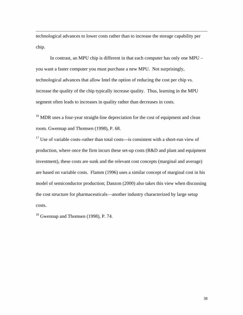
15T The cost structures for MPUs and DRAMs are fairly similar and so some of the sources

for learning economies are common to both. One important difference in the two is that

DRAM chips are fairly simple – they store data – and the storage capability of the chip is

such that if you want more storage you can simply buy more chips (rather than buy a

bigger memory chip). Perhaps this is why DRAM producers have focused on using

38

technological advances to lower costs rather than to increase the storage capability per

chip.

In contrast, an MPU chip is different in that each computer has only one MPU –

you want a faster computer you must purchase a new MPU. Not surprisingly,

technological advances that allow Intel the option of reducing the cost per chip vs.

increase the quality of the chip typically increase quality. Thus, learning in the MPU

segment often leads to increases in quality rather than decreases in costs.

T

16T MDR uses a four-year straight-line depreciation for the cost of equipment and clean

room. Gwennap and Thomsen (1998), P. 68.

T

17T Use of variable costs–rather than total costs—is consistent with a short-run view of

production, where once the firm incurs these set-up costs (R&D and plant and equipment

investment), these costs are sunk and the relevant cost concepts (marginal and average)

are based on variable costs. Flamm (1996) uses a similar concept of marginal cost in his

model of semiconductor production; Danzon (2000) also takes this view when discussing

the cost structure for pharmaceuticals—another industry characterized by large setup

costs.

T

18T Gwennap and Thomsen (1998), P. 74.