Who’s Employed? An in Depth Comparison of Employment Data Sources Gregory Giaimo, PE Samuel Granato, PE Andrew Hurst The Ohio Department of Transportation Division of Planning Presented at The 14 th Transportation Planning Applications Conference May 6, 2013

Who’s Employed? An in Depth Comparison of Employment Data Sources Gregory Giaimo, PE Samuel Granato, PE Andrew Hurst The Ohio Department of Transportation.
Jan 02, 2016
Welcome message from author
This document is posted to help you gain knowledge. Please leave a comment to let me know what you think about it! Share it to your friends and learn new things together.
Transcript

Who’s Employed? An in Depth Comparison of Employment Data Sources
Gregory Giaimo, PESamuel Granato, PE
Andrew HurstThe Ohio Department of Transportation
Division of Planning
Presented atThe 14th Transportation Planning Applications Conference
May 6, 2013

Overview
• Motivation
• Macro View-QCEW vs. BEA Control Totals for Data Expansion
• Micro View-QCEW vs. Purchased Data for Possible Replacement

Motivation• For Travel Modeling Want Employment Data With:
• Accuracy (correct employment/employers)• Completeness (all employment/employers)• Spatial Precision (geocodable address of individual employers at actual
place of business activity)• Temporal Consistency (no defunct businesses, contain new businesses
extant on the supposed date of the dataset)• Categorization (correct NAICS or similar)• Disaggregate (individual employer records allows data checking, finer
TAZ disaggregation and future travel demand models (particularly freight) will include disaggregate attraction end modeling including business synthesizers similar to current household synthesizers)
• There Area a Number of Potential Employment Data Sources

Motivation• QCEW (Quarterly Census of Employment and Wages)
• Regulatory dataset for Federal unemployment insurance• Pros: cheap, regulatory basis implies it is complete and temporally consistent for
covered sectors• Cons: confidentiality restrictions, uncovered sectors for those exempt from
Federal unemployment insurance laws (sole proprietors, small farms, railroads, military, small non-profits, student workers, elected officials etc.), sub-county location must be geocoded by user from mailing addresses (regulations only require correct county and ability to mail a bill), single site reporting for multi-site businesses, government particularly poor
• BEA (Bureau of Economic Analysis)• Dataset maintained by Federal Government for Macro-Economic Analysis• Pros: based on QCEW but enhanced with other administrative sources such as
income tax data to provide complete and temporally consistent data• Cons: Only aggregate county level data available

Motivation• LEHD (Longitudinal Employer-Household Dynamics)
• Census Bureau product based on QCEW and linked with ACS data• Pros: Same pros as other QCEW based sources, no confidentiality restrictions or
costs, in addition dataset provides linkages between employee residences and employer locations
• Cons: Same pros as other QCEW based sources, plus no employer records only aggregate employment, Census Bureau masking, a PUMS-like product for employment would alleviate some of this constraint
• Private Sources (InfoGroup’s InfoUSA/ReferenceUSA, Dun & Bradstreet’s Global Commercial Database etc.)• Several firms assemble employment data, primarily for resale for business
marketing purposes, they use phone directories and other publicly available sources and then enhance and verify it with their staff
• Pros: Good spatial precision, few of the multi-site problems in QCEW, reasonably complete
• Cons: Cost, lack of regulatory basis means incompleteness is ill-defined, temporal consistency is poor because primary purpose of dataset makes it more likely that defunct businesses are retained

Motivation• Since 2000 ODOT has utilized QCEW as its primary source of employment
data, confidentiality requirements mean model employment data can’t be given out freely creating some logistical issues with the models and consultant contracts, also the latest confidentiality agreement includes stricter personal liability making some hesitant to sign
• Ohio library system has a license for Infogroups’s ReferenceUSA, allowing state agencies to query 50 records at a time, based on this data, ODOT also received a small area sample of their InfoUSA database for this study
• ODOT Economic Development and Planning Offices also recently purchased two separate version of the Dun and Bradstreet database for their own purposes (largely due to QCEW confidentiality limits)
• Taken with the public availability of LEHD and BEA data this provided an opportunity and need for ODOT to compare and contrast data sources
Employees0
1000000
2000000
3000000
4000000
5000000
6000000
7000000
Ohio Employment Sources
BEA ProprietorsExtra BEA WageUngeocodedGeocoded
Total Employment
Employees Percent
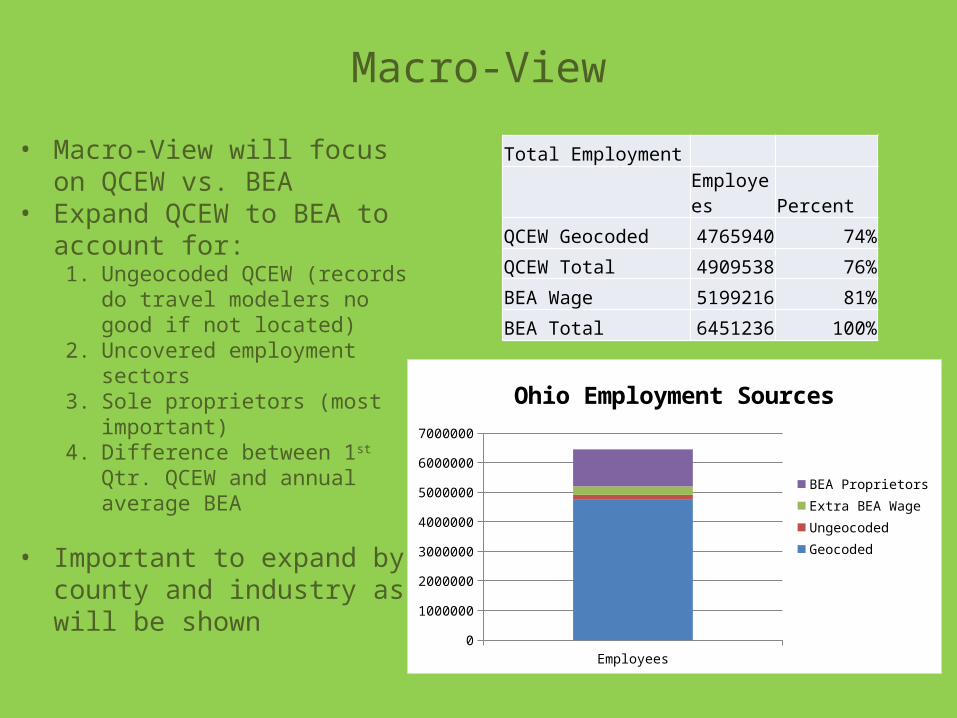
QCEW Geocoded 4765940 74%
QCEW Total 4909538 76%
BEA Wage 5199216 81%
BEA Total 6451236 100%
Macro-View
• Macro-View will focus on QCEW vs. BEA
• Expand QCEW to BEA to account for:
1. Ungeocoded QCEW (records do travel modelers no good if not located)
2. Uncovered employment sectors3. Sole proprietors (most important)4. Difference between 1st Qtr. QCEW
and annual average BEA
• Important to expand by county and industry as will be shown

Industry Level QCEW vs. BEAQCEW BEAEmployers Employees County
INDUSTRY GeocodedUngeocoded%GeocodedGeocodedUngeocoded%GeocodedTotal Allocated %Allocated%QCEWofBEAAG/FISH/FOREST1150 47 96% 11770 128 99% 91078 84038 92% 13%MINNING 709 83 90% 9885 462 96% 27895 19410 70% 37%UTILITIES 894 86 91% 29659 1946 94% 20765 17853 86% 152%CONSTRUCTION22411 2235 91% 150915 6822 96% 296852 291608 98% 53%MANUFACTURING16008 524 97% 608488 2580 100% 648564 647290 100% 94%WHOLESALE 15815 7228 69% 193657 21674 90% 236906 226113 95% 91%RETAIL 35467 1080 97% 536292 4922 99% 671615 671615 100% 81%TRANS/WAREHOUSE8000 763 91% 183774 3288 98% 215452 196664 91% 87%INFORMATION 3730 913 80% 86949 5673 94% 93023 92724 100% 100%FINANCE/INS 16390 1292 93% 203054 6198 97% 331883 331377 100% 63%REAL ESTATE/RENT9642 696 93% 55617 1679 97% 234520 233849 100% 24%PROF/TECH SERVICES24846 4983 83% 227422 16112 93% 367974 355874 97% 66%MGMT SERVICES1531 215 88% 106652 1344 99% 113014 110997 98% 96%ADMIN/SUPPORT SRV13990 2470 85% 248063 17312 93% 387132 383296 99% 69%EDUCATION 6419 324 95% 456385 5389 99% 147691 137663 93% 313%HEALTH CARE/SOCIAL26928 858 97% 805857 14069 98% 830432 778222 94% 99%ARTS/REC 3739 300 93% 56763 2282 96% 119530 119412 100% 49%ACCOMODATION/FOOD22412 529 98% 413534 3468 99% 443910 443303 100% 94%OTHER SERVICES22661 1390 94% 146197 3370 98% 338268 337561 100% 44%PUBLIC ADMIN 6850 1153 86% 234043 24569 90% 834732 834732 100% 31%UNCLASSIFIED 547 309 64% 964 311 76% 0 0 0Total 260139 27478 90% 4765940 143598 97% 6451236 6451236 100% 76%
QCEW vs. BEA

QCEW vs. BEA• There are significant
differences so it’s worth delving a bit deeper

AG/FISH
/FORES
T
MINNING
UTILITI
ES
CONSTRUCTIO
N
MANUFACTU
RING
WHOLES
ALE
RETAIL
TRANS/W
AREHOUSE
INFORMATIO
N
FINANCE/I
NS
REAL E
STATE
/REN
T
PROF/TEC
H SERVICES
MGMT SER
VICES
ADMIN/SUPPORT S
RV
EDUCATIO
N
HEALTH
CARE/SOCIAL
ARTS/R
EC
ACCOMODATION/FO
OD
OTHER
SERVICES
PUBLIC ADMIN
UNCLASS
IFIED
0%
10%
20%
30%
40%
50%
60%
70%
80%
90%
100%
QCEW Geocoding Percentages
EmployersEmployees
• Mostly automated but manual passes on large employers (hence while only 90% of employers geocoded, 97% of employment)
• Geocoding not even across industry categories or counties• ODOT spent a lot of time fixing multi-site employers,
especially school districts which now appear in Ohio’s official file
QCEW Geocoding
AG/FISH
/FORES
T
MINNING
UTILITI
ES
CONSTRUCTIO
N
MANUFACTU
RING
WHOLES
ALE
RETAIL
TRANS/W
AREHOUSE
INFORMATIO
N
FINANCE/I
NS
REAL E
STATE
/REN
T
PROF/TEC
H SERVICES
MGMT SER
VICES
ADMIN/SUPPORT S
RV
EDUCATIO
N
HEALTH
CARE/SOCIAL
ARTS/R
EC
ACCOMODATION/FO
OD
OTHER
SERVICES
PUBLIC ADMIN
UNCLASS
IFIED
0%10%20%30%40%50%60%70%80%90%
100%
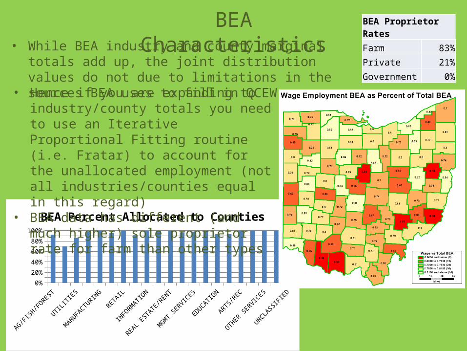
BEA Percent Allocated to Counties
BEA Proprietor Rates
Farm 83%
Private 21%
Government 0%
• While BEA industry and county marginal totals add up, the joint distribution values do not due to limitations in the sources BEA uses to fill in QCEW gaps
BEA Characteristics
• Hence if you are expanding to industry/county totals you need to use an Iterative Proportional Fitting routine (i.e. Fratar) to account for the unallocated employment (not all industries/counties equal in this regard)
• BEA data has different (and much higher) sole proprietor rate for farm than other types

AG/FISH
/FORES
T
MINNING
UTILITI
ES
CONSTRUCTIO
N
MANUFACTU
RING
WHOLES
ALE
RETAIL
TRANS/W
AREHOUSE
INFORMATIO
N
FINANCE/I
NS
REAL E
STATE
/REN
T
PROF/TEC
H SERVICES
MGMT SER
VICES
ADMIN/SUPPORT S
RV
EDUCATIO
N
HEALTH
CARE/SOCIAL
ARTS/R
EC
ACCOMODATION/FO
OD
OTHER
SERVICES
PUBLIC ADMIN
UNCLASS
IFIED
0%
50%
100%
150%
200%
250%
300%350%
Percent Total QCEW to Total BEA
Comparing QCEW/BEA
• Note similarity to previous map
• BEA adds many commission only employees in NAICS 50 categories, particularly real estate so you should expect high expansion factors here
• ODOT uses Q1 QCEW so we get high expansion factors in seasonal industries (construction and arts/recreation)
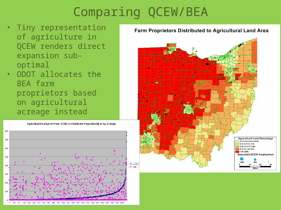
Agricultural Employment From ES202 vs Distributed Proportionally to Ag. Acreage
0
100
200
300
400
500
600
700
800
1 46 91 136 181 226 271 316 361 406 451 496 541 586 631 676 721 766 811 856 901 946 991 1036
es202
farm
Comparing QCEW/BEA• Tiny representation of
agriculture in QCEW renders direct expansion sub-optimal
• ODOT allocates the BEA farm proprietors based on agricultural acreage instead

Comparing QCEW/BEA• While of minor importance, we decided to allocate some of the missing
transportation employment to rail terminals prior to expansion

Macro-View Wrap Up• As mentioned previous, ODOT evaluated other sources beyond QCEW
• At a macro level, there are significant differences
• These are more difficult to understand at this level, so ODOT conducted some micro analysis at several locations

Micro-View• This presentation will focus
on one location for clarity
• A relatively recent and growing commercial/ industrial area in the western suburbs of Columbus
• Contains diverse mix of employment types
• However, due to small study area, results shown here should not be generalized, consider them as illustrative only

• The same area looks a bit different depending on the source
• RefUSA data only obtained for a subarea
• D&B data only obtained for 4+ employee employers
Micro-View

• Obtained data for (mostly) the same area
• Compared the employment records by address since no other common unique identifier
• Combined this with detailed local knowledge and aerial imagery (study areas were selected based on analyst knowledge)
• Necessary to determine when duplicate addresses are valid (office parks, suite’s, corporate vs. franchise and subsidiaries often have employee’s at same address) or when multiple occupants from different year’s are in data
• Theoretical maximum employment for an address taken as the maximum valid employment from any of the sources (this is not necessarily the true value since that source may have over-stated the number)
• LEHD not included in most comparison’s since it is aggregate data
Comparison Methodology

• Purchased data sources contain many duplicate businesses which need removed prior to comparison
• More problematic for smaller employers
Comparison Methodology
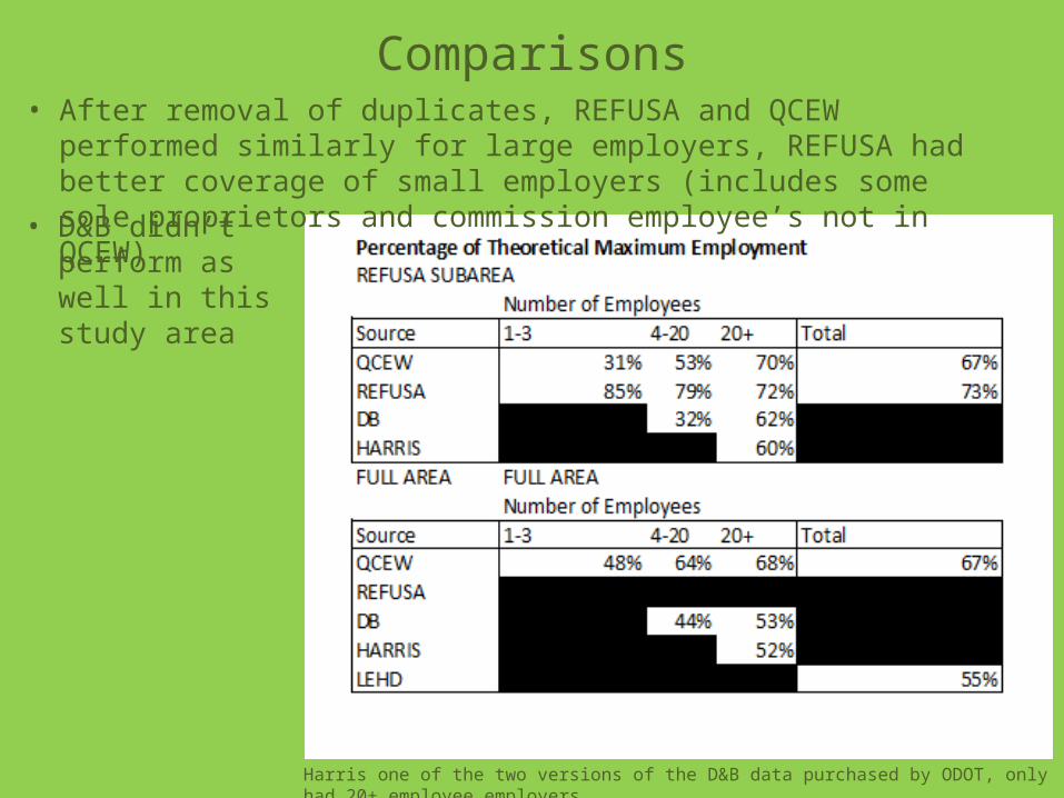
• After removal of duplicates, REFUSA and QCEW performed similarly for large employers, REFUSA had better coverage of small employers (includes some sole proprietors and commission employee’s not in QCEW)
Harris one of the two versions of the D&B data purchased by ODOT, only had 20+ employee employers
• D&B didn’t perform as well in this study area
Comparisons

QCEW QCEW/REFUSA QCEW/D&B REFUSA D&B0
20
40
60
80
100
120
140Number of Employers (4+ employees) by Source
DRDRQRDQDQRQ
Number of Employers if Only Use These Sourceas
• Employers included in purchased data and QCEW were nearly statistically independent
• Given the 75% and 92% employer coverage in QCEW and Reference USA, one would expect 98% coverage by combining the sources (analyst could not identify any missing employers which implies 100% was obtained but there is certainly some margin of error)
Combining Datasets

Categorization
• Categorization by industry was similar (89% same for same employers)

• Given these results and the desire to produce model datasets not subject to confidentiality constraints ODOT will purchase employment data and develop a process to:
1. Geocode2. Remove duplicates3. Cross match with previous
year’s data4. Cross match with QCEW5. Develop an employment
estimate for employer’s identified by QCEW rather than using value directly
Future Direction
Related Documents