Who pays for it? The heterogeneous wage effects of …doku.iab.de/veranstaltungen/2011/ws_flex2011_leonardi... · 2011-10-11 · Who pays for it? The Heterogeneous Wage E⁄ects of

Who pays for it? The Heterogeneous Wage E¤ects ofEmployment Protection Legislation�

Marco Leonardiy

University of Milan and IZAGiovanni Picaz

University of Salerno and CSEF

November 12, 2010

Abstract

Theory predicts that the wage e¤ects of government-mandated severance paymentsdepend on workers� and �rms� relative bargaining power. This paper estimates thee¤ect of employment protection legislation (EPL) on workers� individual wages in aquasi-experimental setting, exploiting a reform that introduced unjust-dismissal costsin Italy for �rms below 15 employees and left �ring costs unchanged for bigger �rms.Accounting for the endogeneity of the treatment status, we �nd that high-bargainingpower workers (stayers, white collar and workers above 45) are almost left una¤ectedby the increase in EPL, while low-bargaining power workers (movers, blue collar andyoung workers) su¤er a drop both in the wage level and its growth rate.

Keywords: Costs of Unjust Dismissals, Severance Payments, Policy Evaluation,Endogeneity of Treatment Status.JEL Classi�cation: E24, J63, J65.

�This is a revised version of a paper previously circulated under the title �Employment Protection Leg-islation and Wages�. We are grateful to Giuseppe Bertola, David Card, Ken Chay, Enrico Moretti, MichelePellizzari, and Steve Pischke for useful suggestions. Comments from seminar participants at the Universityof California at Berkeley, Boston College, Georgetown University, the University of Milan, the University ofSalerno, the University of Padova, the University of Venezia, the Fifth IZA/SOLE Transatlantic Meeting, andthe 7th ECB/CEPR Labour Market Workshop are also gratefully acknowledged. We thank Giuseppe Tat-tara and Marco Valentini for providing us with the VWH (Veneto Workers History) dataset (Miur Projects1999�2001 #9913193479 and 2001�2003 #2001134473). The usual disclaimer applies.

yE-mail: [email protected]: [email protected]

1

1 Introduction

Since the work of Lazear (1990), it has been well-known that in a perfectly competitive

labour market the cost of employment protection legislation (EPL) is fully shifted onto

lower wages if dismissal costs entail a transfer from �rms to risk neutral workers. Wages

are also expected to fall if risk averse workers value job security and are willing to pay for

an increase in EPL (Pissarides, 2001; Bertola, 2004). Potentially o¤setting the negative

e¤ect of EPL on wages, job security provisions may strengthen the bargaining position of

workers vis-à-vis employers, allowing them to reap a larger share of the surplus and obtain

higher wages in markets where individual or collective negotiation takes place (Mortensen

and Pissarides, 1999; Ljungqvist, 2002). Moreover, stricter EPL may raise �rms�incentives

to invest in training, thereby fostering the accumulation of �rm-speci�c human capital and

increasing both productivity and wages (Autor et al., 2003; Wasmer, 2006; Cingano et al.,

2010).

Thus, theory predicts an ambiguous impact of EPL on wages, with heterogenous e¤ects

possibly stemming from di¤erences in the bargaining positions of workers vis-à-vis employers

(Dolado et al., 2007).

This paper attempts to provide evidence for the e¤ects of EPL on workers� individual

wages. The analysis is based on data from Italy, one of the strictest countries in terms of

employment protection legislation. Italy is an interesting country to study for two additional

reasons: First, although in Italy wage determination is to a large extent centralized, an

important component of workers�compensation is determined at the �rm level in the form

of company-level wage increments, production bonuses and other variable bene�ts (Guiso et

al., 2005).1 Second, the changes in the Italian institutional framework allow us to achieve

a clean identi�cation, exploiting EPL variation both across �rms and over time. In fact,

until 1990 the Italian labour code, enacted in 1970, provided a sharp discontinuity in the

application of EPL at the 15 employee threshold, with no protection for workers in small �rms

and high protection for those in large �rms. In July 1990, severance payments were increased

from zero to between 2.5 and 6 months of pay for �rms with fewer than 15 employees, and

left unchanged for �rms with more than 15 employees.

We are therefore able to identify the e¤ects of employment protection legislation compar-

ing wages of small versus large �rms workers before and after the law change in a neighbour-

1In terms of the magnitude of the �rm-speci�c part of the wage, between one sixth and one quarter ofthe compensation is �rm-speci�c. In terms of di¤usion, half of Italian workers were involved in �rm-levelnegotiations in the period covered by our sample. These estimates, based on data in the metal products,machinery and equipment industry are reported by CESOS, an association of trade unions. See Ericksonand Ichino (1995) for further details on wage formation in Italy for the period covered by our data.

2

hood of the 15 employees threshold, thus combining a regression discontinuity design (RDD)

with a di¤erence in di¤erence (DID) approach. Our identi�cation assumption is essentially

that, after conditioning, the average wages of individuals employed in �rms marginally above

the 15 employees threshold (16�25) represents a valid counterfactual for the wages of workers

employed in �rms just below the threshold (5�15) both before and after the reform, i.e., we

expect conditional wages in the treated and control groups to diverge after the law change

for no other reason than the reform itself.

One natural concern, in our case, is the endogeneity of the treatment status. On the one

side, it is possible that marginal �rms which kept their size just below 15 before the reform

to avoid strict EPL rules, increased their size because of the reform. To control for �rms

sorting into the large or small group according to time-invariant characteristics, we estimate

�rm �xed e¤ects models. Additionally, we instrument the treatment status with �rm size in

1989 and 1988, when the reform was not in place and was unexpected. On the other side,

workers may also sort around the 15 employees according to their preferences over the mix

of employment protection and wages. To control for workers sorting into large or small �rms

according to �xed characteristics, we estimate the model using worker �xed e¤ects.

This paper uses administrative data from the Italian Social Security Institute (INPS),

and exploits a matched employer�employee panel which contains the entire population of

workers and �rms located in the Italian provinces of Vicenza and Treviso. Baseline OLS

estimates indicate a signi�cant wage loss in small relative to large �rms after the 1990 reform

that ranges, on average, between 0.5 and 1 percent. The negative e¤ect is, however, highly

heterogeneous. Movers su¤er a drop in the wage rate in small relative to large �rms after the

reform of about 2 percent, while incumbent workers seem not to be harmed by stricter EPL.

Blue collar in small �rms experience a reduction of the wage rate after the reform of about

1.5 percent, whereas white collar are left una¤ected. Similarly, wages of workers below 45 in

small �rms go down by 1 to 2 percent after the reform, while older workers su¤er no wage

loss. The negative e¤ect is robust to the inclusion of worker �xed e¤ects, �rm �xed e¤ects

and appears also when �rm size is instrumented, suggesting that the sorting of �rms may

not be a big issue.

In order to investigate whether job security provisions a¤ect not only the level of the wage

but also its growth rate, we look at the e¤ects of EPL on year-to-year log wage changes.

Results show that small �rms workers lose on average 1 percent in terms of wage growth after

the reform relative to large �rms workers. The speci�cation in changes exhibits a similar

pattern as the speci�cation in levels: even though all groups of workers (except white collar)

seem to be negatively a¤ected by the reform, the losses are quantitatively stronger among

3

movers, young workers and blue collar.

This pattern of results favours the interpretation that the ability of the employers to shift

the cost of EPL onto wages depends on workers�bargaining power. Firms are better able to

negotiate lower wages with new entrants rather than to renegotiate incumbents wages. At

the same time, it is plausible to think that young and blue collar workers are in a weaker

position within the �rm compared to older and white collar workers.

While there is a large literature on the e¤ects of EPL on job �ows, relative little empirical

evidence is available on the wage e¤ects of dismissal costs.2 Bertola (1990) shows that in

high job security countries, wages tend to be lower. More recently, using �rm-level data,

Martins (2009) shows that EPL raises wages in Portugal while Bird and Knopf (2009) �nd

evidence of a relationship between the adoption of wrongful-discharge protections and the

increase in labour expenses of US commercial banks.

More related to this paper are the studies conducted on individual data which reach

disparate conclusions. Autor et al. (2006) �nd no evidence that wrongful-discharge laws had

a signi�cant impact on wage levels in the US. Cervini Plá et al. (2010) analyse the 1997

reform of Spanish severance pay and payroll taxes and conclude that decreased �ring costs

and payroll taxes have a positive e¤ect on wages. Van der Wiel (2010) �nds opposite results

for the Netherlands using a reform that a¤ected di¤erently high- and low-tenured workers.3

The rest of this paper is organized as follows. Section 2 describes how �ring restrictions

evolved in Italy. Section 3 describes the dataset and the sample selection rules. Section

4 explains the identi�cation strategy used to evaluate the impact of EPL on the wage dis-

tribution. Section 5 presents OLS and IV estimates of the impact of increased strictness

of employment protection in small �rms in Italy after 1990 on average wages. Section 6

discusses the results and concludes with a back of the envelope calculation of the share of

EPL costs transferred to lower wages.

2The previous empirical literature mostly concentrates on the e¤ects of EPL on employment �ows, oftenusing the cross-state variation of EPL within the US. Autor (2003) looks at the e¤ect of EPL on the use oftemporary help agencies. Kugler and Saint-Paul (2004) consider re-employment probabilities. Some papersexploit the discontinuities in �ring costs regimes that apply to �rms of di¤erent sizes within countries. Boeriand Jimeno (2005) assess the e¤ect of EPL on lay-o¤ probabilities by comparing �rms below and above15 employees in Italy, while Kugler and Pica (2006) examine the joint impact of EPL and product marketregulation on job �ows in Italy using both the �rm size threshold and a law change. Using a di¤erence-in-di¤erences approach, Bauer et al. (2007) investigate the impact of granting employees the right to claimunfair dismissal on employment in small German �rms.

3Related to this paper are also Autor et al. (2007) and Cingano et al. (2010) who study the e¤ect of EPLon �rm-level productivity.

4

2 Institutional background

The Italian labour code favours open-ended contracts over �xed-term or temporary contracts.

As a form of worker protection for open-ended contracts, labour codes specify which causes

are considered justi�ed causes for dismissal, and establish workers�compensation depending

on the reason for the termination. In contrast, temporary contracts can be terminated at

no cost provided that the duration of the contract has expired. Labour codes also limit trial

periods� that is, the period of time during which a �rm can test and dismiss a worker at no

cost (in Italy 3 months) and mandate a minimum advance notice period prior to termination

(1 month).

Over the years the Italian legislation ruling unfair dismissals has changed several times.

Both the magnitude of the �ring cost and the coverage of the �rms subject to the restrictions

have gone through extensive changes. Individual dismissals were �rst regulated in Italy in

1966 through Law 604, which established that employers could freely dismiss workers either

for economic reasons (considered as fair �objective�motives) or in case of misconduct (con-

sidered as fair �subjective�motives). However, in these cases workers could take employers

to court and judges would determine if the dismissals were indeed fair or unfair. In case of

unfair dismissal, employers had the choice to either reinstate the worker or pay severance,

which depended on tenure and �rm size. Severance pay for unfair dismissals ranged between

5 and 8 months for workers with less than two and a half years of tenure, between 5 and

12 months for those between two and a half and 20 years of tenure, and between 5 and 14

months for workers with more than 20 years of tenure in �rms with more than 60 employees.

Firms with fewer than 60 employees had to pay half the severance paid by �rms with more

than 60 employees, and �rms with fewer than 35 workers were completely exempt.

In 1970, the Statuto dei Lavoratori (Law 300) established that all �rms with more than 15

employees had to reinstate workers and pay their foregone wages in case of unfair dismissals.

Firms with fewer than 15 employees remained exempt. The law prescribes that the 15

employees threshold should refer to establishments rather than to �rms. In the data we only

have information at the �rm level. However, this is not likely to be a concern as in the

empirical analysis we focus on �rms between 10 and 20 employees that are plausibly single-

plant �rms. Although severance pay in case of dismissal is due only to permanent workers,

the labour code computes the 15 employees threshold in terms of full-time equivalents rather

than in terms of heads in order to avoid �rms bypassing EPL regulations by hiring workers

under �xed-term contracts.

Finally, Law 108 was introduced in July 1990 restricting dismissals for permanent con-

5

tracts. This law introduced severance payments of between 2.5 and 6 months pay for unfair

dismissals in �rms with fewer than 15 employees. Firms with more than 15 employees still

had to reinstate workers and pay foregone wages in case of unfair dismissals. This means

that the cost of unfair dismissals for �rms with fewer than 15 employees increased relative

to the cost for �rms with more than 15 employees after 1990.4 For our purposes, this reform

has two attractive features. First, it was largely unexpected: the �rst published news of

the intention to change the EPL rules for small �rms appeared in the main Italian �nancial

newspaper� Il Sole 24 Ore� at the end of January 1990. Second, it imposed substantial

costs on small �rms. Kugler and Pica (2008) look at the e¤ect of this reform on job and

workers �ows and �nd that accessions and separations decreased by about 13% and 15% in

small relative to large �rms after the reform.

3 Data description

This paper uses the VWH data set which is an employer�employee panel with information on

the characteristics of both workers and �rms. The longitudinal panel is constructed from the

administrative records of the Italian Social Security System (INPS). It refers to the entire

population of employers and workers of the private sector in two provinces, Treviso and

Vicenza, of the Italian region of Veneto. The two provinces are located in the north-eastern

part of the country. In the year 2000, GDP per capita was 22,400 euros, 20% higher than

the national average and accounted for 3.3% of the Italian GDP. The overall population

was 1.6 million people (2.7% of the total Italian population) as of the 2001 Population

Census.5 Although limited to two relatively small provinces, the data are well suited for

studying the e¤ect of the 1990 EPL reform because the Italian north-east is characterized by

4A further reform was passed in 1991 concerning collective dismissals. A special procedure was introducedfor �rms with more than 15 employees willing to dismiss �ve or more workers within 120 days because ofplant closure or restructuring. According to this procedure, �rms were required to engage in negotiationswith unions and government to reach an agreement on the dismissals. However, if public administrationo¢ cials determine that an agreement cannot be reached, the �rm is free to downsize and the employees arenot allowed to take the �rm to court. Kugler and Pica (2008) try to empirically distinguish the 1990 and the1991 reforms and �nd no additional signi�cant e¤ect of the 1991 reform on workers and job �ows. Hence,this reform is unlikely to cloud our results. Paggiaro, Rettore and Trivellato (2008) also examine aspects ofthe 1991 law concerning active labour market policies and �nd limited e¤ects only on workers aged 50+.

5The average establishment size in Veneto is 13 employees. Half of the employment stock is not subject toprotection against dismissal as stated by art. 18 of the Statuto dei Lavoratori. For a decade Veneto has beenalso a full employment region with a positive rate of job creation in manufacturing, compared to a negativenational rate and positive migration �ows. Typical manufacturing activities are garments, mechanical goods,goldsmiths, leather, textile, furniture and plastics. The stock of manufacturing workers in the two Venetoprovinces of Treviso and Vicenza has varied between 194,000 employees in the early 1980s and 233,000employees in 1996, with a yearly positive average rate of variation of 1.4%. The average rate of growth inemployment is the result of a marked increase in white collar and women (see Tattara and Valentini, 2005).

6

a high concentration of small �rms and a tight labour market. Moreover, the availability of

information on the universe of workers and �rms allows of building suitable instruments for

�rm size and of applying IV techniques.6 The use of a random sample of the Italian working

population would only allow OLS estimates (available upon request).

The data include universal information on all plants and employees working at least one

day in any plant of the two provinces from 1984 to 1997. The data include information on

employees�age, gender, occupation (blue collar/white collar), yearly wage, number of paid

weeks, type of contract (permanent/temporary), and information on �rms�location, sector

of employment, average number of employees and date of closure. Unfortunately, we have

no information on education. The unit of observation is the employer-day; such information

is used to build a complete history of the working life of each employee. Once they are in

the dataset, employees are followed, independently of their place of residence, even in their

occupational spells out of Treviso and Vicenza.

The only reason of dropping out of the dataset is exit from the private sector or from

employment status altogether. Since the individual longitudinal records are generated using

social security numbers and collect information on private sector employees for the purpose of

computing retirement bene�ts, employees are only followed through their employment spells.

The data stop following individuals who move into self-employment, the public sector, the

agricultural sector, the underground economy, unemployment, or retirement.

We select all males of ages between 20 and 55 hired on a permanent basis. We exclude

females because in their case the trade-o¤ between job security and wages is likely to be

a¤ected by fertility decisions on which we have no information. We also exclude temporary

workers because employment protection provisions are guaranteed only to workers on a

permanent contract.7

We focus on 1989�1993 and remove 1990 because the reform occurred in the month of

July and the wages of 1990 are likely to be a mixture of pre-reform and post-reform wages.

To preserve the comparability of treatment and control groups, we further select the sample

to �rms within the interval 5�25 employees. In the course of the paper we use weekly wages

after eliminating the upper and lower 1% of the wage distribution in each year. In case the

6Card et al. (2010) investigate the evidence on rent-sharing and holdup on the same data.7A further concern is that �rms can bypass the EPL regulation based on the 15 employees threshold hiring

workers on a �xed term contract. The de�nition of the threshold is based on full-time equivalents ratherthan on heads and therefore leaves little room for �rms to circumvent the rule. In particular, the labourcode excludes apprentices and temporary workers below nine months, and includes part-time workers andall other temporary contracts in proportion to their actual time. Our dataset records the type of contract(full-time, part-time, apprentices and temporary workers) but does not contain information on the numberof hours worked. For this reason, in our estimates the threshold is calculated on the basis of full-time workerson permanent contracts.

7

same individual has multiple employment spells in di¤erent �rms in the same year we keep

the longest spell. The �nal sample is of 9,914 �rms and 29,177 workers.

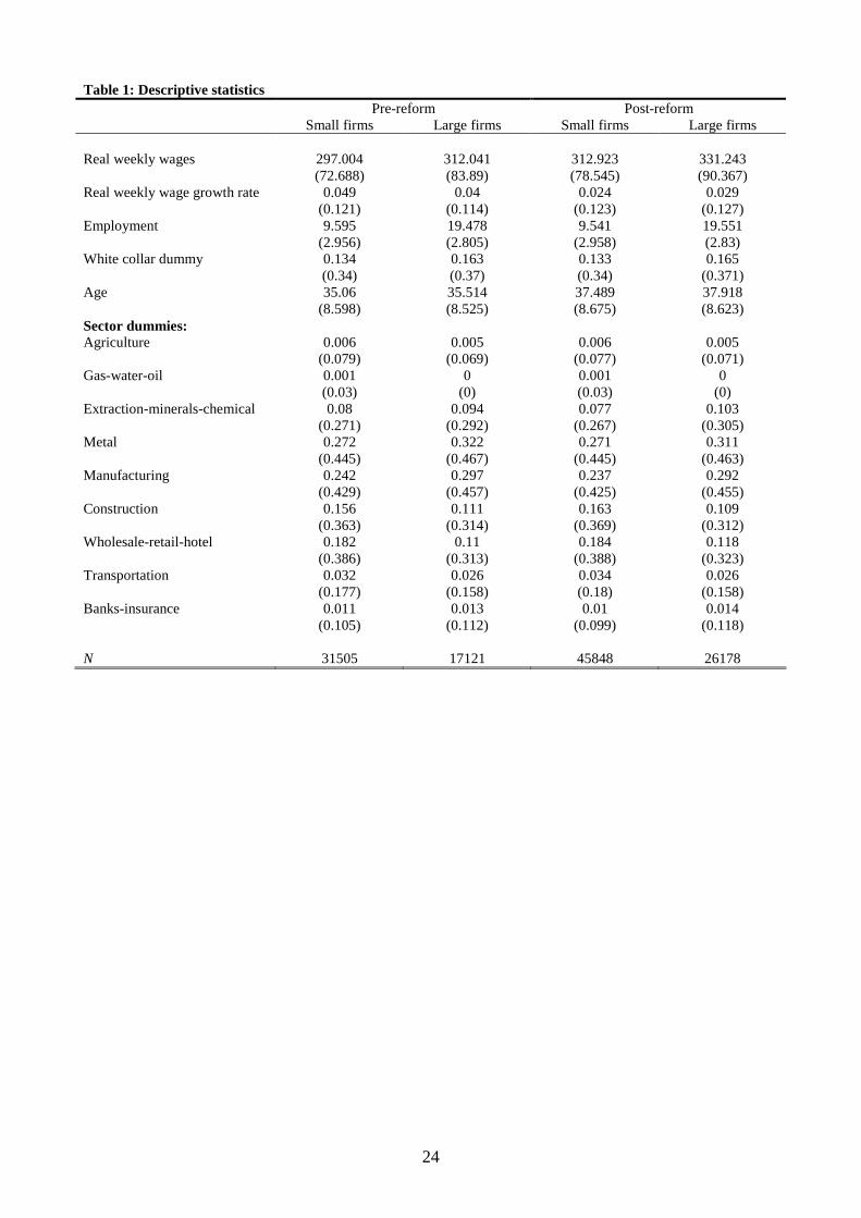
Descriptive statistics for the main variables used in the analysis are shown in Table 1.

The number of small �rms (5�15) is higher than the number of large �rms (16�25), so is the

number of workers working in small �rms. The real weekly wage of workers in large �rms

is around 325 euros per week vs. a signi�cantly lower wage of 308 euros per week in small

�rms. The year-to-year average wage change is however similar in the two groups at 3% per

year. The average age of workers is not signi�cantly di¤erent across the two groups while

larger �rms employ a slightly higher proportion of white collar workers.

4 Identi�cation strategy

The estimand of interest is the average treatment e¤ect of EPL on wages. The conditional

comparison of wages in small and big �rms does not generally provide an unbiassed estimate

of the average treatment e¤ect, because �rms with di¤erent unobservable characteristics

may endogenously choose their size and their wages. The fact that in Italy the level of EPL

depends on �rm size, coupled with the reform of EPL which a¤ected only small �rms, can

be exploited to build an RDD combined with a DID strategy to estimate the causal e¤ect of

EPL on wages.

In order to identify the impact of dismissal costs on wages, we compare the change in

mean wages paid by �rms just below 15 employees before and after the 1990 reform to the

change in mean wages paid by �rms just above 15 employees. In other words, the assumption

that guarantees that the e¤ect of EPL on wages can be interpreted as causal is that the

characteristics of workers and �rms should not display any discontinuity at the threshold.

Another identi�cation assumption is that the average wage of individuals employed in �rms

marginally below the 15 employees threshold (5�15) is expected to diverge from the wage

of the control group employed in �rms just above the threshold (16�25) for no other reason

than the law change.

If workers and �rms were exogenously assigned to the treatment and control groups, OLS

estimates of the following model would identify the causal e¤ect of EPL on wages:

Yijt = �0Xijt + �1D

Sjt + �2

�DSjt � Post

�+

3Xk=1

( kfsizek) + ut + eijt (1)

DSjt = 1 [�rm size � 15 in year t]

Post = 1 [year � 1991]

8

The dependent variable is the log of the weekly wage paid to worker i by �rm j in year t

(or the �rst di¤erence of log wages in the speci�cation in wage changes, see Table 6) and is

given by the yearly wage divided by the number of paid weeks.

The variable Post is a dummy that takes the value of 1 starting from 1991 and zero

otherwise; DSjt is a dummy that takes the value of 1 if the worker is employed in year t in a

�rm with fewer than 15 employees and 0 if the worker is employed in a �rm with strictly more

than 15 employees. The interaction term DSjt�Post between the small �rm dummy and the

post-reform dummy is included to capture the e¤ect of the EPL reform. All speci�cations

contain a polynomial of third degree in �rm size.8 The matrix Xijt includes age dummies,

an occupation (white collar/blue collar) dummy and nine industry dummies. Macro shocks

denoted by ut are accounted for by a full set of year dummies. The reported standard errors

account for possible error correlations at the individual level.

Equation (1) gives unbiassed estimates only if workers and �rms are exogenously assigned

to the treatment status. However, individuals may decide to work in small or large �rms, and

�rms in turn may decide to grow above or shrink below the 15 employees threshold. Thus,

a fundamental concern of this paper is the non-random selection of workers and �rms above

and below the �fteen employees threshold. To control for the sorting of workers into large

or small �rms according to time-invariant workers characteristics, we estimate the model

using worker �xed e¤ects. In the same way, to control for the sorting of �rms into the large

or small group, we estimate a model that includes �rm �xed e¤ects and, in an alternative

speci�cation, we use an instrumental variable approach to which we now turn.

4.1 Firm sorting: the instrumental variable model

Identi�cation in (1) is threatened by the possibility that �rms sort around the 15 employees

threshold. Regressions using �rm �xed e¤ects control for all time-invariant unobserved fac-

tors that may a¤ect the propensity of �rms to self-select into (or out of) treatment. However,

they do not account for the selection due to the reform itself. Firms in the neighbourhood

of the 15 employees�threshold may change their size in response to the 1990 reform of EPL,

thus biassing the estimates. For example, �rms which kept their size just below 15 before

the reform to avoid strict EPL rules, may have increased their size because the reform made

the gap in EPL provisions narrower. The sign of the bias due to �rms�sorting is not easy

to establish. If �rms which were keeping their size below 15 before the reform for fear of

8Results are robust to this functional form assumption. Alternatively, a split polinomial approximation(as in Lee, 2008) or a local linear regression can be used in RDD regressions. See Imbens and Lemieux (2008)for an overview of di¤erent alternatives.

9

incurring a much higher EPL were those with bad growth perspectives and lower wages,

then presumably OLS estimates understate the e¤ect of the reform on wages. But it may

also be the case that the �rms which were keeping under the threshold were instead those

which were paying higher wages.

In this section, we assess the validity of the identi�cation strategy discussed in Section 4

with two di¤erent testing procedures. First, to formally check for the absence of manipulation

of the running variable at 15 (violated if �rms were able to alter their size and sort above

or below the threshold), we test the null hypothesis of continuity of the density of �rm size

at 15 as proposed by McCrary (2008). Second, we regress the probability of �rm growth on

pre-existing �rm characteristics.

In Figure 1, we plot the frequency of �rms with less than 25 employees, using di¤erent

bin sizes (0.5 and 1) for 1989 (before the reform) and for 1991 (after the reform). Visual

inspection does not reveal any clear discontinuity at the 15 employees threshold.9 In the

right panel of the same �gure, we zoom in on the shape of the running variable around the

15 employees threshold. There, no evidence of manipulative sorting can be detected. We

formally test for the presence of a density discontinuity at this threshold with a McCrary test

by running kernel local linear regressions of the log of the density separately on both sides of

the threshold (McCrary, 2008). As we can see from the �gure, the log-di¤erence between the

frequency to the right and to the left of the threshold is not statistically signi�cant. In fact,

the point estimate is -0.007 (with a standard error of 0.236). However, density tests have

low power if manipulation has occurred on both sides of the threshold. In that case, there

might be non-random sorting not detectable in the distribution of the running variable.

For this reason we perform a further test. Firms may sort around the threshold according

to both observable and unobservable characteristics. To verify if sorting happens according

to pre-existing unobservable characteristics, we �rst estimate a regression of �rms�average

wages paid in 1986�1989 (before the reform) on �rm size, �rm age, year dummies and �rm

�xed e¤ects. We then use the time-invariant portion of the residual as one of the determinants

of the �rm probability of growing. The probit regression is of the form

djt = �0Xjt + �0Post+ �1dummySjt�1 + �2FEj + �0 (dummySjt�1 � Post) (2)

+�1 (FEj � Post) + �2 (dummySjt�1 � Post� FEj) + "jt;

where djt = 1 if �rm j in year t has a larger size than in t�1: The term dummySjt�1 denotes9The average �rm size in Italy is approximately half that of the European Union and expensive EPL

for �rms larger than 15 is often wrongly indicated as one of the factors responsible for such a skewed sizedistribution. The non-existence of lumps at 15 can be explained by the fact that �rms choose their size onthe basis of several factors and not only on the basis of EPL (Schivardi and Torrini, 2008).

10

020

040

060

080

0

frequ

ency

5 15 25

Firm size - 1989

0.0

5.1

.15

.2.2

5

10 12 14 16 18 20

020

040

060

080

010

00

frequ

ency

5 15 25

Firm size - 1991

0.1

.2.3

.4

10 12 14 16 18 20

Bin=0.5 Bin=1

Figure 1: Frequency of �rm size and McCrary test of density continuity. Weighted kernelestimation of the log density, performed separately on either side of the threshold. Optimalbinwidth and binsize as in McCrary (2008).

11

a set of �rm size dummies while the variable Post takes the value of one from 1991. The

term FEj denotes the estimated �rm �xed e¤ects. The matrix Xjt�1 includes a quadratic

in �rms�age, year dummies, sector dummies and a polynomial in lagged �rm size.

Column 1 of Table 2 shows that on average �rms just below 15 employees are 2% less

likely to grow of one unit than larger �rms. These results are consistent with Schivardi and

Torrini (2008) and Borgarello, Garibaldi and Pacelli (2004) who �nd that more stringent job

security provisions hamper �rm growth. They �nd that the discontinuous change in EPL

at the 15 employees threshold reduces by 2% the probability that �rms pass the threshold.

Additionally, column 2 shows that the e¤ect is stronger after the reform (coe¢ cient on Post

1990 � Dummy 15). However, column 3 shows that the e¤ect is similar for �rms with

di¤erent average pre-reform wages, as the coe¢ cient of the triple interaction Post 1990 �Firms Fixed E¤ect � Dummy 15 is not signi�cantly di¤erent from zero.

While the fact that there is little evidence of �rm sorting is reassuring, we also show

results adopting an IV strategy to address the further concern that residual unobserved

heterogeneity may drive �rms�sorting behaviour. As an instrument for the treatment status

(the �rm size dummy), we use �rm size in 1989 and in 1988. These instruments are not

a¤ected by the reform as long as the reform was unexpected (see Section 2). The formal

speci�cation is

logwijt = �0Xijt + �0Post+ �1DSjt + �2

�DSjt � Post

�+

3Xk=1

( kfsizek) + �ijt (3)

DSjt =

0

0Xijt + 1Post+ 2SSjpre + 3

�SSjpre � Post

�+

3Xk=1

( kfsizek) + �jt;

where SSjpre is a vector that includes �rm size in 1989 and in 1988. The term DSjt � Post is

also instrumented using as an instrument SSjpre � Post.

4.2 Worker sorting

Identi�cation in (1) may be threatened also by workers non-randomly sorting around the 15

employees threshold. The idea is that workers (particularly job-to-job movers) may be able

to choose their own EPL regime by selecting the size of the �rm they work for. This may bias

our results as long this selection process is driven by worker characteristics that we are not

able to control for. Suppose, for example, that low-productivity workers disproportionately

apply to (and are subsequently hired in) more protected jobs. In this case, a negative

association between wages and job protection cannot be interpreted as the causal e¤ect

12

of EPL on wages, as it rather re�ects the di¤erent composition of the pool of workers in

protected and non protected jobs.

Including worker �xed e¤ects into (1) helps address this concern to the extent that it

allows of controlling for all time-invariant unobservable worker attributes that a¤ect the

choice of the workers regarding their EPL regime. Of course, worker �xed e¤ects do not

allow of controlling for the time-varying factors that a¤ect worker self-selection, including

the reform itself.

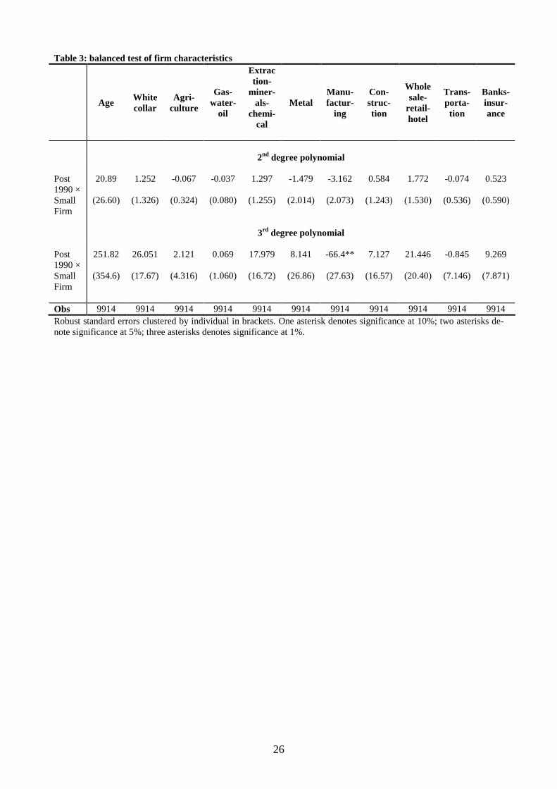
It is therefore desirable to test whether workers non-randomly sort into �rms above and

below the 15 employees threshold. We do so adopting two strategies. First, we check whether

�rms observable characteristics, such as industry, age, and occupation (white collar/blue col-

lar) composition of the workforce, are balanced in the neighbourhood of the 15 employees

threshold. If non-random workers sorting were to occur, we would expect these character-

istics to di¤er systematically between treated and untreated �rms around the 15 employees

threshold. The balance tests are performed running the �rm-level regression:

Xjt = �0Post+ �1DSjt + �2

�DSjt � Post

�+

nXk=1

( kfsizek) + ejt: (4)

Notice that this test gives also insights on whether other (unobserved) policies di¤erentially

a¤ect small and large �rms since 1990. Indeed, our empirical strategy may be hampered

by the presence of unobserved factors (for example another policy change) that are also

discontinuous at the threshold exactly at the time of the reform, thus confounding the e¤ect

of the reform itself. Although we cannot directly test this assumption, we can investigate

whether �rms observable characteristics have discontinuities at the threshold in 1990. Table

3 shows the coe¢ cients and standard errors of �2: No pre-treatment characteristics show a

signi�cant discontinuity at the 15 employees threshold after the reform in the 2nd degree

polynomial speci�cation. In particular, the age, occupation, and industry composition of

�rms across the two sides of the threshold is not signi�cantly di¤erent after the reform.

The only signi�cant coe¢ cient is of the manufacturing industry dummy in the case of a 3rd

degree polynomial speci�cation.

We further test for non-random selection of workers by explicitly looking at their �ows

across �rms. If the reform lowers the wage in small �rms relative to big �rms after the

reform, one may expect larger �ows of workers from small to big �rms and smaller �ows

from big to small �rms after the reform. In order to assess the extent of worker sorting we

run regressions of the probability of workers moving to a big �rm or to a small �rm on a

number of determinants that include a small �rm dummy interacted with year dummies.

13

The probit regression is of the form

dij0t = �0Xijt�1 + �0D

Sjt�1 + �1Tt + �2FEi + �0

�Tt �DS

jt�1�+ �1 (Tt � FEi) + (5)

+�2�Tt �DS

jt�1 � FEi�+ "ijt;

where dij0 t equals 1 if in year t worker i moves from �rm j to a �rm j0with more than 15

employees (Table 4, columns 1 and 2) or to a �rm j0with fewer than 15 employees (Table

4, columns 3 and 4). The dummy DSjt�1 indicates the size of the �rm of origin and it equals

1 if the �rm has fewer than 15 employees. The term Tt denotes a set of year dummies. The

variable FEi (indicated as Workers Fixed E¤ect in Table 4) is the time-invariant component

of the individual�s average pre-reform wage (between 1986 and 1989) purged of age, a third

degree polynomial in �rm size and year dummies. The matrix Xijt�1 includes a quadratic

in worker age, sector dummies and a polynomial in the size of the �rm of origin.

Columns 1 and 2 of Table 4 show that there is a lower probability of moving to �rms

larger than 15 coming from a small �rm in the year of the reform (negative and signi�cant

coe¢ cient on T1990�DSjt�1). Reassuringly, however, the Table also shows that the probability

of moving from a small to a large �rm is independent of (the time-invariant component of)

workers wages (insigni�cant coe¢ cient on T1990 � DSjt�1 � FEi), i.e., it is apparently not

driven by workers�attributes correlated with their productivity. Results for the probability

of moving from small to small �rms (columns 3 and 4) indicates that there are no di¤erential

e¤ects around 1990 (insigni�cant coe¢ cients on both T1990�DSjt�1 and T1990�DS

jt�1�FEi).The results in Tables 3 and 4 suggest that non-random sorting of workers around the 15

employees threshold is not a major issue. Still, for robustness purposes, the next section will

also show results from workers��xed e¤ects regressions.

5 Results

Theory delivers ambiguous predictions on the wage e¤ects of EPL as workers are subject to

two o¤setting forces: on the one hand according to the Coasean�Lazear model we should

expect EPL to lower wages as �rms try and translate part of their cost increase onto workers.

On the other hand insider�outsider theories suggest that EPL strengthens workers�bargain-

ing position and possibly leads to an increase in wages. This is why in what follows we

cut our sample into high- (stayers, white collar, old) and low-bargaining power subsamples

(movers, blue collar, young).

Before turning to the estimates, let us provide a visual summary of the relationship

between EPL and wages. Figure 2 draws a scatter plot of the di¤erence between post-reform

14

.05

.1.1

5.2

10 12 14 16 18 20Firm size of 1989

Average delta log wage Fitted valuesStandard error

logwage(post)-logwage(pre)

Figure 2: The solid line is a �tted regression of the variable on the vertical axis on a 3rddegree polynomial in �rm size in 1989, performed separately on either side of the threshold.The dots are the observed log wage di¤erences averaged in intervals of 0.1 �rm size in 1989.Log wage (post) is the average individual wage in years 1991, 1992 and 1993, log wage (pre)is the average in years 1988 and 1989.

and pre-reform log wages against �rm size in 1989. Each point is the average log wage

di¤erence within �rms of the same size.10 The �gure also reports the �tted values of a third

degree polynomial regression of the average log wage di¤erences with respect to �rm size in

1989. As �rm size is taken to be that of 1989 to minimize endogeneity issues, the picture can

be thought of as representing the reduced form of the IV speci�cation. The �gure shows a

positive jump in the di¤erence between post- and pre-reform log wages at the 15 employees

threshold, meaning that in the neighbourhood of the threshold wages in small �rms decrease

after 1990 relative to wages in large �rms. This is consistent with the interpretation that

small �rms translate part of the increased cost of EPL into lower wages. The general patterns

presented in the �gure are also borne out in the regression results to which we now turn.

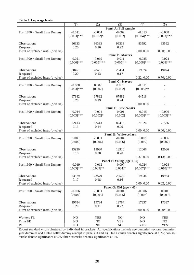
Table 5 reports regression results from the estimation of (1). Panel A focusses on the full

10The variable �rm size varies almost continuously as it measures the average size of the �rm during theyear.

15

sample which includes all workers with a valid wage between 1989 and 1993. The sample is

otherwise unrestricted and is therefore unbalanced. We then move to the subsample of �rm

movers (Panel B), i.e., the sample of individuals with a valid wage between 1989 and 1993

who change �rm at least once. Next, we consider the sample of stayers (Panel C), i.e., the

sample of all individuals with a valid wage between 1989 and 1993 who stay in the same �rm

for the whole period. Of course, the full sample is the sum of the �rm stayers and the �rm

movers samples. We �nally report separate estimates for blue collar workers (Panel D), white

collar workers (Panel E), young workers below 30 (Panel F), and old workers above 45 (Panel

G). For the sake of brevity we only show the coe¢ cient of interest on the interaction term

between the small �rm dummy and the post-reform dummy, which measures the average

increase in log wages in small �rms after the reform.

OLS results for the full sample (Column 1, Panel A) suggest that workers in �rms just

below the �rm size threshold of 15 employees are paid 1.1 percent less than workers in �rms

immediately above the cuto¤ after 1990. Columns 2 and 3 refer to worker and �rm �xed

e¤ects estimates, respectively, and show that the negative OLS result is robust (albeit lower

in magnitude) to the inclusion of worker �xed e¤ects but does not survive the inclusion of

�rm-speci�c dummies. This may be due to the heterogeneity of the e¤ects across di¤erent

workers within the same �rm, as the within-�rm variation (that identi�es the �rm �xed

e¤ects coe¢ cients) derives from the aggregation of potentially highly heterogeneous and o¤-

setting worker e¤ects. Finally, columns 4 and 5 refer to IV and IV with worker �xed e¤ects

estimates, respectively. Both speci�cations deliver negative and signi�cant coe¢ cients of

approximately the same magnitude as the OLS results.11 This is reassuring as it con�rms

the impression that �rm sorting is not a major source of bias.

Panels B and C of Table 5 look at movers and stayers separately and indicate that the

results obtained for the full sample are mainly driven by the former. Results for the sample

of stayers in Panel C show in fact low and insigni�cant e¤ects once we control for worker and

�rm �xed e¤ects. These results �t the interpretation that the strength of the wage e¤ects

of EPL is inversely related to the bargaining power of workers, as newly hired workers are

often endowed with low bargaining power and �rms can more easily lower their wages than

those of incumbent workers.

In Panels D and E of Table 5 we analyse the subsamples of blue collar and white collar,

respectively. Results show that the e¤ect found on the total sample is driven by blue collar

workers: the coe¢ cients in Panel D are of the same magnitude as those shown in Panel A,

11The power of the instruments is strong as indicated by the F-tests of the excluded instruments whichequal 8:04 and 40727:76 in the �rst-stage regressions for DS

jt and DSjt � Post respectively.

16

while the results for white collar are smaller in magnitude and insigni�cant. We also �nd

that the e¤ects of EPL on wages are stronger among young workers aged less than 30 (Panel

F) and insigni�cant among old workers aged more than 45 (Panel G). The negative e¤ect on

young workers�wages is almost twice as large as the e¤ect found on the full sample in the

OLS and the IV speci�cation (columns 1 and 4) and even larger in the other cases (columns

2, 3 and 5). These results are again in line with a bargaining power type of interpretation,

as blue collar and young workers have arguably low bargaining power vis-à-vis employers.

Of course, the strength of bargaining power does not refer necessarily to unionization rates

(which are very low among small �rms workers in Veneto, as in the whole country, while

coverage is very high) but to the option value of workers in the market.

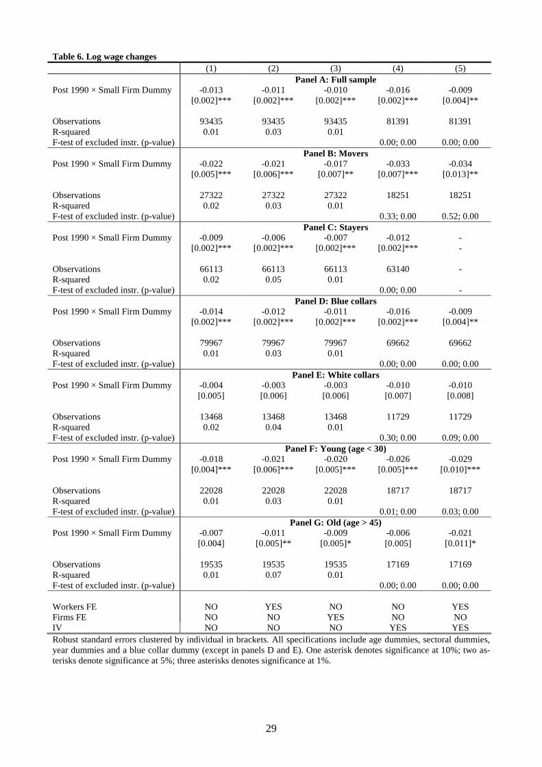
Finally, we look at e¤ects of the EPL reform on log wage changes to investigate whether

stricter EPL a¤ects wage growth on top of levels. Results in Table 6 show that indeed

this is the case. Full sample estimates in Panel A show that workers lose on average 1%

in terms of wage growth after the reform in small �rms relative to large �rms. The e¤ect

is negative and signi�cant in all speci�cations (worker �xed e¤ects, �rm �xed e¤ects and

IVs). It is worth noticing that the fact that the speci�cation in changes yields a negative

and signi�cant coe¢ cient even including �rm �xed e¤ects (and the coe¢ cient of interest

is identi�ed by within �rm variation) seems to indicate that the negative e¤ects on wage

growth are more evenly spread across di¤erent workers types, contrary to the case of wage

levels.

This impression is con�rmed in the analysis of the di¤erent subsamples. Both movers

(Panel B) and stayers (Panel C) in small �rms su¤er signi�cant wage losses after the reform

relative to large �rms workers. While the negative e¤ect on movers is larger in magnitude,

the fact that also stayers are hit by the reform suggests that they also pay part of the increase

in EPL in the form of lower wage growth (or, given that these workers stay in the same �rm,

in the form of a lower tenure pro�le). As long as a large part of the wage is decided at the

�rm level, incumbents have higher bargaining power and can impede renegotiation of wages

to the bottom but probably cannot avoid a slower wage growth for the part not included

in union contracts. Consistently with this story, blue collar (Panel D) and young workers

(Panel F) lose more in terms of percentage wage changes than white collar (Panel E) and

older workers (Panel G).

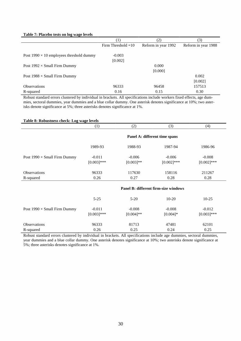
5.1 Robustness checks and placebo tests

This section shows that our results are robust to a number of checks. In Table 7 we run

robustness checks with respect to the time span of the sample� enlarging the sample from

17

the benchmark 1989�1993 to 1988�1993, 1987�1994 and 1986�1996� and with respect to the

window of �rm size� from the benchmark 5�25 to 5�20, 10�20 and 10�25. The �rst two

panels show that our results are robust to changes in the sample.

In Table 8 we also show that the results are robust to a di¤erent speci�cation. To test

the robustness of the estimates to the polynomial speci�cation we also �t a linear regression

function to the observations distributed within a distance � on both sides of the threshold:

logwijt = �0Xijt + �0Post+ �1D

Sjt + �2

�DSjt � Post

�for �rm size 2 [15��; 15 +�]: (6)

We choose � with the cross-validation method of Imbens and Lemieux (2008). The cross-

validation method consists in choosing � so as to minimize the loss function: L(�) =1N

PNi=1(logwi�[logw�(fsizej))2, where, for every fsizej to the left (right) of the threshold

15, we predict [logw�(fsizej) as if it were at the boundary of the estimation using onlyobservations in the interval fsizej 2 [15 � �; 15 + �]. We choose the optimal � between

1 and 15. The optimal �� = 5 with L(5) =0.03762235. Table 8 shows that not always are

the results robust to the speci�cation change: the local linear regression estimator yields a

negative signi�cant coe¢ cient for OLS and non-signi�cant results for worker and �rm �xed

e¤ects. IVs are also imprecise and the OLS results are not always robust to the estimation

sample�s being taken over di¤erent years (Panel B).

Finally, in Table 9 we implement placebo tests by estimating the treatment e¤ect at fake

thresholds, where there should be no e¤ect. In particular, we look at �rms below and above

the fake 10 employees threshold and we estimate the treatment e¤ect before and after 1993

and before and after 1988. The results are reassuring in that the coe¢ cients of the treated

group are either insigni�cant or positive and signi�cant, the opposite of what we �nd in our

exercise.

6 Conclusion

This paper examined the e¤ect of employment protection legislation (EPL) on wages, a

largely underexplored issue in the wide literature on EPL. It exploited, as a natural experi-

ment, a reform of EPL in Italy which increased severance payments after 1990 for �rms with

fewer than 15 employees relative to larger �rms.

We �nd that average wages of male workers declined by around 0.7%�1.5% in �rms

below 15 employees, relative to larger �rms, because of the 1990 EPL reform. Our result are

consistent with an explanation based on bargaining power because the e¤ect is concentrated

on new hires (rather than stayers), on blue collar and on young workers, all groups with a

18

relatively low bargaining power. Stayers su¤ered a moderate reduction of wage growth after

the reform. We showed that our results are robust to many changes in the sample time span

and in the window of �rm size considered around the 15 employees threshold. Placebo tests

con�rmed that the results apply only in 1990 for �rms at the 15 employees threshold and

not in other cases.

It is important to stress that our empirical exercise� which is local in nature as any

RDD� cannot help determining whether any increase in EPL would be o¤set by lower wages.

However, the Italian case o¤ers not only a clean natural experiment which involved a vast

quantity of �rms and workers, but may also provide insights on the e¤ects of EPL in the

many countries which have �rm-level thresholds in the application of EPL.

Using our estimates, it is possible to calculate how much of the increase in the �ring

cost is translated onto lower wages.12 We start by considering the situation of a employer-

initiated dismissal of a worker of average tenure in a small �rm after the reform. If the

dismissal is ruled unfair by the judge, the �ring cost will range between 2.5 and 6 months

(on average 16 weeks) of the last wage. On the basis of our data, the post-reform average

weekly wage amounts to approximately 313 euros. Therefore, the severance pay transferred

to the worker amounts to 313 � 16 weeks = 5; 008 euros, excluding the legal expenses thatcan be roughly calculated to be as much as 5; 000 euros. The above computation results in

a very high �ring cost, but we should keep in mind that this is the worst possible scenario

for the �rm. Ex-ante, the �rm does not know with certainty whether the separation will

be ruled unfair by the court. Furthermore, �rms and workers may �nd a settlement out

of court. Galdón-Sánchez and Güell (2000), using data based on actual court sentences,

estimate that in Italy the probability of reaching an out-of-court agreement to be around

0:5 and the probability that the dismissal is ruled unfair to be about 0:5. If we assume that

in case of an out-of-court agreement the employer pays approximately the same sum that

would be paid in the form of severance pay, �rms below 15 employees can expect a �ring

cost equal to 5; 008� 0:5 = 2; 504 euros excluding legal expenses. If we assume a probabilityof 10% of the occurrence of individual �ring for economic reasons, the total expected cost

ex-ante is (5; 000 + 2; 504)=10 = 750:4 euros.

Heckman and Pagès (2004) develop a measure of the expected present discounted cost to

the �rm, at the time a worker is hired, associated with severance payments to that worker in

the future (they also take into account notice period, which is not of interest here). Adopting

an analogous approach, one could use the estimates in the paper to compute the e¤ect of

12This quanti�cation exercise is, as our empirical approach, purely partial equilibrium and assumes anyadditional e¤ects of EPL away. We leave the quanti�cation of the general equilibrium impact of EPL withina dynamic GE model for future work.

19

severance payments on the expected present discounted value of wages, also at the time the

worker is hired. On the basis of our estimates in Table 5 (columns 1), the wage loss for an

average worker in a small �rm (with average tenure 3.5 years) after the reform (b�2 = �0:011)amounts to about 3:4 euros per week (313� 0:011) or approximately 179 euros per year.We use an annual discount rate of 8%, i.e., a discount factor of � = 0:92. To match an

average tenure of 3.5 years, we use an annual survival probability of � = 0:71. LetW be the

present discounted value of the wage loss due to the reform W (b�2j�; �) = 179�P1t=0[��]

t =

516:1. This implies that around 68:8% (516=750 = 0:688) of the expected �ring cost is

translated into lower wages. Notice that a 68.8% o¤setting e¤ect is not inconsistent with the

view that severance payments may actually strengthen the bargaining power of (incumbent)

workers: in fact the average hides heterogenous e¤ects across di¤erent workers.

References

[1] Autor, David H., (2003), Outsourcing at Will: The Contribution of Unjust Dismissal

Doctrine to the Growth of Employment Outsourcing, Journal of Labor Economics,

21(1), January, 1�42.

[2] Autor, David H., John J. Donohue and Stewart J. Schwab, (2006), The Costs of

Wrongful-Discharge Laws, Review of Economics and Statistics, 88(2), May, 211�231.

[3] Autor, David H., William R. Kerr and Adriana D. Kugler, (2007), Do Employment

Protections Reduce Productivity? Evidence from U.S. States, The Economic Journal,

117, June, 189�217.

[4] Bauer, Thomas K., S. Bender and H. Bonin (2007), Dismissal Protection and Worker

Flows in Small Establishments. Economica, 296 (74): 804�821.

[5] Bentolila, Samuel, and Giuseppe Bertola, (1990), Firing Costs and Labour Demand:

How bad is Eurosclerosis?, Review of Economic Studies, 57, 381�402.

[6] Bertola, Giuseppe, (1990), Job Security, Employment, and Wages, European Economic

Review, 54(4), 851�79.

[7] Bertola, Giuseppe, (2004), A Pure Theory of Job Security and Labor Income Risk,

Review of Economic Studies, 71(1), 43�61.

[8] Bird, Robert C., and John D. Knopf, (2009), Do Wrongful-Discharge Laws Impair Firm

Performance?, Journal of Law and Economics, 52, 197�222.

20

[9] Boeri, Tito, and Juan F. Jimeno, (2005), The E¤ects of Employment Protection: Learn-

ing from Variable Enforcement, European Economic Review, 49(8), 2057�2077.

[10] Borgarello, Andrea, Pietro Garibaldi and Lia Pacelli, (2004), Employment Protection

Legislation and the Size of Firms, Il Giornale degli Economisti, 63(1), 33�66.

[11] Cervini Plá, María, Xavier Ramos and José Ignacio Silva, (2010),Wage E¤ects of Non-

Wage Labour Costs, mimeo.

[12] Cingano, Federico, Marco Leonardi, Julián Messina and Giovanni Pica, (2010), The

E¤ect of Employment Protection Legislation and Financial Market Imperfections on In-

vestment: Evidence from a Firm-Level Panel of EU countries, Economic Policy, 25(61),

117�163.

[13] Dolado, J. J., M. Jansen and J. F. Jimeno (2007): A Positive Analysis of Targeted

Employment Protection Legislation, The B. E. Journal of Macroeconomics. Topics,

7(1), Article 14.

[14] Erickson, C. L., and Andrea Ichino, (1995), Wage di¤erentials in Italy: market forces,

institutions, and in�ation, in: R. B. Freeman and L. F. Katz (eds.), Di¤erences and

Changes in Wage Structures, Chicago: The Univ. of Chicago Press.

[15] Galdón-Sánchez, José, and Maia Güell, (2000), Let�s Go to Court! Firing Costs and

Dismissal Con�icts, Industrial Relations Sections, Princeton University, Working Paper

no. 444.

[16] Guiso, L., L. Pistaferri and Fabiano Schivardi, (2005), Insurance Within the Firm,

Journal of Political Economy, 113, 1054�1087.

[17] Heckman, J. J., and Carmen Pagés, (2004), Law and Employment: Lessons from Latin

American and the Caribbean, NBER Books, National Bureau of Economic Research.

[18] Imbens, G., and T. Lemieux, 2008. Regression Discontinuity Designs: A Guide to Prac-

tice. Journal of Econometrics 142, 615�635.

[19] Kugler, Adriana, and Giovanni Pica, (2006), The E¤ects of Employment Protection

and Product Market Regulations on the Italian Labor Market, in: Julián Messina,

Claudio Michelacci, Jarkko Turunen and Gyl�Zoega (eds.), Labour Market Adjustments

in Europe. Edward Elgar Publishing.

21

[20] Kugler, Adriana, and Giovanni Pica, (2008), E¤ects of Employment Protection on

Worker and Job Flows: Evidence from the 1990 Italian Reform, Labour Economics,

15(1), 78�95.

[21] Kugler, Adriana, and Gilles Saint-Paul, (2004), How Do Firing Costs A¤ect Worker

Flows in a World with Adverse Selection?, Journal of Labor Economics, 22(3), 553�584.

[22] Lazear, Edward, (1990), Job Security Provisions and Employment, Quarterly Journal

of Economics, 105(3), 699�726.

[23] Lee, David, (2007), Randomized Experiments from Non-random Selection in U.S. House

Elections, Journal of Econometrics, 142, 675�697.

[24] Ljungqvist, Lars, (2002), How Do Lay-O¤ Cost A¤ect Employment?, The Economic

Journal, 112 (October), 829�853.

[25] Martins, Pedro S., (2009), Dismissals for Cause: The Di¤erence That Just Eight Para-

graphs Can Make, Journal of Labor Economics, 27(2), 257�279.

[26] McCrary, Justin, (2008), Manipulation of the Running Variable in the Regression Dis-

continuity Design: A Density Test, Journal of Econometrics, 142(2), 698�714.

[27] Mortensen, Dale, and Cristopher Pissarides, (1999), New Developments in Models of

Search in the Labour Market, in: O. Ashenfelter and D. Card (eds.), Handbook of Labour

Economics, Vol 3B, Amsterdam: Elsevier.

[28] Paggiaro, A., Enrico Rettore and Ugo Trivellato, (2008), The E¤ect of Extending the

Duration of Eligibility in an Italian Labour Market Programme for Dismissed Workers,

CESIFO WP 2340.

[29] Pissarides, Christopher A., (2001), Employment Protection, Labour Economics, 8, 131�

159.

[30] Schivardi, F., and Roberto Torrini, (2008), Identifying the e¤ects of �ring restrictions

through size-contingent di¤erences in regulation, Labour Economics, 15(3), 482�511.

[31] Tattara, G., and Marco Valentini, (2005), Job Flows, Worker Flows and Mismatching

in Veneto Manufacturing. 1982�1996, mimeo, University of Venice.

[32] Van der Wiel, Karen (2010), Better Protected, Better Paid: Evidence on how Employ-

ment Protection A¤ects Wages, Labour Economics, 7(1), 829�849.

22

[33] Wasmer, E., (2006), Interpreting Europe�US labor market di¤erences: the speci�city of

human capital investments, American Economic Review, 96(3), 811�31.

23

24

Table 1: Descriptive statistics Pre-reform Post-reform Small firms Large firms Small firms Large firms

Real weekly wages 297.004 312.041 312.923 331.243 (72.688) (83.89) (78.545) (90.367) Real weekly wage growth rate 0.049 0.04 0.024 0.029 (0.121) (0.114) (0.123) (0.127) Employment 9.595 19.478 9.541 19.551 (2.956) (2.805) (2.958) (2.83) White collar dummy 0.134 0.163 0.133 0.165 (0.34) (0.37) (0.34) (0.371) Age 35.06 35.514 37.489 37.918 (8.598) (8.525) (8.675) (8.623) Sector dummies: Agriculture 0.006 0.005 0.006 0.005 (0.079) (0.069) (0.077) (0.071) Gas-water-oil 0.001 0 0.001 0 (0.03) (0) (0.03) (0) Extraction-minerals-chemical 0.08 0.094 0.077 0.103 (0.271) (0.292) (0.267) (0.305) Metal 0.272 0.322 0.271 0.311 (0.445) (0.467) (0.445) (0.463) Manufacturing 0.242 0.297 0.237 0.292 (0.429) (0.457) (0.425) (0.455) Construction 0.156 0.111 0.163 0.109 (0.363) (0.314) (0.369) (0.312) Wholesale-retail-hotel 0.182 0.11 0.184 0.118 (0.386) (0.313) (0.388) (0.323) Transportation 0.032 0.026 0.034 0.026 (0.177) (0.158) (0.18) (0.158) Banks-insurance 0.011 0.013 0.01 0.014 (0.105) (0.112) (0.099) (0.118) N 31505 17121 45848 26178

25

Table 2: Firm sorting (1) (2) (4) Dummy 13 -0.020 -0.008 -0.010 (0.013) (0.020) (0.020) Dummy 14 -0.032 0.006 0.009 (0.014)** (0.021) (0.022) Dummy 15 0.000 0.004 0.002 (0.015) (0.024) (0.024) Post 1990 × Dummy 13 -0.021 -0.013 (0.025) (0.026) Post 1990 × Dummy 14 -0.062 -0.062 (0.025)** (0.026)** Post 1990 × Dummy 15 -0.006 0.009 (0.029) (0.030) Firms Fixed Effect 0.212 (0.025)*** Firms Fixed Effect × Dummy 13 0.053 (0.101) Firms Fixed Effect × Dummy 14 -0.106 (0.112) Firms Fixed Effect × Dummy 15 0.141 (0.123) Post 1990 × Firms Fixed Effect -0.171 (0.030)*** Post 1990 × Firms Fixed Effect × Dummy 13 -0.149 (0.133) Post 1990 × Firms Fixed Effect × Dummy 14 0.042 (0.139) Post 1990 × Firms Fixed Effect × Dummy 15 -0.168 (0.151) Observations 33149 33149 31751 Notes: The dependent variable is a dummy that takes the value of 1 if in firm j employment at time t is larger than em-ployment at time t-1, and 0 otherwise. Firms between 5 and 25 workers are included. All specifications include a third degree polynomial in lagged firm size, a quadratic in firms' age, sector dummies and year dummies. One asterisk de-notes significance at 10%; two asterisks denote significance at 5%; three asterisks denotes significance at 1%.

26

Table 3: balanced test of firm characteristics

Age White collar

Agri-culture

Gas-water-

oil

Extraction-

miner-als-

chemi-cal

Metal Manu-factur-

ing

Con-struc-tion

Wholesale-

retail-hotel

Trans-porta-tion

Banks-insur-ance

2nd degree polynomial

20.89 1.252 -0.067 -0.037 1.297 -1.479 -3.162 0.584 1.772 -0.074 0.523 Post 1990 × Small Firm

(26.60) (1.326) (0.324) (0.080) (1.255) (2.014) (2.073) (1.243) (1.530) (0.536) (0.590)

3rd degree polynomial

251.82 26.051 2.121 0.069 17.979 8.141 -66.4** 7.127 21.446 -0.845 9.269 Post 1990 × Small Firm

(354.6) (17.67) (4.316) (1.060) (16.72) (26.86) (27.63) (16.57) (20.40) (7.146) (7.871)

Obs 9914 9914 9914 9914 9914 9914 9914 9914 9914 9914 9914 Robust standard errors clustered by individual in brackets. One asterisk denotes significance at 10%; two asterisks de-note significance at 5%; three asterisks denotes significance at 1%.

27

Table 4: Workers' sorting Dependent Variable: mover dummy (probit)

P > 15 P ≤ 15

Small firm dummy 0.009 0.009 -0.000 0.000 (0.003)*** (0.003)*** (0.004) (0.004) Small firm dummy × Dummy 1990 -0.010 -0.010 -0.003 -0.003 (0.003)*** (0.003)*** (0.004) (0.004) Small firm dummy × Dummy 1991 -0.013 -0.013 0.001 0.001 (0.003)*** (0.003)*** (0.005) (0.005) Small firm dummy × Dummy 1992 -0.014 -0.014 0.024 0.023 (0.003)*** (0.003)*** (0.006)*** (0.006)*** Small firm dummy × Dummy 1993 -0.003 -0.003 0.014 0.014 (0.003) (0.003) (0.005)*** (0.005)*** Workers Fixed Effect -0.010 -0.061 (0.012) (0.014)*** Workers Fixed Effect × Small firm dummy

0.001 0.022

(0.015) (0.017) Workers Fixed Effect × Dummy 1990

-0.008 -0.012

(0.016) (0.019) Workers Fixed Effect × Dummy 1991

-0.020 -0.001

(0.016) (0.020) Workers Fixed Effect × Dummy 1992

-0.019 0.044

(0.017) (0.021)** Workers Fixed Effect × Dummy 1993

-0.008 -0.005

(0.015) (0.023) Workers Fixed Effect × Dummy 1990 × Small Firm Dummy

0.008 0.018

(0.021) (0.024) Workers Fixed Effect × Dummy 1991 × Small Firm Dummy

0.050 0.003

(0.021)** (0.024) Workers Fixed Effect × Dummy 1992 × Small Firm Dummy

0.024 -0.033

(0.022) (0.025) Workers Fixed Effect × Dummy 1993 × Small Firm Dummy

0.016 0.024

(0.018) (0.027) Observations 120652 120652 120583 120583 Notes: In the first (last) two columns the dependent variable is a dummy that takes the value of 1 if worker i moves to a firm with more (less) than 15 employees and 0 otherwise. Firms between 5 and 25 employees included. All specifica-tions include a quadratic in workers' age, year dummies, sector dummies and a polynomial in the size of the firm of origin. Standard errors in brackets. One asterisk denotes significance at 10%; two asterisks denote significance at 5%; three asterisks denote significance at 1%.

28

Table 5. Log wage levels (1) (2) (3) (4) (5) Panel A: Full sample Post 1990 × Small Firm Dummy -0.011 -0.004 -0.002 -0.013 -0.008 [0.003]*** [0.002]* [0.002] [0.004]*** [0.003]*** Observations 96333 96333 96333 83592 83592 R-squared 0.26 0.16 0.22 F-test of excluded instr. (p-value) 0.00; 0.00 0.00; 0.00 Panel B: Movers Post 1990 × Small Firm Dummy -0.021 -0.019 -0.011 -0.025 -0.024 [0.006]*** [0.005]*** [0.005]** [0.008]*** [0.008] *** Observations 28451 28451 28451 19074 19074 R-squared 0.20 0.13 0.17 F-test of excluded instr. (p-value) 0.22; 0.00 0.70; 0.00 Panel C: Stayers Post 1990 × Small Firm Dummy -0.008 0.002 0.001 -0.011 - [0.003]*** [0.002] [0.002] [0.005]** - Observations 67882 67882 67882 64518 - R-squared 0.28 0.19 0.24 F-test of excluded instr. (p-value) 0.00; 0.00 - Panel D: Blue collars Post 1990 × Small Firm Dummy -0.014 -0.004 -0.001 -0.015 -0.006 [0.003]*** [0.002]* [0.002] [0.003]*** [0.003]** Observations 82413 82413 82413 71526 71526 R-squared 0.13 0.14 0.09 F-test of excluded instr. (p-value) 0.00; 0.00 0.00; 0.00 Panel E: White collars Post 1990 × Small Firm Dummy 0.005 -0.001 -0.004 0.003 -0.006 [0.009] [0.006] [0.006] [0.019] [0.007] Observations 13920 13920 13920 12066 12066 R-squared 0.18 0.20 0.20 F-test of excluded instr. (p-value) 0.37; 0.00 0.13; 0.00 Panel F: Young (age < 30) Post 1990 × Small Firm Dummy -0.019 -0.012 -0.007 -0.024 -0.028 [0.005]*** [0.005]** [0.004]* [0.007]*** [0.010]** * Observations 23579 23579 23579 19934 19934 R-squared 0.17 0.18 0.16 F-test of excluded instr. (p-value) 0.00; 0.00 0.02; 0.00 Panel G: Old (age > 45) Post 1990 × Small Firm Dummy -0.006 -0.001 -0.001 -0.006 0.001 [0.007] [0.005] [0.005] [0.008] [0.009] Observations 19784 19784 19784 17337 17337 R-squared 0.29 0.11 0.22 F-test of excluded instr. (p-value) 0.00; 0.00 0.00; 0.00 Workers FE NO YES NO NO YES Firms FE NO NO YES NO NO IV NO NO NO YES YES Robust standard errors clustered by individual in brackets. All specifications include age dummies, sectoral dummies, year dummies and a blue collar dummy (except in panels D and E). One asterisk denotes significance at 10%; two as-terisks denote significance at 5%; three asterisks denotes significance at 1%.

29

Table 6. Log wage changes (1) (2) (3) (4) (5) Panel A: Full sample Post 1990 × Small Firm Dummy -0.013 -0.011 -0.010 -0.016 -0.009 [0.002]*** [0.002]*** [0.002]*** [0.002]*** [0.004 ]** Observations 93435 93435 93435 81391 81391 R-squared 0.01 0.03 0.01 F-test of excluded instr. (p-value) 0.00; 0.00 0.00; 0.00 Panel B: Movers Post 1990 × Small Firm Dummy -0.022 -0.021 -0.017 -0.033 -0.034 [0.005]*** [0.006]*** [0.007]** [0.007]*** [0.013] ** Observations 27322 27322 27322 18251 18251 R-squared 0.02 0.03 0.01 F-test of excluded instr. (p-value) 0.33; 0.00 0.52; 0.00 Panel C: Stayers Post 1990 × Small Firm Dummy -0.009 -0.006 -0.007 -0.012 - [0.002]*** [0.002]*** [0.002]*** [0.002]*** - Observations 66113 66113 66113 63140 - R-squared 0.02 0.05 0.01 F-test of excluded instr. (p-value) 0.00; 0.00 - Panel D: Blue collars Post 1990 × Small Firm Dummy -0.014 -0.012 -0.011 -0.016 -0.009 [0.002]*** [0.002]*** [0.002]*** [0.002]*** [0.004 ]** Observations 79967 79967 79967 69662 69662 R-squared 0.01 0.03 0.01 F-test of excluded instr. (p-value) 0.00; 0.00 0.00; 0.00 Panel E: White collars Post 1990 × Small Firm Dummy -0.004 -0.003 -0.003 -0.010 -0.010 [0.005] [0.006] [0.006] [0.007] [0.008] Observations 13468 13468 13468 11729 11729 R-squared 0.02 0.04 0.01 F-test of excluded instr. (p-value) 0.30; 0.00 0.09; 0.00 Panel F: Young (age < 30) Post 1990 × Small Firm Dummy -0.018 -0.021 -0.020 -0.026 -0.029 [0.004]*** [0.006]*** [0.005]*** [0.005]*** [0.010 ]*** Observations 22028 22028 22028 18717 18717 R-squared 0.01 0.03 0.01 F-test of excluded instr. (p-value) 0.01; 0.00 0.03; 0.00 Panel G: Old (age > 45) Post 1990 × Small Firm Dummy -0.007 -0.011 -0.009 -0.006 -0.021 [0.004] [0.005]** [0.005]* [0.005] [0.011]* Observations 19535 19535 19535 17169 17169 R-squared 0.01 0.07 0.01 F-test of excluded instr. (p-value) 0.00; 0.00 0.00; 0.00 Workers FE NO YES NO NO YES Firms FE NO NO YES NO NO IV NO NO NO YES YES Robust standard errors clustered by individual in brackets. All specifications include age dummies, sectoral dummies, year dummies and a blue collar dummy (except in panels D and E). One asterisk denotes significance at 10%; two as-terisks denote significance at 5%; three asterisks denotes significance at 1%.

30

Table 7: Placebo tests on log wage levels (1) (2) (3) Firm Threshold =10 Reform in year 1992 Reform in year 1988 Post 1990 × 10 employees threshold dummy -0.003 [0.002] Post 1992 × Small Firm Dummy 0.000 [0.000] Post 1988 × Small Firm Dummy 0.002 [0.002] Observations 96333 96458 157513 R-squared 0.16 0.15 0.30

Robust standard errors clustered by individual in brackets. All specifications include workers fixed effects, age dum-mies, sectoral dummies, year dummies and a blue collar dummy. One asterisk denotes significance at 10%; two aster-isks denote significance at 5%; three asterisks denotes significance at 1%. Table 8: Robustness check: Log wage levels (1) (2) (3) (4) Panel A: different time spans 1989-93 1988-93 1987-94 1986-96 Post 1990 × Small Firm Dummy -0.011 -0.006 -0.006 -0.008 [0.003]*** [0.003]** [0.002]*** [0.002]*** Observations 96333 117630 158116 211267 R-squared 0.26 0.27 0.28 0.28 Panel B: different firm-size windows 5-25 5-20 10-20 10-25 Post 1990 × Small Firm Dummy -0.011 -0.008 -0.008 -0.012 [0.003]*** [0.004]** [0.004]* [0.003]*** Observations 96333 81713 47481 62101 R-squared 0.26 0.25 0.24 0.25

Robust standard errors clustered by individual in brackets. All specifications include age dummies, sectoral dummies, year dummies and a blue collar dummy. One asterisk denotes significance at 10%; two asterisks denote significance at 5%; three asterisks denotes significance at 1%.

31

Table 9: Local linear regression: Log wage levels (firm size 5-25) (1) (2) (3) (4) Panel A: different estimators OLS Worker FE Firm FE IV Post 1990 × Small Firm Dummy -0.011 -0.004 -0.003 -0.006 [0.002]*** [0.001]*** [0.002]* [0.003]* Observations 96333 96333 96333 96333 R-squared F-test of excluded instr. (p-value)

0.24 0.88 0.70

8849 (0.00) Panel B: OLS different time spans 1989-93 1988-93 1987-94 1986-96 Post 1990 × Small Firm Dummy -0.011 -0.007 -0.008 -0.011 [0.002]*** [0.002]*** [0.002]*** [0.002]*** Observations 96333 117630 158116 211267 R-squared 0.24 0.26 0.27 0.28

The optimal symmetric bandwidth is chosen with cross-validation methods ∆=10. Robust standard errors clustered by individual in brackets. One asterisk denotes significance at 10%; two asterisks denote significance at 5%; three aster-isks denotes significance at 1%.