WhereNext: a location predictor on trajectory pattern mining

Seediscussions,stats,andauthorprofilesforthispublicationat:https://www.researchgate.net/publication/221654136

WhereNext:Alocationpredictorontrajectorypatternmining

ConferencePaper·June2009

DOI:10.1145/1557019.1557091·Source:DBLP

CITATIONS

206

READS

1,518

4authors,including:

Someoftheauthorsofthispublicationarealsoworkingontheserelatedprojects:

SoBigDataViewproject

Cimplex(FETProactive,grantagreement641191)Viewproject

AnnaMonreale

UniversitàdiPisa

46PUBLICATIONS617CITATIONS

SEEPROFILE

FabioPinelli

IBM,Research

35PUBLICATIONS1,032CITATIONS

SEEPROFILE

FoscaGiannotti

ItalianNationalResearchCouncil

221PUBLICATIONS3,677CITATIONS

SEEPROFILE

AllcontentfollowingthispagewasuploadedbyAnnaMonrealeon30November2016.

Theuserhasrequestedenhancementofthedownloadedfile.Allin-textreferencesunderlinedinbluearelinkedtopublicationsonResearchGate,lettingyouaccessandreadthemimmediately.

WhereNext: a Location Predictor on Trajectory PatternMining

Anna MonrealeDept. Computer ScienceUniversity of Pisa, ItalyISTI - CNR Pisa, [email protected]

Fabio PinelliISTI - CNR Pisa, Italy

[email protected]

Roberto TrasartiDept. Computer ScienceUniversity of Pisa, ItalyISTI - CNR Pisa, Italy

[email protected]

Fosca GiannottiISTI - CNR Pisa, Italy

[email protected]

ABSTRACTThe pervasiveness of mobile devices and location based ser-vices is leading to an increasing volume of mobility data.This side effect provides the opportunity for innovative meth-ods that analyse the behaviors of movements. In this paperwe propose WhereNext, which is a method aimed at pre-dicting with a certain level of accuracy the next location ofa moving object. The prediction uses previously extractedmovement patterns named Trajectory Patterns, which area concise representation of behaviors of moving objects assequences of regions frequently visited with a typical traveltime. A decision tree, named T-pattern Tree, is built andevaluated with a formal training and test process. The treeis learned from the Trajectory Patterns that hold a certainarea and it may be used as a predictor of the next loca-tion of a new trajectory finding the best matching path inthe tree. Three different best matching methods to classifya new moving object are proposed and their impact on thequality of prediction is studied extensively. Using TrajectoryPatterns as predictive rules has the following implications:(I) the learning depends on the movement of all available ob-jects in a certain area instead of on the individual history ofan object; (II) the prediction tree intrinsically contains thespatio-temporal properties that have emerged from the dataand this allows us to define matching methods that stricltydepend on the properties of such movements. In addition,we propose a set of other measures, that evaluate a priorithe predictive power of a set of Trajectory Patterns. Thismeasures were tuned on a real life case study. Finally, anexhaustive set of experiments and results on the real datasetare presented.

Categories and Subject DescriptorsH.2.8 [Database Applications]: Data mining

Permission to make digital or hard copies of all or part of this work forpersonal or classroom use is granted without fee provided that copies arenot made or distributed for profit or commercial advantage and that copiesbear this notice and the full citation on the first page. To copy otherwise, torepublish, to post on servers or to redistribute to lists, requires prior specificpermission and/or a fee.KDD’09, June 28–July 1, 2009, Paris, France.Copyright 2009 ACM 978-1-60558-495-9/09/06 . . .$5. 00.

General TermsAlgorithms

KeywordsTrajectory patterns, Spatio-temporal data mining

1. INTRODUCTIONThe last few years, have witnessed a considerable increase

in the number of mobile devices along with the use of wire-less communication, such as Bluetooth, Wi-fi and GPRS.Such mobile devices are often equipped with positioning sen-sors that utilize Global Positioning Systems (GPS) to accu-rately provide the location of a device. This means thatthe movement of people or vehicles within a given area canbe observed from the digital traces left behind by the per-sonal or vehicular mobile devices, and collected by the wire-less network infrastructures. For instance, mobile phonesleave positioning logs, which specify their localization, orcell, whenever they are connected to the GSM network.Likewise GPS-equipped portable devices can record theirlatitude-longitude position and transmit their trajectoriesto a collecting server. The pervasiveness of such ubiqui-tous technologies guarantees that there will be an increasingavailability of large amounts of data on individual trajecto-ries, with increasing precision in term of localization.Knowledge about the positions of mobile objects has ledto location-based services and applications, which need toknow the approximate position of a mobile user in orderto operate. Examples of such services are navigational ser-vices, traffic management and location-based advertising. Ina typical scenario, a moving object periodically informs thepositioning framework of its current location. Due to the un-reliable nature of mobile devices and the limitations of thepositioning systems, the location of a mobile object is oftenunknown for a long period of time. In such cases, a methodto predict the possible next location of a moving object isrequired in order to anticipate or pre-fetch possible servicesin the next location. Several proposals in the literature useonly the history of movements of the individual object onthe basis of which future location is simply guessed. Theinnovative aspect of our work, on the other hand, is in theuse of the movements of all objects in a certain area to learna classifier. Our basic assumption is that people often fol-low the crowd: individuals tend to follow common paths.

637

For example, people go to work every day by similar routes,and public transport crosses similar routes in different timeperiods. Thus, if we have enough data to model typical be-haviors, we can use such knowledge to predict the futuremovement of most individuals: at least those whose pastmovements are fairly typical.Our method uses the movement patterns previously extractedby using the Trajectory Pattern algorithm developed in [2].The Trajectory Pattern algorithm mines movement patternsas sequences of regions where typical travel times are fre-quently followed.The four main steps of our approach are as follows:

Data Selection : by using spatio-temporal primitives, weselect a spatial area and a time period, in order totake only the portion of trajectories crossing that areain that time period.

Local Models Extraction : the Trajectory Pattern algo-rithm is executed to extract from the selected trajec-tories the frequent movement patterns called Trajec-tory Patterns (hereafter T-patterns). The discrimina-tive power of T-patterns is measured against differentevaluation functions which consider spatial coverage,dataset coverage, and region separation.

T-pattern Tree Building : the extracted local models,T-patterns, are combined in a prefix tree called T-pattern Tree. The nodes of the tree are regions fre-quently visited and the edges represent travel amongregions and are annotated with the typical travel time.Each common prefix of T-patterns becomes commonpath on the tree. This tree may be viewed as a globalmodel of the underlying mobility data, once augmentedwith a default path which represents all infrequent tra-jectories. This method is similar to the use of associ-ation rules as predictive rules in rule based classifiers.

Prediction : The T-pattern Tree is used to predict thefuture location of a moving object. To do this, thealgorithm uses a concept of distance defined in Section4.2 to find the best matching pattern and to predict thenext movement location. We propose three differentbest matching methods to classify a new moving objectand their impact on the accuracy of prediction hasbeen studied extensively, in relation to variations of thespatio-temporal window during the matching process.

The performance of the classifier is evaluated against a realdataset of 17000 cars equipped with GPS. The results ofthe experiments show that the prediction is of a good qual-ity when high spatio-temporal precision is required. Clearlythis is holds for a specific set of moving objects. In factthe precision decreases as the number of moving objects forwhich a prediction is possible grows.The rest of the paper is organized as follows. In Section 2we review the most recent literature regarding location pre-diction methods. In Section 3 we introduce the TrajectoryPattern mining method. Section 4 is the core of the paper,where the innovative aspects of our work are presented. Wedescribe how to build the T-pattern Tree and present ourprediction algorithm. In Section 5 a method to evaluatethe strength of prediction of the extracted patterns beforebuilding the tree is presented. Some experimental resultsare presented in Section 6. Section 7 concludes the paperand highlights the most promising future lines of research.

2. RELATED WORKThere are several studies that address the problem of pre-

dicting future locations. Most of them use a model based onfrequent patterns and association rules and define a trajec-tory as an ordered sequence of locations, where the time isused as a time-stamp [8, 9, 13, 5]. Moreover, some of theseapproaches try to predict the next location of a moving ob-ject by using the movements of all the moving objects ina database [8, 9], while others base the prediction only onthe movement history of the object itself [13, 5]. In [8, 9]Morzy introduces a new method for predicting the locationof a moving object. In particular, he extracts the associ-ation rules from the moving object database. Then, givena trajectory of a moving object, using matching functionshe selects the best association rule that matches this trajec-tory, and then uses it for the prediction. In [8] Morzy usesa modified version of Apriori algorithm to generate associa-tion rules, and in [9] he uses a modified version of PrefixSpanalgorithm. All the matching functions in these papers arebased on the notions of support and confidence and do notconsider any notion of spatial and temporal distance.In [13] the authors propose a method to predict user move-ments in a mobile computing system. This algorithm isbased on three steps: mining the mobility patterns of an in-dividual user, forming association rules from these patterns,and finally predicting a mobile user’s next movements byusing these rules. In order to select the rule used for theprediction, the authors consider the notions of support andconfidence. The support of each candidate is computed bya distance based on the notion of string alignment. Jeunget al. in [5] present an innovative approach which forecastsfuture locations of an object in a hybrid manner. Theycombine predefined motion functions with the movementpatterns of the object, extracted by a modified version ofthe Apriori algorithm. The motion functions are linear ornon-linear models that capture the object’s movements bysophisticated mathematical formulas and are an input of themethod decided by the analyst.In [12] the authors use a time-series analysis with travelspeed simulations to predict future trajectories. They use aprocess based on range querying with spatial-temporal con-straints on a moving object database. The prediction isrepresented by the locations that satisfy the spatio-temporalconstraints.Frequent patterns are also used to build a classification model.An interesting approach based on a framework of frequentpattern-based classification is presented in [1]. There areessentially three steps: feature generation, feature selectionand model learning. In the first step, frequent patterns aregenerated with a specified minimum support. In the secondstep, feature selection is applied on frequent patterns andfinally, a classification model is built from frequent patternsselected.

3. TRAJECTORY PATTERN MININGOver the last five years, attempts have been made to ex-

tend many techniques for knowledge discovery in classicalrelational or transactional data to knowledge discovery inthe context of movement data [10]. Some of the typicaltechniques adapted to the spatio-temporal context are asso-ciation rule mining, frequent pattern discovery, clustering,classification, prediction, and time-series analysis.

638

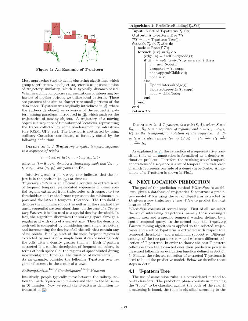
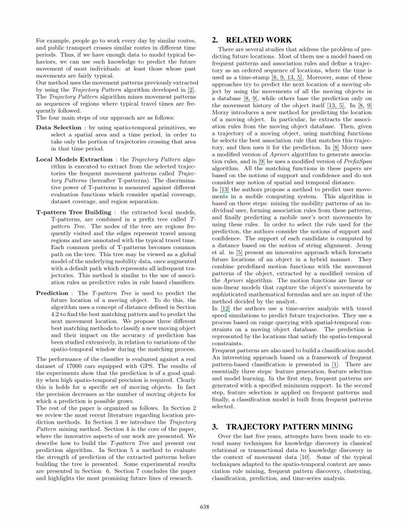
Figure 1: An Example of T-pattern

Most approaches tend to define clustering algorithms, whichgroup together moving object trajectories using some notionof trajectory similarity, which is typically distance-based.When searching for concise representations of interesting be-haviors of moving objects, we define local patterns. Theseare patterns that aim at characterize small portions of thedata space. T-pattern was originally introduced in [3], wherethe authors developed an extension of the sequential pat-tern mining paradigm, introduced in [2], which analyzes thetrajectories of moving objects. A trajectory of a movingobject is a sequence of time-stamped locations, representingthe traces collected by some wireless/mobility infrastruc-ture (GSM, GPS, etc). The location is abstracted by usingordinary Cartesian coordinates, as formally stated by thefollowing definition:

Definition 1. A Trajectory or spatio-temporal sequenceis a sequence of triples

T =< x0, y0, t0 >, . . . , < xn, yn, tn >

where ti (i = 0 . . . n) denotes a timestamp such that ∀0<i<n

ti < ti+1 and (xi, yi) are points in R2.

Intuitively, each triple < xi, yi, ti > indicates that the ob-ject is in the position (xi, yi) at time ti.Trajectory Pattern is an efficient algorithm to extract a setof frequent temporally-annotated sequences of dense spa-tial regions extracted from trajectories with respect to twothresholds σ and τ : the former represents the minimum sup-port and the latter a temporal tolerance. The threshold σdenotes the minimum support as well as in the standard fre-quent sequential pattern algorithms. In the case of a Trajec-tory Pattern, it is also used as a spatial density threshold. Infact, the algorithm discretizes the working space through aregular grid with cells of a user-set size. Then the density ofeach cell is computed by considering each single trajectoryand incrementing the density of all the cells that contain anyof its points. Finally, a set of the most frequent regions isextracted by means of a simple heuristics considering onlythe cells with a density greater than σ. Each T-patternextracted is a concise description of frequent behaviors, interms of both space (i.e. the regions of space visited duringmovements) and time (i.e. the duration of movements).As an example, consider the following T-pattern over re-gions of interest in the center of a town:

RailwayStation15min−→ CastleSquare

50min−→ Museum

Intuitively, people typically move between the railway sta-tion to Castle Square in 15 minutes and then to the Museumin 50 minutes. Now we recall the T-patterns definition in-troduced in [3]:

Algorithm 1: PrefixTreeBuilding(Tp Set)

Input: A Set of T-patterns Tp SetOutput: A T-pattern Tree PTPT = new T-pattern Tree();foreach Tp in Tp Set do

node = Root(PT );foreach (i, r) in Tp do

(edge, n) = findChild(node,r);if � ∃ n ∨ notIncluded(edge.interval,i) then

v = new Node(r);v.support = Tp.supp;node.appendChild(v,i);node = v;

elseUpdateInterval(edge,i);UpdateSupport(n,Tp.supp);node = childNode;

end

end

endreturn PT

Definition 2. A T-pattern, is a pair (S, A), where S =<R0, . . . , Rn > is a sequence of regions, and A = α1, . . . αn ∈Rk

+ is the (temporal) annotation of the sequence. A T-

pattern is also represented as (S, A) = R0α1−−→ R1

α2−−→. . .

αn−−→ Rn.

As explained in [2], the extraction of a representative tran-sition time as an annotation is formalized as a density es-timation problem. Therefore the resulting set of temporalannotations of a sequence is a set of temporal intervals, eachof which represents one side of a dense (hyper)cube. An ex-ample of a T-pattern is shown in Fig.1.

4. NEXT LOCATION PREDICTIONThe goal of the prediction method WhereNext is as fol-

lows: given a database of trajectories D construct a predic-tive model WND using the set of T-patterns extracted byD; given a new trajectory T use WND to predict the nextlocation of T .WhereNext consists of several steps. First of all, we selectthe set of interesting trajectories, namely those crossing aspecific area and a specific temporal window defined by aspatio-temporal query. In the second step, the TrajectoryPattern mining algorithm is applied to the selected trajec-tories and a set of T-patterns is extracted with respect to atemporal threshold τ and a minimum support σ. Differentsettings of the two parameters τ and σ return different col-lection of T-patterns. In order to choose the best T-patterncollection from the extracted ones their predictive power ismeasured following an evaluation function defined in Section5. Finally, the selected collection of extracted T-patterns isused to build the predictive model. Below we describe thesesteps in detail.

4.1 T-pattern TreeThe use of association rules is a consolidated method to

build classifiers. The prediction phase consists in matchingthe “tuple” to be classified against the body of the rule. Ifa matching is found, the tuple is classified according to the

639

value of the head [7, 6]. Following this direction, the firstproblem in our case is how to generate Body ⇒ Head rules

from a T-pattern of the form R0α1−−→ R1

α2−−→ . . .αn−−→ Rn.

Clearly, many possible Body ⇒ Head rules can be derived

from a T-pattern. For example, from R0α1−−→ R1

α2−−→ R2α3−−→

R3 we can generate the rules

R0α1−−→ R1

α2−−→ R2 ⇒α3 R3 (1)

R0α1−−→ R1 ⇒α2 R2

α3−−→ R3 (2)

Thus, the predicted next location of the trajectory (l0, t0) →(l1, t1) → (l2, t2) is the region R3 if some spatio-temporalmatching holds with the body of the rule (1), while thepredicted next location of the trajectory (l0, t0) → (l1, t1) isR2 if some spatio-temporal matching holds with the bodyof the rule (2).To avoid generating several rules from each T-pattern and tomake the prediction phase efficent we adopted a prefix tree,named T-pattern Tree, to compactly represent a collection ofT-patterns. Hereafter the path of a T-pattern Tree indicatesa rule.

T-pattern Tree Definition.The T-pattern Tree is a prefix tree and is defined as a

triple PT = (N, E, Root(PT )), where N is a finite set ofnodes, E is a set of labeled edges and Root(PT ) ∈ N is afictitious node, that represents the root of the tree. Eachedge belonging to E is labeled with a time interval int. Thetriple (u, v, int) ∈ E denotes the edge labeled with the timeinterval int between the parent node u and the child nodev. The time interval int has the form [timemin, timemax].The edges taht link the root node to its child nodes are theonly edges of the tree labeled with an empty time interval,denoted by intε. Each node of the tree (except the root) hasexactly one parent and it can be reached through a path,which is a sequence of labeled edges starting with the rootnode. An example of a path for the node c (denoted byP(c,PT )) is:

P(c,PT ) = (Root(PT ), a, intε), (a, b, int1), (b, c, int2).

Each node v ∈ N , except Root(PT ), contains entries of theform 〈id, region, support, children〉, where:

• id is the identifier of the node v

• region represents a region of a T-pattern

• support is the support of the T-pattern represented bythe path P(v,PT )

• children is the list of child nodes of v.

Given a path P , if (u, v, [timemin, timemax]) is an edge ofP , then [timemin, timemax] intuitively represents the traveltime interval of the transition from the region of the node uto the region of v.

T-pattern Tree Construction.The PrefixTreeBuilding algorithm (see Algorithm 1) de-

scribes how to build the T-pattern Tree given a set of T-patterns Tp Set. The following definition introduces the no-tion of prefix of a T-pattern.

Root

〈 1,C,35 〉

〈 2, B, 20〉

[15,20]

〈 3, D, 35〉

[10,12]

〈 4,A,31 〉

〈 5, A, 26〉

[4,20]

〈 6, C, 21〉

[70,90]

〈 7, D, 21〉

[10,12]

〈 8, B, 10〉

[15,20]

〈 9, B, 31〉

[9,15]

〈 10, E, 21〉

[10,56]

〈 11, B, 28〉

〈 12, E, 38〉

[8,70]

〈 13,F,37 〉

〈 14, D, 37〉

[2,51]

Figure 2: T-pattern Tree construction

Definition 3. Let (S, A) and (S′, A′) be two T-patterns

such that (S, A) = R0α1−−→ R1

α2−−→ . . .αn−−→ Rn and (S′, A′) =

R0β1−→ R1

β2−→ . . .βk−−→ Rk. (S′, A′) is a prefix of (S,A) if

and only if k ≤ n and ∀i = 1 . . . k αi is included in βi.

In order to simplify the description of the algorithm weconsider that a T-pattern is a sequence of pairs 〈interval, region〉.Specifically, given the sequence 〈i1, r1〉 . . . 〈in, rn〉 we use ikto denote the interval of time to reach the region rk fromrk−1. In this representation the first interval i1 is fictitiousand equal to [0,∞].Each T-pattern belonging to Tp Set, is inserted into the T-pattern Tree. Intuitively, given a T-pattern Tp, in the treewe search for the path that corresponds to the longest prefixof Tp. Next, we append a branch, which represents the restof the elements of Tp in this path. A Tp is appended to apath in the tree if this tree is a prefix of Tp.The findChild(node, r) function returns the child of nodethat has the region equal to r and a connection edge. TheUpdateInterval(edge, i) and UpdateSupport(n,Tp.supp) pro-cedures update the label of edge, if the interval i is largerthan the interval of edge, and the support of n, if its supportis smaller than Tp.supp.

Example 1. We present an example of T-pattern Treebuilt on a set of T-patterns. Consider the following T-patterns:

<(),C> <(15,20),B> supp:20 <(),C> <(10,12),D> supp:35

<(),A> <(4,20),A> supp:26 <(),A> <(70,90),C> supp:21

<(),A> <(9,12),C> <(10,12),D> supp:21 <(),F> <(2,51),D> supp:37

<(),A> <(9,12),B> <(10,56),E> supp:21 <(),A> <(9,15),B> supp:31

<(),A> <(9,12),C> <(15,20),B> supp:10 <(),B> <(8,70),E> supp:28

where, capital letters represent different region. Figure 2shows the corresponding T-pattern Tree. Notice that a pathmay group together several T-patterns. For instance, the fol-lowing path of the T-pattern Tree:

(Root, 〈4, A, 31〉, tε),

(〈4, A, 31〉, 〈9, B, 31〉, [9, 15]),

(〈9, B, 31〉, 〈10, E, 21〉, [10, 56])

represents both the T-patterns:<(),A> <(9,15),B> supp:31 <(),A> <(9,12),B> <(10,56),E> supp:21

640

(a) (b) (c)

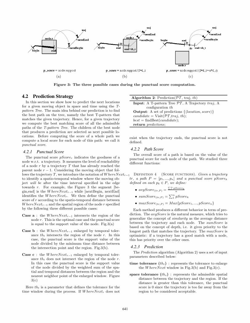
Figure 3: The three possible cases during the punctual score computation.

4.2 Prediction StrategyIn this section we show how to predict the next locations

for a given moving object in space and time using the T-pattern Tree. The main idea behind our prediction is to findthe best path on the tree, namely the best T-pattern thatmatches the given trajectory. Hence, for a given trajectorywe compute the best matching score of all the admissiblepaths of the T-pattern Tree. The children of the best nodethat produces a prediction are selected as next possible lo-cations. Before computing the score of a whole path wecompute a local score for each node of this path: we call itpunctual score.

4.2.1 Punctual ScoreThe punctual score pScorer indicates the goodness of a

node w.r.t. a trajectory. It measures the level of reachabilityof a node r by a trajectory T that has already reached theparent node r − 1. Considering the moving object that fol-lows the trajectory T , we introduce the notation of WhereNextr−1

to identify a spatio-temporal window where the moving ob-ject will be after the time interval specified in the edgetowards r. For example, the Figure 3 the segment [be-gin,end] is the WhereNextr−1 while [nextBegin, nextEnd]identifies the WhereNextr. We then define the punctualscore of r according to the spatio-temporal distance betweenWhereNextr−1 and the spatial region of the node r specifiedby the following three different possible cases:

Case a : the WhereNextr−1 intersects the region of thenode r. This is the optimal case and the punctual scoreis equal to the support value of the node. Fig.3(a)

Case b : the WhereNextr−1 enlarged by temporal toler-ance tht intersects the region of the node r. In thiscase, the punctual score is the support value of thenode divided by the minimum time distance betweenthe intersection point and the region. Fig.3(b).

Case c : the WhereNextr−1 enlarged by temporal toler-ance tht does not intersect the region of the node r.In this case the punctual score is the support valueof the node divided by the weighted sum of the spa-tial and temporal distances between the region and thenearest neighbor point of the enlarged window. Figure3(c)

Here tht is a parameter that defines the tolerance for thetime window during the process. If WhereNextr does not

Algorithm 2: Prediction(PT , traj, th)

Input: A T-pattern Tree PT , A Trajectory traj, Aconfiguration th

Output: A set of predictions {〈location, score〉}candidate = Visit(PT ,traj, th);best = findBest(candidate);return predictions;

exist when the trajectory ends, the punctual score is notdefined.

4.2.2 Path ScoreThe overall score of a path is based on the value of the

punctual score for each node of the path. We studied threedifferent functions:

Definition 4 (Score functions). Given a trajectorytr, a path P = [p1, ..., pn] and a punctual score pScorek

defined on each pk ∈ P , we define:

• avgScore(tr,P ) =∑n

1 pScorek

n

• sumScore(tr,P ) =∑n

1 pScorek

• maxScore(tr,P ) = Max{pScore1, ..., pScoren}

Each method produces a different behavior in term of pre-diction. The avgScore is the natural measure, which tries togeneralize the concept of similarity as the average distancebetween the trajectory and each node. The sumScore isbased on the concept of depth, i.e. it gives priority to thelongest path that matches the trajectory. The maxScore isoptimistic: if a trajectory has a good match with a node,this has priority over the other ones.

4.2.3 PredictionThe Prediction algorithm (Algorithm 2) uses a set of input

parameters described below:

time tolerance (tht) : represents the tolerance to enlargethe WhereNext window in Fig.3(b) and Fig.3(c).

space tolerance (ths) : represents the admissible spatialdistance between the trajectory and the region. If thedistance is greater than this tolerance, the punctualscore is 0 since the trajectory is too far away from theregion to be considered acceptable.

641

0

5

10

15

20

25

30

35

40

45

1.6 1.7 1.8 1.9 2 2.1 2.2 2.3 2.4 2.5

eval

uatio

n m

easu

re

support

Spatial CoverageRegionAggDatasetCov

Rate

0

0.2

0.4

0.6

0.8

1

0.1 0.2 0.3 0.4 0.5 0.6 0.7 0.8 0.9 1

accu

racy

predicted

Model 2 tol = 4 Model 1 tol = 4 Model 2 tol = 2 Model 1 tol = 2 Model 2 tol = 0 Model 1 tol = 0

(a) (b)

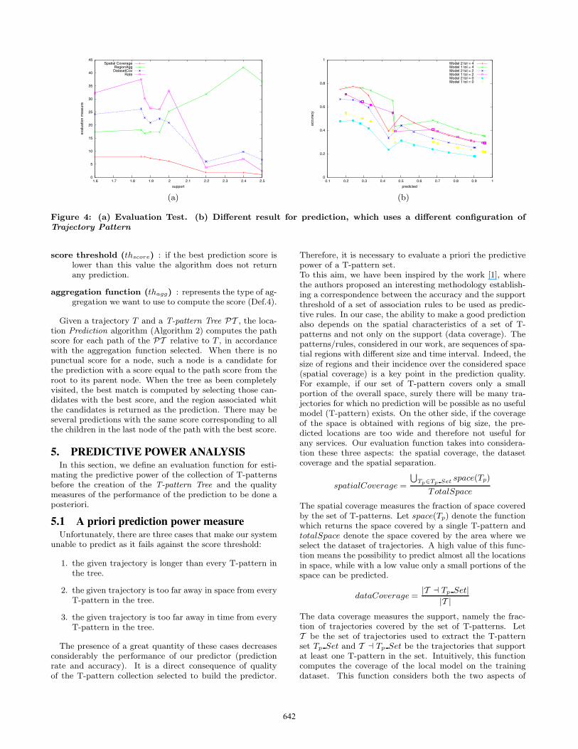
Figure 4: (a) Evaluation Test. (b) Different result for prediction, which uses a different configuration ofTrajectory Pattern

score threshold (thscore) : if the best prediction score islower than this value the algorithm does not returnany prediction.

aggregation function (thagg) : represents the type of ag-gregation we want to use to compute the score (Def.4).

Given a trajectory T and a T-pattern Tree PT , the loca-tion Prediction algorithm (Algorithm 2) computes the pathscore for each path of the PT relative to T , in accordancewith the aggregation function selected. When there is nopunctual score for a node, such a node is a candidate forthe prediction with a score equal to the path score from theroot to its parent node. When the tree as been completelyvisited, the best match is computed by selecting those can-didates with the best score, and the region associated whitthe candidates is returned as the prediction. There may beseveral predictions with the same score corresponding to allthe children in the last node of the path with the best score.

5. PREDICTIVE POWER ANALYSISIn this section, we define an evaluation function for esti-

mating the predictive power of the collection of T-patternsbefore the creation of the T-pattern Tree and the qualitymeasures of the performance of the prediction to be done aposteriori.

5.1 A priori prediction power measureUnfortunately, there are three cases that make our system

unable to predict as it fails against the score threshold:

1. the given trajectory is longer than every T-pattern inthe tree.

2. the given trajectory is too far away in space from everyT-pattern in the tree.

3. the given trajectory is too far away in time from everyT-pattern in the tree.

The presence of a great quantity of these cases decreasesconsiderably the performance of our predictor (predictionrate and accuracy). It is a direct consequence of qualityof the T-pattern collection selected to build the predictor.

Therefore, it is necessary to evaluate a priori the predictivepower of a T-pattern set.To this aim, we have been inspired by the work [1], wherethe authors proposed an interesting methodology establish-ing a correspondence between the accuracy and the supportthreshold of a set of association rules to be used as predic-tive rules. In our case, the ability to make a good predictionalso depends on the spatial characteristics of a set of T-patterns and not only on the support (data coverage). Thepatterns/rules, considered in our work, are sequences of spa-tial regions with different size and time interval. Indeed, thesize of regions and their incidence over the considered space(spatial coverage) is a key point in the prediction quality.For example, if our set of T-pattern covers only a smallportion of the overall space, surely there will be many tra-jectories for which no prediction will be possible as no usefulmodel (T-pattern) exists. On the other side, if the coverageof the space is obtained with regions of big size, the pre-dicted locations are too wide and therefore not useful forany services. Our evaluation function takes into considera-tion these three aspects: the spatial coverage, the datasetcoverage and the spatial separation.

spatialCoverage =

⋃Tp∈Tp Set space(Tp)

TotalSpace

The spatial coverage measures the fraction of space coveredby the set of T-patterns. Let space(Tp) denote the functionwhich returns the space covered by a single T-pattern andtotalSpace denote the space covered by the area where weselect the dataset of trajectories. A high value of this func-tion means the possibility to predict almost all the locationsin space, while with a low value only a small portions of thespace can be predicted.

dataCoverage =|T Tp Set|

|T |The data coverage measures the support, namely the frac-tion of trajectories covered by the set of T-patterns. LetT be the set of trajectories used to extract the T-patternset Tp Set and T Tp Set be the trajectories that supportat least one T-pattern in the set. Intuitively, this functioncomputes the coverage of the local model on the trainingdataset. This function considers both the two aspects of

642

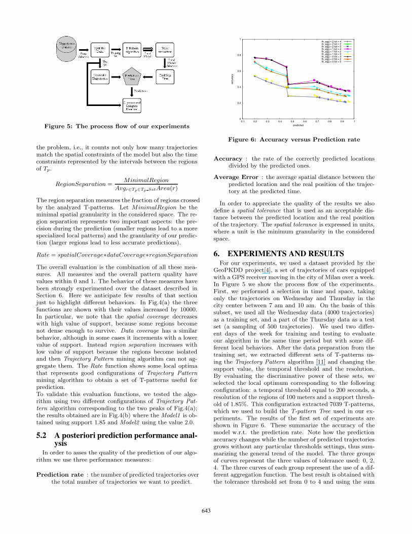
Figure 5: The process flow of our experiments

the problem, i.e., it counts not only how many trajectoriesmatch the spatial constraints of the model but also the timeconstraints represented by the intervals between the regionsof Tp.

RegionSeparation =MinimalRegion

Avgr∈Tp∈Tp SetArea(r)

The region separation measures the fraction of regions crossedby the analyzed T-patterns. Let MinimalRegion be theminimal spatial granularity in the considered space. The re-gion separation represents two important aspects: the pre-cision during the prediction (smaller regions lead to a morespecialized local patterns) and the granularity of our predic-tion (larger regions lead to less accurate predictions).

Rate = spatialCoverage∗dataCoverage∗regionSeparation

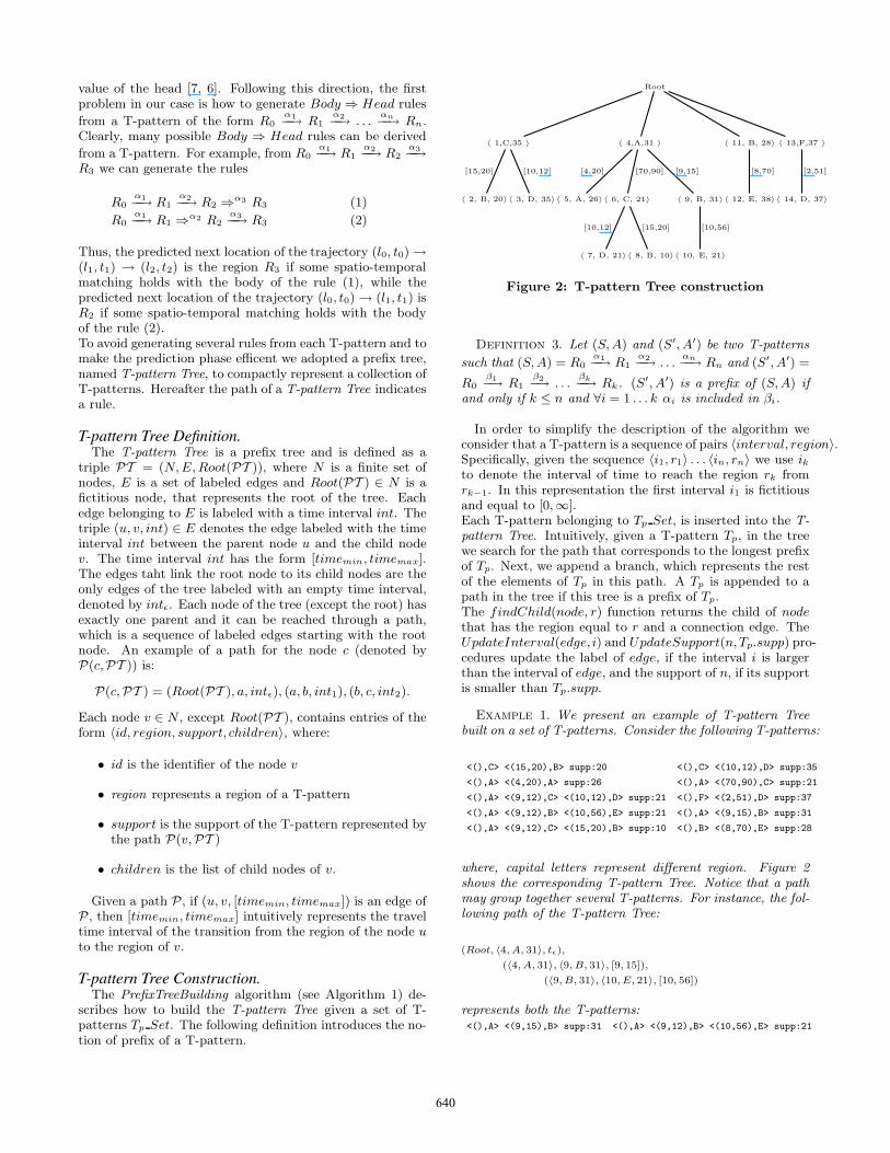
The overall evaluation is the combination of all these mea-sures. All measures and the overall pattern quality havevalues within 0 and 1. The behavior of these measures havebeen strongly experimented over the dataset described inSection 6. Here we anticipate few results of that sectionjust to highlight different behaviors. In Fig.4(a) the threefunctions are shown with their values increased by 10000.In particular, we note that the spatial coverage decreaseswith high value of support, because some regions becomenot dense enough to survive. Data coverage has a similarbehavior, although in some cases it increments with a lowervalue of support. Instead region separation increases withlow value of support because the regions become isolatedand then Trajectory Pattern mining algorithm can not ag-gregate them. The Rate function shows some local optimathat represents good configurations of Trajectory Patternmining algorithm to obtain a set of T-patterns useful forprediction.To validate this evaluation functions, we tested the algo-rithm using two different configurations of Trajectory Pat-tern algorithm corresponding to the two peaks of Fig.4(a);the results obtained are in Fig.4(b) where the Model1 is ob-tained using support 1.85 and Model2 using the value 2.0.

5.2 A posteriori prediction performance anal-ysis

In order to asses the quality of the prediction of our algo-rithm we use three performance measures:

Prediction rate : the number of predicted trajectories overthe total number of trajectories we want to predict.

0

0.2

0.4

0.6

0.8

1

0.1 0.2 0.3 0.4 0.5 0.6 0.7 0.8 0.9 1

accu

racy

predicted

th_agg = 2 tol = 4 th_agg = 2 tol = 2 th_agg = 2 tol = 0 th_agg = 1 tol = 4 th_agg = 1 tol = 2 th_agg = 1 tol = 0 th_agg = 0 tol = 4 th_agg = 0 tol = 2 th_agg = 0 tol = 0

Figure 6: Accuracy versus Prediction rate

Accuracy : the rate of the correctly predicted locationsdivided by the predicted ones.

Average Error : the average spatial distance between thepredicted location and the real position of the trajec-tory at the predicted time.

In order to appreciate the quality of the results we alsodefine a spatial tolerance that is used as an acceptable dis-tance between the predicted location and the real positionof the trajectory. The spatial tolerance is expressed in units,where a unit is the minimum granularity in the consideredspace.

6. EXPERIMENTS AND RESULTSFor our experiments, we used a dataset provided by the

GeoPKDD project[4], a set of trajectories of cars equippedwith a GPS receiver moving in the city of Milan over a week.In Figure 5 we show the process flow of the experiments.First, we performed a selection in time and space, takingonly the trajectories on Wednesday and Thursday in thecity center between 7 am and 10 am. On the basis of thissubset, we used all the Wednesday data (4000 trajectories)as a training set, and a part of the Thursday data as a testset (a sampling of 500 trajectories). We used two differ-ent days of the week for training and testing to evaluateour algorithm in the same time period but with some dif-ferent local behaviors. After the data preparation from thetraining set, we extracted different sets of T-patterns us-ing the Trajectory Pattern algorithm [11] and changing thesupport value, the temporal threshold and the resolution.By evaluating the discriminative power of these sets, weselected the local optimum corresponding to the followingconfiguration: a temporal threshold equal to 200 seconds, aresolution of the regions of 100 meters and a support thresh-old of 1.85%. This configuration extracted 7039 T-patterns,which we used to build the T-pattern Tree used in our ex-periments. The results of the first set of experiments areshown in Figure 6. These summarize the accuracy of themodel w.r.t. the prediction rate. Note how the predictionaccuracy changes while the number of predicted trajectoriesgrows without any particular thresholds settings, thus sum-marizing the general trend of the model. The three groupsof curves represent the three values of tolerance used: 0, 2,4. The three curves of each group represent the use of a dif-ferent aggregation function. The best result is obtained withthe tolerance threshold set from 0 to 4 and using the sum

643

0

0.2

0.4

0.6

0.8

1

0 10 20 30 40 50 60

pred

icte

d

th_space

th_t = 60 th_score = 1

th_agg = 1 tol = 0 th_agg = 0 tol = 2

0

0.2

0.4

0.6

0.8

1

0 10 20 30 40 50 60

accu

racy

th_space

th_t = 60 th_score = 1

th_agg = 2 tol = 4 th_agg = 2 tol = 2 th_agg = 2 tol = 0 th_agg = 1 tol = 4 th_agg = 1 tol = 2 th_agg = 1 tol = 0 th_agg = 0 tol = 4 th_agg = 0 tol = 2 th_agg = 0 tol = 0

(a) (b)

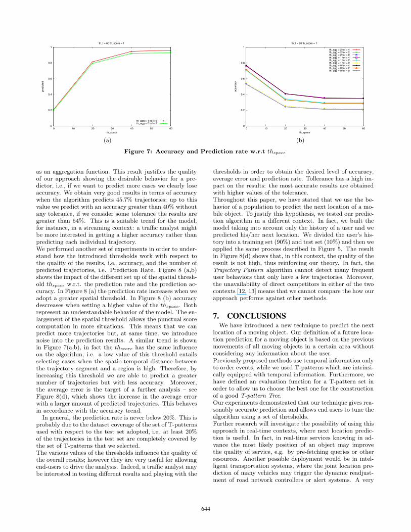
Figure 7: Accuracy and Prediction rate w.r.t thspace

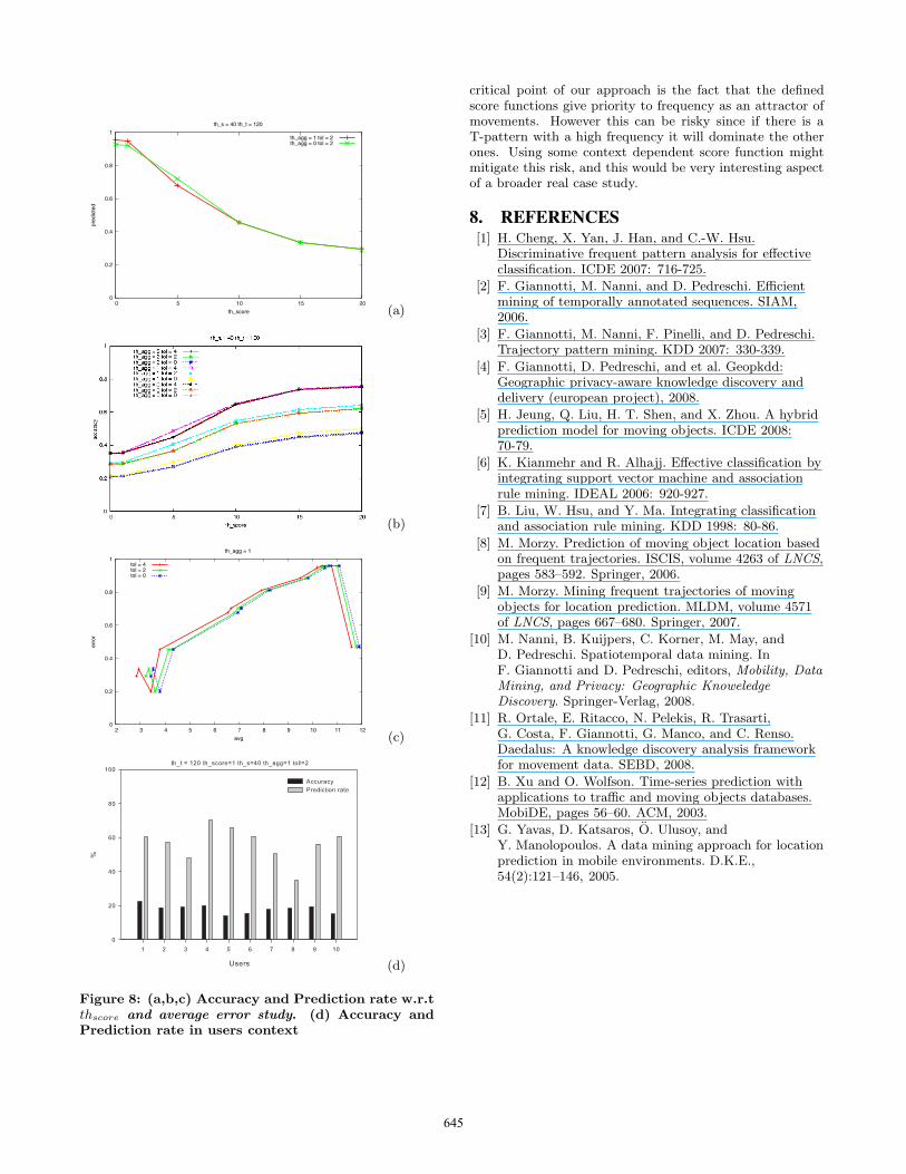
as an aggregation function. This result justifies the qualityof our approach showing the desirable behavior for a pre-dictor, i.e., if we want to predict more cases we clearly loseaccuracy. We obtain very good results in terms of accuracywhen the algorithm predicts 45.7% trajectories; up to thisvalue we predict with an accuracy greater than 40% withoutany tolerance, if we consider some tolerance the results aregreater than 54%. This is a suitable trend for the model,for instance, in a streaming context: a traffic analyst mightbe more interested in getting a higher accuracy rather thanpredicting each individual trajectory.We performed another set of experiments in order to under-stand how the introduced thresholds work with respect tothe quality of the results, i.e. accuracy, and the number ofpredicted trajectories, i.e. Prediction Rate. Figure 8 (a,b)shows the impact of the different set up of the spatial thresh-old thspace w.r.t. the prediction rate and the prediction ac-curacy. In Figure 8 (a) the prediction rate increases when weadopt a greater spatial threshold. In Figure 8 (b) accuracydescreases when setting a higher value of the thspace. Bothrepresent an understandable behavior of the model. The en-largement of the spatial threshold allows the punctual scorecomputation in more situations. This means that we canpredict more trajectories but, at same time, we introducenoise into the prediction results. A similar trend is shownin Figure 7(a,b), in fact the thscore has the same influenceon the algorithm, i.e. a low value of this threshold entailsselecting cases when the spatio-temporal distance betweenthe trajectory segment and a region is high. Therefore, byincreasing this threshold we are able to predict a greaternumber of trajectories but with less accuracy. Moreover,the average error is the target of a further analysis – seeFigure 8(d), which shows the increase in the average errorwith a larger amount of predicted trajectories. This behavesin accordance with the accuracy trend.

In general, the prediction rate is never below 20%. This isprobably due to the dataset coverage of the set of T-patternsused with respect to the test set adopted, i.e. at least 20%of the trajectories in the test set are completely covered bythe set of T-patterns that we selected.The various values of the thresholds influence the quality ofthe overall results; however they are very useful for allowingend-users to drive the analysis. Indeed, a traffic analyst maybe interested in testing different results and playing with the

thresholds in order to obtain the desired level of accuracy,average error and prediction rate. Tollerance has a high im-pact on the results: the most accurate results are obtainedwith higher values of the tolerance.Throughout this paper, we have stated that we use the be-havior of a population to predict the next location of a mo-bile object. To justify this hypothesis, we tested our predic-tion algorithm in a different context. In fact, we built themodel taking into account only the history of a user and wepredicted his/her next location. We divided the user’s his-tory into a training set (90%) and test set (10%) and then weapplied the same process described in Figure 5. The resultin Figure 8(d) shows that, in this context, the quality of theresult is not high, thus reinforcing our theory. In fact, theTrajectory Pattern algorithm cannot detect many frequentuser behaviors that only have a few trajectories. Moreover,the unavailability of direct competitors in either of the twocontexts [12, 13] means that we cannot compare the how ourapproach performs against other methods.

7. CONCLUSIONSWe have introduced a new technique to predict the next

location of a moving object. Our definition of a future loca-tion prediction for a moving object is based on the previousmovements of all moving objects in a certain area withoutconsidering any information about the user.Previously proposed methods use temporal information onlyto order events, while we used T-patterns which are intrinsi-cally equipped with temporal information. Furthermore, wehave defined an evaluation function for a T-pattern set inorder to allow us to choose the best one for the constructionof a good T-pattern Tree.Our experiments demonstrated that our technique gives rea-sonably accurate prediction and allows end users to tune thealgorithm using a set of thresholds.Further research will investigate the possibility of using thisapproach in real-time contexts, where next location predic-tion is useful. In fact, in real-time services knowing in ad-vance the most likely position of an object may improvethe quality of service, e.g. by pre-fetching queries or otherresources. Another possible deployment would be in intel-ligent transportation systems, where the joint location pre-diction of many vehicles may trigger the dynamic readjust-ment of road network controllers or alert systems. A very

644

0

0.2

0.4

0.6

0.8

1

0 5 10 15 20

pred

icte

d

th_score

th_s = 40 th_t = 120

th_agg = 1 tol = 2 th_agg = 0 tol = 2

(a)

(b)

0

0.2

0.4

0.6

0.8

1

2 3 4 5 6 7 8 9 10 11 12

erro

r

avg

th_agg = 1

tol = 4 tol = 2 tol = 0

(c)

(d)

Figure 8: (a,b,c) Accuracy and Prediction rate w.r.tthscore and average error study. (d) Accuracy andPrediction rate in users context

critical point of our approach is the fact that the definedscore functions give priority to frequency as an attractor ofmovements. However this can be risky since if there is aT-pattern with a high frequency it will dominate the otherones. Using some context dependent score function mightmitigate this risk, and this would be very interesting aspectof a broader real case study.

8. REFERENCES[1] H. Cheng, X. Yan, J. Han, and C.-W. Hsu.

Discriminative frequent pattern analysis for effectiveclassification. ICDE 2007: 716-725.

[2] F. Giannotti, M. Nanni, and D. Pedreschi. Efficientmining of temporally annotated sequences. SIAM,2006.

[3] F. Giannotti, M. Nanni, F. Pinelli, and D. Pedreschi.Trajectory pattern mining. KDD 2007: 330-339.

[4] F. Giannotti, D. Pedreschi, and et al. Geopkdd:Geographic privacy-aware knowledge discovery anddelivery (european project), 2008.

[5] H. Jeung, Q. Liu, H. T. Shen, and X. Zhou. A hybridprediction model for moving objects. ICDE 2008:70-79.

[6] K. Kianmehr and R. Alhajj. Effective classification byintegrating support vector machine and associationrule mining. IDEAL 2006: 920-927.

[7] B. Liu, W. Hsu, and Y. Ma. Integrating classificationand association rule mining. KDD 1998: 80-86.

[8] M. Morzy. Prediction of moving object location basedon frequent trajectories. ISCIS, volume 4263 of LNCS,pages 583–592. Springer, 2006.

[9] M. Morzy. Mining frequent trajectories of movingobjects for location prediction. MLDM, volume 4571of LNCS, pages 667–680. Springer, 2007.

[10] M. Nanni, B. Kuijpers, C. Korner, M. May, andD. Pedreschi. Spatiotemporal data mining. InF. Giannotti and D. Pedreschi, editors, Mobility, DataMining, and Privacy: Geographic KnoweledgeDiscovery. Springer-Verlag, 2008.

[11] R. Ortale, E. Ritacco, N. Pelekis, R. Trasarti,G. Costa, F. Giannotti, G. Manco, and C. Renso.Daedalus: A knowledge discovery analysis frameworkfor movement data. SEBD, 2008.

[12] B. Xu and O. Wolfson. Time-series prediction withapplications to traffic and moving objects databases.MobiDE, pages 56–60. ACM, 2003.

[13] G. Yavas, D. Katsaros, O. Ulusoy, andY. Manolopoulos. A data mining approach for locationprediction in mobile environments. D.K.E.,54(2):121–146, 2005.

645