When safe-haven asset is less than a safe-haven play - ARX ...

1

When safe-haven asset is less than a safe-haven play

Leon Li

Associate Professor of Finance

Waikato Management School

University of Waikato, New Zealand

E-mail: [email protected]

Carl Chen

Professor of Finance

Department of Economics and Finance

University of Dayton, USA

E-mail: [email protected]

November 2021

mailto:[email protected]

mailto:[email protected]

2

When safe-haven asset is less than a safe-haven play

ABSTRACT

We propose a four-state regime-switching model that pairs low volatility (LV) and high

volatility (HV) states to test the risk properties of eight stock-safe haven asset portfolios. We

find the correlations between gold, U.S. T-bond, and Swiss Franc, and stock markets are

negative or zero in all states, including the HV-HV state, while between Bitcoin and stock

markets are positive in the HV-HV state, implying that gold, T-bond, and Swiss Franc are

full-safe havens and Bitcoin is a partial-safe haven asset. Moreover, our model is effective in

portfolio construction, which performs better than the conventional time-varying GARCH-

based models.

JEL

Classification:

C58, G11

Keywords: Safe-haven assets; portfolio; correlations; regime-switching model

Data Availability: From the sources identified in this paper

3

1. Introduction

Portfolio theory postulates that the risk reduction effect from diversification depends

on the correlations among the assets in the portfolio. To maximize the effect, investors

include negatively correlated assets in their portfolios (Jackwerth & Slavutskaya, 2016). The

literature (e.g., Baur & Lucey, 2010; Ratner & Chiu, 2013) employs the magnitude and sign

of the cross-asset correlation to classify assets into three levels: a diversifier, a hedge, and a

safe-haven. A diversifier has a small but positive correlation with another asset; a hedge is an

asset that has a zero (or negative) correlation with another asset, and a hedge asset levels up

to a safe-haven if a zero (or negative) correlation persists during chaotic times. Accordingly,

a diversifier and a safe-haven are assets with the lowest and highest level of risk reduction

capability respectively, while a hedge lies between them.

The literature has researched several safe-haven assets for stock investors, including

gold (e.g. Hillier et al., 2006; Baur & Lucey, 2010; Pullen et al., 2014; Bekiros et al., 2017),

US government bonds (e.g. Fleming et al., 1998; Hartmann et al., 2004; Baur & Lucey, 2010;

Noeth & Sengupta, 2010; Chan et al., 2011;) and Swiss Franc (e.g. Kaul & Sapp, 2006;

Ranaldo & Söderlind, 2010; Grisse & Nitschka, 2015). In addition to these traditional safe-

haven assets, some recent studies (e.g. Bouri et al., 2017; Stensås et al., 2019; Urquhart &

Zhang, 2019; Garcia-Jorcanoa & Benito, 2020; Hafner, 2020; Mariana et al., 2021) include

Bitcoin. Indeed, several US companies hold a large quantity of Bitcoin (e.g., Microstrategy

and Tesla). The critical character of safe-haven assets is their zero or negative correlation

with stocks, hence acting as an instrument against stock asset risk. The research of safe-haven

assets has renewed attention because of the 2008 Global Financial Crisis (e.g., Cheema et al.,

2020) and the COVID-19 pandemic (e.g., Baker et al., 2020 and Mariana et al., 2021).

This study contributes to the safe-haven assets literature in three directions. First, we

develop a theoretical perspective to distinguish two types of safe-haven assets: partial-safe

4

and full-safe. Considering a portfolio consisting of stocks and a safe-haven asset with two

turmoil circumstances: (1) only one market (either stock or safe-haven asset) experiences a

chaotic condition, and (2) both stock and safe-haven asset markets experience a chaotic

condition. We define a safe-haven asset as partial-safe if its correlation with the stock market

is zero or negative under the first turmoil event but positive under the second event. On the

other hand, a safe-haven asset is full-safe if its correlation with stock markets is zero or

negative under both turmoil events. While literature lacks this distinction, addressing the

difference between these two turmoil events is meaningful. If the risk-benefit of the safe-

haven asset is partial, it may protect stock investors when only the stock market encounters

turmoil. However, when both stock and safe-haven asset markets are in a turbulent state, the

partial-safe haven asset is unable to effectively reduce portfolio risk because of its positive

correlation with stocks. The most recent evidence occurred in March 2020 when Covid-19 hit

the world hard, both stock market and Bitcoin market crumbled, e.g., the S&P 500 and BTC

returned -7.90% and -14.08%, respectively on March 9; -9.99% and -46.47%, respectively on

March 12; and -12.77% and -10.39%, respectively on March 16. To the best of our

knowledge, the literature has not distinguished these two types of safe-haven assets because

they only consider the stock market condition.

Second, to differentiate a partial-safe from a full-safe haven asset and empirically test

our argument, we develop a regime-switching approach to identity various volatility state

combinations in the stock and safe-haven asset markets and jointly analyze their correlation

dynamics. While the existing studies have addressed and tested the dynamic correlations

between stock and safe-haven assets (e.g., Cappiello et al., 2006; Hood & Malik, 2013; Ciner

et al., 2013; Pullen et al., 2014; Bouri et al., 2017a and 2017b; Wu et al., 2019; Mariana et al.,

2021; Mokni et al., 2021), we argue that their two-step methodologies suffer from limitations

and yield compromised empirical results due to sample selection bias (see Heckman, 1979).

5

Third, we conduct a practical portfolio construction test employing our regime-

switching model. As evidenced in our empirical results, the magnitude and the sign of the

stock-safe haven correlations are non-uniform across various volatility state combinations. As

volatilities and correlations are the critical factors for effective portfolio construction, a

follow-up question is if our proposed state-varying volatilities and correlations help investors

achieve a more efficient stock-safe haven asset portfolio. To the best of our knowledge, few,

if any, prior studies have conducted this practical test since they are constrained by the usage

of a two-step estimation method in which the sample segmentation and the use of dummy

variables are not decided by the data.

The rest of our study proceeds as follows. First, we review related studies and develop

research questions in Section 2. In Section 3, we present the models used in this study,

including the conventional GARCH (Generalized Autoregressive Conditional

Heteroskedasticity), DCC (Dynamic Conditional Correlations) models, and the proposed

regime-switching model. We further demonstrate why our regime-switching approach is

more appropriate than the conventional DCC model to measure the correlation dynamics in

the stock-safe haven asset markets. In Section 4, we report the estimation results. We then

discuss our results and conduct the practical portfolio construction test in Section 5. Finally,

Section 6 concludes.

2. Literature review and research development

2.1 Studies on safe-haven assets

The recurring financial and economic crises in the past decades reinforce researchers’

interest in risk management, one of the most critical issues in finance research. While stock

markets provide investors with a significant capital gain over the long run, rare but

unanticipated disasters cause a severe short-term loss. There are two commonly used

6

practices to manage risk: hedge by financial derivatives and diversification by portfolio. This

study focuses on the second method. The concept of diversification (investing in two or more

assets) rests on the notion that asset values do not always move in the same direction at the

same time. Therefore, an investor can reduce risk via investing in a portfolio. For effective

diversification, the less-than-perfect linkage between assets is essential, particularly during

periods of financial chaos. This is because when these unlikely and rare disasters occur,

different markets do not crash jointly, or they may move in an opposite direction, i.e., the loss

in one market can be offset by the gain in another market.

Whether other assets can be used to control stock risk relies on their correlations with

stocks. The literature (e.g., Baur & Lucey, 2010; Ratner & Chiu, 2013) defines three types of

assets against stock risk: (1) a diversifier (an asset with a slight positive correlation with

stocks), (2) a hedge (an asset with a zero or negative correlation with stocks), and (3) a safe-

haven (an asset with a zero or negative correlation with stocks during chaotic events). By

definition, including a safe-haven asset in the portfolio is an ideal tool to offset stock risk,

particularly during periods of financial and economic distresses.

Certain safe-haven assets have been well documented in the literature, including gold

(e.g., Hillier et al., 2006; Baur & Lucey, 2010; Pullen et al., 2014), government bonds

(Fleming et al., 1998; Hartmann et al., 2004; Noeth and Sengupta, 2010; Chan et al., 2011;),

currencies such as Swiss Franc and the US dollar (e.g. Grisse and Nitschka, 2015; Kaul and

Sapp, 2006; Ranaldo and Söderlind, 2010). In addition to these traditional safe-haven assets,

recent studies endorse digital currencies such as Bitcoin as a safe-haven asset against stock

risk because factors driving cryptocurrency prices are different from those affecting stock

markets (e.g. Stensås et al., 2019; Urquhart & Zhang, 2019; Garcia-Jorcanoa & Benito, 2020;

Hafner, 2020; Mariana et al., 2021).

7

Although numerous studies have examined these safe-haven assets, the evidence is

inconclusive. Capie et al. (2005), Hammoudeh et al. (2009), and Ciner et al. (2013) highlight

the characteristics of gold as a safe-haven asset. Baur and Lucey (2010) and Chan et al. (2011)

argue that government bonds outperform gold to diversify stock risk during chaotic times.

Grisse & Nitschka (2015) demonstrate the Swiss Franc’s safe-haven characteristics against

other currencies. While some studies (Kliber et al., 2019; Gil-Alana et al., 2020; Bouri et al.,

2020; Mariana et al., 2021) suggest that cryptocurrencies are qualified as a safe haven for

stocks, others argue that cryptocurrencies are a poor hedge (Isah & Raheem, 2019; Conlon &

McGee,2020; Corbet et al., 2020). In the following section, we advance a new perspective

that distinguishes a partial-safe haven from a full-safe haven. To this end, we develop a

regime-switching system where combinations of four volatility states are implemented to test

our argument.

2.2 Research development

Our research aims to shed light on the debate of safe-haven assets in the literature. We

develop combinations of market volatility states in the stock-safe haven asset markets and

differentiate two types of safe-haven assets: partial-safe and full-safe. Our conjectures are

explained as follows. First, prior studies have well documented the linkage between financial

crises and market volatilities, i.e., high market volatility serves as a signal of financial crises

(Engle et al., 2013; Baker et al., 2016; Gulen & Ion, 2016; Danielsson et al., 2018).

Considering a portfolio consisting of stocks and safe-haven assets, both the stock volatility

and safe-haven asset volatility should be taken into account when constructing a portfolio.

Therefore, with a regime-switching between a low volatility (LV) and a high volatility (HV)

regime for each asset, we develop a four-state system for the stock-safe haven asset portfolios,

i.e., LV-LV, HV-LV, LV-HV, and HV-HV.

8

Second, among the four states, we highlight the “HV-HV” state. This state reflects

extreme economic and/or financial distresses (e.g., COVID-19 pandemic) causing both the

stock and safe-haven asset markets to experience excessive price movements concurrently. If

the safe-haven asset is positively correlated with stocks in the HV-HV state, then the safe-

haven asset and stock will move in tandem and thus the loss in the stock position will meet

another loss in the safe-haven asset position. Accordingly, the safe-haven asset position is

unable to offset the stock position under this situation, and its protective function is limited

during this chaotic condition. Based on this logic, we define two types of safe-haven assets:

(1) a full-safe haven asset if its correlation with stocks continues to be zero or negative under

the HV-HV state, and (2) a partial-safe haven asset if its correlation with stocks is zero or

negative under all states except the HV-HV state.

Our views relate to the literature on the contagion effect. A number of researchers

have documented that global equity markets are more strongly correlated during turbulent

times (see King & Wadhwani, 1990; Erb et al., 1994; Longin & Solnik, 1995, 2001; Karolyi

& Stulz, 1996; Jacquier & Marcus, 2001; Ang & Bekaert, 2002; Forbes & Rigobon, 2002;

Bae et al., 2003; Das & Uppal, 2004). However, the contagion effect among international

stock markets is not very helpful in explaining the correlation between stocks and safe-haven

assets since different fundamentals drive them. Nevertheless, we argue that stocks and safe-

haven assets could still be positively correlated. The following two theories help to elucidate

our argument. The first theory is the cross-market rebalancing channel of financial contagion

as modeled by Kodres & Pritsker (2002). In their model, shocks are transmitted across

markets as investors respond to shocks in one market by optimally readjusting their portfolios.

This model setting can generate contagion across various markets that do not share common

macroeconomic fundamentals. The second theory is the social learning channel proposed by

Trevino (2020). In the model, Trevino (2020) demonstrates that contagion occurs when

9

investors are fearful of a crisis in one market after observing a crisis in the other market albeit

these two markets are not fundamentally linked. We contend that these two contagion

channels exacerbate the cross-market correlations between stocks and safe-haven assets,

particularly when both are experiencing chaotic times (i.e., the HV-HV state).

To test the dynamic cross-market correlations between stocks and safe-haven assets,

the majority of prior studies (e.g., Hood & Malik, 2013; Ciner et al., 2013; Pullen et al., 2014;

Bouri et al., 2017a, and 2017b; Wu et al., 2019; Mariana et al., 2021; Mokni et al., 2021)

employ one of the two econometric methods. The first method is the dynamic conditional

correlation (DCC) model proposed by Engle (2002). Prior researches use the DCC model to

estimate the time-varying correlations between stock and safe-haven assets. They first

partition the whole testing period into sub-periods, e.g., crisis versus non-crisis period,

followed by a comparative analysis between the two sub-periods (e.g., Cappiello et al., 2006;

Ciner et al., 2013; Urquhart & Zhang, 2019; Mariana et al., 2021). The second method is the

quantile regression approach employed by Baur and Lucey (2010) and Baur and McDermott

(2010). These researches use the 1%, 2.5%, or 5% lower percentiles of stock returns (i.e.,

stressed or extreme stock returns) to define several quantile dummy variables. They include

these dummy variables in the conventional regression analyses of safe-haven asset returns on

stock returns and use the estimated results of these dummy variables to infer whether the

stocks and safe-haven asset correlations change in chaotic times.

We notice caveats in these two econometric methods adopted by prior studies. First,

while Engle’s DCC model is the most popular method to estimate the dynamic correlations

among assets (Goeij & Marquering, 2004), it uses a two-step approach to estimate the model

parameters, hence fails to take into account the linkage between variances and correlations

(e.g., Bae et al., 2003; Das & Uppal, 2004). Further, the sample partitioning process (i.e.,

crisis versus non-crisis periods) is subjective, which may yield compromised empirical results

10

due to sample selection bias (Heckman, 1979). Second, the approach that uses quantile

threshold variables to diagnose and examine the impact of turmoil market conditions on the

relationship between stock and safe-haven asset markets also bears the limitation of a two-

step process and the use of subjective dummy variables. By contrast, our proposed regime-

switching approach has two key advantages and thus effectively mitigates these limitations.

First, in our regime-switching approach, all the parameters for volatilities and correlations are

jointly estimated. Second, the partition of various volatility regimes (i.e., a high or a low

volatility regime) is endogenously determined by the data, thus mitigating the bias due to the

subjective sample partitioning and the usage of dummy variables.

3. Research methodologies

3.1 Bivariate GARCH model

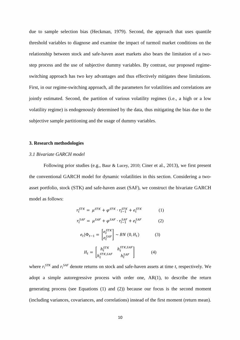
Following prior studies (e.g., Baur & Lucey, 2010; Ciner et al., 2013), we first present

the conventional GARCH model for dynamic volatilities in this section. Considering a two-

asset portfolio, stock (STK) and safe-haven asset (SAF), we construct the bivariate GARCH

model as follows:

𝑟𝑡𝑆𝑇𝐾 = 𝜇𝑆𝑇𝐾 + 𝜑𝑆𝑇𝐾 ∙ 𝑟𝑡−1

𝑆𝑇𝐾 + 𝑒𝑡𝑆𝑇𝐾 (1)

𝑟𝑡𝑆𝐴𝐹 = 𝜇𝑆𝐴𝐹 + 𝜑𝑆𝐴𝐹 ∙ 𝑟𝑡−1

𝑆𝐴𝐹 + 𝑒𝑡𝑆𝐴𝐹 (2)

𝑒𝑡|Φ𝑡−1 = [𝑒𝑡

𝑆𝑇𝐾

𝑒𝑡𝑆𝐴𝐹] ~ 𝐵𝑁 (0, 𝐻𝑡) (3)

𝐻𝑡 = [ℎ𝑡

𝑆𝑇𝐾 ℎ𝑡𝑆𝑇𝐾,𝑆𝐴𝐹

ℎ𝑡𝑆𝑇𝐾,𝑆𝐴𝐹 ℎ𝑡

𝑆𝐴𝐹] (4)

where rtSTK and rt

SAF denote returns on stock and safe-haven assets at time t, respectively. We

adopt a simple autoregressive process with order one, AR(1), to describe the return

generating process (see Equations (1) and (2)) because our focus is the second moment

(including variances, covariances, and correlations) instead of the first moment (return mean).

11

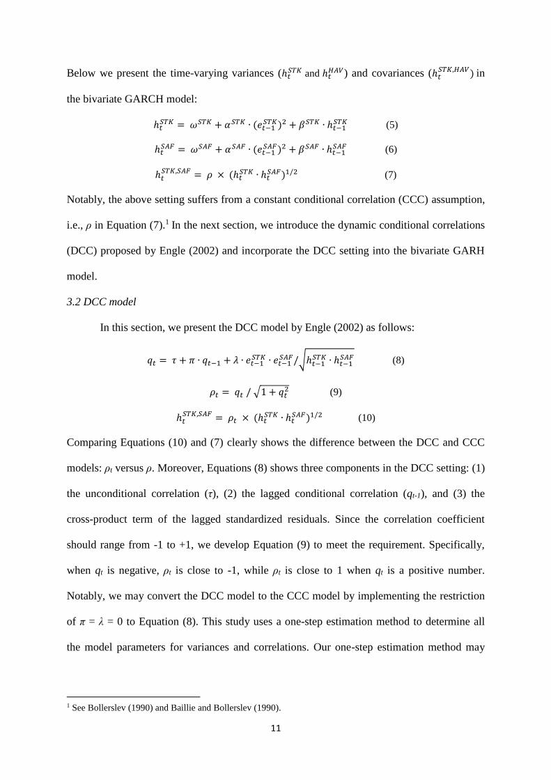
Below we present the time-varying variances (ℎ𝑡𝑆𝑇𝐾 and ℎ𝑡

𝐻𝐴𝑉) and covariances (ℎ𝑡𝑆𝑇𝐾,𝐻𝐴𝑉) in

the bivariate GARCH model:

ℎ𝑡𝑆𝑇𝐾 = 𝜔𝑆𝑇𝐾 + 𝛼𝑆𝑇𝐾 ∙ (𝑒𝑡−1

𝑆𝑇𝐾)2 + 𝛽𝑆𝑇𝐾 ∙ ℎ𝑡−1𝑆𝑇𝐾 (5)

ℎ𝑡𝑆𝐴𝐹 = 𝜔𝑆𝐴𝐹 + 𝛼𝑆𝐴𝐹 ∙ (𝑒𝑡−1

𝑆𝐴𝐹)2 + 𝛽𝑆𝐴𝐹 ∙ ℎ𝑡−1𝑆𝐴𝐹 (6)

ℎ𝑡𝑆𝑇𝐾,𝑆𝐴𝐹 = 𝜌 × (ℎ𝑡

𝑆𝑇𝐾 ∙ ℎ𝑡𝑆𝐴𝐹)1/2 (7)

Notably, the above setting suffers from a constant conditional correlation (CCC) assumption,

i.e., ρ in Equation (7).1 In the next section, we introduce the dynamic conditional correlations

(DCC) proposed by Engle (2002) and incorporate the DCC setting into the bivariate GARH

model.

3.2 DCC model

In this section, we present the DCC model by Engle (2002) as follows:

𝑞𝑡 = 𝜏 + 𝜋 ∙ 𝑞𝑡−1 + 𝜆 ∙ 𝑒𝑡−1𝑆𝑇𝐾 ∙ 𝑒𝑡−1

𝑆𝐴𝐹/√ℎ𝑡−1𝑆𝑇𝐾 ∙ ℎ𝑡−1

𝑆𝐴𝐹 (8)

𝜌𝑡 = 𝑞𝑡 / √1 + 𝑞𝑡2 (9)

ℎ𝑡𝑆𝑇𝐾,𝑆𝐴𝐹 = 𝜌𝑡 × (ℎ𝑡


Comparing Equations (10) and (7) clearly shows the difference between the DCC and CCC

models: ρt versus ρ. Moreover, Equations (8) shows three components in the DCC setting: (1)

the unconditional correlation (τ), (2) the lagged conditional correlation (qt-1), and (3) the

cross-product term of the lagged standardized residuals. Since the correlation coefficient

should range from -1 to +1, we develop Equation (9) to meet the requirement. Specifically,

when qt is negative, ρt is close to -1, while ρt is close to 1 when qt is a positive number.

Notably, we may convert the DCC model to the CCC model by implementing the restriction

of π = λ = 0 to Equation (8). This study uses a one-step estimation method to determine all

the model parameters for variances and correlations. Our one-step estimation method may

1 See Bollerslev (1990) and Baillie and Bollerslev (1990).

12

effectively mitigate the unrealistic assumptions involved in the two-step estimation process

(see Section 2.2).2

3.3 Bivariate Markov-switching autoregressive conditional heteroskedasticity model

The critical character of the GARCH and DCC models is to use the past variances and

correlations to predict future variances and correlations (see Equations (5), (6), and (8)). The

literature (e.g., Schmitt & Westerhoff, 2017; Akhtaruzzaman et al., 2020; Corbet et al., 2020;

Mariana et al., 2021) has well documented the clustering phenomena of volatilities and

correlations, i.e., a high variance/correlation followed by a high variance/correlation.

However, these simple and pure time-dependent settings fail to control discrete volatility

jumps and are unable to capture the relation between volatilities and correlations (Nelson,

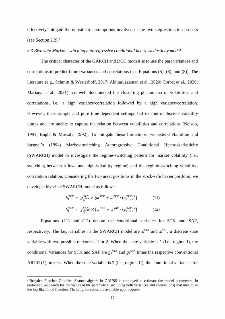
1991; Engle & Mustafa, 1992). To mitigate these limitations, we extend Hamilton and

Susmel’s (1994) Markov-switching Autoregressive Conditional Heteroskedasticity

(SWARCH) model to investigate the regime-switching pattern for market volatility (i.e.,

switching between a low- and high-volatility regime) and the regime-switching volatility-

correlation relation. Considering the two asset positions in the stock-safe haven portfolio, we

develop a bivariate SWARCH model as follows:

ℎ𝑡𝑆𝑇𝐾 = 𝑔

𝑠𝑡𝑆𝑇𝐾

𝑆𝑇𝐾 × [𝜔𝑆𝑇𝐾 + 𝛼𝑆𝑇𝐾 ∙ (𝑒𝑡−1𝑆𝑇𝐾)2] (11)

ℎ𝑡𝑆𝐴𝐹 = 𝑔

𝑠𝑡𝐻𝐴𝑉

𝑆𝐴𝐹 × [𝜔𝑆𝐴𝐹 + 𝛼𝑆𝐴𝐹 ∙ (𝑒𝑡−1𝑆𝐴𝐹)2] (12)

Equations (11) and (12) denote the conditional variance for STK and SAF,

respectively. The key variables in the SWARCH model are stSTK and st

SAF, a discrete state

variable with two possible outcomes: 1 or 2. When the state variable is 1 (i.e., regime I), the

conditional variances for STK and SAF are g1STK and g1

SAF times the respective conventional

ARCH (1) process. When the state variable is 2 (i.e., regime II), the conditional variances for

2 Broyden–Fletcher–Goldfarb–Shanno algebra in GAUSS is employed to estimate the model parameters. In

particular, we search for the values of the parameters (including both variances and correlations) that maximize

the log-likelihood function. The program codes are available upon request.

13

STK and SAF are g2STK and g2

SAF times the respective ARCH (1) process. We normalize g1STK

and g1SAF, the volatility degree parameter for regime I, to be unity (i.e., g1

STK = g1SAF = 1).

Accordingly, the variance under regime II is g2STK multiples of regime I for STK returns, and

for SAF returns, the variance under regime II is g2SAF multiples of regime I. As shown in

Tables 6 and 7, the estimated g2STK and g2

SAF coefficients are significantly higher than the value of one.

Based on the results, we define regime II and regime I as a high volatility (HV) and a low

volatility (LV) regime, respectively.

Next, we model the conditional correlations for the STK-SAF portfolio. Given a two-

state setting for the conditional variance of each asset in the portfolio, we define a four-state

conditional correlation as follows:

ℎ𝑡𝑆𝑇𝐾,𝑆𝐴𝐹 = 𝜌𝑠𝑡

𝑆𝑇𝐾,𝑠𝑡𝑆𝐴𝐹 × (ℎ𝑡


As shown in Equation (13), the STK-SAF correlation is ρ1,1 when both the STK and

SAF markets are in an LV state (i.e., stSTK = 1 and st

SAF = 1). The correlation is ρ2,2 when both

the STK and SAF markets are experiencing an HV state. If the two markets are in opposite

state (i.e., one is an HV and the other one is an LV), the cross-market correlations are ρ2,1

(stSTK = 2 and st

SAF = 1) or ρ1,2 (stSTK = 1 and st

SAF = 2). The four-state correlations in Equation

(13) depict the relationship between market volatilities and correlations; hence it is suitable

for testing our argument of partial-safe versus full-safe haven assets (see Section 2.2). In

short, we establish a one-step estimation method to jointly determine volatilities and

correlations, which effectively mitigates the biased results obtained from the two-step

estimation method seen in the extant studies.

Last but not least, we use a first-order Markov chain process to control the regime-

switching pattern for the discrete state variables, as proposed by Hamilton and Susmel (1994):

𝑃(𝑠𝑡𝑆𝑇𝐾 = 1|𝑠𝑡−1

𝑆𝑇𝐾 = 1) = 𝑝11𝑆𝑇𝐾, 𝑝(𝑠𝑡

𝑆𝑇𝐾 = 2|𝑠𝑡−1𝑆𝑇𝐾 = 2) = 𝑝22

𝑆𝑇𝐾 (14)

𝑃(𝑠𝑡𝑆𝐴𝐹 = 1|𝑠𝑡−1

𝑆𝐴𝐹 = 1) = 𝑝11𝑆𝐴𝐹 , 𝑝(𝑠𝑡

𝑆𝐴𝐹 = 2|𝑠𝑡−1𝑆𝐴𝐹 = 2) = 𝑝22

𝑆𝐴𝐹 (15)

14

4. Data and model estimation results

4.1 Data

There are two positions in the stock-safe haven asset portfolio – stock and safe-haven.

For the stock position, we employ two international stock indexes: S&P500 and FTSE100.

For the safe-haven asset position, we consider gold, U.S. Treasury bond (T-Bond), Swiss

Franc (CHF), and Bitcoin (BTC). Based on these two stock indexes and four safe-haven

assets, we thus construct up to eight ( 4 x 2) portfolios for our empirical tests. The testing

period is between April 30, 2003, and January 18, 2021, for a total of 2,015 daily

observations. To ensure that the data used for the empirical analysis are stationary, we use the

return series rather than the price level series. The data are collected from the DataStream

database except for Swiss Franc and Bitcoin, which are obtained from the online database of

the Swiss National Bank and https://coinmarketcap.com/, respectively.

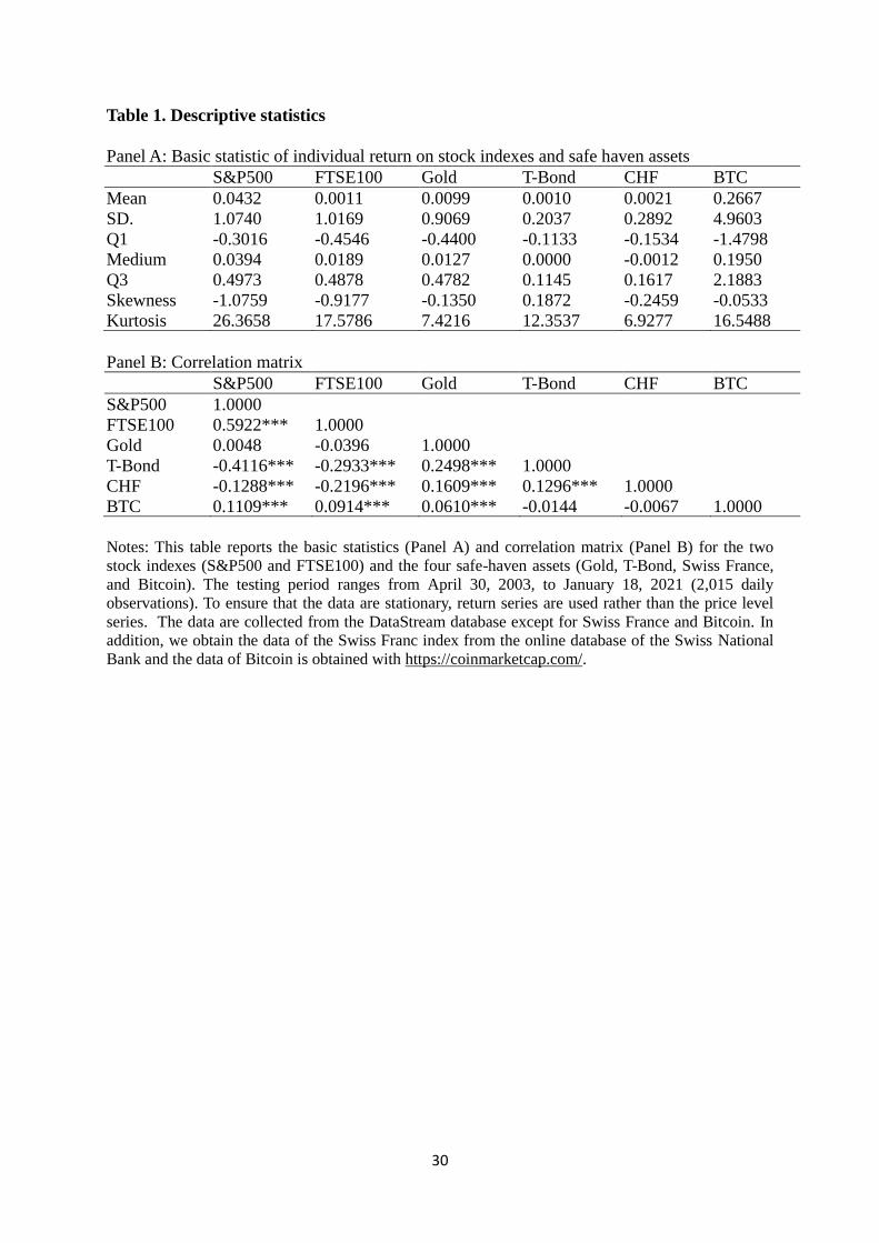
Table 1 presents the descriptive statistics for the two stock indexes and the four safe-

haven assets. As shown in Panel B, the correlation between S&P500 and FTSE100 is 0.5922

(p-value < 0.001), which is much larger than the correlations between stocks and safe-haven

assets (range between -0.4116 and 0.1109). We further examine the correlations between two

stock indexes and four safe-haven assets. First, the correlations between stock indexes and

Bitcoin are positive and significant (e.g., the S&P500-BTC correlation = 0.1109 with p-value

< 0.01). Second, the correlations with gold are positive but insignificant (e.g., the S&P500-

Gold correlation = 0.0048 with p-value > 0.05). Third, the correlations with T-Bond and CHF

are negative and significant (e.g., the S&P500-TBond correlation = -0.4116 with p-value <

0.01). These preliminary results imply that T-Bond and CHF outperform gold in diversifying

stock risk and that Bitcoin might be less qualified as a safe-haven asset.

(Insert Table 1 about here)

4.2 Illustration of volatility regimes

https://coinmarketcap.com/

15

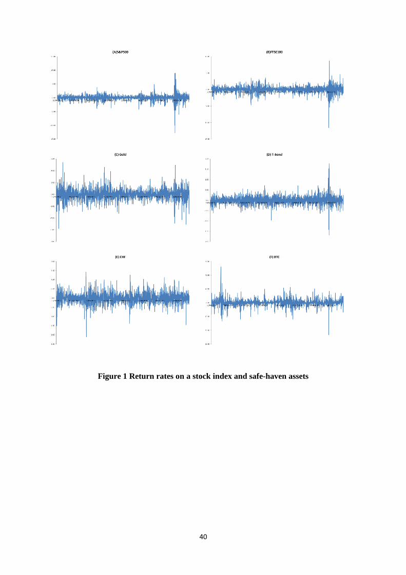
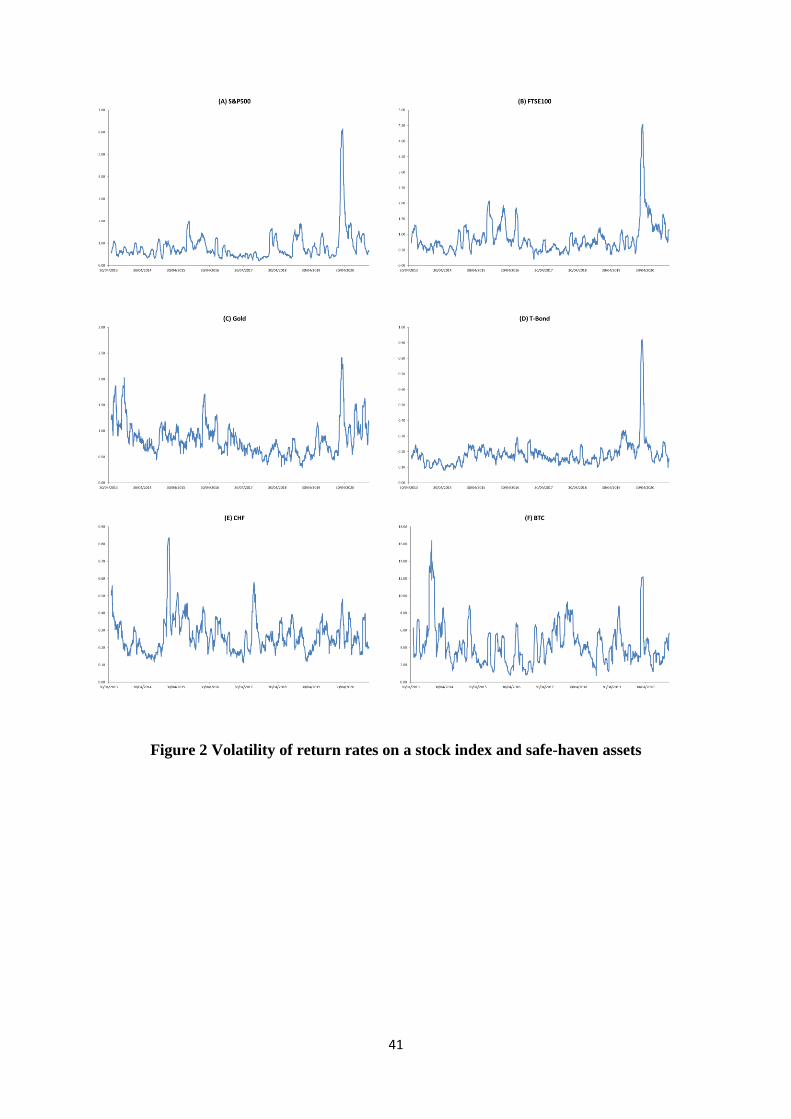
To illustrate volatility regimes in the stock and cryptocurrency markets, we calculate

the volatilities of their daily returns over one month (i.e., 21 trading days) rolling windows.

Figure 1 graphs the daily return series, and Figure 2 graphs the return volatilities. As shown

in Figure 2, the volatilities of stocks and safe-haven assets are non-constant. Moreover,

frequent prominent moves (i.e., several peaks) are observed in Figure 2. These peaks provide

evidence of volatility regimes in the markets. For instance, peaks are identified in mid-March

2020, which correspond to the economic and financial distresses due to the COVID-19

pandemic.

(Insert Figures 1 and 2 about here)

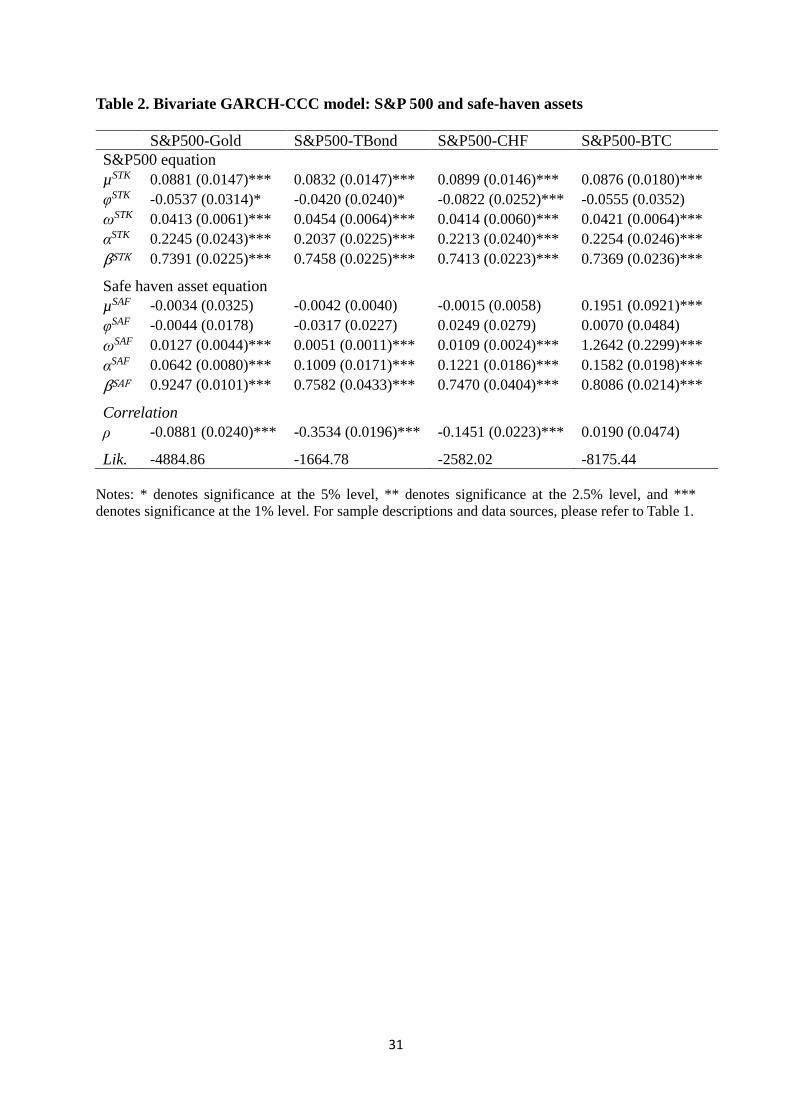
4.3 Results of bivariate GARCH-CCC and -DCC models

In this section, we apply the conventional GARCH models to the eight stock-safe

haven asset portfolios. First, the results of the bivariate GARCH-CCC model are presented in

Tables 2 and 3. As shown in these two tables, the two GARCH parameter estimates, αSTK ,

and βSTK for the stock position and αSAF and βSAF for the safe-have asset position, are positive

and significant (p-value < 0.01) for all the portfolios. Moreover, the sums of the two GARCH

parameter estimates are close to unity. These results indicate that the volatilities of the stock-

safe haven asset markets are not constant, and the GARCH-based volatilities exhibit

persistence (i.e., high volatility is followed by high volatility). Last but not least, the

correlations between stock indexes (S&P500 and FTSE100) and the traditional safe-haven

assets (gold, T-Bond, and CHF) are negative and significant (e.g., the FTSE100-TBond

correlation = -0.2718 with p-value < 0.01). However, their correlations with Bitcoin are

positive, with the FTSE100-BTC correlation significant at the 5% level.

(Insert Tables 2 and 3 about here)

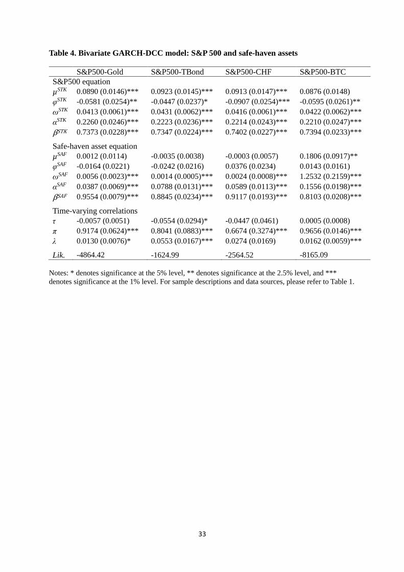
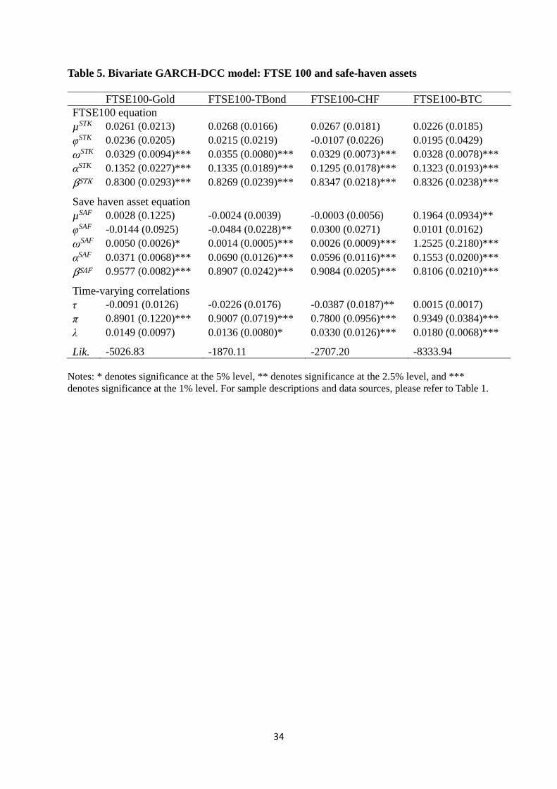
Tables 4 and 5 present the estimation results of the bivariate GARCH-DCC model.

16

Consistent with Tables 2 and 3, the two GARCH parameter estimates are significantly

positive, and the sums of the two estimates are close to unity, implying a volatility clustering

property. Furthermore, the DCC parameter estimates are positive and significant for all

portfolios (e.g., S&P500-Gold portfolio: π = 0.9174 with p-value < 0.01 and λ = 0.0130 with

p-value < 0.05), which support a correlation clustering property (i.e., high correlation

associates with high correlation).


4.4 Results of bivariate SWARCH model

While the results of the bivariate GARCH-DCC model support the notion of time-

varying volatilities and correlations in the stock-safe haven assets markets, the relationship

between their volatilities and correlations warrants further investigation per our discussions in

Section 2.2. Accordingly, we develop the bivariate SWARCH model with four volatility

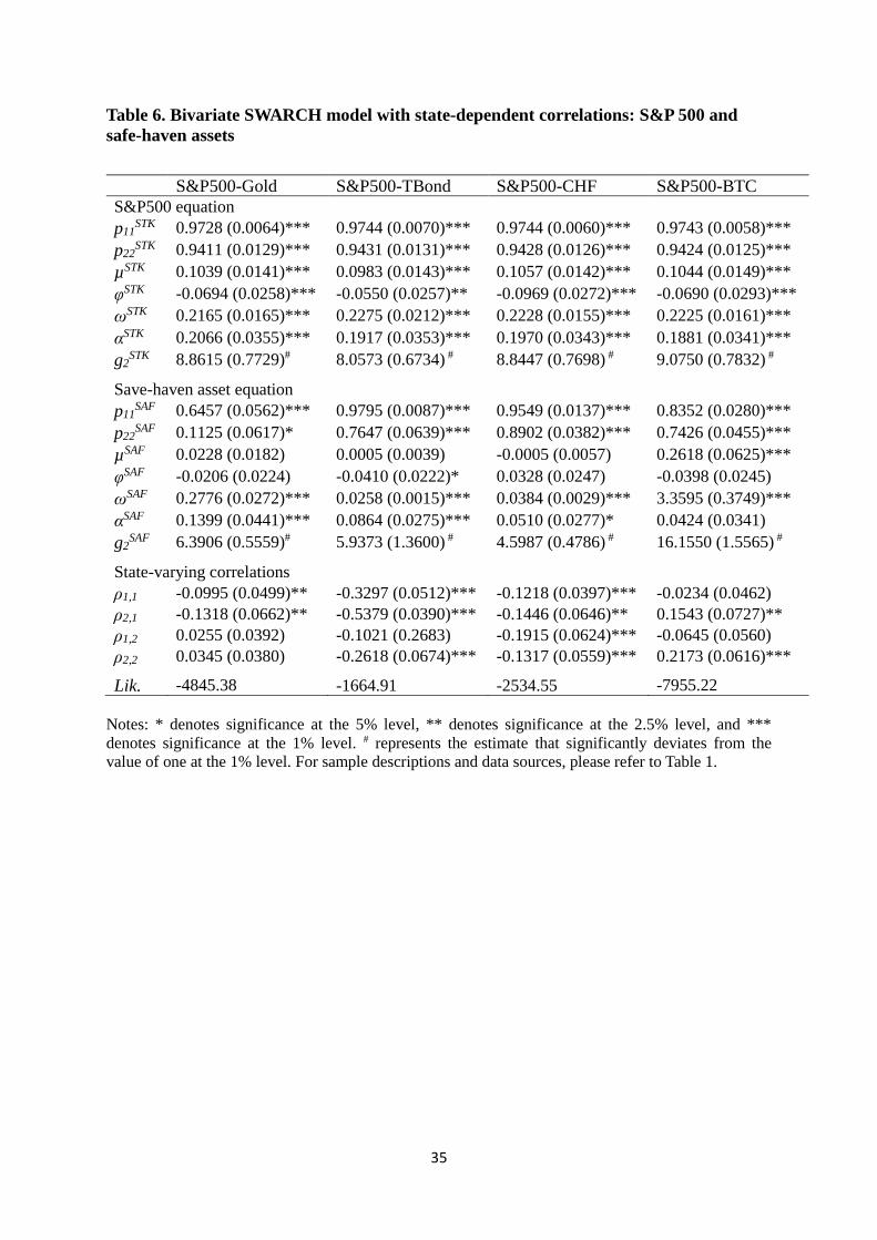
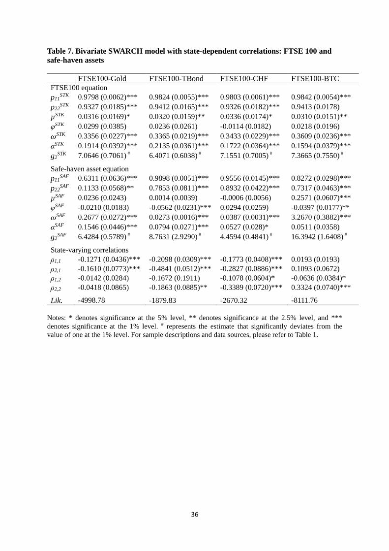
regime combinations to further examine the relationship. Table 6 reports the estimation

results for the portfolios consisting of S&P500 and four safe-haven assets, while the results

for the portfolios combining FTE100 and four safe-haven assets are presented in Table 7.


First, as shown in Tables 6 and 7, the scale of regime II volatility (i.e., g2STK for the

stock market and g2SAF for the safe-haven asset market) is significantly higher than one for all

eight portfolios. Using the S&P500-Gold portfolio as an example, the g2STK estimate is 8.8615

with a standard deviation of 0.7729 and the g2SAF estimate is 6.3906 with a standard deviation

of 0.5559. Notably, their 99% confidence intervals do not overlap with the value of one, the

scale of regime I volatility. We thus define regime II as a high volatility (HV) regime and

regime I as a low volatility (LV) regime. In addition, the ARCH parameter estimates (i.e.,

17

αSTK and αSAF) are positive and significant for all portfolios, indicating a time-varying

volatility property. To sum up, both time-varying and regime-varying properties are observed

in the conditional volatilities of the stock-safe haven asset markets.

Next, we turn our attention to conditional correlations. Based on the setting of the two

discrete volatility regimes (HV versus LV) for each asset in the portfolios, we investigate the

dynamic conditional correlations under four (2 X 2) volatility regime combinations (i.e., LV-

LV, HV-LV, LV-HV, and HV-HV). As shown in Tables 6 and 7, while these correlation

estimates are significantly negative or insignificant for most cases, the estimated correlations

between the two stock indexes (S&P500 and FTSE100) and Bitcoin are positive and

significant under the HV-HV state. To be sure, the S&P500-BTC and FTSE100-BTC

correlation estimates under the HV-HV state (i.e., ρ2,2) are 0.2173 and 0.3324 respectively,

with p-value < 0.01.

5. Discussion and portfolio construction

5.1 Explanation and discussion

By definition, a safe-haven asset for stock investors should be negatively correlated

(or zero correlation) with stocks during chaotic times (e.g., Baur & Lucey, 2010; Ratner &

Chiu, 2013). This study reexamines the issue on the four representative safe-haven assets

commonly seen in the literature: gold, government bond, Swiss Franc and Bitcoin. First, we

consider four volatility regime combinations in the stock-safe haven asset portfolios and

classify safe-haven assets into partial-safe and full-safe havens. Our theoretical arguments are

based on the cross-market rebalancing channel by Kodres and Pritsker (2002) and the social

learning channel by Trevino (2020). We argue that the correlation between stocks and safe-

haven assets might be heightened under high volatility conditions through these two channels.

As shown in Tables 6 and 7, the correlations between stocks (S&P500 and FTSE100)

18

and three traditional safe-haven assets (gold, T-Bond, and CHF) are significantly negative or

insignificant in all states, including the HV-HV state. These results support the notion that

these assets are full-safe haven assets for stock investors. However, the correlations between

stocks and Bitcoin are positive and significant under the HV-HV state (i.e., ρ2,2), although the

correlations are either insignificant or negative under other volatility states (i.e., ρ1,1, ρ2,1 and

ρ1,2). This result implies that Bitcoin is a partial-safe haven asset, falls short of a full-safe

haven against stocks.

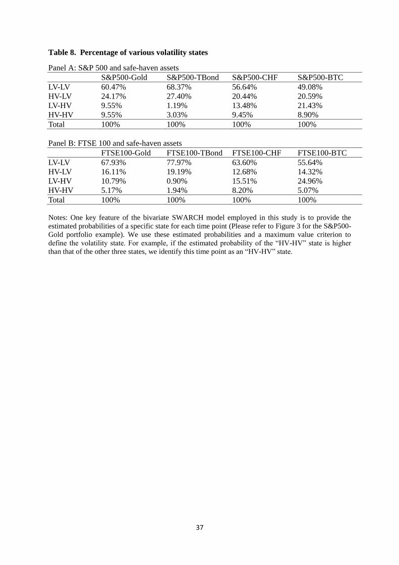
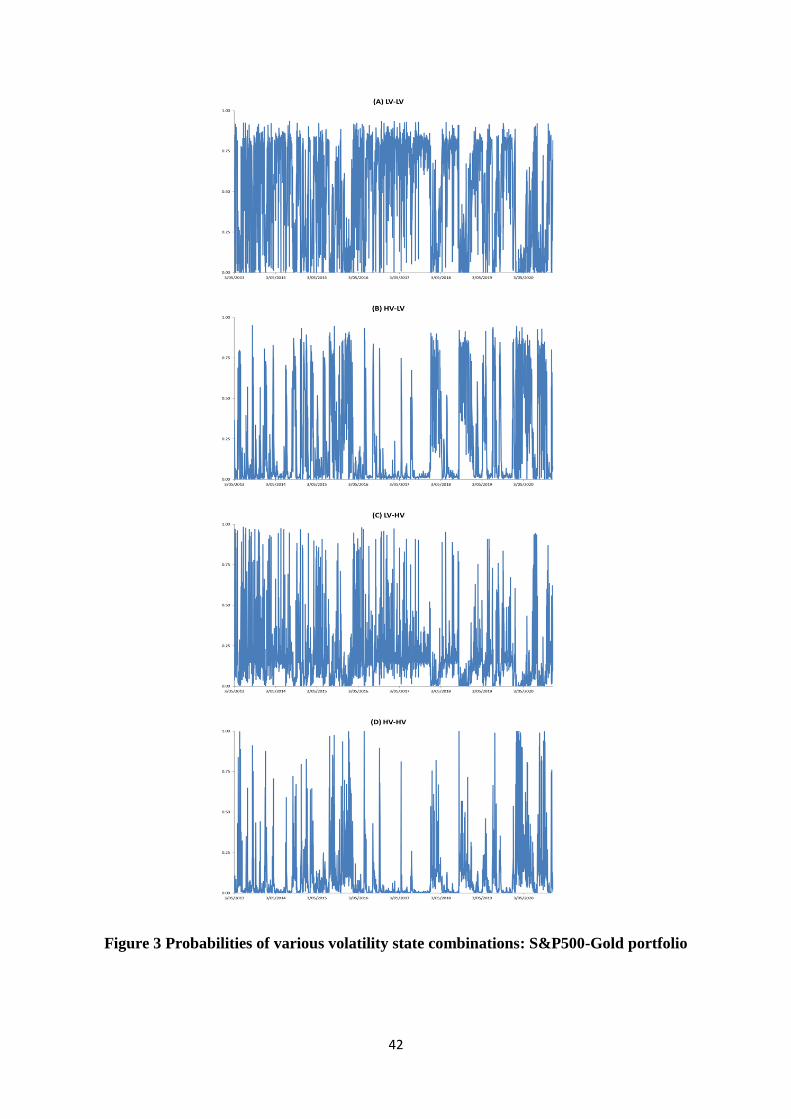
These findings require further discussion and elucidations. First, using the S&P500-

Gold portfolio as an example, Figure 3 graphs the probabilities of various volatility state

combinations estimated from our bivariate SWARCH model. We then adopt a maximum

value criterion to define the state for each time point. For example, if the estimated

probability of the “HV-HV” state is higher than that of the other three states, an “HV-HV”

state is defined at this time point. Table 8 lists the percentage of different volatility state

combinations observed for the eight stock-safe haven asset portfolios. The percentage of the

“HV-HV” state ranges between 1.94% for the FTSE100-TBond portfolio and 9.55% for the

S&P500-Gold portfolio. Therefore, the percentage of realizing any of the other three states

(i.e., LV-LV, LV-HV, and HV-LV) ranges from 90.45% and 98.06%. Among the four-state

combinations, the LV-LV is consistently the most commonly realized state (with a percentage

ranging from 49.08% to 77.97%) across all eight stock-safe haven asset pairs. Since ρ1,1

estimates reported in Tables 6 and 7 are either negative or zero in the LV-LV state, all of these

four non-stock assets examined live up to their generally expected role as a diversifying or

hedging asset for stock investors for a majority of the time.

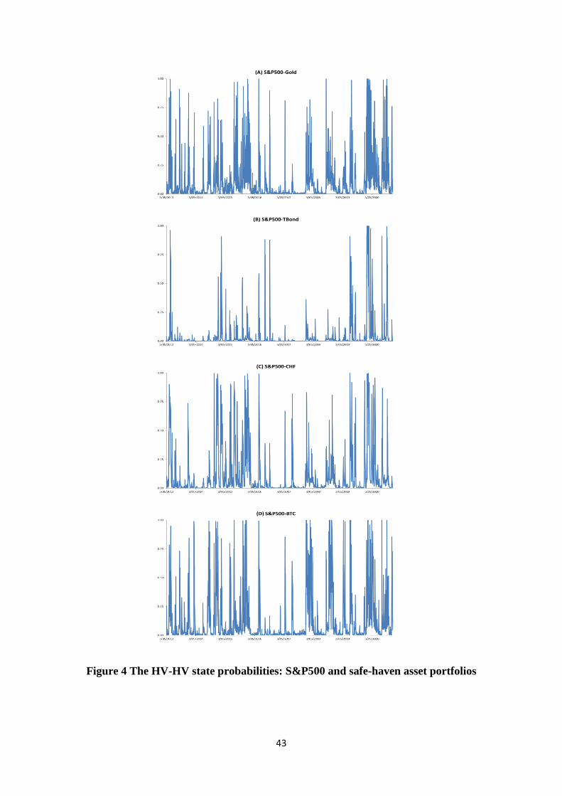
However, it is less certain if these non-stock assets can serve as safe-haven assets for

stock investors when both markets are in distress. Figure 4 graphs the HV-HV probabilities

for the four S&P500-safe haven asset portfolios. Consistent with the statistics shown in Table

19

8, the HV-HV state occurs less often compared with the LV-LV state. The HV-HV state

corresponds to periods during which both stocks and safe-haven assets experience volatile

movements. For instance, in mid-March 2020, the coronavirus pandemic triggered the

concern of global recession. As a result, the stock markets experienced some worst days in

early mid-March, 2020, e.g., S&P500 = -7.90% and FTSE100 = -7.99% on the 9th of March;

S&P500 = -9.99% and FTSE100 = -11.51% on the 12th of March; S&P500 = -12.77% and

FTSE100 = -4.09% on the 16th of March. The Bitcoin market also suffered from a huge

negative return on the same days, i.e., BTC = -14.09% (March 9), -46.47% (March 12), and -

10.39% (March 16). By contrast, the three traditional safe-haven assets fared better with

either a small loss or a positive gain on the same days, e.g., Gold = -0.14%, T-Bond = 0.73%

and CHF = 0.79% on the 9th of March; Gold = -4.88%, T-Bond = -0.27% and CHF = 0.54%

on the 12th of March; Gold = -1.89%, T-Bond = 1.53% and CHF = 0.66% on the 16th of

March. These observations corroborate our findings that gold, U.S. Treasury bond, and Swiss

Franc play a better role as a full-safe haven asset against stock market risk because their

prices do not move in the same direction with stocks under the HV-HV state. However, with

prices move in the same direction as stocks, Bitcoin is a partial-safe haven asset as it cannot

protect stock investors well under the “HV-HV” state.

Stock markets mainly reflect investors’ expectations on the future corporate profits

and macroeconomic conditions, such as economic growth, inflation, interest rate, and

unemployment. By contrast, the Bitcoin market is unregulated, and its prices are mainly

driven by media coverage, speculative activities, and market sentiment (e.g., Dastgir et al.,

2019; Lyócsa et al., 2020). Since different factors drive stock and Bitcoin markets, a weak

and negative correlation between them is possible; hence Bitcoin may provide diversification

benefit against the risk of stocks. However, we conjecture that two contagion channels, the

cross-market rebalancing channel (Kodres and Pritsker, 2002) and the social learning channel

20

(Trevino, 2020), may explain the possibility of a positive correlation between stock and

Bitcoin markets under the “HV-HV” state.

It should be highlighted that our empirical findings show that the cross-market

correlations between stocks and the three traditional safe-haven assets (Gold, T-Bond, and

CHF) are either insignificant or significantly negative even under the most strict “HV-HV”

state. These results imply that the financial contagion does not occur between stocks and

these three traditional safe-haven assets. It is plausible that these traditional safe-haven assets

are influenced by risk factors fundamentally different from stocks. For example, as

fixed‐income securities, bonds are much more sensitive to interest rate risk than stocks.

Sovereign risk in a nation’s government bonds is different from corporate default risks in

stocks. During periods of crisis, Federal Reserve purchases or sells government bonds to

influence interest rates and bond prices, whereas Federal Reserve does not directly trade

stocks in markets. The most recent evidence occurred in March 2020 when Covid-19 hit the

nation hard, both stock and government bond markets crumbled. However, the near-

meltdown in the government bond markets prompted the U.S. Fed to buy a massive $1

trillion Treasuries in less than one month.

5.2 Portfolio construction: A beauty contest

As is well known, effective portfolio construction relies on the estimation quality of

variances and correlations. Accordingly, a related question is whether the state-varying

variances and correlations addressed in this study may help an investor construct a more

efficient stock-safe haven asset portfolio. Since the use of safe-haven assets is to reduce

portfolio risk, we employ a minimum variance portfolio construction strategy to conduct this

test (e.g., French and Poterba, 1991; Tesar and Werner, 1992; Ramchand and Susmel, 1998).

Considering the portfolio consisting of stock (STK) and safe-haven asset (SAF), the weight

21

given to each position is presented as follows:

𝑤𝑡𝑆𝑇𝐾 = [ℎ𝑡

𝑆𝐴𝐹 − 𝜌𝑡(ℎ𝑡𝑆𝐴𝐹 ∙ ℎ𝑡

𝑆𝑇𝐾)1/2]/[ℎ𝑡𝑆𝑇𝐾 + ℎ𝑡

𝑆𝐴𝐹 − 2 ∙ 𝜌𝑡(ℎ𝑡𝑆𝐴𝐹 ∙ ℎ𝑡

𝑆𝑇𝐾)1/2] (16)

𝑤𝑡𝑆𝐴𝐹 = 1 − 𝑤𝑡

𝑆𝑇𝐾 (17)

where wtSTK and wt

SAF represent the weight given to stock (STK) and safe-haven asset position

(SAF), respectively. htSTK and ht

SAF denote the conditional variances of STK and SAF

respectively, and ρt is the correlation between them.

Given the weights, we then calculate the return of the stock-safe haven asset portfolio

at time t (rtPOT):

𝑟𝑡𝑃𝑂𝑇 = 𝑤𝑡

𝑆𝑇𝐾 ∙ 𝑟𝑡𝑆𝑇𝐾 + 𝑤𝑡

𝑆𝐴𝐹 ∙ 𝑟𝑡𝑆𝐴𝐹 (18)

Next, we calculate the STK-SAF portfolio's return mean and volatility over the testing period

to examine whether the state-varying bivariate SWARCH model outperforms the time-

varying bivariate GARCH-CCC and -DCC models.

First, we compare the performance of different models using the bivariable GARCH-

CCC model as a benchmark. We examine the four portfolios consisting of S&P500 and safe-

haven assets and present the results in Table 9, in which Panels A and B show portfolio mean

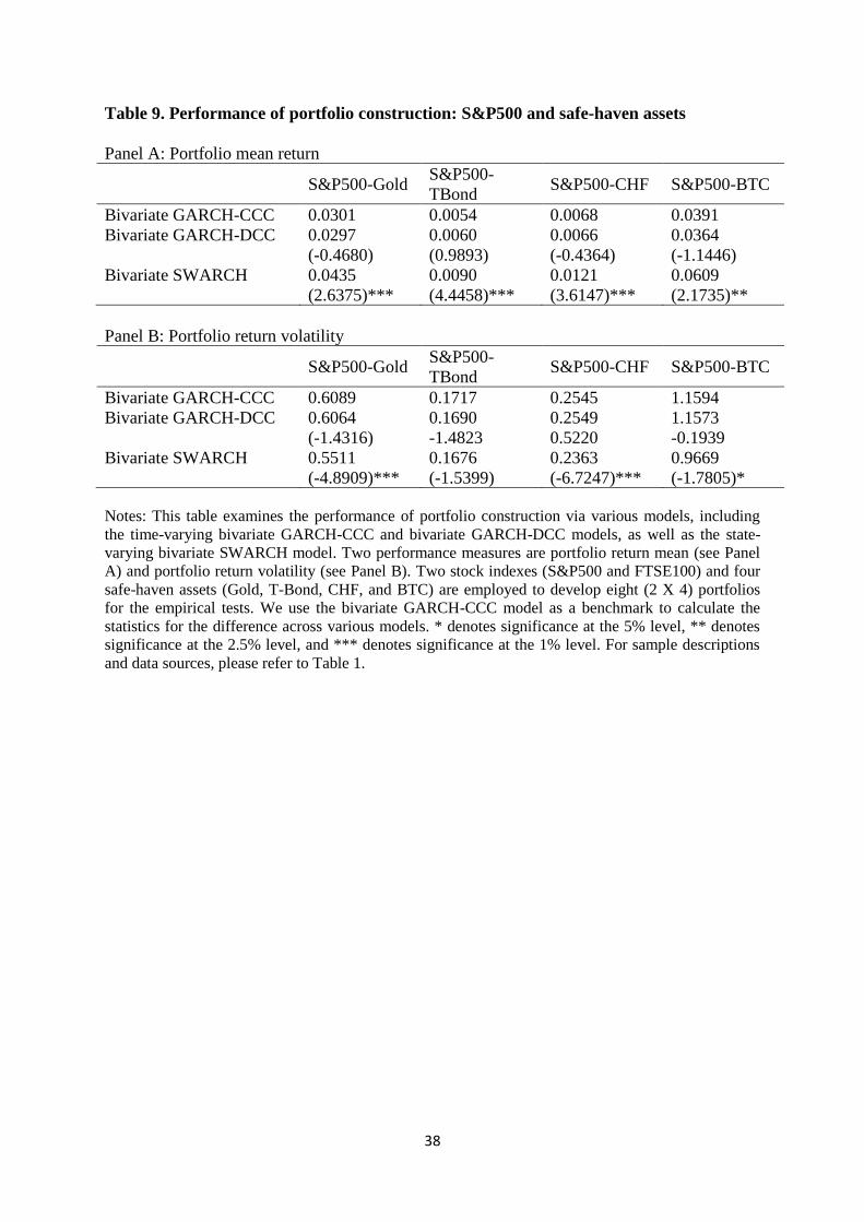
return and volatility, respectively. As shown in Table 9, comparing with the bivariate

GARCH-CCC and -DCC models, the bivariate SWARCH model produces portfolios of stock

and safe-haven assets with higher mean returns and lower return volatilities. Moreover, the

return and volatility differences between the bivariate SWARCH model and the bivariate

GARCH-CCC model are significant at the 1% level for most cases, except for the return

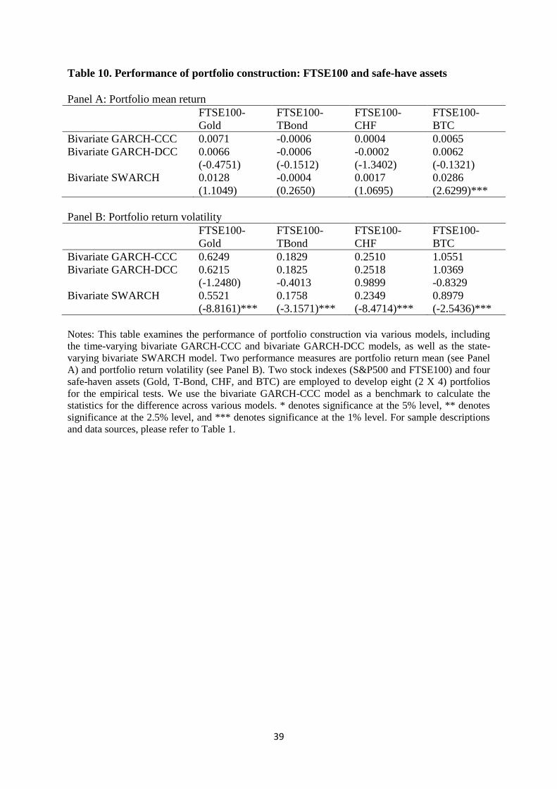
mean of the S&P500-TBond portfolio. Table 10 presents the results of the portfolios

consisting of FTSE100 and four safe-haven assets. Similarly, the portfolios constructed by the

bivariate SWARCH model have higher return means and lower return volatilities comparing

with the bivariate GARCH-CCC and -DCC models. The differences in volatilities between

the bivariate SWARCH model and the bivariate GARCH-CCC model are significant at the

22

1% level for all cases. In short, the state-varying volatilities and correlations in our proposed

bivariate SWARCH model enhance the performance of stock-safe haven asset portfolios

constructed.

Next, we compare the differences in performances among various stock-safe haven

portfolios. As shown in Panel B of Table 9, given the model, i.e., bivariate SWARCH model,

the return volatilities of S&P500-TBond and S&P500-CHF portfolios (0.1676 and 0.2363)

are lower than those of S&P500-Gold and S&P500-BTC (0.5511 and 0.9669). These results

echo our four-state correlation system presented earlier. Recall the results in Table 6, the

correlations under the HV-HV state (i.e., ρ2,2) for S&P500-TBond and S&P500-CHF pairs

are negative and significant (-0.2618 with p-value < 0.01 and -0.1317 with p-value < 0.01),

while the same statistic for S&P500-Gold pair is positive but insignificant (0.0345 with p-

value > 0.05) and the estimate of ρ2,2 for S&P500-BTC pair is positive and significant

(0.2173 with p-value <0.01). Overall, this is consistent with our notion that T-Bond and CHF

are better safe-havens than gold, while Bitcoin, at best, is a partial-safe haven asset. While

gold is the most legendary safe-haven asset and its safe-haven characteristics during the

previous crises such as the 1987 stock market crash and the 2008 Global Financial Crisis

have been well documented in the literature (see Baur and McDermott, 2010), recent

experiences cast doubt on its credibility. Gold prices reached a historical high of $1898.25 on

September 5, 2011, but lost their peak value by 45% by December 17, 2015. Over four years,

the 45% value depreciation causes investors to lose trust in gold and question its effectiveness

as a safe-haven asset (The Business Times, 2021).3 Our empirical results resonate with this

concern. Lastly, as shown in Panel A of Table 9, the mean returns of S&P500-BTC and

S&P500-Gold portfolios (0.0609 and 0.0435) are higher than those of S&P500-TBond and

S&P500-CHF portfolios (0.0090 and 0.0121). This result is consistent with the risk-return

3 See https://www.businesstimes.com.sg/companies-markets/recent-events-prove-gold-is-no-longer-a-safe-haven:

Recent events prove gold is no longer a safe haven by Neil Behrmann.

https://www.businesstimes.com.sg/companies-markets/recent-events-prove-gold-is-no-longer-a-safe-haven

23

trade-off principle. In Table 10, similar findings apply to the portfolios consisting of

FTSE100 and safe-have assets.

6. Conclusion

In this paper, we examine the dynamic conditional correlations between stocks

(S&P500 and FTSE100) and safe-have assets (gold, U.S. government bond, Swiss Franc and

Bitcoin). Our contributions to the literature are in three facades. First, we provide theoretical

grounds to address the difference between partial-safe haven assets and full-safe haven assets,

which is overlooked by the extant literature. Second, we develop a bivariate SWARCH model

with four-state volatility combinations and employ the realized data to test the model

empirically. Last but not least, we conduct portfolio construction, a practical test, to validate

our proposed regime-switching approach.

Based on the two discrete volatility regimes (HV versus LV) for each position in the

stock-safe haven asset portfolios, we develop a novel system with four volatility regime

combinations (i.e., LV-LV, HV-LV, LV-HV, and HV-HV) and examine the dynamic

conditional correlations under these volatility regimes. While existing studies have tested the

dynamic conditional correlations in the stock-safe haven asset markets (the majority of the

studies use the conventional DCC models), to the best of our knowledge, they have neither

explicitly addressed the correlation dynamics under various volatility regimes, nor developed

a theoretical foundation to explain the dynamic correlations. This study fills these gaps in the

literature and offers several contributions, including developing a theoretical hypothesis,

constructing a specific econometric method, and conducting two practical risk management

tests. Our hypothesis and tests are meaningful and bring the statistical estimation results

closer to practices.

24

Our empirical results are consistent with the following notions. First, the correlations

between the three traditional safe-haven assets (gold, U.S. Treasury bond, and Swiss Franc)

and the two stock markets (S&P500 and FTSE100) are significantly negative or zero under

all volatility states, including the most strict HV-HV state (i.e., both stock and safe-haven

asset markets experience high volatility). These results imply that gold, U.S. Treasury bonds,

and Swiss Franc are full-safe haven assets. Second, the correlations between Bitcoin and the

two major stock markets are positive and significant in the HV-HV state, although

insignificant or negative in other volatility states. Our results imply that contagion occurs

between stocks and Bitcoin markets when both of them experience chaotic conditions,

rendering Bitcoin a less than a full-safe haven asset. Third, the regime-switching model

proposed in this study proves to be more effective than the conventional GARCH-based

models in portfolio construction. Fourth, comparing three traditional safe-haven assets, our

results indicate that U.S. Treasury bonds and Swiss Franc are stronger safe havens than gold,

which echos the press opinions, including Russ Koesterich of the BlackRock Global

Allocation Fund, that gold’s role as a safe haven has been exaggerated and waned.4

4 For example, MacDonald and Shumsky, Wall Street Journal: https://www.wsj.com/articles/golds-role-as-safe-

haven-investment-wanes-1445250762.

https://www.wsj.com/articles/golds-role-as-safe-haven-investment-wanes-1445250762

https://www.wsj.com/articles/golds-role-as-safe-haven-investment-wanes-1445250762

25

References

Akhtaruzzaman, M., Boubaker, S. & Sensoy, A. (2021) Financial contagion during COVID–

19 crisis, Finance Research Letters 38, 101604.

Ang, A. & Bekaert, G. (2002) International asset allocation with regime shifts, Review of

Financial Studies 15, 1137-1187.

Baker, S.R., Bloom, N. & Davis, S.J. (2016) Measuring economic policy uncertainty,

Quarterly Journal of Economics 131, 1593-636.

Bae, K.H., Karolyi, G.A. & Stulz, R.M. (2003) A new approach to measuring financial

contagion, Review of Financial Studies 16, 717-763.

Baker, S.R., Bloom, N., Davis, S.J., Kost, K., Sammon, M. & Viratyosin, T. (2020) The

unprecedented stock market reaction to COVID-19, Working paper, Northwestern

University.

Baillie, R.T., & Bollerslev, T. (1990) A multivariate generalized ARCH approach to

modeling risk premia in the forward foreign exchange rate, Journal of International

Money and Finance 9, 309-324.

Baur, D.G. & Lucey, B.M. (2010) Is gold a hedge or a safe haven? An analysis of stocks,

bonds and gold, Financial Review 45, 217-229.

Baur, D.G. & McDermott, T.K. (2010) Is gold a safe haven? International evidence, Journal

of Banking and Finance 34, 1886-1898.

Bekiros, S., Boubaker, S., Nguyen, D.K. & Uddin, G.S. (2017) Black swan events and safe

havens: The role of gold in globally integrated emerging markets, Journal of

International Money and Finance 73, 317-334.

Bollerslev, T. (1990) Modelling the coherence in short-run nominal exchange rates: A

multivariate generalized ARCH model, Review of Economics and Statistics 72, 498-505.

Bouri, E., Das, M., Gupta, R. & David, R. (2018) Spillovers between Bitcoin and other assets

during bear and bull markets, Applied Economics 50, 5935-5949.

Bouri, E., Gupta, R., Tiwari, A., & Roubaud, D. (2017a) Does Bitcoin hedge global

uncertainty? Evidence from wavelet-based quantile-in-quantile regressions, Finance

Research Letters 23, 87-95.

Bouri, E., Jalkh, N., Molnár, P., & Roubaud, D. (2017b) Bitcoin for energy commodities

before and after the December 2013 crash: Diversifier, hedge or safe haven? Applied

Economics 49, 5063-5073.

Bouri, E., Shahzad, S.J. & Roubaud, D. (2020) Cryptocurrencies as hedges and safe-havens

for US equity sectors, Quarterly Review of Economics and Finance 75, 294-307.

Capie, F., Mills, T.C., & Wood, G. (2005) Gold as a hedge against the dollar, Journal of

International Financial Markets, Institutions and Money, 15, 343-352.

26

Cappiello, L., Engle, R.F. & Sheppard, K. (2006) Asymmetric dynamics in the correlations of

global equity and bond returns, Journal of Financial Econometrics 4, 537-572.

Chan, K.F., Treepongkaruna, S., Brooks, R. & Gray, S. (2011) Asset market linkages:

Evidence from financial, commodity and real estate assets, Journal of Banking and

Finance 35, 1415-1426.

Cheema, M.A., Faff, R.W. & Szulczuk, K. (2020) The 2008 global financial crisis and

COVID-19 pandemic: How safe are the safe haven assets? Working paper, SSRN.

Ciner, C., Gurdgiev, C. & Lucey, B.M. (2013) Hedges and safe havens: An examination of

stocks, bonds, gold, oil and exchange rates, International Review of Financial Analysis

29, 202-211.

Conlon, T. & McGee, R. (2020) Safe haven or risky hazard? Bitcoin during the COVID-19

bear market, Finance Research Letters 35, 1-5.

Corbet, S., Hou, Y., Hu, Y., Lucey, B. & Oxley, L. (2020) Aye Corona! The contagion

effects of being named Corona during the COVID-19 pandemic, Finance Research

Letters 38, 101591.

Danielsson, J., Valenzuela, M. & Zer, I. (2018) Learning from history: volatility and financial

crises, The Review of Financial Studies 31, 2774-2805.

Das, S.R. & Uppal, R. (2004) Systemic risk and international portfolio choice, Journal of

Finance 59, 2809-2834.

Dastgir, S., Demir, E., Downing, G., Gozgor, G. & Lau, C.K. (2019) The causal relationship

between Bitcoin attention and Bitcoin returns: Evidence from the Copula-based Granger

causality test, Finance Research Letters 28, 160-164.

Engle, R. (2002) Dynamic conditional correlation: a simple class of multivariate generalized

autoregressive conditional heteroskedasticity models, Journal of Business and Economic

Statistics 20, 339-350.

Engle, R. & Mustafa, C. (1992) Implied ARCH models from options prices, Journal of

Econometrics 52, 289-311.

Engle, R., Ghysels, E. & Sohn, B. (2013) Stock market volatility and macroeconomic

fundamentals, Review of Economics and Statistics 95, 776-97.

Erb, C.B., Harvey, C.R. & Viskanta, T.E. (1994) Forecasting international equity correlations,

Financial Analysts Journal, 32-45.

Fleming, J., Kirby, C. & Ostdiek, B. (1998) Information and volatility linkages in the stock,

bond, and money markets, Journal of Financial Economics 49, 111-137.

Forbes, K.J. & Rigobon, R. (2002) No contagion, only interdependence: Measuring stock

market co-movement, Journal of Finance 57, 2223-2261.

French, K.R. & Poterba, J M. (1991) Investor diversification and international equity markets,

American Economic Review 81, 222-226.

27

Garcia-Jorcanoa, L. & Benito, S. (2020) Studying the properties of the Bitcoin as a

diversifying and hedging asset through a copula analysis: Constant and time-varying,

Research in International Business and Finance 54, 101300.

Gil-Alana, L.A., Abakah, E.J.A. & Rojo, M.F.R. (2020) Cryptocurrencies and stock market

indices: Are they related? Research in International Business and Finance 51, 101063.

Goeij, P.D. & Marquering, W. (2004) Modeling the conditional covariance between stock

and bond returns: A multivariate GARCH approach, Journal of Financial Econometrics

2, 531-564.

Grisse, C. & Nitschka, T. (2015) On financial risk and the safe haven characteristics of Swiss

franc exchange rates, Journal of Empirical Finance 32, 153-164.

Gulen, H., & Ion, M. (2016) Policy uncertainty and corporate investment, Review of

Financial Studies 29, 523-64.

Hafner, C.M. (2020) Testing for bubbles in cryptocurrencies with time-varying volatility,

Journal of Financial Econometrics 18, 233-249.

Hamilton, J.D. & Susmel, R. (1994) Autoregressive conditional heteroscedasticity and

changes in regime, Journal of Econometrics 64, 307-333.

Hammoudeh, S., Sari, R., & Ewing, B. (2009) Relationships among strategic commodities

and with financial variables: A new look, Contemporary Economic Policy 27, 251-264.

Hartmann, P., Straetmans, S. & Vries, C.D. (2004) Asset market linkages in crisis periods,

Review of Economics and Statistics 86, 313-326.

Heckman, J. (1979) Sample selection bias as a specification error, Econometrica 47, 153-161.

Hillier, D., Draper, P. & Faff, R. (2006) Do precious metals shine? An investment

perspective, Financial Analysts Journal 62, 98-106.

Hood, M. & Malik, F. (2013) Is gold the best hedge and a safe haven under changing stock

market volatility? Review of Financial Economics 22, 47-52.

Isah, K.O. & Raheem, I. (2019) The hidden predictive power of cryptocurrencies and QE:

evidence from US stock market, Physica A: Statistical Mechanics and its Applications

536, 121032.

Jackwerth, J.C. & Slavutskaya, A. (2016) The total benefit of alternative assets to pension

fund portfolios, Journal of Financial Markets 31, 25-42.

Jacquier, E. & Marcus, A.J. (2001) Asset allocation models and market volatility, Financial

Analysts Journal 57, 16-31.

Karolyi, G.A. & Stulz, R.M. (1996) Why do markets move together? An investigation of

U.S.-Japan stock return comovements, Journal of Finance 51, 951-986.

Kaul, A. & Sapp, S. (2006) Y2K fears and safe haven trading of the US dollar, Journal of

International Money and Finance 25, 760-779.

28

King, M.A., & Wadhwani, S. (1990) Transmission of volatility between stock markets,

Review of Financial Studies 3, 5-33.

Kliber, A., Marszałek, P., Musiałkowska, I., Świerczyńska, K. (2019) Bitcoin: safe haven,

hedge or diversifier? Perception of bitcoin in the context of a country’s economic

situation – a stochastic volatility approach, Physica A: Statistical Mechanics and its

Applications 524, 246-257.

Kodres, L. & Pritsker, M. (2002) A rational expectations model of financial contagion,

Journal of Finance 57, 769-800.

Longin, F. & Solnik, M.B. (1995) Is the correlation on international equity returns constant:

1960-1990? Journal of international Money and Finance 14, 3-23.

Longin, F. & Solnik, M.B. (2001) Extreme correlation of international equity markets,

Journal of Finance 56, 649-676.

Lyócsa, S., Molnár, P., Plíhal T. & Širanová, S. (2020) Impact of macroeconomic news,

regulation and hacking exchange markets on the volatility of bitcoin, Journal of

Economic Dynamics and Control 119, 103980.

Mariana, C.D., Ekaputra, I.A. & Husodo, Z.A. (2021) Are Bitcoin and Ethereum safe-havens

for stocks during the COVID-19 pandemic? Finance Research Letters 38, 101798.

Mokni, K., Bouri, E., Ajmi, A.N. & Vo, X.V. (2021) Does Bitcoin hedge categorical

economic uncertainty? A quantile analysis, SAGE Open, 1-14.

Nelson, D.B. (1991) Conditional heteroskedasticity in asset returns: A new approach,

Econometrica 59, 347-370.

Noeth, B.J. & Sengupta, R. (2010) Flight to safety and US Treasury securities, The Regional

Economist 18, 18-19.

Pullen, T., Benson, K. & Faff, R. (2014) A comparative analysis of the investment

characteristics of alternative gold assets, Abacus 50, 76-92.

Ranaldo, A. & Söderlind, P. (2010) Safe haven currencies, Review of Finance 14, 385-407.

Ramchand, L. & Susmel, R. (1998) Volatility and cross-correlation across major stock

markets, Journal of Empirical Finance 5, 397-416.

Ratner, M. & Chiu, C. (2013) Hedging stock sector risk with credit default swaps,

International Review of Financial Analysis 30, 18-25.

Schmitt, N. & Westerhoff, F. (2017) Herding behaviour and volatility clustering in financial

markets, Quantitative Finance 17, 1187-1203.

Stensås, A., Nygaard, M.F., Kyaw, K. & Treepongkaruna, S. (2019) Can Bitcoin be a

diversifier, hedge or safe haven tool? Cogent Economics and Finance 7, 1-17.

Tesar, L.L. & Werner, I. (1992) Home bias and the globalization of securities markets, NBER

Working Paper, No. 4218, National Bureau of Economic Research, Cambridge.

29

Trevino, I. (2020) Informational channels of financial contagion, Econometrica 88, 297-335.

Urquhart, A. & Zhang, H. (2019) Is Bitcoin a hedge or safe haven for currencies? An intraday

analysis, International Review of Financial Analysis 63, 49-57.

Wu, S., Tong, M., Yang, Z., & Derbali, A. (2019) Does gold or bitcoin hedge economic

policy uncertainty? Finance Research Letters 31, 171-178.

30

Table 1. Descriptive statistics

Panel A: Basic statistic of individual return on stock indexes and safe haven assets

S&P500 FTSE100 Gold T-Bond CHF BTC

Mean 0.0432 0.0011 0.0099 0.0010 0.0021 0.2667

SD. 1.0740 1.0169 0.9069 0.2037 0.2892 4.9603

Q1 -0.3016 -0.4546 -0.4400 -0.1133 -0.1534 -1.4798

Medium 0.0394 0.0189 0.0127 0.0000 -0.0012 0.1950

Q3 0.4973 0.4878 0.4782 0.1145 0.1617 2.1883

Skewness -1.0759 -0.9177 -0.1350 0.1872 -0.2459 -0.0533

Kurtosis 26.3658 17.5786 7.4216 12.3537 6.9277 16.5488

Panel B: Correlation matrix

S&P500 FTSE100 Gold T-Bond CHF BTC

S&P500 1.0000

FTSE100 0.5922*** 1.0000

Gold 0.0048 -0.0396 1.0000

T-Bond -0.4116*** -0.2933*** 0.2498*** 1.0000

CHF -0.1288*** -0.2196*** 0.1609*** 0.1296*** 1.0000

BTC 0.1109*** 0.0914*** 0.0610*** -0.0144 -0.0067 1.0000

Notes: This table reports the basic statistics (Panel A) and correlation matrix (Panel B) for the two

stock indexes (S&P500 and FTSE100) and the four safe-haven assets (Gold, T-Bond, Swiss France,

and Bitcoin). The testing period ranges from April 30, 2003, to January 18, 2021 (2,015 daily

observations). To ensure that the data are stationary, return series are used rather than the price level

series. The data are collected from the DataStream database except for Swiss France and Bitcoin. In

addition, we obtain the data of the Swiss Franc index from the online database of the Swiss National

Bank and the data of Bitcoin is obtained with https://coinmarketcap.com/.

https://coinmarketcap.com/

31

Table 2. Bivariate GARCH-CCC model: S&P 500 and safe-haven assets

S&P500-Gold S&P500-TBond S&P500-CHF S&P500-BTC

S&P500 equation

µSTK 0.0881 (0.0147)*** 0.0832 (0.0147)*** 0.0899 (0.0146)*** 0.0876 (0.0180)***

φSTK -0.0537 (0.0314)* -0.0420 (0.0240)* -0.0822 (0.0252)*** -0.0555 (0.0352)

ωSTK 0.0413 (0.0061)*** 0.0454 (0.0064)*** 0.0414 (0.0060)*** 0.0421 (0.0064)***

αSTK 0.2245 (0.0243)*** 0.2037 (0.0225)*** 0.2213 (0.0240)*** 0.2254 (0.0246)***

βSTK 0.7391 (0.0225)*** 0.7458 (0.0225)*** 0.7413 (0.0223)*** 0.7369 (0.0236)***

Safe haven asset equation

µSAF -0.0034 (0.0325) -0.0042 (0.0040) -0.0015 (0.0058) 0.1951 (0.0921)***

φSAF -0.0044 (0.0178) -0.0317 (0.0227) 0.0249 (0.0279) 0.0070 (0.0484)

ωSAF 0.0127 (0.0044)*** 0.0051 (0.0011)*** 0.0109 (0.0024)*** 1.2642 (0.2299)***

αSAF 0.0642 (0.0080)*** 0.1009 (0.0171)*** 0.1221 (0.0186)*** 0.1582 (0.0198)***

βSAF 0.9247 (0.0101)*** 0.7582 (0.0433)*** 0.7470 (0.0404)*** 0.8086 (0.0214)***

Correlation

ρ -0.0881 (0.0240)*** -0.3534 (0.0196)*** -0.1451 (0.0223)*** 0.0190 (0.0474)

Lik. -4884.86 -1664.78 -2582.02 -8175.44

Notes: * denotes significance at the 5% level, ** denotes significance at the 2.5% level, and ***

denotes significance at the 1% level. For sample descriptions and data sources, please refer to Table 1.

32

Table 3. Bivariate GARCH-CCC model: FTSE 100 and safe-haven assets

FTSE100-Gold FTSE100-TBond FTSE100-CHF FTSE100-BTC

FTSE100 equation

µSTK 0.0295 (0.0173)* 0.0287 (0.0167)* 0.0284 (0.0175) 0.0286 (0.0153)*

φSTK 0.0200 (0.0242) 0.0207 (0.0266) -0.0111 (0.0349) 0.0168 (0.0209)

ωSTK 0.0461 (0.0078)*** 0.0465 (0.0081)*** 0.0448 (0.0074)*** 0.0467 (0.0078)***

αSTK 0.1524 (0.0192)*** 0.1419 (0.0185)*** 0.1428 (0.0180)*** 0.1546 (0.0194)***

βSTK 0.7981 (0.0222)*** 0.8055 (0.0227)*** 0.8075 (0.0210)*** 0.7954 (0.0222)***

Safe-haven asset equation

µSAF -0.0018 (0.0283) -0.0029 (0.0040) -0.0009 (0.0060) 0.1960 (0.0856)***

φSAF -0.0043 (0.0282) -0.0504 (0.0244)* 0.0216 (0.0331) 0.0071 (0.0037)*

ωSAF 0.0122 (0.0042)*** 0.0051 (0.0012)*** 0.0110 (0.0025)*** 1.2647 (0.2178)***

αSAF 0.0639 (0.0079)*** 0.1042 (0.0181)*** 0.1218 (0.0194)*** 0.1585 (0.0198)***

βSAF 0.9257 (0.0096)*** 0.7541 (0.0454)*** 0.7468 (0.0428)*** 0.8084 (0.0208)***

Correlation

ρ -0.0986 (0.0225)*** -0.2718 (0.0208)*** -0.2042 (0.0217)*** 0.0295 (0.0136)**

Lik. -5054.10 -1891.97 -2732.11 -8346.17



33

Table 4. Bivariate GARCH-DCC model: S&P 500 and safe-haven assets


S&P500 equation

µSTK 0.0890 (0.0146)*** 0.0923 (0.0145)*** 0.0913 (0.0147)*** 0.0876 (0.0148)

φSTK -0.0581 (0.0254)** -0.0447 (0.0237)* -0.0907 (0.0254)*** -0.0595 (0.0261)**

ωSTK 0.0413 (0.0061)*** 0.0431 (0.0062)*** 0.0416 (0.0061)*** 0.0422 (0.0062)***

αSTK 0.2260 (0.0246)*** 0.2223 (0.0236)*** 0.2214 (0.0243)*** 0.2210 (0.0247)***

βSTK 0.7373 (0.0228)*** 0.7347 (0.0224)*** 0.7402 (0.0227)*** 0.7394 (0.0233)***


µSAF 0.0012 (0.0114) -0.0035 (0.0038) -0.0003 (0.0057) 0.1806 (0.0917)**

φSAF -0.0164 (0.0221) -0.0242 (0.0216) 0.0376 (0.0234) 0.0143 (0.0161)

ωSAF 0.0056 (0.0023)*** 0.0014 (0.0005)*** 0.0024 (0.0008)*** 1.2532 (0.2159)***

αSAF 0.0387 (0.0069)*** 0.0788 (0.0131)*** 0.0589 (0.0113)*** 0.1556 (0.0198)***

βSAF 0.9554 (0.0079)*** 0.8845 (0.0234)*** 0.9117 (0.0193)*** 0.8103 (0.0208)***

Time-varying correlations

τ -0.0057 (0.0051) -0.0554 (0.0294)* -0.0447 (0.0461) 0.0005 (0.0008)

π 0.9174 (0.0624)*** 0.8041 (0.0883)*** 0.6674 (0.3274)*** 0.9656 (0.0146)***

λ 0.0130 (0.0076)* 0.0553 (0.0167)*** 0.0274 (0.0169) 0.0162 (0.0059)***

Lik. -4864.42 -1624.99 -2564.52 -8165.09



34

Table 5. Bivariate GARCH-DCC model: FTSE 100 and safe-haven assets


FTSE100 equation

µSTK 0.0261 (0.0213) 0.0268 (0.0166) 0.0267 (0.0181) 0.0226 (0.0185)

φSTK 0.0236 (0.0205) 0.0215 (0.0219) -0.0107 (0.0226) 0.0195 (0.0429)

ωSTK 0.0329 (0.0094)*** 0.0355 (0.0080)*** 0.0329 (0.0073)*** 0.0328 (0.0078)***

αSTK 0.1352 (0.0227)*** 0.1335 (0.0189)*** 0.1295 (0.0178)*** 0.1323 (0.0193)***

βSTK 0.8300 (0.0293)*** 0.8269 (0.0239)*** 0.8347 (0.0218)*** 0.8326 (0.0238)***

Save haven asset equation

µSAF 0.0028 (0.1225) -0.0024 (0.0039) -0.0003 (0.0056) 0.1964 (0.0934)**

φSAF -0.0144 (0.0925) -0.0484 (0.0228)** 0.0300 (0.0271) 0.0101 (0.0162)

ωSAF 0.0050 (0.0026)* 0.0014 (0.0005)*** 0.0026 (0.0009)*** 1.2525 (0.2180)***

αSAF 0.0371 (0.0068)*** 0.0690 (0.0126)*** 0.0596 (0.0116)*** 0.1553 (0.0200)***

βSAF 0.9577 (0.0082)*** 0.8907 (0.0242)*** 0.9084 (0.0205)*** 0.8106 (0.0210)***

Time-varying correlations

τ -0.0091 (0.0126) -0.0226 (0.0176) -0.0387 (0.0187)** 0.0015 (0.0017)

π 0.8901 (0.1220)*** 0.9007 (0.0719)*** 0.7800 (0.0956)*** 0.9349 (0.0384)***

λ 0.0149 (0.0097) 0.0136 (0.0080)* 0.0330 (0.0126)*** 0.0180 (0.0068)***

Lik. -5026.83 -1870.11 -2707.20 -8333.94



35

Table 6. Bivariate SWARCH model with state-dependent correlations: S&P 500 and

safe-haven assets


S&P500 equation

p11STK 0.9728 (0.0064)*** 0.9744 (0.0070)*** 0.9744 (0.0060)*** 0.9743 (0.0058)***

p22STK

0.9411 (0.0129)*** 0.9431 (0.0131)*** 0.9428 (0.0126)*** 0.9424 (0.0125)***

µSTK 0.1039 (0.0141)*** 0.0983 (0.0143)*** 0.1057 (0.0142)*** 0.1044 (0.0149)***

φSTK -0.0694 (0.0258)*** -0.0550 (0.0257)** -0.0969 (0.0272)*** -0.0690 (0.0293)***

ωSTK 0.2165 (0.0165)*** 0.2275 (0.0212)*** 0.2228 (0.0155)*** 0.2225 (0.0161)***

αSTK 0.2066 (0.0355)*** 0.1917 (0.0353)*** 0.1970 (0.0343)*** 0.1881 (0.0341)***

g2STK 8.8615 (0.7729)# 8.0573 (0.6734) # 8.8447 (0.7698) # 9.0750 (0.7832) #

Save-haven asset equation

p11SAF 0.6457 (0.0562)*** 0.9795 (0.0087)*** 0.9549 (0.0137)*** 0.8352 (0.0280)***

p22SAF

0.1125 (0.0617)* 0.7647 (0.0639)*** 0.8902 (0.0382)*** 0.7426 (0.0455)***

µSAF 0.0228 (0.0182) 0.0005 (0.0039) -0.0005 (0.0057) 0.2618 (0.0625)***

φSAF -0.0206 (0.0224) -0.0410 (0.0222)* 0.0328 (0.0247) -0.0398 (0.0245)

ωSAF 0.2776 (0.0272)*** 0.0258 (0.0015)*** 0.0384 (0.0029)*** 3.3595 (0.3749)***

αSAF 0.1399 (0.0441)*** 0.0864 (0.0275)*** 0.0510 (0.0277)* 0.0424 (0.0341)

g2SAF 6.3906 (0.5559)# 5.9373 (1.3600) # 4.5987 (0.4786) # 16.1550 (1.5565) #

State-varying correlations

ρ1,1 -0.0995 (0.0499)** -0.3297 (0.0512)*** -0.1218 (0.0397)*** -0.0234 (0.0462)

ρ2,1 -0.1318 (0.0662)** -0.5379 (0.0390)*** -0.1446 (0.0646)** 0.1543 (0.0727)**

ρ1,2 0.0255 (0.0392) -0.1021 (0.2683) -0.1915 (0.0624)*** -0.0645 (0.0560)

ρ2,2 0.0345 (0.0380) -0.2618 (0.0674)*** -0.1317 (0.0559)*** 0.2173 (0.0616)***

Lik. -4845.38 -1664.91 -2534.55 -7955.22


denotes significance at the 1% level. # represents the estimate that significantly deviates from the

value of one at the 1% level. For sample descriptions and data sources, please refer to Table 1.

36

Table 7. Bivariate SWARCH model with state-dependent correlations: FTSE 100 and

safe-haven assets


FTSE100 equation

p11STK 0.9798 (0.0062)*** 0.9824 (0.0055)*** 0.9803 (0.0061)*** 0.9842 (0.0054)***

p22STK

0.9327 (0.0185)*** 0.9412 (0.0165)*** 0.9326 (0.0182)*** 0.9413 (0.0178)

µSTK 0.0316 (0.0169)* 0.0320 (0.0159)** 0.0336 (0.0174)* 0.0310 (0.0151)**

φSTK 0.0299 (0.0385) 0.0236 (0.0261) -0.0114 (0.0182) 0.0218 (0.0196)

ωSTK 0.3356 (0.0227)*** 0.3365 (0.0219)*** 0.3433 (0.0229)*** 0.3609 (0.0236)***

αSTK 0.1914 (0.0392)*** 0.2135 (0.0361)*** 0.1722 (0.0364)*** 0.1594 (0.0379)***

g2STK 7.0646 (0.7061) # 6.4071 (0.6038) # 7.1551 (0.7005) # 7.3665 (0.7550) #


p11SAF 0.6311 (0.0636)*** 0.9898 (0.0051)*** 0.9556 (0.0145)*** 0.8272 (0.0298)***

p22SAF

0.1133 (0.0568)** 0.7853 (0.0811)*** 0.8932 (0.0422)*** 0.7317 (0.0463)***

µSAF 0.0236 (0.0243) 0.0014 (0.0039) -0.0006 (0.0056) 0.2571 (0.0607)***

φSAF -0.0210 (0.0183) -0.0562 (0.0231)*** 0.0294 (0.0259) -0.0397 (0.0177)**

ωSAF 0.2677 (0.0272)*** 0.0273 (0.0016)*** 0.0387 (0.0031)*** 3.2670 (0.3882)***

αSAF 0.1546 (0.0446)*** 0.0794 (0.0271)*** 0.0527 (0.028)* 0.0511 (0.0358)

g2SAF 6.4284 (0.5789) # 8.7631 (2.9290) # 4.4594 (0.4841) # 16.3942 (1.6408) #

State-varying correlations

ρ1,1 -0.1271 (0.0436)*** -0.2098 (0.0309)*** -0.1773 (0.0408)*** 0.0193 (0.0193)

ρ2,1 -0.1610 (0.0773)*** -0.4841 (0.0512)*** -0.2827 (0.0886)*** 0.1093 (0.0672)

ρ1,2 -0.0142 (0.0284) -0.1672 (0.1911) -0.1078 (0.0604)* -0.0636 (0.0384)*

ρ2,2 -0.0418 (0.0865) -0.1863 (0.0885)** -0.3389 (0.0720)*** 0.3324 (0.0740)***

Lik. -4998.78 -1879.83 -2670.32 -8111.76


denotes significance at the 1% level. # represents the estimate that significantly deviates from the

value of one at the 1% level. For sample descriptions and data sources, please refer to Table 1.

37

Table 8. Percentage of various volatility states

Panel A: S&P 500 and safe-haven assets


LV-LV 60.47% 68.37% 56.64% 49.08%

HV-LV 24.17% 27.40% 20.44% 20.59%

LV-HV 9.55% 1.19% 13.48% 21.43%

HV-HV 9.55% 3.03% 9.45% 8.90%

Total 100% 100% 100% 100%

Panel B: FTSE 100 and safe-haven assets


LV-LV 67.93% 77.97% 63.60% 55.64%

HV-LV 16.11% 19.19% 12.68% 14.32%

LV-HV 10.79% 0.90% 15.51% 24.96%

HV-HV 5.17% 1.94% 8.20% 5.07%

Total 100% 100% 100% 100%

Notes: One key feature of the bivariate SWARCH model employed in this study is to provide the

estimated probabilities of a specific state for each time point (Please refer to Figure 3 for the S&P500-

Gold portfolio example). We use these estimated probabilities and a maximum value criterion to

define the volatility state. For example, if the estimated probability of the “HV-HV” state is higher

than that of the other three states, we identify this time point as an “HV-HV” state.

38

Table 9. Performance of portfolio construction: S&P500 and safe-haven assets

Panel A: Portfolio mean return

S&P500-Gold

S&P500-

TBond S&P500-CHF S&P500-BTC

Bivariate GARCH-CCC 0.0301 0.0054 0.0068 0.0391

Bivariate GARCH-DCC 0.0297

(-0.4680)

0.0060

(0.9893)

0.0066

(-0.4364)

0.0364

(-1.1446)

Bivariate SWARCH 0.0435

(2.6375)***

0.0090

(4.4458)***

0.0121

(3.6147)***

0.0609

(2.1735)**

Panel B: Portfolio return volatility

S&P500-Gold

S&P500-

TBond S&P500-CHF S&P500-BTC



(-1.4316)

0.1690

-1.4823

0.2549

0.5220

1.1573

-0.1939


(-4.8909)***

0.1676

(-1.5399)

0.2363

(-6.7247)***

0.9669

(-1.7805)*

Notes: This table examines the performance of portfolio construction via various models, including

the time-varying bivariate GARCH-CCC and bivariate GARCH-DCC models, as well as the state-

varying bivariate SWARCH model. Two performance measures are portfolio return mean (see Panel

A) and portfolio return volatility (see Panel B). Two stock indexes (S&P500 and FTSE100) and four

safe-haven assets (Gold, T-Bond, CHF, and BTC) are employed to develop eight (2 X 4) portfolios

for the empirical tests. We use the bivariate GARCH-CCC model as a benchmark to calculate the

statistics for the difference across various models. * denotes significance at the 5% level, ** denotes

significance at the 2.5% level, and *** denotes significance at the 1% level. For sample descriptions

and data sources, please refer to Table 1.

39

Table 10. Performance of portfolio construction: FTSE100 and safe-have assets

Panel A: Portfolio mean return

FTSE100-

Gold

FTSE100-

TBond

FTSE100-

CHF

FTSE100-

BTC

Bivariate GARCH-CCC 0.0071 -0.0006 0.0004 0.0065


(-0.4751)

-0.0006

(-0.1512)

-0.0002

(-1.3402)

0.0062

(-0.1321)


(1.1049)

-0.0004

(0.2650)

0.0017

(1.0695)

0.0286

(2.6299)***

Panel B: Portfolio return volatility

FTSE100-

Gold

FTSE100-

TBond

FTSE100-

CHF

FTSE100-

BTC



(-1.2480)

0.1825

-0.4013

0.2518

0.9899

1.0369

-0.8329


(-8.8161)***

0.1758

(-3.1571)***

0.2349

(-8.4714)***

0.8979

(-2.5436)***

Notes: This table examines the performance of portfolio construction via various models, including

the time-varying bivariate GARCH-CCC and bivariate GARCH-DCC models, as well as the state-

varying bivariate SWARCH model. Two performance measures are portfolio return mean (see Panel

A) and portfolio return volatility (see Panel B). Two stock indexes (S&P500 and FTSE100) and four

safe-haven assets (Gold, T-Bond, CHF, and BTC) are employed to develop eight (2 X 4) portfolios

for the empirical tests. We use the bivariate GARCH-CCC model as a benchmark to calculate the

statistics for the difference across various models. * denotes significance at the 5% level, ** denotes

significance at the 2.5% level, and *** denotes significance at the 1% level. For sample descriptions

and data sources, please refer to Table 1.

40

Figure 1 Return rates on a stock index and safe-haven assets

41

Figure 2 Volatility of return rates on a stock index and safe-haven assets

42

Figure 3 Probabilities of various volatility state combinations: S&P500-Gold portfolio

43

Figure 4 The HV-HV state probabilities: S&P500 and safe-haven asset portfolios

When safe-haven asset is less than a safe-haven play - ARX ...

Documents