When does unreliable grid supply become unacceptable ... · When does unreliable grid supply become unacceptable policy? Costs of power supply and outages in rural India Santosh M.

When does unreliable grid supply become unacceptable policy?Costs of power supply and outages in rural India

Santosh M. Harish n, Granger M. Morgan, Eswaran SubrahmanianDepartment of Engineering and Public Policy, Carnegie Mellon University, Pittsburgh, PA-15213, USA

H I G H L I G H T S

� We question the reliance on conventional grid in rural electricity supply in India.� Alternatives compared through government subsidies and consumer interruption costs.� Interruption costs are estimated based on loss of consumer surplus due to outages.� Augmenting unreliable grid with local biomass or diesel based backups preferable.� With efficient lighting, standalone biomass plants are optimal at very low distances.

a r t i c l e i n f o

Article history:Received 24 September 2013Received in revised form22 January 2014Accepted 24 January 2014Available online 19 February 2014

Keywords:Rural electrificationIndiaUnreliabilityConsumer interruption costsEnergy efficient lighting

a b s t r a c t

Despite frequent blackouts and brownouts, extension of the central grid remains the Indian govern-ment's preferred strategy for the country's rural electrification policy. This study reports an assessmentthat compares grid extension with distributed generation (DG) alternatives, based on the subsidies theywill necessitate, and costs of service interruptions that are appropriate in the rural Indian context. Usingcross-sectional household expenditure data and region fixed-effects models, average household demandis estimated. The price elasticity of demand is found to be in the range of �0.3 to �0.4. Interruption costsare estimated based on the loss of consumer surplus due to reduced consumption of electric lightingenergy that results from intermittent power supply. Different grid reliability scenarios are simulated.Despite the inclusion of interruption costs, standalone DG does not appear to be competitive with gridextension at distances of less than 17 km. However, backing up unreliable grid service with local DGplants is attractive when reliability is very poor, even in previously electrified villages. Introduction ofenergy efficient lighting changes these economics, and the threshold for acceptable grid unreliabilitysignificantly reduces. A variety of polices to promote accelerated deployment and the wider adoption ofimproved end-use efficiency, warrant serious consideration.

& 2014 Elsevier Ltd. All rights reserved.

1. Introduction

About 45% of the 168 million rural households in India remainunelectrified (Census of India, 2011). Since the adoption of theElectricity Act of 2003 and the Rajiv Gandhi Grameen VidyutikaranYojana (Rural Electrification Program) (RGGVY) in 2005, ruralelectrification (RE) has received renewed attentionwith significantgovernment funding and ambitious targets. When it was launched,the goal of the RGGVY was to electrify all villages by 2012,although at the time 26% of the 600 thousand villages in the

country and 56% of rural households were unelectrified (PrayasEnergy Group, 2011). The apparent discrepancy between thevillage and household figures is because a village is deemedelectrified if 10% of its households are electrified and the basicinfrastructure installed. Using this metric, ‘village electrification’levels have now increased to almost 93% (Ministry of Power (MOP)website).

However, the quality and reliability of electricity supplyremains poor in many parts of the country. Even the limited goalof guaranteeing at least 6 h of daily supply has not been met insome states (Udupa et al., 2011). For example, Oda and Tsujita(2011) estimated that villages surveyed in the state of Bihar in2008–2009 received, on average, 6.3 h of daily supply in “goodmonths” and 1.3 h in “bad” ones. The extension of the central grid

Contents lists available at ScienceDirect

journal homepage: www.elsevier.com/locate/enpol

Energy Policy

http://dx.doi.org/10.1016/j.enpol.2014.01.0370301-4215 & 2014 Elsevier Ltd. All rights reserved.

n Corresponding author. Tel.: þ1 302 438 5252.E-mail address: [email protected] (S.M. Harish).

Energy Policy 68 (2014) 158–169

has been the primary route of electrification under the RGGVY,despite the known limitations with the supply. As the intendedtargets have not been achieved, the program is very likely to getextended beyond 2012. In parallel, the Ministry of New andRenewable Energy (MNRE) has begun extending support to solarlighting systems under the National Solar Mission (Ministry ofNew and Renewable Energy (MNRE), 2010), and is also looking torevamp the Remote Village Electrification (RVE) program (Ministryof New and Renewable Energy (MNRE), 2012).

Much of the analysis on rural electrification routes has focusedon costs of supply and the distance beyond which extension offeeders is more expensive than the adoption of distributed gen-eration plants (e.g. Sinha and Kandpal (1991), Banerjee (2006),Nouni et al. (2009)). Here we ask when the standard mode of gridextension is not the optimal choice if the costs of unreliable supplyare included. There are two related research questions: (1) forvillages that have not been electrified, how unreliable mustconventional grid be, both currently and in the foreseeable future,for one to consider an alternative, local source of generation;(2) for villages that are already electrified by the grid, howunreliable must the supply be before one should consider aug-menting it with an additional local source of power.

We compare conventional grid extension with standalonedistributed generation (DG) plants as well as “grid-plus” optionswhich involve augmenting the central grid with local DG plants.The alternatives are compared based on ‘societal costs’—the sumof the necessary subsidies borne by the government, and thecosts incurred by customers that result from unreliable supply.This societal cost framework is analogous to estimating the ‘cost’of subsidizing more reliable supply that has the ‘benefit’ ofreducing consumer interruption costs, with the aim of identify-ing the ‘optimal’ alternative with the highest net benefit tosociety. We explore which alternatives, if any, have higher netbenefits when compared to conventional grid extension witherratic supply.

Section 2 describes the methods and data used in this study.Section 3 discusses the results of our analysis and explores thesensitivity of the choice of each alternative to different levels ofgrid supply availability as well as demand side measures such aspolicies encouraging efficient lighting. Section 4 provides a dis-cussion on the broader policy implications of the results for ruralelectrification policy.

2. Methods

Section 2.1 discusses the problem formulation in this study—Sections 2.1.1, 2.1.2 and 2.1.3. Section 2.2 describes the estimationof electricity demand and its price elasticity from sample surveydata. Section 2.3 elaborates the methods for estimating subsidyand consumer interruption costs.

2.1. Problem formulation

2.1.1. The decision maker(s)Electricity falls under the jurisdiction of the central (federal)

and state governments. As a result, multiple decision makers withdifferent perspectives on the objective have to be considered.

Under the rural electrification (RE) policy currently operatio-nalized by RGGVY, the central MOP funds 90% of the capital costsof the infrastructure in electrifying a new village. Grid extension isthe “normal way of electrification” (Ministry of Power (MOP),2006). The choice of which villages are to be electrified by the grid,and implementation, are both left to the state governments andthe state-owned distribution utilities. State governments maychoose to support the remaining 10% of the infrastructure costs;

otherwise, the remaining costs can be passed down to theconsumers. Villages deemed too remote or unviable for gridextension, can be covered under RGGVY's DG program or underthe central MNRE's RVE program. Both these programs cover 90%of the (higher) costs of the DG plants. As the capital costs arefunded upfront, the tariffs in the case of grid extension or DGreflect only the costs of operation and maintenance, fuel, andpower purchase, as applicable.

The federal government has a limited role in the subsequentsupply of electricity. In the case of DG plants, it supports thedifference between the recurring costs of supply and tariffs setby the project developers in consultation with state govern-ment authorities. With grid extension, for a utility to receivecapital subsidies from the Center, the federal government onlyrequires that utilities provide a minimum of 6–8 h of supply perday to villages chosen for grid electrification. There are noapparent penalties if, after grid extension, this condition isnot met.

Tariffs are proposed by distribution utilities and regulated by stateregulatory boards. With most of the generation sourced within agiven state, power purchase costs differ by state. Tariffs are sub-sidized for domestic and agricultural consumers, partly due to equityconcerns and partly due to their populist appeal. The domestic tariffsare cross-subsidized by charging commercial and industrial consu-mers tariffs that are greater than costs of supply. Subsidies for thepoorest domestic consumers and agricultural consumers are fundedby the state governments. Agricultural pump-sets, that are largeloads, form a particularly problematic category. Even when they arecharged for supply, they only pay flat annual charges, and typicallyare unmetered. As a result, distribution utilities, facing both powerdeficits and financial losses, have an incentive to “load shed” ruralareas more than urban or industrial consumers.

While this study considers the priorities of these differentstakeholders, our analytic formulation adopts the perspective ofa single composite decision maker who is trying to achieve anoptimal social outcome that minimizes the subsidies required overa long term, while providing reliable supply. Following theRGGVY's priorities, we focus only on residential and communalloads. Agricultural loads are not considered.

2.1.2. AlternativesIn recent years, with the dramatic drop in photovoltaic (PV)

prices (Aanesen et al., 2012), solar home lighting systems andvillage level micro-grids have become more popular. The currentRE program allows for DG, using micro-hydro, biofuel, biomassgasification or solar PV based generation, to be used where gridsupply is deemed infeasible (Ministry of Power (MOP), 2006).These are allowed recognized because they are relatively mature,both technologically and commercially. In this study, only biomassgasification and solar PV have been included as the resources areavailable in most parts of the country, and several private micro-grid firms already use these technologies.

In our analysis, we consider five electrification routes:

(1) Grid extension involves installing pole-mounted 11 kV feederlines, local transformers (11 kV/400 V) and a low voltagedistribution network. Setting up sub-stations is sometimesnecessary while electrifying new areas but these are assumedto exist in this analysis.

(2) A biomass gasification plant converts waste products fromagricultural processes, or energy crops grown for the purpose,into producer gas which is then used in an internal combus-tion engine. There are two primary parts of the gasificationsystem – the gasifier which includes fuel processing andpreparation units – and the generator engine.

S.M. Harish et al. / Energy Policy 68 (2014) 158–169 159

(3) Solar PV systems consist of PV modules which convert solarenergy into electrical energy, a charge controller that regulatesthe system to prevent damage, a battery to store the energy,and a power conditioning unit or an inverter to convert the DCto AC. While DC could be used directly, especially for lighting,this has not been common practice.

(4) Diesel DG plants with a generator that runs on diesel alone.The price of diesel is regulated in the country and is sub-sidized. Diesel generators, while widely used, are not encour-aged under RGGVY as a primary DG source because of theirenvironmental and fiscal implications.

(5) Grid extension backed up with local DG plants. The generatorsare sized to meet the entire daily load of the village. Thesupply mix from the central grid and the DG plant is optimizedto minimize the costs of supply. Power generated by the DG isnot exported to the grid.

In this analysis, the biomass and solar PV standalone plants areassumed to have diesel backup generators to mitigate constraintsin fuel supply or insufficient sunshine. The sizing of backupgenerators is for the aggregate daily peak load and this redun-dancy ensures that the standalone DG plants are close to perfectlyreliable.

2.1.3. Metrics-societal costsThe alternatives are compared based on societal costs com-

puted as the present value of the sum of the capital subsidiesreceived by the utilities, and supply interruption costs experiencedby the consumers. These two costs are borne by two very differentgroups of stakeholders. Weighting them equally prioritizes reliableenergy access in a very different way than that implied by currentpolicy. We are essentially assuming that society should value thereliability of the supply to the consumer to the same degree asconsumers themselves (although perhaps with a different timevalue of money).

2.1.3.1. Subsidy costs. Subsidy costs are computed as the presentvalue of the unrecovered costs of supply. To do this, we consider aconstant, flat tariff. Monthly household demand is estimated as afunction of this tariff using a cross-sectional dataset as describedin Sections 2.2.1 and 2.2.2. The estimates of load profiles are basedon assumptions regarding the distribution of demand through theaverage day as well as village size and community facilities. Theplants are sized to match the peak aggregate demand in thevillage. Estimates of supply costs are a function of cost schedules ofthe alternatives and the assumed aggregate load profile. The costsof supply depend on the tariffs, the costs of components and fuel,the village size, as well as the nature of the household demand.For example, the efficiency of the lighting appliances used maydramatically affect the supply costs of the alternatives, asdescribed in Section 3.

2.1.3.2. Interruption costs. The method adopted to assessinterruption costs is based on an estimate of forgone consumersurplus, rather than an elicitation of willingness to pay (WTP)which has become the more standard approach (Lawton et al.,2003; Woo and Pupp, 1992). As ability to pay is the primaryconstraint in an RE context and rural households tend tooverestimate their WTP, survey responses may be misleading(Cust et al., 2007). With uninterrupted supply, consumption willbe a function of tariff. The value of the forced decrease in usagewill then be the area under the demand curve between thisreduced usage and the estimated usage with uninterruptedsupply (i.e., demand). The interruption cost is then the

lost surplus, if there is no alternative for the foregone service.If a back-up service is used, the interruption cost would be thenet of lost surplus and the surplus associated with the back-upsource.

Woo and Pupp (1992) identify three broad techniques forestimating interruption costs-proxy based, consumer surplus andcontingent valuation methods. The approach used here combinesthe consumer surplus method of estimating interruption costs,with the proxy method of considering costs of backup. Serviceunreliability and its implications on rural residential loads in thedeveloping world have not witnessed a significant body of work.The exceptions are Sarkar (1996) (contingent valuation) andKanase-Patil et al. (2010) (proxy based). In the RE context,consumer surplus methods have been used by Munasinghe(1988), van den Broek and Lemmens (1997) and World Bank(2008) to quantify the benefits of rural electrification.

While we believe it is superior for our purposes, theapproach of using consumer surplus involves a number oflimitations. First, reduction in planned consumption due totariff increases is not equivalent to forced reduction in con-sumption due to outages (Munasinghe and Gellerson, 1979; Wooand Pupp, 1992). Estimating lost surplus based on the formerunderestimates the latter. Second, non-linear demand curves,especially double log functions, can overestimate the lostsurplus because the demand reduces to zero only when the costper unit tends to infinity (Woo and Pupp, 1992; IAEA, 1984).Third, Munasinghe and Gellerson (1979) suggests that theconsumer surplus method inherently assumes that electricityis a product, and not an intermediate service for a productiveactivity. Fourth, the demand curves used must correspond to theperiods of loss for the outage costs for the estimated costs to beappropriate. In our analysis, while the first limitation remains,intermediate modifications and assumptions are made toaddress the other three.

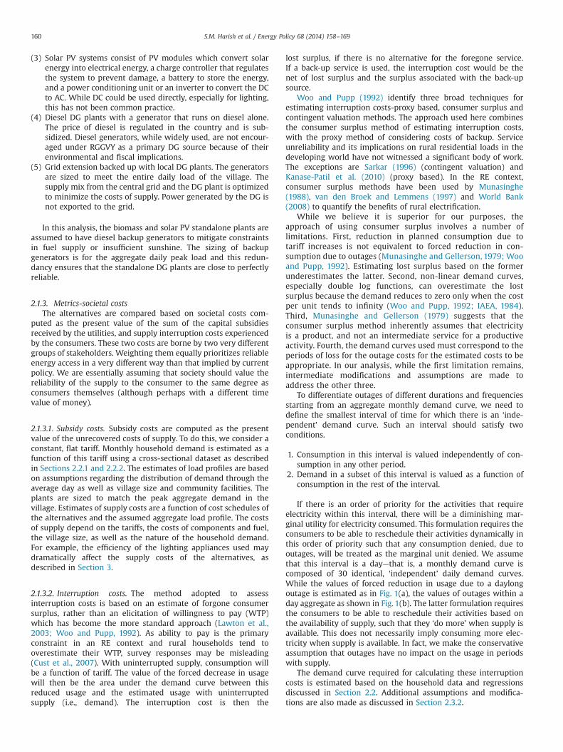
To differentiate outages of different durations and frequenciesstarting from an aggregate monthly demand curve, we need todefine the smallest interval of time for which there is an ‘inde-pendent’ demand curve. Such an interval should satisfy twoconditions.

1. Consumption in this interval is valued independently of con-sumption in any other period.

2. Demand in a subset of this interval is valued as a function ofconsumption in the rest of the interval.

If there is an order of priority for the activities that requireelectricity within this interval, there will be a diminishing mar-ginal utility for electricity consumed. This formulation requires theconsumers to be able to reschedule their activities dynamically inthis order of priority such that any consumption denied, due tooutages, will be treated as the marginal unit denied. We assumethat this interval is a day—that is, a monthly demand curve iscomposed of 30 identical, ‘independent’ daily demand curves.While the values of forced reduction in usage due to a daylongoutage is estimated as in Fig. 1(a), the values of outages within aday aggregate as shown in Fig. 1(b). The latter formulation requiresthe consumers to be able to reschedule their activities based onthe availability of supply, such that they ‘do more’ when supply isavailable. This does not necessarily imply consuming more elec-tricity when supply is available. In fact, we make the conservativeassumption that outages have no impact on the usage in periodswith supply.

The demand curve required for calculating these interruptioncosts is estimated based on the household data and regressionsdiscussed in Section 2.2. Additional assumptions and modifica-tions are also made as discussed in Section 2.3.2.

S.M. Harish et al. / Energy Policy 68 (2014) 158–169160

2.2. Estimating electricity demand

The principal objective of this part of the analysis is to estimatehousehold demand as a function of tariff. The analysis is based onhousehold data collected by the National Sample Survey Organiza-tion (NSSO) in their 2009–2010 surveys. These sampling surveysare conducted every five years. They collect data on consumptionexpenditure from over 100,000 households, including about59,000 rural households) from all the districts in the country.The analysis uses district level mean values for the relevantvariables, resulting in 593 data points for the regression.

2.2.1. Summary of data usedThe household surveys were done by NSSO over the course of a

year, and the electricity consumption data were based on a 30 dayrecall period. Each respondent was surveyed only once, butsampling was done in each district throughout the year. To checkwhether there are discernible seasonal patterns that are missedwhile using district means, the dates of surveys were used tocategorize the observations into different seasons. The averageconsumptions across the four seasons (as per the Indian Meteor-ological Department) are reported in Fig. 2. Average monthlyhousehold consumption in most of the states is less than60 kW h/month. While, the national averages are almost constantacross the seasons, some spikes in consumption during wintersoccur in a few states in the north and north-east. Cross statevariations in consumption of power are neglected in the rest of theanalysis for simplification.

Tariff structures are regulated by bodies at the state level, andcross state variations in tariffs facilitate the cross-sectional analysishere. The national mean is Rs. 2.4/kW h, and the average tariffsrange from Rs. 0.7/kW h in Pondicherry to Rs. 3.8/kW h in

Rajasthan. These average tariffs have been estimated usingreported monthly expenditure on, and consumption of, electricity.As state level tariffs have a multi-part structure, the averagetariffs may depend on the consumption. However, the standarddeviations were less than 5% of estimated mean tariffs in moststates, and within 10% for all. As the estimated tariffs fall within anarrow range, it seems reasonable to treat the tariffs as indepen-dent of consumption, and ignore simultaneity issues.

2.2.2. RegressionsA simple population model should suffice in estimating price

elasticity as long as there are no omitted variables that arecorrelated with the tariffs. For example, while average monthlyper capita total expenditure (MPCE) is positively correlated withaverage monthly electricity consumption, it has close to zerocorrelation (0.01) with the average tariffs. Hence, MPCE need notbe included in our regression models. On the other hand, thefraction of rural households owning televisions (PropTV) is bothpositively correlated with consumption and moderately negativelycorrelated with tariffs, and hence, has to be included.

To estimate demand based on usage data, we need to controlfor unreliability in the supply. For demand estimation, we usestate-specific estimates of deficits as a fraction of demand at peakloading (PeakDeficit), as estimated by the Central ElectricityAuthority (CEA) for the months of May 2009–April 2010 (theperiod of the surveys). On average, only 87% of the peak demandwas met. In the state of Bihar, only 66% of the demand was met,while supply in states like Gujarat and Himachal Pradesh met peakdemand. As the rural residential peaks coincide with the aggregatepeaks, and as utilities “load shed” more from rural areas duringthese times, PeakDeficit is a reasonable proxy for the supply avail-ability.

Fig. 1. Illustration of the assumed valuations of day long outages (left) or for a few hours during the day (right).

Fig. 2. Mean reported household consumption over the four seasons for different states.

S.M. Harish et al. / Energy Policy 68 (2014) 158–169 161

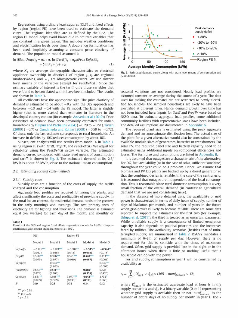
Regressions using ordinary least squares (OLS) and fixed effectsby region (region FE) have been used to estimate the demandcurve. The ‘regions’ identified are as defined by the CEA. Theregion FE model helps avoid biases due to omitted variables thatare constant in a given region. This includes weather conditionsand electrification levels over time. A double log formulation hasbeen used, implicitly assuming a constant price elasticity ofdemand. The population model assumed is

ln ðElec: UsageÞij ¼ α0þαt ln ðTarif f ÞijþαpdðPeak Def icitÞijþ∑αiXijþrjþA ij ð1Þ

where Xij are average demographic characteristics or electricalappliance ownership in district i of region j. rj are regionalunobservables, and A ij are idiosyncratic errors. We use districtlevel means of the variables (except for PeakDeficit). Since theprimary variable of interest is the tariff, only those variables thatwere found to be correlated with it have been included. The resultsare shown in Table 1.

All coefficients have the appropriate sign. The price elasticity ofdemand is estimated to be about �0.2 with the OLS approach andbetween �0.3 and �0.4 with the FE model. The latter is slightlyhigher (that is, more elastic) than estimates in literature in thedeveloped country context (for example, Azevedo et al. (2010)). Priceelasticities of demand have been previously estimated for Indianhouseholds by Fillipini and Pachauri (2004) (�0.29 to �0.51), Tiwari(2000) (�0.7) or Gundimeda and Kohlin (2008) (�0.59 to �0.72).Of these, only the last estimate corresponds to rural households. Anincrease in deficits by 10% reduces consumption by about 10%.

Subsequent analysis will use results from model 4 in Table 1using region FE (with Tariff, PropTV, and PeakDeficit). We adjust forreliability using the PeakDeficit proxy variable. The estimateddemand curve, juxtaposed with state level means of consumptionand tariff, is shown in Fig. 3. The estimated demand at Rs. 2.5/kW h is about 58 kW h, close to the national mean consumption.

2.3. Estimating societal costs-methods

2.3.1. Subsidy costsSubsidy costs are a function of the costs of supply, the tariffs

charged and the consumption.Aggregate load profiles are required for sizing the plants, and

affect significantly the costs and profitability of providing supply. Inthe rural Indian context, the residential demand tends to be greatestin the early mornings and evenings. The two primary uses ofelectricity are for lighting and televisions. The demand is assumedequal (on average) for each day of the month, and monthly or

seasonal variations are not considered. Hourly load profiles areassumed constant on average during the course of a year. The dataused for making the estimates are not restricted to newly electri-fied households; the sampled households are likely to have beenelectrified at different times. Hence, demand growth over time hasnot been included here. Inputs for Tariff and PropTV were based onNSSO data. To estimate aggregate load profiles, some additionalcommunity facilities with representative loads have been included.The detailed assumptions are documented in Appendix A.

The required plant size is estimated using the peak aggregatedemand and an approximate distribution loss. The actual size ofthe plant for a given alternative would also be constrained by theavailable module sizes of generators, batteries or transformers. Forsolar PV, the required panel size and battery capacity need to beestimated using additional inputs on component efficiencies andlosses. The formulae and assumptions are listed in Appendix B.

It is assumed that outages are a characteristic of the alternative.For DG, fuel availability (or in the case of solar, sufficient sunshine)throughout the year could be a problem. Hence, we assume thatbiomass and PV DG plants are backed up by a diesel generator sothat the combined design is reliable. In the case of the central grid,it is assumed that outages are independent of the local consump-tion. This is reasonable since rural domestic consumption is a verysmall fraction of the overall demand (in contrast to agriculturaldemand that we are not considering here).

In the absence of more detailed data, the availability of gridpower is characterized in terms of daily hours of supply, number ofdays of blackouts per month, and number of years in the futurewhen grid-power is likely to become reliable. There are some datareported to support the estimates for the first two (for example,Udupa et al. (2011)), the third is treated as an uncertain parameter.While unreliable supply is a consequence of limited generationcapacity, it also depends on political priorities and the incentivesfaced by utilities. The availability scenarios (besides that of unin-terrupted supply) are summarized in Table 2. RGGVY mandates aminimum of 6–8 h of supply per day. However, there is norequirement for this to coincide with the times of maximumdemand. Often, grid supply is provided late in the night or in theafternoon hours, when there is little or nothing useful that ahousehold can do with the power.

For grid supply, consumption in year t will be constrained byavailability as

ct ¼ ∑24

h ¼ 1ð Dk

agg;h � skh;tÞ � ð365� numkblackout;t � 12Þ ð2Þ

where Dkagg; h is the estimated aggregate load at hour h in the

supply scenario k and skh;t is a binary variable (0 or 1) representingwhether grid supply is available then or not. numk

blackout;t is thenumber of entire days of no supply per month in year t. The k

Table 1Results of the OLS and region fixed effects regression models for ln(Elec. Usage)—coefficients with robust standard errors (n¼592).

OLS Region FE

Model 1 Model 2 Model 3 Model 4 Model 5

ln(tariff) �0.181nnn �0.199nnn �0.384nn �0.343nn �0.324nn

(0.037) (0.035) (0.118) (0.098) (0.078)PropTV 0.558nnn 0.396nnn 0.521nnn 0.540nnn 0.413nnn

(0.075) (0.077) (0.089) (0.087) (0.061)ln(mpce) 0.354nnn 0.342nn

(0.053) (0.095)PeakDeficit 0.663nnn 0.511nnn 0.869n 0.826

(0.178) (0.163) (0.358) (0.420)Constant 3.861nn 1.508nnn 3.977nnn 4.043nnn 1.734n

(0.069) (0.359) (0.133) (0.113) 0.666)R2 0.19 0.28 0.31 0.34 0.42

nnn po0.01.nn po0.05.n po0.1.

Fig. 3. Estimated demand curve, along with state level means of consumption andpeak deficit.

S.M. Harish et al. / Energy Policy 68 (2014) 158–169162

scenarios include the uninterrupted, 18-h and 6-h scenarios asdescribed in Table 2. With DG, consumption will be identical touninterrupted grid availability scenario. Appliance ownership isassumed to be unaffected by the intermittency in supply.

The cost estimation methodology follows from prior literature.A detailed description of the cost inputs and assumptions for eachalternative is provided in Appendix C. The subsidy costs areestimated over a 10 year period, using a real discount rate of10%. As the lifetimes of some of the components are higher, theircapital costs are annualized.

The levelized cost of energy (LCOE) is estimated as,

LCOE¼ ∑10

t ¼ 1

xcap�annþxO&Mþxfuel tðor; xgridpower;tÞð1þrÞt ∑

10

t ¼ 1

ctð1þrÞt

�ð3Þ

xcap-ann are the annualized capital costs of the infrastructure fora given alternative, xO&M, the annual operation and maintenancecosts, xfuel,t the costs of the fuel in the plants in year t and xgridpower,t

the costs of supply for the utilities. r is the discount rate used.Although the LCOEs could be computed for the unreliable grid

supply scenarios as well, comparisons are not entirely meaningfulwhen their denominators vary. As a result, the analysis hereconsiders the subsidy costs instead.

Cost of subsidy¼ ðLCOE�Tarif f Þ ∑10

t ¼ 1

ctð1þrÞt ð4Þ

Interestingly, in terms of subsidy costs, providing unreliablegrid supply is cheaper for the utilities than providing uninter-rupted supply from the grid or through DG. As the costs of powerpurchased contribute a significant amount to the LCOE of gridsupply, and because the tariffs tend to be lower than costs ofsupply, subsidy costs favor extending the grid, over DG alterna-tives, despite the former's poor reliability. To make reasonablecomparisons, interruption costs must be considered.

2.3.2. Interruption costsFollowing the earlier discussion, interruption costs are estimated

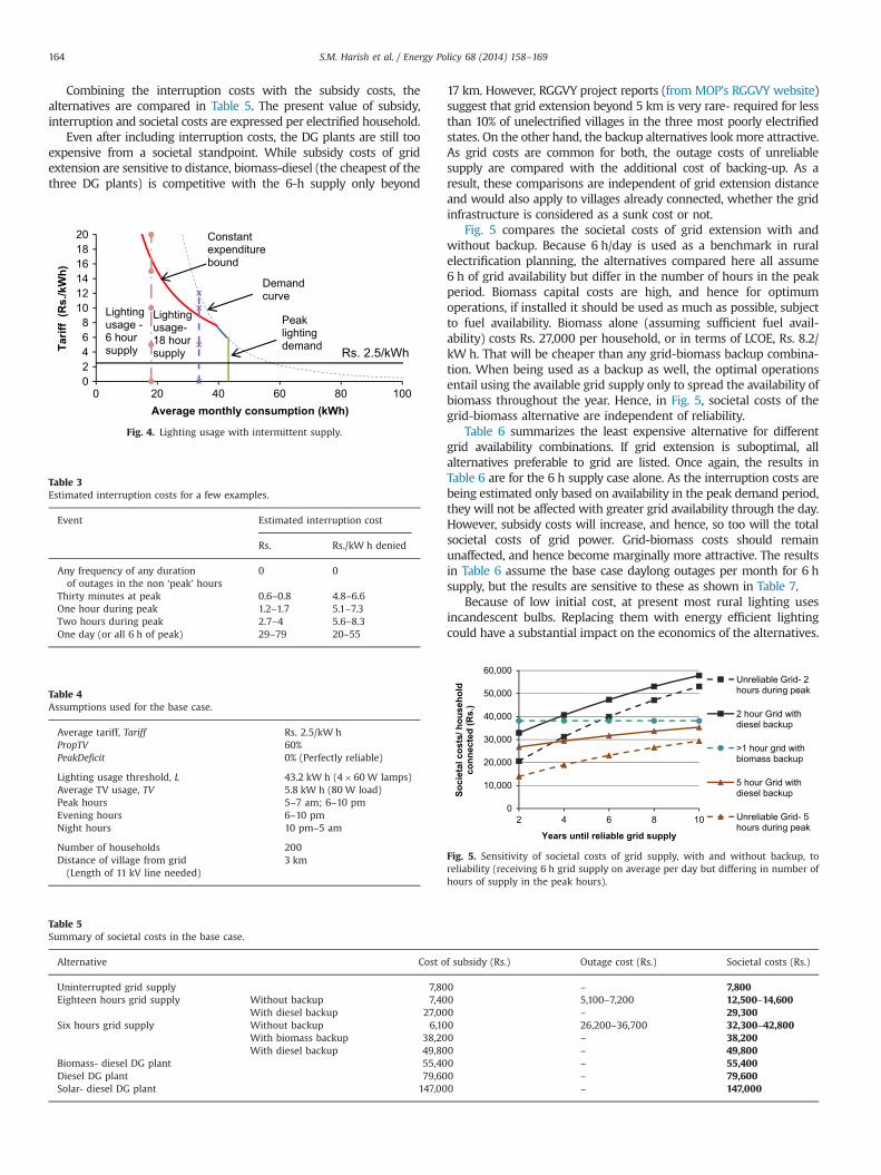
based on loss of consumer surplus using daily demand curves. As asimplification, the interruption costs are estimated based on lightingin the ‘peak’ hours alone. Hence, the consumption in this case couldalternatively be measured using kilolumen-hour, i.e. total light out-put ‘used’ over time. While such an estimate would at best be a lowerbound, lighting is the primary domestic end-use of electricity in ruralIndia. In the absence of reliable electricity, different back-up sourcesof lighting are used which help in understanding the willingness topay and validating the estimates.

While the demand curves from Section 2.2.2 provide thefoundation of the interruption costs estimate, modifications aremade at low consumption where the double-log curve will over-estimate the consumer surplus. Two constant expenditure lines of

Rs. 200/month and Rs. 300/month are used as bounds. Thesecorrespond to estimated expenditures at Rs. 4/kW h andRs. 8/kW h, and are in the ballpark of the amortized costs of solarlanterns and lighting systems that are becoming increasinglypopular as primary and backup lighting. 1

It is assumed that during outages, kerosene lanterns are used. Asthe light output is very low, the value of consumption of kerosenewill be very low but bound the interruption costs from going toinfinity. As a result, the interruption costs will now comprise thevalue lost by consuming kerosene lighting and not electricity, and netcosts of the backup lighting energy source (that is, expenditure onkerosene less the saved expenditure on unconsumed electricity).

Based on demand as a function F of tariff, annual interruptioncost is estimated as,

xint erruption ¼ð30�numk

blackout;tÞ30

Z eT

e'TF �1ðlÞdl

þðnumk

blackout;tÞ30

Z eT

ekeroseneF �1ðlÞdlþxkerosene�ðeT �e'T Þpe

!

�12 ð5Þ

where eT, e'T and ekerosene are the consumption of lighting energy (inklm-h, say) with uninterrupted supply at tariff pe, with unreliablesupply, and forced usage of kerosene due to outages, respectively

xkerosene ¼ ð6numkblackout;tþð30�numk

blackout;tÞð6�∑hApeakskh;tÞÞ

�pkerosene � ηkerosene � lanterns ð6Þ

pkerosene is the price of kerosene. Up to 4 l/month, subsidizedkerosene at Rs. 15/l is available, and beyond that kerosene must bepurchased in the market at Rs. 25/l.

ηkerosene is the fuel efficiency of kerosene lanterns. A mass-manufactured “hurricane” lantern consumes 0.03 l/h (Mills, 2003).

The variable lanterns is the number of kerosene lamps. It isassumed that two lamps are used during outages. With highernumbers, kerosene consumption becomes impracticably high, espe-cially in the 6 h supply scenario

By design, the interruption cost will be zero in the case ofuninterrupted grid and decentralized plants. For unreliable gridsupply, these costs will be positive. The estimated consumption inthe base-case with the different unreliable scenarios is shown inFig. 4. Table 3 summarizes estimated costs for a few blackoutevents. Because of our assumptions, the interruption cost per unittime (or per unit consumption denied) increases with the cumu-lative duration of the outages within a single day.

3. Results and discussion

Table 4 summarizes the inputs for the ‘base case’. Based onthese inputs, the peak aggregate demand is 63 kW, and the totaldaily consumption is about 420 kW h.

Table 2Reliability scenarios considered.

‘Poor’ quality ‘Intermediate’quality

Daily hours of supply Six hours in all: 3 in thepeak period- 1 in theevening, 2 morning; 3 hin the rest

Eighteen hours in all:Single phase: 6 PM–6AM; Three phase:6 AM–12 noon

Average day-longoutages/month

5 2

Years required for gridto become reliable

10 (2–10) 5 (2–10)

1 We assume that the cost of the solar lighting system is Rs. 12,000- purchasedthrough a loan with a term of 5 years, at 12% interest rate, and 20% down-payment.Such a lighting system typically has 3–4 CFL lights. A system lifetime of 10 years isassumed, with a battery lifetime of 6–8 years (replacement costs of Rs. 4000). Asolar lantern costs Rs.1600 and is assumed to be purchased with a one-time cashtransaction. The lifetime of such a product is assumed 3–5 years, and the battery isreplaced every year at a cost of Rs. 150. Based on these cost assumptions anddiscount rates at 30–60%, the amortized monthly costs of purchasing a solarlighting system is Rs. 275–370, and two solar lanterns is Rs. 130–265. Purchase of asolar product would imply high upfront costs, and the consumer will likely use asignificantly higher discount rate than the social planner's 10%. Ekholm et al. (2010)use discount rates of 62–74% for rural households and 53–70% for urban. Reddy andReddy (1994) estimate an internal rate of return of 28% for a switch from kerosenelamps to electricity- which could be a lower bound on the discount rate.

S.M. Harish et al. / Energy Policy 68 (2014) 158–169 163

Combining the interruption costs with the subsidy costs, thealternatives are compared in Table 5. The present value of subsidy,interruption and societal costs are expressed per electrified household.

Even after including interruption costs, the DG plants are still tooexpensive from a societal standpoint. While subsidy costs of gridextension are sensitive to distance, biomass-diesel (the cheapest of thethree DG plants) is competitive with the 6-h supply only beyond

17 km. However, RGGVY project reports (from MOP's RGGVY website)suggest that grid extension beyond 5 km is very rare- required for lessthan 10% of unelectrified villages in the three most poorly electrifiedstates. On the other hand, the backup alternatives lookmore attractive.As grid costs are common for both, the outage costs of unreliablesupply are compared with the additional cost of backing-up. As aresult, these comparisons are independent of grid extension distanceand would also apply to villages already connected, whether the gridinfrastructure is considered as a sunk cost or not.

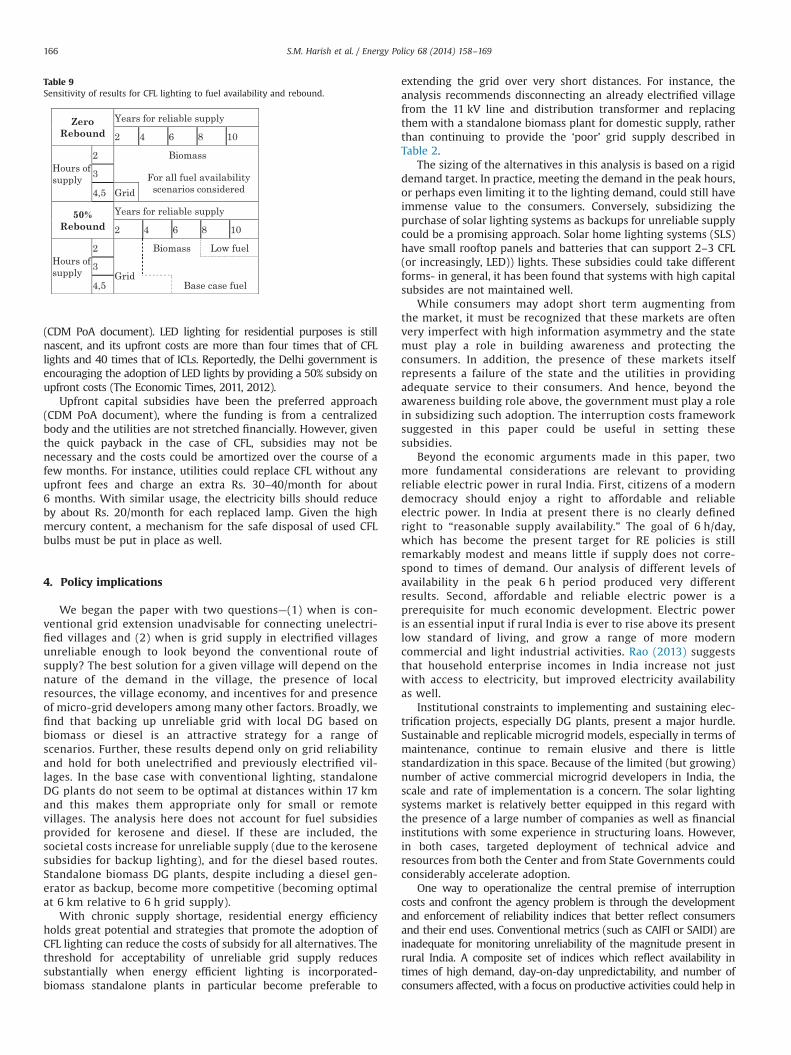
Fig. 5 compares the societal costs of grid extension with andwithout backup. Because 6 h/day is used as a benchmark in ruralelectrification planning, the alternatives compared here all assume6 h of grid availability but differ in the number of hours in the peakperiod. Biomass capital costs are high, and hence for optimumoperations, if installed it should be used as much as possible, subjectto fuel availability. Biomass alone (assuming sufficient fuel avail-ability) costs Rs. 27,000 per household, or in terms of LCOE, Rs. 8.2/kW h. That will be cheaper than any grid-biomass backup combina-tion. When being used as a backup as well, the optimal operationsentail using the available grid supply only to spread the availability ofbiomass throughout the year. Hence, in Fig. 5, societal costs of thegrid-biomass alternative are independent of reliability.

Table 6 summarizes the least expensive alternative for differentgrid availability combinations. If grid extension is suboptimal, allalternatives preferable to grid are listed. Once again, the results inTable 6 are for the 6 h supply case alone. As the interruption costs arebeing estimated only based on availability in the peak demand period,they will not be affected with greater grid availability through the day.However, subsidy costs will increase, and hence, so too will the totalsocietal costs of grid power. Grid-biomass costs should remainunaffected, and hence become marginally more attractive. The resultsin Table 6 assume the base case daylong outages per month for 6 hsupply, but the results are sensitive to these as shown in Table 7.

Because of low initial cost, at present most rural lighting usesincandescent bulbs. Replacing them with energy efficient lightingcould have a substantial impact on the economics of the alternatives.

Table 3Estimated interruption costs for a few examples.

Event Estimated interruption cost

Rs. Rs./kW h denied

Any frequency of any durationof outages in the non ‘peak’ hours

0 0

Thirty minutes at peak 0.6–0.8 4.8–6.6One hour during peak 1.2–1.7 5.1–7.3Two hours during peak 2.7–4 5.6–8.3One day (or all 6 h of peak) 29–79 20–55

Fig. 4. Lighting usage with intermittent supply.

Table 4Assumptions used for the base case.

Average tariff, Tariff Rs. 2.5/kW hPropTV 60%PeakDeficit 0% (Perfectly reliable)

Lighting usage threshold, L 43.2 kW h (4�60 W lamps)Average TV usage, TV 5.8 kW h (80 W load)Peak hours 5–7 am; 6–10 pmEvening hours 6–10 pmNight hours 10 pm–5 am

Number of households 200Distance of village from grid(Length of 11 kV line needed)

3 km

Table 5Summary of societal costs in the base case.

Alternative Cost of subsidy (Rs.) Outage cost (Rs.) Societal costs (Rs.)

Uninterrupted grid supply 7,800 – 7,800Eighteen hours grid supply Without backup 7,400 5,100–7,200 12,500–14,600

With diesel backup 27,000 – 29,300Six hours grid supply Without backup 6,100 26,200–36,700 32,300–42,800

With biomass backup 38,200 – 38,200With diesel backup 49,800 – 49,800

Biomass- diesel DG plant 55,400 – 55,400Diesel DG plant 79,600 – 79,600Solar- diesel DG plant 147,000 – 147,000

Fig. 5. Sensitivity of societal costs of grid supply, with and without backup, toreliability (receiving 6 h grid supply on average per day but differing in number ofhours of supply in the peak hours).

S.M. Harish et al. / Energy Policy 68 (2014) 158–169164

Hence, we study how a switch to compact fluorescent lamps (CFL)affects the costs through a reduction in demand. While incandescentlamps are assumed to have a luminosity of 12 lm/W, CFL areassumed to provide 50 lm/W (based on Azevedo et al. (2010)).Rebound in consumption is parameterized. With zero rebound, theestimated monthly household demand in the base case reduces from58 kW h to 25 kW h. Similarly, the aggregate peak demand reducesfrom 63 kW to 25 kW.

The inclusion of energy efficient lighting, leads to lowerestimated peak demands and higher load factors. Because of thelower consumption, the subsidy costs for all the alternativesdecrease, but the interruption costs are unaffected. The alternativemost significantly affected by the change is standalone biomass.While the improvement in plant load factor improves the effi-ciency of power production, the reduction in demand leads to areduction in the requirement for backup; in some cases, thebackup generator is no longer required, reducing capital costs.The biomass alternative becomes much more competitive as aresult, as shown in Table 8.

The two most sensitive parameters for these results will be theamount of rebound and the biomass fuel availability. Note that inthis case, rebound in consumption should not be viewed as a bad

thing because it implies that low income energy-limited ruralconsumers are able to increase consumption and experiencegreater utility. Biomass becomes less preferable as fuel availabilitydecreases and as rebound increases. Table 9 captures this two-waysensitivity. With 50% rebound and low fuel availability, biomass iscompetitive with grid extension of 1 km or more only when gridsupply is available for 2 h at peak and will become reliable onlyafter 10 years.

An obvious barrier to large-scale adoption of energy efficient lightsis the higher upfront cost relative to ICL. Over their lifetimes, CFLs aresignificantly less expensive. In fact, the payback period is 6–7 months(with a 15W CFL costing Rs. 150–200 compared to Rs. 15 for a 60WICL), assuming a daily usage of 6 h. To encourage the replacement ofincandescent bulbs with CFL, the government initiated a policy, BachatLamp Yojana (“Efficient Lighting Program”), under which householdscould purchase CFLs at the price of incandescent bulbs. The differencewas to be financed using Clean Development Mechanism (CDM) fund.While the program eventually ran into trouble when the market forCertified Emission Ratings crashed, some of the states have reportedlyachieved some success (Forbes India, 2012; Hindu Business Line,2011). Previous attempts by some of the utilities could not besustained due to the limited financial resources available to them

Table 6Alternative with least societal cost for different reliability scenarios (grid availability for 6 h/day on most days, but differing availability during peak demand).

Years for reliable grid supply

o4 6 8 10

Hours of grid availability in peak demand period (6 h) 2 Grid Biomass backup (Grid) Biomass backup (Grid) Biomass backup (Grid)3 Grid Grid Grid Biomass backup (Grid)

Z4 Grid Grid Grid Grid

Table 7Sensitivity to number of daylong outages per month- alternative with least societal cost for different reliability scenarios (grid availability for 6 h/day on most days; differingavailability during peak demand; supply becoming reliable after 6 years).

Number of daylong outages/month

Upper bound of interruption costs Lower bound of interruption costs

0–2 5 10 0–5 10

Hours of supply in peak demand period 2 Grid Biomass backup Biomass or Diesel backup Grid Biomass backup3 Grid Grid Biomass or Diesel backup Grid Grid

Z4 Grid Grid Diesel backup Grid Grid

Table 8Alternative with least societal cost for different reliability scenarios with CFL lighting (grid availability for 6 h/day on most days, but differing availability during peakdemand). Biomass DG plant is not competitive with the grid at reasonable distances (*) or is optimal beyond 1 km (1), 3 km (3) and 5 km (5) or at any distance (0).

Years for reliable grid supply

2 4 6 8 10

Upper bound of interruption costsHours of grid availabilityin peak demand period (6 h)

2 Diesel backup1 Diesel backup0 Biomass or Diesel backup0 Biomass or Diesel backup0 Biomass or Diesel backup0

3 Grid5 Diesel backup0 Diesel backup0 Diesel backup0 Biomass or Diesel backup0

4 Gridn Diesel backup0 Diesel backup0 Diesel backup0 Biomass or Diesel backup0

5 Gridn Diesel backup3 Diesel backup0 Diesel backup0 Diesel backup0

Lower bound of interruption costs2 Gridn Grid0 Biomass or Diesel backup0 Biomass or Diesel backup0 Biomass or Diesel backup0

3 Gridn Grid3 Grid0 Diesel backup0 Biomass or Diesel backup0

4 Gridn Grid5 Grid3 Grid1 Diesel backup0

5 Gridn Gridn Gridnn Grid5 Grid3

S.M. Harish et al. / Energy Policy 68 (2014) 158–169 165

(CDM PoA document). LED lighting for residential purposes is stillnascent, and its upfront costs are more than four times that of CFLlights and 40 times that of ICLs. Reportedly, the Delhi government isencouraging the adoption of LED lights by providing a 50% subsidy onupfront costs (The Economic Times, 2011, 2012).

Upfront capital subsidies have been the preferred approach(CDM PoA document), where the funding is from a centralizedbody and the utilities are not stretched financially. However, giventhe quick payback in the case of CFL, subsidies may not benecessary and the costs could be amortized over the course of afew months. For instance, utilities could replace CFL without anyupfront fees and charge an extra Rs. 30–40/month for about6 months. With similar usage, the electricity bills should reduceby about Rs. 20/month for each replaced lamp. Given the highmercury content, a mechanism for the safe disposal of used CFLbulbs must be put in place as well.

4. Policy implications

We began the paper with two questions—(1) when is con-ventional grid extension unadvisable for connecting unelectri-fied villages and (2) when is grid supply in electrified villagesunreliable enough to look beyond the conventional route ofsupply? The best solution for a given village will depend on thenature of the demand in the village, the presence of localresources, the village economy, and incentives for and presenceof micro-grid developers among many other factors. Broadly, wefind that backing up unreliable grid with local DG based onbiomass or diesel is an attractive strategy for a range ofscenarios. Further, these results depend only on grid reliabilityand hold for both unelectrified and previously electrified vil-lages. In the base case with conventional lighting, standaloneDG plants do not seem to be optimal at distances within 17 kmand this makes them appropriate only for small or remotevillages. The analysis here does not account for fuel subsidiesprovided for kerosene and diesel. If these are included, thesocietal costs increase for unreliable supply (due to the kerosenesubsidies for backup lighting), and for the diesel based routes.Standalone biomass DG plants, despite including a diesel gen-erator as backup, become more competitive (becoming optimalat 6 km relative to 6 h grid supply).

With chronic supply shortage, residential energy efficiencyholds great potential and strategies that promote the adoption ofCFL lighting can reduce the costs of subsidy for all alternatives. Thethreshold for acceptability of unreliable grid supply reducessubstantially when energy efficient lighting is incorporated-biomass standalone plants in particular become preferable to

extending the grid over very short distances. For instance, theanalysis recommends disconnecting an already electrified villagefrom the 11 kV line and distribution transformer and replacingthem with a standalone biomass plant for domestic supply, ratherthan continuing to provide the ‘poor’ grid supply described inTable 2.

The sizing of the alternatives in this analysis is based on a rigiddemand target. In practice, meeting the demand in the peak hours,or perhaps even limiting it to the lighting demand, could still haveimmense value to the consumers. Conversely, subsidizing thepurchase of solar lighting systems as backups for unreliable supplycould be a promising approach. Solar home lighting systems (SLS)have small rooftop panels and batteries that can support 2–3 CFL(or increasingly, LED)) lights. These subsidies could take differentforms- in general, it has been found that systems with high capitalsubsides are not maintained well.

While consumers may adopt short term augmenting fromthe market, it must be recognized that these markets are oftenvery imperfect with high information asymmetry and the statemust play a role in building awareness and protecting theconsumers. In addition, the presence of these markets itselfrepresents a failure of the state and the utilities in providingadequate service to their consumers. And hence, beyond theawareness building role above, the government must play a rolein subsidizing such adoption. The interruption costs frameworksuggested in this paper could be useful in setting thesesubsidies.

Beyond the economic arguments made in this paper, twomore fundamental considerations are relevant to providingreliable electric power in rural India. First, citizens of a moderndemocracy should enjoy a right to affordable and reliableelectric power. In India at present there is no clearly definedright to “reasonable supply availability.” The goal of 6 h/day,which has become the present target for RE policies is stillremarkably modest and means little if supply does not corre-spond to times of demand. Our analysis of different levels ofavailability in the peak 6 h period produced very differentresults. Second, affordable and reliable electric power is aprerequisite for much economic development. Electric poweris an essential input if rural India is ever to rise above its presentlow standard of living, and grow a range of more moderncommercial and light industrial activities. Rao (2013) suggeststhat household enterprise incomes in India increase not justwith access to electricity, but improved electricity availabilityas well.

Institutional constraints to implementing and sustaining elec-trification projects, especially DG plants, present a major hurdle.Sustainable and replicable microgrid models, especially in terms ofmaintenance, continue to remain elusive and there is littlestandardization in this space. Because of the limited (but growing)number of active commercial microgrid developers in India, thescale and rate of implementation is a concern. The solar lightingsystems market is relatively better equipped in this regard withthe presence of a large number of companies as well as financialinstitutions with some experience in structuring loans. However,in both cases, targeted deployment of technical advice andresources from both the Center and from State Governments couldconsiderably accelerate adoption.

One way to operationalize the central premise of interruptioncosts and confront the agency problem is through the developmentand enforcement of reliability indices that better reflect consumersand their end uses. Conventional metrics (such as CAIFI or SAIDI) areinadequate for monitoring unreliability of the magnitude present inrural India. A composite set of indices which reflect availability intimes of high demand, day-on-day unpredictability, and number ofconsumers affected, with a focus on productive activities could help in

Table 9Sensitivity of results for CFL lighting to fuel availability and rebound.

S.M. Harish et al. / Energy Policy 68 (2014) 158–169166

setting up better targets and more comprehensive monitoring. In theevent of the utilities being unable to meet these targets with centralpower procurement alone, appropriate penalties could create incen-tives for the utilities themselves to serve as an intermediary indiffusing and supporting the use of decentralized energy solutions.

A number of models that have been developed elsewherearound the world might be usefully adapted to the rural Indiansetting. One example is a program called Efficiency Vermont,developed by the U.S. state of Vermont (see: www.efficiencyvermont.com). By adding a charge of 5–10 mills2/kW h, the statecollects a fund that is then administered by a competitivelyselected non-profit entity to promote improvements in end-useefficiency and subsidize things such as more efficient lamps. InIndia, such a program might also subsidize solar lighting.Alternatively, State Electricity Boards, or local Indian utilities,might develop strategies to help consumers amortize the cost ofcompact fluorescents or solid-state lights through programssuch as offering slightly lower rates for the first few kW h fora limited time to those consumers who participate in bulbreplacement projects.

5. Conclusions

The principal implication of this study is that programs like theRGGVY have not solved the ‘problem of rural electrification’ becauseacute unreliability of supply continues to occur in much of rural India.While no single solutionwill be applicable everywhere in the country,some combination of better service standards (perhaps through thereliability indices discussed in the last section), energy efficientlighting, a willingness to support decentralized energy alternatives,and identifying scalable institutional models could be the wayforward. Interestingly, abandoning its previous focus on unelectrifiedremote villages alone, MNRE's draft Remote Village Lighting policyproposes to support the use of local DG plants and solar lightingsystems in electrified villages receiving less than 6 h of grid supply perday (Ministry of New and Renewable Energy (MNRE), 2012). This iscertainly a step in the right direction.

In summary, the cost to India, and its rural citizens, of unreli-able electric power is very high. The time has come for some newthinking about how to rectify this problem that, despite ambitiousdevelopment goals, has continued to fester for decades.

Acknowledgments

This work was supported by academic and alumni funds fromCarnegie Mellon University. We thank the editor and the twoanonymous referees for their comments and suggestions.

Appendix A. Domestic end use assumptions

Average daily demand, controlling for reliability (using Peak-Deficit),

Ddaily ¼DmonthlyðTarif f ;PropTV Þ

30ðA1:1Þ

where Dmonthly is the estimated average monthly demandand is a function of Tariff and PropTV. Naturally, the sum ofhourly demands dh will be equal to the daily demand,

(Table A1.1)

∑24

h ¼ 1dh ¼Ddaily ðA1:2Þ

There are two primary applications-lighting and television,with lighting being the more basic demand. After a thresholdlighting demand is met, the TV is assumed to be purchased andused. Once lighting and TV loads are met in the peak demandperiod, electricity usage in the morning and afternoon hours isassumed to increase (Table A3.1 and A3.2).

The average lighting load in the peak hours (which in thisstudy, will be assumed to comprise 6 h/day—early mornings 5–7AM and evenings 6–10 PM) are estimated as below.

lightingh A peak ¼Ddaily

6if ;Ddailyo6L ¼ L otherwise ðA1:3Þ

where L is the maximum hourly electricity consumption onlighting in the six peak demand hours. It is assumed thatincandescent bulbs are used for lighting. Similarly, the averageload in the four evening hours (6–10 PM) due to TV usage isestimated as,

tvh A evening

¼ ðDdaily� lightingh A peakÞ4

ifðDdaily� lightingh A peakÞo4TV

�PropTV¼ TV � PropTV ; otherwise ðA1:4ÞTV is the assumed maximum hourly household TV consump-

tion. Residual hourly demand distributed uniformly through theday (except for nighttime) will then be,

anyh A night' ¼Ddaily�ð6lightingh A peakþ4tvh A eveningÞ

ð17Þ ðA1:5Þ

To be clear,

dh ¼ lightinghþtvhþanyh ðA1:6ÞAverage household load profiles were estimated using the

approach above and assumptions listed in Table 2. The loadassumptions for community level facilities are summarized inTable A1.1.

Appendix B. Plant sizing

Required plant size (for biomass and diesel DG) or transformerrating should be,

C ¼ maxðDaggh Þ

pf � ð1� lossdistÞðA2:1Þ

where Daggh is the aggregate load at hour h, pf is the power factor,

and lossdist is the distribution loss in the local network.In the case of solar, sizing is slightly different because of the

need for battery storage. Assuming all supply is through storedenergy, the required plant and battery capacities are sized asfollows (following Chaurey and Kandpal (2010)).

Table A1.1Community load assumptions.

Load (W) Time of operation

Streetlights (per light) 100 6 PM–7AMSchool 600 10 AM–4 PMDrinking water pump 2238 (or 5 HP) 2 AM–4 AM

2 1 mill is one-tenth of a cent.

S.M. Harish et al. / Energy Policy 68 (2014) 158–169 167

where ηinverter, ηbattery, and ηCC are the efficiencies of the inverter,battery, and charge controller ftemp, fdust and fmismatch are the lossesassociated with ambient temperature, dust, and mismatch among cells.

EHFS is the expected hours of full sunshine—the level of solarradiation is translated in terms of hours of full sunshine thatprovides 1 kW/m2.

Csolar�battery ¼∑24

h ¼ 1Daggh

pf � ð1� lossdistÞ � ηinverter � ηbattery �MDoD � V

ðA2:3Þ

where MDoD is the maximum depth of discharge and V is theterminal voltage

Appendix C. Capital and operations costs

Cost of grid supply is estimated as power purchase costsinflated by the reciprocal of (1—transmission and distributionlosses).

The fuel costs for the biomass plant will be,

xBiomass DGfuel; t ¼∑24

h ¼ 1½ηbiomassðdh;t ;CbiomassÞ � pbiomass � dh;t � daysbiomassoperating

þηdieselðdh;t ;CdieselÞ � pdiesel � dh;t � ð365�daysbiomassoperatingÞ�

ðA3:1Þ

Table A3.1Cost inputs and assumptions for the different alternatives.

Equipment Capital cost(in Rs.)

Annual O&M costs(fraction of capitalcosts)

Lifetime(years)

References

LT line (per km) 190,000 0.03 20 Bangalore Electricity Supply Company(2010-Schedule of costs)

Grid extension 11 kV line (per km) 210,000 0.03 20Transformers (in kVA)25 87,000 0.03 2063 117,000100 153,000

Biomass Gasification Gasifier (per kW) 25,000 0.05 10 Nouni et al. (2007)Engine (per kW) 30,000 0.05 20 Banerjee (2006)Civil works 72,000þ9000n

(Capacity)0.02 20 (Ministry of New and Renewable Energy (MNRE)

(2008)-VESP guidelines)

Solar PV PV panel (per kW) 80,000 0.02 20 Aanesen et al. (2012) Nouni et al. (2006)Chaurey and Kandpal (2010)Ministry of New and Renewable Energy (MNRE), 2010

Battery (per 12 V–200 Ah battery) 22,000 0.02 10Power conditioning unit (per kW) 40,000 0.02 20

Diesel Generator (per kW) 20,000 0.1 20 Nouni et al. (2007)

Table A3.2Summary of inputs for costs, efficiencies and other operational variables.

Length of the LT line 2 km AssumptionLocal distribution loss 5% AssumptionPower Factor 0.95 Assumption

Grid extension Cost of power purchased (Rs./kW h) 2.5 (2-3) ParameterTechnical and commercial losses 20% (15–30%) Parameter

Biomass gasification Cost of biomass fuel (Rs./kg) 1.5 (1–3) ParameterNumber of working days 300 (200–360) ParameterLoad factor Fuel efficiency (kg/kW h) Nouni et al. (2007)0 050% 1.6875% 1.54100% 1.40

Solar PV Energy loss due to ambient temperature 0.1 Chaurey and Kandpal (2010)Energy loss due to dust 0.03Energy loss due to mismatch among solar cells 0.02Inverter efficiency 0.98Battery efficiency 0.8Charge controller efficiency 0.9Effective hours of full sunshine (per day) 5.5 (4.5–6) ParameterNumber of working days 300 (250–320) ParameterTerminal Voltage 120 V Chaurey and Kandpal (2010)Maximum Depth of Discharge 0.7 Input

Diesel Diesel fuel cost (Rs./l) 40 Ministry of Petroleum andNatural Gas (2013)

Fuel efficiency (l/kW h) 0.3 Nouni et al. (2007)

Csolar ¼∑24

h ¼ 1Daggh

pf � ð1� lossdistÞ � ηinverter � ηbattery � ηcc � ð1� f tempÞ � ð1� f dustÞ � ð1� f mismatchÞ � EHFSðA2:2Þ

S.M. Harish et al. / Energy Policy 68 (2014) 158–169168

where ηbiomass and ηdiesel are the fuel efficiencies of the biomass anddiesel generators and are functions of load factors (dh,t/Cbiomass ordh,t/Cdiesel), Cbiomass and Cdiesel are the installed capacity of thegenerators, pbiomass and pdiesel are the fuel prices of biomass anddiesel, and daysbiomass

operating are the number of operating days of thebiomass generator.

The cost of the backup diesel fuel will be,

xSolarf uel; t ¼∑24h ¼ 1ηdieselðdh;t ;CdieselÞ � pdiesel � dh;t

�ð365�dayssolaroperatingÞ ðA3:2Þ

Table A3.1 and A3.2 list all the cost inputs and assumptions foreach of the alternatives.

References

Aanesen, A., Heck, S., Pinner, D., 2012. Solar Power: Darkest before Dawn.M.c.Kinsey on Sustainability and Resource Productivity. McKinsey andCompany.

Azevedo, I.M.L., Morgan, M.G., Lave, L., 2010. Residential and regional electricityconsumption in the US and EU: how much will higher prices reduce CO2

emissions? Electr. J. 24 (1).Banerjee, R., 2006. Comparison of options for distributed generation in India.

Energy Policy 34, 101–111.Bangalore Electricity Supply Company (BESCOM), Cost data sheet 2010-11.Census of India, 2011. Source of Lighting: 2001–2011. Available online on ⟨http://

www.censusindia.gov.in/2011census/hlo/Data_sheet/Source%20of%20Lighting.pdf⟩ (last accessed on August 20, 2012).

Chaurey, A., Kandpal, T.C., 2010. A techno-economic comparison of rural electrifica-tion based on solar home systems and PV microgrids. Energy Policy 38,3118–3129.

Cust, J., Singh, A., Neuhoff, K., 2007. Rural Electrification in India: Economic andInstitutional Aspects of Renewables EPRG 0730 and CWPE. 0763.

Ekholm, T., Krey, V., Pachauri, S., Riahi, K., 2010. Determinants of household energyconsumption in India. Energy Policy 38, 5696–5707.

Fillipini, M., Pachauri, S., 2004. Elasticities of electricity demand in urban Indianhouseholds. Energy Policy 32, 429–436.

Gundimeda, H., Kohlin, G., 2008. Fuel demand elasticities for energy and environ-mental policies: Indian sample survey evidence. Energy Econ. 30, 517–546.

IAEA, 1984. Expansion Planning for Electrical Generating Systems—A Guidebook.Technical Reports Series No. 241.

Kanase-Patil, A.B., Saini, R.P., Sharma, M.P., 2010. Integrated renewable energysystems for off grid rural electrification of remote area. Renewable Energy 35,1342–1349.

Lawton, L., Sullivan, M., van Liere, K., Katz, A., Eto, J., 2003. A Framework and Reviewof Customer Outage Costs: Integration and Analysis of Electric Utility OutageCost Surveys. Ernest Orlando Lawrence Berkeley National Laboratory, Environ-mental Energy Technology Division, LBNL-54365.

Mills, E., 2003. Technical and Economic Performance Analysis of Kerosene Lampsand Alternative Approaches to Illumination in Developing Countries. LawrenceBerkeley National Laboratory.

Ministry of New and Renewable Energy (MNRE), 2008. Implementation of VillageEnergy Security Test Projects during 2008–2009 and 2009–2010, Sanction reg.No. 51/2/2007-08/VESP. Government of India.

Ministry of New and Renewable Energy (MNRE), 2010. Guidelines for Off-Grid andDecentralized Solar Application, ⟨http://mnre.gov.in/file-manager/UserFiles/jnnsm_g170610.pdf⟩ (accessed on April 30, 2012). Government of India.

Ministry of New and Renewable Energy (MNRE), 2012. Village Lighting Programme(Draft). Government of India 13/14/2011-12/RVE.

Ministry of Petroleum and Natural Gas, 2013. Price Build-up of Sensitive Products.Petroleum Planning and Analysis Cell. Government of India. Available on

⟨http://ppac.org.in/writereaddata/Price%20Build%20up%20Sensitive%20Products.pdf⟩ (last accessed on August 2, 2013).

Ministry of Power (MOP), 2006. Resolution-Rural Electrification Policy. No.44/25/5-RE (Vol II).

Ministry of Power (MOP), Website Summarizing RGGVY Progress, ⟨http://rggvy.gov.in/rggvy/rggvyportal/plgsheet_frame3.jsp⟩, (accessed on January 2, 2012a Gov-ernment of India).

Ministry of Power (MOP), Project Reports, Accessible Through ⟨http://rggvy.gov.in/rggvy/rggvyportal/covered_frame.jsp⟩, (accessed on January 2, 2012b Govern-ment of India).

Munasinghe, M., Gellerson, M., 1979. Economic criteria for optimizing power sectorreliability levels. Bell J. Econ. 10 (1), 353–365 (1979).

Munasinghe, M., 1988. The Economics of rural electrification projects. Energy Econ.(January 1988).

Nouni, M.R., Mullick, S.C., Kandpal, T.C., 2006. Photovoltaic projects for decentralizedpower supply in India: a financial evaluation. Energy Policy 34, 3727–3738.

Nouni, M.R., Mullick, S.C., Kandpal, T.C., 2007. Biomass gasifier projects fordecentralized power supply in India: a financial evaluation. Energy Policy 35,1373–1385.

Nouni, M.R., Mullick, S.C., Kandpal, T.C., 2009. Providing electricity access to remoteareas in India: niche areas for decentralized electricity supply. RenewableEnergy 34, 430–434.

Oda, H., Tsujita, Y., 2011. The determinants of rural electrification: the case study ofBihar in India. Energy Policy 29 (6).

Prayas Energy Group, 2011. Rajiv Gandhi Rural Electrification Program: Urgent Needfor Mid-course Correction. Discussion Paper, Accessible online on ⟨http://www.prayaspune.org/peg/publications/item/162-rajiv-gandhi-rural-electrification-program-urgent-need-for-mid-course-correction.html⟩.

Rao, N.D., 2013. Does (better) electricity supply increase household enterpriseincome in India? Energy Policy 57, 532–541.

Reddy, A.K.N., Reddy, B.S., 1994. Substitution of energy carriers for cooking inBangalore. Energy 19 (5), 561–571.

Sarkar, A., 1996. Reliability evaluation of a generation-resource plan using customeroutage costs in India. Energy 21 (9), 795–803.

Sinha, C.S., Kandpal, T.C., 1991. Decentralized v grid electricity for rural India—theeconomic factors. Energy Policy (June 1991).

Tiwari, P., 2000. Architectural, demographic and economic causes of electricityconsumption in Bombay. J. Policy Model. 22 (1), 81–98.

Udupa, A., Kumar,R., Ram, M., Harish, S., 2011. Failed Aspiration: an Inside view ofthe RGGVY. Greenpeace Report, Available online on ⟨http://www.greenpeace.org/india/Global/india/report/RGGVY%20national%20report.pdf⟩, (accessed onJanuary 2, 2012).

van den Broek, R., Lemmens, L., 1997. Rural electrification in Tanzania—constructiveuse of project appraisal. Energy Policy 25 (1), 43–54.

Woo, C.K., Pupp, R.L., 1992. Costs of service disruptions to electricity consumers.Energy 17 (2), 109–126.

World Bank, 2008. The Welfare Impact of Rural Electrification: A Reassessment ofCosts and Benefits. Independent Evaluation Group.

Web references

Forbes India, 2012. CFL Bulbs Dim out in Delhi. ⟨http://forbesindia.com/article/numerix/cfl-bulbs-dim-out-in-delhi/32416/1⟩ (accessed on 4 September 2012).

Hindu Business Line, 2011.Kerala, Karnataka Roll out CFL Scheme. ⟨http://www.thehindubusinessline.com/industry-and-economy/article2201639.ece⟩(accessed on 4 September 2012).

The Economic Times, 2011. Prices of LED Lamps and Luminaires Halve over Last9 months. ⟨http://articles.economictimes.indiatimes.com/2011-07-19/news/29790897_1_cfls-leds-lamps⟩ (accessed on September 4, 2012).

The Economic Times, 2012. LED Bulbs to be Sold in the City at Half the Market Price.⟨http://articles.economictimes.indiatimes.com/2012-07-20/news/32764525_1_cfl-bulbs-ordinary-bulbs-compact-fluorescent-lamp⟩ (accessed onSeptember 4 2012).

S.M. Harish et al. / Energy Policy 68 (2014) 158–169 169