When causation does not imply correlation: robust violations of the Faithfulness axiom

When causation does not imply correlation:robust violations of the Faithfulness axiom

Richard Kennaway, [email protected] of Computing Sciences

University of East AngliaNorwich NR4 7TJ, UK

17 June 2013

Abstract

We demonstrate that the Faithfulness property that is assumed in much causal analysis is robustlyviolated for a large class of systems of a type that occurs throughout the life and social sciences:control systems. These systems exhibit correlations indistinguishable from zero between variablesthat are strongly causally connected, and can show very high correlations between variables thathave no direct causal connection, only a connection via causal links between uncorrelated variables.Their patterns of correlation are robust, in that they remain unchanged when their parameters arevaried. The violation of Faithfulness is fundamental to what a control system does: hold somevariable constant despite the disturbing influences on it. No method of causal analysis that requiresFaithfulness is applicable to such systems.

1 Introduction

The problem of deducing causal information from correlations in observational data is a substantialresearch area, the simple maxim that “correlation does not imply causation” having been superceded bymethods such as those set out in [9, 14], and in shorter form in [10]. The purpose of this paper is toexhibit a substantial class of systems to which these methods and recently developed extensions of themfail to apply.

The works just cited limit attention to systems whose causal connections form a directed acyclic graph,together with certain further restrictions, and also do not consider dynamical systems or time series data.As such, dynamical systems with feedback simply lie outside their scope. Attempts have been made toextend these methods towards dynamical systems, and systems with cyclic causation, by relaxing oneor more of the basic assumptions. However, among the class of dynamical systems with feedback isa subclass of ubiquitous occurrence in the real world, for which, we argue, no such extension of thesemethods can succeed.

These are control systems: systems which have been designed, whether by a human designer or byevolution, to destroy the correlations that these causal inference methods work from. In addition, theytend to create high correlations between variables that are only indirectly causally linked. In section 4we discuss in detail some of the papers that have attempted such extensions. It is not an accident thatin every case the assumptions made, while allowing some dynamical systems with feedback, excludecontrol systems. We show where control systems violate their assumptions, and analyse the result ofapplying their methods anyway, exhibiting where they break down.

1

arX

iv:1

505.

0311

8v1

[st

at.M

E]

12

May

201

5

2 Preliminaries

2.1 Causal inference

We briefly summarise the concepts of causal inference set out in the works cited above. For full technicaldefinitions the reader should consult the original sources.

A hypothesis about the causal relationships existing among a set of variables V is assumed to be ex-pressible as a directed acyclic graph G (the DAG assumption). An arrow from x to y means that thereis a direct causal influence of x on y, and its absence, that there is none. Given such a graph, and ajoint probability distribution P over V , we can ask whether this distribution is consistent with the causalrelationships being exactly as stated by G: could this distribution arise from these causal relationships?Besides the DAG assumption, there are two further axioms that are generally required for P to be con-sidered consistent with G: the Markov condition and the Faithfulness property.

P satisfies the Markov condition if it factorises as the product of the conditional distributionsP (Vi|pred(Vi)),where pred(Vi) is the set of immediate predecessors of Vi in G. This amounts to the assumption that allof the other, unknown influences on each Vi are independent of each other; otherwise put, it is the as-sumption that G contains all the variables responsible for all of the causal connections that exist amongthe variables. It can be summed up as the slogan “no correlation without causation”.

The Faithfulness assumption is that no conditional correlation among the variables is zero unless it isnecessarily so given the Markov property. For example, if G is a graph of just two nodes x and y withan arrow from x to y, then every probability distribution over x and y has the Markov property, but onlythose yielding a non-zero correlation between x and y are faithful. It is not obvious in general whichof the many conditional correlations for a given graph G must be zero, but a syntactically checkablecondition was given by [8], called d-separation. Its definition will not concern us here. Faithfulness canbe summed up as the slogan “no causation without correlation”.

The idea behind Faithfulness is that if there are multiple causal connections between x and y, then whileit is possible that the causal effects might happen to exactly cancel out, leaving no correlation between xand y, this is very unlikely to happen. Technically, if the distributions P are drawn from some reasonablemeasure space of possible distributions, then the subset of non-faithful distributions has measure zero.

When these assumptions are satisfied, the correlations present in observational data can be used to narrowthe set of causal graphs that are consistent with the data.

The assumptions have all been the subject of debate, but we are primarily concerned here with theFaithfulness assumption. Attacks on it have been based on the argument that very low correlations maybe experimentally indistinguishable from zero, and therefore that one may conclude from a set of datathat no causal connection can exist even when there is one. But, it can be countered, that merely reflectson the inadequate statistical power of one’s data set, the response to which should be to collect more datarather than question this axiom. However, we shall not be concerned with this argument.

Instead, our purpose is to exhibit a large class of robust counterexamples to Faithfulness: systems whichcontain zero correlations that do not become nonzero by any small variation of their parameters, norby the collection of more data, yet are not implied by the Markov property. Some of these systemseven exhibit large correlations (absolute value above 0.95) between variables that have no direct causalconnection, but are only connected by a series of direct links, each of which is associated with corre-lations indistinguishable from zero. These systems are neither exotic, nor artificially contrived for thesole purpose of being counterexamples. On the contrary, systems of this form are common in both livingorganisms and man-made systems.

It follows that for these systems, this general method of causal analysis of nonexperimental data cannotbe applied, however the basic assumptions are weakened. Interventional experiments are capable of

2

obtaining information about the true causal relationships, but for some of these systems it is paradoxicallythe lack of correlation between an experimentally imposed value for x and the observed value of y thatwill suggest the presence of a causal connection between them.

2.2 Zero correlation between a variable and its derivative

As a preliminary to the main results in the following sections, we consider the statistical relation betweena function, stochastic or deterministic, and its first derivative. In the appendix we demonstrate that undercertain mild boundedness conditions, the correlation between a differentiable real function and its firstderivative is zero. (The obvious counterexample of ex, identical to its first derivative, violates theseconditions.)

An example of a physical system with two variables, both bounded, one being the derivative of the otheris that of a voltage source connected across a capacitor. The current I is related to the voltage V byI = C dV/dt, C being the capacitance. If V is the output of a laboratory power supply, its magnitudecontinuously variable by turning a dial, then whatever the word “causation” means, it would be perverseto say that the voltage across the capacitor does not cause the current through it. Within the limits of whatthe power supply can generate and the capacitor can withstand, I can be caused to follow any smoothtrajectory by suitably and smoothly varying V . The voltage is differentiable, so by Theorem 1 of theAppendix, on any finite interval in which the final voltage is the same as the initial, cV,I is zero. ByTheorem 2, the boundedness of the voltage implies that the same is true in the limit of infinite time.

This is not a merely fortuitous cancelling out of multiple causal connections. There is a single causalconnection, the physical mechanism of a capacitor. The mechanism deterministically relates the currentand the voltage. (The voltage itself may be generated by a stochastic process.) Despite this strongphysical connection, the correlation between the variables is zero.

Some laboratory power supplies can be set to generate a constant current instead of a constant voltage.When a constant current is applied to a capacitor, the mathematical relation between voltage and currentis the same as before, but the causal connection is reversed: the current now causes the voltage. Withinthe limits of the apparatus, any smooth trajectory of voltage can be produced by suitably varying thecurrent.

It can be argued that the reason for this paradox is that the product-moment correlation is too insensitivea tool to detect the causal connection. For example, if the voltage is drawn from a signal generator setto produce a sine wave, a plot of voltage against current will trace a circle or an axis-aligned ellipse.One can immediately see from such a plot that there is a tight connection between the variables, butone which is invisible to the product-moment correlation. A more general measure, such as mutualinformation, would reveal the connection.

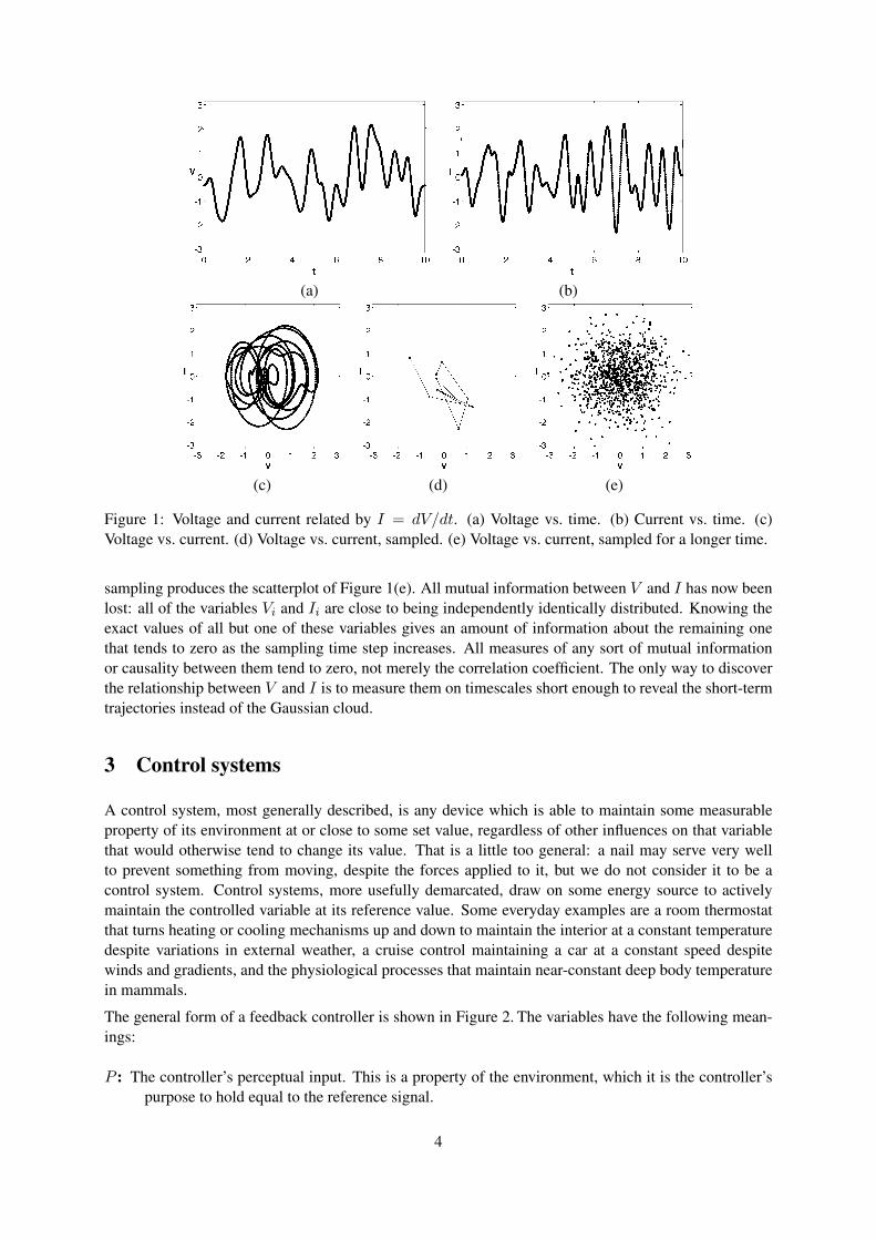
However, let us suppose that V is not generated by any periodic source, but varies randomly andsmoothly, with a waveform such as that of Figure 1(a). This waveform has been designed to have anautocorrelation time of 1 unit: the correlation between V (t) and V (t + δ) is zero whenever |δ| >= 1.(It is generated as the convolution of white noise with an infinitely differentiable function which is zerooutside a unit interval.1) Choosing the capacitance C, which is merely a scaling factor, such that V and Ihave the same standard deviation, the resulting current is shown in Figure 1(b). A plot of voltage againstcurrent is shown in Figure 1(c). One can clearly see trajectories, but it is not immediately obvious fromthe plot that there is a simple relation between voltage and current and that no other unobserved variablesare involved. If we then sample the system with a time interval longer than the autocorrelation time ofthe voltage source, then the result is the scatterplot of Figure 1(d). The points are connected in sequence,but each step is a random jump whose destination is independent of its source. Over a longer time, this

1We used Matlab to perform all the simulations and plot the graphs. The source code is available as supplementary material.

3

(a) (b)

(c) (d) (e)

Figure 1: Voltage and current related by I = dV/dt. (a) Voltage vs. time. (b) Current vs. time. (c)Voltage vs. current. (d) Voltage vs. current, sampled. (e) Voltage vs. current, sampled for a longer time.

sampling produces the scatterplot of Figure 1(e). All mutual information between V and I has now beenlost: all of the variables Vi and Ii are close to being independently identically distributed. Knowing theexact values of all but one of these variables gives an amount of information about the remaining onethat tends to zero as the sampling time step increases. All measures of any sort of mutual informationor causality between them tend to zero, not merely the correlation coefficient. The only way to discoverthe relationship between V and I is to measure them on timescales short enough to reveal the short-termtrajectories instead of the Gaussian cloud.

3 Control systems

A control system, most generally described, is any device which is able to maintain some measurableproperty of its environment at or close to some set value, regardless of other influences on that variablethat would otherwise tend to change its value. That is a little too general: a nail may serve very wellto prevent something from moving, despite the forces applied to it, but we do not consider it to be acontrol system. Control systems, more usefully demarcated, draw on some energy source to activelymaintain the controlled variable at its reference value. Some everyday examples are a room thermostatthat turns heating or cooling mechanisms up and down to maintain the interior at a constant temperaturedespite variations in external weather, a cruise control maintaining a car at a constant speed despitewinds and gradients, and the physiological processes that maintain near-constant deep body temperaturein mammals.

The general form of a feedback controller is shown in Figure 2. The variables have the following mean-ings:

P : The controller’s perceptual input. This is a property of the environment, which it is the controller’spurpose to hold equal to the reference signal.

4

Figure 2: The basic block diagram of any feedback control system. The controller is above the shadedline; its environment (the plant that it controls) is below the line.

R: The reference signal. This is the value that the control system tries to keep P equal to. It is shownas a part of the controller. In an industrial setting it might be a dial set by an operator, or it couldbe the output of another control system. In a living organism, R will be somewhere inside theorganism and may be difficult to discover.

O: The output signal of the controller. This is some function of the perception and the reference (andpossibly their past history). This is the action the control system takes to maintain P equal to R.Often, and in all the examples of the present paper, O depends only on the difference R− P , alsocalled the error signal.

D: The disturbance: all of the influences on P besides O. P is some function G of the output and thedisturbance (and possibly their past history).

We shall now give some very simple didactic examples of control systems, and exhibit the patterns ofcorrelations they yield among P , R, O, and D under various circumstances.

Example 1

Figure 3 illustrates a simple control system acting within a simple environment, defined by the followingequations, all of the variables being time-dependent.

O = k(R− P ) (1)

P = O +D (2)

Equation 1 describes an integrating controller, i.e. one whose output signal O is proportional to the inte-gral of the error signal R−P . Equation 2 describes the environment of the controller, which determinesthe effect that its output action and the disturbing variable D have upon the controlled variable P . In thiscase O and D add together to produce P . Figure 4 illustrates the response to step and random changes inthe reference and disturbance. The random changes are smoothly varying with an autocorrelation timeof 1 second. The gain k is 100. Observe that when R and D are constant, P converges to R and O toR−D. The settling time for step changes in R or D is of the order of 1/k = 0.01.

The physical connections between O, R, P , and D are as shown in Figure 3: O is caused by R andP , P is caused by O and D, and there are no other causal connections. We now demonstrate thatthe correlations between the variables of this system bear no resemblance to the causal connections. We

5

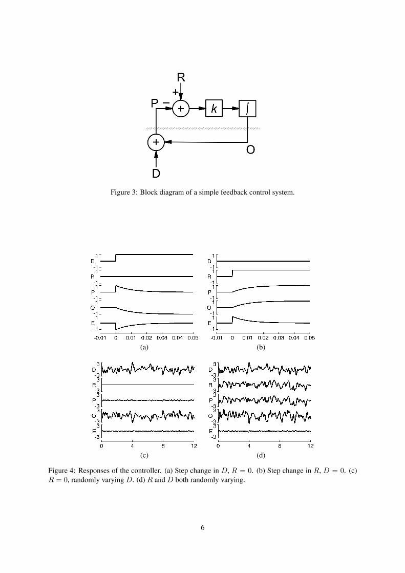
Figure 3: Block diagram of a simple feedback control system.

(a) (b)

(c) (d)

Figure 4: Responses of the controller. (a) Step change in D, R = 0. (b) Step change in R, D = 0. (c)R = 0, randomly varying D. (d) R and D both randomly varying.

6

P D

O 0.002 −0.999P 0.043

Table 1: Correlations for an integrating controller (Example 1).

generate a smoothly randomly varying disturbanceD, which varies on a timescale much longer than 1/k,with a standard deviation of 1 (in arbitrary units). The referenceR is held constant at 0. Table 1 shows thecorrelations in a simulation run of 1000 seconds with a time step of 0.001 seconds. The performance ofthe controller can be measured by its disturbance rejection ratio, σ(D)/σ(R−P ) = 23.2. The numbersvary between runs only in the third decimal place. For this system, correlations are very high (close to±1) exactly where direct causal connection is absent, and close to zero where direct causal connection ispresent. There is a causal connection between D and O, but it proceeds only via P , with which neithervariable is correlated.

Here is a visual contrast between the causal links and the non-zero pairwise correlations.

P

D

>

O

<

>

P

D1

OCausality Non-zero pairwise correlations

It is difficult to calculate significance levels for these correlations, since the random waveforms thatwe generate for D (and in some of our simulations, also for R) are deliberately designed to be heavilybandwidth-limited. They have essentially no energy at wavelengths below about 0.2 seconds. Successivesamples are therefore not independent, and formulas for the standard error of the correlation do not apply.Empirically, if we repeat the simulation many times, we find that the variance of the correlation betweentwo independently generated waveforms like D is proportional to the support interval of the filter thatgenerates them from white noise. This implies that as one reduces the sampling time step below thepoint at which there is any new structure to discover, the variance of the correlation will not decrease.When the samples already contain almost all the information there is to find in the signal, increasing thesampling rate cannot yield new information.

All of the simulations presented here were use runs of 106 time steps of 0.001 seconds, and a coherencetime for each of the exogenous random time series of 1 second. For two such series, independentlygenerated, we find a standard deviation of the correlation (estimated from 1000 runs) of 0.023, comparedwith 0.001 for the same quantity of independent samples of white noise. Therefore, for the examplesreported here, any correlation whose magnitude is below about 0.05 must be judged statistically notsignificant.2 The correlations observed here between D and both O and P are thus indistinguishablefrom zero. These correlations are approximately summarised in Table 2. This behaviour is quite differentfrom that of a passive equilibrium system, such as a ball in a bowl (or something nailed down, whichis a similar situation with a much higher spring constant). In the latter system, if we identify D withan external force applied to the ball, P with its position, and O with the component of gravitationalforce parallel to the surface of the bowl, we will find (assuming some amount of viscous friction, anda measurement timescale long enough for the system to always be in equilibrium), that O and P are

2Significance, in the everyday sense of practical usefulness, deserves a mention. For the practical task of estimating thevalue of one variable from another it is correlated with, far higher correlations are required. For a bivariate Gaussian, even witha correlation of 0.5, the probability of guessing from the value of one variable just whether the other is above or below its meanis only 67%, compared with 50% for blind guessing. To be right 9 times out of 10 requires a correlation of 0.95. To estimate itsvalue within half a decile 9 times out of 10 takes a correlation of 0.995. And to be sure from a finite sample that the correlationreally is that high would require its true value to be even higher.

7

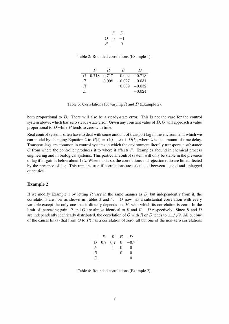
P D

O 0 −1P 0

Table 2: Rounded correlations (Example 1).

P R E D

O 0.718 0.717 −0.002 −0.718P 0.998 −0.027 −0.031R 0.039 −0.032E −0.024

Table 3: Correlations for varying R and D (Example 2).

both proportional to D. There will also be a steady-state error. This is not the case for the controlsystem above, which has zero steady-state error. Given any constant value of D, O will approach a valueproportional to D while P tends to zero with time.

Real control systems often have to deal with some amount of transport lag in the environment, which wecan model by changing Equation 2 to P (t) = O(t − λ) + D(t), where λ is the amount of time delay.Transport lags are common in control systems in which the environment literally transports a substanceO from where the controller produces it to where it affects P . Examples abound in chemical processengineering and in biological systems. This particular control system will only be stable in the presenceof lag if its gain is below about 1/λ. When this is so, the correlations and rejection ratio are little affectedby the presence of lag. This remains true if correlations are calculated between lagged and unlaggedquantities.

Example 2

If we modify Example 1 by letting R vary in the same manner as D, but independently from it, thecorrelations are now as shown in Tables 3 and 4. O now has a substantial correlation with everyvariable except the only one that it directly depends on, E, with which its correlation is zero. In thelimit of increasing gain, P and O are almost identical to R and R − D respectively. Since R and Dare independently identically distributed, the correlation of O with R or D tends to ±1/

√2. All but one

of the causal links (that from O to P ) has a correlation of zero; all but one of the non-zero correlations

P R E D

O 0.7 0.7 0 −0.7P 1 0 0R 0 0E 0

Table 4: Rounded correlations (Example 2).

8

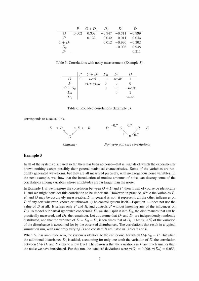
P O +D0 D0 D1 D

O 0.002 0.308 −0.947 −0.311 −0.999P 0.132 0.042 0.011 0.043

O +D0 0.012 −0.990 −0.302D0 −0.006 0.948D1 0.311

Table 5: Correlations with noisy measurement (Example 3).

P O +D0 D0 D1 D

O 0 weak −1 −weak 1P very weak 0 0 0

O +D0 0 −1 −weakD0 0 1D1 weak

Table 6: Rounded correlations (Example 3).

corresponds to a causal link.

D > P > E < R

O<

< D−0.7

O0.7

R E

P0.71

Causality Non-zero pairwise correlations

Example 3

In all of the systems discussed so far, there has been no noise—that is, signals of which the experimenterknows nothing except possibly their general statistical characteristics. Some of the variables are ran-domly generated waveforms, but they are all measured precisely, with no exogenous noise variables. Inthe next example, we show that the introduction of modest amounts of noise can destroy some of thecorrelations among variables whose amplitudes are far larger than the noise.

In Example 1, if we measure the correlation between O +D and P , then it will of course be identically1, and we might consider this correlation to be important. However, in practice, while the variables P ,R, and O may be accurately measureable, D in general is not: it represents all the other influences onP of any sort whatever, known or unknown. (The control system itself—Equation 1—does not use thevalue of D at all. It senses only P and R, and controls P without knowing any of the influences onP .) To model our partial ignorance concerning D, we shall split it into D0, the disturbances that can bepractically measured, and D1, the remainder. Let us assume that D0 and D1 are independently randomlydistributed, and that the variance of D = D0 +D1 is ten times that of D1. That is, 90% of the variationof the disturbance is accounted for by the observed disturbances. The correlations that result in a typicalsimulation run, with randomly varying D and constant R are listed in Tables 5 and 6.

WhenD1 has amplitude zero, the system is identical to the earlier one, for whichO+D0 = P . But whenthe additional disturbance D1 is added, accounting for only one tenth the variation of D, the correlationbetween O+D0 and P sinks to a low level. The reason is that the variations in P are much smaller thanthe noise we have introduced. For this run, the standard deviations were σ(O) = 0.999, σ(D0) = 0.953,

9

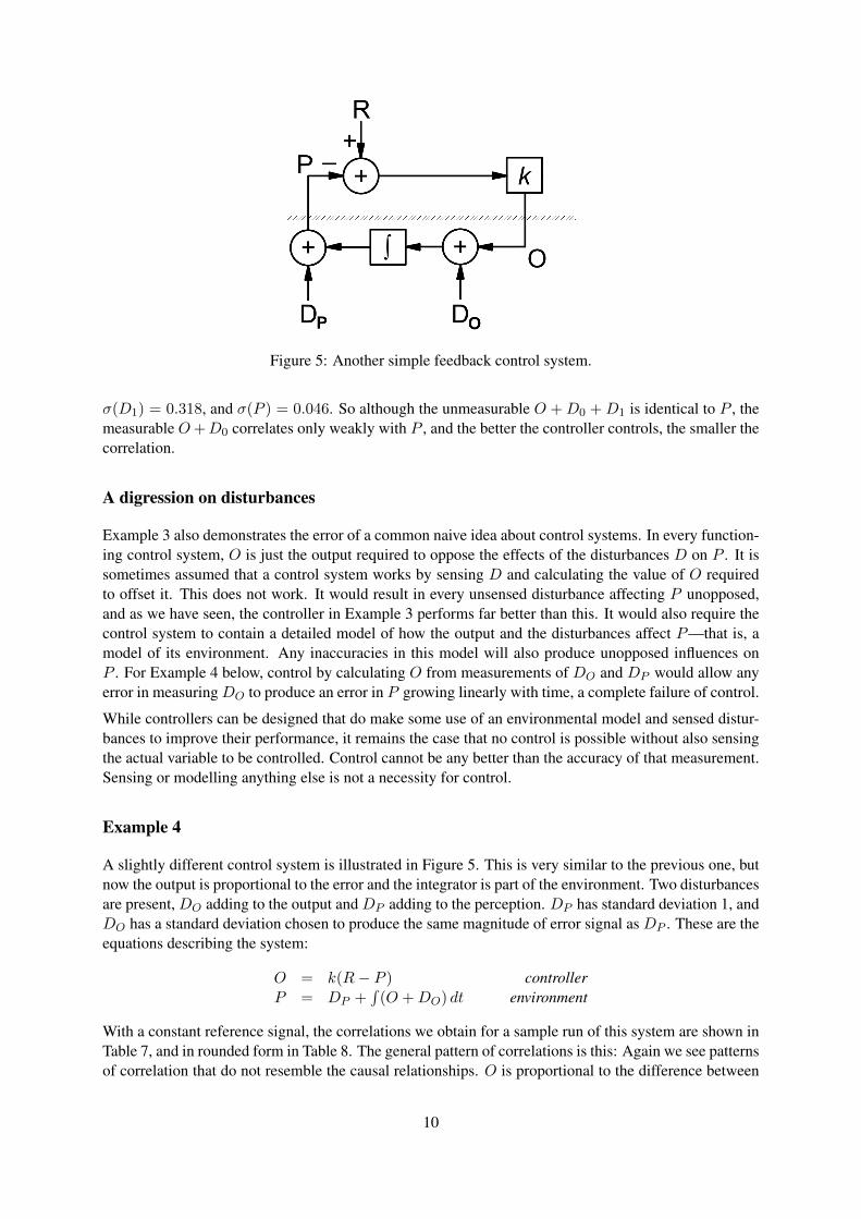
Figure 5: Another simple feedback control system.

σ(D1) = 0.318, and σ(P ) = 0.046. So although the unmeasurable O +D0 +D1 is identical to P , themeasurable O+D0 correlates only weakly with P , and the better the controller controls, the smaller thecorrelation.

A digression on disturbances

Example 3 also demonstrates the error of a common naive idea about control systems. In every function-ing control system, O is just the output required to oppose the effects of the disturbances D on P . It issometimes assumed that a control system works by sensing D and calculating the value of O requiredto offset it. This does not work. It would result in every unsensed disturbance affecting P unopposed,and as we have seen, the controller in Example 3 performs far better than this. It would also require thecontrol system to contain a detailed model of how the output and the disturbances affect P—that is, amodel of its environment. Any inaccuracies in this model will also produce unopposed influences onP . For Example 4 below, control by calculating O from measurements of DO and DP would allow anyerror in measuringDO to produce an error in P growing linearly with time, a complete failure of control.

While controllers can be designed that do make some use of an environmental model and sensed distur-bances to improve their performance, it remains the case that no control is possible without also sensingthe actual variable to be controlled. Control cannot be any better than the accuracy of that measurement.Sensing or modelling anything else is not a necessity for control.

Example 4

A slightly different control system is illustrated in Figure 5. This is very similar to the previous one, butnow the output is proportional to the error and the integrator is part of the environment. Two disturbancesare present, DO adding to the output and DP adding to the perception. DP has standard deviation 1, andDO has a standard deviation chosen to produce the same magnitude of error signal as DP . These are theequations describing the system:

O = k(R− P ) controllerP = DP +

∫(O +DO) dt environment

With a constant reference signal, the correlations we obtain for a sample run of this system are shown inTable 7, and in rounded form in Table 8. The general pattern of correlations is this: Again we see patternsof correlation that do not resemble the causal relationships. O is proportional to the difference between

10

P R E DO DP

O −0.041 0.034 1.000 −0.527 −0.031P 0.997 −0.041 0.008 0.001R 0.034 −0.032 −0.002E −0.527 −0.031DO −0.006

Table 7: Correlations for a proportional controller (Example 4).

P R E DO DP

O 0 0 1 −0.5 0P 1 0 0 0R 0 0 0E −0.5 0DO 0

Table 8: Rounded correlations (Example 4).

P and R, and is not directly influenced by anything else, but is correlated with neither of them. DP hasno correlation with any other variable. O correlates perfectly with E, because O = kE by definition,but the only other variable it has a correlation with is DO, whose causal influence on O proceeds via analmost complete circuit of the control loop.

R > E > O

DP > P

∧

<<

DO

R E1

O

DP P

1

DO

−0.5−0.5

Causality Non-zero pairwise correlations

As with the integral control system, the addition of transport lag of no more than 1/k does not changethis behaviour.

The apparently paradoxical relationships in Examples 1–4 between causation and correlation can in factbe used to discover the presence of control systems. Suppose that D0 is an observable and experimen-tally manipulable disturbance which one expects to affect a variable P (because one can see a physicalmechanism whereby it should do so), but when D0 is experimentally varied, it is found that P remainsconstant, or varies far less than expected. This should immediately suggest the presence of a controlsystem which is maintaining P at a reference level. This is called the Test for the Controlled Variableby [11, 13]. Something else must be happening to counteract the effect of D0, and if one finds such avariable O that varies in such a way as to do this, then one may hypothesise that O is the output variableof the control system. Further investigation would be required to discover the whole control system:the actual variable being perceived (which might not be what the experimenter is measuring as P , butsomething closely connected with it), the referenceR (which is internal to the control system), the actualoutput (which might not be exactly what the experimenter is observing as O), and the mechanism thatproduces that output from the perception and the reference. For this test to be effective, the disturbancemust be of a magnitude and speed that the control system can handle. Only by letting the control systemcontrol can one observe that it is doing so.

A further paradox of control systems also appears here. Unlike the control systems of the earlier ex-

11

P D

O 0 0P 1

P O +D0 D0 D1 D

O 0 0 0 0 0P 1 1 weak 1

O +D0 1 0 1D0 0 1D1 0

Example 5(1) Example 5(3)

P R E D

O 0 0 0 0P 0 −0.7 1R 0.7 0E −0.7

P R E DO DP

O −0.7 0.7 1 0 −0.7P 0 −0.7 0 0.7R 0.7 0 0E 0 −0.7DO 0

Example 5(2) Example 5(4)

Table 9: Correlations in the presence of fast disturbances (Example 5).

amples, this one has a certain amount of steady-state error. When R, DO, and DP are constant, thesteady-state values of E and O are −DO/k and −DO respectively. When the gain k is large, E maybe experimentally indistinguishable from zero, while O may be clearly observed. E is, however, theonly immediate causal ancestor of O. For the systems of Examples 1–3, the paradox is even stronger:the steady-state error and output signals are both zero, for any constant values of the disturbances andreference. Superficial examination of the system could lead one to wrongly conclude that they play norole in its functioning.

Example 5

In all of the above examples, the disturbances and the reference signal vary only on timescales muchlonger than the settling time of the control system: 1 second vs. 0.01 seconds. If we repeat these simu-lations with signals varying on a much shorter timescale than the settling time, then we find completelydifferent patterns of correlation. Table 9 shows the general form of the results for examples 1–4 with again of 1 (giving a settling time of 1 second) and a coherence time for the random signals of 0.1 seconds.

Notice that Faithfulness is still violated. For example, the new version of Example 1 has a zero correlationbetween O and P , although the only causal arcs involving O are with P . For this system, O is just theintegral of P , and so Theorem 2 applies: O and P necessarily have zero correlation regardless of thesignal injected as D. For the new versions of Examples 2 and 3, O does not correlate with any othervariable, and for Example 4, DO correlates with no other variable. When a variable correlates withnothing else, no system of causal inference from non-interventional data can reveal a causal connectionthat includes it.

Summary

We could go through many more examples of control systems of different architectures and differenttypes of disturbances, but these should be enough to illustrate the general pattern. The presence ofcontrol systems typically results in patterns of correlation among the observable variables that bear noresemblance to their causal relationships. These patterns are robust: neither varying the parameters ofthe control systems nor collecting longer runs of data would reveal stronger correlations or diminish the

12

extreme correlations between variables with no direct connection.

We shall later discuss why this is so, but first we shall examine some current work on causal inferenceand demonstrate in each case that the authors’ hypotheses exclude systems such as the above, and, ifapplied despite that, that their methods indeed fail to correctly discover the true causal relations.

4 Current causal discovery methods applied to these examples

When a theorem shows that certain causal information can be obtained from non-experimental obser-vations on some class of systems, and yet no such information is obtainable from the systems we haveexhibited, it follows that these systems must lie outside the scope of these theorems. Here we shall surveysome such methods and exhibit where the systems we consider here violate their hypotheses.

Dynamical systems are excluded from all of the causal analyses of both [9] and [14], which do notconsider time dependency. In addition, control systems inherently include cyclic dependencies: theoutput affects the perception and the perception affects the output. Control systems therefore fall outsidethe scope of any method of causal analysis that excludes cycles, and both of these works restrict attentionto directed acyclic causal graphs.

[6] consider dynamical systems sampled at intervals, and allows for cyclic dependencies, but a conditionis imposed that in any equation giving xn+1 as a weighted sum of the variables, possibly including x,at time n, the coefficient of xn in that sum must be less than 1. This excludes any relation of the formx = dy/dt, which in discrete time is approximated by the difference equation xn+1 = xn + yn δt. Inaddition, they recommend sampling such systems on timescales longer than any transient effects. As canbe seen from Figure 1(c,d,e), the organised trajectories visible when the system is sampled on a shorttime scale vanish at longer sampling intervals: only the transient effects reveal anything about the truerelation between the variables. This recommendation thus rules out any possibility of discerning causalinfluences from nonexperimental data in the presence of control systems.

The problems that dynamical systems pose for causal analysis have been considered in terms of theconcept of “equilibration”. [5] demonstrate how the apparent causal relationships in a dynamical systemmay depend on the timescale at which one views it, the timescale determining which of the feedbackloops within the system have equilibrated. (Although he describes a variable which depends on its ownderivative as “self-regulating”, the didactic example that he discusses, of a leaky bathtub, is not a controlsystem.)

[1, 2] considers the interaction of the Equilibration operator of [5] and the Do operator of [9], andconsiders the question of when they commute. He shows that they often do not, and recommends thatwhen this is so, manipulation be performed before equilibration. This amounts to recommending thatthe system be acted on and sampled on a timescale shorter than its equilibration time, so that transientbehaviour may be observed. Even when this is done, however, the true causal relationships may failto manifest themselves in the correlations, as shown by the examples of section 2.2, and in Example 5,where the disturbance is ten times as fast as the controller’s response time. When intermediate timescalesof disturbance are applied to the example control systems, some mixture of the equilibrium and non-equilibrium patterns of correlation will be seen. With more complicated systems of several controlsystems acting together at different timescales (as in the case of cascade control, where the output ofone control system sets the reference of another, usually faster one), the patterns of correlations in theface of rapid disturbances will be merely confusing. A further moral to be drawn from this is that“equilibration” is not necessarily a passive process, like the ball-in-a-bowl described after Example 1,or the bathtub example studied in [5, 1, 2]. Unlike those systems, control systems typically exhibit verysmall or zero steady-state error (which is almost their defining characteristic).

[3] are concerned with techniques for making successful predictions rather than learning the correct

13

causal structure. However, for some of our examples this is impossible even in principle. If a variablehas zero correlation with any other variable, conditional on any set of variables, then no information aboutits value can be obtained from the other variables. This is the case, for example, with Example 5(1) andthe variable O, and for the examples of section 2.2.

[4] propose a method of causal analysis capable of deriving cyclic models. They first generalise causalgraphs to the cyclic case. Whereas in the acyclic case one can demonstrate that the conditional proba-bility distribution on the whole graph factorises into conditional distributions of each variable given itsimmediate causes, this is not always so for cyclic graphs. They therefore consider only graphs for whicha generalisation of this holds. Given the conditional distribution of each variable given its immediatecausal predecessors, a joint distribution of all the variables is said to be induced by them if (i) a localversion of factorisation holds, and (ii) nodes are independent under d-separation. (We refer to that paperfor the complete technical definition.) The requirement that the authors impose is that the conditionaldistributions must induce a unique global distribution.

This fails for the control systems considered here, because the presence of high correlations betweenvariables connected by paths of low correlation results in non-uniqueness of such a global distribution.For Example 1, the causal graph is D → P ←→ O. The required condition involves distributions f(D),f(O;P ), and f(P ;O,D). The actual global distribution has O and D normally distributed with meansof 0, standard deviations of 1, and correlation−0.997. P has distribution δP (O+D), by which we denotethe distribution in which all of the probability is concentrated at P = O + D. This implies what theconditional distributions must be: f(D) = N(0, 1), f(O;P ) = N(0, 1), and f(P ;O,D) = δP (O+D).But these are induced by any global distribution of the form P (O,D)δP (O +D), where P (O,D) is abivariate Gaussian with any correlation, and unconditional standard deviations for O and D of 1. Thishappens because the conditional distributions omit any information about the joint distribution of O andD, variables which are connected only via a third variable with which they have no correlation.

[15] consider dynamical systems with cyclic dependencies, but their results on the learnability of suchsystems depend on the Faithfulness assumption, which, the authors note, is violated when there is anequilibrium. Our Examples 1–4 all maintain equilibria, and indeed the authors’ Theorem 2 fails to applyto them. However, the examples of section 2.2, and Example 5 are not systems in equilibrium. Eventhose systems violate Faithfulness, and the conclusions of the authors’ theorems do not hold for them.

For the dynamical systems of section 2.2, the property is trivially satisfied, but the same distributionbetween the two variables—a bivariate Gaussian with zero correlation—would satisfy the assumptionsfor the causal graph on V and I with no edges. So long as data are collected at intervals long comparedwith the coherence time of the waveforms, none of the four possible graphs on two nodes can be excluded.

[16] consider the possibility of making a weaker Faithfulness assumption which is still sufficient to con-duct causal analysis. They demonstrate that Faithfulness implies two properties which they call Adja-cency Faithfulness and Orientation Faithfulness and that, while these do not together imply Faithfulness,they are (given the Markov assumption) all that is necessary for standard methods of causal inference.They then prove that if Adjacency Faithfulness is satisfied, then Orientation Faithfulness can be testedfrom the data, obviating the need to assume it. If Orientation Faithfulness fails the test, then the data arenot faithful to any causal graph. They also find a condition weaker than Adjacency Faithfulness, calledTriangle Faithfulness, having a similar property: if Triangle Faithfulness is satisfied, Adjacency Faithful-ness can be tested from the data. Each of these Faithfulness conditions is a requirement that some classof conditional correlations be non-zero.

The work is restricted to acyclic graphs, so control systems are ruled out on that ground. However, if weinvestigate Triangle Faithfulness anyway for our examples, we find that the only triangle present in any ofour causal graphs is the cyclic triangle connecting P , E, and O in Examples 2 and 4. The three vertexesof this triangle are all non-colliders (i.e. the causal arrows do not both go towards the vertex). TriangleFaithfulness requires all of the correlations between any two of these vertexes, conditional on any set of

14

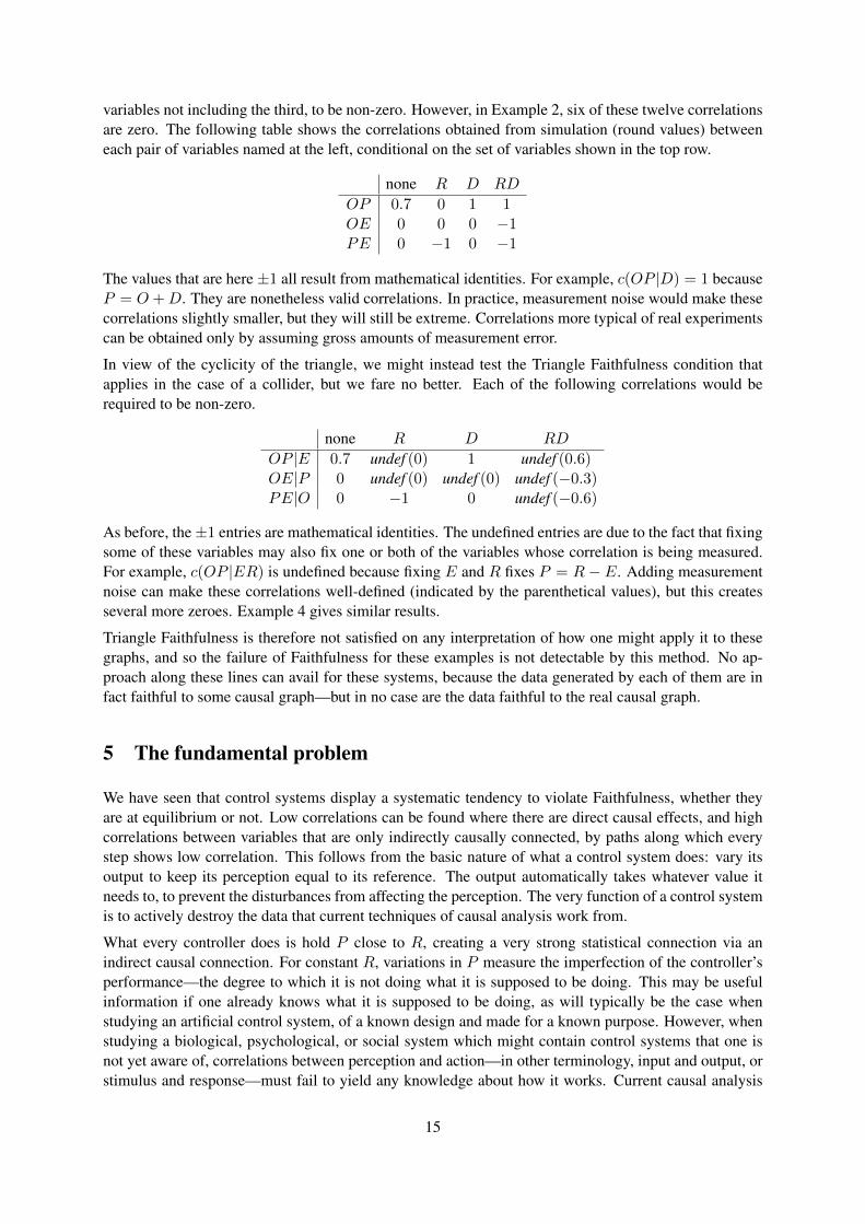
variables not including the third, to be non-zero. However, in Example 2, six of these twelve correlationsare zero. The following table shows the correlations obtained from simulation (round values) betweeneach pair of variables named at the left, conditional on the set of variables shown in the top row.

none R D RD

OP 0.7 0 1 1OE 0 0 0 −1PE 0 −1 0 −1

The values that are here ±1 all result from mathematical identities. For example, c(OP |D) = 1 becauseP = O +D. They are nonetheless valid correlations. In practice, measurement noise would make thesecorrelations slightly smaller, but they will still be extreme. Correlations more typical of real experimentscan be obtained only by assuming gross amounts of measurement error.

In view of the cyclicity of the triangle, we might instead test the Triangle Faithfulness condition thatapplies in the case of a collider, but we fare no better. Each of the following correlations would berequired to be non-zero.

none R D RD

OP |E 0.7 undef (0) 1 undef (0.6)OE|P 0 undef (0) undef (0) undef (−0.3)PE|O 0 −1 0 undef (−0.6)

As before, the±1 entries are mathematical identities. The undefined entries are due to the fact that fixingsome of these variables may also fix one or both of the variables whose correlation is being measured.For example, c(OP |ER) is undefined because fixing E and R fixes P = R − E. Adding measurementnoise can make these correlations well-defined (indicated by the parenthetical values), but this createsseveral more zeroes. Example 4 gives similar results.

Triangle Faithfulness is therefore not satisfied on any interpretation of how one might apply it to thesegraphs, and so the failure of Faithfulness for these examples is not detectable by this method. No ap-proach along these lines can avail for these systems, because the data generated by each of them are infact faithful to some causal graph—but in no case are the data faithful to the real causal graph.

5 The fundamental problem

We have seen that control systems display a systematic tendency to violate Faithfulness, whether theyare at equilibrium or not. Low correlations can be found where there are direct causal effects, and highcorrelations between variables that are only indirectly causally connected, by paths along which everystep shows low correlation. This follows from the basic nature of what a control system does: vary itsoutput to keep its perception equal to its reference. The output automatically takes whatever value itneeds to, to prevent the disturbances from affecting the perception. The very function of a control systemis to actively destroy the data that current techniques of causal analysis work from.

What every controller does is hold P close to R, creating a very strong statistical connection via anindirect causal connection. For constant R, variations in P measure the imperfection of the controller’sperformance—the degree to which it is not doing what it is supposed to be doing. This may be usefulinformation if one already knows what it is supposed to be doing, as will typically be the case whenstudying an artificial control system, of a known design and made for a known purpose. However, whenstudying a biological, psychological, or social system which might contain control systems that one isnot yet aware of, correlations between perception and action—in other terminology, input and output, orstimulus and response—must fail to yield any knowledge about how it works. Current causal analysis

15

methods can only proceed by making assumptions to rule out the problematic cases. However, theseproblematic cases are not few, extreme, or unusual, but are ubiquitous in the life and social sciences. Forpsychology, this point has been made experimentally in [12, 7].

Control systems also create problems for interventions. To intervene to set a variable to a given value, re-gardless of all other causal influences on it, one must act so as to block or overwhelm all those influences.This is problematic when the variable to be intervened on happens to be the controlled perception of acontrol system. One must either act so strongly as to defeat the control system’s own efforts to control,or fail to successfully set the perception. In the former case, the control system is driven into a stateatypical of its normal operation, and the resulting observations may not be relevant to finding out how itworks in normal circumstances. In the latter case, all one has really done is to introduce another disturb-ing variable. One has not so much done surgery on the causal graph as attach a prosthesis. Arguably,introducing a new variable is the only way of intervening in a system, in the absence of hypotheses aboutthe causal relationships among its existing variables.

When interventions are performed, a lack of appreciation of the phenomena peculiar to control systemscan lead to erroneous conclusions. A candle placed near to a room thermostat will not warm it up, butapparently cool the rest of the room. If one does not know the thermostat is there, this will be puzzling. Ifone has discovered the furnace, and noticed that the presence of the candle correlates with reduced outputfrom the furnace, one might be led to seek some mechanism whereby the furnace is sensing the presenceof the candle. And yet there is no such sensor: the thermostat senses nothing but its own temperatureand the reference setting. It cannot distinguish between a nearby candle, a crowd of people in the room,or warm weather outside.

To test for the presence of control systems, one must take a different approach, by applying disturbancesand looking for variables that remain roughly constant despite there being a clear causal path from thedisturbance to that variable (the Test for Controlled Variables). When both a causal path and an absenceof causal effect are observed, it is evidence that a control system may be present. If, at the same time,something else changes in such a way as to oppose the disturbance, that is a candidate for the controlsystem’s output action.

Discovering exactly what the control system is perceiving, what reference it is comparing it with, and howit generates its output action, may be more difficult to discover. For example, it is easy to demonstratethat mammals control their deep body temperature, less easy to find the mechanism that they sense thattemperature with. The task is made more difficult by the fact that in a well-functioning control system,the error may be so small as to be practically unmeasurable, even though the error is what drives theoutput action.

6 Conclusion

Dynamical systems exhibiting equilibrium behaviour are already known to be problematic for causalinference, although methods have been developed to extend methods of causal inference to include someparts of this class. But the subclass of control systems poses fundamental difficulties which cannotbe addressed by any extension along those lines. They specifically destroy the connections betweencorrelation and causation which these methods depend on.

The investigations here have been theoretical. It remains to be seen how substantially these phenomenaaffect causal analysis of the increasingly massive data sets that are being gathered from gene expressionarrays and high-resolution neuroimaging techniques.

16

A Sufficient conditions for zero correlation between a function and itsderivative

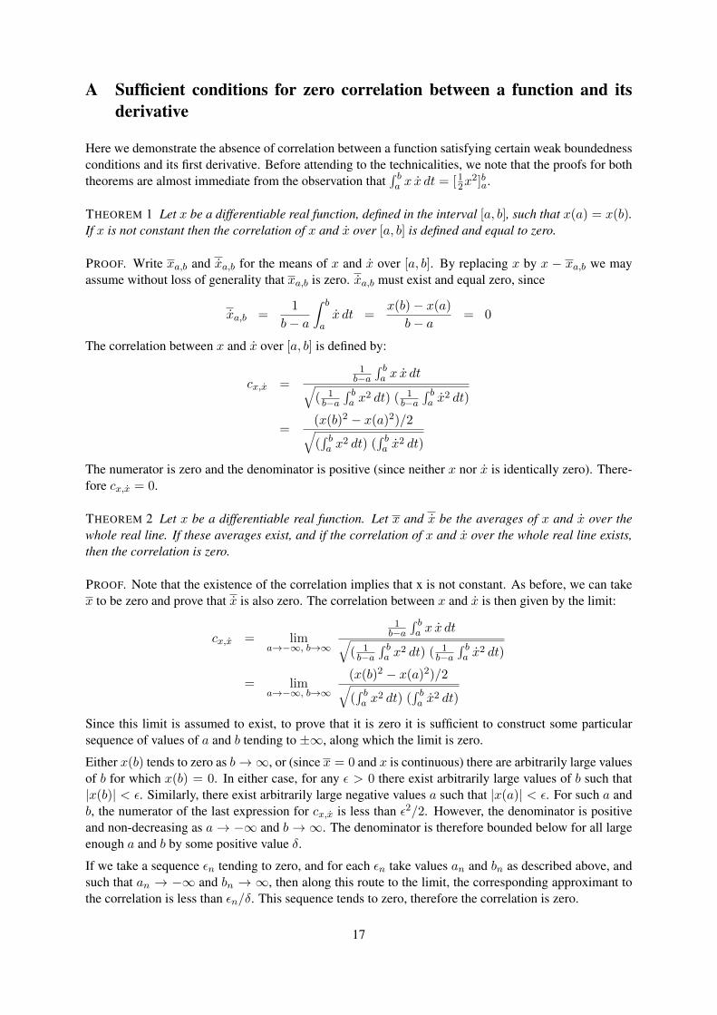
Here we demonstrate the absence of correlation between a function satisfying certain weak boundednessconditions and its first derivative. Before attending to the technicalities, we note that the proofs for boththeorems are almost immediate from the observation that

∫ ba x x dt = [12x

2]ba.

THEOREM 1 Let x be a differentiable real function, defined in the interval [a, b], such that x(a) = x(b).If x is not constant then the correlation of x and x over [a, b] is defined and equal to zero.

PROOF. Write xa,b and xa,b for the means of x and x over [a, b]. By replacing x by x − xa,b we mayassume without loss of generality that xa,b is zero. xa,b must exist and equal zero, since

xa,b =1

b− a

∫ b

ax dt =

x(b)− x(a)b− a

= 0

The correlation between x and x over [a, b] is defined by:

cx,x =1

b−a∫ ba x x dt√

( 1b−a

∫ ba x

2 dt) ( 1b−a

∫ ba x

2 dt)

=(x(b)2 − x(a)2)/2√(∫ ba x

2 dt) (∫ ba x

2 dt)

The numerator is zero and the denominator is positive (since neither x nor x is identically zero). There-fore cx,x = 0.

THEOREM 2 Let x be a differentiable real function. Let x and x be the averages of x and x over thewhole real line. If these averages exist, and if the correlation of x and x over the whole real line exists,then the correlation is zero.

PROOF. Note that the existence of the correlation implies that x is not constant. As before, we can takex to be zero and prove that x is also zero. The correlation between x and x is then given by the limit:

cx,x = lima→−∞, b→∞

1b−a

∫ ba x x dt√

( 1b−a

∫ ba x

2 dt) ( 1b−a

∫ ba x

2 dt)

= lima→−∞, b→∞

(x(b)2 − x(a)2)/2√(∫ ba x

2 dt) (∫ ba x

2 dt)

Since this limit is assumed to exist, to prove that it is zero it is sufficient to construct some particularsequence of values of a and b tending to ±∞, along which the limit is zero.

Either x(b) tends to zero as b→∞, or (since x = 0 and x is continuous) there are arbitrarily large valuesof b for which x(b) = 0. In either case, for any ε > 0 there exist arbitrarily large values of b such that|x(b)| < ε. Similarly, there exist arbitrarily large negative values a such that |x(a)| < ε. For such a andb, the numerator of the last expression for cx,x is less than ε2/2. However, the denominator is positiveand non-decreasing as a→ −∞ and b→∞. The denominator is therefore bounded below for all largeenough a and b by some positive value δ.

If we take a sequence εn tending to zero, and for each εn take values an and bn as described above, andsuch that an → −∞ and bn → ∞, then along this route to the limit, the corresponding approximant tothe correlation is less than εn/δ. This sequence tends to zero, therefore the correlation is zero.

17

The conditions that x(a) = x(b) in the first theorem and the existence of x in the second are essential.If we take x = et, which violates both conditions, then x = x and the correlation is 1 over every finitetime interval. That x and cx,x exist is a technicality that rules out certain pathological cases such asx = sin(log(1 + |t|)), which are unlikely to arise in any practical application.

We remark that although we do not require them here, corresponding results hold for discrete time series,for the same reason in its finite difference form: that (xi + xi+1)(xi+1 − xi) = x2i+1 − x2i .

References

[1] Denver Dash. Caveats for causal reasoning with equilibrium models. PhD thesis, University ofPittsburgh, 2003.

[2] Denver Dash. Restructuring dynamic causal systems in equilibrium. In Robert G. Cowell andZoubin Ghahramani, editors, Proceedings of the Tenth International Workshop on Artificial Intelli-gence and Statistics (AIStats 2005), pages 81–88. Society for Artificial Intelligence and Statistics,2005.

[3] David Duvenaud, Daniel Eaton, Kevin Murphy, and Mark Schmidt. Causal learning without DAGs.In NIPS 2008 Workshop on Causality, pages 177–190, 2008.

[4] Sleiman Itani, Mesrob Ohannesian, Karen Sachs, Garry P. Nolan, and Munther A. Dahleh. Structurelearning in causal cyclic networks. In NIPS 2008 Workshop on Causality, pages 165–176, 2008.

[5] Yumi Iwasaki and Herbert A. Simon. Causality and model abstraction. Artificial Intelligence,67(1):143–194, 1994.

[6] Gustavo Lacerda, Peter Spirtes, Joseph Ramsey, and Patrik O. Hoyer. Discovering cyclic causalmodels by independent components analysis. In David A. McAllester and Petri Myllymaki, editors,Proc. 24th Conference on Uncertainty in Artificial Intelligence, pages 366–374. AUAI Press, 2008.

[7] R. S. Marken and B. Horth. When causality does not imply correlation: More spadework at thefoundations of scientific psychology. Psychological Reports, 108:1–12, 2011.

[8] Judea Pearl. Probabilistic Reasoning in Intelligent Systems. Morgan and Kaufman, 1998.

[9] Judea Pearl. Causality: Models, Reasoning, and Inference. Cambridge University Press, 2000.

[10] Judea Pearl. Causal inference in statistics: an overview. Stat. Surv., 3:96–146, 2009.

[11] William T. Powers. Behavior: The Control of Perception. Aldine, 1974.

[12] William T. Powers. Quantitative analysis of purposive systems: Some spadework at the foundationsof scientific psychology. Psychological Review, 85(5):417–435, 1978.

[13] William T. Powers. Making Sense of Behavior: The Meaning of Control. Benchmark, 1998.

[14] Peter Spirtes, Clark Glymour, and Richard Scheines. Causation, Prediction, and Search. MITPress, 2001.

[15] Mark Voortman, Denver Dash, and Marek J. Druzdzel. Learning why things change: Thedifference-based causality learner. In Proc. 26th Conference on Uncertainty in Artificial Intelli-gence, pages 641–650. AUAI Press, 2010.

[16] J. Zhang and P. Spirtes. Detection of unfaithfulness and robust causal inference. Minds and Ma-chines, 18(2):239–271, 2008.

18