To Lidia What thou lovest well remains, the rest is dross What thou lov’st well shall not be reft from thee What thou lov’st well is thy true heritage. (Pound, Cantos , LXXXI)

Welcome message from author
This document is posted to help you gain knowledge. Please leave a comment to let me know what you think about it! Share it to your friends and learn new things together.
Transcript
To Lidia
What thou lovest well remains, the rest is drossWhat thou lov’st well shall not be reft from theeWhat thou lov’st well is thy true heritage.
(Pound, Cantos, LXXXI)
Foreword
Odifreddi has written a delightful yet scholarly treatise on recursion theory.Where else can one read about mezoic sets? His book constitutes his answerto the central question of recursion theory: what is recursion theory? Hisanswer, I am pleased to note, is idiosyncratic. He makes numerous referencesto set theory, for example Baire’s category theorem, the analytical hierarchy,the constructible hierarchy, and the axiom of determinateness. To my mindan understanding of recursion theory, even at the level of Turing degrees andrecursively enumerable sets, is incomplete until the connection to higher levelsis made via set theory.
If recursion theory is about computations, then the familiar finite case allowsonly a shallow view of the matter. Infinitely long computations, as in Kleene’saccount of finite type objects, or as in Takeuti’s version of recursive functionsof ordinals, permit a deeper insight into the nature of computation. This isborne out by the work of Slaman and others on fragments of arithmetic andpolynomial reducibility, in which ideas from high up are applied low down.
The author’s use of ‘classical’ in his title is partially meant, in this volume,to date the material he covers. He concentrates on the early days of recursiontheory. Perhaps those were the glory days. Perhaps only the early results willsurvive.
The author makes the set theoretic connection but does not pursue it fullyhere. Let us hope he writes his next volumes on ‘modern’ recursion theory. Hissparkling first volume proves him worthy of the task.
G.E. SacksHarvard University and M.I.T.
November 1987
vii
viii
Preface
The origins of this book go back to fourteen years ago when, having donemy studies in a country that, as Kreisel later remarked to me, was ‘logicallyunderdeveloped’, I thought I could learn Recursion Theory by writing it. Therewere at the time a few textbooks, prominent among them Kleene [1952] andRogers [1967], but I was unsatisfied with them because papers I was interestedin, on progressions of formal systems, seemingly required many results thatthey did not cover. Thus I sat down, read a lot, and wrote a first version inItalian. Fortunately, I did not publish it.
Meanwhile, I had gotten in touch with some recursion theorists, and decidedI would go to the United States to study some more. The Italian Centerof Researches (C.N.R.) provided support, and in 1978 I landed in Urbana-Champaign, where the world opened up to me. I found there a very sensitiveand kind teacher, Carl Jockusch, who taught me in one pleasant year morethan I could have taught myself in a lifetime. And I found a friend in DickEpstein, from whom I learned how to write mathematics. Then, having readsome of their papers, I went to the U.C.L.A. people for a year, and I’m afraidI tried their patience with my many questions. There I learned what I know ofSet Theory and Generalized Recursion Theory, through the teaching and helpof Tony Martin, Yannis Moschovakis and John Steel. Back in Italy, I rewrotethe whole book, this time in English.
In the meantime, I had grown aware of the fact that mathematics was notthe universal science that I had once thought it was: not only personal, butalso social and historical influences shape the work of the researchers. Morespecifically, I had learned that the Soviets were doing, in Recursion Theory,work that the Westerners did not know much about, and they themselves werelargely unaware of what people did in the West. I found this an odd situation,and decided I would go to the Soviet Union to bridge the gap, at least in myknowledge. The Italian and Soviet State Departments provided support, and Istayed in Novosibirsk for one and a half years, in 1982-83, again learning a lot,in both mathematical and human terms. In particular, great help was providedby Marat Arslanov, Sergei Denisov, Yuri Ershov, and Victor Selivanov. Despite
ix

x Preface
some difficulties there, which cost me a marriage among other things, I cameback with more experience, and the book was now ready.
A final and unexpected touch was added by Anil Nerode and Richard Shore,who invited me to Cornell for a year in 1985, and in the following summers.With them I started a (for me) very fruitful collaboration, partly financed by ajoint N.S.F.-C.N.R. grant. In particular, Richard Shore has relentlessly provedtheorems that covered blank spots in the book. In Cornell I also met JurisHartmanis, who changed my perspective in Complexity Theory.
In addition to all the people mentioned above, I was greatly helped by thosewho have read, and commented upon, substantial parts of the manuscript, orhave taught me different things, including Klaus Ambos-Spies, Felice Cardo-ne, Alexander Degtev, Leo Harrington, Georg Kreisel, Georgi Kobzev, MannyLerman, Jim Lipton, Gabriele Lolli, Flavio Previale, Mark Simpson, and BobSoare. Many other people have provided various kinds of help and correc-tions, in particular those who attended classes and seminars on various partsof the book in Torino and Siena (Italy), Urbana, U.C.L.A. and Cornell (UnitedStates), Novosibirsk and Kazan (Soviet Union). It would take too much spaceto mention them all, but to everybody go my sincerest thanks.
Since Gutenberg, books have usually been written to be printed. In mycase this was made possible by Solomon Feferman and Richard Shore, whointroduced the book to different editors. Michael Morley convinced me that Icould type it myself in LATEX, at a time when I did not even know how to turna computer on, and he and Anil Nerode helped afterwards with the machines,in many ways. While I was preparing the typescript, the amazing Bill Gasarchand Richard Shore provided overall corrections in real time. Finally, supportfor typesetting was provided by the C.N.R. Thanks to all of them, too.
Different and very special thanks go to Lidia. She was there before it all,saw the book taking shape, and heard about it more than anybody else. Shefollowed me on my pilgrimages, and I could perceive how great a toll this wastaking on her only when it was too late. She is not here anymore, to see theend of it, and this is most sad. The immense amount of time stolen from herand devoted to this work is partly responsible for her absence. No doubt itwas a stupid trade, but now, after fourteen years, here is the book: devoted toher as a partial, late compensation for what she deserved, and I was unable togive.
Torino - Urbana - Los AngelesNovosibirsk - Ithaca
1974–1988

Contents
Foreword by G.E. Sacks vii
Preface ix
Introduction 1What is ‘Classical’ . . . . . . . . . . . . . . . . . . . . . . . . . . . . 1What is in the Book . . . . . . . . . . . . . . . . . . . . . . . . . . . 2Applications of Recursion Theory . . . . . . . . . . . . . . . . . . . . 5How to Use the Book . . . . . . . . . . . . . . . . . . . . . . . . . . 11Notations and Conventions . . . . . . . . . . . . . . . . . . . . . . . 13
I RECURSIVENESS AND COMPUTABILITY 17I.1 Induction . . . . . . . . . . . . . . . . . . . . . . . . . . . . . 18
Definitions by inductions . . . . . . . . . . . . . . . . . . . . . . 20Proofs by induction . . . . . . . . . . . . . . . . . . . . . . . . . 20Recursiveness . . . . . . . . . . . . . . . . . . . . . . . . . . . . 22Historical roots of Recursion Theory ? . . . . . . . . . . . . . . 22Formal Arithmetic ? . . . . . . . . . . . . . . . . . . . . . . . . 23Some primitive recursive functions and predicates . . . . . . . . 24Codings of the plane . . . . . . . . . . . . . . . . . . . . . . . . 27Elimination of primitive recursion . . . . . . . . . . . . . . . . . 28
I.2 Systems of Equations . . . . . . . . . . . . . . . . . . . . . . 32The formalism of equations . . . . . . . . . . . . . . . . . . . . 32Definability by systems of equations . . . . . . . . . . . . . . . 33Derivability from systems of equations . . . . . . . . . . . . . . 36A logical programming language ? . . . . . . . . . . . . . . . . 39
I.3 Arithmetical Formal Systems . . . . . . . . . . . . . . . . . 39Notions of representability . . . . . . . . . . . . . . . . . . . . . 40Formal systems representing the recursive functions . . . . . . 43Invariant definability ? . . . . . . . . . . . . . . . . . . . . . . . 45
xi

xii Preface
Definability of functions ? . . . . . . . . . . . . . . . . . . . . . 46I.4 Turing Machines . . . . . . . . . . . . . . . . . . . . . . . . . 47
Variations of the Turing machine model . . . . . . . . . . . . . 50Physical Turing machines ? . . . . . . . . . . . . . . . . . . . . 51Finite automata ? . . . . . . . . . . . . . . . . . . . . . . . . . 53Turing machine computability . . . . . . . . . . . . . . . . . . . 54Machine-dependent programming languages ? . . . . . . . . . . 60
I.5 Flowcharts . . . . . . . . . . . . . . . . . . . . . . . . . . . . . 62Unstructured programming languages ? . . . . . . . . . . . . . 64Unlimited register, random access machines ? . . . . . . . . . . 65Flowchart computability . . . . . . . . . . . . . . . . . . . . . . 65Structured programming languages ? . . . . . . . . . . . . . . . 69Programs for primitive recursion ? . . . . . . . . . . . . . . . . 71Petri nets ? . . . . . . . . . . . . . . . . . . . . . . . . . . . . . 75
I.6 Functions as Rules . . . . . . . . . . . . . . . . . . . . . . . 76λ-calculus . . . . . . . . . . . . . . . . . . . . . . . . . . . . . . 77Other formulations of the λ-calculus ? . . . . . . . . . . . . . . 83λ-definability . . . . . . . . . . . . . . . . . . . . . . . . . . . . 84Functional programming languages ? . . . . . . . . . . . . . . . 87
I.7 Arithmetization . . . . . . . . . . . . . . . . . . . . . . . . . 88Historical remarks ? . . . . . . . . . . . . . . . . . . . . . . . . 88Numerical tools for arithmetization . . . . . . . . . . . . . . . . 89The Normal Form Theorem . . . . . . . . . . . . . . . . . . . . 91Equivalence of the various approaches to recursiveness . . . . . 98The basic result of the foundations of Recursion Theory . . . . 101
I.8 Church’s Thesis ? . . . . . . . . . . . . . . . . . . . . . . . . 102Introduction to Church’s Thesis . . . . . . . . . . . . . . . . . . 103Historical remarks . . . . . . . . . . . . . . . . . . . . . . . . . 106Computers and physics . . . . . . . . . . . . . . . . . . . . . . . 107Classical mechanics . . . . . . . . . . . . . . . . . . . . . . . . . 108Probabilistic physics . . . . . . . . . . . . . . . . . . . . . . . . 110Computers and thought . . . . . . . . . . . . . . . . . . . . . . 114The brain . . . . . . . . . . . . . . . . . . . . . . . . . . . . . . 116Constructivism . . . . . . . . . . . . . . . . . . . . . . . . . . . 119Conclusion . . . . . . . . . . . . . . . . . . . . . . . . . . . . . 123
II BASIC RECURSION THEORY 125II.1 Partial Recursive Functions . . . . . . . . . . . . . . . . . . 126
The notion of partial function . . . . . . . . . . . . . . . . . . . 127Partial recursive functions . . . . . . . . . . . . . . . . . . . . . 127Universal Turing machines and computers ? . . . . . . . . . . . 132Recursively enumerable sets . . . . . . . . . . . . . . . . . . . . 134
Preface xiii
R.e. sets as foundation of Recursion Theory ? . . . . . . . . . . 143A programming language based on r.e. sets ? . . . . . . . . . . 144
II.2 Diagonalization . . . . . . . . . . . . . . . . . . . . . . . . . . 145The essence of diagonalization . . . . . . . . . . . . . . . . . . . 145Recursive undecidability results . . . . . . . . . . . . . . . . . . 146Limitations of mechanisms ? . . . . . . . . . . . . . . . . . . . . 150Fixed-Point Theorem . . . . . . . . . . . . . . . . . . . . . . . . 152Limitations of formalism ? . . . . . . . . . . . . . . . . . . . . . 159Self-reference ? . . . . . . . . . . . . . . . . . . . . . . . . . . . 165Self-reproduction and cellular automata ? . . . . . . . . . . . . 170
II.3 Partial Recursive Functionals . . . . . . . . . . . . . . . . . 174Oracle computations and Turing degrees . . . . . . . . . . . . . 175The notion of functional . . . . . . . . . . . . . . . . . . . . . . 177Partial recursive functionals . . . . . . . . . . . . . . . . . . . . 178First Recursion Theorem . . . . . . . . . . . . . . . . . . . . . . 181Recursive programs ? . . . . . . . . . . . . . . . . . . . . . . . 185Topological digression . . . . . . . . . . . . . . . . . . . . . . . 186Iteration and fixed-points ? . . . . . . . . . . . . . . . . . . . . 192Models of λ-calculus (part I) ? . . . . . . . . . . . . . . . . . . 194Different notions of recursive functionals ? . . . . . . . . . . . . 196Higher Types Recursion Theory ? . . . . . . . . . . . . . . . . . 199Computability on abstract structures ? . . . . . . . . . . . . . . 202
II.4 Effective Operations . . . . . . . . . . . . . . . . . . . . . . 205Effective operations on partial recursive functions . . . . . . . . 205Effective operations on total recursive functions . . . . . . . . . 208Effective operations in general ? . . . . . . . . . . . . . . . . . . 210Recursive analysis ? . . . . . . . . . . . . . . . . . . . . . . . . 213
II.5 Indices and Enumerations ? . . . . . . . . . . . . . . . . . . 215Acceptable systems of indices . . . . . . . . . . . . . . . . . . . 215Axiomatic Recursion Theory ? . . . . . . . . . . . . . . . . . . 222Models of λ-calculus (part II) ? . . . . . . . . . . . . . . . . . . 223Indices for recursive and finite sets . . . . . . . . . . . . . . . . 225Enumerations of classes of r.e. sets . . . . . . . . . . . . . . . . 228The Theory of Enumerations ? . . . . . . . . . . . . . . . . . . 236
II.6 Retraceable and Regressive Sets ? . . . . . . . . . . . . . . 238Retraceable versus recursive . . . . . . . . . . . . . . . . . . . . 239Regressive versus r.e. . . . . . . . . . . . . . . . . . . . . . . . . 242Existence theorems and nondeficiency sets . . . . . . . . . . . . 245Regressive versus retraceable . . . . . . . . . . . . . . . . . . . 249
xiv Preface
IIIPOST’S PROBLEM AND STRONG REDUCIBILITIES 251III.1 Post’s Problem . . . . . . . . . . . . . . . . . . . . . . . . . . 252
Origins of Post’s Problem ? . . . . . . . . . . . . . . . . . . . . 253Turing reducibility on r.e. sets . . . . . . . . . . . . . . . . . . . 254
III.2 Simple Sets and Many-One Degrees . . . . . . . . . . . . 256Many-one degrees . . . . . . . . . . . . . . . . . . . . . . . . . . 257Simple sets . . . . . . . . . . . . . . . . . . . . . . . . . . . . . 259Effectively simple sets ? . . . . . . . . . . . . . . . . . . . . . . 263
III.3 Hypersimple Sets and Truth-Table Degrees . . . . . . . . 267Truth-table degrees . . . . . . . . . . . . . . . . . . . . . . . . . 269Hypersimple sets . . . . . . . . . . . . . . . . . . . . . . . . . . 272The permitting method ? . . . . . . . . . . . . . . . . . . . . . 277
III.4 Hyperhypersimple Sets and Q-Degrees . . . . . . . . . . 280Q-reducibility . . . . . . . . . . . . . . . . . . . . . . . . . . . . 281Hyperhypersimple sets . . . . . . . . . . . . . . . . . . . . . . . 282Maximal sets ? . . . . . . . . . . . . . . . . . . . . . . . . . . . 288
III.5 A Solution to Post’s Problem . . . . . . . . . . . . . . . . . 294Semirecursive sets . . . . . . . . . . . . . . . . . . . . . . . . . 294η-hyperhypersimple sets . . . . . . . . . . . . . . . . . . . . . . 299
III.6 Creative Sets and Completeness . . . . . . . . . . . . . . . 304Effectively nonrecursive sets . . . . . . . . . . . . . . . . . . . . 304Creative sets . . . . . . . . . . . . . . . . . . . . . . . . . . . . 306Quasicreative sets ? . . . . . . . . . . . . . . . . . . . . . . . . 311Subcreative sets ? . . . . . . . . . . . . . . . . . . . . . . . . . 314Effectively inseparable pairs of r.e. sets . . . . . . . . . . . . . . 316
III.7 Recursive Isomorphism Types . . . . . . . . . . . . . . . . 319Mezoic sets and 1-degrees . . . . . . . . . . . . . . . . . . . . . 320Recursive isomorphism types . . . . . . . . . . . . . . . . . . . 324Recursive equivalence types and isols ? . . . . . . . . . . . . . . 328
III.8 Variations of Truth-Table Reducibility ? . . . . . . . . . . 330Bounded truth-table degrees . . . . . . . . . . . . . . . . . . . . 331Weak truth-table degrees . . . . . . . . . . . . . . . . . . . . . 337Other notions of reducibility ? . . . . . . . . . . . . . . . . . . 340
III.9 The World of Complete Sets ? . . . . . . . . . . . . . . . . 341Relationships among completeness notions . . . . . . . . . . . . 341Structural properties and completeness . . . . . . . . . . . . . . 349
III.10Formal Systems and R.E. Sets ? . . . . . . . . . . . . . . 350Formal systems and r.e. sets ? . . . . . . . . . . . . . . . . . . . 350Undecidability . . . . . . . . . . . . . . . . . . . . . . . . . . . 352Essential undecidability . . . . . . . . . . . . . . . . . . . . . . 354Independent axiomatizability . . . . . . . . . . . . . . . . . . . 357
Preface xv
IV HIERARCHIES AND WEAK REDUCIBILITIES 361IV.1 The Arithmetical Hierarchy . . . . . . . . . . . . . . . . . . 363
The definition of truth ? . . . . . . . . . . . . . . . . . . . . . . 363Truth in First-Order Arithmetic . . . . . . . . . . . . . . . . . 363The Arithmetical Hierarchy . . . . . . . . . . . . . . . . . . . . 365The levels of the Arithmetical Hierarchy . . . . . . . . . . . . . 368∆0
2 sets . . . . . . . . . . . . . . . . . . . . . . . . . . . . . . . 373Relativizations ? . . . . . . . . . . . . . . . . . . . . . . . . . . 375
IV.2 The Analytical Hierarchy . . . . . . . . . . . . . . . . . . . 376Truth in Second-Order Arithmetic . . . . . . . . . . . . . . . . 376The Analytical Hierarchy . . . . . . . . . . . . . . . . . . . . . 377The levels of the Analytical Hierarchy . . . . . . . . . . . . . . 380Π1
1 sets . . . . . . . . . . . . . . . . . . . . . . . . . . . . . . . . 381∆1
1 sets . . . . . . . . . . . . . . . . . . . . . . . . . . . . . . . 387Descriptive Set Theory ? . . . . . . . . . . . . . . . . . . . . . . 392Relativizations ? . . . . . . . . . . . . . . . . . . . . . . . . . . 394Post’s Theorem in the Analytical Hierarchy ? . . . . . . . . . . 396
IV.3 The Set-Theoretical Hierarchy . . . . . . . . . . . . . . . . 397Truth in Set Theory . . . . . . . . . . . . . . . . . . . . . . . . 397Standard structures . . . . . . . . . . . . . . . . . . . . . . . . 401The Set-Theoretical Hierarchy . . . . . . . . . . . . . . . . . . . 405∆GKP
1 functions . . . . . . . . . . . . . . . . . . . . . . . . . . 407The levels of the Set-Theoretical Hierarchy . . . . . . . . . . . 411HF and the Arithmetical Hierarchy . . . . . . . . . . . . . . . 414Absoluteness and the Analytical Hierarchy . . . . . . . . . . . . 418Admissible sets ? . . . . . . . . . . . . . . . . . . . . . . . . . . 421
IV.4 The Constructible Hierarchy . . . . . . . . . . . . . . . . . 422The Constructible Hierarchy . . . . . . . . . . . . . . . . . . . . 422The levels of the Constructible Hierarchy . . . . . . . . . . . . 424The structure of L . . . . . . . . . . . . . . . . . . . . . . . . . 426Constructible sets of natural numbers . . . . . . . . . . . . . . 433Σ1
2 sets . . . . . . . . . . . . . . . . . . . . . . . . . . . . . . . . 438HC and the Analytical Hierarchy . . . . . . . . . . . . . . . . . 441Recursion Theory on the ordinals ? . . . . . . . . . . . . . . . . 444Relativizations ? . . . . . . . . . . . . . . . . . . . . . . . . . . 445
V TURING DEGREES 447V.1 The Language of Degree Theory . . . . . . . . . . . . . . . 448
The join operator . . . . . . . . . . . . . . . . . . . . . . . . . . 448The jump operator . . . . . . . . . . . . . . . . . . . . . . . . . 450First properties of degrees . . . . . . . . . . . . . . . . . . . . . 451The Axiom of Determinacy ? . . . . . . . . . . . . . . . . . . . 453

xvi Preface
V.2 The Finite Extension Method . . . . . . . . . . . . . . . . 456Incomparable degrees . . . . . . . . . . . . . . . . . . . . . . . 457Embeddability results . . . . . . . . . . . . . . . . . . . . . . . 459The splitting method . . . . . . . . . . . . . . . . . . . . . . . . 463Forcing the jump . . . . . . . . . . . . . . . . . . . . . . . . . . 467
V.3 Baire Category ? . . . . . . . . . . . . . . . . . . . . . . . . . 471Topologies on total functions . . . . . . . . . . . . . . . . . . . 472Comeager sets . . . . . . . . . . . . . . . . . . . . . . . . . . . . 473Baire Category and Degree Theory . . . . . . . . . . . . . . . . 477Meager sets of degrees . . . . . . . . . . . . . . . . . . . . . . . 481Measure Theory and Degree Theory ? . . . . . . . . . . . . . . 484
V.4 The Coinfinite Extension Method . . . . . . . . . . . . . . 484Exact pairs and ideals . . . . . . . . . . . . . . . . . . . . . . . 485Greatest lower bounds and least upper bounds . . . . . . . . . 488Extensions of embeddings . . . . . . . . . . . . . . . . . . . . . 490
V.5 The Tree Method . . . . . . . . . . . . . . . . . . . . . . . . 493Hyperimmune-free degrees . . . . . . . . . . . . . . . . . . . . . 495Minimal degrees . . . . . . . . . . . . . . . . . . . . . . . . . . 498Minimal upper bounds ? . . . . . . . . . . . . . . . . . . . . . . 503Konig’s Lemma and Π0
1 classes ? . . . . . . . . . . . . . . . . . 505Complete extensions of Peano Arithmetic ? . . . . . . . . . . . 510
V.6 Initial Segments ? . . . . . . . . . . . . . . . . . . . . . . . . 516Uniform trees . . . . . . . . . . . . . . . . . . . . . . . . . . . . 516Minimal degrees by recursive coinfinite extensions . . . . . . . . 520The three-element chain . . . . . . . . . . . . . . . . . . . . . . 524The initial segments of the degrees ? . . . . . . . . . . . . . . . 529
V.7 Global Properties . . . . . . . . . . . . . . . . . . . . . . . . 530Definability from parameters . . . . . . . . . . . . . . . . . . . 531The complexity of the theory of degrees . . . . . . . . . . . . . 537Absolute definability . . . . . . . . . . . . . . . . . . . . . . . . 541Homogeneity . . . . . . . . . . . . . . . . . . . . . . . . . . . . 544Automorphisms . . . . . . . . . . . . . . . . . . . . . . . . . . . 547
V.8 Degree Theory with Jump ? . . . . . . . . . . . . . . . . . 551
VI MANY-ONE AND OTHER DEGREES 555VI.1 Distributivity . . . . . . . . . . . . . . . . . . . . . . . . . . . 555
Distributive uppersemilattices . . . . . . . . . . . . . . . . . . . 556Ideals of distributive uppersemilattices . . . . . . . . . . . . . . 558
VI.2 Countable Initial Segments . . . . . . . . . . . . . . . . . . 561Finite initial segments . . . . . . . . . . . . . . . . . . . . . . . 562Countable initial segments . . . . . . . . . . . . . . . . . . . . . 566
VI.3 Uncountable Initial Segments . . . . . . . . . . . . . . . . 569

Contents xvii
Strong minimal covers . . . . . . . . . . . . . . . . . . . . . . . 569Uncountable linear orderings . . . . . . . . . . . . . . . . . . . 570Uncountable initial segments . . . . . . . . . . . . . . . . . . . 571
VI.4 Global Properties . . . . . . . . . . . . . . . . . . . . . . . . 574Characterization of the structure of many-one degrees . . . . . 575Definability, homogeneity, and automorphisms . . . . . . . . . . 575The complexity of the theory of many-one degrees . . . . . . . 577
VI.5 Comparison of Degree Theories ? . . . . . . . . . . . . . . 5821-degrees . . . . . . . . . . . . . . . . . . . . . . . . . . . . . . 582Truth-table degrees and weak truth-table degrees . . . . . . . . 584Elementary inequivalences . . . . . . . . . . . . . . . . . . . . . 589
VI.6 Structure Inside Degrees ? . . . . . . . . . . . . . . . . . . 591Cylinders . . . . . . . . . . . . . . . . . . . . . . . . . . . . . . 591Inside many-one degrees . . . . . . . . . . . . . . . . . . . . . . 594Inside truth-table degrees . . . . . . . . . . . . . . . . . . . . . 598Inside Turing degrees . . . . . . . . . . . . . . . . . . . . . . . . 600
Bibliography 603
Notation Index 643
Subject Index 649
xviii Contents
Introduction
Classical Recursion Theory is the study of real numbers or, equiva-lently, functions over the natural numbers. As such it has a long history,and a number of notions and results that were originally proved in differentfields and for different purposes are incorporated, unified and extended in asystematic study. We are thinking here, for example, of the different equiv-alent definitions of real number, of Cantor’s theorem that the real numbersare uncountable, of Godel’s class of constructible real numbers, and so on. Allof these are now part of Recursion Theory and of our study, but the theoryalso provides new tools of its own, the origins of which can be traced back toDedekind [1888]: he introduced the study of functions definable over the setω of the natural numbers by recurrence using the well-ordered structure of ω,whence the name Recursion Theory.
The power of recursion as a tool for defining functions was analyzed indetail by Skolem [1923], Peter [1934], and Hilbert and Bernays [1934], butits limitations were also pointed out. Gradually the collective work of Post[1922], Church [1933], Godel [1934], Kleene [1936], and Turing [1936], led to theidentification of the most general form of the recursion principle and to whatwe now call recursive functions. In a bold philosophical abstraction Church[1936] proposed to identify the notion of ‘effectively computable function’ ofnatural numbers with that of recursive function, thus providing a feeling ofabsoluteness to the notion. With Post [1944] Recursion Theory became anindependent branch of mathematics, studied for its own sake.
What is ‘Classical’
In more recent decades Recursion Theory has been generalized in various waysto different domains: ordinals bigger than ω, functionals of higher order, ab-stract sets. All these subjects belong to what we call Generalized RecursionTheory. We use the word ‘classical’ to emphasize the fact that we confine ourtreatment to the original setting, and we will deal with notions of Generalized
1
2 Introduction
Recursion Theory only when the theory provides results for the case we areinterested in.
If we see classical mathematics as the study of concrete structures, like theset of natural numbers in Number Theory, or the set of functions over the realor complex numbers in Analysis (as opposed to modern mathematics, wherethe emphasis is on abstract structures, like algebraic or topological ones), thenClassical Recursion Theory is part of classical mathematics, and sits betweenNumber Theory and Analysis. This provides another reason for the word ‘clas-sical’ in our subject.
Mathematics is usually formalized in well-established systems of Set The-ory such as ZFC (the Zermelo-Fraenkel system, together with the Axiom ofChoice). Our final use of the word ‘classical’ emphasizes the fact that we willbe working mostly in ZFC. It is not surprising, due to the well-known in-dependence results of Godel [1938] and Cohen [1963], that only a part of thestudy of real numbers can be carried out in ZFC and we will point out thelimits of our approach, together with possible extensions of ZFC suitable forRecursion Theory, at the end of the book.
What is in the Book
The basic methods of analysis of the real numbers that we are going to use aretwo:
Hierarchies. A hierarchy is a stratification of a class of reals built from below,starting from a subclass that is taken as primitive (either because wellunderstood, or because already previously analyzed), and obtained byiteration of an operation of class construction.
Degrees. Degrees are equivalence classes of reals under given equivalence re-lations, that identify reals with similar properties. Once a class of realshas been studied and understood, degrees are usually defined by identify-ing reals that look the same from that class point of view. Degrees wereused for the purpose of a classification of reals already in Euclid’s Book X(w.r.t. a geometrical equivalence relation, between rational and algebraicdependence). See Knorr [1983] for a survey.
As might be imagined the two methods are complementary: first a class isanalyzed in terms of intrinsic properties, for example by appropriately strati-fying it in hierarchies, and then the whole structure of real numbers is studiedmodulo that analysis with the appropriate notion of degrees induced by thegiven class. The two methods also have a different flavor: the first is essentiallydefinitional, the second essentially computational.

Introduction 3
To give the reader an idea of what (s)he will find in the book we outline itsbare skeleton, referring to the introductions of the chapters for more detailedoutlines.
The starting point of our study is the class of recursive functions intro-duced in Chapter I. The idea of its definition is simple: we try to isolate thefunctions over ω that are ‘computable’ in ways appealing both to the math-ematician and to the computer scientist. Having many different approachesavailable, and various different intuitions of the notion of computability, we trythem all, and discover that they all produce, once appropriately formalized,the same class of functions (and sets, through characteristic functions).
Chapter II considers two fundamental generalizations of the notion of re-cursiveness. Partial recursive functions are the natural formalization ofalgorithms: these, in the common use of the term, do not necessarily definetotal functions but only provide for specifications that allow the computationof values if particular conditions are satisfied. Partial recursive functionalstake care of a different aspect of computations, namely the interactive proce-dure according to which a machine can be piloted, in its behavior, by a humanagent. This can be formalized by the use of oracles that help the computationwhen requested by the machine.
A set is recursive if membership in it is effectively computable. The nextlevel of complexity is reached when a set is effectively generated. In this casemembership still can be effectively determined by waiting long enough in thegeneration of the set until the given element appears, but nonmembership re-quires waiting forever, and thus does not have effective content. Such setsare called recursively enumerable, and are the subject of Chapter III. Butthe emphasis of the study here is on the relative difficulty of computation. Inother words, we identify sets which are equally difficult to compute. Then weattack the problem of whether the only relevant distinction among recursivelyenumerable sets, from a computational point of view, is between recursive andnonrecursive. The answer is that the world of recursively enumerable sets is avariegated one, in which different nonrecursive effectively generated sets mayhave different computational difficulty.
Chapter IV introduces the first hierarchies, by building on the fact that therecursively enumerable sets are exactly those definable in the language of First-Order Arithmetic with exactly one existential quantifier (coding the fact thatan element is in a given recursively enumerable set if and only if there is a stageof the enumeration in which it appears). A natural hierarchy is thus obtainedby looking at the arithmetical sets as those sets which are definable in First-Order Arithmetic, counting the number of alternations of quantifiers. Otherhierarchies in the same vein are possible: counting alternations of functionquantifiers in Second-Order Arithmetic which stratifies the analytical sets;or measuring the complexity of the definition of a set of natural numbers in

4 Introduction
the language of Set Theory in terms of previously defined sets which definesthe constructible sets of integers.
Hierarchies are, by their nature, only partial tools of analysis. The notionof degree is instead a global one, classifying all sets modulo some equivalencerelation. Chapters V and VI study the structure of the continuum with respectto two notions of relative computability, Turing degrees and m-degrees,and obtain two structural results. The first equates the complexities of thedecision problem for the theories of Turing and m-degrees with that of Second-Order Arithmetic, the second gives a complete algebraic characterization of thecontinuum in terms of the structure of m-degrees. The Baire Category method,in both its original version and generalized forms, is the basic method of proof.
This completes Volume I, which introduces the fundamental notions andmethods. Volumes II and III are a deeper and more sophisticated study ofthe same topics, in which the structures already introduced are revisited andanalyzed more carefully and thoroughly. Volume II deals with sets of thearithmetical hierarchy, Volume III with the rest.
Chapters VII and VIII resume the analysis of the fundamental objectsin Recursion Theory, the recursive sets and functions, and provide a micro-scopic picture of them. We start in Chapter VII with an abstract study ofthe complexity of computation of recursive functions. Then in Chapter VIIIwe will attempt to build from below the world of recursive sets and func-tions that was previously introduced in just one go. A number of subclassesof interest from a computational point of view are introduced and discussed,among them: the polynomial time (or space) computable functionswhich provide an upper bound for the class of feasibly computable functions(as opposed to the abstractly computable ones); the elementary functions,which are the smallest known class of functions closed under time (deterministicor not) and space computations; the primitive recursive functions, whichare those computable by the ‘for’ instruction of programming languages likePASCAL, i.e. with a preassigned number of iterations (as opposed to the re-cursive functions, computable by the ‘while’ instruction, which permits an un-limited number of iterations).
Chapters IX and X return to the treatment of recursively enumerable sets.In Chapter III a good deal of information on their structure had been gathered,but here a systematic study of the structures of both the lattice of recursivelyenumerable sets and of the partial ordering of recursively enumerabledegrees is undertaken. Special tools for their treatment are introduced, mostprominent among them being the priority method, a constructive variationof the Baire Category method.
Chapter XI deals with limit sets, also known as ∆02 sets, which are limits
of recursive functions. They are a natural formalization of the notion of setsfor which membership can be determined by effective trials and errors, unlike

Introduction 5
recursive sets (for which membership can be effectively determined), and re-cursively enumerable sets (for which membership can be determined with atmost one mistake, by first guessing that an element is not in the set, and thenchanging opinion if it shows up during the generation of the set).
The following chapters produce an analysis of the sets introduced, and onlytouched upon, in Chapter IV, in particular arithmetical, hyperarithmeti-cal, ∆1
2, and constructible sets, and various other classes. In all these chap-ters the study proceeds by first analyzing the classes themselves, and then look-ing at the notions of degree associated with them (respectively: arithmeticaldegrees, hyperdegrees, ∆1
2-degrees, constructibility degrees, as well as degreeswith respect to appropriate admissible ordinals).
The final chapter deals with nonclassical set-theoretical worlds in orderto point out the limitations of the classical approach, to exactly establish itslimits, and to reach beyond it by adding appropriate axioms (prominent amongthem the Axiom of Projective Determinacy).
Starred subsections deal with topics related to the ones at hand thoughtsometimes quite far away from the immediate concern. They provide thoseconnections of Recursion Theory to the rest of mathematics and computerscience which make our subject part of a more articulate and vast scientificexperience. Limitations of our knowledge and expertise in these fields make ourtreatment of the connections rather limited, but we feel they add importantmotivation and direct the reader to more detailed references.
Particular themes on which continuous commentary is made throughoutthe book are relationships with computers, logic, and the theory of formalsystems, in particular the results known as Godel’s Theorems. As our devel-opment becomes more technical, connections to fields outside logic in general,and other branches of Recursion Theory in particular, become less important.
As will be clear by now, we have opted for breadth rather than depth,and have provided rudiments of many branches of Classical Recursion Theory,rather than complete and detailed expositions of a small number of topics. Inthis respect our book is in the tradition of Kleene [1952] and Rogers [1967], anddiffers from recent texts like Hinman [1978], Epstein [1979], Moschovakis [1980],Lerman [1983], and Soare [1987], which can be used as useful complements andadvanced textbooks in their specialized areas.
Applications of Recursion Theory
No sound mathematical theory is self-contained or detached from the rest ofmathematics or science. It takes inspiration from, and provides matter ofreflection to other branches of knowledge. Recursion Theory is no exceptionand, despite this being a book on the pure theory, we will touch on applications
6 Introduction
and connections whenever possible. Here we give an idea of the applicationsthat our subject can have in other branches of science some of which will betaken up again in more detail in the book.
Philosophy
If one of the main goals of Philosophy of Science is the conceptual analysisof epistemological notions, then the foundations of Recursion Theory providesome astounding successes for it. One of the original concerns of RecursionTheory had been the analysis of the notion of effective computability and ofthe related concept of algorithm. The isolation of the technical notion of recur-siveness as a formal proposal intended to capture the essence of computabilityon natural numbers (see Chapter I) is a first success of the philosophical side ofthe theory, but by no means the only one. After all, computability on naturalnumbers is just one part of the whole story.
A great deal of work has been spent on axiomatizing the abstract notion ofcomputability (see p. 222), and on analyzing the role of the special properties ofnatural numbers in computations. Decent notions of elementary computabilityhave been proposed for abstract domains (see p. 202), and deeper propertieshave been shown to extend to a variety of domains more general than ω (suchas admissible ordinals, see p. 444). This has required an analysis of the roleof finiteness in computations, and an isolation of its essential properties. Thefamiliarity of the notion involved, which is usually used unconsciously, magnifiesthe success obtained.
The concern of Recursion Theory with predicativity predates even its con-cern with computability (see p. 22), and it is reflected in its widespread use ofhierarchies as a mean of building classes of functions from below. One of thesehierarchies (the hyperarithmetical, see p. 391) has turned out to be particularlyinteresting and to provide for an upper bound to the notion of a predicativelydefined set of natural number (Kreisel [1960]). Related work has subsequentlybeen able to isolate a precise analogue of this notion (Feferman [1964]), thusdoubling the success obtained with computability.
Computer Science
The area of Recursion Theory that deals with recursiveness is part of Theoreti-cal Computer Science. Turing’s analysis of computability in terms of machinesprovided the conceptual basis for the construction of physical computers in thelate Forties: in the United States through Von Neumann, who knew Turing’swork, and in the United Kingdom through Turing himself (see p. 132). Differentapproaches to recursiveness generate different types of programming languages,and we discuss (Chapter I and Section II.1) how the computational core of

Introduction 7
PASCAL, LISP, PROLOG, and SNOBOL can easily be obtained from the ap-propriate versions of recursiveness (a topic that will be fully developed in ourforthcoming book Logical Foundations of Programming). Finally, a good dealof Recursion Theory is devoted to the analysis of the complexity of algorithmsand to a classification of recursive functions according to the tools needed tocompute them. This is rapidly becoming a field of its own, called Complex-ity Theory, with methods and results strongly influenced by other parts ofRecursion Theory (see Chapters VII and VIII).
Number Theory
The very origins of Recursion Theory place it close to Number Theory: the mo-tivation of Dedekind [1888] was the analysis of the concept of natural number(see p. 22), while Skolem [1923] wanted to present a formulation of Arithmeticthat avoided the difficulties of the common solutions to the paradoxes. Butperhaps the most striking application of Recursion Theory to Number Theoryis the solution of Hilbert’s Tenth Problem (see p. 135) which asked for a de-cision procedure to determine the existence of solutions of given diophantineequations. Matiyasevitch [1970] proved a representation theorem, showing thatthe sets of (non-negative) solutions of diophantine equations are exactly the re-cursively enumerable sets. A negative solution to Hilbert’s Tenth Problem thenfollows from the existence of a recursively enumerable, nonrecursive set.
Algebra
Until the second half of the last century, including the work of Lagrange, Gauss,Abel, and Galois, algebra had been developed in a strictly constructive way.The dichotomy between constructive and nonconstructive methods arose withthe notion of prime ideal, which both Kronecker and Dedekind discoveredfrom the usual constructive approach, but which Dedekind published in thenow common set-theoretical framework. After that, nonconstructive methodswhich may produce less informative but more easily graspable arguments havebecome standard (see Metakides and Nerode [1982] for more historical back-ground). Recursion Theory makes possible the analysis of the constructivecontent of classical results, as the following typical case illustrates. SteinitzTheorem shows that a field has an algebraic closure which is unique up to iso-morphism. Its original proof does not constructivize: this is an accident forthe existence part, but necessary for the uniqueness. The former follows fromRabin [1960] who, using a different existence proof, showed that a recursivelypresented field (i.e. a field with recursive set of elements and field operations,including equality) always has a recursively presented algebraic closure. Thelatter comes from Metakides and Nerode [1979], who showed that uniqueness
8 Introduction
(up to recursive isomorphism) of the recursively presented algebraic closureis equivalent to the existence of a splitting algorithm (to determine whethera polynomial is irreducible or not), a result that uses the priority method(Chapter X). The analysis of the effective content of classical algebra has beenthoroughly pursued: see Ershov [1980], Crossley [1981], Nerode and Remmel[1985] for references.
The usefulness of Recursion Theory in the analysis of constructivity in al-gebra is plausible. But there are unexpected uses too, such as in Higman [1961]who shows that the finitely generated groups embeddable in a finitely presentedgroup are exactly the recursively presented ones (i.e. those for which the setof words equal to 1 is recursively enumerable), thus linking a purely algebraicnotion with the notion of recursiveness.
Higman’s representation theorem easily implies the undecidability of theword problem (to determine whether two words are equal) for finitely presentedgroups, proposed by Dehn in 1911 and solved by Novikov [1954] and Boone[1959]. The undecidability of the easier word problem for semigroups, proposedby Thue [1914] and solved by Post [1944] and Markov [1947], is historicallyimportant, being the first undecidability result of a problem from classicalmathematics. These results started a whole area of research, devoted to thedetermination of which properties of algebraic structures are (un)decidable.See Tarski, Mostowski and Robinson [1953], Ershov, Lavrov, Taimanov andTaislin [1965], Ershov [1980], and Hanson [198?] for detailed treatments andreferences.
Analysis
Borel [1912] introduced the notion of computable real number, using the in-tuitive notion of computability. The very paper in which Turing introducedhis influential approach to computability was motivated by the search for aformal definition of computable reals, and was thus the beginning of recursiveanalysis. Turing isolated a class of recursive reals that is independent of theproposed constructivization (in the sense that all classically equivalent defini-tions of real number remain equivalent when appropriately constructivized),contains all commonly used reals, and is algebraically closed. Subsequent workextending the notion of recursive functional (Section II.4) defined the notionof a recursive function of a real variable as a function defined on all reals, notonly on the recursive ones.
This provided the needed tools to analyze the effective content of analysis:a result is constructive if whenever it has recursive data it provides us withrecursive solutions. As a typical example, Weierstrass proof of the existence of amaximum for a continuous real function on a closed interval is constructive; butan argument at which the maximum is attained cannot be constructively found

Introduction 9
(Lacombe [1957], Specker [1959]). Another example is provided by the ordinarydifferential equation y′ = f(x, y): the original proof of Picard that if f satisfiesa Lipschitz condition the solution exists and is unique is constructive, butAberth [1971] and Pour El and Richards [1979] showed that even the existencealone is not constructive if f is only uniformly continuous. See p. 213 for moreon the subject.
As for algebra, one can look for undecidability results as well, some of whichhave been obtained by Richardson [1968], Adler [1969] and Wang [1974]. Asan example, the latter proves that there is no recursive procedure to decidewhether a real elementary function has a zero.
Set Theory
Recursion Theory and Set Theory have a large overlap in the study of sets ofintegers of high complexity: the material dealt with in Volume III could hardlybe classified as solely belonging to one of them; it is rather a new field sprungfrom their marriage. But Recursion Theory does have successful applications topure Set Theory in areas were the latter seems to be classically impotent. Thebetter developed applications have been two theories about cardinals: recursiveequivalence types, and admissible ordinals.
The former deals with sets that, in a constructive sense, are infinite butDedekind-finite, i.e. can be one-one mapped neither to a proper initial segmentof ω, nor to a proper subset of themselves. Classically such sets do not exist inthe presence of the Axiom of Choice, but their recursive versions have generateda rich theory that provides new insights into the notion of finiteness (see p. 328).
Another branch of Set Theory which is classically unmanageable is thetheory of large cardinals: even the inaccessible ones, the smallest proposedtype, cannot be proved to exist in classical Set Theory. The lack of examplesdifferent from ω forces one to resort to trivial cases, such as considering 1 asweakly but not strongly inaccessible because 00 = 1 (Godel [1964]). RecursionTheory provides a well-developed analogue of the theory of large cardinals, inwhich the role of the first regular cardinal is taken by the first ordinal whichis not the order type of a recursive well ordering of ω (see p. 385). The notionof admissible ordinal (p. 444) takes care of the analogue of regular cardinalin general as an ordinal closed under recursive operations on ordinals, andanalogues of a great variety of large cardinals can already be seen to existamong the countable ordinals. The existence of analogues of Ramsey cardinalscan be disproved which might prompt some reflection on the role of very largecardinals in Set Theory (see Volume III for details).
10 Introduction
Descriptive Set Theory
Cantor’s Set Theory, and in particular the unlimited use of the power set,provoked various reactions at the turn of the century, one of which producedDescriptive Set Theory as a study of larger and larger classes of sets of realswhich were explicitly defined (see p. 392). This approach, in which hierarchiesare one of the main tools, is obviously a forerunner and an analogue of variousrecursion theoretical hierarchies (see Chapter IV), the main difference beingone level of complexity: sets of reals are considered in the first case, sets ofintegers in the second. But Addison [1954], [1959] discovered that not only arethere analogies: the full classical theory can be obtained by relativization ofthe recursive hierarchy theory by substituting continuous functions and opensets for recursive functions and recursively enumerable sets (see p. 392). Thisimplies that all classical theorems have recursive versions of which they areconsequences (but not conversely). This allows a unified approach, with recur-sion theoretical methods applicable to the classical case, and the theory hasbeen resurrected from the state of lethargy in which it had fallen in the Forties.
Constructive Mathematics
The use of constructivism in classical mathematical theories is conservative:nonconstructive methods are accepted, and the issue is only whether givenproofs are constructive as they stand, or can be replaced by constructive ones,a negative answer being interesting and acceptable. But constructivism can betaken more seriously as a philosophy of mathematics that would simply ban-ish nonconstructive notions and proofs from practice. One possible approachto constructive mathematics consists of using the notion of recursiveness as asubstitute for the notion of constructivity. This can be taken literally, as inMarkov’s school (see p. 214), which considers only those mathematical objectsand operations on them that can be effectively described by recursive proce-dures as existing. But it can also be taken as a tool of analysis to comparedifferent approaches.
For example, in Kolmogorov [1932] intuitionism is seen as a logic of prob-lems: α∨β means to solve one of α and β, α→ β to reduce the problem of solv-ing β to that of solving α, ∃xα(x) to solve α(x) for some x, and so on. Kleene[1945] then introduced the notion of recursive realizability for IntuitionisticNumber Theory: numbers realize formulas if they code, inductively, recursiveprocedures that prove the formula according to the constructive meaning of thelogical operations. Realizability has been extended to Intuitionistic Set Theoryby Kreisel and Troelstra [1970] and, even if not accepted as the only possibleway of interpreting intuitionistic provability, it has become a common tool ofanalysis since it provides for constructive models of theories. See Troelstra
Introduction 11
[1973] and Beeson [1985] for detailed treatments of the subject.
Logic
After the first fifty years in which Recursion Theory was mainly motivated bymathematical problems about Arithmetic, the logicians took over. Their maininterest was still in Arithmetic, but their point of view was metamathematical.In their hands the theory obtained its most astonishing and revolutionary re-sults which are also the best known applications of the subject and one of themain impulses to its growth. By a balanced use of two of the most fundamentalmethods of proof of Recursion Theory, arithmetization and diagonalization, acomplete characterization of the expressiveness of formal systems was obtained,the result being that (as in the case of diophantine equations) exactly the re-cursively enumerable sets are (weakly) representable in any consistent formalsystem having a minimal arithmetical strength. The existence of a recursivelyenumerable, nonrecursive set then implies the undecidability and incomplete-ness of any such system (see Section II.2), thus showing the inadequacy of theconcept of formal system. These are the highlights of the extensional analysisof formal systems provided by recursion theoretical methods, but by no meansthe only ones (see p. 350). A result of Myhill [1955] (III.7.13) points out thelimits of this analysis and shows that, from an extensional point of view, allformal systems of common use look alike in the sense of being all recursivelyisomorphic.
How to Use the Book
This book has been written with two opposite, and somewhat irreconcilable,goals: to provide for both an adequate textbook, and a reference manual.Supposedly, the audiences in the two cases are different, consisting mainly ofstudents in the former, and researchers in the latter. This has resulted in dif-ferent styles of exposition, reflecting different primary goals: self-containmentand detailed explanations for textbooks, and completeness of treatment formanuals. We have tried to solve the dilemma by giving a detailed treatmentof the main topics in the text, and sketches of the remaining arguments in theexercises and in the starred parts.
The exercises usually cover material directly connected to the subject justtreated and provide hints of proofs in the majority of cases, in various degrees ofdetail. In a few cases, for completeness of treatment and easiness of reference,some of the exercises use notions or methods of proof introduced later in thebook.
The starred chapters and sections treat topics that can be omitted on a
12 Introduction
first reading. The starred subsections deal with side material, usually givingbroad overviews of subjects that are more or less related to the main flow ofthought, but which we believe provide interesting connections of RecursionTheory with other branches of Logic or Mathematics. The style is mostlysuggestive: we try to convey the spirit of the subject by quoting the mainresults and, sometimes, the general ideas of their proofs. Detailed referencesare usually given, both for the original sources and for appropriate updatedtreatments.
The general prerequisite for this book is a working knowledge of first yearundergraduate mathematics. When dealing with applications, knowledge ofthe subject will be assumed but, since the treatment is kept separate from themain text, there will be no loss in skipping the relative parts.
The chapters have been kept self-contained as far as possible. We have doneour best to keep the style informal and devoid of technicalities, and we haveresorted to technical details only when we have not been able to avoid them,no doubt because of our inadequacy.
Instead of the usual complicated diagrams of dependencies, we give sugges-tions on how the first two volumes of the book can be used as a textbook forclasses in which Recursion Theory is the main ingredient.
Elementary Recursion Theory
Chapters I and II provide a number of alternative approaches to recursivenessand the basic development of the theory. Sections 2 to 6 of Chapter I areindependent and can be chosen according to the audience in the class. Moreprecisely, mathematicians can concentrate on Sections 2 and 3 and cover alsothe Incompleteness and Undecidability Results, treated in Section II.2. On theother hand, computer scientists will find more interest in Sections 4 to 6 ofChapter I and Section II.1, where the foundations of a number of programminglanguages are laid, and can also cover self-reproducing machines, touched uponin Section II.2, and the tools needed to build models of λ-calculus and com-binatory logic, covered in Sections II.3 and II.5. Section I.8 treats Church’sThesis in a less simple-minded way than usual (i.e. facing the problems, in-stead of sweeping them under the rug), and it is perhaps more appropriate forphilosophers.
Recursively Enumerable Sets
The elementary theory of r.e. sets and degrees is contained in Chapter IIIwhich requires only some background in elementary Recursion Theory. Thechapter goes up to the solution to Post’s problem (Sections 1 to 5) and thebasic classes of r.e. sets. It can be used either as a final section of a course
Introduction 13
on elementary Recursion Theory (not dealing with alternative definitions ofrecursiveness), or as the initial segment of an advanced course on r.e. sets. Inthe latter case, it should be followed by Chapter IX, dealing with the lattice ofr.e. sets, and a choice of material from Chapter X, in which priority argumentsare introduced. Some of the material here, e.g. the theory of r.e. m-degrees,is not standard, but is useful in various respects: intrinsically, this structure ismuch better behaved than the schizoid one of r.e. T -degrees, and it reflects theglobal structure of degrees, which the latter does not; moreover, arguments onT -degrees (such as the coding method) are better understood in their simplerversions for m-degrees.
Degree Theory
Elementary degree theory is treated in Chapter V which, with some backgroundin elementary Recursion Theory, can be read autonomously. We develop thetheory up to a point where it is possible to prove the global results of thelast ten years. This forms the nucleus of a course, and it can be followed bya number of advanced topics including a choice of results from Chapters XIand XII, on degrees of ∆0
2 and arithmetical sets. Chapter VI, on m-degrees, isoften unjustly neglected, but it does provide for the only existing example ofglobal characterization of a structure of degrees. It can be read independentlyof Chapter V.
Complexity Theory
Chapters VII and VIII deal with abstract complexity theory and complexityclasses, and do not require any background, except for a working knowledgeof recursiveness and Turing machines (like Sections 1 and 4 of Chapter I).The treatment is fairly complete but, going beyond the usual unbalanced con-finement to polynomial time and space computable functions, it also coversunjustly neglected classes of recursive functions, such as elementary, primitiverecursive, and ε0-recursive ones which are of interest to the computer scientist.
Notations and Conventions
ω = 0, 1, . . . is the set of natural numbers, with the usual operations of plus(+) and times (× or ·), and the order relation ≤. P(ω) is the power set of ω,i.e. the set of all subsets of ω. ωω and P are, respectively, the sets of total andpartial functions from ω to itself.
We reserve certain lower or upper case letters to denote special objects:
• a, b, c, . . . , x, y, z, . . . for natural numbers
14 Introduction
• f, g, h, . . . for total functions of any number of variables
• α, β, γ, . . . , ϕ, ψ, χ, . . . for partial functions of any number of variables
• F,G,H, . . . for functionals, i.e. functions with some variables ranging overnumbers, and some over functions
• A,B,C, . . . ,X, Y, Z, . . . for sets of natural numbers
• P,Q,R, . . . for predicates of any number of variables
• σ, τ, . . . for strings, i.e. partial functions with finite domain and values in0, 1.
Regarding sets:
• x ∈ A means that x is an element of A
• |A| is the cardinality of A, i.e. the number of its elements
• A ⊆ B and A ⊂ B are the relations of inclusion and strict inclusion
• A is the complement of A, and the prefix ‘co-’ in front of a property of aset means that the complement has this property (i.e. a set is co-immuneif its complement is immune)
• A ∪ B is the union of A and B, i.e. the set of elements belonging to atleast one of A and B
• A ⊕ B is the disjoint union of A and B, i.e. the set of elements of theform 2x if x ∈ A, and 2x+ 1 if x ∈ B
• A ∩ B is the intersection of A and B, i.e. the set of elements belongingto both A and B
• A × B is the cartesian product of A and B, i.e. the set of pairs (x, y)whose first and second components are, respectively, in A and B
• A · B is the recursive product of A and B, i.e. the set of codes 〈x, y〉 ofpairs (x, y) ∈ A×B (see p. 27 for codings)
• cA is the characteristic function of A, with value 1 if the given argumentis in the set, and 0 otherwise.
Regarding predicates:
Introduction 15
• ¬P , P ∧ Q, P ∨ Q, P → Q, P ↔ Q, ∀xP , ∃xP are the usual logicaloperations of negation, conjunction, disjunction, implication, equivalence,universal and existential quantification.
The symbols → and ↔ will be used in a formal way, to build new prop-erties from given ones. The symbols ⇒ and ⇔ will be used informally,as abbreviations for ‘if . . . then’, and ‘if and only if’.
We use bounded quantifiers as abbreviations:
(∃x ≤ y)P (x) for (∃x)[x ≤ y ∧ P (x)](∀x ≤ y)P (x) for (∀x)[x ≤ y → P (x)].
• cP is the characteristic function of P , with value 1 if P holds for the givenargument and 0 otherwise.
Regarding binary relations on a set A, R is:
• reflexive if xRx for every x ∈ A
• antireflexive if ¬(xRx), for every x ∈ A
• symmetric if xRy ⇒ yRx for every x, y ∈ A
• transitive if xRy ∧ yRz ⇒ xRz for every x, y, z ∈ A
• a (weak) partial ordering if it is reflexive and transitive (weak partialorderings are indicated by ≤, , or v)
• a (strict) partial ordering if it is antireflexive and transitive (strong partialorderings are indicated by <, ≺, or <)
• a total ordering if it is a partial ordering, and xRy ∨ yRx ∨ (x = y) forevery x, y ∈ A
• an equivalence relation if it is reflexive, transitive, and symmetric; in thiscase the set A is partitioned into equivalence classes (each consisting ofthe elements that are in the relation R with each other)
• an uppersemilattice if any pair of elements of A has a l.u.b., and a latticeif any pair of elements of A has both l.u.b. and g.l.b. (given two elementsx and y, their least upper bound (l.u.b.) and greatest lower bound (g.l.b.)are, respectively, the smallest element of A greater than both x and y,and the greatest element of A smaller than both x and y).
Regarding functions:
• f g or fg denote the composition of f and g

16 Introduction
• f (n) denotes the result of n iterations of f , i.e. n successive applicationsof f (by convention, f (0)(x) = x)
• ϕ(x)↓ means that ϕ is defined on x
• ϕ(x)↑ means that ϕ is undefined on x
• the set of elements on which ϕ is defined is called its domain, and the setof elements which are values of ϕ for some argument is called its range
• ϕ ' ψ means that ϕ and ψ are equal as partial functions, i.e. on eachargument they are either both undefined, or both defined and equal
• the set of pairs (x, y) such that ϕ(x) ' y is called the graph of ϕ
• α ⊆ β means that as partial functions β extends α, i.e. if α is defined onan argument, then β is too and has the same value.
Each chapter is divided into numbered sections, and each section is dividedinto unnumbered subsections. There is a unique progressive numbering insidesections, including definitions, results, and exercises. Internal references in agiven chapter may omit the chapter number.
The bibliography only includes papers quoted in the book. We have doneour best to attribute results and quote the original sources. In case of unpub-lished results, when an attribution has been possible through personal com-munication or other sources we have attached names without references, andthe mistakes that may have occurred are unintentional. We are, of course,well aware of the fact that simply quoting original sources is only a ghost ofhistory, and it barely hints at the growth and interaction of ideas. But at leastit provides the bare facts.
It is now time to plunge into the real work. We hope you will find the bookreadable, despite the difficulties imposed partly by the subject, but mostly byour limitations. Try to be patient,
and remember patience is the great thing, and above all things elsewe must avoid anything like being or becoming out of patience.
(Joyce, Finnegans Wake)
Chapter I
Recursiveness andComputability
This chapter attacks the problem of characterizing the notion of effectivecomputability, by isolating various different proposals. The methods intro-duced in Section 7 show them all to be equivalent, thus demonstrating that wehave certainly found a natural and fundamental class of functions. In Section8 we discuss whether we have reached a satisfactory solution, and to whichextent it is possible to believe that the class of functions so isolated coincideswith the class of effectively computable functions.
The various approaches we introduce can be roughly classified into twogroups:
Mathematical. We start in Section 1 with a class of functions defined by mim-icking the basic arithmetical notions, the principle of induction amongthem. We note that the functions of this class are naturally defined bymeans of equations, and thus undertake in Section 2 a general study ofsystems of equations. We then discover that by adopting special formalrules we can derive the values of a function from a system of equationsdefining it. In Section 3 we thus investigate the functions whose valuescan be derived by any logical means in current formal systems suitablefor arithmetic.
Computational. By analyzing the human process of routine calculation, weset up in Section 4 a machine-like model of computation and programsfor it. In Section 5 we then consider the purely algorithmical skeletonof programs, by abstracting from the specific implementation of the ma-chine. In a final generalization we then set up, in Section 6, a theory of
17

18 I. Recursiveness and Computability
functions as abstract programs.
Of course different classifications are possible. A particularly relevant one,from a computational point of view, would make a distinction between de-terministic and nondeterministic notions. So, e.g., Herbrand-Godel com-putability, representability in formal arithmetical systems, λ-definability and,more generally, all notions of derivability in suitable formal systems (the mostcomprehensive formulation in this direction being Post canonical systems, in-troduced in Section II.1) are nondeterministic, since they provide rules whichcan be applied in certain situations, but do not establish the order of appli-cation when multiple choices are available. It is however possible to introducerestrictions in nondeterministic approaches to turn them into deterministicones, usually without affecting their power (and this is actually done whenthese approaches are taken as basis for programming languages).
It is important to stress that for much of the later development ofRecursion Theory, alternative characterizations of recursiveness, aswell as its relation with effective computability, are not needed. Thevarious sections have been kept mostly independent from each other, so thatthey can be read separately. The reader not interested in foundational aspectsof Recursion Theory can even skip the whole chapter, except for Sections 1 andthe first part of Section 7, in which the recursive functions and the fundamentalmethod of arithmetization are respectively introduced. Arithmetization is abasic technical tool, which is here applied to produce a normal form for therecursive functions, and to show the equivalence of the various approaches torecursiveness.
As a whole, this introductory chapter (and the first two sections of thenext one) may be thought of as a technical version of what Webb [1980] doesphilosophically and Hofstadter [1979] pyrotechnically. These books may offervarious (and sometimes unexpected) complements to the matters here discussed(especially so for those we just hint at). They are recommended reading.
I.1 Induction
The subject of this book is a close look at functions from natural numbers tonatural numbers. The interest of our study is evident: the natural numbers areone of the most natural type of mathematical objects, and thus our functionsare among the most natural mathematical functions. But to even understandwhat such functions are, we must first of all have a good grasp of the objectsthey relate. We then start by analyzing the intuitive picture of the naturalnumbers, trying to characterize their structure. Something is clear: the naturalnumbers are all in a single discrete row, with a first but no last element. Sincewhat matters to us is just their mutual relationship and not their ultimate
I.1 Induction 19
individual nature, we may imagine them as obtained from a first element (thenumber 0), by iteration of a generation procedure (the successor operation S).Thus the numbers are
0 S(0) S(S(0)) · · ·
or (by using now the natural numbers metalinguistically, to indicate the numberof iterations of S)
0 S1(0) S2(0) · · ·
We simply write n for Sn(0).Three axioms that we take for granted from our intuitive picture above are
the following (in a first-order logic with equality):
Axioms I.1.1 (Dedekind [1888])
A1 S(x) = S(y) → x = y
A2 0 6= S(y)
A3 x 6= 0 → (∃y)(x = S(y)).
They say that the successor induces an isomorphism between ω (the set ofnatural numbers) and ω − 0. Also, they rule out some unwanted pictures ofthe natural numbers, like ones with cycles, or with two infinite sequences ofelements like
a0 a1 a2 · · · b0 b1 b2 · · ·
Unfortunately, they leave space for structures like
a0 a1 a2 · · · · · · b−2 b−1 b0 b1 b2 · · ·
and to be able to isolate just the initial part of these structures we need to saythat every element can be reached from 0 by a finite number of applicationsof S. This seems to involve the very notion of integer that we are trying tocharacterize, and might seem to be circular (It is actually impossible to do thisin a first-order way. See the related remarks on p. 24).
We then take an operational stand, and begin to study how we can deal withfunctions and properties of natural numbers. There are basically two ways: wemay want to define something new, or to check properties of something wealready have. Necessarily (according to our intuition) we have to proceed inboth cases by induction, i.e. starting from 0 and going on by means of thesuccessor operation.
20 I. Recursiveness and Computability
Definitions by inductions
A typical example is given in the following definitions of sum and product,that reduce each of these two binary functions to an infinite family of unaryfunctions (obtained by fixing the first argument).
Definition I.1.2 (Grassmann [1861])
A4 x+ 0 = x
A5 x+ S(y) = S(x+ y)
A6 x · 0 = 0
A7 x · S(y) = x · y + x.
In both cases a new function is defined, first for 0 and then for a genericS(y), using the work already done for y. A general formulation of this process(with parameters) is the following, where we write y + 1 for S(y), as usual.
Definition I.1.3 (Dedekind [1888]) A function f is defined from g and hby primitive recursion if
f(~x, 0) = g(~x)f(~x, y + 1) = h(~x, y, f(~x, y)).
Proofs by induction
Suppose we have a property ϕ of natural numbers and we wish to check thatit holds for every number. From the way the numbers are generated, thisfollows if the property holds for 0 and it propagates through the successoroperation, since every number is obtained from 0 by a finite iteration of S.This is expressed by the Axiom of Induction:
Axiom I.1.4 (Dedekind [1888]) If ϕ is a formula with one free variablethen
A8 ϕ(0) ∧ (∀x)[ϕ(x) → ϕ(S(x))] → (∀y)ϕ(y).
In terms of sets this means that any set containing 0 and closed undersuccessor contains ω, or that the numerals Sn(0) exhaust the natural numbers.This is thus a tentative to restrict the possible models of the axioms A1–A3.
I.1 Induction 21
For our purposes it is better to express this principle in the equivalent formof Complete Induction, which refers to the natural ordering of the naturalnumbers, that can be introduced for example as:
x ≤ y ⇔ (∃z)(x+ z = y)x < y ⇔ x ≤ y ∧ x 6= y.
We then have the following equivalent form of A8:
(∀z)[(∀x < z)ϕ(x) → ϕ(z)] → (∀y)ϕ(y).
By writing ψ in place of ¬ϕ and taking the contrapositive, Complete Inductionis equivalent to the following Least Number Principle:
(∃y)ψ(y) → (∃z)[ψ(z) ∧ (∀x < z)¬ψ(x)].
Its content is simply that if we know that a number with a certain propertyexists, then we also know that there is the least number satisfying that property.A general formulation of this principle (with parameters) in terms of functionsis:
Definition I.1.5 (Kleene [1936]) A function f is defined from a relation Rby µ-recursion1 if
1. R is a regular predicate, i.e. (∀~x)(∃y)R(~x, y).
2. f(~x) = µyR(~x, y), where µyR(~x, y) is the least number y such that R(~x, y)holds.
Similarly, f is defined from g by µ-recursion if
1. (∀~x)(∃y)(g(~x, y) = 0)
2. f(~x) = µy(g(~x, y) = 0).
Note that the Least Number Principle can be simply written in µ-notationas (∃y)ψ(y) → (∃z)(z = µyψ(y)).
The name recursion for both the processes above (primitive recursion andµ-recursion) is justified by the fact that they are both defined by recurrence onthe natural numbers.
1µ is the Greek equivalent of the first letter of ‘minimum’.
22 I. Recursiveness and Computability
Recursiveness
We are now ready for our first attack on the notion of effective computability.The idea is simple: the two processes just introduced certainly produce effec-tively computable functions when applied to effectively computable functionsand predicates. We just have to take an inductive approach, by starting fromthe effectively computable functions corresponding to 0 and S and by succes-sively building up new functions using primitive recursion and µ-recursion. Wewill also permit a rudimentary logical intuition to contribute to the class, bothin initial functions (identities or projections) and in building rules (compositionof known functions), to allow for useful manipulations. We are thus led to thefollowing notion.
Definition I.1.6 (Dedekind [1888], Skolem [1923], Godel [1931])The class of primitive recursive functions is the smallest class of functions
1. containing the initial functions
O(x) = 0S(x) = x+ 1
Ini (x1, . . . , xn) = xi (1 ≤ i ≤ n)
2. closed under composition, i.e. the schema that given g1,. . . ,gm,h produces
f(~x) = h(g1(~x), . . . , gm(~x))
3. closed under primitive recursion.
A predicate is primitive recursive if its characteristic function is.
Definition I.1.7 (Kleene [1936]) The class of recursive functions is thesmallest class of functions
1. containing the initial functions
2. closed under composition, primitive recursion and µ-recursion.
A predicate is recursive if its characteristic function is.
Historical roots of Recursion Theory ?
Dedekind [1888], improving the work of Grassmann [1861], was the first tosucceed in the analysis of the concept of natural number. He was able toisolate the axioms for 0 and S, and the principle of second-order induction.
I.1 Induction 23
He was immediately faced with the problem of justifying his formal theoryas adequately describing the informal notion of number. For this purpose heoffered a characterization theorem: the theory described, up to isomorphism,only one structure (in modern terms, it was categorical). The basic idea forthe proof was to see that an isomorphism of any two structures satisfying theaxioms can be immediately defined by (primitive) recursion. The main taskfor Dedekind was, thus, the justification of the existence of functions definedby such a principle. By doing this he pulled the trigger of Recursion Theory.
A great impetus for the early work on the field was set by the suggestionof considering only effectively defined functions: this underlay various con-structive approaches to mathematics, among which two have been particularlyrelevant to our subject. Semi-intuitionists (like Kronecker [1887], Poincare[1903], [1913], and Lebesgue [1905]) were interested, on the positive side, ineffective solutions to mathematical (especially algebraic) problems. They werealso reacting, on the negative side, to Cantor’s Set Theory and his use of thepower set (which, they thought, should be taken as consisting of just those setsof natural numbers which are somehow explicitly definable). Finitists (Hilbert[1904] and his school), stimulated by the discovery of paradoxes, were tryingto constructivize Dedekind’s second-order result on Arithmetic by bringing itinto the realm of first-order logic: one of their main interests was a consistencyproof for Arithmetic done by finitary means. This soon led to general prob-lems of characterizing finitistic arithmetical methods and their relationshipswith primitive recursion.
Formal Arithmetic ?
The simplest partial formalization of arithmetic that can be extracted fromour treatment is the Robinson Arithmetic Q (R.M. Robinson [1950]). Itconsists, in the language of first-order logic with equality, of a constant 0,functional symbols S, + and · , and the axioms A1–A7. Local variations arepossible, e.g. both the constants 0 and S can be defined (and thus eliminated)in the following way:
x = 0 ⇔ x+ x = x
x = 1 ⇔ x · x = x ∧ x 6= 0S(x) = y ⇔ y = x+ 1.
Also, axiom A3 can be replaced by the following:
x = 0 ∨ x > 0
where < is the predicate so defined:
x < y ⇔ (∃z)(x+ S(z) = y).
24 I. Recursiveness and Computability
This system is quite weak, but nevertheless sufficient to represent every recur-sive function (in a precise sense introduced in definition I.3.1).
Robinson Arithmetic adds the defining equations of plus and times to theaxioms for successor. Primitive Recursive Arithmetic (Skolem [1923]) ac-tually adds axioms corresponding to the definitions of all the primitive recursivefunctions. Equivalently, one could add a general schema of primitive recursion:
R(f, x, 0) = x
R(f, x,S(y)) = f(R(f, x, y), y).
The next step would be to add the equation for µ-recursion (or equiva-lently, as we know, the induction principle), and this would result in PeanoArithmetic PA (a first-order version of Peano [1889]), which can be definedas the extension of Q obtained by adding to it the axiom A8. Note that A8 isactually a schema of axioms, one for each formula of the language with one freevariable. Axiom A3 now becomes derivable from the others, and it is usuallydropped. But dramatic simplifications are not possible: PA, although inde-pendently axiomatizable, is not finitely axiomatizable (Ryll-Nardzewski [1952],Montague and Tarski [1957]).
Leaving aside formal systems, we can consider the structure 〈ω,+, ·〉 un-derlying our intuition of natural numbers and take a semantic approach toarithmetic. This pertains to the following chapters of our study and we quotehere two extremal cases: First-Order Arithmetic, that is, the set of formulasof the first-order language with equality true in the structure; and Second-Order Arithmetic, obtained similarly by considering the second-order lan-guage. Note that First-Order Arithmetic, though completely determining thefirst-order sentences true in the standard model (i.e. determining the structureup to elementary equivalence), admits countable models not isomorphic to it(Skolem [1934]). This shows that no purely first-order version of Dedekind’sisomorphism theorem exists. But, quite appropriately, the notion of recur-siveness does provide the missing ingredient: any recursive model of PeanoArithmetic is isomorphic to the standard one (Tennenbaum [1959]).
Some primitive recursive functions and predicates
We begin our treatment by noting (after Skolem [1923]) that many interestingarithmetical functions and predicates in common use are primitive recursive.To illustrate the use of identities and composition, we show that addition isprimitive recursive. Recall its defining equations
x+ 0 = x
x+ S(y) = S(x+ y).

I.1 Induction 25
They define a function f(x, y) = x+ y such that
f(x, 0) = x
f(x, y + 1) = S(f(x, y)).
This can be put in the form allowed by Definition 1.3 by letting (by compositionof initial functions)
h(x, y, z) = S(I33 (x, y, z))
f(x, 0) = I11 (x)
f(x, y + 1) = h(x, y, f(x, y)).
In the following we do not attempt to put definitions in the allowed forms,which can be easily done as an exercise by the reader. It should be clearhowever that, due to the existence of the identity functions Ini and the possi-bility of substitutions (compositions), the schemata of primitive recursion andµ-recursion may be applied quite freely by interchanging, identifying and intro-ducing variables when needed .
The following are primitive recursive:
• Predecessor
pd(0) = 0pd(x+ 1) = x.
• Integer difference2
x− 0 = x
x− (y + 1) = pd(x− y).
• Bounded sums ∑y≤0
f(~x, y) = f(~x, 0)
∑y≤z+1
f(~x, y) = (∑y≤z
f(~x, y)) + f(~x, z + 1).
∑y<z
f(~x, y) =∑y≤z−1
f(~x, y).
2Since we do not consider negative integers, the difference of two numbers is set equal to0 when it would give a negative value.
26 I. Recursiveness and Computability
• Bounded products, as above.
This shows that the primitive recursive predicates are closed under logicalconnectives and bounded quantifiers, since e.g. the characteristic functions of¬P , P∧Q and (∀y ≤ z)R(~x, y) are respectively 1−cP , cP ·cQ and
∏y≤z cR(~x, y).
This allows us to translate usual arithmetical definitions into logical terms, andto often find out that they are primitive recursive. For example:
• x divides yx | y ⇔ (∃z ≤ y)(x · z = y).
• x is a prime
Pr(x) ⇔ x ≥ 2 ∧ (∀y ≤ z)(y | x → y = 1 ∨ y = x).
To define the sequence of prime numbers px, the natural guess would be:
p0 = 2px+1 = the smallest prime number greater than px
= µy(Pr(y) ∧ y > px).
This is a permissible application of the µ-operator since the predicate is regular(there are infinitely many prime numbers), but we are not allowed to use theµ-operator in primitive recursion. However px+1 ≤ px! + 1 (by Euclid’s proof),i.e. we have a primitive recursive bound (the factorial is primitive recursivebecause z! =
∏y<z(y + 1)). And the primitive recursive functions are closed
under the bounded µ-operator
µy≤zR(~x, y) =µyR(~x, y) if (∃y ≤ z)R(~x, y)0 otherwise.
Indeed, if
g(~x, y) = characteristic function of R(~x, y) ∧ (∀z < y)¬R(~x, z)
thenµy≤zR(~x, y) =
∑y≤z
(y · g(~x, y)).
We can also decompose a number in a primitive recursive way:
• the exponent of k in the decomposition of y
exp(y, k) = µx≤y[kx | y ∧ ¬(kx+1 | y)].
Here we stop our first taste of primitive recursion: the unsatiated reader canhave a bellyful by turning to Chapter VIII.
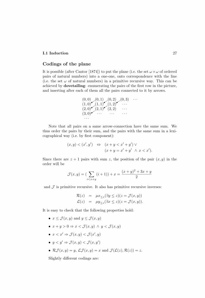
I.1 Induction 27
Codings of the plane
It is possible (after Cantor [1874]) to put the plane (i.e. the set ω×ω of orderedpairs of natural numbers) into a one-one, onto correspondence with the line(i.e. the set ω of natural numbers) in a primitive recursive way. This can beachieved by dovetailing: enumerating the pairs of the first row in the picture,and inserting after each of them all the pairs connected to it by arrows.
(0, 0) (0, 1) (0, 2) (0, 3) · · ·(1, 0) (1, 1) (1, 2) · · ·(2, 0) (2, 1) (2, 2) · · ·(3, 0) · · · · · · · · ·· · ·
+ + +
+ +
+
Note that all pairs on a same arrow-connection have the same sum. Wethus order the pairs by their sum, and the pairs with the same sum in a lexi-cographical way (i.e. by first component):
(x, y) < (x′, y′) ⇔ (x+ y < x′ + y′) ∨(x+ y = x′ + y′ ∧ x < x′).
Since there are z + 1 pairs with sum z, the position of the pair (x, y) in theorder will be
J (x, y) = (∑i<x+y
(i+ 1)) + x =(x+ y)2 + 3x+ y
2
and J is primitive recursive. It also has primitive recursive inverses:
R(z) = µx≤z(∃y ≤ z)(z = J (x, y))L(z) = µy≤z(∃x ≤ z)(z = J (x, y)).
It is easy to check that the following properties hold:
• x ≤ J (x, y) and y ≤ J (x, y)
• x+ y > 0 ⇒ x < J (x, y) ∧ y < J (x, y)
• x < x′ ⇒ J (x, y) < J (x′, y)
• y < y′ ⇒ J (x, y) < J (x, y′)
• RJ (x, y) = y, LJ (x, y) = x and J (L(z),R(z)) = z.
Slightly different codings are:

28 I. Recursiveness and Computability
1. By noting that each natural number different from 0 can be uniquelywritten as the product of an even (2x) and an odd (2y + 1) number, themap
(x, y) 7→ 2x(2y + 1)− 1.
2. By considering the 1’s in the binary expansion of natural numbers asmarkers, the map
(x, y) 7→ 1 0 . . . 0︸ ︷︷ ︸x times
1 0 . . . 0︸ ︷︷ ︸y times
= 2y + 2x+y+1.
This is not onto as a coding of pairs. But since every natural number canbe thought of as coding a finite sequence of natural numbers this way,this actually provides an onto coding of all finite sequences (Minsky[1967]).
Other codings will be considered in the next theorem (Godel’s function β)and in Section 7.
Elimination of primitive recursion
We have introduced two definitional schemata based on induction: primitiverecursion and µ-recursion. The next result shows that the former is subsumedunder the latter, modulo appropriate initial functions. The intuition comesfrom Peano Arithmetic, which is built only on plus, times and the inductionprinciple.
Theorem I.1.8 (Godel [1931], Kleene [1936a]) The class of recursivefunctions is the smallest class
1. containing sum, product, identities Ini and the characteristic function δof equality
2. closed under composition
3. closed under µ-recursion.
Proof. Let C be the smallest class satisfying the conditions of the theorem:clearly every function in C is recursive, and for the converse we only have toshow that the constant function O and the successor S are in C, and that C isclosed under primitive recursion.
Since 0 is the least number equal to 0,
On(~x) = µy(In+1n+1 (~x, y) = 0).

I.1 Induction 29
Also, since
δ(x, y) =
0 if x 6= y1 otherwise
and 1 is the least number different from 0,
1(x) = µy(δ(O2(x, y), I22 (x, y)) = 0)
= µy(δ(0, y) = 0) = 1S(x) = I1
1 (x) + 1(x).
The whole problem is thus to show the closure of C under primitive recur-sion. The idea is the following: we will show that it is possible to define in Ca function β such that for every finite sequence a0, . . . , an of natural numbersthere is one natural number a coding the sequence via β, i.e. such that
(∀i ≤ n)(β(a, i) = ai).
Then, if f is defined from g and h in C by primitive recursion as
f(~x, 0) = g(~x)f(~x, y + 1) = h(~x, y, f(~x, y))
we can code the sequence of values of f from 0 to y by using β:
t(~x, y) = µz[β(z, 0) = g(~x) ∧ (∀i < y)(β(z, i+ 1) = h(~x, i, β(z, i)))].
Since thenf(~x, y) = β(t(~x, y), y),
f will be in C if t is, and this is the case if C is closed under logical operations(including universal bounded quantifier). We thus have three steps to perform:
1. Existence of βThis is a purely number-theoretical argument. We want β s.t. for anysequence a0, . . . , an there is a s.t. for i ≤ n, β(a, i) = ai. We will try toget the ai’s as remainders of the division of a number c by given numbersd0, . . . , dn. That is, we want ai = rm(c, di). Then c = qidi + ai, ai < di.Suppose this holds for another c′: c′ = q′idi + ai. By subtracting we getc − c′ = (qi − q′i)di, i.e. the difference c − c′ is also divisible by di. Ifthe di are relatively prime, then c − c′ is also divisible by their productp = d0 · · · dn. This means that for different c, c′ < p we get differentsequences of remainders when dividing by di (otherwise c − c′ ≥ p).Moreover, any sequence of n + 1 numbers less than the di’s is obtained(since the number of possible sequences is p, and different c < p givedifferent sequences, i.e. we get them all). Then one of these sequences isthe given one a0, . . . , an.3
3This is the Chinese Remainder Theorem, so called because it was known to the Chinesealready in the VIth century B.C.
30 I. Recursiveness and Computability
We now have to obtain the di’s, with the stated conditions that they berelatively prime and ai < di.The easiest way to get them relatively prime is to consider the sequence
1 + d 1 + 2d · · · 1 + (n+ 1)d
for any d = s!, s ≥ n. (1 + rd, 1 + r′d are relatively prime since if qdivides both of them, then it also divides their difference (r − r′)d, andhence it divides d because r − r′ ≤ n is a factor of d = s!, since s ≥ n.But then q divides d and 1 + rd, i.e. it divides 1.) We also want thesenumbers to be greater than the respective ai’s: for this is enough to haved ≥ ai, hence s ≥ ai.We can then let di = 1 + (i + 1)d with d = s!, for any s greater than nand the ai’s. By coding c and d into a = J (c, d) we can actually define
β(a, i) = rm(c, di) = rm(c, 1 + (i+ 1)d)= rm(L(a), 1 + (i+ 1)R(a))
2. Closure of C under logical operationsFor the propositional connectives:
• negationWe need a function interchanging 0 and 1. Note that
δ(x, 0) =
0 if x 6= 01 otherwise
and thus c¬R(x) = δ(cR(x), 0).• disjunction
We need a function which is 0 exactly when both the arguments are0, i.e. when x + y = 0. Then d(x, y) = δ(δ(x + y, 0), 0) satisfies theneed, and cR∨S(x) = d(cR(x), cS(x)).
Closure under negation implies that in C we can apply the µ-operatordirectly to predicates:
µyR(~x, y) = µy(cR(~x, y) = 1) = µ(c¬R(~x, y) = 0).
• bounded µ-operatorWe use, in this proof only, the form
µy<zR(~x, y) =µyR(~x, y) if (∃y < z)R(~x, y)z otherwise
which is expressible in C as
µy<zR(~x, y) = µy(R(~x, y) ∨ y = z).
I.1 Induction 31
• bounded existential quantifierBy the particular form of bounded µ-operator defined above we have:
(∃y < z)R(~x, y) ⇔ (µy<zR(~x, y)) 6= z.
• The other operations are obtained by composition as usual, e.g.
R ∧ S ⇔ ¬(¬R ∨ ¬S)(∀y < z)R(~x, y) ⇔ ¬(∃y < z)¬R(~x, y)
3. Definition of β in CWe simply need to show that J ,R,L and rm are in C.
• J is defined as
J (x, y) =(x+ y)2 + 3x+ y
2Since in C we have sum, product and composition, we only need thefunction f(z) = z/2:
f(z) = µy(2y = z ∨ 2y + 1 = z)
• R and L are in C by their very definitions, e.g.
R(z) = µx(∃y < z + 1)(z = J (x, y))
• the remainder of the division of x by y is defined as
rm(x, y) = µz<y(∃q < x+ 1)(x = qy + z). 2
The use of Godel’s function β in the proof above can be avoided by usingdifferent codings. Of course the usual coding by prime numbers (see Section7) would not work here, since the relevant functions and predicates are de-fined by primitive recursion, which is exactly what we have to avoid. For veryelementary coding techniques, see Quine [1946] and Smullyan [1961].
Complementary results have been obtained by J. Robinson [1950], [1968],one of them being that the recursive functions of any number of variables canbe obtained, by composition alone, from the recursive functions of just one vari-able, plus sum and identities. And the recursive functions of just one variablecan be defined independently, without using functions of more variables, by theoperations of composition and inversion of onto functions (the latter clearlycorresponding to µ-recursion applied to regular predicates), from two (but notfrom only one) suitable initial functions.

32 I. Recursiveness and Computability
I.2 Systems of Equations
From a mathematical point of view a function is usually defined from a set ofequations, and we have used this fact informally in the previous section. Wenow undertake an analysis of the expressive power of systems of equations,bearing in mind that our concern is effective computability, and that we there-fore require not only a definition of a function, but also some way to computeit.
The formalism of equations
Definitions are linguistic objects, and we then need, first of all, an appropriatelanguage to express them. Also, since we are dealing with numerical functions,we need linguistic analogues of the numbers, which we can generate from 0 bythe successor operation. Our formalism thus consists of:
1. symbols
• equality ‘=’
• constants 0 (for the number 0) and S (for the successor operation)
• parentheses ‘(’ and ‘)’
• comma ‘,’ (to separate variables)
• variables x0, x1, . . . for numbers
• constants fn0 , fn1 , . . . for n-ary functions (for each n).
2. numerals
• 0 is a numeral
• if a is a numeral, so is S(a)
• nothing else is a numeral.
We will write n for the numeral Sn(0) representing the number n.
3. terms
• 0 is a term
• variables and 0-ary functional letters are terms
• if t is a terms then so is S(t)
• if t1, . . . , tn are terms then so is fni (t1, . . . , tn)
• nothing else is a term.

I.2 Systems of Equations 33
Note, in particular, that the numerals are terms.
4. equationsIf t and s are terms, and t is of the form fni (t1, . . . , tn) for some n, i andt1, . . . , tn not containing any functional letter except possibly S, thent = s is an equation.
The idea is that equations define functions by their right-hand sides, whileleft-hand sides just tell which functions are defined.
5. systems of equationsA system of equations is simply a finite set of equations.
We will write E(f1, . . . , fn;~z) for a system of equations whose functionalletters and numerical variables are all, respectively, among f1, . . . , fn, and~z.
Definability by systems of equations
The first thought that comes to mind is to consider systems of equations thatdefine functions uniquely w.r.t. a given letter (which we may always supposeto be f1):
Definition I.2.1 (Herbrand [1931]) A function f is definable by a sys-tem of equations if there is a system E such that:
1. there is a solution to the system:
(∃f1) . . . (∃fn)(∀~z)E(f1, . . . , fn;~z)
(i.e. there are functions satisfying every equation of E)
2. any solution determines uniquely f1 as f : for every f1, . . . , fn
(∀~z)E(f1, . . . , fn;~z) ⇒ (∀~x)(f1(~x) = f(~x))
(i.e. if f1, . . . , fn are solutions of E, then f1 = f).
Note that the existence condition 1) is necessary, otherwise any system ofequations E without solutions would define any function f , since then the clause(∀~z)E(f1, . . . , fn;~z) would be false, and the implication of condition 2) wouldbe vacuously true.
For our purposes of identifying computable functions this notion of defin-ability is however unsatisfactory, because each value f(~x) is determined (inde-pendently of ~x) by a global infinitary condition involving every ~z. Herbrandprobably intended the uniqueness condition 2) to be proved constructively,

34 I. Recursiveness and Computability
and such a proof would probably give an explicit computation procedure forf . But, we do not have a precise notion of constructiveness (after all, we areprecisely trying to characterize the related notion of effectiveness). And froma classical standpoint the class of functions definable by systems of equationsis too comprehensive (although mathematically very interesting), and it verymuch transcends the class of recursive functions (Kalmar [1955]): it coincideswith the class of hyperarithmetical functions (Grzegorczyck, Mostowskiand Ryll-Nardzewski [1958]), which will be studied in Volume III (see alsop. 391).
Computations, whatever they might be, are certainly finite objects andthus each value f(~x) should be uniquely determined by just a finite amountof information. We are thus led to the following modification of the notionintroduced above.
Definition I.2.2 (Kreisel and Tait [1961]) A function f is finitely de-finable by a system of equations if there is a system E such that:
1. (∃f1) . . . (∃fn)(∀~z)E(f1, . . . , fn;~z)
2. for every ~x there is a finite set ~z1, . . . , ~zp (p depending on ~x) such thatthe substitution instances of E by them determines the value of f(~x), i.e.such that for every f1, . . . , fn
E(f1, . . . , fn; ~z1) ∧ · · · ∧ E(f1, . . . , fn; ~zp) ⇒ f1(~x) = f(~x).
For example, the system of equations (written informally)
f(0) = 0 f(x+ 1) = f(x) + 2 g(x) = f(g(x))
defines (for every x) f(x) = 2x and g(x) = 0. Here f is finitely defined (bythe first two equations), while g is not: indeed g is uniquely determined by theinfinite set of equations
g(0) = 2 · g(1) = 4 · g(2) = . . .
but there are infinitely many solutions to any finite subset of these equations.
Theorem I.2.3 (Herbrand [1931], Godel [1934], Kleene [1935]) Everyrecursive function is finitely definable.
Proof.

I.2 Systems of Equations 35
1. initial functionsO,S and Ini are, respectively, finitely defined by:
f10 (x0) = 0f10 (x0) = S(x0)
fn0 (x1, . . . , xn) = xi.
2. compositionSuppose gi(x1, . . . , xn) (i = 1, . . . ,m) and h are finitely defined, respec-tively, by Ei and E w.r.t. fni and fmm+1 (by changing the letters if needed,we can always reduce to this case). Then
f(x1, . . . , xn) = h(g1(x1, . . . , xn), . . . , gm(x1, . . . , xn))
is finitely defined by E1 ∪ · · · ∪ Em ∪ E together with
fn0 (x1, . . . , xn) = fmm+1(fn1 (x1, . . . , xn), . . . , fnm(x1, . . . , xn)).
Of course we must suppose (here and in the following) that there areno conflicts of functional letters in E1, . . . , Em, E (which can always beachieved by possible changes of letters).
3. primitive recursionIf g and h are finitely defined by E1 and E2 w.r.t. fn0 and fn+2
0 then
f(x1, . . . , xn, 0) = g(x1, . . . , xn)f(x1, . . . , xn, y + 1) = h(x1, . . . , xn, y, f(x1, . . . , xn, y)).
is finitely defined by E1 ∪ E2 together with
fn+10 (x1, . . . , xn, 0) = fn0 (x1, . . . , xn)
and
fn+10 (x1, . . . , xn,S(xn+1)) =
fn+20 (x1, . . . , xn, xn+1, f
n+10 (x1, . . . , xn, xn+1)).
4. µ-recursionIf g is finitely defined by E1 w.r.t. fn+1
0 and
f(x1, . . . , xn) = µy(g(x1, . . . , xn, y) = 0)

36 I. Recursiveness and Computability
then let E be E1 plus the equations defining sum and product (which areprimitive recursive, and for which we then already have finite definabil-ity), together with
f10 (0) = 0 f1
0 (S(x0)) = 1f11 (0) = 1 f1
1 (S(x0)) = 0
and the formal translations of the following:
fn+11 (x1, . . . , xn, xn+1) =
f10 (fn+1
0 (x1, . . . , xn, xn+1)) · fn+11 (x1, . . . , xn,S(xn+1))
+ f11 (fn+1
0 (x1, . . . , xn, xn+1)) · xn+1
fn0 (x1, . . . , xn) = fn+11 (x1, . . . , xn, 0).
Then E finitely defines f w.r.t. fn0 , because the system just translates thefollowing facts: it defines
h(~x, y) =y if g(~x, y) = 0h(~x, y + 1) otherwise
w.r.t. fn+11 (by using two auxiliary functions f1
0 and f11 to allow for case
distinction), and then it defines
f(~x) = h(~x, 0)
w.r.t. fn0 . Indeedh(~x, 0) = µy(g(~x, y) = 0)
because if µy[g(~x, y) = 0] = z then
h(~x, 0) = h(~x, 1) = · · · = h(~x, z) = z.
Note that E has solutions: the only trouble might come from fn+11 , but
here the natural interpretation applies: either for a given ~x there areinfinitely many y’s such that g(~x, y) = 0, and then the definition of fn+1
1
is the natural step function, or there are only finitely many such y’s, andthen any function constant from the last one of such y’s would work. 2
Derivability from systems of equations
Having shown that every recursive function is finitely definable by systems ofequations (in logical terms), we would also like to concoct explicit rules to ob-tain the values of a function from a system of equations finitely defining it, thus
I.2 Systems of Equations 37
determining a syntactical counterpart to the semantical notion of finite defin-ability. Since this amounts to finding an appropriate formal system (capturinga notion of validity for a given interpretation) we have as natural candidatesthe analogues of well-known rules used for logical formal systems: substitutionand cut.
Definition I.2.4 (Godel [1934]) An n-ary function f is Herbrand-Godelcomputable if there is a finite system of equations E such that if fni is theleftmost letter in the last equation of E, then
f(a1, . . . , an) = b
holds if and only if the equation
fni (a1, . . . , an) = b
can be derived from E by means of the following two rules:
R1 Substitution of a numeral for every occurrence of a particular variablein an equation.
R2 Replacement in the right-hand side of an equation of a term of the formfmj (c1, . . . , cm) with a numeral d, provided fmj (c1, . . . , cm) = d has alreadybeen derived.
We say that E defines f w.r.t. the letter fni .
Theorem I.2.5 (Herbrand [1931], Godel [1934], Church [1936],Kleene [1936]) Every recursive function is Herbrand-Godel computable.
Proof. We consider here the systems of equations defined in the proof ofTheorem I.2.3. There are two things to prove:
1. Completeness property (the values can be deduced from the appropriatesystems of equations).
This is quite evident from the informal discussion of I.2.3.
2. Consistency property (no other value can be deduced, i.e. the values areuniquely determined).
This follows by induction on the construction of the systems. As anexample, we show the case of primitive recursion (with notations as inI.2.3). Suppose
fn+10 (x1, . . . , xn, y) = b
has been derived. There are two cases:

38 I. Recursiveness and Computability
• y = 0Then, since R2 only allows for replacement on the right-hand side,and since there is only one equation with fn+1
0 (x1, . . . , xn, 0) on theleft-hand side, it follows that
fn+10 (x1, . . . , xn, 0) = fn0 (x1, . . . , xn)
fn0 (x1, . . . , xn) = b
have been previously derived. But the consistency property holdsfor fn0 by induction hypothesis.
• y = S(z)Then, as in the above case, an equation
fn+10 (x1, . . . , xn,S(z)) =
fn+20 (x1, . . . , xn, z, f
n+10 (x1, . . . , xn, z))
must have been derived. Note that by definition there can be noequation with the left-hand side like the right-hand side of the aboveequation. Also, R2 only allows for replacement of terms of the form:functional letter followed by numerals. Then equations like
fn+10 (x1, . . . , xn, z) = a fn+2
0 (x1, . . . , xn, z, a) = b
must have been derived. But then again the induction hypothesisapplies. 2
In Section 7 we will prove that the syntactical notion of Herbrand-Godelcomputability and the semantical notion of finite definability are globally equiv-alent, by showing them equivalent to recursiveness. Also, by the proof justgiven, every recursive function is Herbrand-Godel computable from a system ofequations finitely defining it . But the two notions are not locally equivalent, inthe sense that given a system E the following may happen:
1. g can be finitely defined by E without being Herbrand-Godel computablefrom it , as the system
f(x) = 0 f(x) = h(x) g(x) = h(x).
and the function g(x) = 0 show. This simply results from the fact thatthe rules R1 and R2 are of a very specific form, and do not even allowfor full logical substitution of equal entities.
2. g can be Herbrand-Godel computable from E without being finitely definedby it , as the system
f(0) = 0 f(S(x)) = S(f(S(x))) g(x) = f(0)

I.3 Arithmetical Formal Systems 39
and the function g(x) = 0 show. Here Herbrand-Godel computabilityfollows because only f(0) is used among the values of f , but finite defin-ability fails because there is no total function f satisfying every equation(since f(z) = f(z) + 1 for z > 0).
Kreisel and Tait [1961] isolate a notion of derivability from systems of equa-tions, which is locally equivalent to finite definability. Basically, the rules cor-respond to the logical axioms for equality and successor. See Statman [1977]for a proof-theoretical analysis.
Herbrand-Godel computability has the advantage of using simple rules, andthe disadvantage of not being complete, in the sense of not allowing the deriva-tion of everything which is logically derivable.
A logical programming language ?
Note that an equation can be put into a normal form of the kind
R1 ∧ · · · ∧Rn → Q
with Ri, Q atomic equations of the form fnj (x1, . . . , xn) = y and xi, y variablesor constants (the interpretation of variables being that they are all universallyquantified). For example,
f(x) = g(h(x))
can be written ash(x) = y ∧ g(y) = z → f(x) = z.
Then the previous results show that the values of recursive functions can belogically deduced from axioms of the described kind.
The programming language PROLOG(Programming in Logic, Colmer-auer, Kanoui, Pasero and Roussel [1972], Kowalski and Van Emden [1976]) isbased on logical deductions from clauses of the form above, with Ri, Q atomicrelations holding of terms. These are called Horn clauses, and are especiallyinteresting because proof procedures for them are particularly manageable.They can be thought of as conditions breaking up a goal Q into a series ofsubgoals Ri. The results of this section show that PROLOG, although con-cocted to handle deductive more than computational problems, has neverthelessthe power of computing all the recursive functions.
I.3 Arithmetical Formal Systems
The general trend of this century’s mathematics has been to work in formalsystems which are supposed to capture, more or less accurately, some aspects
40 I. Recursiveness and Computability
of the objects in which we are interested. From a formalistic point of view wecan thus consider a function as computable when we have a consistent formalsystem representing it, i.e. allowing us to prove for the appropriate numbers(and for nothing else) that they are the function’s values for given arguments.
Certainly the approach of Herbrand-Godel computability falls in this trend,but the formal system involved there, concocted for different goals, is somewhatunnatural from a purely arithmetical point of view. The same will be true of theapproach of λ-definability, see Section 6. Since we are considering arithmeticalfunctions, it is natural to investigate which functions are representable in theusual logical systems for arithmetic, for example in Peano Arithmetic (seep. 24).
We attack the problem in a general way, by isolating minimal conditions(which will turn out to be very weak) sufficient to represent every recursivefunction. In this section, ‘formal system’ will always mean ‘formal systemextending first-order logic with equality, and having constants terms n, callednumerals, for each n’. For more details on formal systems, see p. 350.
Notions of representability
Definition I.3.1 (Tarski [1931], Godel [1931], [1934], Tarski, Mostow-ski and Robinson [1953]) Given a formal system F and a function f , wesay that:
1. f is weakly representable in F if, for some formula ϕ of the languageof F ,
f(x1, . . . , xn) = y ⇔ `F ϕ(x1, . . . , xn, y)
2. f is representable in F if, for some formula ϕ,
f(x1, . . . , xn) = y ⇒ `F ϕ(x1, . . . , xn, y)f(x1, . . . , xn) 6= y ⇒ `F ¬ϕ(x1, . . . , xn, y)
3. f is strongly representable in F if for some formula ϕ, f is repre-sentable by ϕ, and moreover the following uniqueness condition holds:
`F (∀y)(∀z)[ϕ(x1, . . . , xn, y) ∧ ϕ(x1, . . . , xn, z) → y = z].
The relationships among the various notions are: if f is strongly repre-sentable then it is representable, and if f is representable in a consistent formalsystem then it is weakly representable (because if F is consistent and `F ¬ϕthen 6`F ϕ).

I.3 Arithmetical Formal Systems 41
Exercises I.3.2 a) The two conditions
f(x1, . . . , xn) = y ⇒ `F ϕ(x1, . . . , xn, y)
`F (∀y)(∀z)[ϕ(x1, . . . , xn, y) ∧ ϕ(x1, . . . , xn, z) → y = z]
are equivalent to the unique condition
`F (∀y)[ϕ(x1, . . . , xn, y) ↔ y = f(x1, . . . , xn)].
b) If F is such that
x 6= y ⇒ `F ¬(x = y)
then strong representability of f in F is equivalent to the unique condition
`F (∀y)[ϕ(x1, . . . , xn, y) ↔ y = f(x1, . . . , xn)].
Proposition I.3.3 (Tarski, Mostowski and Robinson [1953]) If F is aconsistent formal system with a predicate < satisfying the axiom schemata
1. ¬(x < 0)
2. x < n+ 1 ↔ x = 0 ∨ · · · ∨ x = n
3. x < n ∧ x = n ∧ n < x
then any function representable in F is strongly representable in it.
Proof. Suppose ψ represents f in F . Then the formula
ϕ(x1, . . . , xn, y) ⇔ ψ(x1, . . . , xn, y) ∧ (∀z < y)¬ψ(x1, . . . , xn, z)
strongly represents f . Indeed:
• If f(x1, . . . , xn) = y then f(x1, . . . , xn) 6= z, for every z < y. By repre-sentability of f via ψ
`F ¬ψ(x1, . . . , xn, 0) ∧ · · · ∧ ¬ψ(x1, . . . , xn, y − 1) ∧ ψ(x1, . . . , xn, y).
Axioms 1 and 2 (depending on whether y = 0 or y > 0) take care of allthe z < y in the first part of the formula. Thus
`F ψ(x1, . . . , xn, y) ∧ (∀z < y)¬ψ(x1, . . . , xn, z)
(if y = 0 the second part is vacuously true, since there is no z < y), and`F ϕ(x1, . . . , xn, y).

42 I. Recursiveness and Computability
• If f(x1, . . . , xn) 6= y then, by representability, `F ¬ψ(x1, . . . , xn, y) andso `F ¬ϕ(x1, . . . , xn, y).
• To show the uniqueness condition we prove (see I.3.2.a) that
`F (∀y)[ϕ(x1, . . . , xn, y) ⇔ y = f(x1, . . . , xn)].
We have `F ϕ(x1, . . . , xn, f(x1, . . . , xn)) from the first part of the proof.Suppose now `F ϕ(x1, . . . , xn, y). By axiom 3 the only possibilities are
y < f(x1, . . . , xn) ∨ y = f(x1, . . . , xn) ∨ f(x1, . . . , xn) < y.
The first one is ruled out, since from `F ϕ(x1, . . . , xn, f(x1, . . . , xn)) wehave `F ¬ψ(x1, . . . , xn, y), while from `F ϕ(x1, . . . , xn, y) (assumed byhypothesis) we have `F ψ(x1, . . . , xn, y), and F is consistent. Similarlywe can rule out f(x1, . . . , xn) < y. Then y = f(x1, . . . , xn). 2
The notion of representability makes sense for predicates as well:
Definition I.3.4 Given a formal system F and a relation R, we say that:
1. R is weakly representable if, for some ϕ,
R(x1, . . . , xn) ⇔ `F ϕ(x1, . . . , xn)
2. R is representable if, for some ϕ,
R(x1, . . . , xn) ⇔ `F ϕ(x1, . . . , xn)¬R(x1, . . . , xn) ⇔ `F ¬ϕ(x1, . . . , xn).
Note that if the characteristic function cR of R is (weakly) represented byϕ(x1, . . . , xn, z), then R is (weakly) representable by ϕ(x1, . . . , xn, 1). Also, ifF is such that
x 6= y ⇒ `F ¬(x = y)
and R is represented by ϕ(x1, . . . , xn), then cR is (strongly) representable by
(ϕ(x1, . . . , xn) ∧ z = 1 ) ∨ (¬ϕ(x1, . . . , xn) ∧ z = 0 )
(this follows from I.3.2.b). Note that the axioms are needed even for simplerepresentability of cR, because when cR(x1, . . . , xn) 6= z and z 6= 0, 1 we needto know z 6= 0, 1 to be able to infer that the formula intended to represent cRis not provable.

I.3 Arithmetical Formal Systems 43
Formal systems representing the recursive functions
Note that if f(x1, . . . , xn) = µyR(x1, . . . , xn, y) then
f(x1, . . . , xn) = y ⇔ R(x1, . . . , xn, y) ∧ (∀z < y)¬R(x1, . . . , xn, z).
The axioms of proposition I.3.3 then imply, by means of the same proof, thatthe strongly representable functions are closed under µ-operator. We turn nowto the other conditions.
Proposition I.3.5 (Tarski, Mostowski and Robinson [1953]) If F is aformal system such that
x 6= y ⇒ `F ¬(x = y)
then the functions strongly representable in F are closed under composition.
Proof. Supposef(~x) = h(g1(~x), . . . , gm(~x))
and g, hi are strongly represented by, respectively, χ and ψi. Then f is stronglyrepresented by
ϕ(~x, y) ⇔ (∃y1) . . . (∃ym)[ψ1(~x, y1) ∧ · · · ∧ ψm(~x, ym) ∧ χ(y1, . . . , ym, y)].
To show this we use (since we have the appropriate axioms for F) the form ofstrong representability given in I.3.2.b. Then:
• if f(~x) = y let hi(~x) = yi and g(y1, . . . , ym) = y, so that `F ψi(~x, yi) and`F χ(y1, . . . , ym, y). Then `F ϕ(~x, y) and `F ϕ(~x, f(~x)).
• if `F ϕ(~x, y) let y1, . . . , ym be such that
`F ψ1(~x, y1) ∧ · · · ∧ ψm(~x, ym) ∧ χ(y1, . . . , ym, y).
By strong representability it must be yi = hi(~x) and thus
y = g(h1(~x), . . . , hm(~x)) = f(~x). 2
We are now ready to conclude our search for axioms which allow repre-sentability of every recursive function.
Theorem I.3.6 (Godel [1936], Mostowski [1947], Tarski, Mostowskiand Robinson [1953]) In any formal system F with a predicate < and func-tions + and · satisfying the following axiom schemata, any recursive functionis (strongly) representable (and thus, if the system is consistent, also weaklyrepresentable):

44 I. Recursiveness and Computability
B1 ¬(x = y), for x 6= y
B2 x < n ∨ x = n ∨ n < x
B3 ¬(x < 0)
B4 x < n+ 1 ↔ x = 0 ∨ · · · ∨ x = n
B5 x + y = x+ y
B6 x · y = x · y
Proof. We refer to the characterization of recursive functions given in Theo-rem I.1.8. We have just proved that closure under composition is implied byB1, and closure under µ-recursion follows from B2–B4, as in I.3.3. It thensuffices to note that:
• Equality is representable because if x = y then obviously `F x = y, andif x 6= y then `F ¬(x = y) by B1. Then its characteristic function isrepresentable too.
• Sum is representable by
ϕ(x, y, z) ⇔ x+ y = z.
Indeed, if x + y = z then `F x+ y = z and (by B5) `F x + y = z,i.e. `F ϕ(x, y, z). And if x + y 6= z then `F ¬(x+ y = z) by B1 and`F ¬(x+ y = z) by B5, i.e. `F ¬ϕ(x, y, z).
• Product is similarly represented by
ϕ(x, y, z) ⇔ x · y = z.
• Identities Ini are obviously represented by
ϕ(x1, . . . , xn, z) ⇔ z = xi. 2
The axioms B1–B6 define a theory R with infinitely many axioms. Tarski,Mostowski and Robinson [1953] show that R is not finitely axiomatizable, sinceany finite subset of the axioms (and thus, by compactness, any finite set oftheorems) admits a natural finite model consisting (for n sufficiently big) of thenumbers 0, 1, . . . , n naturally ordered, and having the operations restrictedto value equal to n when the original value would exceed it. Of course Rcannot have a finite model (by B1) and thus it is not reducible to a finite set oftheorems. This also proves that any closed theorem of R is true in some finite

I.3 Arithmetical Formal Systems 45
model, and thus the power of R is very limited. Theorem I.3.6 is, thus, verygeneral.
Local improvements of Theorem I.3.6 are possible however, as Cobham (seeVaught [1960]) and Jones and Shepherdson [1983] have shown. The conclusionstill holds if B2 and B5 are dropped. Moreover, by changing the language andintroducing a predicate ≤ in place of <, B2–B4 may be reduced to two axiomschemata
x ≤ n ∧ n ≤ x
x ≤ n ↔ x = 0 ∨ · · · ∨ x = n.
Robinson Arithmetic Q (see p. 23) is an extension of R, and thus providesan example of a finitely axiomatized theory in which every recursive functionis representable. Robinson has proved that if any one of the axioms of Q isremoved, then some recursive function is not strongly representable. Thus Qis a minimal finitely axiomatizable theory in which every recursive function isstrongly representable. For details and more information, see Tarski, Mostowskiand Robinson [1953].
Invariant definability ?
Every model A of R has a submodel isomorphic to ω, which is called thestandard part of the model and is still denoted by ω. Given a formula ϕ anda subset A of the universe of A, we say that A is defined by ϕ in A if
A = x : A |= ϕ(x)
(where |= is the usual notion of satisfaction in a structure, see IV.1.1). A isdefined on ω by ϕ in A if
A = ω ∩ x : A |= ϕ(x).
We can also introduce uniform versions of these notions, by saying that A isinvariantly defined (on ω) by ϕ if A is defined (on ω) by the same ϕ inevery model A of R.
The Compactness Theorem implies that a set is invariantly definable if andonly if it is a finite subset of ω, while the proof of I.3.6 (together with theresults of Section 7) shows that invariant definability on ω and recursivenesscoincide (Kreisel [1965a]). Thus we have a purely model-theoretical reformu-lation of recursiveness, and by changing the class of models one gets naturalgeneralizations of it (see Mostowski [1962] and Kreisel [1965a]), some of whichwill be considered in Volume III.
Note that the reformulation of finiteness explains the need of consideringthe relative notion of invariant definability: ω is not invariantly definable in

46 I. Recursiveness and Computability
models of R. For models of PA a stronger fact is true: ω is not even definablein a single nonstandard model of PA. Indeed, given a formula ϕ defining aset A, consider ¬ϕ. If there is no element satisfying it then A is the wholeuniverse, which is nonstandard. If there is an element satisfying ¬ϕ then, bythe Axiom of Induction, there is a minimal one x, which is not in A because¬ϕ(x) holds. If x is 0 or the successor of a standard element then A does notcontain all standard elements. If x is the successor of a nonstandard elementy then, by minimality of x, ϕ(y) holds and A contains a nonstandard element.In any case, A is not ω.
Definability of functions ?
We say that f is definable in F if for some term t(~x), `F t(~x) = f(~x). IfF satisfies B1 then definability implies strong representability (by the formulat(~x) = z, see I.3.2). But definability is not an absolute notion, since thefact that a function is definable is quite accidental and simply depends onthe functional constants of the theory language. For example, in RobinsonArithmetic only polynomials are definable, because the language has only thefunction symbols S,+ and · .
By extending a theory with axioms for a formal analogue of the µ-operator,namely
(∃z)A(z) → A(µyA(y))(∀z)¬A(z) → (µyA(y) = 0)(∀z)[z < µyA(y) → ¬A(z)],
every function which is strongly representable by ϕ(~x, y) becomes definableby µyϕ(~x, y). In particular, there are formal systems in which every recursivefunction is definable.
In any theory with a predicate <, a functional symbol f can be introducedin a conservative way (i.e. not producing new theorems in the old language) forany function which is strongly represented by ϕ(~x, y), together with the axioms
ϕ(~x, f(~x))(∀z)[z < f(~x) → ¬ϕ(~x, z)]
In any theory with the Axiom of Induction (e.g. Peano Arithmetic andits extensions) the same can be done even more generally, in the sense thatonly (∃y)ϕ(~x, y) is required, instead of strong representability. The provableexistence of µyϕ(~x, y) then follows by the Least Number Principle.
From I.7.7 it follows that functions definable in consistent formal systemssatisfying B1 are recursive, since in this case definability implies representabil-ity, as noted above.
I.4 Turing Machines 47
I.4 Turing Machines
We have been analyzing the notion of effectiveness by taking our inspirationfrom mathematical activity. We now switch our point of view and begin ananalysis based on computational activity, by providing a model of certain as-pects of human behavior during routine computations. The final goal is tounderstand what we are doing when we compute, in such a way to be able tosimulate this activity by a machine. In this section we present the analysis ofTuring [1936] and Post [1936].
In doing a computation we are given an input and then produce an output,usually after an appropriate amount of written calculations. Fortunately, forthe pure writing activity we already have a mechanical device: the type-writer. On it we base our model. We may imagine our abstract machine asbeing capable of printing symbols on paper. In real life writing is usuallydone on planar sheets of paper, but since we write in consecutive (horizontalor vertical) lines we may simplify, and just think of our machines as writing ona linear tape. Since we do not put a priori bounds on the amount of scratchwork needed for a computation, we think of our tape as potentially infinite inboth directions (i.e. we suppose that we are always able to glue more tape ateither end, when needed). Also, since symbols are actually (or can be) writtenone at a time, we think of our tape as consisting of cells, each of which cancontain a single symbol.
Although we might, in general, need symbols for infinitely many entities(e.g. one for each number), we can certainly use complex symbols (like words)built up from a finite stock of atomic ones (like letters). Thus our machine willsimply be capable of printing symbols from a finite alphabet, as in real life.And as in concrete typewriters, we allow for the possibility of two directionsof movement along the tape, one cell at a time. Movement is necessary toprint symbols in different cells, and the two directions allow for a recall of thework already done. It does not matter whether we picture the situation as anactual movement of the tape, or of the machine, or even just of an extendibletelescopic arm examining the tape and transmitting the information to themachine. Since we can come back to cells containing a printed symbol, weallow for the possibility of erasing it (as modern typewriters can do).
An abstract human being can carry on his computation by using just suchan abstract machine for his explicit writing activity, but his assistance is atthis point obviously still necessary (as it would be for writing something by atypewriter). We now take advantage of our restriction to routine work: no stepmust require ingenuity, and thus each move must be automatically carried onon the basis of the previous work. In particular, the machine needs a memory,i.e. a way to recall the crucial features of what it has already done.
One possible way to implement this requirement is to think of the machine
48 I. Recursiveness and Computability
as being at each moment in some particular physical state, determined by theprevious action up to this point, and determining the successive action. As asimple example, consider once again the typewriter: one possible routine de-cision that is done when we write something in most western languages is tobegin a word coming after a dot with a capital letter. We might thus builda typewriter that automatically steps, after printing a dot, from its currentwriting state to the state for printing capital letters (in actual machines thischange of state is obtained by pushing an appropriate key). If we allow for suf-ficiently (possibly infinitely) many states we can certainly record any action: itis enough to consider the tree of all possibilities, associate states to its nodesand, by representing possible actions as paths of the tree, to change states byfollowing a given path. But infinitely many states would contradict the intu-ition both of routine work (as the implementation of an effectively describabletask) and of machine (as a device of limited complexity). We thus impose thelimitation of having only finitely many states.
To be able to work automatically, the machine must perform its elementaryoperations according to given instructions, telling it what to do on the basisof given information. Some of this information reaches the machine throughits internal memory (codified by the current state), but other (in particularthe input) might be fed from outside. The connections with the outer world(the tape) consists not only in getting, but also in providing information (theoutput among others) and it may be pictured (following the parallel with thetypewriter) as happening through a head, which is both able to read andwrite. Since the tape consists of cells, the head’s range of action will just beone single cell, both statically (when reading and printing) and dynamically(when moving).
It is clear at this point that only finitely many instructions are needed,specifying what to do in a given situation. Indeed, there are only finitely manypossible local situations (determined by state and read symbol) and actions(consisting in printing or erasing a symbol, possibly moving the head one cellleft or right, and possibly changing state).
We need not analyze the actual physical implementation of the machinework. Just imagine the existence of a black box, which somehow knows theinstructions and the way to carry them out (for more on this see the remarkson pp. 53 and 117). Thus the machine hardware consists of a tape, a headand a black box. It can be pictured as follows:
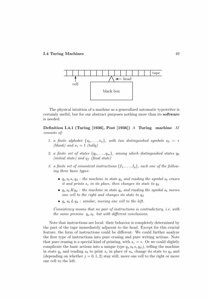
I.4 Turing Machines 49
AA head
tape
black box
6
cell
The physical intuition of a machine as a generalized automatic typewriter iscertainly useful, but for our abstract purposes nothing more than its softwareis needed:
Definition I.4.1 (Turing [1936], Post [1936]) A Turing machine Mconsists of:
1. a finite alphabet s0, . . . , sn, with two distinguished symbols s0 = ∗(blank) and s1 = 1 (tally)
2. a finite set of states q0, . . . , qm, among which distinguished states q0(initial state) and qf (final state)
3. a finite set of consistent instructions I1, . . . , Ip, each one of the follow-ing three basic types:
• qa sb sc qd : the machine in state qa and reading the symbol sb erasesit and prints sc in its place, then changes its state to qd
• qa sbRqd : the machine in state qa and reading the symbol sb movesone cell to the right and changes its state to qd
• qa sb L qd : similar, moving one cell to the left.
Consistency means that no pair of instructions is contradictory, i.e. withthe same premise qa sb but with different conclusions.
Note that instructions are local: their behavior is completely determined bythe part of the tape immediately adjacent to the head. Except for this crucialfeature, the form of instructions could be different. We could further analyzethe first type of instructions into pure erasing and pure writing actions. Notethat pure erasing is a special kind of printing, with sc = ∗. Or we could slightlycomplicate the basic actions into a unique type qa sb sc qd j, telling the machinein state qa and reading sb to print sc in place of sb, change its state to qd and(depending on whether j = 0, 1, 2) stay still, move one cell to the right or moveone cell to the left.

50 I. Recursiveness and Computability
An instantaneous configuration of the machine is a complete recordingof all the relevant data in a given instant. It can be represented by a sequence
σ1 . . . σj qa σj+1 . . . σz
in which all the consecutive symbols σi (including the blanks) written in therelevant portion of the tape (at least the one between the two outermost non-blank symbols) are indicated, together with the state and the head position(shown by the position of the state symbol among the alphabet symbols). Thusthe sequence above records the following situation:
AA qa -blanks blanks
∗ ∗ ∗ ∗ ∗ ∗σ1 σj σz· · · · · ·
The machine behavior can be represented by a sequence of instantaneousconfigurations, each obtained from the previous one by application of a neces-sarily unique instruction, and starting from an initial configuration (codingthe input and the initial state). A final configuration is reached when themachine finds itself in the final state, and we say figuratively that the machinestops. An alternative formulation, not using final states, simply states: themachine stops when no instruction is applicable.
We will show in I.4.2 how a Turing machine can compute a function, whichis our real concern. Before that we discuss Turing machines in more detail, butthe interested reader can skip this, and go directly to p. 54.
Variations of the Turing machine model
The particular model of a Turing machine introduced in definition I.4.1 isabsolutely unimportant, as long as we are only concerned with computationalpower and not with efficiency. Since in this book we do not deal with machinetheory (although we will prove some scattered results in Chapter VIII), we willonly quote some facts, and refer to Minsky [1967], Arbib [1969] and Hopcroftand Ullman [1979] for their proofs and for further information.
States. Although only one state is not in general enough to compute everyrecursive function (Shannon [1956], Wang [1957]: basically, a one-stateTuring machine must behave in the same way on every cell outside theinput), two states are (Shannon [1956]). Thus it is not relevant whetherwe restrict our model to machines with only a fixed number n ≥ 2 ofstates, or we allow any number of states.
I.4 Turing Machines 51
Symbols. Clearly we must have at least two symbols, since we consider blankas a symbol. Two symbols are enough to compute any recursive function(Shannon [1956]), since it is possible to economize on the number ofsymbols by increasing the number of states. See Priese [1979] for resultsconcerning the simultaneous economy of states and symbols.
Erasing. This is dispensable (Wang [1957]), in the sense that all the recursivefunctions can be appropriately computed by machines that never erase.Basically, given a Turing machine it is possible to simulate it by a newnonerasing machine, that writes on its tape codes of successive configu-rations of the original machine. The result shows that in principle we donot need erasable material, like magnetic tapes or disks, for the externalmemory of computers. See also p. 52.
Tapes and heads. Here the freedom is practically absolute. We synthesizeit in the following result. A Turing machine with finitely many tapes,each with its own (finite, or even countable) dimension and its own finitenumber of heads simultaneously scanning it, can be simulated by a Turingmachine with only one linear tape, infinite in just one direction, andscanned by a single head (Hartmanis and Stearns [1965]). However, wedo need the two directions of movement, since to restrict it to one wouldbe compatible only with finite or periodical behavior on cells outside theinputs (Wang [1957]).
Determinism. Our model of a Turing machine is deterministic, in the sensethat the instructions are required to be consistent (at most one of themis applicable in any given situation). Randomizing elements in comput-ing devices were introduced early on by Shannon [1948] and De Leeuw,Moore, Shannon and Shapiro [1956]. There are basically two models.Nondeterministic Turing machines behave, in an ambiguous situationwhere conflicting instructions might be applicable, by randomly choosingone of them: their computational power, at least for 0, 1-valued functions(sets), does not exceed the power of deterministic ones. Probabilisticmachines differ from nondeterministic ones in that the next state has aprobability, and thus conflicting instructions do not have the same chanceof being chosen by the machine.
Physical Turing machines ?
Turing machines are theoretical devices, but have been designed with an eye tophysical limitations. In particular, we have incorporated in our model restric-tions coming from: (a) atomism, by ensuring that the amount of informationthat can be coded in any configuration of the machine (as a finite system) is

52 I. Recursiveness and Computability
bounded; and (b) relativity, by excluding actions at a distance, and makingcausal effect propagate through local interactions. Gandy [1980] has shownthat the notion of a Turing machine is sufficiently general to subsume, in aprecise sense, any computing device satisfying similar limitations.
However, there is at least one aspect which has been neglected in our dis-cussion, namely energy consumption. This is a central problem especiallyfor actual modern computers, whose sizes are getting increasingly bigger. Thepoint is that in devices with packed components, energy dissipation is pro-portional to volume, while heat removal is proportional only to surface. Toprovide adequate cooling, it would thus seem necessary to expand machinesonly in two dimensions, and keep them flat and thin. But this would mean aspread of components in space and an increase in the time needed to transmitinformation, thus a decrease in speed. It is then crucial to limit energy con-sumption in computations, not only for costs limitation, but also for physicalrealization.
At a macroscopical level, energy seems to be needed in at least two differentways. First of all, physical computations involve data handling (like storing andtransmitting), and thus measurements: this implies energy consumption. Sec-ondly, Turing machines and real computers are irreversible devices (manysets of inputs may produce the same output, and it is usually impossible toinvert computations): this implies energy dissipation. Theoretical bounds onenergy requirements have been computed by various authors (e.g. from theuncertainty principle ∆E ·∆t ≈ h, by arguing that if ∆t represents a switch-ing time, then ∆E must represent energy dissipation). See Landauer [1961],Bremermann [1962], [1982], and Mundici [1981].
At a microscopical level, dynamical physical laws are reversible: it is thusnatural to look for reversible models of Turing machines. Logical reversibil-ity (of rules) is easy to achieve (Bennett [1973]). First note that a computationcan be trivially simulated in a reversible way, by having an extra tape that suc-cessively records the quadruples of the Turing machine used, so that the presentconfiguration, and the last record on the history tape, allow for a recovery ofthe previous configuration. Then note that erasing a computation done byreversible rules is also reversible, and that it can be done after the output hasbeen copied (to be saved) on a separate blank tape: no record is needed at thisstage, since copying onto a blank tape is a one-one operation. Then the wholecomputation, including the erasure of scratch work, can be done by reversiblerules. The next step is to look at energetic reversibility. Bennet [1973] andLandauer [1976] provide Brownian models for any finite computation on Turingmachines, dissipating arbitrarily little energy when proceeding slowly enough.The final step is to look for plainly conservative models of Turing machines,not dissipating any energy at all, while computing at finite speed. For classicalmechanics, Fredkin and Toffoli [1982] give a ballistic model consisting of hard
I.4 Turing Machines 53
spheres (whose presence or absence in a constant flow code digits 1 or 0) thatcollide elastically with each other and with fixed barriers placed inside the com-puter (see also Landauer [1981] and Toffoli [1981]). For quantum mechanics,models have been given by Benioff [1980], [1981], [1982].
It should be noted that all these models are mathematical. They only showthat dissipationless computations are not contrary to current physical laws, notthat they are physically realizable. Moreover, energy dissipation does occur inthese systems, in interactions with external observers (to receive inputs andgive outputs): it is not needed for the internal system evolution, i.e. for thecomputation itself, but it is needed in the end to capture and communicate theinformation that is wandering inside the process, devoid of meaning.
For more on physics of computations, see the issue devoted to the subjectby the International Journal of Theoretical Physics (vol. 21 (1982) nos. 3,4),and the review papers Bennet [1982] and Landauer [1985].
Finite automata ?
The control box of a Turing machine exemplifies the notion of finite automa-ton (McCulloch and Pitts [1943]), as a machine with finite sets of states andof inputs and outputs, together with functions for next state and for outputbehavior (both depending on input and current state): this is a mathematicallyrendition of finite state system. Having only a finite number of possible inputsand outputs, the possible behavior of a finite automaton is a logical function0, 1n → 0, 1m, and it is thus representable by a switching circuit (Shan-non [1938]) or a neuronic net (McCulloch and Pitts [1943], see also p. 117),by writing a truth-table representation for it in disjunctive normal form, andby using chips for the logical connectives.
A finite automaton is basically a passive device, producing only an outputfrom an input by a series of internal changes. Moreover, it has only a finiteshort-term memory, since the only way it is able to record is by changingits state. A Turing machine is a more complex device, and it may be seen asa finite automaton supplied with an external, potentially infinite long-termmemory, and with the ability of interacting with the outer world (the tape)in a dynamical, active way (through the head). Actual modern computers liesomewhere between finite automata and Turing machines.
The theory of finite automata is highly developed, and we will only touchon it in Chapter VIII. For more information see Hartmanis and Stearns [1966],Minsky [1967], Arbib [1969], Trakhtenbrot and Bardzin [1973], Eilenberg [1974],and Hopcroft and Ullman [1979].
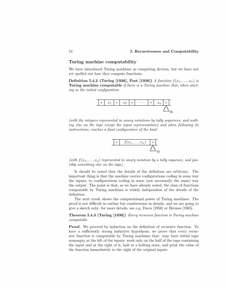
54 I. Recursiveness and Computability
Turing machine computability
We have introduced Turing machines as computing devices, but we have notyet spelled out how they compute functions.
Definition I.4.2 (Turing [1936], Post [1936]) A function f(x1, . . . , xn) isTuring machine computable if there is a Turing machine that, when start-ing in the initial configuration
AA q0
∗ ∗ ∗ ∗ ∗x1 x2 xn· · ·
(with the integers represented in unary notations by tally sequences, and noth-ing else on the tape except the input representation) and when following itsinstructions, reaches a final configuration of the kind
AA qf
∗ ∗f(x1, . . . , xn)
(with f(x1, . . . , xn) represented in unary notation by a tally sequence, and pos-sibly something else on the tape).
It should be noted that the details of the definition are arbitrary. Theimportant thing is that the machine carries configurations coding in some waythe inputs, to configurations coding in some (not necessarily the same) waythe output. The point is that, as we have already noted, the class of functionscomputable by Turing machines is widely independent of the details of thedefinition.
The next result shows the computational power of Turing machines. Theproof is not difficult in outline but cumbersome in details, and we are going togive a sketch only: for more details, see e.g. Davis [1958] or Hermes [1965].
Theorem I.4.3 (Turing [1936]) Every recursive function is Turing machinecomputable.
Proof. We proceed by induction on the definition of recursive function. Tohave a sufficiently strong inductive hypothesis, we prove that every recur-sive function is computable by Turing machines that: may have initial tapenonempty at the left of the inputs, work only on the half of the tape containingthe input and at the right of it, halt in a halting state, and print the value ofthe function immediately to the right of the original inputs.
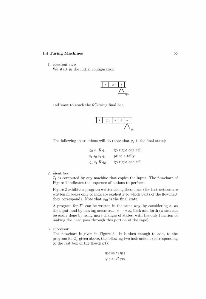
I.4 Turing Machines 55
1. constant zeroWe start in the initial configuration
AA q0
∗ ∗x1
and want to reach the following final one:
AA q0
∗ ∗x1 ∗1
The following instructions will do (note that q2 is the final state):
q0 s0 R q1 go right one cellq1 s0 s1 q1 print a tallyq1 s1 R q2 go right one cell
2. identitiesI1
1 is computed by any machine that copies the input. The flowchart ofFigure 1 indicates the sequence of actions to perform.
Figure 2 exhibits a program written along these lines (the instructions arewritten in boxes only to indicate explicitly to which parts of the flowchartthey correspond). Note that q10 is the final state.
A program for Ini can be written in the same way, by considering xi asthe input, and by moving across xi+1 ∗ · · · ∗ xn back and forth (which canbe easily done by using more changes of states, with the only function ofmaking the head pass through this portion of the tape).
3. successorThe flowchart is given in Figure 3. It is then enough to add, to theprogram for I1
1 given above, the following two instructions (correspondingto the last box of the flowchart):
q10 s0 s1 q13
q13 s1 R q13

56 I. Recursiveness and Computability
Go to the right ofthe output.
Restore the input. Go to therightmost tally of
the output.
Search for therightmost tallyremained of the
input and erase it.
Move one cell tothe right andprint a tally.
was itthe
last?
?
? ?
?
?
@@
@
@@
@
yes no
Figure I.1: Flowchart for I11
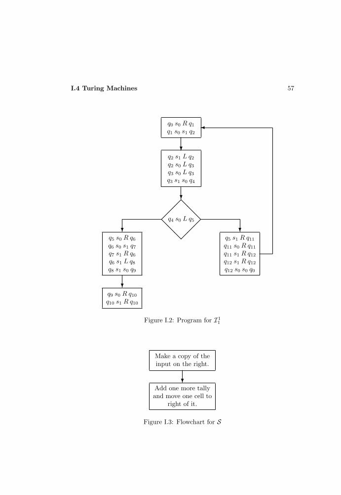
I.4 Turing Machines 57
q9 s0 R q10q10 s1 R q10
q5 s0 R q6q6 s0 s1 q7q7 s1 R q6q6 s1 L q8q8 s1 s0 q9
q5 s1 R q11q11 s0 R q11q11 s1 R q12q12 s1 R q12q12 s0 s0 q0
q2 s1 L q2q2 s0 L q3q3 s0 L q3q3 s1 s0 q4
q0 s0 R q1q1 s0 s1 q2
q4 s0 L q5
?
?
?
?
?
@@
@
@@
@
Figure I.2: Program for I11
Add one more tallyand move one cell to
right of it.
Make a copy of theinput on the right.
?
Figure I.3: Flowchart for S
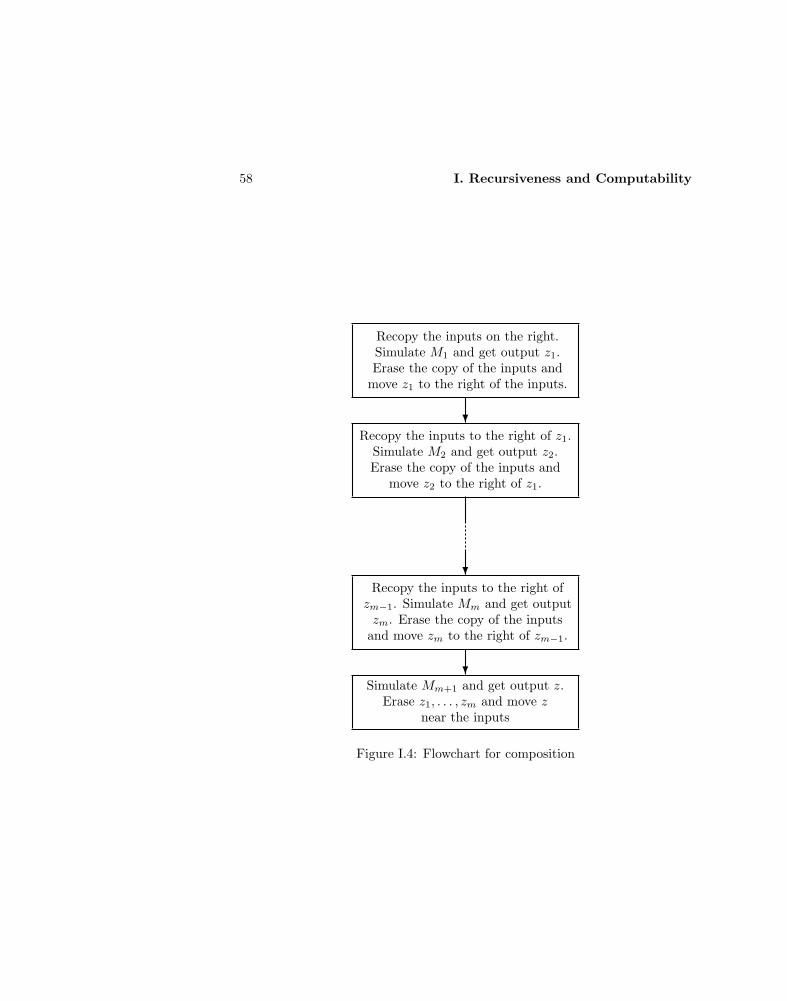
58 I. Recursiveness and Computability
Simulate Mm+1 and get output z.Erase z1, . . . , zm and move z
near the inputs
Recopy the inputs to the right ofzm−1. Simulate Mm and get outputzm. Erase the copy of the inputs
and move zm to the right of zm−1.
Recopy the inputs to the right of z1.Simulate M2 and get output z2.Erase the copy of the inputs and
move z2 to the right of z1.
Recopy the inputs on the right.Simulate M1 and get output z1.Erase the copy of the inputs and
move z1 to the right of the inputs.
?
?
?
Figure I.4: Flowchart for composition

I.4 Turing Machines 59
As we can see from these examples, to write programs is quite routine,once we have the appropriate flowcharts. In the following we will then restrictourselves to the latter, and leave as an exercise their translation into programs.
4. compositionLet
f(~x) = h(g1(~x), . . . , gm(~x)),
and suppose g1, . . . , gm, h are computed, in the sense explained at thebeginning of the proof, by machines M1, . . . ,Mm,Mm+1. Then f is com-puted by a machine implementing the flowchart of Figure 4, where sim-ulation of a given machine means changing the name of its states in theappropriate way: by renaming its initial state by the name of the statein which the new machine begins its simulation, renaming the remain-ing states by new names not yet used, and continuing the work of thesimulating machine from the halting state of the simulated one.
5. primitive recursionLet
f(~x, 0) = g(~x)f(~x, y + 1) = h(~x, y, f(~x, y)),
and suppose g and h are computed, in the sense explained at the begin-ning of the proof, by machines M1 and M2. Then f is computed by amachine implementing the flowchart of Figure 5. The idea is to computesuccessive values of f , using the previous one each time, until we reachthe one we are interested in. To keep track of the number of iterationsstill to be done we introduce a counter s, initially set up to the valuey, and decreased by one at each step. We do different simulations, de-pending on whether y = 0 or not. In the computation we also need anadditional input, which is not present at the first step (computation of g),and increases by one at each step afterwards: we then introduce a secondcounter t, which is initially empty. The tape then codes a situation ofthe kind:
x1 ∗ · · · ∗ xn ∗ y ∗ s ∗ x1 ∗ · · · ∗ xn ∗ t ∗ f(x1, . . . , xn, t)
where s+ t = y.
6. µ-recursionLet
f(~x) = µy[g(~x, y) = 0],

60 I. Recursiveness and Computability
Erase everythingbetween the inputsand z, and move z
near the inputs.
Increase t anddecrease s by one tally
each. Simulate M2,get a new output zand move it near t
(erasing the old one).
Write, to the right ofthe inputs, a copy s ofy, a copy of the inputsand an empty string t.Simulate M1 and get
output z.
? ?
?
@@
@
@@
@
s = 0?yes no
Figure I.5: Flowchart for primitive recursion
and suppose g is computed, in the sense explained at the beginning of theproof, by a machine M . Then f is computed by a machine implementingthe flowchart of Figure 6. The idea is to compute successive values ofg(~x, y), starting with y = 0, until one with output 0 is reached. Then yis the value of f . 2
Exercise I.4.4 Fill in the details of the proof of Theorem I.4.3, by specifying Turing
machine programs implementing the flowcharts given there.
Machine-dependent programming languages ?
To show that a certain function is Turing machine computable we have towrite a complete program, using only the elementary instructions of defini-tion I.4.1. Since they spell out explicitly the elementary physical operationsthat the machine has to perform, such programs are said to be written in ma-chine language. Examples have been given for O, I1
1 and S in the proof ofI.4.3.
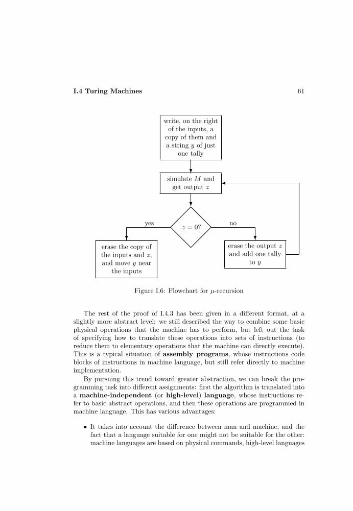
I.4 Turing Machines 61
erase the copy ofthe inputs and z,and move y near
the inputs
erase the output zand add one tally
to y
simulate M andget output z
write, on the rightof the inputs, a
copy of them anda string y of just
one tally
? ?
?
?
@@
@
@@
@
z = 0?yes no
Figure I.6: Flowchart for µ-recursion
The rest of the proof of I.4.3 has been given in a different format, at aslightly more abstract level: we still described the way to combine some basicphysical operations that the machine has to perform, but left out the taskof specifying how to translate these operations into sets of instructions (toreduce them to elementary operations that the machine can directly execute).This is a typical situation of assembly programs, whose instructions codeblocks of instructions in machine language, but still refer directly to machineimplementation.
By pursuing this trend toward greater abstraction, we can break the pro-gramming task into different assignments: first the algorithm is translated intoa machine-independent (or high-level) language, whose instructions re-fer to basic abstract operations, and then these operations are programmed inmachine language. This has various advantages:
• It takes into account the difference between man and machine, and thefact that a language suitable for one might not be suitable for the other:machine languages are based on physical commands, high-level languages
62 I. Recursiveness and Computability
are closer to ordinary language.
• The translation of the basic abstract operations into machine languagecan be done once and for all, by means of fixed programs called com-pilers or interpreters. The distinction between the two is, at least inorigin, that the compiler translates the given high-level program into aprogram in machine language, which is then executed; the interpreterinstead proceeds directly to the execution of the given high-level pro-gram, by translating an instruction only if and when it needs it in thecomputation.
• The abstract analysis of the algorithm is more easily carried out in termsof basic abstract operations, without paying attention to concrete prob-lems of implementation. The advantage is somewhat reflected by thecompiler’s complexity, since whatever is done automatically does not haveto be taken care of directly in the program.
• The same abstract analysis can be implemented by many different typesof machines, each one using its own compiler or interpreter.
The general skeleton of programming thus takes the following form. Onone side the given function is analyzed into an algorithm, which is then trans-lated into a machine-independent program. On the other side the behavior ofthe given machine is structured into a set of basic instructions in machine (orassembly) language. A compiler or interpreter then relates the two parts andproduces a machine-dependent program that can be executed by the machine.
I.5 Flowcharts
Every program written in a machine-dependent language has an abstract corethat can be written in a machine-independent language. It is not clear, atthis stage of our development, whether the opposite also holds, i.e. whether themost general programs can be implemented on abstract machines (if not step bystep at least globally, in the sense of having a machine computing the functiondefined by the program). Since, however, programs do provide formalizationsof algorithms, and our concern is effective computability, we feel compelled toanalyze the notion of program as a natural approximation to it. The analysiswill make the notion precise and, as a by-product, it will be possible to clarifythe relationships between programs and machines.
To define the most general notion of arithmetical program we rely on theintuition given by the experience with Turing machines. It seems that theconstituents of abstract programs are reducible to actions of two kinds: performsome basic operations, and ask some basic questions. Both are clearly needed,

I.5 Flowcharts 63
since without operations we cannot compute, and without conditional actionswe cannot exercise judgments or make choices, and then we could only havefixed behaviors.
To picture programs we thus need to distinguish the two types of action,which we do figuratively by using (as in the proof of Theorem I.4.3) boxes forbasic operations, and diamonds for basic questions. We are then faced with theusual problem of choosing the basic constituents of our programs. For reasonsalready discussed for the other approaches, we stick to the most elementaryarithmetical functions and predicates.
As usual in Computer Science, we adopt in this section the convention ofwriting variables in capital letters.
Definition I.5.1 (Goldstine and Von Neumann [1947]) A flowchartprogram is a diagram having exactly one entry and a finite number (possiblyzero) of exit points, and built up by connecting (through the outward edges)parts of the following kinds:
1. assignment statements of one of the following forms:
X := 0 X := X + 1 X := X − 1
? ? ?
The sign ‘:=’ means: set the left-hand side equal to the right-hand one.Thus the three assignments correspond, respectively, to instructions of theform: set X equal to 0, increase X by 1, and decrease X by 1.
2. conditional statements of the form:
@@@
@@@
? ?
yes noX = 0?
In a flowchart, edges can split only when passing through conditional state-ments, but they are allowed to merge in a point (thus, even if formally manyexit points are permissible, in practice they can be connected and reduced to atmost one). Also, the outward edges of conditional statements must exit fromthe diamond but can go anywhere. In particular, they can re-enter the diagramand thus produce closed paths.

64 I. Recursiveness and Computability
Exercises I.5.2 Choices of primitives. a) From the assignments X := X+1 andX := X−1 and the conditional ‘X = 0?’ one can derive the assignments X := 0 andX := Y , and the conditional ‘X = Y ?’ . (Hint: decrease X and Y simultaneously by1, until one or both vanish.)
b) From the assignments X = X + 1 and X := 0 and the conditional ‘X = Y ?’one can derive the assignment X := X − 1. (Hint: use two variables, set initially to0 and 1, and increased simultaneously by 1 until the greatest reaches X.)
c) Both choices of primitives above are minimal . (Hint: without conditionals the
arguments cannot influence the form of the computation; without predecessor in a),
the only property that can influence a computation is whether an argument is zero
or not; without successor there would be no way to write down numbers greater than
the arguments.)
Unstructured programming languages ?
The motivation that led to the introduction of the planar structure of flowchartsis best explained by its own inventor:
There is reason to suspect that our predilection for linear codes,which have a simple, almost temporal sequence, is chiefly a literaryhabit, corresponding to our not particularly high level of combina-torial cleverness, and that a very efficient language would probablydepart from linearity. (Von Neumann [1966])
The description of algorithms by means of flowcharts has led to the program-ming language GPSS (General Purpose Simulation System, Gordon [1961]; seeSammett [1969] and Wexelblat [1981] for history and references), which usesblock diagram notation directly. This is useful for the simulation of discretesystems, since it allows for a direct representation of the system structure (withblocks standing for operations performed in the system, and edges correspond-ing to possible sequences of events).
However, in practice, most programming languages represent algorithms assequences of instructions. We thus have to devise a way to unwind flowcharts,and lay them out (which does not mean eliminating their planar structure,but only representing them in a different way). A simple method is to labelstatements (e.g. by natural numbers). Then a flowchart can be representedas a juxtaposition of labeled statements (the order in the sequence, not theorder of labels, indicating the progressive order of execution), by translatingconditional statements via conditional jumps (Post[1936]) of the kind
if X = 0 go to n
(with the meaning: if X = 0 then jump to the statement with label n, otherwisecontinue with the next statement in the list). Note that it is also possible to

I.5 Flowcharts 65
define unconditional jumpsgo to n
as: if 0 = 0 then go to n. This permits the treatment of merging edges of aflowchart.
A ‘go to’ program is a finite sequence of labeled statements of the kind
X := 0 X := X + 1 X := X − 1if X = 0 go to n,
with the conditions that different statements have different labels, and everynumber mentioned after a ‘go to’ is the label of a statement. ‘Go to’ programsand flowcharts programs are mutually translatable, and hence equivalent .
‘Go to’ statements are the natural solution to flowchart unwinding: theyare typical of unstructured programming languages, like FORTRAN (FormulaTranslator, Backus et al. [1957]; see Sammett [1969] and Wexelblat [1981] forhistory and references). However, ‘go to’ statements are currently out of fashion(see p. 69).
Unlimited register, random access machines ?
Turing-like machines implementing ‘go to’ programs have been proposed byPost [1936] (independently of Turing [1936]) and Wang [1957]. A differentmodel is the unlimited register, random access machine (Melzak [1961],Lambek [1961], Shepherdson and Sturgis [1963], Peter [1963], Elgot and Robin-son [1964]). It consists of a finite number of registers of unbounded capacity,each able to contain an integer, and labeled (by a number). The machine isable to perform the following operations: clear a register (set its content equalto zero), and increase or decrease by one the content of a register. The machineperforms the operations by following the instructions of a ‘go to’ program, withthe convention that variables represent the content of associated registers.
This model is somewhat closer to real computers than Turing machines,since the memory consists of labeled registers whose content can be made avail-able by a direct call to the label. The advantage of this kind of random accessmemory, versus a sequential access memory like the tape of a Turing ma-chine, is subdivision (and consequent greater accessibility) of information. Inreal computers both kinds of memory are present: the random access (chips) isinternal and limited, while the sequential access (e.g. magnetic tapes or disks)is external and potentially (in theory, at least) unlimited. Of course, unlikerandom access machines, real computers’ registers have only a finite capacity.
Flowchart computability
Flowcharts have a natural semantics:
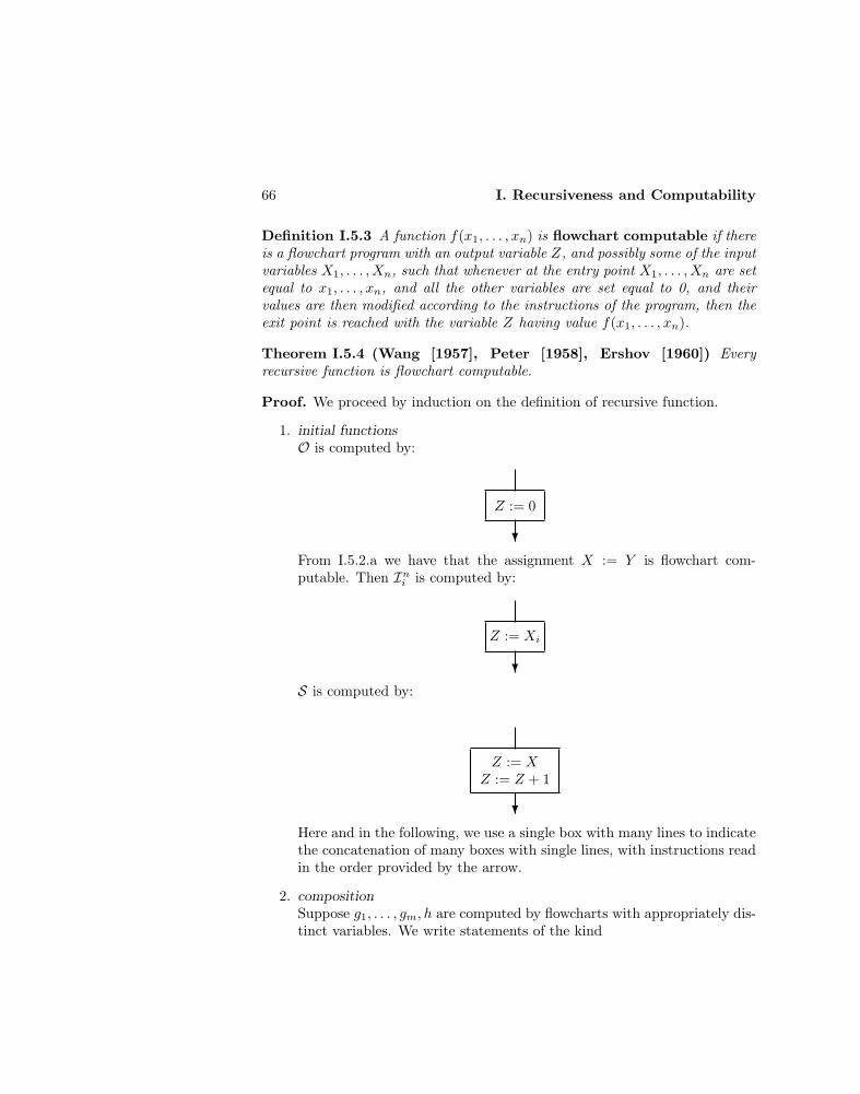
66 I. Recursiveness and Computability
Definition I.5.3 A function f(x1, . . . , xn) is flowchart computable if thereis a flowchart program with an output variable Z, and possibly some of the inputvariables X1, . . . , Xn, such that whenever at the entry point X1, . . . , Xn are setequal to x1, . . . , xn, and all the other variables are set equal to 0, and theirvalues are then modified according to the instructions of the program, then theexit point is reached with the variable Z having value f(x1, . . . , xn).
Theorem I.5.4 (Wang [1957], Peter [1958], Ershov [1960]) Everyrecursive function is flowchart computable.
Proof. We proceed by induction on the definition of recursive function.
1. initial functionsO is computed by:
Z := 0
?
From I.5.2.a we have that the assignment X := Y is flowchart com-putable. Then Ini is computed by:
Z := Xi
?
S is computed by:
Z := XZ := Z + 1
?
Here and in the following, we use a single box with many lines to indicatethe concatenation of many boxes with single lines, with instructions readin the order provided by the arrow.
2. compositionSuppose g1, . . . , gm, h are computed by flowcharts with appropriately dis-tinct variables. We write statements of the kind

I.5 Flowcharts 67
Y := g(X1, . . . , Xn)
?
as shorthand for the program computing g with respect to input variablesX1, . . . , Xn and output variable Y , and such that the input variables have,in exit, the same values they had in entry (which can be done by storingtheir original values by using new variables, and restoring them at theend).
. Then if
f(x1, . . . , xn) = h(g1(x1, . . . , xn), . . . , gm(x1, . . . , xn)),
f is computed by the program of Figure 7.
Z := h(Y1, . . . , Ym)
Ym := gm(X1, . . . , Xn)
Y1 := g1(X1, . . . , Xm)
?
Figure I.7: Flowchart for composition
3. primitive recursionLet
f(x1, . . . , xn, 0) = g(x1, . . . , xn)f(x1, . . . , xn, y + 1) = h(x1, . . . , xn, y, f(x1, . . . , xn, y)),
and suppose g and h are computed by programs with appropriately dis-tinct variables. Then f is computed by the program shown in Figure 8.
4. µ-recursionLet
f(x1, . . . , xn) = µy(g(x1, . . . , xn, y) = 0),
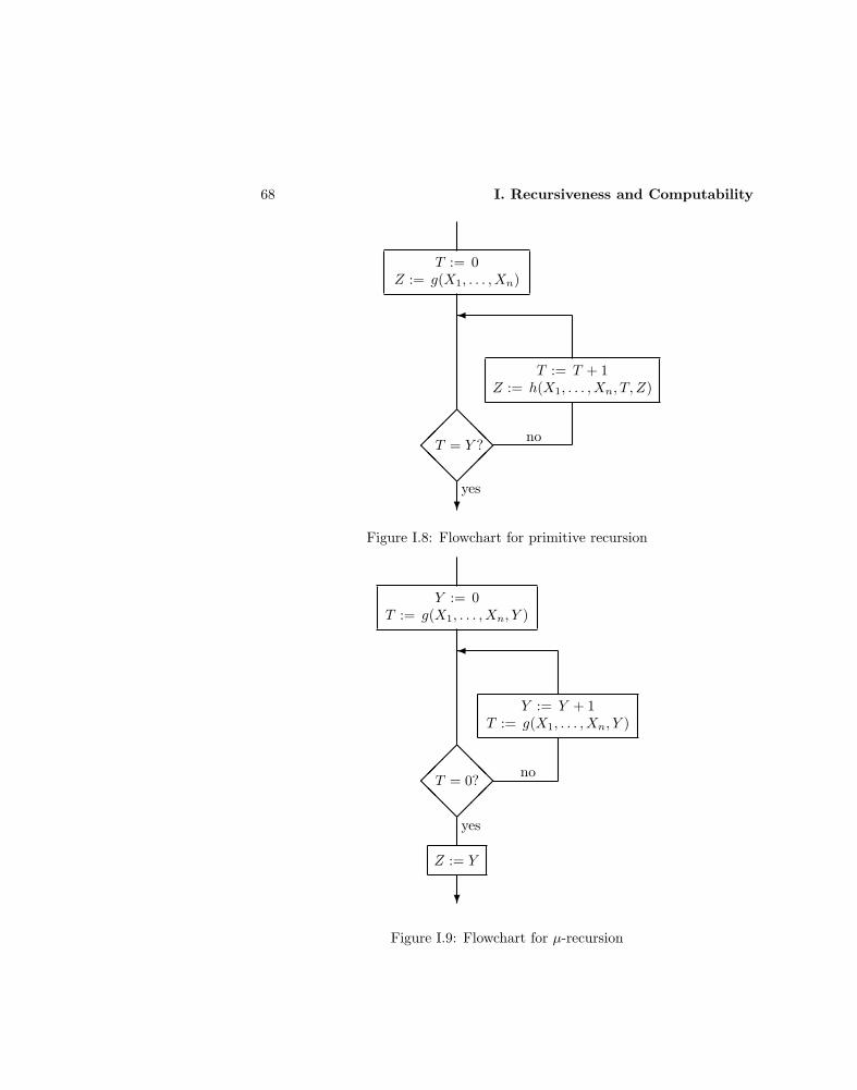
68 I. Recursiveness and Computability
T := T + 1Z := h(X1, . . . , Xn, T, Z)
T := 0Z := g(X1, . . . , Xn)
@@@
@@@
?
yes
noT = Y ?
Figure I.8: Flowchart for primitive recursion
Y := Y + 1T := g(X1, . . . , Xn, Y )
Y := 0T := g(X1, . . . , Xn, Y )
@@@
@@@
yes
noT = 0?
Z := Y
?
Figure I.9: Flowchart for µ-recursion
I.5 Flowcharts 69
and suppose g is computed by a program. Then so is f , by the programshown in Figure 9. 2
Structured programming languages ?
It has been argued by many (e.g. Dijkstra [1968]) that unstructured flow chartspresent definite disadvantages: they may be excessively complicated and dif-ficult to visualize, even for their authors, and errors are consequently easy tomake and difficult to debug. The proof of I.5.4 clearly shows that there is noneed of complicated flowcharts, with intricate interlacements of edges, at leastfor the computation of all the recursive functions.
The current trend - with a departure from planarity (see p. 64) and a returnto linearity) - is, thus, to stick to structured flowcharts (Dahl, Dijkstraand Hoare [1972]), inductively made up from the assignments and conditionalstatements of blocks with one entry and one exit line, connected only in theways shown by Figure 10.
One crucial advantage of structured flowcharts is the possibility of a top-down approach, in which the algorithm is successively approximated and ex-panded, from general to specific diagrams. Related to this is the fact that,while unstructured programs cannot, in general, be thought of as more thansets of isolated instructions, structured programs are really built up from sub-programs. This brings in a consideration of operations on programs andthe need (stressed in Backus [1981]) of an algebraic study of their properties.
Definition I.5.5 Consider the programming language whose statements arethe following:
1. assignment statements (X := 0, X := X + 1 and X := X − 1)
2. ‘while’ statements (while X 6= Y do S, with S arbitrary statement)
3. compound statements (begin S1, . . . , Sn end, with Si arbitrary statements).
A ‘while’ program is any compound statement.
‘While’ programs generate all the recursive functions, as shown by the proofof I.5.4. However, although ‘while’ programs are sufficient for recursion theory,to simplify the overall picture of programs it is useful in practice to have athand more instructions than just those which are really needed. The commonuse instructions of structured programming languages considered in Figure 10can easily be defined as shorthand expressions for appropriate ‘while’ programs(for any Boolean combination C of atomic expressions of the kind a = b anda < b, with a, b variables or numbers). The language obtained by enriching
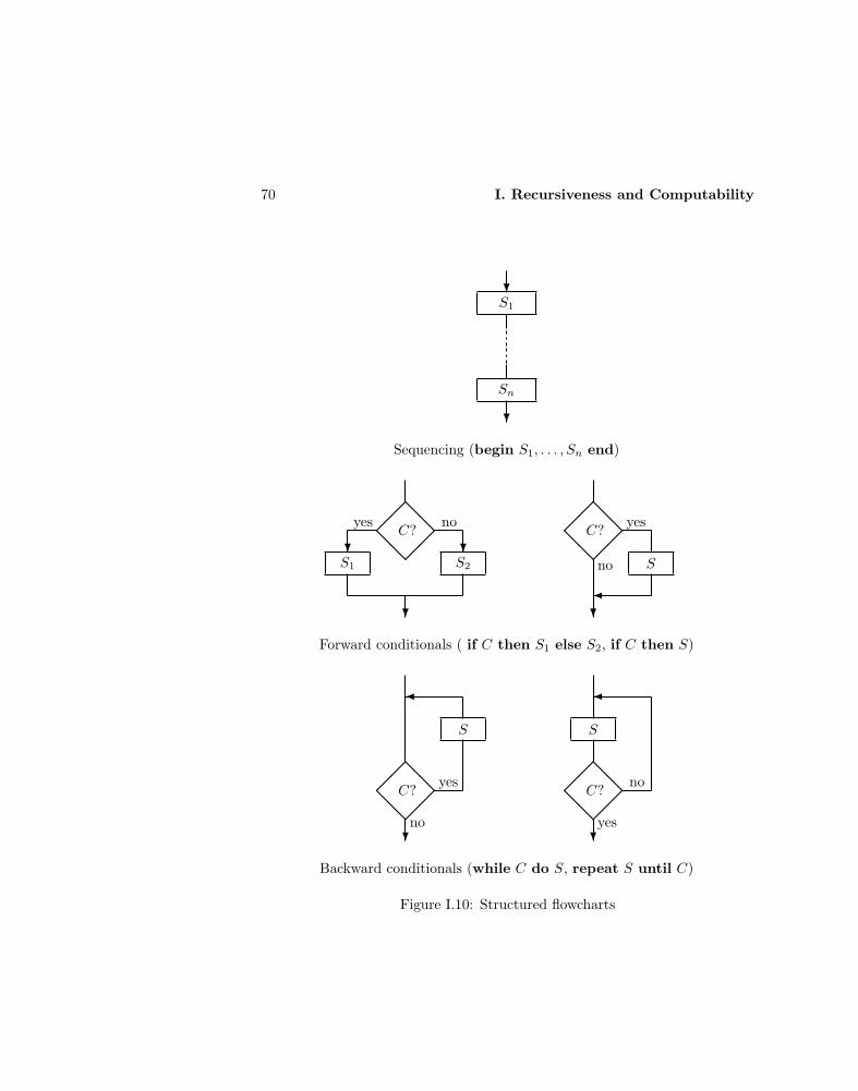
70 I. Recursiveness and Computability
Backward conditionals (while C do S, repeat S until C)
?
S
@@
@@C? yes
no?
S
@@
@@C? no
yes
Forward conditionals ( if C then S1 else S2, if C then S)
?
? ?
@
@
@@
S1 S2
C?yes no
?
@@
@@
S
C? yes
no
Sequencing (begin S1, . . . , Sn end)
?
?
S1
Sn
Figure I.10: Structured flowcharts
I.5 Flowcharts 71
‘while’ programs by these definitions is essentially PASCAL (Wirth [1971])without declarations (variables being directly available) and the special featuresnecessary to handle non-numerical data. PASCAL is a modern derivative ofthe ALGOL family (see Sammett [1969] and Wexelblat [1981] for the saga ofits collective gestation, birth and development).
Structured and unstructured flowcharts are equivalent (Bohm and Jacopini[1966]) in the sense that they compute the same functions. This follows indi-rectly from the fact, to be proved in Section 7, that unstructured flowchartsonly compute recursive functions, but this can easily be shown directly by ananalysis of unstructured flowcharts. Equivalence is the best result that can beachieved, since we cannot expect, in general, to be able to decompose unstruc-tured flowcharts into parts with only a fixed number of patterns (because wecan build unstructured flowcharts with any number of conditional nestings).
Note that our treatment of flowchart and ‘while’ programs is independentof Turing machines. A different proof, based on I.5.4, of Theorem I.4.3 wouldthen consist of showing how to compute the assignment statements and howto compose Turing machine programs by ‘sequencing’ and ‘while’. In otherwords, we would just need a compiler (see p. 62). This can be done as a usefulexercise (see Davis [1974] for details).
Exercises I.5.6 a) ’If then else’ and ‘repeat’ can be defined as ‘while’ programs.
b) ‘While’ can be defined using sequencing, ‘if then else’ and ‘repeat’ .
Programs for primitive recursion ?
An examination of the proof of Theorem I.5.4 shows that primitive recursionand µ-recursion are defined by similar flowcharts programs, with one basicdifference: the number of iterations is fixed in advance in the first case, andunknown in the second. We thus isolate, in the class of ‘while’ programs definedin I.5.5, the following class of structured programs:
Definition I.5.7 (Meyer and Ritchie [1967]) Consider the programminglanguage whose statements are the following:
1. assignment statements
2. ‘for’ statements ‘ for Y do S’, with S arbitrary statement (meaning: it-erate S for Y times)
3. compound statements (begin S1, . . . , Sn end, with Si arbitrary statements).
A ‘for’ program is any compound statement.
72 I. Recursiveness and Computability
The ‘for’ statement is commonly used in programming languages, and it isobviously definable as a ‘while’ program, as follows:
(begin T := 0, (while T 6= Y do (begin T := T + 1, S end))end)
(with T variable not appearing in S).
Proposition I.5.8 (Meyer and Ritchie [1967]) A function is ‘for’ com-putable if and only if it is primitive recursive.
Proof. Every primitive recursive function is ‘for’ computable, by the proof ofTheorem I.5.4. The opposite is shown by induction on the depth of nesting of‘for’ statements in a program. It is convenient, to have a stronger inductivehypothesis, to show that each variable of the program has, at the end of theprogram execution, a value which is a primitive recursive function of all thevariables (we would need this only for the output variable, as a function of theinput variables).
When there is no ‘for’ (i.e. when the depth of nesting is 0) the programconsists of the sequencing of a finite number of assignment statements, andeach variable has a primitive recursive value (obtained by composition of O, Sand the predecessor operation).
Consider now ‘for Y do S’, and suppose S satisfies the inductive hypothesis:if the variables of the program S are among X1, . . . , Xn, there are primitiverecursive functions g1, . . . , gn such that Xi = gi(X1, . . . , Xn). For 1 ≤ i ≤ n, letfi(X1, . . . , Xn, Z) be the value of Xi after Z executions of S. Then: f1(X1, . . . , Xn, 0) = X1
· · ·fn(X1, . . . , Xn, 0) = Xn
f1(X1, . . . , Xn, Z + 1) = g1(f1(X1, . . . , Xn, Z), . . . , fn(X1, . . . , Xn, Z))· · ·fn(X1, . . . , Xn, Z + 1) = gn(f1(X1, . . . , Xn, Z), . . . , fn(X1, . . . , Xn, Z)).
This is a simultaneous recursion on primitive recursive functions, which iseasily seen (by coding, see I.7.2) to define primitive recursive functions. Afterthe execution of ‘for Y do S’, the variable Xi will have value fi(X1, . . . , Xn, Y ).In particular, the output variable will be a primitive recursive function of theinput variables. 2
The result suggests a natural way of classifying the primitive recursive func-tions, by measuring the smallest depth of nesting of ‘for’ statements in programs
I.5 Flowcharts 73
computing a given function. This is essentially equivalent to the Grzegor-czyck hierarchy (Grzegorczyck [1953]), which will be studied in detail inChapter VIII.
A consequence of I.5.8 is that primitive recursion in the form of defini-tion I.1.3 is not necessary: a simpler operation of simultaneous iteration issufficient. This result can be further refined, and we now show that, at the costof a slight increase of the stock of initial functions, even simple iteration aloneis sufficient.
Definition I.5.9 A function f is defined by iteration from a function t if
f(x, n) = t(n)(x),
where t(n)(x) denotes the result of n successive applications of t (by convention,t(0)(x) = x).
Proposition I.5.10 (Robinson [1947], Bernays) The class of primitive re-cursive functions is the smallest class of functions
1. containing the initial functions, together with coding and decoding func-tions for pairs
2. closed under composition
3. closed under iteration.
Proof. Let C be the smallest class of functions satisfying the conditions juststated: every function in C is primitive recursive, because the coding and de-coding functions for pairs are primitive recursive, and the class of primitiverecursive functions is closed under composition and iteration, the former bythe definition, and the latter because iteration is a special case of primitiverecursion:
f(x, 0) = x
f(x, n+ 1) = t(f(x, n)).
For the converse, we only have to show that primitive recursion can bereduced to iteration. First of all note that, since C has coding and decodingfunctions for pairs and is closed under composition, it also has coding anddecoding functions for n-tuples, for any fixed n. We continue to use for themthe standard notations for coding and decoding functions. Let g and h befunctions in C, and
f(~x, 0) = g(~x)f(~x, y + 1) = h(~x, y, f(~x, y)).
74 I. Recursiveness and Computability
We will show that the function
s(~x, n) = 〈~x, n, f(~x, n)〉
is in C. Then so is f , by composition, because
f(~x, n) = (s(~x, n))m+2
(where m is the number of elements in the vector ~x).Note that
s(~x, 0) = 〈~x, 0, f(~x, 0)〉= 〈~x, 0, g(~x)〉
and thus s(~x, 0) is in C, as a function of ~x. Moreover,
s(~x, n+ 1) = 〈~x, n+ 1, f(~x, n+ 1)〉= 〈~x, n+ 1, h(~x, n, f(~x, n)〉.
Sinces(~x, n) = 〈~x, n, f(~x, n)〉,
s(~x, n+ 1) can be obtained from s(~x, n) by one application of the function
t(〈~x, n, z〉) = 〈~x, n+ 1, h(~x, n, z)〉,
which is in C by composition, since g, h, the successor, and the coding functionsare in C. Finally,
s(~x, n) = t(n)(s(~x, 0)),
and s(~x, n) is thus the composition of s(~x, 0) and the iteration of t. Since theseare both in C, so is s. 2
The result just proved can be variously improved. First of all, Glad-stone [1967], [1971] shows that the introduction of new initial functions canbe avoided : the class of primitive recursive functions is the smallest class con-taining the initial functions, and closed under composition and iteration.
Second, the iteration schema can be further weakened in the followingschema of pure iteration:
f(n) = t(n)(0)
(Robinson [1947]). Some new initial functions are needed here, since by compo-sition and pure iteration we never get, from the initial functions, any functiondepending on two variables, like x+y. Choices of initial functions that generatethe primitive recursive functions by pure iteration, and a study of the algebraic
I.5 Flowcharts 75
structure of the class of primitive recursive functions, are in Robinson [1947],Poliakov [1964], [1964a], Lavrov [1967], Kozmnikh [1968], and Gladstone [1971].
R. Robinson [1947], [1955], and J. Robinson [1955], also show that the pureiteration schema is enough to generate the unary primitive recursive func-tions by composition, starting from two (but not from only one) appropriateunary functions. Thus we do not need to use nonunary functions to get anyunary primitive recursive function. See also Peter [1951] for a treatment of thistopic, and Georgieva [1976] for further simplifications.
Petri nets ?
Systems of separate, interacting components (like finite automata or computerhardware, flowcharts or computer software, physical systems, and so on) canbe modeled by Petri nets (Petri [1962]), which consist of bipartite, directedmultigraphs whose vertices can be either places or transitions (represented,respectively, by circles and bars), and whose arcs connect places to transitions,or transitions to places. Tokens can be assigned to (and can be thought toreside in) the places of a Petri net (which becomes marked), and their numberin a place may change during the execution.
The execution is controlled by the number and distribution of tokens inthe net, and consists of transition firings, which remove tokens from their inputplaces, and deposit new ones in their output places. A transition fires whenenabled, i.e. when each of its input places has at least as many tokens in itas there are arcs from the place to the transition (that is, arcs are seen asconductors of capacity one). Firing continues as long as there exist enabledtransitions, then it halts.
Thus, nets model systems, and executions model the flow of informationin them. Some of the places may be singled out as inputs or outputs, tomodel interactive behavior of a system with the outer world, and thus allowinga computational interpretation of the behavior of a net. Petri nets are quitegeneral devices, apt to model concurrence, due to their inherent parallelism,asynchronicity and nondeterminism. Events which are both enabled anddo not interact may occur independently, there is no inherent measure of timeflow in the execution, and no order is placed on transition firings when manytransitions are enabled.
An extension of Petri nets (Agerwala [1974], Hack [1975]) allows for in-hibitor arcs from places to transitions (which are pictured differently, as ar-rows with the arrowhead substituted by a small circle). The new firing rule isthat a transition is enabled if it is in the previous sense, and moreover the inputplaces corresponding to inhibitor arcs are empty. Thus inhibitor arcs permitzero testing. The interest of this extension is that Petri nets with inhibitor arcscompute all the recursive functions. This is easily seen by modeling ‘go to’
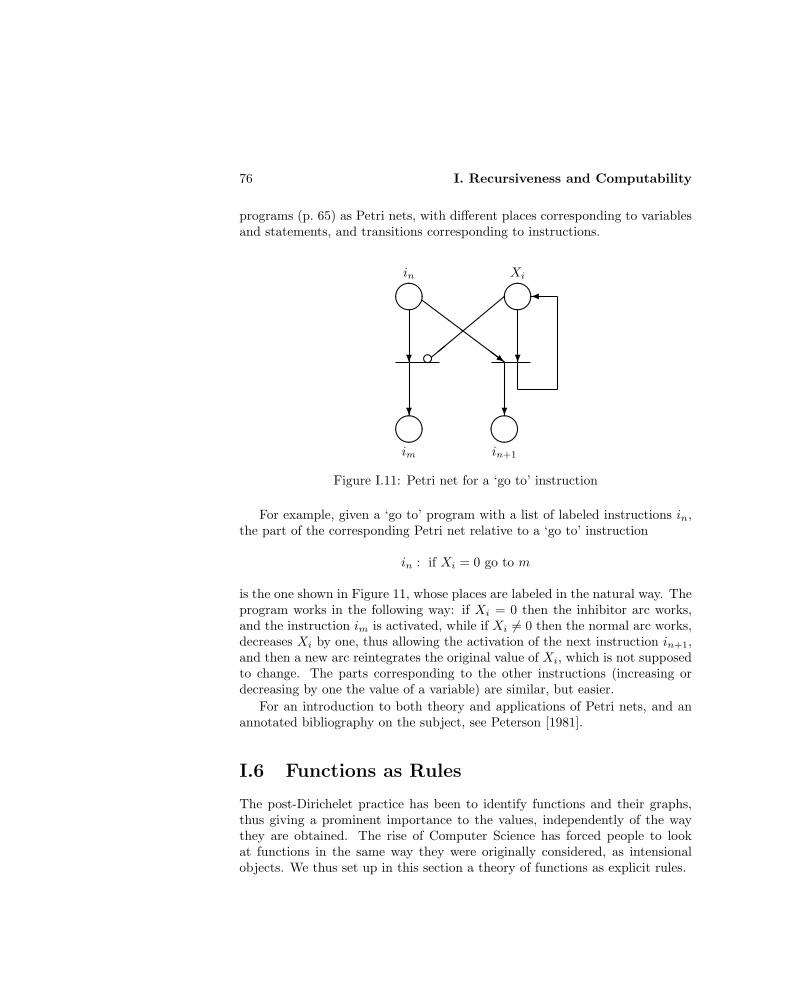
76 I. Recursiveness and Computability
programs (p. 65) as Petri nets, with different places corresponding to variablesand statements, and transitions corresponding to instructions.
im
in
in+1
Xi
?
?
?
?
ZZ
ZZ
ZZZ~
,,
,,
,,
e
Figure I.11: Petri net for a ‘go to’ instruction
For example, given a ‘go to’ program with a list of labeled instructions in,the part of the corresponding Petri net relative to a ‘go to’ instruction
in : if Xi = 0 go to m
is the one shown in Figure 11, whose places are labeled in the natural way. Theprogram works in the following way: if Xi = 0 then the inhibitor arc works,and the instruction im is activated, while if Xi 6= 0 then the normal arc works,decreases Xi by one, thus allowing the activation of the next instruction in+1,and then a new arc reintegrates the original value of Xi, which is not supposedto change. The parts corresponding to the other instructions (increasing ordecreasing by one the value of a variable) are similar, but easier.
For an introduction to both theory and applications of Petri nets, and anannotated bibliography on the subject, see Peterson [1981].
I.6 Functions as Rules
The post-Dirichelet practice has been to identify functions and their graphs,thus giving a prominent importance to the values, independently of the waythey are obtained. The rise of Computer Science has forced people to lookat functions in the same way they were originally considered, as intensionalobjects. We thus set up in this section a theory of functions as explicit rules.

I.6 Functions as Rules 77
λ-calculus
Rules must be expressed somehow, and they can thus be identified with termsin an appropriate language. A term t(x) can be seen as the value of a functionfor the argument x. We introduce an abstraction symbol ‘λ’ to indicate thestep from the value t(x) to the function x 7→ t(x), which we indicate by λx. t(x).
To begin with, we work in full generality and consider a language havingmerely the essential ingredients.
1. Symbols.
• variables x0, x1, . . .
• the abstraction symbol ‘λ’
• parentheses ‘(’ and ‘)’
• dot ‘.’ .
Note that there is only one kind of variable, and no theoretical distinction ismade between functions and arguments. The common practice in mathematics,following Russell [1908], is to consider a function as being an object of a typehigher than its arguments and values. This was introduced as one possibleway out of Russell’s paradox (see p. 82), which arose from the consideration ofsets belonging to themselves. Since self-membership corresponds, in functionalterms, to application of a function to itself, the practice of λ-calculus (of dealingwith only one kind of object, that can be function or argument at will) soundsat least suspicious, and will have to be justified. Appropriately, RecursionTheory provides us with various ways of doing this, see pp. 194 and 223.
2. Terms.
• a variable x alone is a term, and x occurs free in it
• if M,N are terms then the application (MN) of M to N is a term,and free or bound occurrences of variables in M or N remain so in(MN)
• if M is a term and x is a variable then the λ-abstraction (λx.M)of M w.r.t. x is a term, x is bound in it, and the other variables arefree or bound in it according to what they were in M .
By convention,
λx1 · · · xn.M means λx1(· · · (λxn. M) · · · )M1M2 · · · Mn means (· · · (M1M2) · · · Mn).

78 I. Recursiveness and Computability
The latter just avoids the need of many parentheses, but the former is theoret-ically important, since it defines functions of several arguments as compositionof functions of a single argument .
As we see, notations in λ-calculus are quite different from the commonpractice, and they might be confusing at first sight, both for the treatment ofapplication (which is just written as juxtaposition) and of multiple arguments(which are not treated simultaneously, but one at a time). E.g., what is usuallywritten f(t1, t2) is here rendered as (ft1)t2 or simply, by the conventions juststated, ft1t2.
Terms are names for the objects of λ-calculus (which, as already noted,may be thought of as both functions and arguments). We now set up a theoryof transformations for them, and introduce rules that allow us to manipulateterms. The idea is to compute values of functions by purely syntactical trans-formations of the terms representing the functions and their arguments.
3. Reduction rules.
α-rule. We can rename bound variables:
λx.Mα→ λy.M [x/y]
provided y does not occur in M , where M [x/y] indicates the resultof the substitution of x by y everywhere.
β-rule. We can apply a function λx. M to an argument N :
(λx.M)Nβ→M [x/N ]
provided whatever was free in N before the substitution remainsfree afterwards. This proviso can always be fulfilled, by a possibleapplication of the α-rule. For example,
(λxy. xy)y → λy. yy
is an illegal application of the β-rule, and indeed would not preservethe intended meaning , but it can be replaced by
(λxy. xy)y → λz. yz,
which can be derived by first changing the bound variable y into zby the α-rule, and then applying the β-rule.
We write t1β= t2, and say that t1 and t2 are equal (modulo α or β re-
ductions), if t1 and t2 can be reduced to the same term by a finite number of

I.6 Functions as Rules 79
applications of the α or β rules. Also, a term is said to be in normal form ifit cannot be β-reduced (i.e. the β-rule is not applicable to any of its subterms),and it is reducible otherwise.
A term is normalizable if it has a normal form, in the sense of being equalto a term in normal form. Normal forms of terms can be considered as their‘values’, and it is natural to investigate when they exist and how to computethem. Unfortunately, a normal form does not necessarily exist (thus, in somesense, the functions of λ-calculus are partial ones, see p. 127). To see this,we can simply produce a circular example of a term reducing to itself via theβ-rule, say MN
β→ MN : M must then have a λ-abstraction (to allow for anapplication of the β-rule), and produce an application. For example,
∆ = λx. xx
applies a term to itself:
∆tβ= tt,
and hence it self-reproduces:
∆∆β= ∆∆.
A second negative point is that even if a normal form exists, not all se-quences of reductions can produce it , e.g. a term might be reduced to normalform by one reduction and enter a loop by another:
(λxy. y) (∆∆) aβ= a by using the outer λ
(λxy. y) (∆∆) aβ= (λxy. y) (∆∆) a by using the λ in ∆.
Terms in which every subterm has a normal form are called strongly nor-malizable, and the example just given shows that a term can be normalizablewithout being strongly so.
On the positive side, Church and Rosser [1936] have shown (by a difficultproof, outside the scope of this book) that terminating reductions of a sameterm always give the same result, up to renaming of bound variables. In partic-ular, the normal form is unique when it exists. Moreover, there are reductionstrategies that produce the normal form, whenever it exists. One such strategyis to always reduce the leftmost reducible λ. Then subterms are evaluated ex-actly as many times as needed, which means that they may be evaluated morethan once in some cases, but also that they are not evaluated if not useful.
A different strategy would be to evaluate M and N before doing MN .This does not work in general (as the example above shows), but each termis evaluated only once, which means that the strategy is fast when it works,
80 I. Recursiveness and Computability
although some unnecessary terms may happen to be evaluated (and this maybe fatal if one of these is a nonterminating one).
We have already noted a peculiar aspect of λ-calculus: the absence of dis-tinction between functions and arguments, which may be seen as a collapseof the concept of type. In Recursion Theory a cumbersome technique (themethod of arithmetization of Section 7) is used for the related purpose of as-similating functions with numbers. This is partly achieved by identifying therecursive functions with their finite descriptions, e.g. programs, and by codingthese as numbers. Being indirectly obtained, this assimilation does not avoidthe need of continuously going back and forth between functions and numbersrepresenting them, and some arguments may at times become darkened. Thisis the case of the Fixed-Point Theorem II.2.10 and its proof, which are some-times considered quite mysterious. When recast in terms of λ-calculus, boththe statement and the proof of this result (based on methods fully explored inSection II.2) become more transparent.
Theorem I.6.1 (Kleene [1936b], Turing [1937a], Curry [1942], Rosen-bloom [1950]) There is a fixed-point operator Y which produces, for everyterm M , a fixed-point for it:
YM β= M(YM).
Proof. We give two different proofs.
1. We start with an informal argument. Recall that we have defined a term
∆ = λx. xx
such that, for any term t,
∆tβ= tt.
By applying ∆ to itself, we then have
∆∆β= ∆∆.
Given a term M , we want a term z such that zβ= Mz: then z reproduces
not itself, but the application ofM to itself. It is then enough to generalizethe definition of ∆, which gives what we want when M is the identityoperator. Let
∆M = λx.M(xx).
Then, for any term t,
∆M tβ= M(tt).
I.6 Functions as Rules 81
By applying ∆M to itself we then have
∆M∆Mβ= M(∆M∆M ),
and a fixed-point of M is given by
∆M∆M = (λx.M(xx))(λx.M(xx)).
Since this definition is uniform in M , we can actually abstract M fromit, and obtain
Y = λy. (λx. y(xx))(λx. y(xx)).
ThenYM β
= ∆M∆Mβ= M(∆M∆M ) = M(YM).
2. We now give a proof based on the (contrapositive of the) diagonal method
of Section II.2. Consider M : a fixed-point z for it is such that zβ= Mz,
i.e. it must be of the form titj for some terms ti, tj . Also, M must bethought of as the result of a transformation of terms of this kind. Considera possible enumeration of all pairs of λ-terms:
t0t0 t0t1 t0t2 t0t3 · · ·t1t0 t1t1 t1t2 · · ·t2t0 t2t1 t2t2 · · ·t3t0 · · · · · · · · ·· · ·
and the effect of M on the diagonal:
M(t0t0) M(t1t1) M(t2t2) . . .
This is a sequence of λ-terms, of the form
tntiβ= M(titi)
for some n. But then it is just the n-th row of the matrix, in particular
tntnβ= M(tntn)
is a fixed-point of M . Explicitly,
tn = λx.M(xx)
tntnβ= (λx.M(xx))(λx.M(xx)),
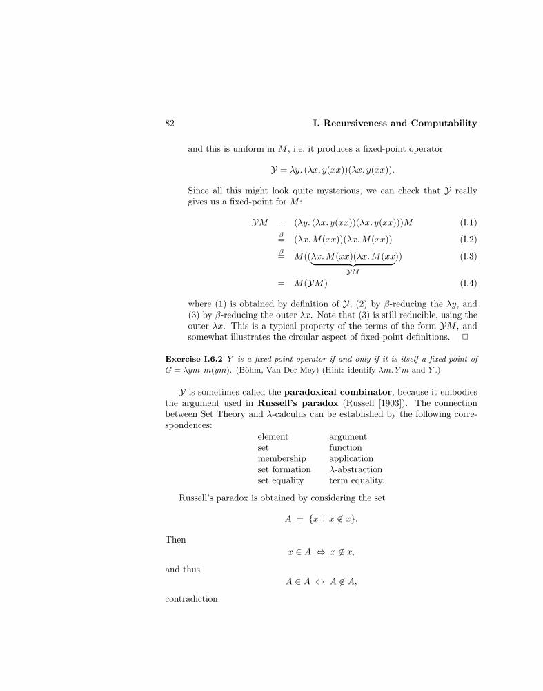
82 I. Recursiveness and Computability
and this is uniform in M , i.e. it produces a fixed-point operator
Y = λy. (λx. y(xx))(λx. y(xx)).
Since all this might look quite mysterious, we can check that Y reallygives us a fixed-point for M :
YM = (λy. (λx. y(xx))(λx. y(xx)))M (I.1)β= (λx.M(xx))(λx.M(xx)) (I.2)β= M((λx.M(xx)(λx.M(xx︸ ︷︷ ︸
YM
)) (I.3)
= M(YM) (I.4)
where (1) is obtained by definition of Y, (2) by β-reducing the λy, and(3) by β-reducing the outer λx. Note that (3) is still reducible, using theouter λx. This is a typical property of the terms of the form YM , andsomewhat illustrates the circular aspect of fixed-point definitions. 2
Exercise I.6.2 Y is a fixed-point operator if and only if it is itself a fixed-point of
G = λym.m(ym). (Bohm, Van Der Mey) (Hint: identify λm. Y m and Y .)
Y is sometimes called the paradoxical combinator, because it embodiesthe argument used in Russell’s paradox (Russell [1903]). The connectionbetween Set Theory and λ-calculus can be established by the following corre-spondences:
element argumentset functionmembership applicationset formation λ-abstractionset equality term equality.
Russell’s paradox is obtained by considering the set
A = x : x 6∈ x.
Thenx ∈ A ⇔ x 6∈ x,
and thusA ∈ A ⇔ A 6∈ A,
contradiction.

I.6 Functions as Rules 83
In terms of λ-calculus, the negation operator can be considered as a term Nthat is never the identity. Since membership corresponds to application, self-membership corresponds to self-application, and then the set A corresponds tothe term
λx.N(xx).
By β-reduction,
(λx.N(xx))xβ= N(xx),
and thus
(λx.N(xx))(λx.N(xx))β= N((λx.N(xx))(λx.N(xx))),
i.e.YN β
= N(YN).
Note however that here there is no paradox: from the last assertion, which istrue, we just deduce that there is no term N that is never the identity.
Other formulations of the λ-calculus ?
Our approach (Church [1933]) has been to define (by means of λ-abstractions)terms, called combinators, reflecting the way functional letters can be effectivelycombined to produce names for intensionally presented functions. Our termformation rules allow λx.M to be a term whenever M is. This version iscalled the λK-calculus. If a restriction were imposed on M , requiring thatx occur free in it, we would obtain a version called the λI-calculus, in whichfunctions with fictitious arguments are excluded. This restriction has beenintroduced to avoid some pathologies, like the existence of normalizable, notstrongly normalizable terms, as seen above.
The α and β rules define a system called the calculus of β-conversion.Various modifications of it are possible, e.g. by adding an extensionality lawfor λ-terms:
η-rule. We can identify every term with a function:
λx.Mxη→M
provided x is not free in M . Note that, by the rules of term formation,for any term M the expression λx.Mx is also a term, and thus it repre-sents a function: the rule ensures that this is exactly the function that isrepresented by the term M itself.
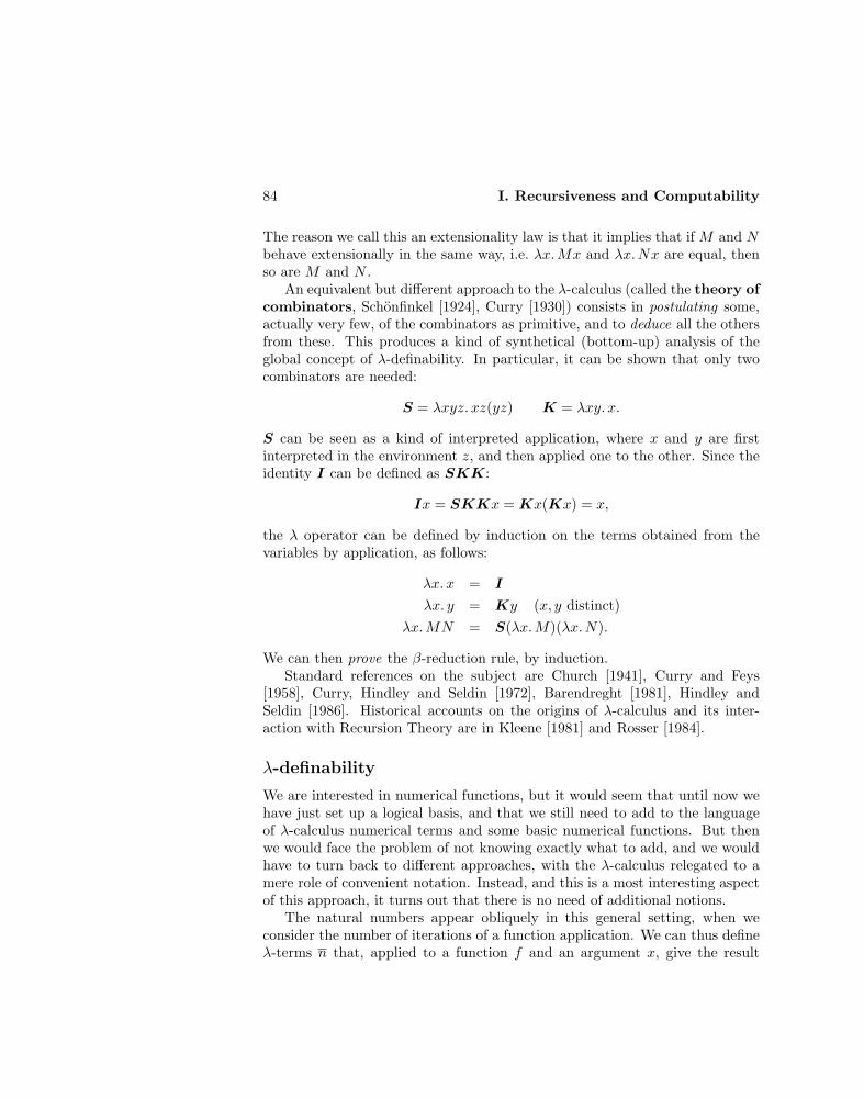
84 I. Recursiveness and Computability
The reason we call this an extensionality law is that it implies that if M and Nbehave extensionally in the same way, i.e. λx.Mx and λx.Nx are equal, thenso are M and N .
An equivalent but different approach to the λ-calculus (called the theory ofcombinators, Schonfinkel [1924], Curry [1930]) consists in postulating some,actually very few, of the combinators as primitive, and to deduce all the othersfrom these. This produces a kind of synthetical (bottom-up) analysis of theglobal concept of λ-definability. In particular, it can be shown that only twocombinators are needed:
S = λxyz. xz(yz) K = λxy. x.
S can be seen as a kind of interpreted application, where x and y are firstinterpreted in the environment z, and then applied one to the other. Since theidentity I can be defined as SKK:
Ix = SKKx = Kx(Kx) = x,
the λ operator can be defined by induction on the terms obtained from thevariables by application, as follows:
λx. x = I
λx. y = Ky (x, y distinct)λx.MN = S(λx.M)(λx.N).
We can then prove the β-reduction rule, by induction.Standard references on the subject are Church [1941], Curry and Feys
[1958], Curry, Hindley and Seldin [1972], Barendreght [1981], Hindley andSeldin [1986]. Historical accounts on the origins of λ-calculus and its inter-action with Recursion Theory are in Kleene [1981] and Rosser [1984].
λ-definability
We are interested in numerical functions, but it would seem that until now wehave just set up a logical basis, and that we still need to add to the languageof λ-calculus numerical terms and some basic numerical functions. But thenwe would face the problem of not knowing exactly what to add, and we wouldhave to turn back to different approaches, with the λ-calculus relegated to amere role of convenient notation. Instead, and this is a most interesting aspectof this approach, it turns out that there is no need of additional notions.
The natural numbers appear obliquely in this general setting, when weconsider the number of iterations of a function application. We can thus defineλ-terms n that, applied to a function f and an argument x, give the result
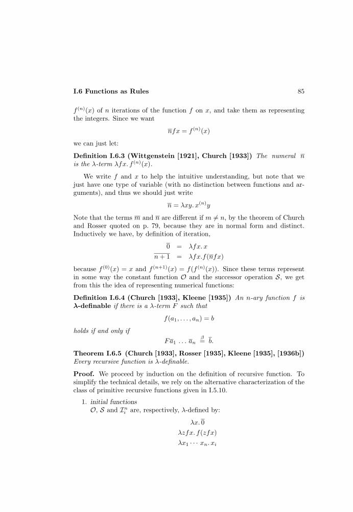
I.6 Functions as Rules 85
f (n)(x) of n iterations of the function f on x, and take them as representingthe integers. Since we want
nfx = f (n)(x)
we can just let:
Definition I.6.3 (Wittgenstein [1921], Church [1933]) The numeral nis the λ-term λfx. f (n)(x).
We write f and x to help the intuitive understanding, but note that wejust have one type of variable (with no distinction between functions and ar-guments), and thus we should just write
n = λxy. x(n)y
Note that the terms m and n are different if m 6= n, by the theorem of Churchand Rosser quoted on p. 79, because they are in normal form and distinct.Inductively we have, by definition of iteration,
0 = λfx. x
n+ 1 = λfx.f(nfx)
because f (0)(x) = x and f (n+1)(x) = f(f (n)(x)). Since these terms representin some way the constant function O and the successor operation S, we getfrom this the idea of representing numerical functions:
Definition I.6.4 (Church [1933], Kleene [1935]) An n-ary function f isλ-definable if there is a λ-term F such that
f(a1, . . . , an) = b
holds if and only ifFa1 . . . an
β= b.
Theorem I.6.5 (Church [1933], Rosser [1935], Kleene [1935], [1936b])Every recursive function is λ-definable.
Proof. We proceed by induction on the definition of recursive function. Tosimplify the technical details, we rely on the alternative characterization of theclass of primitive recursive functions given in I.5.10.
1. initial functionsO, S and Ini are, respectively, λ-defined by:
λx. 0λzfx. f(zfx)λx1 · · · xn. xi

86 I. Recursiveness and Computability
2. coding and decoding functions for pairsThis is obtained, in analogy with the representation of natural numbers,as:
(n,m) = λfgx. f (n)(g(m(x)).
Thus the pairing function is
λyzfgx. yf(zgx).
Decoding is then immediate: if I is the representation of I11 , i.e. of the
identity function, then
λfx. (n,m)fIx = λfx. f (n)x = n
λgx. (n,m)Igx = λfx. g(m)x = m.
Thus the decoding functions are
λyfx. y(fIx) and λygx. y(Igx).
3. compositionSuppose f, gi are λ-defined by F,Gi. Then
f(x1, . . . , xn) = h(g1(x1, . . . , xn), . . . , gm(x1, . . . , xn))
is λ-defined by
λx1, . . . , xn.H(G1x1 · · · xn) · · · (Gmx1 · · · xn).
4. iterationThis is an immediate consequence of the representation of natural num-bers: if T is a term representing the function t, then the iteration
f(x, n) = t(n)(x)
is represented byλxy. yTx.
5. µ-recursionThis is obtained as in the proof of I.2.3. Recall that if
f(~x) = µy(g(~x, y) = 0)
thenf(~x) = h(~x, 0),
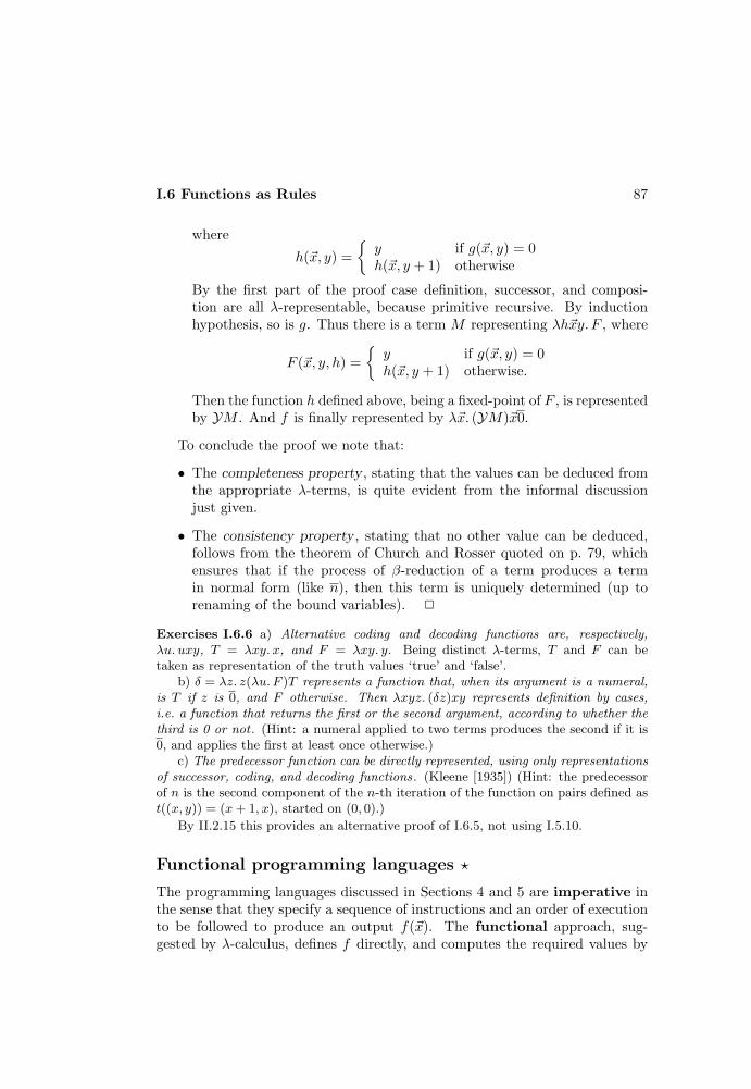
I.6 Functions as Rules 87
where
h(~x, y) =y if g(~x, y) = 0h(~x, y + 1) otherwise
By the first part of the proof case definition, successor, and composi-tion are all λ-representable, because primitive recursive. By inductionhypothesis, so is g. Thus there is a term M representing λh~xy. F , where
F (~x, y, h) =y if g(~x, y) = 0h(~x, y + 1) otherwise.
Then the function h defined above, being a fixed-point of F , is representedby YM . And f is finally represented by λ~x. (YM)~x0.
To conclude the proof we note that:
• The completeness property , stating that the values can be deduced fromthe appropriate λ-terms, is quite evident from the informal discussionjust given.
• The consistency property , stating that no other value can be deduced,follows from the theorem of Church and Rosser quoted on p. 79, whichensures that if the process of β-reduction of a term produces a termin normal form (like n), then this term is uniquely determined (up torenaming of the bound variables). 2
Exercises I.6.6 a) Alternative coding and decoding functions are, respectively,λu. uxy, T = λxy. x, and F = λxy. y. Being distinct λ-terms, T and F can betaken as representation of the truth values ‘true’ and ‘false’.
b) δ = λz. z(λu. F )T represents a function that, when its argument is a numeral,is T if z is 0, and F otherwise. Then λxyz. (δz)xy represents definition by cases,i.e. a function that returns the first or the second argument, according to whether thethird is 0 or not . (Hint: a numeral applied to two terms produces the second if it is0, and applies the first at least once otherwise.)
c) The predecessor function can be directly represented, using only representationsof successor, coding, and decoding functions. (Kleene [1935]) (Hint: the predecessorof n is the second component of the n-th iteration of the function on pairs defined ast((x, y)) = (x+ 1, x), started on (0, 0).)
By II.2.15 this provides an alternative proof of I.6.5, not using I.5.10.
Functional programming languages ?
The programming languages discussed in Sections 4 and 5 are imperative inthe sense that they specify a sequence of instructions and an order of executionto be followed to produce an output f(~x). The functional approach, sug-gested by λ-calculus, defines f directly, and computes the required values by
88 I. Recursiveness and Computability
β-reductions. The name ‘functional’ reflects the emphasis put on the functionsthemselves as intensional objects, as opposed to extensional emphasis on thevalues.
Relying on the characterization of recursive functions given in II.2.15, Mc-Carthy [1960] notes that a function is recursive if and only if:
• there is a definition of it from identities, successor, and predecessor bymeans of λ-abstraction, composition and the conditional operator
if t(~x) = 0 then g(~x) else h(~x).
• the function is computable from this definition by a call by value proce-dure, i.e. a computation which evaluates first the innermost (and leftmost,if there is more than one) occurrence of the letter defining the function.
Clearly the conditional operator replaces the definition by cases, and the fixed-point operator is eliminated, in favor of a computational approach that justproduces it.
This formulation of recursive functions can be extended from numericalfunctions to functions on words of a given alphabet and, as such, it has furnishedthe computational basis for the programming language LISP (List Processing,McCarthy [1960]; see Sammett [1969] and Wexelblat [1981] for history andreferences).
Since there is no reason that functional programming languages shouldbe forced to run on machines designed for imperative ones, work has beendone to design hardware directly inspired by the functional approach, based onλ-calculus (the SECD machine, Landin [1963], implementing β-reductions)or on the theory of combinators (the SK machine, Turner [1979], implement-ing reductions of graphs that represent the definition of a function, in terms ofthe combinators S and K, see p. 84).
I.7 Arithmetization
Arithmetization simply means translation into the language of arithmetic. Wewill give one detailed example of the method, and show how to code the ma-chinery of computation of recursive functions in a primitive recursive way. Thedetails are quite cumbersome, and in the rest of our work we will contentourselves to sketch similar arguments, leaving the details to the reader.
Historical remarks ?
The first attempt to find number-like connections between propositions of var-ious sorts probably goes back to Lullus’ Ars Magna, but it was Leibniz [1666]

I.7 Arithmetization 89
who dreamt of arithmetization as a general method to replace reasoning innatural language by arithmetical propositions, with the goal of substituting ar-guments with computations. Leibniz went further than just this oneiric activity,and devised (see [1903]) a precise coding method, by first assigning numbers toprimitive notions, and then showing how to associate composite numbers (e.g.by multiplication) to composite notions. However, his tentative work was leftunpublished until 1903, and did not influence modern developments.
Hilbert [1904] again envisaged arithmetization in his idea of formalizingconsistency proofs into Arithmetic, but it was Godel [1931] who first used itexplicitly and formally to translate the concepts relative to formal systems intoan arithmetical language. Tarski [1936] independently arrived at the methodin his investigations of the concept of truth.
Contrary to Leibniz’s dreams, the effect of arithmetization was, ironically,not to shield the language against its oddities, but rather to spring a leak inArithmetic, through which the linguistic paradoxes poured only to reveal theinadequacies of formalism (see II.2.17).
Numerical tools for arithmetization
Primitive recursive functions and predicates are more than enough to carryout arithmetizations. We will use prime numbers and factorizations (recall,see p. 26, that the sequence pxx∈ω of prime numbers is primitive recursive),because this coding is particularly simple. It should however be noted that wecould use functions from much smaller classes: this will be done in ChapterVIII, when the necessity for more efficient codings will arise.
To code the sequence 〈x0, . . . , xn〉, the simplest way would be to use thenumber px0
0 · · · pxnn . But then we could not uniquely decode a number, since
we would not know whether a prime in the decomposition has exponent 0accidentally or meaningfully (in the sense that it is coding the number 0).Thus, either we rule out 0 as a meaningful exponent, and let
〈x0, . . . , xn〉 = px0+10 · · · pxn+1
n ,
or we tell in advance how many numbers we are coding, and let
〈x1, . . . , xn〉 = pn0 · px11 · · · pxn
n .
Since we have to make a choice for the following, we decide to use the sec-ond proposal. The decoding system is given by the following functions andpredicates, all primitive recursive (see p. 26):
(x)n = exp(x, pn)ln(x) = (x)0
Seq(x) ⇔ (∀n ≤ x)[n > 0 ∧ (x)n 6= 0 → n ≤ ln(x)].
90 I. Recursiveness and Computability
We call ln(x) the length of x, and (x)n the n-th component of x. If Seq(x)holds then we say that x is a sequence number. In this case,
x = 〈(x)1, . . . , (x)ln(x)〉.
We will also need a concatenation operation ∗, such that
〈x1, . . . , xn〉 ∗ 〈y1, . . . , ym〉 = 〈x1, . . . , xn, y1, . . . , ym〉.
This is formally defined as:
x ∗ y = pln(x)+ln(y)0 · p(x)1
1 · · · p(x)ln(x)
ln(x) · p(y)1ln(x)+1 · · · p
(y)ln(y)
ln(x)+ln(y)
= pln(x)+ln(y)0 ·
∏i<ln(x)
p(x)i+1i+1 ·
∏i<ln(y)
p(y)i+1
ln(x)+i+1
if Seq(x) ∧ Seq(y) holds, and 0 otherwise.Finally, we will need the notion of initial subsequence, defined as
x v y ⇔ Seq(x) ∧ Seq(y) ∧ (∃u ≤ y)(Seq(u) ∧ x ∗ u = y)x < y ⇔ x v y ∧ x 6= y.
As a first use of sequence numbers we get the following useful result.
Proposition I.7.1 Course-of-values recursion (Skolem [1923], Peter[1934]) The class of primitive recursive functions is closed under recursions inwhich the definition of f(~x, y + 1) may involve not only the last value f(~x, y),but any number of (and possibly all) the values f(~x, z)z≤y already obtained.
Formally, let f be the history function of f , defined as:
f(~x, y) = 〈f(~x, 0), . . . , f(~x, y)〉.
Then, if f is defined as
f(~x, 0) = g(~x)
f(~x, y + 1) = h(~x, y, f(~x, y))
and g, h are primitive recursive, so is f .
Proof. It is enough to show that f is primitive recursive, since then also f is:
f(~x, y) =(f(~x, y)
)y+1
.
I.7 Arithmetization 91
But this is immediate, since
f(~x, 0) = 〈f(~x, 0)〉= 〈g(~x)〉
f(~x, y + 1) = 〈f(~x, 0), . . . , f(~x, y), f(~x, y + 1)〉= f(~x, y) ∗ 〈f(~x, y + 1)〉= f(~x, y) ∗ 〈h(~x, y, f(~x, y))〉.
Thus f(~x, y + 1) only uses the last previous value f(~x, y), and f is primitiverecursive because so are coding and concatenation. 2
Exercise I.7.2 Simultaneous primitive recursion. The class of primitive re-
cursive functions is closed under simultaneous recursion on more than one function.
(Hilbert and Bernays [1934]) (Hint: reduce simultaneous primitive recursion of, say,
f1(~x) and f2(~x), to primitive recursion of the single function 〈f1(~x), f2(~x)〉, by cod-
ing.)
The Normal Form Theorem
We are now in position to give our first and only complete example of arithme-tization, by reducing the recursive functions to a normal form. Any approachto recursiveness would produce similar results, and we will sketch the versionsrelative to the approaches of Sections 2–6 later in this section, but here we givea self-contained treatment based on recursiveness alone.
Theorem I.7.3 Normal Form Theorem (Kleene [1936]) There is a prim-itive recursive function U and (for each n ≥ 1) primitive recursive predicatesTn, such that for every recursive function f of n variables there is a number e(called index of f) for which the following hold:
1. ∀x1 . . .∀xn∃ yTn(e, x1, . . . , xn, y)
2. f(x1, . . . , xn) = U(µyTn(e, x1, . . . , xn, y)).
Proof. The idea of the proof is to associate numbers to functions and com-putations in such a way that the predicate Tn(e, x1, . . . , xn, y) translates theassertion: y is the number of a computation of the value of the function withassociated number e, on inputs x1, . . . , xn. Having this, µyTn(e, x1, . . . , xn, y)will give the number of one such computation, and the function U will extractthe value of the output from it. This is more easily said than done, and toachieve it we need to carry out a number of steps.

92 I. Recursiveness and Computability
1. associate numbers to recursive functionsThis is done according to the inductive procedure that generates therecursive functions. The details are obviously irrelevant, and we just giveone possible assignment:
• 〈0〉 to O• 〈1〉 to S• 〈2, n, i〉 to Ini , for 1 ≤ i ≤ n
• 〈3, b1, . . . , bm, a〉 to f(~x) = g(h1(~x), . . . , hm(~x)), where b1, . . . , bmand a are numbers respectively associated to h1, . . . , hm, and g
• 〈4, a, b〉 to f(~x, y) defined by primitive recursion from g and h, wherea and b are respectively associated to g and h
• 〈5, a〉 to f(~x) = µy(g(~x, y) = 0), if ∀~x∃y(g(~x, y) = 0) and a isassociated to g.
Any number associated to a recursive function is called an index of thisfunction. Since there are many ways to define the same function, therewill be many indices for each recursive function (see II.1.6). Also, manynumbers are not indices of recursive functions, either because they arenot sequence numbers of the right form, or because some of their relevantcomponents are not indices of recursive functions. We will see (p. 146)that in general there is no effective way to tell whether a number is indeedthe index of a recursive function, because basically there is no way to tellwhether ∀~x∃y(g(~x, y) = 0).
2. put computations in a canonical formA natural way to organize a computation for the values of a given recur-sive function, is by way of computation trees. Each node of such a treewill tell how a value needed in the computation can be inductively ob-tained. Of course, the only possibilities are those given by the permissibleschemata of definition I.1.7, namely:
• nodes without predecessors:
f(x) = 0 if f = Of(x) = x+ 1 if f = S
f(x1, . . . , xn) = xi if f = Ini
• compositionIf f(~x) = g(h1(~x), . . . , hm(~x)) then the node f(~x) = z has m + 1predecessors:

I.7 Arithmetization 93
h1(~x) = z1 · · · hm(~x) = zm g(z1, . . . , zm) = z
f(~x) = z
r r r rr
##
##
#
cc
cc
c
PPPPPPPPPPPP
• primitive recursionIf f(~x, y) is defined by primitive recursion from g and h there aretwo cases, respectively with one or two predecessors:
rr
r rrf(~x, 0) = z
g(~x) = z f(~x, y) = z1 h(~x, y, z1) = z
f(~x, y + 1) = z
@@
@@
• µ-recursionIf f(~x) = µy(g(~x, y) = 0) then there is no fixed pattern to thepredecessors of f(~x) = y. The general situation is:
g(~x, 0) = t0 · · · g(~x, z − 1) = tz−1 g(~x, z) = 0
f(~x) = z
r r r rr
##
##
#
cc
cc
c
PPPPPPPPPPPP
where t0, . . . , tz−1 are all different from 0.
3. associate numbers to computationsThis is done by induction on the construction of the computation tree.First of all, we assign numbers to nodes: since they are expressions of thekind f(x1, . . . , xn) = z, we give them numbers
〈e, 〈x1, . . . , xn〉, z〉,
where e is a given index of f . Thus a node is represented by threenumbers, corresponding respectively to the function, the inputs and theoutput.
We then assign numbers to trees: each tree T consists of a vertex vwith associated number v, and of a certain number (finite, and possiblyequal to zero) of ordered predecessors, each one being a subtree Ti. By
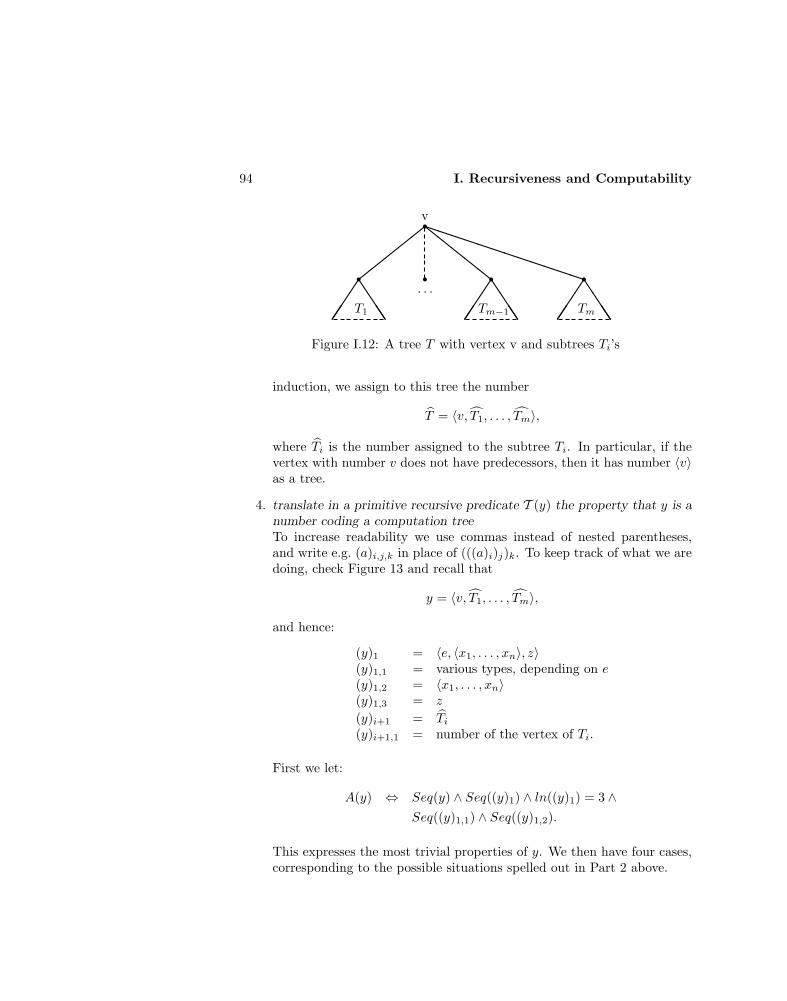
94 I. Recursiveness and Computability
rr r r r
##
##
#
cc
cc
c
PPPPPPPPPPPP
JJ
JJ
JJ
JJ
JJ
JJT1 Tm−1 Tm
. . .
v
Figure I.12: A tree T with vertex v and subtrees Ti’s
induction, we assign to this tree the number
T = 〈v, T1, . . . , Tm〉,
where Ti is the number assigned to the subtree Ti. In particular, if thevertex with number v does not have predecessors, then it has number 〈v〉as a tree.
4. translate in a primitive recursive predicate T (y) the property that y is anumber coding a computation treeTo increase readability we use commas instead of nested parentheses,and write e.g. (a)i,j,k in place of (((a)i)j)k. To keep track of what we aredoing, check Figure 13 and recall that
y = 〈v, T1, . . . , Tm〉,
and hence:
(y)1 = 〈e, 〈x1, . . . , xn〉, z〉(y)1,1 = various types, depending on e(y)1,2 = 〈x1, . . . , xn〉(y)1,3 = z
(y)i+1 = Ti(y)i+1,1 = number of the vertex of Ti.
First we let:
A(y) ⇔ Seq(y) ∧ Seq((y)1) ∧ ln((y)1) = 3 ∧Seq((y)1,1) ∧ Seq((y)1,2).
This expresses the most trivial properties of y. We then have four cases,corresponding to the possible situations spelled out in Part 2 above.

I.7 Arithmetization 95
r r r rr
XXXXXXXXXXXXXXXX〈b1, 〈x1, . . . , xn〉, z1〉 〈bm, 〈x1, . . . , xn〉, zm〉 〈a, 〈z1, . . . , zm〉, z〉· · ·
〈〈3, b1, . . . , bm, a〉, 〈x1, . . . , xn〉, z〉
= = =(y)2,1 (y)m+1,1 (y)m+2,1
a) composition
rr
〈a, 〈x1, . . . , xn〉, z〉
〈〈4, a, b〉, 〈x1, . . . , xn, 0〉, z〉
=(y)2,1
rr r
HHHHHHHH
〈〈4, a, b〉, 〈x1, . . . , xn, y + 1〉, z〉
〈〈4, a, b〉, 〈x1, . . . , xn, y〉, z1〉 〈〈b〉, 〈x1, . . . , xn, y, z1〉, z〉= =
(y)2,1 (y)3,1
b) primitive recursion
r r r rr
XXXXXXXXXXXXXXXX〈a, 〈x1, . . . , xn, 0〉, t1〉 〈a, 〈x1, . . . , xn, z − 1〉, tz〉 〈a, 〈x1, . . . , xn, z〉, 0〉· · ·
〈〈5, a〉, 〈x1, . . . , xn〉, z〉
= = =(y)2,1 (y)z+1,1 (y)z+2,1
c) µ-recursion
Figure I.13: Cases for the definition of T

96 I. Recursiveness and Computability
For the initial functions, there are three possibilities for v = (y)1:
〈〈0〉, 〈x〉, 0〉〈〈1〉, 〈x〉, x+ 1〉
〈〈2, n, i〉, 〈x1, . . . , xn〉, xi〉.
We then let:
B(y) ⇔ ln(y) = 1 ∧[(y)1,1 = 〈0〉 ∧ ln((y)1,2) = 1 ∧ (y)1,3 = 0] ∨[(y)1,1 = 〈1〉 ∧ ln((y)1,2) = 1 ∧ (y)1,3 = (y)1,2,1 + 1] ∨[ln((y)1,1) = 3 ∧ (y)1,1,1 = 2 ∧ (y)1,1,2 = ln((y)1,2) ∧1 ≤ (y)1,1,3 ≤ (y)1,1,2 ∧ (y)1,3 = ((y)1,2)(y)1,1,3
].
For composition we let:
C(y) ⇔ ln((y)1,1) ≥ 3 ∧ (y)1,1,1 = 3 ∧ ln(y) = ln((y)1,1) ∧(∀i)2≤i<ln(y)[(y)i,1,1 = (y)1,1,i ∧ (y)i,1,2 = (y)1,2] ∧(y)ln(y),1,1 = (y)1,1,ln(y) ∧ (y)ln(y),1,3 = (y)1,3 ∧(y)ln(y),1,2 = 〈(y)2,1,3, . . . , (y)ln(y)−1,1,3〉.
For primitive recursion, recall that there are two possible cases:
D(y) ⇔ ln((y)1,1) = 3 ∧ (y)1,1,1 = 4 ∧[(y)1,2,ln((y)1,2) = 0 ∧ ln(y) = 2 ∧ (y)2,1,1 = (y)1,1,2 ∧
(y)2,1,2, ∗ 〈0〉 = (y)1,2 ∧ (y)2,1,3 = (y)1,3] ∨[(y)1,2,ln((y)1,2) > 0 ∧ ln(y) = 3 ∧(y)2,1,1 = (y)1,1 ∧ ln((y)2,1,2) = ln((y)1,2) ∧(∀i)1≤i<ln((y)1,2)((y)2,1,2,i = (y)1,2,i) ∧(y)2,1,2,ln((y)1,2) + 1 = (y)1,2,ln((y)1,2) ∧(y)3,1,1 = 〈(y)1,1,3〉 ∧ (y)3,1,3 = (y)1,3 ∧(y)3,1,2 = (y)2,1,2 ∗ 〈(y)2,1,3〉].
For µ-recursion we let:
E(y) ⇔ ln((y)1,1) = 2 ∧ (y)1,1,1 = 5 ∧ln(y) ≥ 2 ∧ (y)1,3 = ln(y)− 2 ∧(∀i)2≤i≤ln(y)[(y)i,1,1 = (y)1,1,2 ∧(y)i,1,2 = (y)1,2 ∗ 〈i− 2〉] ∧(∀i)2≤i<ln(y)[(y)i,1,3 6= 0] ∧ (y)ln(y),1,3 = 0.
I.7 Arithmetization 97
These conditions take care of all possible cases, and thus we may defineinductively:
T (y) ⇔ A(y) ∧ [B(y) ∨ C(y) ∨D(y) ∨ E(y)] ∧[ln(y) > 1 → (∀i)2≤i≤ln(y)T ((y)i)].
Then T is primitive recursive because it is defined by using only primitiverecursive clauses and values (of its characteristic function) for previousarguments because, by definition of coding, (y)i < y. That is, T is definedby course of value recursion, which is a primitive recursive operation byI.7.1.
5. define Tn and UWe are now ready to conclude our work. Namely, for each n ≥ 1 we let:
Tn(e, x1, . . . , xn, y) ⇔ T (y) ∧ (y)1,1 = e ∧ (y)1,2 = 〈x1, . . . , xn〉
andU(y) = (y)1,3
These are obviously primitive recursive.
Let now f be a recursive n-ary function with index e. Since f is total, forevery x1, . . . , xn there is a computation tree for f(x1, . . . , xn) relative to thecomputation procedure coded by e. This is formally expressed by:
∀x1 . . .∀xn∃ yTn(e, x1, . . . , xn, y).
Moreover, from any computation tree (in particular from the one with thesmallest code number) we can extract the value of the function by looking atthe third component of its vertex. This is formally expressed by:
f(x1, . . . , xn) = U(µyTn(e, x1, . . . , xn, y)). 2
Exercise I.7.4 There is a recursive function enumerating the unary primitive recur-sive functions, i.e. a recursive function f(e, x) such that: for every e the functionλx. f(e, x) is primitive recursive, and every primitive recursive function is equal toλx. f(e, x) for some e. (Peter [1935]) (Hint: let
f(e, x) =
U(µyT1(e, x, y)) if e is a primitive recursive index0 otherwise,
where being a primitive recursive index means to define a recursive function from
the initial functions by composition and primitive recursion alone, without using the
µ-operator.)
98 I. Recursiveness and Computability
Equivalence of the various approaches to recursiveness
By using the method of arithmetization we can get a cascade of results relativeto the various approaches introduced in Sections 2–6. We will not go beyondsketches because we believe that, once the method is understood, the transla-tion of these into formal proofs should not present theoretical difficulties. It is,however, a very useful exercise to try to fill in the cumbersome details of someof these sketches.
We begin by dealing with the notions of Section 2.
Proposition I.7.5 (Kreisel and Tait [1961]) Every finitely definable func-tion is recursive.
Proof. Suppose f is finitely definable by E w.r.t. f1. We know that if f(~x) = zthen f1(~x) = z is a logical consequence of
E(f1, . . . , fm; ~z1) ∧ · · · ∧ E(f1, . . . , fm; ~zp),
for some ~z1, . . . , ~zp. By the completeness of the predicate calculus, and thefact that whenever we have a model we also have an ω-model (i.e. one withdomain the integers, and with 0 and S interpreted as zero and successor), this isequivalent of saying that if f(~x) = z then f1(~x) = z is derivable in any completeformalization of the predicate calculus with equality, from the premises
E(f1, . . . , fm; ~z1) ∧ · · · ∧ E(f1, . . . , fm; ~zp)
and the axioms for the successor operation:
(∀x)(S(x) 6= 0)(∀x)(S(n)(x) 6= x) (for n > 0)
(∀x)(∀y)(S(x) = S(y) → x = y)
(with the f1, . . . , fm held fixed in the derivation). By arithmetization we candefine a primitive recursive predicate Tn(e, ~x, y) (where n is the number ofcomponents of the vector ~x) meaning:
y codes a derivation of an equation of the form f1(~x) = z, in thepredicate calculus with equality, from the axioms for successor anda finite conjunction of substitution instances of the system of equa-tions coded by e.
Let U be a primitive recursive function such that
whenever y codes a derivation, then U(y) gives the value of thenumeral on the right-hand side of the last equation coded by y.
I.7 Arithmetization 99
Then we have that f is recursive, because
f(~x) = U(µyTn(e, ~x, y)). 2
Proposition I.7.6 (Kleene [1936]) Every Herbrand-Godel computable func-tion is recursive.
Proof. By arithmetization we can define Tn(e, x1, . . . , xn, y) primitive recur-sive, meaning:
y codes a derivation, by means of the rules R1 and R2 and fromthe system of equations coded by e, of an equation of the formfni (x1, . . . , xn) = z, where fni is the leftmost letter in the last equa-tion of the system coded by e.
Let U be a primitive recursive function such that
if y codes a derivation then U(y) is the value of the numeral in theright-hand side of the last equation coded by y.
If f is Herbrand-Godel computable from the system of equations coded by ethen f is recursive, because
f(x1, . . . , xn) = U(µyTn(e, x1, . . . , xn, y)). 2
We turn now to the representability approach of Section 3.
Proposition I.7.7 (Godel [1936], Church[1936]) Every function weaklyrepresentable in a consistent formal system (with recursive sets of axioms andof recursive rules) is recursive.
Proof. By arithmetization we can define Tn(e, x1, . . . , xn, y) primitive recur-sive, meaning:
y codes a derivation of a sentence of the form φ(x1, . . . , xn, z), whereφ is the formula coded by e, from the axioms of the given systemand by means of its rules.
Let U be a primitive recursive function such that
if y codes a derivation then U(y) is the value of the numeral whichinstantiates the last variable of the last formula of the derivationcoded by y.
If f is weakly representable by the formula coded by e then f is recursive,because
f(x1, . . . , xn) = U(µyTn(e, x1, . . . , xn, y)). 2
100 I. Recursiveness and Computability
Corollary I.7.8 For any consistent formal system extending R, the followingare equivalent:
1. f is weakly representable
2. f is representable
3. f is strongly representable.
Proof. Indeed,
recursive ⇒ strongly representable (by I.3.6)⇒ representable (by definition)⇒ weakly representable (by consistency)⇒ recursive (by the proposition). 2
We now turn to the computational approaches of Sections 4 and 5.
Proposition I.7.9 (Turing [1936], [1937]) Every Turing machine computa-ble function is recursive.
Proof. By arithmetization we can define Tn(e, x1, . . . , xn, y) primitive recur-sive, meaning:
y codes a computation carried out by the Turing machine coded bye, on inputs x1, . . . , xn.
Let U be a primitive recursive function such that
if y codes a computation then U(y) is the value of the numberwritten on the tape to the left of the head, in the last configurationof the computation coded by y.
If f is computed by the Turing machine coded by e then f is recursive, because
f(x1, . . . , xn) = U(µyTn(e, x1, . . . , xn, y)). 2
Proposition I.7.10 (Wang [1957], Peter [1959]) Every flowchart com-putable function is recursive.
Proof. To simplify the details we can make the following conventions: anyprogram has only variables named X0, X1, . . .; the inputs are indicated byX1, . . . , Xn, and the output by X0. By arithmetization we can define a primi-tive recursive predicate Tn(e, x1, . . . , xn, y), meaning:
y codes a computation of the program coded by e when, at thebeginning, the input variables are set equal to x1, . . . , xn, and allthe remaining variables are set equal to 0.

I.7 Arithmetization 101
Let U be a primitive recursive function such that
if y codes a computation, then U(y) is the value of the outputvariable, in the last step of the computation coded by y.
If f is computed by the program coded by e then f is recursive, because
f(x1, . . . , xn) = U(µyTn(e, x1, . . . , xn, y)). 2
We finally turn to the λ-definability approach of Section 6.
Proposition I.7.11 (Church [1936], Kleene [1936b]) Every λ-definablefunction is recursive.
Proof. By arithmetization we can define Tn(e, x1, . . . , xn, y) primitive recur-sive, meaning:
y codes a reduction to a numeral, via α or β rules, of the term codedby e, applied to x1, . . . , xn.
Let U be a primitive recursive function such that
if y codes a reduction then U(y) is the value of the numeral obtainedin its last step.
If f is λ-definable by the term coded by e then f is recursive, because
f(x1, . . . , xn) = U(µyTn(e, x1, . . . , xn, y)). 2
The basic result of the foundations of Recursion Theory
The results proved in this first part of the book imply that all the approaches toeffective computability introduced so far are equivalent, and thus show that thenotion of recursiveness is absolute and very stable. This is a striking fact, andto stress its importance we isolate it in a theorem of its own, which capturesthe essence of this chapter:
ancor diro, perche tu veggi purala verita che la giu si confonde,equivocando in sı fatta lettura.4
(Dante, Paradiso, XXIX)
Theorem I.7.12 Basic result. The following are equivalent:4I shall say more, so that you may see clearlythe truth that, there below, has been confusedby teaching that may be ambiguous.
102 I. Recursiveness and Computability
1. f is recursive
2. f is finitely definable
3. f is Herbrand-Godel computable
4. f is representable in a consistent formal system extending R
5. f is Turing computable
6. f is flowchart (or ‘while’) computable
7. f is λ-definable.
Proof. The direction showing that all these notions are not more extensivethan recursiveness is given by the results just proved in this section.
The opposite direction, showing that all these notions are at least as ex-tensive as recursiveness, is given by Theorems I.2.3, I.2.5, I.3.6, I.4.3, I.5.4 andI.6.5. 2
It should be noted that the equivalence proofs among different notions ofcomputability are effective and efficient . Effectiveness means that for any pairof notions there is a recursive function that, given the code of a recursivefunction relative to one notion, produces a code of the same recursive functionrelative to the other notion. This is the basis of the definition of acceptablesystem of indices, see II.5.2. A precise statement of efficiency requires conceptsintroduced in Chapter VII, and will be given there. The intuitive idea is thatthe code of a function not only defines the function, but also shows a method tocompute it, and the translation roughly preserves the computational efficiencyof the methods.
I.8 Church’s Thesis ?
In this section we discuss the assertion that every effectively computable func-tion is recursive, by considering physical and biological computers. For theformer we rely on physical theory, and try first to determine how far the par-ticular model of determinism provided by recursiveness accounts for the generalmodel of determinism, and then to establish the extent of determinism itself.For the latter, due to lack of theory, we pursue the synthetical and analyticalapproaches, by analyzing the brain structure and formulations of constructivereasoning.
Due to the generality of the discussion, we will freely quote results whicheither will be proved later in the book, or will not be proved at all, beingoutside the scope of our work. However, appropriate references will be given,whenever needed.
I.8 Church’s Thesis ? 103
Introduction to Church’s Thesis
The work done so far shows that the class of recursive functions is certainly avery basic one, since it arises in fields as varied as mathematics, logic, com-puter science and linguistics, with quite independent approaches (and each oneinteresting in its own right), that turn out to be equivalent a posteriori (bythe Basic Result I.7.12). The generality of the method of arithmetization, thatallows for these equivalence results, also leads us to believe that other possibleapproaches to the notion of computability are likely to produce notions notmore extensive than recursiveness, if not outright equivalent.
The fact that many variations in the details of the various approaches donot produce changes in the defined class (see e.g. the discussion on p. 50), showsthat the notion of recursiveness is very stable.
By Theorem I.7.12, the class of recursive functions is not sensitive to changesin the formal systems considered to represent its functions: that is, the samefunctions are representable in any consistent formal system having a least min-imal power, independently of the system strength. And even more is true:Kreisel [1972] shows that not only in formal systems, but even in vast classesof recursive transfinite progressions of formal systems, only recursive functionsare representable. Thus the notion is absolute in a certainly astonishing way,with few (if any) analogues among other logical notions. To quote Godel [1946]:
With this concept one has for the first time succeeded in giving anabsolute definition of an interesting epistemological notion, i.e. onenot depending on the formalism chosen. In all other cases treatedpreviously, such as demonstrability or definability, one has beenable to define them only relative to a given language, and for eachindividual language it is clear that the one thus obtained is not theone looked for. For the concept of computability however, althoughit is merely a special kind of demonstrability or definability, thesituation is different.
Godel referred to the situation as ‘a kind of miracle’.These facts point out the exceptional importance of the class of recursive
functions, and have led (see the next subsection for historical notes) to proposethe following as a working hypothesis:
Church’s Thesis (Church [1936], Turing [1936]) Every effec-tively computable function is recursive.
The Thesis, if true, would have a great relevance as a piece of appliedphilosophy, since it imposes a precise, mathematical upper bound to the vague,intuitive but basic notion of algorithm that underlies the concept of effective

104 I. Recursiveness and Computability
computability, and that has permeated technique and mathematical experiencefor thousands of years. Post [1944] emphasizes that
if general recursive functions is the formal equivalent of effectivecalculability, its formalization may play a role in the history ofcombinatorial mathematics second only to that of the formulationof the concept of natural number.
In applications, the Thesis has an essential use in metamathematics. Lim-iting the extension of the concept of algorithm allows for proofs of absoluteunsolvability: if we prove that a function is not recursive then, by the Thesis,it is not computable by any effective means. Thus, to see that a problem iseffectively unsolvable, is enough to faithfully translate it into a function, andprove that this is not recursive.
Like the classical unsolvability proofs, these proofs are of unsolv-ability by means of given instruments. What is new is that in thepresent case these instruments, in effect, seem to be the only in-struments at man’s disposal. (Post [1944])
Thus undecidability proofs rest on two conceptually different bases: a math-ematical proof of recursive unsolvability (independent of the Thesis), and anappeal to the Thesis, to deduce from it absolute unsolvability .
There is another avoidable use of the Thesis, in Recursion Theory . Giv-ing an algorithm for a function amounts, by the Thesis, to showing that thisfunction is recursive. Although theoretically not important, and in principlealways avoidable (if the Thesis is true), this use is often quite convenient, sinceit avoids the need for producing a precise recursive definition of a function(which might be cumbersome in details). Strictly speaking, however, this usedoes not even require a Thesis: it is just an expression of a general preference,widespread in mathematics, for informal (more intelligible) arguments, when-ever their formalization appears to be straightforward, and not particularlyinformative. We will do this (and have already done it) throughout the book.
The meaning of the above formulation of Church’s Thesis is ambiguous in atleast two respects. First of all, the statement can be taken as saying that eacheffectively computable function is extensionally equivalent to a recursive one or,more strongly, that every effective rule is intensionally equivalent to, say, someprogram for an idealized computer. Following Kreisel [1971] we will distinguishthe two meanings, and refer to them, respectively, as Thesis and Superthesis.Second, and this is the crux of the matter, there are various possible meaningsfor the word ‘effective’, partly depending on one’s philosophy of mathematics.
Extremal attitudes are possible. One (Church [1936]) is to take recursive-ness as a precise definition of the otherwise vague notion of effective com-putability: this makes the Thesis empty. An opposite one (Kalmar [1959]) is
I.8 Church’s Thesis ? 105
to consider effective computability as an open concept, that can only be suc-cessively approximated: this only allows for partial verifications of the Thesis,relative to given approximations (although it would allow for a disproval ofit). The popular attitude is, however, to consider the facts that various at-tempts to characterize the notion of effectiveness have all led to the same classof functions, and that no counterexample to the Thesis has ever been found,as conclusive arguments in favor of it, and to regard the matter as (positively)settled. Kreisel [1972] has stressed the fact that equivalence of attempts is notparticularly significant (there might be systematic errors), and that only theintrinsic values of each model can be relevant (one good reason is better thanmany bad ones).
Church’s Thesis can be analyzed from various points of view, some of whichdealt with in the special issue of the Notre Dame Journal of Formal Logic (vol.28, no. 4, 1987) on the subject. The task we set for ourselves in this section isto analyze some meanings of the word ‘effective’, and to discuss the (lack of)evidence of the Thesis for these meanings. Precisely, we consider physical andbiological computers.
A physical computer, as described here, is a discrete physical systemtogether with a theory for its behavior (according to which the values areunder experimental control). We restrict our attention to discrete systemsbecause we are considering discrete functions (from natural numbers to naturalnumbers), although continuous systems can be treated via approximations (seebelow). The fact that we have a theory (physical laws) to work with, is whatmakes the Thesis in this case less pretentious, therefore less simple-minded,than in the original intended meaning (considered afterwards): it allows usto compare an abstract model of computability with descriptions of classesof physical devices. Obviously we do not question here the validity of theworld description in terms of (present day) physical laws: the relevance of ourdiscussion will be proportional to the degree of confidence we have in it. SinceTuring machines are locally deterministic devices, to ask whether any physicalcomputer computes only recursive functions actually splits into two questions:it means first to determine how far a particular model of determinism accountsfor all of it, then to establish the extent of determinism itself. Clearly the formeris less problematic, and it therefore produces a more satisfactory analysis.
For the biological computer, we do not have yet a theory, and discussionsof human computability are mostly rambling talk. We pursue both the syn-thetical (bottom-up) and the analytical (top-down) approaches, by analyzingthe brain structure and theories of constructive reasoning, but we reach a deadend soon in both cases.
Before we plunge into our work, we would like to warn about what effectivecomputability does not mean: it is not practical (feasible) computability.The relationship between these two notions is the distinction between Recursion
106 I. Recursiveness and Computability
Theory and Computer Science, i.e. between ideal computers and real ones.The issue in Computer Science is not Church’s Thesis (whether the class ofrecursive functions is broad enough), but its dual (which recursive functionsare practically computable): from this the attempt to define restricted versionsof recursiveness, like polynomial-time computability (considered in ChapterVIII). Actually, from a strict point of view, practical computability is not eveninterested in asymptotical behavior, and it will never use infinitely many values.In this respect even the attempt to restrict the class of recursive functions toother abstract models may be irrelevant.
Historical remarks
Post was working, at the beginning of the Twenties, toward a general formu-lation of the undecidability results he had obtained. He defined the notion ofcanonical systems (p. 143) as an abstraction of the notion of formal systems,and proposed (on the basis of reductions he had of known formal systems tocanonical ones) the identification of the notions of a set of strings effectivelygenerable on one side, and generable by canonical systems on the other. Thisis equivalent to saying, in modern terminology, that the effectively generablesets are the recursively enumerable ones, and it is thus indirectly equivalent toChurch’s Thesis (for partial functions). However, Post had a platonist philo-sophical view, and saw his proposal as something that had to be proved some-how, by a kind of
psychological analysis of the mental processes involved in combina-torial mathematical processes.
In particular, he believed that the analysis he had at the moment was ‘fun-damentally weak’, and thus that the proposal was not completely convincing.All this work (Post [1922]) was left unpublished, and so did not influence laterdevelopments.
At the beginning of the thirties Church formulated the λ-calculus, in a foun-dational attempt to develop a system of logic from the primitive notion of func-tion (Section 6). It gradually turned out (in 1932–33) that there was a naturalway to represent integers in λ-notation, and that a great number of functionswere λ-definable (ultimately that all the recursive ones were, Theorem I.6.5). In1934 Church proposed his Thesis (Church [1936]), as a mathematical definitionof the informal concept of computability.
Meanwhile Godel, dissatisfied with Church’s approach, believed (somewhatfollowing Hilbert [1926]) that the computable functions could all be definedby some general kind of recursion. This again turns out to be equivalent toChurch’s Thesis, through the Fixed-Point Theorem. Godel [1934] even ven-tured to formulate the notion of Herbrand-Godel computability (Section 2) as
I.8 Church’s Thesis ? 107
a test, but was not at all convinced that this concept really comprises all pos-sible recursion. His proposal was similar to Post’s: to analyze the notion ofcomputability, aiming at the isolation of its essential features.
This was done (in a way satisfactory to Godel) by Turing [1936], who -unaware of the work referred to above - proposed his model of an abstractcomputer (Section 4), and an equivalent version of Church’s Thesis. Simulta-neously and independently, Post [1936] attained a very similar analysis, andadmitted that
a fundamental discovery in the limitations of the mathematicizingpower of Homo Sapiens has been made.
Godel made this more precise (see Davis [1965], p. 73):
The results mentioned . . . do not establish any bounds for the powerof human reason, but rather for the potentiality of pure formalismin mathematics.
For more information on the history of Church’s Thesis see Kleene [1981],[1981a], [1987], Davis [1982], Shanker [1987], Webb [1980] and the originalpapers in Davis [1965].
Computers and physics
The notion of a deterministic reality that evolves according to mathematicallyexplicit laws is typical of classical mechanics. Galilei [1623], [1638] intro-duces the modern scientific methodology of experimenting in order to verifythe results of theoretical reasoning, and stresses the importance of mathemat-ics (‘the language the book of nature is written in’). Newton [1687] achieves aninformal axiomatization of mechanics, for the first time unifying large tracts ofexperience into a coherent picture. With him the mechanization of the worldpicture (see Dijksterhuis [1961] for an historical account) is accomplished: asystem with k degrees of freedom needs only 2k parameters (positions and mo-ments) to completely specify every value of physical quantity for the systemat a given time and the evolution in time of the system state. If some of theparameters are unknown, by averaging over them in some way it is still possibleto obtain statistical prevision (like in thermodynamics, where the hidden 2kparameters needed to describe a system of k molecules produce a statisticaldescription in terms of pressure and temperature alone).
Plank’s discovery in 1900 of energy packets ignited a new physics (quan-tum mechanics, see Feynman, Leighton and Sands [1963] for background),with philosophical foundations as distant from those of classical mechanics asthey can be. The concept itself of reality is at stake: matter has a double
108 I. Recursiveness and Computability
appearance, as waves and as particles (Einstein, De Broglie), and its physicalquantities cannot in general be simultaneously measured with absolute pre-cision (Heisenberg). A system with k degrees of freedom is now describedby a wave function Ψ(q1, . . . , qk), which still evolves deterministically in time(Schrodinger), but allows only statistical prevision on the values of physicalquantities for the system at a given time (Born). This last fact can be var-iously interpreted as necessary (change at subatomic level is casual, and canonly be accounted for probabilistically), accidental (as in the case of thermody-namics, hidden variables might deterministically account for change, and givequantum-mechanics states as average), or contingent (the wave function repre-sents not only possibilities, but realities in simultaneously coexisting worlds: ameasurement, forcing a possibility into an actuality, corresponds to choosing apath in the tree of all possible universes, see DeWitt and Graham [1973]).
Classical mechanics
The first aspect that we examine of Church’s Thesis can be phrased as fol-lows: the notion of recursiveness (a technical isolation of a restricted class ofmechanical processes) captures the essence of mechanism. We can formulate,more precisely:
Thesis M (for ‘mechanical’) (Kreisel [1965]) The behavior ofany discrete physical system evolving according to local mechanicallaws is recursive.
This clearly implies our real interest: that any function computable by sucha device is recursive as well (each output being obtained by a finite iteration ofa recursive procedure applied to the input). The Thesis formulation in termsof behavior of physical systems, in addition to being more general, has theadvantage of being directly suitable for analysis (since we do not need to knowdetails on how the device computes a function).
The Turing-Post analysis of Section 4 is certainly not sufficient to proveThesis M since, being explicitly patterned on human behavior, it sees compu-tations as well-ordered sequences of atomic steps, and thus (at least) it doesnot account for parallel computations. Arguments in favor of Thesis M fall intothree distinct categories, which we analyze separately.
a) A general theory of discrete, deterministic devices
The analysis (Church [1957], Kolmogorov and Uspenskii [1958], Gandy [1980])starts from the assumptions of atomism and relativity. The former reduces thestructure of matter to a finite set of basic particles of bounded dimensions,and thus justifies the theoretical possibility of dismantling a machine down to

I.8 Church’s Thesis ? 109
a set of basic constituents. The latter imposes an upper bound (the speedof light) on the propagation speed of causal changes, and thus justifies thetheoretical possibility of reducing the causal effect produced in an instant t ona bounded region of space V , to actions produced by the region whose pointsare within distance c · t from some point of V . Of course, the assumptions donot take into account systems which are continuous, or which allow unboundedaction-at-a-distance (like Newtonian gravitational systems).
Gandy’s analysis shows that the behavior is recursive, for any device witha fixed bound on the complexity of its possible configurations (in the sense thatboth the levels of conceptual build-up from constituents, and the number ofconstituents in any structured part of any configuration, are bounded), andfixed finite, deterministic sets of instructions for local and global action (theformer telling how to determine the effect of action on structured parts, thelatter how to assemble the local effects). Moreover, the analysis is optimal in thesense that, when made precise, any relaxing of conditions becomes compatiblewith any behavior, and it thus provides a sufficient and necessary descriptionof recursive behavior.
b) Numerical approximations of the local differentiable equations ofclassical mechanics
The work in classical mechanics, from Newton to Hamilton, has led to a de-scription of the evolution of mechanical systems by local differentiable equa-tions. More precisely, a conservative Hamiltonian system is defined, in localcoordinates, by Hamilton’s equations:
qi =∂H
∂pipi = −∂H
∂qi
where q = (q1, . . . , qk) and p = (p1, . . . , pk) are the vectors of, respectively,positions and momenta of the system, k being the number of degrees of freedomof the system. Then the evolution in continuous time of the system state s(completely describing the relevant variables of the system) can be expressedby a vector differential equation of the form s = f(s). By assuming sufficientsmoothness conditions on the derivative involved, and stepping from continuousto discrete time (in which the evolution of the system is sampled at regular,sufficiently small, discrete time intervals) we can linearly approximate the rateof change given by the previous equation, as
s(t+ ∆t) ≈ s(t) + f(s(t)) ·∆t.
By taking ∆t as the unit interval of sampling, we get
s(t+ 1) ≈ s(t) + f(s(t))
110 I. Recursiveness and Computability
and this gives, for mechanical (not necessarily discrete) systems, a recursivelydescribed system evolution (in the form of a simultaneous recursive definitionof all the relevant variables explicit in s) (Kreisel [1965]).
Note that the other, equivalent, way to describe the evolution of systems inclassical mechanics, namely by global variational principles (like Maupertuis’principle of least action), does not seem to be useful for a similar analysis,because of its teleological approach (see Von Neumann [1954]).
c) Discrete models for classical mechanics
In classical mechanics discrete data (coming from experiments) are used tobuild continuous models, from which discrete data have to be deduced by nu-merical approximation methods. The step from discrete to discrete through acontinuous model seems logically unbalanced: as Feynman [1982] puts it,
It is really true, somehow, that the physical world is representablein a discretized way, and . . . we are going to have to change the lawsof physics.
Discrete models, studying the dynamical behavior of systems entirely interms of (high speed) arithmetic, have been obtained for classical mechanics,including special relativity and conservative Hamiltonian theory (Greenspan[1973], [1980], [1982], La Budde [1980]). Their dynamical equations are dif-ference (opposed to differential) equations, whose solutions are discrete func-tions. This approach still yields various conservation and symmetry laws ofcontinuous mechanics, and it also has direct applications to non-linear physicalbehavior. Related to this, cellular automata have been investigated as a basisfor the representation of partial differential equation models in a direct com-puter simulation, again avoiding indirect numerical approximation (Vichniac[1984], Toffoli [1984]). See also Ord-Smith and Stephenson [1975] for a generaltreatment of computer simulation of continuous systems.
To sum up the discussion above, it is plausible that the behavior of a discretephysical system, evolving according to the local and causal laws of classical me-chanics, can be simulated by a computer, and it is thus, in particular, recursive.
Probabilistic physics
We try now to formulate Church’s Thesis for abstract machines, in the mostgeneral way. We will have to account for analog computers, that is anyphysical system computing some function, by representing numerical data ‘byanalogy’ (based on any physical, and possibly continuous, quantity, like in-tensity of an electrical current, or rotation angles of a watch hand). More
I.8 Church’s Thesis ? 111
precisely, an analogue computation is a combination of physical processes, be-having (mathematically) in the same way as some other process, which is thereal object of study, but which for some reason is more manageable or betterobservable than it (e.g., because of difference in scale). In the extreme case,any physical process is an analog calculation of its own behavior.5 We thusformulate:
Thesis P (for ‘probabilistic’) (Kreisel [1965]) Any possible be-havior of a discrete physical system (according to present day phys-ical theory) is recursive.
Possible behavior means a sequence of states with non-zero probability: wecannot simply talk of behavior according to present day physical theory, be-cause this (as opposed to classical mechanics) is formulated also in terms ofprobability.
We collect our observations under categories parallel to those used for clas-sical mechanics.
a) A general theory of analog machines
Nothing similar in spirit to the theory of Gandy [1980] for discrete deterministicdevices has yet been developed. A first step has been undertaken by Shannon[1941], who generalized the notion of finite automaton into that of generalpurpose analog computer. This is a device consisting of electronic circuits,and a series of black-boxes (hooked up with lots of instantaneous feedback),of four elementary kinds: constant (producing any desired constant voltage),adder and multiplier (producing sum and product of the inputs), and integrator(producing, given inputs u and v, the output
∫ t0u(s)dv(s) +C, where C is the
‘initial setting’ of the integrator). Once the connections and the initial settingsare made, the device is permitted to run in real time, and any voltage that canbe read in the circuit (as a function of time) is an output.
A characterization of the behavior of these devices has been obtained (Shan-non [1941], Pour El [1974], Lipschitz and Rubel [1987]): a function f(x) is theoutput of a general purpose analog computer if and only if it is differentiallyalgebraic, i.e. the solution of an algebraic differential equation
P (x, f(x), f ′(x), . . . , f (n)(x)) = 0
where P is a polynomial (over the complex field) in all its variables. Such func-tions provide an extremely rich class, including almost all the special functions
5In this case, Church’s Thesis amounts to saying that the universe is, or at least can besimulated by, a computer. This is reminiscent of similar tentatives to assimilate nature tothe most sophisticated available machine, like the mechanical clock in the XVII century, andthe heat engine in the XIX, and it might soon appear to be as simplistic.

112 I. Recursiveness and Computability
in common use (algebraic, trigonometric, Bessel functions), and with strongclosure properties (see Rubel [1982], Rubel and Singer [1985]), including theexistence of analogues of the universal function (Rubel [1981]). Also, despitethe fact that some transcendental functions (notably, Euler’s Γ and Riemann’sζ) are not exact solutions of algebraic differential equations, any continuousfunction can be approximated, with arbitrary preassigned accuracy, by differ-ential algebraic functions.
This approach thus describes a wide variety of physical phenomena, but itis still only a first step toward a general theory of analog computers. Some ex-tensions have been recently proposed, e.g. allowing black-boxes for convolution(which would add memory to the device, since convolutions involve the wholepast history of their inputs and introduce time delays).
Digital simulations with arbitrary precision (which are our real concern,since we talk about functions of integral, not real or complex, variables) shouldbe possible, by replacing the black boxes by digital approximations to them(e.g., integration can be performed by some appropriate numerical integration,say via Simpson’s rule), but details have not yet been worked out.
b) Analysis of the formulation of probabilistic physical laws
The dynamics of classical physical systems with probabilistic behavior may bedescribed by Markov chains, which consist of a finite set of states q1, . . . , qn,together with a n×n stochastic matrix P = (pij)1≤i,j≤n, whose interpretationis: if the system is in a given state qi at a certain instant of time, the probabilitythat it be in state qj at the next instant (in a discrete time scale) is pij . A systemdescribed by a Markov chain satisfies Thesis P, and actually something moregeneral holds: any sequence of states with non-zero probability, in a stochasticprocess with infinitely many discrete states and recursive matrix of transitionprobabilities, is recursive (Kreisel [1970a]). The reason is simply that such asequence is an isolated branch of a recursive tree (the tree of possible sequencesof states), since there are only finitely many possible sequences of a given non-zero probability.
The remark just made teaches a more general lesson. Suppose we considera structurally stable system, i.e. such that slight changes of the parametersin the equations describing the system behavior produce only slight changesin the behavior itself. The stability of the solutions tend to require that theybe isolated in the relevant spaces and, if these space are recursively described,the solutions are recursive as well. Thus it is likely that if Thesis P fails,counterexamples have to be looked for in unstable systems.
It can be noted that it is known that some differential equations in recursiveanalysis (of the kind arising in the description of physical phenomena) haverecursive data but no recursive solutions (see e.g. Pour El and Richards [1979],
I.8 Church’s Thesis ? 113
[1981], [1983]). These results are, however, not directly relevant to Thesis P,since their data are mathematically concocted, and do not apparently arisefrom the description of physical phenomena (see Kreisel [1982] for a review).
c) Deterministic models of quantum mechanics
We have already noted above that quantum mechanics is not deterministic, asit stands. Hidden-variables theories were postulated to leave open the pos-sibility of a deterministic description of subatomic phenomena: their existencewould prove quantum mechanics observably inadequate, but at the same timequantum theory - although incomplete - could be complemented to obtain afull description of individual systems.
Impossibility proofs of the existence of hidden-variables theories had beenproposed, from Von Neumann [1932] on, but with unsatisfactory features an-alyzed in Bell [1966]. A breakthrough was Bell [1964]: he proved that realismand hidden variables are not only philosophically, but also theoretically incom-patible with quantum theory . He devised (in the style of Einstein, Podolski andRosen [1935]) a simple experiment, and computed probabilistic lower boundsto the outcome predictions, assuming that well-defined states really exist, priorto their observation. This bound is greater than the one obtained by quantumtheory considerations.
Recently (1981–82) the experiment has been actually carried out, and seem-ingly conclusive evidence provided that the quantistic predictions are correct(see Mermin [1985] for an elementary description, and references). This movesthe incompatibility of realism with quantum theory from philosophical andtheoretical ground to the experimental one, and seems to settle the matter.
At first sight it might seem impossible to simulate Bell’s experiment deter-ministically, since the theoretical outcome predictions would clash with exper-imental evidence, but we should not forget that these predictions are obtainedby using a particular kind of inductive inference based, in particular, on clas-sical probability theory. Now the same inference theory is used in quantummechanics, and this flatly produces its incompatibility with determinism. But,as Feynman [1982] points out, there could be a problem with probability theoryitself, at quantum level : we assume that we can always do and repeat any ex-periment that we want, without taking into account the constrictions (stressedby quantum theory!) imposed by the fact that we are all part of the sameuniverse, and that the universe does not remain the same. On the other hand,we do not know of any version of Bell’s experiment that avoids probabilisticcomputations.
Besides probability, logic is the other tool used in the inductive inferenceof Bell’s theorem, and classical logic itself seems to be inadequate to describephenomena at quantum level . See e.g. Birkoff and Von Neumann [1936], where

114 I. Recursiveness and Computability
it is argued that the experimental propositions concerning a system in classicalmechanics form a Boolean algebra, while (due to the fact that only compatibleobservations commute, and incompatible observations cannot be independentlyperformed) they are a complemented but nondistributive lattice in quantummechanics.
To sum up the discussion, we have only scarce evidence in favor of Thesis Pand, despite the fact that no outright refutation exists, there is plenty of roomto doubt its validity .
Computers and thought
The reduction of soul to (atomistic) physics has an old pre-Socratic tradition,centering around Leucippus and Democritus. The Socratic revolution, and thestanding success of Plato and Aristotle, has led to a tradition of organismicphysics that has left little space for pure mechanism until more recent times.A notable exception was Lucretius, who devoted two books of his De RerumNatura to an atomistic account of the mind and its functions.
Descartes [1637] laid the foundation of the modern mechanistic world view,by trying to devitalize the human organism as much as was logically possible,in particular by including into physics (as he envisaged it) a great deal ofwhat later came to be called psychology, but not the mind itself. He sawself-consciousness and language sophistication (in particular, the ability to seethe meaning of signs and events) as the privilege and exclusive ability of animmaterial, unextended mind.
Hobbes [1655] provided the dissenting note: by relying on the apparentlyeffective manipulation, in reasoning, of names as symbols for thoughts, andon Pascal’s construction of the first calculating machine in 1645, he defendeda global mechanism, and did not hesitate to obliterate the difference betweenmind and matter. In his extreme dedication to mechanism, Hobbes was a ratherlonely figure in his day, but with the advent and the success of machines, it wasinevitable that mechanism would attract more advocates. La Mettrie [1748]provided a most notorious attempt, aimed at wholesale reductionism.
Once the terms of the debate had been set up, endless arguments developed,and new life to the dispute has been provided by modern advances in the areasthat supported Hobbes and Descartes, respectively. On the one hand, muchcurrent mathematical practice has been formalized (from Boole to Bourbaki),and thus indeed mechanized (and Godel Completeness Theorem [1930] showsthat, for what concerns first-order logic, the formalization is complete). More-over, the quality of computers (from Babbage to the Fifth Generation) hasimproved enormously, and machines are now capable of quite sophisticated be-havior themselves. On the other hand, the undecidability and incompleteness

I.8 Church’s Thesis ? 115
results (Section II.2) expose the limitations of the formalization and mecha-nization programs. Moreover, these results have sometimes been used to inferthe superiority of men over machines, basically with the following arguments:
Undecidability. Church’s Theorem II.2.18 shows that first-order logical rea-soning is not mechanically decidable. It might thus appear that man, thebearer of this reasoning, is capable of nonmechanical behavior, and thusnot a machine. It is easy to see the weak point of this argument: a mecha-nism is such because of local mechanical behavior, and the CompletenessTheorem for Predicate Calculus (Godel [1930]) does indeed show thatclassical logical reasoning can be formalized, and thus simulated by lo-cally mechanical steps. But a mechanism does not need to have a global,mechanically predictable behavior, as discussed on p. 151.
Undefinability. Tarski’s Theorem (see p. 166) shows that, for a classical for-mal system, truth is not representable in it. Again, it would seem thatman has a notion of truth, and thus that thought has nonmechanical ele-ments. The difficulty of this argument is two-fold: on the one hand, it isonly global truth that it is not representable, while for each fixed boundof logical complexity there is a representable notion of truth (at the nextlevel of complexity); on the other hand, not only does man not appear tohave a global notion of truth: he even seems unable to handle (by directintuition) more than four or five alternations of quantifiers, and hencelocal truth itself, beyond very small levels of complexity.
Incompleteness. Godel’s Theorem II.2.17 tells us that any consistent andsufficiently strong formal system is incomplete, in the sense that it doesnot prove some numerical sentence which we know is true. It would seemthat man, being able to produce, for any machine (formal system), atask that can be solved by him but not by the machine, is not himself amachine.
The first objection to this is that the proof of the result is effective, i.e.there is a machine that, given the number of a formal system, producesthe undecidable sentence (this effectiveness is actually one of the crucialfeatures of Godel’s result, since - by showing the incompleteness of everysufficiently strong formal system - it points to inadequacies in the conceptof formal system itself). Post [1922] has noted that such an effectivenessdoes not show up by chance: given an argument intended to prove thatman can fool any machine, if this argument can be made sufficientlyprecise, then it becomes itself mechanizable, and it backfires.
Another important feature of Godel’s proof is that the undecidable sen-tence is shown to be true only under the hypothesis of the consistency of

116 I. Recursiveness and Computability
the system. Certainly the problem of deciding the consistency of givenformal systems is not recursively solvable, but there is no hint that manhas a decision procedure for such a problem (and hence for the truth ofthe undecidable sentence relative to a given consistent system). If it wereso, this would be a direct refutation of mechanism.
Finally, although Godel’s Theorem does not by itself refute mechanism, itdoes so when combined with the assumptions that there are no number-theoretical questions undecidable for the human mind, and that the mindis somehow consistent. But this does not solve the problem, it just movesit to a different level. Also, although the second assumption seems quitereasonable, the first one is certainly more problematic and controversial,even if understood (as it should be) as saying that the human mind hasno limitation regarding the problems it poses itself in the limit (givenenough time and resources), and taking the words ‘deciding a question’as meaning ‘settling the problem’, possibly by showing it to be unsolvable.
See the papers in Anderson [1964], and Hofstadter and Dennett [1981] forsome discussions on the relevance of these topics for the mind-brain debate,and Popper and Eccles [1977] for a modern philosophical and neurological in-troduction to the latter.
The brain
Our first global approach to Church’s Thesis for human thought is to look atthe brain, the physical basis of intelligence. We begin by discussing:
Superthesis B (for ‘brain’) (Descartes [1637) The brain is amachine.
It should be stressed that the statement is not to be taken as reducing the braincomplexity to the roughness of present-day machines: a proof of Superthesis Bwould probably revolutionize the contemporary idea of machine, and preciselyin this lies its interest. In particular, Turing (see p. 164) has stressed thesignificance of the limitation results (Section II.2) in showing how a purelydeterministic model of machine cannot fully account for intelligence.
It is, however, instructive to compare the brain and the most sophisticatedavailable machine, the computer6 (for information on the brain see Von Neu-
6History teaches us that this should not be taken too literally: Descartes [1664] sawthe brain as a complex hydraulic system, permitting the periodic flow of vital spirits fromthe central reservoir into the muscles; Pearson [1892] described it as a telephone exchange,consisting of fixed wires and mobile switches (a model that proved useful for an understandingof spinal reflex response); Ashby [1952] provided a cybernetic model as a collection of self-controlling systems. The computer model might look as simplistic in the not too distantfuture.

I.8 Church’s Thesis ? 117
mann [1958], Arbib [1964], [1972], Eccles [1973], Young [1978], Kandel andSchwartz [1981]). Computers are electromagnetic devices with fixed wiring be-tween more or less linearly connected elements, operating mostly sequentially,and at high speed. Brains are dynamical electrochemical organs with exten-sively branched connections, operating with massive parallel action at a slowspeed and low energetic cost, continuously capable of generating new elements,and perhaps making new connections. The architectural differences are great:see e.g. Haddon and Lamola [1985] for a survey of the technical foreseeableadvances regarding chip dimensions. The holistic logic employed by the brainis simply out of reach: we do not know how it concentrates on essential infor-mation and experiences it as structured.
We are thus forced to suspend judgement on the validity of Superthesis B ,until enough might be known on these problems. If ever, since it is certainlyconceivable (La Mettrie [1748], Von Neumann [1951]) that, due to the extremecomplexity involved, a linguistic (mechanical) description of the cerebral func-tions might be simply unfeasible or uninforming: that is, the system itself couldbe its own most intelligible description (in the terminology of p. 151, the braincould be a random object).
On the positive side there are some results worth mentioning which showthe mechanical behavior of some simplified neuron nets. As a first approxima-tion to the great complexity of natural neuron systems, McCulloch and Pitts[1943] introduce regularity assumptions for artificial neurons: they are infal-lible all-or-nothing devices with fixed synaptic threshold, firing synchronouslyat discrete intervals (when the algebraic sum of the adjacent neurons effectsreaches the threshold). The behavior of an isolated system of artificial neuronsis completely characterized by the input conditions, and the system then worksas an abstract machine (actually, this is simply an equivalent description, andthe original one, of finite automata, see p. 53). Since the control box of a Tur-ing machine can be regarded as a finite automaton, it can thus be seen as anabstract brain of the Turing machine. We thus have two complementaryanalyses: Turing’s analytical (top-down) approach describes the functioning ofthe computing device, without further analyzing the way it is actually built,while McCulloch and Pitts’s synthetical (bottom-up) analysis shows how to ob-tain the same functioning by organizing, in a possibly very complex way, simpleparts of described structure.
Much work has been done toward a relaxation of the restrictive assump-tions on artificial neuron nets. Von Neumann [1956], and Winograd and Cowan[1963] consider systems in which the unreliability of the components doesnot affect the reliability of the whole net, by transmitting the same informa-tion in a highly redundant way, along multiple parallel lines or, respectively,blocks of components. Hebb [1949] and Eccles [1953] permit variable synap-tic thresholds: their systems have feedback information, by which they can
118 I. Recursiveness and Computability
somehow realize whether the outputs are conforming to the expectations. Bytrials and errors it is possible to gather sufficient information and determinethresholds that give the expected output, that is the systems have the abil-ity to learn. This represents short-term memory by the variable states ofthe system, and long-term memory by the level of the synaptic thresholds.Hopfield [1982], [1984] has considered very general neural networks, with back-ward coupling (where neurons can act indirectly, through other neurons, onthemselves), asynchronous firing, graded continuous response (in the form of asigmoid input-output relation, as opposed to a 0,1-valued step function) andintegrative time delays (due to capacitance). He has shown that (if the con-nections between neurons are symmetric) these general networks are still com-putational devices, since any set of inputs leads to stable states. This providesa model of content-addressable memory, where a stable state representsmemorized information, that can be retrieved by setting the right input thatwould lead to it. Various other models have been proposed, see e.g. Arbib[1973], Bienestock, Fogelman Soulie and Weisbuch [1985], Selverston [1985],McClelland and Rumelhart [1986], and recent issues of Biological Cybernetics.
The models just discussed are all digital (based on neuron nets), and havebeen obviously inspired by the structure of digital computers (finite automata,in particular). But it is known that parts of the central nervous system func-tion analogically, e.g. many neurons never fire, and are engaged in differentactivities (see Rakic [1975], Shepherd [1979], Roberts and Bush [1981], Crickand Asanuma [1986]). To be closer to reality, the digital model of the brainshould thus be supplemented, and substituted by a hybrid one, partly digitaland partly analog. A natural approach seems to be the use of the general pur-pose analogue computer of p. 111 (Rubel [1985]): neurons or neuron-circuitsthat perform the functions of the black-boxes have been already identified, andthus at least the basic components of the general purpose analog computer arepresent in the central nervous system.
It is only fair to note that (some of) the results quoted might be more rel-evant to the problem of whether machines can think (in the operative sense,introduced by Turing [1950], of being able to simulate aspects that we believeto be characteristic of thought) than to our discussion of Superthesis B. It isnot clear whether the models proposed above really describe the brain’s own so-lutions to problems of unreliability, learning, memorization and organization ofinformation. However, they are certainly relevant to the following ‘Prometheanirreverence’:
Thesis AI (for ‘Artificial Intelligence’) (Wiener [1948], Tur-ing [1950]) The mental functions can be simulated by machines.
All work in Artificial Intelligence (pattern recognition, language reproduc-tion, problem solving, theorem proving, game playing, learning and under-
I.8 Church’s Thesis ? 119
standing) produces inductive evidence for Thesis AI.Note that Thesis AI is not simply the extensional version of Superthesis B.
The step from the latter to the former is not automatic: it requires psycho-logical materialism, in the form (La Mettrie [1748]) of human thought beingcompletely determined by the brain, with no intervention of an extraphysicalmind. But, stepping down to the simulation level introduced by Thesis AI, weare not interested - in our discussion of Church’s Thesis - in its full version,since our present concern is just mathematical thought.
Constructivism
We thus isolate our real interest in:
Thesis C (for ‘constructive’) (Kleene [1943], Beth [1947])Any constructive function is recursive.
In view of the discussion in the last part of the previous subsection, even estab-lishing Superthesis B would not automatically establish Thesis C. Conversely,failure of Thesis C would not disprove Superthesis B. Also, a failure of Thesis Cdoes not disprove materialism, unless (the extensional version of) SuperthesisB holds simultaneously.
Actually, establishing both Superthesis B and Thesis AI is probably as far aswe can go toward a possible justification of (the above form of) materialism. Itis obviously impossible to disprove the existence of mind without using Ockhamrazor, i.e. beyond showing its unusefulness in explaining thought activities. Onthe other hand, as Godel has suggested (Wang [1974], p. 326), it might bepossible to disprove mechanism by showing that there is not sufficient structure(at nerve level) to perform all tasks actually performed by man.
We turn now to a discussion of Thesis C. A first step has already been car-ried out by Turing and Post, with an analysis of routine computations (Section4). This provides, at the same time, more and less of what we need: it gives anintensional argument, but it concerns only a portion of the intended meaningof ‘constructive’. We can however say that in the limited context to which itapplies, this analysis is conclusive. We isolate what is proved in the following:
Superthesis R (for ‘routine’) (Turing [1936], Post [1936])Any computation performed by an abstract human being workingin a routine way, is isomorphic to a computation performed by aTuring machine.
But this is still a far cry from Thesis C. We cannot rely on the analysis ofmechanical reasoning given by Turing machines: constructive and mechanical
120 I. Recursiveness and Computability
are apparently independent concepts. It seems that we understand (by grasp-ing abstract objects) nonmechanical rules, and do not understand rules which(although mechanical) are too long or too detailed.
We thus have to lean on analyses of the notion of mathematical constructivereasoning. There are many of them, based on different approaches. Followingthe detailed treatments of (and, for more information, referring to) Godel [1958]and Kreisel [1965], [1966], we just hint at the basic features of the most popular,increasingly more comprehensive ones:
formalism (Frege, Russell) considers as constructive what can be done onphysical objects (symbols), by purely combinatorial (hence mechanical)means (formal rules of derivation for symbols sequences).
finitism (Hilbert) accepts also what can be seen by pure intuition, providedonly concrete (spatio-temporal) objects are used, and claims that anythinking process of this kind must be finite (though not necessarily me-chanical).
intuitionism (Brouwer) allows for whatever is mentally understandable, pos-sibly using also abstract objects (like higher-type objects, or generalizedinductive definitions).
Nonconstructive reasoning enters only into platonism, which regards math-ematical objects not as thoughts but as real objects, that the mental processdoes not create, but only discovers. Their properties are thus perfectly definedas those of physical objects, and this justifies use of, for example, tertium nondatur and actual infinity.
Formalism is directly related to Thesis C . On one hand, the very formalisticprogram (of compressing mathematical knowledge into formal systems) restson the belief that some form of the Thesis holds (that this knowledge canbe mechanically reproduced); on the other hand, since everything computablein formal systems is recursive (by arithmetization, see I.7.7), each success offormalism is partial proof of the Thesis validity.
Thesis C is true when constructive is taken in the finitistic meaning as well:indeed, a finitistically defined arithmetical function is certainly (as shown byan analysis of computations) finitely defined by a system of equations (Section2), and hence recursive (by I.7.12).
Thus the whole problem of Thesis C lies in the intuitionistic meaning of con-structive (law-like) function. Since allowing for abstract objects (which are notnecessarily finitely representable) might make arithmetization of the involvedmental processes troublesome, we will concentrate our discussion on formalsystems capturing aspects of the intuitionistic (constructive) reasoning. Thefact that formal systems usually capture semantical notions of reasoning onlyextensionally is not important here, since the Thesis is precisely extensional.
I.8 Church’s Thesis ? 121
The technical advantage of formal systems is not only a matter of conve-nience (of having a syntactical, concrete version for semantical, abstract no-tions): it could be instrumental in outright proving Thesis C. For this, sincewe know that only recursive functions are representable in formal systems (byarithmetization), it would be enough to find a formal system equivalent to con-structive arithmetical intuition (by Kreisel [1972], even a recursive transfiniteprogression of formal systems would suffice). This is certainly a delicate point:such an equivalence proof might require unfamiliar principles of evidence, andwould certainly provide a better insight into the notion of constructive valid-ity. On the other hand, failure of Thesis C would show the unfeasibility of thisreductionist program. Of course, no consistent formal system can be arithmeti-cally complete in the classical sense, by II.2.17 (and the same holds for recursiveprogressions of formal systems, by Feferman and Spector [1962]). But this isnot relevant to the reductionist program, since we do not expect constructiveintuition to be itself classically complete: the problem would be to succeed inderiving what is constructively valid, not to decide (let alone constructively)everything.7
The realization of this reductionist program does not appear easy, also inlight of a result of Kreisel [1962], [1965], by which Thesis C implies that the setof constructively valid formulas of first-order logic is not recursively enumer-able. In particular, if Thesis C holds then there is no formal system capturingconstructive logical validity : thus, if a formal system capturing constructivearithmetic validity exists, it cannot be obtained by just extending (by meansof arithmetical axioms) a logical system that can be detached from it by re-cursive means. We thus have the amusing situation that, in the process ofsearching for a complete formalization of constructive arithmetical reasoning,we might begin by a formulation of the purely logical constructive reasoning,and discover that we lose the war by overwinning a battle: if we are completelysuccessful with the logical formalization, then Thesis C does not hold, and weare bound to fail in the arithmetical formalization. Also, and this is a situationwith no analogue in classical mathematics, constructive validity for first-orderlogical formulas somehow depends on what the constructive arithmetical func-tions are (in particular, on their being or not all recursive). Otherwise said,first-order constructive validity is actually a second-order notion.
Short of proving Thesis C by the reductionist program, we may considerrelated questions, technically more manageable but, as we will see, more mod-erately interesting. We isolate two of them.
Given an intuitionistic formal system F , we might see whether in F therecursive functions provide uniformization, in the sense of II.1.13. This is
7Note that, as Godel himself has admitted (see Wang [1974], p. 324), it might evenbe possible to find, or have already found, a formal system equivalent to full, not onlyconstructive, mathematical intuition, although of course, in this case, not provably so.

122 I. Recursiveness and Computability
expressed in a weak form by the following rule:
Church’s Rule CR. If `F ∀x∃yR(x, y) then, for some recursivefunction f and all x, `F R(x, f(x)).
By Kreisel [1972], CR is actually equivalent to the following:
Constructive ∃-Rule. `F ∃yϕ(y) ⇒ `F ϕ(y), for some y.
To be sure (Kreisel [1972]), there are ad hoc intuitionistic systems for whichCR fails. But this does not automatically disprove Thesis C: it could merely bea symptom of incompleteness, since ∀xϕ(x, f(x)) might hold for some recursivef , but we might not be able to prove even its numerical instances in F . Onthe other hand, no intuitionistic system is known to be inconsistent with CR,something that would disprove Thesis C. Moreover, for all current intuitionisticsystems CR has actually been established , even in the stronger form:
`F ∀x∃yR(x, y) ⇒ `F ∃e∀x∃z[T1(e, x, z) ∧R(x,U(z))]
(see e.g. Kleene [1945], Kreisel and Troelstra [1970]). This is however only avery indirect evidence in favor of Thesis C: it merely excludes the inconsistencyof CR with these systems, and it thus shows that they cannot be used todisprove the Thesis.
We might be tempted (on the acceptable argument that constructive va-lidity of an existential statement should exhibit explicit witnesses) to consideronly those systems for which the Constructive ∃-Rule holds. But, since weknow that there must be incompleteness (for any sufficiently strong arithmeti-cal system, see II.2.17), there is no reason to expect it to show up necessarilysomewhere else than in numerical instantiations of existential theorems. Only aformal system complete for constructive reasoning would automatically satisfythe Constructive ∃-Rule (but then not only CR would hold: Thesis C wouldindeed be true).
Another property at least formally related to Thesis C, is its formal version:
CT1 ∀f∃e∀x∃z[T1(e, x, z) ∧ f(x) = U(z)]
CT2 ∀x∃yR(x, y) → ∃e∀x∃z[T1(e, x, z) ∧R(x,U(z))].
The former tells, via the Normal Form Theorem, that every function is recursiveand is suitable for second-order systems with functional variables. The latteris the axiom of choice (extracting a function from a ∀∃ form), plus the factthat every function is recursive and is also suitable for first-order systems. Ofcourse, both forms are false in usual classical systems, and thus CT1 and CT2are not provable in usual intuitionistic systems (in which the correspondingclassical systems are interpretable).
I.8 Church’s Thesis ? 123
The relevance of the two principles to our discussion is quite feeble. Even ifwe can disprove one of them in a formal system for constructive mathematics,this would not disprove Thesis C : it would simply mean that it is absurd thatall functions can be proved recursive in the system (not that some functionsare not recursive). Kripke has given a formalization of Brouwer’s theory of thecreative subject, and has shown that it implies the negation of CT. However, forall current intuitionistic systems (not involving the concept of choice sequence)the consistency with CT has actually been established (see e.g. Kleene [1945],Kreisel and Troelstra [1970]). Once again this is not evidence in favor of ThesisC, not even indirect (as it was for CR): indeed, even a proof of CT would justshow that every function we can talk about in the system is recursive and, onceagain, this would be interesting only for a system complete for constructivereasoning (since these functions would then be all the constructive functions).
The reader will find more information on the philosophical analysis and(proofs of) the technical results of this subsection in Kreisel [1970], [1972],Troelstra [1973] and McCarty [1987].
To sum up, the arguments for Thesis C point out how it could be provedby a formal analysis of constructive reasoning (reductionist program), and dis-proved by showing - for any acceptable constructive arithmetical formal system- the inconsistency of closure under Church’s Rule. Both validity and failureof Thesis C have interesting consequences for constructive mathematics. Ex-cept for these methodological remarks, we have collected only very weak, andcertainly inconclusive, evidence in favor of Thesis C, whose validity must beretained as unproved (which is after all not surprising, since we do not evenfully understand it: we still have only a partial grasp of what ‘constructive’means).
Conclusion
To recapitulate our discussion, recursiveness seems to be a model of discrete,deterministic processes general enough to account for mechanical phenomena,according to classical physics. The notion certainly reaches beyond this, e.g.it takes care of probabilistic phenomena described by Markov’s chains, and ofa wide variety of structurally stable systems. But we have no positive results,and actually some positive doubts, for what concerns subatomic phenomenagoverned by quantum mechanics.
Turning to biological computers, only very rough simplifications allow usto look at the brain as a kind of machine, and we are still far from a com-plete theory. The analysis of human computations and reasoning produces arecursive description only under assumptions of routinnes and formal (at mostfinitistic) manipulation of symbols, respectively. It is an open problem whether

124 I. Recursiveness and Computability
constructive reasoning in intuitionistic sense is recursive.Despite the weak evidence for some of them, the various theses have been
proposed not out of empire-builder rashness (with the tacit ambition of convinc-ing, short of proving, that recursiveness is somehow a universally permeatingconcept), but rather out of experimenters circumspection (with the manifesthope of understanding the exact limits of the notion). The validity of Church’sThesis (presently proved to some, but certainly not full, extent) is not whatwould give importance to Recursive Function Theory, although undoubtedlyit adds to it (to the extent it holds). The notion of recursiveness has morethan sufficient motivations (reviewed in the introduction to this section) to de-serve a thorough mathematical study, disregarding its - certainly fascinating -connections with mechanism, neurophysiology, and constructivism. But, inde-pendently of its practical relevance, work along the line of this section has anabstract importance. To quote Kreisel [1970]:
The principal interest is philosophical: not to confine oneself towhat is necessary for (current) practice, but to see what is possibleby way of theoretical analysis.
æ

Chapter II
Basic Recursion Theory
This chapter contains the core of Recursion Theory, and introduces its basicnotions, methods and results. We start, in Section 1, with an extension of thenotion of recursiveness, by dropping a weak point in the various definitions ofChapter I (the request, not effectively verifiable, of totality for an algorithm).This leads to the class of partial recursive functions and their set-theoreticalcounterparts, the recursively enumerable sets. The elementary propertiesof these functions and sets are explored throughout the chapter, while a deeperstructural analysis will begin in Chapter III, and continue in Volume II.
Two fundamental tools for nontrivial results are the method of diagonal-ization and the notion of degree. The former, one of the innovative inventionsof Cantor, is an extremely helpful technique which has become, in various dis-guises, a pervasive element of Recursion Theory. In Section 2 we introducethe fundamentals of the method, including a codified version of it called theFixed-Point Theorem. This is a powerful and somewhat mysterious resultwhich underlies the famous undecidability results of the Thirties, also treatedand discussed in Section 2.
The notion of degree is introduced in Section 3, which is devoted to rela-tive computability as opposed to the absolute computability dealt with sofar. We generalize computations that can be performed solely by machines, andallow the machine to stop, from time to time, and ask questions. The modelstill describes real computations, but the machine is not autonomous anymore,and may rely on interactions with the external world (that is, also during thecomputation and not only, as previously, in the input-output activity). Thedistinction between absolute and relative computations is the one between fullyautomatic and interactive (man-machine) behavior of computers, the latter be-ing the common practice in sophisticated (not purely computational) projects,e.g. in automatic theorem provers, or in Artificial Intelligence tasks. The deci-
125
126 II. Basic Recursion Theory
sion to relax the autonomy of the machine still leaves various possibilities openin terms of the amount and the structure of the interaction with the outerworld. In Section 3 we deal with Turing computability, the most general andfundamental case, imposing no limitation on the help given to the machine,except for an obvious finiteness requirement. Other, more restrictive, notionsof relative computability will be introduced in Chapter III.
A fundamental property of partial recursive functions is the possibility ofenumerating their programs in an effective way, and thus of assigning indicesto them, according to their place in the enumeration. Indices thus code descrip-tions of partial recursive functions, and can be used to refer to a function in anoblique (intensional) way. Section 4 deals with the effective operations thatcan be defined intensionally on the (partial) recursive functions (by workingon their indices), and their relations with the partial recursive functionals,which are their extensional analogues (working directly on functions). Section5 considers various topics connected with indices.
The results of this Chapter collectively show that the class of partial re-cursive functions is very comprehensive as a result of its striking closure prop-erties. First of all, the universal partial function (Theorem II.1.8) provides adescriptional closure. Second, the recursive functions are closed under recursivediagonalization, with a two-fold escape from contradiction: for total recursivefunctions there is no universal function (Theorem II.2.1), hence any recursiveclass of total recursive functions is not exhaustive, and diagonalization justproduces another recursive function, which is not in the given class; for par-tial recursive functions, diagonalization simply produces particular undefinedvalues (see p. 152). Finally, and this accounts for the name of the class, theRecursion Theorems II.2.10 and II.3.15 ensure closure under recursion of anykind (where ‘recursion’ can be taken to mean, in its greatest generality, thedefinition of a function in terms of itself and of known functions).
II.1 Partial Recursive Functions
We have introduced in Chapter I various independent approaches to the notionof effective computability, and the methods of Section I.7 showed them to beall equivalent. We might thus be quite satisfied, but there is still a point thatseems a bit out of tune: we have been longing for a precise notion of effec-tive computable function, and all our definitions have a strongly noneffectiveelement in them, namely the infinitary restriction that we consider devices com-puting only total functions. Having a device potentially computing a function,we did not accept it as an algorithm until we had somehow recognized that itproduces answers for any input: since it is possible to prove (see p. 146) thatthis cannot be done in general by any recursive means, the class of recursive

II.1 Partial Recursive Functions 127
functions seems to depend on something external to it, and it is even conceiv-able that it depends on the methods of proof allowed for the recognition of thetotality of an algorithm.
All this might sound quite discouraging, but the final solution to the prob-lem of characterizing effective procedures is at hand: we only have to set amissing brick, and the construction will be completed. Since it is the verifica-tion of totality that troubles us, we simply decide to drop it.
The notion of partial function
A partial function is simply a function that may be undefined for some (andpossibly all) arguments. The set of arguments for which it is defined is calledits domain. Of course a partial function is total on its domain, but here wegive a privileged status to the set of natural numbers, and consider a functionwhose domain is properly included in ω as only partially defined.
The step from total to partial functions should be appreciated: it was alongstanding philosophical position that there cannot be precise logical laws forpropositions about incompletely defined objects, from Aristotle (Metaphysica,Γ 7, 1012a, 21–24) to this century. It was probably Brouwer [1919] (see also[1927]) who first corrected this position with his work on choice sequences.
We use Greek letters to indicate partial functions, and an ex-tended equality relation ‘'’, meaning that both sides are equal as partialfunctions (i.e. their respective values are either both undefined, or both definedand with the same value). Also, ϕ(~x) ↓ means that ϕ is defined (also said:it converges) for the arguments ~x, while ϕ(~x) ↑ means the opposite (alsosaid: it diverges). Finally, partial functions can be partially ordered by theinclusion relation ⊆, naturally defined as:
α ⊆ β ⇔ ∀x[α(x)↓ ⇒ β(x) ' α(x)].
Thus whenever α is defined so is β, and with the same value.
Partial recursive functions
We adapt definition I.1.7 to partial functions:
Definition II.1.1 (Kleene [1938]) The class of partial recursive func-tions is the smallest class of functions
1. containing the initial functions O, S and Ini2. closed under composition, i.e. the schema that given γ1, . . . , γm, ψ pro-
ducesϕ(~x) ' ψ(γ1(~x), . . . , γm(~x)),
128 II. Basic Recursion Theory
where the left-hand side is undefined when at least one of the values ofγ1, . . . , γm, ψ for the given arguments is undefined
3. closed under primitive recursion, i.e. the schema that given ψ, γ produces
ϕ(~x, 0) ' ψ(~x)ϕ(~x, y + 1) ' γ(~x, y, ϕ(~x, y))
4. closed under unrestricted µ-recursion, i.e. the schema that given ψ pro-duces
ϕ(~x) ' µy[(∀z ≤ y)(ψ(~x, z)↓) ∧ ψ(~x, y) ' 0],
where ϕ(~x) is undefined if there is no such y.
At first sight, we may think to define the µ-recursion schema as:
ϕ(~x) ' µy(ψ(~x, y) ' 0).
This would mean to look for the least y such that ψ(~x, y) ' 0 and, for everyz < y,
ψ(~x, z)↓⇒ ψ(~x, z) 6' 0
(thus allowing for ψ(~x, z)↑), but it is unacceptable for various reasons. First, ona computational ground: to discover whether a given z has the stated propertywe can only compute ψ(~x, z), and since the computation gives an answer onlyif it converges, this brings us back to the original proposal. Second, there isno recursive method to decide whether a partial recursive function converges(see II.2.7), and thus the schema just proposed would have the same flaw ofthe regularity condition for the (restricted) µ-recursion. In particular it wouldagain give rise to a notion which is not self-contained. Finally, even after thefacts the proposal does not work: the partial recursive functions are not closedunder the schema
ϕ(~x) ' µy(ψ(~x, y) ' 0)
(Kleene [1952]). This is easy to see, using later results. Let A be an r.e.nonrecursive set (II.2.3), and define:
ψ(x, y) ' 0 ⇔ (y = 0 ∧ x ∈ A) ∨ y = 1.
Then ψ is partial recursive (II.1.11), but if
f(x) = µy(ψ(x, y) ' 0)
then f (total) is not partial recursive, otherwise it would be recursive (by II.1.3),and since
f(x) = 0 ⇔ x ∈ A
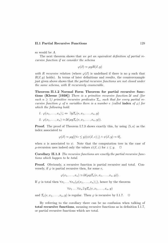
II.1 Partial Recursive Functions 129
so would be A.The next theorem shows that we get an equivalent definition of partial re-
cursive function if we consider the schema
ϕ(~x) ' µyR(~x, y)
with R recursive relation (where ϕ(~x) is undefined if there is no y such thatR(~x, y) holds). In terms of later definitions and results, the counterexamplejust given above shows that the partial recursive functions are not closed underthe same schema, with R recursively enumerable.
Theorem II.1.2 Normal Form Theorem for partial recursive func-tions (Kleene [1938]) There is a primitive recursive function U and (foreach n ≥ 1) primitive recursive predicates Tn, such that for every partial re-cursive function ϕ of n variables there is a number e (called index of ϕ) forwhich the following hold:
1. ϕ(x1, . . . , xn)↓ ⇔ ∃yTn(e, x1, . . . , xn, y)
2. ϕ(x1, . . . , xn) ' U(µyTn(e, x1, . . . , xn, y)).
Proof. The proof of Theorem I.7.3 shows exactly this, by using 〈5, a〉 as theindex associated to
ϕ(~x) ' µy[(∀z ≤ y)(ψ(~x, z)↓) ∧ ψ(~x, y) ' 0],
when a is associated to ψ. Note that the computation tree in the case ofµ-recursion uses indeed only the values ψ(~x, z) for z ≤ y. 2
Corollary II.1.3 The recursive functions are exactly the partial recursive func-tions which happen to be total.
Proof. Obviously, a recursive function is partial recursive and total. Con-versely, if ϕ is partial recursive then, for some e,
ϕ(x1, . . . , xn) ' U(µyTn(e, x1, . . . , xn, y)).
If ϕ is total then ∀x1 . . .∀xn(ϕ(x1, . . . , xn)↓), hence by the theorem
∀x1 . . .∀xn∃ yTn(e, x1, . . . , xn, y)
and Tn(e, x1, . . . , xn, y) is regular. Then ϕ is recursive by I.1.7. 2
By referring to the corollary there can be no confusion when talking oftotal recursive functions, meaning recursive functions as in definition I.1.7,or partial recursive functions which are total.
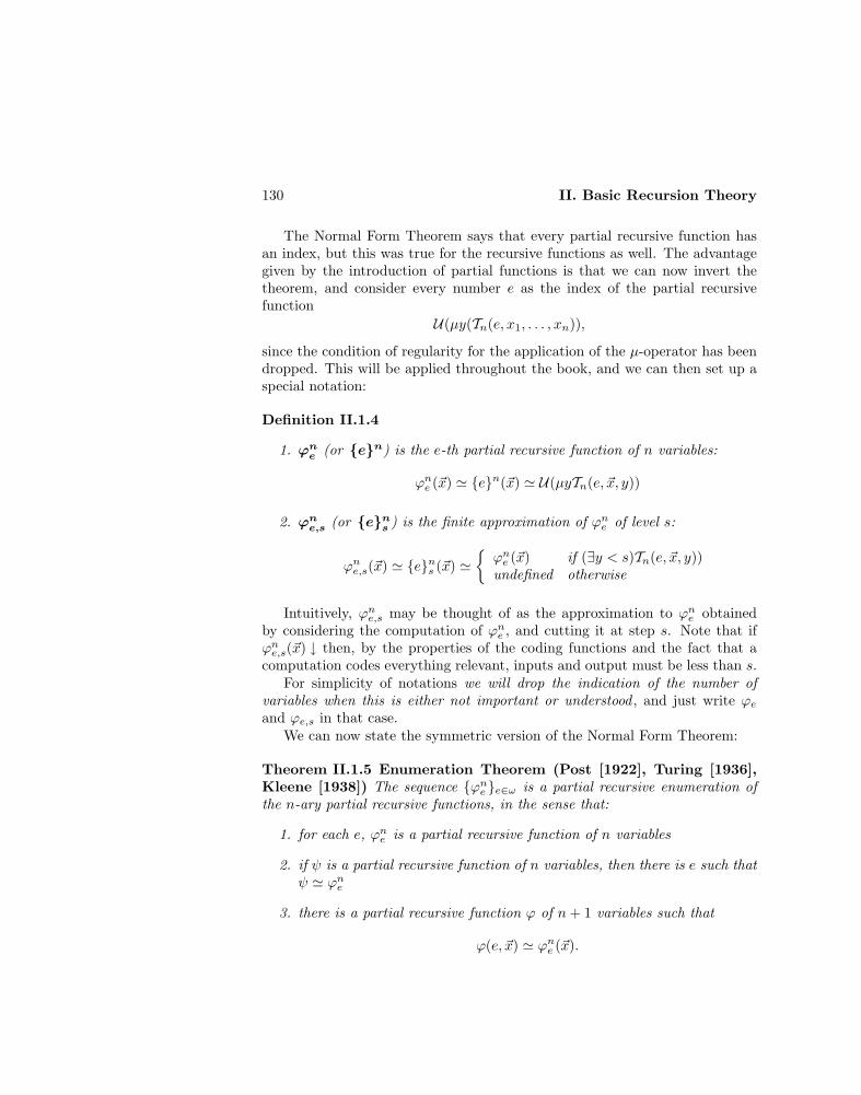
130 II. Basic Recursion Theory
The Normal Form Theorem says that every partial recursive function hasan index, but this was true for the recursive functions as well. The advantagegiven by the introduction of partial functions is that we can now invert thetheorem, and consider every number e as the index of the partial recursivefunction
U(µy(Tn(e, x1, . . . , xn)),
since the condition of regularity for the application of the µ-operator has beendropped. This will be applied throughout the book, and we can then set up aspecial notation:
Definition II.1.4
1. ϕne (or en) is the e-th partial recursive function of n variables:
ϕne (~x) ' en(~x) ' U(µyTn(e, ~x, y))
2. ϕne,s (or en
s ) is the finite approximation of ϕne of level s:
ϕne,s(~x) ' ens (~x) 'ϕne (~x) if (∃y < s)Tn(e, ~x, y))undefined otherwise
Intuitively, ϕne,s may be thought of as the approximation to ϕne obtainedby considering the computation of ϕne , and cutting it at step s. Note that ifϕne,s(~x) ↓ then, by the properties of the coding functions and the fact that acomputation codes everything relevant, inputs and output must be less than s.
For simplicity of notations we will drop the indication of the number ofvariables when this is either not important or understood , and just write ϕeand ϕe,s in that case.
We can now state the symmetric version of the Normal Form Theorem:
Theorem II.1.5 Enumeration Theorem (Post [1922], Turing [1936],Kleene [1938]) The sequence ϕne e∈ω is a partial recursive enumeration ofthe n-ary partial recursive functions, in the sense that:
1. for each e, ϕne is a partial recursive function of n variables
2. if ψ is a partial recursive function of n variables, then there is e such thatψ ' ϕne
3. there is a partial recursive function ϕ of n+ 1 variables such that
ϕ(e, ~x) ' ϕne (~x).
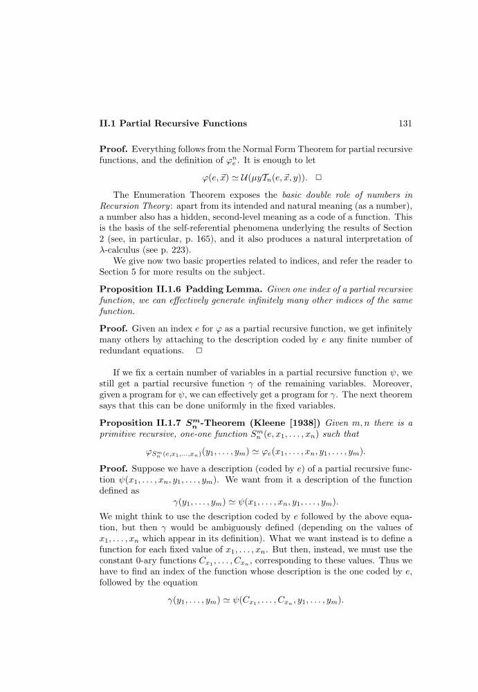
II.1 Partial Recursive Functions 131
Proof. Everything follows from the Normal Form Theorem for partial recursivefunctions, and the definition of ϕne . It is enough to let
ϕ(e, ~x) ' U(µyTn(e, ~x, y)). 2
The Enumeration Theorem exposes the basic double role of numbers inRecursion Theory : apart from its intended and natural meaning (as a number),a number also has a hidden, second-level meaning as a code of a function. Thisis the basis of the self-referential phenomena underlying the results of Section2 (see, in particular, p. 165), and it also produces a natural interpretation ofλ-calculus (see p. 223).
We give now two basic properties related to indices, and refer the reader toSection 5 for more results on the subject.
Proposition II.1.6 Padding Lemma. Given one index of a partial recursivefunction, we can effectively generate infinitely many other indices of the samefunction.
Proof. Given an index e for ϕ as a partial recursive function, we get infinitelymany others by attaching to the description coded by e any finite number ofredundant equations. 2
If we fix a certain number of variables in a partial recursive function ψ, westill get a partial recursive function γ of the remaining variables. Moreover,given a program for ψ, we can effectively get a program for γ. The next theoremsays that this can be done uniformly in the fixed variables.
Proposition II.1.7 Smn -Theorem (Kleene [1938]) Given m,n there is a
primitive recursive, one-one function Smn (e, x1, . . . , xn) such that
ϕSmn (e,x1,...,xn)(y1, . . . , ym) ' ϕe(x1, . . . , xn, y1, . . . , ym).
Proof. Suppose we have a description (coded by e) of a partial recursive func-tion ψ(x1, . . . , xn, y1, . . . , ym). We want from it a description of the functiondefined as
γ(y1, . . . , ym) ' ψ(x1, . . . , xn, y1, . . . , ym).
We might think to use the description coded by e followed by the above equa-tion, but then γ would be ambiguously defined (depending on the values ofx1, . . . , xn which appear in its definition). What we want instead is to define afunction for each fixed value of x1, . . . , xn. But then, instead, we must use theconstant 0-ary functions Cx1 , . . . , Cxn , corresponding to these values. Thus wehave to find an index of the function whose description is the one coded by e,followed by the equation
γ(y1, . . . , ym) ' ψ(Cx1 , . . . , Cxn , y1, . . . , ym).

132 II. Basic Recursion Theory
This is now a good description of γ, depending uniformly on e and the valuesgiven to x1, . . . , xn. Its index is thus a function Smn (e, x1, . . . , xm), and can bemade primitive recursive by the method of arithmetization used in Section I.7.It is one-one by its definition and the properties of the coding functions. 2
The Smn -Theorem (also called the Parametrization Theorem, or the It-eration Theorem) looks, at first sight, innocuous, and simply appears to bestating that data can be effectively incorporated into a program. But we shouldnot forget the fundamental double role of numbers in Recursion Theory: datacan code programs themselves, and thus incorporating them into a programmay have the effect that the program interprets them as subprograms. Thusthe Smn -Theorem actually embodies a notion of subcomputation and an effectiveversion of composition.
In a precise sense, enumeration and parametrization are inverse transla-tions, and provide the technical tools needed to handle the basic duality ofnumbers: by enumeration an index can be considered as an argument, andby parametrization an argument can be considered as an index. This explainstheir fundamental role, analyzed in Section 5.
It should be noted that all the other approaches of Chapter I could be sim-ilarly adapted to the treatment of partial functions by dropping the totalityrequirements. Thus we could consider partial functions computed by Turingmachines, and say that for given inputs a Turing machine computes a value if ithalts in the prescribed way, and it does not otherwise (i.e. if it does not halt, orit does, but not in the prescribed way). Flowchart programs, Herbrand-Godelcomputability, λ-definability, and so on are treated similarly. As it was the casefor total functions, the various approaches remain equivalent for partial func-tions as well, with similar proofs. Thus the class of partial recursive functionsretains the absoluteness and stability of the class of recursive functions, and ithas the extra quality of admitting an intrinsic definition, without reference tononconstructive notions.
Universal Turing machines and computers ?
The Enumeration Theorem admits a stronger formulation, due to the unifor-mities of the definition of Tn w.r.t. n.
Theorem II.1.8 Universal Partial Function (Post [1922], Turing[1936], Kleene [1938]) There is a partial recursive function ϕ(e, x), calleduniversal partial function, which generates all the partial recursive func-tions of any number of variables, in the sense that for every partial recursive
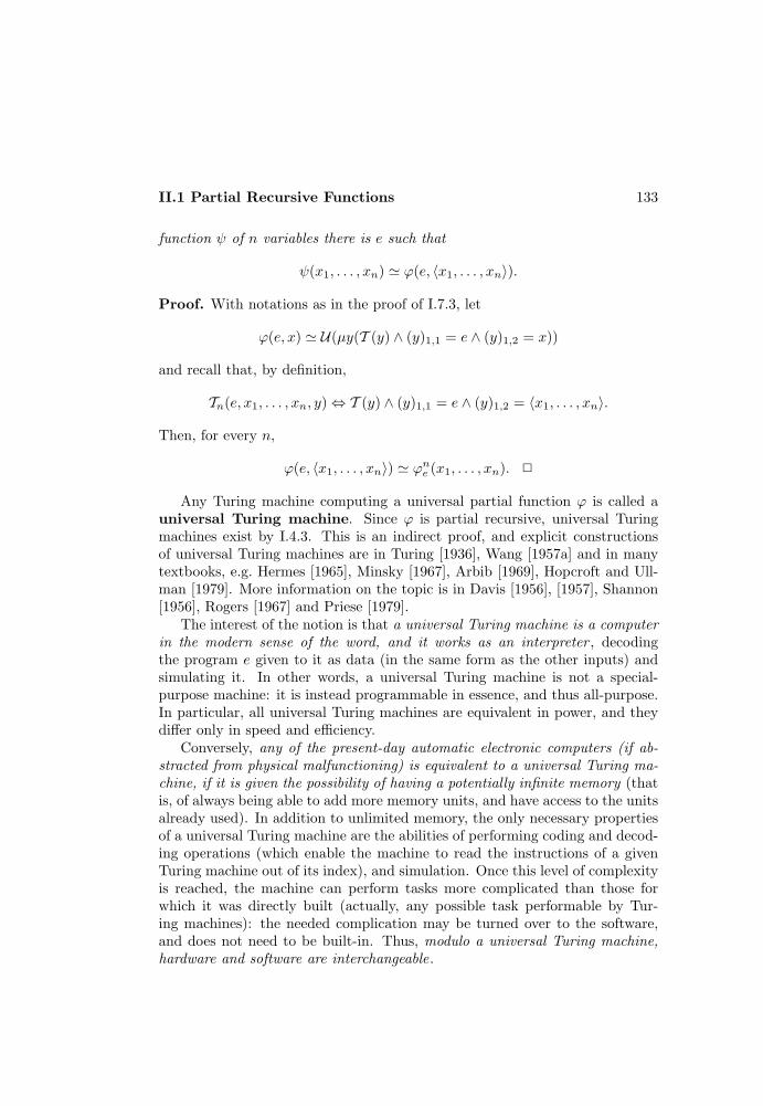
II.1 Partial Recursive Functions 133
function ψ of n variables there is e such that
ψ(x1, . . . , xn) ' ϕ(e, 〈x1, . . . , xn〉).
Proof. With notations as in the proof of I.7.3, let
ϕ(e, x) ' U(µy(T (y) ∧ (y)1,1 = e ∧ (y)1,2 = x))
and recall that, by definition,
Tn(e, x1, . . . , xn, y) ⇔ T (y) ∧ (y)1,1 = e ∧ (y)1,2 = 〈x1, . . . , xn〉.
Then, for every n,
ϕ(e, 〈x1, . . . , xn〉) ' ϕne (x1, . . . , xn). 2
Any Turing machine computing a universal partial function ϕ is called auniversal Turing machine. Since ϕ is partial recursive, universal Turingmachines exist by I.4.3. This is an indirect proof, and explicit constructionsof universal Turing machines are in Turing [1936], Wang [1957a] and in manytextbooks, e.g. Hermes [1965], Minsky [1967], Arbib [1969], Hopcroft and Ull-man [1979]. More information on the topic is in Davis [1956], [1957], Shannon[1956], Rogers [1967] and Priese [1979].
The interest of the notion is that a universal Turing machine is a computerin the modern sense of the word, and it works as an interpreter , decodingthe program e given to it as data (in the same form as the other inputs) andsimulating it. In other words, a universal Turing machine is not a special-purpose machine: it is instead programmable in essence, and thus all-purpose.In particular, all universal Turing machines are equivalent in power, and theydiffer only in speed and efficiency.
Conversely, any of the present-day automatic electronic computers (if ab-stracted from physical malfunctioning) is equivalent to a universal Turing ma-chine, if it is given the possibility of having a potentially infinite memory (thatis, of always being able to add more memory units, and have access to the unitsalready used). In addition to unlimited memory, the only necessary propertiesof a universal Turing machine are the abilities of performing coding and decod-ing operations (which enable the machine to read the instructions of a givenTuring machine out of its index), and simulation. Once this level of complexityis reached, the machine can perform tasks more complicated than those forwhich it was directly built (actually, any possible task performable by Tur-ing machines): the needed complication may be turned over to the software,and does not need to be built-in. Thus, modulo a universal Turing machine,hardware and software are interchangeable.
134 II. Basic Recursion Theory
The realization that a machine could be universal-purpose, by being ableto simulate other machines through their programs, antedates both RecursionTheory and Computer Science: it goes back to Babbage’s [1837] conception ofthe analytical engine. This crucial notion appears natural nowadays, but itdid not always look so. This was the case not only in Babbage’s time, but evenafter Turing’s abstract development, and well into the process of building realcomputers: see e.g. Hodges [1983] for an account of the resistance Turing hadto face in his own computer project, against (in his words)
the tradition of solving one’s difficulties by means of much equip-ment rather than by thought
which meant a privilege of hardware and special-purpose machines over soft-ware.
Recursively enumerable sets
Having looked at the notion of partial recursive function, we turn now to itsanalogue in terms of sets and relations. For total recursive functions we had nodoubts: the analogues were just those sets and relations whose characteristicfunctions were recursive. But since a characteristic function is always total,partial recursive characteristic functions would again give the recursive sets,by II.1.3.
Natural sets associated to partial functions are their domains.
Definition II.1.9 (Post[1922], Kleene [1936]) An n-ary relation is recur-sively enumerable (abbreviated r.e.) if it is the domain of an n-ary partialrecursive function.
We indicate by Wne and Wn
e,s, respectively, the domains of ϕne and ϕne,s.
As we have already done for functions, we will drop the mention of thenumber of arguments for relations as well, when no confusion arises. Also, wewill identify sets and unary relations, and thus write x ∈ We for W1
e (x).From the definition we have immediately:
Theorem II.1.10 Normal Form Theorem for r.e. relations (Kleene[1936], Rosser [1936], Mostowski [1947]) An n-ary relation P is r.e. ifand only if there is a n+ 1-ary recursive relation R such that
P (~x) ⇔ ∃yR(~x, y),
i.e. if and only if there is a number e (called index of P ) such that
P (~x) ⇔ Wne (~x) ⇔ ∃yTn(e, ~x, y).

II.1 Partial Recursive Functions 135
Proof. If P is r.e. then P is the domain of a recursive function ϕe, i.e. P isequal to We. Then, by II.1.2,
We(~x) ⇔ ϕe(~x)↓⇔ ∃yTn(e, ~x, y).
Conversely, if
P (~x) ⇔ ∃yR(~x, y)
with R recursive, then P is the domain of the partial recursive function
ϕ(~x) ' µyR(~x, y). 2
R.e. relations appear naturally and abundantly in mathematics. Considere.g. a diophantine equation p(~x, y) = q(~x, y), where p and q are polynomi-als in ~x, y with coefficients in the natural numbers. The set of non-negative,integral solutions of the equation, defined as:
y ∈ D ⇔ ∃~x [p(~x, y) = q(~x, y)]
is r.e., by the theorem just proved. Matiyasevitch [1970] has shown that theconverse also holds, and thus the r.e. sets are exactly the sets of non-negative1
integral solutions of diophantine equations. See Matiyasevitch [1972] or Davis[1973] for an exposition of this remarkable result, which improves the NormalForm Theorem, and also solves Hilbert’s Tenth Problem (Hilbert [1900]).A discussion of its significance is in Davis, Matiyasevitch and Robinson [1976],and an easy proof of a slightly weaker version of it is in Jones and Matiyasevitch[1984].
The notion of r.e. set has been defined from that of partial recursive func-tion, but the next result shows that the opposite approach is also possible.
Proposition II.1.11 Graph Theorem. Let ϕ and f be, respectively, a par-tial and a total function. Then:
1. ϕ is partial recursive if and only if its graph is r.e.
2. f is recursive if and only if its graph is recursive.
Proof. Recall that the graph Gϕ of ϕ is the set so defined:
Gϕ(~x, z) ⇔ ϕ(~x) ' z.
1This condition cannot be eliminated: it is known e.g. that there is no diophantine equa-tion whose integral solutions are exactly the prime numbers.
136 II. Basic Recursion Theory
If ϕ is partial recursive then ϕ ' ϕe, for some e. It follows that
Gϕ(~x, z) ⇔ ϕe(~x) ' z
⇔ U(µyTn(e, ~x, y)) ' z
⇔ ∃y[Tn(e, ~x, y) ∧ (∀t < y)¬Tn(e, ~x, t) ∧ U(y) = z]
and thus (by II.1.10) Gϕ is r.e. Conversely, if Gϕ is r.e. then
Gϕ(~x, z) ⇔ ∃yR(~x, z, y)
for some recursive R, again by II.1.10. Thus
ϕ(~x)↓⇔ ∃z∃yR(~x, z, y).
By coding z and y into a single number t = 〈z, y〉, we have
ϕ(~x) ' (µtR(~x, (t)1, (t)2))1 .
Intuitively, this is nothing more than a dovetailed verification of Gϕ(~x, z) forevery z, until one of these verification succeeds. The reason we cannot simplyverify the z’s one by one, is that we could get stuck with the first one which isnot a value of ϕ(~x), and never get to consider the remaining possible values.
If f is recursive, so is Gf :
cGf(~x, z) =
1 if f(~x) = z0 otherwise.
Conversely, let Gf be recursive. Since
f(~x) = µzGf (~x, z),
and the hypothesis that f is total can be written as
∀~x∃z Gf (~x, z),
we have that f is defined by µ-recursion over a regular predicate (I.1.5), and itis then recursive. 2
Exercises II.1.12 Partial functions with recursive graph. a) If ϕ is a partialfunction, then ϕ has a recursive graph if and only if there is a recursive R such thatϕ(~x) ' µyR(~x, y).
b) There are partial recursive, nontotal functions with recursive graph. (Hint: letWe be an r.e. set different from ω, and let ϕ(x) ' µs(x ∈ We,s).)
c) There are partial recursive functions with nonrecursive graph. (Hint: let A bean r.e. nonrecursive set, see II.2.3, and ϕ(x) ' 0 ⇔ x ∈ A.)

II.1 Partial Recursive Functions 137
See Chapter VIII for more on this topic.
The close relationship between partial recursive functions and r.e. relationsis also indicated by the following property, defined by Lusin [1930] in a descrip-tive set-theoretical context.
Proposition II.1.13 Uniformization Property (Kleene [1936])
1. If P is r.e., there is a partial recursive function ϕ such that
∃yP (~x, y) ⇒ ϕ(~x)↓ ∧ P (~x, ϕ(~x))
2. If P is r.e. and regular, there is a recursive function f such that
∀~xP (~x, f(~x)).
Proof. This is similar to part 2 of the proof of II.1.11. Since P is r.e., there isR recursive such that
P (~x, y) ⇔ ∃zR(~x, y, z).
Then it is enough to let
ϕ(~x) ' (µtR(~x, (t)1, (t)2))1 .
Intuitively, ϕ chooses the first element y such that P (~x, y) has been verified(which, as the next exercise shows, is not necessarily the first one for whichP holds). If P is regular (I.1.5), then such a y always exists, and ϕ is thenrecursive. 2
Exercise II.1.14 If P is recursive, a uniformizing function is simply µyP (~x, y).This does not hold in general, for P r.e. (Uspenskii [1957]) (Hint: see the remarksafter II.1.1.)
Exercises II.1.15 Choice functions for r.e. sets. a) There is a partial recursivechoice function for the r.e. sets, i.e. a partial recursive function ϕ such that
We 6= ∅ ⇒ ϕ(e)↓ ∧ ϕ(e) ∈ We.
(Hint: uniformize P (e, y) ⇔ y ∈ We.)
b) There is no invariant, partial recursive choice function for the r.e. sets, i.e. achoice function ϕ such that
Wi = We 6= ∅ ⇒ ϕ(i)↓ ∧ ϕ(e)↓ ∧ ϕ(i) = ϕ(e).
138 II. Basic Recursion Theory
Thus no partial recursive analogue of Hilbert’s ∈-choice function exists for r.e. sets.(Kleene [1952]) (Hint: suppose such a function exists. Assume there exists a nonre-cursive r.e. set A, see II.2.3, and let:
y ∈ Wg(e) ⇔ y = 0 ∨ (y = 1 ∧ e ∈ A)
y ∈ Wh(e) ⇔ y = 1 ∨ (y = 0 ∧ e ∈ A)
Then ϕg(e) and ϕh(e) both converge, and
e ∈ A ⇔ ϕg(e) = ϕh(e),
i.e. A would be recursive.)
c) There is no recursive choice function for the r.e. sets. (Hint: let f be one such,
set Wh(e) = f(e) + 1 and apply the Fixed-Point Theorem II.2.10.)
Having analyzed the analogies of r.e. sets versus partial recursive functions,we turn now to the differences between r.e. and recursive sets. We first char-acterize both notions in terms of enumeration properties, and in so doing weaccount for the name ‘recursively enumerable’ (which suggests ranges, morethan domains). The next result is very useful and will be applied repeatedly.
Theorem II.1.16 Characterization of the r.e. sets (Kleene [1936]) Thefollowing are equivalent:
1. A is r.e.
2. A is the range of a partial recursive function ϕ
3. A = ∅ or A is the range of a recursive function f .
Proof. We prove the result in a round robin style.
• 1 ⇒ 2If A is r.e. then A = We, for some e. Let
ϕ(x) ' x⇔ ϕe(x)↓ .
Then the domain of ϕe is equal to the range of ϕ, and ϕ is partial recur-sive, e.g. because ϕ(x) ' x+ 0 · ϕe(x).
• 2 ⇒ 3Let A be nonempty, and the range of a partial recursive function ϕe.Choose a ∈ A: we would like to set
f(x) =z if ϕe(x)↓ ∧ ϕe(x) ' za otherwise.
II.1 Partial Recursive Functions 139
As it stands f is not however recursive, because we cannot decide recur-sively whether ϕ(x) ↓ (see II.2.7). To avoid being stuck while waitingfor some undefined value to converge, we dovetail the computation of allpossible values, and put them in the range of f as soon as they appear,the value a being used for the stages in which no new value appears (tokeep f total). Thus the following modified version of f is recursive:
f(J (x, s)) =z if ϕe,s(x) ↓ ∧ ϕe,s(x) ' za otherwise.
Here J is a recursive, onto pairing function (see e.g. p. 27), and ontonessis required to have f total.
• 3 ⇒ 1If A = ∅ then A is the domain of the completely undefined function,which is obviously partial recursive. If A is the range of a recursive f , wewant a partial recursive ϕ with domain A, i.e.
ϕ(x)↓ ⇔ ∃z(f(z) = x).
Then we can just let ϕ(x) ' µz(f(z) = x). 2
Also the recursive sets can be characterized in terms of enumerating func-tions.
Proposition II.1.17 The following are equivalent:
1. A is recursive
2. A = ∅ or A is the range of a nondecreasing, recursive function f .
Proof. If A is recursive and nonempty, let a be its smallest element, and
f(0) = a
f(n+ 1) =n+ 1 if n+ 1 ∈ Af(n) otherwise.
Conversely, if A is finite then it is recursive. If A is infinite and the rangeof a nondecreasing recursive function f , to know whether z ∈ A, search for thesmallest x such that f(x) > z (which exists because A is infinite). Since f isnondecreasing, then
z ∈ A⇔ z ∈ f(0), . . . , f(x). 2

140 II. Basic Recursion Theory
Exercises II.1.18 One-one enumerating functions. a) An infinite r.e. set is therange of a one-one recursive function. (Kleene [1936], Rosser [1936]) (Hint: define fby primitive recursion, looking at each stage for the next element generated in theset, which has not been previously generated.)
b) An infinite recursive set is the range of an increasing recursive function.
(Kleene [1936]) (Hint: define f by primitive recursion, looking at each stage for
the next element in the set.)
The description of a set consists of the infinitely many facts that tell, forany given element, if it is in the set or not. In general, although they alwaysanswer yes or no to a question, these facts are just a sequence of accidents, withno common pattern. The recursive sets are those for which a pattern exists,and a general procedure to give effective answers can be finitely described. Therecursively enumerable sets present a basic asymmetry between membership,that can be effectively determined by a finite amount of information, and non-membership, whose determination may instead require an infinite amount of it(the partial test for membership of a given element being simply to recursivelygenerate the set, and wait for that element to appear). The r.e. sets are thussomehow only ‘half-recursive’.2
The distinction between recursive and recursively enumerable can then betraced back to the informal distinction between a decision procedure and agenerating procedure, envisaged once again by Leibniz [1666], when he talkedof ars iudicandi (checking the correctness of a proof) and ars inveniendi(finding a proof).
Another reason to see the r.e. sets as half-recursive is given by the next re-sult, which also characterizes recursiveness in terms of recursive enumerability.It is sometimes called Post’s Theorem, and it will be used repeatedly.
Theorem II.1.19 (Post [1943], Kleene [1943], Mostowski [1947]) Aset is recursive if and only if both the set and its complement are recursivelyenumerable.
Proof. If A is recursive then both A and A are r.e., since e.g. functions withdomain A and A are
ϕ(x) '
1 if cA(x) = 1↑ otherwise
ψ(x) '
0 if cA(x) = 0↑ otherwise.
2For this reason the r.e. sets are sometimes called semirecursive. We will use this term ina different context, see p. 294.
II.1 Partial Recursive Functions 141
Let now both A and A be r.e., and suppose they are nonempty (if one isempty the other is ω, and they are already both recursive as wanted). Thenthere are recursive functions f and g generating them:
A = f(0), f(1), . . .A = g(0), g(1), . . ..
The two lists are disjoint and exhaustive, and to know whether a given x is inA or in A is enough to generate them simultaneously, until x appears in one ofthe two lists.
More formally, if A and A are r.e., there are recursive relations R and Qsuch that
x ∈ A ⇔ ∃yR(x, y)x ∈ A ⇔ ∃yQ(x, y).
Since∀x∃y(R(x, y) ∨Q(x, y))
holds, the functionf(x) = µy(R(x, y) ∨Q(x, y))
is recursive, and exactly one of R(x, f(x)) and Q(x, f(x)) holds. Then A isrecursive, since
cA(x) =
1 if R(x, f(x))0 otherwise 2
Proposition II.1.20 (Post [1944]) Every infinite r.e. set has an infinite re-cursive subset.
Proof. Let A be infinite, and the range of a recursive function f . Define grecursive and increasing as:
g(0) = f(0)g(n+ 1) = the first element generated in A and greater than g(n)
= f(µy(f(y) > g(n))).
Then the range of g is recursive by II.1.17, and it is an infinite subset of A bydefinition. 2
Infinite sets which do not have infinite r.e. (equivalently, by the previousproposition, infinite recursive) subsets are called immune, and will be studiedin Sections 6 and III.2.
142 II. Basic Recursion Theory
Proposition II.1.21 Set-theoretical properties of r.e. sets (Post [1943],Mostowski [1947])
1. With respect to set-theoretical inclusion, the r.e. sets form a distributivelattice with smallest and greatest element, and with the recursive sets asthe only complemented elements.
2. The property of being r.e. is preserved under images and inverse imagesvia partial recursive functions.
Proof. Smallest and greatest elements are clearly ∅ and ω. The part relativeto complementation follows from II.1.19. Finally, if A and B are r.e. then soare A ∩ B and A ∪ B: generate A and B simultaneously, put in A ∩ B theelements appearing in both lists, and in A ∪B those appearing in at least onelist.
Given A r.e. and ϕ partial recursive, ϕ(A) consists of all elements ϕ(x), forx ∈ A. To generate ϕ(A) is thus enough to generate A and, simultaneously, todovetail the computations of ϕ(x), for the various x’s which are found to be inA. Similarly, ϕ−1(A) consists of all x such that ϕ(x)↓ and ϕ(x) ∈ A. 2
Corollary II.1.22 Set-theoretical properties of recursive sets.
1. With respect to set-theoretical inclusion, the recursive sets form a Booleanalgebra.
2. The property of being recursive is preserved under inverse images viarecursive functions.
Proof. If A is recursive both A and A are r.e., and then so are f−1(A) andf−1(A). But f−1(A) = f−1(A), and so both f−1(A) and its complement arer.e., and f−1(A) is recursive by II.1.19. 2
Note that if A and f are recursive, then f(A) is r.e. by the propositionabove, but is not necessarily recursive. Indeed, any nonempty r.e. set A is therange of a recursive function f , and thus the image of ω (which is recursive)via f , but not every r.e. set is recursive (see II.2.3).
A detailed study of the set-theoretical structure of both recursive and r.e.sets will be made in Volume II. For now we just prove an additional property,defined by Kuratowski [1936] in a descriptive set-theoretical context.
Proposition II.1.23 Reduction Property (Rosser [1936], Kleene[1950]) The union of two r.e. sets can be reduced to the union of two dis-joint r.e. sets. Precisely, given two r.e. sets A and B there are two r.e. setsA′ ⊆ A and B′ ⊆ B such that
A′ ∩B′ = ∅ and A′ ∪B′ = A ∪B.
II.1 Partial Recursive Functions 143
Proof. Given A and B r.e., the only problem is to decide where to put theelements of A ∩ B. We let speed of generation decide: if z ∈ A ∩ B and z isgenerated by A faster than by B, then z goes into A′, otherwise it goes intoB′. More formally, if
x ∈ A ⇔ ∃yR(x, y)x ∈ B ⇔ ∃yQ(x, y)
with R and Q recursive, let
x ∈ A′ ⇔ ∃y[R(x, y) ∧ (∀z ≤ y)¬Q(x, z)]x ∈ B′ ⇔ ∃y[Q(x, y) ∧ (∀z < y)¬R(x, z)]. 2
Exercise II.1.24 The reduction property follows from the uniformization property .
R.e. sets as foundation of Recursion Theory ?
We have derived the notion of recursive enumerability from that of partialrecursive function, but we have already noted that, by II.1.11, the opposite isalso possible: the partial recursive functions are those with an r.e. graph. Whatis needed to avoid circularities, is an independent characterization of recursiveenumerability.
This has been provided by Post [1922], [1943] (incidentally, quite beforethe notion of recursiveness had been isolated). His formulation comes from ananalysis of derivations in formal systems, and it is thus the natural conclusionof our journey of Chapter I (see p. 18). The underlying idea is that effectivemathematical and, more generally, linguistical activity can be seen as a way ofgenerating words from words (of a given language), according to rules. Withconsiderations similar to those of Section I.4, one is quickly led to restrictattention to canonical systems consisting of finite alphabets (possibly withdistinguished symbols), finite sets of axioms and finite sets of finitary rules(called productions), telling how to decompose a word and rearrange its parts(by possibly dropping some and adding others). Formally, a production hasthe form
x0 1 x1 · · · xn−1 n xn −→ y0 i1 y1 · · · ym−1 im ym
where ij ∈ 1, . . . , n, with the meaning: if a word can be decomposed inthe way written on the left (by somehow filling up the boxes), then it can betransformed into the word written on the right (where the boxes on the rightwith a given label are supposed to contain exactly what the boxes on the leftwith the same label did). Since decompositions of words are usually not unique,productions are not deterministic rules.
144 II. Basic Recursion Theory
It is possible to show that the sets of words produced by canonical systemsare exactly (under suitable coding) the r.e. ones (one direction comes by arith-metization; the other can be seen by noting that Turing machines transitionsbetween successive configurations can be written as productions, operating onwords expressing the configurations).
Post also showed that systems with multiple-premise productions arereducible to canonical systems, and that these are in turn reducible to normalsystems, with just one axiom, and with productions of the very specific form
x 1 → 1 y.
For a proof of this and a treatment of the whole subject, see Minsky [1967].The approach sketched above is relevant not only to computability but
also (and even more naturally) to linguistics, and it provides a frameworkfor studying structural descriptions of sentences, in formal approximations tonatural languages. A system with productions only of the form
1 x 2 → 1 y 2
(that can be written simply as x→ y), is called a grammar (Thue [1914]). Thenotion is sufficiently general, since the simulation of Turing machines referredto above can be naturally carried out by means of grammar productions (in-structions act only locally on the tape of a Turing machine). Chomsky [1956],[1959] has introduced a hierarchy on the types of grammar productions, whichhas turned out to be strongly connected with machine models. We will onlyprove some scattered results (see Chapter VIII) and thus refer to Hopcroft andUllman [1979] for a detailed study of the subject, and to Greibach [1981] for abroad overview and an historical account.
A programming language based on r.e. sets ?
Although Post’s productions are intended to provide a basis for recursive enu-merability, they can be used directly to define partial algorithms for partialfunctions on strings, by introducing restrictions that make the production pro-cess deterministic.
A finite sequence of grammar productions (some of which are singled outas final) computes a partial function on strings ϕ if, given any string w, thefollowing partial algorithm produces the string ϕ(w): at each step (startingfrom w), search for the first production in the sequence which can be applied(i.e. such that the premise of the production matches a substring of the givenstring), and apply the production to the leftmost possible substring to which itcan be applied; then stop the process if the production is a final one, and repeat
II.2 Diagonalization 145
the process otherwise. This approach has been introduced by Markov [1951],[1954] and it is easily seen (Detlovs [1953], [1958]) to be equivalent to partialrecursiveness (one direction follows as sketched above for Turing machines, theother by arithmetization). It is usually referred to as Markov algorithms.
This suggests the possibility of using the production approach as a basis fora programming language for string operations, which has been done with theintroduction of SNOBOL (String Oriented Symbolic Language) by Farber,Griswold and Polonsky [1964] (see Sammett [1969] and Wexelblat [1981] forhistory and references). The instructions of this language are labelled, and areeither assignment statements (giving values to the variables) or replacementstatements (telling to substitute the leftmost occurrence of a substring in astring by another string), the latter together with conditional jump instruc-tions (sending to other instructions, depending on whether the given substi-tutions was successfully applied, or could not be applied). The language isthus unstructured (see p. 64), and it does not need any primitive operation(pattern matching being sufficient for all purposes: the needed operations canbe specified each time, as production rules).
II.2 Diagonalization
In this section we introduce one of the basic methods of proof in RecursionTheory: diagonalization. We will give a number of applications, but the methodwill be used throughout the book either directly or in some codified way (likethe unsolvability of the Halting Problem, or the Fixed-Point Theorem, bothproved below).
The essence of diagonalization
Given a set S, a function d : S → S which is never the identity on S (i.e.d(a) 6= a for every element a of S) and an infinite matrix of elements of S
a0,0 a0,1 a0,2 · · ·a1,0 a1,1 a1,2 · · ·a2,0 a2,1 a2,2 · · ·. . . . . . . . . . . .
we get a transformed diagonal sequence of elements of S
d(a0,0) d(a1,1) d(a2,2) · · ·
which is not equal to any row of the matrix, because it differs from the n-throw on the n-th element (by the hypothesis on d). That’s all.

146 II. Basic Recursion Theory
The ingredients of the method are two:
1. the use of the diagonal an,nn∈ωThis was systematically done by Du Bois Reymond, in his study of ordersof infinity (see Hardy [1910] for a neat exposition).
2. the use of the switching function dThis crucial part was introduced by Cantor [1874] to prove his celebratedtheorem that the set of subsets of ω is not denumerable.
In many applications, like the results proved or quoted from p. 165 on, the twoingredients take the form of self-reference and negation.
Recursive undecidability results
As a sample application of the method we prove a constructive analogue ofCantor’s Theorem, whose original form can be stated by saying that there isno function on ω which enumerates all subsets of ω (or, equivalently, the set ofcharacteristic functions, i.e. the set of total functions from ω to 0, 1).
Proposition II.2.1 Recursive version of Cantor’s Theorem (Kleene[1936], Turing [1936]) There is no recursive function which enumerates (atleast one index of) each recursive (0,1-valued) function.
Proof. Let f be a recursive function such that ϕf(x) is total for every x, anddefine
g(x) ' 1− ϕf(x)(x).
Then g is a 0,1-valued function, which is partial recursive by the EnumerationTheorem II.1.5, and total by the hypothesis on f . Moreover, g is different fromϕf(x) (on the element x) for every x, and thus no index of g is in the range off . 2
The proof just given falls under the general framework of diagonalization,by letting ai,j = ϕf(i)(j), and d(a) = 1− a. It also implies that the set
Tot = x : ϕx is total
is not r.e. In particular it is not recursive, and thus there is no recursive wayto detect whether a number codes a total recursive function or not .
Note that we expressed our results in terms of 0,1-valued functions, and notof sets. This is because there are many different ways to associate numbers torecursive sets, and different results hold for them (see p. 226).
II.2 Diagonalization 147
Exercises II.2.2 a) A function is called potentially recursive (Church [1936]) ifit has a total recursive extension. There is a partial recursive function which is notpotentially recursive. (Kleene [1938]) (Hint: let ϕ(x) ' 1− ϕx(x).)
b) There is a recursive, not primitive recursive set . (Sudan [1927], Ackermann
[1928]) (Hint: consider 0,1-valued functions, and use the function of I.7.4.)
We now prove one of the crucial results of Recursion Theory.
Theorem II.2.3 Combinatorial core of the undecidability results(Post [1922], Godel [1931], Kleene [1936]) There is an r.e. nonrecursiveset. Explicitly, the set defined by
x ∈ K ⇔ x ∈ Wx ⇔ ϕx(x)↓
is r.e. and nonrecursive.
Proof. By the Enumeration Theorem II.1.5, there is a partial recursive func-tion ϕ such that
ϕ(x) ' ϕx(x).
Then K is r.e., becausex ∈ K ⇔ ϕ(x)↓ .
To show that K is not recursive we give two different proofs, based onthe two equivalent definitions of K given above (in terms of partial recursivefunctions and of r.e. sets).
• If K were recursive, so would be the function
f(x) =
0 if x ∈ Kundefined otherwise.
Then f ' ϕe for some e, and
ϕe(e)↓ ⇔ e ∈ K,
contradicting the definition of K.
• If K were recursive, then K would be r.e. But
x ∈ K ⇔ x 6∈ Wx,
and so K differs on the element x from the xth r.e. sets, and cannot beitself r.e. 2
148 II. Basic Recursion Theory
The argument to show that K is not recursive falls under the general frame-work of diagonalization, by letting
ai,j =
1 if j ∈ Wi
0 otherwise,
and d(a) = 1− a.K obviously resembles the set used in Russell’s paradox (Russell [1903]),
namely the set of sets not belonging to themselves (see p. 82). Here K is theset of numbers not belonging to the r.e. sets they code. There is no paradoxhere because Russell’s argument simply shows that such a set is not r.e. itself.
We have used the word ‘undecidability’ in the theorem head, and we willuse it over and over again throughout the book, interchangeably with the word‘unsolvability’. In both cases we really mean undecidability and unsolvabilityby recursive means. The reason we do not write this down explicitly is thatthere are good reasons to suspect that in fact something much stronger isinvolved here, namely absolute undecidability and unsolvability. The step fromrecursive to absolute unsolvability requires an appeal to Church’s Thesis (seeSection I.8, and p. 104 in particular).
We now strengthen the theorem just proved. The starting point is the factthat A is recursive if and only if both A and A are r.e. (II.1.19). This suggeststhe possibility of extending the theory of r.e. sets to pairs of disjoint r.e. sets.The next property is a recursive version of one defined by Lusin, in a descriptiveset-theoretical context.
Definition II.2.4 (Kleene [1950], Trakhtenbrot [1953]) Two disjointsets A and B are called:
1. recursively separable if there is a recursive set C such that A ⊆ C andB ⊆ C
2. recursively inseparable if they are not recursively separable.
Clearly, A is recursive if and only if A and A are recursively separable. Theexistence of a disjoint pair of recursively inseparable r.e. sets is thus a strongerresult than the simple existence of r.e. nonrecursive sets.
Theorem II.2.5 (Rosser [1936], Kleene [1950], Novikov, Trakhten-brot [1953]) There are two disjoint, recursively inseparable r.e. sets.
Proof. We give two different proofs, which generalize the two of Theorem II.2.3.
• Define two disjoint r.e. sets as
x ∈ A ⇔ ϕx(x) ' 0x ∈ B ⇔ ϕx(x) ' 1.

II.2 Diagonalization 149
Suppose there is a recursive set C such that A ⊆ C and B ⊆ C. Thenthe function
f(x) =
1 if x ∈ C0 otherwise
is recursive. If e is an index for it, we get a contradiction:
ϕe(e) ' 0 ⇒ e ∈ A⇒ e ∈ C ⇒ ϕe(e) ' f(e) ' 1ϕe(e) ' 1 ⇒ e ∈ B ⇒ e ∈ C ⇒ ϕe(e) ' f(e) ' 0.
• Define two r.e. sets as
x ∈ A ⇔ x ∈ W(x)1
x ∈ B ⇔ x ∈ W(x)2 .
They are not necessarily disjoint, but A − B and B − A are recursivelyinseparable. Indeed, suppose that A− B ⊆ C and B − A ⊆ C, for somerecursive set C. Let C = Wa and C = Wb (since both C and C are r.e.),and set x = 〈b, a〉. Then x 6∈ A ∩B, because
x ∈ A⇔ x ∈ Wb ⇔ x ∈ Cx ∈ B ⇔ x ∈ Wa ⇔ x ∈ C.
Moreover,
x ∈ A⇒ x ∈ C (contradicting A−B ⊆ C)x ∈ B ⇒ x ∈ C (contradicting B −A ⊆ C),
and so C cannot exist.The only trouble is that A − B and B − A are not necessarily r.e., butclearly any two disjoint r.e. supersets of them will still be recursivelyinseparable. Then it is enough to reduce (II.1.23) A and B, to get a pairof disjoint r.e. sets which extend A − B and B − A, and which are thusrecursively inseparable. 2
Exercises II.2.6 a) Another proof of the existence of recursively inseparable r.e. setscan be obtained by first getting an enumeration (An, Bn)n∈ω of the disjoint pairsof r.e. sets, and then letting
x ∈ A ⇔ x ∈ Axx ∈ B ⇔ x ∈ Bx.
(Hint: for the first part, consider a double enumeration of the r.e. sets, and reduceeach pair uniformly. Then prove that there cannot be a pair (Aa, Ba) such thatA ⊆ Ba and B ⊆ Aa.)
b) Any two disjoint co-r.e. sets A and B are recursively separable (Sierpinski
[1924], Laventrieff [1925]). (Hint: reduce A and B, and show that the reduced sets
are complementary, and hence recursive, r.e. sets.)

150 II. Basic Recursion Theory
Limitations of mechanisms ?
A slight reformulation of Theorem II.2.3 is the following, which rules out theexistence of a recursive procedure to decide whether a partial recursive functionconverges for given arguments. The name comes from its original formulation,which was in terms of Turing machines, and in that setting it shows that thereis no Turing machine that decides whether a universal Turing machine halts ornot on given arguments.
Theorem II.2.7 Unsolvability of the Halting Problem (Turing [1936])The set defined by
〈x, e〉 ∈ K0 ⇔ x ∈ We ⇔ ϕe(x)↓
is r.e. and nonrecursive.
Proof. K0 is shown to be r.e. as in II.2.3, by the Enumeration Theorem. Andif K0 were recursive so would be K, because
x ∈ K ⇔ 〈x, x〉 ∈ K0. 2
Actually, the unsolvability of the Halting Problem is just the tip of theiceberg. To measure the complexity of a problem about recursive functions, weintroduce the following notion.
Definition II.2.8 A set A is the index set of a class A of partial recursivefunctions if
A = x : ϕx ∈ A.
If A is the index set of A, we write A = θA.
Index sets contain all possible programs that compute functions belongingto a given class, and are useful in classifying the complexity of such classes.In particular, a class of partial recursive functions is called completely re-cursive if its index set is recursive (Dekker [1953a], Rice [1953]). Completelyrecursive classes of partial recursive functions correspond to (recursively) solv-able problems about them, and are characterized by the next result.
Theorem II.2.9 Rice’s Theorem (Rice [1953]) A class of partial recursivefunctions A is completely recursive if and only if it is trivial, i.e. either emptyor containing all partial recursive functions.
Proof. If A = ∅ then its index set is ∅, and if A contains all partial recursivefunctions then its index set is ω. Suppose then that A is nontrivial: there are
II.2 Diagonalization 151
a, b such that ϕa ∈ A and ϕb 6∈ A. If the completely undefined function is notin A, let f be a recursive function such that
ϕf(x) =ϕa if x ∈ Kundefined otherwise.
Thenx ∈ K ⇔ ϕf(x) ∈ A ⇔ f(x) ∈ A,
where A is the index set of A. Then A is not recursive, otherwise so wouldbe K. The case of the completely undefined function being in A is treatedsimilarly, this time using ϕb, and showing that A is not recursive. 2
Rice’s Theorem is quite powerful, since it incorporates a number of unde-cidability results. Its content is that any nontrivial property of partial recur-sive functions is undecidable. Thus, undecidability proofs of given propertiesare reduced to proofs of nontriviality, which are usually immediate. E.g., thefollowing problems for partial recursive functions are undecidable: being thecompletely undefined function, being defined for a given fixed argument, beingtotal, having a given number as value, being onto, being equal to a given partialrecursive function, and so on.
A mechanism is a device with a predictable local behavior, in the sensethat each move is governed by a mechanical rule. The unsolvability resultsjust proved show that the behavior of a mechanism does not need to be globallypredictable, and that a purely mechanical analysis of mechanisms is bound tofail.
This has consequences for the possible description of mechanisms (VonNeumann [1951], [1966]). These are of two kinds: purely descriptive (tellinghow the device is made, out of its constituent parts), and operational (tellinghow it behaves in given situations). The two descriptions do not need to be atthe same logical level: the former is always a number (the index of the machine),but the latter is a number only if the mechanism has a sufficiently simplebehavior (describable by a recursive function, and thus again by a number).This is however not necessary: in general the behavior is not recursive, andthen a function is needed to describe it for every possible input. Thus forsufficiently complicated mechanisms, the device itself is its own best (logicallysimplest) description, and it might be impossible to effectively say substantiallymore about it than how it is made.
To measure the complexity of (codes of) finite objects, we can introduce theso called Kolmogorov complexity (Kolmogorov [1963], [1965], Solomonov[1964], Chaitin [1966]):
K(x) def= µe(ϕe(0) ' x),

152 II. Basic Recursion Theory
whose intuitive meaning is to pick up the smallest description of the number xin terms of programs printing it (on a fixed input, like 0), and thus to measurethe quantity of information carried by x. A number x and the object codedby it are called random (Church [1940]) if x is its shortest description, i.e. ifx ≤ K(x). Randomness of an object can be determined by reasons antitheticalin nature, but indistinguishable: extreme structural complexity and chaos.Thus a sufficiently complicated mechanism is a random object , and II.2.7 canbe taken to mean a universal Turing machine is a random object. See p. 261for a discussion of random numbers and their properties.
The confusion between the two meanings of predictability is somewhatwidespread and harmful. For example, scientific theories describing local me-chanical behavior of biological (Darwin [1859]), historical (Marx and Engels[1848]) and psychological (Freud [1917]) evolution, are often rejected or op-posed on social grounds, on the false belief that the local mechanisms explainedby them might imply global predictability (i.e. a forecast of the final outcomeof evolution), something which might be felt as antihumanistic.
Fixed-Point Theorem
We try now to generalize the proof of II.2.1 and, given a recursive function f ,we try to get a partial recursive function ψ which is not in the set ϕf(x)x∈ω.Of course we do not suppose anymore that the ϕf(x) be always total, since wehave already disposed of this case. The natural idea is to diagonalize as inII.2.1, and let
ψ(x) ' 1− ϕf(x)(x).
The trouble here is that ψ, although partial recursive, is not necessarily dif-ferent from ϕf(x), since this might be undefined on x, and then so would beψ too. Thus the notion of partial recursive function seems to have a built-indefense against diagonalization. That it is indeed so is the content of the nexttheorem, one of the most tricky and useful applications of the diagonal method.
Io sentiva osannar di coro in coroal punto fisso che li tiene alli ubi3
(Dante, Paradiso, XXVIII)
Theorem II.2.10 Fixed-Point Theorem (Kleene [1938]) Given a recur-sive function f , there is an e such that e and f(e) compute the same function,i.e.
ϕe ' ϕf(e) and hence We = Wf(e).
3I heard ‘Hosanna’ sung, from choir to choir,to that fixed point that holds each to his place.
II.2 Diagonalization 153
Proof. We give two different proofs.
1. We start with an informal argument. Since f can be thought of as aprogram transformation, it would be enough to take a program as follows:
transform this very program according to f , and then applythe result to x.
If e codes this program then, by definition, ϕe ' ϕf(e). But this programis self-referential, and thus not well-formed. We have to unravel the self-reference, which we will achieve by two successive diagonalizations.
Since we are searching for a code e of the program written above, weknow that e must also code the program:
transform the program with number e according to f , and thenapply the result to x.
First of all we compute a number coding the program just written. Thisnumber will depend on e, and it will thus be h(e), for some recursivefunction h. If h ' ϕa, this number will be ϕa(e). We now know that ifsuch a program exists, it must have a number of the form ϕa(e), for somea and e, and this number must code the program:
transform the program with number ϕa(e) according to f , andthen apply the result to x.
Now this program depends on two parameters a and e, and if we computea number coding it we are going to add a new one, and so on. If we wantto avoid an infinite regress, we have to stop adding parameters. Wethus try to find a program with code number of the form ϕe(e) (firstdiagonalization), since this depends on just one parameter, and it hasthe right form. In other words, we consider the program:
transform the program with number ϕe(e) according to f , andthen apply the result to x.
Now there is a recursive function ϕb giving the code of this programdepending on e, and the program has thus number ϕb(e).
We now just have to let e = b (second diagonalization), since thenϕb(b) codes the program:
transform the program with number ϕb(b) according to f , andthen apply it to x.

154 II. Basic Recursion Theory
Apart from the motivation, we can extract from the argument just givena formal proof. Let b be an index of the recursive function defined as:
ϕϕb(e) ' ϕf(ϕe(e))
(i.e. of a function giving a code of the program coded by f(ϕe(e)), as afunction of e). Then, for e = b, we have
ϕϕb(b) ' ϕf(ϕb(b)).
Thus ϕb(b) is a fixed-point of f .
2. (Owings [1973]) Referring to the general framework for diagonalizationgiven at the beginning of the section, note that the diagonal method canalso be expressed in a contrapositive form: given a function d : S → Sand a matrix ai,ji,j∈ω of elements of S, if the transformed diagonalsequence is a row of the matrix, then d has a fixed-point, i.e. there isa ∈ S such that d(a) = a.
Let d(ϕe) ' ϕf(e): we want a fixed-point for d, that is an e such thatd(ϕe) ' ϕe. Let then S be the set of partial recursive functions. Sincef ' ϕa for some a, the values of d are of the form ϕϕa(e). Then considerthe matrix
ai,j = ϕϕi(j)
where, if ϕi(j) diverges, ai,j is the completely undefined function. Thetransformed diagonal sequence is
ϕf(ϕ0(0)) ϕf(ϕ1(1)) · · ·
and this is a recursive sequence of partial recursive functions, and thus arow of the matrix. Then a fixed-point for d exists.
If we also want to know exactly what the fixed-point is, just note that itmust be the element of the transformed sequence that lies on the diagonal.So let g be a recursive function (which exists by the Enumeration Theoremand the Smn -Theorem) such that
ϕg(e) ' ϕf(ϕe(e)).
If b is any index of g, then g(b) = ϕb(b) is a fixed-point for f , since
ϕg(b) ' ϕf(ϕb(b)) ' ϕf(g(b)). 2
Some remarks might be worthwhile. First, if ϕg(e) ' ϕf(ϕe(e)) then g(e)is not f(ϕe(e)): indeed g(e) is always defined, as an index of ϕf(ϕe(e)), while

II.2 Diagonalization 155
f(ϕe(e)) is undefined when ϕe(e) is, in which case g(e) is an index of thecompletely undefined function.
Second, f does not need to be extensional , i.e. it does not need to induce amap of functions such that
ϕe ' ϕi ⇒ ϕf(e) ' ϕf(i).
In particular, in the second proof of the theorem the diagonal function d neednot be a function on the set ϕϕi(j)i,j∈ω as a set of partial recursive functions,but this does not affect the proof.
Third, the proofs of the Fixed-Point Theorem given above are uniform andconstructive: they not only tell that a fixed-point exist, but they also explicitlyproduce it, in a way depending only on (an index of) the given function f .Thus there actually exists a recursive function h such that
ϕa total ⇒ ϕh(a) ' ϕϕa(h(a)).
Finally, the constructions of fixed-points in the proofs given above are noth-ing else than a version of the fixed-point operator Y in λ-calculus (see I.6.1),with the complications produced by the fact that we have to distinguish be-tween numbers as arguments, and numbers as codes of functions. Specifically,
ϕe(e) corresponds to xxϕf(ϕe(e)) corresponds to y(xx)ϕb(e) corresponds to λx. y(xx)ϕb(b) corresponds to (λx. y(xx))(λx. y(xx)).
Here the two diagonalizations are explicit, in the form of terms applied tothemselves.
Exercises II.2.11 a) Fixed-Point Theorem with parameters. If f is a recur-sive n+ 1-ary function, there is a recursive n-ary function h such that
ϕf(x1,...,xn,h(x1,...,xn)) ' ϕh(x1,...,xn).
Moreover, h may be taken to be one-one. (Hint: for the last part recall, from II.1.7,that the Smn functions can be taken to be one-one.)
b) Double Fixed-Point Theorem. If f, g are recursive functions of two vari-ables, there are a and b such that
ϕa ' ϕf(a,b) and ϕb ' ϕg(a,b).
(Muchnik [1958a], Smullyan [1961]). (Hint: first get h such that ϕh(x) ' ϕf(h(x),x),by part a). Then get b such that ϕb ' ϕg(h(b),b), and let a = h(b).) Note that it isin general impossible to find a such that ϕa ' ϕf(a) ' ϕg(a), since f and g could beconstant functions giving indices of two different functions.

156 II. Basic Recursion Theory
Exercises II.2.12 Sets of fixed-points. a) No recursive function has only finitelymany fixed-points. (Rogers [1967]) (Hint: if f has only a finite set A of fixed-points,let ψ be a partial recursive function different from all those whose index is in A. Thenthe recursive function g such that
ϕg(x) '
ψ if x ∈ Aϕf(x) otherwise
would have no fixed-point.)b) There are nontrivial recursive sets which are sets of fixed-points of some recur-
sive function. (Hint: let
ϕf(x) '
ϕx if x ∈ Rundefined otherwise,
with R a recursive set not containing any index for the completely undefined function.)c) There are nontrivial recursive sets which are not sets of fixed-points of any re-
cursive function. Actually, a recursive set is not a set of fixed-points if its complementis. (Shore) (Hint: if R,R are sets of fixed-points for f, g, and
ϕh(x) '
ϕg(x) if x ∈ Rϕf(x) otherwise,
then h has no fixed-point.)
d) There are nonrecursive sets of fixed-points of recursive functions, e.g. the set
of indices of the constant function 0. In a sense this is a worst-case example, since
(with terminology to be introduced later, see IV.1.6) it is Π02-complete, and a set of
fixed-points must be Π02.
We now give an equivalent form of the Fixed-Point Theorem, with Kleene’soriginal proof. The reason for the name is purely contingent, namely the orderof presentation in Kleene’s classical book [1952]. The First Recursion Theoremwill be given in II.3.15.
Theorem II.2.13 Second Recursion Theorem (Kleene [1938]) If ψ isa partial recursive function, there is an index e such that
ϕe(x) ' ψ(e, x).
Proof. Fix any recursive function h: since the function ψ(h(e), x) is partialrecursive, it has an index a (depending on h). By the Smn -Theorem,
ψ(h(e), x) ' ϕS11(a,e)(x).
In particular, this holds for h(e) = S11(e, e), for the appropriate a:
ψ(S11(e, e), x) ' ϕS1
1(a,e)(x).
II.2 Diagonalization 157
Thenψ(S1
1(a, a), x) ' ϕS11(a,a)(x). 2
Exercise II.2.14 The Fixed-Point Theorem and the Second Recursion Theorem are
equivalent . (Hint: in one direction use the Smn -Theorem, in the other the Enumera-
tion Theorem.)
Although the results are equivalent, the proofs of the Fixed-Point and theSecond Recursion Theorems require different tools: the Smn -Theorem is usedin both, but the first also uses the Enumeration Theorem. Thus versions ofthe Second Recursion Theorem and the Fixed-Point Theorem may respectivelyhold and fail for classes of functions having the Smn , but not the enumerationproperty (like the primitive recursive functions, see Chapter VIII).
The Fixed-Point Theorem, in any of its forms, and the extensions consideredin the exercises, assure that it is possible to define (any finite number of) partialrecursive functions in a (simultaneous) self-referential way , by using the indicesof the functions in their own recursive definitions. Otherwise said, the partialrecursive functions are closed under fixed-point definitions. But more is true,as the following result shows.
Theorem II.2.15 (Kleene [1952]) The class of partial recursive functionsis the smallest class of functions:
1. containing initial functions and predecessor
2. closed under composition
3. closed under definition by cases
4. closed under fixed-point definitions.
Proof. By definition by cases we mean the schema that produces
f(~x) =g(~x) if t(~x) = 0h(~x) otherwise
from g, h and t. Note that, having composition, closure under definition bycases follows by adding the following to the initial functions:
f(x, y, z) =x if z = 0y otherwise.
Let C be the smallest class of functions satisfying the stated conditions.Clearly C is contained in the class of the partial recursive functions, by the

158 II. Basic Recursion Theory
Fixed-Point Theorem, and because case definition is a primitive recursive op-eration. To prove the converse, we proceed by induction on the definitionof partial recursive function. Since identities, successor, and composition aregiven, we only have to consider:
1. primitive recursionIf
f(~x, 0) = g(~x)f(~x, y + 1) = h(~x, y, f(~x, y))
then f can be defined as the fixed-point of the following equation:
f(~x, y) =g(~x) if y = 0h(~x, y − 1, f(~x, y − 1)) otherwise.
This uses only predecessor, definition by cases, and composition.
2. µ-recursionIf
f(~x) = µy[g(~x, y) = 0],
let h be the fixed-point of the following equations:
h(~x, y) =y if g(~x, y) = 0h(~x, y + 1) otherwise.
Then, as already shown in the proof of Theorem I.2.3,
f(~x) = h(~x, 0).
This uses only O, S, definition by cases, and composition. 2
It follows that the Fixed-Point Theorem, together with composition and casedefinition, generates the partial recursive functions, in an approach with in-dices. Usually this is done indirectly, by postulating the Smn -Theorem and theEnumeration Theorem (see Section 6 for a discussion of the central role of thesetwo properties in Recursion Theory), since from these the Fixed-Point Theo-rem follows immediately, as in II.2.13. This approach has been taken by Kleene[1959], and it has proved useful in contexts like recursion on higher types (see p.199) or on abstract domains (see p. 203), where no analogue of the µ-operatoris available.
For further comments on the role of the Fixed-Point Theorem, see pp. 182and 184.

II.2 Diagonalization 159
Limitations of formalism ?
We are now ready to prove the celebrated results of the Thirties on the limita-tions of formalism. They rest on two main foundations:
1. a combinatorial argumentThis is embodied in Theorem II.2.3, whose proof, as we have alreadynoted, is a positive recasting of the diagonalization used by Russell in hisparadox, but actually goes back to much older paradoxes (see the nextsubsection).
2. an analysis of formal systems expressivenessThis is the content of the next theorem, which determines exactly whatis representable and what is not in sufficiently powerful formal systems.This provides the link with the combinatorial part, by allowing the rep-resentation of r.e. nonrecursive sets in formal systems.
We now prove the missing result, which has interest on its own: it points outanother difference between recursiveness and recursive enumerability, this timein terms of representability notions. The reader interested only in TheoremII.2.17 should note that, for its proof, only part 1 of the next result is needed(and it has already been established, see I.7.12). Part 2 can thus be skipped,if wanted, but it will provide a different proof of II.2.17.
Theorem II.2.16 Expressiveness of formal systems (Godel [1931],[1936], Mostowski [1947], Tarski, Mostowski and Robinson [1953],Ehrenfeucht and Feferman [1960], Shepherdson [1960]). In any consis-tent formal system extending R:
1. a relation is representable if and only if it is recursive
2. a relation is weakly representable if and only if it is recursively enumer-able.
Proof. The part relative to recursiveness is immediate, from previous results:the remarks following definition I.3.4 show that, by the axioms of R, a relationis representable if and only if its characteristic function is representable, andthis last condition is equivalent to recursiveness (of the characteristic function,and hence of the relation itself), by I.7.12.
Again immediate is the fact that if P is weakly representable in a formalsystem F , then P is r.e. Suppose indeed that
P (x1, . . . , xn) ⇔ `F ϕ(x1, . . . , xn),
for some ϕ. By arithmetization, the predicate
T (x1, . . . , xn, y) ⇔ y codes a proof of ϕ(x1, . . . , xn) in F
160 II. Basic Recursion Theory
is recursive, and so P is r.e. by the Normal Form Theorem, since
P (x1, . . . , xn) ⇔ ∃yT (x1, . . . , xn, y).
The only real thing to prove is thus the weak representability of P r.e.,in any consistent formal system F extending R. For simplicity of notations,we restrict ourselves to the case of sets. There is a recursive R such thatP (x) ⇔ ∃yR(x, y) and, by the part of the theorem already proved, there mustbe ϕ which represents R:
R(x, y) ⇒ `F ϕ(x, y)¬R(x, y) ⇒ `F ¬ϕ(x, y).
• The idea would be to represent P by the formula
ψ(x) ⇔ ∃yϕ(x, y).
One direction follows immediately: if P (x) holds, then so does R(x, y),for some y, and thus `F ϕ(x, y). In particular, `F ψ(x).
But suppose now that `F ∃yϕ(x, y): if we could deduce that, for some y,`F ϕ(x, y), then we would have R(x, y), and hence P (x). But
`F ∃yϕ(x, y) ⇒ for some y, `F ϕ(x, y)
is a strong assumption: it would follow from an infinitary axiom of thekind
y = 0 ∨ y = 1 ∨ y = 2 ∨ · · ·But in R we only have the finitary axioms
y < n+ 1 ↔ y = 0 ∨ · · · ∨ y = n,
from which it only follows
`F (∃y ≤ n)ϕ(x, y) ⇒ for some y, `F ϕ(x, y).
Actually, we would just need the weaker assumption
`F ∃yϕ(x, y) ⇒ for some y, not `F ¬ϕ(x, y),
because then, from `F ∃yϕ(x, y), we would know that, for some y, not`F ¬ϕ(x, y). Since ϕ strongly represents R, for that y it could not be¬R(x, y), otherwise `F ¬ϕ(x, y) would follow, and hence R(x, y) wouldhold, which is what we wanted.
But even this weaker assumption is a strong one, called ω-consistency(Godel [1931], Tarski [1933]), and it does not follow from simple consis-tency. Thus we have only proved the theorem for ω-consistent systems.
II.2 Diagonalization 161
• We now modify this naive approach, and define a new formula ψ(x) thatstill says ∃yϕ(x, y), but which moreover safely bounds y below a numeral,whenever it is provable (recall that this is exactly where we ran intotroubles above, and that bounded quantifiers can be handled in R). Butwhat exactly do we know when ψ(x) is provable? Precisely this, and thenwe play a trick (the Rosser trick) and use a number coding a proof forit, to bound y: to be sure we stay below the number of any proof, wepick up only those y’s which do not bound any number coding a proof ofψ(x). This is the intuition behind the definition that follows:
ψ(x) ⇔ ∃y [ϕ(x, y) ∧ (∀z ≤ y)(z does not code a proof of ψ(x))].
If we succeed in defining such a formula (which, as it stays, is self-referential), then we pay a price by having a more difficult proof for thedirection that was trivial before, but we win in the troublesome direction:
1. If P (x) holds, then so does R(x, y) for some y, and `F ϕ(x, y) bystrong representability of R. Suppose ψ(x) is not provable: thenno number z codes a proof for it, and in particular this is true forz ≤ y, and it is provable in F because the predicate ‘coding a proof’is recursive, and thus strongly representable. By the axioms on R,we can also show (see e.g. the proof of I.3.3)
(∀z ≤ y)(z does not code a proof of ψ(x)).
Since we know already that we can prove ϕ(x, y), we can then proveψ(x), contradiction. Then ψ(x) is provable.
2. If ψ(x) is provable, there is a number z coding a proof of it and (bystrong representability of the recursive predicate ‘coding a proof’)we can prove this in F . But then the definition of ψ implies that`F (∃y < z)ϕ(x, y). This time we can indeed apply the axioms ofR, and get `F ϕ(x, y), for some y. Hence R(x, y) and P (x) hold.
It only remains to show how to find such a formula ψ. We use diago-nalization as in the Fixed-Point Theorem: let ψnn∈ω be an effectiveenumeration of the formulas of F with two free variables, and ϕ1(z, x, n)be a formula strongly representing the recursive predicate ‘z codes a proofof ψn(x, n)’. Let e be such that
ψe(x, n) ⇔ ∃y [ϕ(x, y) ∧ (∀z ≤ y)¬ϕ1(z, x, n)]
(where, recall, ϕ strongly represents R). Then
ψ(x) ⇔ ψe(x, e)
162 II. Basic Recursion Theory
satisfies the requirements (since then ϕ1(z, x, e) represents the predicate‘z codes a proof of ψe(x, e)’, i.e. ‘z codes a proof of ψ(x)’).
Following the informal sketch given above, it should now be easy to for-malize the argument and show that ψ weakly represents P . 2
The proof of this theorem uses a number of the arguments we have in-troduced until now: arithmetization (in showing that the predicate ‘coding aproof’ is recursive), diagonalization in self-referential form, like in the Fixed-Point Theorem (in the construction of ψ), and the so called Rosser trick (used,in a simpler context, in the proof of the Reduction Property II.1.23). Forsimilar proofs, see the next subsection.
The difficulty that lies behind the theorem just proved is that weak repre-sentability, unlike representability, is not preserved in consistent extensions: ifx ∈ A ⇔ `F ϕ(x), and A is not recursive, then A is not strongly representable.Thus there must be x ∈ A for which `F ¬ϕ(x) fails. If we take the consistentsystem F ∪ ϕ(x), then ϕ no longer weakly represents A in it.
We now have all the necessary results to approach Godel’s First Theo-rem in a modern version. This is one of the jewels of logic in this century, andit should be contemplated with due reverence.
Leva dunque, lettore, all’alte ruotemeco la vista4. . .
(Dante, Paradiso, X)
Theorem II.2.17 Limitations of logical systems (Post [1922], Godel[1931], [1934], Rosser [1936], Church [1936], Tarski, Mostowski andRobinson [1953])
1. Every consistent extension F of R (i.e. any consistent set of formulasclosed under logical consequence, and containing all axioms of R) is un-decidable.
2. If, moreover, F is a formal system (i.e. the set of its theorems is r.e.),then F is incomplete.
Proof. We give two proofs, exploiting different properties of F .
• Let ψnn∈ω be an effective enumeration of the formulas in the languageof F , with one free variable. If F is decidable, the diagonal set
n ∈ F ⇔ `F ψn(n)4Then, reader, lift your eyes with me to seethe lofty wheels . . .
II.2 Diagonalization 163
is recursive, and then so is F . Every recursive set is representable in F , bythe proof of II.2.16 (which does not use, in this direction, the fact that Fis a formal system) and hence, by consistency of F , weakly representable.Then there is an a such that
n ∈ F ⇔ `F ψa(n).
For n = a we get a contradiction.
If, moreover, F is a formal system then, by arithmetization, the set ofits theorems is an r.e. set. If F were complete then we would know thateither a sentence is a theorem, or its negation is. But then F wouldbe decidable: to know whether a sentence is a theorem, generate thetheorems until either the sentence or its negation appear.
• This second proof works only for formal systems. Since K is r.e., by theproof of II.2.16 there is a formula ϕ that weakly represents it:
x ∈ K ⇔ `F ϕ(x).
Then F cannot be recursively decidable, as otherwise K would be recur-sive, contradicting II.2.3.
Moreover, K cannot be strongly represented by ϕ, otherwise it would berecursive. Then there is at least one x such that
x ∈ K ∧ not `F ¬ϕ(x).
By weak representability, from x ∈ K we also have
not `F ϕ(x).
Then F is incomplete, since ϕ(x) and ¬ϕ(x) are not provable. 2
The two proofs of the theorem are quite different. The first requires onlythe weak representability of all recursive sets, which is given by I.7.12, as wellas a simple diagonal argument, given directly in the proof (showing that theset of non-theorems of any consistent system is not weakly representable init). The second requires the weak representability of some nonrecursive set,and thus the full version of II.2.16, whose proof uses the Fixed-Point Theoremtechniques. For a discussion of the two methods of undecidability proofs, seep. 352.
As far as incompleteness is concerned, the proofs given in II.2.17 are in-direct, and do not explicitly exhibit undecidable sentences, which are nei-ther provable nor disprovable. To obtain this, even under the hypothesis ofω-consistency, a full use of the self-referential diagonalization must be made
164 II. Basic Recursion Theory
(see the next subsection), but even the examples thus obtained have been re-garded as somewhat artificial, from a mathematical point of view. Great effortshave been made to obtain natural undecidable sentences, for various systemsin common use: two extreme and classical examples are the Continuum Hy-pothesis for Set Theory (Godel [1938], Cohen [1963]), and a finite versionof Ramsey’s Theorem for Peano Arithmetic (Paris and Harrington [1977]).See Harrington, Morley, Scedrov and Simpson [1985] for an account of recentresults in this area, due mainly to H. Friedman.
The fatal consequences for formalism embodied in Theorem II.2.17 can beexpressed as follows: any classical formal system is inadequate, being eitherinconsistent, or undecidable (and hence also incomplete), or not sufficientlystrong (to prove at least the elementary arithmetical facts expressed by theaxioms of R). Turing (see Hodges [1983], p. 361) interprets these facts as
saying almost exactly that if a machine is expected to be infallible,it cannot also be intelligent
thus isolating in the rigid, purely deterministic approach to knowledge thesource of formal systems limitations.
A limitation of a different kind (which holds, by Godel’s First Theorem, forevery sufficiently strong, consistent formal system) comes from the followingobservation: in any undecidable formal system there are infinitely many theo-rems with arbitrarily long proofs, with respect to the length of their statements.Indeed, take any recursive function f . If f(n) were a bound for the length of atleast one proof of any theorem of length n, then the system would be decidable:to find out, for a formula of length n, whether it is a theorem or not, produceall the proofs of length at most f(n), and see if one proves it. Thus there mustbe (infinitely many) n for which a theorem of length n has its shortest prooflonger than f(n).
The combinatorial part of Godel’s Theorem (II.2.3), together with the Mati-yasevich result quoted on p. 135, shows that arithmetic is already complicatedat low levels of complexity: there is no decision method for one-quantifierformulas in the language of plus and times. Consider indeed a diophantinerepresentation of K:
y ∈ K ⇔ ∃~x [p(~x, y) = q(~x, y)].
If we could decide one-quantifier formulas, then K would be recursive.
We conclude our presentation of limitation results by proving another fa-mous one: Church’s Theorem. It concerns first-order Predicate Calculus,and shows that the dream of Leibniz [1666], of having a calculus ratiocina-tor that would decide the logical truths, is an unfulfillable dream.
II.2 Diagonalization 165
Theorem II.2.18 Unsolvability of the Entscheidungsproblem (Church[1936a], Turing [1936]) The Predicate Calculus is undecidable.
Proof. Let Q be Robinson Arithmetic (p. 23): since Q is a consistent exten-sion of R, it is undecidable. Let ψ be the conjunction of its axioms (recall,and this is the crucial point, that Q is finitely axiomatized). By the DeductionTheorem of Predicate Calculus, `R ϕ holds if and only if ψ → ϕ is provablein Predicate Calculus, and thus any decision procedure for this would give onefor Q, contradicting II.2.17. 2
The extent of undecidability and decidability of subsystems of the PredicateCalculus has been thoroughly analyzed. See Ackermann [1954], Dreben andGoldfarb [1979] for the former, and Lewis [1979] for the latter.
Self-reference ?
And God said unto Moses:‘I am that I am’.
(Exodus, III, 14)
The Fixed-Point Theorem can be used directly to find programs exhibitingself-referential features. E.g., by considering f recursive such that ϕf(e)(x) = e,we get an index e such that ϕe(x) = e, which can be interpreted as the code ofa program printing itself (Lee [1963]). Thatcher [1963] has explicitly writtendown such a program. A more sophisticated self-referential program, able notonly to print itself, but also to simulate any given recursive function g, is codedby e such that ϕe(x) = 〈e, g(x)〉, and can be obtained in a similar way.
The technique underlying the Fixed-Point Theorem (or its equivalent form,the Second Recursion Theorem) is the tool allowing the unraveling of self-referential statements, and their replacement by incontrovertible versions. Inparticular (being obviously impossible to have a finite phrase with itself as aproper part) self-reference is never direct: it comes from a controlled confusionof two levels of meaning for integers, which are seen both as numbers and asnames for formulas. Then a formula telling some arithmetical fact about aninteger may be seen as the translation - by arithmetization - of a metamathe-matical property.
It is easy to adapt the methods used in II.2.10 to build a sentence that, fora given property P weakly representable in an extension of R, says of itself thatit has the property P (Carnap [1934], Godel [1934]). It is enough to consideran enumeration ψnn∈ω of the formulas with one free variable, and let (withthe notations of p. 145)
d(ψ) = the sentence ‘ψ has the property P ’
166 II. Basic Recursion Theory
ai,j = the sentence ‘ψj has the property expressed by ψi’.
The transformed diagonal sequence is still a row of the matrix (up to provableequivalence), and thus there is a ψ such that d(ψ) is provably equivalent to ψ,i.e. ψ says of itself that it has the property P .
An old example of paradoxical self-reference goes back to Epimenides (sixthcentury B.C.), a Cretan who said that Cretans are always liars. This is knownas the liar paradox, and it was quoted (not very sympathetically) by Paul(Epistle to Titus, 1.12), as an example of teaching by
unruly and vain talkers and deceivers,5 . . . whose mouths must bestopped, who subvert whole houses, teaching things which theyought not, for filthy lucre’s sake.
For more elaborated discussions of the liar paradox, see Martin [1978], [1984].The modern version of the liar paradox is the positive result (usually referredto as Tarski’s Theorem), that truth cannot be weakly representable in anyconsistent extension of R (Godel [1934], Tarski [1936]): otherwise its negationwould be weakly representable too, and by the general result obtained abovewe would get a contradictory sentence asserting its own falsehood.
Provability is instead weakly representable in consistent extensions of R,and in this case the general result obtained above gives a sentence assertingits own unprovability (Godel [1931]), an explicit example of a sentence notprovable in a system which proves only truths, and hence true. From this weimmediately get the limitation results already proved in the previous subsec-tion. Specifically:
1. undecidability of any consistent extension F of R (Church [1936], [1936a])Suppose F is decidable: this means that ‘being a theorem of F ’ is recur-sive, hence representable (since F extends R) by some ψ:
`F ψx ⇒ `F ψ(x) (II.1)not `F ψx ⇒ `F ¬ψ(x). (II.2)
Let now ψx assert its own unprovability, i.e.
`F ψx ↔ ¬ψ(x). (II.3)
Then`F ψx ⇒ `F ψ(x) ⇒ `F ¬ψx
by II.1 and II.3, contradicting consistency, and
not `F ψx ⇒ `F ¬ψ(x) ⇒ `F ψx
by II.2 and II.3, contradiction. Thus F cannot be decidable.5Presumably including, nowadays, the logicians.

II.2 Diagonalization 167
2. an explicit example of incompleteness, for any ω-consistent formal systemF extending R (Godel [1931])Since F is a formal system, ‘y codes a proof of ψx’ is recursive, and sorepresentable (since F extends R) by some ϕ:
y codes a proof of ψx ⇒ `F ϕ(x, y)y does not code a proof of ψx ⇒ `F ¬ϕ(x, y).
Then the formulaψ(x) ⇔ ∃yϕ(x, y)
weakly represents provability in F (see the proof of II.2.16, where thehypothesis of ω-consistency is used to show this).
Let now ψx assert its own unprovability, i.e.
`F ψx ↔ ¬ψ(x) (II.4)
Then:
• ψx is not provable in F : if it were, both ψ(x) and ¬ψ(x) would beprovable (contradicting consistency), the former because ψ weaklyrepresents provability, the latter because of II.4.
• ¬ψx is not provable in F : if it were, II.4 would imply that ψ(x)is provable, and ψx would then be provable (contradicting consis-tency), because ψ weakly represents provability.
Note that we can decide, from the outside, that ψx is true: it is notprovable, and it asserts its own unprovability.
3. an explicit example of incompleteness, for any consistent formal systemF extending R (Rosser [1936])Let ϕ be as above, ψneg x ⇔ ¬ψx, and
ψ(x) ⇔ ψx is provable before ¬ψx is⇔ ∃y [ϕ(x, y) ∧ (∀z ≤ y)¬ϕ(neg x, z)].
We cannot assert that ψ weakly represents provability in F (see II.2.16for a formula that does this). But at least we do have
`F ψx ⇒ `F ψ(x). (II.5)
Suppose indeed that ψx is provable. Then `F ϕ(x, y), for some y. Byconsistency of F , ¬ψx is not provable, and hence `F ¬ϕ(neg x, z), for

168 II. Basic Recursion Theory
every z ≤ y. By the axioms of R, `F (∀z ≤ y)¬ϕ(neg x, z). Thus`F ψ(x).
Let now ψx assert that it is not provable before its own negation, i.e.
`F ψx ↔ ¬ψ(x). (II.6)
Then:
• ψx is not provable in F , otherwise so would be ψ(x)and ¬ψ(x),respectively by II.5 and II.6, contradicting consistency.
• ¬ψx is not provable in F , otherwise so would be ψ(x) and ¬ψ(x)(contradicting consistency), the former by II.6, the latter by thefollowing reasoning. Note that
¬ψ(x) ⇔ ∀y[ϕ(x, y) → (∃z ≤ y)ϕ(neg x, z)].
If ¬ψx is provable, let z code a proof of it. Then `F ϕ(neg x, z).By the axioms of R, y < z ∨ z ≤ y, for any y. In the first case y isa numeral less than z, by the axioms of R, and thus `F ¬ϕ(x, y),because if ϕ(x, y) holds then ψx would be provable, contradictingconsistency. In the second case `F (∃z ≤ y)ϕ(neg x, z), because`F ϕ(neg x, z). Then
`F (∀y)[¬ϕ(x, y) ∨ (∃z ≤ y)ϕ(neg x, z),
and hence `F ¬ψ(x).
As before, ψx is true because it is not provable, in particular not provablebefore its negation.
It is interesting to note that the sentence asserting its own unprovabilityis equivalent to the assertion of consistency of the system: if the system isconsistent then ψx is not provable (otherwise both ψ(x) and ¬ψ(x) wouldfollow, the first by the properties of ψ, the second by definition of ψx), andhence ψx holds; and if ψx holds then it is not provable, and the system isconsistent (otherwise everything would be provable). This equivalence proofis informal, and the simple assumption of representability of provability in Fis not sufficient to reproduce the proof inside the system. But under somestronger assumptions (see below), it is possible to prove it inside F , i.e.
`F ConF ↔ ψx,
where ConF is a formal translation of consistency, for example the assertionthat ‘0 = 1’ is not provable. It then follows, from the unprovability of ψx, that
II.2 Diagonalization 169
the consistency of a consistent formal system is not provable inside the systemitself (Godel [1931]), a result known as Godel’s Second Theorem, and whichdestroyed Hilbert’s program of justifying abstract mathematics by proving theconsistency of formal systems of common use by elementary (finitary) means,e.g. in PA, or in any other sufficiently weak formal system in which onlyfinitistically acceptable reasoning could be formalized.
The assumptions on the provability predicate ψ needed for the proof ofGodel’s Second Theorem (Godel [1933], Hilbert and Bernays [1939], Lob [1955],Jeroslow [1973]) are worth examining also for another reason, directly relatedto the subject of self-reference. Since they are outside the scope of RecursionTheory, because not purely extensional, we just quote them:
1. `F ψx ⇒ `F ψ(x)This says that if a formula is a theorem of F , we can prove inside F thatit is. It expresses half of the condition for weak representability of theprovability predicate.
2. `F ψ(x) → ψ(pr(x))where ψpr(x) = ψ(x). The first condition was external to F , saying thatany single provable formula can be recognized to be provable by F . Thissecond condition is internal to F , and says that F is aware of the firstcondition: inside F we know that if a formula is provable, then we canprove this fact.
3. `F ψ(x) ∧ ψ(impl(x, y)) → ψ(y)where ψimpl(x,y) = ψx → ψy. This says that F is aware of the fact thatthe provability relation is closed under modus ponens.
These conditions are satisfied by usual first-order formal systems extendingPA (see Bezboruah and Shepherdson [1976] for a version of Godel’s SecondTheorem for Q), and can be loosely stated as: in F we can prove that a provableformula is provable, and we are aware of this fact and of modus ponens.
Going back to self-reference, we have seen that the sentence asserting its ownunprovability is true and not provable. We now want to show that, under theconditions stated above, the sentence asserting its own provability is true andprovable. This provides an example of true self-referential statement whichmakes no use of negation. The general result is that, under the conditionsstated above, a sentence ψ(x) → ψx (asserting that if ψx is provable then itis true, and thus expressing a form of soundness) is provable if and only if ψxis (Lob’s Theorem, Lob [1955]). The only nontrivial direction is to provethat if ψ(x) → ψx is provable then so is ψx. Suppose ψx is not provable.Then F ∪ ¬ψx is consistent, and its consistency cannot be proved in it, byGodel’s Second Theorem. I.e. we cannot prove in it that ψx cannot be proved
170 II. Basic Recursion Theory
in F , which is expressed by the formula ¬ψ(x). But if F ∪¬ψx cannot prove¬ψ(x) then, by the Deduction Theorem and contrapositive, F cannot proveψ(x) → ψx.
Since the formula that asserts its own provability has the property that`F ψ(x) ↔ ψx, we have in particular that ψ(x) → ψx is provable, and thenso is ψx itself, by Lob’s Theorem. A similar example, relying on the sameconditions on the provability predicate but not using Godel’s Second Theorem,is the sentence asserting of itself that if it is provable then it is true, i.e.
`F ψx ↔ (ψ(x) → ψx).
Suppose ψx is provable. Then `F ψ(x) by representability of provability, and`F ψ(x) → ψx by definition of ψx. By modus ponens, `F ψx. Thus we haveproved that if ψx is provable, i.e. if ψ(x) holds, then so does ψx. This establishesthat if ψx is provable then it is true. By ψx asserts exactly this, and thus it istrue and provable.
For more information on the topics of this subsection, see Smorynski [1977].
Self-reproduction and cellular automata ?
Vergine madre, figlia del tuo figlio6
(Dante, Paradiso, XXXIII)
On a linguistic level, to build self-reproducing objects is not difficult. Anontrivial example (quoted by Hofstadter [1985]) is:
Alphabetize and append, copied in quote, these words: ‘these ap-pend, in Alphabetize and words: quote, copied’
which both lists its parts at the word level, and tells how to put them togetherto reconstitute itself. By acting according to the rules stated in it on the wordsquoted in it we get the same sentence, but this is somewhat unsatisfactory asan example of self-reproduction, since it obviously requires an external agentthat understands the rules and performs them.
On a mechanical level, at first sight it might appear that a machine canonly reproduce less complicated machines, since the building machine mustsomehow contain a complete description of the built one, together with someadditional device to do the actual building. This was a stumbling block forDescartes [1637], who thought that animals and human bodies are machines,but had to resort to miracles to explain biological reproduction. The crucialpoint missed by the above discussion is that descriptions of machines are ata lower logical level than machines themselves, and can be brought down to
6Virgin mother, daughter of your son
II.2 Diagonalization 171
the same logical level of their inputs. Thus a machine can reproduce itself,whenever it is able to build machines by following their descriptions, and isfed its own description. When this minimal complexity is attained, obstaclesare removed not only for self-reproduction, but even for reproduction of morecomplicated machines. In this subsection we flesh out these observations.
The ideas of the Fixed-Point Theorem can be used to build a self-reproduc-ing mechanical automaton (Von Neumann [1951]). The first machine weneed is a universal constructor A, with the property that, when it is fed thedescription dX of a machine X, it searches in the surrounding environment forthe needed mechanical parts, and builds X. In symbols:
(A, dX) −→ X.
Of course universality refers to a fixed class of machines, all particular specimenfrom a common species, that can be described in a uniform way. Thus A hasthe ability to understand all plans of a given type, and realize them. A alone isnot yet self-reproducing because, when it is given its own description, it doesbuild a copy of itself, but the result is lacking the description that was fed atthe beginning:
(A, dA) −→ A.
We thus introduce a second machine B, with the simple task of reproducingany description given to it:
(B, dX) −→ dX .
To coordinate the two machines A and B, a third one C is introduced, and thecompound machine A + B + C will now work in the following way. Given adescription dX , A builds a copy of X, while B reproduces a copy of dX ; thenthe copy of X is fed the copy of dX :
(A+B + C, dX) −→ (X, dX).
Then, if we call D the resulting machine A+B + C, we get
(D, dD) −→ (D, dD).
Thus S = (D, dD) is self-reproducing.The same ideas allow not only for self-reproduction, but even for production
of more complicated machines (a sort of evolutionary process). Indeed, itis enough to insert in D a description dD+F of a machine composed of D andsome other machine F . Then S will produce itself, together with F .
Some observations on the ideas used in the construction just sketched are inorder. First, note that there is no circularity involved, since we first obtained

172 II. Basic Recursion Theory
D, and then we fed it its own description; also, none of the three parts A,B,Cis self-reproducing by itself, but their combination is. Second, the crucial factthat circumvents the difficulties pointed out at the beginning is that B, whilebeing of fixed size, can copy descriptions of any length: thus the description ofthe constructed machine need not be incorporated in the parent machine, butonly coupled to it. Third, descriptions (i.e. indirect reproductions) are neces-sary in actual realizations: if we wish to reproduce a machine X directly, pieceby piece, we need to interfere with it (to know how it is built) in some possi-bly disrupting way, while the reproduction process presupposes an unchangingoriginal. For similar reasons, descriptions must be directly given, and cannotin general be deduced by machine observation. Note that descriptions are usedat two different levels: one time they are purely duplicated (and so used as rawmaterial), and another time they are followed as projects (and so interpretedas instructions). Finally, alterations of some parts of S might produce differenteffects: a change in D itself might inhibit or perturb the whole productionprocess; a change in dD+F might affect the constructed machine, directly inthe copy of D (thus producing a machine that might not be self-reproducinganymore), or possibly only in the by-product F .
Note that real life reproduces exactly this way : living cells contain universalconstructors, basically the same for plants and animals, and only the geneticalmaterial (the program) is different. More precisely, a suggestive biologicalreinterpretation of the construction of S is the following: dX works like agene (a segment of DNA) that codifies the reproduction information; B (aspecial enzyme - RNA polymerase) has the function of duplicating the geneticmaterial into a segment of RNA; A (a set of ribosomes) builds proteins byfollowing (a segment of RNA containing) the reproduction information; S isa self-reproducing cell. This is thus an abstract, simplified representation ofgenetical reproduction. One of the simplifications occurs in the fact thatthe gene has only a partial codification of the reproduction information, andthis allows for a partial modification of the reproduced object. The additionalparts possibly produced are the analogues of enzymes that the gene produces,or whose production it stimulates. The effect of alterations on S are reminis-cent of mutations: they may be lethal or sterilizing (killing the organism orinhibiting reproduction), produce modified (and possibly sterile) successors, orproduce fertile successors with changed hereditary strain (generating differentby-products). See Watson [1970] for general information, Arbib [1969a] for adiscussion of the relevance of self-reproducing automata in biological contexts,and Burks and Farmer [1984] for a model of DNA sequences as automata.
The troublesome part in the discussion above lies in the assumption of theexistence of a universal constructor. We might reason by analogy, and thinkthat an argument like the one used for universal Turing machines (p. 132) mightsuffice. However, for Turing machines the actions needed for universality are of
II.2 Diagonalization 173
quite limited complexity (writing, reading, moving), and at the same level asthose of the simulated machines. For actual constructors much more is certainlyneeded (recognizing, moving, manipulating and assembling components). Thusthe possibility again arises of an infinite regress, in the sense of needing anadditional level of complexity, to build machines at a certain level.
Von Neumann [1966] was, however, able to solve the problem by abstractingsome of the properties of the mechanical model seen above. He noted thatconstructions can be seen as series of events taking place in a space, and he thusconsidered - by a sort of cartesian representation - a space of cells that can be ina certain number of states (intended to represent presence or absence of certainparts of the mechanical model, so that motion of parts is represented by changeof state in cells). Von Neumann thus used particular cellular automata,which are simply potentially infinite, directed graphs (spaces), whose nodes(cells) are finite state machines (see p. 53): the global behavior consists of thesimultaneous and coordinated behavior (change of state) of the single cells. VonNeumann’s particular automaton consisted of a planar space with 29-state cellsof a single type, each connected to the four orthogonally adjacent neighbors:what he did was to find a finite quiescent configuration (of around 200,000cells) that, given any other finite quiescent configuration, reproduces it in adifferent part of the space, without erasing itself: he thus found a universalconstructor for the class of quiescent configurations. See some of the essaysin Burks [1970] for more explanations on this model, Codd [1968] and Arbib[1969] for improved treatments (with opposite emphasis: the former on localsimplicity of cells, the latter on global simplicity of construction), and Langton[1984] for a simple, nontrivial (although not construction universal) cellularmodel of self-reproduction.
The simplest automaton admitting self-reproducing configurations we knowof is Conway’s Life automaton, so called because modelled on life-like behav-ior. It consists of a planar space, with each cell connected to the eight adjacentones. The cells have just two states: 0 (death) and 1 (life), and the Life rulesare the following: a dead cell gets born when exactly 3 neighbors are alive; alive cell survives if 2 or 3 neighbors are alive, and it dies otherwise (by over-population or starvation). Conway (see Berlekamp, Conway and Guy [1982])has shown that there are self-reproducing Life configurations, and that the Lifeautomaton is universal , in the sense that any cellular automaton can be con-structed by taking sufficiently large squares of Life cells as its basic cells. Theseresults are also interesting because, unlike other cellular automata admittingself-reproductive behaviors, Life’s rules were not introduced with the purposeof making self-reproduction possible. Also, Life is about as simple as it can be(it is known that 2-state cells with a Von Neumann neighborhood do not ad-mit nontrivial self-reproduction), and it shows that self-reproduction does notneed a complicated universe (since it is logically possible from simple physical
174 II. Basic Recursion Theory
models). For more information on Life, see Poundstone [1985].A notion somewhat opposite to self-reproduction is the impossibility of be-
ing reproduced. A finite pattern in a cellular automaton is called a Garden-of-Eden configuration if it cannot be obtained from any previous configuration:it corresponds to a machine that cannot be built, in the sense that it cannotarise as a result of any past state of its universe. Obviously, a self-reproducingconfiguration (being obtainable from itself) cannot contain any Garden-of-Edenconfiguration: this places limits on the possibilities of universal constructors(since it exhibits nonconstructible configurations), as well as on the possiblepatterns of self-reproducing machines (this being relevant for the determina-tion of the simplest possible conditions for self-reproduction, and hence forthe computation of the probability of getting living organisms by chance in-teraction of nonliving ones). Garden-of-Eden configurations exist on a cellularautomata (satisfying some general conditions) if and only if the automata is notbackwards-deterministic, i.e. if there are configurations that can be obtained inmore than one way (Moore [1962], Myhill [1963]). This condition obviouslyapplies when erasing is possible, erasing being an irreversible process that losesinformation.
Note that cellular automata are quite general devices: given any Turingmachine, it is possible to build a cellular automaton that simulates the compu-tation of the machine on any given input (the automaton is a linear tape; thestate of each cell will reflect the situation of the corresponding cell in the tapeby telling which symbol is written there, and whether the head is scanning sucha cell or not and, if so, in which state the machine is). In particular, a cellularautomata can simulate a universal Turing machine (Smith [1972]). The uni-versal constructor we have been quoting above can be made complex, in thesense of being simultaneously able to simulate a universal Turing machine (andthus being both computation and construction universal).
For more on cellular automata see Toffoli and Margolus [1987], and thepapers in Burks [1970], Farmer, Toffoli and Wolfram [1984], Demongeot, Golesand Tchuente [1985], and Wolfram [1986]. Actual computer machines modelledon cellular automata are studied in Preston and Duff [1984], and Toffoli andMargolus [1987]. Problems of reversibility for cellular automata, analogousto those considered on p. 51 for Turing machines, are considered in Toffoli[1977], [1981] (where the existence of computation and construction universal,reversible cellular automata is shown).
II.3 Partial Recursive Functionals
In Chapter I we introduced the notion of recursive functions, in various equiv-alent formulations. In Section II.1 we then extended this notion to encompass

II.3 Partial Recursive Functionals 175
the case of partial functions. Here we present a further, substantial generaliza-tion of recursiveness by considering effective procedures that act not only onnumbers, but on functions as well. That is, we extend the notion of recursive-ness from functions to functionals.
Oracle computations and Turing degrees
Let us revisit the definition of recursiveness: we had a set of initial functions,and a set of operations, transforming given functions into new functions. Theidea was that the initial functions were effectively computable, and the opera-tions transformed effectively computable functions into effectively computableones. If a function g is added to the initial functions, then the class obtainedis the same if g is recursive, but it is otherwise more comprehensive.
Definition II.3.1 (Turing [1939]) If g is a total function, the class of func-tions recursive in g is the smallest class of functions
1. containing the initial functions and g
2. closed under composition, primitive recursion and restricted µ-recursion.
If A is a set, the class of functions recursive in A is the class of functionsrecursive in cA.
A predicate is recursive in g or A if its characteristic function is.
The extension of recursiveness relative to a given function corresponds tothe algebraic procedure of transcendental extension. The functions recursivein g are not all outright computable, unless g itself is, but they are still ‘com-putable modulo g’. A pictorial way to express this state of affairs is to say thatthey are computable with the help of an oracle, a term introduced by Turing[1939] and now standard.
χαι δη πoτε χαι ειζ ∆ελϕoυζ ελϑωνετ oλµησε τoυτo µαντευσασϑαι·τ ι πoτε λεγει o ϑεoζ;oυ γαρ δηπoυ ψευδεται γε·7
(Πλατω, Aπoλoγια Σωχρατoυσ)
The oracle, as the word emphasizes, is an extrarecursive entity, helping thecomputation of any function recursive in g in its troublesome spots, when acall to g (which could be effectively answered only if g were recursive) is made.The oracle supplies the answer to any such call for free.
7And thus once, gone even to Delphi, he dared to consult the oracle on this: what doesthe god say? He certainly does not lie.
176 II. Basic Recursion Theory
An oracle f may also help the computation of f itself, in some nontrivialway. For example, some of the information coded by f may be redundant, andrecoverable from the rest of it in various ways (see III.5.9 and V.5.15 for someprecise formulations).
Definition II.3.2 Given two functions f and g, we say that:
1. f is Turing reducible to g (f ≤T g) if f is recursive in g
2. f is Turing equivalent to g (f ≡T g) if f ≤T g and g ≤T f .
Note that ≤T is a reflexive and transitive relation, and thus ≡T is an equiv-alence relation. Although trivial, this is a crucial fact for later development,since then ≡T partitions the class of total functions (and in particular the classof characteristic functions, i.e. the class of sets) into equivalence classes, calleddegrees of unsolvability.
Definition II.3.3 (Post [1948]) The equivalence classes of total functionsw.r.t. Turing equivalence are called Turing degrees (or T -degrees). (D, ≤)is the structure of Turing degrees, with the partial ordering ≤ induced on themby ≤T .
Two functions are Turing equivalent (in the same T -degree) when they arerecursive in each other: thus, they help each other’s computation, and they arein the same relationship as the recursive functions are among themselves. Thecontinuum is thus classified from a recursion-theoretical point of view, and thestudy of such a classification (and of related ones) is one of the main subjectsof our book.
Exercises II.3.4 a) Every T -degree contains a set . (Hint: consider the graph of agiven function, and code it into a set.)
b) There is a smallest T -degree. (Hint: the degree of recursive sets.)
The notion of relative recursiveness is easily generalized to partial functions:
Definition II.3.5 If β is a partial function, the class of functions partialrecursive in β is the smallest class of functions
1. containing the initial functions and β
2. closed under composition, primitive recursion and unrestricted µ-recur-sion.
II.3 Partial Recursive Functionals 177
Relative partial recursiveness is still called Turing reducibility, and we stillwrite α ≤T β when α is partial recursive in β.
By substituting the concept of recursiveness with its version relativized to agiven (total) function or set, notions and results dealt with so far generalize.For example, we can define a set as r.e. in A if it is the domain of a functionpartial recursive in A, and prove that
A ≤T B ⇔ both A and A are r.e. in B.
In the following we will refer to theorems in relativized form when needed,but it must be clear that the fact that a result relativizes should not be takenfor granted : claiming a relativized form of a result which holds unrelativizedrequires a proof, even if only a check that everything relativizes in the originalproof. In Chapter V we will actually see that some results do not relativize(V.7.13).
The notion of functional
A functional is simply a function whose variables range over numbers or overfunctions of numbers, and whose values are numbers. For simplicity of nota-tions, we will mostly consider the function variables of a functional to rangeover unary functions, and will leave to the reader the care of extending no-tions and results to the general case. Our convention is not a restrictive one,since any function with many variables can be recursively reduced to a unaryfunction by coding its arguments into a single one.
We may suppose that the function variables of a functional range only overtotal functions, or we may allow them to range over partial functions as well.We use the word functional to refer to the latter case, and talk of restrictedfunctional in the former.
As for functions, a functional can be undefined for some of its arguments.We call total functional a functional which is always defined whenever itsfunction arguments are total. Thus a total functional can be undefined forsome of its partial arguments, but a total restricted functional is always defined.Examples of total and nontotal functionals are, respectively, the applicationfunctional
Ap(α, x) ' α(x),
and the (unrestricted) µ-operation schema
Mu(α, x) ' µy(α(〈x, y〉) ' 0).
It is precisely the existence of nontotal, restricted functionals that makes theconsideration of nonrestricted functionals natural.
We can also talk of (restricted) relations of numbers and functions,by just referring to the characteristic (restricted) functional.
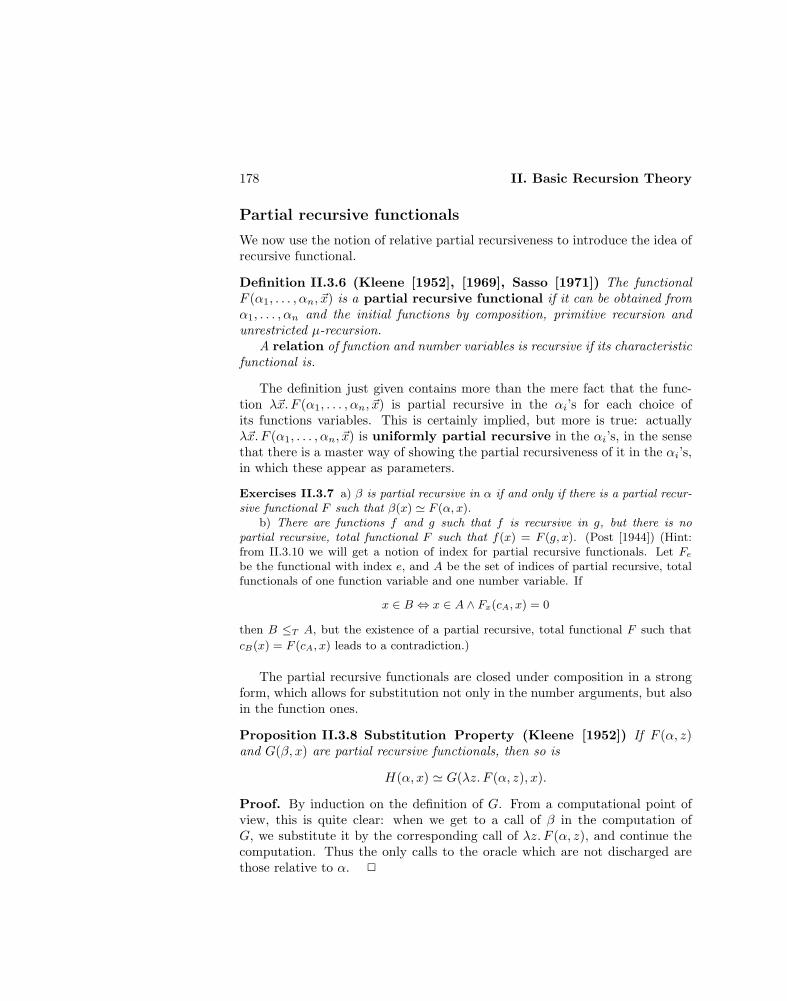
178 II. Basic Recursion Theory
Partial recursive functionals
We now use the notion of relative partial recursiveness to introduce the idea ofrecursive functional.
Definition II.3.6 (Kleene [1952], [1969], Sasso [1971]) The functionalF (α1, . . . , αn, ~x) is a partial recursive functional if it can be obtained fromα1, . . . , αn and the initial functions by composition, primitive recursion andunrestricted µ-recursion.
A relation of function and number variables is recursive if its characteristicfunctional is.
The definition just given contains more than the mere fact that the func-tion λ~x. F (α1, . . . , αn, ~x) is partial recursive in the αi’s for each choice ofits functions variables. This is certainly implied, but more is true: actuallyλ~x. F (α1, . . . , αn, ~x) is uniformly partial recursive in the αi’s, in the sensethat there is a master way of showing the partial recursiveness of it in the αi’s,in which these appear as parameters.
Exercises II.3.7 a) β is partial recursive in α if and only if there is a partial recur-sive functional F such that β(x) ' F (α, x).
b) There are functions f and g such that f is recursive in g, but there is nopartial recursive, total functional F such that f(x) = F (g, x). (Post [1944]) (Hint:from II.3.10 we will get a notion of index for partial recursive functionals. Let Febe the functional with index e, and A be the set of indices of partial recursive, totalfunctionals of one function variable and one number variable. If
x ∈ B ⇔ x ∈ A ∧ Fx(cA, x) = 0
then B ≤T A, but the existence of a partial recursive, total functional F such that
cB(x) = F (cA, x) leads to a contradiction.)
The partial recursive functionals are closed under composition in a strongform, which allows for substitution not only in the number arguments, but alsoin the function ones.
Proposition II.3.8 Substitution Property (Kleene [1952]) If F (α, z)and G(β, x) are partial recursive functionals, then so is
H(α, x) ' G(λz. F (α, z), x).
Proof. By induction on the definition of G. From a computational point ofview, this is quite clear: when we get to a call of β in the computation ofG, we substitute it by the corresponding call of λz. F (α, z), and continue thecomputation. Thus the only calls to the oracle which are not discharged arethose relative to α. 2

II.3 Partial Recursive Functionals 179
Exercises II.3.9 a) Substitution holds for partial recursive, restricted total function-als. (Kleene [1955])
b) Substitution fails for partial recursive, restricted functionals. (Kleene [1963],
Kreisel) (Hint: let G(f, x) ' 0, and F (x, z) ' 0 ⇔ x ∈ Kz Then the function
H(x) ' G(λz. F (x, z), x) would converge if and only if λz. F (x, z) is total, i.e. when
x 6∈ K, and K would be recursive.)
Theorem II.3.10 Normal Form Theorem for partial recursive func-tionals (Kleene [1952], [1969], Davis [1958], Sasso [1971]) There is aprimitive recursive function U and (for each m,n ≥ 1) recursive predicatesTm,n such that, for every partial recursive functional F of m function variablesand n number variables, there is a number e (called index of F ) for which thefollowing hold:
1. F (α1, . . . , αm, x1, . . . , xn)↓ ⇔ ∃yTm,n(e, x1, . . . , xn, α1, . . . , αm, y)
2. F (α1, . . . , αm, x1, . . . , xn) ' U(µyTm,n(e, x1, . . . , xn, α1, . . . , αm, y)).
Proof. We cannot use the functions αi in computations, since they might notbe recursive, and we then use finite approximations to them. We refer to theproofs of I.7.3 and II.1.2, and just indicate the appropriate changes to be made.
1. The index of a partial recursive functional can be defined by just addingclauses for the function arguments αi’s, as if they were initial functions.
2. Computations are put in canonical form as usual. Now some of the nodescan be expressions of the kind αi(x) = z.
3. Numbers to nodes of the computation trees are assigned in the form
〈e, 〈x1, . . . , xn〉, 〈a1, . . . , am〉, z〉
where e is the index of the functional, and ai is the code of a fixed finiteapproximation to αi, e.g. of the following function:
ai(x) 'exp(ai, px)− 1 if exp(ai, px) > 0undefined otherwise.
Numbers to computations are assigned in the usual way.
4. The definition of T remains the same, except for a local modification ofclause B, to take care of the new case corresponding to nodes of the kindαi(x) = z, where the evaluation is made by means of the finite functionai, in place of αi.

180 II. Basic Recursion Theory
5. Tm,n is the predicate defined as:
Tm,n(e, x1, . . . , xn, α1, . . . , αm, y) ⇔ T (y)∧(y)1,1 = e ∧ (y)1,2 = 〈x1, . . . , xn〉 ∧ln((y)1,3) = m ∧ (∀i)1≤i≤m(αi|(y)1,3,i).
Here α|a means that α extends the finite function coded by a, i.e.
(∀x ≤ a)(exp(a, px) 6= 0 ⇒ exp(a, px) = α(x) + 1).
6. Finally, since now nodes are quadruples, and the value is the last compo-nent,
U(y) = (y)1,4. 2
In the case of restricted functionals, we get a smoother version (where,recall, gi is the course-of-value of gi, see I.7.1):
Theorem II.3.11 Normal Form Theorem for partial recursive restrict-ed functionals (Kleene [1952], Davis [1958]) There is a primitive recursivefunction U and (for each m,n ≥ 1) primitive recursive predicates Tm,n of onlynumerical variables such that, for every partial recursive restricted functionalF of m function variables and n number variables, there is a number e (calledindex of F ) for which the following hold:
1. F (g1, . . . , gm, ~x)↓ ⇔ ∃yTm,n(e, ~x, g1(y), . . . , gm(y), y)
2. F (g1, . . . , gm, ~x) ' U(µyTm,n(e, ~x, g1(y), . . . , gm(y), y)).
Proof. It is enough to modify, in the previous theorem, the definition of Tm,nas:
Tm,n(e, x1, . . . , xn, z1, . . . , zm, y) ⇔ T (y)∧(y)1,1 = e ∧ (y)1,2 = 〈x1, . . . , xn〉 ∧ ln((y)1,3) = m ∧(∀i)1≤i≤m(Seq(zi) ∧ ln(zi) = y + 1 ∧ zi|(y)1,3,i).
Here z|a now means
(∀x ≤ a)(exp(a, px) 6= 0 ⇒ exp(a, px) = (z)x+1 + 1).
The idea is that we have to take a computation coded by y, consider the finitefunctions used in it (coded by (y)1,3,i < y), and note that only values up toy of the function arguments gi can be needed in the computation. But thesevalues are all coded in the sequence numbers gi(y). The definition of Tm,n isslightly complicated by the fact that the gi’s do not appear directly in it, but
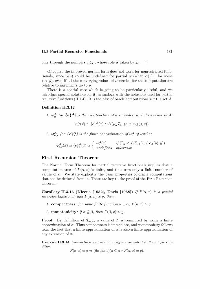
II.3 Partial Recursive Functionals 181
only through the numbers gi(y), whose role is taken by zi. 2
Of course the improved normal form does not work for nonrestricted func-tionals, since α(y) could be undefined for partial α (when α(z) ↑ for somez < y), even if all the converging values of α needed for the computation arerelative to arguments up to y.
There is a special case which is going to be particularly useful, and weintroduce special notations for it, in analogy with the notations used for partialrecursive functions (II.1.4). It is the case of oracle computations w.r.t. a set A.
Definition II.3.12
1. ϕAe (or eA) is the e-th function of n variables, partial recursive in A:
ϕAe (~x) ' eA(~x) ' U(µyTn,1(e, ~x, cA(y), y))
2. ϕAe,s (or eA
s ) is the finite approximation of ϕAe of level s:
ϕAe,s(~x) ' eAs (~x) 'ϕAe (~x) if (∃y < s)Tn,1(e, ~x, cA(y), y))undefined otherwise
First Recursion Theorem
The Normal Form Theorem for partial recursive functionals implies that acomputation tree of F (α, x) is finite, and thus uses only a finite number ofvalues of α. We state explicitly the basic properties of oracle computationsthat can be deduced from it. These are key to the proof of the First RecursionTheorem.
Corollary II.3.13 (Kleene [1952], Davis [1958]) If F (α, x) is a partialrecursive functional, and F (α, x) ' y, then:
1. compactness: for some finite function u ⊆ α, F (u, x) ' y
2. monotonicity: if α ⊆ β, then F (β, x) ' y.
Proof. By definition of Tm,n, a value of F is computed by using a finiteapproximation of α. Thus compactness is immediate, and monotonicity followsfrom the fact that a finite approximation of α is also a finite approximation ofany extension of it. 2
Exercise II.3.14 Compactness and monotonicity are equivalent to the unique con-dition
F (α, x) ' y ⇔ (∃u finite)(u ⊆ α ∧ F (u, x) ' y).
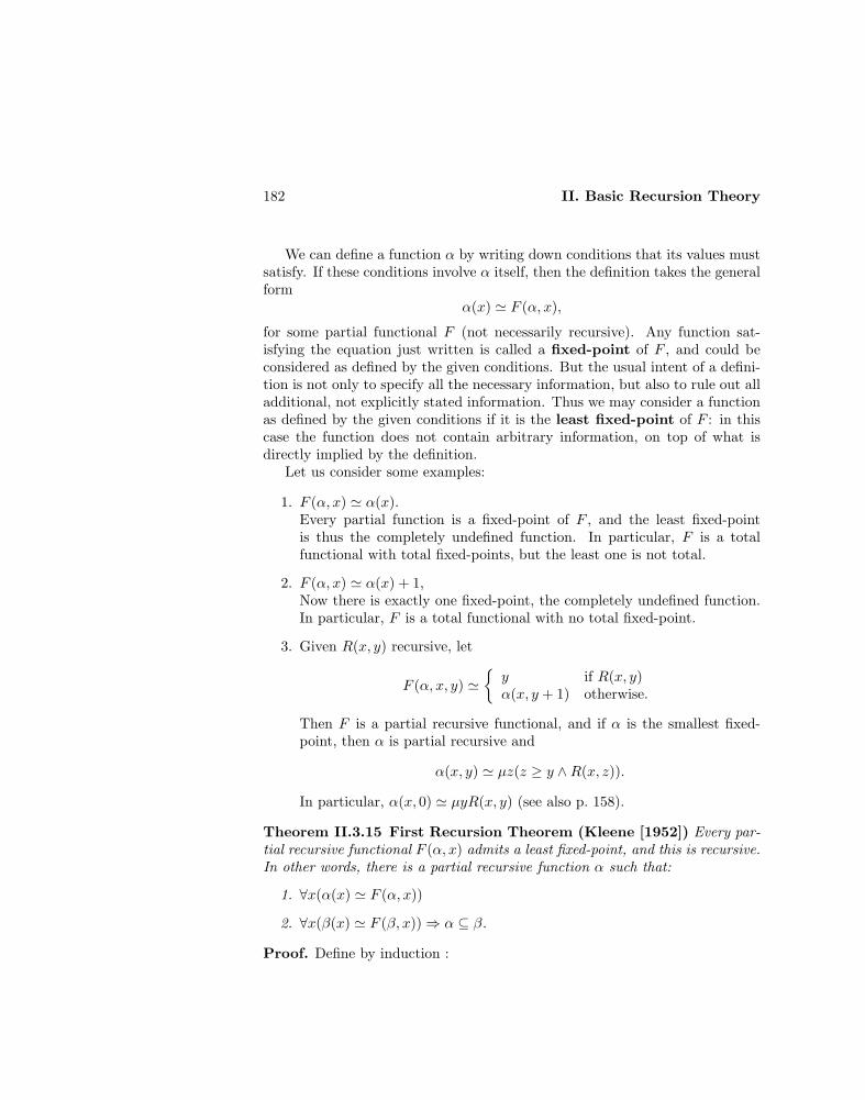
182 II. Basic Recursion Theory
We can define a function α by writing down conditions that its values mustsatisfy. If these conditions involve α itself, then the definition takes the generalform
α(x) ' F (α, x),
for some partial functional F (not necessarily recursive). Any function sat-isfying the equation just written is called a fixed-point of F , and could beconsidered as defined by the given conditions. But the usual intent of a defini-tion is not only to specify all the necessary information, but also to rule out alladditional, not explicitly stated information. Thus we may consider a functionas defined by the given conditions if it is the least fixed-point of F : in thiscase the function does not contain arbitrary information, on top of what isdirectly implied by the definition.
Let us consider some examples:
1. F (α, x) ' α(x).Every partial function is a fixed-point of F , and the least fixed-pointis thus the completely undefined function. In particular, F is a totalfunctional with total fixed-points, but the least one is not total.
2. F (α, x) ' α(x) + 1,Now there is exactly one fixed-point, the completely undefined function.In particular, F is a total functional with no total fixed-point.
3. Given R(x, y) recursive, let
F (α, x, y) 'y if R(x, y)α(x, y + 1) otherwise.
Then F is a partial recursive functional, and if α is the smallest fixed-point, then α is partial recursive and
α(x, y) ' µz(z ≥ y ∧R(x, z)).
In particular, α(x, 0) ' µyR(x, y) (see also p. 158).
Theorem II.3.15 First Recursion Theorem (Kleene [1952]) Every par-tial recursive functional F (α, x) admits a least fixed-point, and this is recursive.In other words, there is a partial recursive function α such that:
1. ∀x(α(x) ' F (α, x))
2. ∀x(β(x) ' F (β, x)) ⇒ α ⊆ β.
Proof. Define by induction :
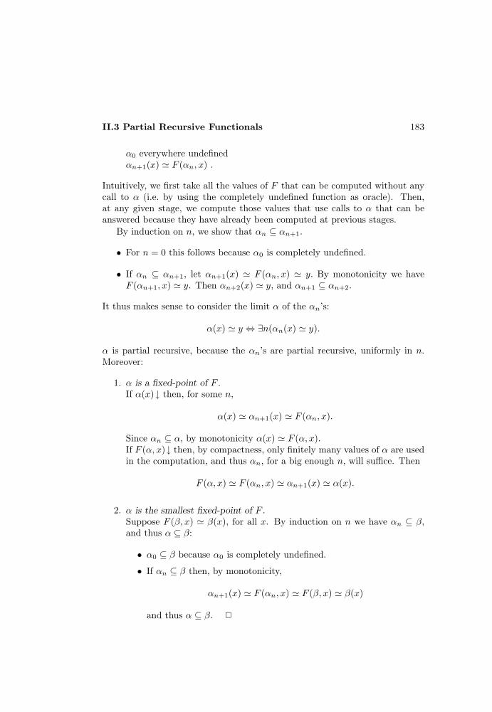
II.3 Partial Recursive Functionals 183
α0 everywhere undefinedαn+1(x) ' F (αn, x) .
Intuitively, we first take all the values of F that can be computed without anycall to α (i.e. by using the completely undefined function as oracle). Then,at any given stage, we compute those values that use calls to α that can beanswered because they have already been computed at previous stages.
By induction on n, we show that αn ⊆ αn+1.
• For n = 0 this follows because α0 is completely undefined.
• If αn ⊆ αn+1, let αn+1(x) ' F (αn, x) ' y. By monotonicity we haveF (αn+1, x) ' y. Then αn+2(x) ' y, and αn+1 ⊆ αn+2.
It thus makes sense to consider the limit α of the αn’s:
α(x) ' y ⇔ ∃n(αn(x) ' y).
α is partial recursive, because the αn’s are partial recursive, uniformly in n.Moreover:
1. α is a fixed-point of F .If α(x)↓ then, for some n,
α(x) ' αn+1(x) ' F (αn, x).
Since αn ⊆ α, by monotonicity α(x) ' F (α, x).If F (α, x)↓ then, by compactness, only finitely many values of α are usedin the computation, and thus αn, for a big enough n, will suffice. Then
F (α, x) ' F (αn, x) ' αn+1(x) ' α(x).
2. α is the smallest fixed-point of F .Suppose F (β, x) ' β(x), for all x. By induction on n we have αn ⊆ β,and thus α ⊆ β:
• α0 ⊆ β because α0 is completely undefined.
• If αn ⊆ β then, by monotonicity,
αn+1(x) ' F (αn, x) ' F (β, x) ' β(x)
and thus α ⊆ β. 2

184 II. Basic Recursion Theory
The proof of the First Recursion Theorem gives a computation procedure forthe least fixed-point of F (α, x): take the usual computation tree for F , and anytime a node calling for a computation of a value α(z) is reached, continue thecomputation by substituting F (α, z) to α(z). If every branch of the tree comesto an end, then α has been completely discharged, and the value is obtained.
This shows that there is nothing mysterious about the definition of a func-tion in terms of itself. What actually happens is that the values are definedin terms of previously obtained ones (in a precise sense, although not alwaysa trivial one, like in the case of primitive recursion). Of course, in general,there will be values which can be computed without any call to previous val-ues. Otherwise the function is really defined circularly, and it is then thecompletely undefined function.
As for the Fixed-Point Theorem, the First Recursion Theorem, togetherwith composition and case definition, generates the partial recursive functions.Kleene [1978], [1981a], [1985] reverses our approach, and develops RecursionTheory by taking the least fixed-point as a primitive schema. This approach isquite natural, and it accounts for the name ‘recursive’ for functions whose valuesare somehow defined (by recurrence) using other values of the same function.The disadvantage of this approach is that it needs partial recursive functionalsfor the definition of partial recursive functions, and thus it does not providean intrinsic characterization of the latter (which is defined simultaneously withthe former). The approach with indices and the Fixed-Point Theorem (II.2.15)is similar, but without this drawback.
This brings us to the obvious analogies and differences between the FirstRecursion Theorem and the Fixed-Point Theorem II.2.10 (or, equivalently, theSecond Recursion Theorem II.2.13). The former produces not only a fixed-point, but the least one. The latter has a wider range of application, since itdoes not require any extensionality (in the sense that ϕf(e) is not necessarilya functional on partial recursive functions, see p. 155). Actually, a case canbe made that the Second Recursion Theorem is more general than the FirstRecursion Theorem:
Proposition II.3.16 (Rogers [1967]) Let F (α, x) be a partial recursive func-tional, and ψ be the partial recursive function
ψ(e, x) ' F (ϕe, x).
The fixed-point of ψ produced by the proof of the Second Recursion Theorem isthe least fixed-point of F .
Proof. First note that ψ is indeed partial recursive, by the Substitution Prop-erty II.3.8. Let e be the fixed-point of ψ produced by the proof of II.2.13:then
ϕe(x) ' F (ϕe, x),
II.3 Partial Recursive Functionals 185
and ϕe is a fixed-point of F .Recall that ϕe(x) ' ϕS1
1(a,a)(x) for an appropriate a and, by definition ofSmn (see II.1.7), to compute ϕS1
1(a,a)(x) we must first compute ψ(S11(a, a), x),
i.e. ψ(e, x). In other words, whenever ϕe(x) converges, its computation is longerthan that of ψ(e, x).
To see that ϕe is the least fixed-point of F , let β be any fixed-point of F .We show that ϕe ⊆ β, by induction on the length of computations. Supposeϕe(x)↓: then F (ϕe, x)↓ and, by compactness, only a finite subfunction u of ϕe isused in the computation. Choose u minimal: obviously, all the values of u haveto be computed before we get ψ(e, x) ' F (ϕe, x). Thus all the computationsof values of u have length smaller than the length of computation of ϕe, andby induction hypothesis we have u ⊆ β. Then
ϕe(x) ' F (ϕe, x) ' F (u, x) ' F (β, x) ' β(x),
by monotonicity. 2
The last result shows that the fixed-point operator defined by the proof ofII.2.10 (which is the analogue of the fixed-point operator Y in λ-calculus) isactually a least fixed-point operator .
Recursive programs ?
Let us look at extended ‘while’ programs (I.5.5), obtained by adding to theassignment statements the name P (for an unspecified program). A recursive‘while’ program is an extended ‘while’ program, preceded by an instructionof the kind:
procedure P .
The program is interpreted as follows: the extended ‘while’ program definesa program depending on the unspecified program P , and the recursive clauseadded at the beginning tells that P must be the program defined by the ex-tended ‘while’ program itself. Thus P is a program with a self-referential flavor.
As ‘while’ programs define partial recursive functions, extended ‘while’ pro-grams define partial recursive functionals. The First Recursion Theorem tellsthat there is a ‘while’ program defining a recursive function which is the leastfixed-point of the extended ‘while’ program. Thus recursive programs are inprinciple avoidable, in the sense of being equivalent to usual ‘while’ programs(or flowcharts) with no recursive calls. A direct method to translate recursiveprograms into flowcharts equivalent to them is given by Strong [1971].
However, in practice, using recursive programs is a very useful tool, sinceit often allows us to write easy and concise programs (with self-referentialcalls), in situations which might require elaborate nonrecursive programs. Thus

186 II. Basic Recursion Theory
recursive programs are widely used (after McCarthy [1963]) in programminglanguages allowing definitions (like those of the ALGOL family, and LISP), aswell in languages naturally suited for recursive calls (like PROLOG).
A computational approach to recursive programs can be deduced from theremarks after the First Recursion Theorem: it corresponds to substituting ev-ery occurrence of P in the computation, with the whole program (completereplacement). A detailed study of computation procedures more efficient thanthis (i.e. requiring less substitutions), but still sufficient to compute the leastfixed-point of a recursive program, can be found in Manna [1974].
Topological digression
An instructive way to look at the results on partial recursive functionals is bytaking a more general stand, and considering the set P of partial (unary) func-tions as a topological space, following Uspenskii [1955] and Nerode [1957] (seeKelley [1955] for a reference on topology). This is easily done, by noting thatP can be viewed as a product space Sω, with S = ω ∪ ↑, ↑ being a distin-guished element (for the undefined value). A natural topology on S is definedby taking as open sets all subsets of ω, and the space S (thus no nontrivialopen set contains ↑, and S is not a Hausdorff space). Then P can be given theproduct topology. This is called the positive information topology, sincea countable basis for it consists of the finite functions (together with P itself),which contain a finite amount of positive information (specifying the values fora finite set of arguments). More precisely, the basic open sets are
u = α : u ⊆ α,
where u is a finite function. These sets form a basis because they are closedunder intersection:
u ∩ v = α : u ∪ v ⊆ α,
where u∪ v is undefined on x if both u(x) and v(x) are undefined, or both aredefined and different.
Proposition II.3.17 X ⊆ P is open if and only if both of the following hold:
1. α ∈ X ⇒ for some finite u, u ∈ X ∧ u ⊆ α.
2. α ∈ X ∧ α ⊆ β ⇒ β ∈ X.
Proof. Let X be open. Then X is a union of u’s. If α ∈ X, then α ∈ u forsome u ⊆ X. But then u ⊆ α, and u ∈ X because u ∈ u. If moreover α ⊆ β,then u ⊆ β and β ∈ u, so β ∈ X.
II.3 Partial Recursive Functionals 187
Suppose now that the two conditions hold for X. Then X is the union ofthe u’s such that u ∈ X (and hence it is open), because: if α ∈ X then, by 1,there is u ∈ X such that u ⊆ α, so α ∈ u; and if α ∈ u for some u ∈ X, thenu ⊆ α and α ∈ X by 2. 2
An equivalent way to restate the characterization of open sets is: X is openif and only if
α ∈ X ⇔ (∃u finite)(u ∈ X ∧ u ⊆ α).
We call X effectively open if the set of finite functions belonging to it isr.e. This requires the identification between finite functions and numbers inany effective way, e.g. let u be the number coding the finite function u in thefollowing way:
(∀x ≤ u)(exp(u, px) 6= 0 ⇔ u(x)↓ ∧ exp(u, px) = u(x) + 1).
In the following, for simplicity of notations, we will not distinguish between afinite function u and the number u coding it.
Proposition II.3.18 (Uspenskii [1955], Nerode [1957]) A functionF : P → P is continuous if and only if it is compact and monotone.
Proof. Since the u’s are a basis for the topology, F is continuous if and onlyif F−1(u) is open, for every finite u.
• Let F be continuous, and F (α)(x) ' y (note that F (α) is a function fromω to ω). The finite function u(x) ' y (undefined otherwise) defines theopen set u, so F−1(u) is open, and α is in it. By the characterizationof open sets, α ∈ v for some v ⊆ F−1(u): since v ∈ F−1(u), we haveF (v)(x) ' y and v ⊆ α, hence F is compact. If moreover α ⊆ β, thenv ⊆ β and β ∈ v, so F (β)(x) ' y, and F is monotone.
• Let now F be compact and monotone. We want to show that F−1(u) isopen, using the characterization of open sets given above.
If α ∈ F−1(u) then u ⊆ F (α): u is finite, and for each pair (xi, yi) suchthat u(xi) ' yi is F (α)(xi) ' yi. By compactness of F , F (ui)(xi) ' yifor some finite ui ⊆ α. Let w be the union of the ui’s: then w ⊆ α andu ⊆ F (w), so w ∈ F−1(u) and 1 of II.3.17 is verified.
If α ∈ F−1(u) and α ⊆ β, F (α) ∈ u and so u ⊆ F (α). By monotonicityof F , u ⊆ F (β). So β ∈ F−1(u) and 2 of II.3.17 is verified. Then F−1(u)is open. 2
188 II. Basic Recursion Theory
The behavior of a continuous function on P is then completely determinedby its behavior on finite functions:
F (α) =⋃F (u) : u finite ∧ u ⊆ α.
The function β(u) ' F (u) for finite u’s is called the modulus of continuityof F , and under suitable coding can be thought of as a partial function from ωto ω. We call a function effectively continuous if its modulus of continuityis partial recursive.
We have considered functionals, i.e. functions from P × ω to ω, but thereis an obvious correspondence between functionals and functions from P to P:if F (α, x) is a functional then λx. F (α, x) is such a function, and if F is such afunction then F (α)(x) is a functional. Thus the result just proved shows that:
Proposition II.3.19 (Uspenskii [1955], Nerode [1957]) The partial re-cursive functionals are effectively continuous.
On the other hand, the converse fails.
Proposition II.3.20 (Sasso [1971], [1975]) There are effectively continuousfunctionals which are not partial recursive.
Proof. The idea is simple: define F (α) on x by using two possible values ofα, e.g.
F (α)(x) '
0 if α(2x) ' 0 ∨ α(2x+ 1) ' 0undefined otherwise.
Then F is effectively continuous, but it should not be partial recursive, becausea computation tree of F (α)(x) might get stuck on one undefined value of α,even when the other is defined. To turn this into a proof, we build α in such away that F (α) is not the value of any partial recursive functional. Let
Fe(α) ' λx.U(µyT1,1(e, x, α, y))
be an enumeration of the partial recursive functionals of one function variable.We want α such that F (α) 6' Fe(α) for every e, and we define it by stages.Start with α0 being the completely undefined function. Having αn, choose xsuch that both 2x and 2x + 1 are greater than all the values for which αn isdefined, as well as those for which αn is and must remain undefined becauseso required by the construction at previous stages. Consider Fn(αn)(x). Thereare two cases:
• Fn(αn)(x)↓.Then only values of αn which have already been defined have been usedin the computation. Since αn ⊆ α, Fn(α)(x)↓ by monotonicity. It is thenenough to have F (α)(x)↑, and this only requires leaving α undefined onboth 2x, 2x+ 1 at this and later stages.

II.3 Partial Recursive Functionals 189
• Fn(αn)(x)↑.Then either it diverges by using only convergent values of αn in thecomputation, and then it will remain divergent, or some value of αn usedin the computation is undefined. In the latter case, pick up one: it isenough that also α be undefined on it, to force Fn(α)(x)↑ as well, sincethe computation is always going to be stuck on this value. We then wantF (α)(x)↓, and this is ensured but letting one of α(2x) or α(2x+ 1) be 0.Since one of 2x, 2x+ 1 is free (because both were at the beginning of thisstage, and at most one of them is required to remain so by the previouswork), define αn+1 as the extension of αn that gives it value 0.
Then α =⋃n∈ω αn satisfies the requirements. 2
An equivalent way of looking at P is by considering it as a partially orderedset, under ⊆. In this case P is a chain-complete partial ordering, in thesense that every linearly ordered chain has a least upper bound (which is justthe union of the chain). We can state the First Recursion Theorem in fullgenerality, by considering any chain-complete partial ordering (D,v).8 Call tthe l.u.b. operation, and ⊥ the least element (which exists, being the l.u.b. ofthe empty chain). A function f : D → D is:
monotone if it preserves the partial ordering
continuous if it preserves l.u.b.’s of chains.
A continuous function is monotone, since
x v y ⇒ y = x t y⇒ f(y) = f(x) t f(y)⇒ f(x) v f(y).
The general existence theorem for least fixed-points is the following:
Theorem II.3.21 (Knaster [1928], Tarski [1955], Abian and Brown[1961]) If (D,v) is a chain-complete partial ordering, and f is a monotonefunction on it, then f has a least fixed-point.
Proof. Iterate f transfinitely, starting with ⊥ and taking l.u.b.’s at limit stages(which always exist, since D is chain-complete):
x0 = ⊥xα+1 = f(xα)xβ =
⊔α<β f(xα), if β limit.
8The partial ordering v should not be confused with the partial ordering of sequencenumbers introduced on p. 90.

190 II. Basic Recursion Theory
This defines a nondecreasing chain in D (because f is monotone), whose lengthcannot exceed the maximal length of chains of D. Let xα0 be its last element,which must exist by the definition at limit stages (otherwise the l.u.b. of thechain would produce a bigger member). Then f(xα0) = xα0 , otherwise xα0
would not be the last element of the chain.And xα0 is not only a fixed-point of f , but the least one: if y is any fixed-
point of f , by induction we have xα v y for each α (in particular xα0 v y):
• x0 v y, because ⊥ is the least element of D
• if xα v y then, by monotonicity and the fact that y is a fixed-point of f ,
xα+1 = f(xα) v f(y) = y
• if xα v y for all α < β, then xβ v y by definition of l.u.b. 2
In particular, continuous functions on a chain-complete partial orderinghave least fixed-points. Continuity being stronger than monotonicity, we mighthowever expect a stronger result. Indeed, if f is continuous then only ω itera-tions are necessary to reach the least fixed- point :
f(xω) = f(⊔n∈ω
xn) =⊔n∈ω
f(xn) =⊔n∈ω
xn+1 = xω.
Exercises II.3.22 More on Fixed-Points. a) Call f expansionary if x v f(x).Every expansionary function on a chain-complete partial ordering has a fixed-point .
b) A complete lattice is a partially ordered set in which every subset has l.u.b.and g.l.b. There is a purely algebraic proof of the existence of least fixed-points formonotone functions on a complete lattice. (Knaster [1928], Tarski [1955]) (Hint:consider the set x : f(x) v x, which contains every fixed-point of f . Its g.l.b. is theleast fixed-point of f .)
c) A nonmonotone function on a chain-complete partial ordering need not have aleast fixed-point . (Hint: on P, consider
F (α, x) '
1 if α(x) ' 00 otherwise.
Note that F (α, x) is defined also when α(x) is not.)
Before we can apply II.3.21 to P, we have to show that the two notions ofcontinuity obtained by viewing it as a topological space and as a chain-completepartial ordering coincide.
Proposition II.3.23 For a functional F on P the following are equivalent:
1. F is compact and monotone
II.3 Partial Recursive Functionals 191
2. F preserves l.u.b.’s of (countable) chains.
Proof. Let F be compact and monotone, and αββ<β0 be a chain of partialfunctions with l.u.b. α. We want
F (α) =⋃β<β0
F (αβ).
By monotonicity, from αβ ⊆ α we have F (αβ) ⊆ F (α), and thus⋃β<β0
F (αβ) ⊇ F (α).
Suppose now F (α)(x) ' y: by compactness, F (u)(x) ' y for some finitefunction u ⊆ α. There must be β such that u ⊆ αβ . By monotonicity we thenhave F (αβ)(x) ' y, and hence
F (α) ⊆⋃β<β0
F (αβ).
Thus F preserves l.u.b.’s of arbitrary chains.Let F now preserve l.u.b.’s of countable chains. It is automatically mono-
tone (see p. 189). For compactness, suppose F (α)(x) ' y. Since α is the l.u.b.of a chain αnn∈ω of finite functions (e.g. αn can be taken to be the restrictionof α to the arguments from 0 to n), we have
F (α) =⋃n∈ω
F (αn),
and thus F (αn)(x) ' y for some finite αn ⊆ α. 2
We then have the general fixed-point existence result:
Theorem II.3.24 (Uspenskii [1955], Nerode [1957]) Let F be a func-tional on P:
1. if F is continuous, F has a least fixed-point
2. if F is effectively continuous, its least fixed-point is partial recursive.
We have proved the results of this subsection by using only a few particularproperties of P, namely:
1. Two partial functions are compatible if they have a common extension.
192 II. Basic Recursion Theory
2. A chain of partial functions is a set of compatible elements, containingthe l.u.b. of every pair of functions in it.
3. Every chain has a l.u.b.
4. Every function is the least upper bound of a chain of finite subfunctions.
We can then guess that the results just proved would extend to partialorderings with similar properties: we only have to turn them into definitions.Consider a partially ordered set (D,v). Two elements are compatible if theyhave a common extension. A non-empty set of compatible elements is directedif it contains, together with each pair of elements, a common extension of them.D is a complete partial ordering (c.p.o.) if every directed set has a l.u.b.in D. A function on D is continuous if it preserves l.u.b.’s of directed sets.
To be able to extend property 4 above we need a notion of finite elementin D. The idea comes from the observation that in P the finite functions areexactly those functions which, whenever covered by the l.u.b. of a chain offunctions, are already covered by some element of the chain. We then call anelement of D compact if, whenever it is bounded by the l.u.b. of a directedset A, it is already bounded by an element of A. The compact elements playthe role of finite elements, and we call D algebraic if, for every element x, theset of elements below it form a directed set with l.u.b. x. Different names usedfor algebraic c.p.o.’s are complete f0-spaces (Ershov [1972]) and domains(Scott [1982]).
Having defined a notion of finite element we can now impose on D the Scotttopology (Scott [1972]), generated by the basic open sets
u = x : u compact ∧ u v x,
and consider the associated notion of continuity. On algebraic c.p.o.’s the twonotions of continuity coincide, and the behavior of a continuous function iscompletely determined by its behavior on compact elements.
To be able to extend the notion of effective continuity, we need the possibil-ity of effectively manipulating the compact elements. We call D an effectivealgebraic c.p.o. if there is an enumeration (see p. 238) of the set of compactelements, which makes the relations of partial ordering and of compatibility, aswell as the operation of l.u.b. for compatible elements, recursive. A continuousfunction on D is then effectively continuous if its modulus of continuity ispartial recursive, w.r.t. the given enumeration.
Iteration and fixed-points ?
The method of proof used for the First Recursion Theorem and its refinementsis an old and fruitful one. It was first applied by Newton [1669] to obtain zeros
II.3 Partial Recursive Functionals 193
of differentiable real functions f , by starting from any point x0 and iterating
F (xn) = xn −f(xn)f ′(xn)
.
By the geometrical interpretation of derivative this procedure converges to afixed-point x of F such that f(x) = 0, whenever the starting point x0 is suffi-ciently close to x and the derivative of f is not zero (under these hypotheses,each step doubles the number of the correct decimal digits of the approxima-tion).
It is natural to ask whether the method would always produce a zero, start-ing from any point x0. Cayley [1879] showed that for quadratic functions onthe complex plane every point not on the line bisecting the segment connectingthe two zeros converges to one of them. Barna [1956] showed that in generalNewton’s method works for real polynomials with real zeros, except on a setof measure 0. The result fails for complex coefficients (Curry, Garnett, andSullivan [1983]).
This prompts the more general question of when the iteration of a givenfunction with fixed-points would lead to one of them (in our setting that isalways the case if f is expansionary, see II.3.22.a). A modern study case isthe iteration of the quadratic function x2 + c on the complex numbers, whichhas at most two fixed-points. For a given c, the set of points whose set ofiterations is bounded (containing in particular the points converging to a fixed-point, and those with a periodic behavior) has an interesting boundary, calledthe Julia set Jc (Julia [1918]), which is either connected or pulverized. Theshapes of these sets describe, for different c’s, an incredible variety of forms,whose behavior is related to the position of c in Mandelbrot set, definedas the set of c such that Jc is connected (Mandelbrot [1980]). This amazingset contains, on a smaller scale, a reproduction of all Julia sets Jc. It alsohas a sort of universality, since it appears in the study of the iteration of agreat number of functions (precisely, of any function one of whose iterationsbehaves like x2 in some portion of the plane). One aspect of Julia (and, lessstringently, of Mandelbrot) sets is their self-resemblance: they contain copies ofthemselves and present, at any scale of observation, the same global character.Sets with this property are called fractals, and are useful to describe naturalphenomena involving chaotic behavior. See Mandelbrot [1982] and Peitgen andRichter [1986] for more on this.
Another example of a situation in which the iteration of a function alwaysproduces a fixed-point is the one described by Banach Fixed-Point Theo-rem (Banach [1922]): a contraction function on a complete metric space hasa unique fixed-point, given by the limit of the iterations of f starting on anypoint , where f is a contraction if |f(x) − f(y)| ≤ c · |x − y| for some fixed
194 II. Basic Recursion Theory
constant c such that 0 < c < 1 (|x − y| being the distance between x and y).Indeed, given any x then, by induction,
|f (n+1)(x)− f (n)(x)| ≤ cn · |f(x)− x|.
By the triangle inequality,
|f (n+m)(x)− f (n)(x)| ≤∑i<m
|f (n+i+1)(x)− f (n+i)(x)|
≤ (∑i<m
cn+i) · |f(x)− x|.
Thus f (n)(x)n∈ω, and hence f (n+1)(x)n∈ω, converge to a point x0. Sincef is continuous, the latter also converges to f(x0), and thus f(x0) = x0. More-over, if x1 is another fixed-point of f then
|x0 − x1| = |f(x0)− f(x1)| ≤ c · |x0 − x1|
and, being c > 0, it must be x0 = x1.
Models of λ-calculus (part I) ?
The only objects of λ-calculus are terms, and thus a model will be a set Dover which terms are interpreted, in such a way that provably equal terms areinterpreted by the same object. The presence of the λ-operator forces someterms to be interpreted as functions acting on terms, and thus some elementsof D will have to be interpreted as functions on D, i.e. an appropriate set[D → D] of functions from D to D will have to be identified with a subspace ofD. This rules out, by cardinality considerations, the naive approach of takingas [D → D] the set of all functions from D to D. Finally, both λ-abstractionand functional application will have to be interpreted over D, the first beinga term formation operator, the second because of the β-conversion rule. Seep. 223 and Meyer [1982] for a discussion of the notion of model of λ-calculus.
Methods and results of the last subsection are all relevant to the presentsubject. To start with, P is a model of λ-calculus, when [P → P] is takento be the set of continuous functionals (this model is connected to the graphmodel of Plotkin [1972] and Scott [1975], see below). The reason is thatcontinuous functionals are completely determined by their behavior on finitefunctions, and thus they can be coded by a single function (the modulus ofcontinuity). The only additional piece of information needed to turn this intoa model of λ-calculus is to note that functional application of continuous func-tionals is continuous, and thus again representable in P. This also applies to

II.3 Partial Recursive Functionals 195
λ-abstraction, as well as to the operator Fix, that produces the least fixed-point of continuous functionals. By II.3.16, the interpretation of Fix coincideswith the interpretation of the combinator Y (Park [1970]). What P does notautomatically provide for, is a model of extensionality (η-rule, p. 83, accordingto which every term is identified with a function): the embedding of [P → P]into P does not cover P itself (not every continuous function is a modulus ofcontinuity).
As it might be expected, there is nothing special about P: its place canbe taken by any other reflexive c.p.o., i.e. any (algebraic) c.p.o. in which theset [D → D] of continuous functions is embeddable (meaning that there arecontinuous functions
i : D → [D → D] and j : [D → D] → D
such that i j is the identity on [D → D]). E.g., in the literature P is usuallyreplaced by P(ω), the set of subsets of ω, with the positive information topologygenerated by the finite sets. Here functions are represented by their graphs,hence the name ‘graph model’ quoted above.
To get models of extensionality as well, we need not only to embed [D → D]into D, but to identify the two. This obviously sounds like a fixed-point, andwe do have a general existence theorem (II.3.21). To be able to apply it, weneed to consider the function F (D) = [D → D] as monotone over a giantchain-complete partial ordering, whose members are (algebraic) c.p.o.’s. Wethus need an appropriate partial ordering on them, and it turns out that thefollowing natural one will work:
D D′ ⇔ there are continuous functionsi : D → D′ and j : D′ → D
such that j(i(x)) = x and i(j(y)) v y.
The intuition behind this definition is that D′ is supposed to contain moreinformation than D, and D has to be embedded into it. So i(x) is the elementin D′ that corresponds to x in D and, going back, we simply recover it (since xand i(x) have the same information content). But an element y in D′ might notcorrespond to any element in D, and j(y) is only the closest approximation toit in D: going back, we might lose some information, and thus only i(j(y)) v yholds.
With this notion of partial ordering for c.p.o.’s, it is easy to show thatthe l.u.b.’s of a chain Dnn∈ω exists: we just have to take the c.p.o. D∞that sums up exactly the information contained in the chain. Note that ifjn : Dn+1 → Dn, then jn(x) is an element in Dn that approximates x. Thuswe only need to consider chains 〈xn〉n∈ω such that xn ∈ Dn and jn(xn+1) = xn,
196 II. Basic Recursion Theory
as elements of D∞. Then xn may be thought of as the approximation of thechain at stage n (think of x as a real number given by its decimal expansion:then xn is the expansion truncated at the n-th digit, and the projection jnsimply cuts out the last digit of xn+1).
F is first of all a function on c.p.o.’s (since [D → D] can be turned into ac.p.o. by ordering its elements pointwisely). Second, F commutes with l.u.b.’sof chains (and it is thus continuous). Moreover, F is expansionary, in the sensethat F (D) [D → D]. Thus not only F admits least fixed-points, and theycan be reached in at most ω iterations of F : they exist above any given D.Thus any (algebraic) c.p.o. D can be embedded in an extensional model D∞ ofλ-calculus (Scott [1972]).
All this machinery can be appropriately formalized in the cartesian closedcategory of (algebraic) c.p.o.’s (where continuous functions, l.u.b.’s and mono-tonicity of F become, respectively, morphisms, inverse limits and functorialcovariance, and D is a reflexive object if DDD). Again, there is nothing spe-cial about this category: any reflexive object with enough points in a cartesianclosed category gives rise to a model of λ-calculus and, conversely, any model ofλ-calculus is a reflexive object with enough points in a cartesian closed category(the condition of having enough points basically meaning that different func-tions must behave differently on some point) (Scott [1980a], Koymans [1982]).This completely characterizes the models of λ-calculus.
For history, exposition, and philosophy see Scott [1973], [1975], [1975a],[1976], [1977], [1980], [1980a]. For technical development and other models seeStoy [1977], Barendregt [1981], Beeson [1985], Hindley and Seldin [1986].
Different notions of recursive functionals ?
We have defined partial recursive functionals, obtained from a uniformizationof the notion of relative recursiveness ≤T for partial functions. The topologicalapproach developed above suggests the consideration of the broader class ofeffectively continuous functionals as well. These are expressible in the form
F (α, x) ' z ⇔ (∃u)(u ⊆ α ∧ ϕ(x, u) ' z),
with ϕ partial recursive and u, here and in the following, (code of a) finitefunction. By II.1.11, an equivalent formulation is
F (α, x) ' z ⇔ (∃u)(u ⊆ α ∧R(x, u, z)),
with R r.e. Of course, such an expression defines a functional only if the relationR (that embodies the graph of the continuity modulus) gives consistent answers.We thus have two ways to turn this general form into a definition of functional:
II.3 Partial Recursive Functionals 197
1. A partial recursive operator (Myhill [1961a], Rogers [1967]) is a func-tional F that can be defined as
F (α, x) ' z ⇔ (∃u)(u ⊆ α ∧R(x, u, z)) ∧(∀u′)(∀z′)(u′ ⊆ α ∧R(x, u′, z′) ⇒ z = z′),
with R r.e. relation.
2. A recursive operator (Davis [1958], Rogers [1967]) is a functional Fthat can be defined as
F (α, x) ' z ⇔ (∃u)(u ⊆ α ∧R(x, u, z))
with R consistent r.e. relation, i.e. such that
R(x, u, z) ∧R(x, u′, z′) ∧ u, u′ compatible ⇒ z = z′.
Thus the difference between partial recursive operators and recursive oper-ators is in the consistency condition required on R: only relative to the inputfunction for partial recursive operators, and global for recursive operators.
It is clear that, from a computational point of view, the first notion is notsatisfactory, since it requires a consistency check relative to a given partialfunction. It is not surprising that there is no Enumeration Theorem for partialrecursive operators. A better way of thinking of partial recursive operators is interms of functionals on multivalued functions or, better still, sets, rather thanon partial functions, and the associated reducibility notion for sets is calledenumeration reducibility:
A ≤e B ⇔ for some r.e. relation R,x ∈ A⇔ (∃u)(Du ⊆ B ∧R(x, u)).
The structure of degrees associated with this reducibility (called partial de-grees) will be studied in Volume II.
An Enumeration Theorem for recursive operators (Rogers [1967]) can easilybe obtained by stepping from an enumeration W3
e e∈ω of all the r.e. ternaryrelations, to an enumeration W3
f(e)e∈ω of the consistent ones, where W3f(e) is
obtained from an enumeration ofW3e , by dropping the triple (x, u′, z′) whenever
a triple (x, u, z) with u, u′ consistent has already been generated.The basic difference between recursive operators on the one hand, and par-
tial recursive functionals on the other, is computational: the latter are serial,and a computation gets stuck if it tries to query the oracle for an undefinedvalue; the former are parallel, and can get around undefined values by dove-tailing computations (for general discussions of parallelism, see Elgot, Robinson
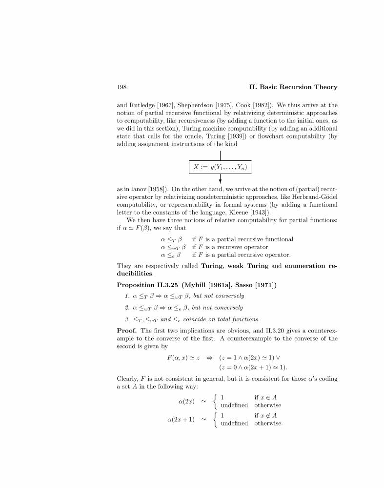
198 II. Basic Recursion Theory
and Rutledge [1967], Shepherdson [1975], Cook [1982]). We thus arrive at thenotion of partial recursive functional by relativizing deterministic approachesto computability, like recursiveness (by adding a function to the initial ones, aswe did in this section), Turing machine computability (by adding an additionalstate that calls for the oracle, Turing [1939]) or flowchart computability (byadding assignment instructions of the kind
X := g(Y1, . . . , Yn)
?as in Ianov [1958]). On the other hand, we arrive at the notion of (partial) recur-sive operator by relativizing nondeterministic approaches, like Herbrand-Godelcomputability, or representability in formal systems (by adding a functionalletter to the constants of the language, Kleene [1943]).
We then have three notions of relative computability for partial functions:if α ' F (β), we say that
α ≤T β if F is a partial recursive functionalα ≤wT β if F is a recursive operatorα ≤e β if F is a partial recursive operator.
They are respectively called Turing, weak Turing and enumeration re-ducibilities.
Proposition II.3.25 (Myhill [1961a], Sasso [1971])
1. α ≤T β ⇒ α ≤wT β, but not conversely
2. α ≤wT β ⇒ α ≤e β, but not conversely
3. ≤T ,≤wT and ≤e coincide on total functions.
Proof. The first two implications are obvious, and II.3.20 gives a counterex-ample to the converse of the first. A counterexample to the converse of thesecond is given by
F (α, x) ' z ⇔ (z = 1 ∧ α(2x) ' 1) ∨(z = 0 ∧ α(2x+ 1) ' 1).
Clearly, F is not consistent in general, but it is consistent for those α’s codinga set A in the following way:
α(2x) '
1 if x ∈ Aundefined otherwise
α(2x+ 1) '
1 if x 6∈ Aundefined otherwise.
II.3 Partial Recursive Functionals 199
In this case F (α) is the characteristic function of the set coded by α, andF (α) ≤e α. But if F (α) ≤wT α, then F (α) ≤wT β for any β extending α, (thisuses the consistency property, and it fails in general for ≤e). In particular,this holds e.g. when β is the constant function with value 1, and then α codesa recursive set (because F (α) is the characteristic function of this set, and itis recursive since β is). Thus, if α codes a nonrecursive set, F (α) ≤e α butF (α) 6≤wT α.
To show that the three reducibilities agree on total functions, suppose thatα ≤e g, i.e.
α(x) ' z ⇔ (∃u)(u ⊆ g ∧R(x, u, z))
with R r.e. Then there is Q recursive such that
α(x) ' z ⇔ (∃u)(∃y)(u ⊆ g ∧Q(x, u, z, y)),
andα(x) ' (µt[(t)1 ⊆ g ∧Q(x, (t)1, (t)2, (t)3)])2 .
This is a correct application of the µ-operator, since u ⊆ g is recursive in g(because we know that g is total, and we only have to check the values). Thusα ≤T g. Note that, when β is partial, u ⊆ β would only be r.e. in β, and thusthe µ-operator could not be directly applied. 2
Since we are only dealing with degrees of sets, we will not study the degreesof partial functions under ≤T and ≤wT . We refer to Sasso [1975] for a surveyof results (see also Casalegno [1985] for later advances). For degrees under ≤e,see Volume II.
Higher Types Recursion Theory ?
Let Tn, the set of objects of type n, be defined as:
T0 = ωTn+1 = total functions from
⋃i≤n Ti to ω.
We have so far introduced notions of recursiveness for objects of type 1 (func-tions) and 2 (functionals). Recursiveness can be successively extended to ob-jects of higher types by iterating the process that has led to the theory of thissection, namely by relativizing in a uniform way the notion at lower types.This has led (at least for restricted functionals, defined only on total objects)to a highly developed theory, begun by Kleene in two epochal papers ([1959],[1963]).
A basic fact which is a source of divergence with the classical theory, and oftechnical complications, is the failure of compactness: a computation tree still

200 II. Basic Recursion Theory
has finite branches when a value is defined, but it does not need to be finitelybranching (and hence finite), since a higher type object might need to knowinfinitely many values of its arguments, already at level two, as for:
E(f, x) '
0 if (∀z)(f(z) = 0)1 otherwise.
This rules out a Normal Form Theorem (since a computation can no longer becoded by a number), and the µ-operator loses its central role (as it is restrictedto a search on ω, and as no natural analogue is available at higher levels).The normal form is replaced by the Enumeration Theorem, which states thata functional may see one of its number arguments as an index and simulate thefunctional coded by it. This principle is taken as primitive, something whichrequires an index approach from the very beginning, see p. 158. The µ-operatoris partly replaced by Selection Theorems (Gandy [1967]), which are analoguesof the Uniformization Theorem II.1.13, and provide for choice operators at thenumber level (the choice being now made according to the stage of generationin the inductive definition of the predicate to be uniformized).
Another source of trouble is equality for objects of a given type, which isrecursive only at the integer (type 0) level. The theory has shown a dichotomybetween objects strong enough to compute equality at the level of their argu-ments (normal objects, for which strong regularity results - like the SelectionTheorems quoted above - hold, and which are, from a topological point of view,effectively discontinuous, see Grilliott [1971], Hinman [1973]), and those whichare not (see below). A treatment of various parts of Recursion Theory for nor-mal, higher types objects may be found in Hinman [1978], and Fenstad [1980].For an elegant introduction, see Kechris and Moschovakis [1977].
A completely different way to extend Recursion Theory to higher types isby taking compactness and monotonicity, and hence continuity, as a basis. Thishas been proposed by Davis [1959], Kleene [1959a], and Kreisel [1959], and hasled to a theory of countable functionals, quite similar to the one of thissection. The basic aspect is that computation trees are still finite, and henceat the same level of numbers. A functional F (g) of type 2 is continuous if andonly if its values are determined by finite pieces of its arguments: this can beformally coded by an associate f : ω → ω which, on increasingly long segmentsof g, takes value 0 for a certain time, and a constant greater than 0 from acertain point on. Thus
F (g) = f(g(n))− 1, for any sufficiently large n.
This notion can easily be generalized to higher types. If F is of type n+ 1, andG of type n, an associate for F is any function f as above such that, for any
II.3 Partial Recursive Functionals 201
associate g of G,
F (G) = f(g(n))− 1, for any sufficiently large n.
A (recursive) countable functional is any functional with a (recursive) associate.Note that countable functionals act on finite pieces not of their arguments(at type > 2), but of associates for them. Thus associates are algorithms tocompute functionals, that act on algorithms for their arguments.
It is clear that a notion of continuity is underlying that of countable func-tionals. One way to make this precise (Hyland [1979]) is to consider filterspaces (see Kelley [1955]), i.e. sets with collections of abstract approximationsfor each element (each approximation being a filter of sets, and at least thefollowing being approximations to an element: the principal ultrafilter gener-ated by that element, as well as any filter including an approximation to it).A continuous function between filter spaces is a function that respects approx-imations. Products and sets of continuous maps on filter spaces are still filterspaces, and they nicely commute. Thus a hierarchy, coinciding exactly withthat of countable functionals, can be obtained inductively, by starting with ω(organized as a filter space by taking, as only approximation to n, the principalultrafilter containing n).
Another way to look topologically at the countable functionals (Ershov[1972]) is via effective algebraic c.p.o.’s (see p. 192). Products of and setsof continuous maps on effective algebraic c.p.o.’s are still such, and they nicelycommute. Then a class C of partial continuous functionals of higher typecan be defined inductively, by letting:
C0 = finite sets with the canonical enumerationC(σ,τ) = Cσ × CτCσ→τ = [Cσ → Cτ ].
The objects in these spaces are not, in general, extensional or total. The(effective) extensional, hereditarily total functionals are exactly the (recursive)countable functionals (Ershov [1974]). The condition on totality is requiredbecause the countable functionals are, by definition, restricted functionals.
Other approaches to countable functionals can be found in Feferman [1977],Normann [1981], Longo and Moggi [1984]. For an exposition of the theory, seeErshov [1977], and Normann [1980], [1981].
There are relationships between the two extensions of recursiveness to highertypes quoted above, surveyed in Gandy and Hyland [1977]. In one direction,a recursive higher type object restricted to countable arguments is countable(Kleene [1959]). In the other direction, there are recursive countable functionalswhich are not recursive as higher type objects, e.g. the functional that gives
202 II. Basic Recursion Theory
a modulus of continuity for any continuous functional of type 2 on compactsets of functions (Tait). However, the countable functionals can be generatedby an extension of the schemata generating the higher type recursive objects(Normann [1981]).
Computability on abstract structures ?
Recursion Theory is a notion of computability on the structure of the naturalnumbers. Recursiveness relative to given oracles suggests one possible way ofextending the notion of computability to abstract structures
〈A, f1, . . . , fn, R1, . . . , Rm〉
with a given domain A, and functions and relations on it. Of course, thevarious approaches to relative computability, which are equivalent in the caseof the structure of natural numbers (see p. 198), generalize in ways whichare not necessarily equivalent on abstract structures. We briefly describe themost popular ones, and leave to Kreisel [1971], Ershov [1981] and Shepherdson[1985] the discussion of other possible approaches, including the case of partialstructures.
Formalized algorithmic procedures (fap) (Ianov [1958], Ershov [1960],Luckham and Park [1964], Paterson [1968], Friedman [1971a], Kfoury[1974]) are finite lists of labelled instructions (called program schemata),each one of the following kind:
y := fi(~x)if Rj(~x) go to p, else go to q
stop.
This is an extension of (unstructured) flowchart computability, using thefunctions and relations of the structure as primitives, and with the vari-ables ranging over the elements of the domain. See Manna [1974] for anextensive treatment.
Fap with counting (fapc) (Friedman [1971a], Kfoury [1974]) are extensionsof fap using also natural numbers, over which range special variablesX,Y, . . . The following counting instructions are also available:
X := 0X := X + 1
if X = Y go to p, else go to q.
This is equivalent to expanding the given structure to a structure
〈A ∪ ω, f1, . . . , fn, R1, . . . , Rm, 0, pd,S〉
II.3 Partial Recursive Functionals 203
(with pd and S the predecessor and successor functions for natural num-bers), and considering fap over it.
Recursive schemata (McCarthy [1963], Platek [1966]) are based on fixed-points, and allow for functions explicitly definable over the structure bycase definitions (on the relations of the structure), and fixed-point oper-ators. Alternatively, one could simply use recursive schemata
g1( ~x1) = if P1( ~x1) then h1,1( ~x1) else h1,2( ~x1)· · ·gp( ~xp) = if Pp( ~xp) then hp,1( ~xp) else hp,2( ~xp),
where the Pi’s are predicates in their variables over the structure, andthe h’s are terms in their variables over the structure, possibly using thegi’s.
Generalized Turing algorithms (Friedman [1971a]) are programs for ex-tended Turing machines which, on top of performing the usual operationsand working with their own alphabet, can also handle elements of the do-main of the structure on the tape, in the following way. First, the inputsare placed on the tape at the beginning, in adjacent cells to the left ofthe head, the rest of the tape being empty. Elements on the tape can bemoved around, and possibly copied, one cell at a time. A new elementcan be introduced in the scanned cell, but only if it is the value of oneof the functions of the structure for the arguments, placed in consecutivecells to the right of the head. Finally, the machine can test the validityof a predicate of the structure for the arguments, placed in consecutivecells to the right of the head.
Effective definitional schemata (Friedman [1971a], Gordon [1974]) are r.e.sequences of specifications, each giving a value (in the form of a term overthe structure) under mutually exclusive conditions, expressed as quanti-fier free formulas over the structure. They correspond to effective in-finitary case definitions, and generalize the approach to recursiveness bysystems of equations (see p. 39).
Prime computability (Moschovakis [1969]) extends the original definitionof (relative) recursiveness reformulated, as on p. 158, with indices andenumeration. The approach with indices is used because the µ-operatorobviously works only for well-ordered structures. Indices are here ele-ments of the domain of the structure, and to make this approach workwe also need a coding mechanism. This is obtained by considering theschemata for recursion on the expanded structure
〈A ∪ I, f1, . . . , fn, R1, . . . , Rm, 0, pd,S,J ,R,L〉,
204 II. Basic Recursion Theory
where I is a set of indices containing ω, J is a one-one pairing functionon I, and K and L are its decoding functions.
Search computability (Moschovakis [1969]) adds to prime computability anunordered search operator, performed by an oracle that searches througharbitrarily large parts of the domain. This requires an approach withmultiple-valued functions because the effect of the search operator is totake all elements satisfying a given condition, instead of selecting one(since there is, in general, no canonical choice). Prime and search com-putability correspond, respectively, to deterministic and nondeterministiccomputations on the given structure.
Despite the great variety of approaches, some of the equivalences whichhold for the classical notions retain their validity. E.g., generalized Turingalgorithms, effective definitional schemata, and prime computability are equiv-alent (Friedman [1971a], Gordon [1974]). We thus have only five notions avail-able, namely fap, fapc, recursive schemata, prime and search computability.It should be clear that both fapc and recursive schemata extend fap, in in-comparable ways, and prime computability extends both. Obviously, searchcomputability is stronger than prime computability.
The obvious problem at this point is to choose the ‘right’ notion of com-putability on an abstract domain, among the nonequivalent ones. By Friedman[1971a] and Kfoury [1974], fap’s are equivalent to fapc’s if the structure hasanalogues of the natural numbers, and the counting instructions can be defined .By Moldestad, Stoltenberg-Hansen, and Tucker [1980a], fapc’s are equivalentto prime computability if term evaluation is fapc-computable (uniformly in thenumber of variables). Thus these four approaches are equivalent for sufficientlyrich structures (like all the infinite algebraic structures of common use, e.g.rings and fields of characteristic zero). It seems to be a reasonable assump-tion to allow the use the natural numbers in computations as an auxiliary tool(think, for example, about the order of an element in a group, or the charac-teristic of an element in a field), and to have term evaluation as a computablefunction. Under these assumptions, the four notions discussed above coincidewith prime computability.
Search computability is also equivalent to a great number of other notions,see Moschovakis [1969a], Gordon [1970], [1974], and Grilliot [1971a]. In particu-lar, it coincides with extended effective definitional schemata, using existentialformulas in place of quantifier free ones. Also, for countable domains (withcomputable equality) search computability coincides with the very natural no-tion of ∀-recursiveness (Lacombe [1964]), so defined. Since the structure iscountable, there are one-one onto functions between the domain and ω, eachof which allows us to translate functions and relations from the domain to ω.

II.4 Effective Operations 205
A function or relation over the domain is ∀-recursive if its translation is, for allone-one onto translating functions.
It thus seems that prime and search computability are the natural notionsof deterministic and nondeterministic computability on an abstract domain.
II.4 Effective Operations
The previous section introduced various notions of functionals, with the com-mon characteristic that the function arguments are treated extensionally. Thisis not avoidable in general, but for the particular case of partial recursive func-tions we could also treat the arguments intensionally, through (codes for) theirprograms. In this section we study the intensional version of extensional recur-sive functionals, and their mutual relationships.
Effective operations on partial recursive functions
Having studied (effective) continuity on P, it is natural to look at the samenotion on its effective part, namely the set PR of partial recursive functions.We will consider functionals on PR or, equivalently, extensional functions onindices, where f is extensional if
ϕe ' ϕe′ ⇒ ϕf(e) ' ϕf(e′).
One approach consists in seeing PR as a subspace of P. This automati-cally induces a topology, whose (effectively) open sets are the intersections of(effectively) open sets of P, and whose (effectively) continuous functionals arethe restrictions of (effectively) continuous functionals on P.
Another approach exploits the fact that the members of PR have indices.We call a class of partial recursive functions a completely r.e. class if its indexset (see p. 150) is r.e. (Dekker [1953a], Rice [1953]). The Ershov topologyon PR (Ershov [1972]) is the topology generated by taking the completelyr.e. classes of partial recursive functions as basic open sets. Thus open setsare unions of completely r.e. classes, and effectively open sets can be definedas r.e. unions of basic open sets (since r.e. unions of r.e. sets are still r.e.,the effectively open sets are just the completely r.e. classes). Unraveling thedefinition of continuity shows that a function f induces a continuous functionalif, for every e and every r.e. index set A such that f(e) ∈ A, there is an r.e. indexset containing e and included in f−1(A). This suggests the following notionof effective continuity, obtained by considering extensional recursive functions(since then f−1(A) is itself r.e.).
206 II. Basic Recursion Theory
Definition II.4.1 An effective operation on PR is a functional F on PRinduced by a recursive function, i.e. F (ϕe) ' ϕf(e) for some extensional, re-cursive function f .
We now wish to compare the two approaches just introduced. To startwith, the next result implies that the two topologies on PR (and hence thetwo notions of continuity) coincide. Recall (see p. 187) that we identify finitefunctions and numbers by explicitly coding the graphs of finite functions insome effective way.
Theorem II.4.2 (Myhill and Shepherdson [1955], McNaughton,Shapiro) A class A of partial recursive functions is completely r.e. if andonly if there is an r.e. set A such that
ϕe ∈ A ⇔ (∃u finite)(u ∈ A ∧ u ⊆ ϕe).
Proof. If there is such an r.e. set A, then A is completely r.e. To see if ϕe ∈ A,generate simultaneously A and the graph of ϕe, and wait until, for some u ∈ A,the graph of the finite function coded by u (which can be completely decodedfrom u in finitely many steps) is contained in the part already generated of thegraph of ϕe.
Conversely, let A be nonempty and completely r.e., and θA be its indexset. The obvious guess for an r.e. set of finite functions generating A is the setof its finite functions: they are indeed an r.e set (let g(u) be an index of thefinite function (coded by) u: to see if u ∈ A, it is enough to see if g(u) ∈ θA,because θA contains all indices of any function in A). We then have to provethe following.
1. A is monotone on partial recursive functions, i.e. if α ∈ A, β is partialrecursive, and α ⊆ β, then β ∈ A.Suppose that α and β are partial recursive functions such that α ∈ A,α ⊆ β, but β 6∈ A. Let f be a recursive function such that
ϕf(e)(x) ' y ⇔ α(x) ' y ∨ [e ∈ K ∧ β(x) ' y].
The function ϕf(e) is well-defined, because α ⊆ β. Then
e ∈ K ⇔ ϕf(e) ∈ A.
Indeed, if e ∈ K then ϕf(e) ' β, while if e 6∈ K then ϕf(e) ' α.
Since A is completely r.e., K is r.e., contradiction.
II.4 Effective Operations 207
2. A is compact, i.e. if α ∈ A then, for some finite function u ⊆ α, u ∈ A.Suppose that α is a partial recursive function such that α is in A, but nofinite subfunction of it is. Let f be a recursive function such that
ϕf(e)(x) ' y ⇔ e 6∈ Kx ∧ α(x) ' y.
Thene ∈ K ⇔ ϕf(e) ∈ A.
Indeed, if e ∈ K then e ∈ Kx for all sufficiently big stages x, and henceϕf(e) is a finite subfunction of α, and cannot be in A. Conversely, if e 6∈ Kthen e 6∈ Kx, for any x, and ϕf(e) ' α.
Since A is completely r.e., K is r.e., contradiction. 2
By the definition of an effectively open set of functions (p. 187), the resultshows that a completely r.e. class is the intersection of PR with an (effectively)open set of P. Conversely, it is immediate that the intersection of PR witha basic open set of P is completely r.e. This shows the coincidence of thetwo topologies (and hence of the two notions of continuity) on PR introducedabove. Moreover, the effectively open sets (in both topologies) are exactly thecompletely r.e. classes. It only remains to show that the two notions of effectivecontinuity coincide as well.
Theorem II.4.3 (Myhill and Shepherdson [1955], Uspenskii [1955])The effective operations on PR are exactly the restrictions to PR of effectivelycontinuous functionals on P.
Proof. Let F be an effectively continuous functional: then the functionϕ(e, x) ' F (ϕe, x) is partial recursive because, for some r.e. relation R,
F (ϕe, x) ' z ⇔ (∃u finite)(u ⊆ ϕe ∧R(x, u, z)),
and thus the graph of ϕ is r.e. (see II.1.11). By the Smn -Theorem, there is frecursive such that
ϕf(e)(x) ' ϕ(e, x) ' F (ϕe, x),
and F is an effective operation.Let now f define an effective operation F on PR. It is enough to show that
F is compact and monotone on PR, i.e. that for some r.e. relation R,
F (ϕe, x) ' z ⇔ (∃u finite)(u ⊆ ϕe ∧R(x, u, z)).
Then we can extend F to all of P, by just letting
F (α, x) ' z ⇔ (∃u finite)(u ⊆ α ∧R(x, u, z)).
208 II. Basic Recursion Theory
But sinceF (ϕe, x) ' z ⇔ ϕf(e)(x) ' z,
for fixed x and z the class
ϕe : F (ϕe, x) ' z
is completely r.e. Then all the work has already been done in II.4.2: there isan r.e. set A such that
F (ϕe, x) ' z ⇔ (∃u finite)(u ⊆ ϕe ∧ u ∈ A).
This holds, as said, for fixed x, z. But they appear as parameters in the argu-ment, and then A depends uniformly on them. In other words, A is really anr.e. relation R depending on u, x, z. Then, this time for every x and z,
F (ϕe, x) ' z ⇔ (∃u finite)(u ⊆ ϕe ∧R(x, u, z))
as wanted. 2
Note that the proof shows that every effective operation is induced by aunique continuous functional (which turns out to be recursive), since its valuesare completely determined by the behavior on finite functions (which are allpartial recursive). This, in turn, uniquely determines a continuous functional.
Exercise II.4.4 There is a continuous functional whose restriction to PR is not aneffective operation. (Dekker and Myhill [1958]) (Hint: there are only countably manyeffective operations on PR, so it is enough to build uncountably many continuousfunctionals, with distinct restrictions to PR. Given a partial function β, let
Fβ(α) '
constant function 1 if dom α ∩ dom β 6= ∅completely undefined otherwise.
If dom β0 ∩ dom β1 6= ∅, then Fβ0 and Fβ1 differ on PR.)
Effective operations on total recursive functions
The notion of effective operation can be generalized from PR to any class Aof partial recursive functions:
Definition II.4.5 An effective operation on a set A of partial recursivefunctions is a functional F mapping A to A and such that, for some partialrecursive function ψ,
ϕe ∈ A ⇒ ψ(e)↓ ∧ F (ϕe) ' ϕψ(e).

II.4 Effective Operations 209
Under which conditions for A does an analogue of Theorem II.4.3 hold? Wefirst prove an important special case, and then discuss the general situation.In the following, R is going to be the class of total recursive functions.
Theorem II.4.6 (Kreisel, Lacombe and Shoenfield [1957], Ceitin[1959]) The effective operations on R are exactly the restrictions of the ef-fectively continuous functionals mapping R to R.
Proof. As in the previous theorem, an effectively continuous functional map-ping R to R induces an effective operation on R. Let now F be an effectiveoperation on R. We approximate the result by a series of steps.
1. If f is recursive and F (f, x) = z, for any preassigned length k there is afunction u of finite support (i.e. 0 almost everywhere) which agrees withf up to k, and such that F (u, x) = z.This provides a sort of compactness, with functions of finite supporttaking place of finite functions (which cannot be considered here becausethey are not total). Suppose the claim fails: then a recursive function tcan be defined, such that ϕt(e) agrees with f up to the maximum of k and(if e ∈ K) the least stage in which e in generated in K, and afterwardsagrees with a function u of finite support and such that F (u, x) 6= z(which exists by the hypothesis that the claim fails). Then, by definition,
e ∈ K ⇔ F (ϕt(e), x) = z,
and K is recursive, contradiction.
2. If f is recursive and F (f, x) = z, there is a fixed length kf (which canbe found effectively) such that, for any function u of finite support whichagrees with f up to kf , F (u, x) = z.This provides a sort of modulus of continuity : the value of F (f, x) isdetermined by the initial segment of f up to kf . The existence proof is thesame as given above (dropping k), but we want to obtain kf effectively.Then define ϕt(e) as above, but as a partial function (i.e. look for theappropriate u, and if this is found, proceed as above). Notice that theset
e ∈ C ⇔ F (ϕt(e), x) ' z
is r.e. If a is an index for it, it cannot be a ∈ K, otherwise by constructionϕt(a) = f : then a ∈ C = Wa, and hence a ∈ K. Thus it must be a ∈ K:let kf be the least stage in which a is generated in K. There cannot exista function u of finite support which agrees with f up to kf , and such thatF (u, x) 6= z, otherwise ϕt(a) would be one such, forcing a 6∈ C, againstthe fact that a ∈ K. But F is defined for any recursive function, and thenif u agrees with f up to kf , it must be F (u, x) = z.
210 II. Basic Recursion Theory
3. The two parts just shown prove that, for f recursive,
F (f, x) = z ⇔ (∃u of finite support)(u agrees with f up to ku ∧ F (u, x) = z).
One direction follows from part 1, since if F (f, x) = z there are functionsu of finite support, agreeing with f up to any preassigned length, andsuch that F (u, x) = z.
Conversely, let u agree with f up to ku, and F (u, x) = z. By part 1 thereis v of finite support, agreeing with f up to the maximum of kf , ku. Bypart 2 then F (v, x) = F (f, x), because v agrees with f up to kf . AndF (v, x) = F (u, x) because v agrees with u up to ku (since v agrees withf up to ku, and so does u).
4. F can then be extended to an effectively continuous functional on all ofP, by letting
F (α, x) ' z ⇔ (∃u of finite support)(u agrees with α up to ku ∧ F (u, x) = z)
for any partial function α. 2
Note that the condition that an effectively continuous functional map R toR is weaker than totality (which requires mapping any total function to a totalfunction, not only recursive ones).
Exercise II.4.7 There is an effective operation on R, which is not the restriction toR of any total effectively continuous functional . (Rogers [1967]) (Hint: let F (α, x)be the smallest z such that z ∈ K and α(z) = ϕz(z), if it exists. F is an effectiveoperation on R, but if G is a total effectively continuous functional agreeing with Fon R, let
α(z) =
ϕz(z) + 1 if z ∈ K0 otherwise.
Consider any value G(α, x), the finite part of α used in the computation, and a
function β agreeing with α on that part, and equal to ϕa(a) otherwise, with a the
first element generated in K and different from G(α, x). Then F (β, x) is both equal
and different to a, contradiction.)
Effective operations in general ?
An analysis of the proofs of Theorems II.4.3 and II.4.6 from a constructivepoint of view has been provided by Beeson [1975], and Beeson and Scedrov[1984]. In particular, both results are derivable in Intuitionistic Arithmetic
II.4 Effective Operations 211
from Markov’s Principle, but without this principle they are not derivable evenin Intuitionistic Set Theory. Both results describe phenomena which hold insettings much more general than those here considered.
For the first, given an effective algebraic c.p.o. X (p. 192) we canconsider its effective part Xe, consisting of the elements for which the set ofcompact approximations is r.e. (w.r.t. the given enumeration). The enumera-tion of the compact elements of X generates an enumeration of Xe, and we canthen impose on it the Ershov topology, with the completely r.e. sets (w.r.t.the enumeration of Xe) as basic sets. Then II.4.2 and II.4.3 are respectivelygeneralized as: Ershov’s topology on Xe is induced by Scott’s topology on X,and the morphisms on Xe as an enumerated set (i.e. functions commuting withthe enumeration, through a recursive function) are exactly the restrictions toXe of effectively continuous functions on X (Ershov [1973]).
For the second, Ceitin [1959], [1962] and Moschovakis [1964] show that itholds on every effective complete separable metric space, i.e. a space witha recursive metric function on the recursive reals (see p. 213), with a dense r.e.subset, and in which one can effectively compute limits of recursive, recursivelyconvergent Cauchy sequences. A more general framework for the theorem isthe notion of effective topological space, see Nogina [1966], [1978].
Spreen and Young [1984] give a uniform generalization of both resultsabove by considering countable T0-spaces satisfying certain effectivity re-quirements, which hold for both PR and R.
We return now to the question formulated above, and look for conditionson A ensuring that the effective operations on A are exactly the restrictions ofeffectively continuous functionals mapping A to A. The positive results provedabove apply to more general situations, but some conditions on A are necessary.
Exercises II.4.8 The effective operations on A are exactly the restrictions of effec-tively continuous functionals mapping A on A, in the following cases:
a) A is completely r.e. (Myhill and Shepherdson [1955]) (Hint: see II.4.3.)
b) A is the intersection of a completely r.e. class with R. Such classes are called
totally r.e. (Kreisel, Lacombe and Shoenfield [1957], Ceitin [1959]) (Hint: see II.4.6
and, when defining ϕt(e), use functions of finite support which are in A.)
Proposition II.4.9 (Pour El [1960], Myhill) There is an effective oper-ation on a class A, which is not compact (and thus not the restriction of acontinuous functional).
Proof. Let A consist of the constant functions 0 and 1, and of the recursivefunctions which take a value different from 0 for an argument smaller than their
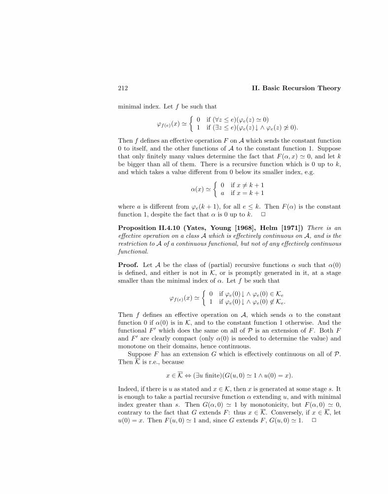
212 II. Basic Recursion Theory
minimal index. Let f be such that
ϕf(e)(x) '
0 if (∀z ≤ e)(ϕe(z) ' 0)1 if (∃z ≤ e)(ϕe(z)↓ ∧ ϕe(z) 6' 0).
Then f defines an effective operation F on A which sends the constant function0 to itself, and the other functions of A to the constant function 1. Supposethat only finitely many values determine the fact that F (α, x) ' 0, and let kbe bigger than all of them. There is a recursive function which is 0 up to k,and which takes a value different from 0 below its smaller index, e.g.
α(x) '
0 if x 6= k + 1a if x = k + 1
where a is different from ϕe(k + 1), for all e ≤ k. Then F (α) is the constantfunction 1, despite the fact that α is 0 up to k. 2
Proposition II.4.10 (Yates, Young [1968], Helm [1971]) There is aneffective operation on a class A which is effectively continuous on A, and is therestriction to A of a continuous functional, but not of any effectively continuousfunctional.
Proof. Let A be the class of (partial) recursive functions α such that α(0)is defined, and either is not in K, or is promptly generated in it, at a stagesmaller than the minimal index of α. Let f be such that
ϕf(e)(x) '
0 if ϕe(0)↓ ∧ ϕe(0) ∈ Ke1 if ϕe(0)↓ ∧ ϕe(0) 6∈ Ke.
Then f defines an effective operation on A, which sends α to the constantfunction 0 if α(0) is in K, and to the constant function 1 otherwise. And thefunctional F ′ which does the same on all of P is an extension of F . Both Fand F ′ are clearly compact (only α(0) is needed to determine the value) andmonotone on their domains, hence continuous.
Suppose F has an extension G which is effectively continuous on all of P.Then K is r.e., because
x ∈ K ⇔ (∃u finite)(G(u, 0) ' 1 ∧ u(0) = x).
Indeed, if there is u as stated and x ∈ K, then x is generated at some stage s. Itis enough to take a partial recursive function α extending u, and with minimalindex greater than s. Then G(α, 0) ' 1 by monotonicity, but F (α, 0) ' 0,contrary to the fact that G extends F : thus x ∈ K. Conversely, if x ∈ K, letu(0) = x. Then F (u, 0) ' 1 and, since G extends F , G(u, 0) ' 1. 2

II.4 Effective Operations 213
The two examples succeed because they both use not only values of thearguments, but also algorithms for them. The proofs are similar but quitedifferent, because they fail to extend to all of P for distinct reasons. Theyprovide examples as far apart as they can be: the first does not extend for purelytopological reasons (not being compact), the second for purely computationalones (being extendable to a continuous functional, but not to an effectivelycontinuous one).
Exercise II.4.11 Weak effective operations. A weak effective operation on A isdefined as in II.4.5, without the condition that F map A to itself.
a) If A is completely r.e., the weak effective operations on A are restrictions ofeffectively continuous functionals. (Myhill and Shepherdson [1955]) (Hint: see II.4.3.)
b) There is a weak effective operation on R which is not compact . (Friedberg
[1958b], Muchnick) (Hint: let ϕf(e)(x) be 0 if ϕe is either 0 for all arguments up to
e, or it coincides, up to the first argument in which is not 0, with a function ϕi that
has index i smaller than that argument. Then f induces a weak effective operation
F on R because it is extensional, and F is not compact, as in II.4.9.)
We have only touched on the subject of effective operations. For moreinformation see Grzegorczyck [1955], Friedberg [1958a], Kreisel, Lacombe andShoenfield [1959], Pour El [1960], Ceitin [1962], Lachlan [1964], Young [1968],[1969], Lob [1970], Helm [1971], and Freivald [1978].
Recursive analysis ?
The real numbers can be classically defined in many equivalent ways, eitheras particular sequences or sets of rational numbers, or axiomatically (up toisomorphism) as archimedean complete ordered fields. Since rational numberscan be effectively coded by integers, we have notions of recursive sequencesand recursive sets of rational numbers, and different recursive analogues of thereal numbers (Borel [1912], Turing [1936], Specker [1949]), using e.g. recursivedecimal expansions, recursive Cauchy sequences with a recursive modulus ofconvergence, recursive Dedekind cuts, recursive sequences of nested intervalswith length approaching zero. All of these notions turn out to be equivalent(Robinson [1951], Myhill [1953]), and thus a stable notion of a recursive realnumber is available. The recursive real numbers form a countable subfield Rof the reals, which contains all the algebraic reals, as well as the real zeros ofthe Bessel functions, and becomes algebraically closed by the adjunction of theimaginary unit (Rice [1954]).
Recursive real numbers are coded by integers (the indices of their recursivepresentations), and thus a notion of a recursive function of recursive realvariable is available, as an effective operation on the codes. Under this defi-nition, the field operations on R are recursive (on the codes obtained from the
214 II. Basic Recursion Theory
Cauchy sequences definition), and Moschovakis [1965] characterizes R up to re-cursive isomorphism, by a recursive analogue of the notion of an archimedeancomplete ordered field. Thus R appears to be a good recursive counterpart tothe reals.
There are two different approaches to what may be called recursive anal-ysis, which are respectively parts of constructive and classical mathematics.The first has been followed by the ‘Markov school’, which advocates a philoso-phy (Markov [1954]) in which every mathematical object is described by a wordof a given alphabet, manipulated by Markov algorithms (p. 145) and discussedby means of constructive logic (intuitionistic logic plus Markov’s principle).Under these philosophical assumptions, analysis is the study of R and of therecursive functions on it.
The second approach remains in the realm of classical logic and mathemat-ics, and it can be seen as a study of the extent of constructivity in classicalanalysis, by an examination of which results remain valid when constructivized(either by the same proofs or by new ones), and which results instead fail.Once we live in a classical world, there is no particular reason to stick to recur-sive functions on R, and a notion of recursive functions of real variablehas been introduced (Grzegorczyck [1955], [1957], Lacombe [1955], [1957]) inanalogy to the effectively continuous functionals, as opposed to effective op-erations. This provides a new level of analysis, since it isolates computablefunctions (defined on all the reals) among the classical ones.
Typical theorems of recursive analysis are that every recursive functionon R is continuous, although not necessarily uniformly so (the positive partrephrases II.4.6, the negative one follows from the failure of the recursive ana-logue of Konig lemma, see V.5.25), and that the least upper bound principlefails (Specker [1949]) in the sense that there is a bounded, strictly increasing,recursive sequence of rationals which does not converge to any recursive realnumber (simply, the sequence of the rm =
∑mn=0 1/2f(n), with f a recursive
one-one function with a nonrecursive range).
For a treatment of recursive analysis, see Grzegorczyck [1959], Goodstein[1961], Kusner [1973], Aberth [1980], Pour El and Richards [1983a], Kreitz andWeihrauch [1984], and Beeson [1985]. Although not especially on recursiveanalysis, Bishop [1967] is also relevant.
A broader perspective can be obtained by looking at recursive interpreta-tions of (intuitionistic) set theory, in which analysis can then be formalized.The effective topos (Hyland [1982]) and the recursive topos (Mulry [1982])generalize, respectively, the constructive and classical approach to analysis (thefirst using recursive realizability, and the second using forcing). Analogies anddifferences are investigated in Scedrov [1984], [1987], and Rosolini [1986].
II.5 Indices and Enumerations ? 215
II.5 Indices and Enumerations ?
In II.1.4 and II.1.9 we introduced a particular system of indices for partialrecursive functions and r.e. sets, and later proved some of its properties. Inthis section we investigate systems of indices in general, both for all partialrecursive functions and r.e. sets (giving new examples, some equivalent to theone we already know, and some radically different) and for subclasses of them.
Acceptable systems of indices
A number of results have been proved so far for recursive functions, and someof them mention indices in their statements, or use them in their proofs. Thequestion naturally arises: do these results depend on the particular formalismchosen to work with (through which the indices were defined), or are theyinstead somehow model-independent?
To study the problem, we first note that the basic results mentioning indicesare:
• Enumeration Theorem II.1.5
• Smn -Theorem II.1.7
• Padding Lemma II.1.6.
Indeed, the remaining results mentioning indices, or using them in their proofs,merely refer to these (e.g. the Fixed-Point Theorem II.2.10 follows from Enu-meration and Smn -Theorem alone).
We now characterize the systems of indices for which these theorems hold.
Definition II.5.1 (Uspenskii [1956], Rogers [1967]) We call a system ofindices any family ψ of maps ψn from ω onto the set of n-ary partial recursivefunctions (by ψne we will indicate the partial recursive function correspondingto the index e). We say that:
1. ψ satisfies enumeration if for every n there is a number a such that
ψn+1a (e, x1, . . . , xn) ' ψne (x1, . . . , xn)
2. ψ satisfies parametrization if for every m,n there is a total recursivefunction s such that
ψms(e,x1,...,xn)(y1, . . . , ym) ' ψm+ne (x1, . . . , xn, y1, . . . , ym).

216 II. Basic Recursion Theory
As usual we will drop the mention of the number of variables, when this isunderstood.
An example of a system of indices is obviously given by the usual ϕne , whichalso satisfies both enumeration and parametrization: we call it the standardsystem. A system may resemble the standard one, in the sense that it ispossible to go effectively from the former to the latter, and conversely:
Definition II.5.2 (Rogers [1958]) A system of indices ψ is acceptable if,for every n, there are total recursive functions f and g such that
ψne ' ϕnf(e) ϕne ' ψng(e).
Note that in practice the equivalence among different definitions of the classof partial recursive functions is usually proved precisely by showing that thesystems of indices induced by them resemble one another, in the sense justgiven (see the proof of I.7.12). The next result shows that they satisfy thesame basic properties, and also gives an intrinsic characterization of the notionof an acceptable system of indices.
Proposition II.5.3 (Rogers [1967]) A system of indices is acceptable if andonly if it satisfies both enumeration and parametrization.
Proof. Suppose ψ satisfies both enumeration and parametrization. Then ψ isacceptable:
• Given ψne , by the enumeration property this is a recursive function ofn + 1 variables. Since systems of indices must enumerate all the partialrecursive function, there is an index a for ψne with respect to ϕ. Then
ψne (~x) ' ϕn+1a (e, ~x) ' ϕnS1
1(a,e)(~x).
Thus we can let f(e) = S11(a, e), and have ψne ' ϕnf(e).
• g is obtained, symmetrically, by using the Enumeration Theorem for ϕand the parametrization property for ψ.
Conversely, suppose that ψ is acceptable.
• To show enumeration, note that
ψne (~x) ' ϕnf(e)(~x).
But ϕnf(e)(~x) is partial recursive as a function of e, ~x (by the EnumerationTheorem), and thus it must admit an index a in the system ψ.
II.5 Indices and Enumerations ? 217
• To show parametrization, consider ψn+me (~x, ~y). By the enumeration prop-
erty just proved, this is a partial recursive function of m+n+ 1 variables(including e), and thus there is an index a for it with respect to ϕ:
ψn+me (~x, ~y) ' ϕm+n+1
a (e, ~x, ~y) ' ϕmSmn+1(a,e,~x)
(~y).
Since g allows us to go back to the system ψ, if we let
s(e, ~x) = g(Smn+1(a, e, ~x))
we getψn+me (~x, ~y) ' ψms(e,~x)(~y). 2
Corollary II.5.4 Every acceptable system of indices satisfies the Fixed-PointTheorem. In other words, given a recursive function f there is an index e suchthat ψe ' ψf(e).
Proof. The only properties used in the proof of the Fixed-Point Theorem areenumeration and parametrization. 2
Exercises II.5.5 a) A system satisfying enumeration alone is not necessarily ac-ceptable. (Friedberg [1958]) (Hint: a recursive enumeration without repetitions of thepartial recursive functions, see II.5.23, does not satisfy II.5.6.)
b) A system satisfying enumeration and fixed-point, i.e. the existence of a recursivefunction f such that, for ψi total, ψψi(f(i)) ' ψf(i), is not necessarily acceptable.(Machtey, Winklmann and Young [1978]) (Hint: let ϕh(e) be a recursive enumerationwithout repetitions of the partial recursive functions, see II.5.23. Then ψe ' ϕh(ϕe(0))
satisfies enumeration and fixed-point, the latter because ψe depends extensionally onϕe, and thus fixed-points transfer from ϕ to ψ. Note that any partial recursivefunction is equal to ϕh(i) for a unique i, and then can be equal to ψe only whenϕe(0) ' i: thus it has an r.e. set of indices w.r.t. ψ. But e.g. the completely undefinedfunction cannot have an r.e. set of indices in any acceptable system, and thus ψ isnot acceptable.)
c) A system satisfying enumeration and composition, i.e. the existence of a recur-sive function c such that ψe ψi ' ψc(e,i), is acceptable. (Machtey, Winklmann andYoung [1978]) (Hint: by coding the arguments, parametrization can be reduced tocomposition and its special case for sequence numbers, e.g. if ψf(x)(y) = 〈x, y〉 then
ψe(〈x, y〉) ' ψe(ψf(x)(y)) ' ψc(e,f(x))(y).
And f can be defined by successive compositions of the two functions g(y) = 〈0, y〉and h(〈x, y〉) = 〈x+ 1, y〉.)
The results just proved show that the notion of a universal machine, em-bodied in the enumeration property, is not sufficient for elementary Recursion
218 II. Basic Recursion Theory
Theory: it has to be supplemented with the notion of subcomputation, throughthe possibility of either effectively incorporating data into a program (expressedby the parametrization property), or effectively concatenating programs (ex-pressed by composition). On the other hand, the Fixed-Point Theorem, andthus the possibility of having self-referential programs (so-called recursive pro-grams), does not appear to be as fundamental.
Notice that enumeration and parametrization imply, among other things, aback and forth translation between the function spaces
ωn × ωm → ω and ωn → (ωm → ω).
Indeed, a partial recursive function of n + m variables becomes, by parame-trization, a partial recursive function of n variables, whose values are (indicesof) partial recursive functions of m variables. Conversely, any partial recursivefunction of n variables whose values are indices of partial recursive functionsof m variables becomes, by enumeration and composition, a partial recursivefunction of n+m variables.
To the reader acquainted with Category Theory (Mac Lane [1971]), this isreminiscent of the typical property of cartesian closed categories, i.e. thosecategories in which the sets of morphisms between objects are at the samelevel of the objects themselves. More precisely, in a cartesian closed categoryproducts A×B and exponents BA (which generalize the notions, respectively,of cartesian product of A and B, and of sets of functions from A to B) nicelycommute, in the sense that the following sets of morphisms are isomorphic, ina natural way:
Hom(A×B,C) and Hom(A,CB).
For a development of Recursion Theory from a categorical point of view, seeEilenberg and Elgot [1970], and Di Paola and Heller [1987].
We still have to analyze the role of the Padding Lemma. For explicitlygiven systems of indices (like the ones induced by the approaches to partialrecursiveness of Chapter I and Section II.1) this property holds trivially, andit simply amounts to adding redundant information in the given descriptionof the function. But having infinitely many indices in one acceptable systemdoes not help in another one, since the translations provided by the definitionof acceptability are not necessarily one-one. Nevertheless, the result holds ingeneral.
Proposition II.5.6 Padding Lemma (Rogers [1958]) In any acceptablesystem, given one index of a partial recursive function, we can effectively gen-erate infinitely many indices of the same function.
Proof. It is enough to show that, given α partial recursive and D finite set ofindices for it in the acceptable system ψ, we can effectively find an index for α

II.5 Indices and Enumerations ? 219
which is not in D. Define, by parametrization, a recursive function f such that
ψf(e) 'α if e 6∈ Dundefined otherwise.
By the Fixed-Point Theorem for ψ, there is e such that ψe ' ψf(e). Now twocases may occur:
• e 6∈ DThen we must be in the first case of the definition of f , and henceψe ' ψf(e) ' α. Thus e is an index of α which is not in D.
• e ∈ DNow we must be in the second case of the definition, and ψe is the com-pletely undefined function. But e, being in D, is an index of α, and thusα is also completely undefined. Then we can play a symmetric game, thistime letting g be such that
ψg(a) '
constant 0 if a ∈ Dundefined otherwise.
By the Fixed-Point Theorem, there is a such that ψa ' ψg(a). Now itcannot be the case that a ∈ D, otherwise (as above) α would be theconstant function 0, while we know it is completely undefined. Then wemust be in the second case, i.e. a 6∈ D and ψa is completely undefined.Thus a is an index of α which is not in D. 2
Now we have, for acceptable systems of indices, all the results proved forthe standard one, but this does not guarantee that the same will remain truefor future results. We will now prove two general theorems, showing how muchany acceptable system must resemble the standard one. They will ensure thatacceptable systems are really very much alike.
The first theorem shows that any acceptable system, viewed as a sequenceof partial recursive functions
ψ0 ψ1 ψ2 · · ·
is nothing else than a recursive permutation of the standard sequence
ϕ0 ϕ1 ϕ2 · · ·
Theorem II.5.7 (Rogers [1958]) ψee∈ω is an acceptable system of indicesif and only if there is a recursive permutation h such that
ψe(x) ' ϕh(e)(x).
220 II. Basic Recursion Theory
Proof. One direction obviously holds: if h exists, its inverse h−1 is also arecursive permutation, and h and h−1 provide the needed translations of thesystems ψ and ϕ into each other.
Suppose now that ψ is acceptable: we define a recursive permutation h thatinterchanges indices in ψ and ϕ. Since h has to be total, we ensure at evenstages that the least element not yet in the domain gets into it (by defining hon it). Similarly, h has to be onto, and at odd stages we ensure that the leastelement not yet in the range gets into it (by letting it be the value of h for someargument). We then have to show how to ensure that h is both one-one anda function. But h is a function when h−1 is one-one, and thus we will have asymmetric construction that alternates steps to make h total and one-one, tosteps to make it onto and a function. We just show the steps that have to bealternately taken. Suppose h is defined on x0, . . . , xn.
If we want to add one element to the domain of h (even stages), let e bethe least number not in x0, . . . , xn: we have to define h(e) in such a waythat h(e) 6∈ h(x0), . . . , h(xn) (to have h one-one), and ψe ' ϕh(e). Since ψ isacceptable, given ψe we can effectively find an index of the same function w.r.t.ϕ. The Padding Lemma II.1.6 ensures that we can effectively generate infinitelymany others, and thus one can be found that is not in h(x0), . . . , h(xn). Thefirst such one is the needed value of h(e).
If we want to add one element to the range of h (odd stages), let y be theleast number not in h(x0), . . . , h(xn): we have to define e in such a way thate 6∈ x0, . . . , xn (since h has to be a function), and ψe ' ϕy. Then we will leth(e) = y. Since ψ is acceptable, given ϕy we can effectively find an index ofthe same function w.r.t. ψ. The Padding Lemma II.5.6 for ψ ensures that wecan effectively generate infinitely many others, and thus one can be found thatis not in x0, . . . , xn. The first such one is the needed value for e. 2.
The previous result is not completely satisfactory, because it misses thebasic duality of Recursion Theory (see p. 131). It translates a number whenit is a code of a function, but it leaves the same number untouched when thisbehaves as a number (i.e. as an argument or a value). The next result showsthat any acceptable system is really the standard one, and merely works withan appropriated reinterpretation of the numbers (with no distinction made onwhether they code programs or not). Thus the isomorphism provided here isnot an isomorphism of the sequence of function, but rather an isomorphism ofthe underlying structure of the natural numbers.
Theorem II.5.8 (Blum) If ψee∈ω is an acceptable system of indices, thenthere is a recursive permutation h such that
h(ψe(x)) ' ϕh(e)(h(x)).
II.5 Indices and Enumerations ? 221
Proof. There are actually two different things to ensure, namely two reinter-pretations of the numbers, one taking care of the case when they are seen asarguments and values, and the other when they are seen as codes for programs.Moreover, the two have to coincide.
If we only had to define a recursive permutation h that produces the givenisomorphism on the numbers as codes for a given reinterpretation α of thenumbers as values and arguments, then we could simply proceed as in the pre-vious theorem. Namely, let α−1 be any partial recursive function that invertsα, i.e. any function that, given z, dovetails computations of α until it finds,and outputs, a number x such that α(x) ' z. We have to ensure that
α(ψe(x)) ' ϕh(e)(α(x)),
and this can be restated as both:
ψe(x) ' α−1(ϕh(e)(α(x)))
andϕh(e)(z) ' α(ψe(α−1(z))).
If e has to be added to the domain of h, we use the fact that αψeα−1 ispartial recursive, and an infinite number of indices w.r.t. ϕ for it can theneffectively be found.
If y has to be added to the range of h, we use the fact that α−1ϕyα is partialrecursive, and an infinite number of indices w.r.t. ψ for it can then effectivelybe found.
Thus, given any partial recursive function α, we obtain, uniformly in it, arecursive permutation hα that satisfies the given conditions. If we could startwith a function α equal to the function hα we obtain from it, then we wouldhave what we want. That this can be done is ensured by the Fixed-PointTheorem. Formally, given α ' ϕz, let ϕf(z) ' hα be the recursive permutationobtained from it:
ϕz(ψe(x)) ' ϕϕf(z)(e)(ϕz(x)).
Let a be such that ϕa ' ϕf(a). Then ϕa is a recursive permutation such that
ϕa(ψe(x)) ' ϕϕa(e)(ϕa(x)),
as wanted. 2
We thus see that acceptable systems of indices provide the same structuretheory for recursive functions as the standard one we have been using so far,and from now on we will just suppose that ϕne is any acceptable system. Inparticular, any of the approaches to partial recursiveness (Chapter I and SectionII.1) would be a perfectly adequate basis for Recursion Theory.
222 II. Basic Recursion Theory
For more on acceptable systems of indices see Rogers [1958], Lachlan [1964],Schnorr [1975], Hartmanis and Baker [1975], Schinzel [1977], Machtey, Winkl-mann and Young [1978], and Hartmanis [1982].
Axiomatic Recursion Theory ?
The central role of enumeration and parametrization, and the fact that they arepurely algebraic properties seemingly having nothing to do with computations,suggest their use in an axiomatic treatment of the part of Recursion Theorydeveloped so far for abstract domains and collections of partial functions overthem.
Wagner [1969] and Strong [1968] introduce the notion of Basic RecursiveFunction Theory BRFT as a structure 〈D,F , ϕnn∈ω〉, with D an infiniteset, F a set of partial functions on D, and ϕn an n + 1-ary function of Fenumerating (over D) the n-ary functions of F . Moreover, F contains theidentities, the constant functions on D, a function
f(x, a, b, c) =b if x = ac otherwise
(for case definition), all the ϕn, and parametrization functions. The notion ofBRFT can be variously polished (see e.g. Moschovakis [1971], for an alternativeequivalent notion of precomputation theory).
BRFT basically captures the essence of elementary Recursion Theory , thatis, the part that does not explicitly involve the notion of length of computation(like the proof of the Reduction Property II.1.23). It thus appears that thispart of Recursion Theory does not use any particular property of the set ofnatural numbers (like being countable, well-ordered, etc.).
A particularly interesting special case is the one of ω-BRFT, where D isω, and the successor function is in F . It is not surprising (see p. 158) thatevery ω-BRFT contains all partial recursive functions: this means that thepartial recursive functions, together with an acceptable system of indices, are aminimal ω-BRFT. Thus the axiomatization extends the properties of the classof partial recursive functions to bigger classes. The result holds in general, andprovides a connection between the axiomatic approach and computability onabstract structures (see p. 202): the minimal BRFT on an abstract domain isthe set of prime computable functions over it (Moschovakis [1971]).
A strengthening of II.5.3 shows that any two ω-BRFT with the same set F ofpartial functions are mutually translatable by functions in F , in the sense that,given 〈ω,F , ϕnn∈ω〉 and 〈ω,F , ψnn∈ω〉, there are, for every n, functions fand g in F such that
ϕn(e, x1, . . . , xn) ' ψn(f(e), x1, . . . , xn)
II.5 Indices and Enumerations ? 223
ψn(e, x1, . . . , xn) ' ϕn(g(e), x1, . . . , xn).
A strengthening of II.5.8 shows that any two such ω-BRFT are isomorphicas structures (Friedman [1971]), in the sense that there is a one-one, ontofunction i (in F) such that, for every n,
i(ϕn(e, x1. . . . , xn)) ' ψn(i(e), i(x1), . . . , i(xn)).
In particular, there is only one ω-BRFT with the set of all partial recursivefunctions as the set of partial functions, up to recursive isomorphism, see II.5.8.Note that these ω-BRFT ’s are exactly the ones corresponding to acceptablesystems of indices. On the other hand, Friedman [1971] shows that there areuncountably many ω-BRFT’s with the set of total recursive functions as the setof total functions.
As we have noted, BRFT captures only elementary Recursion Theory. As afirst step toward an extension that also covers arguments like II.3.16, Moschova-kis [1971] introduces the notion of computation theory, basically by addingthe primitive notion of length of computation, and postulating the fact thatthe computation of ϕSm
n (e,~x)(~y) takes longer than the computation of ϕe(~x, ~y).Then the First Recursion Theorem becomes provable in a computation theory,as in II.3.16. An equivalent formulation of computation theory, based on theprimitive notion of immediate subcomputation, is given by Fenstad [1974].
For more information on BRFT and computation theories, see Barendregt[1975], Fenstad [1980], Beeson [1985], Byerly [1985].
To consider abstract domains and collections of functions over them is tak-ing the point of view of Category Theory. Not surprisingly, Recursion Theorycan be formulated and developed in this setting, see Eilenberg and Elgot [1970]for the basics, and Di Paola and Heller [1987] for the consequences of enumer-ation and parametrization.
Models of λ-calculus (part II) ?
We have seen (p. 84) that the two combinators
S = λxyz. xz(yz) and K = λxy. x
allow us to define a version of λ-abstraction, and thus to interpret λ-terms ascombinators built up from S and K. Conversely, combinators built up from Sand K can be naturally translated into λ-terms. This suggests the introduc-tion of a first-order theory with equality, called combinatory logic, with twoprimitive symbols S and K, an application operation between terms (writtenas left-associative juxtaposition), and with axioms reflecting the behavior of Sand K:
Kxy = x and Sxyz = xz(yz).
224 II. Basic Recursion Theory
Then combinatory logic and λ-calculus can be interpreted one in the other,although (without additional assumptions, such as extensionality) the inter-pretations are not inverses.
Models of combinatory logic can be easily defined: a combinatory algebrais a structure (A, · , k, s), with · a binary operation, and k and s distinct elementsof A satisfying the axioms above. An extensional combinatory algebra isa combinatory algebra such that, whenever a · c = b · c for every c in A, a andb are equal.
The notions of combinatory logic and combinatory algebra can be easilyextended to allow for partial application, with strong equality = substitutedby a partial one ' (Klop [1982], see Beeson [1985] for details). Then thestructure (ω, ·), with partial application defined as
e · x ' ϕe(x),
is a partial combinatory algebra, because there are numbers k and s such that
ϕk(x, y) ' x and ϕs(x, y, z) ' ϕϕx(z)(ϕy(z)).
By II.5.8, this structure is independent (up to recursive isomorphism) of theacceptable system ϕee∈ω. Since only enumeration and Smn -Theorem are usedto determine s and k, any ω-BRFT is naturally interpreted as a partial combi-natory algebra, and thus provides a model of partial combinatory logic.
Models of partial combinatory logic are not automatically models ofλ-calculus. A first problem is that application is total in the latter, and thusonly total combinatory algebras are eligible (but this could be solved by defin-ing a version of partial λ-calculus). A more serious problem is due to the factthat the translations of λ-calculus and combinatory logic are not inverses. Thesolution here consists of additional requirements that force the interpretationof λ-terms defined in a total combinatory algebra to more fully reflect thestructure of λ-terms. There are various possibilities.
1. Clearly, a model of λ-calculus should identify terms that are equal (mod-ulo α or β reductions). A combinatory algebra that preserves equality ofλ-terms is called a λ-algebra.
2. Unfortunately, a λ-algebra does not necessarily satisfy the requirementthat terms behaving the same way (i.e. such that Mx = Nx for everyx) are equal as functions (i.e. λx.Mx = λx.Nx), a kind of weak exten-sionality that is obviously valid in λ-calculus. A λ-algebra which is alsoweakly extensional in this sense is called a λ-model, and this notion isconsidered to be the correct notion of model (Scott [1980a], Meyer [1982]).
3. A stronger notion of extensionality is that terms that behave the sameway are equal not only as functions, but as terms. An extensional
II.5 Indices and Enumerations ? 225
combinatory algebra satisfies this, and can actually be interpreted asa λ-model (and actually as a model of extensional λ-calculus, see p. 83)in a unique way. Recall that, in this case, the translations of λ-calculusand combinatory logic are inverses.
Not every combinatory algebra can be extended to a λ-model and, when itcan, the extension is not necessarily unique. Typical examples of combinatoryalgebras which are λ-models in a unique way are D∞ and P(ω) (p. 194). Theformer, but not the latter, is also an extensional combinatory algebra.
For a treatment of this topic, see Barendregt [1981], Beeson [1985], Hindleyand Seldin [1986]. See also Byerly [1982], and Freyd and Scedrov [1987].
Indices for recursive and finite sets
Recursive and finite sets, being r.e., have r.e. indices which code ways to gen-erate them. But they also have special properties that allow for different rep-resentations.
Definition II.5.9 A recursive set A may be given three different types of in-dices:
1. characteristic indices, i.e. the indices of its characteristic function.We write A = Ce if ϕe ' cA.
2. complementary indices, i.e. the pairs of indices of the set and itscomplement, as r.e. sets. We write A = Re, with e = 〈a, b〉, if A = Wa
and A = Wb.
3. r.e. indices, i.e. the indices of the set as an r.e. set.
Exercise II.5.10 Characteristic and complementary indices are equivalent , in the
sense that it is possible to go effectively from one to the other, and conversely. (Hint:
see II.1.19.)
Proposition II.5.11 (Suzuki [1959]) It is possible to go effectively fromcomplementary indices to r.e. indices of recursive sets, but not conversely.
Proof. The positive assertion is obvious. As a counterexample to the converse,suppose there is ϕ partial recursive such that
We recursive ⇒ ϕ(e)↓ ∧We = Rϕ(e).
Then there is also ψ partial recursive such that
We recursive ⇒ ψ(e)↓ ∧We = Wψ(e).
226 II. Basic Recursion Theory
Let f be a recursive function such that
Wf(e) =ω if e ∈ K∅ otherwise.
Then Wf(e) is always recursive, so ψf(e) is total and
Wψf(e) =∅ if e ∈ Kω otherwise.
Hencee ∈ K ⇔ Wψf(e) is nonempty,
and K would be r.e., contradicting II.2.3. 2
Exercise II.5.12 There is no partial recursive function ϕ such that
We recursive ⇒ ϕ(e)↓ ∧ (∃i ≤ ϕ(e))(Wi = We).
Thus not only can an r.e. index for the complement of a recursive set not be found
effectively, it cannot even be bounded effectively. (Gold [1967]) (Hint: define Wh(e)
to contain an element from each nonempty Wi, for i ≤ ϕ(e), so that its complement
cannot be any of the Wi, and apply the Fixed-Point Theorem.)
The content of the results just proved is that the characteristic functionof a recursive sets and a pair of enumerations of it and its complement havethe same information, while a simple enumeration of the set is less informativethan both.
Note that proposition II.2.1 shows that there is no recursive function whichenumerates at least one characteristic index for each recursive set, and that theset
Char = x : ϕx is total and 0,1-valued
is not r.e. Different results hold for r.e. indices. By II.5.19 it is still true thatthe set
Rec = x : Wx is recursive
is not r.e. (a computation of its complexity will be given in Chapter X). Buta recursive function does exist that enumerates at least one r.e. index for eachrecursive set (II.5.26).
Definition II.5.13 A finite set A may be given three different types of indices:
1. canonical index, i.e. a number explicitly coding all the elements of theset. We write A = De if e = 2x0 + · · · + 2xn , and A consists of thedistinct elements x0, . . . , xn. By convention, D0 = ∅.

II.5 Indices and Enumerations ? 227
2. characteristic indices, i.e. the indices of its characteristic function.We write A = Ce if ϕe ' cA.
3. r.e. indices, i.e. the indices of the set as an r.e. set.
The requirement, in the definition of De, that the xi be distinct is needed tohave unique decompositions. Also, note that a canonical index, when written inbinary expansion, simply codes (from left to right) the relevant finite segmentof the characteristic function of a finite set. E.g. e = 1001101 codes the setD77 = 0, 2, 3, 6.
As it might be imagined, canonical, characteristic and r.e. indices are in-creasingly less effective, and give less and less information on the sets theycode:
Proposition II.5.14 (Rogers [1967]) It is possible to go effectively fromcanonical indices to characteristic indices, and from characteristic indices tor.e. indices, but not conversely.
Proof. The positive directions are obvious. Suppose it is possible to go effec-tively from characteristic indices to canonical ones, i.e. that for some partialrecursive function ψ:
ϕe characteristic function of a finite set A ⇒ ψ(e)↓ ∧ A = Dψ(e).
Define a recursive function g such that ϕg(e) is the characteristic function of anonempty finite set if e ∈ K, and of ∅ otherwise, e.g.
ϕg(e)(x) '
1 if e = f(x)0 otherwise
where f is a one-one enumeration of K. Then ψg(e) is total, and
e ∈ K ⇔ Dψg(e) = ∅ ⇔ ψg(e) = 0,
and K would be recursive.Similarly, suppose that, for some partial recursive function ψ,
We finite ⇒ ψ(e)↓ ∧ ϕψ(e) characteristic function of We.
If
Wg(e) =e if e ∈ K∅ otherwise
then ψg(e) is total, and again K would be recursive, since
e ∈ K ⇔ ϕψg(e)(e) ' 0. 2
228 II. Basic Recursion Theory
Exercise II.5.15 The r.e. indices may be arbitrarily smaller than the canonical ones:if h is recursive, there are x, y such thatWx = Dy and y > h(x). Thus less informationis more easily coded. (Hint: given h, let
Wg(x) = 1 +max(⋃
z≤h(x)
Dz),
and apply the Fixed-Point Theorem.)
As already for the r.e. indices of recursive sets, by II.5.19 the set
Fin = x : Wx is finite
is not r.e. A computation of its complexity will be given in Chapter X.The next definition introduces useful terminology, that we will use repeat-
edly.
Definition II.5.16 An array is an r.e. set whose elements code finite sets.It is called:
1. weak if its elements are viewed as r.e. indices
2. strong if its elements are viewed as canonical indices
3. disjoint if its elements code pairwise disjoint, finite sets.
A strong array is nothing more than a weak array together with a recursivefunction giving the cardinality of the members of the array. Since, if we knowhow to enumerate a set and how many elements there are in it, then we canobtain all its elements: enumerate the set, until the right number of elementshas been generated.
We will still call a (weak or strong) array the collection of finite sets codedby the elements of a given (weak or strong) array.
Exercise II.5.17 There are weak arrays which are not strong . (Hint: let A be r.e.
and nonrecursive, and An = z : z ∈ A ∧ z ≤ n.)
Enumerations of classes of r.e. sets
In this section we consider classes of r.e. sets, and possible ways of enumer-ating them. Some of the results we prove could also be stated for classes ofpartial recursive functions, but the consideration of r.e. sets sometimes allowsfor smoother formulations and proofs.
Definition II.5.18 (Dekker [1953a], Rice [1953]) A class A of r.e. sets iscalled:
II.5 Indices and Enumerations ? 229
1. completely r.e. if its index set (i.e. the set containing all indices of eachmember of A) is r.e.
2. r.e. if there is a recursive function f which enumerates at least one indexof each member of A, i.e. A = Wf(x)x∈ω.
3. r.e. without repetitions if there is a recursive function f which enu-merates exactly one index of each member of A, i.e.
A = Wf(x)x∈ω and (Wf(x) = Wf(y) ⇒ x = y).
The characterization of completely r.e. classes of r.e. sets is the same asthat of completely r.e. classes of partial recursive functions (see II.4.2), and weleave the routine modification of the proof to the reader.
Proposition II.5.19 (Myhill and Shepherdson [1955], McNaughton,Shapiro) A class of r.e. sets A is completely r.e. if and only if it consists ofthe r.e. supersets of the elements of a strong array, i.e. for some r.e. set A:
Wx ∈ A ⇔ (∃y)(y ∈ A ∧Dy ⊆ Wx).
We can now show that a number of classes of r.e. sets are not completely r.e.For example: any finite class, any class containing only finite (or only infinite)sets, the class of recursive sets (since any finite set admits an r.e. nonrecursiveextension), and so on. On the other hand, the class of the r.e. supersets offinitely many finite sets is completely r.e.
Exercises II.5.20 a) Not every completely r.e. class is the class of the r.e. supersetsof the elements of a recursive strong array . (Rice [1956]) (Hint: let A be the class ofr.e. supersets of the strong array x : x ∈ K.)
b) There is a completely r.e. class such that any strong array that generates it mustcontain superfluous information. (Rice [1956]) (Hint: the only array not containingsuperfluous information is the core, i.e. the set of minimal finite sets belonging to theclass. Let A be the class of r.e. supersets of the finite sets f(x), f(x)+1, . . . , f(y)−1for f(x) < f(y), with f recursive one-one function enumerating an r.e. nonrecursiveset B containing 0. Then the core of A is not r.e., otherwise B would be recursive.)
c) Not every class consisting of the r.e. supersets of the elements of a weak array
is completely r.e. (Myhill and Shepherdson [1955]) (Hint: there is an r.e. set A which
is hypersimple but not hyperhypersimple, see III.4.12. Then there is a disjoint weak
array B, but no disjoint strong array, whose members intersect A. Let A be the class
of r.e. supersets of the elements of B.)
We turn now to r.e. classes. Obviously, the class of r.e. sets is r.e. (anynumber codes an r.e. set), but there seems to be no natural way to extract anenumeration without repetitions.
230 II. Basic Recursion Theory
Exercise II.5.21 There is no invariant recursive choice function for indices of r.e.sets, i.e. a recursive function f such that f(e) is an index of We, and
Wi = We ⇒ f(i) = f(e).
(Hint: suppose f exists, and let
Wg(e) =
ω if x ∈ K∅ otherwise.
For any a ∈ K, e ∈ K ⇔ fg(e) = fg(a), and K would be recursive.)
Nevertheless, we have the following result.
Theorem II.5.22 (Friedberg [1958]) The class of r.e. sets is r.e. withoutrepetitions.
Proof. A natural idea would be to pick up, for each r.e. set, its minimal index,but we know from the exercise that this cannot be done recursively. The ideaof the proof is to try anyway, with an indirect approach: we simulate each r.e.set, until we discover that it looks too much like some other r.e. set with asmaller index, in which case we drop the finite approximation of the former.By doing so, we actually introduce a number of additional finite sets to theoriginal enumeration of the r.e. sets, but this does not interfere with our goalas finite sets are r.e. anyway.
Consider any acceptable enumeration Wxx∈ω of the r.e. sets, such thatW0 = ω. We are going to define an r.e. sequence Sxx∈ω of r.e. sets, inwhich every r.e. set appears exactly once (the existence of f recursive suchthat Sx = Wf(x) will follow by the Smn -Theorem, since the sequence Sx is r.e.).Since we enumerate the sets Sx’s, we let Sx,s be the part of Sx enumerated bythe end of stage s. We call x a follower of e if we try to make, in the end,Sx = We. If and when we decide, for whatever reason, that we no longer wantto pursue Sx = We, we release x, and x will never return to be a follower. If,instead, x is never released, it is a permanent follower. At any stage each e hasat most one follower, and x is called unused at a certain stage if at that stageit is not, and has never been, a follower.
The construction starts by letting 0 be a follower of 0 (i.e. we try to makeS0 = W0), and Sx,0 = ∅.
At step n+ 1, suppose x is a follower of e (hence, by construction, we haveSx,n = We,n). We release it in the following situations:
1. for some i < e, Wi,n and We,n look the same up to x (i.e. for each z ≤ x),the reason being that e does not look as a minimal index for We up to x.

II.5 Indices and Enumerations ? 231
2. x > 0 and, for some y already released, Sx,n = Sy,n, the reason beingthat We might just be the finite set Sy,n = Sy, and e might be a minimalindex for it, so if we let x continue to be a follower of e we would get, inthe end, Sx = Sy.
Note that 0 is never released. If x has just been released, Sx will not changeanymore after this stage. Since we want to have all the Si’s distinct, let b bean element larger than
⋃e∈ω Se,n (which is a finite set), and let
Sx = Sx,n+1 = z : z < x+ b.
Certainly Sx is different from all the other sets at this stage, and Sx,n ⊆ Sx.To keep things going we have to add followers, at least from time to time,
to elements that do not have them: e.g. we assign the smallest unused elementas a follower to e, if e does not have one (either because it never did, or becauseit lost it) and n = 〈e, t〉 (so that e gets infinitely many chances to receive afollower).
Finally, if x is a follower of e at this stage, we let
Sx,n+1 = We,n+1.
We now prove that the construction works.
1. every r.e. set appears at least once: ∀e∃x(We = Sx).We may suppose that e is a minimal index. Then there is a stage n0 suchthat
(∀n ≥ n0)(∀z ≥ n0)(∀i < e)(Wi,n and We,n look different up to z).
If e has a permanent follower x, then Sx = We. And this must be the case,otherwise e keeps on getting new followers that sooner or later becomereleased. After stage n0 the only possibility for release is the second one,and this means that for each follower x there is a stage n and a releasedelement y such that
We,n = Sx,n = Sy,n = z : z < cy
for increasingly big cy’s. Hence We = ω and, by minimality of e, e = 0.But 0 has a permanent follower, namely 0.
2. every r.e. set appears at most once: x 6= y ⇒ Sx 6= Sy.By construction no element is always unused (there are infinitely manyr.e. sets, and we always choose as followers the smallest unused elements).So four cases may happen, for different x and y:

232 II. Basic Recursion Theory
• both are permanent followers, say Sx = We and Sy = Wi
Since an index has at most one permanent follower, i 6= e. Supposee.g. that i < e. If Sx = Sy then Wi = We, so there is n0 such that
(∀n ≥ n0)(Wi,n and We,n look the same up to x).
Then x is released at stage n+ 1, contradiction.
• both x and y are releasedIf they are released at the same stage then Sx 6= Sy, because (forthe appropriate b) x+ b 6= y+ b. If e.g. x is released after y is, then(for the appropriate b) b ∈ Sx but b 6∈ Sy.
• one is released and the other is permanentSay x is released and y is permanent. If Sx = Sy then Sy is finite,so y 6= 0 (since S0 = ω). Hence, at some stage n, Sx,n = Sy,n and yis released at stage n+ 1, contradiction. 2
The method of proof just used (where, as II.5.21 shows, release of followersis not avoidable) is a weak version of the priority method, in which there arerequirements, positive (trying to put elements in a set) or negative (trying toleave them out), that have to be satisfied, and actions to satisfy one type mightinterfere with the satisfaction of the other type. Here the positive requirementstry to putWe in the enumeration, while the negative requirements tend to makethe Sx’s distinct. The crucial fact is that the action to satisfy a given positiverequirement can be interfered with (by releasing a follower) only finitely often,and thus the construction succeeds. The priority method will be introducedand fully exploited in Chapter X.
Exercises II.5.23 a) The class of partial recursive functions is r.e. without repeti-tions. (Friedberg [1958]) (Hint: start with an enumeration of the partial recursivefunctions, given by their graphs, and make the set Sx different from all the other Si’sas a partial function, instead of simply as a set, when x is released.)
b) An r.e. class A = Axx∈ω of disjoint, nonempty r.e. sets is r.e. without repe-
titions if and only if it satisfies the effective choice principle, i.e. there is a recursive
function f such that f(x) ∈ Ax, and Ax = Ay ⇒ f(x) = f(y). (Pour El and Howard
[1964])
Corollary II.5.24 (Pour El and Putnam [1965]) Every r.e. class contain-ing all finite sets is r.e. without repetitions.
Proof. The proof above did not use any assumption about the r.e. sets, exceptthe fact that they are an r.e. class containing all finite sets and ω. Given anyr.e. class containing the finite sets, augment an enumeration of it by putting ωin the first place: the proof above will give an enumeration without repetitions
II.5 Indices and Enumerations ? 233
of its elements. If ω was not in the given class, it is enough to drop the firstelement from the newly obtained class. 2
Some more criteria for enumeration without repetitions are in Pour El andHoward [1964], Lachlan [1965a], [1967], Khutorezkii [1969], and Marchenkov[1971]. The one just given by the corollary provides a number of examples, inview of the fact that the r.e. classes containing all finite sets are completelycharacterized by the following result (expressed in terms of a classification ofsets introduced in Chapter IV, see IV.1.6).
Proposition II.5.25 (Yates [1969]) A class of r.e. sets containing all finitesets is r.e. if and only if its index set is Σ0
3.
Proof. If A = Wf(x)x∈ω then
We ∈ A ⇔ ∃x(We = Wf(x))⇔ ∃x∀y(y ∈ We ↔ y ∈ Wf(x))⇔ ∃x∀y[(y ∈ We → y ∈ Wf(x)) ∧ (y ∈ Wf(x) → y ∈ We)]
and θA is Σ03.
Conversely, suppose A contains all finite sets, and θA is Σ03, i.e.
We ∈ A ⇔ ∃x∀y∃zR(e, x, y, z),
with R recursive. Define
t ∈ A〈e,x〉 ⇔ t ∈ We ∧ (∀y ≤ t)(∃z)R(e, x, y, z).
If A〈e,x〉 is finite, then it is in A by hypothesis; if it is infinite, then it is in Abecause A〈e,x〉 = We ∈ A. Finally, if We ∈ A then ∀y∃zR(e, x, y, z), for somex, and so We = A〈e,x〉. Thus A = A〈e,x〉e,x∈ω, and A is r.e. 2
A particularly interesting example of r.e. class is the one of recursive sets.This follows from the criterion just given, but it can be easily proved directly:
Proposition II.5.26 (Muchnik [1958a], Suzuki [1959]) The class of re-cursive sets is r.e. (without repetitions).
Proof. Let Wf(e) be the following r.e. set, obtained uniformly from e: gener-ate We, and put a new element appearing in it in Wf(e) only if it is greaterthan all the elements which are already in Wf(e). Each Wf(e) is either finite orenumerated in increasing order, hence recursive by II.1.17. And each recursiveset has an index coding the instructions to enumerate it in increasing order,

234 II. Basic Recursion Theory
and so it appears among the Wf(e)’s. Since every finite set is recursive, fromsimple enumerability we get enumerability without repetitions, by II.5.24. 2
What the proposition tells us is that the recursive sets are uniformly r.e.,in the sense that there is an r.e. relation R(e, x) such that, while e ranges overω, the set x : R(e, x) ranges over the recursive sets, and each recursive setis x : R(e, x), for some e. Obviously, by diagonalization and closure withrespect to complementation, the recursive sets are not uniformly recursive.
Also, the result just proved shows that there is an r.e. subset of Rec (definedon p. 226), which contains at least one index of each recursive set, although theset Rec is not itself r.e. (by II.5.19). On the other hand, no such property holdsfor characteristic indices of recursive sets in place of r.e. indices, by II.2.1.
Exercises II.5.27 a) The classes of the infinite r.e. sets and of the infinite recursivesets are not r.e. (Uspenskii [1955], [1957], Dekker and Myhill [1958a]) (Hint: if theywere, an infinite recursive set intersecting each element of the given class could bebuilt by enumerating it in increasing order.)
b) The class of the coinfinite r.e. sets is not r.e. (Hint: criterion II.5.25 can be
applied, but it is difficult to show that the index set of this class is not Σ03. See Chap-
ter X for a proof. A direct diagonalization is easier, although not trivial, and again
requires the priority method introduced in Chapter X. Elements from complements
of r.e. sets, instead of from the sets themselves, are needed. Positive requirements
ask for a nonempty intersection with the complement of each set in the class, and
negative requirements ask for the infinity of the complement of the set thus built.)
We briefly discuss now classes of finite sets, which are at the opposite ex-treme of those taken care of by the criterion II.5.25.
Proposition II.5.28 (Lachlan [1965a], Pour El and Putnam [1965])There is a class of finite sets which is r.e. (and it actually admits an enumer-ation in which every element has at most two indices), but is not r.e. withoutrepetitions.
Proof. Let R2x, R2x+1 be generated as follows:
• R2x: put 2x in it, then generate K and, if x ∈ K, add 2x+ 1.
• R2x+1: put 2x+ 1 in it, then generate K and, if x ∈ K, add 2x.
Then:
• if x ∈ K, R2x = R2x+1 = 2x, 2x+ 1
• if x 6∈ K, R2x = 2x and R2x+1 = 2x+ 1.
II.5 Indices and Enumerations ? 235
If there were an enumeration without repetitions of A = Ree∈ω then K wouldbe r.e., since x ∈ K if and only if there are two sets in the enumeration, onewith 2x in it, the other with 2x+ 1. 2
Exercises II.5.29 (Pour El and Putnam [1965]) a) For every n ≥ 1, there is an r.e.class of finite sets which is r.e with at most n+ 1 repetitions, but not with at most nrepetitions. (Hint: use sets with at most n+ 1 elements.)
b) There is an r.e. class of finite sets which is r.e. with at most finitely manyrepetitions, but not with at most n repetitions, for any fixed n. (Hint: use sets withunbounded cardinality.)
c) Every r.e. class of disjoint finite sets is r.e. with finitely many, possibly un-bounded, repetitions.
d) There is an r.e. class of finite sets which is not r.e. with at most finitely manyrepetitions. (Hint: instead of considering, as above, an r.e. nonrecursive set, considera set Σ0
2 −Π02, see IV.1.13.)
e) There is no r.e. class of finite sets such that every enumeration of it repeatseach element infinitely often. (Hint: if A is r.e. and A ∈ A is finite, then A − Ais still an r.e. class, since we can simply enumerate the elements of A which containsome element which is not A.)
For more on this topic see Pour El and Putnam [1965], Young [1966], and Florence
[1967], [1969], [1975].
Exercises II.5.30 Standard classes of r.e. sets. (Lachlan [1964a]) An r.e. classA = Sxx∈ω of r.e. sets is standard if, whenever We ∈ A, Se = We. Thus standardclasses are r.e. classes indexed in the same way as the class of the r.e. sets.
a) The Fixed-Point Theorem holds for standard classes. (Hint: let f be a recursivefunction such that Sx = Wf(x). Given Sg(x) with g recursive, by the Fixed-PointTheorem there is e such that Sg(e) = Wfg(e) = We. Then We ∈ A and We = Se, i.e.Sg(e) = Se.)
b) The class ∅, A, with A nonempty r.e. set, is standard . (Hint: define Wf(x)
as ∅ or A, depending on whether Wx is empty or not.)c) If a standard class contains a finite set, it contains a least member . (Hint: let
A be a finite set in A, and consider the supersets of A, and the sets intersecting A:since they are complementary classes, by an analogue of Rice’s Theorem for A theirunion can cover A only if one of them does already. Since A is in A, either A is theleast member of A, or a finite subset of it is in A.)
d) A finite class is standard if and only if it has a least member . (Hint: supposeA = A1, . . . , An, and choose finite subsets Bi of Ai such that
Bi ⊆ Aj ⇔ Ai ⊆ Aj
Bi ⊆ Bj ⇔ Ai ⊆ Aj .
If A is standard, as in c) we can show that it has a least member, by consideringthe supersets of the B’s. And if A has a least member Ai0 , then we may supposeBi0 = ∅, and construct a standard enumeration by letting Se be the union of the A’scorresponding to a maximal strictly increasing sequence of B’s included in We.)
236 II. Basic Recursion Theory
e) A strong array is a standard class if and only if there is no infinite r.e. set whichis the union of an increasing sequence of members of the array . (Hint: one directionis like part d) above, by letting A = Axx∈ω, A0 = ∅ and Bi = Ai. We may supposethat ∅ is in A, since by b) above there is a least member, and the class obtained bysubtracting it to every element of A is still standard. For the other direction, let C bean infinite r.e. set which is the union of an increasing sequence of members of A. Wemay suppose C =
⋃x∈ω Cx, for a strong array Cxx∈ω of members of A. Consider
Wf(e) = C0 ∪⋃Cn+1 : Cn ⊆ Ae,
and choose e such that Wf(e) = We. Then We is finite by definition of f , but at the
same time it should also, inductively, include every Cn, and hence C.)
We conclude by giving the relationships among the various concepts ofenumerability for classes of r.e. sets:
Proposition II.5.31 (Pour El and Howard [1964])
1. Any completely r.e. class is r.e. without repetition, but not conversely.
2. Any class r.e. without repetitions is r.e., but not conversely.
Proof. Let A be completely r.e.: then A is the class of r.e. supersets of astrong array. To get an enumeration of A without repetitions, start with suchan enumeration Sxx∈ω for the r.e. sets, and put in the new enumeration ofA only the Sx’s for which it is discovered that they extend one element ofthe strong array, in a dovetailed generation of each Sx and of the elements ofthe strong array. Thus a completely r.e. class is r.e. without repetitions. Theconverse does not hold, as the example of recursive sets shows (see II.5.26).
A class r.e. without repetitions is obviously r.e., but the converse does nothold, as II.5.28 shows. 2
The Theory of Enumerations ?
The results of the last subsection suggest the possibility (proposed by Kol-mogorov) of a systematic study (begun by Uspenskii [1955], [1955a], [1956]) ofthe recursive enumerations of an r.e. class A of r.e. sets, defined as functionsν : ω onto−→ A such that the sets Wν(x) are uniformly r.e. Given two such enu-merations ν0 and ν1, we let
ν0 ≤ ν1 if there is a total recursive function f such that ν0 = ν1 fν0 ≡ ν1 if ν0 ≤ ν1 ∧ ν1 ≤ ν0.
Then ≡ is an equivalence relation (already used in II.5.3). L(A) is the struc-ture of equivalence classes of the r.e. enumerations of A, partially ordered by
II.5 Indices and Enumerations ? 237
the order induced by ≤. The Theory of Enumerations studies the algebraicstructure of L(A), for any class A. Its emphasis is thus somewhat opposite tothat of BRFT (p. 222), being on subclasses of the class of r.e. sets, instead ofon superclasses of it.
The scattered results of this section can be seen in a new light in this frame-work. Call ν principal if it is in the greatest element of L(A) (so that ν0 ≤ ν,for every ν0), and minimal if it is in a minimal one (so that, for every ν0, ifν0 ≤ ν then ν0 ≡ ν). Then, for the class of all r.e. sets, an enumeration isprincipal if and only if it is acceptable, and is minimal if it is an enumerationwithout repetitions. The enumeration without repetitions given by II.5.22 isnot the only possible one, up to equivalence: there are countably many other,pairwisely inequivalent ones (Pour El [1964], Khutorezkii [1969]), and the di-rected sum of some recursive family of them is acceptable (Schinzel [1977]). Onthe other hand, there are also countably many, pairwisely inequivalent mini-mal enumerations, which are not equivalent to enumerations without repeti-tions (Ershov [1968b]). Finally, there are countably many, pairwisely inequiv-alent enumerations, which do not bound minimal enumerations (Khutorezkii[1969a]). Note also that the fact that the r.e. sets are not uniformly recursiveimplies that there is no least enumeration (i.e. such that ν ≤ ν0, for every ν0).
The case of finite classes A has been thoroughly examined, and it is knownthat the structure of L(A) depends only on the set-theoretical structure ofA under inclusion. Moreover, L(A) is a distributive uppersemilattice withleast and greatest element, and it is either trivial (a single element), or veryrich (having an ideal isomorphic to the structure of r.e. m-degrees, see ChapterX). Since, for L(A) and L(A′) to be isomorphic, the number of minimalelements (under inclusion) of A and A′ must be equal, there are countablymany isomorphism types, but a complete classification of them has not yetbeen obtained.
The case of infinite classes A presents an even greater variety: not even thegreatest or the least element exist necessarily in L(A) (as shown, respectively,by the classes of recursive sets, and of all the r.e. sets ). But, even in this case,L(A) either has only one element (e.g. when A is a disjoint strong array), orit is infinite and complicated (not linear and not a lattice).
A particularly useful notion is that of complete enumeration (Malc’ev[1961], [1963], Lacombe [1965]). This is an enumeration of A for which thereexists an element e such that, whenever ϕ is a partial recursive function, thereis a total recursive function f such that
νf(x) =νϕ(x) if ϕ(x)↓e otherwise.
Clearly, for the class of all r.e. sets, the standard enumeration is complete (withe = ∅). The classes A possessing a complete enumeration are exactly those
238 II. Basic Recursion Theory
containing a smallest set (Malc’ev [1964]). The interest of the notion comesfrom the fact that it implies versions of (and thus it generalizes) the Fixed-Point Theorem (for every recursive function f there is e such that νf(e) = νe),of Rice’s Theorem (a subset A′of A has a recursive index set ν−1(A′) if andonly if it is trivial) and of the Padding Lemma (for every element a ∈ A, itsindex set ν−1(a) is infinite).
Lacombe [1960] and Malc’ev [1961] have suggested (with motivations fromconstructive algebra) the extension of the notion of enumeration, from classesof r.e. sets to any countable, nonempty set S. They drop effectiveness require-ments, and consider as enumeration of S any function ν : ω onto−→ S. Theequivalence relation ≡ still makes sense, and L(S) is the set of equivalenceclasses of enumerations of S: it is now an uppersemilattice, either trivial oruncountable.
The theory has been here very successful: there are only three possibleisomorphism types for L(S), corresponding to cardinalities of S equal to 1,finite and greater than 1, and infinite. In the first case there is only oneelement. In the second, the structure has been characterized (Ershov [1975])up to isomorphism, as a strongly universal uppersemilattice with a least element(it is actually isomorphic to the structure of m-degrees, which is the special caseL(0, 1), see VI.4.1). The last case differs from the other two, e.g. becausethere is no least element.
For detailed treatments of the Theory of Enumerations see Lacombe [1965],Malc’ev [1965], and Ershov [1977].
II.6 Retraceable and Regressive Sets ?
Chapter II has been characterized by the search for possible extensions of thenotion of recursiveness. Our last attempt is inspired by the property of recursivesets of being effectively enumerable in increasing or decreasing order.
Consider a recursive set A = a0 < a1 < a2 < . . . . There are two recursivefunctions f and g, such that:
1. f(an) = an+1, unless an is the maximum element of A, in which casef(an) = an
2. g(an+1) = an and g(a0) = a0.
Exercise II.6.1 Property 1 is characteristic of the recursive sets, i.e. if there is a
recursive function f as above, then A is recursive. (Hint: use II.1.17)
It is natural to see if property 2 is also characteristic of recursive sets, andif not, to study the sets which share this property with them.
II.6 Retraceable and Regressive Sets ? 239
Definition II.6.2 (Tennenbaum, Dekker [1962])
1. If a0, a1, a2, . . . is an enumeration without repetitions of A, and ϕ is apartial recursive function such that
ϕ(an+1) ' an and ϕ(a0) ' a0,
then A is called regressive via ϕ, and with respect to the given enumer-ation.
2. Under the same conditions, and if the enumeration is in order of magni-tude (principal enumeration), then A is called retraceable.
We stress the fact that the enumeration of A does not have to be recursive.
Exercises II.6.3 a) If A is retraced by ϕ, we can always suppose ϕ(x) ≤ x, wheneverϕ(x) is defined .
b) If A is regressed by ϕ, we may always suppose range ϕ ⊆ domain ϕ and, when-
ever ϕ(x) is defined, ϕn(x) ' a0, for some n.
There is a surface analogy
r.e.recursive
=regressive
retraceable
and we now explore the extent to which it holds.
Retraceable versus recursive
The following notion will be helpful in our study:
Definition II.6.4 A set A is immune if it is infinite, but it does not containinfinite r.e. subsets.
Note that, by II.1.20, an infinite set is immune if and only if it does notcontain infinite recursive subsets.
Proposition II.6.5 (Dekker and Myhill [1958])Recursive ⇒ retraceable ⇒ recursive or immune.
Proof. If A is recursive, then there is a recursive function f which enumeratesit in increasing order, i.e.
A = f(0) < f(1) < · · · .

240 II. Basic Recursion Theory
It is then enough to define
ϕ(f(0)) ' f(0) ϕ(f(n+ 1)) ' f(n)
to have a partial recursive function retracing A. Actually, since f is increasing,we can get ϕ total recursive, e.g. by letting it be 0 in the intervals between anytwo successive values of f .
Let now A be retraceable (via ϕ) and infinite (if A is finite, it is certainlyrecursive), and suppose A is not immune: then A has an infinite recursive sub-set B. But then A is recursive: given x, find an element g(x) of B greater thanit (which exists and can be found recursively, because B is infinite and recur-sive). Now g(x) is certainly in A (because B ⊆ A), and we can then repeatedlyapply ϕ to it, to generate the elements of A smaller than g(x) in decreas-ing order, until one is repeated (which means we hit the smallest one). And x,being smaller than g(x), is in A if and only if it is generated in this process. 2
We will see, in the subsection of existence theorems, that it is far from beingtrue that every retraceable set is recursive, but there is a nontrivial special casein which this holds:
Proposition II.6.6 (Mansfield) If A and A are both retraceable, then A isrecursive.
Proof. The proof is in two steps:
1. If A and A are retraceable, so is the set
A⊕A = 2x : x ∈ A ∪ 2x+ 1 : x ∈ A.
The basic fact here is that exactly one element of each pair (2x, 2x + 1)is in A⊕ A. Let ϕ and ϕ′ retrace A and A, respectively. Then A⊕ A isretraced by ψ so defined:
ψ(2x) '
2x− 2 if ϕ(x) ' x− 12x− 1 if ϕ(x) ' x ∨ ϕ(x) < x− 1
ψ(2x+ 1) '
2x− 1 if ϕ′(x) ' x− 12x− 2 if ϕ′(x) ' x ∨ ϕ′(x) < x− 1.
Indeed, if x ∈ A then 2x ∈ A⊕A, and we need to define ψ(2x) as 2x− 1or 2x− 2, depending on whether x− 1 is in A or in A. But the first casehappens when ϕ(x) ' x−1, and the second when either x is the smallestelement of A (and ϕ(x) ' x) or the next element of A in descendingorder is smaller than x − 1 (and ϕ(x) < x − 1). The case x ∈ A, i.e.2x+ 1 ∈ A⊕A, is symmetric, using ϕ′.
II.6 Retraceable and Regressive Sets ? 241
2. If A⊕A is retraceable, A is recursive.We prove that any set B retraceable and with exactly one element ineach pair (2x, 2x+ 1), is r.e. (and hence recursive: to know which one of2x, 2x + 1 is in B, generate B until one of them appears). If ψ retracesB, two cases are possible:
• If 2x, 2x + 1 are both sent by ψ onto the same element c (meaningthat some iteration of ψ on 2x is c, and similarly for some iteration,not necessarily the same number of times, of ψ on 2x + 1), thenc ∈ B (because one of 2x, 2x+1 is in B). And then ψ automaticallygenerates every element of B smaller than c. Then, if there areinfinitely many pairs 2x, 2x + 1 as such it is enough to look forthem, and each of them will generate an initial segment of B, via ψ.
• If there are only finitely many such pairs, let b ∈ B be greaterthan all of their elements (if it does not exist, B is finite and hencerecursive). To generate B is now enough to generate all the x’s suchthat x > b and x is sent by ψ onto b. Indeed, there cannot be onesuch element that is not in B, since otherwise the other element ofthe pair to which x belongs would be sent to b by ψ as well, againstthe choice of b. 2
Note that we proved that A is recursive, but did not produce an algorithmto compute it, since the proof is by nonconstructive cases (we only producedtwo algorithms, one of which will work, but we do not know which one).
Exercises II.6.7 Introreducible sets. The proof of II.6.5 suggests the followingnotion: A is introreducible if it is recursive in each of its infinite subsets (Ten-nenbaum). Not much is known on the results which generalize from retraceable tointroreducible sets. In particular it is open whether A is recursive, whenever A andA are introreducible. A stronger and more tractable notion is: A is uniformly in-troreducible if there is an index e such that, whenever B is an infinite subset of A,then A = ϕBe (Jockusch [1968]).
a) Every retraceable set is uniformly introreducible. (Hint: see the proof of II.6.5.)b) Not every uniformly introreducible set is retraceable. (Dekker and Myhill
[1958]) (Hint: use the intervals (2x, 2x+1), and put in A exactly one element of eachinterval, extremes excluded, by letting 2x + 1 + f(x) be in A if x is, where f is anynonrecursive 0,1-valued function. Then A is retraceable, via the function that sendsthe interval (2x, 2x+1) to x, and nonrecursive, hence immune. Let B code A on theextremes of the intervals, i.e. 2x ∈ B if and only if x ∈ A. Then B is retraceable,since A is. But A ∪ B is not, otherwise an infinite recursive subset of A could begenerated, since if x is in A then 2x is in B, and a retracing function would give anelement of A greater than x. And A ∪ B is uniformly introreducible, because if C isan infinite subset of A ∪ B then one of C ∩ A and C ∩ B is infinite, and then one ofA and B is recoverable, and so is A ∪B.)

242 II. Basic Recursion Theory
c) Not every introreducible set is uniformly introreducible. (Lachlan) (Hint: thisuses priority, see Chapter X. Build A r.e. such that A is as wanted. Given B r.e. andco-retraceable, and such that K ≤T B, see II.6.16, encode B into A, allowing finitelymany errors to ensure that A is not uniformly introreducible. Since A is r.e., A ≤T B.The coding ensures B ≤T A. Since then A ≡T B, if A is uniformly introreduciblethere is e such that, whenever C is an infinite subset of A, B = ϕCe . Then spoiluniform introreducibility, by looking at B and using Sacks’ agreement method, whichsucceeds because B is not recursive.)
d) If A and A are uniformly introreducible, then A is recursive. (Jockusch [1968])
(Hint: prove that if B is uniformly introreducible and immune, then any infinite r.e.
set of disjoint finite sets intersecting B has members of unbounded cardinality. Apply
this to A⊕A, which is uniformly introreducible, and to the set of pairs 2x, 2x+1.)
Regressive versus r.e.
We follow the path set up by the previous subsection.
Proposition II.6.8 (Dekker and Myhill [1958])R.e. ⇒ regressive ⇒ r.e. or immune.
Proof. If A is r.e. and infinite, there is a recursive function f which enumeratesit without repetitions:
A = f(0), f(1), . . . .
It is then enough to define
ϕ(f(0)) ' f(0) ϕ(f(n+ 1)) ' f(n)
to have a partial recursive function regressing A. Note that (unlike in theproof of II.6.5) ϕ is not immediately extendable to a total recursive function(see II.6.11 for a reason).
Let now A be regressive (via ϕ) and infinite, and suppose A is not immune:then A has an infinite recursive subset B. But then A is r.e.: to generate it,repeatedly apply ϕ to any element of B, until the smallest element of A is hit(this can be recognized, since it is left fixed by ϕ). 2
It is not true that if both A and A are regressive, then A is recursive: anynonrecursive, co-regressive r.e. set (see II.6.16) is a counterexample. By sym-metry, not even the conclusion that A is r.e. holds. The correct generalizationof II.6.6 is the following:
Proposition II.6.9 (Appel and McLaughlin [1965]) If A and A are bothregressive, then one of A and A is r.e.
II.6 Retraceable and Regressive Sets ? 243
Proof. We try to extend the proof of II.6.6. Part 2 of it generalizes (using nowany enumeration of B), and shows that if B is regressive and there is an infiniter.e. set of disjoint pairs intersecting B, then B is r.e. (note that the facts thatexactly one element of each pair was in B, and that the pairs covered ω, wereused only to deduce the stronger conclusion that B was recursive).
It is not however true that if both A and A are regressive, then so is A⊕A(see the exercises below). We then proceed directly. Let A be regressed by ϕ,and define
x ∈ Sn ⇔ ϕ(n+1)(x) ' ϕ(n)(x) 6' ϕ(n−1)(x).
The Sn’s are disjoint r.e. sets, and each contains exactly one element of A (then-th in the given enumeration).
If there are only finitely many Sn’s with at least two elements, then A hasan infinite r.e. subset (each Sn with exactly one element contributes to it), andis not immune. Being regressive, A is then r.e.
If there are infinitely many Sn’s with at least two elements, we can get aninfinite r.e. set of disjoint pairs intersecting A (each Sn with at least two ele-ments contributes two elements, and at most one of them can be in A). ThenA is r.e. by the first part of the proof, being regressive. 2
Note that again, as in II.6.6, we proved that one of A and A is r.e., but wedo not know which one, since the proof is by nonconstructive cases.
Exercises II.6.10 (Appel and McLaughlin [1965]) a) If A⊕A is regressive, then Ais recursive. (Hint: use the first part of the proof above.)
b) If B is regressive and there is an infinite r.e. set of disjoint finite sets of bounded
cardinality intersecting B, then B is r.e. (Hint: consider the greatest number n such
that there are infinitely many n-tuples from the same set, all regressing on the same
element.)
We have shown that an r.e. set is regressive, but the proof of II.6.8 does notgive a total regressive function. The reason is that such a function does notalways exist.
Proposition II.6.11 (Appel and McLaughlin [1965]) There are r.e. setswhich are not regressed by any total recursive function.
Proof. We use the fact that there is an r.e. set A with immune complement (asimple set, see III.2.11), and we prove that any function regressing such a setcannot have a total recursive extension. Suppose f is such an extension, andlet
x ∈ Sn ⇔ f (n+1)(x) = f (n)(x) 6= f (n−1)(x).
244 II. Basic Recursion Theory
Sn contains exactly one element of A (the n-th in the given enumeration).It is enough to prove that there are infinitely many Sn’s with at least twoelements, since then we can get an infinite r.e. set of disjoint pairs intersectingA, and from it an infinite r.e. subset of A (against simplicity): either from acertain point on all pairs are contained in A, or there are infinitely many pairsintersecting A, and then it is enough to generate A to discriminate which onesdo, and choose the element of A.
The claim is easy to prove:
• The setx, f(x), f (2)(x), . . .
(called the splinter of f at x) is finite for any x, because either it con-tains an element of A, and then it stops after the first element in theenumeration of A is hit, or it is an r.e. subset of A, and it is finite bysimplicity (A cannot contain infinite r.e. subsets).
• The set S =⋃n∈ω Sn is then recursive: to check if x is in it, it is enough
to generate the splinter of f at x, and see whether the conditions formembership in Sn are satisfied for some n (f being total, and the splinterbeing finite, f must cycle over the elements of the splinter, and thus theconditions can be checked recursively).
• Since A ⊆ S, S is finite (being an r.e. subset of A). But A is infinite, andthen so is S ∩ A: thus the Sn’s have to cover an infinite part of A. Buteach Sn is finite (it contains only one element of A, and the rest of it isan r.e. subset of A), and each contains one element of A: then infinitelymany Sn’s must contain more than one element. 2
Exercises II.6.12 Splinters. A set A is a splinter if, for some recursive function gand some x,
A = x, g(x), g(2)(x), . . . .A splinter is obviously r.e., but the converse fails by III.7.10.a.
a) There are nonrecursive splinters. (Ullian [1960]) (Hint: let A be an r.e. non-recursive set enumerated by a recursive function g, and define f recursive as follows.On a sequence number of the form
〈g(x), g(0), g(1), . . . , g(x), g(x+ 1)〉
f gives 〈g(x+ 1)〉. On all other sequence numbers x, f gives x ∗ 〈g(ln(x)− 1)〉. Thenthe splinter of f at 〈g(0)〉 contains 〈x〉 if and only if x ∈ A, and it is nonrecursive.)A different proof will be given in III.7.10.c, but the present one actually shows thatevery r.e. degree contains a splinter .
b) An r.e. set is regressed by a total recursive function if and only if it is a splinter .(Degtev [1970]) (Hint: if A is regressed by g w.r.t. a0, a1, . . ., the enumeration can be

II.6 Retraceable and Regressive Sets ? 245
recovered because A is r.e. Extract an infinite recursive subset B = b0 < b1 < . . .,with b0 = a0 and a1 < b1. Define f(x) = g(x) if x ∈ B ∧ x 6= a1, so that f sweeps theintervals between b’s, and
f(x) =
g(b1) if x = a0 = b0g(b2) if x = a1
g(bn+2) if x = bn ∧ n > 0
so that f visits successive intervals. The converse is similar.)
For more information on splinters see III.7.10 and Myhill [1959], Ullian [1960],
Young [1965], [1966], [1967].
Results proved later (see III.4.9) will show the existence of:
1. a retraceable set which is not regressed by total recursive functions
2. a set retraced by a total recursive function, which is not regressed by totalmany-one recursive functions.
Existence theorems and nondeficiency sets
We state our results in strong form, using the notion of degree introduced inII.3.3.
Proposition II.6.13 (Dekker and Myhill [1958]) Every T -degree containsa retraceable set.
Proof. If A is finite then it is recursive and retraceable. Let A be infinite,and f be the enumeration of A in order of magnitude (f is not recursive, ingeneral). Let B be enumerated (in order of magnitude) by the function
g(n) = 〈f(0), f(1), . . . , f(n)〉.
Then B is retraceable via the recursive function that chops off the last compo-nent of a sequence number of length greater than 1, and leaves unchanged theremaining numbers. Clearly B ≤T A by definition, and A ≤T B because
x ∈ A⇔ x is a component of g(x),
since x ≤ g(x). 2
Corollary II.6.14 There are 2ℵ0 retraceable sets.
The recursive sets are the simplest retraceable sets. R.e. nonrecursive setscannot be retraceable (by II.6.5 a nonrecursive, retraceable set must be im-mune), and thus the next level of complexity, and the first nontrivial one, forretraceable sets is being co-r.e.

246 II. Basic Recursion Theory
Exercise II.6.15 If A is retraceable and co-r.e., it is retraced by a total recursive
function. (Hint: given x, see if ϕ(x)↓ or x ∈ A.)
We now prove that such sets not only exist, but are as abundant as theycan be.
Theorem II.6.16 (Dekker and Myhill [1958]) Every r.e. T -degree con-tains a retraceable, co-r.e. set.
Proof. If A is recursive then it is itself co-retraceable and r.e. Let then A ber.e. nonrecursive, and let f be a recursive, one-one enumeration of it. Let
x ∈ B ⇔ (∃y > x)(f(y) < f(x))x ∈ B ⇔ (∀y > x)(f(y) > f(x)).
The elements of B are called stages of nondeficiency, or true stages, inthe enumeration of A given by f , because no new element of A smaller thanf(x) is generated by f in the future. Hence, for x ∈ B,
f(0), . . . , f(x) ∩ 0, . . . , f(x) = A ∩ 0, . . . , f(x).
B is clearly r.e. Moreover:
• A ≤T BTo see if z ∈ A it is enough to find x ∈ B such that f(x) > z, and see if
z ∈ f(0), . . . , f(x).
And x exists because f is one-one and B is infinite (given an elementb ∈ B, a greater one can be obtained by taking first the smallest elementa ∈ A which is not in f(0), . . . , f(b), and then the stage in which a isgenerated by f).
• B ≤T Ax ∈ B if and only if there is some element in
(A ∩ 0, . . . , f(x))− f(0), . . . , f(x).
• B is co-retraceableGiven x ∈ B, we want to give an effective procedure to find the greatestelement of B smaller than x. Since for y > x is f(y) > f(x), it is enoughto check the values of f for arguments below x. In other words, for z < x,
z ∈ B ⇔ (∀y > z)(f(y) > f(z))⇔ (∀y)(z < y ≤ x⇒ f(z) < f(y)).
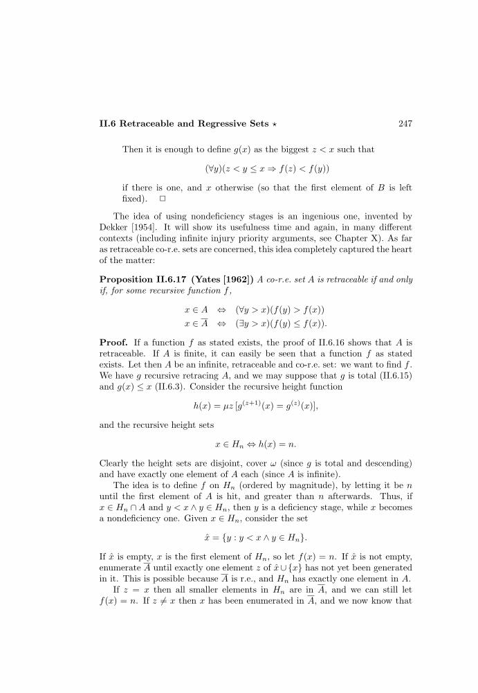
II.6 Retraceable and Regressive Sets ? 247
Then it is enough to define g(x) as the biggest z < x such that
(∀y)(z < y ≤ x⇒ f(z) < f(y))
if there is one, and x otherwise (so that the first element of B is leftfixed). 2
The idea of using nondeficiency stages is an ingenious one, invented byDekker [1954]. It will show its usefulness time and again, in many differentcontexts (including infinite injury priority arguments, see Chapter X). As faras retraceable co-r.e. sets are concerned, this idea completely captured the heartof the matter:
Proposition II.6.17 (Yates [1962]) A co-r.e. set A is retraceable if and onlyif, for some recursive function f ,
x ∈ A ⇔ (∀y > x)(f(y) > f(x))x ∈ A ⇔ (∃y > x)(f(y) ≤ f(x)).
Proof. If a function f as stated exists, the proof of II.6.16 shows that A isretraceable. If A is finite, it can easily be seen that a function f as statedexists. Let then A be an infinite, retraceable and co-r.e. set: we want to find f .We have g recursive retracing A, and we may suppose that g is total (II.6.15)and g(x) ≤ x (II.6.3). Consider the recursive height function
h(x) = µz [g(z+1)(x) = g(z)(x)],
and the recursive height sets
x ∈ Hn ⇔ h(x) = n.
Clearly the height sets are disjoint, cover ω (since g is total and descending)and have exactly one element of A each (since A is infinite).
The idea is to define f on Hn (ordered by magnitude), by letting it be nuntil the first element of A is hit, and greater than n afterwards. Thus, ifx ∈ Hn ∩A and y < x ∧ y ∈ Hn, then y is a deficiency stage, while x becomesa nondeficiency one. Given x ∈ Hn, consider the set
x = y : y < x ∧ y ∈ Hn.
If x is empty, x is the first element of Hn, so let f(x) = n. If x is not empty,enumerate A until exactly one element z of x∪x has not yet been generatedin it. This is possible because A is r.e., and Hn has exactly one element in A.
If z = x then all smaller elements in Hn are in A, and we can still letf(x) = n. If z 6= x then x has been enumerated in A, and we now know that

248 II. Basic Recursion Theory
x has to be a deficiency stage. Then we want y > x such that f(y) ≤ f(x).Note that f(x) = n + 1 is not enough, since it might be that Hn+1 containsno element y > x. And m > n such that Hm has an element y > x is notenough either, since the unique element t ∈ Hm ∩ A might be smaller than x,and setting f(x) = m would make f(t) = f(x), while t < x, and t has to be anondeficiency stage (since t ∈ A). But then let f(x) = m for m > n such thatHm contains no element smaller than x. 2
Exercises II.6.18 Nondeficiency sets. A set A is a nondeficiency set if, for somerecursive function f ,
x ∈ A⇔ (∀y > x)(f(y) > f(x)).
a) If f is not finite-one, the nondeficiency set of f is finite.
b) A co-r.e. set is retraceable if and only if it is the nondeficiency set of a finite-onefunction. (Yates [1962]) (Hint: see the proof above.)
c) Not every co-r.e. retraceable set is the nondeficiency set of a one-one func-tion. (Degtev [1970]) (Hint: let A(g) be the deficiency set of g, and An(g) be itsapproximation up to n, i.e.
x ∈ An(g) ⇔ x < n ∧ (∃y)(x < y ≤ n ∧ g(y) ≤ g(x)).
Define f as follows. Given f(0), . . . , f(n), let n = 〈e, x〉 be the first stage in whichϕe,n is total and one-one on 0, . . . , x, and An0(f) ⊆ Ax(ϕe), where
n0 = maxx ≤ n : f(x) = e.
Then let f(n + 1) = e. Otherwise, let f(x) = n. If ϕe is one-one and total, then
A(ϕe) is infinite, and it cannot be A(ϕe) = A(f), otherwise by construction f takes
the value e infinitely often, and then A(f) is finite.)
Proposition II.6.19 (Marchenkov [1976a]) The class of r.e. co-retraceablesets is r.e. without repetitions.
Proof. Since every finite set is co-retraceable, it is enough (by II.5.24) to showthat the class of r.e. co-retraceable sets is r.e. Let
x ∈ Ae ⇔ (∃y)[(∀z ≤ y)(ϕe(z)↓) ∧ y > z ∧ ϕe(y) ≤ ϕe(x)].
Then Aee∈ω is an r.e. class, and each Ae is either finite (if ϕe is not total) orco-retraceable (by II.6.17). 2
The class of r.e. co-retraceable sets is not completely r.e. (by II.4.2), sinceit is not closed under supersets (see II.6.21.b).

II.6 Retraceable and Regressive Sets ? 249
Regressive versus retraceable
We now briefly come back to the original question of the extent of the analogywith recursive and r.e. sets, and we show that it fails quite strongly. First wegive a positive result, which is the analogue of II.1.20.
Proposition II.6.20 (Dekker [1962]) Every infinite regressive set has aninfinite retraceable subset.
Proof. Let A be regressed by ϕ w.r.t. a0, a1, . . . , and
b0 = a0
bn+1 = the first element in the list of A greater than bn.
Then B = b0, b1, . . . is infinite, because A is. To define the retracing functionfor B on a given x, we first iterate ϕ until we stop, which we must if x ∈ A.Then we recreate the initial segment of B from b0 to x, by dropping the ele-ments that break the monotone growing, and take the biggest element obtainedwhich is smaller than x. If x ∈ B then we do recreate the initial segment of B,and we do choose the right element. 2
There are two properties that we consider essential to claim a nontrivialanalogy with recursive and r.e. sets, namely:
1. The recursive sets are closed under complementation.
2. A set which is r.e., together with its complement, is recursive (II.1.19).
They both fail here:
1. There is a retraceable set with a nonretraceable complement .Take any retraceable, nonrecursive set: its complement is not retraceable,by II.6.6.
2. There is a set regressive together with its complement, but not retraceable.Take any set A r.e. and nonrecursive, with a retraceable complement.Then both A (being r.e.) and A are regressive, but if A were retraceablethen it would also be recursive, again by II.6.6.
Exercises II.6.21 (Dekker and Myhill [1958]) a) If A and B are retraceable, so isA ∩ B. (Hint: given x, consider the greatest element smaller than it on which x issent by both functions retracing A and B.) Appel [1967] has shown that this fails forregressive sets.
b) There are retraceable sets A and B such that A ∪ B is not regressive. (Hint:
let A be an infinite recursive set, and B a nonrecursive, retraceable and co-r.e. set. If
250 II. Basic Recursion Theory
A ∪B were regressive, it would be r.e. because A is an infinite recursive subset of it,
and B would be recursive.)
Despite the failure of the analogy with r.e. and recursive sets, retraceableand regressive sets are interesting on their own, and are useful in some partsof Recursion Theory. See McLaughlin [1982] for a detailed study of them.
æ
Chapter III
Post’s Problem andStrong Reducibilities
One theme of this chapter is relative computability. In Chapter II weintroduced the most general and fundamental case: Turing reducibility. Itwill be recalled that no limitation was imposed there on the help given to themachine by the oracle, except for an obvious finiteness requirement. Here wetake an opposite stand, and look at various possible limitations. Section 2 dealswith the most restrictive case of m-reducibility, in which only one question isallowed to the machine during a computation, and only at the very end of it.Section 3 treats the case of Boolean combinations of atomic questions, calledtt-reducibility, while a number of other, less fundamental, reducibilities aredealt with in Sections 4, 7 and 8.
Relative computations induce equivalence classes, by identifying functionsand sets which have the same degree of difficulty of computation. A secondtheme in the chapter is Post’s problem, introduced in Section 1, which askswhether there are only two such classes of r.e. sets. The solution, obtainedin Section 5, will tell whether the r.e. sets can be distinguished, from a com-putational point of view, only between recursive and nonrecursive, or whetherinstead this rough dichotomy can somehow be essentially refined. The strategyfor a solution to the problem is to analyze the possible structure of r.e. sets (asopposed to giving direct constructions, a strategy pursued instead in ChapterX), and the tactic is to solve the problem first for m-reducibility, in Section 2,and then gradually improve the solution for weaker and weaker reducibilities,in Sections 3 and 4, until we reach the one we are really interested in.
The original motivation for the study of r.e. sets was that they code (byarithmetization) the sets of theorems of formal systems. A third theme of
251

252 III. Post’s Problem and Strong Reducibilities
this chapter is the analysis of formal systems, from this abstract point ofview. We make the relationship between formal systems and r.e. sets precisein Section 10, where we also revisit some of the notions and results obtained inthe chapter, and discuss their bearing on the subject of formal systems.
III.1 Post’s Problem
We have so far encountered only two different kinds of r.e. sets, namely therecursive sets and K, and they generate different degrees.
Definition III.1.1 An r.e. T -degree is a degree containing at least one r.e.set. Two r.e. T -degrees are:
1. the T -degree 0 of the recursive sets
2. the T -degree 0′ of K.
Note that, because of Post’s Theorem and the fact that a set and its comple-ment are in the same degree (being obviously computable one from the other),a degree contains only r.e. sets if and only if it contains only recursive sets.This explains why we only require the existence of an r.e. set in an r.e. degree.
Recall that there is a partial order on the degrees, induced by the relation≤T . It is obvious that 0 is the least degree with respect to it, and the nextresult shows that 0′ is the greatest r.e. degree.
Proposition III.1.2 (Post [1944]) If A is any r.e. set then A ≤T K.
Proof. We prove that there is a recursive function f such that
x ∈ A⇔ f(x) ∈ K ⇔ f(x) ∈ Wf(x),
where the last equivalence holds by definition of K. By the Smn -Theorem, let fbe a recursive function such that
Wf(x) =ω if x ∈ A∅ otherwise.
Then:
• x ∈ A⇒Wf(x) = ω ⇒ f(x) ∈ Wf(x) ⇒ f(x) ∈ K
• f(x) ∈ K ⇒ f(x) ∈ Wf(x) ⇒Wf(x) 6= ∅ ⇒ x ∈ A. 2
Thus, since A ≤T K automatically holds for r.e. sets, an r.e. set A is in thegreatest r.e. degree 0′ if and only if K ≤T A.
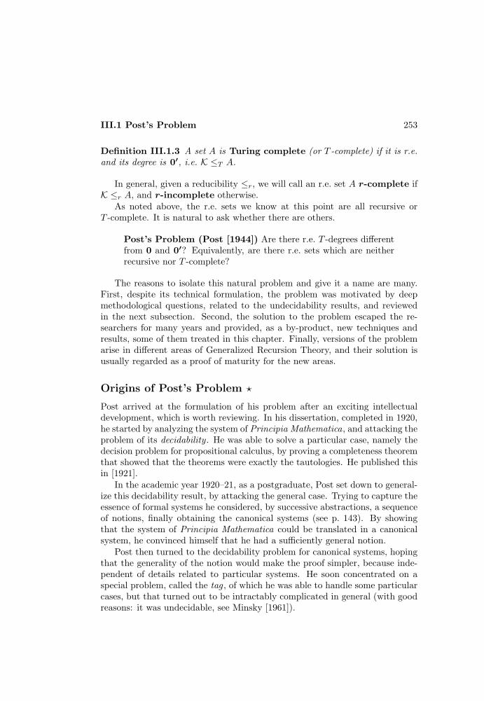
III.1 Post’s Problem 253
Definition III.1.3 A set A is Turing complete (or T -complete) if it is r.e.and its degree is 0′, i.e. K ≤T A.
In general, given a reducibility ≤r, we will call an r.e. set A r-complete ifK ≤r A, and r-incomplete otherwise.
As noted above, the r.e. sets we know at this point are all recursive orT -complete. It is natural to ask whether there are others.
Post’s Problem (Post [1944]) Are there r.e. T -degrees differentfrom 0 and 0′? Equivalently, are there r.e. sets which are neitherrecursive nor T -complete?
The reasons to isolate this natural problem and give it a name are many.First, despite its technical formulation, the problem was motivated by deepmethodological questions, related to the undecidability results, and reviewedin the next subsection. Second, the solution to the problem escaped the re-searchers for many years and provided, as a by-product, new techniques andresults, some of them treated in this chapter. Finally, versions of the problemarise in different areas of Generalized Recursion Theory, and their solution isusually regarded as a proof of maturity for the new areas.
Origins of Post’s Problem ?
Post arrived at the formulation of his problem after an exciting intellectualdevelopment, which is worth reviewing. In his dissertation, completed in 1920,he started by analyzing the system of Principia Mathematica, and attacking theproblem of its decidability . He was able to solve a particular case, namely thedecision problem for propositional calculus, by proving a completeness theoremthat showed that the theorems were exactly the tautologies. He published thisin [1921].
In the academic year 1920–21, as a postgraduate, Post set down to general-ize this decidability result, by attacking the general case. Trying to capture theessence of formal systems he considered, by successive abstractions, a sequenceof notions, finally obtaining the canonical systems (see p. 143). By showingthat the system of Principia Mathematica could be translated in a canonicalsystem, he convinced himself that he had a sufficiently general notion.
Post then turned to the decidability problem for canonical systems, hopingthat the generality of the notion would make the proof simpler, because inde-pendent of details related to particular systems. He soon concentrated on aspecial problem, called the tag , of which he was able to handle some particularcases, but that turned out to be intractably complicated in general (with goodreasons: it was undecidable, see Minsky [1961]).
254 III. Post’s Problem and Strong Reducibilities
At this point, the unsuccessful attempts prompted a revision of the plan,and Post turned to undecidability . He defined a universal canonical system,which is just a version of the set K0 of 150, and showed its diagonal set, i.e.K, to be, in modern terms, r.e. but nonrecursive. To be able to deduce fromthis a general unsolvability result Post needed a version of Church’s Thesis,which he stated in the form: every effectively generable set can be generatedby a canonical system. From this the existence of incomplete formal systemsfollowed easily.
All this work, concluded in 1921, and anticipating a number of results byGodel, Church, and Turing that would follow much later, was left unpublished(see [1922]), because Post was not convinced of (his version of) Church’s The-sis. He took it as a working hypothesis that needed verification, in the formof psychological analysis of the computational process. A step toward suchanalysis was [1936], in which Post proposed a version of Turing machines, in-dependently of Turing. The canonical systems were published only in [1943],and the form of Godel’s theorem based on canonical systems only in [1944].
The mutual reductions among various notions of canonical systems, as wellas particular formal systems like Principia Mathematica, led Post to the con-cept of m-reducibility between sets. And the fact that known undecidabilityproofs, by Post, Church, and others, were all obtained by appropriately reduc-ing K to the problem in question, prompted the problem of whether the onlyundecidable systems were the universal ones, in which K could interpreted.Post [1944] was able to disprove this for m-reducibility, and then he asked thesame question for the general notion of T -reducibility, introduced by Turing[1936]. Despite a good deal of intermediate work, he could not reach a solu-tion. Sections 2 to 4 are a report of Post’s work and of modern improvements,and Section 5 provides the missing brick.
Turing reducibility on r.e. sets
Since the solution to Post’s Problem will require a detailed study of the struc-ture of the r.e. sets, we prove some technical results that will facilitate thetask.
Proposition III.1.4 T -reducibility on r.e. sets (Rogers [1967]) If A andB are r.e. sets, then A ≤T B if and only if, for some r.e. relation R,
x ∈ A⇔ (∃u)(Du ⊆ B ∧R(x, u)).
Proof. By compactness and monotonicity of oracle computations (II.3.13) andthe Normal Form Theorem for restricted functionals (II.3.12) we have, for agiven e and some r.e. relation Q,
ϕBe (x) ' z ⇔ (∃v)(∃u)(Dv ⊆ B ∧Du ⊆ B ∧Q(x, u, v, z)),

III.1 Post’s Problem 255
because Dv and Du together specify a finite subfunction of cB . If A ≤T B thencA ' ϕBe , for some e. In particular
x ∈ A⇔ (∃v)(∃u)(Dv ⊆ B ∧Du ⊆ B ∧Q(x, u, v, 0)).
If moreover B is r.e., the expression Dv ⊆ B is r.e. itself, and thus there is Rr.e. such that
x ∈ A⇔ (∃u)(Du ⊆ B ∧R(x, u)).
Conversely, if this expression for A holds for some r.e. relation R, then A isr.e. in B. If moreover A is r.e., then it is r.e. in B and, by the relativization ofPost’s Theorem to B, A is recursive in B. 2
The next result is a strong generalization of the Fixed-Point Theorem, toany function which is recursive in an incomplete r.e. set.
Theorem III.1.5 T -completeness of r.e. sets (Martin [1966], Lachlan[1968], Arslanov [1981]) An r.e. set A is T -complete if and only if there isa function f ≤T A without fixed-points, i.e. such that ∀x(Wx 6= Wf(x)).
Proof. If A is T -complete, the set x : 0 6∈ Wx is recursive in A, being co-r.e.By the relativized Smn -Theorem, there is f ≤T A such that
Wf(x) =ω if 0 6∈ Wx
∅ otherwise.
Then Wf(x) 6= Wx, because the two sets differ on 0.Suppose now that A is r.e., and f ≤T A has no fixed-points. The idea to
get K ≤T A, thus showing that A is T -complete, is the following. Consider thefunction
sx =µs(x ∈ Ks) if x ∈ K0 otherwise.
Then x ∈ K ⇔ x ∈ Ksx . We want to majorize sx recursively in A, i.e. to findψ recursive in A, such that ψ(x) ≥ sx. Then x ∈ K ⇔ x ∈ Kψ(x), and thisimplies K ≤T A.
Since f ≤T A, there is e such that f ' ϕAe . Moreover A is r.e., and it canbe recursively approximated by an enumeration Ass∈ω. Although ϕAe is onlyrecursive in A, it can be approximated by the recursive function ϕAs
e,s. Fix nowx ∈ K: by the Fixed-Point Theorem, there is z such that
Wz = Wϕ
Asxe,sx (z)
.
By the assumption on f , it cannot be Wz = Wf(z). This means that, whileϕAsxe,sx(z) is an approximation of f(z), it must be a wrong one. Recursively in
256 III. Post’s Problem and Strong Reducibilities
A we can first compute ϕAe (z), and find the length of the least initial segmentcA(y) that gives the right value. Then we can recursively enumerate A to finda stage s ≥ y in which all the elements of A used in the computation have beengenerated, i.e. cAs(y) = cA(y). From this point on the approximations will givethe right value, i.e. ϕAt
e,t(z) = f(z), for any t ≥ s. Then it must be s ≥ sx.We have only to do this in general now. By the Fixed-Point Theorem with
parameters (II.2.11), there is g recursive such that
Wg(x) =
Wϕ
Asxe,sx (g(x))
if x ∈ K∅ otherwise.
Let ψ(x) be a stage in which A has generated all the elements needed to com-pute the right value of f(g(x)) from then on, as above. Then ψ is recursivein A, and ψ(x) ≥ sx (if x ∈ K as above, and if x 6∈ K because then sx = 0). 2
Note that the condition that A be r.e. is essential, since without it the resultfails in general.
Exercise III.1.6 There is a set A ≤T K, and a function f ≤T A, such that f hasno fixed-points, but K 6≤T A. (Arslanov [1981]) (Hint: by the proof of III.2.18, it isenough to find A effectively immune, recursive in K, and such that K 6≤T A. Andsuch a set exists by the Low Basis Theorem V.5.32, applied to the Π0
1 class
A : A ⊆ S ∧ (∀x)(Dg(x) ∩A 6= ∅),
where S is Post’s simple set, see III.2.11, and g enumerates a strong array intersecting
S.)
For more results on fixed-points, see Arslanov [1981], Jockusch, Lerman,Soare, and Solovay [198?], Kucera [1986], [198?], and Jockusch [198?]. In par-ticular, Kucera [1986] (see Volume II) solves Post’s problem by showing thatany degree below 0′ and containing no function without fixed-points boundsan r.e. nonrecursive degree.
III.2 Simple Sets and Many-One Degrees
The path we shall follow to attack Post’s Problem is the one suggested byPost himself, which is also a natural mathematical practice: confronted witha difficult problem, try first with simpler versions of it and, once a solution isfound for them, proceed to more difficult cases, in the hope of finally reachingthe solution of the original problem. This will be a long path, but it will finallypay off in III.5.20, leaving us with a deep knowledge of the structure of the r.e.sets.

III.2 Simple Sets and Many-One Degrees 257
Our present approach is structural, since it tries to solve the problemby isolating nonempty properties of r.e. sets that imply nonrecursiveness andT -incompleteness. A different approach consists of trying to build ad hoc so-lutions by brute force, and will be considered in Chapter X.
Many-one degrees
The simplest special case of Turing reducibility, which we have been usingalready in many of the previous proofs, is the following:
Definition III.2.1 (Post [1944]) A is m-reducible to B (A ≤m B) if, forsome recursive function f , the following equivalent conditions are satisfied:
1. ∀x(x ∈ A⇔ f(x) ∈ B)
2. A = f−1(B)
3. f(A) ⊆ B ∧ f(A) ⊆ B.
A is m-equivalent to B (A ≡m B) if A ≤m B and B ≤m A.
Exercises III.2.2 a) If A 6= ∅, ω is recursive, then A ≤m B for any set B.b) If A ≤m B and B is recursive, so is A.c) If A ≤m B and B is r.e. then so is A.d) If A is r.e. then A ≤m A if and only if A is recursive and A 6= ∅, ω.e) There is a nonrecursive set A such that A ≤m A. (Hint: consider K ⊕K.)
e) If A and B differ finitely, then A ≡m B.
Note that ≤m is a reflexive and transitive relation, and thus ≡m is anequivalence relation.
Definition III.2.3 The equivalence classes of sets w.r.t. m-equivalence arecalled m-degrees, and (Dm, ≤) is the structure of m-degrees, with the partialordering ≤ induced on them by ≤m.
The m-degrees containing r.e. sets are called r.e. m-degrees, and two ofthem are:
1. 0m, the m-degree of the recursive sets different from ∅ and ω
2. 0′m, the m-degree of K.
Note that an r.e. m-degree contains only r.e. sets. The m-degrees containingrecursive sets are three: 0m, ∅, ω. The last two are incomparable andsmaller than 0m, but every other m-degree is greater than or equal to 0m.In the following we will always consider nontrivial sets, and thus 0m may beconsidered as the least m-degree. We now show that 0′
m is the greatest r.e.m-degree.
258 III. Post’s Problem and Strong Reducibilities
Proposition III.2.4 (Post [1944]) A set A is r.e. if and only if A ≤m K.
Proof. If A is r.e. then A ≤m K by the proof of III.1.2. Conversely, ifx ∈ A⇔ f(x) ∈ K then the elements of A are exactly those in the intersectionof K and the range of f , and hence A is r.e. 2
Definition III.2.5 A set A is m-complete if it is r.e. and its m-degree is0′
m, i.e. K ≤m A.
Exercises III.2.6 Both K and the notion of m-completeness are defined w.r.t. theclass of the r.e. sets. Let a recursive enumeration Wh(x)x∈ω of the recursive sets begiven (see II.5.26).
a) The set x ∈ K∗ ⇔ x ∈ Wh(x), obtained by diagonalization over the recursivesets, is m-complete. (Muchnik [1958a]) (Hint: let
Wh(g(x)) =
ω if x ∈ K∅ otherwise.
Then x ∈ K ⇔ g(x) ∈ K∗.)b) If the recursive sets are uniformly m-reducible to an r.e. set A, then A is
m-complete. (Smullyan [1961]) (Hint: if z ∈ Wh(x) ⇔ f(z, x) ∈ A, then K∗ ≤m A.)
The analogue of Post’s Problem for m-reducibility is: are there r.e. setswhich are neither recursive, nor m-complete? The beginning of our story is thefollowing observation.
Proposition III.2.7 (Post [1944]) If A is m-complete, then A contains aninfinite r.e. subset.
Proof. First consider the special case of the m-complete set K. Note that
Wx ⊆ K ⇒ x ∈ K −Wx.
Suppose indeed that x ∈ Wx: then x is in K by definition, and in K becauseWx ⊆ K, contradiction. Then it must be x 6∈ Wx, and thus also x ∈ K.
Then the index of an r.e. subset of K is an element of K but not of the givensubset, and this permits us to generate an infinite r.e. subset of K, by startingwith the emptyset, and getting new elements at each stage. Formally, if f is arecursive function such that:
f(0) = an index of ∅f(n+ 1) = an index of f(0), . . . , f(n),
then the range of f is an infinite r.e. subset of K.
III.2 Simple Sets and Many-One Degrees 259
To extend this to any m-complete set A, let
x ∈ K ⇔ g(x) ∈ A.
Given an r.e. subset B of A, first pull it back (through g) to an r.e. subset ofK. Use the property of K proved above, to get an element in K but not in thepull back of B, then project it via g to an element in A but not in B. Formally,let f be a recursive function such that:
f(0) = g(a0) with a0 index of ∅f(n+ 1) = g(an+1) with an+1 index of the r.e. set
g−1(f(0), . . . , f(n)).
Then the range of f is an infinite r.e. subset of A. 2
Exercise III.2.8 A different proof of the result above consists of noting that any
infinite r.e. set of indices of ∅ is an infinite r.e. subset of K, and can be projected to
A because the function that reduces K to A can be taken to be one-one.
Simple sets
Since coinfinite recursive sets and m-complete sets have complement with aninfinite r.e. subset, a solution to Post’s Problem for m-degrees would be givenby sets without this property. Recall (p. 141, and II.6.4) that an infinite set isimmune if it does not contain infinite r.e. (or recursive) subsets.
Definition III.2.9 (Post [1944]) A set is simple if it is r.e. and coimmune,i.e. its complement is infinite and does not contain infinite r.e. subsets.
Exercises III.2.10 a) A coinfinite r.e. set is simple if and only if it has no coinfinite,recursive superset . (Hint: use II.1.20.)
b) If A and B are simple then A ∩ B is simple, and A ∪ B is simple or cofinite.Thus simple or cofinite sets are a filter in the lattice of the r.e. sets under inclusion.(Dekker [1953])
c) If A is simple and Wx is infinite, then A ∩Wx is infinite.
It only remains to show that the notion of simplicity is not empty.
Theorem III.2.11 (Post [1944]) There exists a simple set.
Proof. We give two different constructions.
1. Post’s simple set S.The idea is to build S intersecting each infinite r.e. set, so that S doesnot contain any infinite r.e. subset. We cannot recursively enumerate the

260 III. Post’s Problem and Strong Reducibilities
infinite r.e. sets (II.5.27.a), so we will intersect S with each r.e. set withenough elements. To prevent the collapse of the complement of S, we donot want to put too many elements in S, so we make sure that each timea new element goes into S, another one will stay out. Precisely, we putat most half of 0, 1, . . . , 2x into S, for each x. The set S is defined asfollows: dovetail an enumeration of all the r.e. sets and, for each e, putinto S the first element greater than 2e enumerated into We.
S is r.e. by construction. S is infinite since an element of 0, . . . , 2x canenter S only if it comes from some We such that 2e < 2x: but there areat most x such sets, and each contributes at most one element. Thus Shas at least x + 1 elements, for each x, and it is then infinite. And S issimple, because if We is infinite then it has elements greater than 2e, andone of them will be in S.
2. A direct construction.We build a simple set A by stages. At stage s we will have As, and wewill let As = as0 < as1 < · · · . In the end A = a0 < a1 < · · · , wherean = lims→∞ asn. We want to satisfy the following requirements:
Pe : We infinite ⇒We ∩A 6= ∅Ne : A has at least e elements, or lims→∞ ase <∞.
P stands for positive, because to satisfy the Pe’s we have to do some-thing positive on A (namely, to put some element in it). N stands fornegative, because to satisfy the Ne’s we have to do something negativeon A (namely, to leave some element out of A).
The construction is as follows. We start with A0 = ∅ (hence a0n = n). At
stage s+ 1 we search for the smallest e ≤ s such that:
• We,s ∩As = ∅• for some n ≥ e, asn ∈ We,s.
Note that both As and We,s are finite, and we only look at e ≤ s, so thesearch is effective. If e does not exist, we go to the next stage. Otherwise,Pe is the condition with smallest index which looks unsatisfied, and witha chance to be satisfied. Then we put asn into A, where n is the smallestone such that n ≥ e and asn ∈ We,s. This makes all the asm with m ≥ nmove to the next one (since they enumerate the complement). In otherwords,
as+1m = asm if m < nas+1m = asm+1 if m ≥ n.
Since the construction is effective, A =⋃s∈ω As is r.e. Moreover:

III.2 Simple Sets and Many-One Degrees 261
• A is infinite.It is enough to prove that lims→∞ asm exists. Indeed, asm may moveat a certain stage s + 1 only if it happens that asn ∈ We, for somee ≤ n ≤ m. Since each We contributes at most one element for eache, and there are only finitely many e ≤ m, asm moves only finitelymany times. So all negative requirements are satisfied.
• A is simple.By induction, suppose that s0 is such that s0 ≥ e, and all Pi’s withi < e have been satisfied at stage s0 (i.e. We,s0 ∩ As0 6= ∅if We isinfinite). If We is an infinite subset of A, there are s ≥ s0 and n ≥ esuch that asn = an ∈ We,s. Then one such an goes into A at stages+ 1 (because e is the smallest index for which Pe looks unsatisfied,and with a chance to be satisfied), contradiction. 2
The second proof given above is a typical priority argument with noinjury, with
P0 > N0 > P1 > N1 > · · ·
as order of priority for the satisfaction of the requirements. Indeed, we allowasn to move only to satisfy Pe for some e ≤ n, so e.g. as0 can move only to satisfyP0, as1 only to satisfy P0 or P1, and so on. Moreover, we choose the smallestpossible positive requirement for satisfaction, and this says that the positiverequirements are ordered by their indices. There is no injury, because oncea positive requirement is satisfied it remains so forever (since we never takeelements out of A). The priority method will be discussed in full generality inChapter X.
The two examples of simple sets given above are direct constructions, andthus somehow unnatural. There are however sets which can be naturally de-fined, and that turn out to be simple. The first uses the notion (p. 151) ofrandom number, as a number that is its own shorter description. In termsof the Kolmogorov complexity K, defined (on p. 151) as
K(x) = µe(ϕe(0) ' x),
a number is random if x ≤ K(x).
Proposition III.2.12 (Kolmogorov [1963], [1965]) The set of nonrandomnumbers is simple.
Proof. Let A = x : K(x) < x. Then A is r.e., because
x ∈ A⇔ (∃e < x)(ϕe(0) ' x).
262 III. Post’s Problem and Strong Reducibilities
To show that A is infinite consider, given any n, the converging valuesamong
ϕ0(0), ϕ1(0), . . . , ϕn(0).
If x is different from all of them, then n+ 1 ≤ K(x) by definition. And if x isthe least number not among them, x ≤ n + 1 (since we considered only n + 1possible values, and in the worst case they are the numbers from 0 to n). Thenx ≤ K(x), and x is random. Thus there is a random number with complexityat least n + 1. Since this holds for every n, there are infinitely many randomnumbers, and A is infinite.
To show that there is no infinite r.e. set of random numbers, first note thatthe index e of an r.e. set We provides a uniform description of the elements ofthe set: if We = x0, x1, . . . then
xn = the n-th element enumerated in We.
Moreover, this description of xn is uniform and linear in e and n, hence isbounded by a linear function h(e, n). If we could prove that for some n wehave h(e, n) < xn, we would know that xn is not random. This is certainlythe case if n is big enough, and xn is greater than n2 (since then h(e, n), beinglinear in n for a fixed e, is bounded by n2 almost everywhere).
It is now enough to note that, given We, we can uniformly obtain an r.e.subset Wg(e) of it, whose n-th element is bigger than n2, by waiting until suchan element is generated in We. If We is infinite so is Wg(e), and then it containsa nonrandom element. Thus there is no infinite r.e. set of random numbers,and A is simple. 2
The proof just given is a positive use of Berry’s paradox (Russell [1906]),a version of which is: given n, consider ‘the least number that cannot be definedin less than n characters’. This defines, in c + |n| characters (where |n| is thelength of n and c is a constant), a number whose definition needs more than ncharacters, and it is paradoxical for all n such that c+ |n| ≤ n, i.e. for almostevery n.
This proof contains additional information, exploited on p. 265. A quick,less informative proof is provided by the Fixed-Point Theorem. Suppose A isan infinite r.e. set of random numbers, and let h be a recursive function suchthat
ϕh(e)(0) ' the smallest x > e generated in A.
By the Fixed-Point Theorem, there is e such that ϕe ' ϕh(e). By definitionϕe(0) is a random number (being in A), hence it cannot be bigger than e. Butthis is exactly how it was defined, contradiction.
The immunity of the set of random numbers is a strong result, implying :
III.2 Simple Sets and Many-One Degrees 263
1. a version of the incompleteness results: in any consistent formal systemsound for arithmetic, we can prove that a random number is so onlyin finitely many cases, since the set of provably random numbers is r.e.(Chaitin [1974]).
2. the undecidability of the halting problem: if we could decide whetherϕe(0) ↓, then we could compute K(x) and decide whether a number israndom or not. Actually, the halting problem and the Kolmogorov com-plexity function have the same T -degree: K is obviously recursive in K, bydefinition, and the converse holds because the set of nonrandom numbersis T -complete, see p. 265.
Exercise III.2.13 The existence of infinitely many random numbers implies the ex-
istence of infinitely many prime numbers. (Chaitin [1979]) (Hint: if there are only
n+ 1 primes, say p0, . . . , pn, then for every x, x = px00 · · · pxn
n . But xi ≤ log x, and so
x can be described in ≈ n · log x bits of information. For big enough x, then x is not
random.)
The next example of simple sets provides with such sets in every nonzeroT -degree, and thus shows that a simple set is not necessarily T -incomplete.
Proposition III.2.14 (Dekker [1954]) Every nonrecursive r.e. T -degreecontains a simple set.
Proof. Given A r.e. and nonrecursive, let B be its deficiency set (II.6.16).Then A ≡T B, and B is a coinfinite and coretraceable r.e. set. So B is (byII.6.5) recursive or immune. Since A is nonrecursive, B is immune, and thenB is simple. 2
Exercise III.2.15 Give a direct proof that the deficiency set of f recursive and one-
one is recursive or immune. (Hint: if B has an infinite recursive subset C, given x
find y ∈ C such that f(y) > x. Then x ∈ A ⇔ x ∈ f(0), . . . , f(y). Thus A, and
hence B, are recursive.)
Effectively simple sets ?
We have just seen that a simple set can be T -complete, and thus simple setsdo not automatically solve Post’s Problem. But before we go on with differenttrials, we want to make sure that none of the simple sets built above is alreadyT -incomplete. The idea is to effectivize the notion of simplicity.
Definition III.2.16 (Smullyan [1964]) A is effectively simple if it is acoinfinite r.e. set, and there is a recursive function g such that
We ⊆ A ⇒ |We| ≤ g(e).
264 III. Post’s Problem and Strong Reducibilities
Exercise III.2.17 We show that other natural attempts to define effective simplicityare either equivalent to the one proposed, or impossible.
a) A coinfinite r.e. set A is effectively simple if and only if there is a partialrecursive function ϕ such that We ⊆ A⇒ ϕ(e)↓ ∧ |We| ≤ ϕ(e). (Sacks [1964])
b) For every simple set A there is a partial recursive function ϕ such that if We
is infinite then ϕ(e)↓ ∧ ϕ(e) ∈ We ∩A.
c) For no simple set there is a similar total recursive function. (Hint: consider g
recursive such that Wg(x) = f(x), and apply the Fixed-Point Theorem.)
Thus for simple sets we only know that an r.e. subset of the complementis finite, while for effectively simple sets we also know a recursive bound on itscardinality. The interest of the notion is that it implies T -completeness.
Proposition III.2.18 (Martin [1966]) Every effectively simple set isT -complete.
Proof. LetWe ⊆ A ⇒ |We| ≤ g(e).
Define f ≤T A such that
Wf(e) = the first g(e) + 1 elements of A.
Then f has no fixed-points: if We = Wf(e) then We ⊆ A, but |We| = g(e) + 1.By the criterion for T -completeness III.1.5, A is then T -complete. 2
Exercises III.2.19 a) There are simple sets which are not effectively simple. (Sacks[1964]) (Hint: a direct proof is difficult, requiring priority and Fixed-Point Theorem.To build A as wanted, we want to destroy
Wx ⊆ A ⇒ |We| ≤ ϕe(x).
Given x and e, we build an r.e. set Wf(e,x) with the property that
Wf(e,x) ⊆ A ∧ |Wf(e,x)| > ϕe(x).
Then we need the Fixed-Point Theorem to step from the sets Wf(e,x) to sets ofthe form Wx. What III.2.18 accomplishes is to separate the use of the Fixed-PointTheorem, to give the T -completeness of effectively simple sets, and of priority, tobuild a T -incomplete simple set or just, due to III.2.14, a nonrecursive, T -incompleter.e. set.)
b) There are simple, not effectively simple, and T -complete sets. (Hint: take asimple T -complete set A, a simple not effectively simple set B, and consider A⊕B.)
c) A simple set A is T -complete if and only if there is g ≤T A such that
We ⊆ A ⇒ |We| ≤ g(e).

III.2 Simple Sets and Many-One Degrees 265
(Lachlan [1968]) (Hint: T -completeness is proved as in III.2.18. If A is T -complete, it
is recursive in A to ask if We ⊆ A, i.e. if ∃x(x ∈ We∩A). If We ⊆ A then We is finite,
by simplicity, and recursively in A we can search for an x such that (∃y > x)(y ∈ We)
fails.)
We can now show that the simple sets constructed above are all effectivelysimple, and thus T -complete. We refer to the proofs of III.2.11 and III.2.12,and use the same notations as there.
1. Post’s simple set .If We ⊆ S then |We| ≤ 2e+ 1, since otherwise We has more than 2e+ 1elements, so one of them is greater than 2e, and goes into S.
2. The set A built in III.2.11.If We ⊆ A then |We| ≤ e, since otherwise there is n ≥ e such thatan ∈ We. By going to a stage s after which the Wi’s with i < e donot contribute anymore elements to A, the elements of A up to an havesettled, and an ∈ We,s, we would then put one element of We into A.
3. The set of nonrandom numbers.The linear function h(e, n) which bounds the description of the n-th el-ement of We can be made recursive (by bounding the code number of aTuring machine program that prints xn on input 0). If
f(e) = smallest number n such that h(g(e), n) ≤ n2
then Wg(e) contains a nonrandom number, if it has at least f(e) elements.And since Wg(e) has at least n elements if We has at least n2 +n, if |We|contains only random numbers it must be |We| ≤ f(e)2 + f(e).
We consider now the simple sets provided by III.2.14.
Proposition III.2.20 (Smullyan [1964]) The deficiency set of K is effec-tively simple.
Proof. Let f be a one-one recursive function with range K, and
x ∈ B ⇔ (∃y > x)(f(y) < f(x)).
We want to find g recursive such that
We ⊆ B ⇒ |We| ≤ g(e).
Suppose then We ⊆ B. Since we already know that B is simple, We isfinite, say x1 < · · · < xn. Consider the behavior of f on these elements.

266 III. Post’s Problem and Strong Reducibilities
f(x1) f(x2) f(xn−1) f(xn)
x1 x2 xn−1 xnr r r rr r r
7
CCCCO
Since each xi is a nondeficiency stage, there is no crossover. It is then enoughto find effectively a > f(xn): since f is one-one, a ≥ |We|.
To find a, we use the fact that
Wa ⊆ K ⇒ a ∈ K −Wa.
Since K is the range of f , it is enough to choose Wa containing all the elementsof K below f(xn). This is possible because xn ∈ B, so
K ∩ 0, . . . , f(xn) = 0, . . . , f(xn) − f(0), . . . , f(xn).
We then do this in general. Given We, let
Wg(e) = z : (∃y ∈ We)(z < f(y) ∧ z 6∈ f(0), . . . , f(y)).
Then
We ⊆ B ⇒Wg(e) ⊆ K ⇒ g(e) ∈ K −Wg(e) ⇒ |Wg(e)| ≤ g(e). 2
Exercises III.2.21 Strongly effectively simple sets. (McLaughlin [1965]) A isstrongly effectively simple (s.e.s.) if it is a coinfinite r.e. set, and there is a partialrecursive function ψ such that
We ⊆ A ⇒ ψ(e)↓ ∧ (maxWe) < ψ(e).
An example is given by Post’s simple set.
a) ψ may always be supposed to be total .
b) There are effectively simple sets which are not s.e.s. (Martin [1966]) (Hint: thisfollows from results in III.4.24, since a s.e.s. is not maximal, and there are maximal,effectively simple sets. A direct construction, e.g. in the style of III.2.19.a, is alsopossible.)
McLaughlin [1973], and Cohen and Jockusch [1975], prove in different ways that
the deficiency set of K is not s.e.s.
Exercises III.2.22 Immune sets. a) There are 2ℵ0 sets immune and coimmune,called bi-immune. (Hint: enumerate a set of pairs (xn, yn) such that xn and ynare different elements of the n-th infinite r.e. set, not yet enumerated in the previouspairs. Any set with exactly one element of each pair is bi-immune.)

III.3 Hypersimple Sets and Truth-Table Degrees 267
b) A set A is effectively immune if it is infinite and, for some partial recursivefunction ψ,
We ⊆ A ⇒ ψ(e)↓ ∧ |We| ≤ ψ(e).
ψ may always be supposed to be total . Similarly for strongly effectively immunesets, where instead
We ⊆ A ⇒ ψ(e)↓ ∧ (maxWe) ≤ ψ(e).
(Hint: let g be a recursive function such that
Wg(e) =
We if ψ(e)↓∅ otherwise.
Then one of ψ(e) and ψ(g(e)) converges.)c) There are effectively bi-immune sets, i.e. sets effectively immune and effectively
coimmune. (Ullian) (Hint: a natural construction, in which each We contributes atmost two elements, one for A and one for A, gives a bi-immune set A such that ifWe ⊆ A or We ⊆ A, then |We| ≤ 2e+ 1.)
d) If A is strongly effectively immune, then A cannot be immune. (McLaughlin[1965]) (Hint: suppose
We ⊆ A ⇒ max(We) < f(e).
Let sx be the smallest stage in which x appears in K, if it ever does, and 0 otherwise.Define
Wt(x) =
sx if x ∈ K∅ otherwise.
Then x ∈ K ∧ sx ≥ f(t(x)) ⇒ sx ∈ A. There are infinitely many such sx’s, otherwisefor almost every x is x ∈ K ⇔ x ∈ Kf(t(x)), and K is recursive. But the condition
x ∈ K ∧ sx ≥ f(t(x)) is r.e., so A contains an infinite r.e. subset.)e) A set A is constructively immune if, for some partial recursive ϕ,
We infinite ⇒ ϕ(e)↓ ∧ ϕ(e) ∈ We ∩A.
If A is constructively immune, then A cannot be immune. (Li Xiang [1983]) (Hint:an infinite r.e. subset of A can be built, by starting with an r.e. index of ω.)
f) The notions of effective and constructive immunity are independent . (Li Xiang
[1983]) (Hint: every simple set is constructively coimmune; for the other directions,
see c) and e) above.)
III.3 Hypersimple Sets andTruth-Table Degrees
We have solved Post’s Problem for m-reducibility by constructing a simple set,but have noticed that this does not automatically imply a solution to Post’sProblem for T -reducibility, because there are simple sets which are T -complete

268 III. Post’s Problem and Strong Reducibilities
(actually, all the simple sets we built were such). The next step is to relaxm-reducibility somewhat, and solve Post’s Problem for the weaker notion.
In m-reducibility we only allowed one positive query to the oracle. Thereare many possible extensions, depending on the number of queries allowed (afixed bounded number, or unboundedly many), their nature (only positive, i.e.asking whether some elements are in the oracle, or also negative, asking whethersome elements are not in it), and the way they are combined (conjunctions,disjunctions, or any possible combination). Some of the possible reducibilities,called respectively conjunctive, disjunctive, and positive (Jockusch [1966])are the following:
A ≤c B ⇔ for some recursive function f ,x ∈ A⇔ Df(x) ⊆ B.
A ≤d B ⇔ for some recursive function f ,x ∈ A⇔ Df(x) ∩B 6= ∅.
A ≤p B ⇔ for some recursive function f ,x ∈ A⇔ ∃u(u ∈ Df(x) ∧Du ⊆ B).
The consideration of these reducibilities makes good sense for the study ofr.e. sets, due to the fact that they only use positive information on the oracle,which is exactly what we may obtain from r.e. sets (note that A is r.e. if andonly if A ≤p K). We will not be too much concerned with them, since thepicture we get from m-reducibility is finer, but we will prove some scatteredresults here and in Chapter X.
Since our present concern is the solution to Post’s Problem, we might aswell consider the strongest possible generalization along these lines: to allowfor any (finite) number of questions, both positive and negative, to the oracle.To define this notion precisely, let σnn∈ω be an effective enumeration of allthe propositional formulas, built from the atomic ones ‘m ∈ X’, for m ∈ ω.These are also called truth-table conditions, since they can be arrangedin truth-tables. Given a set B, B |= σn means that B satisfies σn, i.e. thatthe propositional formula σn becomes true when X in the atomic formulas isinterpreted as B.
Definition III.3.1 (Post [1944]) A is tt-reducible to B (A ≤tt B) if, forsome recursive function f ,
x ∈ A⇔ B |= σf(x).
A is tt-equivalent to B (A ≡tt B) if A ≤tt B and B ≤tt A.
In terms of connectives, the various truth-table reducibilities correspond totruth-table conditions built up from the atomic ones by means of the following
III.3 Hypersimple Sets and Truth-Table Degrees 269
connectives:
≤tt= ¬,∧,∨ ≤p= ∧,∨ ≤c= ∧ ≤d= ∨,
while ≤m correspond to using only atomic formulas. We will see in III.8.4that, on the r.e. sets, ≤m= ¬. Since ¬, together with any one of ∧ and ∨,generates all the propositional formulas, this would seem to take care of all thepossible types of truth-table-like reducibilities. Bulitko [1980] and Selivanov[1982] have shown that it is almost so, in the sense that only another one suchreducibility exists, called linear reducibility, corresponding to the logical sum(i.e. addition modulo 2). Its definition can be put as:
A ≤l B ⇔ for some recursive function f
x ∈ A⇔ |Df(x) ∩B| ≡ 1 (mod 2).
Truth-table degrees
Out first concern is to make clear the difference between truth-table and Turingreducibility. Recall that a relative computation consists of two different kindsof actions, one purely computational (performed by a machine), and the otherinteractive (queries answered by the oracle). In Turing computations the twoparts can be strongly interwoven, and impossible to unravel: we may cometo know the questions we need to ask the oracle only during the computationitself, and there might even be no recursive bound on their number or size (asa function of the input). On the other hand, truth-table computations clearlyseparate the two parts of the relative computation, computing ahead of timenot only the elements which need to be queried, but also the outcome of thecomputation for any possible answer the oracle is going to provide for them.
Another way to see the difference is in terms of functionals. Recall thatA ≤T B if and only if cA ' F (cB), for some partial recursive functional F .
Proposition III.3.2 (Trakhtenbrot [1955], Nerode [1957]) A ≤tt B ifand only if cA ' F (cB) for some partial recursive, total functional F .
Proof. Letx ∈ A⇔ B |= σf(x),
and define F (α, x) as follows. First see if α(z)↓ for every z such that the atomicformula z ∈ X occurs in σf(x). If so, consider any set C such that, for any zas just said, z ∈ C ⇔ α(z) ' 1, and let
F (α, x) '
1 if C |= σf(x)
0 otherwise.
270 III. Post’s Problem and Strong Reducibilities
F is partial recursive and total by definition, and cA ' F (cB).Suppose now that F is a partial recursive, total functional. For each x and
X, F (cX , x) is defined, and for every branch of the space 2ω of sets, the in-formation on X needed to compute F (cX , x) is bounded, by compactness. ByKonig’s Lemma, there is a bound which works for all branches. Another wayto see this is to note that F is continuous and total on 2ω, which is a compactspace in the positive information topology: then F is uniformly continuous,and there is a modulus of continuity that works for every member of 2ω. Inany case, we may thus write down a truth-table that gives F (cX , x) for anyX, because only values of X up to the bound are needed, and there are onlyfinitely many possible combinations. 2
By II.3.7.b we then know that T -reducibility and tt-reducibility do notcoincide. We now turn to a study of tt-reducibility.
Exercises III.3.3 a) If A is recursive, then A ≤tt B for any set B.
b) If A ≤tt B and B is recursive, so is A.
c) A ≤tt A.
Note that ≤tt is a reflexive and transitive relation, and thus ≡tt is an equiv-alence relation.
Definition III.3.4 The equivalence classes of sets w.r.t. tt-equivalence arecalled tt-degrees, and (Dtt, ≤) is the structure of tt-degrees, with the partialordering ≤ induced on them by ≤tt.
The tt-degrees containing r.e. sets are called r.e. tt-degrees, and two ofthem are:
1. 0tt, the tt-degree of the recursive sets
2. 0′tt, the tt-degree of K.
An r.e. set A is tt-complete if its tt-degree is 0′tt, i.e. if K ≤tt A.
Note that an r.e. tt-degree, being closed under complementation, containsonly r.e. sets if and only if it contains only recursive sets. Also, 0tt and 0′
tt are,respectively, the least and the greatest r.e. tt-degrees.
The analogue of Post’s Problem for tt-reducibility is: are there r.e. setswhich are neither recursive, nor tt-complete? We already know that simplesets are not m-complete, and we make sure that they are not automaticallytt-incomplete.
Proposition III.3.5 (Post [1944]) There is a simple, tt-complete set.
III.3 Hypersimple Sets and Truth-Table Degrees 271
Proof. Consider Post’s simple set S (III.2.11). Any coinfinite r.e. superset ofit will still be simple (since any infinite r.e. subset of its complement would alsobe a subset of S). We then look for an r.e. set S∗ such that:
1. K ≤tt S∗, i.e. K is coded into S∗ by truth tables
2. S ⊆ S∗, and S∗ coinfinite.
Let Fxx∈ω be a strong array of disjoint finite sets intersecting S. It exists,because the construction of S ensures that at most z elements of 0, . . . , 2z gointo S, so S intersects each subset of 0, . . . , 2z with at least z + 1 elements.It is then enough to let
Fx = n : 2x − 1 ≤ n < 2x+1 − 1.
We can then use the set Fx to code the fact that x ∈ K, by putting it into S∗
if this holds, and not otherwise. We also want S∗ to be a superset of S, andwe thus let
S∗ = S ∪⋃x∈K
Fx.
Then:
1. K ≤tt S∗, because x ∈ K ⇔ Fx ⊆ S∗. Indeed, if x ∈ K then Fx ⊆ S∗
by construction. And if x 6∈ K then Fx contains an element of S, whichnever goes into S∗ because the Fy’s are disjoint: thus Fx 6⊆ S∗.
2. S∗ is infinite, because there are infinitely many elements x not in K, andthus infinitely many Fx not contributing to S∗. Each one contains anelement of S, which cannot go in S∗ because the Fy’s are disjoint. 2
Note that S∗ is effectively simple, being a superset of S. Thus there are ef-fectively simple, tt-complete sets. But this does not mean that every effectivelysimple set is not only T -complete, but actually tt-complete (since hypersimplesets, which are not tt-complete, may be effectively simple, see III.3.15.b).
The tt-complete, simple set obtained above is a modification of Post’s sim-ple set. It is natural to wonder whether Post’s simple set is already tt-completeitself. The surprising answer is that this depends on the acceptable system ofindices we are working with (one half of the result is given below, the otherhalf in III.9.2). Thus Recursion Theory is not completely independent of theacceptable system of indices chosen to work with. This was first shown byJockusch and Soare [1973], who proved that another set constructed by Post[1944] (namely his hypersimple set) could be T -complete or T -incomplete, de-pending on the acceptable system of indices. This cannot be the case for Post’ssimple set, which is always T -complete (being effectively simple).
272 III. Post’s Problem and Strong Reducibilities
Exercise III.3.6 There is an acceptable system of indices for which Post’s simple setis tt-complete. (Lachlan [1975]) (Hint: given Wxx∈ω acceptable, define Wxx∈ωacceptable, S relative to it, and a strong array Bxx∈ω such that
x ∈ K ⇔ Bx ⊆ S.
To have all the r.e. sets in the enumeration, let W2x = Wx. Note that, by construction,if z > 2e and We = z then z ∈ S. If x ∈ K thus let
W2x+n = 2x+1 + 2n+ 1
for 0 < n < 2x. If x ∈ K, then let W2x+n = ∅. For definiteness, let W0 = ∅. Finally,let
Bx = 2x+1 + 2n+ 1 : 0 < n < 2x. )
Hypersimple sets
Since simple sets do not solve Post’s Problem for tt-reducibility, we look for astronger notion. The idea comes from the fact that tt-reducibility uses finitequestions about sets, while m-reducibility uses only one question. We may thusthink of replacing, in the definition of simple sets, infinite r.e. sets by disjointstrong arrays. Of course, a disjoint strong array contained in A produces aninfinite r.e. subset of it (by choosing one number in each element of the array),and to rule out disjoint strong arrays contained in A is thus equivalent tosimplicity. We thus relax the condition a bit:
Definition III.3.7 (Post [1944]) A set A is hyperimmune if it is infinite,and there is no disjoint strong array (with members all) intersecting it, i.e.there is no recursive function f such that:
• x 6= y ⇒ Df(x) ∩Df(y) = ∅
• Df(x) ∩A 6= ∅.
A set is hypersimple if it is r.e. and co-hyperimmune.
We give some conditions equivalent to hyperimmunity.
Proposition III.3.8 (Medvedev [1955], Rice [1956a], Uspenskii [1957],Kuznekov) For an infinite set A, the following are equivalent:
1. A is hyperimmune
2. there is no recursive function f such that

III.3 Hypersimple Sets and Truth-Table Degrees 273
• x 6= y ⇒ Df(x) ∩Df(y) = ∅• Df(x) ∩A 6= ∅•
⋃x∈ωDf(x) ⊇ A.
3. there is no recursive function f such that, for each n, A has at least nelements smaller that f(n)
4. there is no recursive function f such that, for each n, an ≤ f(n), wherean is the n-th element of A in increasing order.
Proof. The last two conditions are clearly equivalent. Moreover:
• 1 ⇒ 2 by definition
• 2 ⇒ 3 because, if A has at least n elements below f(n), there is anelement of A between n and f(n + 2), and thus a disjoint strong arrayintersecting A and covering ω can be obtained by iteration:
0, . . . , f(1)− 1, f(1), . . . , f(f(1) + 2), · · ·
• 3 ⇒ 1 because if Dh(x)x∈ω is any disjoint strong array intersecting A,then
f(n) = max(⋃i<n
Dh(i))
has at least n elements of A below it. 2
The intuitive content of the various characterizations of hyperimmunity isthat a hyperimmune set has very sparse elements, from a recursion theoreticalpoint of view : for any recursive function f , no matter how fast growing, thereare infinitely many elements an in the ordering of A by magnitude, such thatf(n) < an.
Exercises III.3.9 Domination properties. We say that f dominates ϕ if, foralmost every argument x, f(x) ≥ ϕ(x) whenever ϕ(x) ↓. Let pA be the functionenumerating the infinite set A by magnitude (principal enumeration), so that pA(n)is the n-th element of A.
a) A is hyperimmune if and only if pA is not dominated by any recursive function.b) Call a set A dense immune if pA dominates every total recursive function,
and an r.e. set dense simple if its complement is dense immune (Martin [1963]).Then a dense simple set is hypersimple.
c) A strongly effectively simple set is not dense simple. (Cohen and Jockusch[1975]) (Hint: let A be dense, and s.e.s. via g:
We ⊆ A ⇒ (maxWe) < g(e).
274 III. Post’s Problem and Strong Reducibilities
Let an and asn be the n-th element of A and As. If h is a recursive function going toinfinity, there is n0 such that (∀n ≥ n0)(an ≥ h(n)). We get that A is cofinite if weshow
(∀n ≥ n0)(∀x)(an ≥ h(x)),
since h goes to infinity. This follows by induction if, for n ≤ x,
an ≥ h(x) ∧ an+1 ≥ h(x+ 1) ⇒ an ≥ h(x+ 1).
It is enough to define f and g such that h(x) ≥ g(f(n, x)), and
Wf(n,x) = asn, with s minimal such that asn ≥ h(x) ∧ asn+1 ≥ h(x+ 1).
This can be done by the Fixed-Point Theorem. Then asn 6= an by s.e.s., hencean ≥ asn+1 ≥ h(x+ 1).)
d) If pA dominates every partial recursive function, then K ≤T A. (Tennenbaum
[1962]) (Hint: see the proof of III.1.5.)
The following result shows that the intuition that led to the definition ofhypersimple sets was correct.
Theorem III.3.10 (Post [1944]) A hypersimple set is not tt-complete.
Proof. Let x ∈ K ⇔ A |= σf(x). We prove that A is not hypersimple byfinding effectively, given n, a number m ≥ n such that
A ∩ n, n+ 1, . . . ,m 6= ∅.
This will automatically produce, by iteration, a disjoint strong array intersect-ing A. Let
z ∈ A∗ ⇔ (z ∈ A ∧ z < n) ∨ z ≥ n
x ∈ C ⇔ ¬(A∗ |= σf(x)).
C is r.e. because A∗ is recursive (being cofinite). So let C = Wa:
• if a ∈ K then A |= σf(a) but ¬(A∗ |= σf(a)), since a ∈ Wa = C
• if a ∈ K then ¬(A |= σf(a)) but A∗ |= σf(a), since a 6∈ Wa = C.
So A |= σf(a) ⇔ ¬(A∗ |= σf(a)), and since A and A∗ agree below n, they mustdisagree above it. But by definition everything above n is in A∗, so one of theelements used in σf(a) is not in A.
The first thought would be to let m be greater than all the elements usedin σf(a), but we cannot get this effectively from n, because the definition of A∗
uses A, which is only r.e. But since only elements below n are considered, thereare only finitely many subsets Bi (i < 2n) of 0, . . . , n− 1, and one of them is

III.3 Hypersimple Sets and Truth-Table Degrees 275
reallyA∩0, . . . , n−1. So if we consider them all, and letA∗i = Bi∪z : z ≥ n,we can proceed as before, getting Ci = Wai . Now we cannot anymore assertin general that one of the elements used in σf(ai) is not in A, since A∗i mightnot be A∗, but if we let
m = 1 + maxi<2n
elements used in σf(ai)
then m is in particular greater than all elements used in σf(a), and we still haveA ∩ n, . . . ,m 6= ∅. 2
Exercises III.3.11 a) A coinfinite r.e. set A is hypersimple if and only if it has noc-complete superset . (Hint: if A ⊆ B and B is hypersimple, then B is hypersimple orcofinite, hence not tt-complete. For the converse, see the proof of III.3.5.)
b) If A and B are hypersimple sets then A ∩ B is hypersimple, and A ∪ B is
hypersimple or cofinite. Thus hypersimple or cofinite sets form a filter in the lattice
of the r.e. sets under inclusion. (Dekker [1953])
We have now to turn to the existence of hypersimple sets. Post’s simple setis obviously not hypersimple, but a modification of the second existence proofof simple sets in III.2.11 will produce a hypersimple one.
Theorem III.3.12 (Post [1944]) There exists a hypersimple set.
Proof. We build a hypersimple set A by stages. At stage s we will have As,and we will let As = as0 < as1 < · · · . In the end A = a0 < a1 < · · · , wherean = lims→∞ asn. We want to satisfy the following requirements:
Pe : We infinite disjoint strong array ⇒ (∃z ∈ We)(Dz ⊆ A)Ne : A has at least e elements, or lims→∞ ase <∞.
The construction is as follows. We start with A0 = ∅ (hence a0n = n). At
stage s+ 1 we search for the smallest e ≤ s such that:
• z ∈ We,s ⇒ Dz ∩As 6= ∅
• for some z ∈ We,s, Dz ⊆ [ase,∞).
Note that both As and We,s are finite, and we only look at e ≤ s, so the searchis effective. If e does not exist, we go to the next stage. Otherwise, Pe is thecondition with smallest index which looks unsatisfied and with a chance to besatisfied. Then we put all of Dz into A, where z is the smallest one such thatz ∈ We,s and Dz ⊆ [ase,∞).
Since the construction is effective, A =⋃s∈ω As is r.e. Moreover:
276 III. Post’s Problem and Strong Reducibilities
• A is infinite.It is enough to prove that lims→∞ asn exists. Indeed, asn may move at acertain stage s + 1 only if it happens that asn ∈ Dz, for some z ∈ We,e ≤ n. Since each We contributes at most one finite set for each e, andthere are only finitely many e ≤ n, asn moves only finitely many times.So all Ne’s are satisfied.
• A is hypersimple.By induction, suppose that s0 is such that s0 ≥ e, all Pi with i < e havebeen satisfied at stage s0, and no finite set with index in Wi (i < e) goesinto A after stage s0. If We is a disjoint strong array intersecting A, thereare s ≥ s0 and z ∈ We,s such that Dz ⊆ [ase,∞). Then, for one of these z,Dz goes into A at stage s+1 (because e is the smallest index for which Pelooks unsatisfied and with a chance to be satisfied), contradiction. 2
Also III.2.14 generalizes, and shows that a hypersimple set is not necessarilyT -incomplete.
Proposition III.3.13 (Dekker [1954]) Every nonrecursive r.e. T -degreecontains a hypersimple set.
Proof. Given A r.e. nonrecursive enumerated by f recursive, let B be itsdeficiency set (II.6.16):
x ∈ B ⇔ (∃y > x)(f(y) < f(x)).
We already know that B is r.e. and coinfinite, and A ≡T B. Suppose there isa recursive function g majorizing B, i.e. g(x) greater than the x-th element ofB, and in particular of x itself. Then f(g(x)) is also greater than x, because fis increasing on nondeficiency stages, and after stage g(x) no element smallerthan f(g(x)) is going to be enumerated. Then
x ∈ A⇔ x ∈ f(0), f(1), . . . , f(g(x)),
and A would be recursive. 2
Note that, although the proof given above produces B ≤tt A, we only haveA ≤T B, and this is necessary: not every nonrecursive r.e. tt-degree contains ahypersimple set (because a hypersimple set cannot be tt-complete). Jockusch[1981a] actually shows that not every nonrecursive r.e. tt-degree contains asimple set .
Exercises III.3.14 a) Every r.e. nonrecursive coregressive set is hypersimple.(Dekker and Myhill [1958], Dekker [1962]) (Hint: see III.5.6 and III.5.3.)
b) There are nonrecursive retraceable sets which are not hyperimmune. (Dekker
and Myhill [1958]) (Hint: see II.6.7.b.)
III.3 Hypersimple Sets and Truth-Table Degrees 277
Exercises III.3.15 A is effectively hyperimmune if it is coinfinite, and there isa recursive function f such that, whenever We is a disjoint strong array intersectingA, |We| ≤ f(e). A set is effectively hypersimple if it is r.e., and its complement iseffectively hyperimmune.
a) An effectively hypersimple set is effectively simple, and hence T -complete.(Hint: given We, let Wh(e) be the set of canonical indices of the singletons consisting
of the elements of We. Then We ⊆ A⇒ |We| ≤ f(h(e)).)b) The hypersimple set constructed in III.3.12 is effectively hypersimple. (Hint:
let f(e) = e.) Thus there are effectively simple sets which are not tt-complete, andIII.2.18 cannot be improved.
c) There are hypersimple, not effectively hypersimple, T -complete sets. (Arslanov[1970]) (Hint: see III.2.19.b.)
d) A hypersimple set A is T -complete if and only if there is f ≤T A such that,whenever We is a disjoint strong array intersecting A, |We| ≤ f(e). (Arslanov [1970])(Hint: see III.2.19.c.)
e) A and A cannot both be effectively hyperimmune. Note that this is not true foreffective simplicity, see III.2.22.c. (Arslanov [1969]) (Hint: by taking the maximum ofthe two functions, A and A can be supposed effectively immune via the same function.Build a disjoint strong array intersecting both of them. Put in Wg(x) the canonicalindices of the singletons y, for y ≤ f(x) + 1, and choose e such that Wg(e) = We.Then We is a disjoint strong array with more than f(e) elements, so it intersectsboth A and A. Thus 0, . . . , f(e) + 1 is the first set of the wanted array. Continuesimilarly.)
For different notions of effective hypersimplicity see Arslanov [1969], [1970], [1985],
Arslanov and Soloviev [1978], and Kanovich [1975].
The permitting method ?
The proof of the existence of hypersimple sets in each nonrecursive r.e.T -degree used deficiency stages, and was thus elegant but a bit artificial. Inparticular, it does not appear to be useful to prove different results. But wecan isolate from it a useful tool that was used there implicitly, and that hasinstead a vast range of applications.
Proposition III.3.16 Permitting method (Dekker [1954], Muchnik[1956], Friedberg [1957], Yates [1965]) If A and C are r.e. sets, Ass∈ωand Css∈ω are recursive enumerations of them, and for every x
x ∈ As+1 −As ⇒ (∃y ≤ x)(y ∈ Cs+1 − Cs),
then A ≤T C.
Proof. To see if x ∈ A, look at the stages in which some y ≤ x is generatedin C: recursively in C we may determine if y ∈ C, and if so we just have to
278 III. Post’s Problem and Strong Reducibilities
generate C until y appears in it. Then x ∈ A if and only if x is generated atone of these stages. 2
The name of the method comes from the fact that an element may go intoA only if it is permitted by some element of C (smaller than it). The method isvery useful when we have a construction of an r.e. set with certain properties,and we want to build one such set below any given (nonrecursive) r.e. set.
Exercise III.3.17 The permitting method does not produce A ≤tt C. (Hint: by pri-
ority method, see Chapter X, build A and B disjoint r.e. sets, such that A 6≤tt A∪B.
If C = A ∪ B and Cs = As ∪ Bs, x ∈ As+1 − As ⇒ x ∈ Cs+1 − Cs. To satisfy
x 6∈ A ⇔ A ∪ B |= σϕe(x), pick up a witness ze 6∈ As ∪ Bs, and wait until ϕe(ze)
converges. Let As+1 ∪ Bs+1 = As ∪ Bs ∪ ze. To decide where ze should go, see if
As+1 ∪Bs+1 |= σϕe(ze). If so, let ze ∈ B, otherwise let ze ∈ A.)
As an example, we show how to apply permitting to the construction ofPost’s simple set.
Proposition III.3.18 (Yates [1965]) Every nonrecursive r.e. T -degree con-tains a simple not hypersimple set.
Proof. Given C r.e. nonrecursive, we build A simple, nonhypersimple andsuch that A ≤T C, by adding permitting to the first proof of III.2.11: at stages, for every e ≤ s such that We,s ∩As = ∅, put in A the smallest x such that
x > 2e ∧ x ∈ We,s ∧ x permitted by C at stage s,
where x is permitted by C at stage s if (∃y ≤ x)(y ∈ Cs+1 − Cs).Since A ⊆ S, where S is Post’s simple set, it is immediate that A is coinfinite
and not hypersimple. By permitting, A ≤T C. It remains to show that A issimple, and this is not automatic, because less elements go into A than in S.Suppose We is infinite, and We ⊆ A. Then, by construction,
x > 2e ∧ x ∈ We,s ∧ e ≤ s⇒ x is not permitted by C at stage s.
We prove that then C must be recursive. Given y, to see if y ∈ C look for xand s such that
x > 2e ∧ x ∈ We,s ∧ e ≤ s ∧ y ≤ x
(which exist, because We is infinite). Then y ∈ C ⇔ y ∈ Cs, because ify ∈ C − Cs then, for some t ≥ s, y ∈ Ct+1 − Ct, and x is permitted by y atstage t (since We,s ⊆ We,t).
We still have to get C ≤T A. Let B = A⊕ A∗, where A∗ is a hypersimpleset such that A∗ ≡T C (III.3.13). Then C ≤T A∗ ≤T B. Moreover, both A
III.3 Hypersimple Sets and Truth-Table Degrees 279
and A∗ are reducible to C, so B ≤T C. And B is simple and not hypersimple,because so are A and A∗ (an infinite subset of B induces an infinite subset ofA or A∗). 2
Exercises III.3.19 a) C ≤T A can be ensured directly by a coding procedure, asfollows: at stage s, if y is the element of C enumerated at stage s + 1, put asy (they-th element of As) into A. (Hint: to see if y ∈ C, search recursively in A a stages such that asy = ay. Then y ∈ C ⇔ y ∈ Cs. Note also that asn moves only finitelymany times for the coding, at most once for each y ≤ n.) If this method is used, thenwe have a different proof of III.2.14.
b) C ≤T A is automatic in the proof above. This generalizes the fact that Post’ssimple set is automatically T -complete. (Jockusch and Soare [1972a]) (Hint: by theFixed-Point Theorem, find g recursive and one-one such that
Wg(e) =
ase
0 , . . . , ase2·g(e) if e ∈ C
∅ otherwise,
where
se =
µs(e ∈ Cs) if e ∈ C0 otherwise.
Let also re = µs(∀n ≤ 2g(e))(asn = an). Since re is recursive in A, if e ∈ C ⇔ e ∈ Cre
then C ≤T A. So consider C = e : e ∈ C − Cre. This is r.e. in A, since C is r.e.and re is recursive in A. If it is finite, then C ≤T A. So suppose it is infinite. Thenthere are infinitely many e such that se > re, in particular Wg(e) ⊆ A, and Wg(e) has2g(e) + 1 elements, so there is x ∈ Wg(e) ∧x > 2g(e). Given y, to test for y ∈ C look,recursively in A, for:
e ∈ C such that 2g(e) > y (C is infinite, and g is one-one)x ∈ Wg(e) ∧ x > 2g(e)a stage s such that x ∈ Wg(e),s ∧ g(e) ≤ s.
Then, since x ∈ Wg(e),s ∧ x > 2g(e) ∧ g(e) ≤ s but Wg(e) ⊆ A, x is never permitted.So no element smaller than it can enter C after that stage. Hence y ∈ C ⇔ y ∈ Cs.)
c) The existence of hypersimple sets in any nonrecursive r.e. T -degree can be
proved directly, by permitting and coding .
To avoid false expectations, we must stress the fact that none of the follow-ing is true:
1. permitting can be applied to any construction of r.e. sets
2. when permitting can be applied, it can also be combined with a codingprocedure to give a set with the highest possible degree.
As we will see in Chapter X, the first fails for maximal sets (since no maximalset can be built below a low degree), the second for contiguous degrees or

280 III. Post’s Problem and Strong Reducibilities
η-maximal semirecursive sets (since they exist below any given nonrecursivedegree, but not in every degree).
It is however true that there seems to be a sort of maximum degree prin-ciple (Jockusch and Soare [1972a]), according to which natural constructionswith ‘weak negative requirements’ usually give sets with the highest possibledegree not explicitly ruled out by the construction.
Another fact, related to the one above and which might be called effectivityprinciple, is that sets which are constructed in some natural way to satisfysome requirements, tend to satisfy them in some effective way .
For example, the constructions of simple sets (III.2.11) and of hypersimplesets (III.3.12) automatically produced sets which are both T -complete, andeffectively simple or hypersimple. We will see many other manifestations ofthe two principles in the following. In particular, Section 6 is an elaboration ofthe fact that K is effectively nonrecursive.
III.4 Hyperhypersimple Sets and Q-degrees
We have solved Post’s problem for tt-reducibility by constructing a hypersimpleset, but have noticed that this does not automatically imply a solution toPost’s problem for T -reducibility, because there are T -complete hypersimplesets. Once again the next step is to relax tt-reducibility, and solve Post’sproblem for the weaker notion.
Since there seems to be no easy way to weaken tt-reducibility withoutfalling into T -reducibility, we pursue a complementary tactic, and strengthenT -reducibility instead. Recall (III.1.4) that, for r.e. sets A and B, A ≤T B isequivalent to the existence of an r.e. relation R such that
x ∈ A⇔ (∃u)(Du ⊆ B ∧R(x, u)).
This means, intuitively, that from time to time we ask the oracle questionsabout containment of a finite set Du. We thus propose to ask the oracle onlyquestions about singletons. This can be expressed by the existence of an r.e.relation R such that
x ∈ A⇔ (∃u)(u ∈ B ∧R(x, u)).
By the Smn -Theorem, the existence of a binary r.e. relation R is equivalent tothe existence of a recursive function f such that R(x, u) ⇔ u ∈ Wf(x). We canthen express the previous formulation as
x ∈ A ⇔ (∃u)(u ∈ B ∧ u ∈ Wf(x)) ⇔Wf(x) ∩B 6= ∅.

III.4 Hyperhypersimple Sets and Q-Degrees 281
Q-reducibility
The discussion above leads us to the following notion.
Definition III.4.1 (Tennenbaum) A is Q-reducible to B (A ≤Q B) if,for some recursive function f ,
x ∈ A⇔Wf(x) ⊆ B.
Thus Q-reducibility is similar to c-reducibility (p. 268), only using r.e. setsof questions in place of finite sets. On r.e. sets, which are our real concern,the similarity is even greater, since we can actually use only finite r.e. sets ofquestions.
Proposition III.4.2 (Soloviev [1974]) If A and B are r.e. sets, thenA ≤Q B if and only if there is g recursive such that, for every x,
1. Wg(x) is finite
2. x ∈ A⇔Wg(x) ⊆ B.
Proof. Given f as in the original definition of ≤Q, let Wg(x) be the r.e. setgenerated as follows. Generate simultaneously Wf(x), A, and B. At each stageof the enumeration, put the elements already generated in Wf(x) into Wg(x),unless either x has already been generated in A (this is a permanent block),or some z has already been generated in Wg(x), but not yet in B (this is atemporary block, that could later be removed if z is generated in B).
If x ∈ A then Wf(x) ⊆ B, and hence Wg(x) ⊆ B, because Wg(x) is a subsetof Wf(x). Moreover, Wg(x) is finite because its enumeration stops no later thanx has been generated in A.
If x 6∈ A then Wf(x) ∩ B 6= ∅: if z is any element of the intersection, theenumeration of Wg(x) stops permanently no later than z has been generated inWg(x), and thus Wg(x) is finite. Moreover, Wg(x) contains one such z, becausex is not in A, and thus Wg(x) 6⊆ B. 2
Notice that if A ≤Q B then A is not necessarily recursive in B. To knowif x is in A we must check whether Wf(x) is contained in B, and there are twoproblems: first of all, Wf(x) may be infinite, and thus the check could not bedone in finite time; second, even if Wf(x) were finite, we would not know whenits enumeration had been completed. What we can say in general is only thatA is r.e. in B, since to know if x is in A we only have to find an element ofWf(x) which is not in B. If A is r.e. (in B), then we also have the missing half,and A is recursive in B by Post’s Theorem.

282 III. Post’s Problem and Strong Reducibilities
Exercises III.4.3 Q-reducibility. We have just noted that ≤Q is a nonstandardreducibility, and we introduce it mostly for the sake of solution to Post’s problem.Here are some properties of ≤Q and the associated notion of Q-degree, some of whichdepend on the definition of the Arithmetical Hierarchy, see IV.1.6.
a) ≤Q is reflexive and transitive.b) If A ≤Q B and B ∈ Π0
n then A ∈ Π0n.
c) There is a least Q-degree, containing exactly the Π01 sets. (Hint: if A ∈ Π0
1 andB 6= ω is any set, let b 6∈ B, and
Wf(x) =
b if x ∈ A∅ otherwise.
Then x ∈ A⇔Wf(x) ⊆ B, and A ≤Q B.)d) A ≤Q K if and only if A ∈ Π0
2. (Hint: if A ∈ Π02 then x ∈ A ⇔ (∀y)R(x, y),
with R r.e. Then there is a recursive function f such that R(x, y) ⇔ f(x, y) ∈ K. IfWg(x) = f(x, y) : y ∈ ω, then x ∈ A⇔Wg(x) ⊆ K.)
e) If A ≤m B then A ≤Q B.f) If A ≤Q B then A ≤T B for r.e. sets, but not in general . (Hint: for the
counterexample, see e.g. part d) above.)
g) Neither of A ≤tt B and A ≤Q B implies the other, even on the r.e. sets. (Hint:
there is a hypersimple Q-complete set, see p. 297, and thus Q-reducibility does not
imply tt-reducibility. For the converse build by priority method, see Chapter X, A
and B such that 〈x, y〉 ∈ A ⇔ x ∈ B ∨ y ∈ B, so that A ≤tt B. To spoil the e-th
Q-reduction x ∈ A ⇔ Wϕe(z) ⊆ B, pick up distinct witnesses xe, ye and enumerate
Wϕe(ze), where ze = 〈xe, ye〉. If at stage s we find, for the first time, Wϕe(ze),s 6⊆ Bsthen pick up ue ∈ Wϕe(ze) ∩Bs. Since xe and ye are distinct , one of them is distinct
from ue: put it into B (so ze ∈ A), and restrain ue from entering B. If such a stage
is never found, then Wϕe(ze) ⊆ B, but we never put either xe or ye into B, so ze 6∈ A.
Intuitively, the reason why this works is that A is defined from B in a disjunctive
way, whereas Q-reducibility uses a conjunctive request on B.)
As usual we have the notion of completeness:
Definition III.4.4 A set A is Q-complete if it is r.e. and K ≤Q A.
The analogue of Post’s problem for Q-reducibility is: are there r.e. setswhich are neither recursive, nor Q-complete? A solution is not automaticallyprovided by hypersimple sets, since they can be Q-complete (p. 297).
Hyperhypersimple sets
The idea to get r.e. sets which are automatically not Q-complete comes fromthe fact that the hypersimple sets are not tt-complete, and in particular notc-complete. Since Q-reducibility corresponds to c-reducibility, with finite sets

III.4 Hyperhypersimple Sets and Q-Degrees 283
given by canonical indices replaced by finite sets given by r.e. indices, we changestrong arrays into weak arrays in the definition of hypersimple sets.
Definition III.4.5 (Post [1944]) A is hyperhypersimple if it is a coinfi-nite r.e. set, and there is no disjoint weak array (with members all) intersectingA, i.e. if there is no recursive function f such that
• Wf(x) finite
• x 6= y ⇒Wf(x) ∩Wf(y) = ∅
• Wf(x) ∩A 6= ∅.
This definition is the point where Post got stuck in his epochal paper [1944].He left open the problems of existence and T -completeness of hyperhypersimplesets, both of which will be solved in this section.
First we give some characterizations of hyperhypersimple sets. The first oneshows that, in place of r.e. sets of disjoint finite sets given by their r.e. indices,we may only look at r.e. sets of (not necessarily finite) r.e. sets, disjoint on A.
Proposition III.4.6 (Yates [1962]) A is hyperhypersimple if and only if itis a coinfinite r.e. set, and there is no recursive function f such that:
• x 6= y ⇒Wf(x) ∩Wf(y) ∩A = ∅
• Wf(x) ∩A 6= ∅.
Proof. Suppose such an f exists. We first build g recursive such that:
• x 6= y ⇒Wg(x) ∩Wg(y) = ∅
• Wg(x) ∩A 6= ∅.
For this it is enough to generate the Wf(x)’s simultaneously, and eliminaterepetitions. If at some stage we consider Wf(x), and a new element of it comesout, we put it into Wg(x), unless it has already been put in some other Wg(y)
before. Then, if x 6= y, Wg(x) ∩Wg(y) = ∅. And since Wf(x) ∩ A 6= ∅, we alsohave Wg(x) ∩A 6= ∅, because on A the Wf(x)’s are disjoint.
Now from g we build h recursive with the additional property that Wh(x)
is finite. To define Wh(x), simultaneously generate Wg(x) and A, and at eachstage put the elements already generated in Wg(x) into Wh(x), unless some zhas already been generated in Wh(x), but not yet in A (this is a temporaryblock, that could later be removed if z is generated in A). Since Wg(x)∩A 6= ∅,as soon as the first element of the intersection is generated in Wh(x) the enu-meration stops permanently, and Wh(x) is finite. But since such an element

284 III. Post’s Problem and Strong Reducibilities
has entered Wh(x), its intersection with A is nonempty. 2
The second characterization of hyperhypersimple sets parallels the defini-tion of simple sets, with r.e. or recursive sets replaced by regressive or retrace-able ones.
Proposition III.4.7 (Yates [1962]) The following are equivalent, for r.e.coinfinite sets:
1. A is hyperhypersimple
2. A does not contain infinite retraceable sets
3. A does not contain infinite regressive sets.
Proof. The last two conditions are equivalent by II.6.20, so we can considerany of them.
If A contains B retraceable via ϕ we may suppose that ϕ(x) ≤ x, wheneverϕ(x)↓ (by II.6.3.a). Let
Wf(n) = z : n = µx(ϕ(x)(z) ' ϕ(x+1)(z)).
Then the Wf(n)’s are disjoint. Since the n-th element of B in order of magni-tude is in Wf(n), Wf(n) ∩A 6= ∅, and A is not hyperhypersimple.
Let now A be not hyperhypersimple, and f be a recursive function suchthat:
• x 6= y ⇒Wf(x) ∩Wf(y) = ∅
• Wf(x) ∩A 6= ∅.
If we could effectively pick up an element zn ∈ Wf(n) ∩ A, we could simplylet ϕ send Wf(0) over z0, and Wf(n+1) over zn. Then ϕ would regress theinfinite subset znn∈ω of A. This we cannot do, but since the effective choiceof zn is needed only to have ϕ partial recursive (because the enumeration ofthe regressed set need not be effective), there is an easy way out: we just haveto do the same for each element of each Wf(n), not just for zn. E.g., let ϕ′
send Wf(0) over z0, and Wf(〈x,y〉+1) over the x-th element generated in Wf(y).Then ϕ′ regresses the set inductively defined as follows: z′0 = z0, and if z′n isthe x-th generated in Wf(y), then z′n+1 ∈ Wf(〈x,y〉+1) ∩A. 2
Exercises III.4.8 Hyperhyperimmune sets. Two definitions are possible. A isstrongly hyperhyperimmune if there is no r.e. set of disjoint r.e. sets intersectingit, and it is hyperhyperimmune if there is no disjoint weak array intersecting it.The difference is that in the first case the r.e. sets are not necessarily finite.
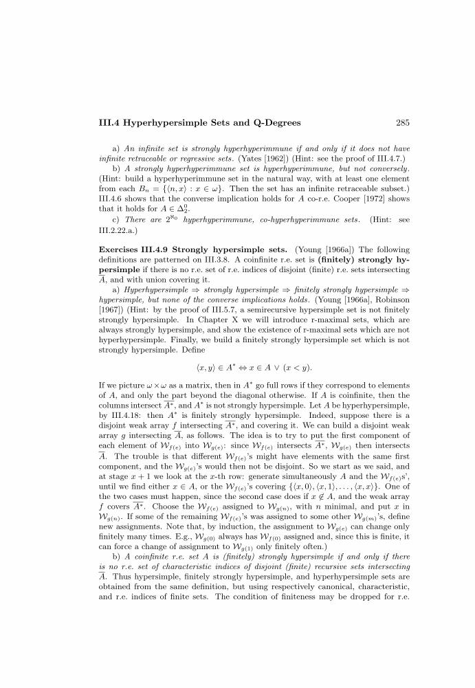
III.4 Hyperhypersimple Sets and Q-Degrees 285
a) An infinite set is strongly hyperhyperimmune if and only if it does not haveinfinite retraceable or regressive sets. (Yates [1962]) (Hint: see the proof of III.4.7.)
b) A strongly hyperhyperimmune set is hyperhyperimmune, but not conversely .(Hint: build a hyperhyperimmune set in the natural way, with at least one elementfrom each Bn = 〈n, x〉 : x ∈ ω. Then the set has an infinite retraceable subset.)III.4.6 shows that the converse implication holds for A co-r.e. Cooper [1972] showsthat it holds for A ∈ ∆0
2.
c) There are 2ℵ0 hyperhyperimmune, co-hyperhyperimmune sets. (Hint: see
III.2.22.a.)
Exercises III.4.9 Strongly hypersimple sets. (Young [1966a]) The followingdefinitions are patterned on III.3.8. A coinfinite r.e. set is (finitely) strongly hy-persimple if there is no r.e. set of r.e. indices of disjoint (finite) r.e. sets intersectingA, and with union covering it.
a) Hyperhypersimple ⇒ strongly hypersimple ⇒ finitely strongly hypersimple ⇒hypersimple, but none of the converse implications holds. (Young [1966a], Robinson[1967]) (Hint: by the proof of III.5.7, a semirecursive hypersimple set is not finitelystrongly hypersimple. In Chapter X we will introduce r-maximal sets, which arealways strongly hypersimple, and show the existence of r-maximal sets which are nothyperhypersimple. Finally, we build a finitely strongly hypersimple set which is notstrongly hypersimple. Define
〈x, y〉 ∈ A∗ ⇔ x ∈ A ∨ (x < y).
If we picture ω×ω as a matrix, then in A∗ go full rows if they correspond to elementsof A, and only the part beyond the diagonal otherwise. If A is coinfinite, then thecolumns intersectA∗, andA∗ is not strongly hypersimple. LetA be hyperhypersimple,by III.4.18: then A∗ is finitely strongly hypersimple. Indeed, suppose there is adisjoint weak array f intersecting A∗, and covering it. We can build a disjoint weakarray g intersecting A, as follows. The idea is to try to put the first component ofeach element of Wf(e) into Wg(e): since Wf(e) intersects A∗, Wg(e) then intersects
A. The trouble is that different Wf(e)’s might have elements with the same firstcomponent, and the Wg(e)’s would then not be disjoint. So we start as we said, andat stage x + 1 we look at the x-th row: generate simultaneously A and the Wf(e)s’,until we find either x ∈ A, or the Wf(e)’s covering 〈x, 0〉, 〈x, 1〉, . . . , 〈x, x〉. One ofthe two cases must happen, since the second case does if x 6∈ A, and the weak arrayf covers A∗. Choose the Wf(e) assigned to Wg(n), with n minimal, and put x inWg(n). If some of the remaining Wf(e)’s was assigned to some other Wg(m)’s, definenew assignments. Note that, by induction, the assignment to Wg(e) can change onlyfinitely many times. E.g., Wg(0) always has Wf(0) assigned and, since this is finite, itcan force a change of assignment to Wg(1) only finitely often.)
b) A coinfinite r.e. set A is (finitely) strongly hypersimple if and only if thereis no r.e. set of characteristic indices of disjoint (finite) recursive sets intersectingA. Thus hypersimple, finitely strongly hypersimple, and hyperhypersimple sets areobtained from the same definition, but using respectively canonical, characteristic,and r.e. indices of finite sets. The condition of finiteness may be dropped for r.e.
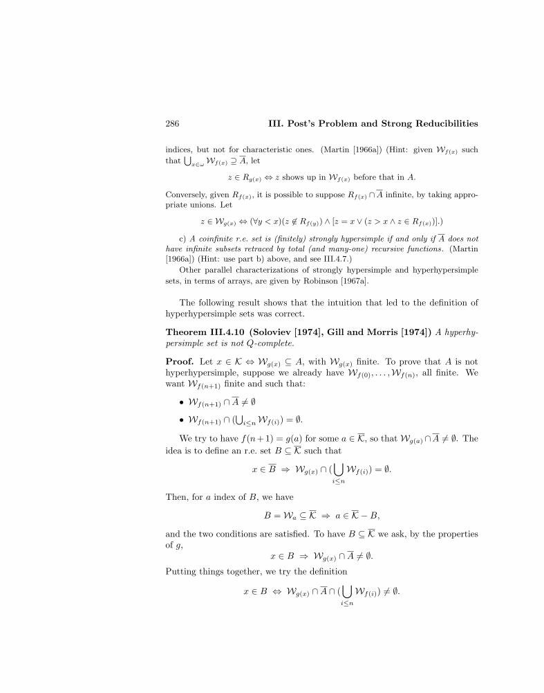
286 III. Post’s Problem and Strong Reducibilities
indices, but not for characteristic ones. (Martin [1966a]) (Hint: given Wf(x) such
that⋃x∈ωWf(x) ⊇ A, let
z ∈ Rg(x) ⇔ z shows up in Wf(x) before that in A.
Conversely, given Rf(x), it is possible to suppose Rf(x) ∩A infinite, by taking appro-priate unions. Let
z ∈ Wg(x) ⇔ (∀y < x)(z 6∈ Rf(y)) ∧ [z = x ∨ (z > x ∧ z ∈ Rf(x))].)
c) A coinfinite r.e. set is (finitely) strongly hypersimple if and only if A does nothave infinite subsets retraced by total (and many-one) recursive functions. (Martin[1966a]) (Hint: use part b) above, and see III.4.7.)
Other parallel characterizations of strongly hypersimple and hyperhypersimple
sets, in terms of arrays, are given by Robinson [1967a].
The following result shows that the intuition that led to the definition ofhyperhypersimple sets was correct.
Theorem III.4.10 (Soloviev [1974], Gill and Morris [1974]) A hyperhy-persimple set is not Q-complete.
Proof. Let x ∈ K ⇔ Wg(x) ⊆ A, with Wg(x) finite. To prove that A is nothyperhypersimple, suppose we already have Wf(0), . . . ,Wf(n), all finite. Wewant Wf(n+1) finite and such that:
• Wf(n+1) ∩A 6= ∅
• Wf(n+1) ∩ (⋃i≤nWf(i)) = ∅.
We try to have f(n+ 1) = g(a) for some a ∈ K, so that Wg(a) ∩A 6= ∅. Theidea is to define an r.e. set B ⊆ K such that
x ∈ B ⇒ Wg(x) ∩ (⋃i≤n
Wf(i)) = ∅.
Then, for a index of B, we have
B = Wa ⊆ K ⇒ a ∈ K −B,
and the two conditions are satisfied. To have B ⊆ K we ask, by the propertiesof g,
x ∈ B ⇒ Wg(x) ∩A 6= ∅.Putting things together, we try the definition
x ∈ B ⇔ Wg(x) ∩A ∩ (⋃i≤n
Wf(i)) 6= ∅.
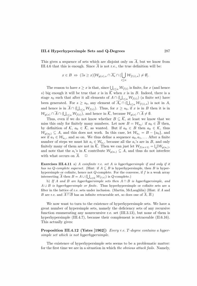
III.4 Hyperhypersimple Sets and Q-Degrees 287
This gives a sequence of sets which are disjoint only on A, but we know fromIII.4.6 that this is enough. Since A is not r.e., the true definition will be:
x ∈ B ⇔ (∃s ≥ x)[Wg(x),s ∩As ∩ (⋃i≤n
Wf(i),s) 6= ∅].
The reason to have s ≥ x is that, since⋃i≤nWf(i) is finite, for x (and hence
s) big enough it will be true that x is in K when x is in B. Indeed, there is astage s0 such that after it all elements of A ∩ (
⋃i≤nWf(i)) (a finite set) have
been generated. For s ≥ s0, any element of As ∩ (⋃i≤nWf(i),s) is not in A,
and hence is in A ∩ (⋃i≤nWf(i)). Thus, for x ≥ s0, if x is in B then it is in
Wg(x) ∩A ∩ (⋃i≤nWf(i)), and hence in K, because Wg(x) ∩A 6= ∅.
Thus, even if we do not know whether B ⊆ K, at least we know that wemiss this only for finitely many numbers. Let now B = Wa0 : if a0 ∈ B then,by definition of K, a0 ∈ K, as wanted. But if a0 ∈ B then a0 ∈ K, thusWg(a0) ⊆ A, and this does not work. In this case, let Wa1 = B − a0, andsee if a1 ∈ Wa1 , and so on. We thus define a sequence a0, a1, . . . After a finitenumber of steps we must hit ai ∈ Wai , because all the ai’s are in B, and onlyfinitely many of them are not in K. Then we can just let Wf(n+1) =
⋃Wg(ai),
and note that the ai’s in K contribute Wg(ai) ⊆ A, and thus do not interferewith what occurs on A. 2
Exercises III.4.11 a) A coinfinite r.e. set A is hyperhypersimple if and only if ithas no Q-complete superset . (Hint: if A ⊆ B is hyperhypersimple, then B is hyper-hypersimple or cofinite, hence not Q-complete. For the converse, if f is a weak arrayintersecting A then B = A ∪ (
⋃x∈KWf(x)) is Q-complete.)
b) If A and B are hyperhypersimple sets then A ∩ B is hyperhypersimple, and
A ∪ B is hyperhypersimple or finite. Thus hyperhypersimple or cofinite sets are a
filter in the lattice of r.e. sets under inclusion. (Martin, McLaughlin) (Hint: if A and
B are r.e. and A ∩B has an infinite retraceable set, so does one of A, B.)
We now want to turn to the existence of hyperhypersimple sets. We have agreat number of hypersimple sets, namely the deficiency sets of any recursivefunction enumerating any nonrecursive r.e. set (III.3.13), but none of them ishyperhypersimple (III.4.7), because their complement is retraceable (II.6.16).This actually gives:
Proposition III.4.12 (Yates [1962]) Every r.e. T -degree contains a hyper-simple set which is not hyperhypersimple.
The existence of hyperhypersimple sets seems to be a problematic matter:for the first time we are in a situation in which the obvious attack fails. Namely,
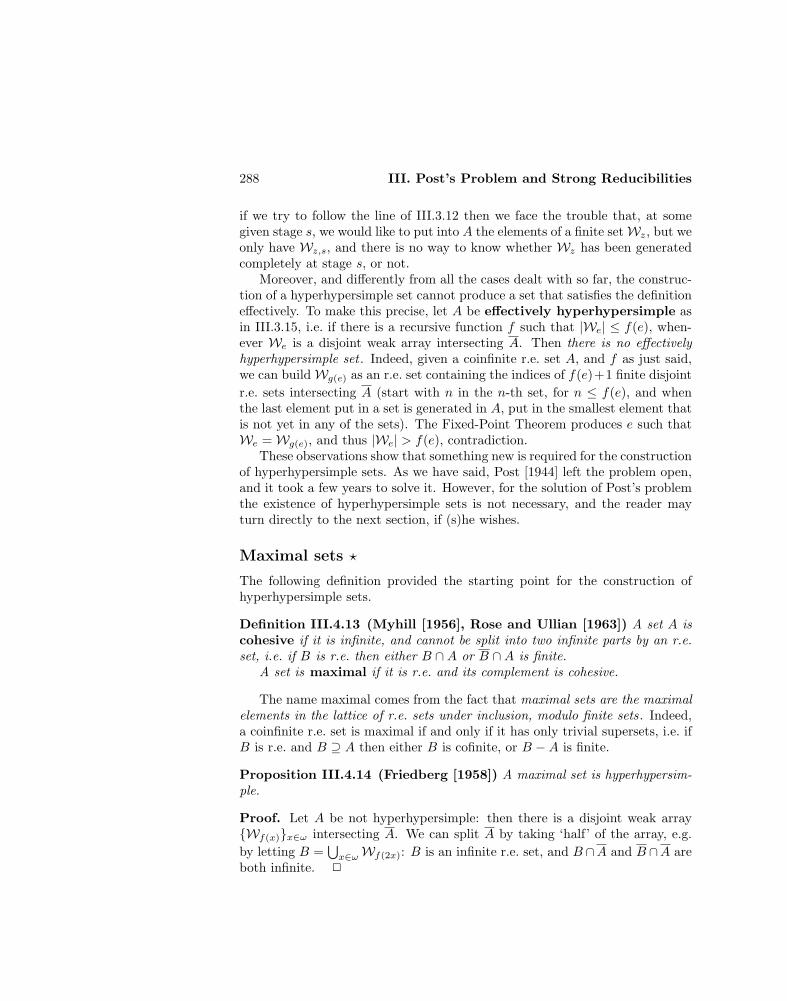
288 III. Post’s Problem and Strong Reducibilities
if we try to follow the line of III.3.12 then we face the trouble that, at somegiven stage s, we would like to put into A the elements of a finite set Wz, but weonly have Wz,s, and there is no way to know whether Wz has been generatedcompletely at stage s, or not.
Moreover, and differently from all the cases dealt with so far, the construc-tion of a hyperhypersimple set cannot produce a set that satisfies the definitioneffectively. To make this precise, let A be effectively hyperhypersimple asin III.3.15, i.e. if there is a recursive function f such that |We| ≤ f(e), when-ever We is a disjoint weak array intersecting A. Then there is no effectivelyhyperhypersimple set . Indeed, given a coinfinite r.e. set A, and f as just said,we can build Wg(e) as an r.e. set containing the indices of f(e)+1 finite disjointr.e. sets intersecting A (start with n in the n-th set, for n ≤ f(e), and whenthe last element put in a set is generated in A, put in the smallest element thatis not yet in any of the sets). The Fixed-Point Theorem produces e such thatWe = Wg(e), and thus |We| > f(e), contradiction.
These observations show that something new is required for the constructionof hyperhypersimple sets. As we have said, Post [1944] left the problem open,and it took a few years to solve it. However, for the solution of Post’s problemthe existence of hyperhypersimple sets is not necessary, and the reader mayturn directly to the next section, if (s)he wishes.
Maximal sets ?
The following definition provided the starting point for the construction ofhyperhypersimple sets.
Definition III.4.13 (Myhill [1956], Rose and Ullian [1963]) A set A iscohesive if it is infinite, and cannot be split into two infinite parts by an r.e.set, i.e. if B is r.e. then either B ∩A or B ∩A is finite.
A set is maximal if it is r.e. and its complement is cohesive.
The name maximal comes from the fact that maximal sets are the maximalelements in the lattice of r.e. sets under inclusion, modulo finite sets. Indeed,a coinfinite r.e. set is maximal if and only if it has only trivial supersets, i.e. ifB is r.e. and B ⊇ A then either B is cofinite, or B −A is finite.
Proposition III.4.14 (Friedberg [1958]) A maximal set is hyperhypersim-ple.
Proof. Let A be not hyperhypersimple: then there is a disjoint weak arrayWf(x)x∈ω intersecting A. We can split A by taking ‘half’ of the array, e.g.by letting B =
⋃x∈ωWf(2x): B is an infinite r.e. set, and B ∩A and B ∩A are
both infinite. 2
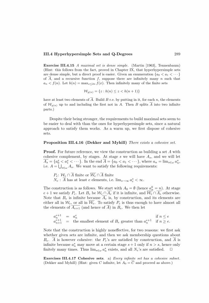
III.4 Hyperhypersimple Sets and Q-Degrees 289
Exercise III.4.15 A maximal set is dense simple. (Martin [1963], Tennenbaum)(Hint: this follows from the fact, proved in Chapter IX, that hyperhypersimple setsare dense simple, but a direct proof is easier. Given an enumeration a0 < a1 < · · · of A, and a recursive function f , suppose there are infinitely many n such thatan < f(n). Let h(n) = maxx≤2n f(x). Then infinitely many of the finite sets
Wg(n) = z : h(n) ≤ z < h(n+ 1)
have at least two elements of A. Build B r.e. by putting in it, for each n, the elements
of Wg(n) up to and including the first not in A. Then B splits A into two infinite
parts.)
Despite their being stronger, the requirements to build maximal sets seem tobe easier to deal with than the ones for hyperhypersimple sets, since a naturalapproach to satisfy them works. As a warm up, we first dispose of cohesivesets.
Proposition III.4.16 (Dekker and Myhill) There exists a cohesive set.
Proof. For future reference, we view the construction as building a set A withcohesive complement, by stages. At stage s we will have As, and we will letAs = as0 < as1 < · · · . In the end A = a0 < a1 < · · · , where an = lims∈ω a
sn,
i.e. A =⋃s∈ω As. We want to satisfy the following requirements:
Pe: We ∩A finite or We ∩A finiteNe : A has at least e elements, i.e. lims→∞ ase <∞.
The construction is as follows. We start with A0 = ∅ (hence a0n = n). At stage
e+ 1 we satisfy Pe. Let Be be We ∩Ae if it is infinite, and We ∩Ae otherwise.Note that Be is infinite because Ae is, by construction, and its elements areeither all in We, or all in We. To satisfy Pe is thus enough to have almost allthe elements of Ae+1 (and hence of A) in Be. We then let
ae+1n = aen if n ≤ eae+1n+1 = the smallest element of Be greater than ae+1
n if n ≥ e.
Note that the construction is highly noneffective, for two reasons: we first askwhether given sets are infinite, and then we ask membership questions aboutBe. A is however cohesive: the Pe’s are satisfied by construction, and A isinfinite because asn may move at a certain stage s+ 1 only if n > s, hence onlyfinitely many times. Thus lims∈ω a
sn exists, and all Ne’s are satisfied. 2
Exercises III.4.17 Cohesive sets. a) Every infinite set has a cohesive subset .(Dekker and Myhill) (Hint: given C infinite, let A0 = C and proceed as above.)
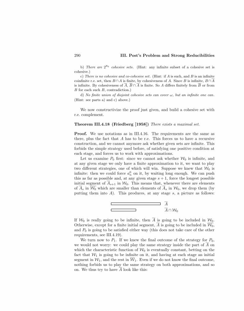
290 III. Post’s Problem and Strong Reducibilities
b) There are 2ℵ0 cohesive sets. (Hint: any infinite subset of a cohesive set iscohesive.)
c) There is no cohesive and co-cohesive set . (Hint: if A is such, and B is an infinitecoinfinite r.e. set, then B∩A is finite, by cohesiveness of A. Since B is infinite, B∩Ais infinite. By cohesiveness of A, B ∩A is finite. So A differs finitely from B or fromB for each such B, contradiction.)
d) No finite union of disjoint cohesive sets can cover ω, but an infinite one can.
(Hint: see parts a) and c) above.)
We now constructivize the proof just given, and build a cohesive set withr.e. complement.
Theorem III.4.18 (Friedberg [1958]) There exists a maximal set.
Proof. We use notations as in III.4.16. The requirements are the same asthere, plus the fact that A has to be r.e. This forces us to have a recursiveconstruction, and we cannot anymore ask whether given sets are infinite. Thisforbids the simple strategy used before, of satisfying one positive condition ateach stage, and forces us to work with approximations.
Let us examine P0 first: since we cannot ask whether W0 is infinite, andat any given stage we only have a finite approximation to it, we want to playtwo different strategies, one of which will win. Suppose we knew that W0 isinfinite: then we could force a0
n on it, by waiting long enough. We can pushthis as far as possible and, at any given stage s+ 1, force the longest possibleinitial segment of As+1 in W0. This means that, whenever there are elementsof As in W0 which are smaller than elements of As in W0, we drop them (byputting them into A). This produces, at any stage s, a picture as follows:
A
A ∩W0
If W0 is really going to be infinite, then A is going to be included in W0.Otherwise, except for a finite initial segment, A is going to be included in W0,and P0 is going to be satisfied either way (this does not take care of the otherrequirements, see III.4.19).
We turn now to P1. If we knew the final outcome of the strategy for P0,we would not worry: we could play the same strategy inside the part of A onwhich the characteristic function of W0 is eventually constant, betting on thefact that W1 is going to be infinite on it, and having at each stage an initialsegment in W1, and the rest in W1. Even if we do not know the final outcome,nothing forbids us to play the same strategy on both approximations, and soon. We thus try to have A look like this:
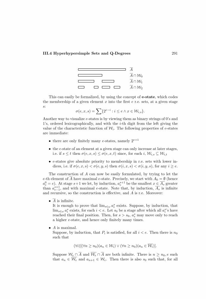
III.4 Hyperhypersimple Sets and Q-Degrees 291
A
A ∩W0
A ∩W1
A ∩W2
This can easily be formalized, by using the concept of e-state, which codesthe membership of a given element x into the first e r.e. sets, at a given stages:
σ(e, x, s) =∑
2e−i : i ≤ e ∧ x ∈ Wi,s.
Another way to visualize e-states is by viewing them as binary strings of 0’s and1’s, ordered lexicographically, and with the i-th digit from the left giving thevalue of the characteristic function of Wi. The following properties of e-statesare immediate:
• there are only finitely many e-states, namely 2e+1
• the e-state of an element at a given stage can only increase at later stages,i.e. if s ≤ t then σ(e, x, s) ≤ σ(e, x, t) since, for each i, Wi,s ⊆ Wi,t
• e-states give absolute priority to membership in r.e. sets with lower in-dices, i.e. if σ(e, x, s) < σ(e, y, s) then σ(i, x, s) < σ(i, y, s), for any i ≥ e.
The construction of A can now be easily formulated, by trying to let thee-th element of A have maximal e-state. Precisely, we start with A0 = ∅ (hencea0e = e). At stage s+1 we let, by induction, as+1
e be the smallest x ∈ As greaterthan as+1
e−1, and with maximal e-state. Note that, by induction, As is infiniteand recursive, so the construction is effective, and A is r.e. Moreover:
• A is infinite.It is enough to prove that lims∈ω a
se exists. Suppose, by induction, that
lims∈ω asi exists, for each i < e. Let s0 be a stage after which all asi ’s have
reached their final position. Then, for s > s0, ase may move only to reacha higher e-state, and hence only finitely many times.
• A is maximal.Suppose, by induction, that Pi is satisfied, for all i < e. Then there is n0
such that
(∀i)[(∀n ≥ n0)(an ∈ Wi) ∨ (∀n ≥ n0)(an ∈ Wi)].
Suppose We ∩ A and We ∩ A are both infinite. There is n ≥ n0, e suchthat an ∈ We and an+1 ∈ We. Then there is also s0 such that, for all
292 III. Post’s Problem and Strong Reducibilities
s ≥ s0,(∀x ≤ n+ 1)(asx = ax)(∀i < e)(an ∈ Wi ⇔ an ∈ Wi,s)(∀i ≤ e)(an+1 ∈ Wi ⇔ an+1 ∈ Wi,s).
Then, by definition of e-state,
σ(e, asn, s) < σ(e, asn+1, s)
and hence, since n ≥ e,
σ(n, asn, s) < σ(n, asn+1, s).
By construction we then have that as+1n should be the smallest element of
As greater than asn−1 = an−1 and with maximal n-state, hence it cannotbe an, contradiction. 2
Exercise III.4.19 There is an acceptable system of indices Wee∈ω of the r.e. sets
such that W0 is infinite, but the complement of the maximal set constructed above
has no element in W0. (Hint: define Wx+1 = Wx, and generate elements in W0 only
after they have already been generated in A.)
The e-state method used in the proof above is a kind of priority method,with the usual order of priority
P0 > N0 > P1 > N1 > . . .
The basic difference between the constructions of maximal and simple (or hy-persimple) sets is that the positive requirements Pe are infinitary , and we cannothope to satisfy them with a finite action. Actually, since they only allow forfinitely many exceptions, each requirement has to be considered cofinitely manytimes, and at any given stage we have to consider many positive requirementsall together. But the requirements have different priorities, and e-states area device to assign priorities not to single requirements, but to groups of them.E.g., the order of priorities assigned by 2-states is
(P0, P1, P2) ≥ (P0, P1) ≥ (P0, P2) ≥ (P0) ≥ (P1, P2) ≥ (P1) ≥ (P2).
We might say that locally this is a finite injury argument, since every el-ement of A moves at most finitely many times, but globally it is an infiniteinjury argument, since a positive requirement may be injured infinitely often,each time for different elements of A.
Exercises III.4.20 a) Maximal sets are not closed under intersection. (Yates [1962])(Hint: take A maximal, and let x ∈ B ⇔ x+ 1 ∈ A.)

III.4 Hyperhypersimple Sets and Q-Degrees 293
b) There are hyperhypersimple set which are not maximal . (Hint: the hyperhy-
persimple sets are closed under intersection.)
Maximal sets have thinnest possible complement. The existence of maxi-mal T -complete sets would shows that a notion of thin complement alone isnot sufficient to solve Post’s problem. In fact, the maximal set just built isT -complete, as we now prove, as usual, by showing that it is maximal in aneffective way.
Definition III.4.21 (Lachlan [1968]) A is effectively maximal if it is acoinfinite r.e. set, and there is a recursive function g such that, for every e, thesequence of 0’s and 1’s consisting of the values of the characteristic function ofWe on the elements of A in increasing order has at most g(e) alternations.
Note that having finitely many alternations simply means that one ofWe∩Aand We ∩A is finite.
Proposition III.4.22 (Lachlan [1968]) Every effectively maximal set isT -complete.
Proof. Let g witness that A is effectively maximal, and define f ≤T A suchthat
Wf(e) = a finite set with g(e) + 1 alternations on A.
This is possible because A is infinite, e.g.
Wf(e) = a2i : i ≤ g(e) + 1.
Then f has no fixed-points and, by the criterion for T -completeness III.1.5, Ais T -complete. 2
Corollary III.4.23 (Yates [1965]) There exists a T -complete maximal set.
Proof. The maximal set built in III.4.18 is effectively maximal, since We canhave at most g(e) = 2e+1 alternations on A. 2
Exercises III.4.24 a) For no coinfinite r.e. set A there is a recursive function gsuch that
We ∩A infinite ⇒ |We ∩A| ≤ g(e).
Similarly forWe ∩A infinite ⇒ |We ∩A| ≤ g(e).
Thus these natural candidates for effective maximality fail. (Lachlan [1968]) (Hint:for the second property, put in Wh(e) the first g(e)+1 elements of A, by starting with0, . . . , g(e) and, each time that one element goes into A, adding the first element

294 III. Post’s Problem and Strong Reducibilities
not yet in Wh(e), and not yet generated in A. By the Fixed-Point Theorem there is
e such that We = Wh(e). Thus We ∩A is infinite, but |We ∩A| = g(e) + 1.)
b) There is a maximal, effectively simple set . (Cohen and Jockusch [1975]) (Hint:modify the construction of a maximal set given above by inserting steps to make Asimple, as in the second proof of III.2.11. Note that each asn may move more timesthan it did for maximality alone, but still only finitely often.)
c) A maximal set is not strongly effectively simple. (Cohen and Jockusch [1975])(Hint: by III.4.15 a maximal set is dense, and by III.3.9 is not strongly effectivelysimple. See III.6.21 for a different proof.)
d) A strongly effective simple set is not contained in maximal sets. Thus Post’s
simple set is not contained in maximal sets. (Cohen and Jockusch [1975]) (Hint: a
coinfinite r.e. superset of a strongly effectively simple set is still strongly effectively
simple.)
III.5 A Solution to Post’s Problem
Post concluded his paper [1944] by saying:
we are left completely on the fence as to whether there exists arecursively enumerable set of positive integers of absolutely lowerdegree of unsolvability than the complete set K, or whether, indeed,all recursively enumerable sets of positive integers with recursivelyunsolvable decision problems are absolutely of the same degree ofunsolvability. On the other hand, if this question can be answered,that answer would seem to be not far off, if not in time, then in thenumber of special results to be gotten on the way.
This section can be seen as the missing conclusion to Post’s paper, and showsthat he was indeed right, regarding the number of special results needed tosolve his problem.
Semirecursive sets
We know that hyperhypersimple sets are not Q-complete. We are then lookingfor a notion that, together with T -completeness, would imply Q-completeness.By coupling it with hyperhypersimplicity we would then have a notion implyingT -incompleteness, and Post’s problem would be solved.
Since the difference between Q-reducibility and T -reducibility is that wequery the oracle on single elements in the first case, and on finite sets in thesecond, we need a notion that would reduce a question of inclusion of a finiteset to the question of membership of a single element.

III.5 A Solution to Post’s Problem 295
Definition III.5.1 (Jockusch [1968a]) A set A is semirecursive if thereis a recursive function f of two variables such that
1. f(x, y) = x or f(x, y) = y
2. x ∈ A ∨ y ∈ A⇒ f(x, y) ∈ A.
Clearly a recursive set is semirecursive, since we can simply decide whetherone of x and y is in the set. Also, the complement of a semirecursive set issemirecursive: if f witnesses the semirecursiveness of A, then the function thatalways chooses, between x and y, the element not chosen by f , witnesses thesemirecursiveness of A.
The next result is not unexpected, and is actually the reason why we intro-duced the notion of semirecursiveness.
Proposition III.5.2 (Marchenkov [1976]) If an r.e. set A is semirecursiveand T -complete, then it is also Q-complete.
Proof. We only have to show how to reduce finite questions of the formDu ⊆ Ato single questions g(u) ∈ A, for some recursive g. Let f be as in the definitionIII.5.1. Given Du = x1, . . . , xn, let
y1 = x1
yi+1 = f(yi, xi+1) (i < n)g(u) = yn.
Then we obviously have Du ⊆ A⇔ g(u) ∈ A, because if one element of Du isin A, then so is g(u). 2
Exercises III.5.3 a) A semirecursive simple set is hypersimple. (Jockusch [1968a])(Hint: if A is semirecursive so is A, and thus a finite set intersecting A effectivelyproduces an element of A.)
b) A semirecursive set is not p-complete. (Jockusch [1968a]) (Hint: a semirecur-
sive p-complete set would be m-complete, and thus every r.e. set would be semirecur-
sive, contradicting the existence of simple, nonhypersimple sets.)
We are obviously interested in knowing which sets are semirecursive. Sincethe definition of semirecursive sets might appear somewhat ad hoc, we firstgive an interesting alternative characterization.
Proposition III.5.4 (Appel, McLaughlin) A set is semirecursive if andonly if it is a cut of a recursive linear ordering of ω.

296 III. Post’s Problem and Strong Reducibilities
Proof. Let A be semirecursive via f . We define, by induction, a recursivelinear ordering ≺ such that
x ≺ y ∧ y ∈ A⇒ x ∈ A.
Let x0 ≺ x1 ≺ . . . ≺ xn be the ordering of the numbers up to n. We want toextend it to n+ 1. Three cases are possible:
1. f(n+ 1, x0) = n+ 1If x0 ∈ A then n + 1 ∈ A, by the properties of f , and we can then letn+ 1 ≺ x0.
2. the first case fails, and f(n+ 1, xn) = xnSimilarly, if n+ 1 ∈ A then xn ∈ A, and we let xn ≺ n+ 1.
3. the first two cases failThen f(n + 1, x0) = x0 and f(n + 1, xn) = n + 1. Then there is i suchthat
f(n+ 1, xi) = xi ∧ f(n+ 1, xi+1) = n+ 1,
and thusxi+1 ∈ A⇒ n+ 1 ∈ A⇒ xi ∈ A.
Then we can let xi ≺ n+ 1 ≺ xi+1.
Let now A be the lower cut of a recursive linear ordering ≺. If
f(x, y) = least element of x, y w.r.t. ≺
then f(x, y) = x or f(x, y) = y by definition, and if one of x and y is in Athen so is f(x, y), because A is closed downward w.r.t. ≺. Thus f satisfies theconditions of III.5.1, and A is semirecursive. 2
Exercises III.5.5 a) Every tt-degree contains a semirecursive set . (Jockusch[1968a]) (Hint: let A be infinite and coinfinite, and define r =
∑n∈A 2−n. For
any x, let rx =∑
n∈Dx2−n. Then x ≺ y ⇔ rx < ry is recursive. Let B be the lower
cut determined by r. A ≤T B because if Dx = (A ∩ 0, . . . , n − 1) ∪ n then, byinduction,
n ∈ A⇔ Dx ⊆ A⇔ rx < r ⇔ x ∈ B.And B ≤T A because x ∈ B, i.e. rx < r, if and only if there is a finite set Dycontained in 0, . . . ,maxDx, such that rx ≤ ry and Dy ⊆ A.)
b) There are 2ℵ0 semirecursive sets. (Martin, McLaughlin)
We turn now to the investigation of which sets, among the ones introducedso far for the solution of Post’s problem, are semirecursive.
III.5 A Solution to Post’s Problem 297
Proposition III.5.6 (Jockusch [1968a]) Every coregressive r.e. set is semi-recursive.
Proof. Let A be an r.e. set, coregressive via ϕ. Given x and y, note thateither one of x and y is in A, or they are both in A, and thus one of themfollows the other in the given enumeration of A, and it is then sent over it byϕ (meaning that some iteration of ϕ on the former produces the latter). Todefine f generate simultaneously A, ϕ(n)(x)n∈ω and ϕ(n)(y)n∈ω, and let
f(x, y) =x if x ∈ A or y ∈ ϕ(n)(x)n∈ωy if y ∈ A or x ∈ ϕ(n)(y)n∈ω.
Suppose f(x, y) ∈ A: then e.g. f(x, y) = y and x ∈ ϕ(n)(y)n∈ω, so y ∈ A andx ∈ A, and A is semirecursive. 2
The result implies, by II.6.16 and III.3.13, that many hypersimple sets aresemirecursive. Actually, every r.e. T -degree contains a semirecursive hypersim-ple set (in particular there are hypersimple sets which are Q-complete, namelyany T -complete semirecursive hypersimple set). But the result we were reallylooking for escapes us.
Proposition III.5.7 (Martin) No hyperhypersimple set can be semirecur-sive.
Proof. We know (III.4.7) that the complement of a hyperhypersimple set can-not contain infinite retraceable sets. Since the complement of a set is semire-cursive when the set is, it is enough to show that an infinite semirecursive setcontains an infinite retraceable set. Let A be infinite and semirecursive. Wemay suppose A immune, otherwise it has infinite recursive, hence retraceable,subsets. Let ≺ be a recursive linear ordering of which A is a lower cut: then A iswell-ordered by ≺ with order type ω, because for any x ∈ A the set y : y ≺ xis a recursive subset of A, hence finite by immunity. Let
f(x) =n if x is the n-th element of A w.r.t. ≺∞ if x 6∈ A.
Consider the elements corresponding to nondeficiency stages of f :
x ∈ B ⇔ (∀y > x)(f(y) > f(x))⇔ (∀y)(y > x⇒ y x).
B is a subset of A because, given x ∈ B, there is y ∈ A greater than it(since A is infinite): then y x, and x ∈ A because A is closed downward
298 III. Post’s Problem and Strong Reducibilities
w.r.t. ≺. And B is infinite, as usual for nondeficiency stages (note that f isone-one on A).
To show that B is retraceable, we cannot appeal directly to the fact thatso are nondeficiency sets, because f is not recursive, but an argument similarto that of II.6.16 can be reproduced directly. Given x ∈ B, we want to get aneffective procedure to find the greatest element of B smaller than x. Since fory > x we have y x, we only have to check numbers below x. In other words,for z < x,
z ∈ B ⇔ (∀y)(z < y ⇒ z ≺ y)⇔ (∀y)(z < y ≤ x⇒ z ≺ y).
Thus it is enough to define g(x) as the biggest z < x such that
(∀y)(z < y ≤ x⇒ z ≺ y)
if b0 ≺ x (where b0 is the least element of B), and x otherwise. 2
Actually, the proof shows that no finitely strongly hypersimple set is semire-cursive, because the retracing function defined above is total and many-one (seeIII.4.9).
Exercises III.5.8 Hereditary sets. A set A is hereditary if there is a recursivefunction f such that x ∈ A ∧ y ∈ A⇔ f(x, y) ∈ A.
a) A set A is hereditary if and only if there is a recursive function g such thatDx ⊆ A⇔ g(x) ∈ A. (Lavrov [1968])
b) For any set A, the set Aω = x : Dx ⊆ A is hereditary . (Degtev [1972])c) Semirecursive ⇒ hereditary, but not conversely . (Degtev [1972]) (Hint: K is
not semirecursive, see III.5.3.b, but is hereditary because it is recursively isomorphicto Kω, see III.7.14.)
Degtev [1972] has shown that some of the properties of semirecursive sets, e.g.
III.5.7, hold for hereditary sets as well.
Exercises III.5.9 Verbose and terse sets. (Beigel, Gasarch, Gill, and Owings[198?]) We say that we can do ‘n for m’ on a set A if n questions of membership to Acan be answered by a recursive procedure that asks at most m question to the oracleA. A set A is verbose if, for every n, we can do 2n − 1 for n on it, and it is terse ifwe cannot do n for n− 1.
a) If we can do 2n for n on A, then A is recursive. Thus the definition of verbosesets is optimal. (Hint: we show the proof for n = 1. Suppose we can do 2 for 1on A: given two elements x and y, we can compute A(x) and A(y) by a recursiveprocedure that asks only one question to the oracle A. Since the answer to the querycan be only 0 or 1, there are two partial recursive functions ϕ0 and ϕ1, respectivelyusing the answer 0 and 1, one of which gives the correct values for A(x) and A(y).
III.5 A Solution to Post’s Problem 299
To compute A recursively, consider two cases. If for every x there is y such that ϕ0
and ϕ1 compute the same value of A(x), then this must be the right value of A(x),and to compute it it is enough to look for such a y. If there is x such that, for everyy, ϕ0 and ϕ1 give different answers for A(x), then fix x, and consider the right valueA(x). For every y, the right value of A(y) is computed by the one, between ϕ0 andϕ1, that computes the right value of A(x).) Note that A plays no role as an oracle,and thus A would be recursive even if we could answer 2n membership questions onA by a recursive procedure asking n questions to an oracle B.
b) K is verbose. (Hint: we show how to do 3 for 2. To know which of x1, x2, x3
are in K, first ask if at least two are. This is an r.e. question, hence K can answerit. If the answer is yes, ask if all three are, otherwise ask if at least one is. Thewhole procedure requires only two questions, and determines how many of the threeelements are in K. To know exactly which ones are, generate K until that manyappear.) Since verbose sets are closed are under m-equivalence, every m-complete setis verbose.
c) A semirecursive set is verbose. (Hint: let A be the upper cut of a recursivelinear ordering, by III.5.4. To determine which of 2n−1 elements are in A, first orderthem according to the linear ordering. To know which are is A and which are not, itis enough to find the first element which is in A, and this can be done by a binarysearch, thus requiring only n steps and n questions to the oracle A.)
d) (R.e.) verbose sets exist in every (r.e.) T -degree. (Hint: by III.5.5.a andIII.5.6, because verbose sets are closed under complements.)
e) Every nonzero T -degree contains terse sets. (Hint: given a semirecursive,
nonrecursive set A, notice that, given elements x1, . . . , xn, if we know how many are
in A, then we can determine exactly which ones: order them according to the ordering
w.r.t. which A is an upper cut, and count from the biggest one. Given 2n−1 elements,
less than 2n can be in A, and thus their number can be written, in binary, with at
most n digits. Define a set B, by putting 〈x1, . . . , x2n−1, i〉 in it if and only if the i-th
digit in the binary representation of |A∩x1, . . . , x2n−1| is 1. Clearly A ≡T B. And
2n− 1 questions on A can be reduced to n questions on B. If we could do n for n− 1
on B then we could do 2n − 1 for n− 1 on A, with oracle B, and hence 2n for n with
oracle B ⊕A, contradicting part a).)
η-hyperhypersimple sets
Despite the fact that hyperhypersimple sets are not semirecursive, we are notwilling to give up and waste all the work done so far, especially so after hav-ing been so close to a solution of Post’s problem. The idea is to look for aweakening of the notion of hyperhypersimplicity that is still incompatible withQ-completeness, but is compatible with semirecursiveness. We simply general-ize the notion of number, and substitute it with the notion of equivalence classw.r.t. an r.e. equivalence relation.
300 III. Post’s Problem and Strong Reducibilities
Definition III.5.10 (Malcev [1965], Ershov [1971]) An equivalence rela-tion η is called positive if R(x, y) ⇔ xηy is r.e.
Exercise III.5.11 The class of positive equivalence relations is a sublattice of the
complete lattice of all the equivalence relations on ω under inclusion. (Ershov [1971])
(Hint: the smallest element is the equality relation, the greatest one the trivial equiv-
alence relation. The g.l.b. is the set-theoretical intersection, the l.u.b. the smallest
equivalence relation including the given ones.)
Definition III.5.12 A set A is η-closed if it consists of equivalence classesw.r.t. η, i.e. x ∈ A ∧ xηy ⇒ y ∈ A.
The η-closure [A]η of a set A is the smallest η-closed set containing it.
Exercises III.5.13 (Ershov [1971]) a) If A is r.e. then
xηAy ⇔ (x ∈ A ∧ y ∈ A) ∨ x = y
is a positive equivalence relation, with (if A has more than one element) A as the onlynontrivial equivalence class. A set is ηA-closed if and only if it either contains A, oris disjoint from it .
b) If ϕ is a partial recursive function, then
xηϕy ⇔ (ϕ(x) ' ϕ(y)↓) ∨ x = y
is positive. A set A is ηϕ-closed if and only if ϕ−1(ϕ(A)) ⊆ A.c) If ϕ is a partial recursive function, then
xηiϕy ⇔ ∃m∃n(ϕ(m)(x) ' ϕ(n)(y)↓)
is positive. (Hint: recall that, by definition, ϕ(0)(x) ' x.)
d) η is a positive equivalence relation if and only if, for some partial recursive
function ϕ, η = ηiϕ. (Hint: let η be approximated monotonically by ηs. Approximate
ϕ as follows: given ϕs, extend it by defining, when possible, ϕs+1(x) ' µy(xηs+1y).)
Definition III.5.14 An η-closed set A is η-finite or η-infinite, according towhether it consists of a finite or an infinite number of equivalence classes of η.
By restricting our attention to η-closed sets, and replacing the notion offiniteness by η-finiteness, we can relativize to η the notions introduced so far.
Definition III.5.15 (Ershov [1971]) Let η be a positive equivalence relation,and A be an η-closed and co-η-infinite r.e. set. Then A is:
1. η-simple if any η-closed r.e. set contained in A is η-finite
2. η-hypersimple if there is no recursive function f such that

III.5 A Solution to Post’s Problem 301
• x 6= y ⇒ [Df(x)]η ∩ [Df(y)]η = ∅
• [Df(x)]η ∩A 6= ∅
3. η-hyperhypersimple if there is no recursive function f such that
• Wf(x) finite
• x 6= y ⇒ [Wf(x)]η ∩ [Wf(y)]η = ∅
• [Wf(x)]η ∩A 6= ∅
4. η-maximal if, for every η-closed r.e. set B ⊇ A, one of B−A and B isη-finite.
The implications among the various concepts still hold, but nontrivialityconditions are not automatically satisfied.
Proposition III.5.16 An η-maximal set can be empty.
Proof. Let A be any maximal set, and
xηAy ⇔ (x ∈ A ∧ y ∈ A) ∨ x = y.
If B is r.e. and ηA-closed, then either it contains A or it is contained in A. Inthe second case it is finite by maximality, hence ηA-finite. In the first, eitherB − A is finite, hence B is ηA-finite because A consists of just one class, or Bis finite, and hence ηA-finite. But then the empty set is ηA-maximal. 2
Exercise III.5.17 Every nonrecursive η-maximal set A whose equivalence classes on
A are all finite is simple. We will show in Chapter X that such a set in not necessarily
hypersimple. (Hint: if B is r.e. and B ⊆ A, consider the closure of A ∪B. It cannot
be co-η-finite, otherwise A is recursive. So B is contained in finitely many classes,
and thus finite.)
It is convenient to picture a positive equivalence relation as a series ofboxes, representing the equivalence classes. Since the equivalence relations wedeal with are positive, there is an effective procedure that builds up the boxes.At some given stage, boxes that were previously separated may be put togetherto form a bigger box. We may also suppose that, at each stage, all boxes arefinite.
We are now ready for the final steps of our long journey.
Proposition III.5.18 (Marchenkov [1976]) An η-hyperhypersimple set isnot Q-complete.

302 III. Post’s Problem and Strong Reducibilities
Proof. The proof is like the one of III.4.10, after the following modificationsare made, for A η-closed:
• if x ∈ K ⇔ Wg(x) ⊆ A, then Wg(x) is η-closed. If it is not so, take itsη-closure: it still works, because A is η-closed itself.
• A consists of equivalence classes with finitely many elements each. If it isnot so, define a new positive equivalence relation η′ coinciding with η onA, hence with no effect on η-hyperhypersimplicity, as follows. At stages + 1, a given box of η is also a box of η′ if either it does not intersectAs, or s is the first stage in which it does intersect A. 2
Theorem III.5.19 (Degtev [1973]) There exists an r.e. set A which is non-recursive, semirecursive, and η-maximal, for some positive equivalence relationη.
Proof. We define A, which may thought of as one big box, and infinitelymany boxes, which are going to be the equivalence classes of A. Thus A willautomatically be η-closed and η-infinite. Let Bsnn∈ω be an enumeration ofthe boxes of As at stage s, such that if m < n then maxBsm < minBsn.
We start with A0 = ∅, and B0n = n. In the construction we alternately
take care of the positive requirements (for nonrecursiveness and semirecursive-ness) and of the negative ones (for η-maximality). Thus at stage s+ 1 we takedifferent actions, according to whether s is even or odd.
1. s evenTo make A nonrecursive, we make it simple. Thus we search for thesmallest e ≤ s such that:
• We,s ∩As = ∅• for some n ≥ e, Bsn ∩We,s 6= ∅.
If there is such an e, we put all of Bsn into A, where n is the smallest onesuch that n ≥ e and Bsn ∩We,s 6= ∅. If there is no such e, we go to thenext stage.
To ensure semirecursiveness we also put in A, together with Bsn, all thefollowing boxes up to the one containing s. This ensures, because ofthe way the boxes are grouped together during the construction, thatwhenever an element z goes into A at stage s + 1, so do all elements ysuch that z ≤ y ≤ s. To see that this has the desired effect, let
f(x, y) =
x if x ∈ Amaxx,yy if x 6∈ Amaxx,y ∧ y ∈ Amaxx,ymaxx, y otherwise.
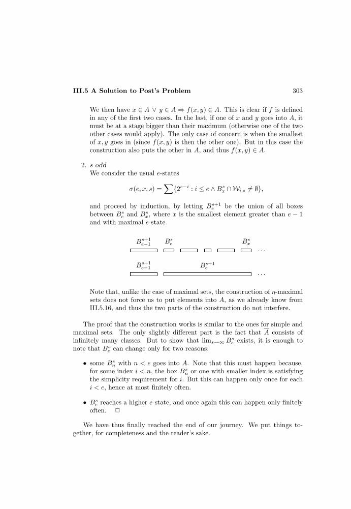
III.5 A Solution to Post’s Problem 303
We then have x ∈ A ∨ y ∈ A⇒ f(x, y) ∈ A. This is clear if f is definedin any of the first two cases. In the last, if one of x and y goes into A, itmust be at a stage bigger than their maximum (otherwise one of the twoother cases would apply). The only case of concern is when the smallestof x, y goes in (since f(x, y) is then the other one). But in this case theconstruction also puts the other in A, and thus f(x, y) ∈ A.
2. s oddWe consider the usual e-states
σ(e, x, s) =∑
2e−i : i ≤ e ∧Bsx ∩Wi,s 6= ∅,
and proceed by induction, by letting Bs+1e be the union of all boxes
between Bse and Bsx, where x is the smallest element greater than e − 1and with maximal e-state.
Bs+1e−1 Bs+1
e
Bs+1e−1 Bse Bsx
· · ·
· · ·
Note that, unlike the case of maximal sets, the construction of η-maximalsets does not force us to put elements into A, as we already know fromIII.5.16, and thus the two parts of the construction do not interfere.
The proof that the construction works is similar to the ones for simple andmaximal sets. The only slightly different part is the fact that A consists ofinfinitely many classes. But to show that lims→∞Bse exists, it is enough tonote that Bse can change only for two reasons:
• some Bsn with n < e goes into A. Note that this must happen because,for some index i < n, the box Bsn or one with smaller index is satisfyingthe simplicity requirement for i. But this can happen only once for eachi < e, hence at most finitely often.
• Bse reaches a higher e-state, and once again this can happen only finitelyoften. 2
We have thus finally reached the end of our journey. We put things to-gether, for completeness and the reader’s sake.
304 III. Post’s Problem and Strong Reducibilities
Or quel che t’era dietro t’e davanti:ma perche sappi che di te mi giova,un corollario voglio che t’ammanti.1
(Dante, Paradiso, VIII)
Corollary III.5.20 Solution to Post’s problem (Muchnik [1956],Friedberg [1957a]) There exists an r.e. set which is neither recursive norT -complete.
Proof. Consider a nonrecursive, semirecursive, η-hyperhypersimple r.e. set: itis not Q-complete by III.5.18, and hence not T -complete by III.5.2. 2
This shows in particular that there are more than two r.e. T -degrees, and im-mediately raises the question of how complicated the structure of r.e.T -degrees is. A complete description of it as a partial ordering is not known,but Chapter X will provide a good deal of information about it, as well asdifferent methods to solve Post’s problem.
III.6 Creative Sets and Completeness
For an r.e. set A, to be nonrecursive means that A is not r.e. The fact that∀x(A 6= Wx) may be formalized in different ways:
1. ∃y(y ∈ A⇔ y ∈ Wx)
2. Wx ⊆ A⇒ ∃y(y ∈ A−Wx)
3. A ⊆ Wx ⇒ ∃y(y ∈ A ∩Wx).
We cannot expect in general to find y recursively in x, and we now investigatewhat happens if we impose this requirement.
Effectively nonrecursive sets
We begin by constructivizing the first notion, which also appears to be themost natural and symmetric.
Definition III.6.1 (Dekker [1955a]) A set A is completely productiveif there is a recursive function f such that, for every x,
f(x) ∈ A⇔ f(x) ∈ Wx.
1Now that which stood behind you, stands in front:but so that you may know the joy you give me,I now would cloak you with a corollary.
III.6 Creative Sets and Completeness 305
A set is effectively nonrecursive if it is r.e., and its complement is com-pletely productive.
K is effectively nonrecursive because, by definition, x ∈ K ⇔ x ∈ Wx.
Proposition III.6.2 (Myhill [1955]) A set is effectively nonrecursive if andonly if it is m-complete.
Proof. Let f be a recursive function such that f(x) ∈ A⇔ f(x) ∈ Wx. If
Wg(x) =ω if x ∈ K∅ otherwise
then x ∈ K ⇔ f(g(x)) ∈ A, because:
• x ∈ K ⇒ Wg(x) = ω ⇒ f(g(x)) ∈ Wg(x) ⇒ f(g(x)) ∈ A
• f(g(x)) ∈ A ⇒ f(g(x)) ∈ Wg(x) ⇒ Wg(x) 6= ∅ ⇒ x ∈ K.
Thus A is m-complete.Let now x ∈ K ⇔ f(x) ∈ A, and z ∈ Wg(x) ⇔ f(z) ∈ Wx. Then
f(g(x)) ∈ A ⇔ g(x) ∈ K ⇔ g(x) ∈ Wg(x) ⇔ f(g(x)) ∈ Wx,
and A is effectively nonrecursive. 2
This shows that any set built by effective diagonalization over the r.e. setsmust be m-complete, and thus Post’s problem cannot be solved by effectivelysatisfying the requirements for nonrecursiveness.
Exercises III.6.3 (Rogers [1967]) a) B is effectively nonrecursive in A if, forsome recursive function f , f(x) ∈ B ⇔ f(x) ∈ WA
x . Post’s problem cannot be solvedby effectively satisfying the requirements for T -incompleteness, in the sense of buildingan r.e. set A such that K is effectively nonrecursive in it. (Hint: if A and B are r.e.and B is effectively nonrecursive in A then A is recursive, because if
WAg(x) =
ω if x ∈ A∅ otherwise
then x ∈ A⇔ f(g(x)) ∈ B.)b) B is effectively not m-reducible to A if, for some recursive function f ,
ϕe total ⇒ [f(e) ∈ B ⇔ ϕe(f(e)) ∈ A],
i.e. f(e) witnesses the fact that ϕe is not an m-reduction of B to A. Post’s prob-
lem for m-reducibility cannot be solved by effectively satisfying the requirements for
m-incompleteness, in the sense of building an r.e. set A such that K is effectively not

306 III. Post’s Problem and Strong Reducibilities
m-reducible to it. (Hint: as above, by considering as ϕg(x) the constant function with
value x.)
Effective nonrecursiveness gives a nice criterion for m-completeness. Withlittle effort it is possible to generalize it, and get similar criteria for all thereducibilities so far introduced.
Exercises III.6.4 (Friedberg and Rogers [1959]) Let ≤r be defined as:
A ≤r B ⇔ for some recursive function f, x ∈ A⇔ Qr(f(x), B,B)
where Qr is a predicate with the following properties:
Qr(z,Wx,Wy) is r.e. as a predicate of x, y, zQr(z,X, Y ) is monotone in Y .
Note that monotonicity of Qr for r.e. arguments follows from the first property, andthat if Qr is also monotone in X then A ≤r B ⇒ A ≤T B.
a) All the reducibilities introduced so far can be so expressed . (Hint: Qtt(z,X, Y )holds if σz is satisfied when positive and negative atomic formulas are respectivelyinterpreted over Y and X. Qp(z,X, Y ) holds when every finite set with canonicalindex inDz intersects Y . For r.e. sets, QT (z,X, Y ) holds when ∃u(Du ⊆ Y ∧u ∈ Wz).)
b) An r.e. set A is r-complete if and only if, for some recursive function g,
Qr(g(x), A,A) ⇔ ¬Qr(g(x), A,Wx).
Explicitly, the interesting criteria are (for some recursive function g):
d-completeness: Dg(x) ⊆ A ⇔ Dg(x) 6⊆ Wx
c-completeness: Dg(x) ∩A 6= ∅ ⇔ Dg(x) ⊆ Wx
Q-completeness: Wg(x) ∩A 6= ∅ ⇔ Wg(x) ⊆ Wx.
Creative sets
We now constructivize the second notion of nonrecursiveness given at the be-ginning.
Definition III.6.5 (Post [1944], Dekker [1953]) A set A is productiveif there is a recursive function f such that, for every x,
Wx ⊆ A ⇒ f(x) ∈ A−Wx.
A set is creative if it is r.e. and coproductive.
III.6 Creative Sets and Completeness 307
As we have already noted, K is creative: if Wx ⊆ K then x cannot be inWx (otherwise x ∈ K by definition, and x ∈ K from Wx ⊆ K, contradiction).Then x 6∈ Wx, and thus also x ∈ K.
The term ‘creative’ was introduced by Post [1944] because K (as well asK0, defined in II.2.7) embodied the essence of the incompleteness theorems ofthe Thirties (II.2.17), and the property of productiveness captured the mainconsequence of these results, namely that
every symbolic logic is incomplete and extendible relative to theclass of propositions constituting K0. The conclusion is inescapablethat even for such a fixed, well defined body of mathematical propo-sitions, mathematical thinking is, and must remain, essentially cre-ative.
That Post got the right notion is proved by the next result: if F is anyconsistent extension of R, then every r.e. set is weakly representable in it (seeII.2.16), and hence m-reducible to the set of (codes of) its theorems, which isthen m-complete.
Theorem III.6.6 (Myhill [1955]) A set is creative if and only if it ism-complete.
Proof. If A is m-complete it is effectively nonrecursive, and hence creative.Directly, if x ∈ K ⇔ g(x) ∈ A, let z ∈ Wh(x) ⇔ g(z) ∈ Wx. Then
Wx ⊆ A ⇒ Wh(x) ⊆ K ⇒ h(x) ∈ K −Wh(x) ⇒ g(h(x)) ∈ A−Wx,
and f(x) = g(h(x)) is a productive function for A.Suppose now that A is creative, and Wx ⊆ A⇒ f(x) ∈ A−Wx. We want
to find a recursive function h such that z ∈ K ⇔ h(z) ∈ A. Since we want touse f , we define g such that z ∈ K ⇔ f(g(z)) ∈ A.
• If z ∈ K, f gives naturally an element of A, if we start from Wg(x) ⊆ A.The simplest way to ensure this is to let Wg(x) = ∅ when z ∈ K: then wehave f(g(z)) ∈ A.
• We try now the converse, i.e. to have f(g(z)) ∈ A⇒ z ∈ K. If f(g(z)) ∈ Athen f(g(z)) ⊆ A, and by productivity it cannot be Wg(z) = f(g(z)),otherwise f(g(z)) ∈ A−Wg(z). We thus define Wg(z) = f(g(z)) whenz ∈ K: then f(g(z)) ∈ A.
Let then g be a recursive function such that
Wg(z) =f(g(z)) if z ∈ K∅ otherwise.

308 III. Post’s Problem and Strong Reducibilities
The existence of g is ensured by the Fixed-Point Theorem, e.g. let
Wϕt(e)(z) =f(ϕe(z)) if z ∈ K∅ otherwise,
and choose e such that ϕe ' ϕt(e). 2
Exercises III.6.7 a) An r.e. set A is creative if and only if, for some recursiveone-one function f , f(x) ∈ A⇔ f(x) ∈ Wx. (Rogers [1967], Gill and Morris [1974])(Hint: if A is creative then A is completely productive and, by III.7.6, it has a one-onecompletely productive function f : then A can be represented as stated. Conversely, iff is one-one then there is a set A satisfying the given conditions, since membership off(x) in A is determined solely by Wx. Note that, if we had f(x) = f(y) with x 6= y,then Wx and Wy could give contradictory answers for membership of f(x) in A.)
b) An r.e. set A is creative if and only if, for some acceptable system of indicesWxx∈ω of the r.e. sets, A = K. (Rogers [1958], Lynch [1974]) (Hint: use III.7.14 toget a recursive isomorphism f between A and K, and let x ∈ We ⇔ f(x) ∈ Wf(e).)
c) A creative set is neither recursive nor simple. (Hint: see III.2.7.)d) Every infinite r.e. set is the disjoint union of a creative and a productive set .
(Dekker [1955a]) (Hint: if A is the range of a one-one recursive function f , considerthe images of K and K.)
e) Every infinite r.e. set is the union of a creative and an infinite recursive set .
(Myhill [1959]) (Hint: let A be r.e. and infinite, and f be a recursive one-one function
whose range is an infinite recursive subset B of A. f(K) is creative, and then so is
f(K) ∪ (A−B), and A = f(K) ∪ (A−B) ∪B.)
The next result is an analogue of III.1.5, and provides a criterion form-completeness based on fixed-points. We use the following generalizationof m-reducibility to functions: f ≤m A if and only if there are recursivefunctions f1, f2, and g such that
f(x) =f1(x) if g(x) ∈ Af2(x) otherwise.
Clearly, B ≤m A if and only if cB ≤m A.
Proposition III.6.8 (Arslanov) An r.e. set A is m-complete if and only ifthere is a function f ≤m A without fixed-points.
Proof. If A is m-complete, the set x : 0 ∈ Wx is m-reducible to A, beingr.e. Let g be a recursive function such that
0 ∈ Wx ⇔ g(x) ∈ A,
and define f ≤m A as:
f(x) =a if g(x) ∈ Ab otherwise,

III.6 Creative Sets and Completeness 309
where a and b are indices of, respectively, ∅ and ω. Then Wf(x) 6= Wx, becausethe two sets differ on 0.
Suppose now that A is r.e., and f ≤m A has no fixed-points. We show thatA is m-complete by proving that it is creative. Given Wx, let
ϕ(z) '
f1(x) if g(z) shows up in A before than in Wx
f2(x) if g(z) shows up in Wx before than in Aundefined otherwise.
Note that if g(z) ∈ A ∪ Wx then ϕ(z) ↓, and if Wx ⊆ A then ϕ(z) = f(z),if convergent. Consider a recursive function h such that Wh(z) = Wϕ(z), i.e.such that Wh(z) = ∅ if ϕ(z) ↑: if Wx ⊆ A, which is the only case of in-terest, then Wh(x) = Wf(x) if ϕ(x) converges. Let e be a fixed-point for h:Wh(e) = We. Since f has no fixed-points ϕ(e) must diverge, and then it mustbe g(e) 6∈ A ∪ Wx. Since the procedure is uniform in x (by using the Fixed-Point Theorem with parameters II.2.11.a), we have a recursive function thatproduces an element of A−Wx whenever Wx ⊆ A, and A is creative. 2
Exercises III.6.9 Weakenings of creativeness. a) An r.e. set A is creative ifand only if there is a partial recursive function ϕ such that
Wx empty or singleton ∧Wx ⊆ A ⇒ ϕ(x)↓ ∧ ϕ(x) ∈ A−Wx.
(Dekker [1955a], Myhill [1955]) (Hint: see the proof of III.6.6.)b) For any r.e. nonrecursive set A there is a partial recursive function ϕ such that
Rx ⊆ A ⇒ ϕ(x)↓ ∧ ϕ(e) ∈ A−Rx.
(Mitchell [1966]) This cannot be interpreted as saying that every nonrecursive r.e. setis effectively nonrecursive, because the system of indices Rxx∈ω for the recursivesets is not effective itself. (Hint: if Rx = Wa = Wb let ϕ(x) be the first elementgenerated in A ∩Wb. Since A is nonrecursive, if Rx = Wa ⊆ A then A ∩Wb 6= ∅.)
c) An r.e. set A is T -complete if and only if A has a productive function recursivein A. (Lachlan [1968]) (Hint: if A is T -complete, is recursive in A to ask if Wx ⊆ A,i.e. if ∃z(z ∈ Wx ∩ A). If Wx ⊆ A, Wx is properly included in A, since A is notrecursive, and an element in A −Wx can be found, recursively in A. Conversely, iff ≤T A is a productive function for A, the function g ≤T A such that
Wg(x) =
f(x) if f(x) ∈ A∅ otherwise
has no fixed-points, and A is T -complete by III.1.5.)
Exercises III.6.10 Productive sets. a) A set A is productive if and only if thereis a partial recursive function ϕ such that
Wx ⊆ A ⇒ ϕ(x)↓ ∧ ϕ(x) ∈ A−Wx.
310 III. Post’s Problem and Strong Reducibilities
(Dekker and Myhill [1958]) (Hint: given ϕ and
Wh(x) =
Wx if ϕ(x)↓∅ otherwise,
then one of ϕ(x) and ϕ(h(x)) converges.)b) A set A is productive if and only if K ≤m A. Thus the T -degrees containing
productive sets are exactly those above 0′. (Dekker and Myhill [1958]) (Hint: see theproof of III.6.6.)
c) A set is productive if and only if it is completely productive. (Myhill [1955])d) There are 2ℵ0 productive and co-productive sets, and the T -degrees containing
such sets are exactly those above 0′. (Karp) (Hint: if A is productive, A ⊕ A isproductive and co-productive.)
e) The set x : Wx ⊆ K is properly contained in K. Thus even transfinite itera-tions of the process starting from ∅, and generating new elements of K (as in III.2.7),does not exhaust K. (Dekker [1955a]) (Hint: the Fixed-Point Theorem produces xsuch that Wx = x: then x ∈ K, but Wx 6⊆ K.)
f) There is a set A productive w.r.t. f , such that A = f(x) : Wx ⊆ A. (Dekker
[1955a]) (Hint: let A be the intersection of all sets for which f is a productive func-
tion.)
We still have to take care of the last notion considered at the beginning ofthis section.
Definition III.6.11 (Dekker [1955a]) A set A is contraproductive ifthere is a recursive function f such that, for every x,
A ⊆ Wx ⇒ f(x) ∈ A ∩Wx.
Proposition III.6.12 (Muchnik [1958a], McLaughlin [1962]) An r.e. setA is creative if and only if A is contraproductive.
Proof. A creative set is effectively nonrecursive, and then A is contraproduc-tive. For the converse, suppose A ⊆ Wx ⇒ f(x) ∈ A ∩Wx, and let
Wg(x) =ω if x ∈ Kω − f(g(x)) otherwise.
Then x ∈ K ⇔ f(g(x)) ∈ A, because:
• x ∈ K ⇒ Wg(x) = ω ⊇ A⇒ f(g(x)) ∈ A
• f(g(x)) ∈ A⇒Wg(x) ⊇ A⇒ f(g(x)) ∈ Wg(x) ⇒ x ∈ K
Thus A is m-complete, and hence creative. 2
III.6 Creative Sets and Completeness 311
Exercises III.6.13 a) A set is contraproductive if and only if it is productive.b) If A is an r.e. nonrecursive set, there is ϕ partial recursive such that
A ⊆ Wx ⇒ ϕ(x)↓ ∧ ϕ(x) ∈ A ∩Wx.
(Dekker [1955a])
For more information on productiveness and creativeness see Dekker [1955a],Friedberg and Rogers [1959], McLaughlin [1964], Lachlan [1965], Mitchell[1966], Soloviev [1976], and Omanadze [1978].
Quasicreative sets ?
Exercise III.6.4 considers reducibilities ≤r generated by relations Qr, and gen-eralizes the criterion of m-completeness given by effective nonrecursiveness, byconsidering r.e. sets A such that, for some recursive function f ,
Qr(f(x), A,A) ⇔ ¬Qr(f(x), A,Wx).
We might then try to extend the criterion of m-completeness given by creative-ness, by considering r.e. sets A such that, for some recursive function f ,
Wx ⊆ A ⇒ Qr(f(x), A,A) ∧ ¬Qr(f(x), A,Wx).
Exercise III.6.14 The criterion fails for c-reducibility . (Omanadze [1978a]) (Hint:let A be a strongly effectively simple, not hypersimple, tt-incomplete set. It ex-ists because there is an acceptable system of indices for which Post’s simple set istt-incomplete, see III.9.2, and all the acceptable systems are isomorphic, see II.5.7.Such a set is thus c-incomplete. Let h be a strong array intersecting A, and g be suchthat Wx ⊆ A ⇒ |Wx| < g(x). To get f such that
Wx ⊆ A⇒ Df(x) 6⊆ A ∧Df(x) ⊆ Wx,
let Df(x) = (⋃z≤g(x)+1
Dh(z))− 0, . . . , g(x).)
Thus this criterion does not always work, and we do not know of anyother formulation as general as III.6.4 (see Lachlan [1965], Soloviev [1976],Omanadze [1976] for weaker results). There are however two special interest-ing cases, which we treat in this and the following subsection, in which theproposed formulation succeeds. We begin with ≤d which, we recall, is definedby Qd(z,X, Y ) ⇔ Dz ⊆ Y . The proposed criterion for d-completeness is thusthe following:
Definition III.6.15 (Shoenfield [1957]) A is quasicreative if it is r.e.and, for some recursive function f ,
Wx ⊆ A ⇒ Df(x) ⊆ A ∧ Df(x) 6⊆ Wx.

312 III. Post’s Problem and Strong Reducibilities
&%'$
"!# A
Wx
Df(x)
Obviously, a creative set is quasicreative: if h is a productive function forA, and Df(x) = h(x), then
Wx ⊆ A ⇒ h(x) ∈ A−Wx ⇒ Df(x) ⊆ A ∧Df(x) 6⊆ Wx.
Proposition III.6.16 (Shoenfield [1957]) A set is quasicreative if and onlyif it is d-complete.
Proof. That a d-complete set is quasicreative follows from the stronger crite-rion for d-completeness given in III.6.4. Or directly, as in the case ofm-completeness, if x ∈ K ⇔ Dg(x) ∩ A 6= ∅ let z ∈ Wh(x) ⇔ Dg(z) ⊆ Wx.Then f(x) = g(h(x)) witnesses the quasicreativeness of A, since
Wx ⊆ A ⇒Wh(x) ⊆ K ⇒ h(x) ∈ K −Wh(x)
⇒ Dg(h(x)) ⊆ A ∧Dg(h(x)) 6⊆ Wx.
Conversely, as in III.6.6, if f witnesses the quasicreativeness of A and g isa recursive function (which exists by the Fixed-Point Theorem) such that
Wg(z) =Df(g(z)) if z ∈ K∅ otherwise,
then z ∈ K ⇔ Df(g(z)) ∩A 6= ∅, and A is d-complete. 2
Proposition III.6.17 (Shoenfield [1957]) There exists a quasicreative, notcreative set.
Proof. The idea is to build a quasicreative set A with a simple superset B,such that B − A is r.e. Then A is not creative, otherwise the usual procedure(see the proof of III.2.7) would give an infinite r.e. subset of B, starting withB −A.
Fix a strong array Fxx∈ω intersecting Post’s simple set (see III.3.5). Weproceed as in the construction of a simple tt-complete, with the role of the setK = x : x ∈ Wx taken by x : Fx ⊆ Wx. If
B = S ∪⋃
Fx⊆Wx
Fx
III.6 Creative Sets and Completeness 313
then B is simple, if coinfinite. Moreover
Fx ⊆ B ⇔ Fx ⊆ Wx.
To have A quasicreative, we can ensure the stronger condition
Fx ⊆ A ⇔ Fx 6⊆ Wx,
equivalent toFx ∩A 6= ∅ ⇔ Fx ⊆ Wx ⇔ Fx ⊆ B.
To build A generate B and, when Fx ⊆ B is found, put into A the element ofFx which has been generated last in B. This makes A ⊆ B, and both A andB −A r.e.
Since A is quasicreative A is not r.e., and so B must be infinite (otherwiseA = (B −A) ∪B would be r.e.). 2
A different proof, relying on completeness (i.e. building a d-complete setwhich is not Q-complete, and thus not m-complete) will be given on p. 342.
Exercises III.6.18 a) A quasicreative set is not simple. (Shoenfield [1957]) (Hint:let x ∈ K ⇔ Df(x) ⊆ A, for some recursive function f . Given distinct elements
x1, . . . , xn of A, let x ∈ C ⇔ Df(x) ⊆ x1, . . . , xn . If C = Wa then Df(a) ⊆ A but
Df(a) 6⊆ x1, . . . , xn. This builds an infinite r.e. subset of A.)
b) An r.e. set A is c-complete if and only if there is a recursive function f suchthat
A ⊆ Wx ⇒ Df(x) ⊆ A ∧Df(x) 6⊆ Wx.
This provides an analogue of contraproductiveness. (Lachlan [1965]) (Hint: seeIII.6.12.)
c) An r.e. set A is semicreative if, for some recursive function f ,
Wx ⊆ A⇒Wf(x) ⊆ A ∧Wf(x) 6⊆ Wx.
(Dekker [1955a]). This provides an analogue of quasicreativeness. Every nonrecursiver.e. T -degree contains a semicreative set . (Yates [1965]) (Hint: use permitting, seep. 277. The most natural example of semicreative set is K, but it is not useful forpermitting, because eachWx contributes at most one element. As a variation consider〈x, e〉 ∈ A ⇔ 〈x, e〉 ∈ We, and Wf(e) = 〈x, e〉 : x ∈ ω. A is semicreative because,
if We ⊆ A, then 〈x, e〉 ∈ A −We, and hence Wf(e) ⊆ A and Wf(e) 6⊆ We. Given anr.e. nonrecursive set C, modify the construction of A by adding permitting, in sucha way to obtain A⊕ C semicreative.)
d) A semicreative set is not simple.
314 III. Post’s Problem and Strong Reducibilities
Subcreative sets ?
We examine now the completeness criterion proposed in the last subsection, inthe case of Q-reducibility. Recall that ≤Q is defined by
QQ(z,X, Y ) ⇔ ∃u(u ∈ Y ∧ u ∈ Wz).
The criterion thus takes the following form:
Definition III.6.19 (Blum and Marques [1973]) A is subcreative if itis r.e. and, for some recursive function f ,
Wx ⊆ A ⇒ Wf(x) 6⊆ A ∧ Wf(x) ⊆ Wx.
&%'$
"!# A
Wx
Wf(x)
Equivalently, by taking unions with A, we might require the existence of arecursive function g such that Wx ⊆ A⇒ A ⊂ Wg(x) ⊆ Wx.
Obviously, a creative set is subcreative: if h is the productive function forA, and Wf(x) = h(x), then
Wx ⊆ A ⇒ h(x) ∈ A−Wx ⇒ Wf(x) 6⊆ A ∧Wf(x) ⊆ Wx.
Proposition III.6.20 (Blum and Marques [1973], Gill and Morris[1974]) A set is subcreative if and only if it is Q-complete.
Proof. That a Q-complete set is subcreative follows from the stronger criterionfor Q-completeness given in III.6.4. Or directly, as in the case ofm-completeness, let x ∈ K ⇔ Wg(x) ⊆ A, and
z ∈ Wh(x) ⇔Wg(z) ∩Wx 6= ∅.
Then f(x) = g(h(x)) witnesses the quasicreativeness of A, since
Wx ⊆ A ⇒ Wh(x) ⊆ K ⇒ h(x) ∈ K −Wh(x)
⇒Wg(h(x)) 6⊆ A ∧Wg(h(x)) ⊆ Wx.
Suppose now that A is subcreative:
Wx ⊆ A⇒Wf(x) 6⊆ A ∧Wf(x) ⊆ Wx.
We want to find a recursive function h such that z ∈ K ⇔ Wh(z) ⊆ A. Sincewe want to use f , we define g such that z ∈ K ⇔ Wf(g(z)) ⊆ A.

III.6 Creative Sets and Completeness 315
• If z ∈ K, f gives naturally a set not contained in A, if we only start fromWg(x) ⊆ A. The simplest way to ensure this is to let Wg(x) = ∅ whenz ∈ K: then Wf(g(z)) 6⊆ A.
• We try now the converse, i.e. we want Wf(g(z)) 6⊆ A ⇒ z ∈ K. IfWf(g(z)) 6⊆ A, there is an element a ∈ Wf(g(z)) ∩ A. By subcreativityit cannot be Wg(z) = a, otherwise Wg(z) ⊆ A and Wf(g(z)) ⊆ Wg(z),while a ∈ Wf(g(z)). We thus define, when z ∈ K, Wg(z) as a set thatchooses an element of Wf(g(z)) ∩ A if there is one, and is empty other-wise. Then Wf(g(x)) ∩A 6= ∅ ⇒ z ∈ K.
We now have to define g. The fact that g is self-referential is taken care ofby the Fixed-Point Theorem, but the naive approach leads to another problem.If we try the natural procedure to pick up an element from Wf(g(z)) ∩ A, wesimultaneously generate Wf(g(z)) and A. At each stage of the enumeration,we put the elements already generated in Wf(g(z)) into Wg(z), unless someelement has already been generated in Wg(z) but not yet in A. This certainlyputs an element of A in Wg(z) if there is one in Wf(g(z)), but may also putother elements of A (ones which are in A, but are generated in it only afterhaving been generated in Wf(g(z))). The effect is that Wg(z) is not containedin A, and the discussion above fails.
To override this we would like to make sure that, if Wf(g(z)) ∩ A 6= ∅, oneelement of the intersection is generated in Wf(g(z)) as the first element. Thinkof the process of generating an r.e. set, and to pass from it to a new r.e. setwhich consists of the elements of the given set generated until the first stage inwhich it is found that the first element of the enumeration is in A. If the givenset is infinite, it can be a fixed-point of this process only if the first elementenumerated in it is in A. Note that Wf(x) may always be supposed infinite(otherwise consider A ∪Wf(x)).
To defineWg(z), first wait until it is discovered that z ∈ K. Then letWf(g(z))
be a fixed-point of the process described above, and let Wg(z) consist of thefirst element generated in it (note that the definition of g actually requires adouble use of the Fixed-Point Theorem). Then:
• z ∈ K ⇒ Wg(z) = ∅ ⊆ A⇒Wf(g(z)) 6⊆ A.
• Wf(g(z)) 6⊆ A⇒ z ∈ K.Otherwise Wg(z) = a, for some a ∈ Wf(g(z)) ∩A (actually, for the firstelement generated in Wf(g(z))). Then
Wg(z) ⊆ A⇒Wf(g(z)) ⊆ Wg(z),
contradiction. 2
316 III. Post’s Problem and Strong Reducibilities
Exercises III.6.21 Strongly effectively simple sets. a) Every strongly effec-tively simple set is Q-complete. (Gill and Morris [1974]) (Hint: if g is a recursivefunction such that We ⊆ A⇒ (maxWe) < g(e), let Wf(e) consist of all the elements
greater than g(e). Then f witnesses the subcreativeness of A, because A is infinite.)
b) A strongly effectively simple set is neither hyperhypersimple, nor contained in
maximal sets. (Cohen and Jockusch [1975]) (Hint: by III.4.10, and the fact that
coinfinite r.e. supersets of strongly effectively hyperhypersimple sets are such.)
Effectively inseparable pairs of r.e. sets
The fact that a set A is recursive if and only if both A and A are r.e. suggeststhe possibility of extending the theory of r.e. sets to pairs of disjoint r.e. sets.The first step was taken in II.2.4, with the definition of the notion of recursiveinseparability as an analogue of nonrecursiveness. The existence of recursivelyinseparable pairs of r.e. sets was proved in II.2.5, and we now strengthen thatresult.
Proposition III.6.22 (Shoenfield [1958]) Every nonrecursive r.e. T -degreecontains a recursively inseparable pair of r.e. sets.
Proof. Let C be a nonrecursive r.e. set. We modify the first proof of II.2.5,and define
x ∈ A ⇔ (x)1 ∈ C ∧ ϕ(x)2(x) ' 0 before (x)1 ∈ Cx ∈ B ⇔ (x)1 ∈ C ∧ ϕ(x)2(x) ' 1 before (x)1 ∈ C.
Then A and B are a disjoint pair of r.e. sets. Moreover:
• A ≤T C and B ≤T CTo see if x ∈ A first see, recursively in C, if (x)1 ∈ C. If not, then x 6∈ A.If so, simultaneously generate C and compute ϕ(x)2(x). Then x ∈ A ifand only if the computation of ϕ(x)2(x) converges to 0 before than (x)1appears in C. Thus A ≤T C, and B ≤T C similarly.
• C ≤T A and C ≤T BTo see if z ∈ C, let x = 〈z, a〉, where a is an index of the constant function0. See, recursively in A, if x ∈ A. If so, then z ∈ C. If not, simultaneouslygenerate C and compute ϕa(x). Then z ∈ C if and only if it has beengenerated in it by the time ϕa(x) converges. Thus C ≤T A, and C ≤T Bsimilarly.
• A and B are recursively inseparableSuppose D is a recursive set such that A ⊆ D and B ⊆ D, and let
ϕe(x) =
1 if x ∈ D0 otherwise.
III.6 Creative Sets and Completeness 317
Then
z ∈ C ⇔ z is generated in C before ϕe(〈z, e〉) converges.
Indeed, if z ∈ C and ϕe(〈z, e〉) converges before z is generated in C, then
ϕe(〈z, e〉) ' 0 ⇒ 〈z, e〉 ∈ A⇒ 〈z, e〉 ∈ D ⇒ ϕe(〈z, e〉) ' 1ϕe(〈z, e〉) ' 1 ⇒ 〈z, e〉 ∈ B ⇒ 〈z, e〉 ∈ D ⇒ ϕe(〈z, e〉) ' 0.
But then C is recursive, contradiction. 2
Exercises III.6.23 a) K is part of a recursively inseparable pair of r.e. sets. (Hint:let A and B be a recursively inseparable pair of r.e. sets. Then A ≤m K, and there is aone-one recursive function f such that x ∈ A⇔ f(x) ∈ K, namely the function givenby III.1.2, being obtained by the Smn -Theorem. Then K and f(B) are recursivelyinseparable.)
b) If B ≤m A and B is part of a recursively inseparable pair of r.e. sets, then A isnot simple. This generalizes the fact that m-complete sets are not simple. (Hint: if freduces B to A, and B and C are recursively inseparable, then D = f(C) is infinite,otherwise f−1(D) is a recursive set separating B and C.)
c) If B ≤tt A and B is part of a recursively inseparable pair of r.e. sets, then Bis not hypersimple. This generalizes the fact that tt-complete sets are not hypersim-ple. (Denisov [1974]) (Hint: if x ∈ B ⇔ A |= σf(x), and B and C are recursivelyinseparable, then
x ∈ B ∧ y ∈ C ⇒ A |= σf(x) ∧ ¬(A |= σf(y)).
With notations as in III.3.10, if
x ∈ B ∧ y ∈ C ∧ (A∗ |= σf(x) ⇔ A∗ |= σf(y))
then A and A∗ differ on some element used in σf(x) or σf(y). There must be x and ysuch that
x ∈ B ∧ y ∈ C ∧ (∀i < 2n)(A∗i |= σf(x) ⇔ A∗i |= σf(y)),
otherwise we could recursively separate B and C, because
xηy ⇔ (∀i < 2n)(A∗i |= σf(x) ⇔ A∗i |= σf(y))
is a recursive equivalence relation with only finitely many classes, and we could takethe union of the equivalence classes containing elements of B.)
d) Not every nonrecursive r.e. tt-degree contains a recursively inseparable pair of
r.e. sets. (Hint: from c) above.)
Effective nonrecursiveness can be generalized as follows:

318 III. Post’s Problem and Strong Reducibilities
Definition III.6.24 (Kleene [1950], Uspenskii [1953]) A and B are ef-fectively inseparable if they are disjoint r.e. sets and, for some recursivefunction f ,
A ⊆ Wx ∧B ⊆ Wy ∧ Wx ∩Wy = ∅ ⇒ f(x, y) ∈ Wx ∪Wy.
&%'$&%'$
q
A B
Wx Wy
f(x, y)
The recursively inseparable pairs constructed in II.2.5 are both effectivelyinseparable. For example, if
x ∈ A⇔ ϕx(x) ' 0 and x ∈ B ⇔ ϕx(x) ' 1,
let f(x, y) be an index of the partial recursive function which gives z value 1if the stage in which z appears in Wx is not greater than the stage in which zappears in Wy, and 0 in the opposite case. Then, if A ⊆ Wx and B ⊆ Wy andWx, Wy are disjoint, f(x, y) ∈ Wx ∪Wy, because e.g.
f(x, y) ∈ Wx ⇒ ϕf(x,y)(f(x, y)) ' 1 ⇒ f(x, y) ∈ B ⇒ f(x, y) ∈ Wy,
contradiction.
Proposition III.6.25 If A and B are effectively inseparable, any r.e. supersetof one disjoint from the other is creative. In particular, so are A and B.
Proof. Let A ⊆ C and B ⊆ C, Wg(x) = Wx ∪ B and C = Wa. If f witnessesthe effective inseparability of A and B, then
Wx ⊆ C ⇒ A ⊆ Wa ∧B ⊆ Wg(x) ⇒ f(a, g(x)) ∈ C −Wx. 2
Exercises III.6.26 a) There are recursively inseparable, not effectively inseparablepairs of r.e. sets. (Muchnik [1956a], Shoenfield [1957], Tennenbaum [1961a]) (Hint:from III.6.22 and III.5.20, since effectively inseparable pairs must be T -complete. Ordirectly, as in the construction of Post’s simple set, by building A and B r.e. anddisjoint, intersecting each infinite r.e. set, and with A ∪B infinite. To achieve thelast condition, consider only elements of We greater that 3e.)
b) The sets A and B − A in the proof of III.6.17 are recursively inseparable,but not effectively inseparable. (Shoenfield [1957]) (Hint: they cannot be effectivelyinseparable, since A is not creative. Suppose A ⊆ C and B−A ⊆ C, with C recursive.Since A is quasicreative we can build, by iteration, an r.e. set D ⊇ C such that D∩Cis infinite, and then B is not simple, contradiction.)
III.7 Recursive Isomorphism Types 319
c) There are two disjoint creative sets which are recursively inseparable, but noteffectively inseparable. (McLaughlin [1962a]) (Hint: use the fact, proved in ChapterIX, that every infinite nonrecursive r.e. set is the disjoint union of two infinite nonre-cursive r.e. sets. Split this way a maximal set, and consider each component as theunion of an infinite recursive set and of a creative set, see III.6.7.e. The two creativesets thus obtained are as wanted.)
d) There are two disjoint creative sets which are recursively separable. (Hint: let
2x ∈ A⇔ x ∈ K, and 2x+ 1 ∈ B ⇔ x ∈ K. They are creative sets, separated by the
even numbers.)
Exercises III.6.27 Conditions equivalent to effective inseparability. Let Aand B be disjoint r.e. sets. The following conditions are equivalent to effective insep-arability of A and B.
a) For some recursive function f ,
A ⊆ Wx ∧B ⊆ Wy ∧Wx ∪Wf(y) = ω ⇒ f(x, y) ∈ Wx ∩Wy.
This is the dual of the notion of recursive inseparability. (Muchnik [1958a])b) For some recursive function f ,
Wx ⊆ A ∧Wy ⊆ B ∧Wx ∩Wy = ∅ ⇒ f(x, y) ∈ A ∪B − (Wx ∪Wy).
This is the analogue of creativeness. (Muchnik [1958a], Smullyan [1961]) (Hint: theequivalence is trivial, and it does not use the Fixed-Point Theorem.)
c) For some recursive function f ,
A ⊆ Wx ∧B ⊆ Wy ⇒ f(x, y) ∈ (A ∩Wx) ∪ (B ∪Wy).
This is the analogue of contraproductiveness.d) For every pair (Wx,Wy) of disjoint r.e. sets, there is a recursive function f
that simultaneously m-reduces them to (A,B), i.e.
z ∈ Wx ⇔ f(z) ∈ A and z ∈ Wy ⇔ f(z) ∈ B.
This the analogue of m-completeness. (Muchnik [1958a], Smullyan [1961]) (Hint: see
III.6.6, and use the Double Fixed-Point Theorem II.2.11.b.)
Further generalizations of creativeness (e.g. to infinite sequences of pair-wisely disjoint r.e. sets) are considered in Cleave [1961], Lachlan [1964], [1964a],[1965b], Malcev [1963], Vuckovich [1967], Carpentier [1968], [1969], [1970], Er-shov [1977].
III.7 Recursive Isomorphism Types
In this section we introduce two natural generalizations of the notion ofm-reducibility, obtained by considering special reducing functions. Interest-ingly, these two reducibilities are different, but the notions of degree inducedby them coincide.

320 III. Post’s Problem and Strong Reducibilities
Mezoic sets and 1-degrees
A natural strengthening of m-reducibility is obtained by asking one-oneness ofthe reducing function.
Definition III.7.1 (Post [1944]) A is 1-reducible to B (A ≤1 B) if, forsome one-one recursive function f , x ∈ A⇔ f(x) ∈ B.
A is 1-equivalent to B (A ≡1 B) if A ≤1 B and B ≤1 A.
Note that, since the proof of III.1.2 was obtained by the Smn -Theorem, whichautomatically provides one-one functions (II.1.7), a set A is r.e. if and only ifA ≤1 K.
Exercises III.7.2 a) If A ≤1 B and B is recursive, so is A.
b) If A ≤1 B and B is r.e. then so is A.
c) If A is r.e. then A ≤1 A if and only if A is infinite, coinfinite and recursive.
d) If A ≤1 B then |A| ≤ |B| and |A| ≤ |B|. Thus, if A ≡1 B, A and B, as well asA and B, must have the same cardinality.
e) If A and B are recursive sets,|A| ≤ |B|, and |A| ≤ |B|, then A ≤1 B.
f) If A and B are infinite and coinfinite recursive sets, then A ≡1 B.
Note that ≤1 is a reflexive and transitive relation, and thus ≡1 is an equiv-alence relation.
Definition III.7.3 The equivalence classes of sets w.r.t. 1-equivalence arecalled 1-degrees, and (D1, ≤) is the structure of 1-degrees, with the par-tial ordering ≤ induced on them by ≤1.
The 1-degrees containing r.e. sets are called r.e. 1-degrees, and two ofthem are:
1. 01, the 1-degree of the infinite and coinfinite recursive sets
2. 0′1, the 1-degree of K.
A set A is 1-complete if it is r.e. and its 1-degree is 0′1, i.e. K ≤1 A.
Note that an r.e. 1-degree contains only r.e. sets. The 1-degrees containingrecursive sets are infinitely many: one for each finite or cofinite cardinality,together with 01, ordered as follows:

III.7 Recursive Isomorphism Types 321
r
rrr rrrppp ppp
@
@
01
a0
a1
a2
b0
b1
b2
where an is the 1-degree of the finite sets with n elements, and bn the 1-degreeof the cofinite sets with n elements in the complement. Even if we consideronly the 1-degrees of infinite and coinfinite sets, 01 is not the least 1-degree:
Proposition III.7.4 If a set A has 1-degree above 01, then A is neither im-mune nor coimmune. In particular, if A is r.e. then it is not simple.
Proof. If B is an infinite and coinfinite recursive set, and f is a one-one re-cursive function such that x ∈ B ⇔ f(x) ∈ A, then f(B) ⊆ A and f(B) ⊆ A,and both f(B) and f(B) are infinite r.e. sets. 2
Simple sets are neither recursive nor 1-complete, and thus they solve a ver-sion of Post’s problem for 1-degrees. But we could also formulate the problemas: are there (r.e.) 1-degrees strictly between 01 and 0′
1? Then simple sets areof no help any more, since their 1-degrees are all incomparable with 01. Tosolve this version, we must first understand what the 1-complete sets are.
Theorem III.7.5 (Myhill [1955]) A set is 1-complete if and only if it iscreative.
Proof. A 1-complete set is m-complete, and hence creative (by III.6.6). Letnow A be creative, and f be a recursive function such that
Wx ⊆ A ⇒ f(x) ∈ A−Wx.
The same proof of III.6.6 would show that A is 1-complete, if we knew that fcan be supposed to be one-one (recall that the reduction function of K to A isthe composition of f and a function g obtained by the Fixed-Point Theorem,hence by the Smn -Theorem, and thus one-one by II.1.7). We then show how tobuild a one-one productive function h for A, by induction. We can start byletting h(0) = f(0). Suppose h(0), . . . , h(n − 1) have been defined: we wanth(n) such that
• h(n) 6∈ h(0), . . . , h(n− 1)
• Wn ⊆ A ⇒ h(n) ∈ A−Wn.
322 III. Post’s Problem and Strong Reducibilities
Note that, by iteration, if Wt(x) = Wx ∪ f(x) then, when Wn ⊆ A, theelements f(n), f(t(n)), f(t2(n)), . . . are all distinct and in A −Wn. Given n,generate this list, and see which of the following happens first.
• If we first find a repetition, we know that it cannot be Wn ⊆ A, and thenh(n) can be anything, as long as it does not interfere with the requirementthat h be one-one. For example, let h(n) be the least number differentfrom h(0), . . . , h(n− 1).
• If we first find an element not in h(0), . . . , h(n − 1), then we can leth(n) be the first such one. Then, as above, h(n) ∈ A −Wn if Wn ⊆ A.2
Exercises III.7.6 Special productive functions. a) A set is productive if andonly if it has a one-one, onto productive function. (Rogers [1967]) (Hint: the proofabove shows how to get a one-one productive function f . To get from it an onto one,let g be a recursive one-one enumeration of an infinite recursive set B of r.e. indicesof ω, and let
h(x) =
g−1(x) if x ∈ Bf(x) otherwise.)
b) A set is contraproductive if and only if it has a one-one, onto contraproductivefunction. (Horowitz [1978]) (Hint: symmetric to part a), using III.6.12.)
c) A set is completely productive if and only if it has a one-one completely pro-ductive function. (Horowitz [1978]) (Hint: if A is completely productive then, bypart a), it has a one-one productive function f . By the Fixed-Point Theorem thereis a one-one recursive function h such that Wh(x) = Wx ∩ f(h(x)). Then fh is aone-one completely productive function for A.)
d) If a set has an onto completely productive function, then its complement is r.e.(and hence creative). (Horowitz [1978]) (Hint: if A is completely productive, there isa recursive function f such that f(x) ∈ A⇔ f(x) ∈ Wx. If f is onto then, for any y,there is x such that f(x) = y, and y is in A if and only if it is in Wx.)
e) The complement of every creative set A has an onto completely productive func-
tion. (Horowitz [1978]) (Hint: as in part a), starting with a completely productive
function for A, and using A in place of ω.)
Now that we know that the 1-complete sets are exactly the creative ones,we have a candidate for the solution to Post’s problem for 1-degrees.
Definition III.7.7 (Dekker [1953]) A is mezoic if it is an r.e. set whichis neither recursive, nor creative, nor simple.
We only have to show that such sets exist. Actually, they are quite abun-dant.
III.7 Recursive Isomorphism Types 323
Proposition III.7.8 (Dekker [1953]) Every nonrecursive r.e. T -degree con-tains a mezoic set.
Proof. Let A be a simple set in the given r.e. nonrecursive T -degree (byIII.2.14), and
〈x, y〉 ∈ B ⇔ x ∈ A.
Clearly B is an r.e. set in the same T -degree as A. Moreover B is mezoic,because:
• B is not recursive, because so is A.
• B is not simple, because the set 〈a, y〉 : y ∈ ω, for any a 6∈ A, is arecursive subset of B.
• B is not creative, because if f were a productive function for B, andWh(x) = 〈z, y〉 : z ∈ Wx, then
Wx ⊆ A ⇒ Wh(x) ⊆ B ⇒ f(h(x)) ∈ B −Wh(x)
⇒ (f(h(x)))1 ∈ A−Wx,
and A would be creative too. 2
Exercises III.7.9 A classification of the r.e. sets (Uspenskii [1957]) An r.e.set A is pseudocreative if, for every r.e. subset B of A, there is an infinite subset ofA disjoint from B. The creative sets are exactly the effectively pseudocreative sets.An r.e. set A is pseudosimple if there is an infinite r.e. subset B of A, such thatA ∪B is simple.
a) The recursive, simple, pseudosimple, and pseudocreative sets are a partition ofthe class of the r.e. sets.
a) Every nonrecursive r.e. T -degree contains a pseudocreative set . (Hint: see theproof of III.7.8.)
b) Every nonrecursive r.e. T -degree contains a pseudosimple set . (Hint: if A is
simple, let 2x ∈ B ⇔ x ∈ A.)
Exercises III.7.10 Splinters again. a) Every splinter is recursive or pseudocre-ative, in particular is not simple. (Ullian [1960]) (Hint: let A = a, f(a), . . . benonrecursive and suppose that, for some r.e. set B ⊆ A disjoint from A, A ∪ B issimple. Given x, consider x, f(x), . . .. If it is finite, then x 6∈ A, otherwise A isfinite and hence recursive. If it is infinite, by simplicity of A ∪ B there must be nsuch that f (n)(x) ∈ A or f (n)(x) ∈ B. In the second case, x 6∈ A. In the first,f (n)(x) = f (m)(a) for some m, and x is in A if and only if m ≥ n and x = f (m−n)(a).Then A is recursive.)
b) Every recursive set is a splinter . (Ullian [1960])c) Every creative set is a splinter . (Myhill [1959], Ullian [1960]) (Hint: let B be
creative, and 〈x, y〉 ∈ A ⇔ x ∈ B. A and B have the same m-degree and hence, by
324 III. Post’s Problem and Strong Reducibilities
III.7.5, the same 1-degree. By III.7.13, they are recursively isomorphic. Thus we canjust prove that A is a splinter. Let ann∈ω be a one-one enumeration of B. Picturethe pairs of numbers as a double array: we have to generate the rows correspondingto pairs with first elements in B, i.e. the elements of the kind 〈an, y〉. Note thatA = A0 ∪ A1, where A0 = 〈an, y〉 : n < y,and A1 = 〈an, y〉 : y ≤ n. A0 isrecursive, and thus there is an enumeration bnn∈ω of it in increasing order. It isthen enough to define f recursive that steps from one element of the following list tothe following:
〈a0, 0〉, b0〈a1, 0〉, 〈a1, 1〉, b1〈a2, 0〉, 〈a2, 1〉, 〈a2, 2〉, b2. . .
Then let f(〈an, n〉) = bn, f(bn) = 〈an+1, 0〉, and f(〈x, y〉) = 〈x, y + 1〉) otherwise.)
Young [1967] has proved that there are pseudocreative sets which are not splin-
ters.
Recursive isomorphism types
After having strengthened m-reducibility by requiring the reducing function tobe one-one, we can make a further step and ask for ontoness as well.
Definition III.7.11 (Post [1944]) A is recursively isomorphic to B(A ≡ B) if, for some one-one onto recursive function f , x ∈ A⇔ f(x) ∈ B.
The equivalence classes of sets w.r.t. recursive isomorphism are called re-cursive isomorphism types.
Note that ≡ is an equivalence relation, because the class of one-one and ontorecursive functions (called recursive permutations) is closed under inverses.
Exercises III.7.12 (Rogers [1967]) a) The recursive permutations form a group,which is not finitely generated . (Hint: if the group were finitely generated, the recur-sive permutations could be recursively enumerated, and the diagonal method wouldproduce a contradiction.)
b) The group of the recursive permutations is not a normal subgroup of the groupof all permutations of ω. (Hint let h be a nonrecursive permutation, and
f(x) =
x if x odd2h(x
2) if x even
g(x) =
x− 1 if x oddx+ 1 if x even.
Then f−1gf is not a recursive permutation.)
In Set Theory, the Cantor-Schroder Theorem shows that two sets which canbe one-one mapped into one another must have the same cardinality. The nextresult is a constructive version of it.
III.7 Recursive Isomorphism Types 325
Theorem III.7.13 (Isomorphism Theorem (Myhill [1955]) 1-degreesand isomorphism types coincide, i.e. for any pair of sets A and B,
A ≡1 B ⇔ A ≡ B.
Proof. Let f and g be one-one recursive functions, such that
x ∈ A⇔ f(x) ∈ B and x ∈ B ⇔ g(x) ∈ A.
We want to define a recursive permutation h that interchanges A and B, andthus we will satisfy the condition x ∈ A ⇔ h(x) ∈ B. Since h has to be total,from time to time we ensure that the least element not yet in the domain getsinto it (by defining h on it). Similarly, h has to be onto, and from time to timewe ensure that the least element not yet in the range gets into it (by lettingit be the value of h for some argument). We then have to show how to ensurethat h is both one-one and a function. But h is a function when h−1 is one-one,and thus we will have a symmetric construction, that alternates steps to makeh total and one-one, to steps to make it onto and a function.
We can easily start by letting h(0) = f(0). Then
0 ∈ A⇔ f(0) ∈ B ⇔ h(0) ∈ B.
Now take the first y not yet in the range (i.e. y 6= f(0)): we want an elementx such that h(x) = y (towards ontoness), and x 6= 0 (to ensure that h is afunction). We obviously try g(y): if this is not 0 then we have what we want,and can let h(y) = g(y), since
y ∈ B ⇔ g(y) ∈ A⇔ h(y) ∈ A.
But if g(y) = 0 then we have two different elements y and f(0), and we knowthat g(f(0)) cannot be 0, since g is one-one. Then we can let h(g(f(0))) = y,since
y ∈ B ⇔ g(y) = 0 ∈ A⇔ f(0) ∈ B ⇔ g(f(0)) = h(y) ∈ A.
The procedure is perfectly general. At any stage, having defined h on a setof elements x0, . . . , xn in such a way that
xi ∈ A⇔ h(xi) ∈ B,
we know that, given x 6∈ x0, . . . , xn and y 6∈ h(x0), . . . , h(xn),
• one of f(x), f(x0), . . . , f(xn) is not in h(x0), . . . , h(xn)
• one of g(y), g(h(x0)), . . . , g(h(xn)) is not in x0, . . . , xn.
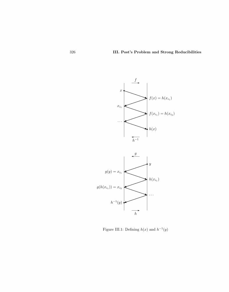
326 III. Post’s Problem and Strong Reducibilities
)
)
)
)
PPPPPPq
PPPPPPq
PPPPPPq
PPPPPPq
r
r
r
r
PPPPPPq
)
-
-
f(x) = h(xi1)
f(xi1) = h(xi2)
h(x)
y
h(xi1)
· · ·
x
xi1
· · ·
g(y) = xi1
g(h(xi1)) = xi2
h−1(y)
f
h−1
g
h
Figure III.1: Defining h(x) and h−1(y)
III.7 Recursive Isomorphism Types 327
We can then proceed inductively, and extend h to a new element xn+1, byletting xn+1 be the least element not yet in x0, . . . , xn if n is odd, and h(xn+1)be the least element not yet in h(x0), . . . , h(xn) if n is even.
The procedure to find h(xn+1) given xn+1 must succeed after at most n+ 1trials. It is illustrated in Figure 1, and can be described recursively as follows.Given x not yet in the domain of h, let z = x, and consider f(z): if it is notyet in the range of h, let h(x) = f(z). Otherwise, change z into h−1(f(z)),and try again. The procedure must stop after finitely many steps, as alreadynoted, because the domain of h is finite, x is not in it, and f is one-one. Andx ∈ A ⇔ h(x) ∈ B because both f and h have this property, the latter byinduction hypothesis.
The procedure to find xn+1 given h(xn+1) is symmetric, by using g and hin place of f and h−1. 2
Corollary III.7.14 The creative sets are all recursively isomorphic.
Proof. The creative sets are exactly the 1-complete ones, by III.7.5, and thusare all 1-equivalent. 2
Note that it also immediately follows that the infinite, coinfinite recursivesets are all recursive isomorphic (Post [1944], Dekker [1953]), although this caneasily be proved directly.
Exercise III.7.15 The effectively inseparable pairs of r.e. sets are all recursively
isomorphic, i.e. if (A,B) and (C,D) are effectively inseparable, there is a recur-
sive permutation that simultaneously exchanges A and C, and B and D. (Muchnik
[1958a], Smullyan [1961]) (Hint: use III.6.27.d.)
Rogers [1967] introduced Klein’s approach in Recursion Theory, and stressedthe importance of considering properties invariant under recursive permuta-tions. We leave to the reader the verification that all concepts introduced sofar (with only one exception, see III.7.16.c), as well as those that will be in-troduced in the next chapters, are indeed recursively invariant. Frequently,III.7.13 is a useful tool in such verifications.
Exercises III.7.16 a) The property of being regressive is invariant under recursivepermutations. (Hint: if A = a0, a1, . . . is regressed by ϕ, then the partial recursivefunction ψ such that ψ(h(x)) ' h(ϕ(x)) regresses h(A) = h(a0), h(a1), . . .. Notethat the enumeration of the set has changed: thus, even if A is retraceable, in generalh(A) is only regressive.)
b) The property of containing an infinite retraceable subset is invariant underrecursive permutations. (Dekker [1962]) (Hint: if A contains an infinite retraceableset B, and h is a recursive permutation, then h(B) is an infinite regressive subset ofh(A), by part a), and it contains, by II.6.20, an infinite retraceable subset.)
328 III. Post’s Problem and Strong Reducibilities
c) The property of being retraceable is not invariant under recursive permutations,even for co-r.e. sets. (McLaughlin [1966]) (Hint: this requires the priority method.We fix the permutation in advance, and let h exchange 2x and 2x + 1. We thenbuild A = a0 < a1 < · · · , and ϕ retracing it. The construction has to be effectiveto give ϕ partial recursive, and this produces A co-r.e. We ensure that h(A) is notretraceable. Choose a2e and a2e+1 to witness the fact that ϕe does not retrace h(A).Also, let ϕ(an+1) = an and ϕ(a0) = a0, so that ϕ retraces A. At stage s + 1, letϕs be the approximation of ϕ obtained so far. Consider the smallest e ≤ s suchthat the condition ‘ϕe does not retrace h(A)’ has not yet been satisfied and notinjured afterwards (in particular, as2e+1 = as2e + 1), and ϕe,s(a
s2e+1) = as2e. Then
ϕe,s(h(as2e)) = h(as2e+1), and we want to destroy this. Let x be the smallest odd
element which is greater than both as2e+1 and every element in the domain of ϕs, andlet x = as+1
2e+1, and ϕs+1(x) = as2e. The reason for doing this is that, if as2e = a2e,then ϕe(h(a2e)) is not in h(A), and so ϕe does not retrace h(A).)
d) There are r.e. sets coregressive, but not coretraceable. (McLaughlin [1966])(Hint: by the proof of part c), h(A) = h(A) is such a set.)
Degtev [1971] and Soare [1972] have shown that every nonrecursive r.e. T -degree
contains an r.e. set which is coregressive but not coretraceable.
Recursive equivalence types and isols ?
Dekker [1955] defines the relation of recursive equivalence as:
A ∼= B ⇔ for some one-one, partial recursive function ϕ,
A ⊆ domϕ and ϕ(A) = B.
∼= is an equivalence relation, which may be seen as a constructivization ofthe property of having same cardinality, and its equivalence classes are calledrecursive equivalence types (r.e.t.), and are thus constructive analogues ofcardinals.
In Set Theory there are two notions of finiteness: A is finite if it can beone-one mapped on a proper initial segment of ω, and is Dedekind-finite ifit cannot be one-one mapped on a proper subset of itself. The two notionscoincide if choice is assumed, but in choiceless Set Theory the latter is weaker,and some infinite sets may still be Dedekind-finite. A set A is recursivelyequivalent to a proper subset of itself if and only if it is infinite and not immune,and thus the r.e.t.’s of finite or immune sets (called isols, because such sets areisolated in the usual topology, see p. 186) may be seen as a constructive versionof Dedekind-finite cardinals (even more appropriately they arise, via Kleenerealizability, from standard cardinal arithmetic on subsets of ω, in IntuitionisticSet Theory, see McCarty [1986]).
The set Λ of isols can be given operations of sum and product, induced by
III.7 Recursive Isomorphism Types 329
A⊕B and A ·B, and a partial order relation ≤ defined as
x ≤ y ⇔ (∃z)(x+ z = y).
The structure of isols is quite rich: ω is embedded in Λ (by identifying n withthe isol of finite sets of cardinality n), Λ has 2ℵ0 elements, and 〈Λ,≤〉 embedsevery countable partial ordering (as well as many others, see Ellentuck [1973]).
Myhill [1958] has introduced a way to extend certain functions from ω toΛ. First note that each function f : ω → ω can be written as
f(n) =∞∑i=0
ci
(ni
)where the ci’s (Sterling coefficients) are positive or negative integers. If theyare all positive or null, then f is called a combinatorial function. Thus everyfunction on ω is the difference of two combinatorial ones. A combinatorial func-tion is recursive if and only if the sequence cii∈ω is. Combinatorial functionsof many variables are defined similarly. The class of combinatorial functionsis a rich one, closed under composition, and containing Ini , the constant func-tions, sum, product, factorial and positive-base exponential. A combinatorialset function is a function on P(ω) that maps each finite set to a finite set,and that respects cardinalities, intersections and countable unions (in partic-ular, the function is generated by its behavior on the finite sets). It is calledeffective if the restriction to finite sets is recursive (on the characteristic in-dices). Combinatorial set functions induce functions on ω (since they preservefinite cardinalities), and effective combinatorial set functions induce functionson r.e.t.’s, in particular on Λ. The basic connection between the two notionsis that the (recursive) combinatorial functions are exactly those induced by(effective) combinatorial set functions. Thus for each recursive combinatorialfunction f on ω, there is a function fΛ on Λ extending it .
It is immediate to note that for each recursive relation R on ω there is a re-lation RΛ on Λ extending it , since given R there are f, g recursive combinatorialfunctions such that
R(x) ⇔ f(x) = g(x),
and thus it is enough to define
RΛ(x) ⇔ fΛ(x) = gΛ(x).
Note that if a recursive relation R admits an algebraic characterization on ω,RΛ does not necessarily coincide with the interpretation of the characterization

330 III. Post’s Problem and Strong Reducibilities
on Λ. E.g., if Pr is the set of prime numbers, PrΛ is different from the set ofprime isols, defined as
x prime ⇔ 2 ≤ x ∧ ∀y∀z(y · z = x⇒ y = 1 ∨ z = 1).
Nerode [1961], [1962] has used these translations to show that a substantialpart of the theory of (finite cardinal) arithmetic can be extended to isols. Con-sider a first-order language with equality, function constants for all recursivecombinatorial functions, and relation constants for all recursive relations. Thena universal Horn sentence (see p. 39) holds over ω if and only if its translationholds over Λ. It immediately follows that, e.g., the following hold for isols:
x 6= x+ 1, nx = ny ⇒ x = y, 2x · 2y = 2x+y.
The result holds in much greater generality than stated, but some restric-tions are needed, because there are universal sentences true in ω that fail in Λ,e.g. the fact that every element is even or odd. Ellentuck [1967] has discovereda notion of universal isol (as an isol avoiding RΛ, for each coinfinite recursiveR, and thus having a sort of genericity): there are 2ℵ0 such isols, and each ofthem provides counterexamples to each universal sentence true in ω but falsein Λ. E.g. a universal isol is prime, but not a member of PrΛ.
The notion of isol can be regarded as an extension not only of the notionof integer, but also of nonstandard integer . Indeed, Nerode [1966] has provedthat any countable nonstandard model of Arithmetic correct for diophantineequations (i.e. such that if an equation has a solution in the model, then it hasa solution in the integers) can be embedded in the isols. Conversely, any subsetof the isols whose differences generate an integral domain can be embedded ina nonstandard model of Arithmetic.
The theory of 〈Λ,+, ·〉 is at least as complicated as that of 〈ω,+, ·〉 (inparticular is not decidable), because the set of finite isols is definable over Λ,by the formula
Fin(x) ⇔ (∀y)(x ≤ y ∨ y ≤ x)
(Dekker and Myhill [1960]). Actually, the first-order theory of 〈Λ,≤〉 is re-cursively isomorphic to the Second Order Arithmetic (Nerode and Manaster[1971]), and the same holds for the theory of 〈Λ,+, ·〉 (Ellentuck [1973a]).
For a treatment of the theory of isols (and r.e.t.’s in general) see Dekker andMyhill [1960], Dekker [1966], Crossley and Nerode [1974], McLaughlin [1982].
III.8 Variations of Truth-Table Reducibility ?
In this section we play on the theme of tt-reducibility, by first consideringbounds on the number of elements used in the truth-tables, and then by relaxing
III.8 Variations of Truth-Table Reducibility ? 331
the condition that we know in advance the effect of the answers to the queriesmade to the oracle. At the end we also introduce a number of other strongreducibilities.
Bounded truth-table degrees
The variation we consider first is, like c-reducibility or d-reducibility, a strength-ening of tt-reducibility, but in a different direction. We impose restrictions noton the kind of truth tables we allow, but rather on their size.
Definition III.8.1 (Post [1944]) A is btt-reducible to B (A ≤btt B) if,for some recursive function f and some number m, called the norm of thereduction,
1. x ∈ A⇔ B |= σf(x)
2. σf(x) uses at most m elements.
If m is the norm, we also write A ≤btt(m) B.A is btt-equivalent to B (A ≡btt B) if A ≤btt B and B ≤btt A.
Exercises III.8.2 a) If A is recursive, then A ≤btt B for any set B.b) If A ≤btt B and B is recursive, so is A.
c) A ≤btt(1) A.
Note that ≤btt is a reflexive and transitive relation, and thus ≡btt is anequivalence relation.
Definition III.8.3 The equivalence classes of sets w.r.t. btt-equivalence arecalled btt-degrees, and (Dbtt, ≤) is the structure of btt-degrees, with thepartial ordering ≤ induced on them by ≤btt.
The btt-degrees containing r.e. sets are called r.e. btt-degrees, and two ofthem are:
1. 0btt, the btt-degree of recursive sets
2. 0′btt, the btt-degree of K.
A set A is btt-complete if its r.e. and its btt-degree is 0′btt, i.e. if K ≤btt A.
In general ≤btt(m) is not transitive, but ≤btt(1) is. Since a set is alwaysreducible to its complement by a bounded truth-table reduction of norm 1, butnot always by m-reductions, ≤m and ≤btt(1) differ in general. But they agreeon nontrivial r.e. sets.

332 III. Post’s Problem and Strong Reducibilities
Proposition III.8.4 If A and B are r.e. sets, B 6= ∅, ω and A ≤btt(1) B, thenA ≤m B.
Proof. Since A ≤btt(1) B, there is a recursive function f such that, dependingon x,
x ∈ A⇔ f(x) ∈ B or x ∈ A⇔ f(x) 6∈ B.
We want a recursive function g such that x ∈ A ⇔ g(x) ∈ B. There are twocases:
• if x ∈ A⇔ f(x) ∈ B, we just let g(x) = f(x)
• if x ∈ A⇔ f(x) 6∈ B, then exactly one of x ∈ A and f(x) ∈ B happens.Generate A and B simultaneously, and find out which one. If x ∈ A thenwe want g(x) ∈ B. If f(x) ∈ B then x 6∈ A, and we want g(x) 6∈ B. SinceB 6= ∅, ω we can pick up a ∈ B and b 6∈ B, and let g(x) be a in the firstcase, and b in the second. 2
Exercise III.8.5 m-reducibility and btt-reducibility differ on the r.e. sets. (Fischer
[1963]) (Hint: Let 〈x, y〉 ∈ A ⇔ x ∈ B ∧ y ∈ B, where B is the simple tt-complete
set of III.3.5: then A ≤btt(2) B. If A ≤m B, there would be g recursive such that
x ∈ B ∧ y ∈ B ⇔ g(x, y) ∈ B, and B would be creative because, if h is gotten by
iteration of g, x ∈ K ⇔ Fx ⊆ B ⇔ h(x) ∈ B.)
When A ≤btt B, only a finite number m of elements are used in the reduc-tion, and hence at most 22m
truth-tables may be used. Actually much moreis true: a single truth-table is enough (although, in general, with a differentnorm).
Proposition III.8.6 (Fischer) If B 6= ∅, ω and A ≤btt B, then A is reducibleto B by a fixed truth-table.
Proof. Consider e.g. the case of norm 1, and let A be reducible to B via σf(x).Fix a ∈ B and b 6∈ B. Since σf(x) is either y ∈ X or y 6∈ X for some y, let σg(x)be the fixed formula
(y ∈ X ∧ z ∈ X) ∨ (y 6∈ X ∧ z 6∈ X),
where y is the element appearing in σf(x), and
z = a if σf(x) is y ∈ Xz = b if σf(x) is y 6∈ X.
Then B |= σf(x) ⇔ B |= σg(x).
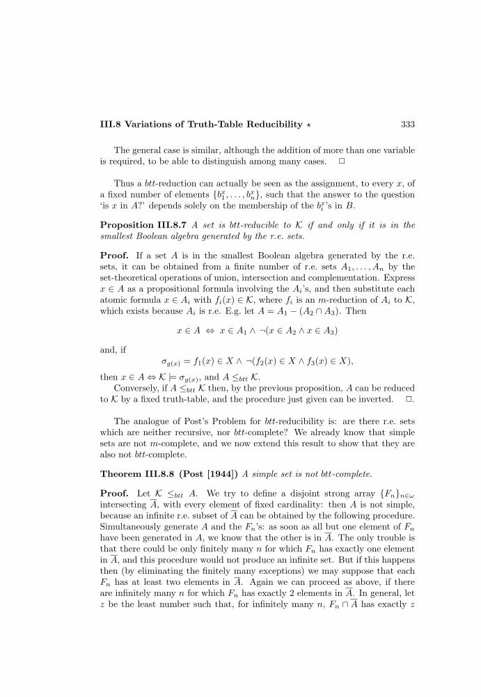
III.8 Variations of Truth-Table Reducibility ? 333
The general case is similar, although the addition of more than one variableis required, to be able to distinguish among many cases. 2
Thus a btt-reduction can actually be seen as the assignment, to every x, ofa fixed number of elements bx1 , . . . , bxn, such that the answer to the question‘is x in A?’ depends solely on the membership of the bxi ’s in B.
Proposition III.8.7 A set is btt-reducible to K if and only if it is in thesmallest Boolean algebra generated by the r.e. sets.
Proof. If a set A is in the smallest Boolean algebra generated by the r.e.sets, it can be obtained from a finite number of r.e. sets A1, . . . , An by theset-theoretical operations of union, intersection and complementation. Expressx ∈ A as a propositional formula involving the Ai’s, and then substitute eachatomic formula x ∈ Ai with fi(x) ∈ K, where fi is an m-reduction of Ai to K,which exists because Ai is r.e. E.g. let A = A1 − (A2 ∩A3). Then
x ∈ A ⇔ x ∈ A1 ∧ ¬(x ∈ A2 ∧ x ∈ A3)
and, ifσg(x) = f1(x) ∈ X ∧ ¬(f2(x) ∈ X ∧ f3(x) ∈ X),
then x ∈ A⇔ K |= σg(x), and A ≤btt K.Conversely, if A ≤btt K then, by the previous proposition, A can be reduced
to K by a fixed truth-table, and the procedure just given can be inverted. 2.
The analogue of Post’s Problem for btt-reducibility is: are there r.e. setswhich are neither recursive, nor btt-complete? We already know that simplesets are not m-complete, and we now extend this result to show that they arealso not btt-complete.
Theorem III.8.8 (Post [1944]) A simple set is not btt-complete.
Proof. Let K ≤btt A. We try to define a disjoint strong array Fnn∈ωintersecting A, with every element of fixed cardinality: then A is not simple,because an infinite r.e. subset of A can be obtained by the following procedure.Simultaneously generate A and the Fn’s: as soon as all but one element of Fnhave been generated in A, we know that the other is in A. The only trouble isthat there could be only finitely many n for which Fn has exactly one elementin A, and this procedure would not produce an infinite set. But if this happensthen (by eliminating the finitely many exceptions) we may suppose that eachFn has at least two elements in A. Again we can proceed as above, if thereare infinitely many n for which Fn has exactly 2 elements in A. In general, letz be the least number such that, for infinitely many n, Fn ∩ A has exactly z

334 III. Post’s Problem and Strong Reducibilities
elements. Then, for some n0 and all n ≥ n0, Fn ∩ A has at least z elements.Generate simultaneously A and the Fn’s, for n ≥ n0: as soon as all but zelements of some Fn have been generated in A, the others must be in A.
If K ≤btt A, then so too is K ≤btt A. Let x ∈ K ⇔ A |= σf(x), for somerecursive function f , with a given reduction bx1 , . . . , bxm. Suppose we havealready chosen
F0 = bx01 , . . . , bx0
m · · · Fn−1 = bxn−11 , . . . , bxn−1
m
with the property that
Fi ∩A 6= ∅ and A |= σf(xi).
To define Fn, let C be the set consisting of all the x for which the formula σf(x)
is deducible, in the propositional calculus, from σf(x0), . . . , σf(xn−1) and theconditions ‘z ∈ X’, for z ∈ A. By the inductive hypothesis (that A |= σf(xi))and logical properties,
x ∈ C ⇔ A |= σf(x) ⇔ x ∈ K,
and hence C ⊆ K. If C = Wa, let xn = a. From a ∈ K − C we have:
• A |= σf(a), because a ∈ K
• ba1 , . . . , bam ∩ A 6= ∅. Otherwise, being σf(a) true in A, and using onlythe elements ba1 , . . . , b
am which are all in A, σf(a) would be deducible from
the conditions ‘z ∈ X’ for z ∈ A. Then a ∈ C, contradiction.
However, we cannot prove that the Fn’s are disjoint on A. But this is unnec-essary: it is enough to show that, given Fn, there are only finitely many sets ofour sequence, with the same intersection on A. Indeed, consider bx1 , . . . , bxm:since only membership in A or A matters, there are only 2m possibilities, If twogiven conditions have same elements on A, they are not only equivalent: theyare also deducible one from the other from the conditions ‘z ∈ X’ for z ∈ A.Thus in our sequence, by definition of C, at most 2m conditions may have thesame intersection on A. Then the procedure described at the beginning stillproduces an infinite subset of A. 2
Corollary III.8.9 There are tt-complete, btt-incomplete sets.
Proof. By III.3.5 there is a simple tt-complete set: by simplicity it cannot bebtt-complete. 2

III.8 Variations of Truth-Table Reducibility ? 335
Exercises III.8.10 a) A pseudosimple set is not btt-complete. (Shoenfield [1957])b) If B ≤btt A and B is part of a recursively inseparable pair of r.e. sets, then A
is not simple. (Kobzev [1973]) (Hint: by induction on m, prove that if A is simpleand Fnn∈ω is a strong array of m-tuples intersecting A, there is a finite set D ⊆ Asuch that, for all n, Fn∩D 6= ∅. Then let B ≤btt A via bx1 , . . . , bxm, and consider thetwo cases bx1 , . . . , bxm ⊆ A⇒ x ∈ B, and bx1 , . . . , bxm ⊆ A⇒ x 6∈ B. If e.g. the firstholds, and B and C are recursively inseparable, then x ∈ C ⇒ bx1 , . . . , bxm ∩A 6= ∅.Let D ⊆ A be finite, and such that x ∈ C ⇒ bx1 , . . . , bxm ∩ D 6= ∅. Moreover, letx ∈ R⇔ bx1 , . . . , bxm ∩D 6= ∅.Then R is recursive, C ⊆ R, and B ∩ R and C arerecursively inseparable. Split R into m recursive parts
x ∈ R1 ⇔ x ∈ R ∧ bx1 ∈ D x ∈ R2 ⇔ x ∈ R−R1 ∧ bx2 ∈ D · · ·
For at least one i, B ∩Ri and C ∩Ri are recursively inseparable, and B ∩Ri ≤btt Awith norm m− 1. So A is not simple by induction hypothesis. For m = 1 recall that
≤btt(1) coincides with ≤m on the r.e. sets, and see III.6.23.)
Theorem III.8.11 (Kobzev [1974], Lachlan [1975]) A btt-complete set isd-complete.
Proof. Let K ≤btt A: for some recursive f
x ∈ K ⇔ A |= σf(x)
and, for some n, σf(x) uses exactly n elements. We want to get
x ∈ K ⇔ Dh(x) ∩A 6= ∅,
for some recursive h. The obvious approach is to consider
Gx = elements used in σf(x).
We can certainly modify the reduction in such a way to suppose that, wheneverx is enumerated in K, then some element of Gx is enumerated in A at the samestage. This gives in particular
x ∈ K ⇒ Gx ∩A 6= ∅,
but we do not have the opposite: some element of Gx could go in A even ifx 6∈ K.
We thus consider the set Gx dynamically: at every stage s we see the setGx ∩ As+1, and can consider the remaining elements of Gx. We thus have nr.e. sets Fi, and Fi consists of elements zix which, at a certain stage s+ 1, areput in Fi because |Gzi
x∩As+1| = i. We try to consider zix in place of x and, as
above,if x ∈ K ⇒ zix ∈ K then x ∈ K ⇒ |Gzi
x∩As+1| > i.
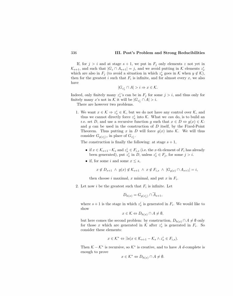
336 III. Post’s Problem and Strong Reducibilities
If, for j > i and at stage s + 1, we put in Fj only elements z not yet inKs+1, and such that |Gz ∩ As+1| = j, and we avoid putting in K elements zixwhich are also in Fj (to avoid a situation in which ziy goes in K when y 6∈ K),then for the greatest i such that Fi is infinite, and for almost every x, we alsohave
|Gzix∩A| > i⇒ x ∈ K.
Indeed, only finitely many zix’s can be in Fj for some j > i, and thus only forfinitely many x’s not in K it will be |Gzi
x∩A| > i.
There are however two problems.
1. We want x ∈ K ⇒ zix ∈ K, but we do not have any control over K, andthus we cannot directly force zix into K. What we can do, is to build anr.e. set D, and use a recursive function g such that x ∈ D ⇔ g(x) ∈ K:and g can be used in the construction of D itself, by the Fixed-PointTheorem. Thus putting x in D will force g(x) into K. We will thusconsider Gg(zi
x), in place of Gzix.
The construction is finally the following: at stage s+ 1,
• if x ∈ Ks+1−Ks and zix ∈ Fi,s (i.e. the x-th element of Fi has alreadybeen generated), put zix in D, unless zix ∈ Fj , for some j > i.
• if, for some i and some x ≤ s,
x 6∈ Ds+1 ∧ g(x) 6∈ Ks+1 ∧ x 6∈ Fi,s ∧ |Gg(x) ∩As+1| = i,
then choose i maximal, x minimal, and put x in Fi.
2. Let now i be the greatest such that Fi is infinite. Let
Dh(x) = Gg(zix) ∩As+1,
where s+ 1 is the stage in which zix is generated in Fi. We would like toshow
x ∈ K ⇔ Dh(x) ∩A 6= ∅,
but here comes the second problem: by construction, Dh(x) ∩A 6= ∅ onlyfor those x which are generated in K after zix is generated in Fi. Soconsider these elements:
x ∈ K∗ ⇔ ∃s(x ∈ Ks+1 −Ks ∧ zix ∈ Fi,s).
Then K−K∗ is recursive, so K∗ is creative, and to have A d-complete isenough to prove
x ∈ K∗ ⇔ Dh(x) ∩A 6= ∅.
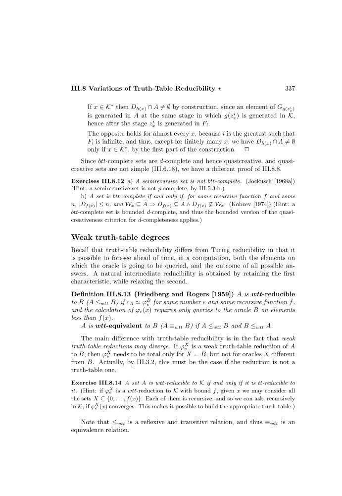
III.8 Variations of Truth-Table Reducibility ? 337
If x ∈ K∗ then Dh(x) ∩A 6= ∅ by construction, since an element of Gg(zix)
is generated in A at the same stage in which g(zix) is generated in K,hence after the stage zix is generated in Fi.
The opposite holds for almost every x, because i is the greatest such thatFi is infinite, and thus, except for finitely many x, we have Dh(x)∩A 6= ∅only if x ∈ K∗, by the first part of the construction. 2
Since btt-complete sets are d-complete and hence quasicreative, and quasi-creative sets are not simple (III.6.18), we have a different proof of III.8.8.
Exercises III.8.12 a) A semirecursive set is not btt-complete. (Jockusch [1968a])(Hint: a semirecursive set is not p-complete, by III.5.3.b.)
b) A set is btt-complete if and only if, for some recursive function f and some
n, |Df(x)| ≤ n, and Wx ⊆ A ⇒ Df(x) ⊆ A ∧Df(x) 6⊆ Wx. (Kobzev [1974]) (Hint: a
btt-complete set is bounded d-complete, and thus the bounded version of the quasi-
creativeness criterion for d-completeness applies.)
Weak truth-table degrees
Recall that truth-table reducibility differs from Turing reducibility in that itis possible to foresee ahead of time, in a computation, both the elements onwhich the oracle is going to be queried, and the outcome of all possible an-swers. A natural intermediate reducibility is obtained by retaining the firstcharacteristic, while relaxing the second.
Definition III.8.13 (Friedberg and Rogers [1959]) A is wtt-reducibleto B (A ≤wtt B) if cA ' ϕBe for some number e and some recursive function f ,and the calculation of ϕe(x) requires only queries to the oracle B on elementsless than f(x).
A is wtt-equivalent to B (A ≡wtt B) if A ≤wtt B and B ≤wtt A.
The main difference with truth-table reducibility is in the fact that weaktruth-table reductions may diverge. If ϕXe is a weak truth-table reduction of Ato B, then ϕXe needs to be total only for X = B, but not for oracles X differentfrom B. Actually, by III.3.2, this must be the case if the reduction is not atruth-table one.
Exercise III.8.14 A set A is wtt-reducible to K if and only if it is tt-reducible to
it . (Hint: if ϕXe is a wtt-reduction to K with bound f , given x we may consider all
the sets X ⊆ 0, . . . , f(x). Each of them is recursive, and so we can ask, recursively
in K, if ϕXe (x) converges. This makes it possible to build the appropriate truth-table.)
Note that ≤wtt is a reflexive and transitive relation, and thus ≡wtt is anequivalence relation.

338 III. Post’s Problem and Strong Reducibilities
Definition III.8.15 The equivalence classes of sets w.r.t. wtt-equivalence arecalled wtt-degrees, and (Dwtt, ≤) is the structure of wtt-degrees, with thepartial ordering ≤ induced on them by ≤wtt.
The wtt-degrees containing r.e. sets are called r.e. wtt-degrees, and twoof them are:
1. 0wtt, the wtt-degree of recursive sets
2. 0′wtt, the wtt-degree of K.
A set A is wtt-complete if it is r.e. and its wtt-degree is 0′wtt, i.e. if K ≤wtt A.
Proposition III.8.16 (Friedberg and Rogers [1959]) A hypersimple setis not wtt-complete.
Proof. We refer to the proof of III.3.10, which goes through practically un-changed, by letting
x ∈ C ⇔ ϕA∗
e (x) ' 0,
where cK ' ϕAe , with bound f . If C = Wa then ϕA∗
e (a) and ϕAe (a) are bothconvergent and different, so there must be an element of A between the givenn and f(a). The rest proceeds as before. 2.
A simple but useful observation is that permitting preserves wtt-reducibi-lity . This allows us to extend many results from T -degrees to wtt-degrees. E.g.every nonrecursive r.e. wtt-degree contains a simple set (III.3.18), althoughnot always a hypersimple one (since a hypersimple set is not wtt-complete).Jockusch [1981a] shows that not every nonrecursive r.e. tt-degree contains asimple set .
Another useful fact to notice is that the completeness criterion forT -reducibility (III.1.5) extends to wtt-reducibility as well, with the obviousdefinition of wtt-reducibility for functions, and a similar proof:
Proposition III.8.17 (Arslanov [1981]) An r.e. set A is wtt-complete ifand only if there is a function f ≤wtt A without fixed-points.
Recall that an application of the original criterion showed that every effec-tively simple set is T -complete (III.2.18). Here the same results holds, for allthe effectively simple sets not ruled out by the previous result.
Proposition III.8.18 (Kanovich [1970], [1970a], Arslanov [1981]) Ev-ery effectively simple, not hypersimple set is wtt-complete.

III.8 Variations of Truth-Table Reducibility ? 339
Proof. LetWe ⊆ A⇒ |We| ≤ g(e).
Define f ≤T A such that
Wf(e) = the first g(e) + 1 elements of A.
Then f has no fixed-points, as in III.2.18. We show that f ≤wtt A. Since A isnot hypersimple, there is a strong array h intersecting A. Thus the first g(e)+1elements of A are below the maximum of
⋃z≤g(e)Dh(z), and this provides the
needed recursive bound to the questions f has to answer. 2
In particular, Post’s simple set is wtt-complete (Ladner). As we have al-ready noted, the tt-completeness of Post’s simple set depends on the acceptablesystem of indices for the r.e. sets (III.3.6, III.9.2).
Exercise III.8.19 Not every strongly effectively simple set is wtt-complete. (Hint:
let A be any coinfinite r.e. set. If it is not hypersimple itself, it has a hypersimple
superset, namely A ∪⋃x∈B Df(x), where f is a disjoint strong array intersecting A,
and B any hypersimple set. And if A is strongly effectively simple, so is any coinfinite
r.e. superset of it.)
Exercises III.8.20 a) An r.e. set A is wtt-complete if and only if
Wx ⊆ A⇒ Dg(x) 6⊆ A ∪Wx
for some recursive function g. (Kanovich [1969], [1970a]) (Hint: if such a g exists,let Wf(x) = Dg(x) ∩ A. Then f ≤wtt A, since it uses the oracle only for elements
in Dg(x). Suppose Wf(x) = Wx: then Wx ⊆ A, so Dg(x) 6⊆ A ∪ Wx, contradicting
Wx = Dg(x) ∩A. Then f has no fixed-points, and A is wtt-complete. Conversely, letf ' ϕAe with bound h be without fixed-points. Given x, let
ϕi(z) '
1 if z shows up first in A0 if z shows up first in Wx.
Since ϕi is recursive, there is z such that Wϕϕie (z) = Wz (by the Fixed-Point Theo-
rem). Since Wf(z) 6= Wz, ϕϕie (z) 6= f(z). If Wx ⊆ A, then ϕi is correct on A ∪Wx,
hence there must be an element of A ∪Wx below h(z). Then let Dg(x) be the set0, . . . , h(z).)
b) For every nonrecursive r.e. set A there is f recursive such that
Wx ⊆ A⇒Wf(x) finite ∧Wf(x) 6⊆ A ∪Wx.
(Soloviev [1976]) (Hint: put in Wf(x) the smallest element that does not appear tobe in A ∪Wx.)

340 III. Post’s Problem and Strong Reducibilities
c) The class of wtt-complete sets is properly included in the class of T -complete,
not hypersimple sets. (Soloviev [1976]) (Hint: let A be T -complete and hypersimple,
and B be an infinite recursive subset of it. Consider A−B: it is T -complete because
A is, and is not simple. It is also not wtt-complete, since A−B ≤wtt A, and A is not
wtt-complete.)
Other notions of reducibility ?
The reader certainly feels that we have introduced enough reducibilities, butmany more have been considered. We just review some of them.
A natural way to weaken reducibilities is by letting the finiteness conditionin the sets defining them become an r.e. condition, like we did e.g. for c-reduci-bility, obtaining Q-reducibility. In a similar way, d-reducibility is weakened intos-reducibility, defined as follows: A ≤s B if and only if, for some recursivefunction f ,
x ∈ A ⇔ Wf(x) ∩B 6= ∅.
Then the r.e. sets fall in just two s-degrees, one consisting of all the nonemptyr.e. sets, and the other consisting of ∅ alone.
Similarly, positive reducibility is weakened in enumeration reducibility,introduced in Section II.3 (p. 197). Recall that A ≤e B if and only if, for somerecursive function f ,
x ∈ A ⇔ (∃u)(Du ⊆ B ∧ u ∈ Wf(x)).
There is just one r.e. e-degree, which is also the least e-degree. As we havealready seen, this reducibility is particularly suitable for the study of partialfunction (through their graphs), and we will deal with it in volume II.
A number of other reducibilities can be introduced by limiting the size of thesets used in defining known reducibilities, like we did for btt-reducibility. Thuswe can define, in a natural way, notions of bounded conjunctive, disjunc-tive, positive, weak truth-table and Q-reducibility. Also T -reducibilitycan be restricted in a similar way, once we recall (III.1.4) that, on r.e. sets,A ≤T B if and only if there is a recursive function f such that
x ∈ A⇔ (∃u)(Du ⊆ B ∧ u ∈ Wf(x)).
Then A is bounded Turing reducible to B if, moreover, there is a fixednumber n bounding the size of Wf(x).
There are other ways of imposing bounds on known reducibilities. E.g.wtt-reducibility is obtained by restricting the number of elements queried ina computation. A restriction on the number of queries can be imposed too.Jockusch [1972a] calls A bounded search reducible to B (A ≤bs B) if A

III.9 The World of Complete Sets ? 341
is Turing reducible to B with a recursive bound on the number of queries tothe oracle. Since we may suppose that, once the oracle has been queried, theanswer to the query is stored and remembered, a bound on the size of thequeries implies a bound on their number. Thus
A ≤wtt B ⇒ A ≤bs B ⇒ A ≤T B.
Jockusch [1972a] proves that ≤bs is not transitive, the intuitive reason beingthat if A ≤bs B ≤bs C then, given x, we know that the oracle on B is queried arecursively bounded number of times, but we do not know for which elements,and thus we cannot use the fact that the queries on C are also recursivelybounded. The special case of a constant recursive bound is obviously transi-tive. Jockusch has proved that there are bs-complete sets which are not wtt-complete, and Soloviev [1976] shows that there are T -complete sets which arenotbs-complete.
A different way to weaken reducibilities is by considering partial function inplace of total ones, thus obtaining partial reducibilities. E.g. Ershov [1977]calls a set A partially m-reducible to a set B (A ≤pm B) if, for some partialrecursive function ϕ,
x ∈ A ⇔ ϕ(x)↓ ∧ ϕ(x) ∈ B.
This reducibility is particularly important for the study of the ∆02 sets.
For results on some of the reducibilities quoted above, see Degtev [1979],[1981], [1982], [1983], Soloviev [1976a], Omanadze [1976a], [1980], Zakharov[1984], [1986].
III.9 The World of Complete Sets ?
We summarize here the work done in this chapter with respect to completenessproperties. We have already proved most of the positive results, and onlysome counterexamples are missing. Some of them are constructed by using thepriority method, and should therefore wait until Chapter X. Since however thisis the right place for them, we sketch their proofs here anyway, for the readeralready acquainted with the method.
Relationships among completeness notions
Our goal is to show that the following implications hold, and no other one does:

342 III. Post’s Problem and Strong Reducibilities
mp tt wtt
T
btt d
c
Q
3QQ
Qs@
@R -
- - -
1QQ
QQs
All the implications are trivially true, except for the fact, proved in III.8.11,that a btt-complete set is d-complete. We thus have only to provide counterex-amples to the missing implications. They come from different sources, includingPost [1944], Lachlan [1965], Young [1965], Jockusch [1968a], Gill and Morris[1974], Odifreddi [1981].
We first prove that no other arrow holds.
1. There is a Q-complete, not wtt-complete setA hypersimple set is not wtt-complete, by III.8.16, and we proved onp. 297 that there is a Q-complete, hypersimple set.
2. There is a btt-complete, not Q-complete setWe build two r.e. sets A and B such that K ≤btt A, and B 6≤Q A. Thefirst condition ensures that A is btt-complete, the second that it is notQ-complete.
To get K ≤btt A we let
x ∈ K ⇔ 2x, 2x+ 1 ∩A 6= ∅.
If at stage s+ 1 we see x ∈ Ks but 2x, 2x+ 1∩As = ∅, we put in A thefirst element between 2x and 2x+ 1 which is not restrained. If both arerestrained, we put in A the one restrained by the condition with lowerpriority.
To get B 6≤Q A, we want to spoil every reduction
x ∈ B ⇔ Wϕe(x) ⊆ A.
Pick up a witness ae, and wait until ϕe(ae) converges. If it does not,then ϕe was not a Q-reduction. Otherwise, wait for a later stage s + 1for which Wϕe(ae) 6⊆ As, i.e. Wϕe(ae) ∩ As 6= ∅. If it never comes, thenWϕe(ae) ⊆ A, and ae never gets into B, so ϕe does not Q-reduce B toA. Otherwise, choose an element xe of Wϕe(ae) which is not yet in A,restrain it from entering A, and put ae into B. If the condition is neverinjured, i.e. xe does not go into A for satisfaction of a requirement of the

III.9 The World of Complete Sets ? 343
first type (to make A btt-complete), then Wϕe(ae) 6⊆ A, while ae ∈ B, andagain ϕe does not reduce B to A. Otherwise, a new attempt will have tobe made, to satisfy the requirement.
3. There is a c-complete, not d-complete setPost’s example III.3.5 of a simple set which is tt-complete, actually pro-duces a c-complete set. But no simple set can be d-complete, by III.6.18.
4. There is a btt-complete, not c-complete setThe set built in part 2 above is btt-complete, and not Q-complete. Itcannot be c-complete, since c-reducibility implies Q-reducibility.
We now prove that no arrow can be reversed.
5. There is a T -complete, not Q-complete setBy III.4.23, there is a T -complete maximal set. Being hyperhypersimple,it cannot be Q-complete (by III.4.10).
6. There is a Q-complete, not c-complete setWe noted on p. 297 that a hypersimple set can be Q-complete, but byIII.8.16 such a set cannot be wtt-complete, and in particular it cannot bec-complete.
7. There is a c-complete, not m-complete setThere is a simple tt-complete set, by III.3.5, but a simple set is notm-complete, by III.2.7.
8. There is a btt-complete, hence p-complete, set which is not c-complete,hence not m-completeThe set built in part 2 is p-complete but not Q-complete, and hence notc-complete.
9. There is a d-complete, not btt-complete setThis is a modification of the proof of part 2. We build two r.e. sets Aand B such that K ≤d A, and B 6≤btt A. Thus A is d-complete, but isnot btt-complete.
To get K ≤d A we let
x ∈ K ⇔ Ix ∩A 6= ∅,
where I0 = 0, I1 = 1, 2, . . . , and Ix has x + 1 elements. Of coursewe have to use tables with unbounded number of elements, otherwisewe would have K ≤btt A, and there would be no hope of satisfying theremaining condition. To spoil btt-reductions with norm n we have to take
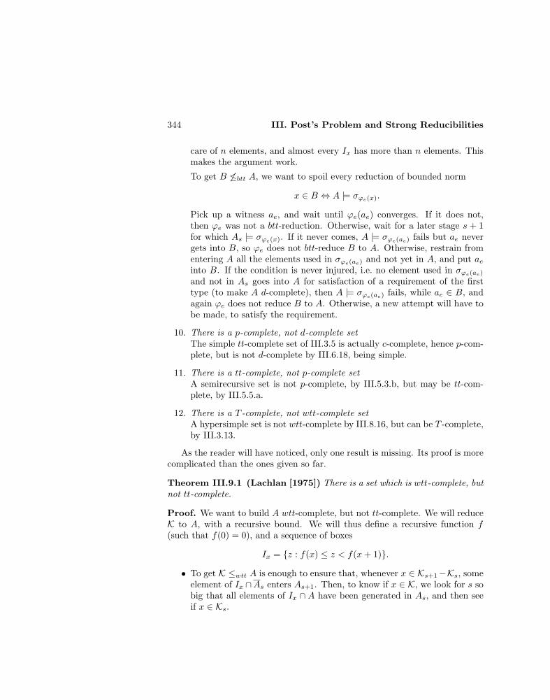
344 III. Post’s Problem and Strong Reducibilities
care of n elements, and almost every Ix has more than n elements. Thismakes the argument work.
To get B 6≤btt A, we want to spoil every reduction of bounded norm
x ∈ B ⇔ A |= σϕe(x).
Pick up a witness ae, and wait until ϕe(ae) converges. If it does not,then ϕe was not a btt-reduction. Otherwise, wait for a later stage s + 1for which As |= σϕe(x). If it never comes, A |= σϕe(ae) fails but ae nevergets into B, so ϕe does not btt-reduce B to A. Otherwise, restrain fromentering A all the elements used in σϕe(ae) and not yet in A, and put aeinto B. If the condition is never injured, i.e. no element used in σϕe(ae)
and not in As goes into A for satisfaction of a requirement of the firsttype (to make A d-complete), then A |= σϕe(ae) fails, while ae ∈ B, andagain ϕe does not reduce B to A. Otherwise, a new attempt will have tobe made, to satisfy the requirement.
10. There is a p-complete, not d-complete setThe simple tt-complete set of III.3.5 is actually c-complete, hence p-com-plete, but is not d-complete by III.6.18, being simple.
11. There is a tt-complete, not p-complete setA semirecursive set is not p-complete, by III.5.3.b, but may be tt-com-plete, by III.5.5.a.
12. There is a T -complete, not wtt-complete setA hypersimple set is not wtt-complete by III.8.16, but can be T -complete,by III.3.13.
As the reader will have noticed, only one result is missing. Its proof is morecomplicated than the ones given so far.
Theorem III.9.1 (Lachlan [1975]) There is a set which is wtt-complete, butnot tt-complete.
Proof. We want to build A wtt-complete, but not tt-complete. We will reduceK to A, with a recursive bound. We will thus define a recursive function f(such that f(0) = 0), and a sequence of boxes
Ix = z : f(x) ≤ z < f(x+ 1).
• To get K ≤wtt A is enough to ensure that, whenever x ∈ Ks+1−Ks, someelement of Ix ∩As enters As+1. Then, to know if x ∈ K, we look for s sobig that all elements of Ix ∩ A have been generated in As, and then seeif x ∈ Ks.
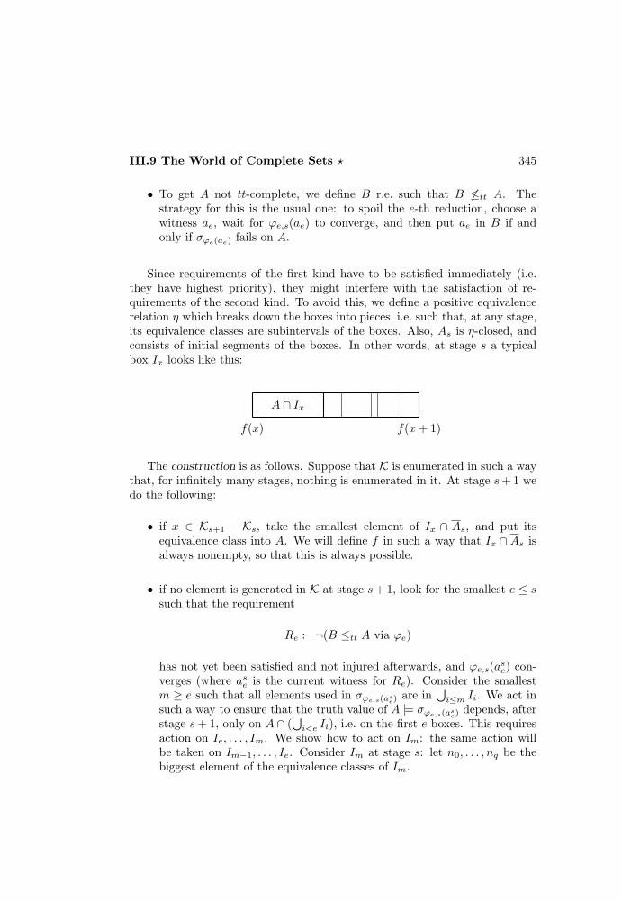
III.9 The World of Complete Sets ? 345
• To get A not tt-complete, we define B r.e. such that B 6≤tt A. Thestrategy for this is the usual one: to spoil the e-th reduction, choose awitness ae, wait for ϕe,s(ae) to converge, and then put ae in B if andonly if σϕe(ae) fails on A.
Since requirements of the first kind have to be satisfied immediately (i.e.they have highest priority), they might interfere with the satisfaction of re-quirements of the second kind. To avoid this, we define a positive equivalencerelation η which breaks down the boxes into pieces, i.e. such that, at any stage,its equivalence classes are subintervals of the boxes. Also, As is η-closed, andconsists of initial segments of the boxes. In other words, at stage s a typicalbox Ix looks like this:
A ∩ Ix
f(x) f(x+ 1)
The construction is as follows. Suppose that K is enumerated in such a waythat, for infinitely many stages, nothing is enumerated in it. At stage s+ 1 wedo the following:
• if x ∈ Ks+1 − Ks, take the smallest element of Ix ∩ As, and put itsequivalence class into A. We will define f in such a way that Ix ∩ As isalways nonempty, so that this is always possible.
• if no element is generated in K at stage s+ 1, look for the smallest e ≤ ssuch that the requirement
Re : ¬(B ≤tt A via ϕe)
has not yet been satisfied and not injured afterwards, and ϕe,s(ase) con-verges (where ase is the current witness for Re). Consider the smallestm ≥ e such that all elements used in σϕe,s(as
e) are in⋃i≤m Ii. We act in
such a way to ensure that the truth value of A |= σϕe,s(ase) depends, after
stage s+ 1, only on A ∩ (⋃i<e Ii), i.e. on the first e boxes. This requires
action on Ie, . . . , Im. We show how to act on Im: the same action willbe taken on Im−1, . . . , Ie. Consider Im at stage s: let n0, . . . , nq be thebiggest element of the equivalence classes of Im.
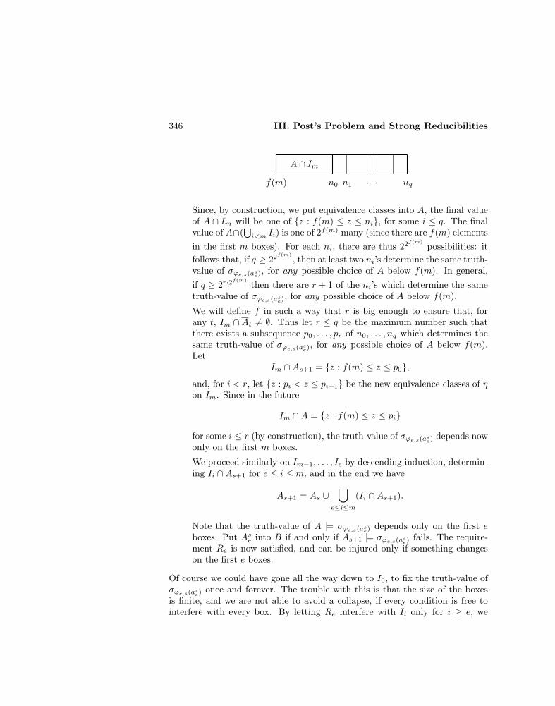
346 III. Post’s Problem and Strong Reducibilities
A ∩ Im
f(m) nqn0 n1 . . .
Since, by construction, we put equivalence classes into A, the final valueof A ∩ Im will be one of z : f(m) ≤ z ≤ ni, for some i ≤ q. The finalvalue of A∩(
⋃i<m Ii) is one of 2f(m) many (since there are f(m) elements
in the first m boxes). For each ni, there are thus 22f(m)possibilities: it
follows that, if q ≥ 22f(m), then at least two ni’s determine the same truth-
value of σϕe,s(ase), for any possible choice of A below f(m). In general,
if q ≥ 2r·2f(m)
then there are r + 1 of the ni’s which determine the sametruth-value of σϕe,s(as
e), for any possible choice of A below f(m).
We will define f in such a way that r is big enough to ensure that, forany t, Im ∩ At 6= ∅. Thus let r ≤ q be the maximum number such thatthere exists a subsequence p0, . . . , pr of n0, . . . , nq which determines thesame truth-value of σϕe,s(as
e), for any possible choice of A below f(m).Let
Im ∩As+1 = z : f(m) ≤ z ≤ p0,
and, for i < r, let z : pi < z ≤ pi+1 be the new equivalence classes of ηon Im. Since in the future
Im ∩A = z : f(m) ≤ z ≤ pi
for some i ≤ r (by construction), the truth-value of σϕe,s(ase) depends now
only on the first m boxes.
We proceed similarly on Im−1, . . . , Ie by descending induction, determin-ing Ii ∩As+1 for e ≤ i ≤ m, and in the end we have
As+1 = As ∪⋃
e≤i≤m
(Ii ∩As+1).
Note that the truth-value of A |= σϕe,s(ase) depends only on the first e
boxes. Put Ase into B if and only if As+1 |= σϕe,s(ase) fails. The require-
ment Re is now satisfied, and can be injured only if something changeson the first e boxes.
Of course we could have gone all the way down to I0, to fix the truth-value ofσϕe,s(as
e) once and forever. The trouble with this is that the size of the boxesis finite, and we are not able to avoid a collapse, if every condition is free tointerfere with every box. By letting Re interfere with Ii only for i ≥ e, we
III.9 The World of Complete Sets ? 347
ensure that only finitely many conditions interfere with a given box Ix, andwe are thus able to show that Ix ∩As is always nonempty (something which isneeded to satisfy the first kind of requirements).
It only remains to determine f . Note that the internal situation of Ix canbe changed only if either x gets into K, or some Re with e ≤ x is satisfied. NowRe can be satisfied at two different stages only if it gets injured between them,and to injure Re we must take action on
⋃i<e Ii. This is possible only if some
i < e gets into K (which can happen only e times), or some Ri with i < e issatisfied. By induction, it follows that Re can be satisfied less than 2e+1 times,hence Ix can change at most
∑e≤x 2e+1 = 2x+2 times. It is thus enough to let:
f(0) = 0f(x+ 1) = 22x+2·2f(x)
. 2
Exercise III.9.2 There is an acceptable system of indices for which Post’s simple
set is tt-incomplete. (Lachlan [1975]) (Hint: apply the method of III.3.6 to the above
proof.)
We briefly discuss now bounded truth-table reducibilities (p. 340). Theinteresting fact is that the notions of bd, bp, btt and bwtt-completeness coincide(Lachlan [1975], Kobzev [1974], [1977]), the first three because a btt-completeset is d-complete and p-complete (III.8.11), and the last two with a proof similarto III.9.1. Moreover, from the next theorem it follows that bc and m-complete-ness coincide, and thus there are only two interesting notions of completenessfor bounded truth-table reducibilities.
Theorem III.9.3 (Lachlan [1966]) If A ·B is m-complete, so is at least oneof A and B.
Proof. We want to build an r.e. set D such that one of the following holds:
1. K ≤m D ≤m A
2. K ≤m D ≤m B.
Note that, no matter how we define D, it will be an r.e. set. Since A · B ism-complete, there will be a recursive function h such that
x ∈ D ⇔ h(x) ∈ A ·B,
and thus there will be two recursive functions f and g such that
x ∈ D ⇔ f(x) ∈ A ∧ g(x) ∈ B.
348 III. Post’s Problem and Strong Reducibilities
By the Fixed-Point Theorem we can use D itself in its own definition, andhence we may suppose f and g given beforehand.
Consider the set
D∗ = z : (∃t)(z 6∈ Dt ∧ g(z) ∈ Bt.
For z ∈ D∗ we have z ∈ D ⇔ f(z) ∈ A, since g(z) ∈ B already. There are thentwo cases:
• If D∗ is infinite, let z0, z1, . . . be a recursive enumeration of it. Thenzx ∈ D ⇔ f(zx) ∈ A, and we can easily ensure condition 1 by lettingx ∈ K ⇔ zx ∈ D.
• If D∗ is finite we have z ∈ D ⇔ g(z) ∈ B, with at most finitely manyexceptions. Indeed, if z ∈ D then g(z) ∈ B; and there are only finitelymany z such that g(z) ∈ B ∧ z 6∈ D, since they must be in D∗. Then wecan easily ensure condition 2 by letting D and K differ only finitely.
The construction of D is the following. At stage s+ 1 we have Ks, Ds, andan enumeration z0, . . . , zi of the elements of
D∗s = z : (∃t ≤ s)(z 6∈ Dt ∧ g(z) ∈ Bt.
Then:
• if x ∈ Ks+1, let zx ∈ Ds+1 (if zx exists, i.e. if enough elements havealready been generated in D∗)
• if x ∈ Ks+1 and x 6∈ D∗s , let x ∈ Ds+1 (this kills x, in the sense that it
ensures x 6∈ D∗, since x goes into D).
If D∗ is infinite then x ∈ K ⇔ zx ∈ D: if x ∈ K then zx ∈ D by the firstpart of the construction; and if zx ∈ D then it must be x ∈ K, since the secondpart of the construction puts in D only elements of D∗, while zx ∈ D∗.
If D∗ is finite, then the second part of the construction applies, except forfinitely many cases, and thus, for almost every z, z ∈ K ⇔ x ∈ D. 2
Corollary III.9.4 A bc-complete set is m-complete.
Proof. A set A is bc-complete if there is a recursive function f such that
x ∈ K ⇔ Df(x) ⊆ A,
where the size of Df(x) is bounded by a fixed number n. By possibly addingelements of A to it, we can suppose that Df(x) always has exactly n elements.But then there are n recursive functions fi such that
x ∈ K ⇔ f1(x) ∈ A ∧ · · · ∧ fn(x) ∈ A⇔ 〈f1(x), . . . , fn(x)〉 ∈ A · · ·A.
III.9 The World of Complete Sets ? 349
But then A · · ·A is m-complete and thus, by repeatedly applying the theorem,so is A. 2
Structural properties and completeness
We now summarize the connections between structural properties on one side,and completeness properties on the other.
We first look at properties implying completeness.
1. A set is creative if and only if it is 1-complete (or m-complete) (III.6.6,III.7.5).
2. A set is quasicreative if and only if it is d-complete (III.6.16).
3. A set is subcreative if and only if it is Q-complete (III.6.20).
4. An effectively simple set is T -complete (III.2.18), but it may be Q-incom-plete (III.4.24.b, III.4.10) or wtt-incomplete (III.8.19).
5. A strongly effectively simple set is Q-complete (III.6.21.a), but it may bewtt-incomplete (III.8.19).
We then look at properties implying incompleteness.
6. A simple set is not d-complete, and hence not btt-complete (III.6.18.a),but it may be c-complete (III.3.5).
7. A hypersimple set is not wtt-complete (III.8.16), but it may be Q-complete(p. 297).
8. A hyperhypersimple set is not Q-complete (III.4.10), but it may beT -complete (III.4.23).
9. A semirecursive set is not p-complete, and hence not btt-complete(III.5.3.b), but it may be tt-complete (III.5.5.a) or Q-complete (p. 297).
We finally look at naturally defined sets with completeness properties.
10. K is 1-complete and m-complete.
11. Post’s simple set (III.2.11) is wtt-complete (being effectively simple andnot hypersimple, III.8.18) and not m-complete (being simple), and canbe tt-complete (actually c-complete, III.3.6) or not (III.9.2), dependingon the acceptable system of indices.
12. The deficiency set of K is T -complete (III.3.13) but not wtt-complete(being hypersimple).

350 III. Post’s Problem and Strong Reducibilities
III.10 Formal Systems and R.E. Sets ?
As we have seen (p. 253), the theory of r.e. sets arose from problems con-nected with the study of formal systems, and Post’s problem was motivatedby methodological considerations. But we have pushed the study of r.e. setsquite far, and it is natural to enquire whether we have lost touch with ‘reality’.We will see here that, far from being so, many of the notions so far introducedhave bearing on our original study of formal systems, and provide appropriatetools to describe natural phenomena.
Formal systems and r.e. sets ?
An abstract approach to formal systems, which isolates their basic properties,is the following. Fix a formal countable language, and identify (by arithme-tization) the sets of well-formed formulas and of sentences (formulas with nofree variable) with two recursive sets F and S, with S ⊆ F .
Definition III.10.1 A formal system F in the given language is a pair(T,R) of r.e. sets contained in S and interpreted, respectively, as the sets of(codes of) theorems and of refutable formulas. F is said to be:
1. consistent if T ∩R = ∅
2. complete if T ∪R = S
3. decidable if T and R are recursive
4. undecidable if T is not recursive.
By Post’s Theorem, a consistent and complete formal system is decidable(Janiczak [1950]): given the code n ∈ S of a sentence, enumerate T and Rsimultaneously, until n appears in one (and exactly one) of them.
Usually T is generated by isolating an r.e. subset Ax of S (set of axioms),and n-ary functions r : Sn → S (called rules of deduction). Then T isthe closure of Ax under the rules. R can be generated in the same way, andindependently of T , or there may be a function n : S → S (called negation)such that R = n(T ).
Exercise III.10.2 Every formal system can be generated by means of finitely many
recursive rules of deduction, from a finite set of axioms. (Kleene [1952]) (Hint: since
T is r.e., for some recursive R is x ∈ T ⇔ ∃yR(x, y). As a system of axioms take
the equations of a system which Herbrand-Godel computes the characteristic func-
tion f of R. As rules, take R1 and R2, together with the rule that produces x from
III.10 Formal Systems and R.E. Sets ? 351
f(x, y) = 1.)
While the abstract notion of formal system is certainly broad enough toinclude all the common examples, the formal systems associated to r.e. sets(like in III.10.2) may look unnatural and ad hoc. In mathematics one usuallyuses first-order formal systems, whose axioms include all axioms of first-order logic with equality, the set of theorems is generated from the axiomsby the first-order logical rules, and the refutable formulas are the negationsof theorems. For first-order formal systems, inconsistency implies that everysentence is a theorem, because if ϕ and ¬ϕ are both provable then so is ¬ϕ∨ψ(i.e. ϕ→ ψ) for any sentence ψ, and then ψ follows by modus ponens.
The next result shows that the r.e. sets do describe (at least up to T -equiv-alence) formal systems of common use.
Proposition III.10.3 (Feferman [1957]) Every r.e. T -degree contains afirst-order formal system.
Proof. Let A r.e. be given. The idea is to consider a decidable theory, andcode A into it. Consider the language of field theory (containing =,0,1,+,×).First note that:
• The theory of algebraically closed fields of any given characteristic is com-plete and decidable.If neither ϕ nor ¬ϕ are provable, both are consistent with the theory,and by the Completeness Theorem of first-order logic there are two al-gebraically closed fields of the given characteristic and same uncountablecardinality, satisfying one ϕ, and the other ¬ϕ. But this is against SteinitzTheorem, according to which any two such fields must be isomorphic, andin particular must satisfy the same formulas. Thus the theory is a com-plete and consistent formal system, and it is then decidable.
We use field characteristics to code the given r.e. set A: let TA be the theoryof algebraically closed fields whose characteristic is not pn, for any n ∈ A (i.e.add to the axioms of algebraically closed fields the statements 1 + . . .+ 1︸ ︷︷ ︸
pn times
6= 0,
for n ∈ A). Then:
• A ≤T TAIndeed n ∈ A ⇔ `TA
1 + . . .+ 1︸ ︷︷ ︸pn times
6= 0, for the following reasons.
If n ∈ A then 1 + . . .+ 1︸ ︷︷ ︸pn times
6= 0 is obviously provable, being an axiom. And

352 III. Post’s Problem and Strong Reducibilities
if n 6∈ A then 1 + . . .+ 1︸ ︷︷ ︸pn times
6= 0 cannot be provable, because in this case TA
is consistent with the theory of algebraically closed fields of characteristicpn.
• TA ≤T ABy definition TA is r.e. in A. It is then enough to show also that itscomplement is r.e. in A. Since a formula ϕ is provable in TA if and onlyif it is true in some algebraically closed field of characteristic 0 or pn, forsome n 6∈ A, by completeness of the theories of algebraically closed fieldsof given characteristic we have that ϕ is not provable in TA if and onlyits negation is true in some field of characteristic either 0 or pn, for somen 6∈ A. Then, by decidability of the same theories, TA is r.e. in A. 2
More results on the connections between degrees and formal systems arein Feferman [1957], Shoenfield [1958], and Hanf [1965]. In particular, everyr.e. tt-degree contains a finitely axiomatizable first-order formal system. Onthe other hand, not every r.e. m-degree contains a first-order formal system,because closure under conjunction implies that if A is the set of theorems ofa first-order formal system, then A · A ≤m A, and this fails in general for r.e.sets (see III.8.5).
Undecidability
To express in full generality the methods to prove undecidability, suppose thatthe language contains constants n, for every n. Fix an effective enumerationψee∈ω of the formulas of the language with one free variable, and supposethat there is a recursive substitution function s, such that s(e, n) is the codeof ψe(n) as a sentence. The notion of representability of predicates (I.3.4) canbe easily generalized to this abstract setting: a set A is weakly representablein F if, for some e,
x ∈ A⇔ s(e, x) ∈ T.
Note that every set weakly representable in a formal system must be r.e.The direct methods to prove the undecidability of a formal system are
summarized in the following:
Theorem III.10.4 Direct undecidability proofs (Tarski, Mostowskiand Robinson [1953], Bernays [1957], Putnam [1957], Smullyan[1958], Vaught) A formal system F is undecidable if one of the followingholds:
1. Every recursive set is weakly representable in F .
III.10 Formal Systems and R.E. Sets ? 353
2. Some nonrecursive r.e. set is weakly representable in F .
Proof. If F is decidable, the diagonal set
n ∈ T ∗ ⇔ s(n, n) ∈ T
is recursive, and then so is T ∗. If every recursive set is representable in F ,there is e such that
n ∈ T ∗ ⇔ s(e, n) ∈ T.
For n = e we get a contradiction, and this proves the first part.The second method is trivial: if F is decidable, every set weakly repre-
sentable in it must be recursive. 2
The two methods are substantially different in principle: the undecidabil-ity is forced in one case by the quantity of sets represented, despite the factthat all of them may be computable (the underlying reason being that thereis no recursive enumeration of all the recursive sets), in the other by the (non-computable) quality of some of them. It is not obvious however that theyare distinct, since it could be that once all the recursive sets are weakly rep-resentable, also some nonrecursive r.e. set is. Actually, for the examples ofII.2.17 much more is true: every r.e. set is weakly representable. In particular,all these examples weakly represent K, and thus the sets of their theorems areall T -complete. Thus the positive solution to Post’s Problem implies that notevery undecidable formal system can weakly represent every r.e. set , but thisdoes not solve our question yet. The answer has been obtained by Shoenfield[1961], with a formal system in which the weakly representable sets are exactlythe recursive ones. The proof introduces a difficult extension of the prioritymethod used for the solution of Post’s Problem, and will be given in Chapter X.
There is also an indirect method to prove undecidability, and this was Post’sdirect concern. Formal systems can be interpreted one into another. Thesimplest way is having a recursive function f that translates formulas andpreserves theorems: given F and F ′ with sets of theorems F and F ′,
x ∈ F ⇔ f(x) ∈ F ′.
But this is only one possible way, and we can say in general that F is inter-pretable in F ′ if F ≤T F ′. Then the following is simply an observation:
Theorem III.10.5 Indirect undecidability proofs. F is undecidable if anundecidable formal system is interpretable in it.
354 III. Post’s Problem and Strong Reducibilities
The undecidability of the Predicate Calculus was obtained this way (II.2.18),as well as the undecidability of the formal systems of current use in mathemat-ics (see e.g. Tarski, Mostowski and Robinson [1953], Ershov, Lavrov, Taimanovand Taitslin [1965], Hanson [198?]), using as starting point systems that (likeR) are all T -complete, and thus showing that they are all T -complete as well.Thus the positive solution to Post’s Problem implies that there are undecidableformal systems that cannot be proved undecidable by interpreting R in them.
Essential undecidability
Since a consistent formal system F is described in terms of a pair of disjoint r.e.sets (T,R) contained in a recursive set S, and respectively coding the theoremsand the refutable formulas, we may first of all expect that the theory of pairsof r.e. sets might be relevant.
Definition III.10.6 (Tarski [1949]) A consistent formal system F = (T,R)is essentially undecidable if T and R are recursively inseparable.
If we say that F ′ = (T ′, R′) is an extension of F = (T,R) (in the samelanguage) when T ′, R′ ⊆ S, T ⊆ T ′ and R ⊆ R′, then essential undecidabilitymeans that not only the system itself, but also every consistent extension of itin the same language is undecidable.
The notion of representability of sets can be generalized to pairs. Recallthat s is the substitution function, and s(e, n) is the code of the formula ψe(n),for a given enumeration ψee∈ω of the formulas of the language with one freevariable.
Definition III.10.7 (Kleene [1952], Putnam and Smullyan [1960])Given a formal system F = (T,R) and two disjoint sets A and B, we saythat A and B are separable in F if there is e such that
x ∈ A⇒ s(e, x) ∈ T and x ∈ B ⇒ s(e, x) ∈ R.
As in the case of simple undecidability, we have two methods to proveessential undecidability.
Theorem III.10.8 Direct proofs of essential undecidability (Kleene[1952], Tarski, Mostowski and Robinson [1953], Smullyan [1958],Putnam and Smullyan [1960]) A consistent formal system F is essentiallyundecidable if one of the following holds:
1. Every pair of disjoint recursive sets is separable in F .

III.10 Formal Systems and R.E. Sets ? 355
2. Some recursively inseparable pair is representable in F .
Proof. Note that everything separable in F remains separable in any consistentextension of it. And if every pair of disjoint recursive sets is separable ina consistent system (T ′, R′), every recursive set is weakly representable in it(given A recursive, let e be the number of the formula separating A and A:then
x ∈ A ⇒ s(e, x) ∈ T ′x ∈ A ⇒ s(e, x) ∈ R′ ⇒ s(e, x) 6∈ T ′
by consistency, and hence x ∈ A ⇔ s(e, x) ∈ T ′). Then every consistentextension of F is undecidable, by III.10.4 (because every recursive set is weaklyrepresentable in it), and F is essentially undecidable.
The second part holds because F , if not essentially undecidable, has a de-cidable consistent extension (T ′, R′), in which the given recursively inseparablepair (A,B) is still separable:
x ∈ A⇒ s(e, x) ∈ T ′ and x ∈ B ⇒ s(e, x) ∈ R′.
But then the recursive set x : s(e, x) ∈ T ′ would separate A and B. 2
Exercises III.10.9 A set A is representable in F = (T,R) if, for some e,
x ∈ A⇒ s(e, x) ∈ T and x ∈ A⇒ s(e, x) ∈ R,
i.e. if A and A are separable in F .
a) Every recursive set is representable in F if and only if every pair of disjointrecursive sets is separable in it .
b) If some nonrecursive set is representable in F , then some recursively insepara-
ble pair of sets is separable in it, but not conversely . (Hint: in R only recursive sets
are representable, by II.2.16, but every pair of disjoint r.e. sets is separable, see below.)
As already for the undecidability proofs, the two methods for essential un-decidability are substantially different and distinct. We now see that they bothapply, as usual, to consistent extensions of R.
Theorem III.10.10 (Rosser [1936], Putnam and Smullyan [1960]) Inany consistent formal system F extending R, every disjoint pair of r.e. sets isseparable.
Proof. If A and B are disjoint r.e. sets, there exist recursive relations R andQ such that
x ∈ A⇔ ∃yR(x, y) and x ∈ B ⇔ ∃yQ(x, y).

356 III. Post’s Problem and Strong Reducibilities
We already know that all the recursive relations are representable in F (II.2.16),and then there are formulas ψ1 and ψ2 such that
R(x, y) ⇒ `F ψ1(x, y) and ¬R(x, y) ⇒ ` ¬ψ1(x, y)Q(x, y) ⇒ `F ψ2(x, y) and ¬Q(x, y) ⇒ ` ¬ψ2(x, y).
Then the formula
ϕ(x) ⇔ ∃y[ψ1(x, y) ∧ (∀z < y)¬ψ2(x, z)]
separates A and B:
• x ∈ A ⇒ `F ϕ(x)If x ∈ A then, for some y, R(x, y) holds, and hence `F ψ1(x, y). SinceA and B are disjoint, x 6∈ B: hence, for every z, ¬Q(x, z) and so `F¬ψ2(x, z). By the axioms of R we can treat bounded quantifiers, andhence we also have `F (∀z < y)¬ψ2(x, z). Then `F ϕ(x).
• x ∈ B ⇒ `F ¬ϕ(x)Note that ¬ϕ(x) ⇔ ∀y[¬ψ1(x, y) ∨ (∃z < y)ψ2(x, z)]. If x ∈ B then,for some z, Q(x, z) holds, and hence `F ψ2(x, z). Since A and B aredisjoint, x 6∈ A and so, for every y, ¬R(x, z) holds, and `F ¬ψ1(x, y). Bythe axioms of R we know that, for every y and a fixed z, y ≤ z ∨ z < y.Thus we only have to consider finitely many cases because, again by theaxioms of R, y ≤ z means that y is actually the numeral correspondingto some y ≤ z. If y ≤ z then `F ¬ψ1(x, y). If z < y then, from ψ2(x, z),we have (∃z < y)ψ2(x, z)). Thus `F ¬ϕ(x). 2
Corollary III.10.11 If F is a consistent formal system extending R then Fis essentially undecidable, and the sets of (codes of) theorems and of refutableformulas of F are effectively inseparable (and in particular creative).
Proof. Both criteria for essential undecidability are applicable, since everypair of disjoint r.e. sets is separable in F , in particular every pair of disjointrecursive sets, and any recursively inseparable pair.
Moreover, separability of A and B provides a simultaneous m-reduction ofthem to the sets of theorems and of refutable formulas. These are then effec-tively inseparable, because there is a pair A and B of effectively inseparabler.e. sets. 2
Smullyan [1961] calls F = (T,R) a Godel theory if every r.e. set is weaklyrepresentable in it, and a Rosser theory if every pair of disjoint r.e. sets isseparable in it. These two notions simply express m-completeness, respectivelyfor r.e. sets and pairs of disjoint r.e. sets. Thus if F is a Godel theory then T is
III.10 Formal Systems and R.E. Sets ? 357
creative, and if F is a Rosser theory then T and R are effectively inseparable.The fact that two disjoint creative sets may be recursively separable (III.6.26.d)can be seen as saying that a Godel theory is not necessarily essentially unde-cidable. On the other hand, the existence of recursively inseparable pairs inany nonrecursive r.e. T -degree (III.6.22) shows that an essentially undecidableformal system is not necessarily a Rosser theory .
Pour El [1968] calls effectively extensible a theory F = (T,R) for whichthere is an effective procedure that produces, for any consistent extension F ′ ofit, a formula which is neither provable nor refutable in F ′. This notion is clearlyequivalent to the effective inseparability of T and R (see III.6.27.b), and stressesthe effective content of the proof of Godel’s Theorem, which effectively exhibitsundecidable sentences for any sufficiently strong consistent formal system.
The last results and comments show that the notions of creativeness andeffective inseparability are useful tools for the description of common theories,for what concerns the description of undecidability and related phenomena.The limits of this usefulness are pointed out by III.7.13 and III.7.15 (and theirextensions considered in Pour El and Kripke [1967], Pour El [1968]): from arecursion-theoretic point of view, all effectively inseparable (and, in particular,a great number of common) formal systems are isomorphic, and thus merevariations one of another. To get a finer analysis the recursive, purely exten-sional approach (only considering the sets of theorems) has to give in to aproof-theoretical, intensional one (accounting for the way the theorems are ob-tained). As Kreisel [1971] puts it, Proof Theory begins where Recursion Theoryends.
Independent axiomatizability
Since consistent theories have disjoint sets of theorems and refutable formulas, ifwe call a formal system nontrivial when it has at least infinitely many theoremsand infinitely many refutable formulas, then (the sets associated to) consistentnontrivial formal systems are not simple. This does not mean that the notionof simplicity, as well as its strengthenings, has no relevance for the descriptionof formal systems, as we now see.
Until now we have looked at decidability questions, and thus recursive enu-merability was seen as opposed to recursiveness. This depended on the factthat we considered formal systems only, that is r.e. sets of formulas. But inmathematics theories need not be r.e. (and the results on the limitations offormal systems show that there is no other way to override the incompletenessphenomena, while preserving expressive power).
Definition III.10.12 A set of formulas in a given language is called a first-order theory if it is closed under logical consequence. A theory is:
358 III. Post’s Problem and Strong Reducibilities
1. axiomatizable if it is the closure under logical consequence of an r.e.set of formulas αee∈ω, called the axioms
2. independently axiomatizable if moreover, for every e, the axiom αeis not a logical consequence of the remaining axioms
3. finitely axiomatizable if it has a finite set of axioms.
Note that the axiomatizable theories are just the first-order formal systems,because the closure of an r.e. set of formulas under recursive rules (like the onesof any standard complete formalization of the Predicate Calculus) is still an r.e.set of formulas. Moreover, axiomatizable theories always have a recursive setof axioms (Craig [1953]), because any formula is implied by the conjunction ofitself with other formulas, and thus we can substitute the n-th axiom with theconjunction of the first n ones, obtaining a set enumerated in increasing order,and hence recursive. Finally, a finitely axiomatizable theory is independentlyaxiomatizable.
Proposition III.10.13 (Kreisel [1957], Pour El [1968a]) The followingare equivalent, for an axiomatizable first-order theory F :
1. F is independently axiomatizable
2. for any axiomatization αee∈ω of F , the set
n ∈ A⇔ α0 ∧ · · · ∧ αn |= αn+1
is not hypersimple
3. for some axiomatization αee∈ω of F , the set
n ∈ A⇔ α0 ∧ · · · ∧ αn |= αn+1
is not hypersimple.
Proof. Note that the conditions are trivially equivalent when F is finitelyaxiomatizable (because in this case the set A is finite, and certainly not hyper-simple), and then we can suppose that F is not finitely axiomatizable. We firstprove that if F is independently axiomatizable, and αee∈ω is any axiomati-zation of it, then the set
n ∈ A⇔ α0 ∧ · · · ∧ αn |= αn+1
is not hypersimple. Fix an independent axiomatization βnn∈ω of F . It isenough to show that, given any n, we can effectively find an m > n such that

III.10 Formal Systems and R.E. Sets ? 359
n, . . . ,m− 1 ∩A 6= ∅ (since this permits an inductive generation of a strongarray intersecting A). Given α0, · · · , αn we can find first of all a number p suchthat they are deducible from β0, . . . , βp. Then we can find a number m suchthat βp+1 is deducible from α0, . . . , αm. Now one of n, . . . ,m − 1 is not in Aotherwise, inductively, all of αn+1, . . . , αm would be deducible from α0, . . . , αn,and hence from β0, . . . , βp. But then so would be βp+1, contradicting the factthat the β’s are an independent axiomatization.
We now show that if, for any axiomatization αee∈ω of F , the set
n ∈ A⇔ α0 ∧ . . . ∧ αn |= αn+1
is not hypersimple, then F is independently axiomatizable. We do this in twosteps:
• there is an effective procedure that produces, given any theorem γ of F ,another theorem γ′ that is not deducible from itBy hypothesis, we have a strong array Df(x)x∈ω that intersects A.Given any theorem γ of F , find first an n such that γ is deducible fromα0, . . . , αn, and then an x such that Df(x) contains only numbers greaterthan n. The conjunction γ′ of the αn+1’s such that n is in Df(x) isthen a theorem of F (because a conjunction of axioms) that cannot bededuced from γ. Indeed, one number n in Df(x) is not in A, i.e. αn+1
cannot be deduced from the α’s with smaller indices, and in particular isnot deducible from γ. But αn+1 is a conjunct of γ′, and thus γ′ is notdeducible from γ either.
• there is an independent axiomatization of FLet αnn∈ω be an enumeration of the theorems of F . We want togenerate this set with a set of independent axioms βnn∈ω. The first partof the proof produces, given any formula γ, a formula γ′ not deduciblefrom it. The opposite is not necessarily true, since γ′ could be too strong,and imply γ. To have independent formulas, we have to relax γ′ a little,and this can be done by considering ¬γ ∨ γ′, i.e. γ → γ′. This is notdeducible from γ as before, since otherwise (by modus ponens) so wouldbe γ′. And if γ is not valid, it is not deducible from γ → γ′, otherwisefrom ¬γ (which is stronger than ¬γ ∨ γ′) we would get γ, and then γwould be valid. More generally, the sequence
γ γ → γ′ γ′ → γ′′ · · ·
is independent. We still have to make sure that all the αn’s are goingto be deducible from the axioms, and we simply add them one by oneas conclusions, so that αn can be obtained from the first n + 1 axioms.

360 III. Post’s Problem and Strong Reducibilities
Thus our set of independent axioms for F is a set of formulas inductivelydefined as follows. First we let
β0 = α′0.
This makes sure that we start from a formula that is not valid. Then, ifβn = δn → γn,
βn+1 = γn → αn ∧ (αn ∧ γn)′. 2
Exercise III.10.14 For any hypersimple set A there is a consistent first-order formalsystem F extending R, and an axiomatization αee∈ω of it, such that
n ∈ A⇔ α0 ∧ · · · ∧ αn |= αn+1
In particular, F is not independently axiomatizable. (Kreisel [1957]) (Hint: let α0
be the conjunction of the finitely many axioms of Q, see p. 23, and of the formula
∀x(ϕ(x) → P (x)), where P is a new predicate, and ϕ weakly represents A in R.
Moreover, let αn+1 be P (n). Then αn+1 can be deduced from α0 only when n ∈ A.)
Pour El [1968a] shows that Q, and more generally every theory with effec-tively inseparable sets of theorems and of refutable formulas, has a consistentextension which is not independently axiomatizable, and with the same lan-guage as the original theory.
For more recursion-theoretical results about formal systems see p. 510, aswell as Smullyan [1961], Martin and Pour El [1970], and Downey [1987].
æ
Chapter IV
Hierarchies andWeak Reducibilities
The theme of this chapter is definability in given languages, and a classifica-tion of sets and relations according to their best definition. Of course definabil-ity is not an absolute notion, and it depends on the given language. Here wewill consider three natural ones, the first two for Arithmetic, the last one forSet Theory. The first two will differ in that we will allow only number quan-tifications in one case, but also function (or set) quantifications in the other,and will define, respectively, the arithmetical and analytical sets. The thirdapproach will lead us to the constructible sets.
Definability is a linguistical, more than computational, notion. However,we already know that it is possible to characterize the recursive sets in a purelylinguistical way, see I.3.6. This suggests the possibility of considering definabil-ity as an abstract version of computability, and we will see in later chaptersthat this program is indeed feasible, for some of the definability notions thatwill be introduced in this chapter.
We only scratch the surface of the subject in here, and refer to VolumesII and III for a detailed study of the arithmetical and the analytical sets, towhich the two volumes are respectively dedicated. But we will prove a numberof interesting results already in this chapter, providing some nontrivial charac-terizations of a number of classes. In particular, we deal with: the limit sets,that can be obtained as limits of recursive functions; the hyperarithmeticalsets, that can be effectively computed modulo number-theoretical quantifica-tion; and the Σ1
2 sets, that can be defined over the constructible universe in aparticularly simple way.
361
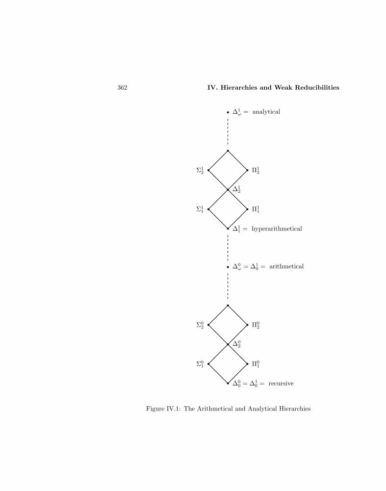
362 IV. Hierarchies and Weak Reducibilities
@@
@
@@
@
@@
@
@@
@
r
r
r
r
r
r
r
r
∆00 = ∆1
0 = recursive
∆02
∆0ω = ∆1
0 = arithmetical
Π01
Π02
Σ01
Σ02
@@
@
@@
@
@@
@
@@
@
r
r
r
r
r
r
r
r
∆11 = hyperarithmetical
∆12
∆1ω = analytical
Π11
Π12
Σ11
Σ12
Figure IV.1: The Arithmetical and Analytical Hierarchies

IV.1 The Arithmetical Hierarchy 363
IV.1 The Arithmetical Hierarchy
We start by considering, as the simplest framework for the definition of setsof natural numbers, First-Order Arithmetic. We first introduce the notionof arithmetical definability, and then classify sets definable in Arithmetic bylooking at their best possible definitions. We will thus obtain classes closelyrelated, both in computational content and in structure theory, to the classesof recursive and recursively enumerable sets.
The definition of truth ?
Pilate said unto him, What is truth?And when he had said this, he went out.
(John, Gospel , XVIII, 38)
The idea for a definition of truth comes from Aristotle (Metaphysica, Γ 7,1011b, 25–27):
it is false to say that the being is not or that the non-being is; it istrue to say that the being is and that the non-being is not.
Thus e.g.‘it is raining’ is true if and only if it is raining,
where the quoted phrase is the one whose truth we are trying to establish, andit is considered as a purely syntactical object, while the unquoted phrase istaken semantically, for what it means. And the quoted phrase is true if andonly if it reflects what happens in the world, as expressed by the unquotedphrase.
For natural languages this explains the meaning of truth, but it is notparticularly manageable. The advantage of formal languages is that they arebuilt by induction, and thus we can actually apply the ideas just introduced toproduce an inductive definition of truth. The original definition will be applieddirectly only to atomic formulas, while for compound formulas we will rely oninduction, and will force only the interpretation of the new symbols introduced.This was first done by Tarski [1936].
Truth in First-Order Arithmetic
There are two natural first-order languages that come to mind, for the pur-pose of classifying arithmetical definitions. They are in some sense extremeexamples, allowing respectively for a minimal and a maximal set of nonlogicalprimitive functions and predicates. We consider both of them, and prove thattheir definitional power is the same.
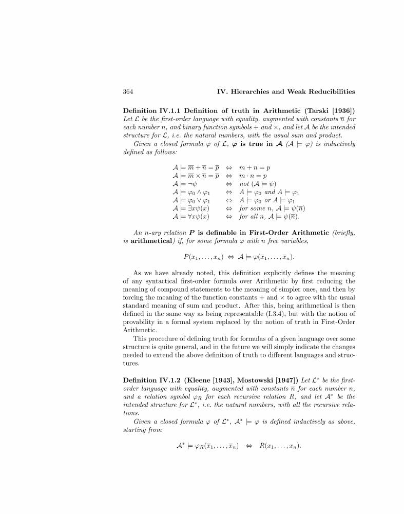
364 IV. Hierarchies and Weak Reducibilities
Definition IV.1.1 Definition of truth in Arithmetic (Tarski [1936])Let L be the first-order language with equality, augmented with constants n foreach number n, and binary function symbols + and ×, and let A be the intendedstructure for L, i.e. the natural numbers, with the usual sum and product.
Given a closed formula ϕ of L, ϕ is true in A (A |= ϕ) is inductivelydefined as follows:
A |= m+ n = p ⇔ m+ n = pA |= m× n = p ⇔ m · n = pA |= ¬ψ ⇔ not (A |= ψ)A |= ϕ0 ∧ ϕ1 ⇔ A |= ϕ0 and A |= ϕ1
A |= ϕ0 ∨ ϕ1 ⇔ A |= ϕ0 or A |= ϕ1
A |= ∃xψ(x) ⇔ for some n, A |= ψ(n)A |= ∀xψ(x) ⇔ for all n, A |= ψ(n).
An n-ary relation P is definable in First-Order Arithmetic (briefly,is arithmetical) if, for some formula ϕ with n free variables,
P (x1, . . . , xn) ⇔ A |= ϕ(x1, . . . , xn).
As we have already noted, this definition explicitly defines the meaningof any syntactical first-order formula over Arithmetic by first reducing themeaning of compound statements to the meaning of simpler ones, and then byforcing the meaning of the function constants + and × to agree with the usualstandard meaning of sum and product. After this, being arithmetical is thendefined in the same way as being representable (I.3.4), but with the notion ofprovability in a formal system replaced by the notion of truth in First-OrderArithmetic.
This procedure of defining truth for formulas of a given language over somestructure is quite general, and in the future we will simply indicate the changesneeded to extend the above definition of truth to different languages and struc-tures.
Definition IV.1.2 (Kleene [1943], Mostowski [1947]) Let L∗ be the first-order language with equality, augmented with constants n for each number n,and a relation symbol ϕR for each recursive relation R, and let A∗ be theintended structure for L∗, i.e. the natural numbers, with all the recursive rela-tions.
Given a closed formula ϕ of L∗, A∗ |= ϕ is defined inductively as above,starting from
A∗ |= ϕR(x1, . . . , xn) ⇔ R(x1, . . . , xn).

IV.1 The Arithmetical Hierarchy 365
An n-ary relation P is in the Arithmetical Hierarchy if, for some for-mula ϕ of L∗ with n free variables,
P (x1, . . . , xn) ⇔ A∗ |= ϕ(x1, . . . , xn).
Briefly stated, the Arithmetical Hierarchy consists of the relations definablein First-Order Arithmetic, with the recursive relations as parameters. Thisseems natural from our point of view, since we want to classify sets and relationsaccording to their noneffectiveness, as expressed by the complexity of theirdefinition, and thus the recursive relations may be given for free. The nextresult shows that we are classifying the same sets as before.
Theorem IV.1.3 (Godel [1931]) The Arithmetical Hierarchy contains ex-actly the arithmetical relations.
Proof. One direction comes from the fact that the relations represented bythe atomic formulas of the language L are recursive, being built up from plusand times only. The other direction follows from the fact, proved in I.3.6, thatthe recursive relations are representable in R, and hence (since the axioms ofR are true in A) are arithmetical. 2
The Arithmetical Hierarchy
Before we can classify relations according to their definition in L∗, we need tobe able to put these definitions in some kind of normal form. This is easilyaccomplished in a standard way, by manipulation of quantifiers.
Proposition IV.1.4 The following transformations of quantifiers are permis-sible (up to logical equivalence):
1. permutation of quantifiers of the same type
2. contraction of quantifiers of the same type
3. permutation of two quantifiers, one of which bounded
4. substitution of a bounded quantifier with an unbounded one of the sametype.
Proof. Part 1 is obvious. Part 2 can be accomplished by codifying the variousquantified variables into a single one. E.g., given a formula
∀x1 . . .∀xnR(x1, . . . , xn),
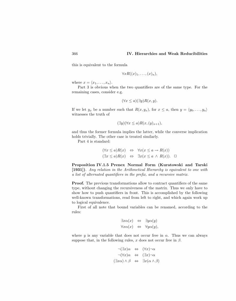
366 IV. Hierarchies and Weak Reducibilities
this is equivalent to the formula
∀xR((x)1, . . . , (x)n),
where x = 〈x1, . . . , xn〉.Part 3 is obvious when the two quantifiers are of the same type. For the
remaining cases, consider e.g.
(∀x ≤ a)(∃y)R(x, y).
If we let yx be a number such that R(x, yx), for x ≤ a, then y = 〈y0, . . . , ya〉witnesses the truth of
(∃y)(∀x ≤ a)R(x, (y)x+1),
and thus the former formula implies the latter, while the converse implicationholds trivially. The other case is treated similarly.
Part 4 is standard:
(∀x ≤ a)R(x) ⇔ ∀x(x ≤ a→ R(x))(∃x ≤ a)R(x) ⇔ ∃x(x ≤ a ∧ R(x)). 2
Proposition IV.1.5 Prenex Normal Form (Kuratowski and Tarski[1931]). Any relation in the Arithmetical Hierarchy is equivalent to one witha list of alternated quantifiers in the prefix, and a recursive matrix.
Proof. The previous transformations allow to contract quantifiers of the sametype, without changing the recursiveness of the matrix. Thus we only have toshow how to push quantifiers in front. This is accomplished by the followingwell-known transformations, read from left to right, and which again work upto logical equivalence.
First of all note that bound variables can be renamed, according to therules:
∃xα(x) ⇔ ∃yα(y)∀xα(x) ⇔ ∀yα(y),
where y is any variable that does not occur free in α. Thus we can alwayssuppose that, in the following rules, x does not occur free in β.
¬(∃x)α ⇔ (∀x)¬α¬(∀x)α ⇔ (∃x)¬α
(∃xα) ∧ β ⇔ ∃x(α ∧ β)
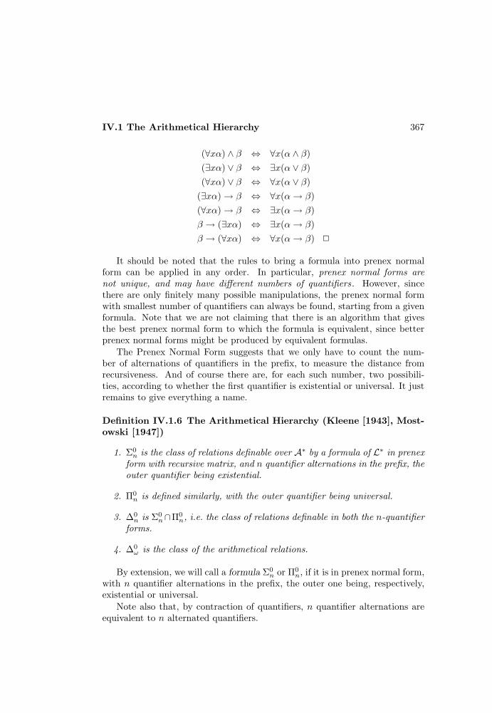
IV.1 The Arithmetical Hierarchy 367
(∀xα) ∧ β ⇔ ∀x(α ∧ β)(∃xα) ∨ β ⇔ ∃x(α ∨ β)(∀xα) ∨ β ⇔ ∀x(α ∨ β)
(∃xα) → β ⇔ ∀x(α→ β)(∀xα) → β ⇔ ∃x(α→ β)β → (∃xα) ⇔ ∃x(α→ β)β → (∀xα) ⇔ ∀x(α→ β) 2
It should be noted that the rules to bring a formula into prenex normalform can be applied in any order. In particular, prenex normal forms arenot unique, and may have different numbers of quantifiers. However, sincethere are only finitely many possible manipulations, the prenex normal formwith smallest number of quantifiers can always be found, starting from a givenformula. Note that we are not claiming that there is an algorithm that givesthe best prenex normal form to which the formula is equivalent, since betterprenex normal forms might be produced by equivalent formulas.
The Prenex Normal Form suggests that we only have to count the num-ber of alternations of quantifiers in the prefix, to measure the distance fromrecursiveness. And of course there are, for each such number, two possibili-ties, according to whether the first quantifier is existential or universal. It justremains to give everything a name.
Definition IV.1.6 The Arithmetical Hierarchy (Kleene [1943], Most-owski [1947])
1. Σ0n is the class of relations definable over A∗ by a formula of L∗ in prenex
form with recursive matrix, and n quantifier alternations in the prefix, theouter quantifier being existential.
2. Π0n is defined similarly, with the outer quantifier being universal.
3. ∆0n is Σ0
n∩Π0n, i.e. the class of relations definable in both the n-quantifier
forms.
4. ∆0ω is the class of the arithmetical relations.
By extension, we will call a formula Σ0n or Π0
n, if it is in prenex normal form,with n quantifier alternations in the prefix, the outer one being, respectively,existential or universal.
Note also that, by contraction of quantifiers, n quantifier alternations areequivalent to n alternated quantifiers.

368 IV. Hierarchies and Weak Reducibilities
The levels of the Arithmetical Hierarchy
The first levels of the hierarchy are inhabited by old friends. First of all, thelevel 0 obviously consists of the recursive relations (because no quantifier isinvolved). More interestingly,
∆01 = recursive
Σ01 = recursively enumerable.
This obviously follows from II.1.10 and II.1.19.If we wished to, we could define a similar hierarchy for formulas of L. If
we count quantifier alternations, and ask the matrix to be quantifier free (i.e.a Boolean combination of diophantine equations), we still get the r.e. sets atthe first existential level, by Matiyasevitch result (see p. 135), and thus thishierarchy coincides, from the first level on, with the Arithmetical Hierarchy.By using L∗ we simply avoid the proof of this representation theorem for ther.e. sets on one side, and have more freedom in the computations on the other.
If we are willing to compromise a little, we may allow the matrix to containbounded quantifiers. Then the proof of IV.1.3 would suffice to show that ther.e. sets are at the first existential level of this hierarchy (because of the formthe formulas that represent recursive relations in R have). The ∆0
0 relationsof this hierarchy (namely the sets definable with plus and times, by using con-nectives and bounded quantifiers) form the interesting class of rudimentarypredicates (Smullyan [1961]), to which we will return in Chapter VIII.
Exercises IV.1.7 The Bounded Arithmetical Hierarchy (Davis [1958], Harrow[1978]) Let ∆0
0 be the class of relations definable over L by using only connectives andbounded quantifiers. We can stratify it by counting the number of bounded quantifieralternations, getting classes Σ0
0,n and Π00,n in the natural way. Because of the collapse
in d) below, ∆00,n is defined as the class of sets A such that both A and A are in the
n-th level of the hierarchy.a) Π0
0,n and Σ00,n are closed under conjunction and disjunction.
b) For n ≥ 1, Π00,n is closed under universal quantification bounded by a poly-
nomial, and Σ00,n is closed under existential quantification bounded by a polynomial .
(Hint: by induction, since e.g.
(∃z ≤ p(~x) + q(~x))P (z) ⇔ (∃a ≤ p(~x))(∃b ≤ q(~x))P (a+ b)
(∃z ≤ p(~x) · q(~x))P (z) ⇔ (∃a ≤ p(~x))(∃b < q(~x))P (p(~x) · b+ a).)
c) The matrix can always be reduced to a diophantine equation. (Hint: diophantineequations p(~x) = 0, where p is a polynomial with integral coefficients, are closed underBoolean combinations. Precisely,
p(~x) = q(~x) ⇔ p(~x)− q(~x) = 0
p(~x) 6= 0 ⇔ p(~x) < 0 ∨ 0 < p(~x)
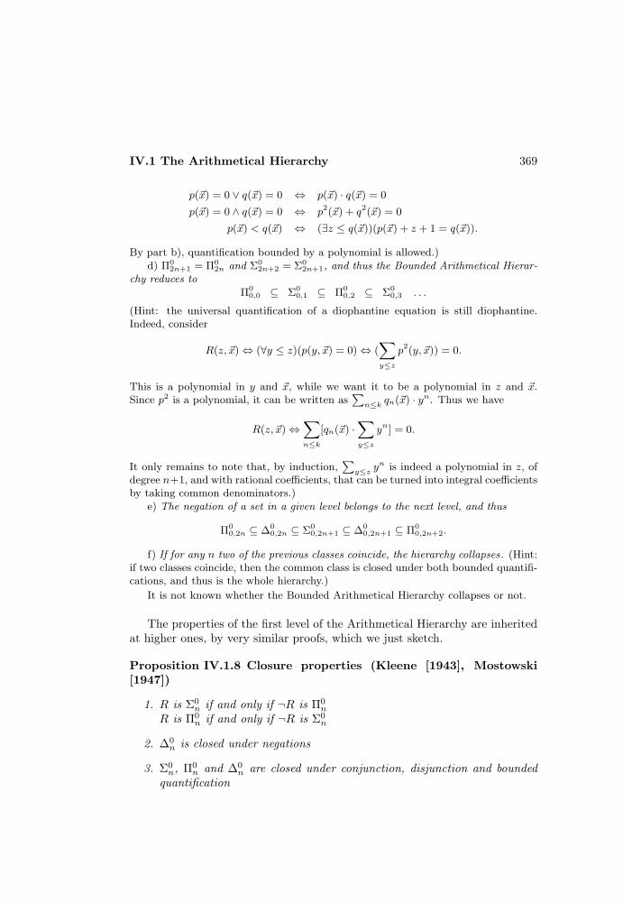
IV.1 The Arithmetical Hierarchy 369
p(~x) = 0 ∨ q(~x) = 0 ⇔ p(~x) · q(~x) = 0
p(~x) = 0 ∧ q(~x) = 0 ⇔ p2(~x) + q2(~x) = 0
p(~x) < q(~x) ⇔ (∃z ≤ q(~x))(p(~x) + z + 1 = q(~x)).
By part b), quantification bounded by a polynomial is allowed.)d) Π0
2n+1 = Π02n and Σ0
2n+2 = Σ02n+1, and thus the Bounded Arithmetical Hierar-
chy reduces to
Π00,0 ⊆ Σ0
0,1 ⊆ Π00,2 ⊆ Σ0
0,3 . . .
(Hint: the universal quantification of a diophantine equation is still diophantine.Indeed, consider
R(z, ~x) ⇔ (∀y ≤ z)(p(y, ~x) = 0) ⇔ (∑y≤z
p2(y, ~x)) = 0.
This is a polynomial in y and ~x, while we want it to be a polynomial in z and ~x.Since p2 is a polynomial, it can be written as
∑n≤k qn(~x) · yn. Thus we have
R(z, ~x) ⇔∑n≤k
[qn(~x) ·∑y≤z
yn] = 0.
It only remains to note that, by induction,∑
y≤z yn is indeed a polynomial in z, of
degree n+1, and with rational coefficients, that can be turned into integral coefficientsby taking common denominators.)
e) The negation of a set in a given level belongs to the next level, and thus
Π00,2n ⊆ ∆0
0,2n ⊆ Σ00,2n+1 ⊆ ∆0
0,2n+1 ⊆ Π00,2n+2.
f) If for any n two of the previous classes coincide, the hierarchy collapses. (Hint:if two classes coincide, then the common class is closed under both bounded quantifi-cations, and thus is the whole hierarchy.)
It is not known whether the Bounded Arithmetical Hierarchy collapses or not.
The properties of the first level of the Arithmetical Hierarchy are inheritedat higher ones, by very similar proofs, which we just sketch.
Proposition IV.1.8 Closure properties (Kleene [1943], Mostowski[1947])
1. R is Σ0n if and only if ¬R is Π0
n
R is Π0n if and only if ¬R is Σ0
n
2. ∆0n is closed under negations
3. Σ0n, Π0
n and ∆0n are closed under conjunction, disjunction and bounded
quantification

370 IV. Hierarchies and Weak Reducibilities
4. for n ≥ 1, Σ0n is closed under existential quantification, and Π0
n is closedunder universal quantification
5. the universal quantification of a Σ0n relation is Π0
n+1, and the existentialquantification of a Π0
n relation is Σ0n+1.
Proof. Everything easily follows from logical operations and quantifier manip-ulations. E.g., let ∃x∀yR and ∃x∀yQ be Σ0
2 formulas. Then, if v, w, z, and wdo not occur free in Q or R,
(∃x∀yR) ∧ (∃x∀yQ) ⇔ (∃v∀wR) ∧ (∃z∀tQ)⇔ ∃v∃z∀w∀t(R ∧Q),
and this is a Σ02 formula. 2
Theorem IV.1.9 Enumeration Theorem (Kleene [1943], Mostowski[1947]) For each n,m ≥ 1 there is an m+ 1-ary Σ0
n relation that enumeratesthe m-ary Σ0
n relations. Similarly for Π0n.
Proof. This is simply a consequence of the Normal Form Theorem for r.e.relations, II.1.10, according to which there is an m + 1-ary Σ0
1 relation enu-merating the m-ary Σ0
1 relations. Then its negation enumerates the m-ary Π01
relations.Inductively, let R(e, x, ~z) be an m + 2-ary Σ0
n relation enumerating them+ 1-ary Σ0
n relations. Then ∀xR(e, x, ~z) is an m+ 1-ary Π0n+1 relation enu-
merating the m-ary Π0n+1 relations, and its negation enumerates the m-ary
Σ0n+1 relations. 2
Definition IV.1.10 A set A is Σ0n-complete if it is Σ0
n, and every Σ0n set is
m-reducible to it. Π0n-complete sets are defined similarly.
The concept of Σ0n-completeness is the analogue, at level n, of the concept
of m-completeness for r.e. sets. By induction we thus have:
Proposition IV.1.11 For each n ≥ 1, Σ0n-complete and Π0
n-complete setsexist.
In Chapter X we will see that many natural index sets (p. II.2.8) are com-plete at some level of the Arithmetical Hierarchy.
Exercises IV.1.12 Partial truth definitions. Let ψee∈ω be an effective enu-meration of the closed formulas of L.
a) For each n ≥ 1, the set
e ∈ Tn ⇔ ψe is Σ0n ∧ A |= ψe

IV.1 The Arithmetical Hierarchy 371
is Σ0n-complete. Similarly for Π0
n. (Hint: first note that to check, of a given formula,whether it is Σ0
n is a recursive procedure. To show that Tn is Σ0n proceed induc-
tively, using the definition of truth in A: note that if there are no quantifiers thenthe formulas are recursive, and their truth can be effectively determined. To showcompleteness, use the existence of Σ0
n-complete sets.)b) The set
〈e, n〉 ∈ T ⇔ e ∈ Tnis not arithmetical . (Tarski [1936]) (Hint: if it were, it would be Σ0
n for some n. This
would contradict the Hierarchy Theorem given below.)
Theorem IV.1.13 Hierarchy Theorem (Kleene [1943], Mostowski[1947] The Arithmetical Hierarchy does not collapse. More precisely, for anyn ≥ 1 the following hold:
1. Σ0n −Π0
n 6= ∅, and hence ∆0n ⊂ Σ0
n
2. Π0n − Σ0
n 6= ∅, and hence ∆0n ⊂ Π0
n
3. Σ0n ∪Π0
n ⊂ ∆0n+1.
Proof. The first two parts are equivalent, by taking negations. The proof ofthe first one is similar to the one of II.2.3: if R(e, x) enumerates the unary Σ0
n
relations, thenP (x) ⇔ R(x, x)
is Σ0n. But it cannot be Π0
n, otherwise its negation would be Σ0n, and there
would be e such that
R(e, x) ⇔ ¬P (x) ⇔ ¬R(x, x).
For x = e a contradiction would follow.For the last part, note that we can always add dummy quantifiers in front or
at the end of the prefix, and thus Σ0n ∪Π0
n ⊆ ∆0n+1. To show that the inclusion
is strict, let P ∈ Σ0n −Π0
n: then ¬P ∈ Π0n − Σ0
n. If
Q(x, z) ⇔ [P (x) ∧ z = 0] ∨ [¬P (x) ∧ z = 1]
then Q ∈ ∆0n+1. But Q is not in Π0
n, otherwise so would be
P (x) ⇔ Q(x, 0),
and similarly Q is not in Σ0n. 2
The results just proved justify the picture of the Arithmetical Hierarchygiven in Figure 1 (p. 362), where upward connections mean strict inclusion,and no other inclusion holds.
372 IV. Hierarchies and Weak Reducibilities
We have defined the Arithmetical Hierarchy by iterating quantifiers andproved, by direct arguments, properties of the various levels similar to those ofthe first level. The next result gives a different, purely recursion-theoretical,definition of the Arithmetical Hierarchy, and explains the similarities of thevarious levels. It also suggests the possibility of different proofs for the resultsproved above, by relativization of the results of the first level.
Theorem IV.1.14 Post’s Theorem (Post [1948], Kleene) A relation is:
1. ∆0n+1 if and only if it is recursive in a Σ0
n or a Π0n relation
2. Σ0n+1 if and only if it is recursively enumerable in a Σ0
n or a Π0n relation.
Proof. First note that, for what concerns relative recursive computations,Σ0n and Π0
n are interchangeable, because an oracle and its complement areequivalent. We can thus use any of them.
We first prove part 2. Suppose P is Σ0n+1: then, for some R in Π0
n,
P (~x) ⇔ ∃yR(~x, y).
By the relativized version of II.1.10, P is then r.e. in R, and hence r.e. in a Π0n
relation.Conversely, let P be r.e. in a Π0
n relation Q. Then P is r.e. in a Π0n set A,
obtained by coding Q:
〈x1, . . . , xm〉 ∈ A⇔ Q(x1, . . . , xm).
By the relativized version of II.1.10, together with compactness and monotonic-ity (II.3.13), there is an r.e. relation R such that
P (~x) ⇔ ∃u∃v(Du ⊆ A ∧Dv ⊆ A ∧R(~x, u, v)).
Note thatDu ⊆ A⇔ (∀x ∈ Du)(x ∈ A).
Since Du is finite, the quantifier is bounded: but A is in Π0n, and then so is the
whole expression Du ⊆ A. Similarly,
Dv ⊆ A⇔ (∀x ∈ Dv)(x 6∈ A)
is Σ0n, because the negation of A is used. Thus both expressions are Σ0
n+1,and so is R, being r.e. (and hence Σ0
1). But Σ0n+1 is closed under existential
quantification, and thus P is in it.Part 1 follows from part 2 and the relativized version of II.1.19. If P is
recursive in a Σ0n relation, then both P and ¬P are r.e. in it, and hence Σ0
n+1.
IV.1 The Arithmetical Hierarchy 373
But then P is both Σ0n+1 and Π0
n+1, and hence ∆0n+1. The converse is similar:
suppose that P and ¬P are each r.e. in some (not necessarily the same one)Σ0n+1 relation. Then they are r.e. in the complete Σ0
n+1 set, and hence bothΣ0n+1. Thus P is ∆0
n+1. 2
Exercises IV.1.15 a) For any n ≥ 1, the union of two Σ0n sets can be reduced to
the union of two disjoint Σ0n sets. (Hint: see II.1.23.)
b) For any n ≥ 1, there are two disjoint Σ0n sets that cannot be separated by a ∆0
n
set . (Hint: see II.2.5.)
c) Any two Σ0n-complete sets are recursively isomorphic. (Hint: use III.7.13.)
∆02 sets
As a special case of Post’s Theorem, we get:
Proposition IV.1.16 A set is ∆02 if and only if it is recursive in K.
Proof. K is Σ01-complete, and hence any Σ0
1 or Π01 relations is recursive in it.
Thus, being recursive in some Σ01 or Π0
1 relation is equivalent to being recursivein K. 2
This allows us to prove an interesting characterization, useful in construc-tions.
Proposition IV.1.17 The Limit Lemma (Shoenfield [1959]) A is ∆02 if
and only if its characteristic function is the limit of a recursive function g, i.e.
cA(x) = lims→∞
g(x, s).
Proof. If g is given, then
x ∈ A ⇔ ∀s∃t(t ≥ s ∧ g(x, t) = 1)⇔ ∃s∀t(t ≥ s→ g(x, t) = 1),
and A is ∆02.
Conversely, if A is ∆02 then A ≤T K. Let e be such that cA ' ϕKe , and
g(x, s) ' ϕKse (x).
Then cA is the limit of g. 2
This characterization of ∆02 suggests a possible hierarchy for it, obtained
by bounding the number of times the approximating function g may change.The r.e. sets can be obtained by approximations that change at most once (let
374 IV. Hierarchies and Weak Reducibilities
g(x, s) be 0 until it is discovered that x is in the set, and 1 afterwards). Ifwe consider the sets whose approximation may change only n times, we havethe Boolean Hierarchy, which stratifies the set belonging to the smallestBoolean algebra generated by the r.e. sets (or, by III.8.7, the sets btt-reducibleto K) (Addison [1965], Gold [1965], Putnam [1965], Ershov [1968]). Obviously,∆0
2 is not exhausted by the Boolean Hierarchy (since there are sets recursivein K and not btt-reducible to it), but this can be achieved by an appropriatetransfinite extension of the hierarchy (Ershov [1968a], [1970], see Chapter XI).
Exercises IV.1.18 The Boolean hierarchy (Ershov [1968]). For n ≥ 1, let Σ−1n
be the class of sets with a recursive approximation g which changes at most n times,and such that g(x, 0) = 0. Π−1
n is the class of complements of sets in Σ−1n , and
∆−1n = Σ−1
n ∩ Π−1n . A set is called n-r.e. if it is Σ−1
n , and weakly n-r.e. if it is∆−1n+1.
a) Σ−11 is the class of r.e. sets.
b) For n ≥ 1, Σ−1n is the class of sets of the form (A1−A2)∪ (A3−A4) · · · , with
Ai r.e.c) For each n ≥ 1, there are Σ−1
n -complete sets. (Hint: let
〈x, y〉 ∈ A ·B ⇔ x ∈ A ∧ y ∈ B and 〈x, y〉 ∈ A+B ⇔ x ∈ A ∨ y ∈ B,
and consider the sequence of sets
K K · K (K · K) +K · · · )
d) For each n ≥ 1, Σ−1n −Π−1
n 6= ∅, and Π−1n −Σ−1
n 6= ∅. (Hint: use the sets givenin part c.)
e) For each n ≥ 2, there is a ∆−1n -complete set . (Hint: if A and B are, respectively,
Σ−1n -complete and Π−1
n -complete, then A⊕B is ∆−1n+1-complete.)
f) For any n, Σ−1n ∪Π−1
n ⊂ ∆−1n+1. (Hint: use the set given in part e.)
g) For n ≥ 1, a set is ∆−1n+1 if and only if it has a recursive approximation that
changes at most n times. (Hint: suppose A is both Σ−1n and Π−1
n . Then both A and
its complement can be approximated by recursive functions g and h that change at
most n + 1 times, and with value 0 at stage 0. For any x, we then know that one
of g(x, 0) and h(x, 0) is wrong. Look for the first s such that g(x, s) 6= h(x, s), and
let g(x, s) be the first value of a new function f approximating A. Let f change only
when g does, and g and h differ. Then f changes at most n times.)
Note that there is nothing special about the second level: the characteriza-tion of ∆0
2 obviously extends, by relativization, to all levels.
Proposition IV.1.19 Shoenfield [1959]) For n ≥ 1, A is ∆0n+1 if and only
if there is an n+ 1-ary recursive function g such that
cA(x) = lims1→∞
· · · limsn→∞
g(x, s1, . . . , sn).
IV.1 The Arithmetical Hierarchy 375
Relativizations ?
We can relativize all the work done so far to a given oracle X, defining theclasses Σ0,X
n , Π0,Xn and ∆0,X
n , and obtaining similar results, simply by substi-tuting ‘recursive’ with ‘recursive in X’. In particular, we have
A ≤T B ⇔ A ∈ ∆0,B1 .
We might thus think that a number of other reducibilities can be defined, bylooking at higher levels. The next result shows that this is not the case.
Proposition IV.1.20 The relation
A ≤∆0nB ⇔ A ∈ ∆0,B
n
is transitive only for n = 1.
Proof. The transitivity for n = 1 follows from the fact that in this case ≤∆01
is simply Turing reducibility. For any n > 1, we show a counterexample. LetA ∈ Σ0
n−Π0n, which exists by the Hierarchy Theorem. Then there is B ∈ Π0
n−1
such thatx ∈ A⇔ ∃yB(x, y).
By definition A is in Σ0,B1 , and hence in ∆0,B
n (since n > 1). Since B is in ∆0n
by its choice, if ≤∆0n
were transitive we would have A ∈ ∆0n, and hence A ∈ Π0
n,contradiction. 2
The obvious reason why the transitivity of ≤∆0n
fails for n > 1, is thatquantifiers simply sum up: if B has n quantifiers, and we stick n more in frontof it, one might collapse (if the leftmost quantifier of the prefix of B is of thesame type of the rightmost added in front of it), but the others are going toremain. This ceases to be a problem, if we do not care anymore for a fixednumber of quantifiers.
Definition IV.1.21 A is arithmetical in B (A ≤a B) if it is in the Arith-metical Hierarchy relativized to B.
A is arithmetically equivalent to B (A ≡a B) if A ≤a B and B ≤a A.
Exercises IV.1.22 a) If A is arithmetical, then A ≤a B for any set B.
b) If A ≤a B and B is arithmetical, so is A.
Note that ≤a is a reflexive and transitive relation, and thus ≡a is an equiv-alence relation.
Definition IV.1.23 The equivalence classes of sets w.r.t. arithmetical equiv-alence are called a-degrees, and (Da, ≤) is the structure of a-degrees, withthe partial ordering ≤ induced on them by ≤a.
The structure of the a-degrees will be studied in Chapter XIII.

376 IV. Hierarchies and Weak Reducibilities
IV.2 The Analytical Hierarchy
The Arithmetical Hierarchy certainly includes only a small portion of all pos-sible sets, being countable (each set has a definition in L∗, and there are onlycountably many definitions). Moreover, by Tarski’s Theorem (see p. 166, orIV.1.12.b), there are natural examples of nonarithmetical sets (namely, the setof codes of sentences of L true in Arithmetic). We thus feel the need of enlarg-ing the Arithmetical Hierarchy. One natural way to proceed is by extendingthe language and going to the second order, i.e. by considering quantifiers notonly over numbers, but also over functions.
Truth in Second-Order Arithmetic
As already for First-Order Arithmetic, there are at least two possible languagesof interest.
Definition IV.2.1 Definition of truth in Second-Order Arithmetic(Tarski [1936]). Let L2 be the second-order language with first-order equality,augmented with number constants n for each number n, and function constantsf for each total function f , among them + and ×. Let also A2 be the intendedstructure for L2, i.e. the set of natural numbers and total functions over them.
Given a closed formula ϕ of L2, A2 |= ϕ is defined inductively as usual.A relation P of n number variables and m function variables is definable
in Second-Order Arithmetic (from parameters) if, for some closed for-mula ϕ of L∗2 with n free number variables and m free function variables,
P (x1, . . . , xn, f1, . . . , fm) ⇔ A∗2 |= ϕ(x1, . . . , xn, f1, . . . , fm).
If ϕ contains no function constant except plus and times, then P is simplyanalytical.
Notice that ‘analytical’ is defined without the use of parameters (i.e. func-tion constants other than + and ×). Since the use of parameters is like theuse of oracles (see Section II.3), the analytical relations are those that can bedefined in Second-Order Arithmetic, without any help.
The reason for the name ‘analytical’ comes from the fact that Second-OrderArithmetic allows for the formalization of elementary Analysis, by coding realnumbers as functions of integers.
Definition IV.2.2 (Lusin [1925], Sierpinski [1925], Kleene [1955]) LetL∗2 be the second-order language with first-order equality, augmented with num-ber constants n for each number n, function constants f for each total functionf , and relation symbols ϕR for each restricted recursive relation of numbers
IV.2 The Analytical Hierarchy 377
and total functions. Let also A∗2 be the intended structure for L∗2, i.e. the set ofnatural numbers and total functions over them, with all the restricted recursiverelations of numbers and total functions.
Given a closed formula ϕ of L∗2, A∗2 |= ϕ is defined inductively as usual.A relation P of n number variables and m function variables is in the Pro-
jective Hierarchy if, for some closed formula ϕ of L∗2 with n free numbervariables and m free function variables,
P (x1, . . . , xn, f1, . . . , fm) ⇔ A∗2 |= ϕ(x1, . . . , xn, f1, . . . , fm).
If ϕ contains no function constant except plus and times, then P is in theAnalytical Hierarchy.
It follows from IV.1.3 relativized that the Analytical Hierarchy containsexactly the analytical relations.
The Analytical Hierarchy
Function quantifiers can be manipulated in a way similar to number quantifiers.
Proposition IV.2.3 The following transformations of function quantifiers arepermissible (up to logical equivalence):
1. permutation of quantifiers of the same type
2. contraction of quantifiers of the same type
3. permutation of a number quantifier and a function quantifier
4. substitution of a number quantifier with a function quantifier of the sametype.
Proof. Part 1 is obvious. Parts 2 needs only a way to code and decode finitelymany functions, e.g.
〈f1, . . . , fn〉(x) = 〈f1(x), . . . , fn(x)〉(f)n(x) = (f(x))n.
Then e.g. the formula∀f1 . . .∀fnR(f1, . . . , fn),
is equivalent to∀fR((f)1, . . . , (f)n).
378 IV. Hierarchies and Weak Reducibilities
Part 3 needs a way to code and decode infinitely many functions, e.g.
f(x) =fn(z) if x = 〈n, z〉0 otherwise
(f)n(z) = f(〈n, z〉).
Having this, and given e.g.
(∀x)(∃f)R(f, x),
let fn be such that R(fn, n) holds. Then the given formula is equivalent to
(∃f)(∀x)R((f)x, x).
Part 4 is easily obtained, noting that
∃xR(x) ⇔ ∃fR(f(0)) and ∀xR(x) ⇔ ∀fR(f(0)). 2
Proposition IV.2.4 Prenex Normal Form (Kuratowski and Tarski[1931]). Any relation in the Analytical Hierarchy is equivalent to one witha list of alternated function quantifiers in the prefix, and an arithmetical ma-trix.
Proof. Similar to IV.1.5. 2
Proposition IV.2.5 (Kleene [1955]) The matrix of a relation in the Ana-lytical Hierarchy can always be reduced to a single number quantifier, oppositein type to the rightmost function quantifier of the prefix, followed by a recursivepredicate.
Proof. Having a formula in prenex normal form, with a prefix consisting ofalternated function quantifiers, and an arithmetical matrix, there are two cases.If there are at least two function quantifiers, then all the number quantifierscan be eliminated, by first moving near to the function quantifier of the sametype, then rising to function quantifiers, and being contracted; afterwards, onedummy number quantifier can be reintroduced. If there is only one numberquantifier, then this works only for the number quantifiers of its same type,while the other remain, and can be contracted to a single one.
More precisely, proceed as follows.
• Reduce the matrix in prenex normal form, with a prefix of alternatednumber quantifiers, and a recursive matrix.
• Take the leftmost number quantifier, and confront it with the rightmostfunction quantifier of the prefix. If they are of the same type, raise thenumber quantifier to a function quantifier, and then contract.

IV.2 The Analytical Hierarchy 379
• If they are not of the same type, permute them. See if there is a functionquantifier to the left. If so, it must be of the same type as the numberquantifier, which can thus be eliminated as above. If not, proceed withthe next number quantifier in the matrix, inductively.
• At the end, either all number quantifiers have been eliminated, or a se-quence of them, of the same type, lies to the left of the (necessarilyunique) function quantifier. Contract them, and permute the resultingnumber quantifier back to the matrix. 2
Exercises IV.2.6 Set quantifiers. a) The same analytical classes are obtained ifwe use set quantifiers in place of function quantifiers, and matrices with at most twonumber quantifiers. (Kleene [1955]) (Hint: sets and their characteristic functions canbe identified, and we can thus work with the latter. In one direction, to say that afunction is a characteristic function only involves a number quantifier, e.g.
(∃A)R(cA) ⇔ ∃f [∀x(f(x) ≤ 1) ∧ R(f).]
In the other direction, functions can be substituted by their graphs, and saying thatf is the characteristic function of the graph of a total function is an arithmeticalcondition: f has values bounded by 1; whenever it is 1 for z, then z = 〈x, y〉, i.e. itcodes a relation; whenever it is 1 for 〈x, y〉 and 〈x, y′〉 then y = y′, i.e. the relationis a function; and for every x there is y such that f(〈x, y〉) = 1, i.e. the function istotal. Note that this last condition introduces two number quantifiers.)
b) Set quantifiers and matrices with only one number quantifier are not suffi-
cient to generate the whole Analytical Hierarchy . (Kreisel) (Hint: the predicate
∀A∃xR(cA(x)), with R recursive, is r.e. Indeed, the set of sets is finitely branch-
ing. Thus, by Konig’s Lemma, if for every A there is x such that R(cA(x)) holds,
there must be an x that works for every A. This means that we only have to look for
x such that (∀A)R(cA(x)) holds. For a fixed x this is a recursive condition, because
there are only finitely many possible sequence numbers of length x. Thus the whole
condition is r.e.)
Exactly like we did for the Arithmetical Hierarchy, we can now count thenumber of alternations of function quantifiers, and stratify the Analytical Hi-erarchy.
Definition IV.2.7 The Analytical Hierarchy (Lusin [1925], Sierpinski[1925], Kleene [1955])
1. Σ1n is the class of relations definable over A∗2 by a formula of L∗2 (without
parameters) in prenex form with arithmetical matrix, and n quantifieralternations in the prefix, the outer quantifier being existential.
2. Π1n is defined similarly, with the outer quantifier being universal.
380 IV. Hierarchies and Weak Reducibilities
3. ∆1n is Σ1
n∩Π1n, i.e. the class of relations definable in both the n-quantifier
forms.
4. ∆1ω is the class of the analytical relations.
By extension, we will call a formula without parameters Σ1n or Π1
n if it is inprenex normal form with n function quantifier alternations in the prefix, thefirst of which, respectively, existential or universal.
Note also that, by contraction of quantifiers, n function quantifier alterna-tions are equivalent to n alternated function quantifiers.
The levels of the Analytical Hierarchy
A good part of the theory of the Arithmetical Hierarchy goes through for theAnalytical Hierarchy as well, with similar proofs, that we do not repeat.
Proposition IV.2.8 Closure properties (Kleene [1955])
1. R is Σ1n if and only if ¬R is Π1
n
R is Π1n if and only if ¬R is Σ1
n
2. ∆1n is closed under negations
3. Σ1n, Π1
n and ∆1n are closed under conjunction, disjunction and number
quantification
4. for n ≥ 1, Σ1n is closed under existential function quantification, and Π1
n
is closed under universal function quantification
5. the universal function quantification of a Σ1n relation is Π1
n+1, and theexistential function quantification of a Π1
n relation is Σ1n+1.
Proof. Everything easily follows from logical operations and quantifier ma-nipulations. E.g., closure under number quantification follows by moving thenumber quantifier to the matrix, by successive permutations. 2
Theorem IV.2.9 Enumeration Theorem (Kleene [1955]) For each n andm ≥ 1, and any l, there is a Σ1
n relation with m + 1 number variables and lfunction variables that enumerates the Σ1
n relations with m number variablesand l function variables. Similarly for Π1
n.
Proof. Similar to IV.1.9, using this time the Normal Form Theorem for r.e.relations of numbers and total functions, that follows from II.3.11. Note that,because of IV.2.5, the hierarchy is inductively built up by starting from the r.e.predicates, by negations and function quantifications. 2
IV.2 The Analytical Hierarchy 381
Corollary IV.2.10 Normal Form Theorem for Π11 sets (Lusin [1917],
Suslin [1917], Kleene [1955]) A is Π11 if and only if, for some recursive
predicate R,x ∈ A⇔ ∀f∃yR(x, f(y)).
Definition IV.2.11 A set A is Σ1n-complete if it is Σ1
n, and every Σ1n set is
m-reducible to it. Π1n-complete sets are defined similarly.
Proposition IV.2.12 For each n ≥ 1, Σ1n-complete and Π1
n-complete setsexist.
Theorem IV.2.13 Hierarchy Theorem (Lebesgue [1905], Lusin [1925],Sierpinski [1925], Kleene [1955]) The Analytical Hierarchy does not col-lapse. More precisely, for any n ≥ 1 the following hold:
1. Σ1n −Π1
n 6= ∅, and hence ∆1n ⊂ Σ1
n
2. Π1n − Σ1
n 6= ∅, and hence ∆1n ⊂ Π1
n
3. Σ1n ∪Π1
n ⊂ ∆1n+1.
We thus get a picture for the Analytical Hierarchy similar to the one ob-tained for the Arithmetical Hierarchy, see Figure 1 (p. 362).
Despite the similarities between the Arithmetical and Analytical Hierar-chies, there are differences. The most striking one seems to be the fact thatthere is no recursion-theoretical generation of the Analytical Hierarchy frombelow. Thus function quantifiers, unlike number quantifiers (that correspondto relative recursive enumerability) seem to have no computational content . Seep. 395 for a precise statement of this fact.
Π11 sets
The Normal Form Theorem for Π11 sets suggests some natural representations
for them, in set-theoretical terms. To state them precisely, we first introducesome terminology.
Definition IV.2.14 A set of sequence numbers T is a tree if it is closedunder subsequences. 〈∅〉 is the root, or vertex, of the tree. Elements of thetree are called nodes. A branch of T is a maximal linearly ordered subset ofT . The terminal node of a branch is a leaf. A tree is well-founded if it hasno infinite branch.
Thus a tree is simply a subset of the tree of all sequence numbers orderedby extension, such that whenever a node is in T , so are all nodes between it

382 IV. Hierarchies and Weak Reducibilities
rr r rr r rr r
bb
bb
b
""
""
"
@@
@
@@
@
〈∅〉
〈7〉〈3〉 〈10〉
〈3, 1〉〈10, 1〉 〈10, 3〉
〈3, 1, 0〉 〈3, 1, 4〉
Figure IV.2: A tree
and the vertex 〈∅〉. Moreover, an infinite branch of a tree can be thought ofas a function f whose course-of-values determines the branch (recall, see p.90, that the course-of-value of f is the function f , where f(y) is the sequencenumber coding the first y values of f).
Well-foundedness of a partial ordering usually refers to lack of infinite de-scending sequences. Here a branch can be thought of as a descending sequence(if we picture the tree as growing downward, as in Figure 2): thus the termi-nology is consistent, and a tree is well-founded as a tree if and only if it is soas a partial ordering. What makes well-founded trees interesting is that it ispossible to proceed by induction on them, from the leaves to the vertex. Thisprocedure of backward induction is called bar-recursion. The next result ismostly a rephrasing of the Normal Form Theorem IV.2.10.
Theorem IV.2.15 First Representation Theorem for Π11 sets (Lusin
and Sierpinski [1923], Kleene [1955]) A set A is Π11 if and only if there is
a recursive sequence Txx∈ω of recursive trees, such that
x ∈ A⇔ Tx is well -founded.
Proof. If A is Π11 then, for some recursive R,
x ∈ A⇔ ∀f∃yR(x, f(y)).
It is now enough to define
u ∈ Tx ⇔ Seq(u) ∧ (∀v < u)¬R(x, v),
where u and v range over sequence numbers and (see p. 90) < means properinitial subsequence. Clearly Tx is a recursive tree, uniformly in x. A leaf corre-sponds to a first place in which R holds. An infinite branch of Tx corresponds
IV.2 The Analytical Hierarchy 383
to a function f such that ∀y¬R(x, f(y)), and it exists if and only if x 6∈ A.Thus x ∈ A if and only if Tx is well-founded.
Conversely, let Txx∈ω be a recursive sequence of recursive trees, and sup-pose
x ∈ A⇔ Tx is well-founded.
Then A is Π11, since
x ∈ A ⇔ ¬∃f∀y(f(y) ∈ Tx)
⇔ ∀f∃y(f(y) 6∈ Tx),
by the interpretation of infinite branches of trees as functions. Note that therelation f(y) 6∈ Tx is recursive, as a relation of f , x, and y, because Tx isuniformly recursive in x. 2
Corollary IV.2.16 The set T of characteristic indices of well -founded recur-sive trees is Π1
1-complete.
Proof. T is Π11 because ‘being the index of the characteristic function of a
tree’ is an arithmetical condition, and ‘having no infinite branch’ is Π11:
e ∈ T ⇔ (∀x)(∃y)[y ≤ 1 ∧ ϕe(x) ' y] ∧(∀x)[ϕe(x) ' 1 → Seq(x)] ∧(∀x)(∀y)[x v y ∧ ϕe(y) ' 1 → ϕe(x) ' 1] ∧(∀f)(∃y)[ϕe(f(y)) ' 0].
T is Π11-complete by the proof of the First Representation Theorem. More
precisely, ifx ∈ A⇔ ∀f∃yR(x, f(y))
for some recursive R then there is, by the Smn -Theorem, a recursive function gsuch that
ϕg(x)(u) '
1 Seq(u) ∧ (∀v < u)¬R(x, v)0 otherwise.
Then A ≤m T , because
x ∈ A⇔ g(x) ∈ T . 2
Notice that it is possible to assign to each well-founded tree T an ordinal,as follows (by bar-recursion):

384 IV. Hierarchies and Weak Reducibilities
Definition IV.2.17 If T is a well -founded tree, the ordinal of a node u onT is defined as:
ordT (u) =sup1 + ordT (u ∗ 〈n〉) if (∃n)(u ∗ 〈n〉 ∈ T )1 otherwise.
The ordinal of a well-founded tree T is defined as:
ord(T ) =ordT (〈∅〉) if T 6= ∅0 otherwise.
Thus we assign 1 to the terminal nodes of each branch of a tree, and then weclimb the tree by assigning to each nonterminal node the least ordinal not yetassigned to any of its successors. A nonempty tree has the ordinal of its vertex〈∅〉. Of course the whole procedure works because the tree is well-founded,and thus the inductive procedure of climbing the tree from the terminal nodesmakes sense. The interesting fact is that this is really an equivalent way tolook at countable ordinals.
Proposition IV.2.18 An ordinal α is countable if and only if there is a well -founded tree T such that α = ord(T ).
Proof. Note that an ordinal is assigned to a node of T only if all the smallerordinals have already been assigned to some of its successors. Since a tree hasonly countably many nodes, being made of sequence numbers, its ordinal canhave only countably many predecessors, and it is thus countable.
Let now α be a countable ordinal: we define a well-founded tree T suchthat α = ord(T ), by induction on the countable ordinals.
• α = 0.Let T = ∅.
• α = β + 1Let T0 be a well-founded tree such that β = ord(T0). We only have tobuild a tree T that consists of a subtree isomorphic to T0, and one vertexon top of it. Let
T = 〈∅〉 ∪ 〈0〉 ∗ u : u ∈ T0.
• α = supn∈ω αnLet Tn be well-founded trees such that αn = ord(Tn). We only have tobuild a tree T that consists of subtrees isomorphic to the Tn’s, and onevertex on top of them. Let
T = 〈∅〉 ∪⋃n∈ω
〈n〉 ∗ u : u ∈ Tn. 2
IV.2 The Analytical Hierarchy 385
Since the notion of well-founded tree is easily constructivized, by consideringrecursive well-founded trees, we have a natural constructive analogue of thenotion of ordinal: a recursive ordinal is an ordinal α such that α = ord(T ),for some recursive well-founded tree T . Since the node of a tree is assigned anordinal only if all smaller ordinals have already been assigned to some of itssuccessors, and the subtree consisting of the extensions of a node of a recursivetree is isomorphic to a recursive tree, the recursive ordinals form an initialsegment of the ordinals. The first nonrecursive ordinal is indicated by ωck
1 ,because it is the constructive analogue of the first uncountable ordinal ω1,and it was introduced by Church and Kleene [1937]. Clearly ωck1 is countable,because there are only countably many recursive trees, and thus only countablymany recursive ordinals. The theory of recursive ordinals will be developed inVolume III, and will be useful for a finer analysis of the hyperarithmetical(p. 391) and Π1
1 sets.Another way to introduce countable ordinals is by looking at countable
well-orderings (equivalently, at well-orderings of ω), and thus we may guessthat there is a result similar to IV.2.15, using well-orderings instead of well-founded trees.
Definition IV.2.19 A (recursive) partial ordering is a (recursive) bi-nary relation on a (recursive) set A of numbers which is reflexive, antisymmet-ric and transitive, i.e. such that, for every x, y, z ∈ A,
1. x x
2. x y ∧ y x⇒ x = y
3. x y ∧ y z ⇒ x z.
A linear partial ordering is a partial ordering which is total on A, i.e. suchthat, for every x, y ∈ A,
4. x y ∨ y x.
A well-ordering is a linear partial ordering with no infinite descending se-quence of elements.
As usual, we will write x ≺ y for x y ∧ x 6= y.
Theorem IV.2.20 Second Representation Theorem for Π11 sets (Lusin
and Sierpinski [1923], Kleene [1955], Spector [1955]) A set A is Π11 if
and only if there is a recursive sequence ≺xx∈ω of recursive linear orderings,such that
x ∈ A ⇔ ≺x is a well -ordering.

386 IV. Hierarchies and Weak Reducibilities
Proof. By IV.2.15, it is enough to show that it is possible to go back andforth, in an effective way, from recursive trees to recursive linear orderings ofω, preserving well-foundedness and well-ordering.
Let ≺ be a recursive linear ordering of ω: we want a recursive tree T≺ suchthat
≺ is a well-ordering ⇔ T≺ is well-founded.
It is enough to define
〈x1, . . . , xn〉 ⇔ xn ≺ · · · ≺ x1.
Thus branches of T≺ code maximal descending sequences of elements w.r.t. ≺,and there are infinite branches in T≺ if and only if there are infinite descendingsequences in ≺.
Let T be a recursive tree: we want a recursive linear ordering ≺T such that
T is well-founded ⇔ ≺T is a well-ordering.
A natural way to linearly order a tree is the lexicographical one: given twosequence numbers, we look at the branches on which they lie, and give theprecedence to the one on the leftmost branch when the branches differ, and tothe one on the higher level if they are on the same branch. But for our purposesthis is overkilling: the resulting order is always a well-ordering (since each nodehas only finitely many predecessors at the same level, on different branches, andonly finitely many predecessors at lower levels, on the same branch).
The reason why this ordering is not sensitive to infinite branches of thetree is because it follows each branch in increasing order: we then have onlyto modify it, and reverse the order on single branches. Thus we will still orderlexicographically sequence numbers lying on different branches, but reverse thelexicographical order on single branches (and thus the only way to produceinfinite descending sequences will be to have infinite branches). The wantedlinear ordering is thus, for x, y ∈ T ,
x ≺T y ⇔ y < x ∨ (∃n)[(x)n < (y)n ∧ (∀i < n)((x)i = (y)i)].
This is sometimes called the Kleene-Brouwer ordering (Lusin and Sierpinski[1923], Brouwer [1924]) associated to T . 2
Exercises IV.2.21 a) The set W of characteristic indices of recursive well-orderingsof ω is Π1
1-complete. (Lusin and Sierpinski [1923], Spector [1955]) (Hint: the proofabove shows that T ≤m W, if ≺T is extended to a total ordering, e.g. by putting allnumbers not in T before everything, with their usual ordering. Thus it is enough toshow that W is Π1
1.)

IV.2 The Analytical Hierarchy 387
b) T and W are recursively isomorphic. (Hint: this holds in general, for Π11-com-
plete sets.)
Since well-orderings of ω are another way of looking at countable ordinals,we might think of defining the recursive ordinals by looking at recursive well-orderings, instead than recursive well-founded trees. Happily, by the proofjust given, the class of ordinals defined by recursive well -founded trees on oneside and recursive well -orderings on the other coincide, thus showing that thenotion of recursive ordinal is natural and stable.
We have just scratched the surface of the theory of Π11 sets, which will be
developed in detail in Volume III. We just hint here at the fact that Π11 sets
admit a natural interpretation in terms of infinitary computations. Consider arecursive finitely branching tree: by Konig’s Lemma, the process of determiningwhether it is well-founded or not is r.e. (see IV.2.6.b). Thus the process ofdetermining whether a recursive tree is well-founded can be seen as an infinitaryanalogue of an r.e. question. This can be made precise, and it turns out thatthe Π1
1 sets are exactly the r.e. sets relative to the ordinal ωck1 (see p. 385).
∆11 sets
The level 0 of the Analytical Hierarchy corresponds to the arithmetical sets, be-cause we allow for arithmetical matrices. To describe ∆1
1 we take a constructivestand, and will show how to obtain any member of it from below.
Recall that we constructed the smallest Boolean algebra generated by ther.e. sets by closing them under complements and finite unions, and by so doingwe did not even exhaust ∆0
2. The idea here is to consider not only finiteunions, but infinite ones as well. Of course we have to be careful, since thesingletons are r.e. sets, and if we allow arbitrary countable unions then we getany possible set: this shows that infinite unions are too powerful. We consideronly constructive unions, i.e. unions of r.e. families of sets, and a great deal ofthe power is maintained, since we obtain this way all the ∆1
1 sets.
Theorem IV.2.22 Suslin-Kleene Theorem (Suslin [1917], Kleene[1955a]) ∆1
1 is the smallest class of sets
1. containing every singleton set n
2. closed under complements
3. closed under effective unions.
Proof. To be able to talk about effective unions, we are going to assign indicesto sets in the class, and operate on them by using recursive functions. We thus
388 IV. Hierarchies and Weak Reducibilities
call a class of sets C = Cxx∈C an SK-class (for Suslin-Kleene) if there arerecursive functions f1, f2 and ϕ such that
• Cf1(n) = n
• Cf2(n) = Cn
• if ϕn is total then ϕ(n)↓ and Cϕ(n) =⋃x∈ω Cϕn(x).
The theorem thus amounts to proving that ∆11 is the smallest SK-class. We
do this in two steps, first explicitly defining the smallest SK-class, and thenshowing that it coincides with ∆1
1.
1. Definition of the smallest SK-class GWe first define, by induction, the system of indices we are going to use,as the smallest set G such that
• 〈0, n〉 ∈ G• if n ∈ G then 〈1, n〉 ∈ G• if ϕn is total and ∀x(ϕn(x) ∈ G) then 〈2, n〉 ∈ G.
These indices obviously correspond to the three clauses of the definitionof a SK-class. We can then define the class G = Gxx∈G in the naturalway:
• G〈0,n〉 = n
• G〈1,n〉 = Gn
• G〈2,n〉 =⋃x∈ω Gϕn(x).
By definition, G is a SK-class. It is also the smallest such one, intuitivelybecause we put in it only what is strictly required by the definition ofSK-class, and formally because if C = Cxx∈ω is a SK-class, andf1, f2, ϕ are the recursive functions associated to it, then
x ∈ G⇒ Gx = Cg(x),
i.e. each element of G is in C, where g is any recursive function such that
g(x) =
f1(n) if x = 〈0, n〉f2(g(n)) if x = 〈1, n〉ϕ(e) if x = 〈2, n〉 and ϕe(z) ' g(ϕn(z))0 otherwise.
Note that such a function exists by the Fixed-Point Theorem.

IV.2 The Analytical Hierarchy 389
2. G is contained in ∆11
We have to show that if x ∈ G then Gx ∈ ∆11. It is enough to prove
that Gx ∈ Π11 for every x ∈ G: then, since Gx = G〈1,n〉, Gx ∈ Π1
1 andGx ∈ Σ1
1, hence Gx ∈ ∆11.
The reason why Gx ∈ Π11 is that G is the smallest class of sets satisfying an
arithmetical condition, which means that every class satisfying the samecondition must contain it: this can be expressed by a universal quantifierover classes of sets, and an arithmetical matrix, and it is ‘almost’ Π1
1.We only have to talk about sets, rather than classes of sets, and this caneasily be accomplished by considering an indexed class of sets as a binaryrelation, which can then be coded as a set. Precisely, we are going toshow that G is uniformly Π1
1, i.e. that there is a Π11 set A such that
z ∈ Gx ⇔ 〈z, x〉 ∈ A.
We will write an arithmetical predicate P (z, x,X), meaning that X is aset coding a class satisfying the conditions of the definition of SK-class,and then we will say that A is the smallest such set, as follows:
〈z, x〉 ∈ A⇔ (∀X)(P (z, x,X) → 〈z, x〉 ∈ X).
Then A will be Π11. It just remains to define P :
P (z, x,X) ⇔ [x = 〈0, n〉 ∧ z = n] ∨[x = 〈1, n〉 ∧ 〈z, n〉 6∈ X] ∨[x = 〈2, n〉 ∧ ϕn total ∧ (∃t)(〈z, ϕn(t)〉 ∈ X)].
3. ∆11 is contained in G
Suppose A is ∆11: there are two recursive relations R and Q such that
x ∈ A ⇔ ∀f∃yR(x, f(y))x ∈ A ⇔ ∀g∃y Q(x, g(y)).
To show that A ∈ G, it is enough to find a recursive function h such that
Gh(x) =x if x ∈ A∅ otherwise.
Then A =⋃x∈ω Gf(x), i.e. A is an effective union of members of G, and
hence is in G.
Since A is Π11, consider the representation of A by uniformly recursive
trees Tx given by the First Representation Theorem IV.2.15. If x ∈ A

390 IV. Hierarchies and Weak Reducibilities
then Tx is well-founded, and thus each branch is finite. We might labelthe leaves with the set x, and climb our way to the top of the tree,by giving the same label x to any node whose successors all have thatlabel. Then, if x ∈ A, the vertex (corresponding to the empty sequencenumber 〈∅〉) also has that label. This is easily defined in recursive terms,by first giving the function
ϕ0(x, u) 'x if R(x, u) ∧ (∀v < u)¬R(x, v)⋃n∈ω ϕ0(x, u ∗ 〈n〉) otherwise,
and then considering ϕ0(x, 〈∅〉). Note that there is a partial recursivefunction ψ0(x, u) such that Gψ0(x,u) = ϕ0(x, u), by the Fixed-Point The-orem:
ψ0(x, u) '〈1, x〉 if R(x, u) ∧ (∀v < u)¬R(x, v)〈2, e〉 if ϕe(n) ' ψ0(x, u ∗ 〈n〉), otherwise.
This almost produces what we want, and there is only one problem:ϕ0(x, 〈∅〉) is undefined when x ∈ A, because in this case some branch ofthe tree has no leaf, and thus we cannot climb our way to the top, sincewe never define ϕ0 on that path. However, if x ∈ A then we can playa similar strategy on the other tree, corresponding to Q. We can thusget a function ϕ1 such that ϕ1(x, 〈∅〉) gives ∅ if x ∈ A, and is undefinedotherwise. Moreover, we can find a partial recursive function ψ1 suchthat Gψ1(x,u) = ϕ1(x, u).
Since x is either in A or in A, one and only one of ϕ0(x, 〈∅〉) and ϕ1(x, 〈∅〉)is defined, and we can thus let
h(x) =ψ0(x, 〈∅〉) if ψ0(x, 〈∅〉) convergesψ1(x, 〈∅〉) if ψ1(x, 〈∅〉) converges.
Then, as wanted,
Gh(x) =x if x ∈ A∅ otherwise. 2
Corollary IV.2.23 The arithmetical sets are properly included in ∆11.
Proof. We prove, by induction on n, that every Σ0n set is ∆1
1. Each r.e. setcan be obtained as effective union of recursive sets. Precisely, if
x ∈ A⇔ (∃y)R(x, y)
IV.2 The Analytical Hierarchy 391
then A is the union, over y ∈ ω, of the sets
Ay = x : R(x, y).
By relativization, each Σ0n+1 can be obtained as the effective union of Π0
n sets.By induction hypothesis, every Σ0
n set is ∆11, and by closure under complements
so is every Π0n set. Thus every Σ0
n+1 set is ∆11.
Let now Bn be a Σ0n-complete set, for every n ≥ 1. The set
Cn = 〈x, n〉 : x ∈ Bn
is still Σ0n, and hence ∆1
1. Then the set
C =⋃n≥1
Cn
is also ∆11. If it were arithmetical, it would be Σ0
n for some n. But then e.g.
x ∈ Bn+1 ⇔ 〈x, n+ 1〉 ∈ C,
and the Σ0n+1-complete set Bn would be Σ0
n, contradiction. 2
The characterization just given suggests the possibility of building a hier-archy for ∆1
1, by looking at the stages in which a given relation is generated, inthe inductive definition of the class. This will be done in Volume III, and willdefine the Hyperarithmetical Hierarchy (Davis [1950], Mostowski [1951],Kleene [1955a]), which can be seen as a transfinite extension (of length ωck1 ,see p. 385) of the Arithmetical Hierarchy (by the proof of the corollary).
A suggestive reformulation of the Suslin-Kleene Theorem is that the ∆11 sets
are exactly the sets computable with the help of an oracle that embodies numberquantification (disguised in the operation of union). Otherwise stated, the ∆1
1
sets are the sets computable modulo a finite number of quantifications over ω.This can be made precise with the extension of the notion of relative recursive-ness to higher types (see p. 199). Then the ∆1
1 sets are the sets recursive inthe type-2 object
E(f) '
0 if ∃x(f(x) = 0)1 otherwise
(Kleene [1959]).Before too great expectations arise, we immediately show that no result
similar to the Suslin-Kleene Theorem may possibly hold for higher levels ofthe Analytical Hierarchy , in a precise sense. Thus IV.2.22 is an exceptionalcharacterization, working only because one function quantifier is needed toexpress the notion of ‘smallest set satisfying a given condition’: ∆1
1 has nopower to swallow it up, but all other higher ∆1
n’s do.

392 IV. Hierarchies and Weak Reducibilities
Proposition IV.2.24 (Addison and Kleene [1957]) There is no n > 0such that ∆1
n+1 is the smallest indexed class of sets uniformly satisfying a ∆1n
condition.
Proof. Let P (z, x,X) be a ∆1n formula meaning that X codes a class of sets
indexed by numbers, as follows:
z ∈ Gx ⇔ 〈z, x〉 ∈ X.
Then the smallest class of sets G defined by P is strictly contained in ∆1n+1.
Indeed, let A be the set coding it:
〈z, x〉 ∈ A⇔ (∀X)(P (z, x,X) → 〈z, x〉 ∈ X).
Then A is Π1n and hence, since n > 0, ∆1
n+1. The set B defined as
x ∈ B ⇔ 〈x, x〉 6∈ A
is thus ∆1n+1 too, but it cannot be in the class coded by A, otherwise there
would be an e such that
x ∈ B ⇔ 〈x, e〉 ∈ A,
and for x = e we would get a contradiction. 2
Descriptive Set Theory ?
The Arithmetical and Analytical Hierarchies resemble very much, both in no-tions and results, classical hierarchies that were studied at the beginning of thecentury in Descriptive Set Theory, which started as a way of generating frombelow interesting and graspable classes of functions and sets (on reals, not onnatural numbers), as opposed to the definition of the continuum as a whole,by the power axiom. Part of the motivation was to prove the Continuum Hy-pothesis for larger and larger classes of sets, with the hope of finally getting toa complete solution of the problem.
The classical development has its first landmarks in Borel [1898], who in-troduces Borel sets (as the smallest class containing the open sets, and closedunder complements and countable unions), Baire [1899], who introduces Bairesets (via Baire functions, defined as the smallest class containing the contin-uous functions, and closed under limits), and Lebesgue [1905], in which theclasses of Borel and Baire sets are proved to coincide. Lebesgue also introducesthe analytic sets (not to be confused with the analytical sets dealt with in thissection) as projections of Borel sets, and falsely claims that an analytic setis Borel. This is corrected by Suslin [1917], where it is proved that a set is
IV.2 The Analytical Hierarchy 393
Borel if and only if it is both analytic and coanalytic. The projective hierarchy,obtained by iterating projections and complements, is defined and studied inLusin [1925] and Sierpinski [1925]. The classical period ends in the late Thir-ties, when a stumbling block is reached, with the impossibility of extendingthe theory beyond the second level of the Projective Hierarchy. This will beexplained later, after the introduction of the methods to prove the indepen-dence of the Continuum Hypothesis (Godel [1940], Cohen [1963]): the theoryof higher projective classes is mostly independent of ZFC, and thus it cannotbe pursued without additional set-theoretical hypothesis.
A second period of development for the subject comes when the recursiontheorists attempt to classify sets of natural numbers, from their own point ofview. Kleene [1943] and Mostowski [1947] introduce the Arithmetical Hierar-chy, and while the former works without awareness of the classical work, thelatter explicitly develops the hierarchy as an analogue of the Projective Hier-archy. After the introduction by Kleene [1955] of the Analytical Hierarchy, theanalogies begin to clarify. Addison [1954], [1959] not only makes them precise,but also sees that there is more: classical Descriptive Set Theory can be ob-tained by relativization of the theory of recursion-theoretical hierarchies, usingthe fol- lowing translations (in which the left-hand side is the effective versionof the right-hand one):
recursive function continuous functionr.e. set open sethyperarithmetical set Borel setΣ1
1 set analytic setanalytical set projective set.
In particular, the recursion-theoretical versions of classical results are stronger,and imply their classical counterparts. This explains the double assignment ofcredit to results, in this section.
After the classical and the effective periods, the subject has entered its mod-ern era with the introduction of new set-theoretical axioms (which, as we havequoted, are necessary to go beyond the first two levels of the Analytical Hier-archy). The first axiom to imply results about analytical sets was the Axiomof Constructibility (IV.4.2): Godel [1940] and Addison [1959a] showed that acoherent theory for all levels of the Analytical Hierarchy can be obtained fromit. Although provably consistent with ZFC, the Axiom of Constructibility ishowever taken more as a useful technical tool than as a real additional axiomof Set Theory. The existence of measurable cardinals is taken more seriously,and it does provide for additional results about analytical sets (Solovay [1969],Martin and Solovay [1969]), but its influence does not seem to extend muchbeyond the fourth level of the hierarchy. The most successful axiom to date for
394 IV. Hierarchies and Weak Reducibilities
the development of Descriptive Set Theory is the Axiom of Projective Deter-minacy , a restricted version of the full Axiom of Determinacy (V.1.15) sayingthat all projective games are determined. This can be seen as an axiom aboutthe existence of very large cardinals and, starting from Blackwell [1967], Ad-dison and Moschovakis [1968], and Martin [1968], have implied an extremelycoherent picture of the Analytical Hierarchy. We will come back to this subjectin the last chapter of our book.
Classical references for Descriptive Set Theory are Hausdorff [1917], Lusin[1930a], Sierpinski [1950], Kuratowski and Mostowski [1968]. The definitive testabout the subject, treating classical, effective and modern theory, is Moschova-kis [1980].
Relativizations ?
As for the Arithmetical Hierarchy, the work done for the Analytical Hierarchycan also be relativized to a given oracle X, defining the classes Σ1,X
n , Π1,Xn and
∆1,Xn , and obtaining similar results. This time a number of new reducibilities
do arise.
Proposition IV.2.25 (Shoenfield [1962]) The relation
A ≤∆1nB ⇔ A ∈ ∆1,B
n
is transitive, for any n.
Proof. For n = 0 this is obvious, since then ≤∆10
is just arithmetical reducibil-ity. Let then n > 0, A ∈ ∆1,B
n , and B ∈ ∆1,Cn . There are P ∈ Π1,B
n−1 andR ∈ Σ1,B
n−1 such that
x ∈ A⇔ ∃fP (x, f,B) ⇔ ∀fR(x, f,B).
To show that A ∈ Σ1,Cn , note that
x ∈ A⇔ ∃D[D = B ∧ ∃fP (x, f,D)].
The expression B = D can be rewritten as
∀x[(x ∈ B → x ∈ D) ∧ (x ∈ D → x ∈ B)].
By using the Π1,Cn form for B in the first conjunct, and the Σ1,C
n form in thesecond one we get, by manipulation of quantifiers, a Σ1,C
n form for B = Dwhich, substituted above, produces a Σ1,C
n form for A.Similarly, noting that
x ∈ A⇔ ∀D[D = B → ∀fR(x, f,D)],
IV.2 The Analytical Hierarchy 395
we get a Π1,Cn form for A, which is then ∆1,C
n . 2
The relation ≤∆1n
is obviously reflexive and thus it induces, as usual, anequivalence relation.
Definition IV.2.26 For n ≥ 1, the equivalence classes of sets w.r.t. the equiv-alence relation
A ≡∆1nB ⇔ A ≤∆1
nB ∧B ≤∆1
nA
are called ∆1n-degrees, and (D1
n, ≤) is the structure of ∆1n-degrees, with the
partial ordering ≤ induced on them by ≤∆1n.
The ∆11-degrees are also called hyperdegrees, and will be studied in Vol-
ume III, together with the other ∆1n-degrees. For an anticipation, see p. 441.
The nice closure properties that produce the transitivity of ≤∆1n
also havesome very negative consequences, to the effect that no level of the AnalyticalHierarchy can be thought of as built from below . More precisely, no analogueof Post’s Theorem IV.1.14 exists. Recall that, for the Arithmetical Hierarchy,∆0n+1 was actually the class of sets recursive in some Σ0
n set. This result failsvery badly to generalize here, even if recursive (i.e. ∆0
1) is substituted by any∆1n.
Proposition IV.2.27 (Addison and Kleene [1957], Shoenfield [1962])There is no n such that ∆1
n+1 is the class of sets ∆1n in some Σ1
n set.
Proof. By the result proved above, the class of sets ∆1n in some Σ1
n set iscontained in ∆1
n+1. We have to show that the inclusion is always proper. Forn = 0 this is clear, since there are ∆1
1 sets which are not arithmetic. Supposethen n ≥ 1: we prove that there is A ∈ ∆1
n+1 such that, for any set B ∈ Σ1n, A
is not ∆1n in it. Let C be a Σ1
n-complete set: since any other Σ1n set is recursive
in it, it is enough to get A not ∆1n in C. Since we want to limit its complexity,
the obvious first choice for A is a Σ1,Cn -complete set, which is certainly not ∆1
n
in C. Moreover, by the transitivity of ≤∆1n+1
, A is ∆1n+1, being Σ1
n in the Σ1n
set C. 2
Recall that we also proved another negative result (IV.2.24), to the effectthat only ∆1
1 can be constructed from below. Notice that even this case is nota real exception: the very notion of ‘smallest set satisfying a given condition’ isΠ1
1, and thus in some sense is more complicated than the class ∆11 itself. And
as soon as it becomes less complicated than a given class ∆1n (i.e. for n > 1),
no such characterization is possible anymore.
396 IV. Hierarchies and Weak Reducibilities
Post’s Theorem in the Analytical Hierarchy ?
We have seen that, in a precise sense, Post’s Theorem IV.1.14 has no analoguein the Analytical Hierarchy. But we should not forget that, in stepping up fromthe Arithmetical to the Analytical Hierarchy, the universe has changed quiteradically: functions are now treated as objects, like we did with numbers allalong, and we quantify over them. But there has been no corresponding increasein the power of computations: we have retained the notion of computabilitythat we found suitable for numbers. In particular, the µ-operator is available asa search operator over numbers, but nothing of the kind exists over functions.The negative results obtained above could thus be interpreted as signs of theinadequacy of the notion of recursiveness as a notion of computability over thecontinuum.
Notions of computability over abstract domains have been proposed, seep. 202, and they all basically reduce to either prime or search computability(p. 203), which are abstract analogues of deterministic and nondeterministiccomputability. We have made a great use of searches over numbers in theproofs of the results of Section 1: computationally, the existential quantifiersare handled by searching for elements that satisfy the matrix. In particular,Post’s Theorem is a relativization of II.1.19, whose proof amounted to a parallelsearch. This suggests that, in an abstract setting, it is search computabilitythat we need. Moschovakis [1969] has indeed proved that, once the notionof recursiveness is replaced by that of search computability, and a ProjectiveHierarchy is defined in analogy to the Arithmetical Hierarchy (i.e. by allowingsearch computable matrices, and quantifications over the domain), then thetheory of the Arithmetical Hierarchy, including Post’s Theorem, generalizes toabstract domains.
It only remains to apply the general theory, and translate the notion ofsearch computability over the continuum in the familiar terms of the AnalyticalHierarchy. It turns out that a relation is ∆1
n+2 if and only if it is searchcomputable in Π1
n+1, and this provides for an analogue of Post’s Theorem forthe Analytical Hierarchy (Hinman and Moschovakis [1971]).
The idea of the proof for n = 0 (the other cases being similar by rela-tivization) is the following. The main computation concerns the complexityof domains of functions search computable in Π1
1, which are the analogues of(relativized) r.e. relations. One direction requires an arithmetization of thecomputation tree similar to that of I.7.3. Since the relevant objects can becoded only as functions (instead than as numbers), a search computable func-tion converges if and only if there is a function coding a computation tree forit, and this introduces an outer existential function quantifier. Moreover, sincecomputation trees are not finite objects anymore, they must well-founded, andto express this we need a universal function quantifier. Thus the whole relation
IV.3 The Set-Theoretical Hierarchy 397
is Σ12. If the function is search computable in some oracle the complexity of
the computation tree is accordingly increased, but Π11 oracles only require a
universal quantifier, which is present anyway because of well-foundedness, andin this case the total complexity is still Σ1
2. Conversely, let A be Σ12: then the
function that searches for a witness of the Π11 matrix is search computable in
the characteristic function of the latter, and converges if and only if the witnessexists. Thus A is the domain of a function search computable in Π1
1.By a refinement of the argument sketched above, Hinman and Moschovakis
[1971] show that a relation is ∆12 if and only if it is search computable in the
equality predicate for functions.These results point out that the proper analogue of recursiveness on the
continuum seems to be ∆12, rather than ∆1
1. See also p. 442 on this.
IV.3 The Set-Theoretical Hierarchy
Arithmetic is a natural environment for the study of sets and functions ofnatural numbers, since these can arguably be seen as primitive objects. Butmodern mathematics is usually done (formally or informally) in the frameworkof Set Theory, in which the natural numbers can be defined. In this section welook at definability in the language of (formalized) Set Theory, with an eye tothe applications to our subject.
Since this is not a book on Set Theory, we refer to Godel [1944], [1964],and Kreisel and Krivine [1966] for general discussion, Fraenkel, Bar-Hillel, andLevy [1958] for foundations and history, Monk [1969] and Levy [1979] for thefundamentals of the subject, and Cohen [1966], Jech [1978], and Kunen [1980]for more advanced topics. However, this section and the next are mostly self-contained, and require only the working knowledge of elementary Set Theoryused until now. We will also recall the needed concepts and results.
Truth in Set Theory
A primordial notion of set (Frege [1893]) corresponds to an extensional percep-tion of properties. It can be formulated on two simple principles: extension-ality, which ensures that a set is completely determined by its elements, andfull comprehension, according to which one can consider the set of all theobjects for which a given property holds, abstracting from the intensional waythe given property is expressed. Unless one admits partial properties, that maypossibly be undefined for a given argument, this naive point of view is shakenby Russell’s paradox (p. 82), since the set corresponding to the property of notbeing a member of itself is contradictory.
398 IV. Hierarchies and Weak Reducibilities
One possible remedy to the situation is to switch to a different notion ofset, corresponding to an arbitrary collection of elements taken from a givencollection, like when we consider a set of natural numbers. This implies acumulative conception of the universe, in which sets are obtained by stages,from simple to more complicated ones, and it suggests a number of propertiesof the membership relation ∈. They fall into five different categories:
1. extensionalityMembership being the only concept at hand, a set is completely deter-mined by its elements, and thus two sets with the same elements areindistinguishable. As a particular instance of a more general principlegoing back to Leibniz (identitas indiscernibilium), according to whichtwo objects that cannot be distinguished are equal, we get the Axiom ofExtensionality:
(∀z)(z ∈ x↔ z ∈ y) ⇒ x = y.
2. comprehensionFull comprehension is simply false for the present notion of set (Godel[1958]), since now a set is a collection not of arbitrary elements, but onlyof elements already belonging to a given collection. In this setting ittakes the form of the Axiom of Separation, according to which one canconsider the subset of a given set consisting of all the objects in it forwhich a given property holds.
3. set constructionSince the Axiom of Separation only isolates subsets of given sets, withoutadditional axioms we could not produce sets bigger than the given ones.On the other hand the paradoxes show that there are collections that aresimply too big to be sets, and thus some restrain is needed. We com-promise by adopting the doctrine of limitation of size (Cantor [1899],Russell [1906]), according to which a construction principle should pro-duce only sets which are not too large, compared to sets on which theybuild.
Typical examples of natural construction principles are the following:Pairing, Union, Power Set (taking the set P(a) of all subsets of a seta), and Replacement (taking the image of a set under a function). Toavoid the consideration of functions replacement can be substituted, inpresence of the other axioms, by Collection (taking a set b such that(∀x ∈ a)(∃y ∈ b)ϕ(x, y), provided (∀x ∈ a)(∃y)ϕ(x, y) holds).
4. set existenceThe axioms given until now do not ensure, by themselves, the existence
IV.3 The Set-Theoretical Hierarchy 399
of any set: separation only produces subsets of given sets, while theconstruction principles have to build on something. We thus need topostulate the existence of at least a set. Even a single set, together withthe previous axioms, makes the subject nontrivial, as we will see in thissection. But to make possible the definition of the usual mathematicalobjects, like the real numbers, we actually need an infinite set (say ω),whose existence is ensured by the Axiom of Infinity.
The existence of a single infinite set, combined with the constructionprinciples, produces large sets. But the existence of very large sets (e.g.of sets closed under replacement and power set) does not follow from theaxioms, and it must be postulated independently, if needed. See Drake[1974] for a treatment of such axioms that, like the Axiom of Infinity,usually postulate the existence of large cardinals.
5. foundationIf the membership relation is well-founded, not only sets are obtainedfrom simpler constituents: there are atomic constituents (urelements),which all sets are ultimately built of. Then the process of generation ofsets can be seen as a well-ordered sequence of stages, through which thecumulative universe comes into being. This implies a form of the viciouscircle principle, according to which a totality cannot contain membersthat presuppose it (Poincare [1906], Russell [1908]). In particular, therecannot be sets x such that x ∈ x, otherwise they would give rise to aninfinitely descending chain · · · ∈ x ∈ x.
The well-foundedness of ∈ is stated by the Axiom of Foundation (Mir-imanoff [1917])
(∃y)(y ∈ x) → (∃y)[y ∈ x ∧ (∀z ∈ y)(z 6∈ x)],
which says that every nonempty set has a minimal element w.r.t. ∈ (notethe analogy with the Least Number Principle, p. 21).
The usefulness of foundation is that it allows for recursion on ∈, alsocalled ∈–induction:
(∀z)[(∀y ∈ z)ϕ(y) → ϕ(z)] ⇒ (∀x)ϕ(x).
Suppose indeed that (∃x)¬ϕ(x). We have to find a nonempty set towhich apply the Axiom of Foundation. Fix x such that ¬ϕ(x) holds, andconsider
x = x ∪ the downward closure of x w.r.t. ∈,
which is a set (see IV.3.12). By separation, consider the set consisting ofthe elements of x that do not satisfy ϕ. By foundation, it has a minimal
400 IV. Hierarchies and Weak Reducibilities
element z w.r.t. ∈: by minimality, no element of x belonging to z satisfiesϕ. But every element of z is in x, by its downward closure, and thusevery element of z satisfies ϕ. Then, by hypothesis, also z satisfies it,contradiction.
The Zermelo-Fraenkel system ZF (Zermelo [1908], Fraenkel [1922]) isthe first-order theory with equality, the relation symbol ∈ as the only nonlogicalsymbol, and the axioms just stated. ZFC is obtained by adding to it theAxiom of Choice or, equivalently, the Well-Ordering Principle (every set canbe well-ordered). We will mostly be concerned with the Generalized Kripke-Platek system GKP (Kripke [1964], Platek [1966]), which is obtained fromZF by dropping Infinity and Power Set (see also p. 421), and with ZF −, whichinstead only drops the Power Set Axiom.
For convenience, the language of Set Theory is enriched of a term formationsymbol , defined according to the following rule: whenever we can prove that
∃y∀x(x ∈ y ↔ ϕ(x)),
then we can denote such a y (which, by extensionality, is necessarily unique)by
x : ϕ(x).
The existence of distinct urelements is not necessary for a development ofSet Theory, since a single object is enough to start the whole process, and itis provided by the empty set (which has no elements). By extensionality, theempty set is the only urelement. The existence of other urelements is sometimesuseful, and in these cases one can state the Axiom of Extensionality only fornonempty sets.
Definition IV.3.1 The cumulative hierarchy is described, in terms of or-dinals, as follows:
V0 = ∅Vα+1 = P(Vα)Vβ =
⋃α<β Vα (β limit)
V =⋃α Vα.
In ZF we can prove, by ∈–induction, that ∀x∃α(x ∈ Vα). Indeed, suppose(∀y ∈ x)(∃α)(x ∈ Vα). By collection, (∃α)(∀y ∈ x)(x ∈ Vα), and thus x ⊆ Vα,i.e. x ∈ Vα+1.
The notion of extension of a property, which axiomatic Set Theory meantto tame, can now be dealt with precisely. For any property ϕ, x : ϕ(x)is a class. A class can be either a proper class, or a set. Sets are exactlythose classes which are members of (or, equivalently, are contained in) some
IV.3 The Set-Theoretical Hierarchy 401
Vα, and are thus not too big. Proper classes are exactly those classes whichare equinumerous to V .
V can be seen as the intuitive universe of Set Theory, and ZF as its axiom-atization. To gain a better understanding of them we will consider differentstructures, that can be seen as ‘models’ of (parts of) ZF , in the sense that theysatisfy some of the axioms of ZF . To make this more precise we need a notionof truth for formulas of the language of Set Theory in given structures, whichwe can define as usual (see IV.1.1).
Definition IV.3.2 Definition of truth in Set Theory (Tarski [1936])Consider A = 〈A, ε〉, where A is a class, and ε is a binary relation on it. LetLA be the first-order language with equality and ∈, augmented with constantsa for any a in A.
Given a closed formula ϕ of LA, ϕ is true in A (A |= ϕ) is inductivelydefined as usual, starting with:
A |= a ∈ b ⇔ a ε b
A |= a = b ⇔ a = b.
An n-ary relation P is definable over A if, for some formula ϕ with nfree variables and x1, . . . , xn ∈ A,
P (x1, . . . , xn) ⇔ A |= ϕ(x1, . . . , xn).
Intuitively, ϕ is true in 〈A, ε〉 if the formula obtained from ϕ by replacing∈ with ε, and restricting all quantifiers to A, is true (i.e. it holds in 〈V,∈〉).
Definition IV.3.3 A structure A is a model of a theory T with axioms inthe language of Set Theory, if all the axioms of T are true in A.
This notion is standard in logic, and so is the result that a first-order theoryis consistent if and only if it has a model whose universe is a set (Godel [1930]).By Godel’s Second Theorem (p. 169), we cannot then prove in ZF that thereis a model of ZF with a set as universe. We will however find models whoseuniverse is a class.
Standard structures
Among the various possible structures for Set Theory we isolate a particularlyinteresting class. The idea is that we would like our structures to satisfy someminimal conditions, namely extensionality and well-foundedness.
The first property is completely captured by the Axiom of Extensionality,which is satisfied by A if
〈A,∈〉 |= [(∀z)(z ∈ x↔ z ∈ y) → x = y].

402 IV. Hierarchies and Weak Reducibilities
By the definition of truth this means that, whenever x, y ∈ A,
(∀z ∈ A)(z ∈ x↔ z ∈ y) ⇒ x = y,
that isx ∩A = y ∩A ⇒ x = y.
A condition implying extensionality is thus transitivity of ∈ (i.e. if z ∈ x andx ∈ A then z ∈ A), which amounts to saying that if x ∈ A then x ⊆ A, andhence x ∩A = x.
For what concerns well-foundedness, there is some difficulty. A relation ε onA is well-founded (on A) if every nonempty subset of A has a minimal elementwith respect to ε. This can be written as:
(∃y)(y ∈ x) → (∃y)[y ∈ x ∧ (∀z ε y)(z 6∈ x)].
If we think of simply requesting 〈A, ε〉 to satisfy this, then we do not ensure well-foundedness of ε. The reason is that the intention is to consider every possiblesubset x of A, but either we leave the schema as such (by substituting x withany formula ϕ), and then we only talk about the countably many definablesubsets of A, or we turn the schema into a second-order axiom, by universallyquantifying x, and then we only talk about the members of A (because of theinterpretation of quantifiers over a structure). In either case, a great deal ofsubsets of A are not considered, by Cantor’s Theorem.
One reason to insist on well-foundedness of ε is that it almost justifies (inpresence of separation) transfinite induction on ε, i.e.
(∀y ∈ A)[(∀z ε y)ϕ(z) → ϕ(y)] ⇒ (∀y ∈ A)ϕ(y).
The only thing that does not go through in the proof of recursion on ∈ (p. 399)is that we cannot prove that x is a set. This is taken care by the additionalassumption that the predecessors of any element of A w.r.t. ε form a set (inwhich case ε is called left-narrow).
One obvious way to have a well-founded membership relation is to let it bethe usual ∈. We are thus led to the following notion.
Definition IV.3.4 A structure 〈A, ε〉 is standard if A is transitive, and ε isthe membership relation restricted to A.
Since ε is intended as ∈, a standard structure is completely determined byits universe A, and we will usually refer only to it. Also, by definition of ordinal(set of smaller ordinals) and transitivity, the ordinals of a standard structureare closed downward. If A is a transitive set it thus makes sense to talk of theordinal of A, meaning the smallest ordinal not in it or, equivalently, the setof ordinals in it.
IV.3 The Set-Theoretical Hierarchy 403
The next result shows that standard structures really capture the essenceof extensionality and well-foundedness, and it can be seen as a generalizationof the fact that a well-ordered set is isomorphic, in a unique way, to an ordinal(which is obtained as a special case of it, when ε is a total ordering on the setA).
Theorem IV.3.5 The Collapsing Lemma (Godel [1939], Mostowski[1949]) If 〈A, ε〉 is an extensional, left-narrow, and well -founded structure,i.e.
1. for every x, y ∈ A, if (∀z ∈ A)(z ε x↔ z ε y) then x = y
2. for every x ∈ A, the class y : y ∈ A ∧ y ε x is a set
3. every nonempty subset of A has a minimal element w.r.t. ε
then 〈A, ε〉 is isomorphic, in a unique way, to a standard structure.
Proof. Suppose 〈A, ε〉 is extensional and well-founded. The idea of the proofis quite simple. We picture the internal structure of A w.r.t. ε as a tree, whichis well-founded because so is ε. We then relabel the tree, by assigning ∅ tothe leaves, and the set of its predecessors (which, by left-narrowness, is reallya set) to any nonterminal node. Thus we obtain a set which is transitive byconstruction (because we never skip a level, and proceed from the leaves in anorderly fashion), and is isomorphic to 〈A, ε〉 because their internal structuresare represented by the same tree.
Formally, we define the collapsing function f as
f(x) = f(y) : y ∈ A ∧ y ε x,
and show that f is the required isomorphism between 〈A, ε〉 and 〈f(A),∈〉.
1. f is a function on ABy induction on ε it is easy to prove that, for each x ∈ A, f(x) exist and isunique. Existence follows by collection and separation (or replacement),applied to the set of predecessors (w.r.t. ε) of x in A, which is a set byleft-narrowness. Uniqueness follows by the Axiom of Extensionality, sincea set is completely determined by its elements. For more details, see theproof of IV.3.10.
2. f(A) is transitiveLet z ∈ u ∈ f(A): by definition of f , there exists x ∈ A such thatu = f(x) = f(y) : y ∈ A ∧ y ε x. Since z ∈ u, there is y ∈ A such thatz = f(y), i.e. z ∈ f(A).
404 IV. Hierarchies and Weak Reducibilities
3. if y ∈ A then y ε x⇒ f(y) ∈ f(x)Since f(x) = f(y) : y ∈ A ∧ y ε x, from y ∈ A ∧ y ε x it follows thatf(y) ∈ f(x).
4. f is one-oneWe show, by induction on the well-founded relation ε, that
if x, y ∈ A then f(x) = f(y) ⇒ x = y.
By induction hypothesis,
(∀s ε A)(∀t ε A)(s ε x ∧ t ε y ∧ f(s) = f(t) ⇒ s = t).
By extensionality, we will have x = y (since x, y ∈ A) if
(∀s ∈ A)(s ε x↔ s ε y).
Suppose s ∈ A ∧ s ε x. Then, by part 3, f(s) ∈ f(x). If f(x) = f(y)then f(s) ∈ f(y) = f(t) : t ∈ A ∧ t ε y. Thus f(s) = f(t), for somet ∈ A ∧ t ε y. By the induction hypothesis s = t, and hence s ε y. Theconverse in similar.
5. if y ∈ A then f(y) ∈ f(x) ⇒ y ε xSince f(x) = f(t) : t ∈ A ∧ t ε x, if f(y) ∈ f(x) then f(y) = f(t) forsome t ∈ A ∧ t ε x. From t ∈ A ∧ y ∈ A we have y = t by part 4, andfrom t ε x then y ε x.
6. f is uniqueSuppose there are two such isomorphisms: they induce an isomorphismof two transitive classes. We prove, by induction on ∈, that if g : B → Cis an isomorphism and B,C are transitive, then g is the identity. Supposex ∈ B, and g(y) = y for every y ∈ x ∩B: we show that g(x) = x.
• x ⊆ g(x)If y ∈ x then y ∈ B by transitivity, and thus y ∈ x∩B. By inductionhypothesis, g(y) = y. Since g is an isomorphism, g(y) ∈ g(x) becausey ∈ x, and thus y ∈ g(x).
• g(x) ⊆ xIf z ∈ g(x) then z ∈ C by transitivity and, since g is onto, thereis y ∈ B such that g(y) = z. Then g(y) ∈ g(x) and, since g is anisomorphism, y ∈ x. From y ∈ x ∩ B and the inductive hypothesis,y = g(y) = z. Thus z ∈ x.
Since g is the identity, there can be only one isomorphism of 〈A, ε〉 witha transitive class. 2

IV.3 The Set-Theoretical Hierarchy 405
Corollary IV.3.6 An extensional class A can be collapsed to an isomorphictransitive class in a unique way, with the transitive subclasses of A left un-changed.
Proof. The Collapsing Lemma can be applied to 〈A,∈〉, since extensionalityholds by hypothesis, and ∈ is automatically left-narrow and well-founded. Thusthere is a unique isomorphism with a transitive class. Since now ε is ∈, thedefinition of f is simply
f(x) = f(y) : y ∈ x ∩A.
Suppose z ⊆ A is transitive. We want to show, by induction on ∈, thatf(x) = x for x ∈ z, so that f does not change z. But if x ∈ z then x ⊆ z bytransitivity, thus x ⊆ A and x ∩A = x. Then
f(x) = f(y) : y ∈ x.
By induction hypothesis, f(y) = y if y ∈ x (since then y ∈ z, by transitivity),and thus
f(x) = y : y ∈ x = x. 2
Note that, in particular, the transitive collapse of an extensional class doesnot change the ordinals of the class.
For any Set Theory with the Axiom of Extensionality, the Collapsing Lemmashows that there are only two kinds of models for it: the ones which are notwell-founded and, up to isomorphism, the standard ones. We will thus identifythe latter with the transitive models.
The Set-Theoretical Hierarchy
Manipulation of quantifiers similar to those already seen for number and func-tion quantifiers in Arithmetic are possible also in our present context. Here wecall bounded quantifier a quantifier of the type (∀x ∈ a) or (∃x ∈ a).
Proposition IV.3.7 The following transformations of quantifiers are permis-sible (up to provable equivalence in GKP ):
1. permutation of quantifiers of the same type
2. contraction of quantifiers of the same type
3. permutation of two quantifiers, one of which is bounded
4. substitution of a bounded quantifier with an unbounded one of the sametype.

406 IV. Hierarchies and Weak Reducibilities
Proof. Part 1 is obvious. Part 2 uses the Pairing Axiom:
∃x∃yϕ(x, y) ⇔ ∃z(∃x ∈ z)(∃y ∈ z)[z = x, y ∧ ϕ(x, y)],
where z is a variable not occurring in ϕ.Part 3 uses the Axiom of Collection:
(∀x ∈ z)(∃y)ϕ(x, y) ⇔ (∃a)(∀x ∈ z)(∃y ∈ a)ϕ(x, y),
where a is a variable not occurring in ϕ.Part 4 is just the definition of bounded quantifiers:
(∀x ∈ a)ϕ(x) ⇔ ∀x(x ∈ a→ ϕ(x))(∃x ∈ a)ϕ(x) ⇔ ∃x(x ∈ a ∧ ϕ(x)). 2
Proposition IV.3.8 Prenex Normal Form (Kuratowski and Tarski[1931]). Any relation definable in the language of Set Theory is equivalentin GKP to one with a list of alternated quantifiers in the prefix, and a matrixwithout unbounded quantifiers.
Proof. The previous transformations allow us to contract quantifiers of thesame type, without introducing unbounded quantifiers in the matrix. Andquantifiers can be pushed in front by the usual transformations (see the proofof IV.1.5). 2
In the style of the Arithmetical and Analytical Hierarchies, we can nowintroduce a hierarchy for formulas of Set Theory.
Definition IV.3.9 The Set-Theoretical Hierarchy (Levy [1965])
1. Σn is the class of relations definable over the language of Set Theory bya formula in prenex normal form with no unbounded quantifiers in thematrix and n quantifier alternations in the prefix, the outer quantifierbeing existential.
2. Πn is defined similarly, with the outer quantifier being universal.
3. ∆n is Σn∩Πn, i.e. the class of relations definable in both the n-quantifierforms.
4. ΣTn , ΠTn , ∆T
n are the classes of relations definable by formulas provablyequivalent, in the theory T , to (respectively) Σn,Πn,∆n formulas.
5. ΣAn , ΠAn , ∆A
n are the classes of relations definable over the structure A by(respectively) Σn,Πn,∆n formulas (also called Σn,Πn,∆n-definable overA).
IV.3 The Set-Theoretical Hierarchy 407
By extension, we will call a formula Σn or Πn if it is in prenex normal formwith n quantifier alternations in the prefix, the outer one being, respectively,existential or universal.
We will also say that a function is in a given class if its graph is.
∆GKP1 functions
The level 0 of the Levy’s Hierarchy, which consists of the relations definableby formulas without unbounded quantifiers, is quite interesting: inclusion, setequality, ordered pair and relative projections, function, domain, range, graph,ordinal, ordinal successor, limit, n, natural number (i.e. x ∈ ω), x ⊆ ω, andx = ω are all ∆GKP
0 notions, as their natural definitions show. E.g., an ordinalis a transitive set which is totally ordered by the ∈ relation (which induces theorder relation on the ordinals); x is a natural number if and only if it is either0 (i.e. ∅) or a successor ordinal (i.e. of the form x ∪ x, with x ordinal),together with all its predecessors; x is ω if it is a limit ordinal (i.e. neither 0nor a successor) such that all its elements are natural numbers. However, theexistence of ω as a constant (is equivalent to, and hence) requires the Axiomof Infinity, and is thus not provable in GKP alone. Thus we can use the singlenatural numbers, but not their collection. Of course, ω is ∆KP−
1 .The level 1 contains various other interesting notions. For example, well-
foundedness is ∆GKP1 : a relation on a set x is well-founded if and only if every
nonempty subset of x has a minimal element w.r.t. it (this provides the ΠGKP1
form), and if and only if there is a function with domain x and range containedin the ordinals which is order preserving (this provides the ΣGKP1 form). Notethat the last assertion exploits the possibility of defining a function by recursionon a well-founded relation (see IV.2.17 for details)
To prove a strong and useful closure property of ∆GKP1 , we consider the
analogue of primitive recursion for set functions. Recall that a nonzero naturalnumber is inductively generated by its predecessor. A set is instead inductivelygenerated by its elements. In both cases, primitive recursion gives the value ofa function on a given element when its values are given for the elements thatinductively generate it.
Theorem IV.3.10 Primitive recursion on ∈ (Von Neumann [1923],[1928], Karp [1967]) The class ∆GKP
1 is closed under primitive recursion on∈. Formally, let g be a total ∆GKP
1 function, and
f(~x, y) = f(~x, z) : z ∈ y.
Then the functionf(~x, y) = g(~x, y, f(~x, y))
is total and ∆GKP1 .
408 IV. Hierarchies and Weak Reducibilities
Proof. We omit the parameters ~x, which are kept constant in the proof. Weconsider the functions that satisfy the recursion equation on their domain: iftheir domains are closed downward w.r.t. ∈ (i.e. transitive), they can be seenas approximations to f . Formally, let
P (h) ⇔ h is a function ∧Dom h is closed downward w.r.t. ∈ ∧(∀y ∈ Dom h)[h(y) = g(y, h(y)],
where Dom h is the domain of h. By the hypothesis on g, and the fact thatthe remaining notions used in the definition are ∆GKP
0 , P is ∆GKP1 . If we let
f(y) = z ⇔ (∃h)[P (h) ∧ h(y) = z],
then f is ΣGKP1 . We now show that f is the required function.
1. f is uniqueBy induction on ∈. Suppose P (h1)∧P (h2), and let h1 and h2 be definedon y. Then
h1(y) = g(y, h1(y)) and h2(y) = g(y, h2(y)).
If z ∈ y then, by closure downward of the domains of h1 and h2 w.r.t.∈, z is in them, and thus h1 and h2 are both defined on z. By inductionhypothesis they agree on z ∈ y: thus h1(y) = h2(y), and h1(y) = h2(y).
2. f is totalBy induction on ∈ we show that f is defined on y. This means finding afunction h defined on y and satisfying P . By induction hypothesis,
(∀z ∈ y)(∃hz)[P (hz) ∧ z ∈ Dom hz].
By collection and separation, there is a set A containing the functionssatisfying P , and with some z ∈ y in their domains. The union of mem-bers of A is thus a function defined on all z ∈ y, and we can let h be thisfunction extended to y by:
h(y) = g(y, h(y)).
Note that h(y) is determined by the (union of) functions in A. It remainsto be shown that h satisfies P , which can be easily verified:
• h is a functionBecause g and the members of A are.

IV.3 The Set-Theoretical Hierarchy 409
• Dom h is transitiveBecause the domain of h is the union of y and the domains ofthe functions in A, and the union of the latter is a transitive setcontaining all the predecessors of y w.r.t. ∈.
• h satisfies the recursion equation on its domainOn y this holds by the definition of h. On elements z of the domaindifferent from y, it is enough to note that they are in the domain ofsome function h1 in A, which satisfies the recursion equation on itsdomain by hypothesis (since it satisfies P ). But the domain of h1
is transitive, and thus h1 is defined on all predecessors of z. Thenh1(z) = h(z), and
h(z) = h1(z) = g(z, h1(z)) = g(z, h(z)).
3. f is ∆GKP1
We already know that f is ΣGKP1 . Being total, it is also ΠGKP1 :
f(y) 6= z ⇔ (∃u)[f(y) = u ∧ u 6= z].
4. f satisfies the recursion equationThis is similar to what we have proved at the end of part 2. Given y, leth be a function satisfying P and defined on y. Its domain is transitive,and thus it contains all predecessors of y w.r.t. ∈. By the uniqueness of f ,h(y) = f(y). But h satisfies the recursion equation on its domain, sinceit satisfies P , and thus
f(y) = h(y) = g(y, h(y)) = g(y, f(y)). 2
Course-of-values recursion on natural numbers gives the value of a functionusing any set of values for previous elements, and not only the value for theimmediate predecessor. For sets, the set of previously generated elements canbe seen as the transitive closure of the set, i.e. its downward closure under ∈.
Definition IV.3.11 The transitive closure Tc(x)of a set x is the smallesttransitive set containing all elements of x.
Corollary IV.3.12 The transitive closure is a ∆GKP1 function.
Proof. LetTc(x) = x ∪ (
⋃y∈x
Tc(y)).
By the theorem, Tc(x) exists and it is ∆GKP1 . Moreover, it is really the tran-
sitive closure:
410 IV. Hierarchies and Weak Reducibilities
1. x ⊆ Tc(x)By definition.
2. Tc(x) is transitiveBy induction on ∈. Suppose that Tc(y) is transitive, for every y ∈ x. Letz ∈ t ∈ Tc(x). By definition, there are two cases:
• t ∈ xThen Tc(t) is transitive, z ∈ Tc(t) ⊆ Tc(x), and z ∈ Tc(x).
• t ∈⋃y∈x Tc(y)
Then t ∈ Tc(y) for some y ∈ x, and Tc(y) is transitive. Thusz ∈ Tc(y) ⊆ Tc(x), and z ∈ Tc(x).
3. x ⊆ z ∧ z transitive ⇒ Tc(x) ⊆ zBy induction on ∈. Suppose
y ⊆ z ∧ z transitive ⇒ Tc(y) ⊆ z,
for every y ∈ x. Given such a y, from x ⊆ z we have y ∈ z, and y ⊆ zby transitivity. Then the induction hypothesis applies, and Tc(y) ⊆ z.Thus (
⋃y∈x Tc(y)) ⊆ z. Since x ⊆ z by hypothesis, Tc(x) ⊆ z. 2
We can think of primitive recursion on the transitive closure as being theanalogue of course-of-values recursion. The next result is thus the analogueof I.7.1, and it shows that ∆GKP
1 has sufficiently strong closure properties toallow for the usual arithmetization results, in set-theoretical setting.
Corollary IV.3.13 Course-of-values recursion on ∈ (Von Neumann[1923], [1928], Karp [1967]) The class ∆GKP
1 is closed under course-of-values recursion over ∈. Formally, let g be a total ∆GKP
1 function, and
f(~x, y) = g(~x, y, f(~x, T c(y))).
Then f is total and ∆GKP1 .
Proof. The proof of IV.3.10 is based on induction on ∈, i.e.
(∀z)[(∀y ∈ z)P (y) → P (z)] ⇒ (∀x)P (x).
The same proof goes through, once we prove that a similar principle of inductionon the transitive closure holds:
(∀z)[(∀y ∈ Tc(z))P (y) → P (z)] ⇒ (∀x)P (x).
Its hypothesis suggests to prove not (∀x)P (x) directly, but rather
(∀z)(∀x ∈ Tc(z))P (x)
IV.3 The Set-Theoretical Hierarchy 411
(from which the former follows, since x ∈ Tc(x)). We proceed by inductionon ∈. Given z we have, by induction hypothesis,
(∀y ∈ z)(∀x ∈ Tc(y))P (x),
and we want to prove (∀x ∈ Tc(z))P (x). If x ∈ Tc(z), there are two cases:
• x ∈ zThen, by the induction hypothesis, (∀u ∈ Tc(x))P (u), and thus P (x)holds by the hypothesis of the principle.
• x ∈⋃y∈z Tc(y)
Then, by the induction hypothesis, P (x) holds. 2
Exercises IV.3.14 a) Sum and product on the ordinals are ∆GKP1 . (Hint: the order
relation on the ordinals is induced by ∈.)
b) The ∆GKP1 functions are closed under composition and case definition. (Hint:
by logical operations and quantifier manipulations.)
The levels of the Set-Theoretical Hierarchy
The classes of the Set-Theoretical Hierarchy share a number of properties withtheir analogues in the Arithmetical and Analytical Hierarchies.
Proposition IV.3.15 Closure properties (Levy [1965])
1. R is ΣGKPn if and only if ¬R is ΠGKPn
R is ΠGKPn if and only if ¬R is ΣGKPn
2. ∆GKPn is closed under negations
3. ΣGKPn , ΠGKPn , and ∆GKP
n are closed under conjunction, disjunction, andbounded quantification
4. for n ≥ 1, ΣGKPn is closed under existential quantification, and ΠGKPn is
closed under universal quantification
5. the universal quantification of a ΣGKPn relation is ΠGKPn+1 , and the exis-
tential quantification of a ΠGKPn relation is ΣGKPn+1 .
Proof. Everything easily follows from logical operations and quantifier manip-ulations, as in IV.1.8. 2
The closure properties just proved can be dealt with in formal theories forSet Theory, like GKP , because they only require formulas manipulations. Theremaining properties need instead the existence of elements, and hence theywill be proved not for theories, but for models.
412 IV. Hierarchies and Weak Reducibilities
Theorem IV.3.16 Enumeration Theorem (Kripke [1964], Levy [1965],Platek [1966]) For any standard model A of GKP , and each n,m ≥ 1, thereis an m+ 1- ary ΣAn relation that enumerates over A the m-ary ΣAn relations.Similarly for ΠA
n .
Proof. We prove the result for n = 1. The remaining cases follow from it byinduction on n, as in IV.1.9. First we introduce some general tools:
1. a ∆GKP1 coding and decoding mechanism
We want to show how to code and decode finite sequences of sets. Theidea is to use the ∆GKP
0 notions of ordered pair:
(x, y) = z ⇔ (∃a ∈ z)(∃b ∈ z)(a = x ∧ b = x, y ∧ z = a, b),
and relative projections:
(z)1 = x ⇔ (∃y ∈ z)(z = (x, y))(z)2 = y ⇔ (∃x ∈ z)(z = (x, y)).
By course-of-values recursion (since the ordered pair of two sets is twolevels higher than its components) we can define
〈〉 = ∅〈x1, . . . , xn+1〉 = (〈x1, . . . , xn〉, xn+1).
It is then immediate to obtain, again by course-of-values recursion, a∆GKP
1 predicate telling whether a set is a coding sequence, and ∆GKP1
functions giving the length of a coding sequence, and the components ofan n-tuple.
Note that the Axiom of Infinity is not needed in the coding procedure:we use the natural numbers individually, but we never need to considertheir set. Recall that the expressions x ∈ ω, x ⊆ ω, x = ω are all ∆GKP
0 ,even without the Axiom of Infinity.
2. a ∆GKP1 satisfaction predicate for ∆GKP
0 formulasBy using the coding and decoding mechanism, and the possibility of do-ing course-of-values recursions, we can now proceed as in usual arith-metizations. In particular, we can define a ∆GKP
1 satisfaction predicateT (e, x, y), meaning:
the formula coded by e, with inputs coded by x (i.e. when itsfree variables v1, v2, . . . are substituted, in an orderly fashion,by the components of x), is true in the transitive closure of y.

IV.3 The Set-Theoretical Hierarchy 413
T is ∆GKP1 because the definition of truth in a standard structure is a
course-of-values recursion over ∈ (in general, it would only be a course-of-values recursion over the membership relation of the structure).
Note that what we have here is a ∆GKP1 satisfaction predicate for ∆GKP
0
formulas, since the effect of interpreting a formula over a (transitive) setis to bound all quantifiers over the set.
3. a ΣGKP1 universal predicateThe definition of a universal ΣGKP1 predicate for ΣGKP1 m-ary relationsis now immediate:
W(e, x1, . . . , xm) ⇔(∃a)[a is transitive ∧ x1, . . . , xm ∈ a ∧ T (e, 〈x1, . . . , xm〉, a)].
Note that we only dealt with relations without parameters, but the caseof relations with parameters can be treated similarly: all parameters canbe coded into one, and thus m-ary relations with parameters are justm + 1-ary relations without parameters, in which one variable has beensubstituted with a constant.
Let now A be a standard model of GKP , and consider
WA(e, x1, . . . , xm) ⇔ 〈A,∈〉 |= W(e, x1, . . . , xm),
i.e. interpret W over A. This is obviously a ΣA1 predicate, and we want to showthat it enumerates the m-ary ΣA1 predicates.
If ϕ ∈ ΣA1 , let v1, . . . , vm be its free variables, and x1, . . . , xm be in A.It is enough to show that if ϕ(x1, . . . , xm) holds in A, it also holds in sometransitive set a ∈ A (this is called Σ1-reflection). Then, if e codes ϕ, Asatisfies W(e, x1, . . . , xm) by definition, as wanted.
Suppose ϕ(x1, . . . , xm) holds in A. Since ϕ is ΣA1 , there is ψ without un-bounded quantifiers, such that ϕ(x1, . . . , xm) ↔ (∃y)ψ(x1, . . . , xm, y). To saythat, for x1, . . . , xn ∈ A, ϕ(x1, . . . , xm) holds in A, means that there is y ∈ Asuch that ψ(x1, . . . , xm, y) is true over A. But since ψ has no unbounded quan-tifiers, this is true in the transitive closure of x1, . . . , xm, y as well, which is amember of A (by the closure properties of A, which is a model of GKP ). 2
We can rephrase what we proved as follows. Since to interpret a formula ofany complexity over a set turns it into ∆GKP
0 form, by bounding the quantifiers,the global satisfaction predicate over a set is ∆GKP
1 . The satisfaction predicatefor ΣGKPn+1 formulas over a class is ΣGKPn+1 . Of course, there is no definable notionof global satisfiability over a class, by Tarski’s Theorem (see p. 166).

414 IV. Hierarchies and Weak Reducibilities
Exercise IV.3.17 The Fixed-Point Theorem for ΣA1 relations. If A is a stan-
dard model of GKP , WA is the enumeration predicate for ΣA1 m-ary relations, andR is an m+ 1-ary relation, there is e ∈ A such that
WA(e, x1, . . . , xm) ⇔ R(e, x1, . . . , xm).
(Hint: there is a ∆A1 analogue of the Smn -Theorem, by standard methods. Moreover
ΣA1 relations are closed under substitution of ∆A1 functions, because
P (~x, f(~x)) ⇔ (∃y)[y = f(~x) ∧ P (~x, y)],
and ΣA1 is closed under conjunctions and existential quantifications.)
Theorem IV.3.18 Hierarchy Theorem (Kripke [1964], Levy [1965],Platek [1966]) For any standard model A of GKP , the Set-Theoretical Hi-erarchy over it does not collapse. More precisely, for any n ≥ 1 the followinghold:
1. ΣAn −ΠAn 6= ∅, and hence ∆A
n ⊂ ΣAn
2. ΠAn − ΣAn 6= ∅, and hence ∆A
n ⊂ ΠAn
3. ΣAn ∪ΠAn ⊂ ∆A
n+1.
Proof. By diagonalization and IV.3.16, as in IV.1.13. 2
HF and the Arithmetical Hierarchy
We have noted that the Axiom of Foundation allows a representation of thetransitive closure of a set as a well-founded tree, describing the set-theoreticalbuild-up of the set from the empty set. We now analyze the sets whose associ-ated tree is finite.
Definition IV.3.19 HF is the set of hereditarily finite sets, i.e. thesmallest class A of sets such that:
1. ∅ ∈ A
2. if x1, . . . , xn ∈ A then x1, . . . , xn ∈ A.
Note the difference between being finite, i.e. having only finitely many el-ements (like ω, that consists of only one element), and being hereditarilyfinite, i.e. having only finitely many elements, each of which is hereditarily fi-nite (a definition by course-of-value recursion). In other words, a set is in HFif and only if its transitive closure is finite.
Proposition IV.3.20 HF is the smallest transitive model of GKP .
IV.3 The Set-Theoretical Hierarchy 415
Proof. We first verify that HF is a transitive model of GKP :
1. transitivityThe tree representation of an element of x is a subtree of the representa-tion of x, and it is finite if this is.
2. extensionality and foundationAutomatic from transitivity.
3. pairThe tree representation of x, y consists of a vertex on top of the treerepresentations of x and y, and thus it is finite if these are.
4. unionThe tree representation of
⋃x consists of a vertex on top of the tree
representation of the elements of the elements of x, and thus it is finiteif there are only finitely many of these trees, each of them finite.
5. separationThe tree representation of a subset of x is a subtree of the representationof x, and it is finite if this is.
6. collectionSuppose (∀x ∈ a)(∃y)ϕ(x, y) holds in HF . Since a is finite, it has onlyfinitely many elements x1, . . . , xn. For each of them, there is a set yi inHF such that ϕ(xi, yi) holds. By pair and union, which we have alreadyverified, b = y1, . . . , yn is in HF , and thus (∀x ∈ a)(∃y ∈ b)ϕ(x, y)holds in HF .
We now verify that HF is the smallest transitive model of GKP . SupposeA is such a model: then it contains ∅, and it is closed under pair and union.We want to show that HF ⊆ A. This is easily seen by induction, since eachelement x ∈ HF is obtained from the emptyset, by finitely many applicationsof pairing and union. 2
Note that the natural numbers, represented in set-theoretical terms (asfinite ordinals), are all in HF , by induction:
0 = ∅ and n+ 1 = n ∪ n.
Exercises IV.3.21 a) HF = Vω.
b) HF is the smallest model of ZFC with the Axiom of Infinity replaced by its
own negation. (Hint: the power set of a finite set is finite. Choice is trivial, since the
elements of HF are all finite. Since ω is not in HF , the Axiom of Infinity does not
416 IV. Hierarchies and Weak Reducibilities
hold. Its negation, that every set is finite, holds because if x ∈ HF then any function
from x to some natural number is already in HF .)
The reason we are particularly interested in HF is that, for sets of naturalnumbers, set-theoretical definability over it coincides (and not only globally,but level by level) with arithmetical definability. This provides an alternative,set-theoretical way of seeing Recursion Theory, and it is the starting point forsome interesting generalizations (see p. 421).
Theorem IV.3.22 Set-theoretical definability of the ArithmeticalHierarchy (Ackermann [1937]) Let A ⊆ ω. Then:
1. A ∈ HF if and only if A is finite
2. A is definable over HF if and only if A is arithmetical. More precisely,for n ≥ 1:
A ∈ ∆HFn ⇔ A ∈ ∆0
n
A ∈ ΣHFn ⇔ A ∈ Σ0n.
Similarly for relations, of any number of variables.
Proof. The first assertion is easy to see: an hereditarily finite set is, in par-ticular, finite; and a finite set of natural numbers is hereditarily finite, becauseso are the natural numbers (as set-theoretical objects).
The proof of the second assertion is more cumbersome, and it amounts toshow that we can translate, by preserving the logical complexity, arithmeticalassertions into set-theoretical ones, and conversely:
1. translation from Arithmetic to Set TheoryWe already know how to interpret natural numbers in set-theoreticalterms. Then number quantifiers can be easily turned into set quantifiers:
(∃x)ϕ(x) ⇔ (∃x)(x ∈ ω ∧ ϕ(x))(∀x)ϕ(x) ⇔ (∀x)(x ∈ ω → ϕ(x)).
The expression x ∈ ω is ∆GKP0 , hence ∆HF
0 , and thus it does not increasethe complexity of the matrix. It only remains to translate recursive matri-ces, i.e. graphs of recursive functions, into ∆GKP
1 predicates. We refer tothe characterization of recursive functions given in I.1.8. Sum, product,and composition have already been dealt with in IV.3.14, while identitiesand equality are trivially ∆GKP
1 . For µ-recursion, let
f(~x) = µyR(~x, y).

IV.3 The Set-Theoretical Hierarchy 417
Thenf(~x) = y ⇔ R(~x, y) ∧ (∀z < y)¬R(~x, z).
If R is ∆GKP1 then so is the graph of f , by the closure properties of ∆GKP
1 ,and the fact that bounded number quantifiers translate into boundedset quantifiers (because the order relation on ordinals is induced by themembership relation).
Note that the whole argument does not require the existence of ω. Ifω were present (i.e. if we worked with a model of GKP plus infinity),the translations of arithmetical formulas would simply become all ∆1,because the number quantifiers would then be translated into boundedset quantifiers (see p. 420 for more on this point).
2. translation from Set Theory to ArithmeticFirst of all we have to interpret members of HF as natural numbers, andthis can be done by induction on the construction of HF :
f(∅) = 0f(x1, . . . , xn) = 2f(x1) + · · ·+ 2f(xn)
(we suppose all the xi distinct, since a set is determined solely by its ele-ments). This simply amounts to using canonical indices (II.5.13) hered-itarily, by inductively decomposing the exponents in the binary decom-position of a number.
Now set-theoretical quantifiers can be turned into number quantifiers:
(∃x)ϕ(x) ⇔ (∃n)ϕ(f−1(n))(∀x)ϕ(x) ⇔ (∀n)ϕ(f−1(n)).
It remains to be proved that the translations of ∆HF0 formulas are recur-
sive. By the parallel closure properties of ∆GKP0 formulas and recursive
relations, this reduces to show how to deal with membership and con-stants. For the former, note that
x ∈ y ⇔ f(x) ∈ Df(y),
which is a recursive relation. To deal with constants, note that among thevalues of f there are some that naturally correspond to the set-theoreticalintegers:
g(0) = 0g(n+ 1) = g(n) + 2g(n)

418 IV. Hierarchies and Weak Reducibilities
(because 0 = ∅, and n + 1 = n ∪ n). Now g can be thought of asa function both from HF to ω, and from ω to ω. In the latter case,it is a recursive function. And g can be used to substitute occurrencesof set-theoretical natural numbers with occurrences of the correspondingnatural numbers coding them as sets. 2
We have proved a correspondence between definability on Arithmetic andHF , for relations on natural numbers. This suffices for our recursion-theoreticalpurposes, but there is more to it. It can actually be shown that, for statementsabout natural numbers, PA is equivalent to ZFC with the Axiom of Infinityreplaced by its negation (which is equivalent to V = HF) (Ackermann [1937]).In other words, the translations provided in the proof above are actually faith-ful interpretations of the stated theories into one another (where interpreta-tion means that provable statements are translated into provable statements,and faithfulness that no translation is provable unless its original version wasalready provable). Note that a symmetric role is played by induction andfoundation, which is the reason to consider Peano Arithmetic, and not weakersystems.
The absence of the Axiom of Infinity is enough for the faithfulness of thetranslation of PA into Set Theory. The substitution of the Axiom of Infinitywith its negation is instead crucial to prove the faithfulness of the translationof Set Theory in PA (since otherwise (∀x)(x ∈ HF), which is equivalent tothe negation of the Axiom of Infinity, is not provable in Set Theory, while itstranslation, which amounts to (∀x)(x ∈ ω), is provable in PA).
Absoluteness and the Analytical Hierarchy
Since there is no single privileged standard structure for Set Theory, we willhave to interpret the formulas on the various structures. The problem is thatthe same formula could be true in some model of GKP and false in some other,thus not having an absolute meaning.
As an example, consider the set
x ∈ b⇔ x ∈ a ∧ (∀z)ϕ(x, z),
obtained from a by separation. Suppose ϕ has no quantifier. For any A suchthat a ∈ A, there is a set bA obtained by interpreting the definition of b overA:
x ∈ bA ⇔ x ∈ a ∩A ∧ (∀z ∈ A)ϕ(x, z).
If A is transitive then a ∩A = a, so
x ∈ bA ⇔ x ∈ a ∧ (∀z ∈ A)ϕ(x, z),
IV.3 The Set-Theoretical Hierarchy 419
But (∀z ∈ A)ϕ(x, z) could hold even if (∀z)ϕ(x, z) does not. Thus b ⊆ bA, and‘A believes bA is b’, while this is not necessarily so.
Similarly, by changing the universal quantifier into an existential one, wecould have bA ⊆ b, while for more complicated formulas there is no simplerelationship between the true b and the set bA, that A believes to be b. Thisis of course an unpleasant situation, introducing an element of relativity in SetTheory: on one side we have the ‘real’ sets, on the other their interpretationsover given models, with no apparent connection between them.
The situation is not as disruptive as it might seem at first sight, since anumber of formulas turn out to have an absolute meaning, in the sense ofdefining the same set on every model.
Definition IV.3.23 (Godel [1940]) A formula is absolute for a class ofstructures if it has the same truth value in each structure of the given class.
The next result isolates a class of formulas that are absolute, and it is quiteuseful in applications. The notion of standard model is used in a crucial way,thus providing another reason to restrict our attention to such models.
Proposition IV.3.24 ∆T1 formulas are absolute for the standard models of T .
Proof. Fix a transitive model A of T : we show that the truth value of any∆T
1 formula interpreted over A is independent of A, and it coincides with thetruth value of the formula in the universe V of sets.
First of all note that, over elements of a transitive set A, membership isabsolute: indeed, if x ∈ A then x ∩ A = x, and thus z ∈ x has the samemeaning over A and over V . This shows that, in particular, bounded quantifierspreserve absoluteness and thus, by induction on their complexity, ∆T
0 formulasare absolute for standard models of T .
Suppose now ϕ is ∆T1 . We want to show that ϕ is true over A if and only
if it is true (over V ). Let ψ1 and ψ2 be ∆T0 formulas such that, in T ,
ϕ(~x) ↔ (∃y)ψ1(~x, y) ↔ (∀y)ψ2(~x, y).
Suppose ϕ(~x), i.e. (∃y)ψ1(~x, y), is true over A. This means that, for somey ∈ A, ψ1(~x, y) is true over A. But this is a ∆T
0 formula, which is absolute.Then ψ1(~x, y), and hence (∃y)ψ1(~x, y) and ϕ(~x), are true.
Suppose now ϕ(~x), i.e. (∀y)ψ2(~x, y), is true. Then ψ2(~x, y) is true for all y,in particular for all y ∈ A. Thus (∀y)ψ2(~x, y), and hence ϕ(~x), are true overA. 2
In the Arithmetical Hierarchy quantifiers range over ω. For any model Aof GKP and the Axiom of Infinity, ω ∈ A. Then number quantifiers can be

420 IV. Hierarchies and Weak Reducibilities
interpreted as bounded set-theoretical quantifiers, and arithmetical relationsare absolute, being translated into ∆A
1 formulas (when sum and product arereplaced by their ∆GKP
1 definitions, see IV.3.14.a).In the Analytical Hierarchy quantifiers range also over P(ω), which is only
a ΠGKP1 object:
x = P(ω) ⇔ ∀y(y ∈ x↔ y ⊆ ω).
P(ω) is not absolute, and hence not ∆GKP1 : by absoluteness of y ⊆ ω, its
interpretation over a transitive model A of GKP is P(ω) ∩ A, and thus itvaries with A (see also IV.4.27.c). This means that function quantifiers do notautomatically translate into bounded quantifiers, and analytical relations arenot automatically absolute. But relations in the first two levels are, as we nowsee.
Proposition IV.3.25 (Mostowski [1949]) Π11 relations are absolute for
standard models of GKP containing ω (i.e. models of ZF−).
Proof. By the First Representation Theorem for Π11 sets (IV.2.15), A is Π1
1 ifand only if there is a recursive sequence Txx∈ω of recursive trees, such that
x ∈ A⇔ Tx is well-founded.
But we have already noted that recursive relations (being arithmetical) andwell-foundedness (being ∆GKP
1 ) are absolute. Then so is A. 2
Note that the proof shows that every Π11 relation is actually ∆1 over GKP
plus infinity. Similarly for Σ11 relations, by taking negations.
Exercise IV.3.26 Π11 formulas are not absolute for standard models of ZFC minus
infinity . (Hint: HF is a model for it, but the relations over ω definable over it are
all arithmetical.)
Theorem IV.3.27 (Shoenfield [1961a]) Σ12 relations are absolute for stan-
dard models of GKP containing all countable ordinals.
Proof. By the relativized version of the First Representation Theorem for Π11
sets, A is Σ12 if and only if there is a recursive sequence Tx,fx∈ω of trees
uniformly recursive in f , such that
x ∈ A⇔ (∃f)(Tx,f is well-founded).
Since well-foundedness of Tx,f is equivalent to the existence of an order-preserv-ing map from Tx,f to the countable ordinals (because the trees are countable),
x ∈ A⇔ (∃f)(∃g)(g : Tx,f → ω1 is order-preserving).
IV.3 The Set-Theoretical Hierarchy 421
Now we can reproduce the proof of the First Representation Theorem IV.2.15(by looking at the first places in which the matrix fails), and get uniformlyabsolute trees Rx,f,g on ω × ω1 such that
x ∈ A⇔ Rx,f,g is not well-founded
(since A is now defined by existential quantifiers, in place of universal ones).Thus, if M contains all countable ordinals, A is absolute for M . 2
Note that the proof shows that every Σ12 relation is actually of the form
(∃α countable)ϕ, with α ranging over countable ordinals, and ϕ ∆1 over GKPplus infinity.
Exercise IV.3.28 Σ12 formulas are not absolute for standard models of ZFC. (Hint:
the formula translating ‘the set X ⊆ ω codes a countable transitive model of ZFC’
is ∆11, by arithmetization. ‘There exists a set X coding a transitive model of ZFC’
is thus a true Σ12 formula, which is not true in the least countable transitive model of
ZFC. Note that this reasoning requires the existence of a standard model of ZFC,
and thus it is not formalizable in ZFC. For the weaker result relative to standard
models of ZFC− only, i.e. without the Power Set Axiom, such an assumption is not
necessary.)
Admissible sets ?
We have worked with the theory GKP because we wanted to have structuralresults for all levels of the Set-Theoretical Hierarchy. But the full power ofGKP is needed only for the full results, and it is possible to refine GKP ,and isolate what is needed to get the structural results for the first (or, moregenerally, the n-th) level only.
The Kripke-Platek system KP (Kripke [1964], Platek [1966]) has thesame axioms of GKP , with separation and collection limited to ∆0 formulas,and it can be seen as a kind of constructive Set Theory. This theory is strongenough to prove (separation for ∆1 formulas, collection for Σ1 formulas, and)the closure properties of the first level of the Levy’s Hierarchy.
The transitive sets which are models of KP (i.e. the standard models) arecalled admissible sets, and can be seen as domains suitable for a theory of Σ1
relations and functions analogous to that of r.e. relations and partial recursivefunctions, and hence for a Generalized Recursion Theory on sets. Note thatHF is the smallest admissible set, and thus the usual notion of recursiveness isa special case of recursion on an admissible set (by IV.3.22). Moreover, Gordon[1968] has proved that on an admissible set the notion of recursiveness coincideswith that of search computability (see p. 204).

422 IV. Hierarchies and Weak Reducibilities
This should not be taken to mean that the notion of admissibility is eithersufficient or necessary for an abstract analogue of all parts of Recursion The-ory: Simpson [1974] and Harrington (see Chong [1984]) have shown that thereare admissible sets which do not admit a positive solution to the analogue ofPost’s Problem, while Friedman and Sacks [1977] have extended a good dealof Recursion Theory, including a positive solution to the analogue of Post’sProblem, to special nonadmissible sets.
The full power of GKP is not always avoidable, even in the study of thefirst level of the Set-Theoretical Hierarchy. A crucial example is the notion ofwell-foundedness, which is ∆GKP
1 but not ∆KP1 , and thus is not absolute for
admissible sets. What fails here, since well-foundedness is ΠKP1 by definition, is
the possibility of carrying on recursion on well-founded relations (the so calledβ-property, Mostowski [1959]), and thus to provide the ΣKP1 form: we havenoted that the justification of recursion on well-founded relations requires someform of separation. ∆1-separation, provided by admissibility, is not enough,although Σ1-separation is. In particular, the Collapsing Lemma IV.3.5 is notprovable in KP , although its corollary is (because its proof requires only acourse-of-value recursion on ∈).
For a development of the theory of admissibility see Barwise [1975] andFenstad [1980]. The implications of the notion of admissibility for the study ofP(ω) will be dealt with in Volume III.
IV.4 The Constructible Hierarchy
The Analytical Hierarchy is immensely extended and it contains, already atlow levels, all sets of natural numbers naturally occurring in practical consid-erations. Nevertheless it is still countable, and this has to be true of all thehierarchies that simply stratify the relations definable in some fixed countablelanguage, including the universal language of Set Theory. If we want to over-come this defect, we have to allow for an extension of the notion of definability.One way to do this is by transfinitely iterating definitions, and we pursue thispath here.
The Constructible Hierarchy
At the turn of the century various mathematicians began to feel uncomfortablewith the development of Set Theory. The center of the dispute was the PowerSet Axiom that, in one of its simplest applications, allowed consideration of theclass of all sets of natural numbers as a completed totality. The discovery ofparadoxes added ground to the objections, and one possible way out was seenin a strong form of the vicious circle principle, according to which a totality
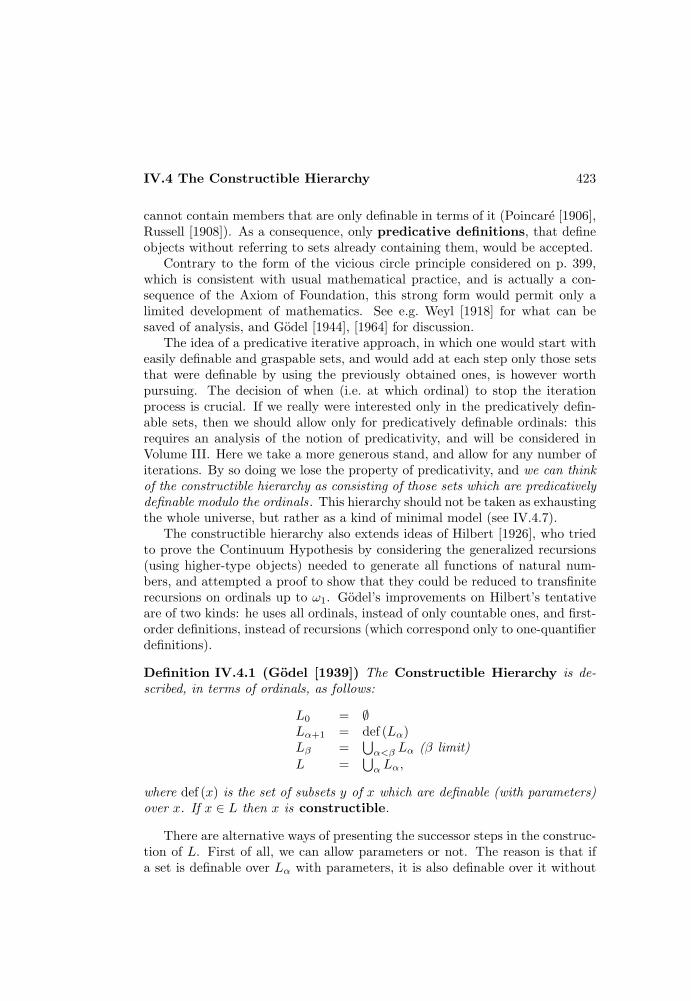
IV.4 The Constructible Hierarchy 423
cannot contain members that are only definable in terms of it (Poincare [1906],Russell [1908]). As a consequence, only predicative definitions, that defineobjects without referring to sets already containing them, would be accepted.
Contrary to the form of the vicious circle principle considered on p. 399,which is consistent with usual mathematical practice, and is actually a con-sequence of the Axiom of Foundation, this strong form would permit only alimited development of mathematics. See e.g. Weyl [1918] for what can besaved of analysis, and Godel [1944], [1964] for discussion.
The idea of a predicative iterative approach, in which one would start witheasily definable and graspable sets, and would add at each step only those setsthat were definable by using the previously obtained ones, is however worthpursuing. The decision of when (i.e. at which ordinal) to stop the iterationprocess is crucial. If we really were interested only in the predicatively defin-able sets, then we should allow only for predicatively definable ordinals: thisrequires an analysis of the notion of predicativity, and will be considered inVolume III. Here we take a more generous stand, and allow for any number ofiterations. By so doing we lose the property of predicativity, and we can thinkof the constructible hierarchy as consisting of those sets which are predicativelydefinable modulo the ordinals. This hierarchy should not be taken as exhaustingthe whole universe, but rather as a kind of minimal model (see IV.4.7).
The constructible hierarchy also extends ideas of Hilbert [1926], who triedto prove the Continuum Hypothesis by considering the generalized recursions(using higher-type objects) needed to generate all functions of natural num-bers, and attempted a proof to show that they could be reduced to transfiniterecursions on ordinals up to ω1. Godel’s improvements on Hilbert’s tentativeare of two kinds: he uses all ordinals, instead of only countable ones, and first-order definitions, instead of recursions (which correspond only to one-quantifierdefinitions).
Definition IV.4.1 (Godel [1939]) The Constructible Hierarchy is de-scribed, in terms of ordinals, as follows:
L0 = ∅Lα+1 = def (Lα)Lβ =
⋃α<β Lα (β limit)
L =⋃α Lα,
where def (x) is the set of subsets y of x which are definable (with parameters)over x. If x ∈ L then x is constructible.
There are alternative ways of presenting the successor steps in the construc-tion of L. First of all, we can allow parameters or not. The reason is that ifa set is definable over Lα with parameters, it is also definable over it without

424 IV. Hierarchies and Weak Reducibilities
parameters, by hereditarily substituting the parameters with their definitions(in the sense that the definition of a parameter may involve other parameters,which have to be discharged as well). Note that no circularity is involved, be-cause the definition of an element of Lα can only use parameters from Lβ withβ < α, and thus the ordinals are decreasing, although an ordinal greater thanα may be needed to carry out the induction.
Another way to define L (Godel [1940]) relies on an analysis of the operationdef (x), and on the isolation of finitely many (eight) operations that explicitlyproduce, by composition over the transitive closure of x, any set definableover x. This approach effectively reduces the infinitely many formulas of thelanguage of Set Theory to a finite set of operations, and it allows a finite axiom-atization of Set Theory, based on the concept of class (the Von Neumann-Godel-Bernays system NGB, see Fraenkel, Bar-Hillel, and Levy [1958]).
Finally, it has turned out that the levels Lα of the constructible hierarchyare well-behaved only for limit ordinals, while in general they are not closedunder very natural functions (like ordered pairing) that, although obviouslyconstructible, increase levels. For a finer analysis, the constructible hierarchyhas been substituted by Jensen Hierarchy (Jensen [1972]), whose levels Jαare extensions of Lα, and possess the closure properties that only the limitlevels of L have. The levels of the two hierarchies coincide exactly at thosestages α such that ω · α = α. See Devlin [1984] for a treatment.
Axiom IV.4.2 The Axiom of Constructibility is the assertion V = L thatevery set is constructible, i.e. (∀x)(x ∈ L).
Here we develop the study of L only for what concerns our immediateinterest, i.e. the study of subsets of ω. General references for constructible setsare Godel [1940], Mostowski [1969], and Devlin [1984].
The levels of the Constructible Hierarchy
The first few levels of the L have already been considered: since, for finite sets,def (x) = P(x), for α ≤ ω we have Lα = Vα. In particular, Lω = HF .
Some of the properties of these first levels generalize to every level.
Proposition IV.4.3 (Godel [1939]) Lα is transitive, and it has finite car-dinality if α < ω, and the same cardinality as α otherwise.
Proof. Lα is transitive, by induction on α:
• α = 0Obvious.
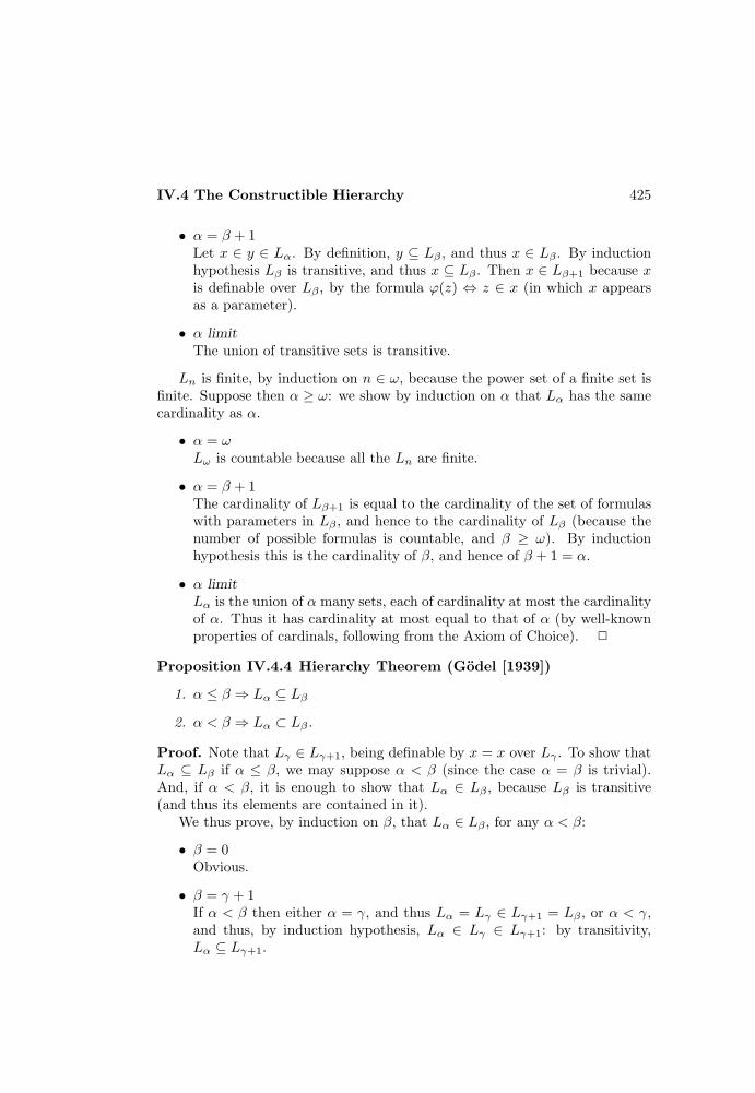
IV.4 The Constructible Hierarchy 425
• α = β + 1Let x ∈ y ∈ Lα. By definition, y ⊆ Lβ , and thus x ∈ Lβ . By inductionhypothesis Lβ is transitive, and thus x ⊆ Lβ . Then x ∈ Lβ+1 because xis definable over Lβ , by the formula ϕ(z) ⇔ z ∈ x (in which x appearsas a parameter).
• α limitThe union of transitive sets is transitive.
Ln is finite, by induction on n ∈ ω, because the power set of a finite set isfinite. Suppose then α ≥ ω: we show by induction on α that Lα has the samecardinality as α.
• α = ωLω is countable because all the Ln are finite.
• α = β + 1The cardinality of Lβ+1 is equal to the cardinality of the set of formulaswith parameters in Lβ , and hence to the cardinality of Lβ (because thenumber of possible formulas is countable, and β ≥ ω). By inductionhypothesis this is the cardinality of β, and hence of β + 1 = α.
• α limitLα is the union of α many sets, each of cardinality at most the cardinalityof α. Thus it has cardinality at most equal to that of α (by well-knownproperties of cardinals, following from the Axiom of Choice). 2
Proposition IV.4.4 Hierarchy Theorem (Godel [1939])
1. α ≤ β ⇒ Lα ⊆ Lβ
2. α < β ⇒ Lα ⊂ Lβ.
Proof. Note that Lγ ∈ Lγ+1, being definable by x = x over Lγ . To show thatLα ⊆ Lβ if α ≤ β, we may suppose α < β (since the case α = β is trivial).And, if α < β, it is enough to show that Lα ∈ Lβ , because Lβ is transitive(and thus its elements are contained in it).
We thus prove, by induction on β, that Lα ∈ Lβ , for any α < β:
• β = 0Obvious.
• β = γ + 1If α < β then either α = γ, and thus Lα = Lγ ∈ Lγ+1 = Lβ , or α < γ,and thus, by induction hypothesis, Lα ∈ Lγ ∈ Lγ+1: by transitivity,Lα ⊆ Lγ+1.
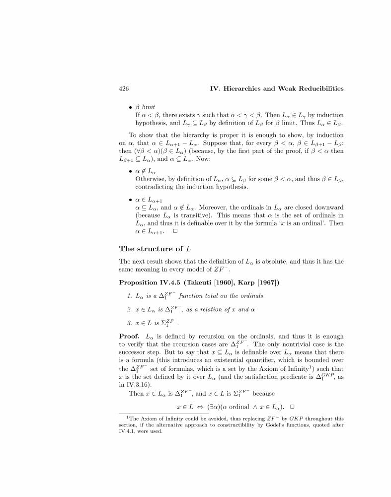
426 IV. Hierarchies and Weak Reducibilities
• β limitIf α < β, there exists γ such that α < γ < β. Then Lα ∈ Lγ by inductionhypothesis, and Lγ ⊆ Lβ by definition of Lβ for β limit. Thus Lα ∈ Lβ .
To show that the hierarchy is proper it is enough to show, by inductionon α, that α ∈ Lα+1 − Lα. Suppose that, for every β < α, β ∈ Lβ+1 − Lβ :then (∀β < α)(β ∈ Lα) (because, by the first part of the proof, if β < α thenLβ+1 ⊆ Lα), and α ⊆ Lα. Now:
• α 6∈ LαOtherwise, by definition of Lα, α ⊆ Lβ for some β < α, and thus β ∈ Lβ ,contradicting the induction hypothesis.
• α ∈ Lα+1
α ⊆ Lα, and α 6∈ Lα. Moreover, the ordinals in Lα are closed downward(because Lα is transitive). This means that α is the set of ordinals inLα, and thus it is definable over it by the formula ‘x is an ordinal’. Thenα ∈ Lα+1. 2
The structure of L
The next result shows that the definition of Lα is absolute, and thus it has thesame meaning in every model of ZF−.
Proposition IV.4.5 (Takeuti [1960], Karp [1967])
1. Lα is a ∆ZF−
1 function total on the ordinals
2. x ∈ Lα is ∆ZF−
1 , as a relation of x and α
3. x ∈ L is ΣZF−
1 .
Proof. Lα is defined by recursion on the ordinals, and thus it is enoughto verify that the recursion cases are ∆ZF−
1 . The only nontrivial case is thesuccessor step. But to say that x ⊆ Lα is definable over Lα means that thereis a formula (this introduces an existential quantifier, which is bounded overthe ∆ZF−
1 set of formulas, which is a set by the Axiom of Infinity1) such thatx is the set defined by it over Lα (and the satisfaction predicate is ∆GKP
1 , asin IV.3.16).
Then x ∈ Lα is ∆ZF−
1 , and x ∈ L is ΣZF−
1 because
x ∈ L ⇔ (∃α)(α ordinal ∧ x ∈ Lα). 2
1The Axiom of Infinity could be avoided, thus replacing ZF− by GKP throughout thissection, if the alternative approach to constructibility by Godel’s functions, quoted afterIV.4.1, were used.
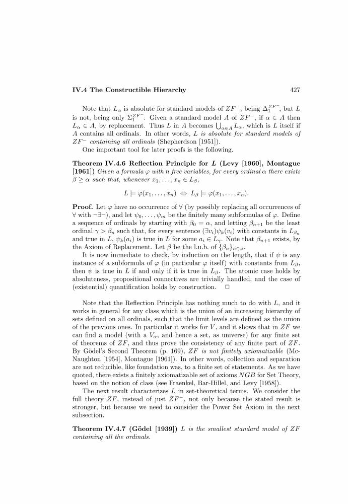
IV.4 The Constructible Hierarchy 427
Note that Lα is absolute for standard models of ZF−, being ∆ZF−
1 , but Lis not, being only ΣZF
−
1 . Given a standard model A of ZF−, if α ∈ A thenLα ∈ A, by replacement. Thus L in A becomes
⋃α∈A Lα, which is L itself if
A contains all ordinals. In other words, L is absolute for standard models ofZF− containing all ordinals (Shepherdson [1951]).
One important tool for later proofs is the following.
Theorem IV.4.6 Reflection Principle for L (Levy [1960], Montague[1961]) Given a formula ϕ with n free variables, for every ordinal α there existsβ ≥ α such that, whenever x1, . . . , xn ∈ Lβ,
L |= ϕ(x1, . . . , xn) ⇔ Lβ |= ϕ(x1, . . . , xn).
Proof. Let ϕ have no occurrence of ∀ (by possibly replacing all occurrences of∀ with ¬∃¬), and let ψ0, . . . , ψm be the finitely many subformulas of ϕ. Definea sequence of ordinals by starting with β0 = α, and letting βn+1 be the leastordinal γ > βn such that, for every sentence (∃vi)ψk(vi) with constants in Lβn
and true in L, ψk(ai) is true in L for some ai ∈ Lγ . Note that βn+1 exists, bythe Axiom of Replacement. Let β be the l.u.b. of βnn∈ω.
It is now immediate to check, by induction on the length, that if ψ is anyinstance of a subformula of ϕ (in particular ϕ itself) with constants from Lβ ,then ψ is true in L if and only if it is true in Lβ . The atomic case holds byabsoluteness, propositional connectives are trivially handled, and the case of(existential) quantification holds by construction. 2
Note that the Reflection Principle has nothing much to do with L, and itworks in general for any class which is the union of an increasing hierarchy ofsets defined on all ordinals, such that the limit levels are defined as the unionof the previous ones. In particular it works for V , and it shows that in ZF wecan find a model (with a Vα, and hence a set, as universe) for any finite setof theorems of ZF , and thus prove the consistency of any finite part of ZF .By Godel’s Second Theorem (p. 169), ZF is not finitely axiomatizable (Mc-Naughton [1954], Montague [1961]). In other words, collection and separationare not reducible, like foundation was, to a finite set of statements. As we havequoted, there exists a finitely axiomatizable set of axioms NGB for Set Theory,based on the notion of class (see Fraenkel, Bar-Hillel, and Levy [1958]).
The next result characterizes L in set-theoretical terms. We consider thefull theory ZF , instead of just ZF−, not only because the stated result isstronger, but because we need to consider the Power Set Axiom in the nextsubsection.
Theorem IV.4.7 (Godel [1939]) L is the smallest standard model of ZFcontaining all the ordinals.
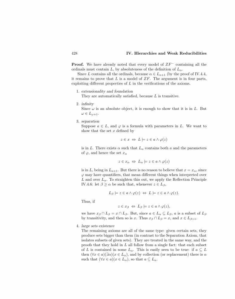
428 IV. Hierarchies and Weak Reducibilities
Proof. We have already noted that every model of ZF− containing all theordinals must contain L, by absoluteness of the definition of Lα.
Since L contains all the ordinals, because α ∈ Lα+1 (by the proof of IV.4.4,it remains to prove that L is a model of ZF . The argument is in four parts,exploiting different properties of L in the verifications of the axioms.
1. extensionality and foundationThey are automatically satisfied, because L is transitive.
2. infinitySince ω is an absolute object, it is enough to show that it is in L. Butω ∈ Lω+1.
3. separationSuppose a ∈ L, and ϕ is a formula with parameters in L. We want toshow that the set x defined by
z ∈ x ⇔ L |= z ∈ a ∧ ϕ(z)
is in L. There exists α such that Lα contains both a and the parametersof ϕ, and hence the set xα
z ∈ xα ⇔ Lα |= z ∈ a ∧ ϕ(z)
is in L, being in Lα+1. But there is no reason to believe that x = xα, sinceϕ may have quantifiers, that mean different things when interpreted overL and over Lα. To straighten this out, we apply the Reflection PrincipleIV.4.6: let β ≥ α be such that, whenever z ∈ Lβ ,
Lβ |= z ∈ a ∧ ϕ(z) ⇔ L |= z ∈ a ∧ ϕ(z).
Thus, ifz ∈ xβ ⇔ Lβ |= z ∈ a ∧ ϕ(z),
we have xβ ∩ Lβ = x ∩ Lβ . But, since a ∈ Lα ⊆ Lβ , a is a subset of Lβby transitivity, and then so is x. Thus xβ ∩ Lβ = x, and x ∈ Lβ+1.
4. large sets existenceThe remaining axioms are all of the same type: given certain sets, theyproduce sets bigger than them (in contrast to the Separation Axiom, thatisolates subsets of given sets). They are treated in the same way, and theproofs that they hold in L all follow from a single fact: that each subsetof L is contained in some Lα. This is easily seen to be true: if a ⊆ Lthen (∀x ∈ a)(∃α)(x ∈ Lα), and by collection (or replacement) there is αsuch that (∀x ∈ a)(x ∈ Lα), so that a ⊆ Lα.
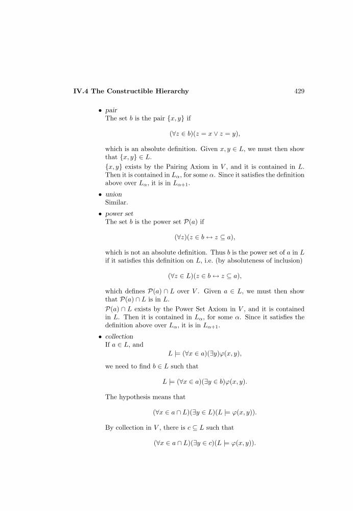
IV.4 The Constructible Hierarchy 429
• pairThe set b is the pair x, y if
(∀z ∈ b)(z = x ∨ z = y),
which is an absolute definition. Given x, y ∈ L, we must then showthat x, y ∈ L.x, y exists by the Pairing Axiom in V , and it is contained in L.Then it is contained in Lα, for some α. Since it satisfies the definitionabove over Lα, it is in Lα+1.
• unionSimilar.
• power setThe set b is the power set P(a) if
(∀z)(z ∈ b↔ z ⊆ a),
which is not an absolute definition. Thus b is the power set of a in Lif it satisfies this definition on L, i.e. (by absoluteness of inclusion)
(∀z ∈ L)(z ∈ b↔ z ⊆ a),
which defines P(a) ∩ L over V . Given a ∈ L, we must then showthat P(a) ∩ L is in L.P(a) ∩ L exists by the Power Set Axiom in V , and it is containedin L. Then it is contained in Lα, for some α. Since it satisfies thedefinition above over Lα, it is in Lα+1.
• collectionIf a ∈ L, and
L |= (∀x ∈ a)(∃y)ϕ(x, y),
we need to find b ∈ L such that
L |= (∀x ∈ a)(∃y ∈ b)ϕ(x, y).
The hypothesis means that
(∀x ∈ a ∩ L)(∃y ∈ L)(L |= ϕ(x, y)).
By collection in V , there is c ⊆ L such that
(∀x ∈ a ∩ L)(∃y ∈ c)(L |= ϕ(x, y)).

430 IV. Hierarchies and Weak Reducibilities
Then c ⊆ Lα for some α, and hence
(∀x ∈ a ∩ L)(∃y ∈ Lα)(L |= ϕ(x, y)).
Since Lα ∈ L, it is enough to let b = Lα to have
(∀x ∈ a ∩ L)(∃y ∈ b)(L |= ϕ(x, y)),
and henceL |= (∀x ∈ a)(∃y ∈ b)ϕ(x, y). 2
Corollary IV.4.8 L is a model of V = L.
Proof. We have to proveL |= (∀x)(x ∈ L).
Since L is absolute for models of ZF− containing all ordinals, and L is such amodel, this amounts to showing that
(∀x ∈ L)(x ∈ L),
which is trivially true. 2.
The corollary is not only interesting for its own sake, but also in applica-tions: to prove that some fact holds in L, it is enough to show that it is provablein ZF plus V = L.
Corollary IV.4.9 (Kreisel [1956], Shoenfield [1961a]) If ϕ is a Σ13 sen-
tence of Second-Order Arithmetic provable in ZF plus V = L, then ϕ is alreadyprovable in ZF alone.
Proof. Let ϕ ↔ (∃A)ψ(A), with ψ ∈ Π12. If ϕ is provable in ZF plus V = L
then it is true in L, i.e. there is A ∈ L such that ψ(A) holds in L. By absolute-ness of Π1
2 formulas for L (IV.3.27) ψ(A) must then be true, and thus ϕ holds.But the whole reasoning took place in ZF , since only ZF is needed to proveIV.4.12 and IV.3.27. Thus ϕ has been proved in ZF alone. 2
The result is best possible since, by IV.4.22, (∀A)(A ∈ L) is a Π13 statement
true in L (because L satisfies V = L), but not provable in ZFC (because itsnegation is consistent with ZFC).
The usefulness of the corollary is quite evident: V = L does not prove anynew Σ1
3 sentence of Second-Order Arithmetic, and thus it can be used freelywhen trying to prove such a sentence in ZF alone. The same of course holds forany of the consequences of V = L, like the Axiom of Choice and the ContinuumHypothesis, proved below. Actually, in the latter cases the result is not thebest possible, and it can be improved to hold for bigger classes of sentences(see Platek [1969]).

IV.4 The Constructible Hierarchy 431
Theorem IV.4.10 (Godel [1939], Karp [1967])
1. There exists a ∆ZF−
1 well-ordering <α of Lα.
2. There exists a ΣZF−
1 well-ordering <L of L.
Proof. We define a ∆ZF−
1 well-ordering <α of Lα, by recursion on the ordinals.
1. α = 0Since L0 = ∅, <0 = ∅.
2. α = β + 1By induction hypothesis we have <β that well-orders Lβ . Let
x <α y ⇔ (x ∈ Lβ ∧ y ∈ Lβ ∧ x <β y) ∨(x ∈ Lβ ∧ y ∈ Lβ+1 − Lβ) ∨(x ∈ Lβ+1 − Lβ ∧ y ∈ Lβ+1 − Lβ ∧the first formula defining x over Lβ precedesthe first formula defining y over Lβ).
3. α limit
x <α y ⇔ (∃β < α)(x <β y).
By definition, if α < β then <α is an initial segment of <β . Since thedefinition is by recursion on the ordinals, it is enough to verify that the recursionis ∆ZF−
1 . Since Lα is ∆ZF−
1 , the only point to check is the case of α = β + 1and x, y ∈ Lβ+1 − Lβ .
The formulas without parameters of the set-theoretical language are count-ably many, and there is a natural (lexicographical) ∆ZF−
1 well-ordering of them,of length ω. By arithmetization everything can be coded in HF = Lω, whichexists by the Axiom of Infinity.
For what concerns parameters, they are in Lβ and, by induction hypothesis,<β well-orders Lβ . We can then say that ϕ with parameters a1, . . . , an (orderedby <β) precedes ψ with parameters b1, . . . , bm (ordered by <β) if and only if:
• n < m
• n = m and ϕ precedes ψ (as formulas)
• n = m, ϕ = ψ and, for the first i such that ai 6= bi, ai <β bi.

432 IV. Hierarchies and Weak Reducibilities
Again the conditions in this definition are ∆ZF−
1 , and thus the whole well-ordering is ∆ZF−
1 . Then
x <L y ⇔ (∃α)(x ∈ Lα ∧ y ∈ Lα ∧ x <α y)
is ΣZF−
1 . Note that, for each α, <α is an initial segment of <L. 2
Exercises IV.4.11 a) If Lα is a model of ZF−, the well-ordering <α of Lα haslength α. (Hint: by replacement, Lα is closed under the rang function of <α
f(y) = supf(x) + 1 : x <α y,
and thus supf(x) : x ∈ Lα ≤ α. Conversely, since f is one-one, f−1 is a functionwith range Lα, and if the length of <α were β < α, then the range of f−1 would bein Lα, i.e. Lα ∈ Lα, contradiction.)
b) If V = L then ≤L is ∆ZF−1 . (Hint: in this case
¬(x <L y) ⇔ x = y ∨ (∃α)(x ∈ Lα ∧ y ∈ Lα ∧ y <α x),
and thus <L is also ΠZF−1 .)
One of the original reasons to introduce L was to prove the following fact,whose consequence is that the Axiom of Choice is consistent with ZF (Godel[1938]), since it holds in a model of ZF . Note that also V is a model of ZF ,but there is no obvious way to show that it satisfies the Axiom of Choice, thedifficulty being in well-ordering the power set of a given (well-ordered) set.
Corollary IV.4.12 L is a model of ZFC plus V = L.
Proof. By IV.4.7 and IV.4.8, it only remains to prove that the Axiom ofChoice holds in L. The theorem just proved shows that L is well-orderable, andthus the Axiom of Choice holds if V = L. But L is a model of ZF plus V = L,and hence the Axiom of Choice holds in L. 2
The fact that L is a model of ZFC has an important consequence: alltheorems of ZFC are true in L. In particular, it is possible to carry on insideL the theory of cardinals, which is largely based on the Axiom of Choice.
Of particular interest for us is ωL1 , the analogue of the first uncountable
cardinal, which is the least ordinal α such that no one-one function f : α→ ωexists in L. In other words, ‘L believes ωL1 is ω1’. Clearly ωL1 ≤ ω1: if thereis no function with certain properties in V , there is none in L either. Theassertion ωL1 = ω1 is consistent with ZFC, since so is V = L (by IV.4.8). Butalso the assertion ωL1 < ω1 is consistent with ZFC (Cohen [1966]), by cardi-nal collapsing (see Volume III). It also follows from large cardinals hypothesis(Rowbottom [1971]).

IV.4 The Constructible Hierarchy 433
Constructible sets of natural numbers
We have introduced the Constructible Hierarchy not for its own sake, but tostudy subsets of ω. We thus turn now to our real interest, the set P(ω) ∩ L ofconstructible sets of natural numbers.
Since P(ω) ∩ L ⊆ L, there is α such that P(ω) ∩ L ⊆ Lα, and thus there isa stage after which no subset of ω is ever generated. We now improve on this,by exhibiting such an α (which will turn out to be the best possible).
Theorem IV.4.13 (Godel [1939]) P(ω) ∩ L ⊆ LωL1.
Proof. The theorem reduces to prove, in ZFC, that P(ω)∩L ⊆ Lω1 . Since Lis a model of ZFC, the result also holds in L. To see what this means, recallthat P(ω), the power set of ω, means P(ω) ∩ L in L (see the proof of IV.4.7).L is absolute for L, because L is a model of ZF− containing all ordinals. AndωL1 is, by definition, the ω1 of L. Thus P(ω)∩L ⊆ Lω1 means P(ω)∩L ⊆ LωL
1,
when interpreted inside L, and this is the statement of the theorem.We thus turn to the proof of P(ω) ∩ L ⊆ Lω1 , which roughly consists of
the following. Let A ⊆ ω be constructible, i.e. A ∈ L. Then A ∈ Lα, for someα: we want to show that α may be supposed to be countable. To achieve this,we use the Lowenheim-Skolem Theorem of logic (for the reader not acquaintedwith it, we prove in 2 below the special case we need). Its essence is to cutout, from a model of a sentence, a countable model, leaving unchanged a givencountable subset. Here we know that A ∈ Lα, and thus we only have to find asentence ϕ whose models are exactly the sets of the kind Lα (this is done in 1below). Then Lα is a model of ϕ, and it contains A: the Lowenheim-SkolemTheorem produces a countable model of ϕ containing A, which must thenbe of the form Lα, with α countable (because, by IV.4.3, Lα is countable ifand only if α is). It only remains to find ϕ, and prove the Lowenheim-SkolemTheorem.
1. There is a sentence ϕ such that if a set M is a standard model for ϕ, thenM = Lα for some (limit) α.By absoluteness of Lα, if M is a standard model of ZF− then
⋃α∈M Lα
is L in M , and it is contained in it. Let αM be the smallest ordinal notin M : if αM is limit then, by definition of L,
⋃α∈M Lα = LαM
, and thusLαM
⊆ M . If V = L also holds in M , i.e. M is equal to L in it, thenLαM
= M .
We can then let ϕ be the conjunction of the following:
• the finitely many axioms needed to prove that the notions of ordinaland of Lα are absolute for standard models of them
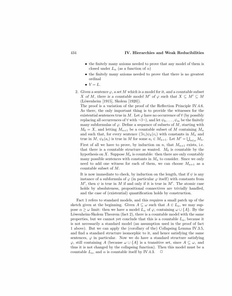
434 IV. Hierarchies and Weak Reducibilities
• the finitely many axioms needed to prove that any model of them isclosed under Lα (as a function of α)
• the finitely many axioms needed to prove that there is no greatestordinal
• V = L.
2. Given a sentence ϕ, a setM which is a model for it, and a countable subsetX of M , there is a countable model M ′ of ϕ such that X ⊆ M ′ ⊆ M(Lowenheim [1915], Skolem [1920]).The proof is a variation of the proof of the Reflection Principle IV.4.6.As there, the only important thing is to provide the witnesses for theexistential sentences true inM . Let ϕ have no occurrence of ∀ (by possiblyreplacing all occurrences of ∀ with ¬∃¬), and let ψ0, . . . , ψm be the finitelymany subformulas of ϕ. Define a sequence of subsets of M , starting withM0 = X, and letting Mn+1 be a countable subset of M containing Mn
and such that, for every sentence (∃vi)ψk(vi) with constants in Mn andtrue in M , ψk(ai) is true in M for some ai ∈Mn+1. Let M ′ =
⋃n∈ωMn.
First of all we have to prove, by induction on n, that Mn+1 exists, i.e.that there is a countable structure as wanted. M0 is countable by thehypothesis on X. Suppose Mn is countable: then there are only countablymany possible sentences with constants in Mn to consider. Since we onlyneed to add one witness for each of them, we can choose Mn+1 as acountable subset of M .It is now immediate to check, by induction on the length, that if ψ is anyinstance of a subformula of ϕ (in particular ϕ itself) with constants fromM ′, then ψ is true in M if and only if it is true in M ′. The atomic caseholds by absoluteness, propositional connectives are trivially handled,and the case of (existential) quantification holds by construction.
Fact 1 refers to standard models, and this requires a small patch up of thesketch given at the beginning. Given A ⊆ ω such that A ∈ Lα, we may sup-pose α ≥ ω limit: then we have a model Lα of ϕ, containing ω ∪ A. By theLowenheim-Skolem Theorem (fact 2), there is a countable model with the sameproperties, but we cannot yet conclude that this is a countable Lα, because itis not necessarily a standard model (an assumption used in the proof of fact1 above). But we can apply the (corollary of the) Collapsing Lemma IV.3.5,and find a standard structure isomorphic to it, and hence satisfying the samesentences, ϕ in particular. Now we do have a standard structure satisfyingϕ, still containing A (because ω ∪ A is a transitive set, since A ⊆ ω, andthus it is not changed by the collapsing function). Then this model must be acountable Lα, and α is countable itself by IV.4.3. 2

IV.4 The Constructible Hierarchy 435
One of the original reasons to introduce L was to prove the following fact,whose consequence is that the Continuum Hypothesis is consistent with ZFC(Godel [1938]), since it holds in a model of ZFC. The reason why the Contin-uum Hypothesis follows from V = L, while it is independent of ZFC, is thatthe former completely specifies the extension of the power set operation (leftundetermined by the latter), by determining which subsets of a given set areavailable, namely only those that can be predicatively defined from the ordi-nals. By providing a sort of minimal interpretation for the power set operation,V = L limits the number of subsets of a given set to the least possible value.
Corollary IV.4.14 The Continuum Hypothesis holds in L.
Proof. We have proved that P(ω) ∩ L ⊆ Lω1 . If V = L then this meansthat the power set of ω has at most the power of Lω1 , which is ω1 by IV.4.3.By Cantor’s Theorem (II.2.1), the cardinality of the power set of ω must beuncountable, and hence at least ω1. Thus it is exactly ω1. This shows that theContinuum Hypothesis follows from ZFC plus V = L (the Axiom of Choiceis needed for cardinal arithmetic, in particular in the proof of IV.4.3), and byIV.4.12 it then holds in L. 2
We will see in Volume III that all the following possibilities are consistentwith ZFC:
1. P(ω) ⊆ L, which follows from V = L.
2. P(ω) 6⊆ L and P(ω) ∩ L countable, by collapsing ωL1 (this also followsfrom large cardinals hypothesis, by Rowbottom [1971]).
3. P(ω) 6⊆ L and P(ω) ∩ L uncountable, by starting with a model of theContinuum Hypothesis, and building a generic extension of it that pre-serves cardinals.
By the proof of the corollary, P(ω) ∩ L is not contained in Lα for α < ωL1 ,because otherwise the power set of ω would be countable in L, contradictingCantor’s Theorem in L. Thus P(ω) ∩ Lαα<ωL
1, as a hierarchy for P(ω) ∩ L,
has the smallest possible length. We now show that the hierarchy is not proper.
Proposition IV.4.15 (Putnam [1963]) There exists α < ωL1 such that nonew subset of ω is generated in L at stage α+ 1, i.e.
P(ω) ∩ (Lα+1 − Lα) = ∅.
Proof. Let ψ be the formula
(∃α)[P(ω) ∩ (Lα+1 − Lα) = ∅].
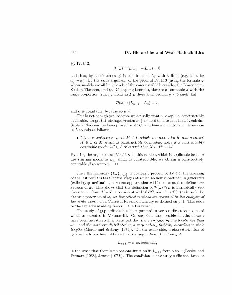
436 IV. Hierarchies and Weak Reducibilities
By IV.4.13,P(ω) ∩ (LωL
1 +1 − LωL1
) = ∅
and thus, by absoluteness, ψ is true in some Lβ with β limit (e.g. let β beωL1 + ω). By the same argument of the proof of IV.4.13 (using the formula ϕwhose models are all limit levels of the constructible hierarchy, the Lowenheim-Skolem Theorem, and the Collapsing Lemma), there is a countable β with thesame properties. Since ψ holds in Lβ , there is an ordinal α < β such that
P(ω) ∩ (Lα+1 − Lα) = ∅,
and α is countable, because so is β.This is not enough yet, because we actually want α < ωL1 , i.e. constructibly
countable. To get this stronger version we just need to note that the Lowenheim-Skolem Theorem has been proved in ZFC, and hence it holds in L. Its versionin L sounds as follows:
• Given a sentence ϕ, a set M ∈ L which is a model for it, and a subsetX ∈ L of M which is constructibly countable, there is a constructiblycountable model M ′ ∈ L of ϕ such that X ⊆M ′ ⊆M .
By using the argument of IV.4.13 with this version, which is applicable becausethe starting model is Lβ , which is constructible, we obtain a constructiblycountable β as wanted. 2
Since the hierarchy Lαα<ωL1
is obviously proper, by IV.4.4, the meaningof the last result is that, at the stages at which no new subset of ω is generated(called gap ordinals), new sets appear, that will later be used to define newsubsets of ω. This shows that the definition of P(ω) ∩ L is intrinsically set-theoretical. Since V = L is consistent with ZFC, and thus P(ω) ∩ L could bethe true power set of ω, set-theoretical methods are essential in the analysis ofthe continuum, i.e. in Classical Recursion Theory as defined on p. 1. This addsto the remarks made by Sacks in the Foreword.
The study of gap ordinals has been pursued in various directions, some ofwhich are treated in Volume III. On one side, the possible lengths of gapshave been investigated: it turns out that there are gaps of any length less thanωL1 , and the gaps are distributed in a very orderly fashion, according to theirlengths (Marek and Srebrny [1974]). On the other side, a characterization ofgap ordinals has been obtained: α is a gap ordinal if and only if
Lα+1 |= α uncountable,
in the sense that there is no one-one function in Lα+1 from α to ω (Boolos andPutnam [1968], Jensen [1972]). The condition is obviously sufficient, because
IV.4 The Constructible Hierarchy 437
such a function induces a well-ordering of ω of length α, that cannot be in Lαsince α is not. The converse is a strengthening of IV.4.13, and it is obviouslynecessary, if Lα+1 is a model of enough Set Theory: in this case IV.4.13 holdsin it, and thus all constructible subsets of ω which are in Lα+1 must be alreadyin L
ωLα+11
, i.e. must be constructed at stages countable in Lα+1. Thus, byabsoluteness,
P(ω) ∩ (Lα+1 − Lω
Lα+11
) = ∅.
And if α is not countable in Lα+1, ωLα+11 ≤ α. Note that the gap could be quite
large, depending on how much of Set Theory is modelled by Lα+1, since Lα+1
could prove the existence of various cardinals (inside it) greater than ωLα+11 .
Exercises IV.4.16 a) The gap ordinals are ωL1 . (Putnam [1963]) (Hint: there is agap above any given constructibly countable ordinal.)
b) For any ordinal γ admitting an absolute definition, there are gaps of length γ.
(Putnam [1963]) (Hint: consider α+ γ instead of α+ 1 in the proof above.)
One might think of mimicking the definition of L in an autonomous way,by relying only on subsets of ω.
Definition IV.4.17 (Kleene [1959b]) The Ramified Analytical Hierar-chy is described, in terms of ordinals, as follows:
RA0 = the arithmetical setsRAα+1 = def 2 (RAα)RAβ =
⋃α<β RAα (β limit)
RA =⋃αRAα,
where def 2 (x) is the set of subsets of ω which are definable in Second-OrderArithmetic with set quantifiers restricted to x, and parameters in x.
RA will be studied in Volume III. Leeds and Putnam [1974] show thatparameters can be avoided in its definition. By cardinality reasons, RA breaksdown at an ordinal β0 (since if each step adds a new subset, the subsets of ωrun out in at most a continuum of steps). Boolos and Putnam [1968] showthat, when account is taken of the different starting points, the Ramified Ana-lytical Hierarchy coincides, up to β0 and level by level, with the ConstructibleHierarchy restricted to P(ω). It is thus not surprising that β0 is the first gapordinal , i.e. the first point in which sets not in P(ω) become essential for thedefinition of new subsets of ω.
Exercises IV.4.18 a) β0 is countable. (Cohen [1963a]) (Hint: by cardinality con-siderations, there is an ordinal α such that RAα+1 = RAα. As in IV.4.15, and byabsoluteness of RAα, there is a countable one.)
438 IV. Hierarchies and Weak Reducibilities
b) RA ⊂ ∆12. (Putnam [1964]) (Hint: there is a ∆1
2 predicate enumerating the
members of RA. Thus the members of RA are uniformly ∆12. By diagonalizing
the enumeration predicate, there is a ∆12 set not in RA. To get the enumeration
predicate, by part a) we may restrict attention to countable ordinals, and hence
to well-orderings of ω. The methods of IV.2.22 and IV.4.5 show that A ∈ RAx is
uniformly ∆11, whenever x varies over the elements of a well-ordering of ω, used as
parameter. Since A ∈ RA if and only if there is a well-ordering of ω such that
A ∈ RAx for some x in it, we have the Σ12 form, because being a well-ordering is a
Π11 condition. Similarly, A ∈ RA if and only if, for every well-ordering of ω which is
sufficiently long, i.e. it has elements y and z such that z is the successor of y in it,
and RAy = RAz, then A ∈ RAx for some x. This provides the Π12 form, because
being a well-ordering is now an hypothesis, and thus it becomes Σ11.)
Σ12 sets
We have studied the set P(ω) ∩ L as a totality, but we do not know yet whichsets are in it. Of course, since V = L is consistent with ZFC, it might be thatall sets (of natural numbers) are constructible. But even if this were the case,this would not be provable in ZFC, because Cohen [1963] has showed that itis consistent with ZFC that P(ω) 6⊆ L (see Volume III).
It is thus a nontrivial problem to ask which subsets of ω are provably in L,in the sense of being provable in ZFC that they are constructible.
Theorem IV.4.19 (Mostowski [1949], Shoenfield [1961a]) Σ12∪Π1
2 ⊆ L.
Proof. Since ω ∈ L, and L satisfies separation, for any formula ϕ there is aset a ∈ L such that
x ∈ a ⇔ L |= x ∈ ω ∧ ϕ(x).
This of course does not mean that every definable subset of ω (in the real world,i.e. in V ) is in L, because ϕ does not need to be absolute, and thus the set itdefines in V is not necessarily a. But this certainly holds for the formulas whosemeanings are the same over L and in the real world. By IV.3.27, this is thecase of Σ1
2 formulas, because L is a standard model of GKP containing all theordinals. Thus Σ1
2 sets are all in L, and the same holds for their complementsin ω, i.e. the Π1
2 sets. 2.
This result is the best possible: Jensen and Solovay [1970] have shown thatit is consistent with ZFC that P(ω) ∩ L is properly contained in ∆1
3. Thisalso follows from large cardinals assumptions (Solovay [1967]). On the otherhand, Harrington [1974] has shown that for any n such that 3 ≤ n ≤ ω, it isconsistent with ZFC that P(ω) ∩ L = ∆1
n. See Volume III for all this.

IV.4 The Constructible Hierarchy 439
Recall that the Arithmetical and Analytical Hierarchies classify sets of nat-ural numbers according to the complexity of their definitions over the structureof Arithmetic. The difference between the two hierarchies is in the range ofquantifiers, over ω in the former case, and over P(ω) in the latter. Our origi-nal motivation for the introduction of the Levy’s Hierarchy was to pursue thistrend, and allow for more general quantifiers, over sets in a given model. Ourfirst example was HF , and definability over it coincided, for subsets of ω, witharithmetical definability (IV.3.22).
We turn now to definability over L. Of course, every set in L is definable overit, using itself as parameter, but this is not what we mean: in the AnalyticalHierarchy we did quantify over sets, but did not allow them as parameters (noattention is needed over HF , because the proof of IV.3.22 shows that elementsof HF and natural numbers are, in a sense, the same thing). What we reallylook for is thus definability without parameters over L.
Theorem IV.4.20 Definability of Σ12 sets (Takeuti and Kino [1962])
Let A ⊆ ω. Then
A ∈ Σ12 ⇔ A ∈ ΣL1 without parameters.
Similarly for relations, of any number of variables.
Proof. Let A ∈ Σ12. By the proof of IV.3.27, A is of the form (∃α countable)ϕ,
with α ranging over countable ordinals, and ϕ ∆1 over GKP plus Infinity.Since L is a model of GKP , and it contains all the countable ordinals, A is ΣL1without parameters.
For the converse, suppose A ⊆ ω is ΣL1 without parameters, i.e.
x ∈ A ⇔ L |= (∃y)ψ(x, y),
with ψ ∈ ∆L1. By definition of satisfaction,
x ∈ A ⇔ (∃y ∈ L)(L |= ψ(x, y)).
By definition of L, and absoluteness of ∆L1 formulas,
x ∈ A ⇔ (∃α)(∃y ∈ Lα)(Lα |= ψ(x, y)),
and hencex ∈ A ⇔ (∃α)(Lα |= (∃y)ψ(x, y)).
Using the Lowenheim-Skolem Theorem and the Collapsing Lemma as in theproof of IV.4.13, and with ϕ as there,
x ∈ A ⇔ (∃a)[a countable transitive ∧ a |= ϕ ∧ (∃y)ψ(x, y)].
440 IV. Hierarchies and Weak Reducibilities
Suppose such an a exists: being countable, 〈a,∈〉 is isomorphic to a well-founded structure 〈ω, ε〉, and the Collapsing Lemma applied to the latter re-produces the original a (because the transitive collapse is unique, and a istransitive). In particular, if f is the collapsing function, x = f(f−1(x)), and(∃y)ψ(x, y) holds on a if and only if (∃y)ψ(z, y), with f(z) = x, holds on 〈ω, ε〉.Thus
x ∈ A ⇔ (∃ε)[〈ω, ε〉 well-founded ∧〈ω, ε〉 |= ϕ ∧ (∃y)(∃z)(f(z) = x ∧ ψ(z, y))],
where f is the collapsing function of 〈ω, ε〉.It only remains to compute the complexity of the last expression for A:
• ε is a binary relation on ω, that can be coded by its characteristic function:the first existential quantifier is thus a function quantifier.
• Well-foundedness is Π11, see e.g. IV.2.15.
• The graph of the collapsing function, when the values are restricted to ω,is ∆1
1, because it can be defined by recursion with clauses arithmetical inε, as follows. First of all, f(z) = 0 if and only if z is the (unique) elementof ω which does not have predecessors w.r.t. ε. And f(z) = n+ 1 if andonly if, for some y, f(y) = n, and z is the successor of y w.r.t. ε (i.e. theset y ∪ y, when membership in interpreted as ε).
• The satisfaction relation is ∆11, by arithmetization.
The whole expression is thus Σ12. 2
Corollary IV.4.21 Let A ⊆ ω. Then
A ∈ Σ12 ⇔ A ∈ ΣLω1
1 without parameters.
Similarly for relations, of any number of variables.
Proof. The first part of the proof goes through because Lω1 is a model ofGKP , and it contains all the countable ordinals. The second part of the proofcan be repeated as above, without appeal to the Lowenheim-Skolem Theorem,since every Lα with α < ω1 is countable. 2
We have proved the result for relations on ω, but little work is needed toextend it to relations on ω and P(ω): we just have to show how to take care ofset variables, and for this it is enough to prove that the graph of the collapsing

IV.4 The Constructible Hierarchy 441
function f , when the values are restricted to P(ω), is still ∆11. Recall that, by
definition of f (see IV.3.5),
f(z) = f(y) : y ∈ ω ∧ y ε z.
Thusf(z) = A ⇔ (∀x)[x ∈ A↔ (∃y)(x = f(y) ∧ y ε z)].
The use of f on the right-hand-side is restricted to number values, and thus itis ∆1
1 by the proof of IV.4.20. Thus the whole expression is ∆11, because only
number quantifiers are used.
Corollary IV.4.22 (Godel [1940], Mostowski, Addison [1959a]) Therelations A ∈ L and A ≤L B, for A and B subsets of ω, are Σ1
2.
Proof. We know from IV.4.5, IV.4.10, and IV.4.7 that x ∈ L and x ≤L y areΣL1. When restricted to P(ω) they become relations of set variables, and thusthey are Σ1
2. 2
The complexity of P(ω)∩L computed above is best possible, since if A ∈ Lis Π1
2 then P(ω) ⊆ L, i.e. every subset of ω is constructible: indeed, if A ∈ L isΠ1
2 then (∃A)(A 6∈ L) is a Σ12 formula false in L, and by absoluteness it is also
false in V , which means that P(ω) ⊆ L.By IV.4.11.b, if V = L then ≤L is actually ∆ZF−
1 , and thus the well-ordering≤L is actually ∆1
2 on P(ω). In particular, A ≤∆12B if A ≤L B. Thus it is
consistent with ZFC that the ∆12-degrees are well -ordered , and no result con-
tradicting this can be proved in ZFC. The study of the structure of ∆12-degrees
can thus be pursued along two different paths: one is to prove consistency re-sults, the other to introduce new axioms and study the structure under them.We will follow both paths, in Volume III. Of course similar considerations holdfor the ∆1
n-degrees, for any n ≥ 2.
HC and the Analytical Hierarchy
We have seen in IV.3.22 that the Arithmetical Hierarchy can be viewed as aset-theoretical hierarchy over the hereditarily finite sets. We now provide asimilar interpretation of the Analytical Hierarchy.
Definition IV.4.23 HC is the set of hereditarily countable sets, i.e. thesmallest class A of sets such that:
1. ∅ ∈ A
2. if (∀n ∈ ω)(xn ∈ A) then xn : n ∈ ω ∈ A.

442 IV. Hierarchies and Weak Reducibilities
A number of properties of HF can be extended to HC, by similar proofs.E.g., a set is hereditarily countable if and only if its transitive closure is count-able.
Proposition IV.4.24 HC is a transitive model of GKP containing all count-able ordinals.
Proof. The axioms of GKP can be checked in a way similar to IV.3.22. More-over, note that an ordinal is transitively closed, and thus it is in HC if and onlyif it is countable. 2
Since a countable subset of HC is a countable set with hereditarily countablemembers, it belongs to HC. In particular, since ω ∈ HC, P(ω) ⊆ HC.
Note that the smallest transitive model of GKP containing all countable or-dinals is Lω1 , and thus Lω1 ⊆ HC (directly, if x ∈ Lω1 then, for some countableα, x is in Lα, which is transitive: then the transitive closure of x is containedin Lα, which is countable). However, since it is consistent with ZFC that somesubset of ω is not constructible, we cannot prove that Lω1 = HC.
Exercises IV.4.25 a) If V = L then HC = Lω1 . (Hint: by ∈-induction. Supposethat (∀y ∈ x)(y ∈ Lω1), and x is countable. Then x ⊆ Lω1 , and x ⊆ Lα for somecountable α. As in IV.4.13, by starting from Lα ∪ x, if V = L then x ∈ Lω1 .)
b) HC is a model of ZFC− plus V = HC. (Hint: choice follows from the following
facts: a subset of HC is well-orderable in V by the Axiom of Choice; a wellordering of
an hereditarily countable set is still such; well- foundedness is absolute for standard
models of GKP . V = HC holds because if x ∈ HC then any function from x into ω
is already in HC.)
The main reason for us to consider HC is the following analogue of IV.3.22,which provides an alternative set-theoretical way of seeing the Analytical Hi-erarchy. One should note that each level of the hierarchy on HC correspondsto the next level of the Analytical Hierarchy. This is not accidental, and it hasalready been observed in the discussion on p. 396.
Theorem IV.4.26 Set-theoretical definability of the AnalyticalHierarchy. Let A ⊆ ω. Then A is definable over HC without parametersif and only if A is analytical. More precisely, for any n:
A ∈ ∆1n+2 ⇔ A ∈ ∆HC
n+1 without parameters
A ∈ Σ1n+2 ⇔ A ∈ ΣHCn+1 without parameters
Similarly for relations, of any number of variables.
IV.4 The Constructible Hierarchy 443
Proof. For n = 0 the proof of IV.4.21 goes through without changes, usingabsoluteness of ∆HC
1 formulas. Moreover, as noted after the proof of IV.4.21,the result holds for relations not only over ω, but also over P(ω). The casesfor n > 0 then follow by adding quantifiers, because P(ω) ⊆ HC. 2
To generalize the result for Σ12 to any level we have used in a crucial way
the fact that P(ω) ⊆ HC. The analogue could not be proved for L, and thiswas the reason we had to content ourselves with the absolute result for Σ1
2,in IV.4.20. Of course, the full result can be obtained also for L if we assumeV = L (Takeuti and Kino [1962]), by the same proof (or by IV.4.25.a).
As it was already the case for IV.3.22, embedded in the proof of IV.4.26are translations of Second-Order Arithmetic and Set Theory on HC into oneanother. The translation of Second-Order Arithmetic to Set Theory is stan-dard, while the other consists of seeing hereditarily countable sets as countabletrees (and then coding them as subsets of ω), and by interpreting equality astree isomorphism. Peano Arithmetic was equivalent to ZFC with the Axiomof Infinity replaced by V = HF : we now have that Second-Order Arithmeticis equivalent to ZFC with the Power Set Axiom replaced by V = HC (Kreisel[1968], Zbierski [1971]).
It should be noted that by Second-Order Arithmetic we mean here thesecond-order version of PA plus the Axiom of Comprehension for analyticalformulas (asserting the existence of the analytical sets), and an Axiom of Choicewhich asserts that if (∀x)(∃A)ϕ(x,A) then there is a subset A of ω × ω suchthat, if Ax is the section of A w.r.t. x, then (∀x)ϕ(x,Ax). This obviouslycorresponds to collection for sets, and it is needed (Gandy [1967a]) to modelthe Axiom of Collection.
Second-Order Arithmetic, as well as subsystems of it obtained by variouslyrestricting the Axioms of Comprehension and Choice, will be studied in VolumeIII.
Exercises IV.4.27 a) Levy Absoluteness Lemma. A ΣZF1 formula with param-eters in HC true in V is already true in HC. (Levy [1965]) (Hint: by Lowenheim-Skolem, Collapsing Lemma, and absoluteness, as in IV.4.13.)
b) P(ω)∩L ⊆ Lω1 follows from Levy’s Absoluteness Lemma and ∆ZF1 -definability
of Lα (Karp [1967]). This provides a slightly different and easier proof of IV.4.13.(Hint: if A ⊆ ω and A ∈ L the ΣZF1 formula (∃α)(A ∈ Lα) with parameter A ∈ HCis true in V . By Levy Absoluteness it is true for some countable ordinal.)
c) P(ω) is not ∆ZF1 . (Hint: otherwise the formula asserting its existence would
be true in HC.)
444 IV. Hierarchies and Weak Reducibilities
Recursion Theory on the ordinals ?
The whole idea of constructibility rests on the fact that L is definable by recur-sion on the ordinals. Since usually the ordinals are defined within Set Theory,so is L. While investigating the theory of ordinals, Takeuti [1957] discoveredthat it could be developed independently of Set Theory. It thus became clearthat if one could also develop independently a theory of recursion on the ordi-nals, this would allow a different approach to L. Takeuti [1960] carried out thetask, by defining the notion of recursive function on the ordinals by schemata,in a way similar to recursiveness on the integers. He then discovered thatGodel’s result IV.4.13 could be recast in recursion-theoretical terms by say-ing that ω1 (and, more generally, any uncountable ordinal) was stable, in thesense of being closed under the recursive functions on all the ordinals. Withthis, Recursion Theory was generalized both to the class of all ordinals, and tocardinals.
Independently, and motivated by needs related to the theory of infinitarylanguages, Machover [1961] developed an equivalent approach to recursion oncardinals, using systems of equations. The circle was closed by Takeuti andKino [1962], when it was realized that recursion on the ordinals was actuallyequivalent to ΣL1 definability.
After discovering that cardinals were appropriate domains for RecursionTheory, it was natural to wonder whether the strong closure properties ofcardinals were somehow needed. Kripke [1964] and Platek [1966] answeredthe question by reversing the attack. They relativized the previous approachesto any ordinal α, by defining the α-recursive functions (e.g. by schemata, usinga search operator on ordinals less than α). Then they defined admissibleordinals as the α’s closed under the α-recursive functions, and showed thatfor them all approaches are equivalent. In particular, for an admissible ordinalα, α-recursiveness means ΣLα
1 definability, and Lα is the smallest standardmodel of KP of ordinal α. This relates effective Set Theory to RecursionTheory on the ordinals, and provides finer versions of various results of thissection. The first two admissible ordinals are ω and ωck1 (see p. 385).
While admissible sets turn out to be nice domains only for elementaryRecursion Theory (see p. 421), many deeper parts of Recursion Theory carryover to any admissible ordinal (see Chong [1984] for a detailed treatment).In particular, Post’s Problem always admits a positive solution (Sacks andSimpson [1972]).
Admissible ordinals will provide, in Volume III, a uniform way of describinga number of classes of subsets of ω, and will also be useful from a methodologicalpoint of view, for a better understanding of which properties of ω are used inproofs of single results.
IV.4 The Constructible Hierarchy 445
Relativizations ?
As for the Arithmetical and Analytical Hierarchies, the work done for theConstructible Hierarchy can also be relativized to a given set A. There are twonatural ways of doing this, corresponding to adding A as a constant or as apredicate.
Definition IV.4.28 (Hajnal [1956], Levy [1960a])
1. The class L[A] is defined like L, by starting with A ∪ Tc(A) in place of∅.
2. The class L(A) is defined like L by allowing, at successor stages, alsoparameters over A.
From a set-theoretical point of view, the two ways are not equivalent. Thefirst produces the smallest standard model of ZF containing A and all the or-dinals, and it does not necessarily satisfy the Axiom of Choice, without furtherassumptions on A. The second produces the smallest standard model M ofZFC containing M ∩A and all the ordinals. From our point of view, however,they are equivalent, since we only consider relativizations to sets A ⊆ ω.
Definition IV.4.29 A is constructible from B (A ≤L B) if it is in L[B].A is constructibly equivalent to B (A ≡L B) if A ≤L B and B ≤L A.
Exercises IV.4.30 a) If A is constructible, then A ≤L B for any B.
b) If A ≤L B and B is constructible, so is A.
Note that ≤L is reflexive and transitive, and thus ≡L is an equivalencerelation.
Definition IV.4.31 The equivalence classes of sets w.r.t. constructibilityequivalence are called L-degrees, and (DL, ≤) is the structure of L-degrees,with the partial ordering ≤ induced on them by ≤L.
Of course, not much can be said about the structure of L-degrees in ZFCalone: the assertion that there is exactly one L-degree (containing all subsets ofω) is consistent with ZFC, since so is V = L, and thus no result contradictingit can be proved in ZFC. The study of the structure of L-degrees can thusbe pursued along two different paths: one is to prove consistency results, theother to introduce new axioms, and study the structure under them. We willfollow both paths, in Volume III.
æ
446 IV. Hierarchies and Weak Reducibilities
Chapter V
Turing Degrees
The first four chapters of this book introduced the basic notions and methodsof Recursion Theory. It is now time to put all this machinery to good use, andbegin a systematic study of the continuum from a recursion-theoretical point ofview. While a great deal of Recursion Theory, as seen in previous and followingchapters, has a more limited scope and analyzes increasingly bigger, but alwayscountable, subsets of P(ω), this and the next chapters attempt a global attack,by trying to characterize the structure of P(ω) in terms of degrees. Here westudy Turing degrees, by developing a paradigm that will later be followed forthe study of many other notions of degrees.
The main results we will obtain are of two kinds:
Algebraic. We will look for results that describe the algebraic structure of de-grees, as a partially ordered set. We will ask natural questions about thisstructure, concerning: linearity, density, embeddability of partial order-ings, ideals, nontrivial automorphisms, and so on. Despite the fact that(contrary to the case of m-degrees) there is no complete characterizationyet, in Section 7 we will be able to derive a number of interesting globalresults.
Computational. The first natural question here is the decidability of theoryof degrees, i.e. the existence of an effective method that would tell, ofany given sentence in the language of degrees, whether it is true or not.We will be able to show in Section 7 that such a method does not exist,and that actually it is as difficult to decide first-order sentences about theorder of degrees as it is to decide analytical sentences of arithmetic. Inprecise words, the theory of degrees is recursively isomorphic to Second-Order Arithmetic. Knowing that the theory is undecidable, we may lookfor partial decidability results: we will discuss the fact that it is possible
447

448 V. Turing Degrees
to decide the theory of two-quantifier sentences, but not that of threequantifiers.
The division in sections is methodological and it reflects the different, in-creasingly more powerful tools used in the proofs. We start in Section 2 withthe finite extension method, which is just a version of Baire Category, therelationship being analyzed in Section 3. We discuss the fact that some results,like the existence of minimal degrees, cannot be proved by finite extensions.We then introduce more powerful tools, namely the coinfinite extensionmethod in Section 4, and the tree method in Section 5. The work culmi-nates in Section 7, where the global structure of T -degrees is investigated, andthe quoted undecidability results are proved.
V.1 The Language of Degree Theory
We have defined the structure of Turing degrees in II.3.3, and here we begina close look at it. To improve readability, as well as to follow common usenotations, we adopt (in this chapter) a number of conventions:
1. degree will always mean T -degree
2. sets will be used as representatives for the degrees, and this is possiblebecause a function and its graph are T -equivalent, and thus each degreecontains a set
3. a set will be identified with its characteristic function
4. partial recursive functions with oracle A will sometimes be denoted byeA, in place of ϕAe
5. we will use lowercase Greek letters for strings, i.e. for partial functionswith finite domains (see V.2.1)
6. degrees will be denoted by lowercase boldface letters
7. a < b will mean a ≤ b ∧ a 6= b
8. a|b will mean a 6≤ b ∧ b 6≤ a, i.e. that a and b are incomparable.
The join operator
Since (D, ≤) is a partially ordered set, it makes sense to talk about the l.u.b.and the g.l.b. of a pair of degrees.
Definition V.1.1 Given a and b, then:

V.1 The Language of Degree Theory 449
1. a ∪ b (also called the join of a and b) is their least upper bound
2. a ∩ b is their greatest lower bound.
We now show that the l.u.b. always exists, and it is induced by the disjointsum of two sets. The g.l.b. of two degrees may instead exist or not (V.2.16 andV.4.7).
Recall that the disjoint sum of two sets is defined as
A⊕B ⇔ 2x : x ∈ A ∪ 2x+ 1 : x ∈ B.
Notice that A⊕B is obviously invariant under T -equivalence, and thus it makessense to consider it as an operator on T -degrees.
Proposition V.1.2 Given a and b, a ∪ b is the degree of A ⊕ B, for anyA ∈ a and B ∈ b.
Proof. Clearly A,B ≤T A⊕B, since
x ∈ A⇔ 2x ∈ A⊕B and x ∈ B ⇔ 2x+ 1 ∈ A⊕B.
And if A,B ≤T C, let A ' ϕCa and B ' ϕCb . Then A⊕ B ' ϕ(x), where ϕ isthe function partial recursive in C such that
ϕ(z) 'ϕCa (x) if z = 2xϕCb (x) if z = 2x+ 1.
Thus A⊕B is the l.u.b. of A and B w.r.t. ≤T . 2
Notice that the join operator is definable in (D, ≤), as
a ∪ b = c ⇔ a ≤ c ∧ b ≤ c ∧ (∀d)(a ≤ d ∧ b ≤ d → c ≤ d).
We can thus freely add ∪ to the structure (D, ≤) simply recalling, whenneeded, that one universal quantifier is needed to express it.
We can also introduce a more general notion of join operation, as follows:
Definition V.1.3 Given a countable family Ann∈I , with I ⊆ ω, then
⊕n∈IAn = 〈n, x〉 : x ∈ An ∧ n ∈ I .
This notion is going to be useful, but we should be aware of the fact thatit is not invariant under T -equivalence.
Exercises V.1.4 (Kleene and Post [1954]) a) If I = a, b then (⊕n∈IAn) is recur-sively equivalent to Aa ⊕Ab.
b) If I is finite then the degree of (⊕n∈IAn) is uniquely determined by the degreesof the An’s, but this fails if I is infinite. (Hint: let A be any set, and x ∈ An ⇔ n ∈ A.Then the An’s are all recursive, but (⊕n∈ωAn) has the degree of A.)
c) If An ≤T Bn uniformly in n ∈ I, then (⊕n∈IAn) ≤T (⊕n∈IBn). (Hint: the
hypothesis means that there is a recursive function f such that A ' ϕBnf(n) if n ∈ I.)
450 V. Turing Degrees
The jump operator
The fact that K is a complete r.e. set, and thus it embodies one existential num-ber quantifier, is now generalized with the introduction of a degree operationthat corresponds to number quantification.
Definition V.1.5 The jump of a set A is the relativization of K to A, definedas
x ∈ A′ ⇔ x ∈ WAx ⇔ xA(x)↓ .
By relativization of the properties of K (recall the general comments onp. 177), we get the following properties of the jump operator:
1. A is r.e. in B if and only if A ≤1 B′
From the fact that A is r.e. if and only if A ≤1 K (p. 320).
2. A ≤1 A′
This is just a particular case of 1.
3. A′ is not recursive in AFrom the fact that K is not recursive (II.2.3).
The next result exhibits a connection between Turing and one-one reducibil-ities, through the jump operator.
Proposition V.1.6 A ≤T B if and only if A′ ≤1 B′.
Proof. If A ≤T B, from A′ r.e. in A we have A′ r.e. in B: by fact 1 above,then A′ ≤1 B
′.To show A ≤T B we just have to prove that both A and A are r.e. in B or,
by fact 1 above, that A ≤1 B′ and A ≤1 B
′. Both follow from A′ ≤1 B′ by
transitivity, the former because A ≤1 A′, the latter because A ≤1 A
′ (since Ais r.e. in A). 2
In particular this shows that the jump operator is invariant underT -equivalence, and thus it induces an operator on degrees.
Definition V.1.7 (Kleene and Post [1954]) The jump a′ of a is the degreeof A′, for any A ∈ a, and (D, ≤ , ′) is the structure of Turing degrees, withthe partial ordering ≤ and the jump operator ′.
We will usually simply write D when we refer to the structure of degreeswithout jump operator, and D′ when we include the jump operator. There is aneed to keep the two distinct, since it is not known whether the jump operatoris definable in D.

V.1 The Language of Degree Theory 451
Recall that we defined 0 as the degree of the recursive sets, and 0′ as thedegree ofK. This is consistent with the present notation, since K is by definitionthe jump of the emptyset, and ∅ ∈ 0.
The jump operator can be iterated, both on sets and on degrees.
Definition V.1.8 For any set A, the n-th jump A(n) of A is defined induc-tively as follows:
A(0) = A A(n+1) = (A(n))′.
The n-th jump a(n) of a degree a is the degree of A(n), for any set A ∈ a.
Of course a(n) can also be directly defined by induction, as follows:
a(0) = a a(n+1) = (a(n))′.
We will use ∅(n) as our usual representative for 0(n).
Exercises V.1.9 a) ∅(n+1) is Σ0n+1-complete. (Hint: by iteration of the fact that
∅′ = K is Σ01-complete.)
b) A set A is arithmetical if and only if it is T -reducible to ∅(n) for some n, i.e.
if its degree is bounded by some 0n.
There is also a transfinite operation of jump, that can be defined using theinfinite join of the finite iterations.
Definition V.1.10 (Kleene and Post [1954]) For any set A, the ω-jumpA(ω) of A is defined as
A(ω) = ⊕n∈ωA(n).
For any degree a, the ω-jump a(ω) of a is the degree of A(ω), for any setA ∈ a.
Exercises V.1.11 a) If A ≤T B then A(ω) ≤1 B(ω). In particular, the ω-jump is
well-defined on degrees. (Hint: if A ≤T B then A ≤1 B′.)
b) The converse fails. (Hint: A and A′ have the same ω-jump.)
First properties of degrees
We now state some simple but basic facts about D and D′.
Proposition V.1.12 (Kleene and Post [1954]) As a partially ordered struc-ture D is an uppersemilattice of cardinality 2ℵ0 with a least but no maximalelement. Moreover, each element has 2ℵ0 successors and at most countablymany predecessors.
452 V. Turing Degrees
Proof. We have already noted that the join operator provides with a leastupper bound operator, and thus D is an uppersemilattice. The least elementis the degree 0 of the recursive sets. There can be no maximal element, sincethe jump operator is a strictly increasing operator.
Given a set A, if B ≤T A then A ' ϕAe for some e ∈ ω, and thus there canbe at most countably many sets T -reducible to A: this means that a degreehas at most countably many predecessors, and it contains at most countablymany sets. In particular, there are at least 2ℵ0 degrees.
There cannot be more than 2ℵ0 degrees, because we can define a one-onemap from the degrees into P(ω), by choosing a set from each degree.
On the other hand, the map B 7→ A⊕B is a one-one map from P(ω) intoX : A ≤T X: this means that there are at least 2ℵ0 sets to which A isT -reducible, and hence there are at least 2ℵ0 successors of any degree. Thenthere are exactly 2ℵ0 ones. 2
Note that 0, being the least degree, is definable in D as
c = 0 ⇔ (∀x)(c ≤ x).
Thus we can freely add 0 to the structure D simply recalling, when needed,that one universal quantifier is needed to express it.
Definition V.1.13 The cone above a is the set
D(≥a) = b : b ≥ a.
The properties just proved for D are obviously true for D(≥ a) as well,and we may wonder whether the structure D is homogeneous, in the sense ofbeing isomorphic (or at least elementarily equivalent, i.e. satisfying the samefirst-order properties) to all of its cones. If it were so, this would justify theprinciple of relativization (p. II.3). As it happens, this actually fails (V.7.13),and thus relativization of a result has to be verified in each case.
A connection between the join and jump operators is given by the followingresult.
Proposition V.1.14 (Kleene and Post [1954]) For any pair of degrees aand b,
a ≤ b ⇒ a′ ≤ b′ and a′ ∪ b′ ≤ (a ∪ b)′.
Proof. We know that if A ≤T B then A′ ≤1 B′, and hence A′ ≤T B′: this
proves the first part.Since a∪b is the l.u.b. of a and b, we have a ≤ a∪b and hence a′ ≤ (a∪b)′.
Similarly b′ ≤ (a ∪ b)′. Since a′ ∪ b′ is the l.u.b. of a′ and b′, it follows that
V.1 The Language of Degree Theory 453
a′ ∪ b′ ≤ (a ∪ b)′. 2
We will see (V.2.27) that the result is best possible, since every possibilitycompatible with the properties above can be realized.
The Axiom of Determinacy ?
We have argued above that the cardinality of D is 2ℵ0 , by providing a one-one map from D to P(ω), but this required the Axiom of Choice (we chosea set from each degree). Yates [1970] has proved that the use of this axiomis not avoidable, since it is consistent with ZF (plus the Axiom of DependentChoices) that there is no one-one map from D into P(ω). We will see the proofin Volume III, but now we introduce a new axiom that implies the same result.
Suppose I and II are two players, that alternately play integers:
I a0 a2 · · ·II a1 a3 · · ·
Putting together their moves, we get a function f(n) = an. To decide who isgoing to win the play, we choose ahead of time a set A of total functions, andwe say that I wins if, at the end of the game, the function f is in A, and IIwins otherwise. Thus any set A defines a game G(A).
One of the two players might not only win, but even have a winningstrategy, i.e. a way to decide his or her moves so that, independently of howthe other player moves, he or she will win. E.g., if A is the set of functionswith value 0 for odd arguments a winning strategy for player II simply consistsof playing 0 when it is his turn. Of course only one of the two players can havea winning strategy, but it is conceivable that there are games for which nonehas one.
Definition V.1.15 (Gale and Stewart [1953], Mycielski and Steinhaus[1962]) A winning strategy for player I in the game G(A) is a functionwI : Seq → ω such that I wins the game if he consistently plays following thestrategy. In other words, any function f such that f(2n) = wI(f(2n− 1)) is inA, independently of the values of f for odd arguments. A winning strategy forplayer II is defined similarly.
The game G(A) is determined if one of the two players has a winningstrategy in it, and the Axiom of Determinacy is the assertion AD thatevery game G(A) is determined.
The interest of the Axiom of Determinacy for Degree Theory lies in thenext result.
454 V. Turing Degrees
Theorem V.1.16 (Martin [1968]) If AD holds, then every set of degreeseither contains a cone or is disjoint from a cone.
Proof. Given a set A of degrees, let A∗ consist of the sets whose degrees arein A. Suppose there is a winning strategy for I in G(A∗). The strategy, being afunction from (sequence) numbers to numbers, has a certain degree a: we showthat every degree b ≥ a must be in A. Choose any function g in b, and letplayer II play according to g (i.e. the n-th move of II is g(n)). Let also playerI play according to the winning strategy. Since the moves of I are determinedby a function of degree a, and those of II by a function of degree b, and a ≤ b,the final outcome will be a function of degree b. But since I was following awinning strategy he wins the game, and thus the outcome must be in A∗: thismeans that its degree, i.e. b, must be in A.
Similarly, if player II has a winning strategy then all degrees above the onein which the strategy lies must be in A, since II wins the game. 2
This results has a number of interesting consequences for degrees. An as-tonishing one is the following.
Theorem V.1.17 (Martin) If AD holds, every map from degrees to sets isconstant on a cone.
Proof. Let F : D → P(ω) be given. F (x) is a set of numbers, for each degreex. Let An = x : n ∈ F (x): this is a set of degrees, and thus there is a degreean which is the base of a cone contained either in An or in An. This meansthat n is in F (x) either for all x’s above an or for none, and thus the behaviorof F (x) on n is fixed on the cone above an. Consider a degree a above all thean’s: it exists, because there are only countably many of them (e.g. take theinfinite join of sets An ∈ an). Then F must be constant on the cone with a asa base, since this time its behavior is fixed for any n. 2
Corollary V.1.18 If AD holds, there is no one-one map from D into P(ω).
This contradicts the Axiom of Choice, which allows to choose a set fromeach degree, thus producing a one-one map from D into P(ω). In particular,the Axiom of Determinacy is inconsistent with the Axiom of Choice (Gale andStewart [1953]).
It should be noted that the proof of the theorem above used a weak form ofthe Axiom of Choice, by actually picking up representatives in countably manydegrees. This weak form is actually a consequence of AD, and can thus befreely used. To see why, note that we know that (∀n)(∃A)(A ∈ an). Considerthe game in which I constantly plays n while II plays the characteristic functionof a set A, and such that II wins if A ∈ an. Player I does not have a winning
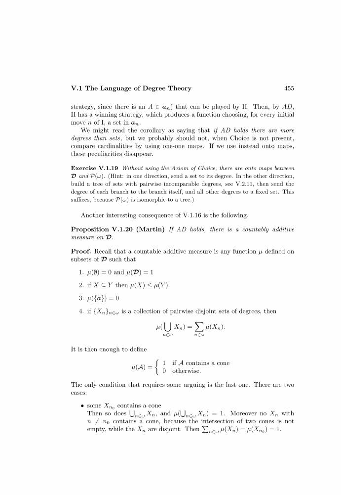
V.1 The Language of Degree Theory 455
strategy, since there is an A ∈ an) that can be played by II. Then, by AD,II has a winning strategy, which produces a function choosing, for every initialmove n of I, a set in an.
We might read the corollary as saying that if AD holds there are moredegrees than sets, but we probably should not, when Choice is not present,compare cardinalities by using one-one maps. If we use instead onto maps,these peculiarities disappear.
Exercise V.1.19 Without using the Axiom of Choice, there are onto maps between
D and P(ω). (Hint: in one direction, send a set to its degree. In the other direction,
build a tree of sets with pairwise incomparable degrees, see V.2.11, then send the
degree of each branch to the branch itself, and all other degrees to a fixed set. This
suffices, because P(ω) is isomorphic to a tree.)
Another interesting consequence of V.1.16 is the following.
Proposition V.1.20 (Martin) If AD holds, there is a countably additivemeasure on D.
Proof. Recall that a countable additive measure is any function µ defined onsubsets of D such that
1. µ(∅) = 0 and µ(D) = 1
2. if X ⊆ Y then µ(X) ≤ µ(Y )
3. µ(a) = 0
4. if Xnn∈ω is a collection of pairwise disjoint sets of degrees, then
µ(⋃n∈ω
Xn) =∑n∈ω
µ(Xn).
It is then enough to define
µ(A) =
1 if A contains a cone0 otherwise.
The only condition that requires some arguing is the last one. There are twocases:
• some Xn0 contains a coneThen so does
⋃n∈ωXn, and µ(
⋃n∈ωXn) = 1. Moreover no Xn with
n 6= n0 contains a cone, because the intersection of two cones is notempty, while the Xn are disjoint. Then
∑n∈ω µ(Xn) = µ(Xn0) = 1.

456 V. Turing Degrees
• no Xn contains a coneThen
∑n∈ω µ(Xn) = 0. Moreover Xn contains a cone for each n, by
V.1.16, and then so does their intersection, as in V.1.17. But⋂n∈ω
Xn =⋃n∈ω
Xn,
and thus⋃n∈ωXn does not contain a cone: hence µ(
⋃n∈ωXn) = 0. 2
Since the countable ordinals are represented by well-ordered sets of naturalnumbers, it immediately follows that if AD holds then ℵ1 is a measurable car-dinal (Solovay), by giving a set A of countable ordinals the same measure asthe set of degrees containing well-orderings with ordinal in A.
One might wonder why we should accept an axiom like AD . The fact isthat, as we will prove in following chapters, various special cases of it can beproved in ZFC, and thus some versions of the results proved above simplyhold. More precisely, Martin [1975] has showed in ZFC that every Borel gameis determined : thus every Borel set of degrees either contains a cone or it isdisjoint from a cone, and every Borel map from D to sets is constant on a cone.We will investigate the effect of restricted versions of AD on Recursion Theoryin Volume III.
V.2 The Finite Extension Method
Degrees are represented by sets, and thus existential properties of degrees canbe proved by building appropriate sets. Since building sets by successive ap-proximations will be our main concern in this chapter, we set up an efficientnotation to deal with the problem. Recall that a set is identified with itscharacteristic function, which is just a sequence of 0’s and 1’s.
Definition V.2.1 A string is a partial function σ : ω → 0, 1 with finitedomain. If the domain of σ is an initial segment of ω, we call σ an initialsegment, and let |σ| be its length. Given two strings σ and σ′, then:
1. σ′ is an extension of σ if it extends it as a partial function, i.e.
σ(x)↓ ⇒ σ′(x)↓ ∧ σ(x) ' σ′(x).
2. σ and σ′ are incompatible if they differ on some argument on whichthey are both defined.
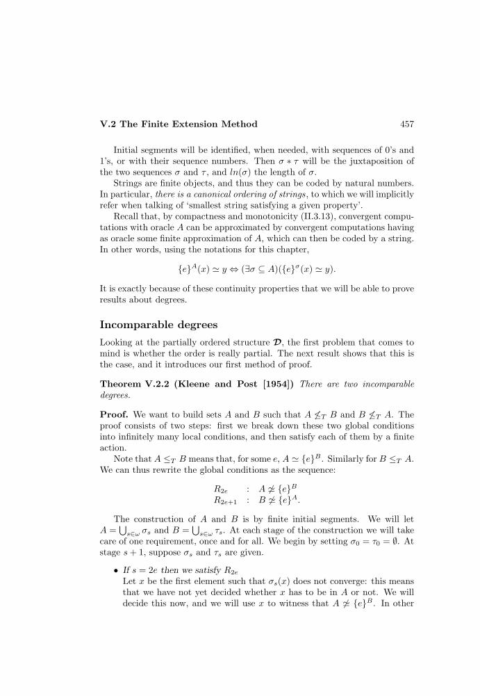
V.2 The Finite Extension Method 457
Initial segments will be identified, when needed, with sequences of 0’s and1’s, or with their sequence numbers. Then σ ∗ τ will be the juxtaposition ofthe two sequences σ and τ , and ln(σ) the length of σ.
Strings are finite objects, and thus they can be coded by natural numbers.In particular, there is a canonical ordering of strings, to which we will implicitlyrefer when talking of ‘smallest string satisfying a given property’.
Recall that, by compactness and monotonicity (II.3.13), convergent compu-tations with oracle A can be approximated by convergent computations havingas oracle some finite approximation of A, which can then be coded by a string.In other words, using the notations for this chapter,
eA(x) ' y ⇔ (∃σ ⊆ A)(eσ(x) ' y).
It is exactly because of these continuity properties that we will be able to proveresults about degrees.
Incomparable degrees
Looking at the partially ordered structure D, the first problem that comes tomind is whether the order is really partial. The next result shows that this isthe case, and it introduces our first method of proof.
Theorem V.2.2 (Kleene and Post [1954]) There are two incomparabledegrees.
Proof. We want to build sets A and B such that A 6≤T B and B 6≤T A. Theproof consists of two steps: first we break down these two global conditionsinto infinitely many local conditions, and then satisfy each of them by a finiteaction.
Note that A ≤T B means that, for some e, A ' eB . Similarly for B ≤T A.We can thus rewrite the global conditions as the sequence:
R2e : A 6' eBR2e+1 : B 6' eA.
The construction of A and B is by finite initial segments. We will letA =
⋃s∈ω σs and B =
⋃s∈ω τs. At each stage of the construction we will take
care of one requirement, once and for all. We begin by setting σ0 = τ0 = ∅. Atstage s+ 1, suppose σs and τs are given.
• If s = 2e then we satisfy R2e
Let x be the first element such that σs(x) does not converge: this meansthat we have not yet decided whether x has to be in A or not. We willdecide this now, and we will use x to witness that A 6' eB . In other
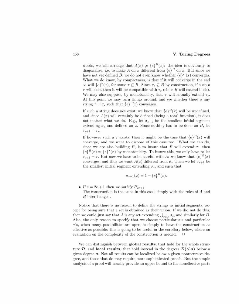
458 V. Turing Degrees
words, we will arrange that A(x) 6' eB(x): the idea is obviously todiagonalize, i.e. to make A on x different from eB on x. But since wehave not yet defined B, we do not even know whether eB(x) converges.What we do know, by compactness, is that if it will converge in the endso will eτ (x), for some τ ⊆ B. Since τs ⊆ B by construction, if such aτ will exist then it will be compatible with τs (since B will extend both).We may also suppose, by monotonicity, that τ will actually extend τs.At this point we may turn things around, and see whether there is anystring τ ⊇ τs such that eτ (x) converges.
If such a string does not exist, we know that eB(x) will be undefined,and since A(x) will certainly be defined (being a total function), it doesnot matter what we do. E.g., let σs+1 be the smallest initial segmentextending σs and defined on x. Since nothing has to be done on B, letτs+1 = τs.
If however such a τ exists, then it might be the case that eB(x) willconverge, and we want to dispose of this case too. What we can do,since we are also building B, is to insure that B will extend τ : theneB(x) ' eτ (x) by monotonicity. To insure this, we only have to letτs+1 = τ . But now we have to be careful with A: we know that eB(x)converges, and thus we want A(x) different from it. Then we let σs+1 bethe smallest initial segment extending σs, and such that
σs+1(x) = 1− eB(x).
• If s = 2e+ 1 then we satisfy R2e+1
The construction is the same in this case, simply with the roles of A andB interchanged.
Notice that there is no reason to define the strings as initial segments, ex-cept for being sure that a set is obtained as their union. If we did not do this,then we could just say that A is any set extending
⋃s∈ω σs, and similarly for B.
Also, the only reason to specify that we choose particular x’s and particularσ’s, when many possibilities are open, is simply to have the construction aseffective as possible: this is going to be useful in the corollary below, where anevaluation on the complexity of the construction is needed. 2
We can distinguish between global results, that hold for the whole struc-ture D, and local results, that hold instead in the degrees D(≤ a) below agiven degree a. Not all results can be localized below a given nonrecursive de-gree, and those that do may require more sophisticated proofs. But the simpleanalysis of a proof will usually provide an upper bound to the noneffective parts
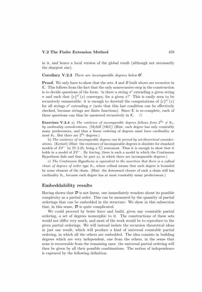
V.2 The Finite Extension Method 459
in it, and hence a local version of the global result (although not necessarilythe sharpest one).
Corollary V.2.3 There are incomparable degrees below 0′.
Proof. We only have to show that the sets A and B built above are recursive inK. This follows from the fact that the only nonrecursive step in the constructionis to decide questions of the form: ‘is there a string σ′ extending a given stringσ and such that eσ′(x) converges, for a given x?’ This is easily seen to berecursively enumerable: it is enough to dovetail the computations of eσ′(x)for all strings σ′ extending σ (note that this last condition can be effectivelychecked, because strings are finite functions). Since K is m-complete, each ofthese questions can thus be answered recursively in K. 2
Exercises V.2.4 a) The existence of incomparable degrees follows from 2ℵ0 6= ℵ1,by cardinality considerations. (Myhill [1961]) (Hint: each degree has only countablymany predecessors, and thus a linear ordering of degrees must have cardinality atmost ℵ1. But there are 2ℵ0 degrees.)
b) The existence of incomparable degrees can be proved by set-theoretical consider-ations. (Kreisel) (Hint: the existence of incomparable degrees is absolute for standardmodels of ZF− by IV.3.25, being a Σ1
1 statement. Thus it is enough to show that itholds in a model of ZF−. By forcing, there is such a model in which the ContinuumHypothesis fails and thus, by part a), in which there are incomparable degrees.)
c) The Continuum Hypothesis is equivalent to the assertion that there is a cofinal
chain of degrees of order type ℵ1, where cofinal means that each degree is bounded
by some element of the chain. (Hint: the downward closure of such a chain still has
cardinality ℵ1, because each degree has at most countably many predecessors.)
Embeddability results
Having shown that D is not linear, one immediately wonders about its possiblecomplexity as a partial order. This can be measured by the quantity of partialorderings that can be embedded in the structure. We show in this subsectionthat, in this sense, D is quite complicated.
We could proceed by brute force and build, given any countable partialordering, a set of degrees isomorphic to it. The constructions of these setswould not differ very much, and most of the work would be to reproduce to thegiven partial orderings. We will instead isolate the recursion theoretical ideasin just one result, which will produce a kind of universal countable partialordering, in which all the others are embedded. The idea consists in buildingdegrees which are very independent, one from the others, in the sense thatnone is recoverable from the remaining ones: the universal partial ordering willthen be given by all their possible combinations. The notion of independenceis captured by the following definition.
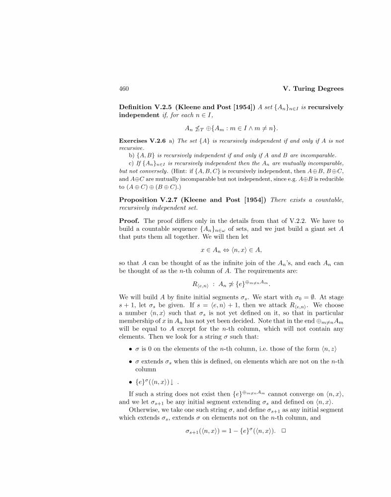
460 V. Turing Degrees
Definition V.2.5 (Kleene and Post [1954]) A set Ann∈I is recursivelyindependent if, for each n ∈ I,
An 6≤T ⊕Am : m ∈ I ∧m 6= n.
Exercises V.2.6 a) The set A is recursively independent if and only if A is notrecursive.
b) A,B is recursively independent if and only if A and B are incomparable.
c) If Ann∈I is recursively independent then the An are mutually incomparable,
but not conversely . (Hint: if A,B,C is recursively independent, then A⊕B, B⊕C,
and A⊕C are mutually incomparable but not independent, since e.g. A⊕B is reducible
to (A⊕ C)⊕ (B ⊕ C).)
Proposition V.2.7 (Kleene and Post [1954]) There exists a countable,recursively independent set.
Proof. The proof differs only in the details from that of V.2.2. We have tobuild a countable sequence Ann∈ω of sets, and we just build a giant set Athat puts them all together. We will then let
x ∈ An ⇔ 〈n, x〉 ∈ A,
so that A can be thought of as the infinite join of the An’s, and each An canbe thought of as the n-th column of A. The requirements are:
R〈e,n〉 : An 6' e⊕m 6=nAm .
We will build A by finite initial segments σs. We start with σ0 = ∅. At stages + 1, let σs be given. If s = 〈e, n〉 + 1, then we attack R〈e,n〉. We choosea number 〈n, x〉 such that σs is not yet defined on it, so that in particularmembership of x in An has not yet been decided. Note that in the end ⊕m6=nAmwill be equal to A except for the n-th column, which will not contain anyelements. Then we look for a string σ such that:
• σ is 0 on the elements of the n-th column, i.e. those of the form 〈n, z〉
• σ extends σs when this is defined, on elements which are not on the n-thcolumn
• eσ(〈n, x〉)↓ .
If such a string does not exist then e⊕m 6=nAm cannot converge on 〈n, x〉,and we let σs+1 be any initial segment extending σs and defined on 〈n, x〉.
Otherwise, we take one such string σ, and define σs+1 as any initial segmentwhich extends σs, extends σ on elements not on the n-th column, and
σs+1(〈n, x〉) = 1− eσ(〈n, x〉). 2

V.2 The Finite Extension Method 461
As we forecasted, the result is enough to prove all the embeddability resultswe need.
Exercise V.2.8 There is a recursive partial ordering in which all the countable par-tial ordering are embeddable. (Mostowski [1938]) (Hint: take the pairs of rationals,ordered as
(x, y) < (x′, y′) ⇔ x < x′ ∧ y < y′.
This a planar version of the fact that every countable linear ordering is embeddable
in the rationals. A direct construction is also possible, by having at any finite stage a
finite approximation, and extending it by adding a new element in each possible way
consistent with the partial ordering requirement.)
Theorem V.2.9 (Sacks [1963]) Any countable partial ordering is embeddablein the degrees (below 0′).
Proof. By the exercise, it is enough to show that any recursive countablepartial ordering is embeddable in the degrees. We use the recursively inde-pendent set Ann∈ω, and associate to each element a in the domain of theset ⊕naAn:
〈n, x〉 ∈ Ba ⇔ n a ∧ x ∈ An.
It remains to show thata b⇔ Ba ≤T Bb,
so that the structure of the degrees of the Ba’s is isomorphic to :
• if a b then Ba ≤T BbNote that, since is transitive, Ba ⊆ Bb in this case, and thus
〈n, x〉 ∈ Ba ⇔ n a ∧ 〈n, x〉 ∈ Bb.
Thus Ba ≤T Bb, because is recursive.
• if Ba ≤T Bb then a bSuppose a 6 b: then each element n b is different from a. It followsthat Bb ≤T (⊕n 6=aAn):
〈n, x〉 ∈ Bb ⇔ n b ∧ 〈n, x〉 ∈ (⊕n 6=aAn).
But Aa ≤T Ba, since a a, and thus it cannot beBa ≤T Bb otherwise, bytransitivity, Aa ≤T (⊕n 6=aAn), contradicting the recursive independenceof the An’s.

462 V. Turing Degrees
If we let An be the set constructed in V.2.9, then ⊕n∈ωAn is recursive inK, and hence so are all the Ba’s. Thus is actually embeddable in the degreesbelow 0′. 2
A sentence in the language of D is a one-quantifier sentence if it is logi-cally equivalent to a sentence in prenex normal form with a prefix consisting ofquantifiers of the same type, and a matrix consisting of a Boolean combinationof atomic formulas of the form x ≤ y.
Corollary V.2.10 (Lerman [1972]) The one-quantifier sentences of D andD(≤0′) admit a decision procedure.
Proof. It is enough to decide the existential sentences. But such a sentencesimply asserts the existence of finitely many elements x1, . . . , xn in a certainorder relationship. Since any countable (and hence any finite) partial orderingis embeddable in D, the sentence is true in D if and only if it is consistent withthe fact that ≤ is a partial ordering. 2
Exercises V.2.11 Independent sets of degrees. Since the infinite join is not adegree-theoretical operation, a set of degrees A is called independent if no element init is bounded by the l.u.b. of some finite subset of A.
a) There is a countable independent set of degrees. (Kleene and Post [1954]) (Hint:see V.2.7.)
b) There is an independent set of degrees of cardinality 2ℵ0 . (Sacks [1961]) (Hint:
build a tree of sets, each branch of which is not recursive in any finite join of different
branches.)
Sacks [1961] has proved that every partial ordering with one of the followingproperties is embeddable in D:
1. cardinality 2ℵ0 and finite predecessor property
2. cardinality ℵ1 and countable predecessor property
3. cardinality 2ℵ0 , countable predecessor property and ℵ1 successor property .
In particular, the last two conditions are equivalent and best possible, if theContinuum Hypothesis is assumed. The best absolute result would clearly beto prove the embeddability of any partial ordering with
4. cardinality 2ℵ0 and countable predecessor property
but it is unknown whether this holds.

V.2 The Finite Extension Method 463
The splitting method
We have completely decided the one-quantifier theory of D. We thus start todeal with two-quantifier sentences, that will be discussed in general on p. 490.A typical problem is to get a degree incomparable with a given one. Here thegame is more subtle than the one in V.2.2: there we could build both sets,while here one of them is given to us and we have no control over it. Thetechnique used in the solution to the problem is going to be extremely useful,and will be exploited in many different situations. The idea is natural, and itis a refinement of the one already used: since we control only one of the twosides, but we still need two possibilities to be able to diagonalize, we look forboth of them on the side we control.
Definition V.2.12 Two strings σ1 and σ2 are an e-splitting if, for some x,eσ1(x) and eσ2(x) both converge, and are different. In this case we saythat σ1 and σ2 e-split on x.
Theorem V.2.13 (Kleene and Post [1954]) Given any nonrecursive degreeb, there is a degree a incomparable with it.
Proof. Let B be nonrecursive: we want A such that
R2e : A 6' eBR2e+1 : B 6' eA.
The two types of requirements look the same, but are very different: B is givenahead of time, while A is constructed. Thus they require different actions.
As usual, we will let A =⋃s∈ω σs. We start with σ0 = ∅. At stage s + 1,
let σs be given.
• If s = 2e then we satisfy R2e
This is done by the method of the last subsection: we choose x on whichσs is not yet defined, and we extend σs to a σs+1 such that
σs+1(x) =
1− eB(x) if eB(x)↓0 otherwise.
Note that we simply ask whether eB(x) converges, instead of asking,as before, whether we may make it converge (because B is given).
• If s = 2e+ 1 then we satisfy R2e+1
We now see if there are e-splitting extensions of σs, i.e. if we have twopossible choices for eA, on some element x. If this the case, chooseτ1 and τ2 extending σs and e-splitting on some x. Then eτ1(x) and

464 V. Turing Degrees
eτ2(x) are both convergent, and one of them must be different fromB(x). Let σs+1 be τi, where
B(x) 6' eτi(x).
If such strings do not exist, let σs+1 = σs.
We still have to argue that R2e+1 is really satisfied, also in the case thate-splitting extensions of σs do not exist. Here is where the nonrecursiveness ofB comes into the game: we claim that, in this case, eA is either not total orrecursive, and thus it must be different from B, which is total and nonrecursive.
Suppose eA is total: by compactness, given any x there must be a stringτ ⊆ A such that eτ (x) gives the right value. We can obviously suppose, bymonotonicity, that τ extends σs. But since there are no e-splitting extendingσs it must be the case that, as long as eτ (x) converges, the value is unique.This then suggests a recursive method to compute eA: given x, dovetail thepossible computations eτ (x), for all strings τ extending σs. The first con-verging one gives the right value. 2
From a topological point of view, the difference between the previous proofand the pure extension method of the last subsection is that the splitting methodrequires something more than simple continuity , since we use the fact that whena functional is constant on an open set (i.e. there is no splitting above a givenstring), then its value is recursive.
Notice also that a simple analysis of the proof does not give the result fordegrees below 0′, since if 0 < b < 0′ we only get a ≤ b′ ≤ 0′′. The result stillholds below 0′, but a different proof is needed. The theory of degrees below 0′
thus requires a separate study, which we will undertake in Chapter XI.
Exercises V.2.14 a) Given a countable set of nonrecursive degrees, there is a degreeincomparable with every element of the set . (Shoenfield [1960]) (Hint: the require-ments to satisfy are still countably many.)
b) Every maximal antichain of degrees is uncountable. (Hint: use part a) andZorn’s Lemma.)
c) Every maximal independent set of degrees is uncountable. (Hint: every count-
able independent set of degrees can be extended.)
The next definition introduces two notions of minimality, one for pairs andone for single degrees, which are going to be useful in the future.
Definition V.2.15
1. Two degrees a and b form a minimal pair if they are nonrecursive andtheir g.l.b. is 0, i.e.
(∀c)(c ≤ a ∧ c ≤ b ⇒ c =0).

V.2 The Finite Extension Method 465
2. A degree a is minimal if it is nonrecursive and there is no degree between0 and a, i.e.
(∀c)(c ≤ a ⇒ c = 0 ∨ c = a).
Clearly two distinct minimal degrees form a minimal pair, but a minimalpair might consist of nonminimal degrees. The existence of minimal degreesis proved in Section 5, and it requires a different method of proof. With thepresent tools we can however prove the existence of minimal pairs.
Proposition V.2.16 There exists a minimal pair of degrees. Actually, eachnonrecursive degree is part of a minimal pair.
Proof. Let B be nonrecursive: we want A such that
R2e : A 6' eR2〈e,i〉+1 : eA ' iB ' C ⇒ C recursive.
The first kind of requirement ensures that A is not recursive, while the secondensures that any set recursive in both A and B is recursive. They are satisfiedas usual, the first by diagonalization, the second by the splitting method.
The idea to satisfy R2〈e,i〉+1 is the following. First one tries to make therequirement vacuously true, by having convergent computations such that
eA(x) 6' iB(x).
This can be done, at a given stage n, by looking for e-splitting extensions ofσs. If they do exist, we choose the one that produces a disagreement with iBon the x for which the two strings e-split. If they do not exist, we can arguethat then eA is recursive if total, as in V.2.13. Note that in this case thehypothesis that B is nonrecursive plays no role in the proof, and it is neededonly to satisfy the definition of minimal pair. 2
Corollary V.2.17 There exists a pair of degrees with greatest lower bound.
Exercises V.2.18 a) Two nonrecursive sets A and B form a minimal pair if, foreach a,
aA ' aB ' C ⇒ C recursive.
(Posner) This slightly simplifies the presentation of requirements. (Hint: choose anelement z in one of the two sets but not in the other, say z ∈ A−B. Consider
aX 'eX if z ∈ XiX otherwise.
Then aA ' eA and aB ' iB .)

466 V. Turing Degrees
b) There is a set of 2ℵ0 degrees, such that each pair from it is a minimal pair .
This will be greatly improved in V.5.12, which however requires a more difficult proof.
(Hint: build a tree of sets such that any two branches are a minimal pair.)
The proof of the next result is quite clever, and it manages to diagonalizeagainst uncountable sets of degrees by a counting trick. It is an example of themethod used by Sacks [1961] to obtain the results on uncountable embeddingsquoted on p. 462.
Definition V.2.19 A set of degrees is:
1. a chain if it is linearly ordered
2. an antichain if its members are mutually incomparable nonzero degrees.
The condition of nonrecursiveness for members of an antichain is imposedonly to avoid the trivial case 0.
Proposition V.2.20 (Sacks [1961])
1. Every countable chain of degrees is extendable, and thus every maximalchain has cardinality ℵ1.
2. Every antichain of cardinality less than 2ℵ0 is extendable, and thus everymaximal antichain has cardinality 2ℵ0 .
Proof. The first part is easy: given any countable set Ann∈ω, the set(⊕n∈ωAn)′ has degree strictly above all the degrees of the An’s. Since ev-ery degree has at most countably many predecessors, the maximal length of achain is ℵ1.
For the second part, let A be a set of degrees of cardinality 2ℵ0 , and suchthat any pair in it is a minimal pair (it exists, by the last exercise above). LetB be any set of nonrecursive degrees of cardinality less than 2ℵ0 . Note that
• the downward closure of B has cardinality less than 2ℵ0 , since each mem-ber of B has at most countably many predecessors
• for each member of B there is at most one member of A above it, sinceany degree below two distinct members of A must be recursive, and hencenot in B.
Then less than 2ℵ0 members of A, and hence not all of them, are comparablewith some member of B. 2
We have noticed in V.2.14 that maximal antichains and maximal indepen-dent sets of degrees are uncountable. We have just strengthened the first result,

V.2 The Finite Extension Method 467
by showing that maximal antichains actually have cardinality 2ℵ0 . A similarstrengthening of the second result is impossible, since the assertion that max-imal independent sets of degrees have cardinality 2ℵ0 is independent of ZFC(Sacks [1961], Groszek and Slaman [1983]).
Forcing the jump
After a first study of some elementary properties of D, we now we turn ourattention to D′. To control the behavior of the jump operator a new idea isneeded, which will be variously mixed with different methods. We first presentit by itself, in the proof of the next result.
Proposition V.2.21 (Spector [1956]) The jump operator is not one-one.
Proof. It is enough to get a > 0 such that a′ = 0′. To get A nonrecursivewe diagonalize, while to have A′ ≤T K we want to decide, for each e, whethereA(e)↓. The requirements are then:
R2e : A 6' eR2e+1 : decide whether eA(e)↓ .
Note that we do not consider the condition K ≤T A′, which is automaticallysatisfied because ∅ ≤T A, and hence K = ∅′ ≤T A′.
As usual we build A by finite initial segments, starting with σ0 = ∅. Atstage s+ 1, let σs be given.
• If s = 2e then we satisfy R2e
Let x be the first element on which σs is undefined, and let σs+1 be thesmallest initial segment extending σs and such that
σs+1(x) =
1− e(x) if e(x)↓0 otherwise.
• If s = 2e+ 1 then we satisfy R2e+1
See if there is an initial segment σ extending σs such that eσ(e) ↓. Ifso, let σ be the smallest one, and σs+1 = σ. Otherwise, let σs+1 = σs.
By construction A is not recursive. Moreover,
e ∈ A′ ⇔ eA(e)↓⇔ eσ2e+2(e)↓
and, since the construction is recursive in K, A′ ≤T K. 2
Corollary V.2.22 The jump operator is never one-one on its range.
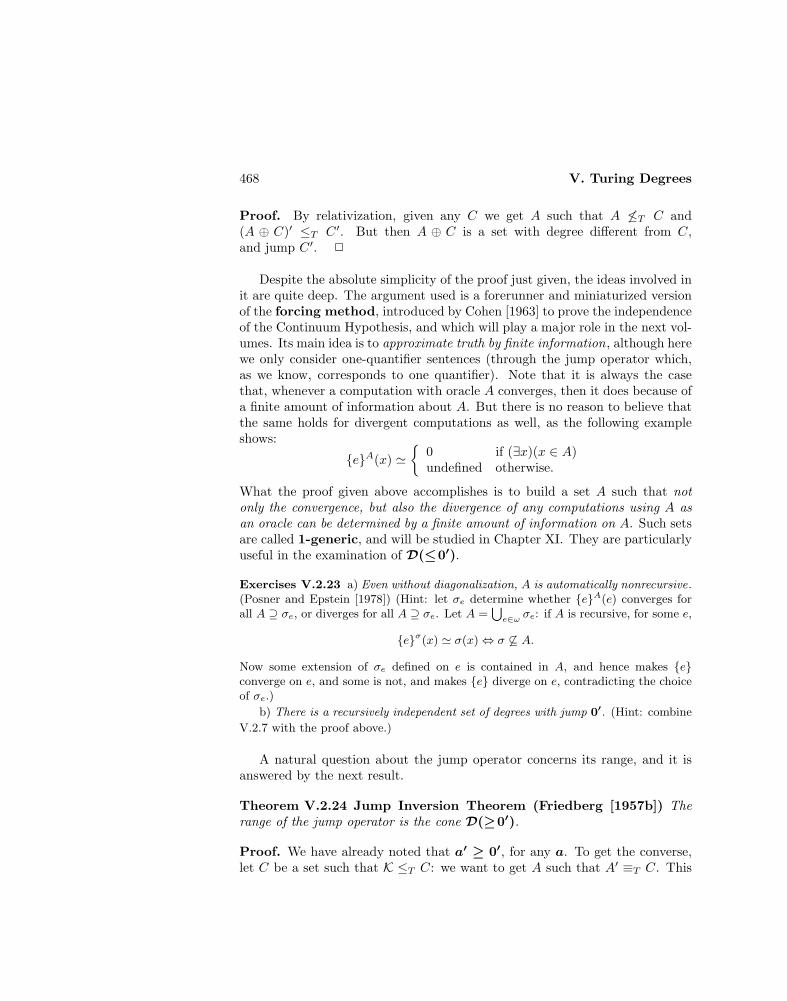
468 V. Turing Degrees
Proof. By relativization, given any C we get A such that A 6≤T C and(A ⊕ C)′ ≤T C ′. But then A ⊕ C is a set with degree different from C,and jump C ′. 2
Despite the absolute simplicity of the proof just given, the ideas involved init are quite deep. The argument used is a forerunner and miniaturized versionof the forcing method, introduced by Cohen [1963] to prove the independenceof the Continuum Hypothesis, and which will play a major role in the next vol-umes. Its main idea is to approximate truth by finite information, although herewe only consider one-quantifier sentences (through the jump operator which,as we know, corresponds to one quantifier). Note that it is always the casethat, whenever a computation with oracle A converges, then it does because ofa finite amount of information about A. But there is no reason to believe thatthe same holds for divergent computations as well, as the following exampleshows:
eA(x) '
0 if (∃x)(x ∈ A)undefined otherwise.
What the proof given above accomplishes is to build a set A such that notonly the convergence, but also the divergence of any computations using A asan oracle can be determined by a finite amount of information on A. Such setsare called 1-generic, and will be studied in Chapter XI. They are particularlyuseful in the examination of D(≤0′).
Exercises V.2.23 a) Even without diagonalization, A is automatically nonrecursive.(Posner and Epstein [1978]) (Hint: let σe determine whether eA(e) converges forall A ⊇ σe, or diverges for all A ⊇ σe. Let A =
⋃e∈ω σe: if A is recursive, for some e,
eσ(x) ' σ(x) ⇔ σ 6⊆ A.
Now some extension of σe defined on e is contained in A, and hence makes econverge on e, and some is not, and makes e diverge on e, contradicting the choiceof σe.)
b) There is a recursively independent set of degrees with jump 0′. (Hint: combine
V.2.7 with the proof above.)
A natural question about the jump operator concerns its range, and it isanswered by the next result.
Theorem V.2.24 Jump Inversion Theorem (Friedberg [1957b]) Therange of the jump operator is the cone D(≥0′).
Proof. We have already noted that a′ ≥ 0′, for any a. To get the converse,let C be a set such that K ≤T C: we want to get A such that A′ ≡T C. This

V.2 The Finite Extension Method 469
splits into two separate conditions: A′ ≤T C, which will be satisfied as above,and C ≤T A′, which will be achieved by coding C into A. The two strategieswill be pursued alternately.
As usual we build A by finite initial segments, starting with σ0 = ∅. Atstage s+ 1, let σs be given.
• If s = 2e then we see if there is an initial segment σ ⊇ σs such thateσ(e)↓. If so, we let σs+1 = σ for the smallest such, and otherwise welet σs+1 = σs.
• If s = 2e+ 1, we code the e-th element of C into A:
σs+1 = σs ∗ 〈C(e)〉.
The construction is recursive in C: the first step is recursive in K, which isrecursive in C by hypothesis, and the second uses C directly. Thus, since
e ∈ A′ ⇔ eσ2e+1(e)↓,
we have A′ ≤T C.The construction is also recursive in K and A: the second step simply
determines the value of A for the next undefined element, which is |σ2e+1|.Then
e ∈ C ⇔ σ2e+2(|σ2e+1|) = 1
and C ≤T A ⊕ K. But A ⊕ K ≤T A′ (because A ≤T A′ and K ≤T A′), andhence C ≤T A′. 2
Notice that the least possible jump of a degree a is a′ = a ∪ 0′, sincea ∪ 0′ ≤ a′ always holds. Not every degree realizes the least possible jump,e.g. any degree c ≥ 0′ does not (since then c ∪ 0′ = c), but the proof aboveactually shows that every degree c ≥ 0′ is the jump of a degree realizing theleast possible jump.
Exercise V.2.25 For any c ≥ 0′ there are infinitely many degrees with jump c.
(Hint: relativize V.2.23.b, and apply the Jump Inversion Theorem.)
The jump operator by itself is not very problematic: using the previousexercise, it can be shown that the first-order theory with equality of (D, ′)is decidable (Jockusch and Soare [1970]). But adding the jump to D is adifferent story, and even the one-quantifier sentences of D′ are not known tobe decidable.
Our last immediate goal is to determine the possible behavior of the jumpoperator. To provide some necessary counterexamples, we first prove a result.

470 V. Turing Degrees
Proposition V.2.26 (Spector [1956]) For any c ≥ 0′ there exist two de-grees a and b such that a ∪ b = a′ = b′ = c.
Proof. We modify the proof of the Jump Inversion Theorem. Let C such thatK ≤T C be given: we want two sets A and B such that A′ ≡T B′ ≡T C, andA ⊕ B ≡T C. The last condition involves the only new idea in the proof, andconsists of building A and B by initial segments of the same length, and to letthe two sides have the same value only when coding elements of C, so that Cwill be recoverable from the two sets together.
We let A =⋃s∈ω σs and B =
⋃s∈ω τs, and we start with σ0 = τ0 = ∅. At
stage s+ 1, let σs and τs be given and of the same length.
• If s = 3e then we see if there is an initial segment σ ⊇ σs such thateσ(e) ↓, and let σs+1 be the smallest such string if one exists, and σsotherwise. Moreover, we also extend τs on the new elements x on whichσs+1 has been defined, if any, by letting
τs+1(x) = 1− σs+1(x),
so that σs+1 and τs+1 differ on these elements.
• If s = 3e + 1 we do the same, interchanging the roles of A and B (andhence of the σ’s and τ ’s).
• If s = 3e+ 2 then we code C(e), by letting
σs+1 = σs ∗ 〈C(e)〉 τs+1 = τs ∗ 〈C(e)〉.
Note that this is the only step where the two sides receive the same value.
As before, we have
A⊕K ≡T B ⊕K ≡T B′ ≡T A′ ≡T C.
To recover C(e), we only have to look at the e-th place in which A and B agree,and this is recursive in A⊕B. So
C ≤T A⊕B ≤T A′ ⊕B′ ≤T C,
and hence the sets A⊕B and C are T -equivalent. 2
Recall that V.1.14 provided some necessary conditions for the behavior ofthe jump operator. We can show now that they are best possible.

V.3 Baire Category ? 471
Proposition V.2.27 (Spector [1956], Shoenfield [1959]) Every possibilitycompatible with any of the properties
a ≤ b ⇒ a′ ≤ b′ and a′ ∪ b′ ≤ (a ∪ b)′
is realized.
Proof. The following are the possible cases:
1. jumps of comparable degreesLet a ≤ b. Then we can have:
• a′ = b′ by the proof of V.2.21.• a′ < b′, if a = 0 and b = 0′.
2. jumps of incomparable degreesLet a|b. Then we can have:
• a′ = b′ by V.2.26, since two degrees with jump c are strictly belowit, and if they join to it then they must be incomparable (otherwisetheir join would be one of them).
• a′ < b′, by having a degree b incomparable with a = 0′ and withjump greater than 0′′. Note that a degree realizing the least possiblejump cannot be above 0′, and thus we only need to avoid b < 0′.This is automatic if b′ > 0′′, and thus it is enough to apply theJump Inversion Theorem, and get b such that b′ = 0′′′.
• a′|b′, by taking two degrees whose jumps are incomparable, whichexist by the Jump Inversion Theorem (since incomparable degreesabove 0′ exist, e.g. by relativization of V.2.2).
3. distributivity of jump over join
• a′ ∪ b′ = (a ∪ b)′ = 0′′ if a = 0 and b = 0′.• a′ ∪ b′ < (a ∪ b)′ for the degrees in V.2.26. 2
V.3 Baire Category ?
In Section II.1 we looked at the class P of partial functions, from a topologicalpoint of view. Here we do the same for the class of total functions, and wewill distinguish the class of functions (ωω, the Baire space) from the class ofcharacteristic functions or sets (P(ω), the Cantor space). There are variousways of introducing a topology on these sets, but the induced topology will beunique, and thus particularly stable. As a reference on topology the reader canconsult Kelley [1955].

472 V. Turing Degrees
Topologies on total functions
Natural topologies on ωω and P(ω) are the following:
1. the topology induced by the topology of PThe open sets are the intersection of open sets of P with ωω or P(ω).Thus a basic open set is determined by a finite initial segment, see p. 186.
2. the product topology of the discrete topology on ω or 0, 1Here every subset of ω is open, and a basic open set on ωω is a product
A0 ×A1 × · · · ×An × ω × ω × · · ·
where the Ai’s are nonempty open sets. Thus the basic open sets areunions of sets determined by finite initial segments, namely the finiteinitial segments σ of length n+ 1 such that σ(i) ∈ Ai.
3. the topology induced by the following metric:
d(f, g) =
0 if f = g1
[µx(f(x) 6=g(x)]+1 otherwise.
Thus the distance between two functions is determined by the smallestargument on which they differ, and the factor ‘+1’ takes care of thepossibility that they differ on 0. The basic open sets are the balls relativeto the metric, and again they are determined by finite initial segments.
4. the topology induced by the order topology on the realsHere we use the canonical homeomorphism between ωω and the irrationalsbetween 0 and 1, which can be produced in two different ways. One is togive the direct map
f 7−→ 1f(0) + 1
f(1)+ ····
For the other, first note that there is a one-one map from ωω to P(ω),given by
f 7−→ 1 . . . 10︸ ︷︷ ︸f(0) + 1
0 . . . 01︸ ︷︷ ︸f(1) + 1
1 . . . 10︸ ︷︷ ︸f(2) + 1
0 . . .
Then consider the reals between 0 and 1, in binary representation. Eachsuch real may be written as
∑i∈I 2−(i+1), for some I ⊆ ω. The bi-
nary irrationals are those reals between 0 and 1 that cannot be so rep-resented with a finite I. The composition of these two maps gives ahomeomorphism between ωω and the binary irrationals. These and theirrationals are homeomorphic, because binary rationals and rationals are
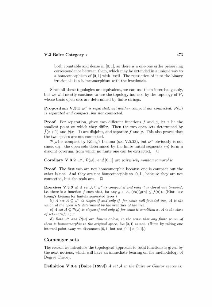
V.3 Baire Category ? 473
both countable and dense in [0, 1], so there is a one-one order preservingcorrespondence between them, which may be extended in a unique way toa homeomorphism of [0, 1] with itself. The restriction of it to the binaryirrationals is a homeomorphism with the irrationals.
Since all these topologies are equivalent, we can use them interchangeably,but we will mostly continue to use the topology induced by the topology of P,whose basic open sets are determined by finite strings.
Proposition V.3.1 ωω is separated, but neither compact nor connected. P(ω)is separated and compact, but not connected.
Proof. For separation, given two different functions f and g, let x be thesmallest point on which they differ. Then the two open sets determined byf(x+ 1) and g(x+ 1) are disjoint, and separate f and g. This also proves thatthe two spaces are not connected.
P(ω) is compact by Konig’s Lemma (see V.5.23), but ωω obviously is notsince, e.g., the open sets determined by the finite initial segments 〈n〉 form adisjoint covering, from which no finite one can be extracted. 2
Corollary V.3.2 ωω, P(ω), and [0, 1] are pairwisely nonhomeomorphic.
Proof. The first two are not homeomorphic because one is compact but theother is not. And they are not homeomorphic to [0, 1], because they are notconnected, but the reals are. 2
Exercises V.3.3 a) A set A ⊆ ωω is compact if and only it is closed and bounded ,i.e. there is a function f such that, for any g ∈ A, (∀n)(g(n) ≤ f(n)). (Hint: useKonig’s Lemma for finitely generated trees.)
b) A set A ⊆ ωω is clopen if and only if, for some well-founded tree, A is theunion of the open sets determined by the branches of the tree.
c) A set A ⊆ P(ω) is clopen if and only if, for some tt-condition σ, A is the classof sets satisfying σ.
d) Both ωω and P(ω) are dimensionless, in the sense that any finite power of
them is homeomorphic to the original space, but [0, 1] is not . (Hint: by taking one
internal point away we disconnect [0, 1] but not [0, 1]× [0, 1].)
Comeager sets
The reason we introduce the topological approach to total functions is given bythe next notions, which will have an immediate bearing on the methodology ofDegree Theory.
Definition V.3.4 (Baire [1899]) A set A in the Baire or Cantor spaces is:
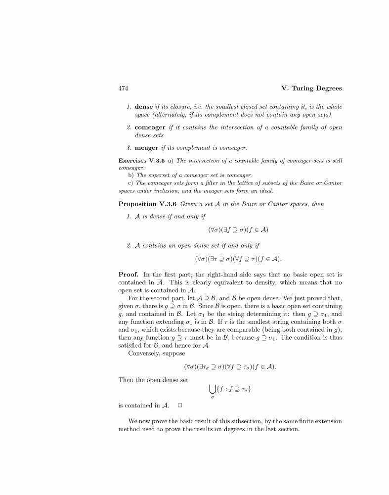
474 V. Turing Degrees
1. dense if its closure, i.e. the smallest closed set containing it, is the wholespace (alternately, if its complement does not contain any open sets)
2. comeager if it contains the intersection of a countable family of opendense sets
3. meager if its complement is comeager.
Exercises V.3.5 a) The intersection of a countable family of comeager sets is stillcomeager .
b) The superset of a comeager set is comeager .
c) The comeager sets form a filter in the lattice of subsets of the Baire or Cantor
spaces under inclusion, and the meager sets form an ideal .
Proposition V.3.6 Given a set A in the Baire or Cantor spaces, then
1. A is dense if and only if
(∀σ)(∃f ⊇ σ)(f ∈ A)
2. A contains an open dense set if and only if
(∀σ)(∃τ ⊇ σ)(∀f ⊇ τ)(f ∈ A).
Proof. In the first part, the right-hand side says that no basic open set iscontained in A. This is clearly equivalent to density, which means that noopen set is contained in A.
For the second part, let A ⊇ B, and B be open dense. We just proved that,given σ, there is g ⊇ σ in B. Since B is open, there is a basic open set containingg, and contained in B. Let σ1 be the string determining it: then g ⊇ σ1, andany function extending σ1 is in B. If τ is the smallest string containing both σand σ1, which exists because they are comparable (being both contained in g),then any function g ⊇ τ must be in B, because g ⊇ σ1. The condition is thussatisfied for B, and hence for A.
Conversely, suppose
(∀σ)(∃τσ ⊇ σ)(∀f ⊇ τσ)(f ∈ A).
Then the open dense set ⋃σ
f : f ⊇ τσ
is contained in A. 2
We now prove the basic result of this subsection, by the same finite extensionmethod used to prove the results on degrees in the last section.
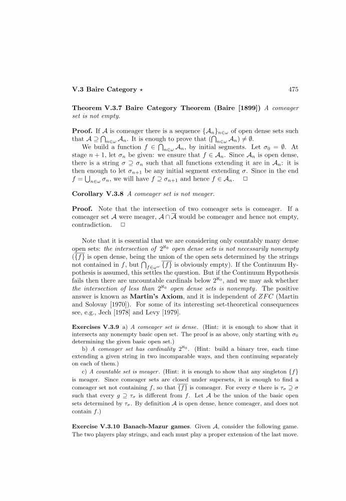
V.3 Baire Category ? 475
Theorem V.3.7 Baire Category Theorem (Baire [1899]) A comeagerset is not empty.
Proof. If A is comeager there is a sequence Ann∈ω of open dense sets suchthat A ⊇
⋂n∈ω An. It is enough to prove that (
⋂n∈ω An) 6= ∅.
We build a function f ∈⋂n∈ω An, by initial segments. Let σ0 = ∅. At
stage n + 1, let σn be given: we ensure that f ∈ An. Since An is open dense,there is a string σ ⊇ σn such that all functions extending it are in An: it isthen enough to let σn+1 be any initial segment extending σ. Since in the endf =
⋃n∈ω σn, we will have f ⊇ σn+1 and hence f ∈ An. 2
Corollary V.3.8 A comeager set is not meager.
Proof. Note that the intersection of two comeager sets is comeager. If acomeager set A were meager, A∩A would be comeager and hence not empty,contradiction. 2
Note that it is essential that we are considering only countably many denseopen sets: the intersection of 2ℵ0 open dense sets is not necessarily nonempty(f is open dense, being the union of the open sets determined by the stringsnot contained in f , but
⋂f∈ωω f is obviously empty). If the Continuum Hy-
pothesis is assumed, this settles the question. But if the Continuum Hypothesisfails then there are uncountable cardinals below 2ℵ0 , and we may ask whetherthe intersection of less than 2ℵ0 open dense sets is nonempty . The positiveanswer is known as Martin’s Axiom, and it is independent of ZFC (Martinand Solovay [1970]). For some of its interesting set-theoretical consequencessee, e.g., Jech [1978] and Levy [1979].
Exercises V.3.9 a) A comeager set is dense. (Hint: it is enough to show that itintersects any nonempty basic open set. The proof is as above, only starting with σ0
determining the given basic open set.)b) A comeager set has cardinality 2ℵ0 . (Hint: build a binary tree, each time
extending a given string in two incomparable ways, and then continuing separatelyon each of them.)
c) A countable set is meager . (Hint: it is enough to show that any singleton fis meager. Since comeager sets are closed under supersets, it is enough to find a
comeager set not containing f , so that f is comeager. For every σ there is τσ ⊇ σ
such that every g ⊇ τσ is different from f . Let A be the union of the basic open
sets determined by τσ. By definition A is open dense, hence comeager, and does not
contain f .)
Exercise V.3.10 Banach-Mazur games. Given A, consider the following game.
The two players play strings, and each must play a proper extension of the last move.
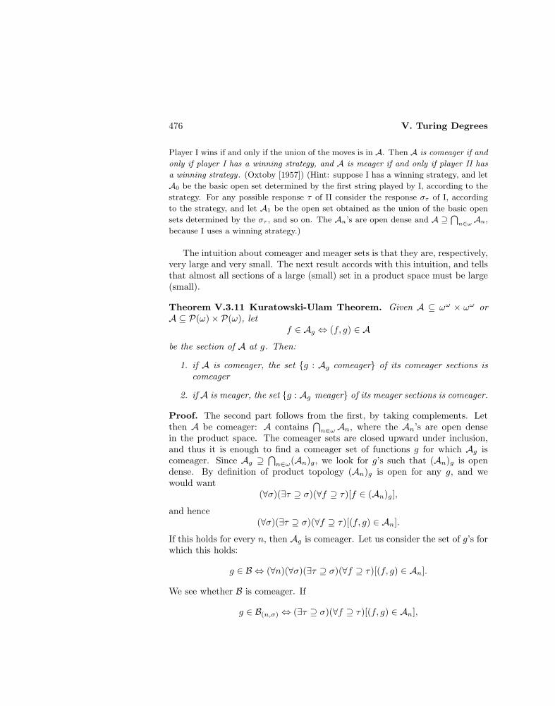
476 V. Turing Degrees
Player I wins if and only if the union of the moves is in A. Then A is comeager if and
only if player I has a winning strategy, and A is meager if and only if player II has
a winning strategy . (Oxtoby [1957]) (Hint: suppose I has a winning strategy, and let
A0 be the basic open set determined by the first string played by I, according to the
strategy. For any possible response τ of II consider the response στ of I, according
to the strategy, and let A1 be the open set obtained as the union of the basic open
sets determined by the στ , and so on. The An’s are open dense and A ⊇⋂n∈ω An,
because I uses a winning strategy.)
The intuition about comeager and meager sets is that they are, respectively,very large and very small. The next result accords with this intuition, and tellsthat almost all sections of a large (small) set in a product space must be large(small).
Theorem V.3.11 Kuratowski-Ulam Theorem. Given A ⊆ ωω × ωω orA ⊆ P(ω)× P(ω), let
f ∈ Ag ⇔ (f, g) ∈ A
be the section of A at g. Then:
1. if A is comeager, the set g : Ag comeager of its comeager sections iscomeager
2. if A is meager, the set g : Ag meager of its meager sections is comeager.
Proof. The second part follows from the first, by taking complements. Letthen A be comeager: A contains
⋂n∈ω An, where the An’s are open dense
in the product space. The comeager sets are closed upward under inclusion,and thus it is enough to find a comeager set of functions g for which Ag iscomeager. Since Ag ⊇
⋂n∈ω(An)g, we look for g’s such that (An)g is open
dense. By definition of product topology (An)g is open for any g, and wewould want
(∀σ)(∃τ ⊇ σ)(∀f ⊇ τ)[f ∈ (An)g],
and hence(∀σ)(∃τ ⊇ σ)(∀f ⊇ τ)[(f, g) ∈ An].
If this holds for every n, then Ag is comeager. Let us consider the set of g’s forwhich this holds:
g ∈ B ⇔ (∀n)(∀σ)(∃τ ⊇ σ)(∀f ⊇ τ)[(f, g) ∈ An].
We see whether B is comeager. If
g ∈ B(n,σ) ⇔ (∃τ ⊇ σ)(∀f ⊇ τ)[(f, g) ∈ An],

V.3 Baire Category ? 477
then B =⋂n,σ B(n,σ), but the B(n,σ) are not necessarily open, because we use
all of g in their definition. Thus B is not necessarily comeager, but a smallvariation of it will do. Let
g ∈ C(n,σ) ⇔ (∃y)(∃τ ⊇ σ)(∀f ⊇ τ)(∀h ⊇ g(y))[(f, h) ∈ An].
Now C(n,σ) is open (because union of basic open sets) and dense (because so isAn). If
C =⋂n,σ
C(n,σ)
then C is comeager and, as above, Ag is comeager whenever g ∈ C. 2
Exercises V.3.12 A has the Baire property if there is an open set U such that
(A−U)∪ (U −A) is meager, i.e. A differs from an open set by a meager set. If A has
the Baire property, then the converse implications in the Kuratowski-Ulam Theorem
hold . (Hint: suppose A is not meager, but g : Ag meager is comeager. Since Agdiffers from the open set Ug by a meager set, Ug must be meager for a comeager set
of g’s. But U is not empty, and it contains a basic open set: hence there is also a
comeager set of g’s such that Ug contains an open set, and thus is not meager. The
intersection of these two comeager sets is not empty by the Baire Category Theorem,
contradiction.)
Baire Category and Degree Theory
Going back to the proofs of the results in Section 2, we notice that they allshared the following characteristic features. We had a set of requirements Rnto satisfy, which may be identified with the class of sets satisfying them. Thegeneral pattern of the proofs was to show that, for each n,
(∀σ)(∃τ)(∀A ⊇ τ)(A ∈ Rn).
Thus we were actually showing that, for each n, there is an open dense setAn contained in Rn (by V.3.6). The Baire Category Theorem could then beapplied to claim that the intersection of requirements is not empty, and hencethat there is a set satisfying all the requirements, without further constructions.More precisely:
Proposition V.3.13 The Finite Extension Method (Myhill [1961],Sacks [1963]) Given a countable collection of requirements Rn such that
(∀σ)(∃τ ⊇ σ)(∀A ⊇ τ)(A ∈ Rn),
the set⋂n∈ω Rn is comeager (and hence nonempty).

478 V. Turing Degrees
The categorical approach is useful for a methodological analysis of the finiteextension method. Precisely, from it we obtain that:
1. requirements can be taken care of separately, by showing that each of themis dense
2. we can freely combine constructions known to be performable separately,as long as the global list of requirements remains countableFor example, suppose we want to prove that, given a countable sequenceA0, A1, . . . of nonrecursive sets, there is a set B incomparable with allof them. Then we only have to prove that, for a given e and a givennonrecursive set C,
• (∀σ)(∃τ)(∀A ⊇ τ)(A 6' eC)
• (∀σ)(∃τ)(∀A ⊇ τ)(C 6' eA).
We know that we can do this, by the work done in Section 2. It thusfollows that, for a fixed nonrecursive set C, the set
A : A 6≤T C ∧ C 6≤T A
is comeager, and hence so is
A : (∀n)(A 6≤T An ∧An 6≤T A),
being a countable intersection of comeager sets. In particular, the set isnot empty by Baire Category Theorem. Note that we could even avoid theconsideration of the condition A 6≤T C, because there are only countablymany sets recursive in C: the set A : A 6≤T C is thus automaticallycomeager.
3. we cannot use the finite extension method to produce sets belonging to ameager classThis follows from the fact that the finite extension method producessets in a comeager class, and the intersection of two comeager classes isnonempty, by the Baire Category Theorem. In particular, if we can usethe finite extension method to build a set satisfying certain requirements,then we cannot use the same method to build a set not satisfying the samerequirements.
4. a game-theoretical approach to Degree Theory is possible, via Banach-Mazur gamesThis follows from V.3.10, and has been developed by Yates [1976]. Seealso p. 495.

V.3 Baire Category ? 479
We can reformulate a number of results proved before in terms of categorynotions, with the convention that a set of degrees A is comeager or meagerif such is the class of sets whose degree is in A. This makes sense because adegree contains only countably many sets, and thus it is a meager class.
Proposition V.3.14 The following sets of degrees are comeager:
1. a : a is incomparable with a fixed nonrecursive degree
2. a : a is the l.u.b. of two incomparable degrees
3. a : a is the l.u.b. of a minimal pair
4. a : a realizes the least possible jump.
The following sets of degrees are meager:
5. a : a is comparable with a fixed nonrecursive degree
6. a : a is a minimal degree.
Proof. The proof of V.2.2 builds two sets A and B with incomparable degree:this can be seen as the construction of a single set A ⊕ B which is the leastupper bound of two incomparable sets, and proves 2. Part 6 follows from this,since a minimal degree cannot be the l.u.b. of two incomparable degrees.
Similarly, the other parts follow from V.2.13, V.2.16 and V.2.24. 2
Note that this shows, in particular, that degrees comparable with a givennonrecursive degree, as well as minimal degrees, cannot be built by the finiteextension method .
The work done so far also allows to decide whether any quantifier-free ques-tion about jumps, l.u.b.’s and g.l.b.’s of degrees holds for a comeager set ofdegrees or not.
Proposition V.3.15 (Stillwell [1972]) The theory of degrees
(D, ≤ , ∪ , ∩ , ′,0),
with subformulas containing a term t1∩ t2 thought of as prefixed by ‘t1∩ t2exists’, and with the quantifiers ∀ and ∃ interpreted, respectively, as meaning‘for a comeager set of degrees’ and ‘¬∀¬’, is decidable.
Proof. For simplicity, we will say ‘almost always’ to mean ‘for a comeager setof n-tuples of degrees’.
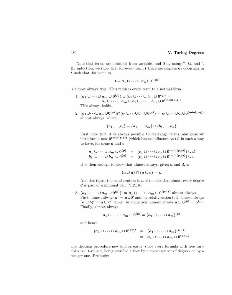
480 V. Turing Degrees
Note that terms are obtained from variables and 0 by using ∩, ∪, and ′.By induction, we show that for every term t there are degrees ai occurring int such that, for some m,
t = a1 ∪ · · · ∪ an ∪ 0(m)
is almost always true. This reduces every term to a normal form.
1. (a1 ∪ · · · ∪ am ∪ 0(p)) ∪ (b1 ∪ · · · ∪ bm ∪ 0(q)) =a1 ∪ · · · ∪ am ∪ b1 ∪ · · · ∪ bm ∪ 0(max(p,q)).
This always holds.
2. (a1∪· · ·∪am∪0(p))∩(b1∪· · ·∪bm∪0(q)) = c1∪· · ·∪cs∪0(min(p,q))
almost always, where
c1,. . . ,cs = a1,. . . ,am ∩ b1,. . . ,bn.
First note that it is always possible to rearrange terms, and possiblyintroduce a new 0(min(p,q)) (which has no influence on ∪) in such a wayto have, for some d and e,
a1 ∪ · · · ∪ am ∪ 0(p) = (c1 ∪ · · · ∪ cs ∪ 0(min(p,q))) ∪ d
b1 ∪ · · · ∪ bn ∪ 0(q) = (c1 ∪ · · · ∪ cs ∪ 0(min(p,q))) ∪ e.
It is then enough to show that almost always, given a and d, is
(a ∪ d) ∩ (a ∪ e) = a.
And this is just the relativization to a of the fact that almost every degreed is part of a minimal pair (V.2.16).
3. (a1 ∪ · · · ∪ am ∪ 0(p))′ = a1 ∪ · · · ∪ am ∪ 0(p+1) almost always.First, almost always a′ = a∪0′ and, by relativization to b, almost always(a ∪ b)′ = a ∪ b′. Then, by induction, almost always a ∪ 0(p) = a(p).Finally, almost always
a1 ∪ · · · ∪ am ∪ 0(p) = (a1 ∪ · · · ∪ am)(p),
and hence
(a1 ∪ · · · ∪ am ∪ 0(p))′ = (a1 ∪ · · · ∪ am)(p+1)
= a1 ∪ · · · ∪ am ∪ 0(p+1).
The decision procedure now follows easily, since every formula with free vari-ables is 0,1-valued, being satisfied either by a comeager set of degrees or by ameager one. Precisely:
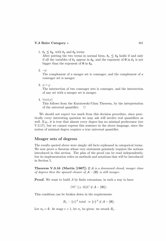
V.3 Baire Category ? 481
1. t1 ≤ t2, with t1 and t2 termsAfter putting the two terms in normal form, t1 ≤ t2 holds if and onlyif all the variables of t1 appear in t2, and the exponent of 0 in t1 is notbigger than the exponent of 0 in t2.
2. ¬ψThe complement of a meager set is comeager, and the complement of acomeager set is meager.
3. ψ ∧ ϕThe intersection of two comeager sets is comeager, and the intersectionof any set with a meager set is meager.
4. ∀xψ(x)This follows from the Kuratowski-Ulam Theorem, by the interpretationof the universal quantifier. 2
We should not expect too much from this decision procedure, since prac-tically every interesting question we may ask will involve real quantifiers aswell. E.g., it is true that almost every degree has no minimal predecessor (seeV.3.17), but we cannot express this sentence in the above language, since thenotion of minimal degree requires a true universal quantifier.
Meager sets of degrees
The results quoted above were simply old facts rephrased in categorical terms.We now prove a theorem whose very statement genuinely requires the notionsintroduced in this section. The plan of the proof can be read independently,but its implementation relies on methods and notations that will be introducedin Section 5.
Theorem V.3.16 (Martin [1967]) If A is a downward closed, meager classof degrees then the upward closure of A− 0 is still meager.
Proof. We want to build A by finite extensions, in such a way to have
(∀C ≤T A)(C 6∈ A − 0).
This condition can be broken down in the requirements
Re : eA total ⇒ eA 6∈ A − 0.
Let σ0 = ∅. At stage e+ 1, let σe be given: we attack Re.
482 V. Turing Degrees
1. If there is σ ⊇ σe such that
(∃x)(∀τ ⊇ σ)(eτ (x)↑)
then we let σe+1 = σ. This ensures that if A ⊇ σe+1 then eA is nottotal.
2. If there is a σ ⊇ σe with no e-splitting extensions, again let σe+1 = σ.This ensures that if A ⊇ σe+1 then eA is recursive.
3. Suppose now that:
• (∀σ ⊇ σe)(∀x)(∃τ ⊇ σ)(eτ (x)↓)• for all σ ⊇ σe there are e-splitting extensions of σ.
It will be useful in the following to picture eσ as a finite string, withthe property that
σ ⊆ σ′ ⇒ eσ ⊆ eσ′.
The proof goes roughly as follows. We build an order-preserving recursivemap Φ from strings to strings such that
(∀τ ⊇ Φ(eσe))(∃σ ⊇ σe)[τ = Φ(eσ)].
This gives a homeomorphism between the set Φ(eσ) : σ ⊇ σe and thewhole space of strings. Since A is meager, there is an open set containedin A, hence there is σ ⊇ σe such that
(∀A ⊇ σ)(Φ(eA) 6∈ A).
But Φ is recursive, and so Φ(eA) ≤T eA. Moreover, A is closeddownward, hence
(∀A ⊇ σ)(eA 6∈ A),
and Re is satisfied.
To finish the proof, it remains to build Φ. We first build an admissibletriple (i.e. a uniform tree, see V.6.2) with the following properties: if T0(n) isthe set of strings extending σe, of length g(n+ 1), and agreeing with fL on theinterval [g(n), g(n+1)), and T1(n) is defined similarly using fR, then wheneverσ0 ∈ T0(n) and σ1 ∈ T1(n), σ0 and σ1 e-split. The construction is the sameas in V.6.5, only we have to consider every string extending σe and of lengthg(n), when we build the n+ 1 level (instead of only the strings of length g(n)which are on the tree, as we did in V.6.5).

V.3 Baire Category ? 483
We now define Φ as follows. If Φ(µ)(m) converges for all m < n and n < |µ|,then:
Φ(µ)(n) '
0 if µ ⊇ eσ for some σ ∈ T0(n)1 if µ ⊇ eσ for some σ ∈ T1(n)1 if µ|eσ for every σ ∈ T0(n) ∪ T1(n)undefined otherwise,
where µ|eσ means that the two strings are incompatible. By definition Φ(µ)is an initial segment, and Φ is order-preserving and single-valued (if σ ∈ T0(n)and σ′ ∈ T1(n) then eσ and eσ′ are incompatible). The third condition inthe definition ensures that Φ(µ)(n) is defined whenever µ is long enough. Moreprecisely, if Φ(µ)(n) converges for all m < n, then so does Φ(µ)(n), whenever
|µ| ≥ sup|eσ| : σ ∈ T0(n) ∪ T1(n).
Hence, in general, Φ(µ)(n) converges if
|µ| ≥ sup|eσ| : σ ∈⋃m≤n
(T0(m) ∪ T1(m)).
This also shows that, if we choose our admissible triple in such a way to have|eσ| ≥ g(n) when σ ∈ T0(n) ∪ T1(n) (which is possible because, for eachA ⊇ σe, eA is total and so supσ |eσ| = ∞). Then Φ(eσ)(n) ↓ for allσ ∈ T0(n) ∪ T1(n), and
Φ(eσ)(n) =
0 if σ ∈ T0(n)1 if σ ∈ T1(n).
Fix now σ ⊇ σe in some T0(n) ∪ T1(n). We show that Φ gives the homeo-morphism we wanted between Φ(eµ) : µ ⊇ σ and the whole space. Givenτ ⊇ Φ(eσ), let µ be the string of length g(|τ |) such that
µ ∈ Tτ(m)(m) for |σ| ≤ m < |τ |.
Then Φ(eµ)(m) = τ(m) by the considerations above, and |Φ(eµ)| = |τ |.This proves the claim. 2
The theorem may be seen as a further step in the determination of theclasses A of degrees for which we can always find a degree incomparable withevery element of A − 0. We showed in V.2.20 that this is possible if A hascardinality less than 2ℵ0 , and the theorem just proved gives a solution also forsome classes of cardinality 2ℵ0 .
Corollary V.3.17 The class of degrees without minimal predecessors is comea-ger, and hence nonempty. In particular, the structure D is not atomic.

484 V. Turing Degrees
Proof. The class of minimal degrees plus 0 is meager, and obviously closeddownward. Thus the upward closure of the class of minimal degrees, i.e. theclass of degrees with minimal predecessors, is still meager. 2
The existence of degrees without minimal predecessors can also be provedby initial segments results, see V.6.16.c.
Measure Theory and Degree Theory ?
In place of using Baire Category we might have used measure theory, byconsidering Lebesgue measure on P(ω) or, equivalently, the product measureof the measure on 0, 1 given by µ(0) = µ(1) = 1
2 . There is a well-knownanalogy, according to which meager and comeager sets correspond, respectively,to sets with measure 0 and 1 (although a comeager set can have measure 0). Themeasure-theoretical approach does not seem to have the same natural bearingon Degree Theory that Baire Category does, and this is reflected in the fact thatproofs of results tend to be more complicated. Usually, however, the pictureobtained by the two points of view is consistent, i.e. a set of degrees looks largein one case if it does in the other (Sacks [1963], Martin [1967], Stillwell [1972]).A notable exception is provided by the analogue of the theorem just proved:Paris [1977] has shown that the upward closure of a measure 0 downward closedset of nonzero degrees is not necessarily of measure 0 (see also Kurtz [1983] fora natural example, namely the set of 1-generic degrees), although the upwardclosure of the minimal degrees still has measure 0 .
V.4 The Coinfinite Extension Method
We have proved in the last section that construction principles more powerfulthan the finite extension method V.3.13 are needed, if we wish to prove resultslike the existence of minimal degrees. We introduce one of them here, byapproximating a set not by finite, but by coinfinite extensions.
Definition V.4.1 A coinfinite condition is a partial function θ : ω → ωwith coinfinite recursive domain. A coinfinite condition is recursive if it isrecursive as a partial function.
The notions of extension and compatibility for coinfinite conditions are theusual ones for partial functions.
Recursive coinfinite conditions are the next logical step after finite strings(which are just particular recursive coinfinite conditions, with finite domain).It thus makes sense to see whether we can build, by using them, sets which we

V.4 The Coinfinite Extension Method 485
cannot build by the finite extension method V.3.13. For example, we will see inSection 6 that we can build a minimal degree by recursive coinfinite extensions.
Nonrecursive coinfinite conditions are also useful because they allow codinga given set in a set we are building, in just one step. In this section we will dealwith applications of this kind. This is also one direct way to prove relativizedresults above given nonrecursive degrees, which cannot be proved by the finiteextension method V.3.13 (by V.3.14).
Exact pairs and ideals
By building a minimal pair we have proved that some pairs of degrees haveg.l.b. We will now prove that there are pairs without g.l.b., by generalizing thenotion of minimal pair.
Definition V.4.2 (Kleene and Post [1954]) Two degrees a and b form anexact pair for a set of degrees C if
1. both a and b are above all degrees in C, i.e.
(∀c ∈ C)(c ≤ a ∧ c ≤ b)
2. any degree below both a and b is also below some degree in C, i.e.
x ≤ a ∧ x ≤ b → (∃c ∈ C)(x ≤ c).
Theorem V.4.3 Spector Theorem (Kleene and Post [1954], Lacombe[1954], Spector [1956]) Every countable set of degrees in which every pair ofelements is bounded has an exact pair.
Proof. Given Bnn∈ω we want to build two sets A and B such that
1. (∀n)(Bn ≤T A,B)
2. C ≤T A,B ⇒ C ≤T Bn, for some n.
Actually, since any pair of Bm’s, and hence any finite set of them, is boundedby some Bn, we can replace the second condition with the weaker one:
3. C ≤T A,B ⇒ C ≤T (⊕m≤nBm), for some n.
The second condition looks like the requirement for minimal pairs, except thathere we require a set recursive in both A and B to be not outright recursive,but only recursive in some element of the given set. We thus extend the proofof V.2.16 in the natural way. First we get one upper bound for free, simply byletting B = ⊕n∈ωBn. We then build A by coinfinite approximations θs.

486 V. Turing Degrees
To ensure that the first condition is satisfied, we require
Ce : Be ≤T A.
This is easily obtained, by coding Be into the e-th column Ae of A, with atmost finitely many exceptions. Using coinfinite conditions will make this steptrivial, and it will be possible to satisfy Ce in just one step. Since Ae and Bewill differ only finitely they will have the same degree, and then A = ⊕n∈ωAnwill also be an upper bound for Bnn∈ω.
The finite modifications are needed to ensure the third condition, with therelative requirements
Re : eA ' eB ' C ⇒ C ≤T (⊕m≤nBm), for some n
(note that we use V.2.18.a to simplify the presentation of the requirements).They will be satisfied as in the minimal pair construction.
We start with θ0 = ∅. At each step e + 1, given θe (see Figure 1), wesimultaneously attack Re and Ce. As in V.2.16, we see if there are e-splittingstrings σ0 and σ1 which are compatible with θe. Note that we still use finitestrings, because they are always enough to determine convergent computations,although now we cannot look for extensions of θe, which is infinite, and thuswe only look for strings compatible with it. If they exist, choose the one σithat produces a disagreement with eB on the element for which σ0 and σ1
split. We then define
θe+1(x) '
θe(x) if θe(x)↓σi(x) if σi(x)↓Be(z) if x = 〈e, z〉, otherwise.
If no e-splitting compatible with θe exists, we let
θe+1(x) 'θe(x) if θe(x)↓Be(z) if x = 〈e, z〉, otherwise.
Let A =⋃e∈ω θe. By construction, θe+1 extends θe infinitely on the e-th
column, and finitely elsewhere. Thus, by induction, we always code Be in thee-th column of A, except for finitely many points. Hence, for almost every z,
z ∈ Be ⇔ 〈e, z〉 ∈ A.
Thus Be ≤T A holds, and the coding requirement Ce is satisfied.It remains to see that Re has been satisfied by the action taken at step e+1.
This is vacuously true if there were e-splitting extensions as required, becausewe then defined θe+1, and hence A, in such a way to have eA 6' eB . And if
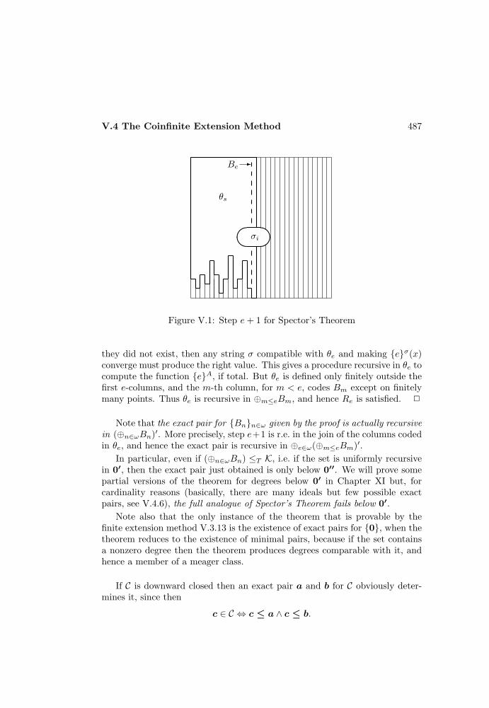
V.4 The Coinfinite Extension Method 487
θs
σi
Be -
Figure V.1: Step e+ 1 for Spector’s Theorem
they did not exist, then any string σ compatible with θe and making eσ(x)converge must produce the right value. This gives a procedure recursive in θe tocompute the function eA, if total. But θe is defined only finitely outside thefirst e-columns, and the m-th column, for m < e, codes Bm except on finitelymany points. Thus θe is recursive in ⊕m≤eBm, and hence Re is satisfied. 2
Note that the exact pair for Bnn∈ω given by the proof is actually recursivein (⊕n∈ωBn)′. More precisely, step e+1 is r.e. in the join of the columns codedin θe, and hence the exact pair is recursive in ⊕e∈ω(⊕m≤eBm)′.
In particular, even if (⊕n∈ωBn) ≤T K, i.e. if the set is uniformly recursivein 0′, then the exact pair just obtained is only below 0′′. We will prove somepartial versions of the theorem for degrees below 0′ in Chapter XI but, forcardinality reasons (basically, there are many ideals but few possible exactpairs, see V.4.6), the full analogue of Spector’s Theorem fails below 0′.
Note also that the only instance of the theorem that is provable by thefinite extension method V.3.13 is the existence of exact pairs for 0, when thetheorem reduces to the existence of minimal pairs, because if the set containsa nonzero degree then the theorem produces degrees comparable with it, andhence a member of a meager class.
If C is downward closed then an exact pair a and b for C obviously deter-mines it, since then
c ∈ C ⇔ c ≤ a ∧ c ≤ b.

488 V. Turing Degrees
There are thus two conditions that have some bearing for exact pairs, and wecollect them in the next definition.
Definition V.4.4 A set of degrees is:
1. an initial segment if is closed downward
2. an ideal if it is closed downward and under joins
3. a principal ideal if it is an ideal determined by a degree a, i.e. it is ofthe form D(≤a) = c : c ≤ a.
Corollary V.4.5 Every countable ideal is the intersection of two principal ide-als.
Proof. An ideal is closed under joins and thus, if countable, it has an exactpair. Being closed downward, it is determined by it. 2
Exercise V.4.6 There are ideals of degrees below 0′, without exact pairs below 0′.
(Hint: let Ann∈ω be a recursively independent set recursive in K, see V.2.9. Then
the ideals generated by Ann∈X , for any X, are distinct for distinct X’s, by recursive
independence. Thus there are 2ℵ0 ideals, but only countably many degrees recursive
in K, and thus only countably many possible exact pairs.)
Greatest lower bounds and least upper bounds
The notion of exact pair is useful for studying l.u.b.’s of sets of degrees, as wellas g.l.b.’s of pairs.
Theorem V.4.7 (Kleene and Post [1954], Spector [1956]) There are twodegrees below 0′ without g.l.b.
Proof. Consider an infinite ascending sequence of degrees: by Spector’s The-orem it has an exact pair. The degrees forming such a pair cannot have g.l.b.,since any lower bound admits an element of the chain above it (by definitionof exact pair), and thus is not the greatest lower bound (because the sequenceis increasing).
An infinite ascending sequence certainly exists (e.g. iterate the jump oper-ator, starting from any degree). But if we wish to get the exact pair below 0′,we have to choose a chain Bnn∈ω such that (⊕n∈ωBn)′ ≤T K, because thisis the bound we obtained from the proof of Spector’s Theorem. For this it isenough to build (see V.2.7 and V.2.21) a recursively independent set Ann∈ωsuch that (⊕n∈ωAn)′ ≤T K: then the sets Bn = ⊕m≤nAm form a strictlyascending sequence, by recursive independence of the An’s, and
(⊕n∈ωBn)′ ≤T (⊕n∈ωAn)′ ≤T K. 2
V.4 The Coinfinite Extension Method 489
Corollary V.4.8 D and D(≤ 0′) are not lattices.
Note that the finite extension method V.3.13 produced a minimal pair,hence a pair with g.l.b., and thus it cannot produce a pair without g.l.b. How-ever, it is possible to prove by the finite extension method that D is not a lattice,as shown in the exercises.
Exercises V.4.9 a) Any pair without g.l.b. is the exact pair of an infinite ascendingchain. Thus the proof given above is in a sense the only possible one. (Hint: given apair of degrees, consider an enumeration of the countable set of degrees below bothof them and, for each n, consider the join of the first n degrees in the list.)
b) A set bounding a pair without g.l.b. can be built by the finite extension method .(Jockusch [1981]) (Hint: build simultaneously an infinite ascending chain and an exactpair for it. More precisely, build a recursively independent set Bnn∈ω, so that thesets B0 ⊕ · · · ⊕Bn form an ascending sequence. Build also another set C, which willprovide finite modifications of the Bn’s, as follows:
An(x) =
C(x) if x ≤ nBn(x) otherwise.
Then the degree of An and Bn is the same. Let
A = ⊕n∈ωAn and B = ⊕n∈ωBn,
and make sure that A and B are an exact pair for the chain Bnn∈ω.)
c) The set of degrees a such that D(≤ a) is not a lattice is comeager . (Jockusch
[1981])
We now turn to l.u.b.’s of sets of degrees.
Proposition V.4.10 Compactness for l.u.b.’s (Spector [1956])
1. A chain of degrees has l.u.b. if and only if it is eventually constant.
2. A set of degrees has l.u.b. if and only if it there is a finite subset of itwhose join provides an upper bound for the whole set.
Proof. Given a chain, consider an exact pair for the ideal generated by it.The l.u.b. of the chain is the g.l.b. of the exact pair, and if the chain is noteventually constant it cannot exist, as in V.4.7. Given a set A, it is enough toreduce it to a chain that has l.u.b. if and only if A has it. First note that wemay suppose A countable, otherwise it cannot have upper bounds. Let thena0,a1, . . . be an enumeration of A, and consider the chain
b0 = a0
bn+1 = bn ∪ an+1.
490 V. Turing Degrees
Now the chain b0 ≤ b1 ≤ · · · has l.u.b. if and only if it is eventually constant,and thus A has l.u.b. if and only if it has an upper bound which is the l.u.b.of a finite subset of it. 2
In particular, no infinite ascending sequence of degrees has l.u.b.
Exercise V.4.11 The existence of a set of degrees without l.u.b. can be proved by the
finite extension method V.3.13. (Kleene and Post [1954]) (Hint: since any countable
partial ordering can be embedded in the degrees below 0′, by V.2.9, there is a set
of degrees below 0′ isomorphic to the rationals. If a subset of it has l.u.b. then this
must be below 0′, and hence only countably many subsets can have l.u.b. But there
are 2ℵ0 such subsets, since they correspond to the reals, as Dedekind sections.)
Extensions of embeddings
We have shown in V.2.10 how the truth of one-quantifier questions reduces toembedding problems. Similarly, Shore [1978] and Lerman [1983] have noticedthat the truth of two-quantifier questions reduces to problems of extension ofembeddings. The idea is that the truth of (∀~x)(∃~y)ϕ(~x, ~y) can be decided if oneknows whether
(∀~x)[D(~x) → (∃~y)ϕ(~x, ~y)],
for each of the finitely many D’s describing a possible order relationship amongthe x’s (i.e. a conjunction of atomic statements xi ≤ xj or negations of them).Moreover, ϕ can be reduced (by writing it into disjunctive normal form) to afinite disjunction of descriptions of possible order relationships among the x’sand y’s.
The general form of the problem we want to study is thus the following:given an embedding of a partial ordering P in D, and an extension R of P , canwe extend the embedding of P to an embedding of R? We cannot expect tobe able to do this in general, since there are three restrictions we have alreadyencountered:
1. D has cardinality 2ℵ0 and countable predecessor property.Thus appropriate bounds on the cardinality of R are needed.
2. D is an uppersemilattice.Thus there is no hope to embed in D any partial ordering which does notrespect the uppersemilattice structure of D. If P is already embeddedthen we do not have to worry about it, but we certainly have to ask thisof R. For example, given a1, a2 and a3 such that a3 < a1 ∪ a2, wecannot introduce a new degree b which is above a1 and a2 but not abovea3.

V.4 The Coinfinite Extension Method 491
3. There are minimal pairs.Thus we cannot expect to extend any given partial ordering by insertingnew elements below given ones. For example, if a1 and a2 are a minimalpair, we cannot introduce a new degree b strictly between them and 0.
We are thus led to the following definition.
Definition V.4.12 The partial ordering (R,vR) is a consistent extensionof the uppersemilattice (P,vP ,tP ) if :
1. R respects the uppersemilattice structure of P , i.e.
a1, a2 ∈ P ∧ b ∈ R ∧ a1, a2 vR b ⇒ a1 tP a2 vR b
2. R is an end-extension of P , i.e.
b ∈ R− P ∧ a ∈ P ⇒ b 6vR a.
The possible extensions of embeddings will always refer to consistent exten-sions.
Theorem V.4.13 (Kleene and Post [1954]) Any embedding of a finite par-tial ordering P in D can be extended to an embedding of any finite consistentextension R of P .
Proof. Since R is finite, it is possible to find a sequence of finitely manysuccessive consistent extensions that add one element at a time, starting fromP and ending with R. Thus we only need to know how to treat one-elementextensions.
This amounts to proving that, given two finite sets Bnn∈F and Cmm∈Gsuch that no Cm is recursive in ⊕n∈FBn, we can build A such that
1. for each n ∈ F , Bn ≤T A
2. for each m ∈ G, Cm 6≤T A.
This can easily be done, by the same methods of the proof of Spector’s Theorem.Since there are only finitely many sets to code, the first conditions can besatisfied ahead of time, simply by setting
θ0(x) ' Be(z) if e ∈ F ∧ x = 〈e, z〉.
To satisfy the second condition let θs be given, and suppose we want to satisfy
Cm 6' eA
492 V. Turing Degrees
for some m ∈ G and e. We look for two strings which are compatible with θsand e-split. If they exist, then we choose the one σ that gives a value differentfrom Cm on the element on which they split, and by letting θs+1 = θs ∪ σwe satisfy the requirement. If they do not exist then eA, if total, will berecursive in θs as usual, and thus recursive in ⊕n∈FBn because, by induction,θs is a finite modification of it. But since Cm is not recursive in ⊕n∈FBn, itcannot be equal to eA. 2.
In the opposite direction, it is possible to show that the condition on R ofbeing a consistent extension of P is necessary, not only for some P (as we havealready argued), but also for any P . One part is trivial (since D an uppersemi-lattice), but it holds also for the other one, since any finite uppersemilatticewith least element P is isomorphic to an initial segment of D (see p. 529), andthus some embedding of P cannot be extended by inserting new elements be-low given ones. This completely characterizes the possible finite extensions ofembeddings of finite uppersemilattices into D, and it allows to give a decisionprocedure for the two-quantifier sentences of D (Shore [1978], Lerman [1983]).Schmerl has instead that the three-quantifier theory of D is undecidable (seeLerman [1983]).
Note that only notational changes are needed in the proof given above (cod-ing one set at a time), to obtain one-element consistent extensions of countableembeddings (the requirements on the Bn’s and Cm’s being now that no Cmis recursive in any finite join of the Bn’s). But not every consistent countableextension can be obtained by a sequence of one-element consistent extensions(e.g. when an infinite descending chain is added above a given element), andsome more work (sketched in the exercise) is needed for the general case.
Exercise V.4.14 Any embedding of a countable partial ordering P in D can be ex-tended to an embedding of any countable consistent extension R of P . (Kleene andPost [1954], Sacks [1961]) (Hint: this extends V.2.9. Given Cnn∈ω, build setsAnn∈ω recursively independent over the Cm’s, and not introducing any new rela-tionships among them, i.e. such that
An 6≤T (⊕m∈ωCm)⊕ (⊕m6=nAm)Cn ≤T (⊕m∈FCm)⊕ (⊕m∈ωAm) ⇒ Cn ≤T (⊕m∈FCm),
for any finite set F . The second condition is ensured by the e-splitting method. Ifnow P = cnn∈ω and R− P = bnn∈ω, and the degrees of the Cn’s are isomorphicto the ordering of the cn’s, we let
Bn = (⊕cmvbnCm)⊕ (⊕bmvbnAm).
Note that the second condition above, together with the fact that R respects theuppersemilattice structure of P , proves the crucial part, namely that
ck 6v bn ⇒ Ck 6≤T Bn.
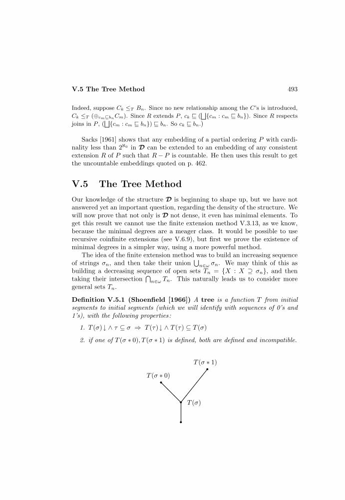
V.5 The Tree Method 493
Indeed, suppose Ck ≤T Bn. Since no new relationship among the C’s is introduced,
Ck ≤T (⊕cmvbnCm). Since R extends P , ck v (⊔cm : cm v bn). Since R respects
joins in P , (⊔cm : cm v bn) v bn. So ck v bn.)
Sacks [1961] shows that any embedding of a partial ordering P with cardi-nality less than 2ℵ0 in D can be extended to an embedding of any consistentextension R of P such that R−P is countable. He then uses this result to getthe uncountable embeddings quoted on p. 462.
V.5 The Tree Method
Our knowledge of the structure D is beginning to shape up, but we have notanswered yet an important question, regarding the density of the structure. Wewill now prove that not only is D not dense, it even has minimal elements. Toget this result we cannot use the finite extension method V.3.13, as we know,because the minimal degrees are a meager class. It would be possible to userecursive coinfinite extensions (see V.6.9), but first we prove the existence ofminimal degrees in a simpler way, using a more powerful method.
The idea of the finite extension method was to build an increasing sequenceof strings σn, and then take their union
⋃n∈ω σn. We may think of this as
building a decreasing sequence of open sets Tn = X : X ⊇ σn, and thentaking their intersection
⋂n∈ω Tn. This naturally leads us to consider more
general sets Tn.
Definition V.5.1 (Shoenfield [1966]) A tree is a function T from initialsegments to initial segments (which we will identify with sequences of 0’s and1’s), with the following properties:
1. T (σ)↓ ∧ τ ⊆ σ ⇒ T (τ)↓ ∧ T (τ) ⊆ T (σ)
2. if one of T (σ ∗ 0), T (σ ∗ 1) is defined, both are defined and incompatible.
T (σ ∗ 0)
T (σ ∗ 1)
T (σ)@@
@
rrr r
494 V. Turing Degrees
This way of looking at trees in not different from the one of IV.2.14: it onlyhas a different emphasis. What really matters in a tree T is always its range(which is still a tree in the sense of IV.2.14), but to think of it in terms of afunction is a useful tool: we can simply talk of T (σ ∗ 0) or T (σ ∗ 1), insteadof ‘the two smallest incompatible extensions of T (σ) on the tree’. Similarly, tostate that both or neither of T (σ∗0), T (σ∗1) are defined is no loss of generality,since if e.g. we are only interested in the branch extending T (σ ∗ 0), we maydefine T (σ∗1) as well, and then let the tree grow afterwards only above T (σ∗0).
A total tree, i.e. a tree which is total as a function from strings to strings,is nothing more than a closed perfect subset of 0, 1ω, in the terminology ofCantor [1883] (according to which a set A ⊆ 0, 1ω is perfect if there is nof ∈ A and an open set O such that O∩A = f, i.e. it has no isolated points).Intuitively, a total tree is just a set of branches or functions, none of which isisolated .
We say that
1. A is on T , or A is a branch of T , if T (σ) ⊆ A for infinitely many σ’s
2. σ is on T if it is in the range of T
3. T ∗ is a subtree of T (T ∗ ⊆ T ) if every σ on T ∗ is also in T
4. T ∗ is the full subtree of T above σ if it consists of every string on Textending σ.
The concept of subtree is for trees what the concept of extension is forstrings. The finite extension method consists of building a decreasing sequenceTnn∈ω of trees, where T0 is the identity tree (consisting of all strings, alsocalled the full binary tree), and Tn+1 is a full subtree of Tn. The method oftrees is more general because it allows Tn+1 to be any subtree of Tn.
The simplest application of the tree method will be with recursive trees,i.e. trees that are recursive as (total) functions from strings to strings (appro-priately coded as numbers). We are really interested in the range of a tree, butthe terminology is consistent: if a tree is recursive as a function, then so is itsrange as a set (to know if σ ∈ T we generate the tree up to a level in whichall branches have length at least equal to the length of σ, and see if σ is on Tat that level). In later applications we will also deal with partial recursivetrees, which need not be total: in this case the range will be r.e.
The method of trees used above can be recast in the same categorical frame-work of Section 3, by using a different topology than the one generated by basicopen sets determined by finite strings. More precisely, consider any set C ofrecursive trees, with the following properties:
• the identity tree is in C
V.5 The Tree Method 495
• if T ∈ C and σ ∈ T , then the full subtree of T above σ is in C.
Then C is the base of a topology on P(ω) finer than the original one dealt within Section 3. We can then say that:
1. A ⊆ C is C-dense if for any T ∈ C there is S ⊆ T such that S ∈ A
2. A ⊆ P(ω) is C-comeager if it contains the intersection of countablymany C-dense sets.
A good deal of the theory of Baire Category can be developed in this generalizedframework (Yates [1976]), in particular the Baire Category Theorem holds.Basic examples of C are given by the set of full trees (in which case we obtainthe same notions as in Section 3), the set of recursive coinfinite conditions, andthe set of recursive trees.
Hyperimmune-free degrees
Dealing with the next notion will provide a useful warm up with the treemethod, before the real applications come. Moreover, the notion will be usefulin extending results from T -degrees to other types of degrees (see VI.6.18).
Definition V.5.2 (Martin and Miller [1968]) A degree a ≥ 0 is hyper-immune-free if for every A ∈ a and f ≤T A, f is majorized by a recursivefunction, i.e. there is a recursive function g such that (∀x)(f(x) ≤ g(x)).
The name ‘hyperimmune-free’ is justified below. The definition has beengiven in a form which makes it easier to deal with it in applications.
Exercises V.5.3 Hyperimmune degrees. (Martin and Miller [1968]) A degree ishyperimmune if it contains a hyperimmune set, see III.3.7.
a) A degree is hyperimmune-free if and only if it is not hyperimmune. (Hint: onedirection follows from III.3.8. The other from the fact that if ann∈ω enumerates Ain increasing order, and f ≤T A is not majorized by any recursive function, then theset B defined as A ⊕ af(n) : n ∈ ω is in the same degree as A, because f ≤T A,and is hyperimmune. Otherwise, there would be a recursive function majorizing theelements of B in increasing order, and thus a recursive function majorizing f too,because f(n) ≤ af(n).)
b) The hyperimmune degrees are closed upwards, and the hyperimmune-free de-grees are closed downward . (Hint: the second assertion holds by definition, the firstfollows from it by part a).)
c) The set of hyperimmune-free degrees is meager . (Hint: we have to build ahyperimmune set by the finite extension method V.3.13, which is immediate by def-inition: given any string σ and an infinite disjoint strong array, there is a stringextending σ such that all sets extending it intersect one element of the strong array.)
496 V. Turing Degrees
d) Every nonzero degree comparable with 0′ is hyperimmune. (Hint: since 0′ con-
tains a hyperimmune degree, by part b) so do all degrees above it. To show that every
nonzero degree below it does too, modify III.3.13 by using the limit lemma IV.1.17.
Precisely, given A ≤T K nonrecursive, let A be the limit of g recursive. If f(x) is the
smallest stage where g gives the right value of A(y), for all y ≤ x, then f is increasing,
and hence its range B is recursive in A. By part b), it is enough to show that B is
hyperimmune. If it were not then A would be recursive, because to know the real
value of A(x) we just have to compute g at x, at the stage given by the x-th element
of B.)
Since the set of hyperimmune-free degrees is meager, we cannot expect tobuild one member of it by the finite extension method V.3.13. By using treeswe can instead easily obtain the result. For later use we isolate the steps neededin the proof.
Proposition V.5.4 Diagonalization Lemma. Given e and a recursive treeT , there is a recursive tree Q ⊆ T such that, for every A on Q, A 6' e.
Proof. Since T (0) and T (1) are incompatible, at least one of them mustdisagree with e on some x. If T (i) is such, let Q be the full subtree of Tabove it. 2
Proposition V.5.5 Totality Lemma (Martin and Miller [1968]) Givene and a recursive tree T , there is a recursive tree Q ⊆ T such that one of thefollowing holds:
1. for every A on Q, eA is not total
2. for every A on Q, eA is total and
(∀n)(∀σ)(|σ| = n ⇒ eQ(σ)(n)↓),
where |σ| is the length of σ.
Proof. See if
(∃σ ∈ T )(∃x)(∀τ ⊇ σ)(τ ∈ T ⇒ eτ (x)↑).
If so, choose such a σ: for any string τ extending it, eτ is undefined on afixed element. It is then enough to let Q be the full subtree of T above σ. Thencase 1 holds.
Otherwise, for any string σ and any x there is an extension τ of σ thatmakes eτ defined on x. We can then build a tree by successive levels, and
V.5 The Tree Method 497
make eA converge on more and more elements. Precisely, let Q be definedas follows. First we start with
Q(∅) = least τ ∈ T such that eτ (0)↓.
Inductively, given Q(σ) on T we know that there is an extension of it on T ,say T (τ) for some τ , such that eT (τ)(|σ|)↓. Then let
Q(σ ∗ i) = T (τ ∗ i),
for i = 0, 1, so that they are two incomparable extensions of Q(σ). 2
Proposition V.5.6 (Martin and Miller [1968]) There are hyperimmune-free degrees.
Proof. The requirements on A are:
R2e : A 6' eR2e+1 : eA total ⇒ for some recursive g, (∀n)(eA(n) ≤ g(n)).
Define a sequence of recursive trees Tn such that Tn+1 ⊆ Tn, and all branchesof Tn+1 satisfy Rn. Precisely:
T0 = identity treeT2e+1 = the Q of the Diagonalization Lemma, for T = T2e
T2e+2 = the Q of the Totality Lemma, for T = T2e+1.
Let now A ∈⋂n∈ω Tn: it exists because Tn(∅) ⊆ Tn+1(∅), since Tn ⊆ Tn+1,
and thus we just have to consider A =⋃n∈ω Tn(∅).
A is not recursive because it is on T2e+1, and hence it is different from e.Suppose now eA is total. Since A is on T2e+2, it must be that the secondcase holds in the Totality Lemma, hence
eA(n) ≤ max|σ|=n
eT2e+2(σ)(n),
since eA(n) is already defined at the n-th level of the tree, for each possiblebranch A. Thus eA is majorized by a recursive function. 2
Exercises V.5.7 (Martin and Miller [1968]) a) There is a hyperimmune-free degreebelow 0′′. (Hint: in the construction above, only two-quantifier questions were asked,and thus the degree is less than or equal to 0′′. To show it is strictly below it, notethat 0′′ is hyperimmune, because comparable with 0′.)
b) There is an infinite ascending sequence of hyperimmune-free degrees. (Hint:by relativization, there is a hyperimmune-free degree above any hyperimmune-freedegree.)
498 V. Turing Degrees
c) There are 2ℵ0 hyperimmune-free degrees. (Hint: build a tree of sets, all of
whose branches are of hyperimmune-free degree. This can be achieved by building a
tree of trees, i.e. a function T from pairs of strings to strings, such that for each σ
the function Tσ(τ) = T (σ, τ) is a tree. The desired tree will be given by the function
Tσ(∅). Start by T∅ being the identity tree. At any stage, instead of just building one
subtree of the given tree, build two, above two incomparable strings. Precisely, given
Tσ, apply the Diagonalization or the Totality Lemma, depending on whether |σ| is 2e
or 2e + 1, to the full subtree of Tσ above Tσ(0) to get Tσ∗0, and above Tσ(1) to get
Tσ∗1.)
Jockusch [1969b] shows that a hyperimmune degree contains a bi-immuneset (while the converse does not necessarily hold), and strengthens V.5.6 byproducing a degree without bi-immune sets. See Jockusch [1972] and Simpson[1977] for more on this topic.
The results of this subsection show that a characterization of the degreescontaining hyperimmune sets cannot be simple. With regard to other immunityproperties introduced in Chapter II, we quote the following results:
1. a immune ⇔ a > 0(Dekker and Myhill [1958], see II.6.13)
2. a′ ≥ 0′′ ⇒ a cohesive ⇒ a hyperhyperimmune ⇒ a′ > 0′
(Jockusch [1969a], [1973a])
3. If a ≤ 0′, then a hyperhyperimmune ⇔ a cohesive ⇔ a′ = 0′′
(Cooper [1972]).
Minimal degrees
We turn now to a most important application of the tree method. We want tobuild a minimal degree, i.e. a nonrecursive set A such that
C ≤T A⇒ C recursive or C ≡T A.
The proof we give is a simplification, due to Shoenfield [1966], of the originalconstruction of Spector, which is given in Section 6.
When we constructed a minimal pair, we used the e-splitting method: ifthere was no e-splitting then we got a recursive set, while in the opposite casewe fixed one side, and diagonalized against it on the other, thus taking fulladvantage of the fact of being able to work with two sets. Here we will have toget by with just one set, and this will complicate our life a bit, but the ideaswill always be the same. The needed change is to use e-splittings in a globalway.
V.5 The Tree Method 499
Definition V.5.8 T is an e-splitting tree if, for every σ, T (σ∗0) and T (σ∗1)e-split.
The interest of the notion comes from the following lemma.
Proposition V.5.9 (Spector [1956]) Given e, a recursive tree T , and A onT , if eA is total then:
1. if there is no e-splitting on T , eA is recursive
2. if T is e-splitting, A ≤T eA.
Proof. Since eA is total, given x we know that eA(x) converges, andthus there must be σ ⊆ A such that eσ(x) converges, and gives the rightvalue. Since A is on T , by monotonicity we may suppose σ ∈ T . If there is noe-splitting on T , to compute eA(x) is then enough to look for any string τon T such that eτ (x) converges, since its value must be equal to eσ(x)(otherwise σ and τ would e-split on x), and hence to eA(x).
Suppose now that T is instead e-splitting. We show how to generate in-creasingly long segments of A recursively in eA. Given T (σ) ⊆ A, since A ison T either T (σ ∗ 0) or T (σ ∗ 1) will be included in A, and we have to decidewhich one. Being T e-splitting, there is an x such that
eT (σ∗0)(x) 6' eT (σ∗1)(x),
with both sides converging. Only one of them can agree with eA(x), and thisdetermines which of the two strings is contained in A. Precisely, T (σ ∗ i) ⊆ Aif eT (σ∗i)(x) ' eA(x). 2
Proposition V.5.10 Minimality Lemma (Spector [1956]) Given e and arecursive tree T , there is a recursive tree Q ⊆ T such that one of the followingholds:
1. for every A on Q, eA total ⇒ eA recursive
2. for every A on Q, eA total ⇒ A ≤T eA.
Proof. The result follows from the previous lemma, if we just build Q witheither no e-splitting on it, or as an e-splitting tree.
If there is a string on T with no e-splitting above it, take Q as the fullsubtree above it: then Q has no e-splitting.
If any string on T has two e-splitting extensions (i.e. two strings on T whichextend it and e-split), then we can build an e-splitting subtree Q of T , by induc-tion: given Q(σ), let Q(σ∗0) and Q(σ∗1) be two e-splitting extensions of it. 2
500 V. Turing Degrees
Note that the last lemma is a modification of the minimal pair construction.If there is a string on T with no e-splitting extensions, we just take the fullsubtree above it, and have eA recursive for any A on it, as in the minimalpair construction. If any string on T has e-splitting extensions, take two ofthem, say σ0 and σ1. Then, for some x, eσ0(x) 6' eσ1(x), with both sidesconverging. Certainly eA(x), whatever A may be, disagrees with one of them,say eσi . Then A does not agree with σi. If σ0 and σ1 were the only possiblebeginnings of A, then A would have to agree with the other string. And we canforce this to happen, by just discharging every other possibility, i.e. by makingσ0 and σ1 the first level of our subtree. And we can continue this, therebybuilding an e-splitting tree such that any set A on it is then recursive in eA.
Theorem V.5.11 (Spector [1956]) There exists a minimal degree.
Proof. We only have to satisfy the requirements
R2e : A 6' eR2e+1 : C ' eA ⇒ C recursive or A ≤T C.
We build a sequence of recursive trees, as follows:
T0 = identity treeT2e+1 = the Q of the Diagonalization Lemma, for T = T2e
T2e+2 = the Q of the Minimality Lemma, for T = T2e+1.
Then A =⋃n∈ω Tn(∅) satisfies the requirements. 2
Having obtained minimal degrees by the tree method, and knowing thatwe cannot obtain them by the finite extension method V.3.13, it is naturalto investigate the situation more thoroughly. More precisely, we would like toknow how much of the machinery just introduced is really needed, in particularwhich methods are sufficient, and which are necessary. To the first question wewill answer in V.6.9, where it will be shown that recursive coinfinite extensionsare sufficient , giving a sort of best possible answer. The second question isless precise, but we can argue that total e-splitting trees are not necessary ,because they can be combined with totality requirements and automaticallyproduce hyperimmune-free minimal degrees (see the exercises below). Nowhyperimmune-free degrees cannot be comparable with 0′, but in Chapter XIwe will show that there are minimal degrees below 0′, which must then be builtby partial trees. There it will be possible to prove that, for minimal degreesbelow 0′, partial e-splitting trees are not only sufficient, but also necessary(Chong [1979]).
V.5 The Tree Method 501
Exercises V.5.12 a) There exists a minimal degree below 0′′. (Spector [1956]) (Hint:in the proof above, only two-quantifier questions were asked, and thus the degree isless than or equal to 0′′. To show it is strictly below it, note that 0′′ is obviously notminimal.)
b) There are 2ℵ0 minimal degrees. (Lacombe) (Hint: build a tree of minimaldegrees, as in V.5.7.c.)
c) The diagonalization steps in the construction of minimal degrees are not needed .
(Posner and Epstein [1978]) (Hint: similar to V.2.23, this time using trees Te which
are either e-splitting or without e-splittings, and A on all of them. Another way is
given by part b), because we can build a tree of sets satisfying all the minimality
conditions, and only countably many of these sets can be recursive.)
Exercises V.5.13 Hyperimmune-free degrees. a) There is a minimal, hyper-immune-free degree. (Martin and Miller [1968]) (Hint: combine the proofs of V.5.11and V.5.6.)
b) There is a hyperimmune-free degree that is not minimal . (Martin and Miller[1968]) (Hint: by V.5.7.b.)
That there is a minimal degree which is not hyperimmune-free will follow from
the existence of minimal degrees below 0′, see Chapter XI.
Exercises V.5.14 Jumps of minimal degrees. a) Not every minimal degree re-alizes the least possible jump. (Sasso [1974]) (Hint: build a set A of minimal degreesuch that A′ 6≤T A⊕K. The requirements are treated by the following lemma: givene and a recursive tree T , there is a recursive tree Q ⊆ T such that, for any A on Q,A′ 6' eA⊕K. The idea is that the question: ‘does A always go left at even levels ofT?’ can be phrased as a question about A′, since it involves only one quantifier overA. Let a be such that
aσ(x) ' 0 ⇔ σ branches right at some even level of T .
By definition of jump, a ∈ A′ ⇔ aA(a) ↓. See if, for some τ ∈ T , eτ⊕K(a) ' 0.If so, to diagonalize we want a ∈ A′, i.e. for every A we require aA(a)↓, and henceA must branch right at some even level of T . Take Q as the full subtree of T aboveτ ∗ 11, since τ ∗ 11 branches right twice, and one of τ ∗ 1 and τ ∗ 11 is at an even level.Otherwise, let Q be the subtree of T that branches left at every even level. Note thatwe use only even levels, because we still need to get a tree, and this is taken care ofat odd levels.)
b) Every degree above 0′′ is the double jump of a minimal degree. (Cooper [1973])(Hint: note that if we also use the Totality Lemma in the construction of a setof minimal degree we can decide, recursively in the construction and hence in ∅′′,whether eA is total or not, depending on which case applies in the lemma. Anyquestion about the second jump of A or, equivalently, with two quantifiers over A,can be rephrased as a question about the totality of a given function recursive in A,and thus A′′ ≤T A⊕ ∅′′. We can now build a tree of T ≤T ∅′′, all of whose branchesA have this property. If ∅′′ ≤T C let A be the branch of T determined by C, i.e.

502 V. Turing Degrees
A =⋃σ⊆C T (σ). Then
A ≤T C ⊕ T ≤T C ⊕ ∅′′ ≤T C,
and hence A⊕ ∅′′ ≤T C. Conversely,
C ≤T A⊕ T ≤T A⊕ ∅′′,
and thus C ≡T A⊕ ∅′′ ≡T A′′.)Jockusch and Posner [1978] show that, for any minimal degree a, a′ = (a ∪ 0′)′,
see Chapter XI. Cooper [1973] proves that actually every degree above 0′ is the jump
of a minimal degree, but this is much more difficult to prove, see Epstein [1975] or
Posner [1981] for a proof by recursive approximations, and Lerman [1983] for one by
approximations recursive in ∅′.
Exercises V.5.15 Autoreducible sets. A set A is autoreducible if, for each x,the question ‘is x in A?’ can be answered recursively in A, without ever asking theoracle about x. Thus every single element encodes redundant information, retrievablefrom the rest of the set. A nonrecursive degree containing only autoreducible sets iscalled completely autoreducible.
a) Every m-degree contains autoreducible sets. (Trakhtenbrot [1970]) (Hint: con-sider A⊕A. Then 2x and 2x+ 1 give the same information.)
b) An introreducible set (II.6.7) is autoreducible. (Jockusch and Paterson [1976])(Hint: let B be nonautoreducible. We build, by the finite extension method V.3.13,an infinite subset A of B such that B 6≤T A. To get B 6' eA at stage n, given σnlook for an extension σ of it such that σ−1(1) ⊆ B, and there is x such that everyτ ⊇ σ such that τ−1(1) ⊆ B satisfies eτ (x) 6' B(x). Such a string must exist, sinceB is not autoreducible. Thus let σn+1 = σn.)
c) The set of completely autoreducible degrees is meager . (Trakhtenbrot [1970])(Hint: build, by the finite extension method, a set A such that, for every e, there isx such that A(x) 6' eA−x(x).)
d) There exists a completely autoreducible degree. (Jockusch and Paterson [1976])(Hint: build a set as in the minimal degree construction, with double e-splittingstaking the place of e-splittings, i.e. using trees T such that, for any σ, there are twodistinct elements on which T (σ ∗ 0) and T (σ ∗ 1) e-split. If T is doubly e-splitting, Ais on T , and eA is a characteristic function, then eA is autoreducible: to computeeA(x) with oracle eA without using this value, first build large enough segmentsof A, with oracle eA but avoiding the particular value eA(x), which is possiblethanks to the double e-splittings. Then compute eA(x) with oracle A.)
Obviously, the completely autoreducible degree just built is minimal. The ex-
istence of minimal, not completely autoreducible degrees and of completely autore-
ducible, not minimal degrees will be proved in V.6.10.d and V.6.16.e. Jockusch and
Paterson [1976] show that nonzero r.e. degrees and degrees above 0′ are not com-
pletely autoreducible.

V.5 The Tree Method 503
Minimal upper bounds ?
Exactly as we generalized the notion of minimal pair to that of exact pair, wecan extend the notion of minimal degree to that of minimal upper bound.
Definition V.5.16 A degree a is a minimal upper bound for a set of de-grees C if
1. it is a strict upper bound to C, i.e. (∀c ∈ C)(c < a)
2. there is no strict upper bound to C below it, i.e.
(∀b)[b ≤ a ∧ (∀c ∈ C)(c < b) ⇒ b = a].
A minimal cover for a degree b is a minimal upper bound for b, i.e. adegree a > b such that there is no degree strictly between a and b.
A strong minimal cover for b is a degree a > b such that anythingstrictly below it is bounded by b, i.e.
(∀c)(c ≤ a ⇒ c ≤ b ∨ c = a).
Both notions of minimal cover are plausible generalizations of the notion ofminimal degree above a given set. Relativizations of the results about minimaldegrees produce results about minimal covers, but not about strong minimalcovers. For example, V.5.11 relativized shows that every degree has a mini-mal cover . On the other hand, not every degree has a strong minimal cover(Shoenfield [1959]), e.g. 0′ does not (by V.2.26 any degree above 0′ is the joinof two strictly smaller degrees, and thus it cannot be a strong minimal cover ofit, otherwise the two degrees would be below 0′, and so would be their join).Jockusch [1981] shows that the set of degrees without strong minimal covers iscomeager , and thus the class of degrees with a strong minimal cover is meager.It is not known whether the minimal degrees are included in it, i.e. if everyminimal degree has a strong minimal cover.
Exercises V.5.17 There is a cone of minimal covers. (Jockusch [1973]) (Hint: ev-
ery minimal degree has a minimal cover, and thus the set of degrees which are not
minimal covers cannot contain a cone. By V.1.16, if AD holds then the set of degrees
which are minimal covers must contain a cone. But this set is arithmetical, and thus
only the Axiom of Determinacy for arithmetical sets is needed, which is provable in
ZFC by Martin [1975].) A direct proof of the result, not using Determinacy, will be
given in Volume II.
Spector’s Theorem showed that any countable ideal has an exact pair. Theproof was an extension of the construction of minimal pairs, plus a coding
504 V. Turing Degrees
method that allowed us to push the set constructed above given degrees. Wenow prove a similar result for minimal upper bounds, by extending the construc-tion of minimal degrees. We also need a coding method, and this is providedby the next notion, implicit in the proof of Spector’s Theorem.
Definition V.5.18 (Sacks [1971]) A recursively pointed tree T is a treewhich is recursive in all of its branches, i.e. T ≤T A whenever A is on T .
Exercises V.5.19 a) If T is recursively pointed, then T has branches of every degreeabove the degree of T . (Sacks [1971]) (Hint: given T ≤T A, consider B =
⋃σ⊆A T (σ).)
b) If T is recursively pointed, Q ⊆ T , and Q ≤T T , then Q is also recursively
pointed, and Q ≡T T . (Sacks [1971]) (Hint: Q is pointed because if A ∈ Q ⊆ T then
Q ≤T T ≤T A. If A is the leftmost branch of Q then T ≤T A by pointedness, and
A ≤T Q by definition, so T ≤T Q.)
Proposition V.5.20 (Sacks [1971]) If T is recursively pointed and T ≤T A,then there is some recursively pointed tree Q ⊆ T such that Q ≡T A.
Proof. We have to code A in Q, and at every even level 2n we thin the treedown by just taking the right or left branch, according to whether n is in A ornot. Precisely, we define Q by induction. Given Q(σ) on T , let τ be a stringsuch that Q(σ) = T (τ), which exists because Q(σ) is on T , by induction. Let
Q(σ ∗ i) = T (τ ∗A(|σ|) ∗ i).
Then Q ≤T T ⊕ A, so Q ≤T A (because T ≤T A). From any path B of Qand T itself we can recover A, and so A ≤T B (since T ≤T B by pointedness).To have A ≤T Q it is enough to choose any B ≤T Q, e.g. the leftmost branch.
Finally, Q is pointed: given B ∈ Q we can recover Q itself from B and T ,by the uniformity of the construction, and again T ≤T B, so Q ≤T B. 2
Proposition V.5.21 (Sacks [1963]) Every countable set of degrees has aminimal upper bound.
Proof. Let A = a0, a1, . . . be a countable set of degrees. We may supposethat A is a chain, otherwise we can just consider the chain defined as
b0 = a0 bn+1 = bn ∪ an+1,
whose minimal upper bounds are exactly those of A. We can also assumethat the chain has no greatest element, otherwise the result is obtained bytaking any minimal cover of it. This assumption is made only to avoid directdiagonalization against all the degrees in A.
V.5 The Tree Method 505
Let then An ∈ an. We will build a set A ∈⋂n∈ω Tn, where Tn is a
recursively pointed tree of degree an. This automatically implies that A is anupper bound for A.
To get minimality, we use the following extension of the Minimality Lemma.Given e and a tree T , there is a tree Q ⊆ T such that one of the following holds:
1. for every A on Q, eA total ⇒ eA ≤T Q
2. for every A on Q, eA total ⇒ A ≤T eA ⊕Q.
This is proved by the proof of V.5.10, simply because when the relevant treesare not recursive then we have to take them into account in our computations.
The construction is as follows. Let T0 be a recursively pointed tree of thesame degree as A0 (which can be obtained by starting from the identity tree,and applying V.5.20). Given Te recursively pointed of the same degree as Ae,first get T ⊆ Te recursively pointed of the same degree as Ae+1, by V.5.20,since Ae ≤T Ae+1. Then let Te+1 be the Q of the Minimality Lemma statedabove, which is still recursively pointed, and of the same degree as Ae+1.
If A ∈⋂n∈ω Tn, suppose eA is total. By construction, there are two
cases:
• eA ≤T Te+1
Then eA ≤T Ae+1 (since Te+1 has the same degree as Ae+1), A is belowsome element of the chain, and it is not an upper bound to it.
• A ≤T eA ⊕ Te+1
If eA is itself an upper bound to the chain then Te+1 ≤T eA, andhence A ≤T eA.
Thus no upper bound to the chain is strictly below A, and A is a minimalupper bound. 2
Exercises V.5.22 a) Every countable set of degrees has 2ℵ0 minimal upper bounds.(Sacks [1963]) (Hint: build a tree of minimal upper bounds.)
b) Every countable ascending chain of hyperim-
mune-free degrees has a hyperimmune-free minimal upper bound (Martin and Miller
[1968]). Note that the result fails for countable sets in place of chains, because the
join of hyperimmune-free degrees in not necessarily hyperimmune-free, see V.6.10.c.
Konig’s Lemma and Π01 classes ?
In this subsection we consider again general trees as in IV.2.14 (i.e. as sets of se-quence numbers closed under subsequences), and study their infinite branches.The classical result in this field is the following.

506 V. Turing Degrees
Theorem V.5.23 Konig’s Lemma (Konig [1926]) An infinite tree in whichevery node has only finitely many immediate successors has an infinite branch.
Proof. Let T be such a tree. We define an infinite branch by induction. Westart with σ0. Given σn with infinitely many extensions on T , let σn+1 be animmediate successor of σn with infinitely many extensions on T . It exists be-cause σn has infinitely many extension on T , but only finitely many immediatesuccessors. Thus at least one of them must have infinitely many extensions onT . 2
The rest of this subsection is devoted to an analysis of constructive versionsof this result. We first investigate binary trees which, by definiteness, wedefine as sets of sequences of 0’s and 1’s.
Definition V.5.24 A class of sets is a Π01 class if it is the set of infinite
branches of some infinite recursive binary tree.
The reason for the name is obvious: if T is a recursive tree, then A is aninfinite branch of it if and only if (∀x)(cA(x) ∈ T ). More generally, if P isa recursive predicate then the class of sets A such that (∀x)P (cA(x)) is a Π0
1
class, since it is the set of infinite branches of the tree obtained by closing Punder subsequences.
Note that, by Konig’s Lemma, a Π01 class is never empty. As a fundamental
example, the sets separating two disjoint r.e. sets A and B form a Π01 class:
C ∈ SA,B ⇔ (∀x)[(x ∈ A→ x ∈ C) ∧ (x ∈ B → x 6∈ C)].
Explicitly, a recursive tree whose branches are exactly the members of SA,B isthe following:
x ∈ TA,B ⇔ Seq(x) ∧ x is correct up to stage ln(x),
where ‘x is correct up to stage s’ means that for every i ≤ ln(x), if i ∈ As then(x)i = 1, and if i ∈ Bs then (x)i = 0. In other words, we seal off a branch ofTA,B as soon as we discover that it is incorrect.
Note that TA,B has an infinite branch if and only if A and B are disjoint.Moreover, an infinite branch of TA,B is the characteristic function of a setseparating A and B. We thus immediately have:
Proposition V.5.25 Failure of the recursive version of Konig’s Lemma(Kleene [1952]) There is an infinite recursive binary tree without infinite re-cursive branches.

V.5 The Tree Method 507
Proof. If A and B are recursively inseparable (II.2.5), then TA,B has no infi-nite recursive branches. 2
It is the existence of finite branches, i.e. the consideration of partial recursivetrees in the sense of this section, that produces the possibility of recursivetrees without infinite recursive branches. If we restricted our attention to totalrecursive trees, then the leftmost branch would be recursive. Instead, theleftmost infinite branch of a partial recursive tree need not even be r.e., althoughit always has r.e. degree (see V.5.26 and V.5.33.a).
Exercise V.5.26 There is an infinite recursive binary tree which has no infinite r.e.branch. (Jockusch and Soare [1972a]) (Hint: let S be Post’s simple set (III.2.11), andconsider a disjoint strong array Df(x)x∈ω intersecting S. Let
A ∈ C ⇔ A ⊆ S ∧ (∀x)(Df(x) ∩A 6= ∅).
C is a nonempty Π01 class because it contains S, and it has no r.e. member because
its members are immune.)
Infinite binary trees without infinite recursive branches must be quite fat:
Proposition V.5.27 (Jockusch and Soare [1972]) A Π01 class without re-
cursive members has cardinality 2ℵ0 .
Proof. It is enough to show that every isolated infinite branch of a recursivetree is recursive: then if there are no infinite recursive branches every branchsplits, and the number of infinite branches is 2ℵ0 .
Suppose A is the unique branch of T above σ ∈ T . To decide whetherx ∈ A, consider all strings of T above σ and of length greater than x. GenerateT until all of them except one die out. The only surviving one is contained inA, and is defined on x. Thus σ(x) tells whether x is in A or not. 2
Exercise V.5.28 A Π01 class without recursive members is meager . (Jockusch and
Soare [1972]) (Hint: a Π01 class is closed, since membership in A is determined by a fi-
nite initial segment, and thus by an open set contained in A. If (∀σ)(∃A ⊇ σ)(A 6∈ A)
then (∀σ)(∃τ ⊇ σ)(∀A ⊇ τ)(A 6∈ A), and by V.3.6 A is comeager. If A is meager,
then (∃σ)(∀A ⊇ σ)(A ∈ A), and one such A is recursive.)
Since the recursive sets do not provide, in general, witnesses for branchesof any infinite binary tree, we introduce the following notion:
Definition V.5.29 A class of sets A is a basis for Π01 classes if every Π0
1
class has an element in A. A class of degrees is a basis if so is the class of setswith degrees in it.
508 V. Turing Degrees
We now start a search of bases for Π01 classes. First we show that it will be
impossible to find a single best answer.
Proposition V.5.30 The intersection of all bases for Π01 classes is the class
of recursive sets, which is not a basis. In particular, there is no least basis.
Proof. Every recursive set must be in every basis, because given B recursivethe condition A = B defines a Π0
1 class with B as the only member.To show that the intersection of all bases is the class of recursive sets, it
is enough to show that given A nonrecursive there is a basis B not containingA. We build B by putting an element of each Π0
1 class in it. Given a Π01 class,
there are two cases: either it has recursive elements, in which case we can putone in B, or (by the proposition above) it has 2ℵ0 elements, and thus we canchoose one different from A. 2.
A simple analysis of the proof of Konig’s Lemma provides the first result.
Proposition V.5.31 Kreisel Basis Lemma (Kreisel [1950]) An infiniterecursive binary tree has a ∆0
2 infinite branch.
Proof. Let T be a given infinite recursive binary tree. Given σn ∈ T , we haveto decide whether to choose σn+1 as σn ∗ 〈0〉 or σn ∗ 〈1〉. We see if
(∀m > n)(∃τ ∈ T )(|τ | = m ∧ τ ⊇ σn ∗ 〈0〉).
If yes, we let σn+1 = σn ∗ 〈0〉. Otherwise, σn+1 = σn ∗ 〈1〉. Let A =⋃n∈ω σn.
Then A ∈ T .Since the quantifier on τ is bounded, because there are only finitely many
strings of length m, and T is recursive, the question is Π01. It can thus be
answered recursively in K. Then A ≤T K, and A ∈ ∆02. 2
Kreisel Basis Lemma has been improved by Shoenfield [1960a], who provedthat there is always a branch of degree less than 0′. The next result is muchstronger.
Theorem V.5.32 Low Basis Theorem (Jockusch and Soare [1972])The degrees a such that a′ = 0′, called low degrees, form a basis for Π0
1
classes.
Proof. We proceed as in V.2.21, on trees. Let T be a given infinite recursivebinary tree. We want to build A on T such that e ∈ A′ can be decidedrecursively in K.
Let T0 = T . Given Te, to decide whether e ∈ A′ we consider the set
Ue = σ ∈ Te : eσ(e)↑.
There are two cases:
V.5 The Tree Method 509
1. Ue is infiniteThen we can let Te+1 = Ue, and for every A on Te+1 we will have e 6∈ A′.Note that Ue is indeed a tree, being closed under subsequences (since if astring does not decide a computation, neither does any substring of it).
2. Ue is finiteThen we can let Te+1 = Te. For every A on Te+1 we will have e ∈ A′,since eσ(e) is undefined for at most finitely many strings on Te+1, andthus it must converge for any string which is big enough.
Since the case distinction is recursive in K, if A ∈⋂e∈ω Te then A′ ≤T K.
And clearly A ∈ T , because T0 = T . 2
Exercises V.5.33 (Jockusch and Soare [1972], [1972a]) a) The r.e. degrees form abasis for Π0
1 classes. (Hint: given an infinite recursive binary tree T , consider itsleftmost infinite branch A. If
σ ∈ B ⇔ σ ∈ T ∧ σ is on the left of A
then A ≡T B. Moreover, B is r.e. because if σ ∈ T is in B then we discover it bygenerating all strings of T of length up to n, for n big enough.)
b) The r.e. degrees strictly below 0′ do not form a basis for Π01 classes. (Hint:
the example given in V.5.26 consists only of effectively immune sets. They, by theproof of III.2.18, cannot have r.e. degree strictly below 0′.)
c) If b ≥ 0′ then 0 and the degrees with jump b form a basis for Π01 classes.
(Hint: let T be an infinite recursive binary tree without infinite recursive branches.
Since it has 2ℵ0 branches, it is possible to build a total subtree Q ≤T K all of whose
branches force the jump, as in V.5.32. If B ≤T K then the branch determined by B,
i.e. turning right at level n if n ∈ B and left otherwise, has jump B.)
Proposition V.5.34 (Jockusch and Soare [1972]) The hyperimmune-freedegrees form a basis for Π0
1 classes.
Proof. We proceed as in V.5.6. Let T be a given infinite recursive binary tree.We want to build A on T such that eA, whenever is total, is majorized by arecursive function.
Let T0 = T . Given Te, consider
Uxe = σ ∈ Te : eσ(x)↑.
There are two cases:
1. Uxe is infinite for some xThen we can let Te+1 = Uxe for one such x, and for every A on Te+1 we willhave eA not total. Note that Uxe is indeed a tree, being closed undersubsequences (since if a string does not decide a computation, neitherdoes any substring of it).

510 V. Turing Degrees
2. Uxe is finite for every xThen we can let Te+1 = Te. For every A on Te+1 it is enough to findrecursively a level n such that, for all strings σ of length n, eσ(x) ↓.Then
eA(x) ≤ maxσ∈T∧|σ|=n
eσ(x). 2
The results just proved for binary recursive trees can easily be seen to holdalso for recursively bounded recursive trees, i.e. recursive trees such thatthe size (i.e., the greatest component) of nodes on T of length n is bounded byf(n), for some recursive f . E.g., a binary tree is recursively bounded by 2.
The results for recursively bounded recursive trees can be extended tofinitely branching recursive trees, i.e. recursive trees such that the numberof nodes on T of length n is finite. The reason is that such trees are boundedby a function recursive in 0′: to know a bound on the size of strings of leveln on T we can ask, for any m, whether the size of every string of level non T is bounded by m. This can be answered recursively in K, and we caninductively determine the smallest m for which such a sentence holds (whichexists, because T is finitely branching). Thus the results of this subsection holdfor finitely branching recursive trees, when relativized to 0′. E.g., V.5.32 showsthat a finitely branching infinite recursive tree has an infinite branch with jumprecursive in 0′′.
If the condition of being finitely branching is dropped, then the situationchanges radically (e.g., V.5.23 fails). The theory of infinite recursive treeswith infinite branches can be developed in a way largely parallel to the one forbinary recursive trees, when the notions of recursive set and Turing degree arereplaced by those of hyperarithmetical set and hyperdegree. See Volume IIIfor a treatment.
Complete extensions of Peano Arithmetic ?
Since the class of sets separating two disjoint r.e. sets is a nonempty Π01 class,
so are:
1. the set of consistent extensions of a given consistent theory
2. the set of complete extensions of a given consistent theory .
Jockusch and Soare [1972] and Hanf [1975] provide converses to these examplesin the spirit of III.10.3, showing that the class of degrees of members of a givenΠ0
1 class coincides with the class of degrees of complete extensions of some(finitely axiomatizable) first-order theory.
V.5 The Tree Method 511
In the following we will restrict our attention to complete extensions ofPeano Arithmetic, because they provide a possible description of the arith-metical world in accord with the partial but fundamental picture given by PA.In particular, we will thus be able to take advantage of the power of PA inproofs, including the Induction Principle.
The basic link with the subject of the last subsection is another basis result.
Theorem V.5.35 Scott Basis Theorem (Scott [1962]) If F is a consistentextension of PA, the sets recursive in F form a basis for Π0
1 classes.
Proof. Let T be an infinite recursive tree. To be able to choose an infinitebranch recursively in F , we proceed inductively. Let σ0 = ∅. Given σn oflength n, consider all its extensions of length n + 1 on T . Given any two ofthem, say τ0 and τ1, we have to decide which one looks better as an initialsegment of an infinite branch of T . The statement
ψ0 ⇔ (∃m)(τ0 has an extension of length m on T , but τ1 does not)
is Σ01 (note that the quantifiers on strings are restricted to strings of a given
length). If it is true then, for some m, so is
τ0 has an extension of length m on T , but τ1 does not.
But this is a true recursive sentence, which is then provable in PA, and hencein F . Then so is ψ0. Similarly for
ψ1 ⇔ (∃m)(τ1 has an extension of length m on T , but τ0 does not).
Now ψ0 and ψ1 cannot both be provable, because F is consistent (otherwisethere would be a number m such that one of τ0 and τ1 has at the same timean extension of length m, and no extension of length m). Thus τi looks betterif ψi is provable in F , and otherwise τ0 and τ1 look the same.
We can now compare all pairs of strings on T of length n+ 1 extending σn.Since there is an infinite branch on T , all strings which do not extend to aninfinite branch are eliminated (when compared to a string that does). All theremaining ones do extend to an infinite branch, and we can choose any of themas σn+1. 2
The next result provides a converse to Scott Basis Theorem.
Theorem V.5.36 Characterization of the degrees of complete exten-sions of PA (Solovay) The following conditions are equivalent:
1. a is the degree of a consistent extension of PA
512 V. Turing Degrees
2. a is the degree of a complete extension of PA
3. D(≤a) is a basis for Π01 classes.
Proof. Clearly, 2 implies 1. Scott Basis Theorem shows that 1 implies 3. If 3holds then there is a complete extension of PA recursive in a (because the setof complete extensions of PA is a Π0
1 class): that 3 implies 2 thus follows fromthe upward closure of the degrees of complete extensions of PA, which we nowprove.
Let F be a complete extension of PA recursive in a set C. It is enough tobuild a tree of complete extensions of PA, recursively in F . Then the branchdetermined by C has the same degree of C. Let ϕnn∈ω be an enumerationof the sentences in the language of arithmetic. We start with F∅ = PA. GivenFσ, we proceed in two steps:
1. completenessGiven ϕn, with n = |σ|, we decide how to consistently add to Fσ one ofϕn and ¬ϕn. As in V.5.35, we let
ψ0 ⇔ (∃m)(m codes a proof of ϕn in Fσ,but no smaller m′ codes a proof of ¬ϕn)
ψ1 ⇔ (∃m)(m codes a proof of ¬ϕn in Fσ,but no smaller m′ codes a proof of ϕn).
Since Fσ is a finite extension of PA, it is a formal system, and thus ψ0
and ψ1 are Σ01, and hence provable in F if true. Moreover, by consistency
of F , they are not both provable. Recursively in F we can see which ofthem, if any, is provable.
If ψ1 is provable in F then we know that ψ0 is not provable in Fσ, andhence that ¬ϕn is consistent with it. We can thus let
F ′σ = Fσ ∪ ¬ϕn.
Otherwise, we can let
F ′σ = Fσ ∪ ϕn.
2. branchingSince the sets of provable and refutable formulas of PA are an effectivelyinseparable pair of r.e. sets (see III.10.11), there is a recursive functionthat produces, given a disjoint pair (A,B) of r.e. sets extending them, anelement not in A ∪ B. This applies in particular to the sets of provableand refutable formulas of F ′σ which is, by construction, a finite extension
V.5 The Tree Method 513
of PA. In other words, there is an effective way to find a sentence ψwhich is neither provable nor refutable from F ′σ. Then we can let
Fσ∗〈0〉 = F ′σ ∪ ψFσ∗〈1〉 = F ′σ ∪ ¬ψ.
If F ≤T C then⋃σ⊆C Fσ is a complete extension of PA of the same degree as
C. 2
The theorem shows that the degrees of consistent or complete extensionsof PA describe particularly simple bases for Π0
1 classes. A complete degree-theoretical characterization of them is not known, but from the basis resultswe already have we can easily derive a number of consequences, both positiveand negative. The latter show that a complete extension of PA cannot betoo simple, in various ways. They generalize II.2.17, which stated only that aconsistent extension of PA cannot be recursive.
Proposition V.5.37 (Scott and Tennenbaum [1960], Jockusch andSoare [1972], [1972a]) A consistent extension of PA can have neither in-complete r.e. degree, nor minimal degree. But there are complete extensions ofPA of low degree, as well as of degree 0′.
Proof. If there were a consistent extension of PA of r.e. incomplete degree, byScott Basis Theorem the r.e. incomplete degrees would be a basis, contradictingV.5.33.b.
Similarly, if there were a consistent extension of PA of minimal degreethen the minimal degrees together with the recursive sets would be a basis,contradicting the fact that the members of the following nonempty Π0
1 classare neither recursive nor of minimal degree:
A⊕B ∈ C ⇔ (∀e)(B(e) 6' e(e)) ∧(∀e)(A(2e) 6' e(2e)) ∧(∀e)(A(2e+ 1) 6' eB(2e+ 1)).
The first two conditions imply that both A and B are not recursive, since theydiagonalize against every recursive function (on fixed arguments). The lastcondition implies that A 6≤T B. Thus A⊕B cannot be recursive or of minimaldegree. And C is Π0
1 because, e.g.,
B(e) 6' e(e) ⇔ e(e)↑ ∨ B(e) 6= e(e),
and to diverge on a given argument is a Π01 condition.
514 V. Turing Degrees
The existence results follow from V.5.32 and V.5.33.a: the latter impliesthe existence of a complete extension of PA of r.e. degree, which must be 0′
because all the r.e. incomplete degrees are ruled out by the first part of theproof. 2
Jockusch and Soare [1972a] show that the complete extensions of an es-sentially undecidable formal system can have both incomplete r.e. degree andminimal degree. Thus the role of PA (through the fact, used in the proofof V.5.36, that the sets of theorems and of refutable formulas are not onlyrecursively, but also effectively inseparable) is crucial.
An interesting way to analyze the behavior of consistent extensions of PAis to see which sets are weakly representable in them. Clearly, in the standardmodel exactly the arithmetical sets are. By II.2.16, in every consistent formalsystem extending R exactly the r.e. sets are weakly representable. But forconsistent extensions F of R which are not formal systems the following mighthappen. If ϕ weakly represents a set A in R, ϕ(x) might become provable inF for some x ∈ A, and thus ϕ represents only a superset of A in F , possibly acofinite (and hence recursive) one. Moreover, since F is not a formal system,the set represented by ϕ is not necessarily r.e.
Proposition V.5.38 For every consistent extension F of PA, the class ofsets weakly representable in F properly includes the recursive sets.
Proof. Since, by II.2.16, the recursive sets are actually strongly representablein R, they remain strongly representable in every extension of it, and henceweakly representable in every consistent extension.
Given a recursive enumeration ϕnn∈ω of the sentences in the language ofarithmetic let, as in V.5.35 and V.5.36,
ψ0(n) ⇔ (∃m)(m codes a proof of ϕn in PA,but no smaller m′ codes a proof of ¬ϕn)
ψ1(n) ⇔ (∃m)(m codes a proof of ¬ϕn in PA,but no smaller m′ codes a proof of ϕn)
By consistency of F , ψ0 weakly represents a set A. If ϕn is a theorem of PAthen ψ0(n) is a true Σ0
1 formula, which is then provable in F . If ¬ϕn is atheorem of PA then ψ1(n) is provable in F and hence, by consistency of F ,ψ0(n) is not provable. Thus A separates theorems and refutable formulas ofPA, and thus it cannot be a recursive set (by III.10.11). 2
We now provide some examples of complete extensions of PA, pathologicalfrom the point of view of weakly representable sets.
V.5 The Tree Method 515
Proposition V.5.39 (Jockusch and Soare [1972])
1. There is a complete extension of PA in which no hypersimple set is weaklyrepresentable.
2. There is a complete extension of PA in which only ∆02 sets are weakly
representable.
3. For any n ≥ 2 there is a complete extension of PA in which only ∆0n+1
sets are weakly representable, but no nonrecursive Σ0n or Π0
n set is.
4. There is a complete extension of PA in which no arithmetical nonrecur-sive set is weakly representable.
Proof. By V.5.34 there is a complete extension F of PA of hyperimmune-free degree. If A is weakly representable in F , it is recursive in it. Thus it hashyperimmune-free degree, because the hyperimmune-free degrees are downwardclosed (V.5.3). Thus A cannot be hyperimmune, and A is not hypersimple.
Similarly, 2 follows from the Low Basis Theorem, which provides a completeextension of PA recursive in K, in which all weakly representable sets mustthen be ∆0
2.For the remaining results, we first show that given countably many nonre-
cursive sets An and an infinite binary recursive tree, there is A on it in whichno An is recursive. This can be obtained inductively as usual, once we knowhow to get, given e, n, and an infinite recursive tree T , an infinite recursivesubtree T ′ of T such that An 6' eA, for every A on T . There are three cases:
1. for some x, there are infinitely many σ ∈ T such that eσ(x)↑Then the set
σ ∈ T : eσ(x)↑
is an infinite subtree of T (being closed under subsequences), and we canlet it be T ′. If A ∈ T ′ then eA is not total, and hence is different fromAn.
2. for some x, there is σ ∈ T such that eσ(x) is defined and different fromAn(x), and σ has infinitely many extensions on TThen we can let T ′ be the full subtree of T above σ. If A ∈ T ′ then eAis different from An.
3. otherwiseThen we let T ′ = T , and show that eA is recursive for any A on T , andhence different from An. Given x, go to a level n of T such that eσ(x)↓for every σ ∈ T of length n: this is possible because we are not in thefirst case. If two strings give different values on x, then they cannot both

516 V. Turing Degrees
have infinitely many extensions on T , otherwise one of them would givea value different from An, and we would be in the second case. We canthus generate enough of the tree to discover which of the strings belongto finite branches, until only strings with the same value remain. Thismust be the value of eA(x), for any A ∈ T .
By letting Ann∈ω be a list of the arithmetical nonrecursive sets, we getpart 3. For part 2 we only have to let Ann∈ω be a ∆0
n+1 list of Σ0n ∪Π0
n, andto compute the complexity of the construction. The division in cases is basedon two-quantifier questions, and thus it is recursive in ∅′′, which accounts forthe bound n ≥ 2. 2
Kucera [1986] has shown that part 2 cannot be improved as in part 3: thereis no complete extension of PA in which only ∆0
2 sets are weakly representable,but no nonrecursive r.e. set is.
For more on Π01 classes and their applications to complete extensions of PA,
see Jockusch and Soare [1971], [1972], [1972a], Jockusch [1974], [198?], Kucera[1985], [1986], [1988], [198?].
V.6 Initial Segments ?
Initial segments more complicated than minimal degrees have been used in theoriginal proofs of many of the global results of the next section. They arenow obsolete in this respect, since much simpler proofs have been obtained.Initial segments are still necessary for a complete algebraic characterizationof the algebraic structure of D, as well as for some advanced parts of DegreeTheory (like the results quoted on p. 492). The techniques involved in theproofs are however mostly not recursion-theoretical, and outside the scope ofour book. The reader is referred to Epstein [1979] and Lerman [1983] fordetailed treatments. We will introduce only techniques which have other usesas well.
Uniform trees
To obtain initial segments we need trees that have more flexibility than thesimple ones used in the previous section. The following notion introduces someuniformities in our trees.
Definition V.6.1 T is a uniform tree if, for every i = 0, 1 and σ,
1. |T (σ)| depends only on |σ|
2. there is a unique τi, depending only on |σ|, such that T (σ ∗ i) = T (σ)∗ τi.

V.6 Initial Segments ? 517
level n
level n+ 1
· · ·
τ0 τ1 τ0 τ1 τ0 τ1
r r rr r r r r r
LL
LL
LL
LL
LL
LL
LL
LL
LL
A uniform tree is nothing more than a tree in which, at each level, thestrings immediately following each node are independent of the node itself, andhave the same length.
A useful way of representing the situation is the following: there are threefunctions g (strictly increasing), and fL, fR (left and right functions) such thatfL and fR take values in 0, 1 and are incompatible (i.e. they differ on at leastone argument) in every interval [g(n), g(n+ 1)). Thus the levels of the tree aredetermined by g, and a branch of the tree is simply a path which at every nodefollows one of fL and fR, up to the next node.
Definition V.6.2 (Spector [1956]) An admissible triple is a triple g, fL,fR of functions from ω into 0, 1, such that:
1. (∀n)[g(n) < g(n+ 1)]
2. (∀n)(∃x)[g(n) ≤ x < g(n+ 1) ∧ fL(x) 6= fR(x)].
The triple is recursive if g, fL, fR are.
level n
level n+ 1
g(n)
g(n+ 1)
fRfL
rr
Our present task is to build minimal degrees by uniform trees. By doing sowe will actually reproduce Spector’s original proof. What we do is to reprovethe lemmas of the last section, this time building uniform trees instead of simpletrees.
518 V. Turing Degrees
Proposition V.6.3 Diagonalization Lemma for uniform trees. Given eand a recursive uniform tree T , there is a recursive uniform tree Q ⊆ T suchthat, for every A on Q, A 6' e.
Proof. The same proof of the Diagonalization Lemma works, because any fullsubtree of a uniform tree is still uniform. 2
Proposition V.6.4 Totality Lemma for uniform trees (Martin andMiller [1968]) Given e and a recursive uniform tree T , there is a recursiveuniform tree Q ⊆ T such that one of the following holds:
1. for every A on Q, eA is not total
2. for every A on Q, eA is total and
(∀n)(∀σ)(|σ| = n ⇒ eQ(σ)(n)↓),
where |σ| is the length of σ.
Proof. See if
(∃σ ∈ T )(∃x)(∀τ ⊇ σ)(τ ∈ T ⇒ eτ (x)↑).
If so, choose such a σ: as in the Totality Lemma, we let Q be the full subtreeof T above σ, which is uniform since T was. Then case 1 holds.
Otherwise, we define Q by induction as follows.
Q(∅) = least τ ∈ T such that eτ (0)↓ .
Given Q(σi), for 1 ≤ i ≤ 2n and σi string of length n, take:
Q(σ1) ∗ τ1 ∈ T such that eQ(σ1)∗τ1(n)↓Q(σ2) ∗ τ1 ∗ τ2 ∈ T such that eQ(σ2)∗τ1∗τ2(n)↓etc.
Let τ = τ1 ∗ · · · ∗ τ2n : for each i we then have eQ(σi)∗τ (n)↓. It is now enoughto take two incomparable extensions µ0 and µ1 of τ with the same length andsuch that Q(σi) ∗ µ0 and Q(σi) ∗ µ1 are on T for every i, which is possiblebecause T is uniform, and let
Q(σi ∗ 0) = Q(σi) ∗ µ0 and Q(σi ∗ 1) = Q(σi) ∗ µ1.
By definition Q is then uniform, since we extend all strings of a given level inthe same way. 2
At this point we know how to build hyperimmune-free degrees by uniformtrees. To obtain the same result for minimal degrees it is enough to show thatwe can handle, by uniform trees, the only case of the Minimality Lemma inwhich we are not taking full subtrees.
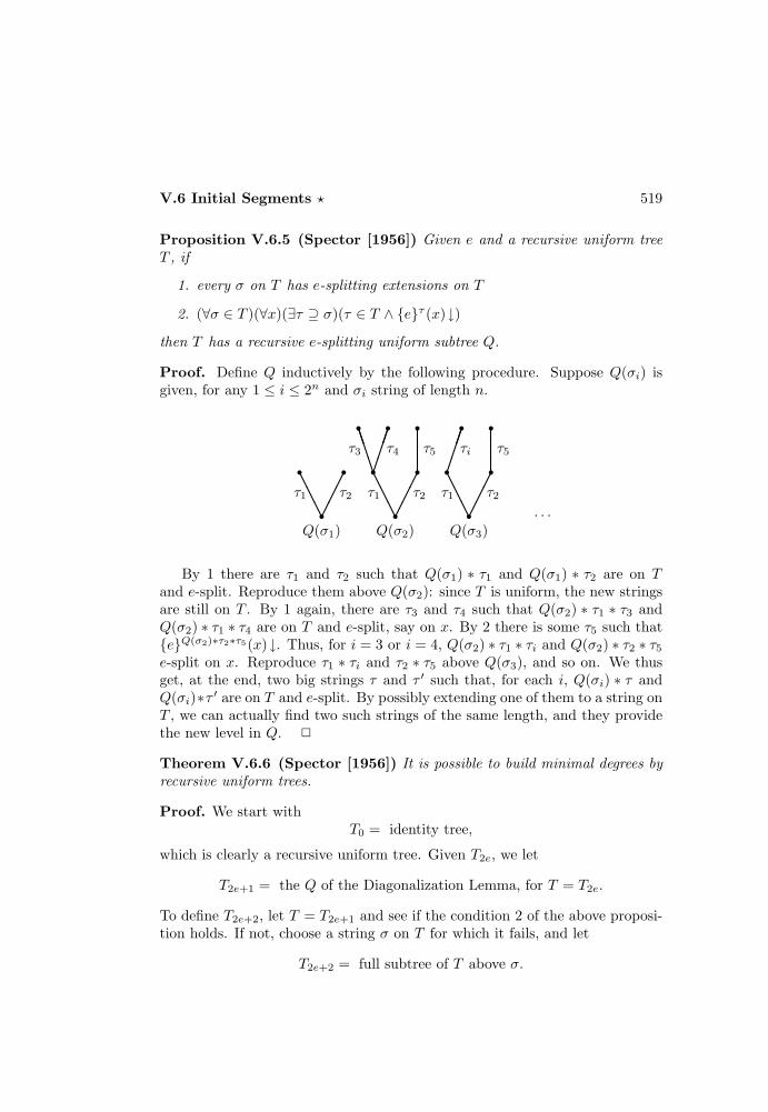
V.6 Initial Segments ? 519
Proposition V.6.5 (Spector [1956]) Given e and a recursive uniform treeT , if
1. every σ on T has e-splitting extensions on T
2. (∀σ ∈ T )(∀x)(∃τ ⊇ σ)(τ ∈ T ∧ eτ (x)↓)
then T has a recursive e-splitting uniform subtree Q.
Proof. Define Q inductively by the following procedure. Suppose Q(σi) isgiven, for any 1 ≤ i ≤ 2n and σi string of length n.
Q(σ1) Q(σ2) Q(σ3)
τ1 τ2 τ1 τ2
τ3 τ4 τ5
· · ·τ1 τ2
τi τ5
rr rrr rr r r
r
AA
A
AA
A
BB
BB r rr r
AA
A
By 1 there are τ1 and τ2 such that Q(σ1) ∗ τ1 and Q(σ1) ∗ τ2 are on Tand e-split. Reproduce them above Q(σ2): since T is uniform, the new stringsare still on T . By 1 again, there are τ3 and τ4 such that Q(σ2) ∗ τ1 ∗ τ3 andQ(σ2) ∗ τ1 ∗ τ4 are on T and e-split, say on x. By 2 there is some τ5 such thateQ(σ2)∗τ2∗τ5(x)↓. Thus, for i = 3 or i = 4, Q(σ2) ∗ τ1 ∗ τi and Q(σ2) ∗ τ2 ∗ τ5e-split on x. Reproduce τ1 ∗ τi and τ2 ∗ τ5 above Q(σ3), and so on. We thusget, at the end, two big strings τ and τ ′ such that, for each i, Q(σi) ∗ τ andQ(σi)∗τ ′ are on T and e-split. By possibly extending one of them to a string onT , we can actually find two such strings of the same length, and they providethe new level in Q. 2
Theorem V.6.6 (Spector [1956]) It is possible to build minimal degrees byrecursive uniform trees.
Proof. We start withT0 = identity tree,
which is clearly a recursive uniform tree. Given T2e, we let
T2e+1 = the Q of the Diagonalization Lemma, for T = T2e.
To define T2e+2, let T = T2e+1 and see if the condition 2 of the above proposi-tion holds. If not, choose a string σ on T for which it fails, and let
T2e+2 = full subtree of T above σ.
520 V. Turing Degrees
Then eA is not total, for any A on it. If condition 2 holds, see if 1 does. Ifnot, there is a string σ with no e-splitting extensions, and we let
T2e+2 = full subtree of T above σ.
Then eA is recursive if total, for any A on it. Otherwise, let
T2e+2 = the Q of the proposition above.
Then A ≤T eA if eA is total, for any A on it. If A is on all the Tn’s, thenit has minimal degree. 2
One might wonder why we should want to build minimal degrees by uniformtrees, since the proof is more complicated than the one given in V.5.11. Thereare two independent answers to this. The first is that this is a first step towardthe construction of minimal degrees by recursive coinfinite conditions. Thesecond is that the proof just given can be modified and, taking advantage ofthe uniformities, turned into a proof of the existence of more complicated initialsegments. These two applications are treated in the next subsections.
Minimal degrees by recursive coinfinite extensions
We close now the circle started in Section 4, by showing how coinfinite condi-tions are nothing else than particular uniform trees.
Definition V.6.7 (Lachlan [1971]) T is a strongly uniform tree (or a1-tree) if it is uniform and, for all σ, T (σ ∗ 0) and T (σ ∗ 1) differ only on oneargument (we say they are adjacent).
Equivalently, we could define strongly uniform trees as admissible triples(V.6.2) satisfying the stronger condition that the functions fL and fR differ,at each level, on exactly one argument. We can see the arguments on whichthe two sides differ as the uncommitted ones, and thus a strongly uniform treedefines a coinfinite condition
θ(x) '
0 if fL(x) = fR(x) = 01 if fL(x) = fR(x) = 1undefined if fL(x) 6= fR(x)
Of course the same translation would work for uniform trees as well. Whatmakes strongly uniform trees special is that any set A extending θ is on the tree(since in each interval there is only one uncommitted point, the two branchesfL and fR take care of all the possibilities). This is not true if the tree is only
V.6 Initial Segments ? 521
uniform (if in an interval there are n uncommitted points then there are 2n
possible extensions, but only two of them are on the tree).Conversely, a coinfinite condition θ defines a strongly uniform tree as follows.
Let g enumerate, in increasing order, the elements on which θ is undefined, and
fL(x) =θ(x) if θ(x)↓0 otherwise fR(x) =
θ(x) if θ(x)↓1 otherwise.
Moreover, the translations just given preserve recursiveness (recall that acoinfinite condition always has recursive domain, and so g is always recursive),and thus recursive strongly uniform trees and recursive coinfinite conditions areinterchangeable.
It is immediate to note that the Totality Lemma proved for uniform treesalso works for strongly uniform ones (since we just split a string at the very end),and thus it is possible to build hyperimmune-free degrees by recursive coinfiniteextensions. To prove the analogue of the Minimality Lemma requires insteadmuch more work.
Proposition V.6.8 (Lachlan [1971]) Given e and a strongly uniform treeT , if
1. every σ ∈ T has e-splitting extensions on T
2. (∀σ ∈ T )(∀x)(∃τ ⊇ σ)(τ ∈ T ∧ eτ (x)↓)
3. T does not have strongly uniform subtrees without e-splittings
then T has a strongly uniform e-splitting subtree Q.
Proof. Clearly condition 1 is redundant, and it follows from 3. We make itexplicit only to show where the new hypothesis is used. Since 2 holds, we maysuppose that
(∀n)(∀σ)(|σ| = n ⇒ eT (σ)(n)↓),
otherwise we apply V.6.4 first. Again we proceed by induction, showing thefirst two steps.
Given σ, by 1 there are τ and τ ′ extending it and e-splitting, say on x.We may suppose they are of the same length (otherwise extend the shortest),and that for all strings µ of that length, eµ(x) ↓ (otherwise go to a levelhigh enough, by the initial observation). Since T is strongly uniform, there isa sequence τ0, . . . , τi of strings on it of the same length, each adjacent to thefollowing in the list, and such that τ = τ0 and τ ′ = τi. Since eτj (x)↓ for allj ≤ i, and eτ0(x) 6' eτi(x), two of these adjacent strings e-split on x. Soσ ∈ T has e-splitting adjacent extensions. This shows how to build the firstlevel of the e-splitting uniform subtree.
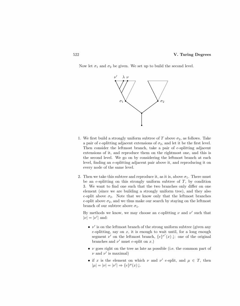
522 V. Turing Degrees
Now let σ1 and σ2 be given. We set up to build the second level.
ν′ λ ν
σ1 σ2
rr
r rr r r
ZZ
ZZ
AA
AA
A
AA
AA
A
1. We first build a strongly uniform subtree of T above σ2, as follows. Takea pair of e-splitting adjacent extensions of σ2, and let it be the first level.Then consider the leftmost branch, take a pair of e-splitting adjacentextensions of it, and reproduce them on the rightmost one, and this isthe second level. We go on by considering the leftmost branch at eachlevel, finding an e-splitting adjacent pair above it, and reproducing it onevery node of the same level.
2. Then we take this subtree and reproduce it, as it is, above σ1. There mustbe an e-splitting on this strongly uniform subtree of T , by condition3. We want to find one such that the two branches only differ on oneelement (since we are building a strongly uniform tree), and they alsoe-split above σ2. Note that we know only that the leftmost branchese-split above σ2, and we thus make our search by staying on the leftmostbranch of our subtree above σ1.
By methods we know, we may choose an e-splitting ν and ν′ such that|ν| = |ν′| and:
• ν′ is on the leftmost branch of the strong uniform subtree (given anye-splitting, say on x, it is enough to wait until, for a long enoughsegment ν′ on the leftmost branch, eν′(x) ↓: one of the originalbranches and ν′ must e-split on x.)
• ν goes right on the tree as late as possible (i.e. the common part ofν and ν′ is maximal)
• if x is the element on which ν and ν′ e-split, and µ ∈ T , then|µ| = |ν| = |ν′| ⇒ eµ(x)↓.

V.6 Initial Segments ? 523
Now take λ which is like ν, only it goes right one level after ν does: λ andν are obviously adjacent, and eλ(x) ' eν′(x) by the choice of ν (sincethe common part of ν and ν′ is maximal). Then eλ(x) 6' eν(x), andλ and ν are an adjacent e-splitting above σ1. By definition they are alsoan (adjacent) e-splitting above σ2 (since ν′ lies on the leftmost branch).
This shows how to build the second level of the e-splitting uniform subtree.The remaining levels can be built inductively, in the same way. 2
Theorem V.6.9 (Lachlan [1971]) It is possible to build minimal degrees byrecursive coinfinite extensions.
Proof. We use strongly uniform recursive trees, which we know to be inter-changeable with recursive coinfinite conditions. Let
T0 = identity tree,
which is clearly a strongly uniform recursive tree. Given T2e, let
T2e+1 = the Q of the Diagonalization Lemma, for T = T2e.
To define T2e+2, let T = T2e+1, and see if condition 2 of the above propositionholds. If not, choose a string σ on T for which it fails, and let
T2e+2 = full subtree of T above σ.
Then eA is not total, for any A on it. If condition 2 holds, see if 3 holds. Ifnot, let
T2e+2 = a strongly uniform subtree of T without e-splittings.
Then eA is recursive if total, for any A on it. Otherwise, let
T2e+2 = the Q of the proposition above.
Then A ≤T eA if eA is total, for any A on it. If A is on all the Tn’s, thenit has minimal degree. 2
Exercises V.6.10 a) The minimal degree built above is below 0′′. (Lachlan [1971])(Hint: to ask whether there is a strongly uniform subtree without e-splitting is toocomplicated. But we can ask if the inductive process of building the e-splitting subtreein the proposition above does terminate or not. If yes, take the e-splitting subtree. Ifnot, we know that there is a strongly uniform subtree without e-splitting, and thuswe can search for an index of it.)
b) There is a cone of degrees such that every element in it is the join of twominimal degrees. (Cooper [1972a]) (Hint: build a strongly uniform tree of minimal
524 V. Turing Degrees
degrees recursive in ∅′′. Given C such that ∅′′ ≤T C, choose A and B on the treeas follows. At level n, let x be the unique element on which the branches differ. LetA follow the branch that on x agrees with C, and B follow the other branch. ThenA,B ≤T C ⊕ ∅′′ ≤T C, so A ⊕ B ≤T C. And C ≤T A ⊕ B, since C(n) can berecovered as the value of A on the n-th element on which A and B differ.)
c) The hyperimmune-free degrees are not closed under join. (Martin and Miller[1968]) (Hint: build a strongly uniform tree of hyperimmune-free degrees recursivein ∅′′. It follows as in part b) that the degrees above 0′′, which are hyperimmunebecause comparable with 0′, are joins of two hyperimmune-free degrees.)
d) There is a minimal, not completely autoreducible degree. (Jockusch and Pater-
son [1976]) (Hint: build a set A of minimal degree, by recursive coinfinite extensions.
Insert steps to insure that A is not autoreducible. The two constructions are com-
patible.)
The three-element chain
Recall that an initial segment is simply a set of degrees closed downward. Theset 0,a, with a minimal degree, is thus the simplest nontrivial initial seg-ment, the two-element chain. The set of minimal degrees and 0 is a nontrivialinitial segment of power 2ℵ0 .
Since every degree has a minimal cover, there are degrees a and b such that0 < b < a, and there is no degree strictly between either 0 and b, or b anda. But there could be some degree c incomparable with b, and still below a.We now want to build a and b as above, but with the additional property that0, b,a is an initial segment, i.e. the only degrees below a are 0 and b. Thisis called a three-element chain.
The idea is to build A such that the odd part of A, defined as
Od(A) = x : 2x+ 1 ∈ A,
plays the role of the intermediate degree. Since Od(A) ≤T A automatically,the requirements on A are thus:
1. Od(A) nonrecursive
2. A 6≤T Od(A)
3. eA total ⇒ eA recursive or eA ≡T Od(A) or eA ≡T A.
These are just generalizations of the conditions for A being minimal, and inmany respects so is the construction, which employs uniform trees. The mostcrucial parts are the idea of forcing Od(A) to be minimal (which allows us tobuild just one set A, instead of the separate sets A and B), and V.6.12 (whichallows us to make A not recursive in its odd part, and uses uniformity in acrucial way, thus forcing us to use uniform trees in the construction of initialsegments).

V.6 Initial Segments ? 525
Proposition V.6.11 Given e and a recursive uniform tree T , if for some σ
T (σ ∗ 0), T (σ ∗ 1) disagree on their odd parts
then there is a recursive uniform tree Q ⊆ T such that, for every A on Q,Od(A) 6' e.
Proof. Since T (σ ∗ 0), T (σ ∗ 1) disagree on their odd parts, the odd part ofone of them, say T (σ ∗ i), disagrees with e. Let Q be the full subtree of Tabove T (σ ∗ i). 2
Proposition V.6.12 (Titgemeyer [1962]) Given e and a recursive uniformtree T , if for some σ
T (σ ∗ 0), T (σ ∗ 1) agree on their odd parts
then there is a recursive uniform tree Q ⊆ T such that, for every A on Q,A 6' eOd(A).
Proof. Let x be such that T (σ ∗ 0)(x) 6= T (σ ∗ 1)(x). Such an x must exist,because T (σ ∗ 0) and T (σ ∗ 1) are incompatible. By the hypothesis on σ, it isnot on their odd parts. See if
(∃τ ⊇ T (σ ∗ 0))(τ ∈ T ∧ eOd(τ)(x)↓).
If not, let Q be the full subtree above T (σ ∗ 0): if A is on Q, eOd(A) isnot total (hence it differs from A).
T (σ)
T (σ ∗ 0) T (σ ∗ 1)
τ0 τ1
r
r rr r
r
@@
@
Otherwise, let τ0 be such a string, and let τ1 extend T (σ∗1) in the same wayas τ0 extends T (σ∗0). Since T is uniform, τ1 ∈ T . Now τ0 and τ1 have the sameodd parts, since they extend in the same way T (σ ∗0) and T (σ ∗1), which have
526 V. Turing Degrees
the same odd parts. Then eOd(τ0)(x) ' eOd(τ1)(x). But τ0(x) 6= τ1(x), andfor i = 0 or i = 1 we have
τi(x) 6= eOd(τi)(x).
Then let Q be the full subtree of T above τi. 2
From the two lemmas we know that we can diagonalize if we use uniformtrees such that T (σ ∗0) and T (σ ∗1) agree on the odds (i.e. on their odd parts)for infinitely many σ’s, and disagree on the odds for infinitely many σ’s. We willwork, from now on, with trees which alternate agreements and disagreementson the odds. The lemmas just proved work for them too, since we are justtaking full subtrees in their proofs.
Of course lemma V.5.9 still holds, and we thus have conditions ensuringthat eA is recursive (A on a tree T with no e-splitting), or A ≤T eA (Aon a e-splitting tree). With a similar proof we get a similar lemma, that takescare of the remaining case:
Proposition V.6.13 (Titgemeyer [1962], Hugill [1969]) Given e, a re-cursive uniform tree T , and A on T , if eA is total then:
1. if on T there is no e-splitting which agrees on the odd, then
eA ≤T Od(A)
2. if whenever T (σ ∗ 0) and T (σ ∗ 1) disagree on the odds they e-split,
Od(A) ≤T eA.
Proof. In the first case we compute eA. Given x, we know that eA(x)↓,and to get the right value it is enough to search for σ on T such that eσ(x)↓and Od(σ) ⊆ Od(A), and this is recursive in Od(A).
In the second case we compute initial segments of Od(A), by induction.Suppose T (σ) such that Od(T (σ)) ⊆ Od(A) is given. If T (σ ∗ 0) and T (σ ∗ 1)agree on the odds, then both work (i.e. their odd parts are contained in theodd part of A). Otherwise, they disagree on the odds, and then they e-split,say on x. If eT (σ∗i)(x) ' eA(x), then T (σ ∗ i) ⊆ Od(A). 2
Now we can prove the analogue of the Minimality Lemma.
Proposition V.6.14 (Hugill [1969]) Given e and a recursive uniform treeT alternating agreements and disagreements on the odds, there is a recursiveuniform tree Q ⊆ T alternating agreements and disagreements on the odds,such that one of the following holds:
V.6 Initial Segments ? 527
1. for every A on Q, eA is not total
2. for every A on Q, eA is recursive
3. for every A on Q, eA ≡T Od(A)
4. for every A on Q, A ≤T eA.
Proof. If there are σ on T and x such that (∀τ ⊇ σ)(τ ∈ T ⇒ eτ (x)↑), thenlet Q be the full subtree above σ. If A is on Q, then eA is not total.
Otherwise, see if there is σ with no e-splitting above it. If so, let Q be thefull tree above it. If A is on Q, then eA is recursive (by V.5.9).
Otherwise, there are e-splittings above any strings. See however if there isσ with no e-splitting extensions agreeing on the odds. If so, let Q be a uniformsubtree of T above σ, alternating branches agreeing on the odds and e-splittingbranches. By hypothesis the e-splittings do not agree on the odds, and on Qthere are no e-splittings agreeing on the odds. The conditions of V.6.13 aresatisfied, and if A is on Q then A ≡T eA.
Otherwise, we can always find e-splitting agreeing on the odds. We wantQ e-splitting uniform tree, alternating agreements and disagreements on theodds. The level agreeing on the odds can be made e-splitting by hypothe-sis. The level disagreeing on the odds can also be done, because we can takee-splittings, and then extend them to disagree on the odds. Let Q be such ane-splitting subtree of T , which can be made uniform by the techniques of V.6.5.If A is on Q then A ≤T eA, because Q is e-splitting (V.5.9). 2
Theorem V.6.15 (Titgemeyer [1962]) The three-element chain is embed-dable as initial segment of D.
Proof. We already have all the ingredients, and the result follows by startingwith
T0 = identity tree,
which is a recursive uniform tree alternating branches agreeing on the odds anddisagreeing on the odds. Then we let:
T3e+1 = the Q of V.6.11, applied to T = T3e
T3e+2 = the Q of V.6.12, applied to T = T3e+1
T3e+3 = the Q of V.6.14, applied to T = T3e+2.
The first two steps make Od(A) not recursive and A not recursive in Od(A),so that we do have one nontrivial degree below A. The last step makes surethat this is the only one. 2
528 V. Turing Degrees
Note that in particular the proof produces a minimal degree with a strongminimal cover (V.5.16). Actually, with terminology as on p. 495, the set of min-imal degrees with a strong minimal cover is comeager, for the topology inducedby recursive uniform trees (Simpson [1977]): it is enough to consider, givensuch a tree T , a recursive uniform tree T ∗ that alternates branches agreeing onthe odds with branches disagreeing on the odds, and such that the odd parts ofthe branches are exactly the branches of T . The proof above shows that the setof degrees which are top elements of three-element chains is comeager, for thetopology induced by the trees T ∗. The intermediate degrees, which are mini-mal degrees with a strong minimal cover, are then comeager for the topologyinduced by the trees T . It can then be argued, as in Section 3, that minimaldegrees without a strong minimal cover cannot be built by recursive uniformtrees. The existence of such degrees is an open problem, and the constructionof one of them would then require new methods of proof.
Exercises V.6.16 More initial segments. a) The diamond is embeddable as ini-tial segment of D, i.e. there is a degree with exactly two nontrivial degrees belowit, and they are incomparable. (Sacks [1963]) (Hint: build A such that Ev(A) =x : 2x ∈ A and Od(A) do the job. The only modification in the proof of thethree-element chain is that Od(A) and Ev(A) have to be treated symmetrically and,whenever we had in V.6.15 branches that simply disagreed on the odds, now we ac-tually want them to agree on the evens. Note that on trees on which all brancheseither agree on the odds or agree on the evens, whenever there are e-splittings thenwe may find them agreeing on the odds or on the evens, by going by adjacent pathsas in the first part of V.6.8, where now adjacent means agreeing on the odds or onthe evens.)
b) Every recursive linear ordering is embeddable as initial segment of D. (Hugill[1969]) (Hint: we may restrict ourselves to infinite orderings of ω in which 0 isthe least element, and 1 the greatest. Choose a set Xnn∈ω of disjoint, uniformlyrecursive sets such that
m n ⇒ Xm ⊆ Xnm ≺ n ⇒ Xn −Xm infinite,
and X0 = ∅, X1 = ω. We build A such that, if we define
x ∈ Xn(A) ⇔ the x-th element (in order of magnitude) of Xn is in A,
then the degrees of Xn(A)n∈ω form an initial segment isomorphic to the partial or-dering. Note that X0(A) = ∅, X1(A) = A, and Xn(A) ≤T A. E.g., in V.6.15 we tookX2 = odd numbers. The idea is simply to approximate the ordering, by consideringat stage s the subordering induced by it on 0, . . . , s, and ensure conditions on Athat make the degrees of Xn(A)n≤s isomorphic to it. The lemmas above can berewritten with reference to any Xn, instead of the odds. To be able to diagonalizewe need to have, whenever m ≺ n, infinitely many branches agreeing on Xm anddisagreeing on Xn. For this we enumerate these pairs 〈m,n〉 with infinitely many

V.6 Initial Segments ? 529
repetitions, and ask that the i-th level of the tree agrees on Xm and disagrees onXn, if 〈m,n〉 is the i-th pair in the enumeration. The reason why dealing with onlyfinitely many conditions at each stage is sufficient, is that every function recursive inA has infinitely many indices and, for all but finitely many such, our trees will havethe desired properties.)
c) There is a degree with no minimal predecessor . (Martin [1967], Hugill [1969])(Hint: embed an ordering with order type 1 + ω∗, i.e. the reverse ordering of thenatural numbers with a least element added to it. For a different proof see V.3.17.)
d) There is an ascending sequence of degrees with an upper bound below whichthere is no minimal upper bound . (Yates [1970]) (Hint: embed an ordering with ordertype ω + ω∗.)
e) There is a completely autoreducible, not minimal degree. (Jockusch and Pater-
son [1976]) (Hint: use double e-splittings in the proof of V.6.15, as in V.5.15.d. This
makes the top degree completely autoreducible.)
The initial segments of the degrees ?
The ideas involved in the proofs of the embeddings of the three-element chainand the diamond can be pushed further, to prove that every finite distributivelattice is embeddable as initial segment of D. This relies on the fact that if afinite lattice is distributive, then it is isomorphic to a sublattice of the power setof some finite set. It is then enough, given a finite distributive lattice, to find apartition of ω into infinite, coinfinite recursive sets whose lattice structure underinclusion mirrors the given lattice (like ∅, Ev,Od and ω did for the diamond),and build the top degree of the initial segment. What is needed is some kindof representation theorem for the lattices, but no new recursion-theoreticalideas are involved. This theorem is due to Lachlan [1968a], but the approachjust sketched comes from Yates [1972], who did it for Boolean algebras (whichrequire only the full power set of some set), and Epstein [1979], who got therepresentation.
The same approach can be adopted for countable bottomed distributivelattices, with a new ingredient: if the lattice is not recursive, its representationvia recursive subsets cannot be chosen ahead of time, and has to be built alongthe way. This gives the result of Lachlan [1968a], and it is as far as the methodcan go: only distributive lattices can be treated this way.
Nondistributive lattices are much more difficult to deal with, and have beentreated by Shoenfield, Lerman [1969], [1971], and Lachlan and Lebeuf [1976].The final result for countable initial segments is the following: a countablepartial ordering is isomorphic to an initial segment of D if and only if it isan uppersemilattice with a least element . This completely characterizes thepossible isomorphism types of D(≤a), since any degree has at most countablymany predecessors. Namely, the principal ideals of D realize every possiblecountable uppersemilattice with least and greatest element. We will prove
530 V. Turing Degrees
that D is not distributive without using initial segments, as a corollary ofan embedding result in the r.e. degrees, see Chapter X. Treatments of theembeddings quoted so far can be found in Epstein [1979] and Lerman [1983].
Uncountable initial segments have been considered by Thomason [1970] andRubin. Here it is not possible to assume the existence of a greatest element, andhence to construct only the top degree. Thus the given uppersemilattice has tobe approximated, and a further obstacle is introduced by the fact that not everyinitial segment is extendible (e.g. not every degree has a strong minimal cover),and thus the approximations cannot simply be end-extensions. The methodof forcing is used to control the amalgamation of the various approximations,and Abraham and Shore [1986] have proved that a partial ordering with powerat most ℵ1 is isomorphic to an initial segment of D if and only if it is anuppersemilattice with a least element, and countable predecessor property . Thiscompletely characterizes the possible isomorphism types of linearly orderedinitial segments, because a linear ordering with countable predecessor propertymust have power at most ℵ1.
This result settles the initial segments problem if the Continuum Hypothe-sis holds, and it is the best possible result in ZFC, since Groszek and Slaman[1983] have shown that it is consistent with ZFC to have an uncountable up-persemilattice (even of power ℵ2 less than the continuum) with countable (evenfinite) predecessor property, which is not embeddable in D as an uppersemilat-tice (and hence as an initial segment).
The characterization of initial segments is just one step toward a completecharacterization of the algebraic structure of D. The next step would be toknow which initial segments are extendable, but not even the very first stephas been answered: it is still not known if every minimal degree has a strongminimal cover.
V.7 Global Properties
Until now we have studied first-order or local properties of degrees, mainlytelling that given configurations exist in the degrees, possibly extending givenones. We now take a different stand, and look at second-order or global prop-erties of degrees: on the one hand we analyze the difficulty of the first-ordertheory of D (proving its undecidability and much more), and on the other handwe study its global algebraic properties. We will capitalize here on the workdone so far, and a cascade of interesting results will be obtained.
V.7 Global Properties 531
Definability from parameters
What Spector’s Theorem accomplishes is to define any countable ideal, by usingtwo parameters. Indeed, if a and b are an exact pair for a countable ideal I,then
c ∈ I ⇔ c ≤ a ∧ c ≤ b.
As we can see, the formula that defines the ideal is always the same, and onlythe parameters change, for different ideals. This uniformity is quite important,because then we can avoid talking about ideals, replacing them by their exactpairs (since the dependence of the ideal on the exact pair is fixed). This showsthat the first-order theory of D includes an interpretation of quantification overcountable ideals.
We are now going to extend this result by showing that, in a little morecomplicated way, any countable relation is uniformly definable from a fixednumber of parameters, which depends only on the number of arguments of therelation. We first prove a weaker result, which provides all the technical work.
Proposition V.7.1 (Slaman and Woodin [1986]) Every countable anti-chain is definable from finitely many parameters in D, in a uniform way.
Proof. Since an antichain C = cnn∈ω is made of pairwise incomparabledegrees, the idea to define it is to find a property P for which the given cn’sare the minimal solutions. We will use an approach symmetric to the oneadopted for Spector’s Theorem, namely we define two degrees a and b and welook at the degrees x satisfying the property P so defined:
P (x) ⇔ x 6= (x ∪ a) ∩ (x ∪ b).
If we can make sure that the elements of C are the minimal solutions of P , then
x ∈ C ⇔ P (x) ∧ ¬(∃z)(z < x ∧ P (z)).
The trouble with this approach is that we are asking too much, because beinga minimal solution of P is a condition involving all degrees, and only countableinformation can be coded into a pair of sets. We thus relax the requirement abit, and consider not all degrees, but only the countably many ones below anygiven degree c bounding C. Then we only need to have:
x ∈ C ⇔ x ≤ c ∧ P (x) ∧ ¬(∃z ≤ c)(z < x ∧ P (z)).
We will thus define C using three parameters a, b, and c, of which c is simplyany degree bounding every cn.
Given Cnn∈ω with Cn ∈ cn, we can simply let C = ⊕n∈ωCn. Theconditions on A and B are the following:

532 V. Turing Degrees
1. cn is a solution of PSince x ≤ (x∪a)∩(x∪b) always holds, we ensure (x∪a)∩(x∪b) 6≤ x,for x in C. This will be achieved by having, for every n, a set Dn suchthat
Dn ≤T Cn ⊕A,Cn ⊕B but Dn 6≤T Cn.
2. cn is a minimal solution of PFor this we need, for any x ≤ c,
x 6= (x ∪ a) ∩ (x ∪ b) ⇒ cn ≤ x, for some n.
Hence, for any X ≤T C,
(∃D)(D ≤T X ⊕A,X ⊕B ∧ D 6≤T X) ⇒ Cn ≤T X, for some n.
As in Spector’s Theorem, A and B will be built by coinfinite extensions θsand ϑs. We will have A =
⋃s∈ω θs and B =
⋃s∈ω ϑs. As usual, A and B will
be thought of as made of columns An and Bn, and corresponding columns inthem will differ only finitely (so that their degrees will be the same). This timehowever it is Dn, rather than Cn, that gets coded in the n-th columns An andBn.
Since Dn has to be recoverable from each of Cn ⊕ A and Cn ⊕ B, we willuse only the elements of Cn to code information in A and B. Precisely,
Dn(x) =
0 if x 6∈ CnAn(x) otherwise.
Then Dn ≤T Cn⊕A by definition, and Dn ≤T Cn⊕B because An and Bn willdiffer only finitely, by construction. It remains to ensure, by diagonalization,that Dn 6≤T Cn, and hence Dn 6≤T eCn , for every e.
Since we use coinfinite conditions, we will be able to take care of all theserequirements, for a fixed n, in just one step. Indeed, we can define
D∗n(x) =
1− eCn(x) if x is the e-th element of Cn, and eCn(x)↓0 otherwise.
D∗n obviously is not recursive in Cn, and neither is any set differing only finitely
from it (because each recursive function has infinitely many indices, and thusD∗n differs infinitely often from every set recursive in Cn). It will then be enough
to have An, and hence Dn, differ only finitely from D∗n.
We now consider the minimality requirements. We will work with a fixedlist Xmm∈ω of the sets recursive in C. Recall that we want, for each m,
D ≤T Xm ⊕A,Xm ⊕B ∧ D 6≤T Xm ⇒ Cn ≤T Xm, for some n.
V.7 Global Properties 533
The requirements are:
Re,m : eXm⊕A ' eXm⊕B ' D ∧D 6≤T Xm ⇒ Cn ≤T Xm, for some n.
(note that we use V.2.18.a to simplify the presentation of the requirements).They will be satisfied as in the proof of Spector’s Theorem.
We start with θ0 = ϑ0 = ∅. At each step s + 1 we are given θs and ϑs,defined on the first s columns and on finitely many other points, and differingon each of the first s columns only finitely. We take care of the requirementRe,m if s = 〈e,m〉, and in any case we will ensure the needed diagonalizationson Ds. There are three possible cases:
• we can make eXm⊕A not totalIn other words, there is a string σ compatible with θs, such that
(∃y)(∀τ ⊇ σ)(τ compatible with θs ⇒ eτ (y)↑).
Then take one such string, and let:
θs+1(x) =
θs(x) if θs(x)↓σ(x) if σ(x)↓D∗s(z) if x = 〈s, z〉, otherwise.
ϑs+1 is obtained similarly, by using ϑs in place of θs.
• otherwise, but we can force a special kind of disagreementIn general we would only look for two strings σ and τ , respectively com-patible with θs and ϑs, which e-split on some x. For reasons that willappear clear later, here we also request that they agree on elements ofCn, on the n-th column, for any n < s. If two such strings exist, takeany of them and define θs+1 and ϑs+1 as above, using σ and θs for theformer, and τ and ϑs for the latter.
• otherwiseThen simply let
θs+1(x) =θs(x) if θs(x)↓D∗s(z) if x = 〈s, z〉, otherwise.
ϑs+1 is obtained by using ϑs in place of θs.
It is clear that in the first two cases the requirement Re,m is vacuouslysatisfied. We now have to argue that it is so also in the last case. Suppose thatin the end we have
eXm⊕A ' eXm⊕B ' D and D 6≤T Xm.

534 V. Turing Degrees
We have to prove thatCn ≤T Xm, for some n.
Suppose there is no e-splitting compatible with θs: then, as usual, we wouldhave eXm⊕A ' D ≤T Xm, but this is impossible by hypothesis. Thus thereare e-splittings compatible with θs, and actually infinitely many such (becausethe same reasoning works above any given string). But we also supposed
eXm⊕A ' eXm⊕B ,
which means that the construction did not succeed in forcing a disagreement.Certainly the first case of the construction cannot have happened, becauseeXm⊕A ' D is a total function. Then it must have been the second stepthat failed. Since θs and ϑs disagree only finitely, there are infinitely manye-splitting pairs, with one side compatible with θs, and the other compatiblewith ϑs. Since we did not pick up any of them, it must be because none satisfiesthe additional condition of case two, and thus the two sides do not always agreeon the elements of Cn, on the n-th columns, for some n < s.
We now show that Cn ≤T Xm, for some n < s, in three steps:
1. for a fixed n < s, there must be infinitely many pairs of e-splitting strings,compatible with θs and differing on some element of CnThis is simply because the same holds for some n < s, and there are onlyfinitely many such n’s. Thus infinitely many disagreements must hold forthe same n. We now fix this n.
2. there is an infinite subset of Cn which is recursive in Xm
We show how to generate an infinite ascending sequence of elements of Cn.Suppose we have an initial segment µ of the characteristic function of sucha subset. Simply look for an e-splitting σ, σ′ extending µ, and compatiblewith θs. As argued above, σ and σ′ must disagree on some element ofCn (unless their pair is one of finitely many exceptions, a case that iseffectively testable because the exceptions can be given in advance). Butthey can also disagree on some other element, not necessarily in Cn. Tobe able to sort out the right element, we only have to interpolate the twostrings, by a sequence of strings σ0, . . . , σi all extending µ, making eσj
converge on the element on which σ and σ′ e-split (which is possible,because we are not in the first case of the construction) and differing,each from the following one, on just one element. Moreover, σ0 = σ andσi = σ′. Since σ0 and σi e-split, there must be j < i such that σj andσj+1 e-split. These strings can effectively be found, and now they differonly on one element, which must then be in Cn.
3. Cn ≤T Xm
We now have an infinite subset of Cn recursive in Xm. To be able to
V.7 Global Properties 535
have all of Cn recursive in Xm, we play a trick: we choose, from the verybeginning, sets Cn’s which are introreducible (see II.6.7), i.e. recursivein each of their infinite subsets. This is possible, because every degreecontains such a set (II.6.13). If Cn is autoreducible, then the previouspart already shows that Cn ≤T Xm. 2
Note that the parameters needed to define Cnn∈ω can be obtained arith-metically in ⊕n∈ωCn.
Theorem V.7.2 Definability from parameters (Slaman and Woodin[1986]) Every countable relation is definable from finitely many parameters inD, in a uniform way.
Proof. We start by dealing with sets. Given C = cnn∈ω, we would like tospread it out to get a set of incomparable degrees, since we know how to definethe latter. Choose c above every element of C (which is possible because C iscountable). Define a set A = ann∈ω of pairwisely incomparable degrees notintroducing any new relation on degrees below c, i.e. such that, for x ≤ c,
x ∪ am ≤ y ∪ an ⇔ x ≤ y ∧m = n.
A can be constructed by the methods of Section 4 (see V.2.9). We now spreadout C by using any infinite subset A∗ = af(n)n∈ω of A, for any one-onetotal function f (for this part of the proof the set A itself would be perfectlysufficient, but the added generality will be useful later on). Clearly A∗ is anantichain (since so is A), and so is the set
C∗ = cn ∪ af(n),
by the choice of A (because cn ∪ af(n) ≤ cm ∪ af(m) only if f(m) = f(n),and hence if m = n, f being one-one). Then both A∗ and C∗ are definable withparameters, by the previous proposition. It follows that:
• C is definableIndeed
x ∈ C ⇔ x ≤ c ∧ (∃a ∈ A∗)(x ∪ a ∈ C∗).Only the right-to-left implication has to be checked. Suppose that x ≤ c,and x ∪ af(n) is in C∗: then
x ∪ af(n) = cm ∪ af(m),
for some m. By the properties of A it must be
x ∪ af(n) = cn ∪ af(n).
Then from x ∪ af(n) ≤ cn ∪ af(n) we have x ≤ cn, and similarlycn ≤ x, from which x = cn. Thus c ∈ C.
536 V. Turing Degrees
• the map f∗ from C to C∗ induced by f is definableAs for C,
f∗(x) = y ⇔ x ∈ C ∧ x ∪ y ∈ C∗.
We now turn to the definability of countable relations. Given an n-aryrelation R on degrees, we can first of all define the n projections of R, sincethe degrees in them are the relevant ones:
x ∈ Ri ⇔ (∃y1)· · ·(∃yn−1)R(y1,. . . ,yi−1,x,yi,. . . ,yn−1).
We can now take as c a degree bounding all the elements of⋃
1≤i≤nRi, asabove. The new problem that we have to face here is a coding problem: wewould like to reduce R to a set of (incomparable) degrees, but we actuallyhave n-tuples of degrees, one in each of the projections. What we do is todefine A as above, with the additional requirement that the finite joins of itselements are uniquely determined by the elements themselves, so that the joinof n elements uniquely codes them. Since we are going to use finite joins ofelements of A, we want all of them to be incomparable. And since we are goingto code the individual projections of R as well, the finite joins will have to notintroduce new relationships among the degrees below c. All these conditionsfollow automatically, when A is a set of degrees recursively independent overthe degrees below c: such a set can be constructed by the methods of Section4 (see V.2.9). Having A, we can first of all pick up n disjoint subsets of it (byusing one-one functions fi) to code the projections Ri. As noted above, notonly the sets Ri, but also the functions f∗i , choosing the elements needed tospread out Ri, are definable. Now we can simply let
B = f∗1 (x1) ∪ · · ·∪f∗n(xn) : R(x1,. . . ,xn).
B is definable, because the degrees f∗1 (x1)∪ · · ·∪f∗n(xn) are finite joins of mem-bers of A, and hence pairwise incomparable. And R is recoverable from B,because the joins of elements of A are uniquely determined by their elements,and hence
R(x1,. . . ,xn) ⇔ f∗1 (x1) ∪· · ·∪f∗n(xn) ∈ B.
Moreover, R is definable because the maps f∗i are definable, and so is B. 2
Note that in a sense the theorem is the best possible, since the parameterscannot be eliminated in general : the relations definable in D are only countablymany, but there are uncountably many countable relations. There are howevermany relations that can be definable without parameters, as we will see.
V.7 Global Properties 537
The complexity of the theory of degrees
The definability result of the last subsection allows for a quick proof of thefollowing theorem, which completely characterizes the complexity of the theoryof degrees.
Theorem V.7.3 Simpson’s Theorem (Simpson [1977]) The first-ordertheory of D has the same degree (and actually the same isomorphism type) asthe theory of Second-Order Arithmetic.
Proof. We prove that the two theories have the same m-degree by interpretingeach in the other, thus providing faithful translations that will preserve theo-rems. Since the translations will actually be one-one, the theories will have thesame 1-degree, and hence will be recursively isomorphic by III.7.13.
One direction is clear, since every formula about the ordering of degrees canbe interpreted, in the natural way, as a formula about sets of integers. Thusthe theory of degrees is interpretable in Second-Order Arithmetic.
For the converse, we want to show that Second-Order Arithmetic is inter-pretable in D. A model of arithmetic is a structure 〈A,R, f1, f2, f3, a〉 suchthat:
1. A is a countable set
2. R is a total ordering on A with first element a, successor given by f1, andsuch that every element different from a has a predecessor
3. f2 and f3 satisfy the axioms of Robinson Arithmetic Q (p. 23), wheninterpreted as sum and product, with f1 interpreted as successor.
A standard model of arithmetic is a model in which R is a well-ordering.A standard model exists in the degrees, since any countable partial ordering
is embeddable in boldmath D (by V.2.9). Moreover, given degrees ~a coding acountable set of degrees (intended to be the universe A of a standard model ofArithmetic in D), we can say in a first-order statement of D that given degrees~c code a relation and (the graphs of) three functions on the set coded by ~a,satisfying the requirements for being a standard model of Arithmetic. This isbecause Q has only finitely many axioms, and well-ordering can be expressedby replacing quantification over subsets of A by quantification over parametersthat define them (since a subset is defined by a fixed number of parameters, ina uniform way).
Then a sentence ϕ of Second-Order Arithmetic is true if and only if thesentence ϕ∗ of D is, where ϕ∗ says that there are degrees ~a and ~c coding astandard model of arithmetic in which the translation of ϕ (obtained, as above,by replacing quantification over subsets of A by quantification over parameters
538 V. Turing Degrees
that define them) holds. Since ϕ∗ can be effectively obtained from ϕ, we thushave an m-reduction of Second-Order Arithmetic to the theory of D. 2
Corollary V.7.4 (Lachlan [1968]) The first-order theory of D is undecid-able and not axiomatizable.
Proof. So is the theory of (first-order) arithmetic. 2
Corollary V.7.5 (Jockusch and Simpson [1976], Simpson [1977]) Thefirst-order theory of D is not absolute with respect to models of ZFC containingall the ordinals.
Proof. There is a sentence about the ordering of degrees which is true in Dif and only if P(ω) ⊆ L, since the latter can be translated into a sentence ofSecond-Order Arithmetic by IV.4.22. 2
Lachlan obtained the undecidability of the theory of degrees as a corollary ofthe embeddability of every countable distributive lattice as an initial segmentof D (see p. 529), by using the undecidability of the theory of distributivelattices (and the Lowenheim-Skolem Theorem, to be able to restrict attentionto countable distributive lattices). Subsequently, Thomason [1970] observedthat the result follows from the embeddability of the finite distributive latticesonly, this time using the fact that the set of sentences true in all distributivelattices and the set of sentences false in some finite distributive lattice arerecursively inseparable.
In the first proofs of Simpson’s Theorem, when only Spector’s Theorem wasavailable, only ideals (and hence initial segments) could be used to code setsand relations in D in a definable way, and more ingenuity was required. Theoriginal coding of Arithmetic by Simpson [1977] was very direct, and interpretedthe natural number n as the degree 0(n), m+n as 0(m+n), and m·n as 0(m·n).To define the set 0(n)n∈ω Simpson hooked it up to an initial segment withcontrolled (double) jump, and the same method was used for sum and product.This required only simple initial segments (namely chains), but the proof thatthe coding worked was not straightforward (in particular, the jump operatorhad to be eliminated). An exposition of this method is in Epstein [1979].
A much simpler coding, requiring more initial segments (the countable dis-tributive lattices) but less direct work, was devised by Nerode and Shore [1980].They noticed that second-order logic on countable sets could be translated intothe theory of countable distributive lattices with quantification over ideals,by first coding relations by graphs, and then graphs by ideals of distributivelattices. The advantages of this method were simplicity, which allowed for im-proved calculations and sharper consequences, and generality, which permittedthe extension of Simpson’s Theorem to a variety of different degree structures.

V.7 Global Properties 539
An exposition of this method for the study of Turing degrees is in Lerman[1983], while the general result is proved in VI.4.7.
The coding method we used is due to Slaman and Woodin [1986]. It is eas-ier than all of the above, since it codes sets and relations directly, and thus itmakes the translation of Arithmetic straightforward. It also has the advantagethat the only needed result (V.7.2) can be proved directly, and with very littlemachinery (only the coinfinite extension method), in particular avoiding initialsegment constructions.
Some additional work provides a substantial generalization of Simpson’sTheorem.
Theorem V.7.6 (Nerode and Shore [1980], [1980a]) If C is an ideal of Dclosed under jump, the first-order theory of C has the same degree (and actuallythe same isomorphism type) as the theory of Second-Order Arithmetic with setquantifiers restricted to sets with degree in C.
Proof. We refine the proof of V.7.3. As there, the translation of the theoryof C into Second-Order Arithmetic with set quantifiers restricted to sets withdegrees in C is immediate.
For the converse, we first need to show that we can pick up a standardmodel of arithmetic in C. Certainly the needed configurations exist in thedegrees below 0′ (by V.2.9), and hence in C. Moreover, also parameters ~a and~c defining a standard model of arithmetic exist in C, because the proof of V.7.2provides parameters coding a given set arithmetically in its infinite join, andthe methods of V.4.7 allow to choose the needed configurations not only below0′, but actually with infinite join below it.
A simple translation of the relevant notions shows that there is a first-ordersentence of the theory of C that says that degrees ~a and ~c code a model ofarithmetic in C. But the method used in V.7.3 to show that the same holdsfor standard models as well does not work here, since by quantifying overparameters in C we do not take care of all possible subsets, and hence we donot define a real well-ordering.
To be able to handle standard models we proceed as follows. Consider thestandard part (corresponding to the set of integers) of a model. If the modelis standard then this part exhausts its universe, and thus every proper initialsegment of the universe is finite and has a least upper bound. Conversely, ifthe model is not standard then the standard part is a proper initial segmentwith no least upper bound. Thus the model is standard if and only if everyproper initial segment of the universe has least upper bound. This is still asecond-order sentence, but it really needs only the standard part of the modeland the finite subsets of the universe. If we show that these subsets are all

540 V. Turing Degrees
coded by parameters in C when the universe is, then we can quantify only overparameters in C and still take care of all the needed subsets.
Finite subsets are easily handled, since C is an ideal closed under jump, andthe parameters coding a finite subset are arithmetical in its join. The standardpart can be enumerated arithmetically in ~a and ~c, because an index relativeto them of the first element (corresponding to 0) can be given for free, whilethe procedure to pick up the index of the successor of a given element onlyinvolves a few quantifiers (needed to express the order relation ≤T , and thesuccessor relation). The parameters coding the standard part are arithmeticalin the enumerating function (which gives the infinite join) and, by transitivity,arithmetical in ~a and ~c.
This already provides a translation of first-order arithmetic into the theoryof C. To be able to handle set quantifiers as well, we need to know which setscan be coded by parameters in C, with respect to standard models of arithmeticin C. We claim they are exactly the sets whose degrees are in C, and this willfinish the proof.
First of all we can identify sets of natural numbers and sets of degrees con-tained in the standard part of the model, by identifying the number n with then-th element of the standard part. This preserves membership of the degree ofthe set in C, since the standard part of the model can be recovered arithmeti-cally from the parameters coding it. Given a set B, parameters ~b coding it canbe obtained arithmetically in it, by the proof of V.7.2. And given parameters~b, the set B coded by them can be recovered arithmetically from them, fromthe definition provided by the proof of V.7.2. Since C is closed under jump, Bhas degree in C if and only if there are parameters ~b coding it in C, which iswhat we wanted to prove. 2
Note that two ideals can be different but isomorphic, as the case of twodifferent minimal degrees illustrates. This cannot happen for ideals closedunder jump.
Corollary V.7.7 Two isomorphic ideals closed under jump are identical.
Proof. The proof above shows that an ideal closed under jump consists exactlyof the degrees of sets which are coded by parameters in the ideal. Then twoisomorphic ideals closed under jump code exactly the same sets, and must thenbe identical. 2
The corollary shows that two different ideals closed under jump are notisomorphic. The theorem implies that whenever the quantifications over setswith degrees in the two ideals have different power, then the two ideals arealso not elementarily equivalent. We provide immediately a first example, andmany others will be given in following chapters.
V.7 Global Properties 541
Corollary V.7.8 (Jockusch [1973], Nerode and Shore [1980a]) D is notelementarily equivalent to the degrees of ∆1
n sets, for any n ≥ 0.
Proof. Clearly the degrees of ∆1n sets are an ideal closed under jump, since
the ∆1n sets are closed under number quantification. We can thus apply the
theorem. The sets definable in Second-Order Arithmetic with set quantifica-tion restricted to ∆1
n sets are all arithmetical in any enumeration of the ∆1n
sets, because set quantifiers can be replaced by number quantifiers over theindices of the enumeration. Since there is such an enumeration which is ∆1
n+1
such sets are all ∆1n+1, by IV.2.25. The complete Σ1
n+1 is thus an example of aset that can be defined in Second-Order Arithmetic, but not by set quantifiersrestricted to ∆1
n sets. 2
This is as far as we can go, since it will be proved in Volume III that theassertion that D is elementarily equivalent to the degrees of analytical sets isindependent of ZFC.
Absolute definability
We know that every countable set or relation is definable in D from parameters.We are not completely satisfied with this, because each set or relation needsdifferent parameters. We may think of uniformly defining sets and relationswhich are definable in Arithmetic simply by using their own definitions inArithmetic, and interpreting them over a fixed standard model of arithmetic inD (as in the previous subsection). This uses only the fixed parameters neededto define the model and it is more satisfactory, in particular the parameters canbe fixed in advance. In this section we show how to get rid of these parameterstoo, for a wide class of sets and relations.
The main results of this subsection, and many others proved below anddepending on it, will be stated in a strong form, without any assumption. Wewill however use a result from Volume II, whose proof relies on methods andideas that do not belong to this chapter (the construction of a minimal degreebelow 0′ among them):
Theorem V.7.9 Definability of the arithmetical degrees (Jockuschand Shore [1984]) The set of arithmetical degrees is definable in D.
The result just quoted is however needed only to get the sharpest formu-lations of the main theorems of this section: the work done here is fruitfuleven without ever getting to the proof of V.7.9, because what we prove can bereinterpreted in the following ways.
542 V. Turing Degrees
1. The set of the arithmetical degrees can be used as a parameter. Theresults so obtained are then not absolute, but the parameter used is fixedand natural.
2. The set of the arithmetical degrees can be defined in D′ in a trivial way(see V.8.1). The results obtained can then be interpreted as results aboutD′, and as such they are absolute, although weaker than when stated forD alone.
The next result is the key to obtain definability and other results.
Proposition V.7.10 (Shore [1982]) For every standard model of arithmeticin the arithmetical degrees, the map taking a degree x above all the arithmeticaldegrees into a set (of natural numbers in the standard model) of degree x isdefinable in D, with parameters the degrees coding the standard model.
Proof. Fix arithmetical degrees coding a standard model of arithmetic. Wewant to define in D the relation
X is a set (of natural numbers in the standard model) of degree x.
Consider the set of degrees
X = z : the sets coded by parameters below z are all recursive in X.
Being definable in Second-Order Arithmetic with the degrees coding the stan-dard model as parameters, X is definable in D with the same parameters. Ifwe showed that deg(X) is its least upper bound, then
x = deg(X) ⇔ x is the l.u.b. of X
would be the definition we are looking for.To be the least upper bound of X , deg(X) must be an upper bound. But if
we take a degree z and parameters below it coding a set, then we can recoverthe set recursively not in z, but only in z ∪ a for some arithmetical degree a,the reason being that we also need to recover the standard part of the model,and this involves a few quantifiers over the (arithmetical) parameters codingit, and hence an arithmetical degree. To be sure that z always stays belowdeg(X), we then modify the definition of X into:
X = z : (∀a arithmetical)(the sets coded byparameters below z ∪ a are recursive in X).
Given z, there is a set of degree z coded by parameters below z ∪ a, for somearithmetical degree a. If z ∈ X then z is recursive in deg(X), and thus deg(X)is now an upper bound of X .
V.7 Global Properties 543
To show that it is the least upper bound, it is enough to show that thereare two degrees in X which join to deg(X). Note that there is a fixed n suchthat if
(∀a arithmetical)[(z ∪ a)(n)≤ deg(X)]
then z is in X . Indeed, below z ∪ a one can code only sets of degree at most(z ∪ a)(n), for a fixed n depending only on the coding procedure. Then it isenough to find two degrees z1 and z2 such that
z(n)1 ∪ z
(n)2 = z1∪ z2 = deg(X).
That such degrees exist follows, by induction on n, from a relativization ofV.2.26, together with the fact that deg(X) is above all the arithmetical degrees,and in particular above 0(n). 2
Theorem V.7.11 Absolute definability (Harrington and Shore [1981],Shore [1981], Jockusch and Shore [1984]) A relation on degrees above allthe arithmetical ones is definable in D if and only if it is definable in Second-Order Arithmetic.
Proof. As usual, a relation can be definable in D only if it is definable inSecond-Order Arithmetic. Let then R be such a relation on degrees x aboveall the arithmetical ones. First consider the relation R∗ on sets that says thatR holds for the degrees of its arguments:
R∗(X1, . . . , Xn) ⇔ R(deg(X1), . . . , deg(Xn)).
R∗ is still analytical and hence, given a standard model of arithmetic in D, itis faithfully translatable into a first-order formula ϕ∗ of D with parameters thedegrees coding the standard model.
Then R(x1, . . . ,xn) holds if and only if for some standard model of arith-metic coded by arithmetical degrees, ϕ∗ holds for some sets X1, . . . , Xn suchthat deg(Xi) = xi. Then R is definable in D because so are the set of thearithmetical degrees, the property of coding a standard model of arithmetic,and the map taking a degree x above all the arithmetical ones into a set X(of natural numbers in the standard model) of degree x. The quantificationover the degrees coding the standard model eliminates the explicit reference tothem. 2
We can actually avoid the restriction on degrees above all the arithmeticalones, with no additional work.
Corollary V.7.12 Let R be a relation on degrees which is invariant underjoin with arithmetical degrees, i.e. such that for every degree xi and every
544 V. Turing Degrees
arithmetical degree ai
R(x1, . . . ,xn) ⇔ R(x1∪ a1, . . . ,xn∪ an).
Then R is definable in D if and only if it is definable in Second-Order Arith-metic.
Proof. It is enough to modify the definition of R given above by stating thatXi is a set of degree xi ∪ ai, for some arithmetical degree ai. 2
We now have a number of interesting examples of definable sets and re-lations. E.g., the sets of degrees of ∆1
n, analytical, and constructible sets areall definable in D. By relativization, also the notions of ∆1
n-degrees and con-structibility degrees are definable in D.
Similarly, individual degrees above all the arithmetical ones and definablein Second-Order Arithmetic are definable in D. An example is 0(ω). Byrelativization, the ω-jump operation is definable in D. Lerman and Shore [198?]have proved that no degree a > 0 is definable in D by a ∃∀–formula.
Of course the definitions provided by the proof above are not very naturalfrom a recursion-theoretical point of view, because they simply translate defi-nitions from Second-Order Arithmetic. In the next section we will start a paththat will be pursued all along the rest of the book, by finding natural recursiontheoretical definitions of particular classes of (and relations on) degrees.
Homogeneity
The fact that every particular result about D seems to relativize above anygiven degree, led to the following conjectures:
1. strong homogeneity (Rogers [1967])For every degree a, the structures D and D(≥a) are isomorphic.
2. homogeneity (Yates [1970])For every degree a, the structures D and D(≥a) are elementarily equiv-alent, i.e. they satisfy the same first-order formulas.
The same relativization phenomenon which led to the homogeneity conjec-tures is the key to their disproval.
Theorem V.7.13 Failure of homogeneity (Shore [1982], Harringtonand Shore [1981], Jockusch and Shore [1984]) If D(≥a) is elementarilyequivalent to D, then a is arithmetical.
V.7 Global Properties 545
Proof. Consider the formula ϕ(x) defining the arithmetical degrees: wheninterpreted in D it defines the set A of the arithmetical degrees, while wheninterpreted in D(≥ a) it defines (by relativization of the proof of V.7.9) theset Aa of the degrees arithmetical in a and above it.
If D and D(≥ a) are elementarily equivalent, then so are A and Aa andhence, by V.7.6, the theories of Second-Order Arithmetic with set quantifiersrestricted, respectively, to sets arithmetical and arithmetical in a. Then a isarithmetical, otherwise the sentence saying that there is a nonarithmetical setwould distinguish them (being false in the former and true in the latter). 2
Corollary V.7.14 D and D(≥0(ω)) are not elementarily equivalent.
Since homogeneity fails, relativized versions of results that hold in D are notautomatically true, and require proofs. Also, there are results that simply failto relativize. However this very result (saying that not everything relativizes)does relativize to degrees b which are definable in Second-Order Arithmetic(because then we can define in Second-Order Arithmetic the formula sayingthat all degrees satisfying ϕ are arithmetical in b). The exercises show that itis consistent, but unlikely, that the relativization holds in general.
Exercises V.7.15 A cone of elementarily equivalent cones is a cone such that,for any a and b in it, the cones D(≥a) and D(≥b) are elementarily equivalent. Theexistence of such a cone would provide a homogeneous substructure of the degrees.
a) If Projective Determinacy holds then there is a cone of elementarily equivalentcones. (Martin [1968]) (Hint: as in V.7.18, using V.1.16 and cones instead of comeagersets. Note that the set of degrees a such that D(≥a) satisfies ϕ is an analytical set,and thus only Projective Determinacy is needed, in place of full Determinacy.)
b) If V = L then there is no cone of elementarily equivalent cones. (Shore [1982])(Hint: if V = L then the degrees above a and b are elementarily equivalent only ifa and b are arithmetically equivalent. Indeed, with notations as in V.7.13, an exactpair for the set of degrees satisfying ϕ defines Ac in D(≥ c). The least such exactpair w.r.t. ≤L, which is definable in Second-Order Arithmetic, defines uniformly thesame set in elementarily equivalent structures.)
c) In a cone of elementarily equivalent cones, no degree can be definable in Second-
Order Arithmetic. (Hint: since V.7.13 relativizes to degrees definable in Second-Order
Arithmetic, in any cone with such a base there is a cone not elementarily equivalent
to it.)
To get a result that fully relativizes we need to look at isomorphism, ratherthan elementary equivalence.
Theorem V.7.16 Failure of strong homogeneity (Shore [1979], [1981],Harrington and Shore [1981], Jockusch and Shore [1984]) If D(≥ a)is isomorphic to D(≥b), then a and b are arithmetically equivalent.

546 V. Turing Degrees
Proof. Consider an isomorphism carrying D(≥a) into D(≥b). The image ofa copy of the standard model of Arithmetic defined in the degrees arithmeticalin and above a is carried into a structure isomorphic to it, in the degree arith-metic in and above b. Indeed, an isomorphism preserves definable properties,and thus degrees satisfying the formula defining the arithmetical degrees inD(≥a) are sent into degrees satisfying the same formula in D(≥b). Now thesets arithmetical in a are coded by degrees arithmetical in a, and their imagesin D(≥ b) must code the same set (by the isomorphism), which is now arith-metical in b. Thus a must be arithmetical in b. The converse holds similarly,and thus a and b have the same arithmetical degree. 2
A cone of isomorphic cones is a cone such that, for any a and b in it,the cones D(≥ a) and D(≥ b) are isomorphic. The existence of such a conewould provide a strongly homogeneous substructure of the degrees.
Corollary V.7.17 There is no cone of isomorphic cones.
Proof. By the previous result, two cones can be isomorphic only if their basesare arithmetical one in the other. Then there are at most countably manycones isomorphic to a given one, and there cannot be any cone of isomorphiccones (because a cone has uncountably many elements). 2
We turn now to positive cases of homogeneity. We do not know whetherthere is a cone with nontrivial base which is elementarily equivalent to D, orwhether there are two isomorphic cones, but certainly there are lots of elemen-tarily equivalent cones.
Proposition V.7.18 (Jockusch [1981]) There is a comeager set of degreeswhich are bases of elementarily equivalent cones, i.e. a comeager set such thatif a and b are in it, the cones D(≥a) and D(≥b) are elementarily equivalent.
Proof. Consider the first-order sentences of the language of partial orderings.For each such sentence ϕ, consider the set of degrees a such that D(≥ a)satisfies ϕ. It is easy to prove (see V.3.15) that this set is either meager orcomeager. Let Aϕ be this set if it is comeager, and its complement otherwise.Then Aϕ is always comeager, and ϕ holds either in every D(≥ a) or in noneof them, for a in Aϕ. Since there are only countably many sentences ϕ, theintersection A of all the Aϕ is still comeager. Moreover, the truth-value of ϕ inD(≥a) is independent of a in A, for every ϕ. This means that the first-ordertheory of D(≥a) is independent of a in A. 2
Exercises V.7.19 a) There is a comeager set of degrees of elementarily equivalentprincipal ideals D(≤a). (Jockusch [1981]) (Hint: as for cones.)

V.7 Global Properties 547
b) There is a cone of elementarily equivalent principal ideals. (Martin [1968])(Hint: as for cones, with the added fact that the set A of degrees a such that D(≤a)satisfies a given formula ϕ is an arithmetical set, because set quantifications over setsrecursive in a fixed set A can be replaced by number quantifications over the indicesrelative to A. Then only Arithmetical Determinacy, which is provable in ZFC byMartin [1975], is needed to show that either A or its complement contains a cone.)
c) The same results hold for jump intervals D([a, a′]).
Note that Simpson’s Theorem has not been fully relativized to any degreea: it is obvious that the first-order theory of D(≥ a) is 1-reducible to thetheory of Second-Order Arithmetic with an added predicate for a, uniformly ina, but it is not known whether the converse holds (the proof of V.7.3 showsonly that the theory of Second-Order Arithmetic is 1-reducible to the theory ofD(≥a), uniformly in a). If this were provable, and in a uniform way, then itwould follow that D(≥a) and D(≥b) are elementarily equivalent if and onlyif a = b, thus giving a final answer to the homogeneity problem.
Automorphisms
The questions of the last subsection, about homogeneity and strong homogene-ity, can be asked about the relationships of D not only with some cone, butalso with itself. The relevant notions are the following.
Definition V.7.20 A map f : D → D is called:
1. an automorphism if it is an isomorphism that preserves the order, i.e.
x ≤ y ⇔ f(x) ≤ f(y)
2. an elementary map if it is preserves the first-order formulas, i.e. forany first-order formula ϕ,
D |= ϕ(x1, . . . ,xn) ⇔ D |= ϕ(f(x1), . . . , f(xn)).
The analogues of homogeneity and strong homogeneity then ask about theexistence of nontrivial elementary maps and automorphisms. First of all, thetwo questions are equivalent.
Proposition V.7.21 (Slaman and Woodin [1986]) A map from D to Dis elementary if and only if it is an automorphism.
Proof. An automorphism obviously is an elementary map. For the converse,an elementary map automatically preserves the order, and it is one-one because
548 V. Turing Degrees
it preserves the equality relation. It remains to prove that any elementary mapf is onto, i.e. that for any y there is x such that y = f(x).
The proof of part 2 of the next theorem will show that f is the identity onthe cone above a degree a (e.g. 0ω). By V.7.2 there are degrees ~c coding a stan-dard model of arithmetic, and ~d coding the graph of a function g enumerating(on the natural numbers of the model) the degrees below y∪a. Moreover, thereis a first-order sentence with parameters y and a stating that ~c and ~d have thedesired properties. Since f is elementary, this statement is true of f(y), f(a),~f(c), and ~f(d). In particular, ~f(c) code a standard model of arithmetic, and~f(d) code a function that enumerates (on the natural numbers of this model)
the degrees below f(y ∪ a). But f(y ∪ a) = y ∪ a because f is the identityabove a, and hence y is one of the degrees enumerated by the function codedby ~f(d), say the n-th in the enumeration. Since f is elementary, it preservesall the relevant properties. In particular, it must be that y is the image via fof the n-th degree x enumerated by the function coded by ~d. This shows thaty is in the range of f , as wanted. 2
We can formulate the analogue of (strong) homogeneity as follows: the onlyautomorphism of D is the identity. Algebraic structures without nontrivialautomorphisms are called rigid. Although the rigidity of D has not beenproved, all known results point in that direction, and at least show that theautomorphisms of D are severely restricted .
Theorem V.7.22 Restrictions on automorphisms (Nerode and Shore[1980a], Harrington and Shore [1981], Shore [1981], Jockusch andShore [1984]) Every automorphism of D:
1. sends any degree into a degree which is arithmetically equivalent to it
2. is the identity on every degree above all the arithmetical ones, in particularon the cone above 0ω.
Proof. Consider an automorphism f : D → D. The first part follows fromV.7.16 and the fact that f induces an isomorphism between the cones above xand f(x), for any x.
For the second part, note that there is a copy of the standard model of arith-metic such that the relation ‘the degrees ~b code a set of degree x’ is analytical,and hence first-order definable for degrees x above all the arithmetical ones,by V.7.10. Then this relation is preserved by f and hence, for any ~b coding aset of degree x above all the arithmetical ones, ~f(b) code a set of degree f(x).But f is an automorphism, and hence the degrees ~b and ~f(b) must actuallycode the same set. Then x = f(x). 2
V.7 Global Properties 549
Actually something better can be achieved, by more direct calculations: anyautomorphism of D is the identity on a cone having an arithmetical degree asa base (Nerode and Shore [1980a], Harrington and Shore [1981], Shore [1981],Jockusch and Shore [1984]).
We now introduce a useful tool for the study of automorphisms.
Definition V.7.23 An automorphism basis for D is any set of degrees Asuch that the behavior of any automorphism is completely determined by itsbehavior on elements of A.
Producing many automorphism bases is one way to show that there are fewautomorphisms. Another one is to show that there are small bases. We willexhibit results in both directions.
The first way to obtain automorphism bases is to consider sets of degreesthat generate D under ∪ and ∩.
Definition V.7.24 Given a set of degrees A, the set generated by A in Dis the smallest set:
1. containing A
2. closed under joins
3. closed under g.l.b.’s, whenever they exist.
Any automorphism of a partially ordered structure must preserve l.u.b.’sand g.l.b.’s, whenever they exist, and thus the behavior of an automorphismon a set A completely determines its behavior on the set generated by it. Inparticular, if A generates D then A is an automorphism basis.
Proposition V.7.25 (Jockusch and Posner [1981]) If A is a comeager setof degrees, then A generates D under ∪ and ∩. More precisely, any degree canbe represented in the form
(a1 ∪ a2) ∩ (a3 ∪ a4),
with ai ∈ A.
Proof. Let a be a given degree: by relativization of the minimal pair con-struction (V.2.16), given b we can get c such that
(a ∪ b) ∩ (a ∪ c) = a.
Fix b ∈ A: then the set of such degrees c is comeager, and hence so is theintersection of this set with A. Thus we have b and c in A such that the above

550 V. Turing Degrees
equation holds. We only have to represent any degree of the form a ∪ d, withd in A, as the join of two degrees in A. Note that, in general,
A⊕D ≡T D ⊕ (A4D)
for any A and D, where A4D is the symmetric difference (A−D) ∪ (D −A).Moreover, if A is comeager then so is the set
A4 = A4D : D has degree in A.
We may then suppose that the degrees b and c above are not only in A, butalso in A4, and then the result follows. 2
Clearly a countable set cannot generate D, which is uncountable. But thereare uncountable meager sets of degrees that do generate D, as the next exerciseshows.
Exercise V.7.26 The minimal degrees generate D. (Jockusch and Posner [1981])(Hint: given two sets A and B such that A ≤T B, we show that there are sets ofminimal degree M1 and M2 such that B and M1⊕M2 have A as g.l.b. We then applythis to any B above A and ∅′′, which by V.6.10.b is the join of two minimal degrees,and have that any degree is generated by four minimal degrees. We extend the proofof V.6.10.b and build M1 and M2 by recursive coinfinite conditions. There are twoadditional requirements:
A ≤T M1 ⊕M2
C ≤T B,M1 ⊕M2 ⇒ C ≤T A.
The first one is satisfied by building a strongly uniform tree of minimal degrees, and
letting M1 be the branch that, at level n, agrees with A(n) on the unique element
on which the two branches disagree, while M2 follows the other branch. The tree
is built by stages, and infinitely many times a new level will be added. The second
condition is satisfied by the usual minimal pair construction, with coinfinite condi-
tions that satisfy the coding requirement: this accounts for the fact that, in absence
of e-splittings, not outright recursiveness, but only recursiveness in A is obtained.)
A proper cone cannot generate the degrees, being closed under l.u.b.’s andg.l.b’s, but can nevertheless be an automorphism basis.
Proposition V.7.27 (Jockusch and Posner [1981]) There is a comeagerset of degrees which are bases of cones that are automorphism bases.
Proof. It is enough to find a comeager set A such that, for any a in it,D(≥a) ∪D(≥0(ω)) generates D. Since every automorphism is the identityabove 0(ω), then D(≥a) must be an automorphism basis.
V.8 Degree Theory with Jump ? 551
First note that, for any b, the set
a : (b ∪ a) ∩ (b ∪ 0(ω)) = b
is comeager (by relativization of the fact that the set of degrees which form aminimal pair together with 0(ω) is comeager, see V.2.16). Then the set of pairsa and b such that (b ∪ a) ∩ (b ∪ 0(ω)) = b is comeager, and so is the set ofdegrees a such that D(≥a)∪D(≥0(ω)) generates a comeager set (and henceD itself, by V.7.25). 2
V.8 Degree Theory with Jump ?
The jump operator is not known to be definable in D, and here we brieflydiscuss what happens when we add it to D, thus obtaining the structure D′.Some of the results are simply implied by results on the structure without jump,e.g. D′ is obviously still undecidable, and recursively equivalent to Second-Order Arithmetic. Other results exploit the extra power provided by the jumpoperator, and produce both easier proofs and sharper definability results. Forexample, the definability of the arithmetical degrees, which we had to postponeto Volume II when working in D alone, is easily obtained with the jump.
Proposition V.8.1 (Jockusch and Soare [1970]) The set A of the arith-metical degrees is definable in D′.
Proof. The natural definition of A is:
A = the smallest jump-ideal.
This is easily expressed in D′, as:
x ∈ A ⇔ (∀a)(∀b)[(∀z)(z ≤ a, b ⇒ z′ ≤ a, b) ⇒ x ≤ a, b]. 2
As we have already noted on p. 541, this result can be used to turn the proofsof the results (about definability, homogeneity and automorphisms) given forD under the assumption of the definability of the arithmetical degrees in D, toproofs of the same results for D′, with the advantage of avoiding the proof ofV.7.9. This use of the jump operator is conservative: the advantage of havingeasier proofs is paid by obtaining weaker results (since the same results areproved in a stronger structure).
A more genuine use of the jump operator would be to take full advantageof the added strength, and prove stronger results for the stronger structure.These require new methods and ideas, some of which we will introduce lateron, and thus here we just quote the statements of the improved results:
552 V. Turing Degrees
1. definabilityEvery relation on degrees above 0(3) which is definable in Second-OrderArithmetic is definable in D′ (Simpson [1977], Nerode and Shore [1980a],Shore [1982]).
2. homogeneityTwo cones can be isomorphic with jump preserved only if their baseshave the same triple jump (Feiner [1970], Yates [1972], Nerode and Shore[1980a], Shore [1981]).
A cone can be elementarily equivalent to D′ only if its base has triplejump 0(3) (Simpson [1977], Nerode and Shore [1980a], Shore [1981]).
3. automorphismsEvery automorphism preserving the jump is the identity on the cone above0(3) (Jockusch and Solovay [1977], Richter [1979], Epstein [1979]).
Some of the results are actually stronger than we stated, and do not requirethe full power of the jump operator, but only a small fraction of it. For example,every automorphism fixing 0′ is the identity on the cone above 0(3) (Nerodeand Shore [1980a]).
A word is perhaps in order, to explain why there is a factor of three jumps inthe results quoted above. The reason is that the current methods of proofs useembeddings of partial orderings into the degrees, and three jumps are alreadyneeded to express the relation ≤T , and hence the order relation. These resultsthus seem to be the best possible obtainable by current methods.
Improving bounds is only one way to improve results. Another way isto improve the explicit definitions of degrees or relations, making them moreintelligible or more natural. As an example, we provide a simple and naturaldefinition in D′ of the ω-jump operator, which we already know to be definablein D by V.7.11. We first extend the notion of least upper bound.
Definition V.8.2 (Sacks [1971]) A degree a is an n-least upper boundfor a set of degrees C if it is the last element of
x(n) : (∀c ∈ C)(c ≤ x).
Note that 0-l.u.b.’s are the usual l.u.b.’s. We now consider the chain0(n)n∈ω which, being an increasing chain, has no l.u.b. (by V.4.10).
Exercises V.8.3 a) 0(ω) is not a minimal upper bound for 0(n)n∈ω. (Kleene andPost [1954]) (Hint: the proof of Spector’s Theorem produces an exact pair for thechain, below 0(ω).)
b) There is a minimal upper bound for 0(n)n∈ω below 0(ω). (Sacks [1963])
(Hint: analyze the proof of V.5.21.)
V.8 Degree Theory with Jump ? 553
Theorem V.8.4 (Enderton and Putnam [1970], Sacks [1971]) 0(ω) isthe 2-least upper bound of 0(n)n∈ω.
Proof. There are two things to prove:
1. if a is an upper bound of 0(n)n∈ω, then 0(ω) ≤ a(2)
The hypothesis is that 0(n) ≤ a, for every n. The problem is that wedo not have a uniform reduction in general, and thus we cannot concludeanything about the relationship between 0(ω) and a. We however showthat 0(n) ≤ a(2) does hold uniformly in n, so that 0(ω) ≤ a(2). To dothis, we have to show how to effectively get an index of ∅(n), relative toA(2), for a fixed A ∈ a. This can be done inductively, because ∅(n+1) =(∅(n))′, and thus there is an e such that
(∀x)(x ∈ ∅(n+1) ⇔ e∅(n)
(x)↓)
Since, by induction hypothesis, we can express ∅(n) recursively in A, bothsides are recursive in A′, and the quantifier adds one more jump. Thuswe can obtain such an e recursively in A(2).
2. there is an upper bound a of 0(n)n∈ω such that 0(ω) = a(2)
To get an upper bound A of ∅(n)n∈ω, we let A ∈⋂n∈ω Tn, where Tn is
a recursively pointed tree of degree 0(n). We use the following extensionof the Totality Lemma V.5.5. Given e and a tree T , there is a tree Q ⊆ Tsuch that one of the following holds:
• for every A on Q, eA is not total
• for every A on Q, eA is total.
This is proved by the proof of V.5.5, simply because when the relevanttrees are not recursive, then we have to take them into account in ourcomputations.
The construction is as follows. Let T0 be the identity tree (which isrecursively pointed). Given Te recursively pointed of the same degree as∅(e), first get T ⊆ Te recursively pointed of the same degree as ∅(e+1), byV.5.20, which is possible because ∅(e) ≤T ∅(e+1). Then let Te+1 be theQ of the Totality Lemma stated above, which is still recursively pointed,and of the same degree as ∅(e+1). The construction is recursive in ∅(ω)
and we can, recursively in it, decide whether eA is total or not. ThenA(2) ≤T ∅(ω). 2
Corollary V.8.5 The ω-jump is definable in D′.
554 V. Turing Degrees
Proof. By relativization, a(ω) is the 2-least upper bound of a(n)n∈ω.Clearly, since a(n)n∈ω is an increasing chain, a(ω) is the 2-l.u.b. of the idealgenerated by it, which is the smallest ideal containing a and closed under jump.Since the ideals are first-order definable in D′ (by Spector’s Theorem), so isthen the ω-jump. 2
Exercises V.8.6 a) 0(ω) is the least element of the set of double jumps of degreeswhich are minimal upper bounds of 0(n)n∈ω. (Sacks [1971]) (Hint: in the secondpart of the previous proof, make A also a minimal upper bound of 0(n)n∈ω, usingthe methods of V.5.21.)
b) 0(n)n∈ω has no 1-l.u.b. (Sacks [1971]) (Hint: given any upper bound B of
it, build another one A such that B′ 6≤T A′, so that B is not the 1-l.u.b. To make A
upper bound, use recursively pointed trees. To satisfy the requirements B′ 6' eA′,
we have to control two-quantifier sentences over A. Start from a tree of sets such that
the two-quantifier sentences over them are all decided by finite strings: such sets can
be obtained by extending the proof of V.2.21, and the tree can be made recursive in
∅′′. Thus all the trees of the construction will be arithmetical. Given one such tree
T , to satisfy B′ 6' eA′
see if there are two strings on T that would decide, on the
same element, eA′
in two different way. If so, choose the full tree above the one
that makes eA′
different from B′. If not, eA′
will be recursive in the tree, hence
arithmetical and different from B′, since B is not arithmetical.)
One trend of next chapters will be to prove a number of results with a similarflavor, producing nice definitions for interesting sets of degrees and operationson them.
æ

Chapter VI
Many-One andOther Degrees
In this chapter we study the structure of m-degrees, with an approach similarto the one used for T -degrees in Chapter V. The main difference between thetwo cases is the fact, proved in Section 1, that the structure of m-degrees isdistributive. This is a major regularity, and the main reason allowing for a nicestructure theory. This time the material is organized structurally, toward acharacterization theorem that will be given in Section 4. We begin in Section 2by an observation of Lachlan, a simple grain of sand that inserted in the oysterof distributivity will produce the final pearl. Having these two ingredientseverything really becomes natural: layer after layer we build all the countableinitial segments in Section 2, and the uncountable ones in Section 3. We disclosethe oyster in Section 4, by giving Ershov’s characterization of the structure ofm-degrees up to isomorphism, as a strongly universal uppersemilattice. Fromit a number of other global results will follow, after which we will have a fairlycomplete understanding of the algebraic structure of m-degrees, a unique casein Recursion Theory.
We conclude with some additional topics, among them a comparison of thestructures of 1-degrees, tt-degrees, and wtt-degrees in Section 5, and thestructure inside degrees of a given kind with respect to stronger reducibil-ities in Section 6.
VI.1 Distributivity
Our subject is the structure Dm introduced in Section III.2. Recall that thereare three m-degrees containing recursive sets, namely 0m, ∅, and ω. Since
555
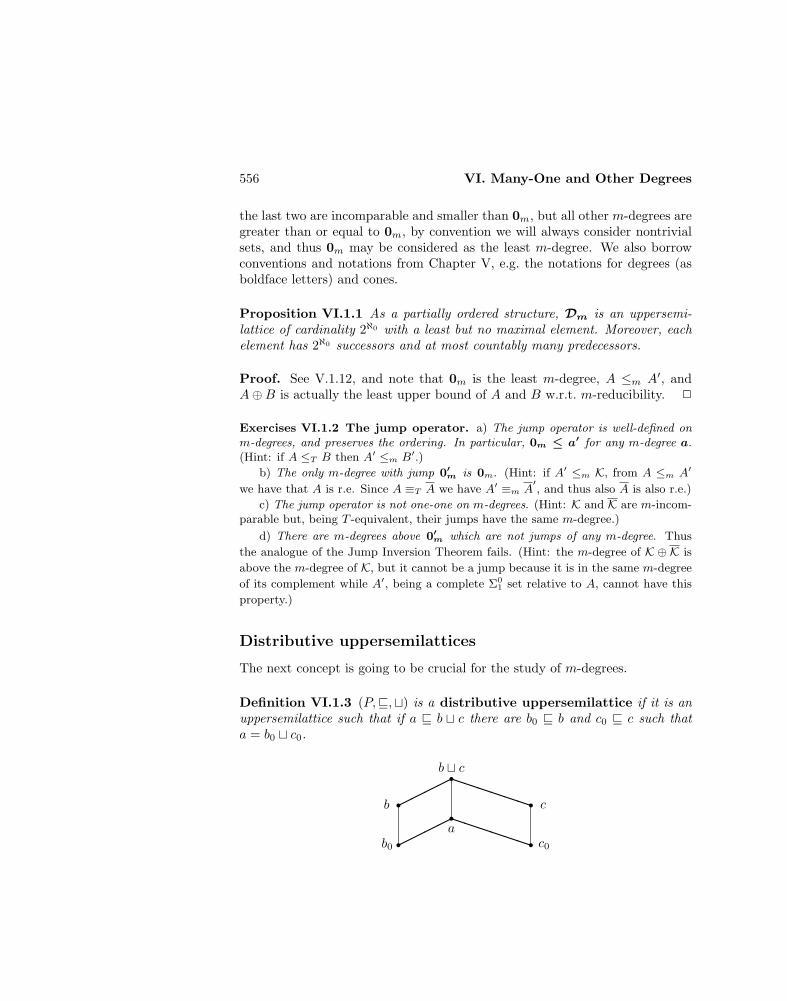
556 VI. Many-One and Other Degrees
the last two are incomparable and smaller than 0m, but all other m-degrees aregreater than or equal to 0m, by convention we will always consider nontrivialsets, and thus 0m may be considered as the least m-degree. We also borrowconventions and notations from Chapter V, e.g. the notations for degrees (asboldface letters) and cones.
Proposition VI.1.1 As a partially ordered structure, Dm is an uppersemi-lattice of cardinality 2ℵ0 with a least but no maximal element. Moreover, eachelement has 2ℵ0 successors and at most countably many predecessors.
Proof. See V.1.12, and note that 0m is the least m-degree, A ≤m A′, andA⊕B is actually the least upper bound of A and B w.r.t. m-reducibility. 2
Exercises VI.1.2 The jump operator. a) The jump operator is well-defined onm-degrees, and preserves the ordering. In particular, 0m ≤ a′ for any m-degree a.(Hint: if A ≤T B then A′ ≤m B′.)
b) The only m-degree with jump 0′m is 0m. (Hint: if A′ ≤m K, from A ≤m A′
we have that A is r.e. Since A ≡T A we have A′ ≡m A′, and thus also A is also r.e.)
c) The jump operator is not one-one on m-degrees. (Hint: K and K are m-incom-parable but, being T -equivalent, their jumps have the same m-degree.)
d) There are m-degrees above 0′m which are not jumps of any m-degree. Thus
the analogue of the Jump Inversion Theorem fails. (Hint: the m-degree of K ⊕ K is
above the m-degree of K, but it cannot be a jump because it is in the same m-degree
of its complement while A′, being a complete Σ01 set relative to A, cannot have this
property.)
Distributive uppersemilattices
The next concept is going to be crucial for the study of m-degrees.
Definition VI.1.3 (P,v,t) is a distributive uppersemilattice if it is anuppersemilattice such that if a v b t c there are b0 v b and c0 v c such thata = b0 t c0.
b0
b
c0
c
a
b t c
rr rrrr
PPPPPP
PPPPPP
VI.1 Distributivity 557
The notion of distributive uppersemilattice is consistent with the usual no-tion of distributivity. Recall that a lattice (P,v,t,u) is distributive if thedistributive laws hold in it, i.e.
a u (b t c) = (a u b) t (a u c)a t (b u c) = (a t b) u (a t c).
By duality, each of the two laws implies the other.
Proposition VI.1.4 A lattice is distributive as a lattice if and only if it isdistributive as an uppersemilattice.
Proof. If the lattice is distributive and a v b t c then
a = a u (b t c) = (a u b) t (a u c).
Then it is enough to let b0 = a u b and c0 = a u c to have distributivity as anuppersemilattice.
If the lattice is distributive as an uppersemilattice, since
(a u b) t (a u c) v a u (b t c)
always holds, it is enough to show that the converse holds too. Since
a u (b t c) v b t c
holds, for some b0 v b and c0 v c is a u (b t c) = b0 t c0. But then b0, c0 v a,and hence
a u (b t c) = b0 t c0 v (a u b) t (a u c). 2
Definition VI.1.5 An element of an uppersemilattice is indecomposable,or an atom, if whenever a = b t c then a = b or a = c.
Proposition VI.1.6 In a distributive uppersemilattice the indecomposable el-ements below b t c are exactly the indecomposable elements below b or c.
Proof. One direction is trivial. Conversely, if a v bt c then, by distributivity,a = b0 t c0 for some b0 v b and c0 v c. If a is indecomposable then a = b0 ora = c0, and hence a v b or a v c. 2
Exercises VI.1.7 a) In a Boolean algebra the indecomposable elements are exactlythe atoms.
b) In a linear ordering every element is indecomposable.
c) In a finite uppersemilattice every element is the l.u.b. of the indecomposable
elements below it .
Our reason to introduce distributive uppersemilattices is the following.

558 VI. Many-One and Other Degrees
Proposition VI.1.8 (Lachlan [1970]) Dm is a distributive uppersemilat-tice.
Proof. Given A ≤m B ⊕ C we want B0 ≤m B and C0 ≤m C such thatA ≡m B0 ⊕ C0. Given f recursive such that x ∈ A⇔ f(x) ∈ B ⊕ C, we let
x ∈ B0 ⇔ f(x) even andf(x)
2∈ B
x ∈ C0 ⇔ f(x) odd andf(x)− 1
2∈ C.
Then, e.g., B0 ≤m B via
g(x) =b if f(x) not evenf(x)
2 otherwise,
where b is a fixed element of B. Similarly for C0 ≤m C. Moreover, it is easilychecked that A ≡m B0 ⊕ C0. 2
Ideals of distributive uppersemilattices
The special properties of distributive uppersemilattices severely limit the pos-sible ideals, and thus produce necessary conditions for the ideals of Dm.
Proposition VI.1.9 A finite distributive uppersemilattice with least elementis a distributive lattice.
Proof. By VI.1.4 it is enough to show that a finite uppersemilattice with leastelement is a lattice. But the greatest lower bound of two elements a and b isthe least upper bound of the set of elements below them, which exists becausethe latter is a nonempty finite set. 2
Corollary VI.1.10 (Lachlan [1970]) Every finite ideal of Dm is a distribu-tive lattice.
To get conditions for any topped ideal we must develop some of the theoryof distributive uppersemilattices.
Proposition VI.1.11 (Lachlan [1972a]) Given a distributive uppersemilat-tice with least element, its ideals ordered by inclusion form a distributive lattice.
Proof. We denote by 0 the least element of (P,v,t), and by I the set of itsideals. The g.l.b. of two ideals is their set-theoretical intersection. The l.u.b. is

VI.1 Distributivity 559
the least ideal containing their union. Since P is distributive, given I1, I2 ∈ Itheir l.u.b. is actually the set
I1 ⊕ I2 = b t c : b ∈ I1 ∧ c ∈ I2.
Indeed, I1, I2 ⊆ I1 ⊕ I2, because 0 is in every ideal. Every ideal containing I1and I2 must clearly contain I1 ⊕ I2. I1 ⊕ I2 is closed under l.u.b. because I1and I2 are. It is closed downward because if a v b t c then a = b0 t c0, withb0 v b and c0 v c: if b t c ∈ I1 ⊕ I2 then we may suppose b ∈ I1 and c ∈ I2,and thus b0 ∈ I1 and c0 ∈ I2, because I1 and I2 are closed downward. Thena ∈ I1 ⊕ I2. Thus I1 ⊕ I2 is an ideal.
Finally, I is distributive as an uppersemilattice: if I ⊆ I1 ⊕ I2 thenI = I∗1 ⊕ I∗2 , where I∗i = Ii ∩ I. Indeed, I∗1 , I
∗2 ⊆ I and thus I∗1 ⊕ I∗2 ⊆ I
because ⊕ is the l.u.b. operation. Conversely, if a ∈ I then a ∈ I1 ⊕ I2, soa = b t c with b ∈ I1 and c ∈ I2: but b, c v a and a ∈ I, hence b ∈ I∗1 andc ∈ I∗2 , from which a ∈ I∗1 ⊕ I∗2 . 2
Proposition VI.1.12 (Ershov [1975]) In a distributive uppersemilattice Pevery finite subset closed under l.u.b. is embedded as an uppersemilattice (i.e.with l.u.b. preserved) in a finite distributive sublattice of P .
Proof. There is a natural embedding from P to I, given by
a 7−→ a = the principal ideal generated by a = b : b v a.
Given a finite uppersemilattice F ⊆ P , consider F ⊆ I so defined:
F = a : a ∈ F.
Let L be the finite distributive lattice generated by F in I (see VI.1.11). Wewant to pull back L in P , but the obvious trouble is that not every element ofL is a principal ideal. Thus we need a one-one homomorphism of uppersemi-lattices ϕ : L → P such that F ⊆ ϕ(L). The obvious approach would be totake, for I ∈ L,
ϕ(I) = l.u.b. of I,
but not every ideal needs to have a l.u.b. (unless it is finite). So we define
GI = a finite subset of Iϕ(I) = l.u.b. of GI .
In particular this gives ϕ(I) ∈ I, since an ideal is closed under l.u.b.
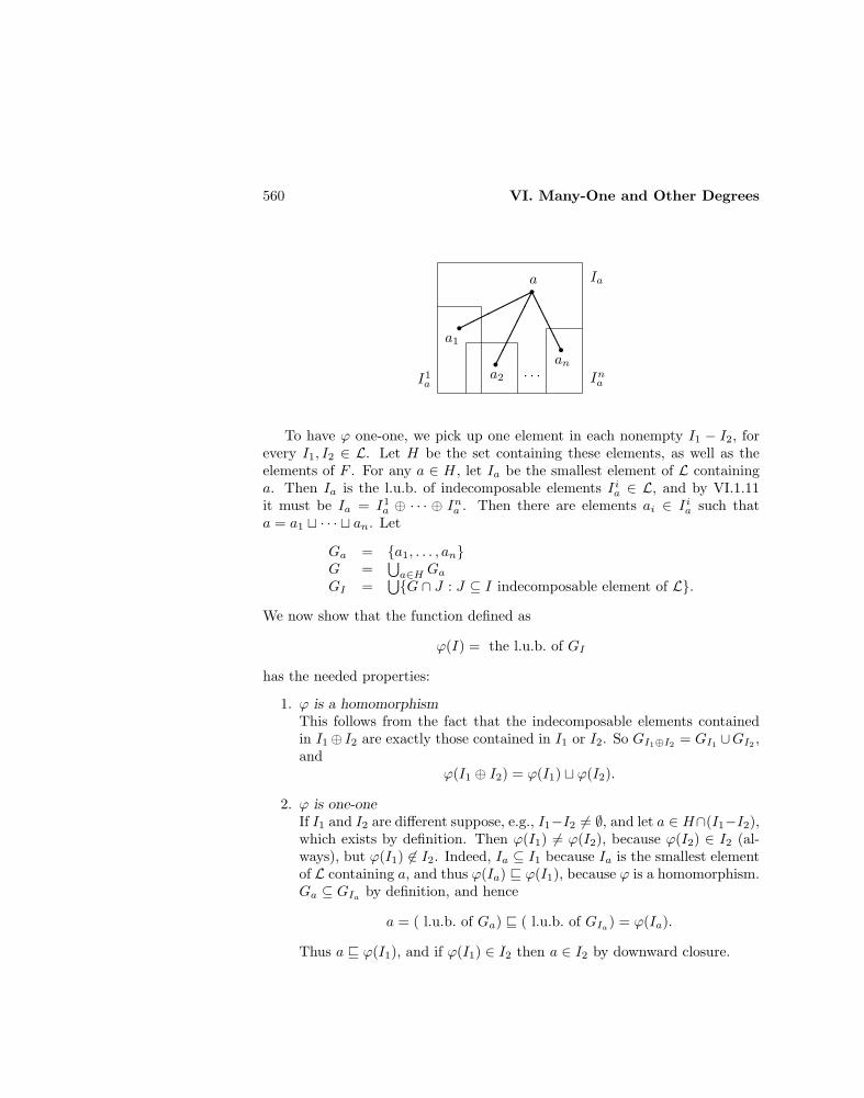
560 VI. Many-One and Other Degrees
I1a Ina
Ia
a1
a
a2
an· · ·
rr rr
AAAA
To have ϕ one-one, we pick up one element in each nonempty I1 − I2, forevery I1, I2 ∈ L. Let H be the set containing these elements, as well as theelements of F . For any a ∈ H, let Ia be the smallest element of L containinga. Then Ia is the l.u.b. of indecomposable elements Iia ∈ L, and by VI.1.11it must be Ia = I1
a ⊕ · · · ⊕ Ina . Then there are elements ai ∈ Iia such thata = a1 t · · · t an. Let
Ga = a1, . . . , anG =
⋃a∈H Ga
GI =⋃G ∩ J : J ⊆ I indecomposable element of L.
We now show that the function defined as
ϕ(I) = the l.u.b. of GI
has the needed properties:
1. ϕ is a homomorphismThis follows from the fact that the indecomposable elements containedin I1⊕ I2 are exactly those contained in I1 or I2. So GI1⊕I2 = GI1 ∪GI2 ,and
ϕ(I1 ⊕ I2) = ϕ(I1) t ϕ(I2).
2. ϕ is one-oneIf I1 and I2 are different suppose, e.g., I1−I2 6= ∅, and let a ∈ H∩(I1−I2),which exists by definition. Then ϕ(I1) 6= ϕ(I2), because ϕ(I2) ∈ I2 (al-ways), but ϕ(I1) 6∈ I2. Indeed, Ia ⊆ I1 because Ia is the smallest elementof L containing a, and thus ϕ(Ia) v ϕ(I1), because ϕ is a homomorphism.Ga ⊆ GIa by definition, and hence
a = ( l.u.b. of Ga) v ( l.u.b. of GIa) = ϕ(Ia).
Thus a v ϕ(I1), and if ϕ(I1) ∈ I2 then a ∈ I2 by downward closure.

VI.2 Countable Initial Segments 561
3. F ⊆ ϕ(L)It is enough to show that ϕ(a) = a, for a ∈ F . Indeed, Ia = a if a ∈ F :so a v ϕ(Ia) = ϕ(a), by the previous part of the proof. Conversely,ϕ(a) v a because ϕ(a) ∈ a always holds. 2
Corollary VI.1.13 (Lachlan [1970]) Every topped ideal of Dm is the di-rect limit (in the sense of uppersemilattices) of an ascending sequence of finitedistributive lattices.
Proof. Consider an enumeration a0,a1, . . . of a topped ideal I = Dm(≤a).Start with D0 = 0m,a. Given Dn ⊆ I consider the finite uppersemilatticegenerated by Dn∪an, which has a as greatest element, and let Dn+1 be thefinite distributive lattice obtained as in the proof above. Since the former isembedded in the latter as an uppersemilattice, a is also the greatest elementof Dn+1, and thus Dn+1 ⊆ I. 2
We now have a necessary condition for topped ideals of Dm. In the nextsection we will show that this condition is also sufficient, thus completely char-acterizing the countable initial segments of Dm.
VI.2 Countable Initial Segments
The following observation is going to be crucial for our later development.
Proposition VI.2.1 (Lachlan [1970]) Let A be a set, and a its m-degree.For any r.e. set We and any recursive function f with range We, let:
x ∈ Φ(We) ⇔ f(x) ∈ A.
Then the map Φ induces a homomorphism of uppersemilattices between the r.e.sets modulo the finite sets (ordered by inclusion) and Dm(≤a).
Proof. We have to check the following:
1. the m-degree of Φ(We) does not depend on fLet g be another recursive function with range We. If
h(x) = µz[g(z) = f(x)] and t(x) = µz[g(x) = f(z)]
then
f(x) ∈ A⇔ gh(x) ∈ A and g(x) ∈ A⇔ ft(x).

562 VI. Many-One and Other Degrees
2. Φ(We) ≤m ABy definition.
3. if B and C are r.e. sets and B ⊆ C then Φ(B) ≤m Φ(C)Let B and C be the ranges of f and g, and h(x) = µz[g(z) = f(x)]. Thenh is total because B ⊆ C, and
x ∈ Φ(B) ⇔ f(x) ∈ A⇔ gh(x) ∈ A⇔ h(x) ∈ Φ(C).
4. if B and C are r.e. sets which differ finitely then Φ(B) ≡m Φ(C)Let B and C be the ranges of f and g. Fix a ∈ Φ(C) and b 6∈ Φ(C), andlet
h(x) =
a if f(x) ∈ A ∩ Cb if f(x) ∈ A ∩ Cµz[g(z) = f(x)] if f(x) ∈ C.
h is recursive because f(x) ∈ B by definition, and B ∩ C is finite (andhence so are B ∩ A ∩ C and B ∩ A ∩ C). Then Φ(B) ≤m Φ(C) via h.Symmetrically, Φ(C) ≤m Φ(B).
5. if C ≤m A then there is an r.e. set B such that Φ(B) ≡m CLet x ∈ C ⇔ f(x) ∈ A: if B is the range of f , Φ(B) = C. 2
The result shows that instead of controlling directly the m-degrees belowA we can control the m-degrees of Φ(We), for every e. This is the techniquethat we are going to use to build initial segments.
Finite initial segments
Our goal is VI.3.6, which completely characterizes the initial segments of Dm.But its proof is quite complicated and it involves a number of separate ideas,taking care of different problems. We thus actually prove a sequence of results,solving one problem at the time. We keep the same notations throughout, andindicate how to adapt previous proofs to the new needs.
To illustrate the technique of construction of initial segments of m-degreeswe start with the simplest case.
Proposition VI.2.2 (Lachlan [1970]) Every finite ordinal is isomorphic toan initial segment of Dm.
Proof. We want to build a set A such that the m-degrees below its m-degreeare isomorphic to 0, 1, . . . , n. We use the homomorphism of VI.2.1 to controlthe m-degrees below the m-degree of A, and thus we only have to control eachΦ(We).
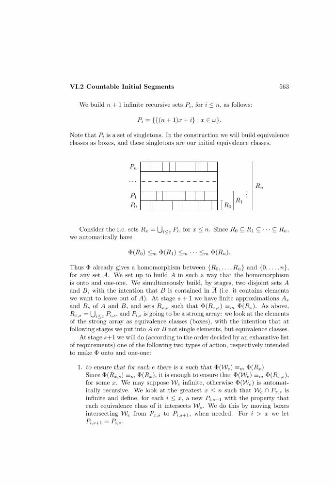
VI.2 Countable Initial Segments 563
We build n+ 1 infinite recursive sets Pi, for i ≤ n, as follows:
Pi = (n+ 1)x+ i : x ∈ ω.
Note that Pi is a set of singletons. In the construction we will build equivalenceclasses as boxes, and these singletons are our initial equivalence classes.
P0
P1
· · ·
Pn
R0
R1
...Rn
Consider the r.e. sets Rx =⋃i≤x Pi, for x ≤ n. Since R0 ⊆ R1 ⊆ · · · ⊆ Rn,
we automatically have
Φ(R0) ≤m Φ(R1) ≤m · · · ≤m Φ(Rn).
Thus Φ already gives a homomorphism between R0, . . . , Rn and 0, . . . , n,for any set A. We set up to build A in such a way that the homomorphismis onto and one-one. We simultaneously build, by stages, two disjoint sets Aand B, with the intention that B is contained in A (i.e. it contains elementswe want to leave out of A). At stage s + 1 we have finite approximations Asand Bs of A and B, and sets Rx,s such that Φ(Rx,s) ≡m Φ(Rx). As above,Rx,s =
⋃i≤x Pi,s, and Pi,s is going to be a strong array: we look at the elements
of the strong array as equivalence classes (boxes), with the intention that atfollowing stages we put into A or B not single elements, but equivalence classes.
At stage s+1 we will do (according to the order decided by an exhaustive listof requirements) one of the following two types of action, respectively intendedto make Φ onto and one-one:
1. to ensure that for each e there is x such that Φ(We) ≡m Φ(Rx)Since Φ(Rx,s) ≡m Φ(Rx), it is enough to ensure that Φ(We) ≡m Φ(Rx,s),for some x. We may suppose We infinite, otherwise Φ(We) is automat-ically recursive. We look at the greatest x ≤ n such that We ∩ Px,s isinfinite and define, for each i ≤ x, a new Pi,s+1 with the property thateach equivalence class of it intersects We. We do this by moving boxesintersecting We from Px,s to Pi,s+1, when needed. For i > x we letPi,s+1 = Pi,s.
564 VI. Many-One and Other Degrees
• Φ(We) ≡m Φ(Rx,s+1)Note that Rn,s ∪ As ∪ Bs = ω, and As ∪ Bs is finite. Then, byconstruction and the choice of x, We is contained in Rx,s, exceptfor at most finitely many elements. Since Φ is invariant under finitedifferences, we may actually suppose that We ⊆ Rx,s = Rx,s+1.Thus Φ(We) ≤m Φ(Rx,s+1) automatically, by the properties of Φ.Conversely, every box of Rx,s+1 contains an element of We by con-struction. If We and Rx,s+1 are respectively the ranges of f and g,let
h(z) = µy[f(y) and g(z) are in the same box of Rx,s+1].
Then
z ∈ Φ(Rx,s+1) ⇔ g(z) ∈ A⇔ fh(z) ∈ A (being in the same box)⇔ h(z) ∈ Φ(We),
and Φ(Rx,s+1) ≤m Φ(We). Note that it is crucial here that in thefollowing we put boxes into A, and not only single elements.
• Φ(Ri,s+1) ≡m Φ(Ri,s)We only have to prove this for i ≤ x, since for i > x we haveRi,s = Ri,s+1. If i ≤ x then Ri,s ⊆ Ri,s+1, since we only enlargeboxes, so Φ(Ri,s) ≤m Φ(Ri,s+1).Since every new box of Ri,s+1 contains an old box of Ri,s, by associ-ating to every element of Ri,s+1 an element of Ri,s in the same box(as above) we get Φ(Ri,s+1) ≤m Φ(Ri,s).
2. to ensure that Φ(Rx) 6≡m Φ(Ry) if x 6= ySince x, y ≤ n we may suppose, e.g., x < y. Then Rx ⊆ Ry, andautomatically Φ(Rx) ≤m Φ(Ry). To ensure Φ(Ry) 6≤m Φ(Rx), supposethat for some recursive function h
z ∈ Φ(Ry) ⇔ h(z) ∈ Φ(Rx).
Let Ry and Rx be the ranges of f and g: then
f(z) ∈ A ⇔ gh(z) ∈ A.
Note that there is a partial recursive function ϕ with domain Ry andrange contained in Rx, and such that w ∈ A ⇔ ϕ(w) ∈ A for each w onwhich ϕ is defined. For example,
ϕ(w) ' gh(z) for the smallest z such that f(z) = w.

VI.2 Countable Initial Segments 565
?
6
6
Ry
ω
ω
Rx
f
h
g
ϕ(w) = gh(z)
w = f(z)
z
h(z)
rrr
r
HHHH
H
H
HH
HH
To ensure Φ(Ry) 6≤m Φ(Rx) is thus enough to look at the partial recursivefunctions ϕ with domain containing Ry and range contained in Rx. SinceRx ⊆ Ry, there is a such that Pa is not contained in Rx, but it is containedin Ry. Consider Pa,s: the construction is such that every box of Pa,scontains a box of from Pa. Choose w ∈ Pa ∩ Pa,s: then ϕ(w) ∈ Rx. Weensure that w ∈ A if and only if ϕ(w) 6∈ A, thus diagonalizing against ϕ:
• if ϕ(w) ∈ As then put the box of w into Bs+1
• if ϕ(w) ∈ Bs then put the box of w into As+1
• if ϕ(w) 6∈ As ∪ Bs then, e.g., put the box of w into As+1, and thebox of ϕ(w) into Bs+1.
In this case Φ(Ri,s) ≡m Φ(Ri,s+1) is automatic, since we just produce afinite modification, moving the box of w and, possibly, the box of ϕ(w)too. 2
The construction just given is the basis for all the embeddings to be ob-tained. In the following we will limit ourselves to indicate the modificationsneeded to take care of the increasingly more complicated situations.
Proposition VI.2.3 (Lachlan [1970]) The topped finite initial segments ofDm are exactly the finite distributive lattices.
Proof. The condition is necessary by VI.1.10. For the converse, let D be afinite distributive lattice. We have to define Rx for x ∈ D in such a way thatΦ(Rx) : x ∈ D is isomorphic to D. This could appear to be complicated,since we have to preserve the relationships among the members of D, but asmall trick makes everything trivial. Let H be the set a0, . . . , an of theindecomposable elements of D (in the case of linear orderings we had D = H).Since H generates D (VI.1.7.a), we only have to define:
Pai = (n+ 1)x+ i : x ∈ ωRx =
⋃Pa : a ≤ x ∧ a ∈ H.

566 VI. Many-One and Other Degrees
The map Φ is a homomorphism from D to Dm(≤ a), where a is them-degree of the set A we build, because D is distributive: if x = y t z thenthe indecomposable elements below x are exactly the indecomposable elementsbelow y or z (VI.1.6), hence Rx = Ry ∪Rz and Φ(Rx) ≡m Φ(Ry)⊕Φ(Rz), bythe properties of Φ.
As before we have to ensure that Φ is onto and one-one, and this is obtainedin the same way as in the previous result, with the following modifications.
1. ontonessGiven We infinite, consider all the i’s such that We∩Pai,s is infinite, andmake all the classes of Paj ,s+1 intersect We, for every j such that aj v aifor some such i. If i0, . . . , im is a list of all such i’s, we have as beforeΦ(We) ≡m Φ(Rx,s+1), where x = ai0 t · · · t aim .
And Φ(Rx) ≡m Φ(Rx,s+1) for all x, since this holds for indecomposableelements as before, and for the other elements because Φ is a homomor-phism.
2. one-onenessIf x 6v y we want Φ(Rx) 6≤m Φ(Ry). This is obtained as before, becauseif x 6v y then there is an indecomposable element a such that a v x anda 6v y (otherwise all the indecomposable elements below x are also belowy, and hence so is their l.u.b. x). But then we can choose an element ofPa,s ∩ Pa to diagonalize. 2
Countable initial segments
The proofs given above may be easily extended to handle infinite initial seg-ments whose representations can be chosen ahead of time (like recursive dis-tributive lattices), but some new ideas are needed to treat the general case.Again we start with the linear orderings.
Proposition VI.2.4 (Lachlan [1970]) Every countable linear ordering withleast element is isomorphic to an initial segment of Dm.
Proof. When we consider a countable linear ordering L we cannot define Rxahead of time for all x ∈ L, unless L is recursive. Then we approximate Lby finite pieces. We may suppose that L has a greatest element, otherwise wecan add one to it, and we call 0 and 1 the least and greatest elements. LetL =
⋃n∈ω Ln, where L0 = 0, 1, and each Ln is finite and contained in Ln+1.
Let Ln = a0 < · · · < am, with a0 = 0 and am = 1. At stage s + 1 we havePai,s. If b is a new element of Ln+1, i.e. b is not one of the ai’s, we have tocreate a new row Pb for it. Since 0 and 1 are already in L0, there must be isuch that ai < b < ai+1. Then we can simply let Paj ,s+1 = Paj ,s if j 6= i + 1,
VI.2 Countable Initial Segments 567
and we create Pb by taking its boxes from Pai+1,s. It is clear that for x ∈ Ln itis still Rx,s+1 = Rx,s, and thus Φ(Rx,s+1) ≡m Φ(Rx,s). 2
Proposition VI.2.5 (Lachlan [1970]) The topped initial segments of Dm
are exactly the direct limits of ascending sequences of finite distributive lattices.
Proof. The condition is necessary by VI.1.10. For the converse, let D bethe limit of Dnn∈ω, with Dn a finite distributive lattice, and Dn ⊆ Dn+1.Suppose also that D0 already contains the least and greatest elements 0 and 1of D, otherwise start from the first Dn that does. As in VI.2.3 we just haveto consider the indecomposable elements, but now D is only approximated byDn, and hence at a given stage we only have
Hn = a0, . . . , am = set of the indecomposable elements of Dn.
When we step from Dn to Dn+1 two new things might happen:
1. a new atom b appearsAs in VI.2.4 we have to create a new Pb for it, and this time the atomsare not linearly ordered. We may simply build Pb as a sequence of boxes,each one being the union of one box from Pai,s for each i such that b < ai(some such i must exist, because the greatest element of D is already inD0). This allows us to get Φ(Rx,s+1) ≡m Φ(Rx,s) as follows.
If b 6< x then there is nothing to prove, since Rx,s+1 = Rx,s. If b < x wemay suppose that x is an atom of Dn, since we only have to prove theproperty for atoms (the rest follows automatically from the fact that Φis a homomorphism). But then:
• Φ(Rx,s) ≤m Φ(Rx,s+1)This follows from Rx,s ⊆ Rx,s+1 (note that Pa may be in Rx,s+1
now).
• Φ(Rx,s+1) ≤m Φ(Rx,s)As usual it is enough to get effectively from every element of Rx,s+1
an element of Rx,s in the same box. The only nontrivial case is whenwe consider elements in boxes of Pb, but each such box contains abox of Px,s by construction.
2. an atom a ∈ Hn becomes decomposable in Dn+1
In this case we do not want to consider Pa,s anymore, and we simply throwit into Bs+1, which then becomes an infinite recursive set (as opposed tothe finite set of the previous propositions). To check
Φ(Rx,s+1) ≡m Φ(Rx,s)

568 VI. Many-One and Other Degrees
we simply note that for a < x is Rx,s+1 = Rx,s − Pa, which is stillr.e. since Pa is recursive. But then Rx,s = Rx,s+1 ∪ Pa,s and, by theproperties of Φ, Φ(Rx,s) ≡m Φ(Rx,s+1) ⊕ Φ(Pa,s). Since Pa,s ⊆ A byconstruction, because we threw it into Bs+1, Φ(Pa) has m-degree 0m andthus Φ(Rx,s) ≡m Φ(Rx,s+1).
Case 2 introduces the need of small adjustments in the proof.
1. We have to suppose that the top element of D is indecomposable in everyDn, so that we always have a top line to use when a new atom appears,and a new line has to be created. For this it is enough to add, if necessary,an element on top of the greatest one, and suppose it is already in D0.
2. To show that Φ is onto we prove as before that Φ(We) ≡m Φ(Rx) forsome x, noting that for an appropriate x we have We ⊆ As ∪ Bs ∪ Rx,s,so that
Φ(We) ≡m Φ(We ∩As)⊕ Φ(We ∩Bs)⊕ Φ(We ∩Rx,s).
But
• Φ(We ∩As) has m-degree 0m because We ∩As is finite
• Φ(We ∩Bs) has m-degree 0m because Bs ⊆ A
• Φ(We ∩Rx,s) ≡m Φ(Rx,s) as usual. 2
Corollary VI.2.6 Every countable distributive lattice is isomorphic to an ini-tial segment of Dm.
Proof. If D is a countable distributive lattice, let D0 = 0, 1. Given Dn takea ∈ D−Dn, if it exists, and consider the finite distributive sublattice Dn+1 ofD generated by Dn ∪ a. Then D is the direct limit of Dnn∈ω. 2
Exercise VI.2.7 Dm is not a lattice. (Hint: let Dn be the finite distributive lattice
consisting of an ascending sequence of n elements, with a diamond on top: the direct
limit of the Dn’s is an infinite chain with two incomparable elements and their join
above it. These two elements have no l.u.b.)
A different method of proving VI.2.5 has been given by Lachlan [1971],and consists of building the same initial segments for T -degrees using stronglyuniform trees (V.6.7). This produces common initial segments of Turing andm-degrees.
Exercise VI.2.8 If A is a set of minimal Turing degree constructed by using strongly
uniform trees, then A has minimal m-degree. (Lachlan [1971]) (Hint: it is enough

VI.3 Uncountable Initial Segments 569
to prove that if fL, fR, g are an e-splitting strongly uniform tree, A is on it, and
eA is an m-reduction, then A ≤m eA. But if B = eA is an m-reduction,
there is h recursive such that x ∈ B ⇔ h(x) ∈ A. To define f recursive such that
x ∈ A⇔ f(x) ∈ B, see if fL and fR agree on x. If so, then let f(x) be a fixed element
of B if the common value is 1, and a fixed element of B otherwise. If not, x is in the
range of h, because the tree is e-splitting. Then let f(x) = h−1(x).)
VI.3 Uncountable Initial Segments
The obvious trouble with uncountable initial segments is that we cannot ap-proximate them by finite pieces in countably many steps. We are able toovercome this difficulty by extending given countable pieces.
Strong minimal covers
Recall (V.5.16) that a is a strong minimal cover of b when, for every c, if c < athen c ≤ b.
Proposition VI.3.1 (Lachlan [1972]) Every m-degree has a strong minimalcover.
Proof. The construction is an extension of the one for minimal m-degrees,which is the special case of VI.2.2 for n = 1. We build two sets
Pa = 2x : x ∈ ωPb = 2x+ 1 : x ∈ ω,
and let Ra = Pa ∪ Pb and Rb = Pb. Since Rb ⊆ Ra, we automatically haveΦ(Rb) ≤m Φ(Ra). We want to ensure that:
1. Φ(Rb) ≡m B, for a given set B ∈ b.
2. Φ(We) ≡m Φ(Ra) or Φ(We) ≤m Φ(Rb), for every e
3. Φ(Ra) 6≤m Φ(Rb).
We indicate the modifications to make in the construction of a minimal degreeto ensure these conditions.
1. Let B ∈ b: we ensure Φ(Rb) ≡m B by putting the x-th box of Pb into Aif and only if x ∈ B. This is the main new idea, to be fully exploited inthis subsection. Let Rb = Pb be the range of f . Then Φ(Rb) ≤m B viag(z) = µx[f(z) = 2x+ 1], since
z ∈ Φ(Rb) ⇔ f(z) ∈ A⇔ g(z) ∈ B,

570 VI. Many-One and Other Degrees
and B ≤m Φ(Rb) via h(x) = µz[f(z) = 2x+ 1], since
x ∈ B ⇔ 2x+ 1 ∈ A⇔ fh(x) ∈ A⇔ h(x) ∈ Φ(Rb).
This part of the construction makes the approximation of A at a givenstage infinite. But we can still think of A at stage s as the union of a finitepart As on a side (obtained by the other two parts of the construction, asin VI.2.2) and of the infinite part of A contained in Pb,s. It is understoodthat anything falling into the x-th box of Pb during the construction goesinto A, if x ∈ B.
2. This is ensured as before. If We ∩Pa,s is infinite then we use appropriateboxes from Pa,s to force all boxes of Ra,s+1 to intersectWe, thus obtainingΦ(We) ≡m Φ(Ra,s+1). If We∩Pa,s is finite then, except for finitely manyelements, We ⊆ Pb,s: then, automatically, Φ(We) ≤m Φ(Rb,s).
3. This is also ensured as before, since we can use elements of Pa ∩ Pa,s todiagonalize against ϕ : Ra → Rb. 2
Recall (V.5.17) that there is a cone of minimal covers in the Turing degrees.A similar proof shows here that there is a cone of strong minimal covers inDm. This stronger result fails for Turing degrees, and actually (in accord withV.1.16) there is a cone without strong minimal covers in D, since by V.2.26 nodegree above 0′ can be a strong minimal cover.
Uncountable linear orderings
Linearly ordered initial segments are especially simple because of the countablepredecessor property, which implies that any such linear ordering can be ob-tained by a (possibly uncountable) sequence of countable extensions. We thushave only to learn how to do countable extensions.
Proposition VI.3.2 (Ershov [1975]) Every countable linearly ordered initialsegment I of Dm can be extended to an initial segment L isomorphic to L, forany countable linear ordering L having an initial segment I isomorphic to I.
Proof. The proof combines the ideas of VI.2.4 and VI.3.1. The only step tobe added to VI.2.4 is the case when a new atom b appearing in Ln+1 is in I.Then we build the corresponding Pb by using the row Pa,s, for the smallesta ∈ Ln − I (which is automatically above b): we may always suppose it exists,by possibly topping L and putting the greatest element in L0. We then orderthe classes of Pb, e.g. by ordering in the natural way their least elements, andput the x-th class into A if and only if x ∈ B, for some fixed B in the m-degreeb of I corresponding to b ∈ I.
VI.3 Uncountable Initial Segments 571
• Φ(Rb) ≡m BΦ(Pb) ≡m B as in VI.3.1, and Rb =
⋃cvb Pc, so Φ(Rb) ≡m ⊕cvbΦ(Pc).
But b ∈ I and I is downward closed, so if c v b is c ∈ I and Pc wasintroduced in the same way as Pb, in particular Φ(Pc) hasm-degree c ≤ b.Thus Φ(Rb) has m-degree b.
• Φ(Rx,s+1) ≡m Φ(Rx,s)For x ∈ Ln − I, which is the only interesting case, Rx,s+1 = Rx,s.
• ontonessThis is obtained as in VI.3.1, by considering the greatest a ∈ Ln − I, ifit exists, such that We ∩ Pa,s is infinite.
• one-onenessThis is obtained as in VI.3.1 and VI.2.4, by ensuring Φ(Ry) 6≤m Φ(Rx)whenever x < y and either (x ∈ I ∧ y 6∈ I) or (x 6∈ I ∧ y 6∈ I). Indeed, forx, y ∈ I this is automatically achieved by the previous strategy. 2
At this point we can already give some final results.
Corollary VI.3.3 The order-types of the linearly ordered initial segments ofDm are exactly the linear orderings with least element and countable predeces-sor property.
Proof. The conditions are obviously necessary. Given a linear ordering Lwith least element 0 and countable predecessor property, let I0 = 0 andI0 = 0m. For any ordinal α < ω1 let Iα and Iα be isomorphic countableinitial segments of L and Dm. Take a ∈ L− Iα, if it exists, and let Iα+1 be thedownward closure of if Iα∪a in L: Iα+1 is countable because L has countablepredecessor property, and Iα ⊆ Iα+1 since Iα is closed downward. By VI.3.2there is an initial segment Iα+1 of Dm isomorphic to Iα+1 and extending Iα.At limit stages take unions. This procedure gives an initial segment isomorphicto L in at most ω1 steps, since L has countable predecessor property. 2
In particular, the ordinals of the well-ordered initial segments of Dm areexactly the ordinals ≤ ω1.
Abraham and Shore [1986] have shown that the linearly ordered initialsegments of D are the same as those of Dm.
Uncountable initial segments
We are finally at the last step of our long journey. In the next result all theingredients so far introduced, and some new ones, will be employed to produceall possible countable extensions of given initial segments. We will then show

572 VI. Many-One and Other Degrees
how the result can be modified and used to characterize the initial segments ofDm.
Proposition VI.3.4 (Ershov [1975]) Every countable ideal I of Dm can beextended to an initial segment L isomorphic to L, for any countable distributiveuppersemilattice L having an ideal I isomorphic to I.
Proof. First note that, by possibly doing countably many successive exten-sions, we may simply restrict our attention to topped countable distributiveuppersemilattices L. As in VI.1.13 we can see that L is a direct limit of anascending sequence of finite distributive lattices. The proof then extends theone of VI.2.5.
When new atoms appear, we treat them as in VI.2.5 and VI.3.2. Namely,we create Pb as a sequence of boxes, each one being the union of one box fromPa,s for each atom a not in I and above b. Two new things might happen here:
1. an atom a ∈ I becomes indecomposableAs in VI.2.5 we throw Pa,s away, i.e. we put it into Bs+1. This nowcauses a little trouble, since Pa,s contains boxes which were in A andthat go now into A, and A is not built monotonically. We still want tohave Φ(Rx,s+1) ≡m Φ(Rx,s). Suppose a v x: since Rx,s+1 = Rx,s − Pa,swe have, as in VI.2.5, Φ(Rx,s) ≡m Φ(Rx,s+1)⊕Φ(Pa,s). It is thus enoughto show that Φ(Pa,s) ≤m Φ(Rx,s+1). We may suppose we already havein Rx,s+1 the Pb’s for the atoms that make a decomposable. Now b v xfor all these b’s, so Pb,s ⊆ Rx,s+1 and Φ(Pb,s) ≤m Φ(Rx,s+1). But b ∈ I,since a ∈ I and I is closed downward: by construction then Φ(Pb,s)has the m-degree b in I corresponding to b in I, and Φ(Pa,s) has them-degree a corresponding to a. But a is the l.u.b. of these b’s, and soΦ(Pa,s) ≤m Φ(Rx,s+1).
2. one-onenessWe want Φ(Ry) 6≤m Φ(Rx) whenever y 6v x. This is automatic if x andy are in I.
If x ∈ I but y 6∈ I then we have no trouble: there is an atom a v y suchthat a 6∈ I, otherwise y ∈ I because I is an ideal, hence closed underl.u.b., and y is the l.u.b. of the atoms below it. But a 6v x since x ∈ Iand I is closed downward, so we can use Pa to diagonalize.
Let us thus suppose that x 6∈ I, y ∈ I, and y 6v x. If we simply considerϕ : Ry → Rx then we might not be able to diagonalize, since ϕ mighthave range contained in Rz, where z v x is the l.u.b. of the atoms of Ibelow x (z ∈ I because I is an ideal): thus ϕ sends rows correspondingto atoms of I to similar rows, and we do not want to touch them because
VI.3 Uncountable Initial Segments 573
they code information. But we now show that if Φ(Ry) ≤m Φ(Rx) thenthere is a partial recursive function ϕ such that:
• ϕ has domain Ry and range contained in Rx
• w ∈ A if and only ϕ(w) ∈ A, whenever ϕ(w) is defined
• the range of ϕ intersects Pa, for some Pa ⊆ Rx and a 6∈ I.
Consider indeed the usual ϕ (VI.2.2), and let W be its range. If ϕ doesnot have the required properties then W ⊆ Rz, for the z ∈ I consideredabove. So Φ(W) ≤m Φ(Rz). Since w ∈ A ⇔ ϕ(w) ∈ A and Ry is thedomain of ϕ, Φ(Ry) ≡m Φ(W) and hence Φ(Ry) ≤m Φ(Rz). But y andz are in I, and Φ is by definition an isomorphism on I, hence y v z v x,contradiction. We can then always consider ϕ with the stated properties,and use a row Pa for some a 6∈ I to diagonalize. 2
The result already has a number of important consequences, e.g. everycountable ideal of Dm has a strong minimal cover, and it is the intersectionof two principal ideals. To derive the most important consequence of all wehowever need a strengthening of it, stated in the exercise.
Exercise VI.3.5 For every countable ideal I of Dm, and any countable distributive
uppersemilattice L having an ideal I isomorphic to I, there is a continuum of initial
segments of Dm isomorphic to L, and such that their parts isomorphic to L− I are
pairwisely disjoint . (Paliutin [1975]) (Hint: the properties of the construction above
are not affected if countably many times we take a box from the line relative to the
top element, and put it into As or Bs. We can thus build a tree of sets whose degrees
are top degrees of extension of I as wanted.)
We can now give the promised characterization of the initial segments ofDm. Note that the exercise allows us to avoid any use of the ContinuumHypothesis, and thus the result is final.
Theorem VI.3.6 Characterization of the ideals of Dm (Ershov [1975],Paliutin [1975]) The ideals of Dm are exactly, up to isomorphism, the dis-tributive uppersemilattices with least element, countable predecessor property,and power at most that of the continuum.
Proof. The conditions are clearly necessary. Conversely, given an uppersemi-lattice L with the stated conditions, we want to define an ideal L of Dm
isomorphic to L. Let 0 be the smallest element of L, and define I0 = 0,I0 = 0m, and ϕ0(0) = 0m.
For α < 2ℵ0 let Iα and Iα be ideals of L and Dm isomorphic via ϕα, and ofpower less than the continuum. Take a ∈ L− Iα, if it exists: a (the set of the
574 VI. Many-One and Other Degrees
predecessors of a in L) is a countable distributive uppersemilattice (because Lhas countable predecessor property) with a∩Iα as a countable ideal (since botha and Iα are ideals). By VI.3.4 we can extend the isomorphism ϕα of domainIα to an isomorphism ϕ of domain a ∪ Iα. Let Iα+1 be the ideal generatedby a ∪ Iα: we want to show that ϕ is extendable to an isomorphism ϕα+1 ofdomain Iα+1. By VI.1.11 the elements of Iα+1 are of the form x t y, for x ∈ aand y ∈ Iα. We then let
ϕα+1(x t y) = ϕ(x) ∪ ϕ(y).
To check that ϕα+1 is well-defined, consider x′ t y′ = x t y. Since x′ v x t y,there are x′0 v x and y′0 v y such that x′ = x′0 t y′0. But ϕ is an isomorphismon a ∪ Iα, and thus ϕ(x′0) ≤ ϕ(x) and ϕ(y′0) ≤ ϕ(y). Then
ϕα+1(x′) = ϕα+1(x′0 t y′0) = ϕ(x′0) ∪ ϕ(y′0) ≤ ϕ(x) ∪ ϕ(y) = ϕα+1(x t y).
Similarly, ϕα+1(y′) ≤ ϕα+1(x t y), and hence
ϕα+1(x′ t y′) = ϕα+1(x′) ∪ ϕα+1(y′) ≤ ϕα+1(x t y).
The converse holds similarly, and then ϕα+1 is well-defined.But if we only use VI.3.4 as stated then there is no reason to believe that
ϕα+1 is also one-one. This is where the strengthening VI.3.5 comes into play:it provides enough choices to make the degrees below ϕ(a) but not in ϕα(a∩Iα)disjoint from ϕα(Iα), and thus ϕα+1 one-one.
At limit stages we take unions. The procedure gives an initial segmentisomorphic to L in at most 2ℵ0 steps, since L has at most the power of thecontinuum. 2
Refinements of the results of this section have been found by Malc’ev [1981],[1984], respectively on localization of initial segments and relativization to theuppersemilattice of immune sets.
VI.4 Global Properties
We now turn to the study of global properties of Dm, following the path set upin Section V.7 for Turing degrees, with two major differences. First of all, wewill be completely successful in characterizing the algebraic structure of Dm,while an analogous characterization is not known for Turing degrees, and mighteven be independent of ZFC (see the results of Grozsek and Slaman quotedon pp. 467 and 530). Secondly, the properties of definability, homogeneity, andautomorphisms for m-degrees are exactly the opposite of those for Turing de-grees: no nontrivial countable set of m-degrees is definable, strong homogeneity

VI.4 Global Properties 575
holds, and there are lots of automorphisms. However, the complexity of thetheories of Turing and m-degrees is the same.
Characterization of the structure of many-one degrees
We now characterize Dm as an algebraic structure. This result is the onlyknown example of an absolute characterization of a degree theory, and it pro-vides an alternative, recursion-theoretical description of the continuum.
The results proved in this chapter, which culminated in VI.3.6, already pro-vide the tools needed to characterize Dm with a two-line proof.
Aguzza qui, lettor, ben li occhi al vero,che ’l velo e ora ben tanto sottile,certo che ’l trapassar dentro e leggero.1
(Dante, Purgatorio, VIII)
Theorem VI.4.1 Characterization of Dm (Ershov [1975], Paliutin[1975]) Up to isomorphism, Dm is the only structure with the following prop-erties:
1. it is a distributive uppersemilattice with least element
2. every element has at most countably many predecessors
3. it has the power of the continuum
4. every ideal I with power less than the continuum can be extended toan ideal L isomorphic to L, for any distributive uppersemilattice L withpower less than the continuum having an ideal isomorphic to I.
Proof. A back-and-forth argument in the style of VI.3.6 easily gives an iso-morphism between any two structures with the given properties. 2
Note that no use is made of extra set-theoretical assumptions, like theContinuum Hypothesis, and thus the result is absolute.
Definability, homogeneity, and automorphisms
The algebraic characterization of Dm contains all the information about thestructure, and it is thus not surprising that we can easily derive from it solutionsto a number of algebraic problems. They should be contrasted with the oppositeones obtained for Turing degrees in Section V.7.
1Sharpen thy sight now, reader, to regardthe truth, for so transparent grows the veil,to pass within will surely not be hard.
576 VI. Many-One and Other Degrees
Theorem VI.4.2 Strong homogeneity. Any two cones of m-degrees areisomorphic.
Proof. Given a, it is enough to show that Dm(≥a) satisfies the properties ofVI.4.1. It then follows that any cone is isomorphic to Dm, and hence any twocones are isomorphic.
The only nontrivial property is the fourth one. Let I be an ideal of Dm(≥a) of power less than the continuum, and L be a distributive uppersemilatticeof power less than the continuum and with an ideal I isomorphic to I. LetI be the downward closure of I in Dm: we can extend I to a distributiveuppersemilattice I isomorphic to I. If we show that I∪L is an uppersemilatticewith I as an ideal, then we can apply the methods of VI.3.6 to extend I to anideal isomorphic to I ∪L in Dm, thus extending I to an ideal isomorphic to Lin Dm(≥a).
Since I is an ideal, so is I by its definition. To show that I ∪ L is anuppersemilattice it is enough, by VI.1.11, to define xty when x ∈ I and y ∈ L.There are two cases:
• if x ∈ L then define x t y as the l.u.b. of x and y in L
• if x 6∈ L then first consider the l.u.b. of x and a (the element of I corre-sponding to a) in I: this is now an element of L, being above a. Thentake the l.u.b. of it and y in L. 2
The next proposition allow us to derive information about definability andautomorphisms.
Proposition VI.4.3 Dm(≤ a) and Dm(≤ b) are isomorphic if and only ifthere is an automorphism of Dm carrying a into b.
Proof. One direction is trivial, since any automorphism carrying a into binduces an isomorphism of Dm(≤ a) and Dm(≤ b). Conversely, given anisomorphism of Dm(≤a) and Dm(≤b) we can extend it to an automorphismof Dm by a back-and-forth argument as in VI.4.1. 2
Corollary VI.4.4 0m is the only m-degree fixed under every automorphism,as well as the only definable m-degree.
Proof. Given a > 0m, Dm(≤ a) is isomorphic to a countable distributiveuppersemilattice I. L = I × I is still a countable distributive uppersemilattice,containing two distinct copies of I as ideals. Extend Dm(≤ a) to an idealisomorphic to L, by VI.3.4, and let b 6= a be the top m-degree correspondingto the second copy of I in L. Then Dm(≤ a) and Dm(≤ b) are isomorphic,and there is an automorphism of Dm carrying a into b. Then a is not fixed

VI.4 Global Properties 577
under every automorphism of Dm, and in particular it cannot be definable.Thus 0m is the only m-degree fixed under every automorphism, and the onlydefinable m-degree. 2
Corollary VI.4.5 Every definable set of m-degrees different from 0m haspower of the continuum.
Proof. Given a set S 6= 0m of m-degrees of power less than the continuum,choose a ∈ S−0m. The m-degree b obtained as in the previous corollary canbe taken to be not in S, because S has power less than the continuum, whilethere are (by VI.3.5) 2ℵ0 possible choices for b. Since there is an automorphismof Dm carrying a into b, S is not closed under automorphisms and hence itcannot be definable. 2
It follows that many natural classes of m-degrees are not definable, e.g. ther.e. and the arithmetical m-degrees. On the other hand, there are nontrivialdefinable sets of m-degrees, e.g. the minimal m-degrees, and thus the result isthe best possible.
From VI.4.3 it easily follows that there are 2ℵ0 automorphisms of Dm: givena minimal m-degree a, for any other minimal m-degree b there is an automor-phism carrying a into b (because Dm(≤ a) and Dm(≤ b) are isomorphic),and there are 2ℵ0 minimal m-degrees. This is not the best possible result, sincethere are 22ℵ0 possible maps from Dm to Dm. We now show that this boundis attained.
Proposition VI.4.6 (Shore) There are 22ℵ0 automorphisms of Dm.
Proof. Note that VI.4.2 produces an automorphism of Dm, if both cones areDm itself. Moreover, the back-and-forth argument of VI.4.1, on which the proofof VI.4.2 relies, takes 2ℵ0 steps (we have to ensure that each m-degree is in boththe domain and the range). The only new step here is to actually build a tree ofheight 2ℵ0 of automorphisms of Dm, by extending every partial automorphismin two different ways (by using VI.3.5) at successor stages, and taking unionsat limit stages. Each branch of the tree is now an automorphism of Dm,and different branches produce different automorphisms by construction. Thusthere are 22ℵ0 automorphisms. 2
The complexity of the theory of many-one degrees
We have characterized the complexity of the first-order theory of D in V.7.3.If we try to adapt the proof used there to Dm we run into trouble. The mainpoint is that we are unable to prove the analogue of V.7.1, because its proof usesin an essential way the fact that every Turing degree contains an introreducible
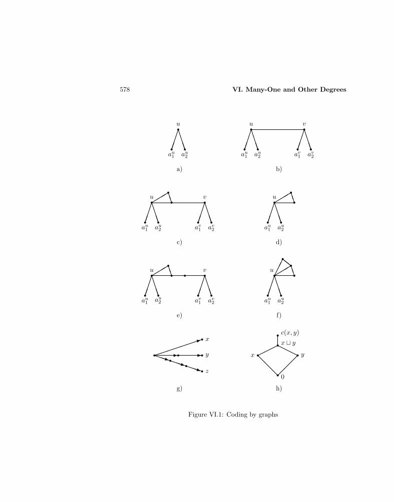
578 VI. Many-One and Other Degrees
a) b)
c) d)
e) f)
g) h)
u
au1 au2
u
au1 au2
v
av1 av2
u
au1 au2
v
av1 av2
u
au1 au2
u
au1 au2
v
av1 av2
u
au1 au2
x
y
z
c(x, y)
x t y
x y
0
rr rBBBB
r rr r r rB
BBB
BBBB
r r rr r r rr
BBBB
BBBB
"""B
B
rr rr rBBBB
"""B
B
rr r r rr r r rB
BBB
BBBB
"""BB
r r rrr rBBBB
"""
BB
cc
rr
r rr r r-1
PPPq-
PPPq PPPq
rrrr rHH
H
@@
@
Figure VI.1: Coding by graphs
VI.4 Global Properties 579
set (II.6.7), and this is false for m-degrees: a nonrecursive, not immune set isnot recursive in each of its infinite subsets (since some of them are recursive),and there are m-degrees containing only nonrecursive, not immune sets (e.g.any m-degree above the m-degree of K, see III.6.10.b).
The next result comes to the rescue and provides a different, slightly lessdirect way of coding arithmetic. We state it in more generality than neededbecause of its interest.
Theorem VI.4.7 (Nerode and Shore [1980]) Let (P,v,t) be an upper-semilattice with least element such that:
1. every countable ideal is the intersection of two principal ideals
2. every countable distributive lattice is isomorphic to an initial segment ofP .
Then the theory of Second-Order Arithmetic is 1-reducible to the first-ordertheory of P .
Proof. There are many steps toward the result:
1. translate Second-Order Arithmetic into second-order logic on countablesetsThis is a standard and well-known procedure, based on the fact thatPeano Axioms actually define ω up to isomorphism, in second-order logic(see p. 23).
2. translate second-order logic on countable sets into the theory of countabledistributive lattices with quantification over idealsThis is the crucial step, which we split into two parts. We refer to thevarious parts of Figure 1.
• code relations by graphs (Lavrov [1963], Rabin and Scott)We start with a binary relation R. Recall that a graph is a sym-metric, irreflexive, binary relation, which we may picture as a set ofpoints related by lines. First of all we have to put down the elementsof the domain. A simple way is the following: for each element u addtwo points au1 and au2 , and relate them as in part a) of the picture.Thus in the graph the elements of the domain of the given relationare the points in which two lines coming from end points arrive.We now have to relate points u and v when R(u, v) holds. A simple-minded solution as in part b) of the picture is not enough, since Rmight be in general not symmetric, while the proposal is. So we addtwo elements, and relate them as in part c) to show that R(u, v),

580 VI. Many-One and Other Degrees
as opposed to R(v, u), holds. This is still not enough since if, e.g.,R(u, u) holds then we would have the situation of part d). But thisis ambiguous, because we might then think that R(u, u) holds when-ever we see a triangle with a vertex in u, while the triangle mightcome from the coding of R(u, v) for some v 6= u. Our final choiceis then the following: given u and v we add three new elements,and relate them as in part e), to show that R(u, v) holds. If R(u, u)holds then we get the unambiguous situation of part f).This technique codes binary relations. But n-ary relations are easilyreduced to binary ones, and thus to graphs as above. For example,if R is ternary we can introduce a nonsymmetric binary relation asfollows. When R(x, y, z) holds introduce four new elements, andrelate them as in part g). An arrow u → v shows that the newbinary relation holds for (u, v). The old elements are those fromwhich no arrow comes out.If there is more than one relation, we simply have to arrange fortheir domains to coincide.
• code graphs by ideals of a distributive latticeGiven graphs on a countable domain we build a countable distribu-tive lattice as follows. The atoms of the lattice correspond to theelements of the domain. Add l.u.b.’s x t y for every pair of atomsx and y, and on top of x t y add an element c(x, y) as a code forx, y, see part h) of the picture (the reason why we do not simplytake c(x, y) = x t y is that we want the codes to be indecompos-able elements, for reason to be explained shortly). Then add thenecessary elements to get a distributive lattice.A graph on the elements is simply a set of unordered pairs, andcan be translated as a set of codes. There is thus a natural corre-spondence between ideals of the lattice and graphs on the atoms, asfollows: an ideal I defines a graph R as
R(x, y) ⇔ c(x, y) ∈ I,
and a graph R defines the ideal generated by the codes c(x, y), forevery x and y such that R(x, y) holds.The crucial fact is that the correspondence is one-one: if R1 and R2
are different graphs, they generate different ideals. Indeed, the onlyobstacle to this could be that, given a graph R, the ideal generatedby R as above also contains codes c(x, y) for x and y such thatR(x, y) does not hold, so that decoding the ideal would not producethe original graph. That this is impossible follows from VI.1.6 andthe fact that the codes are indecomposable elements.
VI.4 Global Properties 581
3. translate the theory of countable distributive lattices with quantificationover ideals into the first-order theory of PA formula ϕ with quantification over elements and ideals can be trans-lated into a formula ϕ∗ by replacing the ideals by exact pairs coding them,and quantification over ideals by quantification over exact pairs.
By the initial segment assumption on P , ϕ is satisfiable in the theory ofcountable distributive lattices if and only if there is an element a ∈ Psuch that the initial segment determined by a in P is a distributive lattice,and ϕ∗ holds in it. 2
Corollary VI.4.8 (Nerode and Shore [1980]) The first-order theory ofDm is recursively isomorphic to the theory of Second-Order Arithmetic.
Proof. We prove that the two theories have the same m-degree by interpretingeach in the other, thus providing faithful translations that will preserve theo-rems. Since the translations will actually be one-one, the theories will have thesame 1-degree, and hence will be recursively isomorphic by III.7.13.
One direction is clear, since every formula about the ordering of m-degreescan be interpreted, in the natural way, as a formula about sets of integers.Thus the theory of m-degrees is interpretable in Second-Order Arithmetic.
For the converse, we want to show that Second-Order Arithmetic is inter-pretable in Dm. It is enough to show that Dm satisfies the conditions of thetheorem, which it does: the required initial segments exist by VI.2.6, whilethe existence of exact pairs follows from VI.3.4, although it is also essentiallyimplied by the proof of Spector’s Theorem for Turing degrees (since m-degreesare closed under finite differences). 2
Corollary VI.4.9 (Lachlan [1970) The first-order theory of Dm is unde-cidable and not axiomatizable.
For what concerns the extent of decidability, as for Turing degrees (seep. 490) we have that the two-quantifier theory of Dm is decidable (Degtev[1979]), but we do not know whether the three-quantifier theory of Dm isundecidable. The methods that provide a positive answer to the same problemfor Turing degrees are highly nondistributive (see Lerman [1983]), and thus notrelevant for Dm.
The next result can now be proved as in Section V.7 (using the presentcoding for arithmetic), and has the same consequences as there.
Theorem VI.4.10 (Nerode and Shore [1980a]) If C is an ideal of Dm
closed under jump, the first-order theory of C has the same degree (and actuallythe same isomorphism type) as the theory of Second-Order Arithmetic with setquantifiers restricted to sets with degree in C.

582 VI. Many-One and Other Degrees
VI.5 Comparison of Degree Theories ?
In this section we consider other notions of degree introduced in Chapter III,namely 1-degrees, tt-degrees, and wtt-degrees. We will mostly quote re-sults about them, and will content ourselves to develop their theories only to thepoint needed to show that they are not elementarily equivalent among them-selves and with Turing and m-degrees (with the only exception of tt-degreesand wtt-degrees, for which it is not known whether this holds).
1-degrees
We have already seen in Section III.7 that D1 is a special case among allthe degree structures we have introduced, because we cannot talk of a least1-degree in any natural way (III.7.4). The next result shows that the differencesare even deeper.
Proposition VI.5.1 (Young [1964]) D1 is neither an upper nor a lowersemilattice, i.e. l.u.b. and g.l.b. do not always exist.
Proof. By III.2.14 every nonrecursive r.e. T -degree contains a simple set. Wewill show in Chapter X that there are incomparable r.e. T -degrees, and thusthere are two incomparable simple sets A and B. Suppose they have a l.u.b.D w.r.t. 1-reducibility:
1. for some z ∈ D, A ≤1 D ∪ z and B ≤1 D ∪ zSince D is an upper bound for A and B, there are recursive one-onefunctions f and g such that
x ∈ A⇔ f(x) ∈ D and x ∈ B ⇔ g(x) ∈ D.
We show that D ∩ range of f 6= ∅ and D ∩ range of g 6= ∅. Suppose, e.g.,that D ∩ range of f = ∅: we show D ≤1 A and thus B ≤1 D ≤1 A,contradicting the fact that A and B are incomparable. Simultaneouslyenumerate D and the range of f , and define h by induction as follows:
• if x shows up first in D, let h(x) be the smallest element of A notyet in h(0), . . . , h(x− 1), so that h(x) ∈ A.
• if x shows up first in the range of f , let y be the unique elementsuch that f(y) = x. If y 6∈ h(0), . . . , h(x− 1) let h(x) = y, so that
x ∈ D ⇔ f(y) ∈ D ⇔ y ∈ A ⇔ h(x) ∈ A.
Otherwise, y must have been defined by the first clause, so let h(x)be the smallest element of A not yet in h(0), . . . , h(x− 1).
VI.5 Comparison of Degree Theories ? 583
Thus D∩ range of f 6= ∅, and D∩ range of g 6= ∅ can be shown similarly.Let then z ∈ D ∩ range of f and z∗ ∈ D ∩ range of g. A ≤1 D ∪ z viaf itself (since z is not in the range of f), and B ≤1 D ∪ z via g∗ sodefined:
g∗(x) =g(x) if g(x) 6= zz∗ otherwise.
Note that g∗ is still one-one, because z∗ is not in the range of g.
2. D ∪ z <1 D, and hence D is not the l.u.b. of A and BFirst note that A,B ≤1 A ⊕ B, so if D is the l.u.b. of A and B thenD ≤1 A⊕B. But A⊕B is simple because so are A and B, and then sois D. Suppose D ≤1 D ∪ z. There is f recursive such that
x ∈ D ⇔ f(x) ∈ D ∪ z.
Then (since z ∈ D) D has an infinite r.e. subset z, f(z), f (2)(z), . . .,contradiction. Thus D ∪ z <1 D, since D ∪ z ≤1 D clearly holds.
By a symmetrical argument (using z ∈ D and D − z) one can show that Aand B have no g.l.b. 2
Even if there is no least 1-degree, one can consider segments above 01.Lachlan [1969] proves that every distributive uppersemilattice which is the directlimit of an ascending sequence of finite distributive lattices is isomorphic to asegment of D1 above 01. The proof consists in forcing all the m-degrees of theinitial segment of Dm built in VI.2.5 to contain only cylinders (see VI.6.1), sothat they are actually 1-degrees.
Exercise VI.5.2 If A is a set of minimal Turing degree constructed by using strongly
uniform trees which is neither immune nor coimmune, then A has minimal 1-degree.
(Hint: as in VI.2.8, using recursive subsets of A and A to make the m-reductions
one-one.)
A complete characterization of the segments of 1-degrees above 01 is notknown, even for the finite ones, and the following results of Lachlan [1969] showthat it might be complicated:
1. every finite segment of D1 is a lattice (this is not as trivial as VI.1.10,since D1 is not an uppersemilattice)
2. some finite segment of D1 is nondistributive
3. not all finite lattices are isomorphic to a finite segment of D1.

584 VI. Many-One and Other Degrees
What is known is however enough for the analogue of Simpson’s Theorem,proved by Nerode and Shore [1980]: the first-order theory of D1 is recursivelyisomorphic to the theory of Second-Order Arithmetic. The proof uses VI.4.7,once some problems are solved.
The first problem is that D1 is not an uppersemilattice, and thus VI.4.7has to be rephrased for directed sets, in which every pair of elements has anupper bound.
The second problem is that the segments we have for D1 are only above01. This does not introduce complications, because 01 is definable in D1: ∅and ω are the only minimal 1-degrees (in the sense of being degrees with nosmaller degree), and 01 is the smallest degree above both of them. Thus wecan work only above 01.
The final problem is the existence of exact pairs. The same proof of Spec-tor’s Theorem V.4.3 shows that for any countable set of 1-degrees in whichevery pair of elements is bounded there is a pair such that every set 1-reducibleto it is also 1-reducible to the disjoint union of finitely many finite modificationsof representatives of the given 1-degrees. By the restriction above we only workwith 1-degrees above 01, which are closed under finite modifications because aset A whose 1-degree is above 01 is neither immune nor coimmune, and thusinfinite recursive subsets of A and A can be used to patch up finite modifica-tions. Closure under disjoint union is needed only for the ideals generated bysubsets of the codes of the distributive lattices used for VI.4.7, and it is provedin Nerode and Shore [1980].
Truth-table degrees and weak truth-table degrees
We will treat the two structures Dtt and Dwtt simultaneously, in the sensethat we will state our results for tt-degrees only, but note here that they allhold for wtt-degrees as well , either by the same proofs or by minor changesthat we will indicate when needed.
To get an elementary difference between D and Dtt we must develop sometheory of the latter. We use for it the usual notation for the jump operator,which is well-defined on tt-degrees by V.1.6. The next result provides theanalogue of the Jump Inversion Theorem V.2.24.
Theorem VI.5.3 Jump Inversion Theorem for Dtt (Mohrherr [1984])The range of the jump operator on Dtt is the cone Dtt(≥0′
tt).
Proof. By V.1.6, for any tt-degree a we have a′ ≥ 0′tt. To get the converse,
let C be a set such that K ≤tt C: we want to get A such that A′ ≡tt C.Consider the construction of V.2.24, with the understanding that ‘the leaststring σ ⊇ σs such that eσ(e) ↓’ means ‘the least string σ ⊇ σs such that
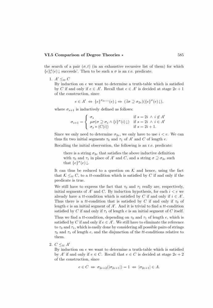
VI.5 Comparison of Degree Theories ? 585
the search of a pair (σ, t) (in an exhaustive recursive list of them) for whicheσt (e)↓ succeeds’. Then to be such a σ is an r.e. predicate.
1. A′ ≤tt CBy induction on e we want to determine a truth-table which is satisfiedby C if and only if e ∈ A′. Recall that e ∈ A′ is decided at stage 2e + 1of the construction, since
e ∈ A′ ⇔ eσ2e+1(e)↓ ⇔ (∃σ ⊇ σ2e)(eσ(e)↓),
where σs+1 is inductively defined as follows:
σs+1 =
σs if s = 2i ∧ i 6∈ A′µσ(σ ⊇ σs ∧ iσ(i)↓) if s = 2i ∧ i ∈ A′σs ∗ 〈C(i)〉 if s = 2i+ 1.
Since we only need to determine σ2e, we only have to use i < e. We canthus fix two initial segments τ0 and τ1 of A′ and C of length e.
Recalling the initial observation, the following is an r.e. predicate:
there is a string σ2e that satisfies the above inductive definitionwith τ0 and τ1 in place of A′ and C, and a string σ ⊇ σ2e suchthat eσ(e)↓.
It can thus be reduced to a question on K and hence, using the factthat K ≤tt C, to a tt-condition which is satisfied by C if and only if thepredicate is true.
We still have to express the fact that τ0 and τ1 really are, respectively,initial segments of A′ and C. By induction hypothesis, for each i < e wealready have a tt-condition which is satisfied by C if and only if i ∈ A′.Thus there is a tt-condition that is satisfied by C if and only if τ0 oflength e is an initial segment of A′. And it is trivial to find a tt-conditionsatisfied by C if and only if τ1 of length e is an initial segment of C itself.
Thus we find a tt-condition, depending on τ0 and τ1 of length e, which issatisfied by C if and only if e ∈ A′. We still have to eliminate the referenceto τ0 and τ1, which is easily done by considering all possible pairs of stringsτ0 and τ1 of length e, and the disjunction of the tt-conditions relative tothem.
2. C ≤tt A′By induction on e we want to determine a truth-table which is satisfiedby A′ if and only if e ∈ C. Recall that e ∈ C is decided at stage 2e + 2of the construction, since
e ∈ C ⇔ σ2e+2(|σ2e+1|) = 1 ⇔ |σ2e+1| ∈ A.
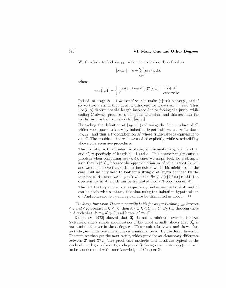
586 VI. Many-One and Other Degrees
We thus have to find |σ2e+1|, which can be explicitly defined as
|σ2e+1| = e+∑i≤e
use (i, A),
where
use (i, A) =|µσ(σ ⊇ σ2i ∧ iσ(i)↓)| if i ∈ A′0 otherwise.
Indeed, at stage 2i + 1 we see if we can make iA(i) converge, and ifso we take a string that does it, otherwise we leave σ2i+1 = σ2i. Thususe (i, A) determines the length increase due to forcing the jump, whilecoding C always produces a one-point extension, and this accounts forthe factor e in the expression for |σ2e+1|.Unraveling the definition of |σ2e+1| (and using the first e values of C,which we suppose to know by induction hypothesis) we can write down|σ2e+1|, and thus a tt-condition on A′ whose truth-value is equivalent toe ∈ C. The trouble is that we have used A′ explicitly, while tt-reducibilityallows only recursive procedures.
The first step is to consider, as above, approximations τ0 and τ1 of A′
and C, respectively of length e + 1 and e. This however might cause aproblem when computing use (i, A), since we might look for a string σsuch that iσ(i)↓ because the approximation to A′ tells us that i ∈ A′,and we thus believe that such a string exists, while this might not be thecase. But we only need to look for a string σ of length bounded by thetrue use (i, A), since we may ask whether (∃σ ⊆ A)(iσ(i) ↓): this is aquestion r.e. in A, which can be translated into a tt-condition on A′.
The fact that τ0 and τ1 are, respectively, initial segments of A′ and Ccan be dealt with as above, this time using the induction hypothesis onC. And reference to τ0 and τ1 can also be eliminated as above. 2
The Jump Inversion Theorem actually holds for any reducibility ≤r between≤tt and ≤T , because if K ≤r C then K ≤tt K⊕C ≡r C. By the theorem thereis A such that A′ ≡tt K ⊕ C, and hence A′ ≡r C.
Kallibekov [1973] showed that 0′tt is not a minimal cover in the r.e.
tt-degrees, and a simple modification of his proof actually shows that 0′tt is
not a minimal cover in the tt-degrees. This result relativizes, and shows thatno tt-degree which contains a jump is a minimal cover. By the Jump InversionTheorem we then get the next result, which provides an elementary differencebetween D and Dtt. The proof uses methods and notations typical of thestudy of r.e. degrees (priority, coding, and Sacks agreement strategy), and willbe best understood with some knowledge of Chapter X.

VI.5 Comparison of Degree Theories ? 587
Theorem VI.5.4 (Mohrherr [1984]) Dtt(≥0′tt) is dense.
Proof. By the Jump Inversion Theorem for Dtt, it is enough to show thatgiven sets A and C such that A <tt C
′ there is a set B such that A <tt B <tt C′.
We build B by columns, as in Section V.4. First of all, we let
〈0, x〉 ∈ B ⇔ x ∈ A.
This codes A into B, and produces A ≤tt B. The other columns of B will beglobally built as a set r.e. in C, hence tt-reducible to C ′. Being B the join ofits columns, B ≤tt C ′ follows from A ≤tt C ′.
The requirements for the construction of B are:
Pe : B 6≤tt A via ϕeNe : C ′ 6≤tt B via ϕe.
Fix an enumeration C ′ss∈ω of C ′ recursive in C (since C ′ is r.e. in C), andan approximation Ass∈ω of A recursive in C and correct in the limit (by theLimit Lemma IV.1.17). Let
lp(e, s) = maxz : (∀y < z)(ϕe,s(y)↓ ∧ y ∈ Bs ⇔ As |= σϕe(y))ln(e, s) = maxz : (∀y < z)(ϕe,s(y)↓ ∧ y ∈ C ′s ⇔ Bs |= σϕe(y)).
The construction is the following. At stage s+ 1, for each e ≤ s,
〈e+ 1, x〉 ∈ Bs+1 if x ∈ C ′s ∧ x < lp(e, s)〈i+ 1, x〉 ∈ Bs+1 if e < i ≤ s ∧ x ≤ s ∧ x ≤ ln(e, s).
Thus Pe takes action only in the e-th column, while Ne takes action on thei+ 1 column, for every i > e.
We show that Pe and Ne are satisfied, by induction on e. Suppose Pi andNi are satisfied for every i < e. Then, for i < e,
lims→∞
lp(i, s) <∞ and lims→∞
ln(i, s) <∞.
Thus Pi puts only finitely many elements on the (i + 1)-th column for i < e,and so does Ni for i ≤ e. Then:
• Pe is satisfiedSuppose B ≤tt A via ϕe. Then lims→∞ lp(e, s) = ∞ and, by construction,
〈e+ 1, x〉 ∈ B ⇔ x ∈ C ′
except for at most finitely many elements, and C ′ ≤tt B ≤tt A, contra-dicting the hypothesis A <tt C
′. It is important to note that the strategysucceeds in this case because no negative condition, except Ni for i < e,can interfere with the e+ 1 column.

588 VI. Many-One and Other Degrees
• Ne is satisfiedSuppose C ′ ≤tt B via ϕe. Then lims→∞ ln(e, s) = ∞, and each (i+ 1)-thcolumn with i > e is contained in B. But then B ≡tt A, since the 0-thcolumn codes A, the (i + 1)-th column for i ≤ e is finite, and the othercolumns are contained in B. Then C ′ ≤tt B ≤tt A, again contradictingthe hypothesis A <tt C
′. 2
The proof actually shows that for any reducibility caught in between ≤1 and≤wtt no degree containing a jump is a minimal cover . The crucial propertyis that if a computation converges at infinitely many stages then it converges.The property and the result both fail for Turing reducibility (every Turingdegree has a minimal cover, and every degree above 0′ is a jump).
For reducibilities (like ≤tt and ≤wtt) for which the Jump Inversion Theo-rem holds it follows that no degree above 0′ is a minimal cover. This fails form-degrees, and we thus have a different proof of the fact that the Jump Inver-sion Theorem fails for m-degrees (VI.1.2.d).
The next result is a typical example of a transfer method that allows us tocarry embedding results from Turing degrees to tt-degrees.
Proposition VI.5.5 (Martin) Any hyperimmune-free minimal Turing de-gree is also a minimal tt-degree. In particular, there is a minimal tt-degree.
Proof. Let a be a hyperimmune-free Turing degree, and A ∈ a. We show thatif B ≤T A then B ≤tt A. If B ' eA then the function
f(x) = µs(eAs (x)↓)
is recursive in A and, being a hyperimmune-free, it is majorized by a recursivefunction g. Then B ≤tt A by III.3.2, since if
eC 'eC(x) if it converges in less than g(x) steps0 otherwise
then eC is total for every C, and eA ' B.If also B ∈ a, by symmetry B ≡tt A if B ≡T A. It follows that, if A has
minimal Turing degree,
B ≤T A ⇒ B recursive or B ≡T A ⇒ B recursive or B ≡tt A.
Thus A has minimal tt-degree as well. 2
For future reference, note that the method just used is not useful below0′, because no nonzero Turing degree comparable with 0′ is hyperimmune-free (V.5.3.d). The method however gives the stronger result that the Turing
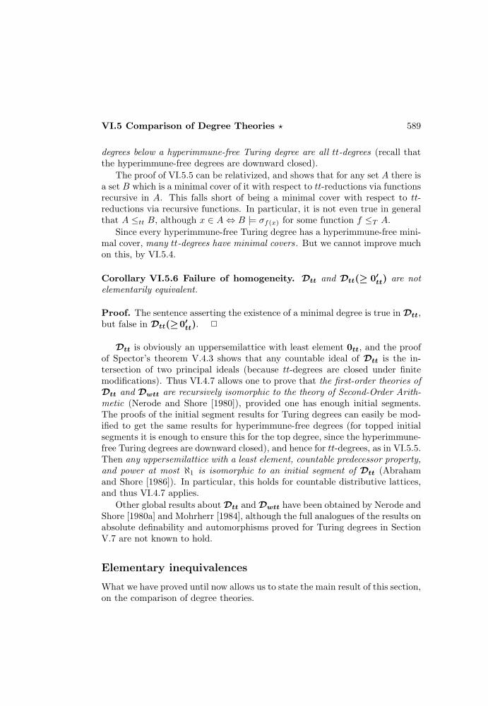
VI.5 Comparison of Degree Theories ? 589
degrees below a hyperimmune-free Turing degree are all tt-degrees (recall thatthe hyperimmune-free degrees are downward closed).
The proof of VI.5.5 can be relativized, and shows that for any set A there isa set B which is a minimal cover of it with respect to tt-reductions via functionsrecursive in A. This falls short of being a minimal cover with respect to tt-reductions via recursive functions. In particular, it is not even true in generalthat A ≤tt B, although x ∈ A⇔ B |= σf(x) for some function f ≤T A.
Since every hyperimmune-free Turing degree has a hyperimmune-free mini-mal cover, many tt-degrees have minimal covers. But we cannot improve muchon this, by VI.5.4.
Corollary VI.5.6 Failure of homogeneity. Dtt and Dtt(≥ 0′tt) are not
elementarily equivalent.
Proof. The sentence asserting the existence of a minimal degree is true in Dtt,but false in Dtt(≥0′
tt). 2
Dtt is obviously an uppersemilattice with least element 0tt, and the proofof Spector’s theorem V.4.3 shows that any countable ideal of Dtt is the in-tersection of two principal ideals (because tt-degrees are closed under finitemodifications). Thus VI.4.7 allows one to prove that the first-order theories ofDtt and Dwtt are recursively isomorphic to the theory of Second-Order Arith-metic (Nerode and Shore [1980]), provided one has enough initial segments.The proofs of the initial segment results for Turing degrees can easily be mod-ified to get the same results for hyperimmune-free degrees (for topped initialsegments it is enough to ensure this for the top degree, since the hyperimmune-free Turing degrees are downward closed), and hence for tt-degrees, as in VI.5.5.Then any uppersemilattice with a least element, countable predecessor property,and power at most ℵ1 is isomorphic to an initial segment of Dtt (Abrahamand Shore [1986]). In particular, this holds for countable distributive lattices,and thus VI.4.7 applies.
Other global results about Dtt and Dwtt have been obtained by Nerode andShore [1980a] and Mohrherr [1984], although the full analogues of the results onabsolute definability and automorphisms proved for Turing degrees in SectionV.7 are not known to hold.
Elementary inequivalences
What we have proved until now allows us to state the main result of this section,on the comparison of degree theories.
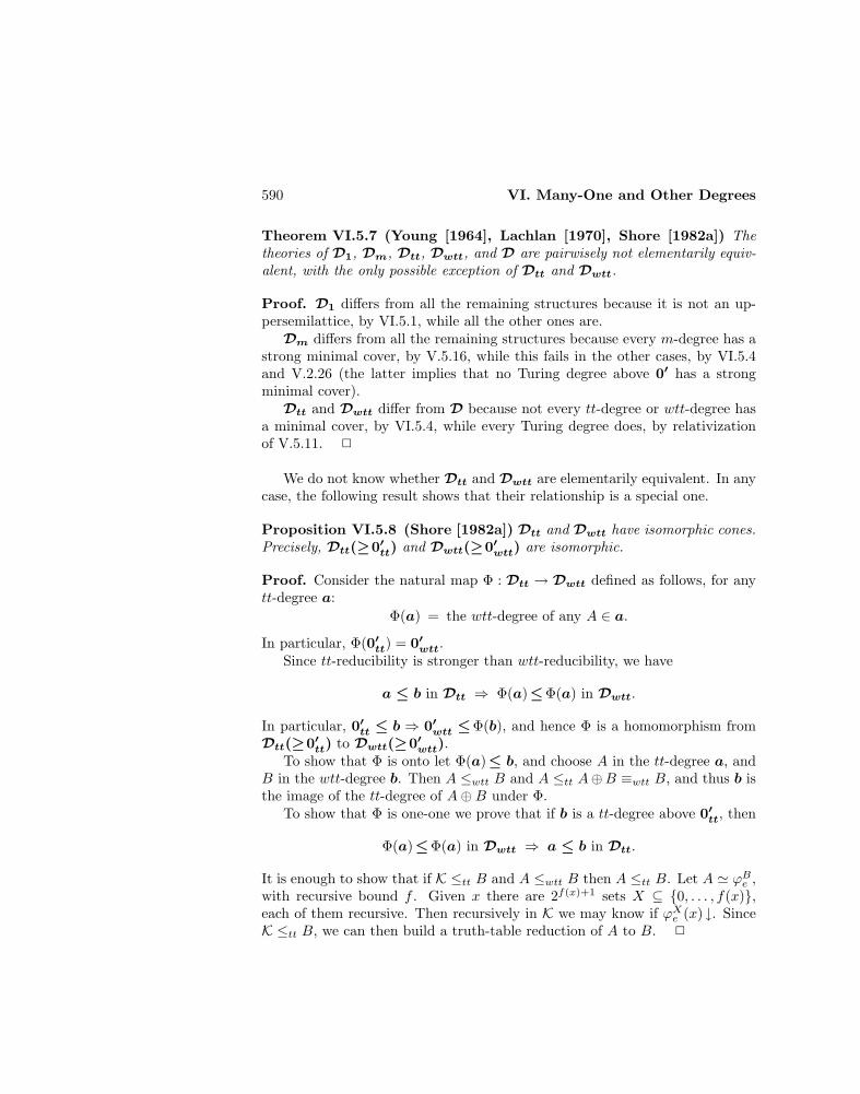
590 VI. Many-One and Other Degrees
Theorem VI.5.7 (Young [1964], Lachlan [1970], Shore [1982a]) Thetheories of D1, Dm, Dtt, Dwtt, and D are pairwisely not elementarily equiv-alent, with the only possible exception of Dtt and Dwtt.
Proof. D1 differs from all the remaining structures because it is not an up-persemilattice, by VI.5.1, while all the other ones are.
Dm differs from all the remaining structures because every m-degree has astrong minimal cover, by V.5.16, while this fails in the other cases, by VI.5.4and V.2.26 (the latter implies that no Turing degree above 0′ has a strongminimal cover).
Dtt and Dwtt differ from D because not every tt-degree or wtt-degree hasa minimal cover, by VI.5.4, while every Turing degree does, by relativizationof V.5.11. 2
We do not know whether Dtt and Dwtt are elementarily equivalent. In anycase, the following result shows that their relationship is a special one.
Proposition VI.5.8 (Shore [1982a]) Dtt and Dwtt have isomorphic cones.Precisely, Dtt(≥0′
tt) and Dwtt(≥0′wtt) are isomorphic.
Proof. Consider the natural map Φ : Dtt → Dwtt defined as follows, for anytt-degree a:
Φ(a) = the wtt-degree of any A ∈ a.
In particular, Φ(0′tt) = 0′
wtt.Since tt-reducibility is stronger than wtt-reducibility, we have
a ≤ b in Dtt ⇒ Φ(a) ≤ Φ(a) in Dwtt.
In particular, 0′tt ≤ b ⇒ 0′
wtt ≤ Φ(b), and hence Φ is a homomorphism fromDtt(≥0′
tt) to Dwtt(≥0′wtt).
To show that Φ is onto let Φ(a) ≤ b, and choose A in the tt-degree a, andB in the wtt-degree b. Then A ≤wtt B and A ≤tt A⊕B ≡wtt B, and thus b isthe image of the tt-degree of A⊕B under Φ.
To show that Φ is one-one we prove that if b is a tt-degree above 0′tt, then
Φ(a) ≤ Φ(a) in Dwtt ⇒ a ≤ b in Dtt.
It is enough to show that if K ≤tt B and A ≤wtt B then A ≤tt B. Let A ' ϕBe ,with recursive bound f . Given x there are 2f(x)+1 sets X ⊆ 0, . . . , f(x),each of them recursive. Then recursively in K we may know if ϕXe (x)↓. SinceK ≤tt B, we can then build a truth-table reduction of A to B. 2

VI.6 Structure Inside Degrees ? 591
Note that no other pair of structures among Dm, Dtt, Dwtt, and D admitsisomorphic cones, because the properties used in VI.5.7 to show elementaryinequivalence actually hold on a cone. Thus, even if Dtt and Dwtt were ele-mentarily inequivalent, they would resemble each other more than any otherof these pairs.
Bulitko [1980] and Selivanov [1982] have shown that the only possible truth-table-like reducibilities are: ≤m, ≤btt(1), ≤l, ≤d, ≤c, ≤p, and ≤tt (see pp. 268and 331 for definitions). Among them, the structures induced by ≤c and ≤dare isomorphic, since
A ≤c B ⇔ A ≤d B,and so are the structures induced ≤m and ≤btt(1) (Malc’ev [1985]). The re-maining ones are pairwisely elementarily inequivalent (Degtev [1979], [1985]),with the only possible exception of the structures induced by ≤p and ≤tt.
VI.6 Structure Inside Degrees ?
In the last section we have compared various notions of degree from the point ofview of the structures they induce. Despite the elementary differences provedin VI.5.7, we have noted a resemblance of methods of proofs in the study of1-degrees and m-degrees on one side, and tt-degrees, wtt-degrees, and Turingdegrees on the other.
In the present section we take a different perspective, and analyze the pos-sible structure of degrees of one type inside degrees of another. We will againdiscover that 1-degrees and m-degrees are close, in the sense that they coincidein a large number of cases, and the same will hold for tt-degrees and Tur-ing degrees (and hence for wtt-degrees). On the other hand, m-degrees andtt-degrees never coincide, and this shows where the real demarcation amongdegree notions lies.
Cylinders
Recall that the jump operator provides a homomorphism from D to D1, since
A ≤T B ⇔ A′ ≤1 B′.
We now define canonical homomorphisms from Dm and Dtt to D1.
Definition VI.6.1 (Myhill [1959], Rogers [1967]) The cylindrification ofa set A is the set
A ·N = 〈x, n〉 : x ∈ A.A is a cylinder if A ≡ A ·N , i.e. A and A ·N are recursively equivalent.
592 VI. Many-One and Other Degrees
Proposition VI.6.2 (Rogers [1967]) A ≡m A ·N . Moreover,
A ≤m B ⇔ A ·N ≤1 B ·N.
Proof. A ≤1 A ·N via f(x) = 〈x, x〉, and A ·N ≤m A via g(x) = (x)1. ThusA ≡m A ·N .
Let A ≤m B: since A · N ≤m A, then A · N ≤m B via some recursivefunction f , and A · N ≤1 B · N via g(x) = 〈f(x), x〉, which is one-one. Con-versely, let A·N ≤1 B·N : since A ≤m A·N and B·N ≤m B, then A ≤m B. 2
We now give some conditions for a set to be a cylinder.
Proposition VI.6.3 (Young [1966a], Rogers [1967]) The following con-ditions are equivalent:
1. A is a cylinder
2. for every set B, B ≤m A⇒ B ≤1 A
3. there is a recursive function f such that, for every x,
• Wf(x) is infinite
• x ∈ A⇒Wf(x) ⊆ A
• x ∈ A⇒Wf(x) ⊆ A.
Proof. 1 implies 3 because if A ≡ A · N then there is a one-one recursivefunction g reducing A ·N to A, and thus it is enough to let
Wf(x) = g(〈x, n〉) : n ∈ ω.
3 implies 2 because we can use Wf(x) to turn a many-one reduction g of B toA into a one-one reduction, as follows. Let h(0) = g(0). Given h(x), let h(x+1)be the first element generated in Wf(g(x+1)) and not in h(0), . . . , h(x).
2 implies 1 because A ≤1 A ·N and A ·N ≤m A always hold, and by 2 thelatter implies A ·N ≤1 A. Thus A ≡1 A ·N , and A ≡ A ·N by III.7.13. 2
Exercises VI.6.4 a) A set A is a cylinder if and only if, for some recursive functiong and every Dx 6= ∅,
Dx ⊆ A⇒ g(x) ∈ A−Dx and Dx ⊆ A⇒ g(x) ∈ A−Dx.
(Rogers [1967]) (Hint: the condition is equivalent to VI.6.3.)b) Logical theories are cylinders. (Hint: show that condition VI.6.3.3 is satisfied,
using the fact that ϕ and ¬¬ϕ are equivalent.)c) Every cylinder is a splinter . (Myhill [1959]) (Hint: see the proof of III.7.10.c.)
VI.6 Structure Inside Degrees ? 593
d) A cylinder is either recursive or pseudocreative. (Hint: by c) and III.7.10.a.)e) The only recursive sets which are cylinders are ∅, ω, and the infinite coinfinite
sets. (Hint: by VI.6.3.3.) It follows that not every splinter is a cylinder. Young [1966]has shown that there are infinite coinfinite splinters which are not cylinders.
f) Every creative set is a cylinder . (Myhill [1959])
g) Not every pseudocreative set is a cylinder . (Young [1964a]) (Hint: let B be a
simple set. Then B · B is pseudocreative, since if x ∈ B then x · B is an infinite
r.e. subset of B ·B. Choose B such that B · B 6≤m B, see III.8.5. Then B · B is not
a cylinder, otherwise there is f like in VI.6.3.3, and since Wf(x) is infinite and B is
simple there is 〈a, b〉 ∈ Wf(x) such that one of a and b is in B. Let g(x) be the other.
Then x ∈ B ·B ⇔ g(x) ∈ B, contradiction.)
We now turn to the analogue of the notion of cylinder for tt-reducibility.
Definition VI.6.5 (Rogers [1967]) The tt-cylindrification of a set A is theset
Att = x : A |= σx.
A is a tt-cylinder if A ≡ Att.
Proposition VI.6.6 (Rogers [1967]) A ≡tt Att. Moreover,
A ≤tt B ⇔ Att ≤1 Btt.
Proof. A ≤1 Att via f such that σf(x) is the tt-condition ‘x ∈ X’, andAtt ≤tt A via the identity function, since x ∈ Att ⇔ A |= σx by definition.
Let A ≤tt B: since Att ≤tt A then Att ≤tt B, and for some recursive f
x ∈ Att ⇔ B |= σf(x) ⇔ f(x) ∈ Btt.
Thus Att ≤m Btt. But f can be made one-one by induction, by substitutingtt-conditions with equivalent ones if necessary (obtained by adding redundantclauses, like n ∈ X ∨ n 6∈ X). Thus Att ≤1 B
tt. Conversely, if Att ≤1 Btt then
A ≤tt B, since A ≤tt Att and Btt ≤tt B. 2
Proposition VI.6.7 (Rogers [1967]) The following conditions are equiva-lent:
1. A is a tt-cylinder
2. for every set B, B ≤tt A⇒ B ≤1 A
Proof. 1 implies 2 because if B ≤tt A then B ≤m Att by definition, and henceB ≤1 A
tt as in the proof of VI.6.6. If A is a tt-cylinder then Att ≤1 A, andhence B ≤1 A.
594 VI. Many-One and Other Degrees
2 implies 1 because A ≤1 Att and Att ≤tt A always hold, and by 2 the latter
implies Att ≤1 A. Thus A ≡1 Att, and A ≡ Att by III.7.13. 2
In particular, a tt-cylinder is a cylinder .
Inside many-one degrees
Since ≤1 is stronger than ≤m, an m-degree can be thought of as consisting of1-degrees.
Definition VI.6.8 An m-degree is irreducible if it consists of only one1-degree.
Obviously, an m-degree is irreducible if and only if it contains only cylin-ders, since A ≡m A ·N always holds.
Trivial examples of irreducible m-degrees are ∅ and ω. The first exam-ple of a nontrivial irreducible m-degree was given by Myhill [1955], who showedthat the m-degree of K is such a degree (see III.6.6 and III.7.5). By relativiza-tion, the m-degree of a jump set A′ is irreducible, and thus every Turing degreeabove 0′ contains an irreducible m-degree.
Proposition VI.6.9 (Kobzev [1975]) If A is r.e. and nonrecursive, them-degree of Att is irreducible.
Proof. Consider B ≡m Att. Since Att is a cylinder, from B ≤m Att we haveB ≤1 A
tt. For the converse, let Att ≤m B via f : we want to show that we haveinfinitely many equivalent choices for each value of f , so that f can be turnedinto a one-one reduction, and Att ≤1 B. Consider
σz = (σx ∧ ¬σy) ∨ (¬σx ∧ σy),
for a given y:
• if x ∈ Att then A |= σx, and thus
z ∈ Att ⇔ A |= σz ⇔ A |= ¬σy ⇔ y 6∈ Att
• if x 6∈ Att then A |= ¬σx, and thus
z ∈ Att ⇔ A |= σz ⇔ A |= σy ⇔ y ∈ Att.
These are still only equivalences, but if we choose y 6∈ Att we explicitly have:
• if x ∈ Att then z ∈ Att and f(z) ∈ B

VI.6 Structure Inside Degrees ? 595
• if x 6∈ Att then z 6∈ Att and f(z) 6∈ B.
Fix then an r.e. subset C of Att. There is a recursive function g such that
f(z) ∈ Wg(x) ⇔ (∃y ∈ C)[σz = (σx ∧ ¬σy) ∨ (¬σx ∧ σy)].
Moreover, Wg(x) is an r.e. subset of B if x ∈ Att, and of B otherwise.It remains to choose C in such a way that Wg(x) is always infinite. Note
that it is enough to have C and Att recursively inseparable, because then ifWg(x) were finite the set
y ∈ R ⇔ f(z) ∈ Wg(x)
(with σz as above) would be a recursive set separating C and Att. Indeed,C ⊆ R by definition. Moreover, once x is fixed the only thing that matters forz, and hence for f(z), is whether y is in Att or not. Since for y ∈ C we havey ∈ R, and C ⊆ Att, it cannot be that y ∈ Att ∩R, and hence R ⊆ Att.
To find C as wanted, note that A ≤1 Att and Att ≤1 Att (the latter because
Att ≤tt Att, and Att is a tt-cylinder). Thus A ≤1 Att. Let C be the image of Aunder this 1-reduction: it is an r.e. set because A is, and it cannot be separablefrom Att by a recursive set, otherwise A would be the inverse image of this set,and it would then be recursive. 2
Corollary VI.6.10 Every nonrecursive r.e. tt-degree contains an irreduciblem-degree.
Proof. A ≡tt Att. 2
Degtev [1979] shows that there are nonrecursive tt-degrees not containingirreducible m-degrees. We do not know whether every nonrecursive Turing de-gree contains an irreducible m-degree, but the possible exceptions are severelyrestricted, as we now prove.
Proposition VI.6.11 (Degtev [1979]) Every Turing degree not below 0′
contains an irreducible m-degree.
Proof. We modify the proof of the previous result to show that if A is non-recursive and the m-degree of Att is not irreducible, then A ∈ ∆0
2. The resultfollows from the Limit Lemma IV.1.17, and the fact that A ≡T Att.
Since Att ≤1 Att (because Att ≤tt Att, and Att is a tt-cylinder), it is enoughto show that Att ∈ Σ0
2. Since Att is a cylinder, if its m-degree is not irreduciblethen it must contain a set B which is not a cylinder, and thus such that
596 VI. Many-One and Other Degrees
Att ≤m B but Att 6≤1 B (by VI.6.3.2). Let f be a recursive function such thatx ∈ Att ⇔ f(x) ∈ B. Given n, let
f(z) ∈ Wg(n,x) ⇔ (∃y)[σz = σx ∧ ( σn ∨ σy)] ∨(∃y)[σz = σx ∨ (¬σn ∧ σy)].
We show thatn ∈ Att ⇔ (∃x)(Wg(n,x) finite).
Then Att ∈ Σ02, because finiteness of an r.e. set is a Σ0
2 condition, since it canbe expressed as saying that there is a number such that all greater ones are notin the set.
1. If n ∈ Att then A |= σn, and hence
A |= σx ∧ (σn ∨ σy) ⇔ A |= σx ∨ (¬σn ∧ σy) ⇔ A |= σx.
If Wg(n,x) is infinite for every x then we can easily get Att ≤1 B, contra-dicting the hypothesis.
2. If n 6∈ Att then A |= ¬σn, and hence
x ∈ Att ⇒ A |= σx ∧ ( σn ∨ σy) iff A |= σy⇒ f(z) : σz = σx ∧ ( σn ∨ σy) is infinite
x 6∈ Att ⇒ A |= σx ∨ (¬σn ∧ σy) iff A |= σy⇒ f(z) : σz = σx ∨ (¬σn ∧ σy) is infinite,
otherwise A is recursive (because A ≤m Att ≤m B). 2
Exercises VI.6.12 A set A is perfect if it is η-closed, for some nontrivial r.e. equiv-alence relation η whose only recursive η-closed sets are ∅ and ω. Note that everyequivalence class of η is infinite and r.e.
a) If A is perfect then its m-degree is irreducible. (Ershov [1971]) (Hint: if B ≤m Avia f , define g one-one reducing B to A by letting f(x) and g(x) be in the sameequivalence class: this works because A is η-closed. If A ≤m B via f , consider thenew equivalence xη∗y ⇔ xηy ∨ f(x) = f(y). A is still closed and perfect w.r.t. η∗.f m-reduces [x]η∗ to f([x]η∗), and thus the latter is still infinite. Define g one-onereducing B to A by letting g(x) ∈ f([x]η∗).)
b) Not every irreducible m-degree contains a perfect set . (Denisov [1974]) (Hint:
modify III.6.23.c to prove that if B ≤tt A and B is perfect then A is not hypersimple.
Then use VI.6.10.)
We have now examples of irreducible m-degrees, as well as of m-degreescontaining infinitely many 1-degrees (like 0m). These are the only possiblecases.

VI.6 Structure Inside Degrees ? 597
Proposition VI.6.13 (Young [1966a]) An m-degree contains either onlyone or infinitely many 1-degrees.
Proof. If there is more than one 1-degree in a given m-degree, there is a setA which is not a cylinder. Note that
A⊕A (A⊕A)⊕ (A⊕A) · · ·
are all in the same m-degree, since ⊕ induces the l.u.b. for m-degrees. SinceB ≤1 B ⊕ B always holds, the two following facts produce, by induction, aninfinite ascending chain of 1-degrees in the given m-degree:
1. B ⊕B ≤1 B ⇒ B ⊕B cylinderGiven f one-one such that
z ∈ B ⊕B ⇔ f(z) ∈ B ⇔ 2f(z) ∈ B ⊕B,
the setWg(z) = z, 2f(z), 2f(2f(z)), . . .
satisfies condition VI.6.3.3.
2. B ⊕B cylinder ⇒ B cylinderIf g satisfies VI.6.3.3 then
x ∈ B ⇒ 2x ∈ B ⊕B ⇒ Wg(2x) ⊆ B ⊕Bx 6∈ B ⇒ 2x 6∈ B ⊕B ⇒ Wg(2x) ⊆ B ⊕B.
It is thus enough to let
Wh(x) = z : 2z ∈ Wg(2x) ∨ 2z + 1 ∈ Wg(2x). 2
The proof shows that if an m-degree contains infinitely many 1-degrees thenit contains an infinite chain. Young [1966a] shows that actually every countablelinear ordering is embeddable in the 1-degrees of such an m-degree. It is notknown whether there must always be an infinite antichain as well.
Exercises VI.6.14 a) Every m-degree contains a greatest 1-degree (consisting ex-actly of the cylinders in the given m- degree). (Rogers [1967]) (Hint: given A considerA ·N .)
b) There are m-degrees without least 1-degree. (Dekker and Myhill [1960]) (Hint:
if A is simple and z ∈ A then A − z ≡m A but A − z <1 A, by the proof of
VI.5.1.)
598 VI. Many-One and Other Degrees
Inside truth-table degrees
We now look at m-degrees inside tt-degrees.
Proposition VI.6.15 (Jockusch [1969]) Every nonrecursive tt-degree con-tains infinitely many m-degrees.
Proof. Let C be a nonrecursive set. Consider the tree of binary sequencenumbers, and the branch A defined by C:
x ∈ A ⇔ Seq(x) ∧ (∀n)1≤n≤ln(x)[(x)n = C(n− 1)].
By definition A ≡tt C (since there are only finitely many binary sequencenumbers of a given length). Moreover, A is retraceable via
f(〈x1, . . . , xn, xn+1〉) = 〈x1, . . . , xn〉.
Being nonrecursive and retraceable, A is immune (by II.6.5). It is also nothyperimmune, because the strong array whose elements are the sets of binarysequence numbers of a given length intersects A.
For n ≥ 1, let (A)n be the recursive product of A with itself n times:
〈x1, . . . , xn〉 ∈ (A)n ⇔ (∀i)1≤i≤n(xi ∈ A).
Clearly, (A)n ≡tt A, and (A)n ≤m (A)n+1. We now prove (A)n+1 6≤m (A)n,so that the tt-degree of A (and hence that of B) contains infinitely manym-degrees.
The plan of the proof is the following. Suppose (A)n+1≤m (A)n. We wantto find an r.e. subset B of A so big that at most 2n elements at any level ofthe tree are in B. We then get a contradiction as follows. From the fact thatA is not hyperimmune we have a recursive function g such that g(x) majorizesthe x-th element (i.e. the one of level x) ax of A. Then we can define Sx suchthat |Sx| ≤ 2n as follows: take all elements less than g(x) which are on levelx of the tree, and eliminate those that are generated in B, until at most 2nremain. Clearly, ax is not eliminated, because B ⊆ A. We thus get a strongarray of bounded cardinality intersecting A, contradicting the fact that A isimmune (II.6.10.b).
It remains to find B. Note that
(A)n ≡m y : |Dy| ≤ n ∧Dy ∩A 6= ∅,
so that the hypothesis (A)n+1≤m (A)n can be reformulated as:
y : |Dy| ≤ n+ 1 ∧Dy ∩A 6= ∅ ≤m y : |Dy| ≤ n ∧Dy ∩A 6= ∅.

VI.6 Structure Inside Degrees ? 599
Thus there is a recursive function h such that
|Dy| ≤ n+ 1 ⇒ |Dh(y)| ≤ n ∧ (Dy ∩A = ∅ ↔ Dh(y) ∩A = ∅).
Let
x ∈ B1 ⇔ (∃y)(|Dy| ≤ n+ 1 ∧ x ∈ Dy ∧ x|Dh(y))x ∈ B2 ⇔ (∃y)(|Dy| ≤ n+ 1 ∧ x|Dy ∧ x 7→ Dh(y)),
where x|Dz means that x and any element of Dz are not sent by iterations of fon a same element, and x 7→ Dz that x is sent by iterations of f on an elementof Dz.
Clearly, B1 ∪B2 is r.e. Moreover:
1. B ⊆ ASuppose x ∈ B1 ∩ A. For some y, x ∈ Dy ∩ A and x|Dh(y), so thatDy ∩A 6= ∅ and hence Dh(y) ∩A 6= ∅. But the latter contradicts x|Dh(y),because the elements of A are all sent by iteration of f on a same element(e.g., a0).
Suppose x ∈ B2∩A. For some y, x|Dy and x 7→ Dh(y), so that Dy∩A = ∅(because x ∈ A and x|Dy) and hence Dh(y) ∩ A = ∅. But the lattercontradicts x 7→ Dh(y), because x ∈ A and it is thus sent only on elementsof A by iterations of f .
2. B has at most 2n elements at any level of the treeFor the sake of contradiction, suppose there is x1, . . . , x2n+1 ⊆ B,whose elements we may suppose to be ordered from the left on the tree.Consider
Dy = x1, x3, x5, . . . , x2n+1,
which has n + 1 elements. By hypothesis Dy ⊆ B, and in particularDy ⊆ B1. Since |Dy| ≤ n + 1 and x2i+1 ∈ Dy, then it cannot bex2i+1|Dh(y). Since |Dh(y)| ≤ n and |Dy| = n + 1, there must be i < jsuch that x2i+1 and x2j+1 are sent on a same element of Dh(y). Sincex2i+1 and x2j+1 are on the same level of the tree, also x2i+2 (which isbetween them and on the same level) must be sent on the same element,by the definition of f . But this is impossible, since then x2i+2|Dy butx2i+2 7→ Dh(y), and hence x2i+2 ∈ B2, contradicting the hypothesis thatx2i+2 ∈ B. 2
The proof shows that every nonrecursive tt-degree contains an infinite chainof m-degrees. It is not known whether it also contains an infinite antichain.
600 VI. Many-One and Other Degrees
Exercises VI.6.16 a) Every tt-degree contains a greatest m-degree and a greatest1-degree. (Rogers [1967]) (Hint: consider Att.)
b) No nonrecursive tt-degree contains a least m-degree. (Jockusch) (Hint: let Abe an immune retraceable set in the given tt-degree, by II.6.13. Then A and A forma minimal pair of m-degrees. Indeed, let x ∈ C ⇔ f(x) ∈ A⇔ g(x) ∈ A. If f(x) andg(x) are sent by the retracing function into the same element, this is in A. The setof such elements is finite, being r.e. Let a ∈ A be greater than its maximum. If Cis not recursive the ranges of f and g are unbounded, and A− 0, . . . , a− 1 is r.e.,contradicting immunity: if z ≥ a choose x such that f(x), g(x) > z. See if one is sentinto z by the retracing function. At most one of them can be, by the choice of a, andif z ∈ A one does.)
c) Every nonrecursive tt-degree contains incomparable m-degrees. (Jockusch
[1968a]) (Hint: let A be a semirecursive set in the given tt-degree, by III.5.5. Then
A and A are m-incomparable.)
Inside Turing degrees
We now look at tt-degrees inside Turing degrees.
Definition VI.6.17 A Turing degree is irreducible if it consists of only onett-degree.
The irreducible Turing degrees are old friends.
Proposition VI.6.18 (Jockusch [1969], Martin) A Turing degree is irre-ducible if and only if it is hyperimmune-free.
Proof. We have already proved in VI.5.5 that if A has hyperimmune-freedegree and B ≡T A then B ≡tt A. Thus a hyperimmune-free degree containsonly one tt-degree.
Suppose now that the Turing degree of A contains only one tt-degree. Wemay suppose that A has the greatest m-degree in it (otherwise we can considerAtt). Suppose f ≤T A is not recursively majorized. With no loss of generalitywe may suppose f increasing. Let
e ∈ B ⇔ e(e) converges in less than f(e) steps, and e(e) 6∈ A.
Then B ≤T A, and A ≡T A⊕B. We now show that B 6≤m A: thus A <m A⊕B,contradicting the fact that A has the greatest m-degree.
Suppose B ≤m A via g. Let e0, e1, . . . be indices of g, with ex > x. Then
ex ∈ B ⇔ g(ex) ∈ A ⇔ ex(ex) ∈ A.
Thus ex(ex) must converge in more than f(ex) > f(x) steps (recall that fis increasing), and the number of steps needed to compute ex(ex) is thus a

VI.6 Structure Inside Degrees ? 601
recursive function majorizing f , contradiction. 2
As in the case of m-degrees, there are only two possibilities.
Corollary VI.6.19 A Turing degree contains either only one or infinitelymany tt-degrees.
Proof. The proof given above works also in the case that a Turing degreehas a greatest tt-degree, by choosing A in the greatest m-degree of the greatesttt-degree. Since A⊕B ≡T A, A⊕B ≤tt A because A is in the greatest tt-degree,and hence actually A ≡tt A⊕B. Thus A <m A⊕B produces a contradiction,because A has greatest m-degree in its tt-degree.
But if there are finitely many tt-degrees, there is a greatest one (their l.u.b.).Thus the Turing degrees consisting of finitely many tt-degrees are still thehyperimmune-free ones, i.e. the irreducible ones. 2
Exercises VI.6.20 a) A Turing degree has greatest tt-degree if and only if it is ir-reducible. (Hint: by the proof of the corollary.)
b) Non-irreducible Turing degrees contain an infinite chain of tt-degrees. (Hint:by part a.)
c) Non-irreducible Turing degrees contain an infinite antichain of tt-degrees. (Deg-
tev [1972]) (Hint: this uses the priority method. Let A = a0 < a1 < · · · , Ahyperimmune. We build Az in the Turing degree of A so that, for m 6= n, Am 6≤tt An.
Code A into Az by letting x ∈ A⇔ 2x+1 ∈ Az: thus A ≤T Az. To ensure Am 6≤tt Anvia ϕe, we want some x such that x ∈ Am ⇔ An 6|= σϕe(x). Wait until a fresh witness
x appears, such that ϕe(x) converges in less than ax steps. Then see if An,s |= σϕe(x).
If so, restrain x out of Am. Otherwise, put x into Am. In both cases, restrain out of
An the elements used in the computation and not yet in it. Note that if ϕe is total
there are infinitely many x such that ϕe(x) converges in less than ax steps, otherwise
A would be majorized by the least number of steps needed to compute ϕe(x). The
construction is recursive in A, and thus Az ≡T A.)
æ
602 VI. Many-One and Other Degrees
Bibliography
We include only references quoted in the book. A complete bibliography on Recursion Theoryhas been edited by Hinman as Volume IV of the Ω-Bibliography of Mathematical Logic,Springer Verlag, 1987.
We indicate publications by abbreviating their original names. The following is a list offull names of Soviet publications, and of their official translations.
1. Algebra i Logika (Algebra and Logic)
2. Doklady Akademii Nauk S.S.S.R. (Soviet Mathematics, Dokladi)
3. Izvestiya Vysshikh Uchebnykh Zavedenij Matematika (Soviet Mathematics, Izvestiya)
4. Kibernetika (Cybernetics)
5. Matematicheskii Sbornik (Mathematics of the U.S.S.R.)
6. Matematicheskie Zametki (Mathematical Notes of the Academy of Science U.S.S.R.)
7. Problemy Kibernetiki (Problems of Cybernetics)
8. Problemi Peredachi Informatsii (Problems of Information Transmission)
9. Sibirskij Matematicheskii Zhurnal (Siberian Mathematical Journal)
10. Uspekhi Matematicheskikh Nauk (Russian Mathematical Surveys).
Aberth, O.[1971] The failure in computable analysis of a classical existence theorem for differential
equations, Proc. Am. Math. Soc. 30 (1971) 151–156.[1980] Computable analysis, McGraw Hill, 1980.
Abian, S., and Brown, A.B.[1961] A theorem on partially ordered sets with applications to fixed-point theorems,
Can. J. Math. 13 (1961) 78–83.
Abraham, U., and Shore, R.A.[1986] Initial segments of the degrees of size ℵ1, Isr. J. Math. 53 (1986) 1–51.
Ackermann, W.[1928] Zum Hilbertschen Aufbau der reellen Zahlen, Math. Ann. 9 (1928) 118–133,
transl. in Van Heijenoort [1967], pp. 493–507.[1937] Die Widerspruchsfreiheit der allegemeinen Mengenlehere, Math. Ann. 114 (1937)
305–315.[1954] Solvable cases of the decision problem, North Holland, 1954.
Addison, J.W.[1954] On some points of the Theory of Recursive Functions, Ph.D. Thesis, University
603

604 Bibliography
of Wisconsin, 1954.[1959] Separation principles in the hierarchies of classical and effective descriptive set
theory, Fund. Math. 46 (1959) 123–135.[1959a] Some consequences of the axiom of constructibility, Fund. Math. 46 (1959) 337–
357.[1965] The undefinability of the definable, Notices Am. Math. Soc. 12 (1965) 347.
Addison, J.W., and Kleene, S.C.[1957] A note on function quantification, Proc. Am. Math. Soc. 8 (1957) 1002–1006.
Addison, J.W., and Moschovakis, Y.N.[1968] Some consequences of the axiom of definable determinateness, Proc. Nat. Acad.
Sci. 59 (1968) 708–712.
Adler, A.[1969] Some recursively unsolvable problems in analysis, Proc. Am. Math. Soc. 22
(1969) 523–526.
Agerwala, T.[1974] A complete model for representing the coordination of asynchronous processes,
Report , John Hopkins University, 1974.
Anderson, A.R.[1964] Minds and machines, Prentice Hall, 1964.
Appel, K.I.[1967] There exist two regressive sets whose intersection is not regressive, J. Symb. Log.
32 (1967) 322–324.
Appel, K.I., and McLaughlin, T.G.[1965] On properties of regressive sets, Trans. Am. Math. Soc. 115 (1965) 83–93.
Arbib, M.A.[1964] Brains, machines and mathematics, Wiley, 1964.[1969] Theories of abstract automata, Prentice Hall, 1969.[1969a] Self-reproducing automata - some implications for theoretical biology, in Towards
a Theoretical Biology, Waddington ed., Edinburgh University Press, 1969, pp.204–226.
[1972] The metaphorical brain, Wiley, 1972.[1973] Automata theory in the context of theoretical neurophysiology, in Foundations of
mathematical biology, Rosen ed., Academic Press, 1973, vol. 3, pp. 191–282.
Arslanov, M.M.[1969] On effectively hypersimple sets, Alg. Log. 8 (1969) 143–153, transl. 8 (1969) 79–
85.[1970] On complete hypersimple sets, Sov. Math. 95 (1970) 30–35.[1981] On some generalizations of the Fixed-Point Theorem, Sov. Math. 228 (1981)
9–16, transl. 228 (1981) 1–10.[1985] Effectively hyperimmune sets and majorization, Mat. Zam. 38 (1985) 302–309,
transl. 38 (1985) 677–680.
Arslanov, M.M., and Soloviev, V.D.[1978] Effectivizations of definitions of classes of simple sets, Alg. Avtom. 10 (1978)
95–99.
Babbage, C.[1837] On the mathematical powers of the calculating engine, in The origins of digital
computers, Randell ed., Springer, 1973, pp. 19–54.
Backus, J.W.[1981] Is computer science based on the wrong fundamental concept of ‘program’? An
Bibliography 605
extended concept, in Algorithmic languages, de Bakker et al. eds., North Holland,1981, pp. 133–165.
Backus, J.W., et al.[1957] The FORTRAN automatic coding system, Proc. West. Joint Comp. Conf. 11
(1957) 188–198.
Baire, R.[1899] Sur les fonctions de variables reelles, Ann. Mat. Pura Appl. 3 (1899) 1–122.
Banach, S.[1922] Sur les operations dans les ensembles abstraits et leurs applications aux equations
integrales, Fund. Math. 3 (1922) 7–33.
Barendregt, H.[1975] Normed uniformly reflexive structures, Springer Lect. Not. Comp. Sci. 37 (1975)
272–286.[1981] The lambda calculus, its syntax and semantics, North Holland, 1981.
Barna, B.[1956] Uber die Divergenzpunkte des Newtonschen Verfahrens zur Bestimmung von
Wurzeln algebraischer Gleichungen, II, Publ. Math. Debr. 4 (1956) 384–397.
Barwise, J.[1975] Admissible sets and structures, Springer, 1975.
Beeson, M.J.[1975] The nonderivability in intuitionistic formal systems of theorems on the continuity
of effective operations, J. Symb. Log. 40 (1975) 321–346.[1985] Foundations of constructive mathematics, Springer, 1985.
Beeson, M.J., and Scedrov, A.[1984] Church’s thesis, continuity, and set theory, J. Symb. Log. 49 (1984) 630–643.
Beigel, R.J., Gasarch, W.I., Gill, J., and Owings, J.C.[198?] Terse, superterse, and verbose sets, to appear.
Bell, J.S.[1964] On the Einstein-Podolski-Rosen paradox, Phys. 1 (1964) 195–200.[1966] On the problem of hidden variables in quantum mechanics, Rev. Mod. Phys. 38
(1966) 447–452.
Benioff, P.A.[1980] The computer as a physical system: a microscopical quantum mechanical Hamil-
tonian model of computers as represented by Turing machines, J. Stat. Phys. 22(1980) 563–591.
[1981] Quantum mechanical Hamiltonian models of discrete processes, J. Math. Phys.22 (1981) 494–507.
[1982] Quantum mechanical Hamiltonian models of discrete processes that erase theirown history: application to Turing machines, Int. J. Theor. Phys. 21 (1982)177–201.
Bennett, C.H.[1973] Logical reversibility of computations, I.B.M. J. Res. Dev. 6 (1973) 525–532.[1982] The thermodynamics of computation - a review, Int. J. Theor. Phys. 21 (1982)
905–940.
Berlekamp, E., Conway, J., and Guy, R.[1982] Winning ways, Academic Press, 1982.
Bernays, P.[1957] Review of Myhill [1955], J. Symb. Log. 22 (1957) 73–76.
606 Bibliography
Beth, E.W.[1947] Semantical considerations on intuitionistic mathematics, Indag. Math. 9 (1947)
572–577.
Bezboruah, A., and Shepherdson, J.C.[1976] Godel’s Incompleteness Theorem for Q, J. Symb. Log. 41 (1976) 503–512.
Bienestock, E., Fogelman Soulie, F., and Weisbuch, G., eds.[1985] Disordered systems and biological organization, Springer, 1985.
Birkoff, G., and Von Neumann, J.[1936] The logic of quantum mechanics, Ann. Math. 37 (1936) 823–843.
Bishop, E.[1967] Foundations of constructive analysis, McGraw Hill, 1967.
Blackwell, D.[1967] Infinite games and analytic sets, Proc. Nat. Acad. Sci. 58 (1967) 1836–1837.
Blum, M., and Marques, I.[1972] On complexity properties of recursively enumerable sets, J. Symb. Log. 38 (1973)
579–593.
Bohm, C., and Jacopini, G.[1966] Flow diagrams, Turing machines and languages with only two formation rules,
Comm. Ass. Comp. Mach. 9 (1966) 366–371.
Boolos, G., and Putnam, H.[1968] Degrees of unsolvability of constructible sets of integers, J. Symb. Log. 33 (1968)
497–513.
Boone, W.W.[1959] The word problem, Ann. Math. 70 (1959) 207–265.
Borel, E.[1898] Lecons sur la theorie des fonctions, Gauthier-Villars, 1898.[1912] Le calcul des integrales definies, J. Math. Pur. Appl. 8 (1912) 159–210.
Bremermann, H.J.[1962] Optimization through evolution and recombination, in Self organizing systems,
Yovits et al. eds., Spartan Books, 1962, pp. 93–106.[1982] Minimum energy requirements of information transfer and computing, Int. J.
Theor. Phys. 21 (1982) 203–217.
Brouwer, L.E.[1919] Intuitionistische Mengenlehre, Jahr. Deutsch. Math. Verein. 28 (1919) 203–208.[1924] Beweiss, dass jede volle Funktion gleichmassig stetig ist, Konin. Neder. Akad.
Weten. Proc. 27 (1924) 189–193.[1927] Uber Definitionsbereiche von Funktionen, Math. Ann. 97 (1927) 60–75, transl. in
Van Heijenoort [1967], pp. 446–463.
Bulitko, V.K.[1980] Reducibility by Zhegalkin linear tables, Sib. Math. J. 21 (1980) 23–31, transl. 21
(1980) 332–339.
Burks, A.W., ed.[1970] Essays on cellular automata, University of Illinois Press, 1970.
Burks, C., and Farmer, D.[1984] Toward modelling DNA sequences as automata, in Farmer, Toffoli and Wolfram
[1984], pp. 157–167.
Byerly, R.B.[1982] Recursion theory and the lambda calculus, J. Symb. Log. 47 (1982) 67–83.

Bibliography 607
[1985] Mathematical aspects of recursive function theory, in Harrington, Morley, Scedr-ov and Simpson [1985], pp. 339–352.
Cantor, G.[1874] Uber eine Eigenschaft des Inbegriffs aller reellen algebraischen Zahlen, J. Math.
77 (1874) 258–262.[1883] Uber unendiche lineare Punktmannigfaltigkeiten, Math. Ann. 21 (1883) 545–586.[1899] Letter to Dedekind, in Van Heijenoort [1967], pp. 113–117.
Carnap, R.[1934] Logische syntax der sprache, Wien, 1934.
Carpentier, A.[1968] Creative sequences and double sequences, Notre Dame J. Form. Log. 9 (1968)
35–61.[1969] Complete enumerations and double sequences, Zeit. Math. Log. Grund. Math. 15
(1969) 1–6.[1970] Uniformly precomplete enumerations, Zeit. Math. Log. Grund. Math. 16 (1970)
463–468.
Casalegno, P.[1985] On the T -degrees of partial functions, J. Symb. Log. 50 (1985) 580–588.
Cayley, A.[1879] The Newton-Fourier imaginary problem, Am. J. Math. 2 (1879) 97.
Ceitin, G.S.[1959] Algorithmic operators in constructive complete separable metric spaces, Dokl.
Acad. Nauk 128 (1959) 49–52.[1962] Algorithmic operators in constructive metric spaces, Trud. Mat. Inst. Steklov 67
(1962) 295–361, A.M.S. transl. 64 (1967) 1–80.
Chaitin, G.J.[1966] On the length of programs for computing finite binary sequences, J. Ass. Comp.
Mach. 13 (1966) 547–569.[1974] Information-theoretic limitations of formal systems, J. Ass. Comp. Mach. 21
(1974) 403–424.[1979] Toward a mathematical definition of ‘life’, in The maximum entropy formalism,
Levine at al. eds., M.I.T. Press, 1979, pp. 477–498.
Chomsky, N.[1956] Three models for the description of languages, IRE Trans. Inf. Th. 2 (1956) 113–
124.[1959] On certain formal properties of grammars, Inf. Contr. 2 (1959) 137–167.
Chong, C.T.[1979] Generic sets and minimal α-degrees, Trans. Am. Math. Soc. 254 (1979) 157–
169.[1984] Techniques of admissible Recursion Theory, Springer Lect. Not. Math. 1106,
1984.
Church, A.[1933] A set of postulates for the foundation of logic (second paper), Ann. Math. 34
(1933) 839–864.[1936] An unsolvable problem of elementary number theory, Am. J. Math. 58 (1936)
345–363, also in Davis [1965], pp. 89–107.[1936a] A note on the Entscheidungsproblem, J. Symb. Log. 1 (1936) 40–41, also in Davis
[1965], pp. 110–115.[1940] On the concept of random sequence, Bull. Am. Math. Soc. 46 (1940) 130–135.
608 Bibliography
[1941] The calculi of lambda conversion, Princeton University Press, 1941.[1957] Application of recursive arithmetic to the problem of circuit synthesis, Talks
Cornell Summ. Inst. Symb. Log., Cornell, 1957, pp. 3–50.
Church, A., and Kleene, S.C.[1937] Formal definitions in the theory of ordinal numbers, Fund. Math. 28 (1937) 11–
21.
Church, A., and Rosser, B.J.[1936] Some properties of conversion, Trans. Am. Math. Soc. 39 (1936) 472–482.
Cleave, J.P.[1961] Creative functions, Zeit. Math. Log. Grund. Math. 7 (1961) 205–212.
Codd, E.F.[1968] Cellular automata, Academic Press, 1968.
Cohen, P.J.[1963] The independence of the continuum hypothesis, Proc. Nat. Acad. Sci. 50 (1963)
1143–1148.[1963a] A minimal model for Set Theory, Bull. Am. Math. Soc. 69 (1963) 537–540.[1966] Set Theory and the Continumm Hypothesis, Benjamin, 1966.
Cohen, P.F., and Jockusch, C.[1975] A lattice property of Post’s simple sets, Ill. J. Math. 19 (1975) 450–453.
Colmerauer, A., Kanoui, H., Pasero, R., and Roussel, P.[1972] Un systeme de communication homme-machine en francais, Rapport prelimi-
naire, Groupe d’Intelligence Artificielle, Universite d’Aix-Marseille, Luminy,1972.
Cook, S.A.[1982] Toward a complexity theory of synchronous parallel computations, Eins. Math.
27 (1982) 99–124.
Cooper, S.B.[1972] Jump equivalence of the ∆0
2 hyperhyperimmune sets, J. Symb. Log. 37 (1972)598–600.
[1972a] Degrees of unsolvability complementary between r.e. degrees, Ann. Math. Log. 4(1972) 31–73.
[1973] Minimal degrees and the jump operator, J. Symb. Log. 38 (1973) 249–271.
Craig, W.[1953] On axiomatizability within a system, J. Symb. Log. 18 (1953) 30–32.
Crick, F., and Asanuma, C.[1986] Certain aspects of the anatomy and physiology of the cerebral cortex, in McClel-
land and Rumelhart [1986], vol. 2, pp. 333–371.
Crossley, J.N., ed.[1981] Aspects of effective algebra, Upside Down, 1981.
Crossley, J.N., and Nerode, A.[1974] Combinatorial functors, Springer, 1974.
Curry, H.B.[1930] Grundlagen der kombinatorischen Logik, Am. J. Math. 52 (1930) 509–536, 789–
834.[1942] The inconsistency of certain formal logics, J. Symb. Log. 7 (1942) 115–117.
Curry, H.B., and Feys, R.[1958] Combinatory logic, North Holland, 1958.

Bibliography 609
Curry, H.B., Hindley, J.R., and Seldin, J.P.[1972] Combinatory logic, volume II, North Holland, 1972.
Curry, J., Garnett, L., and Sullivan, D.[1983] On the iteration of rational functions: computer experiments with Newton’s
method, Comm. Math. Phys. 91 (1983) 267–277.
Dahl, O.J., Dijkstra, E.W., and Hoare, C.A.R.[1972] Structured programming, Academic Press, 1972.
Darwin, C.[1859] On the origin of species by means of natural selection, or the preservation of fa-
vored races in the struggle for life, 1859.
Davis, M.[1950] On the theory of recursive unsolvability, Ph.D. Thesis, Princeton University,
1950.[1956] A note on universal Turing machines, in Shannon and McCarthy [1956],
pp. 167–175.[1957] The definition of universal Turing machine, Proc. Am. Math. Soc. 8 (1957) 1125–
1126.[1958] Computability and unsolvability, McGraw Hill, 1958.[1959] Computable functionals of arbitrary finite types, in Heyting [1959], pp. 281–284.[1965] The undecidable, Raven Press, 1965.[1973] Hilbert’s tenth problem is unsolvable, Am. Math. Month. 80 (1973) 233–269.[1974] Computability, Courant Institute Lecture Notes, New York University, 1974.[1982] Why Godel didn’t have Church’s thesis, Inf. Contr. 54 (1982) 3–24.
Davis, M., Matijasevich, Y., and Robinson, J.[1976] Hilbert’s tenth problem. Diophantine equations: positive aspects of a negative
solution, Proc. Symp. Pure Math. 28 (1976) 323–378.
Dedekind, R.[1888] Was sind und was sollen die Zahlen?, Braunschweig, 1888.
Degtev, A.N.[1970] Remarks on retraceable, regressive and pointwise-decomposable sets, Alg. Log. 9
(1970) 651–660, transl. 9 (1970) 390–395.[1971] Hypersimple sets with retraceable complements, Alg. Log. 10 (1971) 235–246,
transl. 10 (1971) 147–154.[1972] Hereditary sets and tabular reducibility, Alg. Log. 12 (1972) 257–269, transl. 11
(1972) 145–152.[1973] tt and m-degrees, Alg. Log. 12 (1973) 143–161, transl. 12 (1973) 78–89.[1979] Some results on uppersemilattices and m-degrees, Alg. Log. 18 (1979) 664–679,
transl. 18 (1979) 420–430.[1981] Relationships among complete sets, Sov. Math. 228 (1981) 50–55, transl. 228
(1981) 53–61.[1982] Comparison of linear reducibility with other reducibilities truth-table like, Alg.
Log. 21 (1982) 511–529, transl. 21 (1982) 339– 353.[1983] Relationships between truth-table like reducibilities, Alg. Log. 22 (1983) 243–259,
transl. 22 (1983) 173–185.[1985] On the uppersemilattice of disjunctive and linear degrees, Mat. Zam. 38 (1985)
310–316, transl. 38 (1985) 681–684.
Dekker, J.C.E.[1953] Two notes on r.e. sets, Proc. Am. Math. Soc. 4 (1953) 495–501.[1953a] The constructivity of maximal dual ideals in certain Boolean algebras, Pac. J.
Math. 3 (1953) 73–101.

610 Bibliography
[1954] A theorem on hypersimple sets, Proc. Am. Math. Soc. 5 (1954) 791–796.[1955] A non-constructive extension of the number system, J. Symb. Log. 20 (1955)
204–205.[1955a] Productive sets, Trans. Am. Math. Soc. 78 (1955) 129–149.[1962] Infinite series of isols, Proc. Symp. Pure Appl. Math. 5 (1962) 77–96.[1966] Les fonctions combinatoires et les isols, Gauthier-Villars, 1966.
Dekker, J.C.E., and Myhill, J.[1958] Retraceable sets, Can. J. Math. 10 (1958) 357–373.[1958a] Some theorems on classes of recursively enumerable sets, Trans. Am. Math. Soc.
89 (1958) 25–69.[1960] Recursive equivalence types, Univ. Cal. Publ. Math. 3 (1960) 67–214.
De Leeuw, K., Moore, E.F., Shannon, C.E., and Shapiro, N.[1956] Computability and probabilistic machines, in Shannon and McCarthy [1956],
pp. 183–212.
Demongeot, J., Goles, E., and Tchuente, M., eds.[1985] Dynamical systems and cellular automata, Academic Press, 1985.
Denisov, S.D.[1974] Three theorems on elementary theories and tt-reducibility, Alg. Log. 13 (1974)
5–8, transl. 13 (1974) 1–2.
Descartes, R.[1637] Discours de la methode, 1637.[1664] L’homme et un traite de le formation du phoetus, Paris, 1664.
Detlovs, V.K.[1953] Normal algorithms and recursive functions, Dokl. Akad. Nauk 90 (1953) 723–725.[1958] The equivalence of normal algorithms and recursive functions, Trud. Math. Inst.
Stekl. 52 (1958) 75–139, A.M.S. transl. 23 (1963) 15–81.
Devlin, K.J.[1984] Constructibility, Springer, 1984.
De Witt, B., and Graham, N., eds.[1973] The many-worlds interpretation of quantum mechanics, Princeton University
Press, 1973.
Dijksterhuis, E.J.[1961] The mechanization of the world picture, Oxford University Press, 1961.
Dijkstra, E.W.[1968] ‘Go to’ statements considered harmful, Comm. Ass. Comp. Mach. 11 (1968) 417–
418.
Di Paola, R.A., and Heller, A.[1987] Dominical categories: Recursion Theory without elements, J. Symb. Log. 52
(1987) 594–635.
Downey, R.G.[1987] Maximal theories, Ann. Pure Appl. Log. 33 (1987) 245–282.
Drake, F.R.[1974] Set Theory, North Holland, 1974.
Dreben, B., and Goldfarb, W.D.[1979] The decision problem. Solvable cases of quantificational formulas, Addison Wes-
ley, 1979.
Eccles, J.C.[1953] The neurophysiological basis of mind , Clarendon Press, 1953.[1973] The understanding of the brain, McGraw Hill, 1973.
Bibliography 611
Ehrenfeucht, A., and Feferman, S.[1960] Representability of r.e. sets in formal theories, Arch. Math. Log. Grund. 5 (1960)
37–41.
Eilenberg, S.[1974] Automata, languages and machines, Academic Press, 1974.
Eilenberg, S., and Elgot, C.C.[1970] Recursiveness, Academic Press, 1970.
Einstein, A., Podolski, B., and Rosen, N.[1935] Can quantum mechanical description of physical reality be considered complete?,
Phys. Rev. 47 (1935) 777–780.
Elgot, C.C., and Robinson, A.[1964] Random-access stored program machines, an approach to programming lan-
guages, J. Ass. Comp. Mach. 11 (1964) 365–399.
Elgot, C.C., Robinson A., and Rutledge, J.D.[1967] Multiple control computer models, in Systems and computers science, Hart et al.
eds., Toronto University Press, 1967, pp. 60–76.
Ellentuck, E.[1967] Universal isols, Math. Zeitschr. 98 (1967) 1–8.[1973] Uncountable suborderings of the isols, Compos. Math. 26 (1973) 277–282.[1973a] Degrees of isolic integers, Notre Dame J. Form. Log. 14 (1973) 331–340.
Enderton, H.B., and Putnam, H.[1970] A note on the hyperarithmetical hierarchy, J. Symb. Log. 35 (1970) 429–430.
Epstein, R.L.[1975] Minimal degrees of unsolvability and the full approximation construction, Mem-
oirs A.M.S. 163, 1975.[1979] Degrees of unsolvability: structure and theory, Springer Lect. Not. Math. 759,
1979.
Ershov, A.P.[1960] Algorithmic operators, Probl. Kib. 3 (1960) 5–48, transl. 3 (1960) 696–763.[1981] Abstract computability on algebraic structures, Springer Lect. Not. Comp. Sci.
122 (1981) 397–420.
Ershov, Y.L.[1968] A hierarchy of sets, Alg. Log. 7 (1968) 47–74, transl. 7 (1968) 25–43.[1968a] A hierarchy of sets II, Alg. Log. 7 (1968) 15–47, transl. 7 (1968) 212–232.[1968b] On recursive enumerations, Alg. Log. 7 (1968) 71–99, transl. 7 (1968) 330–346.[1970] A hierarchy of sets III, Alg. Log. 9 (1970) 34–51, transl. 9 (1970) 20–31.[1971] Positive equivalences, Alg. Log. 10 (1971) 620–650, transl. 10 (1971) 378–394.[1972] Computable functionals of finite type, Alg. Log. 11 (1972) 367–437, transl. 11
(1972) 203–242.[1973] The theory of A-spaces, Alg. Log. 12 (1973) 369–416, transl. 12 (1973) 209–232.[1974] Maximal and everywhere defined functionals, Alg. Log. 13 (1974) 374–397, transl.
13 (1974) 210–225.[1975] The uppersemilattice of enumerations of a finite set, Alg. Log. 14 (1975) 258–284,
transl. 14 (1975) 159–175.[1977] The theory of enumerations, Nauka, 1977.[1980] Decidability problems and constructive models, Nauka, 1980.
Ershov, Y.L., Lavrov, I.A., Taimanov A.D., and Taislin, M.A.[1965] Elementary theories, Usp. Mat. Nauk 124 (1965) 37–108, transl. 20 (1965) 35–
105.

612 Bibliography
Farber, D.J., Griswold, R.E., and Polonsky. I.P.[1964] SNOBOL, a string manipulation language, J. Ass. Comp. Mach. 11 (1964) 21–
30.
Farmer, D., Toffoli, T., and Wolfram, S., eds.[1984] Cellular automata, North Holland, 1984.
Feferman, S.[1957] Degrees of unsolvability associated with classes of formalized theories, J. Symb.
Log. 22 (1957) 161–175.[1964] Systems of predicative analysis, J. Symb. Log. 29 (1964) 1–30.[1977] Inductive schemata and recursively continuous functionals, in Logic Colloquium
’76, Gandy et al. eds., North Holland, 1977, pp. 373–392.
Feferman, S., and Spector, C.[1962] Incompleteness along paths in progressions of theories, J. Symb. Log. 27 (1962)
383–390.
Feiner, L.[1970] The strong homogeneity conjecture, J. Symb. Log. 35 (1970) 375–377.
Fenstad, J.E.[1974] On axiomatizing recursion theory, in Generalized Recursion Theory, Fenstad et
al. eds., North Holland, 1974, pp. 385–404.[1980] General recursion theory, Springer, 1980.
Feynman, R.P.[1982] Simulating physics with computers, Int. J. Theor. Phys. 21 (1982) 467–488.
Feynman, R.P., Leighton, R.B., and Sands, M.[1963] The Feynman lectures on Physics, Addison Wesley, 1963.
Fischer, P.C.[1963] A note on bounded truth-table reducibility, Proc. Am. Math. Soc. 14 (1963) 875–
877.
Florence, J.B.[1967] Infinite subclasses of recursively enumerable classes, Proc. Am. Math. Soc. 18
(1967) 633–639.[1969] Strong enumeration properties of recursively enumerable sets, Zeit. Math. Log.
Grund. Math. 15 (1969) 181–192.[1975] On splitting an infinite recursively enumerable class, Can. J. Math. 27 (1975)
1127–1140.
Fraenkel, A.A.[1922] Zu den Grundlagen der Cantor-Zermeloschen Mengenlehre, Math. Ann. 86 (1922)
230–137.
Fraenkel, A.A., Bar-Hillel, Y., and Levy, A.[1958] Foundations of Set Theory, North Holland, 1958.
Fredkin, E., and Toffoli, T.[1982] Conservative logic, Int. J. Theor. Phys. 21 (1982) 219–253.
Frege, G.[1893] Grundgesetze der Arithmetik, begriffsschriftlich abgeleitet , Pohle, 1893.
Freivald, R.V.[1978] Effective operations and functionals computable in the limit, Zeit. Math. Log.
Grund. Math. 24 (1978) 193–206.
Freud, S.[1917] Vorlesungen zur Einfuhrung in die Psychoanalyse, 1917.
Bibliography 613
Freyd, P., and Scedrov, A.[1987] Some semantic aspects of polymorphic lambda calculus, I.E.E.E. Log. Comp.
Sci. 2 (1987) 315–319.
Friedberg, R.M.[1957] The fine structure of degrees of unsolvability of recursively enumerable sets, Talks
Cornell Summ. Inst. Symb. Log., Cornell, 1957, pp. 404–406.[1957a] Two recursively enumerable sets of incomparable degrees of unsolvability, Proc.
Nat. Acad. Sci. 43 (1957) 236–238.[1957b] A criterion for completeness of degrees of unsolvability, J. Symb. Log. 22 (1957)
159–160.[1958] Three theorems on recursive enumeration, J. Symb. Log. 23 (1958) 309–316.[1958a] Four-quantifier completeness: a Banach-Mazur functional not uniformly partial
recursive, Bull. Acad. Pol. Sci. 6 (1958) 1–5.[1958b] Un contre-exemple relatif aux fonctionelles recursives, Compt. Rend. Acad. Sci.
247 (1958) 852–854.
Friedberg, R.M., and Rogers, H.[1959] Reducibilities and completeness for sets of integers, Zeit. Math. Log. Grund.
Math. 5 (1959) 117–125.
Friedman, H.[1971] Axiomatic recursive function theory, in Logic Colloquium ’69, Gandy et al. eds.,
North Holland, 1971, pp. 113–137.[1971a] Algorithmic procedures, generalized Turing algorithms, and elementary recursion
theory, in Logic Colloquium ’69 , Gandy et al. eds., North Holland, 1971, pp. 361–389.
Friedman, S., and Sacks, G.E.[1977] Inadmissible Recursion Theory, Bull. Am. Math. Soc. 83 (1977) 255–256.
Gale, D., and Stewart, F.M.[1953] Infinite games with perfect information, Ann. Math. Stud. 28 (1953) 245–266.
Galilei, G.[1923] Il saggiatore, 1623.[1638] Discorsi intorno a due nuove scienze, 1638.
Gandy, R.O.[1967] General recursive functionals of finite type and hierarchies of functions, Ann. Fac.
Sci. Univ. Clermont-Ferrand 35 (1967) 5–24.[1967a] Relations between analysis and set theory, J. Symb. Log. 32 (1967) 434.[1980] Church’s thesis and principles for mechanisms, in Kleene Symposium, Barwise et
al. eds., North Holland, 1980, pp. 123–148.
Gandy, R.O., and Hyland, J.M.E.[1977] Computable and recursively countable functions of higher type, in Logic Collo-
quium ’76, Gandy et al. eds., North Holland, 1977, pp. 407–438.
Georgieva, N.[1976] Another simplification of the recursion schema, Arch. Math. Log. Grund. 18
(1976) 1–3.
Gill, J., and Morris, P.[1974] On subcreative sets and s-reducibility, J. Symb. Log. 39 (1974) 669–677.
Gladstone, M.D.[1967] A reduction of the recursion scheme, J. Symb. Log. 32 (1967) 505–508.[1971] Simplification of the recursion scheme, J. Symb. Log. 36 (1971) 653–665.

614 Bibliography
Godel, K.[1930] Die Vollstandigkeit der Axiome des logischen Funktionenkalkuls, Monash. Math.
Phys. 37 (1930) 349–360, transl. in Van Heijenoort [1967], pp. 583–591.[1931] Uber formal unentscheidbare Satze der Principia mathematica und verwandter
Systeme I, Monash. Math. Phys. 38 (1931) 173–198, transl. in Davis [1965], pp.5–38, also in Van Heijenoort [1967], pp. 595–616.
[1933] Eine Interpretation des intuitionistischen Aussagenkalkuls, Ergeb. Math. Koll. 4(1933) 39–40.
[1934] On undecidable propositions of formal mathematical systems, mimeographednotes, 1934, in Davis [1965], pp. 41–81.
[1936] Uber die Lange der Beweise, Ergeb. Math. Koll. 7 (1936) 23–24, transl. in Davis[1965], pp. 82–83.
[1938] The consistency of the axiom of choice and of the generalized continuum hypoth-esis, Proc. Nat. Acad. Sci. 24 (1938) 556–557.
[1930] Consistency proof for the generalized continuum hypothesis, Proc. Nat. Acad.Sci. 25 (1939) 220–224.
[1940] The consistency of the axiom of choice and of the generalized continuum hypoth-
esis, Princeton University Press, 1940, 2nd ed. 1951.[1944] Russell’s mathematical logic, in The philosophy of Bertrand Russell , Schlipp ed.,
Northwestern University Press, 1944, pp. 123–153.[1946] Remarks before the Princeton bicentennial conference on problems in mathe-
matics, in Davis [1965], pp. 84–88.[1958] Uber eine bisher noch nicht benutze Erweiterung des finiten Standpunktes, Dial.
12 (1958) 280–287.[1964] What is Cantor’s continuum problem, in Philosophy of mathematics, Benacerraf
et al. eds., Prentice-Hall, 1964, pp. 258–273.[1986] Collected works, Oxford University Press, 1986.
Gold, E.M.[1965] Limiting recursion, J. Symb. Log. 30 (1965) 28–48.[1967] Language identification in the limit, Inf. Contr. 10 (1969) 447–474.
Goldstine, H.H., and Von Neumann, J.[1947] Planning and coding of problems for an electronic computing instrument, part
II, Report for U.S. Army Ord. Dept., 1947, also in Von Neumann’s CollectedWorks, 5 (1963) 80–151.
Goodstein, R.L.[1961] Recursive analysis, North Holland, 1961.
Gordon, C.E.[1968] A comparison of abstract computability theories, Ph.D. Thesis, U.C.L.A., 1968.[1970] Comparison between some generalizations of recursion theory, Comp. Math. 22
(1970) 333–346.[1974] Prime and search computability, characterized as definability in certain sublan-
guages of constructible Lω1,ω , Trans. Am. Math. Soc. 197 (1974) 391–407.
Gordon, G.[1961] A general purpose system simulation program, Proc. E.J.C.C. (1961) 87–104.
Grassmann, H.[1861] Lehrbuch der Arithmetik fur hohere Lehranstalten, Berlin, 1861.
Greenspan, D.[1973] Discrete models, Addison Wesley, 1973.[1980] Arithmetic applied mathematics, Pergamon Press, 1980.[1982] Deterministic computer physics, Int. J. Theor. Phys. 21 (1982) 505–523.

Bibliography 615
Greibach, S.A.[1981] Formal languages: origins and directions, Ann. Hist. Comp. 3 (1981) 14–41.
Grilliott, T.J.[1971] On effectively discontinuous type-2 objects, J. Symb. Log. 36 (1971) 245–248.[1971a] Inductive definitions and computability, Trans. Am. Math. Soc. 158 (1971) 309–
317.
Groszek, M.S., and Slaman, T.A.[1983] Independence results on the global structure of the Turing degrees, Trans. Am.
Math. Soc. 277 (1983) 579–588.
Grzegorczyk, A.[1953] Some classes of recursive functions, Rozpr. Mat. 4 (1953) 1–45.[1955] Computable functionals, Fund. Math. 42 (1955) 168–202.[1957] On the definitions of computable real continuous functions, Fund. Math. 44
(1957) 61–71.[1959] Some approaches to constructive analysis, in Heyting [1959], pp. 43–61.
Grzegorczyk, A., Mostowski, A., and Ryll-Nardzewski, C.[1958] The classical and ω-complete arithmetic, J. Symb. Log. 23 (1958) 188–206.
Hack, M.[1975] Decidability question for Petri nets, Ph.D. Thesis, M.I.T., 1975.
Haddon, R.C., and Lamola, A.A.[1985] The molecular electronic device and the biochip computer: present status, Proc.
Nat. Acad. Sci. 82 (1985) 1874–1878.
Hajnal, A.[1956] On a consistency theorem connected with the generalized continuum problem,
Zeit. Math. Log. Grund. Math. 2 (1956) 131–136.
Hanf, W.[1965] Model-theoretic methods in the study of elementary logic, in The theory of mod-
els, Addison et al. eds., North Holland, 1965, pp. 132–145.[1975] The Boolean algebra of logic, Bull. Am. Math. Soc. 81 (1975) 587–589.
Hanson, W.[198?] Decidable and undecidable theories, North Holland, to appear.
Hardy, G.H.[1910] Orders of infinity, Cambridge, 1910.
Harrington, L.A.[1974] The constructible reals can be (almost) anything, Unpublished manuscript ,
1974.
Harrington, L.A., Morley, M.D., Scedrov, A., and Simpson, S.G., eds.[1985] Harvey Friedman’s research on the foundations of mathematics, North Holland,
1985.
Harrington, L.A., and Shore, R.A.[1981] Definable degrees and automorphisms of D, Bull. Am. Math. Soc. 4 (1981) 97–
100.
Harrow, K.[1978] The bounded arithmetical hierarchy, Inf. Contr. 36 (1978) 102–117.
Hartmanis, J.[1982] A note on natural complete sets and Godel numberings, Theor. Comp. Sci. 17
(1982) 75–89.
616 Bibliography
Hartmanis, J., and Baker, T.P.[1975] On simple Godel numberings and translations, S.I.A.M. J. Comp. 4 (1975) 1–
11.
Hartmanis, J., and Stearns, R.E.[1965] On the computational complexity of algorithms, Trans. Am. Math. Soc. 117
(1965) 285–306.[1966] Algebraic structure theory for sequential machines, Prentice Hall, 1966.
Hausdorff, F.[1917] Grundzuge der Mengenlehre, Leipzig, 1917, reprinted Chelsea, 1949.
Hebb, D.O[1949] The organization of behavior , Wiley, 1949.
Helm, J.P.[1971] On effectively computable operators, Zeit. Math. Log. Grund. Math. 17 (1971)
231–244.
Herbrand, J.[1931] Sur la non-contradiction de l’Arithmetique, J. Reine Angew. Math. 166 (1931) 1–
8, transl. in Van Heijenoort [1967], pp. 620–628.
Hermes, H.[1965] Enumerability, decidability, computability, Springer, 1965.
Heyting, A., ed.[1959] Constructivity in mathematics, North Holland, 1959.
Higman, G.[1961] Subgroups of finitely presented groups, Proc. Roy. Soc. 262 (1961) 455–474.
Hilbert, D.[1900] Mathematische Probleme, Proc. Int. Congr. Math. (1900) 58–114.[1904] Uber die Grundlagen der Logik und der Arithmetik, Proc. Int. Congr. Math.
(1904) 174–185, transl. in Van Heijenoort [1967], pp. 129–138.[1926] Uber das Unendliche, Math. Ann. 95 (1926) 161–190, transl. in Van Heijenoort
[1967], pp. 367–392.
Hilbert, D., and Bernays, P.[1934] Grundlagen der Mathematik , Berlin, 1934.[1939] Grundlagen der Mathematik , vol. II, Berlin, 1939.
Hindley, J.R., and Seldin, J.P.[1986] Introduction to combinators and λ-calculus, London Mathematical Society,
1986.
Hinman, P.G.[1973] Degrees of continuous functionals, J. Symb. Log. 38 (1973) 393–395.[1978] Recursion-theoretical hierarchies, Springer, 1978.
Hinman, P.G., and Moschovakis, Y.N.[1971] Computability over the continuum, in Logic Colloquium ’69, Gandy et al. eds.,
North Holland, 1971, pp. 77–105.
Hobbes, T.[1655] De corpore, 1655.
Hodges, A.[1983] Alan Turing: the enigma, Simon and Schuster, 1983.
Hofstadter, D.R.[1979] Godel, Escher, Bach: an Eternal Golden Braid , Basic Books, 1979.
Bibliography 617
[1985] Metamagical themas: questing for the essence of mind and pattern, Basic Books,1985.
Hofstadter, D.R., and Dennett, D.C., eds.[1981] The mind’s I , Basic Books, 1981.
Hopcroft, J.E., and Ullman, J.D.[1979] Introduction to automata theory, languages and computations, Addison Wesley,
1979.
Hopfield, J.J[1982] Neural networks and physical systems with emergent collective computational
abilities, Proc. Nat. Acad. Sci. 79 (1982) 2554–2558.[1984] Neurons with graded response have collective computational properties like those
of two-state neurons, Proc. Nat. Acad. Sci. 81 (1984) 3088–3092.
Horowitz, B.M.[1978] Sets completely creative via recursive permutations, Zeit. Math. Log. Grund.
Math. 24 (1978) 445–452.
Hugill, D.[1969] Initial segments of Turing degrees, Proc. Lond. Math. Soc. 19 (1969) 1–15.
Hyland, J.M.E.[1979] Filter spaces and continuous functionals, Ann. Math. Log. 36 (1979) 101–143.[1982] The effective topos, in The L.E.J. Brouwer centenary symposium, Troelstra et al.
eds., North Holland, 1982, pp. 165–216.
Ianov, Y.I.[1958] The logical schemes of algorithms, Probl. Kib. 1 (1958) 75–127, transl. 1 (1960)
82–140.
Janiczak, A.[1950] A remark concerning decidability of complete theories, J. Symb. Log. 15 (1950)
277–279.
Jech, T.[1978] Set theory, Academic Press, 1978.
Jensen, R.B.[1972] The fine structure of the constructible hierarchy, Ann. Math. Log. 4 (1972) 229–
308.
Jensen, R.B., and Solovay, R.M.[1970] Some applications of almost disjoint sets, in Mathematical logic and foundations
of set theory, Bar-Hillel ed., North Holland, 1970, pp. 84–104.
Jeroslow, R.G.[1973] Redundancies in the Hilbert-Bernays derivability conditions for Godel’s second
incompleteness theorem, J. Symb. Log. 38 (1973) 359–367.
Jockusch, C.G.[1966] Reducibilities in Recursive Function Theories, Ph.D. Thesis, M.I.T., 1966.[1968] Uniformly introreducible sets, J. Symb. Log. 33 (1968) 521–536.[1968a] Semirecursive sets and positive reducibility, Trans. Am. Math. Soc. 131 (1968)
420–436.[1969] Relationships between reducibilities, Trans. Am. Math. Soc. 142 (1969) 229–237.[1969a] The degrees of hyperhyperimmune sets, J. Symb. Log. 34 (1969) 489–493.[1969b] The degrees of bi-immune sets, Zeit. Math. Log. Grund. Math. 15 (1969) 135–
140.[1972] Upward closure of bi-immune degrees, Zeit. Math. Log. Grund. Math. 18 (1972)
285–287.
618 Bibliography
[1972a] A reducibility arising from Boone groups, Math. Scand. 31 (1972) 262–266.[1973] An application of Σ0
4-determinacy to the degrees of unsolvability, J. Symb. Log.38 (1973) 293–294.
[1973a] Upward closure and cohesive degrees, Isr. J. Math. 15 (1973) 332–335.[1974] Π0
1 classes and Boolean combinations of recursively enumerable sets, J. Symb.Log. 39 (1974) 95–96.
[1981] Degrees of generic sets, Lond. Math. Soc. Lect. Not. 45 (1981) 110–139.[1981a] Three easy constructions of recursively enumerable degrees, Springer Lect. Not.
Math. 859 (1981) 83–91.[198?] Degrees of functions with no fixed-points, Log. Phil. Meth. Sci. 8, to appear.
Jockusch, C., Lerman, M., Soare, R.I., and Solovay, R.M.[198?] Recursively enumerable sets modulo iterated jumps and extensions of the Ar-
slanov’s completeness criterion, to appear.
Jockusch, C., and Paterson, M.[1976] Completely autoreducible degrees, Zeit. Math. Log. Grund. Math. 22 (1976) 571–
575.
Jockusch, C., and Posner, D.[1978] Double jumps of minimal degrees, J. Symb. Log. 43 (1978) 715–724.[1981] Automorphism bases for degrees of unsolvability, Isr. J. Math. 40 (1981) 150–
164.
Jockusch, C., and Shore, R.A.[1984] Pseudo-jump operators II: transfinite iterations, hierarchies and minimal covers,
J. Symb. Log. 49 (1984) 1205–1236.
Jockusch, C., and Simpson, S.G.[1976] A degree-theoretic definition of the ramified analytical hierarchy, Ann. Math.
Log. 10 (1976) 1–32.
Jockusch, C., and Soare, R.I.[1970] Minimal covers and arithmetical sets, Proc. Am. Math. Soc. 25 (1970) 856–859.[1971] A minimal pair of Π0
1 classes, J. Symb. Log. 36 (1971) 66–78.[1972] Π0
1 classes and degrees of theories, Trans. Am. Math. Soc. 173 (1972) 33–56.[1972a] Degrees of members of Π0
1 classes, Pac. J. Math. 40 (1972) 605–616.[1973] Post’s problem and his hypersimple set, J. Symb. Log. 38 (1973) 446–452.
Jockusch, C., and Solovay, R.M.[1977] Fixed-points of jump-preserving automorphisms of degrees, Isr. J. Math. 26
(1977) 91–94.
Jones, J.P., and Matijasevich, Y.V.[1984] Register machine proof of the theorem on exponential diophantine representation
of enumerable sets, J. Symb. Log. 49 (1984) 818–829.
Jones, J.P., and Shepherdson, J.C.[1983] Variants of Robinson’s essentially undecidable theoryR, Arch. Math. Log. Grund.
23 (1983) 61–64.
Julia, G.[1918] Sur l’iteration des fonctions rationelles, J. Math. Pur. Appl. 8 (1918) 47–245.
Kallibekov, S.[1973] On degrees of recursively enumerable sets, Sib. Math. J. 14 (1973) 421–426,
transl. 14 (1973) 290–293.
Kalmar, L.[1955] Uber ein problem, betreffend die definition des Begriffes der allegemein-rekursiv-
en Funktion, Zeit. Math. Log. Grund. Math. 1 (1955) 93–96.
Bibliography 619
[1959] An argument against the plausibility of Church’s thesis, in Heyting [1959], pp.72–80.
Kandel, E.R., and Schwartz, J.H.[1981] Principles of neural science, North Holland, 1981.
Kanovich, M.I.[1969] On the decision complexity of algorithms, Dokl. Acad. Nauk 186 (1969) 1008–
1009, transl. 10 (1969) 700–701.[1970] On the decision complexity of r.e. sets, Dokl. Acad. Nauk 192 (1970) 721–723,
transl. 11 (1970) 704–706.[1970a] On the decision complexity of a recursively enumerable set as a criterion for its
completeness, Dokl. Acad. Nauk 194 (1970) 500–503.[1975] Dekker’s construction and effective non-recursiveness, Dokl. Acad. Nauk 222
(1975) 1028–1030, transl. 16 (1975) 719–721.
Karp, C.R.[1967] A proof of the relative consistency of the continuum hypothesis, in Sets, models,
and Recursion Theory, Crossley ed., North Holland, 1967, pp. 1–32.
Kechris, A.S., and Moschovakis, Y.N.[1977] Recursion in higher types, in Handbook of Mathematical Logic, Barwise ed.,
North Holland, 1977, pp. 681–737.
Kelley, J.[1955] General topology, Springer, 1955.
Kfoury, D.[1974] Translatability of schemas over restricted interpretations, J. Comp. Syst. Sci.
(1974) 387–408.
Khutorezkii, A.B.[1969] On the reducibility of computable enumerations, Alg. Log. 8 (1969) 251–262,
transl. 8 (1969) 145–151.[1969a] Two existence theorems for recursive enumerations, Alg. Log. 8 (1969) 483–492,
transl. 8 (1969) 277–282.
Kleene, S.K.[1935] A theory of positive integers in formal logic, Am. J. Math. 57 (1935) 153–173,
219–244.[1936] General recursive functions of natural numbers, Math. Ann. 112 (1936) 727–742,
also in Davis [1965], pp. 237–252.[1936a] A note on recursive functions, Bull. Am. Math. Soc. 42 (1936) 544–546.[1936b] λ-definability and recursiveness, Duke Math. J. 2 (1936) 340–353.[1938] On notations for ordinal numbers, J. Symb. Log. 3 (1938) 150–155.[1943] Recursive predicates and quantifiers, Trans. Am. Math. Soc. 53 (1943) 41–73,
also in Davis [1965], pp. 255–287.[1945] On the interpretation of intuitionistic number theory, J. Symb. Log. 10 (1945)
109–124.[1950] A symmetric form of Godel’s theorem, Ind. Math. 12 (1950) 244–246.[1952] Introduction to metamathematics, North Holland, 1952.[1955] Arithmetical predicates and function quantifiers, Trans. Am. Math. Soc. 79
(1955) 312–340.[1955a] Hierarchies of number theoretic predicates, Bull. Am. Math. Soc. 61 (1955) 193–
213.[1959] Recursive functionals and quantifiers of finite types I, Trans. Am. Math. Soc. 91
(1959) 1–52.[1959a] Countable functionals, in Heyting [1959], pp. 81–100.
620 Bibliography
[1959b] Quantification of number-theoretic functions, Comp. Math. 14 (1959) 23–40.[1963] Recursive functionals and quantifiers of finite type II, Trans. Am. Math. Soc. 108
(1963) 106–142.[1969] Formalized recursive functionals and formalized realizability, A.M.S. Memoirs
89, 1969.[1978] Recursive functionals and quantifiers of finite types revisited I, in Generalized
Recursion Theory II, Fenstad et al. eds., North Holland, 1977, pp. 185–222.[1981] Origins of recursive function theory, Ann. Hist. Comp. 3 (1981) 52–67.[1981a] The theory of recursive functions approaching its centennial, Bull. Am. Math.
Soc. 5 (1981) 43–61.[1985] Unimonotone functions of finite types, Proc. Symp. Pure Math. 42 (1985) 119–
138.[1987] Reflections on Church’s Thesis, Notre Dame J. Form. Log. 28 (1987) 490–498.
Kleene, S.C., and Post, E.L.[1954] The uppersemilattice of degrees of recursive unsolvability, Ann. Math. 59 (1954)
379–407.
Klop, J.W.[1982] Extending partial combinatory algebras, Bull. Europ. Ass. Theor. Comp. Sci. 16
(1982) 30–34.
Knaster, B.[1928] Un theoreme sur les fonctions d’ensembles, Ann. Soc. Polon. Math. 6 (1928) 133–
134.
Knorr, W.[1983] ‘La croix des mathematiciens’: the Euclidean theory of irrational lines, Bull. Am.
Math. Soc. 9 (1983) 41–69.
Kobzev, G.N.[1973] btt-reducibility, Alg. Log. 12 (1973) 190–202, transl. 12 (1973) 107–115.[1974] On the complete btt-degree, Alg. Log. 13 (1974) 22–25, transl. 13 (1974) 10–12.[1975] On r-separable sets, in Studies of Mathematical Logic and the Theory of Algo-
rithms, Tbilisi, 1975, pp. 19–30.[1977] On recursively enumerable bw-degrees, Mat. Zam. 21 (1977) 839–846, transl. 21
(1977) 473–477.
Kolmogorov, A.[1932] Zur Deutung der Intuitionistischen Logik, Math. Zeit. 35 (1932) 58–65.[1963] On tables of random numbers, Ind. J. Stat. 25 (1963) 369–376.[1965] Three approaches to the definition of the concept ‘amount of information’, Probl.
Pered. Inf. 1 (1965) 3–11, transl. 1 (1965) 1–7.
Kolmogorov, A., and Uspenskii, V.A.[1958] On the definition of an algorithm, Usp. Mat. Nauk 13 (1958) 3–28, A.M.S. transl.
29 (1963) 217–245.
Konig, D.[1926] Sur les correspondances multivoques des ensembles, Fund. Math. 8 (1926) 114–
134.
Kowalski, R., and Van Emden, M.[1976] The semantics of predicate logic as programming language, J. Ass. Comp. Mach.
23 (1976) 733–743.
Koymans, K.[1982] Models of λ-calculus, Inf. Contr. 52 (1982) 306–332.
Bibliography 621
Kozmnikh, V.V.[1968] On primitive recursive functions of one argument, Alg. Log. 7 (1968) 75–90,
transl. 7 (1968) 44–53.
Kreisel, G.[1950] Note on arithmetical models for consistent formulae of the predicate calculus,
Fund. Math. 37 (1950) 265–285.[1956] Some uses of metamathematics, Brit. J. Phil. Sci. 7 (1956) 161–173.[1957] Independent recursive axiomatization, J. Symb. Log. 22 (1957) 109.[1959] Interpretation of analysis by means of constructive functionals of finite types, in
Heyting [1959], pp. 101–128.[1960] La predicativite, Bull. Soc. Math. France 88 (1960) 371–391.[1962] On weak completeness of intuitionistic predicate logic, J. Symb. Log. 27 (1962)
139–158.[1965] Mathematical logic, in Lectures on modern mathematics, Saaty ed., Wiley, 1965,
vol. 3, pp. 95–195.[1965a] Model-theoretic invariants: applications to recursive and hyperarithmetic oper-
ations, in The theory of models, Addison et al. eds., North Holland, 1965, pp.190–205.
[1966] Mathematical logic: what has it done for the philosophy of mathematics?, inBertrand Russell. Philosopher of the century, Schoemann ed., Allen and Unwin,1966, pp. 201–272.
[1968] A survey of proof theory, J. Symb. Log. 33 (1968) 321–388.[1970] Church’s thesis: a kind of reducibility axiom for constructive mathematics, in
Intuitionism and proof theory, Kino et al. eds., North Holland, 1970, pp. 121–150.
[1970a] Hilbert’s programme and the search for automatic proof procedures, SpringerLect. Not. Math. 125 (1970) 128–146.
[1971] Some reasons for generalizing recursion theory, in Logic Colloquium ’69, Gandyet al. eds., North Holland, 1971, pp. 139–198.
[1972] Which number-theoretic problems can be solved in recursive progressions on Π11
paths through O?, J. Symb. Log. 37 (1972) 311–334.[1974] A notion of mechanistic theory, Synth. 29 (1974) 11–26.[1982] Review of Pour El and Richards [1979] and [1981], J. Symb. Log. 47 (1982)
900-902.[1987] Church’s Thesis and the ideal of informal rigour, Notre Dame J. Form. Log. 28
(1987) 499–519.
Kreisel, G., and Krivine, J.K.[1966] Elements de logique mathematique, Durad, 1966, transl. North Holland, 1967.
Kreisel, G., Lacombe, D., and Shoenfield, J.R.[1957] Fonctionnelles recursivement definissable et fonctionnelles recursives, Compt.
Rend. Acad. Sci. 245 (1957) 399–402.[1959] Partial recursive functionals and effective operations, in Heyting [1959], pp. 195–
207.
Kreisel, G., and Tait, W.W.[1961] Finite definability of number-theoretical functions and parametric completeness
of equation calculi, Zeit. Math. Log. Grund. Math. 7 (1961) 28–38.
Kreisel, G., and Troelstra, A.S.[1970] Formal systems for some branches of intuitionistic analysis, Ann. Math. Log. 1
(1970) 229–387.
Kreitz, C., and Weihrauch, K.[1984] A unified approach to constructive and recursive analysis, Springer Lect. Not.
622 Bibliography
Math. 1104 (1984) 259–278.
Kripke, S.[1964] Transfinite recursion on admissible ordinals, J. Symb. Log. 29 (1964) 161–162.
Kronecker, L.[1887] Uber den Zahlenbegriff, J. fur Math. 101 (1887) 337–355.
Kucera, A.[1985] Measure, Π0
1 classes and complete extensions of PA, Springer Lect. Not. Math.1141 (1985) 245–259.
[1986] An alternative, priority-free solution to Post’s problem, Springer Lect. Not.Comp. Sci. 233 (1986) 493–500.
[1988] On the role of 0′ in recursion theory, in Logic Colloquium ’86, Drake et al. eds.,North Holland, 1988, pp. 133–141.
[198?] On the use of diagonally nonrecursive functions, to appear.
Kuratowski, C.[1936] Sur les theoremes de separation dans la theorie des ensembles, Fund. Math. 26
(1936) 183–191.[1958] Topologie, Warsaw, 1958, transl. Academic Press, 1966.
Kuratowski, C., and Mostowski, A.[1968] Set Theory, North Holland, 1968.
Kuratowski, C., and Tarski, A.[1931] Les operations logiques et les ensembles projectifs, Fund. Math. 17 (1931) 240–
248.
Kunen, K.[1980] Set Theory, North Holland, 1980.
Kurtz, S.A.[1983] Notions of weak genericity, J. Symb. Log. 48 (1983) 764–770.
Kusner, B.A.[1973] Lectures on constructive mathematical analysis, Nauka, 1973.
La Budde, R.A.[1980] Discrete Hamiltonian mechanics, Int. J. Gen. Syst. 6 (1980) 3–12.
Lachlan, A.H.[1964] Effective operations in a general setting, J. Symb. Log. 29 (1964) 163–178.[1964a] Standard classes of recursively enumerable sets, Zeit. Math. Log. Grund. Math.
10 (1964) 23–42.[1965] Some notions of reducibility and productiveness, Zeit. Math. Log. Grund. Math.
11 (1965) 17–44.[1965a] On recursive enumerations without repetitions, Zeit. Math. Log. Grund. Math.
11 (1965) 209–220.[1965a] Effective inseparability for sequences of sets, Proc. Am. Math. Soc. 16 (1965)
647–653.[1966] A note on universal sets, J. Symb. Log. 31 (1966) 573–574.[1967] On recursive enumerations without repetitions: a correction, Zeit. Math. Log.
Grund. Math. 13 (1967) 99–100.[1968] Complete recursively enumerable sets, Proc. Am. Math. Soc. 19 (1968) 99–102.[1968a] Distributive initial segments of the degrees of unsolvability, Zeit. Math. Log.
Grund. Math. 14 (1968) 457–472.[1969] Initial segments of one-one degrees, Pac. J. Math. 29 (1969) 351–366.[1970] Initial segments of many-one degrees, Can. J. Math. 22 (1970) 75–85.[1971] Solution to a problem of Spector, Can. J. Math. 23 (1971) 247–256.

Bibliography 623
[1972] Two theorems on many-one degrees of recursively enumerable sets, Alg. Log. 11(1972) 216–229, transl. 11 (1972) 127–132.
[1972a] Recursively enumerable many-one degrees, Alg. Log. 11 (1972) 326–358, transl.11 (1972) 186–202.
[1975] wtt-complete sets are not necessarily tt-complete, Proc. Am. Math. Soc. 48(1975) 429–434.
Lachlan, A.H., and Lebeuf, R.[1976] Countable initial segments of the degrees of unsolvability, J. Symb. Log. 41 (1976)
289–300.
Lacombe, D.[1954] Sur le semi-reseau constitue par les degres d’indecidabilite recursive, Compt.
Rend. Ac. Sci. 239 (1954) 1108–1109.[1955] Extension de la notion de fonction recursive aux fonctions d’une ou plusieurs
variables reelles I, II, III, Compt. Rend. Acad. Sci. 240 (1955) 2478–2480, and 241(1955) 13–14, 151–153.
[1957] Les ensembles recursivement ouverts ou fermes et leurs applications a l’analyserecursive, Compt. Rend. Acad. Sci. 244 (1957) 838–840, 996–997, and 245 (1957)1040–1043.
[1960] La theorie des fonctions recursives et ses applications, Bull. Soc. Math. Fran. 88(1960) 393–468.
[1964] Deux generalisations de la notion de recursivite relative, Compt. Rend. Acad. Sci.258 (1964) 3410–3413.
[1965] Proprietes recursives des structures enumerees, Dissertation, Universite deParis, 1965.
Lambek, J.[1961] How to program an infinite abacus, Can. Math. Bull. 4 (1961) 295–302.
La Mettrie, J.O. de[1748] L’homme machine, Leida, 1748.
Landauer, R.[1961] Irreversibility and heat generation in the computing process, I.B.M. J. Res. Dev.
5 (1961) 183–191.[1976] Fundamental limitations in the computational process, Ber. Bunseng. Phys.
Chem. 80 (1976) 1041–1056.[1982] Uncertainty principle and minimal energy dissipation in the computer, Int. J.
Theor. Phys. 21 (1982) 183–297.[1985] Fundamental physical limitations of the computational process, Ann. New York
Acad. Sci. 426 (1985) 161–170.
Landin, P.J.[1963] The mechanical evaluation of expressions, Comp. J. 6 (1963) 308–320.
Langton, C. G.[1984] Self-reproduction in cellular automata, in Farmer, Toffoli and Wolfram [1984],
pp. 135–144.
Laventrieff, M.[1925] Sur les sous-classes de la classification de M. Baire, Compt. Rend. Acad. Sci. 180
(1925) 111-114.
Lavrov, I.A.[1963] Effective inseparability of the sets of identically true formulae and finitely refuta-
ble formulae for certain theories, Alg. Log. 2 (1963) 5–18.[1967] Use of arithmetical progressions of order k for the construction of basis of the
algebra of primitive recursive functions, Dokl. Acad. Nauk 172 (1967) 279–282,
624 Bibliography
transl. 8 (1967) 83–86.[1968] Answer to a question of Young, Alg. Log. 7 (1968) 48–54, transl. 7 (1968) 98–
101.
Lebesgue, H.[1905] Sur les fonctions representables analytiquement, J. de Math. 1 (1905) 139–216.
Lee, C.H.[1963] A Turing machine which prints its own code script, Proc. Symp. Math. Th. Aut.
(1963) 155–164.
Leeds, S., and Putnam, H.[1974] Solution to a problem of Gandy, Fund. Math. 81 (1974) 99–106.
Leibniz, G.W.[1666] Dissertatio de arte combinatoria, 1666.[1903] Opuscules et fragments inedits, Couturat ed., Paris, 1903.
Lerman, M.[1969] Some nondistributive lattices as initial segments of the degrees of unsolvability,
J. Symb. Log. 34 (1969) 85–98.[1971] Initial segments of the degrees of unsolvability, Ann. Math. 93 (1971) 365–389.[1972] On suborderings of the α-recursively enumerable α-degrees, Ann. Math. Log. 4
(1972) 369–392.[1983] The degrees of unsolvability, Springer, 1983.
Lerman, M., and Shore, R.A.[198?] Decidability and invariant classes for degree structures, to appear.
Levy, A.[1960] Axiom schemata of strong infinity in axiomatic set theory, Pac. J. Math. 10
(1960) 223–238.[1960a] A generalization of Godel’s notion of constructibility, J. Symb. Log. 25 (1960)
147–155.[1965] A hierarchy of formulas in set theory, Memoirs A.M.S. 57, 1965.[1979] Basic set theory, Springer, 1979.
Lewis, H.R.[1979] Unsolvable cases of quantificational formulas, Addison Wesley, 1979.
Li, Xiang[1983] Effectively immune sets, program index sets and effectively simple sets, in South-
eastern Asian conference on logic, Chong et al. eds., North Holland, 1983, pp.97–105.
Lipschitz, L., and Rubel, L.A.[1987] A differential algebraic replacement theorem, and analog computability, Proc.
Am. Math. Soc. 99 (1987) 367–372.
Lob, M.H.[1955] Solution of a problem of Leon Henkin, J. Symb. Log. 20 (1955) 115–118.[1970] A model-theoretic characterization of effective operations, J. Symb. Log. 35
(1970) 217–222, correction ibid. 39 (1974) 225.
Longo, G., and Moggi, E.[1984] The hereditary partial effective functionals and recursion theory in higher types,
J. Symb. Log. 49 (1984) 1319–1332.
Lowenheim, L.[1915] Uber Moglichkeiten im Relativkalkul, Math. Ann. 76 (1915) 447–470, transl. in
Van Heijenoort [1967], pp. 232–251.

Bibliography 625
Luckham, D., Park, D.[1964] The undecidability of the equivalence problem for program schemata, Mimeogr.
notes, 1964.
Lusin, N.[1917] Sur la classification de M. Baire, Compt. Rend. Acad. Sci. 164 (1917) 91–94.[1925] Sur les ensembles projectifs de M. Henri Lebesgue, Compt. Rend. Acad. Sci. 180
(1925) 1318–1320, 1572–1574, 1817–1819.[1930] Sur le probleme de M.J. Hadamard d’uniformization des ensembles, Compt.
Rend. Acad. Sci. 190 (1930) 349–351.[1930a] Lecons sur les ensembles analytiques et leurs applications, Gauthier-Villar,
1930.
Lusin, N., and Sierpinski, W.[1923] Sur un ensemble non mesurable, J. Math. 2 (1923) 53–72.
Lynch, N.[1974] Approximations to the halting problem, J. Comp. Syst. Sci. 9 (1974) 143–150.
Machover, M.[1961] The theory of transfinite recursion, Bull. Am. Math. Soc. 67 (1961) 575–578.
Mac Lane, S.[1971] Categories for the working mathematician, Springer, 1971.
Machtey, M., Winklmann, K., and Young, P.R.[1978] Simple Godel numberings, isomorphisms, and programming properties, S.I.A.M.
J. Comp. 7 (1978) 39–60.
Malc’ev, A.A.[1981] Construction of the m-jump, Sib. Math. J. 22 (1981) 129–135, transl. 22 (1981)
583–589.[1984] On the structure of the families of immune, hyperimmune, and hyperhyperim-
mune sets, Math. Sborn. 124 (1984) 307–319, transl. 52 (1985) 301–313.[1985] The structure of the uppersemilattice of btt1-degrees, Sib. Math. J. 26 (1985)
132–139, transl. 26 (1985) 264–270.
Malc’ev, A.I.[1961] Constructive algebras, Usp. Math. Nauk. 16 (1961) 3–60, transl. in [1971], pp.
148–214.[1963] Sets with complete numberings, Alg. Log. 2 (1963) 4–29, transl. in [1971], pp.
287–312.[1964] Toward a theory of computable families of objects, Alg. Log. 3 (1964) 5–31, transl.
in [1971], pp. 353–378.[1965] Algorithms and recursive functions, Nauka, 1965.[1971] The metamathematics of algebraic systems, North Holland, 1971.
Mandelbrot, B.[1980] Fractal aspects of the iteration of z 7→ λ(1− z) for complex λ, Ann. N.Y. Acad.
Sci. 357 (1980) 249–259.[1982] The fractal geometry of nature, Freeman, 1982.
Manna, Z.[1974] Mathematical theory of computation, McGraw Hill, 1974.
Marchenkov, S.S.[1971] On minimal enumerations of the class of recursively enumerable sets, Dokl. Acad.
Nauk 198 (1971) 530–532, transl. 12 (1971) 843–846.[1976] One class of partial sets, Mat. Zam. 20 (1976) 473–478, transl. 20 (1976) 823–
825.

626 Bibliography
[1976a] On the comparison of the uppersemilattice of r.e. m-degrees and tt-degrees, Mat.Zam. 20 (1976) 19–26, transl. 20 (1976) 567–570.
Marek, W., and Srebrny, M.[1974] Gaps in the constructible universe, Ann. Math. Log. 6 (1974) 359–394.
Markov, A.A.[1947] Impossibility of certain algorithms in the theory of associative systems, Dokl.
Acad. Nauk 55 (1947) 587–590, transl. 55 (1947) 583–586.[1951] The theory of algorithms, Trud. Math. Ist. Stekl. 38 (1951) 176–189, A.M.S.
transl. 15 (1960) 1–14.[1954] The theory of algorithms, Trud. Math. Inst. Stekl. 42, 1954.
Martin, D.A.[1963] A theorem on hypersimple sets, J. Symb. Log. 28 (1963) 273–278.[1966] Completeness, the recursion theorem and effectively simple sets, Proc. Am.
Math. Soc. 17 (1966) 838–842.[1966a] Classes of recursively enumerable sets and degrees of unsolvability, Zeit. Math.
Log. Grund. Math. 12 (1966) 295–310.[1967] Measure, category and degrees of unsolvability, Mimeographed Notes, 1967.[1968] The axiom of determinateness and reduction principles in the analytical hierar-
chy, Bull. Am. Math. Soc. 74 (1968) 687–689.[1975] Borel determinacy, Ann. Math. 102 (1975) 363–371.
Martin, D.A., and Pour El, M.B.[1970] Axiomatizable theories with few axiomatic extensions, J. Symb. Log. 35 (1970)
205–209.
Martin, D.A., and Solovay, R.M.[1969] A basis theorem for Σ1
3 sets of reals, Ann. Math. 89 (1969) 138–160.[1970] Internal Cohen extensions, Ann. Math. Log. 2 (1970) 143–178.
Martin, R.L., ed.[1978] The paradox of the liar , Ridgeview, 1978.[1984] Recent essays on truth and the liar paradox , Oxford University Press, 1984.
Marx, K., and Engels, F.[1848] Manifest der Kommunistichen Partei , London, 1848.
Matijasevich, Y.[1970] Enumerable sets are diophantine, Dokl. Acad. Nauk 191 (1970) 279–282.[1972] Diophantine sets, Usp. Mat. Nauk 27 (1972) 185–222, transl. 27 (1972) 124–
164.
McCarthy, J.[1960] Recursive functions of symbolic expressions and their computation by machine,
Comm. Ass. Comp. Mach. 3 (1960) 184–195.[1963] A basis for a mathematical theory of computation, in Computer programming
and formal systems, Braffort et al. eds., North Holland, 1963, pp. 33–70.
McCarty, C.[1986] Realizability and recursive set theory, Ann. Pure Appl. Log. 32 (1986) 153–183.[1987] Variations on a thesis: intuitionism and computability, Notre Dame J. Form.
Log. 28 (1987) 536–580.
McClelland, J.L., and Rumelhart, D.E., eds.[1986] Parallel distributed processing, M.I.T. Press, 1986.
McCulloch, W., and Pitts, W.[1943] A logical calculus of the ideas immanent in nervous activity, Bull. Math. Biophys.
5 (1943) 115–133.

Bibliography 627
McLaughlin, T.G.[1962] A note on contraproductive domains, Math. Scand. 11 (1962) 175–178.[1962a] On an extension of a theorem of Friedberg, Notre Dame J. Form. Log. 3 (1962)
270–273.[1964] On contraproductive sets which are not productive, Zeit. Math. Log. Grund.
Math. 10 (1964) 49–52.[1965] On a class of complete sets, Can. Math. Bull. 8 (1965) 33–37.[1966] Retraceable sets and recursive permutations, Proc. Am. Math. Soc. 17 (1966)
427–429.[1973] On retraceable sets with rapid growth, Proc. Am. Math. Soc. 40 (1973) 573–576.[1982] Regressive sets and the theory of isols, Dekker, 1982.
McNaughton,[1954] A non-standard truth definition, Proc. Am. Math. Soc. 5 (1954) 505–509.
Medvedev, Y.[1955] On non-isomorphic recursively enumerable sets, Dokl. Acad. Nauk 102 (1955)
211–214.
Melzak, Z.A.[1961] An informal arithmetical approach to computability and computation, Can.
Math. Bull. 4 (1961) 279–293.
Mermin, D.N.[1985] Is the moon there when nobody looks? Reality and quantum theory, Phys. Today
38 (1985) 38–47.
Metakides, G., and Nerode, A.[1979] Effective content of field theory, Ann. Math. Log. 17 (1979) 289–320.[1982] The introduction of non-recursive methods into mathematics, in The L.E.J.
Brouwer centenary symposium, Troelstra et al. eds., North Holland, 1982, pp.319–334.
Meyer, A.R.[1982] What is a model of the lambda calculus?, Inf. Contr. 52 (1982) 87–122.
Meyer, A.R., and Ritchie, D.M.[1967] The complexity of loop programs, Proc. Ass. Comp. Mach. Conf. 22 (1967) 465–
469.
Miller, W., and Martin, D.A.[1968] The degrees of hyperimmune sets, Zeit. Math. Log. Grund. Math. 14 (1968) 159–
166.
Minsky, M.L.[1961] Recursive unsolvability of Post’s problem of tag and other topics in the theory
of Turing machines, Ann. Math. 74 (1961) 437–454.[1967] Computation: finite and infinite machines, Prentice Hall, 1967.
Mirimanoff, D.[1917] Les antinomies de Russell et de Burali-Forti et le probleme fondamental de la
theorie des ensembles, Eins. Math. 19 (1917) 37–52.
Mitchell, R.[1966] A generalization of productive sets, J. Symb. Log. 31 (1966) 455–459.
Mohrherr, J.[1984] Density of a final segment of the truth- table degrees, Pac. J. Math. 115 (1984)
409–419.
Moldestad, J., Stoltenberg-Hansen, V., Tucker, J.V.[1980] Finite algorithmic procedures and inductive definability, Math. Scand. 46 (1980)
628 Bibliography
62–76.[1980a] Finite algorithmic procedures and computation theories, Math. Scand. 46 (1980)
77–94.
Monk, D.J.[1969] Introduction to set theory, McGraw-Hill, 1969.
Montague, R.M.[1961] Semantical closure and non-finite axiomatizability I, in Infinitistic methods,
Pergamon Press, 1961, pp. 45–69.
Moore, E.F.[1962] Machine models of self-reproduction, Proc. Symp. Appl. Math. 14 (1962) 17–
23.
Moschovakis, Y.N.[1964] Recursive metric spaces, Fund. Math. 55 (1964) 215–238.[1965] Notations systems and recursive ordered fields, Comp. Math. 17 (1965) 40-71.[1969] Abstract first-order computability I, Trans. Am. Math. Soc. 138 (1969) 427–464.[1969a] Abstract computability and invariant definability, J. Symb. Log. (1969) 605–633.[1971] Axioms for computation theories - First draft, in Logic Colloquium ’69, Gandy et
al. eds., North Holland, 1971, pp. 199–255.[1980] Descriptive Set Theory, North Holland, 1980.
Mostowski, A.[1938] Uber gewisse universelle Relationen, Ann. Soc. Pol. Math. 17 (1938) 117–118.[1947] On definable sets of positive integers, Fund. Math. 34 (1947) 81–112.[1949] An undecidable arithmetical statement, Fund. Math. 36 (1949) 143–164.[1951] A classification of logical systems, Studia Phil. 4 (1951) 237–274.[1959] A class of models for second-order arithmetic, Bull. Acad. Pol. Sci. 7 (1959) 401–
404.[1962] Representability of sets in formal systems, Proc. Symp. Pure Appl. Math. 5
(1962) 29–48.[1969] Constructible sets with applications, North Holland, 1969.
Muchnik, A.A.[1956] Negative answer to the problem of reducibility in the theory of algorithms, Dokl.
Acad. Nauk 108 (1956) 194–197.[1956a] On the separability of recursively enumerable sets, Dokl. Acad. Nauk 109 (1956)
29–32.[1958a] Solution of Post’s reduction problem and of certain other problems in the theory
of algorithms, Trud. Mosk. Math. Obsc. 7 (1958) 391–401, A.M.S. transl. 29(1963) 197–215.
Mulry, P.S.[1982] Generalized Banach-Mazur functionals in the topos of recursive sets, J. Pure
Appl. Alg. 26 (1982) 71–83.
Mundici, D.[1981] Irreversibility, uncertainty, relativity and computer limitations, Nuovo Cimento
61 (1981) 297–305.
Mycielski, J., and Steinhaus, H.[1962] A mathematical axiom contradicting the axiom of choice, Bull. Acad. Pol. Sci. 10
(1962) 1–3.
Myhill, J.[1953] Criteria of constructibility for real numbers, J. Symb. Log. 18 (1953) 7–10.[1955] Creative sets, Zeit. Math. Log. Grund. Math. 1 (1955) 97–108.
Bibliography 629
[1956] The lattice of recursively enumerable sets, J. Symb. Log. 21 (1956) 220.[1958] Recursive equivalence types and combinatorial functions, Bull. Am. Math. Soc.
64 (1958) 373–376.[1959] Recursive diagraphs, splinters and cylinders, Math. Ann. 138 (1959) 211–218.[1961] Category methods in recursion theory, Pac. J. Math. 11 (1961) 1479–1486.[1961a] Note on degrees of partial functions, Proc. Am. Math. Soc. 12 (1961) 519–521.[1963] The converse of Moore’s Garden-of-Eden theorem, Proc. Am. Math. Soc. 14
(1963) 685–686.
Myhill, J., and Shepherdson, J.C.[1955] Effective operations on partial recursive functions, Zeit. Math. Log. Grund.
Math. 1 (1955) 310–317.
Nerode, A.[1957] General topology and partial recursive functionals, Talks Cornell Summ. Inst.
Symb. Log., Cornell, 1957, pp. 247–251.[1961] Extensions to isols, Ann. Math. 73 (1961) 362–403.[1962] Extensions to isolic integers, Ann. Math. 75 (1962) 419–448.[1966] Diophantine correct non-standard models in the isols, Ann. Math. 84 (1966)
421–432.
Nerode, A., and Manaster, A.B.[1971] The degree of the theory of addition of isols, Notices Am. Math. Soc. 18 (1971)
83.
Nerode, A., and Remmel, J.[1985] A survey of lattices of r.e. substructures, Proc. Symp. Pure Math. 42 (1985) 323–
375.
Nerode, A., and Shore, R.A.[1980] Second-order logic and first-order theories of reducibility orderings, in Kleene
symposium, Barwise et al. eds., North Holland, 1980, pp. 181–200.[1980a] Reducibility orderings: theories, definability and automorphisms, Ann. Math.
Log. 18 (1980) 61–89.
Newton, I.[1669] De analysi per aequationes numero terminorum infinitas, in The mathematical
work of Isaac Newton, Whiteside ed., Cambridge University Press, 1964, vol. II,pp. 206–247.
[1687] Philosophiae naturalis principia mathematica, London, 1687.
Nogina, E.J.[1966] On effectively topological spaces, Dokl. Acad. Nauk 169 (1966) 28–31, transl. 7
(1966) 865–868.[1978] Numbered topological spaces, Zeit. Mat. Log. Grund. Math. 24 (1978) 141–
176.
Normann, D.[1980] Recursion on the countable functionals, Springer Lect. Not. Math. 811, 1980.[1981] The continuous functionals: computations, recursions and degrees, Ann. Math.
Log. 21 (1981) 1–26.
Novikov, P.S.[1954] On the unsolvability of the word problem in group theory, Isv. Acad. Nauk 18
(1954) 485–524, A.M.S. transl. 9 (1958) 1–124.
Odifreddi, P.G.[1981] Strong reducibilities, Bull. Am. Math. Soc. 4 (1981) 37–86.[1981a] Trees and degrees, Springer Lect. Not. Math. 839 (1981) 235–271.[1985] The structure of m-degrees, Springer Lect. Not. Math. 1141 (1985) 315–332.
630 Bibliography
Omanadze, R.[1976] On completeness for recursively enumerable sets, Bull. Acad. Sci. Georgia 81
(1976) 529–532.[1976a] On one kind of reducibility, Bull. Acad. Sci. Georgia 83 (1976) 281–284.[1978] On some generalizations of the notion of productive set, Sov. Math. 196 (1978)
84–88, transl. 196 (1978) 65–68.[1978a] On reducibilities for the class of recursively enumerable sets, Bull. Acad. Sci.
Georgia 91 (1978) 549–552.[1980] On bounded Q-reducibility, Bull. Acad. Sci. Georgia 100 (1980) 57–60.
Ord-Smith, R.J., and Stephenson, J.[1975] Computer simulation of continuous systems, Cambridge University Press,
1975.
Ostrowski, A.[1920] Uber Dirichletesche Reihen und algebraische Differentialgleichungen, Math. Zeit.
8 (1920) 241–298.
Owings, J.C.[1973] Diagonalization and the recursion theorem, Notre Dame J. Form. Log. 14 (1973)
95–99.
Oxtoby, J.C.[1957] The Banach-Mazur game and Banach Category theorem, Ann. Math. Stud. 39
(1957) 159–163.
Paliutin, E.[1975] Addendum to the paper of Ershov [1975], Alg. Log. 14 (1975) 284–287, transl. 14
(1975) 176–178.
Paris, J.B.[1977] Measure and minimal degrees, Ann. Math. Log. 11 (1977) 203–216.
Paris, J.B., and Harrington, L.[1977] A mathematical incompleteness in PA, in Handbook of Mathematical Logic, Bar-
wise ed., North Holland, 1977, pp. 1133–1142.
Park, D.M.[1970] The Y combinator in Scott’s lambda-calculus, Memo, University of Warwick,
1970.
Paterson, M.[1968] Program schemata, Mach. Intell. 3 (1968) 19–31.
Peano, G.[1889] Arithmetices principia, novo methodo exposita, Torino, 1889, transl. in Van Hei-
jenoort [1967], pp. 85–97.
Pearson, K.[1892] The grammar of science, Scott, 1892.
Peitgen, H.O., and Richter, P.H.[1986] The beauty of fractals, Springer, 1986.
Peter, R.[1934] Uber den Zusammenhang der verschiedenen Begriffe der rekursiven Funktion,
Math. Ann. 110 (1934) 612–632.[1935] Konstruktion nichtrekursiver Funktionen, Math. Ann. 111 (1935) 42–60.[1951] Recursive Funktionen, Akademiai Kiado, 1951, transl. Academic Press, 1967.[1958] Graphschemata und rekursive Funktionen, Dial. 12 (1958) 373–393.[1959] Uber die Partiell-Rekursivitat der durch Graphschemata definierten Zahlen-
theoretischen Funktionen, Ann. Univ. Sci. Budap. 2 (1959) 41–48.
Bibliography 631
[1963] Programmierung und partiell-rekursive funktionen, Acta Mat. Acad. Sci. Hung.14 (1963) 373–401.
Peterson, J.L.[1981] Petri net theory and the modeling of systems, Prentice Hall, 1981.
Petri, C.[1962] Kommunication mit Automaten, Ph.D. Thesis, University of Bonn, 1962.
Platek, R.A.[1966] Foundations of Recursion Theory, Ph.D. Thesis, Stanford, 1966.[1969] Eliminating the continuum hypothesis, J. Symb. Log. 34 (1969) 219–225.
Plotkin, G.D.[1972] A set-theoretical definition of application, Memo, Univ. of Edinburgh, 1972.
Poincare H.[1903] La science et l’hypothese, Paris, 1903.[1906] Les mathematiques et la logique, Rev. Metaph. Mor. 14 (1906) 294–317.[1913] Dernieres pensees, Paris, 1913.
Poliakov, E.A.[1964] The algebra of recursive functions, Alg. Log. 3.1 (1964) 41–56.[1964a] On some properties of the algebra of recursive functions, Alg. Log. 3.3 (1964)
39–57.
Popper, K.R., and Eccles, J.C.[1977] The self and the brain, Springer, 1977.
Posner, D.[1981] A survey of non r.e. degrees below 0′, Lond. Math. Soc. Lect. Not. 45 (1981) 52–
109.
Posner, D., and Epstein, R.L.[1978] Diagonalization in degree constructions, J. Symb. Log. 43 (1978) 280–283.
Post, E.L.[1921] Introduction to a general theory of elementary propositions, Am. J. Math. 43
(1921) 163–185, also in Van Heijenoort [1967], pp. 265–283.[1922] Absolutely unsolvable problems and relatively undecidable propositions. Ac-
count of an anticipation, in Davis [1965], pp. 340– 433.[1936] Finite combinatory processes. Formulation I, J. Symb. Log. 1 (1936) 103–105,
also in Davis [1965], pp. 289–291.[1943] Formal reductions of the general combinatorial decision problem, Am. J. Math.
65 (1943) 197–215.[1944] Recursively enumerable sets of positive integers and their decision problems,
Bull. Am. Math. Soc. 50 (1944) 284–316, also in Davis [1965], pp. 305–337.[1947] Recursive unsolvability of a problem of Thue, J. Symb. Log. 12 (1947) 1–11, also
in Davis [1965], pp. 293–303.[1948] Degrees of recursive unsolvability, Bull. Am. Math. Soc. 54 (1948) 641–642.
Poundstone, W.[1985] The recursive universe, Contemporary Books, 1985.
Pour El, M.B.[1960] A comparison of five ‘computable’ operators, Zeit. Math. Log. Grund. Math. 6
(1960) 325–340.[1964] Godel numberings versus Friedberg numberings, Proc. Am. Math. Soc. 15 (1964)
252–256.[1968] Effectively extensible theories, J. Symb. Log. 33 (1968) 56–68.[1968a] Independent axiomatization and its relation to the hypersimple set, Zeit. Math.
632 Bibliography
Log. Grund. Math. 14 (1968) 449–456.[1974] Abstract computability and its relations to the general purpose analog computer,
Trans. Am. Math. Soc. 199 (1974) 1–28.
Pour El, M.B., and Howard, W.A.[1964] A structural criterion for recursive enumeration without repetitions, Zeit. Math.
Log. Grund. Math. 10 (1964) 105–114.
Pour El, M.B., and Kripke, S.[1967] Deduction-preserving ‘recursive isomorphisms’ between theories, Bull. Am.
Math. Soc. 73 (1967) 145–148.
Pour El, M.B., and Putnam, H.[1965] Recursively enumerable classes and their application to recursive sequences of
formal theories, Arch. Math. Log. Grund. 8 (1965) 104–121.
Pour El, M.B., and Richards, I.[1979] A computable ordinary differential equation which possesses no computable
solutions, Ann. Math. Log. 17 (1979) 61–90.[1981] The wave equation with computable initial data such that its unique solution is
not computable, Adv. Math. 39 (1981) 215–239.[1983] Non computability in analysis and physics: a complete determination of the class
of non computable linear operators, Adv. Math. 48 (1983) 44–74.[1983a] Computability and non computability in classical analysis, Trans. Am. Math.
Soc. 275 (1983) 539–560.
Preston, K., and Duff, M.J.[1984] Modern cellular automata, Plenum Press, 1984.
Priese, L.[1979] Towards a precise characterization of the complexity of universal and non uni-
versal Turing machines, S.I.A.M. J. Comp. 8 (1979) 508–523.
Putnam, H.[1957] Decidability and essential undecidability, J. Symb. Log. 22 (1957) 39–54.[1963] A note on constructible sets of integers, Notre Dame J. Form. Log. 4 (1963) 270–
273.[1964] On hierarchies and systems of notations, Proc. Am. Math. Soc. 15 (1964) 44–50.[1965] Trial and error predicates and the solution to a problem of Mostowski, J. Symb.
Log. 30 (1965) 49–57.
Putnam, H., and Smullyan, R.M.[1960] Exact separation of recursively enumerable sets within theories, Proc. Am. Math.
Soc. 11 (1960) 574–577.
Quine, W.V.[1946] Concatenation as basis for arithmetic, J. Symb. Log. 11 (1946) 105–114.
Rabin, M.[1960] Computable algebra, general theory and theory of computable fields, Trans. Am.
Math. Soc. 95 (1960) 341–360.
Rakic, P.[1975] Local circuit neurons, Neur. Res. Prog. Bull. 13 (1975) 291–446.
Rice, H.G.[1953] Classes of recursively enumerable sets and their decision problems, Trans. Am.
Math. Soc 74 (1953) 358–366.[1954] Recursive real numbers, Proc. Am. Math. Soc. 5 (1954) 784–790.[1956] On completely r.e. classes and their key arrays, J. Symb. Log. 21 (1956) 304–308.

Bibliography 633
[1956a] Recursive and recursively enumerable orders, Trans. Am. Math. Soc. 83 (1956)277–300.
Richardson, D.[1968] Some undecidable problems involving elementary functions of a real variable, J.
Symb. Log. 33 (1968) 514–520.
Richter, L.[1979] On automorphisms of the degrees that preserve jumps, Isr. J. Math. 32 (1979)
27–31.
Roberts, A., and Bush, M.H., eds.[1981] Neurones without impulses, Cambridge University Press, 1981.
Robinson, J.[1950] General recursive functions, Proc. Am. Math. Soc. 1 (1950) 703–718.[1955] A note on primitive recursive functions, Proc. Am. Math. Soc. 6 (1955) 667–670.[1968] Recursive functions of one variable, Proc. Am. Math. Soc. 19 (1968) 815–820.
Robinson, R.M.[1947] Primitive recursive functions, Bull. Am. Math. Soc. 53 (1947) 925–942.[1950] An essentially undecidable axiom system, Proc. Int. Congr. Math. (1950) 729–
730.[1951] Review of Peter [1951], J. Symb. Log. 16 (1951) 282.[1955] Primitive recursive functions II, Proc. Am. Math. Soc. 6 (1955) 663–666.
Robinson, R.W.[1967] Two theorems on hyperhypersimple sets, Trans. Am. Math. Soc. 128 (1967) 531–
538.[1967a] Simplicity of recursively enumerable sets, J. Symb. Log. 32 (1967) 162–172.
Rogers, H.[1958] Godel numberings of partial recursive functions, J. Symb. Log. 23 (1958) 331–
341.[1965] On universal functions, Proc. Am. Math. Soc. 16 (1965) 39–44.[1967] Theory of recursive functions and effective computability, McGraw Hill, 1967.
Rose, G.F., and Ullian, J.S.[1963] Approximations of functions on the integers, Pac. J. Math. 13 (1963) 693–701.
Rosenbloom, P.C.[1950] The elements of mathematical logic, Dover Press, 1950.
Rosolini, G.[1986] Continuity and effectiveness in topoi , Ph.D. Thesis, Oxford University, 1986.
Rosser, B.J.[1935] A mathematical logic without variables, Ann. Math. 36 (1935) 127–150.[1936] Extensions of some theorems of Godel and Church, J. Symb. Log. 1 (1936) 87–91,
also in Davis [1965], pp. 230–235.[1984] Highlights of the history of the lambda calculus, Ann. Hist. Comp. 6 (1984)
337–349.
Rowbottom, F.[1971] Some strong axioms of infinity incompatible with the axiom of constructibility,
Ann. Math. Log. 3 (1971) 1–44.
Rubel, L.A.[1981] A universal differential equation, Bull. Am. Math. Soc. 4 (1981) 345–349.[1982] An elimination theorem for systems of algebraic differential equations, Houst. J.
Math. 8 (1982) 289–295.[1985] The brain as an analog computer, J. Theor. Neur. 4 (1985) 73–81.

634 Bibliography
Rubel, L.A., and Singer, M.F.[1985] A differential algebraic elimination theorem with application to analog com-
putability in the calculus of variations, Proc. Am. Math. Soc. 94 (1985) 653–658.
Russell, B.[1903] The principles of mathematics, Cambridge University Press, 1903.[1906] On some difficulties in the theory of transfinite numbers and order types, Proc.
Lond. Math. Soc. 4 (1906) 29–53.[1908] Mathematical logic as based on the theory of types, Am. J. Math. 30 (1908)
222-262, also in Van Heijenoort [1967], pp. 150–182.
Ryll-Nardzewski, C.[1952] The role of the axiom of induction in elementary arithmetic, Fund. Math. 39
(1952) 239–263.
Sacks, G.E.[1961] On suborderings of degrees of recursive unsolvability, Zeit. Math. Log. Grund.
Math. 7 (1961) 46–56.
[1963] Degrees of unsolvability, Princeton University Press, 1963, 2nd ed. 1966.[1964] A simple set which is not effectively simple, Proc. Am. Math. Soc. 15 (1964)
51–55.[1971] Forcing with perfect closed sets, Proc. Symp. Pure Math. 17 (1971) 331–355.
Sacks, G.E., and Simpson, S.G.[1972] The α-finite injury method, Ann. Math. Log. 4 (1972) 323–367.
Sammett, J.E.[1969] Programming languages: history and fundamentals, Prentice Hall, 1969.
Sasso, L.P.[1971] Degrees of unsolvability of partial functions, Ph.D. Thesis, University of Califor-
nia, Berkeley, 1971.[1974] A minimal degree not realizing the least possible jump, J. Symb. Log. 39 (1974)
571–573.[1975] A survey of partial degrees, J. Symb. Log. 40 (1975) 130–140.
Scedrov, A.[1984] Differential equations in constructive analysis and in recursive realizability topos,
J. Pure Appl. Alg. 33 (1984) 69–80.[1987] Some aspects of categorical semantics: sheaves and glueing, in Logic Colloquium
’85, Jervell et al. eds., North Holland, 1987, pp. 281–301.
Schinzel, B.[1977] Decomposition of Godel-numberings into Friedberg-numberings, Zeit. Math. Log.
Grund. Math. 23 (1977) 393–399.
Schnorr, C.P.[1975] Optimal enumerations and optimal Godel numberings, Math. Syst. Th. 8 (1975)
182–191.
Schonfinkel, M.[1924] Uber die Bausteine der mathematischen Logik, Math. Ann. 92 (1924) 305–316,
transl. in Van Heijenoort [1967], pp. 357–366.
Scott, D.[1962] Algebras of sets binumerable in complete extension of arithmetic, Proc. Symp.
Pure Appl. Math. 5 (1962) 117–121.[1972] Continuous lattices, Springer Lect. Not. Math. 274 (1972) 97–136.[1973] Models for various type-free calculi, Log. Phil. Meth. Sci. 4 (1973) 157–187.
Bibliography 635
[1975] λ-calculus and recursion theory, in Third Scandinavian Logic Symposium, Kan-ger ed., North Holland, 1975, pp. 154–193.
[1975a] Some philosophical issues concerning theories of combinators, Springer Lect. Not.Comp. Sci. 37 (1975) 346–366.
[1976] Data types as lattices, S.I.A.M. J. Comp. 5 (1976) 522–587.[1977] Logic and programming languages, Comm. Ass. Comp. Mach. 20 (1977) 634–
641.[1980] λ-calculus: some models, some philosophy, in The Kleene Symposium, Barwise
et al. eds., North Holland, 1980, pp. 223–266.[1980a] Relating theories of the λ-calculus, in To H.B. Curry: essays on combinatory
logic, lambda calculus and formalism, Seldin et al. eds., Academic Press, 1980,pp. 403–450.
[1982] Domains for denotational semantics, Springer Lect. Not. Comp. Sci. 140 (1982)577–613.
Scott, D., and Tennenbaum, S.[1960] On the degrees of complete extensions of arithmetic, Notices Am. Math. Soc. 7
(1960) 242–243.
Selivanov, V.L.[1982] On one class of reducibilities in the theory of recursive functions, Probl. Math.
Cyb. 18 (1982) 83–100.
Selverston, A.I., ed.[1985] Model neural network and behavior , Plenum Press, 1985.
Shanker, S.G.[1985] Wittgenstein versus Turing on the nature of Church’s Thesis, Notre Dame J.
Form. Log. 28 (1987) 615–649.
Shannon, C.E.[1938] A symbolic analysis of relay and switching circuits, Trans. Am. Inst. Electr. Eng.
57 (1938) 713–723.[1941] Mathematical theory of the differential analyzer, J. Math. Phys. 20 (1941) 337–
354.[1948] A mathematical theory of communication, Bell Syst. Tech. J. 27 (1948) 379–423,
623–656.[1956] A universal Turing machine with two internal states, in Shannon and McCarthy
[1956], pp. 157–165.
Shannon, C.E., and McCarthy, J., eds.[1956] Automata studies, Princeton University Press, 1956.
Shepherd, G.M.[1979] The synaptic organization of the brain, Oxford University Press, 1979.
Shepherdson, J.C.[1951] Inner models for set theory, J. Symb. Log. 16 (1951) 161–190.[1960] Representability of recursively enumerable sets in formal theories, Arch. Math.
Log. Grund. 5 (1963) 119–127.[1975] Computation over abstract structures: serial and parallel procedures in Fried-
man’s effective definitional schemes, in Logic Colloquium ’73, Rose et al. eds.,North Holland, 1975, pp. 445–513.
[1985] Algorithmic procedures, generalized Turing algorithms, and elementary Recur-sion Theory, in Harrington, Morley, Scedrov, and Simpson [1985], pp. 285–308.
Shepherdson, J.C., and Sturgis, H.E.[1963] Computability of recursive functions, J. Ass. Comp. Mach. 10 (1963) 217–255.

636 Bibliography
Shoenfield, J.R.[1957] Quasicreative sets, Proc. Am. Math. Soc. 8 (1957) 964–967.[1958] Degrees of formal systems, J. Symb. Log. 23 (1958) 389–392.[1959] On degrees of unsolvability, Ann. Math. 69 (1959) 644–653.[1960] An uncountable set of incomparable degrees, Proc. Am. Math. Soc. 11 (1960) 61–
62.[1960a] Degrees of models, J. Symb. Log. 25 (1960) 233–237.[1961] Undecidable and creative theories, Fund. Math. 49 (1961) 171–179.[1961a] The problem of predicativity, in Essays on the foundations of mathematics, Bar
Hillel et al. eds., Magnes Press, 1961, pp. 132–142.[1962] The form of the negation of a predicate, Proc. Symp. Pure Appl. Math. 5 (1962)
131–134.[1966] A theorem on minimal degrees, J. Symb. Log. 31 (1966) 539–544.
Shore, R.A.[1978] On the ∀∃ sentences of α-recursion theory, in Generalized recursion theory, Fen-
stad et al. eds., North Holland, 1978, pp. 331–353.[1979] The homogeneity conjecture, Proc. Nat. Acad. Sci. 76 (1979) 4218–4219.[1981] The degrees of unsolvability: global results, Springer Lect. Not. Math. 859 (1981)
283–301.[1982] On homogeneity and definability in the first-order theory of the Turing degrees,
J. Symb. Log. 47 (1982) 8–16.[1982a] The theories of the truth-table and Turing degrees are not elementarily equiva-
lent, in Logic Colloquium ’80, Van Dalen et al. eds., North Holland, 1982, pp.231–237.
Sierpinski, W.[1924] Sur une propriete des ensembles ambigus, Fund. Math. 6 (1924) 1–5.[1925] Sur une classe d’ensembles, Fund. Math. 7 (1925) 237–243.[1950] Les ensembles projectifs at analytiques, Gauthier-Villars, 1950.
Simpson, S.G.[1974] Post’s problem for admissible sets, in Generalized Recursion Theory, Fenstad et
al. eds., North Holland, 1974, pp. 437–441.[1977] First-order theory of the degrees of recursive unsolvability, Ann. Math. 105 (1977)
121–139.
Skolem, T.[1920] Logisch-kombinatorische Untersuchungen uber die Erfullbarkeit oder Beweis-
barkeit mathematischer Satze nebst einem Theoreme uber dichte Mengen,Vidensk. Skrifter , no. 4, transl. in Van Heijenoort [1967], pp. 254–263.
[1923] Begrundung der elementaren Arithmetik durch die rekurriende Denkweise ohneAnwendung scheinbarer Veranderlichen mit unendlichem Ausdehnungsbereich,Vidensk. Skrifter , no. 6, transl. in Van Heijenoort [1967], pp. 303–333.
[1934] Uber die Nicht-charakterisierbarkeit der Zahlenreihe mittels endlich oder abzahl-bar unendlich vieler Aussagen mit ausschliesslich Zahlenvariablen, Fund. Math.23 (1934) 150–161.
Slaman, T.A., and Woodin, H.W.[1986] Definability in the Turing degrees, Ill. J. Math. 30 (1986) 320–334.
Smith, A.R.[1972] Simple computation-universal cellular spaces, J. Ass. Comp. Mach. 18 (1972)
339–353.
Smorynski, C.[1977] The incompleteness theorems, in Handbook of Mathematical Logic, Barwise ed.,
North Holland, 1977, pp. 821–865.
Bibliography 637
Smullyan, R.M.[1958] Undecidability and recursive inseparability, Zeit. Math. Log. Grund. Math. 4
(1958) 143–147.[1961] Theory of formal systems, Princeton University Press, 1961.[1964] Effectively simple sets, Proc. Am. Math. Soc. 15 (1964) 893–894.
Soare, R.I.[1972] The Friedberg-Muchnik theorem re-examined, Can. J. Math. 24 (1972) 1070–
1078.[1987] Recursively enumerable sets and degrees, Springer, 1987.
Solomonov, R.[1964] A formal theory of inductive inference, Inf. Contr. 7 (1964) 1–2.
Solovay, R.M.[1967] A non-constructible ∆1
3 set of integers, Trans. Am. Math. Soc. 127 (1967) 58–75.[1969] On the cardinality of Σ1
2 sets of reals, in Foundations of mathematics, Bullof et al.eds., Springer, 1969, pp. 58–73.
Soloviev, V.D.[1974] Q-reducibility and hyperhypersimple sets, Probl. Meth. Cyb. 10 (1974) 121–128.[1976] Some generalization of the notion of reducibility and creativity, Math. Univ.
News 166 (1976) 65–72.[1976a] Superhypersimple sets, Math. Univ. News 165 (1976) 108–110.
Specker, E.[1949] Nicht konstruktiv beweisbare Satze der Analysis, J. Symb. Log. 14 (1949) 145–
158.[1959] Der Satz vom Maximum in der rekursiven Analysis, in Heyting [1959], pp.
254–265.
Spector, C.[1955] Recursive well-orderings, J. Symb. Log. 20 (1955) 151–163.[1956] On degrees of recursive unsolvability, Ann. Math. 64 (1956) 581–592.
Spreen, D., and Young, P.[1984] Effective operators in a topological setting, Springer Lect. Not. Math. 1104
(1984) 437–451.
Statman, R.[1977] Herbrand’s theorem and Gentzen’s notion of a direct proof, in Handbook of Math-
ematical Logic, Barwise ed., North Holland, 1977, pp. 897–912.
Stillwell, J.[1972] Decidability of the ‘almost all’ theory of degrees, J. Symb. Log. 37 (1972) 501–
506.
Stoy, J.E.[1977] Denotational semantics, M.I.T. Press, 1977.
Strong, H.R.[1968] Algebraically generalized recursive function theory, I.B.M. J. Res. Dev. 12 (1968)
465–475.[1971] Translating recursion equations into flowcharts, J. Comp. Syst. Sci. 5 (1971) 254–
285.
Sudan, G.[1927] Sur le nombre transfini ωω , Bull. Soc. Roum. Sci. 30 (1927) 11-30.
Suslin, M.[1917] Sur une definition des ensembles mesurables, Compt. Rend. Acad. Sci. 164 (1917)
88–91.
638 Bibliography
Suzuki, Y.[1959] Enumerations of recursive sets, J. Symb. Log. 24 (1959) 311.
Takeuti, G.[1957] On the theory of ordinals numbers, J. Math. Soc. Japan 9 (1957) 93–113.[1960] On the recursive functions of ordinal numbers, J. Math. Soc. Japan 12 (1960)
119–127.
Takeuti, G., and Kino, A.[1962] On hierarchies of predicates of ordinal numbers, J. Math. Soc. Japan 14 (1962)
199–232.
Tarski, A.[1931] Sur les ensembles definissables de nombres reels, Fund. Math. 17 (1931) 210–239.[1933] Einige Betrachtungen uber die Begriffe ω-Widerspruchsfreiheit und der ω-Voll-
standigkeit, Monash. Math. Phys. 40 (1933) 97–112.[1936] Der Wahrheitsbegriff in der formalisierten Sprachen, Studia Phil. 1 (1936) 261–
405.[1949] On essential undecidability, J. Symb. Log. 14 (1949) 75–76.[1955] A lattice-theoretical fixed-point theorem and its applications, Pac. J. Math. 5
(1955) 285–309.
Tarski, A., Mostowski, A., and Robinson, R.M.[1953] Undecidable theories, North Holland, 1953.
Tennenbaum, S.[1959] Non archimedian models for arithmetic, Notices Am. Math. Soc. 6 (1959) 270.[1961] Degrees of unsolvability and the rate of growth of functions, Notices Am. Math.
Soc. 8 (1961) 608.[1961a] Inseparable sets and reducibility, Technical note, Univ. of Michigan, 1961.
Thatcher, T.W.[1963] The construction of a self-describing Turing machine, Proc. Symp. Math. Th.
Aut. (1963) 165–171.
Thomason, S.K.[1970] A theorem on initial segments of degrees, J. Symb. Log. 35 (1970) 41–45.
Thue, A.[1914] Probleme uber Veranderungen von Zeichenreihen nach gegebenen Regeln, Skrif.
Viden. Krist. 10 (1914).
Titgemeyer, D.[1962] Unterseuchen uber die Struktur des Kleene-Postchen Halbverbandes der Grade
der rekursiven Unlosbarkeit, Arch. Math. Log. Grund. 8 (1962) 45–62.
Toffoli, T.[1977] Computation and construction universality of reversible cellular automata,
J. Comp. Syst. Sci. 15 (1977) 213–231.[1981] Bicontinuous extensions of invertible combinatorial functions, Math. Syst. Th. 14
(1981) 13–23.[1984] Cellular automata as an alternative to (rather than an approximation of) differ-
ential equations in modelling physics, in Farmer, Toffoli and Wolfram [1984], pp.117–127.
Toffoli, T., and Margolus, N.[1987] Cellular automata machines, M.I.T. Press, 1987.
Trakhtenbrot, B.A.[1953] On recursive separability, Dokl. Acad. Nauk 88 (1953) 953–956.[1955] Tabular representation of recursive operators, Dokl. Acad. Nauk 101 (1955)
Bibliography 639
417–420.[1970] On autoreducibility, Dokl. Acad. Nauk. 192 (1970) 1224–1227, transl. 11 (1972)
814–817.
Trakhtenbrot, B.A., and Bardzin, Y.M.[1973] Finite automata: behavior and synthesis, North Holland, 1973.
Troelstra, A.S.[1973] Metamathematical investigation of intuitionistic arithmetic and analysis, Sprin-
ger Lect. Not. Math. 344, 1973.
Turing, A.M.[1936] On computable numbers with an application to the Entscheidungsproblem, Proc.
London Math. Soc. 42 (1936) 230–265, corrections ibid. 43 (1937) 544–546, alsoin Davis [1965], pp. 116–154.
[1937] Computability and λ-definability, J. Symb. Log. 2 (1937) 153–163.[1937a] The p-function in λK- conversion, J. Symb. Log. 2 (1937) 164.[1939] Systems of logic based on ordinals, Proc. Lond. Math. Soc. 45 (1939) 161–228,
also in Davis [1965], pp. 155–222.[1950] Computing machinery and intelligence, Mind 59 (1950) 433–460.
Turner, D.A.[1979] A new implementation technique for applicative languages, Softw. Pract. Exp. 9
(1979) 31–49.
Ullian, J.S.[1960] Splinters of recursive functions, J. Symb. Log. 25 (1960) 33–38.
Uspenskii, V.A.[1953] Godel’s theorem and the theory of algorithms, Dokl. Acad. Nauk 91 (1953)
737–740, A.M.S. transl. 23 (1963) 103–107.[1955] On enumeration operators, Dokl. Acad. Nauk 103 (1955) 773–776.[1955a] Systems of enumerable sets and their enumerations, Dokl. Acad. Nauk 105 (1955)
1155–1158.[1956] Enumeration operators and the concept of program, Usp. Mat. Nauk 11 (1956)
172–176.[1957] Some remarks on r.e. sets, Zeit. Math. Log. Grund. Math. 3 (1957) 157–170,
A.M.S. transl. 23 (1963) 89–101.
Van Heijenoort, J., ed.[1967] From Frege to Godel , Harvard University Press, 1967.
Vaught, R.L.[1960] On a theorem of Cobham concerning undecidable theories, Log. Phil. Meth. Sci. 1
(1960) 14–25.
Vichniac, G.Y.[1984] Simulating physics with cellular automata, in Farmer, Toffoli and Wolfram [1984],
pp. 96–116.
Von Neumann, J.[1923] Zur Einfuhrung der transfiniten Zahlen, Acta Sci. Math. 1 (1923) 199–208, transl.
in Van Heijenoort [1967], pp. 347–354.[1928] Uber die Definition durch transfinite Induktion und verwandte Fragen der allge-
meinen Mengenlehre, Math. Ann. 99 (1928) 373–391.[1932] Mathematische grundlagen der Quantum-mechanik , Berlin, 1932.[1951] The general and logical theory of automata, in The Hixon Symposium, Jeffress
ed., Wiley, 1948, pp. 1–31.[1954] The role of mathematics in the sciences and society, in Collected works 6 (1963)
640 Bibliography
477–498.[1956] Probabilistic logic and the synthesis of reliable organisms from unreliable com-
ponents, in Shannon and McCarthy [1956], pp. 43–98.[1958] The computer and the brain, Yale University Press, 1958.[1966] The theory of self-reproducing automata, University of Illinois Press, 1966.
Vuckovich, V.D.[1967] Creative and weakly creative sequences of r.e. sets, Proc. Am. Math. Soc. 17
(1967) 478–483.
Wagner, E.G.[1969] Uniformly reflexive structures: on the nature of Godelizations and relative com-
putability, Trans. Am. Math. Soc. 144 (1969) 1–41.
Wang, H.[1957] A variant of Turing’s theory of calculating machines, J. Ass. Comp. Mach. 4
(1957) 63–92.[1957a] Universal Turing machines: an exercise in coding, Zeit. Math. Log. Grund. Math.
3 (1957) 69–80.[1974] From mathematics to philosophy, Routledge and Kegan, 1974.
Wang, P.[1974] The undecidability of the existence of zeros of real elementary functions, J. Ass.
Comp. Mach. 21 (1974) 586–589.
Watson, J.D.[1970] Molecular biology of the gene, Benjamin, 1970.
Webb, J.C.[1980] Mechanism, mentalism and metamathematics, Reidel, 1980.
Wexelblat, R.L., ed.[1981] History of programming languages, Academic Press, 1981.
Weyl, H.[1918] Das Kontinuum, Veit, 1918.
Wiener, N.[1948] Cybernetics, Wiley, 1948.
Winograd, S., and Cowan, J.D.[1963] Reliable computation in the presence of noise, M.I.T. Press, 1963.
Wirth, N.[1971] The programming language PASCAL, Acta Inf. 1 (1971) 35–63.
Wittgenstein, L.[1921] Logisch-philosophische Abhandlung, Ann. Naturphil. 14 (1921) 185–262.
Wolfram, S., ed.[1986] Theory and applications of cellular automata, World Scientific, 1986.
Yates, C.E.M.[1962] Recursively enumerable sets and retracing functions, Zeit. Mat. Log. Grund.
Math. 8 (1962) 331–345.[1965] Three theorems on the degrees of r.e. sets, Duke Math. J. 32 (1965) 461–468.[1969] On the degrees of index sets II, Trans. Am. Math. Soc. 135 (1969) 249–266.[1970] Initial segments of the degrees of unsolvability, part I, in Mathematical logic and
foundations of set theory, Bar Hillel ed., North Holland, 1970, pp. 63–83.[1972] Initial segments and implications for the structure of degrees, Springer Lect. Not.
Math. 255 (1972) 305–335.[1976] Banach-Mazur games, comeager sets and degrees of unsolvability, Math. Proc.
Cambr. Phil. Soc. 79 (1976) 195–220.
Bibliography 641
Young, J.Z.[1978] Programs of the brain, Oxford University Press, 1978.
Young, P.R.[1964] On reducibility by recursive functions, Proc. Am. Math. Soc. 15 (1964) 889–892.[1964a] A note on pseudo-creative sets and cylinders, Pac. J. Math. 14 (1964) 749–753.[1965] On semi-cylinders, splinters and bounded truth-table reducibility, Trans. Am.
Math. Soc. 115 (1965) 329–339.[1966] A theorem on recursively enumerable classes and splinters, Proc. Am. Math. Soc.
1050–1056.[1966a] Linear orderings under one-one reducibility, J. Symb. Log. 31 (1966) 70–85.[1967] On pseudo-creative sets, splinters and bounded truth-table reducibility, Zeit.
Mat. Log. Grund. Math. 13 (1967) 25–31.[1968] An effective operator, continuous but not partial recursive, Proc. Am. Math. Soc.
19 (1968) 103–108.[1969] Toward a theory of enumerations, J. Ass. Comp. Mach. 16 (1969) 328–348.
Zakharov, S.D.[1984] On e and s-degrees, Alg. Log. 23 (1984) 395–406, transl. 273–281.[1986] Degrees of denumerability reducibilities, Alg. Log. 25 (1986) 121–135, transl. 25
(1986) 75–85.
Zbierski, P.[1971] Models for higher order arithmetics, Bull. Acad. Polon. Sci. 19 (1971) 557–562.
Zermelo, E.[1908] Untersuchungen uber die Grundlagen der Mengenlehre I, Math. Ann. 65 (1908)
261–281, transl. in Van Heijenoort [1967], pp. 200–215.æ

642 Bibliography
Notation Index
Introduction
ω set of natural numbers 13P(ω) power set of ω (set of all subsets of ω) 13ωω set of total functions from ω to ω 13P set of partial functions from ω to ω 13|A| cardinality of A 14A⊕B disjoint union of A and B 14A ·B recursive product of A and B 14cA characteristic function of A 14(∃x ≤ y) bounded existential quantifier 15(∀x ≤ y) bounded universal quantifier 15
Chapter I
S successor function 19µ least number operator 21O constant zero function 22Ini i-th projection of n arguments 22Q Robinson Arithmetic 23PA Peano Arithmetic 24x− y integer difference 25∑
y≤z bounded sum 25∏y≤z bounded product 25
x|y x divides y 25Pr(x) x is a prime 25px the x-th prime number 26µy≤z bounded µ-operator 26exp(y, k) exponent of k in the decomposition of y 26J pairing function 27R, L right and left inverses of J 27β Godel’s β-function 28n numeral for n 32E(f1, . . . , fn; ~z) system of equations 32R Tarski, Mostowski and Robinson arithmetic 44qi state of a Turing machine 48si symbol of a Turing machine 48Ii instruction of a Turing machine 48
643
644 Notation Index
:= assignment 62λ abstraction operator 76Y fixed-point paradoxical combinator 79S, K, I combinators 83〈x1, . . . , xn〉 sequence number coding x1, . . . , xn 88(x)n n-th component of x 88ln(x) length of x 88Seq(x) x is a sequence number 88x ∗ y concatenation of x and y 89v, < subsequence predicates 89f history function (course-of-values) of f 89Tn normal form predicate 90U normal form function 90
Chapter II
' equality for partial functions 127ϕ(x)↓ ϕ is defined (converges) at x 127ϕ(x)↑ ϕ is undefined (diverges) at x 127α ⊆ β β extends α as a partial function 127ϕne , ϕne,s n-ary partial recursive function of index e 130en, ens n-ary partial recursive function of index e 130Smn parametrization function 131Wne , Wn
e,s n-ary r.e. relation of index e 134Tot set of indices of total recursive functions 146K diagonal r.e. set 147K0 master r.e. set 150θA index set of A 150K(x) Kolmogorov complexity of x 151≤T , ≡T Turing reducibility 176D structure of Turing degrees 176F (α, x) functional 177Tm,n normal form predicate for functionals 179, 180ϕAe , ϕAe,s partial recursive function with oracle A of index e 181
eA, eAs partial recursive function with oracle A of index e 181P set of partial functions from ω to ω 186u basic open set determined by u 186[D → D] set of continuous functions from D to D 194 order relation on c.p.o.’s 195D∞ inverse limit of a chain of c.p.o.’s 195≤e enumeration reducibility 197≤wT weak Turing reducibility 198PR set of partial recursive functions 205R set of total recursive functions 208ψne e∈ω system of indices 215Char set of characteristic indices of recursive sets 226Rec set of r.e. indices of recursive sets 226De finite set of canonical index e 226Fin set of r.e. indices of finite sets 228Wf(x)x∈ω r.e. class of r.e. sets 228ν0 ≤ ν1 reducibility for enumerations 236ν0 ≡ ν1 equivalence for enumerations 236
Notation Index 645
L(A) structure of equivalence classes of r.e. enumerations of A 236L(A) structure of equivalence classes of enumerations of A 238
Chapter III
0 T -degree of recursive sets 2520′ T -degree of K 252≤m, ≡m m-reducibility 257Dm structure of m-degrees 2570m m-degree of nontrivial recursive sets 2570′m m-degree of K 257≤c conjunctive reducibility 268≤d disjunctive reducibility 268≤p positive reducibility 268σn truth-table condition 268≤tt, ≡tt truth-table reducibility 268≤l linear reducibility 269Dtt structure of tt-degrees 2700tt tt-degree of recursive sets 2700′tt tt-degree of K 270≤Q Q-reducibility 281σ(e, x, s) e-state of x at stage s 291η, ηA, ηϕ, ηiϕ positive equivalence relations 300[A]η η-closure of A 300f ≤m A m-reducibility for functions 308≤1, ≡1 1-reducibility 320D1 structure of 1-degrees 32001 1-degree of infinite coinfinite recursive sets 3200′1 1-degree of K 320≡ recursive isomorphism 324∼= recursive equivalence 328Λ set of isols 328fΛ, RΛ extensions to isols of f and R 329≤btt, ≡btt bounded truth-table equivalence 331Dbtt structure of btt-degrees 3310btt btt-degree of recursive sets 3310′btt btt-degree of K 331≤wtt, ≡wtt weak truth-table equivalence 337Dwtt structure of wtt-degrees 3370wtt wtt-degree of recursive sets 3370′wtt wtt-degree of K 337≤s s-reducibility 340≤bs bounded search reducibility 340
Chapter IV
L, L∗ languages for first-order arithmetic 364A, A∗ structures for first-order arithmetic 364A |= ϕ ϕ is true in A 364Σ0n, Π0
n, ∆0n arithmetical hierarchy classes 367
∆0ω arithmetical relations 367
Σ00,n, Π0
0,n, ∆00,n bounded arithmetical hierarchy classes 368
646 Notation Index
Σ−1n , Π−1
n , ∆−1n Boolean hierarchy classes 373
Σ0,Xn , Π0,X
n , ∆0,Xn relativized arithmetical hierarchy classes 374
≤∆0n
∆0n-reducibility 375
≤a, ≡a arithmetical reducibility 375Da structure of arithmetical degrees 375L2, L∗2 languages for second-order arithmetic 376A2, A∗2 structures for second-order arithmetic 376A2 |= ϕ ϕ is true in A2 376Σ1n, Π1
n, ∆1n analytical hierarchy classes 379
∆1ω analytical relations 379
T set of characteristic indices of recursive well-founded trees 383ordT (u) ordinal of the node u on the tree T 383ord(T ) ordinal of the tree T 383ωck1 Church-Kleene ordinal 384T≺ tree associated to the ordering ≺ 385≺T ordering associated to the tree T 386W set of characteristic indices of recursive well-orderings of ω 386
Σ1,Xn , Π1,X
n , ∆1,Xn relativized analytical hierarchy classes 394
≤∆1n, ≡∆1
n∆1n-reducibility 394
Dn structure of ∆1n-degrees 394
ZF , ZFC Zermelo-Fraenkel set theory 399GKP generalized Kripke-Platek set theory 399ZF− ZF minus the power set axiom 400Vα cumulative hierarchy classes 400V universe of set theory 400〈A, ε〉 structure for set theory 400A |= ϕ ϕ is true in A 401Σn, Πn, ∆n set-theoretical language hierarchy classes 406ΣTn , ΠTn , ∆T
n set-theoretical theory hierarchy classes 406ΣAn , ΠAn , ∆A
n set-theoretical structure hierarchy classes 406HF hereditarily finite sets 414Lα constructible hierarchy classes 423L constructible sets 423NGB Von Neumann-Godel-Bernays set theory 423V = L axiom of constructibility 423≤α, ≤L well-ordering of L 430P(ω) ∩ L constructible sets of natural numbers 432HC hereditarily countable sets 441L[A], L(A) relative constructibility 444≤L, ≡L constructibility reducibility 444DL structure of constructibility degrees 444
Chapter Va|b incomparable degrees a and b 448a ∪ b least upper bound (join) of a and b 449a ∩ b greatest lower of bound of a and b 449⊕n∈IAn infinite join 449a′ jump of a 450D′ structure of degrees with jump 450A(n), a(n) n-th jump 451A(ω), a(ω) ω-jump 451
Notation Index 647
D(≥ a) cone above a 452AD axiom of determinacy 453σ a string 456|σ| length of σ 456σ ∗ τ concatenation of σ and τ 457θ coinfinite condition 484D(≤ a) principal ideal below a 487T a tree 493T (σ), T (σ ∗ i) nodes of T 493fL, fR left and right functions of an admissible triple 516
Chapter VIA ·N cylinder of A 592Att tt-cylinder of A 593
648 Notation Index

Index
0′ 252, 459, 461, 462, 464, 468, 469, 470, 488,495, 498, 500, 501, 503, 508, 513,570, 589, 594, 595
0′′ 464, 497, 498, 500, 501, 5230(3) 5510(ω) 543, 544, 548, 552, 5531-generic 468, 4841-l.u.b. 5531-tree 5202-l.u.b. 552, 553
α-rule 77β-rule 77∆−1n 374
∆00,n 368, 369
∆02 285, 341, 373, 507, 514, 515
∆0n 367, 369, 372–375, 514, 515
∆0ω 367
∆11 387–392, 395
∆12 396, 437
∆1n 5, 379–381, 391, 395, 438, 540, 543
∆1ω 379
∆GKP1 406–410, 419
∆GKPn 406–411
∆ZF−1 426, 430, 431, 443
∈-induction 399η-
closed 300finite 300(hyper)hypersimple 300infinite 300maximal 280, 301, 302rule 82simple 300
λ-abstraction 76algebra 224calculus 76–87, 194–196, 223–225definability 84, 105, 132model 224, 225
µ-recursion 21, 128, 129
Π−1n 374
Π00,n 368, 369
Π01 classes 505–512
Π0n 367, 369–372, 514
Π11 380–387, 419, 420
Π1n 379–381
ΠGKPn 411-413Σ−1n 373, 374
Σ00,n 368, 369
Σ01 368
Σ0n 367, 369–372, 514
Σ12 361, 420, 437–440, 442
Σ1n 379–381
ΣGKPn 411–413
ΣZF−
1 426, 430ω-BRFT 222–224ω-consistency 160, 163, 167ω-jump 451, 543, 552, 553ωck1 384, 385, 387, 443
ωL1 432
Abel 7Aberth 9, 214Abian 189Abraham 529, 571, 589absoluteness 418–420, 426, 442, 537, 575acceptable system of indices 215–221, 236,
271, 272, 292, 308, 346Ackermann 165, 415, 417AD 453–456Addison 10, 373, 391, 393, 395, 440adjacent strings 520Adler 9admissible
ordinal 9, 443, 444set 421triple 516, 520
Agerwala 74algebra 7, 8
combinatory 223–225
649

650 Subject Index
algebraic c.p.o. 192, 201ALGOL 70, 186Ambos-Spies xanalogue machine 109–113, 117analysis 2, 8, 9, 213, 214, 376, 422
see also second-order arithmeticanalytic set 392, 393analytical
hierarchy 375–397, 418, 419, 420,438, 441, 442
engine 134set 3, 361, 376, 377, 540, 543
Anderson 115antichain 464, 466, 530, 597, 599, 601Appel 242, 243, 295Arbib 50, 53, 116, 117, 133, 172, 173Aristotle 113, 127, 363arithmetic 11
first-order 24, 363–365intuitionistic 10Peano 23, 28, 46, 164, 169, 417, 418,
442, 510–515primitive recursive 23R 44, 99, 101, 159, 162, 165–168, 307,
353, 355, 356, 359, 368, 513Robinson 23, 44, 165, 169, 359second-order 24, 376, 430, 442, 536–539,
541–543, 545, 546, 550,551, 579, 581, 582, 584, 589
arithmetical (a-)degree 375, 541–545, 547hierarchy 362–375, 381, 392, 393,
415–417, 438reducibility 375set 3, 5, 361, 364, 371, 375, 390, 415,
419, 451, 514, 541–545, 548,550, 577
arithmetization 11, 87–90array 228Arslanov ix, 255, 256, 277, 308, 338Asanuma 117Ashby 115assembly programs 60associate 200atomism 51, 113automaton
cellular 109, 170, 173, 174finite 52, 53, 116Life 173, 174
automorphisms 546–551, 576, 577, 590basis 548, 550
autoreducible 501, 502, 523, 528
axiomchoice 399, 430–432, 442, 444, 453–455collection 398, 421, 427, 442comprehension 397, 398, 442constructibility 393, 423, 429–432, 434,
440–442, 544determinacy 393, 453–456, 544, 546extensionality 397, 400–405foundation 399, 422infinity 398, 400, 415, 417, 418, 426, 442Martin 475pairing 398power set 398, 400, 442replacement 398separation 398, 421, 427union 398
axiomatic Recursion Theory 221axiomatizability 350, 352, 357–360, 427, 510,
537, 581finite 357, 510independent 357–360
Babbage 113, 134Backus 64, 68Baire vii, 4, 392, 448, 471, 473–475, 477, 478,
484, 495category 471–484, 495
theorem 475, 477, 495property 477space 471, 473
Baker 221Banach 193, 475, 478
fixed-point theorem 193, 194-Mazur game 475, 476, 478
Bardzin 53Barendregt 83, 196, 223, 225Bar-Hillel 397, 423, 427Barna 193bar-recursion 382Barwise 421basis 507–512
automorphism 548, 550Kreisel 507low 508Scott 510
Beeson 11, 196, 210, 214, 223–225Beigel 298Bell 112Benioff 52Bennett 51Berlekamp 173Bernays 1, 72, 90, 169, 352, 423
Subject Index 651
Berry (paradox) 262Bessel 111Beth 118Bezboruah 169Bienestock 117bi-immune 266, 267, 498biology 172Birkoff 112Bishop 214Blackwell 393Blum 220, 314Bohm 70, 81Boole 113Boolean hierarchy 373, 374Boolos 436, 437Boone 8Borel 8, 213, 392, 456Born 107bounded
µ-operator 26arithmetical hierarchy 368, 369product 25quantifier 15, 25, 365, 369, 405, 411reducibility 340sum 25truth-table (btt-)
completeness 331, 333–335, 337, 341–343, 347, 349
degree 331reducibility 331, 332, 373, 591
Bourbaki 113brain 115–118, 122branch 381, 494, 505–510Bremermann 51BRFT 222Brouwer 119, 122, 127Brown 189Bulitko 269, 591Burks 172–174Bush 117Byerly 223, 225
canonicalindex 226system 105, 143, 144, 253, 254
Cantor 1, 23, 26, 146, 324, 398, 402, 471, 473,474, 494
space 471, 473theorem 146, 402
cardinal 9measurable 393, 456
Cardone x
Carnap 165Carpentier 319cartesian closed category 196, 218Casalegno 199category 196, 218, 223
Baire 471–484, 495Cauchy 211, 213Cayley 193Ceitin 209, 211, 213cellular automaton 109, 170, 173, 174chain of degrees 466, 489, 505, 523Chaitin 151, 263characteristic
function 14, 15index 225–227
chinese remainder theorem 29choice
axiom 399, 430–432, 442, 444, 453–455functions 137, 138, 229, 230, 232
Chomsky 144Chong 421, 443Church 1, 37, 78, 82–84, 98, 100–123, 147,
148, 152, 162, 164–166, 254,385
-Kleene ordinal 384, 385, 387, 443rule 121theorem 164, 165thesis 101–123, 254
class 400, 423, 427Cleave 319Cobham 44Codd 173coding 26, 27, 31, 88
procedure 279Cohen P.J. 2, 164, 392, 397, 432, 437, 468Cohen P.F. 266, 273, 294, 316cohesive 288–290, 498coinfinite
condition 484extension 484, 493, 500, 520–523
collapsing lemma 402–405, 421, 434, 435, 439,442
collection axiom 398, 421, 427, 442Colmerauer 39combinator 81, 83, 87, 223combinatorial (set) function 329combinatory
algebra 223–225logic 223, 224
comeager 473–477, 479, 483, 489, 495,503, 527, 546, 549–550
652 Subject Index
compactness 181, 190, 192, 199, 206, 209,211, 473
compiler 61complementary index 225complete
Π11 set 383, 386
Σ−1n , Π−1
n , ∆−1n set 374
Σ0n, Π0
n set 370, 372, 451Σ1n, Π1
n set 381chain- 189, 190enumeration 237extension 510–515formal system 350partial ordering 189, 192
complete r.e. set 306, 341–3491- 320, 321, 348, 349bs- 340, 341btt- 331, 333–335, 337, 341–343, 347,
349c- 275, 306, 311, 313, 341–343, 348, 349d- 306, 311, 312, 335, 341–344, 347–349m- 258, 259, 305, 307, 308, 319, 341,
343, 347–349p- 295, 341, 343, 344, 347, 349Q- 282, 286, 287, 294, 295, 297, 299,
301, 306, 314, 316, 341–343,349
T - 253, 255, 264, 265, 277, 293–295,304, 309, 339, 341, 342, 344, 349,353
tt- 270–272, 274, 334, 341, 344, 346,347, 349
wtt- 338–342, 344, 347, 349completely
autoreducible 502, 523, 528productive 304, 322
component 89comprehension axiom 397, 398, 442computability 6, 17, 101, 102, 104, 125–126,
197, 202–205, 361, 386,391
flowchart 61–70, 99, 101, 132, 197–198Herbrand-Godel 36–38, 98, 101, 105, 132,
198prime 203–205, 222, 396search 204, 205, 396, 421Turing 53–54, 99, 101, 132, 197
computationdeterministic 18, 50, 107–109, 197(ir)reversible 51, 52, 174nondeterministic 18, 50, 74, 198theory 223
tree 91computers 6, 64, 104, 110, 112, 115–117, 133concatenation 89cone 452, 454, 503, 526, 544, 545, 548, 550,
551, 576, 584, 590, 591configuration of a Turing machine 49conjunctive (c-)
completeness 275, 306, 311, 313,341–343, 348, 349
reducibility 268, 282, 591consistent
extension 491, 492, 510–515formal system 114, 115, 168–170with ZFC 431, 432, 434, 435, 438, 440,
445, 453, 454, 529constructibility axiom 393, 423, 429–432, 434,
440–442, 544constructible 4, 5, 361, 422–445, 543constructive mathematics 7–10constructively immune 267contiguous degree 279continuous function(al) 187–192, 205,
206, 211, 214, 393effectively 188, 189, 191, 207–210, 212,
213continuum hypothesis 164, 392, 422, 430, 434,
459, 468contraction of quantifiers 365, 377, 405contraproductive 310, 311, 313, 319, 322conversion rule 77, 82Conway 173Cook 197Cooper 285, 498, 501, 523countable functional 200, 201course-of-value 89, 410Cowan 116Craig 357creative 306–312, 314, 318, 319, 321, 322,
323, 327, 348, 356, 593pseudo- 323, 324, 593quasi- 311–313, 336, 348semi- 313sub- 314, 315, 349
Crick 117Crossley 8, 330cumulative hierarchy 400Curry H.B. 79, 83Curry J. 193cut 295cylinder 583, 592–594, 597
tt- 593, 594
D 176, 449, 451–455, 457, 459, 462, 463, 483,

Subject Index 653
488, 490–492, 493, 516,526, 528–530, 534, 536–550,587, 591
D′ 450, 467, 469, 541, 550–553D1 320, 582–584, 591Dm 257, 555, 556, 558, 561, 562, 565–568,
570–577, 581, 582, 591Dtt 584–591Dwtt 584, 589–591Dahl 68Dante 100, 152, 162, 170, 304, 575Darwin 152Davis 53, 70, 106, 133, 135, 179–181, 197,
200, 368, 391De Broglie 107De Leeuw 50De Witt 107decidability 253, 350, 462, 492, 581Dedekind 1, 7, 19–24, 213, 328, 490deficiency
set 263, 265, 266, 287, 349stage 246, 277
definabilityabsolute 540–543arithmetical
first-order 361, 364, 415second-order 361, 376, 436, 437, 542,
543, 545, 551invariant 44, 45of functions 45, 46over D 449, 450, 530, 534, 540–543over D′ 550, 551, 553over D1 584over Dm 576, 577over Dtt 590over HC 442over HF 415over L 438–440, 443set-theoretical 361, 401, 423
degrees (notions of) 2, 41- 320, 325, 582–584, 590, 591, 594, 597,
600∆1n- 394, 440, 543
a- 375, 541–545, 547btt- 331e- 340hyper- 395L- 444, 445, 543m- 238, 257, 352, 502, 555–582, 590,
591, 594–598, 600partial 197, 199Q- 282
T - 175, 176, 263, 276, 278, 287, 297,299, 304, 310, 313, 316, 323, 328,351, 447–553, 568, 570,574, 575, 583, 589–591, 595
tt- 270, 276, 296, 317, 338, 352, 584–591, 595, 598–601
wtt- 337, 338, 584–591degrees (types of)
below 0′ 459, 461, 462, 464, 487, 488,498, 500, 501, 589
completely autoreducible 502, 523, 528hyperimmune-free 495, 496, 497,
500, 501, 505, 509, 520, 523, 588,589, 600
low 508, 513minimal 465, 479, 483, 484, 498–502,
513–523, 527, 528, 549, 577,583, 588
r.e. 252, 257, 263, 270, 276, 278, 287,297, 299, 304, 313, 316, 317, 320,323, 328, 331, 337, 338, 351, 352,508, 509, 513, 577, 595
Degtev x, 244, 248, 298, 302, 328, 340, 581,591, 595, 601
Dehn 8Dekker 150, 205, 228, 234, 238, 239, 241, 242,
245, 247–249, 259, 263,275–277, 289, 304, 306, 308–311,313, 322, 323, 327, 328, 330, 498,597
Democritus 113Demongeot 174Denisov ix, 317, 596Dennett 115dense
immune 273(open) set 474, 475, 495simple 273, 289
Descartes 113, 115, 170descriptive set theory 10, 392–394determinacy axiom 393, 453–456, 544, 546
projective 393, 544deterministic computation 18, 50, 107–
109, 197Detlovs 145Devlin , 423, 424diagonalization 11, 145, 146, 152–154,
162, 468, 496, 500lemma 496, 517
diamond 527, 528Dijksterhuis 106Dijkstra 68
654 Subject Index
Di Paola 218, 223directed 192Dirichelet 75disjoint array 228disjunctive (d-)
completeness 306, 311, 312, 335,341–344, 347–349
reducibility 268, 339, 591distributive 529, 555–561, 565, 567, 568, 572,
579–581, 583, 584DNA 172domain of a partial recursive function 16, 192domination 273, 274dovetailing 26Downey 360Drake 398Dreben 165Du Bois Reymond 146Duff 174
e-splitting 463, 498e-state 291, 292Eccles 115, 116effective
algebraic c.p.o. 192, 210definitional schemata 203metric space 211operation 205–213
on partial recursive functions 205–208
on total recursive functions 208–210weak 213
topological space 211topos 214
effectivelybi-immune 267extensible 356hyperhypersimple 288hyperimmune 277hypersimple 277, 280immune 267inseparable 318–319, 327, 356maximal 293non-recursive 280, 304–306, 318not m-reducible 305simple 263–266, 271, 280, 294, 338, 349
effectivity principle 280Ehrenfeucht 159Eilenberg 53, 218, 223Elgot 64, 197, 218, 223Einstein 107, 112elementary
(in)equivalence 540, 544–546, 551,587, 590, 591
map 547Ellentuck 329, 330embeddings 459, 461, 462, 490–493, 526, 528,
529, 537Enderton 552energy (consumption) 51–52Engels 152Entscheidungsproblem 165enumeration of
Σ0n or Π0
n relations 370Σ1n or Π1
n relations 380ΣGKPn or ΠGKPn relations 411classes of r.e. sets 228–236, 248higher type recursive objects 200partial recursive
functions 130, 215, 216operators 197
primitive recursive functions 96r.e. set 138–140recursive
functions 146operators 197set 139–140
enumeration (types of)complete 237minimal 236one-one 140, 229principal 236reducibility (e-) 197
enumerations (theory of) 236–238Epimenides 166Epstein ix, 5, 468, 500, 501, 516, 529, 538,
551equations 31–38equivalent
1- 320a- 375btt- 331m- 257L- 444T - 176tt- 268wtt- 337
Ershov A.P. 65, 202Ershov Y.L. ix, 8, 192, 201, 205, 211, 237,
238, 300, 319, 340, 353, 373, 555,559, 570, 572, 573, 575, 596
topology 205, 211essential undecidability 353–357, 513Euclid 2, 26

Subject Index 655
Euler 111exact pair 485–489, 584expansionary 190, 193extension
coinfinite 484, 493, 500, 520–523complete 510–515consistent 491, 492, 510–515finite 456, 457, 477-479, 487–490,
493, 496, 500extension of
embedding 490–493formal system 354, 510Peano arithmetic 510–515string 456, 494
extensionalλ-calculus 82, 194–196, 224–225combinatory algebra 224–225operator 155, 205
extensionality axiom 397, 400–405
f0-space 192fap 202, 204Farber 145Farmer 172, 174Feferman x, 6, 120, 159, 201, 351Feiner 551Fenstad 200, 223, 421Feynman 106, 112Feys 83filter space 201finite 6
automaton 52–53Dedekind- 9, 328definability 33–36, 97, 101extension 456, 457, 477-479, 487–
490, 493, 496, 500finitely
axiomatizable 357, 510branching tree 509, 510strongly hypersimple 285, 286, 298
finitism 23, 119first-order
arithmetic 24, 363–365formal system 350–352, 593theory of degrees 530, 536–539, 546, 579–
582, 584, 589Fischer 332fixed-point 157, 182, 189, 192–194, 255, 256,
308, 338least 182–185, 189–191operator 79theorem 79, 152–158, 165, 184, 185, 217,
235, 237, 255, 413
Banach 193double 155with parameters 155
Florence 235flowcharts 58, 61–70, 99, 101, 132, 197, 198Fogelman Soulie 117follower 230‘for’ 70, 71forcing method 468formal systems 11, 39, 45, 46, 98, 99, 114,
159–170, 254, 349–360formalism 119, 158–165FORTRAN 64foundation axiom 399, 422fractals 193Fraenkel 2, 397, 399, 423, 427Fredkin 52Frege 119, 397Freivald 213Freud 152Freyd 225Friedberg 213, 217, 230, 232, 277, 288, 290,
306, 311, 337, 338, 468Friedman H. 164, 202–204, 222, 223Friedman S. 421full subtree 494function
choice 137, 138, 229, 230, 232coding 27, 31, 89combinatorial 329continuous 187–192, 214, 393expansionary 190, 193history 89monotone 181, 189, 190partial recursive 125–132, 157, 158, 222,
223primitive recursive 4, 20, 22, 24–28, 70–
74, 88–90, 96, 147, 407recursive 3, 22, 28, 34, 37, 43, 54, 65,
84, 97–102functional 177
countable 200, 201partial recursive 3, 178–181, 188,
196, 197, 269restricted 177, 179
Gale 453, 454Galilei 106Galois 7game 453, 456, 475, 476Gandy 107, 108, 110, 200, 201, 442gap 436, 437
656 Subject Index
garden-of-Eden 174Garnett 193Gasarch x, 298Gauss 7genetics 172Georgieva 74Gill 286, 298, 308, 314, 316, 341GKP 399, 405–421, 426, 441Gladstone 73, 74g.l.b. of degrees 449, 465, 488, 489, 582global results 458, 530–549, 574–582‘go to’ 64God 165, 175Godel 1, 2, 5, 9, 18, 22, 27, 28, 31, 34, 36–39,
43, 44, 88, 98, 102, 105, 106, 113–115, 120, 132, 147,159, 160, 162, 164–167, 169,170, 198, 254, 350, 356, 365, 392,393, 397, 398, 401, 402, 418, 422–427, 430–432, 440,443
theoremfirst 114, 115, 162–164, 167, 254second 168–170, 401, 427
theory 356Gold 226, 373Goldfarb 165Goldstine 62Goles 174Goodstein 214Gordon C.E. 203, 204Gordon G. 63, 421GPSS 63Graham 107grammar 144graph 135–137, 538, 579, 580
model 194Grassmann 20, 22Greenspan 109Greibach 144Grilliott 200, 204Griswold 145Groszek 467, 529, 574Grzegorczyk 33, 72, 213, 214Guy 173
Hack 74Haddon 116Hajnal 444halting problem 150, 263Hamilton 108, 109Hanf 351, 510
Hanson 8, 353Hardy 146Harrington x, 164, 421, 438, 542, 544, 545,
547, 548Harrow 368Hartmanis x, 50, 53, 221Hausdorff 186, 393HC 441–443head of a Turing machine 47, 50Hebb 116Heisenberg 107Heller 218, 223Helm 212, 213Herbrand 18, 33, 34, 36–39, 132, 198, 350Herbrand-Godel computability 36–38, 98, 101,
105, 132, 198hereditarily
countable 441–443finite 414–418, 424, 438, 441
hereditary set 298Hermes 53, 133Heytinghidden-variable 112hierarchy
analytical 375–397, 418, 419, 420, 438,441, 442
arithmetical 362–375, 381, 392, 393, 415–417, 438
Boolean 373, 374bounded arithmetical 368, 369constructible 423–445cumulative 400Grzegorczyck 72hyperarithmetical 362, 391Jensen 423Levy 397–421, 438projective 377, 392, 393ramified analytical 436, 437set-theoretical 397–421, 438theorems 371, 381, 413, 425
higher type 199–201, 422Higman 8Hilbert 1, 7, 23, 88, 90, 105, 119, 135, 169,
422tenth problem 135
Hindley 83, 196, 225Hinman 5, 200, 396history function 89HF 414–418, 424, 438, 441Hoare 68Hobbes 113Hodges 134, 164
Subject Index 657
Hofstadter 18, 115, 170homogeneity 452, 543–546, 551, 576, 589Hopcroft 50, 53, 133, 144Hopfield 117Horn 39, 330Horowitz 322Howard 232, 236Hugill 527, 528Hyland 201, 214hyper-
arithmetical 5, 33, 361, 391, 510degree 395, 510hyperimmune 284, 285, 498hypersimple 282–288, 294, 297, 316, 349immune 272, 273, 276, 277, 495, 498
effectively 277-free 495, 496, 497, 500, 501, 505,
509, 520, 523, 588, 589, 600simple 272–280, 285, 287, 295, 297, 317,
338, 339, 349, 357, 358, 514strongly 285, 286
Ianov 198, 202ideal 487, 488, 530, 538–540, 546, 558, 561,
572, 573, 575, 579, 580, 582immune 141, 239, 259, 263, 266, 267, 273,
321, 328, 498, 579, 583hyper- 272, 273, 276, 277, 495, 498hyperhyper- 284, 285, 498
incomparable degrees 457, 459, 463, 464, 468,479, 483, 600
incompatible strings 456incompleteness 11, 114, 115, 162–164,
167, 254, 262indecomposable 557independent
degrees 462, 464, 466–468of ZFC 392, 467, 468, 475, 540, 574sets 460
independently axiomatizable 357–360index of
finite sets 226, 227partial recursive functions 129, 150r.e. sets 134recursive functions 90, 91recursive sets 225, 226
index set 150, 370index system
acceptable 215–221, 236, 271, 272, 292,308, 346
standard 215, 220, 221index (types of)
canonical 226characteristic 225, 226complementary 225r.e. 225–228
induction 18–21, 46, 399, 402, 510infinity axiom 398, 400, 415, 417, 418, 426,
442initial segment of
D 487, 492, 516, 526–529, 537, 538D1 583, 584Dm 561–574Dtt 589string 456, 457
injury 261, 292inseparable
∆0n- 372
effectively 318, 319, 327, 356recursively 148, 316–319, 334, 353–355
interpretable 353interpreter 61introreducible 241, 502, 534, 579intuitionism 10, 22, 119–122, 210, 214invariant
choice function 137definability 44, 45
irreducible 594–596, 600, 601irreversible computation 51isols 328–330isomorphism
of cones 545, 551, 576, 590, 591theorem 325type 324, 325, 536, 538
iteration 72, 73, 192–194theorem 132
Jacopini 70Janiczak 350Jech 397, 475Jensen 423, 436, 438Jeroslow 169Jockusch ix, 241, 256, 266, 268, 271, 273, 276,
279, 280, 294–297, 316,337, 338, 340, 341, 469, 489, 498,501–503, 506–510, 513–515, 523, 528, 537, 540–542,544–551, 598, 600
John 363join 448, 449, 452, 523Jones 44, 135Joyce 16Julia 193

658 Subject Index
jump 450–452, 467–471, 501, 509, 546, 550–553, 556, 584, 586, 588,594
inversion theorem 468, 556, 584,586, 588
K 147, 148, 164, 252, 254, 258, 259, 265, 266,268, 280, 298, 299, 305, 307, 310,317, 332, 337, 349, 353, 373, 374,450, 579, 594
K0 150, 254, 307Kallibekov 587Kalmar 33, 103Kandel 116Kanoui 39Kanovich 277, 338, 339Karp 310, 410, 425, 430, 443Kechris 200Kelley 186, 201, 471Kfoury 202, 204Khutorezkii 232, 237Kino 438, 442, 443Kleene vii, ix, 1, 5, 10, 21, 22, 28, 34, 37, 79,
83, 84, 86, 90, 98, 100, 118, 119,121, 122, 128–132, 134,137, 138, 140, 142, 146–148,152, 156–158, 178–182, 184,198–201, 318, 328, 350, 354,364, 367, 369–372, 376, 378–382,385–387, 391, 393, 395,436, 449–452, 457, 460, 462,463, 485, 488, 490–492, 506,552
Kleene-Brouwer ordering 386Klein 327Klop 224Knaster 189, 190Knorr 2Kobzev x, 334, 335, 337, 594Kolmogorov 10, 107, 151, 236, 261, 263
complexity 151, 152, 261–263Konig 214, 270, 473, 505–507
lemma 505–507Kowalski 39Koymans 196Kozmnikh 74KP 421, 443Kreisel ix, x, 6, 10, 33, 38, 45, 97, 102–104,
107, 109–112, 119–123, 179,200, 202, 209, 211, 213, 357, 359,379, 397, 430, 442, 459, 507, 508
basis lemma 507
Kreitz 214Kripke 122, 356, 399, 411, 421, 443Kripke-Platek set theory 399, 421Krivine 397Kronecker 7, 22Kucera 256, 515Kunen 397Kuratowski 142, 366, 378, 393, 406, 476, 481Kuratowski-Ulam theorem 476, 477Kurtz 484Kusner 214Kuznekov 272
L 423–440, 444, 445La Budde 109La Mettrie 113, 116, 118Lachlan 213, 221, 232, 234, 235, 241, 255,
265, 272, 293, 309, 311, 313, 319,335, 341, 344, 346, 347, 520, 522,523, 528, 529, 537, 555, 558, 561,562, 565, 566–569, 583, 590
Lacombe 9, 204, 209, 211, 213, 214, 237, 238,485, 500
Ladner 339Lagrange 7lambda-
abstraction 76algebra 224calculus 76–87, 194–196, 223–225definability 84, 105, 132model 224, 225
Lambek 64Lamola 116Landauer 51, 52Landin 87Langton 173lattices 15, 488, 489, 528, 529, 537, 538, 557,
558, 561, 565, 567, 568, 579–581,583, 584
Laventrieff 149Lavrov 8, 74, 298, 353, 579leaf 381least
fixed-point 182–185, 189–191number principle 21, 399possible jump 469, 479, 501upper bound
of degrees 449, 479, 489, 490, 552,582
principle 214Lebesgue 22, 381, 392, 484Lebeuf 529
Subject Index 659
Lee 165Leeds 437left-narrow 402Leibniz 87, 88, 140, 164, 397Leighton 106length of
sequence number 89string 456
Lerman x, 5, 256, 462, 490, 492, 501, 516,529, 538, 543, 581
Leucippus 113Levy 397, 406, 411, 421, 423, 426, 427, 442–
444, 475absoluteness 442, 443hierarchy 397–421, 438
Lewis 165Li Xiang 267liar paradox 166Life 173, 174limit
lemma 373sets 4, 361, 373
limitation of size 398linear (l-)
ordering 385, 527reducibility 269, 591
Lipschitz 110Lipton xLISP 7, 87, 186Lob 169, 170, 213
theorem 169, 170local results 458logic 11, 165Lolli xLongo 201low
basis theorem 508degree 508, 513
Lowenheim 432, 433, 435, 439, 440, 442, 537Lowenheim-Skolem theorem 432, 433,
435, 439, 442, 537Luckham 202Lucretius 113Lullus 87Lusin 148, 376, 379–382, 385, 386, 392, 393Lynch 308
Mac Lane 218machine
analogue 109–113, 117nondeterministic 50, 51probabilistic 50, 51
random access 64SECD 87SK 87Turing 46–61, 116, 132, 203, 204, 254
Machover 443Machtey 217, 221Malc’ev A.A. 574, 591Malc’ev A.I. 237, 238, 300, 319Manaster 330Mandelbrot 193Manna 186Mansfield 240many-one (m-)
completeness 258, 259, 305, 307,308, 319, 341, 343, 347–349
degree 238, 257, 352, 502, 555–582, 590,591, 594–598, 600
reducibility 251, 257, 331, 591Mapertuis 109Marchenkov 232, 248, 295, 301Marek 436Margolus 174Markov 8, 10, 145, 210, 213, 214
algorithms 145chains 112, 122
Marques 314Martin D.A. ix, 255, 264, 266, 273, 286, 287,
289, 296, 297, 360, 393, 454–456,475, 481, 484, 495–497, 500, 501,503, 505, 517, 523, 528, 544, 546,588, 600
axiom 475Martin R.L. 166Marx 152materialism 118Matijasevich 7, 135, 164, 368maximal 279, 288–294, 316
η- 280, 301, 302maximum degree principle 280Mazur 475, 478McCarthy 87, 186, 203McCarty 122, 328McClelland 117McCulloch 52, 116McLaughlin 242, 243, 249, 266, 267, 287, 295,
296, 310, 311, 319, 328, 330McNaughton 206, 229, 427meager 474–477, 479, 481, 495, 502, 507, 549measurable cardinal 393, 456measure 455, 456, 484mechanics 106–113mechanism 113–115
660 Subject Index
mechanisms 150–152Medvedev 272Melzak 64memory 47, 52, 53, 64, 117Mermin 112Metakides 7method
Baire category 471–484, 495coinfinite extension 484, 493, 500, 520–
523e-state 291, 292finite extension 456, 457, 477-479, 487–
490, 493, 496, 500forcing 468permitting 277–280, 338priority 232, 261, 292splitting 463, 464tree 493–495, 500
Meyer 70, 71, 194, 224mezoic 322, 323Miller 495–497, 500, 501, 505, 517, 523mind 113–118minimal
cover 502, 503, 523, 527, 569, 570, 573,587, 588, 589
degree 465, 479, 483, 484, 498–502, 513–523, 527, 528, 549, 577,583, 588
enumeration 236pair 464–466, 479, 490, 499predecessor 483, 528upper bound 502–505, 528, 552, 553
minimality lemma 499, 504, 518, 520, 526Minsky 27, 50, 53, 133, 144, 253Mirimanoff 399Mitchell 309, 311model of
λ-calculus 194–196, 223–225graph model 194, 225D∞ 195, 225
arithmetic 536–539, 541–543set theory 401
modulus of continuity 188, 209Moggi 201Mohrherr 584, 587, 590Moldestad 204Monk 397monotonicity 181, 189, 190, 206Montague 24, 426, 427Moore 50, 174Morley x, 164Morris 286, 308, 314, 316, 341
Moschovakis ix, 5, 200, 203, 204, 211, 213,222, 223, 393, 394, 396
Moses 165Mostowski 8, 33, 39, 40, 42–45, 134, 140, 142,
159, 162, 352–354, 364,367, 369–371, 391, 393, 402,419, 421, 424, 437, 440, 461
Muchnik 155, 213, 233, 258, 277, 310, 318,319, 327
Mulry 214Mundici 51Mycielski 453Myhill 11, 174, 196, 198, 206, 207, 211, 213,
229, 234, 239, 241, 242, 244, 245,249, 276, 288, 289, 305, 307–310,321, 323, 325,329, 330, 459, 477, 498, 592, 593,594, 597
Nerode x, 7, 8, 186–188, 191, 269, 330, 538,540, 547, 548, 551, 579, 581, 582,584, 589, 590
neuronic net 52, 116, 117Newton 106, 108, 192, 193NGB 423, 427n-l.u.b. 552node 381Nogina 211non-
deficiency 246, 248deterministic computations 18, 50, 74,
198standard integer 330
norm 331normal
canonical system 144object 200
normal form ofλ-terms 78Π1
1 sets 380analytical relations 378arithmetical relations 366, 367higher type recursive objects 200partial recursive
functions 129functionals 179, 180
r.e. relations 134recursive functions 90set-theoretical relations 406
Normann 201Novikov 8, 148number theory 7, 10, 29

Subject Index 661
numeral 32, 39, 84
Odifreddi 341Omanadze 311, 340one-one (1-)
completeness 320, 321, 348, 349degree 320, 325, 582–584, 590, 591, 594,
597, 600enumeration 140, 229reducibility 320
open set 186, 205, 472, 474dense 474, 475effectively 187, 207
oracle 175, 251ordinal of
node 383structure 402tree 383
ordinal (types of)admissible 9, 443, 444Church-Kleene 384, 385, 387, 443countable 384gap 436, 437recursive 384–386stable 443
Ord-Smith 109OstrowskiOwings 154, 298Oxtoby 476
padding lemma 131, 218, 237pairing
axiom 398function 27
Paliutin 573, 575paradoxes 23
Berry 262liar 166Russell 76, 81, 148, 159, 397
paradoxical combinator 81, 155, 185parallelism 74, 197parametrization theorem 132, 215, 221Paris 164, 484Park 194, 202partial
degree 197, 199function 127ordering 15, 385, 461
algebraic 192, 210chain-complete 189, 190complete 192effective 192, 210
linear 385, 527reflexive 195
recursivefunction 125–132, 157, 158, 222, 223functional 178–181, 201operator 196–198tree 494uniformly 178, 199
Pascal 113PASCAL 4, 7, 70Pasero 39Paterson 202, 502, 523, 528Paul 166Peano 23, 24, 28, 39, 45, 442, 510
arithmetic 23, 28, 46, 164, 169, 417, 418,442, 510–515
Pearson 115Peitgen 193perfect set 494, 596permitting method 277–280, 338permutation
of quantifiers 365, 377, 405recursive 324, 327
Peter 1, 64, 65, 74, 89, 96, 99Peterson 75Petri (net) 74, 75Picard 9Pitts 52, 116Plank 106Platek 203, 399, 411, 421, 430, 443Plato 113, 175platonism 119Plotkin 194Podolski 112Poincare 22, 399, 422pointed tree 503, 504Poliakov 74Polonsky 145Popper 115positive (p-)
completeness 295, 341, 343, 344,347, 349
equivalence relation 300information topology 186reducibility 268, 306, 340, 591
Posner 465, 468, 500, 501, 549, 550Post 1, 8, 18, 46, 48, 53, 63, 64, 103, 105, 106,
114, 118, 130, 132, 134, 140, 142–144, 147, 162, 176,178, 251–254, 256–259, 267,268, 270–272, 274, 275, 279–283,288, 294, 296, 304–307,
662 Subject Index
320, 324, 327, 331, 333, 339, 341,350, 353, 372, 395, 396, 421, 444,449–452, 457, 460,462, 463, 485, 488, 490–492,506, 552
hypersimple set 271problem 251–254, 256, 258, 259, 263,
267, 268, 270, 282, 288, 293, 294,304, 305, 321, 333, 349, 353, 421,446
simple set 259, 265, 271, 272, 275, 278,279, 339, 346, 349, 506
theorem 140, 372, 373, 395–397Pound vPoundstone 174Pour El 9, 110, 111, 211, 213, 214, 232, 234–
237, 356, 357, 359, 360power set axiom 398, 400, 442precomputation theory 222predicate calculus 165predicativity 6, 422prenex normal form 366, 367, 378, 406Preston 174Previale xPriese 50, 133prime computability 203–205, 222, 396primitive recursive
arithmetic 23function 4, 20, 22, 24–28, 70–74, 88–90,
96, 147, 407principal
enumeration 236ideal of degrees 487, 488
Principia Mathematica 253, 254priority method 232, 261, 292probabilistic machine 50, 51probability 51, 111, 112productions 143, 144productive 306–311, 322
completely 304, 322contra- 310, 311, 313, 319, 322
program schemata 202programming languages 4, 6, 59–61, 63, 64,
68–70, 86, 87, 144, 145, 186ALGOL 70, 186FORTRAN 64GPSS 63LISP 7, 87, 186PASCAL 4, 7, 70PROLOG 7, 38, 39, 186SNOBOL 7, 145
projective
determinacy 393, 544hierarchy 377, 392set 393
PROLOG 7, 38, 39, 186provability 166–170pseudo-
creative 323, 324, 593simple 323, 334
Putnam 232, 234, 235, 352, 354, 355, 373,435–437, 552
Q-completeness 282, 286, 287, 294,
295, 297, 299, 301, 306, 314, 316,341–343, 349
degree 282reducibility 281, 282
Q 23, 24, 44, 165, 169, 359quantifier 15, 25, 365, 369, 377–381, 405, 406,
411, 462, 490, 492, 530, 538, 581contraction 365, 377, 405one- 462permutation 365, 377, 405two- 490, 492, 581
quasicreative 311–313, 336, 348Quine 31
R 44, 99, 101, 159, 162, 165–168, 307, 353,355, 356, 359, 368, 513
Rabin 7, 579Rakic 117ramified analytical hierarchy 436, 437Ramsey theorem 164random
access machine 64object 116, 152, 261–263, 265
range of (partial) recursive functions 138–140realizability 10recursion theorem
first 181–186, 189, 192second 156, 157, 165, 184, 185
Recursion Theoryaxiomatic 221–223basic 222classical 1generalized 1, 421
Recursion Theory onabstract domains 158, 202–205, 222, 396admissible sets 421continuum 395–397higher type objects 158, 199–201ordinals 423, 443, 444
Subject Index 663
recursiveadmissible triple 517analysis 213, 214branch 506completely 150enumeration 236equivalence 328function 3, 22, 28, 34, 37, 43, 54, 65, 84,
97–102graph 136, 137in E 391in K 373isomorphism type 324, 325linear ordering 527operator 197, 198ordinal 9, 384–386partial
function 125–132, 157, 158, 222, 223functional 3, 178–181, 188, 196, 197,
269permutation 324, 327potentially 147predicate 22product 14program 185, 186real 8, 213schemata 203, 204set 3, 139–142, 159, 233, 239–241, 257,
258, 270, 298, 308, 320, 323, 327,331, 353, 355, 367, 368, 507, 514,593
topos 214tree 382, 494, 505–510uniformly 178, 199, 233
recursivelybounded tree 509independent 460inseparable 148, 316–319, 334, 353–355invariant 327, 328isomorphic 324pointed tree 503, 504
recursively enumerableclass of
partial recursive functions 150,205, 206, 228, 232
r.e. sets 228–236completely 205, 228, 229, 236degree 252, 257, 263, 270, 276, 278, 287,
297, 299, 304, 313, 316, 317, 320,323, 328, 331, 337, 338, 351, 352,508, 509, 513, 577, 595
index 225–228
set 3, 134–143, 147–149, 159, 242–249,252, 254, 255, 257, 268, 281, 288,304, 331–333, 355,368, 376, 515
without repetitions 229–236reducibilities
1- 320∆1n- 394
a- 375bounded 340btt- 331, 332, 373, 591c- 268, 282, 591d- 268, 339, 591e- 197, 340l- 269, 591L- 444m- 251, 257, 331, 591p- 268, 306, 340, 591partial 341Q- 281,282s- 340T - 175, 176, 254, 280, 294, 306, 338, 340tt- 251, 268, 306, 337, 591wT - 198wtt- 337
reductionproperty 142, 372rule 77, 82
reflection 413, 426, 427reflexive c.p.o. 195regressive 238, 242–245, 249, 276, 284,
285, 297, 327, 328regular predicate 21relative recursion for
functionals 199partial functions 176total functions 175–177, 251
relativity 51relativization 177, 374, 375, 394, 444Remmel 8replacement axiom 398representability 39–44, 98, 99, 101, 159–166,
198, 307, 352, 353, 355, 513–515strong 40, 42–44, 99weak 40, 41, 43, 98, 99, 159–163, 165,
166, 307, 352, 353, 513–515representation theorems for Π1
1 sets 382, 385requirements 232, 261, 292, 477, 478restricted functional 177, 179retraceable 239–241, 245–249, 276, 284–286,
297, 327, 328reversible computation 51, 52, 174

664 Subject Index
Rice 150, 151, 205, 213, 228, 229, 272theorem 150, 151,237
Richards 9, 111, 214Richardson 9Richter L. 551Richter P.H. 193Riemann 111rigid structure 547Ritchie 70, 71r-maximal 285RNA 172Roberts 117Robinson A. 64, 197Robinson J. 31, 74, 135Robinson R.M. 8, 23, 39, 40, 42–44, 72–74,
159, 162, 165, 213, 352–354arithmetic 23, 44, 165, 169, 359
Robinson R.W. 285, 286Rogers ix, 5, 133, 156, 184, 196, 197, 210,
215, 216, 218, 219, 221, 227, 254,305, 306, 308, 311, 322, 324, 327,337, 338, 544, 592, 593, 597, 600
root 381Rose 288Rosen 112Rosenbloom 79Rosolini 214Rosser 78, 83, 84, 134, 140, 142, 148, 161,
162, 167, 355, 356theory 356trick 161
Roussel 39Rowbottom 432, 435Rubel 110, 111, 117rudimentary predicates 368Rumelhart 117Russell 76, 81, 119, 148, 159, 262, 397–399,
422paradox 76, 81, 148, 159, 397
Rutledge 197Ryll-Nardzewski 24, 33
Smn -theorem 131, 132Sacks vii, 264, 421, 436, 444, 461, 462, 466,
467, 477, 484, 492, 493, 503–505,527, 552, 553, 587
Sammett 63, 64, 70, 87, 145Sands 106Sasso 178, 179, 188, 198, 199, 501Scedrov 164, 210, 214, 225Schinzel 221, 237Schmerl 492
Schnorr 221Schonfinkel 83Schroder 324Schrodinger 107Schwartz 116Scott 192, 194, 196, 211, 224, 510, 511, 513,
579basis theorem 510topology 192, 211
search computability 204, 205, 396, 421SECD machine 87second-order
arithmetic 24, 376, 430, 442, 536–539,541–543, 545, 546, 550,551, 579, 581, 582, 584, 589
definability 361, 376, 436, 437, 542, 543,545, 551
Seldin 83, 196, 225selection theorem 200self-
application 76membership 76reference 146, 153, 157, 162, 165–170reproduction 170–174
Selivanov ix, 269, 591Selverston 117semi-
creative 313intuitionists 22recursive 140, 294–299, 302, 337, 349
separable 354, 355, 506separated space 473separation axiom 398, 421, 427sequence number 89, 381Set Theory 2, 9
descriptive 10, 392–394GKP 399, 405–421, 426, 441KP 421, 443NGB 423, 427ZF− 400, 419, 425–427, 430, 431, 459ZF (C) 2, 399, 401, 417, 420, 427, 430–
432, 434–438, 440–445,453, 467, 475, 529, 537, 540, 574
ShankerShannon 50, 52, 110, 133Shapiro 50, 206, 229Shepherd 117Shepherdson 44, 64, 159, 169, 197, 202, 206,
207, 211, 213, 229, 426Shoenfield 209, 211, 213, 311–313, 316, 318,
334, 351, 353, 373, 374, 394, 395,420, 430, 437, 464, 471, 493, 498,

Subject Index 665
503, 508, 529Shore x, 156, 490, 492, 529, 538, 540–545,
547, 548, 551, 571, 577, 579, 581,582, 584, 589, 590
Sierpinski 149, 376, 379, 381, 382, 385, 386,392, 393
simplehyper- 272–280, 285, 287, 295, 297, 317,
338, 339, 349, 357, 358, 514hyperhyper- 282–288, 294, 297, 316, 349effectively 263–266, 271, 280, 294, 338,
349pseudo- 323, 334set 259–267, 270, 276, 278, 280, 284,
295, 301, 308, 313, 317, 321, 323,333, 334, 338, 339, 349
Simpson M. xSimpson S. 164, 421, 444, 498, 527, 536–538,
546, 551theorem 536–538, 546
simultaneousiteration 72recursion 89
Singer 111SK machine 87Skolem 1, 7, 22–24, 89, 432, 433, 435, 439,
440, 442, 537Slaman vii, 467, 529, 530, 534, 538, 547, 574Smith 174Smorynski 170Smullyan 31, 155, 258, 263, 319, 327, 354–
456, 359, 368SNOBOL 7, 145Soare x, 5, 256, 271, 279, 280, 328, 469, 506–
510, 513–515, 550Socrates 113Solomonov 151Solovay 256, 393, 438, 456, 475, 511, 551Soloviev 277, 281, 286, 311, 339, 340space
Baire 471, 473Cantor 471, 473countable T0- 211f0- 192filter 201metric 211separated 473topological 211
Specker 9, 213, 214Spector 120, 385, 386, 467, 470, 471, 485,
487–489, 491, 498–500, 503,517–519, 530, 537, 581, 584,
589theorem 485–487, 530, 537, 584, 589
splinter 244, 323, 324, 593splitting method 463, 464Spreen 211Srebrny 436stable ordinal 443standard
class 235model of arithmetic 536–539, 541–543part of a model 44structure 401–405, 418–421system of indices 215, 220, 221
state of a Turing machine 47, 50StatmanStearns 50, 53Steel ixSteinhaus 453Steinitz 7, 351Stephenson 109Sterling 329Stewart 453, 454Stillwell 479, 484Stoltenberg-Hansen 204Stoy 196string 456Strong 185, 222strong
array 228, 229, 235homogeneity 544, 545, 576minimal cover 503, 527, 569, 570, 573normalization 78
stronglyeffectively
immune 267simple 266, 273, 294, 316, 339, 349
hyperhyperimmune 284, 285hypersimple 285, 286representable 40, 42–44, 99uniform tree 520–523, 568, 583
Sturgis 64sub-
computation 217, 223creative 314, 315, 349sequence 89tree 494
substitution property 178, 179Sudan 147Sullivan 193superthesis 103, 115–118Suslin 380, 397, 392Suslin-Kleene theorem 387, 391
666 Subject Index
Suzuki 225, 233system of indices 215–221
acceptable 215–221, 236, 271, 272, 292,308, 346
standard 215, 220, 221
tag 253Taimanov 8, 353Taislin 8, 353Tait 33, 38, 97, 201Takeuti vii, 425, 438, 442, 443tape of a Turing machine 46, 50Tarski 8, 24, 39, 40, 42–44, 88, 114, 159, 160,
162, 166, 189, 190, 352–354, 363,364, 366, 371, 376, 378, 400, 406
theorem 114, 166, 376, 413Tchuente 174Tennenbaum 24, 238, 241, 274, 281, 289, 318,
513terse 298, 299Thatcher 165Thomason 529, 537three-
element chain 523–528quantifier theory 492, 581
Thue 8, 144Titgemeyer 524–526Toffoli 52, 109, 174topology 186–192, 205–208, 472, 473, 494,
495, 527Ershov 205, 211positive information 186Scott 192, 211
totalfunctional 177recursive function 129
totality lemma 496, 517, 520, 552Trakhtenbrot 53, 148, 269, 502transitive
closure 409structure 401–405
tree 381, 4931- 520binary 505e-splitting 498, 500finitely branching 509, 510identity 494method 493–495, 500of trees 497pointed 503, 504recursive 494, 505–510recursively bounded 509
strongly uniform 520–523, 568, 583total 494uniform 516, 527, 583
Troelstra 10, 121, 122true stage 246truth 114, 166, 363, 364, 370, 376, 400, 401,
468truth-table (tt-) 268, 473
completeness 270–272, 274, 334,341, 344, 346, 347, 349
cylinder 593, 594degree 270, 276, 296, 317, 338, 352, 584–
591, 595, 598–601reducibility 251, 268, 306, 337, 591weak 337–342, 344, 347, 349, 584–591
Tucker 204Turing vii, 1, 6, 46, 48, 53, 54, 64, 79, 99, 102,
106, 115, 117, 118, 130, 132–134,145, 146, 150, 164,165, 175, 176, 197, 213, 254, 337,538, 581, 582, 589, 590, 595, 600,601
completeness 253, 255, 264, 265,277, 293–295, 304, 309, 339,341, 342, 344, 349, 353
computability 53–54, 99, 101, 132, 197degree 175, 176, 263, 276, 278, 287, 297,
299, 304, 310, 313, 316, 323, 328,351, 447–553, 568,570, 574, 575, 583, 589–591,595
machine 46–61, 116, 132, 203, 204, 254reducibility 175, 176, 254, 280, 294, 306,
338, 340Turner 87two-quantifier theory 490, 492, 581type
isomorphism 324, 325equivalence 328
Ulam 476, 481Ullian 244, 267, 288, 323Ullman 50, 53, 133, 144undecidability 11, 103, 114, 147, 148, 150,
151, 162–166, 253, 254, 263,350, 352–357, 492, 513, 537,550, 581
essential 353–357, 513uniform tree 516, 527, 583
strongly 520–523, 568, 583uniformization 137uniformly recursive 178, 199, 233
Subject Index 667
union axiom 398universal
canonical system 254constructor 172, 173differential algebraic function 111isol 330partial function 132, 217Turing machine 132, 133, 172
unsolvability 103, 148, 150, 151, 254uppersemilattice 15, 451, 529, 556, 558, 559,
561, 572, 573, 575, 579, 583, 589urelement 399, 400Uspenskii 107, 137, 186–188, 191, 207,
215, 234, 236, 272, 318, 323
Van Der Mey 81Van Emden 39Van HeijenoortVaught 44, 352verbose 298, 299vertex of a tree 381Vichniac 109vicious circle principle 399, 422Von Neumann 6, 62, 109, 112, 115, 116, 151,
171, 173, 407, 410, 423Von Neumann-Godel-Bernays set theory 423,
427Vuckovich 319
Wagner 222Wang H. 50, 64, 65, 99, 118, 120, 133Wang P. 9Watson 172weak
array 228, 229effective operation 213partial ordering 14Turing (wT -) 198truth-table (wtt-)
completeness 338–342, 344, 347, 349degree 337, 338, 584–591reducibility 337
weakly representable 40, 41, 43, 98, 99, 159–163, 165, 166, 307, 352,353, 513–515
Webb 18well-
foundedrelation 407, 421structure 402tree 381–384, 386
ordering 395, 386
of L 430, 431principle 399
Weierstrass 8Weihrauch 214Weisbuch 117Wexelblat 63, 64, 70, 87, 145Weyl 422‘while’ 68–70, 185, 186Wiener 117Winklmann 217, 221winning strategy 453Winograd 116Wirth 70Wittgenstein 84Wolfram 174Woodin 530, 534, 538, 547word problem 8
Xiang Li 267
Y 81, 155, 185Yates 212, 233, 247, 248, 277, 278, 283–285,
287, 292, 293, 313, 453, 478, 495,528, 544, 551
Young J.Z. 116Young, P.R. 211, 213, 217, 221, 235, 244, 285,
323, 341, 582, 590, 592, 593, 597
Zakharov 340Zbierski 442Zermelo 2, 399Zermelo-Fraenkel set theory 399ZF− 400, 419, 425–427, 430, 431, 459ZF (C) 2, 399, 401, 417, 420, 427, 430–432,
434–438, 440–445, 453,467, 475, 529, 537, 540, 574
Zorn 464
Related Documents