What dynamics drive future wind scenarios for coastal upwelling off Peru and Chile?

1

1

2

What dynamics drive future wind scenarios for coastal upwelling off Peru and Chile? 3

4

Ali Belmadani1,2,3, Vincent Echevin1, Francis Codron4, Ken Takahashi5, and Clémentine 5

Junquas5,6 6

7

1 Laboratoire d'Océanographie et du Climat: Expérimentations et Approches Numériques 8

(LOCEAN), Institut de Recherche pour le Développement (IRD), Institut Pierre-Simon 9

Laplace (IPSL), Université Pierre et Marie Curie (UPMC), Paris, France 10

2 International Pacific Research Center (IPRC), School of Ocean and Earth Science and 11

Technology (SOEST), University of Hawaii at Manoa, Honolulu, Hawaii 12

3 Department of Geophysics (DGEO), Faculty of Physical and Mathematical Sciences (FCFM), 13

Universidad de Concepcion (UdeC), Concepcion, Chile 14

4 Laboratoire de Météorologie Dynamique (LMD), IPSL, UPMC, Paris, France 15

5 Instituto Geofisico del Peru (IGP), Lima, Peru 16

6 IRD / UJF-Grenoble 1 / CNRS / G-INP, LTHE UMR 5564, Grenoble, France 17

18

Revised for Climate Dynamics 19

November 28th, 2013 20

1 Corresponding author address: Ali Belmadani, DGEO, FCFM, Universidad de Concepcion, Avda. Esteban Iturra s/n - Barrio Universitario, Casilla 160-C, Concepcion, Chile. E-mail: [email protected]. Phone: +56-41-220-3111.

2

Abstract 21

The dynamics of the Peru-Chile Upwelling System (PCUS) are primarily driven by alongshore 22

wind stress and curl, like in other eastern boundary upwelling systems. Previous studies have 23

suggested that upwelling-favorable winds would increase under climate change, due to an 24

enhancement of the thermally-driven cross-shore pressure gradient. Using an atmospheric model 25

on a stretched grid with increased horizontal resolution in the PCUS, a dynamical downscaling 26

of climate scenarios from a global coupled general circulation model (CGCM) is performed to 27

investigate the processes leading to sea-surface wind changes. Downscaled winds associated 28

with present climate show reasonably good agreement with climatological observations. 29

Downscaled winds under climate change show a strengthening off central Chile south of 35°S (at 30

30–35°S) in austral summer (winter) and a weakening elsewhere. An alongshore momentum 31

balance shows that the wind slowdown (strengthening) off Peru and northern Chile (off central 32

Chile) is associated with a decrease (an increase) in the alongshore pressure gradient. Whereas 33

the strengthening off Chile is likely due to the poleward displacement and intensification of the 34

South Pacific Anticyclone, the slowdown off Peru may be associated with increased precipitation 35

over the tropics and associated convective anomalies, as suggested by a vorticity budget analysis. 36

On the other hand, an increase in the land-sea temperature difference is not found to drive similar 37

changes in the cross-shore pressure gradient. Results from another atmospheric model with 38

distinct CGCM forcing and climate scenarios suggest that projected wind changes off Peru are 39

sensitive to concurrent changes in sea surface temperature and rainfall. 40

41

1. Introduction 42

3

Eastern boundary upwelling systems are vast regions of the coastal ocean found in both 43

hemispheres along the western shores of continents bordering the Pacific and Atlantic Oceans. 44

They are characterized by upwelling of cold, nutrient-rich waters that sustain high biological 45

productivity [Chavez, 1995] and the world's most productive fisheries [Fréon et al., 2009]. In 46

particular, the Peru-Chile Upwelling System (PCUS), the eastern boundary upwelling system of 47

the South Pacific Ocean, stands out with fish catch per unit area an order of magnitude larger 48

than in the other eastern boundary upwelling systems [Chavez et al., 2008] and with the second 49

largest fish production in the world ocean, accounting for over 12% of the world fisheries [Food 50

and Agriculture Organization, 2010]. In this context, how the PCUS will respond to global 51

warming appears as a key question from both the scientific and the societal points of view. 52

In the PCUS and other eastern boundary upwelling systems, upwelling-favorable 53

conditions are mainly set by alongshore trade wind stress, which varies along the coast 54

associated with nearshore wind drop-off zones, expansion fans off capes in supercritical 55

conditions, and other effects of coastal topography [e. g. Winant et al., 1988; Capet et al., 2004], 56

although Ekman suction induced by cyclonic wind stress curl could also have an important 57

contribution [Albert et al., 2010]. The future changes in alongshore wind and wind stress curl 58

may be driven by various mechanisms operating on a range of spatial scales. Nearshore 59

equatorward winds are embedded in the eastern branch of the South Pacific Anticyclone (SPA), 60

which is also the lower branch of the Hadley cell. Both observations [Johanson and Fu, 2009] 61

and coupled general circulation model (CGCM) projections [Lu et al., 2007; Previdi and Liepert, 62

2007; Gastineau et al., 2008; Johanson and Fu, 2009] support a poleward expansion of the 63

Hadley cell with global warming, with a likely impact on the latitudinal distribution of 64

upwelling-favorable winds in the PCUS. On the other hand, while the Hadley cell tends to 65

4

weaken in climate change simulations [Held and Soden, 2006; Lu et al., 2007; Vecchi and Soden, 66

2007; Gastineau et al., 2008, 2009], this model trend is weak [Vecchi and Soden, 2007] and 67

reanalysis data does not show any significant change in the southern hemisphere over recent 68

decades [Mitas and Clement, 2005], leaving the future of the Hadley cell strength open to debate 69

and its possible influence on nearshore winds unclear. 70

Besides, the low-level atmospheric circulation in the northern PCUS exhibits a separation 71

of the eastern branch of the SPA into tropical Pacific easterly trade winds and westerlies flowing 72

over the Gulf of Panama [Strub et al., 1998]. The former are associated with the Walker 73

circulation, which presents a weakening in both observations [Vecchi et al., 2006; Tokinaga et 74

al., 2012a] and CGCMs [Vecchi et al., 2006; Vecchi and Soden, 2007; Tokinaga et al., 2012b]. 75

One may argue that such slowdown should cause upwelling-favorable winds to weaken, but the 76

connection between the two systems is relatively weak, and instead, the upwelling-favorable 77

winds have been seen to increase off Peru during El Niño events [Wyrtki, 1975; Enfield 1981; 78

Bakun and Weeks, 2008]. 79

On longer time scales, regional processes may also play an important role. Although the 80

positive trend in upwelling-favorable ship-borne wind presented by Bakun [1990] over the last 81

decades in four eastern boundary upwelling systems including the PCUS may not be significant 82

for the Peruvian coast once the necessary corrections are applied for changes in measuring 83

practices and anemometer heights [Cardone et al., 1990; Tokinaga and Xie, 2011], this trend 84

appears to exist off central Chile (Fig. 1), consistent with QuikSCAT satellite measurements over 85

2000–2007 [Demarcq, 2009]. Indirect evidence for a possible strengthening of the upwelling-86

favorable winds is provided by a negative trend in coastal SST, which has been observed off 87

northern Chile since at least 1979 [Falvey and Garreaud, 2009] and off central-southern Peru 88

5

since the mid-twentieth century [Gutiérrez et al, 2011]. However, it should be considered that 89

natural decadal variability could also be an important contributor to the trends [e. g. Vargas et 90

al., 2007], so the issue of attribution is an open question. 91

A possible strengthening of the wind off central Chile with global warming is understood 92

to be the result of large-scale changes in the subtropical high-pressure bands and their interaction 93

with the Andes [e. g. Garreaud and Falvey, 2009]. For the tropical eastern South Pacific, 94

mechanisms may be more local and subtle. For instance, land-sea thermal gradients associated 95

with changes in coastal cloudiness [Enfield, 1981; Vargas et al., 2007] and enhanced land 96

heating by greenhouse gas forcing [Bakun, 1990; Sutton et al., 2007] have been proposed to lead 97

to the enhancement of geostrophic alongshore wind. On the other hand, alongshore pressure 98

gradients associated with sea surface temperature (SST) anomalies, e.g. during El Niño, can also 99

drive alongshore coastal wind anomalies [Quijano-Vargas, 2011; Takahashi, K., A. G. Martínez, 100

and K. Mosquera-Vásquez, The very strong 1925-26 El Niño in the far eastern Pacific, revisited, 101

Clim. Dyn., in prep.]. Furthermore, wind, SST, and the intertropical convergence zone (ITCZ) 102

are dynamically linked in this region and thus compose a coupled system [e. g. Xie and 103

Philander, 1994; Takahashi and Battisti, 2007a]. Thus, it may not be adequate, for instance, to 104

attribute the changes in winds as a result of the changes in SST or the ITCZ unless a mechanism 105

involving an external forcing can be identified, such as orographic forcing [e. g. Xu et al., 2004; 106

Takahashi and Battisti, 2007a; Sepulchre et al., 2009] or changes in the Atlantic meridional 107

overturning circulation [e.g. Zhang and Delworth, 2005]. Other feedbacks involving low-level 108

clouds could also be playing a role through their albedo [Philander et al., 1996; Takahashi and 109

Battisti, 2007a] or cloud-top cooling [Nigam, 1997]. 110

6

There have been recent attempts to assess changes in the low-level atmospheric 111

circulation in the PCUS at the regional scale. Garreaud and Falvey [2009] found an increase in 112

SPA intensity and equatorward winds off Chile in an ensemble of 15 CGCMs. However, the 113

coarse resolution of these models (table 1) does not allow extrapolating the results to upwelling-114

favorable winds in the nearshore drop-off zone. To overcome this issue, the authors performed a 115

dynamical downscaling of the UKMO-HadCM3 CGCM [Pope et al., 2000; Gordon et al., 2000] 116

using the PRECIS regional climate model [Jones et al., 2004] and consistently found a summer 117

increase in alongshore winds off central Chile. On the other hand, whereas most CGCMs tend to 118

agree in the projected increase in southerly flow off central Chile, there is significant discrepancy 119

in the response of equatorward winds off Peru and northern Chile, with perhaps a slight tendency 120

toward reduced winds in summer off northern and central Peru (Fig. 2). Goubanova et al. [2011] 121

performed a statistical downscaling of PCUS surface winds from the IPSL-CM4 CGCM 122

[Hourdin et al., 2006; Marti et al., 2010] and found a 10–20% increase in the mean alongshore 123

wind off Chile and a ~10% decrease in the summer alongshore wind off Peru with quadrupling 124

of carbon dioxide (CO2) concentrations (the so-called “1pctto4x” scenario [Nakicenovic et al., 125

2000], hereafter 4CO2) compared to preindustrial levels (the so-called “PIcntrl” scenario, 126

hereafter PI), in qualitative agreement with CGCM response (Fig. 2). They also found a 10–20% 127

wind stress curl increase (decrease) in winter (summer) off Peru and a year-round increase of up 128

to 50% off Chile south of 25°S. The authors interpreted the wind and wind stress curl increase 129

off Chile as the result of a strengthening of the large-scale meridional pressure gradient over the 130

subtropical eastern South Pacific and the decrease off Peru as a consequence of both the 131

slowdown of the Walker circulation and the poleward extension of the Hadley cell. In the 132

California Upwelling System, Snyder et al. [2003] downscaled the NCAR-CCSM CGCM 133

7

[Boville and Gent, 1998] using the RegCM2.5 regional climate model [Snyder et al., 2002] with 134

nearly a doubling of CO2 concentrations (the so-called “1pctto2x” scenario, hereafter 2CO2) 135

compared to modern levels and found an increase in cyclonic wind stress curl off northern 136

California during the upwelling season with moderate changes in seasonality, and inconclusive 137

results for the central California coast. They related the increase in the northern region to a 138

strengthening of the land-sea temperature gradient, in agreement with Bakun [1990]'s hypothesis. 139

In this paper, a global circulation model (GCM) with locally high resolution over the 140

PCUS is used to perform a dynamical downscaling of the impacts of global warming on surface 141

winds off the coasts of Peru (4°S–18°S) and Chile (18°S–40°S). In addition, a second 142

configuration of the same GCM with a different experimental setup is used to assess the 143

robustness of the surface wind response. The approach is similar to Garreaud and Falvey [2009] 144

but uses different models and climate scenarios. Furthermore, the study domain extends over the 145

whole PCUS, allowing to assess and contrast the different responses of the Peru and Chile 146

regions. The paper is organized as follows: in the next section, the models and data used in this 147

study are described. The results of the downscaled climate change simulations are presented in 148

section 3. Last, a summary of the results followed by a discussion are proposed in section 4. 149

150

2. Models and data 151

2.1 Main GCM setup (LMDz-ESP05) 152

The GCM used for the dynamical downscaling is LMDz from the Laboratoire de 153

Météorologie Dynamique [Hourdin et al., 2006]. LMDz is an atmospheric GCM with a variable 154

resolution or "zooming" capability. The model has 19 hybrid sigma-pressure levels in the 155

vertical. It has no active microphysics scheme. A Mellor-Yamada parameterization is used for 156

8

the boundary layer with a moist thermal plume scheme. Thermal and evapo-transpiration 157

processes over continental surfaces in the model are described by Hourdin et al. [2006]. 158

The main atmospheric configuration of LMDz has a global 4.9°x2.4° coarse-resolution 159

grid, that is progressively refined to a higher 0.5°x0.5° horizontal resolution in the PCUS region 160

(99°W–61°W,36°S–6°N; Fig. 3a). It will be hereafter called LMDz-ESP05, to highlight the 161

zoomed region and resolution. LMDz in that configuration exhibits reasonably realistic behavior 162

in the PCUS, especially in terms of low clouds and boundary layer structure [Wyant et al., 2010]. 163

The model is run over 10-year periods, after discarding a one-year adjustment period, for climate 164

states with different CO2 concentrations and prescribed SST. Note that in contrast to many 165

downscaling experiments with regional models, the LMDz-ESP05 model is global and does not 166

use nudging outside of the PCUS region. The outputs are saved daily. 167

Four scenarios are considered in this study: present-day, 4CO2, 2CO2, and PI. 168

Climatological SST and sea ice over 1979–1999 from the Atmospheric Model Intercomparison 169

Project (AMIP) merged observational dataset [Hurrell et al., 2008], and CO2 concentrations 170

corresponding to the 20th

century (the so-called “20C3M” scenario) are used for the present-day 171

control run (CR). For the other scenarios, different CO2 concentrations are used, and SST 172

anomalies coming from CGCM experiments (relative to 20C3M climatology) are added to the 173

AMIP climatology. CGCM SST are not used directly to alleviate the large biases in the PCUS 174

region [e.g. Large and Danabasoglu, 2006]. 175

The SST anomalies for the different scenarios are obtained from the IPSL-CM4 CGCM, 176

run with the same CO2 concentrations for the CMIP3 experiments. IPSL-CM4 was chosen for 177

five reasons: 1) its mean response to global warming in terms of SST, sea level pressure and 178

surface winds is very similar to that of the Coupled Model Intercomparison Project phase 3 179

9

(CMIP3) multimodel ensemble mean [Goubanova et al., 2011; Echevin et al., 2012; Fig. 2]; 2) it 180

represents reasonably well large-scale climate features of importance for the PCUS such as 181

ENSO dynamics [Belmadani et al., 2010] and the SPA [Garreaud and Falvey, 2009]; 3) its 182

atmospheric model core is the same as that of LMDz-ESP05, ensuring a dynamical consistency 183

between the CGCM and the GCM; 4) it was the CGCM chosen by Goubanova et al. [2011] to 184

downscale future surface winds in the PCUS, so that the comparison of the results from the 185

present study with those of Goubanova et al. [2011] may be used to highlight differences 186

between dynamical and statistical downscaling methods; 5) this CGCM, coupled with a 187

biogeochemical model, achieved the highest skill score (based on an evaluation of primary 188

production) in the eastern South Pacific, among a set of four global biogeochemical models 189

[Steinacher et al., 2010]. 190

The outputs from the stabilized 4CO2 and 2CO2 LMDz-ESP05 runs are compared to 191

those from the PI run to assess the impact of global warming on PCUS winds. 4CO2 and 2CO2 192

runs are also compared to assess the linearity of the PCUS wind response. Outputs from the CR 193

are directly comparable to present observations and are used for the GCM validation. 194

2.2 Complementary validation experiments (LMDz-SA1) 195

To assess the sensitivity of the downscaled wind response to the chosen models and 196

climate scenarios, an existing and distinct configuration of LMDz, hereafter called LMDz-SA1, 197

is used as a second dynamical downscaling tool [Junquas et al., 2013]. This configuration uses a 198

zoomed grid over the whole South American continent (96.4°W–13.6°W,63.9°S–18.9°N), with 199

lower resolution both inside (1°x1°) and outside (8°x2.6°) the zoomed region compared to the 200

previously described configuration (Fig. 3b). This variable-resolution model is coupled with 201

another instance of LMDz with globally uniform coarse resolution (3.75°x2.5°), following a two-202

10

way nesting technique [Lorenz and Jacob, 2005; Chen et al., 2011]: the resulting circulation is 203

determined by the variable-resolution model inside the high-resolution region, and by the 204

regular-grid model outside. As this configuration has been initially developed to study changes in 205

summertime rainfall over Southeastern South America [Junquas et al., 2013], the runs are 206

performed over November through February (NDJF) with different atmospheric initial states, 207

and outputs are averaged over December through February (DJF). As a cautionary notice, since 208

the model runs last only one season, it is not clear whether land air temperature and moisture 209

have time to fully adjust to changes in SST or CO2 concentration. Since land/sea contrast may 210

play a role in the future wind changes [e.g., Bakun et al., 2010], this limits to some extent the 211

comparison with LMDz-ESP05, although the simulations are still useful for assessing the 212

uncertainty in the downscaled scenarios in relation to large-scale changes in SST and 213

atmospheric circulation. 214

In the LMDz-SA1 CR, both components of the coupled system are forced with AMIP 215

SST and sea-ice. In the so-called FSSTG experiment, the climatological-mean DJF SST 216

differences in a group of 9 CGCMs (which does not include IPSL-CM4) between 2079–2099 in 217

the SRES A1B scenario [Nakicenovic et al., 2000] and 1979–1999 in 20C3M are ensemble-218

averaged and then added to AMIP to force the coupled system. CO2 concentrations are doubled 219

compared to 20C3M (1979–1999). The 9 CGCMs are identified by Junquas et al. [2012] as the 220

most reliable in terms of Southeastern South America precipitation: CCCma CGCM3.1, CCCma 221

CGCM3.1-T63, CSIRO-MK3.0, GFDL CM2.0, GFDL CM2.1, MIROC3.2(hires), 222

MIROC3.2(medres), MIUB-ECHO-G, UKMO-HadCM3. The reader is invited to refer to 223

Junquas et al. [2013] for more details on the coupled system, considered here as a GCM for 224

11

simplicity. The differences between the LMDz-ESP05 and LMDz-SA1 configurations are 225

summarized in Table 2. 226

2.3 CMIP3 models 227

To put the downscaling results in perspective and discuss regional wind changes in the 228

context of larger-scale trends, a subset of 12 CGCMs from the CMIP3 archive (see table 1) is 229

analyzed in terms of future winds, SST, and rainfall. These CGCMs have been chosen because 230

they are the only ones for which surface winds are available for the 4CO2 scenario. The first 100 231

years of the transient regime during which CO2 concentrations are increased by 1% per year are 232

considered, as the time slots corresponding to stabilized CO2 concentrations were not available 233

for all CGCMs. 234

2.4 Observational data 235

Observed surface winds are provided by the QuikSCAT-derived Scatterometer 236

Climatology of Ocean Winds (SCOW) [Risien and Chelton, 2008], updated over the period 237

September 1999–October 2009 and available on a 0.25°x0.25° grid. The European Centre for 238

Medium-Range Weather Forecasts ERA-Interim reanalysis [Dee et al., 2011], which spans the 239

period 1979–present, is used to assess the vertical structure of the alongshore wind and air 240

temperature near the coasts of Peru and Chile. Compared to most state-of-the-art reanalyses, it 241

has higher horizontal and vertical resolutions (1.5°x1.5° and 37 pressure levels, respectively), 242

making it an appropriate tool to analyze the atmospheric circulation in the vicinity of the steep 243

topography of the Andes. 244

245

3. Results 246

3.1. Control run validation 247

12

To illustrate the impact of high resolution on the low-level circulation, the IPSL-CM4 248

and LMDz-ESP05 annual mean surface wind fields corresponding to 20C3M and CR are shown 249

in Fig. 4a and 4b, respectively. Also shown is the climatological mean wind from the SCOW 250

(Fig. 4c). The data represents the SPA and the associated eastern branch of alongshore winds. It 251

also captures the nearshore drop-off zone to some extent, as well as the coastal jets near 4°S, 252

15°S, and 30°S, where the upwelling-favorable winds are locally stronger [Garreaud and Muñoz, 253

2005; Muñoz and Garreaud, 2005; Renault et al., 2009, 2012]. Clear biases are seen in the 254

coarse-resolution CGCM outputs, such as a meridionally-confined SPA, overestimated 255

westerlies, and most importantly, poor representation of the drop-off zone, with an overestimated 256

cross-shore scale (up to ~5°) and very weak nearshore winds (<2 m s-1

) over the whole length of 257

the Peru and Chile shores (Fig. 4a). In fact, the CGCM has a coast well displaced from the actual 258

coastline, which limits the comparison with the SCOW. 259

On the other hand, LMDz-ESP05 reproduces reasonably well most features of the 260

regional circulation, including the nearshore drop-off zone and the coastal jets (Fig. 4b). Some 261

discrepancies are still found with the SCOW data, namely underestimated trade winds offshore 262

and overestimated winds in the coastal jet areas (except at 4°S), as well as a meridionally slightly 263

narrower SPA. Nevertheless, the clear improvement due to downscaling and the overall 264

consistency with the observed data give us confidence in the GCM surface circulation. 265

The LMDz-ESP05 CR alongshore wind and temperature cross-shore structures in the 266

central Peru and central Chile coastal jet areas are then assessed against the ERA-Interim 267

reanalysis data (Fig. 5). The focus is on the peak upwelling season, which occurs in winter off 268

Peru and in summer off Chile. At 15°S, the CR coastal jet core is located at ~500 m height 269

within the first 100 km from the coast, with maximum velocities of ~8.5 m s-1

and a nearly 270

13

barotropic structure within the boundary layer (Fig. 5a). The latter is capped by a temperature 271

inversion resulting from the balance of adiabatic heating by subsidence on the eastern flank of 272

the SPA, upward turbulent air transfer influenced by the relatively cold ocean surface, and 273

radiative cooling [e. g., Haraguchi, 1968]. As a result, low-level winds in the boundary layer are 274

decoupled from the winds aloft, which tend to be weak below ~3000 m. The GCM reproduces 275

the reanalysis winds well, although the boundary layer appears slightly deeper in ERA-Interim 276

(Fig. 5b). Off Chile, the coastal jet core is located at 400-600 m and 200-500 m height in the CR 277

and ERA-Interim data, respectively (Figs. 5c-d). These altitudes may be underestimated, as 278

suggested by observations from radiosondes launched from the coastal station of Santo Domingo 279

(33.7°S) during the 15/10/2008-15/11/2008 period as part of the VAMOS Ocean-Cloud-280

Atmosphere-Land Study Regional Experiment (VOCALS-Rex), which indicate a coastal jet core 281

at 500-1000 m height [Fig. 6h of Rahn and Garreaud, 2010]. The GCM appears to overestimate 282

the coastal jet intensity: ~10 m s-1

, vs ~8.5 m s-1

in ERA-Interim and only 2-3 m s-1

in radiosonde 283

data [Rahn and Garreaud, 2010]. Note that while the discrepancy between ERA-Interim and 284

radiosonde data may be due to the relatively coarse resolution of the reanalysis (1.5°), it may also 285

result from limited sampling of the coastal jet in both space and time. In particular, the soundings 286

were performed in spring rather than summer, during a particular year, and did not allow 287

assessing the geographical location of the coastal jet core. The temperature inversion tends to be 288

shallower in the CR (<500 m) than in ERA-Interim (500-900 m, and up to 1500 m offshore) and 289

in radiosonde data (~600 m, [Figs. 6b, 11a of Rahn and Garreaud, 2010]). Overall, the vertical 290

structure in the model is in relatively good agreement with the reanalysis data in both regions. 291

Note that the Andes topography is represented with greater detail in LMDz-ESP05 than in ERA-292

Interim due to its higher horizontal resolution. 293

14

3.2 Surface wind response to climate change 294

Fig. 6 displays the changes in surface winds in the LMDz-ESP05 climate-change 295

scenarios. The focus is on the austral summer and winter seasons, when the changes are most 296

contrasted. During summer, the SPA is located at its southernmost position and is displaced to 297

the south in 2CO2 and 4CO2 compared to PI, as evidenced by cyclonic (anticyclonic) anomalous 298

circulation north (south) of 35°S (Figs. 6a-b). Off Chile, this displacement generates a 299

weakening of upwelling-favorable winds north of 35°S and a strengthening to the south (Figs. 300

6a-b). The wind increase south of 35°S (0.5–1 m s-1

, i.e. 10–20%) does not vary much from 301

2CO2 to 4CO2, while the wind decrease to the north in 4CO2 (1–2.5 m s-1

, i.e. 20–40%) is twice 302

that in 2CO2 (0.5–1 m s-1

, i.e. 10–25%). During winter, the SPA moves northward and is also 303

displaced to the south in 2CO2 and 4CO2 compared to PI (Figs. 6c-d), generating a moderate 304

wind increase near 30°S–35°S (~0.5 m s-1

in 2CO2 and ~1 m s-1

in 4CO2, i.e. 10–15% and 30–305

40%, Figs. 6c-d). To the south and to the north of this localized increase, the alongshore wind 306

decreases, reaching a maximum (~0.5 m s-1

in 2CO2 and ~1 m s-1

in 4CO2, i.e. ~5% and ~10%) 307

in the coastal jet near 15°S (south of 35°S the wind is dominantly westerly and the weakening 308

corresponds to anomalous easterlies). Overall, surface winds tend to respond roughly linearly to 309

the increase in CO2, except at a few specific locations (see also Fig. 8a). 310

Typical LMDz-ESP05 wind stress curl patterns are shown in Fig. 7. Ekman suction (i.e. 311

negative wind stress curl) indicates upwelling all along the coasts in a 50–100 km-wide coastal 312

band (~1–2 GCM grid points, Fig. 7a). This intense curl (~5.10-7

N m-2

near 15°S–17°S) exceeds 313

the observed values (~3.10-7

N m-2

in QuikSCAT data, Albert et al. [2010]). Offshore of this 314

coastal band, upwelling occurs north of ~28°S. South of this limit, positive wind stress curl 315

indicates offshore downwelling. Small-scale positive wind stress curl structures appear south of 316

15

the coastline orientation change near 15°S. These GCM artifacts, also found in the model 317

seasonal averages (not shown), are not present in QuikSCAT observations (e.g. see Fig. 1 in 318

Albert et al. [2010]). 319

Climate change induces a decrease in nearshore Ekman suction north of 30°S (15–20% 320

near 15°S and ~10% near 25°S–30°S in 2CO2) and an increase (~40% near 35°S–40°S in 2CO2) 321

to the south (Figs. 7b-c). 4CO2 changes are about twice larger than 2CO2 changes. Overall, these 322

changes roughly coincide with changes in the alongshore wind intensity, which are associated 323

with 15–20% and ~10% decreases in 2CO2 alongshore wind stress near 15°S and 30°S, 324

respectively, as well as a ~25% increase near 35°S–40°S, with changes twice larger in 4CO2 (not 325

shown). As a result, both Ekman transport and Ekman suction decrease off Peru and northern 326

Chile, whereas the opposite occurs south of 30–35°S. Seasonal variability does not strongly 327

modify these features (not shown). 328

3.3 Momentum budgets and alongshore wind changes 329

In order to investigate the dynamical processes associated with the surface wind changes, 330

a momentum budget is performed following Muñoz and Garreaud [2005] in a one-degree coastal 331

band. We consider the alongshore momentum budget, which can be written as follows, 332

1m

V V V V PU V W fU V

t x y z y

, (1) 333

where x, y, and z denote the cross-shore, alongshore, and vertical directions, U, V, and W are the 334

cross-shore, alongshore, and vertical components of the near-surface wind vector, ρ is the air 335

density, P is sea level pressure, f is the Coriolis parameter, and Vm includes vertical and 336

horizontal diffusion. The terms represent, from left to right, the rate of change of alongshore 337

velocity, cross-shore, alongshore, and vertical advection of alongshore momentum, alongshore 338

pressure gradient, Coriolis force, and friction. 339

16

The alongshore budget is computed offline from the monthly mean climatological sea level 340

pressure, air density, zonal, meridional, and vertical velocities, assuming a steady state (the left-341

hand side of (1) is zero) and a closed budget, i.e., the friction term is simply estimated as the 342

residual. Trends in the alongshore wind have a negligible contribution due to long time scales 343

(O(10-10

m s-2

) according to Fig. 2), while advection associated with high-frequency synoptic 344

variability not accounted for in the monthly climatological means may contribute to 345

discrepancies between the residual and actual friction. The coastline angle is estimated at each 346

latitude from the position of the coastline defined by the land-sea mask: the resulting angle is 347

smoothed in order to reduce noise originating from model resolution and from the contour of the 348

land-sea mask. 349

Results show that the time-averaged alongshore momentum budget is dominated by two 350

terms, which nearly compensate each other: alongshore pressure gradient and friction (Fig. 8b). 351

With the exception of the weak wind regions near 2–4°S, 20°S, and south of 35°S (Fig. 8a), the 352

pressure gradient term is always positive and larger than the Coriolis and advection terms. The 353

advection terms are generally smaller than the Coriolis term, which itself is weak due to the 354

proximity of the Andes orographic barrier, imposing U~0 in the land gridpoints adjacent to the 355

ocean. Assuming a Rayleigh friction, the balance may be seen as a quasi-linear relation between 356

alongshore pressure gradient and alongshore velocity [Muñoz and Garreaud, 2005], 357

1

m

PV cV

y

, (2) 358

with c>0 the friction coefficient. A quasi-linear relation between NCEP-NCAR reanalysis 359

meridional pressure gradient (along 74°W) and QuikSCAT surface wind (at 33°S) was indeed 360

found near the Chile coast [Garreaud and Falvey, 2009]. 361

17

With CO2 quadrupling, the alongshore pressure gradient term decreases moderately 362

(~20%) north of ~13°S and between 23°S and 33°S, and more strongly (~40%) near 14°S–18°S 363

(Fig. 8b). Off Peru, the friction term also decreases. South of 33°S, differences between the PI 364

and 4CO2 runs become more important. The alongshore pressure gradient maximum shifts 365

poleward from ~32°S in PI to ~35°S in 4CO2 (Fig. 8b), in association with the poleward shift of 366

the SPA (Fig. 6). These results show that the change in alongshore velocity (e.g. weakening off 367

Peru, Fig. 8a) induced by climate change is associated with a change in alongshore pressure 368

gradient (e.g. weakening off Peru, Fig. 8b). 369

In the cross-shore direction, the momentum balance may be written as: 370

1m

U U U U PU V W fV U

t x y z x

, (3) 371

where Um represents friction in the cross-shore direction. According to Garreaud and Muñoz 372

[2005], this balance is simpler as advection and friction are weak, which leads to an 373

approximately geostrophic balance in the steady state, 374

1 PfV

x

(4) 375

Combining (2) and (4) leads to an in-phase relation between the cross-shore and alongshore 376

pressure gradients, 377

P f P

x c y

(5) 378

Thus, this relation predicts a decrease (an increase) in the cross-shore pressure gradient 379

off Peru (off Chile) with climate change, which is indeed found in our model solutions, although 380

we also find that the contribution of friction in the cross-shore momentum balance is not 381

negligible (figures not shown). Fig. 8c shows the alongshore variations of the cross-shore 382

18

gradient of air temperature at 2 m height (at the ~50 km grid scale). This gradient is positive 383

almost everywhere for PI, i. e. with higher air temperature along the coastal landmass than over 384

the adjacent coastal ocean, except near 15°S–26°S. In the 4CO2 scenario, the cross-shore 385

gradient shifts to positive values between 18°S and 28°S, and increases very strongly over most 386

of the coastal domain (from ~50% near 8°S to ~200% near 32°S, Fig. 8c). Changes are generally 387

half as strong in the 2CO2 scenario (Fig. 8c). However, this substantial increase in the coastal 388

land-sea temperature gradient is not sufficient to generate a concurrent increase in the cross-389

shore pressure gradient off Peru as hypothesized by Bakun [1990], indicating that other processes 390

are at least equally important in controlling the coastal wind changes. 391

3.4. Sensitivity to the chosen models and climate scenarios 392

To test the robustness of these results, changes in surface winds are also assessed in 393

another configuration of the atmospheric model, LMDz-SA1, with different SST forcing, climate 394

scenario, and experimental setup (see section 2). The summertime surface winds in the LMDz-395

SA1 CR are compared to their counterparts in the LMDz-ESP05 CR and to the SCOW data in 396

Fig. 9. Most obvious from the figure is that while LMDz-ESP05 significantly overestimates the 397

Chilean coastal jet intensity (9 m s-1

vs. 7.5 m s-1

in SCOW, Figs. 9b-c), LMDz-SA1 represents 398

the coastal jet with the right amplitude but displaced ~5° to the north near 28°S–30°S (Fig. 9a), 399

which corresponds to its wintertime position (not shown). The misplaced coastal jet in LMDz-400

SA1 may be explained by the location of the westerlies, which tend to be too close to the equator 401

at lower horizontal resolutions [Roeckner et al., 2006; Arakelian and Codron, 2012; Figs. 9a-c]. 402

Indeed, the center of the high-pressure system and the adjacent westerly wind belt are displaced 403

to the north in LMDz-SA1 compared to both LMDz-ESP05 and SCOW, just like the respective 404

coastal jets. The meridional location of the westerlies likely controls the anticyclone meridional 405

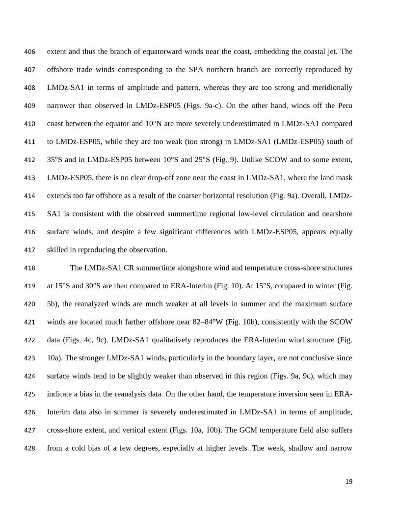
19

extent and thus the branch of equatorward winds near the coast, embedding the coastal jet. The 406

offshore trade winds corresponding to the SPA northern branch are correctly reproduced by 407

LMDz-SA1 in terms of amplitude and pattern, whereas they are too strong and meridionally 408

narrower than observed in LMDz-ESP05 (Figs. 9a-c). On the other hand, winds off the Peru 409

coast between the equator and 10°N are more severely underestimated in LMDz-SA1 compared 410

to LMDz-ESP05, while they are too weak (too strong) in LMDz-SA1 (LMDz-ESP05) south of 411

35°S and in LMDz-ESP05 between 10°S and 25°S (Fig. 9). Unlike SCOW and to some extent, 412

LMDz-ESP05, there is no clear drop-off zone near the coast in LMDz-SA1, where the land mask 413

extends too far offshore as a result of the coarser horizontal resolution (Fig. 9a). Overall, LMDz-414

SA1 is consistent with the observed summertime regional low-level circulation and nearshore 415

surface winds, and despite a few significant differences with LMDz-ESP05, appears equally 416

skilled in reproducing the observation. 417

The LMDz-SA1 CR summertime alongshore wind and temperature cross-shore structures 418

at 15°S and 30°S are then compared to ERA-Interim (Fig. 10). At 15°S, compared to winter (Fig. 419

5b), the reanalyzed winds are much weaker at all levels in summer and the maximum surface 420

winds are located much farther offshore near 82–84°W (Fig. 10b), consistently with the SCOW 421

data (Figs. 4c, 9c). LMDz-SA1 qualitatively reproduces the ERA-Interim wind structure (Fig. 422

10a). The stronger LMDz-SA1 winds, particularly in the boundary layer, are not conclusive since 423

surface winds tend to be slightly weaker than observed in this region (Figs. 9a, 9c), which may 424

indicate a bias in the reanalysis data. On the other hand, the temperature inversion seen in ERA-425

Interim data also in summer is severely underestimated in LMDz-SA1 in terms of amplitude, 426

cross-shore extent, and vertical extent (Figs. 10a, 10b). The GCM temperature field also suffers 427

from a cold bias of a few degrees, especially at higher levels. The weak, shallow and narrow 428

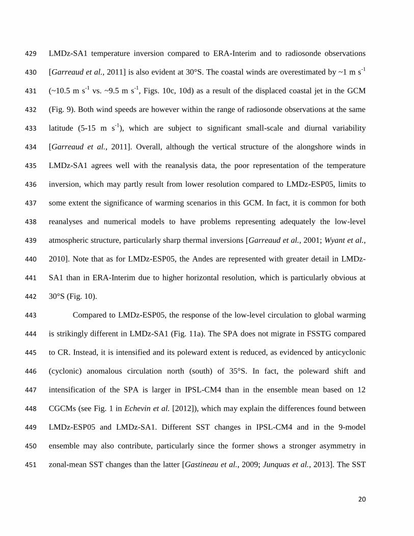
20

LMDz-SA1 temperature inversion compared to ERA-Interim and to radiosonde observations 429

[Garreaud et al., 2011] is also evident at 30°S. The coastal winds are overestimated by ~1 m s-1

430

(~10.5 m s-1

vs. ~9.5 m s-1

, Figs. 10c, 10d) as a result of the displaced coastal jet in the GCM 431

(Fig. 9). Both wind speeds are however within the range of radiosonde observations at the same 432

latitude (5-15 m s-1

), which are subject to significant small-scale and diurnal variability 433

[Garreaud et al., 2011]. Overall, although the vertical structure of the alongshore winds in 434

LMDz-SA1 agrees well with the reanalysis data, the poor representation of the temperature 435

inversion, which may partly result from lower resolution compared to LMDz-ESP05, limits to 436

some extent the significance of warming scenarios in this GCM. In fact, it is common for both 437

reanalyses and numerical models to have problems representing adequately the low-level 438

atmospheric structure, particularly sharp thermal inversions [Garreaud et al., 2001; Wyant et al., 439

2010]. Note that as for LMDz-ESP05, the Andes are represented with greater detail in LMDz-440

SA1 than in ERA-Interim due to higher horizontal resolution, which is particularly obvious at 441

30°S (Fig. 10). 442

Compared to LMDz-ESP05, the response of the low-level circulation to global warming 443

is strikingly different in LMDz-SA1 (Fig. 11a). The SPA does not migrate in FSSTG compared 444

to CR. Instead, it is intensified and its poleward extent is reduced, as evidenced by anticyclonic 445

(cyclonic) anomalous circulation north (south) of 35°S. In fact, the poleward shift and 446

intensification of the SPA is larger in IPSL-CM4 than in the ensemble mean based on 12 447

CGCMs (see Fig. 1 in Echevin et al. [2012]), which may explain the differences found between 448

LMDz-ESP05 and LMDz-SA1. Different SST changes in IPSL-CM4 and in the 9-model 449

ensemble may also contribute, particularly since the former shows a stronger asymmetry in 450

zonal-mean SST changes than the latter [Gastineau et al., 2009; Junquas et al., 2013]. The SST 451

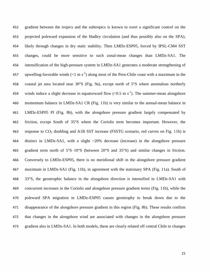
21

gradient between the tropics and the subtropics is known to exert a significant control on the 452

projected poleward expansion of the Hadley circulation (and thus possibly also on the SPA), 453

likely through changes in dry static stability. Then LMDz-ESP05, forced by IPSL-CM4 SST 454

changes, could be more sensitive to such zonal-mean changes than LMDz-SA1. The 455

intensification of the high-pressure system in LMDz-SA1 generates a moderate strengthening of 456

upwelling-favorable winds (<1 m s-1

) along most of the Peru-Chile coast with a maximum in the 457

coastal jet area located near 30°S (Fig. 9a), except north of 5°S where anomalous northerly 458

winds induce a slight decrease in equatorward flow (<0.5 m s-1

). The summer-mean alongshore 459

momentum balance in LMDz-SA1 CR (Fig. 11b) is very similar to the annual-mean balance in 460

LMDz-ESP05 PI (Fig. 8b), with the alongshore pressure gradient largely compensated by 461

friction, except South of 35°S where the Coriolis term becomes important. However, the 462

response to CO2 doubling and A1B SST increase (FSSTG scenario, red curves on Fig. 11b) is 463

distinct in LMDz-SA1, with a slight ~20% decrease (increase) in the alongshore pressure 464

gradient term north of 5°S–10°S (between 20°S and 35°S) and similar changes in friction. 465

Conversely to LMDz-ESP05, there is no meridional shift in the alongshore pressure gradient 466

maximum in LMDz-SA1 (Fig. 11b), in agreement with the stationary SPA (Fig. 11a). South of 467

33°S, the geostrophic balance in the alongshore direction is intensified in LMDz-SA1 with 468

concurrent increases in the Coriolis and alongshore pressure gradient terms (Fig. 11b), while the 469

poleward SPA migration in LMDz-ESP05 causes geostrophy to break down due to the 470

disappearance of the alongshore pressure gradient in this region (Fig. 8b). These results confirm 471

that changes in the alongshore wind are associated with changes in the alongshore pressure 472

gradient also in LMDz-SA1. In both models, these are clearly related off central Chile to changes 473

22

in the SPA position and/or intensity, whereas the origin of opposite changes off Peru are less 474

clear. 475

3.5. Vorticity budget and precipitation/wind/SST feedbacks off Peru 476

Winds off the coast of Peru may be too far from the SPA to be significantly affected by 477

its intensification, although they might be affected by its poleward shift and the related 478

alongshore pressure gradient decrease, inducing a weakening in upwelling-favorable winds and 479

Ekman suction. This may be one reason why the wind reduction off Peru is weaker and confined 480

to the north in the LMDz-SA1 model compared to the LMDz-ESP05 model, since the SPA 481

expands southward only in the latter. However, this may not be the whole story. If alongshore 482

wind changes off Peru were solely driven by changes in the SPA characteristics, there would 483

likely be relatively little dispersion in the responses simulated by CMIP3 CGCMs, as is the case 484

off Chile (Fig. 2), the SPA migration being a relatively consistent feature among the models 485

[Garreaud and Falvey, 2009]. This is not the case, especially in austral winter when the SPA is 486

located in its northernmost position (Fig. 2). Another possibility is related to the existence of 487

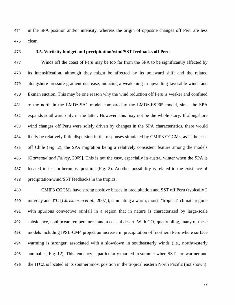
precipitation/wind/SST feedbacks in the tropics. 488

CMIP3 CGCMs have strong positive biases in precipitation and SST off Peru (typically 2 489

mm/day and 3°C [Christensen et al., 2007]), simulating a warm, moist, "tropical" climate regime 490

with spurious convective rainfall in a region that in nature is characterized by large-scale 491

subsidence, cool ocean temperatures, and a coastal desert. With CO2 quadrupling, many of these 492

models including IPSL-CM4 project an increase in precipitation off northern Peru where surface 493

warming is stronger, associated with a slowdown in southeasterly winds (i.e., northwesterly 494

anomalies, Fig. 12). This tendency is particularly marked in summer when SSTs are warmer and 495

the ITCZ is located at its southernmost position in the tropical eastern North Pacific (not shown). 496

23

The increase in rainfall may be the result of increased moisture content and transport in the 497

atmosphere [Held and Soden, 2006] or of a reduction in static stability associated with relatively 498

strong surface warming in the 4CO2 scenario. It is likely associated with an increase in 499

convection and cloud formation in the presence of warmer than observed SST in the CGCMs. 500

The CGCM tendency toward reduced winds and increased precipitation off northern Peru 501

(Fig. 12) is qualitatively reproduced in LMDz-ESP05 in summer, with a strong increase in 502

rainfall (1–2 mm/day or more) off central and northern Peru north of 10°S–15°S (Fig. 13a). 503

Changes in rainfall are weak elsewhere and in winter (Fig. 13b). In LMDz-SA1, rainfall also 504

increases significantly in summer by 0.5–1 mm/day near 5°S–10°S [Junquas et al., 2013; their 505

Fig. 8b]. This region is located just south of northerly wind anomalies and is characterized by 506

anomalous surface wind convergence in the model (Fig. 11a). Note that LMDz-SA1 has almost 507

no bias in precipitation over the ocean in the PCUS compared to observed climatologies 508

[Junquas et al., 2013; their Fig. 4c], while biases in the LMDz-ESP05 CR are much weaker than 509

in CGCM 20C3M simulations (not shown). 510

The analysis of the steady-state vorticity balance on the β-plane can help understanding 511

the dynamical relationship between alongshore wind and vertical motion, which in turn can be 512

associated with moist convection [e. g. Kodama, 1999] and subsidence [e. g. Takahashi and 513

Battisti, 2007b]. For simplicity, consider the case of a purely meridional eastern boundary. 514

Equations (1) and (3) then become the meridional and zonal momentum budgets, respectively. 515

We then subtract the meridional derivative of (3) from the zonal derivative of (1) to derive a 516

vorticity balance: 517

U V W U W VU V W

t x x y y y z x z z

518

24

m mV UU VV f

x y x y

, (6) 519

where V x U y is relative vorticity and β is the meridional gradient of the Coriolis 520

parameter f. At steady state 0t , using the continuity equation 521

U x V y W z that relates surface wind convergence to convection, we obtain the 522

vorticity balance 523

m mV UU V W U W V WV U V W f

x x y y y z x z z z x y

524

(7) 525

Equation (7) states that planetary vorticity (term on the left-hand side) is balanced by the 526

sum of the curl of advection (seven terms in brackets on the right-hand side), vortex stretching 527

(proportional to W z , i.e. to convection/subsidence), and the curl of friction (two terms in 528

brackets on the right-hand side). From the previous analysis of the momentum bugets, it is 529

suspected that the advection term has a weak contribution to the vorticity balance, which is 530

indeed verified (see below). Hence, in regions where changes in the frictional term are small, a 531

decrease (increase) in planetary vorticity and thus in equatorward alongshore wind is then 532

associated with anomalous upward (downward) motion. 533

Similarly to the momentum balances, the vorticity balance is computed from the monthly 534

mean climatological LMDz-ESP05 outputs and from the DJF seasonal mean LMDz-SA1 535

outputs. The residuals of the meridional and zonal momentum balances are used to estimate the 536

curl of friction. Fig. 14 shows the vorticity balance and its change in the climate scenarios for the 537

two GCMs off Peru in summer when the rainfall anomalies occur (Fig. 13a). In both cases, the 538

balance was found to be approximately closed with a negligible residual (not shown). Note that 539

25

successive differenciations used to derive the momentum and vorticity budgets introduce a low 540

signal-to-noise ratio near the coast, where cross-shore gradients in surface winds and sea level 541

pressure are large due to the presence of the Andes. Therefore, the analysis is not appropriate for 542

the nearshore region, but is suitable to infer the dynamics of wind changes in the offshore region 543

where precipitation anomalies are found (Fig. 13a). 544

In both GCMs, the balances are similar, with planetary vorticity balanced by the sum of 545

vortex stretching and the curl of friction (white contours on Fig. 14). The contribution of the curl 546

of advection is found to be weak compared to the other terms (Figs. 14d, 14h), which confirms 547

our hypothesis. The friction term dominates in the regions where convection occurs 548

( 0f W z ) in the LMDz-ESP05 PI (near 5°S–10°S, Figs. 14b-c) and LMDz-SA1 CR (near 549

5°S–15°S, Figs. 14f-g) simulations. The opposite tends to take place further south with planetary 550

vorticity and vortex stretching in approximate balance. 551

With CO2 quadrupling, a strong negative anomaly of vortex stretching near 5°S–14°S 552

(shading on Fig. 14b) is associated with an increase in precipitation (Fig. 13a). This anomaly is 553

only partially equilibrated by a concurrent increase in the friction term (Fig. 14c) because it is 554

itself mostly compensated by a negative anomaly in the advection term (Fig. 14d). Therefore, the 555

northwesterly wind anomaly in the region of precipitation increase (and convective anomaly) 556

between PI and 4CO2 (Fig. 13a) may be interpreted dynamically as the result of approximately 557

balanced reductions in vortex stretching and planetary vorticity with global warming (Figs. 14a-558

b). In LMDz-SA1, only a weak negative anomaly of vortex stretching appears near 5°S–10°S 559

(Fig. 14f) and is compensated by the curls of friction (Fig. 14g) and advection (Fig. 14h), leading 560

to weak wind changes in this region (Fig. 14a) despite the increase in rainfall [Fig. 8b by 561

Junquas et al., 2013]. Such differences between the convective anomalies in the two GCMs may 562

26

be related to the much stronger (twice or more) rainfall increase in LMDz-ESP05 compared to 563

LMDz-SA1. It was checked that similar results were obtained in LMDz-ESP05 with CO2 564

doubling but with weaker changes, consistent with the quasi-linear response to greenhouse gas 565

increase found throughout this paper. 566

In contrast, in the equatorial region (0°N–5°S), the reduction in planetary vorticity rather 567

appears to be associated with a reduction in the curl of friction, both in LMDz-ESP05 and 568

LMDz-SA1 (Figs. 14a, 14c, 14e, 14g), suggesting the same process is taking place in the two 569

GCMs. Both vortex stretching and its change are weak in this region (Figs. 14b, 14f), partly 570

because the Coriolis parameter vanishes at the equator. These results suggest that equatorial and 571

off-equatorial wind changes are driven by different dynamics and that wind/precipitation 572

feedbacks only play a role away from the equator. This provides a possible explanation for the 573

differences in wind and rainfall changes in LMDz-ESP05 and LMDz-SA1. Note that the patch of 574

rainfall increase near the equator in LMDz-ESP05 (Fig. 13a) is not associated with a convective 575

anomaly (Fig. 14b), suggesting it may result from southward anomalous moisture transport from 576

the ITCZ north of the equator. 577

578

4. Discussion and conclusions 579

Regional dynamical downscaling using the LMDz GCM was performed in the Peru-Chile 580

upwelling system to study changes in alongshore surface wind and wind stress curl over the 581

ocean due to global warming. Three idealized climate scenarios (with constant preindustrial, 582

doubled, and quadrupled CO2 concentrations in the atmosphere) from the IPSL-CM4 CGCM 583

were downscaled to examine the surface wind changes and the physical mechanisms at stake. 584

Our results show a weakening of upwelling-favorable winds and Ekman suction off Peru and 585

27

northern Chile, and an intensification off central Chile, with a quasi-linear response to CO2 586

increase. The robustness of these projections was assessed by comparing with a different 587

configuration of the LMDz GCM run under other climate scenarios (20th

century climate and 588

A1B scenario with doubled CO2 concentrations) and CGCM SST forcing (multimodel ensemble 589

mean), in which case reduced winds were only found off northern Peru with intensified winds 590

elsewhere. While quantitatively different, the results from this sensitivity experiment suggest that 591

opposed wind projections, with a weakening off Peru and a strengthening off Chile, may be 592

robust features in the climate scenarios. 593

Consistently with previous studies, the presence of the Andes precludes the establishment 594

of the geostrophic equilibrium in the alongshore direction, imposing a balance between the 595

alongshore pressure gradient and friction in both GCMs [Muñoz and Garreaud, 2005; Garreaud 596

and Falvey, 2009]. In the Chile region, the increase in coastal winds is thus likely due to a 597

poleward displacement and/or an intensification of the maximum alongshore pressure gradient 598

(Figs. 8b, 11b) due to similar changes in the South Pacific anticyclone (SPA; Figs. 6, 11a) and 599

Hadley circulation [e.g., Lu et al., 2007; Previdi and Liepert, 2007]. Further north off Peru, the 600

reduction in coastal winds and Ekman suction may be related either to the SPA southward shift 601

and the associated reduction in the alongshore pressure gradient, or to summertime anomalous 602

upward motion and associated negative vortex stretching anomaly in both the global CMIP3 603

models and the higher-resolution LMDz-ESP05 GCM. Although the dynamical relation (7) does 604

not indicate causality, changes in vertical velocity might be associated with changes in 605

convective precipitation, so the summertime wind reduction off Peru in LMDz-ESP05 could be a 606

result of enhanced convection and rainfall due to the warming of the ocean surface and 607

associated decrease in static stability. In addition to the direct greenhouse gas forcing, the ocean 608

28

warming could also be forced through the equatorial Pacific dynamical response to future global 609

warming, which includes a weakening of the Walker circulation and a flattening of the 610

thermocline [Vecchi and Soden, 2007]. The resulting weakening of the wind could provide a 611

positive feedback that would amplify the initial response. However, given the strong biases in 612

present-climate rainfall and SST off Peru in the CGCMs, the relevance of the projected 613

precipitation/SST changes to the real climate is not clear yet. Other forcing and feedback 614

processes involving low-level clouds may also be contributing to the changes in precipitation, 615

SST and winds, but their analysis is beyond the scope of this paper. 616

These results also raise an important point: how do we reconcile the climate-change wind 617

decrease with the enhanced trade winds during El Niño events, both near the coast and at the 618

large scale [Wyrkti, 1975; Enfield, 1981; Huyer et al., 1987; Halpern, 2002]? This increase could 619

be explained by an enhancement of the land-sea thermal contrast due to changes in coastal 620

cloudiness [Enfield, 1981], but perhaps more likely by the enhanced alongshore thermal gradient 621

associated with maximum warming off northern Peru, as suggested by in-phase relation between 622

the changes in alongshore wind and SST gradients (e.g. Fig. 9 by Rasmusson and Carpenter 623

[1982]), as well as by atmospheric model experiments [Quijano-Vargas, 2011]. The alongshore 624

SST gradient anomalies in climate-change simulations (Fig. 12) appear to be substantially 625

weaker than during the observed El Niño, so the wind response should also be expected to be 626

weaker. On the other hand, northerly wind anomalies have also been observed during El Niño, 627

but to the north of the maximum warming [Rasmusson and Carpenter, 1982]. This was more 628

dramatic during the 1925-1926 El Niño, when strong northerlies and the ITCZ invaded the 629

southern hemisphere [Takahashi, K., A. G. Martínez, and K. Mosquera-Vásquez, The very 630

strong 1925-26 El Niño in the far eastern Pacific, revisited, Clim. Dyn., in prep.]. A situation like 631

29

the latter is unrealistically common in coupled GCMs, likely a reflection of their large biases in 632

this region. 633

We now discuss the limits of our approach. A first limitation is the use of a single GCM, 634

LMDz, which limits the robustness of our findings. However, results show that LMDz is able to 635

reproduce distinct processes leading to opposite wind changes off the coast of Peru, depending 636

on SST forcing and model configuration. Using distinct CGCM, scenario, and atmospheric 637

model, Garreaud and Falvey [2009] found a fall-winter wind increase of 0.4–0.8 m s-1

in the 638

core of the Chilean coastal jet (near 25°S–35°S), which is close to the wind change (0.5–1 m s-1

) 639

in the coastal jet core (near 30°S–37°S) in both LMDz-ESP05 and LMDz-SA1. Our results are 640

also in line with previous findings obtained from statistical downscaling of the same IPSL-CM4 641

scenarios [Goubanova et al., 2011]. In their study, wind changes off Peru and northern Chile 642

were moderate, with a maximum decrease of ~5% (2CO2) to ~10% (4CO2) off Peru in summer 643

and almost no change during winter. Similarly to our study, the largest increase occurred in 644

summer south of 35°S and reached ~10% in 2CO2 and 10–20% in 4CO2, respectively. The main 645

discrepancy between our results and theirs is the stronger decrease off central Chile (10–20%) 646

and central Peru (20–30%) in summer in our simulations. They thus corroborate the assumption 647

of persistence of model-data statistical relations with climate change that was made as part of the 648

statistical downscaling procedure. Using the statistical downscaling method of Goubanova et al. 649

[2011], Goubanova and Ruiz [2010] studied an ensemble of 12 CGCMs under the SRES A2 650

scenario [Nakicenovic et al., 2000]. They found a moderate ensemble-mean wind increase (less 651

than 0.3 m s-1

) during winter and a weak decrease (less than 0.2 m s-1

) in summer off Peru. Off 652

Chile, the wind increases substantially (0.4–0.6 m s-1

near 24°S–32°S) during winter and the 653

increase is weaker (0.1–0.2 m s-1

) during summer. Further south near 35°S–40°S, the wind 654

30

increases strongly all year round, peaking (~0.9 m s-1

) in March-April and in September-655

November. Hence, although different climate scenarios were analyzed here, results from both 656

studies are consistent with our projections for the Chile region. The Goubanova and Ruiz [2010] 657

study that included the Peru region also found reduced summertime winds there, which gives us 658

confidence in the projected changes off Peru. 659

These modelling results, like those of Goubanova et al. [2011] and Goubanova and Ruiz 660

[2010], are consistent with the trends in upwelling-favorable winds observed in the last decades 661

using adjusted ship-based measurements from the Wave and Anemometer-based Sea-surface 662

Wind (WASWind) [Tokinaga and Xie, 2011] to correct for spurious positive trends due to an 663

increase in anemometer height [Cardone et al., 1990]. Indeed, WASWind data shows little signal 664

off Peru but an increase off central Chile (Fig. 1), significantly smaller and even reversed relative 665

to the initial estimations by Bakun [1990]. Although Bakun [1990]’s argument that an increased 666

cross-shore temperature gradient due to increased warming over land drives an increased 667

equatorward wind may hold for several eastern boundary upwelling systems [Falvey and 668

Garreaud, 2009; Snyder et al., 2002; Miranda et al., 2012], it is not clear whether it is important 669

in the Peru region. 670

Indeed, such mechanism requires the intensification of a thermal low-pressure cell over 671

land – and thus of the cross-shore pressure gradient – driving an intensification of equatorward 672

geostrophic wind [Bakun, 1990]. In the model results presented here, the intensified cross-shore 673

temperature gradient is associated with a reduction in the cross-shore pressure gradient off Peru 674

and a weakening of alongshore winds. An increased land-sea thermal gradient may thus not 675

necessarily lead to a wind increase in the Peru region. This will have to be verified using other 676

models with a higher spatial resolution. Note that the recent analysis of observed wind and SST 677

31

trends suggests that similarly to Peru, the Iberian and North African eastern boundary upwelling 678

systems show no significant increase in upwelling-favorable winds and even a warming of the 679

coastal zone [Barton et al., 2013], in disagreement with Bakun [1990]'s hypothesis. 680

A potential limitation of our study is the relatively modest spatial resolutions attained in 681

the LMDz-ESP05 and LMDz-SA1 zooms (~50 km and ~100 km, respectively). Although the 682

relatively low vertical resolution (19 levels) could have an effect on the simulation near the 683

surface, Wyant et al. [2010] did not find any clear relationship between vertical resolution and 684

model skill in simulating the boundary layer structure. Small-scale effects, such as those 685

associated with coastal capes [Boé et al., 2011], sea breeze [Franchito et al., 1998], intensified 686

temperature gradient induced by the warming of the narrow desertic plains located between the 687

coast and the high Andes off Peru and northern Chile (~ 1-2 grid points in our models) could also 688

have an effect. Yet, using the MM5 regional climate model [Grell et al., 1994] in the central 689

Peru coastal jet region at higher horizontal resolutions than in our models (45 km, 15 km, and 5 690

km), Quijano-Vargas [2011] found that friction equilibrated the alongshore pressure gradient, in 691

agreement with Muñoz and Garreaud [2005] and this study. He however found that for 692

mesoscale features, the advection of momentum contributed significantly to the balance in some 693

specific areas of the coastal jet region. 694

Another limitation of our study is the absence of two-way feedback between the ocean 695

and the atmosphere in our regional, SST-forced experiments. The SST fields forcing the GCM 696

are composed of a medium-scale climatology (AMIP, ~1°) and a large-scale SST anomaly from 697

the CGCM (~2°). While the climatological field partly represents the upwelling mesoscale cross-698

shore SST gradient, the spatial scales of the SST anomalies are larger and cross-shore gradients 699

could be underestimated. Regional ocean simulations forced by the LMDz-ESP05 CR wind 700

32

stress fields show that small-scale cross-shore SST gradients are larger (~2.10-5

°C m-1

) near the 701

Peru coast [Oerder, V., F. Colas, V. Echevin, F. Codron, J. Tam, and A. Belmadani, Peru-Chile 702

upwelling dynamics under climate change, Clim. Dyn., in prep.] than in AMIP SST fields (<10-5

703

°C m-1

, not shown). Mesoscale variations in SST may induce variations in the surface wind 704

[Chelton et al., 2007; Small et al., 2008; Boé et al., 2011; Perlin et al., 2011; Renault et al., 705

2012] with a potentially strong impact on the upwelling dynamics (e.g., Jin et al. [2009]). 706

Clearly, a regional ocean-land-atmosphere coupled model is needed to investigate such processes 707

and assess their impact on coastal winds, upwelling and the marine ecosystem. 708

709

Acknowledgements 710

The LMDz-ESP05 simulations were performed on Brodie, the NEC SX8 computer at 711

Institut du Développement et des Ressources en Informatique Scientifique (IDRIS), Orsay, 712

France. The LMDz-SA1 simulations were performed on Calcul Intensif pour le Climat, 713

l’Atmosphère et la Dynamique (CICLAD), a PC cluster at IPSL, within the framework of 714

previous research supported by the European Commission’s Seventh Framework Programme 715

(FP7/2007-2013) under Grant Agreement N°212492 (CLARIS LPB. A Europe-South America 716

Network for Climate Change Assessment and Impact Studies in La Plata Basin), CNRS/LEFE 717

Program, and CONICET PIP 112-200801-00399. A. Belmadani was supported by the Agence 718

Nationale de la Recherche (ANR) Peru Ecosystem Projection Scenarios (PEPS, ANR-08-RISK-719

012) project. Additional support was provided by the Japan Agency for Marine-Earth Science 720

and Technology (JAMSTEC), by the National Aeronautics and Space Administration (NASA) 721

through grant NNX07AG53G, and by the National Oceanic and Atmospheric Administration 722

(NOAA) through grant NA11NMF4320128, which sponsor research at the IPRC. A. Belmadani 723

33

is now supported by the Universidad de Concepcion (UdeC). V. Echevin and C. Junquas are 724

supported by the Institut de Recherche pour le Développement (IRD). F. Codron is supported by 725

the Université Pierre et Marie Curie (UPMC). K. Takahashi is supported by the Instituto 726

Geofisico del Peru (IGP). K. Hamilton, A. Lauer, and Y. Wang are thanked for fruitful 727

discussions. This is the IPRC/SOEST publication #XXXX/YYYY. 728

729

References 730

Albert, A., V. Echevin, M. Lévy, and O. Aumont (2010), Impact of nearshore wind stress curl on 731

coastal circulation and primary productivity in the Peru upwelling system, J. Geophys. Res., 732

115, C12033, doi:10.1029/2010JC006569. 733

Arakelian, A., and F. Codron (2012), Southern hemisphere jet variability in the IPSL GCM at 734

varying resolutions, J. Atmos. Sci., 56, 4032–4048. 735

Bakun, A. (1990), Global climate change and intensification of coastal upwelling, Science, 247, 736

198–201, doi:10.1126/science.247.4939.198. 737

Bakun, A., and S. J. Weeks (2008), The marine ecosystem off Peru: What are the secrets of its 738

fishery productivity and what might its future hold?, Prog. Oceanogr., 79, 290–299, 739

doi:10.1016/j.pocean.2008.10.027. 740

Bakun, A., D. Field, A. Renondo-Rodriguez, and S. J. Weeks (2010), Greenhouse gas, upwelling 741

favourable winds, and the future of upwelling systems, Global Change Biol., 16, 1,213–1,228, 742

doi:10.1111/j.1365-2486.2009.02094.x. 743

Barton, E. D., D. B. Field, and C. Roy (2013), Canary current upwelling: More or less?, Prog. 744

Oceanogr., doi:10.1016/j.pocean.2013.07.007, in press. 745

34

Belmadani, A., B. Dewitte, and S.-I. An (2010), ENSO feedbacks and associated time scales of 746

variability in a multimodel ensemble, J. Clim., 23, 3,181–3,204, doi:10.1175/2010JCLI2830.1. 747

Boé, J., A. Hall, F. Colas, J. C. McWilliams, X. Qu, J. Kurian, and S. B. Kapnick (2011), What 748

shapes mesoscale wind anomalies in coastal upwelling zones?, Clim. Dyn., 36(11-12), 2037-749

2049, doi:10.1007/s00382-011-1058-5. 750

Boville, B. A., and P. R. Gent (1998), The NCAR climate system model, version one, J. Clim., 751

11, 1,115–1,130, doi:10.1175/1520-0442(1998)011<1115:TNCSMV>2.0.CO:2. 752

Capet, X. J., P. Marchesiello, and J. C. McWilliams (2004), Upwelling response to coastal wind 753

profiles, Geophys. Res. Lett., 31, L13311, doi:10.1029/2004GL020123. 754

Cardone, V. J., J. G. Greenwood, and M. A. Cane (1990), On trends in historical marine wind 755

data, J. Clim., 3, 113–127, doi:10.1175/1520-756

0442(1990)003%3C0113%3AOTIHMW%3E2.0.CO%3B2. 757

Chavez, F. P. (1995), A comparison of ship and satellite chlorophyll from California and Peru, J. 758

Geophys. Res., 100, 24,855–24,862, doi:10.1029/95JC02738. 759

Chavez, F. P., A. Bertrand, R. Guevara-Carrasco, P. Soler, and J. Csirke (2008), The northern 760

Humboldt Current System: Brief history, present status and a view towards the future, Prog. 761

Oceanogr., 79, 95–105, doi:10.1016/j.pocean.2008.10.012. 762

Chelton, D. B., M. G. Schlax, and R. M. Samelson (2007), Summertime coupling between sea 763

surface temperature and wind stress in the California Current System, J. Phys. Oceanogr., 37, 764

495–517. 765

Chen, W., Z. Jiang, L. Li, and P. Yiou (2011), Simulation of regional climate change under the 766

IPCC A2 scenario in southeast China, Clim. Dyn., 36, 491–507. 767

35

Christensen, J. H., et al. (2007), Regional Climate Projections, in Climate Change 2007: The 768

Physical Science Basis, Contribution of Working Group I to the Fourth Assessment Report of 769

the Intergovernmental Panel on Climate Change, edited by S. Solomon, D. Qin, M. Manning, 770

Z. Chen, M. Marquis, K. B. Averyt, M. Tignor and H. L. Miller, Cambridge University Press, 771

Cambridge, United Kingdom and New York, NY, USA. 772

Dee, D. P., et al. (2011), The ERA-Interim reanalysis: Configuration and performance of the data 773

assimilation system, Quart. J. Roy. Met. Soc., A, 137, 553–597, doi:10.1002/qj.828. 774

Demarcq, H. (2009), Trends in primary production, sea surface temperature and wind in 775

upwelling systems (1998–2007), Prog. Oceanogr., 83, 376–385, doi:10.1016/j.pocean.2009. 776

07.022. 777

Echevin, V., K. Goubanova, A. Belmadani, and B. Dewitte (2012), Sensitivity of the Humboldt 778

Current system to global warming: A downscaling experiment of the IPSL-CM4 model, Clim. 779

Dyn., 38, 3–4, 761–774, doi:10.1007/s00382-011-1085-2. 780

Enfield, D. B. (1981), Thermally-driven wind variability in the planetary boundary layer above 781

Lima, Peru, J. Geophys. Res., 86(C3), 2005–2016, doi:10.1029/JC086iC03p02005. 782

Falvey, M., and R. Garreaud (2009), Regional cooling in a warming world: Recent temperature 783

trends in the southeast Pacific and along the west coast of subtropical South America (1979–784

2006), J. Geophys. Res., 114, D04102, doi:10.1029/2008JD010519. 785

Food and Agriculture Organization (2010), The state of world fisheries and aquaculture 2010, 786

218 pp., Fish. and Aquacult. Dep., Rome. 787

Franchito, S. H., V. B. Rao, J. L. Stech, and J. A. Lorenzzetti (1998), The effect of coastal 788

upwelling on the sea-breeze circulation at Cabo Frio, Brazil: A numerical experiment, Annales 789

Geophysicae, 16(7), 866–881. 790

36

Fréon, P., M. Barange, and J. Aristegui (2009), Eastern Boundary Upwelling Ecosystems: 791

Integrative and comparative approaches, Prog. Oceanogr., 83, 1–14. 792

Garreaud, R., and M. Falvey (2009), The coastal winds off western subtropical South America in 793

future climate scenarios, Int. J. Climatol., 29, 4, 543–554, doi:10.1002/joc.1716. 794

Garreaud, R. D., and R. C. Muñoz (2005), The low-level jet off the west coast of subtropical 795

South America: Structure and variability, Mon. Wea. Rev., 133, 2,246–2,261, 796

doi:10.1175/MWR2972.1. 797

Garreaud, R. D., J. Rutllant, J. Quintana, J. Carrasco, and P. Minnis (2001), CIMAR-5: A 798

snapshot of the lower troposphere over the subtropical southeast Pacific, Bull. Amer. Meteor. 799

Soc., 82(10), 2,193–2,207. 800

Garreaud, R. D., J. A. Rutllant, R. C. Muñoz, D. A. Rahn, M. Ramos, and D. Figueroa (2011), 801

VOCALS-CUpEx: the Chilean Upwelling Experiment, Atmos. Chem. Phys., 11, 2,015–2,029, 802

doi:10.5194/acp-11-2015-2011. 803

Gastineau, G., H. Le Treut, and L. Li (2008), Hadley circulation changes under global warming 804

conditions indicated by coupled climate models, Tellus, 60A, 863–884, doi:10.1111/j.1600-805

0870.2008.00344.x. 806

Gastineau, G., L. Li, and H. Le Treut (2009), The Hadley and Walker circulation changes in 807

global warming conditions described by idealized atmospheric simulations, J. Clim., 22, 808

3,993–4,013, doi:10.1175/2009JCLI2794.1. 809

Gordon, C., et al. (2000), The simulation of SST, sea ice extents and ocean heat transports in a 810

version of the Hadley Centre coupled model without flux adjustments, Clim. Dyn., 16, 147–811

168, doi:10.1007/s00382-005-0010. 812

37

Goubanova, K., and C. Ruiz (2010), Impact of climate change on wind-driven upwelling off the 813

coasts of Peru-Chile in a multi-model ensemble, in Climate variability in the tropical Pacific: 814

Mechanisms, modelling and observations, edited by Y. duPenhoat and A. V. Kislov, 194–201, 815

Maks-Press, Moscow, Russia. 816

Goubanova, K., V. Echevin, B. Dewitte, F. Codron, K. Takahashi, P. Terray, and M. Vrac 817

(2011), Statistical downscaling of sea-surface wind over the Peru-Chile upwelling region: 818

Diagnosing the impact of climate change from the IPSL-CM4 model, Clim. Dyn., 36, 7–8, 819

1,365–1,378, doi:10.1007/s00382-010-0824-0. 820

Grell, G. A., J. Dudhia, and D. R. Stauffer (1994), A description of the fifth-generation Penn 821

State/NCAR Mesoscale Model (MM5), Tech. Note TN-398+IA, National Center for 822

Atmospheric Research, Boulder, CO, 125 pp. 823

Gutiérrez, D., I. Bouloubassi, A. Sifeddine, S. Purca, K. Goubanova, M. Graco, D. Field, L. 824

Mejanelle, F. Velazco, A. Lorre, R. Salvatteci, D. Quispe, G. Vargas, B. Dewitte, and L. 825

Ortlieb (2011), Coastal cooling and increased productivity in the main upwelling zone off Peru 826

since the mid-twentieth century, Geophys. Res. Lett., 38, L07603, doi:10.1029/2010GL046324. 827

Halpern, D. (2002), Offshore Ekman transport and Ekman pumping off Peru during the 1997–828

1998 El Niño, Geophys. Res. Lett., 29, 1075, doi:10.1029/2001GL014097. 829

Haraguchi, P. Y. (1968), Inversions over the tropical eastern Pacific ocean, Mon. Wea. Rev., 96, 830

177–185. 831

Held, I. M., and B. J. Soden (2006), Robust responses of the hydrological cycle to global 832

warming, J. Clim., 19, 5,686–5,699, doi:10.1175/JCLI3990.1. 833

38

Hourdin, F., et al. (2006), The LMDZ4 general circulation model: Climate performance and 834

sensitivity to parametrized physics with emphasis on tropical convection, Clim. Dyn., 27, 7–8, 835

787–813, doi:10.1007/s00382-006-0158-0. 836

Hurrell, J. W., J. J. Hack, D. Shea, J. M. Caron, and J. Rosinski (2008), A new sea surface 837

temperature and sea ice boundary dataset for the Community Atmosphere Model, J. Clim., 21, 838

5,145–5,153, doi:10.1175/2008JCLI2292.1. 839

Huyer, A., R. L. Smith, and T. Paluszkiewicz (1987), Coastal upwelling off Peru during normal 840

and El Niño times, 1981–1984, J. Geophys. Res., 92(C13), 14297–14307, 841

doi:10.1029/JC092iC13p14297. 842

Jin, X., C. Dong, J. Kurian, J. C. McWilliams, D. B. Chelton, and Z. Li (2009), SST-wind 843

interaction in coastal upwelling: Oceanic simulation with empirical coupling, J. Phys. 844

Oceanogr., 39(11), 2957–2970. 845

Johanson, C. M., and Q. Fu (2009), Hadley cell widening: Model simulations versus 846

observations, J. Clim., 22, 2,713–2,725, doi:10.1175/2008JCLI2620.1. 847

Jones, R. G., M. Noguer, D. C. Hassell, D. Hudson, S. S. Wilson, G. J. Jenkins, and J. F. B. 848

Mitchell (2004), Generating high resolution climate change scenarios using PRECIS, 40 pp., 849

Met. Office Hadley Centre, Exeter. 850

Junquas, C., C. Vera, L. Li, and H. Le Treut (2012), Summer precipitation variability over 851

southeastern South America in a global warming scenario, Clim. Dyn., 38, 1867–1883. 852

Junquas, C., C. S. Vera, L. Li, and H. Le Treut (2013), Impact of projected SST changes on 853

summer rainfall in southeastern South America, Clim. Dyn., 40, 7–8, 1569–1589, 854

doi:10.1007/s00382-013-1695-y. 855

39

Kodama, Y.-M. (1999), Roles of the atmospheric heat sources in maintaining the Subtropical 856

Convergence Zones: An aqua-planet GCM study, J. Atmos. Sci., 56, 4032–4048. 857

Large, W. G., and G. Danabasoglu (2006), Attribution and impacts of upper ocean biases in 858

CCSM3, J. Clim., 19, 2,325–2,346, doi:10.1175/JCLI3740.1. 859

Lorenz, P., and D. Jacob (2005), Influence of regional scale information on the global 860

circulation: A two-way nesting climate simulation, Geophys. Res. Lett., 32, L18706, 861

doi:10.1029/2005GL023351. 862

Lu, J., G. A. Vecchi, and T. Reichler (2007), Expansion of the Hadley cell under global 863

warming, Geophys. Res. Lett., 34, L06805, doi:10.1029/2006GL028443. 864

Marti, O., et al. (2010), Key features of the IPSL ocean atmosphere model and its sensitivity to 865

atmospheric resolution, Clim. Dyn., 34, 1, 1–26, doi:10.1007/s00382-009-0640-6. 866

Miranda, P. M. A., J. M. R. Alves, and N. Serra (2012), Climate change and upwelling: 867

Response of Iberian upwelling to atmospheric forcing in a regional climate scenario, Clim. 868

Dyn., doi:10.1007/s00382-012-1442-9. 869

Mitas, C. M., and A. Clement (2005), Has the Hadley cell been strengthening in recent decades?, 870

Geophys. Res. Lett., 32, L03809, doi:10.1029/2004GL021765. 871

Muñoz, R. C., and R. D. Garreaud (2005), Dynamics of the low-level jet off the west coast of 872

subtropical South America, Mon. Wea. Rev., 133, 3,661–3,677, doi:10.1175/MWR3074.1. 873

Nakicenovic, N., et al. (2000), Special report on emissions scenarios: A special report of 874

working group III of the intergovernmental panel on climate change, 599 pp., Cambridge 875

University Press, Cambridge. 876

Nigam, S. (1997), The annual warm to cold phase transition in the eastern equatorial Pacific: 877

Diagnosis of the role of stratus cloud-top cooling, J. Clim., 10, 2447–2467. 878

40

Perlin, N., E. D. Skyllingstad, and R. M. Samelson (2011), Coastal atmospheric circulation 879

around an idealized cape during wind-driven upwelling studied from a coupled ocean-880

atmosphere model, Mon. Wea. Rev., 139, 809–829. 881

Philander, S. G. H., D. Gu, G. Lambert, N. C. Lau, and R. C. Pacanowski (1996), Why the ITCZ 882

is mostly north of the equator, J. Clim., 9, 2958–2972. 883

Pope, V., M. L. Gallani, P. R. Rowntree, and R. A. Stratton (2000), The impact of new physical 884

parameterizations in the Hadley centre climate model: HadAM3, Clim. Dyn., 16, 123–146, 885

doi:10.1007/s00382-005-0009. 886

Previdi, M., and B. G. Liepert (2007), Annular modes and Hadley cell expansion under global 887

warming, Geophys. Res. Lett., 34, L22701, doi:10.1029/2007GL031243. 888

Quijano-Vargas, J. J. (2011), Simulacion de la dinamica del viento superficial sobre la costa de 889

Ica utilizando el modelo numerico de la atmosfera de mesoescala MM5, Tesis de Maestria, 172 890

p.p., http://www.met.igp.gob.pe/publicaciones/2011/JQuijano_tesisUNMSM.pdf. 891

Rahn, D. A., and R. Garreaud (2010), Marine boundary layer over the subtropical southeast 892

Pacific during VOCALS-Rex – Part 1: Mean structure and diurnal cycle, Atmos. Chem. Phys., 893

10, 4,491–4,506, doi:10.5194/acp-10-4491-2010. 894

Rasmusson, E. M., and T. H. Carpenter (1982), Variations in tropical sea surface temperature 895

and surface wind fields associated with the Southern Oscillation/El Niño, Mon. Wea. Rev., 110, 896

354–384. 897

Renault, L., B. Dewitte, M. Falvey, R. Garreaud, V. Echevin, and F. Bonjean (2009), Impact of 898

atmospheric coastal jet off central Chile on sea surface temperature from satellite observations 899

(2000–2007), J. Geophys. Res., 114, C08006, doi:10.1029/2008JC005083. 900

41

Renault, L., B. Dewitte, P. Marchesiello, S. Illig, V. Echevin, G. Cambon, M. Ramos, O. 901

Astudillo, P. Minnis, and J. K. Ayers (2012), Upwelling response to atmospheric coastal jets 902

off central Chile: A modeling study of the October 2000 event, J. Geophys. Res., 117, C02030, 903

doi:10.1029/2011JC007446. 904

Risien, C. M., and D. B. Chelton (2008), A global climatology of surface wind and wind stress 905

fields from eight years of QuikSCAT scatterometer data, J. Phys. Oceanogr., 38, 2,379–2,413, 906

doi:10.1175/2008JPO3881.1. 907

Roeckner, E., R. Brokopf, M. Esch, M. Giorgetta, S. Hagemann, L. Kornblueh, E. Manzini, U. 908

Schlese, and U. Schulzweida (2006), Sensitivity of simulated climate to horizontal and vertical 909

resolution in the ECHAM5 atmosphere model, J. Clim., 19, 3,771–3,791, 910

doi:10.1175/JCLI3824.1. 911

Sepulchre, P., L. C. Sloan, M. Snyder, and J. Fiechter (2009), Impacts of Andean uplift on the 912

Humboldt Current system: A climate model sensitivity study, Paleoceanogr., 24, PA4215, 913

doi:10.1029/2008PA001668. 914

Small, J., S. P. DeSzoeke, S.-P. Xie, L. O'Neill, H. Seo, Q. Song, P. Cornillon, M. Spall, and S. 915

Minobe (2008), Air-sea interaction over ocean fronts and eddies, Dyn. Atmos. Oceans, 45, 916

274–319. 917

Snyder, M. A., J. L. Bell, L. C. Sloan, P. B. Duffy, and B. Govindasamy (2002), Climate 918

responses to a doubling of atmospheric carbon dioxide for a climatically vulnerable region, 919

Geophys. Res. Lett., 29, 1514, doi:10.1029/2001GL014431. 920

Snyder, M. A., L. C. Sloan, N. S. Diffenbaugh, and J. L. Bell (2003), Future climate change and 921

upwelling in the California Current, Geophys. Res. Lett., 30, 1823, 922

doi:10.1029/2003GL017647. 923

42

Steinacher, M., F. Joos, T. L. Frölicher, L. Bopp, P. Cadule, S.C. Doney, M. Gehlen, B. 924

Schneider, and J. Segschneider (2010), Projected 21st century decrease in marine productivity: 925

A multi-model analysis, Biogeosciences, 7, 979–1005. 926

Strub, P. T., J. M. Mesias, V. Montecino, J. Rutllant, and S. Salinas (1998), Coastal ocean 927

circulation off western South America, in The Sea, vol. 11, edited by A. R. Robinson and K. H. 928

Brink, pp. 273–314, John Wiley, New York, NY. 929

Sutton, R. T., B. Dong, and J. M. Gregory (2007), Land/sea warming ratio in response to climate 930

change: IPCC-AR4 model results and comparison with observations, Geophys. Res. Lett., 34, 931

L02701, doi:10.1029/2006GL028164. 932

Takahashi, K., and D. S. Battisti (2007a), Processes controlling the mean tropical Pacific 933

precipitation pattern. Part I: The Andes and the eastern Pacific ITCZ, J. Clim., 20, 3,434–934

3,451. 935

Takahashi, K., and D. S. Battisti (2007b), Processes controlling the mean tropical Pacific 936

precipitation pattern. Part II: The SPCZ and the southeast Pacific dry zone, J. Clim., 20, 5,696–937

5,706. 938

Tokinaga, H., and S.-P. Xie (2011), Wave and Anemometer-based Sea-surface Wind 939

(WASWind) for climate change analysis, J. Clim., 24, 267–285. 940

Tokinaga, H., S.-P. Xie, A. Timmermann, S. McGregor, T. Ogata, H. Kubota, and Y. M. 941

Okumura (2012a), Regional Patterns of tropical Indo-Pacific climate change: Evidence of the 942

Walker Circulation weakening, J. Clim., 25, 1,689–1,710, doi:10.1175/JCLI-D-11-00263.1. 943

Tokinaga, H., S.-P. Xie, C. Deser, Y. Kosaka, and Y. M. Okumura (2012b), Slowdown of the 944

Walker circulation driven by tropical Indo-Pacific warming, Nature, 491, 439–443, 945

doi:10.1038/nature11576. 946

43

Vargas, G., S. Pantoja, J. Rutllant, C. Lange, and L. Ortlieb (2007), Enhancement of coastal 947

upwelling and interdecadal ENSO-like variability in the Peru-Chile Current since late 19th 948

century, Geophys. Res. Lett., 34, L13607, doi:10.1029/2006GL028812. 949

Vecchi, G. A., and B. J. Soden (2007), Global warming and the weakening of the tropical Pacific 950

circulation, J. Clim., 20, 4,316–4,340, doi:10.1175/JCLI4258.1. 951

Vecchi, G. A., B. J. Soden, A. T. Wittenberg, I. M. Held, A. Leetmaa, and M. J. Harrison (2006), 952

Weakening of tropical Pacific atmospheric circulation due to anthropogenic forcing, Nature, 953

327, 216–219, doi:10.1038/nature04744. 954

Winant, C. D., C. Dorman, C. Friehe, and R. Beardsley (1988), The marine layer off northern 955

California: An example of supercritical channel flow, J. Atmos. Sci., 45, 3588–3605. 956

Wyant, M. C., et al. (2010), The PreVOCA experiment: Modeling the lower troposphere in the 957

Southeast Pacific, Atmos. Chem. Phys., 10, 4,757–4,774, doi:10.5194/acp-10-4757-2010. 958

Wyrtki, K. (1975), El Niño – The dynamic response of the equatorial Pacific Ocean to 959

atmospheric forcing, J. Phys. Oceanogr., 5, 572–584. 960

Xie, S.-P., and S. G. H. Philander (1994), A coupled ocean-atmosphere model of relevance to the 961

ITCZ in the eastern Pacific, Tellus, 46A, 340–350. 962

Xu, H., Y. Wang, and S.-P. Xie (2004), Effects of the Andes on eastern Pacific climate: A 963

regional atmospheric model study, J. Clim., 17, 589–602. 964

Zhang, R., and T. L. Delworth (2005), Simulated tropical response to a substantial weakening of 965

the Atlantic thermohaline circulation, J. Clim., 18(12), 1853–1860. 966

967

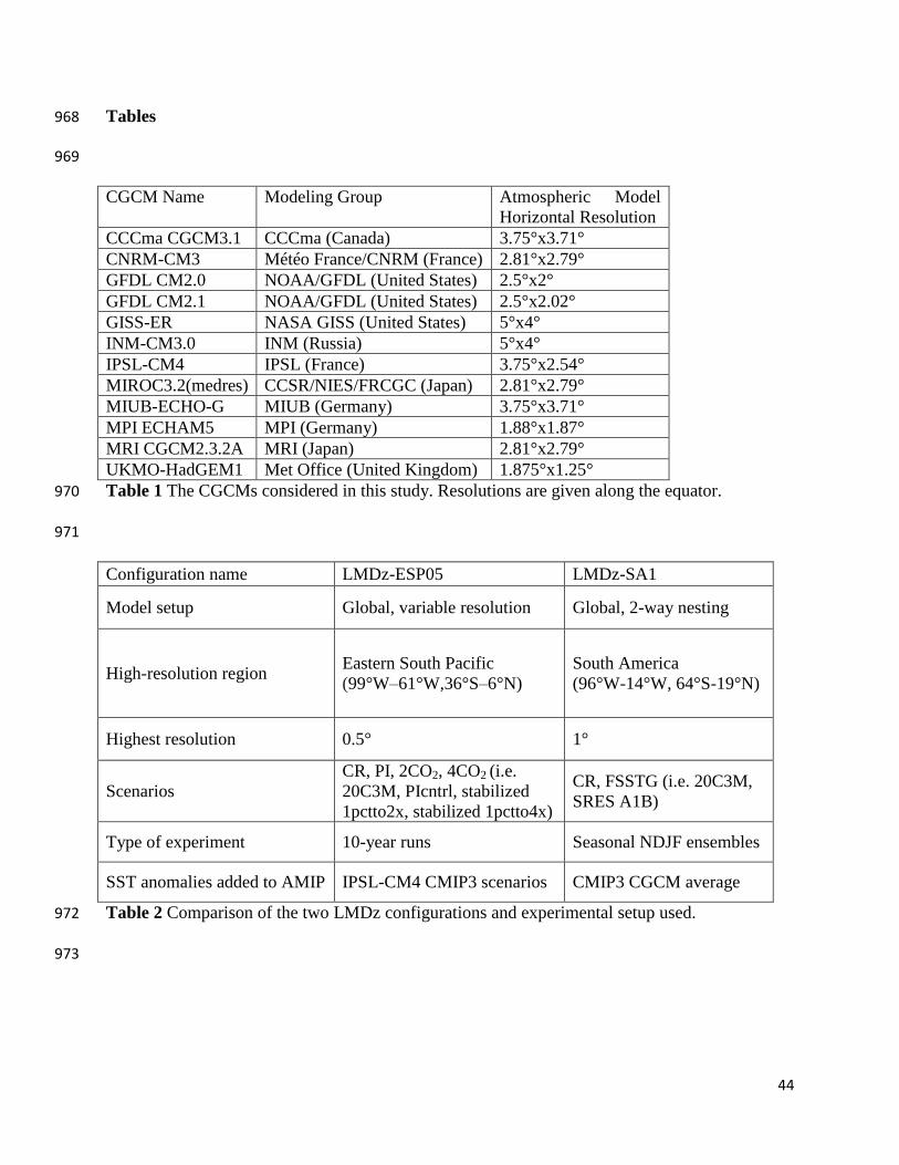
44

Tables 968

969

CGCM Name Modeling Group Atmospheric Model

Horizontal Resolution

CCCma CGCM3.1 CCCma (Canada) 3.75°x3.71°

CNRM-CM3 Météo France/CNRM (France) 2.81°x2.79°

GFDL CM2.0 NOAA/GFDL (United States) 2.5°x2°

GFDL CM2.1 NOAA/GFDL (United States) 2.5°x2.02°

GISS-ER NASA GISS (United States) 5°x4°

INM-CM3.0 INM (Russia) 5°x4°

IPSL-CM4 IPSL (France) 3.75°x2.54°

MIROC3.2(medres) CCSR/NIES/FRCGC (Japan) 2.81°x2.79°

MIUB-ECHO-G MIUB (Germany) 3.75°x3.71°

MPI ECHAM5 MPI (Germany) 1.88°x1.87°

MRI CGCM2.3.2A MRI (Japan) 2.81°x2.79°

UKMO-HadGEM1 Met Office (United Kingdom) 1.875°x1.25°

Table 1 The CGCMs considered in this study. Resolutions are given along the equator. 970

971

Configuration name LMDz-ESP05 LMDz-SA1

Model setup Global, variable resolution Global, 2-way nesting

High-resolution region Eastern South Pacific

(99°W–61°W,36°S–6°N)

South America

(96°W-14°W, 64°S-19°N)

Highest resolution 0.5° 1°

Scenarios

CR, PI, 2CO2, 4CO2 (i.e.

20C3M, PIcntrl, stabilized

1pctto2x, stabilized 1pctto4x)

CR, FSSTG (i.e. 20C3M,

SRES A1B)

Type of experiment 10-year runs Seasonal NDJF ensembles

SST anomalies added to AMIP IPSL-CM4 CMIP3 scenarios CMIP3 CGCM average

Table 2 Comparison of the two LMDz configurations and experimental setup used. 972

973

45

Figure Captions 974

975

Fig. 1 1950-2009 trend in corrected vector and scalar wind (10-2

m s-1

yr-1

) from the WASWind 976

product [Tokinaga and Xie, 2011]. Only grid cells with data available for 98% of the time or 977

more are shown. No offshore data is available due to the lack of ship tracks in this region. 978

979

Fig. 2 Linear trend in alongshore monthly surface wind near the coast (10-2

m s-1

yr-1

) in the 980

PCUS for 12 CGCMs (table 1) with increasing CO2 concentrations in the 4CO2 scenario (see 981

text) in (a) summer (December through February) and (b) winter (June through August). Winds 982

from all the CGCMs are previously interpolated bilinearly onto a common 1°x1° grid. The 983

alongshore direction and nearshore area (typically 1-2° wide) are determined using the land-sea 984

mask. Note that the IPSL-CM4 model (orange curve) agrees well with the ensemble mean over 985

the 12 CGCMs (thick black curve) except south of 30-35°S where it underestimates the wind 986

increase 987

988

Fig. 3 GCM grid for (a) LMDz-ESP05 and (b) LMDz-SA1. The red box on each panel indicates 989

the limits of the zoomed grid. 990

991

Fig. 4 Mean surface wind (m s-1

) from (a) IPSL-CM4 in the 20C3M scenario (1990-1999), (b) 992

LMDz-ESP05 in the CR, and (c) the SCOW (2000-2008). Shading and contours are for wind, 993

arrows are for wind vectors. For clarity, only one arrow was drawn for every 16 and 64 grid 994

points in (b) and (c), respectively 995

996

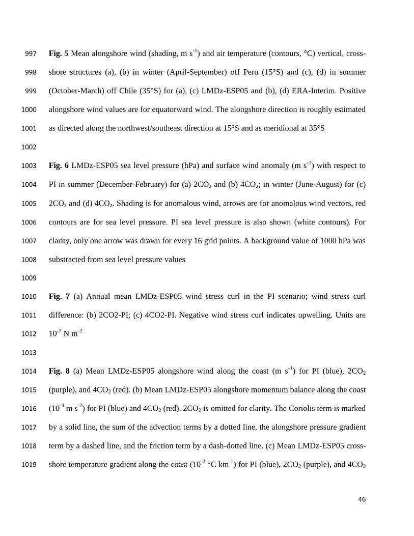
46

Fig. 5 Mean alongshore wind (shading, m s-1

) and air temperature (contours, °C) vertical, cross-997

shore structures (a), (b) in winter (April-September) off Peru (15°S) and (c), (d) in summer 998

(October-March) off Chile (35°S) for (a), (c) LMDz-ESP05 and (b), (d) ERA-Interim. Positive 999

alongshore wind values are for equatorward wind. The alongshore direction is roughly estimated 1000

as directed along the northwest/southeast direction at 15°S and as meridional at 35°S 1001

1002

Fig. 6 LMDz-ESP05 sea level pressure (hPa) and surface wind anomaly (m s-1

) with respect to 1003

PI in summer (December-February) for (a) 2CO2 and (b) 4CO2; in winter (June-August) for (c) 1004

2CO2 and (d) 4CO2. Shading is for anomalous wind, arrows are for anomalous wind vectors, red 1005

contours are for sea level pressure. PI sea level pressure is also shown (white contours). For 1006

clarity, only one arrow was drawn for every 16 grid points. A background value of 1000 hPa was 1007

substracted from sea level pressure values 1008

1009

Fig. 7 (a) Annual mean LMDz-ESP05 wind stress curl in the PI scenario; wind stress curl 1010

difference: (b) 2CO2-PI; (c) 4CO2-PI. Negative wind stress curl indicates upwelling. Units are 1011

10-7

N m-2 1012

1013

Fig. 8 (a) Mean LMDz-ESP05 alongshore wind along the coast (m s-1

) for PI (blue), 2CO2 1014

(purple), and 4CO2 (red). (b) Mean LMDz-ESP05 alongshore momentum balance along the coast 1015

(10-4

m s-2

) for PI (blue) and 4CO2 (red). 2CO2 is omitted for clarity. The Coriolis term is marked 1016

by a solid line, the sum of the advection terms by a dotted line, the alongshore pressure gradient 1017

term by a dashed line, and the friction term by a dash-dotted line. (c) Mean LMDz-ESP05 cross-1018

shore temperature gradient along the coast (10-2

°C km-1

) for PI (blue), 2CO2 (purple), and 4CO2 1019

47

(red). All quantities were computed in a one-degree coastal band using the land-sea mask to 1020

determine the alongshore and cross-shore directions (see text) 1021

1022

Fig. 9 Surface wind (m s-1

) in summer (December-February) from (a) LMDz-SA1 in the CR, (b) 1023

LMDz-ESP05 in the CR, and (c) the SCOW (2000-2008). (d) Alongshore wind in a one-degree 1024

band along the coast (m s-1

) in summer for LMDz-ESP05 (red), LMDz-SA1 (green), and SCOW 1025

(blue). Shading and contours are for wind, arrows are for wind vectors on (a-c). For clarity, only 1026

one arrow was drawn for every 4, 16, and 64 grid points in (a), (b), and (c), respectively 1027

1028

Fig. 10 Same as Fig. 5, except in DJF for (a,c) LMDz-SA1 and (b,d) ERA-Interim, at (a,b) 15°S 1029

and (c,d) 30°S 1030

1031

Fig. 11 (a) LMDz-SA1 FSSTG sea level pressure (hPa) and surface wind anomaly (m s-1

) with 1032

respect to CR in summer (December-February). Shading is for anomalous wind, arrows are for 1033

anomalous wind vectors, red contours are for sea level pressure. CR sea level pressure is also 1034

shown (white contours). For clarity, only one arrow was drawn for every 4 grid points. A 1035

background value of 1000 hPa was substracted from sea level pressure values. (b) Mean LMDz-1036

SA1 alongshore momentum balance along the coast (10-4

m s-2

) for CR (blue) and FSSTG (red). 1037

The different terms are labelled as in Fig. 8b 1038

1039

Fig. 12 Linear trend in monthly surface wind (10-2

m s-1

yr-1

), precipitation (10-2

mm day-1

yr-1

), 1040

and land/sea surface temperature (10-2

°C yr-1

) in the PCUS for 12 CGCMs (table 1) with 1041

increasing CO2 concentrations in the 4CO2 scenario. Shading is for trends in precipitation, 1042

arrows are for trends in wind vectors, white contours are for trends in surface temperature 1043

48

1044

Fig. 13 LMDz-ESP05 4CO2 surface wind anomaly (m s-1

) and precipitation anomaly (mm day-1

) 1045

with respect to PI (a) in summer (December-February) and (b) in winter (June-August). Shading 1046

and contours are for anomalous precipitation, arrows are for anomalous wind vectors. For clarity, 1047

only one arrow was drawn for every 16 grid points 1048

1049

Fig. 14 (a-d) LMDz-ESP05 PI vorticity balance and 4CO2 anomaly with respect to PI (10-10

s-2

) 1050

off Peru in DJF. Note that (a) corresponds to V and that (a) ≈ (b) + (c) + (d). (e-h) Same as (a-1051

d) except for LMDz-SA1 CR vorticity balance and FSSTG anomaly with respect to CR. Shading 1052

is for anomalous vorticity terms, contours are for DJF PI (a-d) and CR (e-h) vorticity terms 1053

Figure 1

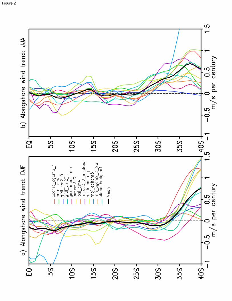
Figure 2

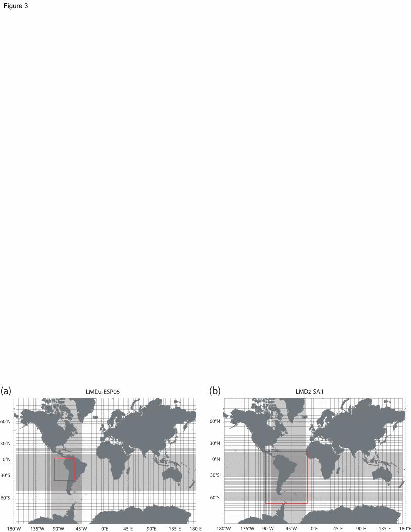
LMDz-ESP05

180°W 90°W 45°W135°W 0°E 45°E 90°E 135°E 180°E

60°S

0°N

30°S

60°N

30°N

60°S

0°N

30°S

60°N

30°N

180°W 90°W 45°W135°W 0°E 45°E 90°E 135°E 180°E

LMDz-SA1(a) (b)

Figure 3

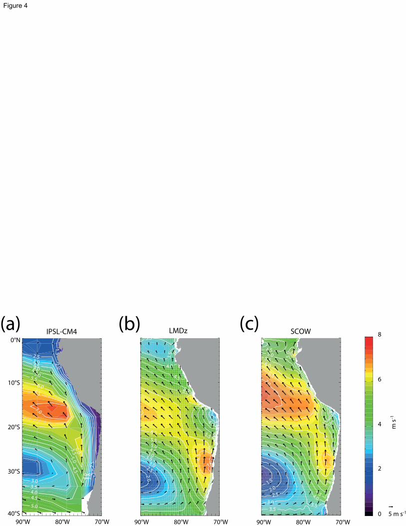
0.5

0.5

1.0

1.5

1.5

2.0

2.0

2.5

2.5

3.0

3.0

3.0

3.5

3.5

3.5

4.0

4.0

4.0

4.5

4.5

4.5

5.0

5.0

5.0

5.5

5.5

6.0

6.0

6.5

7.0

40°S

30°S

20°S

10°S

0°N

(a)

90°W 80°W 70°W

IPSL-CM4

2.0

2.5

3.0

3.5

3.5

3.5

3.5

4.0

4.0

4.0

4.5

4.5

4.5

5.0

5.0

5.0

5.5

5.5

5.56.0

6.0

6.5

7.0

(b) LMDz

90°W 80°W 70°W

1.5

2.0

2.5

3.0

3.53.5

3.5

4.0

4.0

4.5

4.5

4.5

4.5

5.0

5.0

5.05.0

5.5

5.5

5.5

6.0

6.0

6.0

6.5

7.0

SCOW(c)

90°W 80°W 70°W

0

4

2

m s

-1

5 m s-1

6

8

Figure 4

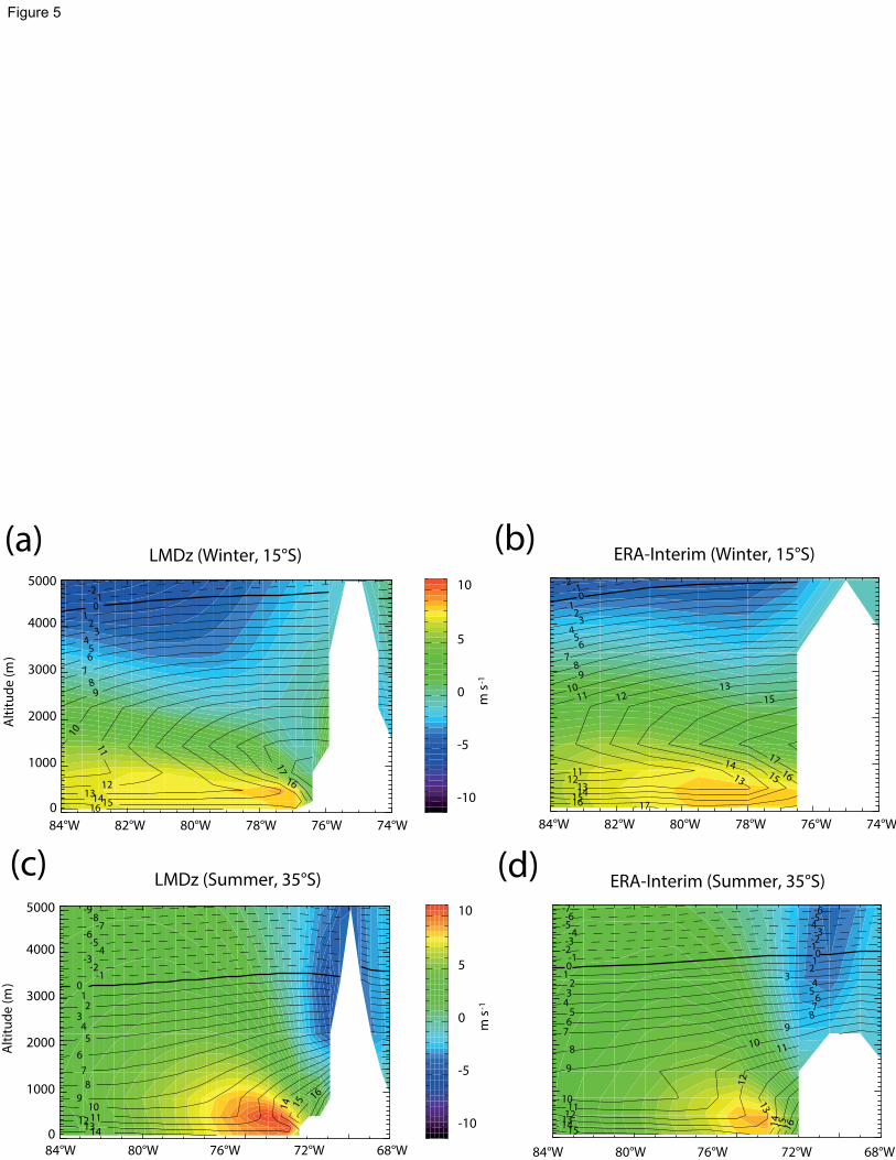
-2-10

12

34

56

7

89

10

11

1213

141516

16

17

0

1000

2000

3000

4000

5000

Alt

itu

de

(m

)

84°W 82°W 80°W 78°W 76°W 74°W

LMDz (Winter, 15°S)

0

5

10

-5

-10

m s

-1

(a)

-2-1

01

23

45

6

78

9

10

11

11

12

12

1313

13

14

14

15

15

15

16

16

17

17

ERA-Interim (Winter, 15°S)(b)

84°W 82°W 80°W 78°W 76°W 74°W

-9-8

-7-6

-5-4

-3-2

-1012

34

5

6

7

8

9101112

1314

14 15 16

LMDz (Summer, 35°S)

84°W 80°W 76°W 72°W 68°W

(c)

0

1000

2000

3000

4000

5000

Alt

itu

de

(m

)

0

5

10

-5

-10

m s

-1

-7-6

-6

-5-5

-4-4

-3-3

-2-2

-1-1

0

0

1

1

2

2

3

3

4

4

5

5

6

6

7

7

8

8

9

9

10

10

11

11

12

12

13

13

14

14 15

15 16

ERA-Interim (Summer, 35°S)

84°W 80°W 76°W 72°W 68°W

(d)

Figure 5

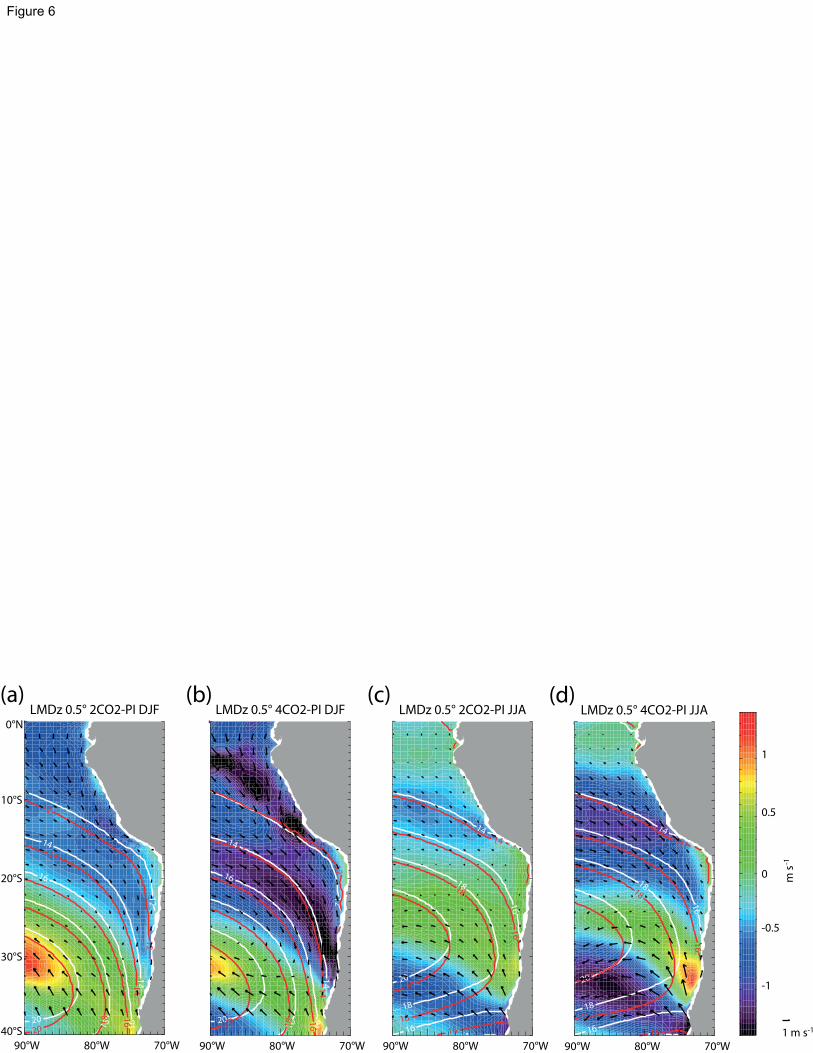
12

14

14

16

16

1820

12

12

14

14

161

8

20

40°S

30°S

20°S

10°S

0°N

(a)

90°W 80°W 70°W

LMDz 0.5° 2CO2-PI DJF

12

14

14

16

16

1820

12

14

14

161

820

LMDz 0.5° 4CO2-PI DJF

(b)

90°W 80°W 70°W

14

14

16

16

18

18

20

14

16

16

18

18

20

LMDz 0.5° 2CO2-PI JJA(c)

90°W 80°W 70°W

14

14

16

16

18

18

20

14

16

16

18

18

20

LMDz 0.5° 4CO2-PI JJA(d)

90°W 80°W 70°W

-1

0

-0.5

m s

-1

0.5

1

1 m s-1

Figure 6

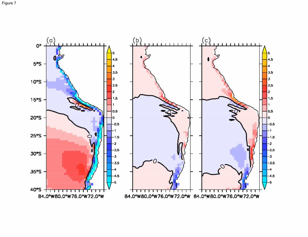
Figure 7

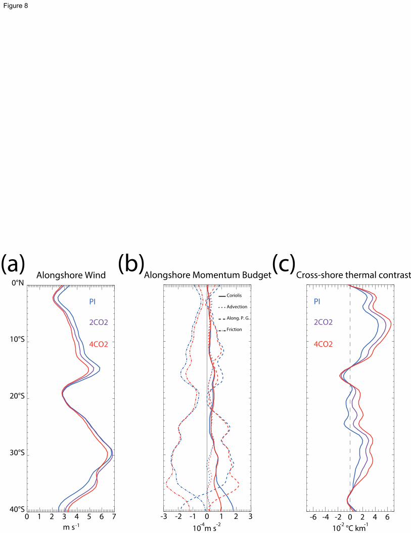
Alongshore Wind

0 1 2 3 4 5 6 740°S

30°S

20°S

10°S

0°N

(a)

m s-1

PI

2CO2

4CO2

Alongshore Momentum Budget

-3 -2 -1 0 1 2 3

10 m s-4 -2

Coriolis

Advection

Along. P. G.

Friction

(b)Cross-shore thermal contrast

-6 -4 -2 0 2 4 6

10 °C km-2 -1

(c)

PI

2CO2

4CO2

Figure 8

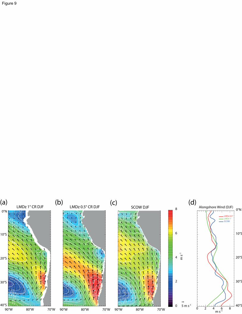
2.02.52.5

2.5

3.03.0

3.0

3.5

3.5

3.54.0

4.0

4.0

4.5

4.5

4.54

.5

5.0

5.0

5.0

5.5

5.5

6.0.0

6.0

6.57

.0

LMDz 1° CR DJF(a)

40°S

30°S

20°S

10°S

0°N

90°W 80°W 70°W80°W

2.53.0

3.0

3.0

3.5

3.5

3.5

4.0

4.0

4.0

4.5

4.5

4.5

5.0

5.0

5.5

5.5

6.0

6.0

6.5 6.57.0

7.5

7.5

8.0

8.5

9.0

LMDz 0.5° CR DJF(b)

90°W 80°W 70°W80°W

2.0

2.53.0

3.5

3.5

3.5

4.0

4.0

4.0

4.0

4.5

4.5

4.5

5.0

5.0

5.5

5.5

6.0

6.0

6.0

6.0

6.57.0

SCOW DJF(c)

90°W 80°W80°W

70°W

0

4

2

m s

-1

6

8

5 m s-1

Alongshore Wind (DJF)

LMDz 0.5°

LMDz 1°

SCOW

0 2 4 6 840°S

30°S

20°S

10°S

0°N

m s-1

(d)

Figure 9

-3

-2

-2

-1

0

1

2

3

4

5

6

7

8

9

10

11

12

13

14

14

15

15

16

16

17

17

18

18

19

0

1000

2000

3000

4000

5000

Alt

itu

de

(m

)

(a)LMDz1 (DJF, 15°S)

0

5

10

-5

-10

m s

-1

84°W 82°W 80°W 78°W 76°W 74°W

12

34

56

78

9

10

11

12

13

13

14

14

15

15

16

16

17

17

18 19 20

ERA-Interim (DJF, 15°S)

84°W 82°W 80°W 78°W 76°W 74°W

(b)

LMDz1 (DJF, 30°S)

84°W 80°W 76°W 72°W 68°W

(c)

0

1000

2000

3000

4000

5000

Alt

itu

de

(m

)

0

5

10

-5

-10

m s

-1

-8-7

-6-5

-4-3

-2-1

0123

456

789

1011

12

1314

1516

17

17

-9-8

-8-7

-7-6

-6-5

-5

-4-4

-3-3

-2-2

-1-1

00

11

22

33

44

55

66

77

8

8

9

9

10

10

11

11

12

12

13

13

14

14

15

15

1616

16

17

17

1818

19

19

ERA-Interim (DJF, 30°S)

84°W 80°W 76°W 72°W 68°W

(d)

Figure 10

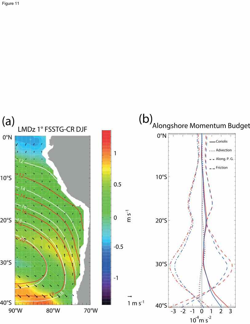
12

14

16

18

18

20

12

14

16

18

18

20

40°S

30°S

20°S

10°S

0°N

90°W 80°W 70°W

LMDz 1° FSSTG-CR DJF

-1

0

-0.5

m s

-1

0.5

1

1 m s-1

(a)

80°W80°W

-3 -2 -1 0 1 2 3

10 m s-4 -2

Coriolis

Advection

Along. P. G.

Friction

Alongshore Momentum Budget(b)

40°S

30°S

20°S

10°S

0°N

Figure 11

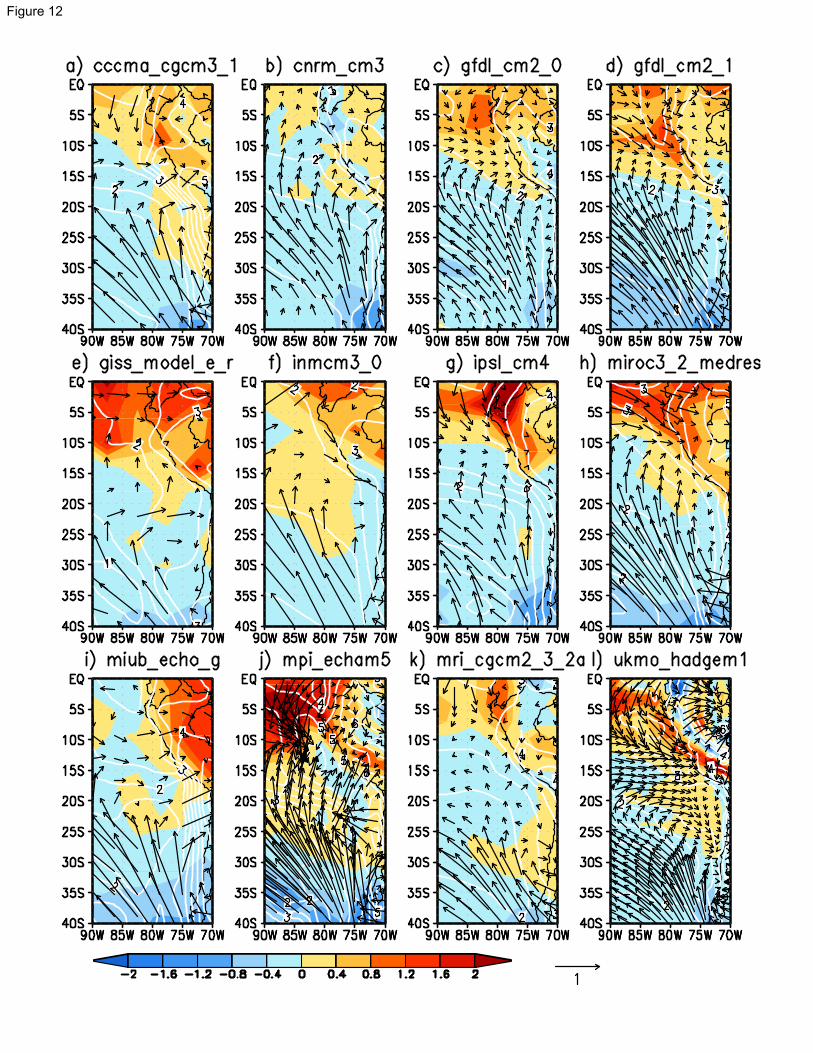
Figure 12

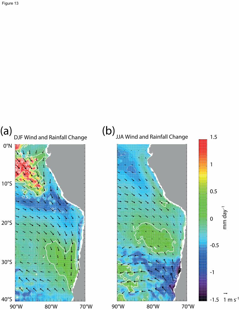
-0.5

-0.5

-0.5

0.0

0.0

1.5

2.0

40°S

30°S

20°S

10°S

0°N

(a)

90°W 80°W 70°W

DJF Wind and Rainfall Change

-1.0

0.0

JJA Wind and Rainfall Change

(b)

90°W 80°W 70°W

0

0.5

1

-1.5

-1

-0.5

1.5

1 m s-1

mm

day

-1

Figure 13

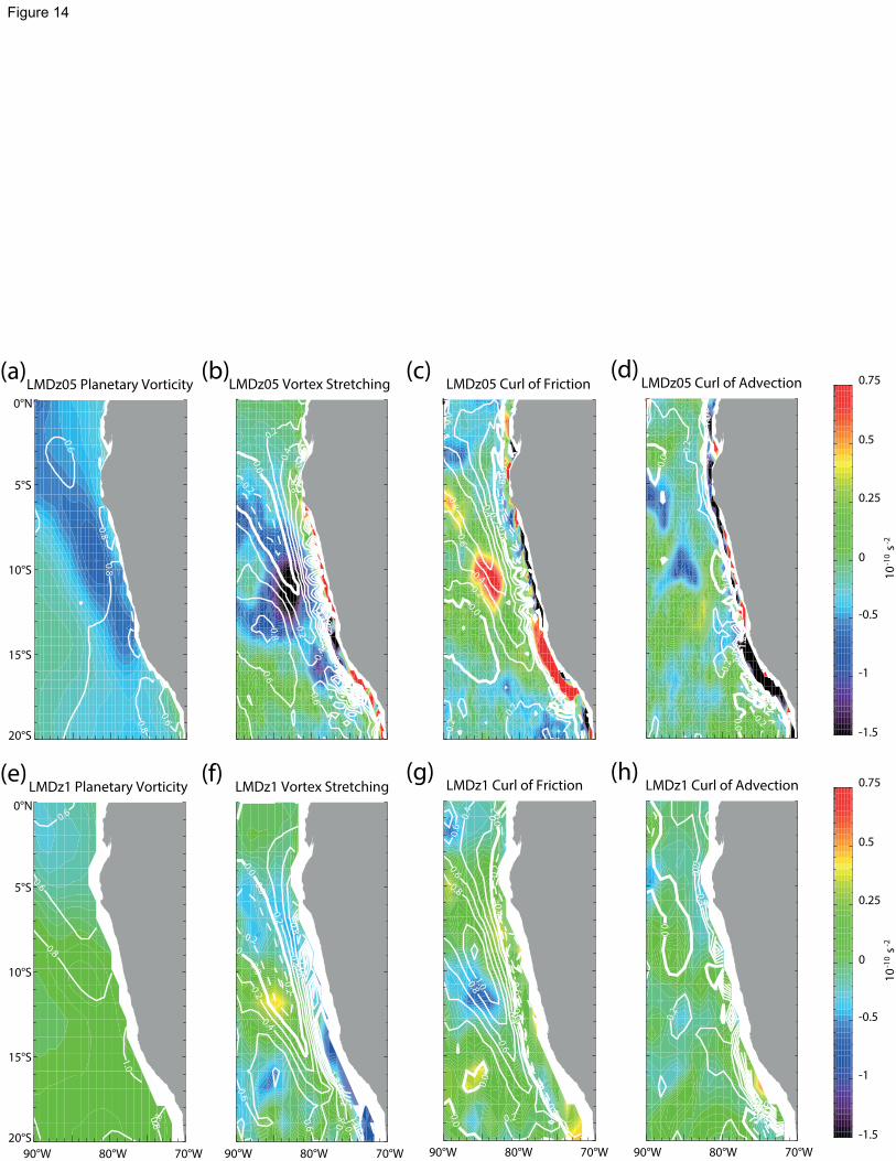
0.6

0.6

0.8

0.8

0.8

20°S

15°S

10°S

5°S

0°N

LMDz05 Planetary Vorticity(a)

-0.2

0.0

0.2

0.2

0.4

0.4

0.6

0.6

0.6

0.6

0.8

0.8

0.8

1.01.21.4

1.6

1.8

2.02

.2

LMDz05 Vortex Stretching(b)

-0.6

-0.6

-0.4

-0.4

-0.2

-0.2

0.0

0.0

0.0

0.2

0.2

0.2

0.2

0.2 0.2

0.4

0.4

0.6

0.6

0.8

LMDz05 Curl of Friction(c)

-0.4-0.4

-0.2

-0.2

0.0

0.0

0.0

0.2

0.2

0.2

0.4

0.4

0.6

0.6

0.8

0.8

1.0

1.0

1.2

1.2

1.2

0.0

LMDz05 Curl of Advection(d)

0

0.25

0.5

-1.5

-1

-0.5

0.75

s-2

10

-10

0.6

0.6

0.8

0.80

.8

1.0

LMDz1 Planetary Vorticity(e)

20°S

15°S

10°S

5°S

0°N

90°W 80°W 70°W

-0.2

-0.2

0.00.0

0.0

0.2

0.2

0.4

0.4

0.6

0.6

0.6

0.8

0.8

1.0

1.0

1.2

1.2

1.4

1.4

1.6

1.61.8

0.0

LMDz1 Vortex Stretching(f)

90°W 80°W 70°W

-0.6

-0.4

-0.4

-0.2

-0.2

0.0

0.0

0.0

0.0

0.2

0.2

0.2

0.4

0.4

0.6

0.6

0.6

0.8

0.81.0

LMDz1 Curl of Friction(g)

90°W 80°W 70°W

0.0

0.00.2

0.20.2

0.2

0.4

0.4

0.60.81.0

1.21.4

1.61.82.0

LMDz1 Curl of Advection(h)

90°W 80°W 70°W

0

0.25

0.5

-1.5

-1

-0.5

0.75

s-2

10

-10

Figure 14