What drives all progress? Or what enhances self preservation? Conservation of angular momentum Watt speed governor Drive shaft speed Almost all men are greedy and ambitious Checks and balances Legal, social and economic Mechanics and aerodynamics Sperry autopilot Aircraft attitude Maxwell electrodynamics PLL, DLL, Power Control Signal frequency, ID, and power levels Underlying Model System Uncertainty reduced KARTIK B. ARIYUR AUTONOMY 09-18-2013

Welcome message from author
This document is posted to help you gain knowledge. Please leave a comment to let me know what you think about it! Share it to your friends and learn new things together.
Transcript

What drives all progress? Or what enhances self preservation?
Conservation of angular momentum
Watt speed governor Drive shaft speed
Almost all men are greedy and ambitious
Checks and balances Legal, social and economic
Mechanics and aerodynamics
Sperry autopilot Aircraft attitude
Maxwell electrodynamics PLL, DLL, Power Control Signal frequency, ID, and power levels
Underlying Model System Uncertainty reduced
KARTIK B. ARIYUR AUTONOMY 09-18-2013

What drives all progress? Or what enhances self preservation?
Wiener-Hammerstein (Ariyur, UCSD)
Extremum seeker Closeness to optimum (to within sensor/actuator
limits)
Thermal-fluid sciences and statistics/estimation (Ariyur, Honeywell)
Gas turbine health monitor Time of component failure (reduce from 1000s to 10s
of hours)
Mechanics and aerodynamics (Ariyur, Purdue)
Coordinated UAV flight Location, orientation and speeds of all aircraft
Maxwell electrodynamics (Ariyur & Kulatunga, Purdue)
Vehicle traction control Road traction forces
Underlying Model System SMALLER
ACCOMPLISHMENTS!
Uncertainty reduced
KARTIK B. ARIYUR AUTONOMY 09-18-2013

Components of Autonomy • Sensing
• Sensing systems and estimators
• Control systems—adapting to changes
• Optimization—tactics
• Gaming—strategy

Sensing
Collaborators:
Yan Cui
KARTIK B. ARIYUR AUTONOMY 09-18-2013

• GPS system not accessible in:
urban and natural canyons;
forests;
indoor locations.
• Current geolocation algorithms:
received signal strength (RSS), error 3~5m
time difference of arrival (TDOA), error 2~3m
radio frequency identification (RFID), error 3~5m
our algorithm (Magnetic map), error: 1.5~2m
Magnetic Mapping
5
indoor locations * urban canyon
* Figure available from http://www.gpsbites.com/indoor-location-positioning-krulwich-interview

• Magnetic Field Model:
Building a Magnetic Map
6
( , ) ,
( , ) IGRF Bias
m x y M
m x y m m
3 3 ( )m IGRF Bias Noisez R m m m
Measurement:
3 3
: magnetic map;
: rotation matrix;
: International Geometric Reference Field;
: local bias;
: measurement noise.
IGRF
Bias
Noise
M
R
m
m
m
2 2 2
m mx my mzz z z z 3 3 1R

Building Magnetic Map
7
• Hardware:
Samsung Galaxy Note II
Measurement unit:
Measurement noise:
• Floor plan:
2 20.0734( )noise Gauss
Part of Mechanical Engineering Building (2nd floor), Purdue University
( )T

Building Magnetic Map
8
( )Magetic Intensity T
( )X meter( )Y meter

Static Estimation
9
Cost Function, c(pt) : ( ) ( , )t mc p z m x y
arg min ( )tp V
p c p
• Optimization:
• Measurement:
3 3 ( )m IGRF Bias Noisez R m m m
2 2 2
m mx my mzz z z z

Static Estimation
10
Definition of Wrapper[6]
:
P: a set; IP: subset of P; IP is a set of wrappers for P, if it satisfies: 1)P and each singleton of P belong to P; 2)IP is closed by intersection.
P1: a subset of P; The smallest wrapper [P1]:
1 1[ ] { | } P X IP P X
• Static Estimation Algorithm

Experimental Results
11
Candidate locations are well bounded within
several small 0.6m×1.25m intervals.
Bounded region from static estimation
State Estimation Results

Sensing Systems and Estimators
Collaborators:
John Barnes and Cheng Liu
KARTIK B. ARIYUR AUTONOMY 09-18-2013

13
Geolocation Approaches Given the sun vector, moon vector or other celestial reference vectors, how to accurately obtain the location?
• Approach 1 [10].
Mathematical transformations between three coordinates.
Cons:
1. Cumbersome calculation.
2. In practical usage , there is no permanent aid of true north to determine celestial reference vectors.
( , )Ref Ref .H ER
cos( )cos( )
Ref sin( )cos( )
sin( )
,andE
H
cos( )cos( )
Ref sin( )cos( )
sin( )

14
Intercept Method and Line of Position (LOP).
• Approach 2: Intercept Method Drawing the Line of Position (LOP) for several celestial objects and find the intersected location [11].
Cons:
1. Only applicable when more than two celestial objects can be observed.
2. As a manual work, accuracy and speed is low.
Pros:
1.Straightforward.
2.No need of the direction of true north.
Geolocation Approaches

15
Generalized Intercept Method
• Define a “Set of Position (SOP)” instead of Line of Position (LOP) as,
• “Ref” can be both azimuth or zenith for drawing SOPs.
SOP(Ref , ) { ( , , ) :| ( , ) Ref | }.t P h f P t
• Define a “successive Set of Position (sSOP)” to apply previous SOPs,
sSOP(Ref , , ) { ( , , ) : SOP(Ref , ), }.t l P h P t P P l
SOP and sSOP for both azimuth and zenith.
b. SOPs for two solutions. a. SOP and sSOP when on solution exists.
ε : expected measurement error

16
Generalized Intercept Method • At an unknown location if n SOP and m sSOP can be estimated
independently, we can find the intersection of them such that,
1 2 1 2 ,n mSOP SOP SOP sSOP sSOP sSOP
( , , ) .P h
( , , ),P h
• If the area of becomes small enough, it can be treated as the geolocation result: a solution set of area instead of a single location point.
• At least two SOPs or sSOPs are required for geolocation. Possible choices:
1. SOP(Z1, t1), SOP(Z2, t2);
2. SOP(A1, t1), SOP(Z1, t2);
3. sSOP(Ref, t1, l), SOP(Ref, t2);
• More and distinct SOP and sSOP combinations are preferred since they
can largely reduce the size of .

17
Iterative Position Matching Algorithm • Since there are infinite locations on the earth, finding SOPs via enumeration is
impossible.
• Due to the spherical shape of the earth, the distribution of “Ref” should be continuous for nearby locations.
• Apply the principle for geolocation via an iterative position matching algorithm.
Theoretical global distribution of solar azimuth and zenith for all longitudes and latitudes at noon March 20th, 2012.
b. Distribution of zenith. a. Distribution of azimuth.

18
Iterative Position Matching Algorithm
• Grid of Locations (GoL).
For a location area
• Position Node (PN).
Figure 5.5 Illustration of GoL, PN and the resized new GoL’.
• Use a threshold ε’ to select qualified PNs to form a smaller GoL.
[ , , , ],min max min max
by ,
and to form a grid.
spliting [ , ]
[ , ] by
min max
min max
The intersected location points on the GoL,
{ ( , ) :| ( ( , ), ) Ref | },PN PN i j f PN i j t
[ ( ), ( ), ( ), ( )].PN PN PN PN
GoL min max min max
• Repeat the steps for smaller ε’ values until the GoL achieves the desired accuracy.

19
Experimental Results
Inputs: (A,Z): (185.59°,28.10°) from Magnetic North Time: UTC 17:49, 04/22/2013 Measurement error: (0.2°,0.1°)
Result: [-86.975°,-86.85°,40.4297°,40.625°]
Pros of the method:
•Fast.
•Accurate.
•Robust to disturbances.
•Fully autonomous and programmable.
Geolocation result of the given sun vector.
20
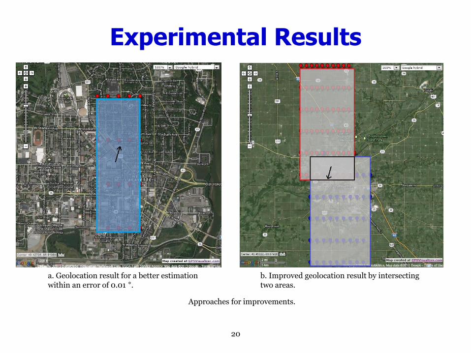
Experimental Results
Approaches for improvements.
b. Improved geolocation result by intersecting two areas.
a. Geolocation result for a better estimation within an error of 0.01 °.

Control Systems—Adapting to Changes
Collaborators:
Poorya Haghi and William S. Black
KARTIK B. ARIYUR AUTONOMY 09-18-2013

ES-MRAC: A New Paradigm for Adaptive Control
Motivation:
Desired objectives in many engineered systems:
– Controlling the exact trajectories of system
– Dealing with uncertainties
One Solution Category: Adaptive Control
– Model reference adaptive control (MRAC)
– Adaptive feedback linearization
– Adaptive back stepping
– ES-MRAC
ES-MRAC Combines extremum seeking optimization (ES) with MRAC

ES-MRAC: A New Paradigm for Adaptive Control
How does ES work?
How we can use this for adaptation: (the extremum seeker!)

ES-MRAC: A New Paradigm for Adaptive Control
• There are many optimization methods. Why ES?
– A very strong real-time optimization tool
– Can change J and C(s)
– Can use non-sinusoidal perturbations
– Can create forms and terms that are impossible for other methods to implement
• There are many control methods. Why mix ES with MRAC?
– MRAC controls both transient and steady state responses
– Thus, we build a very strong adaptive control method (ES-MRAC)!

ES-MRAC: A New Paradigm for Adaptive Control
LTI Systems
• The system:
• The reference (desired) model:
• Plant Assumptions:
P1. States are measurable
P2. Plant parameters are unknown
• Reference Model Assumptions:
M1. The model is stable
M2. The plant and the model have the same order

ES-MRAC: A New Paradigm for Adaptive Control
Theorem (Stabilization):
Let the cost function and compensator be
Assume that plant assumptions P1 and P2 and model assumptions M1 and M2 hold.
Furthermore, assume that
• The probing frequency for each loop is
• Probing frequencies are large and distinct
•
Then, this setup will guarantee global asymptotic convergence of the tracking error vector, to an O(1/ω) neighborhood of the origin.

ES-MRAC: A New Paradigm for Adaptive Control
Features of the method:
Pros:
– Real-time adaptation
– Extendible to virtually all other control methods and nonlinear systems
– PE conditions can be explicit
Cons:
– Perturbation frequencies can get very high if the system is large
– Challenging numerical problems in nonlinear systems

ES-MRAC: A New Paradigm for Adaptive Control
Visualizing the Concept of ES-MRAC:
ES-MRAC: A New Paradigm for Adaptive Control
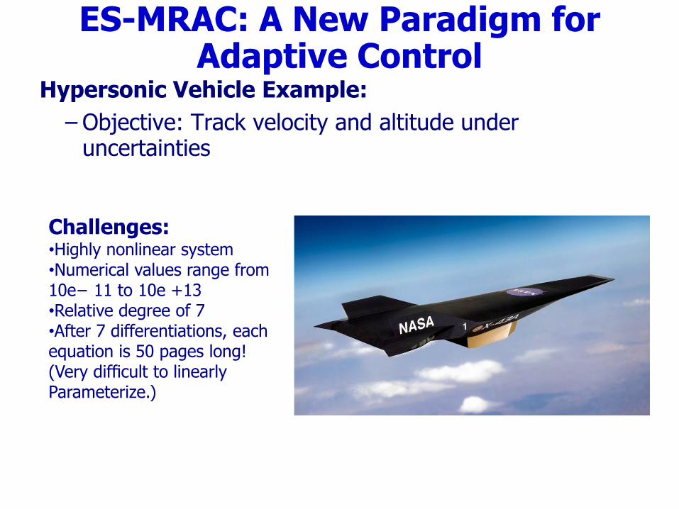
Hypersonic Vehicle Example:
– Objective: Track velocity and altitude under uncertainties
Challenges: •Highly nonlinear system •Numerical values range from 10e− 11 to 10e +13 •Relative degree of 7 •After 7 differentiations, each equation is 50 pages long! (Very difficult to linearly Parameterize.)

ES-MRAC: A New Paradigm for Adaptive Control
Hypersonic Vehicles Simulation Results On a Computer:

Optimization—Tactics
Collaborators:
Sunghun Jung (PhD Fall 2013)
KARTIK B. ARIYUR AUTONOMY 09-18-2013

Scalable UAV Operations
32
•Automated Integrated Surveillance Reconnaissance (ISR) algorithm for multiple UAVs by converting mTSP* to m TSP**.
mTSP*: multiple Traveling Salesman Problem, TSP**: Traveling Salesman Problem.
Figure 1.1: Hierarchy of mission planning.
Figure 1.2: Processes to generate a trajectory of a single UAV.

33
where, threshold,
time taken between and node,
integer between 0,1 ,
UAV,
number of vertices,
time increase due to wind,
time increase due to unexpected obstacles,
total numbe
t
th th
ij
ij
th
T
c i j
x
k k
n
w
o
m
r of UAVs,
time array among nodes .tG n n
1 1 1
1 1,
2
2
min ,
,
1 for any ,
1 for any ,
s.t. 1 for any ,
0 for any ,
,
m n n
mission ijk ijk k k
k i j
m m
p q t
p q p q
n
ijk
j
n
jik
j
ijk
i j
ijk
i j
ijk t
E t c x w o
t t T
x k
x k
x k
x k
c G i j
for ,
, 0,k k
i j
w o
Optimization Problem Formulation
(5.1)
S. Jung

Converting mTSP to m TSPs
34
•Break down mTSP* into m TSPs** using two region division methods:
1. Uniform Region Division (URD),
2. K-means Voronoi Region Division (KVRD).
•TSP** with GA:
Figure 1.3: Simulation of TSP.
Algorithm 1.1: Algorithm structure of the TSP** with GA***.
35
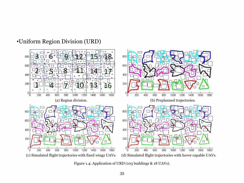
•Uniform Region Division (URD)
Figure 1.4: Application of URD (103 buildings & 18 UAVs).
(a) Region division. (b) Preplanned trajectories.
(c) Simulated flight trajectories with fixed wings UAVs. (d) Simulated flight trajectories with hover capable UAVs.

36
•K-means Voronoi Region Division (KVRD)
Figure 1.5: Application of KVRD (103 buildings & 18 UAVs).
(a) Region division. (b) Preplanned trajectories.
(c) Simulated flight trajectories with fixed wings UAVs. (d) Simulated flight trajectories with hover capable UAVs.

•Robustness of the automated UAV mission planning can be proved by analyzing disjointed error propagations at each step since each algorithm runs independently, in series, and in one direction.
37
Robustifying the Planner
Figure 4.1: Hierarchy of mission planning.
Figure 4.2: Processes to generate a trajectory of a single UAV.

Disjunction of Algorithmic Error
38
•Step 1: Photograph Error
1) Google Earth has positional accuracy of RMSE ( ).
2) Some research works propose a method to use georeferencing to increase the data point accuracy to a positional accuracy of .
3) I will be able to enhance the accuracy using same method up to by using a GPS device with higher accuracy (ex. Sokkia GSR2700 ISX).
4) I can set a constant buffer size, c, as in the mission hierarchy in Fig 5.1 to avoid possible vehicle crashes.
5) Since there are still 50% of chance to have GPS data collected outside of a circle with radius, so I set the buffer zone size as, , where is a safety factor for the photograph error.
• Step 2: Building Detection Error
1) The latest automated building extraction algorithm using IKONOS images has 83.2% building detection rates. By running n times on the same surveillance region, I can get
0.4 error 171.7m m
5 6m
39.7m
1.5m
1.5m
1.5m 1.5 phc N phN
(1 0.832) 0.168 .n n
Disjunction of Algorithmic Error
39
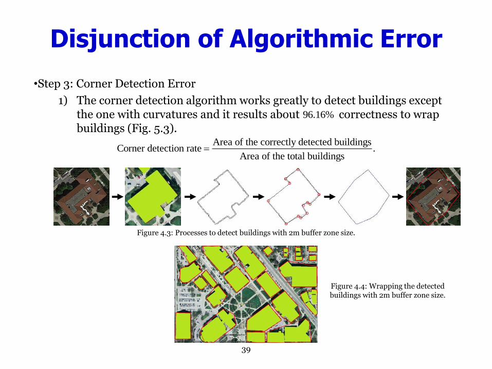
•Step 3: Corner Detection Error
1) The corner detection algorithm works greatly to detect buildings except the one with curvatures and it results about correctness to wrap buildings (Fig. 5.3).
96.16%
Area of the correctly detected buildingsCorner detection rate .
Area of the total buildings
Figure 4.3: Processes to detect buildings with 2m buffer zone size.
Figure 4.4: Wrapping the detected buildings with 2m buffer zone size.

40
•Step 5: Combinatorial Error
1)There are three sources of the combinatorial error in the Voronoi diagram algorithm; distance error (due to incorrect depth comparison of a pixel); resolution error (due to coarse discrete sampling); Z-buffer precision error (due to precision limitations of bits in graphic systems).
2)With an assumption that there is no Z-buffer precision error, the error bound can be expressed as,
3)According to the paper [21],
Since is small enough, I ignore the combinatorial error in step 5.
( , ) ( , ) 2 ,dist P A dist P B where, ( , ) distance from the center of pixel to the site ,
maximum distance error.
dist P A P A
41 cos 6.83 10 ,2
R R
where, acute angle of the isosceles triangle
(1024 1024 has 85 triangles),
radius of the cone (max distance
between site and sample point).
R
(4.3)
(4.4) Figure 4.5:
Calculation of and [21].
R
Disjunction of Algorithmic Error

41
•Step 6: Vehicle Dynamic Error
1) In vehicle UAV dynamic model,
we can introduce dynamic errors in position and velocity as,
With the amount of errors in position becomes,
( 1) ( ) ( ),
( 1) ( ) 1 ( ) ( ),
c c c
ref
c c c c
x v v x v
x k x k Tv k
T T Tv k x k v k x k
3
3
3
where, position vector of the UAV ( ),
vector of the UAV ( ),
sampling time,
tracking reference points ( ),
position tracking time constant,
velocity tracking time consta
c
c
ref
c
x
v
x R
v velocity R
T
x R
nt.
( 1) ( ) ( ) ( ) ( ) ,
( 1) ( ) 1 ( ) ( ) ( ) 1 ( ) .
c c c c c
ref
c c c c c c
x v v x v x v v
x k x k Tv k x k T v k
T T T T Tv k x k v k x k x k v k
0.25 , 0.5 , and 0.01 ,x vs s T s
( ) 0.01 ( ),
3 0.01 0.015,
3 .
p c c
po
po
e x k v k
N
N
Disjunction of Algorithmic Error

42
•Step 8: Environmental Disturbances (wind effect)
•Overall Algorithmic Error
•Step 1 (photograph error): RMSE photograph position error (unit: m),
•Step 2 (building detection error): building detection error,
•Step 3 (corner detection error): corner detection error,
•Step 5 (combinatorial error): Negligible,
•Step6 (vehicle dynamic error): position error (unit: m),
•Step 8 (environmental disturbances):
2 1( 1) ( ) ( ) ( ),
2c c c wx k x k Tv k T a k
2
where, amount of UAV acceleration caused
by the wind (0.1 / ).
wa
m s
Figure 4.6: UAV trajectories when wind causes the UAV to accelerate with magnitude of . 2
0.1 /m s
1.5 phN
100 0.168 %n
3.84 %
3 poN
3.3 0.23 .m
Disjunction of Algorithmic Error

43
•With total error can be calculated as,
•However, not only the overall algorithmic error, but I also need to incorporate UAV system constraints such as to achieve much safer operation.
3 and 2,ph poN N 1 1.5 3 3 2 3.3 13.8 .te m
min max max min, , , and v v a r
2 1 2
2 22 max min
1 max max
max
2
min2 min
max
,
1where, ,
2 2
tan tan .2 2 2 2
t
d d
e b b
v vb v t a t
a
vb r
a
min max max
2 1 2
For the fixed-wing UAVsystem properties of 0.5 / , 2 / , 0.5 / ,
3.75 0.29 4.04 .t
v m s v m s a m s
e b b m
1 2
Therefore, the final buffer size will be,
13.8 4.04 17.84 .t t te e e m
Figure 4.7: Minimum radius which allows a fixed-wing UAV to change its direction without any collision.
minr
(4.9)
Disjunction of Algorithmic Error

Algorithmic Robustness Analysis
44
•All simulations are done with a fixed-wing UAV flying from the starting location, [0,0], to the goal location, [472,808].
•The UAV has system properties of;
(a) UAV trajectories with a buffer size of
2(4.04 ).
te m
(b) UAV trajectories with a buffer size of
1(13.8 ).
te m
(b) UAV trajectories with a buffer size of
1 2 and (17.84 ).
t te e m
Figure 4.8: Robustness verification by changing the buffer size of buildings (Squirrel park at Purdue University (lat: 40.422108, lon: -86.932187)).
min max max
min max
0.5 / , 2 / , [0,0,0] / , 0.5 / ,
3 , 50 , 30 ,
0.01 , 0.25 , 0.5 .
initial
normal
x v
v m s v m s v m s a m s
Altitude m Altitude m Altitude m
T s s s

Gaming—Strategy
Collaborators:
Rajdeep Singh and Michael Hulton (Lockheed Martin)
KARTIK B. ARIYUR AUTONOMY 09-18-2013

• Get security that can be quantified as in cryptography
• Approximate the security produced by the ‘marketplace’
• Incorporate some descriptions of both the security system and the attackers
– Number of defense layers
– Number of attackers
– Practically instant communications within teams
• Eliminate dependence on personnel reliability
Securing Physical Facilities
46

47
Problem Formulation
• M-attacker team (A) vs N-layered defense (D)
• The state of each layer Xb is a binomial r.v in [0,1]—controlled by player or system ‘D’ w/ qb
• Trial or set of attempts, one for each layer with estimates for each layer Zb by attackers. (sequential or parallel)
• For experiment k at layer b, define
,
1 a detection at layer b for D1 if , C
0 a breach at layer b for A0 otherwisek kb b
k k
kb b
bX Z
X ZI Z

• Each layer has its false positives and missed detection rates, defined as follows:
• Control options for player D
• The goal of D (A) is to maximize (minimize) the frequency of detection and minimize (maximize) the breach occurrence given the detector’s false alarm rates.
Detection Rates and False Positives
48
, ,b b bq

• Instantaneous information sharing
• False positive detection for an attacker is counted as true detection/false positive detection for a good guy is counted as not counted as true detection.
• Independence of global estimates for each layer
• Ignore running or terminal costs for A and simplistic cost function for D except for the feedback part
Assumptions
49

Basic Calculations
50
Probability of detection and breach:

Theorem
51

Open Loop Results
Saddle point exists for one layer guess game (0.1,0.5)

Open Loop Results
Equilibrium strategy is an unbiased distribution, yielding
the maximum rate of 0.5

Open Loop summary
54

Summary of Computational Challenges
• There is a lot of scope for fast (enough) embedded algorithms
– This will enable high quality sensing from low quality components
• Systematically handle multiple numerical scales
– When microscopic phenomena can affect macroscopic behavior
• Algorithms need to be analyzed for propagation of error from processes and measurement noise
– This is different from numerical error analysis because errors are large.
KARTIK B. ARIYUR AUTONOMY 09-18-2013
Related Documents