CHEAT SHEET : VLOOKUP Copyright © 2016 Two Rivers Software Training www.trst.com.au All Rights Reserved About VLOOKUP VLOOKUP is one of the most commonly used functions in Excel amongst experienced Excel users. However there are a number of pitfalls that often occur that can easily be avoided with a few simple precautions. This cheat sheet / guide explains how to set up a VLOOKUP from scratch, what to watch out for and what to do if things go wrong. VLOOKUP is actually just one of a number of lookup functions. The ‘V’stands for Vertical and is used where you have a conventional table with column headings across the top and data arranged in rows. There’s also HLOOKUP where, you guessed it, ‘H’ stands for Horizontal and is used on transverse tables – that’s a table that is arranged with the headings listed down the left instead of across the top, and data is arranged left-to-right rather than top-to-bottom. And then there’s LOOKUP, INDEX and MATCH. What does the VLOOKUP function do? First you provide something that you want to find a match for in the first column of the table. This might be a name, an employee ID, a product code, a vehicle registration number … think about the data and table you work with, and you’ll know what you need. The VLOOKUP will check in the first column of the table to try to find a match. If a match is found, the data in one of the cells in that row is returned as the answer. If the VLOOKUP function cannot find a match, a #N/A! error is returned. That’s the 10,000 foot view. Now, let’s dive a little deeper. VLOOKUP: Deconstructed The syntax of the VLOOKUP function is =VLOOKUP(LookupValue, LookupRange, ColumnNo, RangeLookup) The first 3 parameters are mandatory; the last is optional. 1. LookupValue is the data you are trying to find a match for. This data must be in the first column of the table. 2. LookupRange is the cell range of the table.

Welcome message from author
This document is posted to help you gain knowledge. Please leave a comment to let me know what you think about it! Share it to your friends and learn new things together.
Transcript
CHEAT SHEET: VLOOKUP
Copyright © 2016 Two Rivers Software Training
www.trst.com.au All Rights Reserved
About VLOOKUP VLOOKUP is one of the most commonly used functions in Excel amongst experienced Excel users.
However there are a number of pitfalls that often occur that can easily be avoided with a few simple
precautions.
This cheat sheet / guide explains how to set up a VLOOKUP from scratch, what to watch out for and what to
do if things go wrong.
VLOOKUP is actually just one of a number of lookup functions.
The ‘V’stands for Vertical and is used where you have a conventional table with column headings across the
top and data arranged in rows.
There’s also HLOOKUP where, you guessed it, ‘H’ stands for Horizontal and is used on transverse tables –
that’s a table that is arranged with the headings listed down the left instead of across the top, and data is
arranged left-to-right rather than top-to-bottom.
And then there’s LOOKUP, INDEX and MATCH.
What does the VLOOKUP function do? First you provide something that you want to find a match for in the first column of the table. This might be
a name, an employee ID, a product code, a vehicle registration number … think about the data and table you
work with, and you’ll know what you need.
The VLOOKUP will check in the first column of the table to try to find a match.
If a match is found, the data in one of the cells in that row is returned as the answer.
If the VLOOKUP function cannot find a match, a #N/A! error is returned.
That’s the 10,000 foot view. Now, let’s dive a little deeper.
VLOOKUP: Deconstructed The syntax of the VLOOKUP function is
=VLOOKUP(LookupValue, LookupRange, ColumnNo, RangeLookup)
The first 3 parameters are mandatory; the last is optional.
1. LookupValue is the data you are trying to find a match for. This data must be in the first column
of the table.
2. LookupRange is the cell range of the table.
CHEAT SHEET: VLOOKUP
Copyright © 2016 Two Rivers Software Training
www.trst.com.au All Rights Reserved
3. ColumnNo is the column number WITHIN THE TABLE that contains the data you are trying to
return. This has nothing to do with the Excel column letter, e.g. Excel column E does not equate
to column 5.
4. RangeLookup [optional] - Do you want to use an exact match (use FALSE) or closest match (use
TRUE)?
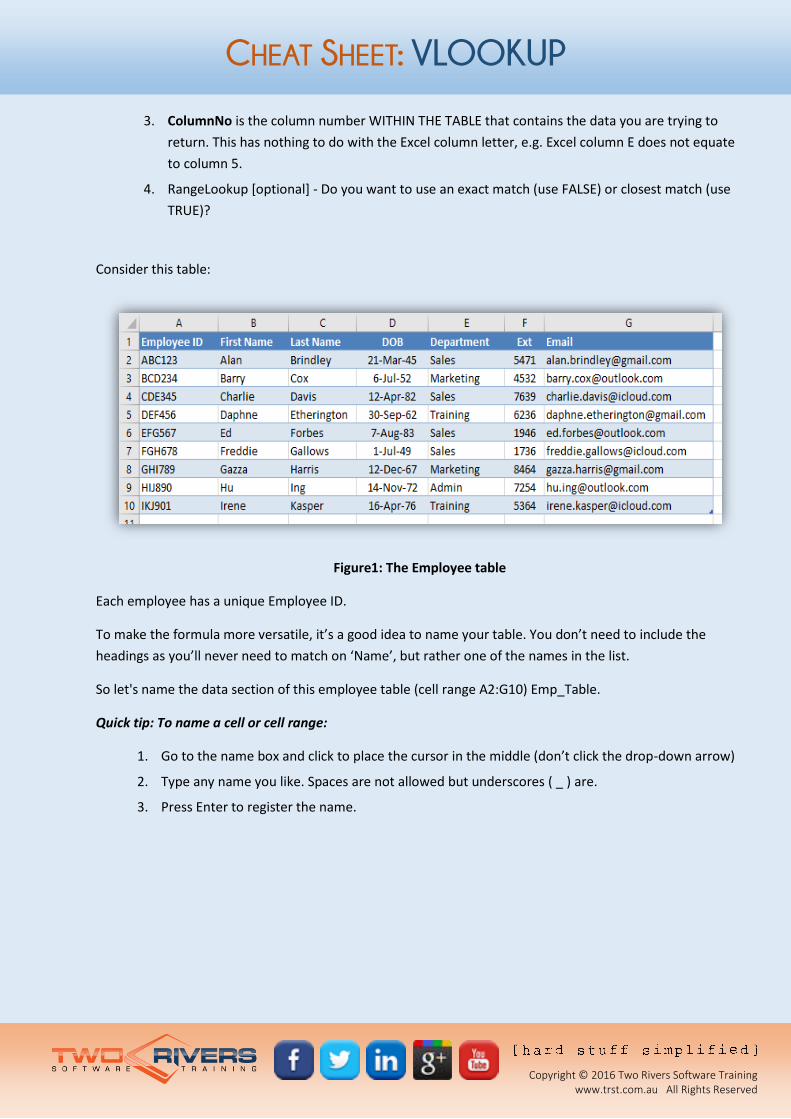
Consider this table:
Figure1: The Employee table
Each employee has a unique Employee ID.
To make the formula more versatile, it’s a good idea to name your table. You don’t need to include the
headings as you’ll never need to match on ‘Name’, but rather one of the names in the list.
So let's name the data section of this employee table (cell range A2:G10) Emp_Table.
Quick tip: To name a cell or cell range:
1. Go to the name box and click to place the cursor in the middle (don’t click the drop-down arrow)
2. Type any name you like. Spaces are not allowed but underscores ( _ ) are.
3. Press Enter to register the name.
CHEAT SHEET: VLOOKUP
Copyright © 2016 Two Rivers Software Training
www.trst.com.au All Rights Reserved
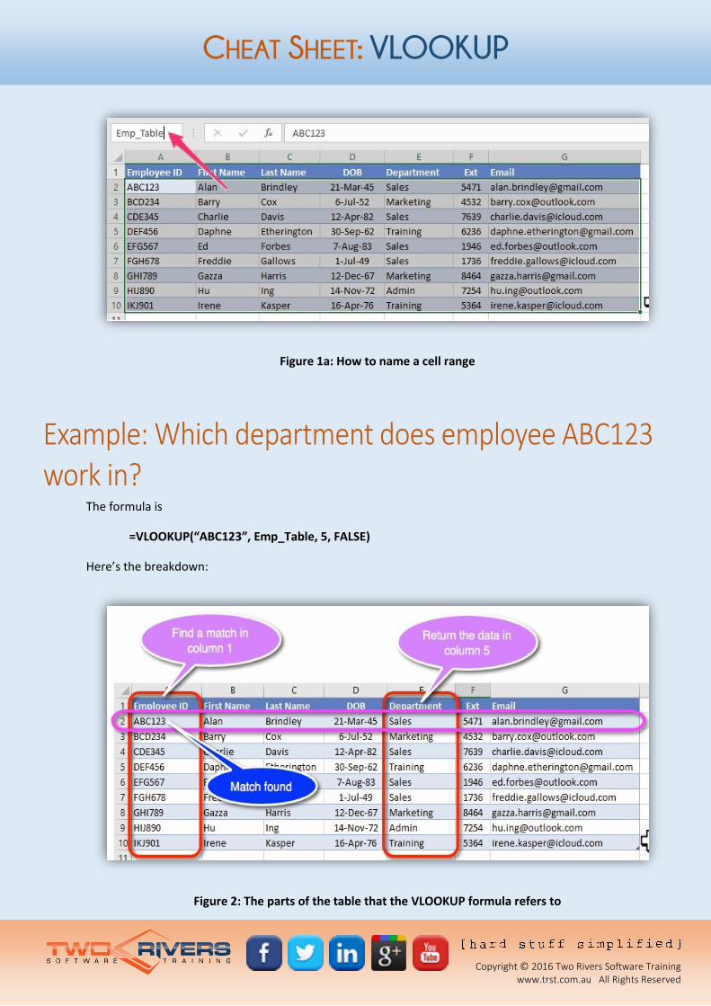
Figure 1a: How to name a cell range
Example: Which department does employee ABC123 work in?
The formula is
=VLOOKUP(“ABC123”, Emp_Table, 5, FALSE)
Here’s the breakdown:
Figure 2: The parts of the table that the VLOOKUP formula refers to
CHEAT SHEET: VLOOKUP
Copyright © 2016 Two Rivers Software Training
www.trst.com.au All Rights Reserved
ABC123 is the lookup value. VLOOKUP finds a match on row 2.
Emp_Table refers to the whole table.
ColumnNo is 5. Return the data from the fifth column.
RangeLookup is FALSE. Find an exact match.
Therefore, employee ABC123 works in Sales.
Some other examples To find the email address for employee “BCD234”, the formula is:
=VLOOKUP(“BCD234”, Emp_Table, 7, FALSE)
To find the extension number for employee “DEF456”, the formula is:
=VLOOKUP(“DEF456”, Emp_Table, 4, FALSE)
To show the full name for the employee whose ID is in cell A1, the formula is:
=CONCATENATE(VLOOKUP(A1, Emp_Table, 2, FALSE), “ ”, VLOOKUP(A1, Emp_Table, 3, FALSE))
This last formula uses two VLOOKUP formulas to return the first name and last name, then concatenates
(joins) them together.
This makes use of the CONCATENATE function which joins together all the elements inside its brackets. You
can read more about that in this blog post (link).
Are you making these mistakes with your VLOOKUP? Mistake 1: Is your key field unique?
The first column in the table must contain unique entries. There cannot be any duplicates.
If there are duplicates, then the VLOOKUP function may sometimes get it right, but may sometimes get it
wrong, which makes it as useful as a chocolate teapot.
In typical tables where the first field contains employee ID, supplier ID, product code, job number etc. these
are unique by design, so barring human error, you should be okay.
However if you are performing a lookup on a field such as First Name or Product Name it’s highly likely that a
duplicate entry could be created. For example, you might end up with 2 Joes or 15 Bruces.
Even if you try to get around the problem by concatenating (joining) the first name with the last name, it’s
still possible to end up with 2 Joe Dodgys or 3 Bruce Deuces.
CHEAT SHEET: VLOOKUP
Copyright © 2016 Two Rivers Software Training
www.trst.com.au All Rights Reserved
Mistake 2: Is your column index number numeric?
The 3rd parameter of the VLOOKUP function asks for the column NUMBER that contains the data you want.
Many people make the mistake of using the Excel column letter (like ‘E’ instead of 5) which results in a
formula error.
Mistake 3: Have you specified the right column number?
The table could be positioned anywhere on the worksheet. It doesn’t always start in column A - it might be
in columns T to Z.
Let’s say that the data you need is in the 3rd column of the table, that starts in column T. The Column
Number is still ‘3’.
Mistake 4: Hidden spaces
Hidden spaces can be hard to spot because you can’t see them, but they will affect whether a match is
found.
Often when you import data from systems like SAP, data has extra leading or trailing spaces. You can quickly
remove these with the TRIM function.
=TRIM(A1)
Mistake 5: Have you specified a match type?
For any text-based matches, the match type is always EXACT, so you must specify FALSE for the match type.
Excel will either find a match or it won’t.
If you do not specify a match type, Excel uses the default setting of TRUE which tries to find a closest match.
For text-based matches a TRUE match type will give an error or return the wrong result. Either way, it’s not
100% reliable.
So, you may be asking …
CHEAT SHEET: VLOOKUP
Copyright © 2016 Two Rivers Software Training
www.trst.com.au All Rights Reserved
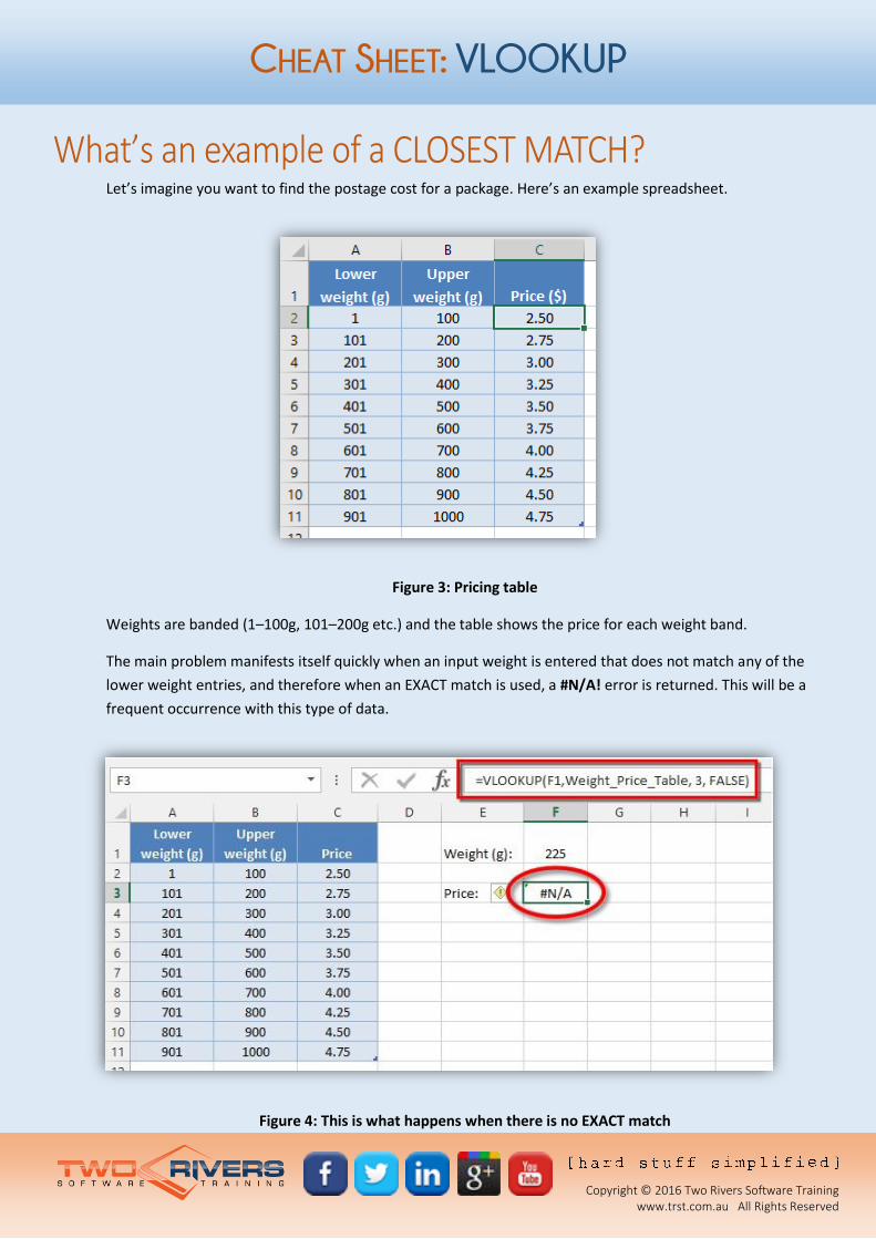
What’s an example of a CLOSEST MATCH? Let’s imagine you want to find the postage cost for a package. Here’s an example spreadsheet.
Figure 3: Pricing table
Weights are banded (1–100g, 101–200g etc.) and the table shows the price for each weight band.
The main problem manifests itself quickly when an input weight is entered that does not match any of the
lower weight entries, and therefore when an EXACT match is used, a #N/A! error is returned. This will be a
frequent occurrence with this type of data.
Figure 4: This is what happens when there is no EXACT match
CHEAT SHEET: VLOOKUP
Copyright © 2016 Two Rivers Software Training
www.trst.com.au All Rights Reserved
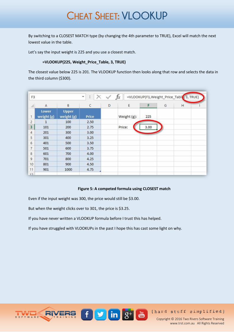
By switching to a CLOSEST MATCH type (by changing the 4th parameter to TRUE), Excel will match the next
lowest value in the table.
Let’s say the input weight is 225 and you use a closest match.
=VLOOKUP(225, Weight_Price_Table, 3, TRUE)
The closest value below 225 is 201. The VLOOKUP function then looks along that row and selects the data in
the third column ($300).
Figure 5: A competed formula using CLOSEST match
Even if the input weight was 300, the price would still be $3.00.
But when the weight clicks over to 301, the price is $3.25.
If you have never written a VLOOKUP formula before I trust this has helped.
If you have struggled with VLOOKUPs in the past I hope this has cast some light on why.
Related Documents