Well-Test Analysis, Schlumberger

Well-Test AnalysisReference: InTouch content ID#4135038Version: 5.0Release Date: 30-Apr-2006EDMS UID: 274758488Produced: 26-Oct-2006 16:20:46Owner: WS TrainingAuthor: Bernadette Gomez

Private well- test analysis, sand control, acidizingadd itives, SWBT, WBT, IT Modules, Interface, WCS,WPC, CTS, TBT

Copyright © 2006 Schlumberger, Unpublished Work. All rights reserved.

Well-Test AnalysisReference: InTouch content ID#4135038Version: 5.0Release Date: 30-Apr-2006EDMS UID: 274758488Published: 26-Oct-2006 16:20:46Owner: WS TrainingAuthor: Bernadette Gomez

Private well- test analysis, sand control, acidizingadd itives, SWBT, WBT, IT Modules, Interface, WCS,WPC, CTS, TBT

Copyright © 2006 Sophia, Unpublished Work. All rights reserved.

Intentionally Blank

PrivateCopyright © 2006 Schlumberger, Unpublished Work. All rights reserved.

Well-Test Analysis / Legal Information

Legal Information

Copyright © 2006 Schlumberger, Unpublished Work. All rights reserved.

This work contains the confidential and proprietary trade secrets of Schlumbergerand may not be copied or stored in an information retrieval system, transferred,used, distributed, translated or retransmitted in any form or by any means,electronic or mechanical, in whole or in part, without the express writtenpermission of the copyright owner.

Trademarks & Service marks

Schlumberger, the Schlumberger logotype, and other words or symbols usedto identify the products and services described herein are either trademarks,trade names or service marks of Schlumberger and its licensors, or are theproperty of their respective owners. These marks may not be copied, imitatedor used, in whole or in part, without the express prior written permission ofSchlumberger. In addition, covers, page headers, custom graphics, icons, andother design elements may be service marks, trademarks, and/or trade dressof Schlumberger, and may not be copied, imitated, or used, in whole or in part,without the express prior written permission of Schlumberger.

A complete list of Schlumberger marks may be viewed at the SchlumbergerOilfield Services Marks page: http://www.hub.slb.com/index.cfm?id=id32083

PrivateCopyright © 2006 Schlumberger, Unpublished Work. All rights reserved.W

STraining\BernadetteGomez\InTouchcontentID#4135038\5.0\ReleaseDate:30-Apr-2006\EDMSUID:274758488\Produced:26-Oct-200616:20:46

http://www.hub.slb.com/index.cfm?id=id32083

Well-Test Analysis / Document Control

Document ControlOwner: WS Training

Author: Bernadette Gomez

Reviewer: Bernadette Gomez

Approver: Torsten Braun,Alice Lee

Contact InformationName: WS TrainingLDAP Alias: IPC-DOC

Revision HistoryRev Effective Date Description Prepared by

5.0 25-Oct-2006 Changed instructions for takingmodule test online. Exercisesand test may be launched fromperception-ws server via LMS ortaken online.

Stuart Averett

4.1 12-Apr-2006 Changed label content, and revisiondates

Torsten Braun

4.0 30-Sep-2005 updated graphics and text. .Addedcaptions

Luisa Attaway,Torsten Braun



Well-Test Analysis / Document Control

Intentionally Blank



v Well-Test Analysis / Table of Contents v

Table of Contents

1 Objectives

2 Introduction2.1 Well Tests ___________________________________________________ 2-2

3 Well Tests3.1 Well Test Fundamentals ______________________________________ 3-13.2 Exercise _____________________________________________________ 3-2

4 Diffusivity Equation for Radial Flow to A Well4.1 Diffusivity Equation for Radial Flow to a Well ___________________ 4-24.2 Exercise _____________________________________________________ 4-3

5 Performing A Well-Test Analysis5.1 Generating The Log-Log Diagnostic Plot ______________________ 5-15.2 Flow Regime Identification ____________________________________ 5-55.3 Specialized Plot Construction ________________________________ 5-235.4 Specialized Plot Parameter Calculation _______________________ 5-245.5 Type Curve _________________________________________________ 5-255.6 Consistency of Results ______________________________________ 5-265.7 Exercise ____________________________________________________ 5-27

6 Summary

7 Take the module test



vi Well-Test Analysis / Table of Contents vi

Intentionally Blank



vii Well-Test Analysis / List of Figures vii

List of Figures

2-1 Direct measurements ______________________________________________ 2-14-1 Diffusivity equation for flow to a well ________________________________ 4-24-2 Diffusivity equation with new boundary conditions____________________ 4-35-1 Pressure transient curve ___________________________________________ 5-15-2 Pressure responses _______________________________________________ 5-35-3 Effects of damage removal ________________________________________ 5-45-4 Radial flow ________________________________________________________ 5-65-5 Wellbore intersecting ______________________________________________ 5-75-6 Direct flow into the wellbore ________________________________________ 5-85-7 Radial flow ________________________________________________________ 5-95-8 Values for permeability and skin ____________________________________ 5-95-9 Infinite acting, radial flow __________________________________________ 5-105-10 Straight line behavior _____________________________________________ 5-115-11 Spherical flow ____________________________________________________ 5-125-12 Spherical and hemispherical flow __________________________________ 5-135-13 Linear flow _______________________________________________________ 5-145-14 Linear flow _______________________________________________________ 5-155-15 Bilinear flow ______________________________________________________ 5-165-16 Bilinear flow regime_______________________________________________ 5-175-17 Wellbore storage _________________________________________________ 5-185-18 Pseudosteady state_______________________________________________ 5-195-19 Steady state______________________________________________________ 5-205-20 Dual porosity/permeability_________________________________________ 5-215-21 Slope doubling ___________________________________________________ 5-225-22 Specialized plot construction ______________________________________ 5-235-23 Specialized plot parameter calculation _____________________________ 5-245-24 Type curve _______________________________________________________ 5-255-25 Comparisons between shapes ____________________________________ 5-26



viii Well-Test Analysis / List of Figures viii

Intentionally Blank



ix Well-Test Analysis / List of Tables ix

List of Tables



x Well-Test Analysis / List of Tables x

Intentionally Blank



1-i Well-Test Analysis / Objectives 1-i

1 Objectives



1-ii Well-Test Analysis / Objectives 1-ii

Intentionally Blank



1-1 Well-Test Analysis / Objectives 1-1

1 ObjectivesMatrix, Acidizing,Well Test, SWBT, WBT, IT Modules,Interface, WCS, WPC, CTS, TBT

In this training module, you will learn to do the following:

• Demonstrate a knowledge of well-test fundamentals.

• Demonstrate a knowledge of the diffusivity equation and its application.

• Demonstrate a knowledge of the performance of a well test analysis.

• Demonstrate an understanding of the six steps in a well test analysis andtheir performance.

• Demonstrate a knowledge of eight flow-regime patterns commonly observedin well test data.



1-2 Well-Test Analysis / Objectives 1-2

Intentionally Blank



2-i Well-Test Analysis / Introduction 2-i

2 Introduction

2.1 Well Tests ______________________________________________________ 2-2



2-ii Well-Test Analysis / Introduction 2-ii

Intentionally Blank



2-1 Well-Test Analysis / Introduction 2-1

2 IntroductionMatrix, Acidizing,Well Test, SWBT, WBT, IT Modules,Interface, WCS, WPC, CTS, TBT

Figure 2-1: Direct measurements

The necessary parameters to optimize the development of a field are obtainedfrom direct measurements, including

• cores

• cuttings

• formation fluid samples.

Other necessary parameters to optimize field development include interpreteddata such as:

• surface seismic

• well logs

• well tests

• pressure-volume-temperature [PVT] analysis.

Only actual well-test data provides information on dynamic reservoirresponse. Actual well-testing data is a key element in the construction of thereservoir model.



2-2 Well-Test Analysis / Introduction 2-2

2.1 Well TestsVarious well tests are achieved by altering production rates:

• A buildup test is performed by closing a valve (shut-in) on a producing well.

• A drawdown test is performed by putting a well into production.

• Multi-rate, multi-well, isochronal and injection-well-falloff tests are alsopossible.

The buildup test is the easiest test to perform. A transient is created in thereservoir through production and is then shut in and the BHP recorded. Thedisadvantage of this test is that production is lost.

For a drawdown test, the well is put on production at a constant rate and thepressure drawdown is monitored. The well stays on production and no revenueis lost. The disadvantage of the drawdown test is that the production rate mustbe constant for the test to be valid. This is the hardest test to perform.

Transient well tests involve conditions during which the production rate is notdirectly proportional to the pressure differential applied, but are a function of time.

A transient (in terms of test data) is the period during which the pressureevolves with time, when a constant production rate (or zero rate for a builduptest) is imposed.

The analysis process for the well-test data remains consistent regardless of thetest type that produced the original data.



3-i Well-Test Analysis / Well Tests 3-i

3 Well Tests

3.1 Well Test Fundamentals ________________________________________ 3-13.2 Exercise ________________________________________________________ 3-2



3-ii Well-Test Analysis / Well Tests 3-ii

Intentionally Blank



3-1 Well-Test Analysis / Well Tests 3-1

3 Well TestsMatrix, Acidizing,Well Test, SWBT, WBT, IT Modules,Interface, WCS, WPC, CTS, TBT

A well test essentially consists of recording the downhole pressure with respectto time after a change in the flow rate.

Depending on its design, a well test can provide

• transmissibility (kh/µ), and, therefore, permeability

• initial or average reservoir pressure

• near wellbore condition (damage or stimulation)

• reservoir flow behavior

• reservoir size

• inflow performance relationship (IPR)

• communication between wells.

3.1 Well Test FundamentalsThe inflow performance relationship (the relationship between pressure drop andrate) is expressed as follows:

The critical variables obtained from well test analysis are

1. reservoir pressure (Pr)

2. skin (s)

3. permeability (k).

The basic reservoir models are

• homogeneous reservoirs

• dual-porosity reservoirs

• double-permeability reservoirs.



3-2 Well-Test Analysis / Well Tests 3-2

These models are affected by

• wellbore storage

• skin

• fractures

• partial penetration.

3.2 ExerciseWell Test Fundamentals (online)

Well Test Fundamentals (offline)



https://perception-ws.oilfield.slb.com/q/open.dll?name=TBT&group=SWBT&session=9442447371939796

4-i Well-Test Analysis / Diffusivity Equation for Radial Flow to A Well 4-i

4 Diffusivity Equation for Radial Flow to A Well

4.1 Diffusivity Equation for Radial Flow to a Well ___________________ 4-24.2 Exercise ________________________________________________________ 4-3



4-ii Well-Test Analysis / Diffusivity Equation for Radial Flow to A Well 4-ii

Intentionally Blank



4-1 Well-Test Analysis / Diffusivity Equation for Radial Flow to A Well 4-1

4 Diffusivity Equation for Radial Flowto A Well

Matrix, Acidizing,Well Test, SWBT, WBT, IT Modules,Interface, WCS, WPC, CTS, TBT

Most of the fundamental theory of well testing assumes the case of a well situatedin a porous medium of infinite radial extent (the infinite-acting radial model).

This model is based on a series of equations comprising the diffusivity equationfor radial flow to a well:

Most of the fundamental theory of well testing assumes the case of a well situatedin a porous medium of infinite radial extent (the infinite-acting radial model).

This model is based on a series of equations comprising the diffusivity equationfor radial flow to a well:




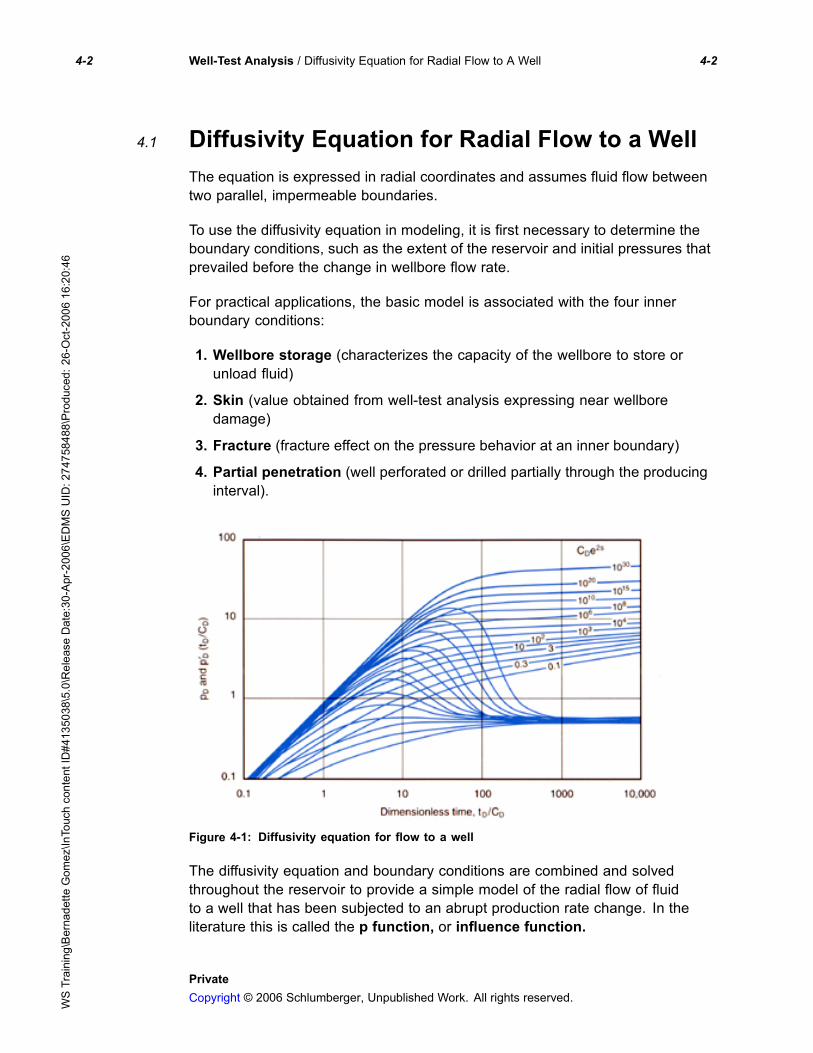
4.1 Diffusivity Equation for Radial Flow to a WellThe equation is expressed in radial coordinates and assumes fluid flow betweentwo parallel, impermeable boundaries.

To use the diffusivity equation in modeling, it is first necessary to determine theboundary conditions, such as the extent of the reservoir and initial pressures thatprevailed before the change in wellbore flow rate.

For practical applications, the basic model is associated with the four innerboundary conditions:

1. Wellbore storage (characterizes the capacity of the wellbore to store orunload fluid)

2. Skin (value obtained from well-test analysis expressing near wellboredamage)

3. Fracture (fracture effect on the pressure behavior at an inner boundary)

4. Partial penetration (well perforated or drilled partially through the producinginterval).

Figure 4-1: Diffusivity equation for flow to a well

The diffusivity equation and boundary conditions are combined and solvedthroughout the reservoir to provide a simple model of the radial flow of fluidto a well that has been subjected to an abrupt production rate change. In theliterature this is called the p function, or influence function.




Use of the same diffusivity equation, but with new boundary conditions, enablesother solutions to be found, such as in a closed-cylindrical reservoir.

Figure 4-2: Diffusivity equation with new boundary conditions

The solution of the diffusivity equation indicates that a plot of pressure versusthe log of time will show a straight line. This fact provides an easy and, to allappearances, precise graphical procedure for interpretation.

The slope of the portion of the curve forming a straight line is used forpermeability calculation.

Before computer-assisted testing, well-test interpretations involved

• plotting observed pressure measurements on semilog paper

• determining permeability estimates from the portion of the curve that formeda straight line (radial flow was assumed to be occurring in this portion ofthe transient).

4.2 ExerciseDiffusivity Equation for Radial Flow to A Well Exercise (online)

Diffusivity Equation for Radial Flow to A Well Exercise (offline)





Intentionally Blank



5-i Well-Test Analysis / Performing A Well-Test Analysis 5-i

5 Performing A Well-Test Analysis

5.1 Generating The Log-Log Diagnostic Plot _______________________ 5-15.1.1 Calculating The Pressure Derivative ___________________________ 5-25.1.2 Example of Reservoir Response ______________________________ 5-35.2 Flow Regime Identification _____________________________________ 5-5

5.2.1 Radial Flow __________________________________________________ 5-65.2.1.1 Infinite-Acting, Radial Flow _______________________________ 5-105.2.2 Spherical Flow ______________________________________________ 5-125.2.3 Linear Flow _________________________________________________ 5-145.2.4 Bilinear Flow ________________________________________________ 5-165.2.5 Compression/Expansion _____________________________________ 5-17

5.2.5.1 Wellbore Storage ________________________________________ 5-185.2.5.2 Pseudosteady State _____________________________________ 5-195.2.6 Steady State ________________________________________________ 5-205.2.7 Dual Porosity/Permeability ___________________________________ 5-215.2.8 Slope Doubling _____________________________________________ 5-225.3 Specialized Plot Construction _________________________________ 5-235.4 Specialized Plot Parameter Calculation ________________________ 5-245.5 Type Curve ____________________________________________________ 5-255.6 Consistency of Results ________________________________________ 5-265.7 Exercise _______________________________________________________ 5-27



5-ii Well-Test Analysis / Performing A Well-Test Analysis 5-ii

Intentionally Blank



5-1 Well-Test Analysis / Performing A Well-Test Analysis 5-1

5 Performing A Well-Test AnalysisMatrix, Acidizing,Well Test, SWBT, WBT, IT Modules,Interface, WCS, WPC, CTS, TBT

The steps in a well-test analysis are

1. Generate a log-log diagnostic plot.

2. Identify the flow regimes.

3. Construct a specialized (Cartesian or semilog) plot.

4. Calculate parameters from the specialized plot.

5. Select the most appropriate type curve and perform type-curve matching.

6. Check for consistency of the results (within 10% error).

5.1 Generating The Log-Log Diagnostic Plot

Figure 5-1: Pressure transient curve

Production changes, carried out during a transient well test, induce pressuredisturbances in the wellbore and surrounding rock. These pressure disturbancesextend into the formation and are affected in various ways by rock features. For




example, a pressure disturbance will have difficulty entering a tight reservoirzone, but will pass unhindered through an area of high permeability. It maydiminish or even vanish upon entering a gas cap.

Therefore, a record of wellbore pressure response over time produces a curvewhose shape is defined by the reservoir’s unique characteristics. Unlockingthe information contained in this "pressure transient curve" is the fundamentalobjective of well-test interpretation.

The derivative curve

is the single most effective interpretation tool, due to its sensitivity to transientfeatures resulting from well and reservoir geometries (which are virtually toosubtle to recognize in the pressure-change response). However, it is alwaysviewed together with the pressure-change curve to quantify skin effects that arenot recognized in the derivative response alone.

The log-log plot is used to identify the flow regime.

5.1.1 Calculating The Pressure DerivativeThe pressure change must first be computed to compute the pressure derivativefor drawdown data.

where

pi = initial reservoir pressure

pwf = bottomhole flowing pressure

t = time measured from start of the transient test

Given the drawdown transient data, the pressure derivative is then computed asthe derivative of delta p with respect to the natural logarithm of elapsed time:




5.1.2 Example of Reservoir Response

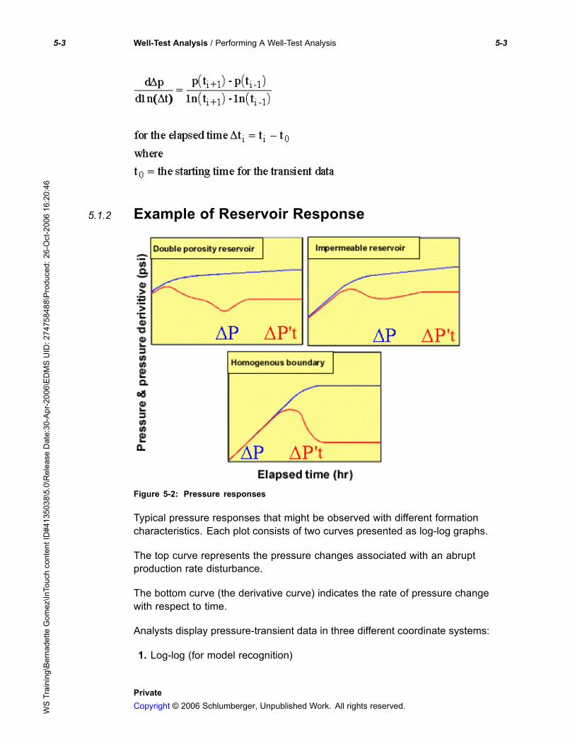
Figure 5-2: Pressure responses

Typical pressure responses that might be observed with different formationcharacteristics. Each plot consists of two curves presented as log-log graphs.

The top curve represents the pressure changes associated with an abruptproduction rate disturbance.

The bottom curve (the derivative curve) indicates the rate of pressure changewith respect to time.

Analysts display pressure-transient data in three different coordinate systems:

1. Log-log (for model recognition)




2. Semilog (for parameter computation for radial flow)

3. Cartesian (for model/parameter verification).

Semilog and Cartesian plots apply only to appropriate flow periods.

Figure 5-3: Effects of damage removal

The effects of damage removal are clearly seen in the after-treatmentpressure-response and derivative curves on this log-log plot. The "hump" in thederivative is clearly smaller after the matrix treatment. The hump in the pre-acidwell test was due to near wellbore pressure drop (skin).

The shape of the pressure transient curve is also affected by the productionhistory of the reservoir. Each change in production rate generates a newpressure transient that passes into the reservoir and merges with previouspressure effects.

The observed pressures at the wellbore are a result of the superposition of allthese pressure changes.




5.2 Flow Regime IdentificationWhen plotted as log-log data, flow regimes show up as characteristic patternsdisplayed by the pressure derivative.

The eight flow-regime patterns commonly observed in well test data are

1. radial

2. spherical

3. linear

4. bilinear

5. compression/expansion

6. steady state

7. dual porosity/permeability

8. slope doubling.

There is a set of well and reservoir parameters that can be computed foreach flow regime (using only the portion of the transient data that exhibits thecharacteristic pattern behavior).




5.2.1 Radial Flow

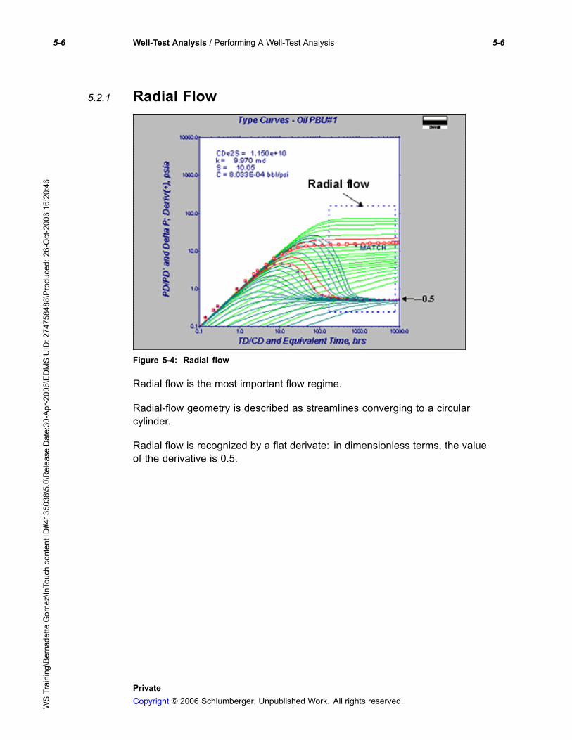
Figure 5-4: Radial flow

Radial flow is the most important flow regime.

Radial-flow geometry is described as streamlines converging to a circularcylinder.

Radial flow is recognized by a flat derivate: in dimensionless terms, the valueof the derivative is 0.5.




Figure 5-5: Wellbore intersecting

With fully completed wells, the cylinder may represent the portion of the wellboreintersecting the entire formation (top figure).

With partially penetrated formations or partially completed wells, the radial flowmay be restricted in early time to only the fraction of the formation thicknesswhere flow is directly into the wellbore (bottom figure).




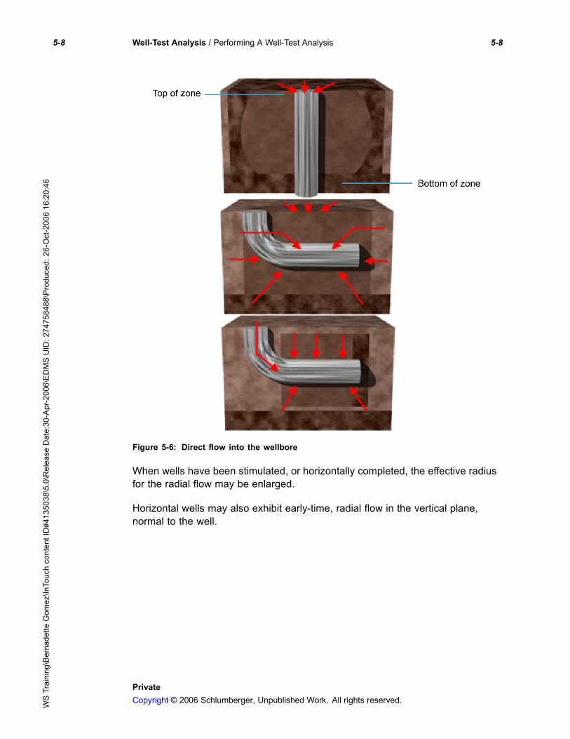
Figure 5-6: Direct flow into the wellbore

When wells have been stimulated, or horizontally completed, the effective radiusfor the radial flow may be enlarged.

Horizontal wells may also exhibit early-time, radial flow in the vertical plane,normal to the well.




Figure 5-7: Radial flow

Finally, if the well is located near a barrier to flow, such as a fault, thepressure-transient response may exhibit radial flow to the well, followed by radialflow to the well plus its image across the barrier.

Figure 5-8: Values for permeability and skin

When radial flow occurs, values for permeability and skin can be determined.




When radial flow occurs in late time, the average reservoir pressure can alsobe computed.

In this well, the radial flow is observed in late time (as evident by the flat slopeof the derivative), and thus, permeability, skin, and extrapolated pressure canbe quantified.

5.2.1.1 Infinite-Acting, Radial Flow

Figure 5-9: Infinite acting, radial flow

Prior to the boundary effects, the reservoir acts as if it were infinite in extent.

This behavior is known as the infinite-acting, radial flow. It starts about 1.5 logcycles after the end of wellbore storage.




Figure 5-10: Straight line behavior

Infinite-acting, radial flow is identified by a flat derivative that corresponds tosemilog straight-line behavior for the interval of time considered.




5.2.2 Spherical Flow

Figure 5-11: Spherical flow

Spherical flow occurs when flow streamlines converge to a point. This flowregime occurs for the partially completed well (top) and partially penetratedformation (bottom).




Figure 5-12: Spherical and hemispherical flow

Both spherical and hemispherical flow are seen on the derivative as a negativehalf-slope. When this appears, the spherical permeability can be determined.

Vertical permeability is important for predicting gas, water coning, or horizontalwell performance.




5.2.3 Linear Flow

Figure 5-13: Linear flow

Linear-flow, streamline geometry consists of strictly parallel flow vectors (top).

Linear flow may be observed in vertically fractured reservoirs.

The slope of pressure and the derivative on a log-log plot is 1/2.




Figure 5-14: Linear flow

Linear flow may also be observed in horizontal wells (top) and in a well producingfrom an elongated reservoir (bottom).




5.2.4 Bilinear Flow

Figure 5-15: Bilinear flow

Hydraulically fractured wells may exhibit bilinear flow instead of, or in additionto, linear flow.

This flow regime occurs because a pressure drop in the fracture accounts forparallel streamlines in the fracture. At the same time, the streamlines in theformation become parallel as they converge to the fracture. Because the twoflow patterns occur simultaneously in normal directions, this flow regime istermed bilinear.




Figure 5-16: Bilinear flow regime

The derivative trend for a bilinear flow regime has a positive quarter-slope. Whenthe fracture half-length and the formation permeability are known independently,the fracture conductivity can be determined.

5.2.5 Compression/ExpansionThe derivative of a compression/expansion flow regime appears as a unit slopetrend whenever the volume containing the pressure disturbance is not changingwith time.

Pressures at all points within this volume vary in the same way.

This volume can be limited by a portion or all of the wellbore, a boundedcommingled zone, or a bounded reservoir.




5.2.5.1 Wellbore Storage

Figure 5-17: Wellbore storage

When the wellbore is the limiting factor, the flow regime is called wellbore storage.

Wellbore storage is the first flow regime that is normally observed during a welltest.

One or more unit-slope trends preceding a stabilized radial flow derivative mayrepresent wellbore-storage effects. The transition from the wellbore-storage-unitslope trend to another flow regime usually appears as a "hump."

The wellbore-storage flow regime represents a response that is effectively limitedto wellbore volume and provides very little information about the reservoir. Apredominance of wellbore storage may mask important early-time responsesthat would otherwise characterize near-wellbore features, including partialpenetration or a finite-damage radius.




5.2.5.2 Pseudosteady State

Figure 5-18: Pseudosteady state

When the limiting factor is the entire drainage volume for the well, this behavioris called pseudosteady state.

When the unit slope occurs as the last observed trend, as in this example, theassumption is that this represents pseudosteady-state conditions for the entirereservoir volume contained in the well-drainage area.

When the unit slope is seen after radial flow, either the zone (or reservoir) volumeor its shape can be determined.

After radial flow has occurred, a unit-slope trend that is not the final observedbehavior may occur. This situation exists because of production from one zoneinto one or more additional zones, commingled in the wellbore. This behavioris accompanied by crossflow in the wellbore, and occurs when commingledzones are differentially depleted.




5.2.6 Steady State

Figure 5-19: Steady state

Steady state implies that pressures in the well-drainage volume are not varyingin time at any point, and that the pressure gradient between any two points in thereservoir is constant.

This condition may occur for wells in an injection/production scheme or wells withsignificant bottom water drive.




5.2.7 Dual Porosity/Permeability

Figure 5-20: Dual porosity/permeability




Dual-porosity/permeability behavior occurs when reservoir rocks containdistributed, internal heterogeneities that have highly-contrasting flowcharacteristics.

Examples are naturally fractured or highly laminated formations.

The derivative behavior for this case may look like the valley-shaped trend shownin the top figure, or it may resemble the behavior in the bottom figure.

From this flow regime, parameters associated with internal heterogeneity aredetermined, including:

• interporosity flow transmissibility

• relative storativity of the contrasted heterogeneities

• geometric factors.

5.2.8 Slope Doubling

Figure 5-21: Slope doubling

Slope doubling describes a succession of two radial flow regimes, with thesecond being at a level exactly twice that of the first. This behavior is frequentlyexplained by a sealing fault, and the distance from the well to the fault can bedetermined.




Because of the similarity of slope doubling to the previous example, it can alsobe due to dual-porosity/permeability heterogeneity, particularly in laminatedreservoirs.

5.3 Specialized Plot Construction

Figure 5-22: Specialized plot construction

Specialized plots are Cartesian and semilog plots, which use data points in arecognized flow regime.

Semilog plots are used for radial flow.

Cartesian plots are used for




5.4 Specialized Plot Parameter Calculation

Figure 5-23: Specialized plot parameter calculation

Permeability, skin, and flow efficiency are determined from semilog data takenfrom a recognized radial flow period.

Flow efficiency (FE) is the percent of production obtained in comparison to anundamaged well.

Data that can be determined from semilog analysis taken from a recognizedradial flow period include

• permeability

• skin

• flow efficiency

• average reservoir pressure

• initial reservoir pressure (Pr).




5.5 Type Curve

Figure 5-24: Type curve

Type curves are graphical representations of the solution of the diffusivityequation under different boundary conditions. These curves are presented interms of dimensionless variables and allow for flow regime identification.

Type curves are available for many reservoir and well types. Some of thesetype curves are

• homogeneous reservoir with or without wellbore storage and skin

• homogeneous reservoir with or without induced fracture

• dual porosity or naturally fractured reservoir

• layered reservoir.




Figure 5-25: Comparisons between shapes

Type curves printed on translucent paper can be placed over log-log data plottedto the same graph size. Comparisons between the shapes of the actual data andthe type curve can help to identify the reservoir model.

This process can now be done electronically using commercially available welltest analysis software.

Data that can be determined from type-curve matching include, but are notlimited to:

• skin

• permeability

• wellbore storage coefficient

• reservoir drainage radius.

5.6 Consistency of ResultsAs the final step in the basic well test analysis, a comparison between the valuescalculated for parameters should be made.

Values to compare include




• semilog or Cartesian

• type-curve.

The degree of difference between the values should not exceed 10 percent.

If a radial flow regime is well defined during a well test, results from curvematching and semilog analysis should be identical, as both analyses use exactlythe same mathematical model to represent transmissibility and skin.

Discrepancies in results are due to slight deviations in the real flow regime thatresult from some heterogeneity of the reservoir.

5.7 ExercisePerforming A Well Test Analysis Exercise (online)

Performing A Well Test Analysis Exercise (offline)





Intentionally Blank



6-i Well-Test Analysis / Summary 6-i

6 Summary



6-ii Well-Test Analysis / Summary 6-ii

Intentionally Blank



6-1 Well-Test Analysis / Summary 6-1

6 SummaryMatrix, Acidizing,Well Test, SWBT, WBT, IT Modules,Interface, WCS, WPC, CTS, TBT

Analysis of pressure-transient curves probably provides more information aboutreservoir characteristics than any other technique.

Horizontal and vertical permeability, pressure, well damage, fracture length,storativity ratio, and interporosity flow coefficient are just a few of the reservoircharacteristics that can be determined.

In addition, pressure transient curves can indicate the reservoir’s extent andboundary geometry. Well test analysis is the key element in the constructionof the reservoir model.



6-2 Well-Test Analysis / Summary 6-2

Intentionally Blank



7-i Well-Test Analysis / Take the module test 7-i

7 Take the module test



7-ii Well-Test Analysis / Take the module test 7-ii

Intentionally Blank



7-1 Well-Test Analysis / Take the module test 7-1

7 Take the module testMatrix, Acidizing,Well Test, SWBT, WBT, IT Modules,Interface, WCS, WPC, CTS, TBT

To receive credit for completing this module, you must take and pass the moduletest. A score of 90% or higher is required to pass the test. If you are viewing thismodule online, you must take the test for this module from the SchlumbergerLearning Management System (LMS).

To take the test online

If you do not know how to take a test from the LMS, go to:http://intouchsupport.com/intouch/MethodInvokerpage.cfm?caseid=4253433 forinstructions.

If you already know how to use the LMS, click here to go to the LMS and takethe test.

To take the test offline

If you are viewing this module offline, click here to take the module test offline.After you take the test, print the test results and have your manager enter theresults in the LMS.



http://intouchsupport.com/intouch/MethodInvokerpage.cfm?caseid=4253433

https://lms.slb.com/SabaWeb

Well-Test Analysis, Schlumberger

Documents

unpublished work

service marks of schlumberger

schlumberger logotype

welltest analysisreference

ws trainingauthor

takingmodule test

exercisesand test

rights res