Welfare Reform and Lone Welfare Reform and Lone Parents Employment in Parents Employment in the UK the UK Paul Gregg and Susan Harkness Paul Gregg and Susan Harkness

Welfare Reform and Lone Parents Employment in the UK Paul Gregg and Susan Harkness.
Dec 30, 2015
Welcome message from author
This document is posted to help you gain knowledge. Please leave a comment to let me know what you think about it! Share it to your friends and learn new things together.
Transcript

Welfare Reform and Lone Welfare Reform and Lone Parents Employment in the UKParents Employment in the UK
Paul Gregg and Susan HarknessPaul Gregg and Susan Harkness

AimsAims
What has happened to lone parents employment What has happened to lone parents employment since 1997?since 1997?
How much of the change can be attributed to policy How much of the change can be attributed to policy change?change?
Employment Rates: Single Mothers, Married Employment Rates: Single Mothers, Married Mothers & Single Childless Women, 1978-2002Mothers & Single Childless Women, 1978-2002
0
10
20
30
40
50
60
70
80
Single Mothers Married Mothers Single childless women
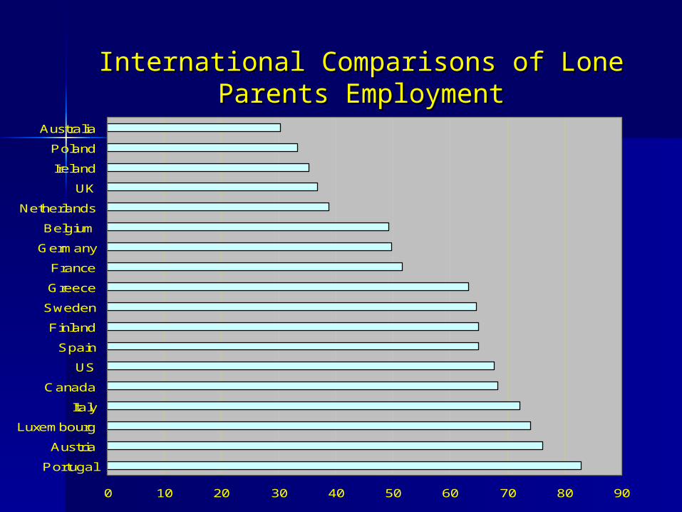
International Comparisons of Lone International Comparisons of Lone Parents EmploymentParents Employment
0 10 20 30 40 50 60 70 80 90
Portugal
Austria
Luxembourg
Italy
Canada
US
Spain
Finland
Sweden
Greece
France
Germany
Belgium
Netherlands
UK
Ireland
Poland
Australia
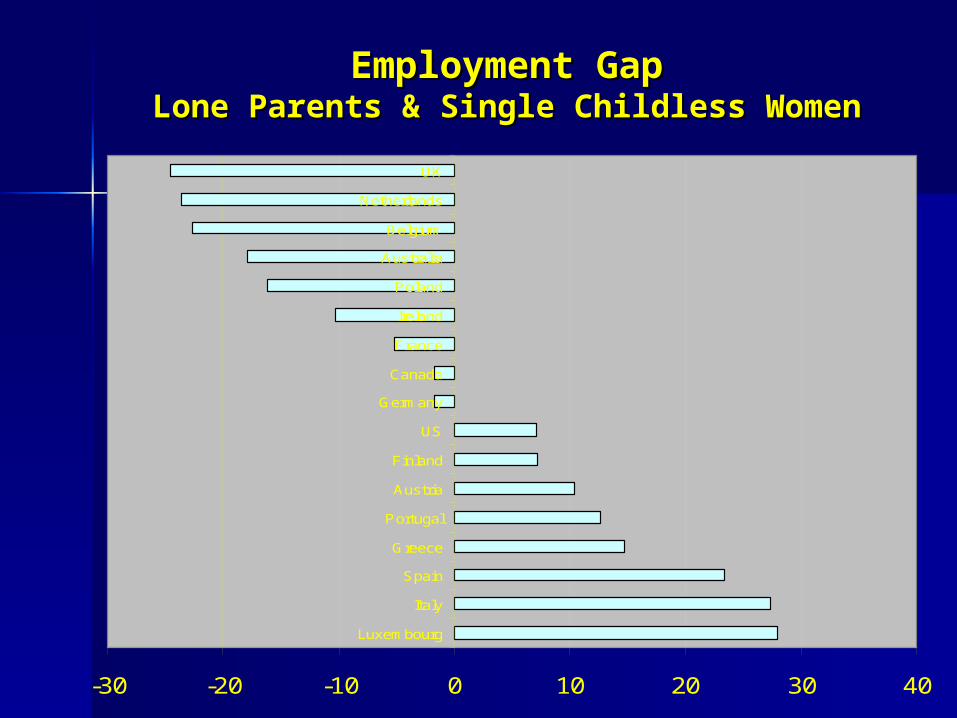
Employment GapEmployment GapLone Parents & Single Childless WomenLone Parents & Single Childless Women
-30 -20 -10 0 10 20 30 40
Luxembourg
Italy
Spain
Greece
Portugal
Austria
Finland
US
Germany
Canada
France
Ireland
Poland
Australia
Belgium
Netherlands
UK
Policy Reform:1997-2002Policy Reform:1997-2002 New Labour pledged to abolish child poverty.New Labour pledged to abolish child poverty. Central to this aim was raising income and employment Central to this aim was raising income and employment
among lone parent households.among lone parent households. A target lone parent employment rate was set at 70 A target lone parent employment rate was set at 70
percent.percent. ““Twin-track” approach:Twin-track” approach:
Improve financial incentives (Working Families Tax Improve financial incentives (Working Families Tax Credit).Credit).
Active caseload management /personal advisors (New Active caseload management /personal advisors (New Deal).Deal).
In contrast to US approach:In contrast to US approach: No time limits on welfare receipt.No time limits on welfare receipt. Searching for work voluntary.Searching for work voluntary. Benefits paid to lone parent families increased for both Benefits paid to lone parent families increased for both
those in and out of work.those in and out of work.

DataData
Household Labour Force Survey Household Labour Force Survey (HLFS):(HLFS):– constructed from the Spring Labour Force constructed from the Spring Labour Force
Surveys from 1992, and since 1996 also Surveys from 1992, and since 1996 also includes the Autumn LFS. includes the Autumn LFS.
– 60,000 households of which just over 60,000 households of which just over 5,000 contain lone parents.5,000 contain lone parents.
General Household Survey (GHS): General Household Survey (GHS): – 6,000-8,000 households with 500-700 lone 6,000-8,000 households with 500-700 lone
parent families.parent families.

MethodologyMethodology Impact of policy Impact of policy YY is difference in post is difference in post
policy outcome Epolicy outcome E11 and the outcome and the outcome that would have occurred without that would have occurred without policy changes Epolicy changes E00..
Y Y = (E= (E11 | L=1) – (E | L=1) – (E00 | L=1) | L=1)
To identify (ETo identify (E00 | L=1) we construct a | L=1) we construct a counterfactual of what would have counterfactual of what would have happened in absence of policy reform.happened in absence of policy reform.

MethodologyMethodology Ideal counterfactual group:Ideal counterfactual group:
– not experienced the policy not experienced the policy shock of interest.shock of interest.
– same observed and same observed and unobserved attributes.unobserved attributes.
– two comparison groups:two comparison groups: couples with childrencouples with children singles without children.singles without children.

MethodologyMethodology Two strands to our approach:Two strands to our approach:
– Account for observable Account for observable differences between the lone differences between the lone parent and non-lone parent parent and non-lone parent populations using propensity populations using propensity score matching .score matching .
– Then use difference-in-difference Then use difference-in-difference estimator to account for estimator to account for unobservables, and to assess the unobservables, and to assess the impact of policy.impact of policy.

Rosenbaum and Rubin (1983) show matching can be Rosenbaum and Rubin (1983) show matching can be done using predicted propensity that an individual is a done using predicted propensity that an individual is a member of the treatment group:member of the treatment group:
P(X)= Pr(L=1,X)P(X)= Pr(L=1,X) Estimate logit models of being a lone parent from the Estimate logit models of being a lone parent from the
populations of lone parents and singles without children.populations of lone parents and singles without children. Variables include gender, age and education, both interacted with Variables include gender, age and education, both interacted with
gender, ethnicity, region of residence and housing tenure type.gender, ethnicity, region of residence and housing tenure type. We use a local linear matching estimator shown to be We use a local linear matching estimator shown to be
computationally efficient by Fan (1992). computationally efficient by Fan (1992). Averages across all observations falling within a window around Averages across all observations falling within a window around
an observation of interest, with a weight derived from the an observation of interest, with a weight derived from the closeness of the outcomescloseness of the outcomes..
Constructing a CounterfactualConstructing a Counterfactual (i) Propensity Score Matching(i) Propensity Score Matching

• Heckman, Ichimura and Todd (1997): Heckman, Ichimura and Todd (1997): • In non-randomised matched samples a conditional difference-in-In non-randomised matched samples a conditional difference-in-
difference estimator mimics the desirable features of an ideal difference estimator mimics the desirable features of an ideal comparator group.comparator group.
Assume unobserved characteristics generate Assume unobserved characteristics generate differences between the focus group and benchmark differences between the focus group and benchmark group prior to policy change. Assuming this gap is group prior to policy change. Assuming this gap is constant, then:constant, then: ( E( E00 | X, L =1) = ( E | X, L =1) = ( E00 | X, L = 0) | X, L = 0) + K+ K
• We can relax the assumption that the gap does not vary We can relax the assumption that the gap does not vary across time as labour market conditions change by across time as labour market conditions change by introducing a time trend:introducing a time trend:
(E(E00|X,L=1) = (E|X,L=1) = (E00|X,L=0) + K + b (Time)|X,L=0) + K + b (Time)
Constructing a CounterfactualConstructing a Counterfactual (ii) Accounting for Unobservables(ii) Accounting for Unobservables

Employment of Lone Parents and Matched Employment of Lone Parents and Matched Samples, and Difference-in-Difference Samples, and Difference-in-Difference Estimates: 1978/80, 1985-87 and 1991/3Estimates: 1978/80, 1985-87 and 1991/3
1978-80(1)
1985-87(2)
1991-93(3)
Change1979-86(4) = (2)-(1)
Difference (from 4,compared to lone parents) (5)
Change1986-92(6) =3-2
Difference(calculated from (6), compared to lone parents) (7)
Difference in difference (8)=(7)-(5)
Lone parents .513 .443 .418 -.075(-.011)
- -.025(-.004)
- -
Matched sample (all)
.669 .592 .595 -.077(-.011)
.002(.000)
.003(.000)
-.028(-.005)
-.0.030(-.005)
Matched single no kids
.738 .663 .642 -.075(-.011)
.000(.000)
-.021(-.004)
-.004(-.001)
-.006(-.001)
Matched couples with kids
.616 .537 .544 -.079(-.011)
.004(.001)
.007(.001)
-.032(-.005)
-.036(-.006)
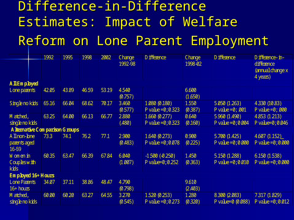
Difference-in-Difference Estimates: Difference-in-Difference Estimates: Impact of Welfare Reform on Lone Parent Impact of Welfare Reform on Lone Parent
EmploymentEmployment
1992
1995
1998
2002 Change 1992-98
Difference
Change 1998-02
Difference
Difference- in-difference (annual change x 4 years)
All Employed Lone parents 42.05 43.89 46.59 53.19 4.540
(0.757) 6.600
(1.650)
Single no kids 65.16 66.04 68.62 70.17 3.460 (0.577)
1.080 (0.180) P value =0; 0.323
1.550 (0.387)
5.050 (1.263) P value =0; .001
4.330 (10.83) P value =0; .000
Matched, single no kids
63.25 64.00 66.13 66.77 2.880 (.480)
1.660 (0.277) P value =0; 0.323
0.640 (0.160)
5.960 (1.490) P value =0; 0.004
4.853 (1.213) P value=0; 0.046
Alternative Comparison Groups All non-lone parents aged 16-59
73.3 74.1 76.2 77.1 2.900 (0.483)
1.640 (0.273) P value =0; 0.078
0.900 (0.225)
5.700 (1.425) P value =0; 0.000
4.607 (1.152)_ P value =0; 0.000
Women in Couples with kids
60.35 63.47 66.39 67.84 6.040 (1.007)
-1.500 (-0.250) P value=0; 0.252
1.450 (0.363)
5.150 (1.288) P value =0; 0.010
6.150 (1.538) P value =0; 0.000
Employed 16+ Hours Lone Parents 16+ hours
34.07 37.11 38.86 48.47 4.790 (0.798)
9.610 (2.403)
Matched, single no kids
60.00 60.20 63.27 64.55 3.270 (0.545)
1.520 (0.253) P value =0; 0.273
1.280 (0.320)
8.300 (2.083) P value=0 (0.088)
7.317 (1.829) P value =0; 0.012

Difference in Difference Estimates: Difference in Difference Estimates: Impact of Welfare Reform on Lone Impact of Welfare Reform on Lone Parent Employment by EducationParent Employment by Education
1992
1995
1998
2002
Change 1992-98
Difference
Change 1998-02
Difference
Difference- in-difference (annual change x 4 years)
O level or lower Lone parents
35.30 36.38 38.98 43.39 3.680 (0.613)
1.450 (0.242) P value =0; 0.018
4.410 (0.242)
6.160 (1.540)_ P value =0; 0.000
5.198 (1.298) P value =0; 0.000
Matched, single no kids
56.40 56.21 58.63 56.88 2.230 (0.372)
-1.750 (-0.438)
A Level and higher Lone Parents
61.44 64.00 64.01 69.73 2.570 (0.428)
-1.470 (-0.245) P value =0; 0.077
5.720 (1.430)
5.410 (1.430) P value =0; 0.000
6.390 (1.598) P value =0; 0.010
Matched, single no kids
74.40 77.42 78.44 78.75 4.040 (0.673)
0.310 (0.078)
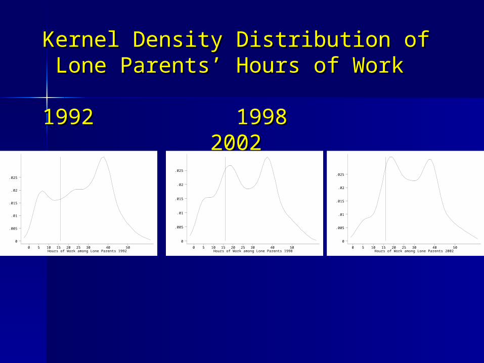
Kernel Density Distribution of Lone Kernel Density Distribution of Lone Parents’ Hours of Work Parents’ Hours of Work
19921992 1998199820022002
Hours of Work among Lone Parents 19920 5 10 15 20 25 30 40 50
0
.005
.01
.015
.02
.025
Hours of Work among Lone Parents 19980 5 10 15 20 25 30 40 50
0
.005
.01
.015
.02
.025
Hours of Work among Lone Parents 20020 5 10 15 20 25 30 40 50
0
.005
.01
.015
.02
.025

Average Hours of Work and Median Average Hours of Work and Median Weekly Earnings among Lone Parents Weekly Earnings among Lone Parents
(2002 prices)(2002 prices) Average Hours of Work
1998 2002 Change All Lone Parents
11.7 14.2 2.5
Working Lone Parents
27.3 28.5 1.2
Working Lone Parents 16+ hours
32.1 30.9 -1.2
Matched Lone Parents 1998-2002
32.0 31.5 -0.5
Predicted Entrants - 29.5 - Median Weekly Earnings among Lone Parents
1998 2002 % Change Working Lone Parents
149 203 36.2
Working Single Women without Children
274 311 13.5
Working Lone Parents 16+ hours
197 219 11.2
Matched Lone Parents 1998-2002
197 224 13.7
Predicted Entrants - 206 -

Dynamic Employment Dynamic Employment EffectsEffects

0%
2%
4%
6%
8%
10%
12%
14%
16%
18%
20%
Q3 Q4 Q1 Q2 Q3 Q4 Q1 Q2 Q3 Q4 Q1 Q2 Q3 Q4 Q1 Q2 Q3 Q4 Q1 Q2 Q3 Q4 Q1 Q2 Q3 Q4 Q1 Q2 Q3 Q4 Q1
94-95 95-96 96-97 97-98 98-99 99-00 00-01 01-02 02-03
Rolling Time Period 1993-2003
Pro
bab
ilit
y o
f E
nte
rin
g W
ork
Entry rate; non-lone parents Entry rate; lone parents
Job-Entry Probabilities 1992-2003Job-Entry Probabilities 1992-2003

0%
2%
4%
6%
8%
10%
12%
14%
16%
18%
Q3 Q4 Q1 Q2 Q3 Q4 Q1 Q2 Q3 Q4 Q1 Q2 Q3 Q4 Q1 Q2 Q3 Q4 Q1 Q2 Q3 Q4 Q1 Q2 Q3 Q4 Q1 Q2 Q3 Q4 Q1
94-95 95-96 96-97 97-98 98-99 99-00 00-01 01-02 02-03
Rolling Time Period 1993-2003
Pro
bab
ilit
y o
f E
xiti
ng
Jo
b
Exit Rate, Non-Lone Parents Exit Rate, Lone Parents
Job-exit Probabilities 1992-2003Job-exit Probabilities 1992-2003
Lone Parents and Non Lone Parents Lone Parents and Non Lone Parents

Differences in Lone Parent Employment Entry and Exit Rates Differences in Lone Parent Employment Entry and Exit Rates 1992-2003 1992-2003
-8%
-6%
-4%
-2%
0%
2%
4%
6%
8%
10%
Q3 Q4 Q1 Q2 Q3 Q4 Q1 Q2 Q3 Q4 Q1 Q2 Q3 Q4 Q1 Q2 Q3 Q4 Q1 Q2 Q3 Q4 Q1 Q2 Q3 Q4 Q1 Q2 Q3 Q4 Q1
94-95 95-96 96-97 97-98 98-99 99-00 00-01 01-02 02-03
Rolling Time Period 1993-2003
Pe
rce
ntg
e P
oin
t D
iffe
ren
ce
be
twe
en
Lo
ne
Pa
ren
ts
an
d N
on
-lo
ne
pa
ren
ts
Difference in Exit Rates
Difference in Entry Rates

Contribution of Change in Entry Contribution of Change in Entry and Exit Rate to Overall Change and Exit Rate to Overall Change in Employmentin Employment
1992: Entry rate 11.5%; Exit Rate 1992: Entry rate 11.5%; Exit Rate 14.0%.14.0%.– Steady state employment rate 45 percent.Steady state employment rate 45 percent.
A rise in the job entry rate to 15 A rise in the job entry rate to 15 percent (2002 rate) leads to a percent (2002 rate) leads to a predicted steady state employment predicted steady state employment rate of 52 percent. rate of 52 percent.
Fall in exit rate to 10 percent leads to Fall in exit rate to 10 percent leads to a rise in employment to 60 percent.a rise in employment to 60 percent.

ConclusionsConclusions Policy reform has increased employment among lone parents by Policy reform has increased employment among lone parents by
4½ to 5 percentage points (75-85,000 families).4½ to 5 percentage points (75-85,000 families). The policy impact of moving people into work of at least 16 hours The policy impact of moving people into work of at least 16 hours
is somewhat larger at 7 percentage points.is somewhat larger at 7 percentage points. Gains in employment have NOT been concentrated on least well Gains in employment have NOT been concentrated on least well
educated.educated. Gains have been achieved in spite of large increases in benefits for Gains have been achieved in spite of large increases in benefits for
those out of work.those out of work. Gains in earnings and hours of work have helped reduce lone Gains in earnings and hours of work have helped reduce lone
parent poverty rates (in absolute and relative terms).parent poverty rates (in absolute and relative terms). Lone parents are now successful in finding work compared to other
populations. But lone parents are leaving work at far greater rates than non-
lone parents. Job exits are related to low pay, especially when linked to part-time
work, and ill health. Pace of change does not look sufficient for the governments target Pace of change does not look sufficient for the governments target
of 70% lone parent employment by 2010 to be metof 70% lone parent employment by 2010 to be met Ensuring lone parents entering work move into high quality, sustainable jobs may be an effective route for policy.
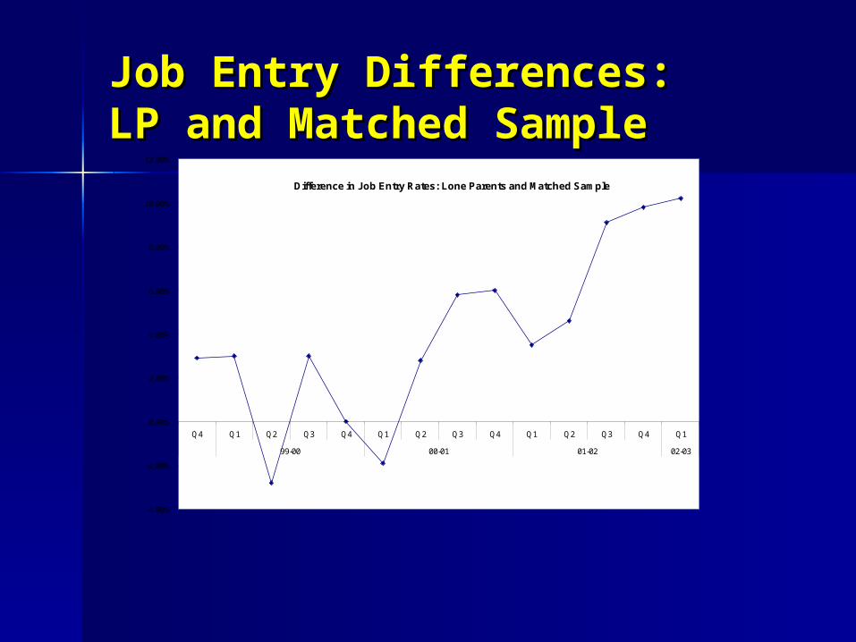
Job Entry Differences: Job Entry Differences: LP and Matched SampleLP and Matched Sample
Difference in Job Entry Rates: Lone Parents and Matched Sample
-4.00%
-2.00%
0.00%
2.00%
4.00%
6.00%
8.00%
10.00%
12.00%
Q4 Q1 Q2 Q3 Q4 Q1 Q2 Q3 Q4 Q1 Q2 Q3 Q4 Q1
99-00 00-01 01-02 02-03

Job Exit Differences: Job Exit Differences: LP and Matched SampleLP and Matched Sample
Difference in Job Exits: Lone Parents and Matched Sample, Personal Characteristics
0.00%
2.00%
4.00%
6.00%
8.00%
10.00%
12.00%
Q3 Q4 Q1 Q2 Q3 Q4 Q1 Q2 Q3 Q4 Q1 Q2 Q3 Q4 Q1 Q2 Q3 Q4 Q1 Q2 Q3 Q4 Q1 Q2 Q3 Q4 Q1 Q2 Q3 Q4 Q1
94-95 95-96 96-97 97-98 98-99 99-00 00-01 01-02 02-03
Difference
Related Documents