Welfare Losses from First-Come-First-Serve Course Enrollment

Claremont CollegesScholarship @ Claremont

CMC Senior Theses CMC Student Scholarship

2019

Welfare Losses from First-Come-First-ServeCourse Enrollment: Outcome Estimation andNon-Market MaximizationRory Fontenot

This Open Access Senior Thesis is brought to you by Scholarship@Claremont. It has been accepted for inclusion in this collection by an authorizedadministrator. For more information, please contact [email protected].

Recommended CitationFontenot, Rory, "Welfare Losses from First-Come-First-Serve Course Enrollment: Outcome Estimation and Non-MarketMaximization" (2019). CMC Senior Theses. 2057.https://scholarship.claremont.edu/cmc_theses/2057

https://scholarship.claremont.edu

https://scholarship.claremont.edu/cmc_theses

https://scholarship.claremont.edu/cmc_student

mailto:[email protected]

Claremont McKenna College

Welfare Losses from First-Come-First-Serve Course Enrollment:

Outcome Estimation and Non-Market Maximization

Submitted to

Professor Laura Grant

By

Rory Fontenot

For

Senior Thesis

Fall 2018

December 10, 2018

Abstract

College course enrollment operates as a market under supply cap. Because of the limited

number of seats available for any given course some students who have a higher demand for a

course are unable to enroll. The current registration system at the Claremont Colleges functions

as a random draw system with added time costs. The lack of price signalling in the markets leads

to a loss in overall welfare of the student body. By running data through simulated demand

curves I am able to determine, on average, how much welfare is being lost by a random draw

system. The percent of maximum welfare achieved compared to maximum possible ranges from

forty-nine to eighty percent and largely depends on the proportion of enrolled students to the sum

of enrolled + enroll requests as well as the demand function type. With price signalling, the

student body would be able to reach the maximum achievable welfare.

Table of Contents

Introduction……………………………………………………………………………….1

Literature Review……………………………………………………………………...….2

Course Enrollment System…………………………………………………………….….4

Theory………………………………………………………………………………….….6

Quasi-Linear Preference Models………………………………………………………..…7

Data………………………………………………………………………………..……….21

Results………………………………………………………………………………..…….23

Creating a Market………………………………………………………………….……….27

Conclusion………………………………………………………………………....……….28

References…………………………………………………………………….…………….30

Appendix………………………………………………………………………...………….31

Introduction

In a free-market system, the supply and demand for any given good floats around a point

of equilibrium. Under such market conditions three conditions are met: the supply is equal to the

demand, those who value the good most are the ones who receive it, and those who can afford to

supply it, do so. Thus, the welfare is maximized in the market. However, a cap on a market’s

supply reduces overall welfare, as not all individuals who are willing to pay for the good receive

it, though if they are able to properly express their demand it is still those with the highest

willingness to pay who receive the good. In markets where individuals are unable to express their

demand through a price signal there is an inefficient allocation of the good. Instead of ensuring

that only those with the highest willingness to pay for the good, it becomes a random assignment

to all individuals that desire the good regardless of their utility.

In order to maximize efficiency in these situations, non-monetary markets can be set up

by the supplier to distinguish each individual’s demand. Instead of individuals using personal

income buy goods, they are allocated credits for the unpriced goods. These credits allow

individuals to show their preferences between multiple goods by ‘spending’ the same way they

would with money.

Enrollment in college courses acts as a market under a supply cap without a price signal.

At every school, there are a limited number of seats for each course offered and not every student

that wants to register for the course can enroll. Because of the supply cap there will always be a

loss of overall welfare if more students than available seats have a demand for the course. The

1

design of the course registration system is what can determine exactly how much welfare is

being lost during selection. This paper sets out to determine what design will lead to welfare

maximization for a student body.

Literature Review

The issue of allocating course enrollment to a student body is an example to setting up a

non-monetary market to reach the economically efficient outcome. Other examples include the

allocation of hunting permits, housing under rent control, and licenses for any good whose

production is capped by government intervention. Economists study non-monetary markets

across different sectors of the economy to find out how well they work and what conditions

cause them to work more efficiently. In researching an auction based system for food distribution

for food banks, Pendergast (2017) found that Feeding America’s system works more efficiently

than a standard queueing system. His findings were that a non-monetary market worked

efficiently because of certain parallels between an active money based market. More specifically,

it gave players the option to hold onto their currency until they were able to spend it on

something they truly desired, and that the players were a part of an extended process with no

known endpoint. Both assumptions seemingly do not apply to students biding to receive a seat in

a class. Students are not able to wait until the next day for a new set of class combinations and

they are only in the market for class bids around eight to twelve times during their college career,

though they are able to put off placing a bid on a course until the next term it is offered.

When a school is put in the position of assigning course schedules to students in an

environment with limited class sizes they are essentially operating in a market under a cap. When

2

a market cap is imposed there will be a number of people who have adequate demand for the

good who are left out, in their paper Glaeser and Luttmer(1997) look at rent controlled markets

to determine how much welfare is lost under these market conditions. They analyze New York

City and find out that market caps do not create a simple slide in allocation and that around 20%

of houses ended up in the wrong hands. Sorting issues and misallocation of limited resources is

important to consider when designing a system to most effectively represent participants’

welfare. Even in money based markets there can be misallocation. Another important finding

from the research is that the losses due to misallocation are larger than losses due to undersupply

in the market. Creating a market that misallocates resources could be more detrimental to a

student body than leaving a market with not enough supply.

Other papers deal directly with course registration setups that currently exist at different

universities at the graduate and undergraduate levels. In the papers by Sonmez and Unver (2005),

and Krishna and Unver (2008) differences in the efficiency of the allocation outcomes are

analyzed for two different non-monetary setups in universities. Two important findings are

discussed in both of these papers. The first is that the market setups for course allocations do not

perfectly match that of a money based market. It was found that students think about the system

like a game and start to treat bidding for classes like a system that can be bested, leading to a

misinterpretation of how much students value each class. The other addition of this research is

the discussion around the Add/Drop period and what that adds to the efficiency of the market

outcome. The conversation surrounding the Add/Drop period is relevant to the system this paper

examines as the Permission to Enroll Requests(PERMs) are key to this step in course registration

and serve as the main signifier of a student’s demand.

3

Course selection systems that do not take into account a student’s demand for the course

perform like a random assortment system for a good in a capped market. Thomas(2018)

examines the potential gains in welfare in Washington state if the government gave marijuana

licenses to the most profitable producers instead of a random assignment. Thomas(2018) finds

that if firms are allowed to enter the market freely that there would be a 21% increase in welfare

and that random allocation makes up 65.9% of that loss in welfare. The loss in welfare is found

by creating simulations of total welfare gained under the current random allocation system and a

hypothetical free entry system. The process of creating a simulation and applying data to it is an

excellent way of estimating loss in welfare and will be applied to course registration systems.

The paper written by Graves, Schrage, and Sankaran (1993) gives a detailed account of

the creation and testing of their own market design for course scheduling. Like some higher

education institutions, they opted for an auction based system. The main goal of the researchers

is the same driving factors that many offices consider when changing their old system: gathering

a more accurate understanding a student’s preferences for any given course schedule. Through

their design they found that they were able to achieve 88.3% of the maximum deliverable value

to students, a surprising increase from a traditional queue. Without changing the supply of

courses, students were given their number one choice in schedule 54% of the time on any given

term.

Course Enrollment System

The current course registration system at the Claremont Colleges involves three steps.

The first part of course registration is that each students is placed into a registration time slot

4

within their class year. Each class is allowed to register before the next. Once course registration

opens the second stage begins where students begin to add courses to their schedule. It is during

this course selection process that students are able to submit Permission to Enroll Requests

(PERMs). If a student is unable to enroll into a course that they desire they are able to submit a

PERM through the registration portal in hopes that they are able to get a seat. There is no limit to

how many PERMs any given student is allowed to submit. The approval of PERMs is a

combination of the professor’s choice to approve any PERM in the pool as well as how many

seats are available in the course. Because the current system is not a direct queue where the first

to PERM is the first to be accepted when a seat opens in the course there is a third step of time

costs. Before the next term starts students have the option of email professors or going to their

office to try to get their PERM accepted for the course. Additionally, when the new term starts

students can choose to attend classes that they have submitted PERMs to. This process leads

students to incur a time cost by attending courses and talking to professors with no guarantee of

enrollment, in the hopes that it will help their chances of having a PERM accepted. This time

spent during registration and at the beginning of semester helps students to express their demand

for the course but it is not a good enough signal to determine which student in the PERM pool

has the highest demand for the course.

Because of the randomization of time periods, the current system can be viewed as a

random selection process with additional time costs. Students are unable to express their demand

through price signals, a PERM only indicates that the student holds a desire to attend a course

and therefore some nonzero demand for the course. Because of this shortcoming those who

5

receive a seat in the course are a random group selected from a pool of students who have some

indistinguishable positive demand for the course.

Theory

In addition to an inability to tell which students have the highest demand for any given

course, the lack of price signals means that there is no method of seeing how the demand for a

course is modeled because of the inability to show much much each additional students values

the course. These demand curves will differ across the courses offered at college. There may be

some courses with consistently high demand through the student body while others diminish.

Some courses may have demand that falls very steeply and others that diminish more uniformly.

In a random selection system there is no way to model demand for courses. If a course covers a

niche area of interest, a small handful of students might have a large demand for taking the

course, however that demand will fall off quickly as people who are less interested in the topic

sign up to take the course. There are other scenarios where a course may be required towards the

beginning of a popular major’s graduation requirements, leading to a consistently high demand

across the student body. Before applying real data from course selection periods, I am going to

simulate different scenarios for varying possible demand curves for any given course. The

differing slopes of these demand lines will determine how much overall welfare is being lost by

an inefficient course selection system. I assume that the demand curve for any given course to

not be uniform. The welfare that each individual student gets out of any given course will change

depending on its topic as well as how frequently it is offered. I expect the amount of lost welfare

6

to be proportionate to the ratio of enrolled students to PERMs submitted and that steeper demand

curves will have a lower percentage of welfare achieved.

I begin with general models for various demand curves, I then take real data and apply

them to the theoretical models to see how much welfare is being lost in each scenario, and how

much welfare can be obtained by using a system that maximizes overall welfare for the capped

market of course enrollment.

Quasi-Linear Preference Models:

A quasi-linear preference model is applied to solve for maximized demand when utility can be

viewed as utility from receiving one good versus a numeraire. This can be applied to a student’s

preferences by starting with the utility function:

U(c,x) = U(c) + U(x)

Where I take U(c) to be a function of the utility gained from the given course and U(x) to be a

function of the utility gained from all other goods. Because I am interested in finding the demand

for any given course at the price I am able to treat “all other goods” as a numeraire and(c)P c

normalize the price to 1. That is to say, in exchange for putting one more dollar towards getting

into any given course you are giving up consuming one dollar of “all other goods”.

This assumption transforms the utility function to:

U(c,x) = U(c) + x

7

Where U(x,c) is the total utility to be gained by any given class and the total amount of “other

goods” consumed by the student. U(c) remains the function for the utility of any given course at

the price . I examine different functions U(c,x) where the utility gained from any given(c)P c

course follows the form:

U(c) = (c) b(c) − a m +

To get a demand slope from the utility functions U(c,x) I find the marginal utility with respect to

c. This is taken as:

= (c) f = McMU (c,x)

1P (c)c P (c) → c

which generates the function of the form (c) which is the price of any given class times theP c

quantity. In these models I am only examining scenarios involving a single class, so I set c = 1.

Leaving us with just (c), the price of any given course. Because college is a fixed cost, eachP c

student shares the same budget so the price of any given course gives each student’s willingness

to pay, a student who gains more welfare from the given course is more willing to pay for it. By

examining the demand function in this way I can see how much welfare is being lost.

In order to create generalized models for each scenario below, I operate under the same

assumptions: we are only looking at a market where 200 students are attempting to get a seat for

a class that has a total cap of 114, assuming there are 6 available sections of 19 seats. The 200 x

values is the sum of students currently enrolled in the course as well as all of the Permission to

8

Enroll Requests. The total welfare for the 200 students in each scenario is normalized to $20,000.

By operating under these assumptions I ensure that the results from each model are comparable.

Under each demand function I will take the maximum achievable welfare by summing

the highest 114 demands out of the 200 total students. This maximum will be compared to the

average sum of 10,000 random draws of 114 students from total 200. A random draw of 114

students mirrors a course selection system that has no method for students to express their

demand for any given course. The ratio between total random selection welfare and maximum

welfare will give a good idea of how much welfare the student is losing out on by not being able

to express their demand for enrollment in courses.

First Scenario:

For the first scenario we will take f(c) to be:

(c) (c) b(c) f = − a 2 +

In order to model a quadratic utility function. The first derivative with respect to c of f(c) is:

a(c) bδcδf (c) = − 2 +

Giving a linear demand function. A course with a linear demand curve has a demand that

diminishes uniformly with each additional student.

9

In this equation ‘a’ is a shifting factor for the slope and b is a shifting factor for the intercept. In

order to normalize total welfare to $20,000 I first integrate the function from 0 to 200 with ‘a’=1

and ‘b’=0

− c 0, 00∫200

02 = − 4 0

In order to bring the utility down to -20,000 I set:

0, 00a−40,000 = − 2 0

0.5 ⇒ a =

With ‘a’ = 0.5 I set ‘b’ equal to a value so that our 200th student has a demand of exactly 0. In

this case:

-(200) + b = 0

b = 200 ⇒

the demand function is then:

= (c) f c) 200 − ( +

The maximum achievable welfare under these model conditions is $16,245. The mean of

10,000 random draws of 114 students is $11,342. This mean gives a welfare ratio of 0.69819,

which suggests that on average, 69.8% of maximum welfare is achieved under a system that does

not allow students to express demand.

10

Additionally, the maximum welfare from random draws was just over $12,500. Out of

10,000 random draws the closest welfare to maximum was still almost $4,000 less than

maximum, a whole quarter of the maximum welfare value.

Figure 1. Linear demand curve for a course with a cap of 114 students. The shaded region is the maximum

achievable welfare, the sum of the first 114 students.

Figure 2. Frequency distribution of total welfare achieved from 10,000 random draws of 114 students with a linear

demand for a course from a pool of 200.

11

Second scenario:

In this scenario I take the function f(c) to be:

(c) (c) b(c) f = − a 3 +

In order to model a cubic utility function. Taking the derivative with respect to c gives:

a(c) bδcδf (c) = − 3 2 +

Giving a quadratic demand function. In this case, the demand for the given course diminishes

slowly at the beginning and then starts to diminish quickly further out in the curve. A quadratic

demand function indicates that there are more students that have a high demand for a given

course than one that is modeled by a linear demand curve.

In order to normalize total welfare I integrate from 0 to 200 with ‘a’ = 1 and ‘b’ = 0.(c) f

12

-8,000,000− (c) ∫200

03 2 =

Because is a quadratic equation, to normalize the total area under the curve we set the total(c) f

area divided by ‘a’ equal to half the desired welfare:

, 00, 00 (a) 10, 00 − 8 0 0 = 0

a 0.00125 ⇒ =

.00125 ( 3 ) 0.00375 0 =

In order to have the 200th student have a demand of 0:

00375(200) b 0 − . 2 + =

b 150 ⇒ =

Giving the demand function:

= (c) f 00375(c) 150 − . 2 +

Under these model conditions the maximum achievable welfare is $15,223. The mean of

the 10,000 random draws of 114 students is $11,357. This gives a welfare ratio of 0.746 which

suggests that on average, 74.6% of maximum welfare is achieved under a system that does not

allow students to express their demand. The maximum welfare achieved by random draws was

under $12,500 which is about $3,000 short from the maximum achievable welfare.

13

Figure 3. Quadratic demand curve for a course with a cap of 114. The shaded region is the maximum achievable

welfare, the sum of the first 114 students.

Figure 4. Frequency distribution of the sum of 10,000 random draws of 114 students with a quadratic demand for a

course from a pool of 200.

14

Third scenario:


(c) (c) b(c) f = − a 0.5 +

In order to model a square root utility function. Taking the derivative with respect to c gives:

.5a(c) bδcδf (c) = − 0 −0.5 +

Giving a square root demand function. Under these conditions we see that a very small number

of students have a large demand for the course but it quickly falls off. The course reaches a

relatively low demand very early in the course selection process and then levels off as the

majority of students have a more consistent low demand for it.

In order to normalize the total welfare I integrate the function with ‘a’=1 and ‘b’ = 0

15

.5c 4.1421∫200

00 −0.5 = 1

Because is a square root function I set equal to twice the desired welfare:(c) f 4.1421(a) 1

4.1421(a) 0, 00 1 = 4 0

2828.5 ⇒ a =

(0.5) 1414.2 a =

Again, ‘b’ is a shifting factor for the intercept such that the 200th student has a utility and

demand of zero. In this case:

414.2(200) b 0 1 −0.5 + =

b 9.9 ⇒ = − 9

The final demand function is:

(c) 1414.2(c) 99.9f = −0.5 −

Under these model conditions the maximum achievable welfare is $16,801. The mean

welfare of 10,000 random draws of 114 students is $10,262. This gives a welfare ratio of 0.61

which suggests that on average, 61% of maximum welfare is achieved under a system that does

not allow students to express their demand. The greatest welfare achieved by random draws was

close to $13,000 about $4,000 less than the maximum achievable welfare.

16

It is interesting to note that the welfare ratio a square root demand function is smaller

than the quadratic and linear demand curves. Because few students have an abnormally high

demand for these courses, and the majority level off at a low demand, the welfare achieved by

random draws can fluctuate greatly depending on how many of these students are selected. It is

especially easy to make up a large fraction of maximum welfare if some of the random 114

draws are the students with the unusually high demand for the course.

Figure 5. Square root demand curve for a course with a cap of 114. The shaded region is the maximum achievable


Figure 6. Frequency distribution of the sum of 10,000 random draws of 114 students with a square root demand for

a course from a pool of 200.

17

Fourth Scenario:


(c) a(log(c)) b(c) f = +

In order to model a logarithmic utility function. The first derivative with respect to c is:

bδcδf (c) = c

a +

This scenario models a class with a logarithmic demand function. Here, a small amount of

students hold a very high demand for the course but the demand quickly falls off with the rest of

the student body, similar to the square root function.

In order to normalize the total welfare I integrate from 0.001 to 200 with ‘a’=1 and b=’0’δcδf (c)

18

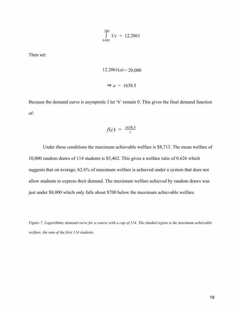
/c 12.2061∫200

0.0011 =

Then set:

= 20,0002.2061(a) 1

1638.5 ⇒ a =

Because the demand curve is asymptotic I let ‘b’ remain 0. This gives the final demand function

of:

(c) f = c1638.5

Under these conditions the maximum achievable welfare is $8,713. The mean welfare of

10,000 random draws of 114 students is $5,462. This gives a welfare ratio of 0.626 which

suggests that on average, 62.6% of maximum welfare is achieved under a system that does not

allow students to express their demand. The maximum welfare achieved by random draws was

just under $8,000 which only falls about $700 below the maximum achievable welfare.

Figure 7. Logarithmic demand curve for a course with a cap of 114. The shaded region is the maximum achievable


19

Figure 8. Frequency distribution of the sum of 10,000 random draws of 114 students with a logarithmic demand for

a course from a pool of 200.

20

Table 1. Mean and maximum welfare achieved by linear, quadratic, square root, and logarithmic demand

functions for a scenario with a total welfare of $20,000.

Demand Function Mean Welfare of

Random Draws

Maximum Achievable

Welfare

% Welfare Achieved

Linear 11,342 16,245 69.8

Quadratic 11,357 15,223 74.6

Square Root 10,262 16,801 61

Logarithmic 5,462 8,713 62.6

Data

Using the generalized framework from the simulations I apply real data from course

registration to estimate the welfare ratio of four separate economics courses at Claremont

McKenna College. The selected courses differ in how many sections are available as well as the

ratio of students currently enrolled in the course and PERMs submitted. The data was taken in

the fall of 2018 from the school’s registration portal after the registration period had closed for

the Spring 2019 semester. Students of all grade levels are included in the enrolled and PERM

numbers.

21

The total welfare for each course is normalized across the different demand curves.

However, each course holds a different total welfare because not every course offered at a

college provides the same utility to the student body. The normalization process for each

scenario is the same as the one taken in the simulation section. The total welfare for ‘Principles

of Economic Analysis’ is $10,000. For ‘Accounting for Decision Making’ total welfare is

$25,000. For ‘Statistics’ total welfare is $15,000. And finally the total welfare for ‘Development

Economics’ is $5,000.

The modeled data only takes into account the welfare loss from random assignment of

students during the initial registration period. No loss in welfare due to time costs incurred by

students’ actions to improve their chances of having a PERM accepted is reflected in these

estimations.

Table 2. Mean and Maximum welfare achieved in each of four courses from linear, quadratic, square root, and

logarithmic demand functions. Total welfare for: Principles of Economics: $10,000, Accounting for Decision

Making: $25,000, Statistics: $15,000, Development Economics: $5,000

Course Name Linear Quadratic Square Root Logarithmic

Mean Random Draw Total

Maximum Achievable Welfare

Welfare Ratio



Welfare Ratio



Welfare Ratio



Welfare Ratio

Principles of Economic Analysis

5,919 8,329 .71 5,943 7,876 .75 5.175 8,135 .63 2,717 4,096 .66

Accounting for Decision Making

10,719 16,843 .63 10,721 15,132 .70 9,696 19,648 .49 5,206 10,410 .50

Statistics 10,749 13,755 .78 10,769 13,379 .80 9,425 12,728 .74 4,978 6,465 .76

Development Economics

3,156 4,304 .73 3,171 4,129 .76 2,621 3,898 .67 1,351 1,909 .70

22

Results

The course ‘Principles of Economics’ has 64 students enrolled in the course and a

combined 107 students who are either enrolled in the course or have submitted a PERM. This

gives a enrolled to request ratio of .59, which means around 60% of students who want to take

the course are able to take it in the Spring of 2019. In order to properly compare the efficiency of

each demand function, the total welfare across all 107 students is $10,000 for this course. Under

the conditions of a linear demand curve if welfare is maximized, meaning the 64 students with

the highest demand for the course were enrolled, it would yield a welfare of $8,329. The mean of

10,000 random draws of 64 random students from the pool of 107 is 5,919, giving a welfare ratio

of 0.71. Under a quadratic demand function the welfare ratio is 0.75. Under a square root

demand function the welfare ratio is 0.63. Under a logarithmic demand function the welfare ratio

is 0.66

The lowest welfare ratio achieved for ‘Principles of Economic Analysis’ is 0.63 under the

square root demand function and the highest is 0.75 under the quadratic demand function. The

welfare ratio has a range of 12% of the maximum achievable welfare. Because ‘Principles of

Economic Analysis’ is an extremely common course for students here to take, both because it is

the introduction to the Economics major as well as a popular general education requirement for

non-Economics majors, I believe the linear model to be the best representation of real life

demand. There are some students with a very high demand for the course but its popularity keeps

the decline in demand constant. Therefore the welfare ratio of 0.71 is likely the most realistic

23

estimate of the welfare achieved for ‘Principles of Economics’ when students can not express

their demand.

‘Accounting for Decision Making’ has 93 students enrolled in the course and a combined

216 students who are either enrolled or have submitted a PERM. This gives a ratio of enrolled to

request ratio of 0.43, which means that only 43% of students who want to take the course in the

spring of 2019 are able to. This ratio is the lowest out of the four courses. The total welfare

across the 216 students is $25,000 in each of the four scenarios. The welfare ratio under a linear

demand curve is 0.63. Under a quadratic demand function the welfare ratio is 0.70. Under a

square root demand function the welfare ratio is 0.49. Under a logarithmic demand function the

welfare ratio is 0.50.

The lowest welfare ratio for ‘Accounting for Decision Making’ is under the square root

function at .49, though it is noteworthy that the ratio under a logarithmic demand function is only

1% higher at 0.50. The highest welfare ratio is achieved under the quadratic demand function at

0.70. The range of welfare ratios for the course is 21% of the maximum achievable welfare, a

larger range than that of ‘Principles of Economics’. This particular course is in an interesting

position in terms of demand. It is usually the second course taken by Economics majors as well

as a course that can be taken for elective credit. However, it serves a role as the first accounting

course available to students and can be the deciding factor in whether a student pursues

Economics-Accounting or Economics as a major. Even if a student decides to go with

Economics over the alternative, this course will still count as a major elective credit. Because of

the importance and applicability I believe the quadratic demand function to be the most likely

representation of demand for ‘Accounting for Decision Making’. Many students will have a high

24

demand for the course, and the demand will diminish slowly across Economics oriented students.

It is only when non-Economics students register for the class that you see a steeper fall in

demand. I believe the welfare ratio of 0.70 is likely the most realistic estimate of welfare

achieved by ‘Accounting for Decision Making’.

‘Statistics’ has 86 students enrolled in the course and a combined 119 students who are

either enrolled or have submitted a PERM. This gives an enrolled to request ratio of 0.72. This

ratio means that 72% of students who want to take the course in the Spring of 2019 are able to. A

ratio of 0.72 is the highest of the four courses. The total welfare across the 119 students is

$15,000. Under a linear demand model the welfare ratio is 0.78. Under a quadratic demand

function the welfare ratio is 0.80. Under a square root demand function the welfare ratio is 0.74.

Under a logarithmic demand function the welfare ratio is 0.76.

The lowest welfare ratio for ‘Statistics’ is achieved under the square root demand

function at 0.74, and the highest is achieved under the quadratic demand function at 0.80, though

the linear demand ratio is just behind quadratic at 0.78. The range in welfare ratios is only 6% of

the maximum achievable welfare, much lower than both ‘Principles of Economic Analysis’ and

‘Accounting for Decision Making’. ‘Statistics’ is generally not a very sought after class, however

it is a prerequisite for a required course in the Economics major. Because there are certain

students who are more interested in the Econometric side of economics I know there will be a

handful of students with a high demand for the course, but I expect that the demand falls off very

quickly once those students are accounted for. Because of the steep decline I assume that the

square root or logarithmic functions best model the demand for this course. The welfare ratios of

25

0.74 to 0.76 are most likely the best estimation of the welfare achieved by this course when

students are unable to express their demand.

‘Development Economics’ has 36 students enrolled in the course and a combined 56

students who are either enrolled or have submitted a PERM. This gives an enrolled to request

ratio of 0.64. This ratio means that 64% of students who want to take the course in the spring of

2019 are able to. The total welfare across the 56 students is $5,000. The welfare ratio under a

linear demand curve is 0.73. The welfare ratio under a quadratic demand curve is 0.76. The

welfare ratio under a square root function is 0.67. The welfare ratio under a logarithmic demand

curve is 0.70.

Just like the other three courses, the lowest ratio is achieved under a square root function

at 0.67 and the highest is achieved under a quadratic function at 0.76. The range in welfare ratios

is 19% of the maximum achievable welfare. Because this course covers a niche interest inside of

economics and is offered as a higher level elective within the Economics major I believe that the

logarithmic demand function best models its demand. Some students who have a serious interest

in the subject matter will have a high demand and as more students who enroll to fulfill the

elective credit come in, the faster the demand drops off comparatively. The welfare ratio of 0.70

is likely the most realistic estimation of the demand for ‘Development Economics’.

For every course, the square root demand yields the lowest welfare ratio and the

quadratic demand yields the highest ratio. This follows intuition as the square root function has

the quickest diminishment, meaning the reduction in demand for each consecutive student is

greater than any other function. Each lower valued student has a bigger impact on the sum when

26

the demand falls quickly. On the other side, quadratic demand stays high and diminishes slowly

at first. If random selection picks a student with slightly lower demand under the quadratic model

it will impact the sum much less.

Additionally it is important to note that the welfare ratio is proportional to the enrolled to

request ratio. The higher the enrolled to request ratio is, the larger the area under the curve is

simply because you are randomly selecting a larger proportion of the students. The greater the

number of students picked the more likely it is that a high demanding student is selected instead

of left out.

Creating a Market

The main drawback of a random draw system for course enrollment is the lack of price

signalling. This can be overcome by implementing a system in which students are able to display

their demand for courses. Pendergrast(2017) notes that a common mechanism to express demand

in education is an individual ranking based system in which students turn in an ordered list of

their course preferences. Demand can be shown by these ranking systems, but only nominally. If

two students submit identical preferences rankings for classes there is still no way to distinguish

which of the two students has a higher demand for their top ranked course. The only information

that is transferred through these rankings are which courses a student values more relative to

others, not how much.

In order to determine a student’s demand, a mechanism that recreates the workings of a

monetary market must be created. A system where students are given a predetermined amount of

27

credits, instead of money, to bid on each course will allow students to express their true demand

for any given course through price signalling. Because students are working with a constrained

budget they must make decisions on where to spend their credits.

Each course can fulfill a different graduation requirement, the student’s willingness to

pay shifts as they move through their college career. Early in the college career, when any course

taken fulfills a requirement, students are less likely to spend most of their credit on one course

and instead wait until the course is necessary for their academic progression(Graves 1993).

Because of a student’s changing preferences based on need, expenditure is not left as solely a

function of interest in subject.

The forces that impact a student’s preference for courses combined with the ability to

spend credits on course enrollment mimics the working of a money based market. Under these

conditions students are able to express their demand and willingness to pay through the credit

system. It is once demand is properly communicated in the market, that those with the highest

willingness to pay will be those who receive a seat in the course. Under these conditions welfare

is maximized.

Conclusion

When schools do not allow a system for students to express their demand for courses the

course registration process acts like a market under a cap. When a market operates under cap

there is a loss in welfare, though it can still be maximized given the conditions if those with the

highest demand for the good are those who receive it. Without price signalling, course

28

enrollment acts as a random assortment to students who have some unspecified positive demand

for the course with added time costs from students trying to display their high demand by

approaching the professor and attending class. In the simulations using real data the ratio of

mean welfare and maximum achievable welfare was as low as 0.49 and as high as 0.80. By

implementing a system where students can spend allocated credits on course enrollment they will

be able to show their demand and ensure that those with the highest willingness to pay are those

who receive a spot in the course. If students are given the ability to show their demand the total

welfare will move towards the maximum achievable welfare under the market cap restraints.

29

References Buschena, David E., et al. “Valuing Non-Marketed Goods: The Case of Elk Permit

Lotteries.” Journal of Environmental Economics and Management, vol. 41, no. 1, 2001, pp. 33–43., doi:10.1006/jeem.2000.1129.

Deacon, Robert T., and Jon Sonstelie. “Rationing by Waiting and the Value of Time: Results from a Natural Experiment.” Journal of Political Economy, vol. 93, no. 4, 1985, pp. 627–647., doi:10.1086/261323.

Deacon, Robert T., and Jon Sonstelie. “The Welfare Costs Of Rationing By Waiting.” Economic Inquiry, vol. 27, no. 2, 1989, pp. 179–196., doi:10.1111/j.1465-7295.1989.tb00777.x.

Glaeser, Edward, and Erzo F. Luttmer. “The Misallocation of Housing Under Rent Control.” 1997, doi:10.3386/w6220.

Graves, Robert L., et al. “An Auction Method for Course Registration.” Interfaces, vol. 23, no. 5, 1993, pp. 81–92., doi:10.1287/inte.23.5.81.

Krishna, Aradhna, and M. Utku Ünver. “Research Note—Improving the Efficiency of Course Bidding at Business Schools: Field and Laboratory Studies.” Marketing Science, vol. 27, no. 2, 2008, pp. 262–282., doi:10.1287/mksc.1070.0297.

Prendergast, Canice. “How Food Banks Use Markets to Feed the Poor.” Journal of Economic Perspectives, vol. 31, no. 4, 2017, pp. 145–162., doi:10.1257/jep.31.4.145.

Sibly, Hugh. “Pricing and Management of Recreational Activities Which Use Natural Resources.” Environmental Resource Economics, Mar. 2001.

Sonmez, Tayfun Oguz, and M. Utku Ünver. “Course Bidding at Business Schools.” SSRN Electronic Journal, 2007, doi:10.2139/ssrn.1079525.

Thomas, Danna. “License Quotas and the Inefficient Regulation of Sin Goods: Evidence from the Washington Recreational Marijuana Market.” 15 Jan. 2018.

30

Appendix Simulation Code:

Linear:

```{r}

n <- c(1:114)

UtilityMax <- sum(-1*n + 200)

X = matrix(ncol = 1,nrow = 10000)

for(i in 1:10000){

X[i] = sum(sample(1:200,114)*-1 + 200)

}

hist(X, main="Frequency of Sum of Welfare", xlab="Sum of Welfare")

mean(X)

UtilityMax

mean(X)/UtilityMax

curve(-1*x + 200, from=0, to=200, xlab="Enrolled + Perms", ylab="Price of Any Given Course")

v <- c(0, 114, 114)

w <- c(200, 86, 0)

polygon(c(0,v), c(0,w), col="skyblue")

abline(v=114)

```

Quadratic:

```{r}

n <- c(1:114)

31

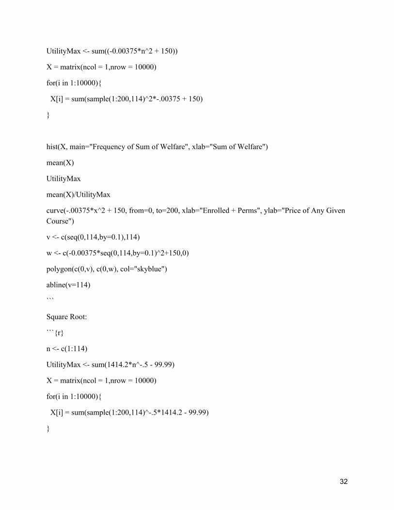
UtilityMax <- sum((-0.00375*n^2 + 150))


for(i in 1:10000){

X[i] = sum(sample(1:200,114)^2*-.00375 + 150)

}


mean(X)

UtilityMax

mean(X)/UtilityMax

curve(-.00375*x^2 + 150, from=0, to=200, xlab="Enrolled + Perms", ylab="Price of Any Given Course")

v <- c(seq(0,114,by=0.1),114)

w <- c(-0.00375*seq(0,114,by=0.1)^2+150,0)


abline(v=114)

```

Square Root:

```{r}

n <- c(1:114)

UtilityMax <- sum(1414.2*n^-.5 - 99.99)


for(i in 1:10000){

X[i] = sum(sample(1:200,114)^-.5*1414.2 - 99.99)

}

32


mean(X)

UtilityMax

mean(X)/UtilityMax

curve(1414.2*x^-.5 - 99.99, from=0, to=200, xlab="Enrolled + Perms", ylab="Price of Any Given Course")

v <- c(seq(0.1,114,by=0.1),114)

w <- c(1414.2*seq(0.1,114,by=0.1)^-0.5 - 99.99,0)


abline(v=114)

```

Logarithmic:

```{r}

n <- c(1:114)

UtilityMax <- sum(1638.5/n)


for(i in 1:10000){

X[i] = sum(1638.5/sample(1:200,114))

}


mean(X)

UtilityMax

mean(X)/UtilityMax

curve(1638.5/x, from=0, to=200, xlab="Enrolled + Perms", ylab="Price of Any Given Course")

v <- c(seq(0.1,114,by=0.1),114)

w <- c(1638.5/seq(0.1,114,by=0.1),0)

33


abline(v=114)

```

Data Code:

##Principles of Economic Analysis

Linear:

```{r}

n <- c(1:64)

UtilityMax <- sum(-1.7469*n + 186.9183)


for(i in 1:10000){

X[i] = sum(sample(1:107,64)*-1.7469 + 186.9183)

}


mean(X)

UtilityMax

mean(X)/UtilityMax

curve(-1.7469*x + 186.9183, from=0, to=107, xlab="Enrolled + Perms", ylab="Price of Any Given Course")

v <- c(0, 64, 64)

w <- c(186.9183, 75.1167, 0)


abline(v=64)

```

34

Quadratic:

```{r}

n <- c(1:64)

UtilityMax <- sum((-0.0122445*n^2) + 140.1873)


for(i in 1:10000){

X[i] = sum(sample(1:107,64)^2*-.0122445 + 140.1873)

}


mean(X)

UtilityMax

mean(X)/UtilityMax

curve(-.0122445*x^2 + 140.1873, from=0, to=107, xlab="Enrolled + Perms", ylab="Price of Any Given Course")

v <- c(seq(0,64,by=0.1),64)

w <- c(-0.0122445*seq(0,64,by=0.1)^2+140.1873,0)


abline(v=64)

```

Square Root:

```{r}

n <- c(1:64)

UtilityMax <- sum(966.733*n^-.5 - 93.45761)


for(i in 1:10000){

X[i] = sum(sample(1:107,64)^-.5*966.733 - 93.45761)

35

}


mean(X)

UtilityMax

mean(X)/UtilityMax


v <- c(seq(0.1,64,by=0.1),64)

w <- c(966.733*seq(0.1,64,by=0.1)^-0.5 - 93.45761,0)


abline(v=64)

```

Logarithmic:

```{r}

n <- c(1:64)



for(i in 1:10000){

X[i] = sum(863.51/sample(1:107,64))

}


mean(X)

UtilityMax

mean(X)/UtilityMax


v <- c(seq(0.1,64,by=0.1),64)

36

w <- c(863.51/seq(0.1,64,by=0.1),0)


abline(v=64)

```

## Accounting for Decision Making

Linear:

```{r}

n <- c(1:93)

UtilityMax <- sum(-1.0717*n + 231.4872)


for(i in 1:10000){

X[i] = sum(sample(1:216,93)*-1.0717 + 231.4872)

}


mean(X)

UtilityMax

mean(X)/UtilityMax


v <- c(0, 93, 93)

w <- c(231.4872, 131.8191, 0)


abline(v=93)

```

37

Quadratic:

```{r}

n <- c(1:93)

UtilityMax <- sum((-0.0037211*n^2) + 173.6116)


for(i in 1:10000){

X[i] = sum(sample(1:216,93)^2*-.0037211 + 173.6116)

}


mean(X)

UtilityMax

mean(X)/UtilityMax


v <- c(seq(0,93,by=0.1),93)

w <- c(-0.003211*seq(0,93,by=0.1)^2+173.6116, 0)


abline(v=93)

```

Square Root:

```{r}

n <- c(1:93)

UtilityMax <- sum(1701*n^-.5 - 115.7384)


for(i in 1:10000){

X[i] = sum(sample(1:216,93)^-.5*1701 - 115.7384)

38

}


mean(X)

UtilityMax

mean(X)/UtilityMax

curve(1701*x^-.5 - 115.7384, from=0, to=216, xlab="Enrolled + Perms", ylab="Price of Any Given Course")

v <- c(seq(0.1,93,by=0.1),93)

w <- c(1701*seq(0.1,93,by=0.1)^-0.5 - 115.7384,0)


abline(v=93)

```

Logarithmic:

```{r}

n <- c(1:93)



for(i in 1:10000){

X[i] = sum(2035.3/sample(1:216,93))

}


mean(X)

UtilityMax

mean(X)/UtilityMax


v <- c(seq(0.1,93,by=0.1),93)

39

w <- c(2035.3/seq(0.1,93,by=0.1),0)


abline(v=93)

```

##Statistics

Linear:

```{r}

n <- c(1:86)

UtilityMax <- sum(-2.1185*n + 252.1015)


for(i in 1:10000){

X[i] = sum(sample(1:119,86)*-2.1185 + 252.1015)

}


mean(X)

UtilityMax

mean(X)/UtilityMax


v <- c(0, 86, 86)

w <- c(252.1015, 69.9105, 0)


abline(v=86)

```

40

Quadratic:

```{r}

n <- c(1:86)

UtilityMax <- sum((-0.0133515*n^2) + 189.0706)


for(i in 1:10000){

X[i] = sum(sample(1:119,86)^2*-.0133515 + 189.0706)

}


mean(X)

UtilityMax

mean(X)/UtilityMax


v <- c(seq(0,86,by=0.1),86)

w <- c(-0.0133515*seq(0,86,by=0.1)^2+189.0706, 0)


abline(v=86)

```

Square Root:

```{r}

n <- c(1:86)

UtilityMax <- sum(1375*n^-.5 - 126.046)


for(i in 1:10000){

X[i] = sum(sample(1:119,86)^-.5*1375 - 126.046)

41

}


mean(X)

UtilityMax

mean(X)/UtilityMax

curve(1375*x^-.5 - 126.046, from=0, to=119, xlab="Enrolled + Perms", ylab="Price of Any Given Course")

v <- c(seq(0.1,86,by=0.1),86)

w <- c(1375*seq(0.1,86,by=0.1)^-0.5 - 126.046,0)


abline(v=86)

```

Logarithmic:

```{r}

n <- c(1:86)



for(i in 1:10000){

X[i] = sum(1283.5/sample(1:119,86))

}


mean(X)

UtilityMax

mean(X)/UtilityMax


v <- c(seq(0.1,86,by=0.1),86)

42

w <- c(1283.5/seq(0.1,86,by=0.1),0)


abline(v=86)

```

##Development Economics

Linear:

```{r}

n <- c(1:36)

UtilityMax <- sum(-3.1888*n + 178.5728)


for(i in 1:10000){

X[i] = sum(sample(1:56,36)*-3.1888 + 178.5728)

}


mean(X)

UtilityMax

mean(X)/UtilityMax


v <- c(0, 36, 36)

w <- c(178.5728, 63.776, 0)


abline(v=36)

```

43

Quadratic:

```{r}

n <- c(1:36)

UtilityMax <- sum((-0.042707*n^2) + 133.9292)


for(i in 1:10000){

X[i] = sum(sample(1:56,36)^2*-.042707 + 133.9292)

}


mean(X)

UtilityMax

mean(X)/UtilityMax


v <- c(seq(0,36,by=0.1),36)

w <- c(-0.042707*seq(0,36,by=0.1)^2+133.9292, 0)


abline(v=36)

```

Square Root:

```{r}

n <- c(1:36)

UtilityMax <- sum(670.9*n^-.5 - 89.66481)


for(i in 1:10000){

X[i] = sum(sample(1:56,36)^-.5*670.9 - 89.66481)

44

}


mean(X)

UtilityMax

mean(X)/UtilityMax


v <- c(seq(0.1,36,by=0.1),36)

w <- c(670.9*seq(0.1,36,by=0.1)^-0.5 - 89.66481,0)


abline(v=36)

```

Logarithmic:

```{r}

n <- c(1:36)



for(i in 1:10000){

X[i] = sum(457.33/sample(1:56,36))

}


mean(X)

UtilityMax

mean(X)/UtilityMax


v <- c(seq(0.1,36,by=0.1),36)

45

w <- c(457.33/seq(0.1,36,by=0.1),0)


abline(v=36)

```

Portal Data:

Course Name Seats Taken Seat Cap PERMs submitted

Total in Course Total Perms

Perms + Enrolled

Principles of Economic Analysis 39 35 33 64 43 107

Principles of Economic Analysis 25 35 10 64 43 107

Accounting for Decision Making 16 20 21 93 123 216





Statistics 22 18 6 86 33 119

Statistics 21 18 9 86 33 119

46

Statistics 24 18 17 86 33 119

Statistics 19 18 1 86 33 119

Development Economics 18 18 11 36 20 56

Development Economics 18 18 9 36 20 56

47

Welfare Losses from First-Come-First-Serve Course Enrollment

Documents