WELFARE IMPLICATIONS OF WASHINGTON WHEAT BREEDING PROGRAMS

Welfare Implications of Washington Wheat Breeding Programs

Lia Nogueira

Assistant Professor

Department of Agricultural and Consumer Economics

University of Illinois

E-mail: [email protected]

Telephone: 217-244-3934

Thomas L. Marsh

Professor

School of Economic Sciences

Washington State University

Working Paper

May 2010

We appreciate the comments and suggestions of the faculty and students who participated in the SES Graduate

Research Seminar – Spring 2008 where this work was presented. We also thank Cory Walters for helpful comments

on an earlier draft. Research assistance was provided by Heather Johnson, Sasi Ponnaluru, and Justin Taylor.

Partial funding for this project was provided by the WSU IMPACT Center and CAHNRS.

1

Welfare Implications of Washington Wheat Breeding Programs

Abstract

We calculate the welfare effects of the WSU wheat breeding programs for producers and

consumers in Washington State, Oregon, Idaho, the United States and the rest of the world. We

develop a partial equilibrium multi-region, multi-product, multi-variety trade model for wheat

that provides consumer, producer and total surplus for each wheat class and region. Our results

provide evidence suggesting that WSU wheat breeding programs have increased welfare in

Washington State, in the United States and the rest of the world.

Keywords: welfare, wheat breeding programs, economic surplus, partial equilibrium.

JEL Codes: F14, F17, Q11, Q16, Q18.

Wheat is an important commodity for the United States and Washington State, both at the

domestic and international levels. Land Grant Universities, such as Washington State University

(WSU), invest in research to improve wheat characteristics that will benefit both producers and

consumers. However, funds available for agricultural research are a scarce resource. To justify

future spending in wheat breeding programs, the providers of the majority of funds, state and

federal legislators, need to be assured that each dollar being spent in wheat breeding programs is

being put to the most efficient use. Measuring the welfare effects of the WSU wheat breeding

programs represents an important contribution in understanding the value of these programs.

The main objective of this study is to calculate the welfare effects of the WSU wheat

breeding programs for producers and consumers in Washington State, Oregon, Idaho, the United

States and the rest of the world. This study will make an important contribution to the literature

since we extend previous work to examine a detailed multi-region, multi-product and multi-

2

variety model that includes spill-over effects, and accounts for the limited substitution among

wheat classes. Our framework and results will be useful to decision makers in the government

since we provide justification for funding the WSU wheat breeding program by calculating the

welfare effects of these programs and comparing them with the associated costs. Finally, this

study will benefit producers and consumers through calculating the welfare effects for both

groups. Consequently, this study will contribute to understanding the specific value of the wheat

breeding programs to producers and consumers and provide justification for them.

There have been various studies examining the effects on welfare of different wheat

breeding programs. Studies related to the impact of wheat breeding research started as early as

the 1970s (Blakeslee, Weeks, Bourque and Beyers 1973; Blakeslee and Sargent 1982; Brennan

1984; Edwards and Freebairn 1984; Zentner and Peterson 1984; Brennan 1989; Brennan, Godyn

and Johnston 1989; Byerlee and Traxler 1995; Barkley 1997; Alston and Venner 2002; Heisey,

Lantican and Dubin 2002; Brennan and Quade 2006). Models have evolved and became more

sophisticated and accurate with time. Most approaches focus on economic surplus measures,

based on partial equilibrium or econometric models. These studies also differ in the

representation of varietal improvement, with yield increase being the most popular.1 Some work

has been done regarding the use of new technologies, specifically the potential benefits of

genetically modified wheat research (Berwald, Carter and Gruère 2005; Crespi, Grunewald,

Barkley, Fox and Marsh 2005). However, none of these studies incorporate multiple regions,

wheat classes, and wheat varieties jointly in their analysis.

In particular, most papers focus on the benefits for the specific area of study. For

example, Blakeslee, Weeks, Bourque and Beyers (1973) provide an input-output study of the

wheat producing sector in Washington State and its relationship with the State’s economy.

1 A popular study to follow when calculating yield increase is Feyerherm, Paulsen and Sebaugh (1984).

3

Blakeslee and Sargent (1982) calculate the internal rate of return as a measure of investment

profitability for expenditures in wheat breeding research and extension in Washington State.

Brennan (1984) evaluates the contribution of wheat breeders to the wheat industry in Australia,

by evaluating three measures of varietal change and reporting an empirical examination of them.

Brennan (1989) uses a discounted cash flow analysis to compare different wheat breeding

methods to determine the changes in costs and benefits from some selected innovations that

could reduce the period of time taken to produce a commercial wheat cultivar, also in Australia.

Byerlee and Traxler (1995) examine the role of International Agricultural Research Center

generated technology in the global system of spring wheat improvement, for the 1977-1990

period. They calculate the total economic surplus generated by wheat improvement research

assuming linear demand and supply schedules and a parallel supply shift. Heisey, Lantican and

Dubin (2002) use a constant elasticity of substitution production function to illustrate potential

changes in wheat yield in farmers’ fields, as well as changes in economic benefits that may be

associated with an increase in experimental wheat yields. They study 36 developing countries.

Some studies incorporate different regions in their analysis. For example, Edwards and

Freebairn (1984) develop a disaggregated commodity supply and demand model with separate

sectors for the home country, and the rest of the world. The model is illustrated by estimating

the gains to Australia, the rest of the world and the world from research into the wool and wheat

industries. Barkley (1997) measures the impact of Kansas wheat breeding research on Kansas

wheat producers and consumers, wheat producers outside of Kansas (including Argentina and

Australia), and wheat consumers outside of Kansas (including China and Japan). A two-country

model of supply and demand was used to estimate the impact of the research-induced supply

shift on producer and consumer surpluses in Kansas and the rest of the world.

4

Brennan, Godyn and Johnston (1989) not only incorporate several regions, but they also

incorporate quality aspects into an analysis based on a partial equilibrium framework for

evaluating new wheat varieties. The analysis estimates the change in producer and consumer

surplus in Australia and the rest of the world resulting from a research-induced shift in the supply

curve. A study by Zentner and Peterson (1984) incorporates different wheat classes for Canada.

This is an econometric analysis of whether public investment in Canadian wheat research has

constituted socially profitable use of scarce public resources, and to what extent the social

benefit from these research activities have accrued to producers and consumers. This article

contributes to the literature by incorporating different regions, wheat classes and varieties into

the model, which has not been done before.

Estimates of the benefits of wheat research programs due to yield improvements vary by

time-frame, country and specific study. The average US farmer in 1980 could expect to receive

additional $29 dollars per acre for wheat production (Blakeslee and Sargent 1982). Barkley

(1997) suggests that while the costs of the Kansas State wheat breeding program averaged $3.8

million dollars per year for the period 1979 to 1994, average benefits per year to Kansas wheat

producers were $52.7 million dollars, $190 thousand dollars to Kansas consumers, and $41.4

million dollars to rest of the world consumers. Surplus for wheat producers in the rest of the

world decreased an average of $40.7 million dollars per year. In Canada, producers and

consumers benefit from wheat research, with annual social benefits of $49 to $143 million

Canadian dollars depending on the scenario considered (Zentner and Peterson 1984). Heisey,

Lantican and Dubin (2002) estimate that returns to international wheat breeding research are $1.6

to $6 billion dollars in annual benefits given a total investment of $150 million dollars per year.

5

Our work complements and contributes to the literature by looking at the different wheat

classes independently, assuming that they are differentiated products, and by calculating welfare

effects for the different regions using wheat varieties developed by WSU (Washington, Oregon

and Idaho) in particular. Thus, we are able to calculate the spillover effects onto Oregon and

Idaho. Our results provide evidence of the value of the WSU wheat breeding programs for

consumers and producers, not only in Washington State but also in Oregon, Idaho, the United

States and the rest of the world.

The rest of the article proceeds as follows. The next section provides background on

wheat production. This is followed by model development. We next present the data used for

the analysis. Results are then presented. The article ends with some brief conclusions.

Background

Wheat ranks fifth in total production among all commodities in Washington State. In the United

States, Washington State is the fourth largest producer of wheat. Washington State is one of the

largest wheat exporting states, with 85 to 90 percent of its crop being exported (Washington

Wheat Commission 2006). Due to favorable growing conditions soft white wheat is primarily

grown in Washington. Wheat varieties in Washington are always being adapted to counteract

disease and pest issues that affect producers yield such as fungi and insects, as well as to meet

producer demand for higher yielding varieties.

In addition to helping producers by increasing yield and / or quality, new varieties should

also maintain or improve consumer desired characteristics, such as milling properties and the

characteristics required for good quality bread, cakes, cookies or pasta, depending on the specific

wheat class. Thus, wheat breeding programs are important to both producers, flour processing,

and consumers. However, it is not always easy to justify increased expenditure in wheat

6

breeding research. One reason is the long period of time from the beginning of the trials to the

adoption of these varieties by growers. Another is the fact that growers do not buy seed every

year, but save some of the harvested grain to plant the following year or years (Heisey, Lantican

and Dubin 2002).2 Welfare implications of wheat breeding programs are relevant concerns for

associated interest groups and the public in general.

The Crop and Soil Sciences Department at WSU has several plant breeding programs,

one of which is wheat. The wheat research program at WSU is funded by a mix of state and

federal funds, as well as contributions from the Washington Wheat Commission.3 Varieties

developed by the WSU wheat breeding programs account for the majority of the wheat acreage

in the State (Jones 2006).

Table A1 in the appendix shows the number of acres planted to WSU varieties in

Washington, Oregon and Idaho by wheat class from 2002 to 2006, as well as the acres to private

varieties and the total number of acres. We can see a great amount of variation in the number of

acres by origin and class over time. The main wheat class planted in Eastern Washington is soft

white wheat. In 2002, 74 percent of soft white wheat acres was planted to varieties developed by

WSU, compared to 61 percent in 2006.

Wheat is not a homogeneous product. The agronomic characteristics of the different

varieties and consumer preferences determine the end use of wheat, making the different wheat

classes differentiated products. For example, flour made from hard wheat is mainly used for

bread, soft wheat flour is mainly used for cakes and cookies and durum wheat flour is mainly

used for pasta. The United States produces five major wheat classes: hard red winter (HRW),

hard red spring (HRS), soft red winter (SRW), soft white winter (SWW) and durum wheat

2 It can take from 7 to 12 years to develop and market a new wheat variety.

3 Funding levels vary by year and by source.

7

(DUR). Production of the different classes of wheat in the United States is highly segregated.

HRW is grown mainly in Kansas and Oklahoma (Central Plains), HRS and durum wheat are

grown mainly in North Dakota (Northern Plains), SRW is produced in the Corn Belt and

Southern States, and SWW is grown in the Pacific Northwest, Michigan and New York (Koo

and Taylor 2006). Given the limited substitutability for milling purposes among these wheat

classes (Marsh 2005, Mulik and Koo 2006), it is important to analyze these different classes on

their own when studying wheat for the United States. We specifically model each wheat class

independently and then subdivide the classes corresponding to varieties developed at WSU into 7

different regions. For Washington, Oregon, and Idaho, we subdivide each state in varieties

developed by WSU and Other, and the rest of the United States is comprised in the other region.

Model

We divide the model section in two parts. First we present the general model following Alston,

Norton and Pardey (1995), what we call the ANP model. Second, we expand the ANP model to

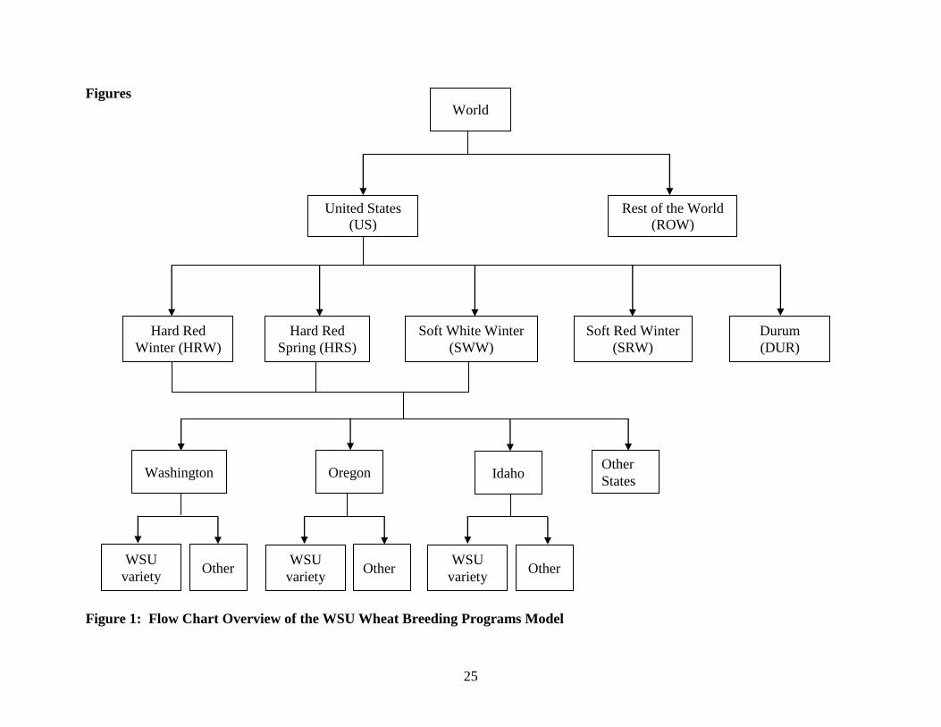
incorporate the different wheat classes and regions. Figure 1 presents a flow chart overview of

the expanded model. We extend this model to include two main regions, the United States and

the rest of the world, and we further divide the United States by wheat class to get a multi-

product model. Furthermore, we subdivide the wheat classes that the WSU wheat breeding

programs have developed varieties for (HRW, HRS, SWW) into Washington State, Oregon,

Idaho and Other States to obtain a multi-region model, where each state studied is further divided

into production due to WSU varieties and Other. In this way, we allow for spillover effects to

Idaho and Oregon. We also incorporate cross commodity price effects to allow for limited

substitution in demand among wheat classes. We call this model the WSU wheat breeding

programs model.

8

The ANP model is also similar to the ones presented in Brennan, Godyn and Johnston

(1989), Byerlee and Traxler (1995), Edwards and Freebaim (1984), and Voon and Edwards

(1992), and it has been used in most studies measuring economic surplus of agricultural research

(Barkley 1997; Crespi et al. 2005; Heisey, Lantican and Dubin 2002; Nalley, Barkley and

Chumley 2006; etc.). Alston, Norton and Pardey (1995) provide a structured, detailed and well

written overview of the methods used for economic surplus estimation, as well as the methods

for agricultural research evaluation and priority setting. Consequently, we follow Alston, Norton

and Pardey (1995) in the development of our theoretical equilibrium displacement model.

ANP Model

We start by defining the supply and demand equations that characterize the wheat market in

general. By characterizing the supply and demand functions we can calculate the changes in

consumer, producer and total surplus associated with a change in price due to a shift in the

supply curve. We assume linear demand and supply functions. The model is divided in different

regions: the region of interest (where the supply shift occurs), W, and other relevant regions to

the study, i=1, …, R. The corresponding supply equations are:

(1) )( WWWWW kPQ

(2) iiii PQ , i=1, …, R,

where Q denotes the quantity of wheat supplied by the corresponding regions, W or i, P is the

price for wheat, k represents a parallel shift down of the supply curve, represents the intercept

parameter and the slope parameter. The demand equations are represented by:

(3) jjjj PC , j=W, 1, …., R,

9

where C denotes the quantity of wheat demanded in the corresponding region j, represents the

intercept parameter, and is the non-negative slope parameter. In equilibrium, total quantity

supplied and total quantity demanded are equal, giving the following market clearing condition:

(4) j jj j CQ , j=W, 1, …, R.

We substitute k=KP0, such that K represents the vertical shift of the supply curve as a

proportion of the initial price, P0. Totally differentiating equations 1 to 3 allows us to re-write

these equations in terms of relative changes and elasticities:

(5) ])([)( WWWW KPEQE

(6) )]([)( iii PEQE , i=1, …, R

(7) )]([)( jjj PECE , j=W, 1, …., R,

where E denotes relative changes, that is, E(Z) = dZ/Z = dlnZ; is the price elasticity of supply,

and is the price elasticity of demand. Now the market equilibrium condition is:

(8) j jjj jj CEdsQEss )()( , j=W, 1, …., R,

where ss represents the corresponding supply share ( j jjj QQss / ) and ds represents the

corresponding demand share ( j jjj CCds / ). This system of equations (5 to 8) can be solved

to obtain the relative change in price:

(9)

j jjjj

WWW

ssds

ssKPE

)()( , j=W, 1, …, R.

Subsequently, equation 9 can be substituted into the region-specific supply and demand

equations 5 to 7 to obtain specific effects on quantities. With this information we can calculate

annual benefits from research-induced shifts in the wheat supply curve by estimating changes in

consumer surplus (CS), producer surplus (PS), and total surplus (TS):

10

(10) )](5.01)][([ jjjjj CEPECPCS

(11) )](5.01][)([ jjjjjj QEKPEQPPS , j=W, 1, …, R,

(12) j jj j PSCSTS

where PC and PQ represent the initial consumer and producer prices, respectively. In this way

total surplus from the research-induced supply shift corresponds to the area below the demand

curve and between the two supply curves. This area represents the sum of the cost saving due to

the yield increase and the economic surplus due to the increment to production and consumption.

A main limitation of this model is that it assumes only a parallel shift in the supply curve.

Additionally, it applies linear demand and supply functions to provide at best a first order

approximation of economic surplus. However, the model is still general and flexible enough to

accommodate a wide range of different market structures and characteristics.

WSU Wheat Breeding Programs Model

We can modify the ANP model to incorporate the different wheat classes and regions to build

our own equilibrium displacement model. Our model represents partial equilibrium because it

only looks at the wheat industry and assumes constant prices for all inputs used in wheat

production. Since we are only interested in simulating the welfare effects due to yield

improvements in WSU developed varieties, we hold all other yield improvements constant,

including improvements due to technology, management practices and other wheat breeding

programs.4

We extend the ANP model to include two main regions or submodels, the United States

submodel and the rest of the world submodel, and we further divide the United States submodel

4 It should be noted that other states could be using wheat varieties with similar yield improvements, and thus,

spillover effects may wash out once other yield improvements are considered.

11

by wheat class to get a multi-product model. Furthermore, we subdivide the wheat classes that

the WSU wheat breeding programs have developed varieties for (HRW, HRS, SWW) into

Washington State, Oregon, Idaho and Other States to obtain a multi-region model, where each

state studied is further divided into production due to WSU varieties and Other (WA-WSU, WA-

Other, OR-WSU, OR-Other, ID-WSU, ID-Other). In this way, we allow for spillover effects to

Idaho and Oregon. We also incorporate cross commodity price effects to allow for limited

substitution in demand among wheat classes.

First we only analyze the US submodel, and we obtain the equilibrium prices and

quantities for each wheat class, region and sub-region given a supply shift due to the yield

improvement in WSU varieties. With those results, we get the aggregate effects for the United

States submodel and we simulate the results of trading between the United States and the rest of

the world. Thus, we can obtain results for the overall model. We then calculate the changes in

consumer, producer and total surplus for each wheat class and region within the United States, as

well as for the United States as an aggregate and the rest of the world associated with a change in

price due to a shift in the supply curve for the regions using varieties developed at WSU. We

assume that the shift is due to yield improvements obtained by using varieties developed by the

WSU wheat breeding programs, holding everything else constant. That is, holding potential

improvements due to other research programs and technology constant. The supply shift

parameter, K, is calculated as the yield increase or improvement due to WSU varieties divided

by the price elasticity of supply (Alston, Norton and Pardey 1995).

The specific supply and demand equations for the US submodel are:

(13) ])([)( ,, aiiiai KPEQE , i = HRW, HRS, SRW, a = WA-WSU, OR-WSU, ID-WSU

(14) )]([)( , iibi PEQE , b = WA-Other, OR-Other, ID-Other, Other States

12

(15) )]([)( jjj PEQE , j = SWW, DUR

(16) c cncn PECE )]([)( , n, c = HRW, HRS, SRW, SWW, DUR

Given that prices among wheat classes are not the same, we have a market equilibrium

condition for each wheat class. Equation 17 corresponds to the equilibrium condition for HRW,

HRS and SWW classes, and equation 18 to SRW and DUR:

(17) d ddd dd CEdsQEss )()( ,

d = WA-WSU, WA-Other, OR-WSU, OR-Other, ID-WSU, ID-Other

(18) )()( jj CEQE

In the overall model we aggregate the change in quantities produced, quantities

consumed, and prices to obtain the corresponding changes in quantity produced, quantity

consumed and price for the United States. Then we allow trade to occur between the United

States and the rest of the world to obtain equilibrium prices and quantities for the rest of the

world. This overall model assumes that changes in production within the United States will

change the equilibrium prices and quantities in the rest of the world (large country effect). We

consider this a valid assumption given that the United States is a large player in the wheat world

market. The United States is the largest wheat exporter in the world with almost half of the US

wheat crop being exported (Vocke, Allen and Ali 2005). The demand and supply equations for

the rest of the world (ROW), and the market equilibrium condition given trade between the

United States and the rest of the world are:

(19) )]([)( ROWROWROW PEQE

(20) )]([)( ROWROWROW PECE

(21) h hhh hh CEdsQEss )()( , h = US, ROW

13

Finally, we calculate changes in consumer, producer and total surplus for each region and

wheat class. Change in producer surplus for each region and wheat class is calculated as in the

general equation for change in producer surplus (equation 11). However, the calculation of

change in consumer surplus is somewhat different given the cross product prices in the demand

equation for the different US wheat classes. Following Marsh (2005) we account for the limited

substitutability for milling purposes among the wheat classes. By allowing the different wheat

classes to be substitutes in consumption we now have a general equilibrium demand function.

Consumption of a particular wheat class responds to changes in its own price, while allowing

other wheat classes’ prices and demand to change according to the cross-price elasticities

(Alston, Norton and Pardey 1995). Therefore, the welfare measures taken from the general

equilibrium demand function will reflect changes in that particular wheat class market, and also

in all the other wheat classes markets. In this case, the general equation for change in consumer

surplus (equation 10) captures the change in consumer surplus plus the change in producer

surplus for the regions without the shift in the supply curve (Alston, Norton and Pardey 1995).

Thus, we calculate the change in consumer surplus for the United States by adding the change in

consumer surplus for wheat classes with a shift in the supply curve (equation 22), and then

subtracting the producer surplus for all regions without a shift in the supply curve (equation 23).

Equation 10 is used to calculate changes in consumer surplus for HRW, HRS and SWW.

(22) SWWHRSHRWUS CSCSCSCS *

(23) l lUSUS PSCSCS * ,

where l = HRW-WAOther, HRW-OROther, HRW-IDOther, HRW-OtherStates, HRS-WAOther,

HRS-OROther, HRS-IDOther, HRS-OtherStates, SRW, SWW-WAOther, SWW-OROther, SWW-

IDOther, SWW-OtherStates, and DUR.

14

Data

Annual wheat production data for Washington, Oregon and Idaho from 2002 to 2006 are

available through the US Department of Agriculture (USDA) National Agricultural Statistics

Service (NASS) website (http://www.nass.usda.gov/Data_and_Statistics/Quick_Stats/). Detailed

information on acreage by variety by state over time was obtained through the NASS Statistical

Bulletins by State. Annual data on price, production and consumption for the United States and

the world are available through the USDA Economic Research Service Wheat Yearbook Tables

(http://www.ers.usda.gov/data/wheat/). Annual prices were deflated to reflect 2006 dollars using

the US consumer price index (CPI) obtained through the Bureau of Labor Statistics website

(http://data.bls.gov/). The CPI was adjusted to represent 2006 dollars by changing the base year

to 2006 instead of 1982-1984. Supply and demand elasticities are obtained from the literature as

discussed below.

First hand consumption data are not available for Washington, Oregon and Idaho. For

these states, we calculated consumption proportionally to the state’s population based on

consumption for the whole United States. Population data for the United States, Washington,

Oregon and Idaho were obtained through the Census Bureau website (http://www.census.gov).

The yield improvement data to calculate the supply shift parameter were obtained from

the NASS website. Yield improvement was calculated as the marginal change in yield trend for

spring and winter wheat. Yield data was not available by wheat class, only by wheat type

(winter or spring). We calculated quantity produced for Washington, Oregon and Idaho for

varieties developed by WSU and others using the acreage data by variety by state over time from

NASS. The varieties were matched to a cultivar list and cross reference guide put together by

Dr. Craig Morris from the Western Wheat Quality Laboratory, USDA. This reference guide

15

contains information regarding the variety name, release date, source and origin, among others.

Even though this list is not comprehensive, it gives a lower bound on the amount of acres planted

to WSU varieties in Washington, Oregon and Idaho. We multiplied acres times yield by wheat

type to get quantity produced for each wheat class and sub-region.

Results

Changes in consumer, producer and total surplus due to a shift in the supply curve for producers

are analyzed for WSU wheat varieties. It is assumed that the shift in the supply curve is due to

the yield improvement provided by using WSU wheat varieties. We calculate a yield

improvement of 1.27 percent for winter wheat (HRW and SWW), and 1.64 percent for spring

wheat (HRS).5 Changes in consumer, producer, and total surplus (equations 10-12, 22 and 23)

are calculated for each region and wheat class, the United States and the rest of the world.

Specifically, we use the supply and demand equations 13-16, 19-20 and the market clearing

condition described in equations 17-18, and 21. We assume that the price elasticity of supply for

the United States is 0.22 (DeVuyst et al. 2001 as taken from Benirschka and Koo 1995), and for

the rest of the world is 1 (Brennan, Godyn and Johnston 1989). The price elasticity of demand

for the rest of the world is assumed to be -1.4 (Voon and Edwards 1992). The own- and cross-

price elasticities of demand for the US wheat classes are presented in table A2 (Marsh 2005).

Table A3 contains quantity consumed and price per wheat class and region in million bushels

and 2006 dollars per bushel, respectively; and table A4, quantity produced by wheat class and

region in million bushels. We use GAMS (version 22.2) to solve for the equilibrium prices and

quantities using the PATH solver for MCP models.

5 Yield improvement was calculated as the marginal change in yield trend for spring and winter wheat in

Washington State.

16

Changes in consumers’ and total surplus are presented in table 1, and changes in

producers’ surplus in table 2. These changes in surplus are in million dollars, 2006. Tables 3

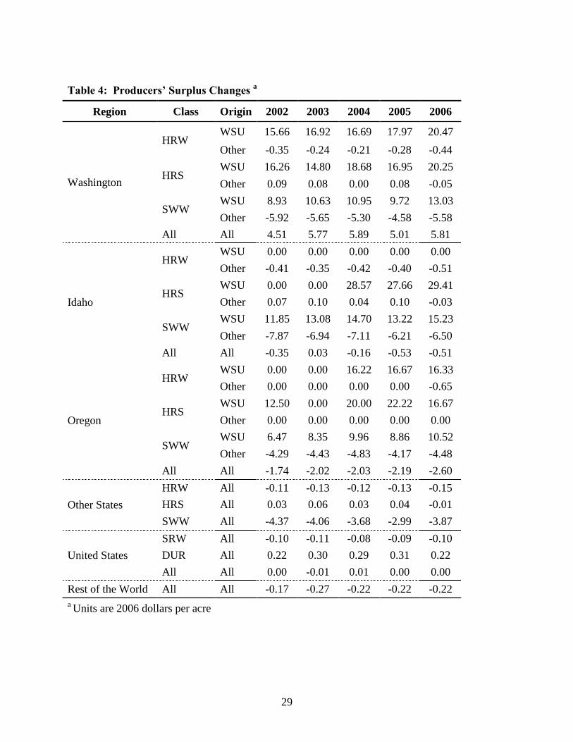
and 4 present surplus changes in 2006 dollars per acre. Our results suggest that producers using

WSU varieties and consumers in all regions have increased surplus from the research-induced

supply shift due to WSU wheat breeding programs. The specific increase in surplus depends on

the region and level of production. The largest surplus increase for producers using WSU

varieties, $11 to $13 million dollars per year, is observed for SWW in Washington State, which

is the majority of the wheat grown in the Pacific Northwest. Surplus increases for producers

using WSU varieties of SWW in Idaho range from $2 to $2.5 million dollars per year. In

Oregon, producers using WSU varieties of SWW have increased surplus by $0.7 to $1.4 million

dollars per year. Producers using WSU varieties gain due to the increased yield. Yield increase

translates into increases in quantity supplied and decreases in prices. Even with lower

equilibrium prices producers using WSU varieties still observe large gains due to higher yield.

Decrease in surplus to producers using other varieties ranges from $10 thousand to

almost $4 million dollars per year for Washington, $10 thousand to almost $3 million dollars per

year for Idaho, and less than $10 thousand to $3.5 million dollars per year for Oregon. Surplus

for producers of SRW decreased by $500 to $900 thousand dollars per year, while surplus for

producers of DUR increased by $400 to $860 thousand dollars per year due to the cross price

effects among wheat classes. At an aggregate level, the effect on US producers depends on the

specific year, with surplus increases in 2002, 2004 and 2005 of $40 to $600 thousand dollars per

year, and surplus decreases in 2003 and 2006 of $10 to $450 thousand dollars per year. Surplus

decrease for producers in the rest of the world ranges from $90 to $140 million dollars per year.

17

Producers using other varieties face decreased surplus given the lower prices and that they did

not benefit from the higher yield due to using WSU varieties.

Changes in consumer surplus are positive in all regions, with the magnitude of the

increase depending on the number of consumers in each region. Consumers in Washington have

increased surplus by $51 to $63 thousand dollars per year, consumers in the United States by

approximately $27 to $29 million dollars per year, while consumers in the rest of the world have

increased surplus by approximately $99 to $160 million dollars. Consumers reap all the benefits

of lower prices, and thus, increases in consumer surplus are dependent on the number of

consumers in each region, and specific quantity consumed.

The net effect in each region is always positive for Washington, the United States and the

rest of the world. Increases in total surplus for Washington State range from approximately $11

to $14 million dollars per year. For the United States increase in total surplus ranges from $27 to

$29 million dollars per year, and for the rest of the world, from $2 to $19 million dollars per

year. However, the change in total surplus is always negative for Oregon, and depending on the

year, it could be negative or positive for Idaho. The decrease in total surplus is small compared

to the overall benefits, as represented in the total surplus changes for the United States as an

aggregate. Specifically, decrease in total surplus for Oregon ranges from approximately $1 to $2

million dollars per year. Net effects for Idaho are smaller in magnitude, with increases of $170

thousand dollars for 2003 and decreases of $60 to $520 thousand dollars per year, for the rest.

Net effects reflect the balance between consumers, producers using WSU varieties and producers

using other varieties, given that surplus increases for the first two groups but decreases for the

third one. We observe positive net effects if the number of consumers and producers using WSU

varieties outweigh producers using other varieties.

18

To provide some perspective about the magnitude of these surplus changes, we divide the

change in surplus by the number of acres to get changes in surplus in dollars per acre. These

results are reported in tables 3 and 4. Producers in Washington have increased surplus by

approximately $4.5 to $6 dollars per acre per year, illustrating the high percentage of

Washington producers using varieties developed at WSU. Producers in Idaho increased surplus

by 3 cents per acre in 2003 and decreased surplus 15 to 50 cents per acre per year for the other

years, which shows the variation in use of WSU varieties in Idaho. Producers in Oregon have

decreased surplus $1.7 to $2.6 dollars per acre per year, revealing a lower proportion of

producers using WSU varieties as compared to Idaho and Washington. On aggregate terms,

producers in the United States have increased or decreased surplus in such small magnitudes that

in dollars per acre the increase or decrease is very close to zero, showing the balance between

producers using WSU varieties and other varieties. Rest of the world producers have decreased

surplus by approximately 20 to 30 cents per acre per year, given that they experienced lower

prices, but not higher yields.

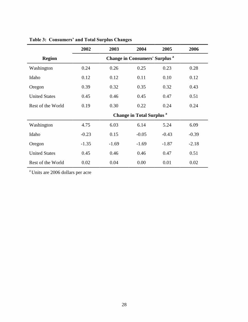
Total surplus changes for Washington represent increases of $4.75 to $6.14 dollars per

acre per year, for Idaho total surplus increases by 15 cents per acre for 2003, and decreases by 5

to 43 cents per acre per year for the other years. These results show that in Washington and

Idaho most of the benefits go to producers using WSU varieties, since increases in total surplus

are only slightly higher than increases in producer surplus. Given the large quantities of wheat

produced in those states relative to the average consumption per capita this result is no surprise.

In the case of Oregon, there are net decreases of $1.35 to $2.18 dollars per acre per year,

showing that producers using other varieties have more to lose than the gains accrued to

consumers and producers using WSU varieties. Net effects for the United States as an aggregate

19

are increases in surplus of approximately 50 cents per acre per year. Overall, in the United

States the gains to consumers and producers using WSU varieties are larger than the loses to

producers using other varieties. Net effects for the rest of the world are quite small, with surplus

increases of 0 to 4 cents per acre per year, showing that the benefits of lower prices to consumers

outweigh the costs to producers using other varieties.

To formally evaluate the WSU wheat breeding programs it is important to compare to the

costs incurred to fund these programs. As mentioned earlier, funds for the WSU wheat breeding

programs come from a variety of sources including: state, federal, university and the Washington

Wheat Commission. Given the public nature of these funds, it is a relevant policy question to

ask if these funds are being used efficiently. We have presented a detailed analysis of the

changes in surplus for several regions due to the use of varieties developed by WSU. Now we

need to compare these net benefits with the cost of research.

Average estimates of expenditures in WSU wheat breeding research from 2002 to 2006

range from $0.97 to $2.28 dollars per acre, depending on a broad or narrow consideration of

expenditure on wheat breeding research.6 Specifically, narrow expenditures represent all

accounts that have “wheat” in the title, while broad expenditures represent all projects where one

of the investigators specializes in “wheat”. The cost data does not reflect the lagged effect of

wheat breeding research. It can take 7 to 12 years from the development to the marketing and

adoption of a new wheat variety. However, these data provide an estimate to put the benefits

obtained in perspective. Thus, the net social welfare (after considering the research costs) for

Washington is on average $3.37 to $4.68 dollars per acre per year, depending on the narrow or

broad version of expenditures. We obtain benefits of $2.49 to $5.84 dollars on average for each

6 Based on calculations from expenditure data collected from the WSU College of Agriculture, Human, and Natural

Resource Sciences and from representative price, cost and yield data for the state of Washington. Additional details

are available from the authors upon request.

20

dollar invested in WSU wheat research from 2002 to 2006. Net welfare results for Washington

are presented in table 5.

Furthermore, the average profit for wheat in the United States from 2002 to 2006 was

$41.56 dollars per acre per year.6 The increase in producer surplus for Washington represents on

average about 13 percent of the average profit for wheat. The percentages for each year (2002 to

2006) are presented in table 6. These numbers provide further evidence of the benefits for

Washington state wheat producers of using the varieties developed by the WSU wheat breeding

programs.

Conclusions

This article presents welfare effects of the WSU wheat breeding programs under a multi-product,

multi-region, multi-variety model including spillover effects to Idaho and Oregon. Given the

specific characteristics of the different wheat classes and regions we believe that it is important

to introduce these differences into the model to obtain more accurate results, since information is

lost by aggregating all wheat classes and regions into one.

Overall, consumers in all regions and producers using WSU developed varieties have

increased surplus from yield increases in wheat due to WSU wheat breeding programs. This is

due to the combination of lower prices and higher yields due to WSU wheat breeding programs.

However, producers using non-WSU varieties, in the rest of the world and of other wheat classes

have decreased surplus due to lower prices and constant yields. It is important to note that this

model is partial equilibrium and thus, we are holding constant all other potential yield increases

due to technology or other wheat breeding programs to concentrate on the effect of WSU wheat

breeding programs. Changes in total surplus are positive for all regions except for Oregon, and

some years for Idaho. However, the surplus decreases in these two states are smaller relative to

21

the increases in all other regions, and the net effects for United States and the rest of the world

are positive.

We have analyzed an important question: if funds allocated to the WSU wheat breeding

programs had a reasonable return. We compare the expenditures in the WSU wheat breeding

programs to the benefits calculated with our model, and we find that for each dollar spent per

acre, farmers obtained on average extra $7 dollars per acre from 2002 to 2006. It is also

important to consider the lagged effect that investment in research has. It takes 7 to 12 years to

develop and market a new variety. Our results are important for Washington State University

and policymakers in general, because they provide justification for the current funds allocated

the wheat breeding programs.

References

Alston, J. M., G. W. Norton, and P. G. Pardey. 1995. Science under Scarcity: Principles and

Practice for Agricultural Research Evaluation and Priority Setting. Ithaca, New York:

Cornell University Press.

Alston, J. M., and R. J. Venner. 2002. “The effects of the US Plant Variety Protection Act on

Wheat Genetic Improvement.” Research Policy, 31(2002): 527-542

Barkley, A. P. 1997. “Kansas Wheat Breeding: An Economic Analysis”. Report of Progress

793, Kansas State University Agricultural Experiment Station and Cooperative Extension

Service.

Benirschka, M., and W. W. Koo. 1995. “World Wheat Policy Simulation Model: Description

and Computer Program Documentation.” Agricultural Economics Report No. 340,

Department of Agricultural Economics, Agricultural Experiment Station, North Dakota

State University, December 1995.

22

Berwald, D., C. A. Carter, and G. P. Gruère. 2005. “Passing Up New Technology: An

Illustration from the Global Wheat Market.” Working Paper, University of California,

Davis, April, 2005.

Blakeslee, L., and R. Sargent. 1982. “Economic Impacts of Public Research and Extension

Related to Wheat Production in Washington.” Research Bulletin XB 0929, Agricultural

Research Center, Washington State University.

Blakeslee, L., E. E. Weeks, P. J. Bourque, and W. B. Beyers. 1973. “Wheat in the Washington

Economy, An Input-Output Study.” Bulletin 775, Washington State University College

of Agriculture Research Center, April 1973.

Brennan, J. P. 1984. “Measuring the Contribution of New Varieties to Increasing Wheat

Yields.” Review of Marketing and Agricultural Economics, 52(3): 175-195.

Brennan, J. P. 1989. “An Analysis of the Economic Potential of Some Innovations in a Wheat

Breeding Programme.” Australian Journal of Agricultural Economics, 33(1): 48-55.

Brennan, J. P., and K. J. Quade. 2006. “Towards the Measurement of the Impacts of Improving

Research Capacity: An Economic Evaluation of Training in Wheat Disease Resistance.”

The Australian Journal of Agricultural and Resource Economics, 50: 247-263.

Brennan, J. P., D. L. Godyn, and B. G. Johnston. 1989. “An Economic Framework for

Evaluating New Wheat Varieties.” Review of Marketing and Agricultural Economics,

57: 75-92.

Byerlee D., and G. Traxler. 1995. “National and International Wheat Improvement Research in

the Post-Green Revolution Period: Evolution and Impact.” American Journal of

Agricultural Economics, 77(May 1995): 268-278.

23

Crespi, J. M., S. Grunewald, A. P. Barkley, J. A. Fox, and T. L. Marsh. 2005. “Potential

Economic Impacts from the Introduction of Genetically Modified Wheat on the Export

Demand for US Wheat.” Report prepared for the Kansas Wheat Commission, May 2005.

DeVuyst, E.A., W.W. Koo, C.S. DeVuyst, and R.D. Taylor. 2001. “Modeling International

Trade Impacts of Genetically Modified Wheat Introductions.” Agribusiness and Applied

Economics Report No. 463, Center for Agricultural Policy and Trade Studies, Department

of Agribusiness and Applied Economics, Agricultural Experiment Station, North Dakota

State University, October 2001.

Edwards, G. W., and J. W. Freebairn. 1984. “The Gains from Research into Tradable

Commodities.” American Journal of Agricultural Economics, 66: 41-49.

Feyerherm, A. M., G. M. Paulsen, and J. L. Sebaugh. 1984. “Contribution of Genetic

Improvement to Recent Wheat Yield Increases in the USA.” Agronomy Journal, 76:

985-990.

Heisey, P. W., M. A. Lantican, and H. J. Dubin. 2002. Impacts of International Wheat Breeding

Research in Developing Countries, 1966-97. Mexico, D. F.: CIMMYT.

Jones, S. 2006. “Breeding Wheat for Sustainable, Perennial and Organic Systems.”

Washington State University, Department of Crop and Soil Sciences Website

http://css.wsu.edu/research/crop_genetics/Jones.htm

Koo, W. W., and R. D. Taylor. 2006. “2006 Outlook of the US and World Wheat Industries,

2005-2015.” Agribusiness and Applied Economics Report No. 586, Center for

Agricultural Policy and Trade Studies, North Dakota State University, July 2006.

Marsh, T. L. 2005. “Economic Substitution for US Wheat Food Use by Class.” The Australian

Journal of Agricultural and Resource Economics 49: 283-301.

24

Mulik, K., and W. W. Koo. 2006. “Substitution between US and Canadian Wheat by Class.”

Agribusiness and Applied Economics Report No. 587, Center for Agricultural Policy and

Trade Studies, North Dakota State University, August 2006.

Nalley, L.L., A. Barkley, and F.G. Chumley. 2006. “The Agronomic and Economic Impacts of

the Kansas Agricultural Station Wheat Breeding program, 1977-2005.” Report of

Progress 948, Kansas State University Agricultural Experiment Station and Cooperative

Extension Service.

Vocke, G., E. W. Allen, and M. Ali. 2005. “Wheat Backgrounder.” Electronic Outlook Report

from the Economic Research Service WHS-05k-01, ERS, USDA.

Voon T. J., and G. W. Edwards. 1992. “Research Payoff from Quality Improvement: The Case

of Protein in Australian Wheat.” American Journal of Agricultural Economics, 74(3):

564-572.

Washington Wheat Commission. 2006. “Washington Wheat Facts 2006.” Website:

http://asotin.wsu.edu/AgNatRes/Documents/2006WFeBook.pdf.

Zentner, R. P., and W. L. Peterson. 1984. “An Economic Evaluation of Public Wheat Research

and Extension Expenditure in Canada.” Canadian Journal of Agricultural Economics,

32(July 1984): 327-353.

25

Figures

Figure 1: Flow Chart Overview of the WSU Wheat Breeding Programs Model

Washington Oregon Idaho Other

States

WSU

variety Other

WSU

variety Other

WSU

variety Other

Hard Red

Winter (HRW)

Hard Red

Spring (HRS)

Soft White Winter

(SWW)

Soft Red Winter

(SRW)

Durum

(DUR)

World

United States

(US)

Rest of the World

(ROW)

26

Table 1: Consumers’ and Total Surplus Changes

2002 2003 2004 2005 2006

Region Change in Consumers' Surplus a

Washington 0.57 0.61 0.57 0.51 0.63

Idaho 0.13 0.14 0.13 0.12 0.14

Oregon 0.33 0.35 0.33 0.29 0.36

United States 27.14 28.73 26.84 26.84 29.27

Rest of the World 98.55 157.70 120.28 127.39 126.48

Change in Total Surplus a

Washington 11.35 14.14 13.97 11.66 13.56

Idaho -0.25 0.17 -0.06 -0.52 -0.47

Oregon -1.13 -1.83 -1.61 -1.67 -1.84

United States 27.18 28.28 27.43 26.94 29.26

Rest of the World 8.47 18.70 1.91 6.14 9.32

a Units are million 2006 dollars

27

Table 2: Producers’ Surplus Changes a

Region Class Origin 2002 2003 2004 2005 2006

Washington

HRW WSU 1.37 1.22 1.44 1.36 2.28

Other -0.02 -0.02 -0.01 -0.01 -0.04

HRS WSU 0.80 0.82 1.22 0.70 1.28

Other 0.01 0.01 0.00 0.01 -0.01

SWW WSU 11.26 13.72 13.17 11.58 13.02

Other -2.63 -2.21 -2.42 -2.49 -3.61

All All 10.78 13.53 13.40 11.15 12.93

Idaho

HRW WSU 0.00 0.00 0.00 0.00 0.00

Other -0.06 -0.07 -0.07 -0.07 -0.10

HRS WSU 0.00 0.00 0.12 0.13 0.30

Other 0.02 0.03 0.01 0.02 -0.01

SWW WSU 2.52 2.54 2.44 1.99 1.95

Other -2.86 -2.47 -2.70 -2.70 -2.75

All All -0.38 0.03 -0.19 -0.64 -0.61

Oregon

HRW WSU 0.00 0.00 0.06 0.09 0.08

Other 0.00 0.00 0.00 0.00 -0.01

HRS WSU 0.01 0.00 0.04 0.04 0.02

Other 0.00 0.00 0.00 0.00 0.00

SWW WSU 1.17 1.36 1.44 0.91 0.71

Other -2.64 -3.54 -3.48 -2.99 -3.01

All All -1.46 -2.18 -1.94 -1.96 -2.20

Other States

HRW All -3.37 -4.28 -3.73 -3.91 -4.24

HRS All 0.39 0.71 0.32 0.50 -0.20

SWW All -5.77 -8.23 -7.37 -5.38 -5.38

United States

SRW All -0.80 -0.89 -0.65 -0.53 -0.71

DUR All 0.65 0.86 0.74 0.86 0.42

All All 0.04 -0.45 0.59 0.10 -0.01

Rest of the World All All -90.08 -139.00 -118.37 -121.25 -117.16 a Units are million 2006 dollars

28

Table 3: Consumers’ and Total Surplus Changes

2002 2003 2004 2005 2006

Region Change in Consumers' Surplus a

Washington 0.24 0.26 0.25 0.23 0.28

Idaho 0.12 0.12 0.11 0.10 0.12

Oregon 0.39 0.32 0.35 0.32 0.43

United States 0.45 0.46 0.45 0.47 0.51

Rest of the World 0.19 0.30 0.22 0.24 0.24

Change in Total Surplus a

Washington 4.75 6.03 6.14 5.24 6.09

Idaho -0.23 0.15 -0.05 -0.43 -0.39

Oregon -1.35 -1.69 -1.69 -1.87 -2.18

United States 0.45 0.46 0.46 0.47 0.51

Rest of the World 0.02 0.04 0.00 0.01 0.02

a Units are 2006 dollars per acre

29

Table 4: Producers’ Surplus Changes a

Region Class Origin 2002 2003 2004 2005 2006

Washington

HRW WSU 15.66 16.92 16.69 17.97 20.47

Other -0.35 -0.24 -0.21 -0.28 -0.44

HRS WSU 16.26 14.80 18.68 16.95 20.25

Other 0.09 0.08 0.00 0.08 -0.05

SWW WSU 8.93 10.63 10.95 9.72 13.03

Other -5.92 -5.65 -5.30 -4.58 -5.58

All All 4.51 5.77 5.89 5.01 5.81

Idaho

HRW WSU 0.00 0.00 0.00 0.00 0.00

Other -0.41 -0.35 -0.42 -0.40 -0.51

HRS WSU 0.00 0.00 28.57 27.66 29.41

Other 0.07 0.10 0.04 0.10 -0.03

SWW WSU 11.85 13.08 14.70 13.22 15.23

Other -7.87 -6.94 -7.11 -6.21 -6.50

All All -0.35 0.03 -0.16 -0.53 -0.51

Oregon

HRW WSU 0.00 0.00 16.22 16.67 16.33

Other 0.00 0.00 0.00 0.00 -0.65

HRS WSU 12.50 0.00 20.00 22.22 16.67

Other 0.00 0.00 0.00 0.00 0.00

SWW WSU 6.47 8.35 9.96 8.86 10.52

Other -4.29 -4.43 -4.83 -4.17 -4.48

All All -1.74 -2.02 -2.03 -2.19 -2.60

Other States

HRW All -0.11 -0.13 -0.12 -0.13 -0.15

HRS All 0.03 0.06 0.03 0.04 -0.01

SWW All -4.37 -4.06 -3.68 -2.99 -3.87

United States

SRW All -0.10 -0.11 -0.08 -0.09 -0.10

DUR All 0.22 0.30 0.29 0.31 0.22

All All 0.00 -0.01 0.01 0.00 0.00

Rest of the World All All -0.17 -0.27 -0.22 -0.22 -0.22

a Units are 2006 dollars per acre

30

Table 5: Cost and Social Welfare of WSU Wheat Breeding Programs a

2002 2003 2004 2005 2006

Average

2002-2006

Broad Cost of WSU Wheat Programs 2.45 2.37 2.30 2.19 2.09 2.28

Narrow Cost of WSU Wheat Programs 1.05 1.01 0.98 0.94 0.89 0.97

Change in Total Surplus Washington 4.75 6.03 6.14 5.24 6.09 5.65

Net Social Welfare Washington (broad) 2.30 3.66 3.84 3.05 4.00 3.37

Net Social Welfare Washington (narrow) 3.70 5.02 5.16 4.31 5.20 4.68

Returns per dollar invested (broad) 1.94 2.54 2.67 2.39 2.91 2.49

Returns per dollar invested (narrow) 4.54 5.96 6.26 5.60 6.82 5.84

a Units are real dollars per acre

Table 6: Producer Surplus and Profit Comparison

2002 2003 2004 2005 2006

Average

2002-2006

Real Average US Profits per acre 28.81 52.48 40.36 28.38 57.76 41.56

Change in Producers' Surplus for

Washington, 2006 dollars per acre 4.51 5.77 5.89 5.01 5.81 5.40

Change in Producers' Surplus as

Percentage of Profit 15.66 10.99 14.59 17.66 10.06 12.99

31

Appendix

Table A1: Number of Acres Planted by State, Wheat Class and Origin

State Class Origin 2002 2003 2004 2005 2006

Washington

HRW

WSU 87,500 72,100 86,300 75,700 111,400

Private 24,200 60,400 17,500 29,200 52,200

Total 144,500 157,000 133,500 111,800 202,000

HRS

WSU 49,200 55,400 65,300 41,300 63,200

Private 81,900 103,700 105,700 81,900 171,500

Total 159,500 186,500 201,000 165,100 275,400

SWW

WSU 1,261,283 1,290,583 1,203,017 1,191,450 999,517

Private 140,783 143,500 174,333 186,700 155,600

Total 1,705,500 1,681,500 1,659,500 1,735,000 1,647,000

Idaho

HRW

WSU 0 0 0 0 0

Private 16,200 27,300 12,700 11,300 12,300

Total 148,000 201,000 165,000 175,000 195,000

HRS

WSU 0 0 4,200 4,700 10,200

Private 16,200 27,300 12,700 11,300 12,300

Total 148,000 201,000 165,000 175,000 195,000

SWW

WSU 212,700 194,200 166,000 150,500 128,000

Private 59,600 41,000 50,600 54,300 68,500

Total 576,000 550,000 546,000 585,000 551,000

Oregon

HRW

WSU 0 0 3,700 5,400 4,900

Private 0 3,400 0 0 6,700

Total 4,200 8,200 4,600 9,400 20,400

HRS

WSU 800 0 2,000 1,800 1,200

Private 11,600 20,000 13,200 12,300 9,000

Total 27,800 30,200 34,600 39,300 53,000

SWW

WSU 180,733 162,883 144,533 102,700 67,517

Private 1,400 2,500 24,900 4,200 17,400

Total 795,800 961,800 865,400 820,400 739,500

32

Table A2: Own- and Cross-Price Elasticities of Demand a

HRW HRS SRW SWW DUR

HRW -0.864 1.522 -0.023 0.366 0.306

HRS 0.949 -1.712 -0.017 -0.373 -0.234

SRW -0.009 -0.011 -0.028 0.024 0.071

SWW 0.066 -0.108 0.011 -0.036 -0.045

DUR 0.067 -0.082 0.04 -0.054 -0.118

a Source: Marsh (2005)

Table A3: Quantity Consumed and Price

2002 2003 2004 2005 2006

Class / Region Quantity Consumed a

HRW 377.13 378.08 382.05 368.11 355.00

HRS 215.00 223.00 228.00 227.00 235.00

SRW 165.00 153.00 155.00 155.00 165.00

SWW 80.00 85.00 75.00 85.00 85.00

DUR 81.49 72.85 69.50 79.18 85.00

ROW 21068 20434 21224 21792 21537

Price b

HRW 4.75 4.54 4.36 4.70 5.44

HRS 5.01 4.80 4.97 5.14 5.41

SRW 3.81 4.01 3.21 3.23 3.98

SWW 4.43 4.33 4.19 3.69 4.87

DUR 4.76 5.82 5.97 6.17 6.49

ROW 5.46 5.28 4.90 5.01 5.92 a

Units are million bushels b

Units are 2006 dollars / bushel

33

Table A4: Quantity Produced a

Class Region Origin 2002 2003 2004 2005 2006

HRW

Washington WSU 5.08 4.69 5.78 5.07 7.35

Other 3.31 5.52 3.16 2.42 5.98

Idaho WSU 0.00 0.00 0.00 0.00 0.00

Other 11.40 16.08 14.85 15.93 15.02

Oregon WSU 0.00 0.00 0.23 0.33 0.26

Other 0.00 0.00 0.05 0.24 0.82

Other States All 600.55 1044.71 832.14 905.83 652.65

HRS

Washington WSU 2.12 2.27 3.27 1.82 3.16

Other 4.74 5.38 6.79 5.45 10.61

Idaho WSU 0.00 0.00 0.33 0.34 0.74

Other 17.94 19.47 22.34 14.35 21.52

Oregon WSU 0.03 0.00 0.10 0.09 0.06

Other 0.97 1.21 1.56 1.95 2.59

Other States All 325.64 471.35 491.08 442.59 393.65

SWW

Washington WSU 73.15 83.89 80.60 79.83 65.97

Other 25.76 25.41 30.58 36.42 42.73

Idaho WSU 16.38 15.54 14.94 13.70 9.86

Other 27.97 28.46 34.20 39.54 32.57

Oregon WSU 7.59 8.31 8.82 6.26 3.58

Other 25.83 40.74 43.97 43.78 35.62

Other States All 56.49 94.67 93.25 78.63 63.66

SRW All All 320.97 380.44 380.31 309.02 390.17

DUR All All 79.96 96.64 89.89 101.11 53.48

All ROW All 19277 18042 20915 20771 19974

a Units are million bushels