Weld Microstructure and Hardnesss Prediction for In ...

Proceedings of IRC 2004 International Pipeline Conference

October 4 - 8, 2004 Calgary, Alberta, Canada

IPC04-0558

WELD MICROSTRUCTURE AND HARDNESS PREDICTION FOR IN-SERVICE HOT-TAP WELDS

Wentao ChengEngineering Mechanics Corporation of Columbus

3518 Riverside Dr., Suite 202 Columbus, OH 43221, USA

[email protected]

William AmendSouthern California Gas Company

P.O. Box 513249 Los Angeles, CA 90051

[email protected]

ABSTRACTWelding onto an in-service pipeline is frequently required

to repair damaged areas and for system modifications. There are often significant economic and enviromnental incentives to perform in-service welding, including the ability to maintain operations during welding and to avoid venting the contents to the atmosphere. Welds made onto in-service pipelines tend to cool at an accelerated rate. These welds are likely to have high heat-affected zone (HAZ) hardness which increases their susceptibility to hydrogen cracking.

Accurate prediction of HAZ hardness is critical in developing successful welding procedures for in-service hot-tap welds. The present PRCI thermal analysis software for hot-tap welding uses an empirical-formula-based HAZ hardness prediction procedure. This paper describes an effort funded by PRCI to produce a significantly improved HAZ hardness prediction procedure over the procedure in the current PRCI thermal analysis software. A markedly improved hardness prediction procedure was developed and systematically validated using extensive experimental data of actual welds. The underlying hardness calculation algorithms were based on the proven state-of-the-art phase transformation models. Although on the average the procedure under-predicts the measured hardness by a small amount, the new hardness prediction procedure is a significant improvement in overall accuracy over the procedure in the current PRCI thermal analysis software. The procedure developed here lays the foundation for a much more accurate hardness prediction module in the future version of the PRCI thermal analysis software.

Yong-Yi WangEngineering Mechanics Corporation of Columbus

3518 Riverside Dr., Suite 202 Columbus, OH 43221, USA

[email protected]

Jim SwatzelColumbia Gas Transmission

301 Maple St.Sugar Grove, OH 43155 [email protected]

INTRODUCTIONWelding onto an in-service pipeline is frequently required

to repair damaged areas and for system modifications. There are often significant economic and enviromnental incentives to perform in-service welding, including the ability to maintain operations during welding and to avoid venting the contents to the atmosphere. Welds made onto in-service pipelines tend to cool at an accelerated rate. These welds are likely to have hardened microstructures in heat-affected zone (HAZ) and consequently high HAZ hardness which increases their susceptibility to hydrogen cracking [1,2,3],

An effective way of minimizing hydrogen-cracking risk is to avoid the formation of hardened microstructures so that the maximum hardness level in the HAZ is below the maximum allowable level. The resulting microstructures in the HAZ of the hot-tap welds are related to the cooling rate during welding and the chemical composition of the material in the HAZ. Rapid cooling is the primary driving force to produce the hardened HAZ microstructures such as martensite. The cooling rate necessary to obtain the hardened microstructures is determined by the composition of the steel. For a given combination of pipeline operation conditions and pipeline geometry, the cooling rate in the HAZ of a hot-tap weld is primarily controlled by the welding heat input level.

The most commonly used option for controlling cooling rate and preventing hydrogen cracking in in-service welds is to specify a minimum-required heat input level. The principle behind this is, for a given pipeline steel, specifying a minimum- required heat input level will result in a cooling rate slow enough to avoid the formation of hardened microstructures so that the maximum hardness level in the HAZ is below the maximum allowable level. Thermal analysis software is one of the useful tools in establishing the proper welding procedures

Copyright © 2004 by ASME

for in-service welds. Such software can be used to predict thermal history and HAZ hardness so that welding parameters can be selected according to the predictions.

HARDNESS PREDICTION OF IN-SERVICE WELDSAccurate prediction of HAZ hardness is critical in

developing successful welding procedure for in-service hot-tap welds. PRCI has been the major driving force behind the development of coimnercial software package for predicting cooling rate and HAZ hardness for hot-tap welding. Previous work sponsored by PRCI at Battelle [4,5] resulted in the development of a PC-based thermal analysis software for hot- tap welding. It can be utilized to predict weld cooling rates and evaluate the risk of bum-through and hydrogen cracking for welds made onto in-service pipelines under different welding conditions. In the Battelle’s hot-tap welding model, the weld cooling rate was calculated as a function of heat input and pipeline operating conditions. The software allowed welding parameters (i.e., heat input levels) to be selected according to the anticipated weld cooling rates, based on the Graville-Read relationship [6] between the IIW carbon equivalents and cooling rates at 1000"F which produces a hardness of 350 Hv.

During the last several years, PRCI has sponsored several projects to enhance the original thermal analysis software developed by Battelle [7,8]. The enhancements made the present PRCI thermal analysis software more useful to users. The enhancements were achieved by adding the following major components to the original software:

• A window-based user interface,• A completely rewritten numerical solver of heat flow,

and• A hardness prediction module.

The numerical heat flow solver provided more accurate predictions of cooling rates for various combinations of hot-tap welding conditions, pipeline geometries, and operating conditions. The hardness prediction module was based on an empirical-formula algoritlun and capable of predicting maximum HAZ hardness. Compared to the Graville-Read approach, the hardness prediction module significantly improved the usefulness of the software, i.e., it enabled selecting the welding heat input based on the predicted maximum HAZ hardness of an in-service weld.

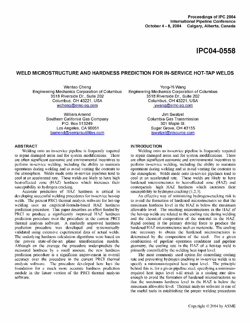
There are number of empirical hardness estimation formulae available in the open literature since the 1970s [9,10,11,12,13,14,15,16], Although these empirical equations are easy to use, their accuracy is often questionable. In a recent study conducted at TWI [17], the applicability of 12 sets of commonly used empirical formulae for HAZ hardness estimation were examined against the measured maximum HAZ hardness of approximately 350 welds for a range of C-Mn and low alloy steels. The formulae by Yurioka et al. [11,12], used in the present PRCI thermal analysis software, appeared to be the best among the 12 sets examined. As shown in Figure 1, the TWI study revealed that the discrepancies between the Yurioka prediction and the measured hardness values can be as high as 100 Hv in the hardness range between 300 to 350 Hv that are most critical to hydrogen induced cracking. In addition, the TWI results indicate that it would be unreliable to “patch” or “calibrate” the Yurioka equations (or any other similar empirical-based equations) with a limited amount of actual weld data, to ensure satisfactory performance of the

“calibrated” empirical model under the diverse weld cooling conditions and the wide range steel compositions encountered in hot-tap welding operations.

The aforementioned shortcoming of the empirical HAZ hardness formulae, most of which were developed in the 1970s to 1980s, can be attributed to the following fundamental fact. These empirical models oversimplify the effects of welding thermal cycle on the complex austenite decomposition processes of steel to a single parameter t8/5 (cooling time from 800 to 500°C). Hyperbolic tangent or exponential functions of t§/5 are used to describe the transition between the high hardness and low hardness plateaus, regardless of the shapes of cooling curves. In reality, different cooling curves of the same t8/5 value could result in the formation of different micro structure constituents (type, percentage and morphology) and the resultant hardness in the HAZ of a steel weld.

YURIOKA 1981

PREDICTED MAXIMUM HARDNESS, IIV

Figure 1 Scattering of predicted maximum HAZhardness by Yurioka equations as compared with measurement values by TWI [17]

The work described in this paper was funded by PRCI [18] to produce a significantly improved HAZ hardness prediction procedure over the procedure in the current PRCI thermal analysis software. The underlying hardness calculation algorithms were based on the proven state-of-the-art phase transformation models for steels. In fact, over the last 15 years or so, there has been significant advancement in microstructural modeling of steels based on the fundamental phase transformation thermodynamics and kinetics theories [19,20,21,22,23,24,25,26,27,28,29], This work led to the development of a markedly improved hardness prediction procedure.

TECHNICAL APPROACHControlled Thermal Severity (CTS) [30] test was simulated

in this study since it was considered standard test for estimating the risk of HAZ hydrogen cracking and a good simulation of hot-tap welds. The analysis results were compared with the experimental measurements supplied by TWI. The finite element (FE) simulation consisted of computations of heat flow, microstructure evolution, and hardness. As mentioned earlier, there has been significant advancement in the past 15 years in microstructural and hardness modeling of steels based on the fundamental phase transformation thermodynamics and


kinetics theories. These state-of-the-art microstructure and hardness prediction algorithms are very robust. The hardness prediction model consisted of the weld heat flow module and the microstructure and hardness module. The weld thermal history was calculated in the heat flow module and used as the input of the microstructure and hardness analysis. The phase- transformation thermodynamics and kinetics computation was executed in microstructure and hardness module to simulate the evolution of microstructure and render the final hardness distribution. The analysis results were compared with the experimental results individually as well as validated against the experimental data using statistical analysis.

ACTUAL WELDING DATAThe availability of actual welding data was critical in order

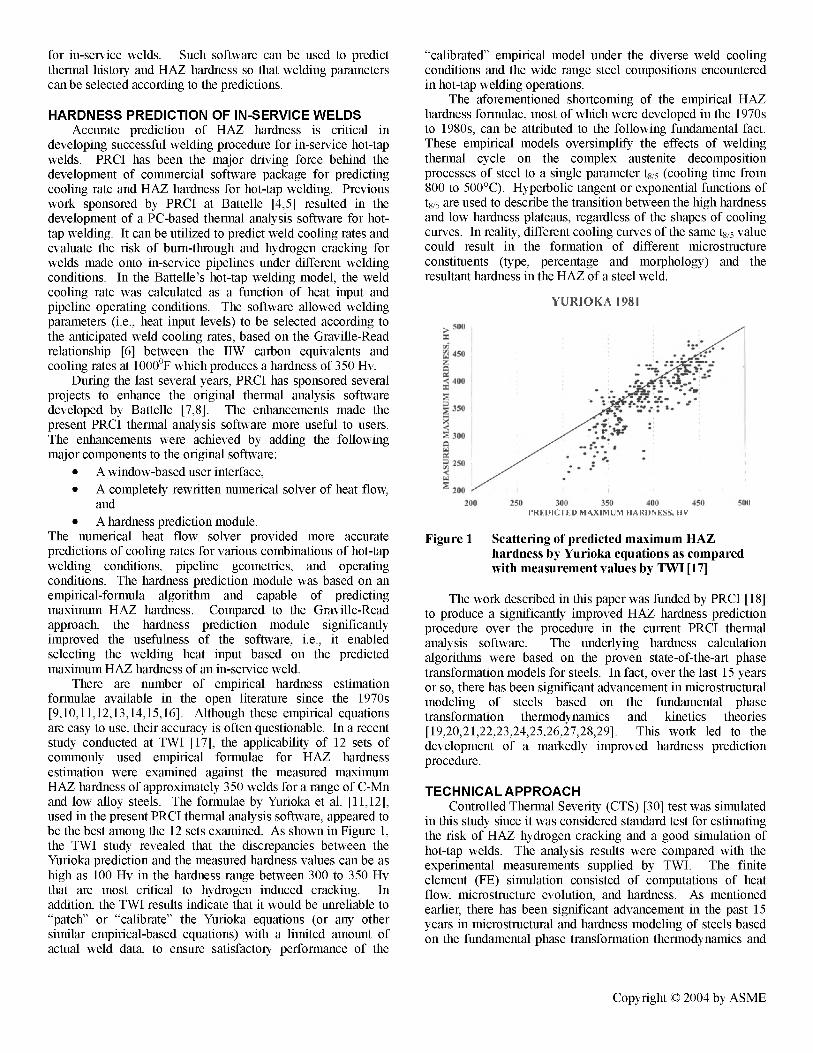
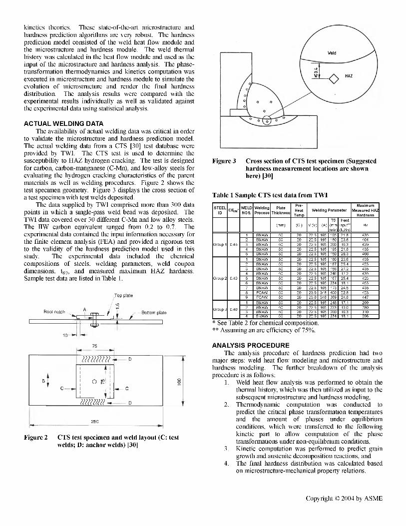
to validate the microstructure and hardness prediction model. The actual welding data from a CTS [30] test database were provided by TWI. The CTS test is used to determine the susceptibility to HAZ hydrogen cracking. The test is designed for carbon, carbon-manganese (C-Mn), and low-alloy steels for evaluating the hydrogen cracking characteristics of the parent materials as well as welding procedures. Figure 2 shows the test specimen geometry. Figure 3 displays the cross section of a test specimen with test welds deposited.

The data supplied by TWI comprised more than 300 data points in which a single-pass weld bead was deposited. The TWI data covered over 30 different C-Mn and low alloy steels. The IIW carbon equivalent ranged from 0.2 to 0.7. The experimental data contained the input information necessary for the finite element analysis (FEA) and provided a rigorous test to the validity of the hardness prediction model used in this study. The experimental data included the chemical compositions of steels, welding parameters, weld coupon dimensions, t8/5, and measured maximum HAZ hardness. Sample test data are listed in Table 1.

Top plate/ 2

Root notch | fry, f 1 r- Bottom plate-------------^ X '-------------

10-

Figure 3 Cross section of CTS test specimen (Suggested hardness measurement locations are shown here) [30]

Table 1 Sample CTS test data from TWI

STEEL

IDCE,iw*

WELD

NOS.

Welding

Process

Plate

Thickness

Pre-

Heat

Temp

Welding Parameter

Maximum

Measured HAZ

Hardness

(mm) (C) V(V) I (A)

TS(mm/min)

Heatinput**(kJ/in)

Hv

Group 1 0.45

1 SMAW 50 20 22.5 165 195 21.8 4352 SMAW 50 20 22.5 165 180 23.6 4043 SMAW 50 20 22.5 165 260 16.3 4294 SMAW 50 20 22.5 165 195 21.8 4355 SMAW 50 20 22.5 165 150 28.3 466

Group 2 0.43

1 SMAW 50 20 22.5 165 180 23.6 4352 SMAW 50 20 22.5 165 167 25.4 4233 SMAW 50 20 22.5 165 156 27.2 4354 SMAW 50 20 22.5 165 246 17.2 4355 SMAW 50 20 22.5 165 167 25.4 4236 SMAW 50 20 22.5 165 234 18.1 4537 SMAW 50 20 22.5 165 173 24.5 4358 FCAW 50 20 23.0 348 400 22.8 4239 FCAW 50 20 23.0 348 369 24.8 447

Group 3 0.401 SMAW 50 20 22.5 165 248 17.1 2992 SMAW 50 20 22.5 165 223 19.0 2803 SMAW 50 20 22.5 165 260 16.3 3104 SMAW 50 20 22.5 234 18.1 25E

* See Table 2 for chemical composition. ** Assuming an arc efficiency of 75%.

75

FT

iII

bt | 0 p iC—► I

j_________ :I'!

mm - - d

250

Figure 2 CTS test specimen and weld layout (C: test welds; D: anchor welds) [30]

ANALYSIS PROCEDUREThe analysis procedure of hardness prediction had two

major steps: weld heat flow modeling and microstructure and hardness modeling. The further breakdown of the analysis procedure is as follows:

1. Weld heat flow analysis was performed to obtain the thermal history, which was then utilized as input to the subsequent microstructure and hardness modeling,

2. Thermodynamic computation was conducted to predict the critical phase transformation temperatures and the amount of phases under equilibrium conditions, which were transferred to the following kinetic part to allow computation of the phase transformations under non-equilibrium conditions,

3. Kinetic computation was performed to predict grain growth and austenite decomposition reactions, and

4. The final hardness distribution was calculated based on microstructure-mechanical property relations.


Step 1 was carried out in weld heat flow modeling and step 2, 3, and 4 were implemented in microstructure and hardness modeling. The necessary input data of the analysis included steel chemical composition, weld geometry, and welding parameters.

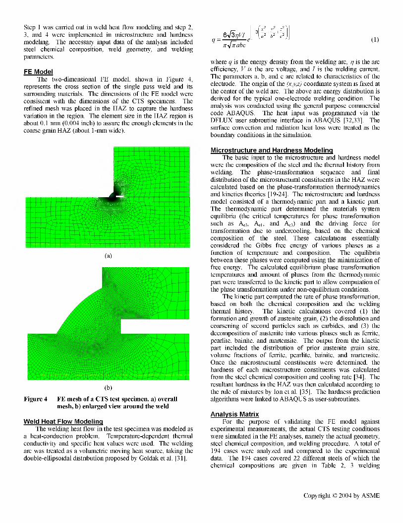
FE ModelThe two-dimensional FE model, shown in Figure 4,

represents the cross section of the single pass weld and its surrounding materials. The dimensions of the FE model were consistent with the dimensions of the CTS specimens. The refined mesh was placed in the HAZ to capture the hardness variation in the region. The element size in the HAZ region is about 0.1 rmn (0.004 inch) to assure the enough elements in the coarse grain HAZ (about 1-mm wide).

(1)

where q is the energy density from the welding arc, 77 is the arc efficiency, V is the arc voltage, and / is the welding current. The parameters a, b, and c are related to characteristics of the electrode. The origin of the (x,v,z) coordinate system is fixed at the center of the weld arc. The above arc energy distribution is derived for the typical one-electrode welding condition. The analysis was conducted using the general purpose coimnercial code ABAQUS. The heat input was prograimned via the DFLUX user subroutine interface in ABAQUS [32,33], The surface convection and radiation heat loss were treated as the boundary conditions in the simulation.

tb —

—

//y/A!©'/ // r

iT

.If

it j i j

(a)

Figure 4 FE mesh of a CTS test specimen, a) overall mesh, b) enlarged view around the weld

Weld Heat Flow ModelingThe welding heat flow in the test specimen was modeled as

a heat-conduction problem. Temperature-dependent thermal conductivity and specific heat values were used. The welding arc was treated as a volumetric moving heat source, taking the double-ellipsoidal distribution proposed by Goldak et al. [31].

Microstructure and Hardness ModelingThe basic input to the microstructure and hardness model

were the composition of the steel and the thermal history from welding. The phase-transformation sequence and final distribution of the micro structural constituents in the HAZ were calculated based on the phase-transformation thermodynamics and kinetics theories [19-24], The microstructure and hardness model consisted of a thermodynamic part and a kinetic part. The thermodynamic part determined the materials system equilibria (the critical temperatures for phase transformation such as Ae3, Ael, and Ac3) and the driving force for transformation due to undercooling, based on the chemical composition of the steel. These calculations essentially considered the Gibbs free energy of various phases as a function of temperature and composition. The equilibria between these phases were computed using the minimization of free energy. The calculated equilibrium phase transformation temperatures and amount of phases from the thermodynamic part were transferred to the kinetic part to allow computation of the phase transformations under non-equilibrium conditions.

The kinetic part computed the rate of phase transformation, based on both the chemical composition and the welding thermal history. The kinetic calculations covered (1) the formation and growth of austenite grain, (2) the dissolution and coarsening of second particles such as carbides, and (3) the decomposition of austenite into various phases such as ferrite, pearlite, bainite, and martensite. The output from the kinetic part included the distribution of prior austenite grain size, volume fractions of ferrite, pearlite, bainite, and martensite. Once the microstructural constituents were determined, the hardness of each microstructure constituents was calculated from the steel chemical composition and cooling rate [34]. The resultant hardness in the HAZ was then calculated according to the rule of mixtures by Ion et al. [35]. The hardness prediction algorithms were linked to ABAQUS as user-subroutines.

Analysis MatrixFor the purpose of validating the FE model against

experimental measurements, the actual CTS testing conditions were simulated in the FE analyses, namely the actual geometry, steel chemical composition, and welding procedure. A total of 194 cases were analyzed and compared to the experimental data. The 194 cases covered 22 different steels of which the chemical compositions are given in Table 2, 3 welding


processes including SMAW, FCAW, and SAW, 4 plate thicknesses including 25 nun (0.984 inch), 30 nun (1.181 inch), 50 mm (1.969 inch), and 100 rmn (3.937 inch), and different heat input levels ranging from 9 kJ/inch (0.354 kJ/mm) to 70 kJ/inch (2.756 kJ/imn).

RESULTS AND DISCUSSIONSince the same analysis procedure was used in all 194

cases, a representative case is first presented in this section with detailed analysis results, including temperature distribution, phase equilibra, microstructure constituent distribution, and hardness distribution. Then the analysis results of all cases are compared with the experimental data. The microstructure and hardness prediction model is validated while the statistical analysis is performed on the predicted and measured HAZ hardness values.

Table 2 Chemical compositions of the steels analyzed

STEEL ID C Mn Si Ni Cr Mo Cu V Nb Ti Al N CE„„

Group 1 0.18 1.57 0.45 0.040 0.020 0.01 0.060 0.002 0.047 0.045 0.008 0.45Group 2 0.19 1.38 0.28 0.010 0.020 0.005 0.024 0.047 0.004 0.43Group 3 0.05 1.39 0.27 0.800 0.010 0.940 0.015 0.011 0.021 0.007 0.40Group 4 0.17 1.17 0.26 0.010 0.010 0.01 0.010 0.063 0.002 0.030 0.007 0.37Group 5 0.10 1.35 0.30 0.005 0.010 0.01 0.005 0.002 0.002 0.005 0.040 0.003 0.33Group 6 0.06 1.28 0.26 0.510 0.010 0.01 0.005 0.002 0.021 0.017 0.038 0.005 0.31Group 7 0.08 1.48 0.26 0.170 0.010 0.160 0.017 0.008 0.024 0.004 0.35Group 8 0.09 1.49 0.26 0.002 0.003 0.005 0.016 0.005 0.028 0.002 0.34Group 9 0.12 1.50 0.37 0.200 0.200 0.220 0.031 0.004 0.029 0.002 0.44Group 10 0.11 1.29 0.37 0.090 0.070 0.01 0.290 0.023 0.002 0.039 0.008 0.37Group 11* 0.12 1.30 0.38 0.090 0.070 0.01 0.290 0.026 0.041 0.007 0.38Group 12* 0.11 1.52 0.37 0.200 0.020 0.220 0.030 0.004 0.030 0.002 0.40Group 13 0.20 1.42 0.32 0.030 0.020 0.020 0.047 0.004 0.027 0.010 0.44Group 14 0.18 1.46 0.31 0.020 0.030 0.02 0.020 0.026 0.030 0.007 0.44Group 15 0.15 1.46 0.32 0.030 0.020 0.030 0.031 0.003 0.027 0.006 0.40Group 16 0.16 1.44 0.36 0.020 0.020 0.020 0.029 0.036 0.007 0.41Group 17 0.10 1.46 0.31 0.020 0.020 0.020 0.036 0.005 0.043 0.005 0.35Group 18 0.10 1.46 0.31 0.020 0.020 0.010 0.034 0.004 0.042 0.005 0.35Group 19 0.14 1.36 0.36 0.070 0.050 0.02 0.020 0.030 0.004 0.024 0.007 0.39Group 20 0.04 1.26 0.13 0.660 0.010 0.005 0.002 0.016 0.006 0.027 0.005 0.30Group 21 0.07 1.34 0.27 0.020 0.020 0.005 0.017 0.008 0.038 0.004 0.30Group 22 0.08 1.50 0.26 0.020 0.030 0.005 0.016 0.005 0.026 0.002 0.34

* Group 23 and 24 have the same compositions as group 11 and 12, respectively.

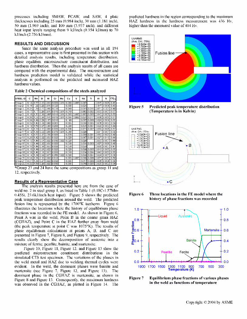
Results of a Representative CaseThe analysis results presented here are from the case of

weld no. 2 in steel group 1, as listed in Table 1 (0.18C-1.57Mn- 0.45Si, 23.6kJ/inch heat input). Figure 5 shows the predicted peak temperature distribution around the weld. The predicted fusion line is represented by the 1700°K isotherm. Figure 6 illustrates the locations where the history of equilibrium phase fractions was recorded in the FE model. As shown in Figure 6, Point A was in the weld. Point B in the coarse grain HAZ (CGHAZ), and Point C in the HAZ further away from weld (the peak temperature at point C was 1075°K). The results of phase equilibrium calculations at points A, B, and C are presented in Figure 7, Figure 8, and Figure 9, respectively. The results clearly show the decomposition of austenite into a mixture of ferrite, pearlite, bainite, and martensite.

Figure 10, Figure 11, Figure 12, and Figure 13 show the predicted microstructure constituent distributions in the simulated CTS test specimen. The variations of the phases in the weld metal and HAZ due to welding thermal cycles were evident. In the weld, the dominant phases were bainite and martensite (see Figure 7, Figure 12, and Figure 13). The dominant phase in the CGHAZ is martensite, as shown in Figure 8 and Figure 13. Consequently, the maximum hardness was observed in the CGHAZ, as plotted in Figure 14. The

predicted hardness in the region corresponding to the maximum HAZ hardness in the hardness measurement was 436 Hv, higher than the measured value of 404 Hv.

Figure 5 Predicted peak temperature distribution (Temperature is in Kelvin)

UVARM3 (Awe. Grit.: 75%)— +2.640e+03

♦ 1.7006*03♦ 1.500e+03♦ 1.3006+03 + 1.1006+03 +9.0006+02

— +3.1656+02

Fusion line

• A B

Figure 6 Three locations in the FE model where the history of phase fractions was recorded

T 1.0

Austenite0.8 -- -- 0.8

Martensite- - 0.6SO.6 --

Bainite - - 0.4

0.2 -- -- 0.2Pearlite Ferrite

r 0.01900 1700 1500 1300 1100 900 700 500 300

Temperature (K)

Figure 7 Equilibrium phase fractions of various phases in the weld as functions of temperature


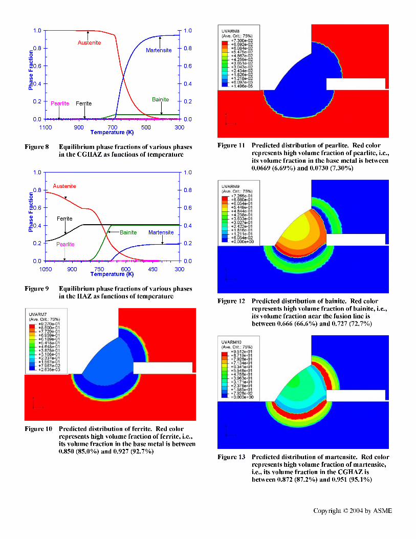
Figure 8 Equilibrium phase fractions of various phases in the CGHAZ as functions of temperature

Austenite-- 0.8

-- 0.6

Ferrite

Bainite Martensite

-- 0.2Pearlite

750 600Temperature (K)

Figure 9 Equilibrium phase fractions of various phasesin the HAZ as functions of temperature

Figure 10 Predicted distribution of ferrite. Red colorrepresents high volume fraction of ferrite, i.e., its volume fraction in the base metal is between 0.850 (85.0%) and 0.927 (92.7%)

Figure 11 Predicted distribution of pearlite. Red colorrepresents high volume fraction of pearlite, i.e., its volume fraction in the base metal is between 0.0669 (6.69%) and 0.0730 (7.30%)

Figure 12 Predicted distribution of bainite. Red colorrepresents high volume fraction of bainite, i.e., its volume fraction near the fusion line is between 0.666 (66.6%) and 0.727 (72.7%)

Figure 13 Predicted distribution of martensite. Red color represents high volume fraction of martensite, i.e., its volume fraction in the CGHAZ is between 0.872 (87.2%) and 0.951 (95.1%)


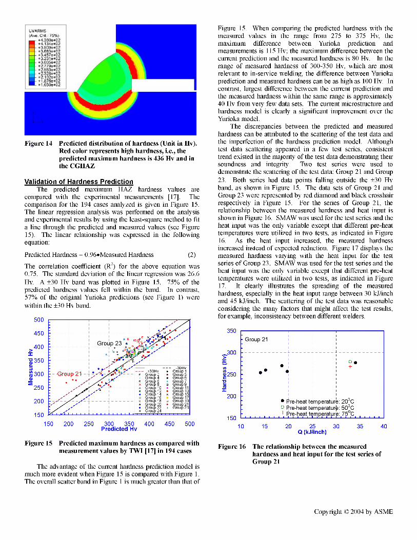
Figure 14 Predicted distribution of hardness (Unit in Hv). Red color represents high hardness, i.e., the predicted maximum hardness is 436 Hv and in the CGHAZ

Validation of Hardness PredictionThe predicted maximum HAZ hardness values are

compared with the experimental measurements [17]. The comparison for the 194 cases analyzed is given in Figure 15. The linear regression analysis was performed on the analysis and experimental results by using the least-square method to fit a line through the predicted and measured values (see Figure 15). The linear relationship was expressed in the following equation:

Predicted Hardness = 0.96»Measured Hardness (2)

The correlation coefficient (R2) for the above equation was 0.75. The standard deviation of the linear regression was 26.6 Hv. A +30 Hv band was plotted in Figure 15. 75% of the predicted hardness values fell within the band. In contrast, 57% of the original Yurioka predictions (see Figure 1) were within the +30 Hv band.

Group 23

--- -30 Hv♦ Group 1♦ Group 3♦ Group 5 a Group 7□ Group 9♦ Group 11 3 Group 13 x Group 15

Group 17□ Group 19♦ Group 21 + Group 23

-- +30Hv □ Group 2 + Group 4 o Group 6 x Group 8 a Group 10 o Group 12♦ Group 14

Group 16o Group 18 a Group 20• Group 22 o Group 24

-Greqp-21- • -•%

Predicted Hv

Figure 15. When comparing the predicted hardness with the measured values in the range from 275 to 375 Hv, the maximum difference between Yurioka prediction and measurements is 115 Hv; the maximum difference between the current prediction and the measured hardness is 80 Hv. In the range of measured hardness of 300-350 Hv, which are most relevant to in-service welding, the difference between Yurioka prediction and measured hardness can be as high as 100 Hv. In contrast, largest difference between the current prediction and the measured hardness within the same range is approximately 40 Hv from very few data sets. The current microstructure and hardness model is clearly a significant improvement over the Yurioka model.

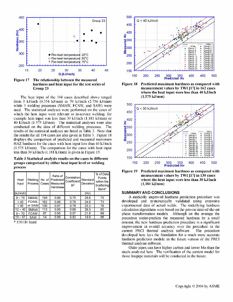
The discrepancies between the predicted and measured hardness can be attributed to the scattering of the test data and the imperfection of the hardness prediction model. Although test data scattering appeared in a few test series, consistent trend existed in the majority of the test data demonstrating their soundness and integrity. Two test series were used to demonstrate the scattering of the test data: Group 21 and Group 23. Both series had data points falling outside the ±30 Hv band, as shown in Figure 15. The data sets of Group 21 and Group 23 were represented by red diamond and black crosshair respectively in Figure 15. For the series of Group 21, the relationship between the measured hardness and heat input is shown in Figure 16. SMAW was used for the test series and the heat input was the only variable except that different pre-heat temperatures were utilized in two tests, as indicated in Figure16. As the heat input increased, the measured hardness increased instead of expected reduction. Figure 17 displays the measured hardness varying with the heat input for the test series of Group 23. SMAW was used for the test series and the heat input was the only variable except that different pre-heat temperatures were utilized in two tests, as indicated in Figure17. It clearly illustrates the spreading of the measured hardness, especially in the heat input range between 30 kJ/inch and 45 kJ/inch. The scattering of the test data was reasonable considering the many factors that might affect the test results, for example, inconsistency between different welders.

350

__300xsa 250irox

200

15010 15 20 25 30 35 40

Q (kJ/inch)

------------ 1------------ 1-------------- Group 21

: .•O *+

. . i i• ^re-heat te 0 F^re-heat te

i + Pre-heat te

mperaturmperaturmperatur ■r‘ ■ ■

e: 20°C b: 50°C e:,7?°,C, ■ ■ ■ ■

Figure 15 Predicted maximum hardness as compared with measurement values by TWI [17] in 194 cases

The advantage of the current hardness prediction model is much more evident when Figure 15 is compared with Figure 1. The overall scatter band in Figure 1 is much greater than that of

Figure 16 The relationship between the measuredhardness and heat input for the test series of Group 21


450

__400xin$350

"5rox300

25015 20 25 30 35 40 45

Q (kJ/inch)

Figure 17 The relationship between the measuredhardness and heat input for the test series of Group 23

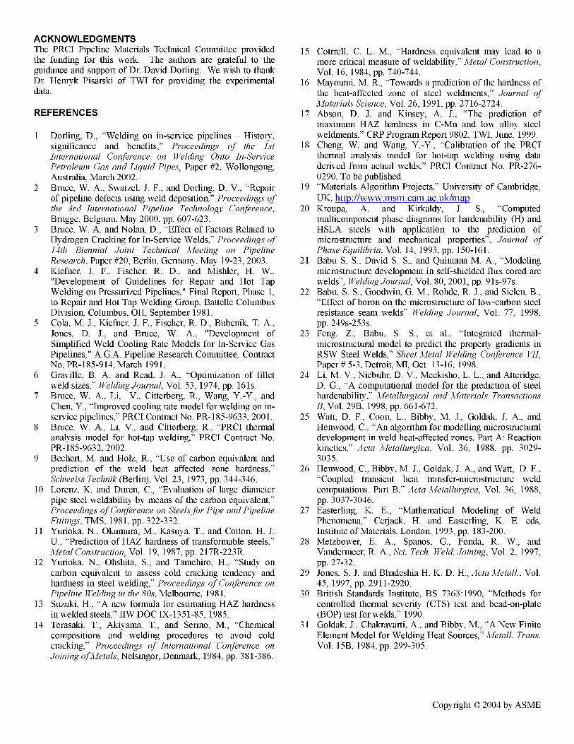
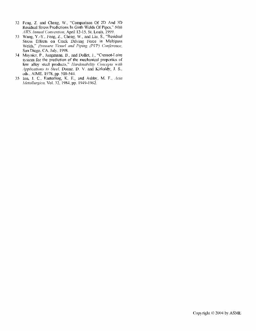
The heat input of the 194 cases described above ranged from 9 kJ/inch (0.354 kJ/mm) to 70 kJ/inch (2.756 kJ/mm) while 3 welding processes (SMAW, FCAW, and SAW) were used. The statistical analyses were performed on the cases of which the heat input were relevant to in-service welding, for example heat input was less than 30 kJ/inch (1.181 kJ/mm) or 40 kJ/inch (1.575 kJ/imn). The statistical analyses were also conducted on the data of different welding processes. The results of the statistical analyses are listed in Table 3. Note that the results for all 194 cases are also given in Table 3. Figure 18 displays the comparison of predicted and measured maximum HAZ hardness for the cases with heat input less than 40 kJ/inch (1.575 kJ/mm). The comparison for the cases with heat input less than 30 kJ/inch (1.181 kJ/imn) is given in Figure 19.

Table 3 Statistical analysis results on the cases in different groups categorized by either heat input level or welding process

HeatInput

WeldingProcess

No. of Cases

Ratio of Predicted/ Measured Hardness

CorrelationCoefficient

R2

StandardDeviation

% of Data Points

within the Scattering

Band*(kJ/inch) (Hv)

CD l 3 SMAW,

FCAW, or SAW

194 0.96 0.75 26.6 75< 40 162 0.96 0.78 24.6 73< 30 130 0.97 0.76 23.2 79

12-43 SMAW 113 0.95 0.68 29.3 85

CD l 3 FCAW 67 0.95 0.57 21.8 69

13-57 SAW 14 0.98 0.82 19.9 86

* +30 Hv band

•cBroup 23

o•

••

# #

•

+ •

Are-heat temperature: 20°C~ o ^re-heat te(nperatur^: 50°C + Pre-heat temperature: 75°C

■ ■ F ■ ■ . . I ■ ■ ■ ■ I ■ ■ .

: Q < 40 kJ/inch

— — — — -30 Hv— - +30 Hv ♦ Group 1□ Group 2 • Group 3+ Group 4 o Group 6* Group 7 x Group 8□ Group 9 a Group 10♦ Group 11 • Group 12• Group 13 ♦ Group 14x Group 15 ■ Group 16

Group 17 o Group 18□ Group 19 a Group 20♦ Group 21 • Group 22+ Group 23 » Group 24

i i I i

Predicted Hv

Figure 18 Predicted maximum hardness as compared with measurement values by TWI [17] in 162 cases where the heat input were less than 40 kJ/inch (1.575 kJ/mm)

:Q < 30 kJ/inch

---- ----- -30 Hv-- +30Hv ♦ Group 1□ Group 2 • Group 3+ Group 4 o Group 6

Group 7 x Group 8□ Group 9 & Group 10♦ Group 11 • Group 12♦ Group 13 ♦ Group 14x Group 15 ■ Group 16

Group 17 o Group 18□ Group 19 a Group 20♦ Group 21 • Group 22+ Group 23 o Group 24J■ +> **■ 1 1 1 1 1 1 1 1 1 1 1 1 1 i—i L

Predicted Hv

Figure 19 Predicted maximum hardness as compared with measurement values by TWI [17] in 130 cases where the heat input were less than 30 kJ/inch (1.181 kJ/mm)

SUMMARY AND CONCLUSIONSA markedly improved hardness prediction procedure was

developed and systematically validated using extensive experimental data of actual welds. The underlying hardness calculation algorithms were based on the proven state-of-the-art phase transformation models. Although on the average the procedure under-predicts the measured hardness by a small amount, the new hardness prediction procedure is a significant improvement in overall accuracy over the procedure in the current PRCI thermal analysis software. The procedure developed here lays the foundation for a much more accurate hardness prediction module in the future version of the PRCI thermal analysis software.

Older pipes can have higher carbon and lower Mn than the steels analyzed here. The verification of the current model for those linepipe materials will be conducted in the future.


ACKNOWLEDGMENTSThe PRCI Pipeline Materials Technical Committee provided the funding for this work. The authors are grateful to the guidance and support of Dr. David Dorling. We wish to thank Dr. Henryk Pisarski of TWI for providing the experimental data.

REFERENCES

1 Dorling, D., “Welding on in-service pipelines - History, significance and benefits,” Proceedings of the 1st International Conference on Welding Onto In-Sennce Petroleum Gas and Liquid Pipes, Paper #2, Wollongong, Australia, March 2002.

2 Bruce, W. A., Swatzel, J. F., and Dorling, D. V., “Repair of pipeline defects using weld deposition,” Proceedings of the 3rd International Pipeline Technology Conference, Brugge, Belgium, May 2000, pp. 607-623.

3 Bruce, W. A. and Nolan, D., “Effect of Factors Related to Hydrogen Cracking for In-Service Welds,” Proceedings of 14th Biennial Joint Technical Meeting on Pipeline Research, Paper #20, Berlin, Germany, May 19-23, 2003.

4 Kiefner, J. F„ Fischer, R. D„ and Mishler, H. W„ "Development of Guidelines for Repair and Hot Tap Welding on Pressurized Pipelines," Final Report, Phase 1, to Repair and Hot Tap Welding Group, Battelle Columbus Division, Columbus, OH, September 1981.

5 Cola, M. J., Kiefner, J. F., Fischer, R. D„ Bubenik, T. A., Jones, D. J., and Bruce, W. A., "Development of Simplified Weld Cooling Rate Models for In-Service Gas Pipelines," A.G.A. Pipeline Research Committee, Contract No. PR-185-914, March 1991.

6 Graville, B. A. and Read, J. A., “Optimization of fillet weld sizes,” Welding Journal, Vol. 53, 1974, pp. 161s.

7 Bruce, W. A., Li, V., Citterberg, R., Wang, Y.-Y., and Chen, Y„ “Improved cooling rate model for welding on in- service pipelines,” PRCI Contract No. PR-185-9633, 2001.

8 Bruce, W. A., Li, V., and Citterberg, R., “PRCI thermal analysis model for hot-tap welding,” PRCI Contract No. PR-185-9632. 2002.

9 Bechert, M. and Holz, R., “Use of carbon equivalent and prediction of the weld heat affected zone hardness,” Schweiss Technik (Berlin), Vol. 23, 1973, pp. 344-346.

10 Lorenz, K. and Duren, C “Evaluation of large diameter pipe steel weldability by means of the carbon equivalent,” Proceedings of Conference on Steels for Pipe and Pipeline Fittings, TMS, 1981, pp. 322-332.

11 Yurioka, N., Okumura, M„ Kasuya, T., and Cotton, H. J. U., “Prediction of HAZ hardness of transformable steels,” Metal Construction^ol. 19, 1987, pp. 217R-223R.

12 Yurioka, N„ Ohshita, S., and Tamehiro, H„ “Study on carbon equivalent to assess cold cracking tendency and hardness in steel welding,” Proceedings of Conference on Pipeline Welding in the 80s, Melbourne, 1981.

13 Suzuki, H., “A new formula for estimating HAZ hardness in welded steels,” IIW DOC IX-1351-85, 1985.

14 Terasaki, T„ Akiyama, T„ and Serino, M„ “Chemical compositions and welding procedures to avoid cold cracking,” Proceedings of International Conference on Joining of Metals, Nelsingor, Demnark, 1984, pp. 381-386.

15 Cotrrell, C. L. M., “Hardness equivalent may lead to a more critical measure of weldability,” Metal Construction, Vol. 16, 1984, pp. 740-744.

16 Mayoumi, M. R„ “Towards a prediction of the hardness of the heat-affected zone of steel weldments,” Journal of Materials Science, Vol. 26, 1991, pp. 2716-2724.

17 Abson, D. J. and Kinsey, A. I, “The prediction of maximum HAZ hardness in C-Mn and low alloy steel weldments,” CRP Program Report 9802, TWI, June, 1999.

18 Cheng, W. and Wang, Y.-Y., “Calibration of the PRCI thermal analysis model for hot-tap welding using data derived from actual welds,” PRCI Contract No. PR-276- 0290, To be published.

19 “Materials Algorithm Projects,” University of Cambridge, UK, http://www.msm.cam.ac.uk/map

20 Kroupa, A. and Kirkaldy, J. S„ “Computedmulticomponent phase diagrams for hardenability (H) and HSLA steels with application to the prediction of microstructure and mechanical properties”. Journal of Phase Equilibria, Vol. 14, 1993, pp. 150-161.

21 Babu S. S., David S. S„ and Quintana M. A., “Modeling microstructure development in self-shielded flux cored arc welds”. Welding Journal, Vol. 80, 2001, pp. 91s-97s.

22 Babu, S. S., Goodwin, G. M„ Rohde, R. J., and Sielen, B., “Effect of boron on the micro structure of low-carbon steel resistance seam welds” Welding Journal, Vol. 77, 1998, pp. 249s-253s.

23 Feng, Z„ Babu, S. S„ et al.. “Integrated thennal- microstmctural model to predict the property gradients in RSW Steel Welds,” Sheet Metal Welding Conference VII, Paper # 5-3, Detroit, MI, Oct. 13-16, 1998.

24 Li, M. V., Niebuhr, D. V., Meekisho, L. L„ and Atteridge, D. G„ “A computational model for the prediction of steel hardenability,” Metallurgical and Materials Transactions B, Vol. 29B, 1998, pp. 661-672.

25 Watt, D. F., Coon, L., Bibby, M. J., Goldak, J. A., and Henwood, C., “An algorithm for modelling microstructural development in weld heat-affected zones. Part A: Reaction kinetics,” Acta Metallurgica, Vol. 36, 1988, pp. 3029- 3035.

26 Henwood, C., Bibby, M. J., Goldak, J. A., and Watt, D. F., “Coupled transient heat transfer-microstructure weld computations. Part B,” Acta Metallurgica, Vol. 36, 1988, pp. 3037-3046.

27 Easterling, K. E., “Mathematical Modeling of Weld Phenomena,” Ceijack, H. and Easterling, K. E. eds. Institute of Materials, London, 1993, pp. 183-200.

28 Metzbower, E. A., Spanos, G., Fonda, R. W„ and Vandenneer, R. A., Sci. Tech. Weld. Joining, Vol. 2, 1997, pp. 27-32.

29 Jones, S. J. and Bhadeshia H. K. D. H„ Acta Metall., Vol. 45, 1997, pp. 2911-2920.

30 British Standards Institute, BS 7363:1990, “Methods for controlled thermal severity (CTS) test and bead-on-plate (BOP) test for welds,” 1990.

31 Goldak, J., Chakravarti, A., and Bibby, M., “A New Finite Element Model for Welding Heat Sources,” Metall. Trans. Vol. 15B, 1984, pp. 299-305.


32 Feng, Z. and Cheng, W., “Comparison Of 2D And 3D Residual Stress Predictions In Girth Welds Of Pipes,” 80th AWSAnnual Convention, April 12-15, St. Louis, 1999.

33 Wang, Y.-Y., Feng, Z., Cheng, W., and Liu, S., “Residual Stress Effects on Crack Driving Force in Multipass Welds,” Pressure Vessel and Piping (PVP) Conference, San Diego, CA, July, 1998.

34 Maynier, P., Jungmann, B., and Dollet, J., “Creusot-Loire system for the prediction of the mechanical properties of low alloy steel products,” Hardenability Concepts with Applications to Steel, Doane, D. V. and Kirkaldy, J. S., eds., AIME, 1978, pp. 518-544.

35 Ion, J. C., Easterling, K. E., and Ashby, M. F., Acta Metallurgica, Vol. 32, 1984, pp. 1949-1962.


Weld Microstructure and Hardnesss Prediction for In ...

Documents