Weizmann 2010 © 1 Introduction to Matlab & Data Analysis Lecture 13: Using Matlab for Numerical Analysis.

1Weizmann 2010 ©

Introduction to Matlab & Data Analysis

Lecture 13: Using Matlab for Numerical

Analysis

2

Outline

Data Smoothing Data interpolation Correlation coefficients Curve Fitting Optimization Derivatives and integrals

3

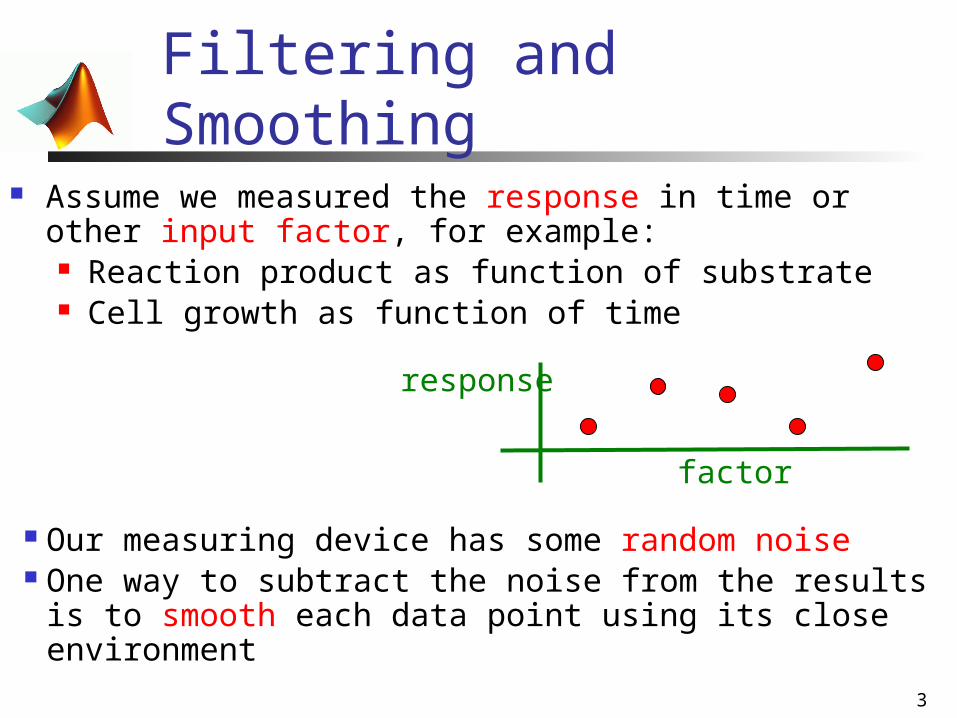
Assume we measured the response in time or other input factor, for example: Reaction product as function of substrate Cell growth as function of time

Filtering and Smoothing

factor

response

Our measuring device has some random noise One way to subtract the noise from the results is to

smooth each data point using its close environment

4

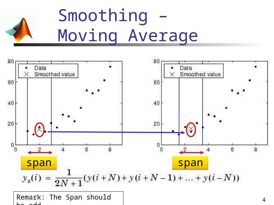
Smoothing – Moving Average

span

Remark: The Span should be odd

span

5

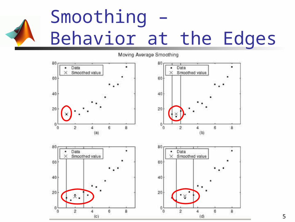
Smoothing – Behavior at the Edges

6

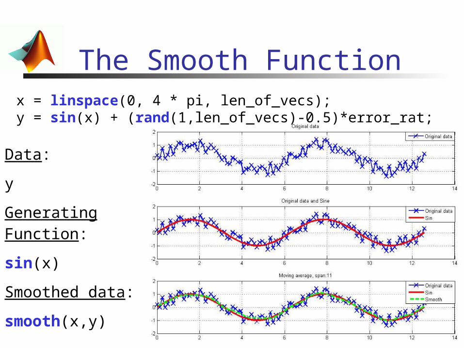
The Smooth Functionx = linspace(0, 4 * pi, len_of_vecs);y = sin(x) + (rand(1,len_of_vecs)-0.5)*error_rat;

Data:

y

Generating Function:

sin(x)

Smoothed data:

smooth(x,y)

7

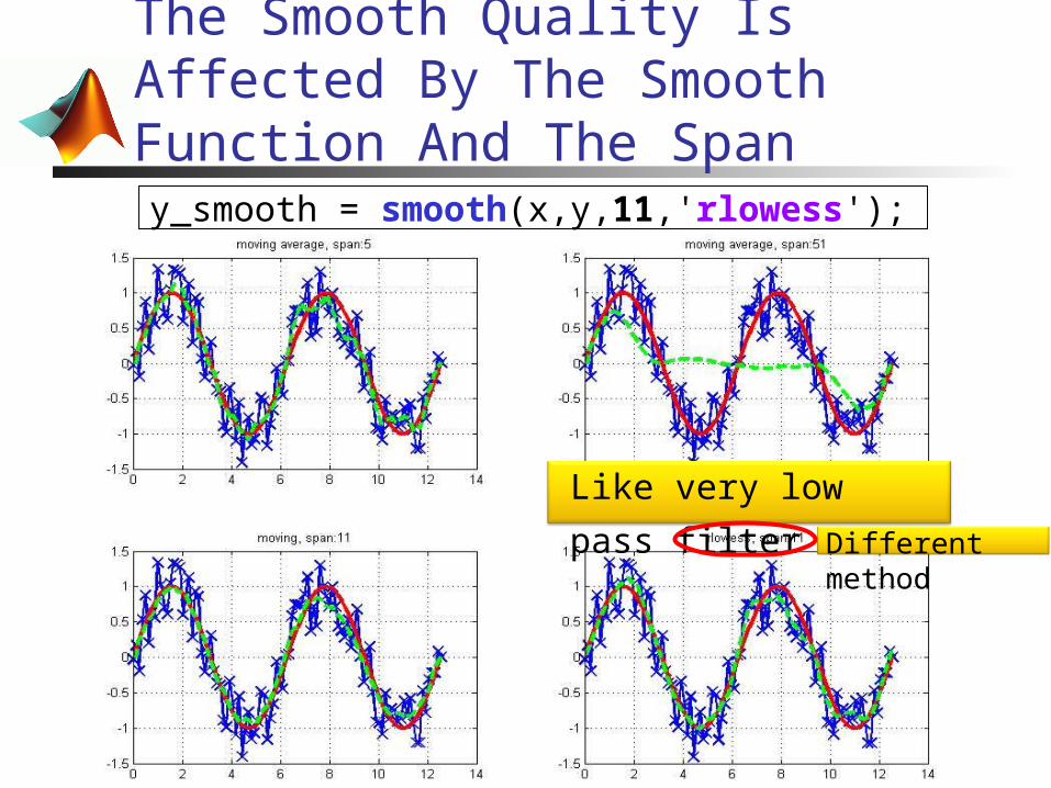
The Smooth Quality Is Affected By The Smooth Function And The Span

Like very low pass

filter Different method

y_smooth = smooth(x,y,11,'rlowess');

8

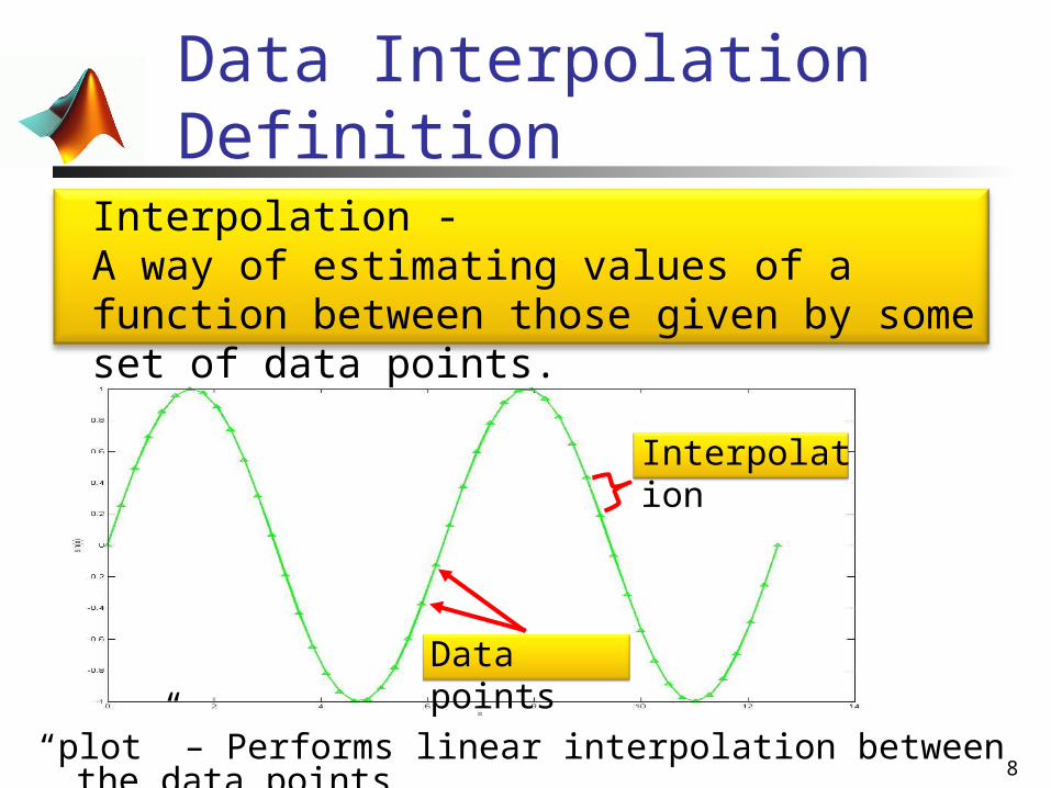
Data Interpolation Definition

“plot” – Performs linear interpolation between the data points

Interpolation - A way of estimating values of a function between those given by some set of data points.

Interpolation

Data points

9

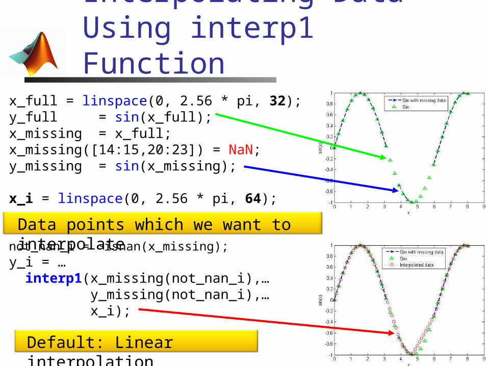
Interpolating Data Using interp1 Function

x_full = linspace(0, 2.56 * pi, 32);y_full = sin(x_full);x_missing = x_full;x_missing([14:15,20:23]) = NaN;y_missing = sin(x_missing); x_i = linspace(0, 2.56 * pi, 64);

not_nan_i = ~isnan(x_missing); y_i = … interp1(x_missing(not_nan_i),… y_missing(not_nan_i),… x_i);

Data points which we want to interpolate

Default: Linear interpolation

10

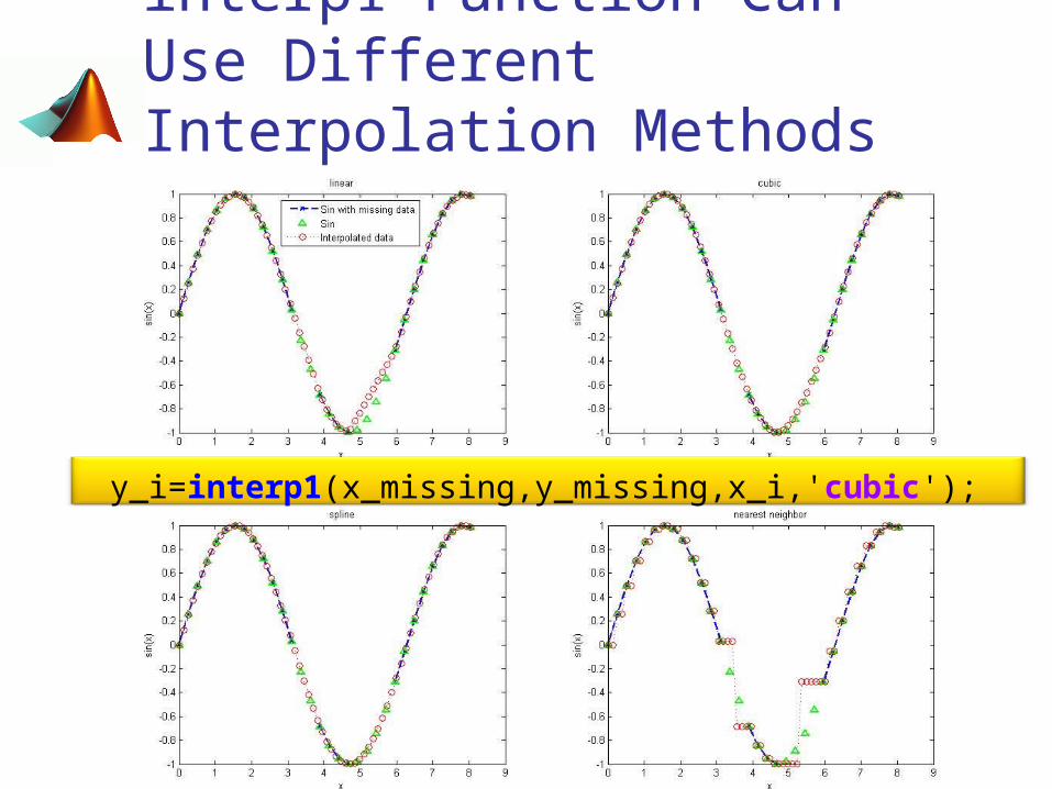
interp1 Function Can Use Different Interpolation Methods

y_i=interp1(x_missing,y_missing,x_i,'cubic');

11

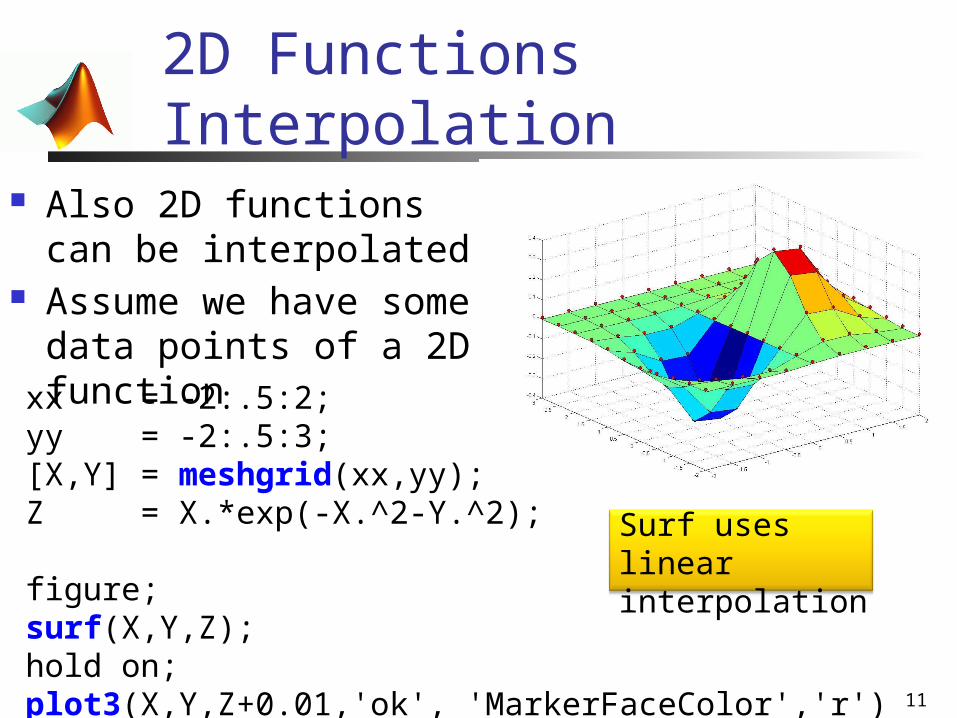
2D Functions Interpolation

Also 2D functions can be interpolated

Assume we have some data points of a 2D function

xx = -2:.5:2;yy = -2:.5:3;[X,Y] = meshgrid(xx,yy);Z = X.*exp(-X.^2-Y.^2); figure;surf(X,Y,Z);hold on;plot3(X,Y,Z+0.01,'ok', 'MarkerFaceColor','r')

Surf uses linear interpolation

12

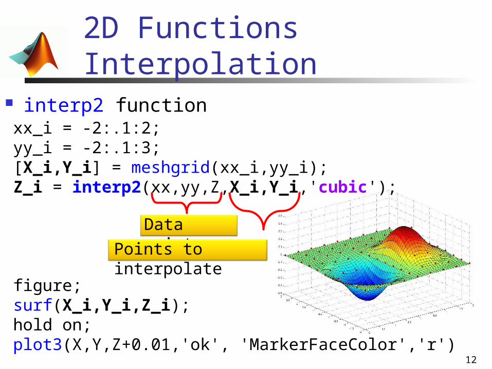
2D Functions Interpolation

interp2 functionxx_i = -2:.1:2;yy_i = -2:.1:3;[X_i,Y_i] = meshgrid(xx_i,yy_i);Z_i = interp2(xx,yy,Z,X_i,Y_i,'cubic');

figure;surf(X_i,Y_i,Z_i);hold on;plot3(X,Y,Z+0.01,'ok', 'MarkerFaceColor','r')

Data points

Points to interpolate

13Weizmann 2010 ©

Optimization and Curve Fitting

14

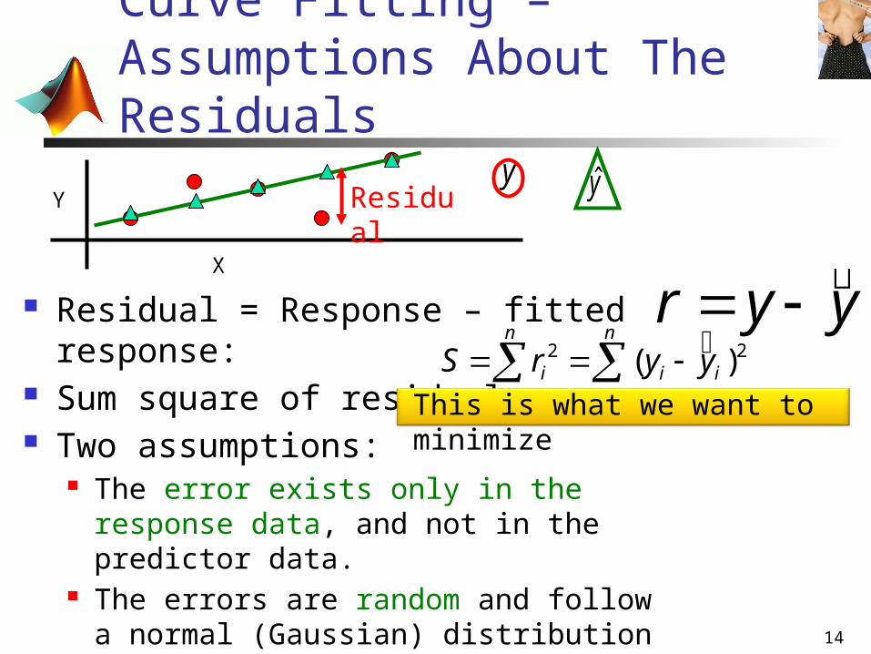
Curve Fitting – Assumptions About The Residuals

Residual = Response – fitted response:

Sum square of residuals Two assumptions:

The error exists only in the response data, and not in the predictor data.

The errors are random and follow a normal (Gaussian) distribution with zero mean and constant variance.

yyr

n

iii

n

ii yyrS

1

2

1

2 )(

This is what we want to minimize

X

Yy yResidu

al

15

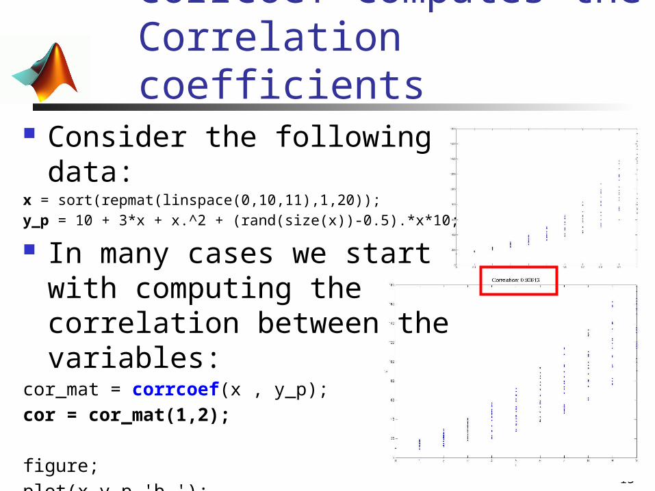
corrcoef Computes the Correlation coefficients

Consider the following data:x = sort(repmat(linspace(0,10,11),1,20));y_p = 10 + 3*x + x.^2 + (rand(size(x))-0.5).*x*10;

In many cases we start with computing the correlation between the variables:

cor_mat = corrcoef(x , y_p);cor = cor_mat(1,2);

figure;plot(x,y_p,'b.');xlabel('x');ylabel('y');title(['Correlation: ' num2str(cor)]);

16

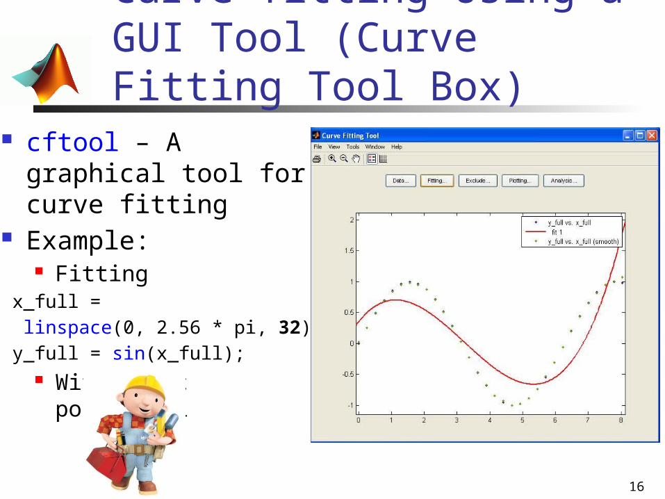
Curve fitting Using a GUI Tool (Curve Fitting Tool Box)

cftool – A graphical tool for curve fitting

Example: Fitting

x_full = linspace(0, 2.56 * pi, 32); y_full = sin(x_full);

With cubic polynomial

17

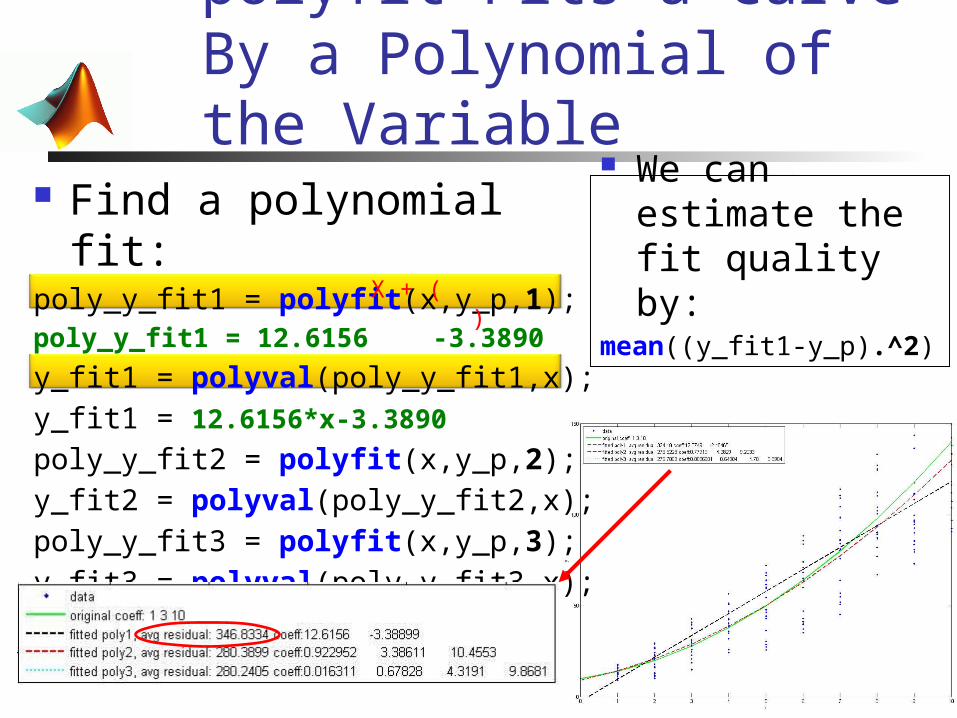
polyfit Fits a Curve By a Polynomial of the Variable

Find a polynomial fit:poly_y_fit1 = polyfit(x,y_p,1);poly_y_fit1 = 12.6156 -3.3890

y_fit1 = polyval(poly_y_fit1,x);y_fit1 = 12.6156*x-3.3890poly_y_fit2 = polyfit(x,y_p,2);y_fit2 = polyval(poly_y_fit2,x);poly_y_fit3 = polyfit(x,y_p,3);y_fit3 = polyval(poly_y_fit3,x);

X + ( )

We can estimate the fit quality by:

mean((y_fit1-y_p).^2)

18

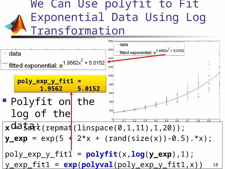
We Can Use polyfit to Fit Exponential Data Using Log Transformation

x = sort(repmat(linspace(0,1,11),1,20));y_exp = exp(5 + 2*x + (rand(size(x))-0.5).*x);

poly_exp_y_fit1 = polyfit(x,log(y_exp),1);y_exp_fit1 = exp(polyval(poly_exp_y_fit1,x))

Polyfit on the log of the data:

poly_exp_y_fit1 = 1.9562 5.0152

19Weizmann 2010 ©

What about fitting a Curve with a linear function of several variables? Can we put constraints on the coefficients values?

332211ˆ xcxcxcy

20Weizmann 2010 ©

For this type of problems (and much more)lets learn the optimization toolbox

http://www.mathworks.com/products/optimization/description1.html

21

Optimization Toolbox Can Solve Many Types of Optimization Problems

Optimization Toolbox – Extends the capability of the MATLAB numeric computing

environment. The toolbox includes routines for many types of

optimization including: Unconstrained nonlinear minimization Constrained nonlinear minimization, including goal

attainment problems and minimax problems Semi-infinite minimization problems Quadratic and linear programming Nonlinear least-squares and curve fitting Nonlinear system of equation solving Constrained linear least squares Sparse structured large-scale problems

==

22

Optimization Toolbox GUI Can Generate M-files

The GUI contains many options.Everything can be done using coding.

23Weizmann 2010 ©

Lets learn some of the things the optimization tool box can do

24

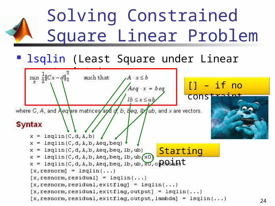
Solving Constrained Square Linear Problem

lsqlin (Least Square under Linear constraints)

Starting point

[] – if no constraint

25

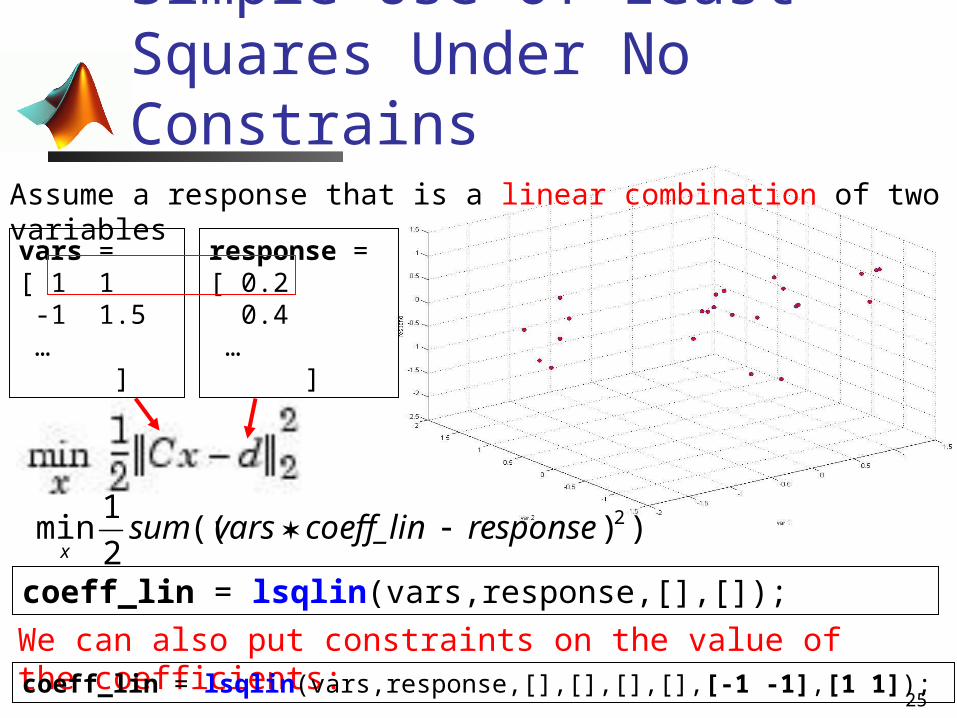
Simple Use Of Least Squares Under No Constrains

Assume a response that is a linear combination of two variables

vars = [ 1 1 -1 1.5 … ]

response = [ 0.2 0.4 … ]

coeff_lin = lsqlin(vars,response,[],[]);

We can also put constraints on the value of the coefficients:coeff_lin = lsqlin(vars,response,[],[],[],[],[-1 -1],[1 1]);

))((2

1min 2responsecoeff_linvarssumx

26

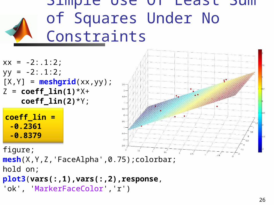
coeff_lin = -0.2361 -0.8379

xx = -2:.1:2;yy = -2:.1:2;[X,Y] = meshgrid(xx,yy);Z = coeff_lin(1)*X+ coeff_lin(2)*Y;

figure;mesh(X,Y,Z,'FaceAlpha',0.75);colorbar;hold on;plot3(vars(:,1),vars(:,2),response,'ok', 'MarkerFaceColor','r')

Simple Use Of Least Sum of Squares Under No Constraints

27Weizmann 2010 ©

What about fitting a Curve with a non linear function?

28

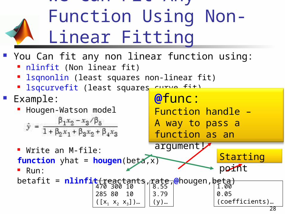
We Can Fit Any Function Using Non-Linear Fitting

You Can fit any non linear function using: nlinfit (Non linear fit) lsqnonlin (least squares non-linear fit) lsqcurvefit (least squares curve fit)

Example: Hougen-Watson model

Write an M-file:function yhat = hougen(beta,x) Run:betafit = nlinfit(reactants,rate,@hougen,beta)

470 300 10285 80 10([x1 x2 x3])…

8.553.79(y)…

@func:Function handle – A way to pass a function as an argument!

1.000.05(coefficients)…

Starting point

29

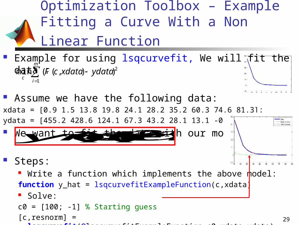
Optimization Toolbox – Example Fitting a Curve With a Non Linear Function

Example for using lsqcurvefit, We will fit the data :

Assume we have the following data:xdata = [0.9 1.5 13.8 19.8 24.1 28.2 35.2 60.3 74.6 81.3];ydata = [455.2 428.6 124.1 67.3 43.2 28.1 13.1 -0.4 -1.3 -1.5];

We want to fit the data with our model:

Steps: Write a function which implements the above model: function y_hat = lsqcurvefitExampleFunction(c,xdata) Solve:c0 = [100; -1] % Starting guess[c,resnorm] =

lsqcurvefit(@lsqcurvefitExampleFunction,c0,xdata,ydata)

m

ic

ydataxdatacF1

2)),((min

)()*2()1()( ixdataceciydata

30Weizmann 2010 ©

What about solving non linear system of equations?

31

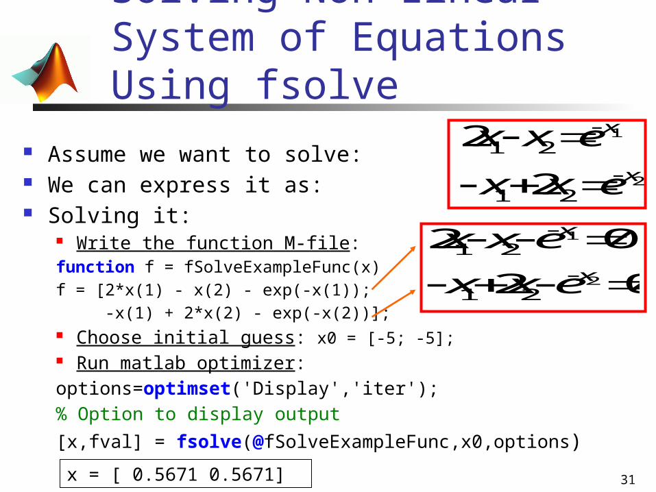
Solving Non Linear System of Equations Using fsolve

Assume we want to solve: We can express it as: Solving it:

Write the function M-file:function f = fSolveExampleFunc(x)f = [2*x(1) - x(2) - exp(-x(1)); -x(1) + 2*x(2) - exp(-x(2))]; Choose initial guess: x0 = [-5; -5]; Run matlab optimizer:options=optimset('Display','iter'); % Option to display output

[x,fval] = fsolve(@fSolveExampleFunc,x0,options)

2

1

21

21

2

2x

x

exx

exx

02

022

1

21

21

x

x

exx

exx

x = [ 0.5671 0.5671]

32Weizmann 2010 ©

Optimization tool box has several features:

Summary:

Minimization Curve fitting Equations solving

33Weizmann 2010 ©

A taste of Symbolic matlab:

Derivatives and integrals

34

What Is Symbolic Matlab?

“Symbolic Math Toolbox uses symbolic objects to represent symbolic variables, expressions, and matrices.”

“Internally, a symbolic object is a data structure that stores a string representation of the symbol.”

35

Defining Symbolic Variables and Functions

Define symbolic variables:a_sym = sym('a')b_sym = sym('b')c_sym = sym('c')x_sym = sym('x') Define a symbolic expressionf = sym('a*x^2 + b*x + c') Substituting variables:g = subs(f,x_sym,3)

g = 9*a+3*b+c

36

We Can Derive And Integrate Symbolic Functions

Deriving a function:diff(f,x_sym)diff('sin(x)',x_sym)

Integrate a function:int(f,x_sym)

Symbolic Matlab can do much more…

This is a good place to stop

38

Summary

Matlab is not Excel…

If you know what you want to do – You will find the right tool!