WEIGHTING SUB-POPULATIONS IN LONGEVITY INEQUALITY RESEARCH ...kolegia.sgh.waw.pl/pl/KAE/Documents/WorkingPapersKAE/WPKAE_2… · WEIGHTING SUB-POPULATIONS IN LONGEVITY INEQUALITY

SGH KAE Working Papers Series Number: 2017/029 September 2017

COLLEGIUM OF ECONOMIC ANALYSIS

WORKING PAPER SERIES

WEIGHTING SUB-POPULATIONS IN LONGEVITY

INEQUALITY RESEARCH:

A PRACTICAL APPROACH

Adam Szulc

1

Adam Szulc1

Institute of Statistics and Demography

Warsaw School of Economics

WEIGHTING SUB-POPULATIONS IN LONGEVITY INEQUALITY RESEARCH:

A PRACTICAL APPROACH

ABSTRACT

The weights allowing calculation of life expectancy for a whole population as a weighted

average of group-specific life expectancies are proposed. They are characterized by a

minimum distance from the actual population shares that are different from those assumed in

life tables. It is demonstrated how they may be obtained by means of constrained regression,

using popular statistical/econometric software. The problem of negative solutions is also

addressed. The empirical examples include longevity inequality calculations under various

weighting systems. The data come from the Human Mortality Database and from Russia’s

regional statistics.

JEL codes: I14, I18

Keywords: life expectancy, inequality, weighted indices

1 ul. Madalińskiego 6/8, 02-513 Warszawa, Poland

e-mail address: [email protected]

2

1. Introduction

In many demographic studies birth cohorts are decomposed into sub-groups. It might be

expected that the whole cohort life expectancy may be calculated as a weighted average of

group-specific life expectancies, weighted by the population shares. This is not true however,

as the stationary populations assumed in calculations of life expectancies are different from

the actual ones. The problem of weights appears, for example, when the world life-tables are

constructed. Smits and Monden (2009) created them just by simple summing up single

country life tables. In this method, each country receives an equal weight equal to reciprocity

of the number of the countries, i. e. the contributions of small and large countries are

identical. Hence, the resulting life expectancy is different from the correct one. The problem

of weighting appears also in calculation of longevity inequality measures between various

sub-populations (countries, regions, socio-economic groups). This issue is explored in the

present research.

In prevailing part of the inequality studies the measures utilize equal or population weights. In

the papers by Anand et al. (2001) and Sholnikov et al. (2001) (hereafter: A & S) weights

allowing calculation of the life expectancy in the overall population as a mean of sub-

population life expectancies are recommended. In the present study two amendments to that

method are proposed. First, it is demonstrated how the same type of weights may be obtained

using constrained regression. The meaning of this modification is purely practical: it allows

avoiding matrix manipulations, which is rather awkward when the number of sub-populations

is large and the weights are to be calculated for numerous datasets (for instance, for ages from

0 to 110, for both sexes). Second, the A& S method is likely to yield negative weights. In the

present study some modifications aimed at reaching the weights positivity are proposed.

Alternatively, Excel tool Solver may be employed for that purpose. All algorithms can be

implemented using popular statistical/econometric packages rather than specialized software

like MatLab. The empirical examples employ three recent datasets: 12 countries included in

Human Mortality Database (women and men separately) and 80 regions of Russia (women

and men together).

The weights proposed by A & S are intended to ensure a “minimum distance” from the

proportion of groups in the overall population. Though this is not pronounced explicitly, the

solution is obtained through minimization of the sum of squared differences, i. e. as a

3

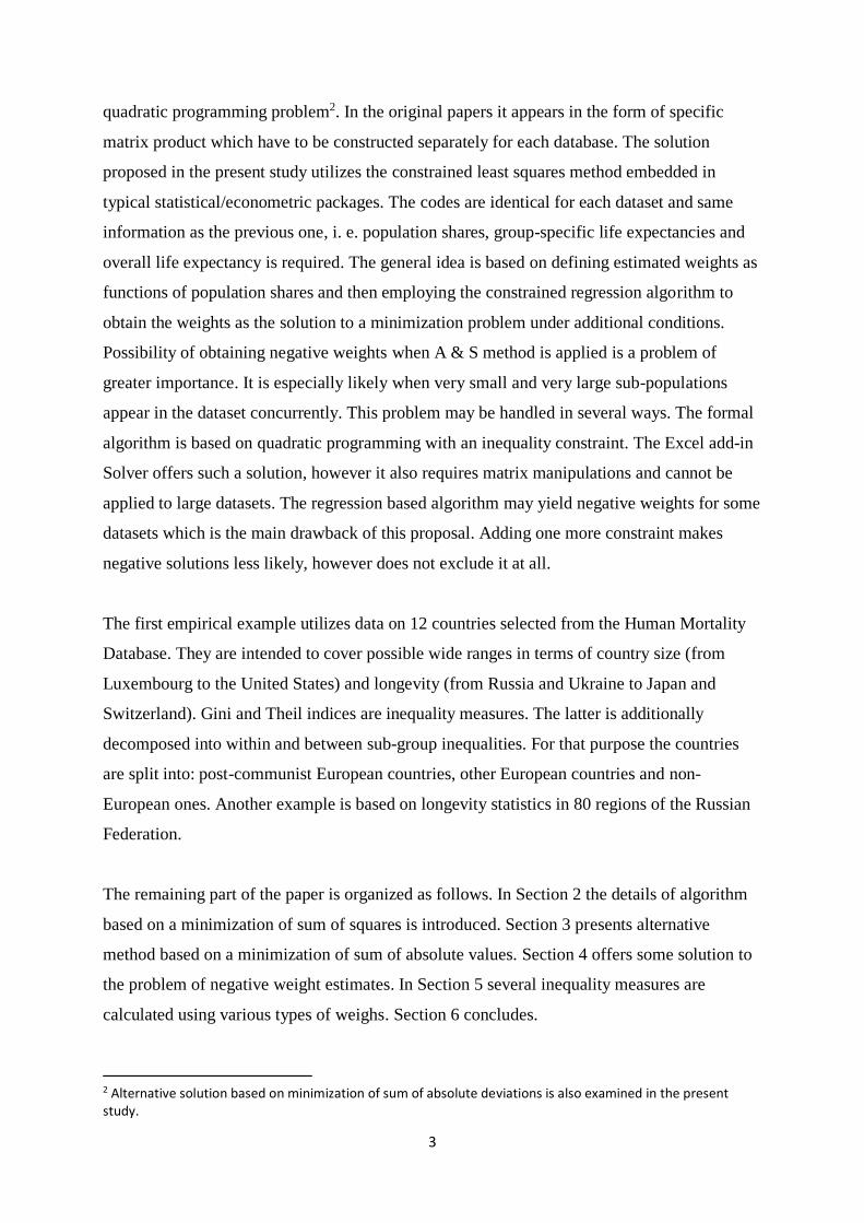
quadratic programming problem2. In the original papers it appears in the form of specific

matrix product which have to be constructed separately for each database. The solution

proposed in the present study utilizes the constrained least squares method embedded in

typical statistical/econometric packages. The codes are identical for each dataset and same

information as the previous one, i. e. population shares, group-specific life expectancies and

overall life expectancy is required. The general idea is based on defining estimated weights as

functions of population shares and then employing the constrained regression algorithm to

obtain the weights as the solution to a minimization problem under additional conditions.

Possibility of obtaining negative weights when A & S method is applied is a problem of

greater importance. It is especially likely when very small and very large sub-populations

appear in the dataset concurrently. This problem may be handled in several ways. The formal

algorithm is based on quadratic programming with an inequality constraint. The Excel add-in

Solver offers such a solution, however it also requires matrix manipulations and cannot be

applied to large datasets. The regression based algorithm may yield negative weights for some

datasets which is the main drawback of this proposal. Adding one more constraint makes

negative solutions less likely, however does not exclude it at all.

The first empirical example utilizes data on 12 countries selected from the Human Mortality

Database. They are intended to cover possible wide ranges in terms of country size (from

Luxembourg to the United States) and longevity (from Russia and Ukraine to Japan and

Switzerland). Gini and Theil indices are inequality measures. The latter is additionally

decomposed into within and between sub-group inequalities. For that purpose the countries

are split into: post-communist European countries, other European countries and non-

European ones. Another example is based on longevity statistics in 80 regions of the Russian

Federation.

The remaining part of the paper is organized as follows. In Section 2 the details of algorithm

based on a minimization of sum of squares is introduced. Section 3 presents alternative

method based on a minimization of sum of absolute values. Section 4 offers some solution to

the problem of negative weight estimates. In Section 5 several inequality measures are

calculated using various types of weighs. Section 6 concludes.

2 Alternative solution based on minimization of sum of absolute deviations is also examined in the present study.

4

2. Practical algorithm for minimizing sum of squares of deviations.

Formally, the problem of weights by which life-expectancies of population groups at age x

(𝑒𝑖𝑥) are weighted together to a given life-expectancy (𝑒𝑥) may be written as a system of two

equations:

∑ 𝑒𝑖𝑥𝑙𝑖𝑥

𝑙𝑥= 𝑒𝑥

𝑛𝑖=1 (1)

∑𝑙𝑖𝑥

𝑙𝑥= 1𝑛

𝑖=1 (2)

where 𝑙𝑖𝑥 stands for a number of the people at age x in i-th group (i = 1, 2, …, n) and 𝑙𝑥 is a

total number of the people at age x. As it is not necessary to know both 𝑙𝑖𝑥 and 𝑙𝑥, the weights

𝑙𝑖𝑥

𝑙𝑥, being a solution to the above system, are denoted hereafter as 𝑤𝑖𝑥. The above equations

give a unique solution if and only if the number of population groups (n) is two. The

algorithms proposed in the present study utilize constrained regression which is included in

standard statistical or econometric packages and may be applied to more than two sub-groups

(countries or regions in the present study). For simplicity, the age subscript x is dropped

hereafter, as the algorithm is identical for each age group.

Let vi denotes i-th population share. The weights wi are the solution to the following

minimization problem

min𝑤

∑ (𝑤𝑖 − 𝑣𝑖)2𝑛𝑖=1 (3)

such that

∑ 𝑤𝑖𝑒𝑖𝑛𝑖=1 = 𝑒 and ∑ 𝑤𝑖 = 1𝑛

𝑖=1 (4)

To take an advantage of minimization algorithms built in statistical/econometric packages one

should write a weight wi as a function of population share, say f(vi). The number of its

parameters should be greater than the number of constraints but not higher than the number of

population shares. It results from simple simulations that the solutions are virtually insensitive

to the type of the function f. Therefore, a quadratic form which may be estimated using a

linear algorithm is used

𝑤𝑖 = 𝑓(𝑣𝑖) = 𝑎(𝑣𝑖)2 + 𝑏𝑣𝑖 + 𝑐 (5)

Hence, the minimization problem (3 – 4) is equivalent to the constrained estimation of the

parameters a, b and c by the least squared method, under following constraints

5

𝑎 ∑ 𝑒𝑖𝑣𝑖2𝑛

𝑖=1 + 𝑏 ∑ 𝑒𝑖𝑣𝑖𝑛𝑖=1 + 𝑐 ∑ 𝑒𝑖 = 𝑒𝑛

𝑖=1 (6)

𝑎 ∑ 𝑣𝑖2𝑛

𝑖=1 + 𝑏 ∑ 𝑣𝑖𝑛𝑖=1 + 𝑛𝑐 = 1 (7)

Once the parameters are estimated, the weights may be calculated using eqn (5).

In the light of the econometric theory, the presented method seems to be nonsensical, as

population shares vi appear both on the left-hand and right-hand sides of the estimated

equation. However, this estimation is performed solely for utilizing an optimization algorithm

included in the least squares method. For the same reason, no post-estimation tests are

necessary. In this study the STATA command ‘cnsreg’ is used. It is also possible to rewrite

eqns (5) - (7) in the way allowing estimation of constrained regression models when the only

available constraint is imposing the intercept equal to zero. This method is described in details

in the next section, presenting the algorithm based on minimization of the absolute deviations,

which may be an alternative to the least squares method.

3. Algorithm for minimizing the sum of absolute deviations.

In that case the general principles of estimation of the weights are identical. The only

difference is in construction of egn (3) which takes the form

min𝑤

∑ |𝑤𝑖 − 𝑣𝑖|𝑛𝑖=1 (8)

This type of estimation is known as the least absolute deviations regression (LAD) or Laplace

regression (Koenker and Bassett, 1978). Though this type of regression is attributed by some

advantages over the least squares method, they are not meaningful in the present context.

Nevertheless, when very small weights appear (less than 0.01), they virtually have no impact

on the final solution when squared differences are minimized. For that reason, minimization

of absolute deviations is worth consideration. Unfortunately, most of statistical/econometric

packages does not allow constrained LAD optimization. Among others, few allows only one

type of constraint: zero intercept (c in eqn 5). Supplementary to the present estimations, TSP

(Time Series Processor) has been experimentally used3. The respective command is ‘LAD’

with the abovementioned constraint. LAD estimation under constraints (6) and (7) is feasible

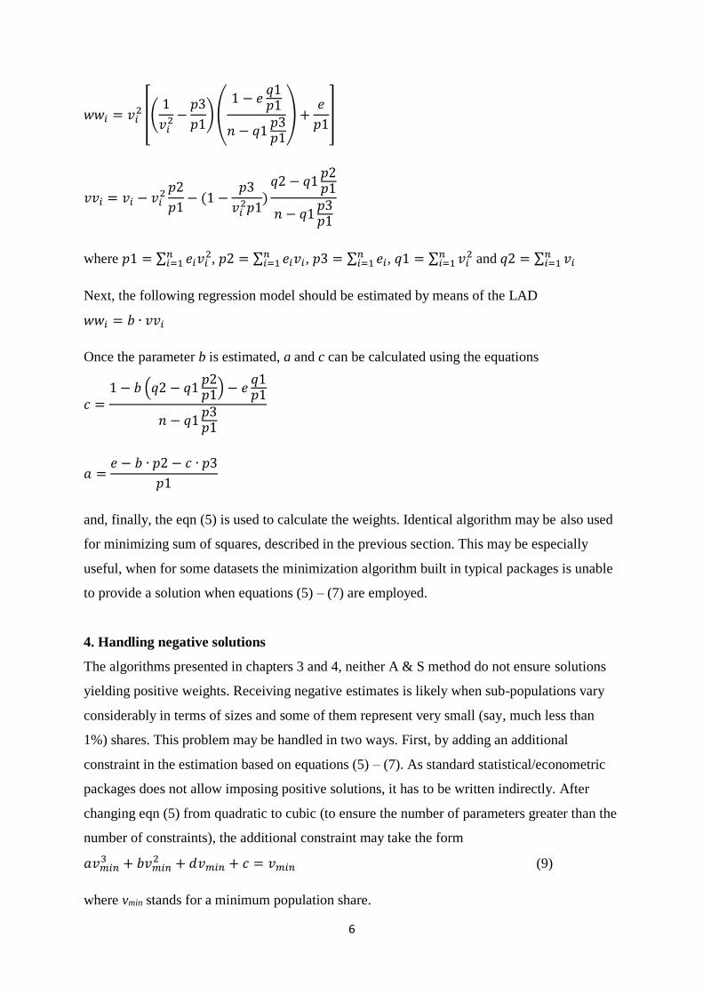
after rewriting dependent and independent variables, wwi and vvi respectively, in the

following manner

3 The results available upon request.

6

𝑤𝑤𝑖 = 𝑣𝑖2 [(

1

𝑣𝑖2 −

𝑝3

𝑝1) (

1 − 𝑒𝑞1𝑝1

𝑛 − 𝑞1𝑝3𝑝1

) +𝑒

𝑝1]

𝑣𝑣𝑖 = 𝑣𝑖 − 𝑣𝑖2 𝑝2

𝑝1− (1 −

𝑝3

𝑣𝑖2𝑝1

)𝑞2 − 𝑞1

𝑝2𝑝1

𝑛 − 𝑞1𝑝3𝑝1

where 𝑝1 = ∑ 𝑒𝑖𝑣𝑖2𝑛

𝑖=1 , 𝑝2 = ∑ 𝑒𝑖𝑣𝑖𝑛𝑖=1 , 𝑝3 = ∑ 𝑒𝑖

𝑛𝑖=1 , 𝑞1 = ∑ 𝑣𝑖

2𝑛𝑖=1 and 𝑞2 = ∑ 𝑣𝑖

𝑛𝑖=1

Next, the following regression model should be estimated by means of the LAD

𝑤𝑤𝑖 = 𝑏 ∙ 𝑣𝑣𝑖

Once the parameter b is estimated, a and c can be calculated using the equations

𝑐 =1 − 𝑏 (𝑞2 − 𝑞1

𝑝2𝑝1) − 𝑒

𝑞1𝑝1

𝑛 − 𝑞1𝑝3𝑝1

𝑎 =𝑒 − 𝑏 ∙ 𝑝2 − 𝑐 ∙ 𝑝3

𝑝1

and, finally, the eqn (5) is used to calculate the weights. Identical algorithm may be also used

for minimizing sum of squares, described in the previous section. This may be especially

useful, when for some datasets the minimization algorithm built in typical packages is unable

to provide a solution when equations (5) – (7) are employed.

4. Handling negative solutions

The algorithms presented in chapters 3 and 4, neither A & S method do not ensure solutions

yielding positive weights. Receiving negative estimates is likely when sub-populations vary

considerably in terms of sizes and some of them represent very small (say, much less than

1%) shares. This problem may be handled in two ways. First, by adding an additional

constraint in the estimation based on equations (5) – (7). As standard statistical/econometric

packages does not allow imposing positive solutions, it has to be written indirectly. After

changing eqn (5) from quadratic to cubic (to ensure the number of parameters greater than the

number of constraints), the additional constraint may take the form

𝑎𝑣𝑚𝑖𝑛3 + 𝑏𝑣𝑚𝑖𝑛

2 + 𝑑𝑣𝑚𝑖𝑛 + 𝑐 = 𝑣𝑚𝑖𝑛 (9)

where vmin stands for a minimum population share.

7

In that way, a minimum estimated share remains unchanged and therefore cannot be negative.

If a weight wi is an increasing function of population share vi all solutions are positive. This

condition is not necessary true, however. Therefore, in some cases vmin might be replaced by a

maximum (or any reliable) value, especially when the estimated weight for highest population

share is greater than actual one. Nevertheless, none of this conditions protects from receiving

negative weights. If this happens one can use Excel add-in Solver (downloadable from the

producer) allowing to reach non-negative weights. However, this requires matrix

manipulations that might be avoided when using methods based on regression. Moreover,

Solver is not capable to manage large datasets. At no circumstances the number of sub-

populations can exceed 200, however with some more complex algorithms this limit may be

reduced to less than 70. Hence, the weights for 80 Russia’s regions could be calculated with

the simplest method only.

Excel Solver is capable to provide both minimization of squares (eqn 3) and of absolute

values (eqn 8). The first one may be handled using built-in nonlinear procedure with two

constraints (eqn 4). Minimization of absolute values may be performed using linear

SIMPLEX method with an additional constraint. As |x| = max{x, -x}, wi non-negativity may

be ensured by adding constraints

∀𝑖: {𝑤𝑖 − 𝑣𝑖 ≥ 𝑤𝑖 − 𝑣𝑖

𝑤𝑖 − 𝑣𝑖 ≥ 𝑣𝑖 − 𝑤𝑖

while the function minimised is (wi - vi). Since Excel Solver does not allow constraints in the

form ‘greater (less) than’ it may be necessary to add one more restriction (at the cost of

further reduction of the data size) in the form 𝑤𝑖 ≥ 𝜀, where ε > 0 stands for a reasonably

small (say, 0.00001) number.

Two more methods might be added to the abovementioned. As negative solutions appear only

for the sub-populations with very small shares, they may be corrected “manually” after the

estimation. The formal solutions might be changed to (e. g.) actual population shares while

one or two largest weights are respectively decreased. Naturally, this method cannot be

justified on the theoretical ground and its usefulness is purely practical, as allows avoiding

matrix manipulations, necessary when Excel Solver is used. Another approach is based on

regressions ensuring the solutions fitting interval [0; 1]. Fractional regression (Papke and

Wooldridge, 1996) or constrained logit regression might be used for that purpose however

8

both techniques are somehow problematic. They are based on maximum likelihood method

rather than on minimization of the deviations. For that reason they hardly can be said to

provide a “minimum distance” between estimated weights and population shares. Moreover,

only few statistical/econometric packages offer aforementioned algorithms.

5. Empirical example.

In this section longevity inequality measures are calculated using various types of weights

described in the previous sections. The data include

12 countries selected from Human Mortality Database (years 2013 or 2014), men and

women separately (hereafter: HMD12)

80 regions (raions) in Russia, 2010, men and women together, source: Human

Development Report, 2013

Table 1. Life expectancy and population shares for 12 HMD countries

Country

Life

expectancy,

women

Population

share

Life

expectancy,

men

Population

share

Czech Republic 81.15 0.01312 75.15 0.01352

Germany 82.86 0.10088 77.99 0.1031

Israel 83.84 0.00988 80.29 0.01035

Japan 86.63 0.15840 80.23 0.160463

Luxembourg 83.43 0.00066 79.37 0.000703

New Zealand 83.42 0.00554 79.8 0.005664

Poland 80.92 0.04876 72.98 0.048824

Russian Federation 76.29 0.18880 65.1 0.173701

Sweden 83.71 0.01174 80.1 0.012477

Switzerland 84.74 0.00998 80.52 0.01039

USA 81.29 0.39238 76.54 0.405933

Ukraine 76.21 0.05985 66.31 0.054875

Weighted mean 81.13

(80.75) -

74.69

(74.49) -

Legend: life expectancies from life tables in parentheses (last row)

Source: own calculations based on Human Mortality Database

9

Table 1 displays life expectancies and population shares for HMD12. The data for Russia are

too large to fit this paper (they may be found in Human Development Report, 2013, Tab. 7.2,

pp. 139-140). Using population shares instead of weights applied in life tables results in

moderate misestimation of average life expectancy: from 0.2 to 0.38 years. Table 2 displays

the differences between maximum and minimum life expectancies (ranges) for three datasets

analyzed. What may be surprising, the range for Russian regions is higher than those observed

for HMD12 countries: by three years for men and by 9.7 years for women.

Table 2. Life expectancy ranges (in years)

HMD12, women HMD12, men Russia 80

range: emax - emin

86.63 - 76.21 = 10.42

(Japan, Ukraine)

80.52 - 65.10 = 15.64

(Switzerland, Russia)

79.08 – 61 = 18.08

(Ingushetia, Tuva)

Source: own calculations based on Human Mortality Database and Human Development Report

(2013)

The estimates of weights4 utilizing STATA constrained regression are satisfactory (all

weights are positive) for HMD12 for men and for the regions of Russia. However, for

HMD12 for women some negative weights were obtained. Therefore it was necessary to

employ Excel Solver ensuring all positive weights. Two abovementioned algorithms, based

on minimization of sums of squares and of absolute values, were applied for all datasets. For

the regions of Russia, however, it was impossible to obtain the weights by means of the latter

method, due to the dataset size exceeding Excel Solver capacity.

The ranges calculated for life expectancies (Table 2) are insensitive to the weighting system,

therefore to evaluate its impact on inequality measures it is necessary to calculate different

inequality indices. In the present study two formulas, Gini and Theil, are employed. The latter

is also decomposed into between- and within-group inequality. In Table 3 Gini inequality

indices for three datasets are displayed. This formula is calculated with the use of four types

of weights described in the previous sections. The most general conclusion is: weighting

matters. The weighted indices range from 80.6% to 114.3% of unweighted formula,

4 Detailed estimates available upon requests.

10

depending on the data employed, however no regularities in the sign of those differences can

be observed. For Russia weighting sub-group life expectancies reduces inequality measures

by from 13% to 19.4%. On the other hand, for HMD12 countries using weights raises indices

by from 5.2% to 14.3%. The latter may be easily explained by the data: five largest countries

constituting more than 90% of the whole population (USA, Russia, Japan, Germany and

Ukraine) are characterized by very large disparities in life expectancy (see Table 1). Similar,

though more sizable, impact of weighting may be observed when Theil inequality index is

utilized (see Table 4): increase for HMD12 countries and reduction for Russia. Higher

absolute differences, as compared to those obtained by means of Gini formula, may be

explained by general properties of those indices. Theil index is much more sensitive to

extreme individual values, while Gini index is responsive to their whole range. This property

is also responsible for much higher relative differences between inequality measures for

women and men when Theil index is employed. All abovementioned observations are valid

irrespectively to the method of the weights estimation, though the differences between the

final inequality measures due to the algorithm applied are non-negligible. For HMD12 data

the results obtained by Excel Solver are closer to those obtained with the use of actual

population shares than the constrained regression estimates. Opposite relations may be

observed for Russia.

Table 3. Gini inequality indices under various weighting of sub-populations

Weights Women HMD12 Men HMD12 Russia 80

Gini index * 100

no weights 1.9544 3.4823 2.11644

actual population shares 2.22533 3.6647 1.84198

(113.9%) (105.2%) (87.0%)

STATA, min. squares n. a. 3.88038 1.80208

(111.4%) (85.1%)

Solver, min. squares 2.23347 3.7847 1.70628

(114.3%) (108.7%) (80.6%)

Solver, min. absolute values 2.19255 3.73571

n. a. (112.2%) (107.3%)

Legend: percentage of unweighted index in parentheses Source: own calculations based on Human Mortality Database and Human Development Report

(2013)

11

Tab.4. Theil inequality indices under various weighting of sub-populations

Weights Women HMD12 Men HMD12 Russia 80

Theil index * 100

no weights 0.0672 0.2337 0.08709

actual population shares 0.08577 0.25652 0.05721

(127.6%) (109.8%) (65.7%)

STATA, min. squares n. a. 0.28188 0.05573

(120.6%) (64.0%)

Solver, min. squares 0.08632 0.26877 0.05003

(128.5%) (115.0%) (57.4%)

Solver, min. absolute values 0.08379 0.26421

n. a. (124.7%) (113.1%)

Legend: percentage of unweighted index in parentheses

Source: own calculations based on Human Mortality Database and Human Development Report

(2013)

In the final step an impact of weighting on decomposition of Theil index into within- and

between-group inequality (for details of the decomposition see e. g. Shorrocks, 1980) is

evaluated. For this purpose the countries included in HMD12 were split into three groups:

post-communist countries (Czech Republic, Poland, Russia and Ukraine), other European

countries (Germany, Luxembourg, Sweden and Switzerland) and non-European countries

(Israel, Japan, New Zealand and USA). In Table 5 results of the decomposition are displayed.

The first term (‘within’) is a relative measure of mean inequality within all groups of the

countries, while the second one measures inequality between mean life expectancies for three

groups. Both components sum up to 100% or to the value calculated for the whole dataset. In

typical applications of Theil index, i. e. measuring welfare (especially income) inequality, a

within-group component is usually much higher than between-group one. Decomposition of

longevity inequality provides opposite picture: between-group inequality appears to be much

higher. Roughly speaking, the gap between Russia or Ukraine and Japan or Switzerland is

much higher than the gap between Russia or Ukraine and Czech Republic or Poland. In

income studies opposite phenomenon may be observed: the gap between mean incomes for,

say, pensioners and employees is much lower than the gap between “poor” and “rich”

employees (or even pensioners). As in the previous cases, weighting country-specific life

12

expectancies changes the results of the decomposition, especially for men when considerable

reduction of within-group component arises.

Table 5. Decomposition of Theil index into within- and between-group inequality (post-

communist countries, ”Western” Europe, non-European countries)

Weights Women, HMD12 Men, HMD12

within between within between

no weights 36.1% 63.9% 25.6% 73.5%

actual population shares 38.6% 61.4% 17.7% 82.3%

STATA, min. squares n. a. n. a. 14.7% 85.3%

Solver, min. squares 35.0% 65.0% 17.1% 82.9%

Solver min. absolute values 35.1% 64.9% 17.2% 82.8%

Source: own calculations based on Human Mortality Database (2013)

6. Concluding remarks.

An answer to the question “to weight or not to weight?” depends on the goal of the study. If it

is aimed at comparing average public health status between sub-groups, then weighting is not

necessary. When, for instance, Russia and Luxembourg are compared with this respect, the

sizes of the countries does not influence a large gap between them. This is also true in

comparisons of more than two countries by means of inequality indices (Gini index may be

interpreted in terms of average absolute relative gap between the units). Weights become

necessary when the question is “how unequal people in a given population are?”. In spite of

large gap in average life expectancy between Russia and Luxembourg, the impact of the latter

on the population composed of two countries is almost negligible, due to its size. Replacing

Luxembourg by Germany, characterized by lower life expectancies (resulting in lower

distance to the Russian average), would result in increase in inequality in the combined

population.

Weighting sub-populations is usually neglected in demographic studies. Works by Ananad et

al (2001) and Shkolnikov et al (2001) are among few exceptions, however they do not offer a

satisfactory solution for two reasons. First, for some datasets the weights calculated by means

of the proposed algorithm may be negative. Second, the calculations utilize matrix algebra

13

that may be troublesome when calculations have to be repeated, for instance for age groups

from 0 to 110 years. Shkolnikov et al (2001) proposed alternative solution based on

specialized software (MatLab) which is capable to ensure weights positivity. However, due to

MatLab price and availability it cannot be considered a universal outcome. In this paper two

alternative solutions, requiring any statistical/econometric package including constrained least

squares regression and/or Excel add-in Solver, are proposed. That based on regression is more

practical, as may be easily repeated as many times as necessary, once the codes are written,

however does not ensure positive weights for some datasets. Using Excel Solver yields

positive weights, however is more awkward when the procedures have to be repeated

numerous times and may be applied only to small and medium datasets.

Empirical calculations based on 12 countries included into Human Mortality Database and

Russia’s regional mortality statistics demonstrated a considerable impact of the weights on the

results. All unweighted inequality indices differ considerably form those using weights,

however the sign of those differences is not fixed and depends on the data specificity.

Important, though smaller, difference appear also between indices obtained by means of

various weight systems. This demonstrates that the problem of weights in demographic

studies (covering also a construction of aggregate life tables) must not be neglected, though

none of the solutions described in the present paper can be recommended as ideal.

Nevertheless, even imperfect weighting system that do not yield robust results in some cases

should be recommended as an alternative to unweighted calculations.

Acknowledgement

I am grateful to Michał Lewandowski for his very helpful advice on mathematical

programming, especially on using Excel Solver. All remaining errors are solely mine.

REFERENCES

Anand, S., F. Diderichsen, T. Evans, V. M. Shkolnikov and M. Wirth (2001), “Measuring

disparities in health: methods and indicators”, in.: T. Evans, M. Whitehead, F.

Diderichsen, A. Bhuiya and M. Wirth (eds.) Challenging inequities in health: from ethics

to action, pp. 48-67. Oxford University Press.

14

Human Mortality Database. University of California, Berkeley (USA) and Max Planck

Institute for Demographic Research (Germany), www.mortality.org.

Koenker, R. W. and G. W.Bassett (1978), Regression Quantiles, Econometrica 46, pp. 33-50.

Smits, J., and C. Monden (2009), Length of life inequality around the globe. Social Science

and Medicine, 68(6), pp. 1114–1123.

Sustainable Development: Rio Challenges, National Human Development Report for the

Russian Federation 2013, UNDP, Moscow.

Papke, L.E. and J. M. Wooldridge (1996), Econometric Methods for Fractional Response

Variables with an Application to 401(k) Plan Participation Rates. Journal of Applied

Econometrics (11), pp. 619–632.

Shkolnikov, V. M., T. Valkonen, A. Begun and E. M. Andreev (2001), Measuring inter-group

inequalities in length of life, Genus, Vol. 57, No. 3/4, pp. 33-62.

Shorrocks, A. F. (1980), The class of additively decomposable inequality measures,

Econometrica, vol. 48, no. 3, pp. 613 – 625.