Wei-Hwa Wu Department of Finance, Ming Chuan … ANNUAL MEETINGS... · 0 TheAsymmetric Predictability of High-yield Bonds Wei-Hwa Wu Department of Finance, Ming Chuan University,

0

The Asymmetric Predictability of High-yield Bonds

Wei-Hwa WuDepartment of Finance, Ming Chuan University, Taipei City, Taiwan, R.O.C.

&Tai-Wei Zhang

Department of Finance, Ming Chuan University, Taipei City, Taiwan, R.O.C.

Abstract

This study examines the relationship between the high-yield bonds market and the

stock market and indicates that stock returns lead high-yield bond returns. Specifically,

this study further shows that this lead-lag relationship is more solid during bear

market periods since a downward trend in the stock market implies a high likelihood

of the exercise of the equity put in short position embedded in a high-yield bond at

maturity. We also conducted out-of-sample forecast using a VAR model, an AR model

and naïve estimation during bear market and non-bear market periods. Our results

demonstrate that high-yield bond returns are better predicted by a VAR model that

includes past stock returns than by an AR model or naive estimation during bear

market periods, but such is not the case during non-bear market periods.

Keywords: High-yield bonds, Predictability, VAR, Embedded options, MarketconditionJEL classification codes: G12, G14, G17

1

The Asymmetric Predictability of High-yield Bonds

1. Introduction

Whether returns on risky assets are predictable is a central issue for financial

economists as it involves how the financial market works and has deep implications

for asset valuation. Given its importance, most of the related studies focus on the

stock market; fewer on the high-yield bond market. According to Forbes, in the U.S.

the full-year total issuance of high-yield bonds for 2012 reached a record high of $346

billion, and the monthly issuance set a record in September 2013 at $47.65 billion.

The phenomenon of booming growth in the high-yield bond market indicates that

understanding high-yield bonds’valuation is of great urgency for academics and

practitioners.

Theoretically, a straight corporate bond is essentially a combination of a pure

default-freeinterest rate instrument and a short position in a put written on the issuer’s

equity (see Merton [1974]; Fridson [1994]). For investment-grade bonds, the

probability that the equity put will be out of the money at maturity is quite small. So

for such a kind of bond, they act more like government bonds. But in the case of

high-yield bonds, on the maturity date, default is likely, so the equity put part is far

from negligible and plays a role in the valuation of high-yield bonds. Thus, high-yield

bonds are bound to fluctuate with the prices of the issuer’s equity despite their debt

nature.1

For high-yield bonds investors, they are like stock put writers. Investors sell the

embedded stock put to the issuing firms and obtain the premium (i.e., the excess

interest rate) in return. But if at maturity the issuing firms fail to meet the obligation

1 Ramaswami (1991) considers the options on underlying equities embedded in high-yield bonds anddeveloped two kinds of hedging strategies against the risks of high-yield bonds: a simple optionshedging strategy, and a composite hedging strategy comprising equity and risk-free bonds. He showsthat the composite hedging strategy performs better in most cases.

2

(so that these firms exercise the right to sell their equities to investors), the investors

will suffer losses. Therefore, high-yield bond investors bet on the future prosperity of

the issuing firms. If the market is efficient, the asset prices will reflect all market

information available, including the market expectation for the future economic

performance. Hence the asset market performance can lead the actual economic

performance just like what we may frequently encounter.

Before maturity, whether the embedded put will be out of the money or not is

unknown, but by inspecting the stock market performance, the relevant information is

gradually disclosed as time passes. If the stock market is trending upward, it implies

that very likely the high-yield bond investors can be repaid in full (and nothing more)

at maturity. In this case, as the probability of default declines, the value of high-yield

bonds rises, but does not in proportion to the level of increase in the stock market. On

the contrary, when the stock market is trending downward, it implies a worsening

future economic situation, and the probability of default rises. With the continuous

decrease of stock prices, the high-yield bond investors begin to worry not only about

the rise in probability of default, but also the loss given default at maturity. So under

the bear market condition, with the probability of default and loss given default

getting larger, the investors gradually devaluate high-yield bonds as stock prices

decline. In this situation, high-yield bonds are more like equities.

In this study, we use the S&P 500 index’s market condition as a proxy for

identifying whether stock puts embedded in high-yield bonds are deeply in-the-money

or not. This is because, during an economic contraction period, even though blue

chips (say, S&P 500 components) could also be faced with some financial problems,

not to speak of the companies rated below BBB. Thus, it is possible that high-yield

bonds could be very likely to default when the S&P 500 index is in a bear market.

The bond market has long been relatively less informationally efficient than

3

stock markets (see Downing, Underwood, and Xing [2009]).2 Therefore, a lead-lag

relationship between common stocks and high-yield bonds has raised concerns in the

extant literature, and its empirical evidence is inconclusive. For example, Hotchkiss

and Ronen (2002) find no evidence that stock returns lead high-yield bond returns. In

contrast, Downing, et al. (2009) find that stock returns lead nonconvertible bonds

rated BBB or lower, but do not lead safer nonconvertible bonds. Rather than using the

individual firm data as can be frequently seen in the past literature, Hong, Lin and Wu

(2012) adopt stock and bond market indices to investigate the predictability of bond

market returns. After conducting a series of econometric tests, Hong et al. (2012)

conclude that the stock market leads both high-yield and investment-grade bond

markets, and the relationship between stocks and high-yield bonds is stronger than

that between stocks and investment-grade bonds.

Similar to Hong, Lin and Wu (2012), we also investigate high-yield bonds’

predictability at the aggregate level. If a lead-lag relationship exists between

high-yield bond and stock markets, we are interested in realizing whether a high-yield

bond return has a better forecasting performance during bear market periods. We

hypothesize that a stronger lead-lag relationship exists between high-yield bond and

stock markets during bear market periods. Then, we also hypothesize that a high-yield

bond has a better out-of-sample forecasting during bear market periods.

In order to test our hypotheses, we adopt the following procedures. First, we use the

bivariate VAR model to capture the lead-lag relationship between stock and high-yield

bond returns. The estimation results show that stock returns lead high-yield bond

returns, but not vice versa. Second, we then modify the VAR model to incorporate a

market condition dummy with lagged returns in both the high-yield bond and the

2 Lee, Huang and Yin (2013) investigate the lead-lag relationships among stock, insurance and bondmarkets. They find that the U.S. and U.K. stock markets lead the insurance market, and bond marketwill be influenced by the insurance market.

4

stock equations. In this setting, we find that the impacts of past stock returns on

high-yield bonds are greater in bear markets. And finally, we include the VAR and

other comparable models to predict future returns of high-yield bonds. Our results

show that the VAR model consistently outperforms other models during bear market

periods, but the prediction performance of the VAR model is not so dominant in

non-bear markets. Thus, we find supportive evidence that validates our hypotheses. To

the best of our knowledge, this paper is the first one that highlights the importance of

market conditions when conducting high-yield bond predictions. In addition, from the

perspective of a practitioner, traders can use our strategy to improve their

out-of-sample forecasting performance.

The rest of this paper is organized as follows. In Section 2, we specify the model

and perform empirical studies. We then forecast future high-yield bond returns by

various models and evaluate their prediction performance in Section 3. Finally, we

explain our conclusions in Section 4.

2. Model Specification and Empirical Results

2.1 Data Description

This study focuses on analyzing whether the Merrill Lynch (BofA ML)

high-yield bond price index can be predicted by the S&P 500 stock index. These two

indices are retrieved from DataStream. Both SP and HY are simple returns on the S&P

500 stock index and the BofA ML high-yield bond price index, respectively. This

choice is based on well-known public indices with easily accessible and reliable data

so that investors can use our investment strategy to forecast.

Our sample covers the period from February 1, 1990 to November 20, 2012. The

occurrence of a few missing pieces of data in our variables shrinks the observations to

5,645 trading days. Our full sample covers two bear periods, from March 1, 2000 to

5

December 31, 2002 (You and Daigler, 2010), and from October 9, 2007 to March 9,

2009 (Meric, et al., 2010).3 Three exogenous variables—changes in the five-year

T-bill rate (DFIVE), changes in the slope of the term structure (DSLOPE), and the

changes of the implied volatility of the CBOE index (DVIX)—are considered in our

VAR model. We define the slope of the term structure as the“difference in yield to

maturities between 10-year and two-year treasuries,” retrieved from the Federal

Reserve Bank of St. Louis’s FRED database. The five-year T-bill rate is also retrieved

from FRED. In addition, the implied volatility of the CBOE index is obtained from the

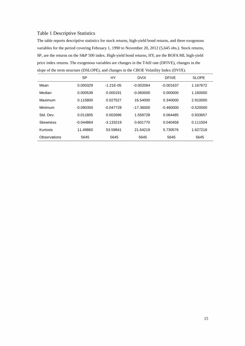
CBOE website. Table 1 provides the descriptive statistics for the series.

<Insert Table 1 here>

In Table 1, we observe that the mean returns of the S&P 500 and high-yield bond

index both lie in the neighborhood of zero: 0.03% and -0.00%, respectively. The range

and the standard deviation of high-yield bond index returns are both smaller than

those of the S&P 500 returns, indicating that the volatility of the high-yield bond

returns is smaller than that of stock returns. Moreover, the skewness of the high-yield

bond returns is about -3.1, whereas the skewness of the S&P 500 index returns is

around zero. This shows as well that larger and negative returns of high-yield bonds

are more frequently encountered than those of stock returns.

2.2 Model Specification and Empirical Results

In this research, we adopt the bivariate Vector Autoregression (VAR) model to

analyze the lead-lag relationships between the stock and high-yield bond markets. The

VAR model can be specified as follows:

3 Accordingly, the three non-bear periods are from February 1, 1990 to February 29, 2000, fromJanuary 2, 2003 to October 8, 2007, and from March 10, 2009 to November 20, 2012.

6

t

m

iiti

l

iiti

l

iitit

t

m

iiti

l

iiti

l

iitit

EXOcHYbSPakHY

EXOcHYbSPakSP

21

,21

21

22

11

,11

11

11

(1)

where SP and HY denote the returns of the S&P 500 index and the high-yield bond

index, respectively; EXO shows the three exogenous variables; ik refers to the

constant terms; ia , ib ,and ic represent the corresponding coefficients; it denotes the

random shocks.

In the VAR model shown in Eq. 1, we consider the following variables as the

exogenous ones—changes in the T-bill rate (DFIVE), changes in the slope of the term

structure (DSLOPE), and changes in the CBOE Volatility Index (DVIX)—as these

variables may have an influence on both the stock and high-yield bond markets.4

After controlling for exogenous variables, we expect that the coefficients on lagged

returns of the stock market should be positive and significant in the high-yield bond

equation if the predictability of the high-yield bond is indeed feasible.

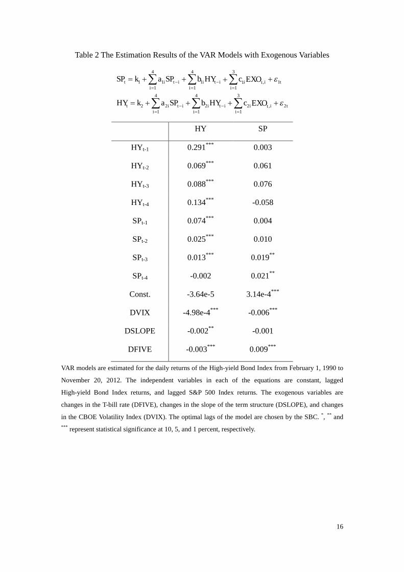
We estimate the VAR model that includes returns of high-yield bonds and stocks

in which the lag length is determined by the Schwarz Information criterion. The

optimal lag length is four. The VAR model estimation results are summarized in Table

2. The high-yield bond equation shows that high-yield bond returns are significantly

related to the lagged returns of the S&P 500 stock index at lags one to three at the

one-percent level. The corresponding coefficients are 0.074, 0.025 and 0.013,

respectively. By contrast, none of the lagged returns of the high-yield bond is

significantly different from zero in the stock market equation, whereas the stock

market returns are significantly related to only their own returns at lag three and four

4 DSLOPE is employed as a proxy for an indication of overall economic health. As for DVIX, we

interpret this proxy as the changes in the market volatility or investor sentiment.

7

at the five-percent level.

<Insert Table 2 here>

The Granger-causality test also confirms these findings. To test the

Granger-causality, the null hypothesis of the Wald test is that the coefficients on the

lagged SP ( HY ) are all equal to zero in the high-yield bond (stock market) equation.

In Table 3, we find that high-yield bond returns are Granger-caused by stock returns,

but not vice versa, indicating that stock market returns lead high-yield bond market

returns, which echos Downing, et al. (2009) in that stock markets are more

informationally efficient.

<Insert Table 3 here>

In order to examine the hypothesis that the lead-lag relationship between the

S&P 500 stock index and the high-yield bond index is much stronger during a bear

market, the interaction terms between a bear market dummy and lagged returns are

therefore employed in the VAR model. The VAR model can be rewritten as follows:

t

m

iitti

l

iitti

l

iitti

m

iiti

l

iiti

l

iitit

t

m

iitti

l

iitti

l

iitti

m

iiti

l

iiti

l

iitit

EXODumfHYDumeSPDumdEXOcHYbSPakHY

EXODumfHYDumeSPDumdEXOcHYbSPakSP

21

,21

21

21

,21

21

22

11

,11

11

11

,11

11

11

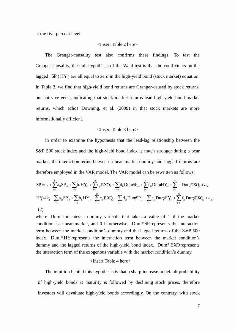
(2)where Dum indicates a dummy variable that takes a value of 1 if the marketcondition is a bear market, and 0 if otherwise; SPDum* represents the interactionterm between the market condition’s dummy and the lagged returns of the S&P 500 index. HYDum* represents the interaction term between the market condition’s dummy and the lagged returns of the high-yield bond index. EXODum* representsthe interaction term of the exogenous variablewith the market condition’s dummy.

<Insert Table 4 here>

The intuition behind this hypothesis is that a sharp increase in default probability

of high-yield bonds at maturity is followed by declining stock prices, therefore

investors will devaluate high-yield bonds accordingly. On the contrary, with stock

8

prices going up, the likelihood that the high-yield bond investors can be fully

redeemed is higher and higher, but investors can gain nothing more. As a result, the

speed of growth in high-yield bond prices is slower than that in stock prices.

Thus, we expect that the coefficients on the interaction terms, id2 , will have a

prominent impact on the high-yield bond equation if high-yield bond returns react to

past returns of the stock market much more strongly during bear periods. As we

expected, we find that the interaction termsof the stock market’s lagged returns with a

bear market dummy have the positively predicted signs and statistical significance to

explain that bear markets play an important role in the predictability of high-yield

bonds. The coefficient estimates are 0.040, 0.022, and 0.019 for )1(* SPDum ,

)2(* SPDum and )3(* SPDum , respectively. In addition, the null hypothesis that

the joint coefficients of the interaction term, id2 , are equal to zero is rejected at the 1%

level. It is evident that past stock returns have a stronger impact on high-yield bond

returns in bear markets than that in non-bear markets as the magnitude of significant

lagged stock returns in the high-yield bond return equation is larger in bear markets

than that in non-bear markets. Thus, this supports the asymmetric predictability of

high-yield bonds.

In order to verify whether or not mutual feedback of information between the

stock market and the high-yield bond market occurs during the bear markets. Next,

we further examine the coefficients of the interaction term between the market

condition’s dummy and the lagged returns of the high-yield bond index in the stock

market return equation. We also expect that the coefficients of the interaction terms, ie1 ,

will have no significant impact on the stock equation as the bond market is less

efficient than the stock market (see Downing, Underwood, and Xing [2009]). The

empirical results generally support our expectations. Although the coefficient 12e ,

which is -0.256, is significantly negative at the one-percent level, the joint test for the

9

coefficients of the interaction term, ie1 , being equal to zero, cannot be rejected at the

5% level. By examining the Granger-causality between the high-yield bond market

index changes and S&P500 index returns, we find no significant feedback effect

emanating from the high-yield bond market to the stock market during bear markets.

In sum, these results indicate that the S&P500 index leads the high-yield bond index,

but not the other way around.

3. Out-of-Sample Performance and Analysis

From an investor’s point of view, one would like to know whether past stock

returns are still important information at the time of a bear market when predicting the

future returns of high-yield bonds. Here we employ three models to address this issue.

One is the bivariate VAR model, which takes the past returns of the stock market into

consideration. Another is the AR model, which considers only its own lag returns of

high-yield bonds. The other uses the sample mean as the predictor. We call the latter

the naive model.5 We then move on to evaluate the prediction performance of

high-yield bond returns during each of the aforementioned sub-periods.

It is worth mentioning that the VAR model we used in this section is different

from the VAR model in Eq. (1). Eq. (3)’s VAR model, below, does not include any

exogenous variables. In this setting, we can avoid adopting the values of exogenous

variables on day t in out-of-sample forecasts. Thus, our forecasting VAR model can be

written as:

t

l

iiti

l

iitit

t

l

iiti

l

iitit

HYbSPakHY

HYbSPakSP

21

21

22

11

11

11

(3)

where SP and HY denote the returns of the S&P 500 index and the high-yield bondindex, respectively; the optimal lags of the model, l , are chosen by the SBC.

5 Many studies usually use historical average return as a benchmark strategy when assessing theout-of-sample performance of the predictive models, including, among others, Campbell andThompson (2008), Welch and Goyal (2008), and Lee, Chen and Chang (2013).

10

As for the AR model, the model can be presented as follows:

t

l

iitit HYbkHY 3

133

(4)

where HY denotes the returns of the high-yield bond index; the optimal lags of the

model, l , are chosen by the SBC.

The naïve model is

tt kHY 44 (5)

where 4k is the rolling sample mean estimated through period t-1.

From a methodological viewpoint, we conduct the out-of-sample forecasting

experiment using a 1/4:3/4 split, following a standard validation split ratio mentioned

in forecasting evaluation literature. Namely, we partition the full sample period into

two periods: the in-sample estimation period (from February 1, 1990 through January

28, 1996) and the out-of-sample forecast comparison period (from January 29, 1996

through November 20, 2012). The rolling process continues, re-estimating the models

at each stage, until the end of the sample is reached. Thus, we end up with 4,234

forecast high-yield bond returns for each model. This procedure therefore assures that

information available at each point in time will be included by investors in the

forecast, and hence can be regarded as mimicking real-time trading behavior.

To assess the out-of-sample forecasting ability of these models, we employed

the mean absolute error (MAE), root mean squared error (RMSE) and the

Mincer-Zarnowitz (MZ) regression:

T

ttt rr

TMAE

1

|)̂(|1

(6)

T

ttt rr

TRMSE

1

2)̂(1 (7)

where T denotes the total sample size of the out-of-sample forecast.

11

ttt rrMZ ˆ: (8)

where tr and tr̂ are the realized returns and the forecast series, respectively.

For MAE and RMSE, the lower these values, the higher the predictive benefits.

Diebold and Mariano (1995) statistics can check which models’ out-of-sample

performances (RMSE or MAE) are statistically significantly better than others’.

Under the MZ regression in Eq. (8), if the forecast is unbiased and efficient, the

constant and coefficient should produce regression estimates of 0 and 1,

respectively. Under the MZ framework, in addition, a good forecast should not reject

the joint hypothesis that )1,0(),( . In terms of bias and forecast efficiency, MZ

tests results allow us in better detail to evaluate whether the performance differences

are statistically significant.

<Insert Table 5 here>

Table 5 shows the out-of-sample forecast results. Panel A presents the results for

the full sample. For RMSE and MAE, the VAR model gives the best results: RMSE,

0.00243, and MAE, 0.00136, both being statistically significant lower than those of

other models. As for the MZ test, none of the models can offer satisfactory results

because the null hypothesis is significantly rejected under the joint 2 -test for all

models. Panels B, D and F provide the results for non-bear market periods. For RMSE

and MAE, which one is the best prediction model is not conclusive. Results for

non-bear market periods, however, are similar with those from the full sample under

the MZ test.

Panels C and E report the results for bear market periods. The prediction

performance of high-yield bond returns under the VAR model is the best regardless of

the criteria. For example, all RMSE and MAE produce the lowest values and

statistically significantly outperform other models when we use Diebold and Mariano

(1995) statistics. Results also show that only the VAR model produces satisfactory

12

results for bear market periods under the MZ test, including both the joint 2 -test

and the individual tests of and . However, the naïve and AR models do not

produce acceptable MZ results for bear market periods.

Taken as a whole, contrary to bear markets, none of the prediction models can

pass the MZ test during non-bear market periods. Thus, we can realize that the price

movements of stock and high-yield bonds are not solid under the non-bear market

condition. We can further see that the VAR model predicts best during bear market

periods, and is the only prediction model that passes the MZ test in bear markets.

Since the VAR model takes past stock returns into account and thus helps improve the

prediction performance of high-yield bond returns, we can readily infer that past stock

returns have a greater influence on high-yield bond returns in bear markets. Hence,

we have obtained the other piece of evidence that the predictability of high-yield

bonds is stronger during bear market conditions.

4. Conclusions

High-yield bonds are a hybrid of securities, comprising a non-defaultable bond

and a short put on the issuing firm’s equity. Hence, with the equity component,

high-yield bonds will fluctuate with stock prices. In terms of previous studies, the

correlation between stock and high-yield bond returns is found to be significant but

weak, which causes curiosity in future researchers, who propose some reasons to

explain the lower-than-expected correlation, such as conflicts of interests, data

frequency, data types (quoted or transaction-based data), etc.

In this research, we point out that high-yield bonds respond to information

revealed by the stock markets asymmetrically, depending on market conditions. In

non-bear markets, the default likelihood of high-yield bonds is low, and hence the

value of the short put embedded in high-yield bonds is nearly zero. But in bear

13

markets, that short put is very likely to be in the money on the maturity date, so the

value of the put in the short position decreases with stock prices. The prices of

high-yield bonds thus go down with stock prices at the same rate during a bear market

condition.

To verify our positions, we conducted three empirical tests. First, the bivariate

VAR model of high-yield bonds and stocks is estimated. The estimation results show

that the influence of past stock returns on high-yield bonds are significant, but not

vice versa. Second, we modify the VAR model by including a market condition

dummy variable. At this time, we find that the impact of past stock returns on

high-yield bonds is greater in bear markets. And finally, we predict future high-yield

bond returns by VAR and other competing models. The VAR model consistently

defeats other models during bear market periods, but the prediction performance of

the VAR model does not overwhelm others in non-bear markets. In sum, high-yield

bond returns react to past returns of the stock market asymmetrically, and high-yield

bonds respond more strongly during bear periods.

14

ReferencesAlexander, G. J., Edwards, A. K., & Ferri, M. G. (2000). What does Nasdaq’s high-yield bond market

reveal about bondholder-stockholder conflicts? Financial Management, 29, 23-39.

Campbell, J. Y., & Thompson, S. B. (2008). Predicting excess returns out of sample: Can anything beat

the historical average. Review of Financial Studies, 21, 1509–1531.

Downing, C., Underwood S., & Xing, Y. (2009). The relative informational efficiency of stocks and

bonds: An intraday analysis. Journal of Financial and Quantitative Analysis, 44, 1081-1122.

Fridson, M. S., 1994, Do high-yield bonds have an equity component? Financial Management, 23(2),

82-84.

Hong, Y.M., Lin, H, & Wu C.C. (2012). Are corporate bond market returns predicable? Journal of

Banking & Finance, 36, 2216-2232.

Hotchkiss, E.S. & Ronen, T. (2002). The informational efficiency of the corporate bond market: an

intraday analysis. The Review of Financial Studies, 15, 1325-1354.

Lee, C.C., Huang,W.L.& Yin,C.H.(2013).The dynamic interactions among the stock, bond and

insurance markets. North American Journal of Economics and Finance, 26, 28-52.

Lee,C. C., Chen, M.P. & Chang, C.H.(2013).Dynamic relationships between industry returns and stock

market returns. North American Journal of Economics and Finance, 26, 119–144.

Meric, I., Dunne, K., McCall, C.W. & Meric, G. (2010). Performance of exchange-traded sector index

funds in the October 9, 2007-March 9, 2009 bear market. Journal of Finance and Accountancy,3,

1-11.

Merton, R. (1974). On the pricing of corporate debt: The risk structure of interest rates. Journal of

Finance, 29,449-470.

Ramaswami, M. (1991). Hedging the equity risk of high-yield bonds. Financial Analysts Journal, 47,

41-50.

Welch, I., & Goyal, A. (2008). A comprehensive look at the empirical performance of equity premium

prediction. Review of Financial Studies, 21, 1455–1508.

You, L. & Daigler, R.T. (2010). Is international diversification really beneficial? Journal of Banking &

Finance, 34, 163-173.

15

Table 1 Descriptive StatisticsThe table reports descriptive statistics for stock returns, high-yield bond returns, and three exogenous

variables for the period covering February 1, 1990 to November 20, 2012 (5,645 obs.). Stock returns,

SP, are the returns on the S&P 500 index. High-yield bond returns, HY, are the BOFA ML high-yield

price index returns. The exogenous variables are changes in the T-bill rate (DFIVE), changes in the

slope of the term structure (DSLOPE), and changes in the CBOE Volatility Index (DVIX).

SP HY DVIX DFIVE SLOPE

Mean 0.000329 -1.21E-05 -0.002064 -0.001637 1.167672

Median 0.000539 0.000191 -0.060000 0.000000 1.160000

Maximum 0.115800 0.027527 16.54000 0.340000 2.910000

Minimum -0.090350 -0.047728 -17.36000 -0.460000 -0.520000

Std. Dev. 0.011805 0.002696 1.559728 0.064485 0.933657

Skewness -0.044864 -3.133219 0.601770 0.040458 0.111504

Kurtosis 11.49860 53.59841 21.64219 5.730576 1.627218

Observations 5645 5645 5645 5645 5645

16

Table 2 The Estimation Results of the VAR Models with Exogenous Variables

ti

itii

itii

itit

ti

itii

itii

itit

EXOcHYbSPakHY

EXOcHYbSPakSP

2

3

1,2

4

12

4

122

1

3

1,1

4

11

4

111

HY SP

HYt-1 0.291*** 0.003

HYt-2 0.069*** 0.061

HYt-3 0.088*** 0.076

HYt-4 0.134*** -0.058

SPt-1 0.074*** 0.004

SPt-2 0.025*** 0.010

SPt-3 0.013*** 0.019**

SPt-4 -0.002 0.021**

Const. -3.64e-5 3.14e-4***

DVIX -4.98e-4*** -0.006***

DSLOPE -0.002** -0.001

DFIVE -0.003*** 0.009***

VAR models are estimated for the daily returns of the High-yield Bond Index from February 1, 1990 to

November 20, 2012. The independent variables in each of the equations are constant, lagged

High-yield Bond Index returns, and lagged S&P 500 Index returns. The exogenous variables are

changes in the T-bill rate (DFIVE), changes in the slope of the term structure (DSLOPE), and changes

in the CBOE Volatility Index (DVIX). The optimal lags of the model are chosen by the SBC. *, ** and*** represent statistical significance at 10, 5, and 1 percent, respectively.

17

Table 3 Testing for the Granger-Causality Relationship between High-yield BondIndex Returns, and Stock Index ReturnsThis table reports the Granger-Causality test results for SP and HY . The null hypothesis of the Wald

test is that the coefficients on the lagged SP ( HY ) are all equal to zero in the high-yield bond (stock

market) equation. *, ** and *** represent statistical significance at 10, 5, and 1 percent, respectively.

Null Hypothesis: Chi-sq P-value

SP does not Granger-cause HY 947.10 0.0000***

HY does not Granger-cause SP 6.6335 0.1566

18

Table 4 The Estimation Results of the VAR Models with Dummy Variables

iitti

iitti

iitti

iiti

iiti

iitit

ti

ittii

ittii

ittii

itii

itii

itit

EXODumfHYDumeSPDumdEXOcHYbSPakHY

EXODumfHYDumeSPDumdEXOcHYbSPakSP

2

3

1,2

4

12

4

12

3

1,2

4

12

4

122

1

3

1,1

4

11

4

11

3

1,1

4

11

4

111

HY SP

HYt-1 0.323*** 0.023

HYt-2 0.077*** 0.181***

HYt-3 0.101*** 0.016

HYt-4 0.047*** -0.057

SPt-1 0.056*** 0.009

SPt-2 0.016*** 0.035***

SPt-3 0.006* -0.008

SPt-4 0.001 0.018

Const. 5.27e-06 3.15e-4***

DVIX -3.94e-4*** -0.005***

DSLOPE 0.003*** 0.004

DFIVE -0.006*** -0.003

Dum*SPt-1 0.040*** -0.014Dum*SPt-2 0.022*** -0.047**

Dum*SPt-3 0.019*** 0.056***

Dum*SPt-4 -0.005 0.011Dum*HYt-1 -0.072*** 0.001Dum*HYt-2 -0.019 -0.256***

Dum*HYt-3 -0.007 0.117Dum*HYt-4 0.151*** -0.042Dum*DVIX -1.48e-4*** -7.63e-4***

Dum*DSLOPE -0.011*** -3.42e-4Dum*DFIVE 0.008*** 0.037***

19

VAR models are estimated for the daily returns of the High-yield Bond Index from February 1, 1990 to

November 20, 2012. The independent variables in each of the equations are constant, lagged

High-yield Bond Index returns, and lagged S&P 500 Index returns. The exogenous variables are

changes in the T-bill rate (DFIVE), changes in the slope of the term structure (DSLOPE), and changes

in the CBOE Volatility Index (DVIX). The bear market dummy takes a value of 1 if the stock market

belongs to a bear market, and 0 otherwise. The optimal lags of the model are chosen by the SBC. *, **

and *** represent statistical significance at 10, 5, and 1 percent, respectively.

20

Table 5: Out-of-Sample Performance: Forecast ErrorsThis table shows the out-of-sample performances for the naïve, AR, and VAR models. Panel A shows

the models’forecast errors for the full sample; Panels B, D and F report models’ forecast errors for

non-bear markets; Panels C and E provide models’ forecast errors for bear markets. Using the mean

absolute error (MAE) and root mean squared error (RMSE) as well as the Mincer-Zarnowitz (MZ)

regression, we assess these models’ out-of-sample forecasting performances. The best performers are

in boldface. Diebold and Mariano (1995) statistics are employed to identify which models’

out-of-sample performances (RMSE or MAE) are statistically significantly better than others. Those

are marked with a star. *, ** and *** represent statistical significance at 10, 5, and 1 percent, respectively.

The results of the MZ tests are shown on the left-hand side of the table. A good forecast model should

not reject the joint hypothesis that )1,0(),( and did not change when and are assessed

individually.

Panel A: Full Sample (Jan 29, 1996–Nov 20, 2012)

2 RMSE MAE

Naïve Model -6.86E-05

(0.139)

-0.5877

(0.000)

23.29

(0.000)

0.00294 0.00164

AR Model -2.54E-05

(0.524)

0.8806

(0.000)

21.55

(0.000)

0.00260 0.00141

VAR Model -2.85E-05

(0.444)

0.9256

(0.000)

13.05

(0.002)

0.00243*** 0.00136***

Panel B: Non-bear Market1 (Jan 29, 1996–Feb 29, 2000)

2 RMSE MAE

Naïve Model -0.0004

(0.000)

2.0789

(0.074)

21.25

(0.000)

0.00164 0.00100

AR Model -0.0001

(0.007)

1.0618

(0.438)

7.59

(0.023)

0.00151 0.00093

VAR Model -0.0001

(0.003)

0.9189

(0.224)

10.98

(0.004)

0.00151 0.00094

Panel C: Bear Market1 (Mar 1, 2000–Dec 31, 2002)

2 RMSE MAE

Naïve Model -0.0005

(0.031)

-0.589

(0.237)

6.01

(0.050)

0.00323 0.00178

AR Model -0.0002

(0.143)

0.8050

(0.011)

7.51

(0.023)

0.00301 0.00155

VAR Model -0.0001 0.9022 2.28 0.00295*** 0.00150**

21

(0.289) (0.203) (0.320)

Panel D: Non-bear Market2 (Jan 2, 2003–Oct 8, 2007)

2 RMSE MAE

Naïve Model -0.0001

(0.067)

-2.5077

(0.000)

59.04

(0.000)

0.00175 0.00123

AR Model 9.28E-05

(0.034)

1.0271

(0.614)

4.86

(0.088)

0.00151 0.00105

VAR Model 8.74E-05

(0.036)

1.0405

(0.376)

5.34

(0.069)

0.00144*** 0.00101***

Panel E: Bear Market2 (Oct 9, 2007–Mar 9, 2009)

2 RMSE MAE

Naïve Model -0.0012

(0.001)

2.039

(0.659)

15.05

(0.001)

0.00643 0.00392

AR Model -0.0007

(0.030)

0.7940

(0.014)

8.83

(0.012)

0.00569 0.00338

VAR Model -0.0004

(0.134)

0.9542

(0.501)

2.36

(0.307)

0.00507** 0.00303***

Panel F: Non-bear Market3 (Mar 10, 2009–Nov 20, 2012)

2 RMSE MAE

Naïve Model -0.0002

(0.027)

-15.99

(0.000)

186.60

(0.000)

0.00292 0.00192

AR Model 0.0002

(0.007)

0.9052

(0.059)

9.13

(0.010)

0.00246 0.00157

VAR Model 0.0002

(0.007)

0.8183

(0.000)

31.49

(0.000)

0.00228*** 0.00152