Week 10: Heteroskedasticity - Denver, Colorado 10: Heteroskedasticity Marcelo Coca Perraillon University of Colorado Anschutz Medical Campus Health Services Research Methods I HSMP

Week 10: Heteroskedasticity

Marcelo Coca Perraillon

University of ColoradoAnschutz Medical Campus

Health Services Research Methods IHSMP 7607

2017

c©2017 PERRAILLON ARR 1

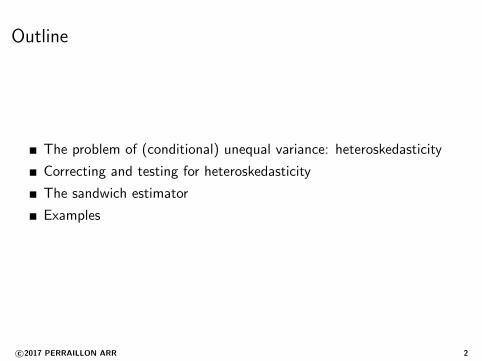
Outline

The problem of (conditional) unequal variance: heteroskedasticity

Correcting and testing for heteroskedasticity

The sandwich estimator

Examples


Big picture

Heteroskedasticity is so common that we should just assume itexists

We can perform some tests to detected it

The solutions depend on the source of heteroskedasticity

The problem is not about the bias or consistency of the OLSestimates; the issue is that SEs are not correct in the presence ofheteroskedasticity

We will follow Chapter 8 of Wooldridge


Homoskedasticity

In the linear model yi = β0 + β1x1i + · · ·+ xpp + εi we assumed thatεi ∼ N(0, σ2)

That is, the error terms have all the same variance conditional on allexplanatory variables: var(εi |x1, ..., xp) = σ2

If this is not the case, then we need to add an index to the varianceto denote that some observations have a different error variance thatdepends on values of x

To simplify, we will focus on the simple linear model (only onecovariate). In the presence of heteroskedasticity: var(εi |xi ) = σ2

i


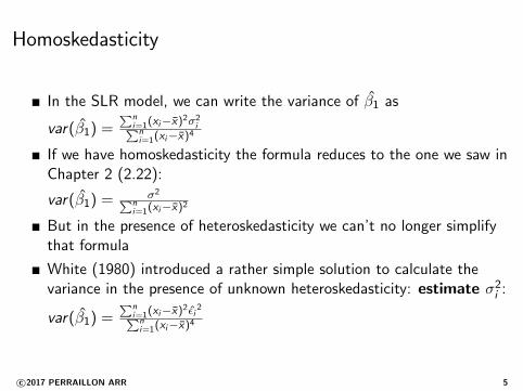
Homoskedasticity

In the SLR model, we can write the variance of β̂1 as

var(β̂1) =∑n

i=1(xi−x̄)2σ2i∑n

i=1(xi−x̄)4

If we have homoskedasticity the formula reduces to the one we saw inChapter 2 (2.22):

var(β̂1) = σ2∑ni=1(xi−x̄)2

But in the presence of heteroskedasticity we can’t no longer simplifythat formula

White (1980) introduced a rather simple solution to calculate thevariance in the presence of unknown heteroskedasticity: estimate σ2

i :

var(β̂1) =∑n

i=1(xi−x̄)2ε̂i2∑n

i=1(xi−x̄)4


Huber-White robust standard errors

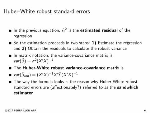
In the previous equation, ε̂i2 is the estimated residual of the

regression

So the estimation proceeds in two steps: 1) Estimate the regressionand 2) Obtain the residuals to calculate the robust variance

In matrix notation, the variance-covariance matrix isvar(β̂) = σ2(X ′X )−1

The Huber-White robust variance-covariance matrix is

var(β̂rob) = (X ′X )−1X ′Σ̂(X ′X )−1

The way the formula looks is the reason why Huber-White robuststandard errors are (affectionately?) referred to as the sandwhichestimator


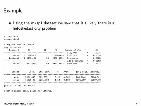
Example

Using the mksp1 dataset we saw that it’s likely there is ahetoskedasticity problem

* Load data

webuse mksp1

* Regress educ on income

reg income educ

Source | SS df MS Number of obs = 100

-------------+---------------------------------- F(1, 98) = 10.34

Model | 2.7896e+09 1 2.7896e+09 Prob > F = 0.0018

Residual | 2.6433e+10 98 269719984 R-squared = 0.0955

-------------+---------------------------------- Adj R-squared = 0.0862

Total | 2.9222e+10 99 295173333 Root MSE = 16423

------------------------------------------------------------------------------

income | Coef. Std. Err. t P>|t| [95% Conf. Interval]

-------------+----------------------------------------------------------------

educ | 2001.493 622.3571 3.22 0.002 766.4461 3236.541

_cons | 14098.23 9221.392 1.53 0.130 -4201.327 32397.78

------------------------------------------------------------------------------

predict incres, rstandard

scatter incres educ, xline(0) jitter(1)


Example

Some evidence of unequal variances conditional on educationc©2017 PERRAILLON ARR 8

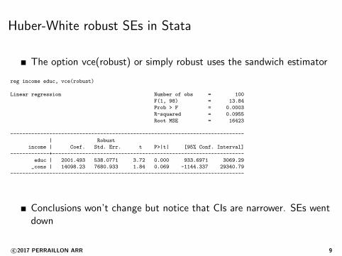
Huber-White robust SEs in Stata

The option vce(robust) or simply robust uses the sandwich estimator

reg income educ, vce(robust)

Linear regression Number of obs = 100

F(1, 98) = 13.84

Prob > F = 0.0003

R-squared = 0.0955

Root MSE = 16423

------------------------------------------------------------------------------

| Robust


-------------+----------------------------------------------------------------

educ | 2001.493 538.0771 3.72 0.000 933.6971 3069.29

_cons | 14098.23 7680.933 1.84 0.069 -1144.337 29340.79

------------------------------------------------------------------------------

Conclusions won’t change but notice that CIs are narrower. SEs wentdown


Huber-White robust SEs in StataCompare models; some tests will of course change now that we havedifferent SEs

qui reg income educ

est sto m1

test educ= 900

( 1) educ = 900

F( 1, 98) = 3.13

Prob > F = 0.0799

qui reg income educ, robust

est sto m2

test educ= 900

( 1) educ = 900

F( 1, 98) = 4.19

Prob > F = 0.0433

est table m1 m2, se stats(N F)

----------------------------------------

Variable | m1 m2

-------------+--------------------------

educ | 2001.4935 2001.4935

| 622.35711 538.07705

_cons | 14098.225 14098.225

| 9221.392 7680.9332

-------------+--------------------------

N | 100 100

F | 10.342584 13.836282

----------------------------------------

Note that Stata calculates a different F statisticsc©2017 PERRAILLON ARR 10

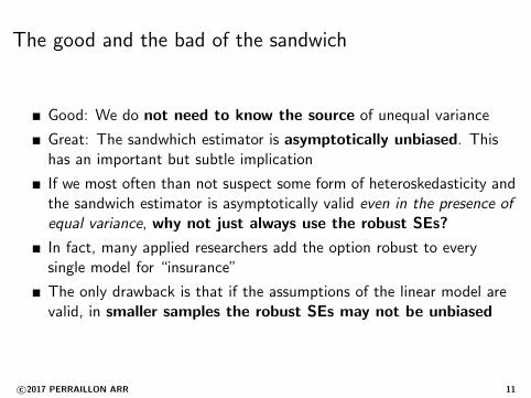
The good and the bad of the sandwich

Good: We do not need to know the source of unequal variance

Great: The sandwhich estimator is asymptotically unbiased. Thishas an important but subtle implication

If we most often than not suspect some form of heteroskedasticity andthe sandwich estimator is asymptotically valid even in the presence ofequal variance, why not just always use the robust SEs?

In fact, many applied researchers add the option robust to everysingle model for “insurance”

The only drawback is that if the assumptions of the linear model arevalid, in smaller samples the robust SEs may not be unbiased


Testing for heteroskedasticity

If small samples and unequal variance in doubt, useful to have a testfor heteroskedasticity rather than just assume it

The null hypothesis is H0 : var(ε|x1, x2, ..., xp) = σ2 (that is,homoskedasticity)

As usual with hypothesis testing, we will look at the data to provideevidence that the variance is not equal conditional on x1, x2, ..., xp

Recall the basic formula of the variance:var(X ) = E [(X − X̄ )2] = E [X 2]− (E [X ])2

Since E [ε] = 0 we can rewrite the null as:H0 : E (ε2|x1, x2, ..., xp) = E [ε2] = σ2

If you see the problem this way, it looks a lot easier. We need tofigure out if the E [ε2] is related to one or more of the explanatoryvariables. If not, we can’t reject the null


Testing for heteroskedasticity

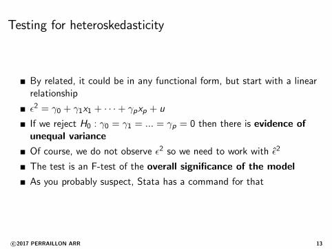
By related, it could be in any functional form, but start with a linearrelationship

ε2 = γ0 + γ1x1 + · · ·+ γpxp + u

If we reject H0 : γ0 = γ1 = ... = γp = 0 then there is evidence ofunequal variance

Of course, we do not observe ε2 so we need to work with ε̂2

The test is an F-test of the overall significance of the model

As you probably suspect, Stata has a command for that


Testing for heteroskedasticity, example

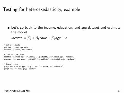
Let’s go back to the income, education, and age dataset and estimatethe model

income = β0 + β1educ + β2age + ε

* Get residuals

qui reg income age edu

predict incress, rstandard

* Combine the plots

scatter incress age, yline(0) legend(off) saving(r1.gph, replace)

scatter incress educ, yline(0) legend(off) saving(r2.gph, replace)

* Export plot

graph combine r1.gph r2.gph, row(1) ysize(10) xsize(20)

graph export rall.png, replace



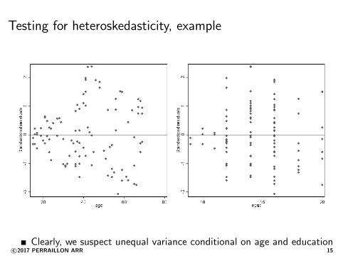
Clearly, we suspect unequal variance conditional on age and educationc©2017 PERRAILLON ARR 15


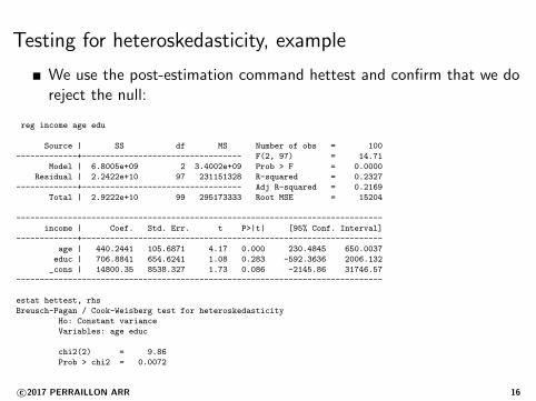
We use the post-estimation command hettest and confirm that we doreject the null:

reg income age edu


-------------+---------------------------------- F(2, 97) = 14.71

Model | 6.8005e+09 2 3.4002e+09 Prob > F = 0.0000

Residual | 2.2422e+10 97 231151328 R-squared = 0.2327

-------------+---------------------------------- Adj R-squared = 0.2169

Total | 2.9222e+10 99 295173333 Root MSE = 15204

------------------------------------------------------------------------------


-------------+----------------------------------------------------------------

age | 440.2441 105.6871 4.17 0.000 230.4845 650.0037

educ | 706.8841 654.6241 1.08 0.283 -592.3636 2006.132

_cons | 14800.35 8538.327 1.73 0.086 -2145.86 31746.57

------------------------------------------------------------------------------

estat hettest, rhs

Breusch-Pagan / Cook-Weisberg test for heteroskedasticity

Ho: Constant variance

Variables: age educ

chi2(2) = 9.86

Prob > chi2 = 0.0072


By handNot exactly the same as the Breusch-Pagan but close (p-value of Ftest: 0.0012)


* Get square of residuals

predict r1, res

gen r12 = r1^2

* Regress

reg r12 age edu


-------------+---------------------------------- F(2, 97) = 7.21

Model | 9.9160e+17 2 4.9580e+17 Prob > F = 0.0012

Residual | 6.6689e+18 97 6.8752e+16 R-squared = 0.1294

-------------+---------------------------------- Adj R-squared = 0.1115

Total | 7.6605e+18 99 7.7379e+16 Root MSE = 2.6e+08

------------------------------------------------------------------------------

r12 | Coef. Std. Err. t P>|t| [95% Conf. Interval]

-------------+----------------------------------------------------------------

age | 6024159 1822704 3.31 0.001 2406596 9641722

educ | 872384 1.13e+07 0.08 0.939 -2.15e+07 2.33e+07

_cons | -3.72e+07 1.47e+08 -0.25 0.801 -3.29e+08 2.55e+08

------------------------------------------------------------------------------

We do gain some intuition: as suspected, the problem is age and notso much educationc©2017 PERRAILLON ARR 17

Using Breusch-Pagan

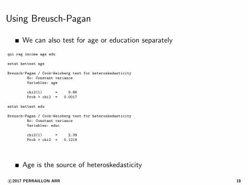
We can also test for age or education separately


estat hettest age



Variables: age

chi2(1) = 9.86

Prob > chi2 = 0.0017

estat hettest edu



Variables: educ

chi2(1) = 2.39

Prob > chi2 = 0.1219

Age is the source of heteroskedasticity



Correcting does change SEs but not by a lot

* Regular


est sto reg

* Robust

qui reg income age edu, robust

est sto rob

* Compare

est table reg rob, se p stats(N F)

----------------------------------------

Variable | reg rob

-------------+--------------------------

age | 440.24407 440.24407

| 105.68708 94.815869

| 0.0001 0.0000

educ | 706.88408 706.88408

| 654.62413 612.81005

| 0.2829 0.2515

_cons | 14800.355 14800.355

| 8538.3265 7245.2375

| 0.0862 0.0438

-------------+--------------------------

N | 100 100

F | 14.71002 21.294124

----------------------------------------

legend: b/se/p


Back to transformations

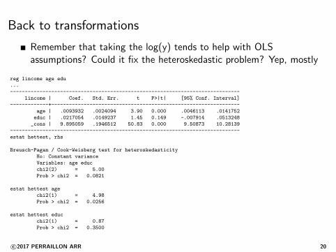
Remember that taking the log(y) tends to help with OLSassumptions? Could it fix the heteroskedastic problem? Yep, mostly

reg lincome age edu

...

------------------------------------------------------------------------------

lincome | Coef. Std. Err. t P>|t| [95% Conf. Interval]

-------------+----------------------------------------------------------------

age | .0093932 .0024094 3.90 0.000 .0046113 .0141752

educ | .0217054 .0149237 1.45 0.149 -.007914 .0513248

_cons | 9.895059 .1946512 50.83 0.000 9.50873 10.28139

------------------------------------------------------------------------------

estat hettest, rhs



Variables: age educ

chi2(2) = 5.00

Prob > chi2 = 0.0821

estat hettest age

chi2(1) = 4.98

Prob > chi2 = 0.0256

estat hettest educ

chi2(1) = 0.87

Prob > chi2 = 0.3500


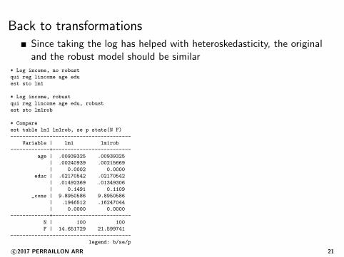
Back to transformationsSince taking the log has helped with heteroskedasticity, the originaland the robust model should be similar

* Log income, no robust

qui reg lincome age edu

est sto lm1

* Log income, robust

qui reg lincome age edu, robust

est sto lm1rob

* Compare

est table lm1 lm1rob, se p stats(N F)

----------------------------------------

Variable | lm1 lm1rob

-------------+--------------------------

age | .00939325 .00939325

| .00240939 .00215669

| 0.0002 0.0000

educ | .02170542 .02170542

| .01492369 .01349306

| 0.1491 0.1109

_cons | 9.8950586 9.8950586

| .1946512 .16247044

| 0.0000 0.0000

-------------+--------------------------

N | 100 100

F | 14.651729 21.599741

----------------------------------------

legend: b/se/p


Alternative: White test

An alternative test that is popular is the White test

It does use more degrees of freedom. The logic is similar to the othertest

White showed that the errors are homokedastic if ε2 is uncorrelatedwith all the covariates, their squares, and cross products

With three covariates, the White test will use 9 predictors rather than3

Easy to implement in Stata (of course)


White

White test in Stata


estat imtest, white

White’s test for Ho: homoskedasticity

against Ha: unrestricted heteroskedasticity

chi2(5) = 23.77

Prob > chi2 = 0.0002

Cameron & Trivedi’s decomposition of IM-test

---------------------------------------------------

Source | chi2 df p

---------------------+-----------------------------

Heteroskedasticity | 23.77 5 0.0002

Skewness | 3.77 2 0.1518

Kurtosis | 2.29 1 0.1302

---------------------+-----------------------------

Total | 29.83 8 0.0002

---------------------------------------------------

Same conclusion, we reject the nullc©2017 PERRAILLON ARR 23

Big picture

With large samples, robust SEs buy you insurance but with smallersamples it would be a good idea to test for heteroskedasticity

Of course, with small samples, the power of the heteroskedasticitytest is itself compromised

No hard rules. Researchers follow different customs; some always addthe robust option (I don’t)

Careful with likelihood ratio tests in the presence ofheteroskedasticity

Stick to robust F tests to compare nested model (use the testcommand in Stata)


Summary

Robust SEs are asymptotically valid even if no heteroskedasticity

Always suspect unequal variance; very common

Taking the log transformation may help

Next class, dealing with unequal variance when we know the source:weighted models

Weighted models for dealing with heteroskedasticity is sort of oldfashioned. I do want to cover weighted models because they are useda lot in survey data analysis and lately in propensity scores


Week 10: Heteroskedasticity - Denver, Colorado 10: Heteroskedasticity Marcelo Coca Perraillon University of Colorado Anschutz Medical Campus Health Services Research Methods I HSMP

Documents