Week 1: Consumption-Based Asset-Pricing Models

Shanghai Advanced Institute of Finance Jun PanShanghai Jiao Tong University [email protected]

Empirical Asset Pricing, Fall 2020

Week 1: Consumption-Based Asset-Pricing ModelsNovember 24, 2020

The empirical asset-pricing literature focuses on the estimation and evaluation of asset-pricing models. For most empiricists, the consumption-based asset-pricing models has anenormous appeal, as it establishes a direct link between the aggregate stock market returnsand the fundamentals of the economy. In an endowment economy, the risk-averse represen-tative agent makes optimal consumption and investment decisions, and his optimization inequilibrium gives rise to a powerful pricing relation that links security returns to risk-aversionand consumption growth. With data on consumption and stock returns ready, this famousfirst-order condition was first tested in the classic paper of Hansen and Singleton (1982),which is the starting point of our today’s class. Written more as a methodological pieceto introduce the generalized method of moments estimators (GMM) of Hansen (1982), thispaper has all the necessary ingredients to show us the equity-premium puzzle. But it is notuntil Mehra and Prescott (1985) that the poor performance of the consumption-based mod-els starts to take center stage in the asset-pricing literature. Over the span of two decadessince the publication of Mehra and Prescott in 1985, solving the equity premium puzzle hasbeen one of the most active literature in asset pricing. Among others, the two most notabledevelopments have been the habit model of Campbell and Cochrane (1999) and the long-runrisk model of Bansal and Yaron (2004). Over the past ten years, this literature has not beenas active, but learning about this literature and understanding the key issues should be anintegral part of your PhD training.

1 Hansen and Singleton (1982)

1.1 Model-Implied Pricing Relation

First-Order Condition: The pricing relation arises from the first-order condition for theoptimal consumption and portfolio formation:

Pt U′ (Ct) = Et [β U ′ (Ct+1) (Pt+1 +Dt+1)] ,

1

where U (·) is the representative agent’s utility function, 0 < β < 1 his time discount factor,and Ct his time-t consumption.

Pricing Kernel: Consider a dividend paying security with time-t dividend Dt. The first-order condition, also known as the Euler equation, links its price Pt at time t to payoffPt+1 +Dt+1 at time t+ 1 via the famous pricing kernel:

Pt = Et [ qt+1 (Pt+1 +Dt+1)] ,

whereqt+1 = β

U ′ (Ct+1)

U ′ (Ct).

Security Returns: For empiricists who are more used to working with returns,

Rt+1 =Pt+1 +Dt+1

Pt

− 1

this pricing relation can be further simplified,

Et [qt+1 (Rt+1 + 1)] = 1 (1)

1.2 Generalized Method of Moments (GMM) Estimations

Moment Conditions: Under the GMM framework, we can express the pricing relation in(1) more generally by,

Et [h (xt+n, b0)] = 0 ,

where xt+n is a k dimensional vector of variables observed by agents and the econometricianas of date t+n, b0 is an l dimensional parameter vector that is unknown to the econometrician,h is a function mapping Rk × Rl into Rm, and Et is the expectations operator conditionedon the agent’s period t information set, It.

Instruments: Let zt denote a q dimensional vector of variables observable as of date t. Tak-ing advantage of the conditional expectation, the original m dimensional moment conditioncan be further expanded by

f (xt+n, zt, b0) = h (xt+n, b0)⊗ zt .

And the unconditional version of the moment condition

E [f (xt+n, zt, b0)] = E [h (xt+n, b0)⊗ zt] = 0 ,

2

represents a set of r = m × q from which an estimator of b0 can be constructed, providedthat r is at least as large as l, the number of unknown parameters.

GMM Estimator: Let g0(b) = E[f (xt+n, zt, b)] be the population mean of the momentsfor any b ∈ Rl and its sample counterpart can be constructed as

gT (b) =1

T

T∑t

f (xt+n, zt, b) , (2)

where T denotes the sample size. If the model is true, then gT (b)|b=b0 should be close to zerofor large values of T . Using this intuition,

bGMMT = argmin

bJT (b) ,

where the criterion function is constructed as

JT (b) = gT (b)′ WT gT (b) ,

where WT is an r by r symmetric, positive definite matrix that can depend on sampleinformation.

Two-Stage GMM: The asymptotic covariance matrix for bGMMT depends on the choice of

weighting matrix WT . It is possible to choose WT optimally in the sense of constructingan estimator with the smallest asymptotic covariance matrix. Under the two-stage GMMof Hansen (1982), the weighting matrix WT does not take into account of conditioninginformation and is calculated via a two-stage iteration of:

W ∗T =

RT (0) +

n−1∑j=1

(RT (j) +RT (j)′)

−1

,

where

RT (j) =1

T

T∑t=1+j

f (xt+n, zt, bT ) f (xt+n−j, zt−j, bT )′ .

To further improve the efficiency of the GMM estimator, the weighting matrix can be con-structed using the conditioning information, as in Hansen (1985).

Under Hansen (1982), the resulting asymptotic covariance matrix of the two-stage GMMestimator can be computed by

(D′T W ∗

T DT )−1

,

3

where

DT =1

T

T∑t=1

∂h

∂b(xt+n, bT )⊗ zt .

To assess the goodness-of-fit and perform hypothesis testing, we go back to the sample meanof the moment condition gT (b) and the criterion function JT (b). If the model is correct, thenall r components of the moment condition equal zero, and all r components of gT (b)|b=b0 areclose to zero for large value of T . In estimating bGMM

T , l of the r moment conditions havebeen used, and the remaining r − l can be used in testing. Indeed, T times the minimizedvalue of the objective function JT (b) can be shown to be asymptotically distributed as achi-square with r − l degrees of freedom.

More on GMM: For a more general weighting matrix of W0, the asymptotic covariancematrix can be computed as

Ω0 = (D′0W0D0)

−1D′

0W0Σ0W0D0 (D′0W0D0)

−1,

whereΣ0 = lim

T→∞TE (gT (b0)gT (b0)

′)

It will be a good exercise for you to prove this. Also, it will be a helpful exercise to show,as special cases of the GMM estimator, the estimations of mean, variance, skewness, andkurtosis, as well as the OLS estimator and the maximum-likelihood estimator. I understandthat nowadays empiricists routinely use canned routines to calculate standard errors, but itwill be a good exercise for you to go through the derivation yourself under the GMM setting.This is particularly true for the OLS regression on a panel structure, where the standarderrors can be clustered by two dimensions and much of the calculation focuses on how youcalculate the sample counterpart of Σ0.

1.3 A Concrete Example

Power Utility: As a concrete example, Hansen and Singleton (1982) focuses their empiricalanalysis on the power utility:

U(c) =C1−γ

1− γ,

where γ is the relative risk aversion coefficient. The pricing kernel for this utility specificationis

qt+1 = β

(Ct+1

Ct

)−γ

.

4

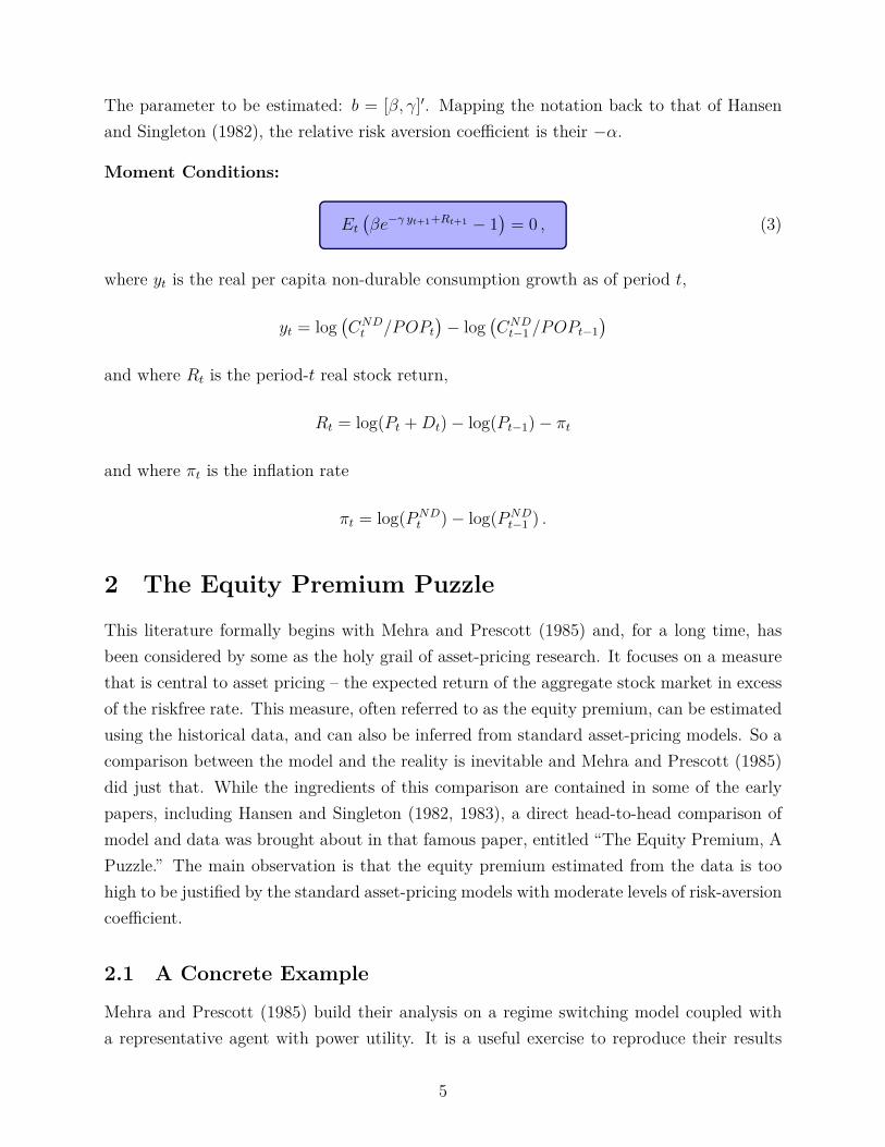
The parameter to be estimated: b = [β, γ]′. Mapping the notation back to that of Hansenand Singleton (1982), the relative risk aversion coefficient is their −α.

Moment Conditions:

Et

(βe−γ yt+1+Rt+1 − 1

)= 0 , (3)

where yt is the real per capita non-durable consumption growth as of period t,

yt = log(CND

t /POPt

)− log

(CND

t−1 /POPt−1

)and where Rt is the period-t real stock return,

Rt = log(Pt +Dt)− log(Pt−1)− πt

and where πt is the inflation rate

πt = log(PNDt )− log(PND

t−1 ) .

2 The Equity Premium PuzzleThis literature formally begins with Mehra and Prescott (1985) and, for a long time, hasbeen considered by some as the holy grail of asset-pricing research. It focuses on a measurethat is central to asset pricing – the expected return of the aggregate stock market in excessof the riskfree rate. This measure, often referred to as the equity premium, can be estimatedusing the historical data, and can also be inferred from standard asset-pricing models. So acomparison between the model and the reality is inevitable and Mehra and Prescott (1985)did just that. While the ingredients of this comparison are contained in some of the earlypapers, including Hansen and Singleton (1982, 1983), a direct head-to-head comparison ofmodel and data was brought about in that famous paper, entitled “The Equity Premium, APuzzle.” The main observation is that the equity premium estimated from the data is toohigh to be justified by the standard asset-pricing models with moderate levels of risk-aversioncoefficient.

2.1 A Concrete Example

Mehra and Prescott (1985) build their analysis on a regime switching model coupled witha representative agent with power utility. It is a useful exercise to reproduce their results

5

if you would like to practice on the regime-switching models. The simple example outlinedin this section delivers the key intuition on the equity premium puzzle. Throughout thesection, we will use annualized numbers and one period in the model is one year.

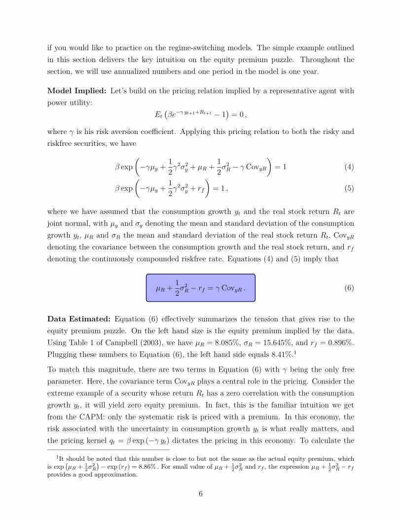
Model Implied: Let’s build on the pricing relation implied by a representative agent withpower utility:

Et

(βe−γ yt+1+Rt+1 − 1

)= 0 ,

where γ is his risk aversion coefficient. Applying this pricing relation to both the risky andriskfree securities, we have

β exp

(−γµy +

1

2γ2σ2

y + µR +1

2σ2R − γ CovyR

)= 1 (4)

β exp

(−γµy +

1

2γ2σ2

y + rf

)= 1 , (5)

where we have assumed that the consumption growth yt and the real stock return Rt arejoint normal, with µy and σy denoting the mean and standard deviation of the consumptiongrowth yt, µR and σR the mean and standard deviation of the real stock return Rt, CovyR

denoting the covariance between the consumption growth and the real stock return, and rf

denoting the continuously compounded riskfree rate. Equations (4) and (5) imply that

µR +1

2σ2R − rf = γ CovyR . (6)

Data Estimated: Equation (6) effectively summarizes the tension that gives rise to theequity premium puzzle. On the left hand size is the equity premium implied by the data.Using Table 1 of Campbell (2003), we have µR = 8.085%, σR = 15.645%, and rf = 0.896%.Plugging these numbers to Equation (6), the left hand side equals 8.41%.1

To match this magnitude, there are two terms in Equation (6) with γ being the only freeparameter. Here, the covariance term CovyR plays a central role in the pricing. Consider theextreme example of a security whose return Rt has a zero correlation with the consumptiongrowth yt, it will yield zero equity premium. In fact, this is the familiar intuition we getfrom the CAPM: only the systematic risk is priced with a premium. In this economy, therisk associated with the uncertainty in consumption growth yt is what really matters, andthe pricing kernel qt = β exp (−γ yt) dictates the pricing in this economy. To calculate the

1It should be noted that this number is close to but not the same as the actual equity premium, whichis exp

(µR + 1

2σ2R

)− exp (rf ) = 8.86% . For small value of µR + 1

2σ2R and rf , the expression µR + 1

2σ2R − rf

provides a good approximation.

6

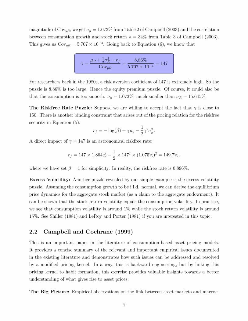
magnitude of CovyR, we get σy = 1.073% from Table 2 of Campbell (2003) and the correlationbetween consumption growth and stock return ρ = 34% from Table 3 of Campbell (2003).This gives us CovyR = 5.707× 10−4. Going back to Equation (6), we know that

γ =µR + 1

2σ2R − rf

CovyR

=8.86%

5.707× 10−4= 147

For researchers back in the 1980s, a risk aversion coefficient of 147 is extremely high. So thepuzzle is 8.86% is too large. Hence the equity premium puzzle. Of course, it could also bethat the consumption is too smooth: σy = 1.073%, much smaller than σR = 15.645%.

The Riskfree Rate Puzzle: Suppose we are willing to accept the fact that γ is close to150. There is another binding constraint that arises out of the pricing relation for the riskfreesecurity in Equation (5):

rf = − log(β) + γµy −1

2γ2σ2

y .

A direct impact of γ = 147 is an astronomical riskfree rate:

rf = 147× 1.864%− 1

2× 1472 × (1.075%)2 = 149.7% .

where we have set β = 1 for simplicity. In reality, the riskfree rate is 0.896%.

Excess Volatility: Another puzzle revealed by our simple example is the excess volatilitypuzzle. Assuming the consumption growth to be i.i.d. normal, we can derive the equilibriumprice dynamics for the aggregate stock market (as a claim to the aggregate endowment). Itcan be shown that the stock return volatility equals the consumption volatility. In practice,we see that consumption volatility is around 1% while the stock return volatility is around15%. See Shiller (1981) and LeRoy and Porter (1981) if you are interested in this topic.

2.2 Campbell and Cochrane (1999)

This is an important paper in the literature of consumption-based asset pricing models.It provides a concise summary of the relevant and important empirical issues documentedin the existing literature and demonstrates how such issues can be addressed and resolvedby a modified pricing kernel. In a way, this is backward engineering, but by linking thispricing kernel to habit formation, this exercise provides valuable insights towards a betterunderstanding of what gives rise to asset prices.

The Big Picture: Empirical observations on the link between asset markets and macroe-

7

conomics indicate countercyclical expected returns: equity risk premia are higher at businesscycle troughs than they are at peaks. Moreover, price-dividend ratios are procyclical, withdepressed stock market prices at business cycle troughs, and are predictive of stock returns.Against this backdrop, the time-varying stock return variance does not move one for onewith estimates of conditional mean returns, indicating that the slope of the conditionalmean-variance frontier, a measure of the price of risk, changes through time with a businesscycle pattern.

These empirical observations are challenging for macroeconomics as standard business cyclemodels fail to reproduce the level, variation, and cyclical comovement of equity premia.For asset-pricing empiricists who study the markets, the pressing question: what are thefundamental sources of risk that drive expected returns?

What They Do: A simple modification of the standard representative-agent consumption-based asset pricing model via slow-moving habit. As consumption declines toward the habitin a business cycle trough, the curvature of the utility function rises, so risky asset pricesfall and expected returns rise.

Unlike the long-run risk model of Bansal and Yaron (2004), the habit model of Campbelland Cochrane keeps the dynamics of the consumption growth simple: i.i.d. lognormal, withits mean and standard deviation calibrated to the postwar data on consumption growth. Byavoiding exogenous variation in the probability distribution of consumption, their focus ison how the pricing kernel, via slow-moving habit, can drive the time-variation of expectedreturns. At a conceptual level, this is very different from the approach of Bansal and Yaron(2004), who rely on an exogenous latent state variable, the long-run mean of the consumptiongrowth, to explain the time-variation of expected returns. As a modeling device, it mightbe convenient to shift the burden to a state variable that cannot be observed, but empiri-cally there is not much evidence in the consumption data to justify such a modification ofthe consumption dynamics. Intuitively, it also makes sense that the effective risk aversionincreases at business cycle troughs.

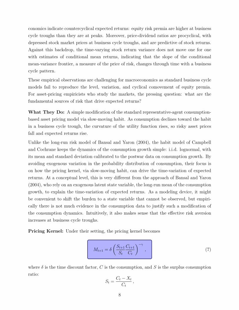
Pricing Kernel: Under their setting, the pricing kernel becomes

Mt+1 = δ

(St+1

St

Ct+1

Ct

)−γ

, (7)

where δ is the time discount factor, C is the consumption, and S is the surplus consumptionratio:

St =Ct −Xt

Ct

,

8

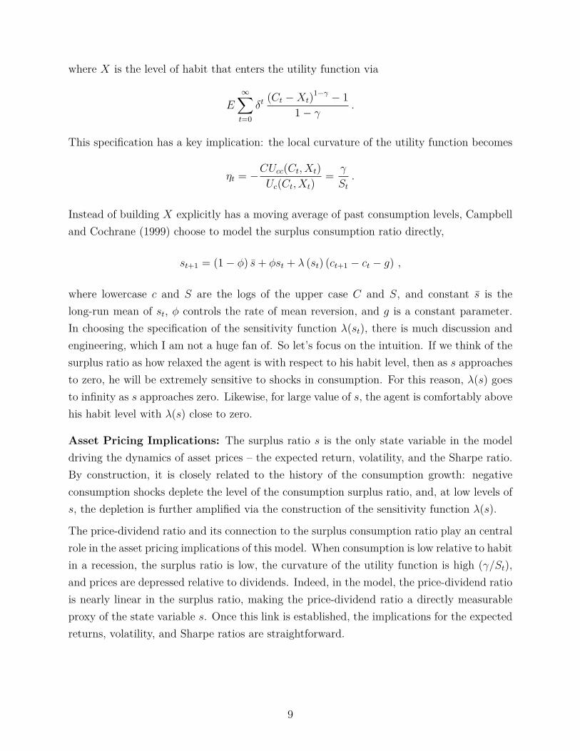
where X is the level of habit that enters the utility function via

E

∞∑t=0

δt(Ct −Xt)

1−γ − 1

1− γ.

This specification has a key implication: the local curvature of the utility function becomes

ηt = −CUcc(Ct, Xt)

Uc(Ct, Xt)=

γ

St

.

Instead of building X explicitly has a moving average of past consumption levels, Campbelland Cochrane (1999) choose to model the surplus consumption ratio directly,

st+1 = (1− ϕ) s+ ϕst + λ (st) (ct+1 − ct − g) ,

where lowercase c and S are the logs of the upper case C and S, and constant s is thelong-run mean of st, ϕ controls the rate of mean reversion, and g is a constant parameter.In choosing the specification of the sensitivity function λ(st), there is much discussion andengineering, which I am not a huge fan of. So let’s focus on the intuition. If we think of thesurplus ratio as how relaxed the agent is with respect to his habit level, then as s approachesto zero, he will be extremely sensitive to shocks in consumption. For this reason, λ(s) goesto infinity as s approaches zero. Likewise, for large value of s, the agent is comfortably abovehis habit level with λ(s) close to zero.

Asset Pricing Implications: The surplus ratio s is the only state variable in the modeldriving the dynamics of asset prices – the expected return, volatility, and the Sharpe ratio.By construction, it is closely related to the history of the consumption growth: negativeconsumption shocks deplete the level of the consumption surplus ratio, and, at low levels ofs, the depletion is further amplified via the construction of the sensitivity function λ(s).

The price-dividend ratio and its connection to the surplus consumption ratio play an centralrole in the asset pricing implications of this model. When consumption is low relative to habitin a recession, the surplus ratio is low, the curvature of the utility function is high (γ/St),and prices are depressed relative to dividends. Indeed, in the model, the price-dividend ratiois nearly linear in the surplus ratio, making the price-dividend ratio a directly measurableproxy of the state variable s. Once this link is established, the implications for the expectedreturns, volatility, and Sharpe ratios are straightforward.

9

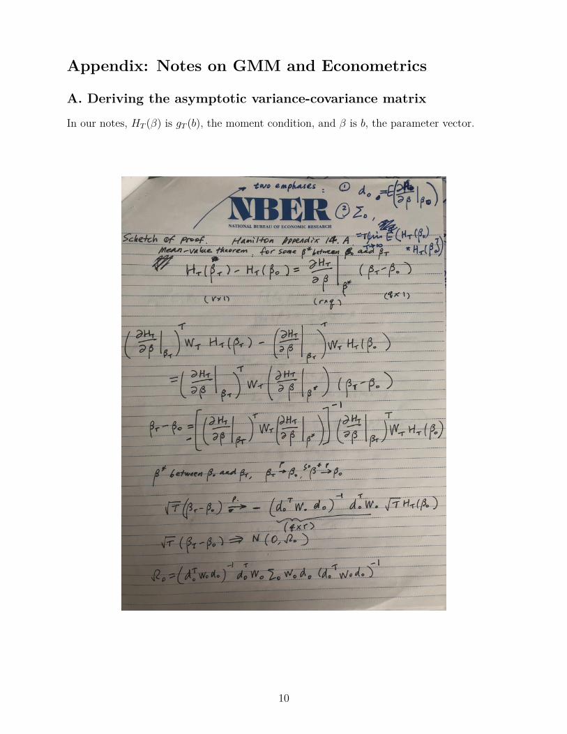
Appendix: Notes on GMM and Econometrics

A. Deriving the asymptotic variance-covariance matrix

In our notes, HT (β) is gT (b), the moment condition, and β is b, the parameter vector.

10

B. GMM and Estimating Moments

11

C. GMM and OLS Regression

12