research.birmingham.ac.uk · Web viewInitial variogram analysis suggested that gravestone decay exhibits poor spatial correlation, which is likely an artifact of significant variation

Correlation of gravestone decay and air quality 1960-2010

Mooers HD1, Carlson, MJ1, Harrison, RM2, Inkpen, RJ3, and Loeffler, S4

1. Department of Earth and Environmental Sciences, University of Minnesota Duluth, 203 Heller Hall, 1114 Kirby Dr., Duluth, MN 55812, USA, email: [email protected]

2. School of Geography, Earth and Environmental Sciences, University of Birmingham, Birmingham, B15 2TT, United Kingdom; Also at: Department of Environmental Sciences / Center of Excellence in Environmental Studies, King Abdulaziz University, Jeddah, 21589, Saudi Arabia

3. Department of Geography, University of Portsmouth, Buckingham Building, Lion Terrace, Portsmouth, PO1 3HE, United Kingdom

4. Department of Earth Sciences, University of Minnesota Twin Cities, 108 Pillsbury Hall, 310 Pillsbury Dr. SE, Minneapolis, MN, 55455, USA

Highlights

Gravestone decay provides a quantitative measure of acid flux Land use strongly correlated with spatial variability in gravestone decay Pronounced increase in deposition efficiency of sulfur dioxide (SO2) after about 1980Abstract

Evaluation of spatial and temporal variability in surface recession of lead-lettered Carrara marble gravestones provides a quantitative measure of acid flux to the stone surfaces and is closely related to local land use and air quality. Correlation of stone decay, land use, and air quality for the period after 1960 when reliable estimates of atmospheric pollution are available is evaluated. Gravestone decay and SO2 measurements are interpolated spatially using deterministic and geostatistical techniques. A general lack of spatial correlation was identified and therefore a land-use-based technique for correlation of stone decay and air quality is employed. Decadally averaged stone decay is highly correlated with land use averaged spatially over an optimum radius of 7 km even though air quality, determined by records from the UK monitoring network, is not highly correlated with gravestone decay. The relationships among stone decay, air-quality, and land use is complicated by the relatively low spatial density of both gravestone decay and air quality data and the fact that air quality data is available only as annual averages and therefore seasonal dependence cannot be evaluated. However, acid deposition calculated from gravestone decay suggests that the deposition efficiency of SO2 has increased appreciably since 1980 indicating an increase in the SO2 oxidation process possibly related to reactions with ammonia.

Key Words: Gravestone decay; acid deposition; air quality; land use, West Midlands;United Kingdom, SO2 deposition velocity.

1

1

2

3456789

101112

13141516

17181920212223242526272829303132

3334

1. Introduction

From the onset of the Industrial Revolution until the environmental revolution of the 1970s

Britain was plagued by air pollution from industrial, urban, and residential sources (Sale and

Foner, 1993; McCormick, 2013). The largest contributors to air pollution were particulate

matter (smoke) and acid in the form of oxides of nitrogen (NOx) and sulfur (SOx) compounds,

particularly sulfur dioxide (SO2). (Marsh, 1978; Bricker and Rice, 1993). As early as the 1840s

there were efforts to measure air pollution in British cities (Moseley, 2009) and Smith (1876)

determined that the burning of coal was the principle source of “acid rain.” It was not until

about 1960 that the network was greatly expanded with the establishment of the National

Survey, which measured daily smoke and sulfur concentrations at over 500 locations (Moseley,

2009). Prior to 1960, air quality measurements were limited in spatial and temporal coverage

and often described anecdotally, particularly during severe air quality events. Proxy records

have been used to reconstruct air quality; these records include physical descriptions (Allen

1966; Allen 1994; Auliciems and Burton, 1973; Fenger, 2009), particulates in lung tissue samples

(Hunt at al. 2003) and sediment cores (Kelly and Thornton, 1996), and lake acidification studies

(Battarbee and Renberg, 1990; Battarbee et al., 1990). Air quality measurements are of great

interest in studies of ambient environmental conditions (Urone and Schroeder, 1969; Eggleston

et al., 1992; Leck and Rodhe, 1989; Fenger, 2009), efficacy of environmental regulation, and

health related studies of mortality and morbidity related to acute and chronic respiratory

ailments (Macfarlane, 1977; Spix et al. 1993; Ito et al. 1993; Greenstone, 2004).

A proxy that has been used successfully to evaluate historical trends in acid deposition is

surface recession of Carrara marble gravestones (Cooke 1989; Cooke et al., 1995; Dragovich,

1991; Inkpen, 1998, 2013; Inpken and Jackson, 2000; Inkpen et al., 2000, 2001, 2008, in press;

Meierding, 1981; Mooers et al., 2016; Mooers and Massman, in press; Thornbush and

Thornbush, 2013; Viles, 1996), hereafter referred to as gravestone decay to be consistent with

the body of recent literature. Mooers et al. (2016) report on a 120-year record of acid

deposition in the West Midlands, UK, reconstructed from lead-lettered marble gravestone

decay. Their record is compiled from measurements on nearly 600 lead-lettered marble

2

35

36

37

38

39

40

41

42

43

44

45

46

47

48

49

50

51

52

53

54

55

56

57

58

59

60

61

62

gravestones and they demonstrate that gravestone decay is a robust measure of acid

deposition. However, the correlation between acid deposition and available air quality data is

more tenuous (Inkpen, 2013; Inkpen et al., in press) and can be influenced by numerous factors

(Wesley and Hicks, 1977; Schaefer et al., 1992). Therefore the goal of this study is to explore the

relationship between gravestone decay and air quality. Correlation between air quality (SO2 and

smoke) and gravestone decay would then allow quantitative estimation of air quality for earlier

periods of time where lead-lettered marble gravestones are available but atmospheric

concentrations of pollutants were not measured.

The correlation between surface recession of lead-lettered, Carrara marble gravestones and

annually averaged atmospheric SO2 and smoke measurements in the West Midlands, UK, for

the period 1960-2010 is evaluated. The study area includes West Midlands County and

surrounding portions of Staffordshire, Worcestershire, and Warwickshire (Figure 1). The

industrial and residential development of the area is well documented, there is a large number

of cemeteries (Figure 1A) with lead-lettered marble gravestones, and a network of air quality

monitoring stations was in place by 1960 (Figure 1B) (Mosley, 2009, 2011). Decadally averaged

rates of gravestone decay and measured SO2 and smoke are interpolated spatially for the

period after 1960 and correlation between them is evaluated. Interpolation techniques include

deterministic and geostatistical methods; however, because of a high degree of spatial non-

stationarity and anisotropy in gravestone decay and limited spatial and temporal coverage of

air quality measurements, there is great uncertainly in the interpolated values and correlation

between stone decay and air quality is poor.

Because acid deposition is directly related to proximity of sources of SO2 and NOx, a land-

use based approach for correlation of gravestone decay rates with air quality is developed.

Sensitivity and optimization analysis were used to determine the optimum radius of influence

of land use on gravestone decay and weighting factors for interpolating intermediate values of

decay. In addition, if stone decay is assumed to result primarily from deposition of sulfuric acid

then stone decay rates are functions of the production rate of sulfuric acid from SO2 oxidation.

The relationship between stone decay and atmospheric concentration is nonlinear, suggesting a

3

63

64

65

66

67

68

69

70

71

72

73

74

75

76

77

78

79

80

81

82

83

84

85

86

87

88

89

90

marked increase in the efficiency of the oxidation process of SO2 after about 1980. The aim of

this investigation is therefore to determine the efficacy of gravestone decay in spatially and

temporally integrating and recording air quality and explore the nonlinearity of the SO2

oxidation process.

2. Methods

Mooers et al. (2016) examined the spatial and temporal pattern of acid deposition over the

period 1890-2010 from decay of lead-lettered Carrara marble gravestones. Their dataset

includes 1417 individual measurements on 591 tombstones in 33 cemeteries collected between

2005 and 2010. The current investigation assesses the correlation of acid deposition and air

quality and is more restricted in both space and time. Therefore only the cemeteries within the

vicinity of the air quality monitoring network were chosen for analysis (Figure 1A). 21 of the

cemeteries reported by Mooers et al. (2016) are used. Additional measurements were taken in

July of 2014 to enhance the spatial resolution of gravestone decay over the past 55 years that

coincide with air quality monitoring data. 485 inscriptions were measured from 227 tombstones

in 10 additional cemeteries with emphasis on post 1950 inscriptions. In addition, Bilston (BIL)

Cemetery was revisited and additional data were acquired to constrain post 1950 decay rates.

Cemeteries, their locations, and associated data are listed in Table 1.

26 air quality monitoring stations lie in the study area; their locations are shown in Figure

1B and the annually averaged SO2 and smoke concentrations for all stations are shown in Figure

2. Despite the expansion of the air-quality monitoring network after 1960, there is still a general

lack of temporal and spatial continuity of records. The period of record of each monitoring

station is highly variable; many stations were only in operation for short periods of time (Table

2).

2.1 Gravestone decay measurements

Gravestones were selected for measurement following the criteria of Mooers et al. (2016),

which closely follow the criteria of Cooke et al. (1995). Measured gravestones were standing

vertically, had planar surfaces, used lead lettering, had limited ornamentation, and contained

4

91

92

93

94

95

96

97

98

99

100

101

102

103

104

105

106

107

108

109

110

111

112

113

114

115

116

117

two or more inscriptions per stone. In addition, inscriptions had to be in chronological order

and there had to be visible evidence that the stone had been resurfaced at the location of each

new inscription.

Surface recession of the marble was measured with the depth probe of a digital caliper

(accuracy of 0.01mm and precision of ± 0.02mm (instrument error)) from the surface of the

lead letters to the stone surface. Resting the digital caliper on two neighboring lead letters

provided stability in measurement while reducing error associated with tilting of the depth

probe. Ten measurements were made along the date line of each inscription without regard to

letter or numeral. Decay for that measurement was then calculated as the trimmed mean

(Tukey, 1962) with the high and low values omitted. The trimmed mean was used to avoid bias

from unusually large or small values that might result from a variety of causes such as poorly

set lettering, odd shaped letters that may hold moisture, etc.

2.2 Determination of Decay Rates

Post 1940 gravestone decay data were plotted vs. inscription date. In general, gravestone

decay as a function of time is nonlinear (Mooers and Massman, in press; Mooers et al., 2016)

and follows a trend similar to SO2 and smoke (Figure 2). Gravestone decay rates were therefore

determined by best-fit least squares regression function, which in most cases was a 2nd order

polynomial. In the case of Rycroft Cemetery in Dudley (DUD) a 3rd order polynomial provided a

higher correlation coefficient and prevented the function from becoming slightly negative in the

most recent decade Decay rates were then determined as the derivative of the best-fit

polynomial at the midpoint of each respective decade.

2.3 Spatial Interpolation of Gravestone Decay

2.3.1 Variogram analysis and Kriging

Since air quality measurements do not coincide geographically with cemeteries, proper

spatial interpolation of gravestone decay is critical for comparison. Variograms of the decadally

averaged gravestone decay rates from the 33 measured cemeteries were evaluated for best

model fit. Stone decay rate for each decade from 1965-2005 was then gridded in ArcGIS® using

5

118

119

120

121

122

123

124

125

126

127

128

129

130

131

132

133

134

135

136

137

138

139

140

141

142

143

144

Empirical Bayesian Kriging (EBK) at a grid spacing of 200 m. Whereas classical Kriging assumes

the estimated semivariogram is the true semivariogram generated from a Gaussian distribution,

EBK generates many semivariogram models and removes local trends (Krivourchko, 2012). EBK

is particularly well suited for small, moderately non-stationary datasets (Chiles and Delfiner,

1999; Pilz and Spöck, 2007). Interpolated decay rates were compared with air quality data.

2.3.2 Land-use-based approach

Initial variogram analysis suggested that gravestone decay exhibits poor spatial correlation,

which is likely an artifact of significant variation in air quality over short spatial scales (Hoek et

al., 2002, 2008). Therefore a land-use-based approach was devised to spatially interpolate

gravestone decay. Land use was organized into three categories; 1.) urban areas with high

concentrations of factories, large buildings and heavy automobile traffic, 2.) residential areas

with dense housing and moderate automobile traffic and 3.) rural/green space with few

residences and light traffic. Land use was digitized from recent aerial photography and

converted to a 200 m grid for analysis. Evaluation of air photos back to 1960 indicates that

there have been few major changes in land-use classification. Grid cells were assigned a land-

use indicator as follows: green space generates essentially no pollution and was assigned a

land-use indicator of 0.0 and urban/industrial areas were assigned a land-use indicator of 1.0.

The relation between urban/industrial and residential is less clear but the land-use indicator will

lie somewhere between 0 and 1 and this value must be determined through optimization.

Three parameters were then optimized: the indicator value of residential land use, the radius of

influence contributing to acid deposition at any location, and a weighting parameter to

determine the influence of proximal versus distal locations within the optimum radius.

2.4.1 Optimization of Parameters

The initial optimization of weighting of the residential land-use and radius of influence were

done using inverse distance weighting as it provides easy variation of parameters. In its

simplest form, the inverse distance weighting parameter (w) is

6

145

146

147

148

149

150

151

152

153

154

155

156

157

158

159

160

161

162

163

164

165

166

167

168

169

170

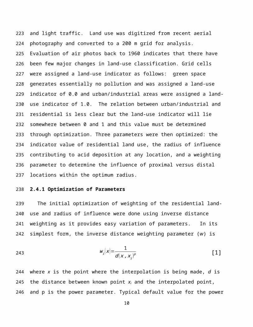
w i ( x )= 1d (x , x i)

p [1]

where x is the point where the interpolation is being made, d is the distance between known

point xi and the interpolated point, and p is the power parameter. Typical default value for the

power parameter for many applications is 2 (inverse distance squared). Reducing the exponent

weighs distant points more heavily. For p=0 (zero) there is no decrease in weight with distance

and the prediction will be simply an average of the values within the search radius. To conduct

the initial sensitivity analysis, values of residential land use were varied from 1.0 to 0.0 in steps

of 0.2, radius varied from 1 to 10 km, and the inverse distance weighting parameter was varied

from 2 to 0. Land use, integrated for each combination of parameters, was calculated for each

cell in the 200 m grid. Integrated land use was then correlated with gravestone decay at each

cemetery and correlation coefficients (R2) determined.

Since deterministic methods such as IDW differ in their application from geostatistical and

interpolation methods (Zimmerman et al., 1999), several additional techniques of land-use

interpolation were employed. These included: ordinary kriging, kernel density, and point

density calculations all done within ArcGIS® Geostatistical Analyst® and Spatial Analyst®. For

each land-use interpolation method the resulting land-use values at cemeteries were correlated

with gravestone decay rate for each decade.

2.4.2 Directional dependence of land-use and gravestone decay rate

The directional dependence of land use on stone decay rate was evaluated by integrating

land use within search windows of 90, 120, and 180 rotated in 45, 60, and 60 degree

increments, respectively. For each search window, land-use indicators were calculated at 200 m

grid cells using the point density function in ArcGIS® Spatial Analyst®. Calculations were made

using optimized parameters for radius and residential land use for each search window. The

interpolated land use at each measured cemetery was again correlated with gravestone decay

at that point. To evaluate directional trends, rose diagrams were constructed using the mean

azimuth of each search window and the correlation coefficient between measured gravestone

decay rate and the calculated land-use indicator for each directional search.

7

171

172

173

174

175

176

177

178

179

180

181

182

183

184

185

186

187

188

189

190

191

192

193

194

195

196

197

2.5 Correlation of gravestone decay rates and measured atmospheric SO2 and smoke

Two separate sets of interpolated grids of gravestone decay rates were generated. First,

decadally averaged decay rates for each cemetery were interpolated spatially using Empirical

Bayesian Kriging. Second, the linear least-squares regression equation describing the relation

between land use and gravestone decay rate was used to assign decay rates spatially. The

interpolated and assigned gravestone decay rates at the location of air quality monitoring

stations were then plotted against measured SO2 and smoke and correlation coefficients (R2)

determined to evaluate the relationship between gravestone decay rates (either spatially

interpolated or assigned based on land use) and air quality.

2.6 Evaluation of SO2 deposition efficiency

Marble gravestone decay is a direct measure of flux density of acid (F) (Mooers and

Massman, in press), which, in turn, is determined by the atmospheric concentration of

pollutants (C) at height z, and the deposition velocity (vd) given as

vd=−FC z

. [2]

SO2 measurements give us a quantitative measure of the atmospheric concentration. If the

stone decay is assumed to result from deposition of sulfuric acid, stone decay rates are a

measure of the flux of acid to the stone surface, which is a function of the production rate of

sulfuric acid from SO2 oxidation. It is therefore instructive to plot vd as a function of time to

evaluate temporal changes in deposition velocity (deposition efficiency) of SO2 , which can be

affected by a number of factors that influence the correlation of gravestone decay with air

quality.

Deposition velocities were calculated at the 26 air quality monitoring stations using the

mean annual SO2 concentration and the interpolated gravestone decay rate determined using

the optimized land use correlation with gravestone decay. Decay rates were then converted to

flux of acid as equivalent SO2 as

8

198

199

200

201

202

203

204

205

206

207

208

209

210

211

212

213

214

215

216

217

218

219

220

221

222

F=e ρwiM (CaCO3)M (H2SO4)

, [3]

where (e) is decay rate (l t-1), is the density of marble (M l-3) (we used 2600 kg m-3, Malaga-Starzec et

al., (2006)), w i is the mass fraction of SO2 in sulfuric acid (0.65), and M(CaCO3) and M(H2SO4) are the

mole weight of calcite (100) and sulfuric acid (98), respectively.

3. Results

3.1 Decay rates

Gravestone decay for the 33 cemeteries included in this study is shown in Figure 3 for the

period 1950 to 2010. There is a great deal of variability in decay among stones within any single

cemetery. Mooers et al. (2016) conducted an investigation of the sources of variability of stone

decay and concluded that by far the largest variability is inherent to the stone. Differences in

the physical setting and local effects influence decay by at most a few percent, therefore the

data plotted are uncorrected for environmental variables. Time-dependent decay rates were

determined by least squares regression (Figure 3, Table 1) for each location.

3.2 Spatial Interpolation of Gravestone Decay

3.2.1 Variogram analysis

Variograms of the decadally averaged gravestone decay rates from the 33 cemeteries for

each decade are shown in Figure 4A-E. In all cases the nugget is large compared with the sill,

particularly for the 1960s – 1980s, which leads to relative equality in kriging weights and

interpolated values are simply averages of known points (Webster and Oliver 1992; University

of Salzburg 2014). The ranges in all cases are between 5 and 10 km; this distance is similar to

the average distance between measured cemeteries, again suggesting a lack of spatial

correlation resulting in simply averaging of known points by kriging. Figure 4F shows the

spatially interpolated gravestone decay rates for the 1960s using Empirical Bayesian Kriging

gridded at 200 m. The interpolated decay rates were then compared with air quality data from

the 11 air quality monitoring stations available in the 1960s; the correlation between

9

223

224

225

226

227

228

229

230

231

232

233

234

235

236

237

238

239

240

241

242

243

244

245

246

247

interpolated gravestone decay (and therefore acid flux) is poor (Figure 4G) and results for

other decades are similar.

3.2.2 Land Use and Optimization of Parameters

Digitized land use is shown in Figure 5 and the results of the optimization of parameters for

the land-use analysis using IDW are shown in Figure 6 and Table 3. The correlation between

land use and gravestone decay was maximized for an effective radius of approximately 7000m

(Figure 6A), a residential land-use indicator of 0.0 (Figure 6B), and an IDW power of < 0.25 with

the best correlation at a value of 0.0 (Figure 6C). Therefore the best correlation between land

use and gravestone decay is achieved using the same indicator for residential area and green

space. Within the study area there are essentially no green spaces larger than 2-3 km in

diameter (Figure 5), which is less than half of the calculated effective radius of influence (7000

m) suggesting that air quality in green spaces is likely no different from, and is controlled by,

surrounding urban/industrial or residential areas. An optimum inverse distance weighting

power of 0.0 indicates that gravestone decay depends basically on an average of the air quality

over a 7000 m radius of the surrounding area. This averaging is consistent with the variogram

analysis, which suggested little spatial correlation in the gravestone decay measurements

among cemeteries.

Land use was then interpolated to a 200 m grid using ordinary Kriging, kernel density, point

density and inverse distance weighting. Figure 7 shows the correlation between the calculated

land-use indicator and gravestone decay rate for the various interpolation techniques for a

radius of 7000m and a residential land-use indicator of 0.0. Although there is reasonable

correlation between land use and stone decay, 4 cemeteries are considered outliers (BEN, COD,

JQK, and WAL). Bentley Cemetery (BEN) has an anonymously low decay rate; it is surrounded by

four other cemeteries (WIL, WAL, DAR, and BIL) all of which have significantly higher decay

rates and far larger number of measurements (Figure 3). Codsall (COD) is anomalously high for

the calculated land use, which is mostly rural farmland. Only the relatively small village of

Codsall has significant residential neighborhoods. The reason for the anomalously high

calculated decay rate is unclear. Key Hill Cemetery (JQK), located in the Birmingham Jewellery

10

248

249

250

251

252

253

254

255

256

257

258

259

260

261

262

263

264

265

266

267

268

269

270

271

272

273

274

275

Quarter, has anomalously low stone decay compared to Warstone Lane Cemetery, which is

located only 100 m away. The dramatic difference in decay rate is attributed to the continuous

tree canopy of 100 to150-year-old London plane at Key Hill Cemetery, whereas Warstone Lane

Cemetery is largely open (Mooers and Massman, in press; Mooers et al. 2016).

Rrycroft Cemetery (WAL) in Walsall has a relatively high decay rate relative to the calculated

land use. Therefore to evaluate the overall effect of these anomalous decay values on the

correlation between land use and gravestone decay, BEN, COD, JQK, and WAL were removed

from the analysis and the results are shown in Figures 7B, D, F, and H. Note that correlation

coefficients are significantly higher with these four outliers omitted.

The highest correlation between the spatially averaged land-use parameter and gravestone

decay at measured cemeteries was achieved using point-density analysis and kriging with the

omission of the aforementioned four anomalous cemeteries. The point density function simply

averages the values within a given radius and kriging, given the poor spatial correlation

suggested by variogram analysis, does little more than average the land use over the same

radius.

Table 4 shows the correlation coefficients of land-use vs. stone decay rates using the point-

density calculation for each decade and for radii of 4000 – 12,000 m. Correlation coefficients

are high for 1960s – 1980s at a radius of approximately 6-7 km. The correlation between land

use and stone decay drops off after 1990 and the radius of highest correlation increases.

3.2.3 Directional dependence of land use on gravestone decay

The correlation between interpolated land use and gravestone decay rate for the

directionally dependent search patterns are shown in Table 5 and Figure 8. Once again omitting

BEN, COD, WAL, and JQK from the analysis improves the correlation for the reason stated

above. Note that the wider the search pattern the better the correlation between land use and

stone decay (Table 5). The correlation coefficients for gravestone decay and land use for each of

directional searches are shown in Table 5. Although the correlation coefficients are not as high

as the omnidirectional calculation there is a clear directional trend. The highest correlation of

11

276

277

278

279

280

281

282

283

284

285

286

287

288

289

290

291

292

293

294

295

296

297

298

299

300

301

302

land use and gravestone decay for the 1960s and 1970s is south and southwest. From the

1980s to the 2000s the correlation coefficients decrease as the directional dependence of stone

decay rate shifts to westerly and then nearly to the north. This change in directional trend

coincides with improving air quality and the increase in effective radius of influence

contributing acid and changing deposition efficiency of SO2.

3. 3 Correlation of land use and air quality

The correlation of gravestone decay rate and optimized land use suggests that interpolated

land use may be used as a proxy for acid deposition and the relationship between land use and

air quality can be evaluated. The decadally averaged SO2 and smoke concentrations for 23

monitoring stations are shown in Table 6. The correlation of land use (calculated using the

point density function, a radius of 7 km, a residential land-use indicator of 0.0) and SO2 and

smoke for the 1960s-1980s is shown in Figure 9. Trends are clearly evident for the 1960s and

1970s even though R2 values are relatively low. By the 1980s, there is little correlation between

land use and SO2 and smoke.

3.4 Evaluation of SO2 deposition efficiency

Figure 10 shows the calculated deposition velocities for all air quality monitoring locations for

all years (Figure 10). Five-year and ten-year moving averages are also plotted to remove high-

frequency variation. Note that after about 1980 there is an increasing trend in the deposition

velocity indicating an increase in the efficiency of SO2 oxidation to sulfuric acid. SO2 emissions in

Europe have decreased substantially since 1980, which has been reflected in large reductions in

airborne concentrations of SO2 (Vestreng et al., 2007). Jones and Harrison (2011) used data

from the European Monitoring and Evaluation Programme (EMEP) to examine relationships

between SO2 and sulfate in rural air. The data from all countries examined could be fit to a

curvilinear relationship:

[SO42-] = a · [SO2]b + c [4]

where [SO42-] and [SO2] are airborne concentrations, and a, b and c are constants. As b takes

values of typically around 0.6, the percentage reduction in SO42- is less than proportionate for a

12

303

304

305

306

307

308

309

310

311

312

313

314

315

316

317

318

319

320

321

322

323

324

325

326

327

328

329

given reduction in SO2. Hidy et al. (2014) examined measured concentrations from sites in the

southeastern United States; between 1999 and 2013, average SO2 concentrations fell by

approximately 84%, while SO42- over the same period fell by only 60%. The trend seen in Figure

10 of higher sulfuric acid production efficiency at lower concentrations of SO2 in more recent

years is consistent with this pattern.

4.0 Discussion and Conclusions

Gravestone decay has been shown to serve as an excellent proxy for acid deposition (Mooers et

al., 2016; Inkpen, 1998, 2013; Cooke, 1989, Cooke et al., 1995). In addition, the results of this

investigation suggest that gravestone decay exhibits a high degree of correlation with

interpolated land use (Figure 7), which when integrated over some optimal area essentially

determines the pollution sources and therefore the acid flux. The correlation between

interpolated land use and air quality, however, is rather poor (Figure 9) and the reasons for the

poor correlation are difficult to determine. The paucity of measurements of SO2 and smoke

and the lack of spatial and temporal continuity of the records all contribute to poor correlation.

In addition, SO2 data are annual averages and gravestone decay may well be sensitive to

seasonal variations or even short-term extreme events that are not represented in the available

data. Correlation between gravestone decay and measured SO2 and smoke concentrations (air

quality) is suggested by their similar exponential trends (Figures 2 and 3). Although spatial

interpolation procedures can be used to determine intermediate values of gravestone decay,

variogram analysis indicates that there is a lack of spatial correlation particularly prior to about

1980. Local factors, likely related to land use (or possibly even microclimatic effects), therefore

appear to overwhelm the spatial continuum. The land-use approach of spatial interpolation is

therefore at least as good as other methods even though the correlation with annually

averaged annual air-quality data is rather poor.

By about 1980 there was a dramatic turnaround in air quality (Mosley, 2009; 2011) that is

evident in both the SO2 and smoke data (Figure 2) and is well documented in decreasing

gravestone decay rates (Mooers et al., 2016) and therefore acid flux. At this time there is a

change in the directional dependence of gravestone decay on land use (Figure 8) and an

13

330

331

332

333

334

335

336

337

338

339

340

341

342

343

344

345

346

347

348

349

350

351

352

353

354

355

356

357

increase in the optimum radius of influence of land use on gravestone decay rates (Tables 3 and

4). Also at this time there appears to be a marked increase in the efficiency of the SO2 oxidation

process (Figure 10). The most probable explanation for the increased deposition efficiency is

non-linearity in the SO2 conversion to sulfate, which is seen in both field measurement data

(Jones and Harrison, 2011; Hidy et al., 2014) and numerical model results (Harrison et al., 2013).

An alternative explanation of Figure 10, which needs to be considered, is that increased

emissions of nitrogen oxides have led to increased concentrations of nitric acid and higher

decay rates. However, UK emission statistics for NOx show a peak in 1990 with continual

decrease until 2013 (National Atmospheric Emissions Inventory, 2016), suggesting that decay

due to nitric acid cannot explain the observed trends.

As sulfuric acid production falls in response to decreased SO2 concentrations, so the extent of

neutralization by ammonia is likely to increase, hence reducing sulfate acidity and working in

the opposite sense to Figure 10. An alternative role for ammonia is in enhancing the deposition

efficiency of SO2 through co-deposition (Erisman and Wyers, 1993). This is expected to enhance

SO2 deposition efficiency at lower concentrations, and if followed by oxidation of the SO2 leads

to enhanced sulfate concentrations, although not necessarily to sulfuric acid.

As overall air quality improves four trends are evident; 1) the correlation between interpolated

land use and stone decay becomes less (Table 4), 2) the effective radius of influence of land use

on local air quality increases (Table 4), 3) the directional dependence of land use on local air

quality changes from southerly to westerly to northerly, and 4) the efficiency of stone decay

increases as SO2 concentrations fall. These trends are consistent with greatly reduced contrast

in air quality among different land-use types. The reason for the change in directional trend

from south to north over 50 years is unclear, but possibly related to industrial decline in the

Midlands over this time (Spencer et al., 1986).

Finally, interpolated land use and the correlation with SO2 and smoke can be used to estimate

average air quality over the study area for each decade (Figure 11). The improvement in air

quality is quite dramatic, particularly between the 1960s and the 1980s. After about the mid-

14

358

359

360

361

362

363

364

365

366

367

368

369

370

371

372

373

374

375

376

377

378

379

380

381

382

383

384

1980s air quality is relatively uniform spatially in the West Midlands and the correlation with

land use is significantly lower.

Acknowledgements

Several people were instrumental in the process of gathering data for this study over the past

ten years. Tony Sames was our guide and natural historian lending his knowledge and

expertise. Special thanks to Liz Ross and Chris and Diane Rance for their logistical support and

friendship and to Lillian Mooers for keeping the batteries charged in the canal boat.

References

Allen, C. G., 1966. The Industrial Development of Birmingham and the Black Country 1860-1927, Frank Cass and Co. Ltd., p. 1-479.

Allen, R. C. (1994). Agriculture during the industrial revolution. The economic history of Britain since, 1700(1), 96-122.

Auliciems, A., & Burton, I. 1973. Trends in smoke concentrations before and after the clean air act of 1956. Atmospheric Environment, 7(11), 1063-1070.

Battarbee, R. W. and Renberg, I., 1990. The Surface Water Acidification Project (SWAP) Palaeolimnology Programme, Philosophical Transactions of the Royal Society of London, Series B, Biological Sciences, v. 327, p. 227-232.

Battarbee, R. W., Howells, G., Skeffington, R. A., and Bradshaw, A. D. , 1990. The Causes of Lake Acidification, with Special Reference to the Role of Acid Deposition (and discussion), Philosophical Transactions of the Royal Society of London, Series B, Biological Sciences, v. 327, no. 1240, p. 339-347.

Bricker, O. P. and Rice, K. C., 1993. Acid Rain, Annual Review of Earth Planetary Science, v. 21, p. 151-174.

Chilès, J-P., and P. Delfiner 1999. Chapter 4 of Geostatistics: Modeling Spatial Uncertainty. New York: John Wiley & Sons, Inc.

Cooke, R. U., 1989. II. Geomorphological Contributions to Acid Rain Research: Studies of Stone Weathering, Geographical Journal, v. 155, p. 361-366.

Cooke, R. U., Inkpen, R. J., and Wiggs, G. F. S., 1995. Using Gravestones to Assess Changing Rates of weathering in the United Kingdom, Earth Surface Processes and Landforms, v. 20, p. 531-546.

Dragovich, D., 1991. Marble Weathering in an Industrial Environment, Eastern Australia,Environmental Geology Water Science, v. 17, no.2, p. 127-132.

Eggleston, S., Hackman, M., Heyes, C., Irwin, J., Timmis, R. & Williams, M., 1992. Trends in urban air pollution in the United Kingdom during recent decades. Atmospheric Environment, 26B (2), 227-239.

15

385

386

387

388

389

390

391

392393394395396397398399400401402403404405406407408409410411412413414415416417418419420

Erisman, J. W. and Wyers, G. P., 1993. Continuous measurements of surface exchange of SO2, and NH3; implications for their possible interaction in the deposition process. Atmospheric Environment, 37A, 1937-1949.

Fenger, J., 2009. Air pollution in the last 50 years – From local to global. Atmospheric Environment, 43, 13-22.

Greenstone, M., 2004. Did the Clean Air Act cause the remarkable decline in sulfur dioxide concentrations? Environmental Economics and Management 47, 585-611

Harrison, R. M., Jones, A. M., Beddows, D. and Derwent, R. G., 2013. The effect of varying primary emissions on the concentrations of inorganic aerosols predicted by the enhanced UK photochemical trajectory model. Atmospheric Environment, 69, 211-218.

Hidy, G. M., Blanchard, C. L., Baumann, K., Edgerton, E., Tanenbaum, S., Shaw, S., Knipping, E., Tombach, I., Jansen, J. and Walters, J., 2014. Chemical climatology of the southeastern United States, 1999-2013. Atmospheric Chemistry & Physics, 14, 11893-11914.

Hoek, G., Meliefste, K., Cyrys, J., Lewne, M., Bellander, T., Brauer, M., Fischer, P., Gehring, U., Heinrich, J., van Vliet, P., Brunekreef, B., 2002. Spatial variability of fine particles concentrations in three European areas. Atmospheric Environment. 36, 4077–4088.

Hoek, G., Beelen, R., De Hoogh, K., Vienneau, D., Gulliver, J., Fischer, P., & Briggs, D. (2008). A review of land-use regression models to assess spatial variation of outdoor air pollution. Atmospheric Environment, 42(33), 7561-7578.

Hunt, A., Abraham, J., Judson, B. and Berry, C., 2003. Toxicologic and Epidemiologic Clues from the Characterization of the 1952 London Smog Fine Particulate Matter in Archival Autopsy Lung Tissues. Environmental Health Perspectives, 111(9), 1209-1214

Inkpen, R. J. and Jackson, J., 2000. Contrasting Weathering Rates in Coastal, Urban and Rural Areas in Southern Britain: Preliminary Investigations Using Gravestones. Earth Surface Processes and Landforms, v. 25, p. 229-238.

Inkpen, R. J., 1998. Gravestones: Problems and potentials as indicators of recent changes in weathering, in Jones, M. and Wakefield, R. (eds.), Aspects of stone weathering, decay and conservation, Imperial College Press, London, p. 16-27.

Inkpen, R., 2013. Reconstructing past atmospheric pollution levels using gravestone erosion rates. Area, 45(3), 321-329.

Inkpen, R. J., & Jackson, J., 2000. Contrasting weathering rates in coastal, urban and rural areas in southern Britain: preliminary investigations using gravestones. Earth Surface Processes and Landforms, 25(3), 229-238.

Inkpen, R. J., Collier, P., and Fontana, D., 2000. Close-Range Photogrammetric Analysis of Rock Surfaces. Zeitschrift fur Geomorphologie Supplementband (120). pp. 67-81.

Inkpen, R. J., Fontana, D., and Collier, P., 2001. Mapping Decay: Integrating Scales of Weathering within a GIS. Earth Surface Processes and Landforms, v. 26, p. 885¬900.

Inkpen, R., Duane, B., Burdett, J., & Yates, T., 2008. Assessing stone degradation using an integrated database and geographical information system (GIS). Environmental geology, 56(3-4), 789-801.

Inkpen, R.J., Mooers, H.D., and Carlson, M.J., in press, Using rates of gravestone decay to reconstruct atmospheric sulphur dioxide levels. Area.

16

421422423424425426427428429430431432433434435436437438439440441442443444445446447448449450451452453454455456457458459460461462

Ito, K., Thurston, G., Hayes, C. & Lippmann, M., 1993. Associations of London, England, Daily mortality with particulate matter, sulfur dioxide, and acidic aerosol pollution. Archives of Environmental Health, 48(4), 213-220.

Jones, A. M., Harrison and R. M., 2011. Temporal trends in sulphate concentrations at European sites and relationships to sulphur dioxide. Atmospheric Environment, 45, 873-882.

Kelly, J. and Thornton, I., 1996. Urban Geochemistry: A study of the influence of anthropogenic activity on the heavy metal content of soils in traditionally industrial and non-industrial areas of Britain. Applied Geochemistry, 11, 363-370.

Krivourchko, K., 2012. Empirical Bayesian Kriging. http://www.esri.com/news/arcuser/1012/empirical-byesian-kriging.html.

Leck, C. & Rodhe, H., 1989. On the relation between anthropogenic SO2 emissions and concentration of sulfate in air and precipitation. Atmospheric Envrionment, 23 (5), 959-966.

Macfarlane, A., 1977. Daily mortality and environment in English conurbations; 1: Air pollution, low temperature, and influenza in Greater London. British Journal of Preventative and Social Medicine, 31, 54-61.

Malaga-Starzec, K., Åkesson, U., Lindqvist, J.E., Schouenborg, B., 2006. Microscopic and macroscopic characterization of the porosity of marble as a function of temperature and impregnation. Construction and Building Materials. 20 (10), 939-947.

Marsh, A.R.W., 1978. Sulphur and nitrogen contributions to the acidity of rain. Atmospheric Environment, vol. 12, pp 401-406.

McCormick, J., 2013. British Politics and the Environment. Routledge.Meierding, T. C., 1981. Marble Tombstone Weathering Rates, A Transect of the United States.

Physical Geography, v. 2, 18 p. Mooers, H.D. and Massman, W.J., in press, Gravestone decay and the determination of

deciduous bulk canopy resistance to acid deposition. Science of the Total Environment.Mooers, H.D., Cota-Guertin, A.R., Regal, R.R., Sames, A.R., Dekan, A.J., and Henlels, L.M., 2016.

A 120-year record of the spatial and temporal distribution of gravestone decay and acid deposition, Atmospheric Environment 127, 139-154

Mosley, S., 2009. A network of trust: Measuring and monitoring air pollution in British cities, 1912-1960. Environment and History, 15, 273-302.

Mosley, S., 2011. Environmental history of air pollution and protection. World Environmental History, Encyclopedia of Life Support Systems.

National Atmospheric Emissions Inventory, 2016. http://naei.defra.gov.uk/.Pilz, J., and G. Spöck, 2007. Why Do We Need and How Should We Implement Bayesian Kriging

Methods. Stochastic Environmental Research and Risk Assessment 22 (5): 621–632.Sale, K., & Foner, E. (1993). The Green Revolution: The Environmental Movement 1962-1992

(Vol. 1). Macmillan. Schaefer, D.A., Conklin, P., Knoerr, K., 1992a. Atmospheric deposition of acid. In: Johnson, D.W.,

Lindberg, S.E. (Eds.), Atmospheric Deposition and Forest Nutrient Cycling. Springer-Verlag, New York, p. 427-444.

Smith, R.A., 1876. What Amendments are Required in the Legislation Necessary to Prevent the Evils Arising from Noxious Vapours and Smoke? Transactions of the National Association for the Promotion of Social Science: 495–542.

17

463464465466467468469470471472473474475476477478479480481482483484485486487488489490491492493494495496497498499500501502503504505506

Spencer, K., 1986. Crisis in the industrial heartland: a study of the West Midlands. Oxford University Press, USA.

Spix, C., Heinrich, J., Dockery, D., Schwartz, J., Volksch, G., Schwinkowski, K., Collen, C., Wichmann, H. E., 1993. Air pollution and daily mortality in Erfurt, East Germany, 1980-1989. Environmental Health Perspectives, 101 (6), 518-526.

Thornbush, M.J., Thornbush, S.E., 2013. The application of a limestone weathering index at churchyards in central Oxford, UK. Applied Geography. 42, 157e164.

Tukey, J.W., 1962. The future of data analysis. Ann. Math. Stat., 1–67.University of Salzburg, 2014. Interfaculty Department of Geoinformatics - Z_GIS, Austria,

http://www.unigis.ac.at/fernstudien/UNIGIS_professional/traun/spatial_interpolation/kriging3.htm.Vestreng, V., Myhre, G., Fagerli, H., Reis, S. and Tarrason, L., 2007. Twenty-five years of

continuous sulphur dioxide emission reduction in Europe. Atmospheric Chemistry & Physics, 7, 3663-3681.

Viles, H., 1996. Unswept stone, besmeer'd by sluttish time: air pollution and building stone decay in Oxford, 1790e1960. Environmental History 2 (3), 359e372.

Webster, R., & Oliver, M. A., 1992. Sample adequately to estimate variograms of soil properties. Journal of Soil Science, 43(1), 177-192.

Wesely, M. L., & Hicks, B. B., 1977. Some factors that affect the deposition rates of sulfur dioxide and similar gases on vegetation. Journal of the Air Pollution Control Association, 27(11), 1110-1116.

Zimmerman, D., Pavlik, C., Ruggles, A., and Armstrong, M.P., 1999. An Experimental Comparison of Ordinary and Universal Kriging and Inverse Distance Weighting, Mathematical Geology, Vol. 31, No. 4, 1999.

18

507508509510511512513514515516517518519520521522523524525526527528529530

531

Figure 1. West Midlands County, UK, showing the locations of cemeteries (A) and air-quality monitoring stations (B).

19

532533

534

Figure 2. SO2 and smoke concentrations from all stations for the period 1960 to 2005, the period of available record. Each data point represents a one-year average of SO2 or smoke for the 23 stations listed in Table 2.

1960 1965 1970 1975 1980 1985 1990 1995 2000 2005 20100

50

100

150

200

250

300

350

Conc

entr

ation

(g

m-3

)

SO2

Smoke

20

535536537

538

539

Figure 3. Gravestone decay for 33 cemeteries in the West Midlands and surrounding area. Each point represents stone decay on a single inscription. Values are the average of 10 measurements on the date line of the inscription with the high and low values removed (trimmed mean). Data are plotted as years before 2010 so that regression equations pass through the graph origin.

21

540541542543544

545

Figure 4. A-E) variograms of the gravestone decay rate for the 1960s – 2000s, respectively; F) results of Empirical Bayesian Kriging of decay rates, and G) correlation of interpolated gravestone decay rate and SO2 concentrations at air quality monitoring locations.

22

546

547548549

550

551

Figure 5. Land use digitized from recent aerial photography.

23

552

553

554

Figure 6. IDW optimization; A) radius, B) residential land-use indicator, and C) inverse-distance weighting factor.

24

555556

557

558

Figure 7. Relationship between Interpolated land use and gravestone decay rate for 33 cemeteries. Land-use interpolation by Kriging (A, B), Kernel Density (C,D), Point Density (E,F), and IDW (G,H). For each method of interpolation the correlation coefficient is greatly improved by omitting the four anomalous cemeteries as described in the text (B, D, F, and H).

25

559560561562

563

564

Figure 8. Rose diagrams of directional dependence of land use on gravestone weathering rate. Diagrams were constructed from the directional searches using the mean azimuth of each search and the correlation coefficient for that search window between gravestone weathering and the interpolated land-use indicator.

26

1960s

2000s1990s

1980s1970s

565566567568

569

570

Figure 9. Correlation between land-use indicator and SO2 and smoke concentrations for the 1960s (A, B), 1970s (C, D), and the 1980s (E, F).

27

571572

573

574

Figure 10. Surrogate deposition velocity (S/q) as a function of year of measurement. Blue diamonds are all data, red squares are 5-year and green triangles are 10-year moving averages. Trend line was calculated from all data points using a third-order polynomial least-squares regression.

28

575576577578

579

580

581

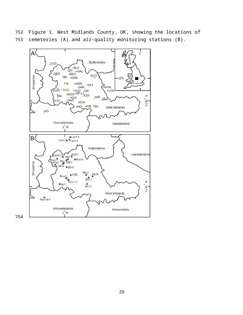
Figure 11. Predicted SO2 and smoke concentrations based on land-use/air quality correlations in Figure 9 for the 1960s through 1980s.

29

582583

584

Table 1. List of cemeteries visited during this investigation. Locations are given in UTM Zone 30. Gravestone decay vs. age for each cemetery was fitted with a non-linear polynomial regression and the equation and R2 value are tabulated. For each decade 1960-2010 mean decay rates were calculated at the derivative of the regression equation for the midpoint year and are given in m/yr.

30

585

586587588589590

591

592

Table2. Name and location of air-quality monitoring stations active within the study area, their location (UTM), and period of record.

31

593594

595

596

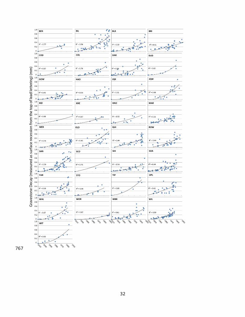
Table 3.Results of optimization of parameters, radius, residential land-use indicator, and inverse distance weighting (IDW) power. Maximum values in bold.

Radius 1960s 1970s 1980s 1990s 2000s

300 0.02 0.01 0.01 0.00 0.02

3000 0.19 0.20 0.19 0.12 0.01

7000 0.33 0.37 0.38 0.28 0.05

8000 0.28 0.33 0.38 0.33 0.10

10000 0.22 0.27 0.34 0.34 0.14

Land Use 1960s 1970s 1980s 1990s 2000s

1.0 0.24 0.28 0.34 0.31 0.12

0.8 0.32 0.35 0.41 0.32 0.12

0.6 0.35 0.40 0.43 0.33 0.11

0.4 0.40 0.44 0.45 0.36 0.10

0.2 0.46 0.50 0.49 0.44 0.11

0.0 0.55 0.57 0.53 0.35 0.07

IDW 1960s 1970s 1980s 1990s 2000s

2.00 0.00 0.00 0.00 0.01 0.03

1.50 0.00 0.00 0.00 0.01 0.03

1.00 0.00 0.00 0.00 0.01 0.03

0.50 0.02 0.02 0.01 0.00 0.01

0.40 0.17 0.18 0.16 0.09 0.00

0.25 0.33 0.36 0.37 0.26 0.04

0.00 0.33 0.37 0.39 0.29 0.06

32

Radius

Residential Land-use

IDW Power

597598

599

600

601

602

Table 4. Correlation coefficients for land-use using the point-density calculation vs. average decadal gravestone stone decay rate for radii of 4000 – 12000 m. Maximum values in bold/italic

Residential Value 0.2Resid.

Ind. Radius 1960s 1970s 1980s 1990s 2000s0.2 4000 0.45 0.48 0.47 0.32 0.060.2 6000 0.56 0.60 0.59 0.40 0.070.2 7000 0.53 0.58 0.59 0.43 0.100.2 8000 0.45 0.51 0.55 0.44 0.120.2 10000 0.37 0.44 0.49 0.43 0.140.2 12000 0.34 0.42 0.48 0.42 0.14

Residential Value 0.00.0 4000 0.45 0.45 0.40 0.23 0.020.0 6000 0.65 0.66 0.60 0.34 0.030.0 7000 0.65 0.68 0.65 0.41 0.060.0 8000 0.52 0.58 0.60 0.45 0.100.0 10000 0.38 0.44 0.48 0.41 0.140.0 12000 0.33 0.40 0.46 0.40 0.14

33

603604

605

606

607

Table 5. Correlation coefficients for gravestone decay and land use for each directional search window. Maximum values in bold/italic with near maximum values in grey.

Azimuth 1960s 1970s 1980s 1990s 2000s

0 0.01 0.02 0.05 0.12 0.1445 0.00 0.00 0.00 0.01 0.0590 0.13 0.14 0.14 0.12 0.04

135 0.39 0.38 0.33 0.16 0.00180 0.33 0.26 0.14 0.01 0.06225 0.31 0.27 0.18 0.03 0.03270 0.32 0.39 0.44 0.34 0.06315 0.15 0.23 0.33 0.39 0.19

0 0.10 0.16 0.26 0.33 0.2045 0.00 0.00 0.01 0.04 0.09

135 0.45 0.41 0.29 0.09 0.01135 0.15 0.15 0.14 0.11 0.03225 0.31 0.27 0.18 0.03 0.03270 0.36 0.44 0.51 0.41 0.09

0 0.08 0.12 0.19 0.27 0.2045 0.12 0.13 0.15 0.15 0.08

135 0.35 0.31 0.23 0.09 0.00180 0.52 0.49 0.37 0.13 0.01225 0.46 0.49 0.45 0.24 0.01315 0.29 0.37 0.46 0.43 0.14

34

608609

610

611

612

613

614

Table 6. Mean decadal SO2 and smoke concentrations (g/m3) for 23 air-quality monitoring stations in the study area. Interpolated land-use indicator determined by point-density function.

Land Use 1960s 1970s 1980s

site_name Indicator SO2Smoke SO2

Smoke SO2

Smoke

BILSTON 3 0.56 99.00128.0

0 -  - - -BILSTON 18 0.55 -  - 64.50 29.00 40.67 25.00BILSTON 19 0.64 -  - - - 42.60 15.60

BIRMINGHAM 11 0.55277.3

3131.1

7 - - - -

BIRMINGHAM 13 0.46202.4

0125.2

0 - -  - -

BIRMINGHAM 21 0.55 - -101.8

6 27.57 75.00 22.67

BIRMINGHAM 26 0.52 - -100.0

0 28.60 46.50 15.30

CANNOCK 15 0.07103.5

0103.5

0 - - - -CANNOCK 17 0.07 - - 88.33 65.50 54.13 50.88CANNOCK 18 0.06 - - - - - -

KIDDERMINSTER 3 0.07167.3

3112.7

5 -  -  - -KIDDERMINSTER 4 0.06 60.00 60.00 47.14 14.86  - -KIDDERMINSTER 5 0.07 - - 72.00 13.00  -  -

OLDBURY 5 0.50127.7

1 94.29108.7

0 37.90116.0

0 25.67

ROWLEY REGIS 1 0.46126.3

3 64.00 86.80 44.40 -  -ROWLEY REGIS 2 0.46 - - 58.80 22.00 63.33 14.67ROWLEY REGIS 3 0.50 - - - - - -

STOURBRIDGE 1 0.24115.3

3 84.00 82.13 34.44 66.00 24.33

WALSALL 13 0.33155.5

0111.6

3 78.60 50.00 44.22 26.78WALSALL 18 0.32 -  - 81.33 29.33 46.44 21.56

WEDNESFIELD 1 0.43117.5

0117.5

0 79.00 46.20 81.00 30.00WEDNESFIELD 2 0.43 - - - - 44.75 15.38

WILLENHALL 1 0.52159.6

7132.7

5 - - - -

WILLENHALL 15 0.53 -  -113.4

0 42.70 52.50 26.00WOLVERHAMPTON 3 0.33

118.71

109.43 85.50 43.90  - -

WOLVERHAMPTO 0.33 102.6 85.00 54.83 23.33 52.63 13.38

35

615616617

N 7 7

36

618

619

620