Web page: Textbook. Abbott and Dayan. Homework and grades Office Hours.

• Web page:

http://www.bcs.rochester.edu/people/alex/bcs547

• Textbook. Abbott and Dayan.

• Homework and grades

• Office Hours

BCS547

Neural Encoding

Computational Neuroscience

• Goal:

• to uncover the general principles of computation and representation in the brain and to understand their neural implementations

• First step: characterizing the neural code

Encoding and decoding

• Encoding: how do neurons encode information

• Crucial issue if we want to decode neural activity

What’s a code? Example

Deterministic code:

A ->10

B -> 01

If you see the string 01, recovering the encoded letter (B) is easy.

What’s a code? Example

Deterministic code:

A ->10

B -> 01

If you see the string 01, recovering the encoded letter (B) is easy.

Noise and coding

Two of the hardest problems with coding come from:

1. Non invertible codes (e.g., two symbols get mapped onto the same code)

2. Noise

Example

Noisy code:A -> 01 with p=0.8

-> 10 with p=0.2B -> 01 with p=0.3

-> 10 with p=0.7

Now, given the string 01, it’s no longer obvious what the encoded letter is…

What types of codes and noises are found in the nervous system?

• Population codes

Receptive field

sDirection of motion

Stimulus

Response

Code: number of spikes10

Receptive field

sDirection of motion

Trial 1

Stimulus

Trial 2

Trial 3

Trial 4

10

7

8

4

The ‘tuning curve plus noise’ model of neural responses

• Population codes

Variance of the noise, i()2

Encoded variable (s)

Mean activity fi()

Variance, i(s)2, can depend on the input

Tuning curve fi(s)

Tuning curves and noise

Example of tuning curves:

Retinal location, orientation, depth, color, eye movements, arm movements, numbers… etc.

Tuning curves and noise

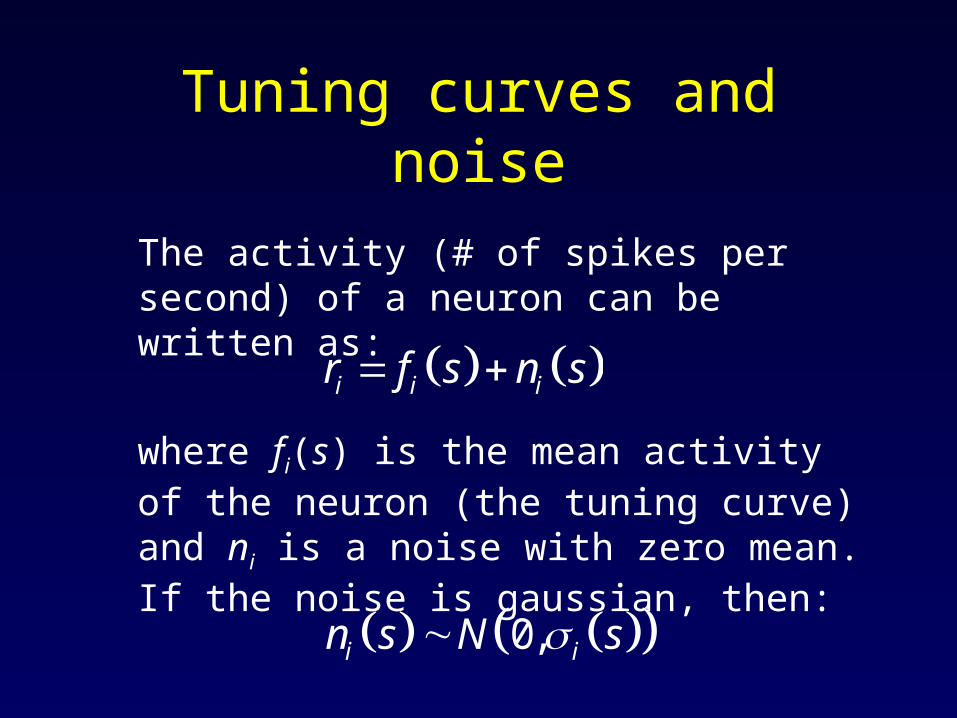
The activity (# of spikes per second) of a neuron can be written as:

where fi(s) is the mean activity of the neuron (the tuning curve) and ni is a noise with zero mean. If the noise is gaussian, then:

i i ir f s n s

0,i in s N s

Probability distributions and activity

• The noise is a random variable which can be characterized by a conditional probability distribution, P(ni|s).

• Since the activity of a neuron i, ri, is the sum of a deterministic term, fi(s), and the noise, it is also a random variable with a conditional probability distribution, p(ri| s).

• The distributions of the activity and the noise differ only by their means (E[ni]=0, E[ri]=fi(s)).

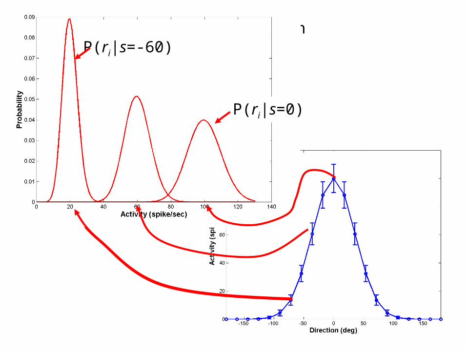
Activity distribution

P(ri|s=-60)

P(ri|s=0)

P(ri|s=-60)

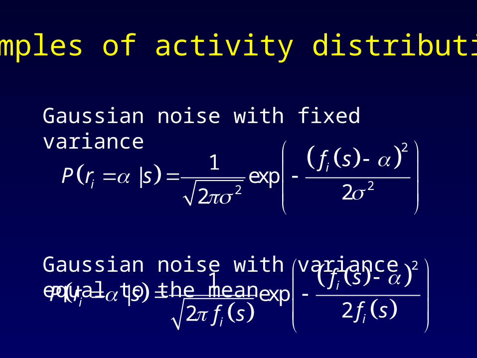
Gaussian noise with fixed variance

Gaussian noise with variance equal to the mean

Examples of activity distributions

222

1| exp

22

ii

f sP r s

2

1| exp

22

ii

ii

f sP r s

f sf s

Poisson activity (or noise):

The Poisson distribution works only for discrete random variables. However, the mean, fi(s), does not have to be an integer.

The variance of a Poisson distribution is equal to its mean.

f

|!

iks

ii

e f sP r k s

k

Comparison of Poisson vs Gaussian noise with variance equal to the mean

0 20 40 60 80 100 120 1400

0.01

0.02

0.03

0.04

0.05

0.06

0.07

0.08

0.09

Activity (spike/sec)

Pro

bab

ilit

y

Poisson noise and renewal process

Imagine the following process: we bin time into small intervals, t. Then, for each interval, we toss a coin with probability, P(head) =p. If we get a head, we record a spike.

For small p, the number of spikes per second follows a Poisson distribution with mean p/t spikes/second (e.g., p=0.01, t=1ms, mean=10 spikes/sec).

Properties of a Poisson process

• The number of events follows a Poisson distribution (in particular the variance should be equal to the mean)

• A Poisson process does not care about the past, i.e., at a given time step, the outcome of the coin toss is independent of the past (renewal process).

• As a result, the inter-event intervals follow an exponential distribution (Caution: this is not a good marker of a Poisson process)

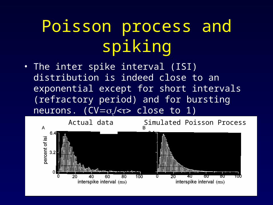
Poisson process and spiking

• The inter spike interval (ISI) distribution is indeed close to an exponential except for short intervals (refractory period) and for bursting neurons. (CV close to 1)

Actual data Simulated Poisson Process

Poisson process and spiking

• The variance in the spike count is proportional to the mean but the the constant of proportionality can be higher than 1 and the variance can be an polynomial function of the mean. Log = Log a +log

Poisson model

Open Questions

• Is this Poisson variability really noise? (unresolved, yet critical, question for neural coding…)

• Where could it come from?

Non-Answers

• It’s probably not in the sensory inputs (e.g. shot noise)

• It’s not the spike initiation mechanism (Mainen and Sejnowski)

• It’s not the stochastic nature of ionic channels

• It’s probably not the unreliable synapses

Possible Answers

• Neurons embedded in a recurrent network with sparse connectivity tend to fire with statistics close to Poisson (Van Vreeswick and Sompolinski, Brunel, Banerjee)

• Random walk model (Shadlen and Newsome; Troyer and Miller)

Possible Answers

• Random walk model: for a given input, the output is always the same, i.e., this model is deterministic

• However, large network are probably chaotic. Small differences in the input result in large differences in the output.

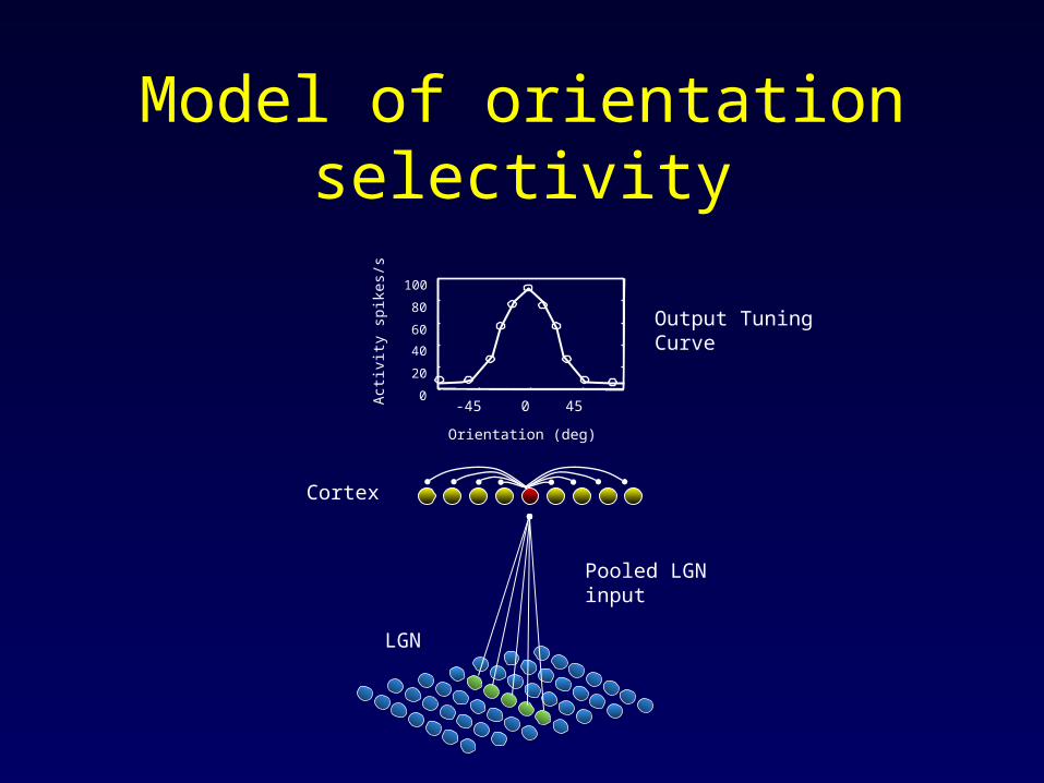
Model of orientation selectivity

Pooled LGN input

Output Tuning Curve

LGN

Cortex

Orientation (deg)

-45 0 450

20

40

60

80

100

Act

ivity

spi

kes/

s

Problems with the random walk model

• The ratio variance over mean is still smaller than the one measured in vivo (0.8)

• It’s unstable over several layers! (this is likely to be a problem for any mechanisms…)

• Noise injection in real neurons fails to produce the predicted variability (Stevens, Zador)

Other sources of noise and uncertainty

• Physical noise in the stimulus• Noise from other areas (why would the nervous

system inject independent white noise in all neurons????)

• If the variability is not noise it may be used to represent the uncertainty inherent to the stimulus (e.g. the aperture problem).

Beyond tuning curves

• Tuning curves are often non invariant under stimulus changes (e.g. motion tuning curves for blobs vs bars)

• Deal poorly with time varying stimulus• Assume a rate code • Assume that you know what s is…

An alternative: information theoryAn alternative: information theory

Information Theory(Shannon)

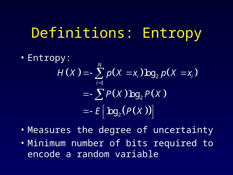
Definitions: Entropy

• Entropy:

• Measures the degree of uncertainty

• Minimum number of bits required to encode a random variable

21

2

2

log

log

log

N

i ii

H X p X x p X x

P X P X

E P X

P(X=1) = pP(X=0) = 1- p

0 0.1 0.2 0.3 0.4 0.5 0.6 0.7 0.8 0.9 10

0.1

0.2

0.3

0.4

0.5

0.6

0.7

0.8

0.9

1

Probability (p)

En

tro

py

(bit

s)

What is the most efficient way to encode a set of signals with binary strings?

• Ex: AADBBAACACBAAAABADBCA…• P(A) = 0.5, P(B)=0.25, P(C)=0.125, P(D)=0.125• 1st Solution: A-> 111, B->110, C->10,D->0• Unambiguous code:

101011111111011011110011101011011110 10 111 111 110 110 111 10 0 111 0 10 110 111C C A A B B A C D A D C B A

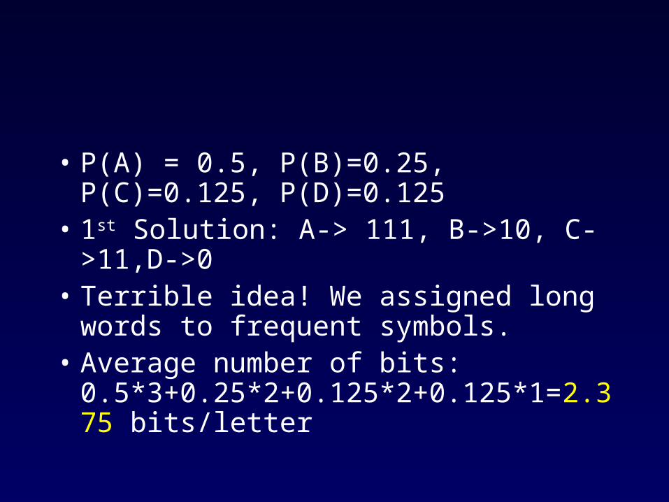
• P(A) = 0.5, P(B)=0.25, P(C)=0.125, P(D)=0.125

• 1st Solution: A-> 111, B->10, C->11,D->0• Terrible idea! We assigned long words to

frequent symbols.• Average number of bits:

0.5*3+0.25*2+0.125*2+0.125*1=2.375 bits/letter

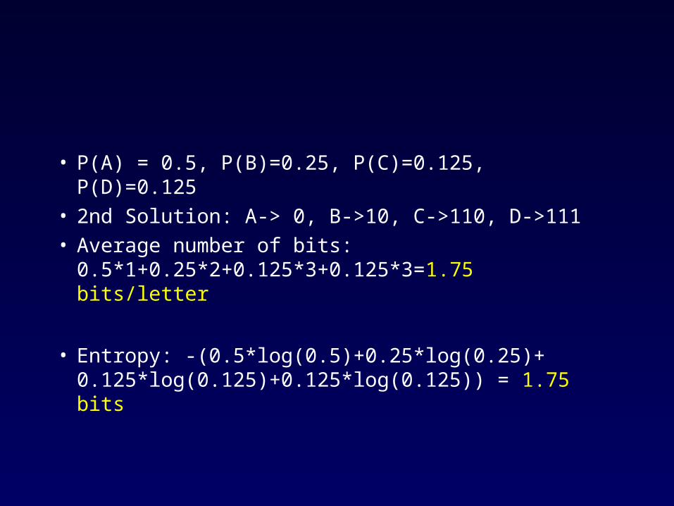
• P(A) = 0.5, P(B)=0.25, P(C)=0.125, P(D)=0.125• 2nd Solution: A-> 0, B->10, C->110, D->111• Average number of bits:

0.5*1+0.25*2+0.125*3+0.125*3=1.75 bits/letter

• Entropy: -(0.5*log(0.5)+0.25*log(0.25)+ 0.125*log(0.125)+0.125*log(0.125)) = 1.75 bits

• Maximum entropy is achieved for flat probability distributions, i.e., for distributions in which events are equally likely.

• For a given variance, the normal distribution is the one with maximum entropy

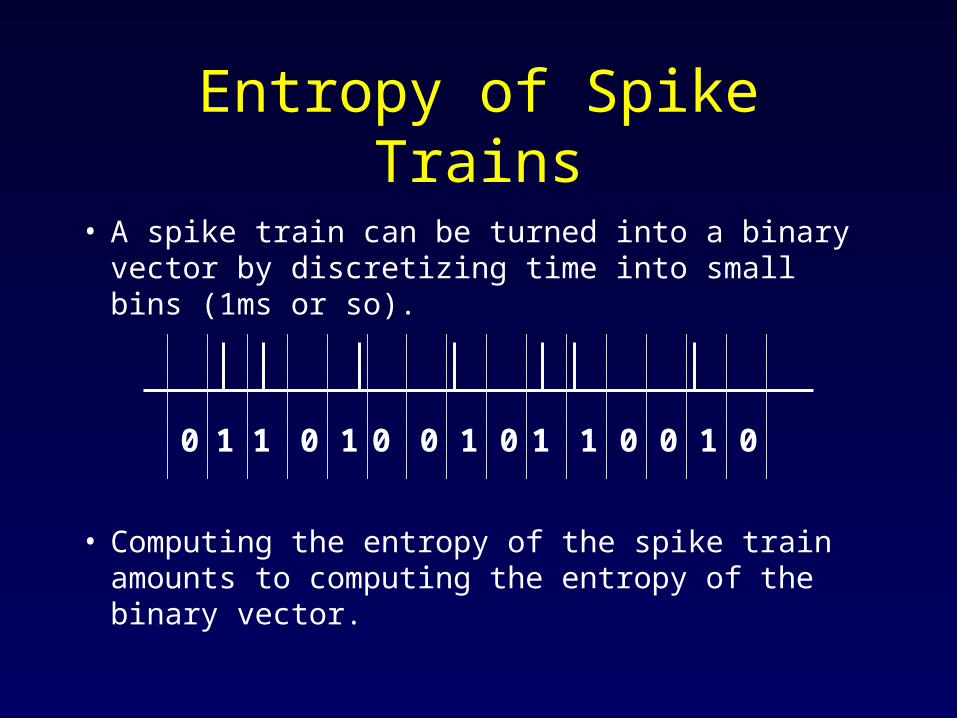
Entropy of Spike Trains

• A spike train can be turned into a binary vector by discretizing time into small bins (1ms or so).

• Computing the entropy of the spike train amounts to computing the entropy of the binary vector.

1 1 1 1 1 1 10 0 0 0 0 0 0 0

Definition: Conditional Entropy

• Conditional entropy:

• Uncertainty due to noise: How uncertain is X knowing Y?

21 1

2

| | log |

, log |

M N

j i j i jj i

H X Y P Y y P X x Y y P X x Y y

P X Y P X Y

Example

H(Y|X) is equal to zero if the mapping from X to Y is deterministic and many to one.

Ex: Y = X for odd X

Y= X+1 for even X

• X=1, Y is equal to 1. H(Y|X=1)=0• Y=3, X is either 2 or 3. H(X|Y=3)>0

Y 1234567…

X 1234567…

Example

In general, H(X|Y)H(Y|X), except for an invertible and deterministic mapping, in which case H(X|Y)=H(Y|X)=0

Ex: Y= X+1 for all X

• Y=2, X is equal to 1. H(X|Y)=0• X=1, Y is equal to 2. H(Y|X)=0

Y 1234567…

X 1234567…

Example

If r=f(s)+noise, H(r|s) and H(s|r) are strictly greater than zero

Knowing the firing rate does not tell you for sure what the stimulus is, H(s|r)>0.

Definition: Joint Entropy

• Joint entropy

, , log ,

( ) ( | )

|

H X Y P X Y P X Y

H Y H X Y

H X H Y X

Independent Variables

• If X and Y are independent, then knowing Y tells you nothing about X. In other words, knowing Y does not reduce the uncertainty about X, i.e., H(X)=H(X|Y). It follows that:

, ( ) ( | )H X Y H X H Y X

H X H Y

Entropy of Spike Trains

• For a given firing rate, the maximum entropy is achieved by a Poisson process because it generates the most unpredictable sequence of spikes .

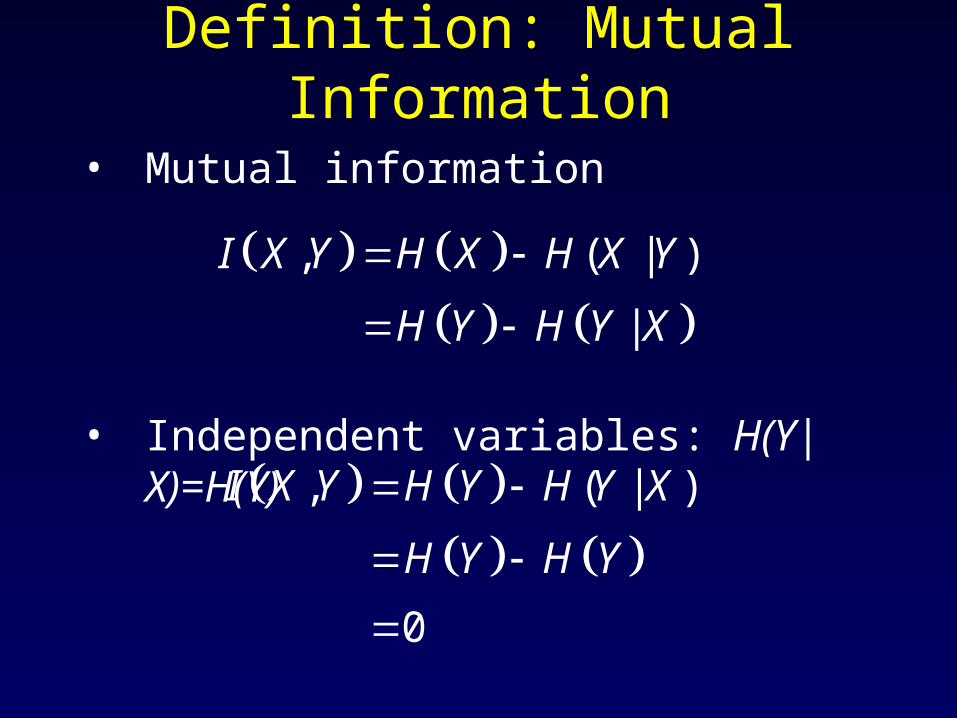
Definition: Mutual Information

• Mutual information

• Independent variables: H(Y|X)=H(Y)

, ( | )

|

I X Y H X H X Y

H Y H Y X

, ( | )

0

I X Y H Y H Y X

H Y H Y

Definition: Mutual Information

• Mutual information: one to many deterministic mapping

• Mutual information is bounded above by the entropy of the variables.

, ( | )I X Y H X H X Y

H X

Data Processing Inequality

• X->Y->Z

• You can’t increase information through processing

, ,I X Y I X Z

Information and independence

• Unfortunately, the information from two variables that are conditionally independent does not sum…

1 2 1 2, , , , ?I X X Y I X Y I X Y

1 2 1 2, , | ,I X X Y H Y H Y X X

If x1 tells us everything we need to know about y, adding x2 tells you nothing more

Definitions: KL distance

• KL distance:

• Always positive• Not symmetric: KL(P|Q) KL(Q|P)• Number of extra bits required to transmit a

random variable when estimating the probability to be Q when in fact it is P.

( | ) logP X

KL P Q P XQ X

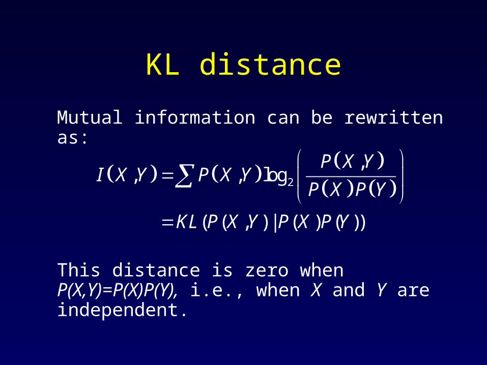
KL distance

Mutual information can be rewritten as:

This distance is zero when P(X,Y)=P(X)P(Y), i.e., when X and Y are independent.

2

,, , log

( ( , ) | ( ) ( ))

P X YI X Y P X Y

P X P Y

KL P X Y P X P Y

Measuring entropy from data

Consider a population of 100 neurons firing for 100ms with 1 ms time bins. Each data point is a 100x100 binary vector. The number of possible data point is 2100x100. To compute the entropy we need to estimate a probability distribution over all these states…Hopeless?…

Direct Method

• Fortunately, in general, only a fraction of all possible states actually occurs

• Direct method: evaluate p(r) and p(r|s) directly from the the data. Still require tons of data… In practice, this works for 1, maybe 2 neurons, but rarely for 3 and above.

Upper Bound

• Assume all distributions are gaussian• Recover SNR in the Fourier domain using simple

averaging• Compute information from the SNR • No need to recover the full p(r) and p(r|s) because

gaussian distributions are fully characterized by their means and variances, although you still have to estimate N2 covariances..

Lower Bound

• Estimate a variable from the neuronal responses and compute the mutual information between the estimate and the stimulus (easy if the estimate follows a gaussian distribution)

• The data processing inequality guarantees that this is a lower bound on information.

• It gives an idea of how well the estimated variable is encoded.

Mutual information in spikes

• Among temporal processes, Poisson processes are the ones with highest entropy because time bins are independent from one another. The entropy of a Poisson spike train vector is the sum of the individual time bins, which is best you can achieve.

Mutual information in spikes

• A deterministic Poisson process is the best way to transmit information with spikes

• Spike trains are indeed close to Poisson BUT they are not deterministic, i.e., they vary from trial to trial even for a fixed input.

• Even worse, the conditional entropy is huge because the noise follows a Poisson distribution

The choice of stimulus

• Neurons are known to be selective to particular features.

• In information theory terms, this means that two sets of stimuli with the same entropy do not necessarily lead to the same mutual information with the firing rates.

• Natural stimuli often lead to larger mutual information (which makes sense since they are more likely)

Animal system Method Bits per second Bits per spike High-freq. cutoff(Neuron) (efficiency) or limiting spikeStimulus timingFly visual10 Lower 64 1 2 ms(H1)Motion

Fly visual15 Direct 81 — 0.7 ms(H1)Motion

Fly visual37 Lower and 36 — —(HS, graded potential) upperMotion 104

Monkey visual16 Lower and 5.5 0.6 100 ms(area MT) directMotion 12 1.5

Frog auditory38 Lower Noise 46 Noise 1.4 750 Hz(Auditory nerve) Call 133 ( 20%)Noise and call Call 7.8 ( 90%)

Salamander visual50 Lower 3.2 1.6 (22%) 10 Hz(Ganglion cells)Random spots

Cricket cercal40 Lower 294 3.2 > 500 Hz(Sensory afferent) ( 50%)Mechanical motion

Cricket cercal51 Lower 75–220 0.6–3.1 500–1000 Hz(Sensory afferent)Wind noise

Cricket cercal11,38 Lower 8–80 Avg = 1 100–400 Hz(10-2 and 10-3)Wind noise

Electric fish12 Absolute 0–200 0–1.2 ( 50%) 200 Hz(P-afferent) lowerAmplitude modulation

Comparison natural vs artificial stimulus

Low in cortex

Information Theory: Pro

• Assumption free: does not assume any particular code

• Read-out free: does not depend on a read-out method (direct method)

• It can be used to identify the features best encoded by a neuron

Information theory: Con’s

• Does not tell you how to read out the code: the code might be unreadable by the rest of the nervous system.

• In general, it’s hard to relate Shanon information to behavior

• Hard to use for continuous variables• Data intensive: needs TONS of data (don’t

even think about it for more than 3 neurons)