Weak and Strong Taylor methods for approximative solutions of SDEs

Weak and Strong Taylor methods forapproximative solutions of SDEs

Maria Siopacha, Josef TeichmannResearch Group of Financial and Actuarial Mathematics

TU Vienna

Second AMaMeF and Banach Center Conference, Bedlewo, Poland

May 4, 2007

Outline of the Talk

• Description of the problem and the method;

• A motivating example;

• The general setting: basic Definitions and Theorems;

• Applications and examples to Interest Rate Theory: the LIBORmarket model, the frozen drift and models with stochasticvolatility.

1

Motivation and Basic Ideas

• European-option prices with underlying assets driven by parameter-dependent equations;

• Analytically tractable formulas available only for particularparameter values;

• Idea: Taylor expansions of expectation functionals around theseknown values;

• Tools: Malliavin calculus and integration-by-parts on the Wienerspace when distribution is unknown;

• Results: Strong and weak Taylor expansions of option prices;Tractable pricing formulas on parameter intervals.

2

The Model and the Problem

Design SDEs smoothly dependent on a parameter a ∈ R:

dXx,at = V (Xx,a

t )dt +d∑

i=1

Vi(Xx,at )dW i

t , Xx,a0 = x ∈ RN . (1)

For a = 0, model reduces to a well-known one, e.g. Black andScholes.

For a 6= 0 there might be no analytically tractable formulas.

Efficiently approximate the expectation functional, f expressespayoff-profile:

ua(T, x) := E(f(Xx,aT )).

3

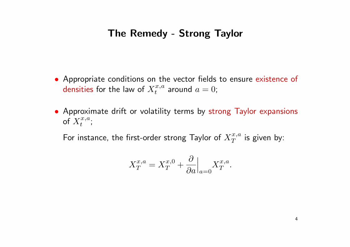
The Remedy - Strong Taylor

• Appropriate conditions on the vector fields to ensure existence ofdensities for the law of Xx,a

t around a = 0;

• Approximate drift or volatility terms by strong Taylor expansionsof Xx,a

t ;

For instance, the first-order strong Taylor of Xx,aT is given by:

Xx,aT = Xx,0

T +∂

∂a

∣∣∣a=0

Xx,aT .

4

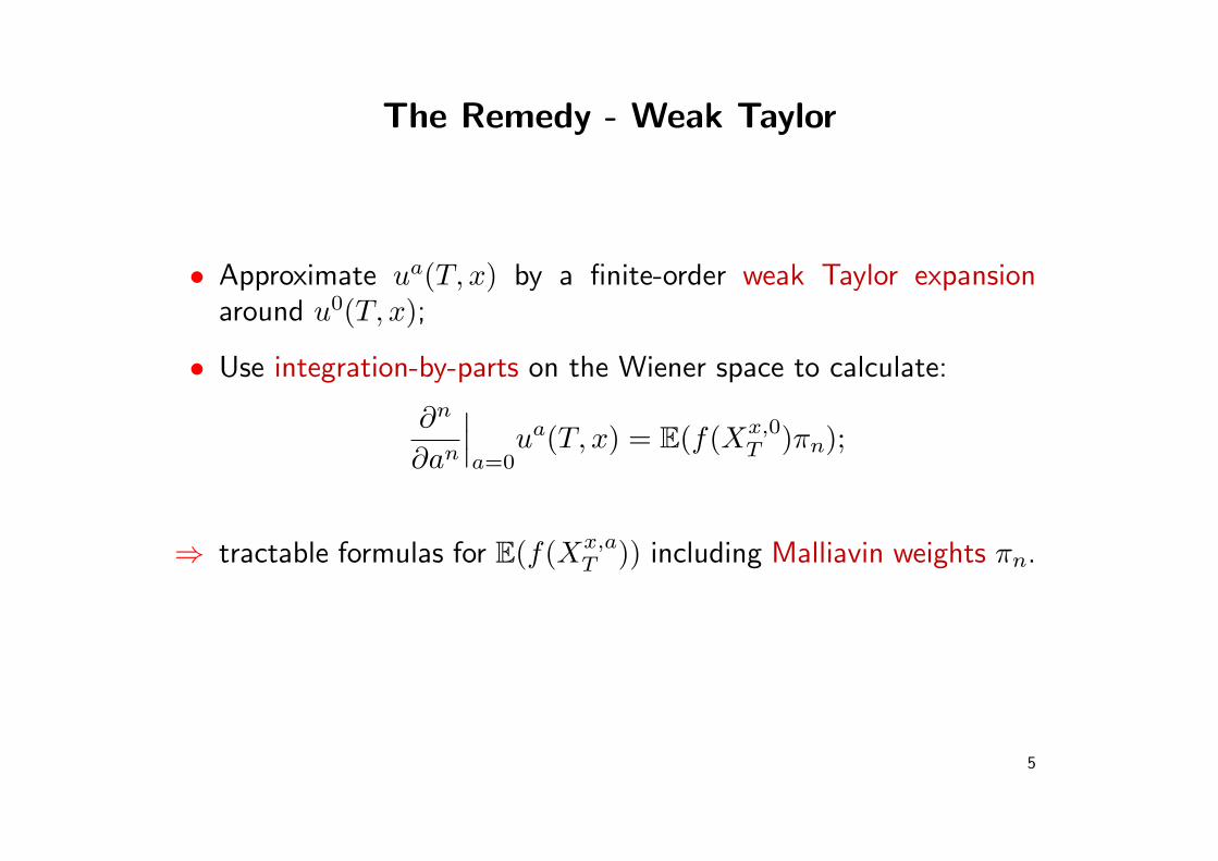
The Remedy - Weak Taylor

• Approximate ua(T, x) by a finite-order weak Taylor expansionaround u0(T, x);

• Use integration-by-parts on the Wiener space to calculate:

∂n

∂an

∣∣∣a=0

ua(T, x) = E(f(Xx,0T )πn);

⇒ tractable formulas for E(f(Xx,aT )) including Malliavin weights πn.

5

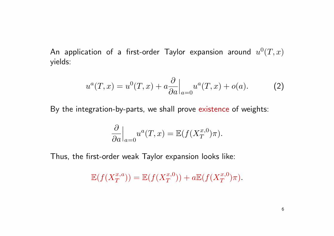
An application of a first-order Taylor expansion around u0(T, x)yields:

ua(T, x) = u0(T, x) + a∂

∂a

∣∣∣a=0

ua(T, x) + o(a). (2)

By the integration-by-parts, we shall prove existence of weights:

∂

∂a

∣∣∣a=0

ua(T, x) = E(f(Xx,0T )π).

Thus, the first-order weak Taylor expansion looks like:

E(f(Xx,aT )) = E(f(Xx,0

T )) + aE(f(Xx,0T )π).

6

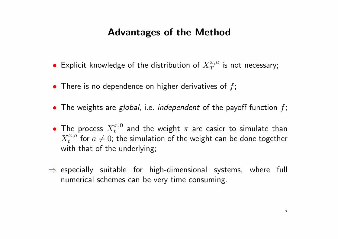
Advantages of the Method

• Explicit knowledge of the distribution of Xx,aT is not necessary;

• There is no dependence on higher derivatives of f ;

• The weights are global, i.e. independent of the payoff function f ;

• The process Xx,0t and the weight π are easier to simulate than

Xx,at for a 6= 0; the simulation of the weight can be done together

with that of the underlying;

⇒ especially suitable for high-dimensional systems, where fullnumerical schemes can be very time consuming.

7

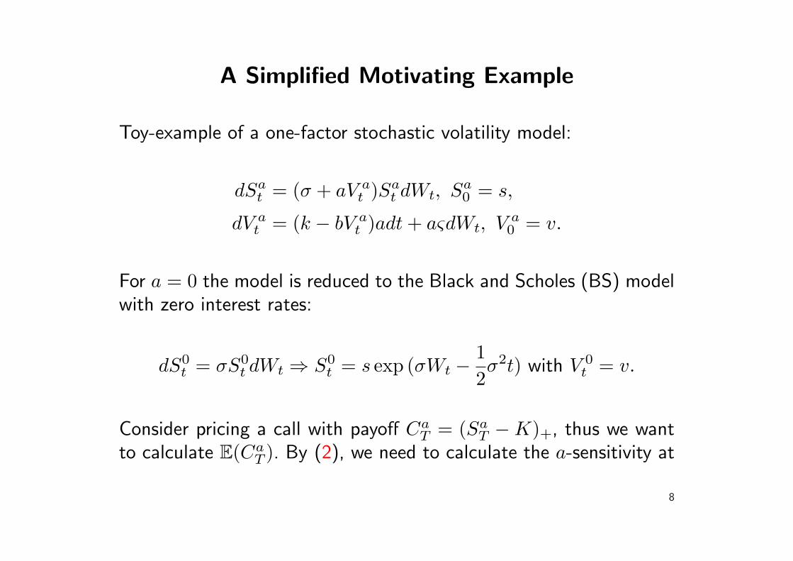
A Simplified Motivating Example

Toy-example of a one-factor stochastic volatility model:

dSat = (σ + aV a

t )Sat dWt, Sa

0 = s,

dV at = (k − bV a

t )adt + aςdWt, V a0 = v.

For a = 0 the model is reduced to the Black and Scholes (BS) modelwith zero interest rates:

dS0t = σS0

t dWt ⇒ S0t = s exp (σWt −

12σ2t) with V 0

t = v.

Consider pricing a call with payoff CaT = (Sa

T −K)+, thus we wantto calculate E(Ca

T ). By (2), we need to calculate the a-sensitivity at

8

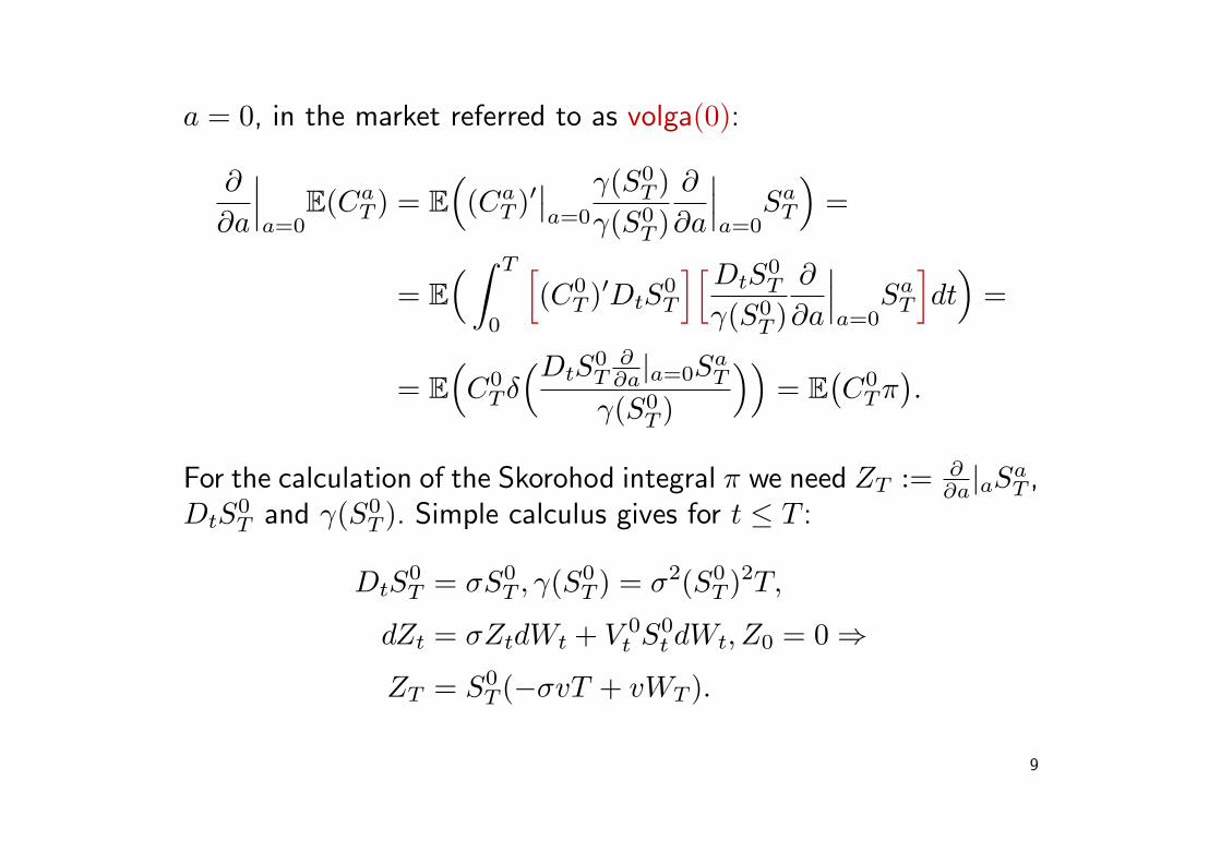
a = 0, in the market referred to as volga(0):

∂

∂a

∣∣∣a=0

E(CaT ) = E

((Ca

T )′∣∣a=0

γ(S0T )

γ(S0T )

∂

∂a

∣∣∣a=0

SaT

)=

= E( ∫ T

0

[(C0

T )′DtS0T

][DtS0T

γ(S0T )

∂

∂a

∣∣∣a=0

SaT

]dt

)=

= E(C0

Tδ(DtS

0T

∂∂a|a=0S

aT

γ(S0T )

))= E

(C0

Tπ).

For the calculation of the Skorohod integral π we need ZT := ∂∂a|aS

aT ,

DtS0T and γ(S0

T ). Simple calculus gives for t ≤ T :

DtS0T = σS0

T , γ(S0T ) = σ2(S0

T )2T,

dZt = σZtdWt + V 0t S0

t dWt, Z0 = 0 ⇒

ZT = S0T (−σvT + vWT ).

9

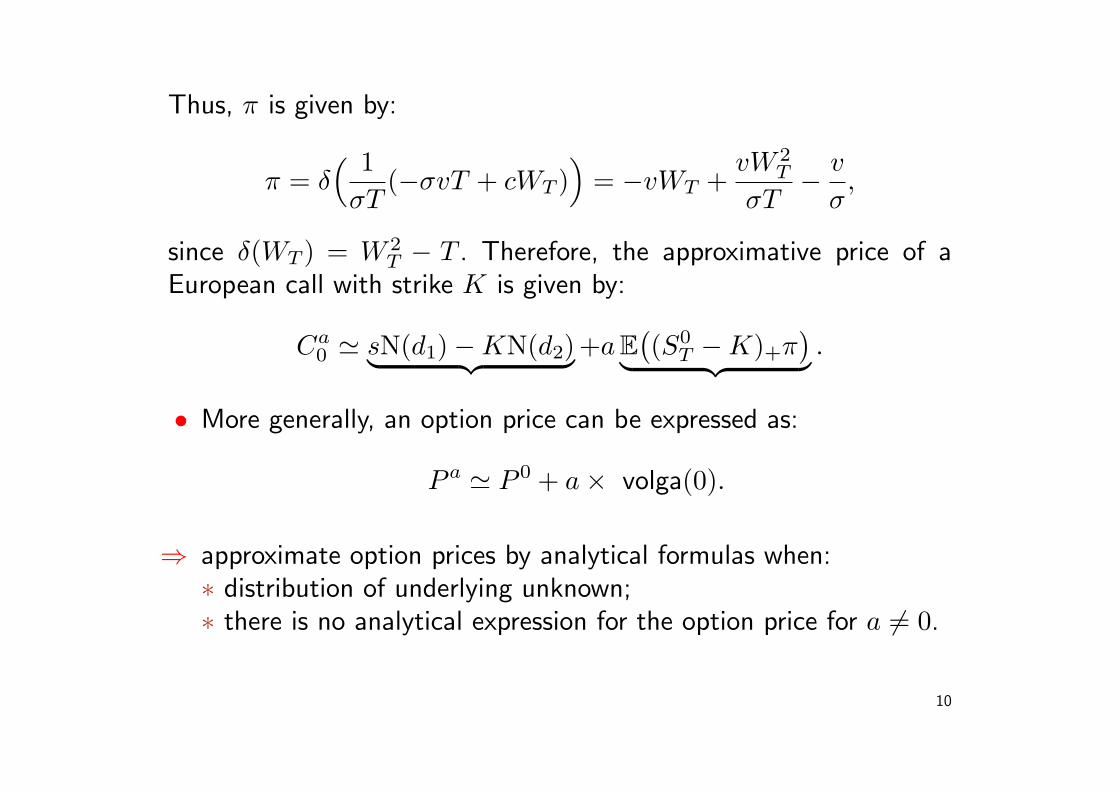
Thus, π is given by:

π = δ( 1σT

(−σvT + cWT ))

= −vWT +vW 2

T

σT− v

σ,

since δ(WT ) = W 2T − T . Therefore, the approximative price of a

European call with strike K is given by:

Ca0 ' sN(d1)−KN(d2)︸ ︷︷ ︸ +a E

((S0

T −K)+π)︸ ︷︷ ︸ .

• More generally, an option price can be expressed as:

P a ' P 0 + a× volga(0).

⇒ approximate option prices by analytical formulas when:∗ distribution of underlying unknown;∗ there is no analytical expression for the option price for a 6= 0.

10

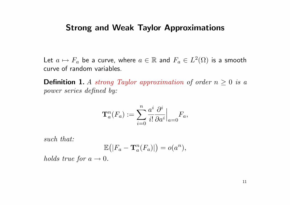
Strong and Weak Taylor Approximations

Let a 7→ Fa be a curve, where a ∈ R and Fa ∈ L2(Ω) is a smoothcurve of random variables.

Definition 1. A strong Taylor approximation of order n ≥ 0 is apower series defined by:

Tna(Fa) :=

n∑i=0

ai

i!∂i

∂ai

∣∣∣a=0

Fa,

such that:E

(|Fa −Tn

a(Fa)|)

= o(an),

holds true for a → 0.

11

Definition 2. A weak Taylor approximation of order n ≥ 0 is apower series, for each bounded measurable f : RN → R defined by:

Wna(f, Fa) :=

n∑i=0

ai

i!E(f(F0)πi), (3)

where πi ∈ L1(Ω) denote real valued, integrable random variables,such that:

|E(f(Fa)

)−Wn

a(f, Fa)| = o(an).

The random variable πi, for i ≥ 1, is called the ith-order Malliavinweight.

12

Existence of Weights Theorem...

Theorem 3. Let Fa be smooth and assume that the Malliavincovariance matrix γ(Fa) is invertible in an open interval arounda = 0. Then there is a weak Taylor approximation of any ordern ≥ 0.

Idea of the proof. We can prove the formula:

d

daE(f(Fa)) = E

(f(Fa)δ

((dFa

da

)T(γ−1(Fa))TDtFa

)). (4)

Make the following notation:

π1 := δ((dFa

da

)T(γ−1(Fa))TDtFa

). (5)

13

The general result for the nth-order weight is obtained by recursionof (4) and differentiation of the Skorohod integral:

vt :=(dFa

da

)T(γ−1(Fa))TDtFa, for 0 ≤ t ≤ T,

πn := δ(vtπn−1) +d

daπn−1, π0 := 1.

Remark 4. If γ(Fa) invertible only for a = 0, the Malliavin weightsare still calculable, since they depend on γ(F0); thus assumption ofinvertibility only necessary at a = 0.

14

... and Option Prices

Theorem 5. Assume that d ≤ N and that the vector fields in (1)written in Stratonovich formulation satisfy condition (H) at a = 0.Then the price of an option E(f(Xx,a

T )) is given by the first-orderweak Taylor approximation:

W1a(f,Xx,a

T ) ' E(f(Xx,0T )) + aE(f(Xx,0

T )π1).

Idea of the proof. From Theorem 3, there exists a first-order weakTaylor approximation, where the first-order weight π1 is given as in(5).

By (3), the result is obtained directly.

15

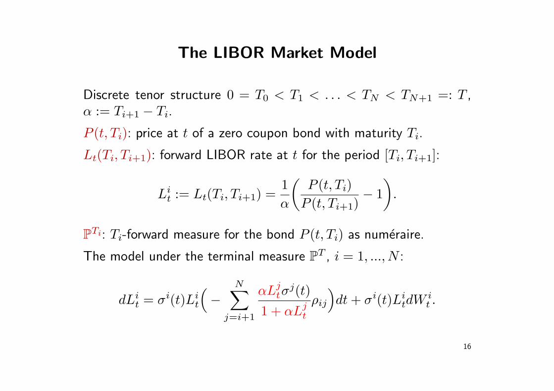
The LIBOR Market Model

Discrete tenor structure 0 = T0 < T1 < . . . < TN < TN+1 =: T ,α := Ti+1 − Ti.

P (t, Ti): price at t of a zero coupon bond with maturity Ti.

Lt(Ti, Ti+1): forward LIBOR rate at t for the period [Ti, Ti+1]:

Lit := Lt(Ti, Ti+1) =

1α

(P (t, Ti)

P (t, Ti+1)− 1

).

PTi: Ti-forward measure for the bond P (t, Ti) as numeraire.

The model under the terminal measure PT , i = 1, ..., N :

dLit = σi(t)Li

t

(−

N∑j=i+1

αLjtσ

j(t)1 + αLj

t

ρij

)dt + σi(t)Li

tdW it .

16

Correcting the Frozen Drift - Strong Taylor

Approximate the random or real drift term by its starting value orfrozen drift:

αLjt

1 + αLjt

≈ αLi0

1 + αLi0

⇒ difference in option prices.

Idea: replace the real drift by its first-order strong Taylorapproximation:

dL(i,ε1)t = σi(t)L(i,ε1)

t

(−

N∑j=i+1

α(T1

ε1(X(j,ε1)

t ))+σj(t)

1 + α(T1

ε1(X(j,ε1)

t ))+

ρijdt+dW it

),

where ε1 ∈ R, dX(i,ε1)t = ε1dL

(i,ε1)t with L

(i,ε1)0 = X

(i,ε1)0 ∀i and ∀ε1,

T1ε1

(X(i,ε1)t ) = X

(i,0)0 + ε1

∂

∂ε1

∣∣ε1=0

X(i,ε1)t .

17

Example 6. Let N = 3, price a caplet on the LIBOR rate L1.

payoff = α((

L1T1−K

)+

),

volatility functions σi(t) =(a(Ti − t) + d

)exp

(− b(Ti − t)

)+ e,

correlations ρij = 0.49 + (1− 0.49) exp (−0.13|i− j|), i, j = 1, 2, 3.

strikes K=3% K=3.5% K=4% K=5.75% K=6.25%price 11.1831 8.5897 6.5503 3.0349 2.4423

strong Taylor 11.0687 8.5691 6.5867 3.1448 2.5513frozen drift 13.9551 11.1822 8.8803 4.6313 3.8506

Table 1: Caplet values in bps for parameters ε1 = 1, α = 0.50137, c1 = 3.86777%,c2 = 3.7574%, c3 = 3.8631% and T1 = 1.53151 and constants a = −0.113035,b = 0.22911, d = −a, e = 0.684784.

⇒ strong Taylor method:• pathwise approximation;

• performs very well; computationally simpler and faster.

18

Correcting Frozen Drift Prices - Weak Taylor

Idea: approximate LIBOR option prices by first-order weak Taylorapproximation.

Example 7. Let N = 3, price a payers swaption, LT1 := (L1T1

, L2T1

).

• Assume existence of γ−1(L0T1

) ⇐⇒ ρ12 6= 1 if ρ23 = 1;

⇒ invertibility of γ(L0T1

) natural assumption.

payoff g(LT1) =(−

∑2k=1 αk

∏2j=k(1 + αLj

T1)− (1 + Kα)

)+,

volatility functions σi(t) := σi, i = 1, 2, 3,

weak Taylor price = W1a(g,Lε1

T1) = E

(g(L0

T1))

+ ε1E(g(L0

T1)ζT1

),

Malliavin weight ζT1 = δ((DtL0

T1)Tγ−1(L0

T1) ∂∂ε1|ε1=0L

ε1T1

)= ζ1

T1+

ζ2T2

.

19

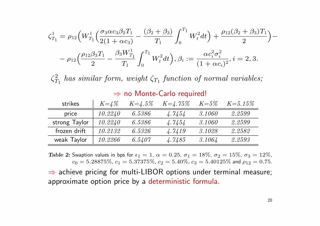
ζ1T1

= ρ12

“W

1T1

“ σ3αc3β2T1

2(1 + αc3)−

(β2 + β3)

T1

Z T1

0

W2t dt

”+

ρ12(β2 + β3)T1

2

”−

− ρ12

“ρ12β3T1

2−

β3W1T1

T1

Z T1

0

W2t dt

”, βi :=

αc2i σ

2i

(1 + αci)2, i = 2, 3.

ζ2T1

has similar form, weight ζT1 function of normal variables;

⇒ no Monte-Carlo required!strikes K=4% K=4.5% K=4.75% K=5% K=5.15%price 10.2240 6.5386 4.7454 3.1060 2.2599

strong Taylor 10.2240 6.5386 4.7454 3.1060 2.2599frozen drift 10.2132 6.5326 4.7419 3.1028 2.2582weak Taylor 10.2266 6.5407 4.7485 3.1064 2.2593

Table 2: Swaption values in bps for ε1 = 1, α = 0.25, σ1 = 18%, σ2 = 15%, σ3 = 12%,c0 = 5.28875%, c1 = 5.37375%, c2 = 5.40%, c3 = 5.40125% and ρ12 = 0.75.

⇒ achieve pricing for multi-LIBOR options under terminal measure;approximate option price by a deterministic formula.

20

The Stochastic Volatility LIBOR Market Model

dL(i,ε1,ε2)t = σi(t)L(i,ε1,ε2)

t

√vε2

t

(−

N∑j=i+1

αX(j,ε1,ε2)t σj(t)

1 + αX(j,ε1,ε2)t

ρij

√vε2

t dt + dW it

),

dvε2t = κ(θ − vε2

t )dt + ε2

√vε2

t

(ρidW i

t +√

1− ρ2idZ

it

).

⇒ no analytic tractability, use the same idea as previously.

Example 8. Let N = 2, price a payers swaption, payoff andvolatility functions as before.

• Assume invertibility of γ(L0,0T1

)⇐⇒ ρ12 6= 1⇒ natural condition.

weak Taylor price =

W1a(g,Lε1,ε2

T1) = E

(g(L0,0

T1))

+ ε1E(g(L0,0

T1)ζT1

)+ ε2E

(g(L0,0

T1)πT1

),

21

Malliavin weightsζT1 = ζ1

T1+ ζ2

T1, πT1 = π1

T1+ π2

T1

⇒ ζ1T1

= −β2ρ12c

“X1Y − Cov(X1, Y )

”, ζ2

T1similar, π1

T1= π1,1

T1− π1,2

T1,

π1,2T1

=ρ122c

“X1(ρ2D2 +

q1 − ρ2

2Z2) +σ1BX1

κ +ρ12B

κ − σ1ρ1e

κ

”with Xi, Y , B normal variables, Di, Zi double stochastic integrals.

strikes K=3.5% K=4% K=5% K=6% K=7%price 3.8984 2.9221 1.2588 0.3858 0.1019

frozen drift and vol 3.8951 2.9053 1.2705 0.3966 0.0942weak Taylor 3.8990 2.9159 1.2694 0.3791 0.1042

Table 3: SV-swaption values in bps for ε1 = 1, α = 1.5, σ1 = 25%, σ2 = 15%,c0 = 5.28875%, c1 = 5.4%, c2 = 5.39%, v0 = 1, ρ1 = −0.75, ρ2 = −0.6,κ = 2.3767, θ = 0.2143, ε2 = 25%, ρ12 = 0.63.

⇒ end up with approximative semi-deterministic pricing formula;weights given by simple Ito integrals!

22

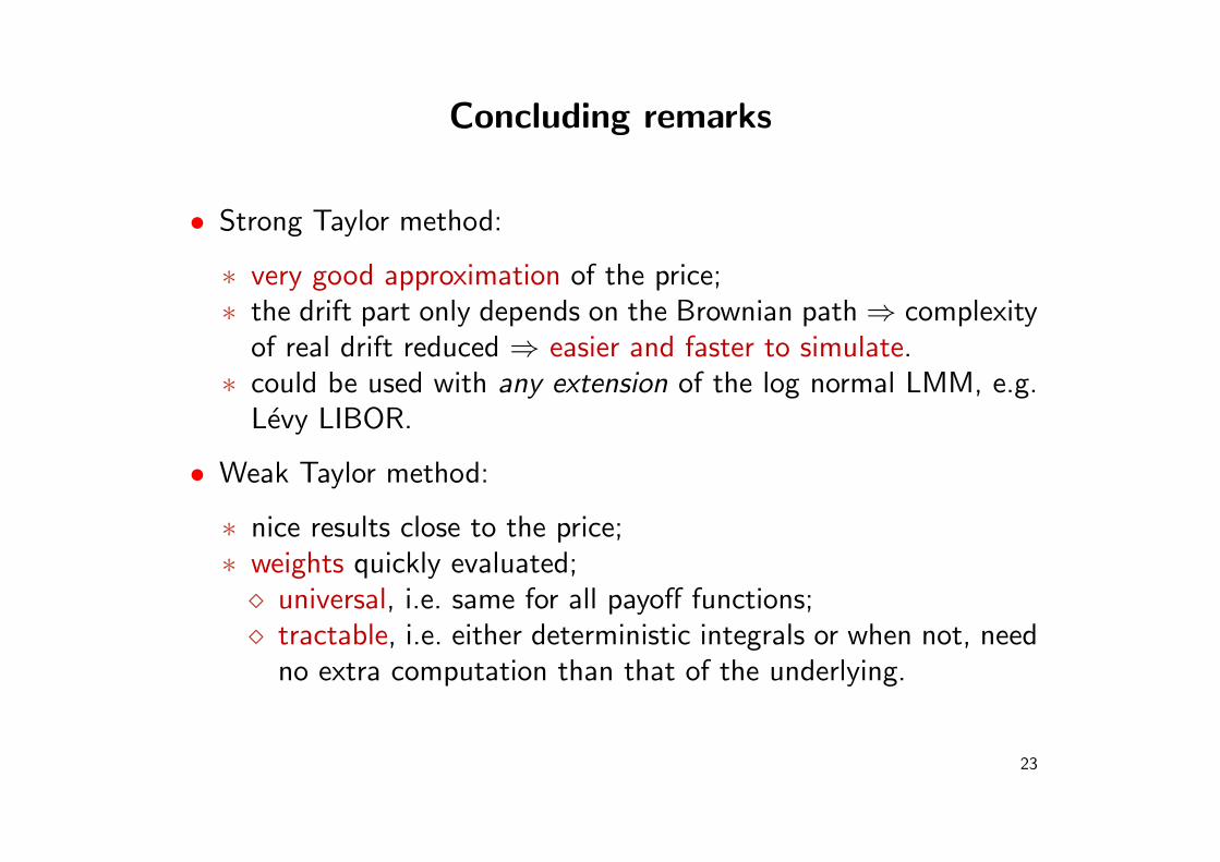
Concluding remarks

• Strong Taylor method:

∗ very good approximation of the price;∗ the drift part only depends on the Brownian path ⇒ complexity

of real drift reduced ⇒ easier and faster to simulate.∗ could be used with any extension of the log normal LMM, e.g.

Levy LIBOR.

• Weak Taylor method:

∗ nice results close to the price;∗ weights quickly evaluated; universal, i.e. same for all payoff functions; tractable, i.e. either deterministic integrals or when not, need

no extra computation than that of the underlying.

23

Future research

• Higher-order strong and weak Taylor approximations;

• Greeks in the LMM and SVLMM;

• Models with jumps - Levy LIBOR;

• Other stochastic volatility models or general multi-factor models;look for approximative closed-form formulas.

24

Talk Contents

• M. Siopacha, J. Teichmann (2007). Weak and strong Taylormethods for numerical solutions of stochastic differentialequations, preprint, available at arXiv.org.

• M. Siopacha (2006). Taylor expansions of option prices by meansof Malliavin calculus, Doctoral Thesis, Vienna University ofTechnology, Austria.

25

Thank you for your attention!