B6b Waves & compressible flow 3–1 3 Theories for linear waves 3.1 Introduction In this section we present several methods for analysing linear wave problems. In finite domains, the well-known technique of separation of variables allows the natural modes and natural frequencies to be determined. Then any solution may be expressed as a superposition of such modes. In infinite domains, instead it is more relevant to seek travelling waves and determine the dispersion relation between their frequency amd wavenumber. Again, an arbitrary wave motion may then be considered as a superpo- sition of such travelling waves, and this is clarified by use of the Fourier transform. It is often difficult to invert the Fourier transforms encountered in practice. Nevertheless, good estimates of the solutions may be obtained using the method of stationary phase. Alternatively, linear hyperbolic problems may be solved by the method of characteristics. Finally, we combine these methods to analyse the flow past a thin wing at sub- and supersonic speeds. 3.2 Separation of variables This technique is suitable for solving linear partial differential equations in finite do- mains. To apply the method, choose a coordinate system in which the domain bound- aries are coordinate surfaces. Example 1: acoustic waves in a box Consider one-dimensional waves in a box of length L, where the two ends x = 0 and x = L are fixed. Thus the velocity potential φ satisfies the one-dimensional wave equation ∂ 2 φ ∂t 2 = c 2 0 ∂ 2 φ ∂x 2 , (3.1a) subject to the boundary conditions ∂φ ∂x =0 at x =0,x = L. (3.1b) We look for a time-periodic solution of the form φ(x,t)= f (x)e −iωt , (3.2)

Welcome message from author
This document is posted to help you gain knowledge. Please leave a comment to let me know what you think about it! Share it to your friends and learn new things together.
Transcript

B6b Waves & compressible flow 3–1
3 Theories for linear waves
3.1 Introduction
In this section we present several methods for analysing linear wave problems. In finitedomains, the well-known technique of separation of variables allows the natural modesand natural frequencies to be determined. Then any solution may be expressed as asuperposition of such modes. In infinite domains, instead it is more relevant to seektravelling waves and determine the dispersion relation between their frequency amdwavenumber. Again, an arbitrary wave motion may then be considered as a superpo-sition of such travelling waves, and this is clarified by use of the Fourier transform. Itis often difficult to invert the Fourier transforms encountered in practice. Nevertheless,good estimates of the solutions may be obtained using the method of stationary phase.Alternatively, linear hyperbolic problems may be solved by the method of characteristics.
Finally, we combine these methods to analyse the flow past a thin wing at sub- andsupersonic speeds.
3.2 Separation of variables
This technique is suitable for solving linear partial differential equations in finite do-mains. To apply the method, choose a coordinate system in which the domain bound-aries are coordinate surfaces.
Example 1: acoustic waves in a box
Consider one-dimensional waves in a box of length L, where the two ends x = 0 andx = L are fixed. Thus the velocity potential φ satisfies the one-dimensional waveequation
∂2φ
∂t2= c20
∂2φ
∂x2, (3.1a)
subject to the boundary conditions
∂φ
∂x= 0 at x = 0, x = L. (3.1b)
We look for a time-periodic solution of the form
φ(x, t) = f(x)e−iωt, (3.2)

3–2 OCIAM Mathematical Institute University of Oxford
where the real part is assumed. This supposes that the gas all oscillates at a singlefrequency ω, assume positive without loss of generality; such a motion is called a normal
mode. Substitution into (3.1) leads to
d2f
dx2+
(ω
c0
)2
f = 0,df
dx(0) =
df
dx(L) = 0. (3.3)
This is an eigenvalue problem, which admits nontrivial solutions of the form
f = A cos(nπxL
), (3.4)
only if ω takes special values, namely
ωn =nπc0L
, (3.5)
where n is a positive integer. Equation (3.5) defines a countably infinite set of frequenciesat which the gas may oscillate without forcing, and these are known as the natural orresonant frequencies of the pipe.
Since the problem (3.1) is linear and homogeneous, the separable solutions foundabove may be superimposed. Thus
φ(x, t) =∞∑
n=1
cos(nπxL
){Bn cos
(nπc0t
L
)+ Cn sin
(nπc0t
L
)}(3.6)
satisfies (3.1) for any values of the arbitrary constants Bn and Cn. If we impose theinitial conditions
φ = f(x),∂φ
∂t= g(x) at t = 0, (3.7)
then the constants may be evaluated using the theory of Fourier series:
Bn =2
L
∫ L
0f(x) cos
(nπxL
)dx, Cn =
2
nπc0
∫ L
0g(x) cos
(nπxL
)dx. (3.8)
Now, suppose the left-hand end of the box is oscillated, so at time t its position isx = ae−iωt, where a is small. The left-hand boundary condition for φ is thus modifiedto
∂φ
∂x= −iωae−iωt at x = ae−iωt. (3.9a)
As shown in section 2, it is consistent, when linearising for small a and φ, to apply thisboundary conditions on x = 0 rather than x = ae−iωt, that is
∂φ
∂x= −iωae−iωt at x = 0. (3.9b)
Now, if we seek a separable solution φ(x, t) = f(x)e−iωt, we find that f must satisfy
d2f
dx2+
(ω
c0
)2
f = 0,df
dx(0) = −iωa,
df
dx(L) = 0, (3.10)

B6b Waves & compressible flow 3–3
which is easily solved to give
f = −ic0a cosec
(ωL
c0
)cos
(ω(L− x)
c0
). (3.11)
Notice that the amplitude of f (and hence also of φ) becomes unbounded as ω ap-proaches one of the natural frequencies ωn. This is the phenomenon of resonance andexplains (among other things) how many musical instruments work: you can createlarge-amplitude sound waves by driving a column of air close to one of its resonantfrequencies.
If ω is at one of the resonant frequencies, then there is no time-periodic solution forφ. We can instead look for a so-called secular solution, in which the amplitude growslinearly with time, by trying
φ(x, t) =(f(x) + tg(x)
)eiωnt. (3.12)
Substitution into the wave equation leads to two differential equations for f and g, whosesolution, subject to the boundary conditions is
f(x) = − iac02ωnL
{2ωn(L− x) sin
(ωnx
c0
)− c0 cos
(ωnx
c0
)}+A cos
(ωnx
c0
), (3.13a)
g(x) = −ac20
Lcos
(ωnx
c0
), (3.13b)
where A is arbitrary.In practice, if ω is at or close to one of the resonant frequencies, then the amplitude of
the oscillations eventually becomes so large that our linearisation is no longer valid. Thenonlinear terms that we have neglected become significant and prevent the amplitudefrom growing without bound. It is also likely that viscous effects may become importantin very large-amplitude oscillations.
It is straightforward to extend the above analysis to higher dimensions. For example,normal modes in gas confined to the two-dimensional box {0 < x < L, 0 < y < b} takethe form
φ = ae−iωt cos(nπxL
)cos
(iπy
b
), (3.14)
where n and i are integers. There is thus a doubly-infinite family of natural frequencies,given by
ω2n,i = π2c20
(n2
L2+i2
b2
). (3.15)
In general, there is an infinite family of normal modes for each spatial dimension inthe problem. For the three-dimensional box {0 < x < L, 0 < y < b, 0 < z < h}, themodes and corresponding frequencies are
φ = ae−iωt cos(nπxL
)cos
(iπy
b
)cos
(jπz
h
), ω2
n,i,j = π2c20
(n2
L2+i2
b2+j2
h2
), (3.16)
for any integer values of n, i, j.

3–4 OCIAM Mathematical Institute University of Oxford
Example 2: spherical waves
Suppose gas is contained in the annular region a < r < b, where r is the usual sphericalpolar coordinate. For spherically symmetric waves, the velocity potential φ(r, t) satisfies
∂2φ
∂t2= c20∇2φ =
c20r
∂2
∂r2(rφ) ,
∂φ
∂r= 0 on r = a,
∂φ
∂r= 0 on r = b. (3.17)
We look for normal modes of the form
φ(r, t) = f(r)e−iωt, (3.18)
so that f must satisfy
d2
dr2(rf) +
(ω
c0
)2
(rf) = 0,df
dr(a) =
df
dr(b) = 0. (3.19)
Hence f is given by
f =A cos (kr) +B sin (kr)
r, (3.20)
where k = ω/c0, and application of the boundary conditions leads to the followingsystem of equations for the arbitrary constants A and B:
(cos(ka) + ka sin(ka) sin(ka) − ka cos(ka)cos(kb) + kb sin(kb) sin(kb) − kb cos(kb)
)(AB
)= 0. (3.21)
For a nontrivial solution to exist, the determinant of the left-hand side must be zero,which leads to the equation
(1 + k2ab
)tan(k(b− a)
)= k(b− a). (3.22)
Given a and b, this transcendental equation has a countably infinite set of solutions fork, each corresponding to a natural frequency.
Example 3: waves in a circle
Consider waves in gas confined to the circle r < a, where r is the plane polar radialcoordinate. The radially-symmetric wave equation reads
∂2φ
∂t2= c20∇2φ = c20
(∂2φ
∂r2+
1
r
∂φ
∂r
), (3.23a)
and, assuming the edge r = a is fixed and that φ is bounded as r → 0, we have theboundary conditions
|φ| <∞ as r → 0,∂φ
∂r= 0 at r = a. (3.23b)

B6b Waves & compressible flow 3–5
We seek normal modes of the form
φ(r, t) = f(r)e−iωt (3.24)
and find that f must satisfy
d2f
dr2+
1
r
df
dr+
(ω
c0
)2
f = 0, |f | <∞ as r → 0,df
dr(a) = 0. (3.25a)
If we define ξ = kr, where k = ω/c0, then (3.25a) becomes
ξ2d2f
dξ2+ ξ
df
dξ+ ξ2f = 0, |f | <∞ as ξ → 0,
df
dξ(ka) = 0. (3.25b)
This is Bessel’s equation of order zero, and the two linearly independent solutions aredenoted J0(ξ) and Y0(ξ), although only J0(ξ) is bounded as ξ → 0.
We must therefore have f = AJ0(ξ) for some constant A, and the condition at r = ais satisfied if
ka = ξ0,i (i = 1, 2, . . .), (3.26a)
where ξ0,1 < ξ0,2 < · · · are the extrema of J0(ξ). As indicated in figure 3.1, there are aninfinite number of these and ξ0,i → ∞ as i→ ∞. The natural frequencies of the gas arethus given by
ωi =c0ξ0,ia
(i = 1, 2, . . .). (3.26b)
Next we drop the assumption of radial symmetry and consider waves in a circularpipe of radius a and length L. In terms of cylindrical polar coordinates (r, θ, z), thevelocity potential φ satisfies
∂2φ
∂t2= c20∇2φ = c20
(∂2φ
∂r2+
1
r
∂φ
∂r+
1
r2∂2φ
∂θ2+∂2φ
∂z2
), (3.27a)
|φ| <∞ as r → 0,∂φ
∂r= 0 at r = a,
∂φ
∂z= 0 at z = 0, L, (3.27b)
plus the condition that φ must be a 2π-periodic function of θ.It is readily shown that time-periodic separable solutions satisfying the boundary
conditions are of the form
φ(r, θ, z, t) = f(r)(A cos(nθ) +B sin(nθ)
)cos
(jπz
L
)e−iωt, (3.28)
where n and j are integers. It follows that f satisfies
r2d2f
dr2+ r
df
dr+(k2r2 − n2
)f = 0, |f | <∞ as r → 0,
df
dr(a) = 0, (3.29a)

3–6 OCIAM Mathematical Institute University of Oxford
5 10 15 20 25 30
-0.4
-0.2
0.2
0.4
0.6
0.8
1
5 10 15 20 25 30
-0.8
-0.6
-0.4
-0.2
0.2
0.4
ξ
ξ
Jn(ξ)
Yn(ξ)
2
2
n = 0
1
1n = 0
Figure 3.1: Plots of the first few Bessel functions Jn(ξ) and Yn(ξ) for n = 0 (solid),n = 1 (dashed), n = 2 (dot-dashed).
where
k2 =ω2
c20− j2π2
L2. (3.29b)
Setting ξ = kr as before, we find that (3.29a) becomes
ξ2d2f
dξ2+ ξ
df
dξ+(ξ2 − n2
)f = 0, |f | <∞ as ξ → 0,
df
dξ(ka) = 0. (3.29c)
This is Bessel’s equation of order n, whose two linearly dependent solutions are denotedJn(ξ) and Yn(ξ); the cases n = 0, 1, 2 are plotted in figure 3.1. For any integer n, Yn(ξ)is singular as ξ → 0, so we must have f = AJn(ξ) for some constant A, and the conditionat r = a is satisfied if
ka = ξn,i (i = 1, 2, . . .), (3.30)
where ξn,1 < ξn,2 < · · · are the extrema of Jn(ξ). Again, there are an infinite number ofthese and ξn,i → ∞ as i→ ∞.

B6b Waves & compressible flow 3–7
The natural frequencies of the pipe are thus given by
ω2n,i,j = c20
(j2π2
L2+ξ2n,ia2
), (3.31)
where n, i and j are arbitrary integers, so there is a triply-infinite family of normalmodes that depend on the three spatial coordinates (r, θ, z).
3.3 Travelling waves
On an infinite domain, instead of normal modes, we can look for travelling harmonicwaves, and attempt to determine the dispersion relation between the frequency and thewavenumber.
Example 1: waveguide
Linear waves propagating in the x-direction through gas contained between two rigidwalls at z = 0 and z = h can be described by a velocity potential of the form
φ(x, z, t) = A cos(nπzh
)ei(kx−ωt), (3.32)
where n is an integer. By substituting this into the wave equation, we find the dispersionrelation
ω2 = c20
(k2 +
n2π2
h2
). (3.33a)
The speed of propagation of waves along the waveguide is thus given by
c2p =ω2
k2= c20
(1 +
n2π2
h2k2
). (3.33b)
Whenever n is nonzero, these waves are dispersive, since cp varies with k.
Multidimensional travelling waves
If the dependent variable (say φ) depends on multiple spatial variables, we can look fora general harmonic travelling wave by setting
φ = ae(ikx+ℓy+mz−ωt) = aei(k·x−ωt), (3.34)
where
k = (k, ℓ,m)T (3.35)
is the wavenumber vector. The direction of k represents the direction in which the wavespropagate, while the magnitude of k is related to the wavelength λ by |k| = 2π/λ.

3–8 OCIAM Mathematical Institute University of Oxford
The phase velocity of the waves is
cp =ωk
|k|2 . (3.36)
For nondispersive waves, we would expect the wave speed |cp| to be independent of k,and we see from (3.36) that this is true if and only if
ω = cp|k|, (3.37)
where cp is constant. If the dispersion relation takes any form other than (3.37), thenthe waves are dispersive.
Example 2: internal gravity waves
As shown in section 2, small-amplitude waves in a stratified fluid of ambient densityρ0 = Reβz are governed by the equation
∂2
∂t2
(∂2w′
∂x2+∂2w′
∂y2+∂2w′
∂z2
)= βg
(∂2w′
∂x2+∂2w′
∂y2− 1
g
∂3w′
∂z∂t2
). (3.38)
If we try a travelling-wave solution of the form
w′ = aei(k·x−ωt), (3.39)
we find that the dispersion relation is
ω2 = −βg(k2 + ℓ2)
|k|2 − iβm, (3.40)
and the waves are thus dispersive. Recall that β < 0 for stable stratification. Nev-ertheless, there are two complex roots for ω whenever m is nonzero and, since (3.40)is an equation for ω2, at least one of these roots must have a positive imaginary part.Thus the amplitude grows exponentially whenever m is nonzero, and the fluid is alwaysunstable to waves in the z-direction.
3.4 Fourier transform
In section 3.2, we showed that a general flow in a finite domain may be written as asuperposition of normal modes. An initial-value problem may thus be solved by choosingthe weightings of the different modes appropriately. Similarly, the general solution inan infinite domain may be written as a superposition of harmonic waves, and initialconditions can be imposed by a suitable choice of the weighting function. Here we showhow this can be achieved in some simple cases using the Fourier transform.
Given a suitable function f , we define the Fourier transform f by
f(k) =
∫ ∞
−∞f(x)e−ikx dx. (3.41)
We will now quote some basic properties of the Fourier transform.

B6b Waves & compressible flow 3–9
1. Inverse Fourier transform
If we have calculated f , the orginal function f is recovered using
f(x) =1
2π
∫ ∞
−∞f(k)eikx dk. (3.42a)
2. Convolution theorem
If f can be written as the product of two Fourier transforms that we know, sayf(k) = g(k)h(k), then f is the convolution of g and h, that is
f(x) = (g ⋆ h)(x) =
∫ ∞
−∞g(ξ)h(x− ξ) dξ. (3.42b)
3. Fourier transform of derivatives
The Fourier transform turns x-derivatives into multiples of k, specifically
dnf
dxn= (ik)nf . (3.42c)
Hence ordinary differential equations are transformed into algebraic equations, andpartial differential equations into ordinary differential equations.
Stokes waves
We now illustrate the use of the Fourier transform to solve the problem of two-dimensionalStokes waves on a semi-infinite layer of fluid. The velocity potential φ(x, z, t) and free-surface displacement z = η(x, t) satisfy the equations and boundary conditions
∂2φ
∂x2+∂2φ
∂z2= 0 z < 0, (3.43a)
∂φ
∂z=∂η
∂t,
∂φ
∂t+ gη = 0 z = 0, (3.43b)
φ→ 0 z → −∞. (3.43c)
The problem is closed by specifying the initial displacement and velocity of the freesurface. We suppose the fluid starts from rest with the free surface given by z = η0(x),so that
η = η0(x),∂η
∂t= 0 at t = 0. (3.43d)
We take a Fourier transform in x, denoted with as above, so the problem becomes
∂2φ
∂z2− k2φ = 0 z < 0, (3.44a)
∂φ
∂z=∂η
∂t,
∂φ
∂t+ gη = 0 z = 0, (3.44b)
φ→ 0 z → −∞, (3.44c)
η = η0,∂η
∂t= 0 t = 0. (3.44d)

3–10 OCIAM Mathematical Institute University of Oxford
It follows that
φ = A(k, t)e|k|z, (3.45)
where A satisfies
|k|A =∂η
∂t,
∂A
∂t+ gη = 0. (3.46)
Solving these equations and applying the initial conditions, we find that
η = η0 cos(ωt), A = −ωη0
|k| sin(ωt), (3.47)
where the frequency ω(k) is given by the dispersion relation
ω(k) =√g|k|. (3.48)
The evolution of the free surface is then found by inverting the transform, resulting in
η(x, t) =1
2π
∫ ∞
−∞η0(k) cos
(ω(k)t
)eikx dk. (3.49a)
If the cosine is expanded out, to give
η(x, t) =1
4π
∫ ∞
−∞η0(k)
(ei(kx−ωt) + ei(kx+ωt)
)dk, (3.49b)
it becomes clear that this represents a superposition of waves travelling up- and down-stream with phase speed cp = ω(k)/k.
If the fluid does not start from rest, say
∂η
∂t= w0(x) at t = 0, (3.50)
then (3.49) becomes
η(x, t) =1
2π
∫ ∞
−∞
(η0(k) cos
(ω(k)t
)+w0(k)
ω(k)sin(ω(k)t
))eikx dk. (3.51)
This expression may be applied to generalised Stokes waves problems (with, for example,finite depth or surface tension) by modifying the dispersion relation for ω(k) appropri-ately. However, except for very simple dispersion relations, it is difficult to evaluate theinversion integrals exactly. Instead, we will show below in section 3.5 how the large-timeasymptotic behaviour of the solution may be estimated.

B6b Waves & compressible flow 3–11
Multidimensional Fourier transform
The methods outlined above can be generalised to higher spatial dimensions. For afunction of three spatial dimensions f(x, y, z), for example, we can define the tripleFourier transform
f(k, ℓ,m) =
∫ ∞
−∞
∫ ∞
−∞
∫ ∞
−∞f(x, y, z)e−i(kx+ℓy+mz) dxdy dz. (3.52a)
If we define the wavenumber vector k = (k, ℓ,m)T as before, then a convenient shorthandfor (3.52a) is
f(k) =
∫∫∫
R3
f(x)e−i(k·x) dx, (3.52b)
and the inverse transform then reads
f(x) =1
8π3
∫∫∫
R3
f(k)ei(k·x) dk. (3.53)
Consider for example the inertial wave equation (3.38). The triple Fourier transformw of w′ satisfies
(|k|2 − iβm
) ∂2w
∂t2= βg
(k2 + ℓ2
)w. (3.54)
If, for example, we start with
w′ = w0(x),∂w′
∂t= 0 at t = 0, (3.55)
then the appropriate solution of (3.54) is
w = w0(k) cos(ω(k)t
), (3.56)
where ω(k) is given by the dispersion relation (3.40). The inverse transform thus gives
w′(x, t) =1
8π3
∫∫∫
R3
w0(k) cos(ω(k)t
)ei(k·x) dk, (3.57a)
or
w′(x, t) =1
16π3
∫∫∫
R3
w0(k)(ei(k·x+ω(k)t) + ei(k·x−ω(k)t)
)dk, (3.57b)
which may be identified as a superposition of harmonic waves with wavenumber vectork and frequency ±ω(k). Now the superposition takes place over all possible vectors k,that is over all possible wavenumbers and propagation directions.
If ω(k) is complex for any k such that w0(k) is nonzero, then (3.57) implies that w′
grows exponentially in time and the base state is therefore unstable. From the dispersionrelation (3.40), we see that ω is complex whenever m is nonzero. The perturbationtherefore grows exponentially unless w0(k, ℓ,m) ≡ 0 whenever m 6= 0, which occurs onlyif w0 is independent of z. Hence the base state in this case is unstable to all z-dependentperturbations.

3–12 OCIAM Mathematical Institute University of Oxford
3.5 Method of stationary phase
Motivation
In section 3.4, we used a Fourier transform to solve the problem of two-dimensionalStokes waves on a semi-infinite fluid layer, subject to zero initial velocity and a givenfree-surface displacement η0(x) at t = 0. From (3.49) we see that an observer travellingat speed V , so that his or her position at time t is x = V t, will observe a free surfacedisplacement
η(V t, t) =1
4π
∫ ∞
−∞η0(k)e
i(kV−ω(k)
)t dk +
1
4π
∫ ∞
−∞η0(k)e
i(kV+ω(k)
)t dk, (3.58)
where ω(k) is given by (3.48) or, in general, by some other dispersion relation.
The Fourier integrals in (3.58) are in general difficult to evalute explicitly. To un-derstand how they behave for large t, we now consider the general case
I(t) =
∫ b
af(k)eiψ(k)t dk, (3.59)
where f and ψ are arbitrary functions, known as the amplitude and phase respectively,while a and b are fixed constants. We will start by illustrating the method for thesimple cases in which ψ is a linear or quadratic function of k. We will apply some ad hoc
asymptotic estimates, but emphasise that these can be made rigorous by using morecareful analysis.
Example 1: linear ψ(k)
First consider the simple case where ψ(k) is a linear function of k, that is
ψ(k) = α+ βk (3.60)
for some real constants α and β, so that I(t) takes the form
I(t) = eiαt
∫ b
af(k)eiβkt dk. (3.61)
When t is large, eiψ(k)t is a highly oscillatory function. The positive and negative con-tributions to the integral I(t) almost exactly cancel each other out, with the cancellationbecoming perfect in the limit t → ∞. This is shown schematically in figure 3.2 for thecase f(k) =
(1 + (k − 1)2
)−1, ψ(k) = 1 + k and t = 10.
The integral I(t) therefore tends to zero as t → ∞; in particular, the Riemann–
Lebesgue Lemma tells us that
I(t) = O
(1
βt
)as t→ ∞. (3.62)

B6b Waves & compressible flow 3–13
-1 -0.5 0.5 1 1.5 2 2.5
-1
-0.5
0.5
1
-1 -0.5 0.5 1 1.5 2 2.5
-1
-0.5
0.5
1
-4 -2 2 4
-1
-0.5
0.5
1
k
k
Re{f(k)eiψ(k)t
}
(b)
(a)
Figure 3.2: (a) The real part of f(k)eiψ(k)t plotted versus k with f(k) =(1+(k−1)2
)−1,
ψ(k) = 1 + k and t = 10. (b) A close-up of (a) indicating cancellation of the positiveand negative contributions.
(To prove (3.62), integrate (3.61) by parts to obtain
I(t)e−iαt =1
iβt
{[f(k)eiβkt
]ba−∫ b
af ′(k)eiβkt dk
}. (3.63)
The term in braces may be bounded using the assumed continuity of f ′, resulting in|I(t)| 6 M/(βt) for some constant M .) The result (3.62) also applies in the limita→ −∞, b→ +∞ provided |f ′(k)| is integrable over this range.
Example 2: quadratic ψ(k)
Next consider the case where ψ(k) is a quadratic function, say
ψ(k) = α+ γk2, (3.64)
where α and γ are real constants. Note that this ψ(k) has a single extremum whichwe have assumed, without loss of generality, to be at k = 0. In figure 3.3 we plotRe{f(k)eiψ(k)t} versus k for the case f(k) =
(1 + (k− 1)2
)−1, ψ(k) = 1 + k2 and t = 10.
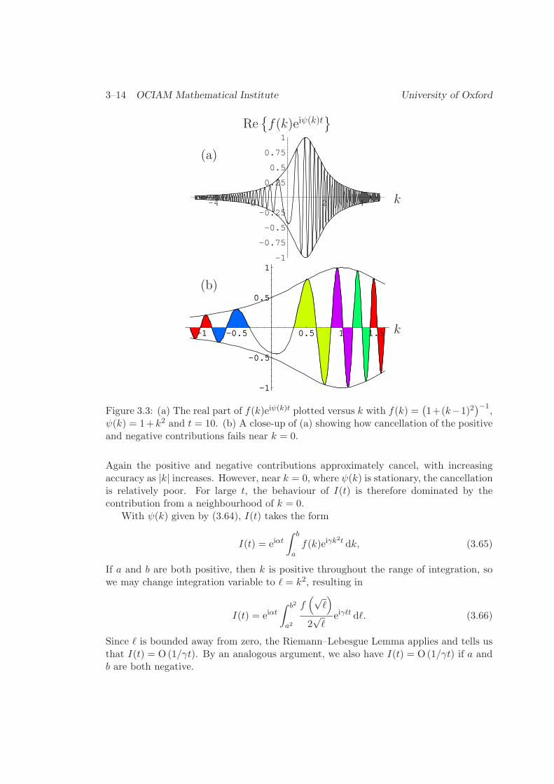
3–14 OCIAM Mathematical Institute University of Oxford
-4 -2 2 4
-1
-0.75
-0.5
-0.25
0.25
0.5
0.75
1
-1 -0.5 0.5 1 1.5
-1
-0.5
0.5
1
-1 -0.5 0.5 1 1.5
-1
-0.5
0.5
1
k
Re{f(k)eiψ(k)t
}
k
(a)
(b)
Figure 3.3: (a) The real part of f(k)eiψ(k)t plotted versus k with f(k) =(1+(k−1)2
)−1,
ψ(k) = 1+k2 and t = 10. (b) A close-up of (a) showing how cancellation of the positiveand negative contributions fails near k = 0.
Again the positive and negative contributions approximately cancel, with increasingaccuracy as |k| increases. However, near k = 0, where ψ(k) is stationary, the cancellationis relatively poor. For large t, the behaviour of I(t) is therefore dominated by thecontribution from a neighbourhood of k = 0.
With ψ(k) given by (3.64), I(t) takes the form
I(t) = eiαt
∫ b
af(k)eiγk2t dk, (3.65)
If a and b are both positive, then k is positive throughout the range of integration, sowe may change integration variable to ℓ = k2, resulting in
I(t) = eiαt
∫ b2
a2
f(√
ℓ)
2√ℓ
eiγℓt dℓ. (3.66)
Since ℓ is bounded away from zero, the Riemann–Lebesgue Lemma applies and tells usthat I(t) = O (1/γt). By an analogous argument, we also have I(t) = O (1/γt) if a andb are both negative.

B6b Waves & compressible flow 3–15
If a < 0 < b, then our integration region includes the origin, so the change of variablethat gives rise to (3.66) is invalid. However, as shown schematically in figure 3.3, weexpect the main contribution to I(t) to come from a neighbourhood of k = 0, so we splitup the range of integration as follows:
I(t)e−iαt =
∫ −ǫ
af(k)eiγk2t dk +
∫ b
ǫf(k)eiγk2t dk +
∫ ǫ
−ǫf(k)eiγk2t dk, (3.67a)
where ǫ is a fixed small constant. The Riemann–Lebesgue Lemma applies to the firsttwo integrals, leaving us with
I(t)e−iαt =
∫ ǫ
−ǫf(k)eiγk2t dk + O
(1
γt
). (3.67b)
If ǫ is sufficiently small then, to leading order, we may replace f(k) with f(0). Supposingfor the moment that γ is positive, the change of variable s = k
√γt thus leads to
I(t)e−iαt ∼ 1√γt
∫ ǫ√γt
−ǫ√γtf(0)eis2 ds+ O
(1
γt
). (3.67c)
A straightforward contour integral shows that
∫ R
−Reis2 ds→ (1 + i)
√π
2+ O
(1
R
)(3.68)
as R → ∞. We therefore deduce from (3.67c) that the leading-order behaviour of I(t)is
I(t) ∼ (1 + i)eiαtf(0)
√π
2γt+ O
(1
γt
)as t→ ∞. (3.69)
This establishes mathematically what is illustrated schematically in figure 3.3. Withψ(k) given by (3.64), the cancellation in the integrand of I(t) is poor near k = 0, and I(t)therefore converges to zero less rapidly than it does when ψ(k) is linear. Furthermore,the large-time behaviour of I(t) is dominated by the behaviour of the integrand neark = 0; hence only f(0) appears in (3.69).
Recall that (3.67c) was obtained under the assumption that γ is positive. For nega-tive γ, the change of variable s = k
√−γt leads to
I(t) ∼ e−iαt
√−γt
∫ ǫ√−γt
−ǫ√−γtf(0)e−is2 ds+ O
(1
γt
), (3.70)
and the result∫ R
−Re−is2 ds→ (1 − i)
√π
2+ O
(1
R
)as R→ ∞, (3.71)
which is an obvious corollary of (3.68), then leads to
I(t) ∼ (1 − i)eiαtf(0)
√π
−2γt+ O
(1
γt
)as t→ ∞. (3.72a)

3–16 OCIAM Mathematical Institute University of Oxford
We can combine (3.69) and (3.72a) into the handy form
I(t) ∼ f(0)ei(αt±π/4)
√π
|γ|t (3.72b)
as t→ ∞, where the ± corresponds to the sign of γ.
The general case
Now we generalise the analysis given above to arbitrary exponents ψ(k). We will assumeonly that ψ is real-valued and twice continuously differentiable.
First suppose that ψ′(k) is nowhere zero on [a, b] and hence is either uniformlypositive or uniformly negative. It follows that ψ(k) is strictly monotonic on [a, b], so wecan invert the one-to-one relation between k and ψ(k) to write
k = κ(ψ). (3.73)
Thus I(t) may be written as
I(t) =
∫ b
af(k)eiψ(k)t dk =
∫ ψ(b)
ψ(a)f(κ(ψ)
)eiψtκ′(ψ) dψ, (3.74)
and the Riemann–Lebesgue Lemma implies that I(t) = O (1/t).Next suppose that ψ′(k) has a simple zero at just one point k∗ ∈ [a, b]. We divide
up the integration range as follows:
I(t) =
∫ k∗−ǫ
af(k)eiψ(k)t dk +
∫ b
k∗+ǫf(k)eiψ(k)t dk +
∫ k∗+ǫ
k∗−ǫf(k)eiψ(k)t dk, (3.75)
where ǫ is a fixed small constant. Since ψ is monotonic over each of the intervals [a, k∗−ǫ]and [k∗ + ǫ, b], the first two integrals in (3.75) are O (1/t), by the argument given above.In the final integral, we use the smallness of ǫ to approximate f and ψ near k = k∗ as
f(k) ∼ f(k∗), ψ(k) ∼ ψ(k∗) +ψ′′(k∗)
2(k − k∗)
2, (3.76)
since ψ′(k∗) = 0. Thus (3.75) becomes
I(t) ∼∫ k∗+ǫ
k∗−ǫf(k∗)e
iψ(k∗)t exp
(itψ′′(k∗)
2(k − k∗)
2
)dk + O
(1
t
)(3.77)
and, if ψ′′(k∗) is positive, the change of variable
k = k∗ + s
√2
tψ′′(k∗)(3.78)
leads to
I(t) ∼ f(k∗)eiψ(k∗)t
√2
ψ′′(k∗)t
∫ ǫ√ψ′′(k∗)t/2
−ǫ√ψ′′(k∗)t/2
eis2 ds+ O
(1
t
). (3.79)

B6b Waves & compressible flow 3–17
Application of (3.68) thus leads to the estimate
I(t) ∼ (1 + i)f(k∗)eiψ(k∗)t
√π
ψ′′(k∗)t+ O
(1
t
)(3.80)
as t → ∞. An analogous argument may also be applied for the case where ψ′′(k∗) isnegative, and leads to the general result
I(t) ∼ f(k∗)ei(ψ(k∗)t±π/4
)√2π
|ψ′′(k∗)| t(3.81)
as t → ∞, where the ± takes the sign of ψ′′(k∗). In either case, we see that I(t) =O(1/
√t)
rather than O (1/t), and that the dominant contribution to I(t) comes from aneighbourhood of k = k∗. Recall that this is where the phase ψ(k) is stationary, and theasymptotic procedure leading to (3.81) is therefore known as the method of stationary
phase.If ψ′(k) has multiple zeros, then each may be considered in isolation by employing a
domain decomposition analogous to (3.75). Hence the leading-order behaviour of I(t) issimply the sum of all the contributions of the form (3.81) due to each point where ψ isstationary. It is also worth noting that, in deriving (3.81), we have assumed that ψ′′(k∗)is nonzero. We will not bother here to spell out the generalised versions of (3.81) thatapply to higher-order zeros of ψ′(k).
Group velocity
Now we are in a position to apply the estimate (3.81) to (3.58), which we write as
η(V t, t) = I+(t) + I−(t), where I±(t) =1
4π
∫ ∞
−∞η0(k)e
i(kV∓ω(k)
)t dk. (3.82)
Each integral I±(t) is of the required form (3.59), with
a = −∞, b = ∞, f(k) =η0(k)
4π, ψ(k) = V k ∓ ω(k). (3.83)
The method of stationary phase tells us that the main contribution to η comes fromwavenumbers k = k∗ where ψ is stationary, that is
ψ′(k∗) = V ∓ ω′(k∗) = 0. (3.84)
Thus an observer travelling at speed V will see waves of wavenumber k∗ satisfying (3.84).In other words, waves with wavenumber k travel at speed V = ±cg(k), where
cg(k) =dw
dk(3.85)
is called the group velocity.

3–18 OCIAM Mathematical Institute University of Oxford
η η
xx
(a) (b)
increasingt
increasingt
Figure 3.4: Schematic of a moving wave packet with (a) cg < cp, (b) cg > cp. One wavecrest is highlighted to illustrate how it moves relative to the packet.
Notice that cg(k) is different from the phase velocity cp(k) = ω/k unless ω/k isconstant, which occurs only for non-dispersive waves. At first glance, it might seemparadoxical that waves can travel at a group velocity different from their phase velocity.The explanation is that, after a long time, dispersive waves separate into wave packets
corresponding to different wavenumbers. Within each wave packet, the waves move atspeed cp, but the packet as a whole moves at speed cg.
This phenomenon is illustrated in figure 3.4 for a single wave packet travelling fromleft to right at speed cg. The wave crests in the packet move with speed cp so, if cg < cpthen, as indicated in figure 3.4(a), the wave crests move through the packet, seemingto appear at the back and disappear at the front. This behaviour can be observed inthe radiating ripples caused by throwing a stone into a pond. On the other hand, if thegroup velocity is greater than the phase velocity then the wave crests move more slowlythan the wave packet, as shown in figure 3.4(b). This can sometimes be observed invery small ripples, which appear to move backwards relative to a radiating wave packet.
For gravity waves on deep water, the dispersion relation is
ω(k) =√g|k|, (3.86a)
so the phase and group velocities are given by
cp =
√g|k|k
, cg =
√g|k|2k
. (3.86b)
We therefore always have |cg| < |cp| in this case, that is the situation depicted infigure 3.4(a).
If surface tension γ is included then it may be shown, as in section 2, that thedispersion relation (3.86a) is modified to
ω(k) =
√g|k|
(1 +
γk2
ρg
). (3.87)

B6b Waves & compressible flow 3–19
It is straightforward to determine the group and phase velocities and hence show that
cgcp
=3
2−(
1 +γk2
ρg
)−1
. (3.88)
It follows that |cg| < |cp| when |k| < kc and |cg| > |cp| when |k| > kc, where the criticalwavenumber kc is given by
kc =
√ρg
γ. (3.89a)
This corresponds to a critical wavelength
λc =2π
kc= 2π
√γ
ρg, (3.89b)
known as the capillary length. Thus waves shorter than λc travel backwards relative totheir wavepackets, like those depicted in figure 3.4(b). For water, ρ ≈ 1000 kg m−3 andγ ≈ 0.07Nm−1, so the capillary length is about 1.7 cm.
Example: localised disturbance
For the two Fourier integrals I±(t) defined by (3.82), the phase and its derivatives aregiven by
ψ(k) = kV ∓√g|k|, ψ′(k) = V ∓
√g|k|2k
, ψ′′(k) = ±√g|k|
4k2. (3.90)
Hence, at the critical wavenumber k∗ where ψ is stationary, we have
k∗ = ± g
4V 2, ψ(k∗) = ∓ g
4V, ψ′′(k∗) = ±2V 3
g. (3.91)
Assuming that V is positive, this means that critical wavenumber is positive for I+ andnegative for I−. By applying the estimate (3.81) to each integral I±(t), we thus obtainthe following asymptotic approximation for the free surface displacement:
η(V t, t) ∼ 1
4
√g
πV 3t
{η0
( g
4V 2
)ei(π/4−gt/4V ) + η0
(− g
4V 2
)ei(gt/4V−π/4)
}. (3.92)
To make further progress, we need to specify the initial displacement η0(x) so thatwe can determine its Fourier transform η0(k). Here we consider the example
η0(x) =ǫa
π (ǫ2 + x2), (3.93)
which represents a localised initial disturbance near x = 0 and might model, for ex-ample, the ripples caused by throwing a stone into a pond. If ǫ is small, then η0(x) isapproximately zero except near x = 0. Nevertheless, η0 has constant area, that is
∫ ∞
−∞η0(x) dx ≡ a, (3.94)

3–20 OCIAM Mathematical Institute University of Oxford
20 40 60 80 100 120 140
-0.04
-0.02
0.02
0.04
x
η
Figure 3.5: Free surface displacement η(x, t) given by (3.97) versus x with
η0(x) = −(π(1 + x2)
)−1and t
√g = 50. The dashed line shows the asymptotic ap-
proximation (3.96).
whatever the value of ǫ. Hence, as ǫ is reduced towards zero, η0 is concentrated in avanishingly small neighbourhood, of size O (ǫ), near x = 0.1
The Fourier transform of η0(x) is readily found by contour integration to be
η0(k) = ae−ǫ|k|, (3.95)
so (3.92) becomes
η(V t, t) ∼ a
2
√g
πV 3te−ǫg/4V
2
cos
(gt
4V− π
4
)(3.96a)
or, substituting V = x/t,
η(x, t) ∼ at
2
√g
πx3e−ǫgt
2/4x2
cos
(gt2
4x− π
4
). (3.96b)
When η0 is given by (3.93), the inverse Fourier transform for η may be calculatedexactly and written in the form
η(x, t) = η0(x) −t√g
2√π
Re
{1
(1 − ix)3/2exp
(− t2g
4(1 − ix)
)erfi
(t√g
2√
1 − ix
)}(3.97)
where erfi is the so-called imaginary error function, and we have chosen a = −1, ǫ = 1for simplicity. In figure 3.5, we compare this exact solution with our asymptotic approx-imation (3.96) when t
√g = 50, showing excellent agreement.
Ifx
t= V ≫
√ǫg
2, (3.98)
1In the limit ǫ →, η0(x) approaches aδ(x), where δ is the so-called Dirac delta-function, which isdefined to be zero for all nonzero x but to have unit area.

B6b Waves & compressible flow 3–21
then (3.96) may be simplified further by approximating the exponential, so that
η(x, t) ∼ at
2
√g
πx3cos
(gt2
4x− π
4
). (3.99)
It may be shown that this is the universal behaviour of η far from an initial localiseddisturbance.
3.6 Method of characteristics
As shown in section 2, acoustic waves in one dimension satisfy the wave equation
∂2φ
∂t2− c20
∂2φ
∂x2= 0, (3.100)
which can be written in the form(∂
∂t+ c0
∂
∂x
)(∂φ
∂t− c0
∂φ
∂x
)= 0. (3.101)
Hence, if we write
Φ =∂φ
∂t− c0
∂φ
∂x, (3.102)
then we have∂Φ
∂t+ c0
∂Φ
∂x= 0, (3.103a)
which implies thatdΦ
dt= 0 when
dx
dt= c0. (3.103b)
It follows that Φ is constant on the straight lines x− c0t = const, so that Φ must bea function only of (x− c0t). By an analogous argument, with the differential operatorsin (3.101) swapped, we find that
(∂φ
∂t± c0
∂φ
∂x
)= const when (x± c0t) = const. (3.104)
The straight lines x ± c0t = const are the characteristics of the partial differentialequation (3.100). It is straightforward (e.g. by changing variables to ξ = x + c0t andη = x− c0t) to show that the general solution of (3.100) is
φ(x, t) = f(x− c0t) + g(x+ c0t), (3.105)
where the scalar functions f and g are arbitrary. If, for example, we impose the initialconditions
φ = φ0(x),∂φ
∂t= v0(x) at t = 0, (3.106)

3–22 OCIAM Mathematical Institute University of Oxford
������������������������
������������������������
������������������������
������������������������ x
yU
y = f+(x)
y = f−(x)
a−a
Figure 3.6: Schematic of a thing wing with upper and lower surfaces given by y = f±(x).
then f and g are readily determined, resulting in the so-called D’Alembert solution:
φ(x, t) =1
2
(φ0(x− c0t) + φ0(x+ c0t)
)+
1
2c0
∫ x+c0t
x−c0tv0(s) ds. (3.107)
For a general second-order linear partial differential equation of the form
A∂2φ
∂t2+ 2B
∂2φ
∂x∂t+ C
∂2φ
∂x2= f, (3.108)
where f may in general depend on φ, ∂φ/∂x and ∂φ/∂t, the characteristics are curveswhose slopes are given by
dx
dt= λ, where Aλ2 − 2Bλ+ C = 0. (3.109)
The equation is hyperbolic if these slopes are real and distinct, that is if B2 > AC.In the simple case where A, B and C are constant and f is zero, (3.108) may be
written as
A
(∂
∂t+ λ1
∂
∂x
)(∂φ
∂t+ λ2
∂φ
∂x
)= 0, (3.110a)
where λk (k = 1, 2) are the roots of (3.109). We thus deduce (provided A is nonzero)that (
∂φ
∂t+ λi
∂φ
∂x
)= const when x− λjt = const, (3.110b)
where i 6= j ∈ {1, 2}, and the general solution of (3.108) is then
φ(x, t) = f(x− λ1t) + g(x− λ2t). (3.111)
3.7 Flow past a thin wing
Equations and boundary conditons
Now we consider two-dimensional flow at speed U past a thin wing. As illustrated infigure 3.6, the wing is assumed to lie along the x-axis between x = −a and x = a, with

B6b Waves & compressible flow 3–23
upper and lower surfaces given by y = f+(x) and y = f−(x) respectively. Since thewing is supposed to be thin, the flow is only slightly disturbed from a uniform velocityu = U ex. As shown in section 2, the disturbance potential therefore satisfies
(1 −M2
) ∂2φ
∂x2+∂2φ
∂y2= 0, (3.112a)
where M = U/c0 is the Mach number as before. The normal velocity on the wing mustbe zero, which leads, after linearisation, to the boundary conditions
∂φ
∂y= U
df±dx
on y = 0±, |x| < a. (3.112b)
Elsewhere on y = 0, both the normal velocity v = ∂φ/∂y and the pressure are continu-ous, so the boundary conditions are
[∂φ
∂x
]+
−=
[∂φ
∂y
]+
−= 0 on y = 0, |x| > a. (3.112c)
The character of the solution to (3.112a), in particular the appropriate far field conditionto apply to φ, depends crucially on whether the flow is subsonic (M < 1) or supersonic
(M > 1). We consider each case in turn below.
Once φ has been determined, the pressure perturbation is given by the linearisedBernoulli equation:
p′ = −ρ0U∂φ
∂x. (3.113)
Hence we can calculate the lift L experienced by the wing as
L =
∫ a
−a−[p′]+− dx = ρ0U
∫ a
−a
[∂φ
∂x
]+
−dx. (3.114a)
Without loss of generality, we suppose that φ is continuous across y = 0 ahead of thewing, that is [φ]+− is zero at x = −a. Then the lift reduces to
L = −ρ0UΓ, where Γ = φ(a, 0−) − φ(a, 0+) (3.114b)
is the circulation around the wing. This reproduces Kutta–Joukowski Lift Theorem,which is well known for incompressible flow past an aerofoil. In particular, if the circu-lation is zero, then the wing experiences no force at all, which is D’Alembert’s Paradox.
Subsonic flow
If M < 1, the partial differential equation (3.112a) is elliptic, and requires a conditionon φ to be imposed at infinity. We assume that the disturbance flow decays to zero farfrom the wing, that is
∇φ→ 0 as |x| → ∞. (3.115)

3–24 OCIAM Mathematical Institute University of Oxford
Now, (3.112a) can be transformed into Laplace’s equation by defining
Y = βy, Φ = βφ, where β =√
1 −M2. (3.116)
Thus Φ(x, Y ) satisfies
∂2Φ
∂x2+∂2Φ
∂Y 2= 0, (3.117a)
∂Φ
∂Y= U
df±dx
Y = 0±, |x| < a, (3.117b)[∂Φ
∂x
]+
−=
[∂Φ
∂Y
]+
−= 0 Y = 0, |x| > a, (3.117c)
∂Φ
∂x,∂Φ
∂Y→ 0 x2 + Y 2 → ∞, (3.117d)
which is identical to the problem of incompressible flow past the same wing. Thus, if wecan calculate the incompressible potential Φi(x, Y ), then the corresponding compressiblepotential is
φ(x, y) =1√
1 −M2Φi
(x, y√
1 −M2). (3.118)
Notice that the disturbance flow grows in amplitude as the Mach number approaches 1,eventually invalidating our linearisation. This explains why the force experienced by anaerofoil increases dramatically as it approaches the speed of sound, which caused greatdifficulties for early attempts to break the “sound barrier”.
The solution of (3.117) is particularly simple if the wing is symmetric, so thatf−(x) ≡ −f+(x). If so, then we can look for a solution that is symmetric about Y = 0and replace (3.117) with
∂2Φ
∂x2+∂2Φ
∂Y 2= 0 Y > 0, (3.119a)
∂Φ
∂Y= Uη(x) Y = 0, (3.119b)
∂Φ
∂x,∂Φ
∂Y→ 0 x2 + Y 2 → ∞, (3.119c)
where
η(x) =
df+
dx|x| < a,
0 |x| > a.(3.120)
This problem can be solved by taking a Fourier transform in x. The Fourier transformof ∂Φ/∂Y is easily found to be
∂Φ
∂Y= Uηe−|k|Y (3.121)
so, by the convolution theorem,
∂Φ
∂Y= Uη ⋆ g, where g = e−|k|Y . (3.122)

B6b Waves & compressible flow 3–25
����������������������������������������������������������������
(1)
(4)
(2)
(3)
(5)
(6)
U
x
y
Figure 3.7: Schematic of the characteristics for supersonic flow past a thin wing.
By inverting g, we obtain
g(x, Y ) =Y
π(x2 + Y 2)(3.123)
and hence∂Φ
∂Y= U
∫ ∞
−∞η(ξ)g(x− ξ, Y ) dξ =
U
π
∫ a
−a
Y f ′+(ξ) dξ
(x− ξ)2 + Y 2. (3.124)
Finally, we integrate both sides with respect to Y , using the condition (3.119c) to obtain(up to an arbitrary constant)
Φ =U
2π
∫ a
−alog((x− ξ)2 + Y 2
)f ′+(ξ) dξ. (3.125)
Thus the wing is represented by a distribution of sources along the x-axis. For anasymmetric wing with f− 6= f+, (3.125) must be generalised to include also a distribution
of vortices.
Supersonic flow
For the case M > 1, (3.112a) is hyperbolic and its general solution may be written as
φ(x, y) = F (x−By) +G(x+By), where B =√M2 − 1. (3.126)
Notice that F (x−By) and G(x+By) are constant on the characteristics x−By = constand x+By = const respectively. Instead of the far field condition (3.115), we now imposethe condition of causality, namely that causes must occur before effects. With the flow

3–26 OCIAM Mathematical Institute University of Oxford
passing the wing from left to right, information therefore travels along the characteristicsfrom left to right, as indicated by the arrows in figure 3.7.
We suppose that the flow upstream of the wing is undisturbed, that is
φ→ 0 as x→ −∞. (3.127)
If follows that F andG are zero along each of the characteristics that enter from x = −∞.Thus φ is zero throughout the regions marked (1) and (4) in figure 3.7. Equally, in regions(3) and (6) we see that the characteristics coming from x = −∞ without intersectingthe wing force both F and G to be zero. Thus there are zones of silence both ahead ofthe wing and behind it, and the flow is only affected by the presence of the wing in theregions of influence (2) and (5).
First consider region (2). The characteristics x+By = const entering from x = −∞imply that G = 0, and the condition (3.112b) on y = 0+ then leads to
−BF ′(x) = Uf ′+(x). (3.128)
The potential in region (2) is thus given by
φ+(x, y) = −UB
(f+(x−By) − f+(−a)
), (3.129a)
where we have subtracted an appropriate constant to make φ continuous between regions(1) and (2). By a similar argument, the potential in region (5) is
φ−(x, y) =U
B
(f−(x+By) − f−(−a)
). (3.129b)
Finally, we can substitute (3.129) into (3.114) to calculate the lift on the wing.Assuming the wing is smooth at either end, we can set
f+(−a) = f−(−a) = 0 (without loss of generality) and f+(a) = f−(a) = λ, (3.130)
so that λ represents the difference between the heights of the two ends. Then the lift isfound to be
L = − 2ρ0λU2
√M2 − 1
. (3.131)
Thus the lift is positive if the rear of the wing is lower than the front, and zero if they areat the same height (as in figure 3.6 for example). Note again that the force experiencedby the wing becomes large as the Mach number approaches 1.