Oscillations and Waves Richard Fitzpatrick Professor of Physics The University of Texas at Austin Contents 1 Introduction 5 2 Simple Harmonic Oscillation 7 2.1 Mass on a Spring ........................ 7 2.2 Simple Harmonic Oscillator Equation ............. 12 2.3 LC Circuit ............................ 14 2.4 Simple Pendulum ........................ 18 2.5 Exercises ............................. 20 3 Damped and Driven Harmonic Oscillation 23 3.1 Damped Harmonic Oscillation ................. 23 3.2 Quality Factor .......................... 26 3.3 LCR Circuit ........................... 28 3.4 Driven Damped Harmonic Oscillation ............. 29 3.5 Driven LCR Circuit ....................... 34 3.6 Transient Oscillator Response ................. 36 3.7 Exercises ............................. 40 4 Coupled Oscillations 43 4.1 Two Spring-Coupled Masses .................. 43 4.2 Two Coupled LC Circuits .................... 48 4.3 Three Spring Coupled Masses ................. 51 4.4 Exercises ............................. 53

Welcome message from author
This document is posted to help you gain knowledge. Please leave a comment to let me know what you think about it! Share it to your friends and learn new things together.
Transcript
Oscillations and Waves
Richard Fitzpatrick
Professor of Physics
The University of Texas at Austin
Contents
1 Introduction 5
2 Simple Harmonic Oscillation 7
2.1 Mass on a Spring . . . . . . . . . . . . . . . . . . . . . . . . 7
2.2 Simple Harmonic Oscillator Equation . . . . . . . . . . . . . 12
2.3 LC Circuit . . . . . . . . . . . . . . . . . . . . . . . . . . . . 14
2.4 Simple Pendulum . . . . . . . . . . . . . . . . . . . . . . . . 18
2.5 Exercises . . . . . . . . . . . . . . . . . . . . . . . . . . . . . 20
3 Damped and Driven Harmonic Oscillation 23
3.1 Damped Harmonic Oscillation . . . . . . . . . . . . . . . . . 23
3.2 Quality Factor . . . . . . . . . . . . . . . . . . . . . . . . . . 26
3.3 LCR Circuit . . . . . . . . . . . . . . . . . . . . . . . . . . . 28
3.4 Driven Damped Harmonic Oscillation . . . . . . . . . . . . . 29
3.5 Driven LCR Circuit . . . . . . . . . . . . . . . . . . . . . . . 34
3.6 Transient Oscillator Response . . . . . . . . . . . . . . . . . 36
3.7 Exercises . . . . . . . . . . . . . . . . . . . . . . . . . . . . . 40
4 Coupled Oscillations 43
4.1 Two Spring-Coupled Masses . . . . . . . . . . . . . . . . . . 43
4.2 Two Coupled LC Circuits . . . . . . . . . . . . . . . . . . . . 48
4.3 Three Spring Coupled Masses . . . . . . . . . . . . . . . . . 51
4.4 Exercises . . . . . . . . . . . . . . . . . . . . . . . . . . . . . 53
2 OSCILLATIONS AND WAVES
5 Transverse Standing Waves 55
5.1 Normal Modes of a Beaded String . . . . . . . . . . . . . . . 55
5.2 Normal Modes of a Uniform String . . . . . . . . . . . . . . 63
5.3 General Time Evolution of a Uniform String . . . . . . . . . 69
5.4 Exercises . . . . . . . . . . . . . . . . . . . . . . . . . . . . . 76
6 Longitudinal Standing Waves 81
6.1 Spring Coupled Masses . . . . . . . . . . . . . . . . . . . . . 81
6.2 Sound Waves in an Elastic Solid . . . . . . . . . . . . . . . . 86
6.3 Sound Waves in an Ideal Gas . . . . . . . . . . . . . . . . . . 91
6.4 Fourier Analysis . . . . . . . . . . . . . . . . . . . . . . . . . 94
6.5 Exercises . . . . . . . . . . . . . . . . . . . . . . . . . . . . . 100
7 Traveling Waves 103
7.1 Standing Waves in a Finite Continuous Medium . . . . . . . 103
7.2 Traveling Waves in an Infinite Continuous Medium . . . . . 104
7.3 Wave Interference . . . . . . . . . . . . . . . . . . . . . . . . 107
7.4 Energy Conservation . . . . . . . . . . . . . . . . . . . . . . 109
7.5 Transmission Lines . . . . . . . . . . . . . . . . . . . . . . . 113
7.6 Reflection and Transmission at Boundaries . . . . . . . . . . 115
7.7 Electromagnetic Waves . . . . . . . . . . . . . . . . . . . . . 122
7.8 Exercises . . . . . . . . . . . . . . . . . . . . . . . . . . . . . 127
8 Wave Pulses 131
8.1 Fourier Transforms . . . . . . . . . . . . . . . . . . . . . . . 131
8.2 General Solution of the Wave Equation . . . . . . . . . . . . 137
8.3 Bandwidth . . . . . . . . . . . . . . . . . . . . . . . . . . . . 142
8.4 Exercises . . . . . . . . . . . . . . . . . . . . . . . . . . . . . 148
9 Dispersive Waves 151
9.1 Pulse Propagation . . . . . . . . . . . . . . . . . . . . . . . . 151
9.2 Electromagnetic Wave Propagation in Plasmas . . . . . . . . 154
9.3 Electromagnetic Wave Propagation in Conductors . . . . . . 161
9.4 Surface Wave Propagation in Water . . . . . . . . . . . . . . 165
9.5 Exercises . . . . . . . . . . . . . . . . . . . . . . . . . . . . . 170
10 Multi-Dimensional Waves 173
10.1 Plane Waves . . . . . . . . . . . . . . . . . . . . . . . . . . . 173
10.2 Three-Dimensional Wave Equation . . . . . . . . . . . . . . 175
10.3 Laws of Geometric Optics . . . . . . . . . . . . . . . . . . . . 175
CONTENTS 3
10.4 Waveguides . . . . . . . . . . . . . . . . . . . . . . . . . . . 178
10.5 Cylindrical Waves . . . . . . . . . . . . . . . . . . . . . . . . 180
10.6 Exercises . . . . . . . . . . . . . . . . . . . . . . . . . . . . . 181
11 Wave Optics 183
11.1 Introduction . . . . . . . . . . . . . . . . . . . . . . . . . . . 183
11.2 Two-Slit Interference . . . . . . . . . . . . . . . . . . . . . . 183
11.3 Coherence . . . . . . . . . . . . . . . . . . . . . . . . . . . . 191
11.4 Multi-Slit Interference . . . . . . . . . . . . . . . . . . . . . 197
11.5 Fourier Optics . . . . . . . . . . . . . . . . . . . . . . . . . . 202
11.6 Single-Slit Diffraction . . . . . . . . . . . . . . . . . . . . . . 203
11.7 Multi-Slit Diffraction . . . . . . . . . . . . . . . . . . . . . . 206
11.8 Exercises . . . . . . . . . . . . . . . . . . . . . . . . . . . . . 208
12 Wave Mechanics 213
12.1 Introduction . . . . . . . . . . . . . . . . . . . . . . . . . . . 213
12.2 Photoelectric Effect . . . . . . . . . . . . . . . . . . . . . . . 214
12.3 Electron Diffraction . . . . . . . . . . . . . . . . . . . . . . . 216
12.4 Representation of Waves via Complex Numbers . . . . . . . 216
12.5 Schrodinger’s Equation . . . . . . . . . . . . . . . . . . . . . 219
12.6 Probability Interpretation of the Wavefunction . . . . . . . . 220
12.7 Wave Packets . . . . . . . . . . . . . . . . . . . . . . . . . . 223
12.8 Heisenberg’s Uncertainty Principle . . . . . . . . . . . . . . . 227
12.9 Collapse of the Wavefunction . . . . . . . . . . . . . . . . . 228
12.10 Stationary States . . . . . . . . . . . . . . . . . . . . . . . . 230
12.11 Three-Dimensional Wave Mechanics . . . . . . . . . . . . . . 234
12.12 Particle in a Finite Potential Well . . . . . . . . . . . . . . . . 237
12.13 Square Potential Barrier . . . . . . . . . . . . . . . . . . . . 241
12.14 Exercises . . . . . . . . . . . . . . . . . . . . . . . . . . . . . 243
A Useful Information 247
A.1 Physical Constants . . . . . . . . . . . . . . . . . . . . . . . 247
A.2 Trigonometric Identities . . . . . . . . . . . . . . . . . . . . 247
A.3 Calculus . . . . . . . . . . . . . . . . . . . . . . . . . . . . . 248
A.4 Power Series . . . . . . . . . . . . . . . . . . . . . . . . . . . 248

4 OSCILLATIONS AND WAVES
Introduction 5
1 Introduction
Oscillations and waves are ubiquitous phenomena that are encountered in
many different areas of physics. An oscillation is a disturbance in a physical
system that is repetitive in time. A wave is a disturbance in an extended phys-
ical system that is both repetitive in time and periodic in space. In general,
an oscillation involves a continuous back and forth flow of energy between
two different energy types: e.g., kinetic and potential energy, in the case of a
pendulum. A wave involves similar repetitive energy flows to an oscillation,
but, in addition, is capable of transmitting energy and information from
place to place. Now, although sound waves and electromagnetic waves,
for example, rely on quite distinct physical mechanisms, they, nevertheless,
share many common properties. The same is true of different types of oscil-
lation. It turns out that the common factor linking various types of wave is
that they are all described by the same mathematical equations. Again, the
same is true of various types of oscillation.
The aim of this course is to develop a unified mathematical theory of
oscillations and waves in physical systems. Examples will be drawn from
the dynamics of discrete mechanical systems; continuous gases, fluids, and
elastic solids; electronic circuits; electromagnetic waves; and quantum me-
chanical systems.
This course assumes a basic familiarity with the laws of physics, such
as might be obtained from a two-semester introductory college-level survey
course. Students are also assumed to be familiar with standard mathemat-
ics, up to and including trigonometry, linear algebra, differential calculus,
integral calculus, ordinary differential equations, partial differential equa-
tions, and Fourier series.
The textbooks which were consulted most often during the development
of the course material are:
Waves, Berkeley Physics Course, Vol. 3, F.S. Crawford, Jr. (McGraw-Hill,
New York NY, 1968).
Vibrations and Waves, A.P. French (W.W. Norton & Co., New York NY,
1971).
Introduction to Wave Phenomena, A. Hirose, and K.E. Lonngren (John Wiley
& Sons, New York NY, 1985).

6 OSCILLATIONS AND WAVES
The Physics of Vibrations and Waves, 5th Edition, H.J. Pain (John Wiley &
Sons, Chichester UK, 1999).
Simple Harmonic Oscillation 7
2 Simple Harmonic Oscillation
2.1 Mass on a Spring
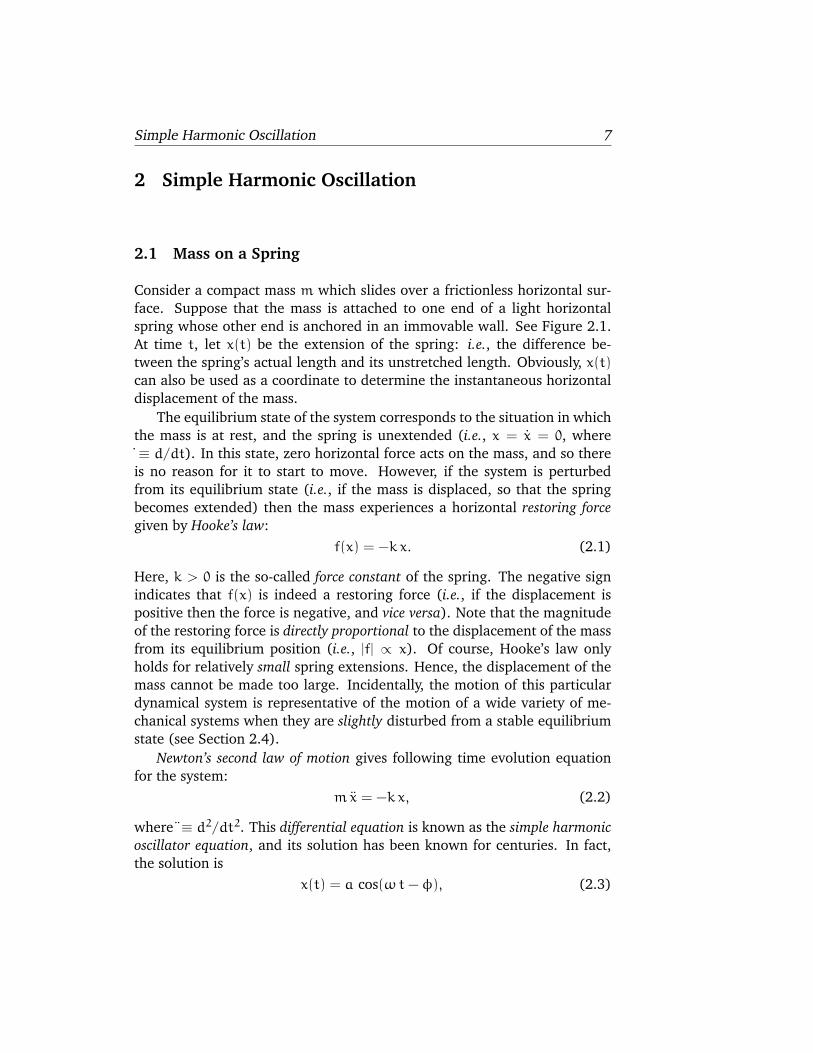
Consider a compact mass m which slides over a frictionless horizontal sur-
face. Suppose that the mass is attached to one end of a light horizontal
spring whose other end is anchored in an immovable wall. See Figure 2.1.
At time t, let x(t) be the extension of the spring: i.e., the difference be-
tween the spring’s actual length and its unstretched length. Obviously, x(t)
can also be used as a coordinate to determine the instantaneous horizontal
displacement of the mass.
The equilibrium state of the system corresponds to the situation in which
the mass is at rest, and the spring is unextended (i.e., x = x = 0, where
˙≡ d/dt). In this state, zero horizontal force acts on the mass, and so there
is no reason for it to start to move. However, if the system is perturbed
from its equilibrium state (i.e., if the mass is displaced, so that the spring
becomes extended) then the mass experiences a horizontal restoring force
given by Hooke’s law:
f(x) = −k x. (2.1)
Here, k > 0 is the so-called force constant of the spring. The negative sign
indicates that f(x) is indeed a restoring force (i.e., if the displacement is
positive then the force is negative, and vice versa). Note that the magnitude
of the restoring force is directly proportional to the displacement of the mass
from its equilibrium position (i.e., |f| ∝ x). Of course, Hooke’s law only
holds for relatively small spring extensions. Hence, the displacement of the
mass cannot be made too large. Incidentally, the motion of this particular
dynamical system is representative of the motion of a wide variety of me-
chanical systems when they are slightly disturbed from a stable equilibrium
state (see Section 2.4).
Newton’s second law of motion gives following time evolution equation
for the system:
mx = −k x, (2.2)
where¨≡ d2/dt2. This differential equation is known as the simple harmonic
oscillator equation, and its solution has been known for centuries. In fact,
the solution is
x(t) = a cos(ωt− φ), (2.3)
8 OSCILLATIONS AND WAVES
x = 0
x
m
Figure 2.1: Mass on a spring
where a > 0, ω > 0, and φ are constants. We can demonstrate that Equa-
tion (2.3) is indeed a solution of Equation (2.2) by direct substitution. Plug-
ging the right-hand side of (2.3) into Equation (2.2), and recalling from
standard calculus that d(cos θ)/dθ = − sin θ and d(sin θ)/dθ = cos θ, so
that x = −ωa sin(ωt − φ) and x = −ω2a cos(ωt − φ), where use has
been made of the chain rule, we obtain
−mω2a cos(ωt− φ) = −ka cos(ωt− φ). (2.4)
It follows that Equation (2.3) is the correct solution provided
ω =
√
k
m. (2.5)
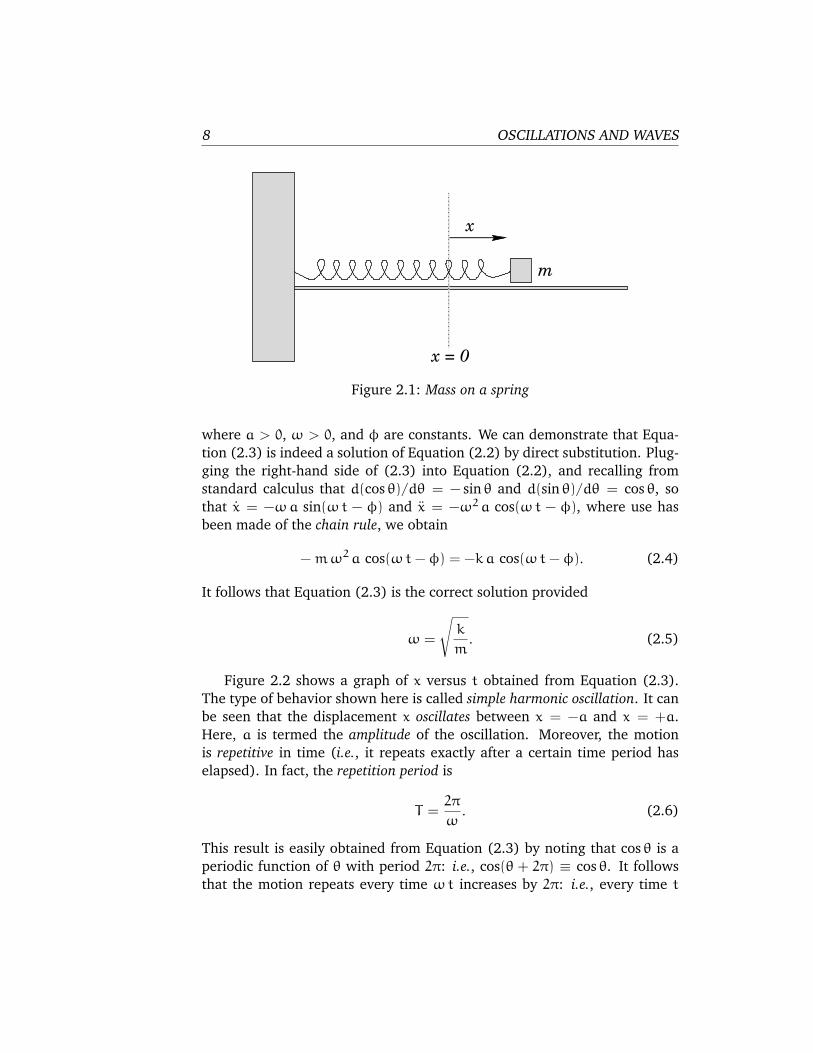
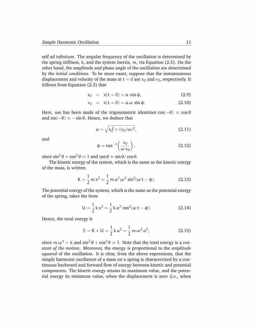
Figure 2.2 shows a graph of x versus t obtained from Equation (2.3).
The type of behavior shown here is called simple harmonic oscillation. It can
be seen that the displacement x oscillates between x = −a and x = +a.
Here, a is termed the amplitude of the oscillation. Moreover, the motion
is repetitive in time (i.e., it repeats exactly after a certain time period has
elapsed). In fact, the repetition period is
T =2π
ω. (2.6)
This result is easily obtained from Equation (2.3) by noting that cos θ is a
periodic function of θ with period 2π: i.e., cos(θ + 2π) ≡ cosθ. It follows
that the motion repeats every time ωt increases by 2π: i.e., every time t
Simple Harmonic Oscillation 9
Figure 2.2: Simple harmonic oscillation.
increases by 2π/ω. The frequency of the motion (i.e., the number of oscilla-
tions completed per second) is
f =1
T=ω
2π. (2.7)
It can be seen that ω is the motion’s angular frequency; i.e., the frequency
f converted into radians per second. Of course, f is measured in Hertz—
otherwise known as cycles per second. Finally, the phase angle, φ, determines
the times at which the oscillation attains its maximum displacement, x = a.
In fact, since the maxima of cos θ occur at θ = n2π, where n is an arbitrary
integer, the times of maximum displacement are
tmax = T
(
n+φ
2π
)
. (2.8)
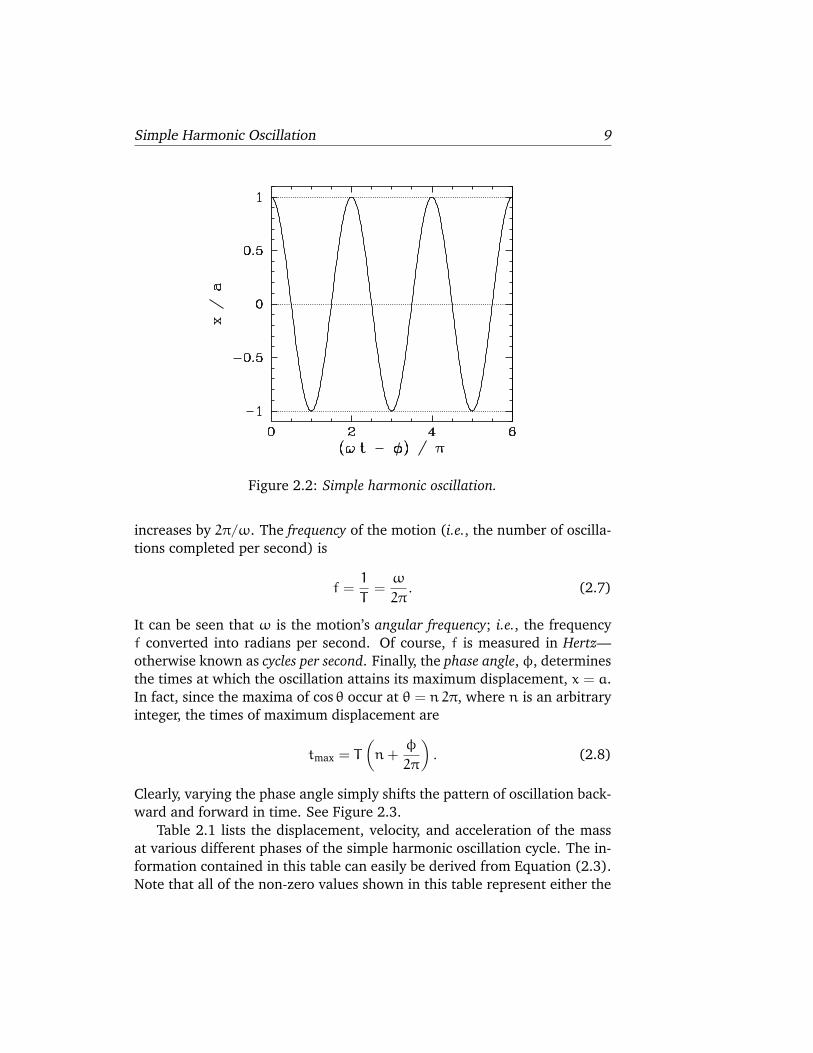
Clearly, varying the phase angle simply shifts the pattern of oscillation back-
ward and forward in time. See Figure 2.3.
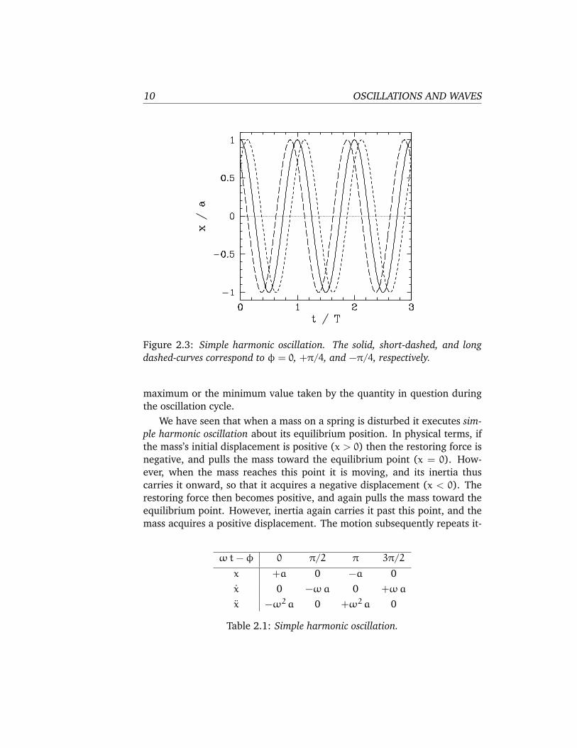
Table 2.1 lists the displacement, velocity, and acceleration of the mass
at various different phases of the simple harmonic oscillation cycle. The in-
formation contained in this table can easily be derived from Equation (2.3).
Note that all of the non-zero values shown in this table represent either the
10 OSCILLATIONS AND WAVES
Figure 2.3: Simple harmonic oscillation. The solid, short-dashed, and long
dashed-curves correspond to φ = 0, +π/4, and −π/4, respectively.
maximum or the minimum value taken by the quantity in question during
the oscillation cycle.
We have seen that when a mass on a spring is disturbed it executes sim-
ple harmonic oscillation about its equilibrium position. In physical terms, if
the mass’s initial displacement is positive (x > 0) then the restoring force is
negative, and pulls the mass toward the equilibrium point (x = 0). How-
ever, when the mass reaches this point it is moving, and its inertia thus
carries it onward, so that it acquires a negative displacement (x < 0). The
restoring force then becomes positive, and again pulls the mass toward the
equilibrium point. However, inertia again carries it past this point, and the
mass acquires a positive displacement. The motion subsequently repeats it-
ωt− φ 0 π/2 π 3π/2
x +a 0 −a 0
x 0 −ωa 0 +ωa
x −ω2a 0 +ω2a 0
Table 2.1: Simple harmonic oscillation.
Simple Harmonic Oscillation 11
self ad infinitum. The angular frequency of the oscillation is determined by
the spring stiffness, k, and the system inertia, m, via Equation (2.5). On the
other hand, the amplitude and phase angle of the oscillation are determined
by the initial conditions. To be more exact, suppose that the instantaneous
displacement and velocity of the mass at t = 0 are x0 and v0, respectively. It
follows from Equation (2.3) that
x0 = x(t = 0) = a cosφ, (2.9)
v0 = x(t = 0) = aω sinφ. (2.10)
Here, use has been made of the trigonometric identities cos(−θ) ≡ cos θ
and sin(−θ) ≡ − sin θ. Hence, we deduce that
a =√
x20 + (v0/ω)2, (2.11)
and
φ = tan−1
(
v0
ωx0
)
, (2.12)
since sin2θ+ cos2θ ≡ 1 and tanθ ≡ sin θ/ cos θ.
The kinetic energy of the system, which is the same as the kinetic energy
of the mass, is written
K =1
2m x2 =
1
2ma2ω2 sin2(ωt− φ). (2.13)
The potential energy of the system, which is the same as the potential energy
of the spring, takes the form
U =1
2k x2 =
1
2ka2 cos2(ωt− φ). (2.14)
Hence, the total energy is
E = K+U =1
2ka2 =
1
2mω2a2, (2.15)
since mω2 = k and sin2θ + cos2θ ≡ 1. Note that the total energy is a con-
stant of the motion. Moreover, the energy is proportional to the amplitude
squared of the oscillation. It is clear, from the above expressions, that the
simple harmonic oscillation of a mass on a spring is characterized by a con-
tinuous backward and forward flow of energy between kinetic and potential
components. The kinetic energy attains its maximum value, and the poten-
tial energy its minimum value, when the displacement is zero (i.e., when
12 OSCILLATIONS AND WAVES
x = 0). Likewise, the potential energy attains its maximum value, and the
kinetic energy its minimum value, when the displacement is maximal (i.e.,
when x = ±a). Note that the minimum value of K is zero, since the system
is instantaneously at rest when the displacement is maximal.
2.2 Simple Harmonic Oscillator Equation
Suppose that a physical system possesing one degree of freedom—i.e., a sys-
tem whose instantaneous state at time t is fully described by a single depen-
dent variable, s(t)—obeys the following time evolution equation [cf., Equa-
tion (2.2)]:
s+ω2 s = 0, (2.16)
where ω > 0 is a constant. As we have seen, this differential equation is
called the simple harmonic oscillator equation, and has the following solution
s(t) = a cos(ωt− φ), (2.17)
where a > 0 and φ are constants. Moreover, the above equation describes a
type of oscillation characterized by a constant amplitude, a, and a constant
angular frequency, ω. The phase angle, φ, determines the times at which
the oscillation attains its maximum value. Finally, the frequency of the os-
cillation (in Hertz) is f = ω/2π, and the period is T = 2π/ω. Note that
the frequency and period of the oscillation are both determined by the con-
stant ω, which appears in the simple harmonic oscillator equation, whereas
the amplitude, a, and phase angle, φ, are both determined by the initial
conditions—see Equations (2.9)–(2.12). In fact, a and φ are the two con-
stants of integration of the second-order ordinary differential equation (2.16).
Recall, from standard differential equation theory, that the most general
solution of an nth-order ordinary differential equation (i.e., an equation in-
volving a single independent variable and a single dependent variable in
which the highest derivative of the dependent with respect to the indepen-
dent variable is nth-order, and the lowest zeroth-order) involves n arbitrary
constants of integration. (Essentially, this is because we have to integrate
the equation n times with respect to the independent variable in order to
reduce it to zeroth-order, and so obtain the solution, and each integration
introduces an arbitrary constant: e.g., the integral of s = a, where a is a
known constant, is s = a t+ b, where b is an arbitrary constant.)
Multiplying Equation (2.16) by s, we obtain
s s+ω2 s s = 0. (2.18)
Simple Harmonic Oscillation 13
However, this can also be written in the form
d
dt
(
1
2s2
)
+d
dt
(
1
2ω2 s2
)
= 0, (2.19)
ordEdt
= 0, (2.20)
where
E =1
2s2 +
1
2ω2 s2. (2.21)
Clearly, E is a conserved quantity: i.e., it does not vary with time. In fact,
this quantity is generally proportional to the overall energy of the system.
For instance, E would be the energy divided by the mass in the mass-spring
system discussed in Section 2.1. Note that E is either zero or positive, since
neither of the terms on the right-hand side of Equation (2.21) can be neg-
ative. Let us search for an equilibrium state. Such a state is characterized
by s = constant, so that s = s = 0. It follows from (2.16) that s = 0,
and from (2.21) that E = 0. We conclude that the system can only remain
permanently at rest when E = 0. Conversely, the system can never perma-
nently come to rest when E > 0, and must, therefore, keep moving for ever.
Furthermore, since the equilibrium state is characterized by s = 0, it follows
that s represents a kind of “displacement” of the system from this state. It is
also apparent, from (2.21), that s attains it maximum value when s = 0. In
fact,
smax =
√2 Eω
. (2.22)
This, of course, is the amplitude of the oscillation: i.e., smax = a. Likewise,
s attains its maximum value when x = 0, and
smax =√2 E . (2.23)
Note that the simple harmonic oscillation (2.17) can also be written in
the form
s(t) = A cos(ωt) + B sin(ωt), (2.24)
where A = a cosφ and B = a sinφ. Here, we have employed the trigono-
metric identity cos(x − y) ≡ cos x cosy + sin x siny. Alternatively, (2.17)
can be written
s(t) = a sin(ωt− φ ′), (2.25)
where φ ′ = φ − π/2, and use has been made of the trigonometric identity
cos θ ≡ sin(π/2+ θ). Clearly, there are many different ways of representing
14 OSCILLATIONS AND WAVES
a simple harmonic oscillation, but they all involve linear combinations of
sine and cosine functions whose arguments take the form ωt + c, where
c is some constant. Note, however, that, whatever form it takes, a general
solution to the simple harmonic oscillator equation must always contain two
arbitrary constants: i.e., A and B in (2.24) or a and φ ′ in (2.25).
The simple harmonic oscillator equation, (2.16), is a linear differential
equation, which means that if s(t) is a solution then so is a s(t), where a
is an arbitrary constant. This can be verified by multiplying the equation
by a, and then making use of the fact that ad2s/dt2 = d2(a s)/dt2. Now,
linear differential equations have a very important and useful property: i.e.,
their solutions are superposable. This means that if s1(t) is a solution to
Equation (2.16), so that
s1 = −ω2 s1, (2.26)
and s2(t) is a different solution, so that
s2 = −ω2 s2, (2.27)
then s1(t) + s2(t) is also a solution. This can be verified by adding the pre-
vious two equations, and making use of the fact that d2s1/dt2 +d2s2/dt
2 =
d2(s1 + s2)/dt2. Furthermore, it is easily demonstrated that any linear com-
bination of s1 and s2, such as a s1 + b s2, where a and b are constants, is
a solution. It is very helpful to know this fact. For instance, the solution
to the simple harmonic oscillator equation (2.16) with the initial conditions
s(0) = 1 and s(0) = 0 is easily shown to be
s1(t) = cos(ωt). (2.28)
Likewise, the solution with the initial conditions s(0) = 0 and s(0) = 1 is
clearly
s2(t) = ω−1 sin(ωt). (2.29)
Thus, since the solutions to the simple harmonic oscillator equation are su-
perposable, the solution with the initial conditions s(0) = s0 and s(0) = s0is s(t) = s0 s1(t) + s0 s2(t), or
s(t) = s0 cos(ωt) +s0
ωsin(ωt). (2.30)
2.3 LC Circuit
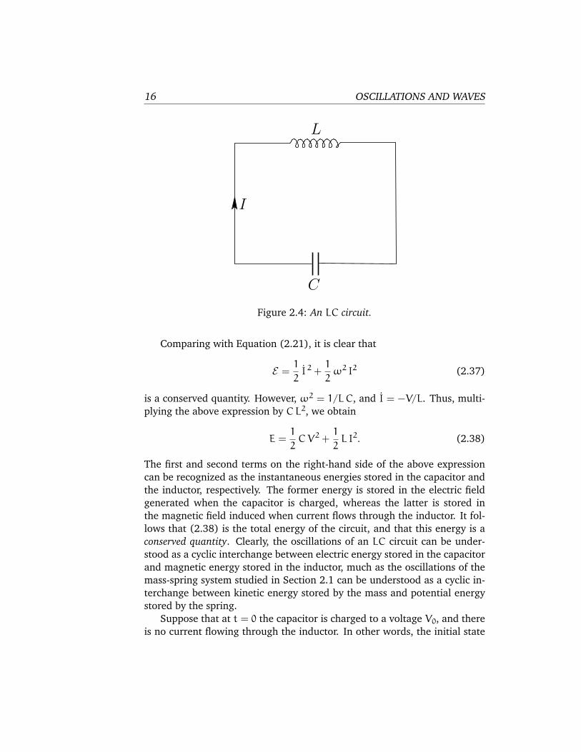
Consider an electrical circuit consisting of an inductor, of inductance L, con-
nected in series with a capacitor, of capacitance C. See Figure 2.4. Such

Simple Harmonic Oscillation 15
a circuit is known as an LC circuit, for obvious reasons. Suppose that I(t)
is the instantaneous current flowing around the circuit. According to stan-
dard electrical circuit theory, the potential difference across the inductor is
L I. Again, from standard electrical circuit theory, the potential difference
across the capacitor is V = Q/C, where Q is the charge stored on the capac-
itor’s positive plate. However, since electric charge is conserved, the current
flowing around the circuit is equal to the rate at which charge accumulates
on the capacitor’s positive plate: i.e., I = Q. Now, according to Kichhoff ’s
second circuital law, the sum of the potential differences across the various
components of a closed circuit loop is equal to zero. In other words,
L I+Q/C = 0. (2.31)
Dividing by L, and differentiating with respect to t, we obtain
I+ω2 I = 0, (2.32)
where
ω =1√LC
. (2.33)
Comparison with Equation (2.16) reveals that (2.32) is a simple harmonic
oscillator equation with the associated angular oscillation frequency ω. We
conclude that the current in an LC circuit executes simple harmonic oscilla-
tions of the form
I(t) = I0 cos(ωt− φ), (2.34)
where I0 > 0 and φ are constants. Now, according to Equation (2.31), the
potential difference, V = Q/C, across the capacitor is minus that across the
inductor, so that V = −L I, giving
V(t) =
√
L
CI0 sin(ωt− φ) =
√
L
CI0 cos(ωt− φ− π/2). (2.35)
Here, use has been made of the trigonometric identity sinθ ≡ cos(θ− π/2).
It follows that the voltage in an LC circuit oscillates at the same frequency
as the current, but with a phase shift of π/2. In other words, the voltage is
maximal when the current is zero, and vice versa. The amplitude of the volt-
age oscillation is that of the current oscillation multiplied by√
L/C. Thus,
we can also write
V(t) =
√
L
CI(t−ω−1π/2). (2.36)
16 OSCILLATIONS AND WAVES
.
L
C
I
Figure 2.4: An LC circuit.
Comparing with Equation (2.21), it is clear that
E =1
2I2 +
1
2ω2 I2 (2.37)
is a conserved quantity. However, ω2 = 1/LC, and I = −V/L. Thus, multi-
plying the above expression by CL2, we obtain
E =1
2CV2 +
1
2L I2. (2.38)
The first and second terms on the right-hand side of the above expression
can be recognized as the instantaneous energies stored in the capacitor and
the inductor, respectively. The former energy is stored in the electric field
generated when the capacitor is charged, whereas the latter is stored in
the magnetic field induced when current flows through the inductor. It fol-
lows that (2.38) is the total energy of the circuit, and that this energy is a
conserved quantity. Clearly, the oscillations of an LC circuit can be under-
stood as a cyclic interchange between electric energy stored in the capacitor
and magnetic energy stored in the inductor, much as the oscillations of the
mass-spring system studied in Section 2.1 can be understood as a cyclic in-
terchange between kinetic energy stored by the mass and potential energy
stored by the spring.
Suppose that at t = 0 the capacitor is charged to a voltage V0, and there
is no current flowing through the inductor. In other words, the initial state
Simple Harmonic Oscillation 17
is one in which all of the circuit energy resides in the capacitor. The initial
conditions are V(0) = −L I(0) = V0 and I(0) = 0. It is easily demonstrated
that the current evolves in time as
I(t) = −V0
√
L/Csin(ωt). (2.39)
Suppose that at t = 0 the capacitor is fully discharged, and there is a current
I0 flowing through the inductor. In other words, the initial state is one in
which all of the circuit energy resides in the inductor. The initial conditions
are V(0) = −L I(0) = 0 and I(0) = I0. It is easily demonstrated that the
current evolves in time as
I(t) = I0 cos(ωt). (2.40)
Suppose, finally, that at t = 0 the capacitor is charged to a voltage V0, and
the current flowing through the inductor is I0. Since the solutions of the
simple harmonic oscillator equation are superposable, it is clear that the
current evolves in time as
I(t) = −V0
√
L/Csin(ωt) + I0 cos(ωt). (2.41)
Furthermore, it follows from Equation (2.36) that the voltage evolves in
time as
V(t) = −V0 sin(ωt− π/2) +
√
L
CI0 cos(ωt− π/2), (2.42)
or
V(t) = V0 cos(ωt) +
√
L
CI0 sin(ωt). (2.43)
Here, use has been made of the trigonometric identities sin(θ − π/2) ≡− cos θ and cos(θ− π/2) ≡ sin θ.
The instantaneous electrical power absorption by the capacitor, which
can easily be shown to be minus the instantaneous power absorption by the
inductor, is
P(t) = I(t)V(t) = I0V0 cos(2ω t) +1
2
I20
√
L
C−
V 20
√
L/C
sin(2ω t),
(2.44)
18 OSCILLATIONS AND WAVES
l
m g
pivot point
fixed support
θ
m
T
Figure 2.5: A simple pendulum.
where use has been made of Equations (2.41) and (2.43), as well as the
trigonometric identities cos(2 θ) ≡ cos2θ−sin2θ and sin(2 θ) ≡ 2 sin θ cos θ.
Hence, the average power absorption during a cycle of the oscillation,
〈P〉 =1
T
∫T
0
P(t)dt, (2.45)
is zero, since it is easily demonstrated that 〈cos(2ω t)〉 = 〈sin(2ω t)〉 = 0. In
other words, any energy which the capacitor absorbs from the circuit during
one part of the oscillation cycle is returned to the circuit without loss during
another. The same goes for the inductor.
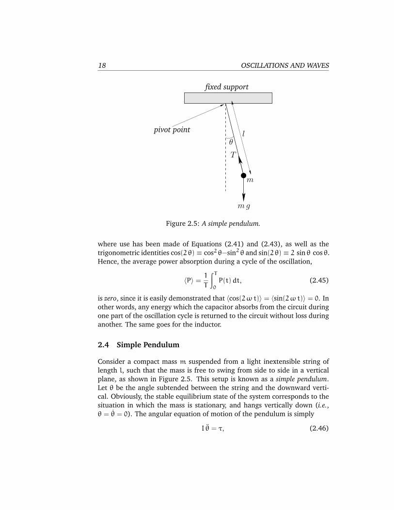
2.4 Simple Pendulum
Consider a compact mass m suspended from a light inextensible string of
length l, such that the mass is free to swing from side to side in a vertical
plane, as shown in Figure 2.5. This setup is known as a simple pendulum.
Let θ be the angle subtended between the string and the downward verti-
cal. Obviously, the stable equilibrium state of the system corresponds to the
situation in which the mass is stationary, and hangs vertically down (i.e.,
θ = θ = 0). The angular equation of motion of the pendulum is simply
I θ = τ, (2.46)
Simple Harmonic Oscillation 19
where I is the moment of inertia of the mass, and τ the torque acting about
the suspension point. For the case in hand, given that the mass is essentially
a point particle, and is situated a distance l from the axis of rotation (i.e.,
the suspension point), it is easily seen that I = ml2.
The two forces acting on the mass are the downward gravitational force,
mg, where g is the acceleration due to gravity, and the tension, T , in the
string. Note, however, that the tension makes no contribution to the torque,
since its line of action clearly passes through the suspension point. From
elementary trigonometry, the line of action of the gravitational force passes
a perpendicular distance l sin θ from the suspension point. Hence, the mag-
nitude of the gravitational torque is mg l sin θ. Moreover, the gravitational
torque is a restoring torque: i.e., if the mass is displaced slightly from its
equilibrium position (i.e., θ = 0) then the gravitational torque clearly acts
to push the mass back towards that position. Thus, we can write
τ = −mg l sin θ. (2.47)
Combining the previous two equations, we obtain the following angular
equation of motion of the pendulum:
l θ+ g sin θ = 0. (2.48)
Note that, unlike all of the other time evolution equations which we have ex-
amined so far in this chapter, the above equation is nonlinear [since sin(aθ) 6=a sin θ], which means that it is generally very difficult to solve.
Suppose, however, that the system does not stray very far from its equi-
librium position (θ = 0). If this is the case then we can expand sin θ in a
Taylor series about θ = 0. We obtain
sin θ = θ−θ3
6+θ5
120+ O(θ7). (2.49)
Clearly, if |θ| is sufficiently small then the series is dominated by its first term,
and we can write sin θ ≃ θ. This is known as the small angle approximation.
Making use of this approximation, the equation of motion (2.48) simplifies
to
θ+ω2θ ≃ 0, (2.50)
where
ω =
√
g
l. (2.51)
20 OSCILLATIONS AND WAVES
Of course, (2.50) is just the simple harmonic oscillator equation. Hence, we
can immediately write its solution in the form
θ(t) = θ0 cos(ωt− φ), (2.52)
where θ0 > 0 and φ are constants. We conclude that the pendulum swings
back and forth at a fixed frequency, ω, which depends on l and g, but is
independent of the amplitude, θ0, of the motion. Of course, this result only
holds as long as the small angle approximation remains valid. It turns out
that sin θ ≃ θ is a good approximation provided |θ| <∼6. Hence, the period
of a simple pendulum is only amplitude independent when the amplitude
of the motion is less than about 6.
2.5 Exercises
1. A mass stands on a platform which executes simple harmonic oscillation ina vertical direction at a frequency of 5Hz. Show that the mass loses contactwith the platform when the displacement exceeds 10−2 m.
2. A small body rests on a horizontal diaphragm of a loudspeaker which issupplies with an alternating current of constant amplitude but variable fre-quency. If diaphragm executes simple harmonic oscillation in the verticaldirection of amplitude 10µm, at all frequencies, find the greatest frequencyfor which the small body stays in contact with the diaphragm.
3. Two light springs have spring constants k1 and k2, respectively, and are usedin a vertical orientation to support an object of mass m. Show that the an-gular frequency of small amplitude oscillations about the equilibrium state is[(k1 + k2)/m]1/2 if the springs are in parallel, and [k1 k2/(k1 + k2)m]1/2 ifthe springs are in series.
4. A body of uniform cross-sectional area A and mass density ρ floats in a liquidof density ρ0 (where ρ < ρ0), and at equilibrium displaces a volume V.Making use of Archimedes principle (that the buoyancy force acting on apartially submerged body is equal to the mass of the displaced liquid), showthat the period of small amplitude oscillations about the equilibrium positionis
T = 2π
√
V
gA.
5. A particle of mass m slides in a frictionless semi-circular depression in theground of radius R. Find the angular frequency of small amplitude oscilla-tions about the particle’s equilibrium position, assuming that the oscillationsare essentially one dimensional, so that the particle passes through the low-est point of the depression during each oscillation cycle.
Simple Harmonic Oscillation 21
6. If a thin wire is twisted through an angle θ then a restoring torque τ = −kθ
develops, where k > 0 is known as the torsional force constant. Considera so-called torsional pendulum, which consists of a horizontal disk of massM, and moment of inertia I, suspended at its center from a thin verticalwire of negligible mass and length l, whose other end is attached to a fixedsupport. The disk is free to rotate about a vertical axis passing through thesuspension point, but such rotation twists the wire. Find the frequency oftorsional oscillations of the disk about its equilibrium position.
7. Suppose that a hole is drilled through a laminar (i.e., flat) object of massM, which is then suspended in a frictionless manner from a horizontal axispassing through the hole, such that it is free to rotate in a vertical plane.Suppose that the moment of inertia of the object about the axis is I, andthat the distance of the hole from the object’s center of mass is d. Findthe frequency of small angle oscillations of the object about its equilibriumposition. Hence, find the frequency of small angle oscillations of a compound
pendulum consisting of a uniform rod of mass M and length l suspendedvertically from a horizontal axis passing through one of its ends.
8. A pendulum consists of a uniform circular disk of radius r which is free toturn about a horizontal axis perpendicular to its plane. Find the position ofthe axis for which the periodic time is a minimum.
9. A particle of mass m executes one-dimensional simple harmonic oscillationunder the action of a conservative force such that its instantaneous x coordi-nate is
x(t) = a cos(ωt− φ).
Find the average values of x, x2, x, and x2 over a single cycle of the oscil-lation. Find the average values of the kinetic and potential energies of theparticle over a single cycle of the oscillation.
10. A particle executes two-dimensional simple harmonic oscillation such that itsinstantaneous coordinates in the x-y plane are
x(t) = a cos(ωt),
y(t) = a cos(ωt− φ).
Describe the motion when (a) φ = 0, (b) φ = π/2, and (c) φ = −π/2. Ineach case, plot the trajectory of the particle in the x-y plane.
11. An LC circuit is such that at t = 0 the capacitor is uncharged and a currentI0 flows through the inductor. Find an expression for the charge Q stored onthe positive plate of the capacitor as a function of time.
12. A simple pendulum of mass m and length l is such that θ(0) = 0 and θ(0) =
ω0. Find the subsequent motion, θ(t), assuming that its amplitude remainssmall. Suppose, instead, that θ(0) = θ0 and θ(0) = 0. Find the subsequentmotion. Suppose, finally, that θ(0) = θ0 and θ(0) = ω0. Find the subsequentmotion.
22 OSCILLATIONS AND WAVES
13. Demonstrate that
E =1
2m l2 θ 2 +mg l (cos θ− 1)
is a constant of the motion of a simple pendulum whose time evolution equa-tion is given by (2.48). (Do not make the small angle approximation.) Hence,show that the amplitude of the motion, θ0, can be written
θ0 = 2 sin−1
(
E
2mg l
)1/2
.
Finally, demonstrate that the period of the motion is determined by
T
T0
=1
π
∫θ0
0
dθ√
sin2(θ0/2) − sin2
(θ/2)
,
where T0 is the period of small angle oscillations. Verify that T/T0 → 1 asθ0 → 0. Does the period increase, or decrease, as the amplitude of themotion increases?
Damped and Driven Harmonic Oscillation 23
3 Damped and Driven Harmonic Oscillation
3.1 Damped Harmonic Oscillation
In the previous chapter, we encountered a number of energy conserving
physical systems which exhibit simple harmonic oscillation about a stable
equilibrium state. One of the main features of such oscillation is that, once
excited, it never dies away. However, the majority of the oscillatory sys-
tems which we generally encounter in everyday life suffer some sort of irre-
versible energy loss due, for instance, to frictional or viscous heat generation
whilst they are oscillating. We would therefore expect oscillations excited in
such systems to eventually be damped away. Let us examine an example of
a damped oscillatory system.
Consider the mass-spring system investigated in Section 2.1. Suppose
that, as it slides over the horizontal surface, the mass is subject to a frictional
damping force which opposes its motion, and is directly proportional to its
instantaneous velocity. It follows that the net force acting on the mass when
its instantaneous displacement is x(t) takes the form
f = −k x−mν x, (3.1)
where m > 0 is the mass, k > 0 the spring force constant, and ν > 0 a
constant (with the dimensions of angular frequency) which parameterizes
the strength of the damping. The time evolution equation of the system thus
becomes [cf., Equation (2.2)]
x+ ν x+ω20 x = 0, (3.2)
where ω0 =√
k/m is the undamped oscillation frequency [cf., Equation
(2.5)]. We shall refer to the above as the damped harmonic oscillator equa-
tion.
Let us search for a solution to Equation (3.2) of the form
x(t) = a e−γt cos(ω1 t− φ), (3.3)
where a > 0, γ > 0, ω1 > 0, and φ are all constants. By analogy with the
discussion in Section 2.1, we can interpret the above solution as a periodic
oscillation, of fixed angular frequency ω1 and phase angle φ, whose ampli-
tude decays exponentially in time as a(t) = a exp(−γ t). So, (3.3) certainly
24 OSCILLATIONS AND WAVES
seems like a plausible solution for a damped oscillatory system. It is easily
demonstrated that
x = −γa e−γt cos(ω1 t− φ) −ω1a e−γt sin(ω1 t− φ), (3.4)
x = (γ2 −ω21)a e−γt cos(ω1 t− φ) + 2 γω1a e−γt sin(ω1 t− φ),
(3.5)
so Equation (3.2) becomes
0 =[
(γ2 −ω21) − νγ+ω2
0
]
a e−γt cos(ω1 t− φ)
+ [2 γω1 − νω1]a e−γt sin(ω1 t− φ). (3.6)
Now, the only way in which the above equation can be satisfied at all times
is if the coefficients of exp(−γ t) cos(ω1 t−φ) and exp(−γ t) sin(ω1 t−φ)
separately equate to zero, so that
(γ2 −ω21) − νγ+ω2
0 = 0, (3.7)
2 γω1 − νω1 = 0. (3.8)
These equations can easily be solved to give
γ = ν/2, (3.9)
ω1 = (ω20 − ν2/4)1/2. (3.10)
Thus, the solution to the damped harmonic oscillator equation is written
x(t) = a e−νt/2 cos (ω1 t− φ) , (3.11)
assuming that ν < 2ω0 (since ω21 = ω2
0 −ν2/4 clearly cannot be negative).
We conclude that the effect of a relatively small amount of damping, pa-
rameterized by the damping constant ν, on a system which exhibits simple
harmonic oscillation about a stable equilibrium state is to reduce the angular
frequency of the oscillation from its undamped value ω0 to (ω20 − ν2/4)1/2,
and to cause the amplitude of the oscillation to decay exponentially in time
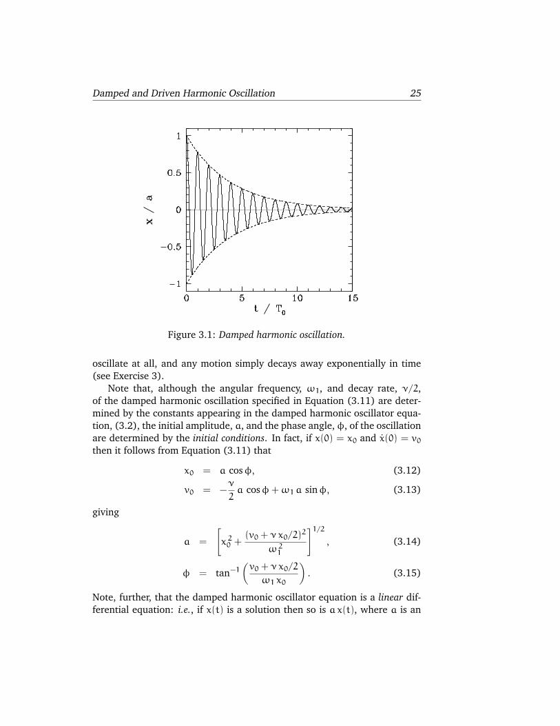
at the rate ν/2. This modified type of oscillation, which we shall refer to as
damped harmonic oscillation, is illustrated in Figure 3.1. [Here, T0 = 2π/ω0,
ν T0 = 0.5, and φ = 0. The solid line shows x(t)/a, whereas the dashed
lines show ±a(t)/a.] Incidentally, if the damping is sufficiently large that
ν ≥ 2ω0, which we shall assume is not the case, then the system does not
Damped and Driven Harmonic Oscillation 25
Figure 3.1: Damped harmonic oscillation.
oscillate at all, and any motion simply decays away exponentially in time
(see Exercise 3).
Note that, although the angular frequency, ω1, and decay rate, ν/2,
of the damped harmonic oscillation specified in Equation (3.11) are deter-
mined by the constants appearing in the damped harmonic oscillator equa-
tion, (3.2), the initial amplitude, a, and the phase angle, φ, of the oscillation
are determined by the initial conditions. In fact, if x(0) = x0 and x(0) = v0
then it follows from Equation (3.11) that
x0 = a cosφ, (3.12)
v0 = −ν
2a cosφ+ω1a sinφ, (3.13)
giving
a =
[
x20 +
(v0 + νx0/2)2
ω21
]1/2
, (3.14)
φ = tan−1
(
v0 + νx0/2
ω1x0
)
. (3.15)
Note, further, that the damped harmonic oscillator equation is a linear dif-
ferential equation: i.e., if x(t) is a solution then so is ax(t), where a is an
26 OSCILLATIONS AND WAVES
arbitrary constant. It follows that the solutions of this equation are superpos-
able, so that if x1(t) and x2(t) are two solutions corresponding to different
initial conditions then ax1(t)+bx2(t) is a third solution, where a and b are
arbitrary constants.
Multiplying the damped harmonic oscillator equation (3.2) by x, we ob-
tain
x x+ ν x2 +ω20 x x = 0, (3.16)
which can be rearranged to give
dE
dt= −mν x2, (3.17)
where
E =1
2m x2 +
1
2k x2 (3.18)
is the total energy of the system: i.e., the sum of the kinetic and potential
energies. Clearly, since the right-hand side of (3.17) cannot be positive, and
is only zero when the system is stationary, the total energy is not a conserved
quantity, but instead decays monotonically in time due to the presence of
damping. Now, the net rate at which the force (3.1) does work on the mass
is
P = f x = −k x x−mν x2. (3.19)
Note that the spring force (i.e., the first term on the right-hand side) does
negative work on the mass (i.e., it reduces the system kinetic energy) when
x and x are of the same sign, and does positive work when they are of the
opposite sign. On average, the spring force does no net work on the mass
during an oscillation cycle. The damping force, on the other hand, (i.e., the
second term on the right-hand side) always does negative work on the mass,
and, therefore, always acts to reduce the system kinetic energy.
3.2 Quality Factor
The energy loss rate of a weakly damped (i.e., ν≪ 2ω0) harmonic oscillator
is conveniently characterized in terms of a parameter,Qf, which is known as
the quality factor. This quantity is defined to be 2π times the energy stored
in the oscillator, divided by the energy lost in a single oscillation period. If
the oscillator is weakly damped then the energy lost per period is relatively
small, and Qf is therefore much larger than unity. Roughly speaking, Qf is
the number of oscillations that the oscillator typically completes, after being
set in motion, before its amplitude decays to a negligible value. For instance,
Damped and Driven Harmonic Oscillation 27
the quality factor for the damped oscillation shown in Figure 3.1 is 12.6. Let
us find an expression for Qf.
As we have seen, the motion of a weakly damped harmonic oscillator is
specified by [see Equation (3.11)]
x = a e−νt/2 cos(ω1 t− φ), (3.20)
It follows that
x = −aν
2e−νt/2 cos(ω1 t− φ) − aω1 e−νt/2 sin(ω1 t− φ). (3.21)
Thus, making use of Equation (3.17), the energy lost during a single oscil-
lation period is
∆E = −
∫ (2π+φ)/ω1
φ/ω1
dE
dtdt (3.22)
= mνa2
∫ (2π+φ)/ω1
φ/ω1
e−νt
[
ν
2cos(ω1 t− φ) +ω1 sin(ω1 t− φ)
]2
dt.
In the weakly damped limit, ν ≪ 2ω0, the exponential factor is approxi-
mately unity in the interval t = φ/ω1 to (2π+ φ)/ω1, so that
∆E ≃ mνa2
ω1
∫2π
0
(
ν2
4cos2θ+ νω1 cos θ sin θ+ω2
1 sin2θ
)
dθ, (3.23)
where θ = ω1 t− φ. Thus,
∆E ≃ πmνa2
ω1
(ν2/4+ω21) = πmω2
0 a2
(
ν
ω1
)
, (3.24)
since, as is easily demonstrated,
∫2π
0
cos2θdθ =
∫2π
0
sin2θdθ = π, (3.25)
∫2π
0
cos θ sin θdθ = 0. (3.26)
Now, the energy stored in the oscillator (at t = 0) is [cf., Equation (2.15)]
E =1
2mω2
0 a2. (3.27)
Hence, we obtain
Qf = 2πE
∆E=ω1
ν≃ ω0
ν. (3.28)
28 OSCILLATIONS AND WAVES
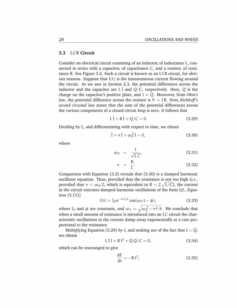
3.3 LCR Circuit
Consider an electrical circuit consisting of an inductor, of inductance L, con-
nected in series with a capacitor, of capacitance C, and a resistor, of resis-
tance R. See Figure 3.2. Such a circuit is known as an LCR circuit, for obvi-
ous reasons. Suppose that I(t) is the instantaneous current flowing around
the circuit. As we saw in Section 2.3, the potential differences across the
inductor and the capacitor are L I and Q/C, respectively. Here, Q is the
charge on the capacitor’s positive plate, and I = Q. Moreover, from Ohm’s
law, the potential difference across the resistor is V = I R. Now, Kichhoff ’s
second circuital law states that the sum of the potential differences across
the various components of a closed circuit loop is zero. It follows that
L I+ R I+Q/C = 0. (3.29)
Dividing by L, and differentiating with respect to time, we obtain
I+ ν I+ω20 I = 0, (3.30)
where
ω0 =1√LC
, (3.31)
ν =R
L. (3.32)
Comparison with Equation (3.2) reveals that (3.30) is a damped harmonic
oscillator equation. Thus, provided that the resistance is not too high (i.e.,
provided that ν < ω0/2, which is equivalent to R < 2√
L/C), the current
in the circuit executes damped harmonic oscillations of the form [cf., Equa-
tion (3.11)]
I(t) = I0 e−νt/2 cos(ω1 t− φ), (3.33)
where I0 and φ are constants, and ω1 =√
ω20 − ν2/4. We conclude that
when a small amount of resistance is introduced into an LC circuit the char-
acteristic oscillations in the current damp away exponentially at a rate pro-
portional to the resistance.
Multiplying Equation (3.29) by I, and making use of the fact that I = Q,
we obtain
L I I+ R I2 + QQ/C = 0, (3.34)
which can be rearranged to give
dE
dt= −R I2, (3.35)
Damped and Driven Harmonic Oscillation 29
.
R
C
I
L
Figure 3.2: An LCR circuit.
where
E =1
2L I2 +
1
2
Q2
C. (3.36)
Clearly, E is the circuit energy: i.e., the sum of the energies stored in the
inductor and the capacitor. Moreover, according to Equation (3.35), the cir-
cuit energy decays in time due to the power R I2 dissipated via Joule heating
in the resistor. Note that the dissipated power is always positive: i.e., the
circuit never gains energy from the resistor.
Finally, a comparison of Equations (3.28), (3.31), and (3.32) reveals
that the quality factor of an LCR circuit is
Qf =
√
L/C
R. (3.37)
3.4 Driven Damped Harmonic Oscillation
We saw earlier, in Section 3.1, that when a damped mechanical oscillator
is set into motion the oscillations eventually die away due to frictional en-
ergy losses. In fact, the only way of maintaining the motion of a damped
oscillator is to continually feed energy into the system in such a manner as
to offset the frictional losses. A steady-state (i.e., constant amplitude) os-
cillation of this type is called driven damped harmonic oscillation. Consider
a modified version of the mass-spring system investigated in Section 3.1 in
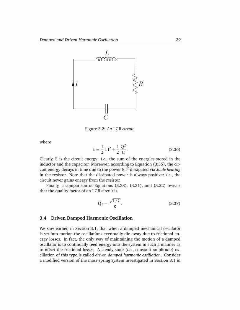
30 OSCILLATIONS AND WAVES
x
m
x = 0
Piston
X
X = 0
Figure 3.3: A driven oscillatory system
which one end of the spring is attached to the mass, and the other to a mov-
ing piston. See Figure 3.3. Let x(t) be the horizontal displacement of the
mass, and X(t) the horizontal displacement of the piston. The extension of
the spring is thus x(t) − X(t), assuming that the spring is unstretched when
x = X = 0. Thus, the horizontal force acting on the mass can be written [cf.,
Equation (3.1)]
f = −k (x− X) −mν x. (3.38)
The equation of motion of the system then becomes [cf., Equation (3.2)]
x+ ν x+ω20 x = ω2
0 X, (3.39)
where ν > 0 is the damping constant, and ω0 > 0 the undamped oscillation
frequency. Suppose, finally, that the piston executes simple harmonic oscil-
lation of angular frequency ω > 0 and amplitude X0 > 0, so that the time
evolution equation of the system takes the form
x+ ν x+ω20 x = ω2
0 X0 cos(ωt). (3.40)
We shall refer to the above as the driven damped harmonic oscillator equa-
tion.
Now, we would generally expect the periodically driven oscillator shown
in Figure 3.3 to eventually settle down to a steady (i.e., constant amplitude)
pattern of oscillation, with the same frequency as the piston, in which the
frictional energy loss per cycle is exactly matched by the work done by the
piston per cycle (see Exercise 7). This suggests that we should search for a
solution to Equation (3.40) of the form
x(t) = x0 cos(ωt−ϕ). (3.41)
Damped and Driven Harmonic Oscillation 31
Here, x0 > 0 is the amplitude of the driven oscillation, whereasϕ is the phase
lag of this oscillation (with respect to the phase of the piston oscillation).
Now, since
x = −ωx0 sin(ωt−ϕ), (3.42)
x = −ω2x0 cos(ωt−ϕ), (3.43)
Equation (3.40) becomes
(ω20 −ω2) x0 cos(ωt−ϕ)−νωx0 sin(ωt−ϕ) = ω2
0 X0 cos(ωt). (3.44)
However, cos(ωt−ϕ) ≡ cos(ωt) cosϕ+ sin(ωt) sinϕ and sin(ωt−ϕ) ≡sin(ωt) cosϕ− cos(ωt) sinϕ, so we obtain
[
x0 (ω20 −ω2) cosϕ+ x0νω sinϕ−ω2
0 X0
]
cos(ωt) (3.45)
+x0
[
(ω20 −ω2) sinϕ− νω cosϕ
]
sin(ωt) = 0.
Now, the only way in which the above equation can be satisfied at all times
is if the coefficients of cos(ωt) and sin(ωt) separately equate to zero. In
other words,
x0 (ω20 −ω2) cosϕ+ x0νω sinϕ−ω2
0 X0 = 0, (3.46)
(ω20 −ω2) sinϕ− νω cosϕ = 0. (3.47)
These two expressions can be combined to give
x0 =ω2
0 X0[
(ω20 −ω2)2 + ν2ω2
]1/2, (3.48)
ϕ = tan−1
(
νω
ω20 −ω2
)
. (3.49)
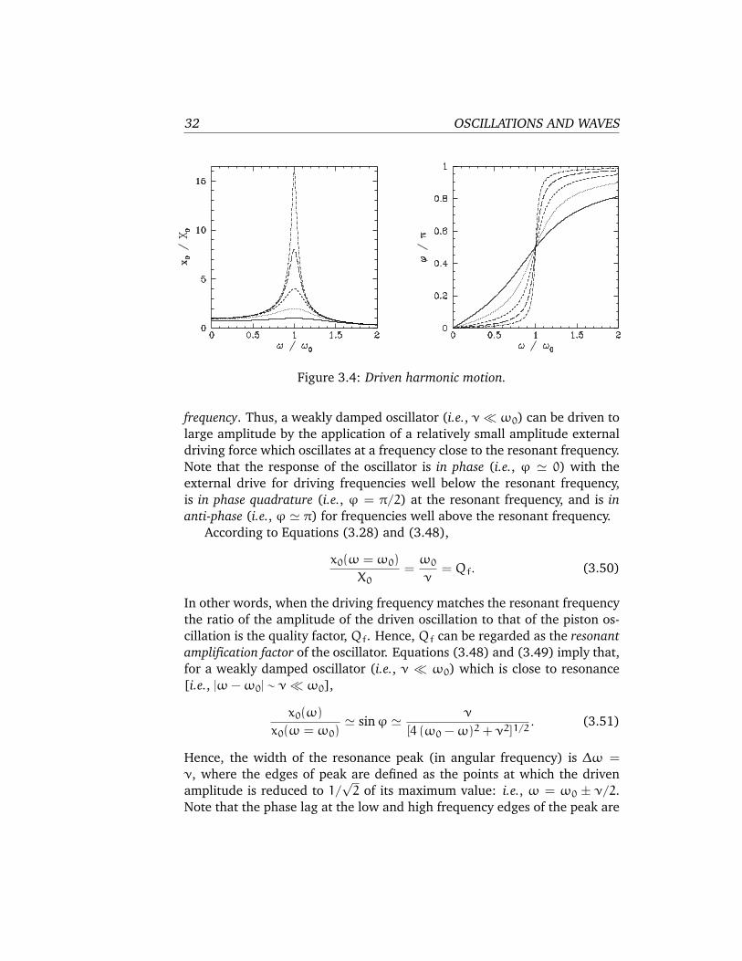
Let us investigate the dependence of the amplitude, x0, and phase lag,
ϕ, of the driven oscillation on the driving frequency, ω. This is most easily
done graphically. Figure 3.4 shows x0/X0 and ϕ plotted as functions of ω
for various different values of ν/ω0. In fact, ν/ω0 = 1/Qf = 1, 1/2, 1/4,
1/8, and 1/16 correspond to the solid, dotted, short-dashed, long-dashed,
and dot-dashed curves, respectively. It can be seen that as the amount of
damping in the system is decreased the amplitude of the response becomes
progressively more peaked at the natural frequency of oscillation of the sys-
tem, ω0. This effect is known as resonance, and ω0 is termed the resonant
32 OSCILLATIONS AND WAVES
Figure 3.4: Driven harmonic motion.
frequency. Thus, a weakly damped oscillator (i.e., ν≪ ω0) can be driven to
large amplitude by the application of a relatively small amplitude external
driving force which oscillates at a frequency close to the resonant frequency.
Note that the response of the oscillator is in phase (i.e., ϕ ≃ 0) with the
external drive for driving frequencies well below the resonant frequency,
is in phase quadrature (i.e., ϕ = π/2) at the resonant frequency, and is in
anti-phase (i.e., ϕ ≃ π) for frequencies well above the resonant frequency.
According to Equations (3.28) and (3.48),
x0(ω = ω0)
X0
=ω0
ν= Qf. (3.50)
In other words, when the driving frequency matches the resonant frequency
the ratio of the amplitude of the driven oscillation to that of the piston os-
cillation is the quality factor, Qf. Hence, Qf can be regarded as the resonant
amplification factor of the oscillator. Equations (3.48) and (3.49) imply that,
for a weakly damped oscillator (i.e., ν ≪ ω0) which is close to resonance
[i.e., |ω−ω0| ∼ ν≪ ω0],
x0(ω)
x0(ω = ω0)≃ sinϕ ≃ ν
[4 (ω0 −ω)2 + ν2]1/2. (3.51)
Hence, the width of the resonance peak (in angular frequency) is ∆ω =
ν, where the edges of peak are defined as the points at which the driven
amplitude is reduced to 1/√2 of its maximum value: i.e., ω = ω0 ± ν/2.
Note that the phase lag at the low and high frequency edges of the peak are
Damped and Driven Harmonic Oscillation 33
π/4 and 3π/4, respectively. Furthermore, the fractional width of the peak is
∆ω
ω0
=ν
ω0
=1
Qf
. (3.52)
We conclude that the height and width of the resonance peak of a weakly
damped (Qf ≫ 1) harmonic oscillator scale as Qf and Q−1f , respectively.
Thus, the area under the resonance peak stays approximately constant as
Qf varies.
Now, the force exerted on the system by the piston is
F(t) = kX0 cos(ωt). (3.53)
Hence, the instantaneous power absorption from the piston becomes
P(t) = F(t) x(t)
= −kX0x0ω cos(ωt) sin(ωt−ϕ) (3.54)
= −kX0x0ω[
cos(ωt) sin(ωt) cosϕ− cos2(ωt) sinϕ]
.
Thus, the average power absorption during an oscillation cycle is
〈P〉 =1
2kX0 x0ω sinϕ, (3.55)
since 〈cos(ωt) sin(ωt)〉 = 0 and 〈cos2(ωt)〉 = 1/2. Of course, given that
the amplitude of the driven oscillation neither grows nor decays, the average
power absorption from the piston during an oscillation cycle must be equal
to the average power dissipation due to friction (see Exercise 7). Making
use of Equations (3.50) and (3.51), the mean power absorption when the
driving frequency is close to the resonant frequency is
〈P〉 ≃ 1
2ω0kX
20 Qf
[
ν2
4 (ω0 −ω)2 + ν2
]
. (3.56)
Thus, the maximum power absorption occurs at the resonance (i.e., ω =
ω0), and the absorption is reduced to half of this maximum value at the
edges of the resonance (i.e., ω = ω0 ± ν/2). Furthermore, the peak power
absorption is proportional to the quality factor, Qf, which means that it is
inversely proportional to the damping constant, ν.
34 OSCILLATIONS AND WAVES
.
V
C R
I
L
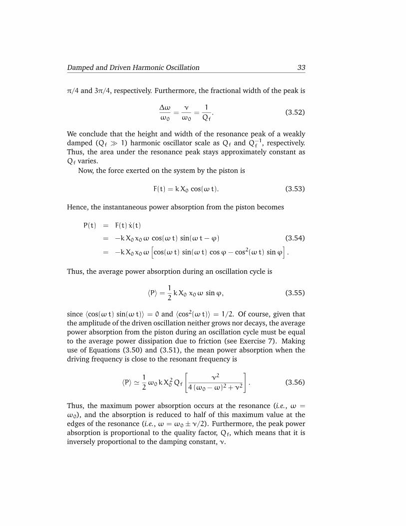
Figure 3.5: A driven LCR circuit.
3.5 Driven LCR Circuit
Consider an LCR circuit consisting of an inductor, L, a capacitor, C, and a re-
sistor, R, connected in series with an emf of voltage V(t). See Figure 3.5. Let
I(t) be the instantaneous current flowing around the circuit. Now, according
to Kichhoff ’s second circuital law, the sum of the potential drops across the
various components of a closed circuit loop is equal to zero. Thus, since the
potential drop across an emf is minus the associated voltage, we obtain [cf.,
Equation (3.29)]
L I+ R I+Q/C = V, (3.57)
where Q = I. Suppose that the emf is such that its voltage oscillates sinu-
soidally at the angular frequency ω > 0, with the peak value V0 > 0, so
that
V(t) = V0 sin(ωt). (3.58)
Dividing Equation (3.57) by L, and differentiating with respect to time, we
obtain [cf., Equation (3.30)]
I+ ν I+ω20 I =
ωV0
Lcos(ωt), (3.59)
whereω0 = 1/√LC and ν = R/L. Comparison with Equation (3.40) reveals
that this is a driven damped harmonic oscillator equation. It follows, by
comparison with the analysis contained in the previous section, that the
current driven in the circuit by the oscillating emf is of the form
I(t) = I0 cos(ωt−ϕ), (3.60)
Damped and Driven Harmonic Oscillation 35
where
I0 =ωV0/L
[
(ω20 −ω2)2 + ν2ω2
]1/2, (3.61)
ϕ = tan−1
(
νω
ω20 −ω2
)
. (3.62)
In the immediate vicinity of the resonance (i.e., |ω −ω0| ∼ ν ≪ ω0) these
expression simplify to
I0 ≃ V0
R
ν
[4 (ω0 −ω)2 + ν2]1/2, (3.63)
sinϕ ≃ ν
[4 (ω−ω0)2 + ν2]1/2. (3.64)
Now, the circuit’s mean power absorption from the emf is written
〈P〉 = 〈I(t)V(t)〉 = I0V0 〈cos(ωt−ϕ) sin(ωt)〉
=1
2I0V0 sinϕ, (3.65)
so that
〈P〉 ≃ 1
2
V 20
R
[
ν2
4 (ω0 −ω)2 + ν2
]
(3.66)
close to the resonance. It follows that the peak power absorption, (1/2)V 20 /R,
takes place when the emf oscillates at the resonant frequency,ω0. Moreover,
the power absorption falls to half of this peak value at the edges of the res-
onant peak: i.e., ω = ω0 ± ν.
LCR circuits are often employed as analogue radio tuners. In this appli-
cation, the emf represents the analogue signal picked-up by a radio antenna.
It is clear, from the above analysis, that the circuit only has a strong response
(i.e., it only absorbs significant energy) when the signal oscillates in the an-
gular frequency range ω0±ν, which corresponds to 1/√LC±R/L. Thus, if
the values of L, C, and R are properly chosen then the circuit can be made
to strongly absorb the signal from a particular radio station, which has a
given carrier frequency and bandwidth, whilst essentially ignoring the sig-
nals from other stations with different carrier frequencies. In practice, the
values of L and R are fixed, whilst the value of C is varied (by turning a
knob which adjusts the degree of overlap between two sets of parallel semi-
circular conducting plates) until the signal from the desired radio station is
found.
36 OSCILLATIONS AND WAVES
3.6 Transient Oscillator Response
The time evolution of the driven mechanical oscillator discussed in Sec-
tion 3.4 is governed by the driven damped harmonic oscillator equation,
x+ ν x+ω20 x = ω2
0 X0 cos(ωt). (3.67)
Recall that the steady-state (i.e., constant amplitude) solution to this equa-
tion which we found earlier takes the form
xta(t) = x0 cos(ωt−ϕ), (3.68)
where
x0 =ω2
0 X0[
(ω20 −ω2)2 + ν2ω2
]1/2, (3.69)
ϕ = tan−1
(
νω
ω20 −ω2
)
. (3.70)
Now, Equation (3.67) is a second-order ordinary differential equation, which
means that its general solution should contain two arbitrary constants. Note,
however, that (3.68) contains no arbitrary constants. It follows that (3.68)
cannot be the most general solution to the driven damped harmonic oscil-
lator equation, (3.67). However, it is fairly easy to see that if we add any
solution of the undriven damped harmonic oscillator equation,
x+ ν x+ω20 x = 0, (3.71)
to (3.68) then the result will still be a solution to Equation (3.67). Now,
from Section 3.1, the most general solution to the above equation can be
written
xtr(t) = A e−νt/2 cos(ω1 t) + B e−νt/2 sin(ω1 t), (3.72)
where ω1 = (ω20 −ν2/4)1/2, and A and B are arbitrary constants. [In terms
of the standard solution (3.11), A = a cosφ and B = a sinφ.] Thus, a
more general solution to (3.67) is
x(t) = xta(t) + xtr(t) (3.73)
= x0 cos(ωt−ϕ) +A e−νt/2 cos(ω1 t) + B e−νt/2 sin(ω1 t).
In fact, since the above solution contains two arbitrary constants, we can be
sure that it is the most general solution. Of course, the constants A and B are
Damped and Driven Harmonic Oscillation 37
determined by the initial conditions. It is, thus, clear that the most general
solution to the driven damped harmonic oscillator equation (3.67) consists
of two parts. First, the solution (3.68), which oscillates at the driving fre-
quency ω with a constant amplitude, and which is independent of the initial
conditions. Second, the solution (3.72), which oscillates at the natural fre-
quency ω1 with an amplitude which decays exponentially in time, and which
depends on the initial conditions. The former is termed the time asymptotic
solution, since if we wait long enough then it becomes dominant. The latter
is called the transient solution, since if we wait long enough then it decays
away.
Suppose, for the sake of argument, that the system is initially in its equi-
librium state: i.e., x(0) = x(0) = 0. It follows from (3.73) that
x(0) = x0 cosϕ+A = 0, (3.74)
x(0) = x0ω sinϕ−ν
2A+ Bω1 = 0. (3.75)
These equations can be solved to give
A = −x0 cosϕ, (3.76)
B = −x0
[
ω sinϕ+ (ν/2) cosϕ
ω1
]
. (3.77)
Now, according to the analysis in Section 3.4, for driving frequencies close
to the resonant frequency (i.e., |ω−ω0| ∼ ν), we can write
x0 ≃ X0ω0
[4 (ω0 −ω)2 + ν2]1/2, (3.78)
sinϕ ≃ ν
[4 (ω0 −ω)2 + ν2]1/2, (3.79)
cosϕ ≃ 2 (ω0 −ω)
[4 (ω0 −ω)2 + ν2]1/2. (3.80)
Hence, in this case, the solution (3.73), combined with (3.76)–(3.80), re-
duces to
x(t) ≃ X0
[
2ω0 (ω0 −ω)
4 (ω0 −ω)2 + ν2
]
[
cos(ωt) − e−νt/2 cos(ω0 t)]
+X0
[
ω0ν
4 (ω0 −ω)2 + ν2
]
[
sin(ωt) − e−νt/2 sin(ω0 t)]
.
(3.81)
38 OSCILLATIONS AND WAVES
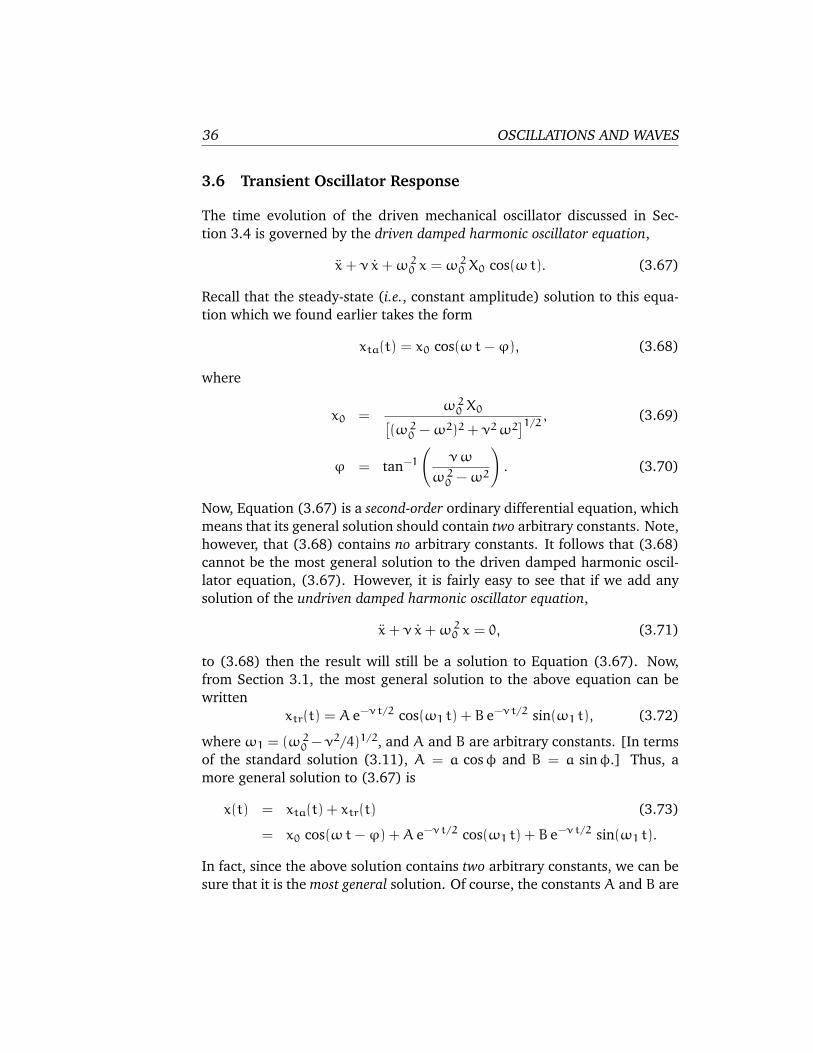
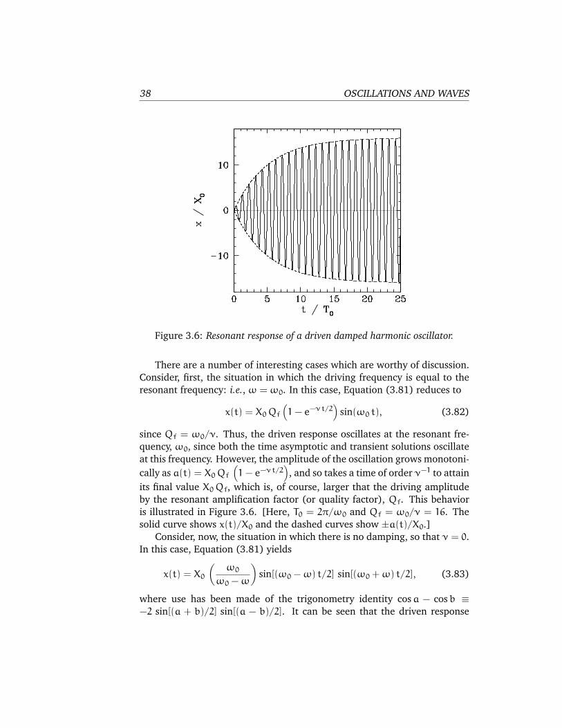
Figure 3.6: Resonant response of a driven damped harmonic oscillator.
There are a number of interesting cases which are worthy of discussion.
Consider, first, the situation in which the driving frequency is equal to the
resonant frequency: i.e., ω = ω0. In this case, Equation (3.81) reduces to
x(t) = X0Qf
(
1− e−νt/2)
sin(ω0 t), (3.82)
since Qf = ω0/ν. Thus, the driven response oscillates at the resonant fre-
quency, ω0, since both the time asymptotic and transient solutions oscillate
at this frequency. However, the amplitude of the oscillation grows monotoni-
cally as a(t) = X0Qf
(
1− e−νt/2)
, and so takes a time of order ν−1 to attain
its final value X0Qf, which is, of course, larger that the driving amplitude
by the resonant amplification factor (or quality factor), Qf. This behavior
is illustrated in Figure 3.6. [Here, T0 = 2π/ω0 and Qf = ω0/ν = 16. The
solid curve shows x(t)/X0 and the dashed curves show ±a(t)/X0.]
Consider, now, the situation in which there is no damping, so that ν = 0.
In this case, Equation (3.81) yields
x(t) = X0
(
ω0
ω0 −ω
)
sin[(ω0 −ω) t/2] sin[(ω0 +ω) t/2], (3.83)
where use has been made of the trigonometry identity cosa − cosb ≡−2 sin[(a + b)/2] sin[(a − b)/2]. It can be seen that the driven response
Damped and Driven Harmonic Oscillation 39
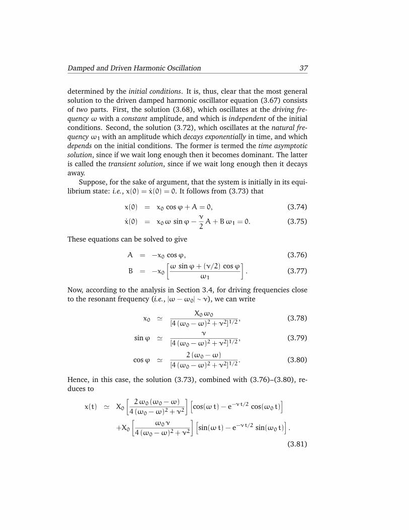
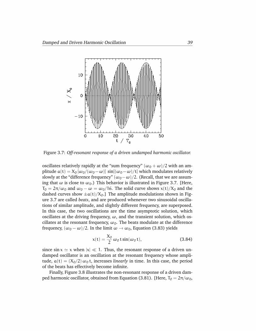
Figure 3.7: Off-resonant response of a driven undamped harmonic oscillator.
oscillates relatively rapidly at the “sum frequency” (ω0 +ω)/2 with an am-
plitude a(t) = X0 [ω0/(ω0−ω)] sin[(ω0−ω)/t] which modulates relatively
slowly at the “difference frequency” (ω0−ω)/2. (Recall, that we are assum-
ing that ω is close to ω0.) This behavior is illustrated in Figure 3.7. [Here,
T0 = 2π/ω0 and ω0 −ω = ω0/16. The solid curve shows x(t)/X0 and the
dashed curves show ±a(t)/X0.] The amplitude modulations shown in Fig-
ure 3.7 are called beats, and are produced whenever two sinusoidal oscilla-
tions of similar amplitude, and slightly different frequency, are superposed.
In this case, the two oscillations are the time asymptotic solution, which
oscillates at the driving frequency, ω, and the transient solution, which os-
cillates at the resonant frequency, ω0. The beats modulate at the difference
frequency, (ω0 −ω)/2. In the limit ω → ω0, Equation (3.83) yields
x(t) =X0
2ω0 t sin(ω0 t), (3.84)
since sin x ≃ x when |x| ≪ 1. Thus, the resonant response of a driven un-
damped oscillator is an oscillation at the resonant frequency whose ampli-
tude, a(t) = (X0/2)ω0 t, increases linearly in time. In this case, the period
of the beats has effectively become infinite.
Finally, Figure 3.8 illustrates the non-resonant response of a driven dam-
ped harmonic oscillator, obtained from Equation (3.81). [Here, T0 = 2π/ω0,
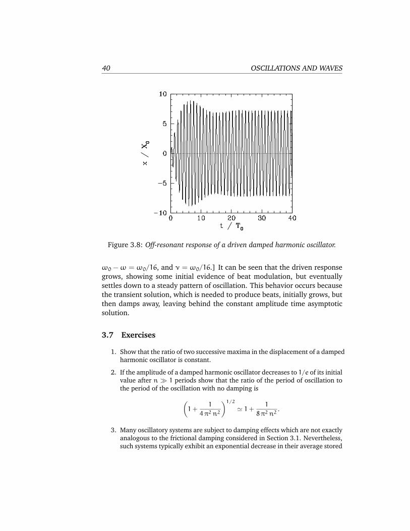
40 OSCILLATIONS AND WAVES
Figure 3.8: Off-resonant response of a driven damped harmonic oscillator.
ω0 −ω = ω0/16, and ν = ω0/16.] It can be seen that the driven response
grows, showing some initial evidence of beat modulation, but eventually
settles down to a steady pattern of oscillation. This behavior occurs because
the transient solution, which is needed to produce beats, initially grows, but
then damps away, leaving behind the constant amplitude time asymptotic
solution.
3.7 Exercises
1. Show that the ratio of two successive maxima in the displacement of a dampedharmonic oscillator is constant.
2. If the amplitude of a damped harmonic oscillator decreases to 1/e of its initialvalue after n ≫ 1 periods show that the ratio of the period of oscillation tothe period of the oscillation with no damping is
(
1+1
4π2 n2
)1/2
≃ 1+1
8π2 n2.
3. Many oscillatory systems are subject to damping effects which are not exactlyanalogous to the frictional damping considered in Section 3.1. Nevertheless,such systems typically exhibit an exponential decrease in their average stored
Damped and Driven Harmonic Oscillation 41
energy of the form 〈E〉 = E0 exp(−ν t). It is possible to define an effectivequality factor for such oscillators as Qf = ω0/ν, where ω0 is the naturalangular oscillation frequency. For example, when the note “middle C” on apiano is struck its oscillation energy decreases to one half of its initial valuein about 1 second. The frequency of middle C is 256 Hz. What is the effectiveQf of the system?
4. According to classical electromagnetic theory, an accelerated electron radi-ates energy at the rate Ke2 a2/c3, where K = 6 × 10⁹ N m2/C2, e is thecharge on an electron, a the instantaneous acceleration, and c the velocityof light. If an electron were oscillating in a straight-line with displacementx(t) = A sin(2π f t) how much energy would it radiate away during a singlecycle? What is the effective Qf of this oscillator? How many periods of oscil-lation would elapse before the energy of the oscillation was reduced to halfof its initial value? Substituting a typical optical frequency (i.e., for visiblelight) for f, give numerical estimates for the Qf and half-life of the radiatingsystem.
5. Demonstrate that in the limit ν → 2ω0 the solution to the damped harmonicoscillator equation becomes
x(t) = (x0 + [v0 + (ν/2) x0] t) e−ν t/2,
where x0 = x(0) and v0 = x(0).
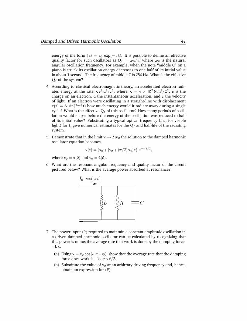
6. What are the resonant angular frequency and quality factor of the circuitpictured below? What is the average power absorbed at resonance?
.
I0 cos(ω t)
L R C
7. The power input 〈P〉 required to maintain a constant amplitude oscillation ina driven damped harmonic oscillator can be calculated by recognizing thatthis power is minus the average rate that work is done by the damping force,−k x.
(a) Using x = x0 cos(ωt−ϕ), show that the average rate that the dampingforce does work is −kω2 x 2
0 /2.
(b) Substitute the value of x0 at an arbitrary driving frequency and, hence,obtain an expression for 〈P〉.
42 OSCILLATIONS AND WAVES
(c) Demonstrate that this expression yields (3.56) in the limit that the driv-ing frequency is close to the resonant frequency.
8. A generator of emf V(t) = V0 cos(ωt) is connected in series with a resistanceR, an inductor L, and a capacitor C. Let I(t) be the current flowing in thecircuit, and Q(t) the charge on the capacitor. Suppose that I = Q = 0 att = 0. Find I(t) and Q(t) for t > 0.
9. The equation mx + k x = F0 sin(ωt) governs the motion of an undampedharmonic oscillator driven by a sinusoidal force of angular frequency ω.Show that the steady-state solution is
x =F0 sin(ωt)
m (ω 20 −ω2)
,
where ω0 =√
k/m. Sketch the behavior of x versus t for ω < ω0 andω > ω0. Demonstrate that if x = x = 0 at t = 0 then the general solution is
x =F0
m (ω 20 −ω2)
[
sin(ωt) −ω
ω0
sin(ω0 t)
]
.
Show, finally, that if ω is close to the resonant frequency ω0 then
x ≃ F0
2ω 20
[sin(ω0 t) −ω0 t cos(ω0 t)] .
Sketch the behavior of x versus t.
Coupled Oscillations 43
4 Coupled Oscillations
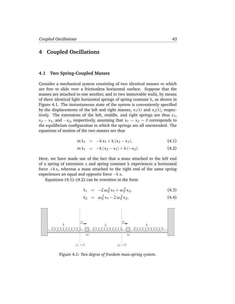
4.1 Two Spring-Coupled Masses
Consider a mechanical system consisting of two identical masses m which
are free to slide over a frictionless horizontal surface. Suppose that the
masses are attached to one another, and to two immovable walls, by means
of three identical light horizontal springs of spring constant k, as shown in
Figure 4.1. The instantaneous state of the system is conveniently specified
by the displacements of the left and right masses, x1(t) and x2(t), respec-
tively. The extensions of the left, middle, and right springs are thus x1,
x2 − x1, and −x2, respectively, assuming that x1 = x2 = 0 corresponds to
the equilibrium configuration in which the springs are all unextended. The
equations of motion of the two masses are thus
mx1 = −k x1 + k (x2 − x1), (4.1)
mx1 = −k (x2 − x1) + k (−x2). (4.2)
Here, we have made use of the fact that a mass attached to the left end
of a spring of extension x and spring constant k experiences a horizontal
force +k x, whereas a mass attached to the right end of the same spring
experiences an equal and opposite force −k x.
Equations (4.1)–(4.2) can be rewritten in the form
x1 = −2ω20 x1 +ω2
0 x2, (4.3)
x2 = ω20 x1 − 2ω2
0 x2, (4.4)
x2
mm
x1
x2 = 0x1 = 0
k kk
Figure 4.1: Two degree of freedom mass-spring system.
44 OSCILLATIONS AND WAVES
where ω0 =√
k/m. Let us search for a solution in which the two masses
oscillate in phase at the same angular frequency, ω. In other words,
x1(t) = x1 cos(ωt− φ), (4.5)
x2(t) = x2 cos(ωt− φ), (4.6)
where x1, x2, and φ are constants. Equations (4.3) and (4.4) yield
−ω2 x1 cos(ωt− φ) =(
−2ω20 x1 +ω2
0 x2
)
cos(ωt− φ), (4.7)
−ω2 x2 cos(ωt− φ) =(
ω20 x1 − 2ω2
0 x2
)
cos(ωt− φ), (4.8)
or
(ω2 − 2) x1 + x2 = 0, (4.9)
x1 + (ω2 − 2) x2 = 0, (4.10)
where ω = ω/ω0. Note that by searching for a solution of the form (4.5)–
(4.6) we have effectively converted the system of two coupled linear differ-
ential equations (4.3)–(4.4) into the much simpler system of two coupled
linear algebraic equations (4.9)–(4.10). The latter equations have the trivial
solutions x1 = x2 = 0, but also yield
x1
x2
= −1
(ω2 − 2)= −(ω2 − 2). (4.11)
Hence, the condition for a nontrivial solution is clearly
(ω2 − 2) (ω2 − 2) − 1 = 0. (4.12)
In fact, if we write Equations (4.9)–(4.10) in the form of a homogenous
(i.e., with a null right-hand side) 2× 2 matrix equation, so that
(
ω2 − 2 1
1 ω2 − 2
)(
x1
x2
)
=
(
0
0
)
, (4.13)
then it is clear that the criterion (4.12) can also be obtained by setting the
determinant of the associated 2× 2 matrix to zero.
Equation (4.12) can be rewritten
ω4 − 4 ω2 + 3 = (ω2 − 1) (ω2 − 3) = 0. (4.14)
Coupled Oscillations 45
It follows that
ω = 1 or√3. (4.15)
Here, we have neglected the two negative frequency roots of (4.14)—i.e.,
ω = −1 and ω = −√3—since a negative frequency oscillation is equivalent
to an oscillation with an equal and opposite positive frequency, and an equal
and opposite phase: i.e., cos(ωt − φ) ≡ cos(−ωt + φ). It is thus apparent
that the dynamical system pictured in Figure 4.1 has two unique frequencies
of oscillation: i.e., ω = ω0 and ω =√3ω0. These are called the normal
frequencies of the system. Since the system possesses two degrees of freedom
(i.e., two independent coordinates are needed to specify its instantaneous
configuration) it is not entirely surprising that it possesses two normal fre-
quencies. In fact, it is a general rule that a dynamical system withN degrees
of freedom possesses N normal frequencies.
The patterns of motion associated with the two normal frequencies can
easily be deduced from Equation (4.11). Thus, for ω = ω0 (i.e., ω = 1), we
get x1 = x2, so that
x1(t) = η1 cos(ω0 t− φ1), (4.16)
x2(t) = η1 cos(ω0 t− φ1), (4.17)
where η1 and φ1 are constants. This first pattern of motion corresponds to
the two masses executing simple harmonic oscillation with the same ampli-
tude and phase. Note that such an oscillation does not stretch the middle
spring. On the other hand, for ω =√3ω0 (i.e., ω =
√3), we get x1 = −x2,
so that
x1(t) = η2 cos(√3ω0 t− φ2
)
, (4.18)
x2(t) = −η2 cos(√3ω0 t− φ2
)
, (4.19)
where η2 and φ2 are constants. This second pattern of motion corresponds
to the two masses executing simple harmonic oscillation with the same am-
plitude but in anti-phase: i.e., with a phase shift of π radians. Such os-
cillations do stretch the middle spring, implying that the restoring force
associated with similar amplitude displacements is greater for the second
pattern of motion than for the first. This accounts for the higher oscillation
frequency in the second case. (The inertia is the same in both cases, so
the oscillation frequency is proportional to the square root of the restoring
force associated with similar amplitude displacements.) The two distinc-
tive patterns of motion which we have found are called the normal modes
46 OSCILLATIONS AND WAVES
of oscillation of the system. Incidentally, it is a general rule that a dynami-
cal system possessing N degrees of freedom has N unique normal modes of
oscillation.
Now, the most general motion of the system is a linear combination of the
two normal modes. This immediately follows because Equations (4.1) and
(4.2) are linear equations. [In other words, if x1(t) and x2(t) are solutions
then so are ax1(t) and ax2(t), where a is an arbitrary constant.] Thus, we
can write
x1(t) = η1 cos(ω0 t− φ1) + η2 cos(√3ω0 t− φ2
)
, (4.20)
x2(t) = η1 cos(ω0 t− φ1) − η2 cos(√3ω0 t− φ2
)
. (4.21)
Note that we can be sure that this represents the most general solution to
Equations (4.1) and (4.2) because it contains four arbitrary constants: i.e.,
η1, φ1, η2, and φ2. (In general, we expect the solution of a second-order
ordinary differential equation to contain two arbitrary constants. It, thus,
follows that the solution of a system of two coupled ordinary differential
equations should contain four arbitrary constants.) Of course, these con-
stants are determined by the initial conditions.
For instance, suppose that x1 = a, x1 = 0, x2 = 0, and x2 = 0 at t = 0. It
follows, from (4.20) and (4.21), that
a = η1 cosφ1 + η2 cosφ2, (4.22)
0 = η1 sinφ1 +√3 η2 sinφ2, (4.23)
0 = η1 cosφ1 − η2 cosφ2, (4.24)
0 = η1 sinφ1 −√3 η2 sinφ2, (4.25)
which implies that φ1 = φ2 = 0 and η1 = η2 = a/2. Thus, the system
evolves in time as
x1(t) = a cos(ω− t) cos(ω+ t), (4.26)
x2(t) = a sin(ω− t) sin(ω+ t), (4.27)
where ω± = [(√3 ± 1)/2]ω0, and use has been made of the trigonometric
identities cos(a + b) ≡ 2 cos[(a + b)/2] cos[(a − b)/2] and cos(a − b) ≡−2 sin[(a + b)/2] sin[(a − b)/2]. This evolution is illustrated in Figure 4.2.
[Here, T0 = 2π/ω0. The solid curve corresponds to x1, and the dashed curve
to x2.]
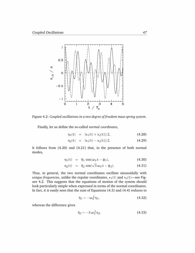
Coupled Oscillations 47
Figure 4.2: Coupled oscillations in a two degree of freedom mass-spring system.
Finally, let us define the so-called normal coordinates,
η1(t) = [x1(t) + x2(t)]/2, (4.28)
η2(t) = [x1(t) − x2(t)]/2. (4.29)
It follows from (4.20) and (4.21) that, in the presence of both normal
modes,
η1(t) = η1 cos(ω0 t− φ1), (4.30)
η2(t) = η2 cos(√3ω0 t− φ2). (4.31)
Thus, in general, the two normal coordinates oscillate sinusoidally with
unique frequencies, unlike the regular coordinates, x1(t) and x2(t)—see Fig-
ure 4.2. This suggests that the equations of motion of the system should
look particularly simple when expressed in terms of the normal coordinates.
In fact, it is easily seen that the sum of Equations (4.3) and (4.4) reduces to
η1 = −ω20 η1, (4.32)
whereas the difference gives
η2 = −3ω20 η2. (4.33)
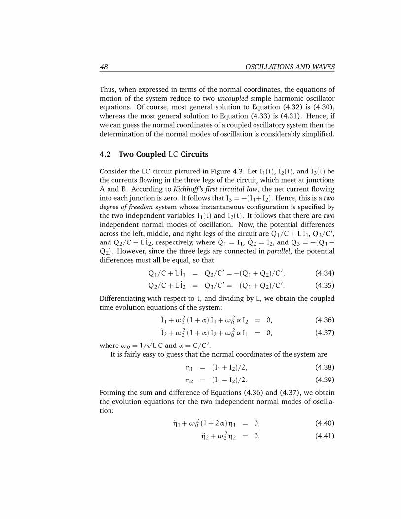
48 OSCILLATIONS AND WAVES
Thus, when expressed in terms of the normal coordinates, the equations of
motion of the system reduce to two uncoupled simple harmonic oscillator
equations. Of course, most general solution to Equation (4.32) is (4.30),
whereas the most general solution to Equation (4.33) is (4.31). Hence, if
we can guess the normal coordinates of a coupled oscillatory system then the
determination of the normal modes of oscillation is considerably simplified.
4.2 Two Coupled LC Circuits
Consider the LC circuit pictured in Figure 4.3. Let I1(t), I2(t), and I3(t) be
the currents flowing in the three legs of the circuit, which meet at junctions
A and B. According to Kichhoff ’s first circuital law, the net current flowing
into each junction is zero. It follows that I3 = −(I1+I2). Hence, this is a two
degree of freedom system whose instantaneous configuration is specified by
the two independent variables I1(t) and I2(t). It follows that there are two
independent normal modes of oscillation. Now, the potential differences
across the left, middle, and right legs of the circuit are Q1/C+ L I1, Q3/C′,
and Q2/C + L I2, respectively, where Q1 = I1, Q2 = I2, and Q3 = −(Q1 +
Q2). However, since the three legs are connected in parallel, the potential
differences must all be equal, so that
Q1/C+ L I1 = Q3/C′ = −(Q1 +Q2)/C
′, (4.34)
Q2/C+ L I2 = Q3/C′ = −(Q1 +Q2)/C
′. (4.35)
Differentiating with respect to t, and dividing by L, we obtain the coupled
time evolution equations of the system:
I1 +ω20 (1+ α) I1 +ω2
0 α I2 = 0, (4.36)
I2 +ω20 (1+ α) I2 +ω2
0 α I1 = 0, (4.37)
where ω0 = 1/√LC and α = C/C ′.
It is fairly easy to guess that the normal coordinates of the system are
η1 = (I1 + I2)/2, (4.38)
η2 = (I1 − I2)/2. (4.39)
Forming the sum and difference of Equations (4.36) and (4.37), we obtain
the evolution equations for the two independent normal modes of oscilla-
tion:
η1 +ω20 (1+ 2α)η1 = 0, (4.40)
η2 +ω20 η2 = 0. (4.41)
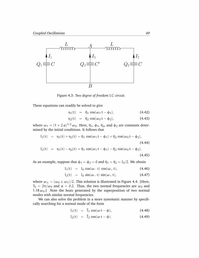
Coupled Oscillations 49
. .
I2
Q3 Q2
I1 I3
C C
LL
C ′
A
B
Q1
Figure 4.3: Two degree of freedom LC circuit.
These equations can readily be solved to give
η1(t) = η1 cos(ω1 t− φ1), (4.42)
η2(t) = η2 cos(ω0 t− φ2), (4.43)
where ω1 = (1 + 2α)1/2ω0. Here, η1, φ1, η2, and φ2 are constants deter-
mined by the initial conditions. It follows that
I1(t) = η1(t) + η2(t) = η1 cos(ω1 t− φ1) + η2 cos(ω0 t− φ2),
(4.44)
I2(t) = η1(t) − η2(t) = η1 cos(ω1 t− φ1) − η2 cos(ω0 t− φ2).
(4.45)
As an example, suppose that φ1 = φ2 = 0 and η1 = η2 = I0/2. We obtain
I1(t) = I0 cos(ω− t) cos(ω+ t), (4.46)
I2(t) = I0 sin(ω− t) sin(ω+ t), (4.47)
where ω± = (ω0 ±ω1)/2. This solution is illustrated in Figure 4.4. [Here,
T0 = 2π/ω0 and α = 0.2. Thus, the two normal frequencies are ω0 and
1.18ω0.] Note the beats generated by the superposition of two normal
modes with similar normal frequencies.
We can also solve the problem in a more systematic manner by specifi-
cally searching for a normal mode of the form
I1(t) = I1 cos(ωt− φ), (4.48)
I2(t) = I2 cos(ωt− φ). (4.49)
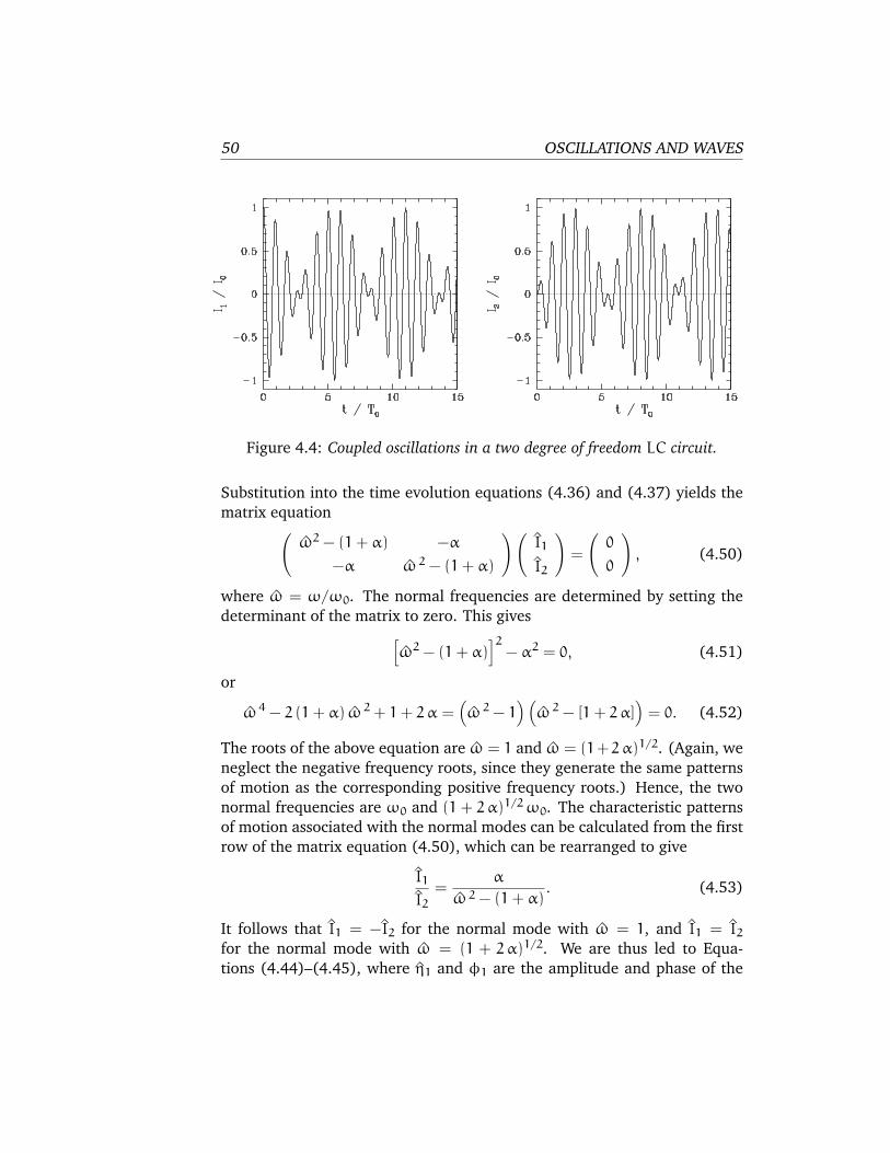
50 OSCILLATIONS AND WAVES
Figure 4.4: Coupled oscillations in a two degree of freedom LC circuit.
Substitution into the time evolution equations (4.36) and (4.37) yields the
matrix equation(
ω2 − (1+ α) −α
−α ω2 − (1+ α)
)(
I1
I2
)
=
(
0
0
)
, (4.50)
where ω = ω/ω0. The normal frequencies are determined by setting the
determinant of the matrix to zero. This gives
[
ω2 − (1+ α)]2
− α2 = 0, (4.51)
or
ω4 − 2 (1+ α) ω2 + 1+ 2α =(
ω2 − 1) (
ω2 − [1+ 2α])
= 0. (4.52)
The roots of the above equation are ω = 1 and ω = (1+ 2α)1/2. (Again, we
neglect the negative frequency roots, since they generate the same patterns
of motion as the corresponding positive frequency roots.) Hence, the two
normal frequencies are ω0 and (1 + 2α)1/2ω0. The characteristic patterns
of motion associated with the normal modes can be calculated from the first
row of the matrix equation (4.50), which can be rearranged to give
I1
I2=
α
ω2 − (1+ α). (4.53)
It follows that I1 = −I2 for the normal mode with ω = 1, and I1 = I2for the normal mode with ω = (1 + 2α)1/2. We are thus led to Equa-
tions (4.44)–(4.45), where η1 and φ1 are the amplitude and phase of the
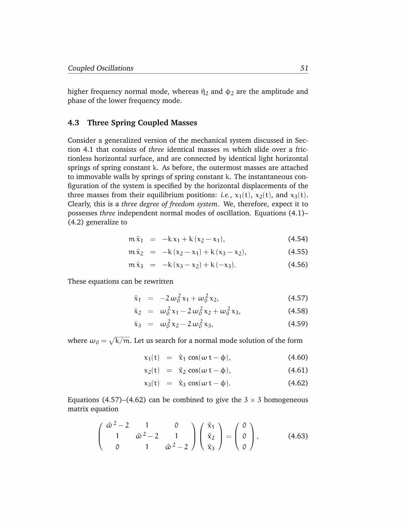
Coupled Oscillations 51
higher frequency normal mode, whereas η2 and φ2 are the amplitude and
phase of the lower frequency mode.
4.3 Three Spring Coupled Masses
Consider a generalized version of the mechanical system discussed in Sec-
tion 4.1 that consists of three identical masses m which slide over a fric-
tionless horizontal surface, and are connected by identical light horizontal
springs of spring constant k. As before, the outermost masses are attached
to immovable walls by springs of spring constant k. The instantaneous con-
figuration of the system is specified by the horizontal displacements of the
three masses from their equilibrium positions: i.e., x1(t), x2(t), and x3(t).
Clearly, this is a three degree of freedom system. We, therefore, expect it to
possesses three independent normal modes of oscillation. Equations (4.1)–
(4.2) generalize to
mx1 = −k x1 + k (x2 − x1), (4.54)
mx2 = −k (x2 − x1) + k (x3 − x2), (4.55)
mx3 = −k (x3 − x2) + k (−x3). (4.56)
These equations can be rewritten
x1 = −2ω20 x1 +ω2
0 x2, (4.57)
x2 = ω20 x1 − 2ω2
0 x2 +ω20 x3, (4.58)
x3 = ω20 x2 − 2ω2
0 x3, (4.59)
where ω0 =√
k/m. Let us search for a normal mode solution of the form
x1(t) = x1 cos(ωt− φ), (4.60)
x2(t) = x2 cos(ωt− φ), (4.61)
x3(t) = x3 cos(ωt− φ). (4.62)
Equations (4.57)–(4.62) can be combined to give the 3 × 3 homogeneous
matrix equation
ω2 − 2 1 0
1 ω2 − 2 1
0 1 ω2 − 2
x1
x2
x3
=
0
0
0
, (4.63)
52 OSCILLATIONS AND WAVES
where ω = ω/ω0. The normal frequencies are determined by setting the
determinant of the matrix to zero: i.e.,
(ω2 − 2)[
(ω2 − 2)2 − 1]
− (ω2 − 2) = 0, (4.64)
or
(ω2 − 2)[
ω2 − 2−√2] [
ω2 − 2+√2]
= 0. (4.65)
Thus, the normal frequencies are ω =√2 (1 − 1/
√2)1/2,
√2, and
√2 (1 +
1/√2)1/2. According to the first and third rows of Equation (4.63),
x1 : x2 : x3 :: 1 : 2− ω2 : 1, (4.66)
provided ω2 6= 2. According to the second row,
x1 : x2 : x3 :: −1 : 0 : 1 (4.67)
when ω2 = 2. Note that we can only determine the relative ratios of x1,
x2, and x3, rather than the absolute values of these quantities. In other
words, only the direction of the vector x = (x1, x2, x3) is well-defined. [This
follows because the most general solution, (4.71), is undetermined to an
arbitrary multiplicative constant. That is, if x(t) = (x1(t), x2(t), x3(t)) is a
solution to the dynamical equations (4.57)–(4.59) then so is a x(t), where
a is an arbitrary constant. This, in turn, follows because the dynamical
equations are linear.] Let us arbitrarily set the magnitude of x to unity. It
follows that the normal mode associated with the normal frequency ω1 =√2 (1− 1/
√2)1/2 is
x1 =
(
1
2,1√2,1
2
)
. (4.68)
Likewise, the normal mode associated with the normal frequency ω2 =√2
is
x2 =
(
−1√2, 0,
1√2
)
. (4.69)
Finally, the normal mode associated with the normal frequency ω3 =√2(1+
1/√2)1/2 is
x3 =
(
1
2,−
1√2,1
2
)
. (4.70)
Let x = (x1, x2, x2). It follows that the most general solution to the problem
is
x(t) = η1(t) x1 + η2(t) x2 + η3(t) x3, (4.71)
Coupled Oscillations 53
where
η1(t) = η1 cos(ω1 t− φ1), (4.72)
η2(t) = η2 cos(ω2 t− φ2), (4.73)
η3(t) = η3 cos(ω3 t− φ3). (4.74)
Here, η1,2,3 and φ1,2,3 are constants. Equation (4.71) yields
x1
x2
x3
=
1/2 1/√2 1/2
−1/√2 0 1/
√2
1/2 −1/√2 1/2
η1
η2
η3
(4.75)
The above equation can easily be inverted by noting that the matrix is uni-
tary: i.e., its transpose is equal to its inverse. Thus, we obtain
η1
η2
η3
=
1/2 −1/√2 1/2
1/√2 0 −1/
√2
1/2 1/√2 1/2
x1
x2
x3
(4.76)
This equation determines the three normal coordinates, η1, η2, η3, in terms
of the three conventional coordinates, x1, x2, x3. Note that, in general, the
normal coordinates are undetermined to arbitrary multiplicative constants.
4.4 Exercises
1. A particle of mass m is attached to a rigid support by means of a spring ofspring constant k. At equilibrium, the spring hangs vertically downward. Anidentical oscillator is added to this system, the spring of the former beingattached to the mass of the latter. Calculate the normal frequencies for one-dimensional vertical oscillations, and describe the associated normal modes.
2. Consider a mass-spring system of the general form shown in Figure 4.1 inwhich the two masses are of mass m, the two outer springs have springconstant k, and the middle spring has spring constant k ′. Find the normalfrequencies and normal modes in terms of ω0 =
√
k/m and α = k ′/k.
3. Consider a mass-spring system of the general form shown in Figure 4.1 inwhich the springs all have spring constant k, and the left and right massesare of mass m and m ′, respectively. Find the normal frequencies and normalmodes in terms of ω0 =
√
k/m and α = m ′/m.
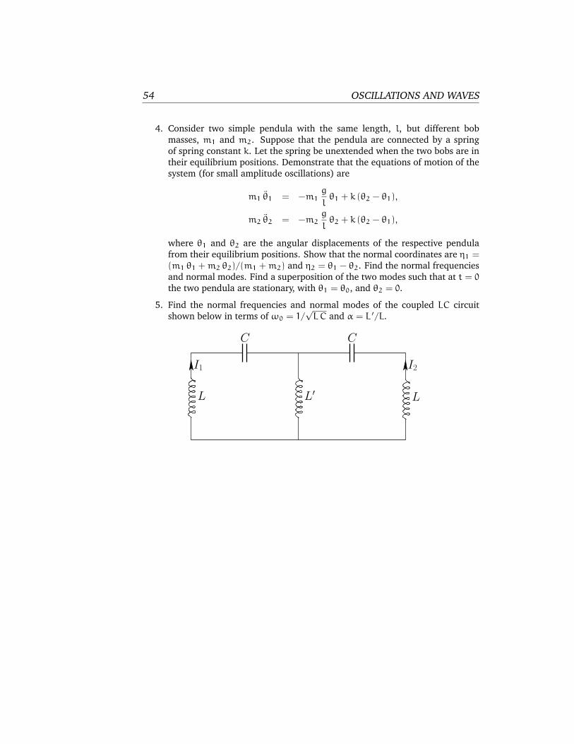
54 OSCILLATIONS AND WAVES
4. Consider two simple pendula with the same length, l, but different bobmasses, m1 and m2. Suppose that the pendula are connected by a springof spring constant k. Let the spring be unextended when the two bobs are intheir equilibrium positions. Demonstrate that the equations of motion of thesystem (for small amplitude oscillations) are
m1 θ1 = −m1
g
lθ1 + k (θ2 − θ1),
m2 θ2 = −m2
g
lθ2 + k (θ2 − θ1),
where θ1 and θ2 are the angular displacements of the respective pendulafrom their equilibrium positions. Show that the normal coordinates are η1 =
(m1 θ1 +m2 θ2)/(m1 +m2) and η2 = θ1 − θ2. Find the normal frequenciesand normal modes. Find a superposition of the two modes such that at t = 0
the two pendula are stationary, with θ1 = θ0, and θ2 = 0.
5. Find the normal frequencies and normal modes of the coupled LC circuitshown below in terms of ω0 = 1/
√LC and α = L ′/L.
. .
.L
C C
L′
I1 I2
L
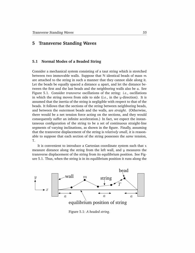
Transverse Standing Waves 55
5 Transverse Standing Waves
5.1 Normal Modes of a Beaded String
Consider a mechanical system consisting of a taut string which is stretched
between two immovable walls. Suppose that N identical beads of mass m
are attached to the string in such a manner that they cannot slide along it.
Let the beads be equally spaced a distance a apart, and let the distance be-
tween the first and the last beads and the neighboring walls also be a. See
Figure 5.1. Consider transverse oscillations of the string: i.e., oscillations
in which the string moves from side to side (i.e., in the y-direction). It is
assumed that the inertia of the string is negligible with respect to that of the
beads. It follows that the sections of the string between neighboring beads,
and between the outermost beads and the walls, are straight. (Otherwise,
there would be a net tension force acting on the sections, and they would
consequently suffer an infinite acceleration.) In fact, we expect the instan-
taneous configuration of the string to be a set of continuous straight-line
segments of varying inclinations, as shown in the figure. Finally, assuming
that the transverse displacement of the string is relatively small, it is reason-
able to suppose that each section of the string possesses the same tension,
T .
It is convenient to introduce a Cartesian coordinate system such that x
measure distance along the string from the left wall, and y measures the
transverse displacement of the string from its equilibrium position. See Fig-
ure 5.1. Thus, when the string is in its equilibrium position it runs along the
xT
a
wall string
equilibrium position of string
bead
m
aa
y
Figure 5.1: A beaded string.
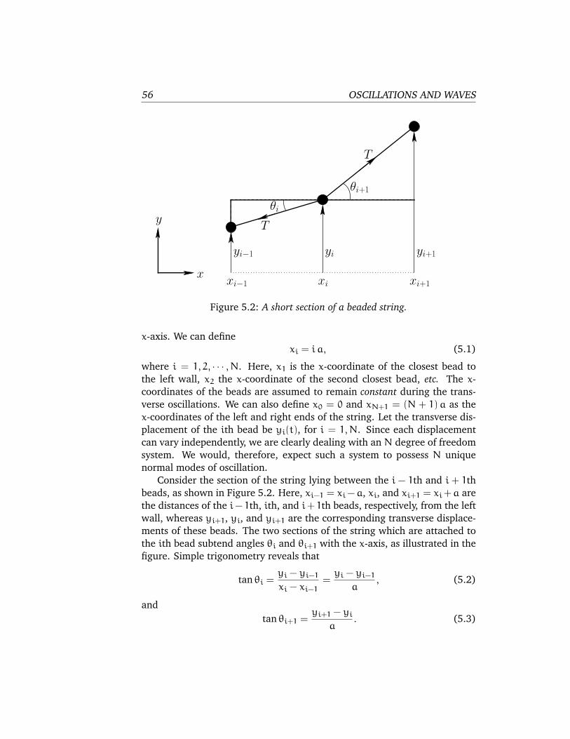
56 OSCILLATIONS AND WAVES
θiy
x
yi−1 yi
xixi−1 xi+1
T
yi+1
θi+1
T
Figure 5.2: A short section of a beaded string.
x-axis. We can define
xi = i a, (5.1)
where i = 1, 2, · · · , N. Here, x1 is the x-coordinate of the closest bead to
the left wall, x2 the x-coordinate of the second closest bead, etc. The x-
coordinates of the beads are assumed to remain constant during the trans-
verse oscillations. We can also define x0 = 0 and xN+1 = (N + 1)a as the
x-coordinates of the left and right ends of the string. Let the transverse dis-
placement of the ith bead be yi(t), for i = 1,N. Since each displacement
can vary independently, we are clearly dealing with an N degree of freedom
system. We would, therefore, expect such a system to possess N unique
normal modes of oscillation.
Consider the section of the string lying between the i − 1th and i + 1th
beads, as shown in Figure 5.2. Here, xi−1 = xi−a, xi, and xi+1 = xi+a are
the distances of the i− 1th, ith, and i+ 1th beads, respectively, from the left
wall, whereas yi+1, yi, and yi+1 are the corresponding transverse displace-
ments of these beads. The two sections of the string which are attached to
the ith bead subtend angles θi and θi+1 with the x-axis, as illustrated in the
figure. Simple trigonometry reveals that
tan θi =yi − yi−1
xi − xi−1
=yi − yi−1
a, (5.2)
and
tan θi+1 =yi+1 − yi
a. (5.3)
Transverse Standing Waves 57
However, if the transverse displacement of the string is relatively small—i.e.,
if |yi| ≪ a for all i—which we shall assume to be the case, then θi and θi+1
are both small angles. Now, it is well known that tan θ ≃ θ when |θ| ≪ 1. It
follows that
θi ≃ yi − yi−1
a, (5.4)
θi+1 ≃ yi+1 − yi
a. (5.5)
Let us find the transverse equation of motion of the ith bead. This bead is
subject to two forces: i.e., the tensions in the sections of the string to the left
and to the right of it. These tensions are of magnitude T , and are directed
parallel to the associated string sections, as shown in Figure 5.2. Thus, the
transverse (i.e., y-directed) components of these two tensions are −T sin θi
and T sin θi+1, respectively. Hence, the transverse equation of motion of the
ith bead becomes
myi = −T sin θi + T sin θi+1. (5.6)
However, since θi and θi+1 are both small angles, we can employ the small
angle approximation sin θ ≃ θ. It follows that
yi ≃T
m(θi+1 − θi) . (5.7)
Finally, making use of Equations (5.4) and (5.5), we obtain
yi = ω20 (yi−1 − 2 yi + yi+1) , (5.8)
where ω0 =√
T/ma. Since there is nothing special about the ith bead, we
deduce that the above equation of motion applies to all N beads: i.e., it is
valid for i = 1,N. Of course, the first (i = 1) and last (i = N) beads are
special cases, since there is no bead corresponding to i = 0 or i = N+ 1. In
fact, i = 0 and i = N+ 1 correspond to the left and right ends of the string,
respectively. However, Equation (5.8) still applies to the first and last beads
as long as we set y0 = 0 and yN+1 = 0. What we are effectively demanding
is that the two ends of the string, which are attached to the left and right
walls, must both have zero transverse displacement.
Let us search for a normal mode solution to Equation (5.8) which takes
the form
yi(t) = A sin(k xi) cos(ωt− φ), (5.9)
where A > 0, k > 0, ω > 0, and φ are constants. This particular type of
solution is such that all of the beads execute transverse simple harmonic

58 OSCILLATIONS AND WAVES
oscillations in phase with one another. See Figure 5.4. Moreover, the os-
cillations have an amplitude A sin(k xi) which varies sinusoidally along the
length of the string (i.e., in the x-direction). The pattern of oscillations is
thus periodic in space. The spatial repetition period, which is usually known
as the wavelength, is λ = 2π/k. [This follows from (5.9) because sin θ is a
periodic function with period 2π: i.e., sin(θ + 2π) ≡ sin θ.] The constant
k, which determines the wavelength, is usually referred to as the wavenum-
ber. Thus, a small wavenumber corresponds to a long wavelength, and vice
versa. The type of solution specified in (5.9) is generally known as a standing
wave. It is a wave because it is periodic in both space and time. (An oscilla-
tion is periodic in time only.) It is a standing wave, rather than a traveling
wave, because the points of maximum and minimum amplitude oscillation
are stationary (in x). See Figure 5.4.
Substituting (5.9) into (5.8), we obtain
−ω2A sin(k xi) cos(ωt− φ) = ω20 A [sin(k xi−1) − 2 sin(k xi)
+ sin(k xi+1)] cos(ωt− φ), (5.10)
which yields
−ω2 sin(k xi) = ω20 (sin[k (xi − a)] − 2 sin(k xi) + sin[k (xi + a)]) . (5.11)
However, since sin(a+ b) ≡ sina cosb+ cosa sinb, we get
−ω2 sin(k xi) = ω20 [cos(ka) − 2+ cos(ka)] sin(k xi), (5.12)
or
ω2 = 4ω20 sin2(ka/2), (5.13)
where use has been made of the trigonometric identity 1−cosθ ≡ 2 sin2(θ/2).
Note that an expression, such as (5.13), which determines the angular fre-
quency, ω, of a wave in terms of its wavenumber, k, is generally known as a
dispersion relation.
Now, the solution (5.9) is only physical provided y0 = yN+1 = 0: i.e.,
provided that the two ends of the string remain stationary. The first con-
straint is automatically satisfied, since x0 = 0 [see (5.1)]. The second con-
straint implies that
sin(k xN+1) = sin[(N+ 1)ka] = 0. (5.14)
This condition can only be satisfied if
k =n
N+ 1
π
a, (5.15)
Transverse Standing Waves 59
where the integer n is known as the mode number. Clearly, a small mode
number translates to a small wavenumber, and, hence, to a long wavelength,
and vice versa. We conclude that the possible wavenumbers, k, of the nor-
mal modes of the system are quantized such that they are integer multiples
of π/[(N + 1)a]. Thus, the nth normal mode is associated with the charac-
teristic pattern of bead displacements
yn,i(t) = An sin
(
n i
N+ 1π
)
cos(ωn t− φn), (5.16)
where
ωn = 2ω0 sin
(
n
N+ 1
π
2
)
. (5.17)
Here, the integer i = 1,N indexes the beads, whereas the mode number n
indexes the normal modes. Furthermore, An and φn are arbitrary constants
determined by the initial conditions. Of course, An is the peak amplitude of
the nth normal mode, whereas φn is the associated phase angle.
So, how many unique normal modes does the system possess? At first
sight, it might seem that there are an infinite number of normal modes,
corresponding to the infinite number of possible values that the integer n
can take. However, this is not the case. For instance, if n = 0 or n = N + 1
then all of the yn,i are zero. Clearly, these cases are not real normal modes.
Moreover, it is easily demonstrated that
ω−n = −ωn, (5.18)
y−n,i(t) = yn,i(t), (5.19)
provided A−n = −An and φ−n = −φn, as well as
ωN+1+n = ωN+1−n, (5.20)
yN+1+n,i(t) = yN+1−n,i(t), (5.21)
provided AN+1+n = −AN+1−n and φN+1+n = φN+1−n. We, thus, conclude
that only those normal modes which have n in the range 1 to N correspond
to unique modes. Modes with n values lying outside this range are either
null modes, or modes that are identical to other modes with n values lying
within the prescribed range. It follows that there are N unique normal
modes of the form (5.16). Hence, given that we are dealing with an N
degree of freedom system, which we would expect to only possess N unique
normal modes, we can be sure that we have found all of the normal modes
of the system.
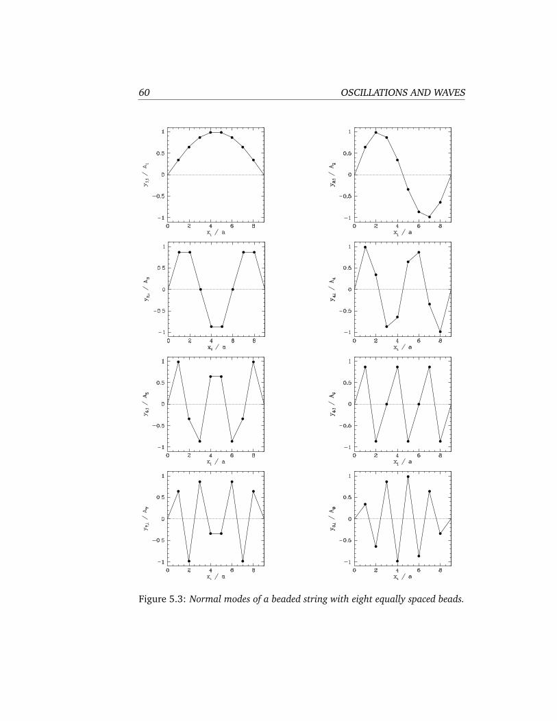
60 OSCILLATIONS AND WAVES
Figure 5.3: Normal modes of a beaded string with eight equally spaced beads.
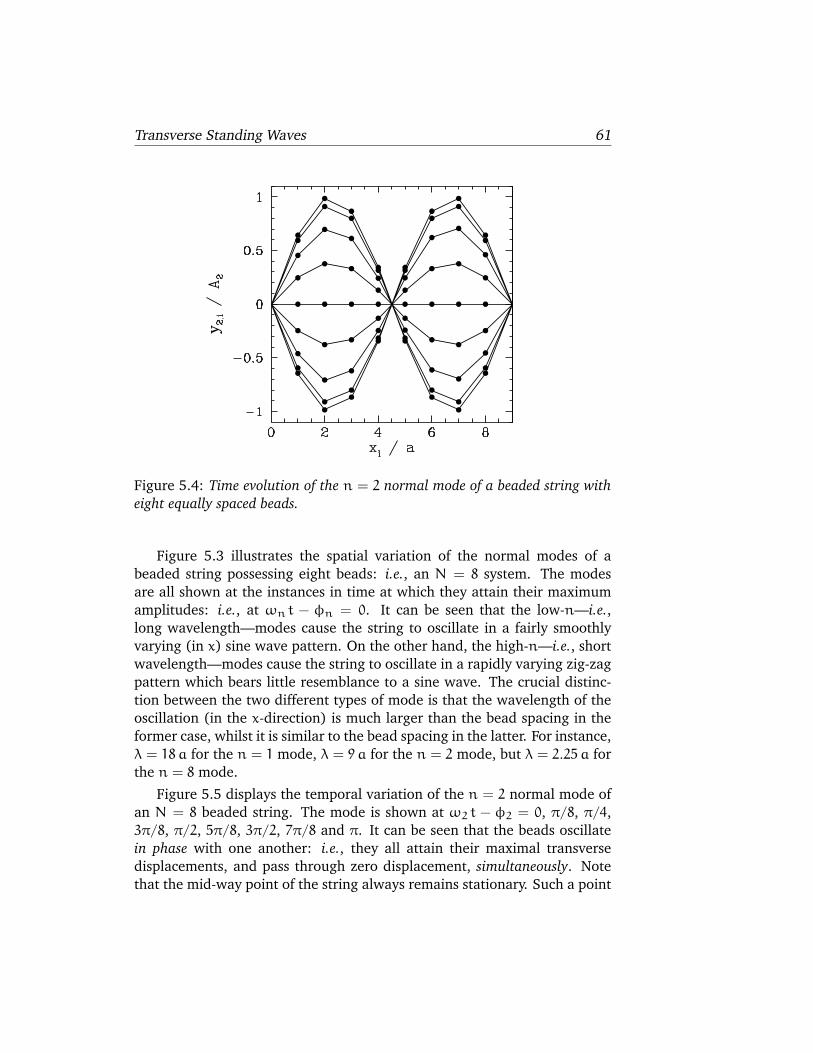
Transverse Standing Waves 61
Figure 5.4: Time evolution of the n = 2 normal mode of a beaded string with
eight equally spaced beads.
Figure 5.3 illustrates the spatial variation of the normal modes of a
beaded string possessing eight beads: i.e., an N = 8 system. The modes
are all shown at the instances in time at which they attain their maximum
amplitudes: i.e., at ωn t − φn = 0. It can be seen that the low-n—i.e.,
long wavelength—modes cause the string to oscillate in a fairly smoothly
varying (in x) sine wave pattern. On the other hand, the high-n—i.e., short
wavelength—modes cause the string to oscillate in a rapidly varying zig-zag
pattern which bears little resemblance to a sine wave. The crucial distinc-
tion between the two different types of mode is that the wavelength of the
oscillation (in the x-direction) is much larger than the bead spacing in the
former case, whilst it is similar to the bead spacing in the latter. For instance,
λ = 18 a for the n = 1 mode, λ = 9 a for the n = 2 mode, but λ = 2.25 a for
the n = 8 mode.
Figure 5.5 displays the temporal variation of the n = 2 normal mode of
an N = 8 beaded string. The mode is shown at ω2 t − φ2 = 0, π/8, π/4,
3π/8, π/2, 5π/8, 3π/2, 7π/8 and π. It can be seen that the beads oscillate
in phase with one another: i.e., they all attain their maximal transverse
displacements, and pass through zero displacement, simultaneously. Note
that the mid-way point of the string always remains stationary. Such a point
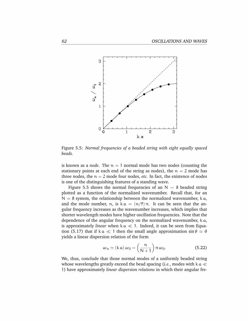
62 OSCILLATIONS AND WAVES
Figure 5.5: Normal frequencies of a beaded string with eight equally spaced
beads.
is known as a node. The n = 1 normal mode has two nodes (counting the
stationary points at each end of the string as nodes), the n = 2 mode has
three nodes, the n = 2 mode four nodes, etc. In fact, the existence of nodes
is one of the distinguishing features of a standing wave.
Figure 5.5 shows the normal frequencies of an N = 8 beaded string
plotted as a function of the normalized wavenumber. Recall that, for an
N = 8 system, the relationship between the normalized wavenumber, ka,
and the mode number, n, is ka = (n/9)π. It can be seen that the an-
gular frequency increases as the wavenumber increases, which implies that
shorter wavelength modes have higher oscillation frequencies. Note that the
dependence of the angular frequency on the normalized wavenumber, ka,
is approximately linear when ka ≪ 1. Indeed, it can be seen from Equa-
tion (5.17) that if ka ≪ 1 then the small angle approximation sin θ ≃ θ
yields a linear dispersion relation of the form
ωn ≃ (ka)ω0 =
(
n
N+ 1
)
πω0. (5.22)
We, thus, conclude that those normal modes of a uniformly beaded string
whose wavelengths greatly exceed the bead spacing (i.e., modes with ka≪1) have approximately linear dispersion relations in which their angular fre-
Transverse Standing Waves 63
quencies are directly proportional to their mode numbers. However, it is
clear from the figure that this linear relationship breaks down as ka → 1,
and the mode wavelength consequently becomes similar to the bead spac-
ing.
5.2 Normal Modes of a Uniform String
Consider a uniformly beaded string in the limit in which the number of
beads, N, becomes increasingly large, whilst the spacing, a, and the indi-
vidual mass, m, of the beads becomes increasingly small. Let the limit be
taken in such a manner that the length, l = (N + 1)a, and the average
mass per unit length, ρ = m/a, of the string both remain constant. Clearly,
as N increases, and becomes very large, such a string will more and more
closely approximate a uniform string of length l and mass per unit length
ρ. What can we guess about the normal modes of a uniform string from
the analysis contained in the previous section? Well, first of all, we would
guess that a uniform string is an infinite degree of freedom system, with an
infinite number of unique normal modes of oscillation. This follows because
a uniform string is the N → ∞ limit of a beaded string, and a beaded string
possesses N unique normal modes. Next, we would guess that the normal
modes of a uniform string exhibit smooth sinusoidal spatial variation in the
x-direction, and that the angular frequency of the modes is directly propor-
tional to their wavenumber. These last two conclusions follow because all
of the normal modes of a beaded string are characterized by ka≪ 1 in the
limit in which the spacing between the beads becomes zero. Let us now
investigate whether these guesses are correct.
Consider the transverse oscillations of a uniform string of length l and
mass per unit length ρ which is stretched between two immovable walls.
It is again convenient to define a Cartesian coordinate system in which x
measures distance along the string from the left wall, and y measures the
transverse displacement of the string. Thus, the instantaneous state of the
system at time t is determined by the function y(x, t) for 0 ≤ x ≤ l. Of
course, this function consists of an infinite number of different y values,
corresponding to the infinite number of different x values in the range 0
to l. Moreover, all of these y values are free to vary independently of one
another. It follows that we are indeed dealing with a dynamical system
possessing an infinite number of degrees of freedom.
Let us try to reuse some of the analysis of the previous section. We can
reinterpret yi(t) as y(x, t), yi−1(t) as y(x−δx, t), and yi+1(t) as y(x+δx, t),
64 OSCILLATIONS AND WAVES
assuming that xi = x and a = δx. Moreover, yi(t) becomes ∂2y(x, t)/∂t2:
i.e., a second derivative of y(x, t) with respect to t at constant x. Finally,
ω20 = T/(ma), where T is the tension in the string, can be rewritten as
T/[ρ (δx)2], since ρ = m/δx. Incidentally, we are again assuming that the
transverse displacement of the string remains sufficiently small that the ten-
sion is approximately constant in x. Thus, the equation of motion of the
beaded string, (5.8), transforms into
∂2y(x, t)
∂t2=T
ρ
[
y(x− δx, t) − 2 y(x, t) + y(x+ δx, t)
(δx)2
]
. (5.23)
However, Taylor expanding y(x+ δx, t) in x at constant t, we obtain
y(x+ δx, t) = y(x, t) +∂y(x, t)
∂xδx+
1
2
∂2y(x, t)
∂x2(δx)2 + O(δx)3. (5.24)
Likewise,
y(x− δx, t) = y(x, t) −∂y(x, t)
∂xδx+
1
2
∂2y(x, t)
∂x2(δx)2 + O(δx)3. (5.25)
It follows that
[
y(x− δx, t) − 2 y(x, t) + y(x+ δx, t)
(δx)2
]
=∂2y(x, t)
∂x2+ O(δx). (5.26)
Thus, in the limit that δx → 0, Equation (5.23) reduces to
∂2y
∂t2= v2 ∂
2y
∂x2, (5.27)
where
v =
√
T
ρ(5.28)
is a quantity having the dimensions of velocity. Equation (5.27), which is
the transverse equation of motion of the string, takes the form of a very
famous partial differential equation known as the wave equation. The quan-
tity v turns out to the the propagation velocity of transverse waves along the
string. See Section 7.1.
By analogy with Equation (5.9), let us search for a solution of the wave
equation of the form
y(x, t) = A sin(k x) cos(ωt− φ), (5.29)
Transverse Standing Waves 65
where A > 0, k > 0, ω > 0, and φ are constants. We would interpret
such a solution as a standing wave of wavenumber k, wavelength λ = 2π/k,
angular frequencyω, peak amplitude A, and phase angle φ. Substitution of
the above expression into Equation (5.27) yields the dispersion relation [cf.,
(5.13)]
ω2 = k2 v2. (5.30)
Now, the standing wave solution (5.29) is subject to the physical con-
straint that the two ends of the string, which are attached to immovable
walls, remain stationary. This leads directly to the boundary conditions
y(0, t) = 0, (5.31)
y(l, t) = 0. (5.32)
It can be seen that the solution (5.29) automatically satisfies the first bound-
ary condition. However, the second boundary condition is only satisfied
when sin(k l) = 0, which immediately implies that
k = nπ
l, (5.33)
where the mode number, n, is an integer. We, thus, conclude that the
possible normal modes of a taut string, of length l and fixed ends, have
wavenumbers which are quantized such that they are integer multiples of
π/l. Moreover, it is clear that this quantization is a direct consequence of
the imposition of the physical boundary conditions at the two ends of the
string.
It follows, from the above analysis, that the nth normal mode of the
string is associated with the pattern of motion
yn(x, t) = An sin
(
nπx
l
)
cos(ωn t− φn), (5.34)
where
ωn = nπv
l. (5.35)
Here, An and φn are constants which are determined by the initial con-
ditions. See Section 5.3. So, how many unique normal modes are there?
Well, the choice n = 0 yields y0(x, t) = 0 for all x and t, so this is not a real
normal mode. Moreover,
ω−n = −ωn, (5.36)
y−n(x, t) = yn(x, t), (5.37)
66 OSCILLATIONS AND WAVES
provided that A−n = −An and φ−n = −φn. We, thus, conclude that modes
with negative mode numbers give rise to the same patterns of motion as
modes with corresponding positive mode numbers. However, the modes
with positive mode numbers each correspond to unique patterns of motion
which oscillate at unique frequencies. It follows that the string possesses
an infinite number of normal modes, corresponding to the mode numbers
n = 1, 2, 3, etc. Recall that we are dealing with an infinite degree of freedom
system, which we would expect to possess an infinite number of unique
normal modes. The fact that we have actually found an infinite number
of such modes suggests that we have found all of the normal modes of the
system.
Figure 5.6 illustrates the spatial variation of the first eight normal modes
of a uniform string with fixed ends. The modes are all shown at the instances
in time at which they attain their maximum amplitudes: i.e., atωn t−φn =
0. It can be seen that the modes are all smoothly varying sine waves. The
low mode number (i.e., long wavelength) modes are actually quite similar
in form to the corresponding normal modes of a uniformly beaded string.
See Figure 5.3. However, the high mode number modes are substantially
different. We conclude that the normal modes of a beaded string are similar
to those of a uniform string, with the same length and mass per unit length,
provided that the wavelength of the mode is much larger than the spacing
between the beads.
Figure 5.7 illustrates the temporal variation of the n = 4 normal mode
of a uniform string. The mode is shown at ω4 t − φ4 = 0, π/8, π/4, 3π/8,
π/2, 5π/8, 3π/2, 7π/8 and π. It can be seen that all points on the string
attain their maximal transverse displacements, and pass through zero dis-
placement, simultaneously. Note that the n = 4 mode possesses five nodes,
at which the string remains stationary. Two of these are located at the ends
of the string, and three in the middle. In fact, it is clear from Equation (5.34)
that the nodes correspond to points at which sin[n (x/l)π] = 0. Hence, the
nodes are located at
xn,j =
(
j
n
)
l, (5.38)
where j is an integer lying in the range 0 to n. Here, n indexes the normal
mode, and j the node. Thus, the j = 0 node lies at the left end of the
string, the j = 1 node is the next node to the right, etc. It is apparent, from
the above formula, that the nth normal mode has n + 1 nodes which are
uniformly spaced a distance l/n apart.
Finally, Figure 5.8 shows the first eight normal frequencies of a uniform
string with fixed ends, plotted as a function of the mode number. It can
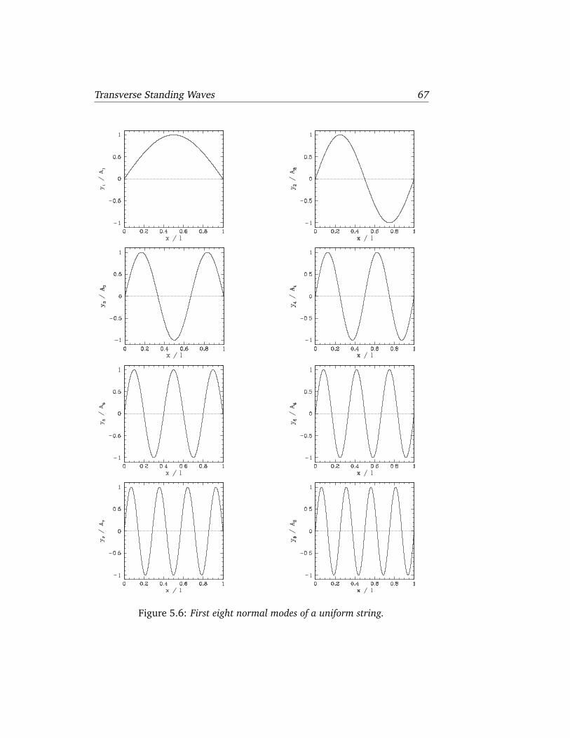
Transverse Standing Waves 67
Figure 5.6: First eight normal modes of a uniform string.
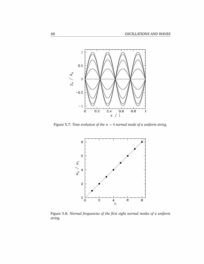
68 OSCILLATIONS AND WAVES
Figure 5.7: Time evolution of the n = 4 normal mode of a uniform string.
Figure 5.8: Normal frequencies of the first eight normal modes of a uniform
string.
Transverse Standing Waves 69
be seen that the angular frequency of oscillation increases linearly with the
mode number. Recall that the low mode number (i.e., long wavelength)
normal modes of a beaded string also exhibit a linear relationship between
normal frequency and mode number of the form [see Equation (5.22)]
ωn =nπ
N+ 1ω0 =
nπ
N+ 1
(
T
ma
)1/2
. (5.39)
However, m = ρa and l = (N+ 1)a, so we obtain
ωn =nπ
l
(
T
ρ
)1/2
= nπv
l, (5.40)
which is identical to Equation (5.35). We, thus, conclude that the normal
frequencies of a uniformly beaded string are similar to those of a uniform
string, with the same length and mass per unit length, as long as the wave-
length of the associated normal mode is much larger than the spacing be-
tween the beads.
5.3 General Time Evolution of a Uniform String
In the previous section, we found the normal modes of a uniform string
of length l, both ends of which are attached to immovable walls. These
modes are spatially periodic solutions of the wave equation (5.27) which
oscillate at unique frequencies and satisfy the boundary conditions (5.31)
and (5.32). Since the wave equation is obviously linear [i.e., if y(x, t) is a
solution then so is ay(x, t), where a is an arbitrary constant], it follows that
its most general solution is a linear combination of all of the normal modes.
In other words,
y(x, t) =∑
n′=1,∞
yn′(x, t) =∑
n′=1,∞
An′ sin
(
n ′ πx
l
)
cos
(
n ′ πv t
l− φn′
)
,
(5.41)
where use has been made of (5.34) and (5.35). Note that this expression is
obviously a solution of (5.27), and also automatically satisfies the boundary
conditions (5.31) and (5.32). As we have already mentioned, the constants
An and φn are determined by the initial conditions. Let us see how this
comes about in more detail.
Suppose that the initial displacement of the string at t = 0 is
y0(x) ≡ y(x, 0). (5.42)
70 OSCILLATIONS AND WAVES
Likewise, let the initial velocity of the string be
v0(x) ≡∂y(x, 0)
∂t. (5.43)
Obviously, for consistency with the boundary conditions, we must have
y0(0) = y0(l) = v0(0) = v0(l) = 0. It follows from Equation (5.41) that
y0(x) =∑
n′=1,∞
An′ cosφn′ sin
(
n ′ πx
l
)
, (5.44)
v0(x) =v
l
∑
n′=1,∞
n ′ πAn′ sinφn′ sin
(
n ′ πx
l
)
. (5.45)
Now, it is readily demonstrated that
2
l
∫ l
0
sin
(
nπx
l
)
sin
(
n ′ πx
l
)
dx
=2
π
∫π
0
sin (nθ) sin(
n ′ θ)
dθ
=1
π
∫π
0
cos[
(n− n ′) θ]
dθ−1
π
∫ l
0
cos[
(n+ n ′) θ]
dθ,
=1
π
[
sin [(n− n ′) θ]
n− n ′−
sin [(n+ n ′) θ]
n+ n ′
]π
0
=sin [(n− n ′)π]
(n− n ′)π−
sin [(n+ n ′)π]
(n+ n ′)π, (5.46)
where n and n ′ are (possibly different) positive integers, θ = πx/l, and use
has been made of the trigonometric identity 2 sina sinb ≡ cos(a − b) −
cos(a+ b). Furthermore, it is easily seen that if k is a non-zero integer then
sin(kπ)
kπ= 0. (5.47)
On the other hand, k = 0 is a special case, since both the numerator and the
denominator in the above expression become zero simultaneously. However,
application of l‘Hopital’s rule yields
limx→0
sin x
x= lim
x→0
d(sin x)/dx
dx/dx= lim
x→0
cos x
1= 1. (5.48)
It follows thatsin(kπ)
kπ=
1 k = 0
0 k 6= 0, (5.49)
Transverse Standing Waves 71
where k is any integer. This result can be combined with Equation (5.46),
recalling that n and n ′ are both positive integers, to give
2
l
∫ l
0
sin
(
nπx
l
)
sin
(
n ′ πx
l
)
dx = δn,n′ . (5.50)
Here, the quantity
δn,n′ =
1 n = n ′
0 n 6= n ′, (5.51)
where n and n ′ are integers, is known as the Kronecker delta function.
Let us multiply Equation (5.44) by (2/l) sin(nπx/l) and integrate over
x from 0 to l. We obtain
2
l
∫ l
0
y0(x) sin
(
nπx
l
)
dx
=∑
n′=1,∞
An′ cosφn′
2
l
∫π
0
sin
(
n ′ πx
l
)
sin
(
nπx
l
)
dx
=∑
n′=1,∞
An′ cosφn′ δn,n′ = An cosφn, (5.52)
where use has been made of Equations (5.50) and (5.51). Similarly, Equa-
tion (5.45) yields
2
v
∫ l
0
v0(x) sin
(
nπx
l
)
dx = nπAn sinφn. (5.53)
Thus, defining the integrals
Cn =2
l
∫ l
0
y0(x) sin
(
nπx
l
)
dx, (5.54)
Sn =2
nπ v
∫ l
0
v0(x) sin
(
nπx
l
)
dx, (5.55)
for n = 1,∞, we obtain
Cn = An cosφn, (5.56)
Sn = An sinφn, (5.57)
and, hence,
An = (C2n + S2
n)1/2, (5.58)
φn = tan−1(Sn/Cn). (5.59)
72 OSCILLATIONS AND WAVES
Thus, the constants An and φn, appearing in the general expression (5.41)
for the time evolution of a uniform string with fixed ends, are ultimately
determined by integrals over the string’s initial displacement and velocity
which are of the form (5.54) and (5.55).
As an example, suppose that the string is initially at rest, so that
v0(x) = 0, (5.60)
but has the initial displacement
y0(x) = 2A
x/l 0 ≤ x < l/2
1− x/l l/2 ≤ x ≤ l . (5.61)
This triangular pattern is zero at both ends of the string, rising linearly to
a peak value of A halfway along the string, and is designed to mimic the
initial displacement of a guitar string which is plucked at its mid-point. See
Figure 5.10. A comparison of Equations (5.55) and (5.60) reveals that, in
this particular example, all of the Sn coefficients are zero. Hence, from
(5.58) and (5.59), An = Cn and φn = 0 for all n. Thus, making use
of Equations (5.41), (5.54), and (5.61), the time evolution of the string is
governed by
y(x, t) =∑
n=1,∞
An sin
(
nπx
l
)
cos
(
n2πt
τ
)
, (5.62)
where τ = 2 l/v is the oscillation period of the n = 1 normal mode, and
An =2
l
∫ l/2
0
2Ax
lsin
(
nπx
l
)
dx+2
l
∫ l
l/2
2A
(
1−x
l
)
sin
(
nπx
l
)
dx.
(5.63)
The above expression transforms to
An = A
(
2
π
)2∫π/2
0
θ sin(nθ)dθ+
∫π
π/2
(π− θ) sin(nθ)dθ
, (5.64)
where θ = πx/l. Integration by parts yields
An = 2Asin(nπ/2)
(nπ/2)2. (5.65)
Note that An = 0 whenever n is even. We conclude that the triangular ini-
tial displacement pattern (5.61) only excites normal modes with odd mode
numbers.
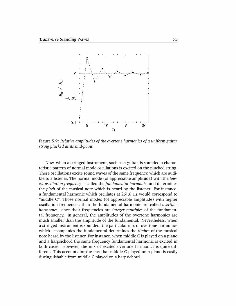
Transverse Standing Waves 73
Figure 5.9: Relative amplitudes of the overtone harmonics of a uniform guitar
string plucked at its mid-point.
Now, when a stringed instrument, such as a guitar, is sounded a charac-
teristic pattern of normal mode oscillations is excited on the plucked string.
These oscillations excite sound waves of the same frequency, which are audi-
ble to a listener. The normal mode (of appreciable amplitude) with the low-
est oscillation frequency is called the fundamental harmonic, and determines
the pitch of the musical note which is heard by the listener. For instance,
a fundamental harmonic which oscillates at 261.6 Hz would correspond to
“middle C”. Those normal modes (of appreciable amplitude) with higher
oscillation frequencies than the fundamental harmonic are called overtone
harmonics, since their frequencies are integer multiples of the fundamen-
tal frequency. In general, the amplitudes of the overtone harmonics are
much smaller than the amplitude of the fundamental. Nevertheless, when
a stringed instrument is sounded, the particular mix of overtone harmonics
which accompanies the fundamental determines the timbre of the musical
note heard by the listener. For instance, when middle C is played on a piano
and a harpsichord the same frequency fundamental harmonic is excited in
both cases. However, the mix of excited overtone harmonics is quite dif-
ferent. This accounts for the fact that middle C played on a piano is easily
distinguishable from middle C played on a harpsichord.
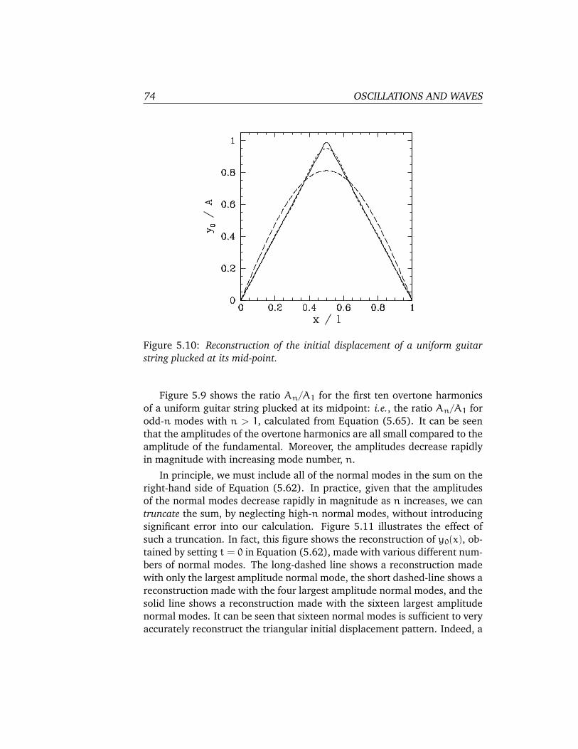
74 OSCILLATIONS AND WAVES
Figure 5.10: Reconstruction of the initial displacement of a uniform guitar
string plucked at its mid-point.
Figure 5.9 shows the ratio An/A1 for the first ten overtone harmonics
of a uniform guitar string plucked at its midpoint: i.e., the ratio An/A1 for
odd-n modes with n > 1, calculated from Equation (5.65). It can be seen
that the amplitudes of the overtone harmonics are all small compared to the
amplitude of the fundamental. Moreover, the amplitudes decrease rapidly
in magnitude with increasing mode number, n.
In principle, we must include all of the normal modes in the sum on the
right-hand side of Equation (5.62). In practice, given that the amplitudes
of the normal modes decrease rapidly in magnitude as n increases, we can
truncate the sum, by neglecting high-n normal modes, without introducing
significant error into our calculation. Figure 5.11 illustrates the effect of
such a truncation. In fact, this figure shows the reconstruction of y0(x), ob-
tained by setting t = 0 in Equation (5.62), made with various different num-
bers of normal modes. The long-dashed line shows a reconstruction made
with only the largest amplitude normal mode, the short dashed-line shows a
reconstruction made with the four largest amplitude normal modes, and the
solid line shows a reconstruction made with the sixteen largest amplitude
normal modes. It can be seen that sixteen normal modes is sufficient to very
accurately reconstruct the triangular initial displacement pattern. Indeed, a
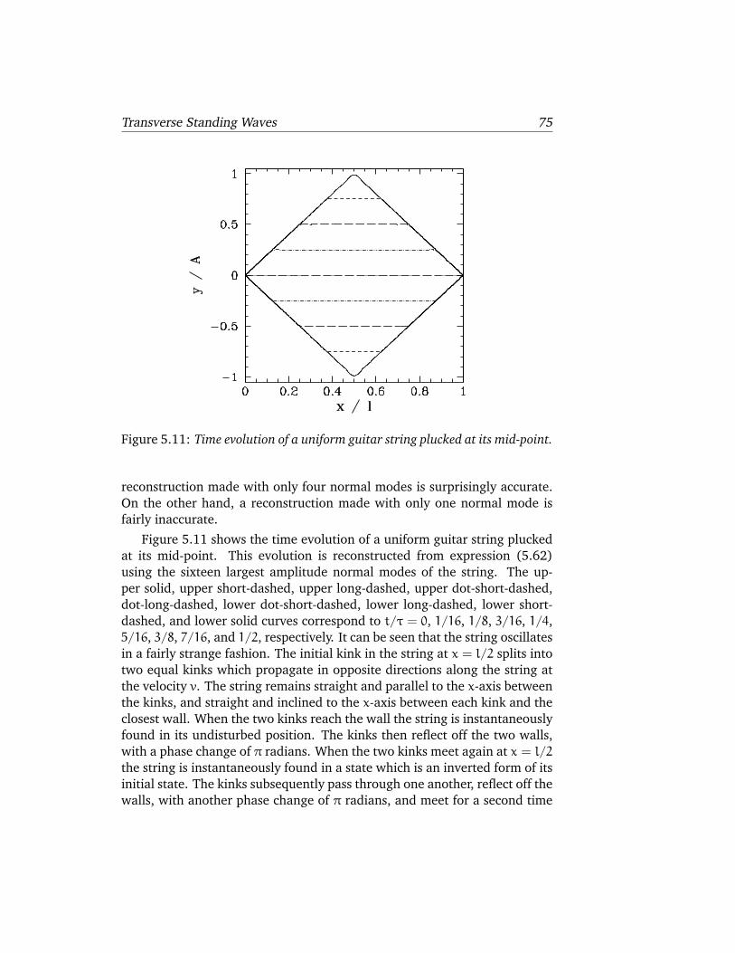
Transverse Standing Waves 75
Figure 5.11: Time evolution of a uniform guitar string plucked at its mid-point.
reconstruction made with only four normal modes is surprisingly accurate.
On the other hand, a reconstruction made with only one normal mode is
fairly inaccurate.
Figure 5.11 shows the time evolution of a uniform guitar string plucked
at its mid-point. This evolution is reconstructed from expression (5.62)
using the sixteen largest amplitude normal modes of the string. The up-
per solid, upper short-dashed, upper long-dashed, upper dot-short-dashed,
dot-long-dashed, lower dot-short-dashed, lower long-dashed, lower short-
dashed, and lower solid curves correspond to t/τ = 0, 1/16, 1/8, 3/16, 1/4,
5/16, 3/8, 7/16, and 1/2, respectively. It can be seen that the string oscillates
in a fairly strange fashion. The initial kink in the string at x = l/2 splits into
two equal kinks which propagate in opposite directions along the string at
the velocity v. The string remains straight and parallel to the x-axis between
the kinks, and straight and inclined to the x-axis between each kink and the
closest wall. When the two kinks reach the wall the string is instantaneously
found in its undisturbed position. The kinks then reflect off the two walls,
with a phase change of π radians. When the two kinks meet again at x = l/2
the string is instantaneously found in a state which is an inverted form of its
initial state. The kinks subsequently pass through one another, reflect off the
walls, with another phase change of π radians, and meet for a second time
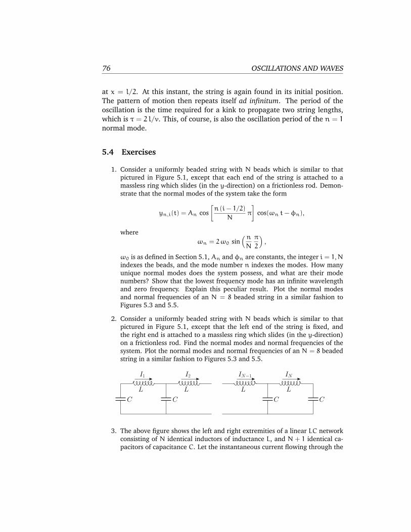
76 OSCILLATIONS AND WAVES
at x = l/2. At this instant, the string is again found in its initial position.
The pattern of motion then repeats itself ad infinitum. The period of the
oscillation is the time required for a kink to propagate two string lengths,
which is τ = 2 l/v. This, of course, is also the oscillation period of the n = 1
normal mode.
5.4 Exercises
1. Consider a uniformly beaded string with N beads which is similar to thatpictured in Figure 5.1, except that each end of the string is attached to amassless ring which slides (in the y-direction) on a frictionless rod. Demon-strate that the normal modes of the system take the form
yn,i(t) = An cos
[
n (i− 1/2)
Nπ
]
cos(ωn t− φn),
where
ωn = 2ω0 sin( n
N
π
2
)
,
ω0 is as defined in Section 5.1, An and φn are constants, the integer i = 1,N
indexes the beads, and the mode number n indexes the modes. How manyunique normal modes does the system possess, and what are their modenumbers? Show that the lowest frequency mode has an infinite wavelengthand zero frequency. Explain this peculiar result. Plot the normal modesand normal frequencies of an N = 8 beaded string in a similar fashion toFigures 5.3 and 5.5.
2. Consider a uniformly beaded string with N beads which is similar to thatpictured in Figure 5.1, except that the left end of the string is fixed, andthe right end is attached to a massless ring which slides (in the y-direction)on a frictionless rod. Find the normal modes and normal frequencies of thesystem. Plot the normal modes and normal frequencies of an N = 8 beadedstring in a similar fashion to Figures 5.3 and 5.5.
.. . .
I2
C
LL L
ININ−1I1
L
C C C
3. The above figure shows the left and right extremities of a linear LC networkconsisting of N identical inductors of inductance L, and N + 1 identical ca-pacitors of capacitance C. Let the instantaneous current flowing through the
Transverse Standing Waves 77
ith inductor be Ii(t), for i = 1,N. Demonstrate from Kirchoff’s circuital lawsthat the currents evolve in time according to the coupled equations
Ii = ω 20 (Ii−1 − 2 Ii + Ii+1),
for i = 1,N, where ω0 = 1/√LC, and I0 = IN+1 = 0. Find the normal
frequencies of the system.
4. Suppose that the outermost two capacitors in the circuit considered in theprevious exercise are short-circuited. Find the new normal frequencies of thesystem.
5. A uniform string of length l, tension T , and mass per unit length ρ, is stretchedbetween two immovable walls. Suppose that the string is initially in its equi-librium state. At t = 0 it is struck by a hammer in such a manner as to impartan impulsive velocity u0 to a small segment of length a < l centered on themid-point. Find an expression for the subsequent motion of the string. Plotthe motion as a function of time in a similar fashion to Figure 5.11, assumingthat a = l/10.
6. A uniform string of length l, tension T , and mass per unit length ρ, is stretchedbetween two massless rings, attached to its ends, which slide (in the y-direction) along frictionless rods. Demonstrate that, in this case, the mostgeneral solution to the wave equation takes the form
y(x, t) = Y0 + V0 t+∑
n>0
An cos(
nπx
l
)
cos
(
nπv t
l− φn
)
,
where v =√
T/ρ, and Y0, V0, An, and φn are arbitrary constants. Show that
2
l
∫ l
0
cos(
nπx
l
)
cos(
n ′ πx
l
)
dx = δn,n ′ ,
where n and n ′ are integers. Use this result to demonstrate that the arbitraryconstants in the above solution can be determined from the initial conditionsas follows:
Y0 =2
l
∫ l
0
y0(x)dx,
V0 =2
l
∫ l
0
v0(x)dx,
An = (C 2n + S 2
n)1/2,
φn = tan−1(Sn/Cn),
where y0(x) ≡ y(x, 0), v0(x) ≡ ∂y(x, 0)/∂t, and
Cn =2
l
∫ l
0
y0(x) cos(
nπx
l
)
dx,
78 OSCILLATIONS AND WAVES
Sn =2
l
∫ l
0
v0(x) cos(
nπx
l
)
dx.
Suppose that the string is initially in its equilibrium state. At t = 0 it is struckby a hammer in such a manner as to impart an impulsive velocity u0 to asmall segment of length a < l centered on the mid-point. Find an expressionfor the subsequent motion of the string. Plot the motion as a function of timein a similar fashion to Figure 5.11, assuming that a = l/10.
7. The linear LC circuit considered in Exercise 3 can be thought of as a discretemodel of a uniform lossless transmission line: e.g., a co-axial cable. In thisinterpretation, Ii(t) represents I(xi, t), where xi = i δx. Moreover, C = C δx,and L = L δx, where C and L are the capacitance per unit length and theinductance per unit length of the line, respectively. Show that, in the limitδx → 0, the evolution equation for the coupled currents given in Exercise 3reduces to the wave equation
∂2I
∂t2= v2 ∂
2I
∂x2,
where I = I(x, t), x measures distance along the line, and v = 1/√LC.
If Vi(t) is the potential difference (measured from the top to the bottom)across the i+ 1th capacitor (from the left) in the circuit shown in Exercise 3,and V(x, t) is the corresponding voltage in the transmission line, show thatthe discrete circuit equations relating the Ii(t) and Vi(t) reduce to
∂V
∂t= −
1
C∂I
∂x,
∂I
∂t= −
1
L∂V
∂x,
in the transmission line limit. Hence, demonstrate that the voltage in a trans-mission line satisfies the wave equation
∂2V
∂t2= v2 ∂
2V
∂x2.
8. Consider a uniform string of length l, tension T , and mass per unit length ρwhich is stretched between two immovable walls. Show that the total energyof the string, which is the sum of its kinetic and potential energies, is
E =1
2
∫ l
0
[
ρ
(
∂y
∂t
)2
+ T
(
∂y
∂x
)2]
dx,
where y(x, t) is the string’s (relatively small) transverse displacement. Now,the general motion of the string can be represented as a linear superpositionof the normal modes:
y(x, t) =∑
n=1,∞
An sin(
nπx
l
)
cos
(
nπv t
l− φn
)
,
Transverse Standing Waves 79
where v =√
T/ρ. Demonstrate that
E =∑
n=1,∞
En,
where
En =1
4mω 2
nA2n
is the energy of the nth normal mode. Here,m = ρ l is the mass of the string,and ωn = nπv/l the angular frequency of the nth normal mode.

80 OSCILLATIONS AND WAVES
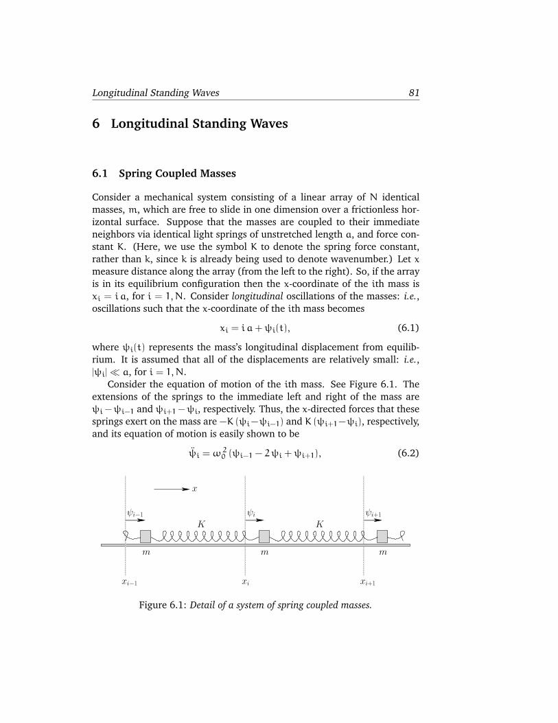
Longitudinal Standing Waves 81
6 Longitudinal Standing Waves
6.1 Spring Coupled Masses
Consider a mechanical system consisting of a linear array of N identical
masses, m, which are free to slide in one dimension over a frictionless hor-
izontal surface. Suppose that the masses are coupled to their immediate
neighbors via identical light springs of unstretched length a, and force con-
stant K. (Here, we use the symbol K to denote the spring force constant,
rather than k, since k is already being used to denote wavenumber.) Let x
measure distance along the array (from the left to the right). So, if the array
is in its equilibrium configuration then the x-coordinate of the ith mass is
xi = i a, for i = 1,N. Consider longitudinal oscillations of the masses: i.e.,
oscillations such that the x-coordinate of the ith mass becomes
xi = i a+ψi(t), (6.1)
where ψi(t) represents the mass’s longitudinal displacement from equilib-
rium. It is assumed that all of the displacements are relatively small: i.e.,
|ψi| ≪ a, for i = 1,N.
Consider the equation of motion of the ith mass. See Figure 6.1. The
extensions of the springs to the immediate left and right of the mass are
ψi −ψi−1 and ψi+1 −ψi, respectively. Thus, the x-directed forces that these
springs exert on the mass are −K (ψi−ψi−1) and K (ψi+1−ψi), respectively,
and its equation of motion is easily shown to be
ψi = ω20 (ψi−1 − 2ψi +ψi+1), (6.2)
ψi+1
xi−1 xi xi+1
mm m
ψi−1 ψiK
x
K
Figure 6.1: Detail of a system of spring coupled masses.
82 OSCILLATIONS AND WAVES
where ω0 =√
K/m. Since there is nothing special about the ith mass,
the above equation is assumed to hold for all N masses: i.e., for i = 1,N.
Note that Equation (6.2), which governs the longitudinal oscillations of a lin-
ear array of spring coupled masses, is analogous in form to Equation (5.8),
which governs the transverse oscillations of a beaded string. This observa-
tion suggests that longitudinal and transverse waves in discrete dynamical
systems (i.e., systems with a finite number of degrees of freedom) can be
described using the same mathematical equations.
We can interpret the quantities ψ0 and ψN+1, which appear in the equa-
tions of motion for ψ1 and ψN, respectively, as the longitudinal displace-
ments of the left and right extremities of springs which are attached to the
outermost masses in such a manner as to form the left and right boundaries
of the array. The respective equilibrium positions of these extremities are
x0 = 0 and xN+1 = (N + 1)a. Now, the end displacements, ψ0 and ψN+1,
must be prescribed, otherwise Equations (6.2) do not constitute a complete
set of equations: i.e., there are more unknowns than equations. The partic-
ular choice of ψ0 and ψN+1 depends on the nature of the physical boundary
conditions at the two ends of the array. Suppose that the left extremity of
the leftmost spring is anchored in an immovable wall. This implies that
ψ0 = 0: i.e., the left extremity of the spring cannot move. Suppose, on the
other hand, that the left extremity of the leftmost spring is not attached to
anything. In this case, there is no reason for the spring to become extended,
which implies that ψ0 = ψ1. In other words, if the left end of the array is
fixed (i.e., attached to an immovable object) then ψ0 = 0, and if the left end
is free (i.e., not attached to anything) then ψ0 = ψ1. Likewise, if the right
end of the array is fixed then ψN+1 = 0, and if the right end is free then
ψN+1 = ψN.
Suppose, for the sake of argument, that the left end of the array is free,
and the right end is fixed. It follows that ψ0 = ψ1, and ψN+1 = 0. Let us
search for normal modes of the general form
ψi(t) = A cos[k (xi − a/2)] cos(ωt− φ), (6.3)
where A > 0, k > 0, ω > 0, and φ are constants. Note that the above
expression automatically satisfies the boundary condition ψ0 = ψ1. This
follows because x0 = 0 and x1 = a, and, consequently, cos[k (x0 − a/2)] =
cos(−ka/2) = cos(ka/2) = cos[k (x1 − a/2)]. The other boundary condi-
tion, ψN+1 = 0, is satisfied provided
cos[k (xN+1 − a/2)] = cos[(N+ 1/2)ka] = 0, (6.4)
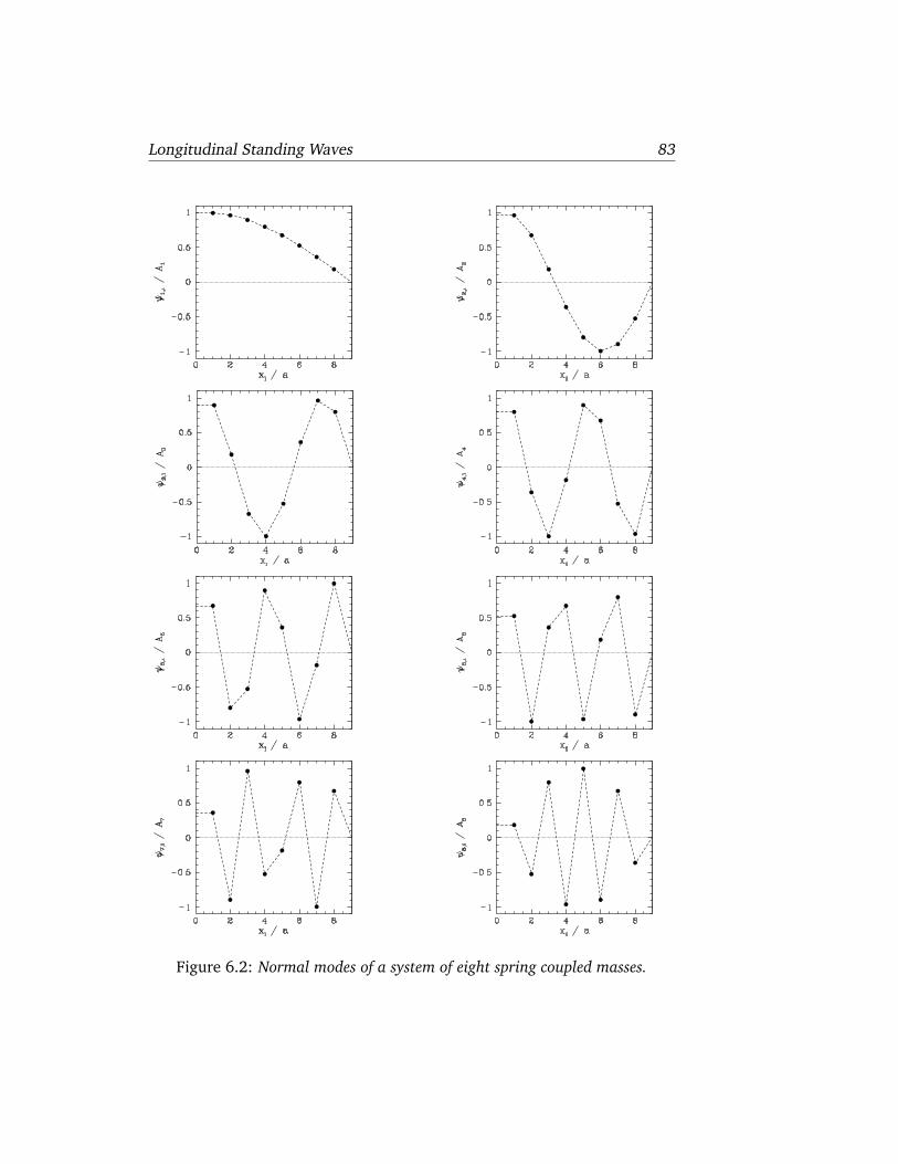
Longitudinal Standing Waves 83
Figure 6.2: Normal modes of a system of eight spring coupled masses.
84 OSCILLATIONS AND WAVES
which yields [cf., (5.15)]
ka =(n− 1/2)π
N+ 1/2, (6.5)
where n is an integer. As before, the imposition of the boundary conditions
causes a quantization of the possible mode wavenumbers (see Section 5.1).
Finally, substitution of (6.3) into (6.2) gives the dispersion relation [cf.,
(5.13)]
ω = 2ω0 sin(ka/2). (6.6)
It follows, from the above analysis, that the longitudinal normal modes
of a linear array of spring coupled masses, the left end of which is free, and
the right end fixed, are associated with the following characteristic displace-
ment patterns:
ψn,i(t) = An cos
[
(n− 1/2) (i− 1/2)
N+ 1/2π
]
cos(ωn − φn), (6.7)
where
ωn = 2ω0 sin
(
n− 1/2
N+ 1/2
π
2
)
, (6.8)
and the An and φn are arbitrary constants determined by the initial condi-
tions. Here, the integer i = 1,N indexes the masses, and the mode number
n indexes the normal modes. It is easily demonstrated that there are only
N unique normal modes, corresponding to mode numbers in the range 1 to
N.
Figures 6.2 and 6.3 display the normal modes and normal frequencies
of a linear array of eight spring coupled masses, the left end of which is
free, and the right end fixed. The data shown in these figures is obtained
from Equations (6.7) and (6.8), respectively, with N = 8. The modes in
Figure 6.2 are all plotted at the instances in time at which they attain their
maximum amplitudes: i.e., when cos(ωn t − φn) = 1. It can be seen that
normal modes with small wavenumbers—i.e., ka ≪ 1, so that n ≪ N—
have displacements which vary in a fairly smooth sinusoidal manner from
mass to mass, and oscillations frequencies which increase approximately
linearly with increasing wavenumber. On the other hand, normal modes
with large wavenumbers—i.e., ka ∼ 1, so that n ∼ N—have displacements
which exhibit large variations from mass to mass, and oscillation frequen-
cies which do not depend linearly on wavenumber. We conclude that the
longitudinal normal modes of an array of spring coupled masses have anal-
ogous properties to the transverse normal modes of a beaded string. See
Section 5.1.
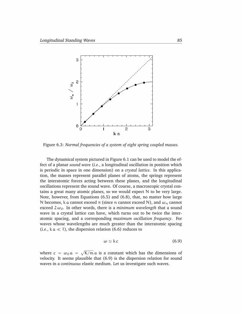
Longitudinal Standing Waves 85
Figure 6.3: Normal frequencies of a system of eight spring coupled masses.
The dynamical system pictured in Figure 6.1 can be used to model the ef-
fect of a planar sound wave (i.e., a longitudinal oscillation in position which
is periodic in space in one dimension) on a crystal lattice. In this applica-
tion, the masses represent parallel planes of atoms, the springs represent
the interatomic forces acting between these planes, and the longitudinal
oscillations represent the sound wave. Of course, a macroscopic crystal con-
tains a great many atomic planes, so we would expect N to be very large.
Note, however, from Equations (6.5) and (6.8), that, no matter how large
N becomes, ka cannot exceed π (since n cannot exceed N), and ωn cannot
exceed 2ω0. In other words, there is a minimum wavelength that a sound
wave in a crystal lattice can have, which turns out to be twice the inter-
atomic spacing, and a corresponding maximum oscillation frequency. For
waves whose wavelengths are much greater than the interatomic spacing
(i.e., ka≪ 1), the dispersion relation (6.6) reduces to
ω ≃ k c (6.9)
where c = ω0a =√
K/ma is a constant which has the dimensions of
velocity. It seems plausible that (6.9) is the dispersion relation for sound
waves in a continuous elastic medium. Let us investigate such waves.
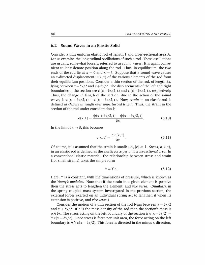
86 OSCILLATIONS AND WAVES
6.2 Sound Waves in an Elastic Solid
Consider a thin uniform elastic rod of length l and cross-sectional area A.
Let us examine the longitudinal oscillations of such a rod. These oscillations
are usually, somewhat loosely, referred to as sound waves. It is again conve-
nient to let x denote position along the rod. Thus, in equilibrium, the two
ends of the rod lie at x = 0 and x = l. Suppose that a sound wave causes
an x-directed displacement ψ(x, t) of the various elements of the rod from
their equilibrium positions. Consider a thin section of the rod, of length δx,
lying between x−δx/2 and x+δx/2. The displacements of the left and right
boundaries of the section are ψ(x− δx/2, t) and ψ(x+ δx/2, t), respectively.
Thus, the change in length of the section, due to the action of the sound
wave, is ψ(x + δx/2, t) − ψ(x − δx/2, t). Now, strain in an elastic rod is
defined as change in length over unperturbed length. Thus, the strain in the
section of the rod under consideration is
ǫ(x, t) =ψ(x+ δx/2, t) −ψ(x− δx/2, t)
δx. (6.10)
In the limit δx → 0, this becomes
ǫ(x, t) =∂ψ(x, t)
∂x. (6.11)
Of course, it is assumed that the strain is small: i.e., |ǫ| ≪ 1. Stress, σ(x, t),
in an elastic rod is defined as the elastic force per unit cross-sectional area. In
a conventional elastic material, the relationship between stress and strain
(for small strains) takes the simple form
σ = Y ǫ. (6.12)
Here, Y is a constant, with the dimensions of pressure, which is known as
the Young’s modulus. Note that if the strain in a given element is positive
then the stress acts to lengthen the element, and vice versa. (Similarly, in
the spring coupled mass system investigated in the previous section, the
external forces exerted on an individual spring act to lengthen it when its
extension is positive, and vice versa.)
Consider the motion of a thin section of the rod lying between x − δx/2
and x + δx/2. If ρ is the mass density of the rod then the section’s mass is
ρAδx. The stress acting on the left boundary of the section is σ(x−δx/2) =
Y ǫ(x− δx/2). Since stress is force per unit area, the force acting on the left
boundary is AY ǫ(x− δx/2). This force is directed in the minus x-direction,
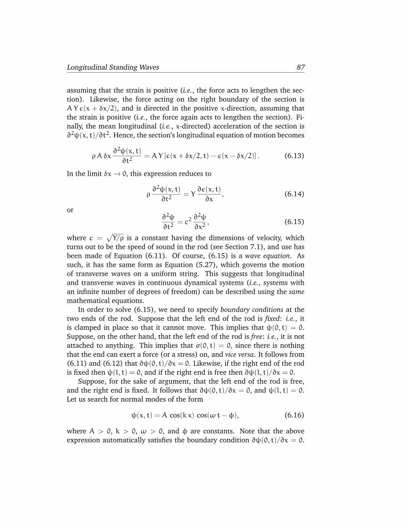
Longitudinal Standing Waves 87
assuming that the strain is positive (i.e., the force acts to lengthen the sec-
tion). Likewise, the force acting on the right boundary of the section is
AY ǫ(x + δx/2), and is directed in the positive x-direction, assuming that
the strain is positive (i.e., the force again acts to lengthen the section). Fi-
nally, the mean longitudinal (i.e., x-directed) acceleration of the section is
∂2ψ(x, t)/∂t2. Hence, the section’s longitudinal equation of motion becomes
ρAδx∂2ψ(x, t)
∂t2= AY [ǫ(x+ δx/2, t) − ǫ(x− δx/2)] . (6.13)
In the limit δx → 0, this expression reduces to
ρ∂2ψ(x, t)
∂t2= Y
∂ǫ(x, t)
∂x, (6.14)
or∂2ψ
∂t2= c2
∂2ψ
∂x2, (6.15)
where c =√
Y/ρ is a constant having the dimensions of velocity, which
turns out to be the speed of sound in the rod (see Section 7.1), and use has
been made of Equation (6.11). Of course, (6.15) is a wave equation. As
such, it has the same form as Equation (5.27), which governs the motion
of transverse waves on a uniform string. This suggests that longitudinal
and transverse waves in continuous dynamical systems (i.e., systems with
an infinite number of degrees of freedom) can be described using the same
mathematical equations.
In order to solve (6.15), we need to specify boundary conditions at the
two ends of the rod. Suppose that the left end of the rod is fixed: i.e., it
is clamped in place so that it cannot move. This implies that ψ(0, t) = 0.
Suppose, on the other hand, that the left end of the rod is free: i.e., it is not
attached to anything. This implies that σ(0, t) = 0, since there is nothing
that the end can exert a force (or a stress) on, and vice versa. It follows from
(6.11) and (6.12) that ∂ψ(0, t)/∂x = 0. Likewise, if the right end of the rod
is fixed then ψ(l, t) = 0, and if the right end is free then ∂ψ(l, t)/∂x = 0.
Suppose, for the sake of argument, that the left end of the rod is free,
and the right end is fixed. It follows that ∂ψ(0, t)/∂x = 0, and ψ(l, t) = 0.
Let us search for normal modes of the form
ψ(x, t) = A cos(k x) cos(ωt− φ), (6.16)
where A > 0, k > 0, ω > 0, and φ are constants. Note that the above
expression automatically satisfies the boundary condition ∂ψ(0, t)/∂x = 0.
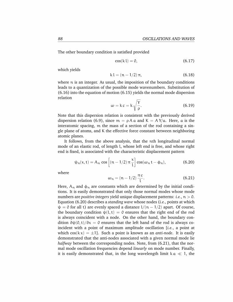
88 OSCILLATIONS AND WAVES
The other boundary condition is satisfied provided
cos(k l) = 0, (6.17)
which yields
k l = (n− 1/2)π, (6.18)
where n is an integer. As usual, the imposition of the boundary conditions
leads to a quantization of the possible mode wavenumbers. Substitution of
(6.16) into the equation of motion (6.15) yields the normal mode dispersion
relation
ω = k c = k
√
Y
ρ. (6.19)
Note that this dispersion relation is consistent with the previously derived
dispersion relation (6.9), since m = ρAa and K = AY/a. Here, a is the
interatomic spacing, m the mass of a section of the rod containing a sin-
gle plane of atoms, and K the effective force constant between neighboring
atomic planes.
It follows, from the above analysis, that the nth longitudinal normal
mode of an elastic rod, of length l, whose left end is free, and whose right
end is fixed, is associated with the characteristic displacement pattern
ψn(x, t) = An cos
[
(n− 1/2)πx
l
]
cos(ωn t− φn), (6.20)
where
ωn = (n− 1/2)π c
l. (6.21)
Here, An and φn are constants which are determined by the initial condi-
tions. It is easily demonstrated that only those normal modes whose mode
numbers are positive integers yield unique displacement patterns: i.e., n > 0.
Equation (6.20) describes a standing wave whose nodes (i.e., points at which
ψ = 0 for all t) are evenly spaced a distance l/(n − 1/2) apart. Of course,
the boundary condition ψ(l, t) = 0 ensures that the right end of the rod
is always coincident with a node. On the other hand, the boundary con-
dition ∂ψ(0, t)/∂x = 0 ensures that the left hand of the rod is always co-
incident with a point of maximum amplitude oscillation [i.e., a point at
which cos(k x) = ±1]. Such a point is known as an anti-node. It is easily
demonstrated that the anti-nodes associated with a given normal mode lie
halfway between the corresponding nodes. Note, from (6.21), that the nor-
mal mode oscillation frequencies depend linearly on mode number. Finally,
it is easily demonstrated that, in the long wavelength limit ka ≪ 1, the
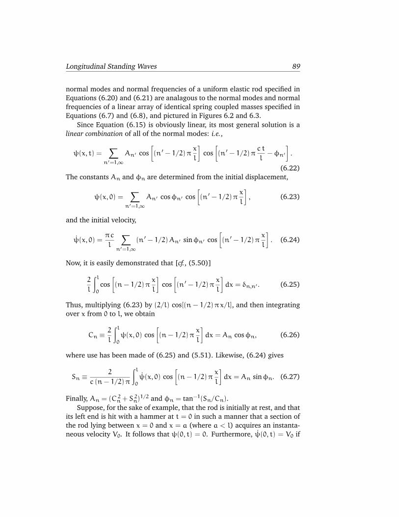
Longitudinal Standing Waves 89
normal modes and normal frequencies of a uniform elastic rod specified in
Equations (6.20) and (6.21) are analagous to the normal modes and normal
frequencies of a linear array of identical spring coupled masses specified in
Equations (6.7) and (6.8), and pictured in Figures 6.2 and 6.3.
Since Equation (6.15) is obviously linear, its most general solution is a
linear combination of all of the normal modes: i.e.,
ψ(x, t) =∑
n′=1,∞
An′ cos
[
(n ′ − 1/2)πx
l
]
cos
[
(n ′ − 1/2)πc t
l− φn′
]
.
(6.22)
The constants An and φn are determined from the initial displacement,
ψ(x, 0) =∑
n′=1,∞
An′ cosφn′ cos
[
(n ′ − 1/2)πx
l
]
, (6.23)
and the initial velocity,
ψ(x, 0) =π c
l
∑
n′=1,∞
(n ′ − 1/2)An′ sinφn′ cos
[
(n ′ − 1/2)πx
l
]
. (6.24)
Now, it is easily demonstrated that [cf., (5.50)]
2
l
∫ l
0
cos
[
(n− 1/2)πx
l
]
cos
[
(n ′ − 1/2)πx
l
]
dx = δn,n′ . (6.25)
Thus, multiplying (6.23) by (2/l) cos[(n − 1/2)πx/l], and then integrating
over x from 0 to l, we obtain
Cn ≡ 2
l
∫ l
0
ψ(x, 0) cos
[
(n− 1/2)πx
l
]
dx = An cosφn, (6.26)
where use has been made of (6.25) and (5.51). Likewise, (6.24) gives
Sn ≡ 2
c (n− 1/2)π
∫ l
0
ψ(x, 0) cos
[
(n− 1/2)πx
l
]
dx = An sinφn. (6.27)
Finally, An = (C2n + S2
n)1/2 and φn = tan−1(Sn/Cn).
Suppose, for the sake of example, that the rod is initially at rest, and that
its left end is hit with a hammer at t = 0 in such a manner that a section of
the rod lying between x = 0 and x = a (where a < l) acquires an instanta-
neous velocity V0. It follows that ψ(0, t) = 0. Furthermore, ψ(0, t) = V0 if
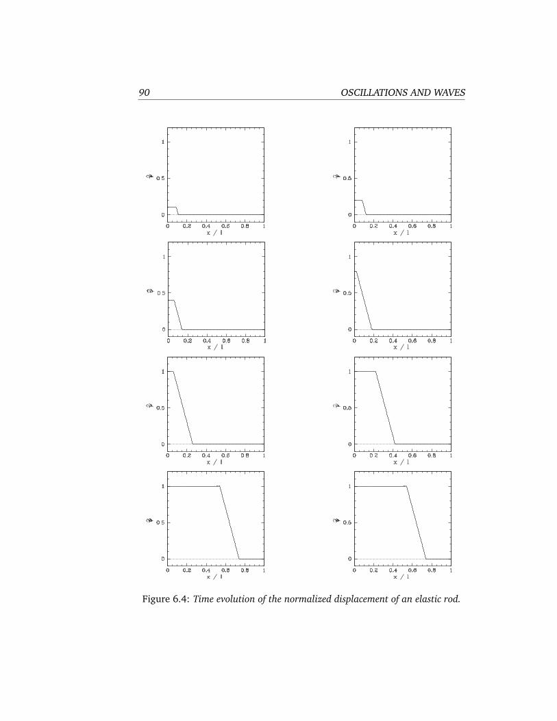
90 OSCILLATIONS AND WAVES
Figure 6.4: Time evolution of the normalized displacement of an elastic rod.
Longitudinal Standing Waves 91
0 ≤ x ≤ a, and ψ(0, t) = 0 otherwise. It is easily demonstrated that these
initial conditions yield Cn = 0, φn = π/2,
An = Sn =V0a
c
2
π
sin[(n− 1/2)πa/l]
(n− 1/2)2πa/l, (6.28)
and
ψ(x, t) =∑
n=1,∞
An cos
[
(n− 1/2)πx
l
]
sin
[
(n− 1/2)πt
τ
]
, (6.29)
where τ = l/c. Figure 6.4 shows the time evolution of the normalized rod
displacement, ψ(x, t) = (c/V0a)ψ(x, t), calculated from the above equa-
tions using the first 100 normal modes (i.e., n = 1, 100), and choosing
a/l = 0.1. The top-left, top-right, middle-left, middle-right, bottom-left,
and bottom-right panels correspond to t/τ = 0.01, 0.02, 0.04, 0.08, 0.16,
0.32, 0.64, and 1.28, respectively. It can be seen that the hammer blow gen-
erates a displacement wave that initially develops at the free end of the rod
(x/l = 0), which is the end that is struck, propagates along the rod at the
velocity c, and reflects off the fixed end (x/l = 1) at time t/τ = 1 with no
phase shift.
6.3 Sound Waves in an Ideal Gas
Consider a uniform ideal gas of equilibrium mass density ρ and equilibrium
pressure p. Let us investigate the longitudinal oscillations of such a gas. Of
course, these oscillations are usually referred to as sound waves. Generally
speaking, a sound wave in an ideal gas oscillates sufficiently rapidly that
heat is unable to flow fast enough to smooth out any temperature perturba-
tions generated by the wave. Under these circumstances, the gas obeys the
adiabatic gas law,
pVγ = constant, (6.30)
where p is the pressure, V the volume, and γ the ratio of specific heats (i.e.,
the ratio of the gas’s specific heat at constant pressure to its specific heat at
constant volume). This ratio is approximately 1.4 for ordinary air.
Consider a sound wave in a column of gas of cross-sectional area A. Let
x measure distance along the column. Suppose that the wave generates an
x-directed displacement of the column, ψ(x, t). Consider a small section of
the column lying between x − δx/2 and x + δx/2. The change in volume of
92 OSCILLATIONS AND WAVES
the section is δV = A [ψ(x + δx/2, t) − ψ(x − δx/2, t)]. Hence, the relative
change in volume, which is assumed to be small, is
δV
V=A [ψ(x+ δx/2, t) −ψ(x− δx/2, t)]
Aδx. (6.31)
In the limit δx → 0, this becomes
δV(x, t)
V=∂ψ(x, t)
∂x. (6.32)
The pressure perturbation δp(x, t) associated with the volume perturbation
δV(x, t) follows from (6.30), which yields
(p+ δp) (V + δV)γ = pVγ, (6.33)
or
(1+ δp/p) (1+ δV/V)γ ≃ 1+ δp/p+ γ δV/V = 1, (6.34)
giving
δp = −γpδV
V= −γp
∂ψ
∂x, (6.35)
where use has been made of (6.32).
Consider a section of the gas column lying between x − δx/2 and x +
δx/2. The mass of this section is ρAδx. The x-directed force acting on
its left boundary is A [p + δp(x − δx/2, t)], whereas the x-directed force
acting on its right boundary is −A [p+ δp(x+ δx/2, t)]. Finally, the average
longitudinal (i.e., x-directed) acceleration of the section is ∂2ψ(x, t)/∂t2.
Thus, the section’s longitudinal equation of motion is written
ρAδx∂2ψ(x, t)
∂t2= −A [δp(x+ δx/2, t) − δp(x− δx/2, t)] . (6.36)
In the limit δx → 0, this equation reduces to
ρ∂2ψ(x, t)
∂t2= −
∂δp(x, t)
∂x. (6.37)
Finally, (6.35) yields
∂2ψ
∂t2= c2
∂2ψ
∂x2, (6.38)
where c =√
γp/ρ is a constant with the dimensions of velocity, which turns
out to be the sound speed in the gas (see Section 7.1).
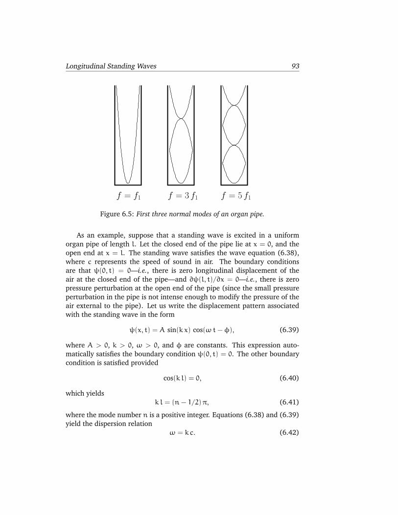
Longitudinal Standing Waves 93
f = 5 f1f = f1 f = 3 f1
Figure 6.5: First three normal modes of an organ pipe.
As an example, suppose that a standing wave is excited in a uniform
organ pipe of length l. Let the closed end of the pipe lie at x = 0, and the
open end at x = l. The standing wave satisfies the wave equation (6.38),
where c represents the speed of sound in air. The boundary conditions
are that ψ(0, t) = 0—i.e., there is zero longitudinal displacement of the
air at the closed end of the pipe—and ∂ψ(l, t)/∂x = 0—i.e., there is zero
pressure perturbation at the open end of the pipe (since the small pressure
perturbation in the pipe is not intense enough to modify the pressure of the
air external to the pipe). Let us write the displacement pattern associated
with the standing wave in the form
ψ(x, t) = A sin(k x) cos(ωt− φ), (6.39)
where A > 0, k > 0, ω > 0, and φ are constants. This expression auto-
matically satisfies the boundary condition ψ(0, t) = 0. The other boundary
condition is satisfied provided
cos(k l) = 0, (6.40)
which yields
k l = (n− 1/2)π, (6.41)
where the mode number n is a positive integer. Equations (6.38) and (6.39)
yield the dispersion relation
ω = k c. (6.42)
94 OSCILLATIONS AND WAVES
Hence, the nth normal mode has a wavelength
λn =4 l
2n− 1, (6.43)
and an oscillation frequency (in Hertz)
fn = (2n− 1) f1, (6.44)
where f1 = c/4 l is the frequency of the fundamental harmonic (i.e., the
normal mode with the lowest oscillation frequency). Figure 6.5 shows the
characteristic displacement patterns (which are pictured as transverse dis-
placements, for the sake of clarity) and oscillation frequencies of the pipe’s
first three normal modes (i.e., n = 1, 2, and 3). It can be seen that the
modes all have a node at the closed end of the pipe, and an anti-node at the
open end. The fundamental harmonic has a wavelength which is four times
the length of the pipe. The first overtone harmonic has a wavelength which
is 4/3rds the length of the pipe, and a frequency which is three times that
of the fundamental. Finally, the second overtone has a wavelength which is
4/5ths the length of the pipe, and a frequency which is five times that of the
fundamental. By contrast, the normal modes of a guitar string have nodes
at either end of the string. See Figure 5.6. Thus, as is easily demonstrated,
the fundamental harmonic has a wavelength which is twice the length of the
string. The first overtone harmonic has a wavelength which is the length of
the string, and a frequency which is twice that of the fundamental. Finally,
the second overtone harmonic has a wavelength which is 2/3rds the length
of the string, and a frequency which is three times that of the fundamental.
6.4 Fourier Analysis
Playing a musical instrument, such as a guitar or an organ, generates a set of
standing waves which cause a sympathetic oscillation in the surrounding air.
Such an oscillation consists of a fundamental harmonic, whose frequency
determines the pitch of the musical note heard by the listener, accompanied
by a set of overtone harmonics which determine the timbre of the note. By
definition, the oscillation frequencies of the overtone harmonics are integer
multiples of that of the fundamental. Thus, we expect the pressure pertur-
bation generated in a listener’s ear when a musical instrument is played to
have the general form
δp(t) =∑
n=1,∞
An cos(nωt− φn), (6.45)
Longitudinal Standing Waves 95
whereω is the angular frequency of the fundamental (i.e., n = 1) harmonic,
and the An and φn are the amplitudes and phases of the various harmonics.
The above expression can also be written
δp(t) =∑
n=1,∞
[Cn cos(nωt) + Sn sin(nωt)] , (6.46)
where Cn = An cosφn and Sn = An sinφn. Note that δp(t) is periodic
in time with period τ = 2π/ω. In other words, δp(t + τ) = δp(t) for all
t. This follows because cos(θ + n2π) = cos θ and sin(θ + n2π) = sin θ
for all angles, θ, and for all integers, n. [Moreover, there is no τ ′ < τ for
which δp(t + τ ′) = δp(t) for all t.] So, the question arises, can any peri-
odic waveform be represented as a linear superposition of sine and cosine
waveforms, whose periods are integer subdivisions of that of the waveform,
such as that shown in Equation (6.46)? To put it another way, given an arbi-
trary periodic waveform δp(t), can we uniquely determine the constants Cn
and Sn appearing in expression (6.46)? Actually, it turns out that we can.
Incidentally, the decomposition of a periodic waveform into a linear super-
position of sinusoidal waveforms is commonly known as Fourier analysis.
Let examine this topic in a little more detail.
The problem under investigation is as follows. Given a periodic wave-
form y(t), where y(t+τ) = y(t) for all t, we need to determine the constants
Cn and Sn in the expansion
y(t) =∑
n′=1,∞
[
Cn′ cos(n ′ωt) + Sn′ sin(n ′ωt)]
, (6.47)
where ω = 2π/τ. Now, it is easily demonstrated that [cf., (5.50)]
2
τ
∫τ
0
cos(nωt) cos(n ′ωt)dt = δn,n′ , (6.48)
2
τ
∫τ
0
sin(nωt) sin(n ′ωt)dt = δn,n′ , (6.49)
2
τ
∫τ
0
cos(nωt) sin(n ′ωt)dt = 0, (6.50)
where n and n ′ are positive integers. Thus, multiplying Equation (6.47) by
(2/τ) cos(nωt), and then integrating over t from 0 to τ, we obtain
Cn =2
τ
∫τ
0
y(t) cos(nωt)dt, (6.51)
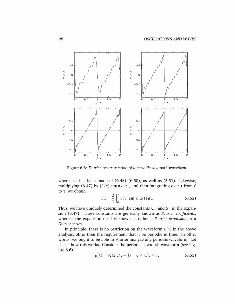
96 OSCILLATIONS AND WAVES
Figure 6.6: Fourier reconstruction of a periodic sawtooth waveform.
where use has been made of (6.48)–(6.50), as well as (5.51). Likewise,
multiplying (6.47) by (2/τ) sin(nωt), and then integrating over t from 0
to τ, we obtain
Sn =2
τ
∫τ
0
y(t) sin(nωt)dt. (6.52)
Thus, we have uniquely determined the constants Cn and Sn in the expan-
sion (6.47). These constants are generally known as Fourier coefficients,
whereas the expansion itself is known as either a Fourier expansion or a
Fourier series.
In principle, there is no restriction on the waveform y(t) in the above
analysis, other than the requirement that it be periodic in time. In other
words, we ought to be able to Fourier analyze any periodic waveform. Let
us see how this works. Consider the periodic sawtooth waveform (see Fig-
ure 6.6)
y(t) = A (2 t/τ− 1) 0 ≤ t/τ ≤ 1, (6.53)
Longitudinal Standing Waves 97
with y(t + τ) = y(t) for all t. This waveform rises linearly from an initial
value −A at t = 0 to a final value +A at t = τ, discontinuously jumps
back to its initial value, and then repeats ad infinitum. According to Equa-
tions (6.51) and (6.52), the Fourier harmonics of the waveform are
Cn =2
τ
∫τ
0
A (2 t/τ− 1) cos(nωt)dt =A
π2
∫2π
0
(θ− π) cos(nθ)dθ,
(6.54)
Sn =2
τ
∫τ
0
A (2 t/τ− 1) sin(nωt)dt =A
π2
∫2π
0
(θ− π) sin(nθ)dθ,
(6.55)
where θ = ωt. Integration by parts yields
Cn = 0, (6.56)
Sn = −2A
nπ. (6.57)
Hence, the Fourier reconstruction of the waveform is written
y(t) = −2A
π
∑
n=1,∞
sin(n2π t/τ)
n. (6.58)
Given that the Fourier coefficients fall off like 1/n, as n increases, it seems
plausible that the above series can be truncated, after a finite number of
terms, without unduly affecting the reconstructed waveform. Figure 6.6
shows the result of truncating the series after 4, 8, 16, and 32 terms (these
cases correspond the top-left, top-right, bottom-left, and bottom-right pan-
els, respectively). It can be seen that the reconstruction becomes increas-
ingly accurate as the number of terms retained in the series increases. The
annoying oscillations in the reconstructed waveform at t = 0, τ, and 2τ are
known as Gibbs phenomena, and are the inevitable consequence of trying
to represent a discontinuous waveform as a Fourier series. In fact, it can be
demonstrated mathematically that, no matter how many terms are retained
in the series, the Gibbs phenomena never entirely go away.
We can slightly generalize the Fourier series (6.47) by including an n = 0
term. In other words,
y(t) = C0 +∑
n′=1,∞
[
Cn′ cos(n ′ωt) + Sn′ sin(n ′ωt)]
, (6.59)
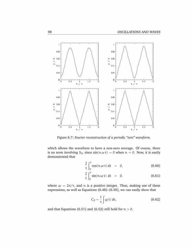
98 OSCILLATIONS AND WAVES
Figure 6.7: Fourier reconstruction of a periodic “tent” waveform.
which allows the waveform to have a non-zero average. Of course, there
is no term involving S0, since sin(nωt) = 0 when n = 0. Now, it is easily
demonstrated that
2
τ
∫τ
0
cos(nωt)dt = 0, (6.60)
2
τ
∫τ
0
sin(nωt) dt = 0, (6.61)
where ω = 2π/τ, and n is a positive integer. Thus, making use of these
expressions, as well as Equations (6.48)–(6.50), we can easily show that
C0 =1
τ
∫
y(t)dt, (6.62)
and that Equations (6.51) and (6.52) still hold for n > 0.
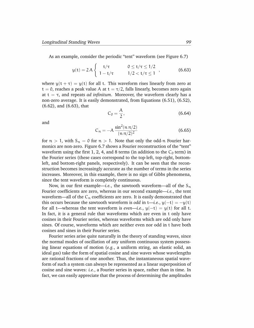
Longitudinal Standing Waves 99
As an example, consider the periodic “tent” waveform (see Figure 6.7)
y(t) = 2A
t/τ 0 ≤ t/τ ≤ 1/2
1− t/τ 1/2 < t/τ ≤ 1 , (6.63)
where y(t + τ) = y(t) for all t. This waveform rises linearly from zero at
t = 0, reaches a peak value A at t = τ/2, falls linearly, becomes zero again
at t = τ, and repeats ad infinitum. Moreover, the waveform clearly has a
non-zero average. It is easily demonstrated, from Equations (6.51), (6.52),
(6.62), and (6.63), that
C0 =A
2, (6.64)
and
Cn = −Asin2(nπ/2)
(nπ/2)2(6.65)
for n > 1, with Sn = 0 for n > 1. Note that only the odd-n Fourier har-
monics are non-zero. Figure 6.7 shows a Fourier reconstruction of the “tent”
waveform using the first 1, 2, 4, and 8 terms (in addition to the C0 term) in
the Fourier series (these cases correspond to the top-left, top-right, bottom-
left, and bottom-right panels, respectively). It can be seen that the recon-
struction becomes increasingly accurate as the number of terms in the series
increases. Moreover, in this example, there is no sign of Gibbs phenomena,
since the tent waveform is completely continuous.
Now, in our first example—i.e., the sawtooth waveform—all of the Sn
Fourier coefficients are zero, whereas in our second example—i.e., the tent
waveform—all of the Cn coefficients are zero. It is easily demonstrated that
this occurs because the sawtooth waveform is odd in t—i.e., y(−t) = −y(t)
for all t—whereas the tent waveform is even—i.e., y(−t) = y(t) for all t.
In fact, it is a general rule that waveforms which are even in t only have
cosines in their Fourier series, whereas waveforms which are odd only have
sines. Of course, waveforms which are neither even nor odd in t have both
cosines and sines in their Fourier series.
Fourier series arise quite naturally in the theory of standing waves, since
the normal modes of oscillation of any uniform continuous system possess-
ing linear equations of motion (e.g., a uniform string, an elastic solid, an
ideal gas) take the form of spatial cosine and sine waves whose wavelengths
are rational fractions of one another. Thus, the instantaneous spatial wave-
form of such a system can always be represented as a linear superposition of
cosine and sine waves: i.e., a Fourier series in space, rather than in time. In
fact, we can easily appreciate that the process of determining the amplitudes
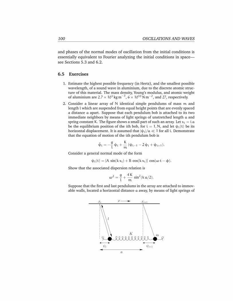
100 OSCILLATIONS AND WAVES
and phases of the normal modes of oscillation from the initial conditions is
essentially equivalent to Fourier analyzing the initial conditions in space—
see Sections 5.3 and 6.2.
6.5 Exercises
1. Estimate the highest possible frequency (in Hertz), and the smallest possiblewavelength, of a sound wave in aluminium, due to the discrete atomic struc-ture of this material. The mass density, Young’s modulus, and atomic weightof aluminium are 2.7× 10³ kg m
−3, 6× 10¹⁰ N m−2, and 27, respectively.
2. Consider a linear array of N identical simple pendulums of mass m andlength lwhich are suspended from equal height points that are evenly spaceda distance a apart. Suppose that each pendulum bob is attached to its twoimmediate neighbors by means of light springs of unstretched length a andspring constant K. The figure shows a small part of such an array. Let xi = i a
be the equilibrium position of the ith bob, for i = 1,N, and let ψi(t) be itshorizontal displacement. It is assumed that |ψi|/a≪ 1 for all i. Demonstratethat the equation of motion of the ith pendulum bob is
ψi = −g
lψi +
K
m(ψi−1 − 2ψi +ψi+1).
Consider a general normal mode of the form
ψi(t) = [A sin(k xi) + B cos(k xi)] cos(ωt− φ).
Show that the associated dispersion relation is
ω2 =g
l+4K
msin2
(ka/2).
Suppose that the first and last pendulums in the array are attached to immov-able walls, located a horizontal distance a away, by means of light springs of
m
xi+1xi
K
ψi+1ψi
x
a
l
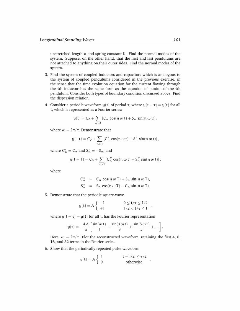
Longitudinal Standing Waves 101
unstretched length a and spring constant K. Find the normal modes of thesystem. Suppose, on the other hand, that the first and last pendulums arenot attached to anything on their outer sides. Find the normal modes of thesystem.
3. Find the system of coupled inductors and capacitors which is analogous tothe system of coupled pendulums considered in the previous exercise, inthe sense that the time evolution equation for the current flowing throughthe ith inductor has the same form as the equation of motion of the ithpendulum. Consider both types of boundary condition discussed above. Findthe dispersion relation.
4. Consider a periodic waveform y(t) of period τ, where y(t+ τ) = y(t) for allt, which is represented as a Fourier series:
y(t) = C0 +∑
n>1
[Cn cos(nωt) + Sn sin(nωt)] ,
where ω = 2π/τ. Demonstrate that
y(−t) = C0 +∑
n>1
[C ′
n cos(nωt) + S ′
n sin(nωt)] ,
where C ′
n = Cn and S ′
n = −Sn, and
y(t+ T) = C0 +∑
n>1
[C ′′
n cos(nωt) + S ′′
n sin(nωt)] ,
where
C ′′
n = Cn cos(nωT) + Sn sin(nωT),
S ′′
n = Sn cos(nωT) − Cn sin(nωT).
5. Demonstrate that the periodic square-wave
y(t) = A
−1 0 ≤ t/τ ≤ 1/2+1 1/2 < t/τ ≤ 1 ,
where y(t+ τ) = y(t) for all t, has the Fourier representation
y(t) = −4A
π
[
sin(ωt)
1+
sin(3ω t)
3+
sin(5ω t)
5+ · · ·
]
.
Here, ω = 2π/τ. Plot the reconstructed waveform, retaining the first 4, 8,16, and 32 terms in the Fourier series.
6. Show that the periodically repeated pulse waveform
y(t) = A
1 |t− T/2| ≤ τ/20 otherwise
,
102 OSCILLATIONS AND WAVES
where y(t+ T) = y(t) for all t, and τ < T , has the Fourier representation
y(t) = Aτ
T+2A
π
∑
n=1,∞
(−1)n sin(nπτ/T)
ncos(n2π t/T)
Demonstrate that if τ≪ T then the most significant terms in the above serieshave frequencies (in Hertz) which range from the fundamental frequency1/T to a frequency of order 1/τ.
Traveling Waves 103
7 Traveling Waves
7.1 Standing Waves in a Finite Continuous Medium
We saw earlier, in Sections 5.2, 6.2, and 6.3, that a small amplitude trans-
verse wave on a uniform string, and a small amplitude longitudinal wave in
an elastic solid or an ideal gas, are all governed by the wave equation, which
(in one dimension) takes the general form
∂2ψ
∂t2= c2
∂2ψ
∂x2, (7.1)
where ψ(x, t) represents the wave disturbance, and c > 0 is a constant, with
the dimensions of velocity, which is a property of the particular medium
that supports the wave. Up to now, we have only considered media of finite
length: e.g., media which extend from x = 0 to x = l. Generally speaking,
we have encountered two distinct types of physical constraint which hold at
the boundaries of such media. Firstly, if a given boundary is fixed then the
wave displacement is constrained to be zero there: e.g., if the left bound-
ary is fixed then ψ(0, t) = 0. Secondly, if a given boundary is free then the
spatial derivative of the displacement (which usually corresponds to some
sort of force) is constrained to be zero there: e.g., if the right boundary is
free then ∂ψ(l, t)/∂x = 0. It follows that a fixed boundary corresponds to a
node—i.e., a point at which the amplitude of the wave disturbance is always
zero—whereas a free boundary corresponds to an anti-node—i.e., a point
at which the amplitude of the wave disturbance is always locally maximal.
Consequently, the nodes and the anti-nodes of a wave, of definite wave-
length, supported in a medium of finite length with stationary boundaries,
which can be either fixed or free, are constrained to be stationary. The only
simple solution of the wave equation (7.1) which has stationary nodes and
anti-nodes is a standing wave of the general form
ψ(x, t) = [A cos(k x) + B sin(k x)] cos(ωt− φ). (7.2)
The associated nodes are located at the values of x that satisfy
A cos(k x) + B sin(k x) = 0, (7.3)
which implies that they are indeed stationary, and also evenly spaced a dis-
tance λ/2 apart, where λ = 2π/k is the wavelength. Moreover, the anti-
nodes are situated halfway between the nodes. For example, suppose that
104 OSCILLATIONS AND WAVES
both boundaries of the medium are fixed boundaries. It follows that the
points x = 0 and x = lmust each correspond to a node. This is only possible
if the length of the medium, l, is a half-integer number of wavelengths: i.e.,
l = nλ/2, where n is a positive integer. We conclude that, in this case, the
possible wavenumbers of standing wave solutions to the wave equation are
quantized such that
k l = nπ. (7.4)
Moreover, the same is true if both boundaries are free boundaries. Fi-
nally, if one boundary is free, and the other fixed, then the quantization
of wavenumbers takes the slightly different form
k l = (n− 1/2)π. (7.5)
Now, those standing wave solutions that satisfy the appropriate quantiza-
tion criterion are known as the normal modes of the system. Moreover,
substitution of (7.2) into the wave equation (7.1) yields the standing wave
dispersion relation
ω2 = k2 c2. (7.6)
Thus, the fact that the normal mode wavenumbers are quantized immedi-
ately implies that the associated oscillation frequencies are also quantized.
Finally, since the wave equation is linear, the most general solution which
satisfies the boundary conditions is a linear superposition of all of the nor-
mal modes. Such a solution has the appropriate node or anti-node at each
of the boundaries, but does not necessarily have any stationary nodes or
anti-nodes in the interior of the medium.
7.2 Traveling Waves in an Infinite Continuous Medium
Let us now consider solutions of the wave equation (7.1) in an infinite
medium. Such a medium does not possess any boundaries, and so is not
subject to boundary conditions. Hence, there is no particular reason why a
wave of definite wavelength should have stationary nodes or anti-nodes. In
other words, (7.2) may not be the only permissible type of wave solution
in an infinite medium. What other kind of solution could we have? Well,
suppose that
ψ(x, t) = A cos(k x−ωt− φ), (7.7)
where A > 0, k > 0, ω > 0, and φ are constants. We would interpret this
solution as a wave of amplitude A, wavenumber k, wavelength λ = 2π/k,
angular frequency ω, frequency (in Hertz) f = ω/2π, period T = 1/f, and
Traveling Waves 105
phase angle φ. Note, in particular, thatψ(x+λ, t) = ψ(x, t) andψ(x, t+T) =
ψ(x, t) for all x and t: i.e., the wave is periodic in space with period λ, and
periodic in time with period T . Now, a wave maximum corresponds to a
point at which cos(k x − ωt − φ) = 1. It follows, from the well known
properties of the cosine function, that the various wave maxima are located
at
k x−ωt− φ = n2π, (7.8)
where n is an integer. Thus, differentiating the above expression with re-
spect to t, and rearranging, the equation of motion of a particular maximum
becomesdx
dt=ω
k. (7.9)
We conclude that the wave maximum in question propagates along the x-
axis at the velocity
vp =ω
k. (7.10)
It is easily demonstrated that the other wave maxima, as well as the wave
minima and the wave zeros, also propagate along the x-axis at the same
velocity. In fact, the whole wave pattern propagates in the positive x-
direction without changing shape. The characteristic propagation velocity
vp is known as the phase velocity of the wave, since it is the velocity with
which points of constant phase in the wave disturbance (i.e., points which
satisfy k x − ωt − φ = constant) move. For obvious reasons, the type of
wave solution given in (7.7) is called a traveling wave.
Substitution of (7.7) into the wave equation (7.1) yields the familiar
dispersion relation
ω2 = k2 c2. (7.11)
We immediately conclude that the traveling wave solution (7.7) satisfies the
wave equation provided
vp =ω
k= c : (7.12)
i.e., provided that the phase velocity of the wave takes the fixed value c.
In other words, the constant c2, which appears in the wave equation (7.1),
can be interpreted as the square of the velocity with which traveling waves
propagate through the medium in question. It follows, from the discussion
in Sections 5.2, 6.2, and 6.3, that transverse waves propagate along strings
of tension T and mass per unit length ρ at the phase velocity√
T/ρ, that
longitudinal sound waves propagate through elastic media of Young’s mod-
ulus Y and mass density ρ at the phase velocity√
Y/ρ, and that sound waves
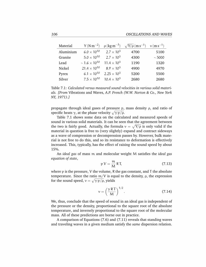
106 OSCILLATIONS AND WAVES
Material Y (N m−2) ρ (kg m−3)√
Y/ρ (m s−1) v (m s−1)
Aluminium 6.0× 10¹⁰ 2.7× 10³ 4700 5100
Granite 5.0× 10¹⁰ 2.7× 10³ 4300 ∼ 5000
Lead ∼ 1.6× 10¹⁰ 11.4× 10³ 1190 1320
Nickel 21.4× 10¹⁰ 8.9× 10³ 4900 4970
Pyrex 6.1× 10¹⁰ 2.25× 10³ 5200 5500
Silver 7.5× 10¹⁰ 10.4× 10³ 2680 2680
Table 7.1: Calculated versus measured sound velocities in various solid materi-
als. [From Vibrations and Waves, A.P. French (W.W. Norton & Co., New York
NY, 1971).]
propagate through ideal gases of pressure p, mass density ρ, and ratio of
specific heats γ, at the phase velocity√
γp/ρ.
Table 7.1 shows some data on the calculated and measured speeds of
sound in various solid materials. It can be seen that the agreement between
the two is fairly good. Actually, the formula v =√
Y/ρ is only valid if the
material in question is free to (very slightly) expand and contract sideways
as a wave of compression or decompression passes by. However, bulk mate-
rial is not free to do this, and so its resistance to deformation is effectively
increased. This, typically, has the effect of raising the sound speed by about
15%.
An ideal gas of mass m and molecular weight M satisfies the ideal gas
equation of state,
pV =m
MRT, (7.13)
where p is the pressure, V the volume, R the gas constant, and T the absolute
temperature. Since the ratio m/V is equal to the density, ρ, the expression
for the sound speed, v =√
γp/ρ, yields
v =
(
γR T
M
)1/2
. (7.14)
We, thus, conclude that the speed of sound in an ideal gas is independent of
the pressure or the density, proportional to the square root of the absolute
temperature, and inversely proportional to the square root of the molecular
mass. All of these predictions are borne out in practice.
A comparison of Equations (7.6) and (7.11) reveals that standing waves
and traveling waves in a given medium satisfy the same dispersion relation.
Traveling Waves 107
However, since traveling waves in infinite media are not subject to boundary
conditions, it follows that there is no restriction on the possible wavenum-
bers, or wavelengths, of such waves. Hence, any traveling wave solution
whose wavenumber, k, and angular frequency, ω, are related according to
ω = k c (7.15)
[which is just the square root of the dispersion relation (7.11)] is a valid
solution of the wave equation. Another way of putting this is that any trav-
eling wave solution whose wavelength, λ = 2π/k, and frequency, f = ω/2π,
are related according to
c = f λ (7.16)
is a valid solution of the wave equation. We, thus, conclude that high fre-
quency traveling waves propagating through a given medium possess short
wavelengths, and vice versa.
Consider the alternative wave solution
ψ(x, t) = A cos(k x+ωt− φ), (7.17)
where A > 0, k > 0, ω > 0, and φ are constants. As before, we would
interpret this solution as a wave of amplitude A, wavenumber k, angular
frequency ω, and phase angle φ. However, the wave maxima are now lo-
cated at
k x+ωt− φ = n2π, (7.18)
where n is an integer, and thus have equations of motion of the form
dx
dt= −
ω
k. (7.19)
Clearly, (7.17) represents a traveling wave that propagates in the minus x-
direction at the phase velocity vp = ω/k. Moreover, substitution of (7.17)
into the wave equation (7.1) again yields the dispersion relation (7.15),
which implies that vp = c. It follows that traveling wave solutions to the
wave equation (7.1) can propagate in either the positive or the negative
x-direction, as long as they always move at the fixed speed c.
7.3 Wave Interference
But, what is the relationship between traveling wave and standing wave so-
lutions to the wave equation (7.1) in an infinite medium? To help answer
108 OSCILLATIONS AND WAVES
this question, let us form a superposition of two traveling wave solutions of
equal amplitudeA, and zero phase angle φ, which have the same wavenum-
ber k, but are moving in opposite directions. In other words,
ψ(x, t) = A cos(k x−ωt) +A cos(k x+ωt). (7.20)
Since the wave equation (7.1) is linear, it follows that the above superpo-
sition is a solution provided the two component waves are also solutions:
i.e., provided that ω = k c, which we shall assume to be the case. How-
ever, making use of the trigonometric identity cosa + cosb ≡ 2 cos[(a +
b)/2] cos[(a− b)/2], the above expression can also be written
ψ(x, t) = 2A cos(k x) cos(ωt), (7.21)
which is clearly a standing wave [cf., (7.2)]. Evidently, a standing wave is
a linear superposition of two, otherwise identical, traveling waves which
propagate in opposite directions. The two waves completely cancel one
another out at the nodes, which are situated at k x = (n − 1/2)π, where n
is an integer. This process is known as total destructive interference. On the
other hand, the waves reinforce one another at the anti-nodes, which are
situated at k x = nπ, generating a wave whose amplitude is twice that of
the component waves. This process is known as constructive interference.
As a more general example of wave interference, consider a superpo-
sition of two traveling waves of unequal amplitudes which again have the
same wavenumber and zero phase angle, and are moving in opposite direc-
tions: i.e.,
ψ(x, t) = A1 cos(k x−ωt) +A2 cos(k x+ωt), (7.22)
where A1, A2 > 0. In this case, the trigonometric identities cos(a − b) ≡cosa cosb+ sina sinb and cos(a+ b) ≡ cosa cosb− sina sinb yield
ψ(x, t) = (A1+A2) cos(k x) cos(ωt)+(A1−A2) sin(k x) sin(ωt). (7.23)
Thus, the two waves interfere destructively at k x = (n − 1/2)π [i.e., at
points where cos(k x) = 0 and | sin(k x)| = 1] to produce a minimum wave
amplitude |A1 −A2|, and interfere constructively at k x = nπ [i.e., at points
where | cos(k x)| = 1 and sin(k x) = 0] to produce a maximum wave ampli-
tude A1+A2. Note, however, that the destructive interference is incomplete
unless A1 = A2. Incidentally, it is a general result that when two waves of
amplitude A1 > 0 and A2 > 0 interfere then the maximum and minimum
possible values of the resulting wave amplitude are A1 +A2 and |A1 −A2|,
respectively.
Traveling Waves 109
7.4 Energy Conservation
Consider a small amplitude transverse wave propagating along a uniform
string of infinite length, tension T , and mass per unit length ρ. See Sec-
tion 5.2. Let x measure distance along the string, and let y(x, t) be the
transverse wave displacement. Of course, y(x, t) satisfies the wave equation
∂2y
∂t2= v2 ∂
2y
∂x2, (7.24)
where v =√
T/ρ is the phase velocity of traveling waves on the string.
Consider a section of the string lying between x = x1 and x = x2. The
kinetic energy of this section is
K =
∫x2
x1
1
2ρ
(
∂y
∂t
)2
dx, (7.25)
since ∂y/∂t is the string’s transverse velocity. The potential energy is simply
the work done in stretching the section, which is T ∆s, where ∆s is the
difference between the section’s stretched and unstretched lengths. Here,
it is assumed that the tension remains approximately constant when the
section is slowly stretched. Now, an element of length of the string is
ds = (dx2 + dy2)1/2 =
[
1+
(
dy
dx
)2]1/2
dx. (7.26)
Hence,
∆s =
∫x2
x1
[
1+
(
dy
dx
)2]1/2
− 1
dx ≃∫x2
x1
1
2
(
∂y
∂x
)2
dx, (7.27)
since it is assumed that |∂y/∂x| ≪ 1: i.e., the transverse displacement is
sufficiently small that the string remains almost parallel to the x-axis. Thus,
the potential energy of the section is U = T ∆s, or
U =
∫x2
x1
1
2T
(
∂y
∂x
)2
dx. (7.28)
It follows that the total energy of the section is
E =
∫x2
x1
1
2
[
ρ
(
∂y
∂t
)2
+ T
(
∂y
∂x
)2]
dx. (7.29)
110 OSCILLATIONS AND WAVES
Multiplying the wave equation (7.24) by ρ (∂y/∂t), we obtain
ρ∂y
∂t
∂2y
∂t2= T
∂y
∂t
∂2y
∂x2, (7.30)
since v2 = T/ρ. This expression yields
ρ∂y
∂t
∂2y
∂t2+ T
∂y
∂x
∂2y
∂t ∂x= T
∂y
∂t
∂2y
∂x2+ T
∂y
∂x
∂2y
∂t ∂x, (7.31)
which can be written in the form
1
2
∂
∂t
[
ρ
(
∂y
∂t
)2
+ T
(
∂y
∂x
)2]
=∂
∂x
(
T∂y
∂t
∂y
∂x
)
, (7.32)
or∂E∂t
+∂I∂x
= 0, (7.33)
where
E(x, t) =1
2
[
ρ
(
∂y
∂t
)2
+ T
(
∂y
∂x
)2]
(7.34)
is the energy per unit length of the string, and
I(x, t) = −T∂y
∂t
∂y
∂x. (7.35)
Finally, integrating (7.33) in x from x1 to x2, we obtain
d
dt
∫x2
x1
E dx+ I(x2, t) − I(x1, t) = 0, (7.36)
ordE
dt= I(x1, t) − I(x2, t). (7.37)
Here, E(t) is the energy stored in the section of the string lying between
x = x1 and x = x2 [see Equation (7.29)]. Now, if we interpret I(x, t) as the
instantaneous energy flux (i.e., rate of energy flow) in the positive-x direc-
tion, at position x and time t, then the above equation can be recognized
as a simple declaration of energy conservation. Basically, the equation states
that the rate of increase in the energy stored in the section of the string lying
between x = x1 and x = x2, which is dE/dt, is equal to the difference be-
tween the rate at which energy flows into the left end of the section, which is
I(x1, t), and the rate at which it flows out of the right end, which is I(x2, t).
Traveling Waves 111
Note that the string must conserve energy, since it lacks any mechanism for
energy dissipation. The same is true of the other wave media discussed in
this section.
Consider a wave propagating in the positive x-direction of the form
y(x, t) = A cos(k x−ωt− φ). (7.38)
According to Equation (7.35), the energy flux associated with this wave is
I(x, t) = T kωA2 sin2(k x−ωt− φ). (7.39)
Thus, the mean energy flux is written
〈I〉 =1
2ω2ZA2, (7.40)
where 〈A〉(x) ≡ (ω/2π)∫t+2π/ω
tA(x, t ′)dt ′ represents an average over a
period of the wave oscillation. Here, use has been made of ω/k =√
T/ρ,
and the easily demonstrated result that 〈sin2(ωt + θ)〉 = 1/2 for all θ.
Moreover, the quantity
Z =√
ρ T (7.41)
is known as the characteristic impedance of the string. The units of Z are
force over velocity. Thus, the string impedance measures the typical ten-
sion required to produce a unit transverse velocity. Finally, according to
Equation (7.40), a traveling wave propagating in the positive x-direction is
associated with a positive energy flux: i.e., the wave transports energy in the
positive x-direction.
Consider a wave propagating in the negative x-direction of the general
form
y(x, t) = A cos(k x+ωt− φ). (7.42)
It is easily demonstrated, from (7.35), that the mean energy flux associated
with this wave is
〈I〉 = −1
2ω2ZA2. (7.43)
The fact that the energy flux is negative means that the wave transports
energy in the negative x-direction.
Suppose that we have a superposition of a wave of amplitude A+ propa-
gating in the positive x-direction, and a wave of amplitude A− propagating
in the negative x-direction, so that
y(x, t) = A+ cos(k x−ωt− φ+) +A− cos(k x+ωt− φ−). (7.44)
112 OSCILLATIONS AND WAVES
According to (7.35), the instantaneous energy flux is written
I(x, t) = ω2Z [A+ sin(k x−ωt− φ+) +A− sin(k x+ωt− φ−)]
[A+ sin(k x−ωt− φ+) −A− sin(k x+ωt− φ−)]
= ω2Z[
A2+ sin2(k x−ωt− φ+) −A2
− sin2(k x+ωt− φ−)]
.
(7.45)
Hence, the mean energy flux,
〈I〉 =1
2ω2ZA2
+ −1
2ω2ZA2
−, (7.46)
is simply the difference between the mean fluxes associated with the waves
traveling to the right (i.e., in the positive x-direction) and to the left, cal-
culated separately. Recall, from the previous section, that a standing wave
is a superposition of two traveling waves of equal amplitude, and frequency,
propagating in opposite directions. It immediately follows, from the above
expression, that a standing wave has zero associated net energy flux. In
other words, a standing wave does not give rise to net energy transport.
Now, we saw earlier, in Section 6.2, that a small amplitude longitudinal
wave in an elastic solid satisfies the wave equation,
∂2ψ
∂t2= c2
∂2ψ
∂x2, (7.47)
where ψ(x, t) is the longitudinal wave displacement, c =√
Y/ρ the phase
velocity of traveling waves in the solid, Y the Young’s modulus, and ρ the
mass density. Using similar analysis to that employed above, we can derive
an energy conservation equation of the form (7.33) from the above wave
equation, where
E =1
2
[
ρ
(
∂ψ
∂t
)2
+ Y
(
∂ψ
∂x
)2]
(7.48)
is the total wave energy per unit volume, and
I = −Y∂ψ
∂t
∂ψ
∂x(7.49)
the wave energy flux (i.e., rate of energy flow per unit area) in the positive
x-direction. For a traveling wave of the form ψ(x, t) = A cos(k x−ωt−φ),
the above expression yields
〈I〉 =1
2ω2ZA2, (7.50)
Traveling Waves 113
where
Z =√
ρ Y (7.51)
is the impedance of the solid. The units of Z are pressure over velocity, so, in
this case, the impedance measures the typical pressure in the solid required
to produce a unit longitudinal velocity. Analogous arguments to the above
reveal that the impedance of an ideal gas of density ρ, pressure p, and ratio
of specific heats γ, is (see Section 6.3)
Z =√ργp. (7.52)
7.5 Transmission Lines
A transmission line is typically used to carry high frequency electromag-
netic signals over large distances: i.e., distances sufficiently large that the
phase of the signal varies significantly along the line (which implies that
the line is much longer than the wavelength of the signal). A common
example of a transmission line is an ethernet cable. In its simplest form,
a transmission line consists of two parallel conductors which carry equal
and opposite electrical currents I(x, t), where x measures distance along
the line. Let V(x, t) be the instantaneous voltage difference between the
two conductors at position x. Consider a small section of the line lying
between x and x + δx. If Q(t) is the electric charge on one of the con-
ducting sections, and −Q(t) the charge on the other, then charge conser-
vation implies that dQ/dt = I(x, t) − I(x + δx, t). However, according to
standard electrical circuit theory, Q(t) = C δxV(x, t), where C is the ca-
pacitance per unit length of the line. Standard circuit theory also yields
V(x + δx, t) − V(x, t) = −L δx ∂I(x, t)/∂t, where L is the inductance per
unit length of the line. Taking the limit δx → 0, we obtain the so-called
Telegrapher’s equations,
∂V
∂t= −
1
C∂I
∂x, (7.53)
∂I
∂t= −
1
L∂V
∂x. (7.54)
These two equations can be combined to give
∂2V
∂t2=
1
LC∂2V
∂x2, (7.55)
together with an analogous equation for I. In other words, V(x, t) and I(x, t)
both obey a wave equation of the form (7.24) in which the associated phase
114 OSCILLATIONS AND WAVES
velocity is v = 1/√LC. Multiplying (7.53) by C V, (7.54) by L I, and then
adding the two resulting expressions, we obtain the energy conservation
equation∂E∂t
+∂I∂x
= 0, (7.56)
where
E =1
2L I2 +
1
2C V2 (7.57)
is the electromagnetic energy per unit length of the line, and
I = I V (7.58)
is the electromagnetic energy flux along the line (i.e., the energy per unit
time which passes a given point) in the positive x-direction. Consider a sig-
nal propagating along the line, in the positive x-direction, whose associated
current takes the form
I(x, t) = I0 cos(k x−ωt− φ). (7.59)
It is easily demonstrated, from (7.53), that the corresponding voltage is
V(x, t) = V0 cos(k x−ωt− φ), (7.60)
where
V0 = I0Z. (7.61)
Here,
Z =
√
LC (7.62)
is the characteristic impedance of the line, and is measured in Ohms. It
follows that the mean energy flux associated with the signal is written
〈I〉 = 〈I V〉 =1
2I0V0 =
1
2Z I2
0 =1
2
V 20
Z. (7.63)
Likewise, for a signal propagating along the line in the negative x-direction,
I(x, t) = I0 cos(k x+ωt− φ), (7.64)
V(x, t) = −V0 cos(k x+ωt− φ), (7.65)
and the mean energy flux is
〈I〉 = −1
2I0V0 = −
1
2Z I2
0 = −1
2
V 20
Z. (7.66)
Traveling Waves 115
As a specific example, consider a transmission line consisting of two uni-
form parallel conducting strips of width w and perpendicular distance apart
d, where d ≪ w. It is easily demonstrated, using elementary electrostatic
theory, that the capacitance per unit length of the line is
C = ǫ0w
d, (7.67)
where ǫ0 = 8.8542×10⁻¹² C2 N−1 m−2 is the electric permittivity of free space.
Likewise, according to elementary magnetostatic theory, the line’s induc-
tance per unit length takes the form
L = µ0d
w, (7.68)
where µ0 = 4π× 10−7 N A−2 is the magnetic permeability of free space. Thus,
the phase velocity of a signal propagating down the line is
v =1√LC
=1√ǫ0µ0
= 2.998× 10⁸ m s−1, (7.69)
which, of course, is the velocity of light in vacuum [see Equation (7.113)].
Furthermore, the impedance of the line is
Z =
√
LC =
d
wZ0, (7.70)
where the quantity
Z0 =
√
µ0
ǫ0
= 376.73Ω (7.71)
is known as the impedance of free space.
7.6 Reflection and Transmission at Boundaries
Consider two uniform semi-infinite strings which run along the x-axis, and
are tied together at x = 0. Let the first string be of density per unit length
ρ1, and occupy the region x < 0, and let the second string be of density per
unit length ρ2, and occupy the region x > 0. Now, the tensions in the two
strings must be equal, otherwise the string interface would not be in force
balance in the x-direction. So, let T be the common tension. Suppose that a
transverse wave of angular frequency ω is launched from a wave source at
x = −∞, and propagates towards the interface. Assuming that ρ1 6= ρ2, we
116 OSCILLATIONS AND WAVES
would expect the wave incident on the interface to be partially reflected, and
partially transmitted. Of course, the frequencies of the incident, reflected,
and transmitted waves are all the same, since this property of the waves
is ultimately determined by the oscillation frequency of the wave source.
Hence, in the region x < 0, the wave displacement takes the form
y(x, t) = Ai cos(k1x−ωt− φi) +Ar cos(k1x+ωt− φr). (7.72)
In other words, the displacement is a linear superposition of an incident
wave and a reflected wave. The incident wave propagates in the positive
x-direction, and is of amplitude Ai, wavenumber k1 = ω/v1, and phase
angle φi. The reflected wave propagates in the negative x-direction, and
is of amplitude Ar, wavenumber k1 = ω/v1, and phase angle φr. Here,
v1 =√
T/ρ1 is the phase velocity of traveling waves on the first string. In
the region x > 0, the wave displacement takes the form
y(x, t) = At cos(k2x−ωt− φt). (7.73)
In other words, the displacement is solely due to a transmitted wave which
propagates in the positive x-direction, and is of amplitude At, wavenumber
k2 = ω/v2, and phase angle φt. Here, v2 =√
T/ρ2 is the phase velocity of
traveling waves on the second string.
Let us now consider the matching conditions at the interface between
the two strings: i.e., at x = 0. Firstly, since the two strings are tied together
at x = 0, their transverse displacements at this point must be equal to one
another. In other words,
y(0−, t) = y(0+, t), (7.74)
or
Ai cos(ωt+ φi) +Ar cos(ωt− φr) = At cos(ωt+ φt). (7.75)
The only way in which the above equation can be satisfied for all values of
t is if φi = −φr = φt. This being the case, the common cos(ωt+φi) factor
cancels out, and we are left with
Ai +Ar = At. (7.76)
Secondly, since the two strings lack an energy dissipation mechanism, the
energy flux into the interface must match that out of the interface. In other
words,1
2ω2Z1 (A2
i −A2r ) =
1
2ω2Z2A
2t , (7.77)
Traveling Waves 117
where Z1 =√ρ1 T and Z2 =
√ρ2 T are the impedances of the first and
second strings, respectively. The above expression reduces to
Z1 (Ai +Ar) (Ai −Ar) = Z2A2t , (7.78)
which, when combined with Equation (7.76), yields
Z1 (Ai −Ar) = Z2At. (7.79)
Equations (7.76) and (7.79) can be solved to give
Ar =
(
Z1 − Z2
Z1 + Z2
)
Ai, (7.80)
At =
(
2Z1
Z1 + Z2
)
Ai. (7.81)
The coefficient of reflection, R, is defined as the ratio of the reflected to the
incident energy flux: i.e.,
R =
(
Ar
Ai
)2
=
(
Z1 − Z2
Z1 + Z2
)2
. (7.82)
The coefficient of transmission, T , is defined as the ratio of the transmitted to
the incident energy flux: i.e.,
T =Z2
Z1
(
At
Ai
)2
=4Z1Z2
(Z1 + Z2)2. (7.83)
Note that
R+ T = 1 : (7.84)
i.e., any incident wave energy which is not reflected is transmitted.
Suppose that the density per unit length of the second string, ρ2, tends
to infinity, so that Z2 =√ρ2 T → ∞. It follows from (7.80) and (7.81)
that Ar = −Ai and At = 0. Likewise, (7.82) and (7.83) yield R = 1 and
T = 0. Hence, the interface between the two strings is stationary (since it
oscillates with amplitude At), and there is no transmitted energy. In other
words, the second string acts exactly like a fixed boundary. It follows that
when a transverse wave on a string is incident on a fixed boundary then
it is perfectly reflected with a phase shift of π: i.e., Ar = −Ai. Thus, the
resultant wave displacement on the string becomes
y(x, t) = Ai cos(k1x−ωt− φi) −Ai cos(k1x+ωt+ φi)
= 2Ai sin(k1x) sin(ωt+ φi), (7.85)
118 OSCILLATIONS AND WAVES
where use has been made of the trigonometric identity cosa − cosb ≡2 sin[(a + b)/2] sin[(b − a)/2]. We conclude that the incident and reflected
waves interfere in such a manner as to produce a standing wave with a node
at the fixed boundary.
Suppose that the density per unit length of the second string, ρ2, tends
to zero, so that Z2 =√ρ2 T → 0. It follows from (7.80) and (7.81) that
Ar = Ai and At = 2Ai. Likewise, (7.82) and (7.83) yield R = 1 and T = 0.
Hence, the interface between the two strings oscillates at twice the ampli-
tude of the incident wave (i.e., the interface is a point of maximal amplitude
oscillation), and there is no transmitted energy. In other words, the second
string acts exactly like a free boundary. It follows that when a transverse
wave on a string is incident on a free boundary then it is perfectly reflected
with no phase shift: i.e., Ar = Ai. Thus, the resultant wave displacement
on the string becomes
y(x, t) = Ai cos(k1x−ωt− φi) +Ai cos(k1x+ωt+ φi)
= 2Ai cos(k1x) cos(ωt+ φi), (7.86)
where use has been made of the trigonometric identity cosa + cosb ≡2 cos[(a+ b)/2] cos[(a− b)/2]. We conclude that the incident and reflected
waves interfere in such a manner as to produce a standing wave with an
anti-node at the free boundary.
Suppose that two strings of mass per unit length ρ1 and ρ2 are separated
by a short section of string of mass per unit length ρ3. Let all three strings
have the common tension T . Suppose that the first and second strings oc-
cupy the regions x < 0 and x > a, respectively. Thus, the middle string
occupies the region 0 ≤ x ≤ a. Moreover, the interface between the first
and middle strings is at x = 0, and the interface between the middle and
second strings is at x = a. Suppose that a wave of angular frequency ω is
launched from a wave source at x = −∞, and propagates towards the two
interfaces. We would expect this wave to be partially reflected and partially
transmitted at the first interface (x = 0), and the resulting transmitted wave
to then be partially reflected and partially transmitted at the second inter-
face (x = a). Thus, we can write the wave displacement in the region x < 0
as
y(x, t) = Ai cos(k1x−ωt) +Ar cos(k1x+ωt), (7.87)
where Ai is the amplitude of the incident wave, Ar is the amplitude of the
reflected wave, and k1 = ω/√
T/ρ1. Here, the phase angles of the two
waves have been chosen so as to facilitate the matching process at x = 0.
Traveling Waves 119
The wave displacement in the region x > a takes the form
y(x, t) = At cos(k2x−ωt− φt), (7.88)
whereAt is the amplitude of the final transmitted wave, and k2 = ω/√
T/ρ2.
Finally, the wave displacement in the region 0 ≤ x ≤ a is written
y(x, t) = A+ cos(k3x−ωt) +A− cos(k3x+ωt), (7.89)
where A+ and A− are the amplitudes of the right and left moving waves
on the middle string, respectively, and k3 = ω/√
T/ρ3. Continuity of the
transverse displacement at x = 0 yields
Ai +Ar = A+ +A−, (7.90)
where a common factor cos(ωt) has cancelled out. Continuity of the energy
flux at x = 0 gives
Z1 (A2i −A2
r ) = Z3 (A2+ −A2
−), (7.91)
so the previous two expressions can be combined to produce
Z1 (Ai −Ar) = Z3 (A+ −A−). (7.92)
Continuity of the transverse displacement at y = a yields
A+ cos(k3a−ωt)+A− cos(k3a+ωt) = At cos(k2a−ωt−φt). (7.93)
Suppose that the length of the middle string is one quarter of a wavelength:
i.e., k3a = π/2. Furthermore, let φt = k2a+π/2. It follows that cos(k3a−
ωt) = sin(ωt), cos(k3a + ωt) = − sin(ωt), and cos(k2a − ωt − φt) =
sin(ωt). Thus, canceling out a common factor sin(ωt), the above expres-
sion yields
A+ −A− = At. (7.94)
Continuity of the energy flux at x = a gives
Z3 (A2+ −A2
−) = Z2A2t . (7.95)
so the previous two equations can be combined to generate
Z3 (A+ +A−) = Z2At. (7.96)
Equations (7.90) and (7.96) yield
Ai +Ar =Z2
Z3
At, (7.97)
120 OSCILLATIONS AND WAVES
whereas Equations (7.92) and (7.94) give
Ai −Ar =Z3
Z1
At, (7.98)
so, combining the previous two expression, we obtain
Ar =
(
Z1Z2 − Z23
Z1Z2 + Z23
)
Ai, (7.99)
At =
(
2Z1Z3
Z1Z2 + Z23
)
Ai. (7.100)
Finally, the overall coefficient of reflection is
R =
(
Ar
Ai
)2
=
(
Z1Z2 − Z23
Z1Z2 + Z23
)2
, (7.101)
whereas the overall coefficient of transmission becomes
T =Z2
Z1
(
At
Ai
)2
=4Z1Z2Z
23
(Z1Z2 + Z23)2
= 1− R. (7.102)
Now, suppose that the impedance of the middle string is the geometric mean
of the impedances of the two outer strings: i.e., Z3 =√Z1Z2. In this case,
it is clear, from the above two equations, that R = 0 and T = 1. In other
words, there is no reflection of the incident wave, and all of the incident
energy ends up being transmitted across the middle string from the leftmost
to the rightmost string. Thus, if we wish to transmit transverse wave energy
from a string of impedance Z1 to a string of impedance Z2 (where Z2 6= Z1)
in the most efficient manner possible—i.e, with no reflection of the incident
energy flux—then we can do this by connecting the two strings via a short
section of string whose length is one quarter of a wavelength, and whose
impedance is√Z1Z2. This procedure is known as impedance matching.
It should be reasonably clear that the above analysis of the reflection and
transmission of transverse waves at a boundary between two strings is also
applicable to the reflection and transmission of other types of wave incident
on a boundary between two media of differing impedances. For example,
consider a transmission line, such as a co-axial cable. Suppose that the line
occupies the region x < 0, and is terminated (at x = 0) by a load resistor of
resistance RL. Such a resistor might represent a radio antenna (which acts
just like a resistor in an electrical circuit, except that the dissipated energy
Traveling Waves 121
is radiated, rather than being converted into heat energy). Suppose that a
signal of angular frequency ω is sent down the line from a wave source at
x = −∞. The current and voltage on the line can be written
I(x, t) = Ii cos(k x−ωt) + Ir cos(k x+ωt), (7.103)
V(x, t) = IiZ cos(k x−ωt) − Z Ir cos(k x+ωt), (7.104)
where Ii is the amplitude of the incident signal, Ir the amplitude of the
signal reflected by the load, Z the characteristic impedance of the line, and
k = ω/v. Here, v is the characteristic phase velocity with which signals
propagate down the line. See Section 7.5. Now, the resistor obeys Ohm’s
law, which yields
V(0, t) = I(0, t)RL. (7.105)
It follows, from the three previous equations, that
Ir =
(
Z− RL
Z+ RL
)
Ii. (7.106)
Hence, the coefficient of reflection, which is the ratio of the power reflected
by the load to the power sent down the line, is
R =
(
Ir
Ii
)2
=
(
Z− RL
Z+ RL
)2
. (7.107)
Furthermore, the coefficient of transmission, which is the ratio of the power
absorbed by the load to the power sent down the line, takes the form
T = 1− R =4ZRL
(Z+ RL)2. (7.108)
It can be seen, by comparison with Equations (7.82) and (7.83), that the
load terminating the line acts just like another transmission line of imped-
ance RL. Moreover, it is clear that power can only be efficiently sent down a
transmission line, and transferred to a terminating load, when the impedan-
ce of the line matches the effective impedance of the load (which, in this
case, is the same as the resistance of the load). In other words, when Z = RL
there is no reflection of the signal sent down the line (i.e., R = 0), and all
of the signal energy is therefore absorbed by the load (i.e., T = 1). As
an example, a half-wave antenna (i.e., an antenna whose length is half the
wavelength of the emitted radiation) has a characteristic impedance of 73Ω.
Hence, a transmission line used to feed energy into such an antenna should
122 OSCILLATIONS AND WAVES
also have a characteristic impedance of 73Ω. Suppose, however, that we en-
counter a situation in which the impedance of a transmission line, Z1, does
not match that of its terminating load, Z2. Can anything be done to avoid
reflection of the signal sent down the line? It turns out, by analogy with the
analysis presented above, that if the line is connected to the load via a short
section of transmission line whose length is one quarter of the wavelength of
the signal, and whose characteristic impedance is Z3 =√Z1Z2, then there
is no reflection of the signal: i.e., all of the signal power is absorbed by the
load. A short section of transmission line used in this manner is known as a
quarter wave transformer.
7.7 Electromagnetic Waves
Consider a plane electromagnetic wave propagating through a vacuum in the
z-direction. Electromagnetic waves are, incidentally, the only commonly oc-
curring waves which do not require a medium through which to propagate.
Suppose that the wave is polarized in the x-direction: i.e., its electric com-
ponent oscillates in the x-direction. It follows that the magnetic component
of the wave oscillates in the y-direction. According to standard electromag-
netic theory, the wave is described by the following pair of coupled partial
differential equations:
∂Ex
∂t= −
1
ǫ0
∂Hy
∂z, (7.109)
∂Hy
∂t= −
1
µ0
∂Ex
∂z, (7.110)
where Ex(z, t) is the electric field-strength, and Hy(z, t) is the magnetic in-
tensity (i.e., the magnetic field-strength divided by µ0). Observe that Equa-
tions (7.109) and (7.110), which govern the propagation of electromagnetic
waves through a vacuum, are analogous to Equations (7.53) and (7.54),
which govern the propagation of electromagnetic signals down a transmis-
sion line. In particular, Ex has units of voltage over length, Hy has units of
current over length, ǫ0 has units of capacitance per unit length, and µ0 has
units of inductance per unit length.
Equations (7.109) and (7.110) can be combined to give
∂2Ex
∂t2=
1
ǫ0µ0
∂2Ex
∂z2, (7.111)
∂2Hy
∂t2=
1
ǫ0µ0
∂2Hy
∂z2. (7.112)

Traveling Waves 123
It follows that the electric and the magnetic components of an electromag-
netic wave propagating through a vacuum both separately satisfy a wave
equation of the form (7.1). Furthermore, the phase velocity of the wave is
clearly
c =1√ǫ0µ0
= 2.998× 10⁸ m s−1. (7.113)
Let us search for a traveling wave solution of (7.109) and (7.110), prop-
agating in the positive z-direction, whose electric component has the form
Ex(z, t) = E0 cos(k z−ωt− φ). (7.114)
As is easily demonstrated, this is a valid solution provided that ω = k c.
According to (7.109), the magnetic component of the wave is written
Hy(z, t) = Z−1E0 cos(k z−ωt− φ), (7.115)
where
Z = Z0 ≡√
µ0
ǫ0
, (7.116)
and Z0 is the impedance of free space [see Equation (7.71)]. Thus, the electric
and magnetic components of an electromagnetic wave propagating through
a vacuum are mutually perpendicular, and also perpendicular to the direction
of propagation. Moreover, the two components oscillate in phase (i.e, they
have simultaneous maxima and zeros), and the amplitude of the magnetic
component is that of the electric component divided by the impedance of
free space.
Multiplying (7.109) by ǫ0Ex, (7.110) by µ0Hy, and adding the two re-
sulting expressions, we obtain the energy conservation equation
∂E∂t
+∂I∂z
= 0, (7.117)
where
E =1
2
(
ǫ0E2x + µ0H
2y
)
(7.118)
is the electromagnetic energy per unit volume of the wave, whereas
I = ExHy (7.119)
is the wave electromagnetic energy flux (i.e., power per unit area) in the
positive z-direction. The mean energy flux associated with the z-directed
electromagnetic wave specified in Equations (7.114) and (7.115) is thus
〈I〉 =1
2
E20
Z. (7.120)
124 OSCILLATIONS AND WAVES
For a similar wave propagating in the negative z-direction, it is easily demon-
strated that
Ex(z, t) = E0 cos(k z+ωt− φ), (7.121)
Hy(z, t) = −Z−1E0 cos(k z+ωt− φ), (7.122)
and
〈I〉 = −1
2
E20
Z. (7.123)
Consider a plane electromagnetic wave, polarized in the x-direction,
which propagates in the z-direction through a transparent dielectric medium,
such as glass or water. As is well known, the electric component of the wave
causes the neutral molecules making up the medium to polarize: i.e., it
causes a small separation to develop between the mean positions of the pos-
itively and negatively charged constituents of the molecules (i.e., the atomic
nuclii and the electrons). (Incidentally, it is easily shown that the magnetic
component of the wave has a negligible influence on the molecules, pro-
vided that the wave amplitude is sufficiently small that the wave electric
field does not cause the electrons and nuclii to move with relativistic veloc-
ities.) Now, if the mean position of the positively charged constituents of
a given molecule, of net charge +q, develops a vector displacement d with
respect to the mean position of the negatively charged constituents, of net
charge −q, in response to a wave electric field E then the associated electric
dipole moment is p = qd, where d is generally parallel to E. Furthermore, if
there are N such molecules per unit volume then the dipole moment per unit
volume is written P = Nqd. Now, in a conventional dielectric medium,
P = ǫ0 (ǫ− 1) E, (7.124)
where ǫ > 1 is a dimensionless quantity, known as the relative dielectric
constant, which is a property of the medium in question. In the presence of
a dielectric medium, Equations (7.109) and (7.110) generalize to give
∂Ex
∂t= −
1
ǫ0
(
∂Px
∂t+∂Hy
∂z
)
, (7.125)
∂Hy
∂t= −
1
µ0
∂Ex
∂z. (7.126)
When combined with Equation (7.124), these expressions yield
∂Ex
∂t= −
1
ǫ ǫ0
∂Hy
∂z, (7.127)
∂Hy
∂t= −
1
µ0
∂Ex
∂z. (7.128)
Traveling Waves 125
It can be seen that the above equations are just like the corresponding vac-
uum equations, (7.109) and (7.110), except that ǫ0 has been replaced by
ǫ ǫ0. It immediately follows that the phase velocity of an electromagnetic
wave propagating through a dielectric medium is
v =1√
ǫ ǫ0µ0
=c
n, (7.129)
where c = 1/√ǫ0µ0 is the velocity of light in vacuum, and the quantity
n =√ǫ (7.130)
is known as the refractive index of the medium. Thus, an electromagnetic
wave propagating through a transparent dielectric medium does so at a
phase velocity which is less than the velocity of light in vacuum by a fac-
tor n (where n > 1). Furthermore, the impedance of a transparent dielectric
medium becomes
Z =
√
µ0
ǫ ǫ0
=Z0
n, (7.131)
where Z0 is the impedance of free space.
Suppose that the plane z = 0 forms the boundary between two trans-
parent dielectric media of refractive indices n1 and n2. Let the first medium
occupy the region z < 0, and the second the region z > 0. Suppose that a
plane electromagnetic wave, polarized in the x-direction, and propagating
in the positive z-direction, is launched toward the boundary from a wave
source of angular frequency ω situated at z = −∞. Of course, we expect
the wave incident on the boundary to be partly reflected, and partly trans-
mitted. The wave electric and magnetic fields in the region z < 0 are written
Ex(z, t) = Ei cos(k1 z−ωt) + Er cos(k1 z+ωt), (7.132)
Hy(z, t) = Z−11 Ei cos(k1 z−ωt) − Z−1
1 Er cos(k1 z+ωt),
(7.133)
where Ei is the amplitude of (the electric component of) the incident wave,
Er the amplitude of the reflected wave, k1 = n1ω/c, and Z1 = Z0/n1. The
wave electric and magnetic fields in the region z > 0 take the form
Ex(z, t) = Et cos(k2 z−ωt), (7.134)
Hy(z, t) = Z−12 Et cos(k2 z−ωt), (7.135)
where Et is the amplitude of the transmitted wave, k2 = n2ω/c, and
Z2 = Z0/n2. According to standard electromagnetic theory, the appropriate
126 OSCILLATIONS AND WAVES
matching conditions at the boundary (z = 0) are simply that Ex and Hy both
be continuous. Thus, continuity of Ex yields
Ei + Er = Et, (7.136)
whereas continuity of Hy gives
n1 (Ei − Er) = n2Et, (7.137)
since Z−1 ∝ n. It follows that
Er =
(
n1 − n2
n1 + n2
)
Ei, (7.138)
Et =
(
2n1
n1 + n2
)
Ei. (7.139)
The coefficient of reflection, R, is defined as the ratio of the reflected to the
incident energy flux, so that
R =
(
Er
Ei
)2
=
(
n1 − n2
n1 + n2
)2
. (7.140)
Likewise, the coefficient of transmission, T , is the ratio of the transmitted to
the incident energy flux, so that
T =Z−1
2
Z−11
(
Et
Ei
)2
=n2
n1
(
Et
Ei
)2
=4n1n2
(n1 + n2)2= 1− R. (7.141)
It can be seen, first of all, that if n1 = n2 then Er = 0 and Et = Ei. In
other words, if the two media have the same indices of refraction then there
is no reflection at the boundary between them, and the transmitted wave is
consequently equal in amplitude to the incident wave. On the other hand,
if n1 6= n2 then there is always some reflection at the boundary. Indeed,
the amplitude of the reflected wave is roughly proportional to the difference
between n1 and n2. This has important practical consequences. We can only
see a clean pane of glass in a window because some of the light incident on
an air/glass boundary is reflected, due to the different refractive indicies of
air and glass. As is well known, it is a lot more difficult to see glass when
it is submerged in water. This is because the refractive indices of glass and
water are quite similar, and so there is very little reflection of light incident
on a water/glass boundary.
According to Equation (7.138), Er/Ei < 0 when n2 > n1. The negative
sign indicates a π radian phase shift of the (electric component of the) re-
flected wave, with respect to the incident wave. We conclude that there is a
Traveling Waves 127
π radian phase shift of the reflected wave, relative to the incident wave, on
reflection from a boundary with a medium of greater refractive index. Con-
versely, there is no phase shift on reflection from a boundary with a medium
of lesser refractive index.
Note that Equations (7.138)–(7.141) are analogous to Equations (7.80)–
(7.83), with refractive index playing the role of impedance. This suggests,
by analogy with earlier analysis, that we can prevent reflection of an elec-
tromagnetic wave normally incident at a boundary between two transparent
dielectric media of different refractive indices by separating the media by a
thin transparent layer whose thickness is one quarter of a wavelength, and
whose refractive index is the geometric mean of the refractive indices of
the two media. This is the physical principle behind the non-reflective lens
coatings used in high-quality optical instruments.
7.8 Exercises
1. Write the traveling wave ψ(x, t) = A cos(k x−ωt) as a superposition of twostanding waves. Write the standing wave ψ(x, t) = A cos(k x) cos(ωt) asa superposition of two traveling waves propagating in opposite directions.Show that the following superposition of traveling waves,
ψ(x, t) = A cos(k x−ωt) +AR cos(k x+ωt),
can be written as the following superposition of standing waves,
ψ(x, t) = A (1+ R) cos(k x) cos(ωt) +A (1− R) sin(k x) sin(ωt).
2. Demonstrate that for a transverse traveling wave propagating on a stretchedstring
〈I〉 = v 〈E〉,where 〈I〉 is the mean energy flux along the string due to the wave, 〈E〉 is themean wave energy per unit length, and v is the phase velocity of the wave.Show that the same relation holds for a longitudinal traveling wave in anelastic solid.
3. A transmission line of characteristic impedance Z occupies the region x < 0,and is terminated at x = 0. Suppose that the current carried by the line takesthe form
I(x, t) = Ii cos(k x−ωt) + Ir cos(k x+ωt)
for x ≤ 0, where Ii is the amplitude of the incident signal, and Ir the am-plitude of the signal reflected at the end of the line. Let the end of the linebe open circuited, such that the line is effectively terminated by an infiniteresistance. Find the relationship between Ir and Ii. Show that the current
128 OSCILLATIONS AND WAVES
and voltage oscillate π/2 radians out of phase everywhere along the line.Demonstrate that there is zero net flux of electromagnetic energy along theline.
4. Suppose that the transmission line in the previous exercise is short circuited,such that the line is effectively terminated by a negligible resistance. Find therelationship between Ir and Ii. Show that the current and voltage oscillateπ/2 radians out of phase everywhere along the line. Demonstrate that thereis zero net flux of electromagnetic energy along the line.
5. Suppose that the transmission line of Exercise 3 is terminated by an inductorof inductance L, such that
V(0, t) = L∂I(0, t)
∂t.
Find the relationship between Ir and Ii. Obtain expressions for the cur-rent, I(x, t), and the voltage, V(x, t), along the line (which only involve Ii).Demonstrate that the incident and the reflected wave both have zero netassociated energy flux.
6. Suppose that the transmission line of Exercise 3 is terminated by a capacitorof capacitance C. Find the relationship between Ir and Ii. Obtain expressionsfor the current, I(x, t), and the voltage, V(x, t), along the line (which onlyinvolve Ii). Demonstrate that the incident and the reflected wave both havezero net associated energy flux.
7. A lossy transmission line has a resistance per unit length R, in addition toan inductance per unit length L, and a capacitance per unit length C. Theresistance can be considered to be in series with the inductance. Demonstratethat the Telegrapher’s equations generalize to
∂V
∂t= −
1
C∂I
∂x,
∂I
∂t= −
RL I−
1
L∂V
∂x,
where I(x, t) and V(x, t) are the voltage and current along the line. Derivean energy conservation equation of the form
∂E∂t
+∂I∂x
= −R I2,
where E is the energy per unit length along the line, and I the energy flux.Give expressions for E and I. What does the right-hand side of the aboveequation represent? Show that the current obeys the wave-diffusion equation
∂2I
∂t2+
RL∂I
∂t=
1
LC∂2I
∂x2.
Traveling Waves 129
Consider the low resistance, high frequency limit ω ≫ R/L. Demonstratethat a signal propagating down the line varies as
I(x, t) ≃ I0 cos[k (x− v t)] e−x/δ,
V(x, t) ≃ Z I0 cos[k (x− v t)] e−x/δ,
where k = ω/v, v = 1/√LC, δ = 2Z/R, and Z =
√
L/C. Show that k δ≪ 1:i.e., that the decay length of the signal is much longer than its wavelength.Estimate the maximum useful length of a low resistance, high frequency,lossy transmission line.
8. Suppose that a transmission line consisting of two uniform parallel conduct-ing strips of width w and perpendicular distance apart d, where d ≪ w,is terminated by a strip of material of uniform resistance per square meter√
µ0/ǫ0 = 376.73Ω. Such material is known as spacecloth. Demonstratethat a signal sent down the line is completely absorbed, with no reflection,by the spacecloth. Incidentally, the resistance of a uniform strip of materialis proportional to its length, and inversely proportional to its cross-sectionalarea.
9. At normal incidence, the mean radiant power from the Sun illuminating onesquare meter of the Earth’s surface is 1.35 kW. Show that the amplitudeof the electric component of solar electromagnetic radiation at the Earth’ssurface is 1010V m−1. Demonstrate that the corresponding amplitude of themagnetic component is 2.7A m−1.
10. According to Einstein’s famous formula, E = mc2, where E is energy, m ismass, and c is the velocity of light in vacuum. This formula implies thatanything that possesses energy also has an effective mass. Use this idea toshow that an electromagnetic wave of mean intensity (energy per unit timeper unit area) 〈I〉 has an associated mean pressure (momentum per unit timeper unit area) 〈P〉 = 〈E〉/c. Hence, estimate the pressure due to sunlight atthe Earth’s surface.
11. A glass lens is coated with a non-reflecting coating of thickness one quarterof a wavelength (in the coating) of light whose wavelength in air is λ0. Theindex of refraction of the glass is n, and that of the coating is
√n. The
refractive index of air can be taken to be unity. Show that the coefficient ofreflection for light normally incident on the lens from air is
R = 4
(
1−√n
1+√n
)2
sin2
(
π
2
[
λ0
λ− 1
])
,
where λ is the wavelength of the incident light in air. Assume that n = 1.5,and that this value remains approximately constant for light whose wave-lengths lie in the visible band. Suppose that λ0 = 550nm, which correspondsto green light. It follows that R = 0 for green light. What is R for blue light of
130 OSCILLATIONS AND WAVES
wavelength λ = 450nm, and for red light of wavelength 650nm? Commenton how effective the coating is at suppressing unwanted reflection of visiblelight incident on the lens.
12. A glass lens is coated with a non-reflective coating whose thickness is onequarter of a wavelength (in the coating) of light whose frequency is f0.Demonstrate that the coating also suppresses reflection from light whose fre-quency is 3 f0, 5 f0, etc., assuming that the refractive index of the coating andthe glass is frequency independent.
13. An plane electromagnetic wave, polarized in the x-direction, and propagatingin the z-direction though a conducting medium of conductivity σ is governedby
∂Ex
∂t= −
σ
ǫ0
Ex −1
ǫ0
∂Hy
∂z,
∂Hy
∂t= −
1
µ0
∂Ex
∂z,
where Ex(z, t) and Hy(z, t) are the electric and magnetic components of thewave. Derive an energy conservation equation of the form
∂E∂t
+∂I∂x
= −σE 2x ,
where E is the electromagnetic energy per unit volume, and I the electro-magnetic energy flux. Give expressions for E and I. What does the right-hand side of the above equation represent? Demonstrate that Ex obeys thewave-diffusion equation
∂2Ex
∂t2+σ
ǫ0
∂Ex
∂t= c2 ∂
2Ex
∂z2,
where c = 1/√ǫ0 µ0. In the high frequency, low conductivity limit ω ≫
σ/ǫ0, show that the above equation has the approximate solution
Ex(z, t) ≃ E0 cos[k (z− c t)] e−z/δ,
where k = ω/c, δ = 2/(Z0 σ), and Z0 =√
µ0/ǫ0. What is the correspond-ing solution for Hy(z, t)? Demonstrate that k δ ≪ 1: i.e., that the wavepenetrates many wavelengths into the medium. Estimate how far a high fre-quency electromagnetic wave penetrates into a low conductivity conductingmedium.
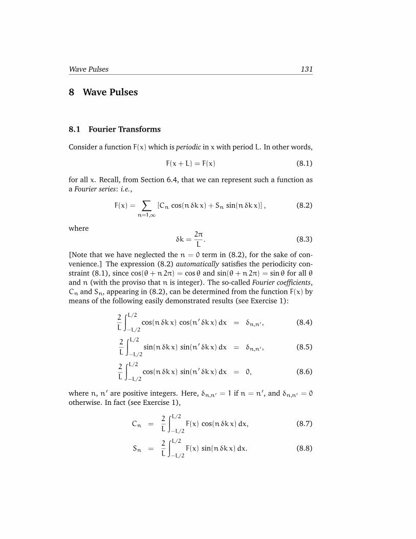
Wave Pulses 131
8 Wave Pulses
8.1 Fourier Transforms
Consider a function F(x) which is periodic in x with period L. In other words,
F(x+ L) = F(x) (8.1)
for all x. Recall, from Section 6.4, that we can represent such a function as
a Fourier series: i.e.,
F(x) =∑
n=1,∞
[Cn cos(nδk x) + Sn sin(nδk x)] , (8.2)
where
δk =2π
L. (8.3)
[Note that we have neglected the n = 0 term in (8.2), for the sake of con-
venience.] The expression (8.2) automatically satisfies the periodicity con-
straint (8.1), since cos(θ + n2π) = cos θ and sin(θ + n2π) = sin θ for all θ
and n (with the proviso that n is integer). The so-called Fourier coefficients,
Cn and Sn, appearing in (8.2), can be determined from the function F(x) by
means of the following easily demonstrated results (see Exercise 1):
2
L
∫L/2
−L/2
cos(nδk x) cos(n ′ δk x)dx = δn,n′ , (8.4)
2
L
∫L/2
−L/2
sin(nδk x) sin(n ′ δk x)dx = δn,n′ , (8.5)
2
L
∫L/2
−L/2
cos(nδk x) sin(n ′ δk x)dx = 0, (8.6)
where n, n ′ are positive integers. Here, δn,n′ = 1 if n = n ′, and δn,n′ = 0
otherwise. In fact (see Exercise 1),
Cn =2
L
∫L/2
−L/2
F(x) cos(nδk x)dx, (8.7)
Sn =2
L
∫L/2
−L/2
F(x) sin(nδk x)dx. (8.8)
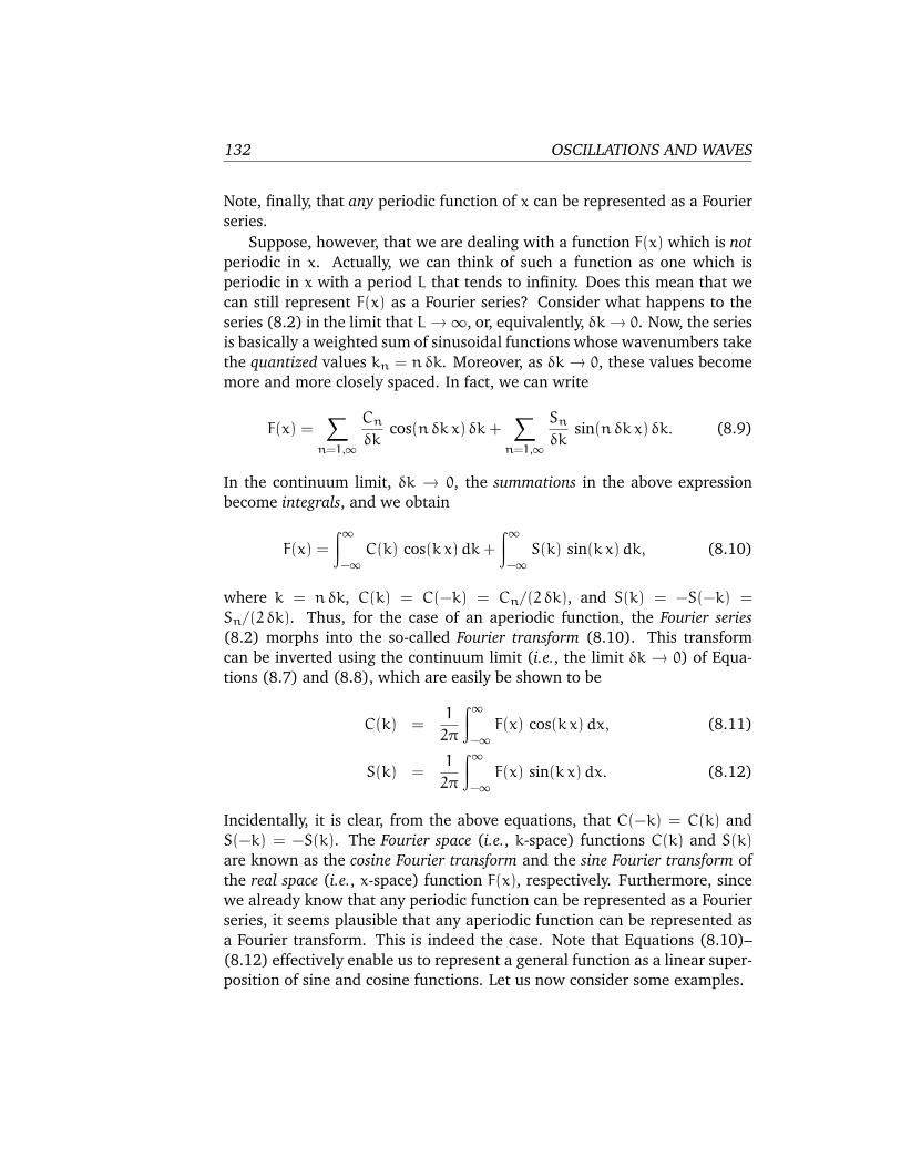
132 OSCILLATIONS AND WAVES
Note, finally, that any periodic function of x can be represented as a Fourier
series.
Suppose, however, that we are dealing with a function F(x) which is not
periodic in x. Actually, we can think of such a function as one which is
periodic in x with a period L that tends to infinity. Does this mean that we
can still represent F(x) as a Fourier series? Consider what happens to the
series (8.2) in the limit that L → ∞, or, equivalently, δk → 0. Now, the series
is basically a weighted sum of sinusoidal functions whose wavenumbers take
the quantized values kn = nδk. Moreover, as δk → 0, these values become
more and more closely spaced. In fact, we can write
F(x) =∑
n=1,∞
Cn
δkcos(nδk x) δk+
∑
n=1,∞
Sn
δksin(nδk x) δk. (8.9)
In the continuum limit, δk → 0, the summations in the above expression
become integrals, and we obtain
F(x) =
∫∞
−∞C(k) cos(k x)dk+
∫∞
−∞S(k) sin(k x)dk, (8.10)
where k = nδk, C(k) = C(−k) = Cn/(2 δk), and S(k) = −S(−k) =
Sn/(2 δk). Thus, for the case of an aperiodic function, the Fourier series
(8.2) morphs into the so-called Fourier transform (8.10). This transform
can be inverted using the continuum limit (i.e., the limit δk → 0) of Equa-
tions (8.7) and (8.8), which are easily be shown to be
C(k) =1
2π
∫∞
−∞F(x) cos(k x)dx, (8.11)
S(k) =1
2π
∫∞
−∞F(x) sin(k x)dx. (8.12)
Incidentally, it is clear, from the above equations, that C(−k) = C(k) and
S(−k) = −S(k). The Fourier space (i.e., k-space) functions C(k) and S(k)
are known as the cosine Fourier transform and the sine Fourier transform of
the real space (i.e., x-space) function F(x), respectively. Furthermore, since
we already know that any periodic function can be represented as a Fourier
series, it seems plausible that any aperiodic function can be represented as
a Fourier transform. This is indeed the case. Note that Equations (8.10)–
(8.12) effectively enable us to represent a general function as a linear super-
position of sine and cosine functions. Let us now consider some examples.
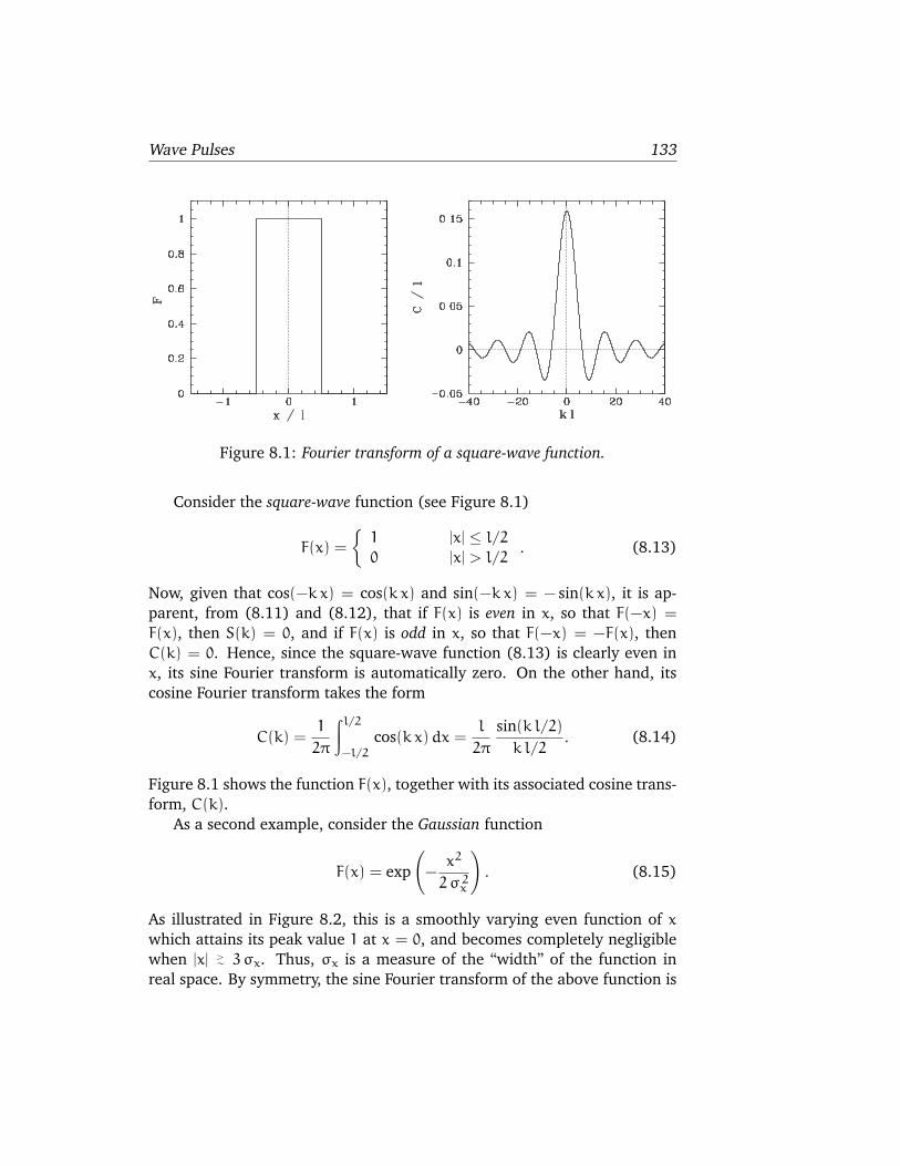
Wave Pulses 133
Figure 8.1: Fourier transform of a square-wave function.
Consider the square-wave function (see Figure 8.1)
F(x) =
1 |x| ≤ l/20 |x| > l/2
. (8.13)
Now, given that cos(−k x) = cos(k x) and sin(−k x) = − sin(k x), it is ap-
parent, from (8.11) and (8.12), that if F(x) is even in x, so that F(−x) =
F(x), then S(k) = 0, and if F(x) is odd in x, so that F(−x) = −F(x), then
C(k) = 0. Hence, since the square-wave function (8.13) is clearly even in
x, its sine Fourier transform is automatically zero. On the other hand, its
cosine Fourier transform takes the form
C(k) =1
2π
∫ l/2
−l/2
cos(k x)dx =l
2π
sin(k l/2)
k l/2. (8.14)
Figure 8.1 shows the function F(x), together with its associated cosine trans-
form, C(k).
As a second example, consider the Gaussian function
F(x) = exp
(
−x2
2 σ2x
)
. (8.15)
As illustrated in Figure 8.2, this is a smoothly varying even function of x
which attains its peak value 1 at x = 0, and becomes completely negligible
when |x| >∼3 σx. Thus, σx is a measure of the “width” of the function in
real space. By symmetry, the sine Fourier transform of the above function is
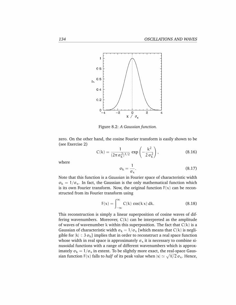
134 OSCILLATIONS AND WAVES
Figure 8.2: A Gaussian function.
zero. On the other hand, the cosine Fourier transform is easily shown to be
(see Exercise 2)
C(k) =1
(2πσ2k)1/2
exp
(
−k2
2 σ2k
)
, (8.16)
where
σk =1
σx. (8.17)
Note that this function is a Gaussian in Fourier space of characteristic width
σk = 1/σx. In fact, the Gaussian is the only mathematical function which
is its own Fourier transform. Now, the original function F(x) can be recon-
structed from its Fourier transform using
F(x) =
∫∞
−∞C(k) cos(k x)dk. (8.18)
This reconstruction is simply a linear superposition of cosine waves of dif-
fering wavenumbers. Moreover, C(k) can be interpreted as the amplitude
of waves of wavenumber k within this superposition. The fact that C(k) is a
Gaussian of characteristic width σk = 1/σx [which means that C(k) is negli-
gible for |k| >∼3 σk] implies that in order to reconstruct a real space function
whose width in real space is approximately σx it is necessary to combine si-
nusoidal functions with a range of different wavenumbers which is approx-
imately σk = 1/σx in extent. To be slightly more exact, the real-space Gaus-
sian function F(x) falls to half of its peak value when |x| ≃√
π/2σx. Hence,
Wave Pulses 135
the full width at half maximum of the function is ∆x = 2√
π/2σx =√2πσx.
Likewise, the full width at half maximum of the Fourier space Gaussian
function C(k) is ∆k =√2 πσk. Thus,
∆x∆k = 2π, (8.19)
since σkσx = 1. Thus, a function which is highly localized in real space
has a transform which is highly delocalized in Fourier space, and vice versa.
Note, finally, that (see Exercise 3)
∫∞
−∞
1
(2πσ2k)1/2
exp
(
−k2
2 σ2k
)
dk = 1. (8.20)
In other words, a Gaussian function in real space, of unit height and char-
acteristic width σx, has a cosine Fourier transform which is a Gaussian in
Fourier space, of characteristic width σk = 1/σx, whose integral over all
k-space is unity.
Consider what happens to the above mentioned real space Gaussian, and
its Fourier transform, in the limit σx → ∞, or, equivalently, σk → 0. There
is no difficulty in seeing, from Equation (8.15), that
F(x) → 1. (8.21)
In other words, the real space Gaussian morphs into a function which takes
the constant value unity everywhere. The Fourier transform is more prob-
lematic. In the limit σk → 0, Equation (8.16) yields a k-space function
which is zero everywhere apart from k = 0 (since the function is negli-
gible for |k| >∼σk), where it is infinite [since the function takes the value
(2πσk)−1/2 at k = 0]. Moreover, according to Equation (8.20), the integral
of the function over all k remains unity. Thus, the Fourier transform of the
uniform function F(x) = 1 is a sort of integrable “spike” located at k = 0.
This strange function is known as the Dirac delta function, and is denoted
δ(k). Thus, one definition of a delta function is
δ(k) ≡ limσk→0
1
(2πσ2k)1/2
exp
(
−k2
2 σ2k
)
. (8.22)
As has already been mentioned, δ(k) = 0 for k 6= 0, and δ(0) = ∞. More-
over, ∫∞
−∞δ(k)dk = 1. (8.23)
136 OSCILLATIONS AND WAVES
Consider the integral∫∞
−∞F(k) δ(k)dk, (8.24)
where F(k) is an arbitrary function. Because of the peculiar properties of the
delta function, the only contribution to the above integral comes from the
region in k-space in the immediate vicinity of k = 0. Furthermore, provided
F(k) is well-behaved in this region, we can write∫∞
−∞F(k) δ(k)dk =
∫∞
−∞F(0) δ(k)dk = F(0)
∫∞
−∞δ(k)dk = F(0), (8.25)
where use has been made of Equation (8.23).
A simple change of variables allows us to define δ(k − k ′), which is a
“spike” function centered on k = k ′. The above result can easily be general-
ized to give ∫∞
−∞F(k) δ(k− k ′)dk = F(k ′), (8.26)
for all F(k). Indeed, this expression can be thought of as an alternative
definition of a delta function.
Now, we have seen that the delta function δ(k) is the cosine Fourier
transform of the uniform function F(x) = 1. It, thus, follows from (8.11)
that
δ(k) =1
2π
∫∞
−∞cos(k x)dx. (8.27)
This result represents yet another definition of the delta function. By sym-
metry, we also have
0 =1
2π
∫∞
−∞sin(k x)dx. (8.28)
It follows that
1
2π
∫∞
−∞cos(k x) cos(k ′ x)dx =
1
4π
∫∞
−∞
cos
[
(k− k ′) x]
+
cos[
(k+ k ′) x]dx
=1
2
[
δ(k− k ′) + δ(k+ k ′)]
, (8.29)
where use has been made of (8.27) and a standard trigonometric identity.
Likewise (see Exercise 4),
1
2π
∫∞
−∞sin(k x) sin(k ′ x)dx =
1
2
[
δ(k− k ′) − δ(k+ k ′)]
, (8.30)
Wave Pulses 137
1
2π
∫∞
−∞cos(k x) sin(k ′ x)dx = 0. (8.31)
Incidentally, Equations (8.29)–(8.31) can be used to derive Equations (8.11)–
(8.12) directly from Equation (8.10) (see Exercise 5).
8.2 General Solution of the Wave Equation
Consider the one dimensional wave equation
∂2ψ
∂t2= v2 ∂
2ψ
∂x2, (8.32)
where ψ(x, t) is the wave amplitude, and v the characteristic phase velocity.
We have seen a number of particular solutions of this equation. For instance,
ψ(x, t) = A cos(k x−ωt− φ) (8.33)
represents a traveling wave of amplitude A, wavenumber k, angular fre-
quency ω, and phase angle φ, which propagates in the positive x-direction.
The above expression is a solution of the wave equation (8.32) provided
that it satisfies the dispersion relation
ω = k v : (8.34)
i.e., provided that the wave propagates with the fixed phase velocity v. We
can also write the solution (8.33) as
ψ(x, t) = C+ cos[k (x− v t)] + S+ sin[k (x− v t)], (8.35)
where C+ = A cosφ, S+ = A sinφ, and we have explicitly incorporated the
dispersion relation ω = k v into the solution. The above expression can be
regarded as the most general form for a traveling wave of wavenumber k
propagating in the positive x-direction. Likewise, the most general form for
a traveling wave of wavenumber k propagating in the negative x-direction
is
ψ(x, t) = C− cos[k (x+ v t)] + S− sin[k (x+ v t)]. (8.36)
Of course, we have also encountered standing wave solutions of (8.32).
However, as we have seen, these can be regarded as linear superpositions
of traveling waves, of equal amplitude and wavenumber, propagating in
opposite directions. In other words, standing waves are not fundamentally
different to traveling waves.
138 OSCILLATIONS AND WAVES
Now, the wave equation (8.32) is linear. This suggests that its most
general solution can be written as a linear superposition of all of its valid
wavelike solutions. In the absence of specific boundary conditions, there is
no restriction on the possible wavenumbers of such solutions. Thus, it is
plausible that the most general solution of (8.32) can be written
ψ(x, t) =
∫∞
−∞C+(k) cos[k (x− v t)]dk
+
∫∞
−∞S+(k) sin[k (x− v t)]dk
+
∫∞
−∞C−(k) cos[k (x+ v t)]dk
+
∫∞
−∞S−(k) sin[k (x+ v t)]dk : (8.37)
i.e., as a linear superposition of traveling waves propagating to the right
(i.e., in the positive x-direction) and to the left. Here, C+(k) represents the
amplitude of right-propagating cosine waves of wavenumber k in this su-
perposition. Moreover, S+(k) represents the amplitude of right-propagating
sine waves of wavenumber k, C−(k) the amplitude of left-propagating co-
sine waves, and S−(k) the amplitude of left-propagating sine waves. Since
each of these waves is individually a solution of (8.32), we are guaranteed,
from the linear nature of this equation, that the above superposition is also
a solution.
But, how can we prove that (8.37) is the most general solution of the
wave equation (8.32)? Well, our understanding of Newtonian dynamics
tells us that if we know the initial wave amplitude ψ(x, 0), and its time
derivative ψ(x, 0), then this should constitute sufficient information to uniqu-
ely specify the solution of (8.32) at all subsequent times. Hence, if (8.37)
is the most general solution of (8.32) then it must be consistent with any
initial wave amplitude, and any initial wave velocity. In other words, given
any ψ(x, 0) and ψ(x, 0), we should be able to uniquely determine the func-
tions C+(k), S+(k), C−(k), and S−(k) appearing in (8.37). Let us see if this
is the case.
Now, from (8.37),
ψ(x, 0) =
∫∞
−∞[C+(k) + C−(k)] cos(k x)dk
+
∫∞
−∞[S+(k) + S−(k)] sin(k x)dk. (8.38)
Wave Pulses 139
However, this is just a Fourier transform of the form (8.10). Moreover,
Equations (8.11) and (8.12) allow us to uniquely invert this transform. In
fact,
C+(k) + C−(k) =1
2π
∫∞
−∞ψ(x, 0) cos(k x)dx, (8.39)
S+(k) + S−(k) =1
2π
∫∞
−∞ψ(x, 0) sin(k x)dx. (8.40)
Equation (8.37) also yields
ψ(x, 0) =
∫∞
−∞k v [C+(k) − C−(k)] sin(k x)dk
−
∫∞
−∞k v [S+(k) − S−(k)] cos(k x)dk. (8.41)
This is, again, a Fourier transform which can be inverted to give
k v [C+(k) − C−(k)] =1
2π
∫∞
−∞ψ(x, 0) sin(k x)dx, (8.42)
k v [S−(k) − S+(k)] =1
2π
∫∞
−∞ψ(x, 0) cos(k x)dx. (8.43)
Hence,
C+(k) =1
4π
[∫∞
−∞ψ(x, 0) cos(k x)dx+
∫∞
−∞
ψ(x, 0)
k vsin(k x)dx
]
,
C−(k) =1
4π
[∫∞
−∞ψ(x, 0) cos(k x)dx−
∫∞
−∞
ψ(x, 0)
k vsin(k x)dx
]
,
S+(k) =1
4π
[∫∞
−∞ψ(x, 0) sin(k x)dx−
∫∞
−∞
ψ(x, 0)
k vcos(k x)dx
]
,
S−(k) =1
4π
[∫∞
−∞ψ(x, 0) sin(k x)dx+
∫∞
−∞
ψ(x, 0)
k vcos(k x)dx
]
.
(8.44)
It follows that we can indeed uniquely determine the functionsC+(k), C−(k),
S+(k), and S−(k), appearing in expression (8.37), for anyψ(x, 0) and ψ(x, 0).
This proves that (8.37) is the most general solution of the wave equation
(8.32).

140 OSCILLATIONS AND WAVES
Let us examine our solution in more detail. Equation (8.37) can be
written (see Exercise 6)
ψ(x, t) = F(x− v t) +G(x+ v t), (8.45)
where
F(x) =
∫∞
−∞[C+(k) cos(k x) + S+(k) sin(k x)]dk, (8.46)
G(x) =
∫∞
−∞[C−(k) cos(k x) + S−(k) sin(k x)]dk. (8.47)
What does the expression (8.45) signify? Well, F(x− v t) represents a wave
disturbance of arbitrary shape which propagates in the positive x-direction,
at the fixed speed v, without changing shape. This should be clear, since a
point with a given amplitude on the wave, F(x − v t) = c, has an equation
of motion x − v t = F−1(c) = constant, and thus propagates in the positive
x-direction at the velocity v. Moreover, since all points on the wave propa-
gate in the same direction at the same velocity it follows that the wave does
not change shape as it moves. Of course, G(x + v t) represents a wave dis-
turbance of arbitrary shape which propagates in the negative x-direction, at
the fixed speed v, without changing shape. Thus, we conclude that the most
general solution to the wave equation (8.32) is a superposition of two wave
disturbances of arbitrary shapes which propagate in opposite directions, at
the fixed speed v, without changing shape. Such solutions are generally
termed wave pulses. So, what is the relationship between a general wave
pulse and the sinusoidal traveling wave solutions to the wave equation that
we found previously. Well, as is clear from Equations (8.46) and (8.47),
a wave pulse can be thought of as a superposition of sinusoidal traveling
waves propagating in the same direction as the pulse. Moreover, the ampli-
tude of cosine waves of wavenumber k in this superposition is simply equal
to the cosine Fourier transform of the pulse shape evaluated at wavenumber
k. Likewise, the amplitude of sine waves of wavenumber k in the superpo-
sition is equal to the sine Fourier transform of the pulse shape evaluated at
wavenumber k.
For instance, suppose that we have a triangular wave pulse of the form
(see Figure 8.3)
F(x) =
1− 2 |x|/l |x| ≤ l/2
0 |x| > l/2. (8.48)
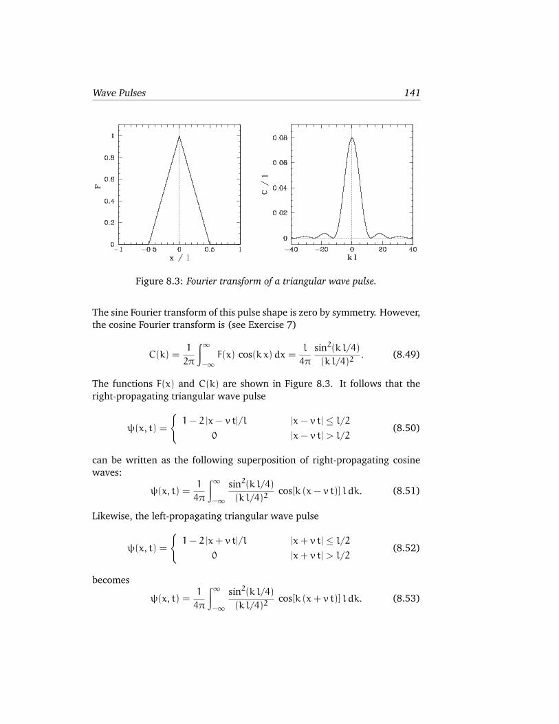
Wave Pulses 141
Figure 8.3: Fourier transform of a triangular wave pulse.
The sine Fourier transform of this pulse shape is zero by symmetry. However,
the cosine Fourier transform is (see Exercise 7)
C(k) =1
2π
∫∞
−∞F(x) cos(k x)dx =
l
4π
sin2(k l/4)
(k l/4)2. (8.49)
The functions F(x) and C(k) are shown in Figure 8.3. It follows that the
right-propagating triangular wave pulse
ψ(x, t) =
1− 2 |x− v t|/l |x− v t| ≤ l/2
0 |x− v t| > l/2(8.50)
can be written as the following superposition of right-propagating cosine
waves:
ψ(x, t) =1
4π
∫∞
−∞
sin2(k l/4)
(k l/4)2cos[k (x− v t)] l dk. (8.51)
Likewise, the left-propagating triangular wave pulse
ψ(x, t) =
1− 2 |x+ v t|/l |x+ v t| ≤ l/2
0 |x+ v t| > l/2(8.52)
becomes
ψ(x, t) =1
4π
∫∞
−∞
sin2(k l/4)
(k l/4)2cos[k (x+ v t)] l dk. (8.53)
142 OSCILLATIONS AND WAVES
8.3 Bandwidth
It is possible to Fourier transform in time, as well as in space. Thus, a gen-
eral temporal waveform F(t) can be written as a superposition of sinusoidal
waveforms of various angular frequencies, ω: i.e.,
F(t) =
∫∞
−∞C(ω) cos(ωt)dω+
∫∞
−∞S(ω) sin(ωt)dω, (8.54)
where C(ω) and S(ω) are the temporal cosine and sine Fourier transforms
of the waveform, respectively. By analogy with Equations (8.10)–(8.12), we
can invert the above expression to give
C(ω) =1
2π
∫∞
−∞F(t) cos(ωt)dt, (8.55)
S(ω) =1
2π
∫∞
−∞F(t) sin(ωt)dt. (8.56)
These equations make it clear that C(−ω) = C(ω), and S(−ω) = −S(ω).
Moreover, it is apparent that if F(t) is an even function of t then S(ω) = 0,
but if it is an odd function then C(ω) = 0.
The current in the antenna of an amplitude-modulated (AM) radio trans-
mitter is driven by a voltage signal which oscillates sinusoidally at a fre-
quency, ω0, which is known as the carrier frequency. In fact, in commercial
(medium wave) AM radio, each station is assigned a single carrier frequency
which lies somewhere between about 500 kHz and 1600 kHz. However,
the voltage signal fed to the antenna does not have a constant amplitude.
Rather, it has a modulated amplitude which can be expressed, somewhat
schematically, as a Fourier series:
A(t) = A0 +∑
n>0
An cos(ωn t− φn), (8.57)
where A(t) − A0 represents the information being transmitted. Typically,
this information is speech or music which is picked up by a microphone,
and converted into an electrical signal. Note that the constant amplitude
A0 is present even when the transmitter is transmitting no information. The
remaining terms in the above expression are due to the signal picked up by
the microphone. The modulation frequencies, ωn, are thus the frequencies
of audible sound waves: i.e., they are so-called audio frequencies lying be-
tween about 20 Hz and 20 kHz. Of course, this implies that the modulation
frequencies are much smaller than the carrier frequency: i.e., ωn ≪ ω0 for
Wave Pulses 143
all n > 0. Furthermore, the modulation amplitudes An are all generally
smaller than the carrier amplitude A0.
The signal transmitted by an AM station, and received by an AM receiver,
is an amplitude modulated sinusoidal oscillation of the form
ψ(t) = A(t) cos(ω0 t)
= A0 cos(ω0 t) +∑
n>0
An cos(ωn t− φn) cos(ω0 t), (8.58)
which, with the help of some standard trigonometric identities, can also be
written
ψ(t) = A0 cos(ω0 t) +1
2
∑
n>0
An cos[(ω0 +ωn) t− φn)]
+1
2
∑
n>0
An cos[(ω0 −ωn) t+ φn)]
= A0 cos(ω0 t) +1
2
∑
n>0
An cosφn cos[(ω0 +ωn) t]
+1
2
∑
n>0
An sinφn sin[(ω0 +ωn) t]
+1
2
∑
n>0
An cosφn cos[(ω0 −ωn) t]
−1
2
∑
n>0
An sinφn sin[(ω0 −ωn) t]. (8.59)
We can calculate the cosine and sine Fourier transforms of the signal,
C(ω) =1
2π
∫∞
−∞ψ(t) cos(ωt)dt, (8.60)
S(ω) =1
2π
∫∞
−∞ψ(t) sin(ωt)dt, (8.61)
by making use of the standard results [cf., (8.29)–(8.31)]
1
2π
∫∞
−∞cos(ωt) cos(ω ′ t)dt =
1
2
[
δ(ω−ω ′) + δ(ω+ω ′)]
,
(8.62)
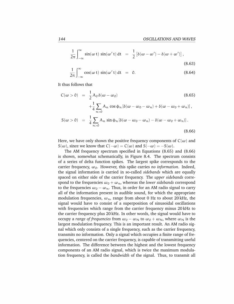
144 OSCILLATIONS AND WAVES
1
2π
∫∞
−∞sin(ωt) sin(ω ′ t)dt =
1
2
[
δ(ω−ω ′) − δ(ω+ω ′)]
,
(8.63)
1
2π
∫∞
−∞cos(ωt) sin(ω ′ t)dt = 0. (8.64)
It thus follows that
C(ω > 0) =1
2A0δ(ω−ω0) (8.65)
+1
4
∑
n>0
An cosφn [δ(ω−ω0 −ωn) + δ(ω−ω0 +ωn)] ,
S(ω > 0) =1
4
∑
n>0
An sinφn [δ(ω−ω0 −ωn) − δ(ω−ω0 +ωn)] .
(8.66)
Here, we have only shown the positive frequency components of C(ω) and
S(ω), since we know that C(−ω) = C(ω) and S(−ω) = −S(ω).
The AM frequency spectrum specified in Equations (8.65) and (8.66)
is shown, somewhat schematically, in Figure 8.4. The spectrum consists
of a series of delta function spikes. The largest spike corresponds to the
carrier frequency, ω0. However, this spike carries no information. Indeed,
the signal information is carried in so-called sidebands which are equally
spaced on either side of the carrier frequency. The upper sidebands corre-
spond to the frequencies ω0 +ωn, whereas the lower sidebands correspond
to the frequencies ω0 −ωn. Thus, in order for an AM radio signal to carry
all of the information present in audible sound, for which the appropriate
modulation frequencies, ωn, range from about 0 Hz to about 20 kHz, the
signal would have to consist of a superposition of sinusoidal oscillations
with frequencies which range from the carrier frequency minus 20 kHz to
the carrier frequency plus 20 kHz. In other words, the signal would have to
occupy a range of frequencies from ω0 −ωN to ω0 +ωN, where ωN is the
largest modulation frequency. This is an important result. An AM radio sig-
nal which only consists of a single frequency, such as the carrier frequency,
transmits no information. Only a signal which occupies a finite range of fre-
quencies, centered on the carrier frequency, is capable of transmitting useful
information. The difference between the highest and the lowest frequency
components of an AM radio signal, which is twice the maximum modula-
tion frequency, is called the bandwidth of the signal. Thus, to transmit all
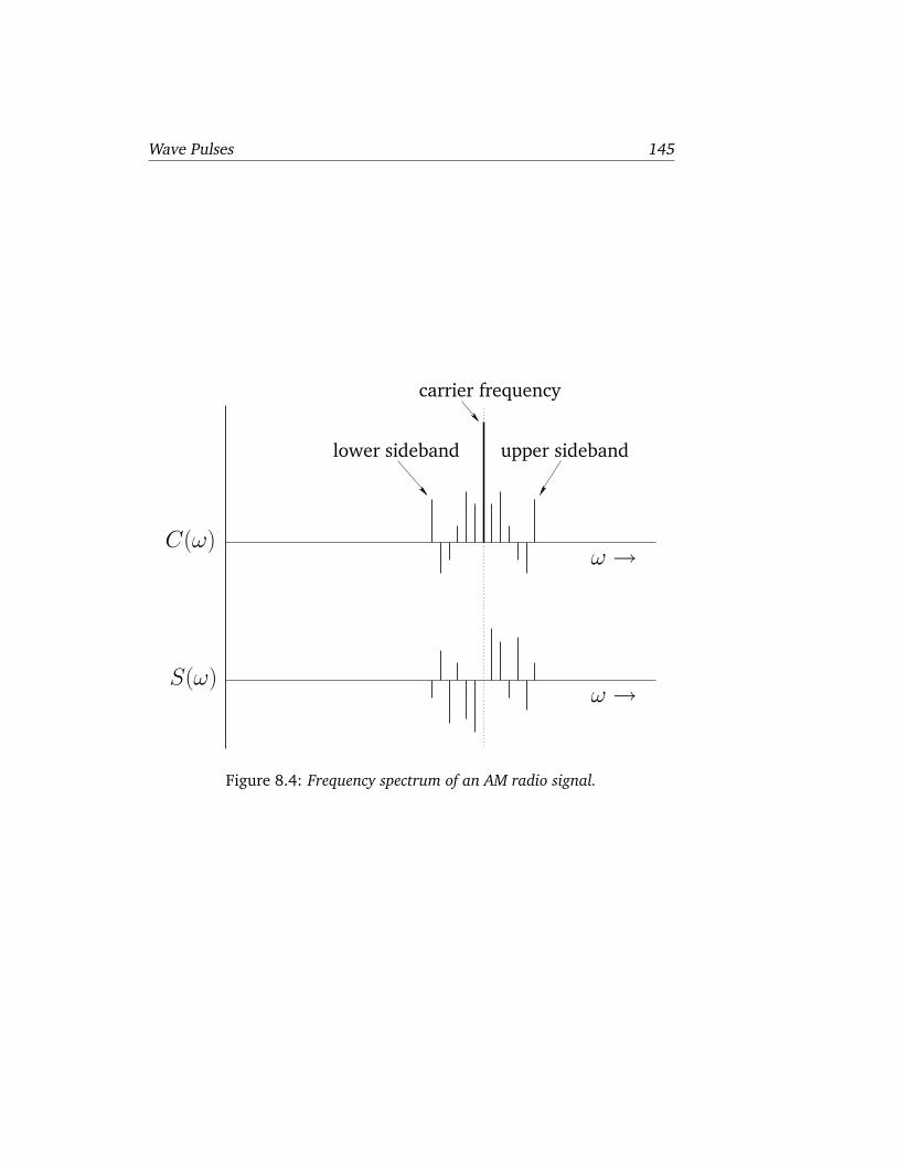
Wave Pulses 145
S(ω)
ω →
ω →
lower sideband
carrier frequency
upper sideband
C(ω)
Figure 8.4: Frequency spectrum of an AM radio signal.
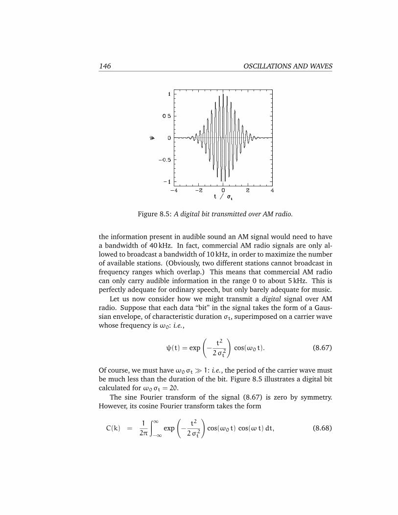
146 OSCILLATIONS AND WAVES
Figure 8.5: A digital bit transmitted over AM radio.
the information present in audible sound an AM signal would need to have
a bandwidth of 40 kHz. In fact, commercial AM radio signals are only al-
lowed to broadcast a bandwidth of 10 kHz, in order to maximize the number
of available stations. (Obviously, two different stations cannot broadcast in
frequency ranges which overlap.) This means that commercial AM radio
can only carry audible information in the range 0 to about 5 kHz. This is
perfectly adequate for ordinary speech, but only barely adequate for music.
Let us now consider how we might transmit a digital signal over AM
radio. Suppose that each data “bit” in the signal takes the form of a Gaus-
sian envelope, of characteristic duration σt, superimposed on a carrier wave
whose frequency is ω0: i.e.,
ψ(t) = exp
(
−t2
2 σ2t
)
cos(ω0 t). (8.67)
Of course, we must haveω0σt ≫ 1: i.e., the period of the carrier wave must
be much less than the duration of the bit. Figure 8.5 illustrates a digital bit
calculated for ω0σt = 20.
The sine Fourier transform of the signal (8.67) is zero by symmetry.
However, its cosine Fourier transform takes the form
C(k) =1
2π
∫∞
−∞exp
(
−t2
2 σ2t
)
cos(ω0 t) cos(ωt)dt, (8.68)
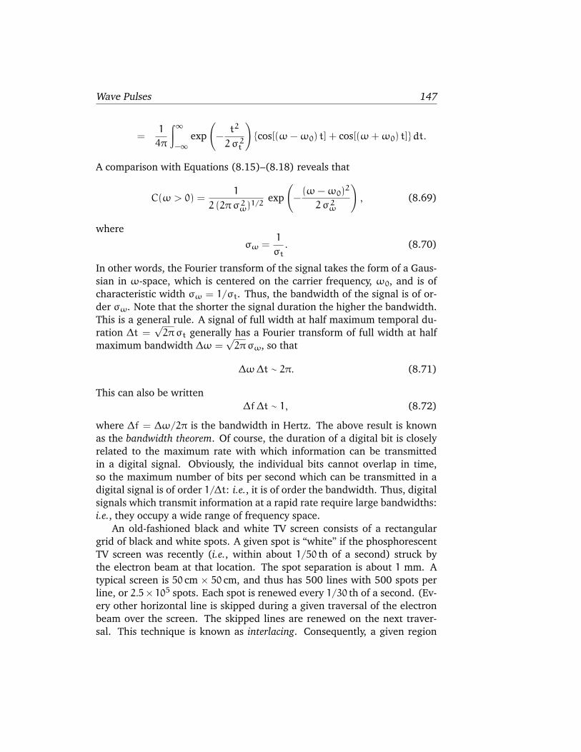
Wave Pulses 147
=1
4π
∫∞
−∞exp
(
−t2
2 σ2t
)
cos[(ω−ω0) t] + cos[(ω+ω0) t]dt.
A comparison with Equations (8.15)–(8.18) reveals that
C(ω > 0) =1
2 (2πσ2ω)1/2
exp
(
−(ω−ω0)
2
2 σ2ω
)
, (8.69)
where
σω =1
σt. (8.70)
In other words, the Fourier transform of the signal takes the form of a Gaus-
sian in ω-space, which is centered on the carrier frequency, ω0, and is of
characteristic width σω = 1/σt. Thus, the bandwidth of the signal is of or-
der σω. Note that the shorter the signal duration the higher the bandwidth.
This is a general rule. A signal of full width at half maximum temporal du-
ration ∆t =√2πσt generally has a Fourier transform of full width at half
maximum bandwidth ∆ω =√2πσω, so that
∆ω∆t ∼ 2π. (8.71)
This can also be written
∆f∆t ∼ 1, (8.72)
where ∆f = ∆ω/2π is the bandwidth in Hertz. The above result is known
as the bandwidth theorem. Of course, the duration of a digital bit is closely
related to the maximum rate with which information can be transmitted
in a digital signal. Obviously, the individual bits cannot overlap in time,
so the maximum number of bits per second which can be transmitted in a
digital signal is of order 1/∆t: i.e., it is of order the bandwidth. Thus, digital
signals which transmit information at a rapid rate require large bandwidths:
i.e., they occupy a wide range of frequency space.
An old-fashioned black and white TV screen consists of a rectangular
grid of black and white spots. A given spot is “white” if the phosphorescent
TV screen was recently (i.e., within about 1/50 th of a second) struck by
the electron beam at that location. The spot separation is about 1 mm. A
typical screen is 50 cm × 50 cm, and thus has 500 lines with 500 spots per
line, or 2.5× 10⁵ spots. Each spot is renewed every 1/30 th of a second. (Ev-
ery other horizontal line is skipped during a given traversal of the electron
beam over the screen. The skipped lines are renewed on the next traver-
sal. This technique is known as interlacing. Consequently, a given region
148 OSCILLATIONS AND WAVES
of the screen, that includes many horizontal lines, has a flicker rate of 60
Hz.) Thus, the rate at which the instructions “turn on” and “turn off” must
be sent to the electron beam is 30 × 2.5 × 105 or 8 × 10⁶ times a second.
The transmitted TV signal must therefore have about 107 on-off instruction
blips per second. If temporal overlap is to be avoided, each blip can be no
longer than ∆t ∼ 10−7 seconds in duration. Thus, the required bandwidth
is ∆f ∼ 1/∆t ∼ 107 Hz = 10MHz. The carrier wave frequencies used for
conventional broadcast TV lie in the so-called VHF band, and range from
about 55 to 210 MHz. Our previous discussion of AM radio might lead us
to think that the 10 MHz bandwidth represents the combined extents of an
upper and a lower sideband of modulation frequencies. In practice, the car-
rier wave and one of the sidebands are suppressed: i.e., they are filtered
out, and never applied to the antenna. However, they are regenerated in
the receiver from the information contained in the single sideband which
is broadcast. This technique, which is called single sideband transmission,
halves the bandwidth requirement to about 5MHz. Thus, between 55 and
210MHz there is room for about 30 TV channels, each using a 5 MHz band-
width. (Actually, there are far fewer TV channels than this in the VHF band,
because part of this band is reserved for FM radio, air traffic control, air
navigation beacons, marine communications, etc.)
8.4 Exercises
1. Verify Equations (8.4)–(8.6). Derive Equations (8.7) and (8.8) from Equa-tion (8.2) and Equations (8.4)–(8.6).
2. Suppose that
F(x) = exp
(
−x2
2 σ 2x
)
.
Demonstrate that
F(k) ≡ 1
2π
∫∞
−∞
F(x) e i k x dx =1
√
2πσ 2k
exp
(
−k2
2 σ 2k
)
,
where i is the square-root of minus one, and σk = 1/σx. [Hint: You willneed to complete the square of the exponent of e, transform the variable of
integration, and then make use of the standard result that∫∞
−∞e−y2
dy =√π.] Hence, show from de Moive’s theorem, exp( ik x) ≡ cos x+ i sin x, that
C(k) ≡ 1
2π
∫∞
−∞
F(x) cos(k x)dx =1
√
2πσ 2k
exp
(
−k2
2 σ 2k
)
,
Wave Pulses 149
S(k) ≡ 1
2π
∫∞
−∞
F(x) sin(k x)dx = 0.
3. Demonstrate that
∫∞
−∞
1√
2πσ 2k
exp
(
−k2
2 σ 2k
)
dk = 1.
4. Verify Equations (8.30) and (8.31).
5. Derive Equations (8.11) and (8.12) directly from Equation (8.10) using theresults (8.29)–(8.31).
6. Verify directly that (8.45) is a solution of the wave equation (8.32), for arbi-trary pulse shapes F(x) and G(x).
7. Verify Equation (8.49).
8. Consider a function F(t) which is zero for negative t, and takes the valueexp(−t/2 τ) for t ≥ 0. Find its Fourier transforms, C(ω) and S(ω), definedin
F(t) =
∫∞
−∞
C(ω) cos(ωt)dω+
∫∞
−∞
S(ω) sin(ωt)dω.
9. Suppose that F(t) is zero, except in the interval from t = −∆t/2 to t = ∆t/2.Suppose that in this interval F(t) makes exactly one sinusoidal oscillation atthe angular frequency ω0 = 2π/∆t, starting and ending with the value zero.Find the above defined Fourier transforms C(ω) and S(ω).
10. Demonstrate that∫∞
−∞
F2(t)dt = 2π
∫∞
−∞
[C2(ω) + S2(ω)]dω,
where the relation between F(t), C(ω), and S(ω) is defined above. Thisresult is known as Parseval’s theorem.
11. Suppose that F(t) and G(t) are both even functions of t with the cosine trans-forms F(ω) and G(ω), so that
F(t) =
∫∞
−∞
F(ω) cos(ωt)dω,
G(t) =
∫∞
−∞
G(ω) cos(ωt)dω.
Let H(t) = F(t)G(t), and let H(ω) be the cosine transform of this evenfunction, so that
H(t) =
∫∞
−∞
H(ω) cos(ωt)dω.
150 OSCILLATIONS AND WAVES
Demonstrate that
H(ω) =1
2
∫∞
−∞
F(ω ′)[
G(ω ′ +ω) + G(ω ′ −ω)]
dω ′.
This result is known as the convolution theorem, since the above type of in-tegral is known as a convolution integral. Suppose that F(t) = cos(ω0 t).Show that
H(ω) =1
2
[
G(ω−ω0) + G(ω+ω0)]
.
Dispersive Waves 151
9 Dispersive Waves
9.1 Pulse Propagation
Consider a one dimensional wave pulse,
ψ(x, t) =
∫∞
−∞C(k) cos(k x−ωt)dk, (9.1)
made up of a linear superposition of cosine waves, with a range of dif-
ferent wavenumbers, all traveling in the positive x-direction. The angular
frequency, ω, of each of these waves is related to its wavenumber, k, via the
so-called dispersion relation, which can be written schematically as
ω = ω(k). (9.2)
In general, this relation is derivable from the wave disturbance’s equation of
motion. Up to now, we have only considered sinusoidal waves which have
linear dispersion relations of the form
ω = k v, (9.3)
where v is a constant. The above expression immediately implies that the
waves all have the same phase velocity,
vp =ω
k= v. (9.4)
Substituting (9.3) into (9.1), we obtain
ψ(x, t) =
∫∞
−∞C(k) cos[k (x− v t)]dk, (9.5)
which is clearly the equation of a wave pulse that propagates in the positive
x-direction, at the fixed speed v, without changing shape (see Chapter 8).
The above analysis would seem to suggest that arbitrarily shaped wave
pulses generally propagate at the same speed as sinusoidal waves, and do so
without dispersing or, otherwise, changing shape. In fact, these statements
are only true of pulses made up of superpositions of sinusoidal waves with
linear dispersion relations. There are, however, many types of sinusoidal
152 OSCILLATIONS AND WAVES
wave whose dispersion relations are nonlinear. For instance, the disper-
sion relation of sinusoidal electromagnetic waves propagating through an
unmagnetized plasma is (see Section 9.2)
ω =√
k2 c2 +ω2p, (9.6)
where c is the speed of light in vacuum, and ωp is a constant, known as
the plasma frequency, which depends on the properties of the plasma [see
Equation (9.28)]. Moreover, the dispersion relation of sinusoidal surface
waves in deep water is (see Section 9.4)
ω =
√
gk+T
ρk3, (9.7)
where g is the acceleration due to gravity, T the surface tension, and ρ the
mass density. Sinusoidal waves which satisfy nonlinear dispersion relations,
such as (9.6) and (9.7), are known as dispersive waves, as opposed to waves
which satisfy linear dispersion relations, such as (9.3), which are known as
non-dispersive waves. As we saw above, a wave pulse made up of a linear
superposition of non-dispersive sinusoidal waves, all traveling in the same
direction, propagates at the common phase velocity of these waves, without
changing shape. But, how does a wave pulse made up of a linear superposi-
tion of dispersive sinusoidal waves evolve in time?
Suppose that
C(k) =1
√
2πσ2k
exp
(
−(k− k0)
2
2 σ2k
)
: (9.8)
i.e., the function C(k) in (9.1) is a Gaussian, of characteristic width σk,
centered on wavenumber k = k0. It follows, from the properties of the
Gaussian function, that C(k) is negligible for |k − k0|>∼3 σk. Thus, the only
significant contributions to the wave integral
ψ(x, t) =
∫∞
−∞
1√
2πσ2k
exp
(
−(k− k0)
2
2 σ2k
)
cos(k x−ωt)dk (9.9)
come from a small region of k-space centered on k = k0. Let us Taylor
expand the dispersion relation,ω = ω(k), about k = k0. Neglecting second-
order terms in the expansion, we obtain
ω ≃ ω(k0) + (k− k0)dω(k0)
dk. (9.10)
Dispersive Waves 153
It follows that
k x−ωt ≃ k0x−ω0 t+ (k− k0) (x− vg t), (9.11)
where ω0 = ω(k0), and
vg =dω(k0)
dk(9.12)
is a constant with the dimensions of velocity. Now, if σk is sufficiently small
then the neglect of second-order terms in the expansion (9.11) is a good
approximation, and expression (9.9) becomes
ψ(x, t) ≃ cos(k0x−ω0 t)√
2πσ2k
∫∞
−∞exp
(
−(k− k0)
2
2 σ2k
)
cos[(k− k0) (x− vg t)]dk
−sin(k0x−ω0 t)
√
2πσ2k
∫∞
−∞exp
(
−(k− k0)
2
2 σ2k
)
sin[(k− k0) (x− vg t)]dk,
(9.13)
where use has been made of a standard trigonometric identity. The inte-
gral involving sin[(k − k0) (x − vg t)] is zero, by symmetry. Moreover, an
examination of Equations (8.15)–(8.18) reveals that
1√
2πσ2k
∫∞
−∞exp
(
−k2
2 σ2k
)
cos(k x)dk = exp
(
−x2
2 σ2x
)
, (9.14)
where σx = 1/σk. Hence, by analogy with the above expression, (9.13)
reduces to
ψ(x, t) ≃ exp
(
−(x− vg t)
2
2 σ2x
)
cos(k0x−ω0 t). (9.15)
This is clearly the equation of a wave pulse, of wavenumber k0 and angular
frequency ω0, with a Gaussian envelope, of characteristic width σx, whose
peak (which is located by setting the argument of the exponential to zero)
has the equation of motion
x = vg t. (9.16)
In other words, the pulse peak—and, hence, the pulse itself—propagates
at the velocity vg, which is known as the group velocity. Of course, in the
case of non-dispersive waves, the group velocity is the same as the phase
154 OSCILLATIONS AND WAVES
velocity (since, if ω = k v then ω/k = dω/dk = v). However, for the case
of dispersive waves, the two velocities are, in general, different.
Equation (9.15) indicates that, as the wave pulse propagates, its en-
velope remains the same shape. Actually, this result is misleading, and is
only obtained because of the neglect of second-order terms in the expan-
sion (9.11). If we keep more terms in this expansion then we can show
that the wave pulse does actually change shape as it propagates. How-
ever, this demonstration is most readily effected by means of the following
simple argument. The pulse extends in Fourier space from k0 − ∆k/2 to
k0+∆k/2, where ∆k ∼ σk. Thus, part of the pulse propagates at the velocity
vg(k0 − ∆k/2), and part at the velocity vg(k0 + ∆k/2). Consequently, the
pulse spreads out as it propagates, since some parts of it move faster than
others. Roughly speaking, the spatial extent of the pulse in real space grows
as
∆x ∼ (∆x)0 + [vg(k0 + ∆k/2) − vg(k0 − ∆k/2)] t ∼ (∆x)0 +dvg(k0)
dk∆k t,
(9.17)
where (∆x)0 ∼ σx = σ−1k is the extent of the pulse at t = 0. Hence, from
(9.12),
∆x ∼ (∆x)0 +d2ω(k0)
dk2
t
(∆x)0
. (9.18)
We, thus, conclude that the spatial extent of the pulse grows linearly in
time, at a rate proportional to the second derivative of the dispersion rela-
tion with respect to k (evaluated at the pulse’s central wavenumber). This
effect is known as pulse dispersion. In summary, a wave pulse made up of a
linear superposition of dispersive sinusoidal waves, with a range of different
wavenumbers, propagates at the group velocity, and also gradually disperses
as time progresses.
9.2 Electromagnetic Wave Propagation in Plasmas
Consider a point particle of mass m and electric charge q interacting with
a sinusoidal electromagnetic wave propagating in the z-direction. Provided
that the wave amplitude is not sufficiently large to cause the particle to
move at relativistic speeds, the electric component of the wave exerts a
much greater force on the particle than the magnetic component. (This
follows, from standard electrodynamics, because the ratio of the magnetic
to the electric force is of order B0 v/E0, where E0 is the amplitude of the
wave electric field-strength, B0 = E0/c the amplitude of the wave magnetic
Dispersive Waves 155
field-strength, v the particle velocity, and c the velocity of light in vacuum.
Hence, the ratio of the forces is approximately v/c.) Suppose that the elec-
tric component of the wave oscillates in the x-direction, and takes the form
Ex(z, t) = E0 cos(k z−ωt), (9.19)
where k is the wavenumber, and ω the angular frequency. The equation of
motion of the particle is thus
md2x
dt2= qEx, (9.20)
where x measures its wave-induced displacement in the x-direction. The
above equation can easily be solved to give
x = −qE0
mω2cos(k z−ωt). (9.21)
Thus, the wave causes the particle to execute sympathetic simple harmonic
oscillations, in the x-direction, with an amplitude which is directly propor-
tional to its charge, and inversely proportional to its mass.
Suppose that the wave is actually propagating through an unmagne-
tized electrically neutral plasma consisting of free electrons, of massme and
charge −e, and free ions, of mass mi and charge +e. Since the plasma is
assumed to be electrically neutral, each species must have the same equi-
librium number density, ne. Now, given that the electrons are much less
massive than the ions (i.e., me ≪ mi), but have the same charge (mod-
ulo a sign), it follows from (9.21) that the wave-induced oscillations of the
electrons are of much higher amplitude than those of the ions. In fact,
to a first approximation, we can say that the electrons oscillate whilst the
ions remain stationary. Assuming that the electrons and ions are evenly
distributed throughout the plasma, the wave-induced displacement of an
individual electron generates an effective electric dipole moment in the x-
direction of the form px = −e x (the other component of the dipole is a
stationary ion of charge +e located at x = 0). Hence, the x-directed electric
dipole moment per unit volume is
Px = nepx = −nee x. (9.22)
Given that all of the electrons oscillate according to Equation (9.21) (with
q = −e and m = me), we obtain
Px = −nee
2E0
meω2cos(k z−ωt). (9.23)
156 OSCILLATIONS AND WAVES
Now, we saw earlier, in Section 7.7, that the z-directed propagation of
an electromagnetic wave, polarized in the x-direction (i.e., with its electric
component oscillating in the x-direction), through a dielectric medium is
governed by
∂Ex
∂t= −
1
ǫ0
(
∂Px
∂t+∂Hy
∂z
)
, (9.24)
∂Hy
∂t= −
1
µ0
∂Ex
∂z. (9.25)
Thus, writing Ex in the form (9.19), Hy in the form
Hy(z, t) = Z−1E0 cos(k z−ωt), (9.26)
where Z is the effective impedance of the plasma, and Px in the form (9.23),
Equations (9.24) and (9.25) can easily be shown to yield the nonlinear dis-
persion relation (see Exercise 1)
ω2 = k2 c2 +ω2p, (9.27)
where c = 1/√ǫ0µ0 is the velocity of light in vacuum, and the so-called
plasma frequency,
ωp =
(
nee2
ǫ0me
)1/2
, (9.28)
is the characteristic frequency of collective electron oscillations in the plasma.
Equations (9.24) and (9.25) also yield
Z =Z0
n, (9.29)
where Z0 =√
µ0/ǫ0 is the impedance of free space, and
n =k c
ω=
(
1−ω2
p
ω2
)1/2
(9.30)
the effective refractive index of the plasma. We, thus, conclude that sinu-
soidal electromagnetic waves propagating through a plasma have a nonlin-
ear dispersion relation. Moreover, it is clear that this nonlinearity arises
because the effective refractive index of the plasma is frequency dependent.
The expression (9.30) for the refractive index of a plasma has some
rather unusual properties. For wave frequencies lying above the plasma
Dispersive Waves 157
frequency (i.e., ω > ωp), it yields a real refractive index which is less than
unity. On the other hand, for wave frequencies lying below the plasma
frequency (i.e., ω < ωp), it yields an imaginary refractive index. Neither
of these results makes much sense. The former result is problematic be-
cause if the refractive index is less than unity then the wave phase velocity,
vp = ω/k = c/n, becomes superluminal (i.e., vp > c), and superluminal
velocities are generally thought to be unphysical. The latter result is prob-
lematic because an imaginary refractive index implies an imaginary phase
velocity, which seems utterly meaningless. Let us investigate further.
Consider, first of all, the high frequency limit, ω > ωp. According to
(9.30), a sinusoidal electromagnetic wave of angular frequency ω > ωp
propagates through the plasma at the superluminal phase velocity
vp =ω
k=c
n=
c
(1−ω2p/ω
2)1/2. (9.31)
But, is this really unphysical? As is well-known, Einstein’s theory of rel-
ativity forbids information from traveling faster than the velocity of light
in vacuum, since this would violate causality (i.e., it would be possible to
transform to a valid frame of reference in which an effect occurs prior to its
cause.) However, a sinusoidal wave with a unique frequency, and an infinite
spatial extent, does not transmit any information. (Recall, for instance, from
Section 8.3, that the carrier wave in an AM radio signal transmits no infor-
mation.) So, at what speed do electromagnetic waves in a plasma transmit
information? Well, the most obvious way of using such waves to transmit
information would be to send a message via Morse code. In other words, we
could transmit a message by means of short wave pulses, of varying lengths
and interpulse spacings, which are made to propagate through the plasma.
The pulses in question would definitely transmit information, so the velocity
of information propagation must be the same as that of the pulses: i.e., the
group velocity, vg = dω/dk. Differentiating the dispersion relation (9.27)
with respect to k, we obtain
2ωdω
dk= 2 k c2, (9.32)
orω
k
dω
dk= vpvg = c2. (9.33)
Thus, it follows, from (9.31), that the group velocity of high frequency elec-
tromagnetic waves in a plasma is
vg = nc = (1−ω2p/ω
2)1/2 c. (9.34)
158 OSCILLATIONS AND WAVES
Note that the group velocity is subluminal (i.e., vg < c). Hence, as long as
we accept that high frequency electromagnetic waves transmit information
through a plasma at the group velocity, rather than the phase velocity, then
there is no problem with causality. Incidentally, it should be clear, from
this discussion, that the phase velocity of dispersive waves has very little
physical significance. It is the group velocity which matters. For instance,
according to Equations (7.120), (9.29), (9.30), and (9.34), the mean flux of
electromagnetic energy in the z-direction due to a high frequency sinusoidal
wave propagating through a plasma is given by
〈I〉 =1
2ǫ0E
20 nc =
1
2ǫ0E
20 vg, (9.35)
since Z0 =√
µ0/ǫ0 and c = 1/√ǫ0µ0. Thus, if the group velocity is zero, as
is the case when ω = ωp, then there is zero energy flux associated with the
wave.
The fact that the energy flux and the group velocity of a sinusoidal wave
propagating through a plasma both go to zero when ω = ωp suggests that
the wave ceases to propagate at all in the low frequency limit,ω < ωp. This
observation leads us to search for spatially decaying standing wave solutions
to (9.24) and (9.25) of the form,
Ex(z, t) = E0 e−kz cos(ωt), (9.36)
Hy(z, t) = Z−1E0 e−kz sin(ωt). (9.37)
It follows from (9.20) and (9.22) that
Px = −nee
2E0
meω2e−kz cos(ωt). (9.38)
Substitution into Equations (9.24) and (9.25) reveals that (9.36) and (9.37)
are indeed the correct solutions when ω < ωp (see Exercise 2), and also
yields
k c =√
ω2p −ω2, (9.39)
as well as
Z = Z0ω
kc= Z0 (ω2
p/ω2 − 1)−1/2. (9.40)
Furthermore, the mean z-directed electromagnetic energy flux becomes
〈I〉 = 〈ExHy〉 = E20 Z
−1 e−2kz 〈cos(ωt) sin(ωt)〉 = 0. (9.41)
Dispersive Waves 159
The above analysis demonstrates that a sinusoidal electromagnetic wave
cannot propagate through a plasma when its frequency lies below the plasma
frequency. Instead, the amplitude of the wave decays exponentially into the
plasma. Moreover, the electric and magnetic components of the wave oscil-
late in phase quadrature (i.e., π/2 radians out of phase), and the wave con-
sequentially has zero associated net energy flux. This suggests that a plasma
reflects, rather than absorbs, an incident electromagnetic wave whose fre-
quency is less than the plasma frequency (since if the wave were absorbed
then there would be a net flux of energy into the plasma). Let us investi-
gate what happens when a low frequency electromagnetic wave is normally
incident on a plasma in more detail.
Suppose that the region z < 0 is a vacuum, and the region z > 0 is
occupied by a plasma of plasma frequency ωp. Let the wave electric and
magnetic fields in the vacuum region take the form
Ex(z, t) = Ei cos[(ω/c) (z− c t)] + Er cos[(ω/c) (z+ c t) + φr], (9.42)
Hy(z, t) = EiZ−10 cos[(ω/c) (z− c t)] − ErZ
−10 cos[(ω/c) (z+ c t) + φr].
(9.43)
Here, Ei is the amplitude of an electromagnetic wave of frequency ω < ωp
which is incident on the plasma, whereas Er is the amplitude of the reflected
wave, and φr the phase of this wave with respect to the incident wave.
Moreover, we have made use of the vacuum dispersion relation ω = k c.
The wave electric and magnetic fields in the plasma are written
Ex(z, t) = Et e−(ω/c)αz cos(ωt+ φt), (9.44)
Hy(z, t) = EtZ−10 α e−(ω/c)αz sin(ωt+ φt), (9.45)
where Et is the amplitude of the decaying wave which penetrates into the
plasma, φt is the phase of this wave with respect to the incident wave, and
α =
(
ω2p
ω2− 1
)1/2
. (9.46)
The appropriate matching conditions are the continuity of Ex and Hy at
z = 0: i.e.,
Ei cos(ωt) + Er cos(ωt+ φr) = Et cos(ωt+ φt), (9.47)
Ei cos(ωt) − Er cos(ωt+ φr) = Etα sin(ωt+ φt). (9.48)
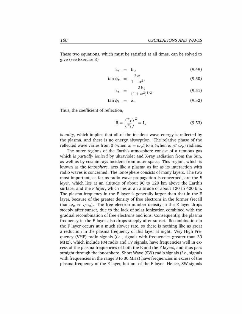
160 OSCILLATIONS AND WAVES
These two equations, which must be satisfied at all times, can be solved to
give (see Exercise 3)
Er = Ei, (9.49)
tanφr =2α
1− α2, (9.50)
Et =2 Ei
(1+ α2)1/2, (9.51)
tanφt = α. (9.52)
Thus, the coefficient of reflection,
R =
(
Er
Ei
)2
= 1, (9.53)
is unity, which implies that all of the incident wave energy is reflected by
the plasma, and there is no energy absorption. The relative phase of the
reflected wave varies from 0 (when ω = ωp) to π (when ω≪ ωp) radians.
The outer regions of the Earth’s atmosphere consist of a tenuous gas
which is partially ionized by ultraviolet and X-ray radiation from the Sun,
as well as by cosmic rays incident from outer space. This region, which is
known as the ionosphere, acts like a plasma as far as its interaction with
radio waves is concerned. The ionosphere consists of many layers. The two
most important, as far as radio wave propagation is concerned, are the E
layer, which lies at an altitude of about 90 to 120 km above the Earth’s
surface, and the F layer, which lies at an altitude of about 120 to 400 km.
The plasma frequency in the F layer is generally larger than that in the E
layer, because of the greater density of free electrons in the former (recall
that ωp ∝ √ne). The free electron number density in the E layer drops
steeply after sunset, due to the lack of solar ionization combined with the
gradual recombination of free electrons and ions. Consequently, the plasma
frequency in the E layer also drops steeply after sunset. Recombination in
the F layer occurs at a much slower rate, so there is nothing like as great
a reduction in the plasma frequency of this layer at night. Very High Fre-
quency (VHF) radio signals (i.e., signals with frequencies greater than 30
MHz), which include FM radio and TV signals, have frequencies well in ex-
cess of the plasma frequencies of both the E and the F layers, and thus pass
straight through the ionosphere. Short Wave (SW) radio signals (i.e., signals
with frequencies in the range 3 to 30 MHz) have frequencies in excess of the
plasma frequency of the E layer, but not of the F layer. Hence, SW signals
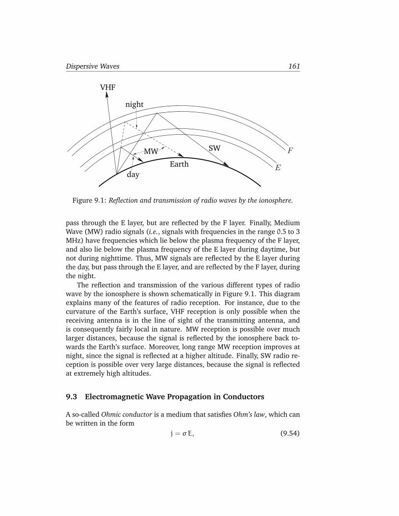
Dispersive Waves 161
EEarth
day
night
SW
VHF
MW F
Figure 9.1: Reflection and transmission of radio waves by the ionosphere.
pass through the E layer, but are reflected by the F layer. Finally, Medium
Wave (MW) radio signals (i.e., signals with frequencies in the range 0.5 to 3
MHz) have frequencies which lie below the plasma frequency of the F layer,
and also lie below the plasma frequency of the E layer during daytime, but
not during nighttime. Thus, MW signals are reflected by the E layer during
the day, but pass through the E layer, and are reflected by the F layer, during
the night.
The reflection and transmission of the various different types of radio
wave by the ionosphere is shown schematically in Figure 9.1. This diagram
explains many of the features of radio reception. For instance, due to the
curvature of the Earth’s surface, VHF reception is only possible when the
receiving antenna is in the line of sight of the transmitting antenna, and
is consequently fairly local in nature. MW reception is possible over much
larger distances, because the signal is reflected by the ionosphere back to-
wards the Earth’s surface. Moreover, long range MW reception improves at
night, since the signal is reflected at a higher altitude. Finally, SW radio re-
ception is possible over very large distances, because the signal is reflected
at extremely high altitudes.
9.3 Electromagnetic Wave Propagation in Conductors
A so-called Ohmic conductor is a medium that satisfies Ohm’s law, which can
be written in the form
j = σE, (9.54)
162 OSCILLATIONS AND WAVES
where j is the current density (i.e., the current per unit area), E the electric
field-strength, and σ a constant known as the conductivity of the medium in
question. (Of course, the current generally flows in the same direction as
the electric field.) The z-directed propagation of an electromagnetic wave,
polarized in the x-direction, through an Ohmic conductor of conductivity σ
is governed by
∂Ex
∂t+σ
ǫ0
Ex = −1
ǫ0
∂Hy
∂z, (9.55)
∂Hy
∂t= −
1
µ0
∂Ex
∂z, (9.56)
For a so-called good conductor, which satisfies the inequality σ ≫ ǫ0ω, the
first term on the left-hand side of Equation (9.55) is negligible with respect
to the second term, and the above two equations can be shown to reduce to
∂Ex
∂t=
1
µ0σ
∂2Ex
∂z2, (9.57)
∂Hy
∂t=
1
µ0
∂Ex
∂z. (9.58)
These equations can be solved to give (see Exercise 4)
Ex(z, t) = E0 e−z/d cos(ωt− z/d), (9.59)
Hy(z, t) = E0Z−1 e−z/d cos(ωt− z/d− π/4), (9.60)
where
d =
(
2
µ0σω
)1/2
, (9.61)
and
Z =
(
ωµ0
σ
)1/2
=
(
ωǫ0
σ
)1/2
Z0. (9.62)
Equations (9.59) and (9.60) indicate that the amplitude of an electromag-
netic wave propagating through a conductor decays exponentially on a char-
acteristic lengthscale, d, which is known as the skin-depth. Consequently, an
electromagnetic wave cannot penetrate more than a few skin-depths into a
conducting medium. Note that the skin-depth is smaller at higher frequen-
cies. This implies that high frequency waves penetrate a shorter distance
into a conductor than low frequency waves.
Dispersive Waves 163
Consider a typical metallic conductor such as copper, whose electrical
conductivity at room temperature is about 6 × 10⁷ (Ωm)−1. Copper, there-
fore, acts as a good conductor for all electromagnetic waves of frequency
below about 1018 Hz. The skin-depth in copper for such waves is thus
d =
√
2
µ0σω≃ 6√
f(Hz)cm. (9.63)
It follows that the skin-depth is about 6 cm at 1 Hz, but only about 2 mm at
1 kHz. This gives rise to the so-called skin-effect in copper wires, by which an
oscillating electromagnetic signal of increasing frequency, transmitted along
such a wire, is confined to an increasingly narrow layer (whose thickness is
of order the skin-depth) on the surface of the wire.
The conductivity of sea-water is only about σ ≃ 5 (Ωm)−1. However,
this is still sufficiently high for sea-water to act as a good conductor for
all radio frequency electromagnetic waves (i.e., f = ω/2π < 1GHz). The
skin-depth at 1 MHz (λ ∼ 2 km) is about 0.2m, whereas that at 1 kHz (λ ∼
2000 km) is still only about 7 m. This obviously poses quite severe restric-
tions for radio communication with submerged submarines. Either the sub-
marines have to come quite close to the surface to communicate (which is
dangerous), or the communication must be performed with extremely low
frequency (ELF) waves (i.e., f < 100Hz). Unfortunately, such waves have
very large wavelengths (λ > 20, 000 km), which means that they can only be
efficiently generated by gigantic antennas.
According to Equation (9.60), the phase of the magnetic component of
an electromagnetic wave propagating through a good conductor lags that of
the electric component by π/4 radians. It follows that the mean energy flux
into the conductor takes the form
〈I〉 = 〈ExHy〉 = |Ex|2Z−1 〈cos(ωt− z/d) cos(ωt− z/d− π/4)〉
=|Ex|
2
√8Z, (9.64)
where |Ex| = E0 e−z/d is the amplitude of the electric component of the
wave. The fact that the mean energy flux is positive indicates that part of
the wave energy is absorbed by the conductor. In fact, the absorbed energy
corresponds to the energy lost due to Ohmic heating in the conductor (see
Exercise 5).
Note, from (9.62), that the impedance of a good conductor is far less
than that of a vacuum (i.e., Z ≪ Z0). This implies that the ratio of the
164 OSCILLATIONS AND WAVES
magnetic to the electric components of an electromagnetic wave propagat-
ing through a good conductor is far larger than that of a wave propagating
through a vacuum.
Suppose that the region z < 0 is a vacuum, and the region z > 0 is
occupied by a good conductor of conductivity σ. Let the wave electric and
magnetic fields in the vacuum region take the form of the incident and re-
flected waves specified in (9.42) and (9.43). The wave electric and magnetic
fields in the conductor are written
Ex(z, t) = Et e−z/d cos(ωt− z/d+ φt), (9.65)
Hy(z, t) = EtZ−10 α−1 e−z/d cos(ωt− z/d− π/4+ φt), (9.66)
where Et is the amplitude of the decaying wave which penetrates into the
conductor, φt is the phase of this wave with respect to the incident wave,
and
α =Z
Z0
=
(
ǫ0ω
σ
)1/2
≪ 1. (9.67)
The appropriate matching conditions are the continuity of Ex and Hy at
z = 0: i.e.,
Ei cos(ωt) + Er cos(ωt+ φr) = Et cos(ωt+ φt), (9.68)
α [Ei cos(ωt) − Er cos(ωt+ φr)] = Et cos(ωt− π/4+ φt).
(9.69)
Equations (9.68) and (9.69), which must be satisfied at all times, can be
solved, in the limit α≪ 1, to give (see Exercise 6)
Er ≃ −(1−√2α)Ei, (9.70)
φr ≃ −√2α, (9.71)
Et ≃ 2αEi, (9.72)
φt ≃ π/4. (9.73)
Hence, the coefficient of reflection becomes
R ≃(
Er
Ei
)2
≃ 1− 2√2α = 1−
(
8 ǫ0ω
σ
)1/2
. (9.74)
According to the above analysis, a good conductor reflects a normally
incident electromagnetic wave with a phase shift of almost π radians (i.e.,
Dispersive Waves 165
Er ≃ −Ei). The coefficient of reflection is just less than unity, indicating
that, whilst most of the incident energy is reflected by the conductor, a small
fraction of it is absorbed.
High-quality metallic mirrors are generally coated in silver, whose con-
ductivity is 6.3×10⁷ (Ωm)−1. It follows, from (9.74), that at optical frequen-
cies (ω = 4× 10¹⁵ rad./s) the coefficient of reflection of a silvered mirror is
R ≃ 93.3%. This implies that about 7% of the light incident on the mirror
is absorbed, rather than being reflected. This rather severe light loss can be
problematic in instruments, such as astronomical telescopes, which are used
to view faint objects.
9.4 Surface Wave Propagation in Water
Consider a stationary body of water, of uniform depth d, located on the sur-
face of the Earth. Let us find the dispersion relation of a wave propagating
across the water’s surface. Suppose that the Cartesian coordinate x mea-
sures horizontal distance, whilst the coordinate z measures vertical height,
with z = 0 corresponding to the unperturbed surface of the water. Let there
be no variation in the y-direction: i.e., let the wavefronts of the wave all be
parallel to the y-axis. Finally, let vx(x, z, t) and vz(x, z, t) be the perturbed
horizontal and vertical velocity fields of the water due to the wave. It is
assumed that there is no motion in the y-direction.
Now, water is essentially incompressible. Thus, any wave disturbance
in water is constrained to preserve the volume of a co-moving volume el-
ement. Equivalently, the inflow rate of water into a stationary volume el-
ement must match the outflow rate. Consider a stationary cubic volume
element lying between x and x + dx, y and y + dy, and z and z + dz. The
element has two faces, of area dydz, perpendicular to the x-axis, located
at x and x + dx. Water flows into the element through the former face at
the rate vx(x, z, t)dydz (i.e., the product of the area of the face and the
normal velocity), and out of the element though the latter face at the rate
vx(x + dx, z, t)dydz. The element also has two faces perpendicular to the
y-axis, but there is no flow through these faces, since vy = 0. Finally, the
element has two faces, of area dxdy, perpendicular to the z-axis, located at
z and z + dz. Water flows into the element through the former face at the
rate vz(x, z, t)dxdy, and out of the element though the latter face at the
rate vz(x, z + dz, t)dxdy. Thus, the net rate at which water flows into the
element is vx(x, z, t)dydz+vz(x, z, t)dxdy. Likewise, the net rate at which
water flows out of the element is vx(x+dx, z, t)dydz+vz(x, z+dz, t)dxdy.
166 OSCILLATIONS AND WAVES
If the water is to remain incompressible then the inflow and outflow rates
must match: i.e.,
vx(x, z, t)dydz+vz(x, z, t)dxdy = vx(x+dx, z, t)dydz+vz(x, z+dz, t)dxdy,
(9.75)
or(
vx(x+ dx, z, t) − vx(x, z, t)
dx+vz(x, z+ dz, t) − vz(x, z, t)
dz
)
dxdydz = 0.
(9.76)
Hence, the incompressibility constraint reduces to
∂vx
∂x+∂vz
∂z= 0. (9.77)
Consider the equation of motion of a small volume element of water ly-
ing between x and x + dx, y and y + dy, and z and z + dz. The mass of
this element is ρdxdydz, where ρ is the uniform mass density of water.
Suppose that p(x, z, t) is the pressure in the water, which is assumed to be
isotropic. The net horizontal force on the element is p(x, z, t)dydz− p(x +
dx, z, t)dydz (since force is pressure times area, and the external pressure
forces acting on the element act inward across its surface). Hence, the ele-
ment’s horizontal equation of motion is
ρdxdydz∂vx(x, z, t)
∂t= −
(
p(x+ dx, z, t) − p(x, z, t)
dx
)
dxdydz, (9.78)
which reduces to
ρ∂vx
∂t= −
∂p
∂x. (9.79)
The vertical equation of motion is similar, except that the element is subject
to a downward acceleration, g, due to gravity. Hence, we obtain
ρ∂vz
∂t= −
∂p
∂z− ρg. (9.80)
Now, we can write
p = p0 − ρg z+ p1, (9.81)
where p0 is atmospheric pressure (i.e., the pressure at the surface of the
water), and p1 is the pressure perturbation due to the wave. Of course, in
the absence of the wave, the water pressure at a depth h below the surface
is p0 + ρgh. Substitution into (9.79) and (9.80) yields
ρ∂vx
∂t= −
∂p1
∂x, (9.82)
ρ∂vz
∂t= −
∂p1
∂z. (9.83)
Dispersive Waves 167
It follows that
ρ∂2vx
∂z ∂t− ρ
∂2vz
∂x ∂t= −
∂2p1
∂z ∂x+∂2p1
∂x ∂z= 0, (9.84)
which implies that
ρ∂
∂t
(
∂vx
∂z−∂vz
∂x
)
= 0, (9.85)
or∂vx
∂z−∂vz
∂x= 0. (9.86)
(Actually, the above quantity could be non-zero and constant in time, but
this is not consistent with an oscillating wave-like solution.)
Equation (9.86) is automatically satisfied if
vx =∂φ
∂x, (9.87)
vz =∂φ
∂z. (9.88)
Equation (9.77) then gives
∂2φ
∂x2+∂2φ
∂z2= 0. (9.89)
Finally, Equations (9.82) and (9.83) yield
p1 = −ρ∂φ
∂t. (9.90)
As we have just seen, surface waves in water are governed by Equation
(9.89), which is known as Laplace’s equation. We next need to derive the
physical constraints which must be satisfied by the solution to this equation
at the water’s upper and lower boundaries. Now, the water is bounded from
below by a solid surface located at z = −d. Assuming that the water always
remains in contact with this surface, the appropriate physical constraint at
the lower boundary is vz(x,−d, t) = 0 (i.e., there is no vertical motion of
the water at the lower boundary), or
∂φ
∂z
∣
∣
∣
∣
z=−d
= 0. (9.91)
The physical constraint at the water’s upper boundary is a little more compli-
cated, since this boundary is a free surface. Let ζ(x, t) represent the vertical
displacement of the water’s surface. It follows that
∂ζ
∂t= vz|z=0 =
∂φ
∂z
∣
∣
∣
∣
z=0
. (9.92)
168 OSCILLATIONS AND WAVES
Now, the physical constraint at the surface is that the water pressure be
equal to atmospheric pressure, since there cannot be a pressure discontinu-
ity across a free surface. Thus, it follows from (9.81) that
p0 = p0 − ρg ζ(x, t) + p1(x, 0, t). (9.93)
Finally, differentiating with respect to t, and making use of Equations (9.90)
and (9.92), we obtain
∂φ
∂z
∣
∣
∣
∣
z=0
= −g−1 ∂2φ
∂t2
∣
∣
∣
∣
∣
z=0
. (9.94)
Hence, the problem boils down to solving Laplace’s equation, (9.89), subject
to the physical constraints (9.91) and (9.94).
Let us search for a propagating wave-like solution of (9.89) of the form
φ(x, z, t) = F(z) cos(k x−ωt). (9.95)
Substitution into (9.89) yields
d2F
dz2− k2 F = 0, (9.96)
whose independent solutions are exp(+k z) and exp(−k z). Hence, the most
general wavelike solution to Laplace’s equation takes the form
φ(x, z, t) = A ekz cos(k x−ωt) + B e−kz cos(k x−ωt), (9.97)
where A and B are arbitrary constants. The boundary condition (9.91) is
satisfied provided that B = A exp(−2 kd), giving
φ(x, z, t) = A[
ekz + e−k(z+2d)]
cos(k x−ωt), (9.98)
The boundary condition (9.94) yields
Ak[
1− e−2kd]
cos(k x−ωt) = Aω2
g
[
1+ e−2kd]
cos(k x−ωt), (9.99)
which reduces to the dispersion relation
ω2 = gk tanh(kd), (9.100)
where the function
tanh x ≡ ex − e−x
ex + e−x(9.101)
Dispersive Waves 169
is known as a hyperbolic tangent.
In shallow water (i.e., kd ≪ 1), Equation (9.100) reduces to the linear
dispersion relation
ω = k√
gd. (9.102)
Here, use has been made of the small argument expansion tanh x ≃ x for
|x| ≪ 1. We, thus, conclude that surface waves in shallow water are non-
dispersive in nature, and propagate at the phase velocity√gd. On the other
hand, in deep water (i.e., kd≫ 1), Equation (9.100) reduces to the nonlin-
ear dispersion relation
ω =√
kg. (9.103)
Here, use has been made of the large argument expansion tanh x ≃ 1 for
x ≫ 1. Hence, we conclude that surface waves in deep water are dispersive
in nature. The phase velocity of the waves is vp = ω/k =√
g/k, whereas
the group velocity is vg = dω/dk = (1/2)√
g/k = vp/2. In other words, the
group velocity is half the phase velocity, and is largest for long wavelength
(i.e., small k) waves.
Water in contact with air actually possesses a surface tension T ≃ 7 ×10⁻² N m−1 which allows there to be a small pressure discontinuity across a
free surface that is curved. In fact,
[p]z=0+
z=0−= −T
∂2ζ
∂x2. (9.104)
Here, (∂ζ/∂x2)−1 is the radius of curvature of the surface. Thus, in the pres-
ence of surface tension, the boundary condition (9.93) takes the modified
form
− T∂2ζ
∂x2= −ρg ζ+ p1|z=0 , (9.105)
which reduces to
∂φ
∂z
∣
∣
∣
∣
z=0
=T
ρ g
∂3φ
∂x2∂z
∣
∣
∣
∣
∣
z=0
−1
g
∂2φ
∂t2
∣
∣
∣
∣
∣
z=0
. (9.106)
This boundary condition can be combined with the solution (9.98), in the
deep water limit kd ≫ 1, to give the modified deep water dispersion rela-
tion
ω =
√
gk+T
ρk3. (9.107)
Hence, the phase velocity of the waves takes the form
vp =ω
k=
√
g
k+T
ρk, (9.108)
170 OSCILLATIONS AND WAVES
and the ratio of the group velocity to the phase velocity can be shown to be
vg
vp=1
2
[
1+ 3 T k2/(ρg)
1+ T k2/(ρg)
]
. (9.109)
Thus, the phase velocity attains a minimum value of√2 (g T/ρ)1/4 ∼ 0.2m s−1
when k = k0 ≡ (ρg/T)1/2, which corresponds to λ ∼ 2 cm. The group veloc-
ity equals the phase velocity at this wavelength. For long wavelength waves
(i.e., k ≪ k0), gravity dominates surface tension, the phase velocity scales
as k−1/2, and the group velocity is half the phase velocity. On the other
hand, for short wavelength waves (i.e., k≫ k0), surface tension dominates
gravity, the phase velocity scales as k1/2, and the group velocity is 3/2 times
the phase velocity. The fact that the phase velocity and the group veloc-
ity both attain minimum values when λ ∼ 2 cm means that when a wave
disturbance containing a wide spectrum of wavelengths, such as might be
generated by throwing a rock into the water, travels across the surface of
a lake, and reaches the shore, the short and long wavelength components
of the disturbance generally arrive before the components of intermediate
wavelength.
9.5 Exercises
1. Derive expressions (9.27) and (9.29) for propagating electromagnetic wavesin a plasma from Equations (9.20), (9.22), (9.24), and (9.25).
2. Derive expressions (9.39) and (9.40) for evanescent electromagnetic wavesin a plasma from Equations (9.20), (9.22), (9.24), and (9.25).
3. Derive Equations (9.49)–(9.52) from Equations (9.47) and (9.48).
4. Derive Equations (9.59)–(9.62) from Equations (9.57) and (9.58).
5. Consider an electromagnetic wave propagating in the positive z-directionthrough a conducting medium of conductivity σ. Suppose that the waveelectric field is
Ex(z, t) = E0 e−z/d cos(ωt− z/d),
where d is the skin-depth. Demonstrate that the mean electromagnetic en-ergy flux across the plane z = 0 matches the mean rate at which electromag-netic energy is dissipated, per unit area, due to Ohmic heating in the regionz > 0. (The rate of ohmic heating per unit volume is σE 2
x ).
6. Derive Equations (9.70)–(9.73) from Equations (9.68) and (9.69), in thelimit α≪ 1.
Dispersive Waves 171
7. Demonstrate that the phase velocity of traveling waves on an infinitely longbeaded string is
vp = v0
sin(ka/2)
(ka/2),
where v0 =√
T a/m, T is the tension in the string, a the spacing betweenthe beads, m the mass of the beads, and k the wavenumber of the wave.What is the group velocity?
8. The number density of free electrons in the ionosphere, ne, as a functionof vertical height, z, is measured by timing how long it takes a radio pulselaunched vertically upward from the ground (z = 0) to return to ground levelagain, after reflection by the ionosphere, as a function of the pulse frequency,ω. It is conventional to define the equivalent height, h(ω), of the reflectionlayer as the height it would need to have off the ground if the pulse alwaystraveled at the velocity of light in vacuum. Demonstrate that
h(ω) =
∫z0
0
dz
[1−ω 2p(z)/ω2]1/2
,
where ω 2p(z) = ne(z) e2/(ǫ0me), and ω 2
p(z0) = ω2. Show that if ne ∝ zp
then h ∝ ω2/p.
9. A uniform rope of mass per unit length ρ and length L hangs vertically. De-termine the tension T in the rope as a function of height from the bottom ofthe rope. Show that the time required for a transverse wave pulse to travelfrom the bottom to the top of the rope is 2
√
L/g.
10. The aluminium foil used in cooking has an electrical conductivity σ = 3.5 ×10⁷ (Ωm)−1, and a typical thickness δ = 2× 10⁻⁴ m. Show that such foil canbe used to shield a region from electromagnetic waves of a given frequency,provided that the skin-depth of the waves in the foil is less than about athird of its thickness. Since skin-depth increases as frequency decreases, itfollows that the foil can only shield waves whose frequency exceeds a criticalvalue. Estimate this critical frequency (in Hertz). What is the correspondingwavelength?
11. A sinusoidal surface wave travels from deep water toward the shore. Does itswavelength increase, decrease, or stay the same, as it approaches the shore?Explain.
12. Demonstrate that the dispersion relation (9.107) for surface water wavesgeneralizes to
ω2 =
(
gk+T
ρk3
)
tanh(kd)
in water of arbitrary depth.
172 OSCILLATIONS AND WAVES
13. Demonstrate that a small amplitude surface wave, of angular frequency ωand wavenumber k, traveling over the surface of a lake of uniform depth dcauses an individual water volume element located at a depth h below thesurface to execute a non-propagating elliptical orbit whose major and mi-nor axes are horizontal and vertical, respectively. Show that the variation ofthe major and minor radii of the orbit with depth is A cosh[k (d − h)] andA sinh[k (d − h)], respectively, where A is a constant. Demonstrate that thevolume elements are moving horizontally in the same direction as the waveat the top of their orbits, and in the opposite direction at the bottom. Showthat a surface wave traveling over the surface of a very deep lake causes wa-ter volume elements to execute non-propagating circular orbits whose radiidecrease exponentially with depth.
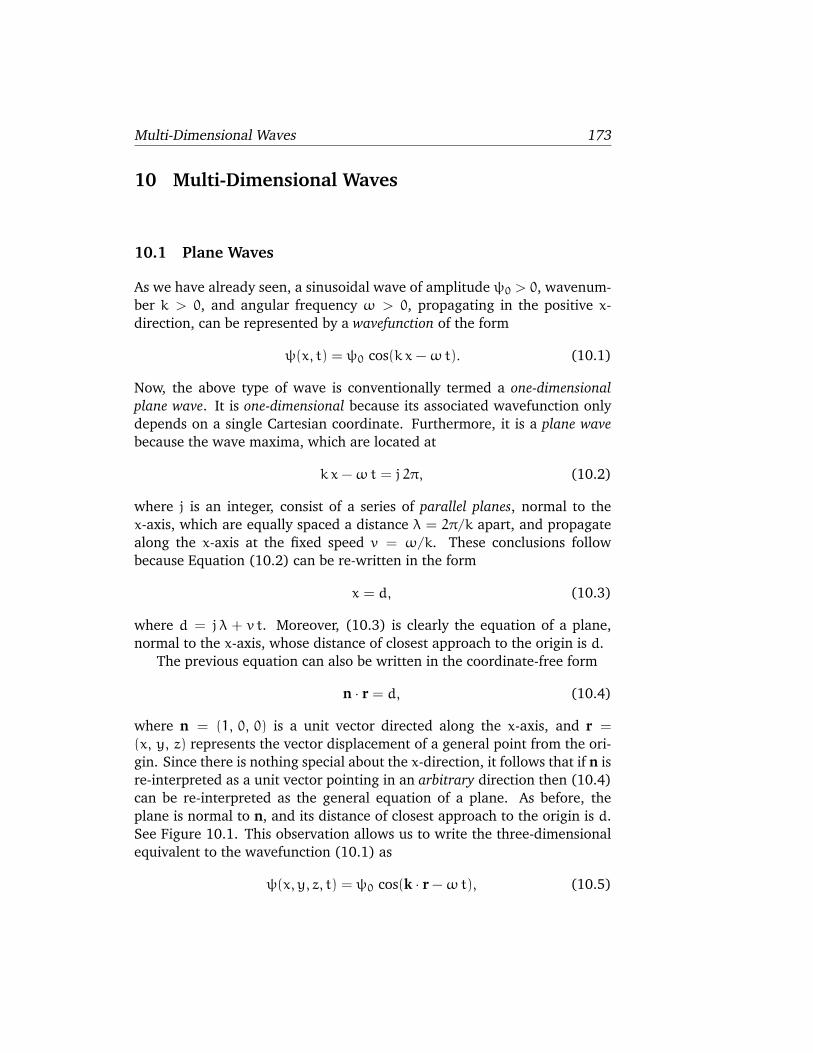
Multi-Dimensional Waves 173
10 Multi-Dimensional Waves
10.1 Plane Waves
As we have already seen, a sinusoidal wave of amplitude ψ0 > 0, wavenum-
ber k > 0, and angular frequency ω > 0, propagating in the positive x-
direction, can be represented by a wavefunction of the form
ψ(x, t) = ψ0 cos(k x−ωt). (10.1)
Now, the above type of wave is conventionally termed a one-dimensional
plane wave. It is one-dimensional because its associated wavefunction only
depends on a single Cartesian coordinate. Furthermore, it is a plane wave
because the wave maxima, which are located at
k x−ωt = j 2π, (10.2)
where j is an integer, consist of a series of parallel planes, normal to the
x-axis, which are equally spaced a distance λ = 2π/k apart, and propagate
along the x-axis at the fixed speed v = ω/k. These conclusions follow
because Equation (10.2) can be re-written in the form
x = d, (10.3)
where d = j λ + v t. Moreover, (10.3) is clearly the equation of a plane,
normal to the x-axis, whose distance of closest approach to the origin is d.
The previous equation can also be written in the coordinate-free form
n · r = d, (10.4)
where n = (1, 0, 0) is a unit vector directed along the x-axis, and r =
(x, y, z) represents the vector displacement of a general point from the ori-
gin. Since there is nothing special about the x-direction, it follows that if n is
re-interpreted as a unit vector pointing in an arbitrary direction then (10.4)
can be re-interpreted as the general equation of a plane. As before, the
plane is normal to n, and its distance of closest approach to the origin is d.
See Figure 10.1. This observation allows us to write the three-dimensional
equivalent to the wavefunction (10.1) as
ψ(x, y, z, t) = ψ0 cos(k · r −ωt), (10.5)
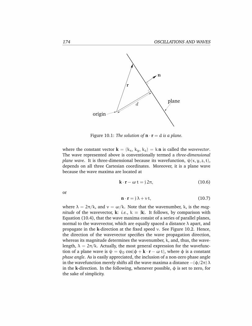
174 OSCILLATIONS AND WAVES
dplane
r
origin
n
Figure 10.1: The solution of n · r = d is a plane.
where the constant vector k = (kx, ky, kz) = kn is called the wavevector.
The wave represented above is conventionally termed a three-dimensional
plane wave. It is three-dimensional because its wavefunction, ψ(x, y, z, t),
depends on all three Cartesian coordinates. Moreover, it is a plane wave
because the wave maxima are located at
k · r −ωt = j 2π, (10.6)
or
n · r = j λ+ v t, (10.7)
where λ = 2π/k, and v = ω/k. Note that the wavenumber, k, is the mag-
nitude of the wavevector, k: i.e., k ≡ |k|. It follows, by comparison with
Equation (10.4), that the wave maxima consist of a series of parallel planes,
normal to the wavevector, which are equally spaced a distance λ apart, and
propagate in the k-direction at the fixed speed v. See Figure 10.2. Hence,
the direction of the wavevector specifies the wave propagation direction,
whereas its magnitude determines the wavenumber, k, and, thus, the wave-
length, λ = 2π/k. Actually, the most general expression for the wavefunc-
tion of a plane wave is ψ = ψ0 cos(φ + k · r −ωt), where φ is a constant
phase angle. As is easily appreciated, the inclusion of a non-zero phase angle
in the wavefunction merely shifts all the wave maxima a distance −(φ/2π) λ
in the k-direction. In the following, whenever possible, φ is set to zero, for
the sake of simplicity.
Multi-Dimensional Waves 175
k
λ
Figure 10.2: Wave maxima associated with a plane wave.
10.2 Three-Dimensional Wave Equation
As is readily demonstrated (see Exercise 1), the one-dimensional plane wave
solution (10.1) satisfies the one-dimensional wave equation,
∂2ψ
∂t2= v2 ∂
2ψ
∂x2. (10.8)
Likewise, the three-dimensional plane wave solution (10.5) satisfies the
three-dimensional wave equation (see Exercise 1),
∂2ψ
∂t2= v2
(
∂2
∂x2+∂2
∂y2+∂2
∂z2
)
ψ. (10.9)
Note that both of these equations are linear, and, thus, have superposable
solutions.
10.3 Laws of Geometric Optics
Suppose that the region z < 0 is occupied by a transparent dielectric medium
of refractive index n1, whereas the region z > 0 is occupied by a second
transparent dielectric medium of refractive index n2. Let a plane light wave
be launched, toward positive z, from a light source of angular frequency ω
located at large negative z. Suppose that this so-called incident wave has
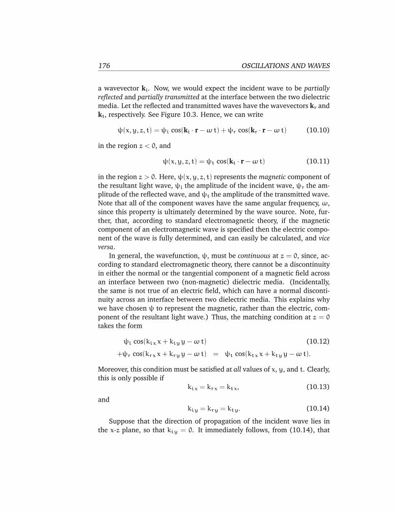
176 OSCILLATIONS AND WAVES
a wavevector ki. Now, we would expect the incident wave to be partially
reflected and partially transmitted at the interface between the two dielectric
media. Let the reflected and transmitted waves have the wavevectors kr and
kt, respectively. See Figure 10.3. Hence, we can write
ψ(x, y, z, t) = ψi cos(ki · r −ωt) +ψr cos(kr · r −ωt) (10.10)
in the region z < 0, and
ψ(x, y, z, t) = ψt cos(kt · r −ωt) (10.11)
in the region z > 0. Here, ψ(x, y, z, t) represents the magnetic component of
the resultant light wave, ψi the amplitude of the incident wave, ψr the am-
plitude of the reflected wave, and ψt the amplitude of the transmitted wave.
Note that all of the component waves have the same angular frequency, ω,
since this property is ultimately determined by the wave source. Note, fur-
ther, that, according to standard electromagnetic theory, if the magnetic
component of an electromagnetic wave is specified then the electric compo-
nent of the wave is fully determined, and can easily be calculated, and vice
versa.
In general, the wavefunction, ψ, must be continuous at z = 0, since, ac-
cording to standard electromagnetic theory, there cannot be a discontinuity
in either the normal or the tangential component of a magnetic field across
an interface between two (non-magnetic) dielectric media. (Incidentally,
the same is not true of an electric field, which can have a normal disconti-
nuity across an interface between two dielectric media. This explains why
we have chosen ψ to represent the magnetic, rather than the electric, com-
ponent of the resultant light wave.) Thus, the matching condition at z = 0
takes the form
ψi cos(kixx+ kiyy−ωt) (10.12)
+ψr cos(krxx+ kryy−ωt) = ψt cos(ktxx+ ktyy−ωt).
Moreover, this condition must be satisfied at all values of x, y, and t. Clearly,
this is only possible if
kix = krx = ktx, (10.13)
and
kiy = kry = kty. (10.14)
Suppose that the direction of propagation of the incident wave lies in
the x-z plane, so that kiy = 0. It immediately follows, from (10.14), that
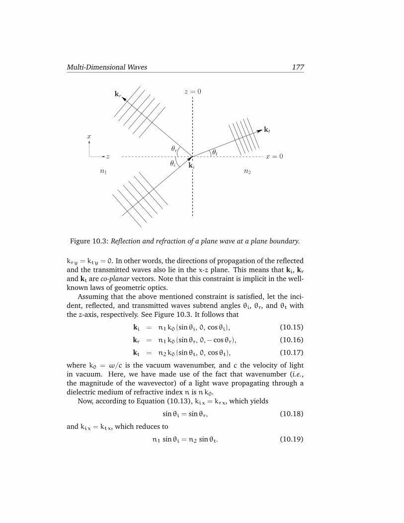
Multi-Dimensional Waves 177
n2n1
θr
kt
x = 0
kr
θi
θt
z = 0
x
z
ki
Figure 10.3: Reflection and refraction of a plane wave at a plane boundary.
kry = kty = 0. In other words, the directions of propagation of the reflected
and the transmitted waves also lie in the x-z plane. This means that ki, kr
and kt are co-planar vectors. Note that this constraint is implicit in the well-
known laws of geometric optics.
Assuming that the above mentioned constraint is satisfied, let the inci-
dent, reflected, and transmitted waves subtend angles θi, θr, and θt with
the z-axis, respectively. See Figure 10.3. It follows that
ki = n1k0 (sin θi, 0, cos θi), (10.15)
kr = n1k0 (sin θr, 0,− cosθr), (10.16)
kt = n2k0 (sin θt, 0, cos θt), (10.17)
where k0 = ω/c is the vacuum wavenumber, and c the velocity of light
in vacuum. Here, we have made use of the fact that wavenumber (i.e.,
the magnitude of the wavevector) of a light wave propagating through a
dielectric medium of refractive index n is nk0.
Now, according to Equation (10.13), kix = krx, which yields
sin θi = sin θr, (10.18)
and kix = ktx, which reduces to
n1 sin θi = n2 sin θt. (10.19)
178 OSCILLATIONS AND WAVES
The first of these relations states that the angle of incidence, θi, is equal to
the angle of reflection, θr. Of course, this is the familiar law of reflection.
Moreover, the second relation corresponds to the equally familiar law of
refraction, otherwise known as Snell’s law.
Incidentally, the fact that a plane wave propagates through a uniform
medium with a constant wavevector, and, therefore, a constant direction of
propagation, is equivalent to the well known law of rectilinear propagation,
which states that light propagates through a uniform medium in a straight-
line.
It is clear, from the above discussion, that the laws of geometric optics
(i.e., the law of rectilinear propagation, the law of reflection, and the law of
refraction) are fully consistent with the wave properties of light, despite the
fact that they do not appear to explicitly depend on these properties.
10.4 Waveguides
As we saw in Section 7.5, transmission lines (e.g., ethernet cables) are used
to carry high frequency electromagnetic signals over distances which are
long compared to the signal wavelength, λ = c/f, where c is the veloc-
ity of light and f the signal frequency (in Hertz). Unfortunately, conven-
tional transmission lines are subject to radiative losses (since the lines ef-
fectively act as antennas) which increase as the fourth power of the signal
frequency. Above a certain critical frequency, which typically lies in the mi-
crowave band, the radiative losses become intolerably large. Under these
circumstances, the transmission line must be replaced by a device known as
a waveguide. A waveguide is basically a long hollow metal box within which
electromagnetic signals propagate. Moreover, if the walls of the box are
much thicker than the skin-depth (see Section 9.3) in the wall material then
the signal is essentially isolated from the outside world, and the radiative
losses are consequently negligible.
Consider an evacuated waveguide of rectangular cross-section which
runs along the z-direction, and is enclosed by perfectly conducting (i.e.,
infinite conductivity) metal walls located at x = 0, x = a, y = 0, and y = b.
Suppose that an electromagnetic wave propagates along the waveguide in
the z-direction. For the sake of simplicity, let there be no y-variation of
the wave electric or magnetic fields. Now, the wave propagation inside the
waveguide is governed by the two-dimensional wave equation [cf., Equa-
Multi-Dimensional Waves 179
tion (10.9)]∂2ψ
∂t2= c2
(
∂2
∂x2+∂2
∂z2
)
ψ, (10.20)
where ψ(x, z, t) represents the electric component of the wave, which is as-
sumed to be everywhere parallel to the y-axis, and c is the velocity of light
in vaccum. The appropriate boundary conditions are
ψ(0, z, t) = 0, (10.21)
ψ(a, z, t) = 0, (10.22)
since the electric field inside a perfect conductor is zero (otherwise, an infi-
nite current would flow), and, according to standard electromagnetic theory,
there cannot be a tangential discontinuity in the electric field at a conduc-
tor/vacuum boundary. (There can, however, be a normal discontinuity. This
allows ψ to be non-zero at y = 0 and y = b.)
Let us search for a separable solution of (10.20) of the form
ψ(x, z, t) = ψ0 sin(kxx) cos(k z−ωt), (10.23)
where k represents the z-component of the wavevector (rather than its mag-
nitude), and is the effective wavenumber for propagation along the waveg-
uide. The above solution automatically satisfies the boundary condition
(10.21). The second boundary condition (10.22) is satisfied provided
kx = jπ
a, (10.24)
where j is a positive integer. Suppose that j takes its smallest possible value
1. (Of course, j cannot be zero, since, in this case, ψ = 0 everywhere.)
Substitution of expression (10.23) into the wave equation (10.20) yields
the dispersion relation
ω2 = k2 c2 +ω20 , (10.25)
where
ω0 =π c
a. (10.26)
Note that this dispersion relation is analogous in form to the dispersion
relation (9.27) for an electromagnetic wave propagating through a plasma,
with the cut-off frequency, ω0, playing the role of the plasma frequency, ωp.
The cut-off frequency is so-called because for ω < ω0 the wavenumber is
imaginary (i.e., k2 < 0), which implies that the wave does not propagate
along the waveguide, but, instead, decays exponentially with increasing z.
180 OSCILLATIONS AND WAVES
On the other hand, for wave frequencies above the cut-off frequency the
phase velocity,
vp =ω
k=
c√
1−ω20/ω
2, (10.27)
is superluminal. This is not a problem, however, since the group velocity,
vg =dω
dk= c
√
1−ω20/ω
2, (10.28)
which is the true signal velocity, remains subluminal. (Recall, from Sec-
tion 9.2, that a high frequency electromagnetic wave propagating through a
plasma exhibits similar behavior.) Not surprisingly, the signal velocity goes
to zero asω → ω0, since the signal ceases to propagate at all whenω = ω0.
It turns out that waveguides support many distinct modes of propaga-
tion. The type of mode discussed above is termed a TE (for transverse
electric-field) mode, since the electric field is transverse to the direction
of propagation. There are many different sorts of TE mode, corresponding,
for instance, to different choices of the mode number, j. However, the j = 1
mode has the lowest cut-off frequency. There are also TM (for transverse
magnetic-field) modes, and TEM (for transverse electric- and magnetic-
field) modes. TM modes also only propagate when the wave frequency
exceeds a cut-off frequency. On the other hand, TEM modes (which are the
same type of mode as that supported by a conventional transmission line)
propagate at all frequencies. Note, however, that TEM modes are only pos-
sible when the waveguide possesses an internal conductor running along its
length.
10.5 Cylindrical Waves
Consider a cylindrically symmetric wavefunctionψ(ρ, t), where ρ =√
x2 + y2
is a conventional cylindrical polar coordinate. Assuming that this func-
tion satisfies the three-dimensional wave equation (10.9), which can be re-
written (see Exercise 3)
∂2ψ
∂t2= v2
(
∂2ψ
∂ρ2+1
ρ
∂ψ
∂ρ
)
, (10.29)
it is easily demonstrated that a sinusoidal cylindrical wave of phase angle φ,
wavenumber k, and angular frequencyω = k v, takes the form (see Exercise
3)
ψ(ρ, t) ≃ ψ0
ρ1/2cos(φ+ k ρ−ωt) (10.30)
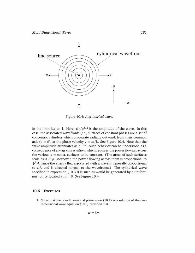
Multi-Dimensional Waves 181
cylindrical wavefront
y
x
line source
v
v
vv
Figure 10.4: A cylindrical wave.
in the limit k ρ ≫ 1. Here, ψ0/ρ1/2 is the amplitude of the wave. In this
case, the associated wavefronts (i.e., surfaces of constant phase) are a set of
concentric cylinders which propagate radially outward, from their common
axis (ρ = 0), at the phase velocity v = ω/k. See Figure 10.4. Note that the
wave amplitude attenuates as ρ−1/2. Such behavior can be understood as a
consequence of energy conservation, which requires the power flowing across
the various ρ = const. surfaces to be constant. (The areas of such surfaces
scale as A ∝ ρ. Moreover, the power flowing across them is proportional to
ψ2A, since the energy flux associated with a wave is generally proportional
to ψ2, and is directed normal to the wavefronts.) The cylindrical wave
specified in expression (10.30) is such as would be generated by a uniform
line source located at ρ = 0. See Figure 10.4.
10.6 Exercises
1. Show that the one-dimensional plane wave (10.1) is a solution of the one-dimensional wave equation (10.8) provided that
ω = k v.
182 OSCILLATIONS AND WAVES
Likewise, demonstrate that the three-dimensional plane wave (10.5) is a so-lution of the three-dimensional wave equation (10.9) as long as
ω = |k| v.
2. Consider a square waveguide of internal dimensions 5 × 10 cm. What is thefrequency (in MHz) of the lowest frequency TE mode which will propagatealong the waveguide without attenuation? What are the phase and groupvelocities (expressed as multiples of c) for a TE mode whose frequency is 5/4times this cut-off frequency?
3. Demonstrate that for a cylindrically symmetric wavefunction ψ(ρ, t), where
ρ =√
x2 + y2, the three-dimensional wave equation (10.9) can be re-written
∂2ψ
∂t2= v2
(
∂2ψ
∂ρ2+1
ρ
∂ψ
∂ρ
)
.
Show that
ψ(ρ, t) ≃ ψ0
ρ1/2cos(φ+ k ρ−ωt)
is an approximate solution of this equation in the limit k ρ ≫ 1, where v =
ω/k.
4. Demonstrate that for a spherically symmetric wavefunction ψ(r, t), where
r =√
x2 + y2 + z2, the three-dimensional wave equation (10.9) can be re-written
∂2ψ
∂t2= v2
(
∂2ψ
∂r2+2
r
∂ψ
∂r
)
.
Show that
ψ(r, t) =ψ0
rcos(φ+ k r−ωt)
is a solution of this equation, where v = ω/k. Explain why the wave am-plitude attenuates as r−1. What sort of wave source would be most likely togenerate the above type of wave solution?
Wave Optics 183
11 Wave Optics
11.1 Introduction
Visible light is a type of electromagnetic radiation whose wavelength lies in
a relatively narrow band extending from about 400 to 700 nm. The branch
of physics which is concerned with the properties of light is known as op-
tics. This chapter is devoted to those optical phenomena which depend
explicitly on the ultimate wave nature of light, and cannot be accounted
for using the well-known laws of geometric optics (see Section 10.3). The
branch of optics which deals with such phenomena is called wave optics.
The two most important topics in wave optics are interference and diffrac-
tion. Interference occurs when beams of light from multiple sources (but
with similar frequencies), or multiple beams from the same source, inter-
sect one another. Diffraction takes place, for instance, when a single beam
of light passes through an opening in an opaque screen whose spatial ex-
tent is comparable to the wavelength of the light. It should be noted that
interference and diffraction depend on the same underlying physical mech-
anisms, so that the distinction which is conventionally made between them
is somewhat arbitrary.
In the following, for the sake of simplicity, we shall only deal with light
emitted from uniform line sources interacting with uniform slits which run
parallel to these sources, since, under such circumstances, the problem re-
mains essentially two-dimensional.
11.2 Two-Slit Interference
Consider a monochromatic plane light wave, propagating in the x-direction,
through a transparent dielectric medium of refractive index unity (e.g., a
vacuum). (Such a wave might be produced by a uniform line source, run-
ning parallel to the z-axis, which is located at x = −∞.) Let the associated
wavefunction take the form
ψ(x, t) = ψ0 cos(φ+ k x−ωt). (11.1)
Here, ψ represents the electric component of the wave, ψ0 > 0 the wave
amplitude, φ the phase angle, k > 0 the wavenumber, ω = k c the angular
frequency, and c the velocity of light in vacuum. Let the wave be normally
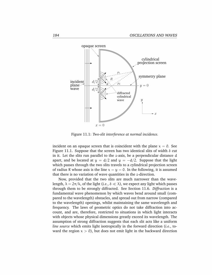
184 OSCILLATIONS AND WAVES
R
cylindrical
symmetry plane
x
planewave
ρ1
x = 0
opaque screen
projection screen
y
y = 0
diffractedcylindricalwave
ρ2d/2
d/2
θincident
Figure 11.1: Two-slit interference at normal incidence.
incident on an opaque screen that is coincident with the plane x = 0. See
Figure 11.1. Suppose that the screen has two identical slits of width δ cut
in it. Let the slits run parallel to the z-axis, be a perpendicular distance d
apart, and be located at y = d/2 and y = −d/2. Suppose that the light
which passes through the two slits travels to a cylindrical projection screen
of radius R whose axis is the line x = y = 0. In the following, it is assumed
that there is no variation of wave quantities in the z-direction.
Now, provided that the two slits are much narrower than the wave-
length, λ = 2π/k, of the light (i.e., δ≪ λ), we expect any light which passes
through them to be strongly diffracted. See Section 11.6. Diffraction is a
fundamental wave phenomenon by which waves bend around small (com-
pared to the wavelength) obstacles, and spread out from narrow (compared
to the wavelength) openings, whilst maintaining the same wavelength and
frequency. The laws of geometric optics do not take diffraction into ac-
count, and are, therefore, restricted to situations in which light interacts
with objects whose physical dimensions greatly exceed its wavelength. The
assumption of strong diffraction suggests that each slit acts like a uniform
line source which emits light isotropically in the forward direction (i.e., to-
ward the region x > 0), but does not emit light in the backward direction
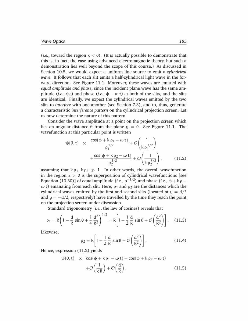
Wave Optics 185
(i.e., toward the region x < 0). (It is actually possible to demonstrate that
this is, in fact, the case using advanced electromagnetic theory, but such a
demonstration lies well beyond the scope of this course.) As discussed in
Section 10.5, we would expect a uniform line source to emit a cylindrical
wave. It follows that each slit emits a half-cylindrical light wave in the for-
ward direction. See Figure 11.1. Moreover, these waves are emitted with
equal amplitude and phase, since the incident plane wave has the same am-
plitude (i.e., ψ0) and phase (i.e., φ −ωt) at both of the slits, and the slits
are identical. Finally, we expect the cylindrical waves emitted by the two
slits to interfere with one another (see Section 7.3), and to, thus, generate
a characteristic interference pattern on the cylindrical projection screen. Let
us now determine the nature of this pattern.
Consider the wave amplitude at a point on the projection screen which
lies an angular distance θ from the plane y = 0. See Figure 11.1. The
wavefunction at this particular point is written
ψ(θ, t) ∝ cos(φ+ k ρ1 −ωt)
ρ1/21
+ O(
1
k ρ3/21
)
+cos(φ+ k ρ2 −ωt)
ρ1/22
+ O(
1
k ρ3/22
)
, (11.2)
assuming that k ρ1, k ρ2 ≫ 1. In other words, the overall wavefunction
in the region x > 0 is the superposition of cylindrical wavefunctions [see
Equation (10.30)] of equal amplitude (i.e., ρ−1/2) and phase (i.e., φ+ k ρ−
ωt) emanating from each slit. Here, ρ1 and ρ2 are the distances which the
cylindrical waves emitted by the first and second slits (located at y = d/2
and y = −d/2, respectively) have travelled by the time they reach the point
on the projection screen under discussion.
Standard trigonometry (i.e., the law of cosines) reveals that
ρ1 = R
(
1−d
Rsin θ+
1
4
d2
R2
)1/2
= R
[
1−1
2
d
Rsin θ+ O
(
d2
R2
)]
. (11.3)
Likewise,
ρ2 = R
[
1+1
2
d
Rsin θ+ O
(
d2
R2
)]
. (11.4)
Hence, expression (11.2) yields
ψ(θ, t) ∝ cos(φ+ k ρ1 −ωt) + cos(φ+ k ρ2 −ωt)
+O(
1
kR
)
+ O(
d
R
)
, (11.5)
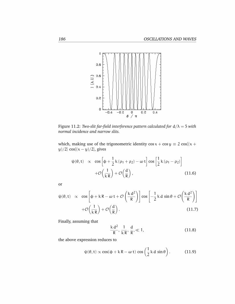
186 OSCILLATIONS AND WAVES
Figure 11.2: Two-slit far-field interference pattern calculated for d/λ = 5 with
normal incidence and narrow slits.
which, making use of the trigonometric identity cos x + cosy ≡ 2 cos[(x +
y)/2] cos[(x− y)/2], gives
ψ(θ, t) ∝ cos
[
φ+1
2k (ρ1 + ρ2) −ωt
]
cos
[
1
2k (ρ1 − ρ2)
]
+O(
1
kR
)
+ O(
d
R
)
, (11.6)
or
ψ(θ, t) ∝ cos
[
φ+ kR−ωt+ O(
kd2
R
)]
cos
[
−1
2kd sin θ+ O
(
kd2
R
)]
+O(
1
kR
)
+ O(
d
R
)
. (11.7)
Finally, assuming that
kd2
R,1
kR,d
R,≪ 1, (11.8)
the above expression reduces to
ψ(θ, t) ∝ cos(φ+ kR−ωt) cos
(
1
2kd sin θ
)
. (11.9)
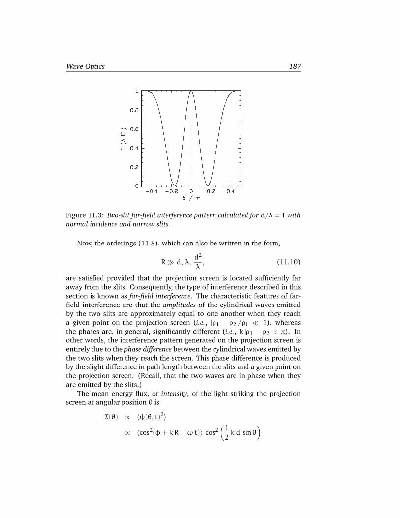
Wave Optics 187
Figure 11.3: Two-slit far-field interference pattern calculated for d/λ = 1 with
normal incidence and narrow slits.
Now, the orderings (11.8), which can also be written in the form,
R≫ d, λ,d2
λ, (11.10)
are satisfied provided that the projection screen is located sufficiently far
away from the slits. Consequently, the type of interference described in this
section is known as far-field interference. The characteristic features of far-
field interference are that the amplitudes of the cylindrical waves emitted
by the two slits are approximately equal to one another when they reach
a given point on the projection screen (i.e., |ρ1 − ρ2|/ρ1 ≪ 1), whereas
the phases are, in general, significantly different (i.e., k |ρ1 − ρ2|>∼π). In
other words, the interference pattern generated on the projection screen is
entirely due to the phase difference between the cylindrical waves emitted by
the two slits when they reach the screen. This phase difference is produced
by the slight difference in path length between the slits and a given point on
the projection screen. (Recall, that the two waves are in phase when they
are emitted by the slits.)
The mean energy flux, or intensity, of the light striking the projection
screen at angular position θ is
I(θ) ∝ 〈ψ(θ, t)2〉
∝ 〈cos2(φ+ kR−ωt)〉 cos2
(
1
2kd sin θ
)
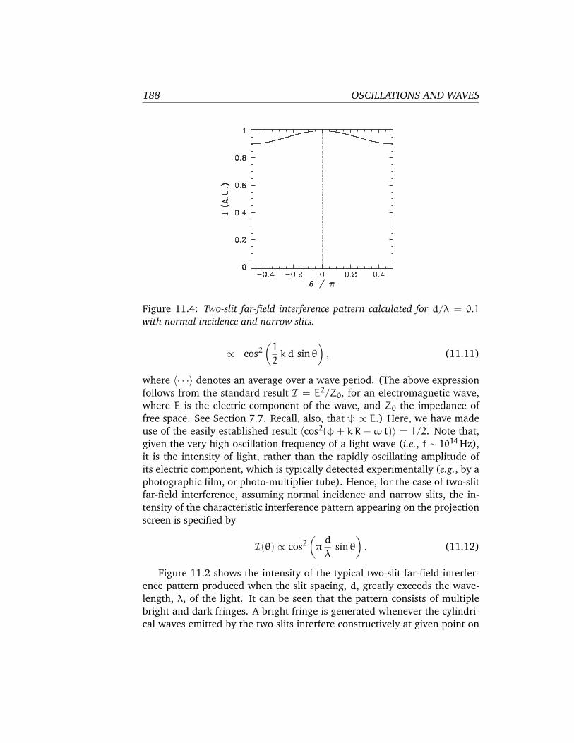
188 OSCILLATIONS AND WAVES
Figure 11.4: Two-slit far-field interference pattern calculated for d/λ = 0.1
with normal incidence and narrow slits.
∝ cos2
(
1
2kd sin θ
)
, (11.11)
where 〈· · ·〉 denotes an average over a wave period. (The above expression
follows from the standard result I = E2/Z0, for an electromagnetic wave,
where E is the electric component of the wave, and Z0 the impedance of
free space. See Section 7.7. Recall, also, that ψ ∝ E.) Here, we have made
use of the easily established result 〈cos2(φ + kR −ωt)〉 = 1/2. Note that,
given the very high oscillation frequency of a light wave (i.e., f ∼ 1014 Hz),
it is the intensity of light, rather than the rapidly oscillating amplitude of
its electric component, which is typically detected experimentally (e.g., by a
photographic film, or photo-multiplier tube). Hence, for the case of two-slit
far-field interference, assuming normal incidence and narrow slits, the in-
tensity of the characteristic interference pattern appearing on the projection
screen is specified by
I(θ) ∝ cos2
(
πd
λsin θ
)
. (11.12)
Figure 11.2 shows the intensity of the typical two-slit far-field interfer-
ence pattern produced when the slit spacing, d, greatly exceeds the wave-
length, λ, of the light. It can be seen that the pattern consists of multiple
bright and dark fringes. A bright fringe is generated whenever the cylindri-
cal waves emitted by the two slits interfere constructively at given point on
Wave Optics 189
the projection screen. This occurs if the path lengths between the two slits
and the point in question differ by an integer number of wavelengths: i.e.,
ρ2 − ρ1 = d sin θ = j λ, (11.13)
where j is an integer, since this ensures that the phases of the two waves
differ by an integer multiple of 2π, and, hence, that the effective phase dif-
ference is zero. Likewise, a dark fringe is generated whenever the cylindrical
waves emitted by the two slits interfere destructively at a given point on the
projection screen. This occurs if the path lengths between the two slits and
the point in question differ by a half-integer number of wavelengths: i.e.,
ρ2 − ρ1 = d sin θ = (j+ 1/2) λ, (11.14)
since this ensures that the effective phase difference between the two waves
is π. We conclude that the innermost (i.e., low j, small θ) bright fringes are
approximately equally-spaced, with a characteristic angular width ∆θ ≃ λ/d.
This result, which follows from Equation (11.13), and the small angle ap-
proximation sin θ ≃ θ, can be used experimentally to determine the wave-
length of a monochromatic light source (see Exercise 11.4).
Figure 11.3 shows the intensity of the interference pattern generated
when the slit spacing is equal to the wavelength of the light. It can be seen
that the width of the central (i.e., j = 0, θ = 0) bright fringe has expanded to
such an extent that the fringe occupies almost half of the projection screen,
leaving room for just two dark fringes on either side of it.
Finally, Figure 11.4 shows the intensity of the interference pattern gen-
erated when the slit spacing is much less than the wavelength of the light. It
can be seen that the width of the central bright fringe has expanded to such
an extent that the band occupies the whole projection screen, and there are
no dark fringes. Indeed, I(θ) becomes constant in the limit that d/λ ≪ 1,
in which case the interference pattern entirely disappears.
It is clear, from Figures 11.2–11.3, that the two-slit far-field interference
apparatus shown in Figure 11.1 only generates an interesting interference
patten when the slit spacing, d, is greater than the wavelength, λ, of the
light.
Suppose, now, that the plane wave which illuminates the interference
apparatus is not normally incident on the slits, but instead propagates at an
angle θ0 to the x-axis, as shown in Figure 11.5. In this case, the incident
wavefunction (11.1) becomes
ψ(x, y, t) = ψ0 cos(φ+ k x cos θ0 + ky sin θ0 −ωt). (11.15)
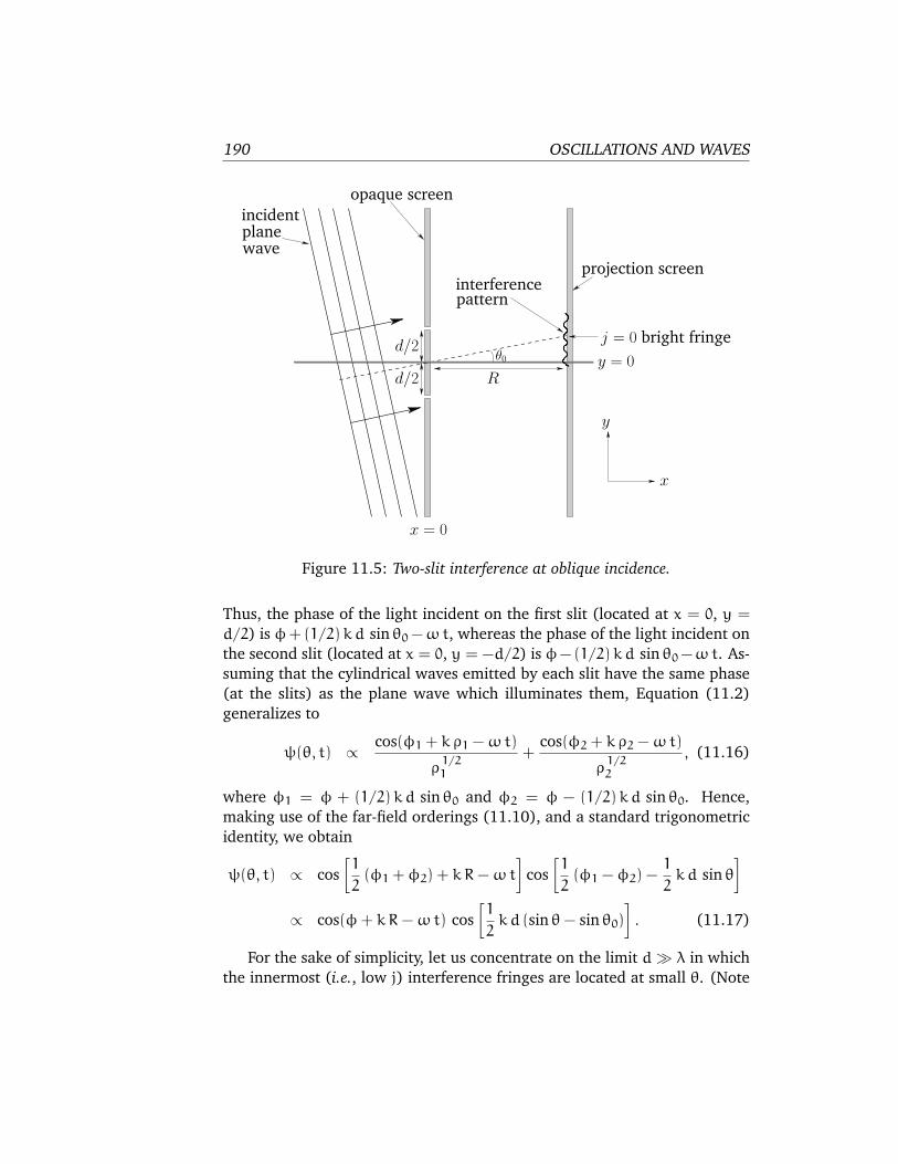
190 OSCILLATIONS AND WAVES
waveplane
d/2
d/2
x = 0
opaque screen
y
x
y = 0
projection screen
incident
R
j = 0 bright fringeθ0
patterninterference
Figure 11.5: Two-slit interference at oblique incidence.
Thus, the phase of the light incident on the first slit (located at x = 0, y =
d/2) is φ+ (1/2)kd sin θ0 −ωt, whereas the phase of the light incident on
the second slit (located at x = 0, y = −d/2) is φ−(1/2)kd sin θ0−ωt. As-
suming that the cylindrical waves emitted by each slit have the same phase
(at the slits) as the plane wave which illuminates them, Equation (11.2)
generalizes to
ψ(θ, t) ∝ cos(φ1 + k ρ1 −ωt)
ρ1/21
+cos(φ2 + k ρ2 −ωt)
ρ1/22
, (11.16)
where φ1 = φ + (1/2)kd sin θ0 and φ2 = φ − (1/2)kd sin θ0. Hence,
making use of the far-field orderings (11.10), and a standard trigonometric
identity, we obtain
ψ(θ, t) ∝ cos
[
1
2(φ1 + φ2) + kR−ωt
]
cos
[
1
2(φ1 − φ2) −
1
2kd sin θ
]
∝ cos(φ+ kR−ωt) cos
[
1
2kd (sin θ− sin θ0)
]
. (11.17)
For the sake of simplicity, let us concentrate on the limit d≫ λ in which
the innermost (i.e., low j) interference fringes are located at small θ. (Note
Wave Optics 191
that the projection screen is approximately planar in this limit, as indicated
in Figure 11.5, since a sufficiently small section of a cylindrical surface looks
like a plane.) Assuming that θ0 is also small, the above expression reduces
to
ψ(θ, t) ∝ cos(φ+ kR−ωt) cos
[
1
2kd (θ− θ0)
]
, (11.18)
and Equation (11.12) becomes
I(θ) ∝ cos2
[
πd
λ(θ− θ0)
]
. (11.19)
Thus, the bright fringes in the interference pattern are located at
θ = θ0 + jλ
d, (11.20)
where j is an integer. We conclude that if the slits in a two-slit interfer-
ence apparatus, such as that shown in Figure 11.5, are illuminated by an
obliquely incident plane wave then the consequent phase difference be-
tween the cylindrical waves emitted by each slit produces an angular shift
in the interference pattern appearing on the projection screen. To be more
exact, the angular shift is equal to the angle of incidence, θ0, of the plane
wave, so that the central (j = 0) bright fringe in the interference pattern is
located at θ = θ0—see Figure 11.5. Of course, this is equivalent to saying
that the position of the central bright fringe can be determined via the rules
of geometric optics. (Futhermore, this conclusion holds even when θ0 is not
small.)
11.3 Coherence
A practical monochromatic light source consists of a collection of similar
atoms which are continually excited by collisions, and then spontaneously
decay back to their electronic ground states, in the process emitting photons
of characteristic angular frequency ω = ∆E/h, where ∆E is the difference
in energy between the excited state and the ground state, and h = 1.055 ×10⁻³⁴ J s−1 is Planck’s constant divided by 2π. Now, an excited electronic
state of an atom has a characteristic lifetime, τ, which can be calculated
from quantum mechanics, and is typically 10−8 s. It follows that when an
atom in an excited state decays back to its ground state it emits a burst of
electromagnetic radiation of duration τ and angular frequencyω. However,
192 OSCILLATIONS AND WAVES
according to the bandwidth theorem (see Section 8.3), a sinusoidal wave of
finite duration τ has a finite bandwidth
∆ω ∼2π
τ. (11.21)
In other words, if the emitted wave is Fourier transformed in time then it
is found to consist of a linear superposition of sinusoidal waves of infinite
duration whose frequencies lie in the approximate range ω− ∆ω/2 to ω+
∆ω/2. We conclude that there is no such thing as a truly monochromatic
light source. In reality, all such sources have a small, but finite, bandwidths
which are inversely proportional to the lifetimes, τ, of the associated excited
atomic states.
So, how do we take the finite bandwidth of a practical “monochromatic”
light source into account in our analysis? Actually, all we need to do is to as-
sume that the phase angle, φ, appearing in Equations (11.1) and (11.15), is
only constant on timescales much less that the lifetime, τ, of the associated
excited atomic state, and is subject to abrupt random changes on timescales
much greater than τ. We can understand this phenomenon as due to the fact
that the radiation emitted by a single atom has a fixed phase angle, φ, but
only lasts a finite time period, τ, combined with the fact that there is gen-
erally no correlation between the phase angles of the radiation emitted by
different atoms. Alternatively, we can account for the variation in the phase
angle in terms of the finite bandwidth of the light source: i.e., since the
light emitted by the source consists of a superposition of sinusoidal waves
of frequencies extending over the range ω−∆ω/2 to ω+∆ω/2 then, even
if all the component waves start off in phase, the phases will be completely
scrambled after a time period 2π/∆ω = τ has elapsed. What we are, in
effect, saying is that a practical monochromatic light source is temporally
coherent on timescales much less than its characteristic coherence time, τ
(which, for visible light, is typically of order 10−8 seconds), and temporally
incoherent on timescales much greater than τ. Incidentally, two waves are
said to be coherent if their phase difference is constant in time, and incoher-
ent if their phase difference varies significantly in time. In this case, the two
waves in question are the same wave observed at two different times.
So, what effect does the temporal incoherence of a practical monochro-
matic light source on timescales greater than τ ∼ 10−8 seconds have on the
two-slit interference patterns discussed in the previous section? Consider
the case of oblique incidence. According to Equation (11.16), the phase
angles, φ1 = φ+(1/2)kd sin θ0, and φ2 = φ−(1/2)kd sin θ0, of the cylin-
drical waves emitted by each slit are subject to abrupt random changes on
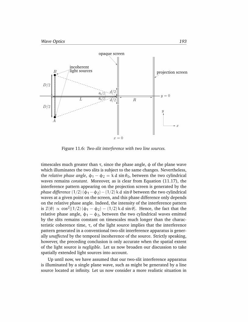
Wave Optics 193
y = 0
projection screen
opaque screen
x
y
d/2
d/2
x = 0
R
D/2
D/2
L
incoherentlight sources
θ0/2
θ0/2
A
B
Figure 11.6: Two-slit interference with two line sources.
timescales much greater than τ, since the phase angle, φ of the plane wave
which illuminates the two slits is subject to the same changes. Nevertheless,
the relative phase angle, φ1 − φ2 = kd sin θ0, between the two cylindrical
waves remains constant. Moreover, as is clear from Equation (11.17), the
interference pattern appearing on the projection screen is generated by the
phase difference (1/2) (φ1−φ2)−(1/2)kd sin θ between the two cylindrical
waves at a given point on the screen, and this phase difference only depends
on the relative phase angle. Indeed, the intensity of the interference pattern
is I(θ) ∝ cos2[(1/2) (φ1 − φ2) − (1/2)kd sin θ]. Hence, the fact that the
relative phase angle, φ1 − φ2, between the two cylindrical waves emitted
by the slits remains constant on timescales much longer than the charac-
teristic coherence time, τ, of the light source implies that the interference
pattern generated in a conventional two-slit interference apparatus is gener-
ally unaffected by the temporal incoherence of the source. Strictly speaking,
however, the preceding conclusion is only accurate when the spatial extent
of the light source is negligible. Let us now broaden our discussion to take
spatially extended light sources into account.
Up until now, we have assumed that our two-slit interference apparatus
is illuminated by a single plane wave, such as might be generated by a line
source located at infinity. Let us now consider a more realistic situation in
194 OSCILLATIONS AND WAVES
which the light source is located a finite distance from the slits, and also has
a finite spatial extent. Figure 11.6 shows the simplest possible case. Here,
the slits are illuminated by two identical line sources, A and B, which are
a distance D apart, and a perpendicular distance L from the opaque screen
containing the slits. Assuming that L ≫ D, d, the light incident on the slits
from source A is effectively a plane wave whose direction of propagation
subtends an angle θ0/2 ≃ D/2L with the x-axis. Likewise, the light incident
on the slits from source B is a plane wave whose direction of propagation
subtends an angle −θ0/2 with the x-axis. Moreover, the net interference
pattern (i.e., wavefunction) appearing on the projection screen is the linear
superposition of the patterns generated by each source taken individually
(since light propagation is ultimately governed by a linear wave equation
with superposable solutions—see Section 10.2.). Let us determine whether
these patterns reinforce one another, or interfere with one another.
The light emitted by source A has a phase angle, φA, which is constant
on timescales much less than the characteristic coherence time of the source,
τ, but is subject to abrupt random changes on timescale much longer than τ.
Likewise, the light emitted by source B has a phase angle, φB, which is con-
stant on timescales much less than τ, and varies significantly on timescales
much greater than τ. Furthermore, there is, in general, no correlation be-
tween φA and φB. In other words, our composite light source, consisting of
the two line sources A and B, is both temporally and spatially incoherent on
timescales much longer than τ.
Again working in the limit d ≫ λ, with θ, θ0 ≪ 1, Equation (11.18)
yields the following expression for the wavefunction on the projection screen:
ψ(θ, t) ∝ cos(φA + kR−ωt) cos
[
1
2kd (θ− θ0/2)
]
+ cos(φB + kR−ωt) cos
[
1
2kd (θ+ θ0/2)
]
. (11.22)
Hence, the intensity of the interference pattern is
I(θ) ∝ 〈ψ2〉 ∝ 〈 cos2(φA + kR−ωt)〉 cos2
[
1
2kd (θ− θ0/2)
]
+2 〈cos(φA + kR−ωt) cos(φB + kR−ωt)〉
× cos
[
1
2kd (θ− θ0/2)
]
cos
[
1
2kd (θ+ θ0/2)
]
+〈 cos2(φB + kR−ωt)〉 cos2
[
1
2kd (θ+ θ0/2)
]
.
Wave Optics 195
(11.23)
However, 〈cos2(φA + kR − ωt)〉 = 〈cos2(φB + kR − ωt)〉 = 1/2, and
〈cos(φA + kR − ωt) cos(φB + kR − ωt)〉 = 0, since the phase angles φA
and φB are uncorrelated. Hence, the above expression reduces to
I(θ) ∝ cos2
[
1
2kd (θ− θ0/2)
]
+ cos2
[
1
2kd (θ+ θ0/2)
]
= 1+ cos
(
2πd
λθ
)
cos
(
πd
λθ0
)
, (11.24)
where use has been made of the trigonometric identities cos2θ ≡ (1 +
cos 2θ)/2, and cos x + cosy ≡ 2 cos[(x + y)/2] cos((x − y)/2]. Note that
if θ0 = λ/2d then cos[π (d/λ) θ0] = 0 and I(θ) ∝ 1. In this case, the bright
fringes of the interference pattern generated by source A exactly overlay
the dark fringes of the pattern generated by source B, and vice versa, and
the net interference pattern is completely washed out. On the other hand,
if θ0 ≪ λ/d then cos[π (d/λ) θ0] = 1 and I(θ) ∝ 1 + cos[2π (d/λ) θ] =
2 cos2[π (d/λ) θ]. In this case, the two interference patterns reinforce one
another, and the net interference pattern is the same as that generated by a
light source of negligible spatial extent.
Suppose, now, that our light source consists of a regularly spaced array
of very many identical incoherent line sources, filling the region between
sources A and B in Figure 11.6. In other words, suppose that our light
source is a uniform incoherent source of angular extent θ0. It is, hopefully,
clear, from the linear nature of the problem, that the associated interference
pattern can be obtained by averaging expression (11.24) over all θ0 values in
the range 0 to θ0: i.e., by operating on this expression with θ−10
∫θ0
0· · · dθ0.
In this manner, we obtain
I(θ) ∝ 1+ cos
(
2πd
λθ
)
sinc
(
πd
λθ0
)
, (11.25)
where sinc(x) ≡ sin x/x. Now, we can conveniently parameterize the visibil-
ity of the interference pattern, appearing on the projection screen, in terms
of the quantity
V =Imax − Imin
Imax + Imin, (11.26)
where the maximum and minimum values of the intensity are taken with
respect to variation in θ (rather than θ0). Of course, V = 1 corresponds to a
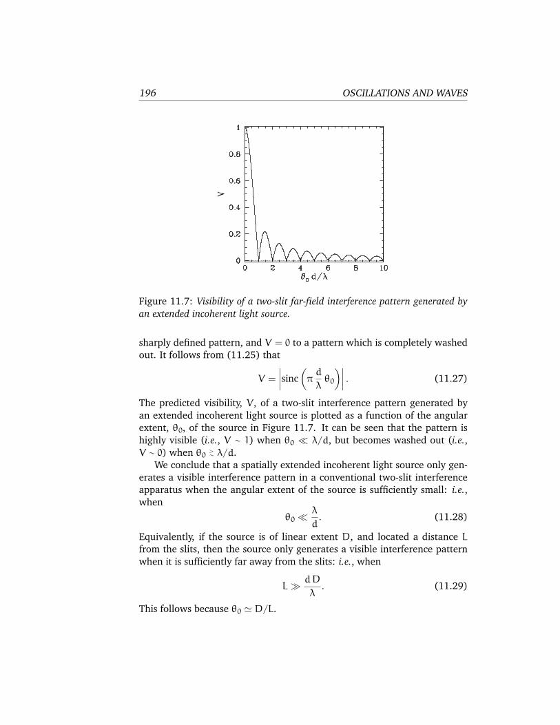
196 OSCILLATIONS AND WAVES
Figure 11.7: Visibility of a two-slit far-field interference pattern generated by
an extended incoherent light source.
sharply defined pattern, and V = 0 to a pattern which is completely washed
out. It follows from (11.25) that
V =
∣
∣
∣
∣
sinc
(
πd
λθ0
)∣
∣
∣
∣
. (11.27)
The predicted visibility, V, of a two-slit interference pattern generated by
an extended incoherent light source is plotted as a function of the angular
extent, θ0, of the source in Figure 11.7. It can be seen that the pattern is
highly visible (i.e., V ∼ 1) when θ0 ≪ λ/d, but becomes washed out (i.e.,
V ∼ 0) when θ0>∼λ/d.
We conclude that a spatially extended incoherent light source only gen-
erates a visible interference pattern in a conventional two-slit interference
apparatus when the angular extent of the source is sufficiently small: i.e.,
when
θ0 ≪ λ
d. (11.28)
Equivalently, if the source is of linear extent D, and located a distance L
from the slits, then the source only generates a visible interference pattern
when it is sufficiently far away from the slits: i.e., when
L≫ dD
λ. (11.29)
This follows because θ0 ≃ D/L.
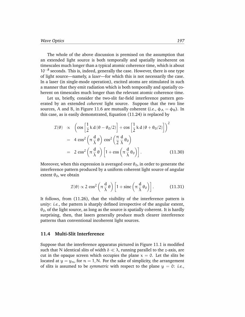
Wave Optics 197
The whole of the above discussion is premised on the assumption that
an extended light source is both temporally and spatially incoherent on
timescales much longer than a typical atomic coherence time, which is about
10−8 seconds. This is, indeed, generally the case. However, there is one type
of light source—namely, a laser—for which this is not necessarily the case.
In a laser (in single-mode operation), excited atoms are stimulated in such
a manner that they emit radiation which is both temporally and spatially co-
herent on timescales much longer than the relevant atomic coherence time.
Let us, briefly, consider the two-slit far-field interference pattern gen-
erated by an extended coherent light source. Suppose that the two line
sources, A and B, in Figure 11.6 are mutually coherent (i.e., φA = φB). In
this case, as is easily demonstrated, Equation (11.24) is replaced by
I(θ) ∝(
cos
[
1
2kd (θ− θ0/2)
]
+ cos
[
1
2kd (θ+ θ0/2)
])2
= 4 cos2
(
πd
λθ
)
cos2
(
π
2
d
λθ0
)
= 2 cos2
(
πd
λθ
)[
1+ cos
(
πd
λθ0
)]
. (11.30)
Moreover, when this expression is averaged over θ0, in order to generate the
interference pattern produced by a uniform coherent light source of angular
extent θ0, we obtain
I(θ) ∝ 2 cos2
(
πd
λθ
)[
1+ sinc
(
πd
λθ0
)]
. (11.31)
It follows, from (11.26), that the visibility of the interference pattern is
unity: i.e., the pattern is sharply defined irrespective of the angular extent,
θ0, of the light source, as long as the source is spatially coherent. It is hardly
surprising, then, that lasers generally produce much clearer interference
patterns than conventional incoherent light sources.
11.4 Multi-Slit Interference
Suppose that the interference apparatus pictured in Figure 11.1 is modified
such that N identical slits of width δ≪ λ, running parallel to the z-axis, are
cut in the opaque screen which occupies the plane x = 0. Let the slits be
located at y = yn, for n = 1,N. For the sake of simplicity, the arrangement
of slits is assumed to be symmetric with respect to the plane y = 0: i.e.,
198 OSCILLATIONS AND WAVES
if there is a slit at y = yn then there is also a slit at y = −yn. Now, the
path length between a point on the projection screen which is an angular
distance θ from the plane y = 0 and the nth slit is [cf., Equation (11.3)]
ρn = R
[
1−yn
Rsin θ+ O
(
y2n
R2
)]
. (11.32)
Thus, making use of the far-field orderings (11.10), where d now repre-
sents the typical spacing between neighboring slits, and assuming normally
incident collimated light, Equation (11.5) generalizes to
ψ(θ, t) ∝∑
n=1,N
cos(φ+ kR−ωt− kyn sin θ), (11.33)
which can also be written
ψ(θ, t) ∝ cos(φ+ kR−ωt)∑
n=1,N
cos(kyn sin θ)
+ sin(φ+ kR−ωt)∑
n=1,N
sin(kyn sin θ), (11.34)
or
ψ(θ, t) ∝ cos(φ+ kR−ωt)∑
n=1,N
cos(kyn sin θ). (11.35)
Here, we have made use of the fact that arrangement of slits is symmetric
with respect to the plane y = 0 (which implies that∑
n=1,N sin(kyn sin θ) =
0). We have also employed the standard identity cos(x − y) ≡ cos x cosy +
sin x siny. It follows that the intensity of the interference pattern appearing
on the projection screen is specified by
I(θ) ∝ 〈ψ(θ, t)2〉 ∝
∑
n=1,N
cos
(
2πyn
λsin θ
)
2
, (11.36)
since 〈cos2(φ + kR − ωt)〉 = 1/2. The above expression is a generalized
version of Equation (11.12).
Suppose that the slits are evenly spaced a distance d apart, so that
yn = [n− (N+ 1)/2]d (11.37)
for n = 1,N. It follows that
I(θ) ∝
∑
n=1,N
cos
(
2π [n− (N+ 1)/2]d
λsin θ
)
2
, (11.38)
Wave Optics 199
Figure 11.8: Multi-slit far-field interference pattern calculated for N = 10 and
d/λ = 5 with normal incidence and narrow slits.
which can be summed to give (see Exercise 11.1)
I(θ) ∝ sin2[πN (d/λ) sin θ]
sin2[π (d/λ) sin θ)]. (11.39)
Now, the multi-slit interference function, (11.39), exhibits strong max-
ima in situations in which its numerator and denominator are simultaneously
zero: i.e., when
sin θ = jλ
d, (11.40)
where j is an integer. In this situation, application of L’Hopital’s rule yields
I = N2. The heights of these so-called principal maxima in the interference
function are very large, being proportional to N2, because there is construc-
tive interference of the light from all N slits. This occurs because the path
lengths between neighboring slits and the point on the projection screen
at which a given maximum is located differ by an integer number of wave-
lengths: i.e., ρn − ρn−1 = d sin θ = j λ. Note, incidentally, that all of the
principle maxima have the same height.
The multi-slit interference function (11.39) is zero when its numerator
is zero but its denominator non-zero: i.e., when
sin θ =l
N
λ
d, (11.41)
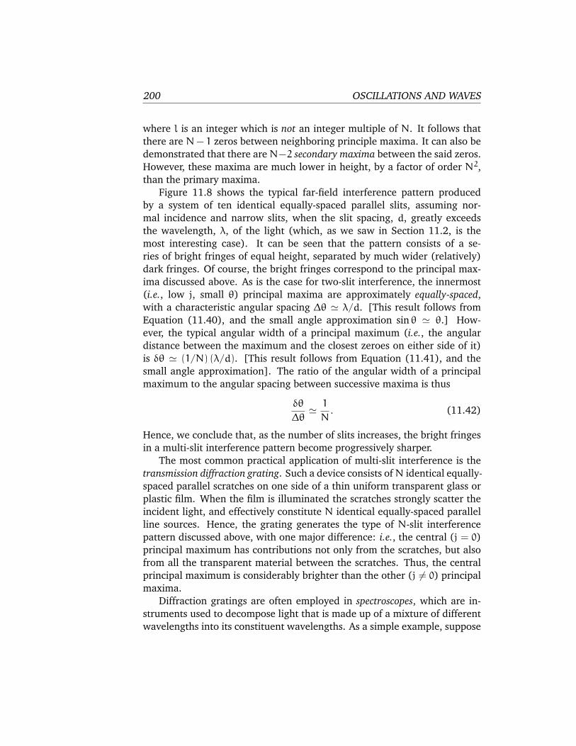
200 OSCILLATIONS AND WAVES
where l is an integer which is not an integer multiple of N. It follows that
there are N− 1 zeros between neighboring principle maxima. It can also be
demonstrated that there areN−2 secondary maxima between the said zeros.
However, these maxima are much lower in height, by a factor of order N2,
than the primary maxima.
Figure 11.8 shows the typical far-field interference pattern produced
by a system of ten identical equally-spaced parallel slits, assuming nor-
mal incidence and narrow slits, when the slit spacing, d, greatly exceeds
the wavelength, λ, of the light (which, as we saw in Section 11.2, is the
most interesting case). It can be seen that the pattern consists of a se-
ries of bright fringes of equal height, separated by much wider (relatively)
dark fringes. Of course, the bright fringes correspond to the principal max-
ima discussed above. As is the case for two-slit interference, the innermost
(i.e., low j, small θ) principal maxima are approximately equally-spaced,
with a characteristic angular spacing ∆θ ≃ λ/d. [This result follows from
Equation (11.40), and the small angle approximation sin θ ≃ θ.] How-
ever, the typical angular width of a principal maximum (i.e., the angular
distance between the maximum and the closest zeroes on either side of it)
is δθ ≃ (1/N) (λ/d). [This result follows from Equation (11.41), and the
small angle approximation]. The ratio of the angular width of a principal
maximum to the angular spacing between successive maxima is thus
δθ
∆θ≃ 1
N. (11.42)
Hence, we conclude that, as the number of slits increases, the bright fringes
in a multi-slit interference pattern become progressively sharper.
The most common practical application of multi-slit interference is the
transmission diffraction grating. Such a device consists ofN identical equally-
spaced parallel scratches on one side of a thin uniform transparent glass or
plastic film. When the film is illuminated the scratches strongly scatter the
incident light, and effectively constitute N identical equally-spaced parallel
line sources. Hence, the grating generates the type of N-slit interference
pattern discussed above, with one major difference: i.e., the central (j = 0)
principal maximum has contributions not only from the scratches, but also
from all the transparent material between the scratches. Thus, the central
principal maximum is considerably brighter than the other (j 6= 0) principal
maxima.
Diffraction gratings are often employed in spectroscopes, which are in-
struments used to decompose light that is made up of a mixture of different
wavelengths into its constituent wavelengths. As a simple example, suppose
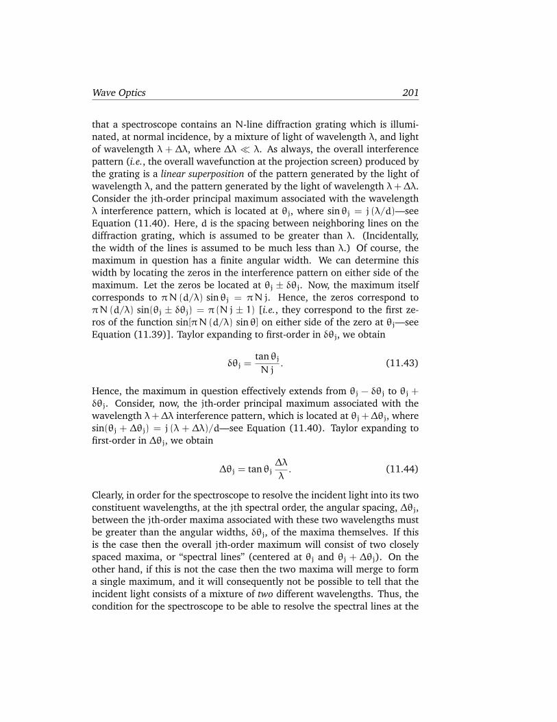
Wave Optics 201
that a spectroscope contains an N-line diffraction grating which is illumi-
nated, at normal incidence, by a mixture of light of wavelength λ, and light
of wavelength λ + ∆λ, where ∆λ ≪ λ. As always, the overall interference
pattern (i.e., the overall wavefunction at the projection screen) produced by
the grating is a linear superposition of the pattern generated by the light of
wavelength λ, and the pattern generated by the light of wavelength λ+∆λ.
Consider the jth-order principal maximum associated with the wavelength
λ interference pattern, which is located at θj, where sin θj = j (λ/d)—see
Equation (11.40). Here, d is the spacing between neighboring lines on the
diffraction grating, which is assumed to be greater than λ. (Incidentally,
the width of the lines is assumed to be much less than λ.) Of course, the
maximum in question has a finite angular width. We can determine this
width by locating the zeros in the interference pattern on either side of the
maximum. Let the zeros be located at θj ± δθj. Now, the maximum itself
corresponds to πN (d/λ) sin θj = πN j. Hence, the zeros correspond to
πN (d/λ) sin(θj ± δθj) = π (Nj ± 1) [i.e., they correspond to the first ze-
ros of the function sin[πN (d/λ) sin θ] on either side of the zero at θj—see
Equation (11.39)]. Taylor expanding to first-order in δθj, we obtain
δθj =tan θj
Nj. (11.43)
Hence, the maximum in question effectively extends from θj − δθj to θj +
δθj. Consider, now, the jth-order principal maximum associated with the
wavelength λ+∆λ interference pattern, which is located at θj +∆θj, where
sin(θj + ∆θj) = j (λ + ∆λ)/d—see Equation (11.40). Taylor expanding to
first-order in ∆θj, we obtain
∆θj = tan θj∆λ
λ. (11.44)
Clearly, in order for the spectroscope to resolve the incident light into its two
constituent wavelengths, at the jth spectral order, the angular spacing, ∆θj,
between the jth-order maxima associated with these two wavelengths must
be greater than the angular widths, δθj, of the maxima themselves. If this
is the case then the overall jth-order maximum will consist of two closely
spaced maxima, or “spectral lines” (centered at θj and θj + ∆θj). On the
other hand, if this is not the case then the two maxima will merge to form
a single maximum, and it will consequently not be possible to tell that the
incident light consists of a mixture of two different wavelengths. Thus, the
condition for the spectroscope to be able to resolve the spectral lines at the
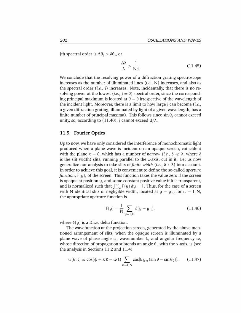
202 OSCILLATIONS AND WAVES
jth spectral order is ∆θj > δθj, or
∆λ
λ>
1
N j. (11.45)
We conclude that the resolving power of a diffraction grating spectroscope
increases as the number of illuminated lines (i.e., N) increases, and also as
the spectral order (i.e., j) increases. Note, incidentally, that there is no re-
solving power at the lowest (i.e., j = 0) spectral order, since the correspond-
ing principal maximum is located at θ = 0 irrespective of the wavelength of
the incident light. Moreover, there is a limit to how large j can become (i.e.,
a given diffraction grating, illuminated by light of a given wavelength, has a
finite number of principal maxima). This follows since sinθj cannot exceed
unity, so, according to (11.40), j cannot exceed d/λ.
11.5 Fourier Optics
Up to now, we have only considered the interference of monochromatic light
produced when a plane wave is incident on an opaque screen, coincident
with the plane x = 0, which has a number of narrow (i.e., δ ≪ λ, where δ
is the slit width) slits, running parallel to the z-axis, cut in it. Let us now
generalize our analysis to take slits of finite width (i.e., δ >∼λ) into account.
In order to achieve this goal, it is convenient to define the so-called aperture
function, F(y), of the screen. This function takes the value zero if the screen
is opaque at position y, and some constant positive value if it is transparent,
and is normalized such that∫∞
−∞ F(y)dy = 1. Thus, for the case of a screen
with N identical slits of negligible width, located at y = yn, for n = 1,N,
the appropriate aperture function is
F(y) =1
N
∑
y=1,N
δ(y− yn), (11.46)
where δ(y) is a Dirac delta function.
The wavefunction at the projection screen, generated by the above men-
tioned arrangement of slits, when the opaque screen is illuminated by a
plane wave of phase angle φ, wavenumber k, and angular frequency ω,
whose direction of propagation subtends an angle θ0 with the x-axis, is (see
the analysis in Sections 11.2 and 11.4)
ψ(θ, t) ∝ cos(φ+ kR−ωt)∑
n=1,N
cos[kyn (sin θ− sin θ0)]. (11.47)
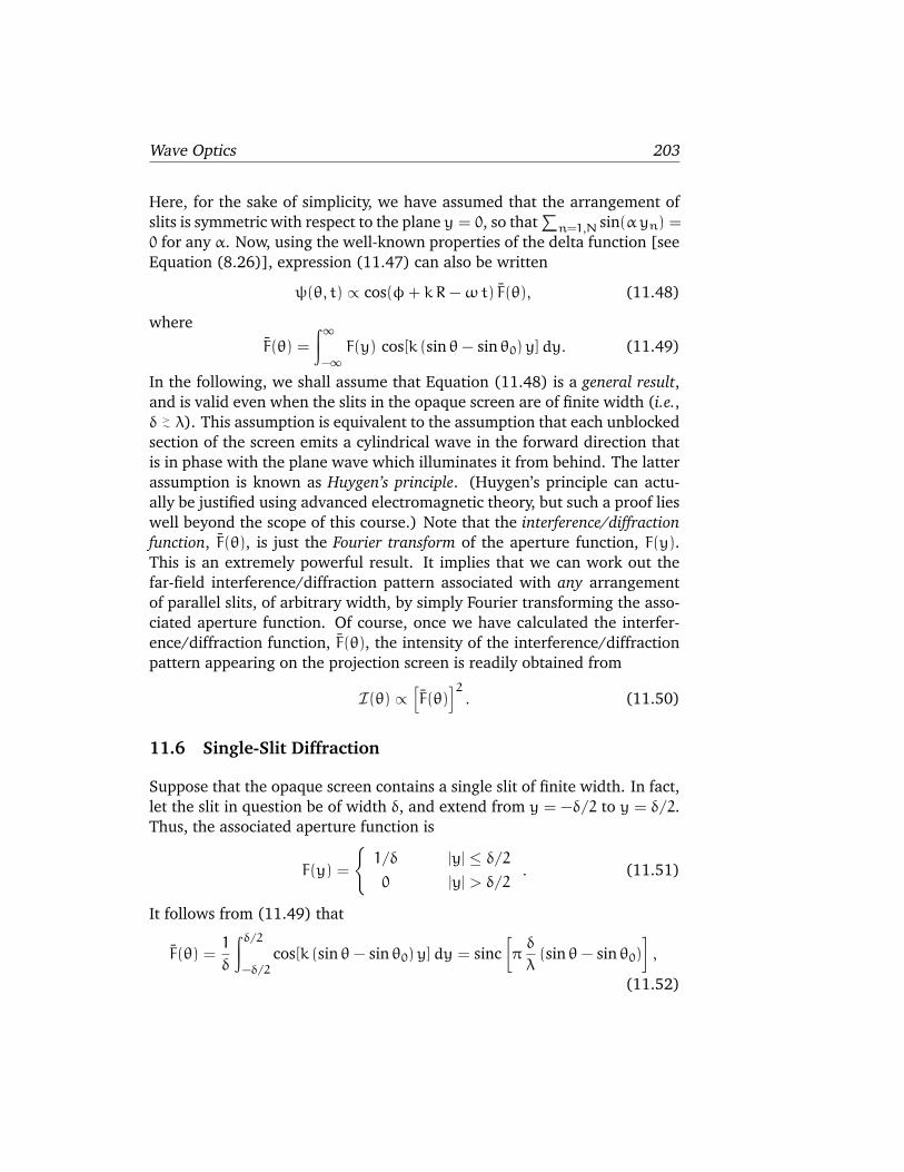
Wave Optics 203
Here, for the sake of simplicity, we have assumed that the arrangement of
slits is symmetric with respect to the plane y = 0, so that∑
n=1,N sin(αyn) =
0 for any α. Now, using the well-known properties of the delta function [see
Equation (8.26)], expression (11.47) can also be written
ψ(θ, t) ∝ cos(φ+ kR−ωt) F(θ), (11.48)
where
F(θ) =
∫∞
−∞F(y) cos[k (sin θ− sin θ0)y]dy. (11.49)
In the following, we shall assume that Equation (11.48) is a general result,
and is valid even when the slits in the opaque screen are of finite width (i.e.,
δ >∼λ). This assumption is equivalent to the assumption that each unblocked
section of the screen emits a cylindrical wave in the forward direction that
is in phase with the plane wave which illuminates it from behind. The latter
assumption is known as Huygen’s principle. (Huygen’s principle can actu-
ally be justified using advanced electromagnetic theory, but such a proof lies
well beyond the scope of this course.) Note that the interference/diffraction
function, F(θ), is just the Fourier transform of the aperture function, F(y).
This is an extremely powerful result. It implies that we can work out the
far-field interference/diffraction pattern associated with any arrangement
of parallel slits, of arbitrary width, by simply Fourier transforming the asso-
ciated aperture function. Of course, once we have calculated the interfer-
ence/diffraction function, F(θ), the intensity of the interference/diffraction
pattern appearing on the projection screen is readily obtained from
I(θ) ∝[
F(θ)]2. (11.50)
11.6 Single-Slit Diffraction
Suppose that the opaque screen contains a single slit of finite width. In fact,
let the slit in question be of width δ, and extend from y = −δ/2 to y = δ/2.
Thus, the associated aperture function is
F(y) =
1/δ |y| ≤ δ/20 |y| > δ/2
. (11.51)
It follows from (11.49) that
F(θ) =1
δ
∫δ/2
−δ/2
cos[k (sin θ− sin θ0)y]dy = sinc
[
πδ
λ(sin θ− sin θ0)
]
,
(11.52)
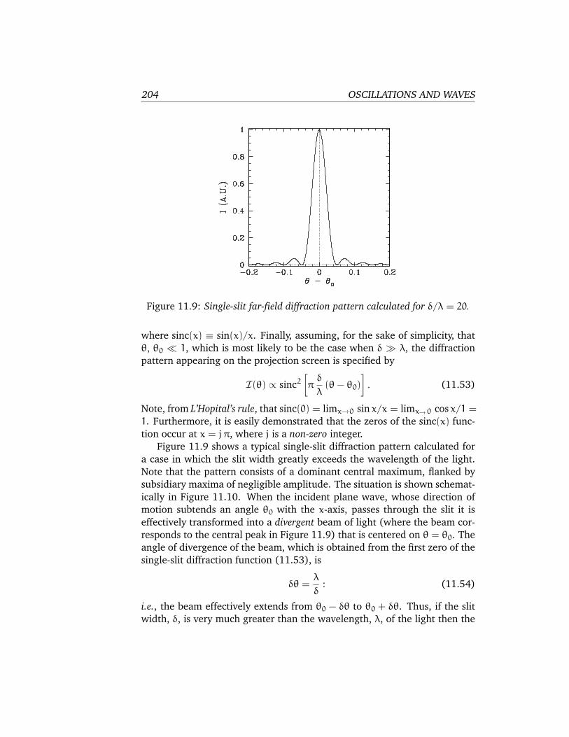
204 OSCILLATIONS AND WAVES
Figure 11.9: Single-slit far-field diffraction pattern calculated for δ/λ = 20.
where sinc(x) ≡ sin(x)/x. Finally, assuming, for the sake of simplicity, that
θ, θ0 ≪ 1, which is most likely to be the case when δ ≫ λ, the diffraction
pattern appearing on the projection screen is specified by
I(θ) ∝ sinc2
[
πδ
λ(θ− θ0)
]
. (11.53)
Note, from L’Hopital’s rule, that sinc(0) = limx→0 sin x/x = limx→ 0 cos x/1 =
1. Furthermore, it is easily demonstrated that the zeros of the sinc(x) func-
tion occur at x = j π, where j is a non-zero integer.
Figure 11.9 shows a typical single-slit diffraction pattern calculated for
a case in which the slit width greatly exceeds the wavelength of the light.
Note that the pattern consists of a dominant central maximum, flanked by
subsidiary maxima of negligible amplitude. The situation is shown schemat-
ically in Figure 11.10. When the incident plane wave, whose direction of
motion subtends an angle θ0 with the x-axis, passes through the slit it is
effectively transformed into a divergent beam of light (where the beam cor-
responds to the central peak in Figure 11.9) that is centered on θ = θ0. The
angle of divergence of the beam, which is obtained from the first zero of the
single-slit diffraction function (11.53), is
δθ =λ
δ: (11.54)
i.e., the beam effectively extends from θ0 − δθ to θ0 + δθ. Thus, if the slit
width, δ, is very much greater than the wavelength, λ, of the light then the
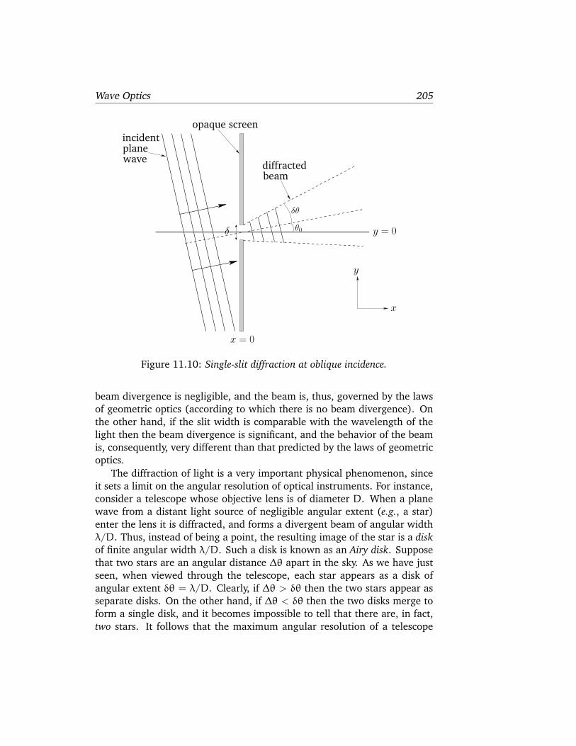
Wave Optics 205
x
incidentplanewave
y = 0
x = 0
y
opaque screen
δ
δθ
θ0
diffractedbeam
Figure 11.10: Single-slit diffraction at oblique incidence.
beam divergence is negligible, and the beam is, thus, governed by the laws
of geometric optics (according to which there is no beam divergence). On
the other hand, if the slit width is comparable with the wavelength of the
light then the beam divergence is significant, and the behavior of the beam
is, consequently, very different than that predicted by the laws of geometric
optics.
The diffraction of light is a very important physical phenomenon, since
it sets a limit on the angular resolution of optical instruments. For instance,
consider a telescope whose objective lens is of diameter D. When a plane
wave from a distant light source of negligible angular extent (e.g., a star)
enter the lens it is diffracted, and forms a divergent beam of angular width
λ/D. Thus, instead of being a point, the resulting image of the star is a disk
of finite angular width λ/D. Such a disk is known as an Airy disk. Suppose
that two stars are an angular distance ∆θ apart in the sky. As we have just
seen, when viewed through the telescope, each star appears as a disk of
angular extent δθ = λ/D. Clearly, if ∆θ > δθ then the two stars appear as
separate disks. On the other hand, if ∆θ < δθ then the two disks merge to
form a single disk, and it becomes impossible to tell that there are, in fact,
two stars. It follows that the maximum angular resolution of a telescope
206 OSCILLATIONS AND WAVES
whose objective lens is of diameter D is
δθ ≃ λ
D. (11.55)
This result is usually called the Rayleigh criterion. Note that the angular
resolution of the telescope increases (i.e., δθ decreases) as the diameter of
its objective lens increases.
11.7 Multi-Slit Diffraction
Suppose, finally, that the opaque screen in our interference/diffraction ap-
paratus contains N identical equally-spaced parallel slits of finite width. Let
the slit spacing be d, and the slit width δ, where δ < d. It follows that the
aperture function for the screen is written
F(y) =1
N
∑
n=1,N
F2(y− yn), (11.56)
where
yn = [n− (N+ 1)/2]d, (11.57)
and
F2(y) =
1/δ |y| ≤ δ/20 |y| > δ/2
. (11.58)
Of course, F2(y) is the aperture function for a single slit, of finite width δ,
which is centered on θ = 0—see Equation (11.51).
Assuming normal incidence (i.e., θ0 = 0), the interference/diffraction
function, which is the Fourier transform of the aperture function, takes the
form [see Equation (11.49)]
F(θ) =
∫∞
−∞F(y) cos(k sin θy)dy. (11.59)
Hence,
F(θ) =1
N
∑
n=1,N
∫∞
−∞F2(y− yn) cos(k sin θy)dy
=1
N
∑
n=1,N
[
cos(k sin θyn)
∫∞
−∞F2(y
′) cos(k sin θy ′)dy ′
Wave Optics 207
− sin(k sin θyn)
∫∞
−∞F2(y
′) sin(k sin θy ′)dy ′
]
(11.60)
=
1
N
∑
n=1,N
cos(k sin θyn)
∫∞
−∞F2(y
′) cos(k sin θy ′)dy ′,
where y ′ = y−yn. Here, we have made use of∫∞
−∞ F2(y′) sin(αy ′)dy ′ = 0,
for any α, which follows because F2(y′) is even in y ′, whereas sin(αy ′) is
odd. We have also employed the standard identity cos(x−y) ≡ cos x cosy−
sin x siny. The above expression reduces to
F(θ) = F1(θ) F2(θ). (11.61)
Here [cf., Equation (11.39)],
F1(θ) =
∫∞
−∞F1(y) cos(k sin θy)dy =
1
N
∑
n=1,N
cos(k sin θyn)
=1
N
sin[πN (d/λ) sin θ]
sin[π (d/λ) sin θ], (11.62)
where
F1(y) =1
N
∑
n=1,N
δ(y− yn), (11.63)
is the interference/diffraction function for N identical parallel slits of neg-
ligible width which are equally-spaced a distance d apart, and F1(y) is the
corresponding aperture function. Furthermore [cf., Equation (11.52)],
F2(θ) =
∫∞
−∞F2(y) cos(k sin θy)dy = sinc[π (δ/λ) sin θ], (11.64)
is the interference/diffraction function for a single slit of width δ.
We conclude, from the above analysis, that the interference/diffraction
function for N identical equally-spaced parallel slits of finite width is the
product of the interference/diffraction function forN identical equally-spac-
ed parallel slits of negligible width, F1(θ), and the interference/diffraction
function for a single slit of finite width, F2(θ). We have already encountered
both of these functions. The former function (see Figure 11.8, which shows
[F1(θ)]2) consists of a series of sharp maxima of equal amplitude located at
[see Equation (11.40)]
θj = sin−1
(
jλ
d
)
, (11.65)
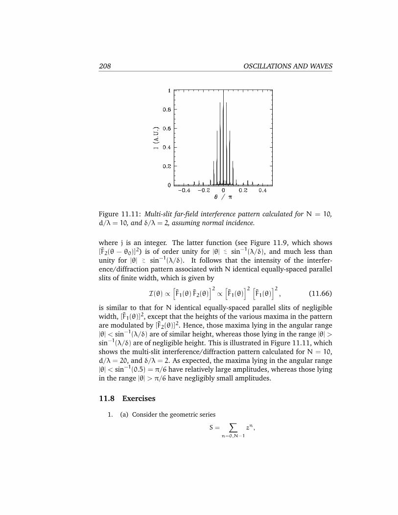
208 OSCILLATIONS AND WAVES
Figure 11.11: Multi-slit far-field interference pattern calculated for N = 10,
d/λ = 10, and δ/λ = 2, assuming normal incidence.
where j is an integer. The latter function (see Figure 11.9, which shows
[F2(θ − θ0)]2) is of order unity for |θ| <
∼sin−1(λ/δ), and much less than
unity for |θ| >∼
sin−1(λ/δ). It follows that the intensity of the interfer-
ence/diffraction pattern associated with N identical equally-spaced parallel
slits of finite width, which is given by
I(θ) ∝[
F1(θ) F2(θ)]2
∝[
F1(θ)]2 [
F1(θ)]2, (11.66)
is similar to that for N identical equally-spaced parallel slits of negligible
width, [F1(θ)]2, except that the heights of the various maxima in the pattern
are modulated by [F2(θ)]2. Hence, those maxima lying in the angular range
|θ| < sin−1(λ/δ) are of similar height, whereas those lying in the range |θ| >
sin−1(λ/δ) are of negligible height. This is illustrated in Figure 11.11, which
shows the multi-slit interference/diffraction pattern calculated for N = 10,
d/λ = 20, and δ/λ = 2. As expected, the maxima lying in the angular range
|θ| < sin−1(0.5) = π/6 have relatively large amplitudes, whereas those lying
in the range |θ| > π/6 have negligibly small amplitudes.
11.8 Exercises
1. (a) Consider the geometric series
S =∑
n=0,N−1
zn,
Wave Optics 209
where z is a complex number. Demonstrate that
S =1− zN
1− z.
(b) Suppose that z = e i θ, where θ is real. Employing the well-knownidentity
sin θ ≡ 1
2 i
(
e i θ − e−i θ)
,
show that
S = e i (N−1) θ/2 sin(Nθ/2)
sin(θ/2).
(c) Finally, making use of de Moivre’s theorem,
e i n θ ≡ cos(nθ) + i sin(nθ),
demonstrate thatC =
∑
n=1,N
cos(αyn),
whereyn = [n− (N+ 1)/2]d,
evaluates to
C =sin(Nαd/2)
sin(αd/2).
2. An interference experiment employs two narrow parallel slits of separation0.25mm, and monochromatic light of wavelength λ = 500nm. Estimate theminimum distance that the projection screen must be placed behind the slitsin order to obtain a far-field interference pattern.
3. A double-slit of slit separation 0.5mm is illuminated at normal incidence bya parallel beam from a helium-neon laser that emits monochromatic lightof wavelength 632.8nm. A projection screen is located 5m behind the slit.What is the separation of the central interference fringes on the screen?
4. Consider a double-slit interference experiment in which the slit spacing is0.1mm, and the projection screen is located 50 cm behind the slits. Assumingmonochromatic illumination at normal incidence, if the observed separationbetween neighboring interference maxima at the center of the projectionscreen is 2.5mm, what is the wavelength of the light illuminating the slits?
5. What is the mean length of the classical wavetrain (wave packet) correspond-ing to the light emitted by an atom whose excited state has a mean lifetimeτ ∼ 10−8 s? In an ordinary gas-discharge source, the excited atomic states donot decay freely, but instead have an effective lifetime τ ∼ 10−9 s, due to col-lisions and Doppler effects. What is the length of the corresponding classicalwavetrain?
210 OSCILLATIONS AND WAVES
6. If a “monochromatic” incoherent “line” source of visible light is not really aline, but has a finite width of 1mm, estimate the minimum distance it can beplaced in front of a double-slit, of slit separation 0.5mm, if the light from theslit is to generate a clear interference pattern.
7. The visible emission spectrum of a sodium atom is dominated by a yellow linewhich actually consists of two closely-spaced lines of wavelength 589.0nmand 589.6nm. Demonstrate that a diffraction grating must have at least 328lines in order to resolve this doublet at the third spectral order.
8. Consider a diffraction grating having 5000 lines per centimeter. Find theangular locations of the principle maxima when the grating is illuminated atnormal incidence by (a) red light of wavelength 700 nm, and (b) violet lightof wavelength 400 nm.
9. Suppose that a monochromatic laser of wavelength 632.8nm emits a diffrac-tion-limited beam of initial diameter 2 mm. Estimate how large a light spotthe beam would produce on the surface of the Moon (which is a mean dis-tance 3.76× 10⁵ km from the surface of the Earth). Neglect any effects of theEarth’s atmosphere.
10. Estimate how far away an automobile is when you can only just barely re-solve the two headlights with your eyes.
11. Venus has a diameter of about 8000 miles. When it is prominently visible inthe sky, in the early morning or late evening, it is about as far away as theSun: i.e., about 93 million miles. Now, Venus commonly appears larger thana point to the unaided eye. Are we seeing the true size of Venus?
12. The world’s largest steerable radio telescope, at the National Radio Astron-omy Observatory, Green Bank, West Virginia, consists of a parabolic diskwhich is 300 ft in diameter. Estimate the angular resolution (in minutes ofan arc) of the telescope when it is observing the well-known 21-cm radiationof hydrogen.
13. Estimate how large the lens of a camera carried by an artificial satellite orbit-ing the Earth at an altitude of 150 miles would have to be in order to resolvefeatures on the Earth’s surface a foot in diameter.
14. Demonstrate that the secondary maxima in the far-field interference patterngenerated by three identical equally-spaced parallel slits of negligible widthare nine times less intense than the principle maxima.
15. Consider a double-slit interference/diffraction experiment in which the slitspacing is d, and the slit width δ. Show that the intensity of the far-fieldinterference pattern, assuming normal incidence by monochromatic light ofwavelength λ, is
I(θ) ∝ cos2
(
πd
λsin θ
)
sinc2
(
πδ
λsin θ
)
.

Wave Optics 211
Plot the intensity pattern for d/λ = 8 and δ/λ = 2.

212 OSCILLATIONS AND WAVES
Wave Mechanics 213
12 Wave Mechanics
12.1 Introduction
According to classical physics (i.e., physics prior to the 20th century), par-
ticles and waves are two completely distinct classes of physical entity that
possess markedly different properties. 1) Particles are discrete: i.e., they
cannot be arbitrarily divided. In other words, it makes sense to talk about
one electron, or two electrons, but not about a third of an electron. Waves,
on the other hand, are continuous: i.e., they can be arbitrarily divided. In
other words, given a wave whose amplitude has a certain value, it makes
sense to talk about a similar wave whose amplitude is one third, or any
other fraction whatsoever, of this value. 2) Particles are highly localized in
space. For example, atomic nuclei have very small radii of order 10−15m,
whilst electrons act like point particles: i.e., they have no discernible spatial
extent. Waves, on the other hand, are non-localized in space. In fact, a wave
is defined to be a disturbance that is periodic in space, with some finite peri-
odicity length: i.e., wavelength. Hence, it is fairly meaningless to talk about
a disturbance being a wave unless it extends over a region of space that is
at least a few wavelengths in dimension.
The classical scenario, described above, in which particles and waves are
completely distinct from one another, had to be significantly modified in the
early decades of the 20th century. During this time period, physicists dis-
covered, much to their surprise, that, under certain circumstances, waves
act as particles, and particles act as waves. This bizarre phenomenon is
known as wave-particle duality. For instance, the photoelectric effect (see Sec-
tion 12.2) indicates that electromagnetic waves sometimes act like swarms
of massless particles called photons. Moreover, the phenomenon of elec-
tron diffraction by atomic lattices (see Section 12.3) implies that electrons
sometimes have wave-like properties. Note, however, that wave-particle
duality usually only manifests itself on atomic and sub-atomic lengthscales
(i.e., on lengthscales less than, or of order, 10−10 m—see Section 12.3). The
classical picture remains valid on significantly longer lengthscales. In other
words, on macroscopic lengthscales, waves only act like waves, particles only
act like particles, and there is no wave-particle duality. However, on mi-
croscopic lengthscales, classical mechanics, which governs the macroscopic
behavior of massive particles, and classical electrodynamics, which governs
the macroscopic behavior of electromagnetic fields—neither of which take
214 OSCILLATIONS AND WAVES
wave-particle duality into account—must be replaced by new theories. The
theories in question are called quantum mechanics and quantum electrody-
namics, respectively. In the following, we shall discuss a simplified version of
quantum mechanics in which the microscopic dynamics of massive particles
(i.e., particles with finite mass) is described entirely in terms of wavefunc-
tions. This particular theory is known as wave mechanics.
12.2 Photoelectric Effect
The so-called photoelectric effect, by which a polished metal surface emits
electrons when illuminated by visible or ultra-violet light, was discovered
by Heinrich Hertz in 1887. The following facts regarding this effect can be
established via careful observation. First, a given surface only emits elec-
trons when the frequency of the light with which it is illuminated exceeds a
certain threshold value, which is a property of the metal. Second, the cur-
rent of photoelectrons, when it exists, is proportional to the intensity of the
light falling on the surface. Third, the energy of the photoelectrons is in-
dependent of the light intensity, but varies linearly with the light frequency.
These facts are inexplicable within the framework of classical physics.
In 1905, Albert Einstein proposed a radical new theory of light in order
to account for the photoelectric effect. According to this theory, light of fixed
angular frequencyω consists of a collection of indivisible discrete packages,
called quanta,1 whose energy is
E = hω. (12.1)
Here, h = 1.055 × 10⁻³⁴ J s is a new constant of nature, known as Planck’s
constant. (Strictly speaking, it is Planck’s constant divided by 2π). Inciden-
tally, h is called Planck’s constant, rather than Einstein’s constant, because
Max Planck first introduced the concept of the quantization of light, in 1900,
whilst trying to account for the electromagnetic spectrum of a black body
(i.e., a perfect emitter and absorber of electromagnetic radiation).
Suppose that the electrons at the surface of a piece of metal lie in a po-
tential well of depth W. In other words, the electrons have to acquire an
energy W in order to be emitted from the surface. Here, W is generally
called the work-function of the surface, and is a property of the metal. Sup-
pose that an electron absorbs a single quantum of light, otherwise known
as a photon. Its energy therefore increases by hω. If hω is greater than
1Plural of quantum: Latin neuter of quantus: how much.
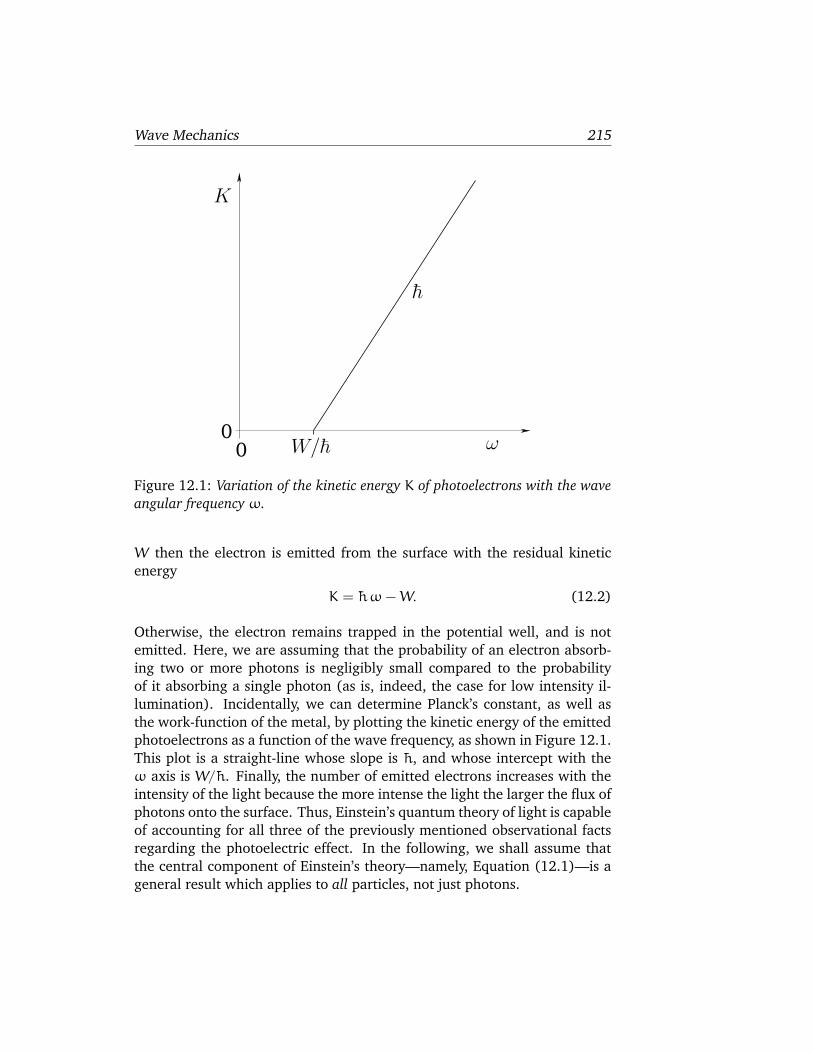
Wave Mechanics 215
ω0
0
K
W/h
h
Figure 12.1: Variation of the kinetic energy K of photoelectrons with the wave
angular frequency ω.
W then the electron is emitted from the surface with the residual kinetic
energy
K = hω−W. (12.2)
Otherwise, the electron remains trapped in the potential well, and is not
emitted. Here, we are assuming that the probability of an electron absorb-
ing two or more photons is negligibly small compared to the probability
of it absorbing a single photon (as is, indeed, the case for low intensity il-
lumination). Incidentally, we can determine Planck’s constant, as well as
the work-function of the metal, by plotting the kinetic energy of the emitted
photoelectrons as a function of the wave frequency, as shown in Figure 12.1.
This plot is a straight-line whose slope is h, and whose intercept with the
ω axis is W/h. Finally, the number of emitted electrons increases with the
intensity of the light because the more intense the light the larger the flux of
photons onto the surface. Thus, Einstein’s quantum theory of light is capable
of accounting for all three of the previously mentioned observational facts
regarding the photoelectric effect. In the following, we shall assume that
the central component of Einstein’s theory—namely, Equation (12.1)—is a
general result which applies to all particles, not just photons.
216 OSCILLATIONS AND WAVES
12.3 Electron Diffraction
In 1927, George Paget Thomson discovered that if a beam of electrons is
made to pass through a thin metal film then the regular atomic array in the
metal acts as a sort of diffraction grating, so that when a photographic film,
placed behind the metal, is developed an interference pattern is discernible.
Of course, this implies that electrons have wave-like properties. Moreover,
the electron wavelength, λ, or, alternatively, the wavenumber, k = 2π/λ,
can be deduced from the spacing of the maxima in the interference pattern
(see Chapter 11). Thomson found that the momentum, p, of an electron is
related to its wavenumber, k, according to the following simple relation:
p = h k. (12.3)
The associated wavelength, λ = 2π/k, is known as the de Broglie wavelength,
since the above relation was first hypothesized by Louis de Broglie in 1926.
In the following, we shall assume that Equation (12.3) is a general result
which applies to all particles, not just electrons.
It turns out that wave-particle duality only manifests itself on length-
scales less than, or of order, the de Broglie wavelength. Note, however,
that this wavelength is generally pretty small. For instance, the de Broglie
wavelength of an electron is
λe = 1.2× 10⁻⁹ [E(eV)]−1/2 m, (12.4)
where the electron energy is conveniently measured in units of electron-
volts (eV). (An electron accelerated from rest through a potential difference
of 1000V acquires an energy of 1000 eV, and so on. Electrons in atoms typ-
ically have energies in the range 10 to 100 eV.) Moreover, the de Broglie
wavelength of a proton is
λp = 2.9× 10⁻¹¹ [E(eV)]−1/2 m. (12.5)
12.4 Representation of Waves via Complex Numbers
In mathematics, the symbol i is conventionally used to represent the square-
root of minus one: i.e., the solution of i2 = −1. Now, a real number, x (say),
can take any value in a continuum of different values lying between −∞and +∞. On the other hand, an imaginary number takes the general form
iy, where y is a real number. It follows that the square of a real number
Wave Mechanics 217
is a positive real number, whereas the square of an imaginary number is a
negative real number. In addition, a general complex number is written
z = x+ iy, (12.6)
where x and y are real numbers. In fact, x is termed the real part of z, and
y the imaginary part of z. This is written mathematically as x = Re(z) and
y = Im(z). Finally, the complex conjugate of z is defined z∗ = x− iy.
Now, just as we can visualize a real number as a point on an infinite
straight-line, we can visualize a complex number as a point in an infinite
plane. The coordinates of the point in question are the real and imagi-
nary parts of the number: i.e., z ≡ (x, y). This idea is illustrated in Fig-
ure 12.2. The distance, r =√
x2 + y2, of the representative point from the
origin is termed the modulus of the corresponding complex number, z. This
is written mathematically as |z| =√
x2 + y2. Incidentally, it follows that
z z∗ = x2 + y2 = |z|2. The angle, θ = tan−1(y/x), that the straight-line
joining the representative point to the origin subtends with the real axis
is termed the argument of the corresponding complex number, z. This is
written mathematically as arg(z) = tan−1(y/x). It follows from standard
trigonometry that x = r cos θ, and y = r sin θ. Hence, z = r cos θ+ i r sin θ.
Complex numbers are often used to represent waves, and wavefunctions.
All such representations depend ultimately on a fundamental mathematical
identity, known as de Moivre’s theorem (see Exercise 12.1), which takes the
form
e i φ ≡ cosφ+ i sinφ, (12.7)
where φ is a real number. Incidentally, given that z = r cosθ + i r sin θ =
r [cosθ + i sin θ], where z is a general complex number, r = |z| its modulus,
and θ = arg(z) its argument, it follows from de Moivre’s theorem that any
complex number, z, can be written
z = r e i θ, (12.8)
where r = |z| and θ = arg(z) are real numbers.
Now, a one-dimensional wavefunction takes the general form
ψ(x, t) = A cos(φ+ k x−ωt), (12.9)
where A > 0 is the wave amplitude, φ the phase angle, k the wavenumber,
and ω the angular frequency. Consider the complex wavefunction
ψ(x, t) = ψ0 e i (kx−ωt), (12.10)
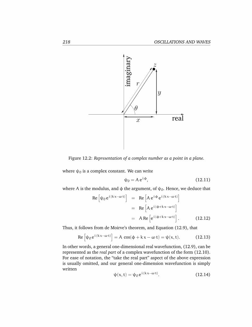
218 OSCILLATIONS AND WAVES
r
real
z
θ
imagin
ary
x
y
Figure 12.2: Representation of a complex number as a point in a plane.
where ψ0 is a complex constant. We can write
ψ0 = A e i φ, (12.11)
where A is the modulus, and φ the argument, of ψ0. Hence, we deduce that
Re[
ψ0 e i (kx−ωt)]
= Re[
A e i φ e i (kx−ωt)]
= Re[
A e i (φ+kx−ωt)]
= ARe[
e i (φ+kx−ωt)]
. (12.12)
Thus, it follows from de Moirve’s theorem, and Equation (12.9), that
Re[
ψ0 e i (kx−ωt)]
= A cos(φ+ k x−ωt) = ψ(x, t). (12.13)
In other words, a general one-dimensional real wavefunction, (12.9), can be
represented as the real part of a complex wavefunction of the form (12.10).
For ease of notation, the “take the real part” aspect of the above expression
is usually omitted, and our general one-dimension wavefunction is simply
written
ψ(x, t) = ψ0 e i (kx−ωt). (12.14)
Wave Mechanics 219
The main advantage of the complex representation, (12.14), over the more
straightforward real representation, (12.9), is that the former enables us to
combine the amplitude, A, and the phase angle, φ, of the wavefunction into
a single complex amplitude, ψ0.
12.5 Schrodinger’s Equation
The basic premise of wave mechanics is that a massive particle of energy E
and linear momentum p, moving in the x-direction (say), can be represented
by a one-dimensional complex wavefunction of the form
ψ(x, t) = ψ0 e i (kx−ωt), (12.15)
where the complex amplitude, ψ0, is arbitrary, whilst the wavenumber, k,
and the angular frequency, ω, are related to the particle momentum, p,
and energy, E, via the fundamental relations (12.3) and (12.1), respectively.
Now, the above one-dimensional wavefunction is, presumably, the solution
of some one-dimensional wave equation that determines how the wavefunc-
tion evolves in time. As described below, we can guess the form of this wave
equation by drawing an analogy with classical physics.
A classical particle of mass m, moving in a one-dimensional potential
U(x), satisfies the energy conservation equation
E = K+U, (12.16)
where
K =p2
2m(12.17)
is the particle’s kinetic energy. Hence,
Eψ = (K+U)ψ (12.18)
is a valid, but not obviously useful, wave equation.
However, it follows from Equations (12.15) and (12.1) that
∂ψ
∂t= −iωψ0 e i (kx−ωt) = −i
E
hψ, (12.19)
which can be rearranged to give
Eψ = i h∂ψ
∂t. (12.20)
220 OSCILLATIONS AND WAVES
Likewise, from (12.15) and (12.3),
∂2ψ
∂x2= −k2ψ0 e i (kx−ωt) = −
p2
h2ψ, (12.21)
which can be rearranged to give
p2
2mψ = −
h2
2m
∂2ψ
∂x2. (12.22)
Thus, combining Equations (12.18), (12.20), and (12.22), we obtain
i h∂ψ
∂t= −
h2
2m
∂2ψ
∂x2+U(x)ψ. (12.23)
This equation, which is known as Schrodinger’s equation—since it was first
formulated by Erwin Schrodinder in 1926—is the fundamental equation of
wave mechanics.
Now, for a massive particle moving in free space (i.e., U = 0), the com-
plex wavefunction (12.15) is a solution of Schrodinger’s equation, (12.23),
provided that
ω =h
2mk2. (12.24)
The above expression can be thought of as the dispersion relation (see Sec-
tion 5.1) for matter waves in free space. The associated phase velocity (see
Section 7.2) is
vp =ω
k=h k
2m=
p
2m, (12.25)
where use has been made of (12.3). Note that this phase velocity is only
half the classical velocity, v = p/m, of a massive (non-relativistic) particle.
12.6 Probability Interpretation of the Wavefunction
After many false starts, physicists in the early 20th century came to the
conclusion that the only self-consistent physical interpretation of a particle
wavefunction, which is consistent with experimental observations, is proba-
bilistic in nature. To be more exact, if ψ(x, t) is the complex wavefunction of
a given particle, moving in one-dimension along the x-axis, then the proba-
bility of finding the particle between x and x+ dx at time t is
P(x, t) = |ψ(x, t)|2dx. (12.26)
Wave Mechanics 221
A probability is, of course, a real number lying in the range 0 to 1. An event
which has a probability 0 is impossible. On the other hand, an event which
has a probability 1 is certain to occur. An event which has an probability 1/2
(say) is such that in a very large number of identical trials the event occurs
in half of the trials. Now, we can interpret
P(t) =
∫∞
−∞|ψ(x, t)|2dx (12.27)
as the probability of the particle being found anywhere between x = −∞and x = +∞ at time t. This follows, via induction, from the fundamental
result in probability theory that the probability of the occurrence of one or
other of two mutually exclusive events (such as the particle being found in
two non-overlapping regions) is the sum (or integral) of the probabilities of
the individual events. (For example, the probability of throwing a 1 on a
six-sided die is 1/6. Likewise, the probability of throwing a 2 is 1/6. Hence,
the probability of throwing a 1 or a 2 is 1/6 + 1/6 = 1/3.) Now, assuming
that the particle exists, it is certain that it will be found somewhere between
x = −∞ and x = +∞ at time t. Since a certain event has probability 1, our
probability interpretation of the wavefunction is only tenable provided that∫∞
−∞|ψ(x, t)|2dx = 1 (12.28)
at all times. A wavefunction which satisfies the above condition is said to be
properly normalized.
Suppose that we have a wavefunction, ψ(x, t), which is such that it satis-
fies the normalization condition (12.28) at time t = 0. Furthermore, let the
wavefunction evolve in time according to Schrodinger’s equation, (12.23).
Our probability interpretation of the wavefunction only makes sense if the
normalization condition remains satisfied at all subsequent times. This fol-
lows because if the particle is certain to be found somewhere on the x-axis
(which is the interpretation put on the normalization condition) at time
t = 0 then it is equally certain to be found somewhere on the x-axis at a
later time (since we are not presently dealing with any physical process by
which particles can be created or destroyed). Thus, it is necessary for us to
demonstrate that Schrodinger’s equation preserves the normalization of the
wavefunction.
Taking Schrodinger’s equation, and multiplying it by ψ∗ (the complex
conjugate of the wavefunction), we obtain
i h∂ψ
∂tψ∗ = −
h2
2m
∂2ψ
∂x2ψ∗ +U(x) |ψ|2. (12.29)
222 OSCILLATIONS AND WAVES
The complex conjugate of the above expression yields
− i h∂ψ∗
∂tψ = −
h2
2m
∂2ψ∗
∂x2ψ+U(x) |ψ|2. (12.30)
Here, we have made use of the easily demonstrated results (ψ∗)∗ = ψ and
i∗ = −i, as well as the fact that U is real. Taking the difference between the
above two expressions, we obtain
i h
(
∂ψ
∂tψ∗ +
∂ψ∗
∂tψ
)
= −h2
2m
(
∂2ψ
∂x2ψ∗ −
∂2ψ∗
∂x2ψ
)
, (12.31)
which can be written
i h∂|ψ|2
∂t= −
h2
2m
∂
∂x
(
∂ψ
∂xψ∗ −
∂ψ∗
∂xψ
)
. (12.32)
Integrating in x, we get
i hd
dt
∫∞
−∞|ψ|2dx = −
h2
2m
[
∂ψ
∂xψ∗ −
∂ψ∗
∂xψ
]∞
−∞. (12.33)
Finally, assuming that the wavefunction is localized in space: i.e.,
|ψ(x, t)| → 0 as |x| → ∞, (12.34)
we obtaind
dt
∫∞
−∞|ψ|2dx = 0. (12.35)
It follows, from the above analysis, that if a localized wavefunction is
properly normalized at t = 0 (i.e., if∫∞
−∞ |ψ(x, 0)|2dx = 1) then it will re-
main properly normalized as it evolves in time according to Schrodinger’s
equation. Incidentally, a wavefunction which is not localized cannot be
properly normalized, since its normalization integral∫∞
−∞ |ψ|2dx is neces-
sarily infinite. For such a wavefunction, |ψ(x, t)|2dx gives the relative prob-
ability, rather than the absolute probability, of finding the particle between
x and x+ dx at time t: i.e., [cf., Equation (12.26)]
P(x, t) ∝ |ψ(x, t)|2dx. (12.36)
Wave Mechanics 223
12.7 Wave Packets
As we have seen, the wavefunction of a massive particle of momentum p
and energy E, moving in free space along the x-axis, can be written
ψ(x, t) = ψ e i (kx−ωt), (12.37)
where k = p/h, ω = E/h, and ψ is a complex constant. Here, ω and k are
linked via the matter wave dispersion relation (12.24). Expression (12.37)
represents a plane wave which propagates in the x-direction with the phase
velocity vp = ω/k. However, according to (12.25), this phase velocity is
only half of the classical velocity of a massive particle.
Now, according to the discussion in the previous section, the most rea-
sonable physical interpretation of the wavefunction is that |ψ(x, t)|2dx is
proportional to (assuming that the wavefunction is not properly normal-
ized) the probability of finding the particle between x and x + dx at time t.
However, the modulus squared of the wavefunction (12.37) is |ψ|2, which is
a constant that depends on neither x nor t. In other words, the above wave-
function represents a particle which is equally likely to be found anywhere on
the x-axis at all times. Hence, the fact that this wavefunction propagates at
a phase velocity which does not correspond to the classical particle velocity
does not have any observable consequences.
So, how can we write the wavefunction of a particle which is localized in
x: i.e., a particle which is more likely to be found at some positions on the
x-axis than at others? It turns out that we can achieve this goal by forming
a linear combination of plane waves of different wavenumbers: i.e.,
ψ(x, t) =
∫∞
−∞ψ(k) e i (kx−ωt)dk. (12.38)
Here, ψ(k) represents the complex amplitude of plane waves of wavenum-
ber k within this combination. In writing the above expression, we are
relying on the assumption that matter waves are superposable: i.e., it is pos-
sible to add two valid wave solutions to form a third valid wave solution.
The ultimate justification for this assumption is that matter waves satisfy the
linear wave equation (12.23).
Now, there is a fundamental mathematical theorem, known as Fourier’s
theorem (see Section 8.1 and Exercise 12.2), which states that if
f(x) =
∫∞
−∞f(k) e i kxdk, (12.39)
224 OSCILLATIONS AND WAVES
then
f(k) =1
2π
∫∞
−∞f(x) e−i kxdx. (12.40)
Here, f(k) is known as the Fourier transform of the function f(x). We can
use Fourier’s theorem to find the k-space function ψ(k) which generates any
given x-space wavefunction ψ(x) at a given time.
For instance, suppose that at t = 0 the wavefunction of our particle takes
the form
ψ(x, 0) ∝ exp
[
ik0x−(x− x0)
2
4 (∆x)2
]
. (12.41)
Thus, the initial probability distribution for the particle’s x-coordinate is
|ψ(x, 0)|2 ∝ exp
[
−(x− x0)
2
2 (∆x)2
]
. (12.42)
This particular distribution is called a Gaussian distribution (see Section 8.1),
and is plotted in Figure 12.3. It can be seen that a measurement of the par-
ticle’s position is most likely to yield the value x0, and very unlikely to yield
a value which differs from x0 by more than 3∆x. Thus, (12.41) is the wave-
function of a particle which is initially localized in some region of x-space,
centered on x = x0, whose width is of order ∆x. This type of wavefunction
is known as a wave packet. Of course, a wave packet is just another name
for a wave pulse (see Chapter 8).
Now, according to Equation (12.38),
ψ(x, 0) =
∫∞
−∞ψ(k) e i kxdk. (12.43)
Hence, we can employ Fourier’s theorem to invert this expression to give
ψ(k) ∝∫∞
−∞ψ(x, 0) e−i kxdx. (12.44)
Making use of Equation (12.41), we obtain
ψ(k) ∝ e−i (k−k0)x0
∫∞
−∞exp
[
−i (k− k0) (x− x0) −(x− x0)
2
4 (∆x)2
]
dx. (12.45)
Changing the variable of integration to y = (x − x0)/(2∆x), the above ex-
pression reduces to
ψ(k) ∝ e−i kx0−β2/4
∫∞
−∞e−(y−y0)2
dy, (12.46)
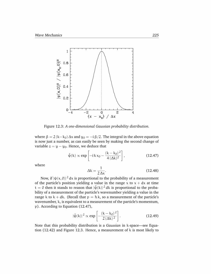
Wave Mechanics 225
Figure 12.3: A one-dimensional Gaussian probability distribution.
where β = 2 (k−k0)∆x and y0 = −iβ/2. The integral in the above equation
is now just a number, as can easily be seen by making the second change of
variable z = y− y0. Hence, we deduce that
ψ(k) ∝ exp
[
−ik x0 −(k− k0)
2
4 (∆k)2
]
, (12.47)
where
∆k =1
2∆x. (12.48)
Now, if |ψ(x, 0)|2dx is proportional to the probability of a measurement
of the particle’s position yielding a value in the range x to x + dx at time
t = 0 then it stands to reason that |ψ(k)|2dk is proportional to the proba-
bility of a measurement of the particle’s wavenumber yielding a value in the
range k to k + dk. (Recall that p = h k, so a measurement of the particle’s
wavenumber, k, is equivalent to a measurement of the particle’s momentum,
p). According to Equation (12.47),
|ψ(k)|2 ∝ exp
[
−(k− k0)
2
2 (∆k)2
]
. (12.49)
Note that this probability distribution is a Gaussian in k-space—see Equa-
tion (12.42) and Figure 12.3. Hence, a measurement of k is most likely to
226 OSCILLATIONS AND WAVES
yield the value k0, and very unlikely to yield a value which differs from k0
by more than 3∆k. Incidentally, as was previously mentioned in Section 8.1,
a Gaussian is the only mathematical function in x-space which has the same
form as its Fourier transform in k-space.
We have just seen that a wave packet with a Gaussian probability dis-
tribution of characteristic width ∆x in x-space [see Equation (12.42)] is
equivalent to a wave packet with a Gaussian probability distribution of char-
acteristic width ∆k in k-space [see Equation (12.49)], where
∆x∆k =1
2. (12.50)
This illustrates an important property of wave packets. Namely, in order
to construct a packet which is highly localized in x-space (i.e., with small
∆x) we need to combine plane waves with a very wide range of different
k-values (i.e., with large ∆k). Conversely, if we only combine plane waves
whose wavenumbers differ by a small amount (i.e., if ∆k is small) then the
resulting wave packet is highly extended in x-space (i.e., ∆x is large).
Now, according to Section 9.1, a wave packet made up of a superposition
of plane waves that is strongly peaked around some central wavenumber k0
propagates at the group velocity,
vg =dω(k0)
dk, (12.51)
rather than the phase velocity, vp = (ω/k)k0, assuming that all of the con-
stituent plane waves satisfy a dispersion relation of the form ω = ω(k).
Now, for the case of matter waves, the dispersion relation is (12.24). Thus,
the associated group velocity is
vg =h k0
m=p
m, (12.52)
where p = h k0. Note that this velocity is identical to the classical velocity
of a (non-relativistic) massive particle. We conclude that the matter wave
dispersion relation (12.24) is perfectly consistent with classical physics, as
long as we recognize that particles must be identified with wave packets
(which propagate at the group velocity) rather than plane waves (which
propagate at the phase velocity).
In Section 9.1, it was also demonstrated that the spatial extent of a wave
packet of initial extent (∆x)0 grows, as the packet evolves in time, like
∆x ≃ (∆x)0 +d2ω(k0)
dk2
t
(∆x)0
, (12.53)
Wave Mechanics 227
where k0 is the packet’s central wavenumber. Thus, it follows from the
matter wave dispersion relation, (12.24), that the width of a particle wave
packet grows in time as
∆x ≃ (∆x)0 +h
m
t
(∆x)0
. (12.54)
For example, if an electron wave packet is initially localized in a region
of atomic dimensions (i.e., ∆x ∼ 10−10 m) then the width of the packet
doubles in about 10−16 s. Clearly, particle wave packets spread out very
rapidly indeed (in free space).
12.8 Heisenberg’s Uncertainty Principle
According to the analysis contained in the previous section, a particle wave
packet that is initially localized in x-space, with characteristic width ∆x, is
also localized in k-space, with characteristic width ∆k = 1/(2∆x). However,
as time progresses, the width of the wave packet in x-space increases [see
Equation (12.54)], whilst that of the packet in k-space stays the same [since
ψ(k) is given by Equation (12.44) at all times.] Hence, in general, we can
say that
∆x∆k >∼
1
2. (12.55)
Furthermore, we can interpret ∆x and ∆k as characterizing our uncertainty
regarding the values of the particle’s position and wavenumber, respectively.
Now, a measurement of a particle’s wavenumber, k, is equivalent to a
measurement of its momentum, p, since p = h k. Hence, an uncertainty
in k of order ∆k translates to an uncertainty in p of order ∆p = h ∆k. It
follows, from the above inequality, that
∆x∆p >∼
h
2. (12.56)
This is the famous Heisenberg uncertainty principle, first proposed by Werner
Heisenberg in 1927. According to this principle, it is impossible to simulta-
neously measure the position and momentum of a particle (exactly). Indeed,
a good knowledge of the particle’s position implies a poor knowledge of its
momentum, and vice versa. Note that the uncertainty principle is a direct
consequence of representing particles as waves.
It is apparent, from expression (12.54), that a particle wave packet of
initial spatial extent (∆x)0 spreads out in such a manner that its spatial
228 OSCILLATIONS AND WAVES
extent becomes
∆x ∼h t
m (∆x)0
(12.57)
at large t. It is easily demonstrated that this spreading of the wave packet
is a consequence of the uncertainty principle. Indeed, since the initial un-
certainty in the particle’s position is (∆x)0, it follows that the uncertainty
in its momentum is of order h/(∆x)0. This translates to an uncertainty in
velocity of ∆v = h/[m (∆x)0]. Thus, if we imagine that part of the wave
packet propagates at v0 + ∆v/2, and another part at v0 − ∆v/2, where v0
is the mean propagation velocity, then it is clear that the wave packet will
spread out as time progresses. Indeed, at large t, we expect the width of the
wave packet to be
∆x ∼ ∆v t ∼h t
m (∆x)0
, (12.58)
which is identical to Equation (12.57). Evidently, the spreading of a particle
wave packet, as time progresses, should be interpreted as representing an
increase in our uncertainty regarding the particle’s position, rather than an
increase in the spatial extent of the particle itself.
12.9 Collapse of the Wavefunction
Consider a spatially extended wavefunction, ψ(x, t). According to our usual
interpretation, |ψ(x, t)|2dx is proportional to the probability of a measure-
ment of the particle’s position yielding a value in the range x to x + dx at
time t. Thus, if the wavefunction is extended then there is a wide range
of likely values that such a measurement could give. Suppose, however,
that we make a measurement of the particle’s position, and obtain the value
x0. We now know that the particle is located at x = x0. If we make another
measurement, immediately after the first one, then what value would we ex-
pect to obtain? Well, common sense tells us that we should obtain the same
value, x0, since the particle cannot have shifted position appreciably in an
infinitesimal time interval. Thus, immediately after the first measurement,
a measurement of the particle’s position is certain to give the value x0, and
has no chance of giving any other value. This implies that the wavefunction
must have collapsed to some sort of “spike” function, centered on x = x0.
This idea is illustrated in Figure 12.4. Of course, as soon as the wavefunc-
tion collapses, it starts to expand again, as described in the previous section.
Thus, the second measurement must be made reasonably quickly after the
first one, otherwise the same result will not necessarily be obtained.
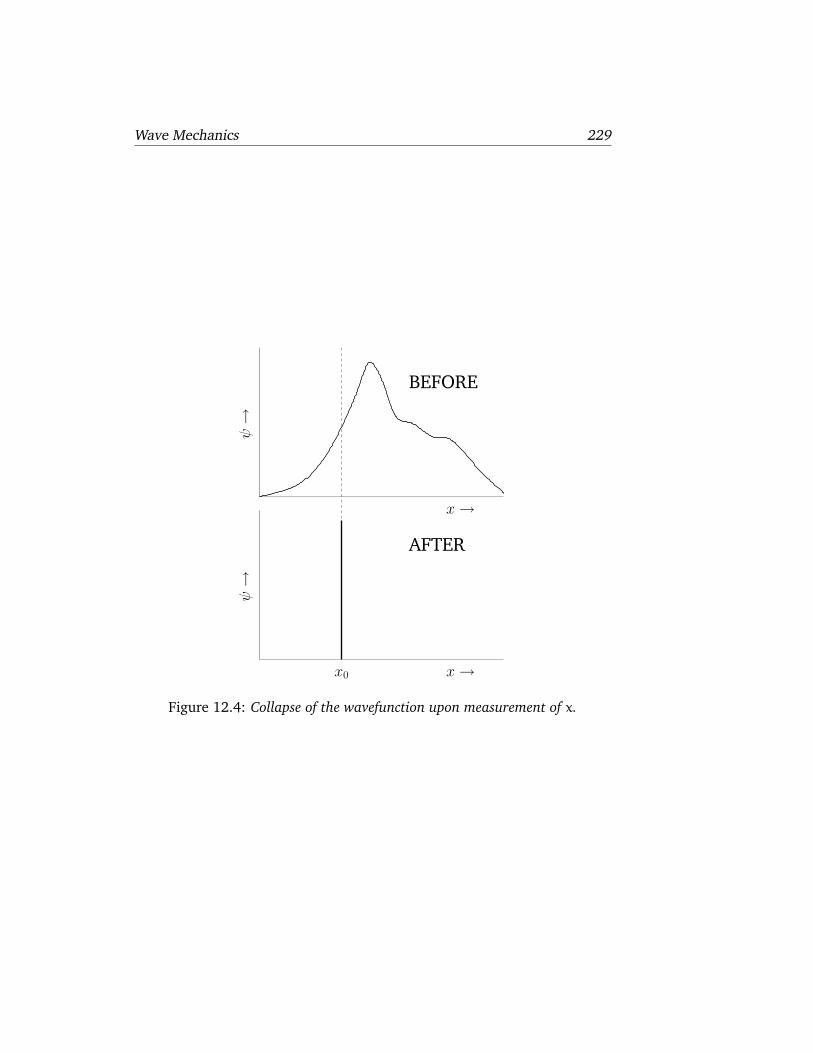
Wave Mechanics 229
x0
ψ→
ψ→
AFTER
BEFORE
x→
x→
Figure 12.4: Collapse of the wavefunction upon measurement of x.
230 OSCILLATIONS AND WAVES
The above discussion illustrates an important point in wave mechanics.
Namely, that the wavefunction of a massive particle changes discontinuously
(in time) whenever a measurement of the particle’s position is made. We
conclude that there are two types of time evolution of the wavefunction in
wave mechanics. First, there is a smooth evolution which is governed by
Schrodinger’s equation. This evolution takes place between measurements.
Second, there is a discontinuous evolution which takes place each time a
measurement is made.
12.10 Stationary States
Consider separable solutions to Schrodinger’s equation of the form
ψ(x, t) = ψ(x) e−i ωt. (12.59)
According to (12.20), such solutions have definite energies E = hω. For
this reason, they are usually written
ψ(x, t) = ψ(x) e−i (E/h)t. (12.60)
Now, the probability of finding the particle between x and x + dx at time t
is
P(x, t) = |ψ(x, t)|2dx = |ψ(x)|2dx. (12.61)
Note that this probability is time independent. For this reason, wavefunctions
of the form (12.60) are known as stationary states. Moreover, ψ(x) is called
a stationary wavefunction. Substituting (12.60) into Schrodinger’s equation,
(12.23), we obtain the following expression for ψ(x):
−h2
2m
d2ψ
dx2+U(x)ψ = Eψ. (12.62)
Not surprisingly, the above equation is called the time independent Schrod-
inger equation.
Consider a particle trapped in a one-dimensional square potential well,
of infinite depth, which is such that
U(x) =
0 0 ≤ x ≤ a∞ otherwise
. (12.63)
The particle is obviously excluded from the region x < 0 or x > a, so ψ = 0
in this region (i.e., there is zero probability of finding the particle outside
Wave Mechanics 231
the well). Within the well, a particle of definite energy E has a stationary
wavefunction, ψ(x), which satisfies
−h2
2m
d2ψ
dx2= Eψ. (12.64)
The boundary conditions are
ψ(0) = ψ(a) = 0. (12.65)
This follows because ψ = 0 in the region x < 0 or x > a, and ψ(x) must be
continuous [since a discontinuous wavefunction would generate a singular
term (i.e., the term involving d2ψ/dx2) in the time independent Schrodinger
equation, (12.62), which could not be balanced, even by an infinite poten-
tial].
Let us search for solutions to (12.64) of the form
ψ(x) = ψ0 sin(k x), (12.66)
where ψ0 is a constant. It follows that
h2k2
2m= E. (12.67)
The solution (12.66) automatically satisfies the boundary condition ψ(0) =
0. The second boundary condition, ψ(a) = 0, leads to a quantization of the
wavenumber: i.e.,
k = nπ
a, (12.68)
where n = 1, 2, 3, etc. (Note that a “quantized” quantity is one which
can only take discrete values.) According to (12.67), the energy is also
quantized. In fact, E = En, where
En = n2 h2π2
2ma2. (12.69)
Thus the allowed wavefunctions for a particle trapped in a one-dimensional
square potential well of infinite depth are
ψn(x, t) = An sin
(
nπx
a
)
exp
(
−in2 E1
ht
)
, (12.70)
where n is a positive integer, and An a constant. Note that we cannot have
n = 0, since, in this case, we obtain a null wavefunction: i.e., ψ = 0, every-
where. Furthermore, if n takes a negative integer value then it generates
232 OSCILLATIONS AND WAVES
exactly the same wavefunction as the corresponding positive integer value
(assuming ψ−n = −ψn).
The constant An, appearing in the above wavefunction, can be deter-
mined from the constraint that the wavefunction be properly normalized.
For the problem presently under consideration, the normalization condition
(12.28) reduces to ∫a
0
|ψ(x)|2dx = 1. (12.71)
It follows from (12.70) that |An|2 = 2/a. Hence, a properly normalized
version of the wavefunction (12.70) is
ψn(x, t) =
(
2
a
)1/2
sin
(
nπx
a
)
exp
(
−in2 E1
ht
)
. (12.72)
Figure 12.5 shows the first four properly normalized stationary wavefunc-
tions for a particle trapped in a one-dimensional square potential well of
infinite depth: i.e., ψn(x) =√
2/a sin(nπx/a), for n = 1 to 4.
Note that the stationary wavefunctions that we have just found are, in
essence, standing wave solutions to Schrodinger’s equation. Indeed, the
wavefunctions are very similar in form to the classical standing wave so-
lutions discussed in Chapters 5 and 6.
At first sight, it seems rather strange that the lowest energy that a par-
ticle trapped in a one-dimensional potential well can have is not zero, as
would be the case in classical mechanics, but rather E1 = h2π2/(2ma2).
In fact, as explained in the following, this residual energy is a direct con-
sequence of Heisenberg’s uncertainty principle. Now, a particle trapped in a
one-dimensional well of width a is likely to be found anywhere inside the
well. Thus, the uncertainty in the particle’s position is ∆x ∼ a. It follows
from the uncertainty principle, (12.56), that
∆p >∼
h
2∆x∼h
a. (12.73)
In other words, the particle cannot have zero momentum. In fact, the par-
ticle’s momentum must be at least p ∼ h/a. However, for a free particle,
E = p2/2m. Hence, the residual energy associated with the particle’s resid-
ual momentum is
E ∼p2
m∼h2
ma2∼ E1. (12.74)
This type of residual energy, which is often found in quantum mechanical
systems, and has no equivalent in classical mechanics, is generally known
as zero point energy.
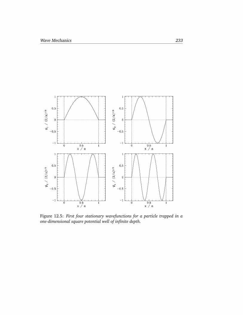
Wave Mechanics 233
Figure 12.5: First four stationary wavefunctions for a particle trapped in a
one-dimensional square potential well of infinite depth.
234 OSCILLATIONS AND WAVES
12.11 Three-Dimensional Wave Mechanics
Up to now, we have only discussed wave mechanics for a particle moving in
one dimension. However, the generalization to a particle moving in three
dimensions is fairly straightforward. A massive particle moving in three
dimensions has a complex wavefunction of the form [cf., (12.15)]
ψ(x, y, z, t) = ψ0 e i (k·r−ωt), (12.75)
where ψ0 is a complex constant, and r = (x, y, z). Here, the wavevector, k,
and the angular frequency, ω, are related to the particle momentum, p, and
energy, E, according to [cf., (12.3)]
p = h k, (12.76)
and [cf., (12.1)]
E = hω, (12.77)
respectively. Generalizing the analysis of Section 12.5, the three-dimensional
version of Schrodinger’s equation is easily shown to take the form [cf., (12.23)]
i h∂ψ
∂t= −
h2
2m∇2ψ+U(r)ψ, (12.78)
where the differential operator
∇2 ≡ ∂2
∂x2+∂2
∂y2+∂2
∂z2(12.79)
is known as the Laplacian. The interpretation of a three-dimensional wave-
function is that the probability of finding the particle between x and x+ dx,
between y and y+ dy, and between z and z+ dz, at time t is [cf., (12.26)]
P(x, y, z, t) = |ψ(x, y, z, t)|2dxdydz. (12.80)
Moreover, the normalization condition for the wavefunction becomes [cf.,
(12.28)] ∫∞
−∞
∫∞
−∞
∫∞
−∞|ψ(x, y, z, t)|2dxdydz = 1. (12.81)
Incidentally, it is easily demonstrated that Schrodinger’s equation, (12.78),
preserves the normalization condition, (12.81), of a localized wavefunction.
Wave Mechanics 235
Heisenberg’s uncertainty principle generalizes to [cf., (12.56)]
∆x∆px>∼
h
2, (12.82)
∆y∆py>∼
h
2, (12.83)
∆z∆pz>∼
h
2. (12.84)
Finally, a stationary state of energy E is written [cf., (12.60)]
ψ(x, y, z, t) = ψ(x, y, z) e−i (E/h)t, (12.85)
where the stationary wavefunction, ψ(x, y, z), satisfies [cf., (12.62)]
−h2
2m∇2ψ+U(r)ψ = Eψ. (12.86)
As an example of a three-dimensional problem in wave mechanics, con-
sider a particle trapped in a square potential well of infinite depth which is
such that
U(x, y, z) =
0 0 ≤ x ≤ a, 0 ≤ y ≤ a, 0 ≤ z ≤ a∞ otherwise
. (12.87)
Within the well, the stationary wavefunction, ψ(x, y, z), satisfies
−h2
2m∇2ψ = Eψ, (12.88)
subject to the boundary conditions
ψ(0, y, z) = ψ(x, 0, z) = ψ(x, y, 0) = 0, (12.89)
and
ψ(a, y, z) = ψ(x, a, z) = ψ(x, y, a) = 0, (12.90)
since ψ = 0 outside the well. Let us try a seperable wavefunction of the
form
ψ(x, y, z) = ψ0 sin(kxx) sin(kyy) sin(kz z). (12.91)
This expression automatically satisfies the boundary conditions (12.89). The
remaining boundary conditions, (12.90), are satisfied provided
kx = nxπ
a, (12.92)
ky = nyπ
a, (12.93)
kz = nzπ
a, (12.94)
236 OSCILLATIONS AND WAVES
where nx, ny, and nz are (independent) positive integers. Substitution of
the wavefunction (12.91) into Equation (12.88) yields
E =h2
2m(k2
x + k2y + k2
z ). (12.95)
Thus, it follows from Equations (12.92)–(12.94) that the particle energy is
quantized, and that the allowed energy levels are
Enx,ny,nz =h2
2ma2(n2
x + n2y + n2
z ). (12.96)
The properly normalized [see Equation (12.81)] stationary wavefunctions
corresponding to these energy levels are
ψnx,ny,nz(x, y, z) =
(
2
a
)3/2
sin
(
nxπx
a
)
sin
(
nyπy
a
)
sin
(
nzπz
a
)
.
(12.97)
As is the case for a particle trapped in a one-dimensional potential well,
the lowest energy level for a particle trapped in a three-dimensional well is
not zero, but rather
E1,1,1 = 3 E1. (12.98)
Here,
E1 =h2
2ma2. (12.99)
is the ground state (i.e., the lowest energy state) energy in the one-dimension-
al case. Now, it is clear, from (12.96), that distinct permutations of nx, ny,
and nz which do not alter the value of n2x + n2
y + n2z also do not alter the
energy. In other words, in three dimensions it is possible for distinct wave-
functions to be associated with the same energy level. In this situation, the
energy level is said to be degenerate. The ground state energy level, 3 E1, is
non-degenerate, since the only combination of (nx, ny, nz) which gives this
energy is (1, 1, 1). However, the next highest energy level, 6 E1, is degener-
ate, since it is obtained when (nx, ny, ny) take the values (2, 1, 1), or (1, 2,
1), or (1, 1, 2). In fact, it is not difficult to see that a non-degenerate energy
level corresponds to a case where the three mode numbers (i.e., nx, ny, and
nz) all have the same value, whereas a three-fold degenerate energy level
corresponds to a case where only two of the mode numbers have the same
value, and, finally, a six-fold degenerate energy level corresponds to a case
where the mode numbers are all different.
Wave Mechanics 237
12.12 Particle in a Finite Potential Well
Consider, now, a particle of mass m trapped in a one-dimensional square
potential well of width a and finite depth V > 0. In fact, suppose that the
potential takes the form
U(x) =
−V |x| ≤ a/20 otherwise
. (12.100)
Here, we have adopted the standard convention that U(x) → 0 as |x| → ∞.
This convention is useful because, just like in classical mechanics, a particle
whose overall energy, E, is negative is bound in the well (i.e., it cannot
escape to infinity), whereas a particle whose overall energy is positive is
unbound. Since we are interested in bound particles, we shall assume that
E < 0. We shall also assume that E+ V > 0, in order to allow the particle to
have a positive kinetic energy inside the well.
Let us search for a stationary state
ψ(x, t) = ψ(x) e−i (E/h)t, (12.101)
whose stationary wavefunction,ψ(x), satisfies the time independent Schrod-
inger equation, (12.62). Now, it is easily appreciated that the solutions to
(12.62) in the symmetric [i.e., U(−x) = U(x)] potential (12.100) must be
either totally symmetric [i.e., ψ(−x) = ψ(x)] or totally antisymmetric [i.e.,
ψ(−x) = −ψ(x)]. Moreover, the solutions must satisfy the boundary condi-
tion
ψ → 0 as |x| → ∞, (12.102)
otherwise they would not correspond to bound states.
Let us, first of all, search for a totally symmetric solution. In the region
to the left of the well (i.e., x < −a/2), the solution of the time independent
Schrodinger equation which satisfies the boundary condition ψ → 0 as x →−∞ is
ψ(x) = A eqx, (12.103)
where
q =
√
2m (−E)
h2, (12.104)
and A is a constant. By symmetry, the solution in the region to the right of
the well (i.e., x > a/2) is
ψ(x) = A e−qx. (12.105)
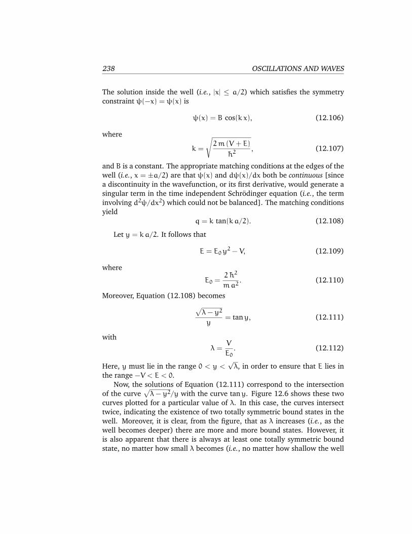
238 OSCILLATIONS AND WAVES
The solution inside the well (i.e., |x| ≤ a/2) which satisfies the symmetry
constraint ψ(−x) = ψ(x) is
ψ(x) = B cos(k x), (12.106)
where
k =
√
2m (V + E)
h2, (12.107)
and B is a constant. The appropriate matching conditions at the edges of the
well (i.e., x = ±a/2) are that ψ(x) and dψ(x)/dx both be continuous [since
a discontinuity in the wavefunction, or its first derivative, would generate a
singular term in the time independent Schrodinger equation (i.e., the term
involving d2ψ/dx2) which could not be balanced]. The matching conditions
yield
q = k tan(ka/2). (12.108)
Let y = ka/2. It follows that
E = E0y2 − V, (12.109)
where
E0 =2 h2
ma2. (12.110)
Moreover, Equation (12.108) becomes
√
λ− y2
y= tany, (12.111)
with
λ =V
E0
. (12.112)
Here, y must lie in the range 0 < y <√λ, in order to ensure that E lies in
the range −V < E < 0.
Now, the solutions of Equation (12.111) correspond to the intersection
of the curve√
λ− y2/y with the curve tany. Figure 12.6 shows these two
curves plotted for a particular value of λ. In this case, the curves intersect
twice, indicating the existence of two totally symmetric bound states in the
well. Moreover, it is clear, from the figure, that as λ increases (i.e., as the
well becomes deeper) there are more and more bound states. However, it
is also apparent that there is always at least one totally symmetric bound
state, no matter how small λ becomes (i.e., no matter how shallow the well
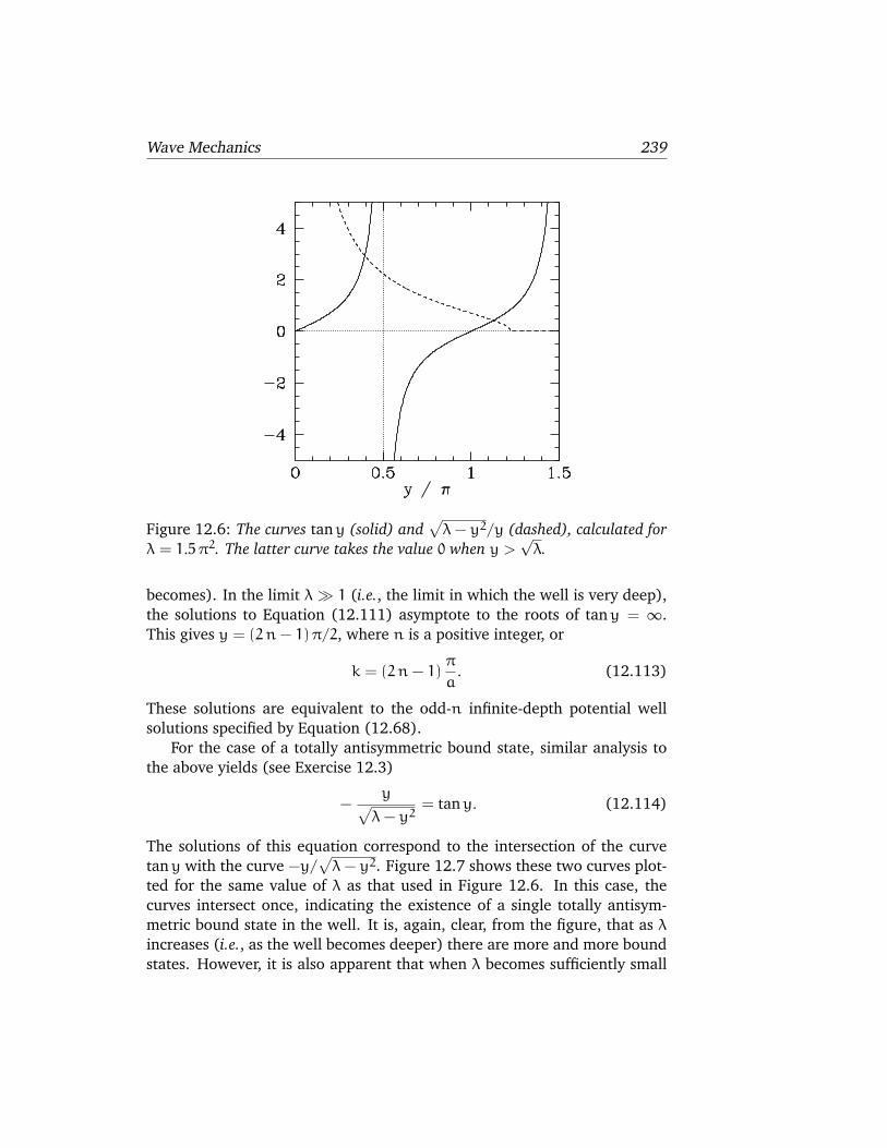
Wave Mechanics 239
Figure 12.6: The curves tany (solid) and√
λ− y2/y (dashed), calculated for
λ = 1.5 π2. The latter curve takes the value 0 when y >√λ.
becomes). In the limit λ≫ 1 (i.e., the limit in which the well is very deep),
the solutions to Equation (12.111) asymptote to the roots of tany = ∞.
This gives y = (2n− 1)π/2, where n is a positive integer, or
k = (2n− 1)π
a. (12.113)
These solutions are equivalent to the odd-n infinite-depth potential well
solutions specified by Equation (12.68).
For the case of a totally antisymmetric bound state, similar analysis to
the above yields (see Exercise 12.3)
−y
√
λ− y2= tany. (12.114)
The solutions of this equation correspond to the intersection of the curve
tany with the curve −y/√
λ− y2. Figure 12.7 shows these two curves plot-
ted for the same value of λ as that used in Figure 12.6. In this case, the
curves intersect once, indicating the existence of a single totally antisym-
metric bound state in the well. It is, again, clear, from the figure, that as λ
increases (i.e., as the well becomes deeper) there are more and more bound
states. However, it is also apparent that when λ becomes sufficiently small
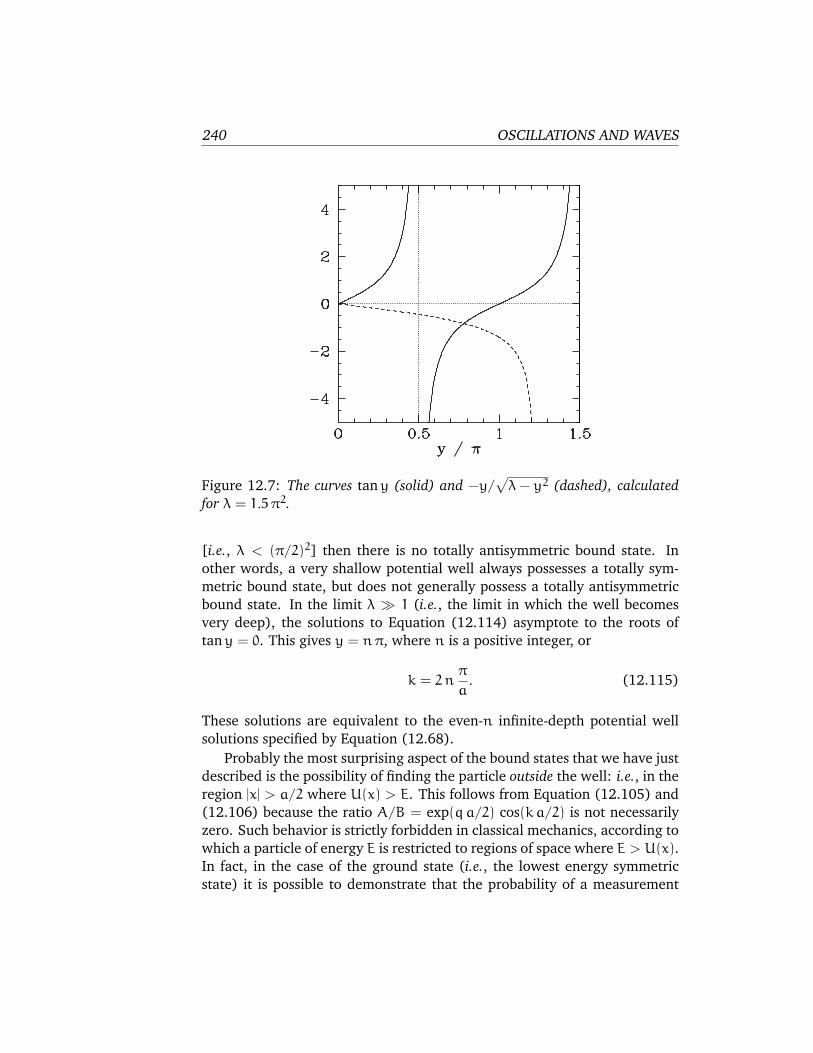
240 OSCILLATIONS AND WAVES
Figure 12.7: The curves tany (solid) and −y/√
λ− y2 (dashed), calculated
for λ = 1.5 π2.
[i.e., λ < (π/2)2] then there is no totally antisymmetric bound state. In
other words, a very shallow potential well always possesses a totally sym-
metric bound state, but does not generally possess a totally antisymmetric
bound state. In the limit λ ≫ 1 (i.e., the limit in which the well becomes
very deep), the solutions to Equation (12.114) asymptote to the roots of
tany = 0. This gives y = nπ, where n is a positive integer, or
k = 2nπ
a. (12.115)
These solutions are equivalent to the even-n infinite-depth potential well
solutions specified by Equation (12.68).
Probably the most surprising aspect of the bound states that we have just
described is the possibility of finding the particle outside the well: i.e., in the
region |x| > a/2 where U(x) > E. This follows from Equation (12.105) and
(12.106) because the ratio A/B = exp(qa/2) cos(ka/2) is not necessarily
zero. Such behavior is strictly forbidden in classical mechanics, according to
which a particle of energy E is restricted to regions of space where E > U(x).
In fact, in the case of the ground state (i.e., the lowest energy symmetric
state) it is possible to demonstrate that the probability of a measurement
Wave Mechanics 241
finding the particle outside the well is (see Exercise 12.4)
Pout ≃ 1− 2 λ (12.116)
for a shallow well (i.e., λ≪ 1), and
Pout ≃π2
4
1
λ3/2(12.117)
for a deep well (i.e., λ ≫ 1). It follows that the particle is very likely to be
found outside a shallow well, and there is a small, but finite, probability of
it being found outside a deep well. In fact, the probability of finding the
particle outside the well only goes to zero in the case of an infinitely deep
well (i.e., λ → ∞).
12.13 Square Potential Barrier
Consider a particle of mass m and energy E > 0 interacting with the simple
potential barrier
U(x) =
V for 0 ≤ x ≤ a0 otherwise
, (12.118)
where V > 0. In the regions to the left and to the right of the barrier, the
stationary wavefunction, ψ(x), satisfies
d2ψ
dx2= −k2ψ, (12.119)
where
k =
√
2mE
h2. (12.120)
Let us adopt the following solution of the above equation to the left of
the barrier (i.e., x < 0):
ψ(x) = e i kx + R e−i kx. (12.121)
This solution consists of a plane wave of unit amplitude traveling to the
right [since the full wavefunction is multiplied by a factor exp(−iE t/h)],
and a plane wave of complex amplitude R traveling to the left. We interpret
the first plane wave as an incoming particle, and the second as a particle
242 OSCILLATIONS AND WAVES
reflected by the potential barrier. Hence, |R|2 is the probability of reflection
(see Section 7.6).
Let us adopt the following solution to Equation (12.119) to the right of
the barrier (i.e. x > a):
ψ(x) = T e i kx. (12.122)
This solution consists of a plane wave of complex amplitude T traveling to
the right. We interpret this as a particle transmitted through the barrier.
Hence, |T |2 is the probability of transmission.
Let us consider the situation in which E < V . In this case, according
to classical mechanics, the particle is unable to penetrate the barrier, so the
coefficient of reflection is unity, and the coefficient of transmission zero.
However, this is not necessarily the case in wave mechanics. In fact, inside
the barrier (i.e., 0 ≤ x ≤ a), ψ(x) satisfies
d2ψ
dx2= q2ψ, (12.123)
where
q =
√
2m (V − E)
h2. (12.124)
The general solution to Equation (12.123) takes the form
ψ(x) = A eqx + B e−qx. (12.125)
Now, continuity of ψ and dψ/dx at the left edge of the barrier (i.e.,
x = 0) yields
1+ R = A+ B, (12.126)
ik (1− R) = q (A− B). (12.127)
Likewise, continuity of ψ and dψ/dx at the right edge of the barrier (i.e.,
x = a) gives
A eqa + B e−qa = T e i ka, (12.128)
q(
A eqa − B e−qa)
= ik T e i ka. (12.129)
After considerable algebra (see Exercise 12.5), the above four equations
yield
|T |2 = 1− |R|2 =4 k2q2
4 k2q2 + (k2 + q2)2 sinh2(qa). (12.130)
Wave Mechanics 243
Here, sinh x ≡ (1/2) (ex − e−x). The fact that |R|2 + |T |2 = 1 ensures that
the probabilities of reflection and transmission sum to unity, as must be the
case, since reflection and transmission are the only possible outcomes for a
particle incident on the barrier. Note that, according to Equation (12.130),
the probability of transmission is not necessarily zero. This means that,
in wave mechanics, there is a finite probability for a particle incident on
a potential barrier, of finite width, to penetrate through the barrier, and
reach the other side, even when the barrier is sufficiently high to completely
reflect the particle according to the laws of classical mechanics. This strange
phenomenon is known as tunneling. For the case of a very high barrier, such
that V ≫ E, the tunneling probability reduces to
|T |2 ≃ 4 E
Ve−2a/λ, (12.131)
where λ =√
h2/2mV is the de Broglie wavelength inside the barrier. Here,
it is assumed that a≫ λ. Note that, even in the limit in which the barrier is
very high, there is an exponentially small, but nevertheless non-zero, tunnel-
ing probability. Tunneling plays an important role in the physics of α-decay
and electron field emission.
12.14 Exercises
1. Use the standard power law expansions,
ex = 1+ x+x2
2!+x3
3!+ · · · ,
sin x = x−x3
3!+x5
5!−x7
7!+ · · · ,
cos x = 1−x2
2!+x4
4!−x6
6!+ · · · ,
which are valid for complex x, to prove de Moivre’s theorem,
e i θ = cos θ+ i sin θ,
where θ is real.
2. Equations (8.27) and (8.28) can be combined with de Moivre’s theorem togive
δ(k) =1
2π
∫∞
−∞
e i k x dx,

244 OSCILLATIONS AND WAVES
where δ(k) is a Dirac delta function. Use this result to prove Fourier’s theo-rem: i.e., if
f(x) =
∫∞
−∞
f(k) e i k x dk,
then
f(k) =1
2π
∫∞
−∞
f(x) e−i k x dx.
3. Derive Equation (12.114).
4. Consider a particle trapped in the finite potential well whose potential isgiven by Equation (12.100). Demonstrate that for a totally symmetric statethe ratio of the probability of finding the particle outside to the probabilityof finding the particle inside the well is
Pout
Pin=
cos3 y
siny (y+ siny cosy),
where√
λ− y2 = y tany, and λ = V/E0. Hence, demonstrate that for ashallow well (i.e., λ≪ 1) Pout ≃ 1− 2 λ, whereas for a deep well (i.e., λ≫ 1)Pout ≃ (π2/4)/λ3/2.
5. Derive expression (12.130) from Equations (12.126)–(12.129).
6. Show that the coefficient of transmission of a particle of mass m and energyE, incident on a square potential barrier of height V < E, and width a, is
|T | 2 =4 k2 q2
4 k2 q2 + (k2 − q2) 2 sin2(qa)
,
where k =
√
2mE/h2 and q =
√
2m (E− V)/h2. Demonstrate that the co-
efficient of transmission is unity (i.e., there is no reflection from the barrier)when qa = nπ, where n is positive integer.
7. A He-Ne laser emits radiation of wavelength λ = 633nm. How many photonsare emitted per second by a laser with a power of 1mW? What force doessuch a laser exert on a body which completely absorbs its radiation?
8. The ionization energy of a hydrogen atom in its ground state is Eion = 13.6 eV.Calculate the frequency (in Hertz), wavelength, and wavenumber of the elec-tromagnetic radiation which will just ionize the atom.
9. The maximum energy of photoelectrons from aluminium is 2.3 eV for radia-tion of wavelength 200nm, and 0.90 eV for radiation of wavelength 258nm.Use this data to calculate Planck’s constant (divided by 2π) and the workfunction of aluminium.
Wave Mechanics 245
10. Show that the de Broglie wavelength of an electron accelerated across a po-tential difference V is given by
λ = 1.29× 10⁻⁹ V−1/2 m,
where V is measured in volts.
11. If the atoms in a regular crystal are separated by 3 × 10⁻¹⁰ m demonstratethat an accelerating voltage of about 3 kV would be required to produce anelectron diffraction pattern from the crystal.
12. A particle of mass m has a wavefunction
ψ(x, t) = A exp[
−a (mx2/h+ i t)]
,
where A and a are positive real constants. For what potential U(x) doesψ(x, t) satisfy Schrodinger’s equation?
13. Show that the wavefunction of a particle of massm trapped in a one-dimensio-nal square potential well of of width a, and infinite depth, returns to itsoriginal form after a quantum revival time T = 4ma2/π h.
14. Show that the normalization constant for the stationary wavefunction
ψ(x, y, z) = A sin(
nx πx
a
)
sin(
ny πy
b
)
sin(
nz πz
c
)
describing an electron trapped in a three-dimensional rectangular potentialwell of dimensions a, b, c, and infinite depth, is A = (8/abc)1/2. Here, nx,ny, and nz are positive integers.
15. An electron of momentum p passes through a slit of width ∆x. Its diffractionas a wave can be regarded in terms of a change of its momentum ∆p in adirection parallel to the plane of the slit (the total momentum remainingconstant). Show that the approximate position of the first maximum of thediffraction pattern is in accordance with Heisenberg’s uncertainty principle.
16. The probability of a particle of mass m penetrating a distance x into a classi-cally forbidden region is proportional to e−2 α x, where
α2 = 2m (V − E)/h2.
If x = 2 × 10⁻¹⁰ m and V − E = 1 eV show that e−2 α x is equal to 0.1 for anelectron, and 10−43 for a proton.

246 OSCILLATIONS AND WAVES
Useful Information 247
A Useful Information
A.1 Physical Constants
Speed of light c 2.998× 10⁸ m s−1
Reduced Planck constant h 1.055× 10⁻³⁴ J s
Electric constant ǫ0 8.854× 10⁻¹² F m−1
Magnetic constant µ0 1.257× 10⁻⁶ N A−2
Elementary charge e 1.602× 10⁻¹⁹ C
Electron mass me 9.109× 10⁻³¹ kg
Proton mass mp 1.673× 10⁻²⁷ kg
A.2 Trigonometric Identities
sin(−α) = − sinα
cos(−α) = + cosα
tan(−α) = − tanα
sin2α+ cos2α = 1
sin(α± β) = sinα cosβ± cosα sinβ
cos(α± β) = cosα cosβ∓ sinα sinβ
sinα+ sinβ = 2 sin
(
α+ β
2
)
cos
(
α− β
2
)
sinα− sinβ = 2 cos
(
α+ β
2
)
sin
(
α− β
2
)
cosα+ cosβ = 2 cos
(
α+ β
2
)
cos
(
α− β
2
)
cosα− cosβ = −2 sin
(
α+ β
2
)
sin
(
α− β
2
)
sinα sinβ =1
2[cos(α− β) − cos(α+ β)]
cosα cosβ =1
2[cos(α− β) + cos(α+ β)]
sinα cosβ =1
2[sin(α− β) + sin(α+ β)]

248 OSCILLATIONS AND WAVES
sin(2α) = 2 sinα cosα
cos(2α) = cos2α− sin2α = 2 cos2α− 1 = 1− 2 sin2α
sin(3α) = −4 sin3α+ 3 sinα
cos(3α) = 4 cos3α− 3 cosα
sin2α = [1− cos(2α)]/2
cos2α = [1+ cos(2α)]/2
A.3 Calculus
d
dxxn = nxn−1
d
dxsin x = cos x
d
dxcos x = − sin x
d
dxex = ex
d
dxln x =
1
x
d
dx(f g) =
df
dxg+
dg
dxf
d
dx
(
f
g
)
=df
dx
1
g−dg
dx
f
g2
∫
fdg
dxdx = f g−
∫df
dxgdx
A.4 Power Series
(1+ x)n = 1+ nx+n (n− 1)
2!x2 + · · ·
ex = 1+ x+x2
2!+x3
3!+ · · ·
ln(1+ x) = x−x2
2+x3
3−x4
4+ · · ·
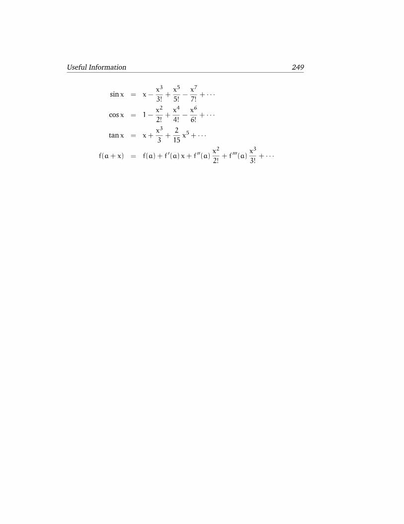
Useful Information 249
sin x = x−x3
3!+x5
5!−x7
7!+ · · ·
cos x = 1−x2
2!+x4
4!−x6
6!+ · · ·
tan x = x+x3
3+2
15x5 + · · ·
f(a+ x) = f(a) + f ′(a) x+ f ′′(a)x2
2!+ f ′′′(a)
x3
3!+ · · ·
Related Documents