Wavelet Bases and Lifting Wavelets - SJTUmin.sjtu.edu.cn/files/wavelet/6-lifting wavelet and filterbank.pdf · Periodic wavelet bases have the disadvantage of creating high-amplitude

Wavelet Bases and Lifting Wavelets

Hongkai Xiong

熊红凯

http://min.sjtu.edu.cn

Department of Electronic Engineering

Shanghai Jiao Tong University

http://ivm.sjtu.edu.cn/


• Wavelet Bases on an Interval

• Separable Wavelet Bases

• Lifting Wavelets





Wavelet Bases

Wavelets Over an Interval

Until now, only wavelets over the real axis have been considered, e.g.

wavelets that are suited to the analysis of signals defined over the whole axis.

In most cases, signals are compactly supported; images, in particular, are

explicitly defined over a rectangle of pixels.

The wavelets considered here are compactly supported.

A 0,𝑁 supported signal can be represented as the product of a general

signal with the characteristic function of 0,𝑁 . The discontinuities of this

function require special attention. Three methods are known to handle them:

wavelet periodization, wavelet folding and boundary wavelets, the last one

being the most efficient.

Wavelet Bases

Wavelet Periodization

A wavelet basis 𝜓𝑗,𝑛 𝑗,𝑛 ∈ℤ2 of 𝐋𝟐 ℝ is transformed into a wavelet basis of 𝐋𝟐 0,1 by

periodizing each 𝜓𝑗,𝑛. The periodization of 𝑓 ∈ 𝐋𝟐 ℝ over 0,1 is defined by

𝑓per 𝑡 = 𝑓 𝑡 + 𝑘

+∞

𝑘=−∞

The resulting periodic wavelets are

𝜓𝑗,𝑛per

𝑡 =1

2𝑗 𝜓

𝑡 − 2𝑗𝑛 + 𝑘

2𝑗

+∞

𝑘=−∞

For 𝑗 ≤ 0, there are 2−𝑗 different 𝜓𝑗,𝑛per

indexed by 0 ≤ 𝑛 < 2−𝑗.

Wavelets whose support are completely inside the interval 0,1 are not changed:

𝜓𝑗,𝑛per

𝑡 = 𝜓𝑗,𝑛 𝑡 for 𝑡 ∈ 0,1 .

The restriction to 0,1 of this periodization modifies only the boundary wavelets with a

support that overlaps 𝑡 = 0 or 𝑡 = 1.

Wavelet Bases


As indicated in the Figure, wavelets that overlap the boundaries are

transformed into boundary wavelets that have two disjoint components

near 𝑡 = 0 and 𝑡 = 1. Taken separately, the components near 𝑡 = 0 and

𝑡 = 1 of these boundary wavelets have no vanishing moments, and thus

create large signal coefficients.

Wavelet Bases


Theorem 7.16 For any 𝐽 ≤ 0,

𝜓𝑗,𝑛per

−∞<𝑗≤𝐽,0≤𝑛<2−𝑗 , 𝜙𝐽,𝑛

per

0≤𝑛<2−𝐽

is an orthogonal basis of 𝐋𝟐 0,1 .

Theorem 7.16 proves that periodic wavelets together with periodized scaling functions

𝜙𝑗,𝑛per

generate an orthogonal basis of 𝐋𝟐 0, 1 :

Periodic wavelet bases have the disadvantage of creating high-amplitude wavelet

coefficients in the neighborhood of 𝑡 = 0 and 𝑡 = 1, because boundary wavelets have

separate components with no vanishing moments.

If 𝑓 0 ≠ 𝑓 1 , the wavelet coefficients behave as if the signal were discontinuous at the

boundaries. This can be verified by extending 𝑓 ∈ 𝐋𝟐 0,1 into an infinite 1 periodic

signal 𝑓per and by showing that:

𝑓 𝑡 𝜓𝑗,𝑛per

𝑡1

0

𝑑𝑡 = 𝑓per+∞

−∞

𝑡 𝜓𝑗,𝑛 𝑡 𝑑𝑡

Wavelet Bases

Wavelet Folding

To avoid creating discontinuous with wavelet periodization, the signal is folded

with respect to 𝑡 = 0: 𝑓0 𝑡 = 𝑓 𝑡 + 𝑓 −𝑡 . The support of 𝑓0 is −1,1 and it is

transformed into a 2 periodic signal:

𝑓repl 𝑡 = 𝑓0 𝑡 − 2𝑘

+∞

𝑘=−∞

= 𝑓 𝑡 − 2𝑘

+∞

𝑘=−∞

+ 𝑓 2𝑘 − 𝑡

+∞

𝑘=−∞

This yields a continuous periodic signal:

The folded signal 𝑓repl 𝑡 is 2 periodic, symmetric about 𝑡 = 0

and 𝑡 = 1, and equal to 𝑓 𝑡 on 0,1

Wavelet Bases

Wavelet Folding

Decomposing 𝑓repl in a wavelet basis 𝜓𝑗,𝑛 𝑗,𝑛 ∈ℤ2 is equivalent to decomposing

𝑓 on a folded wavelet basis. Let 𝜓𝑗,𝑛repl

be the folding of 𝜓𝑗,𝑛, one can verify that:

𝑓 𝑡 𝜓𝑗,𝑛

repl𝑡

1

0

𝑑𝑡 = 𝑓repl+∞

−∞

𝑡 𝜓𝑗,𝑛 𝑡 𝑑𝑡

Suppose that 𝑓 is regular over 0,1 . Then 𝑓repl is continuous at 𝑡 = 0, 1 and

produces smaller boundary wavelet coefficients than 𝑓per. However, it is not

continuously differentiable at 𝑡 = 0, 1, which creates bigger wavelet coefficients

at the boundary than inside.

The folded signal 𝑓repl 𝑡 is 2 periodic, symmetric about 𝑡 = 0

and 𝑡 = 1, and equal to 𝑓 𝑡 on 0,1

Wavelet Bases

Wavelet Folding

To construct a basis of 𝐋𝟐 0, 1 with the folded wavelets 𝜓𝑗,𝑛repl

, it is sufficient

for 𝜓 𝑡 to be either symmetric or antisymmetric with respect to 𝑡 = 1/2.

The Haar wavelet is the only real compactly supported wavelet that is

symmetric or antisymmetric and that generates an orthogonal basis of 𝐋𝟐 ℝ .

If we loosen up the orthogonality constraint, then there exist biorthogonal

bases constructed with compactly supported wavelets that are either

symmetric or antisymmetric.

Wavelet Bases

Boundary Wavelets

Wavelet coefficients are small in regions where the signal is regular only if the

wavelets have enough vanishing moments.

The restriction of periodic and folded “boundary” wavelets to the

neighborhood of 𝑡 = 0 and 𝑡 = 1 have, respectively, 0 and 1 vanishing

moments. Therefore, these “boundary” wavelets produce large inner products,

as if the signal were discontinuous or had a discontinuous derivative.

To avoid creating large-amplitude wavelet coefficients at the boundaries, one

must synthesize boundary wavelets that have as many vanishing moments as

the original wavelet 𝜓.

Wavelet Bases

Multiresolution of 𝐋𝟐 0, 1

A wavelet basis of 𝐋𝟐 0, 1 is constructed with a multiresolution

approximation 𝐕𝑗int

−∞<𝑗≤0. A wavelet has 𝑝 vanishing moments if it is

orthogonal to all polynomials of degree 𝑝 − 1 or smaller.

Since wavelets at a scale 2𝑗 are orthogonal to functions in 𝐕𝑗int, to guarantee

that they have 𝑝 vanishing moments we make sure that polynomials of degree

𝑝 − 1 are inside 𝐕𝑗int

Wavelet Bases

Multiresolution of 𝐋𝟐 0, 1

Consider an approximation space 𝐕𝑗int ⊂ 𝐋𝟐 0, 1 with a compactly supported

Daubechies scaling function 𝜙 associated to a wavelet with 𝑝 vanishing moments.

We translate 𝜙 so that its support is −𝑝 + 1, 𝑝 . At a scale 2𝑗 ≤ 2𝑝−1, there are

2−𝑗 − 2𝑝 scaling functions with a support inside 0, 1 :

𝜙𝑗,𝑛int 𝑡 = 𝜙𝑗,𝑛 𝑡 =

1

2𝑗𝜙

𝑡−2𝑗𝑛

2𝑗 for 𝑝 ≤ 𝑛 < 2−𝑗 − 𝑝

To construct an approximation space 𝐕𝑗int of dimension 2−𝑗 we add 𝑝 scaling

functions with a support on the left boundary near 𝑡 = 0:

𝜙𝑗,𝑛int 𝑡 =

1

2𝑗𝜙𝑛left 𝑡

2𝑗 for 0 ≤ 𝑛 < 𝑝

and 𝑝 scaling functions on the right boundary near 𝑡 = 1:

𝜙𝑗,𝑛int 𝑡 =

1

2𝑗𝜙2−𝑗−1−𝑛

right 𝑡−1

2𝑗 for 2−𝑗 − 𝑝 ≤ 𝑛 < 2−𝑗

Wavelet Bases

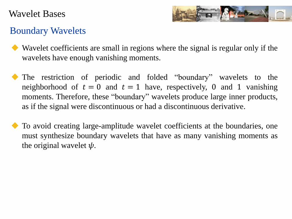
Boundary effects are explicitly handled. Consider a Daubechies orthogonal basis with 𝑝

vanishing moments, the Strang and Fix condition 7.70 implies that there exists a

polynomial 𝑞𝑘 of degree 𝑘 such that:

𝑞𝑘 𝑡 = 𝑛𝑘𝜙 𝑡 − 𝑛

+∞

𝑛=−∞

for 𝑘 < 𝑝

This equation is multiplied by the characteristic function of 0, 𝑁 . Assuming that the

support of 𝜙 is −𝑝 + 1, 𝑝 , scaling functions with indices 𝑝 ≤ 𝑘 < 𝑁 − 𝑝 are not

changed by this restriction. To recover the Strang and Fix condition on the interval, 𝑝 “left”

edge scaling function and 𝑝 “right ” edge scaling functions are to be found such that

𝑞𝑘 𝑡 𝟏 0,𝑁 𝑡 = 𝑛𝑘𝜙 𝑡 − 𝑛 𝟏 0,𝑁 𝑡

+∞

𝑛=−∞

= 𝑎 𝑛

𝑝−1

𝑛=0

𝜙𝑛left 𝑡 + 𝑛𝑘

𝑁−𝑝−1

𝑛=𝑝

𝜙 𝑡 − 𝑛 + 𝑏 𝑛

𝑝−1

𝑛=0

𝜙𝑛right

𝑡

Boundary Wavelets

Wavelet Bases

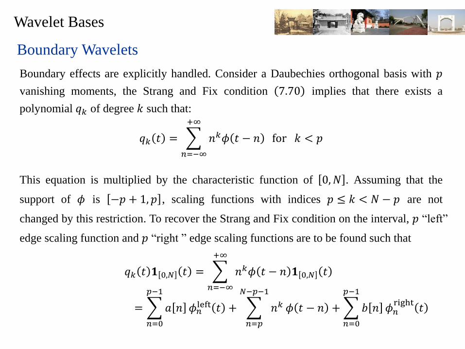
𝑞𝑘 𝑡 𝟏 0,𝑁 𝑡 = 𝑛𝑘𝜙 𝑡 − 𝑛 𝟏 0,𝑁 𝑡

+∞

𝑛=−∞

= 𝑎 𝑛

𝑝−1

𝑛=0

𝜙𝑛left 𝑡 + 𝑛𝑘

𝑁−𝑝−1

𝑛=𝑝

𝜙 𝑡 − 𝑛 + 𝑏 𝑛

𝑝−1

𝑛=0

𝜙𝑛right

𝑡

If this equation is satisfied, it remains valid after rescaling since the 𝑛𝑘, up to a

power of 2, are the scaling coefficients of 𝑞𝑘 at all resolutions. There remains to

find the filters ℎ and 𝐻 which satisfy the scaling equation:

𝜙𝑗,𝑘int= 𝐻𝑘,𝑙

left𝜙𝑗+1,𝑙int𝑝−1

𝑙=0 + ℎ𝑘,𝑚left𝜙𝑗+1,𝑚

int𝑝+2𝑘𝑚=𝑝

where 𝜙𝑗,𝑘int 𝑡 denotes the whole set of scaling functions obtained by translation

at the resolution 𝑗, and to verify the orthogonality condition.

Boundary Wavelets





Wavelet Bases

Separable Wavelet Bases

To any wavelet orthonormal basis 𝜓𝑗,𝑛 𝑗,𝑛 ∈ℤ2 of 𝐋𝟐 ℝ , one can associate a

separable wavelet orthonormal basis of 𝐋𝟐 ℝ2 :

𝜓𝑗1,𝑛1 𝑥1 𝜓𝑗2,𝑛2 𝑥2 𝑗1,𝑗2,𝑛1,𝑛2 ∈ℤ4

The functions 𝜓𝑗1,𝑛1 𝑥1 𝜓𝑗2,𝑛2 𝑥2 mix information at two different scales 2𝑗1

and 2𝑗2 along 𝑥1 and 𝑥2, which we often want to avoid.

Separable multiresolutions lead to another construction of separable wavelet

bases with wavelets that are products of functions dilated at the same scale.

These multiresolution approximations also have important applications in

computer vision, where they are used to process images at different levels.

Wavelet Bases

Anisotropic Wavelet Transform

Separable wavelet orthonormal basis of 𝐋𝟐 ℝ2 :

𝜓𝑗1,𝑗2,𝑛1,𝑛2 𝑥 = 𝜓𝑗1,𝑛1 𝑥1 𝜓𝑗2,𝑛2 𝑥2

Apply 1D wavelet to each column Apply 1D wavelet to each row

Favors horizontal/vertical axis:

Axis-aligned approximation artifacts

Not suitable for natural images

Wavelet Bases 2D Multiresolutions

Separable approximation spaces: 𝐕𝑗2 = 𝐕𝑗 ⊗𝐕𝑗 = Span 𝜙𝑗,𝑛1 𝑥1 𝜙𝑗,𝑛2 𝑥2 𝑛1,𝑛2

𝐋𝟐 ℝ2 ⋯ 𝐕𝑗−1 2 𝐕𝑗

2 𝐕𝑗+12 ⋯ 0

𝐖𝑗−1 2 𝐖𝑗

2 𝐖𝑗+12

Orthogonal basis of 𝐕𝑗: 𝜙𝑗,𝑚 𝑚∈ℤ

Orthogonal basis of 𝐕𝑗2: 𝜙𝑗,𝑛1,𝑛2

2

𝑛1,𝑛2∈ℤ

𝜙𝑗,𝑛1,𝑛22 𝑥 = 𝜙𝑗,𝑛1 𝑥1 𝜙𝑗,𝑛2 𝑥2 =

1

2𝑗𝜙

𝑥1 − 2𝑗𝑛12𝑗

𝜙𝑥2 − 2𝑗𝑛2

2𝑗

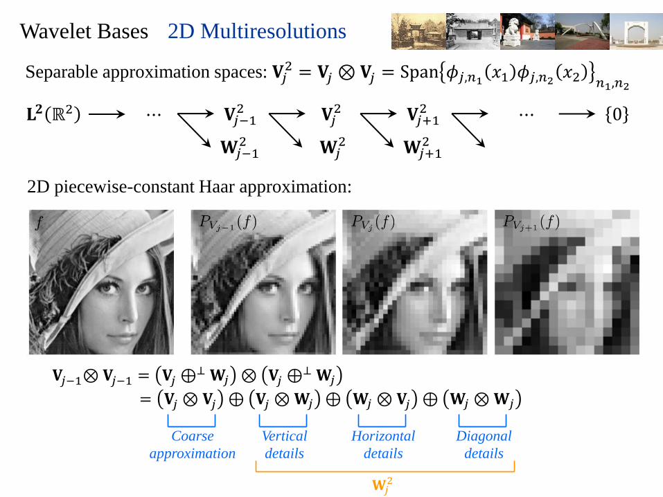
Wavelet Bases 2D Multiresolutions

Separable approximation spaces: 𝐕𝑗2 = 𝐕𝑗 ⊗𝐕𝑗 = Span 𝜙𝑗,𝑛1 𝑥1 𝜙𝑗,𝑛2 𝑥2 𝑛1,𝑛2

𝐋𝟐 ℝ2 ⋯ 𝐕𝑗−1 2 𝐕𝑗

2 𝐕𝑗+12 ⋯ 0

𝐖𝑗−1 2 𝐖𝑗

2 𝐖𝑗+12

2D piecewise-constant Haar approximation:

Coarse

approximation

𝐖𝑗2

𝐕𝑗−1⊗𝐕𝑗−1 = 𝐕𝑗 ⊕⊥ 𝐖𝑗 ⊗ 𝐕𝑗 ⊕

⊥ 𝐖𝑗

= 𝐕𝑗 ⊗𝐕𝑗 ⊕ 𝐕𝑗 ⊗𝐖𝑗 ⊕ 𝐖𝑗 ⊗𝐕𝑗 ⊕ 𝐖𝑗 ⊗𝐖𝑗

Vertical

details

Horizontal

details

Diagonal

details

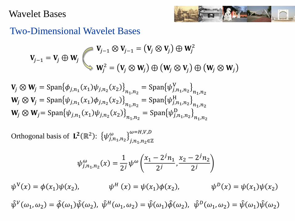
Wavelet Bases

Two-Dimensional Wavelet Bases

𝐕𝑗−1⊗𝐕𝑗−1 = 𝐕𝑗 ⊗𝐕𝑗 ⊕𝐖𝑗2

𝐖𝑗2 = 𝐕𝑗 ⊗𝐖𝑗 ⊕ 𝐖𝑗 ⊗𝐕𝑗 ⊕ 𝐖𝑗 ⊗𝐖𝑗

𝐕𝑗 ⊗𝐖𝑗 = Span 𝜙𝑗,𝑛1 𝑥1 𝜓𝑗,𝑛2 𝑥2 𝑛1,𝑛2= Span 𝜓𝑗,𝑛1,𝑛2

V

𝑛1,𝑛2

𝐖𝑗 ⊗𝐕𝑗 = Span 𝜓𝑗,𝑛1 𝑥1 𝜙𝑗,𝑛2 𝑥2 𝑛1,𝑛2= Span 𝜓𝑗,𝑛1,𝑛2

H

𝑛1,𝑛2

𝐖𝑗 ⊗𝐖𝑗= Span 𝜓𝑗,𝑛1 𝑥1 𝜓𝑗,𝑛2 𝑥2 𝑛1,𝑛2= Span 𝜓𝑗,𝑛1,𝑛2

D

𝑛1,𝑛2

Orthogonal basis of 𝐋𝟐 ℝ2 : 𝜓𝑗,𝑛1,𝑛2𝜔

𝑗,𝑛1,𝑛2∈ℤ

𝜔=𝐻,𝑉,𝐷

𝜓𝑗,𝑛1,𝑛2𝜔 𝑥 =

1

2𝑗𝜓𝜔

𝑥1 − 2𝑗𝑛12𝑗

,𝑥2 − 2𝑗𝑛2

2𝑗

𝜓 V 𝑥 = 𝜙 𝑥1 𝜓 𝑥2 , 𝜓

𝐻 𝑥 = 𝜓 𝑥1 𝜙 𝑥2 , 𝜓 𝐷 𝑥 = 𝜓 𝑥1 𝜓 𝑥2

𝜓 𝑉 𝜔1, 𝜔2 = 𝜙 𝜔1 𝜓 𝜔2 , 𝜓 𝐻 𝜔1, 𝜔2 = 𝜓 𝜔1 𝜙 𝜔2 , 𝜓 𝐷 𝜔1, 𝜔2 = 𝜓 𝜔1 𝜓 𝜔2

𝐕𝑗−1 = 𝐕𝑗 ⊕𝐖𝑗

Wavelet Bases

𝜙 2 𝜔1, 𝜔2 𝜓 𝑉 𝜔1, 𝜔2

𝜓 𝐷 𝜔1, 𝜔2 𝜓 𝐻 𝜔1, 𝜔2

Wavelet Bases

Discrete 2D Wavelets Coefficients

Analog image 𝑓0 ∈ 𝐋𝟐 0,1 2 Discretization points 𝑛1, 𝑛2 2𝐽 𝑛 where 2−𝐽 = 𝑁

Discretized image of 𝑁 pixels: for 𝑛 = 𝑛1, 𝑛2 𝑓 𝑛 = 𝑎𝐽 𝑛 = 𝑓0, 𝜙𝐽,𝑛

Discrete wavelet coefficients: 𝑑𝑗𝜔 𝑛 = 𝑓0, 𝜓𝑗,𝑛

𝜔 = 𝑓0, 𝜓 𝑗,𝑛𝜔

Discrete wavelet basis 𝜓 𝑗,𝑛𝜔

𝑗,𝑛

𝜔 of ℂ𝑁, for

𝐽 < 𝑗 ≤ 0

0 ≤ 𝑛1, 𝑛2 < 2−𝑗

𝜔 ∈ 𝐻, 𝑉, 𝐷

Wavelet Bases







𝑗,𝑛


𝐽 < 𝑗 ≤ 0

0 ≤ 𝑛1, 𝑛2 < 2−𝑗

𝜔 ∈ 𝐻, 𝑉, 𝐷

Wavelet Bases







𝑗,𝑛


𝐽 < 𝑗 ≤ 0

0 ≤ 𝑛1, 𝑛2 < 2−𝑗

𝜔 ∈ 𝐻, 𝑉, 𝐷

Wavelet Bases







𝑗,𝑛


𝐽 < 𝑗 ≤ 0

0 ≤ 𝑛1, 𝑛2 < 2−𝑗

𝜔 ∈ 𝐻, 𝑉, 𝐷

Wavelet Bases Examples

Wavelet Bases

Separable vs. Isotropic

Wavelet bases 28

Fast 2D Wavelet Transform

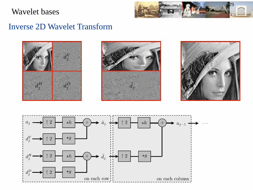
Wavelet bases 29

Inverse 2D Wavelet Transform





Wavelet Bases

The lifting scheme factorizes orthogonal and biorthogonal wavelet transforms

into elementary spatial operators called liftings.

The lifting scheme accelerates the fast wavelet transform. The filter bank

convolution and subsampling operations are factorized into elementary

filterings on even and odd samples, which reduces the number of operations

by nearly 2. Border treatments are also simplified.

The design of such wavelets are adapted to multidimensional-bounded

domains and surfaces, which is not possible with a Fourier transform approach.

Wavelet Bases

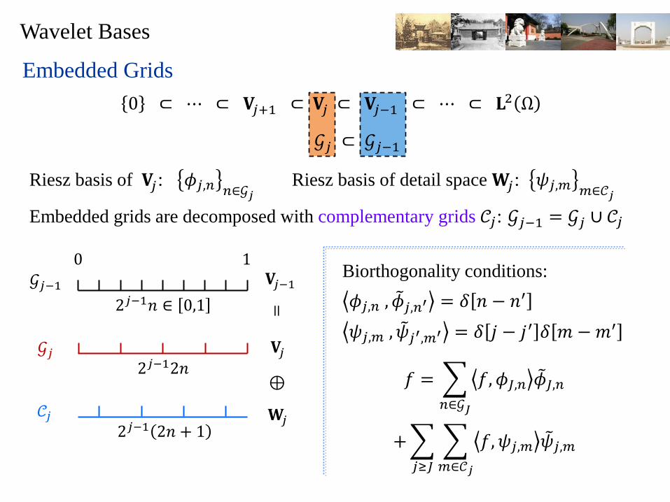
Embedded Grids

0 ⊂ ⋯ ⊂ 𝐕𝑗+1 ⊂ 𝐕𝑗 ⊂ 𝐕𝑗−1 ⊂ ⋯ ⊂ 𝐋2 Ω

𝒢𝑗 ⊂ 𝒢𝑗−1

Riesz basis of 𝐕𝑗 : 𝜙𝑗,𝑛 𝑛∈𝒢𝑗

Riesz basis of detail space 𝐖𝑗 : 𝜓𝑗,𝑚 𝑚∈𝒞𝑗

Embedded grids are decomposed with complementary grids 𝒞𝑗: 𝒢𝑗−1 = 𝒢𝑗 ∪ 𝒞𝑗

𝒢𝑗−1

𝒢𝑗

𝒞𝑗

0 1

2𝑗−1𝑛 ∈ 0,1

2𝑗−12𝑛

2𝑗−1 2𝑛 + 1

𝐕𝑗−1

=

𝐕𝑗

⊕

𝐖𝑗

Biorthogonality conditions:

𝜙𝑗,𝑛 , 𝜙 𝑗,𝑛′ = 𝛿 𝑛 − 𝑛′

𝜓𝑗,𝑚 , 𝜓 𝑗′,𝑚′ = 𝛿 𝑗 − 𝑗′ 𝛿 𝑚 −𝑚′

𝑓 = 𝑓,𝜙𝐽,𝑛 𝜙 𝐽,𝑛

𝑛∈𝒢𝐽

+ 𝑓,𝜓𝑗,𝑚 𝜓 𝑗,𝑚

𝑚∈𝒞𝑗𝑗≥𝐽

Wavelet Bases

Spatially Varying Filters

𝜙𝑗,𝑛 = ℎ𝑗 𝑛, 𝑙 𝜙𝑗−1,𝑙𝑙∈𝒢𝑗−1 𝜓𝑗,𝑚 = 𝑔𝑗 𝑚, 𝑙 𝜙𝑗−1,𝑙𝑙∈𝒢𝑗−1

𝜙 𝑗,𝑛 = ℎ 𝑗 𝑛, 𝑙 𝜙 𝑗−1,𝑙𝑙∈𝒢𝑗−1 𝜓 𝑗,𝑚 = 𝑔 𝑗 𝑚, 𝑙 𝜙 𝑗−1,𝑙𝑙∈𝒢𝑗−1

𝑔𝑗 𝑚, 𝑙 𝑔 𝑗 𝑚′, 𝑙𝑙∈𝒢𝑗−1

= 𝛿 𝑚 −𝑚′ ℎ𝑗 𝑛, 𝑙 ℎ 𝑗 𝑛′, 𝑙𝑙∈𝒢𝑗−1

= 𝛿 𝑛 − 𝑛′

𝑔𝑗 𝑚, 𝑙 ℎ 𝑗 𝑛, 𝑙𝑙∈𝒢𝑗−1= 0 ℎ𝑗 𝑛, 𝑙 𝑔 𝑗 𝑚, 𝑙𝑙∈𝒢𝑗−1

= 0

Biorthogonality filter relations for all 𝑛, 𝑛′ ∈ 𝒢𝑗 and 𝑚,𝑚′ ∈ 𝒞𝑗

Biorthogonality conditions

𝜙𝑗,𝑛 , 𝜙 𝑗,𝑛′ = 𝛿 𝑛 − 𝑛′ 𝜓𝑗,𝑚 , 𝜓 𝑗′,𝑚′ = 𝛿 𝑗 − 𝑗′ 𝛿 𝑚 −𝑚′

To simplify notations, ℎ𝑗 and 𝑔𝑗 are written as matrices:

∀𝑎 ∈ ℂ|𝒢𝑗−1|, ∀ 𝑛 ∈ 𝒢𝑗, 𝐻𝑗𝑎 𝑛 = ℎ𝑗 𝑛, 𝑙 𝑎 𝑙𝑙∈𝒢𝑗−1

∀𝑎 ∈ ℂ|𝒢𝑗−1|, ∀ 𝑚 ∈ 𝒞𝑗, 𝐺𝑗𝑎 𝑚 = 𝑔𝑗 𝑚, 𝑙 𝑎 𝑙𝑙∈𝒢𝑗−1

and similarly for the dual matrices 𝐻 𝑗 and 𝐺 𝑗

Rewritten as matrices

𝐻 𝑗

𝐺 𝑗𝐻𝑗∗ 𝐺𝑗

∗

=Id𝒢𝑗 0

0 Id𝒞𝑗

Wavelet Bases

Basic Idea

The lifting scheme builds filters as a succession of elementary lifting steps

applied to lazy wavelets that are Diracs

The predict step and the update step modify the scaling function and the wavelet

function

Lifting Scheme wavelet transform

Split 𝑎𝑗−1 Predict Update

+

−

even values

odd values

𝑎𝑗𝑜

𝑑𝑗𝑜

𝑎𝑗

𝑑𝑗

−

Update Predict Merge

+

𝑎𝑗−1

even values

odd values

𝑎𝑗𝑜

𝑑𝑗𝑜

Wavelet Bases

Lazy Wavelets

A lifting begins from lazy wavelets, which are Diracs on grid points:

∀𝑙 ∈ 𝒢𝑗−1, ∀𝑛 ∈ 𝒢𝑗 , ∀𝑚 ∈ 𝒞𝑗 ,

ℎ𝑗𝑜 𝑛, 𝑙 = ℎ 𝑗

𝑜 𝑛, 𝑙 = 𝛿 𝑛 − 𝑙

𝑔𝑗𝑜 𝑚, 𝑙 = 𝑔 𝑗

𝑜 𝑚, 𝑙 = 𝛿 𝑚 − 𝑙

This lazy orthogonal wavelet transform splits the coefficients of a grid 𝒢𝑗−1 into

two subgrids 𝒢𝑗 and 𝒞𝑗:

𝑎 ∈ ℂ|𝒢𝑗−1|, 𝐻𝑗𝑜𝑎 ∈ ℂ|𝒢𝑗

|, 𝐺𝑗𝑜𝑎 ∈ ℂ|𝒞𝑗|

𝜓 𝑗,𝑚𝑜 𝑥 = 𝜓𝑗,𝑚

𝑜 = 𝛿 𝑥 − 𝑥𝑚 𝜙 𝑗,𝑛𝑜 𝑥 = 𝜙𝑗,𝑛

𝑜 = 𝛿 𝑥 − 𝑥𝑛

This lazy wavelet basis is improved with a succession of liftings

Wavelet Bases

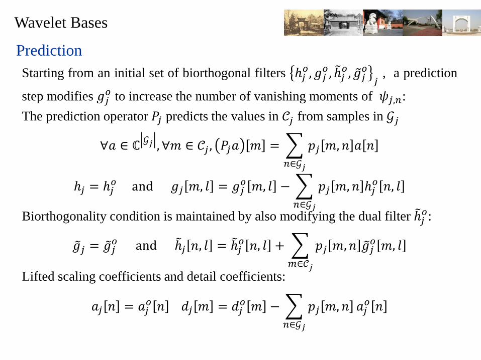
Prediction

Starting from an initial set of biorthogonal filters ℎ𝑗𝑜, 𝑔𝑗

𝑜, ℎ 𝑗𝑜, 𝑔 𝑗

𝑜

𝑗 , a prediction

step modifies 𝑔𝑗𝑜 to increase the number of vanishing moments of 𝜓𝑗,𝑛:

The prediction operator 𝑃𝑗 predicts the values in 𝒞𝑗 from samples in 𝒢𝑗

∀𝑎 ∈ ℂ

𝒢𝑗 , ∀𝑚 ∈ 𝒞𝑗 , 𝑃𝑗𝑎 𝑚 = 𝑝𝑗 𝑚, 𝑛 𝑎 𝑛

𝑛∈𝒢𝑗

ℎ𝑗 = ℎ𝑗

𝑜 and 𝑔𝑗 𝑚, 𝑙 = 𝑔𝑗𝑜 𝑚, 𝑙 − 𝑝𝑗 𝑚, 𝑛 ℎ𝑗

𝑜 𝑛, 𝑙

𝑛∈𝒢𝑗

Biorthogonality condition is maintained by also modifying the dual filter ℎ 𝑗𝑜:

𝑔 𝑗 = 𝑔 𝑗

𝑜 and ℎ 𝑗 𝑛, 𝑙 = ℎ 𝑗𝑜 𝑛, 𝑙 + 𝑝𝑗 𝑚, 𝑛 𝑔 𝑗

𝑜 𝑚, 𝑙

𝑚∈𝒞𝑗

Lifted scaling coefficients and detail coefficients:

𝑎𝑗 𝑛 = 𝑎𝑗

𝑜 𝑛 𝑑𝑗 𝑚 = 𝑑𝑗𝑜 𝑚 − 𝑝𝑗 𝑚, 𝑛

𝑛∈𝒢𝑗

𝑎𝑗𝑜 𝑛

Wavelet Bases

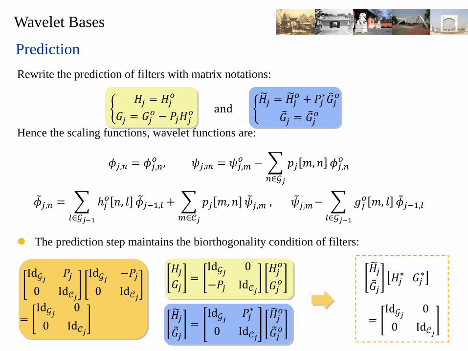
Prediction

Rewrite the prediction of filters with matrix notations:

𝐻𝑗 = 𝐻𝑗

𝑜

𝐺𝑗 = 𝐺𝑗𝑜 − 𝑃𝑗𝐻𝑗

𝑜 and 𝐻 𝑗 = 𝐻 𝑗

𝑜 + 𝑃𝑗∗𝐺 𝑗

𝑜

𝐺 𝑗 = 𝐺 𝑗𝑜

Hence the scaling functions, wavelet functions are:

𝜙𝑗,𝑛 = 𝜙𝑗,𝑛

𝑜 , 𝜓𝑗,𝑚 = 𝜓𝑗,𝑚𝑜 − 𝑝𝑗 𝑚, 𝑛

𝑛∈𝒢𝑗

𝜙𝑗,𝑛𝑜

𝜙 𝑗,𝑛 = ℎ𝑗

𝑜 𝑛, 𝑙

𝑙∈𝒢𝑗−1

𝜙 𝑗−1,𝑙 + 𝑝𝑗 𝑚, 𝑛

𝑚∈𝒞𝑗

𝜓 𝑗,𝑚 , 𝜓 𝑗,𝑚− 𝑔𝑗𝑜 𝑚, 𝑙

𝑙∈𝒢𝑗−1

𝜙 𝑗−1,𝑙

𝐻 𝑗

𝐺 𝑗𝐻𝑗∗ 𝐺𝑗

∗

=Id𝒢𝑗 0

0 Id𝒞𝑗

The prediction step maintains the biorthogonality condition of filters:

𝐻𝑗𝐺𝑗

= Id𝒢𝑗 0

−𝑃𝑗 Id𝒞𝑗

𝐻𝑗𝑜

𝐺𝑗𝑜

𝐻 𝑗

𝐺 𝑗=

Id𝒢𝑗 𝑃𝑗∗

0 Id𝒞𝑗

𝐻 𝑗𝑜

𝐺 𝑗𝑜

Id𝒢𝑗 𝑃𝑗

0 Id𝒞𝑗

Id𝒢𝑗 −𝑃𝑗

0 Id𝒞𝑗

=Id𝒢𝑗 0

0 Id𝒞𝑗

Wavelet Bases

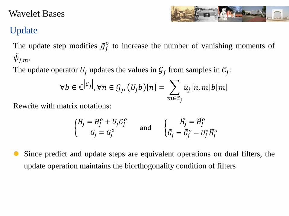
Update

The update step modifies 𝑔 𝑗𝑜 to increase the number of vanishing moments of

𝜓 𝑗,𝑚.

The update operator 𝑈𝑗 updates the values in 𝒢𝑗 from samples in 𝒞𝑗:

∀𝑏 ∈ ℂ

𝒞𝑗 , ∀𝑛 ∈ 𝒢𝑗 , 𝑈𝑗𝑏 𝑛 = 𝑢𝑗 𝑛,𝑚 𝑏 𝑚

𝑚∈𝒞𝑗

Rewrite with matrix notations:

Since predict and update steps are equivalent operations on dual filters, the

update operation maintains the biorthogonality condition of filters

𝐻𝑗 = 𝐻𝑗

𝑜 + 𝑈𝑗𝐺𝑗𝑜

𝐺𝑗 = 𝐺𝑗𝑜 and

𝐻 𝑗 = 𝐻 𝑗𝑜

𝐺 𝑗 = 𝐺 𝑗𝑜 − 𝑈𝑗

∗𝐻 𝑗𝑜

Wavelet Bases

Update

The updated scaling coefficients and detail coefficients:

𝑎𝑗 𝑛 = 𝑎𝑗

𝑜 𝑛 + 𝑢𝑗 𝑛,𝑚

𝑚∈𝒞𝑗

𝑑𝑗𝑜 𝑚 , 𝑑𝑗 𝑛 = 𝑑𝑗

𝑜 𝑛

The scaling functions, wavelet functions are:

𝜙𝑗,𝑛 = ℎ𝑗

𝑜 𝑛, 𝑙

𝑙∈𝒢𝑗−1

𝜙𝑗−1,𝑙 + 𝑢𝑗 𝑛,𝑚

𝑚∈𝒞𝑗

𝜓𝑗,𝑚, 𝜓𝑗,𝑚 = 𝑔𝑗𝑜 𝑚, 𝑙

𝑙∈𝒢𝑗−1

𝜙𝑗−1,𝑙

𝜙 𝑗,𝑛 = 𝜙 𝑗,𝑛

𝑜 , 𝜓 𝑗,𝑚= 𝜓 𝑗,𝑚𝑜 − 𝑢𝑗 𝑛,𝑚

𝑛∈𝒢𝑗

𝜙 𝑗,𝑛𝑜

This update does not modify the number of vanishing moments of the wavelet 𝜓𝑗,𝑚

Wavelet Bases

A fast wavelet transform computes the coefficients by replacing convolution with

conjugate mirror filters by a succession of predict and update steps:

Input 𝑎𝐿 ∈ ℂ 𝒢𝐿 , ∀𝑚 ∈ 𝒞𝑗 , ∀𝑛 ∈ 𝒢𝑗

For 𝑗 = 𝐿 + 1,⋯ , 𝐽 :

Split: 𝑑𝑗𝑜 𝑚 = 𝑎𝑗−1 𝑚 ,𝑎𝑗

𝑜 𝑛 = 𝑎𝑗−1 𝑛 Forward predict: 𝑑𝑗 𝑚 = 𝑑𝑗

𝑜 𝑚 − 𝑝𝑗 𝑚, 𝑛𝑛∈𝒢𝑗𝑎𝑗𝑜 𝑛

Forward update: 𝑎𝑗 𝑛 = 𝑎𝑗

𝑜 𝑛 + 𝑢𝑗 𝑛,𝑚𝑚∈𝒞𝑗𝑑𝑗 𝑚

decomposition

Input 𝑎𝐽, 𝑑𝑗 𝐽≤𝑗<𝐿, ∀𝑚 ∈ 𝒞𝑗 , ∀𝑛 ∈ 𝒢𝑗

For 𝑗 = 𝐽,⋯ , 𝐿 + 1:

Backward update: 𝑎𝑗𝑜 𝑛 = 𝑎𝑗 𝑛 − 𝑢𝑗 𝑛,𝑚𝑚∈𝒞𝑗

𝑑𝑗 𝑚 Backward predict: 𝑑𝑗𝑜 𝑚 = 𝑑𝑗 𝑚 + 𝑝𝑗 𝑚, 𝑛𝑛∈𝒢𝑗

𝑎𝑗𝑜 𝑛

Merge: 𝑎𝑗−1 𝑚 = 𝑑𝑗

𝑜 𝑚 ,𝑎𝑗−1 𝑛 = 𝑎𝑗𝑜 𝑛

reconstruction

Wavelet Bases

A lifting modifies biorthogonal filters in order to increase the number of

vanishing moments of the resulting biorthogonal wavelets, and hopefully their

stability and regularity

Increasing the number of vanishing moments decreases the amplitude of

wavelet coefficients in regions where the signal is regular, but also increases

the wavelet support, which increases the number of large coefficients

produced by isolated singularities

Stability is generally improved when dual wavelets have as much vanishing

moments as original wavelets and a support of similar size. This is why a

lifting procedure also increases the number of vanishing moments of dual

wavelets. It can also improve the regularity of the dual wavelet

Wavelet Bases

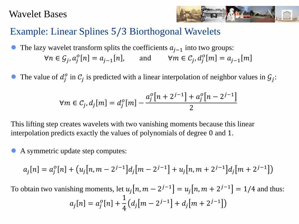
Example: Linear Splines 5/3 Biorthogonal Wavelets

The lazy wavelet transform splits the coefficients 𝑎𝑗−1 into two groups:

∀𝑛 ∈ 𝒢𝑗 , 𝑎𝑗𝑜 𝑛 = 𝑎𝑗−1 𝑛 , and ∀𝑚 ∈ 𝒞𝑗 , 𝑑𝑗

𝑜 𝑚 = 𝑎𝑗−1 𝑚

The value of 𝑑𝑗𝑜 in 𝒞𝑗 is predicted with a linear interpolation of neighbor values in 𝒢𝑗:

∀𝑚 ∈ 𝒞𝑗 , 𝑑𝑗 𝑚 = 𝑑𝑗𝑜 𝑚 −

𝑎𝑗𝑜 𝑛 + 2𝑗−1 + 𝑎𝑗

𝑜 𝑛 − 2𝑗−1

2

This lifting step creates wavelets with two vanishing moments because this linear

interpolation predicts exactly the values of polynomials of degree 0 and 1.

A symmetric update step computes:

𝑎𝑗 𝑛 = 𝑎𝑗𝑜 𝑛 + 𝑢𝑗 𝑛,𝑚 − 2𝑗−1 𝑑𝑗 𝑚 − 2𝑗−1 + 𝑢𝑗 𝑛,𝑚 + 2𝑗−1 𝑑𝑗 𝑚+ 2𝑗−1

To obtain two vanishing moments, let 𝑢𝑗 𝑛,𝑚 − 2𝑗−1 = 𝑢𝑗 𝑛,𝑚 + 2𝑗−1 = 1/4 and thus:

𝑎𝑗 𝑛 = 𝑎𝑗𝑜 𝑛 +

1

4𝑑𝑗 𝑚 − 2𝑗−1 + 𝑑𝑗 𝑚+ 2𝑗−1

Wavelet Bases


Wavelet Bases


Biorthogonal wavelets and

scaling functions computed

with 𝑝 = 𝑝 = 2 vanishing

moments. The dual-scaling

functions and wavelets are

compactly supported linear

splines.

Higher order biorthogonal

spline wavelets are

constructed with a prediction

and an update providing

more vanishing moments.

Wavelet Bases

Homework Chapter 7: 7.11 7.16 (A Wavelet Tour of Signal Processing, 3rd edition)

45

Many Thanks

Q & A

Wavelet Bases and Lifting Wavelets - SJTUmin.sjtu.edu.cn/files/wavelet/6-lifting wavelet and filterbank.pdf · Periodic wavelet bases have the disadvantage of creating high-amplitude

Documents