Waveform Modeling and Comparisons with Ground Truth Events David Norris BBN Technologies 1300 N. 17 th Street Arlington, VA 22209 [email protected] 703-284-1348 14 Nov 2007

Waveform Modeling and Comparisons with Ground Truth Events David Norris BBN Technologies 1300 N. 17 th Street Arlington, VA 22209 [email protected] 703-284-1348.
Dec 16, 2015
Welcome message from author
This document is posted to help you gain knowledge. Please leave a comment to let me know what you think about it! Share it to your friends and learn new things together.
Transcript
Waveform Modeling and Comparisons with Ground Truth Events
David Norris
BBN Technologies
1300 N. 17th Street
Arlington, VA 22209
703-284-1348
14 Nov 2007
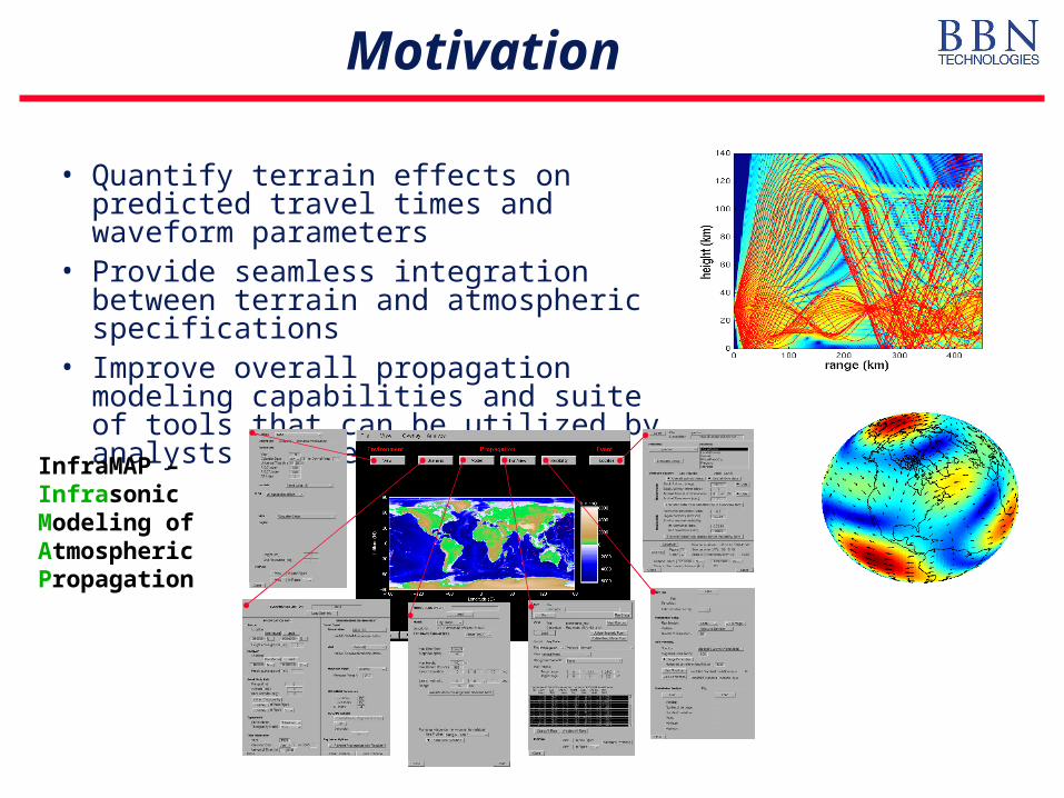
Motivation
• Quantify terrain effects on predicted travel times and waveform parameters
• Provide seamless integration between terrain and atmospheric specifications
• Improve overall propagation modeling capabilities and suite of tools that can be utilized by analysts and researchers
InfraMAP – Infrasonic Modeling of Atmospheric Propagation
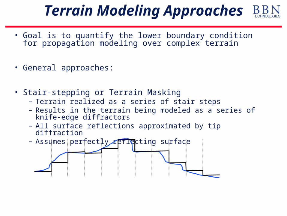
Terrain Modeling Approaches
• Goal is to quantify the lower boundary condition for propagation modeling over complex terrain
• General approaches:
• Stair-stepping or Terrain Masking– Terrain realized as a series of stair steps– Results in the terrain being modeled as a series of knife-edge diffractors– All surface reflections approximated by tip diffraction– Assumes perfectly reflecting surface
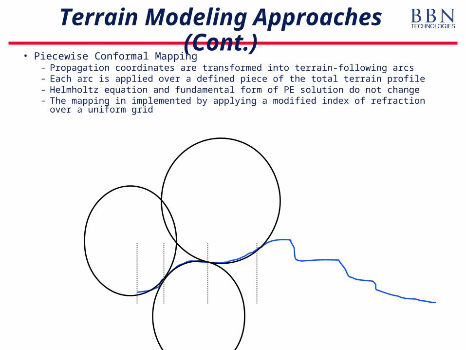
Terrain Modeling Approaches (Cont.)
• Piecewise Conformal Mapping– Propagation coordinates are transformed into terrain-following arcs– Each arc is applied over a defined piece of the total terrain profile– Helmholtz equation and fundamental form of PE solution do not change– The mapping in implemented by applying a modified index of refraction
over a uniform grid
Terrain Modeling Approaches (Cont.)
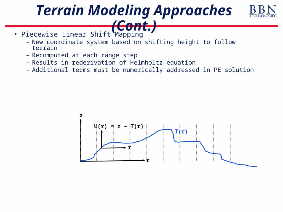
• Piecewise Linear Shift Mapping– New coordinate system based on shifting height to follow terrain– Recomputed at each range step – Results in rederivation of Helmholtz equation– Additional terms must be numerically addressed in PE solution
r
z
T(r)
r
U(r) = z – T(r)
Terrain Masking Approach
Range (km)
He
igh
t (km
)
PE with absorption: Amplitude Field (dB re 1 km)
0 50 1000
5
10
15
20
-100
-80
-60
-40
-20
0
Range (km)
He
igh
t (km
)
PE with absorption: Amplitude Field (dB re 1 km)
0 50 1000
5
10
15
20
-100
-80
-60
-40
-20
0
Range (km)
He
igh
t (km
)
PE with absorption: Amplitude Field (dB re 1 km)
0 50 1000
5
10
15
20
-100
-80
-60
-40
-20
0
Range (km)
He
igh
t (km
)
PE with absorption: Amplitude Field (dB re 1 km)
0 50 1000
5
10
15
20
-100
-80
-60
-40
-20
0
Range (km)
He
igh
t (km
)
PE with absorption: Amplitude Field (dB re 1 km)
0 50 1000
5
10
15
20
-100
-80
-60
-40
-20
0
Range (km)
He
igh
t (km
)
PE with absorption: Amplitude Field (dB re 1 km)
0 50 1000
5
10
15
20
-100
-80
-60
-40
-20
0
Mt. Everest
Mt. Fuji
Mt. Everest
Mt. Fuji
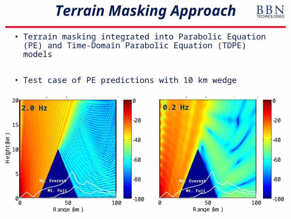
• Terrain masking integrated into Parabolic Equation (PE) and Time-Domain Parabolic Equation (TDPE) models
• Test case of PE predictions with 10 km wedge
2.0 Hz 0.2 Hz
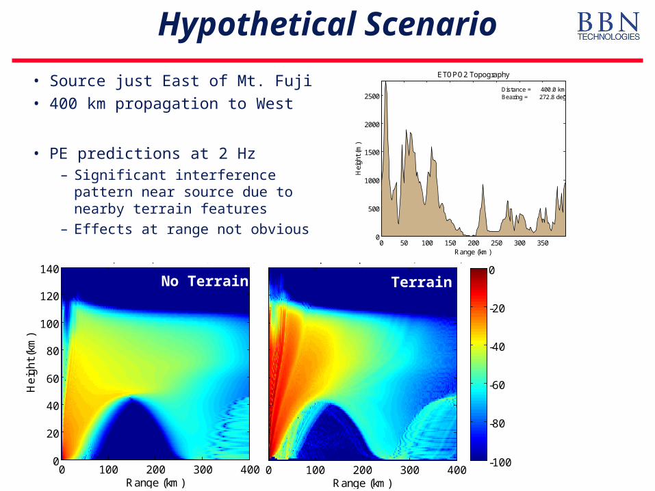
Hypothetical Scenario
• Source just East of Mt. Fuji
• 400 km propagation to West
• PE predictions at 2 Hz– Significant interference pattern
near source due to nearby terrain features
– Effects at range not obvious 0 50 100 150 200 250 300 3500
500
1000
1500
2000
2500
Range (km)
Hei
ght (
m)
ETOPO2 Topography
Distance = 400.0 kmBearing = 272.8 deg
Range (km)
He
igh
t (km
)
PE with absorption: Amplitude Field (dB re 1 km)
0 100 200 300 4000
20
40
60
80
100
120
140
-100
-80
-60
-40
-20
0
Range (km)
He
igh
t (km
)
PE with absorption: Amplitude Field (dB re 1 km)
0 100 200 300 4000
20
40
60
80
100
120
140
-100
-80
-60
-40
-20
0No Terrain Terrain
Hypothetical Scenario (cont.)
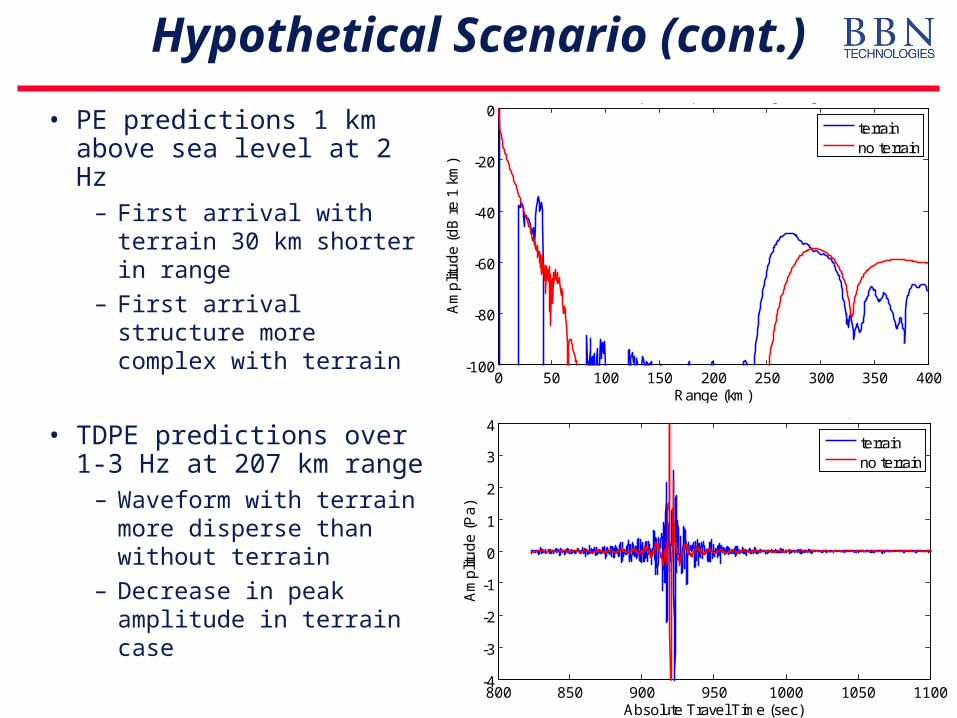
• PE predictions 1 km above sea level at 2 Hz
– First arrival with terrain 30 km shorter in range
– First arrival structure more complex with terrain
• TDPE predictions over 1-3 Hz at 207 km range
– Waveform with terrain more disperse than without terrain
– Decrease in peak amplitude in terrain case
Terrain
0 50 100 150 200 250 300 350 400-100
-80
-60
-40
-20
0
Range (km)
Am
plit
ud
e (
dB
re
1 k
m)
PE with absorption: Amplitude vs. Range, Height: 1 km
terrainno terrain
800 850 900 950 1000 1050 1100-4
-3
-2
-1
0
1
2
3
4
Absolute Travel Time (sec)
Am
plit
ud
e (
Pa
)
Time-domain PE with absorption: Amplitude vs. Time, Height: 1 km
terrainno terrain
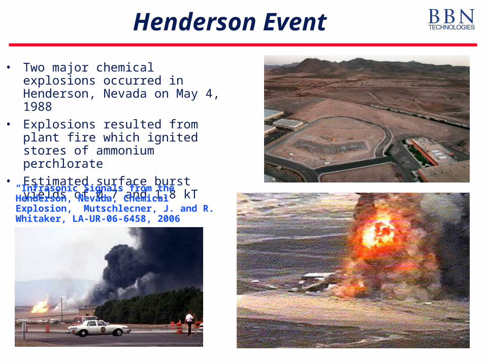
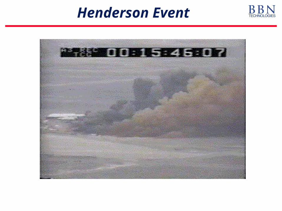
Henderson Event
• Two major chemical explosions occurred in Henderson, Nevada on May 4, 1988
• Explosions resulted from plant fire which ignited stores of ammonium perchlorate
• Estimated surface burst yields of 0.7 and 1.8 kT
“Infrasonic Signals from the Henderson, Nevada, Chemical Explosion,” Mutschlecner, J. and R. Whitaker, LA-UR-06-6458, 2006
Henderson Event
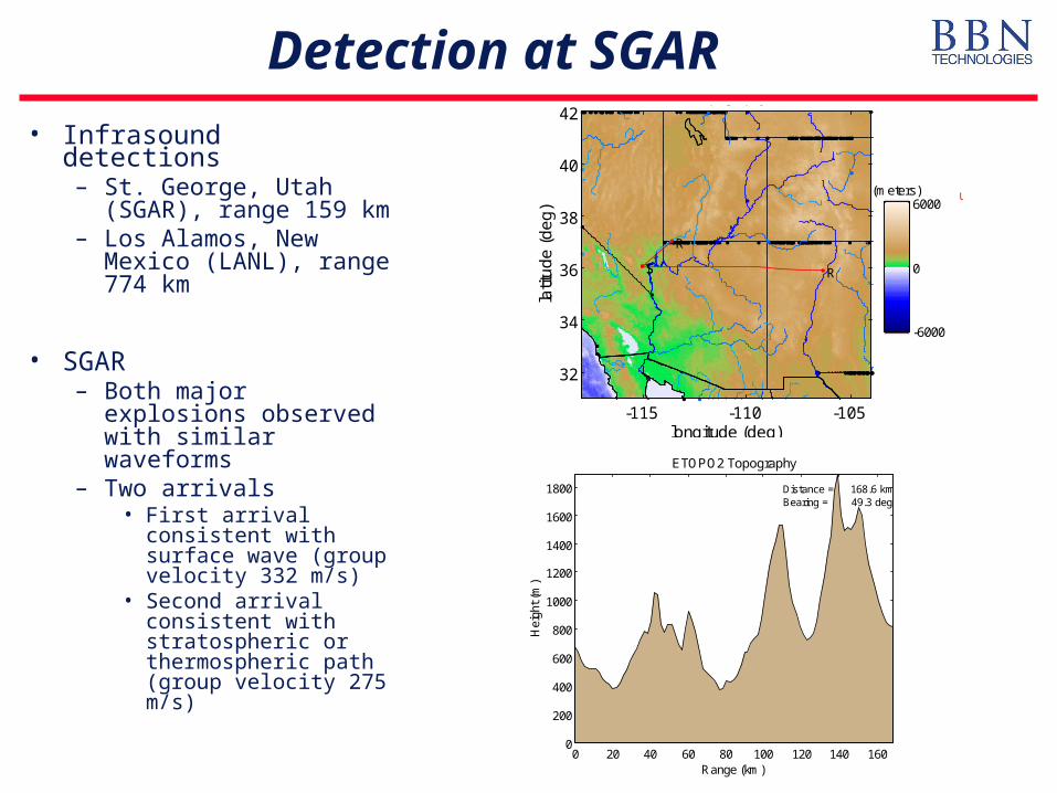
Detection at SGAR
• Infrasound detections– St. George, Utah
(SGAR), range 159 km– Los Alamos, New
Mexico (LANL), range 774 km
• SGAR– Both major explosions
observed with similar waveforms
– Two arrivals• First arrival consistent
with surface wave (group velocity 332 m/s)
• Second arrival consistent with stratospheric or thermospheric path (group velocity 275 m/s)
(meters)
-6000
0
6000
longitude (deg)
latit
ud
e (
de
g)
ETOPO2: Topography (meters)
UNITED STATES
S R S
R
-115 -110 -105
32
34
36
38
40
42
0 20 40 60 80 100 120 140 1600
200
400
600
800
1000
1200
1400
1600
1800
Range (km)
Hei
ght (
m)
ETOPO2 Topography
Distance = 168.6 kmBearing = 49.3 deg
Range (km)
He
igh
t (km
)
0 50 100 1500
20
40
60
80
100
120
140
-100
-80
-60
-40
-20
0
Range (km)
He
igh
t (km
)
0 50 100 1500
20
40
60
80
100
120
140
-100
-80
-60
-40
-20
0No Terrain Terrain
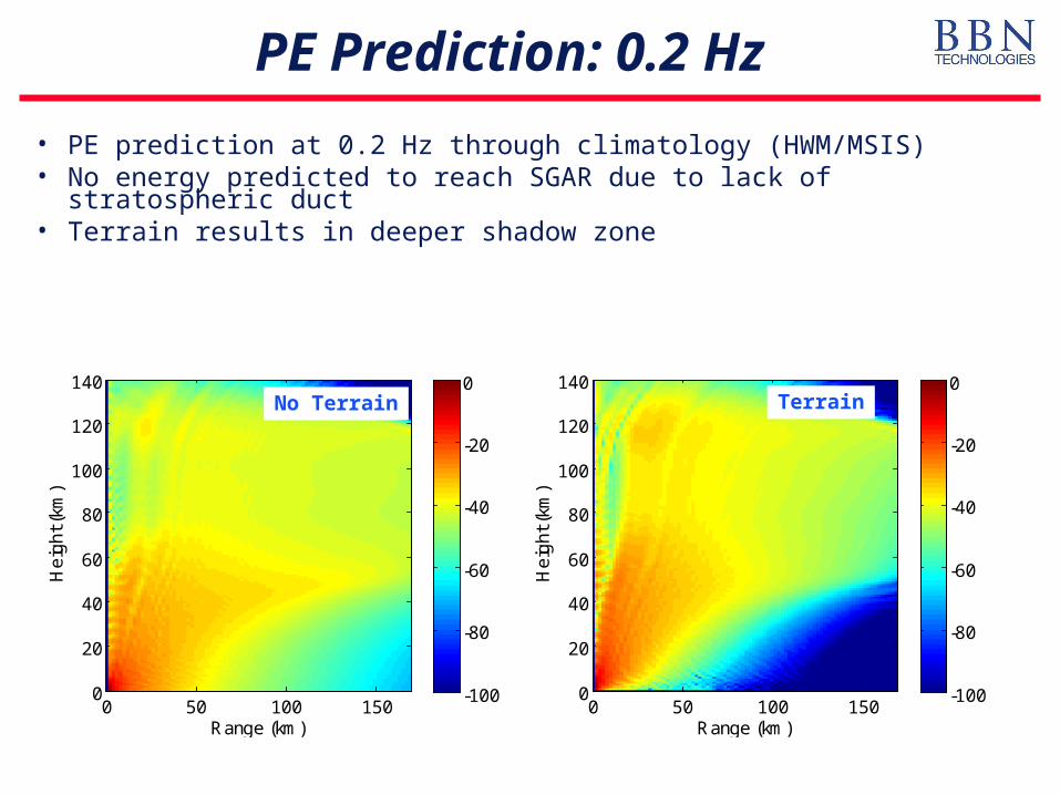
PE Prediction: 0.2 Hz
• PE prediction at 0.2 Hz through climatology (HWM/MSIS)• No energy predicted to reach SGAR due to lack of stratospheric duct• Terrain results in deeper shadow zone
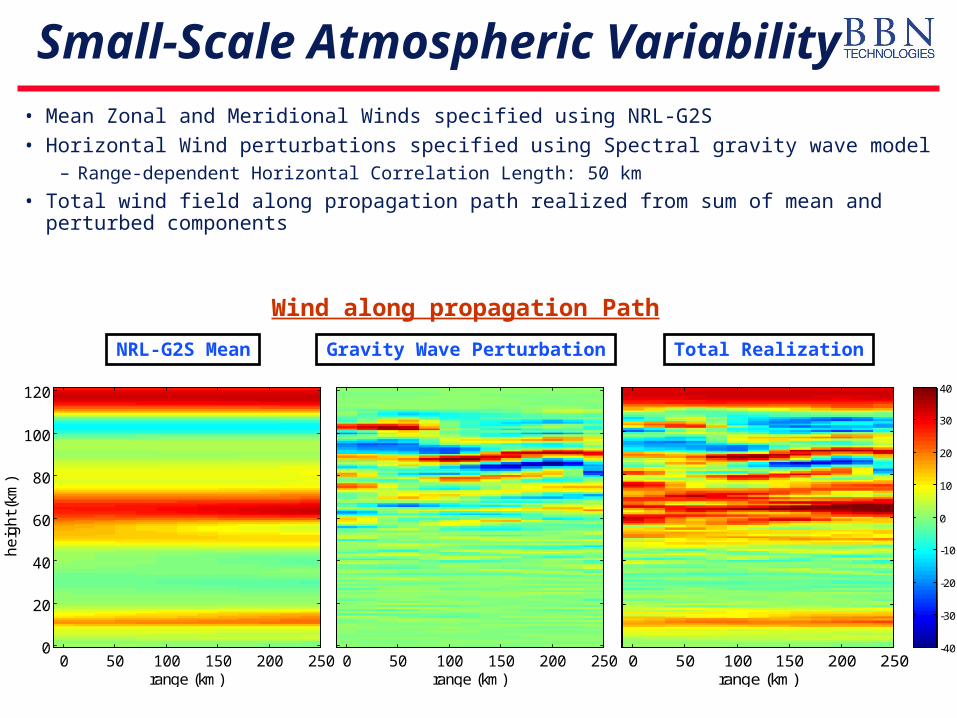
Small-Scale Atmospheric Variability• Mean Zonal and Meridional Winds specified using NRL-G2S
• Horizontal Wind perturbations specified using Spectral gravity wave model– Range-dependent Horizontal Correlation Length: 50 km
• Total wind field along propagation path realized from sum of mean and perturbed components
NRL-G2S Mean Total RealizationGravity Wave Perturbation
range (km)
he
igh
t (km
)
0 50 100 150 200 2500
20
40
60
80
100
120
-40
-30
-20
-10
0
10
20
30
40
range (km)
he
igh
t (km
)
0 50 100 150 200 2500
20
40
60
80
100
120
-40
-30
-20
-10
0
10
20
30
40
range (km)
He
igh
t (k
m)
0 50 100 150 200 2500
20
40
60
80
100
120
-40
-30
-20
-10
0
10
20
30
40
Wind along propagation Path

Range (km)
He
igh
t (km
)
PE with absorption: Amplitude Field (dB re 1 km)
0 50 100 1500
20
40
60
80
100
120
140
-100
-80
-60
-40
-20
0
Range (km)
He
igh
t (km
)
PE with absorption: Amplitude Field (dB re 1 km)
0 50 100 1500
20
40
60
80
100
120
140
-100
-80
-60
-40
-20
0
No Terrain Terrain
PE Prediction: 0.2 Hz
• PE prediction at 0.2 Hz through climatology (HWM/MSIS)• Horizontal wind perturbations introduced by gravity waves model• Terrain results in more distinct scattering paths
500 550 600 650 700-1
-0.5
0
0.5
1
Absolute Travel Time (sec)
Am
plit
ud
e (
Pa
)
500 550 600 650 700-1
-0.5
0
0.5
1
Absolute Travel Time (sec)
Am
plit
ud
e (
Pa
)
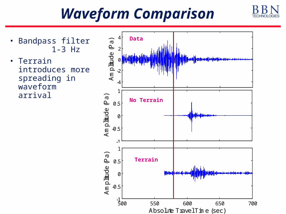
Waveform Comparison
• Bandpass filter 1-3 Hz
• Terrain introduces more spreading in waveform arrival -4
-2
0
2
4
Am
plit
ud
e (
Pa
)
No Terrain
Terrain
Data
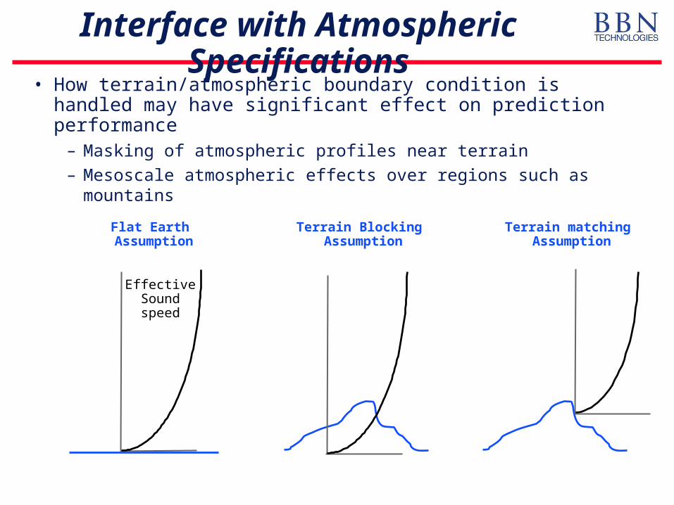
Interface with Atmospheric Specifications
• How terrain/atmospheric boundary condition is handled may have significant effect on prediction performance
– Masking of atmospheric profiles near terrain
– Mesoscale atmospheric effects over regions such as mountains
Terrain
Flat Earth Assumption
Terrain Blocking Assumption
EffectiveSoundspeed
Terrain matching Assumption

Conclusions and Future Research
• Preliminary Conclusions– Terrain appears to disperse down-range waveforms in cases where
significant terrain features are in proximity of source
• Issues for further research– Comparison of terrain masking, conformal mapping, and linear shift
mapping approaches – Sensitivity to ground impedance specification and its variability over
typical propagation paths– Required Topographic database resolution
Related Documents