Wavefield Analysis of Rayleigh Waves for Near-Surface Shear

Wavefield Analysis of Rayleigh Waves for Near-Surface Shear-Wave Velocity

By

Chong Zeng

Submitted to the graduate degree program in the Department of Geology and the Graduate Faculty of the University of Kansas in partial fulfillment of the requirements for

the degree of Doctor of Philosophy.

________________________________

Georgios P. Tsoflias, Chair

________________________________

Jianghai Xia, Co-Chair

________________________________

J. Douglas Walker

________________________________

Jennifer A. Roberts

________________________________

Weizhang Huang

Date Defended: 5/4/2011

ii

The Dissertation Committee for Chong Zeng

certifies that this is the approved version of the following dissertation:

Wavefield Analysis of Rayleigh Waves for Near-Surface Shear-Wave Velocity

________________________________

Georgios P. Tsoflias, Chair

________________________________

Jianghai Xia, Co-Chair

Date approved: 5/4/2011

iii

Abstract

Shear (S)-wave velocity is a key property of near-surface materials and is the

fundamental parameter for many environmental and engineering geophysical studies.

Directly acquiring accurate S-wave velocities from a seismic shot gather is usually

difficult due to the poor signal-to-noise ratio. The relationship between Rayleigh-wave

phase velocity and frequency has been widely utilized to estimate the S-wave velocities

in shallow layers using the multichannel analysis of surface waves (MASW) technique.

Hence, Rayleigh wave is a main focus of most near-surface seismic studies. Conventional

dispersion analysis of Rayleigh waves assumes that the earth is laterally homogeneous

and the free surface is horizontally flat, which limits the application of surface-wave

methods to only 1D earth models or very smooth 2D models. In this study I extend the

analysis of Rayleigh waves to a 2D domain by employing the 2D full elastic wave

equation so as to address the lateral heterogeneity problem. I first discuss the accurate

simulation of Rayleigh waves through finite-difference method and the boundary

absorbing problems in the numerical modeling with a high Poisson’s ratio (> 0.4), which

is a unique near-surface problem. Then I develop an improved vacuum formulation to

generate accurate synthetic seismograms focusing on Rayleigh waves in presence of

surface topography and internal discontinuities. With these solutions to forward modeling

of Rayleigh waves, I evaluate the influence of surface topography to conventional

dispersion analysis in 2D and 3D domains by numerical investigations. At last I examine

the feasibility of inverting waveforms of Rayleigh waves for shallow S-wave velocities

using a genetic algorithm. Results of the study show that Rayleigh waves can be

accurately simulated in near surface using the improved vacuum formulation. Spurious

iv

reflections during the numerical modeling can be efficiently suppressed by the simplified

multiaxial perfectly matched layers. The conventional MASW method can tolerate gentle

topography changes with insignificant errors. Finally, many near-surface features with

strong lateral heterogeneity such as dipping interfaces, faults, and tunnels can be imaged

by the waveform inversion of Rayleigh waves for shallow S-wave velocities.

This thesis consists of four papers that are either published (chapter 1) or in review

(chapter 2, 3, and 4) for consideration of publication to peer-refereed journals. Each

chapter represents a paper, and therefore inadvertently there will be a certain degree of

overlap between chapters (particularly for the introduction parts, where references to

many common papers occur).

v

Acknowledgements

First and foremost I would like to express my sincere gratitude to my primary

academic advisor Dr. Jianghai Xia for his patient, knowledgeable and continuous

guidance during my Ph.D. studies at the University of Kansas. Without his inspiration

and encouragement I would not have been able to complete this dissertation. I appreciate

all his contributions of time and ideas in all the time of my research. I warmly thank for

his great efforts to teach me how to question thoughts and express ideas. I would have

been lost without him.

I greatly appreciate my co-advisor Prof. Georgios P. Tsoflias for his insightful and

fruitful instructions during the work of this dissertation. He has given me the

most-needed and greatest help when I was in difficulties. I am thankful to him for reading

and commenting my manuscripts for publishing.

I would like to acknowledge Dr. Richard D. Miller, the section chief of the

Exploration Services at the Kansas Geological Survey (KGS), for offering me the

continuous and generous financial support for my Ph.D. program. This research would be

impossible without the funding from the KGS.

I am grateful to my thesis and advisory committee that consisted of Prof. J. Douglas

Walker, Prof. Jennifer A. Roberts, and Prof. Weizhang Huang in addition to my advisors.

I thank for their unselfish assistance and excellent advice to my study. I also appreciate

Ross A. Black for his efforts to prepare my oral comprehensive exam.

It is always a pleasure to work with the staff and students at the section of Exploration

Services, KGS, where I have worked as a graduate research assistant in the past few years.

Particularly, I appreciate Brett Bennett for helping me to build the high performance

vi

computing cluster system. Mary Brohammer is acknowledged for her enthusiasm and

assistance on the paperwork. I thank Julian Ivanov and Joseph Kearns for their support

and suggestions during the software development.

Finally, I am forever indebted to my families for their understanding, endless patience

and encouragement. To them I dedicate this thesis.

vii

Table of contents

Abstract .............................................................................................................................. iii

Acknowledgements ............................................................................................................. v

Chapter 1: Application of the multiaxial perfectly matched layer (M-PML) to

near-surface seismic modeling with Rayleigh waves ......................................................... 1

1.1 Summary ................................................................................................................... 1

1.2 Introduction ............................................................................................................... 2

1.3 Modeling of Rayleigh waves with classical PML ..................................................... 6

1.4 Stability tests of classical PML for near-surface earth models ............................... 11

1.5 M-PML technique and its stability for near-surface earth models .......................... 16

1.6 The simplified M-PML and its application ............................................................. 19

1.7 Discussion ............................................................................................................... 24

1.8 Conclusions ............................................................................................................. 26

Chapter 2: An improved vacuum formulation for finite-difference modeling of Rayleigh

waves including surface topography and internal discontinuities .................................... 28

2.1 Summary ................................................................................................................. 28

2.2 Introduction ............................................................................................................. 29

2.3 Modeling of Rayleigh waves in P-SV wavefield .................................................... 33

2.4 The improved vacuum formulation ......................................................................... 35

2.5 Benchmark of the algorithm .................................................................................... 42

2.6 Tests for irregular surface topography .................................................................... 46

2.7 Incorporation of internal discontinuities ................................................................. 50

2.8 Discussion ............................................................................................................... 57

viii

2.9 Conclusions ............................................................................................................. 59

Chapter 3: Numerical investigation of applications of MASW in presence of surface

topography ........................................................................................................................ 61

3.1 Summary ................................................................................................................. 61

3.2 Introduction ............................................................................................................. 62

3.3 Methods for the numerical investigation ................................................................. 65

3.4 Dispersive energy of 2D topographic earth models ................................................ 67

3.5 Dispersive energy of 3D levee earth models ........................................................... 85

3.6 Conclusions ............................................................................................................. 91

Chapter 4: Feasibility of waveform inversion of Rayleigh waves for shallow shear-wave

velocity using genetic algorithm ....................................................................................... 93

4.1 Summary ................................................................................................................. 93

4.2 Introduction ............................................................................................................. 94

4.3 General procedure of GA waveform inversion ....................................................... 98

4.4 Description of the algorithm ................................................................................. 100

4.5 Numerical examples for layered earth models ...................................................... 104

4.6 Application to laterally heterogeneous earth models ............................................ 111

4.7 Conclusions ........................................................................................................... 118

Chapter 5: Discussion and conclusions........................................................................... 119

References ....................................................................................................................... 122

1

Chapter 1: Application of the multiaxial perfectly matched layer

(M-PML) to near-surface seismic modeling with Rayleigh waves

1.1 Summary

Perfectly matched layer (PML) absorbing boundaries are widely used to suppress

spurious edge reflections in seismic modeling. When modeling Rayleigh waves with the

existence of the free surface, the classical PML algorithm becomes unstable when the

Poisson’s ratio of the medium is high. Numerical errors can accumulate exponentially

and terminate the simulation due to computational overflows. Numerical tests show that

the divergence speed of the classical PML has a non-linear relationship with the

Poisson’s ratio. Generally, the higher the Poisson’s ratio, the faster the classical PML

diverges. The multiaxial PML (M-PML) attenuates the waves in PMLs using different

damping profiles that are proportional to each other in orthogonal directions. The

proportion coefficients of the damping profiles usually vary with the specific model

settings. If they are set appropriately, the M-PML algorithm is stable for high Poisson’s

ratio earth models. Through numerical tests of 40 models with Poisson’s ratios that varied

from 0.10 to 0.49, we found that a constant proportion coefficient of 1.0 for both the x-

and z-directional damping profiles is sufficient to stabilize the M-PML for all 2D

isotropic elastic cases. Wavefield simulations indicate that the instability of the classical

PML is strongly related to the wave phenomena near the free surface. When applying the

multiaxial technique only in the corners of the PML near the free surface, the original

M-PML technique can be simplified without losing its stability. The simplified M-PML

works efficiently for both homogeneous and heterogeneous earth models with high

2

Poisson’s ratios. The analysis in this paper is based on 2D finite difference modeling in

the time domain that can easily be extended into the 3D domain with other numerical

methods.

1.2 Introduction

With the increasing demands on environmental and engineering studies, modeling

seismic wave propagation in the near surface is essential and fundamental. The

relationship between Rayleigh-wave phase velocity and frequency has been widely

utilized to estimate the shear (S)-wave velocities in shallow layers (Nazarian and Stokoe,

1984; Xia et al., 1999, 2003, 2006; Calderόn-Macías and Luke, 2007; Socco et al., 2010).

Hence, generating synthetic records containing accurate Rayleigh-wave information is a

primary objective of any near-surface seismic modeling task. High Poisson’s ratio earth

models are often employed in the near-surface studies. Many near-surface materials are

unlithified and have much higher Poisson’s ratios than the sedimentary rocks. For

example, Xia et al. (2002b) showed that the materials of upper 7 m at a mining site in

Wyoming, U.S. have the Poisson’s ratio of about 0.48. They also reported that the

unconsolidated sediments of the Fraser River Delta near Vancouver, Canada have the

Poisson’s ratio of about 0.49, which is close to the maximum theoretical Poisson’s ratio

(0.5). Modeling Rayleigh waves in high Poisson’s ratio earth models is critical to many

near-surface geophysical studies.

Rayleigh waves can be simulated through numerical methods such as finite-difference

(FD) method by applying appropriate free-surface boundary conditions (e.g., Mittet, 2002;

Xu et al., 2007). Absorbing boundary conditions are usually employed to suppress

3

spurious reflections from the truncated edges of a finite-sized discrete earth model.

Cerjan et al. (1985) introduced a sponge-layer absorbing boundary condition for discrete

elastic wave equations. The absorbing effectiveness of this method depends to a large

extent on the distance that the waves propagate in the transition zone. The damping strip

has to be wide enough to yield satisfactory attenuation results, thereby greatly increasing

the computational expense. Bérenger (1994) developed an improved absorbing boundary

condition for attenuating electromagnetic waves. This technique utilizes an absorbing

layer called the perfectly matched layer (PML) to generate a non-reflecting interface

between the artificial boundary and the free medium. Subsequently, the PML method was

successfully introduced to elastic wavefield studies (Chew and Liu, 1996; Collino and

Tsogka, 2001). It is now the most widely used technique for solving the spurious

reflection problem in seismic modeling.

The PML method is based on a nonphysical modification to the wave equation inside

the absorbing strip so that the theoretical reflection coefficient at the strip-model interface

is zero. It allows reduction in the width of the transition zone to nearly 25% of the

classical sponge absorbing methods (Carcione et al., 2002). Festa and Nielsen (2003)

show that the PML method is efficient in the presence of strong Rayleigh waves.

For near-surface seismic modeling, Rayleigh waves dominate the P-SV wavefield

(e.g., Xia et al., 2002b; Saenger and Bohlen, 2004). Compared to conventional seismic

modeling that focuses on P-waves, a higher spatial sample density of grid points per

wavelength (ppw) is required to avoid the numerical dispersion of Rayleigh waves during

the model discretization procedure (Mittet, 2002). The increased spatial sample density

causes an increase in the number of model grids over those in conventional seismic

4

modeling, costing more computer memory and CPU time. Employing the PML technique

can tremendously reduce the cost of computation. However, in many cases the

performance of classical PML absorption (refer to the implementation of Collino and

Tsogka [2001]) does not meet the expectations of near-surface seismic modeling. For a

fine grid near-surface earth model, the time step size during the FD modeling is usually

less than 0.1 ms so that the Courant-Friedrichs-Lewy (CFL) condition is satisfied to

ensure the stability of the modeling algorithm. In this case, the number of time marching

loops is greater than 10,000 to generate a synthetic record of 1-s time length. The

accumulative errors can be significant, which makes the PML algorithm diverge and

causes a computational instability problem during the modeling. Komatitsch and Martin

(2007) introduced a convolutional PML (C-PML) technique as a general representation

of the classical PML method to improve the absorbing effectiveness at grazing incidence.

However, the instability problem still appears in simulations performed for long time

duration.

Physical properties of the medium can cause the PML algorithm to be intrinsically

unstable. For some anisotropic media reported by Bécache et al. (2003), both the classical

PML and C-PML techniques suffer from the instability problem (Komatitsch and Martin,

2007). For a near-surface medium that has a high Poisson’s ratio (> 0.4), we also found

that neither the classical PML nor the C-PML is stable even for a simple isotropic elastic

case with the existence of the free surface. The application of the classical PML to

modeling Rayleigh waves in near-surface materials is challenging due to the instability of

PML in high Poisson’s ratio earth models.

5

Classical PML and C-PML techniques can be considered uniaxial PML methods.

Waves in uniaxial PMLs are attenuated in only one direction using a unique damping

factor. Meza-Fajardo and Papageorgiou (2008) conducted a comprehensive mathematical

analysis on the stability of the classical PML method. They further developed a

multiaxial PML (M-PML) method through eigenvalue sensitivity analysis that improved

on the stability of the original method (PML). The M-PML is based on a more general

coordinate stretching version of the classical split-field PML, in which the waves are

attenuated in all directions with different damping factors (hence the name “multiaxial”).

A stable M-PML algorithm can be constructed by tuning the proportion coefficients of

the damping factors according to the settings of a specific model. This approach was

successfully applied to modeling seismic waves in an orthotropic medium (Meza-Fajardo

and Papageorgiou, 2008), where the classical PML is intrinsically unstable.

In this chapter, we present the instability problem of the classical uniaxial PML

commonly observed in media with different Poisson’s ratios. In the numerical tests a

critical Poisson’s ratio can be estimated as the lowest value of the ratio when the PML

becomes unstable. Then we test the stability of the M-PML method using the same

models with various Poisson’s ratios. We also show that the multiaxial technique is only

necessary for the model grids that are near the free surface. Based on this observation, we

slightly simplified the original M-PML by setting the absorbing zones only near the free

surface to be multiaxial. Finally, we demonstrate the stability of this simplified M-PML

through its application to a layered near-surface earth model. The analysis presented here

is based on time domain, 2D finite-difference modeling. However, the simplification of

the M-PML approach can be extended in a straightforward fashion to the 3D case using

6

other numerical methods such as finite-element, pseudo-spectral, and spectral-element

methods.

1.3 Modeling of Rayleigh waves with classical PML

The vector wave equation in an isotropic medium (Aki and Richards, 2002) is:

( ) ( ) ( )uufu ×∇×∇−⋅∇∇++= µµλρ 2 , (1-1)

where ρ is the mass density, u is the displacement vector, u is the second derivative of

the displacement vector with respect to time, f is the body force vector, and λ and μ are

the Lamé coefficients. A first-order velocity-stress form of the wave equation can be

formulated by differentiating the displacement field with respect to time. In a 2D vertical

plane, it can be written as the following set of equations with the stress-strain relations

(Virieux, 1986):

( )

( )

∂∂

+∂∂

=∂∂

∂∂

+∂∂

+=∂∂

∂∂

+∂∂

+=∂∂

∂∂

+∂∂

=∂∂

∂∂

+∂∂

=∂∂

xv

zv

t

xv

zv

t

zv

xv

t

zxb

tv

zxb

tv

zxxz

xzzz

zxxx

zzxzz

xzxxx

µτ

λµλτ

λµλτ

ττ

ττ

2

2 , (1-2)

where ( xv , zv ) is the particle velocity vector, ),( zxb is the buoyancy (the reciprocal of

mass density), ( xxτ , zzτ , xzτ ) is the stress vector, and t is the time variable. The initial

condition is that at time t = 0, all the velocities and stresses are set to zero throughout the

model. A discretization procedure can be performed using the well-known

7

Madariaga-Virieux staggered grid scheme (Madariaga, 1976; Virieux, 1986) to ensure the

stability in a heterogeneous medium with large variations of Poisson’s ratio. We use the

staggered-grid form presented by Graves (1996) with fourth-order accurate space and

second-order accurate time (Levander, 1988) during implementation of the FD modeling.

For the grids located on the free surface, parameters are updated through a fourth-order

FD scheme developed by Kristek et al. (2002). For the internal model grids, a parameter

averaging technique proposed by Moczo et al. (2002) is used to improve model stability.

By applying a source excitation to the velocity components, particle velocities can be

calculated through a time marching scheme. Rayleigh waves can be modeled with the

simulation of P-SV wave propagation.

The PMLs are attached by surrounding the physical domain of the model with three

transition strips on the left, right and bottom sides, respectively (Figure 1-1). They can be

interpreted by the continuation of the physical model domain using a coordinate

stretching theory (Chew and Liu, 1996). By constructing a PML differential operator and

decomposing the stresses and velocities in orthogonal directions, the 2D wave equation

can be rewritten as (Collino and Tsogka, 2001):

zz

xzz

zx

xxx vvvvvv +=+= ;

( )

( )

( )

( )z

bvd

xbvd

zbvd

xbvd

zzzzzt

xzxzxt

xzzxzt

xxxxxt

∂∂

=+∂

∂∂

=+∂

∂∂

=+∂

∂∂

=+∂

τ

τ

τ

τ

, (1-3)

with the stress-strain relations:

8

zxz

xxzxz

zzz

xzzzz

zxx

xxxxx τττττττττ +=+=+= ; ;

( ) ( )

( )

( )

( ) ( )

( )

( )zvd

xvd

zvd

xvd

zvd

xvd

xzxzzt

zxxzxt

zzzzzt

xxzzxt

zzxxzt

xxxxxt

∂∂

=+∂

∂∂

=+∂

∂∂

+=+∂

∂∂

=+∂

∂∂

=+∂

∂∂

+=+∂

µτ

µτ

µλτ

λτ

λτ

µλτ

2

2

, (1-4)

where dx and dz are the PML damping profiles along x (horizontal) and z (vertical)

directions, respectively. The superscript x and z represent the split PML components in x

and z directions, respectively. This is a nonphysical decomposition to the velocity and

stress vectors so as to accommodate the attenuation algorithm of PML. Within the

Figure 1-1. A sketch of the PML absorbing layers in a 2-D domain. The physical model domain is surrounded by three PMLs. The arrows represent the attenuation direction of the waves inside PMLs. For the lower-left and lower-right corners of the PMLs, the damping profiles are superposed together naturally. For the implementation of uniaxial PML technique, the overlapping in the corner has only two components. While in the M-PML technique, it is implemented by the superposition of four damping profiles.

9

physical model domain, both dx and dz are zero so that equations (1-3) and (1-4) degrade

to equations (1-2). If the damping profiles in the PMLs are well designed, waves can be

attenuated with no significant spurious reflections coming from either the truncated

model edges or the interfaces of the PMLs and the physical model domain.

In the classical PML, waves are only attenuated in one direction (uniaxial). For

example, within the left and right PMLs shown in Figure 1-1, only the damping factor

along the x direction is non-zero. That is:

0 ),( == zxx dxdd . (1-5)

Similarly, within the bottom PML, only the damping profile along the z direction takes

effect:

)( ,0 zddd zzx == . (1-6)

For the bottom-left and bottom-right corners, the x and z damping profiles naturally

superpose together, making the wave decay in all the directions. However, for the

upper-left and upper-right corners, the PMLs should attenuate the waves in only the x

direction. Otherwise strong spurious reflections of Rayleigh waves will occur at the

interface between the PML and the physical domain.

The classical PML method works efficiently when the Poisson’s ratio of a medium is

low. Figure 1-2 displays wavefield simulation snapshots (particle velocities in the z

direction) when a point source vertically excites the free surface of a Poisson’s solid

model (the Poisson’s ratio σ = 0.25). The source wavelet is the first derivative of the

Gaussian function defined as:

20

22 )(0 )(2)( ttfettftw −−−= ππ , (1-7)

10

where f is the dominant frequency, and t0 is the time zero delay. Since the effectiveness of

PML absorption is independent of the source frequency according to its developing

procedure (Bérenger, 1994; Collino and Tsogka, 2001), we use f = 50 Hz and t0 = 24 ms

for all the examples provided in this paper unless otherwise stated. For the model in

Figure 1-2, the minimum PML thickness is only 1/4 of the dominant wavelength of the

P-waves. Both the body waves and Rayleigh waves decay in the PMLs with no

significant spurious reflections.

a)

b)

c)

d)

Figure 1-2. Snapshots of the vertical particle velocities for a Poisson’s solid homogeneous half-space earth model with the classical PML at time instants a) t = 250 ms, b) t = 350 ms, c) t = 450 ms, and d) t = 550 ms. Solid lines are the interfaces between the PMLs and the physical model domain. The source is located at (x, z) = (100 m, 0 m). The P-wave velocity, S-wave velocity, and mass density in the model are 520 m/s, 300 m/s and 1.5×103 kg/m3, respectively. The width of the left and right PMLs are 4 m. The width of the bottom PML is 2.6 m. Both the body waves and surface waves are attenuated efficiently without significant spurious reflections.

11

1.4 Stability tests of classical PML for near-surface earth models

The complexity of shallow earth materials can make the application of classical PML

challenging. A common factor that yields instability is a high Poisson’s ratio in the near

surface medium. Many unlithified materials in the near surface have Poisson’s ratios

greater than 0.4. Some near-surface materials such as saturated sand can even have a

Poisson’s ratio close to 0.5. In those media, the near-surface wavefield is complicated due

to the intricate interaction of various waves with the free surface. A high Poisson’s ratio

near the free surface introduces difficulties to the absorption of PMLs for near-surface

earth models. Numerical errors can be accumulated to significant values in the PMLs

after discretization. The classical uniaxial PML algorithm is unstable during the modeling

even for a simple isotropic elastic case when the Poisson’s ratio is high.

Figure 1-3 shows the wavefield snapshots for a homogeneous half-space earth model.

The P-wave velocity (vp) and S-wave velocity (vs) in the model are 520 m/s and 102 m/s,

respectively. The high vp/vs ratio yields a high Poisson’s ratio of 0.48. The mass density

(ρ) in the model is 1.5 × 103 kg/m3. A point source is excited vertically at (x, z) = (50 m, 0

m). For the FD implementation, the model is uniformly discretized into 0.1 m × 0.1 m

cells so that the grid sample density is sufficient (ppw > 32). The time step size is chosen

as 0.05 ms to ensure the FD algorithm is numerically stable. Both the PML thickness in x

and z directions are 10 m, which is about a dominant wavelength of the P-waves.

On the snapshot at t = 115 ms (Figures 1-3a and 1-3e), the body waves enter the

bottom PML with no significant spurious reflections from the PML and physical model

domain interface. Similarly, the waves are attenuated immediately after they enter the left

12

a)

b)

c)

d)

e)

f)

g)

h)

Figure 1-3. Snapshots of the horizontal (vx) and vertical (vz) particle velocities for a high Poisson’s ratio earth model with the classical PML. a) vx at t = 115 ms, b) vx at t = 132 ms, c) vx at t = 139 ms, d) vx at t = 149 ms; e) vz at t = 115 ms, f) vz at t = 132 ms, g) vz at t = 139 ms, and h) vz at t = 149 ms. On the snapshots of t = 139 ms, numerical errors present at the upper-left and upper-right corners. The error accumulates to significant values on the snapshots of t = 149 ms.

13

and right PMLs at t = 132 ms (Figures 1-3b and 1-3f). However, when the wavefronts

approach the left and right external model edges, the absorption in the left and right

PMLs does not meet expectations. Small numerical errors appear at the upper-left and

upper-right corners of the PMLs on the t = 139 ms snapshot (Figures 1-3c and 1-3g).

With time marching, the amplitudes of particle velocities near the model edges increase

exponentially (e.g. the snapshot in Figures 1-3d and 1-3h). The error propagates with

spurious reflections from the model edges and accumulates abruptly in the PML. This

indicates the PML algorithm loses its stability for this model. The computation is finally

terminated after about 2980 time marching loops due to the numerical overflow.

To test if the instability is caused by the model discretization, we change the model

parameter configuration by reducing the grid spacing of the model to 0.025 m × 0.025 m

and run the simulation again. The physical thickness of the PML is still 10 m. In this case,

the spatial grid sample density in the PML is 16 times of that in previous simulation. The

time step size is also reduced to 0.0125 ms. This is a finer discretization than the previous

configuration. The computation is terminated after about 10,720 time marching loops,

which is much greater than the number in the previous test. Comprehensive tests show

that the program survives with different loop times with various model settings (e.g., grid

spacing, time step size, etc.). This confirms that the instability of the PML is related to

the discretization of the model and mainly controlled by the accumulated numerical

errors.

Although the mathematical analysis on the stability of PML methods is presented by

Meza-Fajardo and Papageorgiou (2008), there is no conclusive criterion related to the

model’s physical parameters to indicate under what conditions the classical PML is

14

unstable. However, by comparing the unstable modeling results in Figure 1-3 with those

in Figure 1-2 where the classical PML works well, it suggests that the stability of the

classical PML is closely related to the values of Poisson’s ratios.

Numerical testing is a convenient way to provide an estimation how the Poisson’s

ratio affects the stability of the classical PML. Here we test 40 models with Poisson’s

ratios varying from 0.10 to 0.49. The detailed physical parameters of the models are

listed in Table 1-1. All the models are constructed with a 50 m × 50 m physical domain

surrounded by three 10 m wide PMLs. The P-wave velocity and mass density remain

constants in all the 40 models as 520 m/s and 1.5 × 103 kg/m3, respectively. The point

source is horizontally centered on the free surface. The grid spacing in both the x and z

directions is 0.1 m. The simulation time is 2 s with a time marching step size of 0.05 ms.

The maximum number of time marching loops is 40,000, which is large enough to allow

the error to accumulate to a significant value if the PML algorithm is unstable.

Since all the test models are homogenous, the kinetic energy 2

21 mvE = for each

particle of the model can be compared directly using the amplitude of the velocities. For

the source wavelet defined in equation (1-7), the maximum velocity value of the source

particle is less than 1.0 m/s. Consequently, in accordance with the laws of energy

conservation none of the particle velocity amplitudes in the model can be greater than 1.0

m/s. However, if the PML algorithm is divergent, this threshold can be exceeded due to

the rapid accumulation of numerical errors. So the PML algorithm would be considered

unstable once the velocity threshold is broken during the modeling time marching

procedure. The modeling program is designed to terminate immediately in this situation.

Table 1-1 lists the maximum number of time marching steps for each model. When the

15

number of time marching steps is 40,000 the modeling was completed without an

abnormal termination. In other words, the PML algorithm is stable for the corresponding

model. Any number less than 40,000 indicates the program terminated due to the

instability in the PML algorithm.

Table 1-1. Physical parameters of the models for stability tests of classical PML

σ vp/vs vs (m/s) Termination loop 0.10 - 0.25 1.50 - 1.73 347 - 300 40000

0.26 1.76 296 40000 0.27 1.78 292 40000 0.28 1.81 287 40000 0.29 1.84 283 40000 0.30 1.87 278 40000 0.31 1.91 273 40000 0.32 1.94 268 40000 0.33 1.99 262 40000 0.34 2.03 256 40000 0.35 2.08 250 40000 0.36 2.14 243 40000 0.37 2.20 236 40000 0.38 2.27 229 40000 0.39 2.35 221 18702 0.40 2.45 212 7834 0.41 2.56 203 5122 0.42 2.69 193 3863 0.43 2.85 182 3153 0.44 3.06 170 2707 0.45 3.32 157 2400 0.46 3.67 142 2149 0.47 4.20 124 1941 0.48 5.10 102 1772 0.49 7.14 73 1653

From Table 1-1 we conclude that the classical PML is unstable if the Poisson’s ratio

of the model is greater than about 0.38. Figure 1-4 also indicates that the relationship

between the rate of divergence in the PML and the Poisson’s ratio is nonlinear because of

16

the different exponential accumulation speed of the numerical errors. Generally, the

higher the Poisson’s ratio, the faster the classical PML algorithm diverges. The error

accumulates exponentially with the increase of Poisson’s ratio. When the Poisson’s ratio

is greater than 0.4, none of the simulations can survive more than 8000 loops.

Figure 1-4. A non-linear relation between the divergence speed of the classical PML and the values of Poisson’s ratios, where n is the loop index when the program terminates due to the violation of velocity threshold, and σ is the Poisson’s ratio. The dots are the computed (σ, n) values extracted from Table 1-1 when the classical PML is unstable.

1.5 M-PML technique and its stability for near-surface earth models

The M-PML technique was developed by Meza-Fajardo and Papageorgiou (2008) to

solve the instability problem of classical PML. The basic idea of the M-PML is that the

waves simultaneously decay with multiple damping profiles in orthogonal directions. The

damping profiles are proportional to each other. For example, in the 2D PML model

shown in Figure 1-1, the damping profile along the x direction can be defined as:

)( ),( )/( xdpdxdd xx

xzz

xxx == , (1-8)

where p(z/x) is the proportion coefficient in either the left or right PML. Similarly, the

damping profile along the z direction can be defined as:

17

)( ),()/( zddzdpd zzz

zz

zxx == , (1-9)

where p(x/z) is the proportion coefficient in the bottom PML.

Equations (1-8) and (1-9) can be considered generalizations of equations (1-6) and

(1-7) for the classical uniaxial PML. When the proportion coefficient is zero, the

multiaxial PML profiles in (1-8) and (1-9) degrade to the uniaxial profiles. A key

characteristic of M-PML is that a single velocity-stress vector is attenuated in multiple

directions. While in uniaxial PML, a single vector is always attenuated in only one

direction.

Meza-Fajardo and Papageorgiou (2008) suggested the M-PML is stable for an

isotropic medium with the existence of surface waves. In their model example, the

Poisson’s ratio is about 0.24. For such a model, the instability problem of classical PML

only appears if the simulation is performed over the long time duration. It was reported

by Festa et al. (2005) that the C-PML technique is more stable than the classical PML for

their model. However, in our test the last 10 models listed in Table 1-1 whose Poisson’s

ratios are greater than 0.39 diverge quickly for both the classical PML and C-PML

algorithm.

Models listed in Table 1-1 are used again for the numerical tests designed to check

the stability of the M-PML algorithm for near-surface earth models with high Poisson’s

ratios. All model parameters are exactly the same as those used in the previous analysis

of classical PML. The only difference is the use of the multiaxial technique. During

implementation, both the proportion coefficient p(z/x) and p(x/z) were set to 1.0. No

violation of the velocity threshold was observed during the modeling tests. The M-PML

18

algorithm is convergent and stable for all models with Poisson’s ratios that vary from

0.10 to 0.49.

To demonstrate the stability of the M-PML technique and its absorbing effectiveness,

we apply the M-PML technique to the homogeneous half-space model (Figure 1-3) where

the classical uniaxial PML is unstable. Figure 1-5 presents the wavefield snapshots of

vertical particle velocities at the same time instants as shown in Figure 1-3. Prior to the

wavefronts reaching the external model edges (Figures 1-5a and 1-5b), the M-PMLs

appear similar to the classical uniaxial PMLs. For the t = 139 ms (Figure 1-5c) and t =

149 ms (Figure 1-5d), no significant numerical error appears in the snapshots for the

M-PML technique. The simulation completed successfully without violating the

thresholds detailed for previous numerical tests.

a)

b)

c)

d)

Figure 1-5. Snapshots of the vertical particle velocities for the exactly same model used in Figure 3 but with the M-PML applied. The time instants are a) t = 115 ms, b) t = 132 ms, c) t = 139 ms, and d) t = 149 ms. No significant numerical errors are observed on any of the snapshots. The simulation was also completed with no violation to the velocity threshold.

19

1.6 The simplified M-PML and its application

It is noteworthy that the only numerical errors appear in the upper part of the left and

right PMLs near the free surface in the wavefield snapshots in Figure 1-3. In the bottom

PML where only body waves exist, the classical PML works efficiently with no

significant accumulative errors. A range of numerical tests (detailed results not shown

here) run on the models with various Poisson’s ratios result in similar observations. The

snapshots from the tests suggest the initial significant numerical error always comes from

the upper-left and upper-right corner of the PMLs (for the 2D case) due to the existence

of the free surface.

Figure 1-6 displays the wavefield snapshots for a model using the classical PML

without a free surface. The model is a 100 m × 100 m homogeneous unbounded medium.

Four classical PMLs are attached at each edge of the model. The source is located at the

center (x = 50 m, z = 50 m) of the model. The physical parameters (vp, vs, and ρ) are

exactly the same as those used for the model in Figure 1-3. The classical PML is unstable

when the free surface exists in this high Poisson’s ratio medium. However, when there is

no free surface, the only seismic waves in the medium are the body waves (P-waves and

S-waves). In Figure 1-6, both the P wave and S wave are efficiently absorbed by the

PMLs with neither spurious reflections nor significant accumulative errors. The classical

PML is stable without the existence of the free surface even when the Poisson’s ratio is

high. This is consistent with the claim that the instability of the classical uniaxial PML

for the earth models with high Poisson’s ratios is due to the existence of the free surface.

20

Specifically, the instability of the classical PML is mainly influenced by the complex

wave phenomena related to the free surface.

a)

b)

Figure 1-6. Snapshots of the vertical particle velocities for an unbounded homogeneous earth model with classical PML. The Poisson’s ratio of the medium is 0.48. The source is located at the center of the model. a) Snapshot at t = 149 ms, when the P wave enters the PMLs. b) Snapshot at t = 600 ms, when the S wave enters the PMLs. The snapshots illustrate that the classical PML is stable without the existence of the free surface even when the Poisson’s ratio is high.

The amplitude of Rayleigh waves decay exponentially with increasing depth. For a

model with a large vertical dimension, the energy of Rayleigh waves near the bottom

edge is usually weak enough to be negligible. In this case, the multiaxial technique for

the bottom PML is unnecessary since only body waves are involved. Moreover, the

algorithm is stable for the left and right absorbing strips after only applying the multiaxial

technique to the upper part of the PMLs. Hence, the M-PML can be simplified so that

only the upper-left and upper-right corners need multiple damping profiles. For other

parts of the PML strips, only one damping profile is used consistent with the classical

uniaxial PML technique. This can reduce the memory cost for storing M-PML profiles

21

during program implementation. It also has the potential to save CPU time for large scale

modeling since there is no need to compute the terms with multiple PML damping

coefficients outside the upper-left and upper-right corners.

Waves in the M-PMLs are attenuated exponentially in both x and z directions due to

the introduction of the proportional damping profiles. For Rayleigh waves whose

amplitudes already decrease exponentially with increasing of depth, the energy reduces

much faster than that of body waves in the vertical direction. Modeling tests show that a

satisfactory absorbing effectiveness can be archived in most cases by setting the vertical

thickness of the upper M-PML zone to a half of the dominant wavelength of the P-waves

near the free surface.

In theory, the horizontal interface between the upper M-PML zone and the beneath

uniaxial PML zone in the simplified M-PML method will generate spurious reflections

due to the abrupt change of absorbing parameters in the vertical direction. The spurious

reflections could propagate as multiples to the free surface and contaminate the synthetic

wavefield. However, these spurious reflections are negligible in practice when modeling

Rayleigh waves in near surface materials if the thickness of the upper M-PML zone is set

appropriately. This is because the energy of the Rayleigh waves at the interface between

the M-PML and the uniaxial PML is already attenuated to be weak enough comparing to

its original value on the free surface. The spurious reflections from the body waves are

also insignificant since their maximum amplitudes after attenuation are usually less than

1% of the peak amplitude of the Rayleigh waves in the high Poisson’s ratio earth models.

The simplified M-PML is stable through the numerical tests with all the models listed

in Table 1-1. Furthermore, we find through numerical modeling that a constant

22

proportion coefficient p(z/x) = p(x/z) = 1.0 can make the M-PML stable for all the models

regardless of Poisson’s ratios. The values used in Meza-Fajardo and Papageorgiou’s

(2008) tests (0.1 and 0.15) for isotropic media, however, cause instability of M-PML for

our cases.

For heterogeneous earth models, the simplified M-PML is still stable and efficient. A

two layered earth model (Xia et al., 2007b) is used to demonstrate the application of the

simplified M-PML to a heterogeneous medium. The model’s physical parameters are

listed in Table 1-2. The dispersion image extracted from the synthetic record, which

indicates the relationship of Rayleigh-wave phase velocities and the frequencies, can be

used to verify the accuracy of the simulation. If the synthetic record is not contaminated

by spurious reflections, the energy concentration on the dispersion image should match

the theoretical dispersion curves. Figure 1-7 is the synthetic shot gather for the model

generated by FD modeling with the simplified M-PML technique. The source is a first

derivative of the Gaussian function with dominant frequency f = 20 Hz and time zero

delay t0 = 60 ms. Both the trace interval and the nearest offset are 1 m. The proportion

coefficients for the PML damping profiles in both x and z directions are 1.0. There are no

significant spurious reflections observed on the shot gather. The dispersion image (Figure

1-8) generated by the high resolution linear Radon transform (Luo et al., 2008b, 2009b)

agrees well with the theoretical dispersion curves (Schwab and Knopoff, 1972), which

indicates the Rayleigh-wave information is accurately modeled without contamination

from spurious reflections or numerical errors.

23

Table 1-2. Physical parameters of a layered earth model (Xia et al., 2007b)

Layer Thickness (m) vp (m/s) vs (m/s) ρ (kg/m3) σ 1 10 800 200 2000 0.47 2 ∞ (half-space) 1200 400 2000 0.44

Figure 1-7. Synthetic shot gather for a two-layer earth model (Xia et al., 2007b) using the simplified M-PML technique. Rayleigh waves are dispersive due to the heterogeneity of the medium. There are no significant spurious reflections on the shot gather.

24

Figure 1-8. Dispersion image computed from the synthetic shot gather of the two-layer earth model. The color scale of the image represents the distribution of the normalized wavefield energy in frequency-velocity domain. The crosses represent the theoretical phase velocities calculated by the Knopoff method (Schwab and Knopoff, 1972). The energy concentration on the dispersion image agrees well with the theoretical dispersion curves, which indicates Rayleigh waves are modeled accurately without contamination by spurious reflections or numerical errors.

1.7 Discussion

The snapshots in Figure 1-3 indicate that the numerical errors always arise from the

corner of the free surface and the truncated edges of the model. In Figure 1-3c, significant

error appears immediately after the wavefronts of the P-S converted waves on the free

surface touched the truncated boundary. For the tests in this paper, the physical truncation

on the model edge is implemented by the Dirichlet boundary condition. However, the

tests without the Dirichlet boundary conditions also yield the instability. Another

25

simulation with a vertical free surface didn’t survive either. The detailed generation

mechanism of these numerical errors needs sophisticated mathematical error analysis.

However, it can be concluded that the instability is a combination effect of the free

surface condition on the top and the physical truncation on the left and right edges in a

high Poisson’s ratio earth model.

To test the stability of the classical PML incorporating with an internal interface

where high Poisson’s ratio appears, we performed a modeling for a two layered earth

model, whose top layer is a Poisson’s solid (σ = 0.25) and the bottom layer has a high

Poisson’s ratio of 0.48. The simulation completed without any instability observed. This

suggests that the instability of the uniaxial PML is controlled by the high Poisson’s ratio

materials near the free surface.

Meza-Fajardo and Papageorgiou (2008) pointed out that the M-PML proportion

coefficients need to take higher values to stabilize the medium when the damping profiles

grow fast. When small damping ratios are used, the M-PML has to be thick enough to

yield stable absorptions. In near-surface modeling that focuses on Rayleigh waves, the

absorbing boundary layers are usually designed to be as thin as possible to reduce the

computational cost due to the employment of small grid spacing. This impels us to use

relative greater values (e.g., 1.0) rather than those used in Meza-Fajardo and

Papageorgiou’s examples (0.1 and 0.15). However, high values of the proportion

coefficients increase the spurious reflections due to the reflection coefficients of PML is

non-zero after discretization. The value of 1.0 for the proportion coefficients used in this

paper is a compromised solution that can stabilize the M-PML with acceptable absorbing

26

effectiveness for the most near-surface earth models. Optimum values of the proportion

coefficients may differ from the proposed value depending on the specific model settings.

1.8 Conclusions

The classical uniaxial PML technique is unstable for near-surface earth models when

the Poisson’s ratio is high (greater than 0.38 in our test examples). The higher the

Poisson’s ratio, the faster the classical PML algorithm diverges. The existence of the free

surface is the reason for this instability. The free-surface related complex wave

phenomena play important roles in the fast accumulation of numerical errors inside the

PMLs. Numerical tests on the models with Poisson’s ratios vary from 0.10 to 0.49

demonstrate that the M-PML technique is stable if the proportion coefficient of the PML

damping profiles is set appropriately. For 2D seismic modeling focusing on Rayleigh

waves, the multiaxial technique is only necessary for the free space (upper-left and

upper-right) corners of the PML. For the other grids inside the PMLs, the conventional

uniaxial PML is stable enough to absorb the spurious reflections. Numerical tests show

that the proportion coefficients of the multiaxial PML damping profiles in both x and z

directions can be set to a constant of 1.0. For isotropic elastodynamics, this constant

proportion coefficient is sufficient to make the M-PML algorithm stable for all models

regardless of Poisson’s ratio. The M-PML can be simplified without losing its stability by

implementing the multiaxial technique only to the upper corners of the PMLs near the

free surface. For both homogeneous and heterogeneous earth models with high Poisson’s

ratios, Rayleigh waves can be simulated accurately through the application of this

27

simplified M-PML technique. All the analysis in this paper is based on 2D FD modeling

in the time domain; however extension to the 3D domain is straightforward.

28

Chapter 2: An improved vacuum formulation for finite-difference

modeling of Rayleigh waves including surface topography and internal

discontinuities

2.1 Summary

Rayleigh waves are generated along the free surface and their propagation can be

strongly influenced by surface topography. Modeling of Rayleigh waves in near surface

in presence of topography is fundamental to the study of surface waves in environmental

and engineering geophysics. The traction-free boundary condition needs to be satisfied on

the free surface for the simulation of Rayleigh waves. Vacuum formulation naturally

incorporates surface topography in finite-difference (FD) modeling by updating surface

grid nodes in a same manner as the internal grid nodes. However, conventional vacuum

formulation does not completely fulfill the free-surface boundary condition and is

unstable for the modeling using high-order FD operators. In this paper, we propose a

stable vacuum formulation that satisfies the free-surface boundary condition by choosing

an appropriate combination of the staggered-grid form and parameter-averaging scheme.

The elastic parameters near the vacuum-elastic interface are averaged to be consistent

with the parameter modification technique in conventional FD modeling with a planar

free surface. Benchmark tests show that Rayleigh waves can be accurately simulated

along a topographic surface for homogeneous and heterogeneous elastic models with

high Poisson’s ratios (> 0.4) by fourth-order staggered-grid FD modeling with the

proposed vacuum formulation. The proposed method requires fewer grid points per

wavelength of modeling than the stress-image based methods. Besides the surface

29

topography, internal discontinuous boundaries in a model can be handled automatically

using the same algorithm. The improved vacuum formulation can be easily implemented

in numerous existing FD modeling codes with only minor changes.

2.2 Introduction

Rayleigh waves propagate along the earth surface and dominate the energy of

near-surface wavefield. The dispersion characteristic of Rayleigh waves is widely

employed to estimate shear (S)-wave velocities in shallow layers (Nazarian and Stokoe,

1984; Xia et al., 1999, 2003, 2004, 2006; Calderόn-Macías and Luke, 2007; Xu et al.,

2006, 2009; Lou et al., 2009a; Socco et al., 2010). Numerical modeling of Rayleigh

waves has been investigated for various purposes (e.g., Carcione, 1992; Gélis et al., 2005)

with the development of near-surface seismology. As the interfering of P-waves and the

vertical component of shear (SV) waves along the free surface, Rayleigh waves can be

simulated in the P-SV wave domain by solving the vector wave equation through

numerical methods. The physical discontinuity of the earth surface results in constraints

on the elastic wave solutions. A vacuum-earth interface is a traction-free surface on

which the free-surface boundary condition is satisfied (Aki and Richards, 2002). That is,

on a vacuum-earth plane normal to the z-axis in the 3D Cartesian coordinate system (x, y,

z), the shear stress tensor components τzx, τzy, and the normal stress tensor component τzz

are all zero. Numerical implementation of this free-surface condition is critical to the

accuracy of the simulated Rayleigh waves. In many cases, the free surface is simply

implemented as a horizontal plane during the modeling. However, the real earth’s surface

is far from flat. The near-surface wavefield can be strongly distorted by the surface

30

topography due to the nature of propagation of the Rayleigh waves. An appropriate

implementation of the free surface including topography is a key to the accurate

simulation of the propagation of Rayleigh waves in near-surface materials.

The specific treatments to the free surface vary from different numerical modeling

techniques. In some numerical methods such as the finite-element method (FEM) (e.g.,

Lysmer and Drake, 1972; Schlue, 1979), the surface topography can be accurately

described by the combination of the triangle-based volume elements. The traction-free

boundary condition on the free surface is naturally satisfied by imposing no constraints at

surface nodes (Carcione et al., 2002). The popularity of FEM, however, is limited in

seismic modeling due to its high computational cost of inverting large matrices for

solving the linear system (De Basabe and Sen, 2009). The spectral-element method (SEM)

(Komatitsch and Tromp, 1999) inherits the merit of incorporating the surface topography

from FEM with improved accuracy; thus, it is quickly gaining the interest for seismic

modeling. Fully solutions to many problems of the practical applications of SEM are still

under development (e.g., Komatitsch et al., 2010).

On the other side, the explicit finite-difference (FD) method has severed the

seismologists for decades with its high computational efficiency and the ease of

implementation on parallel computers. In the FD method, the earth model is usually

discretized into rectangular or cubical cells. All the edges of the model are flat and the

top surface has to be horizontal. In most cases, the numerical implementations of the

free-surface boundary condition in FD modeling are only valid for the horizontal (planar)

earth surface (e.g., Mittet, 2002; Xu et al., 2007). If using the staggered-grid technique

(Virieux, 1986), physical parameters of the model are shifted to different grid locations

31

where the stress tensor components may not be located exactly on the free surface.

Parameter-averaging techniques are usually employed to improve the stability of

algorithms for large variations of Poisson’s ratios. These make it complicated the

implementation of the free-surface boundary condition in FD modeling in the presence of

surface topography.

Jih et al. (1988) introduced a technique to decompose an irregular free surface into

line segments to handle the surface topography using the FD method. Tessmer et al.

(1992) proposed a coordinate mapping method for FD modeling including surface

topography. Robertsson (1996) analyzed the categories of surface grid nodes and

presented a numerical free-surface boundary condition with an arbitrary topography.

Robertsson’s method can be considered as an extension of the classical stress-image

technique originally proposed for the horizontal free surface by Levander (1988). The

topographic earth surface is approximated by a fine-grid staircase shape in this technique.

The stress-image technique is used to update the particle velocities for grid nodes located

on the free surface. For grid nodes above the free surface, the particle velocities are

forced to be zero. This image method is stable for earth models with high Poisson’s

ratios.

In the image method, grid nodes on the free surface are classified into seven

categories for a 2D earth model. Each category of grid nodes uses a different strategy to

update the stress and velocity components within the time marching loop. The

classification of grid nodes is usually performed before the FD calculation. For a 3D

earth model, the classification of surface grid nodes can be complicated for an arbitrary

surface topography, which introduces difficulties to the modeling in the 3D domain. For

32

earth models containing internal discontinuities such as tunnels and cavities, the

application of the image method is challenging because of the increasing complexity of

recognizing free-surface grid nodes. Moreover, the accuracy of the image method is

reduced along the surface topography and requires more grid points per wavelength (ppw)

for the accurate generation of surface waves along the free surface (Robertsson, 1996).

Hayashi et al. (2001) reduced the ppw requirement for P-waves in velocity-stress form

with the modification to Robertsson’s method at the cost of the lower precision of the

simulated Rayleigh waves.

Another approach to accommodate surface topography in FD modeling is to use the

so-called vacuum formulation (Zahradník et al., 1993; Graves, 1996), in which the

physical parameters of the particles are set to zero above the free surface. The

free-surface boundary is then treated as an internal interface inside the model. With this

method, the surface topography and internal discontinuities are automatically identified

by data variations of elastic coefficients. Parameters for all grid nodes throughout the

model are updated in an exactly same manner. This extremely facilitates the program

implementation. Numerical tests, however, indicate that this simple vacuum formulation

is only stable for second-order spatial FD operators (Graves, 1996). Moreover, the

conventional vacuum formulation does not completely fulfill the traction-free boundary

condition on the discretized vacuum-earth interface. The normal stress tensor component

τzz is not zero during the FD calculation for the particles located exactly on the free

surface. Hence, it generates unsatisfactory results for the simulation of Rayleigh waves.

In this paper, we propose an improved vacuum formulation to incorporate surface

topography and internal discontinuities for FD modeling of Rayleigh waves in the near

33

surface. We focus on the simulation of Rayleigh waves not only because of the interest in

near surface seismology, but also because the generation of Rayleigh waves is directly

related to the accurate numerical implementation of the free-surface boundary condition.

The proposed method has all the advantages of the conventional vacuum formulation.

The stability of vacuum formulation is improved by an appropriate parameter-averaging

scheme in the staggered-grid system. Then we show that the improved vacuum

formulation satisfies the traction-free boundary condition on the vacuum-elastic interface

with the consideration of an overlaid fictitious layer. The accuracy of the proposed

method is benchmarked by comparing the synthetic records with the modeling results of

SEM for the models that possess different angles of surface slope. Stability tests of the

algorithm are performed by modeling the surface waves for earth models including

surface topography with Poisson’s ratios varying from 0.25 to 0.49. We also compared

the improved vacuum formulation with the image method. Finally, we demonstrate the

feasibility of using the proposed vacuum formulation to simulate Rayleigh waves for the

models with internal discontinuities. We use 2D FD modeling throughout the paper for

the simplicity of the demonstration, but a more generalized 3D scheme can be extended

easily.

2.3 Modeling of Rayleigh waves in P-SV wavefield

The elastic wave equation in the vertical 2D Cartesian coordinate system can be

written in the following velocity-stress form (Virieux, 1986):

,

∂∂

+∂∂

=∂∂

zxb

tv xzxxx ττ (2-1)

34

,

∂∂

+∂∂

=∂∂

zxb

tv zzxzz ττ (2-2)

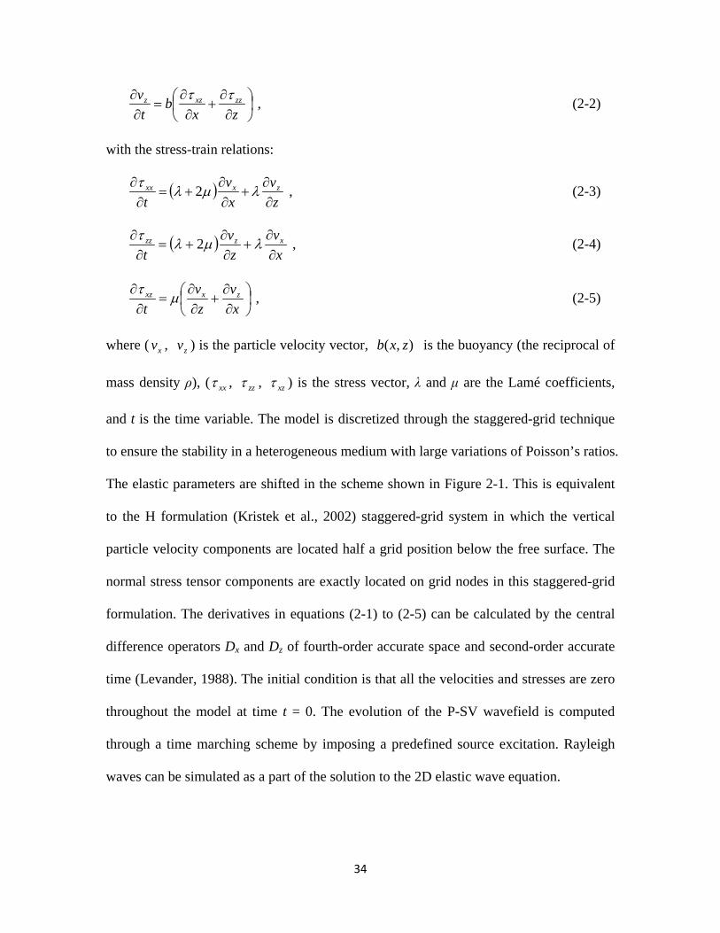
with the stress-train relations:

( ) , 2zv

xv

tzxxx

∂∂

+∂∂

+=∂∂ λµλτ (2-3)

( ) , 2xv

zv

txzzz

∂∂

+∂∂

+=∂∂ λµλτ (2-4)

,

∂∂

+∂∂

=∂∂

xv

zv

tzxxz µτ (2-5)

where ( xv , zv ) is the particle velocity vector, ),( zxb is the buoyancy (the reciprocal of

mass density ρ), ( xxτ , zzτ , xzτ ) is the stress vector, λ and μ are the Lamé coefficients,

and t is the time variable. The model is discretized through the staggered-grid technique

to ensure the stability in a heterogeneous medium with large variations of Poisson’s ratios.

The elastic parameters are shifted in the scheme shown in Figure 2-1. This is equivalent

to the H formulation (Kristek et al., 2002) staggered-grid system in which the vertical

particle velocity components are located half a grid position below the free surface. The

normal stress tensor components are exactly located on grid nodes in this staggered-grid

formulation. The derivatives in equations (2-1) to (2-5) can be calculated by the central

difference operators Dx and Dz of fourth-order accurate space and second-order accurate

time (Levander, 1988). The initial condition is that all the velocities and stresses are zero

throughout the model at time t = 0. The evolution of the P-SV wavefield is computed

through a time marching scheme by imposing a predefined source excitation. Rayleigh

waves can be simulated as a part of the solution to the 2D elastic wave equation.

35

Figure 2-1. The staggered-grid scheme used for the proposed vacuum formulation. The light circles are the grid nodes. The grid position is described by the indices i and k. The normal stress tensor components xxτ and zzτ , Lamé coefficients λ, μ, and the mass density ρ are all defined at the grid nodes. The triangles are the shear stress tensor components ( xzτ ). The solid squares and solid circles represent the horizontal particle velocity (vx) and the vertical particle velocity (vz), respectively.

For a semi-infinite earth model with a planar free surface, the parameters for grid

nodes that are close to the free surface can be evaluated by the stress-image technique in

second-order accuracy. The other edges of the model are usually attached with the

absorbing boundaries to suppress the spurious reflections caused by the physical

truncation of the finite-sized model. The special treatment to surface grid nodes

introduces difficulties to the FD modeling in the presence of topography.

2.4 The improved vacuum formulation

For an earth model with an irregular top surface, a simple solution for using the FD

modeling algorithm is to consider that grid nodes above the free surface are in the

vacuum. All physical parameters in the vacuum are set to zero during the calculation.

This is the so-called vacuum formulation or vacuum formalism (Zahradník et al., 1993).

The oblique segments of the topographic surface boundary can be approximated by the

36

staircase shape (Robertsson, 1996). When using the vacuum formulation, the

vacuum-earth boundary is treated as an internal interface inside the model. Hence, no

explicit free-surface boundary condition needs to be applied. The parameters on the

vacuum-earth interface are updated in a same manner as those for the internal grids.

The concept of vacuum formulation seems very attractive for solving the topography

problem in FD modeling because of its simplicity of implementation. Unfortunately,

simply setting the physical parameters above the free surface to zero does not guarantee

the correct generation of Rayleigh waves even in the simplest case that the free surface is

horizontal. This is mainly because the conventional vacuum formulation does not fulfill

the traction-free boundary condition ( zzτ and xzτ at free-surface grid nodes must be

zero at all times in a 2D case). For example, when using the staggered-grid scheme

shown in Figure 2-1, the shear stress component )21,( +kixzτ is shifted half a grid

position below the free surface; thus, does not need to be considered for the free-surface

boundary condition. The normal stress )0,(izzτ , however, is exactly located on the free

surface. It may differ from zero according to equation (2-4) due to the nonzero Lamé

coefficients at the grid node (i, 0). This violates the traction-free boundary condition and

introduces errors to the simulation of Rayleigh waves.

Generally, the results of FD modeling can be different depending on the specific

choice of staggered-grid configuration. In a 2D staggered-grid technique, one can set vx

exactly located on the free surface, and let vz shift half a grid below it, or vice versa.

These two forms of staggered-grid system have been studied by Kristek et al. (2002) and

the resulting difference on the synthetic record is usually negligible. On the other side,

the parameter-averaging scheme plays an important role in the staggered-grid FD

37

modeling. Parameter averaging is essential when using the staggered-grid FD method

because not all spatial derivatives are exactly evaluated at grid nodes. For example, to

calculate vx in equation (2-1), the central difference xxxD τ yields an approximated

derivative of xxx

∂∂τ at grid position (i+1/2, k), which is shifted half a grid position from

(i, k). Hence, the buoyancy b in equation (2-1) should use a value xb at (i+1/2, k) for the

calculation. Because the original Lamé coefficients λ, μ, and the mass density ρ are all

defined at grid position (i, k) after the model discretization, the buoyancy xb at (i+1/2, k)

should have an averaged value calculated from the adjacent grid nodes. Similarly, the

buoyancy b in equation (2-2) and the rigidity μ in equation (2-5) should be averaged as

zb and xzµ , respectively.

A slight modification in the parameter-averaging scheme may yield distinct stability

and accuracy of the modeling. Graves (1996) investigated the feasibility of using vacuum

formulation as an implementation of the free-surface boundary condition. In his

staggered-grid configuration, the vacuum formulation is not stable when using the

fourth-order staggered-grid FD algorithm. Graves (1996) also proposed that the stability

of the vacuum formulation could be improved through appropriate parameter-averaging

techniques. This leads us to think about the following question: is there an appropriate

combination of the staggered-grid form and a parameter-averaging scheme that can make

the vacuum formulation satisfy the free-surface boundary condition and stable in

high-order FD modeling?

Moczo et al. (2002) presented a comprehensive analysis on different

parameter-averaging schemes in 3D heterogeneous staggered-grid FD modeling. They

38

concluded that volume harmonic averaging should be used for the shear modulus in grid

positions of the stress tensor components, and volume arithmetic averaging should be

used for the density in grid positions of the displacement or velocity components. Mittet

(2002) suggests that the averaged rigidity xzµ should be zero if any shear modulus that

participates the averaging is zero so that the shear stress component xzτ is always zero

on the acoustic-elastic interface. If we only consider the shear modulus µi,k at the grid

node (i, k), the vacuum-elastic interface is similar to the acoustic-elastic interface because

µi,k = 0 in both cases. Hence, by extending Mittet’s scheme to the vacuum-elastic

interface and following the previous principles of parameter averaging, we calculate the

effective parameters xb , zb , and xzµ in our 2D P-SV wave modeling by

≠++=

+

++

;zeroboth are and if , 0

0; if , 2

,1,

k1,iki,,1,

kiki

kikixbρρ

ρρρρ (2-6)

≠++=

+

++

zero;both are and if , 0

0; if , 2

1,,

1,ki,1,,

kiki

kikikizb

ρρ

ρρρρ (2-7)

=

≠

+++

=

++++

++++

−

++++

; 0 if , 0

; 0 if ,111141

1,11,,1,

1,11,,1,

1

1,11,,1,

kikikiki

kikikikikikikiki

xz

µµµµ

µµµµµµµµµ (2-8)

Using the parameter-averaging scheme in equations (2-6), (2-7), and (2-8) is particularly

important to ensure the stability of the modeling with vacuum formulation. We have tried

different parameter-averaging methods for the topographic models and found that the

fourth-order FD algorithm is stable only when using the proposed scheme.

39

By applying the proposed parameter-averaging scheme, the vacuum formulation can

fulfill the traction-free boundary condition by considering a fictitious layer above the

original topographic model surface (Figure 2-2). The thickness of this fictitious layer is

only half a grid spacing so that the free surface is also shifted half a grid above its

original position. In this case, the only stress component located on the free surface is the

shear stress component xzτ . The horizontal particle velocity vx and the vertical particle

velocity vx are exactly on the free surface after the shifting. All the elastic parameters and

physical quantities should be set to zero above this line because they are in the vacuum.

The parameters in the original elastic part of the model are left unchanged. By applying

the proposed parameter-averaging technique, the effective rigidity xzµ on the

free-surface boundary line is always zero (if we set the shear modulus μ to zero for grid

nodes in the vacuum) according to equation (2-8). With this strategy, the value of xzτ

will be always zero automatically during the calculation according to equation (2-5). The

normal stress zzτ is now under the free surface and located in the elastic part of the

model; hence, does not need to be considered for the free-surface boundary condition.

Although we consider a fictitious layer above the model surface for analysis purpose,

no changes are required in the program implementation to explicitly set up this fictitious

layer because it is naturally generated by the combination of the staggered-grid form and

the proposed parameter-averaging technique. For the shear stress components on the

horizontal and vertical surface segments (e.g., points A and C in Figure 2-2) or the inner

and outer corners (e.g., points B and D in Figure 2-2), they are always zero due to the

averaged zero rigidities. The averaged density on the surface boundary line is only half of

the density at the adjacent grid node inside the solid earth. For example, the averaged

40

density ρE at point E can be calculated by ( ) 221 21

21

EEEE ρρρρ =+= ( 01 =Eρ in the

vacuum), where ρE1 and ρE2 are the mass density at grid nodes E1 and E2, respectively.

Similarly, the averaged density at point F is 221

EF ρρ = . This is consistent with the

elastic parameter modification scheme in conventional FD modeling with a planar free

surface (Mittet, 2002; Xu et al., 2007), which is important to the accuracy of the

simulated Rayleigh waves.

Figure 2-2. Grid distribution of the improved vacuum formulation in presence of surface topography. The shadowed area is a fictitious layer whose thickness is only half a cell size. The free surface in actual computation is represented by the bold solid line. All parameters above the free surface are set to zero during the modeling. The oblique surface segment can be approximated by the staircase shape (e.g., left part of the free surface).

41

It is noteworthy that the final output velocity components in the proposed method are

still calculated in a scheme as in the H staggered-grid formulation regardless of the

topography. For instance, the vertical particle velocity on the free surface is calculated by

( )32 21

EEE vvv += , where vE, vE2, and vE3 are the vertical particle velocities at points E,

E2, and E3, respectively (Figure 2-2). This means the vertical particle velocity in the

proposed vacuum formulation is output as an averaged value of the vz on the fictitious

free surface line and that inside the elastic model. Differing from the stress-image method,

the normal stress components on each side of the free surface are not symmetric in the

proposed vacuum formation. The particle velocities vx and vz are considered in the elastic

part of the model rather than in the vacuum. So they will not be reset to zero in each time

marching loop, which is different from the treatment to the outer corner points in the

image method (Robertsson, 1996).

Like in most FD modeling techniques including surface topography, the oblique

segments of the topography are approximated by the staircase shape. The primary

shortcoming of this approximation is that it needs a fine-grid discretization to reduce the

diffractions at the corners of the stairs. In near-surface seismic modeling focusing on

Rayleigh waves, the grid spacing is usually already small enough because the large ppw

requirement (at least 16 ppw for the shortest-wavelength surface waves) is essential to

suppress the numerical dispersion of the synthesized Rayleigh waves in FD modeling

(Mittet, 2002). In most cases, the amplitudes of the diffractions are too weak to be

noticed on the synthetic records compared to the amplitudes of the direct Rayleigh waves.

Hayashi et al. (2001) investigated the diffraction caused by the staircase shape and

42

concluded that the numerical errors are mainly controlled by the grid spacing rather than

the staircase boundary.

2.5 Benchmark of the algorithm

In the staircase approximation, an oblique interface is represented by many small

horizontal and vertical planar segments. Follow the accuracy tests of Robertsson (1996),

we use the flat homogeneous models with different surface slopes to test the accuracy of

the proposed vacuum formulation. If the Rayleigh waves can be accurately simulated

independent of the slope of the surface, they should be modeled successfully with more

complicated topography. In conventional modeling test, analytical solutions are usually

employed to check the accuracy of the results of numerical modeling. However, for a

semi-infinite homogenous elastic medium, the analytical solution to Lamb’s problem

(Lamb, 1904) only exists when the surface is horizontal. Fortunately, SEM can accurately

approximate the surface topography by using the combination of tetrahedral or hexahedra

volume elements. Surface waves can be simulated in a high precision by SEM because

the free-surface condition is natural satisfied regardless of the topography (Komatitsch

and Tromp, 1999). Hence, the proposed vacuum formulation can be benchmarked by

comparing the trace records with the modeling results for the same models calculated by

SEM.

43

Figure 2-3. Geometry of the homogeneous slope model for the benchmark tests. The star represents the location of the source. The triangle indicates the location of the receiver. The slope surface is approximated by the staircase shape. The grid lines sketch the model discretization for FD modeling. The grid spacing illustrated here is only for the demonstration. The actual grid spacing during the computation is much smaller than it is shown in this figure.

The geometry of the 2D model used for the benchmark is sketched in Figure 2-3. The

P-wave velocity vp and the S-wave velocity vs inside the model are 866 m/s, and 500 m/s,

respectively. The mass density ρ of the medium is 2.0 × 103 kg/m3. It is a homogeneous

elastic Poisson’s solid (the Poisson’s ratio σ = 0.25) with a single oblique flat free surface.

The left, right, and bottom edges of the model are attached with the perfectly matched

layer (PML) absorbing boundaries (Collino and Tsogka, 2001) during the modeling so

that the energy of the spurious reflections can be minimized. All physical parameters

above the free surface are set to zero. A vertical point source and a single receiver are

located exactly on the free surface and are separated in a constant horizontal distance of

60 m. The source wavelet is a 20-Hz (peak frequency) Ricker wavelet with a

44

60-ms-time-zero delay. The left and right parts of the model surface beyond the source

and receiver range are rounded to horizontal so as to accommodate the absorbing

boundaries and reduce the spurious diffractions at the transition corners. The model was

discretized in a fine-grid manner (0.1 m × 0.1 m) to ensure the stability of the modeling

and to reduce the influence of the staircase approximation. We change the angle of slope

(θ) of the free surface and run the simulation using fourth-order staggered-grid FD

modeling with the proposed vacuum formulation. Because the source and the receiver are

separated constantly in the horizontal direction, the actual offsets during the simulations

are increased with the increment of θ (the only exception is when θ = 90°, the source and

the receiver are separated 60 m in the vertical direction). The source vibrates in the

vertical direction for all simulations so that it interacts with the free-surface plane in

different angles. Hence, this test simulates the propagation of Rayleigh waves under

various conditions along different oblique planar surfaces. Figure 2-4 demonstrates the

synthetic trace records of horizontal particle velocity vx (Figure 2-4a) and vertical particle

velocity vz (Figure 2-4b) when θ = 0°, 30°, 45°, 60°, and 90° with the comparison of the

SEM results for each corresponding model. All trace records generated by the proposed

vacuum formulation agree with the SEM results with negligible differences. This

indicates that the P-SV wavefield was accurately modeled using the improved vacuum

formulation independent of the angles of slope. Thus, the proposed technique should be

able to successfully simulate the propagation of Rayleigh waves along more general

topographic surfaces.

45

a)

b)

Figure 2-4. a) Horizontal, and b) vertical particle velocities (vx) recorded for different models with the angle of slope θ varies from 0° to 90°. The trace records generated by the proposed vacuum formulation (solid lines) agree well with the overlaid SEM results (dash lines), which shows that the Rayleigh waves are accurately simulated by the proposed vacuum formulation.

46

2.6 Tests for irregular surface topography

To confirm the accuracy of the proposed vacuum formulation, an earth model with

more complicated surface topography (Figure 2-5) is employed for the simulation. The

model is a homogeneous Poisson’s solid with vp = 866 m/s, vs = 500 m/s, and ρ = 2.0 ×

103 kg/m3. The free surface is composed of a ridge and a valley, which is a typical case

for the data acquisition over a small hill in environmental and engineering studies. The

100-channel receiver array is placed on the free surface across the topography. The trace

interval is 1 m in the horizontal direction. The source parameters are the same as those

used in previous benchmark for slope models. To minimize the influence of the staircase

approximation, the model is discretized into 0.1 m × 0.1 m cells. Three PMLs are

attached on the left, right, and bottom edges of the model to absorb the spurious

reflections. The Courant number is about 0.3 during the modeling to ensure the stability

of the FD algorithm. The single trace records of vx in Figure 2-6a and vz in Figure 2-6b

Figure 2-5. A homogeneous model with the surface topography containing a ridge and a valley. The star represents the location of the source. The solid dots are the receivers that are located on the topographic free surface. The grid lines demonstrate the discretization scheme of the model. The grid spacing on this figure is for showing the concept only. The actual gird spacing during the modeling is much smaller than that is displayed.

47

are recorded by the receivers in the horizontal offsets of 25 m, 75 m, and 100 m. The

simulation results from SEM are used again for the trace comparison to check the

accuracy of the modeling. The accuracy of the synthetic Rayleigh waves generated with

the proposed vacuum formulation is confirmed by the good agreement of the vx and vz

records with the SEM results.

The conventional image method is also applied to the exactly same model to simulate

the seismic response in presence of topography for comparison. The trace data (dotted

lines in Figure 2-6) illustrate that the free surface is correctly implemented because both

the amplitude and the arrival time of the Rayleigh waves agree with those generated by

the proposed method and SEM. However, the “tails” after the Rayleigh waves on the

records generated by the image method is a typical characteristic of numerical dispersion

caused by insufficient ppw (Robertsson, 1996). These numerical errors contaminate the

synthetic wavefield and may decrease the accuracy of the dispersion analysis of Rayleigh

waves. To suppress the numerical dispersion, the model needs to be discretized into

smaller cells so the image method requires more ppw for the simulation of Rayleigh

waves. The corresponding time step size also needs to be reduced to ensure the stability

of the FD algorithm. These could tremendously increase the computing cost. According

to our tests, the maximum amplitude of the numerical dispersion in the image method can

be controlled to no more than 1% of the original peak amplitude of the Rayleigh waves

when the model is discretized into 0.02 m × 0.02 m cells, which means the image method

needs about five times more ppw than the proposed vacuum formulation for this

application. Thus, the proposed vacuum formulation helps reduce the computing cost in

FD modeling compared to the image method.

48

a)

b)

Figure 2-6. a) Horizontal, and b) vertical particle velocities (vx) recorded for the homogeneous topographic model from the source-receiver distance of 25 m, 75 m, and 100 m. The solid lines are the records generated with the proposed vacuum formulation. The dash lines are the results from SEM. The dotted lines are the trace records simulated with the image method. All trace records generated from the proposed vacuum formulation agree well with those generated by SEM. The results of the image method have good agreement for a most portion of the wavelet, but with remaining “tails” caused by the numerical dispersion.

To test the stability of the proposed vacuum formulation, we increase the P-wave

velocity in the previous homogeneous model so that the Poisson’s ratio of the model

varies from 0.25 to 0.49 and rerun the modeling. All the simulations are completed

successfully and the results (not shown here) agree well with those computed by SEM,

which indicates the proposed method is stable for the models with high Poisson’s ratios.

49

As the representation of many shallow structures formed by deposition, layered earth

models are usually employed in the studies of Rayleigh waves (e.g., Xia et al., 2007b;

Luo et al., 2009c; Socco et al., 2010). Therefore, we also applied the improved vacuum

formulation to a two-layer earth model (Figure 2-7) for a better approximation to the real

world. This layered earth model has the same surface topography as the previous

homogeneous model. We changed the physical parameters inside the solid to add another

interface beneath the free surface. The geometry of the internal interface is similar but not

identical to the surface topography. This model denotes a simplified deformed geological

structure contains an anticline and an incline, which is common in the real world. The

physical parameters of the top layer are vp = 1600 m/s, vs = 500 m/s, and ρ = 1.8 × 103

kg/m3. The parameters of the materials below the interface (“Layer 2” in Figure 2-7 and

called as the bottom layer in the following discussion) are vp = 2000 m/s, vs = 800 m/s,

and ρ = 2.0 × 103 kg/m3. The Poisson’s ratios of the top and bottom layers are about 0.45,

Figure 2-7. The two-layer earth model with irregular surface topography. The thickness of the top layer varies from 5 m to 10 m. The interface of the two layers has the similar but different geometry as the surface topography. The star is the source located on the free surface at (10 m, 0 m). The solid dots are the receivers that spread along the topographic surface. The last receiver is located at (110 m, –5 m). The trace interval in the horizontal direction is a constant of 1 m. But the trace intervals measured along the free surface are different depending on the topography of its location.

50

and 0.41, respectively. These high Poisson’s ratio materials are commonly seen in the

near surface (e.g., Xia et al., 2002b). The multiaxial perfectly matched layer (M-PML)

(Meza-Fajardo and Papageorgiou, 2008) absorbing boundaries are used here because the

classical PML absorbing technique is unstable under this high Poisson’s ratio

configuration (Zeng et al., 2011). The other model configurations are left unchanged

compared to the previous modeling. The simulation completed successfully without any

instability encountered. The synthetic seismogram generated by fourth-order FD

modeling with the proposed vacuum formulation (Figure 2-8a) is displayed with that

from SEM (Figure 2-8b). Detailed single trace records of the horizontal particle velocities

(Figure 2-9a) and the vertical particle velocities (Figure 2-9b) from the receiver

(horizontal) distance of 25 m, 75 m, and 100 m are listed for more detailed comparisons.

The good agreement of the modeling results from the two different methods illustrates

that Rayleigh waves can be accurately simulated along the topographic earth surface for

heterogeneous earth models using the proposed vacuum formulation.

2.7 Incorporation of internal discontinuities

By using the proposed vacuum formulation, grid nodes on the topographic free

surface are updated in an exactly same manner as internal grid nodes without any special

treatments. This allows the internal discontinuities in a model to be incorporated by the

same algorithm as the surface topography. Near-surface earth models that contain internal

discontinuities such as underground tunnels and shallow cavities have been investigated

in many environmental and engineering studies (e.g., Xia et al., 2004, 2007a; Gélis et al.,

2005). Shallow tunnels are often human-made and angular. The wall of a tunnel can be

51

a)

Figure 2-8a. The synthetic shot gather generated by fourth-order FD modeling with the proposed vacuum formulation for the two-layer earth model. All the events on the seismogram are visually the same as those on the seismogram generated by SEM.

52

b)

Figure 2-8b. The synthetic shot gather generated by SEM for the two-layer earth model. All the events on the seismogram are visually the same as those on the seismogram generated by FD modeling using the proposed vacuum formulation.

53

a)

b)

Figure 2-9. a) Horizontal, and b) vertical particle velocities (vx) recorded for the two-layer topographic earth model with the source-receiver distance of 25 m, 75 m, and 100 m. The solid lines are the records generated with the proposed vacuum formulation. The dash lines are the results from SEM. All trace records generated from the proposed vacuum formulation agree well with those generated by SEM. considered as a high contrast discontinuous interface for the propagation of seismic

waves. Figure 2-10 shows the staggered-grid system with the proposed vacuum

formulation for a model with a rectangular void inside an elastic medium. The internal of

the void can be considered as vacuum during the modeling since the density of air is

much less than that of the surrounding materials. The four edges of the void are

free-surface boundaries and need special treatment for the FD modeling if using the

image method. In contrast, when utilizing the proposed vacuum formulation, they are

naturally incorporated as the internal interfaces with no extra operations.

54

Figure 2-10. Grid distribution for a model containing internal discontinuities. The internal vacuum-elastic interface is attached with a fictitious layer (the shadowed area) so that the boundary of the internal discontinuities can be incorporated using the same algorithm as well as the surface topography.

Figure 2-11 displays the synthetic shot gather generated by the fourth-order FD

modeling with the proposed vacuum formulation for a rectangular tunnel inside a 2D

homogeneous half-space earth model. The tunnel is 10 m × 10 m with its top at depth of

20 m. The center of the tunnel is located exactly in the middle of the 100-channel

receiver array. The nearest offset and the receiver interval are both 1 m. To increase the

resolution of the seismogram, we use a 50-Hz (peak frequency) Ricker wavelet source

with a 24-ms-time-zero delay. The source excites vertically on the free surface to

generate strong Rayleigh waves. The P-wave velocity, the S-wave velocity, and the mass

density of the half-space are 866 m/s, 500 m/s, and 2.0×103 kg/m3, respectively. The

55

Figure 2-11. The synthetic shot gather generated for the tunnel model by fourth-order FD modeling with the improved vacuum formulation. Diffractions are clearly seen on the seismogram at the distance from 5 m to 50 m in the time window of about 100 ms to 250 ms. A large gain factor is applied to the display to enhance the visibility of the diffracted events because the amplitudes of the diffractions from the tunnel corners are usually much lower than those of the direct Rayleigh waves.

56

PML absorbing technique is applied to the left, right, and bottom edges of the model. The

Rayleigh-wave diffractions from the corners of the tunnel are observed on the synthetic

record. The wavefronts of the diffracted waves are clearly shown in the wavefield

snapshots at time t = 150 ms (Figure 2-12). The arrival time of the diffracted Rayleigh

waves on each trace agrees with the theoretical value obtained from the travel time

equation developed by Xia et al. (2007a). Detailed single trace comparison (e.g., the

traces at the distance of 25 m and 75 m) with the modeling results of SEM in Figure 2-13

confirms that the P-SV wavefield is correctly simulated by the proposed vacuum

formulation for the earth model containing internal discontinuities.

Figure 2-12. A wavefield snapshot of the vertical particle velocities (vz) at time slice of 150 ms. The square represents the tunnel. The solid lines are the interfaces of PML absorbing boundaries. The star is the source on the free surface. The dots denote the 100-channel receiver array across the top of tunnel. The wavefronts of the diffractions are significant on the snapshot.

57

2.8 Discussion

This study is mainly focused on the accurate simulation of Rayleigh waves using the

improved vacuum formulation. As parts of the solution, other elastic waves such as

P-waves and SV-waves are automatically taken in account because body waves usually

have less strict restrictions in the modeling than surface waves. In other words, if the

Rayleigh waves are successfully modeled, the body waves should be already correctly

simulated simultaneously. Hence, the proposed vacuum formulation can be extended to

the study on the whole elastic wavefield.

Figure 2-13. The single trace records at distance of 25 m and 75 m that extracted from the synthetic shot gathers for the tunnel model computed by the proposed vacuum formulation and SEM. The good agreements between the time series generated by FD modeling with the proposed vacuum formulation and the SEM results indicates that the P-SV wavefield can be accurately simulated with the proposed technique for the model containing internal discontinuities.

58

Modeling tests presented in this paper and more similar results not shown here

indicate that the application of the improved vacuum formulation in presence of

topography requires more ppw than conventional FD modeling with a horizontal planar

free surface. Generally, at least 16 ppw for the Rayleigh waves in their shortest

wavelength is required to make the numerical dispersion negligible in conventional FD

modeling (Mittet, 2002). The ppw used for the model tests in this paper, however, is

much greater. Take the topographic homogeneous model in the section “tests for irregular

surface topography” as an example, the maximum available frequency for a 20-Hz Ricker

wavelet can be as high as 50 Hz. The Rayleigh waves in that homogeneous medium have

a constant phase velocity of about 0.92 × vs. So the shortest wavelength of the Rayleigh

waves is about 9 m. The grid spacing used in the modeling test is 0.1 m, yields a

maximum ppw of about 90. This number is much greater than the minimum requirement

in conventional FD modeling (16 ppw). More tests show that, when a model contains

only horizontal and vertical free surface (e.g., the slope model in the benchmark section

when θ = 0°, and θ = 90°), only 16 ppw is sufficient to generate accurate Rayleigh waves

with no significant numerical dispersion. When there is an oblique surface, the ppw

requirement increases with the increment of the slope angle. The high ppw requirement

seems to be related to the staircase approximation because only the horizontal and

vertical interface can be accurately represented in FD modeling. The mathematical

analysis on this phenomenon requires further study but could be complicated.

Although the proposed vacuum formulation requires stricter ppw conditions than

conventional modeling with the horizontal planar free surface, the requirement is still

reasonable for many near-surface studies because the topographic surface needs to be

59

discretized in a fairly fine-grid manner for a proper approximation. The actual grid

spacing after discretization in practice usually yields more ppw than the theoretical

requirement. Moreover, we have shown that the image method needs even more ppw

than the proposed vacuum formulation. So the improved vacuum formulation would not

significantly increase computing cost in practice as it apparently does.

2.9 Conclusions

The conventional vacuum formulation can be improved to satisfy the traction-free

boundary condition on the vacuum-elastic interface to simulate accurate Rayleigh waves

using fourth-order FD modeling in presence of surface topography. In the improved

vacuum formulation, parameters at the surface grid nodes are averaged using the same

scheme used for the internal grid nodes. The free surface is shifted half a grid spacing so

that only the shear stress components needs to be considered to fulfill the free-surface

boundary condition. By applying the parameter-averaging scheme described in equations

(2-6), (2-7), and (2-8), the free-surface boundary condition is naturally satisfied during

the computation without any special treatments. Grid nodes on the free surface are

updated in a same manner as internal grid nodes during the time marching loop.

Compared to the image method, the improved vacuum formulation is easier to implement

and needs fewer ppw during the modeling to generate accurate Rayleigh waves without

notable numerical dispersion. Benchmark tests show that the proposed vacuum

formulation can stably incorporate irregular surface topography and internal

discontinuities for homogeneous and heterogeneous models with the Poisson’s ratios

range from 0.25 to 0.49. Rayleigh waves can be accurately simulated along the

60

topographic earth surface using the improved vacuum formulation with fourth-order

staggered-grid FD modeling. The proposed vacuum formulation can be easily

implemented in numerous existing FD modeling codes with only minor changes. The

proposed technique is illustrated in a 2D domain focusing on Rayleigh waves, but the

extension to a 3D domain is straightforward.

61

Chapter 3: Numerical investigation of applications of MASW in

presence of surface topography

3.1 Summary

Rayleigh-wave dispersion analysis of the Multichannel Analysis of Surface Waves

(MASW) technique requires the free surface of an earth model to be horizontally flat.

The accuracy of the dispersion image is important for picking dispersion curves and

subsequent inversion for shear-wave velocities. Surface topography can strongly

influence energy distribution on a dispersion image. In theory, static correction should be

applied to seismic records before generating dispersion images if there are any elevation

variations along a two-dimensional (2D) survey line. Noise from side areas of a survey

line in the three-dimensional (3D) domain can also contaminate the recorded wavefield.

We synthesize the seismograms through finite-difference modeling for 12 types of 2D

earth models that represent the basic elements of topography along a survey line. The

dispersion images are compared with the corresponding theoretical dispersion curves that

calculated by ignoring the topography of the models. The comparison shows that errors

of the picked Rayleigh-wave phase velocities can be constrained within 4% if a slope

angle of the topography is less than about 10°. For steeper topography, errors on

dispersion images are greater than 4% and static correction should be applied before the

dispersion analysis. In the 3D domain, levee shaped earth models are investigated to

evaluate errors caused by the multiples from the side edges of an embankment. The

analysis suggests that the distance between the edge of an embankment and a MASW

survey line should be at least 1/10 of the dominant Rayleigh-wave wavelength so that

62

errors on dispersion images introduced by topography are less significant than that caused

by other noises when picking dispersion curves in most practical MASW applications.

3.2 Introduction

Multichannel analysis of surface waves (MASW) is a non-invasive method to

estimate shear (S)-wave velocities in shallow layers by inverting phase velocities of

surface waves (typically Rayleigh waves) (e.g., Song et al., 1989; Xia et al., 1999). It has

been widely used in various geophysical investigations for environmental and

engineering problems over the past two decades (e.g., Miller et al., 1999; Xia et al.,

2002a, 2003; Luo et al., 2009b). In a 2D application of MASW, a shot gather containing

strong Rayleigh-wave energy is acquired through a multichannel recording system. Then

a dispersion image that represents the energy distribution of the wavefield is generated by

transferring the shot gather into frequency-velocity (f-v) domain. Because the

Rayleigh-wave energy is dominant on most near-surface seismic records (Xia et al.,

2002b), the dispersion curves of Rayleigh waves can be picked by tracing the

high-energy concentration on the dispersion image. These dispersion curves describe the

variation of Rayleigh-wave phase velocities in different frequencies and are used as

inputs of subsequent inversion for S-wave velocities.

The precision of an input Rayleigh-wave dispersion curve is crucial to the accuracy of

inverted S-wave velocities. For a commonly used one-dimensional (1D) layered earth

model, the Rayleigh-wave phase velocity Cr is a function of frequency f, S-wave velocity

vs, P-wave velocity vp, mass density ρ, and layer thickness h (Xia et al., 1999). By giving

the dispersion curves (data set of Cr and f) and the physical parameters in each layer (vp, ρ,

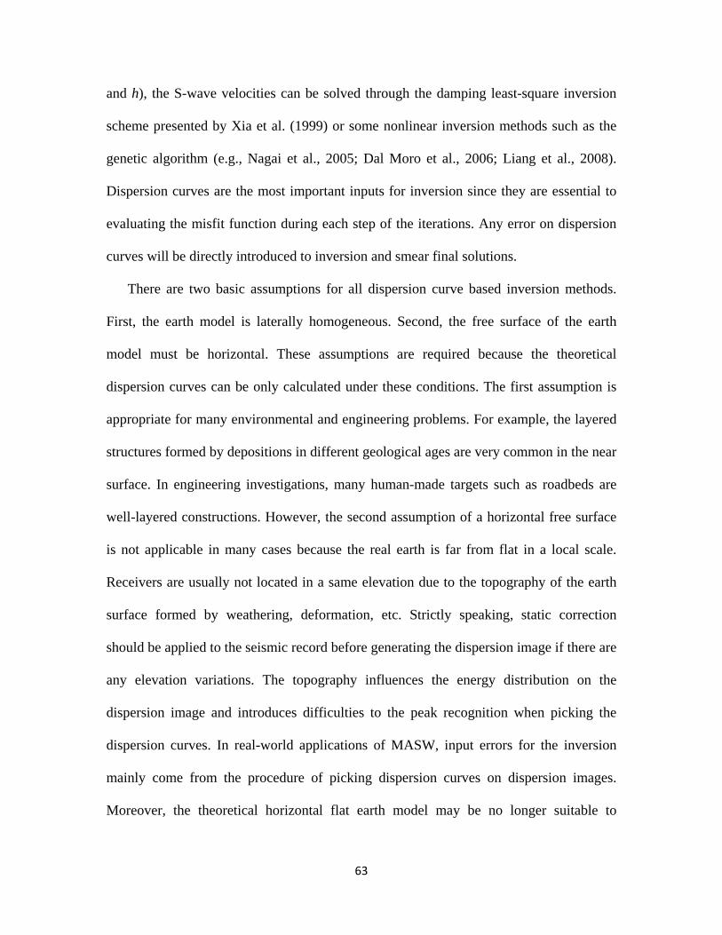
63

and h), the S-wave velocities can be solved through the damping least-square inversion

scheme presented by Xia et al. (1999) or some nonlinear inversion methods such as the

genetic algorithm (e.g., Nagai et al., 2005; Dal Moro et al., 2006; Liang et al., 2008).

Dispersion curves are the most important inputs for inversion since they are essential to

evaluating the misfit function during each step of the iterations. Any error on dispersion

curves will be directly introduced to inversion and smear final solutions.

There are two basic assumptions for all dispersion curve based inversion methods.

First, the earth model is laterally homogeneous. Second, the free surface of the earth

model must be horizontal. These assumptions are required because the theoretical

dispersion curves can be only calculated under these conditions. The first assumption is

appropriate for many environmental and engineering problems. For example, the layered

structures formed by depositions in different geological ages are very common in the near

surface. In engineering investigations, many human-made targets such as roadbeds are

well-layered constructions. However, the second assumption of a horizontal free surface

is not applicable in many cases because the real earth is far from flat in a local scale.

Receivers are usually not located in a same elevation due to the topography of the earth

surface formed by weathering, deformation, etc. Strictly speaking, static correction

should be applied to the seismic record before generating the dispersion image if there are

any elevation variations. The topography influences the energy distribution on the

dispersion image and introduces difficulties to the peak recognition when picking the

dispersion curves. In real-world applications of MASW, input errors for the inversion

mainly come from the procedure of picking dispersion curves on dispersion images.

Moreover, the theoretical horizontal flat earth model may be no longer suitable to

64

approximate the real earth when the topography is significant. Accuracy of the MASW

method will decrease in the presence of surface topography.

Besides the elevation change along a receiver array, noise from side areas that a 2D

survey line does not cover can also contaminate the recorded wavefield because the real

world is always 3D. Surface topography on sides of a 2D survey line can generate

multiples and other complicated wave phenomena that propagate in oblique directions.

The amplitude of this type of noise can be as high as the effective Rayleigh waves that

propagate along the survey line. In this case, extra strong energy concentrations will

appear on dispersion images and make it challenging to pick the dispersion curves by

tracing the peaks of energy. A typical example of this situation is to perform an MASW

survey along a dam or a railroad, where the dipping edges of an embankment can

generate strong multiples. Min and Kim (2006) discussed the feasibility of applying

MASW to 3D layered dam structures. They showed that the Rayleigh-wave dispersion

curves can be distorted by the surrounding materials and the boundaries of dams.

In this paper, we evaluate the influence of the surface topography for dispersion

curves picking in MASW applications through numerical modeling. In the 2D domain,

we synthesize near-surface seismograms in the vertical 2D plane along the receiver line

by finite-difference modeling (FDM) including surface topography. Dispersion images

are generated from the synthetic data for several types of 2D topographic earth models.

The energy concentration on the dispersion images are compared with the theoretical

dispersion curves calculated from the horizontal earth models. Then we extend the

investigation to the 3D domain by emphasizing a layered levee model to simulate the

MASW survey along a railroad embankment. The main purpose of this study is to

65

provide guidelines to the dispersion curve picking for the MASW data gathered in the

presence of surface topography.

3.3 Methods for the numerical investigation

The synthetic records containing strong Rayleigh-wave energy from topographic

earth models are required for the numerical investigation. As interfering of P waves and

the vertical component of shear (SV) waves along the free surface, Rayleigh waves can

be simulated in the P-SV wave domain by solving the vector wave equation with

applying the free-surface boundary condition (Aki and Richards, 2002). For the

numerical methods in this study, we use the explicit fourth-order staggered-grid FDM

(Levander, 1988; Graves, 1996) because of its high efficiency and stability for large

variations of Poisson’s ratio of the near-surface earth models. To incorporate the

elevation variation during the modeling, the free-surface condition needs to be

implemented with an irregular vacuum-elastic interface. The improved vacuum

formulation proposed by Zeng et al. (in review) is stable for high-order FD operators and

more efficient than the conventional extended stress-imaging method (Robertsson, 1996),

thus, is employed in this study to simulate the propagation of Rayleigh waves along the

topographic earth surface. For all 2D and 3D models investigated in this paper, the

multiaxial perfectly matched layer (M-PML) absorbing technique (Meza-Fajardo and

Papageorgiou, 2008; Zeng et al., 2011) is applied on all the edges (except the free surface)

of the models to suppress the spurious reflections.

The dispersion images are generated from the synthetic shot gathers after the FDM to

present the energy distribution of the near-surface wavefield. The resolution limitation of

66

the dispersion image constrains the recognition of the peaks of the energy concentration.

Various image-generating algorithms (e.g. the τ-p transform [McMechan and Yedlin,

1981]) were developed to improve the resolution of the dispersion image so as to

facilitate the picking of the dispersion curves. Xia et al. (2007b) described a slant

stacking method that can accommodate an arbitrary geometry of data acquisition. Luo et

al. (2008b) presented a high-resolution linear Radon transform (LRT) to image the

Rayleigh-wave dispersive energy. Synthetic and real-world examples showed that the

resolution of the dispersion images generated by the high-resolution LRT is 50% higher

than those of the other methods (Luo et al., 2008b; Xia et al., 2009). Therefore we use the

high-resolution LRT technique to image the dispersive energy for all the synthetic data of

the investigated models throughout the paper.

The dispersion image is the energy distribution of the recorded wavefield in the f-v

domain regardless of the existence of the topography. It contains not only the effective

Rayleigh-wave information that is considered as the valid signal but also the noise caused

by the topography. The dispersive energy concentration in presence of topography is

usually distorted compared to that recorded on a horizontal flat earth surface. The peaks

of the energy concentration indicate the Rayleigh-wave phase velocity versus frequency

for the topographic earth models. The dispersion curves picked based on these peaks,

however, are used as the information for the horizontally layered earth model during the

subsequent inversion due to the assumption of planar earth surface. This inconsistence is

a main source for errors of the final inverted S-wave velocities. Hence, the difference

between the actual energy peaks on the dispersion images and the theoretical dispersion

67

curves calculated from the corresponding horizontal earth model should be the focus in

this study.

Based on the previous methodologies, the general procedure of the numerical

investigation can be summarized as follows. First, build a model with topographic free

surface and compute the synthetic seismogram by FDM. Second, generate the dispersion

image through high-resolution LRT from the synthetic seismogram. Then assume the free

surface of the model is horizontally flat and calculate the corresponding theoretical

dispersion curves by the Knopoff’s method (Schwab and Knopoff, 1972). At last, overlay

the theoretical dispersion curves on the dispersion image and evaluate the difference. In

the following sections, we will investigate the models with typical surface topography

and difference slope angles in 2D and 3D domains. All the synthetic records are

calculated by FDM with a 20-Hz (peak frequency) Ricker wavelet source with time zero

delay of 60 ms. The dispersion images are generated in a frequency band of 10 Hz to 60

Hz, which is equivalent to the effective frequency band of a 20-Hz Ricker wavelet

source.

3.4 Dispersive energy of 2D topographic earth models

In the 2D domain, we generalize the topography into three basic categories: slopes,

ridges and valleys. A more complicated topography can be considered as the combination

of them. Both homogeneous half-space (Figures 3-1a to 3-1c) and layered earth models

are investigated in this work. For the convenience of discussion, we simplify all the

layered earth models as two-layer models that composed by an overlaid finite-thick

homogeneous layer (layer 1) and a half-space (layer 2). There are two types of layered

68

topographic earth models. One is that the topography only occurs on the free surface,

while the interface is still horizontal. This type of model represents the field conditions

that the topography is only caused by weathering or other types of erosion. In this case,

the media where the source and receiver locate can be different depends on the slope of

the topography. When the slope is relatively gentle, the source and receivers are on the

same medium (Figures 3-2a, 3-2b, and 3-2c). If the slope is steep, they may distribute on

different media (Figures 3-3a, 3-3b, and 3-3c). The second type of topography is usually

formed by deformation. In this case, the interface is also topographic as well as the free

surface. To simplify the discussion, we assume the layer thickness is invariant so that the

interface always has the same curvature as the free surface. Hence all the typical models

with topography can be represented by the 12 models listed in Figures 3-1a to 3-1c (type

HS), Figures 3-2a to 3-2c (type A), Figures 3-3a to 3-3c (type B), and Figures 3-4a to

3-4c (type C). For all models, the nearest offset (measured along the free surface) is 30 m.

A 60-m length receiver array spreads along the topographic free surface with the trace

interval of 1 m. Particle velocities are recorded on the free surface in the vertical direction.

For the half-space earth models, the medium is set as a Poisson’s solid (the Poisson’s

ratio σ = 0.25) where the P-wave velocity vp, S-wave velocity vs, and mass density ρ are

520 m/s, 300 m/s, and 1500 kg/m3, respectively. For the two-layer earth models, the

model parameters are listed in Table 3-1.

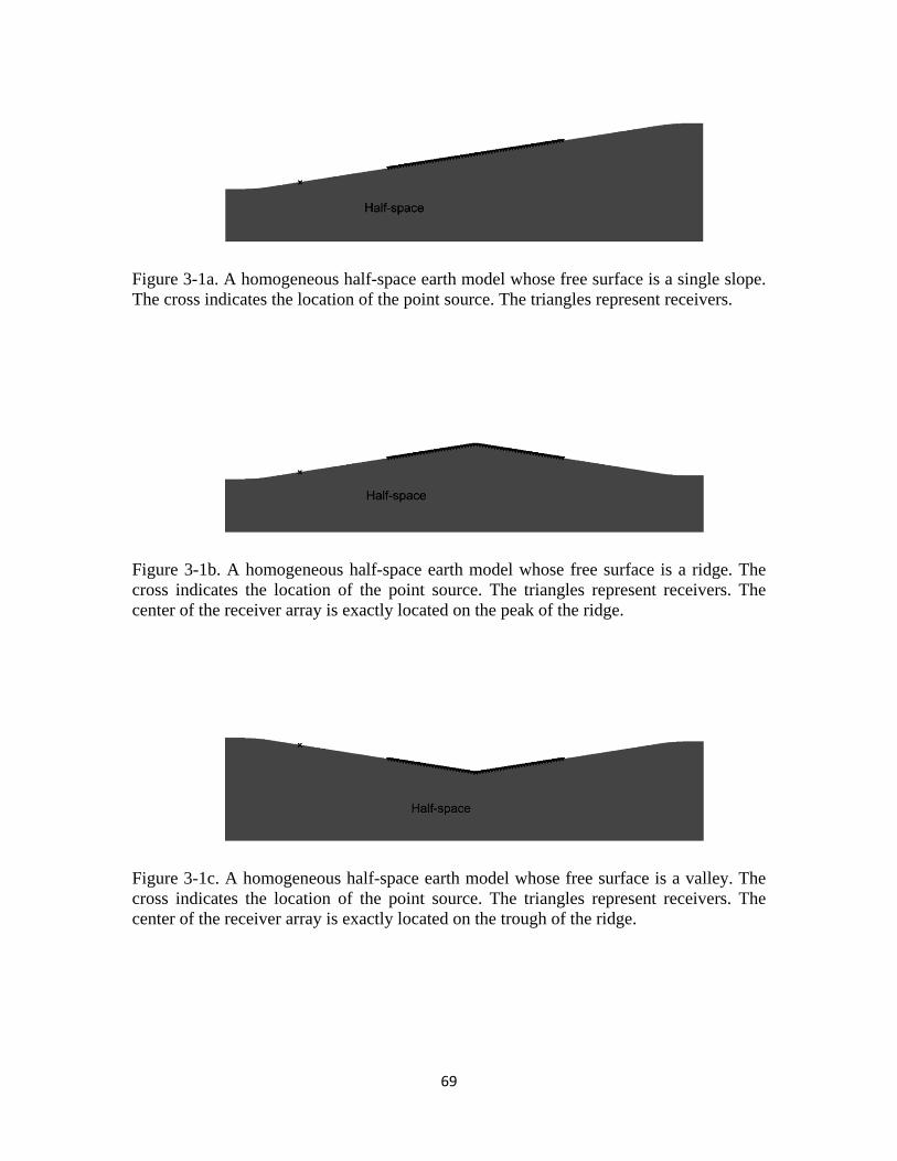
69

Figure 3-1a. A homogeneous half-space earth model whose free surface is a single slope. The cross indicates the location of the point source. The triangles represent receivers.

Figure 3-1b. A homogeneous half-space earth model whose free surface is a ridge. The cross indicates the location of the point source. The triangles represent receivers. The center of the receiver array is exactly located on the peak of the ridge.

Figure 3-1c. A homogeneous half-space earth model whose free surface is a valley. The cross indicates the location of the point source. The triangles represent receivers. The center of the receiver array is exactly located on the trough of the ridge.

70

Figure 3-2a. A two-layer earth model whose free surface is a single slope. The interface is horizontal. The cross indicates the location of the point source. The triangles represent receivers. Both the source and receivers are on layer 1.

Figure 3-2b. A two-layer earth model whose free surface is a ridge. The interface is horizontal. The cross indicates the location of the point source. The triangles represent receivers. The center of the receiver array is exactly located on the peak of the ridge. Both the source and receivers are on layer 1.

Figure 3-2c. A two-layer earth model whose free surface is a valley. The interface is horizontal. The cross indicates the location of the point source. The triangles represent receivers. The center of the receiver array is exactly located on the trough of the ridge. Both the source and receivers are on layer 1.

71

Figure 3-3a. A two-layer earth model whose free surface is a single slope. The interface is horizontal. The cross indicates the location of the point source. The triangles represent receivers. The source is on the half-space, while receivers are on layer 1.

Figure 3-3b. A two-layer earth model whose free surface is a ridge. The interface is horizontal. The cross indicates the location of the point source. The triangles represent receivers. The center of the receiver array is exactly located on the peak of the ridge. The source is on the half-space, while receivers are on layer 1.

Figure 3-3c. A two-layer earth model whose free surface is a valley. The interface is horizontal. The cross indicates the location of the point source. The triangles represent receivers. The center of the receiver array is exactly located on the trough of the ridge. The source is on layer 1, while receivers are on the half-space.

72

Figure 3-4a. A two-layer earth model whose free surface is a single slope. The shape of the interface is the same as the topographic free surface. The cross indicates the location of the point source. The triangles represent receivers. Both the source and receivers are on layer 1.

Figure 3-4b. A two-layer earth model whose free surface is a ridge. The shape of the interface is the same as the topographic free surface. The cross indicates the location of the point source. The triangles represent receivers. The center of the receiver array is exactly located on the peak of the ridge. Both the source and receivers are on layer 1.

Figure 3-4c. A two-layer earth model whose free surface is a valley. The shape of the interface is the same as the topographic free surface. The cross indicates the location of the point source. The triangles represent receivers. The center of the receiver array is exactly located on the trough of the ridge. Both the source and receivers are on layer 1.

73

Table 3-1. Parameters of the two-layer earth model Layer Thickness (m) vp (m/s) vs (m/s) ρ (kg/m3)

1 10 800 200 2000 2 ∞ (half-space) 1200 400 2000

When calculating the theoretical dispersion curves, the thickness of layer 1 of the

two-layer earth models should take the value of the depth for the interface under the

middle point of the receiver array due to the middle-of-receiver-spread assumption (Luo

et al., 2009a). For the simplicity of the investigation, the middle point of the receiver

array is designed to always exactly locate on the peak or trough of the topography (e.g.,

Figures 3-2b and 3-2c). For layered earth models, the distance from the peak or trough to

the interface is fixed as 10 m regardless of the slope angle of the topography so as to be

consistent with the corresponding horizontal earth models.

We start from the simplest case that the model is a half-space with single slope free

surface (Figure 3-1a). The influence of the topography may vary from the slope angle θ

of the surface. Figures 3-5a, 3-5b, and 3-5c present the dispersion image generated from

the synthetic records of the models when θ = 5°, 9°, and 15°, respectively. Theoretical

dispersion curves (indicated by the crosses) when assuming θ = 0° are overlaid on the

dispersion images. It is obvious that the difference between the high-energy concentration

on the dispersion image and the theoretical dispersion curve increases with the slope

angle. For a specific slope model, the error of the picked Rayleigh-wave phase velocity

increases with the frequency. The maximum error of the picked Rayleigh-wave velocity

is only about 2%, which is insignificant by considering the noise and resolution of the

dispersion image for real data.

74

Figure 3-5a. The dispersion image of the half-space slope model (Figure 3-1a) when the slope angle θ = 5°. The crosses represent the theoretical dispersion curve calculated from the corresponding horizontal earth model. The error of the picked dispersion curve is less than 2%.

Figure 3-5b. The dispersion image of the half-space slope model (Figure 3-1a) when the slope angle θ = 9°. The crosses represent the theoretical dispersion curve calculated from the corresponding horizontal earth model. The error of the picked dispersion curve is less than 2%.

75

Figure 3-5c. The dispersion image of the half-space slope model (Figure 3-1a) when the slope angle θ = 15°. The crosses represent the theoretical dispersion curve calculated from the corresponding horizontal earth model. The error of the picked dispersion curve is less than 2%.

The ridge model shown in Figure 3-1b simulates an MASW survey across a small hill.

In a homogeneous half-space model, Rayleigh waves are non-dispersive regardless of the

surface topography. The dispersion image, however, can be distorted due to the

assumption of horizontal flat surface when generating the dispersion image. Figures 3-6a,

3-6b, and 3-6c illustrate the corresponding dispersion images when the slope of the hill is

5°, 9°, and 15°, respectively. When the slope angle is small (such as θ = 5°), the

dispersion image agrees with the theoretical dispersion curve with insignificant difference

(Figure 6a). With the increase of slope, the high-energy concentration is distorted and

poses a false “dispersion” (Figures 3-6b and 3-6c), which may lead to an interpretation

that the Rayleigh-wave phase velocity changes with the frequency in this model. When θ

= 9°, the maximum error of the picked Rayleigh-wave phase velocity is about 2%, which

is less that the dispersion image resolution for many real data (about 4%). The maximum

error of the picked dispersion curve, however, is about 6% when θ = 15°. In this case, the

76

earth model may not be correctly inverted from picked dispersion curves due to errors

associated with the dispersion image.

Figure 3-6a. The dispersion image of the half-space ridge model (Figure 3-1b) when the slope angle θ = 5°. The crosses represent the theoretical dispersion curve calculated from the corresponding horizontal earth model.

Figure 3-6b. The dispersion image of the half-space ridge model (Figure 3-1b) when the slope angle θ = 9°. The crosses represent the theoretical dispersion curve calculated from the corresponding horizontal earth model.

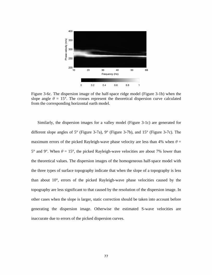
77

Figure 3-6c. The dispersion image of the half-space ridge model (Figure 3-1b) when the slope angle θ = 15°. The crosses represent the theoretical dispersion curve calculated from the corresponding horizontal earth model.

Similarly, the dispersion images for a valley model (Figure 3-1c) are generated for

different slope angles of 5° (Figure 3-7a), 9° (Figure 3-7b), and 15° (Figure 3-7c). The

maximum errors of the picked Rayleigh-wave phase velocity are less than 4% when θ =

5° and 9°. When θ = 15°, the picked Rayleigh-wave velocities are about 7% lower than

the theoretical values. The dispersion images of the homogeneous half-space model with

the three types of surface topography indicate that when the slope of a topography is less

than about 10°, errors of the picked Rayleigh-wave phase velocities caused by the

topography are less significant to that caused by the resolution of the dispersion image. In

other cases when the slope is larger, static correction should be taken into account before

generating the dispersion image. Otherwise the estimated S-wave velocities are

inaccurate due to errors of the picked dispersion curves.

78

Figure 3-7a. The dispersion image of the half-space valley model (Figure 3-1c) when the slope angle θ = 5°. The crosses represent the theoretical dispersion curve calculated from the corresponding horizontal earth model.

Figure 3-7b. The dispersion image of the half-space valley model (Figure 3-1c) when the slope angle θ = 9°. The crosses represent the theoretical dispersion curve calculated from the corresponding horizontal earth model.

79

Figure 3-7c. The dispersion image of the half-space valley model (Figure 3-1c) when the slope angle θ = 15°. The crosses represent the theoretical dispersion curve calculated from the corresponding horizontal earth model.

For the two-layer type A earth models that the source and receivers are all located on

layer 1 (Figures 3-2a, 3-2b, and 3-2c), the dispersion images are illustrated in Figures

3-8a, 3-8b, 3-9a, 3-9b, 3-10a, and 3-10c with slope angle of 5° and 9° for the slope, ridge,

and valley models, respectively. For all the type A models, errors of the picked

fundamental mode Rayleigh-wave phase velocities on the dispersion image are less than

4%. The calculated dispersion of high-mode Rayleigh waves does not agree with the

theoretical values for most models. Different from the homogeneous half-space models,

the maximum errors mainly come from the low frequency part rather than the high

frequency part on the dispersion images. This implies that the long-wavelength Rayleigh

waves are more sensitive to surface topography because the recorded wavefield is

smeared by the shallow topographic features.

80

Figure 3-8a. The dispersion image of the two-layer slope earth model (Figure 3-2a) when the slope angle θ = 5°. The crosses represent the theoretical dispersion curves calculated from the corresponding horizontal earth model.

Figure 3-8b. The dispersion image of the two-layer slope earth model (Figure 3-2a) when the slope angle θ = 9°. The crosses represent the theoretical dispersion curves calculated from the corresponding horizontal earth model.

81

Figure 3-9a. The dispersion image of the two-layer ridge earth model (Figure 3-2b) when the slope angle θ = 5°. The crosses represent the theoretical dispersion curves calculated from the corresponding horizontal earth model.

Figure 3-9b. The dispersion image of the two-layer ridge earth model (Figure 3-2b) when the slope angle θ = 9°. The crosses represent the theoretical dispersion curves calculated from the corresponding horizontal earth model.

82

Figure 3-10a. The dispersion image of the two-layer valley earth model (Figure 3-2c) when the slope angle θ = 5°. The crosses represent the theoretical dispersion curves calculated from the corresponding horizontal earth model.

Figure 3-10b. The dispersion image of the two-layer valley earth model (Figure 3-2c) when the slope angle θ = 9°. The crosses represent the theoretical dispersion curves calculated from the corresponding horizontal earth model.

83

For type B earth models, the source and receivers locate on different media. This

happens when the slope angle of the topography is relative large (e.g., 15° for the survey

design in this study). Figures 3-11a, 3-11b, and 3-11c display the dispersion images for

the slope, ridge, and valley models when θ = 15°. The picked Rayleigh-wave phase

velocity is close to the true values in the layer where the receiver array locates. For the

slope and ridge models, the Rayleigh-wave information from the beneath half-space is

not significant. For the valley model, the picked Rayleigh-wave phase velocity is close to

the value in the half-space. This is because all receivers are located on the half-space

(Figure 3-3c), which is the case similar to the half-space model shown in Figure 3-1c.

Figure 3-11a. The dispersion image of the two-layer slope earth model (Figure 3-3a) when the slope angle θ = 15°. The crosses represent the theoretical dispersion curves calculated from the corresponding horizontal earth model.

84

Figure 3-11b. The dispersion image of the two-layer ridge earth model (Figure 3-3b) when the slope angle θ = 15°. The crosses represent the theoretical dispersion curves calculated from the corresponding horizontal earth model.

Figure 3-11c. The dispersion image of the two-layer valley earth model (Figure 3-3c) when the slope angle θ = 15°. The crosses represent the theoretical dispersion curves calculated from the corresponding horizontal earth model.

85

For a more complicated case that the topography presents on the free surface and the

internal interface (type C models), the situation is equivalent to the case that the earth is

horizontally layered but the wavefield is recorded in oblique directions. We examined the

slope, ridge and valley models with different slope angles (results not shown here) and

find that the all the dispersion images agree with the theoretical dispersion curves in

errors less than 4%. This is consistent with the conclusions of the study on a dipping

interface by Luo et al. (2009c).

The investigation to the previous 2D models shows that errors of the picked

dispersion curves due to topography are less significant than that introduced by noise and

resolution of the dispersion images for real data when the slope of the topography is less

than about 10°. This indicates that 2D applications of MASW can tolerance most surface

topography since the demand of static correction is usually obvious when a slope is

greater than 10° in a field survey. If the source and receivers are not located on a same

medium, however, the Rayleigh-wave information from the layer where the receiver

array does not cover can be absent from the dispersion image.

3.5 Dispersive energy of 3D levee earth models

Besides the topography along the receiver line in a 2D domain, the surface features

besides the receiver line in a 3D domain may also introduce errors to the dispersion

analysis. In this study, we focus a 3D levee-shaped earth model because it is commonly

employed in the MASW survey along the railroad or dam. Figure 3-12 sketches a levee

model in the 3D Cartesian coordinate system. The model is simplified into two layers.

Physical parameters of the layers are the same as those used in previous investigations for

86

2D layered earth models. The top surface of the levee is horizontally flat, but the cross

section in x-z (distance-depth) cut plane (Figure 3-13) is a layered trapezoid. The top

width of the trapezoid is 10 m and the slope of the side is 60°. The survey line is placed

along the y (extension) direction. The distance between the receiver line and the top-right

edge of the levee is d. In many field surveys, the distance d is usually short due to the

existence of rails. The slope side surface of the levee will generate strong Rayleigh waves

that can propagate in oblique directions to the receiver line, which will generate errors on

the calculated dispersion image since the dispersion analysis is based on 2D horizontally

layered models.

We move the survey line along the x direction so that the value of d varies. Synthetic

seismograms are generated by FDM and the corresponding dispersion images are

calculated using the high-resolution LRT. Figures 3-14a, 3-14b, 3-14c, and 3-14d

demonstrate the dispersion images when d is 5 m, 2 m, 1 m, and 0.4 m, respectively. To

incorporate a more general case, we extend the levee model to four layers (Figure 3-15)

and evaluate the dispersion images again. The layer parameters of the model are listed in

Table 3-2. Figures 3-16a and 3-16b display the dispersion images when d is 2 m and 1 m,

respectively.

Table 3-2. Parameters of the four-layer earth model Layer Thickness (m) vp (m/s) vs (m/s) ρ (kg/m3)

1 4 800 200 2000 2 6 900 280 2000 3 8 1000 350 2000 4 ∞ (half-space) 1200 400 2000

87

Figure 3-12. A sketch of a two-layer 3D levee earth model. The dimension of the model is 40 m × 25 m × 95 m. Receivers spread along the y (extension) direction, which is parallel to the top edge lines of the embankment.

Figure 3-13. A cross section in the x-z plane of the two-layer 3D levee model. The cross indicates the projection point of the source and receiver line on x-z plane.

88

Figure 3-14a. The dispersion image generated from the synthetic seismogram for the two-layer 3D levee model (Figure 3-13) when the receiver line is 5 m away from the edge of the embankment. The crosses represent the theoretical dispersion curves calculated from the corresponding horizontal earth model.

Figure 3-14b. The dispersion image generated from the synthetic seismogram for the two-layer 3D levee model (Figure 3-13) when the receiver line is 2 m away from the edge of the embankment. The crosses represent the theoretical dispersion curves calculated from the corresponding horizontal earth model.

89

Figure 3-14c. The dispersion image generated from the synthetic seismogram for the two-layer 3D levee model (Figure 3-13) when the receiver line is 1 m away from the edge of the embankment. The crosses represent the theoretical dispersion curves calculated from the corresponding horizontal earth model.

Figure 3-14d. The dispersion image generated from the synthetic seismogram for the two-layer 3D levee model (Figure 3-13) when the receiver line is 0.4 m away from the edge of the embankment. The crosses represent the theoretical dispersion curves calculated from the corresponding horizontal earth model.

90

Figure 3-15. A cross section in the x-z plane of the four-layer 3D levee model. The cross indicates the projection point of the source and receiver line on x-z plane.

Figure 3-16a. The dispersion image generated from the synthetic seismogram for the four-layer 3D levee model (Figure 3-25) when the receiver line is 2 m away from the edge of the embankment. The crosses represent the theoretical dispersion curves calculated from the corresponding horizontal earth model.

91

Figure 3-16b. The dispersion image generated from the synthetic seismogram for the four-layer 3D levee model (Figure 3-25) when the receiver line is 1 m away from the edge of the embankment. The crosses represent the theoretical dispersion curves calculated from the corresponding horizontal earth model.

The dispersion images for the two-layer levee model and the four-layer levee model

show that the high-energy concentrations generally agree with theoretically dispersion

curves. But the image of the low frequency part (e.g. 10 Hz to 25 Hz in Figure 3-14d) can

be distorted. This is because the generation of long-wavelength (low-frequency) Rayleigh

waves is influenced by the dipping side surface of the levee. An overview to all the

dispersion images of the levee in difference model configurations suggests that the

MASW survey for a 3D levee-shaped structure is effective when the survey line is 1 m or

more far away from the edge of the embankment.

3.6 Conclusions

Topography can influence the accuracy of dispersion images for an MASW survey if

no static correction applied. Numerical investigations to 2D homogeneous and layered

earth models show that errors of picked Rayleigh-wave phase velocities from the

92

dispersion images can be constrained in no more than 4% if a slope of the topography

along the survey line is less than about 10°. For steeper topography, errors on the

dispersion image are significant (greater than 4%) and static correction should be applied

before the dispersion analysis. In a 3D domain, the analysis to levee-shaped earth models

suggests that an MASW survey is effective when the distance of a survey line and edges

of the embankment is at least 1/10 of the dominant Rayleigh-wave wavelength.

93

Chapter 4: Feasibility of waveform inversion of Rayleigh waves for

shallow shear-wave velocity using genetic algorithm

4.1 Summary

Conventional surface-wave inversion for shallow shear-wave (S-wave) velocity relies

on generation of dispersion curves of Rayleigh waves. This constrains the method to only

laterally homogeneous (or very smooth laterally heterogeneous) earth models. Waveform

inversion uses a technique that directly fit waveforms on seismograms, hence, does not

have such a limitation. Waveforms of Rayleigh waves are highly related to S-wave

velocities. By inverting the waveforms of Rayleigh waves on a near-surface seismogram,

shallow S-wave velocities can be estimated for earth models with strong lateral

heterogeneity. We employ genetic algorithm to perform waveform inversion of Rayleigh

waves for S-wave velocities. The forward problem is solved by finite-difference

modeling in time domain. The model space is updated by generating offspring models

using genetic algorithm. Final solutions can be found through an iterative waveform

fitting scheme. By applying the genetic waveform inversion scheme to synthetic

seismograms generated from several typical near-surface earth models, the S-wave

velocities are recovered successfully with errors no more than 10%. For layered earth

models, the proposed method generates 1D S-wave velocity profiles as accurate as

conventional dispersion-curve-based inversion. For earth models containing lateral

heterogeneity in which case the application of conventional inversion is challenging,

waveform inversion can successfully produce S-wave velocity images of subsurface if

providing appropriate priori information. Applications to various earth models indicate

94

that the genetic waveform inversion has a great potential for shallow S-wave velocity

imaging with the existence of strong lateral heterogeneity.

4.2 Introduction

Shallow shear (S)-wave velocity is a fundamental physical parameter for many

near-surface geophysical studies (Craig, 1992). It can be derived by inverting dispersive

phase velocities of surface waves (typically Rayleigh waves in a vertical 2D plane).

Spectral analysis of surface waves (SASW) method (Stokoe and Nazarian, 1983; Stokoe

et al., 1989) was introduced to analyze dispersion curves of ground roll to generate

near-surface S-wave velocity profiles. The latter developed multichannel analysis of

surface waves (MASW) method (Song et al., 1989; Xia et al., 1999) greatly improved the

accuracy of estimated S-wave velocities (Xia et al., 2000, 2002a). The difference between

inverted S-wave velocities using the MASW method and borehole measurements can be

only 15% or less (Xia et al., 2002a). Over the past two decades, the MASW technique has

been widely employed by near-surface seismologists for various purposes such as

bedrock mapping (Miller et al., 1999), near-surface attenuation analysis (Xia et al.,

2002b), and many other environmental and engineering problems (e.g. Xia et al., 2004;

Xia et al., 2006).

In the MASW technique, a shot gather containing strong Rayleigh-wave energy is

acquired through a multichannel recording system. Seismic records are analyzed in the

frequency-velocity (f-v) domain to generate a set of dispersion curves. The dispersion

curves represent phase velocities of Rayleigh waves at different frequencies. Because

Rayleigh-wave phase velocities are highly sensitive to S-wave velocities, S-wave

95

velocities can be stably inverted from the dispersion curves through a damping

least-square scheme (Xia et al. 1999). The basic assumption for a dispersion-curve-based

inversion method is that the earth is horizontally layered, which is required to calculate

theoretical dispersion curves. In this case, only a 1D S-wave velocity distribution in the

vertical direction can be obtained from a single shot gather. The inverted S-wave velocity

can be considered a horizontally averaged value from the underground area beneath the

receiver spread (Luo et al., 2009a). To obtain a 2D distribution of S-wave velocities, a

standard common depth point (CDP) roll-along acquisition format (Mayne, 1962) is

usually required to produce multiple shot gathers so that a pseudo 2D S-wave velocity

section can be inverted from a set of dispersion curves (Xia et al., 2004; Luo et al., 2008).

The accuracy of this pseudo 2D S-wave velocity section depends on the length of the

receiver spread and the degree of lateral heterogeneity of underground materials. The

application of the MASW method is limited if the subsurface is not horizontally layered

or the lateral heterogeneity is strong. Luo et al. (2009b) investigated the effects of

mapping dipping interface and concluded that it is difficult to calculate high accuracy

dispersion curves if the slope of subsurface is greater than 15°. Investigations to the

structures such as shallow faults and tunnels using the dispersion-curve-based inversion

scheme are also challenging.

Since the major difficulty associated with the MASW method comes from generation

of dispersion curves for non-layered earth models, it could be overcome if an inversion

does not directly rely on dispersion curves. Tarantola (1984; 1986) presented an inversion

scheme for seismic reflection data by waveform fitting, which is known as the waveform

inversion technique. In this method waveforms on seismic records are directly used as

96

inputs of the inversion, which indicates that the integrated information of all waves

(including surface, direct, refracted, reflected, or multiply reflected waves) is utilized. In

theory, waveform inversion is not restricted to any specific characteristics of a wave (e.g.,

the dispersion of Rayleigh waves in MASW technique). Hence, it has the ability to

handle complicated earth model with lateral heterogeneity. Moreover, amplitudes of

waves can be used simultaneously with phase information during inversion so as to

improve the accuracy of inverted images.

Rayleigh waves dominate the energy of near-surface wavefield (Xia et al., 2002a;

Saenger and Bohlen, 2004). If we consider Rayleigh waves the major signal for analysis,

the signal-to-noise ratio (S/N) is fairly high for most near-surface seismic records. In

many cases, the most significant waveforms on a near-surface seismogram are mainly the

directly arrived Rayleigh waves and the following dispersive wave trains. Waveforms of

the dispersive Rayleigh waves contain abundant S-wave velocity information. Hence,

S-wave velocities can be directly derived by inverting waveforms of Rayleigh waves

without calculating dispersion curves.

In global and regional seismic studies, Rayleigh waves have already been employed

for waveform inversion but under limited conditions. Lerner-Lam and Jordan (1983) first

attempted the linearly waveform inversion for a laterally homogeneous model by using

only phase information of surface waves. Yomogida and Aki (1987) utilized both

amplitude and phase information for waveform fitting of Rayleigh waves. Snieder (1988)

proposed a large-scale waveform inversion scheme of surface waves using the surface

scattering theory but with the assumption that lateral heterogeneity is smooth (Snieder

and Nolet, 1987). Du (2002) used a ray theory approximation for surface waves

97

originally developed by Levshin (1985) to invert multimode surface waves for tectonic

structures such as continent-ocean boundaries. However, this method is not appropriate

for near-surface studies due to the target is usually small compared to the wavelength of

seismic waves. On the other hand, because gradient based methods are commonly used to

minimize objective functions in inversion, the forward modeling problem during the

waveform inversion is usually linearized by Born (Clayton and Stolt, 1981; Beylkin,

1985; Beydoun and Tarantola, 1988) or Rytov (Bleistein, 1987; Beydoun and Tarantola,

1988; Beylkin and Burridge, 1990) approximation to facilitate computation of the

Jacobian or Hessian matrix. The optimization procedure with these approximations is

usually difficult for an elastic case when strong surface waves present on seismograms

(Gélis et al., 2007).

In this study, we examine the feasibility of using waveform inversion of Rayleigh

waves to estimate shallow S-wave velocities in a 2D domain. To reduce the difficulty of

optimizing the objective function, we do not use any approximations to the wave

equation. Instead a full 2D elastic wave equation is solved in the time domain using the

finite-difference method (FDM). For model updating we use genetic algorithm (GA) to

perform the optimization since it is generally considered more suitable for global

optimization for highly nonlinear problems compared to conventional gradient based

methods (Sambridge and Mosegaard, 2002). In the following sections, we first introduce

the basic procedure of the GA used for waveform inversion. Then we present our

implementation and describe the algorithm in detail. After that, numerical examples are

demonstrated by inverting the synthetic seismograms calculated from several typical

98

near-surface earth models including lateral heterogeneity. Finally, we discuss potential

practical applications of the proposed method for shallow S-wave velocity imaging.

4.3 General procedure of GA waveform inversion

As a category of Monte Carlo method, GA has gained a lot of interest for geophysical

inversion and is developing quickly. It simulates the principles of biological evolution

such as natural selection to find the most appropriate model for a set of data. It has been

successfully applied to problems such as the inversion of seismic reflection data (Stoffa

and Sen, 1991) and static correction estimation (Wilson and Vasudevan, 1991).

Yamanaka and Ishida (1996) presented a GA scheme to invert surface-wave group

velocity for S-wave velocities. Sambridge and Drijkoningen (1992) also demonstrated the

application of GA to waveform inversion for reflection seismograms. A detailed

introduction and overview of the GA methods can be referred to Sambridge and

Drijkoningen (1992), and Sambridge and Mosegaard (2002).

Like most Monte Carlo methods, one benefit of using GA for geophysical inversion is

that it requires no derivative information of the objective function to be minimized

(Sambridge and Drijkoningen, 1992). This indicates that the inversion algorithm is

independent of the methods of solving the forward problem. This greatly simplifies the

implementation of inversion because various numerical methods can be used for forward

modeling. For accurate and fast simulation of Rayleigh waves in near surface,

staggered-grid FDM (Virieux, 1986) with appropriate free-surface conditions (e.g., Mittet,

2002; Xu et al., 2007) can be employed.

99

In a general waveform inversion for S-wave velocities, a set of random models (m1,

m2, …, mq) are generated, where each individual mi is a vector whose length is

determined by the specific dimension of the inversion. The space composed by the q

individual models is the initial population to be updated. Then FDM can be used to

calculate the synthetic data for all the models in the population. The models are ranked by

evaluating the waveform misfit represented by the L2 norm

2obscal uu −=φ , (4-1)

where ucal and uobs are the calculated synthetic trace record and the observed seismic

record, respectively. The model has the minimum misfit is the best-fit model in the

current generation, and the one has the maximum misfit is the worst.

After the population is initialized, p different models are selected from the population.

This operation is the “selection” action in GA. Subsequently, a crossover action is

applied, which means some new models will be generated based on a crossover

probability Pc. Then a mutation actions is applied in a given mutation probability Pm to

modify the existing models. After the three actions, some models in the population are

eliminated based on the evaluated misfit values so that the population is updated with

new models while the size of population keeps a constant. The specific operations of

selection, crossover, and mutation vary with the implementation of GA. By repeating the

three actions, models in the population can be updated in a convergent manner. A final

best model whose synthetic record matches the observed data within a tolerance can be

found if the parameters of the three actions are set appropriately. S-wave velocities are

estimated directly from the seismograms.

100

4.4 Description of the algorithm

One major problem of waveform inversion using GA is that the population updating

often needs many times of iteration and forward modeling. In near-surface seismic

modeling, accurate simulation of Rayleigh waves can be time consuming (Zeng et al.,

2011). To improve the computational efficiency of waveform inversion, the number of

iteration should be controlled as few as possible to reduce the time cost for forward

modeling. Guo et al. (1999) proposed a decimal encoding based stochastic searching

algorithm for solving function optimization. This algorithm is easy to implement and is

highly efficient in global optimization (Kang et al., 2000). It is robust and effective for

inverting fundamental mode and higher mode Rayleigh-wave dispersion curves to

retrieve S-wave velocities in shallow layers (Liang, et al., 2008). The original algorithm

can be described as follows:

1. Randomly generate q models to form the initial population (m1, m2, …, mq);

2. Evaluate the misfit of every model in the population;

3. Rank the population by misfits, find the best model mbest has the minimum misfit

minφ , and the worst model mworst has the maximum misfit maxφ ;

4. If εφ ≤min or maxmin φφ = , then go to step 9 for output, where ε is a given misfit

tolerance;

5. Randomly choose p models ( pmmm ′′′ ..., , , 21 ) as the parents from the population;

6. Generate a new offspring model ∑=

′=p

iii mm

1

~ α , where 11

=∑=

p

iiα , and

5.15.0 ≤≤− iα ;

101

7. Evaluate the generated offspring model m~ ; if the misfit worstm φφ <~ , then replace

mworst with m~ ; otherwise discard m~ ;

8. Go to step 3;

9. Output mbest as a solution to the problem.

Step 5 and 6 are the selection and crossover actions in a common GA implementation. It

is noteworthy that no explicit mutation is introduced in this algorithm, which is

equivalent to the case that the mutation probability pm is zero in general GAs. A

theoretical analysis of the algorithm is presented by Kang et al. (2000). An attracting

feature of this algorithm is that it generates only one new model after an iteration, which

means only once forward modeling is required in each updating. This helps reduce the

cost of forward modeling during the inversion. However, only one (the worst) model is

eliminated in each updating may make the algorithm converge slower than other GA

implementations.

To increase the convergence speed of the algorithm, we increase the pressure for

parent selection. For each reproduction we only choose the parents from the top np

ranked individuals so that the offspring has a higher probability of the goodness of fit.

This helps reduce the iteration times, but increases the risk that the search will be trapped

in a local minima. The convergence speed can also be improved by generating more than

one offspring model (say, nf offspring) during each loop so that the bad fitted models can

be eliminated more quickly. However, this increases the speed of the maturation of the

population and may cause a failure of finding a satisfactory solution due to the population

approaching homogeneous status ( maxmin φφ = ). Hence, tuning the values of np and nf can

greatly influence the convergence behavior of the algorithm. The specific values of np

102

and nf, however, are usually problem dependent (similar to the thermodynamic speed in

simulated annealing [Sambridge and Mosegaard, 2002]). They are usually determined by

trail or experiences. For all the models tested in this study, the number of the random

initial models is about 300. We use np ≈ 100 and nf ≈ 30 and no instability is observed

during the tests. Figure 4-1 demonstrates a representative example of the misfit variation

with the generation during the inversion using the proposed scheme. Similar to most GA

implementation, the proposed algorithm converges very fast at the beginning and then

gradually slows down when the search is approaching the global minima. For all the

models tested in the study, the total generations can be controlled in no more than 200,

which is a number much less than the common generation number (several thousands) in

many GA implementations.

Figure 4-1. An example of the misfit variation with the generation during the inversion for a four-layer earth model. The misfit decreases very fast at the beginning and then gradually slows down when the search is approaching the global minima.

The algorithm can be easily parallelized on parallel computers such as the high

performance computing (HPC) cluster system. At the beginning of the computation, the

initial population can be decomposed so that each part of the population can be evaluated

103

by different computers. The reproduction procedure can be performed in fully parallel

manner because the generation of m~ is only related to the pre-selected p parent models

that can be randomly chosen by the computer nodes independently.

Rayleigh-wave phase velocities are strongly related to S-wave velocities, but are less

influenced by the P-wave velocities and densities. In many cases, the shallow P-wave

velocities can be obtained from first arrivals. Densities can be estimated for most

environmental and engineering investigations. For these reasons we can assume the

P-wave velocities and densities of a model are known during the waveform inversion of

Rayleigh waves for S-wave velocities. With this simplification, the only variable is the

S-wave velocity.

We use FDM to solve the forward problem with the free surface condition described

by Kristek et al. (2002). The simplified multiaxial perfectly layer (M-PML) technique

(Zeng et al., 2011) is utilized to suppress the spurious reflections. The model is composed

by numerous grid points during the computation. Direct taking the S-wave velocity on

each finite-difference grid as an individual variable is not only inessential but also

impractical for the computation due to too many unknowns can make the convergence of

the algorithm extremely slow. Furthermore, it will tremendously increase the

non-uniqueness of the solution, which makes the inversion results meaningless for

geophysical studies. To reduce the number of model parameters and the non-uniqueness

of the inversion, constrains must be applied to the inversion by introducing more priori

information. The specific priori information depends on different types of problems to be

solved. In most cases, the estimated minimum value of possible S-wave velocities should

be taken into account for a practical application to improve the convergence speed of the

104

algorithm. Other information such as the minimum layer thickness or lateral resolution

can be also helpful to reduce the non-uniqueness of the inversion.

Based on the previous description of the algorithm, there are three stop criteria for the

inversion iteration: maximum iteration number reached, the population approached

homogeneous, and the minimum misfit minφ is less or equal than the preset tolerance ε.

The only condition for the success of inversion is that minφ ≤ ε. The geometry

explanation for the misfit is the Euclidean distance of the observed seismogram and the

calculated seismogram since we are using the L2 norm. In theory, the value of ε can be

arbitrary small if the data is noise free. However, the optimum value of ε is usually

problem dependent for a practical application due to the existence of noise. For all the

models and synthetic records used in this study, we find ε ≈ 1 can generate satisfactory

results in most cases if the amplitudes of the seismic traces are normalized to 0 to 100.

4.5 Numerical examples for layered earth models

To test the effectiveness of the proposed algorithm, we use the synthetic records

generated from known earth models to perform the waveform inversion. Since the

inversion procedure should be independent of the size of the model and the observation

system, all the input synthetic records throughout the paper are generated using a 25-Hz

(peak frequency) Ricker wavelet point source that excites vertically on the free surface.

All the models have a same size of 26 m (horizontal direction) × 12 m (vertical direction).

A 24-channel receiver array is placed on the free surface with the nearest offset and the

trace interval of 1 m.

105

The dispersion curve based inversion scheme is very efficient for layered earth

models. The errors of the inverted S-wave velocities can be controlled in less than 15%.

Hence, we employ the conventional layered earth model first to benchmark the waveform

inversion using the proposed algorithm. We start from the simplest case – a homogeneous

half-space (Model A). The physical parameters of the model are vp = 520 m/s, vs = 300

m/s, and ρ = 1500 kg/m3, where vp, vs, and ρ are the P-wave velocity, S-wave velocity,

and mass density, respectively. The Rayleigh wave in this medium is non-dispersive and

has a constant phase velocity of about 276 m/s. We add constraints to the inversion that

the model is known as laterally homogeneous, which is consistent with the assumption in

dispersion curve based inversion. During the computation, the model is divided into 12

equal-thickness layers. So the model vector (S-wave velocity) has the length of 12. In

other words, there are total 12 scalar variables for the inversion. We set the minimum

possible S-wave velocity as 100 m/s, which is reasonable for most near-surface materials.

The resolution of the velocity change is set to 5 m/s, which means the inversion program

will not differentiate the velocity values such as 200 m/s and 204 m/s since the difference

is less than 5 m/s. This helps to reduce the non-uniqueness and to improve the

convergences of the GA iteration. Figure 4-2 displays the inverted S-wave velocity

profile with the comparison to the true values. The (synthetic) seismogram input for the

inversion and the corresponding calculated seismogram for the best-fit model are shown

in Figures 4-3a and 4-3b, respectively. Figure 4-4 demonstrates a detailed comparison of

the final calculated trace data and the observed data is. The waveforms of

106

Figure 4-2. Comparison of the inverted S-wave velocity profile (dashed line) and the true value (solid line) for the homogeneous earth model (Model A). The maximum error of the inverted S-wave velocities is about 3%.

a)

b)

Figure 4-3. a) Input synthetic seismogram of the homogeneous model (Model A) for the waveform inversion. b) Calculated seismogram of the best-fit model from the waveform inversion for Model A. The Rayleigh wave has a constant velocity of about 276 m/s for this model.

Figure 4-4. The trace record at the offset of 20 m of the observed data (solid line) and the final calculated data from the best-fit solution (dashed line) for Model A.

107

Rayleigh waves are fitted with no significant errors. The maximum error of the inverted

S-wave velocity is only about 3%.

Because the proposed inversion scheme is independent of the forward modeling

method, more complicated model can be incorporated as long as the forward modeling

can generate accurate synthetic seismograms. High Poisson’s ratio earth models are

commonly employed in near-surface studies. The simulation of Rayleigh waves in

materials of high Poisson’s ratio may encounter instability problem due to the absorbing

boundary processing (Zeng et al., 2011). The M-PML technique (Meza-Fajardo and

Papageorgiou, 2008; Zeng et al., 2011) can be used in this case to ensure the stability of

the forward modeling. Here we demonstrate the inversion results for a two-layer earth

model (Model B) modified from Xia et al. (2007b). The model parameters are listed in

Table 4-1. The Poisson’s ratios σ of the materials in the two layers are both greater than

4.0. The model is still evenly divided into 12 layers during the inversion. The vs values in

the layers of the initial modes are random. Figure 4-5 is the comparison of the inverted

S-wave velocity profile and the true values, the maximum error of the inverted S-wave

velocity is less than 4%. Both the observed (Figure 4-6a) and calculated (Figure 4-6b)

seismograms and the detailed trace comparison (Figure 4-7) between the observed data

and the final synthetic record from the best fit model show that the directly arrived

Rayleigh wave and the following dispersive wave trains are fitted in a good agreement.

To demonstrate the effectiveness of the proposed method for more complicated earth

models, we extended the computation to a four-layer earth model (Model C). The model

is modified from the six-layer earth model presented by Xia et al. (1999). The model

parameters are listed in Table 4-2. Rayleigh waves are highly dispersive in this layered

108

Figure 4-5. Comparison of the inverted S-wave velocity profile (dashed line) and the true values (solid line) for the two-layer earth model (Model B). The errors of the inverted S-wave velocities are less than 4%.

a)

b)

Figure 4-6. a) Input synthetic seismogram of the two-layer earth model (Model B) for the waveform inversion. b) Calculated seismogram of the best-fit model from the waveform inversion for Model B. The Poisson’s ratios of the top and bottom layer are 0.47 and 0.44, respectively. Dispersion can be observed on the seismogram.

Figure 4-7. Comparison of the single traces at the offset of 20 m extracted from the observed seismogram (solid line) and the final calculated seismogram (dashed line) for the tow-layer earth model (Model B).

109

earth model. An estimated 1D S-wave velocity distribution (Figure 4-8) is obtained after

158 generations by inverting the seismogram in Figure 4-9a with the same inversion

settings in the previous computation for Model B. The maximum error of the inverted

S-wave velocities is less than 10%. This relatively large error mainly comes from the

deeper layers below 10 m, which is reasonable if we consider the penetrating depth

limitation (Xia et al., 2005) of the Rayleigh waves around a 25-Hz peak frequency. The

seismogram calculated from the final output model (Figure 4-9b) is visually the same

with the input seismogram. Figure 4-10 displays the 20th trace record (the offset is also

20 m) extracted from the observed data (solid line) and final calculated data (dashed line).

The final synthesized trace record matches the observed data well with very small

perturbations.

Table 4-1. Physical parameters of Model B Layer Thickness (m) vp (m/s) vs (m/s) ρ (kg/m3) σ

1 6 800 200 2000 0.47 2 ∞ (half-space) 1200 400 2000 0.44

Table 4-2. Physical parameters of Model C Layer Thickness (m) vp (m/s) vs (m/s) ρ (kg/m3) σ

1 2 650 190 1800 0.45 2 2 750 270 1800 0.43 3 4 1200 400 1900 0.44 4 ∞ (half-space) 1600 600 2000 0.42

110

Figure 4-8. The S-wave velocity profile of the true model (solid line) and the inverted values (dashed line) for Model C. The maximum error of the inverted S-wave velocities is less than 10%.

a)

b)

Figure 4-9. a) The seismogram input to the waveform inversion for the four-layer earth model (Model C). b) The calculated seismogram from the best-fit model after the waveform inversion for Model C. The Rayleigh waves are highly dispersive in this model.

Figure 4-10. Comparison of the trace records extracted from the observed seismogram and calculated seismogram at offset of 20 m for Model C.

111

4.6 Application to laterally heterogeneous earth models

It is difficult to apply conventional dispersion curve based inversion to earth models

with lateral heterogeneity due to the basic assumption of horizontally layered earth

models. The GA waveform inversion, however, has no such a shortcoming because there

is no need to compute the dispersion curves. For some near-surface earth models that

look very simple (e.g., a single dipping slope), the dispersion curve inversion may fail. In

this section, we use the proposed scheme to invert the synthetic waveforms calculated

from earth models that contain lateral heterogeneity. Three typical earth models are

discussed to demonstrate the effectiveness of the GA waveform inversion.

The first type of model is a single fault earth model (Model D) shown in Figure 4-11a.

For the convenience of discussion, we simplify the case to that the model contains only

two types of different materials. That is, the two parts of the model that are separated by

the fault line are homogeneous. The physical parameters of the block above the fault line

(the top layer) are vp = 800 m/s, vs = 200 m/s, and ρ = 2000 kg/m3, respectively. The

block beneath the interface (the bottom layer) is a half space of vp = 1200 m/s, vs = 400

m/s, and ρ = 2000 kg/m3, respectively. The lateral heterogeneity of the model occurs at

the materials across the vertical fault plane. The abrupt change of S-wave velocities

introduces difficulties to the dispersion curve based inversion. For a single shot gather,

the dispersion curve based inversion can only generate a horizontally layered S-wave

velocity distribution. For a set of shot gather obtained by a standard CDP roll-along

acquisition, the inverted pseudo S-wave velocity image is smoothed due to the averaging

effect. Hence, the exact location of the fault plane is hard to be determined.

112

Figure 4-11b shows the estimated S-wave velocity distribution by inverting the

seismogram shown in Figure 4-12a through the proposed GA waveform inversion. The

variables of the inversion for this model are the S-wave velocities in the top and bottom

layers, and the location of the fault. The solution is found after 108 generations. The

errors of the inverted S-wave velocities are controlled in 2%. The exact location of the

fault is imaged accurately. The synthetic seismogram calculated from the best-fit model

is shown in Figure 4-12b for comparison to the observed data (Figure 4-12a). Figure 4-13

demonstrates the fitness of the single trace record between the observed data and final

calculated data. The final calculated record agrees with the observed data with negligible

difference.

a)

b)

Figure 4-11. a) The true image, and b) the inverted image of the fault model (Model D). The S-wave velocities above and below the fault plane are 200 m/s and 400 m/s, respectively. The top corner of step shape is at (10 m, 3 m). The location of the fault plane is accurately inverted. The maximum error of the S-wave velocity in the bottom layer is less than 2%.

113

a)

b)

Figure 4-12. a) The synthetic seismogram of Model D. b) Calculated seismogram of the best-fit model from the inversion for Model D. The Rayleigh waves are dispersive. Diffractions from the step corner of the fault can be observed from the offset of 1 m to 7 m. The two seismograms are visually the same.

Figure 4-13. The trace comparison at the offset of 20 m extracted from the observed seismogram (solid line) and the observed seismogram (dashed line) for Model D.

The second type of model is an earth model with a single dipping subsurface (Model

E) (Figure 4-14a). Although the geometry of the model looks very simple, the dispersion

curve based inversion for this model is challenging (Luo et al., 2009c) because the high

lateral heterogeneity – the model cannot be decomposed in horizontal direction into

several laterally homogeneous model because every vertical slice of the model is

114

different. The physical parameters of the material above the dipping interface are vp =

800 m/s, vs = 200 m/s, and ρ = 2000 kg/m3, respectively; and those of the material below

the dipping interface are vp = 1200 m/s, vs = 400 m/s, and ρ = 2000 kg/m3, respectively.

To reduce the non-uniqueness of the GA waveform inversion, we assume that the

interface is flat since the horizontal extension is relatively small (25 m). Then there are

total four variables for the inversion: S-wave velocities of the materials above and below

the dipping interface, and the coordinates of the left and right end points of the dipping

interface. Figure 4-14b shows the inverted S-wave velocity image after 12 generations.

The dipping interface is inverted accurately with the error of the S-wave velocity in the

bottom layer is 5%. The input seismogram (Figure 4-15a) and the calculated synthetic

record for the best-fit model (Figure 4-15b) are visually the same. Figure 4-16 is the

detailed single trace comparison at the offset of 20 m of the observed record and the final

calculated record of the best-fit model. The good agreement between the (mainly

Rayleigh-wave) waveforms of the observed data and of the calculated data indicates that

the final vs model is inverted successfully.

a)

b)

Figure 4-14. a) The true image of the dipping interface model (Model E). b) The inverted image of Model E by the GA waveform inversion. The S-wave velocities above and below the interface are 200 m/s and 400 m/s, respectively. The depth of the left and right end point of the slope is 2 m and 10 m, respectively. The position of the dipping subsurface is inverted accurately with 5% error for the S-wave velocity in the bottom layer.

115

a)

b)

Figure 4-15. a) The synthetic seismogram of Model E input for the waveform inversion. b) Calculated seismogram of the best-fit model from the inversion for Model E.

Figure 4-16. Single trace comparison at the offset of 20 m extracted from the observed seismogram (solid line) and the observed seismogram (dashed line) for Model E.

The third type of model is a tunnel (Model F) inside a homogenous half-space (Figure

4-17a). Similarly, this model contains strong lateral heterogeneity and is difficult to be

imaged through the dispersion curve based inversions. Such near-surface features can be

detected by Rayleigh-wave diffraction analysis (Xia et al., 2007a). Here we demonstrate

that the tunnel can be also located by the proposed inversion scheme conveniently. For a

practical investigation, the approximate tunnel size is known since the tunnel is often

116

human made. For this model, we use a 2 m × 2 m tunnel with the top depth of 4 m. The

background S-wave velocities are also given as the priori information because they can

be easily estimated from the other surrounding area either by the conventional MASW

method or by the proposed inversion scheme. The tunnel is usually filled with air. During

the inversion, we consider the internal materials in the tunnel as vacuum since the density

of air is negligible compared to the surrounding materials. With these simplifications, the

only variable for the inversion is the position of the tunnel. The GA search completed

only after 14 generations for such as single variable problem. The inverted image (Figure

4-17b) matches the true model (Figure 4-17a) very well. The observed data (Figure 4-18a)

and the final calculated seismogram (Figure 4-18b) also agree with each other with no

notable difference. Figure 4-19 shows the detailed single trace comparison at the offset of

5 m for the input seismogram and the final calculated data for the best-fit model. The

tunnel is successfully located by the proposed GA waveform inversion.

a)

b)

Figure 4-17. a) The true image, and b) the inverted image of the tunnel model (Model F). The top left corner of the tunnel is (10 m, 4 m). The size of the tunnel is 2 m × 2 m. The position of the tunnel is accurately inverted with the preset constraints.

117

a)

b)

Figure 4-18. a) Synthetic record calculated by FDM for the tunnel model (Model F). b) Final calculated seismogram from the best-fit model after the GA waveform inversion. The Rayleigh wave diffractions are significant on the seismogram (offset of 1 m to 7 m). The calculated seismogram agrees well with the observed seismogram for the model.

Figure 4-19. Single trace comparison at the offset of 5 m of the observed data (solid line) and the calculated data (dashed line) from the best-fit model from the inversion for Model F.

These three types of models are the simplifications to many targets in near-surface

geophysical investigations. The lateral heterogeneity in these models introduces

difficulties to conventional dispersion curved based analysis. They are all successfully

imaged by the proposed GA waveform inversion scheme, which indicates the great

118

potential of the proposed method for solving the lateral heterogeneity problem in

surface-wave based seismic investigations.

4.7 Conclusions

The waveform inversion that is focused on surface waves for S-wave velocities is

performed successfully through GA for typical types of earth models. For layered earth

models, the GA waveform inversion does not need a good estimated initial mode as the

case in conventional inversion since the initial model space is random in GA. The

inversion results show that errors of inverted S-wave velocities can be constrained in

10%. Although the inversion time cost is more expensive than the conventional

dispersion-curve-based inversion, the cost of fieldwork can be greatly reduced because

only one shot is sufficient to produce the whole image of the subsurface beneath the

receiver spread. The algorithm can be implemented in a highly parallel manner so the

computation cost can be controlled in an acceptable range (usually no more than half an

hour on a 32 CPUs HPC system for the models discussed in this paper). For irregular

models with lateral heterogeneity in which case the application of conventional inversion

is challenging, the GA waveform inversion can still generate accurate images if

appropriate priori information is provided. The successful inversion results for various

models indicates that the GA waveform inversion of Rayleigh waves has the greatly

potential to estimate shallow S-wave velocities in the presence of strong lateral

heterogeneity.

119

Chapter 5: Discussion and conclusions

As interfering of P-waves and SV-waves along the free surface, Rayleigh waves can

be accurately simulated through finite-difference modeling of elastic waves in the P-SV

wave domain. Spurious reflections in the numerical modeling can be suppressed by

classical PML technique when the Poisson’s ratio of the medium is less than 0.4. When

the Poisson’s ratio is greater than 0.4, the M-PML method can be used to overcome the

instability problem of classical PML. The free-surface related complex wave phenomena

play important roles in the fast accumulation of numerical errors inside the PMLs.

Numerical tests on the models with Poisson’s ratios vary from 0.10 to 0.49 demonstrate

that the M-PML technique is stable if the proportion coefficient of the PML damping

profiles is set appropriately. For 2D seismic modeling focusing on Rayleigh waves, the

multiaxial technique is only necessary for the free space (upper-left and upper-right)

corners of the PML. For the other grids inside the PMLs, the conventional uniaxial PML

is stable enough to absorb the spurious reflections. The M-PML can be simplified without

losing its stability by implementing the multiaxial technique only to the upper corners of

the PMLs near the free surface. For both homogeneous and heterogeneous earth models

with high Poisson’s ratios, Rayleigh waves can be accurately simulated through the

application of this simplified M-PML technique.

The near-surface wavefield can be strongly distorted by the surface topography due to

the nature of propagation of Rayleigh waves. The numerical implementation of the

free-surface boundary condition is the key for the accuracy of the simulated Rayleigh

waves. The conventional vacuum formulation can be improved to satisfy the traction-free

boundary condition on the vacuum-elastic interface to simulate accurate Rayleigh waves

120

using fourth-order FD modeling in presence of surface topography. Compared to the

image method, the improved vacuum formulation is easier to implement and needs less

ppw during the modeling to generate accurate Rayleigh waves without notable numerical

dispersion. Benchmark tests show that the proposed vacuum formulation can stably

incorporate the irregular surface topography and internal discontinuities for homogeneous

and heterogeneous models with Poisson’s ratio range from 0.25 to 0.49. The improved

vacuum formulation also incorporates the earth model with internal discontinuities

without any special treatment. This greatly facilitates the simulation of seismic response

to near-surface features with strong lateral heterogeneity such as voids and tunnels.

With the previous solutions to the accurate forward modeling of Rayleigh waves in

near surface, conventional dispersion analysis can be evaluated with the existence of

topography. Numerical investigations to 2D homogeneous and layered earth models

show that errors of picked Rayleigh-wave phase velocities from the dispersion images

can be controlled in no more than 4% if the slope of the topography along the survey line

is less than about 10°. In a 3D domain, the analysis to levee-shaped earth models suggests

that an MASW survey is effective when the distance between the survey line and the

edge of an embankment is 1/10 of the dominant Rayleigh-wave wavelength.

Moreover, the forward modeling of Rayleigh waves through full elastic wave

equation provides the possibility of directly inverting the waveforms of Rayleigh waves

for S-wave velocities. The waveform inversion needs no computation of the dispersion

curves, thus, is no longer limited to lateral homogeneous models as the conventional

dispersion curve based inversion. The earth models with lateral heterogeneity such as

dipping interfaces, faults, and tunnels can be imaged. The waveform inversion that is

121

focused on surface waves for S-wave velocities is performed successfully through genetic

algorithm (GA) for typical types of earth models. For layered earth models, the GA

waveform inversion does not need a good estimated initial model as the case in

conventional inversion since the initial model space is random using GA. The inversion

results of numerous models show that the error of the inverted S-wave velocities can be

controlled within 10%. Although the inversion time cost is more expensive than the

conventional dispersion curve based inversion, the cost of fieldwork can be greatly

reduced because only one shot is sufficient to produce the whole image of the subsurface

beneath the receiver spread. For irregular models with lateral heterogeneity when the

application of conventional inversion is challenging, the GA waveform inversion can still

generate accurate images if appropriate priori information is provided.

In summary, this research extends the study of Rayleigh waves from the 1D domain

to the 2D domain. Although the real-world application still needs further development

due to the complexity of the practical near-surface seismic survey, it provides the basis of

deriving higher resolution 2D S-wave velocity sections by analyzing the Rayleigh waves

in the perspective of full elastic wavefield. The potentially more complicated lateral

heterogeneity problem in 2D and 3D domains can be investigated based on the current

study.

122

References

Aki, K., and P. G. Richards, 2002, Quantitative seismology, second edition: University

Science Books.

Bécache, E., S. Fauqueux, and P. Joly, 2003, Stability of perfectly matched layers, group

velocities and anisotropic waves: Journal of Computational Physics, 188, 399-433.

Bérenger, J., 1994, A perfectly matched layer for the absorption of electromagnetic

waves: Journal of Computational Physics, 114, 185-200.

Beylkin, G., 1985, Imaging of discontinuities in the inverse scattering problem by

inversion of a causal generalized Radon transform: Journal of Mathematical and

Physics, 26, 99–108.

Beylkin, G., and R. Burridge, 1990, Linearized inverse scattering problems in acoustics

and elasticity: Wave Motion, 12, 15–52.

Beydoun, W., and A. Tarantola, 1988, First Born and Rytov approximations: modeling

and inversion conditions in a canonical example: Journal of Acoustical Society of

America, 83, 1045–1055.

Bleistein, N., 1987, On the imaging of reflectors in the earth: Geophysics, 52, 931–942.

Calderόn-Macías, C., and B. Luke, 2007, Improved parameterization to invert

Rayleigh-wave data for shallow profiles containing stiff inclusions: Geophysics, 72,

no. 1, U1-U10.

Carcione, J. M., 1992, Modeling anelastic singular surface waves in the earth:

Geophysics, 57, 781–792.

Carcione, J. M., G. C. Herman, and A. P. E. ten Kroode, 2002, Seismic modeling:

Geophysics, 67, 1304-1325.

123

Cerjan, C., D. Kosloff, R. Kosloff, and M. Reshef, 1985, A nonreflecting boundary

condition for discrete acoustic and elastic wave equations: Geophysics, 50, 705-708.

Chew, W., and Q. H. Liu, 1996, Perfectly matched layers for elastodynamics: a new

absorbing boundary condition: Journal of Computational Acoustics, 4, 341-359.

Clayton, R., and R. Stolt, 1981, A Born-WKBJ inversion method for acoustic reflection

data: Geophysics, 46, 1559–1565.

Collino, F., and C. Tsogka, 2001, Application of the PML absorbing layer model to the

linear elastodynamic problem in anisotropic heterogeneous media: Geophysics, 66,

294-307.

Craig, R. F., 1992, Soil mechanics: Chapman and Hall.

Dal Moro, G., M. Pipan, and P. Gabrielli, 2007, Rayleigh wave dispersion curve

inversion via genetic algorithms and marginal posterior probability density

estimation: Journal of Applied Geophysics, 61, 39–55.

De Basabe, J. D., and M. K. Sen, 2009, New developments in the finite-element method

for seismic modeling: The Leading Edge, 28, 562–576.

Du, Z., 2002, Waveform inversion for lateral heterogeneities using multimode surface

waves: Geophysical Journal International, 149, 300–312.

Festa, G., and S. Nielsen, 2003, PML absorbing boundaries: Bulletin of Seismological

Society of America, 93, 891-903.

Festa, G., E. Delavaud, and J. P. Vilotte, 2005, Interaction between surface waves and

absorbing boundaries for wave propagation in geological basins: 2D numerical

simulations: Geophysical Research Letters, 32, L20306.

124

Gélis, C., D. Leparoux, J. Virieux, A. Bitri, S. Operto, and G. Grandjean, 2005,

Numerical modeling of surface waves over shallow cavities: Journal of

Environmental and Engineering Geophysics, 10, 111–121.

Gélis, C., J. Virieux, and G. Grandjean, 2007, Two-dimensional elastic full waveform

inversion using Born and Rytov formulations in the frequency domain: Geophysical

Journal International, 168, 605–633.

Graves, R. W., 1996, Simulating seismic wave propagation in 3D elastic media using

staggered-grid finite differences: Bulletin of Seismological Society of America, 86,

1091-1106.

Guo, T., L. Tang, Y. Li, 1999, A new algorithm for solving function optimization

problems with inequality constraints: Journal of Wuhan University, 45, 771–775, (in

Chinese with English abstract).

Hayashi, K., D. R. Burns, and M. N. Toksöz, 2001, Discontinuous-grid finite-difference

seismic modeling including surface topography: Bulletin of Seismological Society of

America, 91, 1750–1764.

Jih, R. S., K. L. McLaughlin, and Z. A. Der, 1988, Free-boundary conditions of arbitrary

polygonal topography in a two-dimensional explicit elastic finite-difference scheme:

Geophysics, 53, 1045–1055.

Kang, L., Z. Kang, Y. Li, P. Liu, and Y. Chen, 2000, Asynchronous parallelization of

Guo’s algorithm for function optimization: Evolutionary Computation, 2000,

Proceedings of the 2000 Congress on, 1, 783-789, doi: 10.1109/CEC.2000.870378

125

Komatitsch, D., G. Erlebacher, D. Göddeke, and D. Michéa, 2010, High-order

finite-element seismic wave propagation modeling with MPI on a large GPU cluster:

Journal of Computational Physics, 229, 7692–7714.

Komatitsch, D., and R. Martin, 2007, An unsplit convolutional perfectly matched layer

improved at grazing incidence for the seismic wave equation: Geophysics, 72, no. 5,

SM155-SM167.

Komatitsch, D., and J. Tromp, 1999, Introduction to the spectral-element method for 3-D

seismic wave propagation: Geophysical Journal International, 139, 806–822.

Kristek, J., P. Moczo, and R. J. Archuleta, 2002, Efficient methods to simulate planar free

surface in the 3D 4th-order staggered-grid finite-difference schemes: Studia

Geophysica et Geodaetica, 46, 355-381.

Lamb, H., 1904, On the propagation of tremors over the surface of an elastic solid:

Philosophical Transactions of the Royal Society A, 203, 1–42.

Lerner-Lam, A. L., and T. J. Jordan, 1983, Earth structure from fundamental and

higher-mode waveform analysis: Geophysical Journal Research of Royal

Astronomical Society, 75, 759–797.

Levander, A. R., 1988, Fourth-order finite-difference P-SV seismograms: Geophysics, 53,

1425-1436.

Levshin, A. L., 1985, Effects of lateral inhomogeneities on surface waves amplitude

measurements: Annual Geophysics: B3, 511–518.

Liang, Q., C. Chen, C. Zeng, Y. Luo, and Y. Xu, 2008, Inversion stability analysis of

multimode Rayleigh-wave dispersion curves using low-velocity-layer models: Near

Surface Geophysics, 6, 157–165.

126

Luo, Y., J. Xia, J. Liu, Y. Xu, and Q. Liu, 2008a, Generation of a pseudo-2D shear-wave

velocity section by inversion of a series of 1D dispersion curves: Journal of Applied

Geophysics, 64, 115–124.

Luo, Y., J. Xia, J. Liu, Y. Xu, and Q. Liu, 2009a, Research on the

middle-of-receiver-spread assumption of the MASW method: Soil Dynamics and

Earthquake Engineering, 29, 71–79.

Luo, Y., J. Xia, R. D. Miller, Y. Xu, J. Liu, and Q. Liu, 2008b, Rayleigh-wave dispersive

energy imaging using a high-resolution linear Radon transform: Pure and Applied

Geophysics, 165, 903-922.

Luo, Y., J. Xia, R. D. Miller, Y. Xu, J. Liu, and Q. Liu, 2009b, Rayleigh-wave mode

separation by high-resolution linear Radon transform: Geophysical Journal

International, 179, 254–264.

Luo, Y., J. Xia, Y. Xu, C. Zeng, R. D. Miller, and Q. Liu, 2009c, Dipping-interface

mapping using mode-separated Rayleigh waves: Pure and Applied Geophysics, 166,

353–374.

Lysmer, J., and L. A. Drake, 1972, A finite element method for seismology, in B. Alder,

S. Fernbach, and B. A. Bolt, eds., Methods in computational physics: Academic

Press 11, 181–216.

Madariaga, R., 1976, Dynamics of an expanding circular fault: Bulletin of Seismological

Society of America, 66, 639-666.

Mayne, W. H., 1962, Horizontal data stacking techniques: Supplement to Geophysics, 27,

927–937.

127

McMechan, G. A., and M. J. Yedlin, 1981, Analysis of dispersive waves by wavefield

transformation: Geophysics, 46, 869–874.

Meza-Fajardo, K. C., and A. S. Papageorgiou, 2008, A nonconvolutional, split-field,

perfectly matched layer for wave propagation in isotropic and anisotropic elastic

media: stability analysis: Bulletin of Seismological Society of America, 98,

1811-1836.

Miller, R. D., J. Xia, C. B. Park, and J. M. Ivanov, 1999, Multichannel analysis of surface

waves to map bedrock: The Leading Edge, 18, 1392–1396.

Min, D. J., and H. S. Kim, 2006, Feasibility of the surface-wave method for the

assessment of physical properties of a dam using numerical analysis: Journal of

Applied Geophysics, 59, 236–243.

Mittet, R., 2002, Free-surface boundary conditions for elastic staggered-grid modeling

schemes: Geophysics, 67, 1616-1623.

Moczo, P., J. Kristek, V. Vavryčuk, R. J. Archuleta, and L. Halada, 2002, 3D

heterogeneous staggered-grid finite-difference modeling of seismic motion with

volume harmonic and arithmetic averaging of elastic moduli and densities: Bulletin

of Seismological Society of America, 92, 3042-3066.

Nagai, K., A. O’Neill, Y. Sanada, and Y. Ashida, 2005, Genetic algorithm inversion of

Rayleigh wave dispersion from CMPCC gathers over a shallow fault model: Journal

of Environmental and Engineering Geophysics, 10, 275–286.

Nazarian, S., and K. H. Stokoe II, 1984, In situ shear wave velocities from spectral

analysis of surface waves: 8th Conference on Earthquake Engineering, vol. 3, 31-39.

128

Robertsson, J. O. A., 1996, A numerical free-surface condition for elastic/viscoelastic

finite-difference modeling in the presence of topography: Geophysics, 61,

1921–1934.

Saenger, E. H., and T. Bohlen, 2004, Finite-difference modeling of viscoelastic and

anisotropic wave propagation using the rotated staggered-grid: Geophysics, 69,

583-591.

Sambridge, M., and G. G. Drijkoningen, 1992, Genetic algorithms in seismic waveform

inversion: Geophysical Journal International, 109, 323–342.

Sambridge, M., and K. Mosegaard, 2002, Monte Carlo methods in geophysical inverse

problems: Reviews of Geophysics, 40, 1009, doi: 10.1029/2000RG000089

Schlue, J. W., 1979, Finite element matrices for seismic surface waves in

three-dimensional structures: Bulletin of Seismological Society of America, 69,

1425–1438.

Schwab, F. A., and L. Knopoff, 1972, Fast surface wave and free mode computations, in

Methods in computational physics, edited by B. A. Bolt: Academic Press, 87–180.

Socco, L. V., S. Foti, and D. Boiero, 2010, Surface-wave analysis for building

near-surface velocity models — Established approaches and new perspectives:

Geophysics, 75, no. 5, A83–A102.

Song, Y., J. P. Castagna, R. A. Black, and R. W. Knapp, 1989, Sensitivity of near-surface

shear-wave velocity determination from Rayleigh and Love waves: 59th Annual

International Meeting, SEG, Expanded Abstracts, 509–512.

129

Snieder, R., 1988, Large-scale waveform inversions of surface waves for lateral

heterogeneity 1. theory and numerical examples: Journal of Geophysical Research,

93, 12055–12065.

Snieder, R., and G. Nolet, 1987, Linearized scattering of surface waves on a spherical

earth: Journal of Geophysics, 61, 55–63.

Stoffa, P. L., and M. K. Sen, 1991, Nonlinear multiparameter optimization using genetic

algorithms: inversion of plane wave seismograms: Geophysics, 56, 1794–1810.

Stokoe II, K. H., and S. Nazarian, 1983, Effectiveness of ground improvement from

spectral analysis of surface waves: Proceedings of 8th European Conference on Soil

Mechanics and Foundation Engineering, 1, 91–94.

Stokoe II, K. H., G. W. Wright, J. A. Bay, and J. M. Roesset, 1994, Characterization of

geotechnical sites by SASW method, in R. D. Woods, eds., Geophysical

characterization of sites: Oxford Publishers.

Tarantola, A., 1984, Inversion of seismic reflection data in the acoustic approximation:

Geophysics, 49, 1259–1266.

Tarantola, A., 1986, A strategy for nonlinear elastic inversion of seismic reflection data:

Geophysics, 51, 1893–1903.

Tessmer, E., D. Kosloff, and A. Behle, 1992, Elastic wave propagation simulation in the

presence of surface topography: Geophysical Journal International, 108, 621–632.

Virieux, J., 1986, P-SV wave propagation in heterogeneous media: Velocity-stress

finite-difference method: Geophysics, 51, 889–901.

Wilson, W. G., and K. Vasudevan, 1991, Application of the genetic algorithm to residual

statics estimation: Geophysical Research Letters, 18, 2181–2184.

130

Xia, J., C. Chen, P. H. Li, and M. J. Lewis, 2004, Delineation of a collapse feature in a

noisy environment using a multichannel surface wave technique: Geotechnique, 54,

17–27.

Xia, J., C. Chen, G. Tian, R. D. Miller, and J. Ivanov, 2005, Resolution of high-frequency

Rayleigh-wave data: Journal of Environmental and Engineering Geophysics, 10,

99–110.

Xia, J., J. E. Nyquist, Y. Xu, M. J. S. Roth, and R. D. Miller, 2007a, Feasibility of

detecting near-surface feature with Rayleigh-wave diffraction: Journal of Applied

Geophysics, 62, 244–253.

Xia, J., R. D. Miller, and C. B. Park, 1999, Estimation of near-surface shear-wave

velocity by inversion of Rayleigh waves: Geophysics, 64, 691–700.

Xia, J., R. D. Miller, C. B. Park, and G. Tian, 2002a, Determining Q of near-surface

materials from Rayleigh waves: Journal of Applied Geophysics, 51, 1–9.

Xia, J., R. D. Miller, C. B. Park, J. A. Hunter, J. B. Harris, 2000, Comparing shear-wave

velocity profiles from MASW with borehole measurements in unconsolidated

sediments, Fraser RiverDelta, B. C., Canada: Journal of Environmental and

Engineering Geophysics, 5, no. 3, 1–13.

Xia, J., R. D. Miller, C. B. Park, J. A. Hunter, J. B. Harris, and J. Ivanov, 2002b,

Comparing shear-wave velocity profiles inverted from multichannel surface wave

with borehole measurements: Soil Dynamics and Earthquake Engineering, 22,

181–190.

131

Xia, J., R. D. Miller, C. B. Park, and G. Tian, 2003, Inversion of high frequency surface

waves with fundamental and higher modes: Journal of Applied Geophysics, 52,

45–57.

Xia, J., R. D. Miller, Y. Xu, Y. Luo, C. Chen, J. Liu, J. Ivanov, and C. Zeng, 2009,

High-frequency Rayleigh-wave method: Journal of Earth Science, 20, 563–579.

Xia, J., Y. Xu, and R. D. Miller, 2007b, Generating image of dispersive energy by

frequency decomposition and slant stacking: Pure and Applied Geophysics, 164,

941–856.

Xia, J., Y. Xu, R. D. Miller, and C. Chen, 2006, Estimation of elastic moduli in a

compressible Gibson half-space by inverting Rayleigh wave phase velocity: Surveys

in Geophysics, 27, 1–17.

Xu, Y., J. Xia, and R. D. Miller, 2006, Quantitative estimation of minimum offset for

multichannel surface-wave survey with actively exciting source: Journal of Applied

Geophysics, 59, no. 2, 117–125.

Xu, Y., J. Xia, and R. D. Miller, 2007, Numerical investigation of implementation of

air-earth boundary by acoustic-elastic boundary approach: Geophysics, 72, no. 5,

SM147–SM153.

Xu, Y., J. Xia, and R. D. Miller, 2009, Approximation to cutoffs of higher modes of

Rayleigh waves for a layered earth model: Pure and Applied Geophysics, 166, no. 3,

339–351.

Yilmaz, Ö., 1987, Seismic data processing: Society of Exploration Geophysicists.

132

Yomanaka, H., and H. Ishida, 1996, Application of genetic algorithms to an inversion of

surface-wave dispersion data: Bulletin of the Seismological Society of America, 86,

436–444.

Yomogida, K., and K. Aki, 1987, Amplitude and phase data inversion for phase velocity

anomalies in the Pacific Ocean basin, Geophysical Journal Research of Royal

Astronomical Society, 88, 161–204.

Zahradník, J., P. Moczo, and F. Hron, 1993, Testing four elastic finite-difference schemes

for behavior at discontinuities: Bulletin of Seismological Society of America, 83,

107–129.

Zeng, C., J. Xia, R. D. Miller, and G. P. Tsoflias, 2011, Application of the multiaxial

perfectly matched layer to near-surface seismic modeling with Rayleigh waves:

Geophysics, 76, no. 3, T43–T55.

Zeng, C., J. Xia, R. D. Miller, and G. P. Tsoflias, in review, An improved vacuum

formulation for finite-difference modeling of Rayleigh waves including surface

topography and internal discontinuities: Geophysics.