Wave Optics in Gravitational Lensing

Progress of Theoretical Physics Supplement No. 133, 1999 137

Wave Optics in Gravitational Lensing

Takahiro T. Nakamura and Shuji Deguchi∗

Department of Physics, University of Tokyo, Tokyo 113-0033, Japan∗Nobeyama Radio Observatory, Minamisaku, Nagano 384-1305, Japan

(Received February 10, 1999)

This review on “wave optics in gravitational lensing” includes a derivation of the diffrac-tion integral formula for the lensed wave amplitude using the path integral (§2), reduction ofthis formula to the geometric optics approximation in the short wavelength limit along withdiscussion on the condition that the wave effects become important (§3), examples of waveeffects for a point-mass lens and the fold caustic (§4), and a numerical method of evaluatingthe diffraction integral (§5).

§1. Introduction

Gravitational lensing of astronomical objects causes magnification of their ob-served images. Since geometric optics provides an excellent approximation in mostastrophysical situations for computing this magnification, wave optics, which is morefundamental, is rarely discussed in works on gravitational lensing.

In this paper we review the wave aspects of gravitational lens theory. 1) - 16)

The main purpose is to state clearly the conditions under which wave effects arenon-negligible. They are negligible in usual situations such as optical lensing ofquasars by galaxies, but are non-negligible in such extreme cases as femtolensingof gamma-ray bursts 11), 12) and gravitational lensing of gravitational waves. 16) Moreimportantly, the geometric optics approximation breaks down near the lens mappingsingularity (caustic) where this approximation gives an infinite brightness for a pointsource. This artifact of infinity should be remedied by application of wave opticstheory.

Since wave optics is more fundamental than geometric optics, it is possible toconstruct gravitational lens theory on the basis of the former and with no referenceto the latter. So we attempt to make this paper as self-contained as we can. We usethe c = 1 unit.

§2. Derivation of diffraction integral through the path integral approach

In this section we derive a formula (diffraction integral, Eq. (2.8)) to calculatethe amplitude of lensed waves using the path integral approach.∗)

2.1. Monochromatic waves from a point source

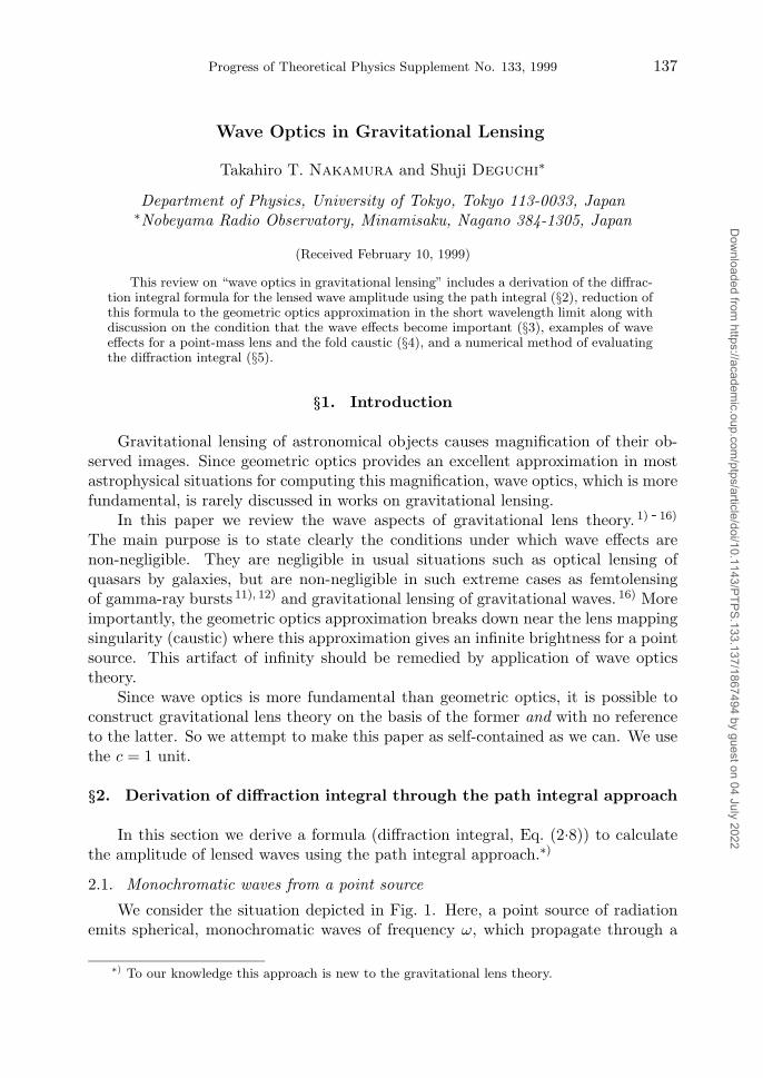
We consider the situation depicted in Fig. 1. Here, a point source of radiationemits spherical, monochromatic waves of frequency ω, which propagate through a

∗) To our knowledge this approach is new to the gravitational lens theory.

Dow

nloaded from https://academ

ic.oup.com/ptps/article/doi/10.1143/PTPS.133.137/1867494 by guest on 04 July 2022

138 T. T. Nakamura and S. Deguchi

source lens

observer

N

0r

rl

2,1,j = l , l+1, N- 1,. . . . . . . . . .

ε

θ0

Fig. 1.

gravitational lens and reach a distant observer. The space-time metric

ds2 = −(1 + 2U)dt2 + (1− 2U)d�r 2 (2.1)

is Minkowskian plus a small disturbance due to the gravitational potential U(�r)(� 1) of the lensing object. The influence of this potential is localized within asmall region around the lens compared with the large distances between source, lensand observer. The propagation equation ∂µ(

√−g gµν∂νφ) = 0 of the wave amplitudeφ(�r, t) = φ(�r) e−iωt is

(∇2 + ω2)φ = 4ω2Uφ (2.2)

to first order in U . We use the spherical coordinates (r, θ, ϕ) with the origin atthe source and the polar-axis pointing toward the lens. The observer is locatedat �r0 = (r0, θ0, ϕ0) with θ0 � 1. Since the waves reaching the observer should beconfined in the region of θ � 1, we can set sin θ � θ in the equations below and regardθ = θ(cosϕ, sinϕ) as a two-dimensional vector on a flat plane. Without the lensingobject, the wave amplitude would be φ0(r) = Aeiωr/r. We define the amplificationfactor F (�r) = φ(�r)/φ0(r) of the wave amplitude due to lensing. Equation (2.2) isrewritten in terms of F as

∂2F

∂r2+ 2iω

∂F

∂r+

1r2

∇2θ F = 4ω2UF , (2.3)

where ∇2θ = ∂2/∂θ2 + θ−1∂/∂θ + θ−2∂2/∂ϕ2. Assuming that ω/|∂ lnF/∂r| ∼ (scale

on which F varies)/(wavelength) � 1, we neglect the first term ∂2F/∂r2 comparedwith the second term (i.e., the eikonal approximation). Then Eq. (2.3) looks like theSchrodinger equation with the “time” coordinate r, the “particle mass” ω, and the“time dependent potential” 2ω U(r,θ). The corresponding Lagrangian which yieldsthe classical equation of motion is

L(r,θ, θ) = ω[

12r

2|θ|2 − 2U(r,θ)], (2.4)

where θ = dθ/dr. From the path integral formulation of quantum mechanics, 17) thesolution of Eq. (2.3) is formally written as

F (�r0) =∫Dθ(r) exp

{i

∫ r0

0dr L[r,θ(r), θ(r)]

}. (2.5)

Dow



Wave Optics in Gravitational Lensing 139

This expression contains the following meanings: i) Choose a particular function θ(r)representing a path from the source at the origin to the observer at �r0 = (r0,θ0); ii)Evaluate the integral in the curly brackets along this particular path. The result isthe “phase” as a functional of θ(r); iii) Sum up these phases for all possible functionsθ(r). We divide the distance r0 between source and observer into infinitesimal “time”steps ε = r0/N by an infinitely large integer N and specifies the path θ(r) by theset of coordinates θj = θ(rj) (j = 1, · · · , N) on the j-th sphere of radius rj = jε(cf. Fig. 1). Let the lens be located on the l-th sphere (lens plane), so that rl = lεis the distance between the source and lens. Here we introduce the “thin lens”approximation, whose formal content is to substitute 1

2δ(r − rl) ψ(θ) for U(r,θ) inEq. (2.5), where

ψ(θ) = 2∫ r0

0dr U(r,θ) (2.6)

is calculated for fixed θ. Thus Eq. (2.5) is rewritten as

F (�r0) =

[N−1∏j=1

∫d2θj

Aj

]exp

{iω

[ε

N−1∑j=1

rjrj+1

2

∣∣∣∣θj − θj+1

ε

∣∣∣∣2

− ψ(θl)

]}, (2.7)

where the normalizations Aj = 2πiε/(ω rjrj+1) are such that F = 1 if ψ = 0. Thethin lens approximation does not imply that the lens is infinitesimally thin, but thatthose paths which contribute to the phase integral (Eq. (2.5)) are well approximatedby a constant vector θ(r) � θl within the tiny region of U(�r) �= 0 compared withthe huge distances r0 and rl. It is shown in the Appendix that Eq. (2.7) reducesstraightforwardly to the desired formula

F (�r0) =ω

2πirlr0rl0

∫d2θl exp

{iω

[rlr02rl0

|θl − θ0|2 − ψ(θl)]}

, (2.8)

where rl0 is the distance between the lens and observer. Thanks to the thin lensapproximation (Eq. (2.6)) we could restrict the possible forms of functions θ(r)within those paths which go straight from the source to a “deflection point” θl andagain go straight from θl to the observer. The first term in the square bracket is thepath length difference between a straight path from the source to the observer anda deflected path penetrating the lens plane through θl. The second term is the timedelay caused by the gravitational field around the lens.

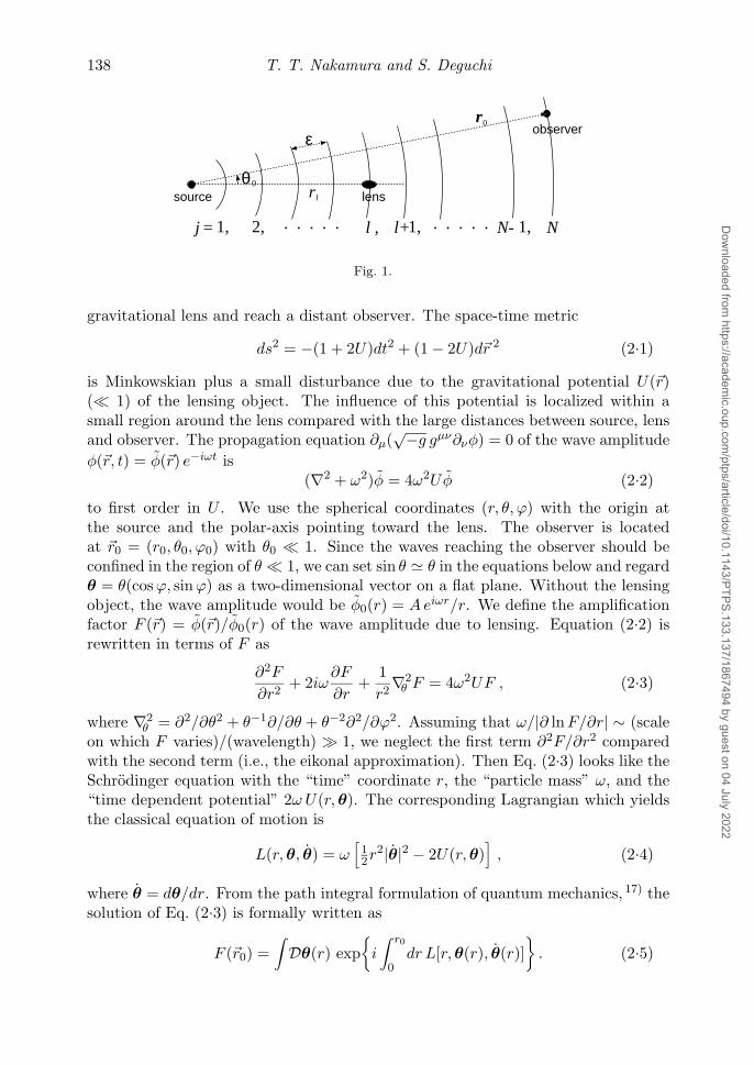
Let us interchange the roles of the source and the observer; namely we setanother coordinate system (cf. Fig. 2) in which the origin is at the observer, the

observer

source

lens

0r

rl

θ0lθ

α

Fig. 2.

Dow




polar-axis is pointing toward the lens, and the source is located at �r0 = (r0,θ0). Ifone repeats the above procedure in this coordinate system, then the time delays inthe two coordinate systems are identical up to order θ2

0. Therefore Eq. (2.8) alsoexpresses the lensed wave amplitude for the source position �r0 if rl is the distancebetween the observer and lens, and rl0 is that between the lens and source.

We rewrite Eq. (2.8) using more compact notation. Introducing the character-istic angle scale θ∗ (e.g. Eq. (4.1)) and defining dimensionless quantities

x = θl/θ∗ , y = θ0/θ∗ , w =rlr0rl0

θ2∗ ω , (2.9)

ψ(x) =rl0

rlr0θ−2∗ ψ(θ∗x) , T (x,y) =

12|x − y|2 − ψ(x) , (2.10)

one obtainsF (w,y) =

w

2πi

∫d2x exp[iw T (x,y)] . (2.11)

This is the diffraction integral formula expressing the amplification factor of lensedwave amplitudes as a function of the frequency w and the source (or observer)position y. The amplification of the wave intensity is |F |2. Hereafter we use thescaled length and time as defined in Eq. (2.9); for example T is simply referred toas the “time delay” instead of the “scaled time delay”.

Although the metric in Eq. (2.1) does not take account of the expansion andgeometry of our universe, all the formulae in this paper are applicable to cosmologicalsituations, if we use the angular diameter distance for r0, rl and rl0, replace ω withω(1+z) where z is the lens redshift, and assume that the wavelength is much smallerthan the horizon scale. Also the scalar wave analysis in this paper is valid for wavesof any helicity, if the rotation of the polarization direction (such as the Faradayrotation of electromagnetic waves) is negligible.

When the lensing object is spherically symmetric, ψ(x) depends only on x = |x|and Eq. (2.11) becomes

F (w, y) = −iw eiwy2/2∫ ∞

0dxxJ0(wxy) exp

{iw

[12x

2 − ψ(x)]}

, (2.12)

where J0 is the Bessel function of zeroth order.

2.2. Non-monochromatic waves from an extended source

Let φ0(w,y) be the amplitude of unlensed waves which are emitted at a pointy on the source plane with frequency w. The observed wave amplitude at time τ isthe superposition of the lensed one F φ0 over y and w:

φ(τ) =∫d2y

∫dw F (w,y) φ0(w,y) e−iwτ . (2.13)

When the source is observed through a band pass filter, φ0 in this equation representsthe source spectrum at y times the filtering function of frequency. Since φ(τ) is real,φ∗0(w) = φ0(−w). Actually φ0 should also depend on time because of the fluctuationin the source activity. This fluctuation of φ0 would be a stochastic process, assuming

Dow




that the source activity is stationary in time. So we define the correlation functionof the observed wave amplitude as

C(τ) =〈φ(τ ′)φ(τ ′ + τ)〉〈|φ(τ ′)|2〉F=1

, (2.14)

where 〈· · ·〉 denotes averaging over the ensemble of stochastic functions φ0. Becauseof the stationarity of the source activity, 〈· · ·〉 is also interpreted as an integral withrespect to τ ′ over sufficiently long time � 1/w. Assuming that the different partsof the source radiate incoherently, one has 〈φ0(w,y) φ∗0(w′,y′)〉 = I(w,y) δ(w −w′) δ2(y − y′), where I(w,y) is the source surface brightness (times the filteringfunction). Therefore one obtains

C(τ) =∫d2y

∫dw |F (w,y)|2 I(w,y) cos(wτ) , (2.15)

where I(w,y) = I(w,y)/[∫d2y

∫dw I(w,y)]. The amplification factor of wave inten-

sity is given by C(0).

§3. Geometric optics limit

In this section the formulae derived in the previous section are reduced to thegeometric optics approximation in the short wavelength limit, in order to discuss theconditions under which the wave effects are non-negligible.

3.1. Monochromatic waves from a point source

Let us imagine a two-dimensional surface T (x) = 12 |x − y|2 − ψ(x) (the time

delay function, Eq. (2.10)) above the x-plane for a fixed y. For example we haveψ(x) = ln |x| for a point mass lens discussed in §4.1. In the short wavelengthlimit w → ∞, the integrant of Eq. (2.11) is a rapidly oscillating function and itscontribution to the value of F comes from regions near the stationary points of thissurface. The stationary points are determined by ∂T (x) = 0 or

y = x − ∂ψ(x) or θ0 = θl − rl0

r0α(θl) , (3.1)

where ∂ = ∂/∂x and α(θl) = r−1l ∂ψ/∂θl. These stationary points correspond to

the “images” in geometric optics, and the condition ∂T (x) = 0 expresses Fermat’sprinciple of least time. In fact Eq. (3.1) is the “lens equation” 10) which determinesthe positions of images x (or θl) for a given source position y (or θ0) with thedeflection angle α of null geodesics (cf. Fig. 2). For a sufficiently “strong” lenspotential ψ(x), the number of images is more than one. We expand T (x) aroundthe j-th image xj(y) as

T (x) = T (xj) +12

∑ab

xaxb ∂a∂bT (xj) +16

∑abc

xaxbxc ∂a∂b∂cT (xj) + · · · , (3.2)

where x = x − xj and the indices abc · · · run from 1 to 2. If the frequency w is solarge as to satisfy

w|∂2T |3 � |∂3T |2 , w|∂2T |2 � |∂4T | , · · · (3.3)

Dow




then the third and higher order terms of this expansion can be neglected in calculat-ing Eq. (2.11) near xj . Assuming that all the images satisfy Eq. (3.3), one obtainsusing the Gaussian integral∗)

F =∑j

|µ(xj)|1/2 exp[iw T (xj)− iπnj] , (3.4)

whereµ(x) = 1/det[∂a∂bT (x)] = 1/det[δab − ∂a∂bψ(x)] , (3.5)

and nj = 0, 1/2, 1 when xj is a minimum, saddle, maximum point of T (x), respec-tively. Equation (3.4) implies that the observed wave is a superposition of waves fromeach image, with the amplitude ratio |µ(xj)|1/2 and the phase shift wT (xj) − πnj.The amplification of wave intensity is

|F |2 =∑j

|µj|+ 2∑j<k

|µj µk|1/2 cos(w Tjk − πnjk) , (3.6)

where µj = µ(xj), Tjk = T (xk)−T (xj) is the arrival time difference between the k-thand j-th images, and njk = nk−nj . Note that in geometric optics, the magnificationfactor of the image size for an infinitesimal source is given as the Jacobian of thelens mapping y �→ x in Eq. (3.1): 10)

µ(x) = 1/det[∂ ⊗ y] = 1/det[δab − ∂a∂bψ(x)] . (3.7)

From the conservation of surface brightness in geometric optics, 18) this image mag-nification is equal to the amplification of source intensity. Thus the first term ofEq. (3.6) coincides with the “geometric optics” result, where |µj | is the magnifica-tion factor for the j-th image. The second term expresses the “interference” betweenthe images which produces a fringe pattern of wave intensity on the source (or ob-server) plane (e.g. Fig. 5). Equation (3.4) is the semi-classical approximation inquantum mechanics.

3.2. Diffraction near lens mapping singularity

According to geometric optics, the image magnification |µj| for a point sourcediverges when the image is located near a critical curve, which is a curve on thex-plane defined by det[∂a∂bT (x)] = 0 (cf. Eq. (3.5)). A caustic is the correspondingcurve on the y-plane mapped by Eq. (3.1). (Figure 6 shows an example of a criticalcurve and a caustic.) Namely, when a point source is located near a caustic, someof the images are near a critical curve and have infinitely large magnifications. Ofcourse this divergence is an artifact of the approximation in Eq. (3.4), because |∂2T |for these images is too small to satisfy Eq. (3.3). Thus the wave amplitude is writtenas a sum of two terms: F = Fc+Fd. The second term Fd, the diffraction part, is givenby Eq. (2.11) evaluated exactly around these images near the critical curve. Thisterm describes the diffraction phenomenon in the sense that the non-geodesic pathscontribute significantly to the wave amplitude. The first term Fc, the semi-classicalpart given by Eq. (3.4), is the contribution from other normal images.

∗) using∫ ∞−∞dx eix2

=√

π eiπ/4 after diagonalizing ∂a∂bT

Dow




Equation (3.3) roughly states that the diffraction effect is unimportant whenthe time delay Tjk between images is much larger than the wave period 1/w. Thisfact is also seen by the following simple consideration. Regarding the double imagein gravitational lensing as the double-slit of Young’s interference experiment, theangle of diffraction is θ ∼ λ/d, where λ is the wavelength and d is distance betweenthe two images. On the other hand, the deflection angle of gravitational lensing isα ∼ d/rl where rl is the distance from observer to lens. Then the condition θ � αis equivalent to stipulating that the time delay between images ∼ rlα

2/c is muchlarger than λ/c.

For a spherically symmetric lens, the point y = 0 just behind the lens is a causticproducing the “Einstein ring” (e.g. §4.1). The diffraction effect near this caustic isevaluated with Eq. (2.12) for small y. When w → ∞ and y � w−1/2, Eq. (2.12)yields

|F |2 � 2πw x2E |1− ψ′′(xE)|−1 J2

0 (wxEy) , (3.8)

where xE is a (positive) solution of x = ψ′(x). Therefore the maximum value of theamplification for a spherically symmetric lens is given by 2πw x2

E/|1−ψ′′(xE)| in theshort wavelength limit.

3.3. Non-monochromatic waves from an extended source

Let ∆y and ∆w be the typical sizes of the region where the source surfacebrightness I is non-zero, and let y and w be the centers of this region; for example,∆y is the radius of a circular source whose center is at y, and ∆w is the width ofa band pass filter whose central frequency is w. For definiteness we assume thatthe source is sufficiently far from caustics, so that the semi-classical approximation(Eq. (3.6)) is valid in this entire region. Then substituting Eq. (3.6) into Eq. (2.15)results in

C(τ) = Re{e−iwτ [C0(τ) + C1(τ) + C2(τ)]} , (3.9)

whereC0(τ) =

∑j

∫d2y′ |µj(y′)| I(τ,y′) , (3.10)

C1,2(τ) =∑j<k

∫d2y′ |µj(y′)µk(y′)|1/2 e±i[w Tjk(y′)−πnjk] I[τ ∓ Tjk(y′), y′] , (3.11)

I(τ,y′) =∫dw′ I(w′,y′) e−i(w′−w)τ . (3.12)

The terms C1 and C2 arise from the interference between images, but the integralin Eq. (3.11) tends to erase the fringe pattern produced by the interference. If thesource size ∆y is much larger than the typical fringe width 1/|w dTjk/dy|, or if thecoherence time 1/∆w is much smaller than the typical time delay |τ ∓ Tjk(y)|, thenthis oscillatory integral makes C1 and C2 much smaller than C0. Conversely, whenthe source size is comparable to or smaller than the fringe width, then it is alwayspossible to choose such a value of τ as to make the interference term C1 or C2

observable (e.g. Fig. 4). In the short wavelength limit w → ∞, the fringe width goesto zero and so the interference terms vanish. The geometric optics approximation

Dow




uses C(τ) = Re[e−iwτ C0(τ)] even when the source is located near or straddling acaustic. In this case Eq. (3.10) remains finite though some of µj(y) are divergentthere. Diffraction near caustics is also unimportant as is interference, when thesource size is much larger than the typical fringe width (e.g. Fig. 3).

In order to observe the interference terms C1 and C2, not only the source size butalso the observer size (or diameter of the telescope) must be smaller than the fringewidth. Otherwise further integration of Eq. (3.11) over y smears out the interferencepattern. Using the double-slit argument (cf. §3.2), this fringe width on the observerplane is of order ∼ λ/α where λ is wavelength and α is deflection angle. On theother hand, in order to resolve the multiple image formed by gravitational lensing,the observer size must be larger than ∼ λ/α. Therefore it is impossible to observeboth the interference pattern and the multiple image simultaneously, in analogy tothe uncertainty principle in quantum mechanics.

§4. Application to specific lens models

In this section some examples of wave effects are discussed for the point masslens model and the fold caustic.

4.1. Point mass lens 5) - 7), 10)

Lensing by a normal star is described by this lens model. If M is the mass of thestar then U(r, θ) = −GM/(r2 − 2rlr cos θ + r2

l )1/2. Substituting this into Eq. (2.6)

and using θ � 1 the lens potential is ψ(θl) = 4GM ln θl + const, where the constantterm is unimportant since it only affects the overall phase factor of F . Choosing thecharacteristic angle scale θ∗ to be the Einstein angle,

θ∗ =(4GMrl0

rlr0

)1/2

∼ 3µarcsec(M

M�

)1/2 (rlr0/rl0

Gpc

)−1/2

, (4.1)

one obtains from Eqs. (2.9) and (2.10)

ψ(x) = lnx , w = 4GMω ∼ 105(M/M�)(ν/GHz) . (4.2)

Note that w ∼ (gravitational radius of lens mass)/(wavelength) is a large numberin usual astrophysical situations. In any case Eq. (2.12) is integrated analytically togive the amplification factor for monochromatic waves from a point source as 19)

|F |2 = πw

1− e−πw

∣∣∣1F1

(12 iw, 1;

12 iwy

2)∣∣∣2 , (4.3)

where 1F1 is the confluent hypergeometric function. In the long wavelength limitw → 0, Eq. (4.3) is identically unity and hence amplification does not occur (i.e.,waves “ignore” the lens). When w � 1, Eq. (4.3) is evaluated accurately by thesemi-classical approximation valid for y � 1/w, and by |F |2 � πw J2

0 (wy) valid fory � w−1/2 (cf. Eq. (3.8)). The time delay function T (x) = 1

2 |x− y|2 − lnx has twostationary points, a minimum point x1 and a saddle point x2 (cf. Eq. (3.6)):

x1,2 =y

2y(y ± √

y2 + 4) , µ1,2 =12± y2 + 2

2y√y2 + 4

, (4.4)

Dow




T12 =12y√y2 + 4 + ln

√y2 + 4 + y√y2 + 4− y

, n12 =12. (4.5)

Thus the semi-classical approximation of Eq. (4.3) is

|F |2 = y2 + 2 + 2 sin(w T12)y√y2 + 4

. (4.6)

When y � 1, Eq. (4.6) becomes |F |2 � [1+sin(2wy)]/y. The sine term represents theinterference between the two images producing circular fringes. The critical curve(cf. §3.2) is a circle of radius x = 1 (Einstein ring) on the lens plane, and the causticis the single point y = 0 on the source plane where Eq. (4.6) diverges. As discussedin §3.2, however, Eq. (4.6) is invalid when the time delay between the two images,T12 � 2y, is comparable to or smaller than the wave period 1/w. In reality theamplification |F |2 at y = 0 remains finite due to the diffraction and has a maximumvalue πw/(1 − e−πw) according to Eq. (4.3). The maximum amplification � πw isof order ∼ (gravitational radius)/(wavelength) when this ratio is much larger thanunity.

Next we consider an extended source. As discussed in §3.3, the interference termsin(w T12) is erased when the source size is much larger than the width betweeninterference fringes. This width is π/w at y � 1 for waves of frequency w, andbecomes narrower for larger y. Thus the conclusion is that if the source size is muchlarger than r0 θ∗(π/w) =

π

ω

√r0rl0

4GMrl∼ 107 km

(ν

GHz

)−1 (M

M�

)−1/2 (r0rl0/rl

Gpc

)1/2

, (4.7)

then the geometric optics approximation, |F |2 = (y2+2)/(y√y2 + 4), is satisfactory.

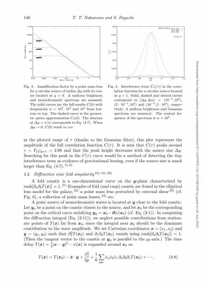
In Fig. 3 is plotted the amplification factor for a circular source of radius ∆y whosecenter is on the caustic y = 0. Here uniform brightness and a monochromaticspectrum are assumed: I(w′, y′) ∝ H(∆y−y′) δ(w′−w) where H is the step function.The solid curves are the full results C(0) = 2

∫ ∆y0 dy y|F |2/(∆y)2 (cf. Eq. (2.15))

with w = 102, 103 and 104 from bottom to top, and the dashed curve is the geometricoptics approximation C0(0) = [1 + (2/∆y)2]1/2 (cf. Eq. (3.10)). This figure revealsthat the diffraction as well as the interference is unimportant when the source sizeis much larger than Eq. (4.7).

As for non-monochromatic waves, the interference terms C1(0) and C2(0) (Eq.(3.11)) vanish even for a point source, when the coherence time 1/∆w is muchsmaller than the time delay T12 (cf. §3.3). For example, for a point source and auniform spectrum I(w′, y′) ∝ δ2(y′ − y)H(∆w − |w′ − w|), C(0) becomes Eq. (4.6)with the sine term multiplied by j0(∆w T12) (where j0(x) = sinx/x). Thereforethe wave effects are unimportant when ∆wT12 � 1 as regards C(0). However,if one observes not only C(0) but also C(τ) with variable τ , then it is possibleto detect C1 or C2 regardless of ∆w. In Fig. 4 |C1(τ)| is plotted for a circularsource located at y = 1. A uniform brightness and a Gaussian spectrum, I(τ,y′) ∝H(∆y − |y′ − y|) exp[−(∆w τ/2)2], are assumed. Since C0 and C2 are negligible

Dow




1

10

100

1000

10000

100000

1e+06

1e-05 0.0001 0.001 0.01 0.1 1 10

C(0

) =

am

plifi

catio

n

Delta y = source size

w=10^2w=10^2

w=10^3

w=10^4

w=10^2

w=10^3

w=10^4

w=10^2

w=10^3

w=10^4

w=10^2

w=10^3

w=10^4

w=10^2

w=10^3

w=10^4

w=10^2

w=10^3

w=10^4

w=10^2

w=10^3

w=10^4

Fig. 3. Amplification factor by a point mass lens

for a circular source of radius ∆y with its cen-

ter located at y = 0. A uniform brightness

and monochromatic spectrum are assumed.

The solid curves are the full results C(0) with

frequencies w = 102, 103 and 104 from bot-

tom to top. The dashed curve is the geomet-

ric optics approximation C0(0). The abscissa

at ∆y = π/w corresponds to Eq. (4.7). When

∆y → 0, C(0) tends to πw.

0

0.0005

0.001

0.0015

0.002

0.0025

0.003

2.02 2.04 2.06 2.08 2.1 2.12 2.14

|C_1

|

tau

(Delta y, Delta w)=

w=1e5, y=1

(1e-4, 1e2)(2e-4, 1e2)(1e-4, 2e2)

Fig. 4. Interference term |C1(τ)| in the corre-

lation function for a circular source located

at y = 1. Solid, dashed and dotted curves

correspond to (∆y,∆w) = (10−4, 102),

(2 · 10−4, 102) and (10−4, 2 · 102), respec-

tively. A uniform brightness and Gaussian

spectrum are assumed. The central fre-

quency of the spectrum is w = 105.

in the plotted range of τ (thanks to the Gaussian filter), this plot represents theamplitude of the full correlation function C(τ). It is seen that C(τ) peaks aroundτ ∼ T12|y=1 ∼ 2.08 and that the peak height decreases with the source size ∆y.Searching for this peak in the C(τ) curve would be a method of detecting the tinyinterference term as evidence of gravitational lensing, even if the source size is muchlarger than Eq. (4.7). 5), 6)

4.2. Diffraction near fold singularity 10), 13), 20)

A fold caustic is a one-dimensional curve on the y-plane characterized byrank[∂a∂bT (x)] = 1. 21) Examples of fold (and cusp) caustic are found in the ellipticallens model for the galaxy, 22) a point mass lens perturbed by external shear 23) (cf.Fig. 6), a collection of point mass lenses, 24) etc.

A point source of monochromatic waves is located at y close to the fold caustic.Let y0 be a point on the caustic closest to the source, and let x0 be the correspondingpoint on the critical curve satisfying y0 = x0−∂ψ(x0) (cf. Eq. (3.1)). In computingthe diffraction integral (Eq. (2.11)), we neglect possible contributions from station-ary points of T (x) far from x0, since the integral near x0 should be the dominantcontribution to the wave amplitude. We set Cartesian coordinates x = (x1, x2) andy = (y1, y2) such that ∂2

1T (x0) and ∂1∂2T (x0) vanish using rank[∂a∂bT (x0)] = 1.(Then the tangent vector to the caustic at y0 is parallel to the y2-axis.) The timedelay T (x) = 1

2 |x − y|2 − ψ(x) is expanded around x0 as

T (x) = T (x0)− x · y +x2

2

2p+

16

∑abc

xaxbxc ∂a∂b∂cT (x0) + · · · , (4.8)

Dow




where x = x−x0, y = y−y0, and p = 1/[∂22T (x0)] = 1/[1−∂2

2ψ(x0)] is assumed tobe of order unity. Due to the absence of a x2

1 term, the third order terms contributeto the diffraction integral in the x1-direction. The fold caustic further requires thenon-vanishing of ∂3

1T (x0) (which guarantees the non-vanishing of the tangent vectorto the fold caustic at y0), and we choose θ∗ (Eq. (2.10)) so that q = 2/[∂3

1T (x0)] =−2/[∂3

1ψ(x0)] is of order unity. In the case of a point mass lens with external shear 23)

or a collection of point mass lenses, 24) the choice of θ∗ in Eq. (4.1) makes q orderunity. Without loss of generality q is taken to be positive by inversion of coordinates(x ↔ −x and y ↔ −y). We omit all the third order terms except the x3

1 term, sincethese terms (x2

1x2, x1x22 and x

32) do not contribute to the wave amplitude (Eq. (2.11))

in the short wavelength limit w → ∞. Without these terms the caustic and criticallines coincide with the y2-axis and x2-axis, respectively, and the amplification factorof the wave intensity is

|F |2 = w2

4π2

∣∣∣∣∫dx1

∫dx2 exp

[iw

(−x1y1 − x2y2 +

x22

2p+x3

1

3q

)] ∣∣∣∣2, (4.9)

= 2πµ∗Ai2(−y1/Y ) , (4.10)

where µ∗ = |p| (q2w)1/3, Y = (qw2)−1/3 and Ai is the Airy function.When |y1|3/2 � 1/w, Eq. (4.10) is evaluated accurately by the semi-classical

approximation. On the positive side y1 > 0 of the caustic, the phase of Eq. (4.9) hastwo stationary points (cf. Eq. (3.6)):

x± = (±√q y1, p y2) , µ± = ±1

2p(q/y1)1/2 , (4.11)

∆T = T (x−)− T (x+) = 43(q y

31)

1/2 , n− − n+ = 1/2 . (4.12)

On the negative side y1 < 0, there are not real stationary points but are imaginaryones. Hence the semi-classical approximation of Eq. (4.10) is

|F |2 = |p|(q/|y1|)1/2 ×{

1 + sin(w∆T ), (y1 > 0)12 exp(−w|∆T |). (y1 < 0) (4.13)

In Fig. 5(a) |F |2 is plotted as a functioin of y1. As a point source crosses the causticline y1 = 0 from its positive side to its negative side with fixed y2, one observestwo images of equal brightness which approach each other, merge on the critical linex1 = 0, and finally disappear. The sine term expresses the interference betweenthese two images, and according to Eq. (4.13) the wave intensity diverges at theinstant of merging. As discussed in §3.2, however, the semi-classical approximationis invalid when the source is so close to the caustic that the time delay between thetwo images, |∆T | ∼ |y1|3/2, is comparable to or smaller than the wave period 1/w.In reality, according to Eq. (4.10), the amplification factor |F |2 has a finite value of0.792µ∗ at y1 = 0, and a maximum value of 1.803µ∗ at y1 = 1.019Y . Despite theabsence of images on the negative side of the caustic, the wave intensity on that sideis not exactly zero but decreases exponentially with |y1|, due to the diffraction ofwaves from the positive side.

Dow




0

0.5

1

1.5

2

2.5

-4 -2 0 2 4 6 8 10

|F|^

2 / m

u_*

y_1 / Y

point source

(a) fullsemi

geom

0

0.5

1

1.5

2

2.5

-4 -2 0 2 4 6 8 10

C(0

) / m

u_*

y_1 / Y

Delta y = 0.2 Y

(b) fullgeom

0

0.5

1

1.5

2

2.5

-4 -2 0 2 4 6 8 10

C(0

) / m

u_*

y_1 / Y

Delta y = 0.5 Y

(c) fullgeom

0

0.5

1

1.5

2

2.5

-4 -2 0 2 4 6 8 10

C(0

) / m

u_*

y_1 / Y

Delta y = Y

(d) fullgeom

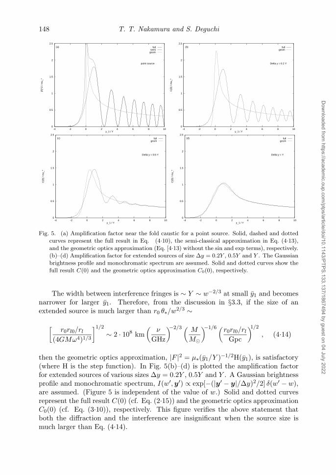
Fig. 5. (a) Amplification factor near the fold caustic for a point source. Solid, dashed and dotted

curves represent the full result in Eq. (4.10), the semi-classical approximation in Eq. (4.13),

and the geometric optics approximation (Eq. [4.13) without the sin and exp terms), respectively.

(b)–(d) Amplification factor for extended sources of size ∆y = 0.2Y , 0.5Y and Y . The Gaussian

brightness profile and monochromatic spectrum are assumed. Solid and dotted curves show the

full result C(0) and the geometric optics approximation C0(0), respectively.

The width between interference fringes is ∼ Y ∼ w−2/3 at small y1 and becomesnarrower for larger y1. Therefore, from the discussion in §3.3, if the size of anextended source is much larger than r0 θ∗/w2/3 ∼

[r0rl0/rl

(4GMω4)1/3

]1/2

∼ 2 · 108 km(

ν

GHz

)−2/3 (M

M�

)−1/6 (r0rl0/rl

Gpc

)1/2

, (4.14)

then the geometric optics approximation, |F |2 = µ∗(y1/Y )−1/2H(y1), is satisfactory(where H is the step function). In Fig. 5(b)–(d) is plotted the amplification factorfor extended sources of various sizes ∆y = 0.2Y , 0.5Y and Y . A Gaussian brightnessprofile and monochromatic spectrum, I(w′,y′) ∝ exp[−(|y′ − y|/∆y)2/2] δ(w′ − w),are assumed. (Figure 5 is independent of the value of w.) Solid and dotted curvesrepresent the full result C(0) (cf. Eq. (2.15)) and the geometric optics approximationC0(0) (cf. Eq. (3.10)), respectively. This figure verifies the above statement thatboth the diffraction and the interference are insignificant when the source size ismuch larger than Eq. (4.14).

Dow




§5. Numerical method of performing the diffraction integral

If the semi-classical approximation Eq. (3.6) is invalid because of diffraction,the diffraction integral Eq. (2.11) need to be evaluated exactly. In this section anumerical method 14) of evaluating Eq. (2.11) for a general lens potential ψ(x) ispresented. First, one calculates the following quantity for a fixed y:

F (τ) =∫ τ

dτ ′∫ ∞

−∞dw

2πe−iwτ ′

F (w) =12π

∫d2x δ[T (x)− τ ] . (5.1)

Note that dF/dτ represents the lensed waveform for a delta-function pulse emittedfrom a point source, and F is defined up to an additive constant. Given a value ofτ , closed contour curves are determined by τ = T (x) on the x-plane (e.g. Fig. 7).Equation (5.1) is written in terms of line integrals along these contours C as

F (τ) =12π

∑C

∮Cdu , (5.2)

where the summation is taken over the number of closed contours, and

dx1

du= −(x2 − y2) + ∂2ψ(x) ,

dx2

du= x1 − y1 − ∂1ψ(x) (5.3)

in Cartesian coordinates x = (x1, x2) and y = (y1, y2), so that dx/du is tangent tothe contours with length |∂T |. The differential equations (5.3) are integrated numer-ically using, e.g., the Runge-Kutta method to evaluate Eq. (5.2). The integration isstarted with u = 0 from a point on the contour and is continued with positive stepsof u until x comes back to the starting point. Computing F in this way, one obtainsF from the Fourier transform of dF/dτ :

F (w) =∫ ∞

−∞dτ eiwτ d

dτF (τ) . (5.4)

Since dF/dτ is the lensed waveform for a delta-function pulse, F (τ) should exhibit adiscontinuous or diverging behavior when τ is equal to the arrival time Tj of the pulse(Tj is the value of T (x) at its stationary point xj ; cf. Eq. (3.4)). Also the numberof closed contours changes by one when τ = Tj , while it is zero when τ → −∞.Assuming that the source is not exactly on a caustic, one can show 14) that F (τ) atτ = Tj suffers a discontinuous increase (decrease) by an amount µj

1/2 when xj isa minimum (maximum) point, and that it diverges as π−1|µj|1/2 ln |τ − Tj |−1 whenxj is a saddle point (e.g. Fig. 8). Let us write these discontinuous contributions toF as

Fc(τ) =∑

nj=0,1

(−1)njµj1/2 H(τ − Tj)− 1

π

∑nj=1/2

|µj|1/2 ln |τ − Tj | , (5.5)

where H is the step function. Note that Fc =∫ ∞−∞dτ eiwτdFc/dτ (cf. Eq. (5.4)) is

equal to∗) the semi-classical approximation of F , given in Eq. (3.4). Hence Eq. (5.5) is∗) using

∫ ∞−∞dx eix/x = iπ

Dow




-1.5

-1

-0.5

0

0.5

1

1.5

-1.5 -1 -0.5 0 0.5 1 1.5

x_2

or y

_2

x_1 or y_1

(a)

gamma = 0.1

causticcrit

sourceimage

-1.5

-1

-0.5

0

0.5

1

1.5

-1.5 -1 -0.5 0 0.5 1 1.5

x_2

or y

_2

x_1 or y_1

(b)

gamma = 0.2

causticcrit

sourceimage

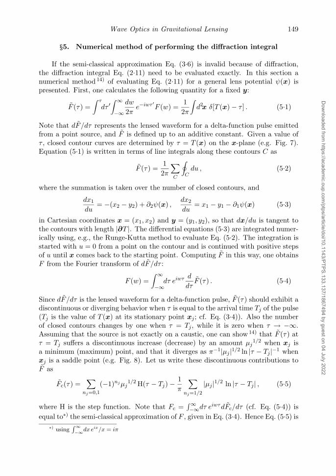
Fig. 6. Point mass lens perturbed by external shear. The critical curve (dotted curve) is expressed

as x(ϕ) = [γ cos 2ϕ + (1 − γ2 sin2 2ϕ)1/2]−1/2 in circular coordinates. The caustic (solid curve)

is the diamond-shaped curve with four cusps. The image positions (crosses) are the stationary

points of Eq. (5.7). The number of images is two or four depending on whether the source

(triangle) is inside or outside the caustic. (a) γ = 0.1. (b) γ = 0.2.

-1.5 -1 -0.5 0 0.5 1 1.5-1.5

-1

-0.5

0

0.5

1

1.5

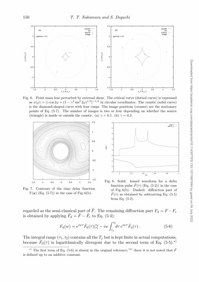
Fig. 7. Contours of the time delay function

T (x) (Eq. (5.7)) in the case of Fig. 6(b).

-3

-2

-1

0

1

2

3

4

5

6

0 0.2 0.4 0.6 0.8 1

tilde

F

tau

tilde Ftilde F_d

Fig. 8. Solid: lensed waveform for a delta

function pulse F (τ) (Eq. (5.2)) in the case

of Fig. 6(b). Dashed: diffraction part of

F (τ) as obtained by subtracting Eq. (5.5)

from Eq. (5.2).

regarded as the semi-classical part of F . The remaining diffraction part Fd = F −Fc

is obtained by applying Fd = F − Fc to Eq. (5.4):

Fd(w) = eiwτ Fd(τ)|τ2τ1− iw

∫ τ2

τ1

dτ eiwτ Fd(τ) . (5.6)

The integral range (τ1, τ2) contains all the Tj but is kept finite in actual computations,because Fd(τ) is logarithmically divergent due to the second term of Eq. (5.5).∗)

∗) The first term of Eq. (5.6) is absent in the original reference; 14) there it is not noted that F

is defined up to an additive constant.

Dow




Thus after removing the discontinuous part Fc from F , it is possible to calculatereliably the second term of Eq. (5.6) for a continuous function Fd using, e.g., theFast-Fourier-Transform. To summarize, i) compute Eq. (5.2) solving the differentialEqs. (5.3), ii) subtract Eq. (5.5) from Eq. (5.2) and insert the result into Eq. (5.6),and iii) add Eqs. (3.4) and (5.6) to obtain Eq. (2.11).

We apply the above algorithm to the lens model of a point mass plus externalshear: 23)

T (x) = 12 |x − y|2 − ln |x| − 1

2γ(x21 − x2

2) . (5.7)

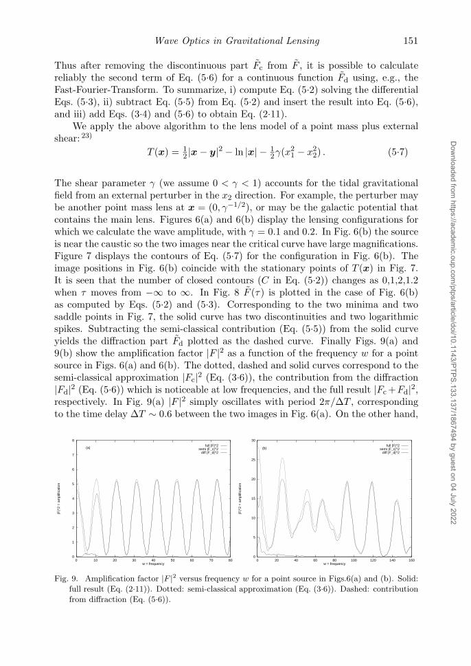
The shear parameter γ (we assume 0 < γ < 1) accounts for the tidal gravitationalfield from an external perturber in the x2 direction. For example, the perturber maybe another point mass lens at x = (0, γ−1/2), or may be the galactic potential thatcontains the main lens. Figures 6(a) and 6(b) display the lensing configurations forwhich we calculate the wave amplitude, with γ = 0.1 and 0.2. In Fig. 6(b) the sourceis near the caustic so the two images near the critical curve have large magnifications.Figure 7 displays the contours of Eq. (5.7) for the configuration in Fig. 6(b). Theimage positions in Fig. 6(b) coincide with the stationary points of T (x) in Fig. 7.It is seen that the number of closed contours (C in Eq. (5.2)) changes as 0,1,2,1.2when τ moves from −∞ to ∞. In Fig. 8 F (τ) is plotted in the case of Fig. 6(b)as computed by Eqs. (5.2) and (5.3). Corresponding to the two minima and twosaddle points in Fig. 7, the solid curve has two discontinuities and two logarithmicspikes. Subtracting the semi-classical contribution (Eq. (5.5)) from the solid curveyields the diffraction part Fd plotted as the dashed curve. Finally Figs. 9(a) and9(b) show the amplification factor |F |2 as a function of the frequency w for a pointsource in Figs. 6(a) and 6(b). The dotted, dashed and solid curves correspond to thesemi-classical approximation |Fc|2 (Eq. (3.6)), the contribution from the diffraction|Fd|2 (Eq. (5.6)) which is noticeable at low frequencies, and the full result |Fc+Fd|2,respectively. In Fig. 9(a) |F |2 simply oscillates with period 2π/∆T , correspondingto the time delay ∆T ∼ 0.6 between the two images in Fig. 6(a). On the other hand,

0

1

2

3

4

5

6

7

8

0 10 20 30 40 50 60 70 80

|F|^

2 =

am

plifi

catio

n

w = frequency

(a)full |F|^2

semi |F_c|^2diff |F_d|^2

0

5

10

15

20

25

30

0 20 40 60 80 100 120 140 160

|F|^

2 =

am

plifi

catio

n

w = frequency

(b)full |F|^2

semi |F_c|^2diff |F_d|^2

Fig. 9. Amplification factor |F |2 versus frequency w for a point source in Figs.6(a) and (b). Solid:

full result (Eq. (2.11)). Dotted: semi-classical approximation (Eq. (3.6)). Dashed: contribution

from diffraction (Eq. (5.6)).

Dow




the spectrum in Fig. 9(b) is rather complex because |Fc|2 has six interference termsout of the four images in Fig. 6(b). Also in Fig. 9(b) the diffraction is noticeableup to high frequency w ∼ 80 because of the small time delay ∆T ∼ 0.013 betweenthe two bright images near the critical curve. This figure exemplifies the conclusionin §3.2 that the diffraction effect is significant when a point source is located near acaustic.

§6. Summary

From the general discussion given in §§2 and 3 and from the examples given in§§4 and 5, we summarize this paper as follows; (1) If the wavelength is comparableto or larger than the gravitational radius of the lens mass, then diffraction is soeffective that large amplification cannot occur; (2) If the time delay between thelensed images is comparable to or smaller than the wave period, then diffractionis important (cf. Fig. 9). This happens when a source is located near a caustic.The condition here also implies the condition in (1), since the time delay is of order∼ (gravitational radius)/(light velocity); (3) If the source size is much larger thanthe width between interference fringes ∼ (wavelength)/(deflection angle), then bothdiffraction and interference are unimportant so that geometric optics is valid (cf.Fig. 3); (4) If the coherence time (band width)−1 is much smaller than time delaybetween images, then geometric optics is valid; (5) If one observes the correlationfunction C(τ) (Eq. (2.14)) with variable τ , then it is possible to detect interferenceterms regardless of the condition in (4) (cf. Fig. 4).

Wave effects in gravitational lensing have not yet been observed. We do notknow of compact radio sources much smaller than Eq. (4.7) at cosmological dis-tances. 25) The sources of gamma-ray bursts should be sufficiently compact, 26) but“femtolenses” of 10−13–10−16M� are hypothetical objects. 27) Gravitational wavesemitted from binary stars are likely to exhibit the effects considered in this paper iflensed, 16) but the detection rate of these waves for planned detectors is uncertain. 28)

In conclusion the geometric optics approximation of gravitational lensing is valid inall the observed situations.

Acknowledgements

The first author thanks M. Sasaki and A. Hosoya for discussions on §§2.1 and3.3, respectively. We are grateful to K. Tomita for the opportunity to publish thisreview.

Appendix

The first l−1 integrals from j = 1 to l−1 in Eq. (2.7) are the Gaussian integralsand give unity, so j = 1 under

∏and

∑can be replaced by j = l. We use the identity

Dow




(proven by induction)N−1∑j=l

rjrj+1|θj − θj+1|2 = εrlr0rl0

|θl − θ0|2 +N−1∑

j=l+1

r2j

rl,j+1

rlj|θj − ulj |2 , (A.1)

where r0 = rN , rlj = rj − rl and ulj = [rlθl + (j − l)rj+1θj+1]/(j rl,j+1). Thus Eq.(2.7) becomes

F (�r0) =∫

d2θl

Alexp

{iω

[rlr02rl0

|θl − θ0|2 − ψ(θl)]}

×[

N−1∏j=l+1

∫d2θj

Aj

]exp

[iω

2ε

N−1∑j=l+1

r2j

rl,j+1

rlj|θj − ulj|2

]. (A.2)

Evaluating the Gaussian integrals in the second line of this equation results in

2nd line of (A.2) =N−1∏

j=l+1

1Aj

2πiεω r2

j

rlj

rl,j+1=

N−1∏j=l+1

rj+1

rj

rlj

rl,j+1=

r0rl+1

ε

rl0. (A.3)

Substituting this into Eq. (A.2) yields Eq. (2.8).

References

1) H. C. Ohanian, Int. J. Theor. Phys. 9 (1974), 425.2) P. V. Bliokh and A. A. Minakov, Astrophys. Space Sci. 34 (1975), L7.3) R. J. Bontz and M. P. Hogan, Astrophys. Space Sci. 78 (1981), 199.4) A. V. Mandzhos, Sov. Astron. Lett. 7 (1982), 213.5) P. Schneider and J. Schmidt-Bergk, Astron. Astrophys. 148 (1985), 369.6) S. Deguchi and W. D. Watson, Phys. Rev. D34 (1986), 1708.7) S. Deguchi and W. D. Watson, Astrophys. J. 307 (1986), 30.8) S. Deguchi and W. D. Watson, Astrophys. J. 315 (1987), 440.9) J. J. Goodman, R. W. Romani, R. D. Blandford and R. Narayan, Mon. Not. R. Astron. Soc.

229 (1987), 73.10) P. Schneider, J. Ehlers and E. E. Falco, Gravitational Lenses, (Springer-Verlag, Berlin,

1992), §7.11) A. Gould, Astrophys. J. 386 (1992), L5.12) K. Z. Stanek, B. Paczynski and J. Goodman, Astrophys. J. 413 (1993), L7.13) M. Jaroszynski and B. Paczynski, Astrophys. J. 455 (1995), 443.14) A. Ulmer and J. Goodman, Astrophys. J. 442 (1995), 67.15) A. Gould and B. S. Gaudi, Astrophys. J. 486 (1997), 687.16) T. T. Nakamura, Phys. Rev. Lett. 80 (1998), 1138.17) R. P. Feynmann, Rev. Mod. Phys. 20 (1948), 267.18) C. W. Misner, K. S. Thorne and J. A. Wheeler, Gravitation (Freeman, San Francisco,

1973), §§22.5 and 22.6.19) I. S. Gradshteyn and I. M. Ryzhik, Table of Integrals, series and products (Academic Press,

New York, 1980), Eq. (6.631.1).20) M. V. Berry and C. Upstill, Prog. Optics 18 (1980), 257.21) R. Blandford and R. Narayan, Astrophys. J. 310 (1986), 568.22) R. D. Blandford and C. S. Kochanek, Astrophys. J. 321 (1987), 658.23) K. Chang and S. Refsdal, Astron. Astrophys. 132 (1984), 168.24) e.g., J. Wambsganss, B. Paczynski and P. Schneider, Astrophys. J. 358 (1990), L33.25) e.g., L. Kedziora-Chudczer, K. L. Jauncey, M. H. Wieringa, M. A. Walker, G. D. Nicolson,

J. E. Reynolds and A. K. Tzioumis, Astrophys. J. 490 (1997), L9.26) e.g., T. Piran, Gen. Rel. Grav. 28 (1996), 1421.27) E. W. Kolb and I. I. Tkachev, Astrophys. J. 460 (1996), L25.28) E. S. Phinny, Astrophys. J. 380 (1991), L17.

Dow



Wave Optics in Gravitational Lensing

Documents