Wave groupiness and spectral bandwidth as relevant ... · spectral bandwidth of sea states. Linear and non-linear systems are implemented to simulate the response of converters equipped

Page 1

Ocean Engineering 38 (2011) 130–147

Contents lists available at ScienceDirect

Ocean Engineering

0029-80

doi:10.1

n Corr

E-m

journal homepage: www.elsevier.com/locate/oceaneng

Wave groupiness and spectral bandwidth as relevant parameters for theperformance assessment of wave energy converters

Jean-Baptiste Saulnier a,n, Alain Clement a, Antonio F. de O. Falc~ao b, Teresa Pontes c,Marc Prevosto d, Pierpaolo Ricci e

a Laboratoire de Mecanique des Fluides, Ecole Centrale de Nantes, 1, rue de la Noe, BP 92101, 44321 Nantes, Franceb IDMEC, Instituto Superior Tecnico, Av. Rovisco Pais, 1, 1049-001 Lisbon, Portugalc Laboratorio Nacional de Energia e Geologia, Estrada do Pac-o do Lumiar, 22, 1649-038 Lisbon, Portugald IFREMER, Brest Centre, DCB/ERT/HO, BP 70, 29280 Plouzane, Francee TECNALIA ENERGlA, Sede de ROBOTIKER-TECNALIA, Parque Tecnologico, Ed. 202, E 48170 Zamudio (Vizcaya), Spain

a r t i c l e i n f o

Article history:

Received 17 April 2010

Accepted 3 October 2010

Editor-in-Chief: A.I. Incecikaddresses the sensitivity of power production from wave energy converters to the wave groupiness and

spectral bandwidth of sea states. Linear and non-linear systems are implemented to simulate the

Available online 6 November 2010

Keywords:

Wave groupiness

Spectral bandwidth

Sea states

Wave climate

Wave energy

Wave energy converters

18/$ - see front matter & 2010 Elsevier Ltd. A

016/j.oceaneng.2010.10.002

esponding author.

ail address: [email protected] (

a b s t r a c t

To date the estimation of long-term wave energy production at a given deployment site has commonly

been limited to a consideration of the significant wave height Hs and mean energy period Te. This paper

response of converters equipped with realistic power take-off devices in real sea states. It is shown in

particular that, when the converters are not much sensitive to wave directionality, the bandwidth

characteristic is appropriate to complete the set of overall wave parameters describing the sea state for

the purpose of estimating wave energy production.

& 2010 Elsevier Ltd. All rights reserved.

1. Introduction

The public interest for marine renewables has been increasing alot in the recent years. Among these new ways of extracting theoutstanding energy contained in seas and oceans, wave energy, inparticular, has given rise to a large panel of investigation projectsand new industrial activities. To date, several technologies – Wave

Energy Converters (WECs) – have broken through already and arebeing tested worldwide. Furthermore, a certain number of publicexperimentation sites for medium- and full-scale units werelaunched in the last years, in the United Kingdom (EMEC testsite in the Orkney Islands, Wave Hub in Cornwall), France (SEM-REV in Le Croisic), Ireland (Galway benign site), etc. Thus, as thedevelopers are being more and more confronted to the sea reality, athorough site-specific knowledge of the maritime and environ-mental conditions is highly desirable for several reasons. Firstly, forthe own WECs’ deployment and maintenance: the devices must beinstalled and handled preferentially during calm weather win-dows. Secondly, for a better evaluation of extreme conditions,where the survivability of the structure must be above all ensured.Lastly – but not the least reason – for a precise prediction of

ll rights reserved.

J.-B. Saulnier).

performance of the WECs, which are expected to supply anoptimized and significant electrical power level to the grid what-ever the sea state.

Since the early years of the wave energy research up to now, thecharacterisation of sea states has been carried out by considering afew synthetic parameters such as the significant wave height Hs

and mean period like Tz (mean zero up-crossing period), Te (meanenergy period, more common among the wave energy community),or even Tp (peak period), following the description of Hogben andLumb (1967) through histograms and height-period scatter tables,which permit to estimate the probability of a sea state (Hs, Te) to beobserved at a given oceanic site. Then, according to some standardsea state spectral densities like e.g. Pierson–Moskowitz (Piersonand Moskowitz, 1964) or JONSWAP (Hasselmann et al., 1973) forfully developed and growing wind-seas, respectively, randomwaves are simulated and input into frequency/time-domainnumerical models, or even generated in tank for model testing.The power figure obtained at the scale of a sea state (from 1 to 3 h ofstationary wave conditions in the open sea) is then used to build aso-called power matrix against Hs and Te, which, after cell-by-cellconvolution with the corresponding joint occurrence table of thelocation, yields a long-term estimation of the energy extracted bythe device. When the structures are sensitive to the directionality ofwaves, it is also frequent to include the peak or mean wavedirection into the set of descriptive sea state parameters. Most of

Page 2

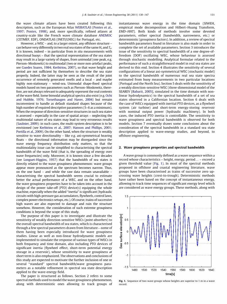
Fig. 1. Sequence of two wave groups whose heights are superior to 1 m in a wave

record.

J.-B. Saulnier et al. / Ocean Engineering 38 (2011) 130–147 131

the wave climate atlases have been created following thisdescription, such as the European Atlas WERATLAS (Pontes et al.,1997; Pontes, 1998), and, more specifically, refined atlases atcountry-scale like the French wave climate database ANEMOC(CETMEF, EDF), ONDATLAS (INETI/LNEG) for Portugal, etc.

However, a WEC – and, to a larger extent, any offshore structure –can behave very differently in two real sea states of the same Hs and Te.It is known, indeed – in particular from in situ measurements withdirectional buoys – that the spectral representation of the sea statesmay result in a large variety of shapes, from unimodal (one peak, e.g.Pierson–Moskowitz) to multimodal (two or more non-artefact peaks,see Guedes Soares, 1984; Kerbiriou, 2007), so that wave height andperiod are not sufficient by themselves to describe the sea stateproperly. Indeed, the latter may be seen as the result of the jointoccurrence of remotely generated swells and a local – and maybehighly non-stationary – wind-sea. Unimodal shape-fixed spectralmodels based on two parameters such as Pierson–Moskowitz, there-fore, are not always relevant to adequately represent the real contentsof the wave field. Some bimodal analytical spectra also exist (e.g. Ochiand Hubble, 1976; Torsethaugen and Haver, 2004) but remaininconvenient to handle as default standard shapes because of thehigh number of required descriptive parameters (5–6 as a minimum).When the response of direction-sensitive structures in such sea statesis assessed – especially in the case of spatial arrays – neglecting themultimodal nature of sea states may lead to very erroneous results(Saulnier, 2009): in such cases, the multi-system description is to beenvisioned (see Kerbiriou et al., 2007; Hanson and Phillips, 2001;Portilla et al., 2009). On the other hand, when the structure is weaklysensitive to wave directionality – like e.g. axi-symmetrical heavingfloats – the directional information may be disregarded since thewave energy frequency distribution only matters, so that themultimodality issue can be simplified to characterising the spectralbandwidth of the wave field (that is, the spreading of energy overwave frequencies) only. Moreover, it is known since a few decades(see Longuet-Higgins, 1957) that the bandwidth of sea states isdirectly related to the wave groupiness phenomenon: wave groupsappear more pronounced as the spectrum becomes narrow. Thus,on the one hand – and while the raw data remain unavailable –characterising the spectral bandwidth seems crucial to estimatebetter the actual performance of a WEC, and on the other hand,the wave groupiness properties have to be taken into account in thedesign of the power take-off (PTO) device(s) equipping the wholemachine, especially when the added ‘‘inertia’’ is significant (hydrauliccircuits with high-pressure gas accumulators, flywheels, control laws,complex power electronics setups, etc.). Of course, trains of successivehigh waves are also expected to damage and ruin the structuresomehow. However, the consideration of such extreme groupinessconditions is beyond the scope of this study.

The purpose of this paper is to investigate and illustrate thesensitivity of weakly direction-sensitive WECs (point absorbers) tothe overall spectral bandwidth of sea states, which is characterisedthrough a few spectral parameters drawn from literature—some ofthem having been especially introduced for wave groupinessstudies. Linear as well as non-linear hydrodynamic models areimplemented to simulate the response of various types of WECs inboth frequency and time domain, also including PTO devices ofsignificant inertia (flywheel effect, short-term potential energystorage in a reservoir), whose sensitivity to wave groupiness atshort term is also emphasized. The observations and conclusions ofthis study are expected to motivate the further inclusion of one orseveral ‘‘standard’’ spectral bandwidth/wave groupiness para-meters as a notable refinement in spectral sea state descriptionapplied to the wave-energy field.

The paper is structured as follows. Section 2 refers to somespectral methods used to model the wave groupiness phenomenon,along with deterministic ones allowing to track groups of

instantaneous wave energy in the time domain (SIWEH,empirical mode decomposition and Hilbert–Huang Transform,EMD–HHT). Both kinds of methods involve some devotedparameters, either spectral (bandwidth, narrowness, etc.) ordeterministic (groupiness factors). In addition, a review of spectralbandwidth parameters found in literature is also made in order tocomplete the set of available parameters. Section 3 introduces theissue of the sensitivity to spectral bandwidth of a one degree-of-freedom (DOF) oscillating WEC, whose behaviour is assessedthrough stochastic modelling. Analytical formulae related to theperformance of such a straightforward model in real sea states arederived to this end. Section 4 illustrates the sensitivity of severalconfigurations of a linear axi-symmetrical WEC (stochastic model)to the spectral bandwidth of numerous real sea state spectraestimated from buoy measurements in two particular locations(Portugal and the North Sea). Section 5 deals with the sensitivity ofa weakly direction-sensitive WEC (three-dimensional model of theSEAREV [Babarit, 2005], simulated in the time domain with non-linear hydrodynamics) to the spectral bandwidth of a set of seastates observed in a Californian location. Section 6 deals withthe case of WECs equipped with inertial PTO devices, as a flywheelsystem (air turbine) and short-term energy-storing reservoirwith nominal output power (hydraulic machinery). In bothcases, the induced PTO inertia is controllable. The sensitivity towave groupiness and spectral bandwidth is observed for bothmodels. Section 7 eventually draws some conclusions about theconsideration of the spectral bandwidth in a standard sea statedescription applied to wave-energy studies, and beyond, tooffshore engineering.

2. Wave groupiness properties and spectral bandwidth

A wave group is commonly defined as a wave sequence within arecord whose characteristics – height, energy, periody – exceed agiven threshold value (Fig. 1). In most of the spectral methodsproposed in offshore and coastal engineering literature, wavegroups have been characterised as trains of successive zero up-crossing wave heights (crest-to-trough). Deterministic methodshave rather been based on the concept of instantaneous energy,allowing to track time sequences of significant energy level whichare considered as wave energy groups. These methods, along with

Page 3

J.-B. Saulnier et al. / Ocean Engineering 38 (2011) 130–147132

the spectral parameters and groupiness factors they involve, aresuccessively presented here below.

2.1. Spectral methods and bandwidth parameters

2.1.1. Sea state spectral representation

The spectral methods are based on the classical spectraldescription of sea states. The ocean water elevation is assumedas a Gaussian zero-mean process, whose variance spectral density(or wave spectrum) S(f) (m2/Hz) may be estimated from in situ

measurements with e.g. buoys, probes, lasers, etc. From thespectral estimation E(f) of S(f), or directly S(f) if the wave spectraare computed by means of hindcast numerical models, the spectralmoments are obtained as (E(f) is kept here as default notation forwave spectra)

mn ¼

Z 10

f nEðf Þdf ð1Þ

which in turn permit to calculate some spectral wave parameterssuch as the significant wave height Hm0 (�Hs) as

Hm0 ¼ 4ffiffiffiffiffiffiffim0p

ð2Þ

and mean energy period T�10 (�Te) as

T�10 ¼m�1

m0ð3Þ

The spectral description of sea states is useful to calculate waveparameters from the spectral estimates of the water elevationwithout the need of carrying out wave-by-wave analysis. In thefollowing, symbols Hm0 and T�10 will be systematically usedinstead of Hs and Te since they are both calculated from spectraldata in this study.

2.1.2. Spectral methods and parameters for wave group statistics

To establish a simple set of statistics on wave group length, Goda(1976) started from the basic assumption that successive waveheights are not correlated, which is asymptotically true when thebandwidth of the wave process is very broad. In reality however,successive waves are not absolutely uncorrelated. This point wasnotably emphasized by Sawnhey (1963) and Rye (1974). Indeed,Goda observed from field measurements that the wave groupinessis more pronounced as the wave spectrum becomes narrow. Thepeakedness factor Qp, calculated as

Qp ¼2

m20

Z 10

fE2ðf Þdf ð4Þ

was introduced by him to characterise the groupiness level. Godashowed – along with Ewing (1973) – that the mean length of runs ofsuccessive wave heights was directly related to the value of Qp. Thisfactor increases as the bandwidth becomes narrow: fully developedwind-seas typically have Qp values close to 2, whereas narrow-banded swells may sometimes reach higher values (44).

To take the dependence of successive wave heights into con-sideration, Kimura (1980) proposed a wave group theory basedon a 1st-order Markov chain. The resulting statistics involve acorrelation parameter k, for which Battjes and van Vledder(1984) gave – from previous works of Ahran and Ezraty (1978)in the case of narrow-banded processes – the following spectralformulation:

k¼ kðtÞ ¼ 1

m0

Z 10

Eðf Þei2pftdf

�������� ð5Þ

where t denotes the mean time lag separating two successivewaves, usually taken equal to the spectral mean zero up-crossingperiod T02 (¼(m0/m2)1/2

�Tz). The correlation increases as thespectral bandwidth decreases.

From the works of Rice (1944, 1945) on narrow-banded randomGaussian processes, Longuet-Higgins (1957, 1984), among others,derived wave group statistics by considering the Hilbert envelopeof the water elevation instead of wave heights. These statisticsinvolve the narrowness parameter u, calculated as

u¼ e2 ¼

ffiffiffiffiffiffiffiffiffiffiffiffiffiffiffiffiffiffiffiffiffim0m2

m21

�1

sð6Þ

which accounts for the bandwidth of the sea state process. Because

of the presence of the 2nd-order moment, such a parameter issomewhat sensitive to the high-frequency contents of the spec-trum. Narrow-banded sea states typically have small values of u –provided the spectra have been appropriately filtered beforehand –and therefore exhibit significant groups of waves. The narrownessparameter is denoted by e2 in the following, with or withoutfiltering.

Many authors (e.g. Nolte and Hsu, 1972; Medina and Hudspeth,1990), investigated the spectrum related to the (Hilbert) envelopeof the water elevation. Prevosto (1988) defined a bandwidthparameter Bw calculated as

Bw ¼4

m20

Z 10

E2ðf Þ f�m1

m0

� �2

df ð7Þ

which permits to define the shape of an ideal envelope spectrum.Let us stress the specificity of this parameter (in Hz), which does notdepend on the frequency location of the spectrum.

2.1.3. Bandwidth parameters from literature

Out of the frame of studies especially devoted to wave groupi-ness, several authors have proposed spectral bandwidth para-meters for other purposes. In Mollison (1985) for instance, aproposal of standard wave parameters for a more completedescription of the wave climate for the wave energy exploitationwas presented. The broadness parameter e0, in particular, isintroduced to characterise the spectral bandwidth of sea states.It is defined as the relative standard deviation of the period wavespectrum (E(T)¼E(1/T¼ f)/T2) and therefore expressed as

e0 ¼

ffiffiffiffiffiffiffiffiffiffiffiffiffiffiffiffiffiffiffiffiffiffiffim0m�2

m2�1

�1

sð8Þ

Very similar to e2 in the formulation, this parameter is verymuch less sensitive to high frequency components due to thepresence of low-order moments.

Smith et al. (2006) computed a new bandwidth parameter –similar to e2 and e0 – from a preliminary study led by Woolf (2002).This parameter, symbolized here by e1, is expressed as

e1 ¼

ffiffiffiffiffiffiffiffiffiffiffiffiffiffiffiffiffiffiffiffiffiffiffim1m�1

m20

�1

sð9Þ

Likewise, such a parameter is expected to be less sensitive to thehigh frequency contents of sea states than e2.

Medina and Hudspeth (1987) introduced the factor Qe – verysimilar to Goda’s Qp – to control the variance variability ofnumerically simulated wave processes. Its expression is

Qe ¼2m1

m30

Z 10

E2ðf Þdf ð10Þ

They indicate that Qe is related to the inverse of the equivalentspectral bandwidth introduced by Blackman and Tukey (1959),here denoted by L (Hz) and calculated as

L¼ðR1

0 Eðf Þdf Þ2R10 E2ðf Þdf

¼m2

0R10 E2ðf Þdf

ð11Þ

Indeed, it can be easily shown that L¼2(e12+1)/(T�10Qe).

Page 4

J.-B. Saulnier et al. / Ocean Engineering 38 (2011) 130–147 133

2.2. Deterministic methods and groupiness factors

2.2.1. Smoothed instantaneous wave energy history

The Smoothed Instantaneous Wave Energy History (SIWEH)was defined by Funke and Mansard (1980) to identify andcontrol the wave groupiness in time series of water elevation forthe generation of grouped waves in tank. The SIWEH (m2) iscomputed as

SIWEHðtÞ ¼1

Tp

Z 1�1

Z2ðtþtÞQ ðtÞdt ð12Þ

where Q(t) is the Bartlett window

Q ðtÞ ¼1�

tTp

, 9t9oTp

0, 9t9ZTp

8><>: ð13Þ

The level of groupiness in a given record is then characterised bythe groupiness factor GFSIWEH defined as

GFSIWEH ¼sSIWEH

SIWEHðtÞð14Þ

where the bar denotes the time average and sSIWEH denotes thestandard deviation of SIWEH(t). For a given sea state with giventarget spectrum, it can be shown that the mean value of the SIWEHis m0, so that GFSIWEH accounts for the relative variability of theenergy signal in time. If this factor is close to 1, the groupiness ishigh; as GFSIWEH tends to 0, the wave signal tends to a sine wave. Forthe sake of exhaustiveness, let us evoke a possible alternativemethod for the calculation of the groupiness factor, which wasintroduced by List (1991). The new factor is calculated from thelow-pass filtering of the water elevation modulus 9Z(t)9 andtherefore requires the definition of an appropriate cut-offfrequency. Yet, it is not included in this study.

2.2.2. Empirical mode decomposition and Hilbert–Huang transform

The Empirical Mode Decomposition and Hilbert–Huang Transform

(EMD–HHT) method was proposed by Huang et al. (1998) as analternative to the classical Fourier decomposition, especially whenthe observed phenomena are not stationary nor linear, just aswaves are by nature. The EMD consists in decomposing – by sifting

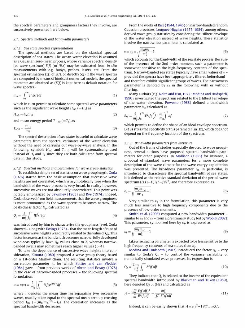
Fig. 2. Extract of IMF (top) derived by EMD–HHT from a wave signal, with related

instantaneous frequency (middle) and amplitude (bottom).

process – the signal into a finite number of narrow-banded signalscj(t) called Intrinsic Mode Functions (IMF), which characterisedifferent time scales of the phenomenon up to a residue (longperiod and small amplitude trend, out of the scope of the analysis),and whose instantaneous frequency oj(t) and amplitude aj(t) canbe properly defined (Fig. 2). The Hilbert spectrum H(o, t)represents the distribution of the amplitude of each IMF againstfrequency and time. By integrating the spectrum againstfrequencies, the instantaneous energy signal IE(t) (m2) is herecalculated as

IEðtÞ ¼X

j

H2ðojðtÞ,tÞ ð15Þ

Similarly to the SIWEH, the groupiness factor GFIE may beformed as the ratio

GFIE ¼sIE

IEðtÞð16Þ

where sIE denotes the standard deviation of IE(t). Let us mentionthat a similar groupiness factor may be found in Dong et al. (2008),which is derived from the wavelet energy density of the wavesignal instead of IE(t).

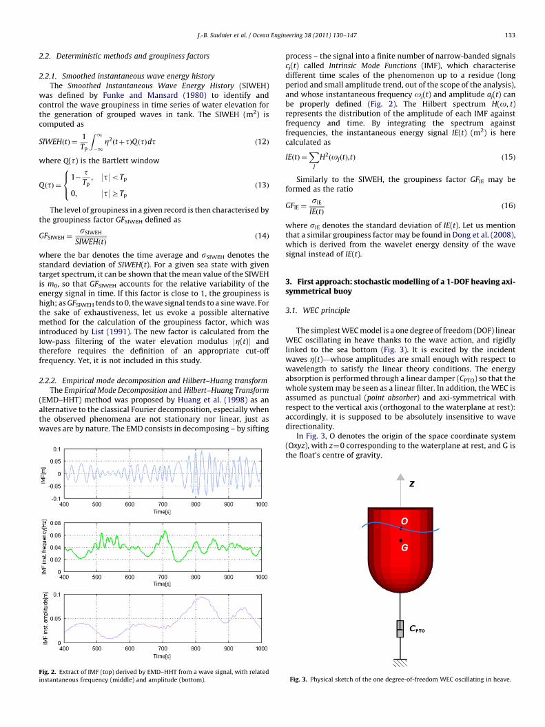
3. First approach: stochastic modelling of a 1-DOF heaving axi-symmetrical buoy

3.1. WEC principle

The simplest WEC model is a one degree of freedom (DOF) linearWEC oscillating in heave thanks to the wave action, and rigidlylinked to the sea bottom (Fig. 3). It is excited by the incidentwaves Z(t)—whose amplitudes are small enough with respect towavelength to satisfy the linear theory conditions. The energyabsorption is performed through a linear damper (CPTO) so that thewhole system may be seen as a linear filter. In addition, the WEC isassumed as punctual (point absorber) and axi-symmetrical withrespect to the vertical axis (orthogonal to the waterplane at rest):accordingly, it is supposed to be absolutely insensitive to wavedirectionality.

In Fig. 3, O denotes the origin of the space coordinate system(Oxyz), with z¼0 corresponding to the waterplane at rest, and G isthe float’s centre of gravity.

Fig. 3. Physical sketch of the one degree-of-freedom WEC oscillating in heave.

Page 5

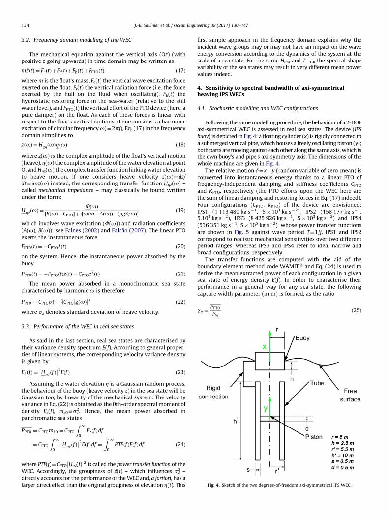
Fig. 4. Sketch of the two degrees-of-freedom axi-symmetrical IPS WEC.

J.-B. Saulnier et al. / Ocean Engineering 38 (2011) 130–147134

3.2. Frequency domain modelling of the WEC

The mechanical equation against the vertical axis (Oz) (withpositive z going upwards) in time domain may be written as

m€zðtÞ ¼ FeðtÞþFrðtÞþFhðtÞþFPTOðtÞ ð17Þ

where m is the float’s mass, Fe(t) the vertical wave excitation forceexerted on the float, Fr(t) the vertical radiation force (i.e. the forceexerted by the hull on the fluid when oscillating), Fh(t) thehydrostatic restoring force in the sea-water (relative to the stillwater level), and FPTO(t) the vertical effort of the PTO device (here, apure damper) on the float. As each of these forces is linear withrespect to the float’s vertical motions, if one considers a harmonicexcitation of circular frequency o(¼2pf), Eq. (17) in the frequencydomain simplifies to

zðoÞ ¼HzZðoÞZðoÞ ð18Þ

where z(o) is the complex amplitude of the float’s vertical motion(heave),Z(o) the complex amplitude of the water elevation at pointO, and HZz(o) the complex transfer function linking water elevationto heave motion. If one considers heave velocity z(o)¼dz/

dt¼ ioz(o) instead, the corresponding transfer function HZz(o) –called mechanical impedance – may classically be found writtenunder the form:

HZ_z ðoÞ ¼FðoÞ

½BðoÞþCPTO�þ i½oðmþAðoÞÞ�ðrgS=oÞ�ð19Þ

which involves wave excitation (F(o)) and radiation coefficients(A(o), B(o)); see Falnes (2002) and Falc~ao (2007). The linear PTOexerts the instantaneous force

FPTOðtÞ ¼ �CPTO _zðtÞ ð20Þ

on the system. Hence, the instantaneous power absorbed by thebuoy

PPTOðtÞ ¼�FPTOðtÞ_zðtÞ ¼ CPTO _z2ðtÞ ð21Þ

The mean power absorbed in a monochromatic sea statecharacterised by harmonic o is therefore

PPTO ¼ CPTOs2_z ¼

12CPTO _zðoÞ

�� ��2 ð22Þ

where sz denotes standard deviation of heave velocity.

3.3. Performance of the WEC in real sea states

As said in the last section, real sea states are characterised bytheir variance density spectrum E(f). According to general proper-ties of linear systems, the corresponding velocity variance densityis given by

E_z ðf Þ ¼ 9HZ_z ðf Þ92Eðf Þ ð23Þ

Assuming the water elevation Z is a Gaussian random process,the behaviour of the buoy (heave velocity z) in the sea state will beGaussian too, by linearity of the mechanical system. The velocityvariance in Eq. (22) is obtained as the 0th-order spectral moment ofdensity Ez(f), mz0�sz

2. Hence, the mean power absorbed inpanchromatic sea states

PPTO ¼ CPTOm _z0 ¼ CPTO

Z 10

E _z ðf Þdf

¼ CPTO

Z 10

9HZ_z ðf Þ92Eðf Þdf ¼

Z 10

PTFðf ÞEðf Þdf ð24Þ

where PTF(f)¼CPTO9HZz(f)92 is called the power transfer function of the

WEC. Accordingly, the groupiness of z(t) – which influences sz2 –

directly accounts for the performance of the WEC and, a fortiori, has alarger direct effect than the original groupiness of elevation Z(t). This

first simple approach in the frequency domain explains why theincident wave groups may or may not have an impact on the waveenergy conversion according to the dynamics of the system at thescale of a sea state. For the same Hm0 and T�10, the spectral shapevariability of the sea states may result in very different mean powervalues indeed.

4. Sensitivity to spectral bandwidth of axi-symmetricalheaving IPS WECs

4.1. Stochastic modelling and WEC configurations

Following the same modelling procedure, the behaviour of a 2-DOFaxi-symmetrical WEC is assessed in real sea states. The device (IPS

buoy) is depicted in Fig. 4: a floating cylinder (x) is rigidly connected toa submerged vertical pipe, which houses a freely oscillating piston (y);both parts are moving against each other along the same axis, which isthe own buoy’s and pipe’s axi-symmetry axis. The dimensions of thewhole machine are given in Fig. 4.

The relative motion d¼x�y (random variable of zero-mean) isconverted into instantaneous energy thanks to a linear PTO offrequency-independent damping and stiffness coefficients CPTO

and KPTO, respectively (the PTO efforts upon the WEC here arethe sum of linear damping and restoring forces in Eq. (17) indeed).Four configurations (CPTO, KPTO) of the device are envisioned:IPS1 (1 113 480 kg s�1, 5�103 kg s�2), IPS2 (158 177 kg s�1,5.103 kg s�2), IPS3 (8 425 926 kg s�1, 5�103 kg s�2) and IPS4(536 351 kg s�1, 5�105 kg s�2), whose power transfer functionsare shown in Fig. 5 against wave period T¼1/f. IPS1 and IPS2correspond to realistic mechanical sensitivities over two differentperiod ranges, whereas IPS3 and IPS4 refer to ideal narrow andbroad configurations, respectively.

The transfer functions are computed with the aid of theboundary element method code WAMITs and Eq. (24) is used toderive the mean extracted power of each configuration in a givensea state of energy density E(f). In order to characterise theirperformance in a general way for any sea state, the followingcapture width parameter (in m) is formed, as the ratio

wP ¼PPTO

Pwð25Þ

Page 6

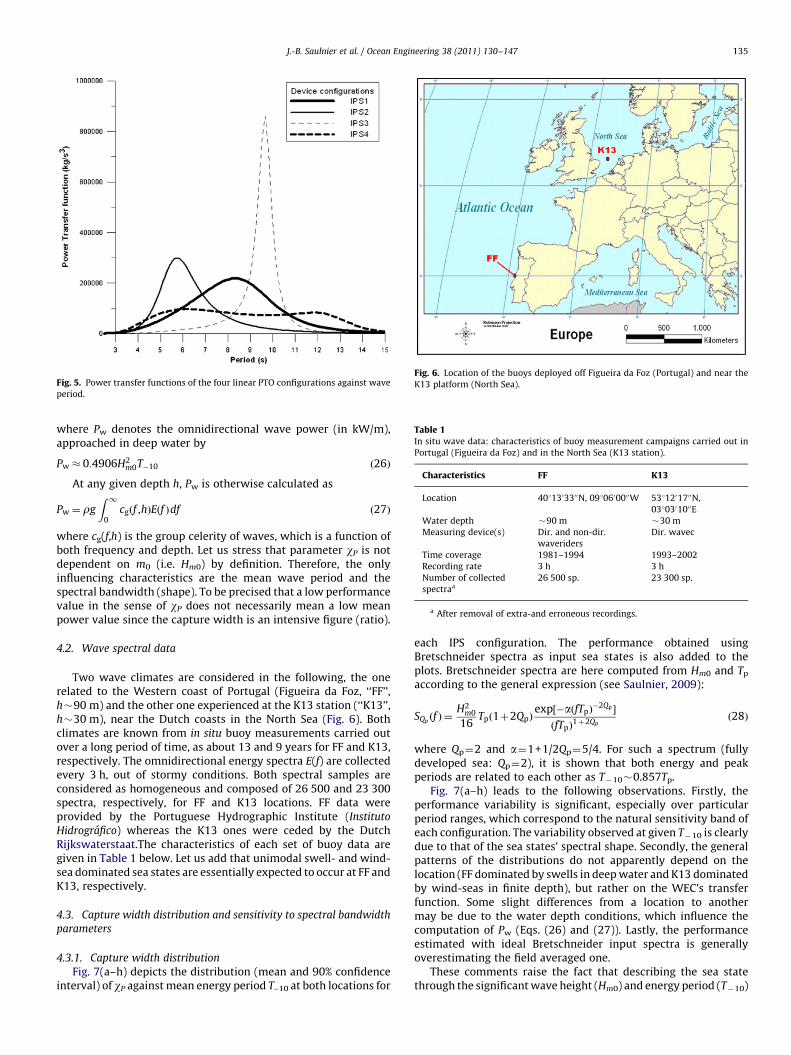
Fig. 5. Power transfer functions of the four linear PTO configurations against wave

period.

Fig. 6. Location of the buoys deployed off Figueira da Foz (Portugal) and near the

K13 platform (North Sea).

Table 1In situ wave data: characteristics of buoy measurement campaigns carried out in

Portugal (Figueira da Foz) and in the North Sea (K13 station).

Characteristics FF K13

Location 4011303300N, 0910600000W 5311201700N,

0310301000E

Water depth �90 m �30 m

Measuring device(s) Dir. and non-dir.

waveriders

Dir. wavec

Time coverage 1981–1994 1993–2002

Recording rate 3 h 3 h

Number of collected

spectraa

26 500 sp. 23 300 sp.

a After removal of extra-and erroneous recordings.

J.-B. Saulnier et al. / Ocean Engineering 38 (2011) 130–147 135

where Pw denotes the omnidirectional wave power (in kW/m),approached in deep water by

Pw � 0:4906H2m0T�10 ð26Þ

At any given depth h, Pw is otherwise calculated as

Pw ¼ rg

Z 10

cgðf ,hÞEðf Þdf ð27Þ

where cg(f,h) is the group celerity of waves, which is a function ofboth frequency and depth. Let us stress that parameter wP is notdependent on m0 (i.e. Hm0) by definition. Therefore, the onlyinfluencing characteristics are the mean wave period and thespectral bandwidth (shape). To be precised that a low performancevalue in the sense of wP does not necessarily mean a low meanpower value since the capture width is an intensive figure (ratio).

4.2. Wave spectral data

Two wave climates are considered in the following, the onerelated to the Western coast of Portugal (Figueira da Foz, ‘‘FF’’,h�90 m) and the other one experienced at the K13 station (‘‘K13’’,h�30 m), near the Dutch coasts in the North Sea (Fig. 6). Bothclimates are known from in situ buoy measurements carried outover a long period of time, as about 13 and 9 years for FF and K13,respectively. The omnidirectional energy spectra E(f) are collectedevery 3 h, out of stormy conditions. Both spectral samples areconsidered as homogeneous and composed of 26 500 and 23 300spectra, respectively, for FF and K13 locations. FF data wereprovided by the Portuguese Hydrographic Institute (Instituto

Hidrografico) whereas the K13 ones were ceded by the DutchRijkswaterstaat.The characteristics of each set of buoy data aregiven in Table 1 below. Let us add that unimodal swell- and wind-sea dominated sea states are essentially expected to occur at FF andK13, respectively.

4.3. Capture width distribution and sensitivity to spectral bandwidth

parameters

4.3.1. Capture width distribution

Fig. 7(a–h) depicts the distribution (mean and 90% confidenceinterval) of wP against mean energy period T–10 at both locations for

each IPS configuration. The performance obtained usingBretschneider spectra as input sea states is also added to theplots. Bretschneider spectra are here computed from Hm0 and Tp

according to the general expression (see Saulnier, 2009):

SQpðf Þ ¼

H2m0

16Tpð1þ2QpÞ

exp½�aðfTpÞ�2Qp �

ðfTpÞ1þ2Qp

ð28Þ

where Qp¼2 and a¼1+1/2Qp¼5/4. For such a spectrum (fullydeveloped sea: Qp¼2), it is shown that both energy and peakperiods are related to each other as T�10�0.857Tp.

Fig. 7(a–h) leads to the following observations. Firstly, theperformance variability is significant, especially over particularperiod ranges, which correspond to the natural sensitivity band ofeach configuration. The variability observed at given T�10 is clearlydue to that of the sea states’ spectral shape. Secondly, the generalpatterns of the distributions do not apparently depend on thelocation (FF dominated by swells in deep water and K13 dominatedby wind-seas in finite depth), but rather on the WEC’s transferfunction. Some slight differences from a location to anothermay be due to the water depth conditions, which influence thecomputation of Pw (Eqs. (26) and (27)). Lastly, the performanceestimated with ideal Bretschneider input spectra is generallyoverestimating the field averaged one.

These comments raise the fact that describing the sea statethrough the significant wave height (Hm0) and energy period (T�10)

Page 7

Fig. 7. Distribution of capture width against mean energy period obtained from long-term wave measurements in Figueira da Foz (left) and K13 (right) for PTO configurations

IPS1–IPS4 (top to bottom); capture width obtained with Bretschneider sea states (dotted line).

J.-B. Saulnier et al. / Ocean Engineering 38 (2011) 130–147136

only is not sufficient to characterise the performance accurately,even for very simple – linear – WEC configurations as thosemodelled here. Accordingly, analytical unimodal and shape-fixed

wave spectra such as Bretschneider (or Pierson–Moskowitz, JONS-WAP 3.3, etc.) are not relevant to predict the actual performance ofsuch WECs.

Page 8

J.-B. Saulnier et al. / Ocean Engineering 38 (2011) 130–147 137

4.3.2. Sensitivity to spectral bandwidth parameters

In order to examine the relevance of characterising the spectralshape of sea states as complementary information to assess theperformance of the WEC, the scatter plot of capture width wP

against some bandwidth parameters listed in Section 2 is observed.Fig. 8 depicts an example for IPS1 simulated in sea states with T�10

around 7 s in FF against parameter e0. In this figure, a clearcorrelation is noticed: this means that for such sea states, theperformance of the device is sensitive to this third parameter, sothat the actual absolute performance (Eq. (24)) may be approachedfrom the knowledge of Hm0, T–10 and e0. A least squares fit withquadratic trend is applied to the scatter in order to evaluate thelevel of correlation. The determination coefficient R2 (A[0;1]) isused as an indicator of the sensitivity to the spectral bandwidthparameter: in the present case, the value is quite high (R2

�0.88). Itis calculated for each bandwidth parameter of e0, e1, e2, Qp,k and Bw

for various energy period bands – with a sufficient amount ofspectra in each sample, never less than 50 – for each IPSconfiguration at FF and K13. The resulting curves are presentedin Fig. 9.

Most of the R2 curves are oscillating: they reach high values oversome particular period bands (high correlation) and drop down tozero over other bands (uncorrelated data). Let us assume here thatthe correlation is good as soon as R2 is higher than e.g. 0.70: thispermits to identify a so-called interval of sensitivity over T–10. Then,the following comments may be formulated. Firstly, the curves –again – are very similar for both wave climates in a general way,even if the period range is not exactly the same for both sinceshorter waves are expected to propagate in the North Sea incomparison to the Atlantic Ocean (the figures for both locationshave been placed side-by-side to help compare the results in eachwave climate). Secondly, some parameters exhibit higher R2 valuesthan others, namely e0, e1 and Bw (about 0.95 for IPS4 with e1,Fig. 9(g and h)); on the contrary, parameters like e2 or Qp do notseem particularly relevant from this point of view. Thirdly, theintervals of sensitivity for each parameter are quite similar at bothlocations: once again, the influence of the corresponding WEC’stransfer function is significant. More precisely, the highestcorrelation values generally occur near the resonance peak. Forexample, IPS1 is highly resonant for waves of period 8–9 s: inFig. 9(a and b), the high values of R2 range within [7 s;10 s]. Lastly,the intervals of sensitivity appear broader when the WEC’stransfer function is broad. This is well observed when looking at

Fig. 8. Distribution of capture width against Mollison’s relative bandwidth para-

meter e0 in 7 s energy period sea states in Figueira da Foz for PTO configuration IPS1;

quadratic regression in the least-squares sense with determination coefficient R2.

configurations IPS3 and IPS4: for the first one – very narrow – highvalues of coefficient R2 only occur over reduced rangesof periods (2 s-wide intervals on average, Fig. 9(e and f))whereas for the second one – very broad – the highest valuesare observed over very broad ranges (7 s-wide intervals on average,Fig. 9(g and h)).

As a conclusion, this study permits to understand that thebandwidth characteristic is relevant to complete the classical Hm0–T�10 description of sea states, especially when the WEC’s responseis broad and tuned to the main frequency components of theincident wave field. In addition, this study shows that parameterssuch as e0 and e1 (among others, not all of the parametersintroduced in Section 2 having been tested) are relevant tocharacterise the bandwidth of sea states in view of assessing theperformance of such axi-symmetrical WECs.

5. Sensitivity to spectral bandwidth of a weakly direction-sensitive three-dimensional WEC (SEAREV)

The sensitivity to wave spectral bandwidth of the three-dimensional WEC SEAREV (see Babarit, 2005) is observed bymeans of a numerical simulator in the time domain developed inEcole Centrale de Nantes. The device is a pitching body, thus notaxi-symmetrical and hence, subject to wave directionality.However, it is assumed and verified numerically that the modelis very little sensitive to variations of directionality, at least within a601-wide sector (less than 3% on the mean extracted power inwaves inducing the highest resonance).

5.1. SEAREV time-domain simulation

The physical WEC corresponds to hull DES1129 depicted inFig. 10(a and b). The body is designed to oscillate in pitch as wavespass by. An inertial pendulum is located inside the hull: it freelymoves around an axis parallel to the own hull’s pitching axis, sothat the relative pitch motion between both bodies (a) enables theextraction of energy from waves by means of a linear damper(CPTO¼107 kg m2 s�1, Eq. (21)). Roll and yaw have been restrictedwith additional stiffness (roll: K44¼109 N m rad�1; yaw: K66¼

108 N m rad�1) in order to favour pitching motions. The simulationcode solves the integro-differential equation of Cummins (1962)with a 4th-order Runge–Kutta scheme. Radiation (added masses,impulse responses) and diffraction (wave excitation) efforts on thehull at rest – under deep water and small motions assumptions –are calculated in the time domain with the 3-D diffraction–radiation code ACHIL3D (Clement, 1997). The model involveshydrodynamic non-linearities coming from the calculation of theinstantaneous Froude–Krylov forces (fluid pressure forces exertedon the hull in undisturbed wave) at each time-step, which thereforejustify the resort to time-domain modelling.

As the simulations in realistic sea states are somewhat timeconsuming, they are run several times over a short duration. Eachrun covers 500 s from rest position with the first 100 s beingdisregarded for they include a transient state from rest to randompermanent regime. From a target directional spectrum E(f,y), linearrandom wave fields are generated using the deterministic spectral

amplitude method (see Miles and Funke, 1989), that is, selectingrandom phases for each frequency-direction component whilewave amplitudes are computed according to

Aðfi,yjÞ ¼

ffiffiffiffiffiffiffiffiffiffiffiffiffiffiffiffiffiffiffiffiffiffiffiffiffiffiffiffiffiffiffi2Eðfi,yjÞDfiDyj

qð29Þ

With this method, running the simulator several times for agiven target directional spectrum permits a faster convergence to

Page 9

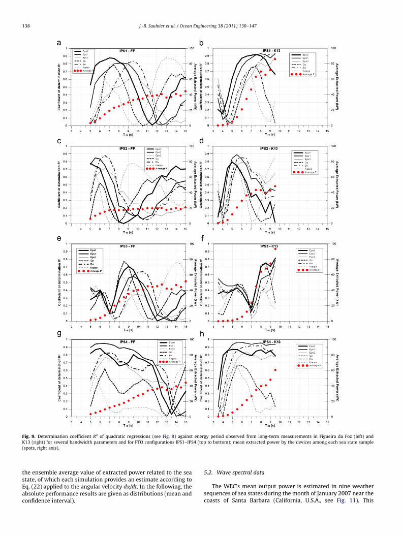
Fig. 9. Determination coefficient R2 of quadratic regressions (see Fig. 8) against energy period observed from long-term measurements in Figueira da Foz (left) and

K13 (right) for several bandwidth parameters and for PTO configurations IPS1–IPS4 (top to bottom); mean extracted power by the devices among each sea state sample

(spots, right axis).

J.-B. Saulnier et al. / Ocean Engineering 38 (2011) 130–147138

the ensemble average value of extracted power related to the seastate, of which each simulation provides an estimate according toEq. (22) applied to the angular velocity da/dt. In the following, theabsolute performance results are given as distributions (mean andconfidence interval).

5.2. Wave spectral data

The WEC’s mean output power is estimated in nine weathersequences of sea states during the month of January 2007 near thecoasts of Santa Barbara (California, U.S.A., see Fig. 11). This

Page 10

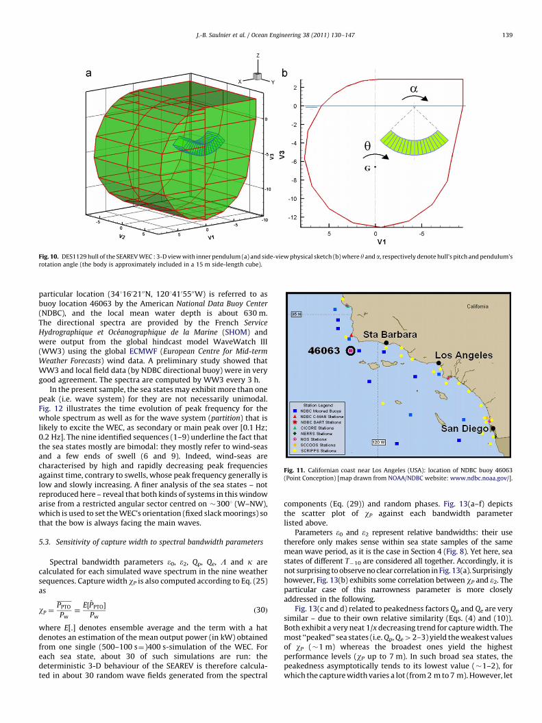
Fig. 10. DES1129 hull of the SEAREV WEC : 3-D view with inner pendulum (a) and side-view physical sketch (b) where y anda, respectively denote hull’s pitch and pendulum’s

rotation angle (the body is approximately included in a 15 m side-length cube).

Fig. 11. Californian coast near Los Angeles (USA): location of NDBC buoy 46063

(Point Conception) [map drawn from NOAA/NDBC website: www.ndbc.noaa.gov/].

J.-B. Saulnier et al. / Ocean Engineering 38 (2011) 130–147 139

particular location (3411602100N, 12014105500W) is referred to asbuoy location 46063 by the American National Data Buoy Center

(NDBC), and the local mean water depth is about 630 m.The directional spectra are provided by the French Service

Hydrographique et Oceanographique de la Marine (SHOM) andwere output from the global hindcast model WaveWatch III(WW3) using the global ECMWF (European Centre for Mid-term

Weather Forecasts) wind data. A preliminary study showed thatWW3 and local field data (by NDBC directional buoy) were in verygood agreement. The spectra are computed by WW3 every 3 h.

In the present sample, the sea states may exhibit more than onepeak (i.e. wave system) for they are not necessarily unimodal.Fig. 12 illustrates the time evolution of peak frequency for thewhole spectrum as well as for the wave system (partition) that islikely to excite the WEC, as secondary or main peak over [0.1 Hz;0.2 Hz]. The nine identified sequences (1–9) underline the fact thatthe sea states mostly are bimodal: they mostly refer to wind-seasand a few ends of swell (6 and 9). Indeed, wind-seas arecharacterised by high and rapidly decreasing peak frequenciesagainst time, contrary to swells, whose peak frequency generally islow and slowly increasing. A finer analysis of the sea states – notreproduced here – reveal that both kinds of systems in this windowarise from a restricted angular sector centred on �3001 (W–NW),which is used to set the WEC’s orientation (fixed slack moorings) sothat the bow is always facing the main waves.

5.3. Sensitivity of capture width to spectral bandwidth parameters

Spectral bandwidth parameters e0, e2, Qp, Qe, L and k arecalculated for each simulated wave spectrum in the nine weathersequences. Capture width wP is also computed according to Eq. (25)as

wP ¼PPTO

Pw�

E½PPTO�

Pwð30Þ

where E[.] denotes ensemble average and the term with a hatdenotes an estimation of the mean output power (in kW) obtainedfrom one single (500–100 s¼)400 s-simulation of the WEC. Foreach sea state, about 30 of such simulations are run: thedeterministic 3-D behaviour of the SEAREV is therefore calcula-ted in about 30 random wave fields generated from the spectral

components (Eq. (29)) and random phases. Fig. 13(a–f) depictsthe scatter plot of wP against each bandwidth parameterlisted above.

Parameters e0 and e2 represent relative bandwidths: their usetherefore only makes sense within sea state samples of the samemean wave period, as it is the case in Section 4 (Fig. 8). Yet here, seastates of different T�10 are considered all together. Accordingly, it isnot surprising to observe no clear correlation in Fig. 13(a). Surprisinglyhowever, Fig. 13(b) exhibits some correlation between wP and e2. Theparticular case of this narrowness parameter is more closelyaddressed in the following.

Fig. 13(c and d) related to peakedness factors Qp and Qe are verysimilar – due to their own relative similarity (Eqs. (4) and (10)).Both exhibit a very neat 1/x decreasing trend for capture width. Themost ‘‘peaked’’ sea states (i.e. Qp, Qe42–3) yield the weakest valuesof wP (�1 m) whereas the broadest ones yield the highestperformance levels (wP up to 7 m). In such broad sea states, thepeakedness asymptotically tends to its lowest value (�1–2), forwhich the capture width varies a lot (from 2 m to 7 m). However, let

Page 11

Fig. 12. Peak frequency of both active wave system partition and whole spectrum at buoy station NDBC 46063 (January 2007, WW3 data) in nine weather sequences.

J.-B. Saulnier et al. / Ocean Engineering 38 (2011) 130–147140

us remind that the calculation of such factors is theoretically validin unimodal sea states only, which is not always the case hereaccording to Fig. 12.

Fig. 13(e and f) related to parameters L and k inspire the sameobservation as previously: the weakest performance valuescorrespond to the most narrow-banded sea states. A roughgeneral correlation is found for L, which permits to estimateapproximately the capture width from the knowledge of thisparameter (in Hz). For k, a linear and homogeneous decreasingtrend is observed as the successive wave height correlationincreases (k40.5). For lower correlation levels, the scatter of wP

may be quite important (1–7 m).According to these observations, and looking back to the case of

the relative bandwidth parameter e2 (Fig. 13(b)), the obtainedscatter plot is particularly unexpected. Indeed, high values of e2

should correspond to very broad sea states, that is, to a highperformance level. Here, the perfect inverse is observed, but stillwith a manifest correlation to wP. The computation of e2 musttherefore be invoked to account for these results since no cut-offfrequency has been applied in Eq. (6) on principle (integration up tothe highest frequency of definition in WW3, 0.716 Hz). This showsthat parameter e2 remains very sensitive to the way it is calculatedand requires particular care when computed. Therefore, it does notseem appropriate as standard bandwidth parameter for suchpurposes.

6. Sensitivity of WECs equipped with realistic power take-offdevices

So far, the response of WECs equipped with linear PTO deviceshas been considered exclusively. Such devices reproduce at theoutput the fluctuations of the power absorbed by the mechanicalsystem since there is no inherent inertia in the model (Eq. (21)). Theterm inertia does not refer here to a property of the mechanicalstructure but is rather related to the short-term energy storagecapacity induced by the electro-mechanical converter onboard. Ifone considers more realistic PTO devices such as hydraulic circuitswith gas accumulators and hydraulic motors (Henderson, 2006;Falc~ao, 2007), air turbines (for oscillating water column systems,see Falc~ao, 2002), low-head water turbines (for overtoppingsystems, see Kofoed, 2002), etc. it is necessary to take thisproperty into account. This allows for a smoothed or stabilizedoutput power at the scale of one single WEC. Without inertia, acomplex – a possibly expensive – power electronics assemblingwould be necessary to end up with a satisfactory power signalready to be input into the grid. With inertia, this assembling islikely to be much reduced, and thus, much cheaper and easier toinstall. Accordingly, WEC developers have to find a reasonablecompromise (performance/expenses/installation) on the level of

inertia they wish inside their PTO device(s). It follows that thesensitivity of such systems to wave groupiness is of a particularconcern. Here, two models are proposed, which aim at encom-passing the most common PTO devices, namely inertial flywheelsfor turbines and short-term energy storage reservoirs for hydraulicinstallations.

6.1. Inertial flywheel

A simplified model of flywheel with adjustable inertia permitsto reproduce the behaviour of air and water turbines. The instan-taneous power absorbed by the mechanical system, denoted byPa(t) (¼PPTO(t) for linear WECs in Sections 3 and 4), supplies energyto a flywheel that is linked to an electrical generator delivering thepower Pe(t) (Fig. 14).

In the model, it is assumed that the output electrical power isrelated to the flywheel’s instantaneous rotational speedO(t) (rad/s)by the relation

PeðtÞ ¼ KO2ðtÞ ð31Þ

where K (kg m2/s) is a constant that can be freely adjusted (control

law). By neglecting energy losses by friction on the rotor, thedynamic equation of the PTO is (Falc~ao, 2002)

PaðtÞ�PeðtÞ ¼ IOðtÞdOðtÞ

dtð32Þ

where I (kg m2) denotes the flywheel’s inertia against the rotationaxis. Combining both Eqs. (31) and (32) leads to the followingdynamic equation:

PaðtÞ ¼ PeðtÞþI

2K

dPeðtÞ

dt¼ PeðtÞþm

dPeðtÞ

dtð33Þ

The inertia of the PTO can be characterised here as the timeconstant m¼ I/2K (s). Indeed, Eq. (33) is similar to that of an RCelectrical circuit with resistor R (�1/2K) and capacitor C (� I), forwhich the product t¼RC represents the circuit’s time constant, i.e.the time required to reach �63% of the permanent regime voltage.For a given control law (K), the higher the flywheel’s inertia (I), thehigher the level of energy storage at short term (m).

With such a model, it is immediately apparent that the (longterm) expected mean power converted by the whole WEC is thesame as for the linear model – denoted here by Pa,m in this section(Eq. (24)) – since no energy loss is included. Thus, at the scale of asea state, this WEC has a similar sensitivity to spectral bandwidthas any of the linear models considered so far (Sections 3 and 4).Now, the instantaneous response will differ somewhat. Indeed, thePTO system constitutes a low-pass filter, which therefore reducesthe high-frequency fluctuations of the absorbed power. Theresulting electrical power signal Pe(t) appears then smootherthan the instantaneous input power Pa(t) as well as slightlydelayed in time. Fig. 15(a and b) give an example of this signal

Page 12

Fig. 14. Simplified sketch of an inertial WEC equipped with flywheel and electrical

generator.

Fig. 13. Scatter plots of SEAREV’s capture width obtained in nine sequences (Fig. 12) against several bandwidth parameters (a–f) at station NDBC 46063 (January 2007).

J.-B. Saulnier et al. / Ocean Engineering 38 (2011) 130–147 141

for three levels of inertia, as m¼5 s (low inertia), m¼25 s (meaninertia) and m¼100 s (high inertia), and, respectively, denoted byPe1(t), Pe2(t) and Pe3(t). The input absorbed power Pa(t) comes from

the stochastic simulation over 3600 s of the axi-symmetricalheaving buoy introduced in Section 3 in a unimodal (Hm0¼2 m,Tp¼8 s) and bimodal (swell: Hm0¼1.41 m, Tp¼11 s; wind-sea:Hm0¼1.41 m, Tp¼5 s) sea state, respectively, using random Fouriercoefficients (see Tucker et al., 1984; Miles and Funke, 1989). Bothtarget spectra are plotted in Fig. 16, and have similar Hm0 (2 m) andT�10 (�7 s). In these excerpts, the wave signal together with theinstantaneous energy histories SIWEH(t) and IE(t) as well as thespectral densities of each electrical power signal are also plotted.

Both simulations emphasize the smoothing effect realized bythe PTO device with respect to the non-filtered input power signalPa(t). As inertiam increases, the level of smoothing is more and more

Page 13

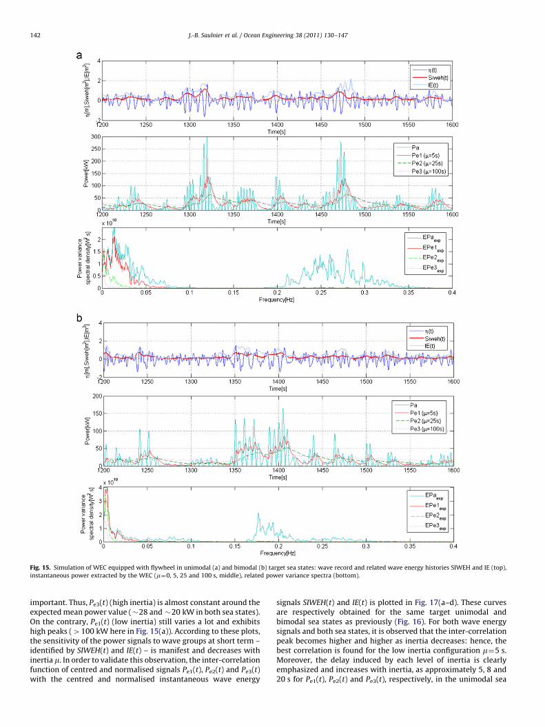
Fig. 15. Simulation of WEC equipped with flywheel in unimodal (a) and bimodal (b) target sea states: wave record and related wave energy histories SIWEH and IE (top),

instantaneous power extracted by the WEC (m¼0, 5, 25 and 100 s, middle), related power variance spectra (bottom).

J.-B. Saulnier et al. / Ocean Engineering 38 (2011) 130–147142

important. Thus, Pe3(t) (high inertia) is almost constant around theexpected mean power value (�28 and �20 kW in both sea states).On the contrary, Pe1(t) (low inertia) still varies a lot and exhibitshigh peaks (4100 kW here in Fig. 15(a)). According to these plots,the sensitivity of the power signals to wave groups at short term –identified by SIWEH(t) and IE(t) – is manifest and decreases withinertia m. In order to validate this observation, the inter-correlationfunction of centred and normalised signals Pe1(t), Pe2(t) and Pe3(t)with the centred and normalised instantaneous wave energy

signals SIWEH(t) and IE(t) is plotted in Fig. 17(a–d). These curvesare respectively obtained for the same target unimodal andbimodal sea states as previously (Fig. 16). For both wave energysignals and both sea states, it is observed that the inter-correlationpeak becomes higher and higher as inertia decreases: hence, thebest correlation is found for the low inertia configuration m¼5 s.Moreover, the delay induced by each level of inertia is clearlyemphasized and increases with inertia, as approximately 5, 8 and20 s for Pe1(t), Pe2(t) and Pe3(t), respectively, in the unimodal sea

Page 14

J.-B. Saulnier et al. / Ocean Engineering 38 (2011) 130–147 143

state. Similar delays are obtained in the bimodal case. This meansthat an optimal inertia may be setup for the flywheel in such seastates by adjusting the control law (K) according to the desireddegree of sensitivity to wave groups. This short-term sensitivity,however, is not supposed to modify the mean converted power bythe WEC in the whole sea state (i.e. in 1–3 h of simulation), asalready mentioned previously.

Fig. 17. Inter-correlation function of (normalised and centred) instantaneous power si

(a and c) and IE (b and d) in unimodal (top) and bimodal (bottom) sea states (Fig. 16).

Fig. 16. Unimodal and bimodal target sea states (Hm0¼2 m and T�10�7 s) used for

the simulations in Fig. 15.

6.2. Short-term energy storage with nominal output power

The second way of simulating an inertial PTO device is byconsidering a simple short-term potential energy reservoir suppliedby the same instantaneous power Pa(t) as previously (instantaneouspower absorbed by the linear heaving buoy) and connected to ahydraulic motor characterised by the nominal output power Pnom

(kW). The instantaneous power output by the whole WEC is denotedby Ps(t): either it is equal to Pnom, when energy is discharged by thereservoir through the motor, or it is zero, when the energy storedinside the reservoir (Ecapa(t)) is not sufficient to actuate the motor.A straightforward algorithm is built to simulate the whole WEC (seeSaulnier, 2009), which is illustrated in Fig. 18. No maximal limit isimposed on the reservoir’s capacity. A 1200 s-simulation of the WEC inthe same target unimodal sea state as previously (Hm0¼2 m, Tp¼8 s)is shown in Fig. 19, where Pnom is set to the expectation Pa,m of Pa(t) inthe sea state (�28 kW, Eq. (24)): as expected, the output power isintermittent, depending on the available energy inside the reservoir.

In order to characterise the performance of the whole system ina sea state, the quality factor (or nominal operating rate, %) is

gnals output from the flywheel with instantaneous wave energy histories SIWEH

Fig. 18. Simplified sketch of an inertial WEC equipped with short-term energy

reservoir and hydraulic motor with nominal power.

Page 15

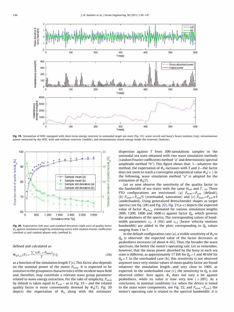
Fig. 19. Simulation of WEC equipped with short-term energy reservoir in unimodal target sea state (Fig. 16): wave record and buoy’s heave motions (top), instantaneous

power extracted by the WEC with and without reservoir (middle), and instantaneous stored energy inside the reservoir (bottom).

Fig. 20. Expectation (left axis) and standard deviation (right axis) of quality factor

Fq against simulation length by simulating waves with random Fourier coefficients

(method a) and random phases only (method b).

J.-B. Saulnier et al. / Ocean Engineering 38 (2011) 130–147144

defined and calculated as

Fq,PnomðTÞ ¼

PtðPs ¼ PnomÞ

T%½ � ð34Þ

as a function of the simulation length T (s). This factor also dependson the nominal power of the motor Pnom. It is expected to besensitive to the groupiness characteristics of the incident wave fieldand, therefore, may constitute a relevant wave group parameterrelated to wave energy extraction. For the sake of simplicity, Pnom

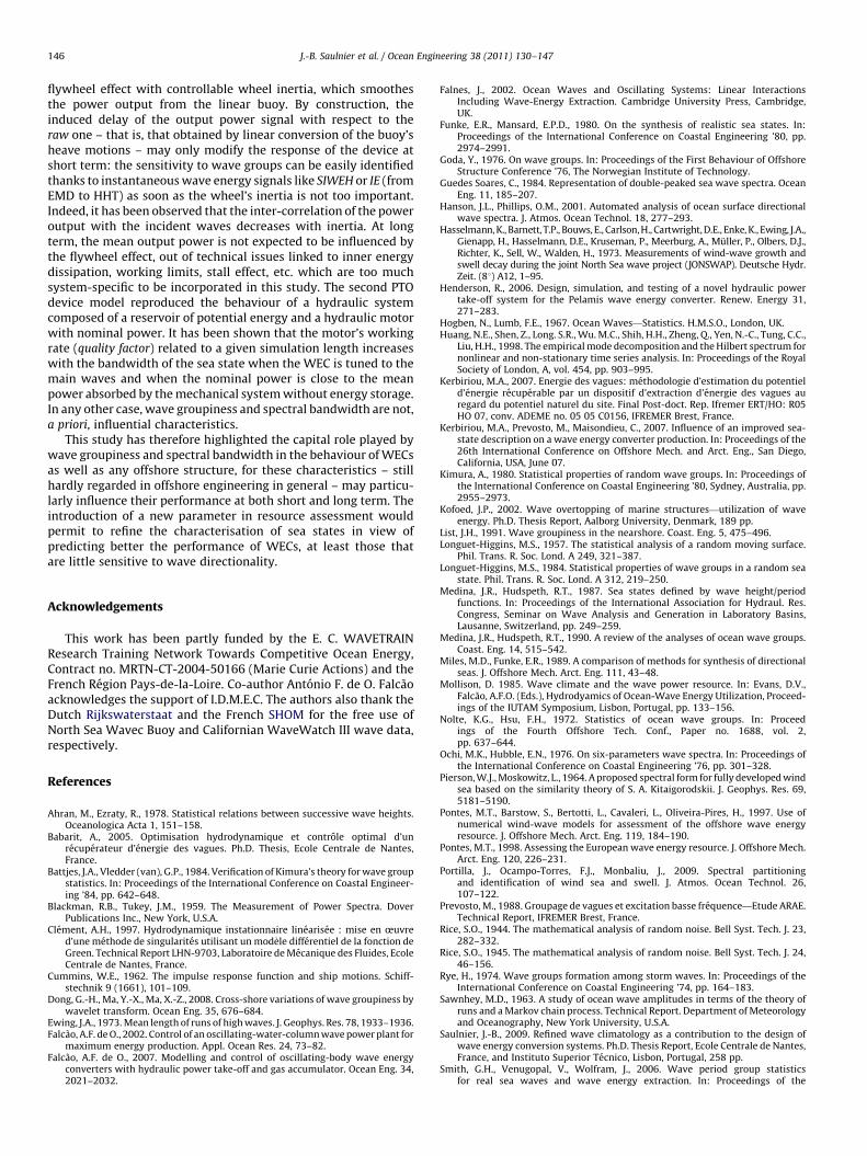
by default is taken equal to Pa,m – as in Fig. 19 – and the relatedquality factor is more conveniently denoted by Fq(T). Fig. 20depicts the expectation of Fq along with the estimates’

dispersion against T from 300-simulations samples in theunimodal sea state obtained with two wave simulation methods(random Fourier coefficients method ‘‘a’’ and deterministic spectralamplitude method ‘‘b’’). This figure shows that: 1—whatever themethod, the expectation of Fq increases with T and 2—the factordoes not seem to reach a convergent asymptotical value Fq(N). Inthe following, wave simulation method ‘‘a’’ is adopted for theestimation of Fq(T).

Let us now observe the sensitivity of the quality factor tothe bandwidth of sea states with the same Hm0 and T�10. ThreePTO configurations are envisioned: (a) Pnom¼Pa,m (default),(b) Pnom¼Pa,m/5 (overloaded, saturation) and (c) Pnom¼Pa,m n5(underloaded). Using generalized Bretschneider shapes as targetspectra (see Eq. (28) and Fig. 22), Fig. 21(a–c) depicts the expectedvalue of factor Fq,Pnom

estimated for various simulation lengths(600, 1200, 1800 and 3600 s) against factor Qp, which governsthe peakedness of the spectra. The corresponding values of band-width parameters e2, L (Hz) and ez,2 (heave velocity motionsbandwidth) are added to the plots corresponding to Qp valuesranging from 1 to 7.

In the default configuration case (a), a visible sensitivity of Fq toQp is observed: the expected value of the factor decreases aspeakedness increases (of about 4–6%). Thus, the broader the wavespectrum, the better the motor’s operating rate. Let us remember,however, that the mean power absorbed by the buoy in each seastate is different, as approximately 17 kW for Qp¼1 and 40 kW forQp¼7. In the overloaded case (b), this sensitivity is not observedanymore since very similar values of mean quality factor are foundwhatever the simulation length—and very close to 100%, asexpected. In the underloaded case (c), the sensitivity to Qp is notobserved either: here again, Fq does not vary a lot againstpeakedness, while its value is now very low (o20%). As aconclusion, in nominal conditions (i.e. when the device is tunedto the main wave components, see Fig. 22, and Pnom�Pa,m), themotor’s operating rate is related to the spectral bandwidth: it is

Page 16

Fig. 21. Expectation of quality factor against peakedness factor Qp (unimodal sea

states) for several simulation lengths (600–3600 s) and three operating situations:

nominal case Pnom¼Pa,m (a), saturation case Pnom¼Pa,m/5 (b) and underload case

Pnom¼Pa,m n5 (c); spectral bandwidth parameters (wave and motions).

Fig. 22. Target unimodal variance spectral densities with modulable peakedness

factor (Qp¼1–7) used in Fig. 21; dimensionless WEC’s power transfer function.

J.-B. Saulnier et al. / Ocean Engineering 38 (2011) 130–147 145

found higher in broad-banded sea states. In critical conditions, thatis, when the system saturates (i.e. Fq�100% while the storedenergy diverges) or when the sea state is too weak to fill up thereservoir with potential energy (i.e. low Fq), the bandwidth ofwaves does not matter anymore.

7. Conclusions

This work addressed the question of the sensitivity of WECs towave groupiness and spectral bandwidth of sea states in addition tothe common wave parameters Hs and Te (respectively denoted byHm0 and T�10 in this paper), in particular when the devices are littleinfluenced by wave directionality (point absorbers). To this end,linear stochastic modelling and non-linear time-domain simula-tions have been carried out involving linear PTO devices (lineardamping). The performance results have led to the followingconclusions.

Firstly, for fixed Hm0 and T�10 in any wave climate, thevariability of the performance – symbolized by a capture widthparameter (wP, in m) – can be very important, especially in seastates whose energy period lies within the response band of theWEC (PTF) due to the shape variability of wave spectra in nature.Secondly, the spectral bandwidth of waves – which is related to thewave groupiness phenomenon through the spectral narrowness –is found to adequately complete the (Hm0, T�10) sea state descrip-tion for characterising the converter’s performance, in particularwhen the mean period of the incoming waves is close to theconverter’s resonance. Thirdly, the sensitivity of a WEC to spectralbandwidth is found to be more pronounced when its response bandis broad (Section 4.3.2, Fig. 9). This, together with the last point,implies that, if the WECs are designed in such a way their responseband is broad and may be automatically tuned to the main waveperiods of each experienced sea state, the spectral bandwidth willconstitute the missing key parameter which provides acomprehensive description of the resource as regards the waveenergy conversion operated by the device. According to the models,some spectral bandwidth parameters have shown to behavesatisfactorily for this purpose. In the case of the linear IPS model,relative bandwidth parameters such as e0 and e1 appearedadequate, particularly in sea states with the same energy periodT�10. From the simulations of the SEAREV 3-D model, parametersand factors like L, k and Qp or Qe were found to be quite correlatedwith the performance, especially when the wave field is narrowbanded.

The consideration of realistic non-linear PTO devices inducinginertia within the energy conversion chain also has been carriedout. Two different systems were envisioned and simply modelled inthe time domain as connected to the output of a linear 1-DOF axi-symmetrical buoy. The first one of them permits to reproduce the

Page 17

J.-B. Saulnier et al. / Ocean Engineering 38 (2011) 130–147146

flywheel effect with controllable wheel inertia, which smoothesthe power output from the linear buoy. By construction, theinduced delay of the output power signal with respect to theraw one – that is, that obtained by linear conversion of the buoy’sheave motions – may only modify the response of the device atshort term: the sensitivity to wave groups can be easily identifiedthanks to instantaneous wave energy signals like SIWEH or IE (fromEMD to HHT) as soon as the wheel’s inertia is not too important.Indeed, it has been observed that the inter-correlation of the poweroutput with the incident waves decreases with inertia. At longterm, the mean output power is not expected to be influenced bythe flywheel effect, out of technical issues linked to inner energydissipation, working limits, stall effect, etc. which are too muchsystem-specific to be incorporated in this study. The second PTOdevice model reproduced the behaviour of a hydraulic systemcomposed of a reservoir of potential energy and a hydraulic motorwith nominal power. It has been shown that the motor’s workingrate (quality factor) related to a given simulation length increaseswith the bandwidth of the sea state when the WEC is tuned to themain waves and when the nominal power is close to the meanpower absorbed by the mechanical system without energy storage.In any other case, wave groupiness and spectral bandwidth are not,a priori, influential characteristics.

This study has therefore highlighted the capital role played bywave groupiness and spectral bandwidth in the behaviour of WECsas well as any offshore structure, for these characteristics – stillhardly regarded in offshore engineering in general – may particu-larly influence their performance at both short and long term. Theintroduction of a new parameter in resource assessment wouldpermit to refine the characterisation of sea states in view ofpredicting better the performance of WECs, at least those thatare little sensitive to wave directionality.

Acknowledgements

This work has been partly funded by the E. C. WAVETRAINResearch Training Network Towards Competitive Ocean Energy,Contract no. MRTN-CT-2004-50166 (Marie Curie Actions) and theFrench Region Pays-de-la-Loire. Co-author Antonio F. de O. Falc~aoacknowledges the support of I.D.M.E.C. The authors also thank theDutch Rijkswaterstaat and the French SHOM for the free use ofNorth Sea Wavec Buoy and Californian WaveWatch III wave data,respectively.

References

Ahran, M., Ezraty, R., 1978. Statistical relations between successive wave heights.Oceanologica Acta 1, 151–158.

Babarit, A., 2005. Optimisation hydrodynamique et controle optimal d’unrecuperateur d’energie des vagues. Ph.D. Thesis, Ecole Centrale de Nantes,France.

Battjes, J.A., Vledder (van), G.P., 1984. Verification of Kimura’s theory for wave groupstatistics. In: Proceedings of the International Conference on Coastal Engineer-ing ’84, pp. 642–648.

Blackman, R.B., Tukey, J.M., 1959. The Measurement of Power Spectra. DoverPublications Inc., New York, U.S.A.

Clement, A.H., 1997. Hydrodynamique instationnaire linearisee : mise en œuvred’une methode de singularites utilisant un mod�ele differentiel de la fonction deGreen. Technical Report LHN-9703, Laboratoire de Mecanique des Fluides, EcoleCentrale de Nantes, France.

Cummins, W.E., 1962. The impulse response function and ship motions. Schiff-stechnik 9 (1661), 101–109.

Dong, G.-H., Ma, Y.-X., Ma, X.-Z., 2008. Cross-shore variations of wave groupiness bywavelet transform. Ocean Eng. 35, 676–684.

Ewing, J.A., 1973. Mean length of runs of high waves. J. Geophys. Res. 78, 1933–1936.Falc~ao, A.F. de O., 2002. Control of an oscillating-water-column wave power plant for

maximum energy production. Appl. Ocean Res. 24, 73–82.Falc~ao, A.F. de O., 2007. Modelling and control of oscillating-body wave energy

converters with hydraulic power take-off and gas accumulator. Ocean Eng. 34,2021–2032.

Falnes, J., 2002. Ocean Waves and Oscillating Systems: Linear InteractionsIncluding Wave-Energy Extraction. Cambridge University Press, Cambridge,UK.

Funke, E.R., Mansard, E.P.D., 1980. On the synthesis of realistic sea states. In:Proceedings of the International Conference on Coastal Engineering ’80, pp.2974–2991.

Goda, Y., 1976. On wave groups. In: Proceedings of the First Behaviour of OffshoreStructure Conference ’76, The Norwegian Institute of Technology.

Guedes Soares, C., 1984. Representation of double-peaked sea wave spectra. OceanEng. 11, 185–207.

Hanson, J.L., Phillips, O.M., 2001. Automated analysis of ocean surface directionalwave spectra. J. Atmos. Ocean Technol. 18, 277–293.

Hasselmann, K., Barnett, T.P., Bouws, E., Carlson, H., Cartwright, D.E., Enke, K., Ewing, J.A.,Gienapp, H., Hasselmann, D.E., Kruseman, P., Meerburg, A., Muller, P., Olbers, D.J.,Richter, K., Sell, W., Walden, H., 1973. Measurements of wind-wave growth andswell decay during the joint North Sea wave project (JONSWAP). Deutsche Hydr.Zeit. (81) A12, 1–95.

Henderson, R., 2006. Design, simulation, and testing of a novel hydraulic powertake-off system for the Pelamis wave energy converter. Renew. Energy 31,271–283.

Hogben, N., Lumb, F.E., 1967. Ocean Waves—Statistics. H.M.S.O., London, UK.Huang, N.E., Shen, Z., Long. S.R., Wu. M.C., Shih, H.H., Zheng, Q., Yen, N.-C., Tung, C.C.,

Liu, H.H., 1998. The empirical mode decomposition and the Hilbert spectrum fornonlinear and non-stationary time series analysis. In: Proceedings of the RoyalSociety of London, A, vol. 454, pp. 903–995.

Kerbiriou, M.A., 2007. Energie des vagues: methodologie d’estimation du potentield’energie recuperable par un dispositif d’extraction d’energie des vagues auregard du potentiel naturel du site. Final Post-doct. Rep. Ifremer ERT/HO: R05HO 07, conv. ADEME no. 05 05 C0156, IFREMER Brest, France.

Kerbiriou, M.A., Prevosto, M., Maisondieu, C., 2007. Influence of an improved sea-state description on a wave energy converter production. In: Proceedings of the26th International Conference on Offshore Mech. and Arct. Eng., San Diego,California, USA, June 07.

Kimura, A., 1980. Statistical properties of random wave groups. In: Proceedings ofthe International Conference on Coastal Engineering ’80, Sydney, Australia, pp.2955–2973.

Kofoed, J.P., 2002. Wave overtopping of marine structures—utilization of waveenergy. Ph.D. Thesis Report, Aalborg University, Denmark, 189 pp.

List, J.H., 1991. Wave groupiness in the nearshore. Coast. Eng. 5, 475–496.Longuet-Higgins, M.S., 1957. The statistical analysis of a random moving surface.

Phil. Trans. R. Soc. Lond. A 249, 321–387.Longuet-Higgins, M.S., 1984. Statistical properties of wave groups in a random sea

state. Phil. Trans. R. Soc. Lond. A 312, 219–250.Medina, J.R., Hudspeth, R.T., 1987. Sea states defined by wave height/period

functions. In: Proceedings of the International Association for Hydraul. Res.Congress, Seminar on Wave Analysis and Generation in Laboratory Basins,Lausanne, Switzerland, pp. 249–259.

Medina, J.R., Hudspeth, R.T., 1990. A review of the analyses of ocean wave groups.Coast. Eng. 14, 515–542.

Miles, M.D., Funke, E.R., 1989. A comparison of methods for synthesis of directionalseas. J. Offshore Mech. Arct. Eng. 111, 43–48.

Mollison, D. 1985. Wave climate and the wave power resource. In: Evans, D.V.,Falc~ao, A.F.O. (Eds.), Hydrodyamics of Ocean-Wave Energy Utilization, Proceed-ings of the IUTAM Symposium, Lisbon, Portugal, pp. 133–156.

Nolte, K.G., Hsu, F.H., 1972. Statistics of ocean wave groups. In: Proceedings of the Fourth Offshore Tech. Conf., Paper no. 1688, vol. 2,pp. 637–644.

Ochi, M.K., Hubble, E.N., 1976. On six-parameters wave spectra. In: Proceedings ofthe International Conference on Coastal Engineering ’76, pp. 301–328.

Pierson, W.J., Moskowitz, L., 1964. A proposed spectral form for fully developed windsea based on the similarity theory of S. A. Kitaigorodskii. J. Geophys. Res. 69,5181–5190.

Pontes, M.T., Barstow, S., Bertotti, L., Cavaleri, L., Oliveira-Pires, H., 1997. Use ofnumerical wind-wave models for assessment of the offshore wave energyresource. J. Offshore Mech. Arct. Eng. 119, 184–190.

Pontes, M.T., 1998. Assessing the European wave energy resource. J. Offshore Mech.Arct. Eng. 120, 226–231.

Portilla, J., Ocampo-Torres, F.J., Monbaliu, J., 2009. Spectral partitioningand identification of wind sea and swell. J. Atmos. Ocean Technol. 26,107–122.

Prevosto, M., 1988. Groupage de vagues et excitation basse frequence—Etude ARAE.Technical Report, IFREMER Brest, France.

Rice, S.O., 1944. The mathematical analysis of random noise. Bell Syst. Tech. J. 23,282–332.

Rice, S.O., 1945. The mathematical analysis of random noise. Bell Syst. Tech. J. 24,46–156.

Rye, H., 1974. Wave groups formation among storm waves. In: Proceedings of theInternational Conference on Coastal Engineering ’74, pp. 164–183.

Sawnhey, M.D., 1963. A study of ocean wave amplitudes in terms of the theory ofruns and a Markov chain process. Technical Report. Department of Meteorologyand Oceanography, New York University, U.S.A.

Saulnier, J.-B., 2009. Refined wave climatology as a contribution to the design ofwave energy conversion systems. Ph.D. Thesis Report, Ecole Centrale de Nantes,France, and Instituto Superior Tecnico, Lisbon, Portugal, 258 pp.

Smith, G.H., Venugopal, V., Wolfram, J., 2006. Wave period group statisticsfor real sea waves and wave energy extraction. In: Proceedings of the

Page 18

J.-B. Saulnier et al. / Ocean Engineering 38 (2011) 130–147 147

International Mechanical Enginering, 220, part M: J. Eng. Marit. Environ.,pp. 99–115.

Torsethaugen, K. Haver, S., 2004. Simplified double peak spectral model for oceanwaves. In: Proceedings of the International Symposium on Offshore and PolarEngineering ’04, Toulon, France.

Tucker, M.J., Challenor, P.G., Carter, D.J.T., 1984. Numerical simulation of a randomsea: a common error and its effect upon wave group statistics. Appl. Ocean Res.6, 118–122.

Woolf, D., 2002. Sensitivity of power output to wave spectral distribution. TechnicalReport, Seapower Ltd.

URLs (last visit on the 22nd of March 2010)

ANEMOC: /http://anemoc.cetmef.developpement-durable.gouv.fr/S.

ECMWF: /http://www.ecmwf.int/S.

NOAA/NDBC: /http://www.ndbc.noaa.gov/S.

Rijkswaterstaat: /http://www.rijkswaterstaat.nl/S.

SHOM: /http://www.shom.fr/S.

WERATLAS: /http://www.ineti.pt/download.aspx?id=23D554A7272EB9BC553C12D3D78B845DS.