Journal of Marine Science and Engineering Article Wave Front Steepness and Influence on Horizontal Deck Impact Loads Carl Trygve Stansberg Ctstansberg Marinteknikk, Julianus Holms veg 10, NO-7041 Trondheim, Norway; [email protected]; Tel.: +47-93268363 Received: 15 January 2020; Accepted: 24 April 2020; Published: 29 April 2020 Abstract: In design storm sea states, wave-in-deck forces need to be analysed for fixed and floating offshore platforms. Due to the complex physics of wave impact phenomena, numerical analyses should be complemented by model test data. With a large statistical variability, such experiments usually involve running many 3-h storm realisations. Efforts are being done to establish efficient procedures and still obtain improved statistical accuracy, by means of an initial simplified screening based on parameters derived from the incident wave record only. Here, we investigate the vertical rise velocity of the incident wave elevation at a fixed point in space, which indirectly measures both the local slope and the near-surface orbital velocity. A derived simple deck slamming model is also suggested, to support the check of the physical basis of the approach. Correlation against data from a GBS wave-in-deck model test is used for checking this model. The results show that, although there is a significant random scatter in the measured impact forces, especially in the local slamming forces but also in the global forces, there is a correlation to the rise velocity. Comparisons to the simple load model also show promising results when seen on background of the complex physics and random scatter of the impact problem. Keywords: ocean waves; wave steepness; platform deck; wave impact; slamming; model test; critical events; data reduction 1. Introduction Wave-in-deck loads on fixed and floating platform decks in stormy weather has become an increasingly important issue for the offshore industry during the last decades. Ideally, platforms are intentionally designed to avoid negative air-gap, but in practice it is difficult to avoid in design storm sea states. Therefore, at least for steep design sea states such as those indicated in Figure 1 it is important to have proper knowledge of such loads, and to include it in structural design. The need for this is further emphasised by actual events such as the COSL Innovator accident December 2015 in the North Sea [1]. Recently, updated and new industry guidelines have been established, such as DNV GL’s new guidelines OTG-13 [2] and OTG-14 [3] for mobile units. Both the air-gap and load problems have been addressed at least since the 1990s [4–6], initially mostly for fixed platforms. It has for quite some time also been well reflected in general industry recommendations, exemplified by DNVGL’s RP-C205 which was recently updated [7] while it was originally issued in 2007. As one can read from these recommendations, standard industry tools are not fully capable of predicting such strongly nonlinear random wave-structure phenomena to a satisfactory level, and hydrodynamic model testing is generally needed (although some simplified formulations are given in case test data are not available). A wave-in-deck model test study on a gravity-based structure (GBS) in extreme random waves is presented in [8], from which an illustrative example is shown in Figure 2. Here, typical time series samples of the wave elevation and resulting horizontal and vertical impact loads are presented, for both global and local slamming forces. Furthermore, three different J. Mar. Sci. Eng. 2020, 8, 314; doi:10.3390/jmse8050314 www.mdpi.com/journal/jmse

Welcome message from author
This document is posted to help you gain knowledge. Please leave a comment to let me know what you think about it! Share it to your friends and learn new things together.
Transcript
Journal of
Marine Science and Engineering
Article
Wave Front Steepness and Influence on HorizontalDeck Impact Loads
Carl Trygve Stansberg
Ctstansberg Marinteknikk, Julianus Holms veg 10, NO-7041 Trondheim, Norway;[email protected]; Tel.: +47-93268363
Received: 15 January 2020; Accepted: 24 April 2020; Published: 29 April 2020�����������������
Abstract: In design storm sea states, wave-in-deck forces need to be analysed for fixed and floatingoffshore platforms. Due to the complex physics of wave impact phenomena, numerical analysesshould be complemented by model test data. With a large statistical variability, such experimentsusually involve running many 3-h storm realisations. Efforts are being done to establish efficientprocedures and still obtain improved statistical accuracy, by means of an initial simplified screeningbased on parameters derived from the incident wave record only. Here, we investigate the verticalrise velocity of the incident wave elevation at a fixed point in space, which indirectly measures boththe local slope and the near-surface orbital velocity. A derived simple deck slamming model is alsosuggested, to support the check of the physical basis of the approach. Correlation against data from aGBS wave-in-deck model test is used for checking this model. The results show that, although thereis a significant random scatter in the measured impact forces, especially in the local slamming forcesbut also in the global forces, there is a correlation to the rise velocity. Comparisons to the simple loadmodel also show promising results when seen on background of the complex physics and randomscatter of the impact problem.
Keywords: ocean waves; wave steepness; platform deck; wave impact; slamming; model test; criticalevents; data reduction
1. Introduction
Wave-in-deck loads on fixed and floating platform decks in stormy weather has become anincreasingly important issue for the offshore industry during the last decades. Ideally, platformsare intentionally designed to avoid negative air-gap, but in practice it is difficult to avoid in designstorm sea states. Therefore, at least for steep design sea states such as those indicated in Figure 1 it isimportant to have proper knowledge of such loads, and to include it in structural design. The need forthis is further emphasised by actual events such as the COSL Innovator accident December 2015 in theNorth Sea [1]. Recently, updated and new industry guidelines have been established, such as DNVGL’s new guidelines OTG-13 [2] and OTG-14 [3] for mobile units. Both the air-gap and load problemshave been addressed at least since the 1990s [4–6], initially mostly for fixed platforms. It has for quitesome time also been well reflected in general industry recommendations, exemplified by DNVGL’sRP-C205 which was recently updated [7] while it was originally issued in 2007.
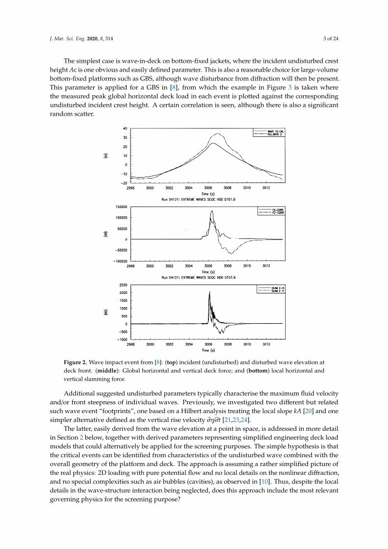
As one can read from these recommendations, standard industry tools are not fully capable ofpredicting such strongly nonlinear random wave-structure phenomena to a satisfactory level, andhydrodynamic model testing is generally needed (although some simplified formulations are givenin case test data are not available). A wave-in-deck model test study on a gravity-based structure(GBS) in extreme random waves is presented in [8], from which an illustrative example is shown inFigure 2. Here, typical time series samples of the wave elevation and resulting horizontal and verticalimpact loads are presented, for both global and local slamming forces. Furthermore, three different
J. Mar. Sci. Eng. 2020, 8, 314; doi:10.3390/jmse8050314 www.mdpi.com/journal/jmse
J. Mar. Sci. Eng. 2020, 8, 314 2 of 24
wave-in-deck experiments have recently been presented in [9–11] where also the corresponding wavecharacteristics as well as detailed complexities in the impact are addressed.
J. Mar. Sci. Eng. 2019, 7, x FOR PEER REVIEW 2 of 24
wave-in-deck experiments have recently been presented in [9–11] where also the corresponding wave characteristics as well as detailed complexities in the impact are addressed.
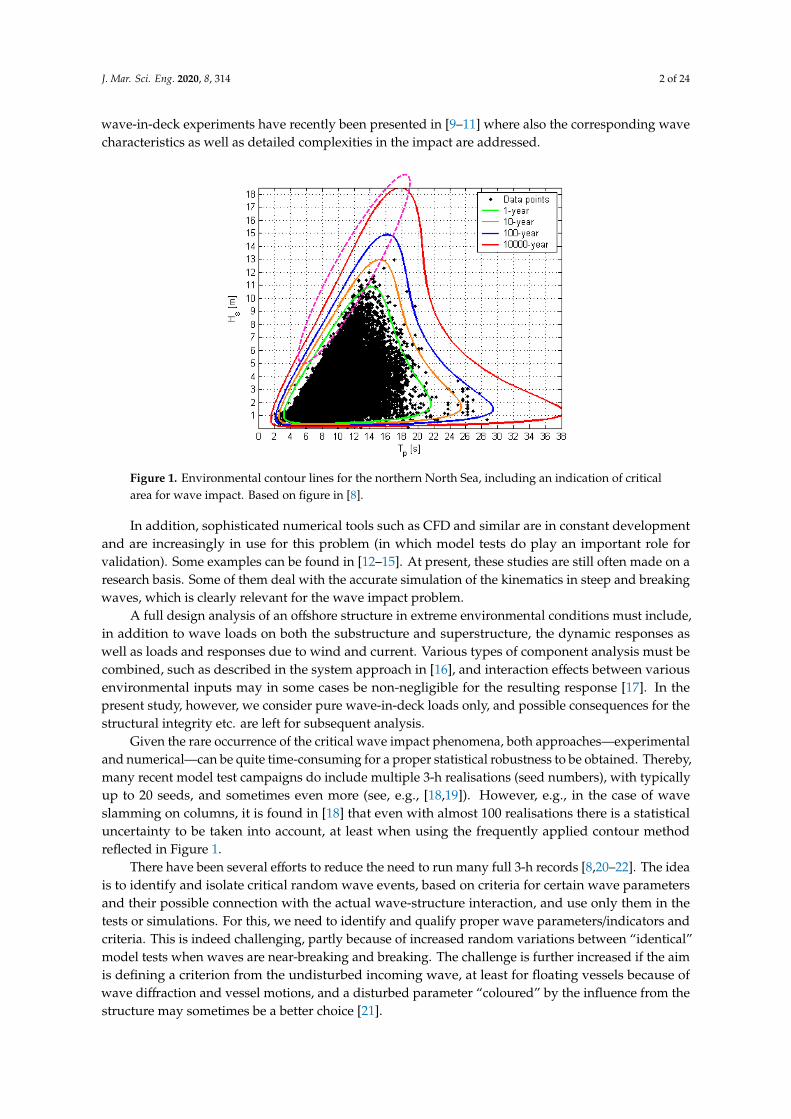
Figure 1. Environmental contour lines for the northern North Sea, including an indication of critical area for wave impact. Based on figure in [8].
Figure 2. Wave impact event from [8]: (top) incident (undisturbed) and disturbed wave elevation at deck front. (middle): Global horizontal and vertical deck force; and (bottom) local horizontal and vertical slamming force.
Figure 1. Environmental contour lines for the northern North Sea, including an indication of criticalarea for wave impact. Based on figure in [8].
In addition, sophisticated numerical tools such as CFD and similar are in constant developmentand are increasingly in use for this problem (in which model tests do play an important role forvalidation). Some examples can be found in [12–15]. At present, these studies are still often made on aresearch basis. Some of them deal with the accurate simulation of the kinematics in steep and breakingwaves, which is clearly relevant for the wave impact problem.
A full design analysis of an offshore structure in extreme environmental conditions must include,in addition to wave loads on both the substructure and superstructure, the dynamic responses aswell as loads and responses due to wind and current. Various types of component analysis must becombined, such as described in the system approach in [16], and interaction effects between variousenvironmental inputs may in some cases be non-negligible for the resulting response [17]. In thepresent study, however, we consider pure wave-in-deck loads only, and possible consequences for thestructural integrity etc. are left for subsequent analysis.
Given the rare occurrence of the critical wave impact phenomena, both approaches—experimentaland numerical—can be quite time-consuming for a proper statistical robustness to be obtained. Thereby,many recent model test campaigns do include multiple 3-h realisations (seed numbers), with typicallyup to 20 seeds, and sometimes even more (see, e.g., [18,19]). However, e.g., in the case of waveslamming on columns, it is found in [18] that even with almost 100 realisations there is a statisticaluncertainty to be taken into account, at least when using the frequently applied contour methodreflected in Figure 1.
There have been several efforts to reduce the need to run many full 3-h records [8,20–22]. The ideais to identify and isolate critical random wave events, based on criteria for certain wave parametersand their possible connection with the actual wave-structure interaction, and use only them in thetests or simulations. For this, we need to identify and qualify proper wave parameters/indicators andcriteria. This is indeed challenging, partly because of increased random variations between “identical”model tests when waves are near-breaking and breaking. The challenge is further increased if the aimis defining a criterion from the undisturbed incoming wave, at least for floating vessels because ofwave diffraction and vessel motions, and a disturbed parameter “coloured” by the influence from thestructure may sometimes be a better choice [21].
J. Mar. Sci. Eng. 2020, 8, 314 3 of 24
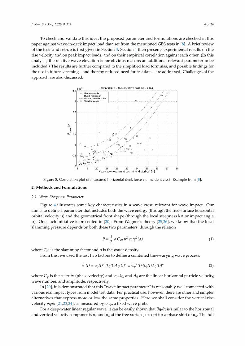
The simplest case is wave-in-deck on bottom-fixed jackets, where the incident undisturbed crestheight Ac is one obvious and easily defined parameter. This is also a reasonable choice for large-volumebottom-fixed platforms such as GBS, although wave disturbance from diffraction will then be present.This parameter is applied for a GBS in [8], from which the example in Figure 3 is taken wherethe measured peak global horizontal deck load in each event is plotted against the correspondingundisturbed incident crest height. A certain correlation is seen, although there is also a significantrandom scatter.
J. Mar. Sci. Eng. 2019, 7, x FOR PEER REVIEW 2 of 24
wave-in-deck experiments have recently been presented in [9–11] where also the corresponding wave characteristics as well as detailed complexities in the impact are addressed.
Figure 1. Environmental contour lines for the northern North Sea, including an indication of critical area for wave impact. Based on figure in [8].
Figure 2. Wave impact event from [8]: (top) incident (undisturbed) and disturbed wave elevation at deck front. (middle): Global horizontal and vertical deck force; and (bottom) local horizontal and vertical slamming force.
Figure 2. Wave impact event from [8]: (top) incident (undisturbed) and disturbed wave elevation atdeck front. (middle): Global horizontal and vertical deck force; and (bottom) local horizontal andvertical slamming force.
Additional suggested undisturbed parameters typically characterise the maximum fluid velocityand/or front steepness of individual waves. Previously, we investigated two different but relatedsuch wave event “footprints”, one based on a Hilbert analysis treating the local slope kA [20] and onesimpler alternative defined as the vertical rise velocity ∂η/∂t [21,23,24].
The latter, easily derived from the wave elevation at a point in space, is addressed in more detailin Section 2 below, together with derived parameters representing simplified engineering deck loadmodels that could alternatively be applied for the screening purposes. The simple hypothesis is thatthe critical events can be identified from characteristics of the undisturbed wave combined with theoverall geometry of the platform and deck. The approach is assuming a rather simplified picture ofthe real physics: 2D loading with pure potential flow and no local details on the nonlinear diffraction,and no special complexities such as air bubbles (cavities), as observed in [10]. Thus, despite the localdetails in the wave-structure interaction being neglected, does this approach include the most relevantgoverning physics for the screening purpose?
J. Mar. Sci. Eng. 2020, 8, 314 4 of 24
To check and validate this idea, the proposed parameter and formulations are checked in thispaper against wave-in-deck impact load data set from the mentioned GBS tests in [8]. A brief reviewof the tests and set-up is first given in Section 3. Section 4 then presents experimental results on therise velocity and on peak impact loads, and on their empirical correlation against each other. (In thisanalysis, the relative wave elevation is for obvious reasons an additional relevant parameter to beincluded.) The results are further compared to the simplified load formulas, and possible findings forthe use in future screening—and thereby reduced need for test data—are addressed. Challenges of theapproach are also discussed.
J. Mar. Sci. Eng. 2019, 7, x FOR PEER REVIEW 4 of 24
analysis, the relative wave elevation is for obvious reasons an additional relevant parameter to be included.) The results are further compared to the simplified load formulas, and possible findings for the use in future screening—and thereby reduced need for test data—are addressed. Challenges of the approach are also discussed.
Figure 3. Correlation plot of measured horizontal deck force vs. incident crest. Example from [8].
2. Methods and Formulations
2.1. Wave Steepness Parameter
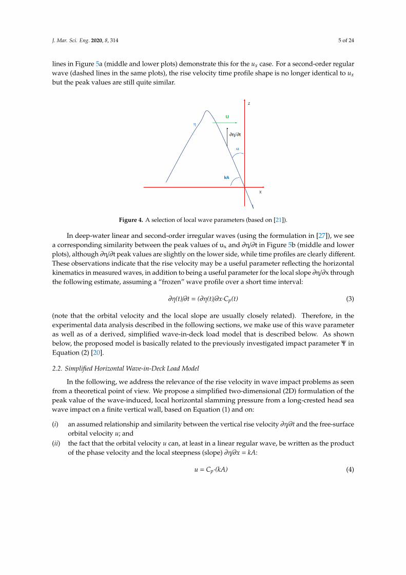
Figure 4 illustrates some key characteristics in a wave crest, relevant for wave impact. Our aim is to define a parameter that includes both the wave energy (through the free-surface horizontal orbital velocity u) and the geometrical front shape (through the local steepness kA or impact angle α). One such initiative is presented in [20]: From Wagner’s theory [25,26], we know that the local slamming pressure depends on both these two parameters, through the relation
P = ½ ρ Cs0 u2 cotg2(α) (1)
where Cs0 is the slamming factor and ρ is the water density. From this, we used the last two factors to define a combined time-varying wave process:
Ψ (t) = u0(t)2∙[k0(t)A0(t)]2 ≡ Cp2(t)∙[k0(t)A0(t)]4 (2)
where Cp is the celerity (phase velocity) and u0, k0, and A0 are the linear horizontal particle velocity, wave number, and amplitude, respectively.
In [20], it is demonstrated that this “wave impact parameter” is reasonably well connected with various real impact types from model test data. For practical use, however, there are other and simpler alternatives that express more or less the same properties. Here we shall consider the vertical rise velocity ∂η/∂t [21,23,24], as measured by, e.g., a fixed wave probe.
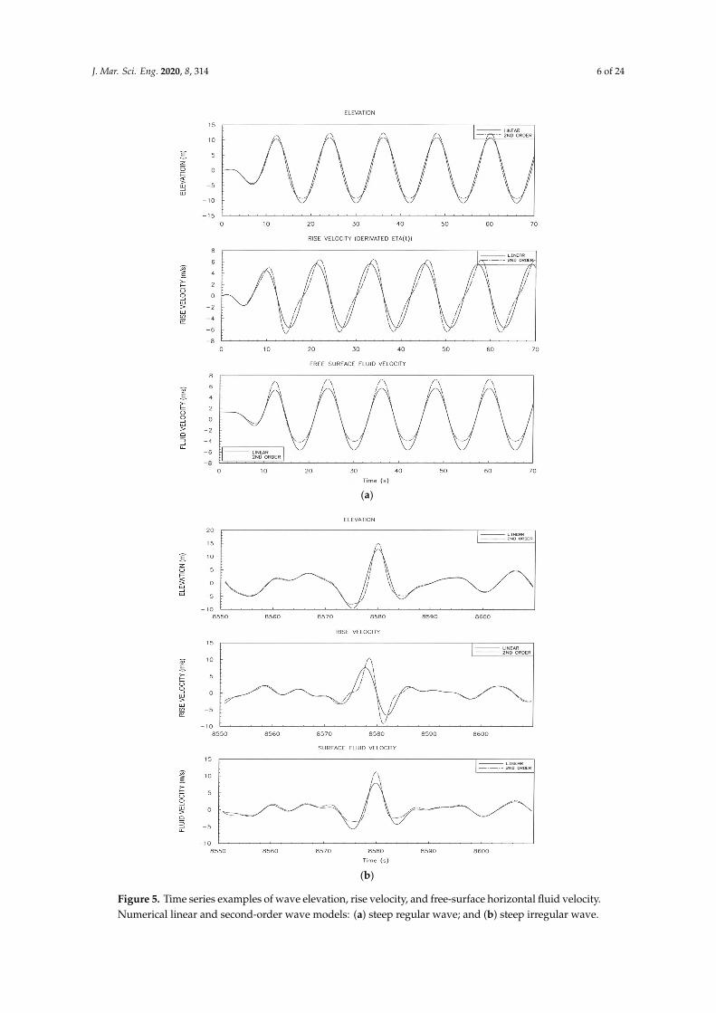
For a deep-water linear regular wave, it can be easily shown that ∂η/∂t is similar to the horizontal and vertical velocity components ux and uz at the free-surface, except for a phase shift of ux. The full lines in Figure 5a (middle and lower plots) demonstrate this for the ux case. For a second-order regular wave (dashed lines in the same plots), the rise velocity time profile shape is no longer identical to ux but the peak values are still quite similar.
Figure 3. Correlation plot of measured horizontal deck force vs. incident crest. Example from [8].
2. Methods and Formulations
2.1. Wave Steepness Parameter
Figure 4 illustrates some key characteristics in a wave crest, relevant for wave impact. Ouraim is to define a parameter that includes both the wave energy (through the free-surface horizontalorbital velocity u) and the geometrical front shape (through the local steepness kA or impact angleα). One such initiative is presented in [20]: From Wagner’s theory [25,26], we know that the localslamming pressure depends on both these two parameters, through the relation
P =12ρ Cs0 u2 cotg2(α) (1)
where Cs0 is the slamming factor and ρ is the water density.From this, we used the last two factors to define a combined time-varying wave process:
Ψ (t) = u0(t)2·[k0(t)A0(t)]2
≡ Cp2(t)·[k0(t)A0(t)]4 (2)
where Cp is the celerity (phase velocity) and u0, k0, and A0 are the linear horizontal particle velocity,wave number, and amplitude, respectively.
In [20], it is demonstrated that this “wave impact parameter” is reasonably well connected withvarious real impact types from model test data. For practical use, however, there are other and simpleralternatives that express more or less the same properties. Here we shall consider the vertical risevelocity ∂η/∂t [21,23,24], as measured by, e.g., a fixed wave probe.
For a deep-water linear regular wave, it can be easily shown that ∂η/∂t is similar to the horizontaland vertical velocity components ux and uz at the free-surface, except for a phase shift of ux. The full
J. Mar. Sci. Eng. 2020, 8, 314 5 of 24
lines in Figure 5a (middle and lower plots) demonstrate this for the ux case. For a second-order regularwave (dashed lines in the same plots), the rise velocity time profile shape is no longer identical to ux
but the peak values are still quite similar.J. Mar. Sci. Eng. 2019, 7, x FOR PEER REVIEW 5 of 24
Figure 4. A selection of local wave parameters (based on [21]).
In deep-water linear and second-order irregular waves (using the formulation in [27]), we see a corresponding similarity between the peak values of ux and ∂η/∂t in Figure 5b (middle and lower plots), although ∂η/∂t peak values are slightly on the lower side, while time profiles are clearly different. These observations indicate that the rise velocity may be a useful parameter reflecting the horizontal kinematics in measured waves, in addition to being a useful parameter for the local slope ∂η/∂x through the following estimate, assuming a “frozen” wave profile over a short time interval:
∂η(t)/∂t = (∂η(t)/∂x∙Cp(t) (3)
(note that the orbital velocity and the local slope are usually closely related). Therefore, in the experimental data analysis described in the following sections, we make use of this wave parameter as well as of a derived, simplified wave-in-deck load model that is described below. As shown below, the proposed model is basically related to the previously investigated impact parameter Ψ in Equation (2) [20].
Figure 4. A selection of local wave parameters (based on [21]).
In deep-water linear and second-order irregular waves (using the formulation in [27]), we seea corresponding similarity between the peak values of ux and ∂η/∂t in Figure 5b (middle and lowerplots), although ∂η/∂t peak values are slightly on the lower side, while time profiles are clearly different.These observations indicate that the rise velocity may be a useful parameter reflecting the horizontalkinematics in measured waves, in addition to being a useful parameter for the local slope ∂η/∂x throughthe following estimate, assuming a “frozen” wave profile over a short time interval:
∂η(t)/∂t = (∂η(t)/∂x·Cp(t) (3)
(note that the orbital velocity and the local slope are usually closely related). Therefore, in theexperimental data analysis described in the following sections, we make use of this wave parameteras well as of a derived, simplified wave-in-deck load model that is described below. As shownbelow, the proposed model is basically related to the previously investigated impact parameter Ψ inEquation (2) [20].
2.2. Simplified Horizontal Wave-in-Deck Load Model
In the following, we address the relevance of the rise velocity in wave impact problems as seenfrom a theoretical point of view. We propose a simplified two-dimensional (2D) formulation of thepeak value of the wave-induced, local horizontal slamming pressure from a long-crested head seawave impact on a finite vertical wall, based on Equation (1) and on:
(i) an assumed relationship and similarity between the vertical rise velocity ∂η/∂t and the free-surfaceorbital velocity u; and
(ii) the fact that the orbital velocity u can, at least in a linear regular wave, be written as the productof the phase velocity and the local steepness (slope) ∂η/∂x = kA:
u = Cp·(kA) (4)
J. Mar. Sci. Eng. 2020, 8, 314 6 of 24
J. Mar. Sci. Eng. 2019, 7, x FOR PEER REVIEW 6 of 24
(a)
(b)
Figure 5. Time series examples of wave elevation, rise velocity, and free-surface horizontal fluid velocity. Numerical linear and second-order wave models: (a) steep regular wave; and (b) steep irregular wave.
Figure 5. Time series examples of wave elevation, rise velocity, and free-surface horizontal fluid velocity.Numerical linear and second-order wave models: (a) steep regular wave; and (b) steep irregular wave.
J. Mar. Sci. Eng. 2020, 8, 314 7 of 24
Thereby, when we include also the hydrostatic pressure P0(h) = ρgh, where g is the acceleration ofgravity and h is the immersion depth at the time and point of observation, our suggested total localslamming pressure formula finally reads:
P(h) = ρgh +12ρ Cs0·[∂η/∂t]4/Cp
2 (5)
For the slamming coefficient Cs0, Wagner theory [25,26] gives:
Cs0 = (π/2)2 (6)
Note that here we assume no vertical variation in the slamming pressure contribution (thesecond term) from a given wave. This is certainly a simplification which we need to keep in mind.The formulation further assumes a 2D scenario, expressing the local impact based on the localcharacteristics of the long-crested incoming wave. This is also a simplification of the real world.There will certainly be additional 3D effects determined by the geometry of the structure. However,our hypothesis is that the formulation describes the main underlying physics, which can be usefulfor a quick analysis such as screening. The hypothesis is checked by experimental validation inSections 3 and 4.
The formulation in Equation (5) should at least be a reasonable choice for linear regular wavesand our suggestion is that it also works for any types of regular and irregular wave records, includingmodel test waves where nonlinear effects can be important. This extension from linear regular wavesto nonlinear irregular waves is of course not immediately obvious, but the logic behind the idea is thatthe slamming is defined by the square of the relative fluid velocity in combination with the relativeangle. Herein, we do not assume anything about linearity since both critical parameters are “bakedinto” the rise velocity formulation for both linear and nonlinear waves, thus we believe that it couldwork at least to some extent when properly calibrated against experimental data.
For the celerity Cp in an irregular sea state, one should ideally use the local time-varying velocityat the instant of the impact. However, this is often complex to estimate directly from measured records,and for simplicity we use here the celerity of the sea state spectral peak wave period, Tp.
As compared to the impact parameter of Equation (2), we see that the present one basicallyexpresses similar physics, but it is much simpler to use for measured waves, and it also representsdirect estimates of physical pressures.
In measured waves, local wave pressures expressed through Equations (1) and (5) will exhibitlarge horizontal and vertical spatial variations, partly due to local variations in the relative impact angleα (i.e., the local kA). For spatial averages over finite areas, which we in practice interpret to be typically~10 m2 and somewhat larger (full scale), DNV GL [7] recommends that, rather than Equation (1) thefollowing formula should be used:
P =12ρ Cs0’ u2 cotg1.1(α) (7)
where Cs0’ was slightly adjusted to 2.5 rather than (π/2)2. (Note that, for a quite steep nonlinear wavewith local slope 45 deg, Equations (1) and (7) give the same pressure results). Instead of Equation (5),we obtain then for the total spatially averaged pressure estimate:
P(h) =ρgh +12ρ Cs0’·[∂η/∂t]3.1/Cp
1.1 (8)
By integrating the pressure over the whole wetted area of a large platform deck wall, we alsoobtain an estimate of the global, horizontal deck impact force. However, over such a large (global) area,the above formulation is a too serious simplification. Local 3D variations in a steep wave impacting ona vertical structure lead to lower average pressure with increasing area. This is particularly the case forbreaking and near-breaking waves. The presence of a large-volume substructure will further enhance
J. Mar. Sci. Eng. 2020, 8, 314 8 of 24
3D spatial variation effects. Furthermore, from the definition of Equation (7) (from [7]), at least forangles α larger than 45 deg, it is reasonable to assume some vertical reduction in the upper parts ofthe slamming pressure contribution. Thereby, the use of the local expressions in both Equations (5)and (8) will likely be too conservative over a very large area. In the case with a large platform deck ofsize 50–100 m, we choose to compensate for this by proposing Equation (8) but now with a simplified,empirical overall reduction factor of 2.5 for the second (slamming) term (which is the most importantone). Thereby, we obtain the following for the spatially integrated horizontal force peak:
Fx = 1/2 ρgZD2L + 1/5 ρ ZD B Cs0’·[∂η/∂t]3.1/Cp
1.1 (9)
where B is the width of the wetted deck wall and ZD is the maximum wetted height at the lateraldeck centre, measured from the lower edge of the wall. However, we must keep in mind that thisarea approximation is certainly a simplified choice, and there are still uncertainties related withthis formulation being applied over a large platform deck full width. Again, the idea is that such aformulation for the global horizontal force can be useful for a fast and analytical check, e.g., for screeningof critical events in a sea state, and this is checked against experiments in the next sections. For detailedwave impact analysis, however, more accurate and detailed approaches should normally be used.
The impact load formulation in Equation (1), and thereby also our derived pressure and forceformulations in Equations (5) and (9), has clear apparent similarities to the well-known API simplesilhouette formula [5], although the latter is known as a drag formulation. In practical use, we see thatour formulation technically is related to a generalisation of the API formula, with the force coefficientin the latter replaced by Cs0 cotg2(α) (for the local pressure) and 0.4Cs0’ cotg1.1(α) (for the integratedforce over a very large deck wall). In addition, we also include a hydrostatic term.
Equations (5) and (9) both express a very strong sensitivity to the peak rise velocity. This supports,as shown by the experimental results, the idea that the slamming term is clearly the dominatingone in steep waves. It also means that the slamming forces will, as confirmed from many previousexperiences, exhibit a large random variability since the exact impact angle α and velocity ∂η/∂t canvary a lot locally for a steep wave impact on a wall. It can also vary between repeated experiments.
Since the present formulation is 2D, it assumes head-on waves. For oblique wave incidence (whichwill usually reduce the slamming loads), it must be generalised to include the effect of the relativewave direction, which we denote with θ. One possible rational approach for such cases would be toreplace the 2D impact angle α with the effective, increased 3D relative angle of the wave front surface,resulting from the combination of α and θ. This could be a matter for further work.
3. Experimental Test Case: Wave-in-Deck Loads on GBS
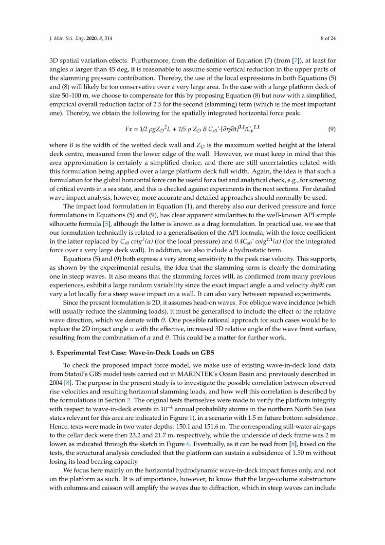
To check the proposed impact force model, we make use of existing wave-in-deck load datafrom Statoil’s GBS model tests carried out in MARINTEK’s Ocean Basin and previously described in2004 [8]. The purpose in the present study is to investigate the possible correlation between observedrise velocities and resulting horizontal slamming loads, and how well this correlation is described bythe formulations in Section 2. The original tests themselves were made to verify the platform integritywith respect to wave-in-deck events in 10−4 annual probability storms in the northern North Sea (seastates relevant for this area are indicated in Figure 1), in a scenario with 1.5 m future bottom subsidence.Hence, tests were made in two water depths: 150.1 and 151.6 m. The corresponding still-water air-gapsto the cellar deck were then 23.2 and 21.7 m, respectively, while the underside of deck frame was 2 mlower, as indicated through the sketch in Figure 6. Eventually, as it can be read from [8], based on thetests, the structural analysis concluded that the platform can sustain a subsidence of 1.50 m withoutlosing its load bearing capacity.
We focus here mainly on the horizontal hydrodynamic wave-in-deck impact forces only, and noton the platform as such. It is of importance, however, to know that the large-volume substructurewith columns and caisson will amplify the waves due to diffraction, which in steep waves can include
J. Mar. Sci. Eng. 2020, 8, 314 9 of 24
significant nonlinear contributions. The latter was investigated for these GBS tests in [8,28], and is alsobriefly addressed in Section 3.2.
J. Mar. Sci. Eng. 2019, 7, x FOR PEER REVIEW 9 of 24
still-water air-gaps to the cellar deck were then 23.2 and 21.7 m, respectively, while the underside of deck frame was 2 m lower, as indicated through the sketch in Figure 6. Eventually, as it can be read from [8], based on the tests, the structural analysis concluded that the platform can sustain a subsidence of 1.50 m without losing its load bearing capacity.
Figure 6. Schematic illustration of the GBS with key data, original condition (full scale) [8].
We focus here mainly on the horizontal hydrodynamic wave-in-deck impact forces only, and not on the platform as such. It is of importance, however, to know that the large-volume substructure with columns and caisson will amplify the waves due to diffraction, which in steep waves can include significant nonlinear contributions. The latter was investigated for these GBS tests in [8,28], and is also briefly addressed in Section 3.2.
3.1. Brief Review of Experiment
The model scale was 1:54. The whole model structure was rigidly bottom-mounted to a stiff tailor-made steel truss foundation. A set of force sensors mounted between the deck and the substructure columns measured six degrees of freedom (6 DOF) global deck forces at a sampling rate of 250 kHz (model scale). Horizontal and vertical local slamming forces were measured by 7.5 m2 stiff force panels at a sampling rate of 2 kHz. They were located at the lower part of the upwave cellar deck wall and under the cellar deck, respectively.
Here, we only address measured horizontal global and local loads; for the latter, we use data from one force panel at the horizontal centre of the wall just above the cellar deck level. We include results from tests in both 150.1 and 151.6 m water depths, in one heading only (0 deg).
The main tests, which are considered here, included one long-crested 10−4 irregular storm sea state, with Hs = 18.2 m and Tp = 17.0 s. Wave pre-calibration was done with 20 × 3-h (full scale) realisations to provide robust statistics. In the tests with the model installed, however, one used compressed wave records including only wave groups with high maximum crests A > 18 m (undisturbed). Such events occurred roughly around 2–3 times within a 3-h interval. More details on this approach are given in [8]. In addition, a set of regular waves were also run from which a few are selected for this presentation.
Waves were measured by conductance wave staffs at a sampling rate of 250 kHz. The derivation to obtain rise velocities from elevation was numerically processed by a frequency-domain low-pass filter at 15 Hz (model scale), which we chose as a reasonable compromise between keeping the signal noise level low and with most of the real velocity signal still remaining. The resulting peak velocity values are to some extent sensitive to the actual filter cut-off frequency. We found that a 20 Hz cut-off will typically increase the relevant peaks by an order of 5% (depending on the events), while 10 kHz
Figure 6. Schematic illustration of the GBS with key data, original condition (full scale) [8].
3.1. Brief Review of Experiment
The model scale was 1:54. The whole model structure was rigidly bottom-mounted to a stifftailor-made steel truss foundation. A set of force sensors mounted between the deck and the substructurecolumns measured six degrees of freedom (6 DOF) global deck forces at a sampling rate of 250 kHz(model scale). Horizontal and vertical local slamming forces were measured by 7.5 m2 stiff force panelsat a sampling rate of 2 kHz. They were located at the lower part of the upwave cellar deck wall andunder the cellar deck, respectively.
Here, we only address measured horizontal global and local loads; for the latter, we use data fromone force panel at the horizontal centre of the wall just above the cellar deck level. We include resultsfrom tests in both 150.1 and 151.6 m water depths, in one heading only (0 deg).
The main tests, which are considered here, included one long-crested 10−4 irregular storm sea state,with Hs = 18.2 m and Tp = 17.0 s. Wave pre-calibration was done with 20 × 3-h (full scale) realisationsto provide robust statistics. In the tests with the model installed, however, one used compressed waverecords including only wave groups with high maximum crests A > 18 m (undisturbed). Such eventsoccurred roughly around 2–3 times within a 3-h interval. More details on this approach are given in [8].In addition, a set of regular waves were also run from which a few are selected for this presentation.
Waves were measured by conductance wave staffs at a sampling rate of 250 kHz. The derivation toobtain rise velocities from elevation was numerically processed by a frequency-domain low-pass filterat 15 Hz (model scale), which we chose as a reasonable compromise between keeping the signal noiselevel low and with most of the real velocity signal still remaining. The resulting peak velocity valuesare to some extent sensitive to the actual filter cut-off frequency. We found that a 20 Hz cut-off willtypically increase the relevant peaks by an order of 5% (depending on the events), while 10 kHz reducesthem by typically 20%. Thereby, the resulting velocities are not considered as exact, unique values, butrather as approximate estimates, possibly slightly on the low side. The actual filter corresponds to alocal time-averaging within a time interval of roughly 0.4 s (full scale). For a consistent interpretation ofthe correlation against loads, it is important that all records are processed with exactly the same filter.
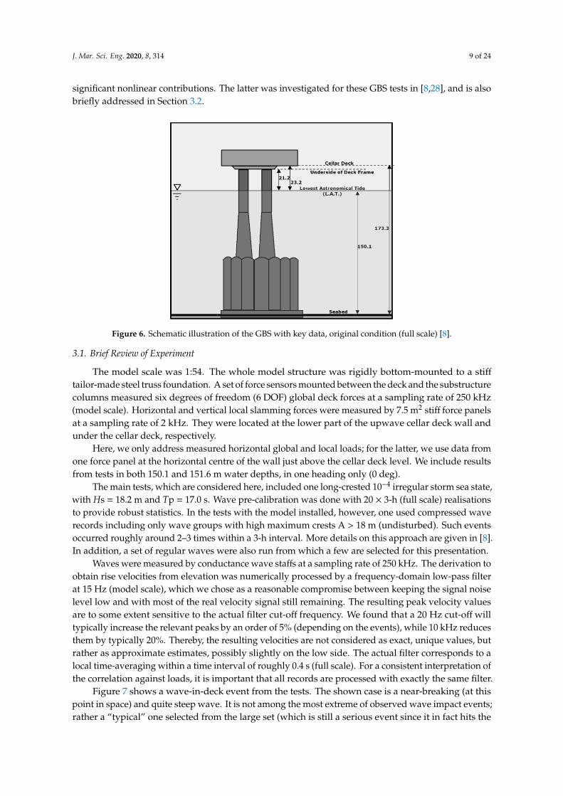
Figure 7 shows a wave-in-deck event from the tests. The shown case is a near-breaking (at thispoint in space) and quite steep wave. It is not among the most extreme of observed wave impact events;rather a “typical” one selected from the large set (which is still a serious event since it in fact hits the
J. Mar. Sci. Eng. 2020, 8, 314 10 of 24
deck). Initially, it reached only slightly higher than the cellar deck, but when it hits the lower part ofthe deck a tongue of green water is seen upwelling on the wall, leading to a significant horizontal deckload. In the most severe events wave breaking also occurred.
J. Mar. Sci. Eng. 2019, 7, x FOR PEER REVIEW 10 of 24
reduces them by typically 20%. Thereby, the resulting velocities are not considered as exact, unique values, but rather as approximate estimates, possibly slightly on the low side. The actual filter corresponds to a local time-averaging within a time interval of roughly 0.4 s (full scale). For a consistent interpretation of the correlation against loads, it is important that all records are processed with exactly the same filter.
Figure 7 shows a wave-in-deck event from the tests. The shown case is a near-breaking (at this point in space) and quite steep wave. It is not among the most extreme of observed wave impact events; rather a “typical” one selected from the large set (which is still a serious event since it in fact hits the deck). Initially, it reached only slightly higher than the cellar deck, but when it hits the lower part of the deck a tongue of green water is seen upwelling on the wall, leading to a significant horizontal deck load. In the most severe events wave breaking also occurred.
Figure 7. Frozen video frame with random wave impact event on GBS deck. Calibrated wave inserted left.
3.2. Practical Use of Slamming Load Formulation
We need to establish the proper practical parameters for the application of the slamming formulation expressed in Section 2.2, for this platform case. Thereby, for each impact event, values are determined for the maximum local immersion depth h in the local hydrostatic pressure of Equation (5), and for the maximum wetted height ZD in the integrated force of Equation (9).
For the immersion depth h, we choose to define it from the centre of the 7.5-m2 slamming force panel and up to the maximum amplified (diffracted) crest height AD during the event. We stipulate this centre, which we define as a zero level for our calculation, to be 2 m above the cellar deck level, i.e. at 25.2- and 23.7-m levels for the two water depths of 150.1 and 151.6 m, respectively.
For the wetted wall height ZD, we define it from the bottom of the girders that reach 2 m below the cellar deck (see Figures 7 and 8), i.e. at 21.2 and 19.7 m, respectively, for the two water depths, and up to the maximum amplified crest height AD. The deck width B is 83.6 m.
The amplified crest height AD, as measured from the still sea level, is a result of the incident crest height AW in combination with global diffraction from the substructure (columns and caisson) and a local upwell amplification effect due to the deck impact, as observed in Figure 6. Measured AD are in fact available from relative wave probes in front of the wall, but we rather choose to use a simplified calculation of AD here, which can be used directly on the incident wave record without any pre-knowledge from the actual platform model tests, as follows: Supported by the empirical formula for amplification near columns presented in [29], we suggest AD = 1.33⋅AW in the present application.
Figure 7. Frozen video frame with random wave impact event on GBS deck. Calibrated waveinserted left.
3.2. Practical Use of Slamming Load Formulation
We need to establish the proper practical parameters for the application of the slammingformulation expressed in Section 2.2, for this platform case. Thereby, for each impact event, values aredetermined for the maximum local immersion depth h in the local hydrostatic pressure of Equation (5),and for the maximum wetted height ZD in the integrated force of Equation (9).
For the immersion depth h, we choose to define it from the centre of the 7.5-m2 slamming forcepanel and up to the maximum amplified (diffracted) crest height AD during the event. We stipulatethis centre, which we define as a zero level for our calculation, to be 2 m above the cellar deck level, i.e.,at 25.2- and 23.7-m levels for the two water depths of 150.1 and 151.6 m, respectively.
For the wetted wall height ZD, we define it from the bottom of the girders that reach 2 m belowthe cellar deck (see Figures 7 and 8), i.e., at 21.2 and 19.7 m, respectively, for the two water depths, andup to the maximum amplified crest height AD. The deck width B is 83.6 m.
The amplified crest height AD, as measured from the still sea level, is a result of the incidentcrest height AW in combination with global diffraction from the substructure (columns and caisson)and a local upwell amplification effect due to the deck impact, as observed in Figure 6. MeasuredAD are in fact available from relative wave probes in front of the wall, but we rather choose to use asimplified calculation of AD here, which can be used directly on the incident wave record without anypre-knowledge from the actual platform model tests, as follows: Supported by the empirical formulafor amplification near columns presented in [29], we suggest AD = 1.33·AW in the present application.This includes both linear and nonlinear diffraction contributions, and is an average factor applied overthe full deck width; in reality it is highest in the centre and decreases to the sides.
This factor choice agrees roughly with findings in steep regular waves previously published fromthis case in [8,28], indicating amplification factors of around 1.2–1.4 due to columns and caisson. Wealso found it to be similar to actual observed factors in the present irregular waves, except for thehighest and steepest waves hitting the deck where it is slightly non-conservative at the lateral centredue to the local upwell on the wall. We should keep this in mind, but there is an uncertainty about
J. Mar. Sci. Eng. 2020, 8, 314 11 of 24
the relevant water height at the very peak of the measured water level on the deck wall in such cases,with the probe close to the wall, and we should also note that our present theoretical model is a clearlysimplified one with several other assumptions as well. In any case, we believe that our choice overallreflects the governing physics of the phenomenon.
J. Mar. Sci. Eng. 2019, 7, x FOR PEER REVIEW 11 of 24
This includes both linear and nonlinear diffraction contributions, and is an average factor applied over the full deck width; in reality it is highest in the centre and decreases to the sides.
This factor choice agrees roughly with findings in steep regular waves previously published from this case in [8,28], indicating amplification factors of around 1.2–1.4 due to columns and caisson. We also found it to be similar to actual observed factors in the present irregular waves, except for the highest and steepest waves hitting the deck where it is slightly non-conservative at the lateral centre due to the local upwell on the wall. We should keep this in mind, but there is an uncertainty about the relevant water height at the very peak of the measured water level on the deck wall in such cases, with the probe close to the wall, and we should also note that our present theoretical model is a clearly simplified one with several other assumptions as well. In any case, we believe that our choice overall reflects the governing physics of the phenomenon.
Thereby, 18- and 19.5-m incident crest heights will reach 24 and 25.5 m, respectively, which are just above the force panel centre in the two different water depth cases of 151. and 150.1 m. Similarly, 15- and 16.5-m incident crest heights will reach to 20 and 21.5 m, respectively, which are just above the girder bottoms in the two cases.
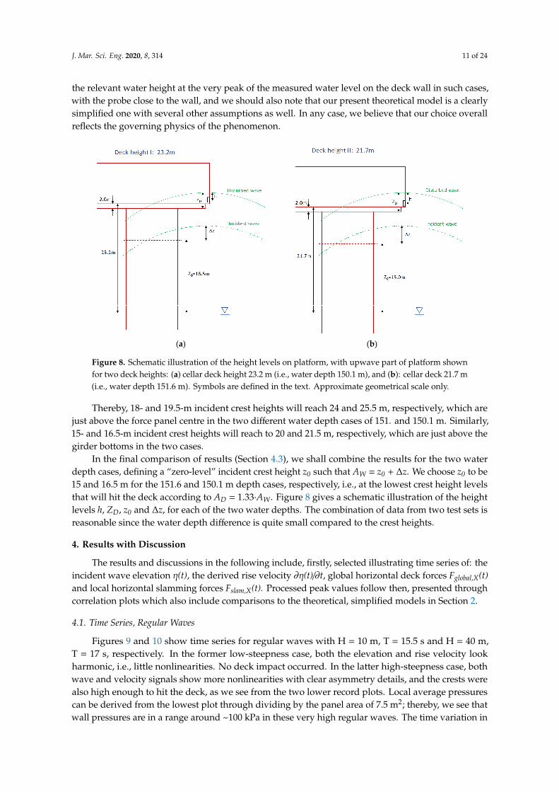
In the final comparison of results (Section 4.3), we shall combine the results for the two water depth cases, defining a “zero-level” incident crest height z0 such that AW = z0 + Δz. We choose z0 to be 15 and 16.5 m for the 151.6 and 150.1 m depth cases, respectively, i.e. at the lowest crest height levels that will hit the deck according to AD = 1.33⋅AW. Figure 8 gives a schematic illustration of the height levels h, ZD, z0 and Δz, for each of the two water depths. The combination of data from two test sets is reasonable since the water depth difference is quite small compared to the crest heights.
(a) (b)
Figure 8. Schematic illustration of the height levels on platform, with upwave part of platform shown for two deck heights: (a) cellar deck height 23.2m (i.e. water depth 150.1m), and (b): cellar deck 21.7m (i.e. water depth 151.6m). Symbols are defined in the text. Approximate geometrical scale only.
4. Results with Discussion
The results and discussions in the following include, firstly, selected illustrating time series of: the incident wave elevation η(t), the derived rise velocity ∂η(t)/∂t, global horizontal deck forces Fglobal,X(t) and local horizontal slamming forces Fslam,X(t). Processed peak values follow then, presented through correlation plots which also include comparisons to the theoretical, simplified models in Section 2.
4.1. Time Series, Regular Waves
Figure 8. Schematic illustration of the height levels on platform, with upwave part of platform shownfor two deck heights: (a) cellar deck height 23.2 m (i.e., water depth 150.1 m), and (b): cellar deck 21.7 m(i.e., water depth 151.6 m). Symbols are defined in the text. Approximate geometrical scale only.
Thereby, 18- and 19.5-m incident crest heights will reach 24 and 25.5 m, respectively, which arejust above the force panel centre in the two different water depth cases of 151. and 150.1 m. Similarly,15- and 16.5-m incident crest heights will reach to 20 and 21.5 m, respectively, which are just above thegirder bottoms in the two cases.
In the final comparison of results (Section 4.3), we shall combine the results for the two waterdepth cases, defining a “zero-level” incident crest height z0 such that AW = z0 + ∆z. We choose z0 to be15 and 16.5 m for the 151.6 and 150.1 m depth cases, respectively, i.e., at the lowest crest height levelsthat will hit the deck according to AD = 1.33·AW. Figure 8 gives a schematic illustration of the heightlevels h, ZD, z0 and ∆z, for each of the two water depths. The combination of data from two test sets isreasonable since the water depth difference is quite small compared to the crest heights.
4. Results with Discussion
The results and discussions in the following include, firstly, selected illustrating time series of: theincident wave elevation η(t), the derived rise velocity ∂η(t)/∂t, global horizontal deck forces Fglobal,X(t)and local horizontal slamming forces Fslam,X(t). Processed peak values follow then, presented throughcorrelation plots which also include comparisons to the theoretical, simplified models in Section 2.
4.1. Time Series, Regular Waves
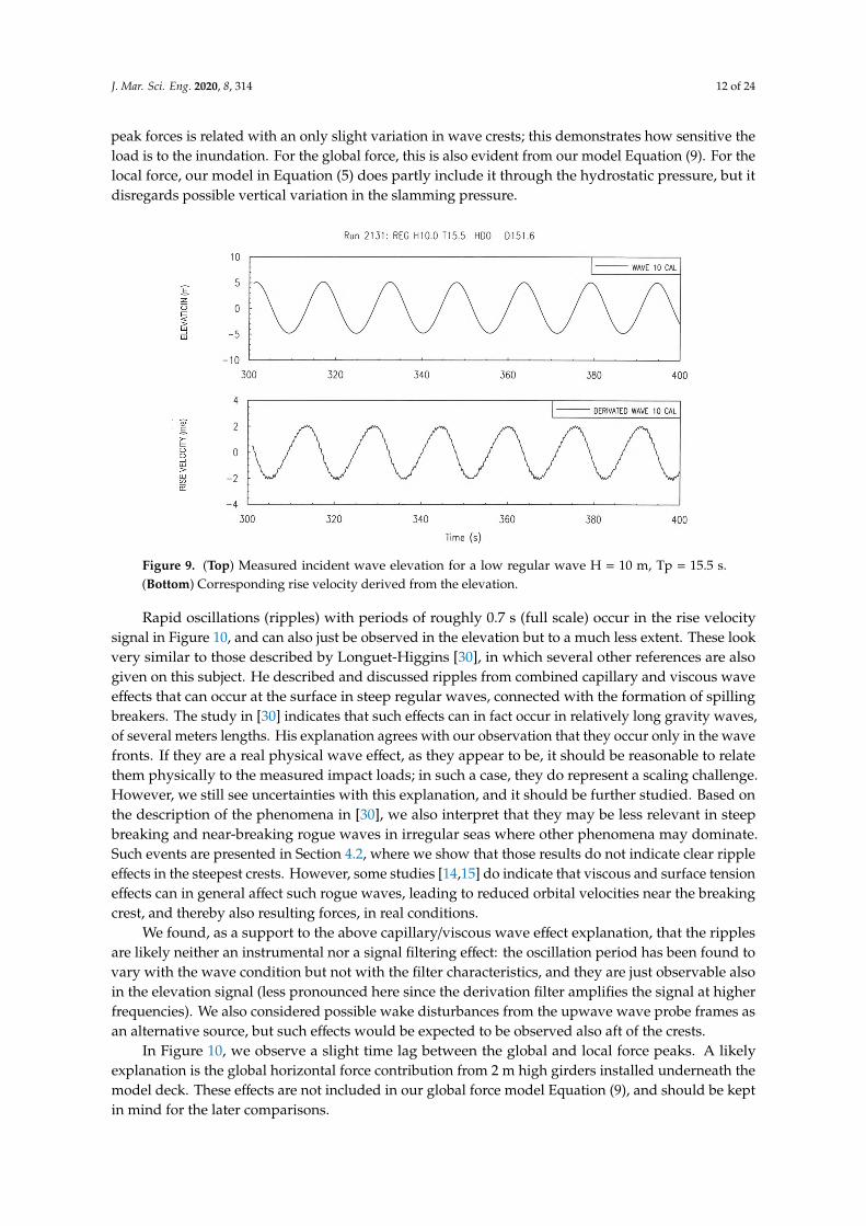
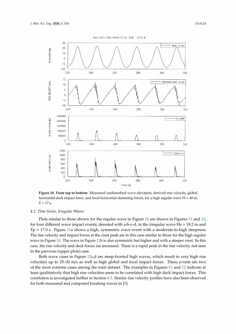
Figures 9 and 10 show time series for regular waves with H = 10 m, T = 15.5 s and H = 40 m,T = 17 s, respectively. In the former low-steepness case, both the elevation and rise velocity lookharmonic, i.e., little nonlinearities. No deck impact occurred. In the latter high-steepness case, bothwave and velocity signals show more nonlinearities with clear asymmetry details, and the crests werealso high enough to hit the deck, as we see from the two lower record plots. Local average pressurescan be derived from the lowest plot through dividing by the panel area of 7.5 m2; thereby, we see thatwall pressures are in a range around ~100 kPa in these very high regular waves. The time variation in
J. Mar. Sci. Eng. 2020, 8, 314 12 of 24
peak forces is related with an only slight variation in wave crests; this demonstrates how sensitive theload is to the inundation. For the global force, this is also evident from our model Equation (9). For thelocal force, our model in Equation (5) does partly include it through the hydrostatic pressure, but itdisregards possible vertical variation in the slamming pressure.
J. Mar. Sci. Eng. 2019, 7, x FOR PEER REVIEW 12 of 24
Figures 9 and 10 show time series for regular waves with H = 10 m, T = 15.5 s and H = 40 m, T = 17 s, respectively. In the former low-steepness case, both the elevation and rise velocity look harmonic, i.e. little nonlinearities. No deck impact occurred. In the latter high-steepness case, both wave and velocity signals show more nonlinearities with clear asymmetry details, and the crests were also high enough to hit the deck, as we see from the two lower record plots. Local average pressures can be derived from the lowest plot through dividing by the panel area of 7.5 m2; thereby, we see that wall pressures are in a range around ∼100 kPa in these very high regular waves. The time variation in peak forces is related with an only slight variation in wave crests; this demonstrates how sensitive the load is to the inundation. For the global force, this is also evident from our model Equation (9). For the local force, our model in Equation (5) does partly include it through the hydrostatic pressure, but it disregards possible vertical variation in the slamming pressure.
Rapid oscillations (ripples) with periods of roughly 0.7 s (full scale) occur in the rise velocity signal in Figure 10, and can also just be observed in the elevation but to a much less extent. These look very similar to those described by Longuet-Higgins [30], in which several other references are also given on this subject. He described and discussed ripples from combined capillary and viscous wave effects that can occur at the surface in steep regular waves, connected with the formation of spilling breakers. The study in [30] indicates that such effects can in fact occur in relatively long
Figure 9. (Top): Measured incident wave elevation for a low regular wave H = 10 m, Tp = 15.5 s. (Bottom): Corresponding rise velocity derived from the elevation.
Figure 9. (Top) Measured incident wave elevation for a low regular wave H = 10 m, Tp = 15.5 s.(Bottom) Corresponding rise velocity derived from the elevation.
Rapid oscillations (ripples) with periods of roughly 0.7 s (full scale) occur in the rise velocitysignal in Figure 10, and can also just be observed in the elevation but to a much less extent. These lookvery similar to those described by Longuet-Higgins [30], in which several other references are alsogiven on this subject. He described and discussed ripples from combined capillary and viscous waveeffects that can occur at the surface in steep regular waves, connected with the formation of spillingbreakers. The study in [30] indicates that such effects can in fact occur in relatively long gravity waves,of several meters lengths. His explanation agrees with our observation that they occur only in the wavefronts. If they are a real physical wave effect, as they appear to be, it should be reasonable to relatethem physically to the measured impact loads; in such a case, they do represent a scaling challenge.However, we still see uncertainties with this explanation, and it should be further studied. Based onthe description of the phenomena in [30], we also interpret that they may be less relevant in steepbreaking and near-breaking rogue waves in irregular seas where other phenomena may dominate.Such events are presented in Section 4.2, where we show that those results do not indicate clear rippleeffects in the steepest crests. However, some studies [14,15] do indicate that viscous and surface tensioneffects can in general affect such rogue waves, leading to reduced orbital velocities near the breakingcrest, and thereby also resulting forces, in real conditions.
We found, as a support to the above capillary/viscous wave effect explanation, that the ripplesare likely neither an instrumental nor a signal filtering effect: the oscillation period has been found tovary with the wave condition but not with the filter characteristics, and they are just observable alsoin the elevation signal (less pronounced here since the derivation filter amplifies the signal at higherfrequencies). We also considered possible wake disturbances from the upwave wave probe frames asan alternative source, but such effects would be expected to be observed also aft of the crests.
In Figure 10, we observe a slight time lag between the global and local force peaks. A likelyexplanation is the global horizontal force contribution from 2 m high girders installed underneath themodel deck. These effects are not included in our global force model Equation (9), and should be keptin mind for the later comparisons.
J. Mar. Sci. Eng. 2020, 8, 314 13 of 24
J. Mar. Sci. Eng. 2019, 7, x FOR PEER REVIEW 13 of 24
Figure 10. From top to bottom: Measured undisturbed wave elevation, derived rise velocity, global horizontal deck impact force, and local horizontal slamming forces, for a high regular wave H = 40 m, T = 17 s.
gravity waves, of several meters lengths. His explanation agrees with our observation that they occur only in the wave fronts. If they are a real physical wave effect, as they appear to be, it should be reasonable to relate them physically to the measured impact loads; in such a case, they do represent a scaling challenge. However, we still see uncertainties with this explanation, and it should be further studied. Based on the description of the phenomena in [30], we also interpret that they may be less relevant in steep breaking and near-breaking rogue waves in irregular seas where other phenomena may dominate. Such events are presented in Section 4.2, where we show that those results do not indicate clear ripple effects in the steepest crests. However, some studies [14,15] do indicate that viscous and surface tension effects can in general affect such rogue waves, leading to reduced orbital velocities near the breaking crest, and thereby also resulting forces, in real conditions.
We found, as a support to the above capillary/viscous wave effect explanation, that the ripples are likely neither an instrumental nor a signal filtering effect: the oscillation period has been found to vary with the wave condition but not with the filter characteristics, and they are just observable also in the elevation signal (less pronounced here since the derivation filter amplifies the signal at higher frequencies). We also considered possible wake disturbances from the upwave wave probe frames as an alternative source, but such effects would be expected to be observed also aft of the crests.
In Figure 10, we observe a slight time lag between the global and local force peaks. A likely explanation is the global horizontal force contribution from 2 m high girders installed underneath the model deck. These effects are not included in our global force model Equation (9), and should be kept in mind for the later comparisons.
Figure 10. From top to bottom: Measured undisturbed wave elevation, derived rise velocity, globalhorizontal deck impact force, and local horizontal slamming forces, for a high regular wave H = 40 m,T = 17 s.
4.2. Time Series, Irregular Waves
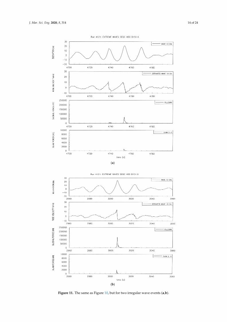
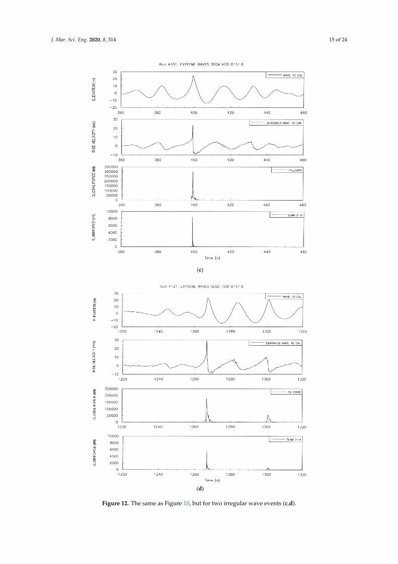
Plots similar to those shown for the regular wave in Figure 10 are shown in Figures 11 and 12,for four different wave impact events, denoted with a-b-c-d, in the irregular wave Hs = 18.2 m andTp = 17.0 s. Figure 11a shows a high, symmetric wave event with a moderate-to-high steepness.The rise velocity and impact forces at the crest peak are in this case similar to those for the high regularwave in Figure 10. The wave in Figure 11b is also symmetric but higher and with a steeper crest. In thiscase, the rise velocity and deck forces are increased. There is a rapid peak in the rise velocity, not seenin the previous (upper plots) case.
Both wave cases in Figure 12c,d are steep-fronted high waves, which result in very high risevelocities up to 25–30 m/s as well as high global and local impact forces. These events are twoof the most extreme cases among the total dataset. The examples in Figures 11 and 12 indicate atleast qualitatively that high rise velocities seem to be correlated with high deck impact forces. Thiscorrelation is investigated further in Section 4.3. Similar rise velocity profiles have also been observedfor both measured and computed breaking waves in [8].
J. Mar. Sci. Eng. 2020, 8, 314 14 of 24
J. Mar. Sci. Eng. 2019, 7, x FOR PEER REVIEW 15 of 24
(a)
(b)
Figure 11. The same as Figure 10, but for two irregular wave events (a,b). Figure 11. The same as Figure 10, but for two irregular wave events (a,b).
J. Mar. Sci. Eng. 2020, 8, 314 15 of 24
J. Mar. Sci. Eng. 2019, 7, x FOR PEER REVIEW 16 of 24
(c)
(d)
Figure 12. The same as Figure 10, but for two irregular wave events (c,d). Figure 12. The same as Figure 10, but for two irregular wave events (c,d).
J. Mar. Sci. Eng. 2020, 8, 314 16 of 24
Furthermore, the two waves in Figure 12 are probably breaking near the platform, although themaximum impact pressures from a breaking wave, which can be many MPa in such sea states [3,18,31],hits at lower positions than the present deck, e.g., on columns. In the present problem, the deck is hitby the upper crest peak of the wave (see Figure 7) where the pressure is somewhat lower. The presentlocal slamming panel forces indicate around 1 and 0.5 MPa, respectively, in these two extreme cases.Pressures are found from dividing the panel force by the panel area 7.5 m2.
For the latter two cases we observe peak rise velocities in the range 25–30 m/s. This is slightlyhigher than the corresponding phase velocity Cp (≈ 20 m/s) as observed from two neighbouring wavestaffs. (Note that for the 17 s regular waves, Cp was ≈ 24 m/s). This velocity, and also the ratio ≈ 1.3to Cp, is fairly similar to maximum orbital velocities observed experimentally and numerically forbreaking waves in [31]. Similar findings are presented in [32], where it is also argued a similaritybetween the incident orbital velocity and run-up velocities on a column in breaking waves. This is anindication that our expected relation between the rise velocity and the orbital velocity is a reasonableassumption also in such high nonlinear waves. The ratio 1.3 is close to 1.2, as recommended forbreaking waves by DNV GL [7], as well as to 1.35, as mentioned in [32].
As mentioned above, the exact magnitudes of the peak rise velocities in Figure 12 are somewhatsensitive to the low-pass filter used during the derivation from the original elevation record. Thereby,some uncertainty in the order of 5% should be considered regarding absolute magnitudes. However,since the same filter, with the same related uncertainty, has been used for all events, results for differentevents can be compared directly, and the uncertainty is therefore not crucial in the study of correlationagainst loads.
4.3. Correlation of Deck Loads Against Wave Parameters and Theoretical Estimates
One basic aim of this study was to check how well the use of the measured rise velocity, throughour simple derived theoretical wave impact load models of Equations (5) and (9), compare to themeasured impact loads. Ideally, an event-by-event correlation between measurement and theorywould be helpful in this. However, we found that, due to significant random variability, such a directcorrelation is not meaningful for the random steep wave events in steep irregular waves, and analternative presentation approach is applied (see the paragraphs below). This large random variabilityin wave slamming loads is quite well known and was expected. For the regular wave tests, however,the impact loads exhibit less random variations.
4.3.1. Regular Waves
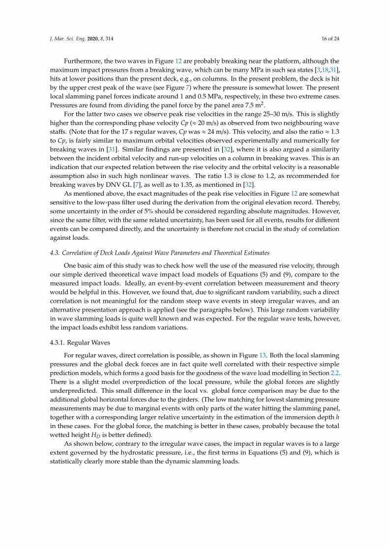
For regular waves, direct correlation is possible, as shown in Figure 13. Both the local slammingpressures and the global deck forces are in fact quite well correlated with their respective simpleprediction models, which forms a good basis for the goodness of the wave load modelling in Section 2.2.There is a slight model overprediction of the local pressure, while the global forces are slightlyunderpredicted. This small difference in the local vs. global force comparison may be due to theadditional global horizontal forces due to the girders. (The low matching for lowest slamming pressuremeasurements may be due to marginal events with only parts of the water hitting the slamming panel,together with a corresponding larger relative uncertainty in the estimation of the immersion depth hin these cases. For the global force, the matching is better in these cases, probably because the totalwetted height HD is better defined).
As shown below, contrary to the irregular wave cases, the impact in regular waves is to a largeextent governed by the hydrostatic pressure, i.e., the first terms in Equations (5) and (9), which isstatistically clearly more stable than the dynamic slamming loads.
J. Mar. Sci. Eng. 2020, 8, 314 17 of 24
J. Mar. Sci. Eng. 2019, 7, x FOR PEER REVIEW 17 of 24
As mentioned above, the exact magnitudes of the peak rise velocities in Figure 12 are somewhat sensitive to the low-pass filter used during the derivation from the original elevation record. Thereby, some uncertainty in the order of 5% should be considered regarding absolute magnitudes. However, since the same filter, with the same related uncertainty, has been used for all events, results for different events can be compared directly, and the uncertainty is therefore not crucial in the study of correlation against loads.
4.3. Correlation of Deck Loads Against Wave Parameters and Theoretical Estimates
One basic aim of this study was to check how well the use of the measured rise velocity, through our simple derived theoretical wave impact load models of Equations (5) and (9), compare to the measured impact loads. Ideally, an event-by-event correlation between measurement and theory would be helpful in this. However, we found that, due to significant random variability, such a direct correlation is not meaningful for the random steep wave events in steep irregular waves, and an alternative presentation approach is applied (see the paragraphs below). This large random variability in wave slamming loads is quite well known and was expected. For the regular wave tests, however, the impact loads exhibit less random variations.
4.3.1. Regular Waves
For regular waves, direct correlation is possible, as shown in Figure 13. Both the local slamming pressures and the global deck forces are in fact quite well correlated with their respective simple prediction models, which forms a good basis for the goodness of the wave load modelling in Section 2.2. There is a slight model overprediction of the local pressure, while the global forces are slightly underpredicted. This small difference in the local vs. global force comparison may be due to the additional global horizontal forces due to the girders. (The low matching for lowest slamming pressure measurements may be due to marginal events with only parts of the water hitting the slamming panel, together with a corresponding larger relative uncertainty in the estimation of the immersion depth h in these cases. For the global force, the matching is better in these cases, probably because the total wetted height HD is better defined).
0
20
40
60
80
100
120
140
0 20 40 60 80 100 120 140
Mea
sure
d sla
m P
ress
ure
[kPa
]
model prediction slam pressure [kPa]
Measured vs. predicted local horizontal slam pressure, regular waves
J. Mar. Sci. Eng. 2019, 7, x FOR PEER REVIEW 18 of 24
Figure 13. Correlation between measured deck impact load peaks and model predictions, regular waves: (top) local horizontal slamming pressure; and (bottom) global horizontal force.
As shown below, contrary to the irregular wave cases, the impact in regular waves is to a large extent governed by the hydrostatic pressure, i.e. the first terms in Equations (5) and (9), which is statistically clearly more stable than the dynamic slamming loads.
4.3.2. Irregular Waves
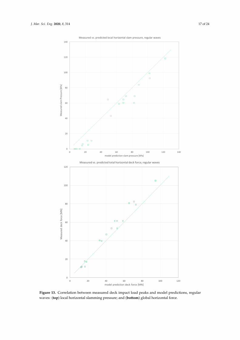
The main results from the irregular waves are presented in a different way in Figures 14 and 15. Here, the measured horizontal impact load peaks from the total dataset are, instead, correlated against the corresponding incident crest peaks, and at the same time compared to corresponding theoretical results based on the incident crests combined with Equations (5) and (9). This presentation approach is an extension of the simple correlation type of plot in Figure 3 and other similar plots in [8], with the aim to also highlight the influence from the peak rise velocity, i.e. local steepness combined with the near-surface orbital velocity.
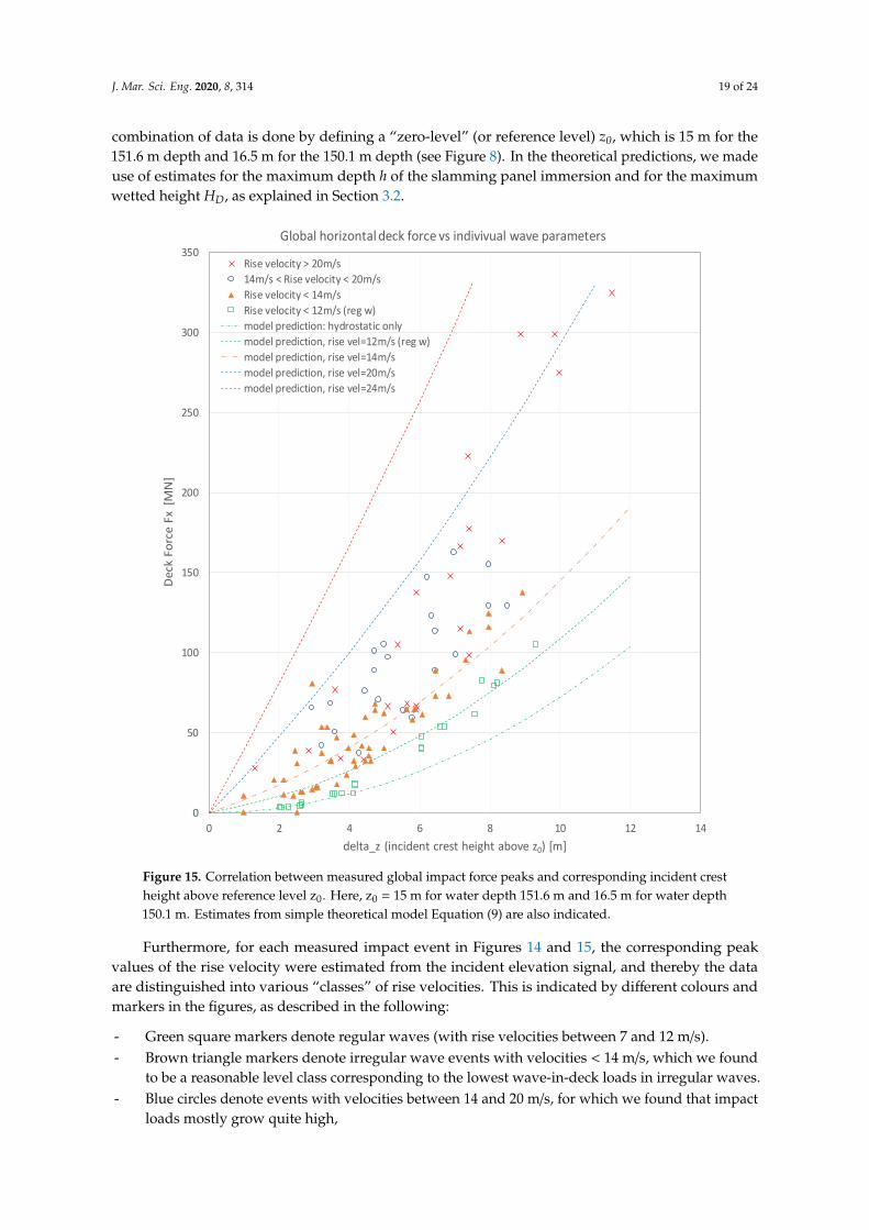
While Figure 14 shows the local slamming pressure from the 7.5-m2 slamming force panel on the lower deck front, Figure 15 shows the global (integrated) deck forces. As explained and argued at the end of Section 3.2, the results in each of the two figures include data from testing in two different water depth, namely 150.1 and 151.6 m, respectively, to obtain one larger dataset instead of two. The combination of data is done by defining a “zero-level” (or reference level) z0, which is 15 m for the 151.6 m depth and 16.5 m for the 150.1 m depth (see Figure 8). In the theoretical predictions, we made use of estimates for the maximum depth h of the slamming panel immersion and for the maximum wetted height HD, as explained in Section 3.2.
Furthermore, for each measured impact event in Figures 14 and 15, the corresponding peak values of the rise velocity were estimated from the incident elevation signal, and thereby the data are distinguished into various “classes” of rise velocities. This is indicated by different colours and markers in the figures, as described in the following:
- Green square markers denote regular waves (with rise velocities between 7 and 12 m/s).
0
20
40
60
80
100
120
0 20 40 60 80 100 120
Mea
sure
d de
ck fo
rce
[MN]
model prediction deck force [MN]
Measured vs. predicted total horizontal deck force, regular waves
Figure 13. Correlation between measured deck impact load peaks and model predictions, regularwaves: (top) local horizontal slamming pressure; and (bottom) global horizontal force.
J. Mar. Sci. Eng. 2020, 8, 314 18 of 24
4.3.2. Irregular Waves
The main results from the irregular waves are presented in a different way in Figures 14 and 15.Here, the measured horizontal impact load peaks from the total dataset are, instead, correlated againstthe corresponding incident crest peaks, and at the same time compared to corresponding theoreticalresults based on the incident crests combined with Equations (5) and (9). This presentation approach isan extension of the simple correlation type of plot in Figure 3 and other similar plots in [8], with theaim to also highlight the influence from the peak rise velocity, i.e., local steepness combined with thenear-surface orbital velocity.
J. Mar. Sci. Eng. 2019, 7, x FOR PEER REVIEW 19 of 24
- Brown triangle markers denote irregular wave events with velocities < 14 m/s, which we found to be a reasonable level class corresponding to the lowest wave-in-deck loads in irregular waves.
- Blue circles denote events with velocities between 14 and 20 m/s, for which we found that impact loads mostly grow quite high,
- Red crosses denote the events with the highest velocities, i.e. >20 m/s (the estimated celerity). The same colours are used in line graphs indicating theoretical estimates relevant for the different classes, respectively: green graphs for zero velocity (i.e., hydrostatic pressure only) and 12 m/s; brown graph for 14 m/s; blue graphs for 20 m/s; and red graphs for 24 m/s.
Figure 14. Correlation between measured local slamming pressure peaks and corresponding incident crest height above reference level z0. Here, z0 = 15 m for water depth 151.6 m and 16.5 m for water depth 150.1 m. Estimates from simple theoretical model Equation (5) are also indicated.
0
200
400
600
800
1000
1200
1400
0 2 4 6 8 10 12 14
Slam
Pre
ssur
e [k
Pa]
delta_z (incident crest height above z0) [m]
Local horizontal slam pressure vs individual wave parameters
Rise velocity > 20m/s14m/s > Rise velocity > 20m/sRise velocity < 14m/sRise velocity < 12m/s (reg w)model prediction: hydrostatic onlymodel prediction, rise vel=12m/s (reg w)model prediction, rise vel=14m/smodel prediction, rise vel=20m/smodel prediction, rise vel=24m/s
Figure 14. Correlation between measured local slamming pressure peaks and corresponding incidentcrest height above reference level z0. Here, z0 = 15 m for water depth 151.6 m and 16.5 m for waterdepth 150.1 m. Estimates from simple theoretical model Equation (5) are also indicated.
While Figure 14 shows the local slamming pressure from the 7.5-m2 slamming force panel on thelower deck front, Figure 15 shows the global (integrated) deck forces. As explained and argued atthe end of Section 3.2, the results in each of the two figures include data from testing in two differentwater depth, namely 150.1 and 151.6 m, respectively, to obtain one larger dataset instead of two. The
J. Mar. Sci. Eng. 2020, 8, 314 19 of 24
combination of data is done by defining a “zero-level” (or reference level) z0, which is 15 m for the151.6 m depth and 16.5 m for the 150.1 m depth (see Figure 8). In the theoretical predictions, we madeuse of estimates for the maximum depth h of the slamming panel immersion and for the maximumwetted height HD, as explained in Section 3.2.J. Mar. Sci. Eng. 2019, 7, x FOR PEER REVIEW 20 of 24
Figure 15. Correlation between measured global impact force peaks and corresponding incident crest height above reference level z0. Here, z0 = 15 m for water depth 151.6 m and 16.5 m for water depth 150.1 m. Estimates from simple theoretical model Equation (9) are also indicated.
4.4. Discussion
The low level of random scatter in the regular wave results means that those results are useful as a first deterministic check of our simple models. The good match in Figure 13 is a promising validation. Among others, this supports our estimation of the crest amplification and corresponding wetted height levels described in Section 3.2, and for the integrated deck force it indicates a good “calibration” of Equation (9) when used with an area defined reduction factor of 2.5 in these waves. These regular wave results are consistent with the good match observed in a previous comparison to CFD analysis of the present GBS case in [33].
For the irregular waves, although the results in Figures 14 and 15 do reflect a considerable random scatter in the results, especially in the local pressures but also somewhat in the global forces, we see a clear trend that increased rise velocities lead to increased deck impact loads. These findings are strengthened by a fairly good match to the theoretical estimates, in the following way: the observations for each “class” seem to be roughly within the limits given by the theoretical lines, with some exceptions. The trends are most clearly seen for the highest relative wave crests Δz. Thereby,
0
50
100
150
200
250
300
350
0 2 4 6 8 10 12 14
Deck
For
ce F
x [M
N]
delta_z (incident crest height above z0) [m]
Global horizontal deck force vs indivivual wave parameters
Rise velocity > 20m/s14m/s < Rise velocity < 20m/sRise velocity < 14m/sRise velocity < 12m/s (reg w)model prediction: hydrostatic onlymodel prediction, rise vel=12m/s (reg w)model prediction, rise vel=14m/smodel prediction, rise vel=20m/smodel prediction, rise vel=24m/s
Figure 15. Correlation between measured global impact force peaks and corresponding incident crestheight above reference level z0. Here, z0 = 15 m for water depth 151.6 m and 16.5 m for water depth150.1 m. Estimates from simple theoretical model Equation (9) are also indicated.
Furthermore, for each measured impact event in Figures 14 and 15, the corresponding peakvalues of the rise velocity were estimated from the incident elevation signal, and thereby the dataare distinguished into various “classes” of rise velocities. This is indicated by different colours andmarkers in the figures, as described in the following:
- Green square markers denote regular waves (with rise velocities between 7 and 12 m/s).- Brown triangle markers denote irregular wave events with velocities < 14 m/s, which we found
to be a reasonable level class corresponding to the lowest wave-in-deck loads in irregular waves.- Blue circles denote events with velocities between 14 and 20 m/s, for which we found that impact
loads mostly grow quite high,
J. Mar. Sci. Eng. 2020, 8, 314 20 of 24
- Red crosses denote the events with the highest velocities, i.e., >20 m/s (the estimated celerity).
The same colours are used in line graphs indicating theoretical estimates relevant for the differentclasses, respectively: green graphs for zero velocity (i.e., hydrostatic pressure only) and 12 m/s; browngraph for 14 m/s; blue graphs for 20 m/s; and red graphs for 24 m/s.
4.4. Discussion
The low level of random scatter in the regular wave results means that those results are useful as afirst deterministic check of our simple models. The good match in Figure 13 is a promising validation.Among others, this supports our estimation of the crest amplification and corresponding wetted heightlevels described in Section 3.2, and for the integrated deck force it indicates a good “calibration” ofEquation (9) when used with an area defined reduction factor of 2.5 in these waves. These regularwave results are consistent with the good match observed in a previous comparison to CFD analysis ofthe present GBS case in [33].
For the irregular waves, although the results in Figures 14 and 15 do reflect a considerable randomscatter in the results, especially in the local pressures but also somewhat in the global forces, we seea clear trend that increased rise velocities lead to increased deck impact loads. These findings arestrengthened by a fairly good match to the theoretical estimates, in the following way: the observationsfor each “class” seem to be roughly within the limits given by the theoretical lines, with some exceptions.The trends are most clearly seen for the highest relative wave crests ∆z. Thereby, the theoretical estimatescan be considered roughly as upper limits of the random scatter in observed loads. The reasons mostevents show lower values are discussed below. In addition, we see that the scatter increases withthe velocity.
The match is quite promising on the background of the simple 2D formulation based on theincident wave characteristics combined with a simple overall geometry model. The observationssupport our hypothesis that such a model based on the incident wave includes main underlyingphysical mechanisms, in a manner that is sufficient for us being able to identify critical events inthis case. However, given the simplifications, the present theoretical models must be used with carein general use. It might be a helpful fast and efficient tool in early engineering stages, while moresophisticated computational tools are recommended for more detailed analysis.
Given that impact occurs, which requires that the incident crest heights Aw are higher than about6 m below the cellar deck for this platform case, the largest impact loads occur with rise velocitieshigher than 14 m/s, as mentioned above. Velocities in the range 7–12 m/s (regular waves) relate to thelowest loads. The plots confirm that in regular waves the hydrostatic pressure dominates, especially inthe lowest load events where rise velocities ≈ 7–10 m/s. On the other hand, for the steepest irregularwave events with velocities ≈ 14–30 m/s (blue circles and red crosses), dynamic slamming pressuresclearly dominate the loads leading to local pressures up to 3–10 times, and global peaks approximately3–4 times, the hydrostatic contribution.
We should keep in mind that the peak rise velocity is defined at the steepest point of the wavefront surface. This point may not be exactly at the part of the crest that hits the deck; most likely, it is atslightly lower level in many cases, which may have two consequences: (1) the predicted loads fromEquations (5) and (8) may to some extent overpredict the loads; and (2) it may increase the randomvariability since the steepest point will vary in space from event to event. Such underpredictionand variability becomes more important the steeper and more nonlinear the wave is, since the risevelocity will then be very sensitive to the exact vertical position, and it may be most relevant for themost extreme cases with breaking waves. To the extent that we believe in the theoretical models inEquations (5) and (9), the underlying rise velocity data (not shown in all details in the correlation plots)do in fact indicate such underprediction for the highest events, especially for the global loads. This isbecause pressures would probably be higher at a lower position. Slamming pressures on columns (i.e.,lower than the deck) in such waves have been found to be many times higher than the present levels of~0.5–1 MPa [3,18,31].
J. Mar. Sci. Eng. 2020, 8, 314 21 of 24
Regarding the global (integrated) loads, as derived from our model, most of the predicted highestglobal loads appear to be caused by events with rise velocities lower than 20 m/s. However, thementioned underlying data do include several events with velocities up to 25–30 m, such as in the timeseries examples in Figure 11. This can be explained by, in addition to the effect of the vertical position,the fact that the highest rise velocities and corresponding pressures are very local in both verticaland horizontal space, while the spatially averaged pressures over the total deck wall is clearly lower.There are 3D effects that disturb our 2D simplified impact picture. Our model in Equation (9) does aimat taking this into account through the reduction factor of 2.5 but is perhaps not complete enough.
3D effects are enhanced when large deck and/or substructure details disturb the waterflow. The tension-leg platform (TLP) green-water CFD study presented in [12] is such a case.The hydrodynamic pressure from wave impact on a relatively small deck module showed significantspatial variations across the module wall, varying roughly from 400 to 800 kPa in a 10,000-yearNorwegian Sea state. However, the average pressure over the module is strikingly similar to the localpressure levels observed in the present GBS tests, which indicates that the underlying physics from theincident wave may still be a governing mechanism there. One should note that the waves and thediffraction effects were somewhat higher for the TLP case than in the present GBS case, but the decklevel was also clearly higher, thus the two cases may be roughly comparable.
Scaling effects in hydrodynamic impact model testing are mainly related with air entrainmentand corresponding surface tension issues [10,34,35]. Thereby, if air is locked in cavities, measuredloads in model scale can be conservative. Evidence of such effects are often seen as rapid oscillationsin the measured load time series (not to be confused with dynamical sensor oscillations, which arequite small in these tests). With regard to the plunging wave-in-deck measurements in [10], air cavitiesseem to be related to the fact that the incident plunging breaking wave crest is clearly higher than thewhole deck wall (which is a very critical condition, and may be not realistic in many design cases),in which case a cavity may be naturally formed by the plunger geometry. In the present wave-in-deckmodel testing, we consider that such cavity effects are smaller for horizontal loads, since: (1) the crestsare only partly exceeding the cellar deck (see, e.g., Figure 7), and air leakage is likely because of thetruncated deck wall height in the wetted zone; and (2) the local slamming time series details (see,e.g., Figure 2, bottom) do not exhibit much oscillations. Other possible scale effects are related withdetails of surface tension and viscous effects in breaking waves [14,15,30], which may possibly lead toconservative forces in model scale. This needs more research.
Given the uncertainties in our model, it must be used with care. However, the present comparisonsdo indicate very promising agreements regarding its purpose. That is, the formulation in Section 2.2,based on the observed vertical rise velocity ∂η(t)/∂t in the undisturbed wave at a fixed point in space,is a reasonable approach for efficient pre-checks or screening of wave-in-deck slamming loads, atleast for a fixed structure. Thereby, the formulation can also be a reasonable basis for further work onthe methods for sampling of only critical random wave events for model testing (or CFD studies) indesign studies of wave impact. However, for more detailed and quantitative numerical analyses, moresophisticated tools such as fully nonlinear or CFD methods should be applied.
5. Summary with Conclusions
The vertical elevation rise velocity ∂η(t)/∂t measured at a fixed location in a wave field is stronglycorrelated both with the near-surface orbital velocity and with the corresponding local wave slope.
In laboratory measured breaking or near-breaking random waves, the rise velocity is found to beroughly similar to, and sometimes even higher than, the phase velocity (celerity). The velocities arealso similar to near-crest orbital velocities as observed in the literature for such waves.
A simple 2D analytical slamming model for expected local and global horizontal wave impactloads on a platform deck is proposed, based on the rise velocity from the incoming wave elevationrecord and the overall platform geometry only. Obviously, such a model has clear limitations in theaccurate load estimation, and it must be used with care, but the idea is that such an efficient approach
J. Mar. Sci. Eng. 2020, 8, 314 22 of 24
can be useful and practical in some engineering applications such as the identification of critical eventsin a long-duration wave train.
Based on data from a previous GBS wave-in-deck experiment, a reasonable correlation is observedbetween measured deck impact loads and the underlying wave rise velocity. There is also a significantrandom scatter in the results; this scatter increases with increasing velocities.
The observed impact loads also generally compare well with the simple model, in that the modelseems to represent an approximate upper limit for the measured impact loads. The agreement is bestfor the highest loads. This compliance supports the idea that the underlying rise velocity, and thusthe load formulation, can be useful in the identification of critical events in a random wave train, andthereby for establishing efficient model testing using only relevant parts of the wave history.
Funding: This research was funded by the Research Council of Norway for the grants provided under theFORINFRA Program (Large Scale Infrastructures), Phase III, grant 269870.
Acknowledgments: The experimental data were made available for this research by the owner Equinor, forwhich the author is grateful. Furthermore, the author is grateful to SINTEF Ocean for the invitation to work onthis project.
Conflicts of Interest: The author declares no conflict of interest. The funders had no role in the design of thestudy; in the collection, analyses, or interpretation of data; in the writing of the manuscript, or in the decision topublish the results.
References
1. PSA. Granskingsrapport Etter Hendelse Med fatalt Utfall på COSL Innovator 30, December 2015, Report, Revisedversion; Petroleum Safety Authority Norway: Stavanger, Norway, 6 July 2016. (In Norwegian)
2. DNV GL OTG-13. Prediction of Air Gap for Column Stabilized Units; DNV GL Guideline: Høvik, Norway, 2019.3. DNV GL OTG-14. Horizontal Wave Impact Loads for Column Stabilized Units; DNV GL Guideline: Høvik,
Norway, 2019.4. Kaplan, P.; Murray, J.J.; Yu, W.C. Theoretical analysis of wave impact forces on platform deck structures.
In Proceedings of the 14th International Conference on Offshore Mechanics and Arctic Engineering,Copenhagen, Denmark, 18–22 June 1995.
5. RP2A-WSD, American Petroleum Institute. Recommended Practice for Planning, Designing and ConstructingFixed Offshore Platforms—Working Stress Design, 21st ed.; American Petroleum Institute: Washington, DC,USA, 2000.
6. Winterstein, S.R.; Sweetman, B. Air Gap Response of Floating Structures: Statistical Predictions vs. ObservedBehavior; Paper # OMAE 99-6042. Proceeding of the 18th International Offshore MeCHANICS & ArcticEngineering Conference (OMAE 99), St. John’s, NFL, Canada, 11–16 June 1999.
7. DNVGL-RP-C205. Environmental Conditions and Environmental Loads; DNV GL Recommended Practice:Høvik, Norway, 2019; Chapter 8.
8. Stansberg, C.T.; Baarholm, R.; Fokk, T.; Gudmestad, O.T.; Haver, S. Wave Amplification and Possible DeckImpact on a Gravity Based Structure in 10-4 Probability Extreme Crest Heights; Paper # OMAE2004-51506.In Proceedings of the 23rd International Conference on Offshore Mechanics and Arctic Engineering (OMAE2004), Vancouver, BC, Canada, 20–25 June 2004.
9. Scharnke, J.; Lindeboom, R.; Duz, B. Wave-in-deck loads in relation with wave kinematics. In Proceedingsof the 36th International Conference on Ocean, Offshore and Arctic Engineering (OMAE2017), Trondheim,Norway, 25–30 June 2017. Paper No. OMAE2017-61406.
10. Yan, B.; Luo, M.; Bai, W. An experimental and numerical study of plunging wave impact on a box-shapestructure. Mar. Struct. 2019, 66, 272–287. [CrossRef]
11. Ma, L.; Swan, C. An experimental study of wave-in-deck loading and its dependence on the properties of theincident waves. J. Fluids Struct. 2020, 92, 102784. [CrossRef]
12. Pakozdi, C.; Östman, A.; Ji, G.; Stansberg, C.T.; Reum, O.; Øvrebø, S.; Vestbøstad, T.; Sørvaag, C.; Ersland, J.Estimation of wave loads due to green water events in 10000-year conditions on a TLP deck structure.In Proceedings of the 35th International Conference on Offshore Mechanics and Arctic Engineering (OMAE2016), Busan, Korea, 19–24 June 2016. Paper # OMAE2016-54389.
J. Mar. Sci. Eng. 2020, 8, 314 23 of 24
13. Duz, B.; Lindeboom, R.C.J.; Scharnke, J.; Helder, J.; Bandringa, H. Comparison of breaking wave kinematicsform numerical simulations with PIV measurements. In Proceedings of the 36th International Conference onOffshore Mechanics and Arctic Engineering (OMAE 2017), Trondheim, Norway, 25–30 June 2017. Paper #OMAE2017-61698.
14. Albarello, A.; Pakozdi, C.; Nelli, F.; Bitner-Gregersen, E.M. Three dimensional velocity field underneath abreaking rogue wave. In Proceedings of the 36th International Conference on Offshore Mechanics and ArcticEngineering (OMAE 2017), Trondheim, Norway, 25–30 June 2017. Paper # OMAE2017-61237.
15. Albarello, A.; Iafrati, A. The velocity field underneath a breaking rogue wave: Laboratory experimentsversus numerical simulations. Fluids 2019, 4, 68. [CrossRef]
16. Petrini, F.; Manenti, S.; Gkoumas, K.; Bontempi, F. Structural design and analysis of offshore wind turbinesfrom a system point of view. Wind. Eng. 2010, 34, 85–108. [CrossRef]
17. Manenti, S.; Petrini, F. Dynamic Analysis of an Offshore Wind Turbine: Wind-Waves Nonlinear Interaction.In Proceedings of the 12th International Conference on Earth and Space, Honolulu, HI, USA, 14–17 March 2010;Code 81209. pp. 2014–2026.
18. Vestbøstad, T.M.; Økland, O.D.; Lian, G.; Stavang, T.P. Column Slamming Loads on a TLP From Steep andBreaking Waves. In Proceedings of the 36th International Conference on Offshore Mechanics and ArcticEngineering (OMAE 2017), Trondheim, Norway, 25–30 June 2017. Paper # OMAE2017-61786.
19. Huang, Z.; Spencer, D.; Oberlies, R.; Watts, G.; Xiao, W. Wave Impact Experiment of a GBS Model in LargeWaves. In Proceedings of the 36th International Conference on Offshore Mechanics and Arctic Engineering(OMAE 2017), Trondheim, Norway, 25–30 June 2017. Paper # OMAE2017-61473.
20. Stansberg, C.T. A Wave Impact Parameter. In Proceedings of the 27th International Conferenceon Offshore Mechanics and Arctic Engineering (OMAE 2008), Estoril, Portugal, 15–20 June 2008.Paper # OMAE2008-57801.
21. Bunnik, T.; Pakozdi, C.; Stansberg, C.T.; Fouques, S.; Somers, L. Useful Indicators for Screening of SeaStates for Wave Impacts on Fixed and Floating Platforms. In Proceedings of the 37th InternationalConference on Offshore Mechanics and Arctic Engineering (OMAE 2018), Madrid, Spain, 17–22 June 2018.Paper # OMAE2018-78544.
22. Bunnik, T.; Scharnke, J.; de Ridder, E.-J. Efficient indicators for screening of random waves for waveimpacts on a jacket platform and a fixed offshore wind turbine. In Proceedings of the 38th InternationalConference on Offshore Mechanics and Arctic Engineering (OMAE 2019), Glasgow, UK, 9–14 June 2019.Paper # OMAE2019-95481.
23. Bitner-Gregersen, E.M.; Mørk, K.; Stansberg, C.T. Extreme Wave Steepness of Second- and Third Order ModelWaves. In Proceedings of the 5th International Offshore and Polar Engineering Conference, The Hague,The Netherlands, 11–16 June 1995; pp. 70–74.
24. Voogt, A.J.; Buchner, B.; Garcia, J.L.-C. Wave Impacts Excitation on Ship-Type Offshore Structures in SteepFronted Waves. In Proceedings of the OMAE Speciality Conference on Integrity of Floating Production,Storage & Offloading (FPSO) Systems, Houston, TX, USA, 30 August–2 September 2004.
25. Wagner, H. Über Stoß- und Gleitvorgänge an der Oberfläche von Flüssigkeiten. ZAMM 1932, 12, 193–215.[CrossRef]
26. Faltinsen, O.M. Sea Loads on Ships and Offshore Structures; Cambridge University Press: Cambridge, UK, 1990;Chapter 9.
27. Stansberg, C.T.; Gudmestad, O.T.; Haver, S.K. Kinematics Under Extreme Waves. J. Offshore Mech. Arct. Eng.2008, 130, 021010. [CrossRef]
28. Stansberg, C.T.; Kristiansen, T. Non-linear scattering of steep surface waves around vertical columns.Appl. Ocean Res. 2005, 27, 65–80. [CrossRef]
29. Stansberg, C.T. Nonlinear Wave Amplification around Column-Based Platforms in Steep Waves.In Proceedings of the 33rd International Conference on Offshore Mechanics and Arctic Engineering (OMAE2014), San Francisco, CA, USA, 8–13 June 2014. Paper # OMAE2014-24569.
30. Longuet-Higgins, M.S. Progress Toward Understanding How Waves Break. In Proceedings of the 21stSymposium on Naval Hydrodynamics, Trondheim, Norway, August 1997; The National Academies Press:Washington, DC, USA, 1997; pp. 7–28.
J. Mar. Sci. Eng. 2020, 8, 314 24 of 24
31. Stansberg, C.T.; Berget, K.; Graczyk, M.; Muthanna, C.; Pakozdi, C. Breaking Wave Kinematics andResulting Slamming Pressures on a Vertical Column. In Proceedings of the 31st International Conferenceon Offshore Mechanics and Arctic Engineering (OMAE 2012), Rio de Janeiro, Brazil, 1–6 June 2012.Paper No. OMAE2013-83929.
32. Roos, J.; Swan, C.; Haver, S. Wave impacts on the column of a gravity based structure. In Proceedings ofthe 29th International Conference on Offshore Mechanics and Arctic Engineering (OMAE 2010), Shanghai,China, 6–11 June 2010. Paper No. OMAE2010-20648.
33. Pakozdi, C.; Ostman, A.; Stansberg, C.T.; Peric, M.; Lu, H.; Baarholm, R. Estimation of Wave in Deck LoadUsing CFD Validated Against Model Test Data. In Proceedings of the 25th International Offshore and PolarEngineering Conference (ISOPE 2015), Kona, HI, USA, 21–26 June 2015. Paper TPC-1134.
34. Abrahamsen, B.; Faltinsen, O.M. Decay of air cavity slamming pressure oscillations during sloshing athigh fillings. In Proceedings of the 24th International Workshop on Water Waves and Floating Bodies,Zelenogorsk, St Petersburg, Russia, 6 March–21 April 2009; pp. 19–22.
35. Cuomo, G.; Allsop, W.; Takahashi, S. Scaling wave impact pressures on vertical walls. Coast. Eng. 2010, 57,604–609. [CrossRef]
© 2020 by the author. Licensee MDPI, Basel, Switzerland. This article is an open accessarticle distributed under the terms and conditions of the Creative Commons Attribution(CC BY) license (http://creativecommons.org/licenses/by/4.0/).
Related Documents