Water, Walls and Bicycles: Wealth Index Composition Using Census Microdata Rodrigo Lovaton Davila† Department of Applied Economics, University of Minnesota Minnesota Population Center Aine Seitz McCarthy† Department of Applied Economics, University of Minnesota Minnesota Population Center Dorothy Gondwe Bayer HealthCare Phatta Kirdruang Faculty of Economics, Thammasat University Uttam Sharma School of Economics, University of Sydney September 2014 Working Paper No. 2014-7 †Correspondence should be directed to: Rodrigo Lovaton Davila and Aine Seitz McCarthy Minnesota Population Center, University of Minnesota, Twin Cities 50 Willey Hall, 225 19th Avenue S., Minneapolis, MN 55455, USA e-mail: [email protected] and [email protected]

Welcome message from author
This document is posted to help you gain knowledge. Please leave a comment to let me know what you think about it! Share it to your friends and learn new things together.
Transcript

Water, Walls and Bicycles:
Wealth Index Composition Using Census Microdata
Rodrigo Lovaton Davila†
Department of Applied Economics, University of Minnesota Minnesota Population Center
Aine Seitz McCarthy†
Department of Applied Economics, University of Minnesota Minnesota Population Center
Dorothy Gondwe Bayer HealthCare
Phatta Kirdruang
Faculty of Economics, Thammasat University
Uttam Sharma School of Economics, University of Sydney
September 2014
Working Paper No. 2014-7
†Correspondence should be directed to: Rodrigo Lovaton Davila and Aine Seitz McCarthy Minnesota Population Center, University of Minnesota, Twin Cities 50 Willey Hall, 225 19th Avenue S., Minneapolis, MN 55455, USA e-mail: [email protected] and [email protected]
Abstract
This research aims to develop a valid and consistent measure for socioeconomic status at the household
level using census microdata from developing countries available from the Integrated Public Use
Microdata Series - International (IPUMS-I), the world's largest census database. We use principal
components analysis to compute a wealth index based on asset ownership, utilities, and dwelling
characteristics. The validation strategies include comparing our proposed index with the widely used
Demographic and Health Survey (DHS) wealth indices and verifying socioeconomic gradients on school
enrollment and educational attainment. Graphical analysis of kernel distributions suggests that our
measure is valid. Results also show a consistently positive effect of the wealth index on education
outcomes. Furthermore, using a stepwise elimination procedure, we identify conditions to produce an
internally consistent asset index given that the availability of indicators varies considerably for census
microdata. As an important practical implication of results, the proposed methodology suggests which
assets are more important in determining household socioeconomic status.
We would like to thank Matt Sobek, Lara Cleveland, Deborah Levison, and Ragui Assaad for their input and guidance on developing this project. We are grateful to Paul Glewwe, Ann Meier, Joe Ritter, and Judy Temple for their valuable feedback and suggestions throughout all the stages of this paper. We also received insightful comments in presentations at the Midwest Economics Association, International Statistics Institute, and the Population Association of America conferences, and at the University of Minnesota Department of Applied Economics. We acknowledge support from the Minnesota Population Center (5R24HD041023), funded through grants from the Eunice Kennedy Shriver National Institute for Child Health and Human Development (NICHD) and the IPUMS-I grant from the National Science Foundation (SES-0851414).
1

1. Introduction Measurement of household socioeconomic status is an important element in most economic and
demographic analyses. It is useful not only in terms of estimating poverty and inequality within a society,
but also as a control variable in assessing the effects of variables correlated with wealth (Filmer and
Pritchett, 2001). Household income or expenditures are often used as measures of socioeconomic status,
but collecting data on either of these can be both challenging and costly. As a result, most demographic
and household surveys that contain thorough measures of income or expenditures tend to have relatively
small sample sizes.
In contrast, large-scale data collection on population and housing through censuses can overcome
problems of sample sizes and the underrepresentation of smaller population groups or lower geographical
units. Although the main feature of census microdata is the enumeration of individuals and households in
a country at a particular point in time, it has advantages over household surveys. First, census microdata
are often more commonly available than nationally representative household surveys.1 Second, due to the
larger scale, census data are more comprehensive when compared to household surveys in representing all
population groups, thus providing more precise estimates for statistical purposes. Given these reasons,
census data are a promising source for conducting social and economic research.
To date, the Integrated Public Use Microdata Series (IPUMS) - International, at the Minnesota
Population Center (University of Minnesota), has collected one of the world's largest archives of census
samples. These are publicly available (though restricted) and free to researchers. Currently, the database
includes more than two hundred census samples taken from 1960 to the present from more than seventy
countries around the world. IPUMS-International provides access to data at the household and individual
levels and the microdata include information on a wide range of population characteristics, such as basic
demographic, fertility, education, occupation, migration, and others, which are systematically coded and
documented across countries and time.
Nevertheless, despite the data availability and its comprehensiveness, most censuses do not
collect information on income or expenditures, particularly in the case of developing countries. The lack
of this metric limits the ability of researchers to perform analyses using census data. Thus, it is essential to
develop a measure of household socioeconomic status based on information usually available in censuses.
We seek to produce measurements of household socioeconomic status in developing countries, where a
better understanding of household poverty through comprehensive research remains of the essence in
global development. Such a measure could improve the use of census data in social and economic
1 For example, IPUMS International has available three censuses for Israel (1972, 1983, and 1995) and one for Palestine (2007), but neither country has microdata from DHS or the Living Standards Measurement Study (LSMS).
2
research and would give insights about the relative socioeconomic status of households in a particular
country.
The asset-based approach to determining socioeconomic status has been widely used as an
appropriate measure of household wealth (Montgomery et al, 2000; Filmer and Pritchett, 1999 and 2001;
Sahn and Stiefel, 2000 and 2003; McKenzie, 2005; among others). Even though census microdata are
widely available and include information on assets, there are no large-scale efforts to date to produce an
asset-based measure of relative household wealth for censuses. The goal of this paper is to develop a valid
and consistent measure of household socioeconomic status using census microdata available for
developing countries from IPUMS-International. More specifically, we attempt to compute an asset index
using non-monetary indicators including asset ownership, utilities, and dwelling characteristics, which are
generally collected in censuses. To validate the asset index calculation, we perform an application on
education outcomes using selected samples from IPUMS-International. Given that the availability of
indicators (number and type) falling in each of the three asset categories varies considerably across census
samples, a key contribution of this paper is the exploration of minimum data requirements to define a
wealth index using a stepwise procedure.
The paper is organized as follows: section two provides a review of the literature on asset-based
wealth indices, section three covers the methodology, section four provides an overview of the data used,
section five is a discussion of results, and section six presents some conclusions and extensions for future
research. The appendices include more detailed figures and tables to support our results.
2. Literature review
The asset index provides an alternative to the limitations and challenges of utilizing household
expenditures or income as proxies for socioeconomic status. Both measures are complicated to collect and
error-prone, as they require lengthy questionnaires covering detailed information over various periods of
time (Howe et al, 2008). Moreover, they are subject to a variety of problems such as seasonal
fluctuations, recall bias, dearth of appropriate market values, and poor quality price deflators (Falkingham
and Namazie, 2002; Sahn and Stiefel, 2003; McKenzie, 2005; Lindelow, 2006). These measures are often
absent from nationally representative surveys in developing countries. In contrast, information on asset
ownership, utilities, and dwelling characteristics is easier to collect and more frequently available in
household surveys. Furthermore, a key contribution of assets in conceptualizing socioeconomic status is
their ability to reflect long-term wealth: asset data are less likely to be prone to fluctuations than
consumption measurements (Lindelow, 2006), and, in response to any economic shock, households are
likely to sell assets only subsequent to reducing consumption expenditures (Howe et al, 2008).
3
Despite the common objective of measuring household wealth, often there are discrepancies in
the ranking of households by measured wealth based on assets versus consumption expenditure (Sahn and
Stiefel, 2003; Filmer and Scott, 2012). This can be explained by certain characteristics that differentiate
asset indices from their expenditures counterpart. First, asset indices exclude direct consumption of food
and some non-food items, possibly large components of aggregate consumption, and instead include
household public goods, such as piped water, and household private goods, such as a cell phone
(Lindelow, 2006; Filmer and Scott, 2012). Thus, for example, households for which food represents a
large share of consumption will be relatively worse-off from the perspective of an asset-based index.
Second, while consumption expenditures reflect relative prices or market value of goods, the weight of an
item in an asset-based index could be derived through a variety of procedures, such as the variance-
covariance structure using principal components analysis (Lindelow, 2006).2 Finally, shocks and random
measurement error affecting expenditures tend to generate discrepancies in household rankings in
comparison to asset-based indices (Filmer and Scott, 2012). Given that these are alternative proxies for
the same underlying variable of interest, the choice of the indicator is typically driven by data availability
(Lindelow, 2006).
Empirical assessments that contrast consumption or income to asset-based indices conclude that
the asset-based measurement is comparable in measuring household wealth. Filmer and Pritchett (2001)
demonstrated the empirical validity and reliability of the asset based wealth index in comparison to
expenditure data using large datasets from India, Indonesia, Nepal, and Pakistan. Their results show
similar classifications of households by wealth quintiles using both measures and, more importantly, that
the asset-based indices predict school enrollment as accurately as expenditures. Sahn and Stiefel (2003),
using data from 12 developing countries, find only moderate correlations when conducting direct
comparisons of household rankings based on the two measures, but they show that the asset index is a
valid predictor of child nutrition outcomes and is similar to or better than reported expenditures. Filmer
and Scott (2012) used 11 data sets from the Living Standards Measurement Study (LSMS) to calculate
seven different asset-based measures through alternative aggregation procedures. Their results indicate
that inequalities in education, health care use, fertility, child mortality, and labor market outcomes using
per capita expenditures or the asset-based measures are strikingly similar; not surprisingly, the authors
suggest that if the goal is to explore inequalities or control for socioeconomic status, the asset-index
approach may be more cost-effective.
2 Although principal component analysis is a widely used approach, other weighting procedures have been applied in the literature: for example, equal weights to each item by using the count of assets per household, the inverse of the asset frequency across households (i.e. relatively scarcer assets receive larger weights), or regression based weights by modeling expenditures (see Montgomery et al, 2000; Falkingham and Namazie, 2002; Bollen et al, 2002; Howe et al, 2008; Filmer and Scott, 2012; among others).
4
In addition, a number of studies assess the effectiveness of the asset index to identify inequalities
or predict outcomes associated with household socioeconomic status. In particular, the economic gradient
or distribution of relevant outcomes across strata of wealth is used to determine the validity of the asset
index. That is, individuals in the least wealthy households are expected to have worse outcomes in
comparison to those classified at the other end of the wealth distribution. Several studies have explored
the empirical validity of the asset-based approach for education outcomes (Filmer and Pritchett, 1999 and
2001; Minujin and Bang, 2002; McKenzie, 2005; Filmer and Scott, 2012), fertility (Bollen et al, 2002,
Filmer and Scott, 2012), nutrition (Sahn and Stiefel, 2003; Wagstaff and Watanabe, 2003), health service
outcomes (Lindelow, 2006), as well as morbidity and mortality (Houweling et al, 2003; Filmer and Scott,
2012). Even though the evidence on the performance of the asset-based measures is mixed, the overall
conclusion points to the validity of the asset index approach.
Why is an index preferred to individual asset variables? A single household wealth measure
offers as advantages that it is easier to interpret and it requires estimating only one regression parameter
(when included as a control) rather than using each asset variable separately. The interpretation of a
summary measure may be more straightforward than assessing, for instance, the effect of owning a radio
or having wood floors on some outcome of interest. Furthermore, as discussed by Filmer and Pritchett
(2001), it may be difficult to disentangle the direct effect of an individual asset on the relevant outcome
(for example, having piped water on children morbidity) from its indirect effect through household
wealth, based on coefficients calculated for each asset variable.
There are both theoretical and practical limitations to an asset-based index. First, this approach
produces only a relative measure based on the household's ranking within the wealth distribution. In fact,
Howe et al (2008) refer to wealth as determined by an asset-based index as socioeconomic position, as
opposed to socioeconomic status, given that the index conveys information about relative positioning. A
related limitation occurs in the context of poverty analysis: while poverty is conventionally estimated
based on the flow of consumption necessary to obtain a determined bundle of goods (Filmer and Pritchett,
2001), the aggregation of assets leads only to a relative measure of a stock of wealth.
Second, the calculation of appropriate weights can be an important challenge given that assets
may have a different relationship with socioeconomic status across sub-groups within a population
(Falkingham and Namazie, 2002; Vyas and Kumaranayake, 2006; Howe et al, 2008). For example,
households residing in rural areas may be disproportionately classified as less wealthy if assets such as
farmland or cattle are not appropriately weighted, given that these are atypical examples for wealth
5
accumulation in urban areas.3 This is not a problem for measures based on monetary values since all
components are translated into a common scale, which can be also subject to adjustments using price
deflators. Furthermore, it is also likely that the weights for specific assets differ across countries or time;
for example, owning a color television (versus a black and white) is expected to be less important for
more recent data. Even though the issue could be moderately resolved by assigning different weights to
the same asset across sub-groups, this may create comparability problems.
Third, inadequate information on assets may cause some practical limitations. Data collection
most often captures ownership but not necessarily the quantity or quality of assets (Falkingham and
Namazie, 2002; McKenzie, 2005; Vyas and Kumaranayake, 2006; Wall and Johnston, 2008). In this
sense, the index may not be able to differentiate between two types of cars, whether an appliance is in
working condition, or if access to water through a public network is affected by service interruptions.
Similarly, the number of items owned by a household may be relevant but not available for assets such as
cellphones, televisions, or vehicles. Furthermore, collecting data only on a few or broad categories of
assets owned by most of the population restricts the sensitivity of the index to capture differences across
households. This leads to the problems of clumping and truncation that have surfaced in previous
research. Clumping occurs when households are grouped in small numbers of clusters of measured wealth
levels; clumping is commonly found in indices with a large proportion of households having similar
access to public services or durable assets (McKenzie, 2005; Vyas and Kumaranayke, 2006; Howe et al,
2008). Truncation refers to a more uniform distribution of socio-economic status spread over a relatively
narrow range, making it difficult to distinguish between the poor and very poor or the rich and very rich
households (McKenzie, 2005; Vyas and Kumaranayke, 2006). In this respect, Minujin and Bang (2002)
state that as a necessary condition for the construction of an asset index, the indicators must be sensitive
to separate households by wealth along the whole wealth distribution (including the tails).
The specific assets or asset types used to define the index may translate into discrepancies in
household rankings. This issue has not been extensively explored in the literature, but it is relevant given
that many microdata sources have varying availability of asset variables. Filmer and Pritchett (2001)
show that there is a large degree of overlap in household rankings when they use different subsets of
assets in the construction of a wealth index. Based on data from the India National Family Health Survey
1992-93, they compare indices including all asset indicators available against: a) all variables excluding
drinking water and toilet facilities; b) ownership of durable assets, housing characteristics, and land
3 Regarding the relative classification of households in urban and rural areas, Lindelow (2006) also indicates that an asset-based index could overestimate socioeconomic status for urban residents due to the "complementarity of some assets and housing characteristics with public infrastructure" (for example, owning appliances that require electricity access.)
6
ownership; and c) only durable asset ownership variables. They find that these alternative indices have
high rank correlations with the index using all assets and contend that adding more variables only
increases the similarity of the rankings. McKenzie (2005) uses the 1998 Mexico's National Income and
Expenditure Survey (ENIGH) to compare an index with all available assets to "specialized indices" based
on differing groups: housing characteristics, access to utilities and infrastructure, and durable assets.
Similarly, the study finds high correlations of the "specialized indices" with the index using all indicators
and also with non-durable consumption.
However, Houweling et al. (2003) show that the ranking of households and inequalities in child
mortality and immunization are sensitive to the types of indicators used to construct the asset index. The
observed size and direction of changes in inequalities differ across outcomes and countries. Houweling et
al (2003) suggest that inequality will decrease when the index excludes direct determinants of the
outcome of interest (i.e. sanitation facilities when analyzing child mortality) or assets that are publicly
provided or depend on community level infrastructure (i.e. electricity). Moreover, the authors hypothesize
that household rankings will change as items are excluded from the initial full set of available assets in the
index. The remaining subset of assets is expected to be more homogenous, have higher common variance,
and to more closely capture household wealth.
As we can conclude from this brief review of the relevant literature, even though the asset index
approach has been extensively used and its validity has been shown in different settings, there are not yet
efforts to develop such measure using census data. The effects of using different types of assets on
household wealth rankings have not yet been fully analyzed. In this paper, we explore the applicability of
the asset index approach on selected IPUMS census samples from developing countries and investigate
which assets may be more important in determining household socioeconomic status.
3. Methodology In applying the asset index approach, we focus on two separate but interrelated questions. First,
we test the validity of the index in measuring household socioeconomic status for census microdata, both
through graphical analysis of the census wealth distributions and by doing an application on education
outcomes. Second, we verify the internal consistency of the index, taking into account that the number
and type of data available vary widely across censuses.
Calculation of the asset index is performed through Principal Component Analysis (PCA), a data
reduction technique, which creates orthogonal linear combinations from a set of variables, assigning
weights according to their contribution to the overall variability. The first principal component is assumed
to represent the household's wealth and is used to generate a relative household score. By construction,
7

the first component explains the maximum amount of variance retained from the indicators, relative to
further components. Although it is possible that the theoretical construct of wealth is multi-dimensional,
utilizing additional principal components may not be required. McKenzie (2005), for example,
demonstrated empirically that while the first principal component was correlated with consumption
expenditure, higher order components were not. Moreover, the objective of this exercise is to define a
single indicator to represent household wealth and it might be unclear what aspects of wealth are captured
by additional components (Howe et al, 2008). Therefore, the asset-based index follows this general form:
kikiii awawawWI +++= 2211 , where WIi is the index calculated for household i, aji is the indicator for
ownership of asset j for household i, and wj is the weight assigned to asset j based on the first principal
component.
In order to apply PCA to census microdata, all variables are transformed into a dichotomous
version, including categorical variables representing housing characteristics (e.g. material of walls or
floor) or access to utilities (e.g. type of water source or sewage service). This procedure follows Filmer
and Pritchett (2001) and other research in this area. If ownership of more than one unit of an item is
reported (e.g. bicycle or television), these are recoded into binary indicators of ownership (or not) over
the specific asset. While we include the other residual categories4 (for example, flooring made of some
other type of material), we exclude missing or unknown responses. Vyas and Kumaranayake (2000) note
that this strategy to handle missing values may lead to lower sample sizes and potentially bias in the
wealth distribution because missing data is hypothesized to occur more often for lower SES households.
However, with large-scale country-level census data, small reductions in the sample size due to missing
values should not be a serious problem. Based on the PCA results, we also verified that the sign of the
weight assigned to each indicator variable was not counterintuitive, which led us to exclude a few
variables from the analysis.5
The first research question refers to the validity of an asset-based index to measure household
socioeconomic status in census microdata for developing countries. For this purpose, we first examine
graphically the census asset index distributions and verify the agreement with results produced using
DHS data coinciding in time of data collection. Since both the DHS and IPUMS-I data are nationally
representative, we would expect similar distributions of an asset-based measure calculated at the
household level. Kernel density estimation was used for the graphical analysis of the wealth distributions
4 The other category may pose a problem for the definition of weights through PCA if it includes both assets types that are hypothesized to be positively and negatively related to unobserved household wealth, such that the expected weight sign is uncertain. However, this residual category usually has relatively small frequencies and, thus, it should not affect the overall index distribution.
5 For example, a negative sign was obtained for dwelling ownership in Cambodia and Thailand (and positive for all other forms of tenure) and for assets such as a hoe, draft animals, a tractor, or a mill in Senegal.
8
and to identify possible issues of clumping and truncation. In order to verify the agreement between
census and DHS, we also calculated statistics representing the distribution of the standardized indices
(percentiles, skewness, and kurtosis) and applied the Kolmogorov-Smirnov test for equality of
distribution functions. Although the DHS wealth indices are by no means a gold standard, they have been
widely used in previous demographic and economic research, hence constituting a good point of
comparison.
The question of validity is further examined through an application on education outcomes, which
are expected to be highly dependent on the household relative standing in the SES distribution. That is,
we expect better education outcomes and statistically significant differences for higher SES as determined
by the index. We first compare distributions of education enrollment and attainment by quintiles using the
census and the DHS wealth indices. Then, we estimate a logit regression for school enrollment (for
children aged 6 to 14 years) using the census microdata, controlling for the wealth index and other
individual and household-level variables. The model takes the following general form:
( ) ( )β'|1Pr XXy Φ== , where ( )Xy |1Pr = is the probability of being enrolled in school given the
wealth index and a variety of other independent variables.
The second research question is focused on general conditions necessary to produce an internally
consistent index based on census microdata. The underlying issue is the variable availability across
censuses, which could have any number of items listed under each asset type. Even though the general
recommendation has been to use the most variables available as long as those are related to unobserved
wealth (Rutstein and Johnson, 2004; McKenzie, 2005), it remains unclear which types of assets make the
most important contributions to the constructed index and how many household variables are necessary to
generate a valid index.
In order to define a standard for input requirements for the index, we perform a stepwise
elimination of variables (one at a time) following the order of the PCA scoring factor (from the smallest
to the largest in absolute value) and recalculate the index at each step with the remaining variables. The
objective of this procedure is to determine how sensitive the index is to changes in variable availability.
Given that PCA is based on the variance-covariance structure, it gives a higher weight to variables
strongly correlated with each other and those contributing more to the total variability of the data
(Rencher, 2003; Lindelow, 2006). That is, variables with smaller PCA scoring factors are those with
relatively lower variation (for example, an asset that nearly all or very few households own) (McKenzie,
2005; Vyas and Kumaranayake, 2006). Therefore, the rationale behind eliminating first variables with
smaller PCA scoring factor is that these are of limited use for differentiating households by socio-
economic status.
9
At each step, we verify the level of agreement of rankings through Spearman rank correlations,
the internal consistency of the indices using the Cronbach’s alpha, and also re-assess validity by
estimating school enrollment regressions. The Spearman rank correlation is a measure of strength of
association between two variables and it allows us to check whether the households were ranked similarly
at each step, from poorest to wealthiest. It is calculated based on the difference in statistical ranks for an
observation (di), which corresponds to the rank given to household i using the index at step k and that
assigned to the same household using the index at step k-1. That is, we apply the following formula:
( )( )
{ } { }( )( )1
61
16
1 2
21
2
2
−−
−=−
−= ∑∑ −
nnWIrankWIrank
nnd k
iki
kikρ
The Cronbach’s alpha measure of reliability will generally increase as the inter-correlations
among variables increase (Cortina, 1993). High values of the Cronbach's alpha are regarded as evidence
that the set of items are measuring a single underlying construct. Therefore, decreasing or increasing
values will indicate the extent to which the remaining assets at each step relate to the unobserved wealth.
The coefficient is calculated using the following formula:
−−
=∑=
21
2
11 X
K
iYi
KK
σ
σα
Where K is the number of variables, 2Xσ is the total variance of the asset index, and 2
iYσ is the variance
of each asset variable.
Finally, we test whether there are changes in socioeconomic gradients based on the asset index as
we reduce the availability of asset variables. We estimate school enrollment regressions at each step and
analyze changes in the size of the effect of the asset index (its coefficient) and in the overall explanatory
power measured by the pseudo R-squared.
4. Data In this study, we used the following IPUMS-I census samples: 1993 Peru, 1996 South Africa,
1998 Cambodia, 2000 Brazil, 2000 Thailand, 2002 Senegal, and 2005 Colombia. The data have
information on a broad range of population and household variables, including household’s asset
ownership, access to utilities, and dwelling characteristics. The initial goal of sample selection was to
include similar counterparts to DHS (by year and country) for the sake of comparison. Additionally, we
used at least one sample from Africa, South America, and Asia to ensure that our methodology was tested
across the developing world. A detailed description of the census samples and variables available for the
asset index is included in Appendix 1. After recoding data into dichotomous variables, the Colombia,
10
Peru, and Senegal samples have relatively more asset variables available (65+ indicators), the Brazil,
South Africa, and Thailand samples are in the middle (with 42, 42, and 43 indicators, respectively) and,
finally, the Cambodia sample has the fewest amount of variables (only 22). In terms of variety of
indicators, the Cambodia and South Africa samples lack almost all asset ownership data, while those two
samples and Brazil report just one item under dwelling characteristics. Other censuses have multiple
items for asset ownership, utilities, and dwelling characteristics. The Cambodia sample is the most limited
in this regard, only including fuel for cooking, fuel for lighting, water source, availability of toilet, and
household members per room. Even though the dearth of diverse information about ownership of wealth
indicators limits the reliability and validity of the wealth index, these samples are included as a point of
comparison. A complete table showing the type and number of variables available for each sample is
shown in Appendix 1.
The question of validity is examined partially through comparisons with microdata from the
Demographic and Health Survey (DHS). We used DHS data from five countries: 1992 Peru, 1996 Brazil,
1998 South Africa, 2005 Colombia, and 2005 Senegal. As previously discussed, this set of countries was
selected because census data available coincide in the year of data collection approximately with the DHS
samples. The DHS typically collects information on a broad range of population characteristics, health
conditions, fertility, maternal and child mortality, family planning methods, access to health services, and
achievement of specific health policy objectives. The DHS surveys are nationally representative and
frequently sample households from specific population groups. In this regard, one important difference
with census microdata is that most DHS samples are based on an eligible population of women of
reproductive age, 15 to 49 years, and can sometimes include men of reproductive age, 15 to 59 years. In
addition, while the DHS surveys include a set of assets that is generally similar across countries (tailored
to the context of each country),6 we observe more differences in asset availability in census microdata. A
table with information on the survey design for each of the selected countries for DHS is included in
Appendix 1.
5. Results 5.1. Validity of the asset index
The question of validity of the asset index is concerned with verifying that the index actually
measures wealth and not some other phenomenon associated with ownership of durable goods, housing
6 For example, the variables used for the DHS wealth index in Latin America include telephone, radio, television, refrigerator, blender, stereo, washing machine, DVD, computer, internet, gas/electric range, oven, microwave, vacuum, hot water heater, air conditioning, VCR, motorcycle, car, fan, shower, domestic servant, water source, type of toilet, type of housing, type of flooring, type of walls, type of fuel for cooking, type of waste disposal, and number of household members per sleeping room.
11

characteristics, or access to utilities. We first compared graphically the distribution of the asset index
based on census and DHS data, using all asset variables available in each database7. Given that we are
working with nationally representative datasets collected at similar points in time, we would expect to
find similar wealth distributions, implying that both indices are measuring the same unobserved
phenomenon. It is important to note, however, that despite being on the same scale, visual ‘distance’ is
not well defined in these distributions; therefore, it is possible that both indices are valid without close
graphical distributions. The kernel densities for the asset index were estimated both for census and DHS
data for five countries: Brazil, Colombia, Peru, Senegal, and South Africa. Figure 1 shows the kernel
density estimation for the 2005 Colombia census and DHS. In Appendix 2, we show summary statistics
for the standardized asset indices (Table A3) and all other kernel density estimations for the countries
under analysis (Figures A1 to A4).
0.1
.2.3
.4.5
Den
sity
-4 -2 0 2 4index
DHS Census
Examination of the DHS index and the census counterpart shows that for all countries we obtain
comparable distributions of wealth, except for the case of South Africa. In particular, the shape of the
7 As a starting point, we recreated the DHS wealth index using the original asset variables. As expected, the index replicated using their data was extremely similar to the constructed asset index provided in the data. Thus, in this paper, we present results using the index calculated by DHS.
Figure 1: Kernel density, Colombia Census and DHS
Data source: Minnesota Population Center, Integrated Public Use Microdata Series (IPUMS) - International; Measure, Demographic and Health Surveys (DHS).
12
asset index distributions almost coincides for all countries8, with small areas of discrepancy, which could
be explained by the fact that the set of variables available in each dataset is not exactly the same (and also
due to differences in data collection). Furthermore, we do not observe considerable problems of clumping
or truncation in any of the countries analyzed, while skewness, kurtosis, and cutoff points for percentiles
are very similar for all samples. For example, in the case of Colombia, the 25th, 50th, and 75th percentiles
have very similar values, while we observe comparable measures for skewness (-0.25 for Census as
compared to -0.48 for DHS) and kurtosis (1.94 for Census as compared to 2.68 for DHS). In the specific
case of South Africa, DHS shows a smoother distribution and the census asset index has some clumping
problems. Clearly, this is due to the fact that the number of variables available in census microdata for
South Africa is smaller and more limited in variety relative to other samples.
The question of validity of the asset indices is further explored through socioeconomic gradients
in education outcomes, which we expect to be highly dependent on household wealth. First, we calculated
differences in school enrollment and educational attainment by quintiles of the asset index. We would
expect considerable differences between the top and bottom quintiles if the asset index is correctly
measuring wealth. The analysis was performed both for census and DHS data, in order to compare the
relative performance of the asset indices defined in each case. Figures 2.1 and 2.2 show the proportion of
children 6-14 years old enrolled in school by asset index quintile for Brazil, South Africa, Peru, Senegal,
and Colombia, both for census and DHS data.
The figures on school enrollment by quintile using census microdata show considerable
differences between the top and bottom quintile, which range between 13 percentage points for Brazil and
Peru to 46 percentage points for Senegal (Figure 2.1). Moreover, we are able to identify a strictly
increasing enrollment pattern as we move from the bottom to the top quintile for all samples analyzed.
When we compare census results with DHS data (Figure 2.2) we observe that the differences between the
top and bottom quintiles are very similar. Furthermore, the increasing pattern seems to coincide in each
case, with South Africa showing slight increases and Senegal sharp increases moving from the bottom to
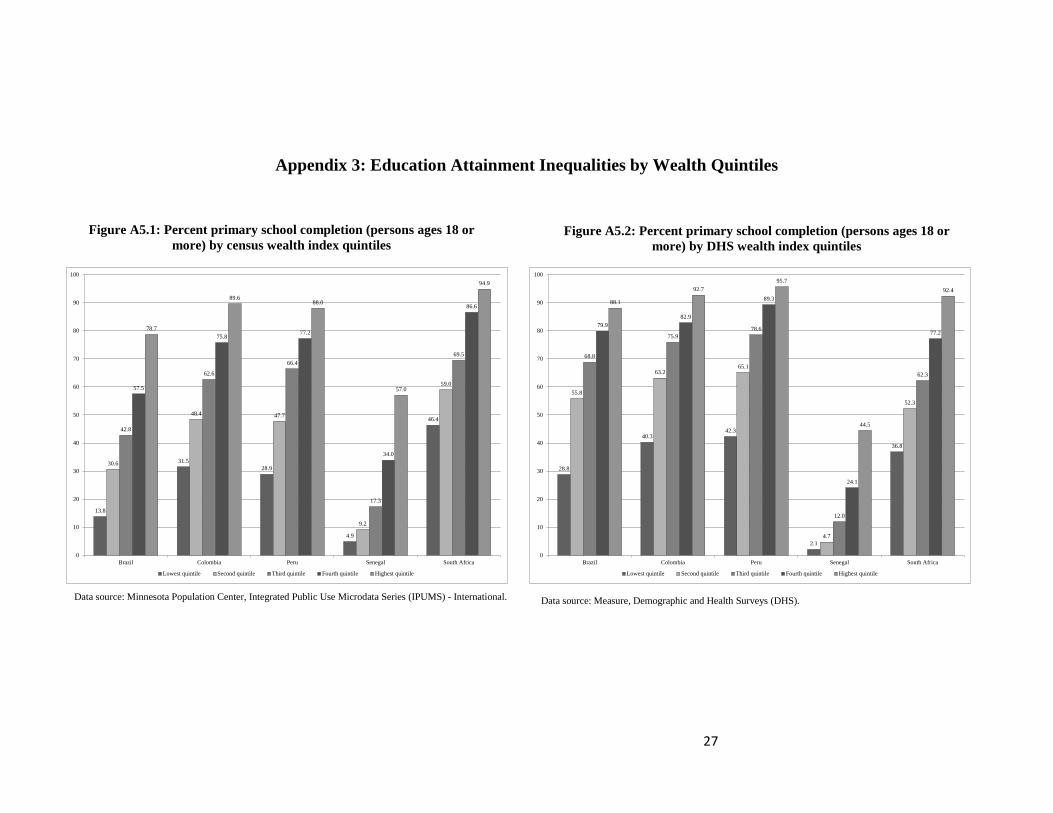
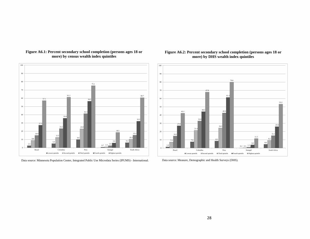
the top of the wealth distribution. As we would expect, this same pattern is reflected in the comparison of
primary and secondary school completion (for persons 18 years old or more) by quintile between census
and DHS data. These education inequality measurements can be seen in Appendix 3 (Figures A5.1 to
A6.2).
8 We also performed the Kolmogorov-Smirnov test for equality of the DHS and census wealth index distributions (results not shown). For all the samples, we rejected the null hypothesis that the data are drawn for the same distribution. However, this finding may be related to the sensitivity of the test to identify any difference between the two indices, since the test statistic is calculated at the point where the difference between the cumulative distribution function (CDF) of both samples is maximum.
13

86.0
77.379.8
30.5
78.4
92.9
88.186.3
40.5
83.3
95.5
91.8 90.5
51.0
86.6
97.395.2
91.7
62.5
90.9
98.6 97.6
92.8
76.9
92.1
0
10
20
30
40
50
60
70
80
90
100
Brazil Colombia Peru Senegal South Africa
Lowest quintile Second quintile Third quintile Fourth quintile Highest quintile
86.0 86.2
79.3
37.9
89.092.1 91.3
88.4
46.4
93.595.6
93.991.5
51.6
95.498.1
95.693.3
61.2
96.899.0
96.8
89.1
75.4
96.8
0
10
20
30
40
50
60
70
80
90
100
Brazil Colombia Peru Senegal South Africa
Lowest quintile Second quintile Third quintile Fourth quintile Highest quintile
Figure 2.1: Percent of children's school enrollment (ages 6-14)
by census wealth index quintiles
Figure 2.2: Percent of children's school enrollment (ages 6-14)
by DHS wealth index quintiles
Data source: Minnesota Population Center, Integrated Public Use Microdata Series (IPUMS) - International. Data source: Measure, Demographic and Health Surveys (DHS).
14

The validity of the asset index was also explored through logit regressions for school enrollment
conditional on the wealth index and other individual, household, and geography variables. Regressions
were estimated for children ages 6 to 14 for the following census samples: Brazil 2000, Cambodia 1998,
Colombia 2005, Peru 1993, Senegal 2002, South Africa 1996, and Thailand 2000. Results are shown in
Table 1. The odds-ratio column shows the odd-ratios and their standard errors for the wealth index in each
sample’s regression. The first model shows the impact of the wealth index on school enrollment
controlling for child characteristics only, the second model adds household characteristics, and the final
version incorporates geography to the estimation. The odds-ratio is larger than 1 and statistically
significant in all cases, as expected. This indicates that the measurement of wealth, as represented by the
census microdata wealth index, has a positive impact on child school enrollment. For example, for a one
unit increase in the value of the wealth index in the first model, we expect the odds of a child being
enrolled in school to be 1.935 times higher (or an increase of 93.5%) in the Brazil 2000 sample. Results
are robust across models. While the values of the odds-ratios are not strictly comparable across samples,
given that wealth is measured by differing assets in each country, the fact that all samples and models
show a positive and significant effect in predicting education enrollment is further evidence of a valid
measure of household wealth.
Table 1: Logit model for Children's School Enrollment (ages 6-14)
Census Wealth Index coefficient (odd-ratios) 1/
Odds-ratio Obs. Pseudo R2 Odds-ratio Obs. Pseudo R2 Odds-ratio Obs. Pseudo R2
1.935*** 1,872,876 0.125 1.798*** 1,872,876 0.132 1.970*** 1,872,876 0.142[0.0046] [0.0050] [0.0086]
1.634*** 297,898 0.142 1.489*** 297,889 0.157 1.444*** 297,889 0.179[0.0088] [0.0082] [0.0103]
2.379*** 725,394 0.118 2.053*** 725,394 0.128 2.121*** 725,394 0.142[0.0106] [0.0103] [0.0141]
1.659*** 392,880 0.043 1.494*** 392,880 0.049 1.296*** 392,880 0.056[0.0108] [0.0109] [0.0116]
2.111*** 246,578 0.090 1.712*** 246,578 0.115 1.772*** 246,578 0.151[0.0106] [0.0096] [0.0153]
1.660*** 678,735 0.185 1.545*** 678,735 0.189 1.572*** 678,735 0.191[0.0068] [0072] [0.0112]
2.300*** 85,797 0.139 2.112*** 85,797 0.144 2.509*** 85,797 0.151[0.0675] [0.0663] [0.0883]
Child characteristicsHousehold characteristicsGeography
Yes YesNo Yes YesNo No Yes
Colombia 2005
Peru 1993
Senegal 2002
South Africa 1996
Thailand 2000
Yes
Census sampleModel 1 Model 2 Model 3
Brazil 2000
Cambodia 1998
Data source: Minnesota Population Center, Integrated Public Use Microdata Series (IPUMS) - International.
Robust standard errors in brackets, *** p<.01,** p<.05, * p<.10
1/ Child characteristics include sex, age, and age squared of the child; household characteristics include sex, age, and educational attainment
dummies for the household head; geography variables include urban residence and dummies for the highest level of geography for each country.
15
5.2. Internal consistency of the asset index
The number and type of assets included in census microdata vary considerably across countries.
We performed a stepwise elimination of variables to determine what assets contribute the most to the final
wealth distribution. In each step, we eliminated the variable with the lowest loading coefficient in
absolute value (therefore, contributing the least to the calculation of the index). Then, Cronbach’s alpha
was calculated to analyze internal consistency of the remaining variables and Spearman rank correlations
to examine changes in the ordering of households given by the asset index distribution. We would expect
increasing internal consistency and higher rank correlations as we eliminate meaningless variables, but
decreasing consistency and relatively smaller rank correlations as we eliminate variables that are more
important in defining the wealth index.
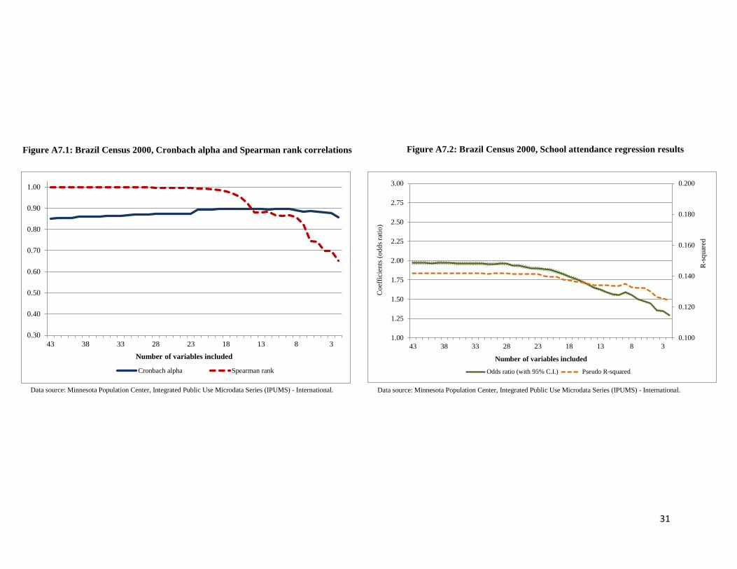
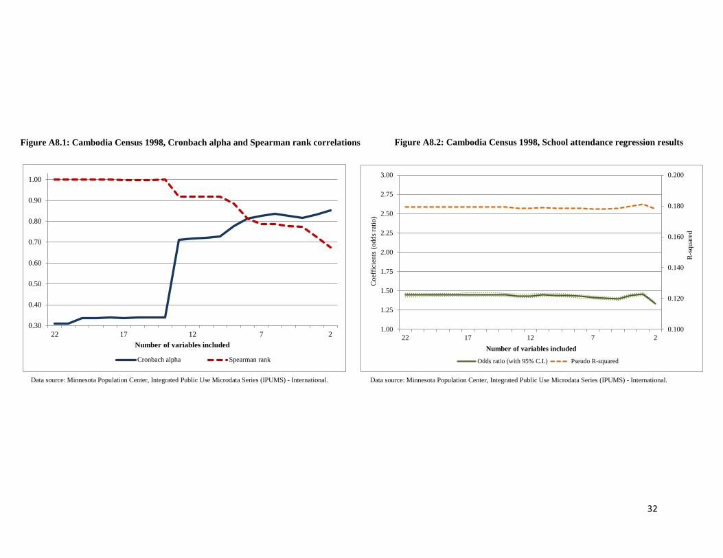
The stepwise procedure was performed separately for seven census samples: Brazil 2000,
Cambodia 1998, Colombia 2005, Peru 1993, Senegal 2002, South Africa 1996, and Thailand 2000. The
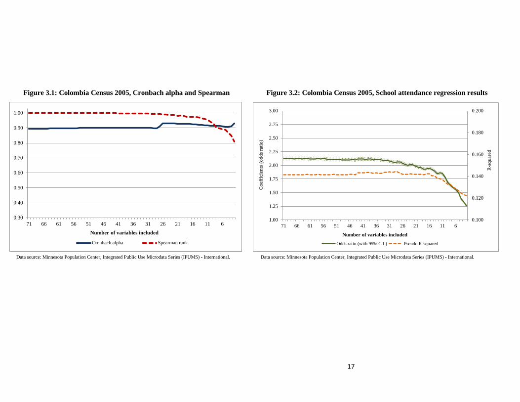
detailed graphs showing results from the stepwise procedure for Colombia 2005 can be seen in Figures
3.1 and 3.2 and the results for other samples are included in Appendix 4. In Figure 3.1 we observe that
internal consistency, as measured by Cronbach alpha, increases during the early variable eliminations.
This result is consistent across samples but is easier to visualize for the samples with a small number of
variables (Brazil, South Africa, Thailand, and particularly for Cambodia). This generally slight increase
follows the hypothesis that by eliminating variables that have a low contribution to the definition of
wealth, we are able to achieve higher internal consistency. For example, the second variable to be
dropped for the Peru data was ‘tricycle for work’ (see Table A4 in Appendix 4), which intuitively should
not be a key determinant of wealth and is owned only by a small proportion of households (3.7%). The
Spearman rank correlations show that the ordering of households by socioeconomic status is almost the
same for all samples for nearly the first third of variables eliminated. In the case of Colombia, for
example, we obtain similar results using all 71 variables available or a subset based on only 46, given the
correlation between indices is higher than 0.999. Furthermore, we observe across all samples that after
eliminating about two-thirds of the available variables, both internal consistency and the rank correlations
begin to decrease considerably. This can be seen, for instance, in Figure 3.1 for Colombia: internal
consistency starts dropping when about 25 variables are remaining. Finally, we observe a sharp change in
the internal consistency when a continuous variable is eliminated, given that almost all variables in the
index are binary; for example, there is a high increase in internal consistency when the number of
household members per bedroom is removed from the index for Colombia 2005 (index with 26 variables
in Figure 3.1) and Cambodia 1998 (index with 13 variables in Figure A8.1 in Appendix 4).
16
0.100
0.120
0.140
0.160
0.180
0.200
1.00
1.25
1.50
1.75
2.00
2.25
2.50
2.75
3.00
71 66 61 56 51 46 41 36 31 26 21 16 11 6
Number of variables included
Odds ratio (with 95% C.I.) Pseudo R-squared
Coe
ffici
ents
(odd
s rat
io)
R-s
quar
ed
0.30
0.40
0.50
0.60
0.70
0.80
0.90
1.00
71 66 61 56 51 46 41 36 31 26 21 16 11 6Number of variables included
Cronbach alpha Spearman rank
Figure 3.2: Colombia Census 2005, School attendance regression results
Figure 3.1: Colombia Census 2005, Cronbach alpha and Spearman
Data source: Minnesota Population Center, Integrated Public Use Microdata Series (IPUMS) - International. Data source: Minnesota Population Center, Integrated Public Use Microdata Series (IPUMS) - International.
17

Based on the stepwise procedure, we also estimated the school enrollment regressions at each step
of the variable elimination process and recorded the wealth index odds-ratios and the pseudo R-squared
from each one (Figures 3.2 and A7.2 to A12.2 in Appendix 4). These figures show a relatively constant
pseudo R-squared value for the most part of the variable elimination, before it begins to drop
(significantly for some countries). Likewise, the odds-ratios for the wealth index are generally stable over
the elimination of about one half of variables, but become less stable and start decreasing when
approximating the wealth index effects with far fewer indicators. The odds-ratios show almost
consistently positive (i.e. larger than one) and statistically significant effects, with the only exception of
the last two steps for Thailand, which have negative and not significant effects. Furthermore, we gain
precision in the estimates for most samples as we eliminate more variables, given the reductions in the
robust standard errors for the wealth index coefficient. In particular, the 95% confidence interval for the
odds ratio coefficients shown in Figures 3.2 and A7.2 to A12.2 is narrower as we drop variables, even
though this is difficult to observe since we have small-sized robust standard errors due to the large
number of observations.
In general, we do not observe large changes in internal consistency, ranks, or regressions results
during most of the stepwise procedure. Changes generally occur when we have only one third or less of
the original set of variables available are remaining. This finding suggests that an index based on a more
restricted subset of assets, dwelling characteristics, and utilities should produce results reasonably similar
to those based on all variables available for each sample. The largest observed changes happen for
Cambodia and Thailand. In both these cases, we argue that because the initial set of household variables
is quite different across samples, this has a major impact on the stepwise procedure results. The wealth
index for Thailand was created using only 42 (dichotomous) household variables while only 22 are
available for Cambodia. The Cambodia index is also limited as it only includes fuel for cooking and
lighting, water source, availability of toilet, and household members per room. In turn, the Thailand
sample has slightly more household variables (such as walls material or type of toilet), but it includes
only one variable for dwelling characteristics and it is the only sample that does not report household
members per room/bedroom. This fact is reflected in the way the ranks change considerably for both and,
particularly, in the dramatic drop in odds-ratios for Thailand when the number of included variables is
reduced. In this sense, we argue that the Cambodia and Thailand results may be less reliable due to the
limited number of variables available and the lack of key asset ownership variables included in the
creation of the wealth index. In effect, this indicates that having less than thirty indicator variables may
affect the consistency and validity of the asset-based index.
18
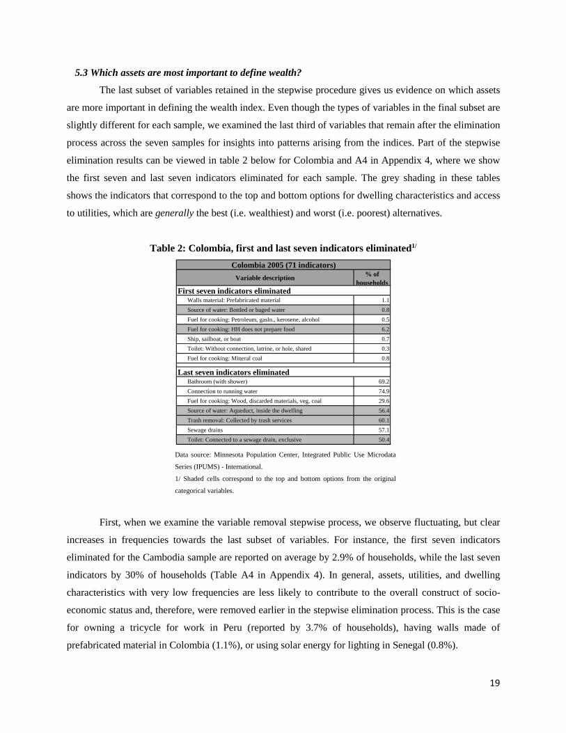
5.3 Which assets are most important to define wealth?
The last subset of variables retained in the stepwise procedure gives us evidence on which assets
are more important in defining the wealth index. Even though the types of variables in the final subset are
slightly different for each sample, we examined the last third of variables that remain after the elimination
process across the seven samples for insights into patterns arising from the indices. Part of the stepwise
elimination results can be viewed in table 2 below for Colombia and A4 in Appendix 4, where we show
the first seven and last seven indicators eliminated for each sample. The grey shading in these tables
shows the indicators that correspond to the top and bottom options for dwelling characteristics and access
to utilities, which are generally the best (i.e. wealthiest) and worst (i.e. poorest) alternatives.
Table 2: Colombia, first and last seven indicators eliminated1/
Colombia 2005 (71 indicators)Variable description % of
householdsFirst seven indicators eliminated
Walls material: Prefabricated material 1.1Source of water: Bottled or baged water 0.8Fuel for cooking: Petroleum, gasln., kerosene, alcohol 0.5Fuel for cooking: HH does not prepare food 6.2Ship, sailboat, or boat 0.7Toilet: Without connection, latrine, or hole, shared 0.3Fuel for cooking: Mineral coal 0.8
Last seven indicators eliminatedBathroom (with shower) 69.2Connection to running water 74.9Fuel for cooking: Wood, discarded materials, veg. coal 29.6Source of water: Aqueduct, inside the dwelling 56.4Trash removal: Collected by trash services 60.1Sewage drains 57.1Toilet: Connected to a sewage drain, exclusive 50.4
Data source: Minnesota Population Center, Integrated Public Use Microdata
Series (IPUMS) - International.
1/ Shaded cells correspond to the top and bottom options from the original
categorical variables.
First, when we examine the variable removal stepwise process, we observe fluctuating, but clear
increases in frequencies towards the last subset of variables. For instance, the first seven indicators
eliminated for the Cambodia sample are reported on average by 2.9% of households, while the last seven
indicators by 30% of households (Table A4 in Appendix 4). In general, assets, utilities, and dwelling
characteristics with very low frequencies are less likely to contribute to the overall construct of socio-
economic status and, therefore, were removed earlier in the stepwise elimination process. This is the case
for owning a tricycle for work in Peru (reported by 3.7% of households), having walls made of
prefabricated material in Colombia (1.1%), or using solar energy for lighting in Senegal (0.8%).
19
The next clear observation about the final subset is that the bottom and top options from each
categorical variable are systematically among the last variables to be removed. For example, the last
seven variables eliminated include "flooring made of earth" for Peru and "walls made of cement" for
Senegal. It is reasonable to assume that these two distinguishing indicators play a significant role in the
determination of a household's socioeconomic status, because they clearly differentiate poorest and
wealthiest households. In addition, across all seven samples, the best and worst water sources and sewage
or toilet types were consistently in the final subset of variables. Having piped water into the dwelling
represents the wealthiest water source option, while water from natural sources, such as a river, rain
water, or an unprotected spring represent the poorest type of water source. Similarly, a flushing toilet
connected to the public system contrasts with the poorest option of lacking a toilet facility. Further, water
source appears to be an important determinant of household wealth because, in addition to having the best
and worst indicators in the final third of variables, we observe that five samples had three or more water
indicators among them.
However, the final subset of variables is not simply about the richest and poorest defining
characteristics. Variables which seemingly represent extreme poverty or wealth (and tend to have low
frequencies) are not included in the final subset. For example, the indicator variable for using water from
a truck or a dealer in the Senegal sample is one of the first variables removed from the index, because it
has an extremely low frequency (only 1.7% of households use on trucked water). Further, in the
Colombia sample, lacking walls completely (in response to a question about wall material) is one of the
variables removed early in the stepwise procedure. This is a characteristic of extreme poverty and, in fact,
0.19% of households in Colombia lack walls. So while asset indicators that distinguish the wealthy and
the poor are important in the index, we observe that the wealthiest and poorest most common options
within categorical variables weigh the most significantly in defining the index. The evidence is consistent
with McKenzie (2005) who noted that principal component analysis places more weight on unequal
distributions of household assets, which more precisely differentiate wealth among households. Thus, not
only does the 'quality' of the asset indicator matter, but also the relative frequency of ownership across the
population.
6. Conclusions In this paper we argue that the census microdata wealth index is both valid and internally
consistent in its representation of household socio-economic status for all samples examined. The
evidence provided by the graphical analysis of kernel density distributions and the education outcomes
gradients shows that we are measuring the unobserved socioeconomic status at the household level and
that we achieve relatively similar performance to the DHS measure. We observe differences in school
20
enrollment and educational attainment across the wealth index quintiles, showing consistently that
households at the top of the distribution have better outcomes than those at the bottom. The logit
regression gives consistently positive and significant effects of the household wealth index on child’s
school enrollment. Moreover, as we remove individual variables and re-run the regression, we see this
effect is consistently positive, while predictive power is generally constant until the wealth index is
comprised of too few household variables. For a majority of samples, ranks and internal consistency
remain also fairly constant during most of the stepwise elimination process.
An important practical implication arises from our results. The stepwise elimination process
provides a methodology to determine which, and how many, household variables are important to include
in the construction of a measurement of household socioeconomic status and, thus, are necessary to obtain
a valid asset index. The fact that, after the stepwise procedure, the final subset of variables always
includes the poorest and wealthiest water supply and sewage or toilet type categories shows their value as
determinants of socio-economic status. More generally, the top and bottom categories for dwelling
characteristics and utilities as well as those with higher frequencies have larger contributions to the
construction of a wealth index. This stepwise procedure is a consistent and robust methodology to
determine which household variables are necessary in the construction of a census microdata wealth
index. Results also suggest that having less than thirty indicator variables, lacking diverse asset
information, or missing key variables such as water source, toilet, or sewage may affect the consistency
and validity of the resulting asset-based index.
The inclusion of the census microdata wealth index in the IPUMS-I dataset will enhance social
science research by giving a robust and cost-effective reference point to represent socio-economic status.
The index will be most applicable in developing countries, where we expect a higher variability in
ownership of assets, dwelling characteristics, and access to utilities. This paper provides evidence of a
valid census microdata wealth index and a new methodology in evaluating which household variables are
more relevant in the construction of this index.
21
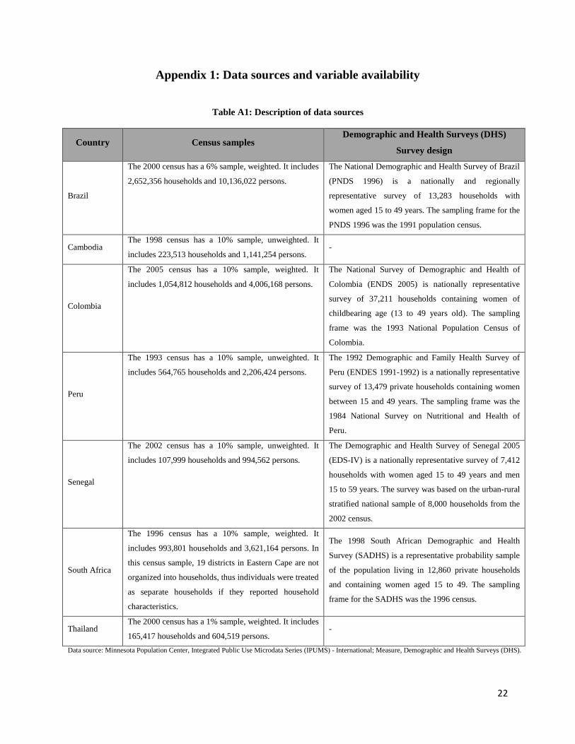
Appendix 1: Data sources and variable availability
Table A1: Description of data sources
Country Census samples Demographic and Health Surveys (DHS)
Survey design
Brazil
The 2000 census has a 6% sample, weighted. It includes
2,652,356 households and 10,136,022 persons.
The National Demographic and Health Survey of Brazil
(PNDS 1996) is a nationally and regionally
representative survey of 13,283 households with
women aged 15 to 49 years. The sampling frame for the
PNDS 1996 was the 1991 population census.
Cambodia The 1998 census has a 10% sample, unweighted. It
includes 223,513 households and 1,141,254 persons. -
Colombia
The 2005 census has a 10% sample, weighted. It
includes 1,054,812 households and 4,006,168 persons.
The National Survey of Demographic and Health of
Colombia (ENDS 2005) is nationally representative
survey of 37,211 households containing women of
childbearing age (13 to 49 years old). The sampling
frame was the 1993 National Population Census of
Colombia.
Peru
The 1993 census has a 10% sample, unweighted. It
includes 564,765 households and 2,206,424 persons.
The 1992 Demographic and Family Health Survey of
Peru (ENDES 1991-1992) is a nationally representative
survey of 13,479 private households containing women
between 15 and 49 years. The sampling frame was the
1984 National Survey on Nutritional and Health of
Peru.
Senegal
The 2002 census has a 10% sample, unweighted. It
includes 107,999 households and 994,562 persons.
The Demographic and Health Survey of Senegal 2005
(EDS-IV) is a nationally representative survey of 7,412
households with women aged 15 to 49 years and men
15 to 59 years. The survey was based on the urban-rural
stratified national sample of 8,000 households from the
2002 census.
South Africa
The 1996 census has a 10% sample, weighted. It
includes 993,801 households and 3,621,164 persons. In
this census sample, 19 districts in Eastern Cape are not
organized into households, thus individuals were treated
as separate households if they reported household
characteristics.
The 1998 South African Demographic and Health
Survey (SADHS) is a representative probability sample
of the population living in 12,860 private households
and containing women aged 15 to 49. The sampling
frame for the SADHS was the 1996 census.
Thailand The 2000 census has a 1% sample, weighted. It includes
165,417 households and 604,519 persons. -
Data source: Minnesota Population Center, Integrated Public Use Microdata Series (IPUMS) - International; Measure, Demographic and Health Surveys (DHS).
22
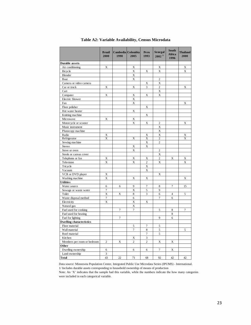
Table A2: Variable Availability, Census Microdata
Brazil 2000
Cambodia 1998
Colombia 2005
Peru 1993
Senegal 2002 1/
South Africa 1996
Thailand 2000
Durable assetsAir conditioning X X X XBicycle X X X XBlender XBoat X 2Camera or video camera X XCar or truck X X 3 2 XCart XComputer X X X XElectric Shower XFan X XFloor polisher XHot water heater XKnitting machine XMicrowave X XMotorcycle or scooter X X 2 XMusic instrument XPhotocopy machine XRadio X X X XRefrigerator X X X 2 XSewing machine X 2Stereo X XStove or oven X 2Stools or canvas cover XTelephone or fax X X X 2 X XTelevision X X 2 X XTricycle XVacuum XVCR or DVD player X XWashing machine X X X X
UtilitiesWater source 6 6 9 7 8 7 15Sewage or waste water 7 X 5 9Toilet X X 8 3 6 4 5Waste disposal method 7 6 7 6Electricity X X XNatural gas XFuel used for cooking 7 7 5 8 7Fuel used for heating 8Fuel for lighting 7 9 6
Dwelling characteristicsFloor material 5 7 5Wall material 7 8 5 5Roof material 7 5Kitchen X 3Members per room or bedroom 2 X 2 2 X X
OtherDwelling ownership 6 6 6 7 XLand ownership 3
Total 43 22 71 68 92 42 42
Data source: Minnesota Population Center, Integrated Public Use Microdata Series (IPUMS) - International. 1/ Includes durable assets corresponding to household ownership of means of production Note: An ‘X’ indicates that the sample had this variable, while the numbers indicate the how many categories were included in each categorical variable.
23
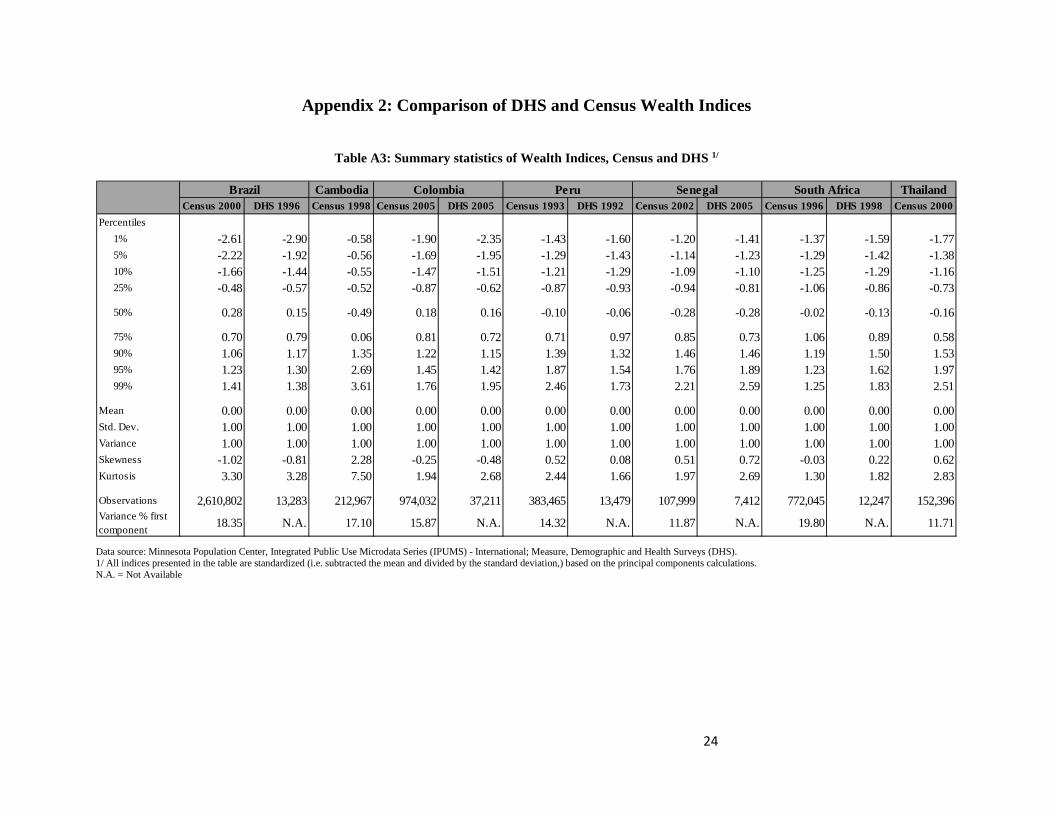
Appendix 2: Comparison of DHS and Census Wealth Indices
Table A3: Summary statistics of Wealth Indices, Census and DHS 1/
Brazil Cambodia Colombia Peru Senegal South Africa ThailandCensus 2000 DHS 1996 Census 1998 Census 2005 DHS 2005 Census 1993 DHS 1992 Census 2002 DHS 2005 Census 1996 DHS 1998 Census 2000
Percentiles1% -2.61 -2.90 -0.58 -1.90 -2.35 -1.43 -1.60 -1.20 -1.41 -1.37 -1.59 -1.775% -2.22 -1.92 -0.56 -1.69 -1.95 -1.29 -1.43 -1.14 -1.23 -1.29 -1.42 -1.3810% -1.66 -1.44 -0.55 -1.47 -1.51 -1.21 -1.29 -1.09 -1.10 -1.25 -1.29 -1.1625% -0.48 -0.57 -0.52 -0.87 -0.62 -0.87 -0.93 -0.94 -0.81 -1.06 -0.86 -0.73
50% 0.28 0.15 -0.49 0.18 0.16 -0.10 -0.06 -0.28 -0.28 -0.02 -0.13 -0.16
75% 0.70 0.79 0.06 0.81 0.72 0.71 0.97 0.85 0.73 1.06 0.89 0.5890% 1.06 1.17 1.35 1.22 1.15 1.39 1.32 1.46 1.46 1.19 1.50 1.5395% 1.23 1.30 2.69 1.45 1.42 1.87 1.54 1.76 1.89 1.23 1.62 1.9799% 1.41 1.38 3.61 1.76 1.95 2.46 1.73 2.21 2.59 1.25 1.83 2.51
Mean 0.00 0.00 0.00 0.00 0.00 0.00 0.00 0.00 0.00 0.00 0.00 0.00Std. Dev. 1.00 1.00 1.00 1.00 1.00 1.00 1.00 1.00 1.00 1.00 1.00 1.00Variance 1.00 1.00 1.00 1.00 1.00 1.00 1.00 1.00 1.00 1.00 1.00 1.00Skewness -1.02 -0.81 2.28 -0.25 -0.48 0.52 0.08 0.51 0.72 -0.03 0.22 0.62Kurtosis 3.30 3.28 7.50 1.94 2.68 2.44 1.66 1.97 2.69 1.30 1.82 2.83
Observations 2,610,802 13,283 212,967 974,032 37,211 383,465 13,479 107,999 7,412 772,045 12,247 152,396Variance % first component 18.35 N.A. 17.10 15.87 N.A. 14.32 N.A. 11.87 N.A. 19.80 N.A. 11.71
Data source: Minnesota Population Center, Integrated Public Use Microdata Series (IPUMS) - International; Measure, Demographic and Health Surveys (DHS). 1/ All indices presented in the table are standardized (i.e. subtracted the mean and divided by the standard deviation,) based on the principal components calculations. N.A. = Not Available
24

0.2
.4.6
.8D
ensi
ty
-4 -2 0 2index
DHS Census
0.2
.4.6
Den
sity
-2 0 2 4index
DHS Census
Figure A1: Kernel density, Brazil Census 2000 and DHS 1996
Figure A2: Kernel density, Peru Census 1993 and DHS 1992
Data source: Minnesota Population Center, Integrated Public Use Microdata Series (IPUMS) - International; Measure, Demographic and Health Surveys (DHS).
Data source: Minnesota Population Center, Integrated Public Use Microdata Series (IPUMS) - International; Measure, Demographic and Health Surveys (DHS).
25

0.2
.4.6
.81
Den
sity
-2 0 2 4index
DHS Census
0.5
11.
5D
ensi
ty
-2 -1 0 1 2index
DHS Census
Figure A3: Kernel density, Senegal Census 2002 and DHS 2005 Figure A4: Kernel density, South Africa Census 1996 and
Data source: Minnesota Population Center, Integrated Public Use Microdata Series (IPUMS) - International; Measure, Demographic and Health Surveys (DHS).
Data source: Minnesota Population Center, Integrated Public Use Microdata Series (IPUMS) - International; Measure, Demographic and Health Surveys (DHS).
26
13.8
31.528.9
4.9
46.4
30.6
48.4 47.7
9.2
59.0
42.8
62.6
66.4
17.3
69.5
57.5
75.877.2
34.0
86.6
78.7
89.688.0
57.0
94.9
0
10
20
30
40
50
60
70
80
90
100
Brazil Colombia Peru Senegal South Africa
Lowest quintile Second quintile Third quintile Fourth quintile Highest quintile
28.8
40.342.3
2.1
36.8
55.8
63.265.1
4.7
52.3
68.8
75.978.6
12.0
62.3
79.982.9
89.3
24.1
77.2
88.1
92.795.7
44.5
92.4
0
10
20
30
40
50
60
70
80
90
100
Brazil Colombia Peru Senegal South Africa
Lowest quintile Second quintile Third quintile Fourth quintile Highest quintile
Appendix 3: Education Attainment Inequalities by Wealth Quintiles
Figure A5.1: Percent primary school completion (persons ages 18 or more) by census wealth index quintiles
Figure A5.2: Percent primary school completion (persons ages 18 or more) by DHS wealth index quintiles
Data source: Measure, Demographic and Health Surveys (DHS). Data source: Minnesota Population Center, Integrated Public Use Microdata Series (IPUMS) - International.
27
2.55.0
9.9
0.7
6.28.8
12.5
23.0
1.3
10.3
14.9
23.2
41.3
2.6
15.2
27.3
35.8
56.5
5.9
32.2
57.1
61.2
75.1
18.5
60.7
0
10
20
30
40
50
60
70
80
90
100
Brazil Colombia Peru Senegal South Africa
Lowest quintile Second quintile Third quintile Fourth quintile Highest quintile
1.4
7.6 8.5
0.2
4.67.3
21.424.3
0.3
9.2
14.5
32.8
42.6
1.2
15.1
27.0
44.2
61.4
3.8
25.9
42.2
67.8
79.8
11.5
53.2
0
10
20
30
40
50
60
70
80
90
100
Brazil Colombia Peru Senegal South Africa
Lowest quintile Second quintile Third quintile Fourth quintile Highest quintile
Figure A6.2: Percent secondary school completion (persons ages 18 or more) by DHS wealth index quintiles
Figure A6.1: Percent secondary school completion (persons ages 18 or more) by census wealth index quintiles
Data source: Measure, Demographic and Health Surveys (DHS). Data source: Minnesota Population Center, Integrated Public Use Microdata Series (IPUMS) - International.
28
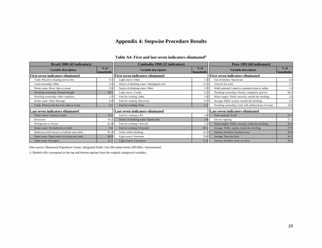
Appendix 4: Stepwise Procedure Results
Table A4: First and last seven indicators eliminated1/ Brazil 2000 (43 indicators) Cambodia 1998 (22 indicators) Peru 1993 (68 indicators)
Variable description % of households
Variable description % of households
Variable description % of households
First seven indicators eliminated First seven indicators eliminated First seven indicators eliminatedTrash: Placed in cleaning service bin 4.7 Light source: Other 1.3 Use of kitchen: Shared use 4.2Land ownership: Other 2.2 Source of drinking water: Tubedpiped well 15.1 Tricycle for work 3.7Waste water: River, lake or ocean 2.6 Source of drinking water: Other 2.5 Walls material: Limed or cemented stone or ashlar 1.3Dwelling ownership: Owned outright 68.7 Light source: Candle 0.2 Dwelling ownership: Owned, completely paid for 68.1Dwelling ownership: Other condition 1.2 Fuel for cooking: Other 1.0 Water supply: Public network, outside the dwelling 3.5Waste water: Other drainage 0.9 Fuel for cooking: Electricity 0.1 Sewage: Public system, outside the dwelling 4.3Trash: Thrown into the river, lake or ocean 0.5 Fuel for cooking: None 0.1 Dwelling ownership: Used with authorization of owner 10.0
Last seven indicators eliminated Last seven indicators eliminated Last seven indicators eliminatedWater source: General system 74.2 Fuel for cooking: LPG 1.8 Floor material: Earth 47.7Electricity 93.2 Source of drinking water: Piped water 5.8 Electric lighting 57.2Refrigerator or freezer 81.0 Fuel for cooking: Charcoal 5.2 Water supply: Public network, inside the dwelling 45.4Waste water: No bathroom or toilet 9.4 Fuel for cooking: Firewood 90.1 Sewage: Public system, inside the dwelling 37.9Bathroom (with shower or bathtub and toilet) 81.2 Toilet within dwelling 14.5 Sanitary facilities: Exclusive use 49.9Piped water: Piped water to at least one room 80.9 Light source: Kerosene 79.8 Sewage: Does not have 36.1Piped water: Not piped 12.1 Light source: City power 12.6 Sanitary facilities: Does not have 36.1
Data source: Minnesota Population Center, Integrated Public Use Microdata Series (IPUMS) - International.
1/ Shaded cells correspond to the top and bottom options from the original categorical variables.
29

Table A4: First and last seven indicators eliminated (continued) Senegal 2002 (92 indicators) South Africa 1996 (42 indicators) Thailand 2000 (42 indicators)Variable description % of
householdsVariable description % of
householdsVariable description % of
householdsFirst seven indicators eliminated First seven indicators eliminated First seven indicators eliminated
Type of lighting: Gas lamp 0.3 Refuse disposal: Other 0.2 Fuel for cooking: Kerosene 0.2Sewage water disposal: Other 2.4 Fuel for heating: Other 0.1 Walls material: Wood and cement or brick 20.2Type of lighting: Generator 0.5 Fuel for cooking: Other 0.0 Fuel for cooking: Other 0.4Type of lighting: Solar energy 0.8 Fuel for lighting: Other 0.0 Water supply: Other 0.5Sewage water disposal: In small river 0.2 Fuel for heating: Electricity from other source 0.2 Motorcycle 65.2Dwelling ownership: Other 0.8 Refuse disposal: Removed by local authority less often 2.3 Water supply: Rain water 1.7Means of production: Motorcycle, scooter, or moped 0.6 Fuel for cooking: Electricity from other source 0.2 Bicycle 42.1
Last seven indicators eliminated Last seven indicators eliminated Last seven indicators eliminatedRoof material: Straw or thatch 29.3 Telephone (including cellular phone) 28.4 Walls material: Cement or brick 27.6Television 29.4 Refuse disposal: Removed by local aut. at least weekly 51.6 Motor car 25.5Wall material: Cement 55.4 Water supply: Piped water in dwelling 43.8 Washing machine 28.7Water source: Tap, inside the house 37.9 Toilet facilities: Flush or chemical toilet 50.0 Telephone 28.1Type of lighting: Electricity 40.9 Fuel for lighting: Electricity direct from authority 57.5 Air conditioner 10.4Fuel for cooking: Wood 54.9 Fuel for cooking: Electricity direct from authority 46.9 Toilet facilities: Flush toilet 8.2Fuel for cooking: Gas 37.4 Fuel for heating: Electricity direct from authority 45.9 Toilet facilities: Molded bucket latrine 85.5
30
0.30
0.40
0.50
0.60
0.70
0.80
0.90
1.00
43 38 33 28 23 18 13 8 3Number of variables included
Cronbach alpha Spearman rank
0.100
0.120
0.140
0.160
0.180
0.200
1.00
1.25
1.50
1.75
2.00
2.25
2.50
2.75
3.00
43 38 33 28 23 18 13 8 3
Number of variables included
Odds ratio (with 95% C.I.) Pseudo R-squaredC
oeffi
cien
ts (o
dds r
atio
)
R-s
quar
ed
Figure A7.2: Brazil Census 2000, School attendance regression results Figure A7.1: Brazil Census 2000, Cronbach alpha and Spearman rank correlations
Data source: Minnesota Population Center, Integrated Public Use Microdata Series (IPUMS) - International. Data source: Minnesota Population Center, Integrated Public Use Microdata Series (IPUMS) - International.
31
0.30
0.40
0.50
0.60
0.70
0.80
0.90
1.00
22 17 12 7 2Number of variables included
Cronbach alpha Spearman rank
0.100
0.120
0.140
0.160
0.180
0.200
1.00
1.25
1.50
1.75
2.00
2.25
2.50
2.75
3.00
22 17 12 7 2Number of variables included
Odds ratio (with 95% C.I.) Pseudo R-squared
Coe
ffici
ents
(odd
s rat
io)
R-s
quar
ed
Figure A8.2: Cambodia Census 1998, School attendance regression results Figure A8.1: Cambodia Census 1998, Cronbach alpha and Spearman rank correlations
Data source: Minnesota Population Center, Integrated Public Use Microdata Series (IPUMS) - International. Data source: Minnesota Population Center, Integrated Public Use Microdata Series (IPUMS) - International.
32
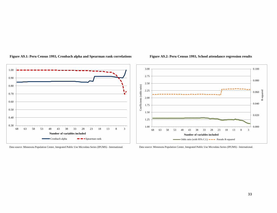
0.30
0.40
0.50
0.60
0.70
0.80
0.90
1.00
68 63 58 53 48 43 38 33 28 23 18 13 8 3Number of variables included
Cronbach alpha Spearman rank
0.000
0.020
0.040
0.060
0.080
0.100
1.00
1.25
1.50
1.75
2.00
2.25
2.50
2.75
3.00
68 63 58 53 48 43 38 33 28 23 18 13 8 3
Number of variables included
Odds ratio (with 95% C.I.) Pseudo R-squaredC
oeffi
cien
ts (o
dds r
atio
)
R-s
quar
ed
Figure A9.1: Peru Census 1993, Cronbach alpha and Spearman rank correlations Figure A9.2: Peru Census 1993, School attendance regression results
Data source: Minnesota Population Center, Integrated Public Use Microdata Series (IPUMS) - International. Data source: Minnesota Population Center, Integrated Public Use Microdata Series (IPUMS) - International.
33

0.30
0.40
0.50
0.60
0.70
0.80
0.90
1.00
92 87 82 77 72 67 62 57 52 47 42 37 32 27 22 17 12 7 2Number of variables included
Cronbach alpha Spearman rank
0.100
0.120
0.140
0.160
0.180
0.200
1.00
1.25
1.50
1.75
2.00
2.25
2.50
2.75
3.00
92 87 82 77 72 67 62 57 52 47 42 37 32 27 22 17 12 7 2
Number of variables included
Odds ratio (with 95% C.I.) Pseudo R-squaredC
oeffi
cien
ts (o
dds r
atio
)
R-s
quar
ed
Figure A10.1: Senegal Census 2002, Cronbach alpha and Spearman rank correlations Figure A10.2: Senegal Census 2002, School attendance regression results
Data source: Minnesota Population Center, Integrated Public Use Microdata Series (IPUMS) - International. Data source: Minnesota Population Center, Integrated Public Use Microdata Series (IPUMS) - International.
34
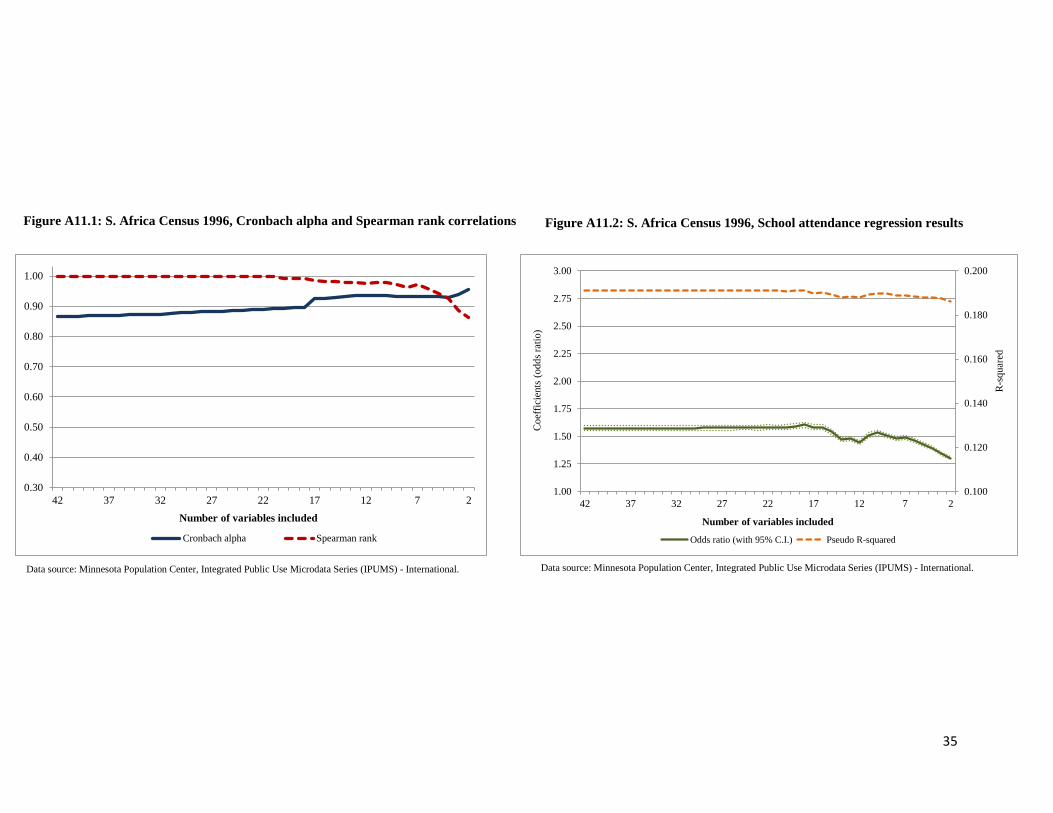
0.30
0.40
0.50
0.60
0.70
0.80
0.90
1.00
42 37 32 27 22 17 12 7 2Number of variables included
Cronbach alpha Spearman rank
0.100
0.120
0.140
0.160
0.180
0.200
1.00
1.25
1.50
1.75
2.00
2.25
2.50
2.75
3.00
42 37 32 27 22 17 12 7 2
Number of variables included
Odds ratio (with 95% C.I.) Pseudo R-squaredC
oeffi
cien
ts (o
dds r
atio
)
R-s
quar
ed
Figure A11.1: S. Africa Census 1996, Cronbach alpha and Spearman rank correlations Figure A11.2: S. Africa Census 1996, School attendance regression results
Data source: Minnesota Population Center, Integrated Public Use Microdata Series (IPUMS) - International. Data source: Minnesota Population Center, Integrated Public Use Microdata Series (IPUMS) - International.
35
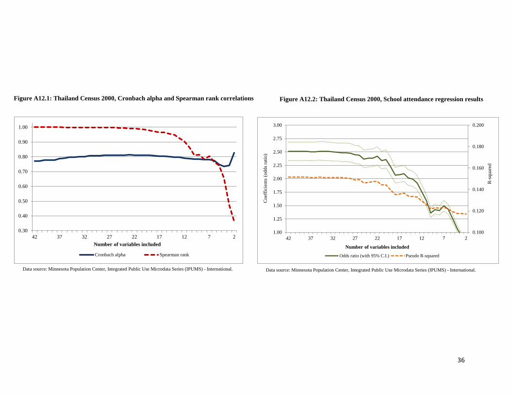
0.30
0.40
0.50
0.60
0.70
0.80
0.90
1.00
42 37 32 27 22 17 12 7 2Number of variables included
Cronbach alpha Spearman rank
0.100
0.120
0.140
0.160
0.180
0.200
1.00
1.25
1.50
1.75
2.00
2.25
2.50
2.75
3.00
42 37 32 27 22 17 12 7 2
Number of variables included
Odds ratio (with 95% C.I.) Pseudo R-squared
Coe
ffici
ents
(odd
s rat
io)
R-s
quar
ed
Figure A12.1: Thailand Census 2000, Cronbach alpha and Spearman rank correlations Figure A12.2: Thailand Census 2000, School attendance regression results
Data source: Minnesota Population Center, Integrated Public Use Microdata Series (IPUMS) - International. Data source: Minnesota Population Center, Integrated Public Use Microdata Series (IPUMS) - International.
36
References Assaad, R., Levison, D., & Zibani, N. (2010). The effect of domestic work on girls' schooling: Evidence
from Egypt. Feminist Economics, 16 (1), 79-128.
Bollen, K., Glanville, J., & Stecklov, G. (2002). Economic status proxies in studies of fertility in
developing countries: Does the measure matter? Population Studies, 56 (1), 81-96.
Cortina, J. (1993). What is coefficient alpha? An examination of theory and applications. Journal of
Applied Psychology, 78 (1), 98-104.
Falkingham, J., & Namazie, C. (2002). Measuring health and poverty: a review of approaches to
identifying the poor. London: DFID Health Systems Resource Centre. Retrieved from
http://r4d.dfid.gov.uk/PDF/Outputs/HOppsIssuesPaperFalkingham.pdf
Filmer, D., & Pritchett, L. (1999). The effect of household wealth on educational attainment: evidence
from 35 countries. Population and development review, 25 (1), 85-120.
Filmer, D., & Pritchett, L. (2001). Estimating wealth effects without expenditure data or tears: an
application to educational enrollments in states of India. Demography, 38 (1), 115-132.
Filmer, D., & Scott, K. (2012). Assessing asset indices. Demography, 49 (1), 359-392.
Houweling, T., Kunst, A., & Mackenbach, J. (2003). Measuring health inequality among children in
developing countries: does the choice of the indicator of economic status matter? International
Journal for Equity and Health, doi: 10.1186/1475-9276-2-8.
Howe, L., Hargreaves, J., & Huttly, S. (2008). Issues in the construction of wealth indices for the
measurement of socio-economic position in low-income countries. Emerging Themes in
Epidemiology, doi: 10.1186/1742-7622-5-3.
Lindelow, M. (2006). Sometimes more equal than others: how health inequalities depend on the choice of
welfare indicator. Health Economics, 15 (3), 263-279.
McKenzie, D. (2005). Measuring inequality with asset indicators. Journal of Population Economics, 18
(2), 229-260.
Minujin, A. & Bang, J. (2002). Indicadores de inequidad social. Acerca del uso del 'índice de bienes' para
la distribución de los hogares. Desarrollo Económico, 42 (165), 129-146.
Montgomery, M., Gragnolati, M., Burke, K., & Paredes, E. (2000). Measuring living standards with
proxy variables. Demography, 37 (2), 155-174.
Rencher, A. C. (2002). Principal component analysis. In: Rencher, A. C., Methods of Multivariate
Analysis (pp. 380-407), Second Edition. New York: John Wiley and Sons.
Rutstein, S. O., & Johnson, K. (2004). The DHS wealth index. Maryland: MEASURE DHS, ORC Macro,
DHS Comparative Reports No. 6. Retrieved from http://dhsprogram.com/pubs/pdf/CR6/CR6.pdf
37
Sahn, D., & Stifel, D. (2000). Poverty comparisons over time and across countries in Africa. World
Development, 28 (12), 2123-2155.
Sahn, D., & Stiefel, D. (2003). Exploring alternative measures of welfare in the absence of expenditure
data. Review of Income and Wealth, 49 (4), 463-489.
Vyas, S., & Kumaranayake, L. (2006). Constructing socio-economic status indices: how to use principal
components analysis. Health Policy and Planning, 21 (6), 459-468.
Wagstaff, A. & Watanabe, N. (2003). What difference does the choice of SES make in health inequality
measurement. Health Economics, 12 (10), 885-890.
Wall, M., & Johnston D. (2008). Counting heads or counting televisions: Can asset-based measures of
welfare assist policy-makers in Russia? Journal of Human Development, 9 (1), 131-147.
38
Related Documents